Sensitivity analysis BSAD 30 Dave Novak Source: Anderson et al., 2013 Quantitative Methods for Business 12 th edition – some slides are directly from J. Loucks © 2013 Cengage Learning

Sensitivity analysis BSAD 30 Dave Novak Source: Anderson et al., 2013 Quantitative Methods for Business 12 th edition – some slides are directly from J.
Dec 19, 2015
Welcome message from author
This document is posted to help you gain knowledge. Please leave a comment to let me know what you think about it! Share it to your friends and learn new things together.
Transcript

Sensitivity analysis
BSAD 30
Dave Novak
Source: Anderson et al., 2013 Quantitative Methods for Business 12th edition – some slides are directly from J. Loucks © 2013 Cengage Learning

Overview
Introduction to sensitivity analysisChanges in objective function coefficientsChanges in RHS values
Interpretation of shadow pricesSunk costs versus relevant costs
Example
Sensitivity analysis
Also called post-optimality analysis considers how changes in the coefficients of a linear programming problem (within specified ranges) affect the optimal solution
Keep in mind that an LP is solved in terms of a specific set of objective function coefficients and constraintsIt is not a generalized formula that you can
automatically use to consider all kinds of different coefficient values

Sensitivity analysis
Sensitivity analysis is important because decision-makers operate in dynamic environments with imperfect informationThe coefficients in the OF, the LHS of the
constraints, and the RHS of the constraints are often estimated, and are typically imprecise
Allows decision-maker to ask what-if questions about the problem

Sensitivity analysis
Prices of raw material change, demand for products change, production capabilities change, stock prices change, etc.
If you are using an LP, you can generally expect some type of change over time
How do these changes affect the optimal solution, and at what point do you need to completely revise (and re-solve) the LP?
Sensitivity analysis
In sensitivity analysis, we consider only ONE change at a timeChange ONE OF coefficientChange ONE RHS constraint value
We cannot use this approach to examine multiple simultaneous changes

Sensitivity analysis
Consider the problem from Lecture 4
Max 5x1 + 7x2
s.t. x1 < 6
2x1 + 3x2 < 19
x1 + x2 < 8
x1 > 0 and x2 > 0
ObjectiveFunction
“Regular”Constraints
Non-negativity Constraints

Sensitivity report
Download Lecture9 example.xlsx from the class website
The problem is already solvedX1 (# of units of product 1) 5X2 (# of units of product 2) 3
Objective Function (Maximize Profit) 46
Constraints LHS RHSST:1) Constraint#1 5 62) Constraint #2 19 193) Constraint #3 8 8

Sensitivity report
The Sensitivity Report is:Variable Cells
Final Reduced Objective Allowable AllowableCell Name Value Cost Coefficient Increase Decrease
$B$1 X1 (# of units of product 1) 5 0 5 2 0.333333333$B$2 X2 (# of units of product 2) 3 0 7 0.5 2
ConstraintsFinal Shadow Constraint Allowable Allowable
Cell Name Value Price R.H. Side Increase Decrease$B$10 3) Constraint #3 LHS 8 1 8 0.333333333 1.666666667$B$8 1) Constraint#1 LHS 5 0 6 1E+30 1$B$9 2) Constraint #2 LHS 19 2 19 5 1

Sensitivity analysis
First, let’s consider how changes in the objective function coefficients might affect the optimal solution
We want to find the range of OF coefficient values (for each coefficient) over which the current solution will remain optimal
Managers should focus on objective coefficients that have a narrow range of optimality and coefficients near the endpoints of the range
Sensitivity analysis
Note that any change in the OF coefficients will NOT impact the feasible region, or the extreme points within the feasible region, as the constraints are not changed in any way
Sensitivity focused on changes in OF coefficient values address the question of “at what point does a change in the profit or cost associated with a particular decision variable result in a different extreme point becoming the “new” optimal solution”?

Sensitivity analysis
We want to know how much each one of the coefficients in the OF can change before the optimal solution changes
Max 5x1 + 7x2
What if (c1) the profit associated with x1 were to change – would the solution of (5,3) still be optimal?
Currently, we want to produce 5 units of x1
and 3 units of x2 at profit of $5 and $7 per unit respectively

Sensitivity report
Variable CellsFinal Reduced Objective Allowable Allowable
Cell Name Value Cost Coefficient Increase Decrease$B$1 X1 (# of units of product 1) 5 0 5 2 0.333333333$B$2 X2 (# of units of product 2) 3 0 7 0.5 2
ConstraintsFinal Shadow Constraint Allowable Allowable
Cell Name Value Price R.H. Side Increase Decrease$B$10 3) Constraint #3 LHS 8 1 8 0.333333333 1.666666667$B$8 1) Constraint#1 LHS 5 0 6 1E+30 1$B$9 2) Constraint #2 LHS 19 2 19 5 1
The “profit” coefficient associated with x1 (referred to as c1) can range between $4.67 and $7 before The optimal solution mix will change from (5, 3) to something else (another extreme point value in our feasible region)

Sensitivity analysis
If the profit associated with x1 were to increase by $1 per unit, we would still produce 5 units of x1, although our total profit would now be $51 instead of $46 6(5) + 7(3) = 51
As long as c1 (the profit contribution associated with x1) is between $4.67 and $7 per unit, the optimal solution mix of 5 units of x1 and 3 units of x2 will not change
Sensitivity report
Variable CellsFinal Reduced Objective Allowable Allowable
Cell Name Value Cost Coefficient Increase Decrease$B$1 X1 (# of units of product 1) 5 0 5 2 0.333333333$B$2 X2 (# of units of product 2) 3 0 7 0.5 2
ConstraintsFinal Shadow Constraint Allowable Allowable
Cell Name Value Price R.H. Side Increase Decrease$B$10 3) Constraint #3 LHS 8 1 8 0.333333333 1.666666667$B$8 1) Constraint#1 LHS 5 0 6 1E+30 1$B$9 2) Constraint #2 LHS 19 2 19 5 1
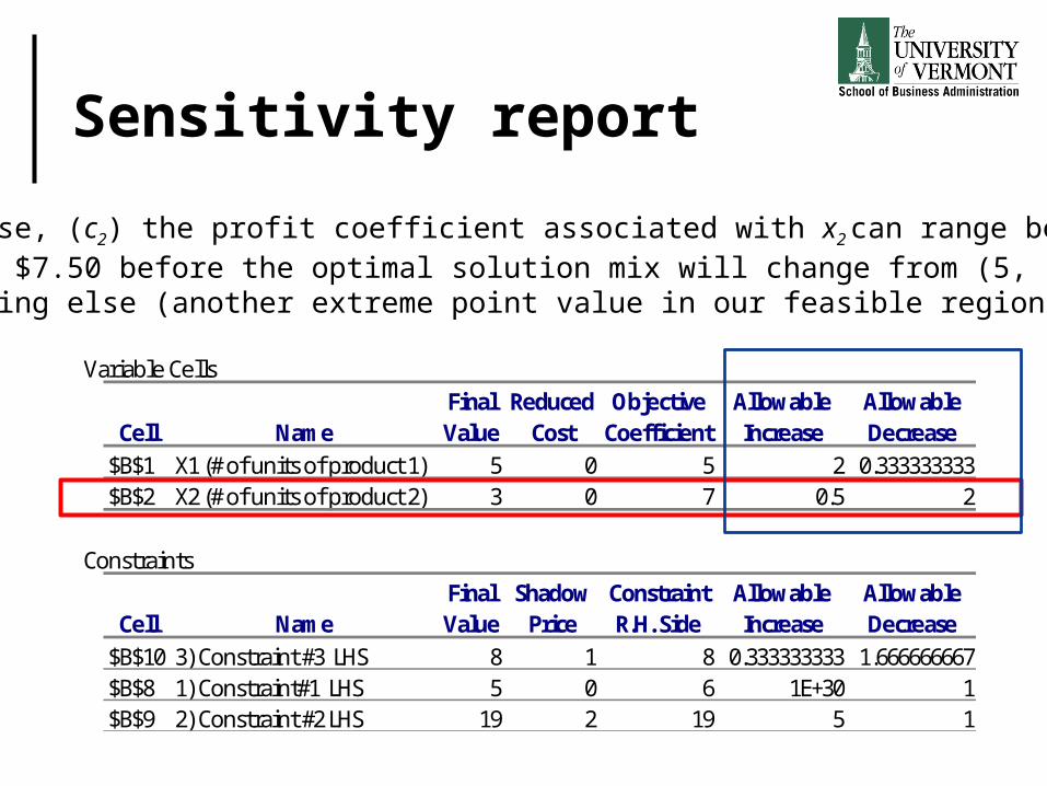
Likewise, (c2) the profit coefficient associated with x2 can range between $5 and $7.50 before the optimal solution mix will change from (5, 3) to something else (another extreme point value in our feasible region)
Sensitivity analysis
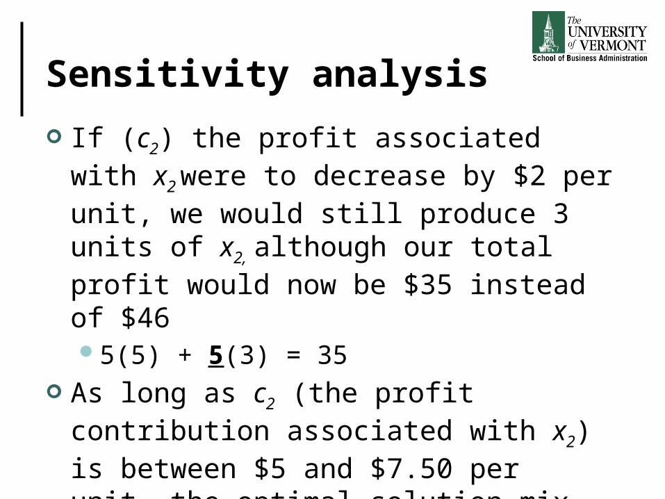
If (c2) the profit associated with x2 were to decrease by $2 per unit, we would still produce 3 units of x2, although our total profit would now be $35 instead of $46 5(5) + 5(3) = 35
As long as c2 (the profit contribution associated with x2) is between $5 and $7.50 per unit, the optimal solution mix of 5 units of x1 and 3 units of x2 will not change

Sensitivity analysis
The range of values c1 and c2 can take on without changing the optimal solution is referred to as the range of optimality for the objective function coefficientRange of optimality for c1: $4.67 – $7
Range of optimality for c2: $5 – $7.50

Graphical solution
Con 2: 2x1 + 3x2 < 19
x2
x1
Con 3: x1 + x2 < 8OF: Max 5x1 + 7x2OF: Max 5x1 + 7x2
Con 1: x1 < 6
Optimal Solution: x1 = 5, x2 = 3
8
7
6
5
4
3
2
1
1 2 3 4 5 6 7 8 9 10

Graphical solution
Con 2: 2x1 + 3x2 < 19
x2
x1
Con 3: x1 + x2 < 8 OF: Max 5x1 + 7x2OF: Max 5x1 + 7x2
Con 1: x1 < 6
Optimal Solution: x1 = 5, x2 = 3
8
7
6
5
4
3
2
1
1 2 3 4 5 6 7 8 9 10

Sensitivity analysis
A change in an OF coefficient changes the slope of the OF line!
Graphically, the limits of a range of optimality are found by changing the slope of the objective function line within the limits of the slopes of the binding constraint lines
Slope of an objective function line, Max c1x1 + c2x2, is (-c1/c2), and the slope of a constraint, a1x1 + a2x2 = b, is (-a1/a2)

Sensitivity analysis
Mathematically find the range of optimality for OF coefficient c1 (the coefficient associated with x1, which is 5)Slope of current OF line = (-c1/c2) = (-5 / 7)

Sensitivity analysis
Two binding constraints: Con 2 and Con 3Con 2: 2x1 + 3x2 = 19
• Slope of Con 2 = (-a1/a2) = (-2 / 3)
Con 3: x1 + x2 = 8• Slope of Con 3 = (-a1/a2) = (-1 / 1) = -1

Sensitivity analysis
Find the range of values for c1 (while holding c2 constant, or staying at $7), such that the slope of the OF line stays between the 2 binding constraints-1 < -c1 / 7 < -2 / 3 Slope of Con 2
Slope of Con 3

Sensitivity analysis
Find the range of optimality for c2 (the OF coefficient associated with x2 while holding c1 constant (fixed at 5)-1 < -5 / c2 < -2 / 3

Sensitivity analysis
x1
FeasibleRegion
x2 Coincides with Con 3: x1 + x2 < 88
7
6
5
4
3
2
1
1 2 3 4 5 6 7 8 9 10
Coincides with Con 2:2x1 + 3x2 < 19
Objective function line for 5x1 + 7x2

Sensitivity analysis
Second, let’s consider how changes in the constraint RHS coefficients might affect the feasible region as well as the optimal solution
Like changes in OF coefficients, we are considering one change at a time!
Changes in the RHS of a constraint are a more complicated sensitivity concept because changes in the RHS can change the entire feasible region for the problem
Sensitivity report
Variable CellsFinal Reduced Objective Allowable Allowable
Cell Name Value Cost Coefficient Increase Decrease$B$1 X1 (# of units of product 1) 5 0 5 2 0.333333333$B$2 X2 (# of units of product 2) 3 0 7 0.5 2
ConstraintsFinal Shadow Constraint Allowable Allowable
Cell Name Value Price R.H. Side Increase Decrease$B$10 3) Constraint #3 LHS 8 1 8 0.333333333 1.666666667$B$8 1) Constraint#1 LHS 5 0 6 1E+30 1$B$9 2) Constraint #2 LHS 19 2 19 5 1
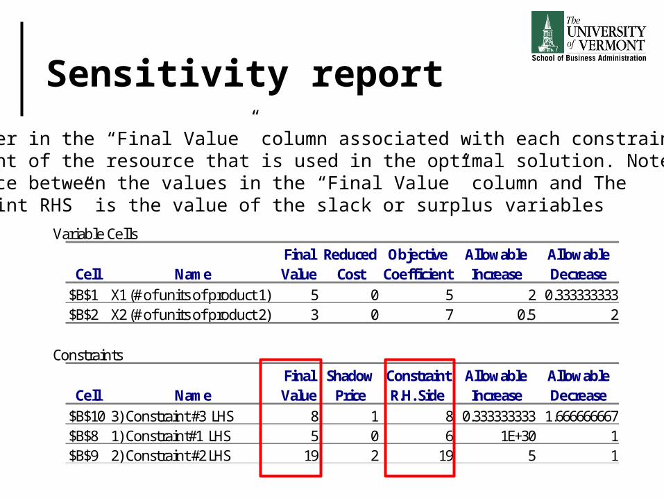
The number in the “Final Value” column associated with each constraint isthe amount of the resource that is used in the optimal solution. Note that the difference between the values in the “Final Value” column and The “Constraint RHS” is the value of the slack or surplus variables

Answer report
Objective Cell (Max)Cell Name Original Value Final Value
$B$4 Objective Function (Maximize Profit) 0 46
Variable CellsCell Name Original Value Final Value Integer
$B$1 X1 (# of units of product 1) 0 5 Contin$B$2 X2 (# of units of product 2) 0 3 Contin
ConstraintsCell Name Cell Value Formula Status Slack
$B$10 3) Constraint #3 LHS 8 $B$10<=$C$10 Binding 0$B$8 1) Constraint#1 LHS 5 $B$8<=$C$8 Not Binding 1$B$9 2) Constraint #2 LHS 19 $B$9<=$C$9 Binding 0
Shadow prices
The shadow price is a measure of the relative value of a resource, or the change in the OF value when increasing the resource by one unit
As the RHS of a constraint increases or decreases, other constraints may become binding and impact the optimal solution, so the shadow price interpretation is only applicable for SMALL changes in the RHS

Sensitivity reportVariable Cells
Final Reduced Objective Allowable AllowableCell Name Value Cost Coefficient Increase Decrease
$B$1 X1 (# of units of product 1) 5 0 5 2 0.333333333$B$2 X2 (# of units of product 2) 3 0 7 0.5 2
ConstraintsFinal Shadow Constraint Allowable Allowable
Cell Name Value Price R.H. Side Increase Decrease$B$10 3) Constraint #3 LHS 8 1 8 0.333333333 1.666666667$B$8 1) Constraint#1 LHS 5 0 6 1E+30 1$B$9 2) Constraint #2 LHS 19 2 19 5 1
Consider constraint #2: if we increase the RHS value from 19 to 20 units,our OF value (or profit) will increase by $2 (from $46 to $48)
If we decrease the RHS value from 19 to 18 units, our OF value (or profit) will decrease by $2 (from $46 to $44)

Graphical change in RHS
x1
FeasibleRegion
x2 Coincides with Con 3: x1 + x2 < 88
7
6
5
4
3
2
1
1 2 3 4 5 6 7 8 9 10
Coincides with NEW Con 2: 2x1 + 3x2 < 20
Coincides with Con 1: x1 < 6
Shadow prices
The Sensitivity Report provides information (although it is limited) on how changes in the values of the RHS of the constraints impact the optimal solution as well as the feasible region
We don’t have to completely reformulate and resolve the LP
Shadow prices
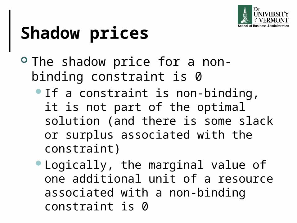
The shadow price for a non-binding constraint is 0If a constraint is non-binding, it is not part of
the optimal solution (and there is some slack or surplus associated with the constraint)
Logically, the marginal value of one additional unit of a resource associated with a non-binding constraint is 0

Shadow prices
The reduced cost associated with each decision variable is equal to the non-negativity constraint associated with the variable
This will become more of a focus as we investigate problems with more than 2 decision variables
Variable CellsFinal Reduced Objective Allowable Allowable
Cell Name Value Cost Coefficient Increase Decrease$B$1 X1 (# of units of product 1) 5 0 5 2 0.333333333$B$2 X2 (# of units of product 2) 3 0 7 0.5 2

Shadow prices
Some words of caution regarding interpretation of shadow pricesThe value of a shadow prices is generally
only applicable for small increases in the RHS • As more resources are available and the RHS
value increases, different sets of constraints become binding and change the optimal solution mix (the optimal values for x1 and x2)

Shadow prices
Some words of caution regarding interpretation of shadow pricesNot all shadow prices can be interpreted the
same wayWhile the shadow price is typically
interpreted as “the maximum amount you should be willing to pay for one additional unit of a resource”, this interpretation is not always correct
Shadow prices
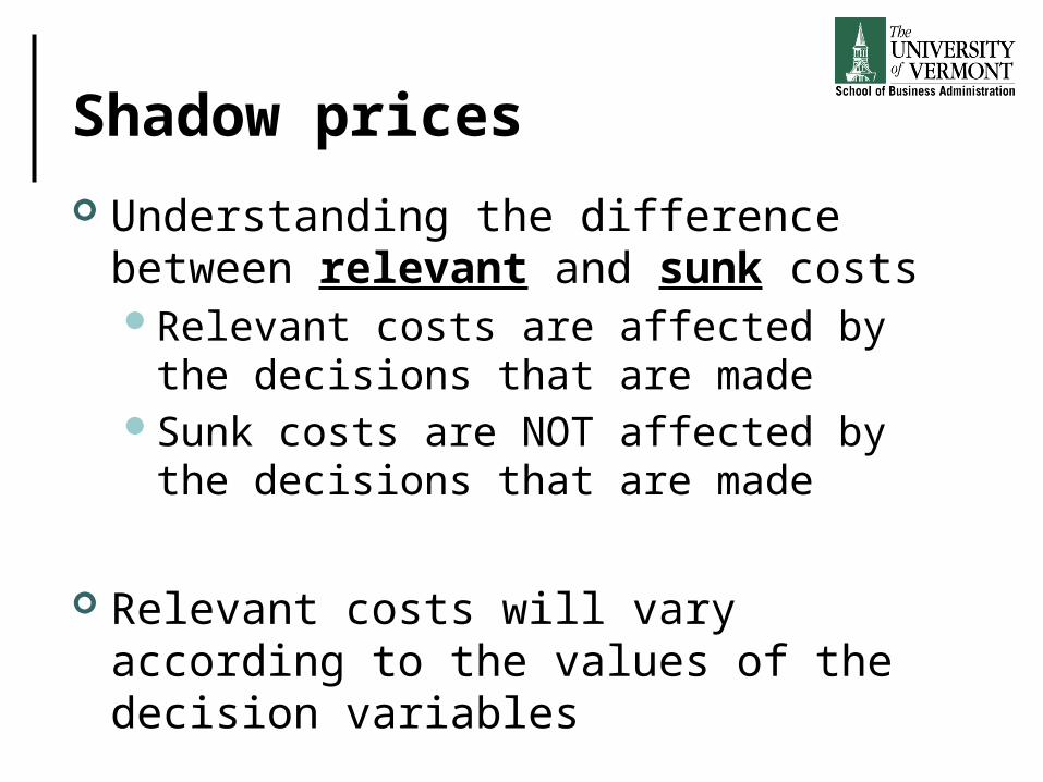
Understanding the difference between relevant and sunk costsRelevant costs are affected by the decisions
that are madeSunk costs are NOT affected by the
decisions that are made
Relevant costs will vary according to the values of the decision variables

Shadow prices
A resource cost is a relevant cost if the amount paid for that resource is dependent on the amount of the resource used by the decision variables
Relevant costs are reflected in the OF coefficients

Shadow prices
A resource cost is a sunk cost if it must be paid regardless of the amount of the resource that is actually used by the decision variables
Sunk costs are NOT reflected in the OF coefficients

Shadow price interpretation
Resource cost is relevantThe shadow price can be interpreted as the
amount by which the value of the resource exceeds its cost (or the premium over the normal cost that you should be willing to pay for one unit of that resource)
Resource cost is sunkThe shadow price can be interpreted as the
maximum that you should be willing to pay for one additional unit of that resource

Shadow prices Con 1: Since x1 < 6 is not a binding
constraint, its shadow price is 0 The allowable increase is
• If the amount of the resource used in the optimal solution is 5, which is less than the amount available (which is 6), increasing the amount of the resource available will not impact the solution in any way
The allowable decrease is 1• Further reducing the amount of the resource
available (below 5 units) will change the optimal solution as Con 1 now becomes binding

Shadow prices
Con 2: Shadow price of Con 2 is 2Adding one additional unit of resource
(increasing the RHS from 19 to 20 units) will increase our total profit by $2
This interpretation of the shadow price is applicable within the range of feasibility
Allowable increase is 5 Allowable decrease is 1
• The same set of binding constraints will remain binding within the RHS range of (18-24)

Shadow prices
Con 3: Shadow price of Con 3 is 1Adding one additional unit of resource
(increasing the RHS from 8 to 9 units) will increase our total profit by $1
This interpretation of the shadow price is applicable within the range of feasibility
Allowable increase is 0.33 Allowable decrease is 1.66
• The same set of binding constraints will remain binding within the RHS range of (6.34-8.33)

Shadow prices
Graphically, the range of feasibility is determined by finding the values of a RHS coefficient such that the same two lines that determined the original optimal solution continue to determine the optimal solution for the problem
To what extent can we make changes to the RHS of any one of the 3 constraints, so that the optimal solution still lies at the intersection of Con 2 and Con 3?

Shadow prices
This does not mean that the optimal solution won’t change within the range of feasibility, just that the same set of binding constraints (currently #2 and #3) will remain binding for changes to the RHS of either constraint – as long as those changes occur within the range of feasibilityWithin the range of feasibility, the
interpretation of the shadow price holds (the range where the shadow price is applicable)

Shadow prices
For changes to the RHS outside of the range of feasibility, the problem must be resolved to find the new shadow price
Only one RHS value can be changed at a time – does not apply to multiple simultaneous changes
Does not apply to changes in LHS constraint coefficients

Olympic bike example
Olympic Bike is introducing two new lightweight bicycle frames, the Deluxe and the Professional, to be made from special aluminum and steel alloys. The anticipated unit profits are $10 for the Deluxe and $15 for the Professional
A supplier delivers 100 lbs. of aluminum alloy and 80 lbs. of steel alloy per week. Each Deluxe requires 2lbs. of aluminum and 3 lbs. of steel. Each Professional requires 4 lbs. of aluminum and 2 lbs. of steel
How many of each type of frame should Olympic produce each week?

Olympic bike example

Olympic bike example
X1 (# of Deluxe frames) 15X2 (# of Professional frames) 17.5
Objective Function (Maximize Profit) 412.5
Constraints LHS RHSST:1) Constraint#1 (materials (aluminum) constraint) 100 1001) Constraint#1 (materials (steel) constraint) 80 80
Olympic bike example
What happens if the unit profit for the Deluxe frame changes from $10 to $20 – is the current solution still optimal?
Olympic bike example
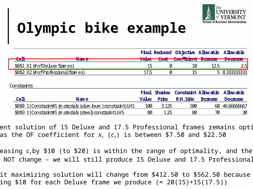
Final Reduced Objective Allowable AllowableCell Name Value Cost Coefficient Increase Decrease
$B$1 X1 (# of Deluxe frames) 15 0 10 12.5 2.5$B$2 X2 (# of Professional frames) 17.5 0 15 5 8.333333333
ConstraintsFinal Shadow Constraint Allowable Allowable
Cell Name Value Price R.H. Side Increase Decrease$B$8 1) Constraint#1 (materials (aluminum) constraint) LHS 100 3.125 100 60 46.66666667$B$9 1) Constraint#1 (materials (steel) constraint) LHS 80 1.25 80 70 30
The current solution of 15 Deluxe and 17.5 Professional frames remains optimalAs long as the OF coefficient for x1 (c1) is between $7.50 and $22.50
So, increasing c1 by $10 (to $20) is within the range of optimality, and the solution mix WILL NOT change – we will still produce 15 Deluxe and 17.5 Professional frames
The profit maximizing solution will change from $412.50 to $562.50 because we Are gaining $10 for each Deluxe frame we produce (= 20(15)+15(17.5))

Olympic bike example
What happens if the unit profit for the Deluxe frame changes from $10 to $6 – is the current solution still optimal?

Olympic bike example
Final Reduced Objective Allowable AllowableCell Name Value Cost Coefficient Increase Decrease
$B$1 X1 (# of Deluxe frames) 15 0 10 12.5 2.5$B$2 X2 (# of Professional frames) 17.5 0 15 5 8.333333333
ConstraintsFinal Shadow Constraint Allowable Allowable
Cell Name Value Price R.H. Side Increase Decrease$B$8 1) Constraint#1 (materials (aluminum) constraint) LHS 100 3.125 100 60 46.66666667$B$9 1) Constraint#1 (materials (steel) constraint) LHS 80 1.25 80 70 30
The current solution of 15 Deluxe and 17.5 Professional frames remains optimalAs long as the OF coefficient for x1 (c1) is between $7.50 and $22.50
So, decreasing c1 by $4 (to $6) is OUTSIDE the range of optimality, and the solution mix WILL change – we have to reformulate and re-solve the problem

Olympic bike example
Assume aluminum alloy is a sunk cost What is the maximum amount Olympic
should pay for 50 extra lbs. of aluminum alloy?

Olympic bike example
Final Reduced Objective Allowable AllowableCell Name Value Cost Coefficient Increase Decrease
$B$1 X1 (# of Deluxe frames) 15 0 10 12.5 2.5$B$2 X2 (# of Professional frames) 17.5 0 15 5 8.333333333
ConstraintsFinal Shadow Constraint Allowable Allowable
Cell Name Value Price R.H. Side Increase Decrease$B$8 1) Constraint#1 (materials (aluminum) constraint) LHS 100 3.125 100 60 46.66666667$B$9 1) Constraint#1 (materials (steel) constraint) LHS 80 1.25 80 70 30
For a sunk cost, the shadow price is interpreted as the value of extra aluminum (wealready have paid for 100 lbs.) – what is the value of 50 additional lbs.?
Shadow price = $3.125 per lb. the allowable increase is 60, so the shadow priceinterpretation holds for 50 additional lbs.
The value of 50 additional lbs. of aluminum alloy is 50 * $3.125 = $156.25
Olympic bike example
Assume aluminum alloy is a relevant cost What is the maximum amount Olympic
should pay for 50 extra lbs. of aluminum alloy?

Olympic bike example
If aluminum alloy is a relevant cost, the shadow price represents the amount above the normal/initial price of aluminum the company should be willing to pay for additional aluminum (the premium Olympic is willing to pay for more of the resource)If aluminum were initially $4 per lb., then
additional units of aluminum (beyond the initial 100 lbs. and within the feasible range) would be worth $7.125 per lb. to Olympic
Summary
Introduction to sensitivity analysisChanges in objective function coefficients
• What does this mean graphically?• How are these changes interpreted?
Changes in RHS values• What does this mean graphically?• How are these changes interpreted?
Summary
Interpretation of shadow pricesWhere to find these on the Sensitivity ReportRange of feasibilitySunk costs versus relevant costs
Olympic bike example
Related Documents