NASA Technical Memorandum 82534 Seneiti~it~IComparieon Study Between the Jacchia 1970, 1971, and 1977 Upper Atmoepheric Density Modele Dale L. Johnson Georpe C. Marshall Space Flight Center Marshall Space Flkht Center, Alabama National Aeronat~t ics and Space Adrn~nistration Sslentlfic and ' chnicrl Intonnrtlon brrnch

Welcome message from author
This document is posted to help you gain knowledge. Please leave a comment to let me know what you think about it! Share it to your friends and learn new things together.
Transcript
NASA Technical Memorandum 82534
Seneiti~it~IComparieon Study Between the Jacchia 1970, 1971, and 1977 Upper Atmoepheric Density Modele
Dale L. Johnson Georpe C. Marshall Space Flight Center Marshall Space Flkht Center, Alabama
National Aeronat~t ics and Space Adrn~nistration
Sslentlfic and ' chnicrl Intonnrtlon brrnch

TABLE OF CONTENTS
Page
. . . . . . . . . . . . . . . . . . . . . . . . . . . . . . . . . . . . . . . . . . . . . . . . . . . . . . . . . I . INTRODUCTION 1
I1 . PRESENTATION OF DATAIRESULTS . . . . . . . . . . . . . . . . . . . . . . . . . . . . . . . . . . . . . . . . 2
. . . . . . . . . . . . . . . . . . . . . . . . . . . . . . . . . . . . I11 DISCUSSION OF COMPARATIVE RESULTS 117
. . . . . . . . . . . . . . . . . . . . . . . . . . . . . . . . . . . . A Intra-Model Testing Under Constant Flux 117 B . Intra-Model Testing Under Constant A . . . . . . . . . . . . . . . . . . . . . . . . . . . . . . . . . . . . 118 C . Inter-Model Testing Under Constant F&X . . . . . . . . . . . . . . . . . . . . . . . . . . . . . . . . . . . 122 D . Inter-Model Testing Under Constant Ap . . . . . . . . . . . . . . . . . . . . . . . . . . . . . . . . . . . . 124
REFERENCES . . . . . . . . . . . . . . . . . . . . . . . . . . . . . . . . . . . . . . . . . . . . . . . . . . . . . . . . . . . . . . . . . . . 130
r m m G PAGE BLANK NOT FILMEa
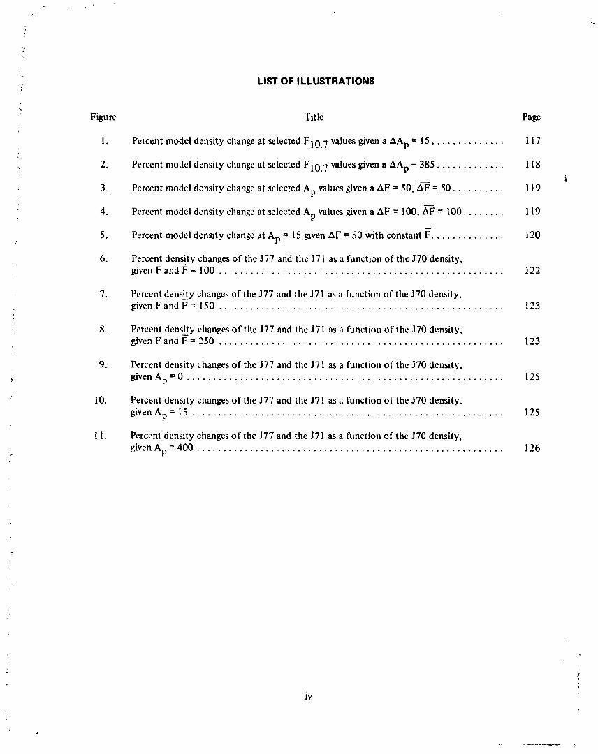
LIST OF ILLUSTRATIONS
Figure Title Page
. . . . . . . . . . . . . 1. Pelcent model density change at selected FlOa7 values given a AAp = 15. 1 17
. . . . . . . . . . . . 2. Percent model density change at selected FlOv7 values given a AAp = 385. 118 i
3. Percent model density change at selected Ap values given a AF = 50, = 50. . . . . . . . . . 1 19
. . . . . . . 4. Percent model density change at selected A values given a AF = 100, = 100. 119 P -
. . . . . . . . . . . . . 5 . Percent model density change at Ap = 15 given AF = 50 with constant F. 120
6 . Percent density changes of the 577 and the J71 as a function of the J70 density, - . . . . . . . . . . . . . . . . . . . . . . . . . . . . . . . . . . . . . . . . . . . . . . . . . . . . . . g ivenFandF=lOO 122
7. Percent density - changes of the 577 and the 371 as a function of the 370 density, g i v e n F a n d F = 1 5 0 . . . . . . . . . . . . . . . . . . . . . . . . . . . . . . . . . . . . . . . . . . . . . . . . . . . . . . 123
8. Percent density - changes of the 577 and the 571 as a function of the 570 density, . . . . . . . . . . . . . . . . . . . . . . . . . . . . . . . . . . . . . . . . . . . . . . . . . . . . . . give : lFandF=250 123
9. Percent density changes of the 577 and the 37 1 as a function of the 570 density, givenAp=O . . . . . . . . . . . . . . . . . . . . . . . . . . . . . . . . . . . . . . . . . . . . . . . . . . . . . . . . . . . . 125
10. Percent density changes of the 377 and the 571 as a function of the 570 density. g ivenAp=15 . . . . . . . . . . . . . . . . . . . . . . . . . . . . . . . . . . . . . . . . . . . . . . . . . . . . . . . . . . . 125
1 1. Percent density changes of the 577 and the 57 1 as a function of the 570 density, g ivenAp=400 . . . . . . . . . . . . . . . . . . . . . . . . . . . . . . . . . . . . . . . . . . . . . . . . . . . . . . . . . . 126
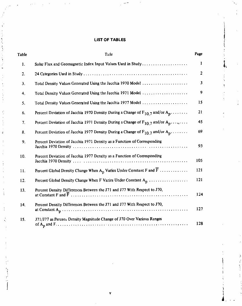
6. LIST OF TABLES
Table Tiile Page
1. Solar Flux and Geomagnetic Index Input Values Used in Study. . . . . . . . . . . . . . . . . . . . . 1 %
2. 24 Categories Used in Study . . . . . . . . . . . . . . . . . . . . . . . . . . . . . . . . . . . . . . . . . . . . . . . . 2
i 3. Total Density Values Generated Using the Jacchia 1970 Model . . . . . . . . . . . . . . . . . . . . . 3
4. Total Density Values Generated Using the Jacchia 1971 Model . . . . . . . . . . . . . . . . . . . . . 9
5. Total Density Values Generated Using the Jacchia 1977 Model . . . , . . . . . . . . . . . . . . . . . 15
6. Percent Deviation of Jacchia 1970 Density During a Change of F10 7 and/or Ap. . . . . . . . 2 1
7. Percent Deviation of Jacchia 1971 Density During a Change of F10 7 and/or Ap. . . ,,. . . . 45
Percent Deviation of Jacchia 1977 Density During a Change of F10 7 and/or Ap. . . . . . . . 69
Percent Deviation of Jacchia 197 1 Density as a Function of Corresponding Jacchia1970Density . . . . . . . . . . . . . . . . . . . . . . . . . . . . . . . . . . . . . . . . . . . . . . . . . . . . . 93
Percent Deviation of Jacchia 1977 Density as a Function of Corresponding Jacchia 1970 Density . . . . . . . . . . . . . . . . . . . . . . . . . . . . . . . . . . . . . . . . . . . . . . . . . . . . 105
Percent Global Density Change When Ap Varies Under Constant F and Y . . . . . . . . . . . . . 1 2 1
Percent Global Density Change When F Varies Under Constant Ap . . . . . . . . . . . . . . . . . . 121
Percent Density Differences - Between the 571 and 577 With Respect to 570, a t C o n s t a n t F a n d F . . . . . . . . . . . . . . . . . . . . . . . . . . . . . . . . . . . . . . . . . . . . . . . . . . . . . . 124
Percent Density Differences Between the 571 and 577 With Respect t o 570, at Constant Ap . . . . . . . . . . . . . . . . . . . . . . . . . . . . . . . . . . . . . . . . . . . . . . . . . . . . . . . . . . 127
J71/J77 as Perceni Density Magnitude Change of J70 Over Various Ranges o f A p a n d F . . . . . . . . . . . . . . . . . . . . . . . . . . . . . . . . . . . . . . . . . . . . . . . . . . . . . . . . . . . . . 128

TECHNICAL MEMORANDUM
SENSITIVITY/COMPARISON STUDY BETWEEN THE JACCHIA 1970, 1971, AND 1977 UPPER ATMOSPHERIC DENSITY MODELS
The thermospheric model curret~tly used by NASA-MSFC in orbital dynamics and lifetime estimates is the 1970 Jacchia (570) model [ 1 I as reported on in 1973 [2]. It was slightly modified in 1974, and has been used as the MSFC standard. Two additional Jacchia models have become available and have been computerized for possible use. These are the 1971 Jacchia (571) model [3 ] and the 1977 Jacchia (J77) model (41. It wan determined that a parametric study was needed involving the computa- tion and comparison of total density from each of the three models. Also the establishment of each models sensitivity to the differing solar input conditions is desirable.
Total atmospheric density computations were made using all three models, over a wide range of solar and geomagnetic conditions. Comparisons were then made based on these results to determine the sensitivity of each model to differing solar/geomagnetic input. Twelve different cases of solar/geomag- netic input were used in the study and are summarized in Table 1. The average, daily solar flux - parameter F10 7, along with the 162-day ceiltered average solar flux parameter F10 7 and three hourly
average geomagnetic index A (or K ) were the three solar/geomagnetic inputs to each model tested.* P P -
Values representing solar conditions close t o low, medium, and high were used. This included FlOs7
values of 100, 150, and 250. Daily FlO., values of 100, 150, 200, 250, and 300 were used, along with
Ap values of 0, 15, and 400 (Kp = 0, 3, and 9). The altitude level of 400 km was chosen because it is close to the orbital levels of many NASA spacecraft. June 20 at 12 UT was selected so the models could run near the Summer Solstice when the diurnal bulge maximum is located north of the equator in the northern hemisphere. All computations were computed over an 81-point latitude/longitude Earth matrix consisting of nine latitudes from 80°N to 80°S, along with nine longitudes from 40°E to 360°, with spacing of 20" for latitude and 40' for longitude.
TABLE 1. SOLAR FLUX AND GEOMAGNETIC INDEX INPUT VALUES USED IN STUDY
Date: June 20; Time: 13, UT; Altitude: 400 km
*In this idealized exercise, the 3-hourly predicted ap values were substituted by the daily Ap values.
Case No.
1 2 3 4
5 6 7 8 9
10 11 12
-
- F10.7
100 100 100 100 150 150 150 150 250 250 250 250
1
F10.7
1 00 100 100 150 150 150 150 200 250 250 250 300
. A ~ l K ~
010 1513
40019 1513
010 1513
40019 1513
1513 010
40019 1513

The currently used 370 modified model atmosphere is considered the standard throughout the study, and most con~putations involved here are expressed as a percentage difference in density ( p ) from the 370, i.e..
J71 - p J70 x 100 = W diff. p J70
Other times, percent differences in density were computed for two different input cases involving the same Jacchia model. In this instance the percent difference equation can be expressed as
p 5'71 (case 2) - p J71 (case 1) x 100 = 76 diff. ,
p 371 (case 1)
where 37 1 caw 2 is expressed as a percent difference from 57 1 case 1. Table 2 lists 24 different coni- binations or categories of percent deviations that were calculated. involving a case difference with respect to the same Jacchia model.
TABLE 2. 24 CATEGORIES USED IN STUDY
Category
A B C D E, F G H I J K L
II. PRESENTATION OF DATA/RESULTS
Case Difference j 2- 1 3-2 3- 1 4-2 6-5 7-6 7-5 8-6 10-9
11-10 11-9
12-10 .
The total density values computed using the 370, 571, and 377 models for the 12 different input 3 cases are presented in Tables 5, 4, and 5, respectively. 1 he units of density are in kg/m and were
computed over an Earth-matrix (81 point grid) with increment spacing of every 20 deg latitude and 40 deg longitude. The maximum density bulge is noticed in most cases to be located at the 20°N latitude and 40°E longitude location. The bulge maximum is located at 40°E only because of the matrix used. Actual bulge maxiniurn is at 23?h0 during Summer Solstice.
- Category
M N 0 P Q R S T U V W X
i
Case Difference
5- 1 9-5 9- 1 6-2 10-6 10-2 7-3 11-7 11-3 8-4 12-8 1 2-4 .

TABLE 3. TOTAL DENSlTY VALUES GENl3RATE.D WING THE lMXHU 1970 MODIU
Cue 1. Input :
htm: .I- 20, la61
Altitud.: 400 b $10.7 = 1 0 0 FlO.76 = 100 b ' 0 ( Q - 0 )
Output : 570 Donrity (r10'~~ 4)
Input : Date: 5 ~ 0 20, 1968 T i n : 12 VT Altitude: 400 It. F10.7 - 100 F10.7B 100 4' ' IS ( I lp-3)
Output : 570 Density (xlO'lt Kg/Ns)

. . . , l L . / , i ' .--
I . : . . , . . - ' . - ' . " < & *--
- m m TABLE 3. (Continued) 0 CQQ(I pllluly
Input : Date: June 20, 1968 T*: 12 w Altitude: 400 I@ $10.7 = 100 P10.78 = 100 Q =400 ( K P - 9 )
Output : J70 Density ( ~ 1 0 ~ ~ ~ 4)
Degrees Latitude (+N)
-60 -40 -20 0 20 40 60 80
Input : Date: June 20, 1968 T i m : 12 UT Altitude: 400 11* F10.7 /50 F10.7B = /00 4' = / 5 (I(p-31
Output : 570 Density (~10'~~ Kg/M3)
Degrees Latitude (+N)

TABLE 3. (Continued)
CIS. 5. Input :
Date: June 20, 1958 T i n : 12 VT Altitude: 400 lb FlO.7 = 1 5 0 F10.7B m 150 AP = 0 (KP 0 1
Output : 570 Density (x10-l1 ~g/n']
Degrees La titude (+N)
Input : Date: June 20, 1968 Time : 12 VT Altitude: 400 K. F10.7 = 150 F10.7B = 150 Ap = / Q ( K p - 2 )
output : 570 Density ( ~ 1 0 ' ~ ~ K~/M')
Degrees Latitude (+N)

C u m jlI Input :
Data: June 20, 1968 Tho: 12 UT Altitude: 400 lh P10.7 = 150 P10.78 = 150 Ap =LFOO ( K P - 9 )
W p u t : J70 Density (xlO'll K&)
Case 8. Input :
Date: June 20, 1968 T i r : 1 2 m Altitude: 200 ta $10.7 = 200 P10.711 = 150 4 w 1 5 (I(p13)
(lutplt: 570 Density ( ~ 1 0 ' ~ ~ KO/M')
Degrees Latitude (+N)

ORIrnAL P a TABLE 3. (Continuo4
OF POOR QUALrrV C.,. 9.
Input : Date: June 20, 1968 Tim : 12 VI Altitude: 400 R F10.7 250 FlO.7B * 250 4 - 0 (lip 0 )
Output : 570 Density ( ~ 1 0 ' ~ ~ wS]
Degrees Latitude (+N)
c a s d O Input :
Date: June 20, 1961 T i n : 12 IIT Altitude: 400 L F10.7 = 250 F10.78 = 250 4 I5 ( b m 3 )
De#roes Latitude (+N)
w -80 -60 -40 - 20 0 20
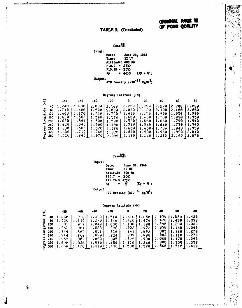
TABLE 3. (Conoluded)
Input : Date: June 20, 1968 Tir: 12UT Altitude: 400 #r P10.7 - 250 F10.7B = 250 4) -400 (KPm9)
Output : 370 Density ( ~ 1 0 ' ~ ~ 4)
Rgrees Latitude (+N) n w -80 -60 -40 - 20 0 20 40 60 80 Y
-
Input : Date: J w e 20, 1%) Tim: 12 VT Altitude: 400 Km F10.7 300 F10.7B = 250 AP - ! 5 (ltP=3)
(ktput : 570 Density ( ~ 1 0 ' ~ ~ Kg/n3)
Degrees Latitude (+N)
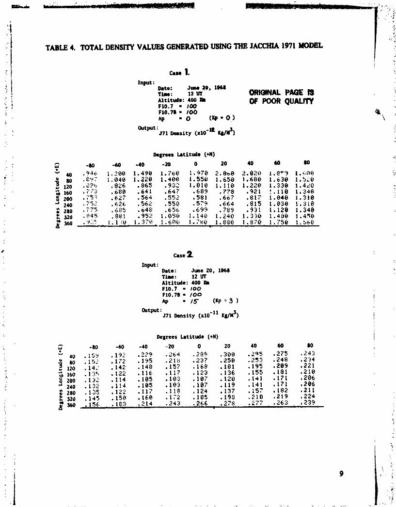
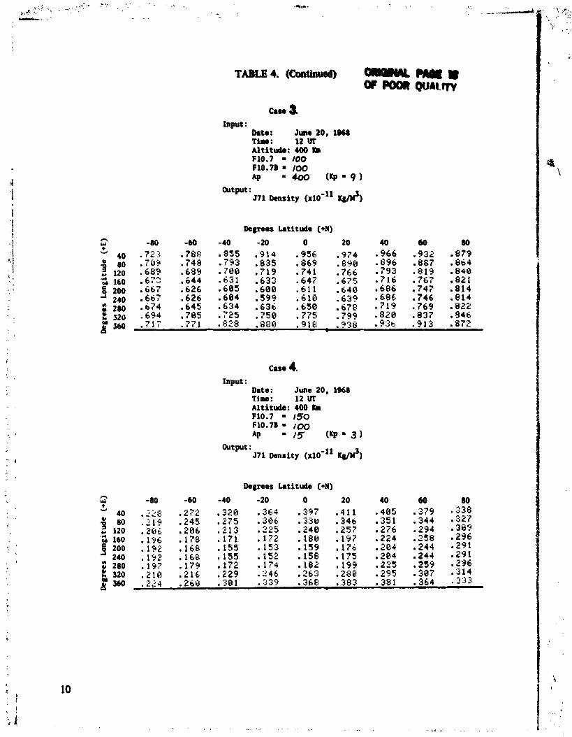
TABLE 4. TOTAL DENSITY VALUES GBNERATBD USING THE JACMU 1971 YODEL
Input : wte: JUW 20. 1W8 T-: 12m ORKWNAL PAGE IS Altitude: 400 F10.7 = 1 6 0
OF POOR QUALITY
output : 571 Density (xlO'lL WN')
Input : mte: JAG 20, 1968 Tiw: 12 ur Altitude: 400 k F10.7 = 100 F10.7B = 100 & = 15 (KP = 3 1
Output : 571 Density
Degrees Latitude (+N) h w -80 -60 -40 -20 0 20 40 60 80 ' 40 . ~ S Y -192 . 3 2 9 , 2 6 4 .283 . 300 .2?5 - 2 7 5 - 2 4 3
80 , , ,172 -195 , 318 .237 .256 . 2 5 3 ,248 ,294 120 1 .I42 .I48 ,157 ,168 ,181 .I95 ,209 ,221
.* 160 .13r, .I22 ,116 ,117 ,123 .136 .I55 ,181 e21B 8 200 ,132 ,114 .I05 ,103 .I07 ,128 .I41 9171 *2Qh -' 240 . I 3 2 .I14 ,185 ,103 -107 ,119 ,141 -171 m206
f 210 .I25 . 192 .I17 118 -124 ,137 ,157 ,182 a211
:PO ,145 .I50 .I60 .1?2 .I85 ,199 .210 .219 , 224 , is(. . 183 .214 .243 .266 .278 . 277 .263 , ,239
Input : b t o : J w 20, 1968 T : 12Vf A l t i t u d . : 400 b F10.7 = 100 FlO.7B = 1 6 0 4 =+oo ( Q = 9 )
Output : J71 Density ( x 1 0 - ~ ~ rp/W5)
Cue 4. Input :
Date: June 20, 1%8 Tim: 12 VT Altitude: 400 k F10.7 = 150 F10.71) = 100 AP 5 (I(p-3)
Output : J7l Density (~10'" Kg/$)
Degrees Latitude (+N)

TABLE 4. (Continued)
Input : ate: June 20, 1W8 Tim: 12 Vf
Output : ~ 7 1 wnrity (x10-l1 wnS)
lkgrecs Latitude (+N)
Input : Date: June 20, 1968 Time: 12Vf
b t p u t : J7l Density ( ~ 1 0 ' ~ ' K~/w')
Degrees Latitude (+N)

- + 40
' 80 4, 120 '$ 160 8 zoo a 240 % 280 s 320 €9
Input : Date: Juae 20, 1W8 Tim: 12 W
Output : J ~ I Density (~10-l1 IWA
Degrees Latitude (*N)
Case 8. Input :
Date: June 20, 1968 T i m : 12 UT Altitude: 400 L F10.7 = 230 F10.7B = 150 b = /5 ( K p - 3 )
output : J7l Density ( ~ 1 0 ' ~ ~ K~/M')
Degrees Latitude (+N)
-60 -40 - 20 0 20 40 60 80 .S29 -607 ,676 ,727 ,749 *739 ,699 ,635 ,484 ,534 ,583 ,623 .648 ,655 .644 ,617 .419 9431 ,451 .476 ,504 ,535 ,564 ,589 3 9357 ,359 ,373 ,403 ,440 ,585 .563 ,352 -336 e 3 2 L . 3 3 6 ,366 4 , 482 ,559 .352 .a29 ,325 ,335 .365 ,415 ,482 ,559 ,372 ,360 .362 .377 ,407 .451 ,587 .568 ,434 0458 ,486 .514 .542 e566 ,585 ,596 . S 10 ~ 5 7 5 . , 636 . .681 a ,705 ,783 - ,675 .627
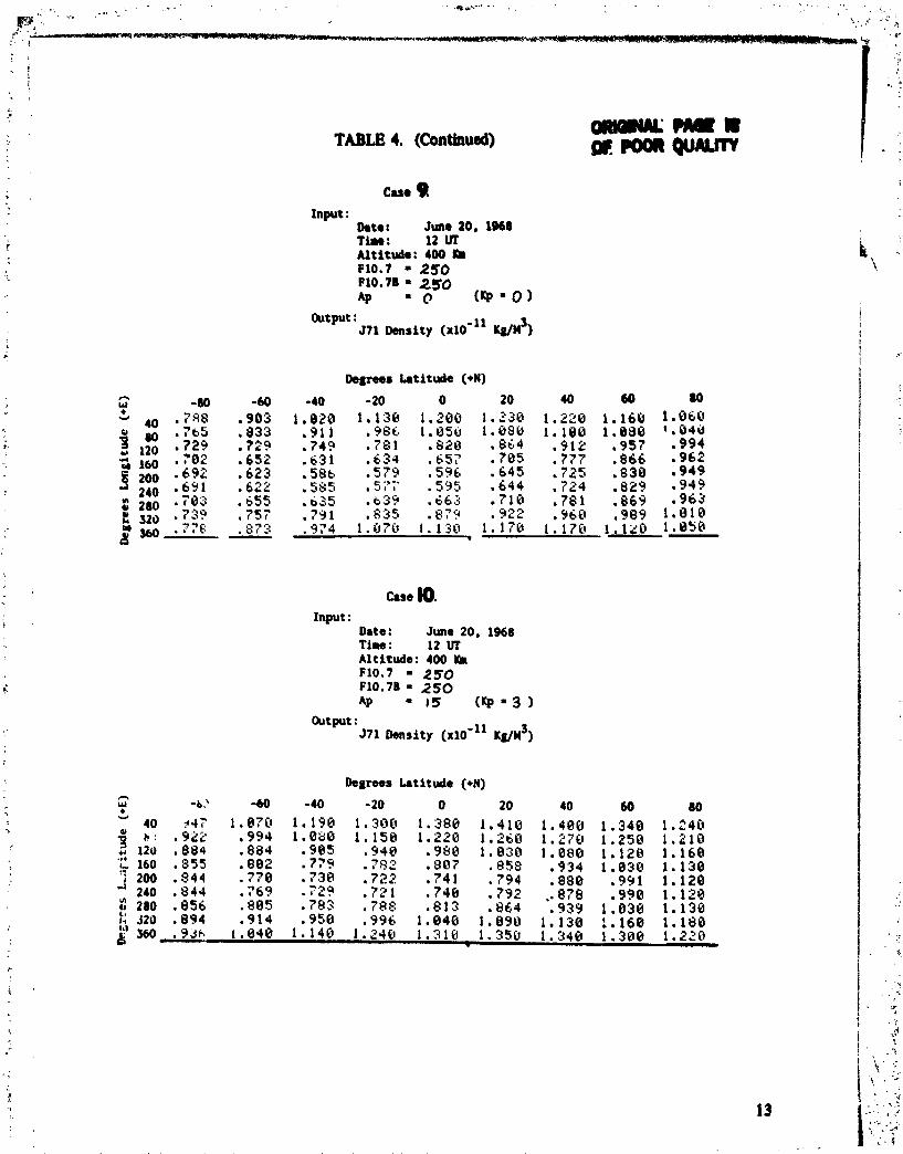
TABLE 4. (Continued)
Input : Date: June 20, 1968 T i n : 12UT Altitude: 400 lb $10.7 = 250 PiO.78 2250 4' - 0 ( Q - 0 )
Output : J7l Density ( ~ 1 0 ' ~ ' ICg/bt3)
Degrees Latitude (+N)
Case 10. Input :
Date: June 20, 1968 T im : 12 UT Altitude: 400 #r ~ 1 0 . 7 = 250 F10.78 = 250 4' = I (KP - 3 1
Output : J7l Density ( ~ 1 0 ' ~ ~ Kg/M3)
Degrees Latitude (+N)

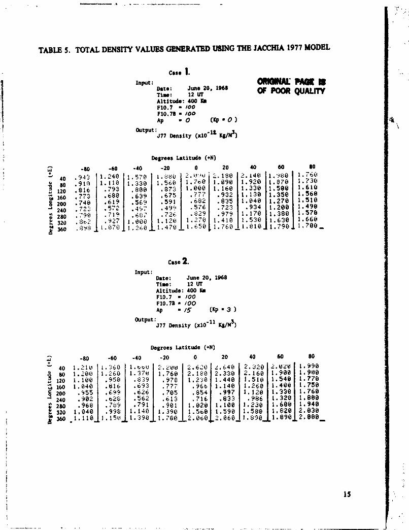
TABLE 5. TOTAL DENSITY VALUBS GEMERATf3D USING THE J A M M 1977 MODEL
Input :
case 1.
Date: J w e 20, 1968 ollmwwII
T i n : 1 2 m OF POOR QUALlFY ~ l t i t u d e : 400 It. FlO.7 100 FlO.7B = 100 Ap - 0 (Kp = 0
Output : J77 Density ( X ~ O - ~ ' Kg/n3)
Degrees b t i t u d e (+N)
Case 2. Input :
Date: June 20, 1968 Time: 12 Altitude: 400 Ylr F10.7 = 100 F10.70 = /00 AP - 15 / U - 3 )
Output : 577 Density (x10-l1 KS/M')
Degrces Latitude (+N) CI -60 -40 -20 0 20 40 60 80 -80
. ti13

TABLE 5. (Continusd)
Irtput : Date: June 20, 1968 Tiw: 12 UT Altitude: 400 #r FlO.7 - 1 0 0 F10.78 = 100 Ap -400 (KP-9
Output : 577 Density ( ~ 1 0 - l 1 &)
Degrees h t i t u d e (+N)
-89 -60 -40 -20 0
Care 4. Input :
Dote: June 20, 1968 T i n : 12 VT Altitude: 400 Km F10.7 = I50 FlO. 7B - 100 e = / 5 ( 4 - 3 )
output : 577 Density ( ~ 1 0 ' ~ ' K~/H')
Degrees Latitude (+N)
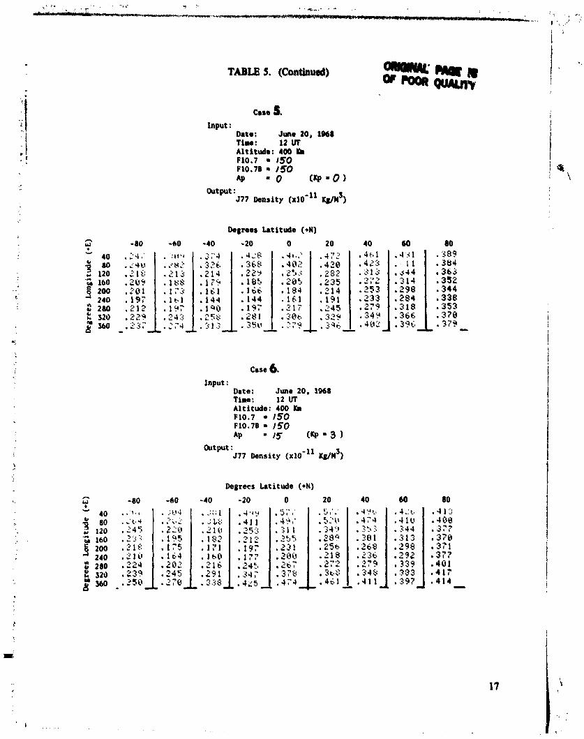
TABLE S. (Continued)
Input : Date: J w o 20, 1068 Time : 12 VT Altitude: 400 lb F10.7 - IS0 F10.70 /50 @ = o ( K p r O )
output : 577 Density (xlO'll wnS)
Degrees Latitude (+N)
Case 6. Input :
Date: June 20, 1968 Time : 12 VT Altitude: 400 L F10.7 = 150 F10.70 = /SO AP = 5 (I@ = 3 1
output : 577 Density (~10 - I ' K&/#')
Degrecs Latitude (+N)

TABLE 5. (Conthud) ORIaNawmrr O F Q O O l P ~ n v
Case I! Input :
Date: June 20, 1968 Tim: 12UT Altitude: 400 R F10.7 = 150 FlO. 71) /SO Ap -a ( I ( p - 9 )
Output : J77 Donsity (~110'~~ wS)
Degrees Latitude (+N)
40 , .,.
. I c &
.810 ,634 498
. 4 30
. 455 . d d l
.73b
. h S 2
Case 8. Input :
Date: June 20, 1968 Ti- : 12 VF Altitude: 400 KB F10.7 = 200 F10.71) / S O 4 ' 1 5 (Kp-3)
Output : 577 Density (xlo-l1 Kg/M3)
Degrees Latitude (+N) n Y -80 -60 -40 - 20 0 20 40 a 80

TABLB 5. (Continual)
Input : Date: Juno 20, 1968 T h e : 12 VT Altitude: 400 KR Pl0.7 = 250 PlO.70 250 rrp = o ( K p = O )
Output : J77 Donsity ( ~ 1 0 ' ~ ~ Kg/$)
Dogrws latitude (+N)
w^ -80 -bO -40 -20 0 20 40 60
Input : Dew: June 20, 1968 T i n : 12 UT Altitude: 400 KR P10.7 = 250 F10.70 = 250 Ap 15 ( K p - 3 )
Output : J77 Density (xl0-" Kg/$)
k g m s latitude (+N)
-40 -20 0 20
, 4 4 3 .683 ,479 ,596
, 697
-
.r :y .a .': :* . ,, , . _ q r . , .?
5 .~ . . , ? ' -
t.".
....
I...
',a
L. , .
\ .;
i'
'[
i
T
4 ?.
4 :
.- . r: A$" . .
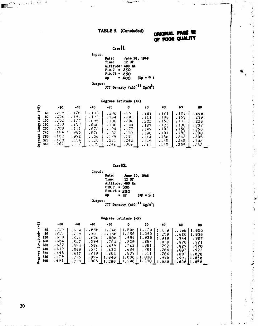
TABLE 5. (Conoluded) -HQ* ormQu-
Input : Date: June 20, 1968 Tim : 12 UT Altitude: 400 k F10.7 m 250 F10.7D = 250 4 -400 (KP-9)
Output: JV Density ( ~ 1 0 - l 1 ~tp /~ ' )
Degrees Latitude (+N)
Input : Date: June 20, 1968 T i u : 12 UT Altitude: 400 L F10.7 300 Fl0.7B 250 4 = I 5 (l(p.3)
Output: J77 Density (~10'" K~/M')
Degrees Lat

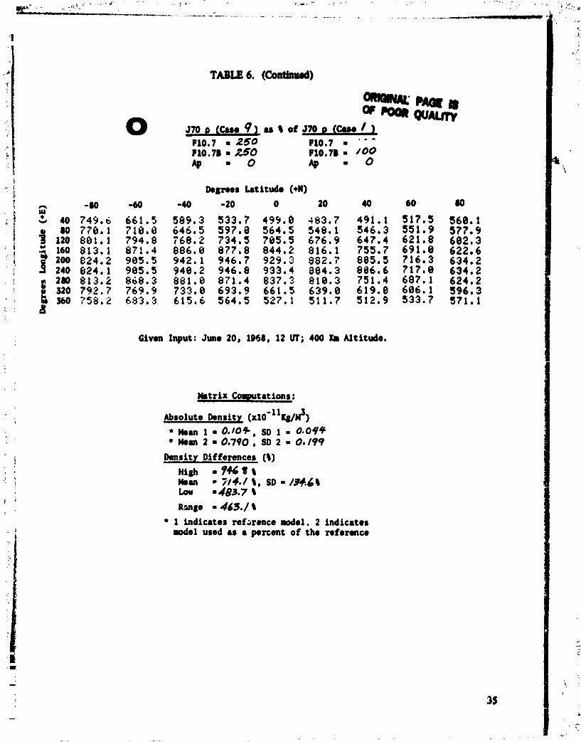
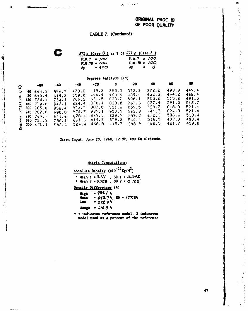
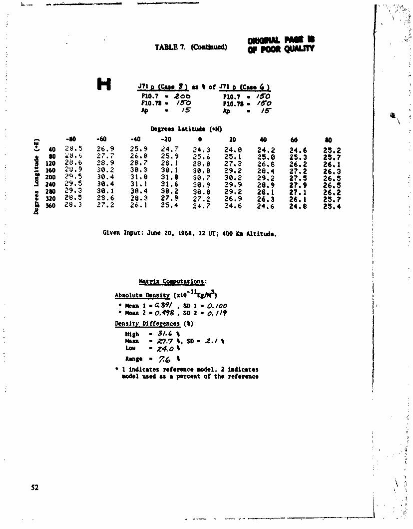
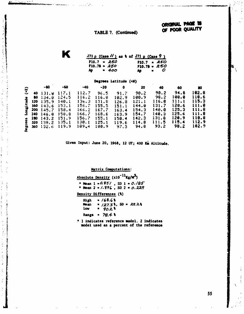
T a b k 6, 7, and 8 @ve the percent difference of intarmodel dendty than@ for the map~t tvc J70, J71, and J77 modela, given a change in flux andlor geomagnetic index. Baddm the rtrndud 81 point matrix output of density change given in percent, the tabla @ve the mean curd rturdud deviation of all 81 matrix computations, slow with the lowest and higheat matrix value (both wed to compute range). Also, the 81 absolute density matrix d u a for each cr# have been pmcewcd and mean, with standard deviation results, have b a n computed and are bted on each table.
TABLE 6. PERCENT DEVIATION OF JACCHIA 1970 DENSITY DURING A CHLVGE OF F10a7 AND/OR Ap
J7n p (Case 2 ) as 8 of 570 p (Cue I 1 FlO.7 = /00 F10.7 100 F10.7B = /00 FlO.7B = 100 4' = 15 4 0
Degrees Latitude (+N)
Given Input: June 20, 1968, 12 UT; 400 1(1 Altitude.
Matrix ColaputatioI!:~.:
Absolute Density (X~O'"K~/M~]
wan 1 = 0.109, SD 1 = 0.044 M ~ M t = 0.172, SD 2 = 0.059
Density Differences (t) High = 93.7 # Mean = 70.4 a, SD = 13.4 % Low = 4 6 . 9 1
Range = 46.0 1 1 indicates reference model. ? indicates model used as a percent of the reference

C~ . ' '" '
TABLE 6. (Continued) - m m cw POOR QUALnY
Degrees Latitude (+N)
Givm Input: June 20, 1968, 12 lR; 400 K. Altitude.
Mtrix Comutrtions:
Density Differences (I)
High = 5351 1 Msm = j n o t , S D m 89.91 Low ' ~ t 2 1 . 4 1 h g e = 313.71
1 indicates reference model. 2 indicates d e l used as a percent o f the reference
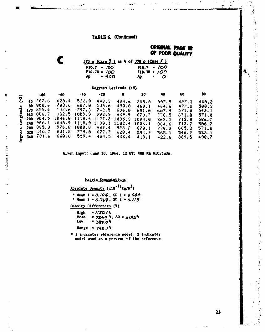
TABLE 6. (Cofitlauab)
Given Input: June 20, 1968, 12 VT; 400 Ku Altitude.
Matrix Computations:
~ s o ~ u t e Density ( x l ~ - ~ ~ ~ g / ~ ~ ) man 1 = 0 , / 0 4 , SD 1 r 0.044 Meu\ 2 0.768s 2 ' 0 . ) ) 5
Density Differences (8) High = //30. I 8 k m 7269 8 r SD * 218.58 LOW =3att.o#
h u e = 742.1 1 I indicates reference model. 2 indicates rodel used as a percent of the reference
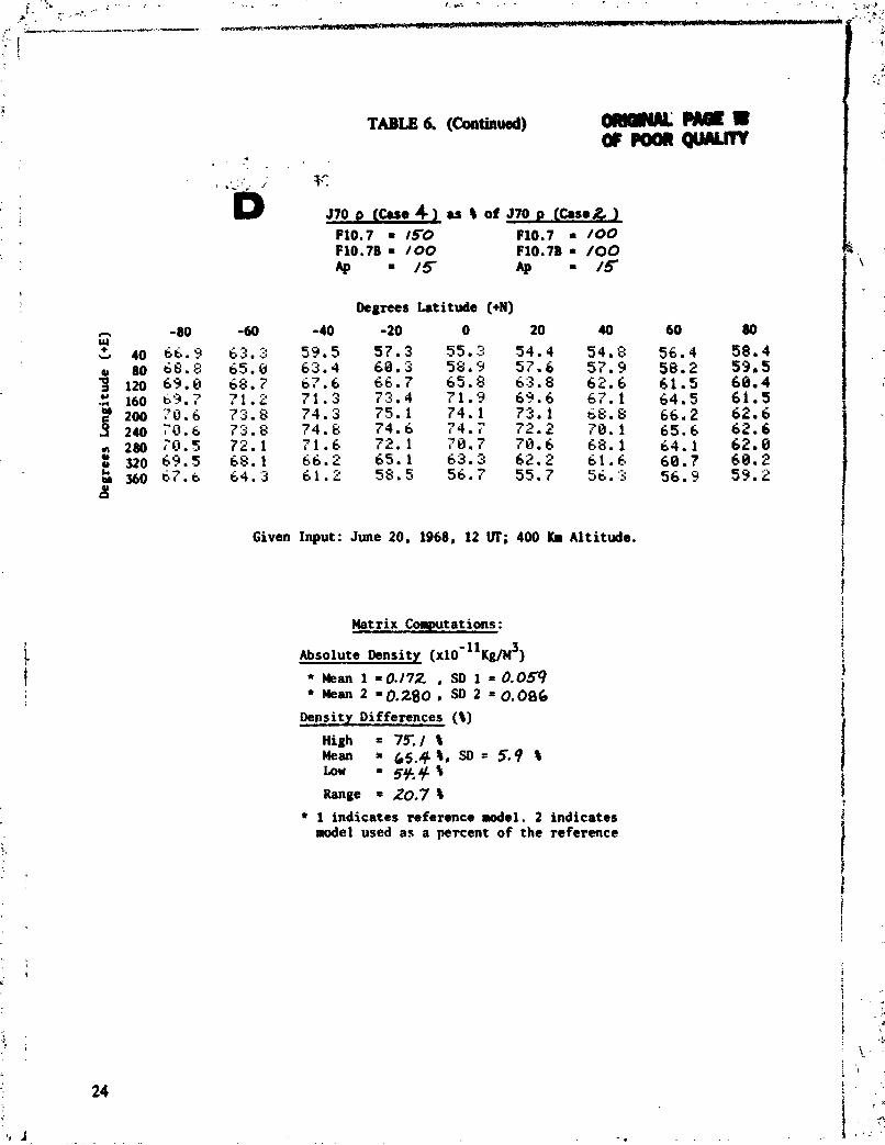
TABLE 6. (htinuedl
Degms Latitude (*N)
-20 0 20 57.3 55.3 54.4 6 8 . 3 58.9 57 .6 66.7 65.8 63.8 73.4 71.9 69.6 75.1 74.1 73.1 74.6 74.7 72.2 72.1 70.7 78.6 65.1 63.3 62.2 58.5 56.7 55.7
Given Input: June 20, 1968, 12 UT'; 400 KB Altitude. :
Matrix Computations:
Absolute Density ( x ~ o - ~ ~ K ~ / M ~ )
Mean 1 00.172 , SD 1 = 0.059 Mean 2 '0.280 2 =0.006
Density Differences ($)
High = 75. / 2 Mean 6 5 . 4 2 , S D = 5.9 2 Low =5*48 Range = 20.7 1
1 indicates reference model. 2 indicates lode1 used as a percent of the reference

TABLE 6. (Continued)
Degrees Latitude (+N)
Given Input: June 20, 1968, 12 UT; 400 Km Altitude.
Matrix Cowtrt ions :
Absolute Dsnsi t y ( X ~ O ' ~ ~ K ~ / M ' ]
* &an 1 = 0.262, SD 1 = 0.091 2 -0.369, SD 2 0.107
Density Differences (8) High - a.0 8 Mean - 43.6 8 , SD = ?. / I LOW = 29, o r Range 2 8 . 4 8
1 indicates reference model. 2 indicates rodel used as a percent of the reference

TABLE 6, (ContinW) -mar " - w w
Degrees Latitude (+N)
Given Input: June 20, 1968, 12 LIT; 400 Ka Altitude.
Absolute Donsitr ( x ~ o - ~ ~ K ~ / M ~ )
Mean 1 = 0.369 , SD 1 = 0.107 &an 2 = / . / 0 8 , SD 2 =0.158
Density Differences (1)
High = Z90.ZI Mean = 211.7 1, SD = &3 t Low =/34c.0% Ranee = /5541
1 indicates reference rodel. 2 indicates rodel used as a ;jercent of the reference

Given Input: June 20, 1968, 1 2 UT; 400 JCa Altitude.
Absolute Pensity ( X ~ O - ~ ~ K ~ / M ~
* ~ U I 1 -0,262, se i - 0.09/ New 2 = / . /03 , So 9 .O . /SS
Density D i f feronces ($1 Hioh . 5/47 $ Mean r3$1 , / t r SD 8 90.5t Low '2043 RmaI 3/0.+
1 indicates roferenca rodel. 2 Indicates node1 used as a percent o f the reference

H J70 p (Case 8 ) as t of J7O p (Case 61 F10.7 ,200 F10.7 = / S O FlO.7B 8 ' 50 F10.7B = 150 Ap = /5 Ap - 15
Degrees Latitude (+N)
Given Input: June 20, 1968, 12 UT; 400 K. Altitude.
Matrix Computations:
Absolute Density (xIo'~~K~/$)
k a n 1 = 0.369 , SO 1 = 0. /07 Mean 2 = 0.521 , SD 2 = 0. /37
Density Di fforences (8)
nigh = 48.58 Mean =42*3 t , SD = 3.8 t Low = 35 / 8
1 indicates reference Prodel. 2 indicates Plodel used as a percent of the reference

Given Input: June 20, 1968, 12 W; 400 K. Altitude.
Matrix Computations:
Absolute hnsity: ( X ~ O - ~ ~ K / Y ~ ) 1 - 8 . 7 9 0 , SO 1 = 0*/W
Mean 2 - 0.9$3, SO 2 = 0.2/0
Density Differences (a) High - 28.0 8 man = 2 / . 6 # , S D ' 3 . 8 9 Low - /4 .8t Raga /5 .2#
1 indicates reference model. 2 indicates rodel wed as 8 percent of the reference

Degrees latitude (+N)
Given Input: June 20, 1968, 12 UT; 400 I(r Altitude.
Matrix Coaputations:
Absolute Deasitr (r10'~~~g/l8)
b a n 1 = 0.953 , SD 1 = 0.210 * Mean 2 = / .82# , SD 2 = 0.227
Density Differences (I) High = 127.3 t Mean = 9K4c t , S O = / 8 . 6 1 Low = 63.6#
1 indicates reference rodel. 2 indicates model used as a percent of the reference
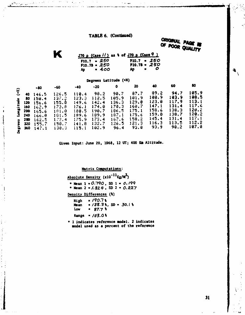
TABLE 6. ~ C o n t h d
Given Input: June 20, 1968, 12 W; 400 Km Altitude.
Matrix Coaputations:
rbsolute ensi it^ ( x l 0 - l l ~ Y 3 b a n 1 r0.790, SD 1 = 0.199 Mean 2 =/.82+# SD 2 = 0.227
Density Differences (8)
~ i ~ h = /90.7$ m =/38.31, SD * 30.1$ Low = 87.7 1
1 indicates reference rodel. 2 indicates wde l used u percent o f the reference

ORmUALPAarn O F m Q O A U r Y
TABLE 6. (Continued)
Degrees Latitude (+N)
Given Input: June 20, 1968, 12 W; 400 K. Altitude.
Matr ix Computations:
~ b v o l u t e Density ( x l ~ - ' l ~ g / h k a n 1 10 .953 , SD 1 8 0.210 Mean 2 = /.I57 , SD 2 8 0.235
Density Differences (%)
High = 252 % Moan = 2 / . 9 S, SD = 2.1 % Low = / 7 . 9 %
1 indicates reference model. 2 indicates rodel used as a percent of the reference

TABLE 6. (Contlnurb) - P # w m OC-QUAUTV
Given Input: June 20, 1968, 12 UT; 400 KB Altitude.
Matrix Computations:
~bsolute Dens42 (~10- l 'K~/M') b a n 1 = 0 . / 0 4 , SD 1 =0*044 Wean 2 = O . Z 6 2 , SO 2 =0.09/
Density Differences ($1 High = /9Io2% &m = Ifl.71, S D = / 9 . 6 1 Low = /24.9 1
+ 1 indicates reference wdel. 2 indicates model used as a percent of the reference

ORlOPULPAQe:?S TABLE 6. (CaMbd) of QUALITY
Given Input: June 20, 1968, 12 UT; 400 Km Altitlde. I ' Matrix Computations:
Density Differences (S) High = 260.8 1 Mem = 2 / / . 3 S , SD - 2 9 . 1 %
=/S9.6% Rmge = / 0 / . 2 S
* 1 indicates reference r , - i e l . 2 indicates d e l wed as a pdrcent o f the reference
Given Input: June 20, 1968, 12 m; 400 Ka Altitude,
Matrix Colwltations:
~bsolute bnsity (xl0-''~2) em 1 m 0.109, SD 1 0.044 N ~ M 2 = 0,790, SO 2 = 0./99
Density Differences (S) High = 9 % V S Mean * 7/4./S, SD =/H,6S Low r483.7 1 Range = 463. / S 1 indicates refsrmce d e l . 2 indicates miel used rur a percent of the reference

&
lbgreos Latitude (+N)
Given Input: June 20, 1968, 12 VT; 400 Ka Altitude,
*bsoluto ~ n r i t r ( x l 0 - l 1 ~ T ' ) + bur 1 =0./7% , SD 1 = 0.059
Man 2 = 0.369 , SD 2 = 0./07 Density Differences (t)
High = /36.9 t bur -//8,$%, SD' /I./% Low = 98.4 1
+ 1 indicrrtes reference model, 2 indicates model used as 8 percant of the rofercnce

Degrees Latitude (+N)
-60 -40 -20 0 20 40 60
-9
g((#(U.PAarn . i:
arroonauunv TABLE 6. (Continued) 3,
S.
*% r \
a
Given Input: June 20, 1968, 12 UT; 400 Km Altitude.
Density Difforonccs ($1 Hilh = /'7*.4\
r /63+4\, SD rn / 8 .1 \ Low l29.9 \
Range = 62.6\ * 1 indicatas reforenc~ model. 2 indicates
model used as a percent of the reference

Given Input: June 20, 1968, 12 UT; 400 1O1 Altitude,
~bsolute ~ n s i t r ( X ~ O - " ~ ~ )
wan 1 .0.172, W I l 010S9 * h m 2 m0.9523, SD 2 l O.Z/O
Donsity Diffenrnces (\)
Hiah 5VI.P \ Man 478.J\, SD 6t7\ Low 356.0 t
1 indicates reference d r l . 2 indicates model used as a percent of the nference

Given 7
ORlOtNAL ?- TABLE . ?Cantinuad) OF ?OOR @ J A W
J7O p (Cue 7 1 as 1 o f J7O p (Casa 3 1 FlO.7 8 / S O F10.7 I /OC F10.75 150 P10.7B /00 4 ' 400 & ' 40C
Degrees Latitude (+N)
input: June 20, 1968, 12 UT; 400 Km Altitude.
Mutrix Computations:
Density Differences (a) Hioh 454% Mean = 43.9 %. SD = 2.1 8 Low =40.2% Range 552 \
1 indicates reference model. 2 indicates nodel used as a percent of the reference

.'?,.\-. : . ' ' -"' . . , , .+ , " . , -. . . .,, &..- '%- - a <
' ."".."~ . . , . , , . % ? , _ , , . . - : L + .
* . . e .' .,. ( -- --,. \-.--*i** ---6-=. .-P . .
I!
.i
TABLE 6. (Continued)
I,
Degrees Latitude (+N)
Given Input: June 20, 1968, 12 UT; 400 K. Altitude.
Matrix Computations:
Absolute Density [ x ~ o - " K ~ / M ~ )
Mean 1 =/ * I03 , SD 1 = 0.158 Mean 2 = /.824 SD 2 - 0.227
Density Differences ( t )
High = 70.6 t Mean - 65.8tD SD= 3 .1 t Low - 5 9 . 9 1 Range = /0.7 %
* 1 indicates reference model. 2 indicates model used as a percent of the reference
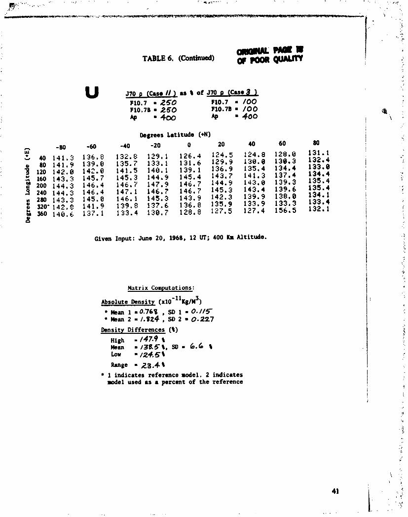
v M Q I TABLE 6. (Continued) w~~
Degrees Latitude (+N) -40 -20 0 20 40 60 80
Given Input : June 20, 1968, 12 UT; 400 Km Altitude. i . ,
i 1
Matrix Computations:
Absolute Density ( ~ ~ O - ~ ~ K O I M ~ )
k m 1 t 0.768 , SD 1 = O * / / 5 b a n 2 = /.t24 , SD 2 = 0.227
Density Differences (2)
High = /47*9 2 Mean = / 3 8 . 5 2 , S D = 6.6 2 Low = / 2 4 , 5 8
Range = 2 3 . 4 2 1 indicates reference model. 2 indicates model used as a percent of the reference
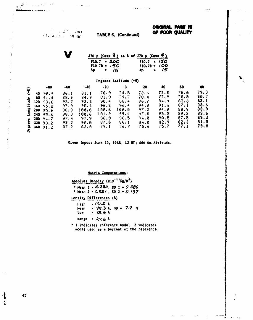
~ 1 0 . 7 ~ . I ~ Q p i o . 7 ~ r o o & . 15 Ap 1 5
Degrees Latitude (+N)
Given Input: June 20, 1968, 12 W; 400 K. Altitude.
Matrix Computations:
Absolute Density [ X ~ O ' * ~ K ~ / M ~ )
* MM 1 @*210, SO z 0,684 bur 2 =0 .52 / , SD 2 = 0. /3?
Density Differences (t) High 8 I0t.Z t Mean 8 B8.3 \ , S O = 7.9 t Low 7 3 . G t
Rurp = 27.6 8 1 indicates reference 111ode1. 2 indicates d e l used as a percent of the reference

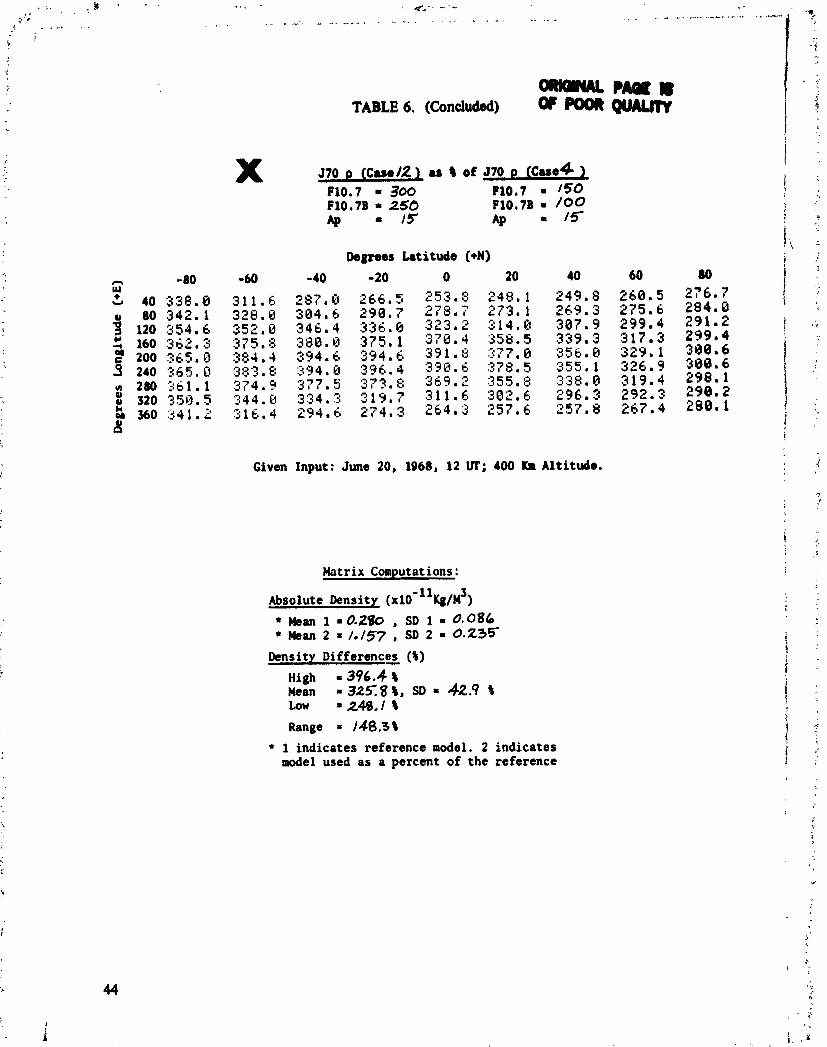
-?Aa I I TABLE 6. (Concluded) of
Degrees Latitude (*Nl -60 -40 -20 0 20 40 60
Given Input: June 20, 1968, 12 W; 400 Km Altitude,
Matrix Computations:
Density Difference2 ( 8 )
~ i g h = 396.4 % Mean =3258%, SD = 42.4 $ L o w =249. I% Range = 148.3%
1 indicates reference model. 2 indicates d e l used as a percent of the reference

TABLE 7. PERCENT DEVIATION OF JACCHIA 1971 DENSITY DURING A CHANGE OF F1oS7 AND/OR $
A 571 p (Case2 ) as li of J7l p (Case / )
FlO.7 = /00 F10.7 = /OO FlO.7B = 100 F10.78 = /OO hp = /5 AP = 0
Degrees Latitude (+N)
Given Input: June 20, 1968, 12 W; 400 b Altitude.
Matrix Conputat ions :
Absolute Density ( x ~ o - ~ ~ K ~ / M ~ )
* Mean 1 S O . / / / , SD 1 1 do92 Mean 2 =O,/SO , SD 2 = 0.055
Density Differences (8)
High = 03.7 li Mean = 65.6 3, SD = ll.9 8 L o w = 45.6 8
Range = 91 -7 li 1 indicates reference model. 2 indicates d e l used as a perccnt of the reference

m ? A a . TABLE 7. (Continued) ar raon
571 p (Cue 3 ) as I of 571 p [Cue 2)
Degrees Latitude (+N)
-20 0 20 2 4 6 . 2 2 3 0 . 8 2 2 4 . 7 2 8 3 . 0 2 6 6 . 7 2 5 6 . 8 358.8 341.1 323.2 4 4 1 . 0 42ee.Q :296.3 482 .5 471.Q 4 3 3 . 3 4 8 1 . 6 4 7 8 . 1 4 3 7 . 8 4 3 9 . 8 4 2 4 . 2 334.9 33Ca.8 318.9 3133.5 2 6 2 , 1 2 4 5 . 1 237.4
Given Input: June 20, 1968, 12 UT; 400 Ka Altitude.
Matrix Computations:
Absolute Density ( X ~ O ' ~ ~ K ~ / M ~ ) Man 1 = 0. /80 , SD 1 = 0.055 Mean 2 = 0.'758 , SD 2 = 0. /05
Density Differences (8)
High = 482.58 Mean = 3 4 4 . 0 8 , SD = 7 4 . 6 8 Low =224.7% Range = 2 5 Z 8 8
* 1 indicates reference model. 2 indicates model used as a percent of the reference
ORIUNAL PAGE IS OF POOR QUALITY
TABLE 7, (Continuad)
Degrees Latitude (+N)
Given Input: June 20, 1968, 12 W; 400 Ka Altitude.
Matrix Computations:
*bsolute Density ( x ~ o - " K ~ / M ~ ) h m 1 mO.lll , SD 1 10.042 Mean 2 10.758 , SD 2 0 . / 0 6
Density Differences (8) High * 989. t Moan 643.7 5, SD /77.11 t o w 372.9 1
Rmge m ll&3 8 * 1 indicates reference model. 2 indicator
model used ns a percent of the reference

TABLE 7. (Continued)
D J7l p (Case 4 1 as I of J7l p (Care 2 1 FlO.7 = /50 P10.7 = 100 FlO.7B = /00 F10,7B = /OO 4 = 15 Ap = 15
Degnes Latitude (*N)
Given Input: June 20, 1968, 12 VF; 400 Km Altitude.
Matrix Computations :
Absolute Density ( X I O - ~ ~ K ~ / M ~ )
Man 1 0./80 , SD 1 = 0.055' Mean 2 = 0.255, SD 2 = 0.072
Density Differences ( 8 )
High = 49.6 1 Mean = 42.9 8 , S D - 3.3% LOW = 37.08
Range = //. 6 %
* 1 indicates reference model. 2 indicates d r l used as a percent o f the reference

h # m s Latitude (+N)
Given Input: Juno 20, 1968, 12 W; 400 Km Altitdo.
Matrix Coputations:
Density Differaces (4) High = m.9 5 b a n = 39.7 S, SD= 6 7 1
= Z t . Z I
1 indicates reference model. 2 indicatrr We1 used as a percent af the reference

. ,. -, . > : , . , . e , *%
. . . _C_Ur*e,____l".Ullr_l I.ICIII -.- ----.-.--I..- - .-.-- - m
--m TABLE 7. (- O r m Q u A u n
J7lp (case? 1 u i of J7l B ( w e 61 PlO*7 rn /60 Fl0.7 rn /SO PlOe7B rn /SO Pl0.78 m /SO @ -400 @ rn 1 5
D e g m s Latitude (*N)
10 -80 -60 -40 -20 iI 20 40 6Q B u 40 1Y8.C 175.8 157.3 143.5 135.9 131.8 F33.6 140.6 15U.CJ
80263.2 187.6 175.5 161.3 154.U 149.0 148.1 149.0 154.6 ,; % 120218.8 210.8 207.5 198.3 198.3 182.8 4 166.2 161.2 I .% 160218.3 233.8 239.8 238.4 232.1 217.9 206.9 182.1 165.6 I 200221et, 242.6 254.8 258.1 251.8 235.6 213.7 188.4 169.2
240:i21.6 242.2 255.9 259.1 252.0 235.2 213.7 189.1 167.0 280218.6 232.5 238.8 237.4 238,';5: 216.5 198.3 160.7 166.7 $20244.1 283.8 196.Q 189.5 179.7 171.7 165.6 162.9 159.5 $ ~ O L O U . W 181.8 163.2 156.5 143.6 138.5 139.4 144.0 152.8
C1
i - I Given Input: June 20, 1968, 12 W; 400 Ka Altitude, : 1 i !
', I
., 1 htrix Col~ut8tions:
Absolute an sit^ ( x 1 0 - l ~ ~ ~ ~ k" 1 = O.39/ , 1 . 0./00 bm 2 = /./@I , So 2 0.145
Density Differences ( 8 ) -. High = 259./1
/9/.6%, SD = 36,3% I b a = /3/.81
b 8 @ 1 2 ~ 3 % t .-. 1 indicates nferenco aodel. 2 indicates .ode1 used 8s 8 percent o f the referrnee
I
A<
;:
I. " :,1
f
' ' , %*.
..< , . < ..C
A % . .
,, *- , 1 ;:
' \ , - . . . "
* . '4 L .. . ' ii- ,... , - .' : . " , . , , . - . r
, - . .

Giver:
Absolute DInsity (XIO-~~WKI) b a n 1 ma284 , SO 1 Mean 2 /. 106 , SD 2 0. /46
Density Differ6nces (t) Hi6h 444.21 Mew 309.91, SD 70-71 Low =/97.21
1 indicate8 reference mdal, 2 indicator M e 1 used as a percant o f the reference
- >. .. . . . j - l , . . . , . ..,, , i
T k 7. (Con-)
J71 o Ikre 7 1 as # o f J71 o C C w 5 L P10.7 /SO ClO,? 1- IrlP.78 m 160 Plb. 7B 1s" Ap m+oo nsl 0
(k8ms Latit* (*)
-40 -20 0 20 242.5 218.1 284.6 197.2 280,ia 212.5 231.4 275.4 250.7 236 .9 228.2 p25.8 228.2 238.8 338.3 321.7 3Oii.C\ 290.2 275.4 268.G 249.6 483.2 402.2 388.7 339.3 325.1 298,2 257.4 43P.6 441.5 427.5 396*3 350.9 382.2 263.9 4bb.W 444.2 43U.8 395.8 358.9 302.2 268.9 4g2.7 398.9 383 .8 3 5 7 . 4 321.7 287.5 268.4 317.3 382.9 284.4 269.4 256.4 252.4 247.5 254.Ct 238 .7 218.2 288.9 210.3 210.8 234 .2
Input: June 26, 1968, 12 Uf; 400 Km Altitude,
.. . .~ , . - , ..
Degrees Latitude (+N)
Given Input: June 20, 1968, 12 W; 400 K. Altitude.
Matrix Coawtations :
Absolute Density (x10 - 1 l d
b m 1 = a391 , SD I = 0.100 Mean 2 -0 ,498, SD 2 - 0 , / / 9
Dens i t y Di fferencas (a) High = 3/06 % Maan 27.7 $, SD Z./ 1
' 2 4 . 0 ~
1 indicates reference model. 2 indicates model wed as a percent of t k reference

TABLE 7, (Continurd) --I Q - ~
Deprws Latitude (+N)
Given Input : June 20, 1968, 12 UI'; 400 Km Altitude.
Matrix Coaputations:
Absolute Density (x10-~'Kg/& 1 =0.35/ , SD 1 = O . / 8 i
b a n 2 = / . 0 / 2 SD 2 = 0.196
Density Differences ( S )
High = 250 8 Mean - 19.6 $, S D = 3.0 $ tow = / 4 , 5 t Range = l 0 . 5 8
1 indicates reference model. 2 indicates wde l used u a percent of the reference

Given Input: June 20, 1968, 12 W; 400 Km Altitude.
Natrix Computations: - Absolute Deasitr (rlo-"rJw?
k o n 1 ./.0/z , SD 1 = d . / W Meon 2 8/.99G , SD 2 0.229
Density Differences (t) High 8 / / so 8 Wean 89.1 8 , SD = /3,9t Low 6 K 7 $
1 indicates reference rodel. 2 indicates rode1 used as 8 percent o f the reference
-60 117.1 121.5 118.1 153.1 158.4 158.8 151.4 13s. 1 119.9
Given
TABLE 7. (Continued)
J71 p [Cue 4 ) ) as t F10.7 = 250 F10.7B = 250 @ = 400
Degrees Latitude
Input: June 20, 1968, 12
of J71 p (Cue 9 ) P10.7 = 250 PlO. 7B = 2s0 M 0
W; 400 6 Altitude.
Matrix Computations:
Absolute b n r i t ~ (X~O'~~K&)
~ e u r 1 * O . l S / , SD 1 = O * / 8 5 Mean 2 = /.396 , SD 2 = 0.229
Density Differences ( 8 ) High = /68.6%
/2~3%, S D = 22.2% Low = 90.2 8
1 indicates reference model. 2 indicates d e l used u a percent o f the refmeace

TABLE 7. (Continued) ORWIOAt-II QfPQORQUAVlV
Given Input: June 20, 1968, 12 UT; 400 KB Altitude.
Matrix Corputatians:
~bsolute Densitr (~Io-"K~/&
k a n 1 =/.0/2 , SO 1 = 0 . / 9 5 Msan 2 = /./58 , SD 2 O . 2 / 3
Density Differences (I) High = 16.4 1 Mean = /4.4 I, S D = /.O 1
/2.6$
1 indicates reference model. 2 indicates model w e d as a percent of the reference
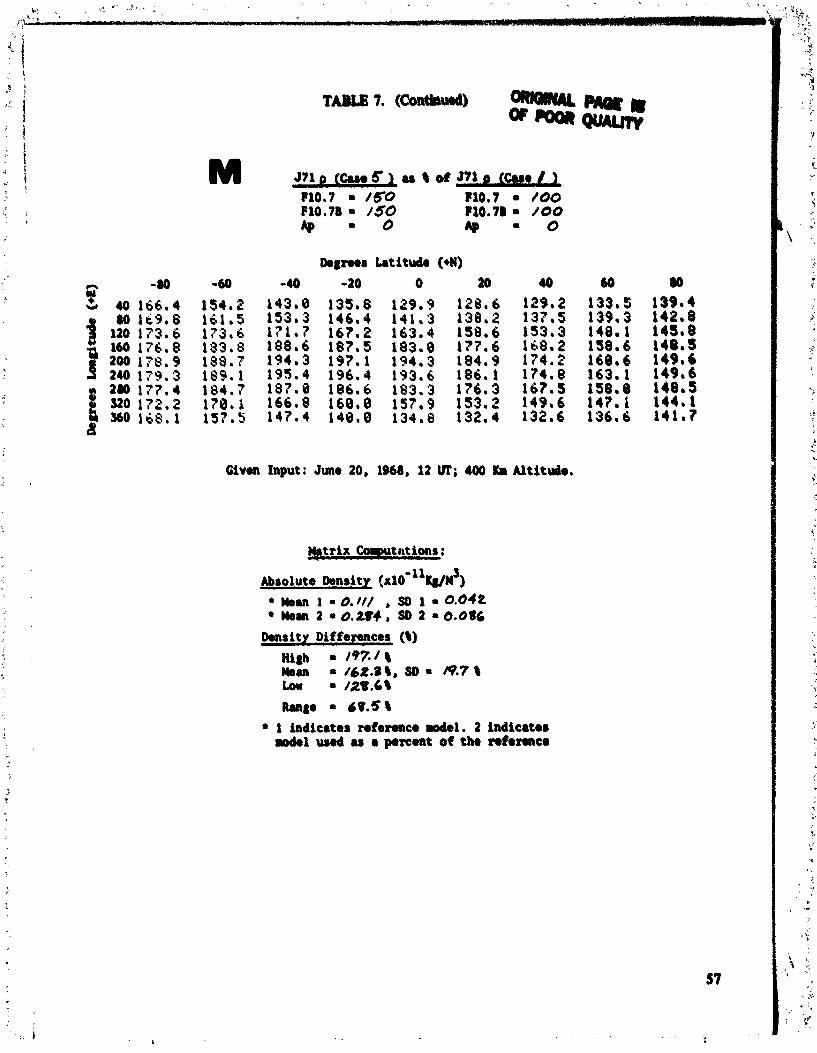
Given Input: June 20, 1968, 12 UT; 400 k Altitwlo.
Mtrix Corputationr :
s s o l u t e h n s i t r ~xlo- l1& man 1 = a/// , SD 1 0.042 Morn 2 .0.2?4 , SD 2 6.086
Density Diffeawrcer (8) High 1 197.t 8 Wan = /&%.St, SD = a 7 8 tow = /28.C8 Up 6 0 . 5 8
1 indicator nfermce -1. 2 indicator mdol wod u a porneat of tho rofomco

TABU 7. (Continued)
N 371 p (Cue 9 ) u 8 o f 571 D (~u,St P10.7 - 250 F10.7 = 150 P10.78 1 250 F10.70 = 150 4 = o A p = o
Degrees Latitude (+N)
Given Input: June 20, 1968, 12 UT; 400 Km Altitude.
Matrix Computations:
Absolute ~ e n s i t r ( ~ 1 o - l ' ~ ~ ~ ) 1 = 0.284, SD 1 0-084
Mtan 2 0 . 3 5 / , SD 2 0 * / 8 5 Density Differences (I)
High - 2*,0 I Mean =c20Z3I, SD- 2 6 . 4 5
= I & / . / 4
* 1 indicates reference m i e l . 2 indicates miel used u a percent o f the r e f e r a c e
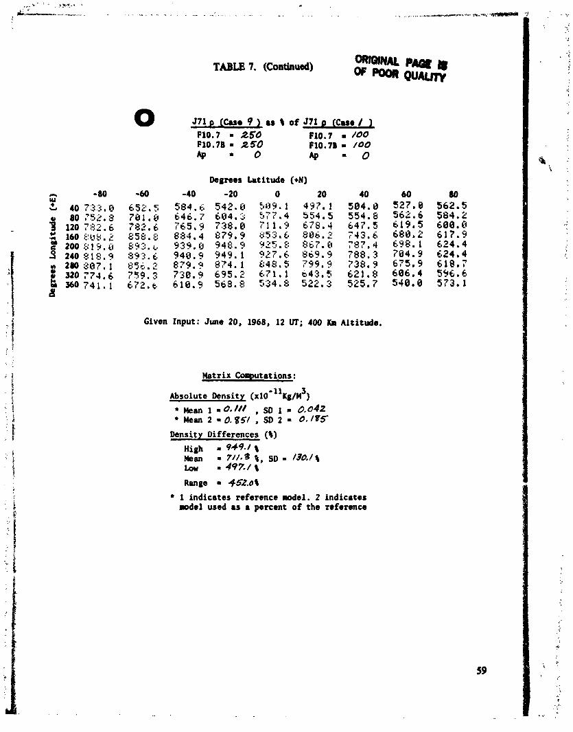
TABLE 7. (continued) - p a * w - q u ~
Degrees Latitude (+N)
Given Input: June 20, 1968, 12 W; 400 Km Altitude.
Matrix Computations:
Absolute Density ( x 1 0 - ~ ~ K g / ~ ~ ) man 1 =O. I f l , SD 1 - 0,042 Man 2 = 0 . 8 5 / , SD 2 = 0.Ig5
Density Differences (I) High 949 . /# man = 7 / / . 3 0, SD 1 /30./ 8 t, = 4 9 7 . / I
Range 452.08 1 indicates reference model. 2 indicates .ode1 used a s 8 percent o f the reference

oRm=f'-~ TABLE 7. (Continued) Q wNrn
571 p (Cue 6 1 as of J7l p (Case Z 1 P10.7 = 150 P10.7 = 100 P10.7B = 160 P10.78 = 100 hp = 1 5 Ap = 1 5
Degrees Latitude (+N)
Given Input: June 20, 1968, 12 UT; 400 K. Altitude.
Matrix Computations;
Absolute dens it^ (~10-I ' K ~ / M ~ ) man 1 = d./FO , 1 = 0.055
2 = 0,39/ , SD 2 1 O,/oO
Density Differences ( t ) High = / # 0 . S t Mean = / Z / . f I, SD - //.4 t Low = /o/. 3 I
Range = 39.5 t 1 indicates reference model. 2 indicates model used as a percent of the reference


.-., . , . . * . r . , , , . . . " . , , . , , . I " . . , . I . ,.. ...- . . ..
. - . - + . , -+-
Given Input: June 20, 1968, 12 W; 400 k Altitude.
Density Differences ( t ) High =LO/.Ot Mean = 403.51, SD - b6,41 Low -370.01
I indicates reference d e l , 2 indicates model used as a percent of the nformce

TABLE 7. (Conthdl OWQllYULWR OF--
Given Input: June 20, 1968, 12 UI'; 400 Km Altitude.
Matrix Computations :
Lknsitv Differences ($)
nigh = 48-11 Wan = 46./$, S D = /.2 $
= 43.7 Range = 44 I
1 indicates reference &el. 2 indicates wdel used as a percent of the reference
Db#reos k: itudrn (*N)
-00 -60 -40 -20 0 20 40 60 $0
40 7 1 . 7 7 8 . 4 7 5 . 0 6 8 . 2 6 6 . 7 67 .1 6 6 . 9 6 7 . 4 69.3 80 7 2 . 1 7 1 . 6 6Y.Q 7 6 . 6 6 9 . 0 6 0 . 2 6 7 . 7 6 8 . 8 7 5 . 2 1 120 7 8 . 3 7 3 . 3 7 1 . 4 7 2 . 4 72 .2 7 0 . 5 6 9 . 8 6 7 5 . 4
- 160 7 2 . 7 7 3 . 4 7 4 . 8 7 3 . 4 7 3 . 1 7 3 . 4 7 1 . 4 7BaS 73.6 7 3 . 3 7 4 . 1 7'*5 7 4 . 5 7 4 . 1 7 3 . 9 7 2 . 3 71.6 68.9
7 3 . 3 74.2: 7 4 . 7 7 4 . 7 7 4 . 3 74 .1 72.3 7 1 . 6 79.3 2@ 7 2 . 6 7'3.5 7 4 . 3 7 3 . 8 7 3 . 3 7 2 . 5 7 2 . 4 7 1 . 4 69.2 U O 72.5 72.8 71 .7 7 0 . 9 7 0 . 8 7 0 . 7 7 8 . 6 7 4 . 6 74.8 S O ':2.4 69.9 7 0 . 8 6 9 . 3 6 7 . 7 68.1 6 7 . 4 6 8 . 2 69.8
4
k. ., " ' .,, ;*, ' ,, '>'.T+.' ' . .* * . , _ . . , ,.a ,.* ,
' ' *.I. ~.. . . . a , . ~. i .-.-- . --
, *.> 3 i i / l . c ":.*fr . . . . *, ; -. ., ' .
TABLE 7. (Cantin&) , / -, ) r i ~ @ . < g ~ % C ~ * , .
-. = , . ' . i. -. .i .; : .*, .? . --- \ . . I ?
i . . ;* ; "t, ,f.\ .*
T . -
i . *-.-
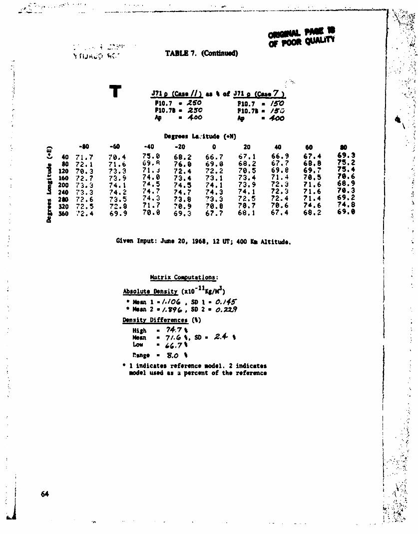
J71n (~urn//> u a of J 7 l p (hrn7 1 *; .;
Given Input: June 20, 1968, 12 UT'; 400 Km Altitude.
910.7 = 250 P10.7 150 P10.7B = 250 P10.7B = /Jb Ap = 400 Ap = -
r
Lhnsitv Differences (t) High = 74.7 t Moan = 7 / .6 t , SD = 2.4 t
= C G 1 7 t
-'. *- .. '1. P ,
-5 2 . \
4' . ! \' , +';
1 indicates reference robel. 2 indicates model used as o percent of the reference

u 371 0 ( C u m // 1 r8 8 of J71 o tCmm 3 1 Pt0,f * 256 PlO.7 rn 186 P10.7B = 250 F10.711 8 100 A@ 4-60 Ap . 406
Given Input: June 20, 1968, 12 UT; 400 Km Altitude.
Density Difforencas ($)
High = /51.8 $ &an 8 /$@*8%, S D m $ 1 $ Low - /90.2$ Range /8.6 b
1 indicates reference model. 2 indicates modal used as a percent of tho reference
21 'ji., . , . C ~ W - W ~
y7 .> . , TABLE 7. (Continued) am-
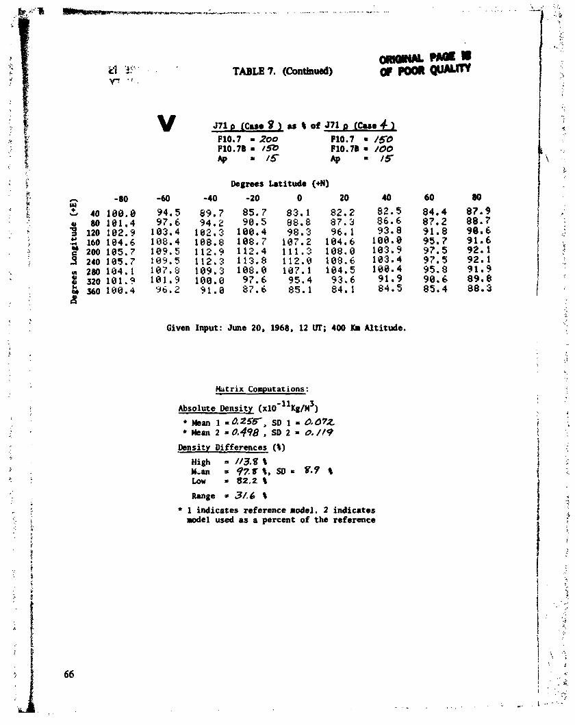
v J7l p [cue 8 1 as t o f J f l p (Cue 4 1 $10.7 = 200 FlO. 7 = /50 P10.7B = FlO.70 /00 ~ r p 1 5 4 = IS
Degrees Latitude (+N)
Given Input: June 20, 1968, 12 UT; 400 Km Altitude.
Matrix Computations:
Absolute Density (xl0- ' K ~ / M ~ ) Mean 1 * 0.255-, SD 1 0.672
+ Mean 2 = 6,498 , SD 2 = 0. / I 9
Density Differences (2)
High = N3.S g &an = 9 ~ g t , S D = 8.9 2 Low = $ 2 . 2 2
Range = 3/.6 8
1 indicates reference rodel. 2 indicates model used as a percent of the reference
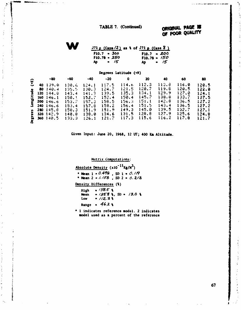
TABLE 7. (Continued) ~ A L P- W P ~ ~ R Q U U J ~ Y
Degrees Latitude (+N)
Given Input: June 20, 1968, 12 UT; 400 Um Altitude.
Mutrix Computations:
Absolute Donritr ( x l ~ - ~ ~ K g / Y ' ) ~ s r n 1 =0.4?8 , SD 1 = 0./)9 M o ~ 2 a/./g8 , SD 2 -6.2/;3
Density Differences (a) High = I579.5" $ Mean =/3C8$, SO- 13.0 Low - / /2 ,3 S
Range = 46.2 \ 1 indicates reference model. 2 indicates rode1 used as a parcent of tha reference

..% . , . . , ,?.
. *? . . I'"
r., , ---,- ,* ---.-..+.. cN---,ac.uraa*n r-T-rarcsn- *I*.-.--- .i--.r--*------------ j., . :: . .
-)AQIiB I t L :
> : . ~ TABLE 7. (Concluded) POOR @M&rtV ; r . .
'
Degrees Latitude (+N)
Given Input: June 20, 1968, 12 W; 400 Ka Altitude.
Matrix Computations:
Absolute Density ( x l ~ - ~ ' K g / d ) &an 1 = 4.155, SD 1 = 6.072 Man 2 = /,I58 , SD 2 = 0.213
Density Differences (8) High = 452.0 $ Mean = 367.68, SD = 46.7 % Low = 2 0 6 . 9 8
1 indicates reference model. 2 indicates model used as a percent of the reference

TABLE 8. PERCENT DEVIATION OF JACCHIA 1977 DENSITY DURING A CHANGE OF FlOa1 AND/OR Ap
- P ~ B $ "-0u~tm
A 577 p (Cum 21 8s t o f 5 7 7 p (Cue / 1 FlO.7 = 100 F 1 0 . 7 = 100 FlO.7B = /OO F10 .7B = 100 4 15 @ = o
Degrees Latitude (4)
Given Input: June 20, 1968, 12 UT; 400 I(r Alt i tde .
Matrix Computations :
Abrolure Density (xlo'"~g/d) * Mean 1 + 0* /20, SD 1 = 0.046
Man 2 = 0 . f 3 6 , SD 2 = 0~05%
Density Differences (I) High = 3.f.8 % &an = /A7 t., SD= 8.1 S LOW a / -6 S
Range = '33.2 1
* 1 indicates reference mrtdel. 2 indicates model used as a percent of the reference

TABLES. (Coartlaobd) BRIOIYAL =-a , .: '4 :. + !:31f ;z
W M Q u A u n , I . . .
-.is. 1 ;? is..: - ' .
Given Input: June 20, 1968, 12 UT; 400 Itr Altitude.
Matrix Computations:
Absolute Density ( x ~ o - ~ ~ K ~ / M ~ )
ken 1 t 0.138 , SO 1 0.052 Meon 2 = 0.663 , SO 2 = 0.57/
Density Differences (I) ~ i g h o 183L.4 t Mean - 393.7 t , SD = 434.3% Low = 72.8 t Range = /743.Gt
1 indicates reference model. 2 indicates model used as a percent o f the reference

TABLE 8. (w*w) mQfNAC PAG€ Is POOR QUALITY
J77 p (Case 3 ) u \ o f J77 D ( C u r P10.7 = /00 P10.7 /bO P10.78 = 100 PlO. 7B = /OO Ap - 4 0 6 AP I 0
Degaws Latitude (+N)
-Z'
Given Input: June 20, 1968, 12 W; 400 KR Altitude. :
Matrix Computations:
Absolute Density (x10"'y~~) Mean 1 = o./ZO , SD 1 = 0.046 Mean 2 =0.663, SD 2 = 0.571
Density Differences (I) High 2513.3 Mean = 490.1 I, SD = 544.0I Low = 76.6 I
Range = 2433.7%
1 indicates reference rodel. 2 indicates model used as a percent o f the reference

TABLE 8. (-ued) of--
I k g m s Latitude (+N)
Given Input: June 20, 1968, 12 UT; 400 Km Altitude.
Matrix Computations:
Density Differences (I)
High = 9 4 I Mean = 70.7 I, SD = 9.9 I L o w = 5S7I
1 indicates reference model. 2 indicates rodel used as a percent of the reference
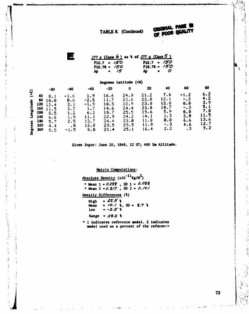
TABLE 8. (Contiawb)
I k p e s Latitude (+N)
A -80 -60 -40 -20 0 20 40 60 80
Given Input: June 20, 1968, 12 UT; 400 Km Altitude.
Matrix Computations:
fisolute Density (xIo-"K~/~) k a n I = 0.288 , SD 1 = 6.088 MOM 2 =0,317 , SD 2 = d. /o /
Density Differences (I) High =.EZS% Mean = /O . / I, S D = 8.7 1 tow -2.5 I Range = 29.0 I 1 indicates reference model. 2 indicates &el used as a percent of the referenec

I . ., .- . F.
- , . I , .*
om--* . 6,t:u..+ G 7 TABLE 8. (Continued) OF--
F 577 P (Cm. 71 u 8 of 577 0 CC& 6 3 P10.7 160 Fl0.7 * 150 Pl0.70 = /so PlO. 7B * 150 @ '400 A@ 1 5
Degrees Latitude (+N)
Given Input: June 20, 1968, 12 W; 400 K. Altitude.
Matrix Computations:
*bsolute Density ( x l ~ - l l ~ ~ / M S ) Mean 1 r 0.317 , SD 1 = 0, /O/ M b ~ r 2 =/eoQ8 , SD 2 -4.565
Density Differences (I) High = 773.5 1 ern - t Z C , ' J ) , SD m 1 Q 3 - 5 1 LOW m 56 -0 1
Range = 716.7) + 1 indicates reference model. 2 indicates
d e l used as a percent of the reference
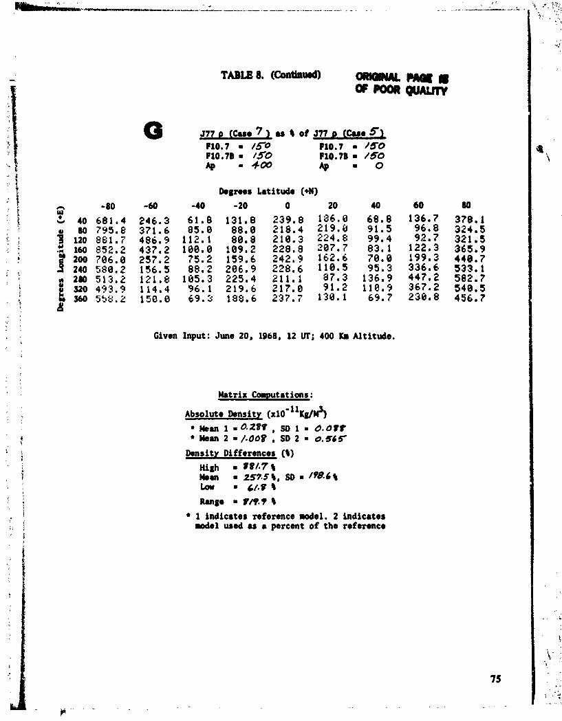
Degms Latitude (+N)
Given Input: June 20, 1968, 12 W; 400 Km Altitude.
Matrix Coaputrtions:
Absolute Density ( ~ 1 0 - ~ ~ ~ I / y l + 1 = 0.280 , SD 1 = 6.0tr + 2 =/.008 , SD 2 = 0 . 5 6 5
Density Differences (5)
nigh = 88/*7 5 m m 257.55, SD = 19B.65 LOW 6/08 5
R.ngo fN .7 1 1 indicates reference W e l . 2 indicates d e l used as r percent of the reference
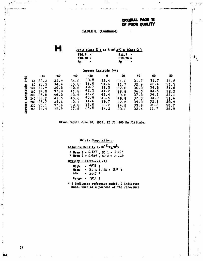
TABLE 8. (Continued)
Degrees Latitude (+N)
Matrix Coaputationr
Absolute Densitr ( x 1 0 - ~ ~ ~ I / y 5 ~ e a n 1 1 0.317, 1 0 . /0 / Mean 2 = 0.42% , SD 2 = 0.129
Density Differences (I) High = 45.8 1 Mean = 36.2 I, SD = 3.9 S
= 30.7% Range = / X /
1 i n d i c a e s reference model. 2 indicates model used as a percent of the reference
Given Input: June 20, 1968, 12 UT; 400 Ka Altitude. i
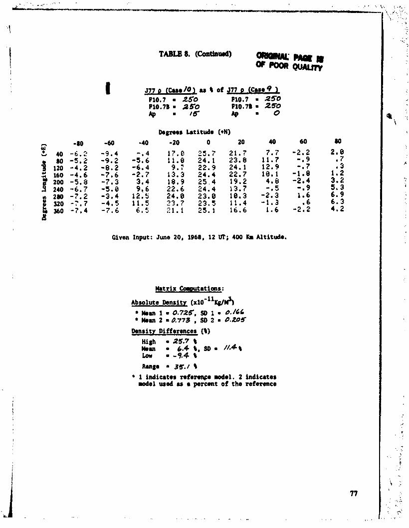
TABLE 8. (cofiti~rud) - m u m w-qwun
Degrees Latitude (+N)
Given Input: June 20, 1968, 12 UT; 400 Km Altitude.
Density Differences [t) High -25.71 Moan = 6.4 1, S D = //*41 tow = -9.4 1
* 1 indicatn mfe-e model. 2 indicator .ode1 used u 8 prcont of the reference
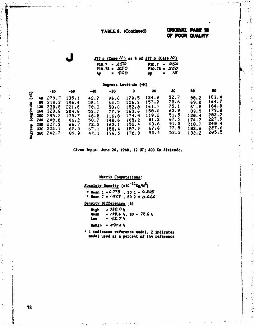
TABLE 8. (Conthud)
Given Input: June 20, 1968, 12 UT; 400 Km Altitude,
Density Differences {t) u 330.0 1
k m = /m,C I, SO = 72.6 4 Low = 42.7%
1 indicates reference model. 2 indicates model used u a percent of the refermce

TABLE 8. (Continued)
Degrees Latitude (4)
Given Input: June 20, 1968, 12 lW; 400 Km Altitude.
Matrix Computations:
Absolute Density (x l~ - ' ' ~g /~? )
+ Mean 1 0 0.725 , SO 1 0 d. 164 Mean 2 = /.VZV , SD 2 = 0.666
Density Differences (I) Hiah 33/10 8 1 Hean = /52.8 %, SO = 74.6 5 Low = 42.1 t Range = Z47.78
+ 1 indicates reference model. 2 indicates rodel used as a percent of the reference

-lRClsrm TABLE 8. (Continuad) w # K M m
Latitude (+N)
0 20 40
Given Input: June 20, 1968, 12 UT; 400 K. Altitude.
Matrix Computations:
Absolute Density ( x l ~ - ~ l K g / & Man 1 = 0.7'3 , SD 1 = 0.265 Man 2 = 0.894, SD 2 = 4.229
Density Differences ( t )
High = 19.2 % Mean = / 5 9 t , SD = 1-5 % Low = / 3 . 4 $
Range = 5 9 t 1 indicates reference model. 2 indicates .ode1 rued u a percent of the reference

- lYOC -- =---. -.;we W l u - r . - - * l - - C . - p p . . - F .1 . .. .' -- .,
) ' - ' I , '
) . ; i
M J77 (Cue qf u I of 377 o (Cue 3 F10.7 = 150 FlO.7 = 100 FlO.7B = 150 F10.7B = 100 M - 0 M - 0
Degrees Latitude (44)
Given Input: June 20, 1968, 12 VT; 400 Km Altitude.
Matrix Computations:
Absolute Density ( x l ~ - ' ~ K g / ~ ~ ) Mean 1 = 0*/20 , SD 1 = 6.046 Man 2 ' 0 - 2 8 8 , SD 2 = 0,088
Density Differences (8)
High = /89.7 8 Mean =/48 . / t , S D = Z / - ~ % tow = / / S + S Range = 74.3 8
* 1 indicates reference model. 2 indicates model used as a percent of the reference
S P W B
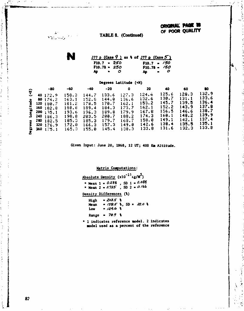
( . . TABLE 8. (Con6inued) OF POOR QUALrn
\,;
Degrees Latitude (+N) -60 -40 -20 0 20 a 60 80
Given Input: June 20, 1968, 12 UT; 400 Km Altitude.
Matrix Computations:
~ b s o l u t e Density (.io-11*g~n3) Maan 1 = 0.288 , a 1 = 0,OSg Mean 2 = fi.725 , SD 2 =
Density Differences (%)
High = ZM.5 % Mean = 158.6 %, SD = 22.0 % Low = 1.Z4.6 %
Range = 78.9 %
1 indicates reference d e l . 2 indicates lode1 used as a percent o f the reference

- P M E B OF #K)R QUALCrY
TABLE 8. (Continued)
577 v (Cue 9 1 8s 8 of 577 p (Cue / 1 F10.7 = 250 F10.7 = 100 FlO.78 = 260 P10.78 = b 0 b = O
Dearees Latitude (+N)
Given Input: June 20, 1968, 12 UT; 400 K. Altitude.
Matrix Computations;
Absolute Density ( x l ~ - ~ ~ l ( ~ / M ~ ) mm 1 = 0,/20 , SD 1 O.fi46 ~ e a n 2 10.725 , SD 2 = O . / 6 6
Density Differences (S) High = 774.3 \ Mean =54c8 S, SD = / / 0 .9S Low = 386.0 S
Range = 399.3 s 1 indicates reference model. 2 indicates model used as a percent o f the reference

--tB TABLE 8. (Continued) Ok QUAL~TY
P 577 p (Caso 6 ) as Si of 577 o [Case 2 ) F10.7 = 150 F10.7 = 160 F10.7B = 150 F10.78 = 169 I\p = 15 Ap = 1 5
Degrees Latitude (4)
Given Input: June 20, 1968, 12 W; 400 K. Altitude.
Matrix Coaputations:
Density Differences ( 8 )
High = 8 /a.o 8 , SD = 21.4%
Low = 106.4 8
Range = $3.3 8
1 indicates reference model. 2 indicates model used as a percent o f the reference

o e g r a s Latitude ("0 -20 0 20 40 60 80
-60 -40 - 137.8 129.1 134.5 128.8 125.5 125.8 125.8 123. r
1 7 139.0 144.7 142.6 137.4 ,. 7 138.8 129.5 125.8 1 5 ~ ~ 8 165.7 1&,8.(. 162.1 153.9 145.4 1'37-8 1?8m4 157.4 176.9 L(II.1 173.7 161.6 158.8 14a-3 tE8*9 16l.1 1aa.i "0.4 in,' 166.8 153.7 14@-6 128.5
1)i.l zoQ.@ 188.5 173.4 155-5 139.4 1zbm5 178, ( ic;$.(. 182.4 178,~ 16" 0 . r .J 156.3 143.4 136.7 123.4 157.6 163.2 157.6 148.9 141.6 134.8 126.4 121.8 148.9 151.5 4 4 , 1311.4 134.3 138.2 126.7 1?2*5'
Given Input: june 20, 1968, 12 mi 400 *Ititude'
plolute ensi it^ ( X ~ O - " ~ ? / M ~ )
Mean 1 0.317 , SD 1 L 0. lo/ * Men 2 m 0.773 , SD 2 = *1*05
Rmge = 78,2 8 1 indicates ref erenee ode1 2 indicates ~ d . 1 8 percent of the mfeance

oawrw,PAQLB TABLE 8. (Continued) W PlOoR QUALlW
R J77 p (Cue 101 as t of 377 0 (Cue 1 $10.7 = 250 $10.7 = 100 P10.7B = 250 PlO.7B = 100 Ap = /5 & - 1s
Degrees Latitude (+N)
Given Input: June 20, 1968, 12 UT; 400 KP Altitude.
Matrix Computations :
Absolute Density ( X ~ O - ~ ~ K ~ / M ~ ) Mean 1 =0, /38 , SD 1 = 0.052
2 1 0 , 7 7 3 , SD 2 6.205
Density Differences (8) High = 766.2 I E h ~ r 491.1 8, SO 1 /02.91 Low = 365.7 8 Range = 4ro.r 8
1 indicates reference model. 2 indicates mdel used as a percent of the reference

Given
, >. 3 &*=' " ' ' , * ; ,. . .,/* . , - ' , ,. . . ." ... . , *
1.w.- 1..-- -. ...... -.. ... " . . . -.. - *-.-. --. ......- *.-*-*
TABU 8. (Continued) OlnGllCYAfPAOEits OF POOR QUAUrV
577 P ( ~ u a 7 1 as t o f 377 a (Case 3 I P10.7 1 I 50 P10.7 100 PIO.7B 0 /SO PlO. 78 r 100 & 0 300 Ap 400
Degrees latitude (+N) -40 -20 0 20 40 60 98.4 123.4 121.1 116.7 105.8 66.9 8 6 . 7 125.4 128.2 123.0 115.4 83.9 34.7 9 0 . 8 145.8 152.4 143.6 128.6 1 6 36.6 184.6 161.5 164.3 151.9 129.5 83.2 32.3 135.8 176.3 169.7 154.3 128.5 63.7 25.7 163.1 188.9 178.4 152.8 102.2 41At 158.3 171.6 161.6 133.6 80.1 27.0 141.0 150.1 141.3 123.0 81.7 38.5 16 .2 122.7 138.2 129.8 121.1 97.1 48.0 22.0
Input : June 20, 1968, 12 UT; 400 Ku Altitude.
Matrix Coaputotions:
Absolute Density (x10'~~Kg/d) 1 10.663 , SD 1 - 0.57/
* b a 2 r A @ 8 , S D 2 = 3 * S L b
Density Differences (8)
High = / S Y e 9 8 ~m - 91.3 t, S D = 54,68 Low - 0 . 5 8
1 indicates reference model. 2 indicates model used as a percent of the reference

o m m W M ) I TABLE 8. (Continued) OF POOR Q U A U w
T J77 P (Cur 11 1 u t of 377 D [Cur 7 L Pl0.7 = 250 P10.7 = 15'0 Pl0.7B = F10.7B 150 Ap = 400 M = 400
Degrees Latitude (+. ')
Given Input: June 20, 1968, 12 VT; 400 m Altitude.
Matrix Computations:
~bsolute ~ e n s i t y (xlo-ll~g/Wf) 1 = / , O O l , SD 1 = ~ . s ~ ~ 2 =/,?Z? , SD 2 @.CLL
Density Differences (S) High = /98*6 8 Mean = /05.0S, SD = 53.3 1 Low = /7.8S
b g e = /80.11' 1 indicates reference Mdel. 2 indicates lode1 used a; a percent of the reference

Degrees Latitude (4)
n -80 -60 -40 -20 20 40 60 80 0 W S 40 34.1 127 .1 326.2 418.0 402.8 386.4 352 .4 19'5.5 79.3
o 80 22 .5 $7.4 288 .8 434.2 440 .1 417.5 394 .7 261.4 9 7 m s 3 120 18.3 77.7 299 .2 539.1 562.4 515.4 456.8 296.i3 105.6 2 160 23 .8 161.6 357.1 616 .2 621.6 558.5 466.8 262.2
91.1
200 43.4 186.8 300.0 694.9 656.4 574.2 428.2 199.9 73m8 3 2 0 64.3 281.6 633.9 7 6 2 . 7 705.3 579.2 348.9 119.2 55.6 , 2(0 71.7 298.3 602 .0 658.5 601.; 478.7 254 .2 77.4
320 7 u . 3 275 .9 509.5 543.5 502.8 428.4 258.0 87.0 48ns 8 560 5 5 , 6 211.3 425 .2 488 .2 449.4 412.1 319.1 136.2 63.8
d
Given Input: June 20, 1968, 12 VI; 400 KB Altitude.
k t r i x Computations:
Density Differences (%)
Rurge = 744.4 S
1 indicates reference nodel. 2 indicates wdel used as a percent of the reference

J770 c ~ u e S 1 u t of J77n t ~ u e 4 1 . P10.7 m ZOO P10.7 150 Pl0.7B m 150 F10 7B 106 A? /d ~p I 1 5
Deglws Latitude (+N)
Given Input: June 20, 1968, 12 UT; 400 Km Altitude.
Density Differences ( t ) - High - 116.8 t Mean = $1.1 t , SDm //od t
= 7 2 , s t
+ i, indicates reference rodel. 2 indicates mod81 used u a porcmtl; o f the reference
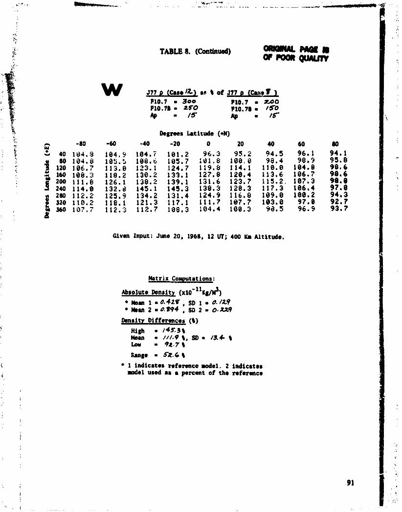
TABLE 8. (Contlausd) - W E B em-
Degrees Latitude (4) -40 -20 0 20
104.7 101.2 96.3 95.2 100.e 105.7 1 . 8 1 0 @ , 0 123.1 124.7 119.8 114.1 130.2 133.1 127.8 120.4 138.2 139.1 131.6 123.7 145.1 145.3 138.3 128.3 134.2 131.4 124.9 116.8 121.3 117.1 111.7 187.7 112.7 108.3 104.4 100.3
Givon In~ut: June 20, 1968, 12 UT; 400 KB Altitude.
h s i t v Differences (t) High = 1 4 5 3 % )bur = / / / . 9 t, SD = 13.4- t Low 92.7%
1 indicates reference model. 2 indicates model used 88 percent of the reference

Givm Input: J m o 20, 1968, ?i tn'; 400 Km Altitude.
Matrix Comutat~ons: -- &~lute Density (rlO-ll~yi)
b m 1 I O.%b/ SO 1 r 0.074 Mom 2 = 0.994, so 2 0.229
tbnsity Differences ($1 High = 49/09 t Ekrn = 360.0$, SD - sa.6 t Low B232,3t
a 1 indicates refbnnsr medal. 2 indic~tos lode1 used as 8 p n m t o f tho reforenm

. . , . +
, . ' ,. )., -marrr - m O O M C r Y
F&; hblb ~$hfS,pmient density for the 12 -, between the 571 and the rtatdud 170. Lgteub, Tabb 10 gives density pmmt8ges of the 577 with respect to the 570 for the - 12 ama. A dimmion of the mulb given in Tables 6 through 10 will be presented in the next metion.
TABLE 9. PERCENT DEVIATION OF JACY3HI.A 1971 DENSITY AS A FUNCTION OF COWRESFONDING JACCHfA 1970 DENSITY
CASE: 1 J7l p (Cue 1 18s t of 570 p (Cue / 1 F10.7 = /00 F10.7 = 100 F10.71 = /00 F10.71 = 100
- 0 Irp = O
Degrees - 20 2.3 3.7 7.1
1B.4 12.8 12.6 111.3 6 . 6 3.2
Lat itude 0
r-f . 8 2 . 8 6 . 2 9.9
13.5 13.8 9.6 4 . 6 .6
Given Input: June 20, 1968, 12 VT; 400 Ka Altitude.
Matrix Cornutationm:
Absolute Density [xlO'llKg/d) 1 = 0./04 , SD 1 = 0.094
k~ 2 = O , / / / 8 a 2 0.042 Density Differences (I)
Hi@ = j5.6 1 = 9.0 I, SD = 4 9 I
Low = -1.4 I Range = 17.0 4 1 indicates reference model. 2 indicates model used as a percent of the reference

Given
. . ( , ... .,. ,. , ~a:-trn'?f' L.; I . ' - " I ' - C
, * , .. ** 8 ',. l-,-J 30 oftWNAtPMB1
TABLE 9. (Continued) 0rpoonQunrm
CASE: 2
b g w s Latitude (+N)
Input : 1968, 12 UT; 400 Ka Altitude.
Matrix Computations :
*solute Density (Xlo- 11wu31
Mean 1 = 0.172 , SD 1 8 0.059 Mean 2 = O . / 8 0 , SD 2 * 0.055
Density Differences (%)
High = iL S Mean = 5 9 I, S D = 3.8 S Low - -2.3 I
+ 1 indicates reference rodel. 2 indicates rodel w e d as a percent of the reference

+,? -'A:;fK;t*,"
.. ,. TABU 9. (Continued) ?C;?<: . ORlQlNAL PAGE IS OF POOR QUALCrY
Degrees Latitude (+N)
Given Input: June 20, 1968, 12 UT; 400 Ka Altitude.
Matrix Computations:
Density Differences (4) High = 0.6 8 Mew a-/./ 8 , SD= 1 - 7 8 Low -4.5 8
Range = 5.1 4 1 indicates reference &el. 2 indicates model used as a percent of the reference
O R ~ Q W A L P A ~ E ~ TABLE 9. (Conthud) gC ~ o ~ u r y
Degrees Latitude (+N)
Given Input: June 20, 1968, 12 VP; 400 K. Altitude.
Natrix Cwutations:
Absolute Density (IC~O'~'K~/~) k a n 1 = 0,280 , 1 = 0.086 Mean 2 = 0.255 , SO 2 = 0.072
Density Differences ( 8 ) High = -5.3 8 M e m -8.6 2, SD = 2.2 1 Low = - 1 3 . 3 %
Range = 8.0 1 1 indicates reference model. 2 indicates model used as a percent of the reference

TABLE 9. (Continued) PA= t8 OF POOR QUALITY
CASE :
Degrees Latitude (+N)
Given Input: June 20, 1968, 12 UT; 400 K. Altitude.
Matrix Computations:
~bsolute tbnsitr ( x l ~ - l l ~ g / ~ ~ ~ Man 1 a 0.262, SD 1 = 6.041
M e a n 2 = 0.284, S D 2 =0,08b
Density Differences (I) ufi a 16.7 I Mean - 10.1 %, S D - 4.0 % LOW 0.2 8
1 indicates reference d e l . 2 indicates &el used as a percent of the reference

Given Input: June 20, 1968, 12 UT; 400 K. Altitude.
Matrix Computations :
Absolute hnrity (XIO-~~K~/M') ~ e a n 1 = 0.369 , SD 1 = 0.107
+ WBan 2 r0.391 , SD 2 = 0.100
Density Differences (I) mfi = 12.4 I Mean = 7.1 I , SDr 3-8 I h w = -0.8 8
m O e 13.2 1 + 1 indicates reference d e l . 2 indicates
rodel wed as a percent of the reference

" d
TABLE 9. (Continued)
Of PdOR QUAL"'y
J7l D (Case 7 1 u I of J7O p (Case 7 ) P10.7 = I50 P10.7 = 150 P10.78 = 150 F10.78 = 150 4 '400 AP = 400
Degrees Latitude (+N)
Given Input: June 20, 1968, 12 LIT; 400 Km Altitude.
Matrix Corrputatians :
Absolute Density ( x l ~ - ~ ~ K g / & ka 1 t /.I03 , SD 1 - 0.158 k e n 2 =/ . /06 , SD 2 0* /45
Density Differences (I) High = 2.4 I Mean = 0.4- I, S D = 1.3 I Low = - 2 . 2 8
1 indicates reference model. 2 indicates model w e d as 8 percent of the reference

TABLE 9. (Continued) Q--,
571 p [cwm 8 1 as t of J7O p (case 8 1 F10.7 = 200 F10.7 = ZOO Pl0,7B = 1 50 Fl0.7B = I SO @ 15 AQ = 15
Degrees Latitude (+N)
Given Input: June 20, 1968, 12 Ul'; 400 Km Altitude.
Matrix Computations :
Absolute Densitl (xlO-ll~g/l?) Mean 1 - 0.521 , SD 1 = 0.137 Mean 2 = 0.490, SD 2 = O-I IQ
Density Differences (I) High = -0.5 t Mean = - 3.4 1, SD = 2.4 t Low = -9.0 1
1 indicates reference model.. 2 indicates model w e d as a percent of the reference

;;! 3; -a'- .r- TABLE 9. (Continued)
tkgrves Latitude (+N)
Given Input: June 20, 1968, 12 UT; 400 KB Altitude.
Matrix Corputations:
Absolute Density (r l~-~~rr/h?) Wba 1 = 0.390 , SD 1 = 0.199 Mean 2 - 0.851 , SD 2 = 0.195
Density Differences (I) Nigh = '3.8 t b a n = 8.7 t , SD r 3.8 1 t o w = 0 . 0 t
* 1 indicates reference model. 2 indicates aodel used u a percent of the reference

TABLE 9, (Continued) GR\Q\NAL p m amauu"
571 o IClsa /O 1 as t of 370 o (Case /O ) PlO. 7 - 250 $10.7 m 250 PlO.7B 250 $10.78 250 Ap 15 Ap 15
Degrees Latitude (+N)
Given Input: June 20, 1968, 12 m; 400 Km Altitude.
Matrix C#~utatians:
Absolute Density ( X 1 0 ' ~ l w f i + 1 r 0.953 , SD 1 = 0-2/0
u8ur 2 * /.0/2 , SO 2 * O . / 9 5 Density Differences (I)
High - 10.9 I Maan - 6.9 t , S O - 3.0 1 Low 0.7 8
1 indicetms reference rodel. 2 indicates lode1 rued u r percent of the reference

TABLE 9. (Continued)
Degrees Latitude (+N)
Given Input: June 20, 1968, 12 VT; 400 K. Altitude,
Matrix Computations :
Absolute Density (xl~."l(l/Y? mm 1 /.824 , 1 * 0.227
2 ml.896 , SD 2 *0.229 Density D l ffermces (I)
MgJl * r.5 I Ebm * 4.0 I, SD * 1.2 1 Low * x,z 1
1 indicates reference mdd. 2 indicates w d e l w e d u 8 percent o f the r e f e r a c e

371 D (Cue 12) 8s I of 370 o [Cue 121 P10.7 300 P10.7 300 PlO.7B 0 250 PlO.7B 1 25(3 AP 15 Ap 15
Ik8ms Latitude (4N) -60 -40 -20 0 20
- 8 0 . 7 -2 .6 -3.1 -3.6 - 9 0.0 -2.2 -2.8 - 2 , 7
2.1 0.0 -. 9 -. 9 0.0 2 .7 1.6 - 9 1 .3 1.9 3 . 0 2.2 1.7 2 .4 3 . 0 3 . 8 2.2 1, 8 2.4 3.1 2.6 1.6 a 8 1.2 1.7 1 . 9 8 .0 -,9 -1.7 -1.6 1.7 - . 8 -104 -3.3 -3.2
Givon Input: June 20, 1968, 12 W; 400 Ka Altitude.
Absolute Donsit). (~10~'~~)) k.n 1 1.157 , SD I . 0.235
* k m 2 / . IS8 , SD 2 10,213 Dmsitv Differences (I)
High 33.2 I Morn 0.4 I, SD = 2.1 I Low -3.6 1
1 indicates mfennce mdel. 2 indicates -1 wod u 8 prcrat of the nference
1
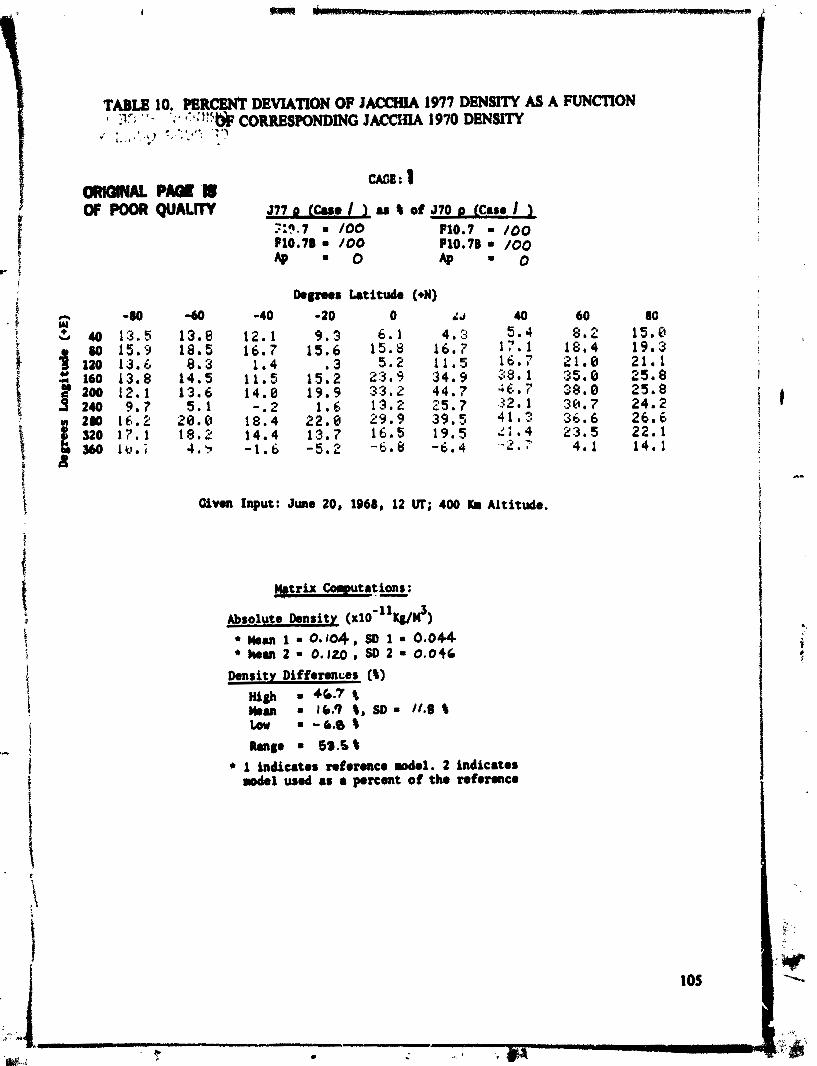
TABLE 10. PERCENT DEVIATION OF JACCiW 1977 DENSITY AS A FUNCTION , ; ~ y ; * ~ - ';. f:':'ts& CORRESPONDING JMcHIA 1970 DENSITY
,,* ;- ,, . '. ,>) f a . - , '..": ,:.?
I
ORmNAl PMZ 'I# WE: 1 i
OF POOR QUALtTY Jff D (&I I 1 u t of J70 0 (Cue I 1 i
i X9.7 • /00 F10.7 1 /OO Pl0.7B /00 F l o e 7B /00 AP . 0 AS, 0
i
(kgaws Latitude (a) i -80 -60 . f 9 -40 -20 0 L 4 40 60 80 I
Y 4 13.5 13.8 12.1 9 . 3 6 . 1 4 .3 5 . 4 8.2 15.0 1
80 15.9 18.5 16.7 15.6 15 .8 16.7 17 .1 18.4 19.3 3 120 13.6 8 .3 1.4 . 3 5 . 2 11.5 16.7' 21 .0 21.1
!
.$:la 13.8 14.5 11.5 15.2 23.9 34 .9 38 .1 35.0 25.8 ! 200 12.1 13.6 14.8 19.9 33.2 44.7 3 8 . 0 25.8
4 2 , 9 .7 5 .1 -. 2 1.6 1 3 . 2 25 .7 .32.1 38 .7 24.2 i t
! 16.2 20.0 18.4 2 2 . 8 29 .9 39 .5 41 .3 36.6 26.6 j
UO 17.1 18.2 14.4 13.7 16.5 1 L i . 4 23 .5 22.1 4.1 14.1 560 1U.i 4 . 4 - 1 . 6 - 5 . 2 -h.E( - 6 . 4 ' - 2 . 7
g: i
f a-
E Givm Input: June 20, 1968, 12 VP; 400 1(. Altitude. 1 i
i 4 i
I j
, 1 i D
I . f i
I ' P
B , Z
I
' T
Absolute mnsity (.10-~~Kg/t+) bur 1 m 0.104, SD 1 m 0.044
* hem 2 - 0.120 , SD 2 - 0.046
Density Differences ( t ) ufi = 46.7 U O ~ 16.9 I, SD = //.a I Low = - 6 . 0 %
1 indicates n f r r m c r d l . 2 indicates wde l used 8s 8 percent o f the n f e n n c r

TABLE 10. (Conthedl
Given Input: June 20, 1968, 12 Ur; 400 Km Altitude.
Matrix Computations:
Density Differences ( 8 )
High = -3-0 4 b a n = -20.5 4, SD 8.7 8 tow = -41.5 4
38.5 8 1 indicates reference d e l . 2 indicates .ode1 wed u a percent of the reference

TABU 10. (Continu&)
~ 7 7 ~ c c a ~ e 3 ~ - r of ~ 1 6 ~ (case3 ) P10.7 = 1 0 0 P10.7 = /OO P10.7B = /00 PlO. 7B = /00 4 I f 0 0 @ -400
Degrees ktittde (+N)
Input : June 20, 1968, 12 W; 400 K. Altitude.
Matrix Computations ;
*bsolute mnsity ( x l O - l l ~ d ) 1 = 0.768 , SD 1 0-115
Wean 2 = 0.663 , SD 2 = 0.571
Density Differences (%)
nigh = 1/0.5 1 Mean = -I+./ 1 , SD= 75+1 LOW -83.0 %
1 indicates reference model. 2 indicates .ode1 used as a percent of the reference

'TABLE 10. (Continued) 0111- PAaL ts OfPooftQUAUTV
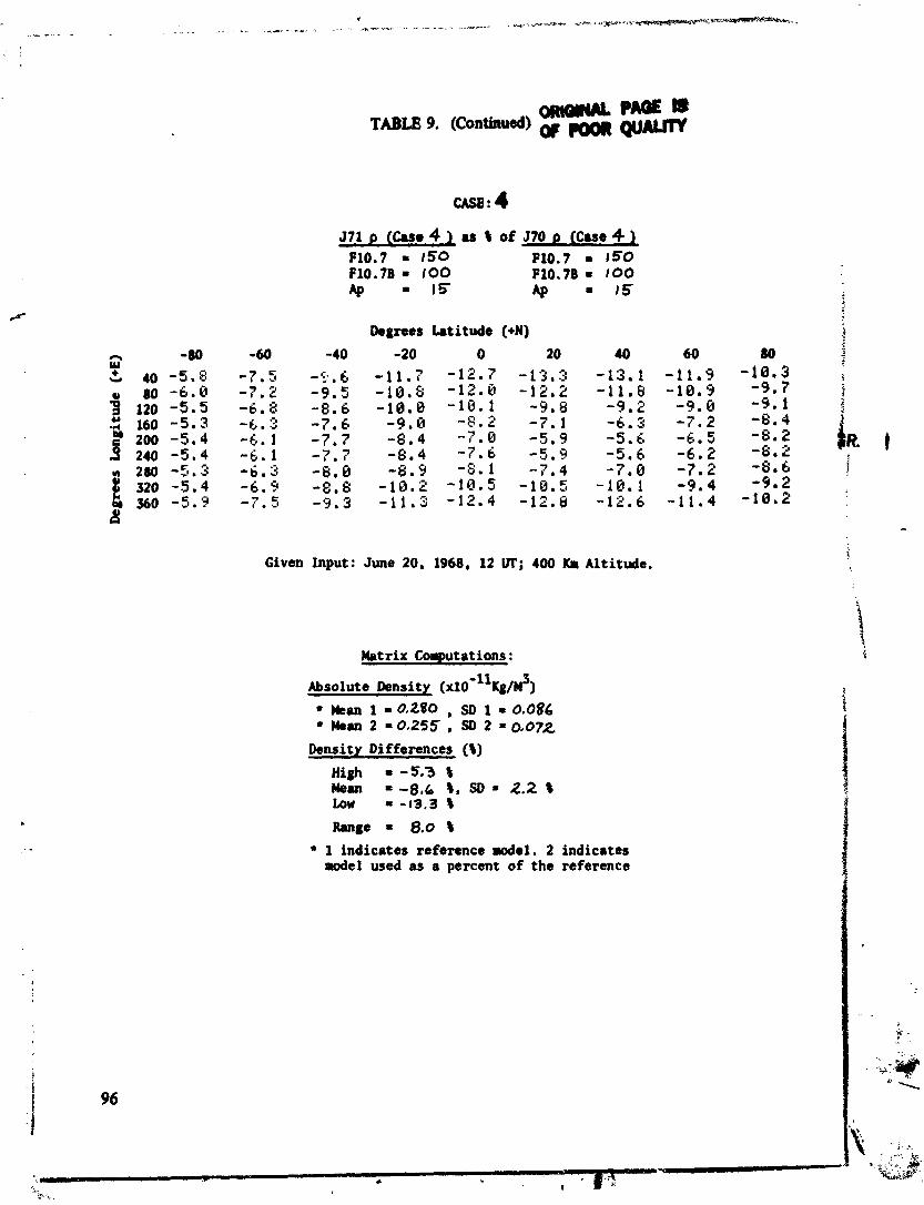
CASE : 4
. 577 p (Case 4 ) as 9 of 570 p (Case 4 ) F10.7 = 150 F10.7 = ' 50 F10.78 = /00 F10.78 = 100 & = 1 5 Ap = 1 5
Degrees Latitude (+N)
Given Input: June 20, 1968, 12 UT; 400 l(m Altitude.
Matrix Computations :
Absolute Density ( x ~ o - ' ~ K ~ / M ~ ) Mean 1 = 0.280 , SD 1 r 0.086 Mean 2 =0.23/ , SD 2 =0 .078
Density Differences (0)
High = -1.8 t Man = -1'9.1 0, SD = 8.1 1 Low = - 3 6 . 3 8
Range = 34.5 0
1 indicates reference model. 2 indicates model used as a percent of the reference

TABLE 10. (Continued) ORIGINAL PAW IS OF POOR QUALITY
CASE : 5 577 p (Case 5 1 as % of 370 p (Case 5 )
F10.7 = 150 F10.7 = 150 F10.7B = /50 F10.78 = 150 & 0 4 ' 0
Degrees Latitude (+N)
Given Input: June 20, 1968, 12 UT; 400 Km Altitude.
Matrix Computations;
Absolute Density ( x ~ o - ~ ~ K ~ / M ~ )
Mean 1 = 0.262, SD 1 = 0.09/ * Mean 2 = 0.288 , SD 2 = 0.088
Density Differences (I)
High = 30.5 li Mean = 11.3 I , SD= 8.3 li Low = - e . / l i Range a 38.6 %
1 indicates reference model. 2 indicates model used as a percent of the reference
IS. 9 10.:5 12 .8 1 4 . 7 1 4 . 7 13. kl 15 .0 11.8
6 . 2

TABLE 10. (Continued) ORlOlNAL PAM IS OF POOR 01 141 JN
577 p (Case 6 ). as $ o f 570 p (Case 6 ) F10.7 = 150 F10.7 = 150 F10.78 = 150 F10.7B = 150 4' = 15 Ap = 1 5
Degrees Latitude (+N)
Given Input: June 20, 1968, 12 UT; 400 Km Altitude.
Matrix Computations;
Absolute Density ( I K I O - ~ ~ K ~ / M ~ )
* hiean 1 ~ 0 . 3 6 9 , SD 1 = 0.107 * Mean 2 = 0 . 3 / 7 , SD 2 = 0 . / 0 /
Density Differences (S)
High = 2.0 % Mean = -14.6 S , SD = 8.4 % Low = - 3 2 . 5 %
Range = 39.5 S
1 indicates reference model. 2 indicates model used as a percent o f the reference

I r..,. . . _ .. .,. ri.: A TABLE 10. (Continued) ORlQlMAL PAGE IS
OF POOR QUALlM
CASE : 7 J77 P (Case 7 ) as S of 570 p (Case 7
F10.7 = 150 F10.7 E 150 F10.7B = 15-0 F10.7B = 150 AP =.ern Ap a 400
Degrees Latitude (+N)
Given Input: June 20, 1968, 12 UT; 400 KIP Altitude.
Matrix Computations:
Absolute Density ( X ~ O - ~ ~ K ~ I M ~ ) - Mean 1 t 1.103 , SD 1 = 0.158
* Mean 2 =/ .008 , SD 2 = 0 . 5 6 5
Density Differences (%)
High = 1/57 Z Mean = -9 .6 %, SD = e.1 % LOW = -69.3 %
1 indicates reference model. 2 indicates model used as a percent of the reference

TABLE 10. (Continued) 0
577 p (Case 8 ) as I of 570 p (Case 8 ) F10.7 = 200 F10.7 = 200 P10.7B = / 50 F10.78 + 150 Ap = 15 Ap = 1 5
Degrees Latitude (+N)
Given Input: June 20, 1968, 12 UI'; 400 Km Altitude.
Matrix Computations:
Absolute Densitr (~Io'''K~/$) &an 1 = 0.52/ , SD 1 = 0,137 Mean 2 = 0.428, SD 2 = 0. /2?
Density Differences (%)
High = -0.7 % Mean =-18.2 2, S D = 8.2. % Low = - 3 4 . 6 %
* 1 indicates reference model. 2 indicates model used as a percent of the reference
- 2 s * 9 - 2 8 . 8 - .-a . :: -14.6, - .-, .-, rrt. 1 -13.7
-14.E1 -17.5 -18.9 -16.8 - ; ,> @ . 5 -14.8 -14 .3 - 1 1 . 6 - 1 8 . 6 -13.2 , .-8 h - L O . Z -18.7

CASE : 9 J77 p (Case 9 ) as t of 570 p [Cue 9 1
P10.7 = 250 F10.7 = 250 F10.7B = 250 P10.78 = 250 A p r O Ap - 0
Degrees Latitude (+N)
Given Input: June 20, 1968, 12 VT; 400 Km Altitude.
Matrix Computations:
Absolute Density (xl0-l1~O/M3) mpn 1 - 0.790 , SD 1 = 0.199
* Msan 2 ~ 0 . 7 2 5 , SD 2 0.166
Density Differences (5) High = 1.1 t Mean = -7.6 5, SD = 4-5 5 Low = - 1 9 . 5 %
Range = 20.6 5
1 indicates reference model. 2 indicates model used as a percent of the reference

ORKY~U l8 TABLE 10. (Continued) Or. rn W L m
577 P (Case / O ) as % of J70 o (Case /O I P10.7 = 250 F10.7 = 250 F10.7B = 250 F10.78 = 250 Ap = 1 5 Ap I 1 5 r
Degrees Latitude (+N)
Given Input: June 20, 1968, 12 VT; 400 Km Altitude.
Matrix Computations:
Absolute Density (x10-''KO/$)
* man 1 0.953 , SD 1 10.210 * Mean 2 = 0.773 , SD 2 = 0.205
Density Differences (t)
High = -0.e t Mean =-19.Zt, S D = S.7 t Low = -34.1 %
Range = 33.3 5 1 indicates reference model. 2 indicates model used as a percent of the reference

-. 7 .". ~. !.. J
1 " . -* ,.', . -, TABLE 10. (Continued)
Degrees Latitude (+N)
Given Input: June 20, 1968, 12 Ul'; 400 K. Altitude.
Matrix Computations:
~ b r 0 1 ~ t e k n ~ i t ~ ( x 1 0 - l ~ ~ $1 1 =/.824 , SD 1 *0*227
Mean 2 = /.828 , SD 2 = 0.666 Density Differences ( 8 )
High = 58.7 1 MOO^ -0.8 1, SD= 30.8% LOW = -52 .0%
* 1 indicates reference model. 2 indicates model used as a percent of the reference

--I8 Ill, D ~ ~ l O N OF COMPARATIVE RESULTS W Q U ~
The anal@ prelented in thb lcction d& with the two percent differencing schemer mentioned in the Introduction. That of percent density differences within each made1 (for differing solar condi- tions), and that of p e n t difference between one model axxi another. The analymb will further be broken down into two condition& Om examines d d t y change8 under a constant Ap ( a l l o m flux to my); the other assumes a conatant FIO 7 flux (allowing Ap to my). Many of Tabla 6 thmu~h 10
a-< results will also be expremed in fob.
A. Intn-Mdol Tdng U W Conrtnt Flux
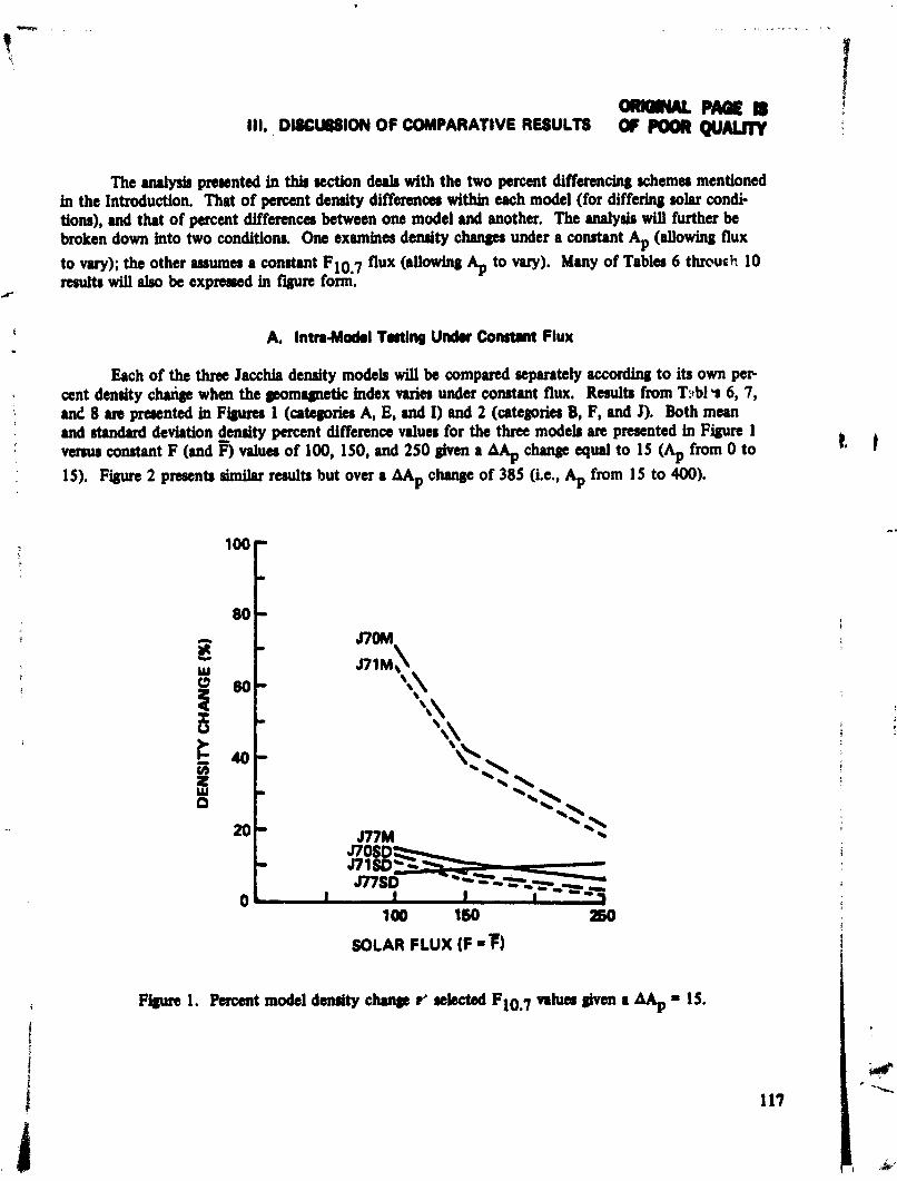
Each of the three Jacchia density modeb will be compared separately according to its own per a n t density chaige when the geomagnetic index varies under constant flux, Results from T:-fbl u 6, 7 , and 8 an pmented in Figum 1 (categories A, E, and I) and 2 (categoria B, F, and J). Both mean and standud deviation density percent difference values for the thra madeb an presented in Figure 1
I v ~ c o m t a n t F ( a n d ~ v a l u c r o f l O O , l 5 O , a n d 2 5 0 ~ a A ~ c h ~ c p u a l t o l S ( A p f m m O t o : IS). Figure 2 presents similar ren~lts but over a % change of 385 (i.c., Ap from 15 to 400).
100 160
SOLAR FLUX (F

SOLAR FLUX (F -F)
F w 2. Percent model daulty ch.rUe at melcctcd Flom7 values (Ivm a % = 385.
Figure 1 shows that the J70 and 171 mean (M) percent diffmnas change by more than 50 per- cent than doer the 177 at F = 100, when AAp = 15. ThL difference is mraller whenever the flux is 150 or 250. The rtandud deviation (SD) for all three modeb is mall (1- than 16 percent) at F = 100, with 170 and 171 miability decrahg at higher flux. The 177 SD increases 8 percent more than the other two modeb at F = 250.
k Ap inaavar 385 unitl from 15 to 400, all three madeb are very #1Uitive to a density change at a low flux (F = 100) (Fb 2). The 177 matrix percent Wersnce values we much mom variable wer latitude (Table 8B) than the 170 or 171 u exprsrred by the huge 177 SD value of 434 pmmt at F - 100, A larger F flux of 150 or 250 produces dpiflcantly lowet density incseuer u shown by the M and SD percent difference valusr of Figure 2.
Thew two ~ a y l a t U u t l f 7 k ~ ~ ~ r ( c r m P m ~ t u d e A p c h u y t than the170 7 1 Wben Ap lev& jump to extremes (Ap = 400) the 177 k jus! a little more W t i w in the m a n
c h p than 170 and 171, but it ir abo much mom v&le in ita percam change of dendty uound tlle globe.


gaqcrr-D Q F W O R Q U ~
Figure 3 presonts conditions (cate~rier M, P, and S) applicable to an incream in F (andm of 50, using data when F incremes from 100 to 150. Percent density increase values ue plotted for constant Ap of O,1$ and ad. Oaty at Ap = 0 conditions do J77 densit j percent inaaua appear equal ; t o o r l o ~ ~ ~ t h a n t h m 0 f J 7 0 ~ J 7 1 . IfApis 1 5 o r W , a M o f 5 0 ~ l 0 l t a a ~ ~ m t d W t y inacrc,withthJ77lhwddoublingthtofthcJ70orJ71 atAp=4lXl. ALoatAp=400,thevar iability (in tenns of SD) of 377 is luge (more than 50 percent) as compared to J70 or J71 (less than 4 perant).
Figure 4 differs from Figure 3 only in that it deals with a flux change of 100 (where F goes from 150 to 250). Indicated in F@m 4 is the same general trend as in Figure 3, except amplitudes of density change percentage am magnifii for the J70 and 571 cases, with little incream shown for the J77 M or SD pma*. Figure 4 represents categories N, Q, and T.
% paan t dcnsity increases on each model for a 50 unit change in the daily flux, during a constant F and cow'mt A, = 15 condition, arc presented in Figure 5. This would probably represent a more typical condition &ally erpuienced on a day-today basis when f would remain approximately constant. Three different categories of AF = SO arc presented in Figure 5: when the daily flux changes 1 1 from 100 to.150, from 150 to 200, d from 250 to 300. M t y percent changes, in terms of M and SD, decrcase as the AF = 50 category occurs for a greater F value. From the f v it appears as if the J71 is ltss sensitive to a AF change than the other two models. Figure 5 represents categories D, H, and L.
SOLAR FLUX? Figure 5. Percent model dartty chute at % = IS given AF OF 50 with constant F.

Table 11 summa&es the results pa+ntud in F M 1 and 2, when Ap is allowed to vary under constant F and F. Table 12 pnsents results from Figures 3,4, and 5, when F (andat times F) is allowed to my, while Ap is kept constant.
TABLE 1 1. PERCENT GLOBAL DENSITY CHANGE WHEN Ap VARIES UNDER CONSTANT F AND F
TABLE !2. PERCENT GLOBAL DENSITY CHANGE WHEN F VARIES UNDER CONSTANT Ap
% = 15 (Ap = 0 to 15)
Cat. F10 FlOB I
A 100 100 E 1 50 150 I 250 250
AA,, = 385 (kp = 15 to 400)
Cat. F10 FlOB
B 100 100 F 150 1 50 J 250 250
J7 1 170 577
M
66 40 20
M
70 44 22
Only F changes. rremains constant. ** Both F and F change the same. 121
I AF= 50
M
16 10 6
SD
12 7 3
SD
13 8 4
1
Cat.
D H L
J70 J7 1
SD
8 9
11
J7 1
M
65 42 22
M
43 28 15
t J77 J70
M
344 192 90
J
J77
Ap 15 15 15
SD
6 4 2
SD
3 2 1
M
377 212 95
SD
75 36 14
M
394 226 139
M
71 36 16
F Range
F = 100 to 150 F = 150 to 200 F = 250 to 300
AF = 50 (F = 100 to 150)**
SD
90 45 19
SD
434 183 73 .
SD
10 4 1
1
570 J7 1
Cat.
M P S
M
160 119 44
M
162 121 46
A,, 0 15
400
J77
SD
19 11 2
SD
20 11 1
M
1 48 136 91
AF = 100 (F = 1 50 to 250)**
SD
2 1 2 1 55
,
J7 1
cat.
N Q T
J70
M
207 163 72
Ap i
0 15 400
M
21 1 163 66
J77
SD
26 16 2
SD
29 18 3
M
158 1 49 105
SD
22' 20 53
, . ' I ' . , P a l8 i
O f P O b R W ~ C. Inm-Modol T d n g Uf&r Conr&nt Flux
This section is included so that percent density differences between one model and another (the E 1
standard) can be computed for a given case. It indicates exactly how much one model's calculated ! densities differ percentwise from another model's &u. Tables 9 and 10 data were used in this analysis.
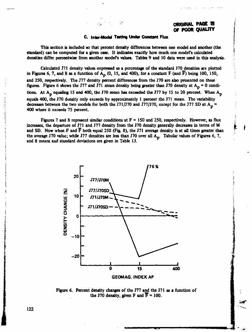
Calculated $71 density values expressed as a percentage of the standard J70 densities are plotted in Figures 6,7, and 8 as a function of Ap (0, 15, and a), for a constant F (and F) being 100, 150, 1
and 250, respectively. The 577 density percent differences from the J70 are also presented on these ftguns. Figure 6 shows the J77 and J71 mean density being greater than J70 density at % = 0 condi- tions. At % equaling 15 and 400, the J70 mean has exceeded the J77 by 15 to 20 percent. When Ap equals 400, the J70 density only exceeds by approximately 1 percent the 571 mean. The variability d w u r s between the two models for both the J71/J70 and J77/J70, except for the J77 SD at Ap = 400 where it exceeds 75 percent.
i
Figures 7 and 8 represent similar conditions at F = 150 and 250, respectively. However, as flux increases, the departure of 371 and J77 density from the $70 density generally decreases in terms of M and SD. Now when F and P both equal 250 (Fig. a), the $71 average density is at all times greater than the average 170 value; while 177 densities are less than 170 over all Ap. Tabular values of Figures 6, 7, and 8 means and standard deviations are given in Table 13.
0 15 400
GEOMAG. INDEX AP
Figure 6. percent density changes of the J77 and the $71 as a function of the J70 dendty, given F and F= 100.

GEOMAG. INDEX AP.
Figure 7. Percent density changes of the J77 and the J71 as a function of the J70 density, given F and F = 150.
GEWAG. INDEX AP
F m 8. Percent denaity changea of the J77 and the J71 as a function of the J70 density, &en F and F = 250.

c.: - '9 ," . . , TABLE 13. PERCENT DENSITY DIFFERENCES BETWEEN THE J7 1 AND J77
WITH RESPECT TO 570, AT CONSTANT F AND P
Both the J77 and J71 density values from Tables 9 and 10 are expressed as percent differences, at constant Ap, with respect to the J70 density in Figures 9, 10, and 11. Figure 9 presents the models mean and standard deviation percent difference values from standard, for F and F conditions of 100, 1 SO, and 250 at constant Ap = 0. Figures 10 and 1 1 represent similar conditions for Ap = 15 and 400, 1
.i respectively. , i
F Held Constant (Ap Varies)
Care Number
(FIO a n d q O = 100) 1. Ap=O 2. Ap= 15 3. Ap=400
( F ~ ~ a r id50 = 150) :. P L p = O 6 . Ap = 15 7. Ap = 400
(FIO and qo = 250) 9. Ap=O
10. Ap= 15 11. Ap=400 .
Figure 9 indicates that the 177 density at Ap = 0 is grater than the J70 by 11 to 16 percent, F
at F (and F ) of 100 and 1 50. However, J77 densities are less than J70 by 7 percent at an F (and F) of 250. The SD of the J77 percent density difference decreases slightly from 11 percent at F = 100 to 4 $
.- percent at F = 250. The M and SD of J71 density as a percent from the J70 is from 4 to 10 percent i greater than the :TO at all three flux values. $
B
Incidently, the 171 relationship to J70 is approximately uniform for all three Ap conditions. This is probably due to the fact that the J71 and J70 Jacchia models are both derived with similar datalequations, resulting in similar construction.
When Ap = 15, the 177 mean density is 15 to 20 percent lower than the 170 at all three flux conditions. The J71 density is win greater than the J70 by 6 to 7 percent, with small variability
i observed over the globe (Fig. 10).
c
J71 p as f (570 p) [%I Mean p%A
9 6
- 1
10 7 0
9 7 4
._I
J77 p as f (570 p) [k] SD p%A
5 4 2
5 4 1
4 3 1
Mean p%A
17 -20 -1 4
-*a-
I I -1 5 -10
- 8 -19 - 1
SD p%A
12 9
75 ". --,
8 8
49
5 9
3 1

SOLAR FLUX (F =F) Figure 9. Percent density changes of the 177 and the 171 as a function of the
170 density, given Ap = 0.
SOLAR FLUX (F -7) Figure 10. Percent density changes of the J77 and the J71 as a function of the
J70 density, given Ap = IS.
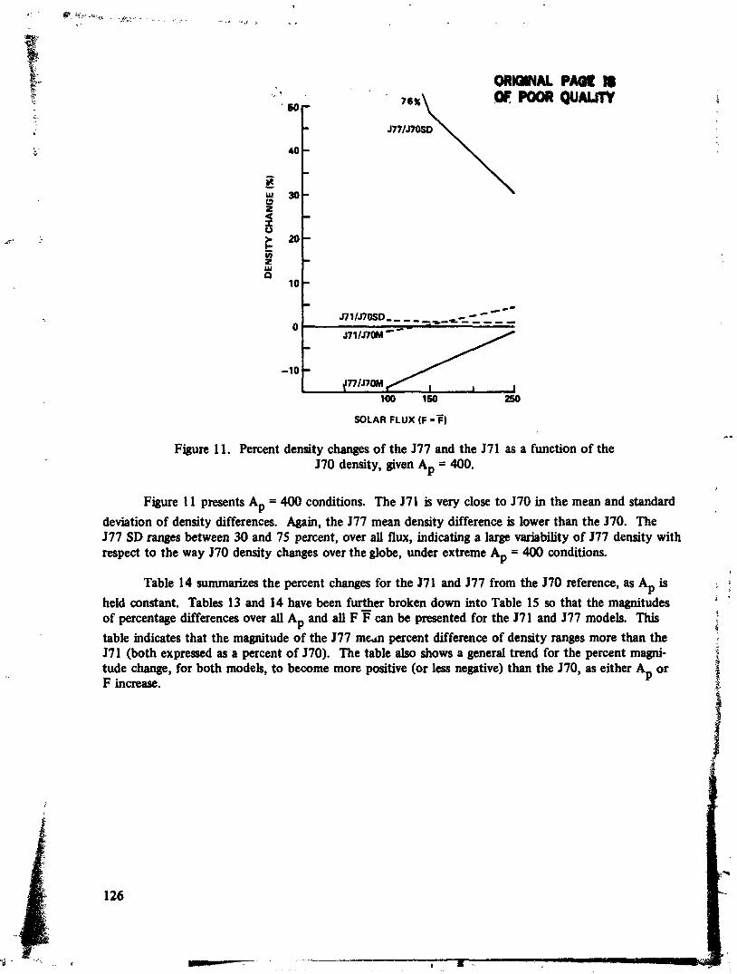
SOLAR FLUX (F =T)
'So -
- 40-
Figure 11. Percent density changes of the 577 and the J71 as a function of the J70 density, given Ap = 400.
* - w 30- (1
2 c 20-
f s' 10
Figure 11 presents Ap = 400 conditions. The J71 is very close to J70 in the mean and standard
m.
-
- -
deviation of density differences. Again, the 577 mean density difference is lower than the 570. The J77 SD ranges between 30 and 75 percent, over all flu, indicating a large variability of 577 density with respect to the way 570 density changes over the globe, under extreme Ap = 400 conditions.
Table 14 summarizes the percent changes for the J71 and 577 from the 570 reference, as Ap is . 1 , i
held constant. Tables 13 and 14 have been further broken down into Table 15 so that the magnitides 1
of percentage differences over all AD and all F can be presented for the J71 and J77 models. This 4 i
table indicates that the magnitude df the J77 m a n percent difference of density ranges more than the 7
J71 (both expressed as a percent of J70). The table also shows a general trend for the percent magni- t tude change, for both models, to become more positive (or less negative) than the J70, as either A or F increase. P i
3

T U L E 14. PERCENT DENSITY DIFFERENCES BETWEEN THE J7 1 AND J77 WITH RESPECT TO J70, AT CONSTANT Ap
# i
Ap Held Constant (F Varia)
Case t
No. F10 "P !OB
1. 100 100 5. 150 150 9. 250 250
(Ap = 15) F10 FlOB
2. 100 100 6. 150 150
10. 250 250
4. 150 100 8. 200 150
12. 300 250
(Ap = -1 F10 FlOB
3. 100 100 7. 150 1 so
11. 250 250
577 p as f (J70
Mean p%A
17 11
- 8
-20 -15 -1 9
-1 8 -1 8 -23
-14 -10 - 1
p) [%I ,
SD p%C -
12 8 5
9 8 9
8 8 8
I
75 49 3 1
J7 1 p as f
Mean p%A
9 10 9
6 7 7
-9 4 0
-1 0 4
(570 P ) [% I
SD p%A
5 5 4
4 4 3
2 2 2
2 1 1

TABLE 15. J7 11577 AS PERCENT DENSIN MAGNITUDE CHANGE OF J70 OVER VARIOUS RANGES OF Ap AND F
9
I
J71 p as f (70 p)
(Inmasing Ap) FFconst. (Table 13)
A~
0 to 15 15 to 400
0 to 400 . (Increasing F and F) Ap Const. (Table 14)
(F F)
100-100 to 150-1 SO 150-1 50 to 250-250
100-100 to 250-250
FF 100-100
- 3 - 7 - -10%
A p = O + 1 - 1 - 0
J77 p as f (70 p)
FF 150-1 50
- 3 - 7 - -1 0
Ap= 15
+ 1 0 -
t 1
FF 250-250
I
-2 -3 - -5
%=400
+1 +4 - +5
FF 250-250
-1 1 +18 - + 7
Ap = 400
+ 4 + 9 - +13
(Increasing Ap) F F ~ o n s t . (Table 1 3)
Ap I
0 to 15 15 to 400
0 to 400 r
(Increasing F and F) Ap Const. (Table 14)
(F F)
100-100 to 150-150 150-1 50 to 250-250
100-100 to 250-250 A
FF 100-100
-37 + 6 - -3 1%
Ap=O
- 6 -19 - -25
,F F 150-1 50
-26 + 5 - -2 1
Ap= 15
t 5 -4 - + 1

IV. SUMMARYJCONCLUSIONS
For the 12 different cases of solar/geomagnetic input used in the 400 km density analysis of three thermospheric models (i.e., 170, 571, and J77), the following has been accomplished under this study:
1) 12 cases of 400 km density data have been generated for 8 1 worldwide latitude/longitude locations, for the three separate Jacchia models of 1970, 1971, and 1977 (Tables 3, 4, and 5).
..t '
2) A small A change from low values (Ap = 0 to 15). over all F = F ( F s = 100 to 250), P indicates the 577 computed density is less sensitive to these changes than the 570 or J71. The variability of 577 is smaller or equal to that of J70 or J71 at F's = 100 and 150; while larger in variability when F's = 250 (Fig. 1 and Table 1 1).
3) A large Ap change from low to high (Ap = 15 to 400), over all F = F, indicates J71 as being less sensitive to density change in terms of global mean density and its variability. The 577 indicates a very high variability of global density as compared with the J70 and J71 (Fig. 2 and Table 11).
4) During an F and change = 50 or = 100, the J77 does not show a density change as much as the J7O or 171 at Ap = 0. However, at Ap = 400 the exact reverse is true, with J77 density change being higher and much more variable than either the J70 or J71 over the globe (Figs. 3, and 4 and Table 12).
5) When a change in F daily alone occurs (i.e., AF = 50, AF = 0, AAp = 0), the 17 1 is the l a . sensitive to density change and it also exhibits less variability of change over the globe (Fig. 5 and Table 12).
6) Intermodel testing over varying Ap and flux indicates the 171 density to be slightly more dense than the J70. The J77 density is generally less than J70 over all conditions, except when Ap = 0. The variability of J77 density over the globe is also very high whenever Ap = 40 (Figs. 6 through 11 and Tables 13 through 15).
7) This study has also indicated the 571 density being closer, in most all categories, to the 170. This is reasonable due to similar data and modeling methods in both.

REFERENCES
1. Jacchia, L. C.: New Static Models of the Thmmphere and'Exmphere with Empirical Tempera- ture Profiles. SAO Report 3 13, May 6, 1970.
4
2. "Models of Earth's Atmosphere (90 to 2500 km)," NASA SP-8021, Revised March 1973. i : i
3. Jacchia, L. G.: Revised Static Models of the Thermmphere and Exosphere with Empirical Tem- perature Profiles. SAO Report 332, May 5, 1971.
4. Jacchia, L. G.: Thmospheric Tempemtun, Density, and Composition: New Modeb. SAO Report 375, March 15, 1977.
Related Documents