Semiparametric Estimator of Time Series Conditional Variance

Semiparametric Estimator of Time Series Conditional

Variance

Santosh Mishra∗, Liangjun Su†, and Aman Ullah‡

October 2008

Abstract

We propose a new combined semiparametric estimator, which incorporates the parametric

and nonparametric estimators of the conditional variance in a multiplicative way. We derive the

asymptotic bias, variance, and normality of the combined estimator under general conditions.

We show that under correct parametric specification, our estimator can do as well as the para-

metric estimator in terms of convergence rates; whereas under parametric mis-specification our

estimator can still be consistent. It also improves over the nonparametric estimator of Ziegelman

(2002) in terms of bias reduction. The superiority of our estimator is verfied by Monte Carlo

simulations and empirical data analysis.

Key Words: Semiparametric Models, Nonparametric Estimator, Conditional Variance

JEL Classifications: C3; C5; G0

∗Department of Economics, Oregon State University, Corvallis, OR, 97330, U.S.A.; e-mail: san-

[email protected].†School of Economics, Singapore Management University, 90 Stamford Road, Singapore 178903; e-mail:

[email protected].‡Corresponding Author. Department of Economics, University of California, Riverside, CA 92521-0427, U.S.A.,

Tel: (951) 827-1591, Fax: (951) 787-5685, e-mail: [email protected].

1

1 Introduction

There are two main approaches to modeling volatility as the conditional variance σ2t for a stochastic

process yt. The first is based upon the GARCH family of models, which was pioneered by Engle

(1982) and soon spawned a plethora of complicated models to capture empirically stylized facts.

The second is based upon the stochastic volatility model, which treats σ2t as a latent variable and is

expressed as a mixture of predictable and noise components. Both approaches provide parametric

models of conditional variance σ2t . It is well known that when the parametric model is correctly

specified it gives a consistent estimator of σ2t , whereas when the parametric model is incorrectly

specified the resulting volatility estimator is usually inconsistent with σ2t .

Nonparametric and semiparametric estimation of conditional variance can provide consistent

estimation of σ2t . Pagan and Schwert (1990) and Pagan and Hong (1990) are among the initial

works in nonparametric ARCH literature. Härdle and Tsybakov (1997) and Härdle et al. (1998)

deal with univariate and multivariate local linear fit for conditional variance, respectively. Fan and

Yao (1998) and Ziegelmann (2002) model squared residuals (from the conditional mean equation)

nonparametrically to capture the volatility dynamics. Most of the above literature includes one lag

in the conditional variance model. Additive and multiplicative models have tried to capture the

impact of several period lags in the conditional variance equation. Yang et al. (1999) propose a

model where the conditional mean is additive and the conditional variance equation is given as

σ2t = γ0Πdj=1σ

2j (yt−j), where γ0 is an unknown parameter and σ2j (

.) , j = 1, ..., d, are smooth but

unknown functions. Linton and Mammen (2005) propose a semiparametric ARCH(∞) model wherethe conditional variance equation is given as σ2t (γ,m) = μt +

P∞j=1 ψj(γ)m(yt−j), where γ is a

finite dimensional parameter, m (.) is a smooth but unknown function and the functional forms of

ψj(.), j = 1, 2, ..., are known. Yang (2006) extends the GJR model (Glosten et al., 1993) to the

semiparametric framework.

As explained in the next section, our paper takes a different approach where we combine a para-

metric estimation with a subsequent nonparametric estimation. We first model the parametric part

of the conditional variance and then model the conditional variance of the standardized residual (non-

parametric correction factor) nonparametrically capturing some features of σ2t that the parametric

model may fail to capture. Thus the combined heteroskedastic model is a multiplicative combination

of the parametric model and the nonparametric model for the correction factor. The global para-

metric estimate of σ2t can be obtained by using any parametric model based on the quasi maximum

likelihood estimation (QMLE) principle, say. The estimate of the nonparametric correction factor

can be obtained by various nonparametric methods, including the local linear or exponential estima-

tion technique. The idea behind the combined estimation is that if the parametric estimator of σ2tcaptures some information about the true shape of σ2t , the standardized residual will be less volatile

2

than σ2t itself, which makes it easy to estimate the nonparametric correction factor.

It is worth mentioning that our semiparametric approach has a close analogy with the well

known prewhitening method in the time series literature. See Press and Tukey (1956), Andrews and

Monahan (1992), among many others. The method has already been applied in the context of kernel

density estimation by Hjort and Glad (1995) and in the context of conditional mean regression by

Glad (1998). The seminonparametric estimators of Gallant (1981, 1987) and Gallant, and Tauchen

(1989) employ a parametric component plus a flexible nonparametric component. Other combined

estimators for density function or conditional mean function include Olkin and Spiegelman (1987),

and Fan and Ullah (1999).

Built on aforementioned works, our paper provides asymptotic theory for the asymptotic bias,

variance, and normality of the semiparametric estimator. It presents several potential improvements

over both pure parametric and nonparametric estimators. First, in the case where the parametric

model is misspecified so that the parametric estimator for the true volatility is usually inconsistent,

our semiparametric estimator can still be consistent with the volatility. Second, in the case where

the parametric model is correctly specified, as expected, our semiparametric estimator is generally

less efficient than the parametric estimator but it can do as well as the parametric estimator in

terms of convergence rates. Third, in comparison with the nonparametric estimator of Ziegelmann

(2002), our estimator can result in bias reduction as long as the parametric model can capture

some roughness feature of the true volatility function, whereas the two estimators have the same

asymptotic variance. In case of correct specification in the first stage parametric modeling, our

semiparametric estimator beats the Ziegelmann’s estimator. Also, our estimator for the conditional

volatility allows the conditioning variable to be estimated from the data and it incorporates the case

where the information set is of infinite dimension but can be summarized by a finite dimensional

conditioning variable (as in the typical GARCH framework), in sharp contrast with the setup in

Ziegelmann (2002).

The structure of the paper is as follows. In Section 2 we introduce the semiparametric model and

estimator, and study in detail the asymptotic properties of the semiparametric estimator without

and with the assumption of correct parametric specification in the first stage. Section 3 provides

simulations and empirical data analysis. Final remarks are contained in Section 4. All technical

details are relegated to the Appendix.

3

2 The Semiparametric Estimation

2.1 The Model and Its Reformulation

In this paper we consider the model

yt = g(Ut,α0) + εt, t = 1, ..., n, (2.1)

where the error term εt satisfies E(εt|Ft−1) = 0, E(ε2t |Ft−1) = σ2t , Ft−1 is the information set attime t− 1, Ut and α0 are vectors of regressors and pseudo-true parameters, respectively. Since theseminal paper of Engle (1982), a vast literature has developed on the specification of σ2t , among

which the (G)ARCH family of models play a fundamental role. The majority of the GARCH family

of models are specified parametrically, which is subject to the issue of misspecification. In case

of misspecification, the conditional variance may not be estimated consistently even though the

parameter estimator in the volatility model is still consistent for some pseudo-true parameter. Similar

remarks also hold for the class of stochastic volatility models.

Here we propose a semiparametric estimator for the conditional variance based on a multiplicative

combined model. The point of divergence from the existing literature is that we represent the

conditional variance in two parts: parametric and nonparametric. Analogous to Glad (1998), the

idea builds on the simple identity

E(ε2t |Ft−1) = σ2p,tE

(µεtσp,t

¶2|Ft−1

), (2.2)

where σ2p,t ∈ Ft−1 is determined by a parametric specification of the conditional variance. Let

σ2np,t = E(εt/σp,t)2 |Ft−1. We then have

σ2t = σ2p,tσ2np,t. (2.3)

The key point is that if the parametric specification σ2p,t captures some roughness features of σ2t ,

the “nonparametric correction factor” σ2np,t will be easier to estimate. In the extreme case when

the parametric part σ2p,t is correctly specified, we would hope σ2np,t to be constant over time. To

facilitate the presentation, we make the following assumption.

Assumption A0. σ2p,t = σ2p(X1,t,γ0) and σ2np,t = E(εt/σp,t)2 |Ft−1 = σ2np(X2,t), where γ0 is

the pseudo-true parameter, and X1,t and X2,t are a d1 × 1 and d2 × 1 vector, respectively.Given Assumption A0, σ2t ≡ σ2(Xt) = σ2p(X1,t,γ

0)σ2np(X2,t), where Xt, a d × 1 vector, is adisjoint union of X1,t and X2,t. We are interested in estimating the volatility function σ2 (.) at an

interior point, x ∈ Rd. To see how restrictive Assumption A0 is, we make a definition:Definition (Minimal reducible dimension d∗) If E(ε2t |Ft−1) = E(ε2t |Zt) for some Zt ∈ Ft−1,

a vector of finite dimension d∗, we say that the information set Ft−1 is reducible. If further

4

E(ε2t |Ft−1) 6= E(ε2t | eZt) for any subvector eZt of Zt, we say that the dimension d∗ is minimal for

estimating σ2t and the set Zt is a minimal reducible set .

Remark 1. Note that the minimal reducible set Zt is not necessarily unique. For example, if

the true data generating process (DGP) for εt is a GARCH(1,1) process:

εt =qσ2tvt, σ

2t = γ00 + γ01σ

2t−1 + γ02ε

2t−1, (2.4)

where vt is a martingale difference sequence (m.d.s.) with mean 0 and variance 1, then σ2t dependson the entire past information set Ft−1 only through σ2t−1 and ε2t−1. In this case, one can take

Zt =¡σ2t−1, ε

2t−1¢Tor Zt =

¡σ2t−1, εt−1

¢Tin the above definition. In either case, d∗ = 2 is minimal.

Remark 2. Clearly, Assumption A0 is a dimension reduction assumption, which is crucial for

our asymptotic analysis. On the surface, both parts of the conditional variance, σ2p,t and σ2np,t, may

depend on a possibly infinite dimension of information in the information set Ft−1. Assumption A0requires that it is possible to summarize the information into a finite dimensional stochastic variable

X1,t or X2,t. This assumption looks restrictive but is not as restrictive as it appears. Suppose the

true DGP for εt is a GARCH (1,1) process in (2.4). If we correctly specify the parametric conditional

variance model, then σ2p,t = γ00 + γ01σ2p,t−1 + γ02ε

2t−1 and σ2np,t ≡ 1. In this case we can simply set

X1,t = (σ2p,t−1, ε

2t−1)

T and X2,t = X1,t or 1, say; σ2p (.,. ) is affine in both X1,t and γ0 ≡ (γ00, γ01, γ02)T ;

and σ2np (.) is a constant function. On the other hand, if we specify the parametric conditional

variance model as an ARCH(1) model, so that we can write σ2p,t = γ∗0 + γ∗2ε2t−1, where (γ

∗0, γ∗2)

is the pseudo-true parameter to which the ARCH(1) parametric estimate converges. In this latter

case, we can easily identify X1,t = ε2t−1 and X2,t = (σ2t−1, ε2t−1)

T ; σ2p (.,. ) is affine in both X1,t

and γ0 ≡ (γ∗0, γ∗2)T ; and σ2np (X2,t) =¡γ00 + γ01σ

2t−1 + γ02ε

2t−1¢/(γ∗0 + γ∗2ε

2t−1) is a highly nonlinear

function.

Remark 3. Xt is not necessarily observable and it summarizes the entire past information set

that has influence on the conditional variance. For example, if one specifies σ2p,t as GARCH(1,1)

process: σ2p,t = γ00 + γ01σ2p,t−1 + γ02ε

2t−1, then γ

0 = (γ00, γ01, γ

02)T , X1,t =

¡σ2p,t−1, ε

2t−1¢T

. So we can

re-write the above process as: σ2p,t = σ2p(X1,t,γ0) = γ00 + γ02σ

2p,t−1 + γ02ε

2t−1. Given X1,t and γ0, we

can recover σ2p,t through the map defined by¡X1,t,γ

0¢→ σ2p(X1,t,γ

0). This is sufficient for our

purpose. If one believes that X1,t summarizes all the past information that affects the conditional

variance at time t but has some doubt on the correct specification of the GARCH (1, 1) model, one

can choose X2,t = X1,t. As a matter of fact, either X1,t or X2,t or both may depend on the unknown

parameter

θ0 =¡α0T ,γ0T

¢T.

For this reason, we shall write X1,t, X2,t, and Xt explicitly as X1,t

¡θ0¢, X2,t

¡θ0¢, and Xt

¡θ0¢.

Remark 4. We don’t need correct specification for modeling the parametric component. To be

concrete, we focus on the case where the set of finite dimensional parameters are estimated by QMLE

5

technique. Suppose the data yt, Ut are generated from the joint density f(y|u)f(u), where f(u) isthe marginal density of Ut and f(y|u) is the density of yt given Ut = u. Let f(α0,γ0)(y|u)f(u) be thedensity under the chosen parametric assumption. Whether the parametric model is true or not, under

some regularity conditions for QMLE, the parameters, α0 and γ0, can be estimated consistently at

the regular√n rate (White, 1994, Chapter 6). One way is to use QMLE to estimateα0 and γ0 jointly.

The other is, under some orthogonality conditions, to estimate α0 in (2.1) first, say by nonlinear

least squares, and then use the residual series bεt to estimate γ0. In either case, we can generallyestablish

√n-rate consistency for estimating the pseudo-true parameter

¡α0T ,γ0T

¢T, which is a

minimizer of the Kullback-Leibler distance from the true density f(y|u)f(u) to the suggested densityf(α0,γ0)(y|u)f(u).

2.2 The Semiparametric Estimator

To introduce our semiparametric estimator, we first define some notation.

Let bα be a consistent estimator of α0 in the conditional mean model (2.1) and bγ be a con-

sistent estimator of γ0 in the parametric conditional variance model specified through the process©σ2p¡X1,t,γ

0¢ª

. Denote bθ = (bαT , bγT )T . Since the processes X1,t , X2,t , and Xt may be unob-servable and depend on the unknown finite dimensional parameter θ0, we will write them as functions

of θ0, that is, X1,t ≡ X1,t

¡θ0¢, X2,t ≡ X2,t

¡θ0¢, and Xt ≡ Xt

¡θ0¢. Since θ0 needs to be estimated,

we use bX1,t, bX2,t, and bXt to denote X1,t

¡θ0¢, X2,t

¡θ0¢, and Xt

¡θ0¢with θ0 being replaced by bθ.

Let εt (α) ≡ yt − g(Ut,α) and bεt = εt (bα) . Then εt = εt¡α0¢. Define the “standardized” residual

as bzt ≡ bεt/σp( bX1,t, bγ). Let brt ≡ σp(x1, bγ)bzt = bεtσp(x1, bγ)/σp( bX1,t, bγ).Let rt ≡ εtσp(x1,γ

0)/σp(X1,t,γ0). Then by (2.2)-(2.3), Assumption A0, and the law of iterated

expectations,

E¡r2t |X2,t = x2

¢=

σ2p(x1,γ0)

σ2p(X1,t,γ0)E£E¡ε2t |Ft−1

¢|X2,t = x2

¤=

σ2p(x1,γ0)

σ2p(X1,t,γ0)σ2p(X1,t,γ

0)σ2np(x2) = σ2(x).

So in principle we can consider estimating σ2(x) by regressing r2t nonparametrically on X2,t, say, by

the Nadaraya-Watson (NW) method or the local linear method. The NW method can ensure the

nonnegativity of the estimate but it has the boundary bias problem. The local linear method does

not have boundary bias problem but it cannot ensure the nonnegativity of the estimate. We now

introduce a method that ensures the nonnegativity of the estimate whose bias on the boundary is of

the same asymptotic order as that in the interior.

In the general setup, the local linear estimation of m (x) ≡ E (Yt|Xt = x) is based upon the

approximation

m (Xt) ≈ m (x) +.m (x)T (Xt − x) (2.5)

6

when Xt is close to x. Here.m (x) ≡ ∂m (x) /∂x. When m (Xt) is positive a.s. and Xt is close to x,

we can approximate m (Xt) as

m (Xt) = exp (log (m (Xt))) ≈ exp³a (x) + b (x)T (Xt − x)

´, (2.6)

where a (x) ≡ log (m (x)) , and b (x) ≡ .m (x) /m (x) is the first derivative of log (m (x)) . In fact, we

can replace the exponential function in (2.6) by any well behaved monotone function Ψ and the log

function in (2.6) by the inverse function of Ψ. This motives our estimator of σ2 (x) below.

To proceed, we first fit the parametric model to obtain bθ. Then we estimate σ2 (x) by the localsmoothing technique:

bβ ≡ argminn−1β

nXt=1

⎧⎨⎩br2t −Ψ⎛⎝β0 +

d2Xj=1

βj( bX2,tj − x2,j)

⎞⎠⎫⎬⎭2

Kh( bX2,t − x2), (2.7)

where β ≡¡β0, β1, ..., βd2

¢T ∈ Rd2+1, Ψ is a monotone function that has at least two continuous

derivatives on its support, h ≡ (h1, ..., hd2)T is a vector of bandwidth parameters, K (.) is a non-

negative product kernel of k (.), and Kh(u) = Πd2i=1h

−1i k(ui/hi). Note that we have suppressed the

dependence of brt and bβ ≡ ³bβ0, bβ1, ..., bβd2´T on x, a disjoint union of x1 and x2. We define the

volatility estimator as bσ2 (x) = Ψ(bβ0).In Theorem 2.1 below, we show that Ψ(bβ0) is consistent for σ2 (x) . We will prove that this

estimator, after being appropriately centered and scaled, is asymptotically normally distributed.

Note that when Ψ(u) ≡ u, we have the local linear estimator for the conditional variance. When

Ψ(u) ≡ exp(u), we have the local exponential estimator of the conditional variance introduced inZiegelmann (2002) where the conditional variance is modeled fully nonparametrically as a function

of a single observable. One obvious advantage of the local exponential approach over the traditional

local linear estimation is to ensure the nonnegativity of the estimator of the conditional variance.

In contrast, our situation is different than Ziegelmann (2002) mainly in two aspects. First, our

volatility function is specified semiparametrically as a product of a parametric component and a

nonparametric component. Second, the arguments in our volatility function may depend on all the

past information and have to be estimated from the data.

To simplify notation, let L(x2,β) ≡ Ψ(β0 +Pd2

j=1 βjx2,j) and σ2p(x1) ≡ σ2p(x1,γ0). Define

Dγσ2p(x1,γ) ≡

∂σ2p(x1,γ)

∂γ , Dγγσ2p(x1,γ) ≡

∂2σ2p(x1,γ)

∂γ∂γT ,.σ2p(x1,γ) ≡

∂σ2p(x1,γ)

∂x1,

.σ2np(x2) ≡

∂σ2np(x2)

∂x2,

..σ2np(x2) ≡

∂2σ2np(x2)

∂x2∂xT2,

.L(x2,β) ≡ ∂L(x2,β)

∂x2,

..

L(x2,β) ≡ ∂2L(x2,β)∂x2∂xT2

.

For i, j = 0, 1, 2, let κij ≡Ruik (u)

jdu. Define a (d2 + 1)× (d2 + 1) matrix:

S ≡

⎛⎝ 1 0

0 κ21Id2

⎞⎠ , (2.8)

7

where Id2 is a d2 × d2 identity matrix.

2.3 Asymptotic Theory for the Semiparametric Estimator under General

Conditions

To introduce the asymptotic theory, we make the following set of assumptions.

Assumptions

A1. (i) α0 lies in the interior of a compact set A ⊂ Rk1 . The first derivative Dαg (Ut,α) of

g (Ut,α) with respect to α exists almost surely (a.s.). Dαg (Ut,α) is Lipschitz continuous in α in

the neighborhood of α0.

(ii) γ0 lies in the interior of a compact set Γ ⊂ Rk2 such that the process σ2p(X1,t,γ0)∞t=1 is

bounded below by a constant σ2p > 0 and is strictly stationary and ergodic. X2,t has a continuous

density f(x2) which is bounded away from zero at x2, an interior point of f (.) .

(iii) L (x2,β) and.L (x2,β) are bounded uniformly when both x2 and β are restricted in compact

sets.

A2. (i) The process©Ut,Xt

¡θ0¢ªis stationary and α-mixing with a mixing coefficient α(j)

satisfying α(j) = O (j−γ) with γ > (2ν − 2) / (ν − 2) and ν > 2.

(ii) LetDθX1,t (θ) ≡ (∂/∂θT )X1,t (θ) andDθX2,t (θ) ≡ (∂/∂θT )X2,t (θ) . DθX1,t (θ) andDθX2,t (θ)

exist and are Lipschitz continuous in the neighborhood of θ0. E°°DθXi,t

¡θ0¢°°ν <∞ for some ν > 2,

i = 1, 2, where k.k denotes the Euclidean norm.(iii) Write εt =

pσ2t vt. The process vt is a stationary m.d.s. such that E (vt|Ft−1) = 0,

E¡v2t |Ft−1

¢= 1. E(|εt|2ν) <∞ and E kXtk2ν <∞ for some ν > 2.

A3. (i) σ2p(X1t,γ) has two continuous derivatives in γ a.s. in the neighborhood of γ0..σ2p(x1,γ)

is Lipschitz continuous in x1 for γ in the neighborhood of γ0. σ2np(x2) has two continuous derivatives

in the neighborhood of x2..σ2np(x2) is Lipschitz continuous in x2.

(ii) The gradient (μ(x1,γ)) and Hessian matrix (υ(x1,γ)) with respect to γ of log(σ2p(x1,γ))

are Lipschitz continuous in the neighborhood of γ0, i.e., for some > 0 such that°°γ − γ0°° ≤

, we have: kμ(x1,γ)− μ(ex1,γ)k ≤ C1 kx1 − ex1k , and kν(x1,γ)− υ(ex1,γ)k ≤ C1 kx1 − ex1k forsome constant C1 and all x1, ex1 ∈ Rd1 , where μ(x1,γ) ≡ Dγσ

2p(x1,γ)/σ

2p(x1,γ) and ν(x1,γ) ≡

σ2p(x1,γ)Dγγσ2p(x1,γ) −Dγσ

2p(x1,γ)

£Dγσ

2p(x1,γ)

¤T /σ2p(x1,γ). Denote μ0(x1) ≡ μ(x1,γ0).

A4.√n(bθ − θ0) = n−1/2

Pnt=1 ϕt

¡θ0¢+ op (1)

d→ N (0, Vθ0) .

A5. (i) The kernel K is a product kernel of k that is a symmetric density with compact support

on R.

(ii) |k(u)− k(v)| ≤ C2|u − v| and |.

k(u) −.

k(v)| ≤ C2|u − v| for some finite constant C2 and allu, v on the support of k, where

.

k(u) is the first derivative of k(u).

A6. As n→∞, (i) h = (h1, ..., hd2)→ 0, (ii) n khkmax(Πd2i=1hi, khk)→∞, and (iii) n(Πd2i=1hi) khk4

8

→ C3 ∈ [0,∞).Assumption A1 is standard in the literature. In particular, Assumption A1(ii) can be met for the

GARCH family of processes as long as the intercept term is strictly positive, and Assumption A1(iii)

is used to show the uniform convergence of some stochastic object. Note that the α-mixing condition

in Assumption A2(i) is weaker than β-mixing condition in Hall et al. (1999) and Assumption A2(iii)

does not require vt to be i.i.d. so that its higher order moments may depend on Xt ∈ Ft−1.Assumption A3 imposes the smoothness properties of σ2p(x1,γ) and can easily be satisfied by a

variety of GARCH-type models. Assumption A4 follows from asymptotic normality results for QMLE

estimators (e.g., Lee and Hansen (1994) and Lumsdaine (1996) for the GARCH(1,1) case and Berkes

et al. (2003) and Berkes and Horváth (2003) for the GARCH(p, q) case). Assumptions A5 is similar

to Assumption C2 in Hall et al. (1999). As they remark, the requirement that K is compactly

supported can be removed at the cost of much lengthier arguments used in the proofs, and in

particular, Gaussian kernel is allowed. Assumption A6(i) is standard. Assumption A6(ii) is used in

the proof of Theorem 2.1, and given A6(i) it is stronger than the usual requirement nΠd2i=1hi → ∞because we use the Taylor expansion in the approximation of Kh( bX2,t − x2) by Kh(X2,t − x2).

Assumption A6(iii) is used toward the end of the proof of Theorem 2.2. Intuitively speaking, it is

needed to ensure that the bias order O(khk2) is of the order no bigger than (nΠd2i=1hi)−1/2.Theorem 2.1 below shows that the estimator bβ defined in (2.7) converges to β0 in probability,

where β0 is uniquely defined by σ2(x) = L(0,β0) and σ2p(x1).σ2np(x2) =

.L(0,β0).

Theorem 2.1 Under Assumptions A0-A6, we have

bβ p→ β0,

where β0 is uniquely defined by σ2(x) = L(0,β0) and σ2p(x1).σ2np(x2) =

.

L(0,β0).

For the proof of the above theorem, see Appendix A. Let.Ψ (u) denote the first derivative of Ψ (u)

with respect to u. Write β0 = (β00,β0T1 )

T . Note that L(0,β0) = Ψ¡β00¢and

.L(0,β0) =

.Ψ¡β00¢β01.

Then Theorem 2.1 implies that

β00 ≡ Ψ−1¡σ2(x)

¢and β01 ≡

σ2p(x1).σ2np(x2)

.

Ψ (Ψ−1 (σ2(x))),

where Ψ−1 (.) is the inverse function of Ψ (.) .

The following theorem states the asymptotic normality of the estimator bσ2 (x) .Theorem 2.2 Under Assumptions A0-A6, we haveq

nΠd2i=1hi

nbσ2 (x)− σ2 (x)− κ212trnDh[σ

2p(x1)

..σ2np(x2)−

..

L¡0,β0

¢]oo

d→ N(0, κd202(E(v4t |X2,t = x2)− 1)f−1(x2)σ4(x)), (2.9)

where recall κij ≡Ruik (u)j du and Dh ≡ diag

¡h21, ..., h

2d2

¢.

9

Remark 5. In the case where X1,t = X2,t ∈ R1, we write the bandwidth h = h1. Then the

asymptotic variance of our estimator is κ02(E(v4t |Xt = x) − 1)f(x)−1σ4(x)/ (nh) and the bias isB(x) ≡ (κ21h2/2)[σ2p(x)

..σ2np(x) −

..L¡0,β0

¢]. We consider two choices for Ψ and compare our result

to that in Theorem 1 of Ziegelmann (2002) for the same bandwidth h and kernel K. For each case,

we can see that the two estimators have exactly the same asymptotic variance and this result does

not depend on the particular choice of Ψ.

(1) If we takeΨ(u) ≡ exp(u), then Theorem 2.1 implies that β0 = (β00, β01)T = (log(σ2(x)),.σ2np(x)/

σ2np(x))T . Hence

..

L¡0,β0

¢=

∂2 exp¡β00 + β01x

¢∂x2

¯¯x=0

= exp(β00)¡β01¢2=

σ2p(x)³.σ2np(x)

´2σ2np(x)

,

so that B(x) = h2κ212

∂2 log(σ2np(x))

∂x2 σ2(x) for our estimator. To compare with the bias for Ziegelmann’s

(2002) estimator, one can write the bias of his estimator as eB(x) = h2κ212

∂2 log(σ2(x))∂x2 σ2(x). This

means that our estimator will achieve bias reduction if one can choose σ2p(x) in such a way that¯¯∂2 log(σ2np(x))∂x2

¯¯ <

¯∂2 log(σ2(x))

∂x2

¯. (2.10)

In other words, if σ2p(x) can capture some of the shape features of σ2(x) in the neighborhood of x,

log¡σ2np(x)

¢will be less rough than log

¡σ2(x)

¢itself so that (2.10) can be easily satisfied and we

achieve bias reduction. Also, in terms of global approximated weighted mean squared error, our

estimator is better than that of Ziegelmann’s (2002) if

Z (∂2 log(σ2np(x))

∂x2

)2w(x)dx <

Z ½∂2 log(σ2(x))

∂x2

¾2w(x)dx, (2.11)

where w(x) is a nonnegative weighting function.

(2) If we take Ψ(u) ≡ u, then..

L¡0,β0

¢= 0 so that the bias for our estimator is B(x) =

h2κ212 σ2p(x)

..σ2np(x) and that for Ziegelmann’s (2002) estimator is eB(x) = h2κ21

2

..σ2(x), where

..σ2(x) is

the second derivative of σ2(x). We will achieve bias reduction provided that¯σ2p(x)

..σ2np(x)

¯<¯..σ2(x)¯. (2.12)

Like in Glad (1998), if the initial parametric choice σ2p(x) happens to be proportional to the true

volatility σ2(x), the nonparametric correction factor σ2np(x) is constant and hence the bias reduces

to a negligible order for all potential values of C3 in Assumption A6. If σ2p(x) captures some of the

shape features of σ2(x), σ2np(x) will be less rough than σ2(x) itself so that (2.12) can be maintained.

For general function Ψ, bias reduction can be achieved with similar weak requirement. That is,

the parametric component σ2p(.) bears some information on the shape of σ2(.) in the neighborhood

10

of x. In the case when the parametric component is correctly specified, i.e., σ2(x) = σ2p(x1,γ0) so

that σ2np(x2) ≡ 1, our estimator is bias-free asymptotically (√nhd2B(x) = 0) while the asymptotic

bias (√nhd2 eB(x)) for the Ziegelmann’s (2002) estimator does not vanish for the case where C3 > 0

in Assumption A6. In the special case when C3 = 0, the bias for both estimators are asymptotically

negligible but different in higher order bias. In short, in case of correct specification for the para-

metric component, our semiparametric estimator always beats the Ziegelmann’s estimator in terms

of (integrated) mean squared error.

Remark 6. Using the notation and theories developed in Masry (1996a, 1996b), one can easily

generalize our theory to allow for the use of higher order polynomials in (2.7). Generally speaking,

higher order local polynomial will help reduce the bias but demand more data due to “sparsity”.

Remark 7. Based on Theorem 2.2, we can develop a nonparametric test for the adequacy of

the parametric conditional variance model. The null hypothesis is

H0 : σ2np (X2,t) = 1 a.s.,

and the alternative hypothesis H1 is the negation of H0. Under H0, the parametric conditional

variance model is correctly specified so that σ2np,t ≡ σ2np (X2,t) = 1 a.s. σ2np (.) is a non-unity

function under the alternative. Let ut ≡ ε2t/σ2p,t − 1. Then the null hypothesis can be written as

H0 : E (ut|X2,t) = 0 a.s. We can construct consistent tests of H0 versus H1 using various distance

measures. One convenient measure is

J ≡ E [utE (ut|X2,t) f (X2,t)] ,

because J = En[E (ut|X2,t)]

2f (X2,t)

o≥ 0 and J = 0 if and only if H0 holds. The sample analog

of J is

Jn ≡1

n2Πd2i=1bi

nXt=1

nXs6=t

butbusKb

³ bX2,t − bX2,s

´where but and bX2,t consistently estimate ut and X2,t under H0 and b = (b1, ..., bd2) is the bandwidth

sequence. A statistic of this type has been recently used by Hsiao and Li (2001) to test for conditional

heteroskedasticity where ut can be estimated at√n-rate under the null. We conjecture that one can

extend their analysis and show that after being suitably scaled, Jn converges to the standard normal

distribution under the null and it diverges to infinity under the alternative. The detailed analysis is

beyond the scope of this paper.

Remark 8. In the above analysis, we did not restrict the density function f (.) of X2,t to be

compactly supported. In the case where f (.) is compactly supported, it is worthwhile to study the

behavior of the estimator at the boundary of the support. Without loss of generality, assume that

d2 = 1 and the support of f (.) is [0, 1] . In this case, we denote the bandwidth simply as h ≡ h (n)

and consider the left boundary point xn2 = ch, where c is a positive constant. Also, following the

11

literature, we assume that f (0) ≡ limx2↓0 f (x2) exists and is strictly positive. In this case, we can

show that the asymptotic bias (Abias) and variance (Avar) of bσ2 (x) are given byAbias

³bσ2 (x)´ = h2

2

μ2c2 − μc1μc3μc0μc2 − μ2c1

[σ2p(x1)..σ2np(0)−

..L¡0,β0

¢] (2.13)

and

Avar³bσ2 (x)´ = R∞

−c (μc2 − μc1z)2 k2 (z) dz

nh (μc0μc2 − μ2c1)2

£E(v4t |X2,t = x2)− 1

¤f−1(0)σ4(x1, 0), (2.14)

where μcj =R∞−c z

jk (z) dz for j = 0, 1, 2, 3. See Appendix C for an outline of the proof.

2.4 Asymptotic Theory for the Semiparametric Estimator under Correct

Parametric Specification

In this subsection, we will derive the asymptotic properties of bβ and bσ2 (x) under the additionalassumption that the parametric conditional variance model is correctly specified, i.e., P (σ2 (Xt) =

σ2p¡X1t,γ

0¢) = 1 for some γ0 ∈ Γ. We will hold the bandwidth sequence h ≡ (h1, ..., hd) fixed and

demonstrate that bβ and bσ2 (x) converges to their population true values at the parametric √n-rate.First, we state the consistency of bβ.

Theorem 2.3 Suppose P¡σ2 (Xt) = σ2p

¡X1t,γ

0¢¢= 1. Let h ≡ (h1, ..., hd2) be fixed. Under As-

sumptions A0-A5, we have bβ p→ β0,

where β0 ≡ (Ψ−1¡σ2p (x1)

¢, 01×d2)

T , and Ψ−1 (.) is the inverse function of Ψ (.) .

Next, we study the asymptotically normality of the estimator bβ.Theorem 2.4 Suppose P

¡σ2 (Xt) = σ2p

¡X1t,γ

0¢¢= 1. Let h ≡ (h1, ..., hd2) be fixed. Under As-

sumptions A0-A5, we have

√n³bβ − β0´ d→ N

µ0,h .Ψ(β00)

i−2Σ−1β0Ωβ0Σ

−1β0

¶,

where

Σβ0 ≡ E

⎡⎣⎛⎝ 1 (X2,t − x2)T

X2,t − x2 (X2,t − x2)(X2,t − x2)T

⎞⎠Kht

⎤⎦ ,Ωβ0 ≡ σ4p(x1)E

⎧⎨⎩£E(v4t |X2,t=x2)− 1¤K2ht

⎛⎝ 1 (X2,t − x2)T

X2,t − x2 (X2,t − x2)(X2,t − x2)T

⎞⎠⎫⎬⎭+ΥVθ0ΥT ,Υ = E

⎡⎣σ2p(x1)⎛⎝ 1

X2,t − x2

⎞⎠Kht

(h01×k1 , (μ0 (x1) -μ0 (X1,t))

Ti−

.σ2p(X1,t,γ

0)T

σ2p(X1,t)DθX1,t

¡θ0¢)⎤⎦ ,

12

Kht ≡ Kh (X2,t − x2) , Vθ0 is defined in Assumption A4, and recall.

Ψ (u) denotes the first derivative

of Ψ (u) with respect to u.

Note that when h is held fixed, Σβ0 and Ωβ0 are generally non-diagonal matrices. By the delta

method, we can prove the following corollary.

Corollary 2.5 Under the conditions of Theorem 2.4,

√n³bσ2 (x)− σ2 (x)

´d→ N

³0, eT1 Σ

−1β0Ωβ0Σ

−1β0e1

´,

where e1 is a (d2 + 1)× 1 vector with 1 in the first entry and 0 elsewhere.

Remark 9. Corollary 2.5 states that in the case where the parametric conditional variance

model is correctly specified, the combined estimator bσ2 (x) converges to σ2 (x) at the parametric

rate and is asymptotically normally distributed. A nice feature about√nbσ2 (x) in Corollary 2.5 is

that it is asymptotically unbiased and its asymptotic variance does not depend on the particular

tilting function Ψ in use. A second feature about√nbσ2 (x) is that its asymptotic variance is affected

by the first stage estimation of the conditional mean and variance models. The impact of the first

stage estimation is accounted for through the term ΥVθ0ΥT in the definition of Ωβ0 .

Remark 10. To compare our estimator with the parametric estimator of conditional variance,

first note that when the parametric component is correctly specified, as expected, our estimator

is usually less efficient than the parametric one since our estimator has a slower convergence rate

than the parametric estimator when h→ 0 as in Theorem 2.2, and generally has a larger asymptotic

variance when h is kept fixed as in Corollary 2.5. To see the last point more clearly, we now explicitly

calculate the asymptotic variance of the parametric conditional variance estimator bσ2 (x1, bγ) . Underthe correct specification of the parametric conditional variance model,

√n³bσ2 (x1, bγ)− σ2 (x)

´d→ N

³0,£Dγσ

2p(x1,γ

0)¤T

Vγ0£Dγσ

2p(x1,γ

0)¤´

,

where Vγ0 is the lower-right k2 × k2 submatrix of Vθ0 . The difference between the two asymptotic

variances is given by

Avar³√

nbσ2 (x)´−Avar³√nbσ2 (x1, bγ)´= eT1 Σ

−1β0Ωβ0Σ

−1β0e1 −

£Dγσ

2p(x1,γ

0)¤T

Vγ0£Dγσ

2p(x1,γ

0)¤,

which is difficult to simplify unless both Ωβ0 and Υ are diagonal. In this sense, we say that our

estimator is as good as the parametric estimator in terms of convergence rates when h is kept fixed,

which is consistent with Glad (1998) even though she did not explicitly point this fact out. In

contrast, Fan and Ullah (1999) consider a combined estimator of the regression mean in the i.i.d.

framework. Their combined estimator is a linear combination of a parametric estimator and a

13

nonparametric estimator with the weights automatically determined by the data. The parametric

rate of convergence of their estimator in case of correct parametric specification can be achieved by

letting the bandwidth approach zero.

Remark 11. Like Fan and Ullah (1999), in case of misspecification the parametric conditional

variance estimator is usually inconsistent (even though bθ is consistent for some pseudo-true parameterθ0) while our semiparametric estimator is still consistent. Moreover, our semiparametric estimator

can capture some shape structure of the conditional variance function that the parametric estimator

fails to capture. Fan and Ullah (1999) also considered the case where the parametric model is

approximately correct. In principle, we can extend their work to our framework and study the

behavior of our combined estimator in the case where the parametric conditional variance model is

approximately correct, that is,

σ2 (Xt) = σ2p¡X1,t,γ

0¢+ δn∆ (Xt) a.s.,

where δn → 0 as n → ∞, and ∆ (x) is continuously differentiable with |∆ (x)| < ∞. We conjecture

that the rate of convergence of bσ2 (x) depends crucially on the magnitude of δn in relation to n−1/2and (nΠd2i=1hi)

−1/2. For example, if δn = o¡n−1/2

¢, we can show that the result in Corollary 2.5

continues to hold by using fixed bandwidth; if δn ∝ n−1/2, then bσ2 (x) continues to converge toσ2 (x) at the parametric rate by using fixed bandwidth and it has non-negligible asymptotic bias

determined by ∆ (x) ; if δnn1/2 →∞ and δn = o((nΠd2i=1hi)−1/2), the result of Theorem 2.2 continues

to hold for diminishing bandwidth; if δn(nΠd2i=1hi) → c ∈ (0,∞], then δn∆ (x) also contributes to

the bias of bσ2 (x) in Theorem 2.2. For brevity, we omit the details.

2.5 Bandwidth Selection

As is the case for all nonparametric curve estimation, the bandwidth parameter plays an essential

role in practice. It is desirable to have a reliable data-driven and yet easily-implementable bandwidth

selection procedure.

One approach is to apply a “plug-in” method to obtain an estimate of h as described for example

in Fan and Gijbels (1996, Ch 4.2 for the single regressor case). Without assuming the correct

specification of the parametric conditional variance model, the asymptotic mean integrated squared

error (AMISE) of bσ2 (x) isAMISE (h) ≡

Z £B2h (x) + Vh (x)

¤w (x) dx (2.15)

whereBh (x) =κ212 tr

nDh[σ

2p(x1)

..σ2np(x2)−

..

L¡0,β0

¢]o, Vh (x) = κd202(E(v

4t |X2,t=x2)−1) f−1(x2)σ4(x)

/(nΠd2i=1hi), and w (x) is a weighting function. In principle, one can choose the vector h to minimize

AMISE(h) but this may not result in an analytic solution. If we restrict that h1 = · · · = hd2 = hn,

14

then we only need to choose a scalar hn to minimize AMISE(hn) , the solution of which is given by

h∗n =

⎧⎨⎩κd202R(E(v4t |X2,t=x2)− 1)f−1(x2)σ4(x)w (x) dx

κ221Rtrn[σ2p(x1)

..σ2np(x2)−

..

L¡0,β0

¢]ow (x) dx

⎫⎬⎭1/(d2+4)

× n−1/(d2+4). (2.16)

Hence h∗n converges to zero at the rate n−1/(d2+4). Since h∗n depends on several unknown quantities,

to obtain an estimate for h∗n, we need to estimate these unknown quantities first. This will generally

require the choice of some pilot bandwidth. The performance of our estimate bσ2 (x) will be contingentupon the choice of such a pilot bandwidth and the estimates of these unknown quantities, which is

a disadvantage of this approach. Another drawback of this approach is that it can never be the

optimal bandwidth in the case of correct parametric specification. In this latter case, Corollary 2.5

suggests that we should hold the bandwidth fixed in order to achieve the parametric convergence

rate of bσ2 (x) . This parallels the case of a general local linear regression where underlying modelmay be linear or not. If the underlying model is indeed linear, it is well known that we should not

let the bandwidth tend to zero. Instead, the bandwidth should be kept fixed.

So we propose to apply the leave-one-out least squares cross validation (LSCV) to obtain the

data-driven bandwidth. Let bσ2(−t)( bXt) be the leave-one-out analog of bσ2( bXt) without using the tth

observation in the estimation. We choose h = (h1, ..., hd2) to minimize the following LSCV criterion

function

CV (h) =1

n

nXt=1

³br2t − bσ2(−t)( bXt)´2

w( bXt), (2.17)

where w (.) is a nonnegative weight function, e.g., w( bXt) = Πdi=11(| bXt,i − xi| ≤ 2si) with xi and si

being the sample mean and standard deviation of bXt,i, respectively. Let bh denote the minimizer ofCV (h) .We conjecture bh converges to the minimizer of AMISE(h) in (2.15) in case of misspecificationof the parametric model and is not convergent to zero in case of correct parametric specification. A

formal study of the theoretical property of bh is beyond the scope of this paper.3 Simulation and Empirical Analysis

3.1 Simulation

To consider the data generating processes (DGPs), we focus on the case where yt = εt, εt = σtvt,

vt ˜ i.i.d.N(0, 1), E(εt|Ft−1) = 0, and E(ε2t |Ft−1) = σ2t . Note that the parameter values for the

DGPs are chosen such that the unconditional variance and persistence are similar across DGPs. The

dynamics considered for σ2t are specified as follows.

DGP 1: The ARCH(1) model of Engle (1982): σ2t = γ0 + γ1ε2t−1, where γ0 = 0.6 and γ1 = 0.4.

DGP 2: The GARCH(1, 1) model of Bollerslev (1986): σ2t = γ0 + γ1σ2t−1 + γ2ε

2t−1, where

γ0 = 0.03, γ1 = 0.94, and γ2 = 0.03.

15

DGP 3: The threshold GARCH (GJR) model of Glosten et al. (1993):

σ2t = γ0 + γ1σ2t−1 + γ2ε

2t−1 + γ3ε

2t−11(εt−1 ≤ 0),

where γ0 = 0.03, γ1 = 0.93, γ2 = 0.02, and γ3 = 0.03.

DGP 4: Combined GARCH (CGARCH): σ2t = (γ0+γ1σ2t−1+γ2ε

2t−1) exp(γ3+γ4σ

2t−1+γ5 |εt−1|),

where γ0 = 0.03, γ1 = 0.94, and γ2 = 0.03, γ3 = 0.56, γ4 = −0.55, and γ5 = 0.02.

DGP 5: Combined ARCH (CARCH): σ2t = (γ0 + γ1ε2t−1) exp(γ2 + γ3 |εt−1|), where γ0 = 0.6,

γ1 = 0.4, γ2 = 0.6, and γ3 = −0.4.DGP 6: Stochastic Volatility (SV): log σ2t = γ0+γ1 log σ

2t−1+γ2ςt, where γ0 = −0.04, γ1 = 0.96,

and γ2 = 0.345. We also assume that (vt, ςt) ˜ i.i.d.N(0, I2), where I2 is a 2× 2 identity matrix.For each DGP, we estimate the conditional variance by ARCH(1), GARCH(1,1), the Nonpara-

metric Local Exponential (NPLE) estimator of Ziegelmann (2002) and two versions of semipara-

metric estimators, SPGARCH and SPARCH, which correspond to the first stage GARCH(1,1) and

ARCH(1) parametric models, respectively. For both the SPARCH estimation and the NPLE estima-

tion, we choose the conditioning variable X2,t = yt−1, while for the SPGARCH estimation, we choose

X2,t = (yt−1, bσ2p,t−1)T where bσ2p,t−1 is the fitted parametric conditional variance in the first stage.In all cases we choose Ψ (u) = exp (u) for our semiparametric estimator to ensure the nonnegativity

of the conditional variance estimator.

To obtain the NPLE estimator and our semiparametric estimator, we need to choose both the

kernel and bandwidth. It is well known that the choice of kernel does not play any significant role

in nonparametrics so that in all cases we use the normalized Epanechnikov kernel:

k (u) =3

4√5

µ1− 1

5u2¶1³|u| ≤

√5´.

In contrast, the choice of bandwidth is very important in nonparametric or semiparametric estima-

tion. To avoid any ambiguity, we use the least squares cross-validation (LSCV) method for both

estimators. The LSCV function for our second-stage nonparametric estimator is given in (2.17) and

that for the NPLE estimator is similarly defined.

We use i, j, and t to denote the index of replications, models and time, respectively. We draw

replications of νit independently (across both i and t) from the standard normal distribution, and

use them to generate εit through the above specified conditional variance DGPs for t = −n0 + 1,−n0 + 2, ..., 1, ..., n. We throw away the first n0 = 500 observations to avoid the starting-out effectand use sample sizes n = 100, 200, and 300. The number of replications is M = 200 for each case.

Let

Bjt =

1

M

MXi=1

[(σjt)2 − (σjit)2], t = 1, ..., n and j = 1, ..., 6,

Sjt =1

M

MXi=1

[(σjit)2 − 1

M

MXi=1

(σjit)2]2, t = 1, ..., n and j = 1, ..., 6,

16

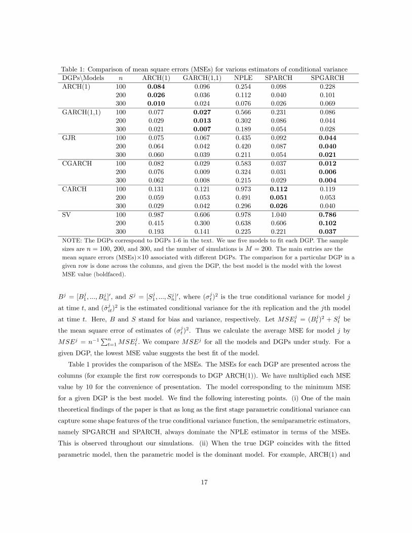
Table 1: Comparison of mean square errors (MSEs) for various estimators of conditional varianceDGPs\Models n ARCH(1) GARCH(1,1) NPLE SPARCH SPGARCHARCH(1) 100 0.084 0.096 0.254 0.098 0.228

200 0.026 0.036 0.112 0.040 0.101300 0.010 0.024 0.076 0.026 0.069

GARCH(1,1) 100 0.077 0.027 0.566 0.231 0.086200 0.029 0.013 0.302 0.086 0.044300 0.021 0.007 0.189 0.054 0.028

GJR 100 0.075 0.067 0.435 0.092 0.044200 0.064 0.042 0.420 0.087 0.040300 0.060 0.039 0.211 0.054 0.021

CGARCH 100 0.082 0.029 0.583 0.037 0.012200 0.076 0.009 0.324 0.031 0.006300 0.062 0.008 0.215 0.029 0.004

CARCH 100 0.131 0.121 0.973 0.112 0.119200 0.059 0.053 0.491 0.051 0.053300 0.029 0.042 0.296 0.026 0.040

SV 100 0.987 0.606 0.978 1.040 0.786200 0.415 0.300 0.638 0.606 0.102300 0.193 0.141 0.225 0.221 0.037

NOTE: The DGPs correspond to DGPs 1-6 in the text. We use five models to fit each DGP. The samplesizes are n = 100, 200, and 300, and the number of simulations is M = 200. The main entries are themean square errors (MSEs)×10 associated with different DGPs. The comparison for a particular DGP in agiven row is done across the columns, and given the DGP, the best model is the model with the lowestMSE value (boldfaced).

Bj = [Bj1, ..., B

jn]0, and Sj = [Sj1, ..., S

jn]0, where (σjt)

2 is the true conditional variance for model j

at time t, and (σjit)2 is the estimated conditional variance for the ith replication and the jth model

at time t. Here, B and S stand for bias and variance, respectively. Let MSEjt = (Bj

t )2 + Sjt be

the mean square error of estimates of (σjt)2. Thus we calculate the average MSE for model j by

MSEj = n−1Pn

t=1MSEjt . We compare MSEj for all the models and DGPs under study. For a

given DGP, the lowest MSE value suggests the best fit of the model.

Table 1 provides the comparison of the MSEs. The MSEs for each DGP are presented across the

columns (for example the first row corresponds to DGP ARCH(1)). We have multiplied each MSE

value by 10 for the convenience of presentation. The model corresponding to the minimum MSE

for a given DGP is the best model. We find the following interesting points. (i) One of the main

theoretical findings of the paper is that as long as the first stage parametric conditional variance can

capture some shape features of the true conditional variance function, the semiparametric estimators,

namely SPGARCH and SPARCH, always dominate the NPLE estimator in terms of the MSEs.

This is observed throughout our simulations. (ii) When the true DGP coincides with the fitted

parametric model, then the parametric model is the dominant model. For example, ARCH(1) and

17

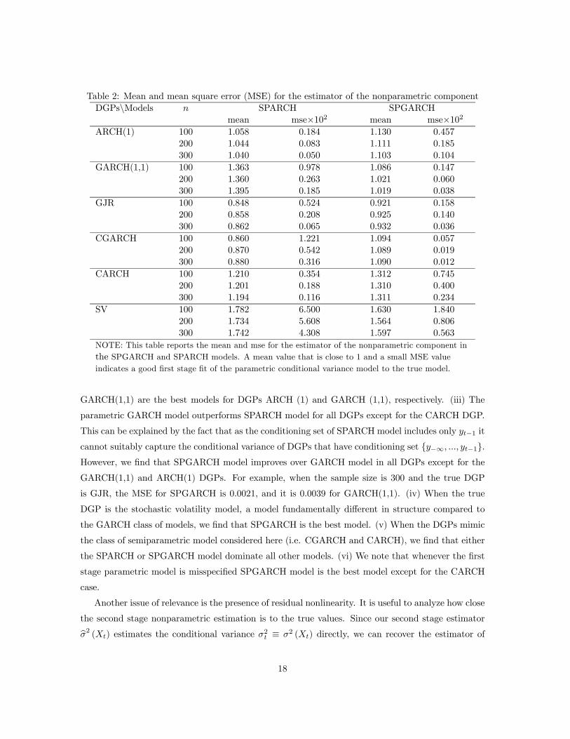
Table 2: Mean and mean square error (MSE) for the estimator of the nonparametric componentDGPs\Models n SPARCH SPGARCH

mean mse×102 mean mse×102ARCH(1) 100 1.058 0.184 1.130 0.457

200 1.044 0.083 1.111 0.185300 1.040 0.050 1.103 0.104

GARCH(1,1) 100 1.363 0.978 1.086 0.147200 1.360 0.263 1.021 0.060300 1.395 0.185 1.019 0.038

GJR 100 0.848 0.524 0.921 0.158200 0.858 0.208 0.925 0.140300 0.862 0.065 0.932 0.036

CGARCH 100 0.860 1.221 1.094 0.057200 0.870 0.542 1.089 0.019300 0.880 0.316 1.090 0.012

CARCH 100 1.210 0.354 1.312 0.745200 1.201 0.188 1.310 0.400300 1.194 0.116 1.311 0.234

SV 100 1.782 6.500 1.630 1.840200 1.734 5.608 1.564 0.806300 1.742 4.308 1.597 0.563

NOTE: This table reports the mean and mse for the estimator of the nonparametric component inthe SPGARCH and SPARCH models. A mean value that is close to 1 and a small MSE valueindicates a good first stage fit of the parametric conditional variance model to the true model.

GARCH(1,1) are the best models for DGPs ARCH (1) and GARCH (1,1), respectively. (iii) The

parametric GARCH model outperforms SPARCH model for all DGPs except for the CARCH DGP.

This can be explained by the fact that as the conditioning set of SPARCH model includes only yt−1 it

cannot suitably capture the conditional variance of DGPs that have conditioning set y−∞, ..., yt−1.However, we find that SPGARCH model improves over GARCH model in all DGPs except for the

GARCH(1,1) and ARCH(1) DGPs. For example, when the sample size is 300 and the true DGP

is GJR, the MSE for SPGARCH is 0.0021, and it is 0.0039 for GARCH(1,1). (iv) When the true

DGP is the stochastic volatility model, a model fundamentally different in structure compared to

the GARCH class of models, we find that SPGARCH is the best model. (v) When the DGPs mimic

the class of semiparametric model considered here (i.e. CGARCH and CARCH), we find that either

the SPARCH or SPGARCH model dominate all other models. (vi) We note that whenever the first

stage parametric model is misspecified SPGARCH model is the best model except for the CARCH

case.

Another issue of relevance is the presence of residual nonlinearity. It is useful to analyze how close

the second stage nonparametric estimation is to the true values. Since our second stage estimatorbσ2 (Xt) estimates the conditional variance σ2t ≡ σ2 (Xt) directly, we can recover the estimator of

18

σ2np (X2,t) by bσ2np (X2,t) ≡ bσ2 (Xt) /σ2p (X1,t, bγ) . If the first stage parametric conditional variance

model is correctly specified, one expects that bσ2np (X2,t) vary in the neighborhood of unity. This is

indeed observed in our simulations. In Table 2 we report the means and MSEs of the bσ2np (X2,t) for

the SPGARCH and SPARCH models under investigation. The MSE values are multiplied by 102 for

the convenience of presentation. We observe that: (i) When the first stage parametric conditional

variance model is correctly specified, the mean of the estimator for the nonparametric component

is close to 1 and the MSE of the estimator for the nonparametric component is lower than the case

where the first stage model is misspecified. For example, when the DGP is GARCH(1,1) and sample

size n = 300, the MSE of bσ2np (X2,t) for the SPGARCH model is 0.00038, which is much lower than

0.00185 for the SPARCH model. (ii) When the first stage parametric model is misspecified, the mean

of the estimator for the nonparametric component can be quite different from 1 and the performance

of the SPGARCH and SPARCH estimators is mixed. For the CARCH process, we find that the

MSE is lower for the SPARCH estimators, but for the GJR, CGARCH and SV processes, we find

that the SPGARCH estimator outperforms SPARCH.

3.2 Empirical Data Analysis

In this subsection we fit the semiparametric model to the real data (collected from Datastream) and

do some diagnostic checking to see whether the model is able to capture the time-varying conditional

variance and leverage effect.

We consider the S&P500 daily returns from January 3rd, 2002 through January 3rd, 2007, a total

of 1258 observations. It is sometimes found that the conditional mean of stock return has AR or MA

components. We therefore first carry out a diagnostic check for the return series to look for possible

AR or MA components. The ACF and PACF of the series indicate no such memory structure. We

also fit AR and MA models of lags of order 1 through 4 to check for the statistical significance of the

parameter estimates. We also find that all the parameter estimates are statistically insignificant at

the 5% level. It is possible to have nonlinear dynamics in the conditional mean equation, but we have

not explored this avenue here. Consequently, we model the return series ytnt=1 of a financial assetas: yt = α+ εt, where E(εt|Ft−1) = 0 and E(ε2t |Ft−1) = σ2t . In addition to the two semiparametric

models considered in the simulation, we consider a third semiparametric model where we fit the

GJR model in the first stage parametric estimation. It is useful to check whether the second stage

estimation can capture some additional nonlinearity in the data.

In the first stage parametric modeling, we estimate α by the sample average of yt, and estimate

the three parametric conditional variance models: ARCH(1), GARCH(1,1), and GJR by using the

Gaussian QMLE method. In the second-stage nonparametric estimation, we use yt−1 as the condi-

tioning variable for the ARCH(1) case and (yt−1, bσ2p,t−1)T for the other two cases; and we denote19

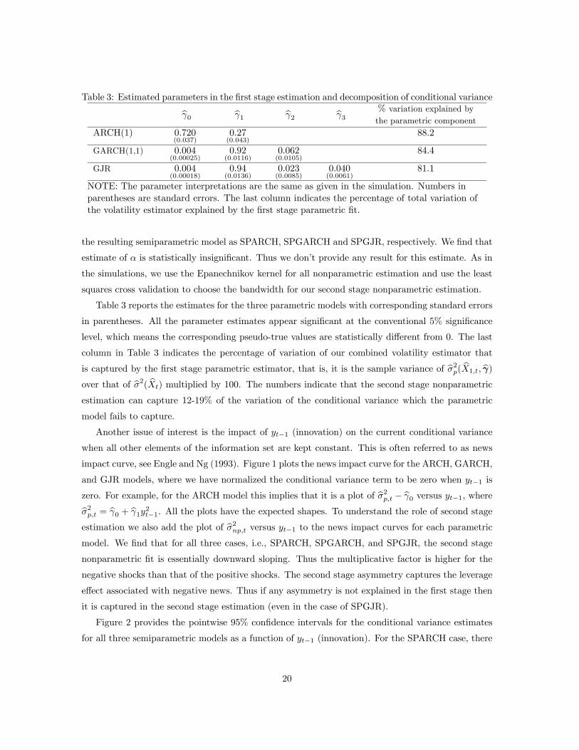
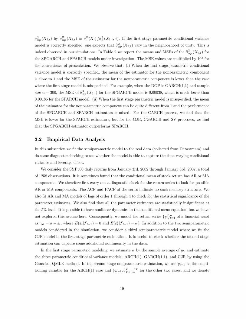
Table 3: Estimated parameters in the first stage estimation and decomposition of conditional variancebγ0 bγ1 bγ2 bγ3 % variation explained bythe parametric component

ARCH(1) 0.720(0.037)

0.27(0.043)

88.2

GARCH(1,1) 0.004(0.00025)

0.92(0.0116)

0.062(0.0105)

84.4

GJR 0.004(0.00018)

0.94(0.0136)

0.023(0.0085)

0.040(0.0061)

81.1

NOTE: The parameter interpretations are the same as given in the simulation. Numbers inparentheses are standard errors. The last column indicates the percentage of total variation ofthe volatility estimator explained by the first stage parametric fit.

the resulting semiparametric model as SPARCH, SPGARCH and SPGJR, respectively. We find that

estimate of α is statistically insignificant. Thus we don’t provide any result for this estimate. As in

the simulations, we use the Epanechnikov kernel for all nonparametric estimation and use the least

squares cross validation to choose the bandwidth for our second stage nonparametric estimation.

Table 3 reports the estimates for the three parametric models with corresponding standard errors

in parentheses. All the parameter estimates appear significant at the conventional 5% significance

level, which means the corresponding pseudo-true values are statistically different from 0. The last

column in Table 3 indicates the percentage of variation of our combined volatility estimator that

is captured by the first stage parametric estimator, that is, it is the sample variance of bσ2p( bX1,t, bγ)over that of bσ2( bXt) multiplied by 100. The numbers indicate that the second stage nonparametric

estimation can capture 12-19% of the variation of the conditional variance which the parametric

model fails to capture.

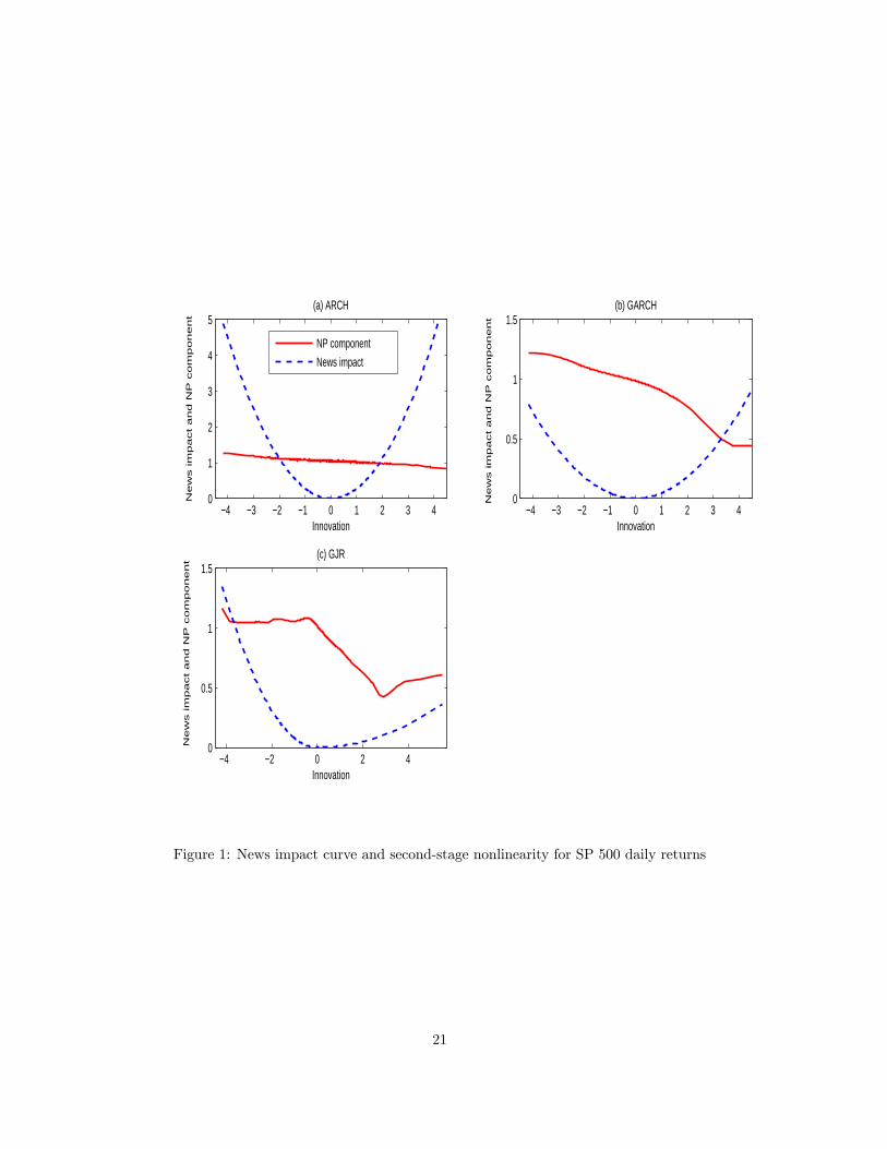
Another issue of interest is the impact of yt−1 (innovation) on the current conditional variance

when all other elements of the information set are kept constant. This is often referred to as news

impact curve, see Engle and Ng (1993). Figure 1 plots the news impact curve for the ARCH, GARCH,

and GJR models, where we have normalized the conditional variance term to be zero when yt−1 is

zero. For example, for the ARCH model this implies that it is a plot of bσ2p,t − bγ0 versus yt−1, wherebσ2p,t = bγ0 + bγ1y2t−1. All the plots have the expected shapes. To understand the role of second stageestimation we also add the plot of bσ2np,t versus yt−1 to the news impact curves for each parametricmodel. We find that for all three cases, i.e., SPARCH, SPGARCH, and SPGJR, the second stage

nonparametric fit is essentially downward sloping. Thus the multiplicative factor is higher for the

negative shocks than that of the positive shocks. The second stage asymmetry captures the leverage

effect associated with negative news. Thus if any asymmetry is not explained in the first stage then

it is captured in the second stage estimation (even in the case of SPGJR).

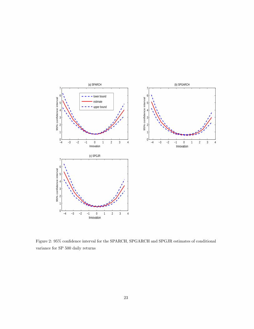
Figure 2 provides the pointwise 95% confidence intervals for the conditional variance estimates

for all three semiparametric models as a function of yt−1 (innovation). For the SPARCH case, there

20

−4 −3 −2 −1 0 1 2 3 40

1

2

3

4

5(a) ARCH

Innovation

Ne

ws im

pa

ct

an

d N

P c

om

po

ne

nt

NP component

News impact

−4 −3 −2 −1 0 1 2 3 40

0.5

1

1.5(b) GARCH

Innovation

Ne

ws im

pa

ct

an

d N

P c

om

po

ne

nt

−4 −2 0 2 40

0.5

1

1.5(c) GJR

Innovation

Ne

ws im

pa

ct

an

d N

P c

om

po

ne

nt

Figure 1: News impact curve and second-stage nonlinearity for SP 500 daily returns

21

is only one conditioning variable, i.e., yt−1, in the construction of the semiparametric estimator. For

the SPGARCH and SPGJR cases, we have two conditioning variables (yt−1 and bσ2p,t−1) to constructthe semiparametric estimator and have held bσ2p,t−1 fixed at their sample mean level in order to obtainplots (b)-(c) in Figure 2. As we can tell from Figure 2, the three semiparametric estimates share

similar shapes despite the fact that different parametric models are fitted in the first stage. All of

them can capture the leverage effects that are well documented in the finance literature.

Diagnostic check for the standardized residuals is an important aspect of modeling exercise.

The basic diagnostic checks include visual inspection of the ACF and PACF plots of standardized

residuals. It is also useful to check correlations of polynomials involving standardized residuals

to detect nonlinear dependence. It is well known that the standard Box-Pierce statistic is not

applicable in our framework due to the presence of conditional heteroskedasticity and nonparametric

estimates. Li and Mak (1994) propose an alternative chi-square-based test to account for conditional

heteroskedasticity. Nevertheless, their test statistic depends on the estimates of the Hessian matrix

from a log-likelihood function (see Lemma 3.3 of Ling and Li (1997) for details), which is not

applicable in the presence of nonparametric estimation. Wong and Ling (2005) propose a modification

to Li and Mak (1994) which allows for potential parametric misspecification. But the test statistic

is posited in a one-step likelihood based framework and not applicable to our case either. Hence

we eschew the Box-Pierce type of chi-square test and limit ourselves to the ACF and PACF tests

indicated above.

We consider the ACF and PACF for the standardized residuals for models SPARCH, SPGARCH,

and SPGJR. The lag length for our analysis is 10 and the 95% confidence bound for testing for white

noise is ±0.057 for our sample. Let ACF10 and PACF10 be the maximum of the absolute value

of ACF and PACF up to lag 10, respectively. First, we find that the ACF and PACF value for

the first lag for SPARCH model is 0.17 and 0.16 respectively, clearly rejecting the null hypothesis

of white noise. However, for the SPGARCH model ACF10 and PACF10 values are 0.051 and

0.052 respectively, so all the ACF and PACF values till lag 10 remain within the 95% confidence

bound. For the SPGJR model the corresponding ACF10 and PACF10 values are 0.049 and 0.050

respectively, thus, qualitatively, we draw the same conclusion as that of the SPGARCH model. To

analyze higher order dependence, we investigate the ACF and PACF values of squared and cubed

standardized residuals for all three models. For the SPARCH model the first order ACF and PACF

for squared standardized residuals are 0.12 and 0.13 respectively, thus rejecting the null of white

noise. The result is qualitatively similar for the cubed standardized residuals. For SPGARCH model

the ACF10 and PACF10 for squared standardized residuals are given as 0.046 and 0.048 respectively.

The corresponding ACF10 and PACF10 values for cubed standardized residuals are 0.050 and 0.053

respectively. Similarly, for SPGJR model ACF10 and PACF10 for squared standardized residuals

are given as 0.049 and 0.047 respectively. The corresponding ACF10 and PACF10 values for cubed

22

−4 −3 −2 −1 0 1 2 3 40

1

2

3

4

5

6

7(a) SPARCH

Innovation

95

% c

on

fid

en

ce

in

terv

al

−4 −3 −2 −1 0 1 2 3 40

1

2

3

4

5

6

7(b) SPGARCH

Innovation9

5%

co

nfid

en

ce

in

terv

al

−4 −3 −2 −1 0 1 2 3 40

1

2

3

4

5

6

7(c) SPGJR

Innovation

95

% c

on

fid

en

ce

in

terv

al

lower bound

estimate

upper bound

Figure 2: 95% confidence interval for the SPARCH, SPGARCH and SPGJR estimates of conditional

variance for SP 500 daily returns

23

standardized residuals are 0.044 and 0.046 respectively. This provides support, albeit partial, for

lack of dependence in standardized residuals obtained from SPGARCH and SPGJR model.

4 Conclusion

This paper proposes a new semiparametric estimator for time varying conditional variance. This is

accomplished by combining the parametric and nonparametric estimators in a multiplicative way.

We provide asymptotic theory for our semiparametric estimator and show that it can improve upon

the pure parametric and nonparametric estimators in different scenarios. We also include simulations

and empirical applications. We find from the simulations that our semiparametric estimators are

superior to their parametric and nonparametric counterparts in terms of MSE criteria. From the

empirical analysis we see that semiparametric models can capture the asymmetric effect in the data

even beyond that captured by the parametric component in the model.

ACKNOWLEDGEMENTS

The authors gratefully thank Arthur Lewbel, Serena Ng, the associate editor, and two anonymous

referees for their many helpful comments and advice that have led to considerable improvements of

the presentation. They are grateful to Torben G. Andersen, John Galbraith, Gloria González-Rivera,

Qi Li, Essie Maasoumi, Nour Meddahi, and Victoria Zinde-Walsh for their discussions and comments

on the subject matter of this paper. They are also thankful for the comments by the participants of

the seminars at McGill University, Southern Methodist University, Syracuse University, Texas A&M

University, Vanderbilt University, Université de Montréal, and University of Guelph. The second

author gratefully acknowledges financial support from the NSFC under the grant numbers 70501001

and 70601001. The third author acknowledges the support from the academic senate, UCR.

24

Appendix

We use k·k to denote the Euclidean norm of ·, C to signify a generic constant whose exact value

may vary from case to case, and aT to denote the transpose of a. For ease of presentation, we assume

that h1 = · · · = hd2 and with a little abuse of notation, we further denote h1 = · · · = hd2 = h. Recall

Kht ≡ Kh(X2,t − x2) and rt ≡ εtσp (x1) /σp (X1,t) . Let ξt ≡ r2t − σ2p (x1)σ2np (X2,t) .

A Proof of Theorem 2.1

Recall that bβ minimizes1

n

nXt=1

nbr2t − L³ bX2,t − x2,β

´o2Kh( bX2,t − x2).

It also minimizes the criterion function

bGn (β) ≡1

n

nXt=1

½hbr2t − L³ bX2,t − x2,β

´i2−h¡br2t ¢2 − ¡r2t ¢2i¾Kh( bX2,t − x2). (A.1)

By Theorem 3.4 of White (1994), it suffices to show that

bGn (β)−Gn (β)p→ 0 uniformly in β on a compact set B, (A.2)

and

lim supn→∞

maxβ∈Nc(β0)

£Gn (β)−Gn

¡β0¢¤

> 0 for any > 0, (A.3)

where

Gn (β) ≡ En£σ2p (x1)σ

2np (X2,t)− ς1t (β)

¤2Kht

o+E

©ξ2tKht

ª(A.4)

ς1t (β) ≡ L (0,β)−.

L (0,β)T(X2,t− x2), N

c¡β0¢is the complement of an open neighborhood of β0

on B of diameter , and β0 is uniquely defined by σ2(x) = L(0,β0) and σ2p(x1).σ2np(x2) =

.

L(0,β0).

Write

bGn (β) =1

n

nXt=1

£r2t − L (X2,t − x2,β)

¤2Kh( bX2,t − x2)

+1

n

nXt=1

nL2( bX2,t − x2,β)− L2 (X2,t − x2,β)

oKh( bX2,t − x2)

− 2n

nXt=1

nbr2tL( bX2,t − x2,β)− r2tL (X2,t − x2,β)oKh( bX2,t − x2)

≡ bGn1 (β) + bGn2 (β)− 2 bGn3 (β) , (A.5)

25

We will show that bGn1 (β) = Gn (β) + op (1) uniformly in β, (A.6)

and bGnj (β) = op (1) uniformly in β for j = 2, 3. (A.7)

By Assumptions A2 and A4-A6, and the Taylor expansion, it is easy to show that bGn1 (β) = eGn1 (β)+

Op

¡n−1/2h−1 + n−1h−(d2+1)

¢= eGn1 (β) + op (1) uniformly in β, where eGn1 (β) ≡ 1

n

Pnt=1Kht[r

2t−

L (X2,t − x2,β)]2. By the ergodic theorem, eGn1 (β)

p→ E [qnt (β)] , where qnt (β) ≡£r2t − L (X2,t − x2,β)

¤2×Kht. To show that this convergence is also uniform in β, it suffices to show the stochastic equicon-

tinuity of eGn1 (β) . We do this by verifying the two conditions of Lemma 3 in Andrews (1992). By

the compactness of B, the fact that K (.) is compactly supported (Assumption A5), and Assumption

A1(iii). qnt (β) ≤ 2r2tKht + 2CKht ≡ qnt. Clearly, E [qnt] < ∞, which implies Assumption DM of

Andrews (1992). Similarly,

¯qnt (β)− qnt

¡β0¢¯≤ 2r2t

¯L (X2,t − x2,β)− L

¡X2,t − x2,β

0¢¯Kht

+¯L2 (X2,t − x2,β)− L2

¡X2,t − x2,β

0¢¯Kht

≤¡r2tC1 + C2

¢ °°β − β0°° for some constants C1 and C2,

which implies Assumption TSE of Andrews (1992) by the Markov inequality. Consequently, eGn1 (β)

is stochastic equicontinuous on B and it converges to E [qnt (β)] uniformly in β.

By the second order Taylor expansion, we have

E [qnt (β)] = En£r2t − ς1t (β)− ς2t (β)

¤2Kht

o= E

n£ξt +

¡σ2p (x1)σ

2np (X2,t)− ς1t (β)

¢− ς2t (β)

¤2Kht

o= Gn (β) +E

©ς22t (β)Kht

ª+ 2E

©ξt£σ2p (x1)σ

2np (X2,t)− ς1t (β)

¤Kht

ª−2E ξtς2t (β)Kht− 2E

©£σ2p (x1)σ

2np (X2,t)− ς1t (β)

¤ς2t (β)Kht

ª≡ Gn (β) +Gn1a (β) +Gn1b (β)− 2Gn1c (β)− 2Gn1d (β) ,

where ς2t (β) ≡ 12(X2,t−x2)T

..

L (Ct(X2,t − x2),β) (X2,t−x2), and Ct is a d2×d2 matrix with elements

that lie on the interval [0, 1].We can easily verify that uniformly in β, Gn1a (β) = O(h4), Gn1b (β) =

Gn1c (β) = 0 because E (ξt|Ft−1) = 0 and Xt ∈ Ft−1, and Gn1d (β) = O¡h2¢. Consequently,

E [qnt (β)] = Gn (β) + o (1) uniformly in β

26

and (A.6) follows. Now, by the Taylor expansion and Assumptions A1(iii)-A2 and A4-A6,

supβ∈B

¯ bGn2 (β)¯≤ sup

β∈B

1

n

nXt=1

¯L2( bX2,t − x2,β)− L2 (X2,t − x2,β)

¯Kh( bX2,t − x2)

= supβ∈B

2

n

nXt=1

¯L¡X∗2,t − x2,β

¢ .

L¡X∗2,t − x2,β

¢( bX2,t −X2,t)

¯Kh( bX2,t − x2)

≤ 2C

n

nXt=1

°°° bX2,t −X2,t

°°°Kh( bX2,t − x2)

=2C

n

nXt=1

°°°DθX2,t (θt) (bθ−θ0)°°° ¯Kht +h .

Kh

¡X∗∗2,t − x2

¢iT( bX2,t −X2,t)

¯

≤ 2C

n

nXt=1

³°°DθX2,t

¡θ0¢°°°°°bθ−θ0°°°+Op

¡n−1

¢´×¯Kht +

h .

Kh (X2,t − x2)iT

DθX2,t

¡θ0¢(bθ−θ0) +Op

¡n−1h−d2−1

¢¯≤ 2C

n

nXt=1

°°DθX2,t

¡θ0¢°°Kht

°°°bθ−θ0°°°+2C

n

nXt=1

°°DθX2,t

¡θ0¢°°2 °°° .

Kh (X2,t − x2)°°°°°°bθ−θ0°°°2 +Op

³n−3/2h−d2−1

´= Op(n

−1/2) +Op

¡n−1h−1

¢+Op

³n−3/2h−d2−1

´= op (1) ,

where X∗2,t and X∗∗2,t lie between bX2,t and X2,t, θt lies between bθ and θ0 and .

Kh (u) ≡ (∂/∂u)Kh (u) .

Similarly, we can show that supβ∈B | bGn3 (β) | = op (1) . Consequently,

bGn (β) = Gn (β) + op (1) uniformly in β.

Note that choosing β to minimize Gn (β) is equivalent to choosing L (0,β) and.

L (0,β) to mini-

mize

G∗n (β) ≡ E

½hσ2p (x1)σ

2np (X2,t)− L (0,β)−

.

L (0,β)T(X2,t − x2)

i2Kht

¾,

It is easy to verify that when L (0,β) = σ2p (x1)σ2np (x2) and

.L (0,β) = σ2p (x1)

.σ2np (x2) , G

∗n (β) =

O¡h4¢is minimized. By the monotonicity of Ψ (.), β0 is uniquely determined by L

¡0,β0

¢=

σ2p (x1)σ2np (x2) and

.

L¡0,β0

¢= σ2p (x1)

.σ2np (x2) . This implies (A.3).¥

B Proof of Theorem 2.2

Let

Rn(x,β) ≡nXt=1

nbr2t − L³ bX2,t − x2,β

´o2Kh( bX2,t − x2). (B.1)

27

A second order Taylor expansion of L( bX2,t − x2,β) around L (0,β) yields:

Rn(x,β) =nXt=1

nbr2t − L (0,β)−.L (0,β)T ( bX2,t − x2)

− 12( bX2,t − x2)

T..

L³Ct( bX2,t − x2),β

´( bX2,t − x2)

¾2Kh( bX2,t − x2),

where Ct is a d2×d2 matrix with elements that lie on the interval [0, 1]. Define R∗n(x,β) as Rn(x,β)

with β in..L(Ct( bX2,t − x2),β) replaced by bβ. Let bβ∗ denote the minimizer of R∗n(x,β) and putbσ2∗(x) = L(0, bβ∗). It suffices to show that

√nhd2

nbσ2∗ (x)− σ2 (x)−B(x)o

d→ N(0, κd202(E(v4t |X2,t = x2)− 1)f(x2)−1σ4(x)). (B.2)

and

bσ2(x) = bσ2∗(x) + op

³n−1/2h−d2/2

´, (B.3)

where B(x) ≡ κ21h2

2 trnσ2p(x1)

..σ2np(x2)−

..L¡0,β0

¢o.

By Ruppert and Wand (1994, p.1348 ) or Fan and Gijbels (1996, p.298),

bσ2∗(x) = eT1

³ bXTxcWx

bXx

´−1 bXTxcWx

bUx,where e1 is the (d2+1) vector having 1 in the first entry and all other entries 0, bXx is an n× (d2 + 1)

matrix whose tth row is given by bXx,t ≡ (1, ( bX2,t − x2)T ), cWx =diagKh( bX2,1 − x2), ...,Kh( bX2,n −

x2), and bUx is an n× 1 vector with typical element

bUx,t ≡ br2t − 12( bX2,t − x2)T..

L³Ct( bX2,t − x2), bβ´ ( bX2,t − x2).

Define the (d2 + 1)× (d2 + 1) matrix

Sn(x2) =

⎛⎝ n−1Pn

t=1Kh( bX2,t − x2) n−1Pn

t=1Kh( bX2,t − x2)(X2,t−x2)T

h

n−1Pn

t=1Kh( bX2,t − x2)X2,t−x2

h n−1Pn

t=1Kh( bX2,t − x2)X2,t−x2

h(X2,t−x2)T

h

⎞⎠(B.4)

and the equivalent kernel

K∗n(u, x2) = eT1 Sn(x2)−1(1, (u− x2)

T /h)TKh(u− x2). (B.5)

Then by Ruppert and Wand (1994, p.1351), bσ2∗(x) =Pnt=1K

∗n( bX2,t, x2)bUx,t, n−1Pn

t=1K∗n( bX2,t, x2)

28

= 1, and n−1Pn

t=1K∗n( bX2,t, x2)( bX2,t − x2) = 0. Hence

bσ2∗(x)− σ2(x)

= n−1nXt=1

K∗n( bX2,t, x2)nbr2t − σ2(x)− σ2p(x1)

.σ2np(x2)

T ( bX2,t − x2)

−12( bX2,t − x2)

T..

L³Ct( bX2,t − x2), bβ´ ( bX2,t − x2)

¾= n−1

nXt=1

K∗n( bX2,t, x2)

½hbr2t − σ2p(x1)σ2np( bX2,t)

i+1

2bAnt

¾

= n−1nXt=1

K∗n(X2,t, x2)hbr2t − σ2p(x1)σ

2np( bX2,t)

i+1

2n−1

nXt=1

K∗n(X2,t, x2) bAnt

+n−1nXt=1

hK∗n( bX2,t, x2)−K∗n(X2,t, x2)

i hbr2t − σ2p(x1)σ2np( bX2,t)

i+1

2n−1

nXt=1

hK∗n( bX2,t, x2)−K∗n(X2,t, x2)

i bAnt

≡ Tn1 + Tn2 + Tn3 + Tn4, (B.6)

where

bAnt = ( bX2,t − x2)Thσ2p(x1)

..σ2np( eCt( bX2,t − x2) + x2)−

..L³Ct( bX2,t − x2), bβ´i ( bX2,t − x2), (B.7)

and eCt is a d2×d2 matrix with elements that lie on the interval [0, 1]. Tnj , j = 1, 2, 3, 4, are analyzed

in Lemmas B.1-B.4 below. Collecting the results in these lemmas, we obtain (B.2).

Next we show (B.3). By Theorem 2.1, under Assumptions A0-A6, β0 ≡ β0(x) is uniquely

defined by σ2(x) = L(0,β0) and σ2p(x1).σ2np(x2) =

.

L(0,β0), and ||bβ − β0|| p→ 0. Further, following

the arguments of Hall et al. (1999, p.163), one can show that bβ∗ − bβ = op(h2). Consequently,

bσ2(x)− bσ2∗(x) = L(0, bβ)− L(0, bβ∗) = op(h2) = op

¡n−1/2h−d2/2

¢.¥

Let Tnj , j = 1, 2, 3, 4, be defined as in (B.6), we prove the following lemmas under the conditions

of Theorem 2.2.

Lemma B.1 Recall Tn1 ≡ n−1Pn

t=1K∗n(X2,t, x2)

hbr2t − σ2p(x1)σ2np( bX2,t)

i. Then

√nhd2Tn1

d→ N(0,

κd202(E(v4t |X2,t=x2)− 1)f(x2)−1σ4(x)).

29

Proof. Noting that bεt = εt + (g¡Ut,α

0¢− g (Ut, bα)), we have

br2t =ε2tσ

2p(x1, bγ)

σ2p(X1,t, bγ) − ε2tσ2p(x1, bγ)

σ2p(X1,t, bγ)Ã1−

σ2p(X1,t, bγ)σ2p( bX1,t, bγ)

!

+2εt£g¡Ut,α

0¢− g (Ut, bα)¤σ2p(x1, bγ)

σ2p( bX1,t, bγ) +

£g¡Ut,α

0¢− g (Ut, bα)¤2 σ2p(x1, bγ)σ2p( bX1,t, bγ)

≡ ξn1t − ξn2t + ξn3t + ξn4t. (B.8)

Then

Tn1 = n−1nXt=1

K∗n(X2,t, x2)£ξn1t − σ2p(x1)σ

2np(X2,t)

¤−n−1

nXt=1

K∗n(X2,t, x2)σ2p(x1)

hσ2np( bX2,t)− σ2np(X2,t)

i−n−1

nXt=1

K∗n(X2,t, x2)ξn2t + n−1nXt=1

K∗n(X2,t, x2)ξn3t + n−1nXt=1

K∗n(X2,t, x2)ξn4t

≡ Tn11 − Tn12 − Tn13 + Tn14 + Tn15.

It suffices to show that

√nhd2Tn11

d→ N(0, κd202(E(v4t |X2,t = x2)− 1)f(x2)−1σ4(x))) (B.9)

and

Tn1j = op(n−1/2h−d2/2) for j = 2, 3, 4, 5. (B.10)

First, by the second order Taylor expansion,

ξn1t =ε2tσ

2p(x1, bγ)

σ2p(X1,t, bγ) = r2t

½1 + (μ0(x1)− μ0(X1,t))

T¡bγ − γ0¢+ 1

2

¡bγ − γ0¢T Gt

¡bγ − γ0¢¾ ,

where recall μ0(x1) ≡ μ(x1,γ0), Gt ≡ (ν∗(x1)− ν∗(X1,t))+(μ∗(x1)−μ∗(X1,t))

T (μ∗(x1)−μ∗(X1,t)),

and μ∗(x1) and ν∗(x1) are the gradient and the Hessian matrix with respect to γ of logσ2p(x1,γ)

evaluated at γ∗t , respectively. Here γ∗t is the intermediate value that lies between γ0 and bγ. By

Assumption A4, ξn1t = r2t 1 + (μ0(x1)− μ0(X1,t))T¡bγ − γ0¢ +Op(n

−1) kGtk, and

Tn11 = n−1nXt=1

K∗n(X2,t, x2)ξt + n−1nXt=1

K∗n(X2,t, x2)r2t (μ0(x1)− μ0(X1,t))

T¡bγ − γ0¢

+Op(n

−1)

2n−1

nXt=1

K∗n(X2,t, x2)r2t kGtk

≡ Tn11a + Tn11b + Tn11c, (B.11)

where recall ξt ≡ r2t − σ2p(x1)σ2np(X2,t).

30

Following Masry (1996b), we can show that Sn(x2) = f(x2)S (1 +Op (h)) , where S is defined

in (2.8). Then√nhd2Tn11a = n−1/2hd2/2f(x2)

−1Pnt=1Khtξt + op(1). Noting that Khtξt,Ft is an

m.d.s., E[Khtξt] = 0, and

Var

Ãn−1/2hd2/2f(x2)

−1nXt=1

Khtξt

!= hd2f(x2)

−2E Khtξt2

→ κd202(E(v4t |X2,t = x2)− 1)f(x2)−1σ4(x),

by the dominated convergence theorem. By Assumptions A2 and A5-A6 and the arguments of Masry

(1996a, Theorem 3),

√nhd2Tn11a

d→ N(0, κd202(E(v4t |X2,t = x2)− 1)f(x2)−1σ4(x)). (B.12)

By the ergodic theorem and Assumptions A2-A6,

Tn11b = n−1f(x2)−1

nXt=1

Kh(X2,t − x2)r2t (μ0(x1)− μ0(X1,t))

T¡bγ − γ0¢

= Op (1)Op(n−1/2) = op(n

−1/2h−d2/2). (B.13)

Now by Assumptions A2-A6 and the weak law of large numbers, kGtk ≤ CP2

i=1 kX1,t − x1ki , and

Tn11c =Op(n

−1)

2n−1

nXt=1

K∗n(X2,t, x2)r2t kGtk

≤ Op(n−1)

2Cn−1

nXt=1

K∗n(X2,t, x2)r2t

2Xi=1

kX1,t − x1ki

=Op(n

−1)

2Cf(x2)

−1n−1nXt=1

Khtr2t

2Xi=1

kX1,t − x1ki 1 +Op (h)

= Op(n−1)Op(1) = Op(n

−1). (B.14)

Hence (B.9) follows from (B.11)-(B.14).

By the Taylor expansion and Assumptions A2 and A4,

|Tn12| =

¯¯n−1

nXt=1

K∗n(X2,t, x2)σ2p(x1)

.σ2np(X

∗2,t)

³ bX2,t −X2,t

´¯¯= σ2p(x1)n

−1f−1 (x2)nXt=1

¯Kht

.σ2np(X2,t)DθX2,t

¡θ0¢ ³bθ − θ0´¯+Op

¡n−1h−d2

¢= Op(n

−1/2) +Op

¡n−1h−d2

¢= op(n

−1/2h−d2/2),

31

where X∗2,t lies between bX2,t and X2,t. Next,

ξn2t =ε2tσ

2p(x1, bγ)

σ2p(X1,t, bγ)Ã1−

σ2p(X1,t, bγσ2p( bX1,t, bγ)

!= r2t 1 + (μ0(x1)− μ0(X1,t))

T¡bγ − γ0¢+Op(n

−1) kGtk

×.σ2p(X1,t,γ

∗t )T

σ2p(X1,t,γ∗t )DθX1,t (θ

∗t ) (bθ − θ0),

where θ∗t lies between bθ and θ0, and γ∗t lies between bγ and γ0.Tn13 = n−1

nXt=1

K∗n(X2,t, x2)r2t

.σ2p(X1,t,γ

∗t )T

σ2p(X1,t,γ∗t )DθX1,t (θ

∗t ) (bθ − θ0) +Op

¡n−1

¢= n−1f (x2)

−1nXt=1

Khtr2t

.σ2p(X1,t,γ

0)T

σ2p(X1,t)DθX1,t

¡θ0¢(bθ − θ0) +Op

¡n−1

¢= Op (1)Op(n

−1/2) +Op

¡n−1

¢= op(n

−1/2h−d2/2).

Similarly, we can show that Tn14 = op(n−1/2h−d2/2) and Tn15 = op(n

−1/2h−d2/2). This completes

the proof of the lemma.

Lemma B.2 Tn2 ≡ 12n−1Pn

t=1K∗n(X2,t, x2) bAnt = B (x) + op(n

−1/2h−d2/2).

Proof. Let Ant be defined as bAnt in (B.7) but with X2,t replacing bX2,t. Decompose

Tn2 ≡ 1

2n−1

nXt=1

K∗n(X2,t, x2)Ant +1

2n−1

nXt=1

K∗n(X2,t, x2)³ bAnt −Ant

´≡ Tn21 + Tn22.

By the ergodic theorem, the dominated convergence theorem, and Assumptions A2-A6,

Tn21 =1

2n−1f(x2)

−1nXt=1

KhtAnt 1 +Op (h)

= B(x) + op(h2) = B(x) + op(n

−1/2h−d2/2). (B.15)

Now, by Taylor expansions,

Tn22 =1

2n−1f(x2)

−1nXt=1

Kht

³ bAnt −Ant

´1 +Op (h)

= Op(n−1/2) = op(n

−1/2h−d2/2).

Hence Tn2 = B(x) + op(n−1/2h−d2/2).

Lemma B.3 Tn3 ≡ n−1Pn

t=1[K∗n( bX2,t, x2)−K∗n(X2,t, x2)][br2t−σ2p(x1)σ2np( bX2,t)] = op(n

−1/2 h−d2/2).

32

Proof. Let ηnt = f(x2)−1Kh( bX2,t − x2) − Kh(X2,t − x2). We can show K∗n( bX2,t, x2) −

K∗n(X2,t, x2) = ηnt 1 +Op (h) where the order Op (h) does not depend on t. Then by the notation

used in the proof of Lemma B.1 (eq. (B.8) in particular),

Tn3 = n−1nXt=1

ηnt

hξt + σ2p(x1)

³σ2np(X2,t)− σ2np( bX2,t)

´− ξn2t + ξn3t + ξn4t

i1 +Op (h)

=

(n−1

nXt=1

ηntξt + n−1nXt=1

ηntσ2p(x1)

³σ2np(X2,t)− σ2np( bX2,t)

´−n−1

nXt=1

ηntξn2t + n−1nXt=1

ηntξn3t + n−1nXt=1

ηntξn4t

)1 +Op (h)

≡ Tn31 + Tn32 + Tn33 + Tn34 + Tn35 1 +Op (h) .

It suffices to show that Tn3j = op(n−1/2h−d2/2), j = 1, 2, ..., 5. First,

Tn31 = n−1f(x2)−1

nXt=1

ξt.Kh(X2,t − x2)

TDθX2,t

¡θ0¢(bθ − θ0) +Op(n

−1h−d2+2)

≡ eTn31(bθ − θ0) +Op

¡n−1h−d2+2

¢,

where.

Kh (u) ≡ (∂/∂u)Kh (u) . It is easy to show thatE(eTn31) = 0 and ||Var( eTn31)|| = O¡n−1h−d2−2

¢.

It follows from the Chebyshev inequality eTn31 = Op

¡n−1/2h−d2/2−1

¢and hence Tn31 = Op(n

−1h−d2/2−1

+n−1h−d2+2) = op(n−1/2h−d2/2). Similarly, we can show that Tn3j = Op(n

−1h−1 +n−1h−d2+1) =

op(n−1/2h−d2/2), for j = 2, 3, 4, 5. This completes the proof.

Lemma B.4 Tn4 ≡ 12n−1Pn

t=1

hK∗n( bX2,t, x2)−K∗n(X2,t, x2)

i bAnt = op(n−1/2h−d2/2).

Proof. Using the arguments and notation in the proof of Lemmas B.1-B.3, we have

Tn4 =

(1

2n−1

nXt=1

ηntAnt +1

2n−1

nXt=1

ηnt

³ bAnt −Ant

´)1 +Op (h)

≡ Tn41 + Tn42 1 +Op (h) .

First,

Tn41 =1

2n−1f(x2)

−1nXt=1

.Kh(X2,t − x2)

TDθX2,t

¡θ0¢ ³bθ − θ0´Ant +Op

¡n−1h−d2+2

¢= Op(n

−1/2h) +Op(n−1h−d2+2) = op(n

−1/2h−d2/2).

Similarly, we can show that Tn42 = Op

¡n−1/2h

¢+ Op

¡n−1h−d2+2

¢= op

¡n−1/2h−d2/2

¢. This com-

pletes the proof.

33

C Proof of (2.13) and (2.14)

Since the proof parallels that of Theorem 2.2, we only sketch the difference. Recall Sn (x) is defined

in B.4. When xn2 = ch, we can show that Sn (xn2)p→ f (0)Sc, where

Sc ≡

⎛⎝ μc0 μc1

μc1 μc2

⎞⎠ .

Following the proof of Lemma B.2, the dominant term in the asymptotic bias is determined by

eTn21 =1

2n−1

nXt=1

eT1 S−1n (xn2)

⎛⎝ 1X2,t−xn2

h

⎞⎠Kh(X2,t − xn2)Ant 1 + op (1)

=1

2n−1

1

f (0) (μc0μc2 − μ2c1)

nXt=1

µμc2 − μc1

X2,t − xn2h

¶Kh(X2,t − xn2)Ant 1 + op (1)

p→ h2

2

μ2c2 − μc1μc3μc0μc2 − μ2c1

[σ2p(x1)..σ2np(0)−

..

L¡0,β0

¢].

Following the proof of Lemma B.1, the dominant term in the asymptotic variance is determined by

√nhd2 eTn11a

= n−1/2hd2/2nXt=1

eT1 S−1n (xn2)

⎛⎝ 1X2,t−xn2

h

⎞⎠Kh(X2,t − xn2)ξt + op(1)

= n−1/2hd2/21

f (0) (μc0μc2 − μ2c1)

nXt=1

µμc2 − μc1

X2,t − xn2h

¶Kh(X2,t − xn2)ξt + op (1)

≡ Vn + op (1) .

Noting that [μc2 − μc1 (X2,t − xn2) /h]Kh(X2,t − xn2)ξt,Ft is an m.d.s., simple calculations show

that E[Vn] = 0, and

Var (Vn) =

R∞−c (μc2 − μc1z)

2k2 (z) dz

(μc0μc2 − μ2c1)2

£E(v4t |X2,t = x2)− 1

¤f−1(0)σ4(x1, 0)) + o (1) .

This completes the proof. ¥

D Proof of Theorem 2.3

The proof parallels that of Theorem 2.1. The major difference lies in three aspects: (a) now we

hold h as fixed; (b) we use the fact that σ2np (.) ≡ 1 under the correct specification of the first stage

parametric conditional variance model; (c) the probability limit Gn (β) now becomes

Gn (β) ≡ E©[σ2p (x1)− L ((X2,t − x2),β)]

2Kht

ª+E

©ξ2tKht

ª.

34

We proceed as in the proof of Theorem 2.1 until (A.7).

By Assumptions A1-A2 and A5, the Taylor expansion and the weak uniform law of large numbers,

it is easy to show that bGn1 (β) =1n

Pnt=1

£r2t − L (X2,t − x2,β)

¤2Kht+Op

¡n−1/2

¢= Gn1 (β)+op (1)

uniformly in β, where Gn1 (β) = E£r2t − L (X2,t − x2,β)

¤2Kht. Now ξt ≡ r2t − σ2p (x1) , and

Gn1 (β) = En£r2t − L ((X2,t − x2),β)

¤2Kht

o= E

n£ξt +

¡σ2p (x1)− L ((X2,t − x2),β)

¢¤2Kht

o= Gn (β) ,

where the last equality follows from the fact that ξt£σ2p (x1)− L ((X2,t − x2),β)

¤Kht,Ft is an

m.d.s. As in the proof of Theorem 2.1, bGn2 (β) = op (1) and bGn3 (β) = op (1) uniformly in β. Hence

bGn (β) = Gn (β) + op (1) uniformly in β.

As in the proof of Theorem 2.1, choosing β to minimize Gn (β) is equivalent to choosing L (0,β)

and.

L (.,β) to minimize

G∗n (β) ≡ E

½hσ2p (x1)− L (0,β)−

.L¡Ct(X2,t − x2),β

¢T(X2,t − x2)

i2Kht

¾,

where Ct is a d2 × d2 matrix with elements that lie on the interval [0, 1]. Clearly, when L (0,β) =

σ2p (x1) and.L (.,β) ≡ 0, G∗n (β) = 0 is minimized. Consequently, β0 is uniquely determined by

L¡0,β0

¢= σ2p (x1) and

.

L¡.,β0

¢≡ 0.Note that L

¡0,β0

¢= Ψ

¡β00¢,.

L¡x2,β

0¢=

.

Ψ³β00 +

Pd2i=1 β

0ix2,i

´β01

and.

Ψ (.) > 0, thus we conclude that β00 = Ψ−1 ¡σ2p (x1)¢ and β01 = 0. ¥

E Proof of Theorem 2.4

The proof parallels that of Theorem 2.2. The major difference lies in three aspects: (a) now we

hold h as fixed; (b) we use the fact that σ2np (.) ≡ 1 under the correct specification of the first stage

parametric conditional variance model; (c) we use the fact.

L¡.,β0

¢≡ 0.

Let Rn(x,β) be defined as in (B.1). By a Taylor expansion of the first order conditions from

minimizing Rn(x,β), we have

√n³bβ − β0´ = −Ã 1

n

∂2Rn(x, eβ)∂β∂βT

!−11√n

∂Rn(x,β0)

∂β, (E.1)

35

where eβ lies between bβ and β0 and thus converges to β0 in probability by Theorem 2.3,

∂Rn(x,β)

∂β= −2

nXt=1

nbr2t − L³ bX2,t − x2,β

´o .

Ψβ,t

⎛⎝ 1bXt − x

⎞⎠Kh( bX2,t − x2),

∂2Rn(x,β)

∂β∂βT= −2

nXt=1

st (β)

⎛⎝ 1 bX2,t − x2bX2,t − x2 ( bX2,t − x2)( bX2,t − x2)T

⎞⎠Kh( bX2,t − x2)

where st (β) ≡ [br2t−L( bX2,t−x2,β)]..Ψβ,t−[

.Ψβ,t]

2,.Ψβ,t ≡

.Ψ((1, ( bX2,t−x2)T )β)),

..Ψβ,t ≡

..Ψ((1, ( bX2,t−

x2)T )β)), and

.Ψ (u) and

..Ψ (u) denote the first and second derivatives of Ψ (u) with respect to u,

respectively. Note that Theorem 2.3 implies

L( bX2,t − x2,β0) = L

¡0,β0

¢= σ2p (x1) ,

.

Ψβ0,t ≡.

Ψ(β00), and..

Ψβ0,t ≡..

Ψ(β00). (E.2)

Let N (β0) denote the -neighborhood of β0 where ≡ (n) → 0 as n → ∞. The proof is

complete if we can show

1

n

∂2Rn(x, eβ)∂β∂βT

− 1n

∂2Rn(x,β0)

∂β∂βT= op (1) uniformly in eβ ∈ N (β0), (E.3)

1

n

∂2Rn(x,β0)

∂β∂βT− 2

h .Ψ(β00)

i2Σβ0 = oP (1) , (E.4)

and1√n

∂Rn(x,β0)

∂βd→ N

µ0, 4

h .Ψ(β00)

i2Ωβ0

¶. (E.5)

We first show (E.3). By Theorem 2.3, (E.2) and Assumptions A1-A5, we can show that supβ∈N (β0) |st(eβ)−st

¡β0¢| = op (1) uniformly in t. (E.3) then follows from this fact by applications of Taylor expan-

sion and weak law of large numbers. Next, by Assumptions A2-A4, Taylor expansions and weak law

of large numbers,

∂2Rn(x,β0)

∂β∂βT= − 2

n

nXt=1

½£r2t − σ2p (x1)

¤ ..Ψ(β00)−

h .Ψ(β00)

i2¾

×

⎛⎝ 1 X2,t − x2

Xt − x (X2,t − x2)(X2,t − x2)T

⎞⎠Kht + op (1)

= 2h .Ψ(β00)

i2Σβ0 + op (1) . (E.6)

Now by (B.8), we make the following decomposition:

1√n

∂Rn(x,β0)

∂β=−2

.

Ψ(β00)√n

nXt=1

©br2t − σ2p (x1)ª eX2,tKh( bX2,t − x2)

= −2.

Ψ(β00)5X

j=1

Vn,j ,

36

where eX2,t ≡ (1, ( bX2,t − x2)T )T , Vn,1 ≡ n−1/2

Pnt=1

©r2t − σ2p (x1)

ª eX2,tKh( bX2,t − x2), Vn,2 ≡

n−1/2Pn

t=1

©ξn1t − r2t

ª eX2,tKh( bX2,t − x2), and Vn,j+1 ≡ n−1/2Pn

t=1 ξn2jeX2,tKh( bX2,t − x2), j =

2, 3, 4. We can show that

Vn,1 =1√n

nXt=1

©r2t − σ2p (x1)

ª⎛⎝ 1

X2,t − x2

⎞⎠Kht + op (1) ,

Vn,2 =1√n

nXt=1

σ2p (x1) (μ0 (x1)− μ0 (X1,t))T ¡bγ − γ0¢

⎛⎝ 1

X2,t − x2

⎞⎠Kht + op (1) ,

Vn,3 =1√n

nXt=1

σ2p (x1).σ2p(X1,t,γ

0)T

σ2p(X1,t)DθX1,t

¡θ0¢(bθ − θ0)

⎛⎝ 1

X2,t − x2

⎞⎠Kht + op (1) ,

Vn,4 = −1√n

nXt=1

2εtσ2p(x)

£Dαg

¡Ut,α

0¢¤T

(bα−α0)σ2p(X1,t)

⎛⎝ 1

X2,t − x2

⎞⎠Kht + op (1) = op (1) ,

and

Vn,5 = −1√n

nXt=1

σ2p(x)n£Dαg

¡Ut,α

0¢¤T

(bα−α0)o2σ2p(X1,t)

⎛⎝ 1

X2,t − x2

⎞⎠Kht + op (1) = op (1) .

Hence,

1√n

∂Rn(x,β0)

∂β

=−2

.Ψ(β00)√n

nXt=1

©r2t − σ2p (x1)

ª⎛⎝ 1

X2,t − x2

⎞⎠Kht

+−2

.

Ψ(β00)

n

nXt=1

σ2p (x1)

⎛⎝ 1

X2,t − x2

⎞⎠Kht

×(h01×k1 , (μ0 (x1) -μ0 (X1,t))

Ti−

.σ2p(X1,t,γ

0)T

σ2p(X1,t)DθX1,t

¡θ0¢)

n−1/2nXs=1

ϕs¡θ0¢+ op (1)

=−2

.

Ψ(β00)√n

nXt=1

⎧⎨⎩£r2t − σ2p (x1)¤⎛⎝ 1

X2,t − x2

⎞⎠Kht +Υϕt¡θ0¢⎫⎬⎭+ op (1)

d→ N

µ0, 4

h .

Ψ(β00)i2Ωβ0

¶.

Consequently,√n³bβ − β0´ d→ N

µ0,h .Ψ(β00)

i−2Σ−1β0Ωβ0Σ

−1β0

¶.¥

37

REFERENCES

Andrews, D. W. K. (1992), “Generic Uniform Convergence,” Econometric Theory 8, 241-257.

Andrews, D. W. K., and Monahan, J.C. (1992), “An Improved Heteroskedasticity and Autocorre-lation Consistent Covariance Matrix Estimator,” Econometrica 60, 953-966.

Berkes, I., and Horváth, L. (2003), “The Rate of Consistency of the Quasi-maximum LikelihoodEstimator,” Statistics & Probability Letters 61, 133-143.

Berkes, I., Horváth, L., and Koloszka, P. (2003), “GARCH Processes: Structure and Estimation,”Bernoulli 9, 201-227.

Bollerslev, T. (1986), “Generalized Autoregressive Conditional Heteroskedasticity,” Journal of Econo-metrics 31, 307-327.

Engle, R. F. (1982), “Autoregressive Conditional Heteroscedasticity with Estimates of the Varianceof UK Inflation,” Econometrica 50, 987-1008.

Engle, R. F., and Ng, V. K. (1993), “Measuring and Testing the Impact of News on Volatility,”Journal of Finance 48, 1749-1778.

Fan, J., and Gijbels, I. (1996), “Local Polynomial Modelling and Its Applications,” Champman andHall.

Fan, J., and Yao, Q. (1998), “Efficient Estimation of Conditional Variance Functions in StochasticRegression,” Biometrika 85, 645-660.

Fan, Y., and Ullah, A. (1999), “Asymptotic Normality of a Combined Regression Estimator,”Journal of Multivariate Analysis 85, 191-240.

Gallant, A. R. (1981), “On the Bias in Flexible Functional Forms and an Essentially UnbiasedForm: the Fourier Flexible Form,” Journal of Econometrics 15, 211-245.

Gallant, A. R. (1987), “Identification and Consistency in Seminonparametric Regression,” in T.F. Bewley (ed.), Advances in Econometrics: Fifth World Congress Vol 1, 145-170, CambridgeUniversity Press, Cambridge, UK.

Gallant, A. R., and Tauchen, G. (1989), “Seminonparametric Estimation of Conditionally Con-strained Heterogeneous Processes: Asset Pricing Applications,” Econometrica 57, 1091-1120.

Glad, I. K. (1998), “Parametrically Guided Non-parametric Regression,” Scandinavian Journal ofStatistics 25, 649-668.

Glosten, L. R., Jagannathan, R., and Runkle, D. (1993), “On the Relationship between the ExpectedValue and the Volatility of the Nominal Excess Return on Stocks,” Journal of Finance 48,1779-1801.

38

Hall, P., Wolf, R.C.L., and Yao, Q. (1999), “Methods of Estimating a Conditional DistributionFunction,” Journal of the American Statistical Association 94, 154-163.

Härdle, W., and Tsybakov, A.B. (1997), “Local Polynomial Estimators of the Volatility Functionin Nonparametric Autoregression,” Journal of Econometrics 81, 223-242.

Härdle, W., Tsybakov, A.B., and Yang, L. (1998), “Nonparametric Vector Autoregression,” Journalof Statistical Planning and Inference 68, 221-245.

Hjort, N., and Glad, I. K. (1995), “Nonparametric Density Estimation with Parametric Start,”Annals of Statistics 23, 882-904.

Hsiao, C. and Li, Q. (2001), “A Consistent Test for Conditional Heteroskedasticity in Time-seriesRegression Models,” Econometric Theory 17, 188-221.

Lee, S. W., and Hansen, B. E. (1994), “Asymptotic Theory for the GARCH(1,1) Quasi-maximumLikelihood Estimator,” Econometric Theory 10, 29-52.

Li, W., and Mak, T.K. (1994), “On the Squared Residual Autocorrelations in Nonlinear Time Serieswith Conditional Heteroskedasticity,” Journal of Time series Analysis 15, 627-636.

Ling, S., and Li, W.K. (1997), “Diagnostic Checking of Nonlinear Multivariate Time Series withMultivariate ARCH Errors,” Journal of Time series Analysis 18, 447-464.

Linton, O., and Mammen, E. (2005), “Estimating Semiparametric ARCH(∞) Models by KernelSmoothing Methods,” Econometrica 73, 771-836.

Lumsdaine, R. L. (1996), “Consistency and Asymptotic Normality of the Quasi-maximum Like-lihood Estimator in IGARCH(1,1) and Covariance Stationary GARCH(1,1) Models,” Econo-metrica 64, 575-596.

Masry, E. (1996a), “Multivariate Regression Estimation: Local Polynomial Fitting for Time Series,”Stochastic Processes and Their Applications 65, 81-101.

Masry, E. (1996b), “Multivariate Local Polynomial Regression for Time Series: Uniform StrongConsistency Rates,” Journal of Time Series Analysis 17, 571-599.

Olkin, I., and Spiegelman, C. (1987), “A Semiparametric Approach to Density Estimation,” Journalof American Statistical Association 88, 858-865.

Pagan, A., and Hong, Y. S. (1990), “Nonparametric Estimation and the Risk Premium,” in W.Barnett, J. Powell, and G. E. Tauchen (eds.) Nonparametric and Semiparametric Methods inEconometrics and Statistics, 51-75, Cambridge University Press, Cambridge, UK.

Pagan, A., and Schwert, G.W. (1990), “Alternative Models for Conditional Stock Volatility,” Jour-nal of Econometrics 45, 267-290.

Press, H., and Tukey, J. W. (1956), “Power Spectral Methods of Analysis and Their Application toProblems in Airline Dynamics,” Flight Test Manual, NATO, Advisory Group for AeronauticalResearch and Development, Vol., IV-C, 1-41.

39

Ruppert, D., and Wand, M. P. (1994), “Multivariate Weighted Least-squares Regression,” Annalsof Statistics 22, 1346-1370.

White, H. (1994), “Estimation, Inference and Specification Analysis,” Cambridge University Press.

Wong, H., and Ling, S. (2005), “Mixed Portmanteau Tests for Time Series Models,” Journal ofTime series Analysis 26, 569-579.

Yang, L. (2006), “A Semiparametric GARCH Model for Foreign Exchange Volatility,” Journal ofEconometrics 130, 365-384.

Yang, L., Härdle, W., and Nielsen, J.P. (1999), “Nonparametric Autoregression with MultiplicativeVolatility and Additive Mean,” Journal of Time Series Analysis 20, 579-604.

Ziegelmann, F. (2002), “Nonparametric Estimation of Volatility Functions: the Local ExponentialEstimator,” Econometric Theory 18, 985-991.

40