SEMINAR DISCUSSION PAPER NO. 245

--- k

MichUDeptEResSIE

D#245

RESEARCH SEMINAR IN INTERNATIONAL ECONOMICS

Department of EconomicsThe University of Michigan

Ann Arbor, Michigan 48109-1220

SEMINAR DISCUSSION PAPER NO. 245

Distance, Demand, and Oligopoly Pricing by

Robert C. FeenstraUniversity of California, Davis

National Bureau of Economic Research

James A. LevinsohnThe University of Michigan

July 17, 1989

JAN 53i

The Sumner andLaura Foster Libr.ry

The University of Michigan

Distance, Demand, and Oligopoly Pricing

by

Robert C. FeenstraUniversity of California, Davis

National Bureau of Economic Research

andJames A. LevinsohnUniversity of Michigan

Current version: September 14, 1989

Abstract. We demonstrate how to estimate a model of product demand and oligopolypricing when products are multi-dimensionally differentiated. We provide an empiricalcounterpart to recent theoretical work on product differentiation. Using specificationsinformed by economic theory, we simultaneously estimate a demand system and price-costmargins for products differentiated in many dimensions.

Address. Prof. Robert Feenstra, Department of Economics, University of Califor-nia, Davis, CA 95616; Prof. James Levinsohn, Department of Economics, University ofMichigan, Ann Arbor, MI 48109

Distance, Demand, and Oligopoly Pricing

Robert C. FeenstraUniversity of California, Davis

National Bureau of Economic Researchand

J ames A. LevinsohnUniversity of Michigan

1. Introduction

Product differentiation plays an important role in many fields of economics. In indus-

trial organization, for example, it is a necessary condition if prices are to exceed marginal

costs with Bertrand competition. While recent empirical work in industrial organization

has focused attention on estimating non-observable price-cost margins, detailed empirical

treatments of product differentiation have been scant. 1 An important exception to this

is Bresnahan (1981, 1987). He has estimated a model of demand and oligopolistic pricing

for products which are differentiated along one dimension as in a Hotelling (1921) model.

In international trade theory, too, product differentiation has been recently integrated

into theoretic models. Much of this literature is well treated in Belpman and Krugman

(1985,1989). One lesson that falls out of this literature is that the market conduct and

product differentiation of firms are critical in determining the welfare impact Qf trade re-

strictions. The industries in which one might hope to evaluate the empirical relevance of

these theories are often characterized by multi-dimensional product differentiation. Exam-

ples include the auto, aircraft, and computer industries. To test the hypotheses developed

in this literature, it is therefore essential to have an econometric model incorporating both

multi-dimensional product differentiation and oligopolistic pricing. 2

We thank Robert Pollak for early discussions on this topic, Gene Grossman for detailedand perceptive comments, and seminar participants at Stockholm, Hebrew and Tel Aviv Universities. Thispaper was completed (with the help of Bitnet) while Feenstra was a visitor at the Institute for AdvancedStudies at the Hebrew University of Jerusalem and while Levinsohn was a visitor at the Institute forInternational Economic Studies, University of Stockholm. Each thanks his respective hosts.

1

Economic theorists have also recently turned their attention to the careful modelling

of product differentiation. On the demand side, Anderson, de Palma, and Thisse (1989)

investigate the conditions under which a demand system for multidimensionally differenti-

ated products satisfy properties such as that of gross substitutes and symmetry. Adding a

supply side, Caplin and Nalebuff (1988) provide conditions under which there exists a pure-

strategy price equilibrium for firms producing multi-dimensionally differentiated products.

It is of special note that this newer theoretical work models product differentiation as

occurring in many dimensions. 3 This is a welcome concession to reality.

In this paper, we demonstrate how to estimate a model of product demand and oligopoly

prices when products are multi-dimensionally differentiated. We provide an empirical coun-

terpart to the recent theoretical work on product differentiation. Using specifications in-

formed by economic theory, we simultaneously estimate a demand system for differentiated

products and price-marginal cost margins.

Our work may be seen as a generalization of Bresnahan's work. In the theory underlying

his empirical methods, varieties of a product are arranged along a line of quality so that

each model (except the lowest and highest) has two competitors on the line. Taking the

quality of each model as exogenous (i.e. solved in the first stage of a two stage game), the

demand and profit-maximizing prices for each variety of the product are simultaneously

determined. A critical variable is the distance between each model and its competitors:

as competitors get closer, the .demand for a model becomes more elastic and its price-

marginal cost markup decreases. Our generalization of Bresnahan's work allows us to

drop the Hotelling set-up and instead allow products to vary over multiple dimensions.

This means that each model of the product can have many competitors. In earlier work

(Levinsohn and Feenstra, 1989), we have shown how the utility function of consumers can

be used to obtain a metric on characteristics space, which makes it possible to identify

competitors. In this paper, we use a particularly simple utility function which implies that

the metric is (the square of) Euclidean distance after the units of each characteristic have

been properly adjusted.

Since a utility function is used in identifying competitors, it should also place restric-

tions on the form of demand. However, demand for each model is evaluated as a multiple

2

integral over the market space, and we are not able to obtain a closed-form solution.

Our central theoretical result evaluates the derivatives of demand, and so a first-order

approximation to the demand function can be determined. We find that the elasticity of

demand is inversely related to the "distance" between a model and its competitors, but

that "distance" should be measured as the harmonic mean of distances from a model to

each of its competitors.' The harmonic mean has the property that if any one competing

model is arbitrarily close, the harmonic mean approaches zero, so the elasticity of demand

approaches infinity: when two models have the same characteristics, they are perfect sub-

stitutes. Thus, our theory gives us an economically meaningful way to measure "distance"

when there are many competitors.

With this first-order approximation to demand, we solve for the profit-maximizing

prices for firms under Bertrand competition, and these prices are directly related to the

harmonic mean of distances to competitors. The pricing equation for each model takes a

particularly simple form: price is a linear function of characteristics (reflecting marginal

cost), the harmonic mean of distances from competitors, and a term which arises from

the joint maximization of profits over all goods sold by a multi-product firm. If models

are arbitrarily close, then the latter terms approach zero and price is just a function of

characteristics: this corresponds to the price schedule derived by Rosen (1974) with a

continuum of products. Thus, our analysis shows how the conventional hedonic regression

must be modified when there are a discrete number of products and oligopoly pricing.

In Section 2, we derive the theoretical results of the paper. These are used to provide

the econometric specification of the demand function and the pricing equation that are

estimated in Section 3. In that section, we use a panel data set from the U.S. automobile

market, and simultaneously estimate the demand and oligopoly pricing equations. We are

able to test several interesting hypotheses that arise from our multi-dimensional set-up.

For example, does the elasticity of demand for a model rise as competing models become

more similar? Do oligopolistic firms really charge a higher price for their product as other

competing products become more different? If the oligopolistic firms are multi-product

firms, do they charge a higher price for products that compete primarily with other of

their own products? A number of rather novel estimation issues arise, and these are

3

discussed in turn. Section 4 presents and interprets the estimation results. In Section 5,

we conduct sensitivity analyses to investigate the robustness of our results. Conclusions

are presented in Section 6, and the proofs of Propositions are gathered in the Appendix.

2. The Model

2.1 Utility and Competitors

While we formalize our ideas generally, we will use automobiles as a running example of our

theory. We describe each car available by a vector of characteristics z = (zi,... , 2K) > 0.

These characteristics are assumed to be exogenous, and we can think of them as being

determined in the first stage of a two-stage game between firms. Consumers obtain utility

U(z,a) from purchasing a car, where a = (a 1 ,... ,aK) is a vector of taste parameters

which varies across consumers. While some of our results can be obtained with a quite

general form of utility (see Levinsohn and Feenstra, 1989), the estimation requires a specific

form which we shall adopt now:

K

U(z,ca) = o ln(zi - ai) (1)i=1

where a-> 0 is common across consumers. 5 We shall assume that a > 0, and this vector

can be interpreted as the minimum acceptable characteristics for a consumer, since z < a

would yield utility of -oo. We assume that the taste parameters of all consumers are given

by a compact set A C R .

The prices and products available to consumers are denoted respectively by pm and zmn,

for models m=1,...,M. In principle, this set of products should also include alternatives to

purchasing a new car, such as used cars and alternative modes of transport. However, in

our estimation we shall only use data on new cars. In this sense, our paper deals with the

choice of which model to purchase, but not with the decision of whether to buy a car at

all. 6

We shall find it convenient to make a change of variables from the taste parameters a

to the consumers' "ideal" product z*. As in Lancaster (1979), the ideal product z* is what

each consumer would purchase if all models z > 0 were hypothetically available. However,

4

in order to determine this optimal choice, we must also specify what prices would be. To

this end, we shall assume that if the continuum of products z > 0 were available, prices

would equal marginal costs. After solving for the equilibrium of our model, we shall be able

to return and justify this assumption (see section 2.3). We shall suppose that marginal

costs C(z) are a linear function of characteristics:

C(z) =fo+3'z, z >0. (2)

When the continuum of products z > 0 are available, consumers face prices equal to costs

C(z), but when the discrete products zm, m = 1,...M are available, consumers then face

actual prices pm. The actual price will generally not equal marginal cost, and the price-cost

margin lrmn is defined as,

7tm =-pm - (O+,8'zm), m = 1,...M. (3)

When all products z > 0 are available consumers are faced with the prices in (2), so

they will choose the ideal products:

z = arg max {U(z,ca) -(/3o + 3 'z)},

or., using the specific utility function in (1):

zZ = ai --. (4)

Condition (4) shows how the ideal product z* is determined by the taste parameters.

We can think of it as establishing a one-to-one mapping from a to z*. Then instead of

identifying consumers by their tastes , we can identify them by their ideal products z".

Inverting (4) shows the taste parameters which correspond to each choice of z-:

i = z.- (4')

)3i

Substituting (4') into (1) we obtain utility as a function of the consumed characteristics

z and the preferred product z-:

5

K

V (z, z*i) = a ln(z - z+ ). (5)

We will use a second-order approximation to (5). Calculating the derivatives with respect

to z, and evaluating at z = z*, we find that ak=,3i and 2 '= -o, using (4). We then

have:

V(z,z ) ~ V(z",z*) +,'(z - z) - 2(z - z")'B(z - z"), (6)

where

B is a diagonal matrix with elements Bii = f32 and Biz = 0 for i 0 j. (6')

Using (5), we calculate that V(z-,z) = a E ln( ), which is constant. The second term

in (6) shows that utility rises with the actual characteristics consumed, reflecting the fact

that consumers prefer higher amounts of any zi. From the last term in (6), we see that

utility decreases with the "distance" between the actual and preferred products, where

"distance" is measured as the square of Euclidean distance after each characteristic z2 is

multiplied by 3 .

A utility function like (6) has been used elsewhere in the literature on product differen-

tiation, and is quite conventional.7 Our derivation using the utility function in (1) shows

exactly how the "weighting" matrix B is constructed (i.e. diagonal with elements 3).

Note that B depends on the parameters of marginal cost function in (2), so the utility

function (6) combines elements of preferences and technology. This occurs because the

mapping from a to z* in (4) depends on the technology. Our theoretical results through-

out section 2 are valid for any positive definite matrix B, but in our estimation we shall

use the specific diagonal form in (6').

Using (6), we can define the "market space" of each product. First, note that the entire

set of ideal products is given by:

S = {z~z= a +-, = 1..K7aEA}. (7)

using (4).s Then the set of consumers with ideal products zw who would choose model zm,

m = 1, ..., M , is given by:

Sm = {z- ES IV(zm,Z) - pm ;>V(zn,z)-p, 1<n<M}

1 MB(1 / (8fi)={ {z E S I-(zm - z)'B(zm - z) + 7rm< -(zn - z)'B(zn - z*)+7r } (8

20- 2u

where the second line of (8) follows from (3) and (6).

To illustrate the "market space" Sm, note that the inequality in (8) can be written as:

*C/ z' Bzn - z' Bzm)zB( - zm) cT(7rn -rm)+ .) (9)2

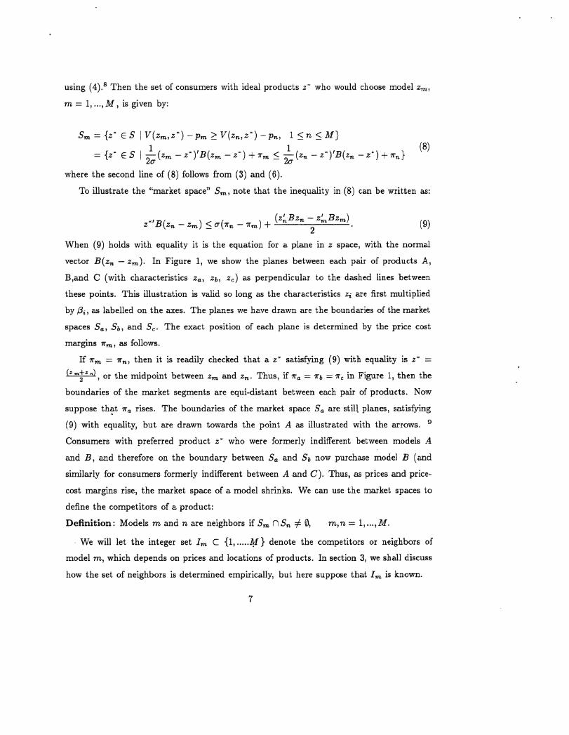
When (9) holds with equality it is the equation for a plane in z space, with the normal

vector B(zn - zm). In Figure 1, we show the planes between each pair of products A,

B,and C (with characteristics za, zb, zc) as perpendicular to the dashed lines between

these points. This illustration is valid so long as the characteristics zi are first multiplied

by ,, as labelled on the axes. The planes we have drawn are the boundaries of the market

spaces Sa, Sb, and Sc. The exact position of each plane is determined by the price cost

margins 'rm, as follows.

If 7rm = 7rs, then it is readily checked that a z* satisfying (9) with equality is z- =

2 or the midpoint between zm and z,. Thus, if 'ra = grk = 7rc in Figure 1, then the

boundaries of the market segments are equi-distant between each pair of products. Now

suppose that 'ra rises. The boundaries of the market space Sa are still planes, satisfying

(9) with equality, but are drawn towards the point A as illustrated with the arrows. 9

Consumers with preferred product z- who were formerly indifferent between models A

and B, and therefore on the boundary between Sa and Sb now purchase model B (and

similarly for consumers formerly indifferent between A and C). Thus, as prices and price-

cost margins rise, the market space of a model shrinks. We can use the market spaces to

define the competitors of a product:

Definition: Models m and n are neighbors if Sm (1 S # 0, m, n = 1,..., M.

. We will let the integer set Im C {1..} denote the competitors or neighbors of

model m, which depends on prices and locations of products. In section 3, we shall discuss

how the set of neighbors is determined empirically, but here suppose that I, is known.

7

2.2 Demand

We shall make the strong assumption that the density of consumers over S is uniform

with parameter p.10 Then demand for model m is:

Qm = pdz*. (10)JS M

Since the market spaces depend on prices, so does demand in (10). We are not able to

obtain a closed-form solution for this multiple integral." However, our central theoretical

result, proved in the Appendix, derives the first derivatives of (10).12 This allows us to

compute a first-order approximation to demand, summarized as follows:

Proposition 1: There exist values 8mn > 0 such that a first-order approximation to

demand Qm around the point 7rm = 7rn, n E lm, is:

nQm ~ InQ* 2Kc( ) 1+:2KT B (11)nEI m

where(a) Bmn = (zm - zn)'B(zrn - zr)

1(b) HHm= 6 ,-

(c) 3 6mn = 1 if Sm is in the strict interior of S.nEmIn

To interpret this result, note that Bmn is the square of Euclidean distance from model

m to n (after the characteristics are first adjusted by fil). Then the derivative of InQm with

respect to 7n is inversely related to this distance: a change in the price of a competitor

will have a smaller effect if it is farther away. The cross-price derivative is directly related

to 8mn, which is an unknown value. In the Appendix (Remarks 1 and 2), we provide an

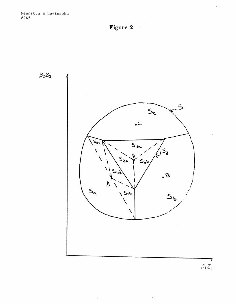
interpretation of 8mn using Figure 2. In Figure 2, the market space Sd is divided into

various sub-spaces as illustrated. Then we can interpret 6dm as equal to area(d), for

n = a, b, c. In other words, 9mn is the volume of a triangle (or more generally a trapezoid)

with vertex at zmL and base at the common boundary of Sm and S, , relative to the entire

volume of Sm. Turning to the derivative of InQm with respect to 7rm, we note that it is

inversely related to Hm. From (b), Hm is interpreted as a weighted harmonic mean of the

8

distances from model m to its neighbors, with the weights 62. If these weights sum to

unity, then it is readily shown that Hm lies between the minimum and maximum values

of Brnn, n E m. In addition, if Bmn = 0 for any one neighbor, then H. = 0: if two

models have the same characteristics, then they are perfect Substitutes, and the elasticity

of demand is infinity.

We will not be able to estimate (11) directly, since the values 6.,, are unknown. For

estimation, we shall let 9, take on the values:

9m, = ), where Nm = number of neighbors of model rn. (12)Nm

This choice for 62, will satisfy the restriction in (c) that Z 6m = 1 for S" in the strict

interior of S. In Figure 2, with four products and two characteristics, only the market

space of model D is in the strict interior of S. However, as the number of products grows

relative to characteristics, more models will be surrounded by neighbors, and then have

their market spaces strictly interior to S. The choice of 62n in (12) means that we will be

replacing the weighted harmonic mean in (b) by the simple harmonic mean.

2.3 Oligopoly Pricing

We will solve for the profit-maximizing prices for each firm under Bertrand competition.

To illustrate the solution, let us initially suppose that each firm produces only one model,

and then consider multiproduct firms. We assume that the marginal costs of producing

a model with characteristics zm are constant and equal to #30 + 3 'zm. The characteristics

of the model are exogenous, i.e. solved in the first stage of a two-stage game. We will

suppose that the profits available from each model are enough to cover fixed costs, but do

not analyse these. Then each firm solves the problem:

max pmQir - (#o +/3'zm)Qm. (13)

Notice that choosing pm 1is the same as choosing rm,7 since they are related by (3).

Then the solution to (13) is calculated using the demand function in (11):

HMpm = #0o +v j'Za + 2K (4

9

Thus, the optimal prices for each product increase according to the harmonic mean of

distances to neighbors. The price-cost margin equals z . The economic intuition behind

this is appealing. If models are very close to each other then Hm approaches zero and

the prices approach marginal cost. This justifies our assumption in section 2.1 that price

would equal marginal cost if all products z > 0 were available. When the continuum of

products is available, the equilibrium schedule Pm =, o+I 3 'zm corresponds to that derived

by Rosen (1974).14

When each firm produces multiple products, let Je C {1, ...M } be the set of models

produced by company c. Then the profit-maximization problem is restated as:

max Z pmQm - (1o +3'z m )Q m. (15)mE Je

The solution to (15) is derived in the Appendix, and using the same notation as in Propo-

sition 1, we have:

Proposition 2: The profit-maximizing prices under Bertrand competition are:

Pm%=_0+)'zm-+ Hm + m . (16)2K 2KcT

where

(a) (F1 ..... , M )'=(C + C 2 +C 3 +...)(H1,....., HM)';

(b) C is an MxM matrix with Cmm = 0, and Cmn = BmanfHm/Bmn if m and n are

neighbors and made by the same company ; Cmn = 0 otherwise.

We see that the optimal prices still increase with the harmonic mean, but (16) contains

an extra term arising from the extra profits that the multi-product oligopolists earns from

collusive within-firm pricing. The matrix C can be arranged to be block-diagonal in the

products of each company, and its rows sum to less than unity so long as no model and

all its neighbors belong to the same company. This will ensure that the infinite sum

C + C2 + C3 +... converges. When actually calculating rm we continue the summation in

(a) until C:(H 1, ... , Hm)' becomes suitably small. -

3. Data and Estimation Issues

10

3.1 Equations to be Estimated

Equations (11) and (16) provide the system comprised of a demand and a oligopoly

pricing equation that is to be estimated. Simple substitutions using the definitions of the

harmonic mean (from equations (11) and (12)), the weighting matrix B (from (6)), price-

cost margins (from (3)), and the term arising from joint profit maximization (from (16))

give the estimating equations in terms of observable data and parameters to be estimated.

With characteristics indexed by j, a model indexed by m and its neighbors by n, and time

indexed by t, we have:

K

Pmt -0o-h( Ejzmtj

lnQ mt = do) + dt + y1j.

(z 1,, m ')((zmt f-lznt )#) (17)K

Pnt ~0o - Zf3zntjj=1

+ '72 K+0mt

ne Im Nm Z 1I((zinj - ztJ )f3)2)J 2

K1-1

pmt = Q0 + 13t + 1 3zmtj + 1Kt

=1Te I m Nm Ey1((zmtj - znt1 )/3)2 (18)

+ A2 rmt (i3, z) + emt.

where do and de are a constant and coefficients on year dummies, respectively, and similarly

for fib and fit.

Note that inmt in (18) is itself a function of Hint's which are themselves non-linear

functions of characteristics z and the 13's. (See Proposition 2(b) for the exact definition.)

Also, the summations over n E Im are summations over the set of neighbors to a given

model. This set is determined by (8) and the definition of neighbors given in section 2.1.

Before any detailed discussion of the data with which we estimate the system or the

estimation techniques employed, first note that the data required to estimate the system

are sales - the Q's, prices - the p's, and characteristics - the z's. The HQ's, y's, and A's

are parameters to be estimated. The theory developed in Section 2 imposes a particular

relationship between the A's and the T's. This relationship is given by:

11

1 _1

-7Y1 = 7y2~Yi~Y2 A - A 2

Rather than impose these restrictions from the outset, we will treat them as testable

implications of the theory. Underlying these restrictions is some straightforward economic

intuition. The restriction -71 = 72 implies that if the prices of all models rise by one

dollar, individual model demands are unaffected. This restriction is an implication of our

assumption that there are no outside goods.

The restriction A = A is related to the pricing strategy employed by multi-product

firms. To better understand this restriction, note that the oligopoly prices in (16) de-

pend on both the harmonic mean of distances to neighbors Hm, and on the joint profit

maximization term rm. As the harmonic mean increases, the optimal price rises with the

coefficient A1 (= 1/2Ko). But now suppose that the harmonic mean for a neighboring

model K, rises, where models m and a are made by the same company. Then the increase

in H leads to a rise in the neighbors price according to A2 (= 1/2Ko-). Of course, this

increase in the neighbor's price would also affect the price of model m due to joint profit

maximization. The restriction A1 = A2 simply says that a company will use the same rule

for all of its products when converting harmonic means to optimal prices. We regard this

as a quite reasonable consistency requirement on the pricing decisions of a multi-product

firm.

The restriction -y 1 = y implies that the demand elasticity resulting from consumer

behavior is the same elasticity used by oligopolists in setting optimal prices.

We have added stochastic disturbance terms, E5mt and Emt in (17) and (18). Comparing

(11) and (17), we see that 5,t = lnQ;k - (d0 - dt). The term lnQmt in (11) is interpreted

as demand for each model if price-cost margins were equal (i.e. r1 = irY,,rn). In this

case, demand would depend on the locations of the products: models whose neighbors

were farther away would have higher demand. We shall treat lnQ *, as iid normal in each

year. Interpreting do + dt as the mean value of lnQ , for each t, we then obtain £5mt as iid

normal with mean zero.

Since equation (16) holds with equality, there should be no error in (18) if we had the

"true" equilibrium prices and our model was an exact description of reality. However, we

12

shall be using the suggested retail prices (SRP), which may differ from the transactions

prices paid by consumers Then one interpretation of Emt is the measurement error arising

from using SRP. We shall treat Emt as iid normal with mean zero, and independent of 6.t.The independence assumption is needed for the system to be identified. Since pmnt -8o -

#'zmt depends on ernt and appears on the right hand side of (17), we could not obtain

unbiased estimates of that equation if 5mt and Eat were correlated. The independence

assumption is justified in our context by our use of suggested retail prices which are

announced at the start of the model-year. In contrast, the quantity data for sales are

over the entire year. This means that pmnt's are announced before Qmt's are known.

Finally, the year dummies in (17) and (18) may be thought of as fixed effects in a

panel context. These variables are included to pick up unmodelled components of the

disturbance terms that are correlated with time. In (17), one might imagine that cyclical

macro variables may effect auto demand in a given year. In (18), the year dummies are

more likely to pick up inflationary trends. 15

3.2 Data

We estimate (17) and (18) using a panel data set comprised of 86 models of automobiles

sold in the United States during the period 1983 through 1987. We include all models sold

for each of these five years except exotica (Lotus, Ferrari, Rolls Royce, and the like.) The

complete list of models is included in Table 1.16

We model automobiles as differentiated over five dimensions. That is, the vector of

characteristics for each model in each period, zt, has five elements. These differentiating

characteristics are weight (in thousands of pounds), horsepower, aerodynamics (measured

as the inverse of height in inches), and dummy variables for whether the car has air con-

ditioning as standard equipment (a proxy for luxury) and whether the car is European.'7

We choose to limit the product differentiation to five characteristics for computational

reasons. In the sensitivity analyses, we check to see how robust results are to the choice

of characteristics.

The sales data are sales by nameplate (measured in thousands), and the price data are

list prices of the base models (in thousands of dollars.) While something like the average

13

transaction price for each model in each year is of course preferable to list prices, such data

are simply not available on an all-encompassing basis. All data are from the Automotive

News Market Data Book (annual issues.)18

3.3 Estimation Issues

Estimating (17) and (18) poses some unique econometric issues. The first of these

involves estimating the set of neighbors for each model. The second issue arises because

each observation is itself summed over a different set of neighbors. The third relates to

the extensive non-linearity of the system. We elaborate on each of these in turn.

The simple harmonic mean of distances from a model to its neighbors appears in both

(17) and (18). Before the system can be estimated, it is necessary to know which models

neighbor which. The first step in estimation, then, is to determine Im - the set of neighbors

to each model.19 The theory developed in section 2.1 guides this process. Recall that two

models m and n are neighbors if Sm n S, , 0, rnn = 1,..., M. We can interpret this

definition as saying that two models are neighbors if consumers indifferent to these models

prefer these models to all other available models. As noted in section 2.1, a particularly

convenient feature of the utility function (1) is that the consumer whose ideal variety is

the midpoint of a line drawn between two models will be indifferent to the two models.

The metric by which the midpoint is determined is simply (the square of) Euclidean

distance when each characteristic has been pre-multiplied by i. The vector 0, though,

is estimated in the system given by (17) and (18), and to estimate these, one must know

the set of neighbors. We address this problem by applying OLS to (2) to get preliminary

estimates of ,3. These #i3's are then used to compute neighbors. In the sensitivity analyses

in Section 5, we will take the /3 that results from estimation of the system, and use that 'ato recompute neighbors. With the new neighbors, the system can then be re-estimated.

The algorithm which computes neighbors is straightforward. We first take a pair of

potential neighbors. We locate the midpoint of the line connecting these two models. 20

With this midpoint as the ideal variety, z-, we then ask if any other available models are

closer to z- using the metric discussed above. If no available model is closer, the two

models are, by our definition, neighbors. Conversely, if another available model is closer,

14

the two are not neighbors. We repeat this procedure for every possible pair of models

within a year. (We do not model possible inter-temporal competition between models.)

This procedure will identify neighbors in multi-dimensional characteristics space which is

needed to form I~ in (17) and (18).21

Once the set of neighbors, r,,,, has been determined, we turn our attention to estimating

(17) and (18). Because the disturbance terms are additive in each equation, estimation

by Non-linear Least Squares (NLS) and Maximum Likelihood (MLE) are asymptotically

equivalent. Since each observation contains variables summed over sets unique to that

observation (the Im's), though, standard NLS and MLE estimation programs are not

suitable. We estimate (17) and (18) using a variant of the Gauss-Newton algorithm for

NLS that was designed specifically for estimating systems with the properties of (17) and

(18)22

The Gauss-Newton algorithm is an iterative method. For the problem at hand, two

issues deserve special note. First, in general, it is preferable to utilize analytic deriva-

tives when using Newton-type methods.23 Given the fairly extreme nonlinearity in our

estimating equations, the advantages of analytic derivatives are magnified. Accordingly,

our Gauss-Newton method employs analytic derivatives.2 4 Second, note that with each

iteration, the estimated values of /3 will typically change. As these change, the set of

neighbors I. might change. We do not allow this to occur. Rather, we assume that the

set of neighbors is constant between iterations. The reason for this is that if the set of

neighbors changed with each iteration, there is no reason to expect iterative methods to

converge. As mentioned above, after obtaining NLS estimates of (17) and (18) using the

neighbors identified by preliminary (OLS) values of 4Q, we shall then re-compute neighbors

and re-estimate the system.

4. Results and Interpretation

The first step in the estimation is identifying the set of neighbors for each of the 86

models in the sample. This is done using the 1985 cohort of models. We assume that

the set In. is constant over the period of estimation.25 Prior to computing these sets of

15

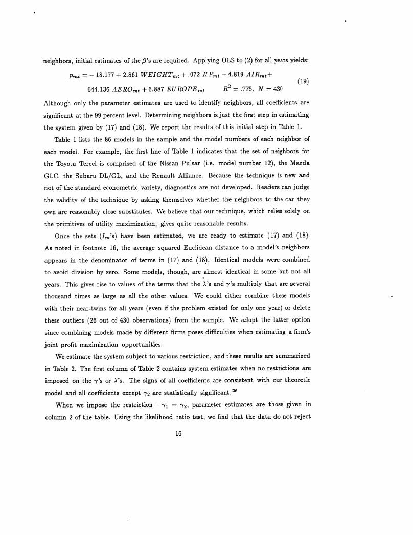
neighbors, initial estimates of the #'s are required. Applying OLS to (2) for all years yields:

Pnt = - 18.177 + 2.861 WEIGH Tmt + .072 HPmt + 4.819 AIRme +(19)

644.136 AEROmt + 6.887 EUROPEmt R2 = .775, N = 430

Although only the parameter estimates are used to identify neighbors, all coefficients are

significant at the 99 percent level. Determining neighbors is just the first step in estimating

the system given by (17) and (18). We report the results of this initial step in Table 1.

Table 1 lists the 86 models in the sample and the model numbers of each neighbor of

each model. For example, the first line of Table 1 indicates that the set of neighbors for

the Toyota Tercel is comprised of the Nissan Pulsar (i.e. model number 12), the Mazda

GLC, the Subaru DL/GL, and the Renault Alliance. Because the technique is new and

not of the standard econometric variety, diagnostics are not developed. Readers can judge

the validity of the technique by asking themselves whether the neighbors to the car they

own are reasonably close substitutes. We believe that our technique, which relies solely on

the primitives of utility maximization, gives quite reasonable results.

Once the sets (Im's) have been estimated, we are ready to estimate (17) and (18).

As noted in footnote 16, the average squared Euclidean distance to a model's neighbors

appears in the denominator of terms in (17) and (18). Identical models were combined

to avoid division by zero. Some models, though, are almost identical in some but not all

years. This gives rise to values of the terms that the A1's and y's multiply that are several

thousand times as large as all the other values. We could either combine these models

with their near-twins for all years (even if the problem existed for only one year) or delete

these outliers (26 out of 430 observations) from the sample. We adopt the latter option

since combining models made by different firms poses difficulties when estimating a firm's

joint profit maximization opportunities.

We estimate the system subject to various restriction, and these results are summarized

in Table 2. The first column of Table 2 contains system estimates when no restrictions are

imposed on the y's or A's. The signs of all coefficients are consistent with our theoretic

model and all coefficients except 72 are statistically significant.26

When we impose the restriction -71 = 72, parameter estimates are those given in

column 2 of the table. Using the likelihood ratio test, we find that the data do not reject

16

this restriction. The test statistic is .8831 and is distributed Chi-Square with one degree

or freedom. Again, the signs are theory-consistent and all coefficients are now statistically

significant.

We next impose the additional constraint that A = A2 and these results are presented

in column 3 of Table 2. Again employing the likelihood ratio test, we find that the data do

not reject this restriction as the test statistic is 1.718 and distributed Chi-Square with two

degrees of freedom. When the restriction is imposed, signs remain consistent with theory

and all coefficients are statistically significant.27

The rest of this section discusses the interpretation of the results. Since the joint

restrictions A1 = A2 and -y1 = 72 are suggested by the theory and accepted by the data,

we shall focus on this case as we discuss results.28

We find that y1 is negative (-.0099) and statistically significant. This supports the

notion that the demand for a model, given the location of its neighbors, falls when the

price of the model rises. The own elasticity of demand is easily computed using (17).

One feature of our model is that every model in each year has a different own elasticity

of demand, and this elasticity depends on the location of neighboring models. All else

equal, models whose neighbors are quite close have more elastic own price responses. We

calculate the elasticity of demand for every model in the sample.29 We find that the own

price elasticity of demand has an average value of -.516 and a median value of only -

.211. These inelastic values are clearly incompatible with an oligopolistic equilibrium. In

general, it appears that the magnitudes of the estimated y's are not theory-consistent. Our

approach to the demand equation attempts to measure levels of demand using derivatives

of demand. We adopt this strategy due to the difficulty of estimating the multiple integral

in (10) directly. While every coefficient in our demand equation was of the correct sign

and statistically significant, the "derivatives" approach does not appear to yield own price

elasticities of demand that are consistent with an oligopolistic equilibrium.30

Also 72 is positive (.0099) and statistically significant. As the prices of a model's

competitors rise, the model's own sales also rise. Again, every model has a different cross-

price elasticity in our set-up. This elasticity is greater the closer a model's competitors are

(using the measure of distance provided by the theory in section 2.) The demand equation

17

also permits estimates of a very wide variety of elasticities. One can perturb the system

on any of a number of margins, and compute how model demand changes. For example,

automobile industry analysts could use (17) to compute the elasticity of demand for Fords

with respect to a change in the price of General Motor's models. Trade economists could

compute the demand elasticity for domestic cars with respect to a price change in Japanese

models; and regulatory economists could compute the demand elasticity for light autos

with respect to a price change (tax) on high horsepower models.3 ' In sum, the estimated

demand equation is useful in a variety of interesting economic situations.

In the oligopoly pricing equation, (18), we find that A,, the term that multiplies the

harmonic mean of neighbors' distances, is positive (.410) and statistically significant. All

else equal, as a model's competitors become farther away, the price-cost margin rises. Just

as the estimated demand equation implies an own price elasticity of demand for every

model, so does the pricing equation. It is straightforward to show that this elasticity for

model m in period t is given by K where Hint is the harmonic mean of distances

to neighbors. The resulting elasticities may be interpreted as the ones used by firms in

setting their prices whereas the elasticities from the demand equation may be thought of as

resulting from consumer behavior. In a theoretically consistent world, these two elasticities

would be the same.

We find that the demand elasticity implied by the pricing equation has a median value

of -51.7. This value seems reasonable when we keep in mind this is the elasticity for

a given model (of the almost 100 available) and that any model has many substitutes.

The distribution of elasticities is illustrated in Figure 3. Figure 3 shows the wide range of

elasticities. The figure lso shows that many models have virtually perfectly elastic demands.

These observations have at least one neighbor that is very similar. In general, the demand

elasticities implied by the pricing equation appear reasonable and are compatible with an

oligopolistic equilibrium.

By computing the harmonic means for each model using the simultaneously estimated

pi's, we can also calculate the mean price-cost margin excluding any returns to collusion

arising from the multi-product nature of the market. That is, we can compute the term

Hm/2Kcr in (16). We find this mark-up has an average value of $599 and a median value

18

of $200. One interpretation of this figure is that it represents the mark-up that would

result if the 86 models in the sample were produced by 86 separate firms. Again due to the

presence of outliers, summary statistics may be misleading. We present the distribution of

these mark-ups for each model-year in Figure 4. There we see that about half the sample

(205 of 404 observations) have a mark-up of $500 or less while 36 have a mark-up of over

$5000.

We find that A2 is also positive (.410) and is precisely estimated. The data strongly

support the hypothesis that oligopolistic multi-product firms increase the prices of those

products that have as competitors products made by the same parent firm. We find the

magnitude of this within-firm collusion can be quite substantial. Using the simultaneously

estimated /3's, we compute the term that A2 multiplies. The average value of this term

for products that have at least one neighbor made by the same firm times the estimated

A2 gives the extra price-cost markup. We find this additional markup due to joint profit

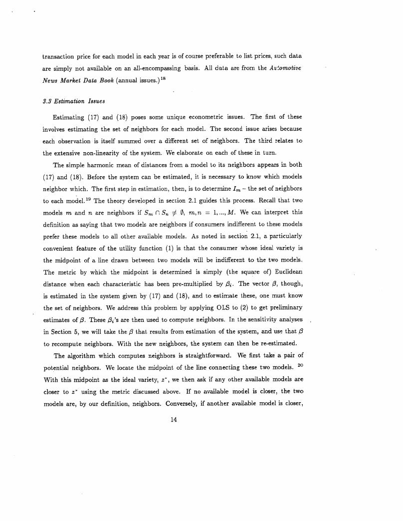
maximization has a median value of $144 and averages $606. The distribution of the

additional mark-ups due to joint profit maximization is illustrated in Figure 5. There we

see that more than half (230 of 404) of the observations have at least one neighbor made by

the own parent firm. Of these observations, about half (128 of 230) have extra mark-ups

of $500 or less while 24 observations have mark-ups greater than $4000.

The estimates of 3 are also reported in Table 2. All of the /3's (except the constant)

are positive which is what our theory predicts. Also, all the parameter estimates are

statistically significant. The /3's that appear in (17)- and (18) are used to measure distances.

Positive /3's indicate that as a model's competitors become farther away in any of the five

dimensions in which the products are differentiated, the own and cross price responses

in demand are reduced and oligopoly markups are increased. We can also go back to

equation (2) (which was substituted into (17) and (18)) to interpret the ,3's. Then each /3

can be thought of as the marginal cost of producing an additional unit of a characteristic.

Here, though, interpretation is tenuous since many of the characteristics are proxying for a

variety of other characteristics. In the instance of air conditioning, p3a,. = 4.894. Clearly, it

does not cost a firm almost $5000 on the margin to add air conditioning to a model. Insofar

as the dummy variable AIR is proxying for the wide range of luxury items associated with

19

air conditioning as standard equipment, the estimate is more reasonable. Similar caution

should be exerched when interpreting the other #3's.

The next to last two lines of Table 2 report the R2 for the demand and the pricing

equations. We find that our specification explains about 81 percent of the variation in

model prices and about 5.0 percent of the variation in model demands. While the data

support the behavioral hypotheses suggested by our theory, a substantial amount of the

variance in model demands remains unexplained.32

The estimates of the parameters on the dummy variables for years are not reported in

Table 2. We find that these parameters are close to zero and not statistically significant in

the demand equation. In the pricing equation, the parameters are positive and significant.

Their magnitude indicates that the average price of all models rises about $500 each year.

5. Sensitivity Analyses

Ideally, the #3's reported in the first three columns of Table 2 should be used to estimate

the sets of neighbors instead of the initial estimates generated by (19). (But then with

different sets of neighbors, 3 will again change which leads to yet another set of neighbors

and so on.) As a sensitivity exercise, we re-calculated the sets of neighbors using the

NLS 3's in column 3 of Table 2. With these new sets of neighbors, we then re-estimated

equations (17) and (18) (still imposing that -1 = 72 and ) = A2 .) Column 4 of Table 2

presents the new system estimates. This experiment shows that the results are quite robust

to our inability to simultaneously estimate distances and sets of neighbors. All coefficients

except the y's that were statistically significant in the base case (column 3) remain so.

(The y's are just statistically insignificant unless we impose our priors that y1 < 0 and

employ a one-tailed test.) Further, the magnitudes of most coefficients in columns 3 and

4 are quite similar. Apparently the inability to simultaneously estimate distances from

neighbors and the set of neighbors is not important to our results.

Leamer (1983, 1985) has argued in a persuasive and entertaining fashion for experiments

which test the importance of ad hoc specification decisions. In our context, the precise

list of characteristics may be viewed as "doubtful." In this spirit, Table 3 investigates how

sensitive results are to the choice of characteristics. In that table, we drop one characteristic

20

and instead use a plausible alternative. For example, we drop horsepower and instead use

engine displacement. The other substitutions are a dummy for foreign instead of the

dummy for European, a continuous measure of luxury33 instead of the dummy for air

conditioning, and an alternative measure of aerodynamics (using the inverse of headroom

instead of inverse height)." In each case, we re-estimate the system using non-linear least

squares and imposing that A = )2 and -3 = 72.

Table 3 reports the average own elasticity of demand, the average price-cost margin,

and the average extra mark-up due to within firm joint profit maximization.35 We find

that using alternate sets of characteristics changes the magnitude of the elasticity and

mark-ups, but never affects our qualitative results. Demand elasticities from the demand

equation are all negative and remain fairly inelastic. Mark-ups are all positive and with

the possible exception of when the SHORT proxy (the inverse of headroom) is used, are

even similar in magnitude. With any of the sets of characteristics, the resulting average

mark-ups lie in the central part of the distribution of base case mark-ups (as illustrated

in Figures 4 and 5.) Overall, we conclude that our qualitative results do not depend on a

fortuitous choice of characteristics.

6. Conclusions

Since theoretic models in many fields of economics assume product differentiation, and

in the real world this differentiation is frequently multi-dimensional, econometric methods

which might allow researchers to test the theories are needed. In this paper, we have

developed a method for estimating demand and oligopoly pricing when products are multi-

dimensionally differentiated.

Our technique is solidly rooted in consumer utility maximization and firm profit max-

imization, and this theoretic model directly guides our econometric specifications. We

derive a demand system for multi-dimensionally differentiated products that has several

testable hypotheses. Our theory, for example, predicts that both the price of a model and

the appropriately measured distance from a model to its competitors will effect the demand

for that model. Similarly, oligopoly pricing depends on the model's own characteristics,

and how far away a model's neighbors are. Our theory also indicates how to estimate

21

the extra oligopoly rent multi-product firms accrue when their products compete with one

another.

We estimate the equations generated by our theory using data from the U.S. automobile

market. We find that the data broadly support the predictions of the model. For example,

the estimated demand equation indicates that demand for a model falls as the model's own

price rises and as the prices of competing models fall. Further, the own- and cross- price

responses becomes more elastic as a model's competitors become closer. The magnitudes of

these demand elasticities, though, are not consistent with an oligopolistic equilibrium. On

the oligopoly pricing side of our model, the data support the notion that a firm will increase

a model's price if that model's competitors are farther away. We also find support for the

existence of extra oligopoly rents due to multi-product firms. The demand elasticities

implied by the pricing equation are consistent with an oligopolistic equilibrium. Were our

model completely supported by the data, the demand elasticities implied by the demand

and by the pricing equations would be the same. They are not.

The within-equation restrictions on the demand and pricing equations were tested and

readily accepted. There are, though, other restrictions which were implicitly imposed and

not tested. For example, for more general utility functions than that in (1), it can be

shown that the 3's which enter the harmonic means and marginal costs indeed differ. We

have not pursued this generalization here since it would substantially increase the number

of parameters to be estimated. Experimenting with more general utility functions, though,

is a direction for further work. Along the same lines, relaxing our -assumption of a uniform

density of consumers may lead to a specification which is better supported by the data.

A more general assumption we have imposed on the model is that of Bertrand compe-

tition. Obviously, it would be desirable to extend the model to allow for other forms of

market conduct and to see if market conduct has changed in response to specific policies.

We are presently studying the effects of the "voluntary" export restraint with Japanese

auto firms, initiated in 1981, on the market conduct of American firms.

Future research, then, is directed toward relaxing some of these restrictive assumptions

while still deriving an empirically implementable model. Also, there are many other indus-

tries for which our approach is applicable. The promising results of this first attempt at

22

estimating the demand and oligopoly pricing for multi-dimensionally differentiated prod-

ucts have prompted us to research these extensions and further applications. We hope

others might be similarly motivated.

23

Appendix

We shall prove Propositions 1 and 2 using results more general than those required in

the text. Let 7rm and ira denote the price cost margins on model m and its neighbors,

n E Im. We restrict these to satisfy:

-Br - 7rm > (Al)

2o

where Bmn = (Zm - zn)'B(zm - zn). From (8), it can be seen that (Al) ensures zm E Sm,

so that the market space of a model contains the model itself.

Demand in (10) is obtained as a multiple integral over Sm. Since the boundaries of the

market space in (8) vary continuously with prices, we shall treat demand as continuously

differentiable. The derivatives of demand are given by:

Theorem 1

There exist values mn ;> 0, depending on prices, such that the derivatives of demand

are:

1 6Qm_ 2oKmn(a) Q 8 Bmn + 2c(7r - 7rm)(b) 18Q m= -2aK ZB mn

Q. aPm nEI m ma + 2Q(7rten-rm)

(c) 1 6mnn = 1 if Sm is in the strict interior of S.

nEIm

Proof:

(a) This follows by defining Gmn as,

lOQ mmn = (1 p )[Bmn + 2 (r - rm)]/2cK. (A2)

m~ [r~ u) Qm (&Pn

From (8), we see that the market space Sm becomes larger as 7rn rises, so that a > 0.

Then using (Al), it follows that 6mn > 0.

(b) The market spaces in (8) depend on (7rs - urm) = [(Pn - pm) + fl'(zm - zn)], from

(3). This means that raising pm by an amount 6 will have the same effect on demand as

lowering pa by 6 for all n E Im. That is,

24

fEm

Then (b) follows directly from (a).

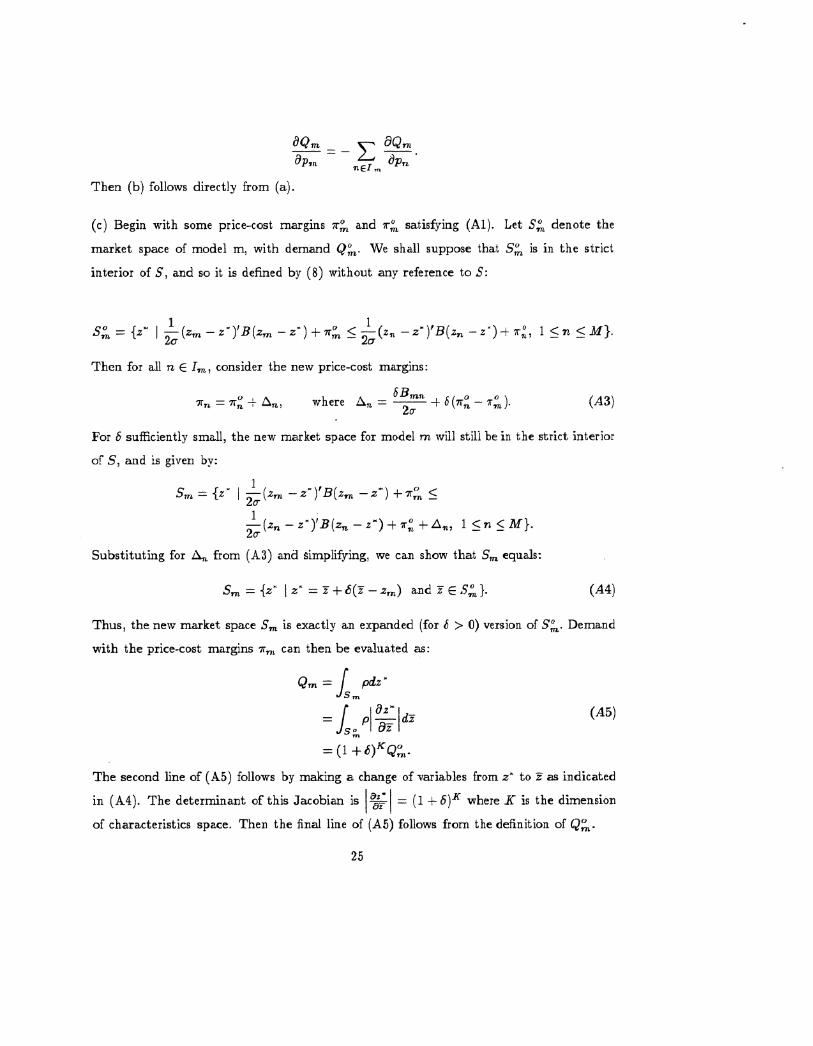
(c) Begin with some price-cost margins ir and 7r,, satisfying (Al). Let S" denote the

market space of model m, with demand Q,. We shall suppose that S, is in the strict

interior of S, and so it is defined by (8) without any reference to S:

S = { z" |-(zm-z)B(zm, - z)+ 7r,"< 1 (z - z")'B(z. -z)-+r", 1 <Cn <M}.

Then for all n E Im, consider the new price-cost margins:

ra = T"+ A, where AO = "'"-+ 6(7r" - 7r*). (A3)2o

For 6 sufficiently small, the new market space for model m will still be in the strict interior

of S, and is given by:

Sm = {z | -(z. -z")'B(z -z") +7r" '

1- (z.- z )' B (zn - z -)+7r" +- ,1 <n(< M}.

Substituting for An from (A3) and Simplifying, we can show that S, equals:

Sm = {z" z +6( - z) and YES,}. (A4)

Thus, the new market space Sm is exactly an expanded (for b > 0) version of S,". Demand

with the price-cost margins 7r~, can then be evaluated as:

Qm = pdz*

=I p di (A5)

=(1+6)KQo

The second line of (A5) follows by making a change of variables from z- to z as indicated

in (A4). The determinant of this Jacobian is = (1 +6)K where K is the dimension

of characteristics space. Then the final line of (A5) follows from the definition of Q".

25

From (A5), we calculate that,

"=0 = KQ°. (A6)06 16=0

However, using (A3), we calculate that,

OQ m m_ 0Qrnj 1rn

06 6=0 OpI |6=0 0 |6=0

a z(A7)

= m [Bmn + 2u-(7rn - lrm)]/2cr.EIm pn 6=0

Setting (AS) equal to (A7), and using (A2), it follows immediately that EnEr.6mn = 1

when evaluated at 7r", and 7r". But since ir," and 7ro were any price-cost margins satisfying

(Al), this proves part (c). Q.E.D.

Evaluating the derivatives in Theorem 1 at the price-cost margins 7vm = lrn,n E In,we obtain Proposition 1 in the text. In order to prove Proposition 2, we need the following

result.

Theorem 2

When demand is continuously differentiable, =

Proof:

Total consumer surplus over the set of available products is,

W= ( j [V(zm,z) -pm]pdz*. (A8)

With each consumer maximizing surplus, W is also maximized. That is, the market spaces

shown in (8) give the highest value of W compared to any other choices of Sm ; S with

5m n Sn of measure zero. Then analogous to the envelope theorem, when differentiating

(A8) with respect to prices, we can hold the market spaces Sm constant. Calculating this

derivative,

Ow= - I pdz* = -Q,.

26

Then by Young's Theorem,

02w _ Qm _ Qn

pPmopn 9pn - apm'

Q.E.D.

Remark 1: Combining the immediately above result with part (a) of Theorem 1, we see

that Qrn6mn = Qn 9nm when 7r7 = 7r,m. This allows us to interpret the 8m, in terms of

Figure 2. The market space Sd for model D in Figure 2 is divided into Sda, Sda, and Sdc.

Define,

=_area (Sdm) m c

area(Sa ) - c

We clearly have 9 ia +Odb +eac = 1. But in addition, with 7rj = Ira in Figure 2, the triangles

Sad and Sda are identical, since their common boundary is perpendicular to and crosses

the mid-point of a line between A and D. Then define 0ad = rea(Sa) . It follows that

area (Sa)6ar = area (S)64a. Since demand is the integral over market spaces, we obtain

Qaa6 = Qi6ra as required. We conclude that (A9) is a valid interpretation of e2. While

we have assumed that 7rm = 7rn, an extension of our argument can show that (A9) is still

valid when ?rm 7rn.

Remark 2: This interpretation of 6mn suggests that for models m where S includes a

boundary of S, we have,

.8-.6mn < 1. (A 10)

n Elm

This is demonstrated by model A in Figure 2, for which area(S a,)+a7ea(S a)+area(Sad) < 1.

We expect that (AlO) is the counterpart to Theorem 1(c) when S,. is not in the strict

interior of S, but do not prove this here.

Returning to Proposition 2, the first order conditions for (15) can be written as:

;r.= - Q - r - 7r n "), m E Jc, (Al1)

nn

where the summation is over n E (Jc Ilm). We can use Theorem 2 to replace by

in (All). Then evaluating all derivatives of Qm at the point 7r, = 7r,, n E I, we can

write (All) as,

27

eHm 6mnHm)n E Jc (Al2).2K- +Bmn

Using the notation of Proposition 2, (A12) can be written as (I - C)ir = 2 - where

7r = (i,....,7rM)' and H = (H,....., H m)' are column vectors. It follows that ir = (I -

C)-2K . Assuming that 9mn > 0 for n E In, the rows of C sum to less than unity

so long as no model and its neighbors all belong to the same company. We then have

(I - C)~ = I + C + C 2 + C3 + .... , and so Proposition 2 is established.

28

Footnotes

1. A survey of the New Empirical Industrial Organization (NEIO), including some studies

of product differentiation, is provided by Bresnahan (1988). A recent study by Trajtenberg

(1989) models consumer preferences with products differentiated in many dimensions, as

we consider here. His paper, though, is quite different from ours. He derives the demand

and welfare gains from the introduction of a new product, while we, in contrast, derive

demand and oligopoly pricing. Because Trajtenberg considers a product with few available

varieties (CT scanners), he is able to estimate demand with a multinornial logit model. We

shall consider a product with many varieties (autos), and this requires new and different

functional forms and estimation techniques. See also footnote 11.

2. Examples of empirical trade papers which do model multi-dimensional product differen-

tiation but do not model oligopolistic firms are Feenstra (1988) who investigates the gains

from trade resulting from the introduction of new products, and Levinsohn (1988) who

analyzes the effect of tariffs on the demand for differentiated products.

3. Our approach is compared to these papers in footnotes 7, 9, and 11

4. The harmonic mean of a series whose observations are denoted by nn, is given by:

1N ~H 1 _

N 7X,n.=1

5. This utility function is a bit more general than it appears, since multiplying z2 by 'Y we

can write l n(yiz2 -jaz) = l in(yi)+ZIn[zi - (0/y)]. The first term in this expression

is constant and can be omitted, and the second term is already captured by (1.)

6. Bresnahan (1981, 1987) is able to estimate' the price and quality of alternatives to

purchasing a new car, as he locates the alternatives at the lower and upper ends of the

quality line. With multiple characteristics, the same approach does not seem feasible.

7. See Lancaster (1979) who uses a single characteristic, and Anderson, Palma, and Thisse

(1989) who use a multi-dimensional version very similar to (6). Caplin and Nalebuff adopt

a general utility function which includes (6) as a special case.

29

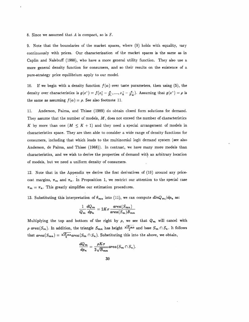
8. Since we assumed that A is compact, so is S.

9. Note that the boundaries of the market spaces, where (9) holds with equality, vary

continuously with prices. Our characterization of the market spaces is the same as in

Caplin and Nalebuff (1988), who have a more general utility function. They also use a

more general density function for consumers, and so their results on the existence of a

pure-strategy price equilibrium apply to our model.

10. If we begin with a density function f(a) over taste parameters, then using (5), the

density over characteristics is g(zX) = f(z* - ,...., z; - g). Assuming that g(z") =p is

the same as assuming f(a) = p. See also footnote 11.

11. Anderson, Palma, and Thisse (1989) do obtain closed form solutions for demand.

They assume that the number of models, M, does not exceed the number of characteristics

K by more than one (M < K + 1) and they need a special arrangement of models in

characteristics space. They are then able to consider a wide range of density functions for

consumers, including that which leads to the multinornial logit demand system (see also

Anderson, de Palma, and Thisse (1988)). In contrast, we have many more models than

characteristics, and we wish to derive the properties of demand with an arbitrary location

of models, but we need a uniform density of consumers.

12. Note that in the Appendix we derive the first derivatives of (10) around any price-

cost margins, 7rm and lr,%. In Proposition 1, we restrict our attention to the special case

rm = r. This greatly simplifies our estimation procedures.

13. Substituting this interpretation of 8mL into (11), we can compute dinQ ,/dpn as:

1 dQm area(Smn )= 2Kcr

Qm dpn area(Sm)Bmn

Multiplying the top and bottom of the right by p, we see that Qm will cancel with

p area(Sm). In addition, the triangle Smn has height E and base Sm f Sn. It follows

that area(Smn) = B area(Sm fl Sn). Substituting this into the above, we obtain,

dQm pKc

dp = - 2 area(SmflSn).dpn 29/mn

30

Thus, the derivative of Qm with respect to pn is directly related to the size of the common

boundary between S, -and S, which reflects the number of consumers who will switch

products as prices change, and inversely related to the Euclidean distance between models.

14. The hedonic price schedule pm = -O + 3 'zm is linear because we have assumed that

marginal costs C(z) are linear in characteristics and independent of quantity. Jones (1988)

has recently examined conditions on consumer preferences which imply a linear hedonic

price schedule, and found that these are very restrictive.

15. With the year dummies appearing in (18), an alternative way to measure the price-cost

margins appearing in the numerators on the right of (17) is (p, - 'o - ,Qt -#,3 'zmt). We

chose to use (pmt - 3o - I3'zmt) in (17) to slightly simplify the estimation, but the two

formulations are equivalent when -yr = 72-.

16. A measure of the distance between a model and its competitors is in the denominator

of several of the terms in (17) and (18). A few models have as neighbors a twin model

that is always made by the same parent firm and has absolutely identical characteristics

(as we measure them.) Hence the distance between the model and the twin is zero. We

combined the sales figures for these twin models and include them as one model.

17. The characteristics for each model are those that come standard with the base model.

18. All data are available as ascii files on floppy disk upon request to the authors.

19. We describe the identification of neighbors in much greater detail, using a more general

utility function, in Levinsohn and Feenstra (1989).

20. As discussed in section 2.1, a consumer with ideal product z* = (zm -+ z)/2 is

indifferent between purchased models m and n when their prices satisfy w = rn. In our

search for neighbors, we are implicitly assuming that 7rm = irnVm, n. Alternatively, we are

assuming that a is very small in (9), so that the term cr7rm - r2r) vanishes.

21. Since we do not map out the hyperplanes which serve as boundaries between market

spaces, our procedure can falsely reject two models as neighbors, but can never falsely

accept. This is illustrated in Figure 2, where the mid-point of a line between B and C lies

31

in Sa. This means that the consumer whose ideal product is midway between B and C

would prefer model A. and our procedure would reject B and C as neighbors. This rejection

is false, however, since Sb and Sc have a non-zero intersection as illustrated. Heuristically,

the false rejection of neighbors seems more likely for models near the boundary of S.

22. The programs for Gauss-Newton are written in Fortran 77. The source code is available

from the authors on request.

23. See Quandt (1983) for a discussion of why this is so.

24. It is not difficult to analytically compute the derivatives of (17) and (18) with respect

to (3, y, A), except for the derivatives with respect to the term rmt(3,z) defined in

Proposition 2. We compute d(r1i.... , rm)/d#= (C + C 2 +C 3 +....)d(H1, H 2 , ..... ,Hm)/d3

for each t, and are therefore ignoring the change in C with respect to ,3. We believe this

simplification is unimportant because the pattern of zero and positive elements in C is

invariant to 3 (for given sets of neighbors Im).

25. Experiments show that while the set Im does change slightly from year to year, the

average of the squared Euclidean distances, which is what matters, is quite stable.

26. We will use the term "statistically significant" to mean statistically different from zero

at the 95 percent confidence level unless we indicate otherwise.

27. Although not reported in Table 2, we also.estimate the model with the additional

cross equation constraint that --y1 = 1/A1 imposed. As a quick glance at the estimates of

the y's and A's indicates, this restriction is resoundingly rejected. Discussion of why this

might be so and the economic implications of this rejection are discussed in Section 6.

28. The reader will note, though, that coefficient estimates in the restricted and unre-

stricted cases are all very similar.

29. These results are available on request to the authors.

30. Bresnahan (1981), in contrast, evaluates the simpler integral that results from his

Hotelling model. He appears to impose the cross- and within-equation restrictions we test

and arrives at reasonable demand elasticities averaging about -2.3.

32

31. See Levinsohn (1988) for a discussion of some of these issues.

32. The low R2 in the demand equation is not surprising since the residual includes lnQ;,

from (11).

33. Our proxy for luxury is (AIR + 1)*Legroom*Headroom

34. We do not substitute for WEIGHT, since without it many of the distances between

models are close to zero (i.e. products are not sufficiently differentiated.)

35. We report the elasticity of demand from the demand instead of pricing equation in

column 1 of Table 3. This is because had we reported the more sensible elasticity from

the pricing equation, we would have no information about how robust estimates of the 7y's

were.

33

References

Anderson, S., A. De Palma, and J-F Thisse (1988) "A Representative Consumer Theory

of the Logit Model," International Economic Review, 29, 461-466.

(1989) "Demand for Differentiated Products, Discrete Choice

Models, and the Characteristics Approach," Review of Economic Studies, 56, 21-35.

Bresnahan, T. (1981) "Departures from Marginal-Cost Pricing in the American Automo-

bile Industry," Journal of Econometrics, 17, 201-227.

- (1987) "Competition and Collusion in the American Automobile Oligopoly: The

1955 Price War," Journal of Industrial Economics, 35, 457-482.

(1988) "Empirical Studies of Industries with Market Power," in Handbook of In-

dustrial Organization, ed. R. Schmalensee and R. Willig. Amsterdam: North Holland.

Caplin, A. and B. Nalebuff (1988) "After Hotelling: Existence of Equilibrium for an Im-

perfectly Competitive Market," mimeo.

Crain Communications (1984-1988 issues) Automotive News Market Data Book. Detroit:

Cram.

Feenstra, R. (1988) "Gains from Trade in Differentiated Products: Japanese Compact

Trucks," in Empirical Methods for International Trade, ed. R. Feenstra. Cambridge:

MIT Press.

Helpman, E. and P. Krugman (1985) Market Structure and Foreign Trade. Cambridge:

MIT Press. -

(1989) Trade Policy and Market Structure. Cambridge: MIT Press.

Hotelling, H. (1921) "Stability in Competition," Economic Journal, 39, 41-57.

Jones, L. (1988) "The Characteristics Model, Hedonic Prices, and the Clientele Effect,"

Journal of Political Economy, 93, 551-567.

Lancaster, K. (1979) Variety, Equity, and Efficiency. New York: Columbia University

Press.

Leamer, E. (1983) "Let's Take the Con Out of Econometrics," American Economic Review,

73, 31-43.

(1985) "Sensitivity Analyses Would Help," American Economic Review, 75, 308-13.

34

Levinsohn, J. (1988) "Empirics of Taxes on Differentiated Products: The Case of Tariffs

in the U.S. Automobile Industry," in Trade Policy Issues and Empirical Analysis, ed.

R. Baldwin. Chicago: University of Chicago Press.

and R. Feenstra (1989) "Identifying the Competition," mimeo.

Quandt, R. (1983) "Computational Problems and Methods," in Handbook of Econometrics,

Vol. 1, ed. Z. Griliches and M. Intriligator. Amsterdam: North Holland.

Rosen, S. (1974) "Hedonic Prices and Implicit Markets: Product differentiation in pure

competition," Journal of Political Economy, 82, 34-55.

Trajtenberg, M. (1989) "The Welfare Analysis of Product Innovations, with an Application

to Computed Tomography Scanners," Journal of Political Economy, 97, 444-479.

35

Feenstra & Levinsohn#245

Figure 1

/32

Z2

S

7

,r3Z 1

Feenstra & Levinsohn#245

Figure 2

\5

\ / /\ 1 Sa~r s7

M1

/3

Z

fof40

observations60 80 1000

0A

0

I 1

0 do

0

20 120 140

C)

C

C-

0

W

C

C

2a

000_

0

0

UqOSUJA87 3g eJnsuaaa

C

Lon

Sof observations0 40 80 120 160 200 240

O 1

Wc

OC

O

C-D

0

C,

0

. -

§ 17Z

GAUSS July 10. 1989 12:21:32 PM

Figure 50

0N

)ooCoO

oo00

o>

(I

i-0

0

0N

0

a a a a ar r///l MT ol

.O01-.5 .50-1.0 1.0-2.0 2.0-3.0 3.0-4.0 4.0-5.0 5.0-6.0 >6.0

Extra Mar-pin '000 $

Feenstra & Levinsohn#245

TABLE 1Models and Their Neighbors

Model Number Model Number of Neighbors

and Name

1

2

3

4

5

6

7

89

10

11

12

'13

14

15

16

17

18

19

20

21

22

23

24

25

26

27

28

29

30

31

32

33

343536

Toyota Tercel

Toyota Corolla

Toyota Celica

Toyata Camry

Toyota Cressida

Toyota Supra

Nissan Sentra

Nissan Maxima

Nissan 300zx

Nissan 200SX

Nissan Stanza

Nissan PulsarNX

Honda Accord

Honda Prelude

Honda Civic

Mazda 626

Mazda RX-7

Mazda GLC

Suburu DL/GLChry/Ply Colt

Volvo DLVolvo 760 GLE

VW Jetta

VW Quantum

BMW 320/318

BMW 530/528BMW 733

Mercedes 300D

Mercedes 300SD

Mercedes 190E

Audi 5000

Audi 4000

Mitsub Tredia

Mitsub CordiaMitsub Starion

Saab 900 S

12 18

40 49

10 30

11 13

6 8

5 918

5 22

6 35

3 11

4 10

1 154 11

11 13

12 19

62 82

34 45

7 12

12 15

15 43

23 26

8 254 21

23 3122 30

21 22

5 826 27

28 47

3 25

21 24

4 10

14 34

14 173 9

24 30

19

53

35

23

27

39

27

38

32

13

18

14

33

20

1

1

31

26

24

32

31

28

28

29

59

36

25

11

45

332231

43

81

51

32

37

73

60

39

45

14

19

40

34

43

50 62

74 79

73

50

32 50 86

82 86

45

43

53

42

35

32

36

38

31

37

47

66

26

23

70

49

38

32

56

37

42

41

56

56

39

52

67

36

24

76

56

51

71 72

38 74

62 82

42 65

79 84

57 59

60 64

68

84

79

86

72

,

60 61 73

68 75 78

41 72

36 50 65

74

72

Feenstra & Levinsohn#245

TABLE 1 (continued)

Models and Their Neighbors

Model Number Model Number of Neighbors

and Name

37

38

39

40

41

42

43

44

45

46

47

48

49

50

51

5253

54

55

56

57

5859

60

61

626364

6566

67

68

69

Saab 900 Turbo

Porsche 944

Porsche 911

Isuzu I-mark

Isuzu Impulse

Peugeot 505

Alliance

EagleTurismo

LeBaron

NewYorker/5thAvOmni

ChargerAries

Dodge600 4drDiplomat

Escort

Mustang

Tempo

T-birdCrown Victoria

Grand Marquis

Continental

MarkViiLincoln

Skyhawk

SkylarkElectra

Cimarron .

SevilleCadillac

ElDoradoChevette

5

9

6

2

24

21

15

42

10

50

2881

2

4

3

28

2

41

70

21

27

47

27

827

4

46

28

24

29

29

28

43

22 27 38 39

22 25 35 37

9 27 37 7313 8231 54 65 71

23 24 44 71

18 20 1 49

71 72 78 85

14 17 33

51 54 63 65

29 52 57 58

34 43 76 81

10 11 32 46

36 46 50 5647 57 60 68

19 69 86

46 63 65 72

76 82

25 26 35 51

47 52 58 59

57 59 66 68

29 47 57 5827 28 52 57

67 80

16 23 50 6354 62 65 72

56 60 74 75

32 41 46 54

47 58 59 68

61 80

29 47 52 57

53 81

79 83 8472 84

69

76

59 66 68

51 62 70

75 78

76 83

64 71 72 74 79 85

60 68

8060 66 68 8059 64 68

65

76

78 79 85

62 63 7680

58 59 60 66

Feenstra & Levinsohn

#245

TABLE 1 (continued)

Models and Their Neighbors

Model Number

and Name

Model Number of Neighbors

70

71

72

73

74

75

76

77

78

79

80

81

82

8384

85

86

Cavalier

Camaro

Celebrity

Corvette

MonteCarlo

Chevrolet Impala

Firenza

Cutlass/Supreme

Olds88

Olds98Toronado

1000

Sunbird ,(2000)

Firebird

Bonneville

GrandPrixRabbit

33

21

21

6

8

28

33

75

28

8

58

2

13

41

21

4411

50

41

24

9

22

52

46

78

44

22

5948

16

54

265613

55 76

42 44 56 83 85

31 36 42 44 54

27 39

35 56 64 75 79

64 74 77 78

49 54 55 63 65

79 84 85

52 64 75 77

26 41 56 64 74

61 66 67

49 6923 40 55

71

41 42 72 77 79

64 71 T4. 77

23 53

56 63 84

85

70

77 84

Feenstra & Levinsohn#245

TABLE 2

Estimates of Demand and Oligopoly Pricing Equations

Restrictions Imposed

No -71 = 72 -71 = 72 -71 = 72

Restrictions A1 = A2 A1 = A2

Results with

New/i

71 -. 0149* -.0101* -.0099* -.0064(.0054) (.0047) (.0045) (.0040)

72 .0063 .0101* .0099* .0064(.0054) (.0047) (.0045) (.0040)

A1 .387* .451* .410* .405*

(.083) (.090) (.071) (.075)

A2 .332* .374* .410* .405*

(.087) (.093) (.071) (.075)90 -16.171* -16.844* -16.769* -14.965*

(.402) (.421) (.422) (.486)

#e 3.146* 2.987* 2.926* 2.675*

(.241) (.238) (.204) (.214)

/,hp .0441* .0398* .0416* .0474*(.0053) (.0052) (.0044) (.0046)

#ar 4.579* 4.885* 4.894* 4.819*(.398) (.398) (.398) (.406)

,et,, 5.454* 5.337* 5.370* 5.185*(.438) (.438) (.430) (.444)

3aero 561.67* 635.33* 631.72* 544.00*(38.69) (32.47) (32.40) (37.70)

do 3.9034* 3.899* 3.899* 3.907*(.128) (.128) (.127) (.127)

R2 ,,... .057 .051 .050 .044

R2cin .815 .816 .816 .818SSRca.da 518.36 522.02 522.15 525.62

SSR,,rcin, 3633.20 3618.34 3616.59 3578.24

Notes: The standard errors are reported in parentheses. An asterisk indicates signifi-cance at the 95 % level.

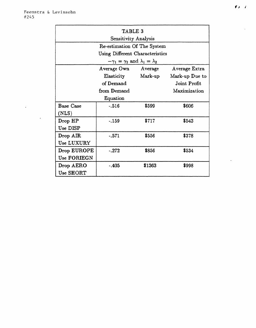
Feenstra & Levinsohn#245

TABLE 3

Sensitivity Analysis

Re-estimation Of The System

Using Different Characteristics

--71= 72 and A1 = AZ

Average Own Average Average Extra

Elasticity Mark-up Mark-up Due to

of Demand Joint Profit

from Demand Maximization

Equation

Base Case -.516 $599 $606

(NLS)

Drop HP -.159 $717 $543

Use DISP

Drop AIR -.571 $556 $378

Use LUXURY

Drop EUROPE -.272 $856 $534

Use FORIEGN

Drop AERO -.405 $1363 $998

Use SHORT