Semi-Supervised Multi-Modal Multi-Instance Multi-Label Deep ...

JOURNAL OF LATEX CLASS FILES, VOL. XX, NO. X, XXX XXX 1

Semi-Supervised Multi-Modal Multi-InstanceMulti-Label Deep Network with Optimal

TransportYang Yang, Zhao-Yang Fu, De-Chuan Zhan, Zhi-Bin Liu, and Yuan Jiang,

Abstract—Complex objects are usually with multiple labels, and can be represented by multiple modal representations, e.g., thecomplex articles contain text and image information as well as multiple annotations. Previous methods assume that the homogeneousmulti-modal data are consistent, while in real applications, the raw data are disordered, e.g., the article constitutes with variable numberof inconsistent text and image instances. Therefore, Multi-modal Multi-instance Multi-label (M3) learning provides a framework forhandling such task and has exhibited excellent performance. However, M3 learning is facing two main challenges: 1) how to effectivelyutilize label correlation; 2) how to take advantage of multi-modal learning to process unlabeled instances. To solve these problems, wefirst propose a novel Multi-modal Multi-instance Multi-label Deep Network (M3DN), which considers M3 learning in an end-to-endmulti-modal deep network and utilizes consistency principle among different modal bag-level predictions. Based on the M3DN, welearn the latent ground label metric with the optimal transport. Moreover, we introduce the extrinsic unlabeled multi-modalmulti-instance data, and propose the M3DNS, which considers the instance-level auto-encoder for single modality and modifiedbag-level optimal transport to strengthen the consistency among modalities. Thereby M3DNS can better predict label and exploit labelcorrelation simultaneously. Experiments on benchmark datasets and real world WKG Game-Hub dataset validate the effectiveness ofthe proposed methods.

Index Terms—Semi-supervised Learning, Multi-Modal Multi-Instance Multi-label Learning, Modal consistency, Optimal Transport.

F

1 INTRODUCTION

W ITH the development of data collection techniques,objects can always be represented by multiple modal

features, e.g., in the forum of famous mobile game “ Strike ofKings”, the articles are with image and content information,and they belong to multiple categories if they are observedfrom different aspects, e.g., an article belongs to “WukongSun” (Game Heroes) as well as “golden cudgel” (GameEquipment) from the images, while it can be categorizedas “game strategy”, “producer name” from contents andso on. The major challenge for addressing such problem ishow to jointly model multiple types of heterogeneities in amutually beneficial way. To solve this problem, multi-modalmulti-label learning approaches utilize multiple modal in-formation, and require modal-based classifiers to generatesimilar predictions, e.g., Huang et al. proposed a multi-label conditional restricted boltzmann machine, which usesmultiple modalities to obtain shared representations underthe supervision [1]; Yang et al. learned a novel graph-basedmodel to learn both label and feature heterogeneities [2].However, a real-world object may contain variable numberof inconsistent multi-modal instances, e.g., the article usu-ally contains multiple images and content paragraphs, inwhich each image or content paragraph can be regarded as

• Yang Yang, Zhao-Yang Fu, De-Chuan Zhan and Yuan Jiang are with Na-tional Key Laboratory for Novel Software Technology, Nanjing University,Nanjing 210023, China.E-mail: yangy, fuzy, zhandc, [email protected]

• Zhi-Bin Liu is with Tencent WXG, ShenZhen 518057, China.E-mail: [email protected]

De-Chuan Zhan is the corresponding author.

an instance, yet the relationships between the images andcontents have not been marked as shown in Figure. 1.

Therefore, several Multi-modal Multi-instance Multi-label methods have been proposed. Nguyen et al. proposedM3LDA with a visual-label part, a textual-label part, anda label topic part, in which the topic decided by visualinformation and the topic decided by textual informationshould be consistent [3]; Nguyen et al. developed a multi-modal MIML framework based on hierarchical bayesiannetwork [4]. Nevertheless, there are two drawbacks of theexisting M3 models. In detail, previous approaches rarelyconsider the correlations among labels, besides, M3 methodsare all supervised methods, which violate the intuition ofmulti-modal learning using unsupervised data.

Thus, considering the label correlation, Yang and Hestudied a hierarchical multi-latent space, which can lever-age the task relatedness, modal consistency and the labelcorrelation simultaneously to improve the learning per-formance [5]; Huang and Zhou proposed the ML-LOCapproach which allows label correlation to be exploitedlocally [6]; Frogner et al. developed a loss function withground metric for multi-label learning, which is based onthe wasserstein distance [7]. Previous works mainly as-sumed that there exists some prior knowledge such as labelsimilarity matrix or the ground metric [7, 8]. In reality, se-mantic information among labels is indirect or complicated,thus the confidence of the label similarity matrix or groundmetric is weak. On the other hand, considering the labelingcost, there are many unlabeled instances. The most impor-tant advantage of multi-modal methods is that they use un-labeled data, e.g., co-training [9] style methods utilized the

arX

iv:2

104.

0848

9v1

[cs

.LG

] 1

7 A

pr 2

021


There is a great correlation between the degree of

difficulty and the level of strength of the heroes in

the King's glory. The heroes with more difficulty in

operation are more powerful in dominant species,

But of course this does not include the operation of

primary school students. Let's talk about the five

most powerful heroes ranked in the game.

This hero has the operation above the skill, especially

for the acceleration of the skills as well as the

prediction of the position of the enemy. All of these

need a strong sense of consciousness in order to truly

complete. Passive skill's maximum health damage

plus 2 skill repelling effects.

This hero is actually terribly difficult to operate, 3

skills will be played out after the absolute

invincibility, marked effects plus continuous use of

big move, basically the enemy is completely

incapable of this hero. The Luna that will play will

even be like a plug-in in the game.

Speaking of this hero, I think a lot of players are

indignant, but this hero really fierce in the game,

especially for the control of passive skills, there is a

reasonable skill of the cast position, in need of the

player's awareness very much .

There is a great correlation between the degree of difficulty and the level of strength

of the heroes in the King's glory. The heroes with more difficulty in operation are

more powerful in dominant species, But of course this does not include the

operation of primary school students. Let's talk about the five most powerful heroes

ranked in the game.

This hero has the operation above the skill, especially for the acceleration of the

skills as well as the prediction of the position of the enemy. All of these need a strong

sense of consciousness in order to truly complete. Passive skill's maximum health

damage plus 2 skill repelling effects.

This hero is actually terribly difficult to operate, 3 skills will be played out after the

absolute invincibility, marked effects plus continuous use of big move, basically the

enemy is completely incapable of this hero. The Luna that will play will even be like

a plug-in in the game.Speaking of this hero, I think a lot of players are indignant, but this hero really

fierce in the game, especially for the control of passive skills, there is a reasonable

skill of the cast position, in need of the player's awareness very much .

• Image bags

• Context bags

Complex Articles

• Multiple Labels

Fig. 1. An illustration of the M3 (Multi-Modal Multi-instance Multi-label)Data in an article of WKG Game-Hub. Each article is with context bagand image bag, each bag contains variable number of instances (contextparagraphs/images), while each article has multiple label representa-tions. It is notable that different modalities are heterogeneous, i.e., therehave no congruent relationships between the articles and images.

complementary principle to label unlabeled data for eachother; co-regularize [10] style methods exploited unlabeledmulti-modal data with consistency principle. Meanwhile, itis notable that previous proposed M3 based methods arehard to adopt the unlabeled instances. Therefore, anotherissue is how to bypass the limitation of M3 style methodsby using unlabeled multi-modal instances.

In this work, aiming at learning the label predictionand exploring label correlation with semi-supervised M3data simultaneously, we proposed a novel general Multi-modal Multi-instance Multi-label Deep Network, whichmodels the independent deep network for each modality,and imposes the modal consistency on bag-level prediction.To better consider the label correlation, M3DN first adoptsOptimal Transport (OT) [11] distance to measure the qualityof prediction. The adoption provides a more meaningfulmeasure in multi-label tasks by capturing the geometricinformation of the underlying label space. The raw datamay not calculate the raw ground metric confidently, thuswe cast the label correlation exploration as a latent groundmetric learning problem. Moreover, considering the unla-beled data information, we propose the semi-supervisedM3DN (M3DNS). M3DNS utilizes the instance-level auto-encoder to build the single modal network, and considersthe bag-level consistency among different unlabeled modalpredictions with the modified OT theory. Consequently,M3DNS could automatically learn the predictors from dif-ferent modalities and the latent shared ground metric.

The main contributions of this paper are summarized inthe following points:

• We propose a novel Multi-modal Multi-instance Multi-label Deep Network (M3DN), which models the deepindependent network for each modality, and imposesthe modal consistency on bag-level prediction;

• We consider label correlation exploration as a latentground metric learning problem between differentmodalities, rather than a fix ground metric using priorraw knowledge;

• We utilize the extrinsic unlabeled data, by consider-ing instance-level auto-encoder, and the bag-level con-

sistency among different unlabeled modal predictionswith the modified OT metric;

• We achieve superior performances on real-world appli-cations, comprehensively evaluate on the performanceand obtain consistently superior performances stably.

Section 2 summarizes related work, our approaches arepresented in Section 3. Section 4 reports our experiments.Finally, Section 5 gives the conclusion.

2 RELATED WORK

THE exploitation of multi-modal multi-instance multi-label learning has attracted much attention recently. In

this paper, our method concentrates on deep multi-labelclassification for semi-supervised inconsistent multi-modalmulti-instance data, and considers the label correlation us-ing optimal transport technique. Therefore, our work isrelated to M3 learning and the optimal transport.

Multi-modal learning deals with data from multiplemodalities, i.e., multiple feature sets. The goals are toimprove performance and reduce the sample complexity.Meanwhile, multi-modal multi-label learning has been wellstudied, e.g., Fang and Zhang proposed a multi-modalmulti-label learning method based on the large marginframework [12]. Yang et al. modeled both the modal con-sistency and the label correlation in a graph-based frame-work [13]. The basic assumption behind these methods isthat multi-modal data is consistent. However, in real ap-plications, the multi-modal data are always heterogeneouson the instance-level, e.g., articles have variable numberof inconsistent images and text paragraphs, videos havevariable length of inconsistent audio and image frames.Articles and videos only have consistency on the bag level,rather than instance level. Thus, multi-modal multi-instancemulti-label learning is proposed recently. Nguyen et al.developed a multi-modal MIML framework based on hi-erarchical bayesian network [4]; Feng and Zhou exploiteddeep neural network to generate instance representationfor MIML and it can be extended to multi-modal scenario.Nevertheless, previous approaches rarely consider the con-fidence of label correlation. More importantly, the currentM3 approaches are supervised, which obviously lose theadvantage of multi-modal learning for processing unlabeleddata.

Considering the label correlation, several multi-labellearning methods are proposed [15, 16, 17]. Recently, Op-timal Transport (OT) [11] is developed to measure thedifference between two distributions based on given groundmetric, and it has been widely used in computer vision andimage processing fields, e.g., Qian et al. proposed a novelmethod that exploits knowledge in both data manifold andfeature correlation [18]; Courty et al. proposed a regularizedunsupervised optimal transportation model to perform thealignment of the representations [19]. However, previousworks mainly assumed that prior knowledge for cost matrixalready exists, and ignored deficiency of information ordomain knowledge. Thus, Cuturi and Avis, Zhao and Zhousuggested to formulate the cost metric learning problemwith the side information [20, 21]. On the other hand,existing M3 methods are almost supervised methods, whilemulti-modal methods aim to utilize the complementary [9]


…

… … …

Bag of imagesRaw articles

Convolutions Pooling Fully connected

Fully connected

Row-wise Max Pooling

Bag of text paragraphs

Fig. 2. The flowchart of the M3DN, the raw articles can be divided intotwo homogeneous modal bag with variable number of heterogeneousinstances, i.e., the image bag with four images and content bag with 5text paragraphs. The instances of different modalities can be calculatedwith different deep networks, and finally represented as x1

lpor x2

lp, the

output features are fully connected with the labels, and we can get thebag-concept layer for different modalities. Eventually, we can acquire thefinal prediction by mean-max pooling the bag-concept layer of differentmodalities.

or consistency [10] principle using the unlabeled instance.Thereby how to take unlabeled data into considerationbecomes a challenge.

3 PROPOSED METHOD

3.1 Notation

IN the multi-instance extension of the multi-modalmulti-label framework, we are given N bags of

instances, let Y = {y1,y2, · · · ,yNl} denotes thelabel set, yi ∈ RL is the label vector of i−th bag,where yi,j = 1 denotes positive class, and yi,j = 0otherwise. On the other hand, suppose we are given Kmodalities, without any loss of generality, we considertwo modalities in our paper, i.e., images and contents. LetD = {([X1

1,X21],y1), ([X1

2,X22],y2), · · · , ([X1

Nl,X2

Nl],yNl),

([X1Nl+1,X

2Nl+1]), · · · , ([X1

Nl+Nu,X2

Nl+Nu])} represents

the training dataset, where Nl/Nu denotes the number oflabelled/unlabelled instances. X1

i = {x1i,1,x

1i,2, · · · ,x1

i,mi}

denotes the bag representation of mi instances ofX1i , similarly, X2

i = {x2i,1,x

2i,2, · · · ,x2

i,ni} is the bag

representation of ni instances of X2i , it is notable that bags

of different modalities may contain variable number ofinstances.

The goal is to generate a learner to annotate new bagsbased on its inputs X1,X2, e.g., annotate a new complexarticle with its images and contents.

3.2 Optimal TransportTraditionally, several measurements such as Kullback-Leibler divergences, Hellinger and total variation, have beenutilized to measure the similarity between two distributions.However, these measurements play little effect when theprobability space has geometrical structures. On the otherhand, Optimal transport [11], also known as Wassersteindistance or earth mover distance [22], defines a reason-able distance between two probability distribution over themetric space. Intuitively, the Wasserstein distance is the

minimum cost of transporting the pile of one distributioninto the pile of another distribution, which formulates theproblem of learning the ground metric as minimizing thedifference between two polyhedral convex functions over aconvex set of distance matrices. Therefore, the Wassersteindistance is more powerful in such situations by consideringthe pairwise cost.

Definition 1. (Transport Polytope) For two probability vec-tors r and c in the simplex

∑L, U(r, c) is the transport

polytope of r and c, namely the polyhedral set of L× Lmatrices,

U(r, c) = {P ∈ RL×L+ |P1L = r, P>1L = c}

Definition 2. (Optimal Transport) Given a L×L cost matrixM , the total cost of mapping from r to c using a transportmatrix (or coupling probability) P can be quantified as〈P,M〉. The optimal transport (OT) problem is definedas,

dM (r, c) = minP∈U(r,c)

〈P,M〉

When M belongs to the cone of metric matrices M,the value of dM (r, c) is a distance [11] between r and c,parameterized by M . In that case, assuming implicitly thatM is fixed and only r and c vary, we will refer to theoptimal transport distance between r and c. It is notable thatdM (r, c) is the cost of the optimal plan for transporting thepredicted mass distribution r to match the target distribu-tion c. The penalty increases when more mass is transportedover longer distances, according to the ground metric M .

Theorem 1. dM defined in Def. 2 is a distance on∑L

whenever M is a metric matrix [11].

3.3 Multi-Modal Multi-instance Multi-label Deep Net-work (M3DN)

Multi-modal Multi-instance Multi-label (M3) learning pro-vides a framework for handling the complex objects, and wepropose a novel M3 based parallel deep network (M3DN).Based on the M3DN, we can bypass the limitation of initiallabel correlation metric using the Optimal Transport (OT)theory, and further take advantage of unlabeled data con-sidering the modal consistency. In this section, we proposethe Multi-Modal Multi-instance Multi-label Deep Network(M3DN) framework. M3DN models deep networks for dif-ferent modalities and imposes the modal consistency.

The raw articles contain variable number of heteroge-neous multi-modal information, i.e., when no correspond-ing relationships exist among each the contents and im-ages, it is difficult to utilize the consistency principle withprevious multi-modal methods. Thus, we turn to utilizethe consistency among the bags of different modalities,rather than the instance-level. Specifically, raw articles canbe divided into two modal bags of heterogeneous instances,i.e., the image bag with 4 images and content bag with 5 textparagraphs as shown in Fig. 2, while only the homogeneousbags share the same multiple labels. Each instance x1(x2) in


… L

Fully Connected

Row-wise Max Pooling

yBag-concept layer

Fig. 3. The schematic of the bag-concept layer. We can acquire thebag-concept layer with the output feature representations of a bag ofinstances, in which each column represents corresponding predictionof each instance. Eventually, the final label prediction is calculated byrow-wise max pooling.

different modal bag can be calculated among several layersand can be finally represented as xlp1(xlp2).

Without any loss of generality, we use the convolu-tional neural network for images and the fully connectednetworks for text. Then, the output features are fullyconnected with the bag-concept layer. All parameters in-cluding deep network facts and fully connected weightscan be organized as Θ1 = {θl1 , θl2 , · · · , θlp1−1 ,W1}(Θ2 ={θl1 , θl2 , · · · , θlp2−1 ,W2}). Concretely, once the label predic-tions of the instances for a bag Xv

i are obtained, we proposea fully connected 2D layer (bag-concept layer) with the sizeof mi(ni) × L as shown in Fig. 3, in which each columnrepresents corresponding prediction of each instance in theimage/content bag. Formally, for a given bag of instancesXvi , the (k, j)-th node in the 2D bag-concept layer represents

the prediction score between the instance xvi,j and the k−thlabel. Therefore, the j-column has the following form ofactivation:

yvj = g(Wvxvi,j + bv) (1)

Here, g(·) can be any convex activation function, and we usesoftmax function here. In the bag-concept layer, we utilizethe row-wise max pooling: fv(i) = max(yi,·). The finalprediction value is:f = f1+f2

2 .

3.4 Explore Label CorrelationHowever, fully connection to the label output rarely con-siders the relationship among labels. Recently, OptimalTransport (OT) theory [11] is used in multi-label learning,which captures geometric information of the underlyinglabel space. According to the Def. 2 and Def. 1, the lossfunction implied in the parallel network structure can beformulated without any loss of generality as:

minPv∈U(f(Xvi ),yi)

2∑v=1

N∑i=1

〈Pv,M〉

s.t. U(f(Xvi ),yi) = {Pv ∈ RL×L

+ |Pv1L = f(Xvi ), P>v 1L = yi}

(2)

where M is the shared latent cost matrix. However, thismethod requires prior knowledge to construct the cost ma-trix M . However, in reality, indirect or incomplete informa-

tion among labels leads to weak cost matrix M and poorclassification performance.

Therefore, we can define the process of learning cost met-ric as an optimization problem. Optimizing the cost metricdirectly is difficult and it consumes O(L2) constraints. Thus,[20, 21] proposed to formulate the cost metric learning prob-lem with the side information, i.e., the label similarity matrixS as [21], and [20] has proved that the cost metric matrix M ,which computes corresponding optimal transport distancedM between pairs of labels, agrees with the side informa-tion. More precisely, this criterion favors matrixM , in whichthe distance dM (r; c) is small for pairs of similar histogramsr and c (corresponding S(r; c) is large) and large for pairsof dissimilar histograms (corresponding S(r; c) is small).Consequently, optimizing M can be turned to optimize theS. Finally, the goal of M3DN can be turned to learn labelpredictor and explore label correlation simultaneously.

In detail, we first introduce the connection betweennonlinear transformation and pseudo-metric:Definition 3. With the nonlinear transformation ∅(·), the Eu-

clidean distance after the transformation can be denotedas:

D∅(r, c) = ‖∅(r)− ∅(c)‖2.

And [23] proved that D∅ satisfies all properties of a well-defined pseudo-metric in the original input space.

Theorem 2. For a pseudo-metric M defined in Def. 3 andhistograms r, c ∈

∑L, the function (r, c)→ 1r 6=cdM (r, c)

satisfies all four distance axioms, i.e., non-negativity,symmetry, definiteness and sub-additivity (triangle in-equality) as in [20].

Thus, M can be turned to learn the kernel S defined bythe non-linear transformation ∅(·):

Sij = S(yi,yj) = ∅(yi)>∅(yj) (3)

where the yi represents the label vector of i−th instance.Besides, it is notable that the cost matrix M is computed asMij = D2

∅(yi,yj), while the kernel S is defined as Eq. 3.Thus, the relation between M and S can be derived as:

Mij = Sii + Sjj − 2Sij . (4)

The non-linear mapping preserves pseudo metric propertiesin Def. 3, therefore it only needs a projection to positivesemi-definite matrix cone when learning the kernel matrixS. Thus, we can avoid the projection to metric space whichis complicated and costly. Therefore, we propose to conductthe label predictions and label correlation exploration si-multaneously based on substituted optimal transport, thecombination of Eq. 4 and Eq. 2 can be reformulated as:

minS,Pv∈U(f(Xvi ),yi)

2∑v=1

N∑i=1

〈Pv,M〉+ λ1r(S, S0)


+ |Pv1L = f(Xvi ), P>v 1L = yi}

S ∈ S+, Mij = Sii + Sjj − 2Sij

(5)

where λ1 is a trade-off parameter, S+ denotes the set ofpositive semi-definite matrix. We adopt OT distance as


…

… …

…

Bag of imagesRaw articles

Convolutions Pooling Fully connected

Fully connected

𝒙𝒍𝒑𝟏

𝒙𝒍𝒑𝟐

Row-wise

Max

Pooling

Bag of text paragraphs

… …

Fully connected

…

…

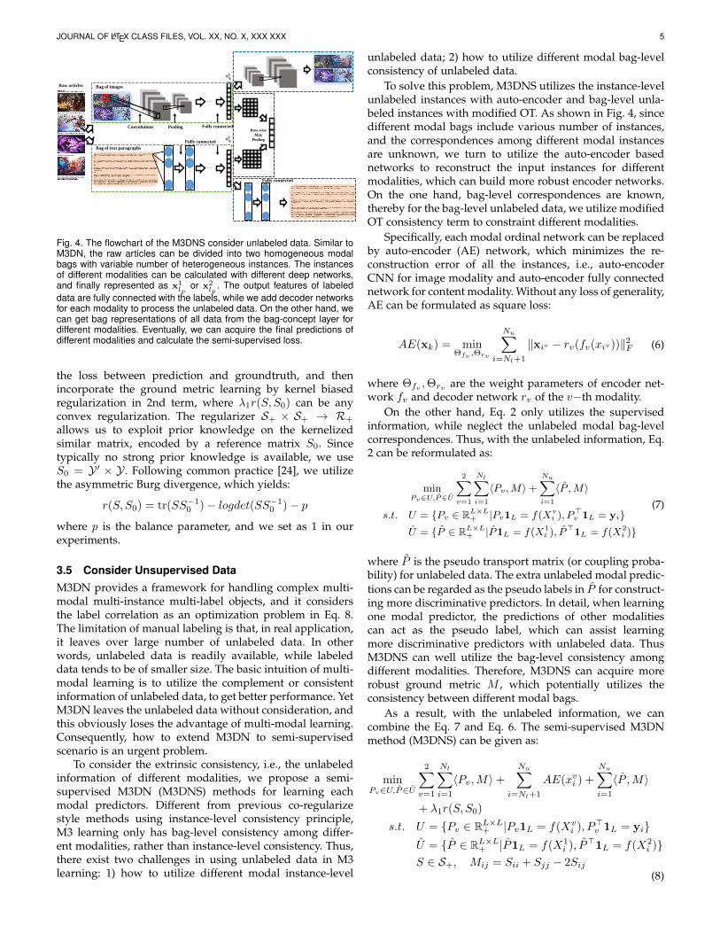
Fig. 4. The flowchart of the M3DNS consider unlabeled data. Similar toM3DN, the raw articles can be divided into two homogeneous modalbags with variable number of heterogeneous instances. The instancesof different modalities can be calculated with different deep networks,and finally represented as x1

lpor x2

lp. The output features of labeled

data are fully connected with the labels, while we add decoder networksfor each modality to process the unlabeled data. On the other hand, wecan get bag representations of all data from the bag-concept layer fordifferent modalities. Eventually, we can acquire the final predictions ofdifferent modalities and calculate the semi-supervised loss.

the loss between prediction and groundtruth, and thenincorporate the ground metric learning by kernel biasedregularization in 2nd term, where λ1r(S, S0) can be anyconvex regularization. The regularizer S+ × S+ → R+

allows us to exploit prior knowledge on the kernelizedsimilar matrix, encoded by a reference matrix S0. Sincetypically no strong prior knowledge is available, we useS0 = Y ′ × Y . Following common practice [24], we utilizethe asymmetric Burg divergence, which yields:

r(S, S0) = tr(SS−10 )− logdet(SS−1

0 )− p

where p is the balance parameter, and we set as 1 in ourexperiments.

3.5 Consider Unsupervised DataM3DN provides a framework for handling complex multi-modal multi-instance multi-label objects, and it considersthe label correlation as an optimization problem in Eq. 8.The limitation of manual labeling is that, in real application,it leaves over large number of unlabeled data. In otherwords, unlabeled data is readily available, while labeleddata tends to be of smaller size. The basic intuition of multi-modal learning is to utilize the complement or consistentinformation of unlabeled data, to get better performance. YetM3DN leaves the unlabeled data without consideration, andthis obviously loses the advantage of multi-modal learning.Consequently, how to extend M3DN to semi-supervisedscenario is an urgent problem.

To consider the extrinsic consistency, i.e., the unlabeledinformation of different modalities, we propose a semi-supervised M3DN (M3DNS) methods for learning eachmodal predictors. Different from previous co-regularizestyle methods using instance-level consistency principle,M3 learning only has bag-level consistency among differ-ent modalities, rather than instance-level consistency. Thus,there exist two challenges in using unlabeled data in M3learning: 1) how to utilize different modal instance-level

unlabeled data; 2) how to utilize different modal bag-levelconsistency of unlabeled data.

To solve this problem, M3DNS utilizes the instance-levelunlabeled instances with auto-encoder and bag-level unla-beled instances with modified OT. As shown in Fig. 4, sincedifferent modal bags include various number of instances,and the correspondences among different modal instancesare unknown, we turn to utilize the auto-encoder basednetworks to reconstruct the input instances for differentmodalities, which can build more robust encoder networks.On the one hand, bag-level correspondences are known,thereby for the bag-level unlabeled data, we utilize modifiedOT consistency term to constraint different modalities.

Specifically, each modal ordinal network can be replacedby auto-encoder (AE) network, which minimizes the re-construction error of all the instances, i.e., auto-encoderCNN for image modality and auto-encoder fully connectednetwork for content modality. Without any loss of generality,AE can be formulated as square loss:

AE(xk) = minΘfv ,Θrv

Nu∑i=Nl+1

‖xiv − rv(fv(xiv ))‖2F (6)

where Θfv ,Θrv are the weight parameters of encoder net-work fv and decoder network rv of the v−th modality.

On the other hand, Eq. 2 only utilizes the supervisedinformation, while neglect the unlabeled modal bag-levelcorrespondences. Thus, with the unlabeled information, Eq.2 can be reformulated as:

minPv∈U,P∈U

2∑v=1

Nl∑i=1

〈Pv,M〉+

Nu∑i=1

〈P ,M〉

s.t. U = {Pv ∈ RL×L+ |Pv1L = f(Xv

i ), P>v 1L = yi}U = {P ∈ RL×L

+ |P1L = f(X1i ), P>1L = f(X2

i )}

(7)

where P is the pseudo transport matrix (or coupling proba-bility) for unlabeled data. The extra unlabeled modal predic-tions can be regarded as the pseudo labels in P for construct-ing more discriminative predictors. In detail, when learningone modal predictor, the predictions of other modalitiescan act as the pseudo label, which can assist learningmore discriminative predictors with unlabeled data. ThusM3DNS can well utilize the bag-level consistency amongdifferent modalities. Therefore, M3DNS can acquire morerobust ground metric M , which potentially utilizes theconsistency between different modal bags.

As a result, with the unlabeled information, we cancombine the Eq. 7 and Eq. 6. The semi-supervised M3DNmethod (M3DNS) can be given as:

minPv∈U,P∈U

2∑v=1

Nl∑i=1

〈Pv,M〉+Nu∑

i=Nl+1

AE(xvi ) +Nu∑i=1

〈P ,M〉

+ λ1r(S, S0)

s.t. U = {Pv ∈ RL×L+ |Pv1L = f(Xvi ), P>v 1L = yi}

U = {P ∈ RL×L+ |P1L = f(X1i ), P>1L = f(X2

i )}S ∈ S+, Mij = Sii + Sjj − 2Sij

(8)


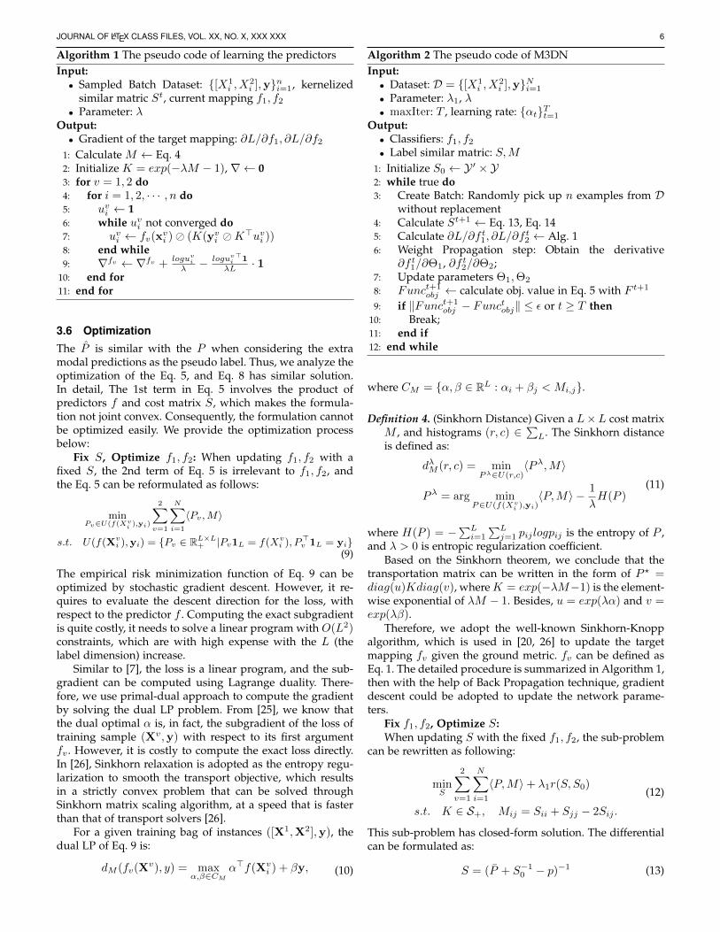
Algorithm 1 The pseudo code of learning the predictorsInput:• Sampled Batch Dataset: {[X1

i , X2i ],y}ni=1, kernelized

similar matric St, current mapping f1, f2

• Parameter: λOutput:• Gradient of the target mapping: ∂L/∂f1, ∂L/∂f2

1: Calculate M ← Eq. 42: Initialize K = exp(−λM − 1), ∇ ← 03: for v = 1, 2 do4: for i = 1, 2, · · · , n do5: uvi ← 16: while uvi not converged do7: uvi ← fv(x

vi )� (K(yvi �K>uvi ))

8: end while9: ∇fv ← ∇fv +

loguviλ − loguvi

>1λL · 1

10: end for11: end for

3.6 Optimization

The P is similar with the P when considering the extramodal predictions as the pseudo label. Thus, we analyze theoptimization of the Eq. 5, and Eq. 8 has similar solution.In detail, The 1st term in Eq. 5 involves the product ofpredictors f and cost matrix S, which makes the formula-tion not joint convex. Consequently, the formulation cannotbe optimized easily. We provide the optimization processbelow:

Fix S, Optimize f1, f2: When updating f1, f2 with afixed S, the 2nd term of Eq. 5 is irrelevant to f1, f2, andthe Eq. 5 can be reformulated as follows:

minPv∈U(f(Xvi ),yi)

2∑v=1

N∑i=1

〈Pv,M〉


+ |Pv1L = f(Xvi ), P>v 1L = yi}

(9)

The empirical risk minimization function of Eq. 9 can beoptimized by stochastic gradient descent. However, it re-quires to evaluate the descent direction for the loss, withrespect to the predictor f . Computing the exact subgradientis quite costly, it needs to solve a linear program with O(L2)constraints, which are with high expense with the L (thelabel dimension) increase.

Similar to [7], the loss is a linear program, and the sub-gradient can be computed using Lagrange duality. There-fore, we use primal-dual approach to compute the gradientby solving the dual LP problem. From [25], we know thatthe dual optimal α is, in fact, the subgradient of the loss oftraining sample (Xv,y) with respect to its first argumentfv . However, it is costly to compute the exact loss directly.In [26], Sinkhorn relaxation is adopted as the entropy regu-larization to smooth the transport objective, which resultsin a strictly convex problem that can be solved throughSinkhorn matrix scaling algorithm, at a speed that is fasterthan that of transport solvers [26].

For a given training bag of instances ([X1,X2],y), thedual LP of Eq. 9 is:

dM (fv(Xv), y) = max

α,β∈CMα>f(Xv

i ) + βy, (10)

Algorithm 2 The pseudo code of M3DNInput:• Dataset: D = {[X1

i , X2i ],y}Ni=1

• Parameter: λ1, λ• maxIter: T , learning rate: {αt}Tt=1

Output:• Classifiers: f1, f2

• Label similar matric: S,M1: Initialize S0 ← Y ′ × Y2: while true do3: Create Batch: Randomly pick up n examples from D

without replacement4: Calculate St+1 ← Eq. 13, Eq. 145: Calculate ∂L/∂f t1, ∂L/∂f

t2 ← Alg. 1

6: Weight Propagation step: Obtain the derivative∂f t1/∂Θ1, ∂f t2/∂Θ2;

7: Update parameters Θ1,Θ2

8: Funct+1obj ← calculate obj. value in Eq. 5 with F t+1

9: if ‖Funct+1obj − Functobj‖ ≤ ε or t ≥ T then

10: Break;11: end if12: end while

where CM = {α, β ∈ RL : αi + βj < Mi,j}.

Definition 4. (Sinkhorn Distance) Given a L×L cost matrixM , and histograms (r, c) ∈

∑L. The Sinkhorn distance

is defined as:

dλM (r, c) = minPλ∈U(r,c)

〈Pλ,M〉

Pλ = arg minP∈U(f(Xvi ),yi)

〈P,M〉 − 1

λH(P )

(11)

where H(P ) = −∑Li=1

∑Lj=1 pij logpij is the entropy of P ,

and λ > 0 is entropic regularization coefficient.Based on the Sinkhorn theorem, we conclude that the

transportation matrix can be written in the form of P ? =diag(u)Kdiag(v), whereK = exp(−λM−1) is the element-wise exponential of λM − 1. Besides, u = exp(λα) and v =exp(λβ).

Therefore, we adopt the well-known Sinkhorn-Knoppalgorithm, which is used in [20, 26] to update the targetmapping fv given the ground metric. fv can be defined asEq. 1. The detailed procedure is summarized in Algorithm 1,then with the help of Back Propagation technique, gradientdescent could be adopted to update the network parame-ters.

Fix f1, f2, Optimize S:When updating S with the fixed f1, f2, the sub-problem

can be rewritten as following:

minS

2∑v=1

N∑i=1

〈P,M〉+ λ1r(S, S0)

s.t. K ∈ S+, Mij = Sii + Sjj − 2Sij .

(12)

This sub-problem has closed-form solution. The differentialcan be formulated as:

S = (P + S−10 − p)−1 (13)


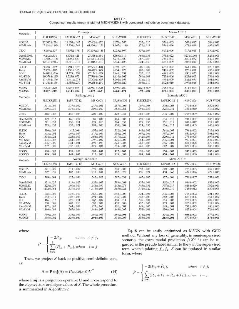
TABLE 1Comparison results (mean ± std.) of M3DN/M3DNS with compared methods on benchmark datasets.

Methods Coverage ↓ Macro AUC ↑

FLICKR25K IAPR TC-12 MS-CoCo NUS-WIDE FLICKR25K IAPRTC-12 MS-CoCo NUS-WIDE

M3LDA 12.345±.214 11.620±.042 47.400±.622 6.670±.205 .532±.015 .526±.003 .507±.015 .509±.012MIMLmix 17.114±1.024 15.720±.543 64.130±1.121 14.167±1.140 .472±.018 .554±.096 .471±.019 .493±.020

CS3G 8.168±.137 7.153±.178 50.138±2.146 8.028±.907 .837±.007 .817±.006 .717±.011 .530±.022

DeepMIML 9.242±.331 8.931±.421 27.358±.654 8.369±.119 .766±.035 .795±.022 .827±0.006 .823±.005M3MIML 11.760±1.121 9.125±.553 42.420±.2.696 5.210±.920 .687±.087 .724±.033 .650±.032 .649±.084MIMLfast 12.155±.913 12.711±.315 41.048±.831 8.634±.028 .524±.050 .485±.009 .506±.010 .522±.008

SLEEC 9.568±.222 9.494±.105 47.502±.448 7.390±.275 .706±.007 .675±.007 .661±.014 .620±.006Tram 7.959±.187 8.156±.163 28.417±.945 9.934±.026 .780±.009 .746±.007 .776±.011 .493±.007ECC 14.818±.086 14.229±.258 47.124±.675 7.941±.194 .532±.013 .484±.009 .630±.023 .634±.009ML-KNN 10.379±.115 9.523±.072 27.568±.066 4.610±.062 .591±.008 .723±.006 .823±.003 .736±.008RankSVM 11.439±.196 11.941±.078 37.300±.835 8.292±.054 .512±.019 .499±.009 .521±.033 .501±.001ML-SVM 11.311±.158 11.755±.270 39.258±.294 7.890±.020 .503±.010 .502±.010 .497±.016 .561±.001

M3DN 7.502±.129 6.936±.065 26.921±.320 4.599±.050 .822 ±.009 .798±.002 .811±.004 .826±.006M3DNS 3.947±.307 4.214±.202 6.119±.262 2.764±.071 .892±.004 .876±.003 .838±.003 .898±.008

Methods Ranking Loss ↓ Example AUC ↑


M3LDA .301±.009 .377±.002 .247±.001 .257±.006 .707±.008 .630±.005 .770±.006 .652±.009MIMLmix .609±.036 .675±.012 .609±.040 .583±.081 .391±.036 .325±.012 .391±.040 .417±.082

CS3G .118±.005 .155±.005 .202±.009 .170±.032 .881±.005 .835±.005 .798±.009 .642±.032

DeepMIML .149±.012 .166±.017 .089±.002 .164±.007 .791±.044 .834±.017 .911±.002 .835±.007M3MIML .271±.053 .250±.011 .191±.016 .284±.030 .729±.053 .751±.011 .811±.017 .717±.031MIMLfast .275±.033 .435±.021 .194±.006 .430±.009 .724±.033 .626±.013 .811±.005 .646±.009

SLEEC .316±.009 .413.006 .455±.005 .512±.008 .843±.003 .761±.005 .796±.002 .713±.008Tram .132±.004 .203±.007 .117±.004 .456±.004 .867±.004 .797±.007 .883±.005 .591±.001ECC .804±.024 .928±.013 .461±.009 .617±.020 .642±.005 .529±.012 .775±.005 .697±.013ML-KNN .235±.005 .264±.004 .097±.002 .176±.003 .764±.005 .736±.004 .903±.001 .824±.003RankSVM .236±.006 .344±.001 .199±.098 .323±.008 .763±.006 .656±.001 .801±.098 .677±.001ML-SVM .232±.005 .337±.009 .179±.004 .314±.002 .768±.005 .662±.009 .822±.004 .686±.002

M3DN .108±.003 .151±.002 .085±.002 .117±.002 .891±.003 .850±.003 .915±.003 .883±.001M3DNS .108±.001 .142±.002 .112±.003 .119±.003 .899±.004 .858±.005 .898±.008 .881±.006

Methods Average Precision ↑ Micro AUC ↑


M3LDA .371±.005 .311±.007 .399±.007 .338±.005 .693±.006 .609±.002 .773±.005 .657±.008MIMLmix .207±.038 .183±.008 .213±.041 .167±.020 .436±.024 .438±.060 .434±.026 .472±.015

CS3G .749±.008 .622±.006 .542±.012 .597±.031 .867±.005 .827±.006 .738±.007 .557±.021

DeepMIML .621±.027 .619±.025 .633±.005 .583±.008 .835±.009 .802±.017 .914±.002 .852±.003M3MIML .423±.056 .490±.020 .446±.030 .443±.076 .745±.034 .707±.017 .816±.020 .762±.020MIMLfast .432±.064 .339±.013 .413±.005 .365±.021 .712±.022 .540±.010 .745±.012 .630±.005

SLEEC .608±.006 .473±.010 .565±.003 .392±.007 .824±.004 .736±.005 .795±.002 .701±.005Tram .653±.011 .523±.008 .494±.007 .336±.002 .842±.003 .782±.007 .883±.006 .554±.002ECC .416±.012 .278±.011 .462±.007 .438±.014 .646±.004 .514±.008 .779±.005 .702±.009ML-KNN .398±.006 .403±.010 .585±.002 .439±.006 .752±.005 .729±.003 .905±.002 .817±.004RankSVM .467±.005 .364±.004 .427±.066 .401±.001 .748±.005 .649±.004 .791±.093 .680±.003ML-SVM .466±.006 .367±.006 .441±.007 .443±.007 .753±.004 .656±.009 .825±.004 .724±.001

M3DN .719±.006 .634±.003 .680±.005 .691±.001 .876±.003 .834±.001 .918±.002 .877±.003M3DNS .698±.002 .637±.007 .691±.004 .634±.003 .858±.003 .863±.004 .877±.006 .878±.005

where

P =

− 2Pij , when i 6= j,L∑k 6=i

(Pik + Pki), when i = j

Then, we project S back to positive semi-definite coneas:

S = Proj(S) = Umax(σ, 0)U> (14)

where Proj is a projection operator, U and σ correspond tothe eigenvectors and eigenvalues of S. The whole procedureis summarized in Algorithm 2.

Eq. 8 can be easily optimized as M3DN with GCDmethod. Without any loss of generality, in semi-supervisedscenario, the extra modal prediction f(X3−i) can be re-garded as the pseudo label similar to the y in the supervisedterm when updating f1, f2. S can be updated in similarform, where

P =

− 2(Pij + Pij), when i 6= j,L∑

k 6=i

(Pik + Pki + Pik + Pki), when i = j


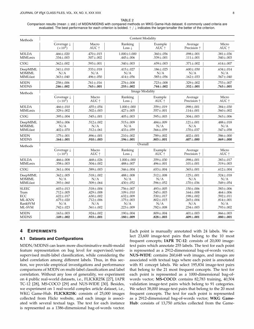
TABLE 2Comparison results (mean ± std.) of M3DN/M3DNS with compared methods on WKG Game-Hub dataset. 6 commonly used criteria are

evaluated. The best performance for each criterion is bolded. ↑ / ↓ indicates the larger/smaller the better of the criterion.

Methods Content Modality

Coverage ↓(×102)

MacroAUC ↑

RankingLoss ↓

ExampleAUC ↑

AveragePrecision ↑

MicroAUC ↑

M3LDA .466±.020 .470±.015 1.000±1.000 .360±.056 .098±.001 .381±.036MIMLmix .334±.003 .507±.002 .445±.006 .539±.001 .111±.001 .540±.003

CS3G .362±.002 .593±.001 .340±.003 .659±.003 .371±.002 .614±.007

DeepMIML .341±.010 .533±.018 .415±.027 .186±.025 .600±.030 .634±.014M3MIML N/A N/A N/A N/A N/A N/AMIMLfast .363±.040 .496±.050 .414±.056 .585±.056 .162±.033 .567±.040

M3DN .258±.006 .761±.016 .276±.008 .723±.008 .329±.002 .753±.007M3DNS .246±.002 .763±.001 .255±.002 .744±.002 .332±.001 .763±.001

Methods Image Modality

Coverage ↓(×102)

MacroAUC ↑

RankingLoss ↓

ExampleAUC ↑


MicroAUC ↑

M3LDA .466±.010 .455±.054 1.000±.000 .359±.019 .098±.001 .384±.030MIMLmix .329±.002 .502±.003 .427±.005 .557±.001 .114±.001 .560±.002

CS3G .395±.004 .545±.001 .405±.003 .595±.003 .304±.003 .563±.006


M3DN .175±.001 .896±.001 .210±.002 .789±.002 .402±.001 .586±.000M3DNS .164±.001 .910±.003 .196±.001 .803±.001 .407±.000 .869±.000

Methods Overall

Coverage ↓(×102)

MacroAUC ↑

RankingLoss ↓

ExampleAUC ↑


MicroAUC ↑

M3LDA .466±.008 .468±.026 1.000±.000 .359±.030 .098±.001 .383±.017MIMLmix .358±.003 .504±.002 .488±.007 .496±.001 .101±.001 .519±.003

CS3G .361±.004 .589±.003 .346±.004 .653±.004 .365±.001 .612±.004


SLEEC .603±.013 .518±.004 .756±.007 .493±.005 .150±.006 .583±.006Tram .712±.005 .429±.008 .109±.010 .545±.003 .164±.008 .464±.006ECC .622±.017 .630±.002 .632±.009 .530±.017 .198±.002 .592±.011ML-KNN .675±.020 .712±.006 .175±.003 .802±.015 .265±.004 .814±.001RankSVM N/A N/A N/A N/A N/A N/AML-SVM .742±.023 .561±.002 .223±.009 .782±.008 .234±.003 .793±.002

M3DN .163±.003 .924±.002 .190±.004 .809±.004 .401±.003 .866±.003M3DNS .149±.002 .933±.001 .180±.009 .828±.003 .409±.001 .880±.001

4 EXPERIMENTS

4.1 Datasets and Configurations

M3DN/M3DNS can learn more discriminative multi-modalfeature representation on bag level for supervised/semi-supervised multi-label classification, while considering thelabel correlation among different labels. Thus, in this sec-tion, we provide empirical investigations and performancecomparisons of M3DN on multi-label classification and labelcorrelation. Without any loss of generality, we experimenton 4 public real-world datasets, i.e., FLICKR25K [27], IAPRTC-12 [28], MS-COCO [29] and NUS-WIDE [30]. Besides,we experiment on 1 real-world complex article dataset, i.e.,WKG Game-Hub. FLICKR25K: consists of 25,000 imagescollected from Flickr website, and each image is associ-ated with several textual tags. The text for each instanceis represented as a 1386-dimensional bag-of-words vector.

Each point is manually annotated with 24 labels. We se-lect 23,600 image-text pairs that belong to the 10 mostfrequent concepts; IAPR TC-12: consists of 20,000 image-text pairs which annotate 255 labels. The text for each pointis represented as a 2912-dimensional bag-of-words vector;NUS-WIDE: contains 260,648 web images, and images areassociated with textual tags where each point is annotatedwith 81 concept labels. We select 195,834 image-text pairsthat belong to the 21 most frequent concepts. The text foreach point is represented as a 1000-dimensional bag-of-words vector; MS-COCO: contains 82,783 training, 40,504validation image-text pairs which belong to 91 categories.We select 38,000 image-text pairs that belong to the 20 mostfrequent concepts. The text for each point is representedas a 2912-dimensional bag-of-words vector; WKG Game-Hub: consists of 13,750 articles collected from the Game-


Fig. 5. Illustration of learned label correlations for different datasets,and the value has been scaled in [-1,1]. Red color indicates a positivecorrelation, and blue one indicates a negative correlation.

Hub of “ Strike of Kings” with 1744 concept labels. We select11,000 image-text pairs that belong to the 54 most frequentconcepts. Each article contains several images and contentparagraphs, and the text for each point is represented as a300-dimensional w2v vector.

We run each compared method 30 times for all datasets,and then randomly select 70% for training and the remain-ing are for test. For all the training examples, we randomlychoose 30% as the labeled data, and the other 70% asunlabeled ones as [31]. For the 4 benchmark datasets, eachimage is divided into 10 regions using [32] as image bag,while the corresponding text tags are also separated intoseveral independent tags as text bag. For the WKG Game-Hub dataset, each article is denoted as an image bag anda content bag. The deep network for image encoder is im-plemented the same as Resnet-18 [33]. We run the followingexperiments with the implementation of an environment onNVIDIA K80 GPUs server, and our model can be trainedaround 290 images per second with a single K80 GPGPU.In the training phase, the parameters λ1 is selected by 5-fold cross validation from {10−5, 10−4, · · · , 104, 105} withfurther splitting on only the training datasets, i.e., thereis no overlap between the test set and the validation setfor parameter picking up. Empirically, when the variationbetween the objective values of Eq. 13 is less than 10−6 initeration, we treat M3DN or M3DNS converged.

4.2 Compared methodsIn our experiments, first, we compare our methodswith multi-modal multi-instance multi-label methods, i.e.,M3LDA [3], MIMLmix [4]. Besides, M3DN can be degen-erated into different settings, we also compare with multi-modal multi-label methods, i.e., CS3G [34]; multi-instancemulti-label methods, i.e., DeepMIML [14], M3MIML [35],MIMLfast [36]. Moreover, we compare our methods withmulti-label methods, i.e., SLEEC [37], Tram [38], ECC [39],ML-KNN [40], RankSVM [41], ML-SVM [42]. Specifically, formulti-modal multi-label methods, we calculate the averageof all instances’ representations as the bag-level feature rep-resentation. In the multi-instance multi-label methods, allmodalities of a dataset are concatenated together as a single

modal input. As to the multi-label learners, we first calcu-late bag-level feature representation for different modalitiesindependently, then we concatenate all modalities togetheras a single modal input. As to the semi-supervised sce-nario, considering that existing M3 methods are supervisedmethods, we compare our methods with semi-supervisedmulti-modal multi-label methods, i.e., CS3G [34]; and semi-supervised multi-label methods, i.e., Tram [38], COINS [17],iMLU [43].

4.3 Benchmark ComparisonsM3DN is compared with other methods on 4 benchmarkdatasets to demonstrate the abilities. Results of comparedmethods and M3DN/M3DNS on 6 commonly used criteriaare listed in Tab. 1. The best performance for each cri-terion is bolded. ↑ / ↓ indicates that the larger/smaller,the better of the criterion. From the results, it is obviousthat our M3DN/M3DNS approaches can achieve the best orsecond performance on most datasets with different perfor-mance measures. Therefore the M3DN/M3DNS approachare highly competitive multi-modal multi-label learningmethods.

4.4 Complex Article ClassificationIn this subsection, M3DN approach is tested on the real-world complex article classification problem, i.e., WKGGame-Hub dataset. There are 13,570 articles in collection,with image and text modalities to promote classification.Specifically, each article contains variable number of imagesand text paragraphs. Thus, each article can be divided intoboth image bag and text bag. Comparison results (inde-pendent modalities and overall) against compared meth-ods are listed in Tab. 2, where notation “N/A” meansthe method cannot give a result in 60 hours. We use thesame 6 measurement criteria as in previous subsection, i.e.,Coverage, Ranking Loss, Average Precision, Macro AUC,example AUC and Micro AUC. It is notable that multi-label methods concatenate all of the modal features, whichhave no independent modal classification performance. Theresults show that on both of the independent modalities andoverall prediction, our M3DN and M3DNS approaches canget the best results over all criteria. The statistics validatesthe effectiveness of our method when solving the complexarticle classification problem.

4.5 Label Correlations ExplorationSince M3DN can learn label correlation explicitly, in thissubsection, we examine effectiveness of M3DN in label cor-relations exploration. Due to page limitation, the explorationis conducted on the real-world dataset WKG Game-Hug. Werandomly sampled 27 labels, with the learned ground metricshown in Figure 5, and scaled the original value in costmatrix into [−1, 1]. Red color indicates a positive correlation,and blue indicates a negative correlation. We can see thatthe learned pairwise cost accords with intuitions. Taking afew examples, the cost between Overwatcha and Tencentindicates a very small correlation, and this is reasonable asthe game Overwatch has no correlation with Tencent. Whilethe cost between (Zhuge Liang, Wizard) indicates a verystrong correlation, since Zhuge Liang belongs to the wizardrole in the game.


0.1

0.2

0.3

0.4

0.5

0.6

Ave

rage

Pre

cisi

on0.1

0.2

0.3

0.4

0.5

0.6

Ran

king

Los

s

Average PrecisionRanking Loss

Average Precision-semiRanking Loss-semi

2 4 6 8 10 12 14 16 18 20

Epoch

0.87

0.89

0.91

0.93

Obj

Fun

ctio

n V

alue

Obj Obj-semi

(a) M3DN

10

20

30

40

50

60

Cov

erag

e

0.4

0.6

0.8

1

1.2

1.4

AU

C

CoverageMacro AUCMicro AUCExample AUC

Coverage-semiMacro AUC-semiMicro AUC-semiExample AUC-semi

2 4 6 8 10 12 14 16 18 20

Epoch

0.87

0.89

0.91

0.93

Obj

Fun

ctio

n V

alue

Obj Obj-semi

(b) M3DNS

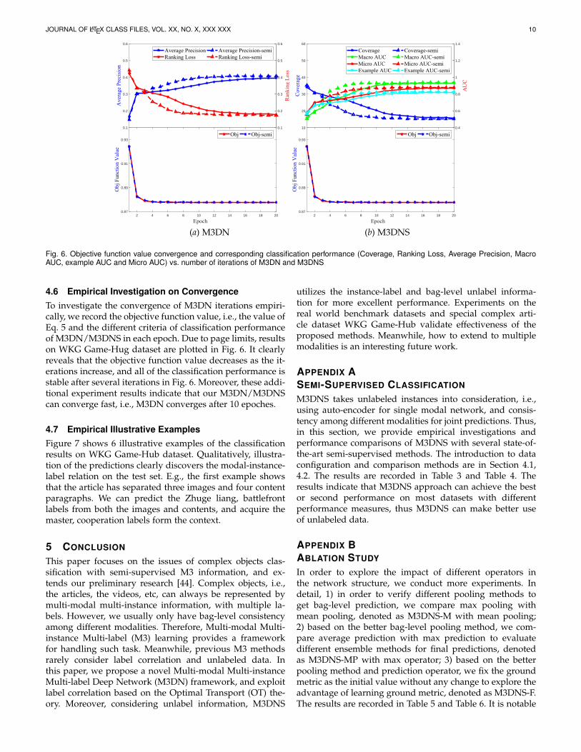
Fig. 6. Objective function value convergence and corresponding classification performance (Coverage, Ranking Loss, Average Precision, MacroAUC, example AUC and Micro AUC) vs. number of iterations of M3DN and M3DNS

4.6 Empirical Investigation on ConvergenceTo investigate the convergence of M3DN iterations empiri-cally, we record the objective function value, i.e., the value ofEq. 5 and the different criteria of classification performanceof M3DN/M3DNS in each epoch. Due to page limits, resultson WKG Game-Hug dataset are plotted in Fig. 6. It clearlyreveals that the objective function value decreases as the it-erations increase, and all of the classification performance isstable after several iterations in Fig. 6. Moreover, these addi-tional experiment results indicate that our M3DN/M3DNScan converge fast, i.e., M3DN converges after 10 epoches.

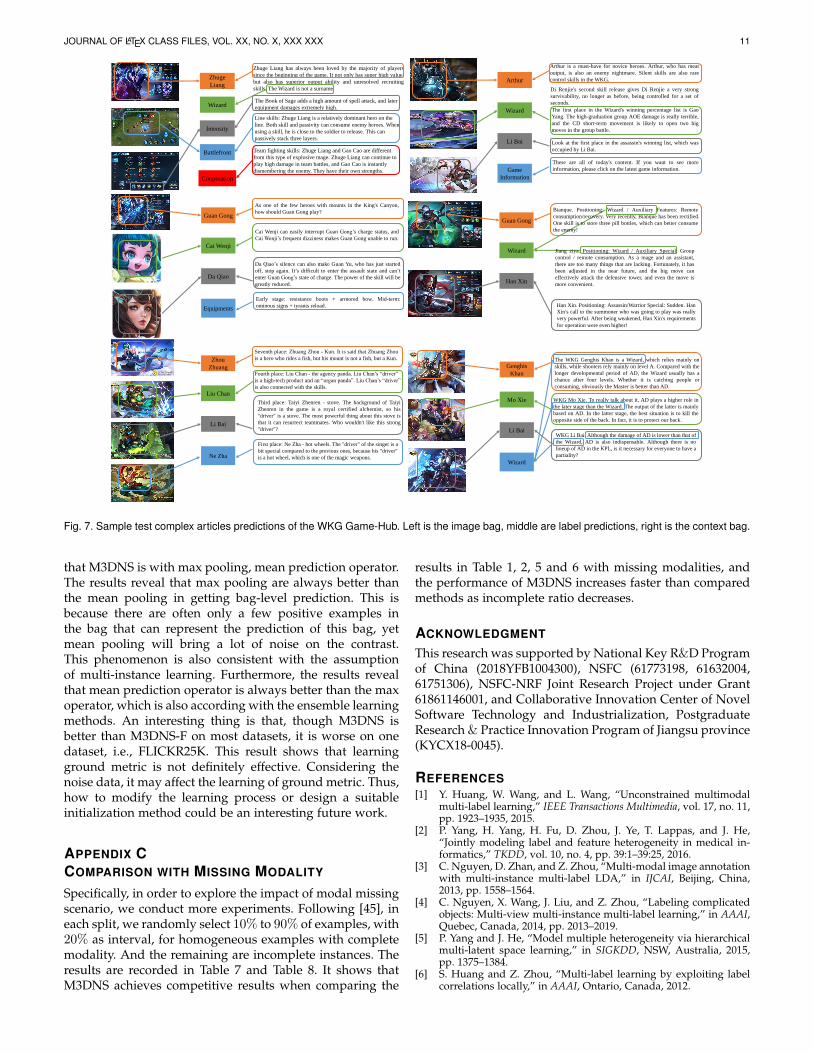
4.7 Empirical Illustrative ExamplesFigure 7 shows 6 illustrative examples of the classificationresults on WKG Game-Hub dataset. Qualitatively, illustra-tion of the predictions clearly discovers the modal-instance-label relation on the test set. E.g., the first example showsthat the article has separated three images and four contentparagraphs. We can predict the Zhuge liang, battlefrontlabels from both the images and contents, and acquire themaster, cooperation labels form the context.

5 CONCLUSION

This paper focuses on the issues of complex objects clas-sification with semi-supervised M3 information, and ex-tends our preliminary research [44]. Complex objects, i.e.,the articles, the videos, etc, can always be represented bymulti-modal multi-instance information, with multiple la-bels. However, we usually only have bag-level consistencyamong different modalities. Therefore, Multi-modal Multi-instance Multi-label (M3) learning provides a frameworkfor handling such task. Meanwhile, previous M3 methodsrarely consider label correlation and unlabeled data. Inthis paper, we propose a novel Multi-modal Multi-instanceMulti-label Deep Network (M3DN) framework, and exploitlabel correlation based on the Optimal Transport (OT) the-ory. Moreover, considering unlabel information, M3DNS

utilizes the instance-label and bag-level unlabel informa-tion for more excellent performance. Experiments on thereal world benchmark datasets and special complex arti-cle dataset WKG Game-Hub validate effectiveness of theproposed methods. Meanwhile, how to extend to multiplemodalities is an interesting future work.

APPENDIX ASEMI-SUPERVISED CLASSIFICATION

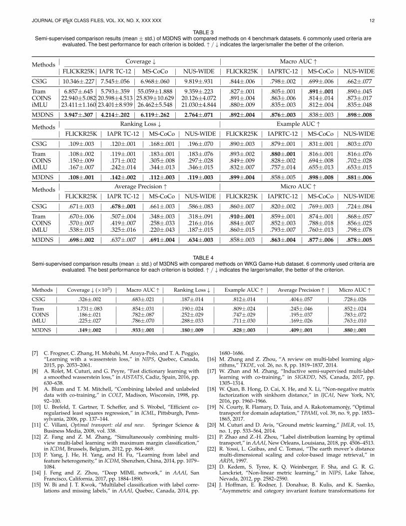
M3DNS takes unlabeled instances into consideration, i.e.,using auto-encoder for single modal network, and consis-tency among different modalities for joint predictions. Thus,in this section, we provide empirical investigations andperformance comparisons of M3DNS with several state-of-the-art semi-supervised methods. The introduction to dataconfiguration and comparison methods are in Section 4.1,4.2. The results are recorded in Table 3 and Table 4. Theresults indicate that M3DNS approach can achieve the bestor second performance on most datasets with differentperformance measures, thus M3DNS can make better useof unlabeled data.

APPENDIX BABLATION STUDY

In order to explore the impact of different operators inthe network structure, we conduct more experiments. Indetail, 1) in order to verify different pooling methods toget bag-level prediction, we compare max pooling withmean pooling, denoted as M3DNS-M with mean pooling;2) based on the better bag-level pooling method, we com-pare average prediction with max prediction to evaluatedifferent ensemble methods for final predictions, denotedas M3DNS-MP with max operator; 3) based on the betterpooling method and prediction operator, we fix the groundmetric as the initial value without any change to explore theadvantage of learning ground metric, denoted as M3DNS-F.The results are recorded in Table 5 and Table 6. It is notable


Zhuge

Liang

Zhuge Liang has always been loved by the majority of players

since the beginning of the game. It not only has super high value,

but also has superior output ability and unresolved recruiting

skills. The Wizard is not a surname.

WizardThe Book of Sage adds a high amount of spell attack, and later

equipment damages extremely high.

Intensity

Line skills: Zhuge Liang is a relatively dominant hero on the

line. Both skill and passivity can consume enemy heroes. When

using a skill, he is close to the soldier to release. This can

passively stack three layers.

Battlefront

Cooperation

Team fighting skills: Zhuge Liang and Gao Cao are different

from this type of explosive mage. Zhuge Liang can continue to

play high damage in team battles, and Gao Cao is instantly

dismembering the enemy. They have their own strengths.

Arthur

Arthur is a must-have for novice heroes. Arthur, who has meat

output, is also an enemy nightmare. Silent skills are also rare

control skills in the WKG.

Wizard

Li Bai

Game

Information

The first place in the Wizard's winning percentage list is Gao

Yang. The high-graduation group AOE damage is really terrible,

and the CD short-term movement is likely to open two big

moves in the group battle.

Di Renjie's second skill release gives Di Renjie a very strong

survivability, no longer as before, being controlled for a set of

seconds.

Look at the first place in the assassin's winning list, which was

occupied by Li Bai.

These are all of today's content. If you want to see more

information, please click on the latest game information.

Guan Gong

Cai Wenji

Da Qiao

Equipments

As one of the few heroes with mounts in the King's Canyon,

how should Guan Gong play?

Cai Wenji can easily interrupt Guan Gong’s charge status, and

Cai Wenji’s frequent dizziness makes Guan Gong unable to run.

Da Qiao’s silence can also make Guan Yu, who has just started

off, stop again. It’s difficult to enter the assault state and can’t

enter Guan Gong’s state of charge. The power of the skill will be

greatly reduced.

Early stage: resistance boots + armored bow. Mid-term:

ominous signs + tyrants reload.

Guan Gong

Wizard

Han Xin

Bianque. Positioning: Wizard / Auxiliary Features: Remote

consumption/recovery. Very recently, Bianque has been rectified.

One skill is to store three pill bottles, which can better consume

the enemy!

Jiang ziya. Positioning: Wizard / Auxiliary Special: Group

control / remote consumption. As a mage and an assistant,

there are too many things that are lacking. Fortunately, it has

been adjusted in the near future, and the big move can

effectively attack the defensive tower, and even the move is

more convenient.

Han Xin. Positioning: Assassin/Warrior Special: Sudden. Han

Xin’s call to the summoner who was going to play was really

very powerful. After being weakened, Han Xin’s requirements

for operation were even higher!

Zhou

Zhuang

Liu Chan

Li Bai

Ne Zha

Seventh place: Zhuang Zhou - Kun. It is said that Zhuang Zhou

is a hero who rides a fish, but his mount is not a fish, but a Kun.

Fourth place: Liu Chan - the agency panda. Liu Chan’s “driver”

is a high-tech product and an “organ panda”. Liu Chan’s “driver”

is also connected with the skills.

Third place: Taiyi Zhenren - stove. The background of Taiyi

Zhenren in the game is a royal certified alchemist, so his

"driver" is a stove. The most powerful thing about this stove is

that it can resurrect teammates. Who wouldn't like this strong

"driver"?

First place: Ne Zha - hot wheels. The "driver" of the singer is a

bit special compared to the previous ones, because his "driver"

is a hot wheel, which is one of the magic weapons.

Genghis

Khan

Mo Xie

Li Bai

Wizard

The WKG Genghis Khan is a Wizard, which relies mainly on

skills, while shooters rely mainly on level A. Compared with the

longer developmental period of AD, the Wizard usually has a

chance after four levels. Whether it is catching people or

consuming, obviously the Master is better than AD.

WKG Mo Xie. To really talk about it, AD plays a higher role in

the later stage than the Wizard. The output of the latter is mainly

based on AD. In the latter stage, the best situation is to kill the

opposite side of the back. In fact, it is to protect our back.

WKG Li Bai. Although the damage of AD is lower than that of

the Wizard, AD is also indispensable. Although there is no

lineup of AD in the KPL, is it necessary for everyone to have a

partiality?

Fig. 7. Sample test complex articles predictions of the WKG Game-Hub. Left is the image bag, middle are label predictions, right is the context bag.

that M3DNS is with max pooling, mean prediction operator.The results reveal that max pooling are always better thanthe mean pooling in getting bag-level prediction. This isbecause there are often only a few positive examples inthe bag that can represent the prediction of this bag, yetmean pooling will bring a lot of noise on the contrast.This phenomenon is also consistent with the assumptionof multi-instance learning. Furthermore, the results revealthat mean prediction operator is always better than the maxoperator, which is also according with the ensemble learningmethods. An interesting thing is that, though M3DNS isbetter than M3DNS-F on most datasets, it is worse on onedataset, i.e., FLICKR25K. This result shows that learningground metric is not definitely effective. Considering thenoise data, it may affect the learning of ground metric. Thus,how to modify the learning process or design a suitableinitialization method could be an interesting future work.

APPENDIX CCOMPARISON WITH MISSING MODALITY

Specifically, in order to explore the impact of modal missingscenario, we conduct more experiments. Following [45], ineach split, we randomly select 10% to 90% of examples, with20% as interval, for homogeneous examples with completemodality. And the remaining are incomplete instances. Theresults are recorded in Table 7 and Table 8. It shows thatM3DNS achieves competitive results when comparing the

results in Table 1, 2, 5 and 6 with missing modalities, andthe performance of M3DNS increases faster than comparedmethods as incomplete ratio decreases.

ACKNOWLEDGMENT

This research was supported by National Key R&D Programof China (2018YFB1004300), NSFC (61773198, 61632004,61751306), NSFC-NRF Joint Research Project under Grant61861146001, and Collaborative Innovation Center of NovelSoftware Technology and Industrialization, PostgraduateResearch & Practice Innovation Program of Jiangsu province(KYCX18-0045).

REFERENCES[1] Y. Huang, W. Wang, and L. Wang, “Unconstrained multimodal

multi-label learning,” IEEE Transactions Multimedia, vol. 17, no. 11,pp. 1923–1935, 2015.

[2] P. Yang, H. Yang, H. Fu, D. Zhou, J. Ye, T. Lappas, and J. He,“Jointly modeling label and feature heterogeneity in medical in-formatics,” TKDD, vol. 10, no. 4, pp. 39:1–39:25, 2016.

[3] C. Nguyen, D. Zhan, and Z. Zhou, “Multi-modal image annotationwith multi-instance multi-label LDA,” in IJCAI, Beijing, China,2013, pp. 1558–1564.

[4] C. Nguyen, X. Wang, J. Liu, and Z. Zhou, “Labeling complicatedobjects: Multi-view multi-instance multi-label learning,” in AAAI,Quebec, Canada, 2014, pp. 2013–2019.

[5] P. Yang and J. He, “Model multiple heterogeneity via hierarchicalmulti-latent space learning,” in SIGKDD, NSW, Australia, 2015,pp. 1375–1384.

[6] S. Huang and Z. Zhou, “Multi-label learning by exploiting labelcorrelations locally,” in AAAI, Ontario, Canada, 2012.


TABLE 3Semi-supervised comparison results (mean ± std.) of M3DNS with compared methods on 4 benchmark datasets. 6 commonly used criteria are

evaluated. The best performance for each criterion is bolded. ↑ / ↓ indicates the larger/smaller the better of the criterion.

Methods Coverage ↓ Macro AUC ↑FLICKR25K IAPR TC-12 MS-CoCo NUS-WIDE FLICKR25K IAPRTC-12 MS-CoCo NUS-WIDE

CS3G 10.346±.227 7.545±.056 6.968±.060 9.819±.931 .844±.006 .798±.002 .699±.006 .662±.077

Tram 6.857±.645 5.793±.359 55.059±1.888 9.359±.223 .827±.001 .805±.001 .891±.001 .890±.045COINS 22.940±5.082 20.598±4.513 25.839±10.629 20.126±4.072 .891±.004 .863±.006 .814±.014 .873±.017iMLU 23.411±1.160 23.401±8.939 26.462±5.548 21.030±4.844 .880±.009 .835±.003 .812±.004 .835±.048

M3DNS 3.947±.307 4.214±.202 6.119±.262 2.764±.071 .892±.004 .876±.003 .838±.003 .898±.008

Methods Ranking Loss ↓ Example AUC ↑FLICKR25K IAPR TC-12 MS-CoCo NUS-WIDE FLICKR25K IAPRTC-12 MS-CoCo NUS-WIDE

CS3G .109±.003 .120±.001 .168±.001 .196±.070 .890±.003 .879±.001 .831±.001 .803±.070

Tram .108±.002 .119±.001 .183±.001 .183±.076 .893±.002 .880±.001 .816±.001 .816±.076COINS .150±.009 .171±.002 .305±.008 .297±.028 .849±.009 .828±.002 .694±.008 .702±.028iMLU .167±.007 .242±.014 .344±.013 .346±.015 .832±.007 .757±.014 .655±.013 .653±.015

M3DNS .108±.001 .142±.002 .112±.003 .119±.003 .899±.004 .858±.005 .898±.008 .881±.006

Methods Average Precision ↑ Micro AUC ↑FLICKR25K IAPR TC-12 MS-CoCo NUS-WIDE FLICKR25K IAPRTC-12 MS-CoCo NUS-WIDE

CS3G .671±.003 .678±.001 .661±.003 .586±.083 .860±.007 .820±.002 .769±.003 .724±.084

Tram .670±.006 .507±.004 .348±.003 .318±.091 .910±.001 .859±.001 .874±.001 .868±.057COINS .570±.007 .419±.007 .258±.033 .216±.016 .884±.007 .852±.003 .788±.018 .856±.025iMLU .538±.015 .325±.016 .220±.043 .187±.015 .860±.015 .793±.007 .760±.013 .798±.078

M3DNS .698±.002 .637±.007 .691±.004 .634±.003 .858±.003 .863±.004 .877±.006 .878±.005

TABLE 4Semi-supervised comparison results (mean ± std.) of M3DNS with compared methods on WKG Game-Hub dataset. 6 commonly used criteria are

evaluated. The best performance for each criterion is bolded. ↑ / ↓ indicates the larger/smaller, the better of the criterion.

Methods Coverage ↓ (×103) Macro AUC ↑ Ranking Loss ↓ Example AUC ↑ Average Precision ↑ Micro AUC ↑

CS3G .326±.002 .683±.021 .187±.014 .812±.014 .404±.057 .728±.026

Tram 1.731±.083 .854±.031 .190±.024 .809±.024 .245±.046 .852±.024COINS .186±.021 .782±.087 .252±.029 .747±.029 .195±.037 .783±.072iMLU .225±.027 .786±.070 .288±.033 .711±.030 .169±.026 .763±.010

M3DNS .149±.002 .933±.001 .180±.009 .828±.003 .409±.001 .880±.001

[7] C. Frogner, C. Zhang, H. Mobahi, M. Araya-Polo, and T. A. Poggio,“Learning with a wasserstein loss,” in NIPS, Quebec, Canada,2015, pp. 2053–2061.

[8] A. Rolet, M. Cuturi, and G. Peyre, “Fast dictionary learning witha smoothed wasserstein loss,” in AISTATS, Cadiz, Spain, 2016, pp.630–638.

[9] A. Blum and T. M. Mitchell, “Combining labeled and unlabeleddata with co-training,” in COLT, Madison, Wisconsin, 1998, pp.92–100.

[10] U. Brefeld, T. Gartner, T. Scheffer, and S. Wrobel, “Efficient co-regularised least squares regression,” in ICML, Pittsburgh, Penn-sylvania, 2006, pp. 137–144.

[11] C. Villani, Optimal transport: old and new. Springer Science &Business Media, 2008, vol. 338.

[12] Z. Fang and Z. M. Zhang, “Simultaneously combining multi-view multi-label learning with maximum margin classification,”in ICDM, Brussels, Belgium, 2012, pp. 864–869.

[13] P. Yang, J. He, H. Yang, and H. Fu, “Learning from label andfeature heterogeneity,” in ICDM, Shenzhen, China, 2014, pp. 1079–1084.

[14] J. Feng and Z. Zhou, “Deep MIML network,” in AAAI, SanFrancisco, California, 2017, pp. 1884–1890.

[15] W. Bi and J. T. Kwok, “Multilabel classification with label corre-lations and missing labels,” in AAAI, Quebec, Canada, 2014, pp.

1680–1686.[16] M. Zhang and Z. Zhou, “A review on multi-label learning algo-

rithms,” TKDE, vol. 26, no. 8, pp. 1819–1837, 2014.[17] W. Zhan and M. Zhang, “Inductive semi-supervised multi-label

learning with co-training,” in SIGKDD, NS, Canada, 2017, pp.1305–1314.

[18] W. Qian, B. Hong, D. Cai, X. He, and X. Li, “Non-negative matrixfactorization with sinkhorn distance,” in IJCAI, New York, NY,2016, pp. 1960–1966.

[19] N. Courty, R. Flamary, D. Tuia, and A. Rakotomamonjy, “Optimaltransport for domain adaptation,” TPAMI, vol. 39, no. 9, pp. 1853–1865, 2017.

[20] M. Cuturi and D. Avis, “Ground metric learning,” JMLR, vol. 15,no. 1, pp. 533–564, 2014.

[21] P. Zhao and Z.-H. Zhou, “Label distribution learning by optimaltransport,” in AAAI, New Orleans, Louisiana, 2018, pp. 4506–4513.

[22] R. Yossi, L. Guibas, and C. Tomasi, “The earth mover’s distancemulti-dimensional scaling and color-based image retrieval,” inARPA, 1997.

[23] D. Kedem, S. Tyree, K. Q. Weinberger, F. Sha, and G. R. G.Lanckriet, “Non-linear metric learning,” in NIPS, Lake Tahoe,Nevada, 2012, pp. 2582–2590.

[24] J. Hoffman, E. Rodner, J. Donahue, B. Kulis, and K. Saenko,“Asymmetric and category invariant feature transformations for


TABLE 5Ablation study results (mean ± std.) of M3DNS on 4 benchmark datasets. 6 commonly used criteria are evaluated. The best performance for each

criterion is bolded. ↑ / ↓ indicates the larger/smaller the better of the criterion.


M3DNS-F 8.678±.002 6.875±.010 9.280±.003 11.042±.009 .896±.000 .868±.000 .829±.002 .858±.001M3DNS-M 8.889±.010 6.964±.003 9.764±.001 11.043±.005 .885±.001 .862±.000 .757±.001 .843±.000M3DNS-MP 4.039±.021 5.047±.038 .8.708±.028 3.230±.003 .874±.000 .860±.000 .779±.001 .837±.001M3DNS 3.947±.307 4.214±.202 6.119±.262 2.764±.071 .892±.004 .876±.003 .838±.003 .898±.008


M3DNS-F .074±.000 .146±.000 .134±.001 .184±.000 .825±.000 .804±.000 .866±.001 .816±.000M3DNS-M .109±.001 .149±.000 .150±.000 .132±.000 .783±.001 .696±.000 .686±.000 .540±.001M3DNS-MP .106±.000 .145±.001 .150±.001 .190±.001 .818±.000 .790±.001 .848±.000 .810±.001M3DNS .108±.001 .142±.002 .112±.003 .119±.003 .899±.004 .858±.005 .898±.008 .881±.006


M3DNS-F .693±.000 .592±.000 .693±.000 .624±.000 .917±.000 .863±.002 .868±.003 .877±.000M3DNS-M .614±.002 .588±.000 .639±.001 .610±.000 .819±.001 .790±.000 .850±.003 .814±.001M3DNS-MP .681±.000 .582±.001 .684±.001 .616±.001 .809±.000 .791±.000 .846±.001 .807±.002M3DNS .698±.002 .637±.007 .691±.004 .634±.003 .858±.003 .863±.004 .877±.006 .878±.005

TABLE 6Ablation study results (mean ± std.) of M3DNS on WKG Game-Hub dataset. 6 commonly used criteria are evaluated. The best performance for

each criterion is bolded. ↑ / ↓ indicates the larger/smaller, the better of the criterion.


M3DNS-F .279±.003 .821±.000 .183±.001 .822±.000 .345±.000 .872±.000M3DNS-M .287±.041 .840±.000 .182±.001 .823±.000 .379±.001 .870±.002M3DNS-MP .286±.008 .818±.000 .190±.001 .817±.001 .333±.000 .869±.002M3DNS .149±.002 .933±.001 .180±.009 .828±.003 .409±.001 .880±.001

domain adaptation,” IJCV, vol. 109, no. 1-2, pp. 28–41, 2014.[25] D. Bertsimas and J. N. Tsitsiklis, Introduction to linear optimization.

Athena Scientific Belmont, MA, 1997, vol. 6.[26] M. Cuturi, “Sinkhorn distances: Lightspeed computation of opti-

mal transport,” in NIPS, Lake Tahoe, Nevada, 2013, pp. 2292–2300.[27] M. J. Huiskes and M. S. Lew, “The MIR flickr retrieval evaluation,”

in SIGMM, British Columbia, Canada, 2008, pp. 39–43.[28] H. J. Escalante, C. A. Hernandez, J. A. Gonzalez, A. Lopez-Lopez,

M. Montes-y-Gomez, E. F. Morales, L. E. Sucar, L. V. Pineda,and M. Grubinger, “The segmented and annotated IAPR TC-12benchmark,” CVIU, vol. 114, no. 4, pp. 419–428, 2010.

[29] T. Lin, M. Maire, S. J. Belongie, J. Hays, P. Perona, D. Ramanan,P. Dollar, and C. L. Zitnick, “Microsoft COCO: common objects incontext,” in ECCV, Zurich, Switzerland, 2014, pp. 740–755.

[30] T. Chua, J. Tang, R. Hong, H. Li, Z. Luo, and Y. Zheng, “NUS-WIDE: a real-world web image database from national universityof singapore,” in CIVR, Santorini Island, Greece, 2009.

[31] M. Zhang, Y. Li, X. Liu, and X. Geng, “Binary relevance for multi-label learning: an overview,” FCS, vol. 12, no. 2, pp. 191–202, 2018.

[32] R. B. Girshick, “Fast R-CNN,” in ICCV, Santiago, Chile, 2015, pp.1440–1448.

[33] K. He, X. Zhang, S. Ren, and J. Sun, “Deep residual learning forimage recognition,” in CVPR, Las Vegas, NV, 2016, pp. 770–778.

[34] H. Ye, D. Zhan, X. Li, Z. Huang, and Y. Jiang, “College studentscholarships and subsidies granting: A multi-modal multi-labelapproach,” in ICDM, Barcelona, Spain, 2016, pp. 559–568.

[35] M. Zhang and Z. Zhou, “M3MIML: A maximum margin methodfor multi-instance multi-label learning,” in ICDM, Pisa, Italy, 2008,pp. 688–697.

[36] S. Huang, W. Gao, and Z. Zhou, “Fast multi-instance multi-labellearning,” in AAAI, Quebec, Canada, 2014, pp. 1868–1874.

[37] K. Bhatia, H. Jain, P. Kar, M. Varma, and P. Jain, “Sparse local em-beddings for extreme multi-label classification,” in NIPS, Quebec,

Canada, 2015, pp. 730–738.[38] X. Kong, M. K. Ng, and Z. Zhou, “Transductive multilabel learning

via label set propagation,” TKDE, vol. 25, no. 3, pp. 704–719, 2013.[39] J. Read, B. Pfahringer, G. Holmes, and E. Frank, “Classifier chains

for multi-label classification,” ML, vol. 85, no. 3, pp. 333–359, 2011.[40] M. Zhang and Z. Zhou, “ML-KNN: A lazy learning approach to

multi-label learning,” PR, vol. 40, no. 7, pp. 2038–2048, 2007.[41] T. Joachims, “Optimizing search engines using click through

data,” in SIGKDD, Alberta, Canada, 2002, pp. 133–142.[42] M. R. Boutell, J. Luo, X. Shen, and C. M. Brown, “Learning multi-

label scene classification,” PR, vol. 37, no. 9, pp. 1757–1771, 2004.[43] L. Wu and M. Zhang, “Multi-label classification with unlabeled

data: An inductive approach,” in ACML, Canberra, Australia,2013, pp. 197–212.

[44] Y. Yang, Y. Wu, D. Zhan, Z. Liu, and Y. Jiang, “Complex objectclassification: A multi-modal multi-instance multi-label deep net-work with optimal transport,” in SIGKDD, London, UK, 2018, pp.2594–2603.

[45] S. Li, Y. Jiang, and Z. Zhou, “Partial multi-view clustering,” inAAAI, Quebec, Canada, 2014, pp. 1968–1974.

Yang Yang is working towards the PhD degreewith the National Key Lab for Novel SoftwareTechnology, the Department of Computer Sci-ence & Technology in Nanjing University, China.His research interests lie primarily in machinelearning and data mining, including heteroge-neous learning, model reuse, and incrementalmining.


TABLE 7Missing modal comparison results (mean ± std.) of M3DNS on 4 benchmark datasets. 6 commonly used criteria are evaluated. The best

performance for each criterion is bolded. ↑ / ↓ indicates the larger/smaller the better of the criterion.


0% 3.947±.307 4.214±.202 6.119±.262 2.764±.071 .892±.004 .876±.003 .838±.003 .898±.00810% 4.012±.013 5.017±.015 6.443±.002 2.815±.018 .891±.000 .858±.001 .822±.000 .865±.00130% 4.033±.009 5.604±.013 6.324±.007 2.834±.010 .888±.001 .870±.001 .817±.001 .866±.00050% 4.080±.003 5.862±.000 6.496±.004 3.381±.002 .887±.000 .862±.004 .812±.000 .834±.00170% 4.180±.021 5.840±.002 6.378±.005 3.213±.001 .880±.000 .861±.000 .806±.001 .846±.00090% 4.485±.004 5.897±.001 6.816±.017 3.615±.004 .869±.000 .856±.000 .781±.000 .820±.001


0% .108±.001 .142±.002 .112±.003 .119±.003 .899±.004 .858±.005 .898±.008 .881±.00610% .178±.000 .159±.000 .140±.000 .178±.000 .892±.000 .840±.000 .859±.000 .871±.00030% .180±.000 .150±.001 .138±.000 .178±.000 .879±.000 .849±.000 .861±.001 .871±.00050% .181±.000 .157±.000 .143±.000 .192±.000 .878±.001 .842±.000 .856±.000 .857±.00070% .185±.001 .155±.000 .139±.000 .187±.001 .874±.001 .844±.000 .854±.000 .862±.00490% .190±.002 .159±.001 .156±.000 .199±.000 .869±.000 .839±.001 .843±.000 .850±.000


0% .698±.002 .637±.007 .691±.004 .634±.003 .858±.003 .863±.004 .877±.006 .878±.00510% .689±.000 .631±.000 .684±.000 .631±.000 .817±.000 .845±.000 .860±.000 .870±.00030% .678±.000 .635±.000 .686±.002 .631±.000 .812±.000 .855±.002 .862±.001 .869±.00050% .678±.000 .628±.000 .679±.001 .598±.000 .815±.000 .849±.000 .857±.000 .853±.00070% .666±.001 .629±.000 .680±.000 .593±.000 .808±.001 .848±.000 .862±.000 .858±.00090% .659±.000 .610±.000 .663±.001 .590±.000 .802±.000 .846±.000 .842±.000 .846±.000

TABLE 8Missing modal comparison results (mean ± std.) of M3DNS on WKG Game-Hub dataset. 6 commonly used criteria are evaluated. The best

performance for each criterion is bolded. ↑ / ↓ indicates the larger/smaller, the better of the criterion.


0% .149±.002 .933±.001 .180±.009 .828±.003 .409±.001 .880±.00110% .264±.007 .844±.000 .183±.000 .776±.000 .379±.000 .877±.00030% .273±.003 .830±.000 .191±.000 .768±.001 .363±.000 .868±.00050% .276±.013 .825±.000 .193±.000 .766±.000 .350±.000 .866±.00070% .284±.002 .812±.000 .201±.000 .758±.000 .336±.000 .859±.00090% .299±.008 .802±.000 .207±.000 .752±.000 .329±.001 .848±.000

Zhao-Yang Fu is working towards the M.Sc.degree with the National Key Lab for NovelSoftware Technology, the Department of Com-puter Science & Technology in Nanjing Univer-sity, China. His research interests lie primarilyin machine learning and data mining, includingmulti-modal learning.

De-Chuan Zhan received the Ph.D. degree incomputer science, Nanjing University, China in2010. At the same year, he became a fac-ulty member in the Department of ComputerScience and Technology at Nanjing University,China. He is currently an Associate Professorwith the Department of Computer Science andTechnology at Nanjing University. His researchinterests are mainly in machine learning, datamining and mobile intelligence. He has pub-lished over 20 papers in leading international

journal/conferences. He serves as an editorial board member of IDA andIJAPR, and serves as SPC/PC in leading conferences such as IJCAI,AAAI, ICML, NIPS, etc.

Zhi-Bin Liu received the Ph.D. degree and M.S.degree in control science and engineering fromTsinghua Universtiy, Beijing, China, in 2010, andthe B.S. degree in automatic control engineeringfrom Central South University, Changsha, China,in 2004. His research interests are in big dataminning, machine learning, AI, NLP, computervision, information fusion and etc.

Yuan Jiang received the PhD degree in com-puter science from Nanjing University, China, in2004. At the same year, she became a facultymember in the Department of Computer Science& Technology at Nanjing University, China andcurrently is a Professor. She was selected inthe Program for New Century Excellent talentsin University, Ministry of Education in 2009. Herresearch interests are mainly in artificial intelli-gence, machine learning, and data mining. Shehas published over 50 papers in leading interna-

tional/national journals and conferences.

Semi-Supervised Multi-Modal Multi-Instance Multi-Label Deep ...

Documents