Semi-structural credit gap estimation - European Central Bank

Working Paper Series Semi-structural credit gap estimation

Jan Hannes Lang, Peter Welz

Disclaimer: This paper should not be reported as representing the views of the European Central Bank (ECB). The views expressed are those of the authors and do not necessarily reflect those of the ECB.

No 2194 / November 2018

Abstract

This paper proposes a semi-structural approach to identifying excessive household credit

developments. Using an overlapping generations model, a normative trend level for the real

household credit stock is derived that depends on four fundamental economic factors: real po-

tential GDP, the equilibrium real interest rate, the population share of the middle-aged cohort,

and institutional quality. Semi-structural household credit gaps are obtained as deviations of the

real household credit stock from this fundamental trend level. Estimates of these credit gaps for

12 EU countries over the past 35 years yield long credit cycles that last between 15 and 25 years

with amplitudes of around 20%. The early warning properties for financial crises are superior

compared to credit gaps that are obtained from purely statistical filters. The proposed semi-

structural household credit gaps could therefore provide useful information for the formulation

of countercyclical macroprudential policy, especially because they allow for economic interpre-

tation of observed credit developments.

Keywords: equilibrium credit, credit cycles, financial crises, macro-prudential analysis,

early-warning models

JEL classification: E32, E51, E21, G01, D15

ECB Working Paper Series No 2194 / November 2018 1

Non-Technical Summary

This paper proposes a theory-based approach to identifying excessive household credit develop-

ments. In a first step, we derive an equilibrium relationship for the trend level of real household

credit using a structural economic model that takes into account household heterogeneity and bor-

rowing constraints. The structural model implies that the equilibrium real household credit stock is

driven by the following four fundamental economic factors: real potential GDP, the equilibrium real

interest rate, the population share of the middle-aged cohort, and the level of institutional quality.

In a second step, the theory-based household credit gaps are derived as deviations of the observed

household credit stock from the credit trend.

We estimate the theory-based household credit gaps in a model that is similar to an unobserved

components framework for 12 EU countries (Belgium, Denmark, Finland, France, Germany, Ire-

land, Italy, Netherlands, Portugal, Spain, Sweden, and Great Britain) using quarterly data for the

period 1980 - 2015. We draw on existing empirical frameworks for estimating potential GDP and

equilibrium real interest rates and the respective gaps. Focussing our analysis on household credit,

which was one of the major drivers sparking the global financial crisis, we also contribute to a better

understanding of the interaction between financial cycles and business cycles.

Without imposing a priori information on the cycle length, the estimated credit gaps display

long cycles that last between 15 to 25 years. In addition, the estimated credit cycles display sub-

stantial amplitudes at the country level, suggesting that the observed household credit stock can

deviate 20% from the level that would be justified by fundamental economic factors. The estimated

theory-based household credit gaps tend to increase many years ahead of systemic financial crises

and they possess superior early warning properties compared to a number of established statistical

credit gaps, notably the commonly used Basel total-credit-to-GDP gap and its household credit-to-

GDP gap variant.

The empirical properties of the estimated credit gaps are appealing. The gaps do not display

excessively long periods of high positive values, which can be the case with purely statistical credit

gaps especially during periods of economic transition. In addition, they do not tend to fall to as

large negative values in the aftermath of financial booms and/or crises as those currently observed

for Basel credit gaps in a number of euro area countries. This property should mitigate the risk of

underestimating cyclical systemic risks.

The estimated credit gaps based on theory are useful for countercyclical macroprudential pol-


icy for the following reasons: first, the trend component has a normative economic interpretation

as it is determined by fundamental economic factors. This is a clear advantage relative to a purely

statistical trend, which can only be a heuristic interpretation of a normative concept. Second, un-

derstanding the driving factors of credit gaps, e.g. via the decomposition technique proposed in the

paper helps informing policy makers in the selection of the most appropriate mix of macropruden-

tial instruments.


1 Introduction

Excessive credit growth and leverage have been identified as key drivers of the recent global financial

crisis and of many other historic episodes of financial instability.1 However, ex ante identification

of periods with excessive leverage and credit growth is difficult, as leverage and credit growth can

vary substantially across countries and time. This can be illustrated through developments in the

household credit-to-GDP ratio, a commonly used measure of leverage, as shown in Figure 1 for 12

EU countries over the last 35 years.

Figure 1: Household credit to GDP ratios across selected EU countries

3040

5060

4050

6070

6080

100

120

140

2040

6080

3040

5060

70

2030

4050

60

2040

6080

100

4060

8010

012

0

1020

3040

4060

8010

012

0

050

100

4050

6070

80

1980q1 1985q1 1990q1 1995q1 2000q1 2005q1 2010q1 2015q1 1980q1 1985q1 1990q1 1995q1 2000q1 2005q1 2010q1 2015q1 1980q1 1985q1 1990q1 1995q1 2000q1 2005q1 2010q1 2015q1 1980q1 1985q1 1990q1 1995q1 2000q1 2005q1 2010q1 2015q1



BE DE DK ES

FI FR GB IE

IT NL PT SE

Tota

l cre

dit t

o H

Hs

/ GD

P (%

)

Sources: Bank for International Settlement, ECB, Eurostat, see also Table B1 in Appendix B.

Oftentimes household credit-to-GDP ratios have trended upwards for a long time after which

they turned down rapidly, reflecting in many cases financial turmoil. The swift increases in credit

relative to GDP could to some extent be justified in periods of economic transition, e.g. after dereg-

ulation in certain economic sectors 2 or due to institutional reforms. For example, it could be argued

1See e.g. Schularick and Taylor (2012), Borio and Lowe (2002), Borio and Drehmann (2009), Detken et al. (2014).2Deregulation in the financial sector may however have triggered periods of financial exuberance in some cases.


that the long phases of credit growth rates exceeding GDP growth rates in Ireland and Spain were

in part justified by the economic development in these countries, but at some point credit develop-

ments became unsustainable.

This paper attempts to address such questions through a theory-based approach to identifying

excessive household credit developments. In a first step, we derive a model-based equilibrium-

relationship for the level of household credit that depends on economic fundamentals. In particu-

lar, an adjusted version of the overlapping generations model by Eggertsson et al. (2017) is used to

derive an equation for the trend of the household credit stock that depends on real potential GDP,

the equilibrium real interest rate, the population share of the middle-aged cohort, and the level

of institutional quality. In a second step, semi-structural household credit gaps are derived as de-

viations of the observed household credit stock from the credit trend that is determined by these

fundamental economic factors.

The resulting semi-structural household credit gap model is estimated in the spirit of an un-

observed components system for the 12 EU countries shown in Figure 1 for the period 1980 - 2015.

Our estimation strategy that incorporates information from economic theory builds on existing em-

pirical frameworks for estimating potential GDP and the equilibrium real interest rate and the re-

spective gaps (Blagrave et al., 2015; Clark, 1987; Holston et al., 2016; Laubach and Williams, 2003;

Mésonnier and Renne, 2007). However, our approach differs from these unobserved components

models as we use data on economic fundamental factors for estimating the trend component. In

this paper we focus our analysis on household credit, which was one of the major drivers spark-

ing the global financial crisis that in turn led to the great recession. We therefore also contribute to

a better understanding of the interaction between financial cycles and business cycles (Glick and

Lansing, 2010; International Monetary Fund, 2012; Mian and Sufi, 2014; Mian et al., 2015).

We estimate long cycles for household credit that last between 15 and 25 years without impos-

ing any ex-ante restrictions on the frequency of the cyclical component as is often done in statistical

approaches.3 In addition, the amplitude of the estimated semi-structural household credit cycles

is large and ranges between +/- 20 % in most of the countries that are studied. The semi-structural

credit gaps tend to increase well before financial crises and decrease slowly afterwards. The esti-

mated credit gaps’ early warning signalling power for financial crises is superior to that of the purely

statistical Basel total credit-to-GDP gap and a Basel-type household credit-to-GDP gap. Our semi-

3For example, the assumption behind the total credit-to-GDP gap as recommended by the Basel Committee on Bank-ing Supervision (2010) and the European Systemic Risk Board (2014) is that cycles last up to 40 years.


structural credit gaps do not seem to suffer from the undesirable property of excessively persistent

positive gaps that are observed for the Basel credit-to-GDP-gap for some euro area countries.4 In

addition, our credit gaps have decreased much less than the standardised Basel credit-to-GDP gaps

since the onset of the global financial crisis.

Since we spell out the economic driving factors of the household credit trend, the proposed

framework allows to attach economic interpretation to the estimated credit gaps. This is a major

advantage compared to purely statistical credit gaps like the Basel total credit-to-GDP gap, where

the trend is computed based on a statistical smoothing method. Our framework implies that house-

hold credit gaps are driven up by real household credit growth and driven down by increases in the

factors that push up the real household credit trend, namely the level of institutional quality, real

potential GDP, the population share of the middle-aged cohort, and reductions in the equilibrium

real interest rate. Such a decomposition of changes in credit gaps can be useful in a policy context as

it allows determining at each point in time whether credit growth is higher than justified by changes

in underlying economic fundamentals. It also helps telling which particular changes in economic

fundamentals justify a given level of credit growth.

Many existing empirical papers rely on purely statistical methods for finding normative bench-

marks for credit, e.g. by removing smooth and persistent statistical trends (see e.g. Aikman et al.,

2015; Basel Committee on Banking Supervision, 2010; Borio and Lowe, 2002; Drehmann et al., 2011;

European Systemic Risk Board, 2014) or by investigating tails of the empirical data density. While

statistical approaches to identifying excessive credit growth and leverage seem to work to some ex-

tent, they have various drawbacks. For example, they cannot account well for structural shifts in

an economy or capture catch-up processes in economic development that would warrant higher

leverage or credit growth. In addition, the longer credit booms last the more will elevated credit

levels transmit to the underlying statistical trend thereby contaminating the trend with possibly ex-

cessive developments. If such a period ends with a rapid credit contraction, large negative gaps will

open because the a priori assumed persistent trend will remain at its inflated level for a long time.

Indeed, at the end of 2015 large negative credit-to-GDP gaps were observed for more than half of the

euro area countries with values ranging between -30 percentage points and -50 percentage points.

Therefore, purely statistical credit gaps are vulnerable to underestimating cyclical systemic risk, in

particular in a recovery period after a credit boom or financial crisis as is currently the case.5 The

4Notably for Spain, Italy, and Portugal, see e.g. Detken et al. (2014).5See Lang and Welz (2017) for a more detailed discussion and possible implications for macroprudential policy.


statistical methods themselves have also been criticised on methodological grounds e.g. by Hamil-

ton (2017) and van Norden and Wildi (2015).

There are a few papers that try to measure equilibrium credit with a more structural approach,

usually in a co-integration framework, but none of the approaches is fully convincing so far.6 One

reason is that the empirical model specifications often lack clear derivations from economic the-

ory. Another more important shortcoming is that observed variables such as GDP, interest rates

and asset prices are commonly used as explanatory variables in the long-term co-integration re-

lationship, although these variables themselves should be affected by credit booms. This can be

problematic and may lead to underestimation of credit excesses, if the co-integration system does

not feature an additional mechanism that pulls all variables back to their long-run equilibrium. For

example, given that house prices can be assumed to be endogenous to the excessive credit boom,

a co-integration relationship that uses observed house prices as an explanatory variable could un-

derestimate deviations of credit from equilibrium, as inflated house prices would push up the credit

trend. To mitigate this potential issue, our proposed framework uses equilibrium concepts of the

explanatory variables that are less susceptible to the impact of excessive credit growth.

Our paper connects to various strands of the theoretical and empirical literature. On the theo-

retical side we relate to the literature on secular stagnation (Eggertsson et al., 2017), exogenous bor-

rowing constraints (Aiyagari, 1994; Kiyotaki and Moore, 1997), endogenous borrowing constraints

due to limited commitment and enforcement in debt contracts (Alvarez and Jermann, 2000; Kehoe

and Levine, 1993; Kocherlakota, 1996), and the role of institutions for economic and financial devel-

opment (Acemoglu et al., 2005). On the empirical side we contribute to the literature on equilibrium

credit estimation (Albuquerque et al., 2015; Buncic and Melecky, 2014; Cottarelli et al., 2005; Juselius

and Drehmann, 2015) and the still nascent literature on financial cycles (Rünstler and Vlekke, 2018;

Schüler et al., 2015). We also add to the recent empirical literature that relates demographic devel-

opments to economic developments and (real) interest rates as in Ferrero et al. (2017) and Favero

et al. (2016). The paper also stands in the context of early warning models (see e.g. Alessi and Detken,

2011; Borio and Lowe, 2002; Kaminsky et al., 1998) and makes use of techniques from the reduced

form estimation of output gaps (Blagrave et al., 2015; Clark, 1987) and the equilibrium real interest

rate (e.g. Hamilton et al., 2015; Holston et al., 2016; Laubach and Williams, 2003) in an unobserved

components setting.

6See for example Cottarelli et al. (2005), Buncic and Melecky (2014), Juselius and Drehmann (2015), Albuquerque et al.(2015).


The remainder of the paper is structured as follows. In Section 2 we use an overlapping gen-

erations model to derive a simple structural equation for the trend of household credit. Section

3 introduces our empirical modeling framework. Section 4 describes the dataset, while Section 5

presents the baseline estimation results for the semi-structural household credit gaps. Additional

robustness analyses are discussed in Section 6. Finally, Section 7 provides a brief conclusion with

an outlook on further research.

2 A structural model for the credit trend

We use a slightly modified version of the overlapping generations model developed by Eggertsson

et al. (2017)7 for the analysis of secular stagnation in order to motivate the factors that should af-

fect the trend component of household credit. We deem the model useful for our purposes due to

the following three reasons: first, heterogeneity in terms of age and income should be important

determinants of household credit as they affect life cycle borrowing and saving patterns. Second,

borrowing constraints should affect the level of household credit and these should be subject to

long-lasting changes over time. Third, it appears more important to have a theory of the trend in

household credit rather than of cyclical credit fluctuations, as the level of household credit relative

to GDP has increased significantly over the last 35 years in most EU countries. Hence, in our view an

overlapping generations model that allows for the study of all of these features appears better suited

than a DSGE model that in most cases assumes stochastic processes for its trend components and

might be better suited to study credit fluctuations at business cycle frequency.

The baseline model by Eggertsson et al. (2017) consists of an endowment economy with overlap-

ping generations, where households go through three stages of life:8 young, middle-aged, and old.

Given the endowment structure in the model, young agents borrow from middle-aged agents who

save for retirement. Young agents face a debt limit that is assumed as exogenous and to be binding

in the model. All borrowing and lending takes place via a one period risk-free bond. In an extension

to their baseline model Eggertsson et al. (2017) also incorporate a simple form of income inequality

by assuming that a certain fraction of middle-aged households remain credit constrained because

of low income. Therefore they need to borrow.

7An earlier version of the paper was circulated as Eggertsson and Mehrotra (2014).8For details of the model set-up, see pages 5-11 of Eggertsson and Mehrotra (2014). In the remainder of the paper the

set-up will only be briefly touched upon in order to focus on the main insights of the paper that are useful in the contextof estimating semi-structural household credit gaps.


In equilibrium, credit demand from young households and middle-aged low-income house-

holds needs to balance with the credit supply from middle-aged high-income households, to jointly

pin down the equilibrium real interest rate. Given the equilibrium real interest rate and the exoge-

nous binding borrowing limit, the aggregate equilibrium quantity of household credit can be easily

obtained from the credit demand equation, and is given by:9

C d ∗t =�

1+η

1+ g t

�

NtDt

1+ r ∗t(1)

where C d ∗t is aggregate equilibrium household credit demand in period t , Nt is the size of the gener-

ation born in period t , the variable g t = (Nt /Nt−1−1) is the population growth rate from one cohort

to the next, η is the fraction of low income middle-aged households (proxy for income inequality),

Dt is the exogenous debt limit, and r ∗t is the equilibrium real interest rate. We take this equation

as a starting point and impose some additional assumptions and modifications to derive a slightly

richer specification that can be taken to the data.

Eggertsson et al. (2017) take the debt limit Dt as exogenous, but argue that they think of it as re-

flecting some form of incentive constraint. The literature on endogenous borrowing constraints10

has shown that limited commitment or limited contract enforcement provide microfoundations

for collateral-based or income-based borrowing constraints. We make use of the latter within the

context of equation (1) to gain further insights into the driving factors of equilibrium household

credit. There are two main reasons for this choice. First, if income is not sufficient to service debt

obligations in the long run, incentives to default should be high. Second, history has shown that

credit excesses often go hand in hand with asset price booms and collateral-based borrowing con-

straints should therefore be based on the fundamental asset rather than the observed asset price.

This however, would greatly complicate the endeavour to determine the trend of household credit

empirically. For the remainder of the paper we therefore assume a borrowing constraint where the

maximum borrowing capacity for a household is limited to a certain fraction of its expected future

income (Y hht+1), or:

Dt =ΘtEt [Yhh

t+1] (2)

Note that the fraction Θt of expected future income that can be borrowed is explicitly indexed

9Let the (binding) borrowing constraint be (1+ rt )B it = Dt . Aggregate credit demand C d

t is given by demand fromyoung (y ) and low-income middle-aged (m , L) households, or C d

t =Nt B yt +ηNt−1B m ,L

t . Using the borrowing constraintwith the equilibrium real interest rate in the credit demand equation and rearranging, yields equation 1.

10See e.g. Kehoe and Levine (1993), Kocherlakota (1996), and Alvarez and Jermann (2000).


by time, reflecting that the tightness of the borrowing constraint should vary with the economic

environment. In particular, the level of economic development, the economy’s structural charac-

teristics and the level of institutional quality should affect the tightness of borrowing constraints,

and these factors can change profoundly over time. For example, the efficiency of the legal system

and notably the level of financial regulation, the existence and quality of credit registers, the regime

for tax deductibility of interest payments, the costs of liquidating assets or the prevalence of full re-

course compared to non-recourse credit contracts should all affect how tight borrowing constraints

are in equilibrium. The parameter Θt can therefore be best thought of as a reduced-form function

of institutional quality and other structural factors that determine the level of equilibrium leverage

(debt relative to income) in an economy.

For tractability, we assume that there is a non-linear relationship between institutional quality

and the tightness of the borrowing constraint. A non-linear relationship can be motivated by the

fact that a household’s borrowing capacity in terms of expected future income should be bounded

below at zero and should reach an upper limit Θ, once institutional quality has reached a certain

saturation level (akin to an S-curve). As an absolute maximum, the entire amount of expected future

income should determine the borrowing constraint. Therefore, a logistic function transformation

of institutional quality (I Qt ) is used to model the tightness of the borrowing constraint, where the

parameters k and x0 determine the slope and the midpoint of the resulting S-curve:11

Θt = Θ1

1+ e −k (I Qt−x0)= ΘΓt (3)

Figure 2 illustrates an example of this non-linear S-curve mapping from an institutional quality

proxy into the tightness of the borrowing constraint. For low levels of institutional quality, max-

imum borrowing relative to future expected income is close to zero. As the level of institutional

quality rises, an increasing share of future expected income can be borrowed by households. Such

higher borrowing could for example be justified by better contract enforcement. Once a certain sat-

uration level is reached, further increases in institutional quality do not lead to further increases in

households’ borrowing capacity relative to future expected income.

11For a similar idea see Ugarte Ruiz (2015).


Figure 2: Mapping from institutional quality proxy into the tightness of the borrowing constraint

0

0.1

0.2

0.3

0.4

0.5

0.6

0.7

0.8

0.9

1

0 5 10 15 20 25 30 35 40 45 50

Value of ϴ

Real potential GDP per capita, 1000 EUR

Notes: The S-curve is drawn for parameters Θ = 1, x0 = 20, and k = 0.15. Real potential GDP per capita is used as aproxy for institutional quality in the chart, as this variable is highly correlated with measures of institutional qualityboth across countries and across time for a given country, as shown in Figure 3 further below in Section 4.

The income-based borrowing constraint in equation (2) and the mapping of institutional quality

into the tightness of the borrowing constraint in equation (3) can be used in equation (1) to rewrite

aggregate equilibrium household credit demand. Taking the natural logarithm, we arrive at the

following equilibrium relationship for real household credit:

l n (C d ∗t ) = l n�

1+η

1+ g t

�

+ l n�

1

1+ e −k (I Qt−x0)

�

+

l n (Nt ) + l n (Et [Yhh

t+1])+ l n (Θ)− l n (1+ r ∗t ) (4)

Equation (4) can be rewritten further if we assume that aggregate household disposable income

is a fraction (λt ) of aggregate GDP (Yt ) and equally distributed amongst all households that receive

income (i.e. Y hht = λt Yt /Pt ) and that the logarithm of aggregate GDP follows a local linear trend

model with an AR(2) cyclical component.12 Although the assumption of equally distributed income

across households is not fully consistent with the structural model and clearly not realistic, it is a

12It is a standard assumption in the literature on output gap estimation to model output as a local linear trend with anAR(2) component for the cycle (see for example Clark, 1987; Laubach and Williams, 2003). The local linear trend AR(2)-model for the natural logarithm of output can be written as:

yt = y ∗t + yt = l n (Yt )

y ∗t = y ∗t−1+dt−1+ε∗t

dt = dt−1+εdt

yt = α1 yt−1+α2 yt−2+ εt ,

where y ∗t is potential GDP, yt the output gap and dt the trend growth rate of potential GDP.


useful simplification that allows us to write down an equilibrium condition for aggregate household

credit that incorporates aggregate macroeconomic concepts, such as potential output, the trend

growth rate of output and the output gap:

l n (C d ∗t ) = l n�

1+η

1+ g t

�

+ l n�

1

1+ e −k (I Qt−x0)

�

+ l n�

Nt

Pt+1

�

+

l n (Y ∗t ) +dt +α1l n (Yt ) +α2l n (Yt−1) +σ2ε∗

2+σ2ε

2+

l n (λt+1) + l n (Θ)− l n (1+ r ∗t ) (5)

The equilibrium condition for aggregate household credit in equation (5) stipulates that the real

household credit stock is a function of population growth (g t ), income inequality (η), institutional

quality (I Qt ), demographics or equivalently the share of young people (borrowers) relative to all

people receiving income (Nt /Pt+1), potential output (Y ∗t ), trend output growth (dt ), the output gap

(Yt ), the disposable income share in GDP (λt+1), and the equilibrium real interest rate (r ∗t ).13 In par-

ticular, the effect from all of these variables on the aggregate real household credit stock should be

positive, with the exception of the equilibrium real interest rate and population growth. In the next

section we use a simplified version of this structural equilibrium equation as the basis for specifying

an empirical trend equation for aggregate real household credit.

3 A theory-based empirical model for credit gaps

As shown in the introduction of the paper, it appears that large parts of the variation in household

credit over time are due to changes in the trend rather than in the cyclical component. In order to

estimate household credit gaps, we therefore adopt an approach where the trend in real household

credit is modelled explicitly with fundamental economic factors as derived in Section 2 and the real

household credit cycle is modelled as a residual statistical process. For this purpose, a simplified

version of the theory-based trend equation (5) for real household credit is used.

Our semi-structural system for real household credit consists of three equations. First, the log-

arithm of observed real household credit (ct ) is decomposed into the sum of a trend (c ∗t ) and a

cyclical component (ct ). Second, the trend of the logarithm of real household credit is modelled to

be driven by four factors: the logarithm of real potential GDP (y ∗t ), the equilibrium real interest rate

13The termsσ2ε∗2 and

σ2ε

2 refer to the variances of the shocks to trend output and to the output gap. To the extent thatthese variances do not change over time, they will show up as constants in the equation for equilibrium household credit.


(r ∗t ), the logarithm of the share of young/middle-aged people relative to all people that receive in-

come (d e mt ), and the logarithm of a non-linear transformation of institutional quality (γt ). These

fundamental economic drivers of the household credit trend are taken one-for-one from the the-

oretical model described in Section 2. Third, it is assumed that the cycle of the logarithm of real

household credit follows an AR(2)-process, which is a common assumption in the empirical litera-

ture on output gap estimation. Hence, the following semi-structural system of equations is used to

estimate household credit gaps:

ct = c ∗t + ct (6)

c ∗t = α0+ y ∗t +γt +α1r ∗t +α2d e mt +εc ∗

t (7)

ct = β1 ct−1+β2 ct−2+εct , (8)

where γt is defined as l n�

11+e −k (I Qt −x0)

�

.

Compared to the structural household credit trend equation (5), the empirical trend equation

has been simplified along a number of dimensions.14 First, the term related to income inequality

was dropped due to practical reasons, as it is impossible to obtain long time series for measures of

income inequality, especially at higher (quarterly or annual) frequencies. Second, the terms related

to trend output growth and the output gap were dropped, as the former would need to be estimated

and the latter appears conceptually of minor importance to determine the medium-term trend in

household credit. Third, we dropped the disposable income share from our empirical specification

of the real household credit trend. There are two main reasons for this. First, as long as the share

of household disposable income in GDP is rather stable over time, it is not necessary to explicitly

model this determinant of the household credit trend. As shown in Figure A1 in Appendix A, this

has indeed been the case over the last 35 years for most of the EU countries in our sample. Second,

long time series for household disposable income are not available for all of the EU countries that

we study. The intercept term α0 in the empirical trend equation will therefore capture the effect of

four constant terms from the theoretical trend equation:σ2ε∗2 ,

σ2ε

2 , l n (λ), l n (Θ).

The household credit trend equation that we employ in our framework is similar in spirit to the

one used by Castro et al. (2016) for total credit. However, our approach differs from their model

in important dimensions. First, we model the credit stock instead of the credit-to-GDP ratio. Sec-

ond, we use an equilibrium real interest rate measure instead of the nominal interest rate. Third,

14Note that the term for the equilibrium real interest rate has been linearized around 0, to simplify the trend equation.


we use a non-linear transformation of potential GDP per capita instead of the simple ratio of GDP

per capita. Fourth, we add a population ratio to the list of explanatory variables and we explicitly

model the dynamics of the credit cycle instead of assuming i.i.d. errors. Finally, we calibrate some

parameter values based on economic theory which eases estimation of country-specific model pa-

rameters, whereas Castro et al. (2016) assume constant parameters across countries and estimate a

panel model.

The next section discusses in detail the data sources and measurement of the variables that enter

our semi-structural system of equations to estimate household credit gaps.

4 Data and descriptive statistics

For the estimation of the model in equations (6) to (8) we use quarterly data for 12 EU countries

spanning the period from 1980 to 2015. The countries are Belgium, Denmark, Finland, France, Ger-

many, Ireland, Italy, The Netherlands, Portugal, Spain, Sweden, and the UK. The data for estimation

is obtained from various sources such as the ECB, Eurostat, BIS, OECD and the European Commis-

sion. Details regarding all of the data sources and variables can be found in Table B1 of Appendix

B. The main data series of interest for our framework are real total household credit, a population

ratio (young/middle-aged cohort compared to all people with income), a proxy for institutional

quality/development of a country, the equilibrium real interest rate, and real potential GDP. Time

series charts for the main variables of interest across the 12 EU countries of interest are shown in

Figures A2 - A6 of Appendix A.

In principle, real potential GDP and the equilibrium real interest rate are both unobserved, en-

dogenous variables and should be jointly estimated alongside the real household credit trend. How-

ever, both concepts are assumed to be observed for the purpose of this paper to keep the empirical

system of equations parsimonious and the number of parameters to estimate as small as possible.

The measurement of real potential GDP is taken from the European Commission’s annual AMECO

database and is linearly interpolated to arrive at a quarterly frequency. The equilibrium real inter-

est rate is approximated by means of an HP-filtered trend component of the real interest rate with

a smoothing parameter of 1,600.

We use 10-year government bond yields provided by the ECB as the relevant interest rate for our

model, because household credit is usually longer-term (related to housing) and therefore debt sus-


tainability should be related to long-term interest rates rather than to short-term interest rates.15 In

order to compute the real interest rate, we subtract the average inflation rate that actually material-

ized over the subsequent 10-years for all of the periods up to 2005Q1 and subtract 1.9 for all periods

after that. This way of constructing real interest rates can be motivated by rational expectations, as

on average realized inflation should be equal to expected inflation under rational expectations.16

Moreover, under the assumption that the ECB’s monetary policy framework is credible, long-term

inflation expectations should be close to but below 2% in all euro area countries.

Household credit is obtained from the Quarterly Sectoral Accounts (QSA) statistics provided by

Eurostat and is backcasted using long time series for household credit from the BIS. The nominal

household credit series are deflated with the consumer price index from the OECD’s Main Economic

Indicators (MEI) to obtain real household credit. The different population ratios of young/middle-

aged people to all people with income are constructed from detailed demographic data provided

by Eurostat. Again, the annual demographic series are linearly interpolated to arrive at a quarterly

frequency.

In order to determine the relevant age cohorts to be used for the population ratios, detailed mi-

cro data on household debt holdings by age is used from the second wave of the Household Finance

and Consumption Survey (HFCS) for all euro area countries (see Household Finance and Consump-

tion Network, 2016, 2017). For Denmark, Sweden and Great Britain, data on debt holdings by age are

taken from Christensen et al. (2013), Ölcer and van Santen (2016), and Office for National Statistics

(2015) respectively. As shown in Table 1, the structure of debt holdings across different age cohorts

varies considerably across euro area countries, which suggests that country-specific population ra-

tios should be used in the household credit trend equation (7). For the baseline household credit

gap estimates that are presented in Section 5, the relevant country-specific cohorts are comprised

of all age groups that hold more than 1.5% of total household credit. The population aged 20 and

older is taken as the relevant group of people that receive some form of income, i.e. this population

group is used as the denominator of the population ratio.

15We acknowledge that there is some heterogeneity in interest rate fixation periods across EU countries.16In practice, expectations could deviate from rational expectations, in which case the proxy for the real 10-year interest

rate that is used in the model could deviate from the real interest rate that is expected by households. However, giventhat long time series for inflation expectations are not available across EU countries, the proposed method constitutes asimple, transparent and theoretically justified way to construct real interest rates.


Table 1: Proxy shares of aggregate household debt held across different age cohorts

age cohort BE DE ES FI FR IE IT NL PTeuroarea

Less than 30 15.6 1.7 10.4 3.3 2.0 0.4 2.3 3.0 13.8 2.330-34 26.0 3.6 33.0 21.9 23.8 22.7 25.1 21.9 22.7 17.435-39 25.0 17.1 17.0 24.6 30.0 26.9 26.9 11.7 22.8 25.540-44 13.4 22.6 10.3 20.2 18.6 19.4 15.1 11.4 16.5 18.045-49 11.0 18.2 10.3 11.5 11.3 16.8 12.1 16.0 9.8 14.250-54 4.4 17.5 10.7 8.0 6.9 7.5 10.0 10.0 7.5 11.155-59 3.0 8.7 4.6 5.4 3.9 4.8 4.2 8.8 4.1 5.860-64 1.4 6.4 2.4 2.6 2.1 1.1 2.2 6.2 1.5 3.365-69 0.3 3.7 0.9 2.0 1.1 0.4 1.7 6.7 1.2 1.870 or more 0.1 0.6 0.5 0.5 0.2 0.1 0.4 4.3 0.2 0.5

Relevant cohort 20 - 59 20 - 69 25 - 64 25 - 69 20 - 64 30 - 59 25 - 69 25 - 74 25 - 59 30 - 64Debt share (%) 98.3 99.4 98.6 99.5 98.7 97.9 99.6 100.0 97.1 95.3

Source: Household Finance and Consumption Network (2017); authors’ calculations.Notes: The table displays proxy values for the share of aggregate household debt that is held by each age cohort. Theproxy values for each age cohort are calculated by multiplying the percentage of households holding debt by the con-ditional median of debt holding and dividing by the sum of this product across all age cohorts. The relevant country-specific cohorts are comprised of all age groups that have a proxy share of more than 1.5%, except for the euro area forwhich all age groups with a proxy share of more than 2.5% are taken. The underlying data is taken from more granularage breakdowns of tables E5 and E6 in Household Finance and Consumption Network (2017). The Household Financeand Consumption Survey does not cover Denmark, Sweden and the Great Britain.

Figure 3: Correlation between institutional quality and potential GDP per capita

(a) Across EU countries

BE

DE

DK

ES

FI

FR

GB

IE

IT

NL

PT

SE

.65

.7.7

5.8

.85

Abs

olut

e ec

onom

ic in

stitu

tiona

l qua

lity(

sim

ple

aver

ages

)

10 20 30 40 50Real potential GDP per capita, 1000 EUR (2010 prices)

(b) Across time (example Finland)

1990q4

1991q41992q4

1993q4

1994q4

1995q41996q4

1997q4

1998q41999q4

2000q4

2001q4

2002q42003q4

2004q4

2005q4

2006q42007q42008q42009q42010q4

.6.6

5.7

.75

.8A

bsol

ute

econ

omic

inst

itutio

nal q

ualit

y(si

mpl

e av

erag

es)

24 26 28 30 32 34 36Real potential GDP per capita, 1000 EUR (2010 prices)

Sources: Kuncic (2014) obtained via the dataset of Teorell et al. (2016); Eurostat.

Notes: (a) Data points are for 2010. (b) Data points are for Finland.

As it is not possible to obtain long time series for variables that capture the institutional quality

of a country17 we need to resort to a proxy variable. Since good institutions should increase the

17Many datasets that provide time series on institutional quality, such as the World Bank’s Doing Business database,only start in the 2000s.


productive potential of an economy (see e.g. Acemoglu et al., 2005), we opt for real potential GDP

per capita as our proxy variable. For our purposes we only need such a proxy variable as we are

not interested in the causal relationship between institutional quality and economic development.

Therefore, it is sufficient that real potential GDP per capita exhibits a high positive correlation with

measures of institutional quality both across countries and across time, which is shown in Figure 3.

5 Estimates of semi-structural credit gaps

We estimate the semi-structural household credit gap model in a state-space set-up by means of

maximum likelihood, where the Kalman filter is used to compute the likelihood function. This flex-

ible estimation approach facilitates the incorporation of insights from economic theory, at least in

a semi-structural manner: the approach is adapted from the business cycle literature for estimating

potential GDP and output gaps as in Clark (1987) and Blagrave et al. (2015), and more recently for

estimating equilibrium real interest rates (Holston et al., 2016; Laubach and Williams, 2003; Méson-

nier and Renne, 2007). The novelty of our approach is that we explicitly model the trend component

to be driven by fundamental economic factors that embed an interpretation of the long-run equi-

librium, such as potential output and the equilibrium real interest rate. In the existing literature

trends are usually assumed to follow stochastic trends.

Our estimation strategy proceeds in three steps. First, we calibrate a number of model coeffi-

cients based on the parameter values that are implied by the theoretical model derived in Section 2.

Second, we use a first-step regression approach to estimate the parameters of the non-linear trans-

formation of institutional quality, as these cannot be estimated in a linear state space set-up. Third,

we estimate the remaining parameters of the model in a linear state space set-up with the Kalman

filter and classical maximum likelihood.

Regarding the group of calibrated parameters, we make explicit use of some parameter restric-

tions that are implied by the structural economic model derived in Section 2. In particular, the

coefficients for the logarithm of real potential GDP and for the logarithm of the non-linear trans-

formation of institutional quality are set to unity, as implied by theory. The unit coefficient for real

potential GDP is intuitive: if two economies are equal in every aspect, except that one is a clone

of the other at twice the size, the equilibrium credit-to-potential GDP ratio should be the same, i.e.

the coefficient should be one. The unit coefficient for the non-linear transformation of institutional

quality can also be justified by logical reasoning: given that the fraction of future expected income


that can be borrowed (Θ) enters the household credit trend equation in logs, the scaling parameter

(θ ) and the S-curve transformation of institutional quality (γt ) show up as separate terms with unit

coefficients. As the scaling parameter θ is time-invariant, it will be captured by the estimated con-

stant term in the trend equation α0. Moreover, for the baseline estimation results in this section,

the coefficient for the logarithm of the share of young/middle-aged people relative to all people

that receive income is also set to unity, as implied by the structural model. This unit coefficient

is intuitive as the aggregate household borrowing capacity should increase one-for-one with every

additional unit of aggregate future expected income that belongs to the class of borrowing house-

holds (the young/middle-aged). In Section 6 this assumption is relaxed and the coefficient for the

demographic variable is estimated alongside the other remaining coefficients.

The parameters for the transformation of the institutional quality proxy γt need to be estimated

outside of the linear state space system, due to the modeled non-linearity. We choose the two pa-

rameters x0, a location parameter, and k , a slope parameter, with the following algorithm. First, we

select the country-specific measurement of young/middle-aged people relative to all people that

receive income based on micro data on household debt holdings described in the previous section.

Conditional on the selected age share, we estimate many single equation models with different non-

linear transformations of the institutional quality proxy (i.e. x0, k pairs), where the logarithm of real

household credit is regressed on the factors that drive the household credit trend in equation (7).18

We then select the country-specific model specifications that yield the lowest root mean squared

error for each country.19 Table 2 provides an overview of the relevant population age shares and

the estimated parameters for the non-linear transformation of the institutional quality proxy for all

twelve EU countries for which the model is implemented. In Section 6 we show that the baseline

results are qualitatively robust to using a common age share and non-linear transformation of the

institutional quality proxy across all twelve countries.

18These simple single equation models are akin to assuming i.i.d. household credit cycles and can be estimated bysimple maximum likelihood, which is computationally much less costly than estimating an unobserved componentsmodel.

19One additional condition for the selection of the appropriate country-specific model is that the estimated interestrate coefficient in the single equation regression is lower or equal to -1, as this is implied by the structural model. Thisadditional condition is only relevant for the selection of models for Finland, Germany, and Ireland.


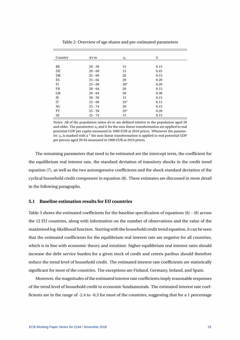
Table 2: Overview of age shares and pre-estimated parameters

Country d e m x0 k

BE 20 - 59 15 0.15DE 20 - 69 15 0.45DK 25 - 69 20 0.15ES 25 - 64 20 0.20FI 25 - 69 30* 0.20FR 20 - 64 20 0.15GB 20 - 64 20 0.30IE 30 - 59 15 0.15IT 25 - 69 35* 0.15NL 25 - 74 20 0.15PT 25 - 59 35* 0.20SE 25 - 74 15 0.15

Notes: All of the population ratios d e m are defined relative to the population aged 20and older. The parameters x0 and k for the non-linear transformation are applied to realpotential GDP per capita measured in 1000 EUR at 2010 prices. Whenever the parame-ter x0 is marked with a * the non-linear transformation is applied to real potential GDPper person aged 20-64 measured in 1000 EUR at 2010 prices.

The remaining parameters that need to be estimated are the intercept term, the coefficient for

the equilibrium real interest rate, the standard deviation of transitory shocks in the credit trend

equation (7), as well as the two autoregressive coefficients and the shock standard deviation of the

cyclical household credit component in equation (8). These estimates are discussed in more detail

in the following paragraphs.

5.1 Baseline estimation results for EU countries

Table 3 shows the estimated coefficients for the baseline specification of equations (6) - (8) across

the 12 EU countries, along with information on the number of observations and the value of the

maximised log-likelihood function. Starting with the household credit trend equation, it can be seen

that the estimated coefficients for the equilibrium real interest rate are negative for all countries,

which is in line with economic theory and intuition: higher equilibrium real interest rates should

increase the debt service burden for a given stock of credit and ceteris paribus should therefore

reduce the trend level of household credit. The estimated interest rate coefficients are statistically

significant for most of the countries. The exceptions are Finland, Germany, Ireland, and Spain.

Moreover, the magnitudes of the estimated interest rate coefficients imply reasonable responses

of the trend level of household credit to economic fundamentals. The estimated interest rate coef-

ficients are in the range of -2.4 to -6.3 for most of the countries, suggesting that for a 1 percentage


Table 3: Coefficient estimates for the baseline household credit gap model

(1) (2) (3) (4) (5) (6) (7) (8) (9) (10) (11) (12)BE DE DK ES FI FR GB IE IT NL PT SE

CREDIT TRENDReal interest rate -5.121∗∗∗ -0.845 -11.786∗∗∗ -1.436 -2.356 -2.497∗ -5.288∗∗∗ -3.654 -4.987∗∗∗ -8.828∗∗ -6.310∗∗∗ -4.874∗∗∗

(0.948) (1.550) (1.586) (1.837) (3.035) (1.441) (1.193) (2.895) (1.923) (4.108) (1.598) (1.831)

Intercept -0.155∗∗∗ -0.252∗∗∗ 0.618∗∗∗ 0.382∗∗∗ -0.326∗∗ -0.282∗∗∗ 0.260∗∗∗ 0.372∗∗∗ -0.496∗∗∗ 0.395∗∗∗ 2.154∗∗∗ -0.055(0.046) (0.068) (0.045) (0.089) (0.130) (0.084) (0.057) (0.140) (0.106) (0.113) (0.083) (0.087)

Shock SD 0.009∗∗∗ 0.006∗∗∗ 0.007∗∗∗ 0.011∗∗∗ 0.006∗∗∗ 0.004∗∗∗ 0.006∗∗∗ 0.013∗∗∗ 0.018∗∗∗ 0.011∗∗∗ 0.008∗∗∗ 0.004∗∗∗

(0.001) (0.000) (0.001) (0.001) (0.001) (0.001) (0.000) (0.001) (0.001) (0.001) (0.001) (0.000)

CREDIT GAPAR(1) coefficient 1.907∗∗∗ 1.912∗∗∗ 1.958∗∗∗ 1.920∗∗∗ 1.906∗∗∗ 1.710∗∗∗ 1.914∗∗∗ 1.957∗∗∗ 1.920∗∗∗ 1.962∗∗∗ 1.799∗∗∗ 1.906∗∗∗

(0.041) (0.041) (0.028) (0.032) (0.048) (0.087) (0.035) (0.026) (0.041) (0.029) (0.068) (0.037)

AR(2) coefficient -0.919∗∗∗ -0.916∗∗∗ -0.971∗∗∗ -0.929∗∗∗ -0.912∗∗∗ -0.716∗∗∗ -0.926∗∗∗ -0.963∗∗∗ -0.925∗∗∗ -0.967∗∗∗ -0.819∗∗∗ -0.913∗∗∗

(0.041) (0.041) (0.028) (0.033) (0.049) (0.088) (0.035) (0.026) (0.042) (0.029) (0.067) (0.037)

Shock SD 0.004∗∗∗ 0.002∗∗∗ 0.003∗∗∗ 0.005∗∗∗ 0.006∗∗∗ 0.007∗∗∗ 0.004∗∗∗ 0.005∗∗∗ 0.005∗∗∗ 0.002∗∗∗ 0.010∗∗∗ 0.005∗∗∗

(0.001) (0.000) (0.001) (0.001) (0.001) (0.001) (0.001) (0.001) (0.001) (0.001) (0.001) (0.001)

Observations 137 140 81 137 140 140 140 140 140 97 128 137Log likelihood 389.472 449.825 246.413 361.654 414.409 443.023 444.541 349.420 316.437 267.392 337.984 442.417

Notes: Details on the country-specific model specifications are given in Table B2. Standard errors are in parentheses. Stars indicate significance: ∗ p < 0.1, ∗∗ p < 0.05, ∗∗∗ p < 0.01.

point reduction in the equilibrium real interest rate, the trend level of household credit increases

by around 2.4% to 6.3%. To put these magnitudes into perspective, the simple structural overlap-

ping generations model in Section 2 that is used to derive the trend equation for household credit

implies a coefficient for the equilibrium real interest rate of -1. Given that the structural model is

fairly simple and abstracts from many aspects of reality, it is reasonable to assume that estimated

coefficients deviate somewhat from the values implied by the model.

Figure 4 illustrates the evolution of the estimated household credit trends. In all of the coun-

tries, both the observed real household credit stock as well as the fundamental household credit

trend have increased considerably over the last 35 years. For example, in Portugal and Ireland the

fundamentally justified household credit stock has increased by around 300% (increase by 3 on a

log scale). In Spain and the UK it has increased by around 200%, while in Belgium, Denmark, Fin-

land, France, Italy, The Netherlands, and Sweden it has increased between 100% and 150%. Figure

4 further shows that in all twelve countries, deviations of the observed real household credit stock

from the fundamentally justified trend can be sizeable and that they tend to be highly persistent.


Figure 4: Real HH credit stock and estimated fundamental trend level4

4.5

55.

5

6.5

77.

5

77.

58

45

67

33.

54

4.5

5

5.5

66.

57

5.5

66.

57

7.5

23

45

55.

56

6.5

5.5

66.

57

23

45

6.5

77.

58




BE DE DK ES

FI FR GB IE

IT NL PT SE

Real HH credit (log) Real HH credit trend (log)

Rea

l HH

cre

dit,

loga

rithm

Notes: The household credit trend estimate is obtained from the baseline model specification. HH credit data for IEbefore 2002 is not available from official statistics. The back-casted HH credit series for IE is confidential and cannot beshown here.

Table 3 shows that the estimated coefficients of the household credit gap equation are all sta-

tistically significant at the 1% level and imply stationary processes for the household credit gaps.

For all twelve EU countries, the AR(1) coefficients are between 1.71 and 1.96, while the AR(2) coef-

ficients are between -0.72 and -0.97. The two AR coefficients always sum to just below unity, which

implies stationary cycles with complex roots that are highly persistent. The standard deviation of

shocks to the household credit gaps ranges between 0.4% and 0.8% in most of the countries. The

next subsection discusses in detail what these estimated coefficients imply for the amplitude and

cycle length of household credit gaps across the 12 EU countries.

5.2 Time-series properties of semi-structural credit gaps

The baseline estimation results for the semi-structural household credit model produce fairly long

cycles for household credit gaps. This property can be seen from Panel (a) of Figure 5, which plots

the cross-country distribution of household credit gaps over the last 35 years. The estimated house-


Figure 5: Properties of semi-structural household credit gaps across EU countries

(a) Evolution of credit gaps over time

-30

-20

-10

010

2030

40S

emi-s

truct

ural

HH

cre

dit g

aps

(%)

1980q1 1985q1 1990q1 1995q1 2000q1 2005q1 2010q1 2015q1

10% - 90% 25% - 75% Median Mean

(b) Maximum amplitudes of credit gaps

9.3

18.4

22.5

9.3

18.720.1

28.126.5

47.5

39.8

15.216.8

19.318.2

54.9

28.7

33.433.2

17.015.9

22.522.9

30.2

23.1

010

2030

4050

60S

emi-s

truct

ural

HH

cre

dit g

aps

(%)

BE DE DK ES FI FR GB IE IT NL PT SE

Largest absolute positive deviation from HH credit trendLargest absolute negative deviation from HH credit trend

Notes: (a) The chart shows the mean, median, interquartile range, and 90-10 percentile range of the semi-structuralhousehold credit gaps across 12 EU countries (Belgium, Denmark, Finland, France, Germany, Ireland, Italy, the Nether-lands, Portugal, Spain, Sweden and the Great Britain). (b) The largest absolute positive and negative deviations of thehousehold credit gaps from the credit trend are computed for the sample 1981q1 to 2014q4.

hold credit cycles have an average length of around 20 years across the 12 EU countries. At the coun-

try level the cycle length varies between 15 and 25 years. For example, the time from one peak in

the household credit cycle to the next one is around 15 years for Belgium and around 25 years for

Sweden, as shown in Figure 6.

This feature of long cycles for household credit gaps is in line with the literature on financial

cycles that has found long cycles for total credit and real estate prices based on statistical filters.20

In contrast to purely statistical approaches, no ex-ante restrictions are imposed on the properties

of the semi-structural household credit gaps, except that they follow AR(2)-processes. The main

identifying information for the semi-structural household credit gaps comes from the credit trend.

In addition to long cycle lengths, we estimate substantial boom and bust episodes for household

credit across the 12 EU countries over the past 35 years. The amplitudes of the semi-structural

household credit gaps tend to range between+/- 15% and+/- 30% in most of the countries as shown

in Panel (b) of Figure 5. In some of the countries that experienced particularly pronounced credit

booms, such as for example Ireland, the semi-structural credit gaps reach levels of more than+ 50%

of the real household credit trend.

Figures 6 and 7 further illustrate the properties of the semi-structural household credit gaps at

the country level. In most countries the household credit gaps display two to three peaks since the

beginning of the 1980s. The difference between one-sided filtered and two-sided smoothed esti-

20See for example Drehmann et al. (2012) and Schüler et al. (2015).


Figure 6: Baseline household credit gap estimates across EU countries I

-20

-15

-10

-50

510

Sem

i-stru

ctur

al H

H c

redi

t gap

s (%

)

1980q1 1985q1 1990q1 1995q1 2000q1 2005q1 2010q1 2015q1

Pre-crisis Systemic crisisHH credit gap (smoothed) HH credit gap (filtered)

BE

-10

010

2030

Sem

i-stru

ctur

al H

H c

redi

t gap

s (%

)

1980q1 1985q1 1990q1 1995q1 2000q1 2005q1 2010q1 2015q1


DE

-20

-10

010

20S

emi-s

truct

ural

HH

cre

dit g

aps

(%)

1980q1 1985q1 1990q1 1995q1 2000q1 2005q1 2010q1 2015q1


DK

-30

-20

-10

010

2030

Sem

i-stru

ctur

al H

H c

redi

t gap

s (%

)

1980q1 1985q1 1990q1 1995q1 2000q1 2005q1 2010q1 2015q1


ES

-40

-20

020

4060

Sem

i-stru

ctur

al H

H c

redi

t gap

s (%

)

1980q1 1985q1 1990q1 1995q1 2000q1 2005q1 2010q1 2015q1


FI-1

5-1

0-5

05

1015

Sem

i-stru

ctur

al H

H c

redi

t gap

s (%

)

1980q1 1985q1 1990q1 1995q1 2000q1 2005q1 2010q1 2015q1


FR

Notes: Details on the country-specific model specifications underlying the baseline household credit gap estimatesare contained in Table B2. The systemic crisis events in the Figure are based on the definition and dating of systemicfinancial crises with either a domestic origin or a combination of a domestic and foreign origin as in Lo Duca et al. (2017).The pre-crisis horizon is defined as 12 to 5 quarters prior to a systemic financial crisis.


Figure 7: Baseline household credit gap estimates across EU countries II

-20

-10

010

20S

emi-s

truct

ural

HH

cre

dit g

aps

(%)

1980q1 1985q1 1990q1 1995q1 2000q1 2005q1 2010q1 2015q1


GB

-40

-20

020

4060

Sem

i-stru

ctur

al H

H c

redi

t gap

s (%

)

1980q1 1985q1 1990q1 1995q1 2000q1 2005q1 2010q1 2015q1


IE

-40

-20

020

40S

emi-s

truct

ural

HH

cre

dit g

aps

(%)

1980q1 1985q1 1990q1 1995q1 2000q1 2005q1 2010q1 2015q1


IT

-20

-10

010

20S

emi-s

truct

ural

HH

cre

dit g

aps

(%)

1980q1 1985q1 1990q1 1995q1 2000q1 2005q1 2010q1 2015q1


NL

-20

-10

010

2030

Sem

i-stru

ctur

al H

H c

redi

t gap

s (%

)

1980q1 1985q1 1990q1 1995q1 2000q1 2005q1 2010q1 2015q1


PT-2

0-1

00

1020

30S

emi-s

truct

ural

HH

cre

dit g

aps

(%)

1980q1 1985q1 1990q1 1995q1 2000q1 2005q1 2010q1 2015q1


SE

Notes: Details on the country-specific model specifications underlying the baseline household credit gap estimates arecontained in Table B2. The systemic crisis events in the figure are based on the definition and dating of systemic financialcrises with either a domestic origin or a combination of a domestic and foreign origin as in Lo Duca et al. (2017). Thepre-crisis horizon is defined as 12 to 5 quarters prior to a systemic financial crisis.


mates of the household credit gaps is negligible, given that most of the identifying information for

the household credit gaps enters through the specification of the household credit trend. As all

fundamental drivers of the household credit trend are assumed to be observed, there is little uncer-

tainty about the true state apart from a transitory shock, once model coefficients are estimated. If

the equilibrium real interest rate and potential output were treated as unobserved endogenous vari-

ables, and were jointly estimated with the household credit trend, uncertainty about the true under-

lying states of household credit would increase. Figures 6 and 7 also show that the semi-structural

household credit gaps tend to be positive and reach rather high levels prior to and at the start of

systemic financial crises.

One of the main advantages of the semi-structural household credit gaps compared to gaps

based on purely statistical filters is that they allow for economic interpretation. In particular, the

trend equation allows to pin down the real household credit stock that is justified by the underlying

fundamental economic factors, i.e. the level of institutional quality, real potential GDP, the equilib-

rium real interest rate and the demographic age structure. While this approach leaves the level of the

household credit gaps as an unexplained statistical residual, the framework allows to decompose

changes of the semi-structural household credit gaps into the underlying driving factors according

to the following equation:

∆ct =∆ct −∆εc ∗

t −∆y ∗t −∆γt −α1∆r ∗t −α2∆d e mt (9)

In words, changes in the semi-structural household credit gaps are driven up by real household

credit growth net of transitory shocks (∆ct −∆εc ∗t ), and driven down by increases in the factors that

push up the real household credit trend. Such decomposition of changes in credit gaps is useful as it

allows to determine at each point in time whether credit growth is higher than justified by changes

in underlying economic fundamentals, and which particular changes in economic fundamentals

justify a given level of credit growth. This can help arriving at an economic narrative of credit devel-

opments and possible excesses. Figure 8 shows such a decomposition of the semi-structural house-

hold credit gaps for Belgium, France, the UK, and Sweden. Ceteris paribus, higher real household

credit growth pushes up the credit gaps. However, the size of the gap can be dampened if the un-

derlying fundamental economic drivers push up the real household credit trend at the same time.

For example, real household credit growth was fairly high in the UK at the beginning of the 1980s,

but given that fundamental economic factors pushed the household credit trend strongly upward


Figure 8: Decomposition of changes in credit gaps into fundamental driving factors

-20

-10

010

20

-4-2

02

4

1980q1 1985q1 1990q1 1995q1 2000q1 2005q1 2010q1 2015q1

HH credit growth Potential real GDP Institutional qualityPopulation ratio Equilibrium interest rate HH credit gap (RHS)

BE

-20

-10

010

20

-4-2

02

4

1980q1 1985q1 1990q1 1995q1 2000q1 2005q1 2010q1 2015q1


FR

-20

-10

010

20

-4-2

02

4

1980q1 1985q1 1990q1 1995q1 2000q1 2005q1 2010q1 2015q1


GB

-40

-20

020

40

-4-2

02

4

1980q1 1985q1 1990q1 1995q1 2000q1 2005q1 2010q1 2015q1


SE

Notes: Details on the country-specific model specifications underlying the different household credit gap estimates arecontained in Table B2. The bars show the contributions of fundamental driving factors to changes in the semi-structuralhousehold credit gaps.

during this period, estimated credit gaps did not rise markedly. In particular, improvements in the

institutional quality proxy, increases in real potential GDP, and reductions in the equilibrium real

interest rate pushed up the real household credit trend in the UK during the early to mid 1980s,

partly justifying high credit growth. Figure 8 also illustrates that very different household credit

growth rates can be justified for a given country at different points in time. For example, in France

there has been a gradual secular decline in the trend growth rate of real household credit that would

be justified by changes in economic fundamentals. The declining negative bars since the mid 1980

illustrate this. In all four countries shown in Figure 8, declining estimates of the equilibrium real

interest rate (yellow bars) have lead to increases in the fundamentally justified real household credit

stock since the beginning of the 1990s.

The next subsection analyses in more detail the behaviour of the semi-structural household

credit gaps around systemic financial crises.


5.3 Signalling properties for systemic financial crises

Since the onset of the global financial crisis, the interest in early warning models for systemic finan-

cial crises has grown substantially. Most papers have found that various statistical transformations

(e.g. changes, growth rates, or filtered cycles) of credit aggregates and asset prices have good early

warning properties to signal financial crises.21 We use a univariate signalling approach, which was

originally applied by Kaminsky et al. (1998) in the context of currency crises, to evaluate the early

warning properties of the semi-structural household credit gaps for systemic financial crises. For

this purpose we use the definition and dating of systemic financial crises with either a domestic

origin or a combination of a domestic and foreign origin contained in the novel crisis database for

EU countries by Lo Duca et al. (2017). There are 13 relevant crisis events in the sample across the

12 EU countries. As has become common practice in the early warning literature, we do not try to

predict the beginning of a crisis but instead try to predict vulnerability periods prior to a crisis. In

total, we test four different pre-crisis horizons: 16-9 quarters, 12 to 5 quarters, 8 to 1 quarters and 4

to 1 quarters prior to a crisis.22

Overall, the baseline semi-structural household credit gaps tend to increase well before systemic

financial crises and decrease slowly afterwards, as shown in Panel (a) of Figure 9. On average, the

semi-structural household credit gaps turn positive more than four years prior to the start of a sys-

temic financial crisis. Moreover, the credit gaps tend to increase continuously during the pre-crisis

periods to reach on average levels of around +20% of the real household credit trend. Once a sys-

temic financial crisis materialises, a slow deleveraging process usually starts that takes on average

more than 4 years to bring real household credit back to its trend level. These dynamics indicate

that the baseline semi-structural household credit gaps could be useful for identifying periods of

excessive leverage building up in the household sector.

Panel (b) of Figure 9 demonstrates further that there seems to be information content in both

the level and the change of the credit gaps. In the vast majority of cases, both the level and the 2-year

change of the credit gaps display high positive values during the 12 to 5 quarters prior to systemic

financial crises. If either the level or the 2-year change of the credit gaps is negative, this tends to

signal that the current period is not a vulnerable pre-crisis period, i.e. not likely to lead up to a

systemic financial crisis over the next 12 to 5 quarters.

21See for example Borio and Lowe (2002), Borio and Drehmann (2009), Schularick and Taylor (2012), Detken et al.(2014), or Lo Duca et al. (2017).

22See e.g. Detken et al. (2014) for a detailed discussion.


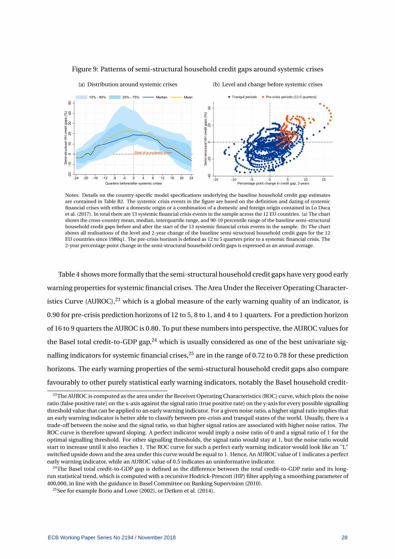
Figure 9: Patterns of semi-structural household credit gaps around systemic crises

(a) Distribution around systemic crises

Start of a systemic crisis

-20

-10

010

2030

4050

Sem

i-stru

ctur

al H

H c

redi

t gap

s (%

)

-24 -20 -16 -12 -8 -4 0 4 8 12 16 20 24Quarters before/after systemic crises

10% - 90% 25% - 75% Median Mean

(b) Level and change before systemic crises

-40

-20

020

40S

emi-s

truc

tura

l HH

cre

dit g

aps

(%)

-15 -10 -5 0 5 10 15Percentage point change in credit gap, 2-years

Tranquil periods Pre-crisis periods (12-5 quarters)

Notes: Details on the country-specific model specifications underlying the baseline household credit gap estimatesare contained in Table B2. The systemic crisis events in the figure are based on the definition and dating of systemicfinancial crises with either a domestic origin or a combination of a domestic and foreign origin contained in Lo Ducaet al. (2017). In total there are 13 systemic financial crisis events in the sample across the 12 EU countries. (a) The chartshows the cross-country mean, median, interquartile range, and 90-10 percentile range of the baseline semi-structuralhousehold credit gaps before and after the start of the 13 systemic financial crisis events in the sample. (b) The chartshows all realisations of the level and 2-year change of the baseline semi-structural household credit gaps for the 12EU countries since 1980q1. The pre-crisis horizon is defined as 12 to 5 quarters prior to a systemic financial crisis. The2-year percentage point change in the semi-structural household credit gaps is expressed as an annual average.

Table 4 shows more formally that the semi-structural household credit gaps have very good early

warning properties for systemic financial crises. The Area Under the Receiver Operating Character-

istics Curve (AUROC),23 which is a global measure of the early warning quality of an indicator, is

0.90 for pre-crisis prediction horizons of 12 to 5, 8 to 1, and 4 to 1 quarters. For a prediction horizon

of 16 to 9 quarters the AUROC is 0.80. To put these numbers into perspective, the AUROC values for

the Basel total credit-to-GDP gap,24 which is usually considered as one of the best univariate sig-

nalling indicators for systemic financial crises,25 are in the range of 0.72 to 0.78 for these prediction

horizons. The early warning properties of the semi-structural household credit gaps also compare

favourably to other purely statistical early warning indicators, notably the Basel household credit-

23The AUROC is computed as the area under the Receiver Operating Characteristics (ROC) curve, which plots the noiseratio (false positive rate) on the x-axis against the signal ratio (true positive rate) on the y-axis for every possible signallingthreshold value that can be applied to an early warning indicator. For a given noise ratio, a higher signal ratio implies thatan early warning indicator is better able to classify between pre-crisis and tranquil states of the world. Usually, there is atrade-off between the noise and the signal ratio, so that higher signal ratios are associated with higher noise ratios. TheROC curve is therefore upward sloping. A perfect indicator would imply a noise ratio of 0 and a signal ratio of 1 for theoptimal signalling threshold. For other signalling thresholds, the signal ratio would stay at 1, but the noise ratio wouldstart to increase until it also reaches 1. The ROC curve for such a perfect early warning indicator would look like an "L"switched upside down and the area under this curve would be equal to 1. Hence, An AUROC value of 1 indicates a perfectearly warning indicator, while an AUROC value of 0.5 indicates an uninformative indicator.

24The Basel total credit-to-GDP gap is defined as the difference between the total credit-to-GDP ratio and its long-run statistical trend, which is computed with a recursive Hodrick-Prescott (HP) filter applying a smoothing parameter of400,000, in line with the guidance in Basel Committee on Banking Supervision (2010).

25See for example Borio and Lowe (2002), or Detken et al. (2014).


Table 4: Overview of early warning properties of semi-structural HH credit gaps

Semi-structuralHH credit

gap

Basel totalcredit-to-GDP

gap

Basel bankcredit-to-GDP

gap

Basel HHcredit-to-GDP

gap

3-year-changein HH

credit-to-GDPratio

3-yeargrowth rate

of realHH credit

Pooled resultsAUROC 16-9q 0.80 0.72 0.76 0.78 0.80 0.69AUROC 12-5q 0.90 0.78 0.79 0.77 0.84 0.74AUROC 8-1q 0.90 0.75 0.74 0.72 0.76 0.66AUROC 4-1q 0.90 0.74 0.72 0.66 0.72 0.60Pseudo R2 12-5q 0.39 0.14 0.15 0.09 0.22 0.07Observations 1,204 1,196 1,204 1,116 1,055 1,055

Country results 12-5 quartersAUROC BE - - - - - -AUROC DE 0.99 1.00 0.96 0.98 0.95 0.75AUROC DK 0.94 1.00 1.00 1.00 1.00 0.96AUROC ES 1.00 1.00 1.00 1.00 1.00 0.93AUROC FI 0.99 0.75 0.63 0.62 0.79 1.00AUROC FR 0.78 0.80 0.88 0.81 0.84 0.95AUROC GB 1.00 0.82 0.81 0.91 0.89 0.85AUROC IE 1.00 1.00 1.00 0.68 1.00 1.00AUROC IT 1.00 0.93 0.83 0.89 0.90 0.45AUROC NL 1.00 0.21 0.39 0.61 0.75 0.31AUROC PT 0.70 0.66 0.64 0.57 0.67 0.27AUROC SE 1.00 0.90 0.97 0.49 0.81 0.97Average AUROC 0.95 0.82 0.83 0.78 0.87 0.77

Notes: The results are based on a sample of 12 EU countries (Belgium, Germany, Denmark, Spain, Finland, France, Ireland, Italy,Netherlands, Portugal, Sweden, and the Great Britain). AUROC stands for Area Under the Receiver Operating CharacteristicsCurve and it is a global measure of the signalling performance of an early warning indicator. An AUROC value of 0.5 indicates anuninformative indicator and a value of 1 indicates a perfect early warning indicator. The AUROC is computed for various pre-crisis horizons (indicated e.g. by "12-5q"), based on the definition and dating of systemic financial crises with either a domesticorigin or a combination of a domestic and foreign origin as in Lo Duca et al. (2017). The Pseudo R-square is obtained for a logitmodel that has the relevant early warning indicator on the right hand side and a binary vulnerability indicator on the left handside, that takes a value of 1 during the 12 to 5 quarters before systemic financial crises, and is zero otherwise, except during the4 quarters before a crisis and during actual crisis quarters, when it is set to missing. The various credit-to-GDP gaps are derivedwith a recursive HP-filter using a smoothing parameter of 400,000, in line with guidance provided by the BIS and the ESRB. TheAUROC cannot be computed for Belgium as there is no relevant systemic financial crisis event in the dataset. The systemic fi-nancial crisis that started in 2007 in Belgium is classified as an imported crisis in the dataset.

to-GDP gap, the Basel bank credit-to-GDP gap, the 3-year change in the household credit-to-GDP

ratio, or the 3-year growth rate of real household credit (See Table 4). At the country-level the semi-

structural household credit gaps also possess very good signalling properties. For a prediction hori-

zon of 12 to 5 quarters eight of the countries attain an AUROC of 0.99 or 1.00. Only two countries

have an AUROC of less than 0.8.


6 Robustness of semi-structural credit gaps

In this section we show robustness exercises with respect to some of the parameter calibrations, real

vs. full sample estimation and a comparison to purely statistical filters and an unobserved compo-

nents model where the trend follows a stochastic process.

6.1 Robustness to model specification

Three robustness exercises are performed for the semi-structural household credit gaps. First, a

common age share and non-linear transformation of the institutional quality proxy are used across

all countries (Model 2). Second, a common non-linear transformation of the institutional quality

proxy is used across countries, but the age share is allowed to be country-specific (Model 3). Third,

both measurements are allowed to be country-specific and the coefficient for the age share is es-

timated alongside the interest rate coefficient (Model 4). Table B2 in Appendix B provides a more

detailed overview of all model specifications that are used across the 12 EU countries.

Figures 10 and 11 show that the dynamics of the estimated household credit gaps are qualita-

tively robust to these various changes in the model specification. In particular, peaks and troughs

coincide for the different model specifications in most of the countries. For Belgium, Denmark, Fin-

land, Germany, the Netherlands, Spain, and Sweden the differences in the various household credit

gap estimates are rather small. For France, Ireland, Italy, Portugal, and the Great Britain some differ-

ences in the levels of the different household credit gaps can be observed in particular at the begin-

ning of the the sample period, while the overall dynamics appear to be robust. The differences that

are observed in the levels of the credit gaps for these countries seem to be mainly driven by whether

country-specific measurements for the age share and non-linear transformation of the institutional

quality proxy are used (Baseline and Model 4) or not (Models 2 and 3). Nevertheless, the very good

early warning properties of the semi-structural household credit gaps for systemic financial crises

are not affected by the different model specifications, as shown in Table B3 in Appendix B.

Table 5 further shows that the estimated coefficients for the equilibrium real interest rate are

negative in all cases and rather stable across the different model specifications. The AR(2) coeffi-

cients of the credit gap equation are also fairly stable across the different model specifications and

imply stationary statistical processes in all cases. Finally, for Model 4 the estimated coefficients for

the share of young/middle-aged people relative to all people that receive income imply reasonable

responses of the trend level of real household credit to changes in the demographic structure of the


Figure 10: Robustness of household credit gap estimates across EU countries I

-20

-10

010

Sem

i-stru

ctur

al H

H c

redi

t gap

s (%

)

1980q1 1985q1 1990q1 1995q1 2000q1 2005q1 2010q1 2015q1

Pre-crisis Systemic crisis Baseline HH credit gapHH credit gap 2 HH credit gap 3 HH credit gap 4

BE

-10

010

2030

Sem

i-stru

ctur

al H

H c

redi

t gap

s (%

)

1980q1 1985q1 1990q1 1995q1 2000q1 2005q1 2010q1 2015q1


DE

-20

-10

010

20S

emi-s

truct

ural

HH

cre

dit g

aps

(%)

1980q1 1985q1 1990q1 1995q1 2000q1 2005q1 2010q1 2015q1


DK

-30

-20

-10

010

2030

Sem

i-stru

ctur

al H

H c

redi

t gap

s (%

)

1980q1 1985q1 1990q1 1995q1 2000q1 2005q1 2010q1 2015q1


ES

-40

-20

020

4060

Sem

i-stru

ctur

al H

H c

redi

t gap

s (%

)

1980q1 1985q1 1990q1 1995q1 2000q1 2005q1 2010q1 2015q1


FI-2

0-1

00

1020

30S

emi-s

truct

ural

HH

cre

dit g

aps

(%)

1980q1 1985q1 1990q1 1995q1 2000q1 2005q1 2010q1 2015q1


FR

Notes: Details on the country-specific model specifications underlying the different household credit gap estimates arecontained in Table B2. The systemic crisis events in the figure are based on the definition and dating of systemic financialcrises with either a domestic origin or a combination of a domestic and foreign origin as in Lo Duca et al. (2017). Thepre-crisis horizon is defined as 12 to 5 quarters prior to a systemic financial crisis.


Figure 11: Robustness of household credit gap estimates across EU countries II

-30

-20

-10

010

2030

Sem

i-stru

ctur

al H

H c

redi

t gap

s (%

)

1980q1 1985q1 1990q1 1995q1 2000q1 2005q1 2010q1 2015q1


GB

-40

-20

020

4060

Sem

i-stru

ctur

al H

H c

redi

t gap

s (%

)

1980q1 1985q1 1990q1 1995q1 2000q1 2005q1 2010q1 2015q1


IE

-40

-20

020

40S

emi-s

truct

ural

HH

cre

dit g

aps

(%)

1980q1 1985q1 1990q1 1995q1 2000q1 2005q1 2010q1 2015q1


IT

-20

-10

010

20S

emi-s

truct

ural

HH

cre

dit g

aps

(%)

1980q1 1985q1 1990q1 1995q1 2000q1 2005q1 2010q1 2015q1


NL

-30

-20

-10

010

2030

Sem

i-stru

ctur

al H

H c

redi

t gap

s (%

)

1980q1 1985q1 1990q1 1995q1 2000q1 2005q1 2010q1 2015q1


PT-2

0-1

00

1020

30S

emi-s

truct

ural

HH

cre

dit g

aps

(%)

1980q1 1985q1 1990q1 1995q1 2000q1 2005q1 2010q1 2015q1


SE

Notes: Details on the country-specific model specifications underlying the different household credit gap estimates arecontained in Table B2. The systemic crisis events in the figure are based on the definition and dating of systemic financialcrises with either a domestic origin or a combination of a domestic and foreign origin as in Lo Duca et al. (2017). Thepre-crisis horizon is defined as 12 to 5 quarters prior to a systemic financial crisis.


population. The estimated age share coefficients are in the range of 0.8 to 3.3, which implies that a

1% increase in the share of young/middle-aged people in the total population leads to an increase

in the trend level of household credit of around 0.8% to 3.3%. To put these magnitudes into perspec-

tive, the simple structural overlapping generations model that is used to derive the trend equation

for household credit implies a unit elasticity for the population ratio: each additional percent of ag-

gregate future expected income that is assigned to people that are most likely to hold debt, should

increase the trend level of borrowing by the same amount.

Table 5: Robustness of coefficient estimates for the household credit gap model

(1) (2) (3) (4) (5) (6) (7) (8) (9) (10) (11) (12)BE DE DK ES FI FR GB IE IT NL PT SE

CREDIT TRENDReal rate (Baseline) -5.121∗∗∗ -0.845 -11.786∗∗∗ -1.436 -2.356 -2.497∗ -5.288∗∗∗ -3.654 -4.987∗∗∗ -8.828∗∗ -6.310∗∗∗ -4.874∗∗∗

(0.948) (1.550) (1.586) (1.837) (3.035) (1.441) (1.193) (2.895) (1.923) (4.108) (1.598) (1.831)

Real rate (Model 2) -4.359∗∗∗ -0.981 -12.636∗∗∗ -0.785 -2.592 -2.285 -8.357∗∗∗ -2.940 -4.534∗∗ -10.600∗∗ -7.739∗∗∗ -6.042∗∗∗

(1.171) (1.478) (1.575) (1.912) (3.021) (1.617) (2.284) (2.656) (2.233) (5.116) (2.211) (2.014)

Real rate (Model 3) -5.397∗∗∗ -0.981 -11.177∗∗∗ -0.524 -2.356 -2.082 -7.957∗∗∗ -3.029 -4.343∗∗ -9.754∗∗ -7.356∗∗∗ -5.678∗∗∗

(1.014) (1.478) (1.473) (1.783) (3.035) (1.507) (1.940) (2.628) (2.147) (4.451) (2.020) (1.788)

Real rate (Model 4) -6.100∗∗∗ -0.724 -13.257∗∗∗ -1.456 -2.278 -3.441∗∗∗ -5.893∗∗∗ -3.436 -5.279∗∗∗ -9.599∗∗ -3.488∗ -5.132∗∗∗

(1.981) (1.927) (1.406) (2.537) (5.949) (1.220) (1.407) (3.032) (1.938) (4.399) (1.864) (1.770)

Age share (Model 4) 3.057 0.978 2.131∗∗ 1.643 1.121 3.117∗∗∗ 2.857 1.535 1.344 3.265 0.774 3.202(3.085) (1.837) (1.054) (2.194) (1.821) (0.841) (3.317) (3.411) (2.601) (4.534) (2.723) (4.481)

CREDIT GAPAR(1) (Baseline) 1.907∗∗∗ 1.912∗∗∗ 1.958∗∗∗ 1.920∗∗∗ 1.906∗∗∗ 1.710∗∗∗ 1.914∗∗∗ 1.957∗∗∗ 1.920∗∗∗ 1.962∗∗∗ 1.799∗∗∗ 1.906∗∗∗

(0.041) (0.041) (0.028) (0.032) (0.048) (0.087) (0.035) (0.026) (0.041) (0.029) (0.068) (0.037)

AR(1) (Model 2) 1.899∗∗∗ 1.902∗∗∗ 1.959∗∗∗ 1.930∗∗∗ 1.910∗∗∗ 1.743∗∗∗ 1.948∗∗∗ 1.963∗∗∗ 1.917∗∗∗ 1.960∗∗∗ 1.814∗∗∗ 1.921∗∗∗

(0.047) (0.044) (0.028) (0.030) (0.044) (0.080) (0.027) (0.022) (0.042) (0.029) (0.070) (0.033)

AR(1) (Model 3) 1.900∗∗∗ 1.902∗∗∗ 1.955∗∗∗ 1.934∗∗∗ 1.906∗∗∗ 1.710∗∗∗ 1.943∗∗∗ 1.962∗∗∗ 1.912∗∗∗ 1.957∗∗∗ 1.810∗∗∗ 1.909∗∗∗

(0.046) (0.044) (0.030) (0.029) (0.048) (0.087) (0.028) (0.023) (0.045) (0.032) (0.069) (0.037)

AR(1) (Model 4) 1.914∗∗∗ 1.920∗∗∗ 1.966∗∗∗ 1.926∗∗∗ 1.916∗∗∗ 1.687∗∗∗ 1.909∗∗∗ 1.954∗∗∗ 1.923∗∗∗ 1.962∗∗∗ 1.773∗∗∗ 1.898∗∗∗

(0.042) (0.044) (0.020) (0.033) (0.060) (0.089) (0.037) (0.028) (0.039) (0.028) (0.073) (0.040)

AR(2) (Baseline) -0.919∗∗∗ -0.916∗∗∗ -0.971∗∗∗ -0.929∗∗∗ -0.912∗∗∗ -0.716∗∗∗ -0.926∗∗∗ -0.963∗∗∗ -0.925∗∗∗ -0.967∗∗∗ -0.819∗∗∗ -0.913∗∗∗

(0.041) (0.041) (0.028) (0.033) (0.049) (0.088) (0.035) (0.026) (0.042) (0.029) (0.067) (0.037)

AR(2) (Model 2) -0.909∗∗∗ -0.907∗∗∗ -0.972∗∗∗ -0.937∗∗∗ -0.916∗∗∗ -0.746∗∗∗ -0.955∗∗∗ -0.967∗∗∗ -0.920∗∗∗ -0.965∗∗∗ -0.829∗∗∗ -0.928∗∗∗

(0.047) (0.044) (0.028) (0.031) (0.044) (0.081) (0.027) (0.023) (0.043) (0.030) (0.071) (0.033)

AR(2) (Model 3) -0.911∗∗∗ -0.907∗∗∗ -0.969∗∗∗ -0.942∗∗∗ -0.912∗∗∗ -0.713∗∗∗ -0.951∗∗∗ -0.966∗∗∗ -0.915∗∗∗ -0.962∗∗∗ -0.827∗∗∗ -0.917∗∗∗

(0.046) (0.044) (0.030) (0.030) (0.049) (0.088) (0.028) (0.023) (0.046) (0.033) (0.070) (0.037)

AR(2) (Model 4) -0.927∗∗∗ -0.923∗∗∗ -0.980∗∗∗ -0.933∗∗∗ -0.921∗∗∗ -0.696∗∗∗ -0.921∗∗∗ -0.959∗∗∗ -0.929∗∗∗ -0.968∗∗∗ -0.791∗∗∗ -0.905∗∗∗

(0.042) (0.043) (0.020) (0.033) (0.063) (0.089) (0.037) (0.029) (0.039) (0.029) (0.073) (0.040)

Shock SD (Baseline) 0.004∗∗∗ 0.002∗∗∗ 0.003∗∗∗ 0.005∗∗∗ 0.006∗∗∗ 0.007∗∗∗ 0.004∗∗∗ 0.005∗∗∗ 0.005∗∗∗ 0.002∗∗∗ 0.010∗∗∗ 0.005∗∗∗

(0.001) (0.000) (0.001) (0.001) (0.001) (0.001) (0.001) (0.001) (0.001) (0.001) (0.001) (0.001)

Shock SD (Model 2) 0.004∗∗∗ 0.003∗∗∗ 0.002∗∗∗ 0.004∗∗∗ 0.007∗∗∗ 0.007∗∗∗ 0.004∗∗∗ 0.005∗∗∗ 0.005∗∗∗ 0.003∗∗∗ 0.010∗∗∗ 0.005∗∗∗

(0.001) (0.000) (0.001) (0.001) (0.001) (0.001) (0.001) (0.001) (0.001) (0.001) (0.001) (0.001)

Shock SD (Model 3) 0.004∗∗∗ 0.003∗∗∗ 0.003∗∗∗ 0.004∗∗∗ 0.006∗∗∗ 0.007∗∗∗ 0.004∗∗∗ 0.005∗∗∗ 0.005∗∗∗ 0.003∗∗∗ 0.010∗∗∗ 0.005∗∗∗

(0.001) (0.000) (0.001) (0.001) (0.001) (0.001) (0.001) (0.001) (0.001) (0.001) (0.001) (0.001)

Shock SD (Model 4) 0.003∗∗∗ 0.003∗∗∗ 0.002∗∗∗ 0.005∗∗∗ 0.006∗∗∗ 0.007∗∗∗ 0.004∗∗∗ 0.005∗∗∗ 0.005∗∗∗ 0.002∗∗∗ 0.012∗∗∗ 0.005∗∗∗

(0.001) (0.000) (0.001) (0.001) (0.001) (0.001) (0.001) (0.001) (0.001) (0.001) (0.002) (0.001)

Notes: Details on the country-specific model specifications are given in Table B2. Standard errors are in parentheses. Stars indicate significance: ∗ p < 0.1, ∗∗ p < 0.05, ∗∗∗ p < 0.01.


6.2 Robustness to real-time estimation

To test the robustness of the model results to real-time estimation, we implement two adjustments

to the baseline model estimation. First, we restrict the sample for estimation of coefficients to the

period 1980 - 2004, so as to test the model performance ahead of the global financial crisis. Second,

we use one-sided recursive HP-filtered trend estimates of the real interest rate and real GDP in or-

der to mimic the real-time estimates of the equilibrium real interest rate and real potential GDP.26

We keep the coefficients in the institutional quality transformation unchanged. Figures A6 and A7

in Appendix A show these quasi real-time estimates of the equilibrium real interest rate and real

potential GDP in comparison to the full-sample estimates used for the baseline model estimation.

As shown in Figures 12 and 13 the dynamics of the semi-structural household credit gaps are

qualitatively robust to real-time estimation. Hence, the model estimated in real-time would have

indicated positive and increasing household credit gaps for most of the twelve EU countries ahead

of the global financial crisis, similar to the gaps based on full sample information. However, for the

majority of countries the real-time gap estimates are around 10 percentage points higher than the

baseline full-sample gap estimates. The higher gap estimates based on the real-time model seem

to be mainly related to the fact that the estimated interest rate semi-elasticities (see Table B4 in

Appendix B) are lower than for the baseline model. Hence, for the benchmark pre-crisis horizon

of 12-5 quarters false positive signals would have been somewhat higher for the real-time gaps and

the AUROC somewhat lower at 0.86 compared to 0.90 for the baseline full-sample gaps. For a longer

pre-crisis horizon of 16-5 quarters, the AUROC of the real-time gaps of 0.87 is only marginally lower

compared to the AUROC of 0.88 for the baseline full-sample gaps.

6.3 Comparison to statistical filters and an unobserved components model

We also compare the estimated baseline credit gaps to results from standard statistical filters and an

unobserved components model.27 First, we compute household credit gaps applying an HP-filter

with smoothing parameter 400,000 as e.g. in the BCBS and ESRB guidance for the credit-to-GDP

ratio. Applying such a smoothing parameter assumes a priori that credit cycles are about four times

longer than business cycles, i.e. in the range of 25-30 years. Second, we implement the band-pass

filter by Christiano and Fitzgerald (2003), which is another prominent statistical filtering method

used e.g. in Aikman et al. (2015). These authors filter credit-to-GDP cycles between 8 and 30 years.

26A smoothing parameter of 1,600 is used.27For a comprehensive overview of these methods and their application to euro area countries see Rünstler et al. (2018).


Figure 12: Comparison of real-time and full-sample credit gap estimates I

-20

-10

010

2030

Sem

i-stru

ctur

al H

H c

redi

t gap

s (%

)

2000q1 2002q1 2004q1 2006q1 2008q1 2010q1 2012q1 2014q1 2016q1

Pre-crisis Systemic crisisHH credit gap (full sample) HH credit gap (2004 real-time)

BE

-20

-10

010

20S

emi-s

truct

ural

HH

cre

dit g

aps

(%)

2000q1 2002q1 2004q1 2006q1 2008q1 2010q1 2012q1 2014q1 2016q1


DE

-20

-10

010

2030

40S

emi-s

truct

ural

HH

cre

dit g

aps

(%)

2000q1 2002q1 2004q1 2006q1 2008q1 2010q1 2012q1 2014q1 2016q1


DK

-20

-10

010

2030

Sem

i-stru

ctur

al H

H c

redi

t gap

s (%

)

2000q1 2002q1 2004q1 2006q1 2008q1 2010q1 2012q1 2014q1 2016q1


ES

-40

-20

020

4060

Sem

i-stru

ctur

al H

H c

redi

t gap

s (%

)

2000q1 2002q1 2004q1 2006q1 2008q1 2010q1 2012q1 2014q1 2016q1


FI-2

0-1

00

1020

3040

Sem

i-stru

ctur

al H

H c

redi

t gap

s (%

)

2000q1 2002q1 2004q1 2006q1 2008q1 2010q1 2012q1 2014q1 2016q1


FR

Notes: Details on the country-specific model specifications underlying the baseline household credit gap estimates arecontained in Table B2. The systemic crisis events in the figure are based on the definition and dating of systemic financialcrises with either a domestic origin or a combination of a domestic and foreign origin contained in Lo Duca et al. (2017).The pre-crisis horizon is defined as 12 to 5 quarters prior to a systemic financial crisis.


Figure 13: Comparison of real-time and full-sample credit gap estimates II

-20

-10

010

2030

40S

emi-s

truct

ural

HH

cre

dit g

aps

(%)

2000q1 2002q1 2004q1 2006q1 2008q1 2010q1 2012q1 2014q1 2016q1


GB

-40

-20

020

4060

80S

emi-s

truct

ural

HH

cre

dit g

aps

(%)

2000q1 2002q1 2004q1 2006q1 2008q1 2010q1 2012q1 2014q1 2016q1


IE

-20

020

4060

80S

emi-s

truct

ural

HH

cre

dit g

aps

(%)

2000q1 2002q1 2004q1 2006q1 2008q1 2010q1 2012q1 2014q1 2016q1


IT

-10

010

2030

Sem

i-stru

ctur

al H

H c

redi

t gap

s (%

)

2000q1 2002q1 2004q1 2006q1 2008q1 2010q1 2012q1 2014q1 2016q1


NL

-20

020

4060

Sem

i-stru

ctur

al H

H c

redi

t gap

s (%

)

2000q1 2002q1 2004q1 2006q1 2008q1 2010q1 2012q1 2014q1 2016q1


PT-2

0-1

00

1020

3040

Sem

i-stru

ctur

al H

H c

redi

t gap

s (%

)

2000q1 2002q1 2004q1 2006q1 2008q1 2010q1 2012q1 2014q1 2016q1


SE

Notes: Details on the country-specific model specifications underlying the baseline household credit gapestimates are contained in Table B2. The systemic crisis events in the figure are based on the definitionand dating of systemic financial crises with either a domestic origin or a combination of a domestic andforeign origin contained in Lo Duca et al. (2017). The pre-crisis horizon is defined as 12 to 5 quarters priorto a systemic financial crisis.


Third, we compare our baseline credit gaps to those estimated from the unobserved components

model used by Grant and Chan (2017) who postulate a standard trend-cycle decomposition, where

the trend is a non-stationary second-order Markov process and the cycle follows a stationary AR(2)-

process.28

Effectively this unobserved components model implies that the trend growth rate of household

credit follows a random walk and that all permanent shocks are classified as shocks to the trend-

growth rate. By contrast, in the standard local-linear trend model with time-varying drift permanent

shocks can affect the trend level and the trend growth rate (see e.g. Clark, 1987). However, the vari-

ances of these shocks are usually difficult to identify in the estimation. Moreover, Grant and Chan

(2017) show that the HP-filter can be recovered as a special case of their model. The state-space

model is estimated by Bayesian methods using a Gibbs-Sampler following the methods outlined

in Chan and Jeliazkov (2009). The resulting gaps of all three methods together with the baseline

semi-structural credit gaps are shown in Figures 14 and 15.

Overall the credit gap dynamics are comparable across the different filtering methods. However,

there are some noticeable differences as well. First, in some countries the statistical methods tend

to estimate somewhat smaller amplitudes. This could mean that there is some leakage of excessive

credit developments into the statistical trend. Second, in the cases of Belgium, Finland, France and

Sweden the semi-structural credit gaps tend to be considerably higher than the statistical credit gaps

at the end of the sample, which appears more in line with recent credit developments in these coun-

tries. Somewhat larger differences can be observed in the case of Italy, where our semi-structural

credit gap is positive at the sample end while all other methods yield negative gaps. The positive

semi-structural gap is partly explained by the low level of Italian potential output, information that

is not available to the other methods which only use the time series of the credit stock. Alessan-

dri et al. (2015) present alternative Basel gap measures for Italy that are also positive around 2014.

While these gaps are not directly comparable to our concept, this shows that estimated credit gaps

in Italy are surrounded by considerable uncertainty.

28The model specification is

ct = ct +τt

∆τt = ∆τt−1+ v τtct = φ1 ct−1+φ2 ct−2+ v c

t

(10)

where τt is the credit trend and ct the credit gap and the shocks v τt and v ct are assumed to be uncorrelated.


Figure 14: Comparison to statistical filters and standard unobserved components model I

Notes: Full sample estimations. Baseline gap refers to the benchmark semi-structural credit gap, UC refersto the unobserved components model by Grant and Chan (2017), CF denotes the Christiano-Fitzgeraldfiler for cycles between 8 and 30 years and HP denotes the HP-filter with smoothing parameter 400,000.


Figure 15: Comparison to statistical filters and standard unobserved components model II

Notes: Full sample estimations. Baseline gap refers to the benchmark semi-structural credit gap, UC refersto the unobserved components model by Grant and Chan (2017), CF denotes the Christiano-Fitzgeraldfiler for cycles between 8 and 30 years and HP denotes the HP-filter with smoothing parameter 400,000.


7 Conclusion

This paper proposes a theory-based approach to identifying excessive household credit develop-

ments. In a first step, we derive an equilibrium relationship for the trend level of real household

credit using a structural economic model that takes into account household heterogeneity and bor-

rowing constraints. The structural model implies that the equilibrium real household credit stock is

driven by the following four fundamental economic factors: real potential GDP, the equilibrium real

interest rate, the population share of the young/middle-aged cohort, and the level of institutional

quality. In a second step, the theory-based household credit gaps are derived as deviations of the

observed household credit stock from the credit trend.

We estimate the theory-based household credit gaps in a model set-up similar to an unobserved

components framework for 12 EU countries using quarterly data for the period 1980 - 2015. Fo-

cussing our analysis on household credit, which was one of the major drivers sparking the global

financial crisis, we also contribute to a better understanding of the interaction between financial

cycles and business cycles.

Without imposing a priori information on the cycle length, the estimated credit gaps display

long cycles that last between 15 to 25 years. In addition, the estimated credit cycles display sub-

stantial amplitudes of around 20% at the country level, which implies that the observed household

credit stock can deviate 20% from the fundamental credit stock. The estimated theory-based house-

hold credit gaps tend to increase around four years ahead of systemic financial crises and they pos-

sess superior early warning properties compared to a number of established statistical credit gaps,

notably the commonly used Basel total-credit-to-GDP gap and its household credit-to-GDP gap

variant. The theory-based credit gaps do not display excessively long periods of high positive val-

ues, which can be the case with purely statistical credit gaps especially during periods of economic

transition. In addition, our estimated credit gaps do not tend to fall to as large negative values in

the aftermath of financial booms and/or crises as those observed for Basel credit gaps in a number

of euro area countries. This property should mitigate the risk of underestimating cyclical systemic

risks.

The estimated credit gaps based on theory may be useful for countercyclical macroprudential

policy for the following reasons: first, the trend component has a normative economic interpre-

tation as it is determined by fundamental economic factors. This is a clear advantage relative to a

purely statistical trend, which can only be a heuristic interpretation of a normative concept. Second,


understanding the driving factors of credit gaps, e.g. via the decomposition technique presented in

the paper helps informing policy makers in the selection of the most appropriate mix of macropru-

dential instruments.

Our framework could be extended to allow for endogeneity of potential GDP and the equilib-

rium real interest rate akin to the set-up used in Laubach and Williams (2003), but augmented with

additional exogenous factors that drive the equilibrium real rate as suggested by Eggertsson et al.

(2017). We are currently working on that approach. In addition, a (semi-)structural approach to

modelling firm credit would be desirable.


References

Acemoglu, D., Johnson, S., and Robinson, J. A. (2005). Institutions as a Fundamental Cause of Long-

Run Growth. In Aghion, P. and Durlauf, S., editors, Handbook of Economic Growth, volume 1 of

Handbook of Economic Growth, chapter 6, pages 385–472. Elsevier.

Aikman, D., Haldane, A., and Nelson, B. (2015). Curbing the credit cycle. The Economic Journal,

125(585):1072–1109.

Aiyagari, S. R. (1994). Uninsured Idiosyncratic Risk and Aggregate Saving. The Quarterly Journal of

Economics, 109(3):659–684.

Albuquerque, B., Baumann, U., and Krustev, G. (2015). U.S. household deleveraging following the

Great Recession - a model-based estimate of equilibrium debt. The B.E. Journal of Macroeco-

nomics, 15(1):53.

Alessandri, P., Bologna, P., Fiori, R., and Sette, E. (2015). A note on the implementation of a Coun-

tercyclical Capital Buffer in Italy. Occasional Papers 278, Banca d’Italia.

Alessi, L. and Detken, C. (2011). Quasi real time early warning indicators for costly asset price

boom/bust cycles: A role for global liquidity. European Journal of Political Economy, 27(3):520–

533.

Alvarez, F. and Jermann, U. J. (2000). Efficiency, equilibrium, and asset pricing with risk of default.

Econometrica, 68(4):775–797.

Basel Committee on Banking Supervision (2010). Guidance for national authorities operating the

countercyclical capital buffer. Bank for International Settlements.

Blagrave, P., Garcia-Saltos, R., Laxton, D., and Zhang, F. (2015). A simple multivariate filter for esti-

mating potential output. IMF Working Paper WP/15/79, International Monetary Fund.

Borio, C. and Drehmann, M. (2009). Assessing the risk of banking crises - revisited. Technical report,

Bank for International Settlements.

Borio, C. and Lowe, P. (2002). Asset prices, financial and monetary stability: exploring the nexus.

BIS Working Papers 114, Bank for International Settlements.


Buncic, D. and Melecky, M. (2014). Equilibrium credit: The reference point for macroprudential

supervisors. Journal of Banking & Finance, 41(C):135–154.

Castro, C., Estrada, Á., and Martínez, J. (2016). The countercyclical capital buffer in Spain: an anal-

ysis of key guiding indicators. Documentos de Trabajo 1601, Banco de España.

Chan, J. C. and Jeliazkov, I. (2009). Efficient simulation and integrated likelihood estimation in state

space models. International Journal of Mathematical Modelling and Numerical Optimisation,

1:101–120.

Christensen, A. M., Andersen, A. L., Oksbjerg, M., Nielsen, N. F., Kaarup, R., and Koob, S. A. (2013).

The wealth and debt of Danish families. In Bank for International Settlements, editor, Proceed-

ings of the Sixth IFC Conference on "Statistical issues and activities in a changing environment",

Basel, 28-29 August 2012, volume 36, pages 465–495. Bank for International Settlements.

Christiano, L. and Fitzgerald, T. (2003). The band pass filter. International Economic Review,

44(2):435–465.

Clark, P. (1987). The cyclical component of U.S. economic activity. The Quarterly Journal of Eco-

nomics, 102(4):797–814.

Cottarelli, C., Dell’Ariccia, G., and Vladkova-Hollar, I. (2005). Early birds, late risers, and sleeping

beauties: Bank credit growth to the private sector in Central and Eastern Europe and in the

Balkans. Journal of Banking & Finance, 29(1):83–104.

Detken, C., Weeken, O., Alessi, L., Bonfim, D., Boucinha, M. M., Castro, C., Frontczak, S., Giordana,

G., Giese, J., Jahn, N., Kakes, J., Klaus, B., Lang, J. H., Puzanova, N., and Welz, P. (2014). Opera-

tionalising the countercyclical capital buffer: indicator selection, threshold identification and

calibration options. ESRB Occasional Paper Series No. 5, European Systemic Risk Board.

Drehmann, M., Borio, C., and Tsatsaronis, K. (2011). Anchoring countercyclical capital buffers: the

role of credit aggregates. International Journal of Central Banking, 7(4):189–240.

Drehmann, M., Borio, C., and Tsatsaronis, K. (2012). Characterising the financial cycle: don’t lose

sight of the medium term! BIS Working Papers 380, Bank for International Settlements.

Eggertsson, G. B. and Mehrotra, N. R. (2014). A model of secular stagnation. Working Paper 20574,

National Bureau of Economic Research.


Eggertsson, G. B., Mehrotra, N. R., and Robbins, J. A. (2017). A model of secular stagnation: Theory

and quantitative evaluation. Working Paper 23093, National Bureau of Economic Research.

European Systemic Risk Board (2014). Recommendation of the European Systemic Risk Board of 18

June 2014 on guidance for setting countercyclical buffer rates (ESRB/2014/1). European Systemic

Risk Board.

Favero, C., Gozluklu, A. E., and Yang, H. (2016). Demographics and the behavior of interest rates.

IMF Economic Review, 64(4):732–776.

Ferrero, G., Gross, M., and Neri, S. (2017). On secular stagnation and low interest rates: demography

matters. Working Paper Series 2088, European Central Bank.

Glick, R. and Lansing, K. J. (2010). Global household leverage, house prices, and consumption.

Economic Letters 1-2010, Federal Reserve Bank of San Francisco.

Grant, A. and Chan, J. C. (2017). Reconciling output gaps: Unobserved components model and

Hodrick-Prescott filter. Journal of Economic Dynamics and Control, 75:114–121.

Hamilton, J. D. (2017). Why you should never use the Hodrick-Prescott filter. Working Paper 23429,

National Bureau of Economic Research.

Hamilton, J. D., Harris, E. S., Hatzius, J., and West, K. D. (2015). The equilibrium real funds rate: Past,

present and future. Working Paper 21476, National Bureau of Economic Research.

Holston, K., Laubach, T., and Williams, J. C. (2016). Measuring the natural rate of interest: Interna-

tional trends and determinants. Finance and Economics Discussion Series 2016-073, Board of

Governors of the Federal Reserve System, Washington, D.C.

Household Finance and Consumption Network (2016). The household finance and consumption

survey: results from the second wave. Statistics Paper Series 18/2016, European Central Bank.

Household Finance and Consumption Network (2017). The household finance and consumption

survey wave 2 - statistical tables. HFCS Statistical Tables, European Central Bank.

International Monetary Fund (2012). Dealing with household debt, chapter 3, pages 89–124. World

Economic Outlook April 2012. International Monetary Fund, Washington, D.C.


Juselius, M. and Drehmann, M. (2015). Leverage dynamics and the real burden of debt. BIS Working

Papers 501, Bank for International Settlements.

Kaminsky, G., Lizondo, S., and Reinhart, C. M. (1998). Leading indicators of currency crises. IMF

Staff Papers, 45(1):1–48.

Kehoe, T. J. and Levine, D. K. (1993). Debt-Constrained Asset Markets. Review of Economic Studies,

60(4):865–888.

Kiyotaki, N. and Moore, J. (1997). Credit Cycles. Journal of Political Economy, 105(2):211–48.

Kocherlakota, N. R. (1996). Implications of efficient risk sharing without commitment. The Review

of Economic Studies, 63(4):595–609.

Kuncic, A. (2014). Institutional quality dataset. Journal of Institutional Economics, 10(01):135–161.

Lang, J. H. and Welz, P. (2017). Measuring credit gaps for macroprudential policy, pages 144–157.

Financial Stability Review, Special Feature B. European Central Bank.

Laubach, T. and Williams, J. C. (2003). Measuring the Natural Rate of Interest. The Review of Eco-

nomics and Statistics, 85(4):1063–1070.

Lo Duca, M., Koban, A., Basten, M., Bengtsson, E., Klaus, B., Kusmierczyk, P., Lang, J. H., Detken, C.,

and Peltonen, T. (2017). A new database for financial crises in European countries. Occasional

Paper Series 194, European Central Bank.

Mésonnier, J.-S. and Renne, J.-P. (2007). A time-varying "natural" rate of interest for the euro area.

European Economic Review, 51(7):1768–1784.

Mian, A. and Sufi, A. (2014). House of Debt: How They (and You) Caused the Great Recession and How

We Can Prevent It From Happening Again. University of Chicago Press: Chicago.

Mian, A. R., Sufi, A., and Verner, E. (2015). Household debt and business cycles worldwide. Working

Paper 21581, National Bureau of Economic Research.

Office for National Statistics (2015). Wealth in Great Britain Wave 3: The burden of financial and

property debt, Great Britain, 2010 to 2012.

Ölcer, D. and van Santen, P. (2016). The indebtedness of Swedish households: Update for 2016.

Economic Commentaries 05/2016, Sveriges Riksbank.


Rünstler, G., Balfoussia, H., Burlon, L., Buss, G., Comunale, M., De Backer, B., Dewachter, H.,

Guarda, P., Haavio, M., Hindrayanto, I., and Iskrev, N. (2018). Real and financial cycles in EU

countries - Stylised facts and modelling implications. Occasional Paper Series 205, European

Central Bank.

Rünstler, G. and Vlekke, M. (2018). Business, housing, and credit cycles. Journal of Applied Econo-

metrics, 33(2):212–226.

Schularick, M. and Taylor, A. M. (2012). Credit booms gone bust: Monetary policy, leverage cycles,

and financial crises, 1870-2008. American Economic Review, 102(2):1029–61.

Schüler, Y., Hiebert, P. P., and Peltonen, T. A. (2015). Characterising the financial cycle: a multivariate

and time-varying approach. Working Paper Series 1846, European Central Bank.

Teorell, J., Kumlin, S., Dahlberg, S., Holmberg, S., Rothstein, B., Khomenko, A., and Svensson, R.

(2016). The quality of government OECD dataset. version Jan2016, University of Gothenburg:

The Quality of Government Institute.

Ugarte Ruiz, A. (2015). Understanding the dichotomy of financial development: credit deepening

versus credit excess. Technical Report 15/01, Banco Bilbao Vizcaya Argentaria, Working Paper.

van Norden, S. and Wildi, M. (2015). Basel III and the prediction of financial crises. mimeo.


Appendix A: Additional figures

Figure A1: Household disposable income-to-GDP ratios across EU countries

.2.4

.6.8

.2.4

.6.8

.2.4

.6.8

.2.4

.6.8

.2.4

.6.8

.2.4

.6.8

.2.4

.6.8

.2.4

.6.8

.2.4

.6.8

.2.4

.6.8

.2.4

.6.8

.2.4

.6.8




BE DE DK ES

FI FR GB IE

IT NL PT SE

HH disposable income / GDP 20-quarter moving average

Sources: See Table B1 in Appendix B.


Figure A2: Real household credit across countries

5010

015

020

025

0

500

1000

1500

2000

1000

1500

2000

2500

050

010

00

050

100

150

050

010

0015

00

050

010

0015

0020

00

5010

015

020

0

200

400

600

800

200

400

600

800

050

100

150

200

1000

2000

3000

4000




BE DE DK ES

FI FR GB IE

IT NL PT SE

Rea

l hou

seho

ld c

redi

t sto

ck, b

n lo

c. c

urr.

(201

0 pr

ices

)


Figure A3: Real potential GDP across countries

200

250

300

350

400

1500

2000

2500

3000

1000

1500

2000

400

600

800

1000

1200

100

150

200

1000

1500

2000

500

1000

1500

2000

5010

015

020

025

0

1000

1200

1400

1600

300

400

500

600

700

5010

015

020

0

2000

2500

3000

3500

4000




BE DE DK ES

FI FR GB IE

IT NL PT SE

Rea

l pot

entia

l GD

P, b

n lo

c. c

urr.

(201

0 pr

ices

)



Figure A4: Real potential GDP per capita across countries

2025

3035

2025

3035

2530

3540

45

1015

2025

2025

3035

2025

3035

2025

3035

1020

3040

50

1520

2530

2025

3035

40

1015

20

2530

3540

45




BE DE DK ES

FI FR GB IE

IT NL PT SE

Rea

l pot

entia

l GD

P p

er c

apita

, 100

0 E

UR

(201

0 pr

ices

)


Figure A5: Population ratio (30-64 / 20 and older) across countries

.58

.59

.6.6

1.6

2

.58

.6.6

2.6

4

.58

.6.6

2.6

4

.58

.6.6

2.6

4

.58

.6.6

2.6

4

.56

.58

.6.6

2

.56

.58

.6.6

2

.55

.6.6

5

.59

.6.6

1.6

2

.58

.6.6

2.6

4.6

6

.59

.6.6

1.6

2

.56

.58

.6.6

2




BE DE DK ES

FI FR GB IE

IT NL PT SE

Pop

ulat

ion

aged

30-

64 /

Pop

ulat

ion

20 a

nd o

lder



Figure A6: Real long-term interest rates across countries

0.0

5.1

-.05

0.0

5.1

0.0

5.1

.15

0.0

5.1

0.0

5.1

.15

0.0

5.1

.15

0.0

5.1

0.0

5.1

.15

0.0

5.1

.15

-.05

0.0

5.1

0.0

5.1

0.0

5.1




BE DE DK ES

FI FR GB IE

IT NL PT SE

Real interest rate Two-sided HP trend One-sided HP trend

Rea

l lon

g-te

rm in

tere

st ra

te


Figure A7: Comparison of potential GDP estimates across countries

5.2

5.4

5.6

5.8

6

7.4

7.6

7.8

8

77.

27.

47.

6

6.2

6.4

6.6

6.8

7

4.5

55.

5

77.

27.

47.

6

6.5

77.

5

3.5

44.

55

5.5

6.8

77.

27.

4

5.8

66.

26.

46.

6

4.4

4.6

4.8

55.

2

7.5

88.

5




BE DE DK ES

FI FR GB IE

IT NL PT SE

EC real potential GDP estimate Real GDP one-sided HP trend

Rea

l pot

entia

l GD

P e

stim

ates

, log

s



Appendix B: Additional tables

Table B1: Overview of variables and data sources

Variable Data source Backcasting

Household credit Eurostat Quarterly Sectoral Accounts BIS long credit seriesConsumer price index OECD Main Economic Indicators N/A10-year bond yield ECB, BIS N/AReal potential GDP European Commission AMECO N/ATotal population European Commission AMECO N/AAge cohort data Eurostat N/AHH debt micro data Household Finance and Consumption Survey N/A

Notes: Annual data is linearly interpolated to arrive at a quarterly frequency.

Table B2: Overview of different model specifications across countries

Baseline Model 2 Model 3 Model 4d e m x0 k d e m x0 k d e m x0 k d e m x0 k

BE 20 - 59 15 0.15 30 - 64 30* 0.20 20 - 64 30* 0.20 20 - 69 15 0.15DE 20 - 69 15 0.45 25 - 54 15 0.40 25 - 54 15 0.40 20 - 69 20* 0.15DK 25 - 69 20 0.15 30 - 64 30* 0.20 35 - 69 30* 0.20 35 - 59 15 0.30ES 25 - 64 20 0.20 30 - 64 30* 0.20 35 - 59 30* 0.20 20 - 59 30* 0.20FI 25 - 69 30* 0.20 30 - 64 30* 0.20 25 - 69 30* 0.20 35 - 69 15 0.40FR 20 - 64 20 0.15 30 - 64 30* 0.20 35 - 64 30* 0.20 35 - 64 15 0.40GB 20 - 64 20 0.30 30 - 64 30* 0.20 35 - 54 30* 0.20 20 - 64 20 0.35IE 30 - 59 15 0.15 30 - 64 30* 0.20 25 - 64 30* 0.20 20 - 59 15 0.20IT 25 - 69 35* 0.15 30 - 64 30* 0.20 35 - 54 30* 0.20 30 - 59 20 0.25NL 25 - 74 20 0.15 30 - 64 30* 0.20 35 - 64 30* 0.20 25 - 74 20 0.15PT 25 - 59 35* 0.20 30 - 64 30* 0.20 35 - 54 30* 0.20 25 - 59 35* 0.20SE 25 - 74 15 0.15 30 - 64 30* 0.20 35 - 74 30* 0.20 20 - 74 35* 0.15

Notes: All of the population ratios d e m are defined relative to the population aged 20 and older. Theparameters x0 and k for the non-linear transformation are applied to real potential GDP per capitameasured in 1000 EUR at 2010 prices. Whenever the parameter x0 is marked with a * the non-lineartransformation is applied to real potential GDP per person aged 20-64 measured in 1000 EUR at 2010prices.


Table B3: Robustness of early warning properties

Baseline gaps Model 2 gaps Model 3 gaps Model 4 gaps

Pooled resultsAUROC 16-9q 0.80 0.83 0.83 0.79AUROC 12-5q 0.90 0.92 0.91 0.90AUROC 8-1q 0.90 0.90 0.90 0.89AUROC 4-1q 0.90 0.90 0.90 0.89Pseudo R2 12-5q 0.39 0.39 0.38 0.35Observations 1,204 1,204 1,204 1,204

Country results 12-5 quartersAUROC BE - - - -AUROC DE 0.99 0.99 0.99 1.00AUROC DK 0.94 0.93 0.95 0.80AUROC ES 1.00 1.00 1.00 1.00AUROC FI 0.99 0.99 0.99 0.88AUROC FR 0.78 0.83 0.83 0.74AUROC GB 1.00 0.99 0.99 0.99AUROC IE 1.00 0.98 0.98 1.00AUROC IT 1.00 1.00 1.00 1.00AUROC NL 1.00 1.00 1.00 1.00AUROC PT 0.70 0.90 0.89 0.90AUROC SE 1.00 1.00 1.00 1.00Average AUROC 0.95 0.97 0.97 0.94

Notes: Details on the country-specific model specifications are given in Table B2. Seenotes to Table 4 for details regarding the early warning exercise.

Table B4: Coefficient estimates for the real-time model specification up to 2004 Q1

(1) (2) (3) (4) (5) (6) (7) (8) (9) (10) (11) (12)BE FI FR DE IE IT NL PT ES DK SE GB

CREDIT TRENDReal interest rate -2.216∗∗∗ -0.879 -0.613 -1.954∗∗∗ -0.299 -1.744∗∗∗ -4.494∗∗∗ -1.738 -0.405 -4.632∗∗∗ -1.626∗∗ -0.941

(0.599) (1.013) (0.554) (0.603) (0.715) (0.674) (1.727) (1.359) (0.591) (1.589) (0.656) (0.741)

Intercept -0.330∗∗∗ -0.477∗∗∗ -0.471∗∗∗ -0.199∗∗∗ 0.080 -0.815∗∗∗ 0.279∗∗ 1.756∗∗∗ 0.300∗∗∗ 0.300∗∗∗ -0.251∗∗∗ -0.034(0.038) (0.078) (0.046) (0.066) (0.055) (0.052) (0.130) (0.099) (0.073) (0.058) (0.062) (0.046)

Shock SD 0.007∗∗∗ 0.004∗∗∗ 0.004∗∗∗ 0.007∗∗∗ 0.014∗∗∗ 0.015∗∗∗ -0.000 0.009∗∗∗ 0.004∗∗∗ 0.007∗∗∗ 0.004∗∗∗ 0.007∗∗∗

(0.001) (0.001) (0.001) (0.001) (0.001) (0.001) (0.021) (0.001) (0.001) (0.001) (0.001) (0.001)CREDIT GAPAR(1) coefficient 1.659∗∗∗ 1.773∗∗∗ 1.566∗∗∗ 1.929∗∗∗ 1.769∗∗∗ 1.805∗∗∗ 1.137∗∗∗ 1.883∗∗∗ 1.825∗∗∗ 1.840∗∗∗ 1.815∗∗∗ 1.924∗∗∗

(0.131) (0.080) (0.135) (0.045) (0.143) (0.080) (0.137) (0.045) (0.070) (0.113) (0.100) (0.070)

AR(2) coefficient -0.689∗∗∗ -0.791∗∗∗ -0.584∗∗∗ -0.933∗∗∗ -0.791∗∗∗ -0.833∗∗∗ -0.147 -0.904∗∗∗ -0.835∗∗∗ -0.884∗∗∗ -0.825∗∗∗ -0.948∗∗∗

(0.131) (0.079) (0.135) (0.045) (0.140) (0.079) (0.138) (0.044) (0.071) (0.114) (0.099) (0.069)

Shock SD 0.006∗∗∗ 0.013∗∗∗ 0.008∗∗∗ 0.003∗∗∗ 0.007∗∗∗ 0.007∗∗∗ 0.017∗∗∗ 0.014∗∗∗ 0.007∗∗∗ 0.005∗∗ 0.006∗∗∗ 0.005∗∗

(0.001) (0.002) (0.001) (0.001) (0.002) (0.002) (0.002) (0.002) (0.001) (0.002) (0.002) (0.002)Observations 94 117 97 97 97 97 54 85 94 38 94 97log likelihood 278.565 322.623 297.608 297.652 232.704 224.013 140.891 202.377 292.638 111.160 300.190 288.470

Notes: Details on the country-specific model specifications are given in Table B2. Standard errors are in parentheses. Stars indicate significance: ∗ p < 0.1, ∗∗ p < 0.05, ∗∗∗ p < 0.01


Acknowledgements We would like thank our discussant Stijn Ferrari, participants at the National Bank of Belgium / ECB / ESRB Workshop 2017 on "Taking stock of the analytical toolkit for macroprudential analysis", the RiskLab/ Bank of Finland / ESRB Conference 2017 on "Systemic Risk Analytics", the 6th EBA policy research workshop 2017 on "The future role of quantitative models in financial regulation", the 11th International Conference on Computational and Financial Econometrics 2017, the Banco de Portugal / ECB / ESRB Workshop 2018 on "Advances in systemic risk analysis", and seminar participants at the Oesterreichische National Bank and the ECB. We also appreciate insightful discussions on earlier drafts with Andreas Beyer, Carsten Detken, Paul Hiebert and Tuomas Peltonen. Any remaining errors are the responsibility of the authors. Jan Hannes Lang European Central Bank, Frankfurt am Main, Germany; email: [email protected] Peter Welz European Central Bank, Frankfurt am Main, Germany; email: [email protected]

© European Central Bank, 2018

Postal address 60640 Frankfurt am Main, Germany Telephone +49 69 1344 0 Website www.ecb.europa.eu

All rights reserved. Any reproduction, publication and reprint in the form of a different publication, whether printed or produced electronically, in whole or in part, is permitted only with the explicit written authorisation of the ECB or the authors.

This paper can be downloaded without charge from www.ecb.europa.eu, from the Social Science Research Network electronic library or from RePEc: Research Papers in Economics. Information on all of the papers published in the ECB Working Paper Series can be found on the ECB’s website.

PDF ISBN 978-92-899-3299-8 ISSN 1725-2806 doi:10.2866/817670 QB-AR-18-074-EN-N

mailto:[email protected]

mailto:[email protected]

http://www.ecb.europa.eu/

http://www.ecb.europa.eu/

http://ssrn.com/

https://ideas.repec.org/s/ecb/ecbwps.html

http://www.ecb.europa.eu/pub/research/working-papers/html/index.en.html

Semi-structural credit gap estimation - European Central Bank

Documents