Semi-automatic Feature Engineering from Transactional Data

1

Paper SAS4438-2020

Semi-automatic Feature Engineering from Transactional Data

James A. Cox, Biruk Gebremariam, and Tao Wang, SAS Institute Inc.

ABSTRACT

Transactional data are ubiquitous: whether you are looking at point-of-sale data, weblog

data, social media data, genomic sequencing data, text, or even a standard relational

database, these data generally come in transactional form. But data mining assumes that all

the data are neatly packaged into a single record f or each individual being observed. With

experts noting that 80% of a data scientist’s time is spent in data preparation, is there a

way to automate this process to make that job easier? We have developed a toolkit that can

be deployed through SAS® Studio and SAS® Data Management Studio software to address

this conundrum. Given transactional tables, which represent both categorical and numerical

data, you can use this toolkit to pipeline a series of steps—including steps to reduce

cardinality of categorical data, to roll columns up to a subject level, and to generate

“embeddings” of those columns at the subject level—in order to prepare the data for the

modeling task. In addition, the process automatically creates a scoring script so that you

can replicate that pipeline for any additional data that come in.

INTRODUCTION

In database theory, it is very important to normalize your data:1,5 that is, to place it in

various tables linked by primary and secondary keys in order to minimize data redundancy

and dependency. Over the years, most organizations have become quite effective at

performing this normalization task.

However, for most forms of modeling, the opposite approach is needed: the data need to be

denormalized. The goal is to create a table that contains all the information necessary to

build an effective predictive model. This resulting table is often referred to as an analytical

base table (ABT).2 The process of creating this table is usually an ad hoc approach of

f iguring out which features need to be extracted and massaged from any of a multitude of

transactional tables to be put into the ABT, with a single row for each subject of interest.

The amount of time that this activity takes can be many times that required for the analysis

itself .3

We have discovered some clever techniques that you can use to effectively perform this

feature extraction across a wide variety of sources and types of transactional data. We have

encapsulated these techniques in a set of SAS® macros that we call the “transactional data

toolbox.” You can plug these tools into a pipeline, and the toolbox is extensible so that you

can write your own additional tools, tailored specif ically to transformations that you want to

perform. In addition, for your convenience, we have created a set of SAS Studio tasks to

call these macros.

The tools communicate with each other via SAS macro variables, and at any point, these

macro variables can be used to do the following:

2

• Indicate the current ABT name that has all transformations applied from the current

pipeline.

• Indicate the current target variable, its level, and all categorical and continuous

predictors added by the various tools.

• Create a macro variable that contains score code concatenated for all tools in the

pipeline, to assist in deploying the data preparation in a production environment.

The remainder of the paper discusses the structure of the tool macros and macro variables,

the types of transactional data that the tools are designed to use, the use of SAS Studio

tasks, and, f inally, an example that shows how to apply these techniques to a database.

As currently formulated, the tasks assume that you have a SAS® Viya® installation, and

many (but not all) tools use analytical techniques that require a license for SAS® Visual

Data Mining and Machine Learning software. However, if you do not currently have SAS

Viya, you could still use the structure as an example of how to create a similar toolbox for

yourself. Planning is underway to provide these tools and to make SAS Studio tasks callable

from SAS® Data Management Studio to facilitate the data preparation task. In the

meantime, we could provide interested users with the macros and tasks on an experimental

basis; you can contact the authors by using the email address at the end of this paper .

TOOL AND TOOLBOX STRUCTURE

The tools are designed to work with an optional “subject” table (which will be massaged into

the ABT when feature extraction is complete) and one or more “transactional” tables. If

there is a subject table, there must be a single join f ield between the subject table (unique

key required) and any transactional tables processed (secondary keys). Each transactional

table contains an optional numeric variable, which can represent either quantities or ratings,

and zero or more categorical variables, which are referred to as “item” variables. What

these item variables are can vary according to the type of data being processed: for

purchase data, the item variable might be a UPC code or department code; for internet

data, it might be a domain name or page name; for genomic data gene assemblage, it

might be a gene or protein, and so on. The current tools all assume unordered data, but in

the future, we plan to include an ordering variable (such as a datetime indicator) to perform

order-specif ic feature extraction. We also plan to provide the ability to have more than one

variable that can link to the subject table; this feature could be useful for any kind of social

network or other data in which the transactions connect to more than one subject.

The f irst tool in any pipeline is the Setup tool. This tool establishes all macro variables as

global variables and sets their initial values. It sets up the initial transaction table and

creates an initial subject table if one is not provided; if a subject table is provided, then the

tool adds summary information to that table for the initial transaction table. The Setup tool

is currently the only tool that can accept input data that are not stored in a CAS library—in

which case the tool moves the data into a CAS library (using the same data set names) for

further processing.

All other tools add to the pipeline that is originally created by this Setup tool. Each tool does

the following:

1. Ensures that its requirements are met, in terms of the tools that precede it in the

pipeline, and that the appropriate input data are present. If the requirements are

not met, it returns an error.

2. Performs any processing that is restricted to training the tool that is not also

done when new data are scored.

3. Saves any tables (such as an analytic store) that are needed for scoring to a

permanent CAS library on disk.

3

4. Appends score code that the tool needs to the &_trans_scoring macro variable.

5. Calls the scoring macro associated with this tool, which does the following:

a. If the macro is called at scoring time, loads any tables needed for scoring

from the permanent disk-based CAS library to the active CAS library.

b. For tools that create a new subject table, creates the name of the new

subject table by appending a tool-specif ic letter to the current subject

table name. Runs code to create the new subject table, and, if successful,

updates the &_subject_table macro variable to correspond.

c. For tools that create a new transaction table, creates the name of the new

transaction table by appending a tool-specif ic letter to the current

transaction table name. Applies code to create the new transaction table,

and, if successful, updates the &_trans_data macro variable to

correspond.

d. Updates macro variables for the current target variable, if it has been

transformed, and for character or numeric predictors.

6. For tools that create multiple new variables added to the subject table, calls a

macro that takes a sample of the data, and projects all new variables down to a

two-dimensional space that can then be shown in a plot visualization to users so

they can visualize the effects of the new variables.

At any point in the list above, if the operation fails to complete successfully, the tool is

aborted and a runtime error is generated. The order ensures that macro variables are not

updated until after the operations complete that they reference.

The current list of tools is shown in Table 1, which displays the name of the tool, the name

of the training macro for that task, the character corresponding to that tool’s naming, which

new tables are created, the requirements for that task, and the effects of running that tool.

Table 1. List of Tools

Tool

Name Training Macro

Char-

acter New Tables

Require-

ments Effects

Setup %setup_trans S Subject None Sets macro variables, including initial score code; creates user-

selected summary statistics for count or rating variables;

calculates user-selected summary statistics for each

subject ID, which is then joined

to subject table if one is selected or used to create subject table if

not; calculates frequency counts for each value of each item

variable.

Reduce

Levels %reduce_levels_sup T Transaction Setup Collapses rarely occurring levels

of item variables that have a similar effect on the target

variable to more common levels,

to reduce their cardinality.

4

MBAnal %mbanal M Subject Setup Generates association rules

for levels of item variables. If the item variables are in a

taxonomy, uses that taxonomy in the rule

creation. Each new rule created adds a new variable

to the subject table.

Rollup

Counts %rollup_cnts R Subject Setup Creates new variables in the

subject table for each item that is among the k most

frequently occurring values

that occur at least i times. The value of each variable is

the frequency of that item weighted by any count

variable.

Pseudodoc %pseudodoc D Subject Setup Creates a pseudo-document

text variable that contains space-separated strings for

each value of each item

variable across all transactions for that subject;

also creates a string indicating the number of

transactions for each subject

ID. Optionally, each string can have the first k

characters in the item variable’s name prefixed to

the string to distinguish the item variables from each

other.

Parse

Document %parse_docs P Subject Document

variable

Parses _document_var.

Parameters indicate whether it should be considered user

text or pseudo-document

text. Optionally creates k topic variables for each

subject.

Predictive

Rule

Generation

%doc_boolrule B Subject Parse

document

Generates rules to predict

target levels based on combinations of presence

and absence of different items, or terms in the case of

document text, from the

documents. One variable is added to the subject table

for each rule generated.

New

Transaction

%new_trans N Subject Setup Sets up a new transaction

table for the subject. This table must use the same join

key as the original transaction table, and it

replaces that key for consideration of all tools that

use the transaction table.

5

As mentioned earlier, the tools in the pipeline, both during training and at deployment time,

use global macro variables. That way, all the key information is included in the Setup tool

and can be used by any other tool. Also, some of this information is modif ied by the tools so

that subsequently used tools have the correct information based on transformations created

by tools previously used in the pipeline. Table 2 displays a list of these macro variables,

which tools set them and modify them, and what they are used for.

Table 2. List of Global Macro Variables

Macro Variable

Name Set by Modified by Description

&_subject_data Setup Cf. Table 1 Name of the current subject table

&_trans_data Setup, New

Transaction

Cf. Table 1 Name of the current transaction table

&_subject_id Setup Name of the key variable by which the subject

and transaction tables are joined

&_trans_target_var Setup Name of the target variable to be used for

modeling

&_target_type Setup Indicator of whether the target is nominal,

binary, or interval

&_item_vars Setup, New

Transaction Reduce Levels List of item variables from the current transaction

table. This is assumed to be ordered so that the

top level of the hierarchy is listed first.

&_count_var Setup, New

Transaction

Name of a variable representing a positive or negative quantity of a given item in a given

transaction

&_rating_var Setup, New

Transaction

Name of a variable corresponding to the rating of

a given item in a given transaction

&_document_var Setup,

Pseudodoc

Name of the current document variable; required

and used by Parse Document tool

&_step_cntr Setup Any that create stored

data

Incremented each time a tool writes a stored table. This ensures that the stored table name

does not interfere with another name from this

pipeline.

&_parse_cntr Setup Parse Incremented each time parsing is done so that the generated data (terms, etc.) do not interfere

with other variables parsed

&_trans_cassess Setup Name of the CAS session

&_trans_caslib Setup Name of the default CAS library. All data from

execution of pipeline during training and scoring

are placed here.

&_store_lib Setup Name of the permanent disk-based CAS library that data sets needed for scoring are written to

during training and loaded from during scoring

6

EXAMPLE USING VAERS DATA

As mentioned, these tools can be used with a wide variety of data. In this section we walk

you through an example, using the publicly available Vaccine Adverse Events Response

System (VAERS) data for 2017.4 These data contain some reports by users and other

reports by clinics. The data consist of three tables for each year:

• VAERSDATA: contains demographic information for each adverse event reported

and text that was used to describe the issue. Also contains a unique identif ier,

VAERS_ID.

• VAERSVAX: contains a row for each vaccination that each patient received, with a

type (VAX_TYPE) and ID (VAERS_ID) to link to the VAERSDATA table.

• VAERSSYMPTOMS: contains a separate line for each symptom reported by the

patient, using the MedDRA classif ication code. Also links to the subject table by

using the VAERS_ID.

We use SAS Studio tasks to call some of the tools that were introduced earlier.

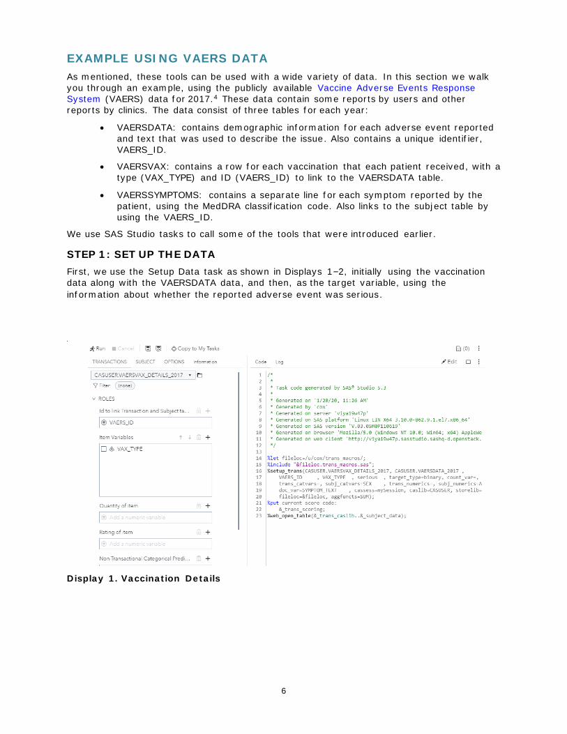
STEP 1: SET UP THE DATA

First, we use the Setup Data task as shown in Displays 1–2, initially using the vaccination

data along with the VAERSDATA data, and then, as the target variable, using the

information about whether the reported adverse event was serious.

Display 1. Vaccination Details

7

Display 2. VAERS Data Subject File

The macro creates a frequency table of the vaccination types, as shown in Display 3. The

table contains 82 values of varying frequency.

Display 3. Vaccination Frequency Counts

8

STEP 2: ROLL UP COUNT FREQUENCIES

The toolkit gives you a number of dif ferent ways to extract features from transactional

items. One of the most important questions to consider is the cardinality of the item

variables. If there are many hundreds or thousands of values, you might want to perform a

dimension reduction or use the Reduce Levels tool to compress the levels. In this case,

however, with only 82 different values, there is no need to do that. Instead you can use the

Rollup Counts tool. In Display 4, we create one variable in the subject table for each of the

vaccinations that occur at least 10 times in the data (in this case, there are 60 variables

created) and then generate a t-distributed stochastic neighbor embedding (t-SNE)7 on a

sample, plotting the result in a two-dimensional plot, colored by the target variable.

Display 4. Results of Using Rollup Counts Tool

From the plot, it appears that the serious event reports are clustered in the bottom left

corner.

Notice how simple the task parameters are on the left. There is no need to enter a table

name or any variable names. That is because the toolbox keeps track of all this information

in its global macro variables, updating them as it goes along.

Now is a good time to look at how the model is affected by the variables in the main table,

as well as by the new variables we have added. We could do this with a task for modeling,

but the purpose of this paper is to show how to prepare the data to be modeled. So let’s use

a code snippet instead, as shown in Display 5.

9

Display 5. Forest Model from Results

First look at the code on the left side of the display. Here we print to the log the value of

some of the macro variables discussed in the earlier section. In the log on the right, notice

some of these values:

• The current subject table is named VAERSDATA_2017sr. Recall from Display 2

that this was originally named VAERSDATA_2017. We have run two tools since

then, each of which added its respective character (cf. Table 1) to the data set

name when creating the new tables.

• There is one character predictor variable at this point: SEX, from the original

subject table.

• There are 62 numeric predictor variables: AGE_YRS (the patient’s age); _FREQ_,

which contains the number of vaccinations each patient received; and 60

variables, VAX_TY1–VAX_TY60, one for each of the vaccinations that occurred at

least 10 times.

• The score code calls two macros here: %setup_trans() and

%rollup_cnts_score(). You could copy and paste this code into a brand-new SAS

session, and it would enable you to score new data without changes, as long as

you set up two macro variables f irst: &score_trans_ds (for transaction data to be

scored) and &score_subj_ds (for subject data to be scored).

Notice how easy it is to specify the syntax for PROC FOREST: this same code can and will be

used many times in our example without the need for any changes, because it always uses

the current target variable as well as the current character and numeric predictors. In this

case, we have a rare target that occurs less than 5% of the time. Model performance

10

metrics such as the misclassif ication rate are not effective for problems with high class

imbalance (rare targets).6 Therefore, we have included code to calculate the precision,

recall, and F1 statistic (the harmonic mean of the two) for the results of the forest model.

We are setting the cutoff in this case to 25%, meaning that if the posterior probability for

“serious” is greater than that, we assign the case as serious. We have also set a seed for

generating the validation set, so that the same data are held out for validation every time

this model is run.

When we run the code, we can see that, with these variables at least, there are no

transactions in the validation set that are assigned as serious, so the F1 statistic is 0 (even

though the misclassif ication rate is only 4.5%).

STEP 3: PARSE DOCUMENT AND GENERATE TOPICS

Note that, in Display 2, we chose a document variable, SYMPTOM_TEXT, that contains any

text typed by the patient or clinic that reported the adverse event. Perhaps that variable can

add some discriminative capability to the model.

To check this, we can use the Parse Document tool, as shown in Display 6.

Display 6. Results of Using Parse Document Tool

11

On the left side of the display, you see that we have chosen to create 50 topics, named

(according to their pref ix) topic1 to topic50. These topics will be added to the subject table.

You can see, in the middle of the display, the key terms for some of the topics that are

generated in this way.

We can then run the PROC FOREST code snippet again, to see how the added topics affect

the results:

Here, Precision is the percentage of adverse events that the model predicted as serious that

were actually serious, Recall is the percentage of adverse events that were actually serious

and were predicted as serious, and the F1 score is the harmonic mean of the two.6

We have now produced a much more useful model, one where topics dominate in

importance (particularly topic 19) but one that also uses some information from vaccination

type.

STEP 4: ADD RULES FROM TEXT TO PREDICT TARGET

Next, we use the Predictive Rule Generation tool to try to predict serious adverse events

based on combinations of the presence and absence of particular terms in the symptom

text. Here we set three parameters. Display 7 shows the resulting rules from the tools.

Display 7. Results of Using Predictive Rule Generation Tool

12

Notice that there are rules associated with both serious=”Y” and serious=”N” and that there

are true positives (TP) and false positives (FP) associated with each one. A tilde (~)

indicates the absence of that term.

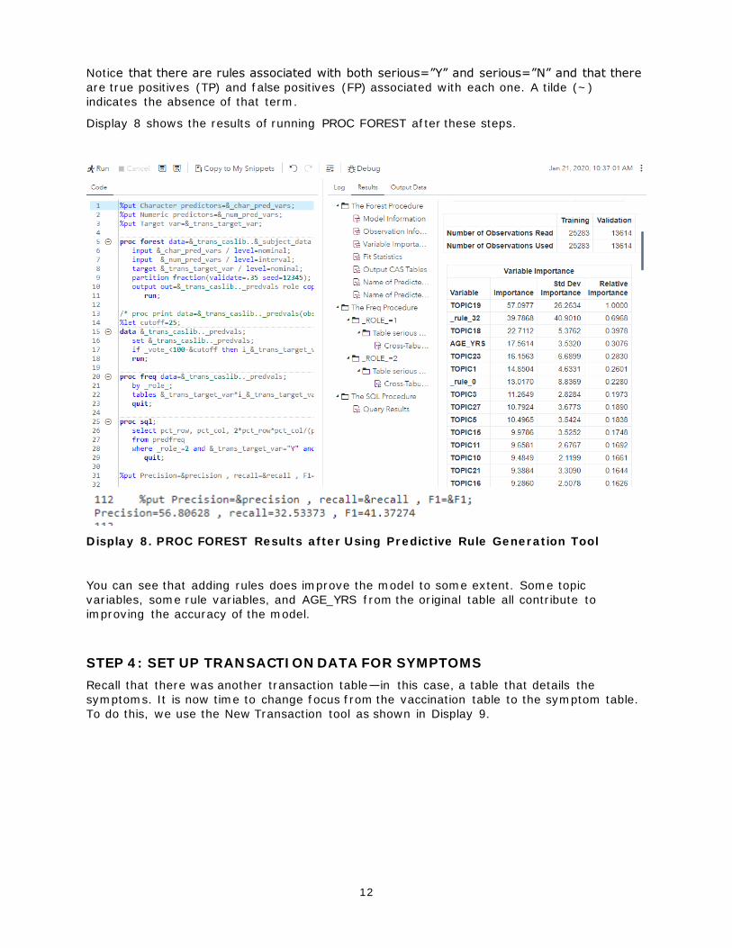
Display 8 shows the results of running PROC FOREST after these steps.

Display 8. PROC FOREST Results after Using Predictive Rule Generation Tool

You can see that adding rules does improve the model to some extent. Some topic

variables, some rule variables, and AGE_YRS from the original table all contribute to

improving the accuracy of the model.

STEP 4: SET UP TRANSACTION DATA FOR SYMPTOMS

Recall that there was another transaction table—in this case, a table that details the

symptoms. It is now time to change focus from the vaccination table to the symptom table.

To do this, we use the New Transaction tool as shown in Display 9.

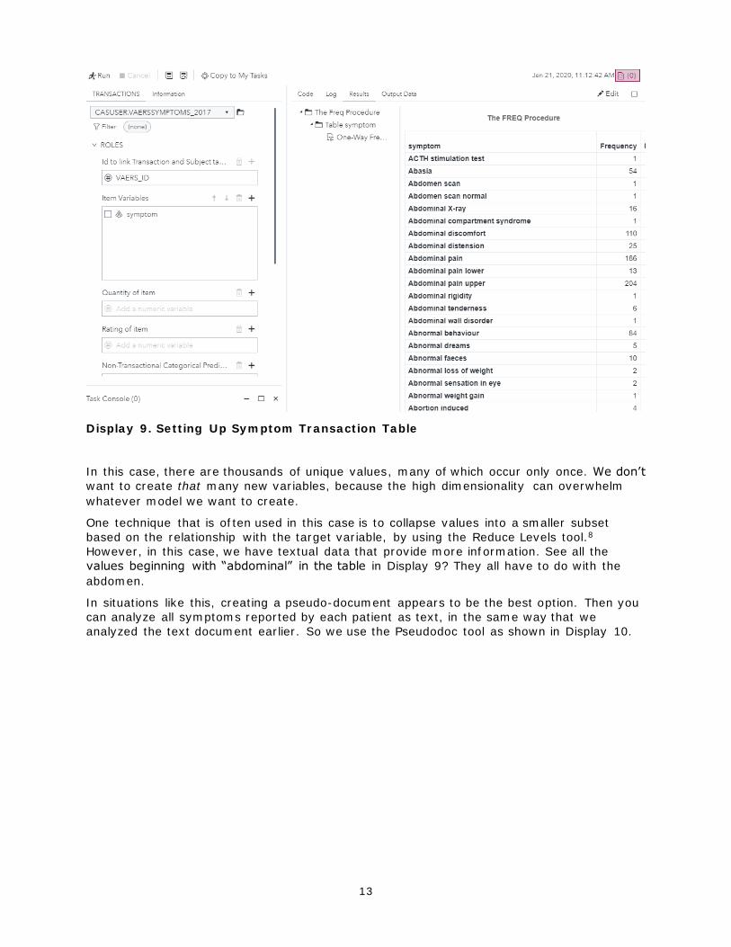
13

Display 9. Setting Up Symptom Transaction Table

In this case, there are thousands of unique values, many of which occur only once. We don’t

want to create that many new variables, because the high dimensionality can overwhelm

whatever model we want to create.

One technique that is often used in this case is to collapse values into a smaller subset

based on the relationship with the target variable, by using the Reduce Levels tool.8

However, in this case, we have textual data that provide more information. See all the

values beginning with “abdominal” in the table in Display 9? They all have to do with the

abdomen.

In situations like this, creating a pseudo-document appears to be the best option. Then you

can analyze all symptoms reported by each patient as text, in the same way that we

analyzed the text document earlier. So we use the Pseudodoc tool as shown in Display 10.

14

Display 10. Results of Using Pseudodoc Tool

This tool concatenates the strings for each reported symptom and adds a special term to

indicate the total number of symptoms reported for that patient.

We can now analyze the pseudo-document that was created in the same way that we

created the symptom text earlier, by running the Parse Document and Predictive Rule

Generation tools, and then running PROC FOREST on the result. Display 11 shows the

results.

15

Display 11. Results of Running PROC FOREST after Parsing Symptom Document

Notice that the model is improved dramatically with the symptom table, and the important

variables come from all of our sources: in this case, symptom<i> is a symptom topic, and

_rule_symp_ is a symptom-based rule. Vaersympt_freq_ represents the number of

symptoms reported.

Output 1 shows the score code generated for all the tools run in the sequence described.

%include "/u/cox/trans_macros/trans_macros.sas";

%setup_trans(&score_trans_ds,&score_subj_ds,VAERS_ID,VAX_TYPE,

target_type=binary,cassess=mySession,caslib=CASUSER,create_subj=false,

aggfuncts=SUM,copyvars=,storelib=CASUSER,scoring=true,

subj_numerics=AGE_YRS,subj_catvars=SEX,

count_var=,rating_var=,trans_numerics=,trans_catvars=);

%rollup_cnts_score(VAERSVAX_DETAILS_2017, VAX_TYPE,prefix=VAX_TY,totvals=60);

%score_parse("_textstate_1",1,document=SYMPTOM_TEXT,ntopics=30,prefix=topic);

%score_doc_boolrule(_rules_3,_ruleterms_3,prefix=_rule_) ;

%let score_trans_ds=&score_trans_ds2;

%new_trans(&score_trans_ds,VAERS_ID,symptom,trans_numerics=,trans_catvars=,

scoring=true,count_var=,rating_var=,aggfuncts=);

%pseudodoc_score(symptom,doc_var=item_doc,prefix_chars=0,doclen=32000,

neg=0,compress_items=0);

%score_parse("_textstate_3",2,document=item_doc,ntopics=30,prefix=symptom) ;

%score_doc_boolrule(_rules_5,_ruleterms_5,prefix=_rule_symp_) ;

Output 1. Score Code for Entire Model

16

Note the following from the score code in Output 1:

• The %include f ile contains all the macro definitions (or has %include statements to

separate f iles for each one).

• There is one scoring macro call for each tool in the pipeline.

• The score code references the subject table to be scored as &score_subj_ds and the

two transaction tables as &score_trans_ds and &score_trans_ds2.

You could put this code in any production system to reproduce the results on any new data,

assuming that you set &score_subj_ds, &score_trans_ds, and &score_trans_ds2 ahead of

that code.

CONCLUSION

This paper presents a toolbox that we have been developing for transactional data and

shows how to apply it to some real-world sample data. Note that this toolbox is extensible

and modular, with an easy API that you can use to create more tools. Each tool consists of a

SAS Studio task and two SAS macros: one for training and another one for scoring. The

tools communicate with each other, both at training time and at scoring time, via SAS

macro variables.

We plan to make this toolbox available in a future version of SAS® Data Management

Studio, but in the meantime, we want to expand the list of available tools to handle other

kinds of transactional data—sequence data, social network data, and so on. But even with

the current toolbox, you can perform many types of feature extraction to prepare your data

for modeling. We hope this toolbox helps you analyze your data in a far easier fashion than

you have done previously.

REFERENCES

1. Kent, W. (1983). “A Simple Guide to Five Normal Forms in Relational Database

Theory.” Communications of the ACM 26:120–125.

2. “Analytical Base Table.” Wikipedia. July 19, 2017. Available at

https://en.wikipedia.org/wiki/Analytical_base_table.

3. Ruiz, A. (2017). “The 80/20 Data Science Dilemma.” InfoWorld. September 26.

Available at https://www.infoworld.com/article/3228245/the-80-20-data-science-

dilemma.html.

4. US Department of Health and Human Services. “VAERS Data.” Accessed February

13, 2020. Available at https://vaers.hhs.gov/data.html.

5. Codd, E. F. (1970). “A Relational Model of Data for Large Shared Data Banks.”

Communications of the ACM 13.

6. Branco, P., Torgo, L., and Ribeiro, R. (2015). “A Survey of Predictive Modelling under

Imbalanced Distributions.” arXiv:1505.01658. Available at

https://arxiv.org/abs/1505.01658.

7. Van der Maaten, L. J. P., and Hinton, G. E. (2008). “Visualizing High-Dimensional

Data Using t-SNE.” Journal of Machine Learning Research 9:2579–2605.

8. Micci-Barreca, D. (2001). “A Preprocessing Scheme for High-Cardinality Categorical

Attributes in Classif ication and Prediction Problems.” ACM SIGKDD Explorations

Newsletter 3:27.

17

CONTACT INFORMATION

Your comments and questions are valued and encouraged. Contact the author:

James A. Cox

SAS Institute, Inc.

[email protected]

SAS and all other SAS Institute Inc. product or service names are registered trademarks or

trademarks of SAS Institute Inc. in the USA and other countries. ® indicates USA

registration.

Other brand and product names are trademarks of their respective companies.