Semi-analytical prediction and experimental evaluation of material damping in wood panels

DOI 10.1515/hf-2012-0095      Holzforschung 2013; 67(3): 333–343

Nathalie Labonnote * , Anders R ø nnquist and Kjell Arne Malo

Semi-analytical prediction and experimental evaluation of material damping in wood panels Abstract: A semi-analytical prediction model of mate-

rial damping in timber panels has been developed. The

approach is derived from the strain energy method and

the input is based on loss factors, which are intrinsic

properties of the considered materials, together with other

material properties and mode shape integrals, whose cal-

culation can easily be implemented in most finite element

codes. Experimental damping evaluations of particle-

boards, oriented strand boards, and structural laminated

veneer lumber panels are presented. Fair goodness of

fit between the experimental results and the prediction

models – relying only on the loss factors and the mode

shapes – reveals an efficient approach for the prediction

of material damping in timber panels including all bound-

ary conditions.

Keywords: damping prediction, experimental modal anal-

ysis, finite element analysis (FEA), LVL panels, material

damping, OSB panels, particleboard (PB) panels

*Corresponding author: Nathalie Labonnote, Department of

Structural Engineering, NTNU Norwegian University of Science and

Technology, Richard Birkelandsvei 1A, NO-7491 Trondheim, Norway,

e-mail: [email protected]

Anders R ø nnquist: Department of Structural Engineering , NTNU

Norwegian University of Science and Technology, Trondheim , Norway

Kjell Arne Malo: Department of Structural Engineering , NTNU

Norwegian University of Science and Technology, Trondheim , Norway

Introduction

Background and general aims

Comfort properties are one of the major limitations for the

development of higher timber buildings (Timmer 2011 ).

Due to their low mass, timber structures are prone to

vibrations. For timber floors, the fundamental frequency

usually coincides with the frequency of walking excita-

tion induced by the inhabitants. However, compared to

steel or other building materials, timber provides ade-

quate compensation due to its greater material damping.

In general, greater damping decreases the duration of

transient vibrations and the amplification of steady-state

vibrations. Both duration and amplitude are largely rec-

ognized as influential parameters on the perception of

vibration by human subjects (Lenzen 1966 ; Nelson 1974 ;

Wiss and Parmelee 1974 ; Ellingwood and Tallin 1984 ;

Ruffell and Griffin 1995 ). Decreasing the duration and

amplitude of vibrations leads in most cases to better

acceptance.

The damping mechanisms are still quite unknown,

probably because of less reliable measuring methods.

As a consequence, the damping quantity itself is usually

neglected in standards requirements and design codes. In

many cases, and especially for timber structures (European

Committee for Standardization 2005), this leads to con-

servative requirements and criteria, which do not consider

the advantages of timber compared to those of other build-

ing materials. Thus, a better understanding of material

damping in timber elements is urgently needed.

In the focus of the present study is a prediction method

to describe damping in timber panels. The dynamic prop-

erties of the oriented strand boards (OSBs), laminated

veneer lumber (LVL) panels, and particle boards (PBs)

will be evaluated by the driving point and roving hammer

method, which relies on the vibrations of the materials

induced by a hammer impact. This type of measurements

belongs to the category of nondestructive evaluation (NDE)

(Brashaw et al. 2009 ). NDEs, also designated as vibration

methods, are well suited for grading of wood (Brancheriau

and Baill è res 2003 ; Arriaga et al. 2012 ). Flexural vibration

tests are successful in predicting mechanical properties

of solid wood (Biechle et al. 2011 ; Yoshihara 2012a,b ).

The vibration methods consider the material-dependent

damping, the loss factors, and system properties, such as

mode shapes. The latter can easily be calculated by means

of finite element analyses (FEA) (Figure 1 a).

In the present work, the experimental damping data

of OSBs, LVLs, and PB panels are compared with those of

model calculations. From the validated model, loss factor

values will be calculated (Figure 1b).

Theoretical background and specific aims

Damping in timber material was seldom measured (Placet

et al. 2007 ), and mainly the quality of musical timber

Authenticated | [email protected] author's copyDownload Date | 7/3/13 9:24 AM

334      N. Labonnote et al.: Prediction models for wood panels

instruments was in focus (Fukada 1950, 1951 ; Ono 1983 ;

Ono and Norimoto 1985 ; Obataya et al. 2000 ; Spycher

et al. 2008 ). Ungar and Kerwin (1962) were one of the first

to define the equivalent viscous damping ratio ξ in terms

of energy:

2 =

2

DW

ξπ

(1)

where D = energy dissipated per cycle, and W = total energy

(kinetic plus potential) associated with the vibration.

However, they recognized that the definition of W as the

total energy for the considered cycle was unambiguous

only for lightly damped structures, for which the total

energy does not fluctuate much throughout a cycle. They

therefore proposed computing W as the total strain energy

at maximum strain in the case of lightly damped struc-

tures. Adams and Bacon (1973b) adopted the quoted sug-

gestion, and defined the specific damping capacity ϕ as

the ratio between the dissipated energy Δ U per cycle of

vibration to the maximum strain energy U :

4

UU

ϕ πξΔ= =

(2)

The dissipated strain energy Δ U has commonly been

defined via the introduction of loss factors η i for each type

of strain energy U i , i.e.:

2

4i i

i

ii

U

U

πηϕ πξ= =

∑∑

(3)

The strain energies are determined with respect to the

strain field ε and the stiffness matrix C . For example, for a

plate of thickness h , U per unit area is expressed as:

{ } { }= ∫/2

- /2

1[ ]

2

hT

h

U dzCε ε

(4)

For small deformations and displacements, the strain

field is derived from the displacement field as:

1

2

jiij

j i

wwx x

ε⎛ ⎞∂∂= +⎜ ⎟∂ ∂⎝ ⎠

(5)

The strain energies may therefore be expressed with

respect to the mode shapes w . Since then, Adams and

Bacon ’ s model was extensively applied in investigations

on composites (Adams and Bacon 1973a ; Ni and Adams

1984 ; Adams and Maheri 1994 ; Kam and Chang 1994 ;

Saravanos 1994 ; Chandra et al. 2003 ; R é billat and Bou-

tillon 2011 ). A slight modification to Adams and Bacon ’ s

model was brought by McIntyre and Woodhouse (1978) ,

who introduced Rayleigh ’ s principle. McIntyre and Wood-

house (1988) were also among the first ones to apply a

damping prediction model to various timber elements.

However, they defined the loss factors with respect to

complex flexural rigidities and did not explicitly deter-

mine the mode shapes as real or complex quantities.

In the present paper, an improved damping predic-

tion model will be developed on the basis of McIntyre and

Woodhouse ’ s approach (1988). Experimental evaluations

of damping in various timber panels will be described as

well as the numerical models for calculating the mode

shape integrals. The fitting procedure and the validation

of the prediction models will be further discussed. The

relative distribution of different types of damping for each

mode shape should also be investigated.

Materials and methods

Analytical prediction model

Kirchhoff theory

Thin rectangular plates, for which the Kirchhoff theory is appropri-

ate, are considered in the present study. The coordinate system de-

scribed in Figure 2 is used. The direction 1 is referred to as longitudi-

nal, and the direction 2 is referred to as transverse. Assumptions for

the study are the following:

– Thickness is small compared to other dimensions.

– Normal sections remain normal to neutral plane, i.e., the shear

deformation is neglected.

– Nonlinear terms in displacement are neglected, i.e., the rotary

inertia is neglected.

– Plane stress conditions, i.e., σ 3 is zero.

Mode shape integrals(FEA)

Loss factors(database)

Predictionmodel

Experimentaldamping

evaluations

Validatedprediction

model

Fittingprocedure

Lossfactors

Nominal material properties(datasheet)

Predicted globaldamping

a

b

Figure 1   Procedure for predicting global material damping in

vibrating timber structures (a) and validation of the proposed

method (b).

Authenticated | [email protected] author's copyDownload Date | 7/3/13 9:24 AM

N. Labonnote et al.: Prediction models for wood panels      335

Assuming separation of variables, the displacement fi eld is writ-

ten as:

1 2 3 3

1

1 2 3 3

2

1 2 3 1 2

( , , , ) -

( , , , ) -

( , , , ) ( , , )

wu x x x t xxwv x x x t xx

w x x x t w x x t

∂=∂∂

=∂

=

(6)

Rayleigh ’ s principle

The kinetic energy of a homogeneous plate of area A and thickness

h is written as:

22 21

2 2A A

hT hw dA w dAρ ωρ= =∫∫ ∫∫�

(7)

where ρ is the density and ω is the frequency of the motion.

If the plate is isotropic, the potential energy V corresponds to

the strain energy and is written as:

( )2 2

,11 ,22

1

2V D w w dA= +∫∫

(8)

with the bending stiff ness D defi ned as:

3

212( 1- )

EhDν

=

(9)

where E = elastic modulus of elasticity, ν = Poisson ’ s ratio, and

2

,ikww

i k∂

=∂ ∂

.

For a specially orthotropic material (Daniel and Ishai 2006 ),

the strain energy V corresponds to the strain energy and is written

as:

( )2 2 2

11 ,11 12 ,11 ,22 22 ,22 66 ,12

12

2 A

V D w D w w D w D w dA= + + +∫∫

(10)

with the diff erent fl exural rigidities defi ned as:

3 3 3

1 12 2 21 111 12

12 21 12 21 12 21

3 3

2 1222 66

12 21

12( 1- ) 12( 1- ) 12( 1- )

12( 1- ) 3

E h v E h v E hD D

E h G hD D

ν ν ν ν ν ν

ν ν

= = =

= =

(11)

According to Rayleigh ’ s principle:

V = T (12)

Finally, for an isotropic homogeneous thin plate:

2 2

,11 ,222

2

( )D w w dAh w dA

ωρ

+= ∫∫

∫∫

(13)

and for a specially orthotropic homogeneous thin plate:

2 2 2

11 ,11 12 ,11 ,22 22 ,22 66 ,12

2

2

( )A

D w D w w D w D w dA

h w dAω

ρ

+ + +=∫∫

∫∫

(14)

Implementation of damping

The complex elastic moduli E 1 * and E

2 * , the complex shear modulus

G 12 * , and the complex Poisson ratios ν

12 * and ν

21 * are defi ned as:

*

1 1 1

*

2 2 2

*

12 12 12

*

12 12 12

*

21 21 21

( 1 )

( 1 )

( 1 )

( 1 )

( 1 )

E

E

G

E E jE E jG G j

jj

ν

ν

η

η

η

ν ν η

ν ν η

≡ +

≡ +

≡ +

≡ +

≡ +

(15)

where j 2 = -1. The loss factors η E 1 , η E

2 , η G

12 , η ν 12

, and η ν 21 are defi ned from

Eq. (15) and are dimensionless. Due to the symmetry of the stiff ness

matrix, the fi ve-loss factors are not independent, and

η ν 12 + η E

2 = η ν 21

+ η E 1 (16)

The complex fundamental frequency is defi ned with respect to

the attenuation α , so that:

3

a b

2

1

100

10

0.1FRF

mag

nitu

de

0.010 50 100

Frequency (Hz)150 200

1

Figure 2   Evaluation methods of the dynamic properties: (a) driving point, (b) roving hammer.

Authenticated | [email protected] author's copyDownload Date | 7/3/13 9:24 AM

336      N. Labonnote et al.: Prediction models for wood panels

ω * ≡ ω 0 + j

α

(17)

The equivalent viscous damping ratio, referred to as ξ , is then

defi ned as:

0

Im( *)

Re( *)

ω αξ

ω ω≡ =

(18)

The assumption of small damping,

α � ω 0 (19)

yields the relationship:

Re( ω *2 ) ≈ ω *2 (20)

Hence,

*2 *2

0 0

2 *2 2 2 2

0 0 0

Im( ) Im( ) 2 22 2

Re( ) -

ω ω ω α ω α αξ

ω ω ω α ω ω= = =� �

(21)

Prediction models (PrMs)

A PrM may therefore be derived for each specifi c material constitutive

behavior. According to the correspondence principle, defi ned among

others by Hashin (1970) , any relationship is still valid when complex

quantities are considered instead of real ones. In addition, Johnson

and Kienholz (1983) , and later Talbot and Woodhouse (1997) , as-

sumed that the real mode shapes obtained for an undamped motion

were an approximation of the true complex mode shapes obtained

for a damped motion. The quoted authors revealed that their approx-

imation was reasonable even for values of material damping higher

than 1 % .

For an isotropic material, the loss factor η E is defi ned as:

η E = η E 1 = η E 2

(22)

Hence, by combination of Eqs. (13), (15), and (21), the damping

PrM for an isotropic thin plate is:

2 ξ = η E (23)

For a specially orthotropic thin plate, combining Eqs. (14), (15),

and (21), the damping PrM becomes:

*2

11 2211 1 22 2*2 2 2

12 6612 12 22 21 11 66 122 2

Im( )2

Re( )

( )

E E

E E G

D DI Ih h

D DI Ih h

ωξ η η

ω ω ρ ω ρ

η η η η ηω ρ ω ρ

= = +

+ + + + +ν ν

(24)

The mode shape integrals I 11

, I 22

, I 12

and I 66

are parameters de-

fi ned as:

2

,11 ,11 ,22

11 122 2

2 2

,22 ,12

22 662 2

w dA w w dAI I

w dA w dA

w dA w dAI I

w dA w dA

= =

= =

∫∫ ∫∫∫∫ ∫∫∫∫ ∫∫∫∫ ∫∫

(25)

where w = real undamped mode shape.

Interpretations

The prediction models may be conveniently interpreted in terms of

energies. From Eq. (24), strain energies may be expressed as:

2

ij ij ijU D I w dA= ∫∫

(26)

Diverse strain energies are exhibited: ( U 11 + U

12 ) is the strain en-

ergy stored in tension-compression in the longitudinal direction 1,

( U 22

+ U 12

) is the strain energy stored in tension-compression in the

transverse direction 2, 2 U 12

is the strain energy induced by Poisson ’ s

eff ect, and U 66

is the strain energy stored in in-plane shear. It has

been observed (Adams and Bacon 1973a ; Ni and Adams 1984 ; Billups

and Cavalli 2008 ; Maheri 2011 ) that in some cases, only U 11

, U 22

and

U 66

contributed signifi cantly to the total strain energy because D 12

≈ 0.

In these cases, the damping PrM in Eq. (24) is reduced to:

11 22 6611 1 22 2 66 122 2 2

2 E E GD D DI I I

h h hξ η η η

ω ρ ω ρ ω ρ= + +

(27)

Damping prediction models in Eqs. (24) and (27) are referred to

as the fi ve-loss factor (5-LF) model and the three-loss factor (3-LF)

model, respectively.

From Eq. (24), it is apparent that the global material damping 2 ξ of a vibrating timber panel can be divided into diff erent global damp-

ing quantities:

– damping due to bending in the longitudinal direction: 2 ξ L

– damping due to bending in the transverse direction: 2 ξ T

– damping due to in-plane shear: 2 ξ S

defined such that:

2 ξ = 2 ξ L + 2 ξ

T + 2 ξ

S (28)

Thus, for the 5-LF model, the global damping quantities are

defi ned by:

11 11 12 12 12 12L 1 212 2

22 22 12 12 12 12T 2 122 2

66 66S 122

2

2

2

E v

E v

G

D I D I D Ih h

D I D I D Ih h

D Ih

ξ η ηω ρ ω ρ

ξ η ηω ρ ω ρ

ξ ηω ρ

+= +

+= +

=

(29)

whereas for the 3-LF model, the global damping quantities are

defi ned by:

11 11L 12

22 22T 22

66 66S 122

2

2

2

E

E

G

D Ih

D Ih

D Ih

ξ ηω ρ

ξ ηω ρ

ξ ηω ρ

=

=

=

(30)

Experimental design A total of 18 sheathing panels were tested: three PB panels (Aasen &

Five AS, Stj ø rdal, Norway), three OSB panels (Aasen & Five AS), and

three structural LVL panels (Moelven Limtre AS, Moelven, Norway).

Authenticated | [email protected] author's copyDownload Date | 7/3/13 9:24 AM

N. Labonnote et al.: Prediction models for wood panels      337

In PBs there is no privileged particle orientation, so they are iso-

tropic. OSB panels are made of longer wood particles and are com-

monly composed of three layers, in which the particles are either

aligned along the long axis of the panel (outer layers) or glued in a

random process (inner layer). OSB panels have therefore transversely

isotropic material properties (Wang and Chen 2001 ). LVL panels are

made of glued layers of wood veneer. In the present study, Kerto-Q

panels (Metsä, Finland) (Mets ä Wood; http://www.metsawood.com/

products/kerto/Pages/Kerto-Q.aspx) are used, which means that

about 80 % of the layers are aligned along the long axis of the panel,

whereas the remaining layers are aligned orthogonally to the main

orientation. LVL panels therefore exhibit orthotropic material prop-

erties. The nominal dimensions for each panel are summarized in

Table 1 . Mean stiff ness values and characteristic density values for

each type of panel are given in Table 2 (European Committee for

Standardization 2001). The orientations refer to the coordinate sys-

tem displayed in Figure 2.

Temperature and relative humidity (20 ° C and 40 – 50 % , respec-

tively) were not controlled but were assumed to follow standard

laboratory conditions. Steel cylinders with outer diameter of 133 mm

and thickness of 4 mm served as supports. Each panel was evaluated

for three diff erent types of boundary condition: simply supported on

the two short sides, simply supported on the two long sides, or sim-

ply supported on four sides. For some panels, an initial warp was

observed, which induced slightly diff erent boundary conditions: sim-

ply supported on three sides rather than on four sides. The boundary

conditions have been chosen to closely represent actual fl oor sys-

tems. It is assumed that friction at support was small enough to be

neglected as a contribution to damping.

The modal hammer “ heavy-duty type 8208 ” (Br ü el & Kj æ r,

N æ rum, Danmark) was used to set the panel into motion and to record

the impact load. A soft tip was employed to excite lower frequencies.

Transient vibrations due to modal hammer impact were recorded by a

ceramic/quartz impedance head Kistler accelerometer type 8770A50

(Scanditest Norge AS, Holmestrand, Norway) that was screwed into

the panel. An experimental modal analysis soft ware was provided by

National Instruments (2011) to record and process the data based on

the graphical development environment LabVIEW. The load and ac-

celeration time series were then digitalized and processed by a dy-

namic signal analyzer. The sampling frequency was fi xed to 2048 Hz,

and 5-s data were recorded for each impact. Noise outside the period

of impact was deemed small enough to be neglected.

Methods

The dynamic properties of the sheathing panels were evaluated by

two successively applied methods (Figure 2). The hammer impact is

soft enough not to infl ict any damage to the panel or modify its prop-

erties. Thus, an unlimited number of repeated measurements can be

performed on each specimen. The “ driving point ” method is faster

(De Silva 2005 ) than the “ roving hammer ” method (Schwarz and

Richardson 1999 ); each panel was evaluated 10 times by the former

and only once by the latter.

For the driving point method, the unique location of both the

accelerometer and the impact was designed so as to maximize the

number of observed modes of vibration. For each panel, and for each

observed mode of vibration, a population of 10 equivalent viscous

damping ratios ξ was evaluated. In addition, the mode shapes corre-

sponding to each type of panel (given thickness and given material)

were evaluated by means of the roving hammer method, which con-

sists of impacting diff erent points, usually organized on a grid, while

the accelerometer remains at one unique location. The grid consisted

of 84 to 91 measurement points, depending on the type of panel. This

is equivalent to a 20- to 25-cm spaced grid.

Modal parameter identification

The fundamental frequencies, the damping ratios, and the mode

shapes of the sheathing panels were determined by means of experi-

mental modal analysis with the fundamental assumption of small

damping (Ewins 2000 ). The frequency response function H relates

the input signal spectrum from the hammer F and the output signal

spectrum from the accelerometer X in the frequency domain:

( )( )

( )

XHF

ωω

ω≡

(31)

where ω = frequency in radians per second. A linear average of the fre-

quency response function over two impacts is performed. Identifi cation

NameNo. of tested

panelsDimensions

(m) ×× (m)Thickness

(mm)

PB-19 3 1.25 × 2.6 19

PB-22 3 1.25 × 2.6 22

OSB-18 3 1.22 × 2.4 18

OSB-22 3 1.22 × 2.4 22

LVL-21 3 1.20 × 2.4 21

LVL-24 3 1.20 × 2.4 24

Table 1   Nominal dimensions of the tested sheathing panels.

PB, particle board; OSB, oriented strand board; LVL, structural

laminated veneer lumber.

Literature data of stiffness and density Data for statistical treatment: numbers of

E1 (MPa) E2 (MPa) E3 (MPa) G12 (MPa) G23 (MPa) G13 (MPa) Density (kg m -3 ) Evaluations Discarded Configurations

PB 1600 1600 1600 770 770 770 550 532 35 21

OSB 3800 3000 3000 1080 50 50 550 450 19 17

LVL 10,000 2400 130 600 22 60 480 502 7 17

Table 2   Mean stiffness, characteristic density values (source: VTT Technical Research Centre 2009 ), and statistical data to evaluation of

the experiments: numbers of evaluation, discarded experiments, and configurations selected.

Authenticated | [email protected] author's copyDownload Date | 7/3/13 9:24 AM

338      N. Labonnote et al.: Prediction models for wood panels

of transfer function models is performed by curve fi tting the averaged

frequency response function with suitable analytical expressions, so

that:

2 21

( )

[ - 2 ]

( ) residues

with natural frequency

equivalent viscous modal damping ratio

ni k r

ikr r r r

i k r

r

r

Hj

ψ ψ

ω ω ξ ω ω

ψ ψ

ω

ξ

=

=+

⎧ =⎪⎪ =⎨⎪ =⎪⎩

∑

(32)

where r = mode number and n = total number of modes. The natural

frequency and the viscous modal damping ratio are directly extract-

ed from Eq. (32). The mode shape vectors Ψ r are extracted from Eq.

(32) as:

2

1 1 2 1 13( ) ( ) ( )r r r rψ ψ ψ ψ ψ=⎡ ⎤⎣ ⎦�ΨΨ

(33)

The parameter identifi cation method is based on the frequency-

domain direct parameter identifi cation fi tting method, which is a fre-

quency domain multiple degree-of-freedom modal analysis method

suitable for narrow frequency band and well-separated modes.

Statistical treatment of the results

A total of 1484 equivalent viscous damping ratio evaluations ξ were

performed and are classifi ed into diff erent “ confi gurations ” . A con-

fi guration is defi ned by a material, a thickness, boundary conditions,

and the mode number. For instance, the confi guration “ OSB-21-

short-3 ” collects equivalent viscous damping ratio evaluations ξ of

OSB panels, 21 mm thick, simply supported along the short sides, for

the third mode of vibration.

It is assumed that most of the equivalent viscous damping ra-

tio evaluations ξ collected under a given configuration are repre-

sentative of a unique population, which is the material damping

related to the given configuration. Equivalent viscous damping

ratio evaluations are identified that are collected under a given

configuration, but do not belong to the assumed population, e.g.,

occurrences of noise or external perturbation acting on the panel.

The criterion for identifying a damping evaluation ξ not belong-

ing to the assumed population for a given configuration is adapt-

ed from Minitab statistical software (2010) , and is defined as

follows:

1 3 1 3 3 1

1 3 1 3 3 1

If [ -1.5( - ); +1.5( - )],

then belongs to the population

If [ -1.5( - ); +1.5( - )],

then does not belong to the population

Q Q Q Q Q Q

Q Q Q Q Q Q

ξ

ξ

ξ

ξ

∈⎧⎪⎪⎨ ∉⎪⎪⎩

(34)

where Q 1 and Q

3 are the lower and upper quartiles (Walpole et al.

2007 ), respectively. Identifi ed evaluations not belonging to the as-

sumed population of a given confi guration are discarded, and sta-

tistical indicators are then computed for each confi guration. The low

percentage of removal actions (4 % ) indicates good consistency of ex-

perimental results. The record of removal actions is given in Table 2.

The mean value, the standard deviation, and the corresponding 95 %

confi dence intervals of the equivalent viscous damping ratio evalua-

tions for each confi guration are presented in Table 3 .

Relevant configurations for comfort properties

Only the confi gurations relevant to the problem of comfort properties

of timber fl oors are fi nally included for parameter fi tting. The relevance

of a given confi guration is assessed according to two principles: funda-

mental frequency related to the mode number in the range defi ned by

Eurocode 5 (European Committee for Standardization 2005 ) and reli-

able enough experimental evaluations, i.e., limited observed scatter.

The corresponding criterion is defi ned as:

length

a ) 35 Hz

b) CI 0.15

f

ξ

≤

≤ ×

(35)

where f = fundamental frequency related to the mode number of the

considered confi guration, and CI length

= width of the 95 % confi dence

interval related to the mean value of the equivalent viscous damp-

ing ratio ξ , expressed as a percentage of the mean value ξ itself.

Nonrelevant confi gurations according to the criterion in Eq. (35) are

mentioned in Table 3.

Numerical analyses

Numerical models

Mode shape integrals defi ned in Eq. (25) were numerically deter-

mined. Finite element analyses were performed by the commercial

soft ware Abaqus, version 6.9 (Dassault Syst è mes Simulia Corp.,

Providence, RI, USA). All timber panels are modeled using the gen-

eral linear, reduced integration, shell element S4R. The mesh size is

chosen to be approximately 0.01 m and corresponding to a converg-

ing model. Numerical results are considered as undamped results.

In accordance with previous assumptions, all material properties

are implemented as nominal values, given in Table 2. Boundary

conditions are implemented following two diff erent methods: either

by the contact between the steel pipes and the timber panel, or by

constraining selected degrees of freedom along the panel edges. The

observed diff erence between the two methods is small; therefore, the

latter method is chosen for its shorter CPU time.

Check of the numerical models

Good agreement is generally observed between experimental and

numerical fundamental frequencies. Lower numerical fundamental

frequencies are observed for all confi gurations related to PBs, which

may suggest that the stiff ness properties of the specimens are prob-

ably larger than the nominal ones. Good agreement is observed be-

tween experimental and numerical results for OSB and LVL panels,

with respect to both fundamental frequencies and mode shapes.

Calculation of mode shape integrals

A procedure is written to calculate the mode shape integrals defi ned

in Eq. (25) via Abaqus. The script is based on numerical integration,

but uses only limited numerical diff erentiation, as Abaqus provides

Authenticated | [email protected] author's copyDownload Date | 7/3/13 9:24 AM

N. Labonnote et al.: Prediction models for wood panels      339

Configuration Mean ξ 95 % CI mean values StdD Frequency (Hz) No. of evaluation

PB-19-4sides-1 0.0142 [0.0139; 0.0145] 0.0007 12.45 26

PB-19-4sides-2 0.0131 [0.0130; 0.0133] 0.0004 19.78 24

PB-19-long-1 0.0134 [0.0129; 0.0138] 0.0011 9.74 29

PB-19-long-2 0.0132 [0.0127; 0.0137] 0.0011 11.92 21

PB-19-long-3 0.0130 [0.0123; 0.0137] 0.0013 18.11 16

PB-19-short-1 0.0115 [0.0108; 0.0121] 0.0017 2.20 29

PB-19-short-3 0.0108 [0.0105; 0.0111] 0.0009 8.90 31

PB-19-short-4 0.0117 [0.0110; 0.0124] 0.0014 16.40 20

PB-19-short-5 0.0107 [0.0103; 0.0111] 0.0009 20.16 21

PB-19-short-6 0.0107 [0.0101; 0.0114] 0.0015 26.72 21

PB-22-4sides-1 0.0166 [0.0159; 0.0173] 0.0011 14.42 11

PB-22-4sides-2 0.0149 [0.0147; 0.0152] 0.0006 22.89 29

PB-22-long-1 0.0135 [0.0131; 0.0138] 0.0008 11.28 30

PB-22-long-2 0.0121 [0.0113; 0.0128] 0.0015 13.79 19

PB-22-long-3 0.0134 [0.0130; 0.0139] 0.0011 20.96 28

PB-22-long-4 0.0120 [0.0114; 0.0126] 0.0008 32.28 8

PB-22-short-1 0.0113 [0.0108; 0.0117] 0.0012 2.55 28

PB-22-short-3 0.0102 [0.0097; 0.0106] 0.0011 10.31 26

PB-22-short-4 0.0091 [0.0083; 0.0098] 0.0011 18.98 10

PB-22-short-5 0.0132 [0.0128; 0.0137] 0.0006 23.33 11

PB-22-short-7 0.0111 [0.0104; 0.0119] 0.0021 33.35 30

OSB-18-3sides-1 0.0168 [0.0147; 0.0179] 0.0029 14.20 30

OSB-18-3sides-2 a 0.0199 [0.0175; 0.0224] 0.0054 20.30 21

OSB-18-long-1 0.0142 [0.0135; 0.0150] 0.0020 13.49 30

OSB-18-long-2 0.0141 [0.0135; 0.0147] 0.0016 16.01 30

OSB-18-long-3 0.0131 [0.0125; 0.0138] 0.0010 24.24 11

OSB-18-short-1 0.0081 [0.0078; 0.0085] 0.0009 3.74 31

OSB-18-short-2 0.0080 [0.0078; 0.0083] 0.0006 9.35 30

OSB-18-short-3 0.0107 [0.0098; 0.0117] 0.0025 15.04 31

OSB-18-short-4 0.0141 [0.0136; 0.0147] 0.0008 22.73 10

OSB-22-4sides-1 0.0153 [0.0148; 0.0158] 0.0013 20.74 31

OSB-22-4sides-2 0.0139 [0.0137; 0.0142] 0.0003 33.71 10

OSB-22-long-1 0.0119 [0.0117; 0.0122] 0.0006 16.43 21

OSB-22-long-2 0.0129 [0.0125; 0.0133] 0.0009 19.47 21

OSB-22-short-1 0.0083 [0.0080; 0.0085] 0.0007 4.57 31

OSB-22-short-2 0.0099 [0.0096; 0.0102] 0.0008 11.36 29

OSB-22-short-3 0.0081 [0.0078; 0.0083] 0.0006 18.29 28

OSB-22-short-4 0.0090 [0.0088; 0.0092] 0.0003 27.55 11

LVL-21-3sides-1 0.0129 [0.0124; 0.0134] 0.0014 14.73 31

LVL-21-3sides-2 a 0.0138 [0.0157; 0.0180] 0.0017 22.31 11

LVL-21-long-1 0.0124 [0.0122; 0.0126] 0.0005 14.17 30

LVL-21-long-2 0.0101 [0.0098; 0.0104] 0.0009 16.14 31

LVL-21-long-3 0.0075 [0.0070; 0.0080] 0.0011 27.35 21

LVL-21-short-1 0.0055 [0.0053; 0.0057] 0.0006 7.29 31

LVL-21-short-2 0.0096 [0.0093; 0.0099] 0.0008 10.63 30

LVL-21-short-3 0.0057 [0.0054; 0.0060] 0.0004 28.68 9

LVL-21-short-4 0.0076 [0.0073; 0.0079] 0.0004 32.46 11

LVL-21-short-5 a 0.0119 – – 36.78 1

LVL-21-short-6 a 0.0060 – – 53.58 1

LVL-24-3sides-1 0.0152 [0.0149; 0.0156] 0.0009 16.75 30

LVL-24-long-1 0.0101 [0.0098; 0.0103] 0.0007 16.61 31

LVL-24-long-2 0.0093 [0.0091; 0.0095] 0.0004 18.34 31

LVL-24-long-3 0.0063 [0.0061; 0.0066] 0.0003 31.05 11

LVL-24-short-1 a 0.0050 [0.0045; 0.0054] 0.0012 8.31 31

LVL-24-short-2 0.0073 [0.0071; 0.0076] 0.0006 12.11 30

Table 3   Experimental damping evaluations, and selected configurations for fitting of parameters.

a Nonrelevant configuration. StD, standard deviation.

Authenticated | [email protected] author's copyDownload Date | 7/3/13 9:24 AM

340      N. Labonnote et al.: Prediction models for wood panels

by itself surface curvatures in the directions of the defi ned coordinate

system. A good convergence of all mode shape integrals, I 11

, I 22

, I 12

and

I 66

, is observed for the selected mesh size, i.e., 10 mm.

Results and discussion

Fitting procedure

For the PB panels, the isotropic damping prediction model

(PrM) in Eq. (23) applies. Consequently, fitting the param-

eter results in finding the value of η E that minimizes the

difference ˆ2 - Eξ η , where ̂ξ = experimental evaluations of

damping.

For the OSB panels, the 5-LF orthotropic model in Eq.

(24) applies, and yields, in matrix form:

ν

η

η η

η ω ρη

⎡ ⎤⎧ ⎫⎢ ⎥⎪ ⎪+⎪ ⎪ ⎢ ⎥= =⎨ ⎬ ⎢ ⎥

⎪ ⎪ ⎢ ⎥⎪ ⎪ ⎢ ⎥⎩ ⎭ ⎣ ⎦

11 111

21 2 12 12

2 22 22

12 66 66

2{ 2 } { } with { } and

TE

E

E

G

D ID I

D IhD I

ξ η ηB B2

1=

(36)

For LVL panels, the strain energy induced by Pois-

son ’ s effect U 12

is found to be nonsignificant compared to

other types of strain energy. Consequently, the 3-LF model

in Eq. (27) applies, and yields, under matrix form:

η

ηω ρ

η

⎡ ⎤⎧ ⎫⎢ ⎥⎪ ⎪= =⎨ ⎬ ⎢ ⎥

⎪ ⎪ ⎢ ⎥⎩ ⎭ ⎣ ⎦

11 111

2 22 22

12 66 66

{ 2 } { } with { } and

T

E

E

G

D ID I

hD I

B Bξ η η2

1=

(37)

The fitted LF vector { }�ηη is obtained from the experi-

mental evaluations of damping ξ̂ as:

{ } -1 ˆ( ) { 2 }T T= B B B�ηη ξ (38)

The goodness of fit is quantified through the coef-

ficient of determination R 2 (Walpole et al. 2007 ), which

measures the proportion of variability explained by the

fitted model. R 2 is defined by:

2 err

tot

1-SSRSS

=

(39)

where SS err

= error sum of squares, corresponds to the

unexplained variation, and SS tot

= total corrected sum

of squares, corresponds to the variation in the response

model that would ideally be explained by the model.

Keeping matrix notations from Eq. (38) yields:

( )

⎡ ⎤⎣ ⎦=⎡ ⎤⎣ ⎦

-1

2

-1

ˆ ˆ{ 2 } - ( ) { 2 }1-

ˆ ˆ{ 2 } -{ } { } { } { } { 2 }

T T Tn

T T Tn

RI B B B B

I 1 1 1 1

ξ ξ

ξ ξ

(40)

with { 1 } = vector of n ones, I n = identity matrix of rank n ,

n = number of available configurations.

The thin isotropic plate PrM in Eq. (23) is applied to

experimental results from PBs.

Validation of the prediction models

Results from the fitting procedures are presented in Table

4 . In particular, negative values for the LFs η ν 12 and η ν 21

were obtained when applying the 5-LF thin orthotropic

plate PrM to experimental results from LVL panels. This is

most likely due to the very low value of the strain energy

induced by the Poisson ’ s effect 2 U 12

.

According to the value of R 2 (70 % ), the 5-LF thin ortho-

tropic plate PrM in Eq. (24) is the best fit for OSB panels,

compared to the R 2 (36 % ) of 3-LF thin orthotropic plate

PrM in Eq. (27).

Concerning LVL panels, the R 2 data are similar for

both PrMs, i.e., 71 % and 73 % . However, the 5-LF thin

orthotropic plate PrM induces nonphysical negative

values for the LFs η ν 12 and η ν 21

. These are due to the very

low value of the strain energy induced by the Pois-

son ’ s effect 2 U 12

. As underlined previously, this effect

had already been observed in several studies. In order

to avoid nonphysical LFs values, the 3-LF thin ortho-

tropic plate PrM in Eq. (27) is to prefer for LVL panels.

In conclusion, the high R 2 values for OSB and LVL

panels for the selected PrMs indicate that the orthotropic

damping PrM agrees well with the experimental damping

evaluations, and thus validates the PrMs.

Comparison of fitted loss factors with those from previous studies

McIntyre and Woodhouse (1988) reported fitted LFs values

for different timber products. For convenience, their

results are quoted in Table 5 , and based on this it can be

stated that thin isotropic plate for PBs, thin orthotropic

plate 5-LF for OSB panels, and thin orthotropic plate 3-LF

for LVL panels, the fitted LF values given in Table 4 are

consistent with the results obtained by McIntyre and

Woodhouse for a plywood plate. More studies would,

however, be needed to build a complete database of LF

values for timber products.

Authenticated | [email protected] author's copyDownload Date | 7/3/13 9:24 AM

N. Labonnote et al.: Prediction models for wood panels      341

Figure 3   Distribution of longitudinal bending, transverse bending, and in-plane shear bending quantities for LVL panels.

Fitted loss factors

Panel type η E 1 η E 2 η G 12

Plywood plate 0.0110 0.0120 0.0237

Quarter cut Norway spruce 0.0051 0.0216 0.0164

40 ° ring angle Norway spruce 0.0074 0.0212 0.0139

Table 5   Fitted loss factors reported by McIntyre and Woodhouse

(1988).

Repartition of bending and shear damping quantities

From Eq. (28), the global system damping is expressed as

the sum of three damping quantities, related either to lon-

gitudinal bending, transverse bending, or in-plane shear.

The repartition of the three damping quantities is given

for each configuration related to LVL panels in Figure 3 . As

Panel Material properties Prediction model Fitted parameters R 2 ( % )

PB Isotropic Isotropic η E = 0.020 –

η E 1 = 0.022

η E 2 = 0.031

OSB Transversely isotropic Orthotropic, 5-LF η G 12

= 0.020 70

η ν 12 = 0.033

η ν 21 = 0.041

η E 1 = 0.016

OSB Transversely isotropic Orthotropic, 3-LF η E 2 = 0.029 36

η G 12

= 0.024

η E 1 = 0.010

η E 2 = 0.023

LVL Orthotropic Orthotropic, 5-LF η G 12

= 0.020 73

η ν 12 = -0.057

η ν 21 = -0.044

η E 1 = 0.011

LVL Orthotropic Orthotropic, 3-LF η E 2 = 0.024 71

η G 12

= 0.018

Table 4   Goodness of fit for each prediction model based on thin plates.

R 2 , goodness of fit.

Authenticated | [email protected] author's copyDownload Date | 7/3/13 9:24 AM

342      N. Labonnote et al.: Prediction models for wood panels

LVL-21-long-1 LVL-21-short-1 LVL-21-short-2

a b c

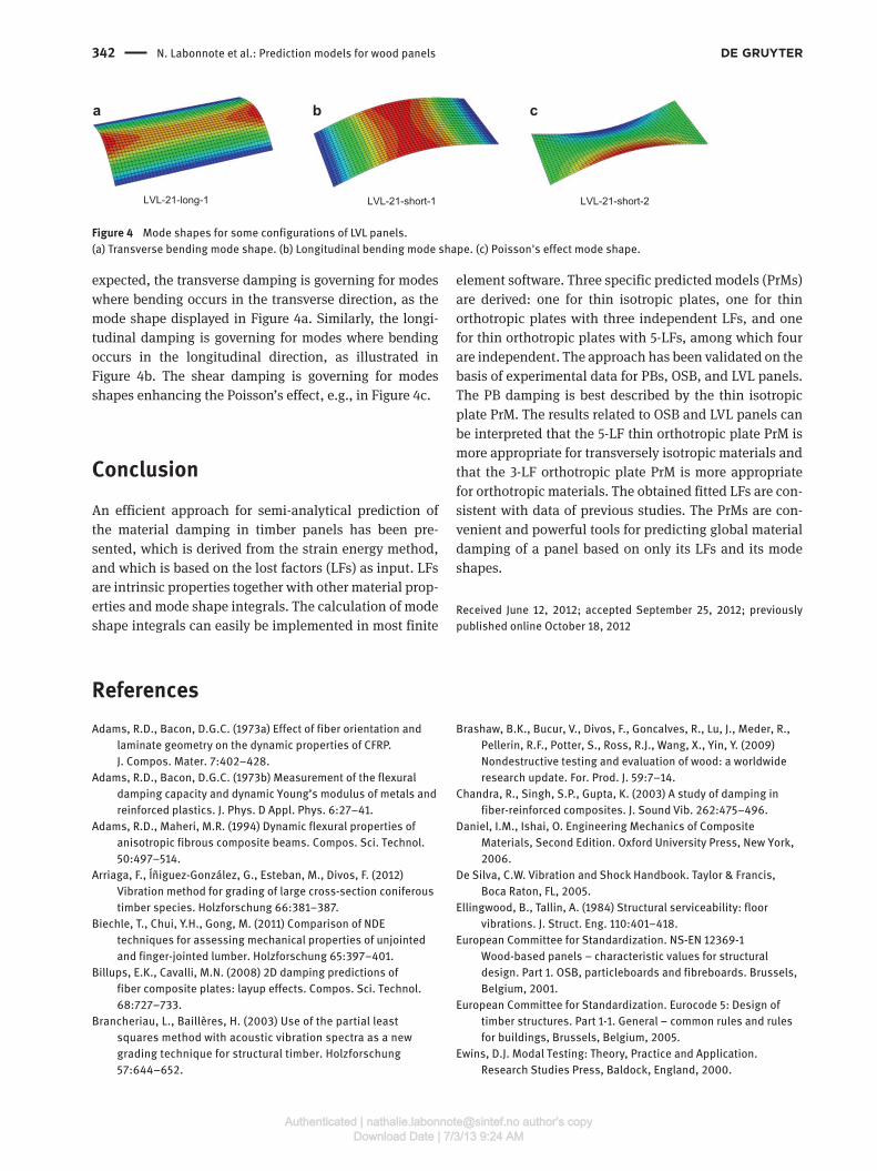
Figure 4   Mode shapes for some configurations of LVL panels.

(a) Transverse bending mode shape. (b) Longitudinal bending mode shape. (c) Poisson's effect mode shape.

expected, the transverse damping is governing for modes

where bending occurs in the transverse direction, as the

mode shape displayed in Figure 4 a. Similarly, the longi-

tudinal damping is governing for modes where bending

occurs in the longitudinal direction, as illustrated in

Figure 4b. The shear damping is governing for modes

shapes enhancing the Poisson ’ s effect, e.g., in Figure 4c.

Conclusion An efficient approach for semi-analytical prediction of

the material damping in timber panels has been pre-

sented, which is derived from the strain energy method,

and which is based on the lost factors (LFs) as input. LFs

are intrinsic properties together with other material prop-

erties and mode shape integrals. The calculation of mode

shape integrals can easily be implemented in most finite

element software. Three specific predicted models (PrMs)

are derived: one for thin isotropic plates, one for thin

orthotropic plates with three independent LFs, and one

for thin orthotropic plates with 5-LFs, among which four

are independent. The approach has been validated on the

basis of experimental data for PBs, OSB, and LVL panels.

The PB damping is best described by the thin isotropic

plate PrM. The results related to OSB and LVL panels can

be interpreted that the 5-LF thin orthotropic plate PrM is

more appropriate for transversely isotropic materials and

that the 3-LF orthotropic plate PrM is more appropriate

for orthotropic materials. The obtained fitted LFs are con-

sistent with data of previous studies. The PrMs are con-

venient and powerful tools for predicting global material

damping of a panel based on only its LFs and its mode

shapes.

Received June 12, 2012; accepted September 25, 2012; previously

published online October 18, 2012

References Adams, R.D., Bacon, D.G.C. (1973a) Effect of fiber orientation and

laminate geometry on the dynamic properties of CFRP.

J. Compos. Mater. 7:402 – 428.

Adams, R.D., Bacon, D.G.C. (1973b) Measurement of the flexural

damping capacity and dynamic Young ’ s modulus of metals and

reinforced plastics. J. Phys. D Appl. Phys. 6:27 – 41.

Adams, R.D., Maheri, M.R. (1994) Dynamic flexural properties of

anisotropic fibrous composite beams. Compos. Sci. Technol.

50:497 – 514.

Arriaga, F., Í ñ iguez-Gonz á lez, G., Esteban, M., Divos, F. (2012)

Vibration method for grading of large cross-section coniferous

timber species. Holzforschung 66:381 – 387.

Biechle, T., Chui, Y.H., Gong, M. (2011) Comparison of NDE

techniques for assessing mechanical properties of unjointed

and finger-jointed lumber. Holzforschung 65:397 – 401.

Billups, E.K., Cavalli, M.N. (2008) 2D damping predictions of

fiber composite plates: layup effects. Compos. Sci. Technol.

68:727 – 733.

Brancheriau, L., Baill è res, H. (2003) Use of the partial least

squares method with acoustic vibration spectra as a new

grading technique for structural timber. Holzforschung

57:644 – 652.

Brashaw, B.K., Bucur, V., Divos, F., Goncalves, R., Lu, J., Meder, R.,

Pellerin, R.F., Potter, S., Ross, R.J., Wang, X., Yin, Y. (2009)

Nondestructive testing and evaluation of wood: a worldwide

research update. For. Prod. J. 59:7 – 14.

Chandra, R., Singh, S.P., Gupta, K. (2003) A study of damping in

fiber-reinforced composites. J. Sound Vib. 262:475 – 496.

Daniel, I.M., Ishai, O. Engineering Mechanics of Composite

Materials, Second Edition. Oxford University Press, New York,

2006.

De Silva, C.W. Vibration and Shock Handbook. Taylor & Francis,

Boca Raton, FL, 2005.

Ellingwood, B., Tallin, A. (1984) Structural serviceability: floor

vibrations. J. Struct. Eng. 110:401 – 418.

European Committee for Standardization. NS-EN 12369-1

Wood-based panels – characteristic values for structural

design. Part 1. OSB, particleboards and fibreboards. Brussels,

Belgium, 2001.

European Committee for Standardization. Eurocode 5: Design of

timber structures. Part 1-1. General – common rules and rules

for buildings, Brussels, Belgium, 2005.

Ewins, D.J. Modal Testing: Theory, Practice and Application.

Research Studies Press, Baldock, England, 2000.

Authenticated | [email protected] author's copyDownload Date | 7/3/13 9:24 AM

N. Labonnote et al.: Prediction models for wood panels      343

Fukada, E. (1950) The vibrational properties of wood I. J. Phys. Soc.

Jpn. 5:321 – 327.

Fukada, E. (1951) The vibrational properties of wood II. J. Phys. Soc.

Jpn. 6:417 – 421.

Hashin, Z. (1970) Complex moduli of viscoelastic composites. I.

General theory and application to particulate composites. Int.

J. Solids Struct. 6:539 – 552.

Johnson, C.D., Kienholz, D.A. (1983) Prediction of damping in

structures with viscoelastic materials. Paper presented at the

MSC Software World Users ’ Conference, 1 March 1983, CA, USA.

Kam, T.Y., Chang, R.R. (1994) Design of thick laminated composite

plates for maximum damping. Compos. Struct. 29:57 – 67.

Lenzen, K.H. (1966) Vibration of steel joist-concrete slab floors. Eng.

J. 3:133 – 136.

Maheri, M.R. (2011) The effect of layup and boundary conditions on

the modal damping of FRP composite panels. J. Compos. Mater.

45:1411 – 1422.

McIntyre, M.E., Woodhouse, J. (1978) The influence of geometry on

linear damping. Acustica 39:209 – 224.

McIntyre, M.E., Woodhouse, J. (1988) On measuring the elastic and

damping constants of orthotropic sheet materials. Acta Metall.

36:1397 – 1416.

Minitab Inc. Minitab StatGuide, State College, PA, 2010.

National Instruments (2011) Modal Analysis. http://zone.ni.com/

devzone/cda/tut/p/id/8276. Accessed 31 January 2011.

Nelson, F.C. (1974) Subjective rating of building floor vibration.

Sound Vib. 8:34 – 37.

Ni, R.G., Adams, R.D. (1984) The damping and dynamic moduli

of symmetric laminated composite beams-theoretical and

experimental results. J. Compos. Mater. 18:104 – 121.

Obataya, E., Ono, T., Norimoto, M. (2000) Vibrational properties of

wood along the grain. J. Mater. Sci. 35:2993 – 3001.

Ono, T. (1983) On dynamic mechanical properties in the trunk of

woods for musical instruments. Holzforschung 37:245 – 250.

Ono, T., Norimoto, M. (1985) Anisotropy of dynamic Young ’ s

modulus and internal friction in wood. Jpn. J. Appl. Phys. 1

24:960 – 964.

Placet, V., Passard, J., Perr é , P. (2007) Viscoelastic properties of

green wood across the grain measured by harmonic tests in

the range 0 – 95 ° C: Hardwood vs. softwood and normal wood

vs. reaction wood. Holzforschung 61:548 – 557.

R é billat, M., Boutillon, X. (2011) Measurement of relevant elastic

and damping material properties in sandwich thick plates.

J. Sound Vib. 330:6098 – 6121.

Ruffell, C.M., Griffin, M.J. (1995) Effects of 1-Hz and 2-Hz transient

vertical vibration on discomfort. J. Acoust. Soc. Am. 98:

2157 – 2157.

Saravanos, D.A. (1994) Integrated damping mechanics for thick

composite laminates and plates. J. Appl. Mech. 61:375 – 383.

Schwarz, B.J., Richardson, M.H. Experimental modal analysis.

In: Proceedings of CSI Reliability Week. Orlando, FL, USA, 1999.

Spycher, M., Schwarze, F., Steiger, R. (2008) Assessment of

resonance wood quality by comparing its physical and

histological properties. Wood Sci. Technol. 42:325 – 342.

Talbot, J.P., Woodhouse, J. (1997) The vibration damping of

laminated plates. Composites Part A 28A:1007 – 1012.

Timmer, S.G.C. Feasibility of Tall Timber Buildings. Delft University

of Technology, Delft, 2011.

Ungar, E.E., Kerwin, E.M. Jr. (1962) Loss factors of viscoelastic

systems in terms of energy concepts. J. Acoust. Soc. Am.

34:954 – 957.

VTT Technical Research Centre. VTT Certificate Kerto-S and Kerto-Q.

VTT Certificate No. 184/03. VTT Expert Services Ltd, Espoo,

Finland, 2009.

Walpole, R.E., Myers, R.H., Myers, S.L., Ye, K. Probability &

Statistics for Engineers and Scientists, 8th Edition. Pearson

Education International, Upper Saddle River, 2007.

Wang, S.Y., Chen, B.J. (2001) The flake ’ s alignment efficiency and

orthotropic properties of oriented strand board. Holzforschung

55:97 – 103.

Wiss, J.F., Parmelee, R.A. (1974) Human perception of transient

vibrations. J. Struct. Div. Am. Soc. Civ. Eng. 100:773 – 787.

Yoshihara, H. (2012a) Off-axis Young ’ s modulus and off-axis

shear modulus of wood measured by flexural vibration tests.

Holzforschung 66:207 – 213.

Yoshihara, H. (2012b) Influence of specimen configuration on the

measurement of the off-axis Young ’ s modulus of wood by

vibration tests. Holzforschung 66:485 – 492.

Authenticated | [email protected] author's copyDownload Date | 7/3/13 9:24 AM