Semi-analytical methods for simulating the groundwater-surface water interface by Ali A Ameli A thesis presented to the University of Waterloo in fulfillment of the thesis requirement for the degree of Doctor of Philosophy in Civil Engineering Waterloo, Ontario, Canada, 2014 © Ali A Ameli 2014

Welcome message from author
This document is posted to help you gain knowledge. Please leave a comment to let me know what you think about it! Share it to your friends and learn new things together.
Transcript
Semi-analytical methods for simulating the
groundwater-surface water interface
by
Ali A Ameli
A thesis
presented to the University of Waterloo
in fulfillment of the
thesis requirement for the degree of
Doctor of Philosophy
in
Civil Engineering
Waterloo, Ontario, Canada, 2014
© Ali A Ameli 2014

ii
AUTHOR'S DECLARATION
I hereby declare that I am the sole author of this thesis. This is a true copy of the thesis, including any
required final revisions, as accepted by my examiners.
I understand that my thesis may be made electronically available to the public.

iii
Abstract
Groundwater-surface water interaction is a key component of the hydrologic cycle. This interaction
plays a key role in many environmental issues such as the impacts of land use and climate change on
water availability and water quality. Modeling of local and regional groundwater-surface water
interactions improves understanding of these environmental issues and assists in addressing them.
Because of the physical and mathematical complexities of this interaction, numerical approaches are
generally used to model water exchange between subsurface and surface domains. The efficiency,
accuracy, and stability of mesh-based numerical models, however, depend upon the resolution of the
underlying grid or mesh.
Grid-free analytical methods can provide fast, accurate, continuous and differentiable solutions to
groundwater-surface water interaction problems. These solutions exactly satisfy mass balance in the
entire internal domain and may improve our understanding of groundwater-surface water interaction
principles. However, to model this interaction, analytical approaches typically required simplifying,
sometimes unrealistic, assumptions. They are typically used to implement linearized mathematical
models in homogenous confined or semi-confined aquifers with geometrically regular domains.
By benefiting from the strengths of both analytical and numerical approaches, grid-free semi-
analytical methods may be able to address more challenging groundwater problems which have been
out of reach of traditional analytical approaches, and/or are poorly simulated using mesh-based
numerical methods. Here, novel 2-D and 3-D semi-analytical solutions for the simulation of
mathematically and physically complex groundwater-surface water interaction problems are
developed, assessed and applied. Those models are based upon the series solution method and
analytic element method (AEM) and are intended to address groundwater-surface water interactions
induced by pumping wells and/or the presence of surface water bodies in naturally complex stratified
unconfined aquifers. Semi-analytical solutions are obtained using the least squares method, which is
used to determine the unknown coefficients in the series expansion and the unknown strengths of
analytic elements. The series and AEM solutions automatically satisfy the groundwater governing
equation. Hence, the resulting solutions are exact over the entire domain except along boundaries and
layer interfaces where boundary and continuity conditions are met with high precision. A robust
iterative algorithm is used to implement a free boundary condition along the phreatic surface with a
priori unknown location.
iv
This thesis addresses three general problem types never addressed within a semi-analytic framework.
First, a steady-state free boundary semi-analytical series solutions model is developed to simulate 2-D
saturated-unsaturated flow in geometrically complex stratified unconfined aquifers. The saturated-
unsaturated flow is controlled by water exchange along the land surface (e.g., evapotranspiration and
infiltration) and the presence of surface water bodies. The water table and capillary fringe are allowed
to intersect stratigraphic interfaces. The capillary fringe zone, unsaturated zone, groundwater zone
and their interactions are incorporated with a high degree of accuracy. This model is used to assess
the influences of important factors on unsaturated flow behavior and the water table elevation.
Second, a 3-D free boundary semi-analytical series solution model is developed to simulate
groundwater-surface water interaction controlled by infiltration, seepage faces and surface water
bodies along the land surface. This model can simulate the water exchange between groundwater and
surface water in geometrically complex stratified phreatic (unconfined) aquifers. The a priori
unknown phreatic surface will be obtained iteratively while the locations of seepage faces don’t have
to be known a priori (i.e., this is a constrained free boundary problem). This accurate grid-free multi-
layer model is here used to investigate the impact of the sediment layer geometry and properties on
lake-aquifer interaction. Using this method, the efficiency of widely-used Dupuit-Forchheimer
approximation used in regional groundwater-surface water interaction models is also assessed. Lastly,
this 3-D groundwater-surface water interaction model is augmented with AEM solutions to simulate
horizontal pumping wells (radial collector well) for assessing surface water impacted by pumping and
determining the source of extracted well water. The resulting model will be used to assess controlling
parameters on the design of a radial collector well in a river bank filtration system. This 3-D Series-
AEM model, in addition, mitigates the limitations of AEM in modeling of general 3-D groundwater-
surface water interaction problems.
v
Acknowledgements
I would like to thank Dr. James Craig, my PhD advisor, for his scientific support and motivations
throughout my PhD studies. Also, I have always been thankful to James for his care and advice on
things other than research, specially for helping me to be a socially professional person.
It is my pleasure to thank my PhD committee members Dr. Jon Sykes and Dr. Leo Rothenburg from
the Department of Civil and Environmental Engineering and Dr. Walter Illman from the Department
of Earth Science of University of Waterloo. I would also like to thank the comments of Dr. Jeffrey
McDonnell on my research during my visit of the Global Institute of Water Security (GIWS) at the
University of Saskatchewan as a guest researcher.
The majority of the thesis contents were peer-reviewed in the form of technical journal papers before
thesis submission. I would like to thank the anonymous reviewers for the journals Advances in Water
Resources and Water Resources Research who reviewed the papers associated with Chapter 4 and
Chapter 5. Their constructive comments significantly improved the contents of my thesis.
vi
Table of Contents
Author's declaration ............................................................................................................................... ii
Abstract ................................................................................................................................................. iii
Acknowledgements ................................................................................................................................ v
Table of Contents .................................................................................................................................. vi
List of Figures ....................................................................................................................................... ix
List of Symbols ..................................................................................................................................... xi
Chapter 1 Introduction ........................................................................................................................... 1
1.1 Subsurface-surface interaction ..................................................................................................... 1
1.1.1. Modeling of Subsurface-surface interaction ......................................................................... 1
1.2 Research objectives and Thesis Structure .................................................................................... 4
Chapter 2 Background ........................................................................................................................... 6
2.1 Groundwater-surface water interaction ........................................................................................ 6
2.2 Groundwater-surface water interaction induced by pumping wells ............................................. 7
2.2.1 Pumping Well orientation ..................................................................................................... 8
2.3 Subsurface flow mathematical formulation ................................................................................. 9
2.3.1 Saturated Flow .................................................................................................................... 10
2.3.2 Unsaturated Flow ................................................................................................................ 11
2.4 Modeling of Groundwater-surface water interaction ................................................................. 12
2.4.1 Numerical models for groundwater-surface water interaction ............................................ 16
2.4.2 Semi - analytical models ..................................................................................................... 17
Chapter 3 Semi-analytical series solution and analytic element method ............................................. 20
3.1 Introduction ................................................................................................................................ 20
3.2 Series solutions .......................................................................................................................... 20

vii
3.3 Analytic Element Method (AEM) .............................................................................................. 22
3.4 Gibbs phenomenon ..................................................................................................................... 23
Chapter 4 Series solutions for saturated-unsaturated flow in multi-layer unconfined aquifers ............ 27
4.1 Introduction ................................................................................................................................ 27
4.2 Background ................................................................................................................................ 27
4.3 Problem statement ...................................................................................................................... 28
4.4 Solution ...................................................................................................................................... 34
4.5 Analysis ...................................................................................................................................... 36
4.5.1 Example 1: Homogenous system ........................................................................................ 37
4.5.2 Example 2: Heterogeneous system ...................................................................................... 40
4.6 Conclusion .................................................................................................................................. 44
Chapter 5 Semi-analytical series solutions for three dimensional groundwater-surface water
interaction ............................................................................................................................................. 46
5.1 Introduction ................................................................................................................................ 46
5.2 Background ................................................................................................................................ 46
5.3 Problem statement ...................................................................................................................... 48
5.4 Solution ...................................................................................................................................... 52
5.5 Analysis ...................................................................................................................................... 54
5.5.1 Example 1: Effect of lake sediment on lake-Aquifer interaction ........................................ 55
5.5.2 Example 2: Surface seepage flow from an unconfined aquifer ........................................... 59
5.6 Conclusion .................................................................................................................................. 62
Chapter 6 3-D semi-analytical solution for pumping well impact on groundwater-surface water
interaction ............................................................................................................................................. 64
6.1 Introduction ................................................................................................................................ 64

viii
6.2 Background ................................................................................................................................ 66
6.3 Problem Statement ..................................................................................................................... 69
6.4 Solution ...................................................................................................................................... 73
6.5 Analysis...................................................................................................................................... 75
6.5.1 Example 1: River Bank Filtration process in a naturally complex unconfined aquifer ...... 75
6.5.2 Example 2: Pumping rate impact on hydrological connection between river and well ...... 81
6.6 Conclusion ................................................................................................................................. 84
Chapter 7 Conclusions and future directions ....................................................................................... 85
7.1 Conclusions ................................................................................................................................ 85
7.2 Future directions ........................................................................................................................ 88
References ........................................................................................................................................... 89
ix
List of Figures
Figure 2-1. Layout of the general groundwater-surface water interaction problem.. ............................. 7
Figure 3-1. Performance of discrete Fourier series in curve fitting of function (x) using least
square algorithm.. ................................................................................................................. 25
Figure 3-2. Performance of the augmented Fourier series with a supplemental function in curve
fitting of function G(x) using least square algorithm. ........................................................... 26
Figure 4-1. Layout of the general problem.. ......................................................................................... 29
Figure 4-2. a) Infiltration and evapotranspiration function used in example 1, b) Layout
of the flow streamlines (grey), equi-potential contours (black), water level and water
table in a homogenous unconfined aquifer adjacent to a constant head river at left
corner after 10 iterations. ...................................................................................................... 37
Figure 4-3. Convergence of the water level moving boundary between saturated and
unsaturated zones. ................................................................................................................. 39
Figure 4-4. Infiltration and evapotranspiration function ( ) used in example 2, for cases a
and b...................................................................................................................................... 40
Figure 4-5. Layout of flow net in the 4-Layer aquifer after 14 iterations, a) case (a), b) case (b).. ..... 41
Figure 4-6. Convergence of the water level moving boundary between saturated and
unsaturated zones in example 2. ........................................................................................... 42
Figure 4-7. Normalized flux boundary and continuity error across internal interfaces (1200
points) after 14 iterations in the example 2 ........................................................................... 43
Figure 4-8. Normalized head continuity error across internal interfaces in the example 2 .................. 44
Figure 5-1. Layout of the general 3-D problem.................................................................................... 48
Figure 5-2. The method to obtain flux along the top surface boundary. ........................................... 51
Figure 5-3. Layout of the normalized seepage flux distribution at the lake bed in lake-aquifer
system.. ................................................................................................................................. 58
Figure 5-4. Solution in 3-Layer unconfined aquifer after 60 iterations. ............................................... 60
Figure 5-5. Contour of normalized flux error across the modeled domain top surface boundary. ....... 61
Figure 5-6. Convergence behaviour of the water table with = 0.06.. ................................................ 62
Figure 6-1. Layout of the general 3-D problem.................................................................................... 69
Figure 6-2. Series-AEM solution in 2-Layer unconfined aquifer after 45 iterations. .......................... 78
Figure 6-3. Convergence behavior of the solution. a) Variation of average normalized head
error along the water table and b) collector well head with respect to iteration
number. ................................................................................................................................. 79
Figure 6-4. Normalized error of boundary and continuity conditions along evaluation
interfaces. a) contours of normalized flux error along the water table surface, b)
contours of normalized continuity of flux error along the first layer interface, c)
x
contours of normalized continuity of head error along the first layer interface, d)
uniformity of head normalized error along the control pints located at 6 sides of the
arm in x (top) and y (bottom) directions. .............................................................................. 81
Figure 6-5. Layout of a radial collector well located in a homogenous unconfined aquifer with
a simple geometry. Red and blue lines show the arm in x and y direction,
respectively........................................................................................................................... 82
Figure 6-6. Series-AEM solution in a homogenous unconfined aquifer after 45 iterations, for a)
= 30000 m3/d, b) = 60000 m
3/d and c) = 120000 m
3/d. ............................................ 83
xi
List of symbols
,
, ,
,
,
Unknown coefficient of series solution of the m
th layer (3-D and 2-D solutions)
[L] The surface water body depth
[L2T-1] The influence function of each analytic element
F(x, y) [LT-1] 3-D infiltration-evapotranspiration function obtained using Equation (5-5)
[LT-1] 2-D infiltration-evapotranspiration function
[L] Water level stage of the river or lake
[L] Head in the radial collector well
[L] Total hydraulic head
[LT-1] Saturated hydraulic conductivity
[LT-1] Unsaturated conductivity
[LT-1] * Saturated hydraulic conductivity of the m
th layer
[L] Domain length
[L] Domain length in x and y directions
[L] Half of the length of each segment of a line element used in AEM
[L] Length of radial collector arm
Number of unsaturated layers
Number of saturated layers
Total number of layers
N , J Number of series terms in each direction
NC Total number of control points along each interface used for least squares
NCx, NCy Number of control points along each interface in x and y directions used for

xii
least squares
The number of segments along a line element used in AEM to represent a
pumping well
Number of image wells
NCw Number of control points along the well screens surface
P The ratio of aquifer to sediment hydraulic conductivity
[L3T-1] Radial collector well pumping rate
, , [LT-1] Specific discharges in x, y and z directions
R [LT-1] Infiltration rate
RE [LT-1] recharge rate
r Iteration number
Specific yield
, , Eigenfunctions of the Laplace equation used in series solutions method
,
, The center of each segment of a line sink in the global coordinate system
[L] Water table elevation
[L] Land surface elevation
[L] Top of the modeled domain elevation
[L] Elevation of the interfaces between different soil layers
[L] Bottom bedrock elevation
[L] Top of capillary fringe elevation
[L] Elevation of radial collector well
The exponential function parameter, Equation (5-5)
[L-1] Sorptive number of the mth
layer
xiii
Transition zone depth, Equation (5-5)
, , Eigenvalues of the Laplace equation used in series solutions method
[L2T-1] The discharge potential correspond to i
th segment of a line element (AEM)
[L2T-1] Saturated discharge potential
[ ] Unsaturated Kirchhoff potential
[L2T-1] Unsaturated stream function of the m
th layer
[L2T-1] Saturated stream function of the m
th layer
[L2T-1] Unsaturated Kirchhoff potential of the m
th layer
[L2T-1] * Saturated discharge potential of the m
th layer
[L] Air entry pressure of the m
th layer
[L] Pressure head
Constant strength of each segment of a line element used in AEM
The relaxation factor of the iterative scheme
volumetric water content
* Superscript or subscript (s) and (u) are only mentioned for coupled saturated-unsaturated
simulation to make a distinction between saturated and unsaturated variables/parameters. If
noting mentioned variables/parameter is for pure saturated simulation.

1
Chapter 1
Introduction
1.1 Subsurface-surface interaction
Groundwater and surface water are not typically isolated from one another. Continual water, nutrient
and contaminant exchange involving a wide range of physical, biological, chemical and
biogeochemical processes have been fundamental concerns in water supply, water quality and
ecosystem management. Lake and stream acidification, lake eutrophication, human activities (e.g.,
agricultural development, loss of wetlands and flood plains due to urban development, excessive
pumping, etc.) and natural hazards such as landslide and flooding have been issues which have
encouraged hydrologists, geologists and ecologists to consider the interaction between subsurface and
surface water. Pumping, for example, may cause decline in groundwater levels in the vicinity of
surface water bodies and capture groundwater which would have potentially discharged into surface
water bodies as base flow. Excessive pumping may similarly induce flow out of surface water bodies
into the aquifer. Both phenomena lead to the depletion of stream flow. Lowering of the water table
level may likewise disconnect ground water and surface water, and alter riparian vegetation. Efficient
land use and water management in different physiographic settings requires a comprehensive
understanding of the interaction between pumping wells, groundwater and surface water bodies. This
understanding can also be helpful to assess the reliability of wells water quality through determining
the pumping wells sources.
Groundwater-surface water interactions have been assessed experimentally in different physiographic
settings. Using field methods, there has been a significant body of field work done to assess stream-
aquifer interaction [e.g., Dunne and Black, 1970; Harvey et al., 1997; Hunt et al., 2001; Sophocleous
et al., 1988] and Lake-aquifer interaction [e.g., Harvey et al., 1997; Smerdon et al., 2005]. Due to the
practical complexities, the utility of experimental analysis alone might be limited [e.g., Halford and
Mayer, 2000; Rushton, 2007], and mathematical models are needed.
1.1.1. Modeling of Subsurface-surface interaction
Modeling of local and regional subsurface-surface water interaction assists in the conceptual
understanding of this interaction and its controlling parameters. In addition, efficient design of
processes and technologies used for groundwater and surface water withdrawal and treatment often
requires a robust subsurface-surface water interaction model. Examples include the design of (1)
2
radial collector (RC) wells which provide a large pumping well yield under low drawdown, (2) bank
filtration process where surface water contaminants are purified (for use as drinking water) by passing
through the banks of rivers or lakes or (3) pump and treat remediation near streams where
groundwater contaminants are captured by vertically or non-vertically oriented pumping wells. All of
these systems may require detailed analysis of the 3-D interaction between surface water bodies,
pumping wells and groundwater.
Accurate simulation of 3-D groundwater-surface water interaction can be cumbersome due to
mathematical complexities including a non-linear governing equation, a constrained non-linear free
boundary along the water table, and/or the presence of heterogeneity, anisotropy and naturally
complex geometry. If unsaturated conditions are explicitly modeled in the vadose zone, material
properties (and therefore the governing equation) may likewise become non-linear. In most cases, 3-D
numerical (rather than analytical) models are generally used to simulate the complex interaction
between the subsurface and surface [e.g., Cardenas and Jiang, 2010; Larabi and De Smedt, 1997; Oz
et al., 2011; Smerdon et al., 2007; Therrien et al., 2008; Werner et al., 2006]. Mesh-based numerical
models, however, are prone to numerical artifacts; the resolution of the underlying grid or mesh
significantly impact the efficiency and accuracy of numerical approaches. The discretization
requirements in numerical models typically increases computational expense, particularly for free
boundary problems [An et al., 2010; Knupp, 1996]. Discretization constraints may also lead to poor
representation of the geometry and properties of surface water bodies at a different scale than the
regional aquifer it is part of [Mehl and Hill, 2010; Rushton, 2007; Sophocleous, 2002; Townley and
Trefry, 2000], or the details of pumping impacts on streams [Moore et al., 2012; Patel et al., 2010].
Along a well screen, for example, a high resolution 3-D discretization is required while the treatment
of the unique boundary condition at the well (using a head dependent boundary cell as is done in
MODFLOW) might be cumbersome for mesh-based approaches [Patel et al., 1998]. Misalignment of
arbitrary-directed wells with respect to the mesh discretization may also compromise the efficiency of
the discrete models [Moore et al., 2012].
Accurate grid-free (mesh-less) analytical approaches have occasionally been employed to address
mathematically and geometrically simplified 1-D [e.g., Boano et al., 2010; Hantush, 2005; McCallum
et al., 2012; Serrano and Workman, 1998; Teloglou and Bansal, 2012; Workman et al., 1997] and 2-
D [e.g., Anderson, 2003; Haitjema and Mitchell-Bruker, 2005] groundwater systems to provide a
better understanding of the basic principles of the interaction between groundwater and surface water,
3
and at the same time serve as a benchmark for numerical model validation. However, in applying
simplifying assumptions regarding problem geometry or physics, analytical approaches cannot
typically provide a realistic representation of the complexity of groundwater-surface water exchange
flows in heterogeneous unconfined aquifers.
Benefiting from the strengths of both analytical and numerical schemes, grid-free semi-analytical
approaches have the potential to address more complex problems at lesser computational cost than
discrete equivalents. The basic idea behind semi-analytical approaches is the augmentation of
standard analytical techniques (e.g., series solutions, analytic element method, separation of variables,
Laplace and Hankel transforms, etc.) with a simple numerical technique such as least squares
minimization or numerical inversion/integration [Craig and Read, 2010]. Semi-analytical methods
such as series solutions and analytic element method (AEM) have been augmented with a least
squares minimization algorithm to successfully address geometrically complex problems [Luther and
Haitjema, 1999; Luther and Haitjema, 2000; Read and Volker, 1993; Wong and Craig, 2010].
Semi-analytical series solution methods have been developed to simulate homogenous [Read and
Volker, 1993] and multi-layer [Craig, 2008; Wong and Craig, 2010] topography-driven flow in
naturally complex two dimensional aquifers with finite domains. Marklund and Wörman [2011]were
able to use such methods to demonstrate that the topography driven flow hypothesis induces a
systematic error and, according to the criterion developed by Haitjema and Mitchell-Bruker [2005], it
is not valid for most groundwater systems. Treatment of the phreatic surface as a free boundary
remains the preferred course of action. This is particularly true when simulating groundwater-surface
water exchanges fluxes, where the water table location can not be prescribed, as done with the
topography driven approach.
Semi-analytical AEM has been also used as a robust alternative to mesh-based numerical models for
(1) the simulation of large-scale regional groundwater-surface water interaction [Haitjema et al.,
2010; Hunt, 2006; Moore et al., 2012; Simpkins, 2006], (2) screening or quick hydrologic analysis
and stepwise modeling [Dripps et al., 2006; Hunt, 2006; Strack, 1989], (3) assessment of the theories
behind the estimation of effective conductivity and dispersion coefficients in highly heterogeneous
formations [Barnes and Janković, 1999; Janković et al., 2003], and (4) 3-D flow toward partially
penetrating vertical, horizontal and slanted pumping well(s) in homogenous unconfined aquifers and
multi layer confined aquifers [Bakker et al., 2005; Luther and Haitjema, 1999; Steward, 1999;

4
Steward and Jin, 2001; 2003]. However, the representation of the phreatic surface, naturally complex
layer stratification and surface water bodies geometry is still challenging using analytic elements
[Hunt, 2006], especially in 3-D.
1.2 Research objectives and Thesis Structure
The objective of this thesis is to extend available semi-analytical series solution methods and the
analytic element method (AEM) for simulation of 2-D and 3-D steady-state groundwater-surface
water interaction in a geometrically complex stratified domain. The interaction can be controlled by
arbitrary-oriented pumping wells, precipitation, evapotranspiration, seepage faces and surface water
bodies. The phreatic surface will be treated as a constrained non-linear free boundary condition. Note
that the developed solutions in this thesis are not integrated groundwater-surface water models, but
are subsurface models aimed at resolving exchange fluxes under a predefined infiltration rate. Direct
exchanges with surface water bodies are also considered. The contributions developed in this thesis
collectively have pushed the series solution and AEM methods from a specialized tool useful for
some constrained problems to a quite general modeling method capable of simulating complex flow
under quite general conditions. Some of these conditions may be challenging to properly address
using mesh-based numerical methods.
This thesis is structured around published and submitted articles. A brief background of field and
modeling studies of groundwater-surface water interaction, and the mathematical formulation for the
governing laws of subsurface flow is presented in chapter 2. Chapter 3 explains the theoretical basics
behind semi-analytical series solutions and AEM. Chapters 4 and 5 correspond to two published
articles [Ameli and Craig, 2014; Ameli et al., 2013] about the extension of series solutions to simulate
2-D and 3-D groundwater-surface water interaction with and without the vadose zone and capillary
fringe. In chapter 4, the series solution approach is extended to address 2-D saturated-unsaturated
flow in naturally complex stratified unconfined aquifers where the free boundary water table interface
can intersect the layer interfaces. This model is extended to simulate 3-D groundwater-surface water
interaction in a geometrically complex stratified unconfined aquifer (chapter 5), where flow is
controlled by water exchange across the land surface including infiltration, seepage faces and
exchange with surface water bodies. The 3-D series solution model is augmented with 3-D AEM
techniques in chapter 6 to assess groundwater-surface water interaction between a group of horizontal
5
wells (radial collector wells) and surface water features in geometrically complex stratified
unconfined aquifers. Wells are allowed to intersect stratigraphic interfaces in this model.
The developed models have the potential to assess factors controlling groundwater-surface water
interaction. Fast, continuous, accurate and grid-free semi-analytical models developed here support
the conceptual understanding of basic principles of groundwater-surface water interaction.
Application examined here include an examination of the important controls on the behavior of
unsaturated and capillary fringe flow (chapter 4), assessment of the validity of Dupuit-Forchheimer
approximation used in regional 2-D models and investigation into lakebed geometry controls on
groundwater-surface water exchange (chapter 5) and design of a radial collector well in a RBF system
(chapter 6).
6
Chapter 2
Background
2.1 Groundwater-surface water interaction
The interaction between groundwater and surface water occurs in different physiographic and
climatic settings around the world. This interaction may take three forms; a surface water feature
loses water and solutes into groundwater, groundwater discharges water and solutes into a surface
water body or a surface water body loses and gains water and solutes along different reaches. Water is
also exchanged across the ground surface via the mechanisms of transpiration, evaporation and
infiltration through the vadose zone.
Groundwater-surface water interactions have been assessed experimentally in different physiographic
settings such as mountain, riverine, coastal, and karst terrains [Carter, 1990; Correll et al., 1992;
Harte and Winter, 1993; Smerdon et al., 2005; Stark et al., 1994; Winter and Rosenberry, 1995],
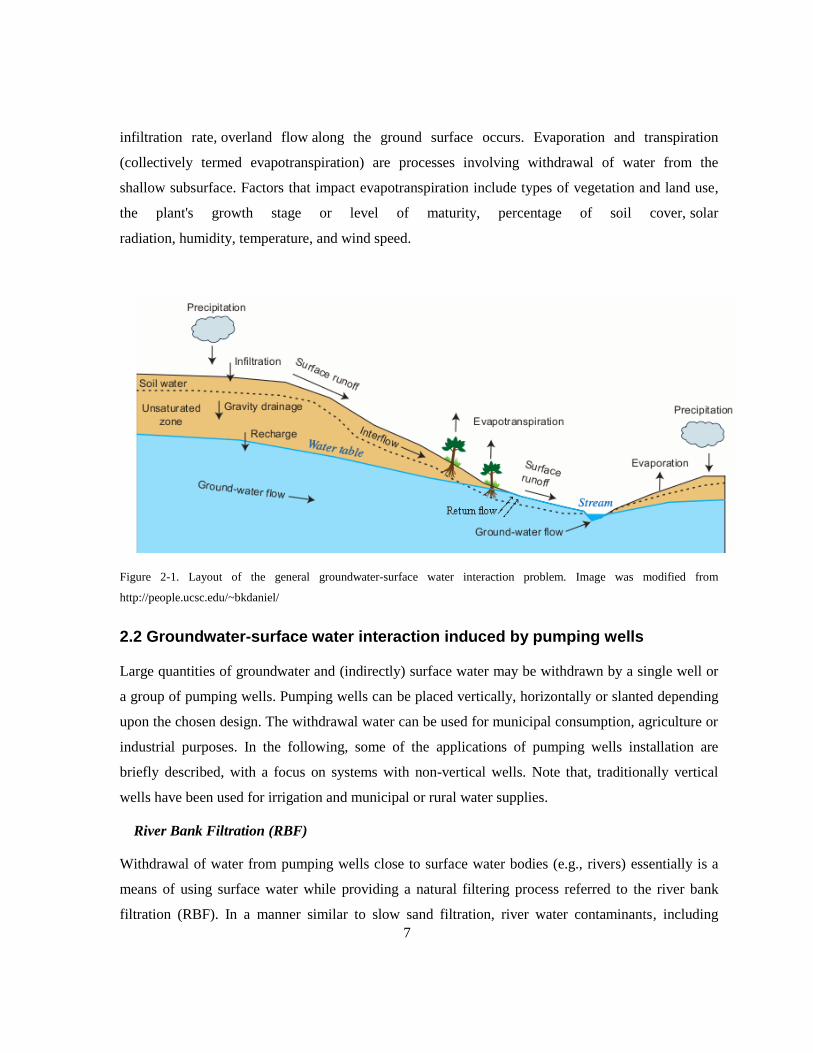
leading to a well-established conceptual model for groundwater-surface water exchange. Figure 2-1
depicts this conceptual model for groundwater-surface water interaction including various surface and
subsurface flow exchange mechanism in an unconfined aquifer. The portion of stream or lake flow
that comes from deeper subsurface flow is called baseflow (groundwater). Interflow is the lateral
movement of shallow subsurface water in unsaturated zone that may return to the ground surface
through seepage faces (return flow or throughflow) or enters a stream or lake prior to infiltrating into
deep groundwater and becoming baseflow; the portion which is infiltrated into groundwater zone is
termed groundwater recharge, usually expressed as a flux across the water table surface. The
groundwater zone is bounded above by the water table surface, which is also called the phreatic
surface. Along the phreatic surface, the water in the soil pores is at atmospheric pressure (zero
pressure head) while in the saturated zone there is positive pore water pressure. The unsaturated zone,
also termed the vadose zone, is the part of an unconfined aquifer between the ground surface and
water table. Water in the vadose zone has a pore pressure head less than atmospheric pressure, and is
retained in the soil matrix by a combination of adhesion and capillary forces. At the ground surface,
water can be exchanged with the atmosphere and ponded at the surface by infiltration, evaporation
and transpiration processes. Infiltration is the process by which water (rain fall or snowmelt) on the
ground surface enters the soil. The infiltration rate is the rate at which soil is able to absorb surface
water, which decreases as the soil becomes more saturated. If the precipitation rate exceeds the
7
infiltration rate, overland flow along the ground surface occurs. Evaporation and transpiration
(collectively termed evapotranspiration) are processes involving withdrawal of water from the
shallow subsurface. Factors that impact evapotranspiration include types of vegetation and land use,
the plant's growth stage or level of maturity, percentage of soil cover, solar
radiation, humidity, temperature, and wind speed.
Figure 2-1. Layout of the general groundwater-surface water interaction problem. Image was modified from
http://people.ucsc.edu/~bkdaniel/
2.2 Groundwater-surface water interaction induced by pumping wells
Large quantities of groundwater and (indirectly) surface water may be withdrawn by a single well or
a group of pumping wells. Pumping wells can be placed vertically, horizontally or slanted depending
upon the chosen design. The withdrawal water can be used for municipal consumption, agriculture or
industrial purposes. In the following, some of the applications of pumping wells installation are
briefly described, with a focus on systems with non-vertical wells. Note that, traditionally vertical
wells have been used for irrigation and municipal or rural water supplies.
River Bank Filtration (RBF)
Withdrawal of water from pumping wells close to surface water bodies (e.g., rivers) essentially is a
means of using surface water while providing a natural filtering process referred to the river bank
filtration (RBF). In a manner similar to slow sand filtration, river water contaminants, including

8
pathogens (e.g., Cryptosporidium and Giardia), organic compounds and turbidity are attenuated
through a combination of processes such as filtration, microbial degradation, sorption to sediments
and dilution with background groundwater [Hiscock and Grischek, 2002; Moore et al., 2012; Ray et
al., 2002]. RBF systems are typically used in alluvial aquifers which may consist of a variety of
deposits ranging from fine sand to pebbles and cobbles. Coarse-grained and permeable deposits are
ideal formations for RBF. Proper design of RBF systems requires the ability to accurately estimate
drawdown and withdrawal rate across the groundwater-surface water interface.
Pump and treat remediation
Pump and treat is one the most common groundwater remediation technologies which involves
pumping of contaminated groundwater to surface for treatment. A group of pumping wells is
designed to capture the plume contaminant followed by a couple of biological and chemical processes
to treat extracted groundwater [Matott et al., 2006]. The efficiency of the technology depends upon
the configuration and number of pumping wells. Pumping near surface resources may lead to
excessive withdrawal of surface water or inefficient, deleterious and inadvertent withdrawal of
surface contamination.
Aquifer tests
Pumping wells are also used to determine the local and regional material properties of the aquifers
through aquifer tests including constant head test, constant rate test, slug test and recovery test [Butler
Jr, 1997; Charbeneau, 2006]. Aquifer tests near surface features must address their presence
appropriately to properly be used to estimate aquifer properties.
2.2.1 Pumping Well orientation
Vertical wells have been traditionally used for most applications, as it is much more challenging
and/or expensive to do otherwise. However, the construction of non-vertical, particularly horizontal,
wells has become more common place after significant advances in drilling technologies [Joshi,
2003]. The benefits of horizontal wells over vertical ones have been reported by many researchers
[Bakker et al., 2005; Joshi, 2003; Moore et al., 2012; Patel et al., 2010; Yeh and Chang, 2013] as
follows:
Horizontal wells can be installed in urban areas with obstructions such as buildings and roads
along the land surface
9
Horizontal wells yield a smaller drawdown near the well to withdraw the desired water
demand
In shallow aquifers, horizontal wells can generally extract more water since useful screen
length does not vary with the changes in the saturated thickness.
The entering groundwater velocity to a horizontal well screen is lower due to a larger
available screen length. This decreases the rate of clogging and minimizes the head loss
between the aquifer and the well.
The operating cost of horizontal wells is lower since fewer wells are required to fulfill the
desired yield.
It seems that horizontal wells can be an appropriate alternative to vertical ones. A group of horizontal
wells may be designed to increase the efficiency of the pumping. As an example, radial collector
(RC) well systems, initially developed by Ranney in 1930, consists of a number of horizontal wells
(lateral arms) screened to the aquifer, and connected to a vertical cylindrical caisson [Moore et al.,
2012]. Traditionally collector wells were made from steel pipes with slots punched or cut into them,
and were installed using a hydraulic jack by driving them into the aquifer through ports in the caisson.
More recently, they are composed of wound stainless steel screens [Bakker et al., 2005]. A radial
collector well system is able to withdraw a large quantity of surface water through alluvial riverbed in
regions where rivers are not perennial. Recently RC wells have been widely applied in river bank
filtration (RBF) and pump and treat processes [Bakker et al., 2005; Hoffman, 1998; Moore et al.,
2012; Patel et al., 2010]. It should be noted that arbitrarily oriented well sections are notably difficult
to simulate using numerical methods.
2.3 Subsurface flow mathematical formulation
In this section, the governing equations for subsurface water flow are presented. First, governing
equations for 3-D transient and steady-state saturated flow in porous media are derived. The 3-D
steady-state governing equation for saturated flow is used in chapters 5 and 6. The 2-D steady-state
governing equation for saturated flow is also used in chapter 4. Second, the governing equations for
3-D transient and steady-state unsaturated flow are described. The 2-D steady-state linearized form of
this equation is used in chapter 4. Note that hereafter ( ) and ( ) describe saturated and unsaturated
properties/variables.
10
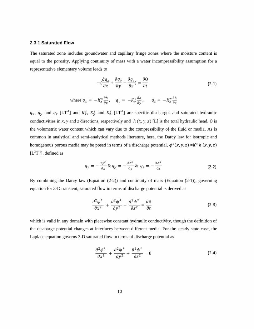
2.3.1 Saturated Flow
The saturated zone includes groundwater and capillary fringe zones where the moisture content is
equal to the porosity. Applying continuity of mass with a water incompressibility assumption for a
representative elementary volume leads to
(2-1)
where
,
,
, and [LT-1
] and ,
and [LT
-1] are specific discharges and saturated hydraulic
conductivities in x, y and z directions, respectively and [L] is the total hydraulic head. is
the volumetric water content which can vary due to the compressibility of the fluid or media. As is
common in analytical and semi-analytical methods literature, here, the Darcy law for isotropic and
homogenous porous media may be posed in terms of a discharge potential, =
[L2T
-1], defined as
&
&
(2-2)
By combining the Darcy law (Equation (2-2)) and continuity of mass (Equation (2-1)), governing
equation for 3-D transient, saturated flow in terms of discharge potential is derived as
(2-3)
which is valid in any domain with piecewise constant hydraulic conductivity, though the definition of
the discharge potential changes at interfaces between different media. For the steady-state case, the
Laplace equation governs 3-D saturated flow in terms of discharge potential as
(2-4)
11
2.3.2 Unsaturated Flow
Buckingham [1907] using the fact that the unsaturated conductivity, is a function of pressure
head [L], has extended the applicability of Darcy law to unsaturated flow as
,
,
-
(2-5)
Richards [1931] coupled continuity of mass (equation (2-1)) and Darcy- Buckingham constitutive
equations (Equation (2-5)) to obtain the 3-D governing equation for transient unsaturated flow in
terms of pressure head as:
(
)
(
)
(
)
(2-6)
The solution of this equation is typically complicated by the non-linear relationships, and
. For the vadose zone, in this thesis, the problem is expressed in terms of a Kirchhoff potential
[ ] in a manner similar to Philip [1998] or Bakker and Nieber [2004]. This facilitates the
linearization of non-linear governing equation of the vadose zone. The Kirchhoff potential is a
function of pressure head [L] as
∫
(2-7)
and the negative of the gradient of this potential corresponds to the unsaturated flow rate. Note that
various non-linear forms of are available. The conductivity-pressure head function proposed
by Gardner [1958] is analytically tractable, and will be used in this thesis. Using the exponential
Gardner model with air entry pressure, .
( ) (2-8)
the Kirchhoff potential becomes:
(2-9)

12
where [L-1
] is sorptive number and [L] is the air entry pressure, and
(
)
[LT-1
]. Note that sorptive number depicts the gravity to capillary potential of an unsaturated soil.
Using the Kirchhoff potential (equation (2-9)) and Gardner soil characteristic model (equation (2-8)),
the 2-D steady-state form of non-linear Richards’ equation is simplified to an equivalent linear 2-D
governing equation for unsaturated flow in the vadose zone [Bakker and Nieber, 2004; Basha, 1999;
2000]:
(2-10)
Equation (2-10) is linear and separable which can be separated into two ordinary differential
equations using the method of separation of variables.
2.4 Modeling of Groundwater-surface water interaction
Modeling groundwater-surface water interaction can support the conceptual understanding of factors
controlling the interaction and, when supported by field data, provides a valuable tool for site-specific
analysis and design. In most cases, numerical (rather than analytical) models are generally used due to
the complexity of such interaction. In the following, the major mathematical and geometrical
complexities which modelers typically must attend to simulate this interaction are outlined.
Non-Linearity
Material and governing equation non-linearity may complicate the simulation of ground water-surface
water interaction. Material non-linearity such as exhibited in the soil characteristic models (e.g.,
equation (2-8)) used for describing unsaturated material properties may significantly increase the
computational cost particularly in transient groundwater-surface water interaction problems which
include the vadose zone. Non-linear material properties may lead to non-linearity in the governing
equation such as the Richards’ equation (equation (2-6)). This equation has been widely used for the
simulation of local and regional ground water-surface water interaction.
Free boundary problem
The phreatic or water table as shown in Figure 2-1, is a boundary interface between groundwater zone
and unsaturated zone (capillary fringe) where water in the soil pores is at atmospheric pressure (zero
pressure head). In some models, the phreatic surface has been treated as a replica of topography or
13
land surface after Toth [1963]. However, Haitjema and Mitchell-Bruker [2005] have presented a
simple dimensionless decision criterion to assess the likelihood for whether topography-driven flow
analysis is able to emulate the location of phreatic surface on the basis of aquifer size and material
properties, and recharge rate. According to their criterion, the phreatic surface is generally a subdued
replica of land surface in flat aquifers with a high recharge to aquifer conductivity ratio. Marklund
and Wörman [2011] have indicated that the topography-driven flow hypothesis induces a systematic
error and it is not valid for most groundwater systems. Treatment of the phreatic surface as a priori
unknown free boundary is desirable. However this treatment leads to a non-linear boundary condition
along the water table (e.g., a kinematic boundary condition) or when cast using the Dupuit-
Forchheimer, a non-linear governing equation (e.g., the Boussinesq [1872] equation). Two boundary
conditions have been proposed along the water table surface for the simulation of 3-D transient free
boundary saturated flow in an unconfined aquifer [Knupp, 1996]. First, the zero pressure head
condition given as
(2-11)
and secondly, the non-linear kinematic boundary condition in terms of total hydraulic head, , given
as follows [Wang et al., 2011]:
(2-12)
where and RE [LT-1
] are specific yield and recharge rate, respectively and is a priori unknown
water table location. Across seepage faces and at surface water bodies, in addition, Dirichlet condition
may be implemented as:
+ (2-13)
where is the land surface location and [L] is the surface water body depth. To accurately
obtain the recharge rate across the water table, a hybrid saturated-unsaturated model is required [An et
al., 2010]. Standard numerical models including MIKE-SHE, HyroGeoSphere and Hydrus 2-D use
the hybrid saturated-unsaturated model with a fixed mesh. Due to a difference mathematical behavior
below and above a priori unknown water table surface, a different mesh discretization for these two
zones are required. Therefore implementation of moving water table interface may be challenging
14
inside a fixed mesh, particularly in dry conditions. Due to the complexity of such a coupled model,
typically the unsaturated zone is neglected and a moving mesh is used to properly represent the
behavior of the a priori unknown water table surface in a fully saturated model [as is done in e.g.,
Flonet and Seco-Flow 3D models]. Using moving mesh scheme, mesh adaptation due to free surface
is challenging and, particularly for high material contrast, may cause a numerical instability. The
mesh discretization should be ideally modified and transformed at each iteration. This is more
problematic in the presence of seepage face or groundwater ridge. In addition, researchers have
experimentally and numerically shown that ignoring flow in unsaturated zone can have an effect on
the magnitude of subsurface flow toward a stream and upon the water table location [Berkowitz et al.,
2004; Romanoa et al., 1999].
To implement equations (2-11), (2-12) and (2-13), typically an iterative scheme with an initial guess
of the phreatic surface is used while constant head (Dirichlet) and flux (Newman) boundary
conditions are implemented along seepage face/surface water locations and recharge zones,
respectively. A zero pressure head condition is imposed at each iteration to modify 1) the a priori
unknown phreatic surface location along recharge zones and 2) the location of seepage faces. This
type of boundary condition may be termed a constrained free boundary since the location of
intersection with the ground surface is not known a priori and the surface is, strictly speaking, only a
free surface in recharge zones. In other words, in 2-D simulation the location of hinge node (or in 3-D
hinge line) which is a separating element between the seepage face/surface water and recharge zone is
not known a priori. Mesh-based numerical models deal with moving mesh issues related to this
constrained free boundary problem [An et al., 2010; Knupp, 1996]. At each iteration which the free
surface is moved, an updated mesh is required. Moving the mesh can disrupt the alignment between
the coordinate lines and principle axes of the conductivity tensor. In addition, it is necessary to
interpolate spatially-varying aquifer properties, such as conductivity, to the correct value within a
moving-mesh cell [Knupp, 1996]. Moving mesh issues are much more challenging in hybrid
saturated-unsaturated models [e.g., An et al., 2010]. A simpler treatment of free boundary problem
has been suggested by Boussinesq [1872] where hydrostatic condition is assumed in a 2-D Dupuit -
Forchheimer model. This leads to a non-linear governing equation and at the same time the accuracy
of the model in the vicinity of 3-D flow features including pumping well, river and lake may not be
acceptable [e.g., Ameli and Craig, 2014; Kacimov, 2000].
15
Implementation of the free boundary condition along the water table is cumbersome for analytical and
semi-analytical models as well. However, grid-free analytical or semi-analytical approaches may
circumvent the issues related to moving mesh in discrete numerical methods. In steady semi-
analytical models a simplified form of equation (2-12) (second order and transient terms are ignored)
can be used as
(2-14)
This equation with the assumption of <<< which is valid for examples presented in this thesis
can be represented as
(2-15)
Luther [1998] and Luther and Haitjema [2000] employed equation (2-15) with a zero recharge
assumption accompanied with the previously mentioned iterative scheme. Alternatively, Tristscher et
al. [2001] minimized the variational formulation generated from the root mean square errors of the
flux condition constrained to a zero pressure head. However, mentioned techniques must assume the
location of seepage faces prior to the simulation or not have seepage faces present. In other words, a
portion of water table is kept in a fixed state. These methods therefore cannot be used to determine
the location of seepage faces or other intersections with the surface. Similar to the implementation of
the free boundary in numerical models, a robust iterative algorithm with the ability to address phreatic
surface as a constrained non-linear free boundary condition is a preferred course of action. In this
thesis efficient iterative schemes are used to implement equations (2-11& 2-13 &2-15) along the a
priori unknown phreatic surface.
Heterogeneity and anisotropy
Material properties of natural aquifers are usually heterogeneous. This heterogeneity is caused by the
redepostion of different types of soil and sediment in an aquifer. The heterogeneity can be vertical,
horizontal or both and is typically addressed rather easily with numerical methods, but presents a
challenge with analytical techniques, which typically require regular system geometry and/or
homogeneity. However, recently vertical heterogeneity or stratification has been addressed quite
successfully using multi-layer analytical models [e.g., Bakker et al., 2005; Wong and Craig, 2010].
16
Anisotropy may be treated by coordinate transformation to isotropic equivalents in numerical and
analytical models [e.g., Craig, 2008; Winter and Pfannkuch, 1984], but this transformation may
become complicated in systems with heterogeneity and/or complex geometry.
Complex geometry
Aquifers are geometrically complex in finite horizontal and vertical extents. Irregular geometry of
bedrock, interfaces between different soil layers and land surface topography, are inseparable
elements of each groundwater system. Treatment of such complexities is typically out of reach of
classical analytical approaches, though some notable exceptions exist [Read and Volker, 1993; Read
and Broadbridge, 1996; Wong and Craig, 2010]
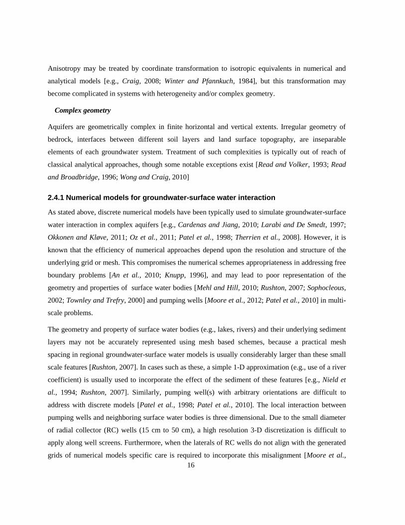
2.4.1 Numerical models for groundwater-surface water interaction
As stated above, discrete numerical models have been typically used to simulate groundwater-surface
water interaction in complex aquifers [e.g., Cardenas and Jiang, 2010; Larabi and De Smedt, 1997;
Okkonen and Kløve, 2011; Oz et al., 2011; Patel et al., 1998; Therrien et al., 2008]. However, it is
known that the efficiency of numerical approaches depend upon the resolution and structure of the
underlying grid or mesh. This compromises the numerical schemes appropriateness in addressing free
boundary problems [An et al., 2010; Knupp, 1996], and may lead to poor representation of the
geometry and properties of surface water bodies [Mehl and Hill, 2010; Rushton, 2007; Sophocleous,
2002; Townley and Trefry, 2000] and pumping wells [Moore et al., 2012; Patel et al., 2010] in multi-
scale problems.
The geometry and property of surface water bodies (e.g., lakes, rivers) and their underlying sediment
layers may not be accurately represented using mesh based schemes, because a practical mesh
spacing in regional groundwater-surface water models is usually considerably larger than these small
scale features [Rushton, 2007]. In cases such as these, a simple 1-D approximation (e.g., use of a river
coefficient) is usually used to incorporate the effect of the sediment of these features [e.g., Nield et
al., 1994; Rushton, 2007]. Similarly, pumping well(s) with arbitrary orientations are difficult to
address with discrete models [Patel et al., 1998; Patel et al., 2010]. The local interaction between
pumping wells and neighboring surface water bodies is three dimensional. Due to the small diameter
of radial collector (RC) wells (15 cm to 50 cm), a high resolution 3-D discretization is difficult to
apply along well screens. Furthermore, when the laterals of RC wells do not align with the generated
grids of numerical models specific care is required to incorporate this misalignment [Moore et al.,
17
2012]. Therefore, numerical models may be inefficient to test all (RC) well configurations and
determine their optimum design for RBF and pump and treat processes [Patel et al., 2010].
Variation of head and discharge along well screens, skin effects and head losses inside the collectors
complicate the boundary condition implementation along each collector screen. There are three
common approaches to treat this unique boundary condition along each collector screen: uniform
inflow [Tsou et al., 2010; Zhan and Zlotnik, 2002; Zhan et al., 2001], uniform head [Moore et al.,
2012; Patel et al., 2010; Samani et al., 2006] or constrained non-uniform head [Bakker et al., 2005].
The first representation of the well screen boundary condition is unrealistic particularly for the
application to long horizontal wells. The second approach, on the other hand, can be valid when the
flow condition inside the well is laminar with negligible head losses [Moore et al., 2012]. Head losses
can be considered in the third approach (preferred) [Bakker et al., 2005]. Mesh-based numerical
models such as MODFLOW roughly approximate this boundary condition using a head dependent
boundary condition, often using conductance factor [Patel et al., 1998].
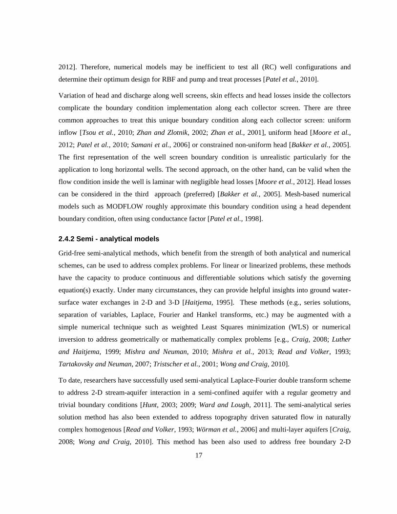
2.4.2 Semi - analytical models
Grid-free semi-analytical methods, which benefit from the strength of both analytical and numerical
schemes, can be used to address complex problems. For linear or linearized problems, these methods
have the capacity to produce continuous and differentiable solutions which satisfy the governing
equation(s) exactly. Under many circumstances, they can provide helpful insights into ground water-
surface water exchanges in 2-D and 3-D [Haitjema, 1995]. These methods (e.g., series solutions,
separation of variables, Laplace, Fourier and Hankel transforms, etc.) may be augmented with a
simple numerical technique such as weighted Least Squares minimization (WLS) or numerical
inversion to address geometrically or mathematically complex problems [e.g., Craig, 2008; Luther
and Haitjema, 1999; Mishra and Neuman, 2010; Mishra et al., 2013; Read and Volker, 1993;
Tartakovsky and Neuman, 2007; Tristscher et al., 2001; Wong and Craig, 2010].
To date, researchers have successfully used semi-analytical Laplace-Fourier double transform scheme
to address 2-D stream-aquifer interaction in a semi-confined aquifer with a regular geometry and
trivial boundary conditions [Hunt, 2003; 2009; Ward and Lough, 2011]. The semi-analytical series
solution method has also been extended to address topography driven saturated flow in naturally
complex homogenous [Read and Volker, 1993; Wörman et al., 2006] and multi-layer aquifers [Craig,
2008; Wong and Craig, 2010]. This method has been also used to address free boundary 2-D
18
saturated-unsaturated steady-state model in homogenous systems [Tristscher et al., 2001]. In spite of
having an ability to address naturally complex geometry and free boundary condition, the series
solution approach has not been extended to address free boundary 2-D and 3-D saturated and
saturated-unsaturated steady flow in geometrically complex stratified unconfined aquifers.
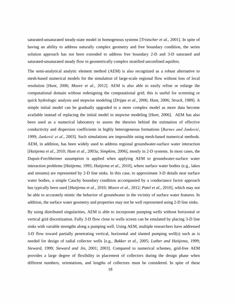
The semi-analytical analytic element method (AEM) is also recognized as a robust alternative to
mesh-based numerical models for the simulation of large-scale regional flow without loss of local
resolution [Hunt, 2006; Moore et al., 2012]. AEM is also able to easily refine or enlarge the
computational domain without redesigning the computational grid; this is useful for screening or
quick hydrologic analysis and stepwise modeling [Dripps et al., 2006; Hunt, 2006; Strack, 1989]. A
simple initial model can be gradually upgraded to a more complex model as more data become
available instead of replacing the initial model in stepwise modeling [Hunt, 2006]. AEM has also
been used as a numerical laboratory to assess the theories behind the estimation of effective
conductivity and dispersion coefficients in highly heterogeneous formations [Barnes and Janković,
1999; Janković et al., 2003]. Such simulations are impossible using mesh-based numerical methods.
AEM, in addition, has been widely used to address regional groundwater-surface water interaction
[Haitjema et al., 2010; Hunt et al., 2003a; Simpkins, 2006], mostly in 2-D systems. In most cases, the
Dupuit-Forchheimer assumption is applied when applying AEM to groundwater-surface water
interaction problems [Haitjema, 1995; Haitjema et al., 2010], where surface water bodies (e.g., lakes
and streams) are represented by 2-D line sinks. In this case, to approximate 3-D details near surface
water bodies, a simple Cauchy boundary condition accompanied by a conductance factor approach
has typically been used [Haitjema et al., 2010; Moore et al., 2012; Patel et al., 2010], which may not
be able to accurately mimic the behavior of groundwater in the vicinity of surface water features. In
addition, the surface water geometry and properties may not be well represented using 2-D line sinks.
By using distributed singularities, AEM is able to incorporate pumping wells without horizontal or
vertical grid discretization. Fully 3-D flow close to wells screen can be emulated by placing 3-D line
sinks with variable strengths along a pumping well. Using AEM, multiple researchers have addressed
3-D flow toward partially penetrating vertical, horizontal and slanted pumping well(s) such as is
needed for design of radial collector wells [e.g., Bakker et al., 2005; Luther and Haitjema, 1999;
Steward, 1999; Steward and Jin, 2001; 2003]. Compared to numerical schemes, grid-free AEM
provides a large degree of flexibility in placement of collectors during the design phase when
different numbers, orientations, and lengths of collectors must be considered. In spite of these
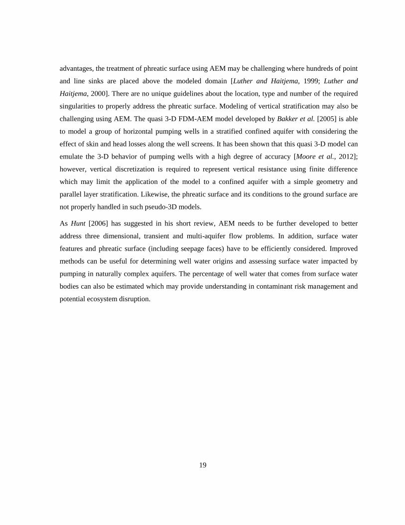
19
advantages, the treatment of phreatic surface using AEM may be challenging where hundreds of point
and line sinks are placed above the modeled domain [Luther and Haitjema, 1999; Luther and
Haitjema, 2000]. There are no unique guidelines about the location, type and number of the required
singularities to properly address the phreatic surface. Modeling of vertical stratification may also be
challenging using AEM. The quasi 3-D FDM-AEM model developed by Bakker et al. [2005] is able
to model a group of horizontal pumping wells in a stratified confined aquifer with considering the
effect of skin and head losses along the well screens. It has been shown that this quasi 3-D model can
emulate the 3-D behavior of pumping wells with a high degree of accuracy [Moore et al., 2012];
however, vertical discretization is required to represent vertical resistance using finite difference
which may limit the application of the model to a confined aquifer with a simple geometry and
parallel layer stratification. Likewise, the phreatic surface and its conditions to the ground surface are
not properly handled in such pseudo-3D models.
As Hunt [2006] has suggested in his short review, AEM needs to be further developed to better
address three dimensional, transient and multi-aquifer flow problems. In addition, surface water
features and phreatic surface (including seepage faces) have to be efficiently considered. Improved
methods can be useful for determining well water origins and assessing surface water impacted by
pumping in naturally complex aquifers. The percentage of well water that comes from surface water
bodies can also be estimated which may provide understanding in contaminant risk management and
potential ecosystem disruption.
20
Chapter 3
Semi-analytical series solution and analytic element method
3.1 Introduction
In this chapter the mathematical background behind the development of semi-analytical approaches
used in this thesis are explained. Their limitations and the possible ways to mitigate these limitations
are presented.
3.2 Series solutions
Over a finite domain, any arbitrary smooth and continuous function can be represented by infinite
terms of orthogonal series (basis functions). Relying upon this strength of orthogonal series,
separation of variables and series solution methods have been applied by many researchers to
analytically solve separable linear governing equation [e.g., Freeze and Witherspoon, 1967; Powers
et al., 1967; Selim, 1975]. Basis functions are typically generated from the method of separation of
variables and therefore satisfy the linear governing equation exactly. Using the method of separation
of variables, for example, to solve the 3-D Laplace equation (Equation (2-4)), a solution of the
following form is assumed
(3-1)
After substitution into the Laplace equation, we obtain three ordinary differential equations for ,
and :
+ & + & - (3-2)
where
Here , and are Eigenvalues and , and are Eigenfunctions of the Laplace
equation. By solving the preceding ODEs and using superposition of solutions for a range of values
for and , a discharge potential function of the following form is obtained as a flexible solution to
the 3-D Laplace equation:

21
∑∑
(3-3)
In the preceding equation, j and n are coefficient indexes approximation in x and y direction
respectively (in practice, the series is truncated to N and J series terms in each direction). Eigen
values ( ,
,
) are typically selected to satisfy boundary conditions at the sides of the domain
(in this thesis no-flow conditions are assumed along all sides of the modeled domain) as is later
discussed in chapter 5. The unknown coefficients , in equation (3-3) are arbitrary and may be
calculated to satisfy continuity and boundary conditions.
Based on the orthogonality of basis functions, unknown coefficients may be obtained using the Euler
formulas (similar to the determination of the Fourier coefficients in a Fourier series approach)[Freeze
and Witherspoon, 1967]. However, this treatment of boundary and continuity conditions is limited to
application to problems with a regular (e.g., square or rectangular) domain [Selim, 1975; Wong and
Craig, 2010]. Indeed along irregular boundaries, the basis functions are, strictly speaking, non-
orthogonal such that the Euler formulas are not valid and alternative approaches must be deployed.
The Gram-Schmidt orthonormalization scheme used by e.g., Selim [1975] slightly mitigated this
issue, but it is overly complicated.
Read and Volker [1993] derived a simpler least squares (LS) approach for simulating flow in single-
layer aquifer systems with irregular boundaries at the top and the bottom using series solutions. This
LS approach was employed by Craig [2008] to consider the effects of an arbitrary number of multiple
parallel or syncline layers. Wong and Craig [2010] further extended this approach to address
topography driven saturated flow in a geometrically complex stratified unconfined aquifer. Using LS,
unknown series solution coefficients , are calculated by minimizing the total sum of squared
errors (TSSE) in all boundary and continuity conditions at a set of control points. These control points
are located along the layer interfaces, topographic surface, bottom boundary, and/or the phreatic
surface.
22
3.3 Analytic Element Method (AEM)
The analytic element method (AEM) initially developed by Strack and Haitjema [1981] is a semi-
analytical method used for the solution of linear partial differential equations including the Laplace,
the Poisson, and the modified Helmholtz equations. In a fashion similar to the series solution method
discussed above, this approach does not rely upon discretization of volumes or areas in the modeled
system; only internal and external boundaries are discretized using a simple numerical collocation or
least squares algorithm.
The basic idea behind AEM is the representation of flow features by geometric elements, such as
point and line sinks. For the purpose of solving steady-state groundwater flow, each element has an
analytic solution which satisfies, for example, the Laplace equation [Strack, 1989]. In a manner
similar to the series solution the influence of analytic elements on the surrounding flow field can be
defined in terms of discharge potential, [L2T
-1], as follows;
∑
(3-4)
The influence function, [L2T
-1], represents the unit contribution of each element ( ) to total
discharge potential of the flow field where is the strength coefficient for each element. Influence
functions are generally designed to generate a specific form of discontinuity in potential or its
gradient along lines, curves, or surfaces, but be continuous elsewhere. The influence function for
various ground water features and governing equations have been developed by many researchers
after Strack and Haitjema [1981] initially used AEM for the simulation of groundwater problems.
Here, the primary interest is in utilizing 3-D AEM techniques. In 3-D, most AEM solutions are
generated from the elementary solution for a point sink in an infinite domain. Analogous to a point
charge in electromagnetic theory, a 3-D ground water point sink contribution to total discharge
potential is
[( ) ( )
( )
]
(3-5)
Where , and are the location of the point sinks in the global coordinate system. By
integrating the preceding equation along a line segment with a known sink distribution, the specific

23
discharge contribution of a line sink can be obtained. A line sink is able to mimic the behavior of an
arbitrary-oriented pumping well. There are various formulations for representing a pumping well
using a line sink in the literature, most of which differ in the strength distribution function along the
line sink [Haitjema, 1995; Luther and Haitjema, 1999; Luther and Haitjema, 2000; Luther, 1998;
Steward and Jin, 2001]. Here pumping wells will be modeled in a manner similar to Steward and Jin
[2003]. Rather than considering a complex strength distribution function along the well, they
subdivided each well (line element) into a set of consecutive segments and represented the discharge
potential of each segment in its local coordinate system. The discharge potential correspond to ith
segment of a line element, i.e., , is then obtained by integrating the potential for a point sink along
the segment with a length of 2l (here , and are local coordinates of each segment where
represents the segment axis) as follows:
∫
(3-6)
where and are the number of segments along a line element and constant strength of each
segment, respectively. Although Steward and Jin [2003] have applied linearly varying strength along
each segment of the line element, in this thesis a constant strength for each segment is used as the
contribution of the linearly varied strength term to the total discharge potential is negligible when the
segment length is small enough (as the number of segments increases, the required linearly varied
strength along each arm can be emulated using segments with constant head). Steward and Jin
[2003] have generated a closed form expression for each segment of a line element in its local
coordinate as
[ ]
(3-7)
3.4 Gibbs phenomenon
Gibbs phenomenon is a common issue with series-based solution methods and occurs whenever an
orthogonal series (e.g., a Fourier series) is used to approximate a function with a discontinuity (in
function or its gradient). In other words, sharp changes in geometry of the layers and/or boundary
conditions implemented across an interface can exacerbate Gibbs phenomenon [for further details see
24
Nahin, 2011]. Strictly speaking, such discontinuities lead to singular behaviour which cannot be
represented using separable solutions. This issue has been reported in research studies which used
series-based approaches to address groundwater flow in geometrically complex systems [e.g., Wong
and Craig, 2010]. In this thesis, Gibbs phenomenon predominantly occurs due to sharp changes in
geometry or boundary condition. Such problems may ideally be rectified by supplementing standard
basis functions with special ‘supplemental solutions’, which handle local departures from generally
smooth solutions. Here, such an approach is discussed for 1-D curve fitting of a discontinuous
function using a discrete Fourier series. In higher dimensions, when supplemental solutions must
additionally satisfy the governing equation, the problem becomes significantly more complex.
Consider a 1-D function (G(x)) with an abrupt change at x = 0 as:
{
(3-8)
where is equal to 0.25. Figure 3-1a shows the function in addition to the fitted 1-D curve to
generated from a Fourier series in the form
∑ (
) (
)
(3-9)
where N =10 and a simple least Squares algorithm through 20 data points (control points) is used for
the curve fitting as follows
∑
(3-10)
Figure 3-1b shows the absolute error at 80 non-control points normalized with respect to the
maximum value of function (x). Apparently the sharp change can not be emulated accurately. Even
worse this sharp change compromises the efficiency of Fourier series in fitting the remaining parts of
function (x).
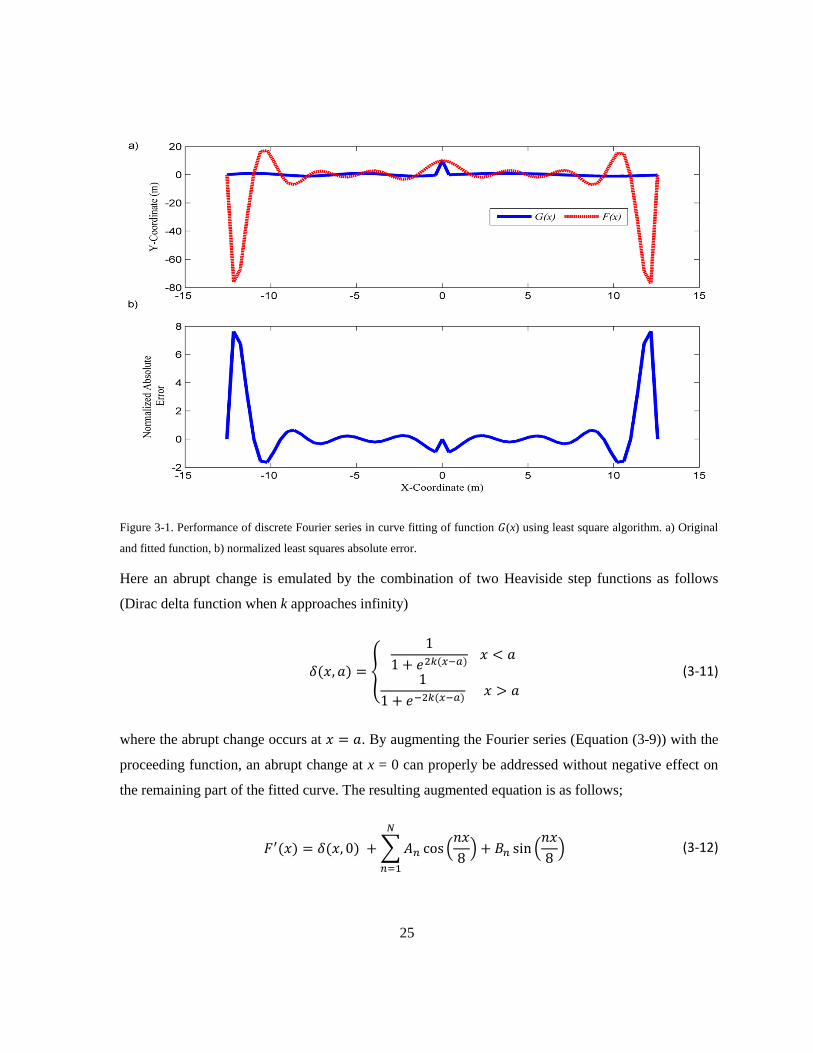
25
Figure 3-1. Performance of discrete Fourier series in curve fitting of function (x) using least square algorithm. a) Original
and fitted function, b) normalized least squares absolute error.
Here an abrupt change is emulated by the combination of two Heaviside step functions as follows
(Dirac delta function when k approaches infinity)
{
(3-11)
where the abrupt change occurs at . By augmenting the Fourier series (Equation (3-9)) with the
proceeding function, an abrupt change at x = 0 can properly be addressed without negative effect on
the remaining part of the fitted curve. The resulting augmented equation is as follows;
∑ (
) (
)
(3-12)
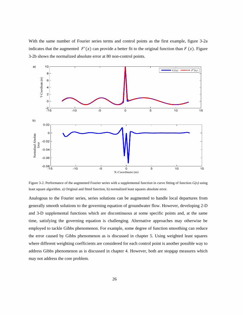
26
With the same number of Fourier series terms and control points as the first example, figure 3-2a
indicates that the augmented can provide a better fit to the original function than . Figure
3-2b shows the normalized absolute error at 80 non-control points.
Figure 3-2. Performance of the augmented Fourier series with a supplemental function in curve fitting of function G(x) using
least square algorithm. a) Original and fitted function, b) normalized least squares absolute error.
Analogous to the Fourier series, series solutions can be augmented to handle local departures from
generally smooth solutions to the governing equation of groundwater flow. However, developing 2-D
and 3-D supplemental functions which are discontinuous at some specific points and, at the same
time, satisfying the governing equation is challenging. Alternative approaches may otherwise be
employed to tackle Gibbs phenomenon. For example, some degree of function smoothing can reduce
the error caused by Gibbs phenomenon as is discussed in chapter 5. Using weighted least squares
where different weighting coefficients are considered for each control point is another possible way to
address Gibbs phenomenon as is discussed in chapter 4. However, both are stopgap measures which
may not address the core problem.
27
Chapter 4
Series solutions for saturated-unsaturated flow in multi-layer
unconfined aquifers
This chapter is based on the following published article. For the coherence of this thesis, changes
have been made in the introduction, background, method and conclusion sections of this
publication. References are presented at the end of the thesis.
Ameli, A. A., J. R. Craig, and S. Wong (2013), Series solutions for saturated-unsaturated flow in
multi-layer unconfined aquifers, Adv. Water Resour., 60, 24-33,
DOI: 10.1016/j.advwatres.2013.07.004.
4.1 Introduction
In many cases, the influence of the unsaturated zone must be included in a groundwater-surface water
interaction model. Analytical and semi-analytical approaches typically neglect or simplify the
unsaturated zone and capillary fringe flow. The purpose of the chapter is to extend semi-analytical
series solution approaches for application to 2-D steady-state free boundary saturated-unsaturated
subsurface flow induced by spatially variable surface fluxes in geometrically complex homogenous
and stratified unconfined aquifers. The capillary fringe zone, unsaturated zone, groundwater zone and
their interactions are incorporated. Continuous solutions for pressure in the saturated and unsaturated
zone are determined iteratively, as is the location of the water table surface. The water table and
capillary fringe are allowed to intersect stratigraphic interfaces. The model can be used to provide a
conceptual understanding of the influence of factors on unsaturated flow behavior and a priori
unknown water table elevation.
4.2 Background
To date, researchers have used series solutions to independently address the free boundary saturated-
unsaturated steady flow in homogenous systems [Tristscher et al., 2001] and topography-driven
saturated flow in heterogeneous aquifers with geometrically complex stratification [Wong and Craig,
2010]. However, these issues have never been addressed concurrently. In addition, a robust regional
subsurface model requires consideration of the interaction between subsurface flow and the
topographic surface. Existing semi-analytical models have paid scarce attention to this issue, and also
28
have neglected the capillary fringe zone [Mishra and Neuman, 2010; Tristscher et al., 2001].
However, researchers have experimentally and numerically shown that horizontal flow in this zone
can have an effect on the magnitude of subsurface flow toward a stream and upon the water table
location [Berkowitz et al., 2004; Romanoa et al., 1999].
4.3 Problem statement
Figure 4-1 shows the general schematic of a stratified soil profile that can be modeled using methods
derived herein. An aquifer with length L is subdivided into M layers with arbitrary geometry, each
with saturated conductivity . Layers are indexed downward from m=1 to m=M and are bounded by
the curve above and below. The bottom bedrock, , and sides of the aquifer
are impermeable. The topographic surface, , is subject to a specified surface flux distribution
function (which may be calculated from rainfall, evaporation and transpiration) and/or a Dirichlet
condition along surface water bodies (e.g., a river with specified width and surface elevation). These
conditions are easily amended to account for the presence of multiple surface water features. The
saturated-unsaturated interface or top of capillary fringe ( ) is a moving boundary which defines
the location of the top of the saturated zone and the bottom of unsaturated zone. The water table is
defined as a boundary with zero pressure head. All layer interfaces, the topographic surface, and the
bedrock surface are specified prior to solution.
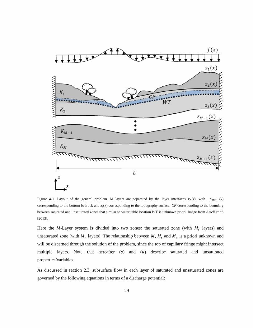
29
Figure 4-1. Layout of the general problem. M layers are separated by the layer interfaces zm(x), with z(M+1) (x)
corresponding to the bottom bedrock and z1(x) corresponding to the topography surface. CF corresponding to the boundary
between saturated and unsaturated zones that similar to water table location is unknown priori. Image from Ameli et al.
[2013].
Here the -Layer system is divided into two zones: the saturated zone (with layers) and
unsaturated zone (with layers). The relationship between , and is a priori unknown and
will be discerned through the solution of the problem, since the top of capillary fringe might intersect
multiple layers. Note that hereafter ( ) and ( ) describe saturated and unsaturated
properties/variables.
As discussed in section 2.3, subsurface flow in each layer of saturated and unsaturated zones are
governed by the following equations in terms of a discharge potential:
30
(4-1)
(4-2)
where is the uppermost layer where the top of capillary fringe interface ( ) exists.
For both unsaturated and saturated 2-D steady flow, the stream function formulation will be useful for
applying some of the continuity and boundary conditions. The stream function formulation can be
obtained using a generalized form of the Cauchy-Riemann equations for unsaturated flow [Read and
Broadbridge, 1996],
=
and
=
(4-3)
and Cauchy-Riemann equations for saturated flow,
=
and
=
(4-4)
where and
are unsaturated and saturated stream function of the mth
layer respectively. The
unsaturated and saturated governing equations are equivalent to the following equations in terms of
the stream function for each layer of unsaturated and saturated zones:
(4-5)
(4-6)
The normal first order derivative of a 2-D function, T, across an interface can be decomposed into
vertical and horizontal components as
√
(4-7)

31
When the cosine of the slope angle describing each evaluation curve approximated as unity (the
denominator of the equation 4-7), in a manner similar to Read and Broadbridge [1996] for the vadose
zone and Wong and Craig [2010] for the saturated zone, the normal first order potential derivatives
across unsaturated and saturated interfaces can be represented as follows:
(4-8a)
(4-8b)
where is the coordinate normal to each interface represented by the function , which is either a
layer interface or the top of capillary fringe . Using the above equations (Equations (4-
8a) and (4-8b)) and Cauchy-Riemann equations (Equations (4-3) and (4-4)) the boundary and
continuity conditions along unsaturated and saturated interfaces can be represented in terms of either
potential or stream function.
Across the sides of the domain in both unsaturated and saturated zones, no-flow conditions in x-
direction are imposed. The stream function equivalent formulas for unsaturated and saturated zones
used in current chapter are:
(4-7a)
(4-9b)
(4-8a)
(4-10b)
where L is the length of the domain (Figure 4-1). The topographic surface boundary condition with
the arbitrary infiltration-evapotranspiration function [LT-1
] is:
( ) (4-9a)
or, using the stream function formulation:
32
(4-11b)
where is taken as positive for infiltration and negative for evapotranspiration. Along surface
water features a uniform hydraulic head is applied. The continuity of flux along the vadose zone
layers interfaces for can be represented as its stream function equivalent:
( )
(4-10)
Similarly, the continuity of head along vadose zone interfaces in terms of the Kirchhoff potential
is
=
(4-11)
For the saturated zone, the continuity of flux (in terms of stream function) and pressure head (in terms
of discharge potential) along each saturated layer interface ( ) can be
represented as:
( )
(4-12)
( )
( )
(4-13)
No-flow conditions are imposed at the bottom of the domain (bedrock) in the saturated zone which
can be also represented in terms of stream function as:
( ) (4-14)
To complete the problem statement, continuity of flux and pressure head must be enforced along the
boundary between unsaturated and saturated zones, here referred to as the top of capillary fringe (cf):
(
)
(4-15)
(
)
=
(4-16)
here is the layer where top of capillary fringe is located. In each unsaturated layer ,
the general stream function solution of the following form can be developed:
33
∑
( ) ( )
( ) ( )
(4-17)
Note that the form of this solution is obtained using the method of separation of variables (in a similar
process to the generation of equation (3-3) as was discussed in section 3.2) and satisfies the governing
equation for unsaturated flow (Equation (4-5)). In the preceding equation, j represents the coefficient
index, J is the order of approximation or total number of terms in the series solution, and ,
are
the series coefficients associated with the mth
unsaturated layer and jth
coefficient index. Through
judicious selection of , and
the sides no-flow conditions (Equations (4-9a) and (4-9b)) are
satisfied:
;
√
(
) ,
√
(
)
(4-18)
The Kirchhoff potential series solution can be obtained using equation (4-3):
∑ ⟨
( ) (
)
( ) (
) ⟩
(4-19)
The series solution of the saturated governing equation (Equation (4-6)) in terms of stream function is
similarly obtained using the method of separation of variables while ,
are the saturated series
coefficients associated with the mth
layer .
∑
( ) ( ) ( ) ( )
(4-20)
Again, through judicious selection of for j = 0 ... J-1, the side no-flow conditions
(Equations (4-10a) and (4-10b)) are satisfied. The saturated discharge potential series solution can be
obtained using Cauchy-Riemann conditions (Equation (4-4)):

34
∑ ( ) ( )
( ) ( )
(4-21)
The unknowns coefficients ,
, and
will be calculated to satisfy the continuity and
boundary conditions (Equations (4-11) to (4-18)).
4.4 Solution
The series solution for above the top of capillary fringe (i.e. the unsaturated zone) and below the top
of capillary fringe (i.e. ground water and capillary fringe zones) will be determined separately by
minimizing the boundary and continuity condition errors at a set of uniformly spaced control
points located along each layer interface, the capillary fringe top, the topographic surface, and the
bedrock. The location of the top of capillary fringe and water table are unknown a priori, and will be
obtained through a robust iterative scheme. Initially, the top of capillary fringe is fixed to be equal to
the river hydraulic head, and a Dirichlet condition of (where is the layer where top of
capillary fringe is located) is applied. The unknown coefficients for the potential within the
unsaturated zone are then calculated by minimizing the boundary and continuity condition errors at a
set of control points along each interface within the unsaturated zone (the topographic surface,
top of capillary fringe, and layer interfaces), for a total of NC ( ) control points. The total
weighted ( is the weight of each equation) sum of squared errors (TWSSE) is here subdivided into
the errors along mentioned evaluation curves, i.e.,
∑
(4-22a)
where
∑
( )
(4-24b)
∑ [ ( )
( )]
+
35
∑ ( )
(4-24c)
∑ (
)
(4-24d)
the subscripts refer to the errors along the topographic surface (t), layer interfaces (m) and top of
capillary fringe (cf). By minimizing equation (4-24a), approximations of the unknown unsaturated
coefficients ( ,
) at the first iteration will be obtained and the series solutions for stream function
(4-19) and Kirchhoff potential (4-21) are fully defined. This intermediate unsaturated zone solution
provides the flux or stream function distribution along the capillary fringe, which acts as the top
boundary condition for the solution of the saturated zone problem (Equation 4-18). In a similar
manner, the saturated unknown coefficients are calculated by minimizing the total weighted sum of
squared error (TWSSE) at a set of control points along top of capillary fringe location, bottom
bedrock and interfaces between saturated layers.
∑
(4-23a)
where
∑ [ (
) (
)]
(4-25b)
and is the layer where top of capillary fringe is located
∑ [ ( )
( )]
∑
(4-25c)
∑
(4-25d)
By minimizing equation (4-25a), an approximation of the unknown saturated coefficients ( ,
) is
obtained and the series solution in terms of stream function (4-22) and discharge potential (4-23) are
fully defined. The saturated series solution provides a water pressure distribution along the
approximate top of capillary fringe surface at each control point ( ). In each iteration, this may
be used to modify the location of the top of capillary fringe according to:
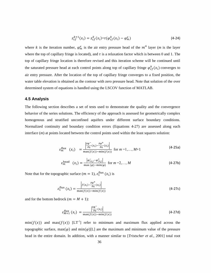
36
+
(4-24)
where is the iteration number, is the air entry pressure head of the th
layer (m is the layer
where the top of capillary fringe is located), and is a relaxation factor which is between 0 and 1. The
top of capillary fringe location is therefore revised and this iteration scheme will be continued until
the saturated pressure head at each control points along top of capillary fringe converges to
air entry pressure. After the location of the top of capillary fringe converges to a fixed position, the
water table elevation is obtained as the contour with zero pressure head. Note that solution of the over
determined system of equations is handled using the LSCOV function of MATLAB.
4.5 Analysis
The following section describes a set of tests used to demonstrate the quality and the convergence
behavior of the series solutions. The efficiency of the approach is assessed for geometrically complex
homogenous and stratified unconfined aquifers under different surface boundary conditions.
Normalized continuity and boundary condition errors (Equations 4-27) are assessed along each
interface (m) at points located between the control points used within the least squares solution:
|
|
for m =1,…, M+1
(4-25a)
|
|
for m =2,…, M (4-27b)
Note that for the topographic surface ( ),
is
|
|
(4-27c)
and for the bottom bedrock ( ):
|
|
(4-27d)
and [LT-1
] refer to minimum and maximum flux applied across the
topographic surface, and [L] are the maximum and minimum value of the pressure
head in the entire domain. In addition, with a manner similar to [Tristscher et al., 2001] total root

37
mean square normalized flux error ( ) and total root mean square normalized head error
( ) are obtain as follows;
√ ∑
∑
∑
(4-26a)
√ ∑
for m =2,…, M (4-28b)
The rate of convergence of the solutions with a free boundary condition will also be assessed in the
below cases.
4.5.1 Example 1: Homogenous system
The configuration for a hypothetical homogenous unconfined aquifer system adjacent to a 20 m wide
river is shown in Figure 4-2. Figure 4-2a shows the infiltration and evapotranspiration function
( ) applied across the topographic surface. The hydrological and hydrogeological parameters used
in example 1 are: , , river head ( ) = 5.5 m, river width
= 20m.
Figure 4-2. a) Infiltration and evapotranspiration function [md-1] used in example 1, b) Layout of the flow streamlines
(grey), equi-potential contours (black), water level and water table in a homogenous unconfined aquifer adjacent to a
constant head river at left corner after 10 iterations. Image from Ameli et al. [2013].
38
The flow net for this problem, along with the calculated top of capillary fringe and water table
locations are shown in Figure 4-2b. This solution was identified after 10 iterations. Hydraulic head
contours in the saturated zone show that conditions are nearly hydrostatic beneath the top of capillary
fringe interface. Above the capillary fringe the flow condition is not hydrostatic (not shown here).
The solution was obtained using ( )(2N+1) =282 coefficients and 1400 control points along
each evaluation curve (i.e., the topographic surface, bedrock and top of capillary fringe). The
topographic surface boundary condition (Eq. (4-11b)), no-flow bedrock boundary condition (Eq. (4-
16)) and continuity of flux (Equation (4-17)) and head (Equation (4-18)) across top of capillary
fringe, have been satisfied by expanding the general series solution (Equations (4-19), (4-21), (4-22)
and (4-23)) at control points along each interface and minimizing error using weighted least square
method (Equations (4-24) and (4-25)). Note that since the units and magnitude of the flux and head
errors are different, weighting coefficients for each control point ( ) were considered as 4 and 1 for
flux and head conditions respectively. A relaxation factor = 0.5 used to control the convergence
behaviour of the top of the capillary fringe (Equation 4-26).
Figure 4-3 demonstrates the quality and the convergence behavior of the series solutions used in
example 1. Figure 4-3a shows the convergence of the solution as the pressure head at 1400 control
points along the free boundary top of capillary fringe converges to air entry pressure ( .
As can be seen from the figure, control points along the intersection of the top of capillary fringe and
topographic surface have the largest absolute error at initial iterations. Figure 4-3b shows the
normalized flux errors across the topographic surface and the bottom bedrock (
) at 1400
points between the control points used for least squares minimization.

39
Figure 4-3. Convergence of the water level moving boundary between saturated and unsaturated zones to air entry pressure
( with relaxation factor ( ) = 0.5, b) Normalized flux error across boundary interfaces (topography surface
and the bottom bedrock). Image from Ameli et al. [2013].
Although there is a flux error across the impermeable bedrock, the net normalized flux error is on the
order 10-17
, which guarantees mass conservation inside the domain. The largest normalized flux
error over both interfaces (2%) occurs along the intersection of the top of capillary fringe and the
topographic surface, and on the right side of the topographic surface with higher (Figure 4-3b).
The error along the topographic surface can result from abrupt changes of surface function
(evapotranspiration to infiltration and vice versa) that cause Gibbs phenomenon. Although a linear
transition was used between infiltration and evapotranspiration (Figure 4-2a), some degree of function
smoothing could have reduced this error. Normalized head errors along the river boundary condition
are also on the order 10-8
(not shown here). In addition, total root mean square normalized flux error
) along the topographic surface and bottom bedrock are on the order of 10-3
. Note that, since
the governing equation is elliptic and satisfied exactly using series solutions method, the largest errors
in the domain occur along the system boundaries. The series solution is seen to be valid and
successful (with acceptable ranges of error along boundaries) in naturally complex homogenous
regional unconfined aquifer as long as Gibbs phenomenon is avoided and the Fourier series
converges.
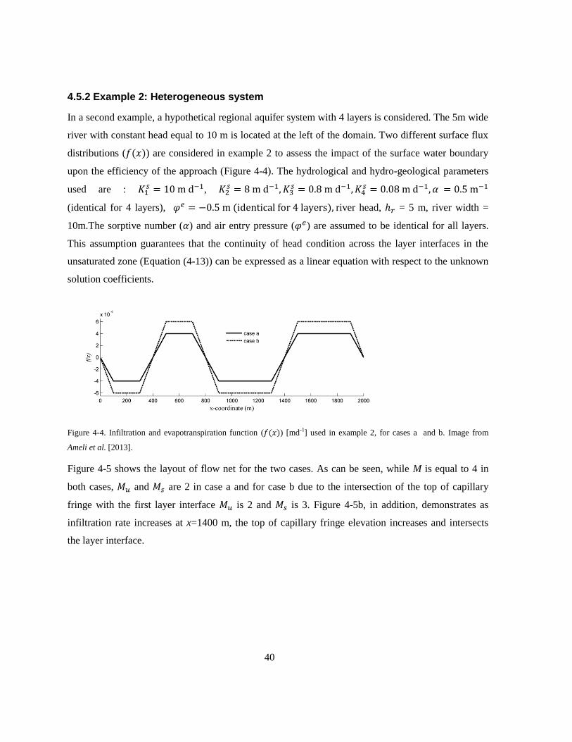
40
4.5.2 Example 2: Heterogeneous system
In a second example, a hypothetical regional aquifer system with 4 layers is considered. The 5m wide
river with constant head equal to 10 m is located at the left of the domain. Two different surface flux
distributions ( ) are considered in example 2 to assess the impact of the surface water boundary
upon the efficiency of the approach (Figure 4-4). The hydrological and hydro-geological parameters
used are : ,
(identical for 4 layers), river head, = 5 m, river width =
10m.The sorptive number ( ) and air entry pressure ( ) are assumed to be identical for all layers.
This assumption guarantees that the continuity of head condition across the layer interfaces in the
unsaturated zone (Equation (4-13)) can be expressed as a linear equation with respect to the unknown
solution coefficients.
Figure 4-4. Infiltration and evapotranspiration function ( ) [md-1] used in example 2, for cases a and b. Image from
Ameli et al. [2013].
Figure 4-5 shows the layout of flow net for the two cases. As can be seen, while M is equal to 4 in
both cases, and are 2 in case a and for case b due to the intersection of the top of capillary
fringe with the first layer interface is 2 and is 3. Figure 4-5b, in addition, demonstrates as
infiltration rate increases at x=1400 m, the top of capillary fringe elevation increases and intersects
the layer interface.
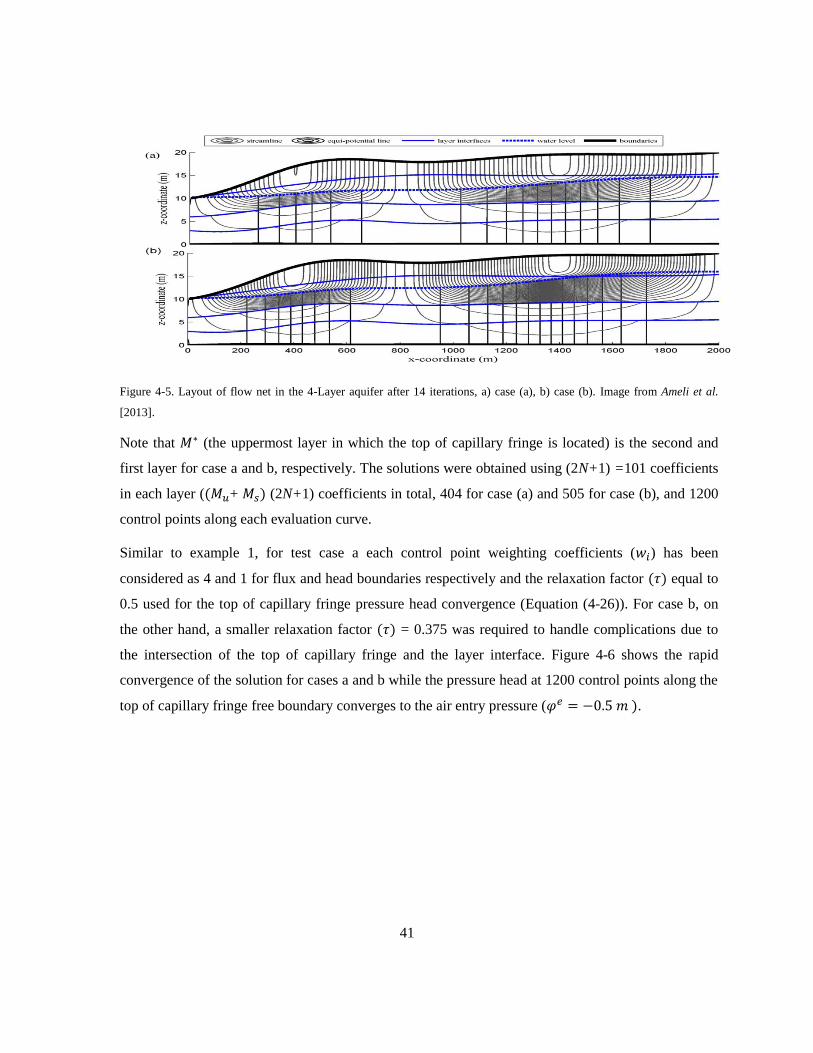
41
Figure 4-5. Layout of flow net in the 4-Layer aquifer after 14 iterations, a) case (a), b) case (b). Image from Ameli et al.
[2013].
Note that (the uppermost layer in which the top of capillary fringe is located) is the second and
first layer for case a and b, respectively. The solutions were obtained using (2N+1) =101 coefficients
in each layer ( + (2N+1) coefficients in total, 404 for case (a) and 505 for case (b), and 1200
control points along each evaluation curve.
Similar to example 1, for test case a each control point weighting coefficients ( ) has been
considered as 4 and 1 for flux and head boundaries respectively and the relaxation factor equal to
0.5 used for the top of capillary fringe pressure head convergence (Equation (4-26)). For case b, on
the other hand, a smaller relaxation factor = 0.375 was required to handle complications due to
the intersection of the top of capillary fringe and the layer interface. Figure 4-6 shows the rapid
convergence of the solution for cases a and b while the pressure head at 1200 control points along the
top of capillary fringe free boundary converges to the air entry pressure ( .
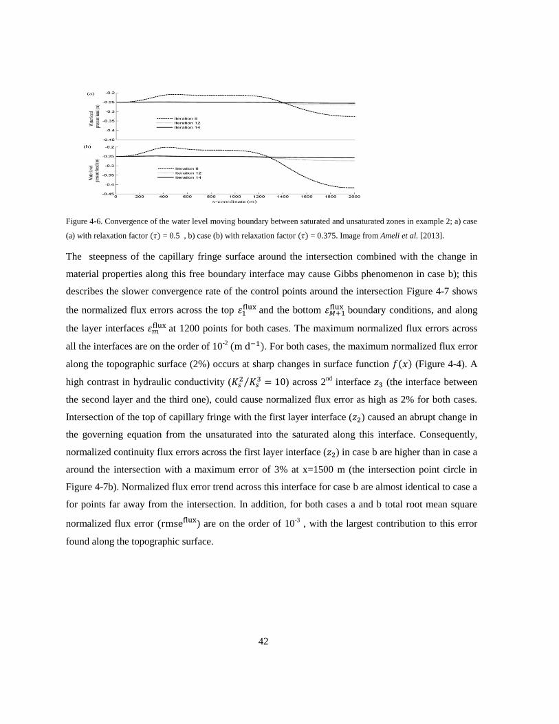
42
Figure 4-6. Convergence of the water level moving boundary between saturated and unsaturated zones in example 2; a) case
(a) with relaxation factor = 0.5 , b) case (b) with relaxation factor = 0.375. Image from Ameli et al. [2013].
The steepness of the capillary fringe surface around the intersection combined with the change in
material properties along this free boundary interface may cause Gibbs phenomenon in case b); this
describes the slower convergence rate of the control points around the intersection Figure 4-7 shows
the normalized flux errors across the top and the bottom
boundary conditions, and along
the layer interfaces at 1200 points for both cases. The maximum normalized flux errors across
all the interfaces are on the order of 10-2 . For both cases, the maximum normalized flux error
along the topographic surface (2%) occurs at sharp changes in surface function (Figure 4-4). A
high contrast in hydraulic conductivity (
⁄ ) across 2nd
interface (the interface between
the second layer and the third one), could cause normalized flux error as high as 2% for both cases.
Intersection of the top of capillary fringe with the first layer interface ( ) caused an abrupt change in
the governing equation from the unsaturated into the saturated along this interface. Consequently,
normalized continuity flux errors across the first layer interface ( ) in case b are higher than in case a
around the intersection with a maximum error of 3% at x=1500 m (the intersection point circle in
Figure 4-7b). Normalized flux error trend across this interface for case b are almost identical to case a
for points far away from the intersection. In addition, for both cases a and b total root mean square
normalized flux error ) are on the order of 10-3
, with the largest contribution to this error
found along the topographic surface.
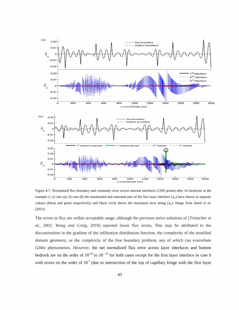
43
Figure 4-7. Normalized flux boundary and continuity error across internal interfaces (1200 points) after 14 iterations in the
example 2; a) case (a), b) case (b) the unsaturated and saturated part of the first layer interface ( ) have shown in separate
colours (black and green respectively) and black circle shows the maximum error along ( ). Image from Ameli et al.
[2013].
The errors in flux are within acceptable range, although the previous series solutions of [Tristscher et
al., 2001; Wong and Craig, 2010] reported lower flux errors. This may be attributed to the
discontinuities in the gradient of the infiltration distribution function, the complexity of the stratified
domain geometry, or the complexity of the free boundary problem, any of which can exacerbate
Gibbs phenomenon. However, the net normalized flux error across layer interfaces and bottom
bedrock are on the order of 10-18
to 10 -14
for both cases except for the first layer interface in case b
with errors on the order of 10-7
(due to intersection of the top of capillary fringe with the first layer
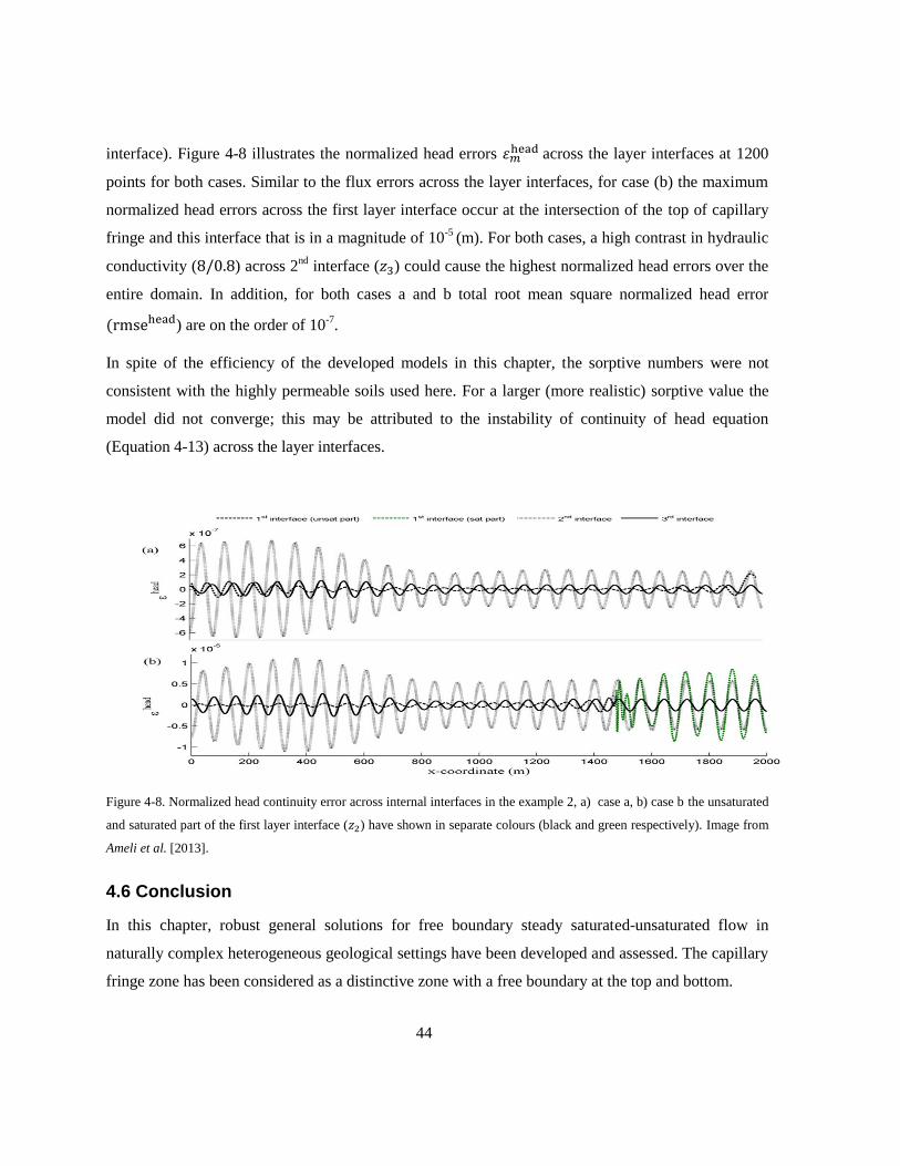
44
interface). Figure 4-8 illustrates the normalized head errors across the layer interfaces at 1200
points for both cases. Similar to the flux errors across the layer interfaces, for case (b) the maximum
normalized head errors across the first layer interface occur at the intersection of the top of capillary
fringe and this interface that is in a magnitude of 10-5
(m). For both cases, a high contrast in hydraulic
conductivity ( ) across 2nd
interface ( ) could cause the highest normalized head errors over the
entire domain. In addition, for both cases a and b total root mean square normalized head error
) are on the order of 10-7
.
In spite of the efficiency of the developed models in this chapter, the sorptive numbers were not
consistent with the highly permeable soils used here. For a larger (more realistic) sorptive value the
model did not converge; this may be attributed to the instability of continuity of head equation
(Equation 4-13) across the layer interfaces.
Figure 4-8. Normalized head continuity error across internal interfaces in the example 2, a) case a, b) case b the unsaturated
and saturated part of the first layer interface ( ) have shown in separate colours (black and green respectively). Image from
Ameli et al. [2013].
4.6 Conclusion
In this chapter, robust general solutions for free boundary steady saturated-unsaturated flow in
naturally complex heterogeneous geological settings have been developed and assessed. The capillary
fringe zone has been considered as a distinctive zone with a free boundary at the top and bottom.
45
Semi-analytical series solutions have been showed to simulate coupled saturated and unsaturated flow
accurately as long as Gibbs phenomenon issue has been addressed and the Fourier series converges.
This is contingent upon
The continuity conditions being linear (e.g., identical sorptive number and air entry
pressure head for all unsaturated layers)
interfaces being continuous in value and gradient
the surface function ( ) being continuous in value and ideally gradient
The solutions converged with acceptable rates of convergence and errors in top of capillary fringe and
water table locations. Without discretization artifacts, introduced by numerical schemes, boundary
errors, pressure head, flux and stream function distributions are immediately available as continuous
function of the space. The number of degrees of freedom required to simulate these complex systems
is small.
46
Chapter 5
Semi-analytical series solutions for three dimensional
groundwater-surface water interaction
This chapter is based on the following published article. For the coherence of this thesis, changes
have been made in the introduction, background, method and conclusion sections of this
publication. References are presented at the end of the thesis.
Ameli, A. A., J. R. Craig, Semi-analytical series solutions for three dimensional groundwater-surface
water interaction Water Resour. Res., 50, Doi:10.1002/2014WR0.
5.1 Introduction
This chapter addresses the extension of the semi-analytical series solutions approach to free boundary
3-D steady subsurface flow controlled by water exchange across the ground surface (e.g.,
evapotranspiration, infiltration, seepage faces) and the presence of surface water bodies in a stratified
aquifer. A priori unknown water table surface including seepage faces and recharge zones, is
determined semi-analytically using a robust iterative scheme. The solutions are derived and
demonstrated on a number of test cases and the errors are assessed and discussed. This accurate and
grid-free 3-D model can be a helpful tool for providing insight into lake-aquifer and stream-aquifer
interactions. Here, it is used to assess the impact of lake sediment geometry and properties on lake-
aquifer interactions. Various combinations of lake sediment are considered and the appropriateness of
the Dupuit-Forchheimer approximation for simulating lake bottom flux distribution is investigated. In
addition, the method is applied to a test problem of surface seepage flows from a complex
topographic surface.
5.2 Background
Semi-analytical series solutions have been used to address 2-D saturated topography-driven flow
[e.g., Craig, 2008; Wong and Craig, 2010] and saturated-unsaturated free boundary flow [Ameli et
al., 2013; Tristscher et al., 2001] in naturally complex homogenous and stratified unconfined
aquifers. This method is able to provide helpful insights into effective controls on groundwater-
surface water interaction including the effect of sediment geometry and material property on seepage
distributions at the lake-aquifer interface, all without the use of grid or mesh.

47
The relative significance of lake size, confined aquifer size, homogenous confined aquifer material
property and precipitation amount in lake-aquifer flow regime have been assessed numerically
[Genereux and Bandopadhyay, 2001; Townley and Trefry, 2000] and analytically [Kacimov, 2000;
2007]. However, the effect of lake sediment material properties and geometry on lake-aquifer
interaction has not been fully investigated. It is known that lake sediment may play a significant role
in altering the lake bed shape [Miller et al., 2013] and will impact the distribution of seepage flux at
the lake bed [Genereux and Bandopadhyay, 2001]. However, the impact of sediment layer geometry
and properties on seepage flux at the lake bed have not been assessed.
In 2-D Dupuit-Forchheimer models [Kirkham, 1967], where the resistance to vertical flow is ignored,
it is common to treat the lake bed as uniform, which leads to a characteristic seepage distribution
where lake's fluxes are highest at the shore and decrease with distance from the shoreline. With
Dupuit-Forchheimer assumption, the extent of this seepage zone as measured from the lake shore is
proportional to a leakage factor, calculated from the sediment and aquifer conductivity and thickness
[e.g., Bakker, 2002; Bakker, 2004; Strack, 1984]. Multiple research studies have shown that the
Dupuit-Forchheimer model may be a reasonable approximation of a fully 3-D system when the lake is
very large compared to the aquifer thickness [e.g., Hunt et al., 2003b; Kacimov, 2000]. Some 3-D and
2-D cross sectional models have been used to estimate sediment layer impacts using this leakage
factor approach instead of explicitly modeling the lake sediment layer [Kacimov, 2000; Nield et al.,
1994]. However, the leakage factor approach neglects horizontal flow through the lake sediment and
may therefore miss lateral flow effects, and it can be accurate only for the case of a very thin and low
permeable lake sediment with uniform thickness [Kacimov, 2000]. To realistically investigate the
effect of lake sediment on lake-aquifer interaction, a robust 3-D multi-layer model with the ability to
explicitly consider the sediment layer is desirable. In one of the few research studies that
independently considered the lake sediment layer, Genereux and Bandopadhyay [2001] have treated
the sediment as porous medium cells (of lower hydraulic conductivity) in direct contact with the lake
bed. Their study did not consider the geometry of the lake sediment layer (a uniform sediment layer
with a specified thickness equal to the discretized mesh thickness was used) and suffered from
numerical discretization errors [Bakker and Anderson, 2002].
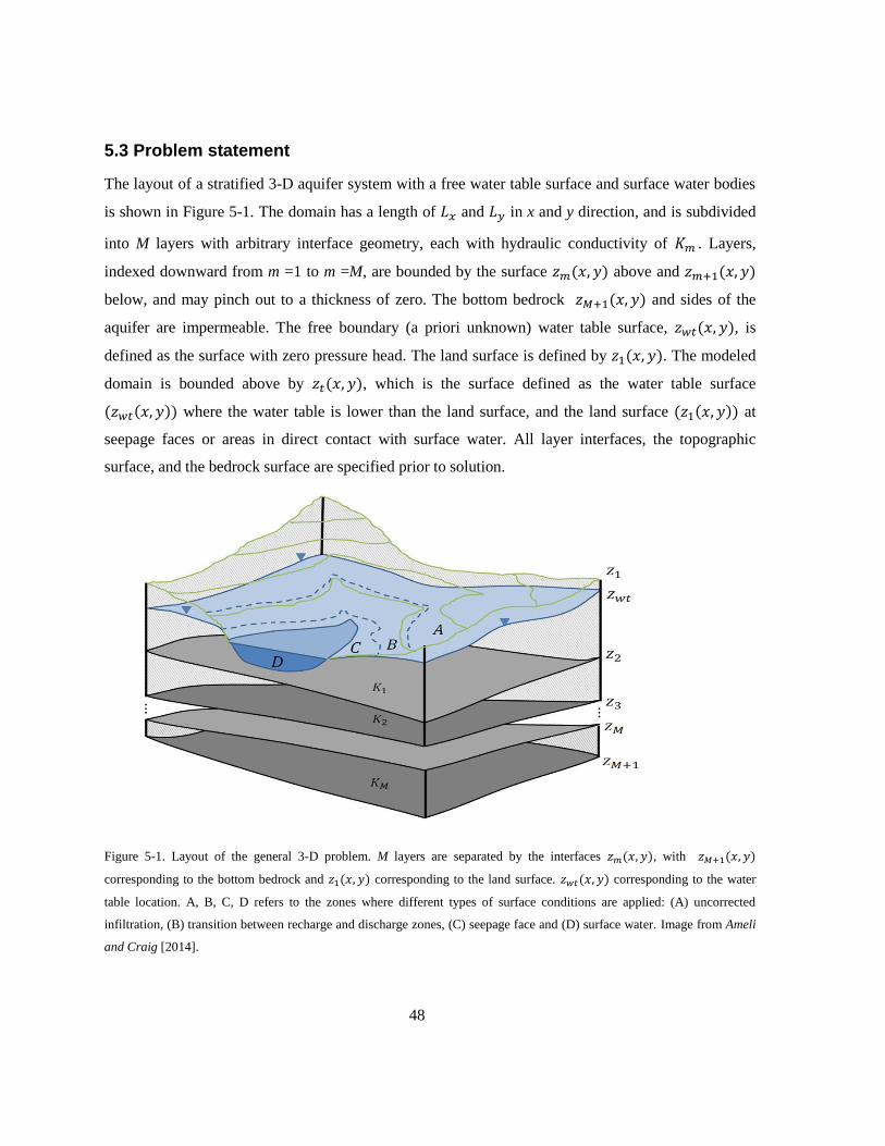
48
5.3 Problem statement
The layout of a stratified 3-D aquifer system with a free water table surface and surface water bodies
is shown in Figure 5-1. The domain has a length of and in x and y direction, and is subdivided
into M layers with arbitrary interface geometry, each with hydraulic conductivity of . Layers,
indexed downward from m =1 to m =M, are bounded by the surface above and
below, and may pinch out to a thickness of zero. The bottom bedrock and sides of the
aquifer are impermeable. The free boundary (a priori unknown) water table surface, , is
defined as the surface with zero pressure head. The land surface is defined by . The modeled
domain is bounded above by , which is the surface defined as the water table surface
where the water table is lower than the land surface, and the land surface at
seepage faces or areas in direct contact with surface water. All layer interfaces, the topographic
surface, and the bedrock surface are specified prior to solution.
Figure 5-1. Layout of the general 3-D problem. M layers are separated by the interfaces , with
corresponding to the bottom bedrock and corresponding to the land surface. corresponding to the water
table location. A, B, C, D refers to the zones where different types of surface conditions are applied: (A) uncorrected
infiltration, (B) transition between recharge and discharge zones, (C) seepage face and (D) surface water. Image from Ameli
and Craig [2014].

49
As described in chapter 3, the problem may be posed in terms of a discharge potential, [ ],
defined as
(5-1)
where [L] is the total hydraulic head in the mth layer. Using continuity of mass and
Darcy’s law, each layer’s discharge potential function must satisfy the Laplace equation:
(5-2)
Flow rates are calculated as the spatial derivative of the discharge potential. In a manner similar to
Wong and Craig [2010] for the 2-D discharge magnitude normal to an interface, the 3-D discharge
across an interface can be decomposed into vertical and horizontal components when the cosine of the
slope angle (in both x and y directions) describing each evaluation surface may be approximated as
unity. The resulting equation is as follows:
(5-3)
where is the coordinate normal to interface surfaces represented by the function , which is
either a layer interface , bottom bedrock surface or top interface ( ).
Across the sides of the domain, no-flow conditions in x and y directions are imposed.
(5-4a)
( ) (5-4b)
The top surface boundary of the modeled domain, , is subject to a specified vertical flux
distribution (recharge), and/or Dirichlet boundary conditions along surface water bodies and seepage
faces. Here, in order to insure convergence of the iterative approach, both Dirichlet and Neumann
conditions along the a priori unknown top surface are treated as being dependent upon the depth of
the water table. Here we extend the approach of Forsyth [1988], where Dirichlet seepage faces and
specified head boundary conditions are implemented as equivalent source/sink terms, to handle the
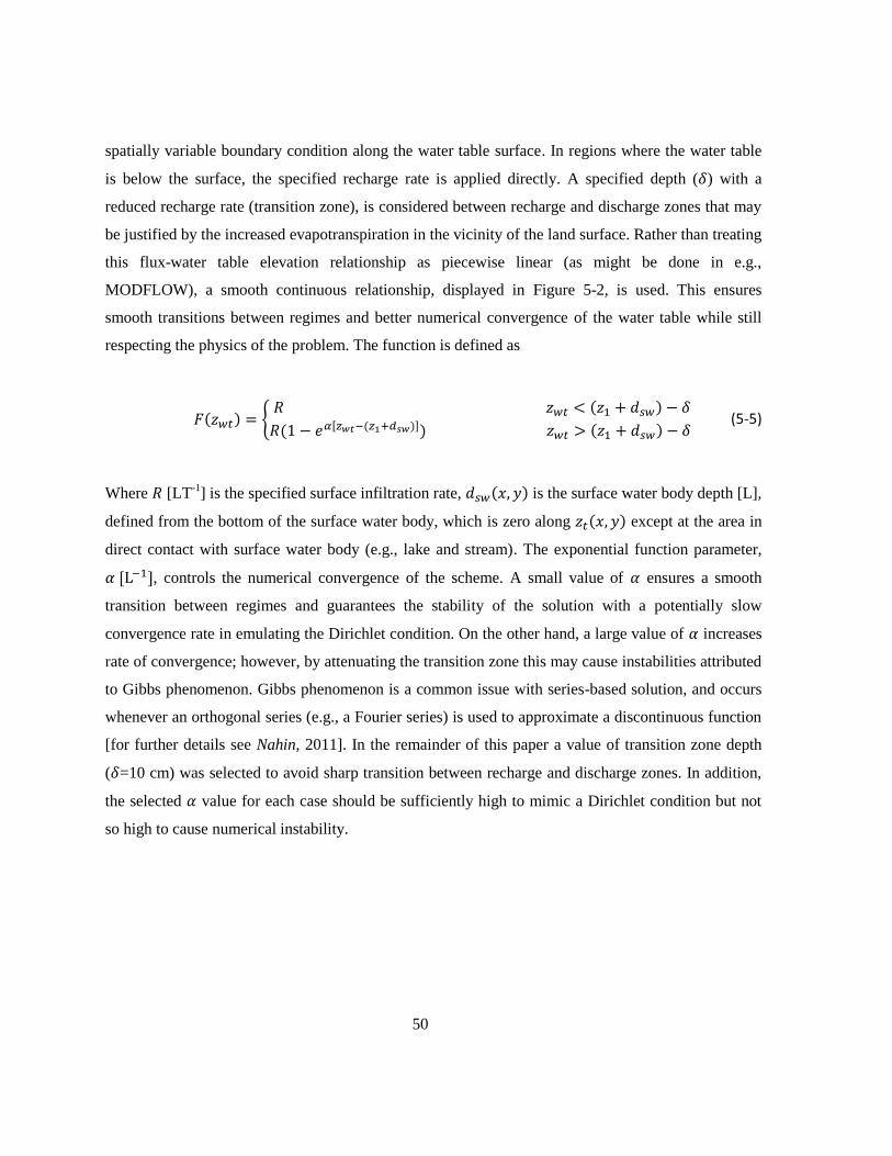
50
spatially variable boundary condition along the water table surface. In regions where the water table
is below the surface, the specified recharge rate is applied directly. A specified depth ( ) with a
reduced recharge rate (transition zone), is considered between recharge and discharge zones that may
be justified by the increased evapotranspiration in the vicinity of the land surface. Rather than treating
this flux-water table elevation relationship as piecewise linear (as might be done in e.g.,
MODFLOW), a smooth continuous relationship, displayed in Figure 5-2, is used. This ensures
smooth transitions between regimes and better numerical convergence of the water table while still
respecting the physics of the problem. The function is defined as
{
(5-5)
Where [LT-1
] is the specified surface infiltration rate, is the surface water body depth [L],
defined from the bottom of the surface water body, which is zero along except at the area in
direct contact with surface water body (e.g., lake and stream). The exponential function parameter,
, controls the numerical convergence of the scheme. A small value of ensures a smooth
transition between regimes and guarantees the stability of the solution with a potentially slow
convergence rate in emulating the Dirichlet condition. On the other hand, a large value of increases
rate of convergence; however, by attenuating the transition zone this may cause instabilities attributed
to Gibbs phenomenon. Gibbs phenomenon is a common issue with series-based solution, and occurs
whenever an orthogonal series (e.g., a Fourier series) is used to approximate a discontinuous function
[for further details see Nahin, 2011]. In the remainder of this paper a value of transition zone depth
( =10 cm) was selected to avoid sharp transition between recharge and discharge zones. In addition,
the selected value for each case should be sufficiently high to mimic a Dirichlet condition but not
so high to cause numerical instability.

51
Figure 5-2. The method to obtain flux along the top surface boundary. Image from Ameli and Craig [2014].
As outlined in Forsyth [1988] such an approach efficiently discharges a sufficient amount of water to
force the Dirichlet condition in areas where the estimated water table elevation is above the land
surface. This treatment of the top boundary with a continuous transition from recharge to discharge
(Dirichlet) conditions ensures that: 1- The locations of seepage faces, do not have to be known a
priori, 2- sharp transitions between regimes do not produce corresponding transitions in conditions
(potentially leading to Gibbs phenomenon) and 3- the algorithm for determining the water table
location is not predisposed to keep portions of the water table in a fixed state. Such an algorithm may
be useful for numerical integrated models (e.g., HydroGeoSphere), as well.
The calculated flux from Equation (5-5) is applied along the top surface of the modeled domain,
,
( ) (5-6)
The continuity of flux and pressure head along each layer interface ( ) can be
represented as:
( )
( ) (5-7)
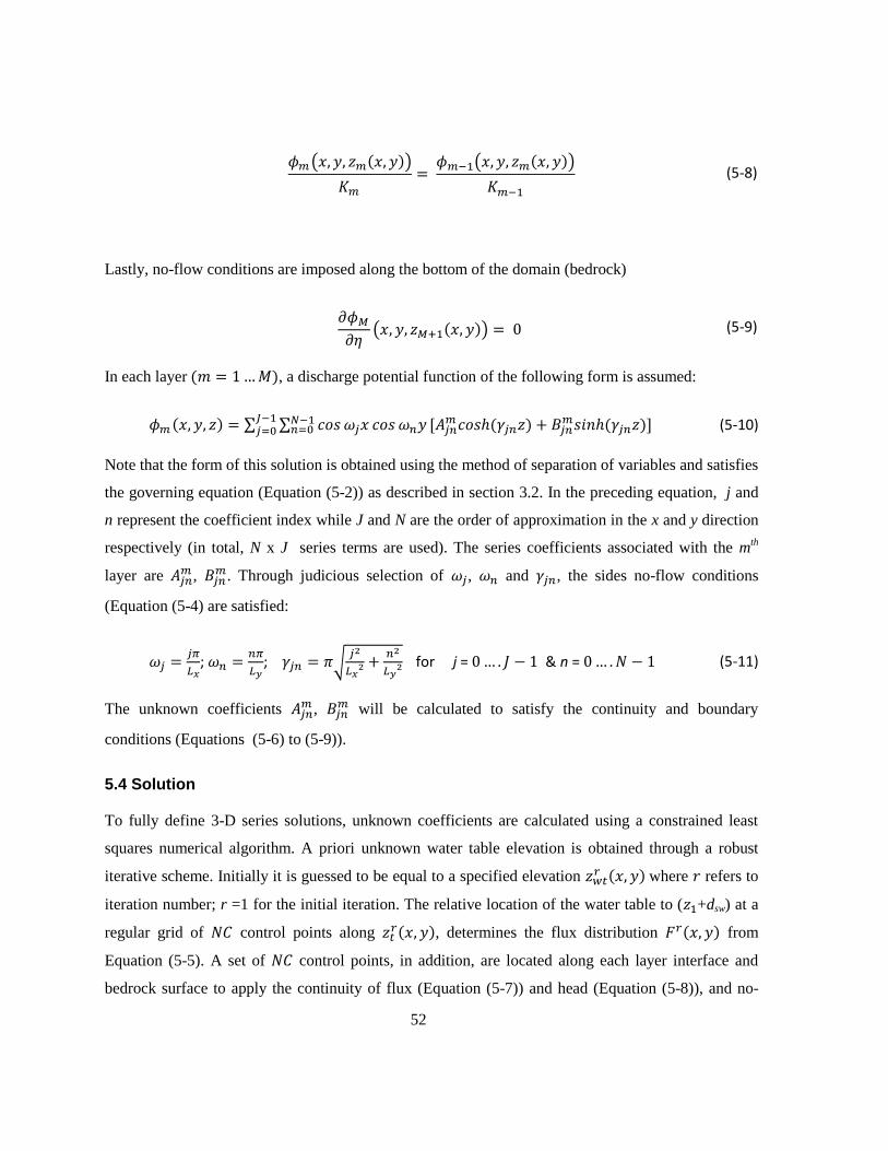
52
( )
( )
(5-8)
Lastly, no-flow conditions are imposed along the bottom of the domain (bedrock)
( ) (5-9)
In each layer , a discharge potential function of the following form is assumed:
∑ ∑
(5-10)
Note that the form of this solution is obtained using the method of separation of variables and satisfies
the governing equation (Equation (5-2)) as described in section 3.2. In the preceding equation, j and
n represent the coefficient index while J and N are the order of approximation in the x and y direction
respectively (in total, N x J series terms are used). The series coefficients associated with the mth
layer are ,
. Through judicious selection of , and , the sides no-flow conditions
(Equation (5-4) are satisfied:
;
; √
for j = & n = (5-11)
The unknown coefficients ,
will be calculated to satisfy the continuity and boundary
conditions (Equations (5-6) to (5-9)).
5.4 Solution
To fully define 3-D series solutions, unknown coefficients are calculated using a constrained least
squares numerical algorithm. A priori unknown water table elevation is obtained through a robust
iterative scheme. Initially it is guessed to be equal to a specified elevation where refers to
iteration number; r =1 for the initial iteration. The relative location of the water table to ( +dsw) at a
regular grid of control points along , determines the flux distribution
from
Equation (5-5). A set of control points, in addition, are located along each layer interface and
bedrock surface to apply the continuity of flux (Equation (5-7)) and head (Equation (5-8)), and no-
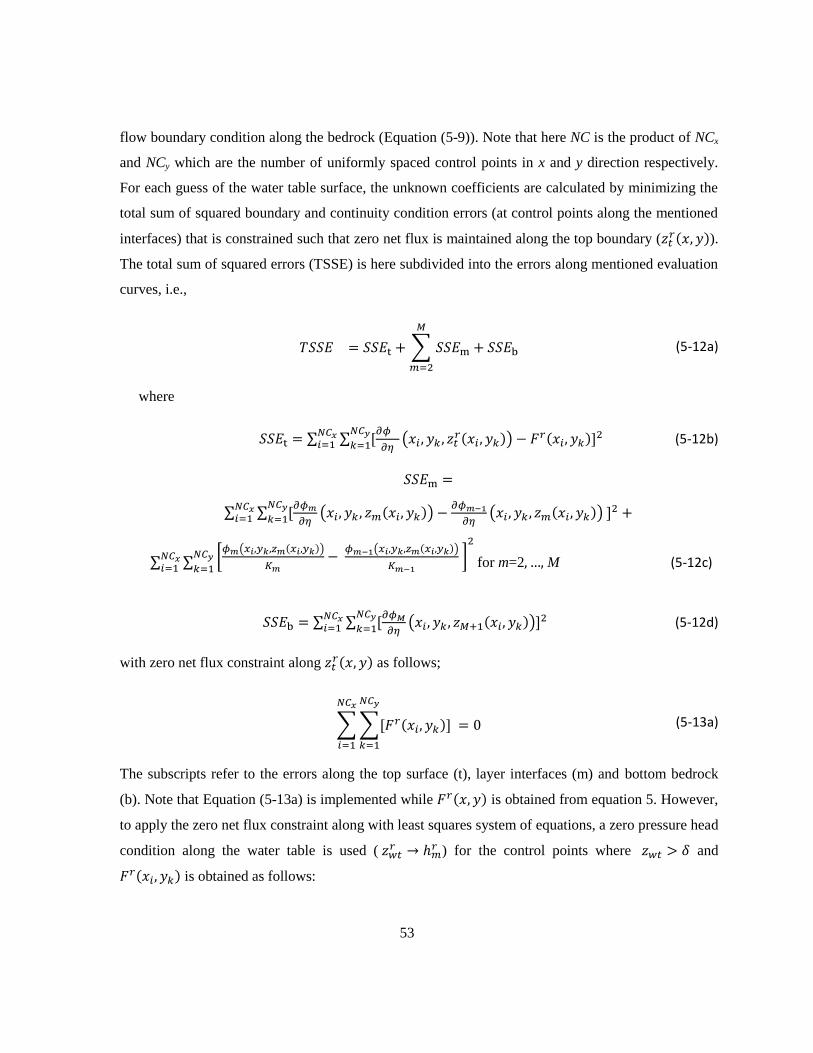
53
flow boundary condition along the bedrock (Equation (5-9)). Note that here NC is the product of NCx
and NCy which are the number of uniformly spaced control points in x and y direction respectively.
For each guess of the water table surface, the unknown coefficients are calculated by minimizing the
total sum of squared boundary and continuity condition errors (at control points along the mentioned
interfaces) that is constrained such that zero net flux is maintained along the top boundary ( ).
The total sum of squared errors (TSSE) is here subdivided into the errors along mentioned evaluation
curves, i.e.,
∑
(5-12a)
where
∑ ∑
(
)
(5-12b)
∑ ∑
( )
( )
∑ ∑ [ ( )
( )
]
for m=2 M (5-12c)
∑ ∑
( )
(5-12d)
with zero net flux constraint along as follows;
∑∑
(5-13a)
The subscripts refer to the errors along the top surface (t), layer interfaces (m) and bottom bedrock
(b). Note that Equation (5-13a) is implemented while is obtained from equation 5. However,
to apply the zero net flux constraint along with least squares system of equations, a zero pressure head
condition along the water table is used (
) for the control points where and
is obtained as follows:
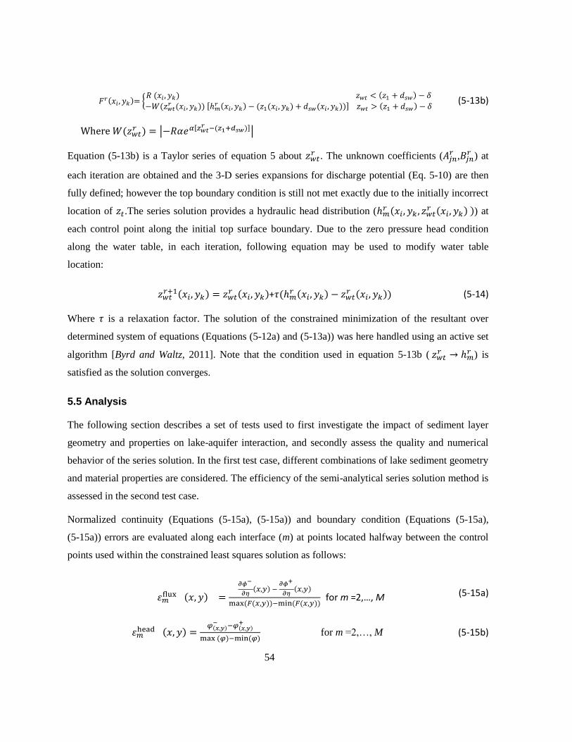
54
= {
(5-13b)
Where |
|
Equation (5-13b) is a Taylor series of equation 5 about . The unknown coefficients (
, ) at
each iteration are obtained and the 3-D series expansions for discharge potential (Eq. 5-10) are then
fully defined; however the top boundary condition is still not met exactly due to the initially incorrect
location of .The series solution provides a hydraulic head distribution (
) at
each control point along the initial top surface boundary. Due to the zero pressure head condition
along the water table, in each iteration, following equation may be used to modify water table
location:
+
(5-14)
Where is a relaxation factor. The solution of the constrained minimization of the resultant over
determined system of equations (Equations (5-12a) and (5-13a)) was here handled using an active set
algorithm [Byrd and Waltz, 2011]. Note that the condition used in equation 5-13b (
) is
satisfied as the solution converges.
5.5 Analysis
The following section describes a set of tests used to first investigate the impact of sediment layer
geometry and properties on lake-aquifer interaction, and secondly assess the quality and numerical
behavior of the series solution. In the first test case, different combinations of lake sediment geometry
and material properties are considered. The efficiency of the semi-analytical series solution method is
assessed in the second test case.
Normalized continuity (Equations (5-15a), (5-15a)) and boundary condition (Equations (5-15a),
(5-15a)) errors are evaluated along each interface (m) at points located halfway between the control
points used within the constrained least squares solution as follows:
for m =2,…, M (5-15a)
for m =2,…, M (5-15b)
55
Along the modeled domain top surface interface, , the normalized flux boundary condition
error is
(5-15c)
and along the bottom bedrock, the no-flow condition error is defined as:
(5-15d)
Here, and [LT-1
] refer to the minimum and maximum flux applied across
the top surface which is also the maximum flux in the domain, and and [L] are the
maximum and minimum value of the pressure head in the entire domain. The (-) and (+) signs refer to
the top and bottom of each interface respectively.
5.5.1 Example 1: Effect of lake sediment on lake-Aquifer interaction
The method derived herein is able to accurately simulate 3-D flow in lake-aquifer systems where the
sediment layer (with an arbitrary geometry) is considered independently rather than using a
conductance condition, as is common. We intend to use this method to evaluate the effect of sediment
geometry and material properties on the flow distribution through the lake bed. The same lake
geometry is used for all examples in this section, , where r is the
radius from the center of the domain. Two different lake sediment geometries are considered: a) a
sediment layer of uniform thickness, and b) a sediment layer with non-uniform thickness which is
more reflective of real lake sediment geometry (Figure 5-3a). To assess the effect of lake sediment
thickness, two different sediment thicknesses are considered for each geometry: a) a thin layer with a
maximum thickness of 23 cm, and b) a thicker layer with a maximum thickness of 46 cm. To
investigate the effect of sediment material properties, three ratios of porous media to sediment
hydraulic conductivity (P =1, 20 and 200) are considered (Figure 5-3b). The uniform hydraulic head
at the lake is set equal to the water elevation of 2.65 m for all the examples in this section
(Figure 5-3a). The parameter chosen are specific to this problem, but the results are expected to
generalize to other system geometries.
All examples are subject to a uniform specified infiltration rate of R =10-4
md-1
. Surface water depth,
dsw, (Equation (5-5)) is zero for all control points along the top surface boundary of the modeled
56
domain, except those in direct contact with surface water body. A value of =20 m-1
is selected for
all 12 examples considered in this section. A 100 m x 100 m computational domain with no-flow
conditions along the sides and bottom is used, where the lake and seepage surfaces are the outlet for
recharge. The initial guess used for the water table location is uniformly equal to the lake uniform
hydraulic head, iteratively determined thereafter. The solutions are obtained for two-layer systems
(aquifer and sediment layer) using J = N = 28, and NCx=NCy =30 (900 control points) along each
evaluation surface (i.e., the modeled domain top boundary, the layer interface between the sediment
layer and aquifer, and the bedrock).
Figure 5-3b illustrates the normalized seepage flux distribution (normalized with respect to the
specified infiltration rate (R)) through a cross section along lake bed for the 12 examples considered
in this section, while Figure 5-3c demonstrates the variation of minimum, average and the maximum
of normalized seepage flux at the lake bed as P increases for 4 sediment layer geometries. Because of
the symmetry of the domain, only the flux distribution along the plane of symmetry through the
middle of the lake is reported. These solutions were identified after 60 iterations with a relaxation
factor of = 0.10 used to control the convergence behavior of the unknown water table. Note that this
strong relaxation is required to insure convergence of the solution where a large value of α=20
generates a sharp transition between recharge and discharge regimes. The solution with a smaller α
value can converge using a larger relaxation factor at the expense of relaxing the top boundary
conditions in the transition zone. For the uniform sediment layer, it is seen that as the ratio of aquifer
to sediment conductivity (P) increases, the flux distribution becomes more spatially uniform, though
only slightly (Figure 5-3b). Figure 5-3c depicts the small increase in the minimum and the average
seepage flux at the lake bed, and decrease in its maximum as P increases. This confirms the result of
Genereux and Bandopadhyay [2001], though in their numerical simulation the thickness of uniform
sediment layer depended upon the mesh size. Unlike with the uniform sediment, changes in thickness
and conductivity in the non-uniform sediment layer have considerable impact, in a totally different
manner, on lake bed flux distribution. As the aquifer to sediment conductivity ratio (P) and/or the
thickness of the sediment layer increase, the flux distribution adjusts to increase the shoreline fluxes
and decrease the off-shore seepage (Figure 5-3b). This effect may increase the risk of seepage-
induced erosion at the shoreline due to the large concentrated flux through the lake bed, and in the
extreme, is consistent with results from 2-D Dupuit- Forchheimer models of lake seepage [Bakker,
2002; 2004; Strack, 1984]. Figure 5-3c shows that for the non-uniform layer problem, as P increases
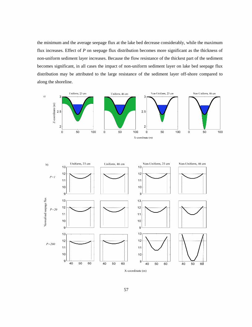
57
the minimum and the average seepage flux at the lake bed decrease considerably, while the maximum
flux increases. Effect of P on seepage flux distribution becomes more significant as the thickness of
non-uniform sediment layer increases. Because the flow resistance of the thickest part of the sediment
becomes significant, in all cases the impact of non-uniform sediment layer on lake bed seepage flux
distribution may be attributed to the large resistance of the sediment layer off-shore compared to
along the shoreline.
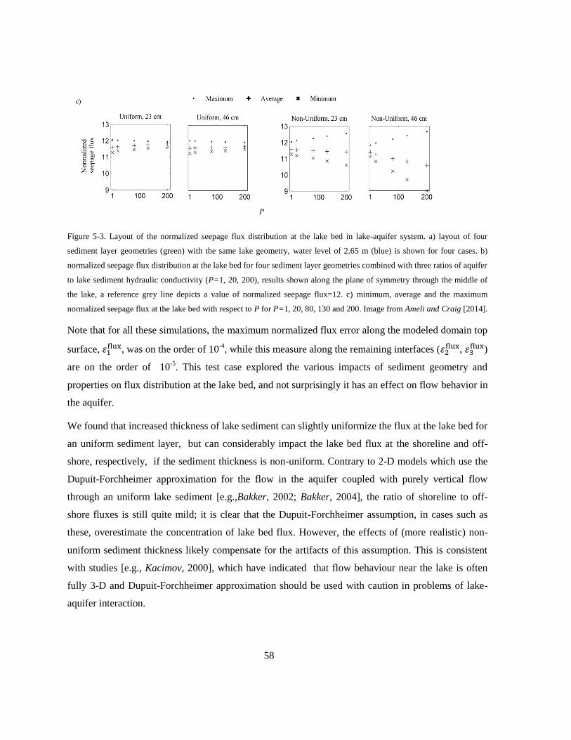
58
Figure 5-3. Layout of the normalized seepage flux distribution at the lake bed in lake-aquifer system. a) layout of four
sediment layer geometries (green) with the same lake geometry, water level of 2.65 m (blue) is shown for four cases. b)
normalized seepage flux distribution at the lake bed for four sediment layer geometries combined with three ratios of aquifer
to lake sediment hydraulic conductivity (P=1, 20, 200), results shown along the plane of symmetry through the middle of
the lake, a reference grey line depicts a value of normalized seepage flux=12. c) minimum, average and the maximum
normalized seepage flux at the lake bed with respect to P for P=1, 20, 80, 130 and 200. Image from Ameli and Craig [2014].
Note that for all these simulations, the maximum normalized flux error along the modeled domain top
surface, , was on the order of 10
-4, while this measure along the remaining interfaces (
, )
are on the order of 10-5
. This test case explored the various impacts of sediment geometry and
properties on flux distribution at the lake bed, and not surprisingly it has an effect on flow behavior in
the aquifer.
We found that increased thickness of lake sediment can slightly uniformize the flux at the lake bed for
an uniform sediment layer, but can considerably impact the lake bed flux at the shoreline and off-
shore, respectively, if the sediment thickness is non-uniform. Contrary to 2-D models which use the
Dupuit-Forchheimer approximation for the flow in the aquifer coupled with purely vertical flow
through an uniform lake sediment [e.g.,Bakker, 2002; Bakker, 2004], the ratio of shoreline to off-
shore fluxes is still quite mild; it is clear that the Dupuit-Forchheimer assumption, in cases such as
these, overestimate the concentration of lake bed flux. However, the effects of (more realistic) non-
uniform sediment thickness likely compensate for the artifacts of this assumption. This is consistent
with studies [e.g., Kacimov, 2000], which have indicated that flow behaviour near the lake is often
fully 3-D and Dupuit-Forchheimer approximation should be used with caution in problems of lake-
aquifer interaction.
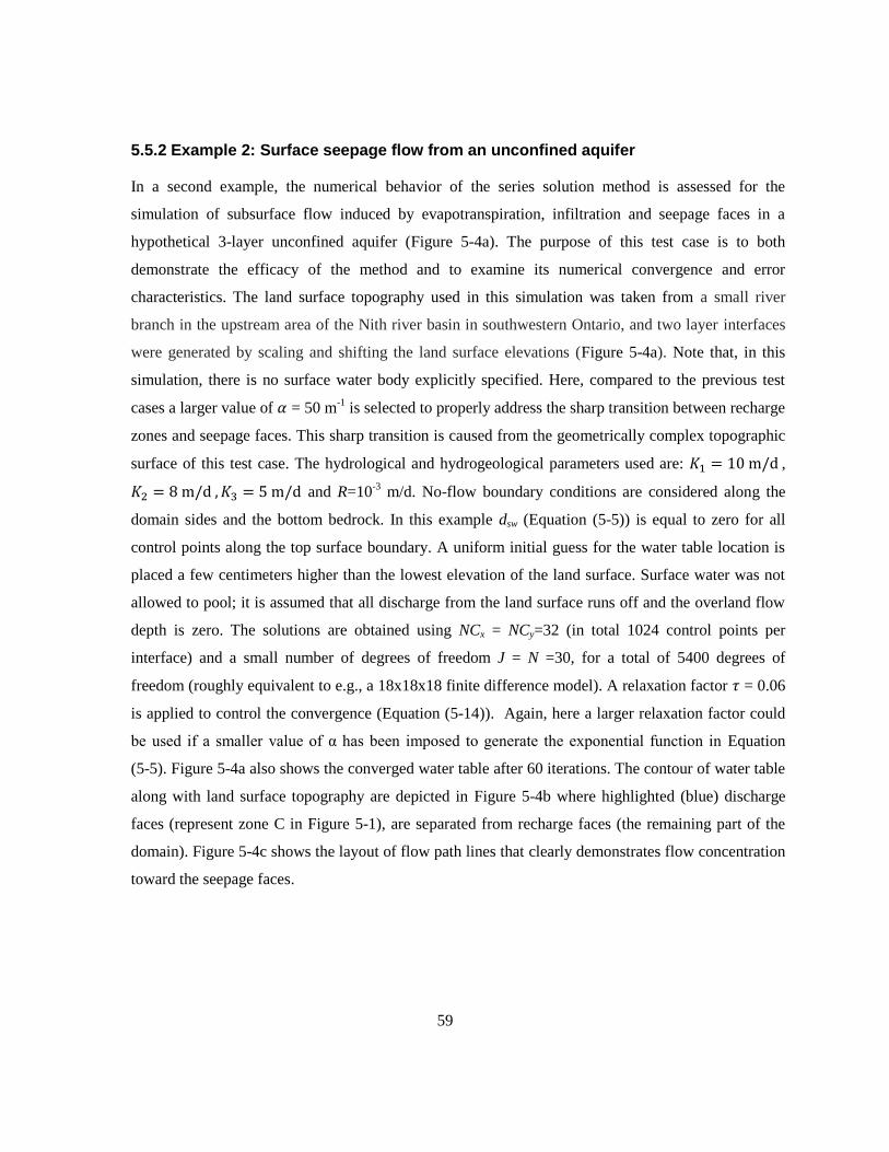
59
5.5.2 Example 2: Surface seepage flow from an unconfined aquifer
In a second example, the numerical behavior of the series solution method is assessed for the
simulation of subsurface flow induced by evapotranspiration, infiltration and seepage faces in a
hypothetical 3-layer unconfined aquifer (Figure 5-4a). The purpose of this test case is to both
demonstrate the efficacy of the method and to examine its numerical convergence and error
characteristics. The land surface topography used in this simulation was taken from a small river
branch in the upstream area of the Nith river basin in southwestern Ontario, and two layer interfaces
were generated by scaling and shifting the land surface elevations (Figure 5-4a). Note that, in this
simulation, there is no surface water body explicitly specified. Here, compared to the previous test
cases a larger value of = 50 m-1
is selected to properly address the sharp transition between recharge
zones and seepage faces. This sharp transition is caused from the geometrically complex topographic
surface of this test case. The hydrological and hydrogeological parameters used are: ,
and R=10-3
m/d. No-flow boundary conditions are considered along the
domain sides and the bottom bedrock. In this example dsw (Equation (5-5)) is equal to zero for all
control points along the top surface boundary. A uniform initial guess for the water table location is
placed a few centimeters higher than the lowest elevation of the land surface. Surface water was not
allowed to pool; it is assumed that all discharge from the land surface runs off and the overland flow
depth is zero. The solutions are obtained using NCx = NCy=32 (in total 1024 control points per
interface) and a small number of degrees of freedom J = N =30, for a total of 5400 degrees of
freedom (roughly equivalent to e.g., a 18x18x18 finite difference model). A relaxation factor = 0.06
is applied to control the convergence (Equation (5-14)). Again, here a larger relaxation factor could
be used if a smaller value of α has been imposed to generate the exponential function in Equation
(5-5). Figure 5-4a also shows the converged water table after 60 iterations. The contour of water table
along with land surface topography are depicted in Figure 5-4b where highlighted (blue) discharge
faces (represent zone C in Figure 5-1), are separated from recharge faces (the remaining part of the
domain). Figure 5-4c shows the layout of flow path lines that clearly demonstrates flow concentration
toward the seepage faces.

60
Figure 5-4. Solution in 3-Layer unconfined aquifer after 60 iterations, a) The layout of the stratified unconfined aquifer
along with the converged water table (blue surface), b) contour of water table along with land surface topography with
highlighted discharge faces, c) The layout of the flow path lines. Image from Ameli and Craig [2014].
Note that using Equation (5-5) to estimate the seepage face with zero pressure head, while
significantly improving convergence skill of the algorithm, can still lead to relatively abrupt changes
in surface fluxes over short distances. This manifests as Gibbs phenomenon. To mitigate this issue,
the land surface has been slightly smoothened using LOWESS function of MATLAB (Figure 5-4a).
This is an inherent challenge for the series solution method: while smooth system geometry leads to
well-behaved solutions, irregular geometry can be problematic.
a)
c)
b)
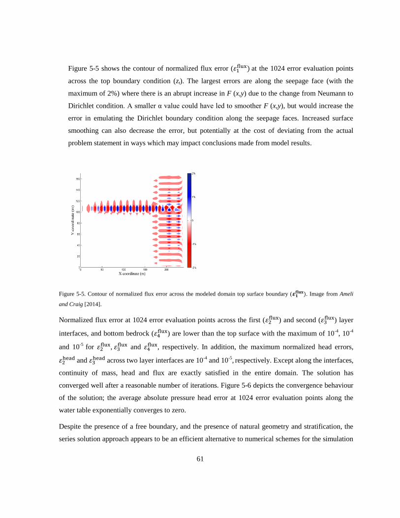
61
Figure 5-5 shows the contour of normalized flux error ( at the 1024 error evaluation points
across the top boundary condition (zt). The largest errors are along the seepage face (with the
maximum of 2%) where there is an abrupt increase in F (x,y) due to the change from Neumann to
Dirichlet condition. A smaller α value could have led to smoother F (x,y), but would increase the
error in emulating the Dirichlet boundary condition along the seepage faces. Increased surface
smoothing can also decrease the error, but potentially at the cost of deviating from the actual
problem statement in ways which may impact conclusions made from model results.
Figure 5-5. Contour of normalized flux error across the modeled domain top surface boundary ( . Image from Ameli
and Craig [2014].
Normalized flux error at 1024 error evaluation points across the first ( ) and second (
) layer
interfaces, and bottom bedrock ( ) are lower than the top surface with the maximum of 10
-4, 10
-4
and 10-5
for ,
and , respectively. In addition, the maximum normalized head errors,
and
across two layer interfaces are 10-4
and 10-5
, respectively. Except along the interfaces,
continuity of mass, head and flux are exactly satisfied in the entire domain. The solution has
converged well after a reasonable number of iterations. Figure 5-6 depicts the convergence behaviour
of the solution; the average absolute pressure head error at 1024 error evaluation points along the
water table exponentially converges to zero.
Despite the presence of a free boundary, and the presence of natural geometry and stratification, the
series solution approach appears to be an efficient alternative to numerical schemes for the simulation
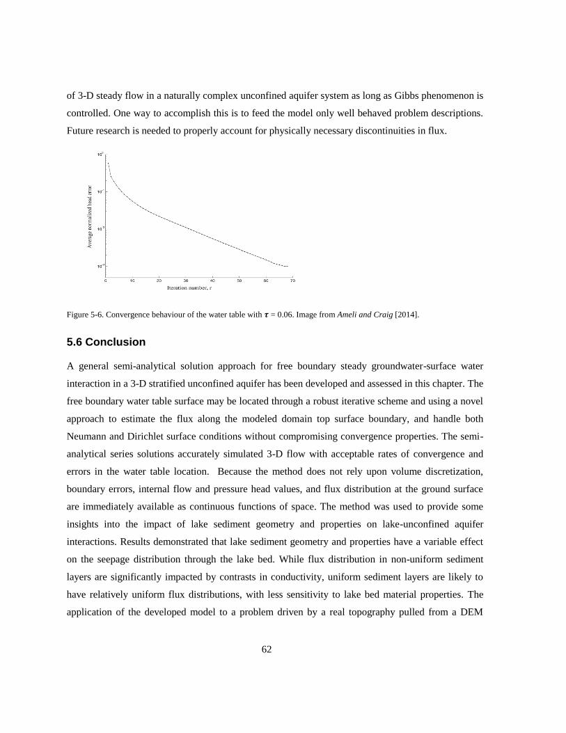
62
of 3-D steady flow in a naturally complex unconfined aquifer system as long as Gibbs phenomenon is
controlled. One way to accomplish this is to feed the model only well behaved problem descriptions.
Future research is needed to properly account for physically necessary discontinuities in flux.
Figure 5-6. Convergence behaviour of the water table with = 0.06. Image from Ameli and Craig [2014].
5.6 Conclusion
A general semi-analytical solution approach for free boundary steady groundwater-surface water
interaction in a 3-D stratified unconfined aquifer has been developed and assessed in this chapter. The
free boundary water table surface may be located through a robust iterative scheme and using a novel
approach to estimate the flux along the modeled domain top surface boundary, and handle both
Neumann and Dirichlet surface conditions without compromising convergence properties. The semi-
analytical series solutions accurately simulated 3-D flow with acceptable rates of convergence and
errors in the water table location. Because the method does not rely upon volume discretization,
boundary errors, internal flow and pressure head values, and flux distribution at the ground surface
are immediately available as continuous functions of space. The method was used to provide some
insights into the impact of lake sediment geometry and properties on lake-unconfined aquifer
interactions. Results demonstrated that lake sediment geometry and properties have a variable effect
on the seepage distribution through the lake bed. While flux distribution in non-uniform sediment
layers are significantly impacted by contrasts in conductivity, uniform sediment layers are likely to
have relatively uniform flux distributions, with less sensitivity to lake bed material properties. The
application of the developed model to a problem driven by a real topography pulled from a DEM
63
indicated that the number of degrees of freedom required to obtain an accurate solution for a realistic
problem with a high rate of convergence is small.

64
Chapter 6
Semi-analytical solutions for assessing pumping impacts on
groundwater-surface water interaction
6.1 Introduction
Horizontal wells and radial collector wells are sometimes considered as suitable alternatives to
vertical wells for water withdrawal or remediation of contaminated groundwater systems. Radial
collector wells are able to withdraw a large quantity of groundwater and surface water with a small
drawdown. The appropriateness of radial collector wells for river bank filtration (RBF) and pump and
treat applications has been reported by many researchers [e.g., Moore et al., 2012; Patel et al., 2010].
Understanding the interaction between radial collector wells, regional groundwater flow and surface
water features requires a robust model with the ability to provide three dimensional details in the
vicinity of both the well and surface water body. In addition, to realistically incorporate the effect of
long radial arms (commonly longer than 80 m), the variation of inflow along these arms must be
taken into account and it is desirable to effectively simulate the head distribution at the resolution of
the well caisson (i.e., at the centimeter scale). Simulation of multi scale problems such as these is
challenging using discrete numerical models. When applying grid-based methods to address arbitrary
orientations of small diameter radials, high grid resolution is required which leads to computational
inefficiency. For example, to accurately obtain the drawdown-discharge relationship of a single
horizontal well in a homogenous aquifer with a regular geometry (a box domain of
150m*480m*24m), Haitjema et al. [2010] used a MODFLOW model of 1,846,314 cells. The
requirements of models used for the design of RBF and pump and treat systems will be even stricter;
in the design process, the assessment of different scenarios including various layouts and length of
radial arms is required.
These conditions are well suited for the application of the analytical element method (AEM) where no
horizontal or vertical grid discretization is required. More importantly, distributed singularities along
the well axis are able to mimic the behavior of each arbitrarily-oriented arm regardless of its length
and diameter. Researchers have recently extended AEM for the simulation of 2-D and 3-D flow
toward a partially penetrating vertical well [Bakker, 2001; Luther and Haitjema, 1999], a single
horizontal well [Bakker and Strack, 2003; Luther, 1998; Steward and Jin, 2001; 2003] and radial
65
collector well [Bakker et al., 2005; Luther and Haitjema, 2000]. However, the discharge-drawdown
relationship in the previously cited literature was obtained for isolated pumping well(s). More
recently Haitjema et al. [2010] and Moore et al. [2012] have extended these AEM models to
incorporate the interaction between horizontal well(s) and other regional features including rivers and
regional flow. Rivers in these models have been treated using a group of constant head line sinks; this
is accompanied by a simple 1-D Cauchy boundary (head dependent) condition to incorporate the
effect of vertical resistance in the vicinity of the river. This treatment compromises the proper
incorporation of river geometry and material properties.
3-D AEM models have been typically developed for flow toward wells located in homogenous
confined aquifers where the no-flow top and bottom boundary conditions can be properly addressed
by the method of images. Emulating free boundary conditions (i.e., the water table) at the top of
modeled domain may be challenging, and in the past has been handed using distributed singularities.
In the few research studies in which a free boundary condition at the water table has been considered,
many auxiliary geometric features (e.g., doublet sinks or panel sinks) were applied external to the
domain to aid in satisfying the phreatic surface boundary conditions [Luther and Haitjema, 1999;
Luther and Haitjema, 2000]. Aquifer stratification with a regular layer interface has also been
included in AEM models where 1) an additional analytic elements are externally applied to assist in
satisfying the continuity conditions across layers [Luther, 1998] or 2) the domain is discretized
vertically into many aquifers each with constant conductivity (the multi-aquifer model of [Bakker et
al., 2005]). In spite of the ability of AEM to emulate pumping well behavior, the treatment of phreatic
surface or layer stratification using auxiliary singularities is challenging particularly in that there are
no unique guidelines about the location, type and number of required singularities.
The series solution model developed in chapter 5 has been shown to properly address the phreatic
surface, complex stratification, and non-regular surface water geometry. As stated in chapter 3, both
series solution methods and AEM satisfy the linear groundwater governing equation exactly. Here,
based on superposition, the series solution model for 3-D groundwater-surface water interaction
developed in chapter 5 is augmented with a set of analytic elements (line sinks) which are used to
represent pumping wells. The coupled series-AEM method was first used by Bakker [2010] to
simulate 2-D interaction between river, homogenous confined aquifer and a vertical pumping well
where series method was employed to emulate the flow boundary conditions at the sides of the
domain. The series-AEM model is here intended to investigate 3-D groundwater-surface water
66
interaction induced by surface water bodies, infiltration, and a radial collector well in a naturally
complex stratified unconfined aquifer. This series-AEM model is able to 1) discern the origin of well
water and 2) estimate the percentage of well water captured from surface sources. It may be an
efficient tool for designing RBF systems. This semi-analytical grid-free model is here used to assess
the impact of pumping rate on the hydrological connectivity between river and radial collector well
which plays a significant role in the performance of RBF systems.
6.2 Background
During the past decade, radial collector wells have been designed and installed in aquifers in the
vicinity of stream or lake to withdraw naturally filtered surface water for supplying municipal
drinking water (e.g., as done in the Saylorville well-field in the Des Moines River Valley, Iowa
[Moore et al., 2012]). The efficiency of each design is assessed by the ability of the well to induce
recharge from surface water [Moore et al., 2012]. In addition to pumping capacity, the quality of the
water obtained using RBF systems is very important. Generally the water captured by RBF is the
mixture of regional groundwater and surface water, each with different qualities. For example, the
installed RBF systems in the vicinity of the Des Moines River Valley captures river waters which are
being naturally treated for undesirable surface water constituents (such as pathogens) by passing
through coarse grained river bed sediment [Gollnitz et al., 2005]. At the same time, groundwater in
this area is higher in hardness, alkalinity, dissolved iron, manganese and solids [Moore et al., 2012].
The identification of the mixture quality prior to construction requires detailed understanding of the
expected interaction between regional groundwater, the radial collector well and adjacent rivers.
Modeling of the interaction between groundwater, surface water and well can provide useful insights
into the physics of this challenging interaction; provided the appropriate boundary conditions are
used. There are typically three assumptions used in the application of boundary conditions along
radial arms in groundwater modeling literature; uniform flux, uniform head and constrained non-
uniform head along the radial well screen. The latter is most in agreement with the actual behavior of
long horizontal arms which exhibit considerable head losses inside the screened pipes where both flux
and head are non-uniform; the friction loss equation (e.g., Darcy-Weisbatch) may be used to define
the relationship between head along the well screen. In the case of laminar flow with negligible head
losses inside the pipes, the second assumption is valid. The uniformity of flux assumption may only
be valid for a very short radial screen, and is not a suitable option for application to the radial
67
collector well problem. Mesh-based numerical models have been widely used to address the
interaction between groundwater, surface waters and wells using the finite element [Ophori and
Farvolden, 1985] and finite difference method [Chen et al., 2003; Haitjema et al., 2010; Patel et al.,
1998; Rushton and Brassington, 2013a; b]. However, a mesh-based model may not be an efficient
tool for the purpose of designing radial collector wells for river bank filtration. In addition to the high
grid resolution required to properly address the small well diameter and arbitrary orientations of
radial arms, the implementation of the boundary condition along the well screen is also challenging in
standard numerical models. Typically, flow toward radial arms is approximated using head dependent
boundary cells [Patel et al., 1998] or the drain package [Kelson, 2012] accompanied by an entry
resistance (conductance factor) in MODFLOW.
Semi-analytical approaches have been applied to simulate flow toward horizontal well(s) in confined
and unconfined aquifers. A boundary integral equation model has been developed by Bischoff [1981]
to simulate 3-D flow toward a 3-arm radial collector well in a confined aquifer. Haitjema [1982] used
third order horizontal line sinks and line doublets to incorporate the 3-D effects of a horizontal well in
a homogenous confined aquifer. These geometric features have been replaced by a set of line sinks at
the centerline of the well each with linearly-varied strength to properly emulate the constant head
condition (or non-uniform flux) along horizontal well(s) in homogenous confined aquifers by Steward
and Jin [2001]; 2003]. Bakker et al. [2005] have discretized a confined aquifer into several (fictitious)
horizontal homogenous aquifers where horizontal flow inside each aquifer is computed analytically
based on Dupuit-Forchheimer approximation; vertical flow is approximated with a vertical resistance
of a leaky layer between aquifers using a finite difference method. This quasi 3-D multi-aquifer
analytic element model accounts for the head losses inside the screen pipe and skin effects (non-
uniform head along the screen). A separate horizontal aquifer is assigned to the collector well which
is represented by a multilayer line sinks. The skin effect is approximated by applying the entry
resistance parameter to inflow of the well screen. Using vertical discretization, this model can
incorporate the effect of stratification with parallel layer interfaces. AEM models have also been
developed to simulate 3-D flow toward horizontal well(s) in homogenous unconfined aquifers [Luther
and Haitjema, 2000]. In these models, the phreatic surface position was located through an iterative
scheme in a manner similar to series solution approach discussed in chapter 4. Using AEM, auxiliary
elements (e.g., point sinks and sink rings) were required outside the flow domain to aid in satisfying a
zero-recharge boundary condition along phreatic surface.
68
Surface water features can also be incorporated in AEM models using a set of line sinks. This enables
AEM to consider the interaction between regional groundwater, surface water and radial collector
wells for the application to RBF system design. For the interaction between a single horizontal well
and river in a 2-D homogenous confined aquifer, Haitjema et al. [2010] estimated entry resistances
for the simulation of converging flow to well and stream in a 2-D Dupuit-Forchheimer AEM code
(GFLOW) generated by Haitjema [1995]. These developed resistances obtained for an infinitely long
single horizontal well in a confined aquifer and can roughly approximate the effect of vertical flow
toward river and horizontal well. These resistances were later used in a 2-D MODFLOW model as
well [Kelson, 2012]. The AEM model developed by Haitjema et al. [2010] was one of the first studies
which semi-analytically approximated the interaction between a river and well; this model has
provided similar well yields to that generated by a high resolution MODFLOW model for a given
well drawdown. Although the model was accurate enough for the purpose of discerning well yield,
the authors suggested that it cannot provide accurate 3-D details in the vicinity of a well and stream
and therefore should not be used for the purpose of designing the radial collector well in RBF
systems. Moore et al. [2012] have linked this 2-D regional model with the quasi 3-D local-scale
multi-aquifer model developed by Bakker et al. [2005] (in a manner similar to the telescoping mesh
refinement used in MODFLOW) to develop a general AEM model for the design of radial collector
well in a RBF system. First, the regional 2-D AEM model is calibrated based on observed steady-
state drawdown and measured water level. At the proper distance from radial collector well where
vertical flow is negligible (three or four times the representative leakage length), the fluxes are
applied as perimeter boundary conditions for the 3-D local-scale model. The local interaction between
the radial collector well and river is then assessed using the quasi-3D Multi-aquifer AEM model.
The study of Moore et al. [2012] has also suggested important guidelines for choosing the optimum
length, number, elevation and location of a radial collector well in the design phase. They showed that
the elevation of lateral arms has a minor impact on well drawdown and yield, and can be determined
based on operational, construction and maintenance considerations. They mentioned that the laterals
should be placed well below the caisson water level while the water level in the caisson should be
located above the pump inlet to meet suction-head requirements and desirable water yield. At the
same time, the relative elevation of radial collector well with respect to the bedrock should be high
enough to avoid hydraulic interference. They have also found that with the same cumulative lateral
screen length, a longer lateral works better than more laterals with shorter length; this is because of
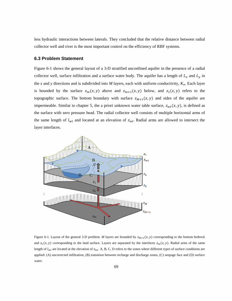
69
less hydraulic interactions between laterals. They concluded that the relative distance between radial
collector well and river is the most important control on the efficiency of RBF systems.
6.3 Problem Statement
Figure 6-1 shows the general layout of a 3-D stratified unconfined aquifer in the presence of a radial
collector well, surface infiltration and a surface water body. The aquifer has a length of and in
the x and y directions and is subdivided into M layers, each with uniform conductivity, Km. Each layer
is bounded by the surface above and below, and refers to the
topographic surface. The bottom boundary with surface and sides of the aquifer are
impermeable. Similar to chapter 5, the a priori unknown water table surface, , is defined as
the surface with zero pressure head. The radial collector well consists of multiple horizontal arms of
the same length of and located at an elevation of Radial arms are allowed to intersect the
layer interfaces.
Figure 6-1. Layout of the general 3-D problem. M layers are bounded by corresponding to the bottom bedrock
and corresponding to the land surface. Layers are separated by the interfaces . Radial arms of the same
length of are located at the elevation of . A, B, C, D refers to the zones where different types of surface conditions are
applied: (A) uncorrected infiltration, (B) transition between recharge and discharge zones, (C) seepage face and (D) surface
water.
A
D C
B
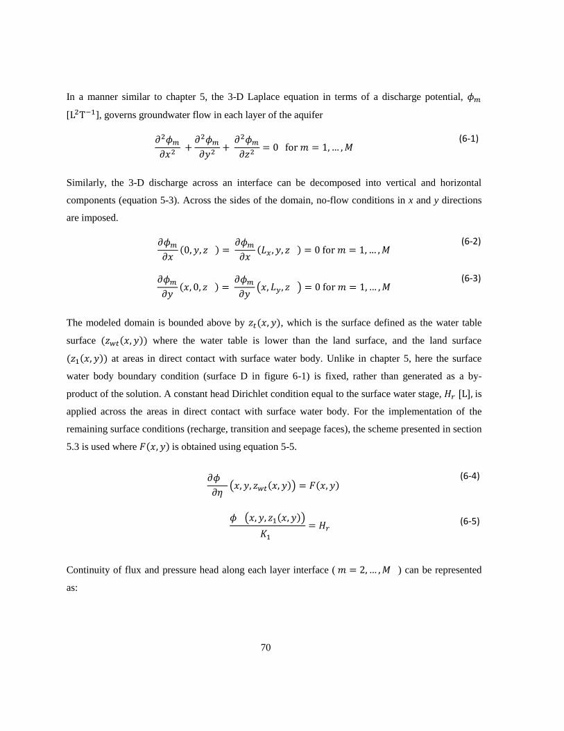
70
In a manner similar to chapter 5, the 3-D Laplace equation in terms of a discharge potential,
[ ], governs groundwater flow in each layer of the aquifer
(6-1)
Similarly, the 3-D discharge across an interface can be decomposed into vertical and horizontal
components (equation 5-3). Across the sides of the domain, no-flow conditions in x and y directions
are imposed.
(6-2)
( ) (6-3)
The modeled domain is bounded above by , which is the surface defined as the water table
surface where the water table is lower than the land surface, and the land surface
at areas in direct contact with surface water body. Unlike in chapter 5, here the surface
water body boundary condition (surface D in figure 6-1) is fixed, rather than generated as a by-
product of the solution. A constant head Dirichlet condition equal to the surface water stage, [L], is
applied across the areas in direct contact with surface water body. For the implementation of the
remaining surface conditions (recharge, transition and seepage faces), the scheme presented in section
5.3 is used where is obtained using equation 5-5.
( )
(6-4)
( )
(6-5)
Continuity of flux and pressure head along each layer interface ( ) can be represented
as:

71
( )
( ) (6-6)
( )
( )
(6-7)
No-flow conditions are also imposed along the bedrock which is a flat interface with a planar
geometry in this chapter.
( ) (6-8)
At the radial collector well, the a priori unknown head is obtained based on a given pumping rate,
although the method is able to properly address the reverse case. In a manner similar to Steward and
Jin [2003], two boundary conditions must be satisfied along the entire well screen length. First, the
head along the cylindrical face of the well must be uniform, which implies zero head loss along the
well screens. This is applied by setting the head at a set of control points (located along screens
surface) equal to the head at a specified but arbitrary position along this boundary.
( )
(6-9)
Here is conditional upon the layer where each control point or the specified point, , are located.
This ensures the ability of the model to address the cases where radial arms intersect the layer. For the
second boundary condition at the collector well, the summation of unknown strengths along a
pumping well is set equal to the pumping rate
∑
(6-10)
where , and are the number of segments, constant strength of each segment, and segment
length, respectively, as discussed in section 3.3. In applying this condition, the unknown head in the
radial collector well, , may be obtained.
72
Both the series solution and AEM solution satisfy the linear 3-D Laplace equation. Therefore
superposition theory suggests that in each layer of a stratified unconfined aquifer, a
discharge potential function of the following form can be applied:
=
(6-11)
The series solution to groundwater flow in each layer of a stratified unconfined aquifer developed in
chapter 5 is (equation 5-10):
∑∑
(6-12)
The AEM solution representing the radial collector well is:
∑
(6-13)
where the discharge potential effect of the th segment, , in global coordinate system is obtained
based on the closed form expression developed by Steward and Jin [2003] in local coordinate system
of each segment (equation (3-8)). The resulting equation is:
[(
) (
) (
) ]
(
)
[( )
(
) (
) ]
(
)
(6-14)
where ,
and refer to the center of each segment in the global coordinate system of the ground
water model. The total discharge potential function (equation (6-11)) must satisfy the no-flow
condition at the sides and bottom of the domain (equations (6-2) & (6-3) & (6-8)). Again based on
superposition both series and AEM solution must satisfy these boundary conditions. As explained in
chapter 5, the series portion of solution already satisfies no-flow condition at the sides by judicious
selection of , and as (repeated form equation 5-11):
73
;
; √
for j = & n = (6-15)
In addition, to satisfy no-flow condition along the bottom bedrock by the series portion of the
solution, (Equation (6-12)) must be equal to zero (similar to [Read et al., 2005]). The method of
images is here used to enable AEM to satisfy no-flow conditions at the sides and bottom of the
domain. Therefore equation (6-11) is modified as
= ∑
∑ ∑
(6-16)
Where refers to discharge potential correspond to the image of i
th segment and is the number of
image wells. As discussed in section 3.3 the strength associated with each image segment is identical
to its real counterpart and only their locations ( ,
and ) are different. Note that, the no-flow
boundary condition at the sides and bottom of the domain only met exactly when approaches
infinity. The uniformity of head condition, in addition, met exactly when approaches infinity.
6.4 Solution
The 3-D semi-analytical series-AEM solution for the interaction between groundwater, surface water
bodies and a radial collector well (Equation (6-16)) in each layer of a stratified unconfined aquifer is
obtained by identifying unknown coefficients of the series solution ( in equation (6-12)) and
AEM terms ( in equation (6-14)). These coefficients are calculated using a constrained least
squares numerical algorithm. Similar to chapter 5, the priori unknown water table elevation,
(where is the iteration number) is obtained through a robust iterative scheme. A set of
control points, are located along the top of the modeled domain surface, , bedrock surface
( ) and each layer interface ( ) to characterize the error in the top boundary
condition, and the continuity of flux and head conditions (equations (6-4) to (6-8)). Note that here NC
is the product of NCx and NCy which are the number of uniformly spaced control points in x and y
direction respectively. Initially, the top of modeled domain surface, , is assumed to be equal
to the river water stage, at all control points. The uniformity of head boundary condition along the
radial screens is satisfied by applying equation (6-9) at a set of NCw control points located along the
screens surface. The unknown coefficients for each guess of the water table surface, are calculated by
74
minimizing the total sum of squared boundary and continuity condition errors (at control points along
the mentioned interfaces and well screen surfaces) that is constrained with equation (6-10) such that
the total inflow be equal to pumping rate Q at the radial collector well. The total sum of squared
errors (TSSE) is here subdivided into the errors along mentioned evaluation curves:
∑ (6-17)
The subscripts refer to the errors along the top surface (t), layer interfaces (m) and radial collector
well screens (w).
where
∑ [
( ) ]
∑ ( )
(6-17a)
Where is the set of coordinate indices for control points in direct contact with the surface water
body (Dirichlet zone). is the layer where the control point along the top surface is located.
∑ [
( )
( ) ]
∑ [ ( )
( )
]
for m=2 M (6-17b)
∑ [
( )
]
(6-17c)
here is defined as the layer where the control points or the point ( ) with a fixed position are
located along the screens.
For each layer (m =1 M), the unknown series solution ( ) and AEM (
) coefficients at the rth
iteration, are calculated and the 3-D series-AEM expansion for discharge potential (equation (6-16))
is then fully obtained; however the top boundary condition along the water table surface ( is still
75
not met exactly due to the initially incorrect location of water table. Equation (6-16) provides a
hydraulic head distribution (
) at each control point along the initial top surface
boundary. Due to the zero pressure head condition along the water table, in each iteration, following
equation may be used to modify water table location:
+
(6-18)
where is a relaxation factor. An active set algorithm proposed by Byrd and Waltz [2011], is used to
solve the constrained least squares solution of the resultant over-determined system of equations
(equations (6-10) & (6-17)) where a Lagrange multiplier is used to implement the constraint equation.
6.5 Analysis
This section describes a set of tests used to first demonstrate the quality and numerical behavior of the
series-AEM method for the simulation of a river bank filtration process and secondly assess the
impact of pumping rate on the hydrological connection between river and radial collector well. In the
first test case, the efficiency of the solution is assessed for the simulation of the interaction between
groundwater, river and radial collector well in the presence of infiltration and a free boundary
phreatic surface in a hypothetical naturally complex stratified unconfined aquifer. Different values of
the pumping rate are considered in the second test case to investigate the impact of pumping rate on
the percentage of surface water body withdrawal by the collector well. This demonstrates that how
the hydrological connection between river and radial collector well varies by pumping rate.
Equations (5-15) are used to evaluate the normalized uniformity, continuity and boundary condition
errors along each interface (m) and radial screens at points located halfway between the control points
used within the constrained least squares solution. Note that the water stage of the river ( ) is used
for normalizing head errors.
6.5.1 Example 1: River Bank Filtration process in a naturally complex unconfined
aquifer
The numerical behavior of the series-AEM solution developed in this chapter is assessed for the
simulation of the interaction between river, groundwater and radial collector well in a 2-layer
unconfined aquifer (shown in figure 6-2). The land surface topography used in this example is the
modified form of a small river branch in the upstream area of the Nith river basin in southwestern
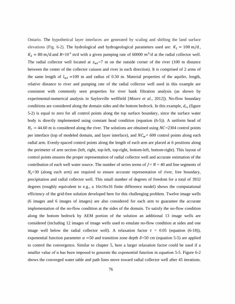
76
Ontario. The hypothetical layer interfaces are generated by scaling and shifting the land surface
elevations (Fig. 6-2). The hydrological and hydrogeological parameters used are: ,
and R=10
-4 m/d with a given pumping rate of 60000 /d at the radial collector well.
The radial collector well located at =7 m on the outside corner of the river (100 m distance
between the center of the collector caisson and river in each direction). It is comprised of 2 arms of
the same length of 100 m and radius of 0.50 m. Material properties of the aquifer, length,
relative distance to river and pumping rate of the radial collector well used in this example are
consistent with commonly seen properties for river bank filtration analysis (as shown by
experimental-numerical analysis in Saylorville wellfield [Moore et al., 2012]). No-flow boundary
conditions are considered along the domain sides and the bottom bedrock. In this example, dsw (figure
5-2) is equal to zero for all control points along the top surface boundary, since the surface water
body is directly implemented using constant head condition (equation (6-5)). A uniform head of
44.60 m is considered along the river. The solutions are obtained using NC =2304 control points
per interface (top of modeled domain, and layer interface), and = 600 control points along each
radial arm. Evenly-spaced control points along the length of each arm are placed at 6 positions along
the perimeter of arm section (left, right, top-left, top-right, bottom-left, bottom-right). This layout of
control points ensures the proper representation of radial collector well and accurate estimation of the
contribution of each well water source. The number of series terms of J = N = 40 and line segments of
=30 (along each arm) are required to ensure accurate representation of river, free boundary,
precipitation and radial collector well. This small number of degrees of freedom for a total of 3932
degrees (roughly equivalent to e.g., a 16x16x16 finite difference model) shows the computational
efficiency of the grid-free solution developed here for this challenging problem. Twelve image wells
(6 images and 6 images of images) are also considered for each arm to guarantee the accurate
implementation of the no-flow condition at the sides of the domain. To satisfy the no-flow condition
along the bottom bedrock by AEM portion of the solution an additional 13 image wells are
considered (including 12 images of image wells used to emulate no-flow condition at sides and one
image well below the radial collector well). A relaxation factor = 0.05 (equation (6-18)),
exponential function parameter 50 and transition zone depth =50 cm (equation 5-5) are applied
to control the convergence. Similar to chapter 5, here a larger relaxation factor could be used if a
smaller value of α has been imposed to generate the exponential function in equation 5-5. Figure 6-2
shows the converged water table and path lines move toward radial collector well after 45 iterations.
77
Figure 6-2 only depicts the layout of flow path lines toward the radial collector well to illustrate the
capacity of the developed model to simulate river bank filtration process. These path lines were
generated using back tracking from 180 particle releasing points located along the radial collector
well (this figure only depicts 60 path lines terminated at the particle releasing points located at the left
and right sides of arms section). Blue path lines originate from the river and move toward two radial
arms aligned with the x and y axes. Red lines depict the path lines which do not originate from the
river. The percentage of well waters captured from the river can be estimated by assigning a weight to
each path line. This weight is equal to the obtained strength of the line sink segment ( which the
path line is terminated in the collector well. Therefore in releasing 180 particles from the well, the
flow-weighted path lines suggest that approximately 57% of radial collector well inflow originate
from the river. This percentage increases as the radial collector well location approaches the river.
Note that to obtain this percentage all 180 particle releasing points (located at 6 sides of arms section)
have been used in the back tracking procedure to generate the path lines. This relative contribution of
each source to radial collector well water seems to be only mildly sensitive to the solution parameters
including the number of control points and , number of particle releasing points, number of
series terms N and J, and number of line sink segments . For example by doubling the number of
control points along each arm or the number of line sink segments, mentioned percentage changes
less than 1%. In addition, this percentage changes less than 2% when only control points located at
the left and right sides of each arm are used in the solution instead of control points located at all 6
sides.
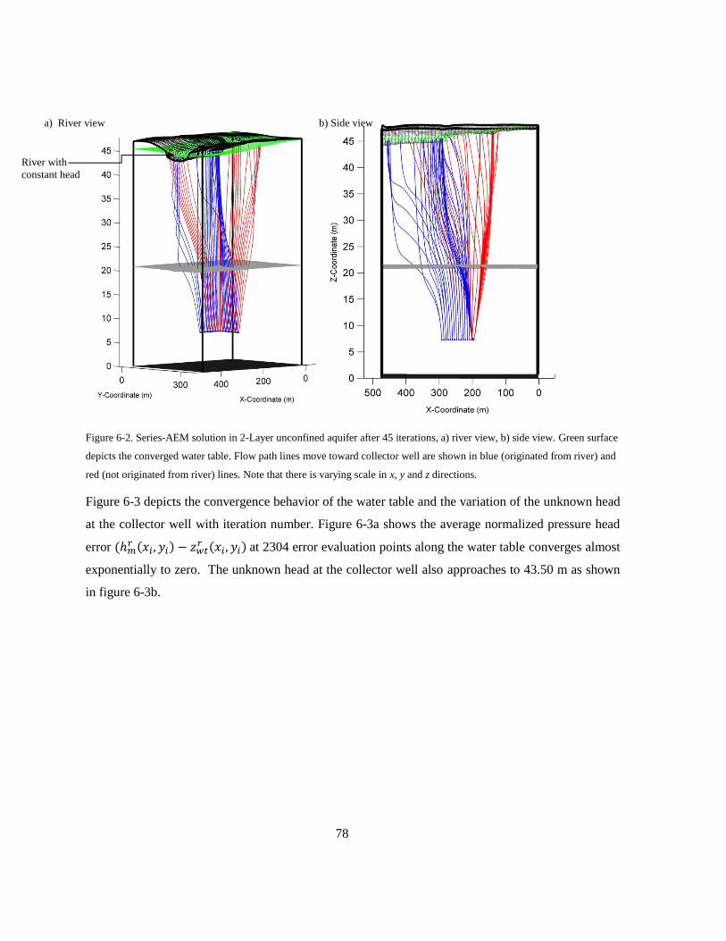
78
Figure 6-2. Series-AEM solution in 2-Layer unconfined aquifer after 45 iterations, a) river view, b) side view. Green surface
depicts the converged water table. Flow path lines move toward collector well are shown in blue (originated from river) and
red (not originated from river) lines. Note that there is varying scale in x, y and z directions.
Figure 6-3 depicts the convergence behavior of the water table and the variation of the unknown head
at the collector well with iteration number. Figure 6-3a shows the average normalized pressure head
error
at 2304 error evaluation points along the water table converges almost
exponentially to zero. The unknown head at the collector well also approaches to 43.50 m as shown
in figure 6-3b.
a) River view b) Side view
River with
constant head

79
Figure 6-3. Convergence behavior of the solution. a) Variation of average normalized head error along the water table and b)
collector well head with respect to iteration number.
As stated earlier, the series-AEM solution developed here satisfies the governing equation exactly.
Using 12 Image wells for each arm, no-flow conditions at the sides of the domain were satisfied with
a normalized error on the order of 10-8
. In addition, no-flow conditions along the bottom bedrock
were satisfied with a normalized error on the order of 10-14
using 13 image wells as discussed earlier.
The constraint on total inflow into the radial collector well (equation (6-10)) is met exactly. Using
least squares (equation (6-17)), however, there are numerical errors along 2304 error evaluation
points in the implementation of boundary and continuity conditions along the top, layer interface and
radial screens as shown in figure 6-4. Figure 6-4a shows the contours of normalized flux error
( at the 2132 error evaluation points (points in direct contact with surface water body are not
included) across the top boundary interface where the specified flux ( from equation 5-5) was
applied. The largest errors are at the projection of radial arms on the top surface with the maximum of
9%. The mean absolute normalized flux error along this interface is 1.3%. At the remaining 172
control points along the top interface which are in direct contact with the river, the normalized head
error is on the order of 10-4
(not shown here). Figures 6-4b show that the normalized flux errors at
a)
b)

80
2304 error evaluation points across the first ( ) layer interface are lower than the top surface with
the maximum of 0.4% for , which again occur at the projection of radial arms along this
interface. In addition, the contour of normalized head error, across 2304 evaluation points at the
layer interface are shown in figure 6-4c with the maximum of 0.4%. The head uniformity at 1200
control points located along two radial arms is also assessed in figure 6-4d. As stated earlier, along
each arm 600 control points are located at 6 sides of the arm section. The top and bottom portions of
figure 6-4d depicts the normalized head error at 6 sides of the arm aligned with the x and y axes,
respectively. The maximum normalized uniformity of head error is 0.6% and 2% along the arm in x
and y directions, respectively, which occurs at the ends of each arm. Note that by increasing the
number of line segments ( ) the maximum error decrease and the uniformity of head along the arms
is met more accurately, but the computational cost considerably increases. For example by doubling
the number of line segments, the maximum normalized uniformity of head error at the ends of each
arm decreases almost 30% (not shown here).
a)
b)
c)
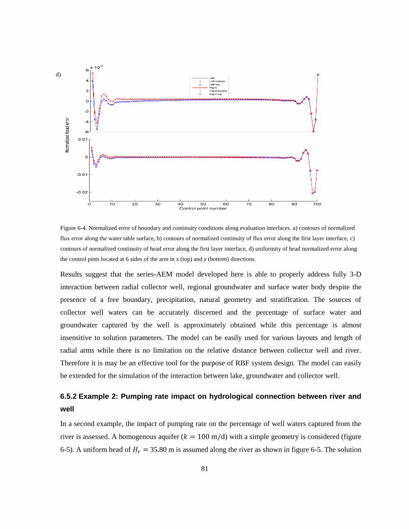
81
Figure 6-4. Normalized error of boundary and continuity conditions along evaluation interfaces. a) contours of normalized
flux error along the water table surface, b) contours of normalized continuity of flux error along the first layer interface, c)
contours of normalized continuity of head error along the first layer interface, d) uniformity of head normalized error along
the control pints located at 6 sides of the arm in x (top) and y (bottom) directions.
Results suggest that the series-AEM model developed here is able to properly address fully 3-D
interaction between radial collector well, regional groundwater and surface water body despite the
presence of a free boundary, precipitation, natural geometry and stratification. The sources of
collector well waters can be accurately discerned and the percentage of surface water and
groundwater captured by the well is approximately obtained while this percentage is almost
insensitive to solution parameters. The model can be easily used for various layouts and length of
radial arms while there is no limitation on the relative distance between collector well and river.
Therefore it is may be an effective tool for the purpose of RBF system design. The model can easily
be extended for the simulation of the interaction between lake, groundwater and collector well.
6.5.2 Example 2: Pumping rate impact on hydrological connection between river and
well
In a second example, the impact of pumping rate on the percentage of well waters captured from the
river is assessed. A homogenous aquifer ( ) with a simple geometry is considered (figure
6-5). A uniform head of 35.80 m is assumed along the river as shown in figure 6-5. The solution
d)
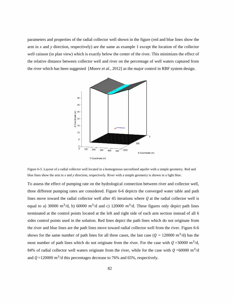
82
parameters and properties of the radial collector well shown in the figure (red and blue lines show the
arm in x and y direction, respectively) are the same as example 1 except the location of the collector
well caisson (in plan view) which is exactly below the center of the river. This minimizes the effect of
the relative distance between collector well and river on the percentage of well waters captured from
the river which has been suggested [Moore et al., 2012] as the major control in RBF system design.
Figure 6-5. Layout of a radial collector well located in a homogenous unconfined aquifer with a simple geometry. Red and
blue lines show the arm in x and y direction, respectively. River with a simple geometry is shown in a light blue.
To assess the effect of pumping rate on the hydrological connection between river and collector well,
three different pumping rates are considered. Figure 6-6 depicts the converged water table and path
lines move toward the radial collector well after 45 iterations where at the radial collector well is
equal to a) 30000 /d, b) 60000 /d and c) 120000 /d. These figures only depict path lines
terminated at the control points located at the left and right side of each arm section instead of all 6
sides control points used in the solution. Red lines depict the path lines which do not originate from
the river and blue lines are the path lines move toward radial collector well from the river. Figure 6-6
shows for the same number of path lines for all three cases, the last case ( = 120000 /d) has the
most number of path lines which do not originate from the river. For the case with Q =30000 /d,
84% of radial collector well waters originate from the river, while for the case with Q =60000 /d
and Q =120000 /d this percentages decrease to 76% and 65%, respectively.
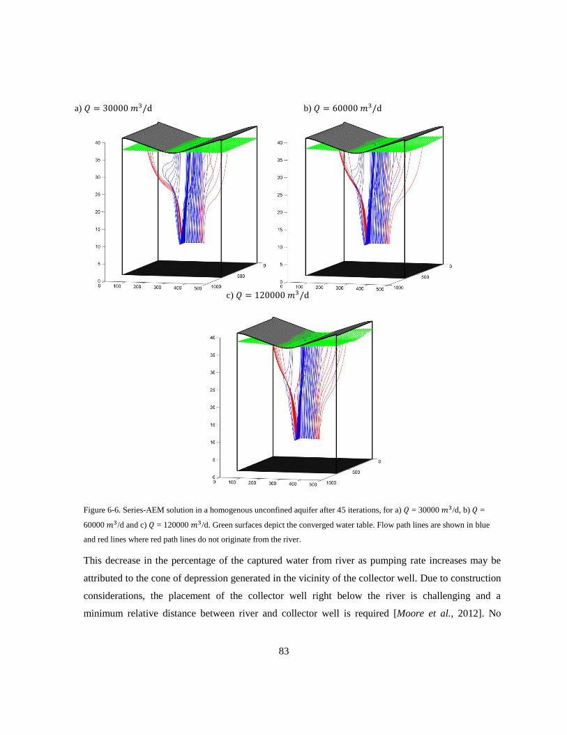
83
Figure 6-6. Series-AEM solution in a homogenous unconfined aquifer after 45 iterations, for a) = 30000 /d, b) =
60000 /d and c) = 120000 /d. Green surfaces depict the converged water table. Flow path lines are shown in blue
and red lines where red path lines do not originate from the river.
This decrease in the percentage of the captured water from river as pumping rate increases may be
attributed to the cone of depression generated in the vicinity of the collector well. Due to construction
considerations, the placement of the collector well right below the river is challenging and a
minimum relative distance between river and collector well is required [Moore et al., 2012]. No
a)
b)
c)
84
doubt, the effect of pumping well on attenuating the well waters captured from the river is increased
as the relative distance between the collector well and river increases.
6.6 Conclusion
A general semi-analytical series-AEM solution for the simulation of fully 3-D interaction between
collector well, free boundary groundwater and surface water body in a naturally complex stratified
unconfined aquifer has been developed and assessed in this chapter. This model accurately simulated
3-D flow with acceptable errors in a priori known water table location. Infiltration, naturally complex
geometry and layer stratification, river geometry and material property, and radial collector well have
been considered. Each arm of the radial collector well in this model is allowed to have an arbitrary
orientation and intersect the layer interface(s). This grid-free model also indicated that for a realistic
problem a small degrees of freedom required to ensure an accurate solution which is converged after
a reasonable number of iterations. Internal flow and pressure head values, radial collector well
inflows, flux distribution at the ground surface and boundary errors are immediately available as
continuous functions of space. This robust model was able to discern well waters origin and
approximate the percentage of well waters captured from different sources (e.g., river, groundwater).
Therefore, it may be used for the purpose of designing RBF systems. In spite of all the advantages of
the model, the mandatory no-flow side boundaries in some specific cases may limit the application of
the model for the simulation of the regional interaction between groundwater, surface water and radial
collector well. It is clear that, for this case at least, there were non-physical boundary artifacts, which
would be alleviated by using larger domain extents.
The method was also used to provide some insights into the impact of pumping rate of the collector
well on hydrological connection between river and collector well. Despite that the radial collector
well was placed below the river, results suggested that as the pumping rate increases the percentage of
well waters originating from the river decreases. This effect can compromise the appropriateness of
RBF systems.

85
Chapter 7
Conclusions and future directions
7.1 Conclusions
This thesis improved the capacity of existing semi-analytical series solution and AEM approaches for
solving groundwater-surface water interaction problems which are challenging to solve using mesh-
based methods. Geometrically complex topography and layer stratification, surface water bodies,
collector well geometry, a priori unknown phreatic surface (free boundary condition) and infiltration
have been properly incorporated into a general model framework which can be successfully applied
to complex systems with small number of degrees of freedom. The free boundary water table surface
was identified using a robust iterative scheme. These solutions exactly satisfied mass balance and
governing equation in the entire domain, as well as no-flow conditions at the sides of the domain.
Boundary and continuity conditions across the layer interfaces are met with acceptable rates of error.
Because the methods developed here do not rely upon volume discretization, internal flow, error and
pressure head values are immediately available as continuous functions of space. These accurate, fast,
continuous and grid-free models were able to assess factors controlling groundwater-surface water
interaction problems with or without pumping well(s). In the following, the main contributions
attained in each chapter are outlined.
In chapter 4, the series solution approach was extended to address 2-D saturated-
unsaturated flow close to a constant head river in geometrically complex stratified
unconfined aquifers. The capillary fringe zone was considered as a distinctive zone with
free boundary at the top and bottom. The continuous saturated-unsaturated series solution
model provided a description of the water distribution and flow direction in both saturated
and unsaturated zones. This model was used to assess the impact of saturated and
unsaturated material properties on the behavior of unsaturated and capillary fringe flow,
and the a priori unknown water table elevation.
In chapter 5, the series solution method was extended to simulate 3-D groundwater-surface
water interaction in a geometrically complex stratified unconfined aquifer, where flow was
controlled by water exchanges across the land surface including evapotranspiration,
infiltration, seepage faces and exchange with surface water bodies. Without having to
86
assume the location of seepage faces, the location of phreatic surface was obtained. This
model was demonstrated to be an efficient tool to simulate flow toward seepage faces in a
realistic stratified unconfined aquifer with a small number of degrees of freedom. In
addition, the grid-free series solution model explicitly represented the lake sediment
geometry and properties. This model was used to show that, for a uniform sediment layer,
increased thickness of lake sediment can slightly uniformize the flux at the lake bed. For
non-uniform sediment layer, increasing the maximum thickness of lake sediment can
considerably increase and decrease the lake bed fluxes at the shoreline and off-shore,
respectively. In spite of this effect, results suggested that the commonly used scheme to
incorporate lake sediment layer effects (the Dupuit-Forchheimer approximation coupled
with the assumption of purely vertical flow through a uniform lake sediment) overestimates
the concentration of lake bed flux.
The 3-D series solution model was augmented with 3-D AEM based approach in chapter 6
to assess steady-state groundwater-surface water interaction between a radial collector well
and river in naturally complex stratified unconfined aquifers. Limitations of AEM for the
accurate representation of constrained free boundary phreatic surface, naturally complex
stratification and surface water body were mitigated by coupling with a series solution
model. The resultant model may be an efficient tool for the purpose of RBF system design.
Radial collector well water sources and the percentage of well waters captured from each
source (e.g., groundwater and river) can be accurately discerned. This continuous and grid-
free model suggested that as pumping rate increases the appropriateness of RBF systems
may be compromised by decreasing the percentage of river water captured by well.
The developed grid-free semi-analytical models in this thesis appear to be efficient alternatives to
numerical methods for the simulation of 3-D steady-state groundwater-surface water interaction in
cases where the mesh-related issues of numerical models can be problematic. However, these models
are only efficient if Gibbs phenomenon is properly addressed. Gibbs phenomenon causes instability at
sharp changes in geometry of the layers or boundary conditions across an interface. The former can
be mitigated by a degree of surface smoothing and the latter may be somewhat addressed by using
weighted least squares as done in chapters 5 and 4, respectively. However, these mentioned
treatments are stopgap schemes and are not able to address the core problem. For example, in the
models developed in this thesis, increasing the number of series term does not always lead to more
87
accuracy. In the examples presented in chapter 5, as N and J increase the accuracy of the top of the
modeled domain free boundary condition increases until N = J = 30 and decreases thereafter. This is
connected to the Gibbs phenomena issue. Indeed, by increasing the number of series terms, the sharp
changes in geometry/boundary condition are mimicked more accurately, but the appropriateness of
the series solution method in the remaining areas is compromised. This issue was simply shown in
figure 3-1 for the curve fitting of a 1-D problem. Increasing the number of control points within the
areas with higher potential for Gibbs phenomenon may not also lead to higher accuracy in the entire
domain. As the number of control points along the areas including sharp changes increases, the
contribution (weight) of these areas to the total series solution increases and the efficiency of the
series solution method in the remaining areas is compromised. Gibbs phenomenon may also limit the
applicability of the methods presented in chapter 6; for example, there must be enough distance
between radial collector well elevation and topographic surface to ensure accurate representation of
free boundary condition along the phreatic surface.
In addition to Gibbs phenomenon, there are other important issues to be recognized. The mandatory
no-flow side boundaries assumed in all developed models may limit their application for the
simulation of regional groundwater-surface water interaction particularly in the presence of pumping
wells with a large discharge rate. Ideally the method may be somehow augmented to handle alternate
boundary conditions. For unsaturated modeling, the unsaturated parameters (sorptive number and air
entry pressure) were here constrained to be identical for different layers to ensure the linearity of the
mathematical model. Using a non-linear least squares algorithm may circumvent this issue. Lastly,
the model for saturated-unsaturated flow was developed based on the Gardner model to ensure
separabality and linearity of the governing equation. Series solutions model will not be able to
incorporate other non-linear soil-water characteristic relationships (e.g., Van Genuchten), as the one
unconquerable requirement of series solution methods is that the governing equation must be linear.
Although the developed series solutions and series-AEM models in this thesis circumvent the mesh-
related issues of numerical models in some specific cases, these methods must be improved
considerably to compete with numerical models in more general settings. In the following section,
some recommendations for the improvement of these models in accompany with the applications of
the developed models in the other fields are listed.
88
7.2 Future directions
As stated above the most challenging issue of the developed models in this thesis is Gibbs
phenomenon. This issue may in the future be rectified by supplementing standard basis functions with
special ‘supplemental solutions’, which handle local departures from generally smooth solutions,
perhaps using the existing library of 2-D and 3-D AEM solutions. This approach properly worked for
1-D curve fitting of a complex function using a discrete Fourier series in chapter 3 but is much more
challenging to implement as part of 2-D and 3-D series solution approach. Developing supplemental
solutions with the ability to address 2-D and 3-D abrupt changes in surface geometry and boundary
conditions may address the Gibbs phenomenon issues reported in this thesis.
Extending the developed models in this thesis for the simulation of transient groundwater-surface
water interaction with or without pumping well(s) can also be a useful progress in the application of
semi-analytical approaches. This may be done using Laplace transform method for topography-driven
flow. For free boundary problems, the Laplace transform method may also be coupled with the
developed models in this thesis to address some simplified transient cases (e.g., with the assumption
of zero specific storage).
The models and techniques presented in this thesis can be used and extended to other fields of
science. For example, the linearized separable equations which govern heat transfer may be addressed
in a manner similar to the developed models in this thesis. Other application areas may include soil
mechanics, laminar fluid flow, and electromagnetic systems.
89
References
Ameli, A. A., and J. R. Craig (2014), Semianalytical series solutions for three‐dimensional
groundwater‐surface water interaction, Water Resources Research, 50(5).
Ameli, A. A., J. R. Craig, and S. Wong (2013), Series solutions for saturated–unsaturated flow in
multi-layer unconfined aquifers, Advances in Water Resources, 60, 24-33.
An, H., Y. Ichikawa, Y. Tachikawa, and M. Shiiba (2010), Three-dimensional finite difference
saturated-unsaturated flow modeling with nonorthogonal grids using a coordinate transformation
method, Water Resources Research, 46(11).
Anderson, E. I. (2003), An analytical solution representing groundwater-surface water interaction,
Water Resources Research, 39(3).
Bakker, M. (2001), An analytic, approximate method for modeling steady, three‐dimensional flow to
partially penetrating wells, Water Resources Research, 37(5), 1301-1308.
Bakker, M. (2002), Two exact solutions for a cylindrical inhomogeneity in a multi-aquifer system,
Advances in Water Resources, 25(1), 9-18.
Bakker, M. (2004), Modeling groundwater flow to elliptical lakes and through multi-aquifer elliptical
inhomogeneities, Advances in Water Resources, 27(5), 497-506.
Bakker, M. (2010), Hydraulic modeling of riverbank filtration systems with curved boundaries using
analytic elements and series solutions, Advances in Water Resources, 33(8), 813-819.
Bakker, M., and E. I. Anderson (2002), Comment on “Numerical investigation of lake bed seepage
patterns: effects of porous medium and lake properties” by Genereux, D., and Bandopadhyay, I.,
2001. Journal of Hydrology 241, 286–303, Journal of Hydrology, 258(1), 260-264.
Bakker, M., and O. D. Strack (2003), Analytic elements for multiaquifer flow, Journal of Hydrology,
271(1), 119-129.
Bakker, M., and J. L. Nieber (2004), Two-dimensional steady unsaturated flow through embedded
elliptical layers, Water Resources Research, 40(12).
Bakker, M., V. A. Kelson, and K. H. Luther (2005), Multilayer Analytic Element Modeling of Radial
Collector Wells, Ground Water, 43(6), 050901015612001.
Barnes, R., and I. Janković (1999), Two-dimensional flow through large numbers of circular
inhomogeneities, Journal of Hydrology, 226(3), 204-210.
Basha, H. (1999), Multidimensional linearized nonsteady infiltration with prescribed boundary
conditions at the soil surface, Water resources research, 35(1), 75-83.
Basha, H. (2000), Multidimensional linearized nonsteady infiltration toward a shallow water table,
Water Resources Research, 36(9), 2567-2573.
Berkowitz, B., S. E. Silliman, and A. M. Dunn (2004), Impact of the capillary fringe on local flow,
chemical migration, and microbiology, Vadose Zone Journal, 3(2), 534-548.
Bischoff, H. (1981), An integral equation method to solve three dimensional confined flow to
drainage systems, Applied Mathematical Modelling, 5(6), 399-404.
Boano, F., C. Camporeale, and R. Revelli (2010), A linear model for the coupled surface-subsurface
flow in a meandering stream, Water Resources Research, 46(7).
Boussinesq, J. (1872), Théorie des ondes et des remous qui se propagent le long d'un canal
rectangulaire horizontal, en communiquant au liquide contenu dans ce canal des vitesses sensiblement
pareilles de la surface au fond, Journal de Mathématiques Pures et Appliquées, 55-108.
Buckingham, E. (1907), Studies on the movement of soil moisture.
Butler Jr, J. J. (1997), The design, performance, and analysis of slug tests, CRC Press.
90
Byrd, R. H., and R. A. Waltz (2011), An active-set algorithm for nonlinear programming using
parametric linear programming, Optimization Methods & Software, 26(1), 47-66.
Cardenas, M. B., and X.-W. Jiang (2010), Groundwater flow, transport, and residence times through
topography-driven basins with exponentially decreasing permeability and porosity, Water Resources
Research, 46(11).
Carter, V. (1990), great dismal swamp: an illustrated case study, Ecosystems of the world.
Charbeneau, R. J. (2006), Groundwater hydraulics and pollutant transport, Waveland Press.
Chen, C., J. Wan, and H. Zhan (2003), Theoretical and experimental studies of coupled seepage-pipe
flow to a horizontal well, Journal of hydrology, 281(1), 159-171.
Correll, D. L., T. E. Jordan, and D. E. Weller (1992), Nutrient flux in a landscape: effects of coastal
land use and terrestrial community mosaic on nutrient transport to coastal waters, Estuaries, 15(4),
431-442.
Craig, J., and W. Read, Wayne, (2010), The future of analytical solution methods for groundwater
flow and transport simulation.
Craig, J. R. (2008), Analytical solutions for 2D topography-driven flow in stratified and syncline
aquifers, Advances in Water Resources, 31(8), 1066-1073.
Dripps, W., R. Hunt, and M. Anderson (2006), Estimating recharge rates with analytic element
models and parameter estimation, Ground Water, 44(1), 47-55.
Dunne, T., and R. D. Black (1970), An experimental investigation of runoff production in permeable
soils, Water Resources Research, 6(2), 478-490.
Forsyth, P. A. (1988), Comparison of the single-phase and two-phase numerical model formulation
for saturated-unsaturated groundwater flow, Computer Methods in Applied Mechanics and
Engineering, 69(2), 243-259.
Freeze, R. A., and P. Witherspoon (1967), Theoretical analysis of regional groundwater flow: 2.
Effect of water‐table configuration and subsurface permeability variation, Water Resources Research,
3(2), 623-634.
Gardner, W. (1958), Some steady-state solutions of the unsaturated moisture flow equation with
application to evaporation from a water table, Soil science, 85(4), 228-232.
Genereux, D., and I. Bandopadhyay (2001), Numerical investigation of lake bed seepage patterns:
effects of porous medium and lake properties, Journal of Hydrology, 241(3), 286-303.
Haitjema, H. (1982), Modeling three-dimensional flow in confined aquifers using distributed
singularities, University of Minnesota.
Haitjema, H. (1995), Analytic element modeling of groundwater flow, Academic Press.
Haitjema, H., S. Kuzin, V. Kelson, and D. Abrams (2010), Modeling Flow into Horizontal Wells in a
Dupuit-Forchheimer Model, Ground Water, 48(6), 878-883.
Haitjema, H. M., and S. Mitchell-Bruker (2005), Are Water Tables a Subdued Replica of the
Topography?, Ground Water, 43 (6), 050824075421008.
Halford, K. J., and G. C. Mayer (2000), Problems Associated with Estimating Ground Water
Discharge and Recharge from Stream‐Discharge Records, Groundwater, 38(3), 331-342.
Hantush, M. M. (2005), Modeling stream–aquifer interactions with linear response functions, Journal
of Hydrology, 311(1-4), 59-79.
Harte, P. T., and T. C. Winter (1993), Factors affecting recharge to crystalline rock in the Mirror Lake
area, Grafton County, New Hampshire, paper presented at USGS Toxic Substances Hydrology
Program—Proceedings of the Technical Meeting, Colorado Springs, Colorado, September 20–24.
Harvey, F. E., D. L. Rudolph, and S. K. Frape (1997), Measurement of hydraulic properties in deep
lake sediments using a tethered pore pressure probe: Applications in the Hamilton Harbour, western
Lake Ontario, Water Resources Research, 33(8), 1917-1928.
91
Hiscock, K. M., and T. Grischek (2002), Attenuation of groundwater pollution by bank filtration,
Journal of Hydrology, 266(3), 139-144.
Hoffman, A. H. (1998), Pump-and-treat rescue, Civil Engineering—ASCE, 68(3), 56-57.
Hunt, B. (2003), Unsteady stream depletion when pumping from semiconfined aquifer, Journal of
Hydrologic Engineering, 8(1), 12-19.
Hunt, B. (2009), Stream depletion in a two-layer leaky aquifer system, Journal of Hydrologic
Engineering, 14(9), 895-903.
Hunt, B., J. Weir, and B. Clausen (2001), A stream depletion field experiment, Groundwater, 39(2),
283-289.
Hunt, R. J. (2006), Ground Water Modeling Applications Using the Analytic Element Method,
Ground Water, 44(1 Ground Water), 5-15.
Hunt, R. J., D. A. Saad, and D. M. Chapel (2003a), Numerical simulation of ground-water flow in La
Crosse County, Wisconsin, and into nearby pools of the Mississippi River, US Department of the
Interior, US Geological Survey.
Hunt, R. J., H. M. Haitjema, J. T. Krohelski, and D. T. Feinstein (2003b), Simulating Ground Water‐Lake Interactions: Approaches and Insights, Ground Water, 41(2), 227-237.
Janković, I., A. Fiori, and G. Dagan (2003), Flow and transport in highly heterogeneous formations:
3. Numerical simulations and comparison with theoretical results, Water Resources Research, 39(9).
Joshi, S. D. (2003), Cost/benefits of horizontal wells, paper presented at SPE Western
Regional/AAPG Pacific Section Joint Meeting, Society of Petroleum Engineers.
Kacimov, A. (2000), Three-dimensional groundwater flow to a lake: an explicit analytical solution,
Journal of Hydrology, 240(1), 80-89.
Kacimov, A. (2007), Three-dimensional groundwater flow to a shallow pond: An explicit solution,
Journal of Hydrology, 337(1), 200-206.
Kelson, V. (2012), Predicting Collector Well Yields with MODFLOW, Ground Water, 50(6), 918-
926.
Kirkham, D. (1967), Explanation of paradoxes in Dupuit Forchheimer Seepage Theory, Water
Resources Research, 3(2), 609-622.
Knupp, P. (1996), A moving mesh algorithm for 3-D regional groundwater flow with water table and
seepage face, Advances in Water Resources, 19(2), 83-95.
Larabi, A., and F. De Smedt (1997), Numerical solution of 3-D groundwater flow involving free
boundaries by a fixed finite element method, Journal of Hydrology, 201(1), 161-182.
Luther, K., and H. M. Haitjema (1999), An analytic element solution to unconfined flow near
partially penetrating wells, Journal of Hydrology, 226(3), 197-203.
Luther, K., and H. Haitjema (2000), Approximate analytic solutions to 3D unconfined groundwater
flow within regional 2D models, Journal of Hydrology, 229(3), 101-117.
Luther, K. H. (1998), Analytic solutions to three-dimensional unconfined groundwater flow near
wells, Indiana University.
Marklund, L., and A. Wörman (2011), The use of spectral analysis-based exact solutions to
characterize topography-controlled groundwater flow, Hydrogeology Journal, 19(8), 1531-1543.
Matott, L. S., A. J. Rabideau, and J. R. Craig (2006), Pump-and-treat optimization using analytic
element method flow models, Advances in Water Resources, 29(5), 760-775.
McCallum, A. M., M. S. Andersen, G. C. Rau, and R. I. Acworth (2012), A 1-D analytical method for
estimating surface water-groundwater interactions and effective thermal diffusivity using temperature
time series, Water Resources Research, 48(11).
Mehl, S., and M. C. Hill (2010), Grid-size dependence of Cauchy boundary conditions used to
simulate stream–aquifer interactions, Advances in Water Resources, 33(4), 430-442.
92
Miller, H., J. M. Bull, C. J. Cotterill, J. K. Dix, I. J. Winfield, A. E. Kemp, and R. B. Pearce (2013),
Lake bed geomorphology and sedimentary processes in glacial lake Windermere, UK, Journal of
Maps, 9(2), 299-312.
Mishra, P. K., and S. P. Neuman (2010), Improved forward and inverse analyses of saturated-
unsaturated flow toward a well in a compressible unconfined aquifer, Water Resources Research,
46(7).
Mishra, P. K., V. Vessilinov, and H. Gupta (2013), On simulation and analysis of variable-rate
pumping tests, Ground Water, 51(3), 469-473.
Moore, R., V. Kelson, J. Wittman, and V. Rash (2012), A Modeling Framework for the Design of
Collector Wells, Ground Water, 50(3), 355-366.
Nahin, P. J. (2011), Dr. Euler's fabulous formula: cures many mathematical ills, Princeton University
Press.
Nield, S. P., L. R. Townley, and A. D. Barr (1994), A framework for quantitative analysis of surface
water‐groundwater interaction: Flow geometry in a vertical section, Water Resources Research,
30(8), 2461-2475.
Okkonen, J., and B. Kløve (2011), A sequential modelling approach to assess groundwater–surface
water resources in a snow dominated region of Finland, Journal of Hydrology, 411(1), 91-107.
Ophori, D. U., and R. N. Farvolden (1985), A hydraulic trap for preventing collector well
contamination: a case study, Groundwater, 23(5), 600-610.
Oz, I., E. Shalev, H. Gvirtzman, Y. Yechieli, and I. Gavrieli (2011), Groundwater flow patterns
adjacent to a long-term stratified (meromictic) lake, Water Resources Research, 47(8), n/a-n/a.
Patel, H., C. Shah, and D. Shah (1998), Modeling of radial collector well for sustained yield: a case
study, paper presented at Proc int conf MODFLOW.
Patel, H., T. Eldho, and A. Rastogi (2010), Simulation of radial collector well in shallow alluvial
riverbed aquifer using analytic element method, Journal of irrigation and drainage engineering,
136(2), 107-119.
Philip, J. (1998), Seepage shedding by parabolic capillary barriers and cavities, Water resources
research, 34(11), 2827-2835.
Powers, W., D. Kirkham, and G. Snowden (1967), Orthonormal function tables and the seepage of
steady rain through soil bedding, Journal of Geophysical Research, 72(24), 6225-6237.
Ray, C., T. Grischek, J. Schubert, J. Z. Wang, and T. F. Speth (2002), A Perspective of Riverbank
Filtration (PDF), Journal-American Water Works Association, 94(4), 149-160.
Read, W., and R. Volker (1993), Series solutions for steady seepage through hillsides with arbitrary
flow boundaries, Water Resources Research, 29(8), 2871-2880.
Read, W., and P. Broadbridge (1996), Series solutions for steady unsaturated flow in irregular porous
domains, Transport in porous media, 22(2), 195-214.
Read, W., S. Belward, P. Higgins, and G. Sneddon (2005), Series solutions for seepage in three
dimensional aquifers, ANZIAM Journal, 46, C1126--C1140.
Richards, L. A. (1931), Capillary conduction of liquids through porous mediums, Journal of Applied
Physics, 1(5), 318-333.
Romanoa, C. G., E. O. Frind, and D. L. Rudolph (1999), Significance of Unsaturated Flow and
Seepage Faces in the Simulation of Steady‐State Subsurface Flow, Groundwater, 37(4), 625-632.
Rushton, K. (2007), Representation in regional models of saturated river–aquifer interaction for
gaining/losing rivers, Journal of Hydrology, 334(1-2), 262-281.
Rushton, K. R., and F. C. Brassington (2013a), Hydraulic behaviour and regional impact of a
horizontal well in a shallow aquifer: example from the Sefton Coast, northwest England (UK),
Hydrogeology Journal, 21(5), 1117-1128.
93
Rushton, K. R., and F. C. Brassington (2013b), Significance of hydraulic head gradients within
horizontal wells in unconfined aquifers of limited saturated thickness, Journal of Hydrology, 492,
281-289.
Samani, N., M. Kompani-Zare, H. Seyyedian, and D. Barry (2006), Flow to horizontal drains in
isotropic unconfined aquifers, Journal of Hydrology, 324(1), 178-194.
Selim, H. (1975), Water flow through a multilayer stratified hillside, Water Resources Research,
11(6), 949-957.
Serrano, S. E., and S. Workman (1998), Modeling transient stream/aquifer interaction with the non-
linear Boussinesq equation and its analytical solution, Journal of Hydrology, 206(3), 245-255.
Simpkins, W. W. (2006), A multiscale investigation of ground water flow at Clear Lake, Iowa,
Ground Water, 44(1), 35-46.
Smerdon, B., K. Devito, and C. Mendoza (2005), Interaction of groundwater and shallow lakes on
outwash sediments in the sub-humid Boreal Plains of Canada, Journal of Hydrology, 314(1), 246-
262.
Smerdon, B., C. Mendoza, and K. Devito (2007), Simulations of fully coupled lake‐groundwater
exchange in a subhumid climate with an integrated hydrologic model, Water Resources Research,
43(1).
Sophocleous, M. (2002), Interactions between groundwater and surface water: the state of the science,
Hydrogeology Journal, 10(1), 52-67.
Sophocleous, M., M. Townsend, L. Vogler, T. McClain, E. Marks, and G. Coble (1988),
Experimental studies in stream-aquifer interaction along the Arkansas River in central Kansas—Field
testing and analysis, Journal of Hydrology, 98(3), 249-273.
Stark, J., D. Armstrong, and D. Zwilling (1994), Stream-aquifer interactions in the Straight River
area, Becker and Hubbard Counties, Minnesota, US Geological Survey.
Steward, D. R. (1999), Three‐dimensional analysis of the capture of contaminated leachate by fully
penetrating, partially penetrating, and horizontal wells, Water Resources Research, 35(2), 461-468.
Steward, D. R., and W. Jin (2001), Gaining and losing sections of horizontal wells, Water Resources
Research, 37(11), 2677-2685.
Steward, D. R., and W. Jin (2003), Drawdown and capture zone topology for nonvertical wells, Water
Resources Research, 39(8).
Strack, O. D. (1984), Three Dimensional Streamlines in Dupuit‐Forchheimer Models, Water
Resources Research, 20(7), 812-822.
Strack, O. D. (Ed.) (1989), Groundwater mechanics, Prentice-Hall, Englewood Cliffs, NJ.
Strack, O. D., and H. M. Haitjema (1981), Modeling double aquifer flow using a comprehensive
potential and distributed singularities: 1. Solution for homogeneous permeability, Water Resources
Research, 17(5), 1535-1549.
Tartakovsky, G. D., and S. P. Neuman (2007), Three-dimensional saturated-unsaturated flow with
axial symmetry to a partially penetrating well in a compressible unconfined aquifer, Water Resources
Research, 43(1).
Teloglou, I. S., and R. K. Bansal (2012), Transient solution for stream–unconfined aquifer interaction
due to time varying stream head and in the presence of leakage, Journal of Hydrology, 428-429, 68-
79.
Therrien, R., R. McLaren, E. Sudicky, and S. Panday (2008), HydroGeoSphere: A three-dimensional
numerical model describing fully-integrated subsurface and surface flow and solute transport,
Groundwater Simul. Group, Waterloo, Ont., Canada.
Townley, L. R., and M. G. Trefry (2000), Surface water-groundwater interaction near shallow
circular lakes: Flow geometry in three dimensions, Water Resources Research, 36(4), 935-948.
94
Tristscher, P., W. Read, P. Broadbridge, and J. Knight (2001), Steady saturated-unsaturated flow in
irregular porous domains, Mathematical and computer modelling, 34(1), 177-194.
Tsou, P. R., Z. Y. Feng, H. D. Yeh, and C. S. Huang (2010), Stream depletion rate with horizontal or
slanted wells in confined aquifers near a stream, Hydrology and Earth System Sciences, 14(8), 1477-
1485.
Wang, X. S., S. P. Neuman, O. D. Strack, A. Verruijt, M. Jamali, B. Seymour, J. Bear, A. H. D.
Cheng, C. Chen, and X. Kuang (2011), Methods to derive the differential equation of the free surface
boundary, Groundwater, 49(2), 133-143.
Ward, N. D., and H. Lough (2011), Stream depletion from pumping a semiconfined aquifer in a two-
layer leaky aquifer system, Journal of Hydrologic Engineering, 16(11), 955-959.
Werner, A. D., M. R. Gallagher, and S. W. Weeks (2006), Regional-scale, fully coupled modelling of
stream–aquifer interaction in a tropical catchment, Journal of Hydrology, 328(3-4), 497-510.
Winter, T., and H. Pfannkuch (1984), Effect of anisotropy and groundwater system geometry on
seepage through lakebeds: 2. Numerical simulation analysis, Journal of Hydrology, 75(1), 239-253.
Winter, T. C., and D. O. Rosenberry (1995), The interaction of ground water with prairie pothole
wetlands in the Cottonwood Lake area, east-central North Dakota, 1979–1990, Wetlands, 15(3), 193-
211.
Wong, S., and J. R. Craig (2010), Series solutions for flow in stratified aquifers with natural
geometry, Advances in Water Resources, 33(1), 48-54.
Workman, S., S. Serrano, and K. Liberty (1997), Development and application of an analytical model
of stream/aquifer interaction, Journal of Hydrology, 200(1), 149-163.
Wörman, A., A. I. Packman, L. Marklund, J. W. Harvey, and S. H. Stone (2006), Exact three-
dimensional spectral solution to surface-groundwater interactions with arbitrary surface topography,
Geophysical Research Letters, 33(7).
Yeh, H.-D., and Y.-C. Chang (2013), Recent advances in modeling of well hydraulics, Advances in
Water Resources, 51, 27-51.
Zhan, H., and V. A. Zlotnik (2002), Groundwater flow to a horizontal or slanted well in an
unconfined aquifer, Water Resources Research, 38(7), 13-11-13-11.
Zhan, H., L. V. Wang, and E. Park (2001), On the horizontal-well pumping tests in anisotropic
confined aquifers, Journal of Hydrology, 252(1), 37-50.
Related Documents