SEMANTIC CLUSTERING OF QUESTIONS - AIMAS · SEMANTIC CLUSTERING OF QUESTIONS ... in a lexical hierarchy such as ... direction change in the path between two terms or the information

Politehnica University of Bucharest

2012

SEMANTIC CLUSTERING OF QUESTIONS

Master of Artificial Intelligence

Research Report, 2nd semester

Author: Cristina Groapă

Scientific Advisors:

Prof. Adina Magda Florea,

Assistant Prof. Andrei Olaru

1

Table of Contents 1. Theoretical aspects .......................................................................................................................... 2

1.1. General concepts ..................................................................................................................... 2

1.1.1. Similarity vs. relatedness .................................................................................................. 2

1.1.2. Specificity ......................................................................................................................... 2

1.2. Path-based similarity measures ................................................................................................ 3

1.2.1. Leacock-Chodorow ........................................................................................................... 3

1.2.2. Wu and Palmer ................................................................................................................. 3

1.3. Information Content-based similarity measures ....................................................................... 4

1.3.1. Resnik............................................................................................................................... 4

1.3.2. Jiang and Conrath ............................................................................................................. 4

1.3.3. Lin .................................................................................................................................... 4

1.4. Relatedness measures .............................................................................................................. 5

1.4.1. Hirst and St.-Onge ............................................................................................................ 5

1.4.2. Lesk and Vector measures ................................................................................................ 5

2. NLP Tools ......................................................................................................................................... 6

2.1. Stanford Core NLP .................................................................................................................... 6

2.2. LingPipe ................................................................................................................................... 7

2.3. Java Wordnet::Similarity .......................................................................................................... 9

3. Implementation ............................................................................................................................... 9

3.1. The SmartPresentation Project ................................................................................................. 9

3.2. Overall architecture ............................................................................................................... 10

4. Results ........................................................................................................................................... 12

5. Conclusions ................................................................................................................................... 14

6. Bibliography .................................................................................................................................. 15

2

1. Theoretical aspects

1.1. General concepts

1.1.1. Similarity vs. relatedness

Although these terms are often considered synonyms, there is a slight difference between them, which

will prove relevant when describing the types of semantic similarity measures.

Similarity is a more restricted term compared to relatedness because it is limited to finding is-a relations

in a lexical hierarchy such as WordNet. Thus, for example, the terms car and bicycle are more similar

than car and gasoline because they are both a type of vehicle.

Semantic relatedness uses more semantic relations and is generally a less restrictive measure. Other

semantic relations employed by relatedness and available in WordNet include has–part, is–made–of, is–

an–attribute–of. Semantic relatedness measures may also take into consideration the definitions of the

two concepts, for example in order to find common words. Therefore, in terms of semantic relatedness,

the terms car and gasoline will be considered semantically closer.

1.1.2. Specificity

Specificity (or Information Content) measures the level of abstraction a word uses to describe reality.

The higher a word' specificity, the less abstract it is and thus the more information content it has.

Specificity might thus be associated with the depth of a word in the WordNet hypernym tree. A more

concrete example: collie and sheepdog bare much more information content than go and be.

In the context of semantic similarity, matching words with higher specificity should weight more in the

evaluation metric than matching general concepts.

There are a few ways in which specificity can be computed. The two main categories are using a

taxonomy of concepts and using a corpus of natural language texts. In the first case, when using

WordNet for example, a word’s specificity might be given by its depth in the taxonomy.

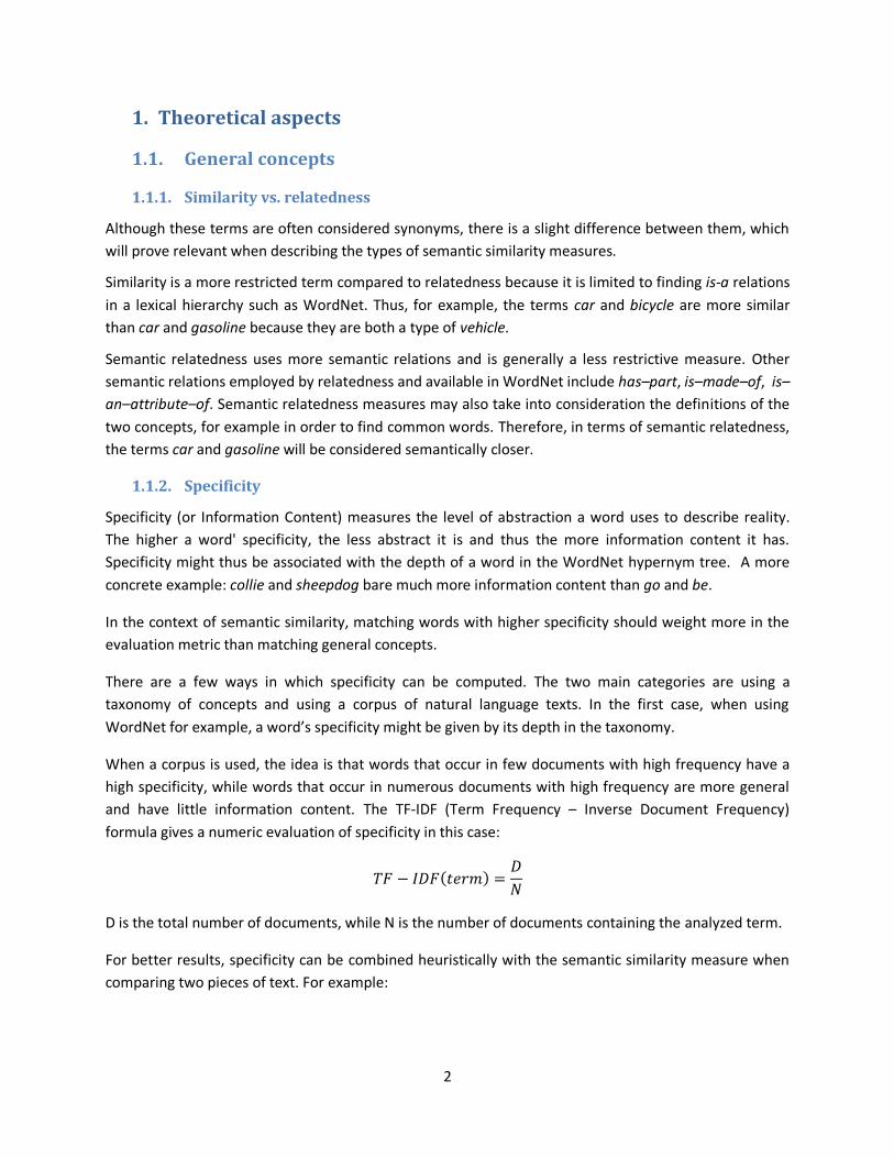
When a corpus is used, the idea is that words that occur in few documents with high frequency have a

high specificity, while words that occur in numerous documents with high frequency are more general

and have little information content. The TF-IDF (Term Frequency – Inverse Document Frequency)

formula gives a numeric evaluation of specificity in this case:

𝑇𝐹 − 𝐼𝐷𝐹 𝑡𝑒𝑟𝑚 =𝐷

𝑁

D is the total number of documents, while N is the number of documents containing the analyzed term.

For better results, specificity can be combined heuristically with the semantic similarity measure when

comparing two pieces of text. For example:

3

𝑠𝑖𝑚(𝑇𝑖 ,𝑇𝑗 )𝑇𝑖 = ( 𝑚𝑎𝑥𝑆𝑖𝑚 𝑤𝑘 ∗ 𝑖𝑑𝑓𝑤𝑘

𝑤∈ 𝑊𝑆𝑝𝑜𝑠 )𝑝𝑜𝑠

𝑖𝑑𝑓𝑤𝑘𝑤∈ 𝑇𝑖𝑝𝑜𝑠

Ti and Tj are the two texts being compared. WSpos is the set of semantically related words between the

two texts.

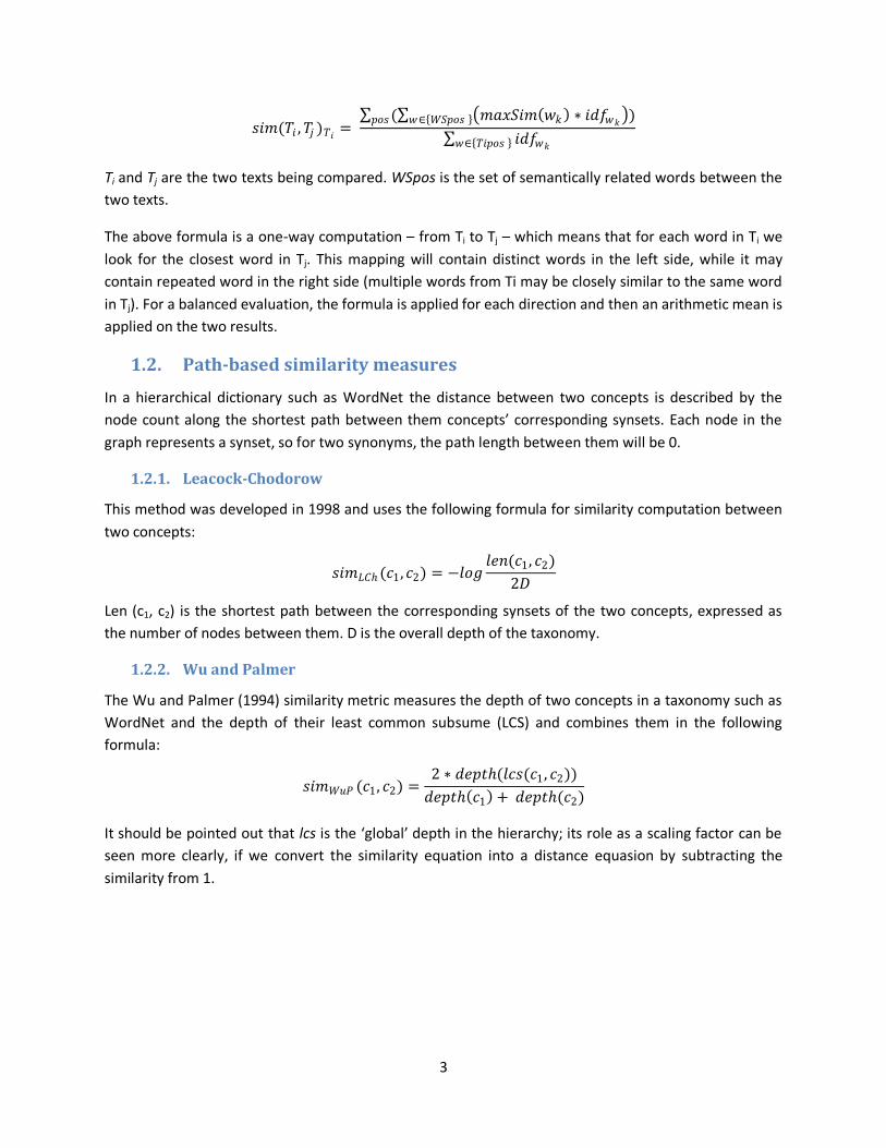
The above formula is a one-way computation – from Ti to Tj – which means that for each word in Ti we

look for the closest word in Tj. This mapping will contain distinct words in the left side, while it may

contain repeated word in the right side (multiple words from Ti may be closely similar to the same word

in Tj). For a balanced evaluation, the formula is applied for each direction and then an arithmetic mean is

applied on the two results.

1.2. Path-based similarity measures

In a hierarchical dictionary such as WordNet the distance between two concepts is described by the

node count along the shortest path between them concepts’ corresponding synsets. Each node in the

graph represents a synset, so for two synonyms, the path length between them will be 0.

1.2.1. Leacock-Chodorow

This method was developed in 1998 and uses the following formula for similarity computation between

two concepts:

𝑠𝑖𝑚𝐿𝐶𝑕(𝑐1, 𝑐2) = −𝑙𝑜𝑔𝑙𝑒𝑛(𝑐1, 𝑐2)

2𝐷

Len (c1, c2) is the shortest path between the corresponding synsets of the two concepts, expressed as

the number of nodes between them. D is the overall depth of the taxonomy.

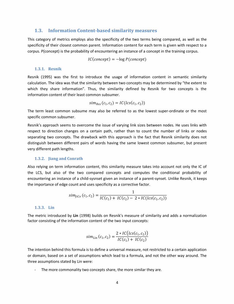
1.2.2. Wu and Palmer

The Wu and Palmer (1994) similarity metric measures the depth of two concepts in a taxonomy such as

WordNet and the depth of their least common subsume (LCS) and combines them in the following

formula:

𝑠𝑖𝑚𝑊𝑢𝑃 (𝑐1, 𝑐2) =2 ∗ 𝑑𝑒𝑝𝑡𝑕(𝑙𝑐𝑠(𝑐1, 𝑐2))

𝑑𝑒𝑝𝑡𝑕 𝑐1 + 𝑑𝑒𝑝𝑡𝑕(𝑐2)

It should be pointed out that lcs is the ‘global’ depth in the hierarchy; its role as a scaling factor can be

seen more clearly, if we convert the similarity equation into a distance equasion by subtracting the

similarity from 1.

4

1.3. Information Content-based similarity measures

This category of metrics employs also the specificity of the two terms being compared, as well as the

specificity of their closest common parent. Information content for each term is given with respect to a

corpus. P(concept) is the probability of encountering an instance of a concept in the training corpus.

𝐼𝐶 𝑐𝑜𝑛𝑐𝑒𝑝𝑡 = −log 𝑃(𝑐𝑜𝑛𝑐𝑒𝑝𝑡)

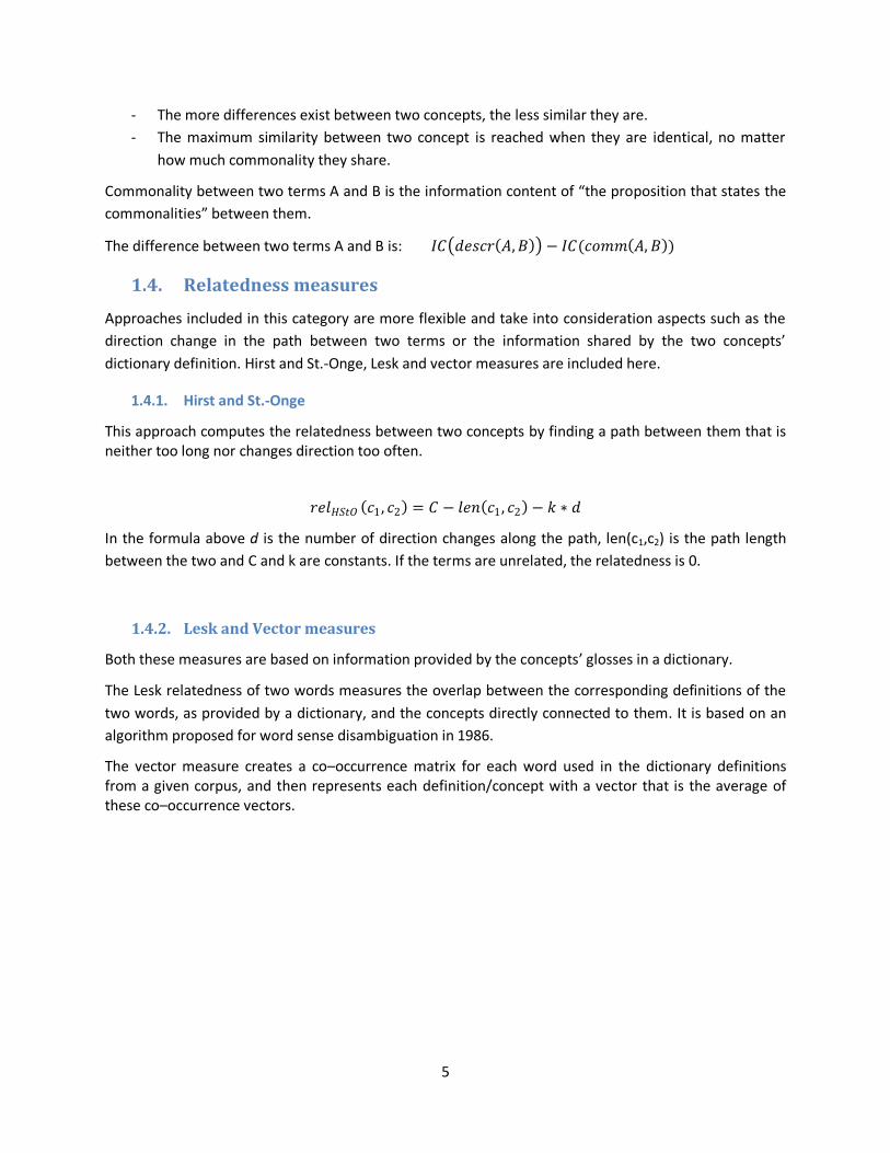
1.3.1. Resnik

Resnik (1995) was the first to introduce the usage of information content in semantic similarity

calculation. The idea was that the similarity between two concepts may be determined by “the extent to

which they share information”. Thus, the similarity defined by Resnik for two concepts is the

information content of their least common subsumer.

𝑠𝑖𝑚𝑅𝑒𝑠 (𝑐1, 𝑐2) = 𝐼𝐶(𝑙𝑐𝑠 𝑐1 , 𝑐2 )

The term least common subsume may also be referred to as the lowest super-ordinate or the most

specific common subsumer.

Resnik’s approach seems to overcome the issue of varying link sizes between nodes. He uses links with

respect to direction changes on a certain path, rather than to count the number of links or nodes

separating two concepts. The drawback with this approach is the fact that Resnik similarity does not

distinguish between different pairs of words having the same lowest common subsumer, but present

very different path lengths.

1.3.2. Jiang and Conrath

Also relying on term information content, this similarity measure takes into account not only the IC of

the LCS, but also of the two compared concepts and computes the conditional probability of

encountering an instance of a child-sysnset given an instance of a parent-synset. Unlike Resnik, it keeps

the importance of edge count and uses specificity as a corrective factor.

𝑠𝑖𝑚𝐽𝑖𝐶𝑜 (𝑐1, 𝑐2) =1

𝐼𝐶 𝑐1 + 𝐼𝐶 𝑐2 − 2 ∗ 𝐼𝐶(𝑙𝑐𝑠 𝑐1, 𝑐2 )

1.3.3. Lin

The metric introduced by Lin (1998) builds on Resnik’s measure of similarity and adds a normalization factor consisting of the information content of the two input concepts:

𝑠𝑖𝑚𝐿𝑖𝑛 𝑐1, 𝑐2 =2 ∗ 𝐼𝐶 𝑙𝑐𝑠 𝑐1, 𝑐2

𝐼𝐶 𝑐1 + 𝐼𝐶 𝑐2

The intention behind this formula is to define a universal measure, not restricted to a certain application

or domain, based on a set of assumptions which lead to a formula, and not the other way around. The

three assumptions stated by Lin were:

- The more commonality two concepts share, the more similar they are.

5

- The more differences exist between two concepts, the less similar they are.

- The maximum similarity between two concept is reached when they are identical, no matter

how much commonality they share.

Commonality between two terms A and B is the information content of “the proposition that states the

commonalities” between them.

The difference between two terms A and B is: 𝐼𝐶 𝑑𝑒𝑠𝑐𝑟 𝐴,𝐵 − 𝐼𝐶(𝑐𝑜𝑚𝑚 𝐴,𝐵 )

1.4. Relatedness measures

Approaches included in this category are more flexible and take into consideration aspects such as the

direction change in the path between two terms or the information shared by the two concepts’

dictionary definition. Hirst and St.-Onge, Lesk and vector measures are included here.

1.4.1. Hirst and St.-Onge

This approach computes the relatedness between two concepts by finding a path between them that is neither too long nor changes direction too often.

𝑟𝑒𝑙𝐻𝑆𝑡𝑂 𝑐1, 𝑐2 = 𝐶 − 𝑙𝑒𝑛 𝑐1, 𝑐2 − 𝑘 ∗ 𝑑

In the formula above d is the number of direction changes along the path, len(c1,c2) is the path length

between the two and C and k are constants. If the terms are unrelated, the relatedness is 0.

1.4.2. Lesk and Vector measures

Both these measures are based on information provided by the concepts’ glosses in a dictionary.

The Lesk relatedness of two words measures the overlap between the corresponding definitions of the

two words, as provided by a dictionary, and the concepts directly connected to them. It is based on an

algorithm proposed for word sense disambiguation in 1986.

The vector measure creates a co–occurrence matrix for each word used in the dictionary definitions from a given corpus, and then represents each definition/concept with a vector that is the average of these co–occurrence vectors.

6

2. NLP Tools

2.1. Stanford Core NLP

Stanford CoreNLP is a free complete Java package for natural language analysis which provides, among

others, tools for tokenization, sentence splitting, part-of-speech tagging, syntactic parsing, named entity

recognition and coreference resolution. It therefore provides the basis for any higher level natural

language processing task, including question clustering. The Stanford CoreNLP code is licensed under the

GNU General Public License.

Stanford CoreNLP tools can be used in command line by specifying the .jars, properties file and the file(s)

to be processed. A command for processing a single file looks like this:

java -cp stanford-corenlp-2012-04-09.jar:

stanford-corenlp-2012-04-09-models.jar:xom.jar:

joda-time.jar

-Xmx3g edu.stanford.nlp.pipeline.StanfordCoreNLP

-annotators tokenize,ssplit,pos,lemma,ner,parse,dcoref

-file input.txt

The annotators parameter specifies a list of the annotators we want to apply on the text.

Stanford CoreNLP also provides a Java API. It is easy to use and the text annotation is performed in only

a few lines of code:

The StanfordCoreNLP object will perform the text analysis, applying the tools specified in props. Some of

these tools are dependent on others. For example the sentence splitting cannot be done without prior

tokenization (to recognize punctuation marks), POS depends on tokenization as well, and syntactical

parsing cannot be done without previous pos-tagging.

The Annotation object will contain all the information added in the parsing process. The information

extraction step is just as intuitive, as shown in the code below.

//specify which annotations to apply using the Properties class Properties props = new Properties(); props.put("annotators", "tokenize, ssplit, pos, lemma, ner, parse"); StanfordCoreNLP pipeline = new StanfordCoreNLP(props); String text = ... // Add your text here! Annotation document = new Annotation(text); pipeline.annotate(document);

7

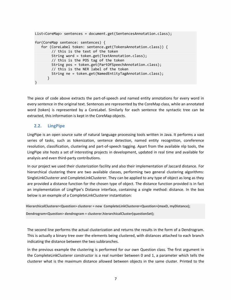
The piece of code above extracts the part-of-speech and named entity annotations for every word in

every sentence in the original text. Sentences are represented by the CoreMap class, while an annotated

word (token) is represented by a CoreLabel. Similarly for each sentence the syntactic tree can be

extracted, this information is kept in the CoreMap objects.

2.2. LingPipe

LingPipe is an open source suite of natural language processing tools written in Java. It performs a vast

series of tasks, such as tokenization, sentence detection, named entity recognition, coreference

resolution, classification, clustering and part-of-speech tagging. Apart from the available nlp tools, the

LingPipe site hosts a set of interesting projects in development, updated in real time and available for

analysis and even third-party contributions.

In our project we used their clusterization facility and also their implementation of Jaccard distance. For

hierarchical clustering there are two available classes, performing two general clustering algorithms:

SingleLinkClusterer and CompleteLinkClusterer. They can be applied to any type of object as long as they

are provided a distance function for the chosen type of object. The distance function provided is in fact

an implementation of LingPipe’s Distance interface, containing a single method: distance. In the box

below is an example of a CompleteLinkClusterer instantiation:

The second line performs the actual clusterization and returns the results in the form of a Dendrogram.

This is actually a binary tree over the elements being clustered, with distances attached to each branch

indicating the distance between the two subbranches.

In the previous example the clustering is performed for our own Question class. The first argument in

the CompleteLinkClusterer constructor is a real number between 0 and 1, a parameter which tells the

clusterer what is the maximum distance allowed between objects in the same cluster. Printed to the

List<CoreMap> sentences = document.get(SentencesAnnotation.class); for(CoreMap sentence: sentences) { for (CoreLabel token: sentence.get(TokensAnnotation.class)) { // this is the text of the token String word = token.get(TextAnnotation.class); // this is the POS tag of the token String pos = token.get(PartOfSpeechAnnotation.class); // this is the NER label of the token String ne = token.get(NamedEntityTagAnnotation.class); } }

HierarchicalClusterer<Question> clusterer = new CompleteLinkClusterer<Question>(maxD, myDistance);

Dendrogram<Question> dendrogram = clusterer.hierarchicalCluster(questionSet);

8

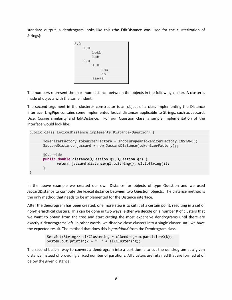
standard output, a dendrogram looks like this (the EditDistance was used for the clusterization of

Strings):

The numbers represent the maximum distance between the objects in the following cluster. A cluster is

made of objects with the same indent.

The second argument in the clusterer constructor is an object of a class implementing the Distance

interface. LingPipe contains some implemented lexical distances applicable to Strings, such as Jaccard,

Dice, Cosine similarity and EditDistance. For our Question class, a simple implementation of the

interface would look like:

In the above example we created our own Distance for objects of type Question and we used

JaccardDistance to compute the lexical distance between two Question objects. The distance method is

the only method that needs to be implemented for the Distance interface.

After the dendrogram has been created, one more step is to cut it at a certain point, resulting in a set of

non-hierarchical clusters. This can be done in two ways: either we decide on a number K of clusters that

we want to obtain from the tree and start cutting the most expensive dendrograms until there are

exactly K dendrograms left. In other words, we dissolve close clusters into a single cluster until we have

the expected result. The method that does this is partitionK from the Dendrogram class:

The second built-in way to convert a dendrogram into a partition is to cut the dendrogram at a given

distance instead of providing a fixed number of partitions. All clusters are retained that are formed at or

below the given distance.

public class LexicalDistance implements Distance<Question> {

TokenizerFactory tokenizerFactory = IndoEuropeanTokenizerFactory.INSTANCE; JaccardDistance jaccard = new JaccardDistance(tokenizerFactory);;

@Override public double distance(Question q1, Question q2) { return jaccard.distance(q1.toString(), q2.toString()); } }

Set<Set<String>> clKClustering = clDendrogram.partitionK(k); System.out.println(k + " " + slKClustering);

3.0

1.0

bbbb

bbb

2.0

1.0

aaa

aa

aaaaa

9

2.3. Java Wordnet::Similarity

There are a number of tools which work with WordNet: JAWS, JWNL, Wordnet::Similarity (Perl and Java

versions available). We chose JWS (Java WordNet Similarity) for our semantic similarity approach

because it is simple to use and offers everything we needed – implementations for all known semantic

similarities. It requires a previous installation of WordNet on the local machine.

A simple example that uses JAWS is in the box below:

JWS is the main object that interacts with the WordNet dictionary and provides various semantic

similarities, such as LeacockAndChodorow, Lin, HirstAndStOnge, Resnik etc. In the example above the

maximum similarity between word1 and word2 is computed. This means that their sense or synset is not

specified, so lch will choose the two synsets for which the semantic similarity is maximum. The max

function has another form where for each of the two words its sense is also given. Pos specifies the part

of speech of the two words, which needs to be the same for both.

3. Implementation

3.1. The SmartPresentation Project

Our Question Clustering task will be integrated in a larger project for Android, SmartPresentation. The project’s finality is an application which makes presentations interactive leading to a better understanding and communication between the audience and the speaker. A typical scenario in which the application would prove highly useful is an academic lecture where students may send questions or comments to the speaker in real time. The speaker receives this feedback grouped according to its topic and users’ ranking. The question clustering task is used to group the audience’s questions according to their semantic similarity in order to avoid redundancy and situations where multiple users ask similar questions.

The integration with the main project will be made through the QuestionHierClusterer class, which coordinates the question preprocessing and the actual clusterer.

Questions and clustering results will be communicated asynchronously and sequentially, which means that the clusterization process will be repeated whenever a new question or set of questions is received from the other module. A caching mechanism is implemented in the clustering side in order to avoid redundancy when computing similarity between words or sentences.

Each new question arrives as a String with a questionID and a referenceID attached. QuestionID identifies the question and will be used when returning the clustering results – the clusters will be formed of IDs and not Strings. Each question may be asked with respect to a slide or a picture or a piece of text. This reference is identified by referenceID. The clusterization algorithm will be applied to each such reference separately; another way of looking at this would be to consider the referenceIDs the main clusters and the associated results from the clustering algorithm would be sub-clusters of these.

JWS ws = new JWS(WORDNET_DIR, "2.0");

LeacockAndChodorow lch = ws.getLeacockAndChodorow();

double sim = lch.max(word1, word2, pos);

10

3.2. Overall architecture

The main challenge in question clustering was evaluating the semantic similarity or distance between

questions in a satisfactory fashion. Based on this evaluation, the clustering step uses a general algorithm

– hierarchical clustering – already implemented by many tools, including LingPipe.

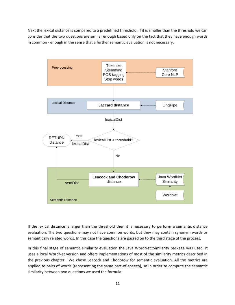
The general architecture behind our semantic similarity evaluation is described in the schema below.

There are three main steps in the process of question clustering – text preprocessing, computation of

lexical distance between questions and computation of semantic distance between questions. The third

step is performed only when a predefined threshold is not reached by the lexical distance. Also, each

step employs a different NLP tool.

The first step processes each question – provided as a string – using the Stanford CoreNLP package. The

process is a pipeline performing the following annotations: tokenization, ssplit, pos, lemma, parse. The

tokenization identifies each word and punctuation mark in the text, which are called tokens. The ssplit

annotator splits the text into sentences. The pos step performs part-of-speech tagging. The lemmatizer

extracts the lemma for each word in the text – this will be useful for dictionary lookup, as well as for the

parsing step. The last activated annotator is a syntactic parser. The resulting parsed sentence is a set of

tokens with lemma and part-of-speech tags.

Also in this step the tokens are divided in three part-of-speech groups: nouns, verbs (including phrasal

verbs) and adjectives. The other parts of speech are not relevant to our task of semantic similarity –

adverbs are rare and don’t usually provide much semantic information; pronouns, prepositions and

conjunctions are a restricted set of common words and again do not bare semantic similarity

significance. However, all the detected tokens (except punctuation marks) are kept in a separate all-

token group. From the verb group some highly general verbs – such as be and have – are excluded as

well (they are included in the stop word list).

The second step computes the lexical distance between questions using the LingPipe package. The

lexical distance we chose for this step is Jaccard, which is provided by the LingPipe package. Jaccard

distance is a simple metric based on the number of common words between the two compared texts. It

receives each of the two questions in the form of a string of lemmas from the initial question (only the

nouns, verbs and adjectives) separated by white spaces.

For example, if the original question was: “What were Napoleon’s favorite fruits?” then it would be

passed to the lexical distance class as the following string: “Napoleon favorite fruit”. It is necessary to

replace each word by its lemma because Jaccard only recognizes exact matches between words

(strings). Also it treats the given string as a sentence and knows to separate the words in it.

The result in step two is a numerical semantic distance with values between 0 and 1, where 0 means

lexically identical and 1 means there is no lexical similarity between the two questions.

11

Next the lexical distance is compared to a predefined threshold. If it is smaller than the threshold we can

consider that the two questions are similar enough based only on the fact that they have enough words

in common - enough in the sense that a further semantic evaluation is not necessary.

If the lexical distance is larger than the threshold then it is necessary to perform a semantic distance

evaluation. The two questions may not have common words, but they may contain synonym words or

semantically related words. In this case the questions are passed on to the third stage of the process.

In this final stage of semantic similarity evaluation the Java WordNet::Similarity package was used. It

uses a local WordNet version and offers implementations of most of the similarity metrics described in

the previous chapter. We chose Leacock and Chodorow for semantic evaluation. All the metrics are

applied to pairs of words (representing the same part-of-speech), so in order to compute the semantic

similarity between two questions we used the formula:

Tokenize

Stemming

POS-tagging

Stop words

Stanford

Core NLP

Jaccard distance LingPipe

lexicalDist < threshold?RETURN

distance

Yes

Preprocessing

Lexical Distance

lexicalDist

Java WordNet

Similarity

Semantic Distance

Leacock and Chodorow

distance

WordNet

No

lexicalDist

semDist

12

𝑠𝑖𝑚𝑠𝑒𝑚 =1

2 max 𝑠𝑠𝑖𝑚 (𝑎𝑖 ,𝑄2)𝑎𝑖 ∈𝑄1

𝑄1 + max 𝑠𝑠𝑖𝑚 (𝑏𝑗 ,𝑄1)𝑏𝑗 ∈𝑄2

𝑄2

The Leacock and Chodorow evaluation returns a number between 0 and 1 where (close to ) 1 means

highly similar and 0 means no semantic relatedness. Therefore, the returned result will be 1-simsem in

order to keep the comparability with the lexical distance.

The final similarity evaluation for each pair of questions is eventually transmitted to LingPipe’s

HierarchicalClusterer which will perform the clusterization.

4. Results Regarding the temporal performance, the results are more than satisfactory. For example, the clustering

algorithm was tested on a set of 143 questions of an average size of 6 words on a dual core processor of

2GHz and a 3GB RAM. The process duration was around 8 minutes.

Considering the fact that in the real case the questions will arrive one by one over the duration of a

lecture or presentation and that the clusterization results will be viewed most probable at the end of the

lecture, the above result is most reassuring.

The caching mechanism had a great impact on time reduction and we believe that in reality the chances

of encountering word repetition in questions which are all related to the same presentation are even

higher. Therefore the caching process will prove to be even more useful.

On the other hand, regarding the partitioning of the questions, some of the question associations are

quite unexpected, while others seem more than reasonable. The bad associations are mostly due to the

fact that our approach does not perform word sense disambiguation and thus sometimes two words are

associated with the synsets that are closest, and which may not always be the ones employed in the

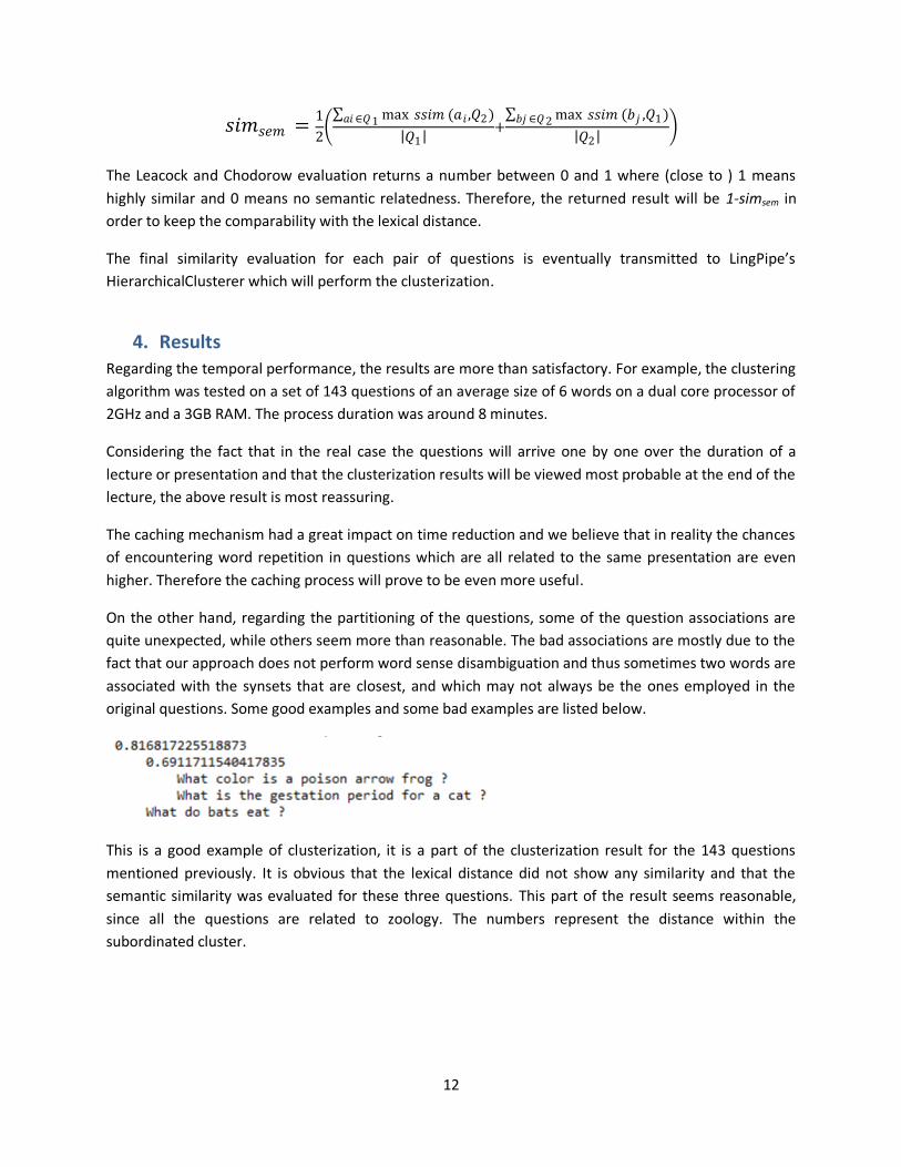
original questions. Some good examples and some bad examples are listed below.

This is a good example of clusterization, it is a part of the clusterization result for the 143 questions

mentioned previously. It is obvious that the lexical distance did not show any similarity and that the

semantic similarity was evaluated for these three questions. This part of the result seems reasonable,

since all the questions are related to zoology. The numbers represent the distance within the

subordinated cluster.

13

The questions in the second example are clearly grouped in two distinct sets – the first with a inner-

cluster distance of 0.81135 – and the second – with a distance of 0.8623. Looked at separately the two

major groups may seem just as reasonable as the first example. However, when regarding the two sets

together and especially considering the total of 143 questions in the entire example, we may wonder

why such distinct sets were created for all these questions which revolve around the concept of

president. This issue may be overcome in the future when in the context of a lecture all the questions

will be related to some extent, so we will be able to cut the dendrogram with a higher, more permissive

inner-cluster distance.

A very bad result is shown below. The explanation here is obviously lack of word sense disambiguation.

Although in the first sentence the sense of the word head is not an anatomical part, this latter sense was

chosen when compared to the second question, and more precisely when compared to the word brain,

because it resulted in a much higher semantic relatedness.

Enlarging the view in the previous example gives us a new question: again, why were these zoology-

related questions placed so far away from the previous set of zoology questions.

14

5. Conclusions There are some limitations associated with our approach and the most important of these is the lack of

word sense disambiguation. This analysis is usually performed in the context of larger texts because the

algorithm is based on finding pairs of synonyms within the same text, which would indicate the actual

sysnset that a word belongs to. Given the fact that our implementation works with texts of one or two

sentences, the word sense disambiguation process would have given poor results.

On the other hand, the reference object attached to each question may to some extent compensate this

problem by pre-grouping questions related to the same object and so we can consider that the first step

of clusterization is already made.

With respect to the corpus on which the module was tested – unfortunately it is not as descriptive of

the SmartPresentation scenario as we would have liked it to be. The questions are simple and direct,

rather resembling a trivia, lacking a certain degree of specificity and elaboration characteristic of a

presentation.

Nonetheless, the corpus is a good start for evaluating our model and did help by pointing out some

issues, such as unexpected associations of questions and the fact that profession and mother are more

semantically related than profession and musician according to all the existing similarity measures.

The next step towards the optimization of the Question Clustering module is testing it on real

presentation data, with reference objects. It will be interesting to see how this separation affects the

clusterization process, which issued fade as a consequence and what other issues appear.

Another direction suggested by recent tests would be increasing the weight for named entities such as

people and organizations. They seem to be more relevant in evaluating semantic similarity than

common nouns.

15

6. Bibliography

Budanitsky, A., & Hirst, G. (2006). EvaluatingWordNet-based Measures of Lexical Semantic Relatedness.

Computational Linguistics .

Clustering Tutorial. (n.d.). Retrieved 2012, from Alias-i LingPipe: http://alias-

i.com/lingpipe/demos/tutorial/cluster/read-me.html

Corley, C., & Mihalcea, R. (2005). Measuring the Semantic Similarity of Texts. Proceedings of the ACL

Workshop on Empirical Modeling of Semantic Equivalence and Entailment, (pp. 13–18).

Java API for WordNet Searching (JAWS). (n.d.). Retrieved 2012, from Bobby B. Lyle School of

Engineering: lyle.smu.edu/~tspell/jaws/index.html

Patwardhan, S., Banerjee, S., & Pedersen, T. (2002). Using Measures of Semantic Relatedness for Word

Sense Disambiguation.

Pedersen, T. (2010). Information Content Measures of Semantic Similarity Perform BetterWithout

Sense-Tagged Text. Human Language Technologies: The 2010 Annual Conference of the North American

Chapter of the ACL, (pp. 329-332).

Pedersen, T., Patwardhan, S., & Michelizzi, J. (2004). WordNet::Similarity - Measuring the Relatedness of

Concepts.

Stanford CoreNLP. (n.d.). Retrieved from The Stanford Natural Language Processing Group:

http://nlp.stanford.edu/software/corenlp.shtml