Sell First, Fix Later: Impact of Patching on Software Quality1

Sell First, Fix Later: Impact of Patching on Software

Quality1

Ashish Arora Jonathan P. Caulkins Rahul Telang {ashish; caulkins; rtelang}@andrew.cmu.edu

H. John Heinz III School of Public Policy and Management

Carnegie Mellon University

August 2003

Revised October 2004

1 We thank the Associated Editor and two anonymous reviewers for many helpful comments.

Sell First, Fix Later: Impact of Patching on Software Quality

Abstract

We present a model of fixing or patching a software problem after the product has been released in the market. Specifically, we model a software firm’s trade-off in releasing a buggy product early and investments in fixing it later. Just as the marginal cost of producing software can be effectively zero, so can be the marginal cost of repairing multiple copies of defective software by issuing patches. We show that due to the fixed cost nature of investments in patching, a software vendor has incentives to release a buggier product early and patch it later in a larger market. Thus, a software monopolist releases a product with fewer bugs but later than what is socially optimal. We contrast this result with physical good markets where market size does not play any role in quality provision.

Keywords: Patching, Software Quality, Time-of-entry, fixed costs, complementarity.

August 2003

Revised: October 2004

1

1. Introduction Software has become an intrinsic part of the very fabric of our lives. As software

becomes ingrained in daily business activities, its failures become even more critical.2 Media

reports of catastrophic effects of software failure abound. For instance, a buffer overflow bug

that caused the Ariane 5 rocket to blow up 40 seconds after liftoff in 1996 (estimated loss of over

$500 million); a software failure interrupted the New York Mercantile Exchange (Washington

Technologies, 1998).3 Software quality has become even more important recently due to

heightened security concerns arising from software vulnerabilities. The business community also

pays close attention to software malfunctions. Fully 97% of the 800 managers surveyed reported

software flaws in their systems in the past year. More than 90% blamed faulty software for lost

revenue or higher costs.4 Some 62% said they believed the software industry was doing a bad job

of producing bug-free software (Information Week, 2002).

The overall quality experienced by a software user is a combination of the bugs in a

software product and the efforts the vendor makes to patch the bugs after shipping. Indeed, most

models of the software development cycle explicitly incorporate the possibility of improving the

product after release (Evans and Reddy 2002). There is also ample evidence that many leading

software vendors routinely release patches (Information Week, 2004: p 18).5 In fact, patching has

become so common that many organizations have “patch-management” systems in place to

efficiently integrate patches in existing software (Information Week, 2004). Patching is most

common in packaged software. With customized, mission critical, or embedded software,

patching is rarely an option because of very high cost of failure. 2 In 2002, the U.S. software market was worth almost $180 billion, with 697,000 employed as software engineers and an additional 585,000 as computer programmers (NIST, 2002: 1). 3 More examples, some possibly apocryphal, can be found at http://www.softwareqatest.com/index.html4 A recent study put the annual cost of major software bugs to the U.S. economy at over $60 billion (NIST, 2002). 5 Sun released more than 200 patches for Solaris 9.0 to fix more than 1200 bugs in six-month period (downloaded from http://sunsolve.sun.com).

2

It is a commonplace that “time to market” pressures are an important reason, if not the

most important reason, why software has bugs. Delay is costly because, all else equal, users

would rather get a product sooner so they can use it longer (see e.g., Baskerville et al. 2001). For

example, a typical view of the manager is “I would rather have it wrong that have it late. We can

always fix it later.” (Paulk et. al. 1995: p 4). However, reducing bugs require time. Indeed, in the

basic model presented here, bugs can only be reduced by delaying release. It is tempting to

assume that firms can reduce the time to market without affecting the product quality by

increasing the number of developers.6 However, Brooks’ famous study of the IBM OS/360

suggests the opposite: The greater costs of coordinating among more developers may outweigh

any gain in efficiency (Brooks, 1995). Further, Amdahl’s law points to a natural limit to the size

of the product development team, especially for new and unprecedented software.

Therefore, our model is more applicable to off-the-shelf packaged software when

reducing bugs takes time and the disutility of the remaining bugs is not so catastrophic that no

one would buy a buggy product.

1.1 Research Questions

In this paper, we formally analyze how the ability to patch the bugs later affects the

vendor’s decision about when to enter the market, and how buggy the initial product is. We then

contrast these decisions when the product is a tangible good like automobile instead of software.

A key finding is that the ability to fix bugs later always leads to an earlier release of the

product, and a larger market increases the incentive to release early with more bugs. A more

striking finding is that it is indeed socially efficient to release the product early and to patch

extensively later. Hence, in market equilibrium, a monopolist – who charges high prices and thus

6 Organizations can, and do, reduce bugs by adopting processes such as CMM or ISO9001. Ultimately, however, having fewer bugs at the time of release depend on careful design, coding and extensive testing under different conditions and for different tasks. This takes time.

3

has lower sales – releases products later and with fewer bugs, but also patches less, than is

socially efficient. The ability to fix or otherwise mitigate software defects after release is an

under-appreciated difference between software and physical goods. Physical goods can, of

course, be recalled to fix defects. However, the key distinction is that while the cost of fixing a

software bug ex-post is roughly independent of the number of copies of the software sold, the

cost of recalling and fixing an automobile will vary directly with the number of cars sold.

Although the cost of actually identifying a bug and writing and testing the code to fix it

can be significant, it often has a fixed-cost nature in the sense of being independent of the

number of copies sold. Of course, sometimes patching costs may vary by number of users

(copies sold). For instance, if the software vendor sent a consultant to each user’s site to help

install the patch like in case of Y2K where sometimes programmers were required to go through

the code at individual organizations. However, a more common practice is to email the patch to

customers or simply make it available on the vendor’s website with no customer specific

adaptation or hand-holding. So, to caricature, in our model, the software aftermarket repairs

entail only fixed costs, whereas for physical goods, variable costs predominate.

The fixed cost nature of patching investment implies that the effective market size plays a

crucial role. Indeed, we formally show that all else equal, a large market size implies earlier

shipping (longer “time in market”) but also more investment in patching (after-sale support), and

higher overall value to the user. This result provides intuition for the otherwise unexpected result

that, relative to the socially efficient outcome, a monopolist ships software products later, with

fewer bugs, but commits to less patching later. In contrast, we show that for physical products,

market size is irrelevant; both the monopolist provides socially efficient levels of defects and

post sale remediation.

4

We assume that a vendor can commit to a chosen level of patching, either contractually

or more likely, through a need to maintain its reputation and maintain future sales. Absent such

a commitment, a vendor has no incentive to patch and rational users would recognize it as well.

Further, ours is a full information model where users are fully aware of existing bugs as well as

the producer’s commitment to fix some fraction of them later. Hence, any sub-optimality is not

due to incomplete information. Even if the number of bugs were stochastic, our model would

still apply provided the vendor did not have private information. Section 5 explores the

robustness of the results to various generalizations, including fixed development costs,

uncertainty, and more general functional forms.

The paper is organized as follows. Section 2 reviews the literature. We outline the model,

including the monopolist’s and social planner’s decisions, in section 3. We also provide the

comparative analysis with a tangible good in this section. Section 4 discusses the robustness of

our results and section 6 summarizes managerial insights and concludes.

2. Prior Literature In software engineering literature it has been argued that better process leads to higher

quality and lower costs and maintenance (Krishnan et al. 2000; Banker et. al. 1997). The

literature agrees that it is cheaper to find and fix bugs early in the development cycle (Banker

and Slaughter 1997). Our focus is not on process economics but on the trade-off between

delaying product release to reduce bugs and investing in patching bugs after release. Banker and

Slaughter (1997) show that managers are often unwilling to delay product release, even though

such delay could save them money in the long run. Hendricks and Singhal (1997) show that

stock markets also punish the firms who delay their products. Cohen et al. (1996) analyze the

performance and time-to-market tradeoff for physical products when repairing defects after

5

product release is exorbitantly costly. The literature shows that higher performance provides

higher value to customers (Zirger and Maidiqui 1990), but it also leads to significant

development delay (Griffin 1993; Yoon and Lilien 1985). Our analysis differs from much of the

work to date in that we allow the vendors to issue patches after the product has been released, as

the empirical evidence overwhelmingly shows is done for software.

3. Model 3.1 Consumer’s Utility All else equal users prefer software products that are released earlier and have fewer

bugs. We define user utility function7 as:

pttBδkVθU −−= )]()([ (1)

V is the baseline utility per unit of time if the product is bug free, B(t) is the number of

bugs when the product is released8, k(δ)B(t) is the cost to the user of the bugs remaining after

patching, and t is the amount of time a user uses the product, where for simplicity we ignore time

discounting. Time t is measured backwards, so a high t means the product is released early

giving the user more time to derive utility from the product while lower t means that the product

is released late. Note that rushing to release results in more bugs, and at an increasing rate, so we

assume that B(t) is increasing and convex in t, i.e., B’ > 0 and B’’ > 0.

Since the proportion of bugs patched by the vendor is δ, (1-δ) proportion of bugs are still

unresolved. To capture the notion that patches can not be a complete substitute for the bug-free

software in the first place, we instead use k(δ) as the proportion of defect costs (to the user) that

has not been reduced by the firm through patching. Since, presumably the utility loss decreases

7 The utility has the form U = θq – p where q is the term in brackets in (1). Such a utility formulation is widely used in literature (e.g., Moorthy 1984) 8 We defined bugs as defects in the original products. The model is unchanged if defects are also interpreted as a “lack of features” which can be added after product-release (e.g., Bessen, 2002).

6

with patching investment (higher δ), albeit at a diminishing rate, so we let k’(δ) < 0 and k’’(δ) >

0. The proportion of defects costs remaining, k(δ)Β(t), ought to be interpreted as an average over

time or in an expectation sense. For some products, it might reflect the proportion of defects

fixed immediately via a “patch” available for download. For others, the proportion of defects

remediated might initially be zero, but might increase over time so that unremediated defect cost,

averaged over t, the time over which the product is used, is k(δ)B(t).9

The price paid by the customer is p, and the coefficient θ captures customer heterogeneity

as they derive different utility per unit time from the software’s functionality. Thus, high θ users,

such as frequent users, derive more utility from the product but also incur higher loss from bugs.

We assume that θ is uniformly distributed in [0, 1]. In section 4, we will relax this assumption.

3.2 Vendor’s Profit Function

We assume that the marginal cost of producing the product is zero so that the vendor’s

objective function consists of revenue minus the fixed cost of patching. The fixed cost of

patching is assumed to be proportional to the number of bugs patched (or proportional to the

number of patches).10 Thus the vendor’s objective function is

δδπ )(),,( tFBptpD −= (2)

3.3 Market Equilibrium under Monopoly

Given (1) and the uniform distribution of θ, the monopolist vendor’s demand is

⎟⎟⎠

⎞⎜⎜⎝

⎛−

−=ttBkV

ptpD )]()([

1 ),,(δ

δ . Hence the profit Equation (2) for the monopolist profit becomes

9 Our results are unchanged if users incur a cost to apply patches. We can also model the utility and cost function in terms of “number of patches” (δ) instead of proportion of patches. In that case, the utility function would be

and the cost function would be F δ. The results remain unchanged. ptktBVU −+−= )]()([ δθ10 In section 4, we also incorporate a fixed development cost where development expenditures affects both release time and bugs.

7

)( )]()([

1 ),,( δδ

δπ tFBpttBkV

ptp −⎟⎟⎠

⎞⎜⎜⎝

⎛−

−= . (3a)

It can be readily verified that after substituting for the profit maximizing price,

)( )]()([41 ),( δδδπ tFBttBkVt −−= . (3b)

It is useful at this stage to introduce Ψ(δ, t; m) = )( )]()([ δδ tFBttBkVm −− . We also

assume that })log()log({})log()'log({2)log()log( tdBddkddkd δδ −<− to ensure that Ψ(δ,

t; m) is concave in t and δ. Roughly, this condition requires that the elasticity of bugs with

respect to delay be high, and that the utility loss from bugs not be very responsive to δ relative to

the change in marginal utility loss. This condition is satisfied for commonly used functional

forms, such as B(t) = t2 and k(δ) = exp(-λδ). The first order conditions for t and δ are

0)(')]()( )(')([ 41),(

=−−−= δδδδπ tFBtBkttBkVdttd (4)

0)( )()('41 ),(

=−−= tFBttBkd

td δδ

δπ . (5)

Also note that for δ satisfying the first order conditions

0)('))( )(')(('41

),(2

>−+−= tFBtBttBkdtdtd δ

δδπ (6)

since Ftk =− **41 )(' δ from Equation (5). This “complementarity” follows naturally from how

defect costs are defined and obtains with very general utility functions (see section 4). Note that

it holds only at the optimal values of δ and is a useful (but not necessary) for our results.

3.4 Benchmark: The Socially Efficient Outcome

It is interesting to compare the choices of the monopolist to the socially efficient level.

Efficiency requires that the product is priced at marginal cost, which we have assumed to be

zero11. At this price, the entire market will be covered. Therefore, the objective function is -

11 The result holds even if we impose a “break even” constraint, since, as we explain, the key is that the monopolist serves fewer customers than is socially efficient.

8

)()]()([21)(

1

0 )]()([ ),( δδδθδθδ tFBttBkVtFBdttBkVtS −−=−∫ −= (7)

Equation (7) and the monopolist’s profit function have the form Ψ(δ, t; m), where m = ½

for the social planner and m = ¼ for the monopolist. We prove in the Appendix that the optimal

values δ* and t* that maximize Ψ(δ, t; m) are increasing in m. This implies that the socially

efficient outcome is to release the product earlier than the monopolist (and hence with more

bugs) but patch more aggressively, as summarized in Proposition 1 below.

Proposition 1: For a software product, the monopolist releases the product later with

fewer bugs but invests less in patching and ex-post support than the socially efficient levels.

This is the principal result of this paper. It is surprising in that contrary to popular belief,

the monopolist releases less buggy products than what is socially optimal. But the monopolist

provides less value by entering the market later and providing less ex-post support.

3.5 Role of Market Size

In our analysis, the market size is normalized to one and m captures the proportion of

market captured by the monopolist or social planner. Should the market be larger, then for the

same m, there will be more users buying the product. Thus, we can also interpret m as an

indicator of market size. It follows from the proof of Proposition 1 that a producer facing a larger

market has a greater incentive to enter the market earlier with a buggy product and provide

extensive patching support later. The costs of patching can be amortized over a larger sales

volume, inducing greater investment in δ and also earlier (and hence also buggier) product

release (i.e., a larger t). Thus a corollary of Proposition 1 is:

Corollary 1: A software producer facing a larger market or lower fixed costs per bug

patched enters the market earlier with more bugs but provides higher patching support later.

9

The costs of patching also depend on the type of product and domain in which firms

operate, such as systems software, and application software. Thus our results provide empirically

testable hypothesis that when the market is large, or the cost of patching is small, or when the

vendors have better support infrastructure, they have an incentive to enter the market earlier with

buggier products.

Microsoft has large market for many of its products, and also provides extensive patching

support. Many of its patches are released in “service-packs” that make it easy for the user to

download and install new patches. These service packs can also scan the computer and networks,

identify bugs and vulnerabilities and automatically download the right patches. Clearly,

Microsoft is willing to incur these large costs in after-sale support because they can be amortized

over a large user base.

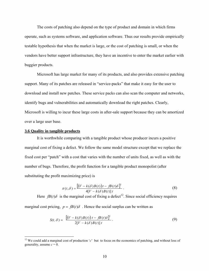
3.6 Quality in tangible products

It is worthwhile comparing with a tangible product whose producer incurs a positive

marginal cost of fixing a defect. We follow the same model structure except that we replace the

fixed cost per “patch” with a cost that varies with the number of units fixed, as well as with the

number of bugs. Therefore, the profit function for a tangible product monopolist (after

substituting the profit maximizing price) is

( )[ ]ttBkVtfBttBkVt

)]()([4)( )()( ),(

2

δδδδπ

−−−

= . (8)

Here )( δtfB is the marginal cost of fixing a defect12. Since social efficiency requires

marginal cost pricing, )( δtfBp = . Hence the social surplus can be written as

( )[ ]ttBkVδtfB ttBkV S(t,

)]()([2)()()()

2

δδδ

−−−

= . (9)

12 We could add a marginal cost of production ‘c’ but to focus on the economics of patching, and without loss of generality, assume c = 0.

10

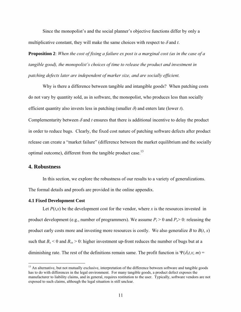
Since the monopolist’s and the social planner’s objective functions differ by only a

multiplicative constant, they will make the same choices with respect to δ and t.

Proposition 2: When the cost of fixing a failure ex post is a marginal cost (as in the case of a

tangible good), the monopolist’s choices of time to release the product and investment in

patching defects later are independent of marker size, and are socially efficient.

Why is there a difference between tangible and intangible goods? When patching costs

do not vary by quantity sold, as in software, the monopolist, who produces less than socially

efficient quantity also invests less in patching (smaller δ) and enters late (lower t).

Complementarity between δ and t ensures that there is additional incentive to delay the product

in order to reduce bugs. Clearly, the fixed cost nature of patching software defects after product

release can create a “market failure” (difference between the market equilibrium and the socially

optimal outcome), different from the tangible product case.13

4. Robustness

In this section, we explore the robustness of our results to a variety of generalizations.

The formal details and proofs are provided in the online appendix.

4.1 Fixed Development Cost

Let P(t,x) be the development cost for the vendor, where x is the resources invested in

product development (e.g., number of programmers). We assume Pt > 0 and Px> 0: releasing the

product early costs more and investing more resources is costly. We also generalize B to B(t, x)

such that Bx < 0 and Bxx > 0: higher investment up-front reduces the number of bugs but at a

diminishing rate. The rest of the definitions remain same. The profit function is Ψ(δ,t,x; m) =

13 An alternative, but not mutually exclusive, interpretation of the difference between software and tangible goods has to do with differences in the legal environment. For many tangible goods, a product defect exposes the manufacturer to liability claims, and in general, requires restitution to the user. Typically, software vendors are not exposed to such claims, although the legal situation is still unclear.

11

),(- ),( )],()([ xtPxtFBtxtBkVm δδ −− . The vendor now optimizes over x as well. In the online

appendix we show that Pxt ≤ 0 and Bxt ≤ 0 are sufficient for all our results to hold.14 For example,

we still have a monopolist entering the market late (lower t) and investing less in patching (lower

δ) than socially efficient. However, since B also depends on x, the monopolist’s product is no

longer unambiguously less buggy than socially efficient.

4.2 General functional form of utility

For brevity and ease of exposition, we use a specific structure for the utility function.

However, our results are robust to a more general utility function of the form ( ) pytVU −= , θ

where y is the utility cost of unresolved bugs, and equal to k(δ)B(t). We would expect that Vt > 0

and Vtt < 0 such that utility is increasing in t but at a decreasing rate. Similarly, Vy < 0 and Vyy <

0, so that unresolved bugs reduce the utility at an increasing rate. One can show that all our

results would continue to hold even with such a specification.15 However, if we additionally

include product development cost P and let development expenditures affect the number of bugs,

as in 4.1, then dmd

dmdt δ and cannot be signed without additional restrictions. As the introduction

notes, often bugs can not be reduced simply by increasing programmers or testers. Therefore, if

Bx were to be small (where x is the investment as above) then even with the general utility

function and fixed development costs, all results would continue to hold.

4.3 Fixing the amount of time a user uses the product

The discussion of the more general utility function also provides reassurance that our results are

not driven by the assumption that the product has a pre-specified date of obsolescence and that

the length of time the product is used enters multiplicatively. We show in the online appendix

14Note that if there is a fixed development cost for tangible goods as well, then proposition 2 will require additional assumptions. 15 The proofs are available upon request.

12

that the results remain intact if instead a product has a fixed life cycle of length τ irrespective of

when it is released, as long as users still value a product released earlier.

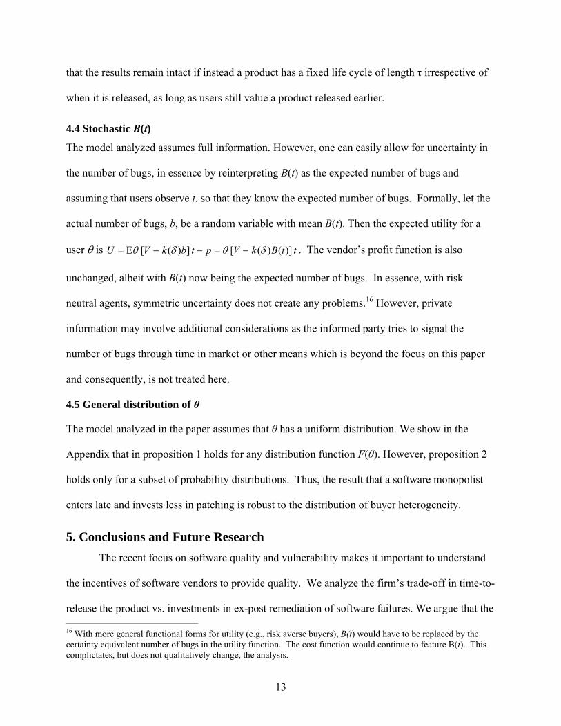
4.4 Stochastic B(t)

The model analyzed assumes full information. However, one can easily allow for uncertainty in

the number of bugs, in essence by reinterpreting B(t) as the expected number of bugs and

assuming that users observe t, so that they know the expected number of bugs. Formally, let the

actual number of bugs, b, be a random variable with mean B(t). Then the expected utility for a

user θ is ttBkVptbkVU )]()([ ])([ E δθδθ −=−−= . The vendor’s profit function is also

unchanged, albeit with B(t) now being the expected number of bugs. In essence, with risk

neutral agents, symmetric uncertainty does not create any problems.16 However, private

information may involve additional considerations as the informed party tries to signal the

number of bugs through time in market or other means which is beyond the focus on this paper

and consequently, is not treated here.

4.5 General distribution of θ

The model analyzed in the paper assumes that θ has a uniform distribution. We show in the

Appendix that in proposition 1 holds for any distribution function F(θ). However, proposition 2

holds only for a subset of probability distributions. Thus, the result that a software monopolist

enters late and invests less in patching is robust to the distribution of buyer heterogeneity.

5. Conclusions and Future Research The recent focus on software quality and vulnerability makes it important to understand

the incentives of software vendors to provide quality. We analyze the firm’s trade-off in time-to-

release the product vs. investments in ex-post remediation of software failures. We argue that the 16 With more general functional forms for utility (e.g., risk averse buyers), B(t) would have to be replaced by the certainty equivalent number of bugs in the utility function. The cost function would continue to feature B(t). This complictates, but does not qualitatively change, the analysis.

13

fixed cost nature of investments in bug-remediation also means that firms facing a larger market

tend to enter early with a buggier product but then invest more in after-sale remediation. Since a

monopolist restricts output relative to socially efficient levels, this leads to counter -intuitive

result that a monopolist in a smaller market actually provides a product with fewer bugs but then

provides less “after-sale” support and therefore, reduces customer value. In contrast, in case of

traditional tangible goods when there are significant marginal costs of remediation and customers

are distributed uniformly, market size does not play any role, and thus a monopolist’s time-of-

release strategy (and hence ex-ante quality) is also socially efficient. We also show in that our

result is quite robust to many generalizations. Consistent with our model, we note that there is

widespread dissatisfaction with, for instance, many security vulnerabilities in Microsoft’s

products, even when compared with products from rivals with smaller market share. But few can

match the extensive system of updates and patches Microsoft provides.

A further extension would allow firms to release at multiple dates, with later versions

being more reliable and fewer bugs, and for customers to optimally decide on which version to

buy. Another extension would consider patching as a dynamic choice variable, not one to which

firms can commit. Finally, exploring oligopoly and duopoly competition would be interesting

although competition would force firms to differentiate their products. A more interesting future

work would be to empirically verify the insights presented in this model.

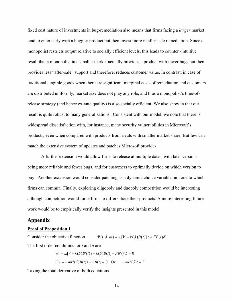
Appendix Proof of Proposition 1

Consider the objective function )( )]()([ );,( δδδ tFBttBkVmmt −−=Ψ

The first order conditions for t and δ are 0)(')]()( )(')([ =−−−=Ψ δδδ tFBtBkttBkVmt

FtmktFBttBmk =−=−−=Ψ )(' Or, 0)( )()(' δδδ

Taking the total derivative of both equations

14

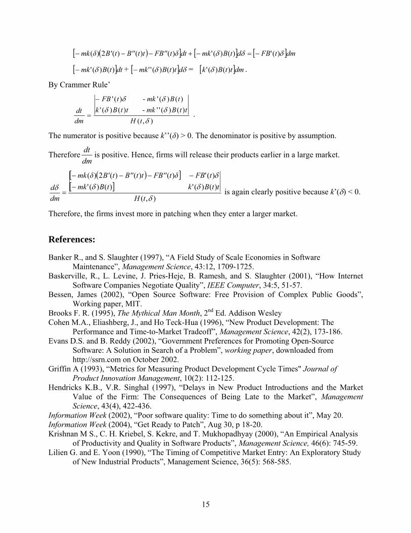
( )[ ] +−−− dtδtFB''ttB''tB'δmk )()()(2)( [ ] =− δδ dtBmk )()(' [ ]dmtFB δ)('−

[ ]dttBmk )()(' δ− + [ ] δδ dttBmk )()(''− = [ ]dmttBk )()(' δ .

By Crammer Rule’

),(

)()(''- )()(')()('- )('

δδδδδ

tHttBmkttBk

tBmktFB

dmdt

−

= .

The numerator is positive because k’’(δ) > 0. The denominator is positive by assumption.

Thereforedmdt is positive. Hence, firms will release their products earlier in a large market.

( )[ ][ ]

),()()(' )()('

)(' )()()(2)(

δδδ

δδ

tHttBktBmk

tFBδtFB''ttB''tB'δmk

dmd −

−−−−

= is again clearly positive because k’(δ) < 0.

Therefore, the firms invest more in patching when they enter a larger market.

References:

Banker R., and S. Slaughter (1997), “A Field Study of Scale Economies in Software Maintenance”, Management Science, 43:12, 1709-1725.

Baskerville, R., L. Levine, J. Pries-Heje, B. Ramesh, and S. Slaughter (2001), “How Internet Software Companies Negotiate Quality”, IEEE Computer, 34:5, 51-57.

Bessen, James (2002), “Open Source Software: Free Provision of Complex Public Goods”, Working paper, MIT.

Brooks F. R. (1995), The Mythical Man Month, 2nd Ed. Addison Wesley Cohen M.A., Eliashberg, J., and Ho Teck-Hua (1996), “New Product Development: The

Performance and Time-to-Market Tradeoff”, Management Science, 42(2), 173-186. Evans D.S. and B. Reddy (2002), “Government Preferences for Promoting Open-Source

Software: A Solution in Search of a Problem”, working paper, downloaded from http://ssrn.com on October 2002.

Griffin A (1993), “Metrics for Measuring Product Development Cycle Times" Journal of Product Innovation Management, 10(2): 112-125.

Hendricks K.B., V.R. Singhal (1997), “Delays in New Product Introductions and the Market Value of the Firm: The Consequences of Being Late to the Market”, Management Science, 43(4), 422-436.

Information Week (2002), “Poor software quality: Time to do something about it”, May 20. Information Week (2004), “Get Ready to Patch”, Aug 30, p 18-20. Krishnan M S., C. H. Kriebel, S. Kekre, and T. Mukhopadhyay (2000), “An Empirical Analysis

of Productivity and Quality in Software Products”, Management Science, 46(6): 745-59. Lilien G. and E. Yoon (1990), “The Timing of Competitive Market Entry: An Exploratory Study

of New Industrial Products”, Management Science, 36(5): 568-585.

15

Milgrom P. and J. Roberts (1990), “The Economics of Modern Manufacturing: Technology, Strategy, and Organization”, The American Economic Review, 80(3): 511-28.

Moorthy, S. (1988), “Product and Price Competition in a Duopoly,” Marketing Science, 7(2): 141-168.

NIST Report (2002), “The Economic Impacts of Inadequate Infrastructure for Software Testing”, National Institute of Standards and Technology, May.

Paulk, M. C., B. Curtis, M. B. Chrissis and C. V Weber (1995), The Capability Maturity Model: Guidelines for Improving the Software Process for Software, Addison-Wesley, Reading, MA

Washington Technology (1998), “Selected Security Events in 1990”, 13(18), October 12. Zirger B. and M. Maidique (1990), “A Model of New Product Development: An Empirical

Test”, Management Science, 36(7), 867-883.

16

Online Appendix Including Fixed Development Cost The profit function is Ψ(δ, t, x; m) = ),(- ),( )],()([ xtPxtFBtxtBkVm δδ −− . Taking the first order conditions 0),(),()],()( ),()([),,(

=−−−−= xtPxtFBxtBktxtBkVmdt

xtdttt δδδδπ

0),( ),()(' ),,(=−−= xtFBtxtBkm

dxtd δ

δδπ

0),(),( ),()( ),,(=−−−= xtPxtFBtxtBkm

dxxtd

xxx δδδπ

Consider the cross partial such that ( ) 0)(),( ),()(' ),,(2>−+−= tFBxtBtxtBmk

dtdxtd

ttδδ

δπ

Since . We still have a complementarity of t and δ. Consider the cross partial Ftmk =− ** )(' δ

),(),(),()(),()( ),,(2xtPxtFBttxBmkxtBmk

dtdxxtd

txtxtxx −−−−= δδδπ

In general, it is hard to sign this unless we make some specific assumption on functional form

because the first term is positive (Bx < 0) and the other term could be positive or negative

depending on the function chosen. As long as Btx(t,x) and Ptx(t,x) are non-positive, the cross

partial will be positive. In particular, Btx(t,x) = 0 and Ptx(t,x) = 0 seem more reasonable. There is

little reason to believe that time to market t may have an impact on the efficiency of investment

x. One vision of the bug function (B) and cost function (P) is that they are additively separable.

For example, B(t,x) = B1(t) + B2(x). This will ensure Btx(t,x) = 0. Note that even if Btx(t,x) > 0 or

Ptx(t,x) > 0, our results would hold but then it would depend on the specific values of derivatives.

To keep the results clean, we make the assumption that Btx(t,x) = 0 and Ptx(t,x) = 0. Therefore,

dtdxxtd ),,(2 δπ >0.

Finally, consider the third cross-partial 0),(),()(' ),,(2=−−= xtFBtxtBmk

dxdxtd

xxδδ

δπ .

This again follows from the fact that . Therefore, investments in development

and ex-post patching are independent. Since all three cross partial are greater >= 0, and the main

effects are all positive, it follows that

Ftmk =− ** )(' δ

0;0;0 >>>dmdxand

dmd

dmdt δ . Therefore, including the

product development cost still leads to the same result.

Fixing the length of time users consume the product

17

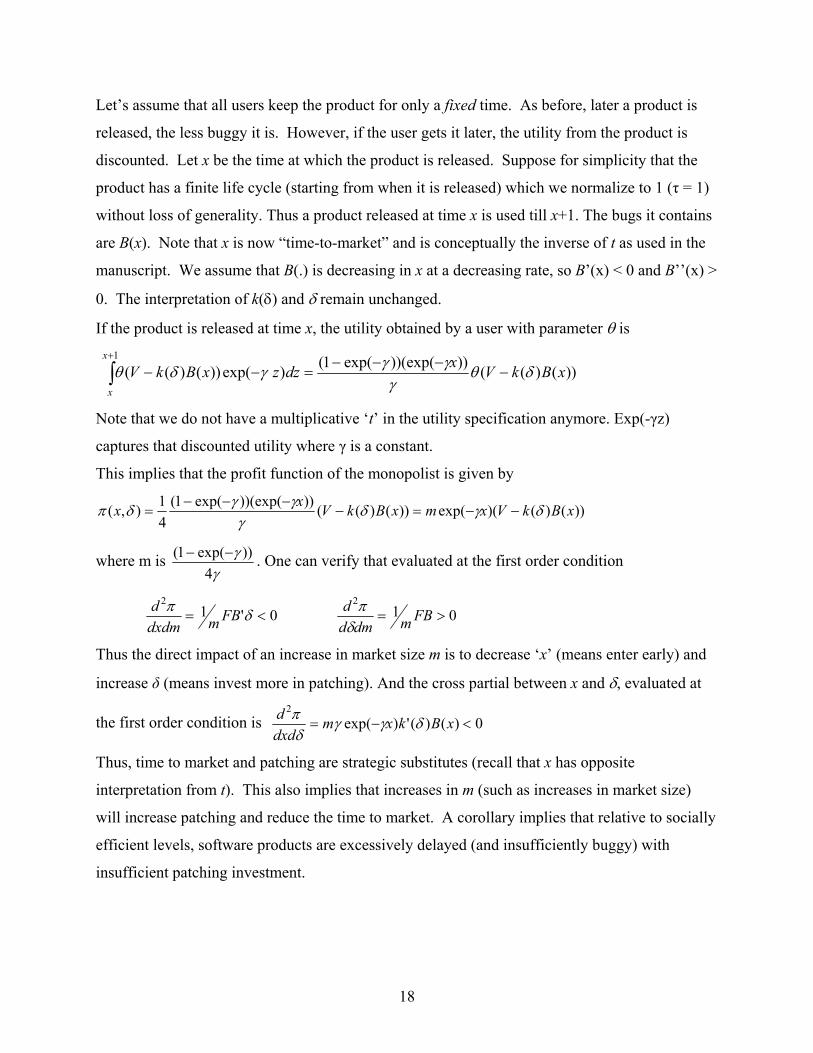
Let’s assume that all users keep the product for only a fixed time. As before, later a product is

released, the less buggy it is. However, if the user gets it later, the utility from the product is

discounted. Let x be the time at which the product is released. Suppose for simplicity that the

product has a finite life cycle (starting from when it is released) which we normalize to 1 (τ = 1)

without loss of generality. Thus a product released at time x is used till x+1. The bugs it contains

are B(x). Note that x is now “time-to-market” and is conceptually the inverse of t as used in the

manuscript. We assume that B(.) is decreasing in x at a decreasing rate, so B’(x) < 0 and B’’(x) >

0. The interpretation of k(δ) and δ remain unchanged.

If the product is released at time x, the utility obtained by a user with parameter θ is

))()(())))(exp(exp(1() exp())()((1

xBkVxdzzxBkVx

x

δθγ

γγγδθ −−−−

=−−∫+

Note that we do not have a multiplicative ‘t’ in the utility specification anymore. Exp(-γz)

captures that discounted utility where γ is a constant.

This implies that the profit function of the monopolist is given by

))()()(exp())()(())))(exp(exp(1(41),( xBkVxmxBkVxx δγδ

γγγδπ −−=−

−−−=

where m is γ

γ4

))exp(1( −− . One can verify that evaluated at the first order condition

0'12

<= δπ FBmdxdmd 01

2>= FBmdmd

dδ

π

Thus the direct impact of an increase in market size m is to decrease ‘x’ (means enter early) and

increase δ (means invest more in patching). And the cross partial between x and δ, evaluated at

the first order condition is 0)()(')exp(2

<−= xBkxmdxdd δγγ

δπ

Thus, time to market and patching are strategic substitutes (recall that x has opposite

interpretation from t). This also implies that increases in m (such as increases in market size)

will increase patching and reduce the time to market. A corollary implies that relative to socially

efficient levels, software products are excessively delayed (and insufficiently buggy) with

insufficient patching investment.

18

General distribution of θ

We assume that θ is distributed on some [0, θ ] with a distribution function F. Let Z =

[ ttBkV )()( ]δ− . If p is the optimal price charged by the monopolist, the demand is given by 1-

F(θ*), where θ* = p/Z. The monopolists profit function is p[1-F(θ*)] – GB(t)δ. Solving for

optimal p leads to 0)()](1[ ** =⎟⎠⎞

⎜⎝⎛−− θθ f

ZpF (A1)

Then the monopolist’s first order conditions for t and δ are (after using the envelope theorem)

0)(')( *2

2=− δθ tGBZf

Zp

t 0)()( *2

2=− tGBZf

Zp

δθ

Using (A1), these can be rewritten as

0)(')](1[ ** =−− δθθ tGBZF t 0)()](1[ ** =−− tGBZF δθθ

Since the socially efficient outcome requires the product to sell at p = 0 (or some small p to cover

the fixed costs) everyone will purchase. Therefore, the social planner’s objective function is m Z

– GB(t)δ where m = average value of θ = ∫θ

θθθ0

)( df

The social planner’s first order conditions are

0)(' =− δtGBmZt and 0)( =− tGBmZδ

Note that one can show that . To see this, )](1[ ** θθ Fm −>

))(1()()()()()( **

*

*

**

*

00

θθθθθθθθθθθθθθθθθθ

θ

θ

θ

θ

θ

θθ

Fdfdfdfdfdfm −=≥≥+== ∫∫∫∫∫

Therefore, rest of the proof of proposition goes through. As before, m in case of a social planner

is larger.

In case of a tangible good, both monopolist and social planner incur marginal cost of

gB(t)δ. Therefore, the demand for the monopolist is going to be [1-F(θm)] where θm = (pm)/Z

where pm is the monopoly price. Hence, using the envelope theorem and taking the first order

derivatives with t and δ, we get

and 0)(' =− δθ tGBZtm 0)( =− tGBZm

δθ

Socially efficient outcome is to price at marginal cost so p = gB(t)δ. Therefore, defining θs =

(ps)/Z where ps is the socially efficient price and maximizing social surplus leads to

19

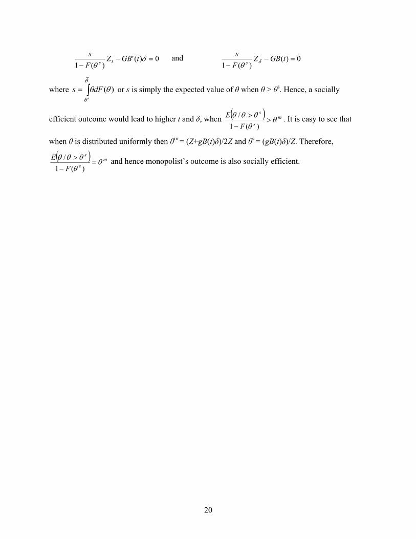
0)(')(1

=−−

δθ

tGBZFs

ts and 0)(

)(1=−

−tGBZ

Fs

s δθ

where ∫=θ

θ

θθs

dFs )( or s is simply the expected value of θ when θ > θs. Hence, a socially

efficient outcome would lead to higher t and δ, when ( ) ms

s

FE θ

θθθθ

>−

>)(1

/ . It is easy to see that

when θ is distributed uniformly then θm = (Z+gB(t)δ)/2Z and θs = (gB(t)δ)/Z. Therefore,

( ) ms

s

FE θ

θθθθ

=−

>)(1

/ and hence monopolist’s outcome is also socially efficient.

20