NIST Technical Note 1881 Self Training of a Fault-Free Model for Residential Air Conditioner Fault Detection and Diagnostics Jaehyeok Heo W. Vance Payne Piotr A. Domanski Zhimin Du http://dx.doi.org/10.6028/NIST.TN.1881

Welcome message from author
This document is posted to help you gain knowledge. Please leave a comment to let me know what you think about it! Share it to your friends and learn new things together.
Transcript

NIST Technical Note 1881
Self Training of a Fault-Free Model for Residential Air Conditioner Fault Detection and Diagnostics
Jaehyeok Heo W Vance Payne
Piotr A Domanski Zhimin Du
httpdxdoiorg106028NISTTN1881
NIST Technical Note 1881
Self Training of a Fault-Free Model for Residential Air Conditioner Fault Detection and Diagnostics
Jaehyeok Heo Korea Institute of Energy Research
New and Renewable Energy Research Division Solar Thermal Laboratory
W Vance Payne Piotr A Domanski
National Institute of Standards and Technology Energy and Environment Division
Engineering Laboratory
Zhimin Du School of Mechanical Engineering
Shanghai Jiao tong University
httpdxdoiorg106028NISTTN1881
May 2015
US Department of Commerce Penny Pritzker Secretary
National Institute of Standards and Technology Willie May Under Secretary of Commerce for Standards and Technology and Director
Certain commercial entities equipment or materials may be identified in this document in order to describe an experimental procedure or concept adequately
Such identification is not intended to imply recommendation or endorsement by the National Institute of Standards and Technology nor is it intended to imply that the entities materials or equipment are necessarily the best available for the purpose
Use of Non-SI Units in a NIST Publication
The policy of the National Institute of Standards and Technology is to use the International System of Units (metric units) in all of its publications However in North America in the heating ventilation and air-conditioning industry certain non-SI units are so widely used instead of SI units that it is more practical and less confusing to include some
measurement values in customary units only
National Institute of Standards and Technology Technical Note 1881 Natl Inst Stand Technol Tech Note 1881 44 pages (May 2015)
httpdxdoiorg106028NISTTN1881 CODEN NTNOEF
Contents 1 Introduction 1
2 Overview of Fault Detection and Diagnostics 1
21 Previous Studies 1
22 Concept of Self training 2
23 Measurement Features for Self training 3
3 Self training Method 4
31 Qualifying Fault‐Free Data for the Self training Dataset 4
32 Domain Coverage Rate 6
33 Fault‐Free Models 7
331 Multivariable Polynomial Regression Models 7
332 Artificial Neural Network Models 8
333 Combined ANN‐MPR Models 10
4 Self training Implementation 10
41 Experimental Setup and Fault‐Free Data Collection 10
42 Fault‐Free Models Performance with the Whole Dataset 13
43 Fault‐Free Models Performance with Different Zone Densities 14
44 Fault‐Free Models Performance with Different Domain Coverage Rates 17
5 Validation 20
51 Validation Dataset and Fault Types 20
52 Fault Detection and Diagnostic Method 21
53 Procedure for Testing and Rating FDD Performance 28
54 Effect of Domain Coverage Rate on FDD Performance 30
6 Concluding Remarks 32
References 33
Acknowledgements 35
Appendix A Temperature Data Distribution 35
Nomenclature
Symbols
a coefficient of multivariable polynomial or a constant C case variable d data distance to zone center dmax maximum distance of the filtered group in the zone h variables of the hidden layer neurons m number of coefficients number of features to determine fault pattern N number of data normal distribution O variable of output neuron P pressure (kPa) or probability r residual s positive constant multiplier of the threshold T temperature (oF) w weight matrix W work (W) x variable representing measured data X variables of the input layer neurons independent variables z standardized feature residual
Greek Symbols
α learning rate δ an error information term ∆ difference ε threshold value μ momentum terms predicted value by fault‐free models σ standard deviation feature parameter
Subscripts
C condenser CA condenser air D compressor discharge DB dry bulb DP dew point E evaporator EA evaporator air FF fault free ID indoor IDP indoor dew point OD outdoor sat saturation
SC SH
Abbreviations
AC ANN avg CF CMF COP DCR EF erf FDD FF HP IoT LL MPR NC OC PDF RH SDR trans TRE TSE UC ZD
subcooling superheat
air conditioner artificial neural network average condenser fouling reduced outdoor air flow rate compressor valve leakage coefficient of performance domain coverage rate evaporator fouling improper indoor air flow rate error function fault detection and diagnosis fault free heat pump Internet of things liquid line restriction multivariable polynomial regression presence of non‐condensable gases refrigerant overcharge probability density function relative humidity successful diagnosis rate () transfer function test relative error () test standard error (oF) refrigerant undercharge zone density
1 Introduction
In 2014 residential cooling consumed 13 of the total US residential home electrical energy
used (189 of 1415 billion kWh) according to the US Energy Information Administration (EIA
2014) Therefore efficient maintenance techniques for cooling systems are very important in
preventing energy waste due to improper operation and lack of fault recognition If a fault
detection and diagnostic (FDD) system could save 1 of the 189 billion kWh used for cooling it
would have saved consumers approximately $229 million (EIA 2013) However building and
applying a generic FDD model is very difficult due to the various installation environments seen
for residential air‐conditioning and heat pump systems Self training FDD methods are the only
way to implement an effective FDD method in these varied installation environments
Fault Detection and Diagnostics (FDD) can be used to commission and maintain the
performance of residential style split‐system air conditioners and heat pumps Previous
investigations by various researchers have provided techniques for detecting and diagnosing all
common faults but these techniques are meant to be applied to systems that have been
thoroughly tested in a carefully instrumented laboratory environment Although such an
approach can be applied to factory‐assembled systems installation variations of field‐
assembled systems require in‐situ adaptation of FDD methods Providing a workable solution
to this problem has been the impetus for the work presented in this report which describes a
method for adapting laboratory generated FDD techniques to field installed systems by
automatically customizing the FDD fault‐free performance models to random installation
differences
2 Overview of Fault Detection and Diagnostics
21 Previous Studies
The development of this fault detection and diagnostics (FDD) method required both extensive
measurements and analytical efforts System characteristics were measured during fault‐free
and faulty operation and analytical work implemented that knowledge and data into
algorithms able to produce a robust determination of the lsquohealthrsquo of the system In earlier work
the National Institute of Standards and Technology (NIST) made detailed measurements on the
cooling (Kim et al 2006) and heating [(Payne et al 2009) (Yoon et al 2011)] performance of a
residential split‐system air‐source heat pump with faults imposed Previous research on FDD
techniques [eg(Rossi and Braun 1997) (Braun 1999) (Chen and Braun 2001)] was used to
refine a rule‐based chart technique able to detect and diagnose common faults which can occur
during operation of an air conditioner (AC) and heat pump (HP) [(Kim et al 2008b)(Kim et al
2010)]
1
22 Concept of Self Training
System parameters sensitive to common faults were identified such as refrigerant subcooling
at the condenser outlet or a difference in the air temperature between the inlet and outlet of
the heat exchanger These parameters are referred to as features The values of these features
during fault‐free heat pump operation were correlated and modeled as functions of different
operating conditions After models of the fault‐free features have been developed detection of
a fault (if it exists) and its diagnosis can be done by comparing featuresrsquo fault‐free values to
those measured during heat pump operation Typically fault‐free features are measured and
correlated for steady‐state operation For this reason feature measurements during regular
heat pump operation must be taken only when the system is steady‐state
For factory‐assembled systems eg windows air conditioners or roof‐top units fault‐free
features can be measured in a laboratory to establish a representation for that model line
These feature measurements (and derived correlations) can be applied to the entire model line
of the tested system However for field‐assembled systems such as split air‐to‐air heat pumps
and air conditioners their fault‐free characteristics may substantially differ due to their
individual installation constraints For this reason for field‐assembled systems fault‐free
feature models need to be developed based on data collected in‐situ after the system has been
installed This challenging task can be carried out by a self training module incorporated into
the FDD unit
The self training module is started by a technician after completing a manual check of the
installed system per manufacturer instructions and ensuring the system operates free of faults
During operation the self training module receives measurements of system features and
operating conditions and processes them according to the scheme shown in Figure 21
First the steady‐state detector evaluates the data and determines whether the heat pump
operation is steady In the next step the data are screened by the fault‐free filter This filter can
be considered as a preliminary FDD scheme provided by the outdoor unit manufacturer It
contains preliminary models for predicting fault‐free values of system features and uses relaxed
thresholds to accommodate different installation constraints and their impact on the system
features The purpose of this screening is to identify significant departures of the measured
features from preliminary fault‐free values and signal them as possible installation errors In
such an instance the self training process would be halted and could only be re‐initiated by
manual restart
Filtered data from a steady‐state detector are recorded until the data are considered fault‐free
based upon quality and distribution within the selected range of specific operating conditions
(independent variables) outdoor dry‐bulb indoor dry‐bulb and indoor humidity The Zone
Density test considers the current independent variables and determines if they are better than
2
any other previously collected data within some predefined variation If the data are acceptable
a decision is made to produce an intermediate fault‐free correlation for all of the dependent
features These intermediate fault‐free correlations are used as new fault‐free tests to select
more fault‐free data The self training process consists of generating several intermediate fault‐
free models with a new model replacing an older one as additional fault‐free data are collected
expanding the self training dataset used to develop the previous model If a new intermediate
set of correlations is developed then the extents of the independent variables are examined to
determine whether the desired range has been covered This data collection process continues
and the models are updated until the operating conditions domain coverage (or preselected
extents of the independent variables) reaches a maximum value Once the domain coverage is
at the maximum value the final fault‐free correlations are generated and self training is
complete The concepts of Zone Density and Coverage Rate will be discussed further in the
following sections
Figure 21 General logic for self training
23 Measurement Features for Self Training
Following the previous NIST study on residential HP and AC FDD (see Kim et al 2008b) the
three independent features TOD TID TIDP and seven dependent features TE TSH TC TD TSC ΔTEA
ΔTCA were chosen for self training (Table 21) The value of the seven dependent features can be
3
correlated as functions of the three independent features within the three‐dimensional
operating data domain
Table 21 Measurement features for self training
Independent Features (operating conditions)
Dependent Features (FDD features)
Outdoor dry‐bulb temperature TOD Evaporator exit refrigerant saturation
temperature TE
Indoor dry‐bulb temperature TID Evaporator exit refrigerant superheat TSH
Indoor dew point temperature TIDP Condenser inlet refrigerant saturation
temperature TC
Compressor discharge refrigerant temperature
TD
Liquid line refrigerant subcooling temperature
TSC
Evaporator air temperature change ΔTEA
Condenser air temperature change ΔTCA
3 Self Training Method
31 Qualifying Fault‐Free Data for the Self Training Dataset
The goal of qualifying the new fault‐free data is to develop a uniformly distributed self training
dataset for generating fault‐free feature models Figure 31 depicts the concept of fault‐free
data storage in a three‐dimensional operating data domain defined in terms of outdoor
temperature indoor temperature and indoor relative humidity The domain is divided into
ldquozonesrdquo (represented by parallelograms) to facilitate managing the fault‐free data distribution
Some measured fault‐free data points are indicated by blue points
4
RH
(
)
) F(o
D
T I
TOD (o
F)
y z
80
60
40
85 80
7520 80 7085 90 95 100 65105
x
Figure 31 Three dimensional operating data domain with sixty zones
The collected data may include multiple data points scattered within the cuboid space of a
particular zone Moreover storage capacity for data collection in the system has a limitation
therefore some means of keeping only the best data in a zone must be implemented To do
this zone housekeeping the concept of zone density (ZD) is introduced to manage and weight
the data efficiently Figure 32 shows the concept of a spherical data filter within six three
dimensional cuboid zones but reduced to two dimensions for clarity of illustration
Illustration of data domain Application of data filter ZD=5
Figure 32 Concept of zone density
To reduce the numerical and dimensional complexity of calculating the spherical radius within
the cuboids the axial dimensions (xyz = TOD TID TIDP) are normalized to create a unit cube with
5
each side having unit area (ie 1x1x1) Only data within the sphere are selected and of the
selected data the data closest to the center are ranked as being higher quality and are selected
for storage Data storage demands are reduced by imposing a zone density (ZD) limit which
means that only a specified number of data points closest to the center of each sphere are
kept Figure 32 shows a ZD equal to 5 any new data within a zone will only be accepted if its
distance d is less than the maximum data point distance occurring in that zone The distance
from the center of the sphere to a data point can be easily calculated as shown in Equation 31
and Figure 33a
2 2 2d (05 x) (05 y) (05 z) (31)
The maximum number of data points in a zone can be adjusted using the zone density concept
(Figure 33b) A ZD of m is defined as the selection of the closest m data points from the center
in each zone For example the allowable data number decreases with the decrease of ZD as
shown in Figure 33b In this study a ZD from 100 to 1 was applied and tested in the self
training FDD logic
Center
(x y z)
1 1
d
A single zone (a) (b)
1
Figure 33 Concept of zone density (a) data distance ldquodrdquo from zone center and (b) various
zone densities
32 Domain Coverage Rate
Before a fault‐free dataset is used to develop models for fault‐free features some numerical
criterion needs to be established to assess the quality and extent of the dataset Preferably
each zone should contain data to avoid extrapolation According to Braun and Li (2001) the
predictions in case of extrapolation showed a deviation 3 to 10 times larger than those
predicted by interpolation Ideally each zone should contain the same number of data points
located close to the center
6
For the purpose of rating the extent of the fault‐free dataset the concept of Domain Coverage
Rate (DCR) is introduced which is the ratio of the number of zones with at least one fault‐free
data point to the total number of zones within the operational data domain The calculation of
the DCR is shown by Equations 32 and 33 If all zones contain at least one data point then the
DCR would equal 100
1 if data found in i zoneIndexi
th (32)
0 if data not found in i zone th
DCR 1
n
Indexi (33)n i1
where n is the total number of zones
33 Fault‐Free Models
Once the domain coverage rate reaches a specified maximum level the self training module will
correlate the data within all zones using the chosen fault‐free model form The following
sections evaluate the performance of several fault‐free model forms developed from cooling
mode laboratory test data previously acquired for an air‐source residential heat pump
331 Multivariable Polynomial Regression Models
Multivariable Polynomial Regression (MPR) models have been widely applied as fault‐free
models [(Li and Braun 2003) (Braun and Li 2001) (Kim et al 2008b) (Heo et al 2012)] due to
their simple structure and ease of programming They belong to the ldquoblack‐boxrdquo category of
models which do not consider the physics of the system and require a large dataset to
accurately predict system performance The higher order MPR models offer better accuracy of
prediction however excessive polynomial order for a relatively small database may worsen
data interpolation
Equations 34 35 and 36 show the general form of the regressed equations for features as 1st
2nd and 3rd order MPR models respectively
(1) = a a T a T a T (34)feature 0 1 OD 2 ID 3 IDP
(2) (1) 2 2 2 = a T T a T T a T T a T a T a T (35)feature feature 4 OD ID 5 ID IDP 6 IDP OD 7 OD 8 ID 9 IDP
(3) (2) 3 3 3 2 = a T a T a T a T T T a T Tfeature feature 10 OD 11 ID 12 IDP 13 OD ID IDP 14 OD ID (36)
2 2 2 2 2 a T T a T T a T T a T T a T T15 OD IDP 16 ID OD 17 ID IDP 18 IDP OD 19 IDP ID
7
332 Artificial Neural Network Models
An Artificial Neural Network (ANN) model was developed for the seven dependent features
The relationship between the three independent variables and seven dependent features is
ldquolearnedrdquo by an artificial neural network using a back propagation algorithm The ANN test
module was developed based on the sample code presented by Frenz (2002) The fault‐free
data are used as targets for the back propagation learning
Figure 34 shows the structure of the 3‐layer ANN(3x3x1) which has three input variables (TOD
TID and TIDP) one hidden layer and one output In general a form of the sigmoid function is
used as the activation function in the nodes of the hidden layer The weight coefficients and
offsets (or bias values) are learned using a momentum back propagation algorithm through
more than 10 000 iterations (Frenz 2002)
Figure 34 Artificial neural network structure (3x3x1)
Each hidden layer neuron is connected to every input neuron and each individual hidden layer
neuron receives the sum of the weighted input neuron values as given in Equation 37 Xi represents the input neuron values (TOD TID and TIDP) and wij represents the weights connecting
the input neurons to the hidden layer neurons In a similar way the output layer neurons are
determined as given in Equation 38 Bipolar sigmoid function was applied to layer transfer
function as given in Equation 39
n
h = hin j biasi
X wi ij
j 1
hout j= trans (hinj ) (37)
n
i 1
O =trans(O )outk ink (38)O = Oin k biasj h w jk out j
8
2trans(x) 1 (bipolar sigmoid) (39)
1 e x
The back‐propagation process utilizes a gradient descent algorithm that seeks to minimize the
errors of the values that are output from the neural network The weight and bias update
equations including the learning rate (α) and momentum terms (μ) are given in Equations 310
through 313 The learning rate fragments the weightbias adjustment taken in each training
iteration The smaller the value of alpha the longer a network takes to train but the smaller
alpha reduces fluctuations in the weight variation from iteration to iteration and generally
produces smaller errors Momentum is added to the weight adjustment equations (Equations
310 and 312) which enables the weight to change in response to the current gradient step
Delta (δ) is calculated by multiplying the difference between the target value and output value
by the derivative of the activation function (Equation 314) Here t represents the current set of
weightsbiases t‐1 the previous set and t+1 the new set being calculated
wjk (t 1)= wjk (t) hout j (wjk (t) wjk (t 1)) (310)
O (t 1)=O (t) (O (t) O (t 1)) (311)biask biask biask biask
wij (t 1)= wij (t) Xi (wij (t) wij (t 1)) (312)
hbias j (t 1)= hbias j (t) (hbias j (t) hbias j (t 1)) (313)
= 1 1 trans(O ) 1 trans(O ) (O O ) (314)in in target out2
The standard deviation (σ) of the ANN model was investigated with the variation of the learning
rate alpha (α) momentum (μ) maximum iteration number and number of hidden layers as
shown in Figure 35 The ANN modelrsquos performance was the most sensitive with learning rate (α) and iteration number which were optimized at 0001 and 10 000 respectively The ANN
modelrsquos performance improved with the increase of the momentum term However with the
momentum term greater than 01 the ANN modelrsquos performance decreased due to too large of
a gradient for training If the number of hidden layers increased the total number of variables
for modeling also increased As a result the ANN model with three layers showed the best
performance
9
8 108
7
6 104
5
100
(T
)
(T
)
ee
(T
)
(T
)
ee
4
3
096
1
0
2
092 10-5 10-4 10-3 10-2 10-1 10-3 10-2 10-1100 100
8 104
7
6 102
5
2 098
1
0 096 102 103 104 105 0 1 2 3 4 5 6 7 8 9
Iteration Layer number
Figure 35 Operating factor optimization for the ANN model
333 Combined ANN‐MPR Models
Used alone the ANN model showed good interpolation performance poor extrapolation
performance and relatively long times required for training The low‐order MPR model had
relatively good extrapolation performance low interpolation performance and very fast
training times In order to combine the strengths of the ANN and MPR models a combined
model was designed as illustrated by Braun and Li (2001)
In this study the first and second order MPR models and the ANN (3x3x1) model were applied
in the combined model First the MPR model was regressed with the training data and then
the residuals between the model output and the training data were fit with an ANN This
combined model is calculated as given in Equation 315
Combine=MPR ANN (315)
4 Self Training Implementation
41 Experimental Setup and Fault‐Free Data Collection
To test and validate the self training scheme presented in the previous sections we developed
a fault‐free database with laboratory data taken on an R410A 88 kW split heat pump operating
in the cooling mode The unit had a Seasonal Energy Efficiency Ratio (SEER) of 13 (AHRI 2008)
4 100
3
10
ll
The unit consisted of an indoor fan‐coil section outdoor section with a scroll compressor
cooling and heating mode thermostatic expansion valves (TXV) and connecting tubing Both
the indoor and outdoor air‐to‐refrigerant heat exchangers were of the finned‐tube type The
unit was installed in environmental chambers and charged with refrigerant according to the
manufacturerrsquos specifications Figure 41 shows a schematic of the experimental setup
indicating the measurement locations On the refrigerant side pressure transducers and T‐type
thermocouple probes were attached at the inlet and exit of every component of the system
The refrigerant mass flow rate was measured using a Coriolis flow meter The air enthalpy
method served as the primary measurement of the system capacity and the refrigerant
enthalpy method served as the secondary measurement These two measurements always
agreed within 5 Uncertainties of the major quantities measured during this work are
summarized in Table 41 Detailed specifications of the test rig including indoor ductwork
dimensions data acquisition measurement uncertainty and instrumentation is described in
Kim et al (2006)
IND
OO
RCH
AMBE
R
OU
TDO
OR
CHAM
BER
Evaporator Condenser
Compressor Scro
Mass flow meter
4-way Valve
PP
P
MFR
TDB TDP
SCFM
W
Thermostatic Expansion Valve
T
P T
P T Tsat
P T
P T
P T
TDB
TDB
P T Tsat
P T Tsat
TDB TDP Valves for LL fault
Valve for CMF fault
Figure 41 Schematic diagram of the experimental setup (Kim et al 2006)
To implement the most efficient test procedure outdoor temperature was fixed at one of four
values the addition of steam to the indoor chamber was set at one of several discrete levels by
modulating a steam valve and the indoor dry‐bulb temperature was changed over the desired
operating range by energizing 10 heaters sequentially From the total number of 10 409
recorded data scans 5830 data sets were allowed by the steady‐state detector The data were
recorded every 18 s and filtered through the steady‐state detector which qualified steady‐state
11
data for use in development of the fault‐free models for the seven features In this process
instability of the system due to on‐off transients and rapid load changes was filtered out by the
steady‐state detector From the total number of 10 409 recorded datasets 5830 datasets were
kept by the steady‐state detector
Table 42 shows operating conditions for the fault‐free tests The four outdoor temperatures
were maintained within plusmn05 degF For the indoor conditions the amount of steam introduced to
the indoor chamber was fixed such that the humidity ratio varied from 00037 to 00168 Data
were recorded every 18 s as indoor dry‐bulb temperature varied from 595 degF to 930 degF The
range of operating conditions for which data were collected defines the applicable limits for the
FDD scheme
Table 41 Measurement uncertainties
Measurement Range Uncertainty at a 95 Confidence Level
Individual temperature ‐04 F to 1994 F 054 F
Temperature difference 0 F to 504 F 054 F
Air nozzle pressure drop 0 Pa to 1245 Pa 10 Pa
Refrigerant mass flow rate 0 kgh to 544 kgh 10
Dew point temperature ‐04 F to 1004 F 072 F
Dry‐bulb temperature ‐04 F to 104 F 072 F
Total cooling capacity 3 kW to 11 kW 40
COP 25 to 60 55
Table 42 Operating conditions for fault‐free tests
Outdoor dry‐bulb temp F 82 90 95 100
Indoor dry‐bulb temp F 595 to 93
Indoor humidity ratio 00037 to 00168
If we assume that the data distribution is similar to that of a field‐installed real system the DCR
can be calculated based on the accumulated dataset as introduced in Equations 32 and 33
Figure 42 shows the fault‐free data distribution with increments of the domain coverage rate
DCR of 20 40 60 and 73 were fulfilled when the accumulated data points reached
2104 2830 4211 and 5830 respectively The datasets corresponding to these four DCRs were
used for the self training of different fault‐free models
12
DCR 20 DCR 40 DCR60 DCR73 120
Do
ma
in c
ove
rag
e r
ate
(
) T
em
pe
ratu
re (
o F)
RH
(
)
100
80
60
40
20
0 80
T OD
T ID
RH
60
40
20
0
0 1000 2000 3000 4000 5000 6000
Data no
Figure 42 Test condition data distribution and progression of domain coverage
42 Fault‐Free Model Performance with the Whole Dataset
Six fault‐free model types [MPR(1st order) MPR(2nd order) MPR(3rd order) ANN and two
combined models (MPR(1st order) + ANN MPR(2nd order) + ANN)] were tested and compared
using the entire dataset Each modelrsquos overall performance was evaluated by calculating the
standard error as given in Equation 41 The test standard error (TSE) is calculated from the
square root of the squared summation of residuals divided by the number of data points N
13
x 2 i iFF
TSE= i (41)N
Among the dependent features the TSE of TD and TC were the highest and the lowest
respectively The MPR(3rd order) model showed the lowest prediction error followed by the
MPR(2nd order) combined MPR(2nd order)+ANN combined MPR(1st order)+ANN and ANN
model (Figure 43) Therefore the MPR methods were applied and tested for additional analysis
of the self training method
Figure 43 Fault‐free models performance on the whole dataset
43 Fault‐Free Model Performance with Different Zone Densities
The zone density (ZD) concept was introduced to limit the data needed to generate a model
while collecting data over the predefined range of independent variables In this section the
prediction performance of the fault‐free model was tested with various zone densities In the
process of training fault‐free models were developed based on the data kept at the desired ZD
and then the prediction performance was tested on the filtered dataset in the test range (4627
of the 5830 original points after eliminating repeated tests)
Limiting the zone density produced a smaller dataset of training data the bigger the zone
density number the larger the training dataset for the training process When the zone density
14
d
d
decreased from 100 to 10 the data quantity drastically decreased from 2968 to 426 (Figure 44)
Therefore as the ZD number decreased the training speed and data storage compactness also
improved due to the smaller dataset However too small of a zone density number can
decrease the prediction performance
10
08
06
04
02 Zone density 100 00
2968 data
01 02 03 04 05 06 07 08 09 10 11 12 13 14 15 16 17 18 19 20 21 22 23 24 25 26 27 28 29 30 31 32 33 34 35 36 37 38 39 40 41 42 43 44 45
10
08
06
04
02 426 data Zone density 10 00
01 02 03 04 05 06 07 08 09 10 11 12 13 14 15 16 17 18 19 20 21 22 23 24 25 26 27 28 29 30 31 32 33 34 35 36 37 38 39 40 41 42 43 44 45
Zone number
Figure 44 Data distance to zone center for different zones for two zone densities
Figure 45 shows the standard error of the fault‐free model for the seven dependent features
with different zone densities Whereas the standard error for TE TC ∆TEA ∆TCA was relatively
non‐sensitive to the variation of zone density the standard error for TSH TD and TSC was more
rapidly increased with the decrease of zone density The MPR(3rd order) model was the most
sensitive to zone density variation The MPR(3rd order) model has a relatively large number of
coefficients (20) compared to the first order (4) and the second order (10) MPR models so that
it requires abundant data for stable regression On average the MPR(3rd order) model showed
the lowest standard error followed by the second and the first order MPR models respectively
At a zone density of 100 the standard error remained at a similar level to the models using all
of the data (5830 non‐filtered case) When the zone density was less than 25 the MPR(3rd
order) model showed similar prediction performance to that of the MPR(2nd order) model The
MPR(3rd order) model with zone density of 100 showed the most stable and best prediction
performance
15
06 06
05 05
04
03
TS
E(T
o
F)
TS
E(T
o
F)
TS
E(T
oF
) T
SE
(T
oF
) C
AS
CC
E
TS
E (
Avg
oF
) T
SE(
T
oF
) T
SE(T
oF
) T
SE(
T o
F)
EA
D
SH
MPR (1st)04 MPR (2nd) MPR (3rd) 03
02
01
02 MPR (1st) MPR (2nd)01 MPR (3rd)
00 00All 100 50 25 10 5 1 All 100 50 25 10 5 1
Zone density Zone density
06 10
MPR (1st)05 08 MPR (2nd) MPR (3rd) 04
06
04 03
02 MPR (1st)
0201 MPR (2nd) MPR (3rd)
00 00All 100 50 25 10 5 1 All 100 50 25 10 5 1
Zone density Zone density
06 06 MPR (1st) MPR (2nd)05 05 MPR (3rd)
MPR (1st) MPR (2nd) MPR (3rd)
04 04
03 03
02 02
01 01
00 00 All 100 50 25 10 5 1 All 100 50 25 10 5 1
Zone density Zone density
06 06
MPR (1st)05 05 MPR (2nd) MPR (3rd)
MPR (1st)
04 04
03
02
03
02
MPR (2nd) MPR (3rd)
00
01 01
00All 100 50 25 10 5 1 All 100 50 25 10 5 1
Zone density Zone density
Figure 45 Fault‐free model performance with zone density (Test Standard Error)
16
44 Fault‐Free Model Performance with Different Domain Coverage Rates
Figure 46 shows the domain coverage rate as the size of the fault‐free dataset increases up to
its maximum value of 5380 data points As the number of accumulated fault‐free data points
increases the DCR increases up to 73 The figure shows four training ranges corresponding to
DCR values of 20 40 60 and 73
80Training range DCR 73
Training range DCR 60 60
DC
R (
)
40 Training range DCR 40
20 Training range DCR 20
0
0 1000 2000 3000 4000 5000 6000
Data no
Figure 46 Domain coverage rate for different accumulated data quantity
Figure 47 shows the standard error of the fault‐free models for the seven dependent features
as a function of the domain coverage rate The standard error on all features decreased with an
increase in the DCR The standard error of the MPR(3rd order) model was the most sensitive to
DCR variation In a real system that is collecting training data when the DCR is low each
feature has a higher likelihood of being estimated by extrapolation using the currently
generated fault‐free model In most cases the first and second order MPR models showed the
lowest standard errors at 20 and 40 DCR conditions respectively The MPR(3rd order)
model was the best at 60 and 73 DCR After the DCR reached 40 the standard errors of
all fault‐free feature correlations were less than 1 oF
17
100 100 MPR (1st) MPR (1st) MPR (2nd) MPR (2nd) MPR (3rd) MPR (3rd)
10 T
SE(T
o
F)
TS
E(T
o
F)
TS
E(T
C o
F)
TS
E (
T o
F)
CA
SC
E
TS
E (
Avg
oF
) T
SE(
T
oF
) T
SE(T
oF
) T
SE(
T o
F)
EA
D
SH
10
1 1
01 01 20 40 60 80 20 40 60 80
Domain coverage rate () Domain coverage rate ()
100 100 MPR (1st) MPR (1st) MPR (2nd) MPR (2nd)10 MPR (3rd) MPR (3rd) 10
1
01 1
001 01 20 40 60 80 20 40 60 80
Domain coverage rate () Domain coverage rate ()
100 100 MPR (1st) MPR (1st) MPR (2nd) MPR (2nd) MPR (3rd) MPR (3rd)
10
1
10
1
01 01 20 40 60 80 20 40 60 80
Domain coverage rate () Domain coverage rate ()
100 100
MPR (1st) MPR (1st) MPR (2nd) MPR (2nd)
MPR (3rd) 10 MPR (3rd)
10
1 1
01 01 20 40 60 80 20 40 60 80
Domain coverage rate () Domain coverage rate ()
Figure 47 Fault‐free models performance with domain coverage rate (Test Standard Error)
18
The above standard error results are consistent with Braun and Li (2001) who commented that
the lower the order of the MPR model the better the extrapolation performance in general
When the DCR is low each feature has a higher likelihood of being estimated by extrapolation
For models generated at higher DCRs extrapolation is less likely and higher‐order MPR models
are better where interpolation is required
Figure 48 shows TSE of the MPR models for 20 40 60 and 73 DCR as a function of zone density At a DCR of 20 the TSE of MPR(3rd order) and MPR(2nd order) exceeded 4 oF and 1 oF respectively with steep increases at low ZD values For the higher DCRs the TSE stayed below 1 oF for all models and ZDs except MPR(3rd order) for 40 DCR and ZD less than 25 For 60 and 73 DCR all three models performed in a stable fashion smoothly improving predictions as DCR and ZD values increased
From this analysis the MPR(1st order) and MPR(2nd order) models are recommendable for the intermediate fault‐free models at a DCR of 20 and 40 respectively After the DCR exceeds 60 the MPR(3rd order) model is the most appropriate for the final fault‐free model A ZD between 100 and 50 is recommended for data filtering and storing criteria
40 10 MPR (1st) MPR (2nd) MPR (3rd)
DCR 20
30 20 08
TS
E(
Avg
oF
) T
SE
(A
vg o F
)
TS
E(
Avg
oF
) T
SE(
Avg
oF
)10 8 06
04 6
4 MPR (1st)DCR 4002 MPR (2nd)2 MPR (3rd)
0 00All 100 50 25 10 5 1 All 100 50 25 10 5 1
Zone density Zone density
10 DCR 60 MPR (1st) MPR (1st)DCR 7309
MPR (2nd) MPR (2nd)08 MPR (3rd) 07
MPR (3rd)
06 05
04 03
02 01
00 All 100 50 25 10 5 1 All 100 50 25 10 5 1
Zone density Zone density
Figure 48 Model standard error with zone density at DCR of 20 40 60 and 73
19
5 Validation
We tested and validated the self training method by applying the fault‐free models developed using the self training scheme to an experimental dataset collected by Kim et al (2006) on a heat pump operating in the cooling mode In addition the FDD performance was compared and analyzed considering different zone densities and domain coverage rates Successful diagnosis ratio false alarm missed detection and misdiagnosis were calculated and presented to evaluate the overall FDD performance
51 Validation Dataset and Fault Types
The dataset assembled by Kim et al (2006) includes performance data during fault‐free
operation (72 points) and with seven faults compressor valve leakage improper outdoor air
flow improper indoor air flow liquid line restriction refrigerant undercharge refrigerant
overcharge and non‐condensables (84 points) (Table 51)
Table 51 Definition and range of studied heat pump operational cases
Fault name Symbol Definition of fault Fault
range () Temperature range (oF)
Number of points
Fault‐free (Normal operation)
FF ‐ ‐TOD 80 to 102 TID 65 to 85 TIDP 42 to 85
72
Compressor valve leakage
(4 to way valve leakage)
CMF reduction in refrigerant flow rate from no‐fault
value 3 to 40
TOD 80 to 100 TID 70 to 80 TIDP 50 to 61
16
Reduced outdoor air TOD 80 to 100 flow rate (condenser CF of coil area blocked 10 to 50 TID 70 to 80 13
fouling) TIDP 50 to 61
Improper indoor air flow rate (evaporator
fouling) EF
below specified air flow rate
6 to 35 TOD 80 to 100 TID 70 to 80 TIDP 42 to 61
19
Liquid line restriction LL
change from no‐fault pressure drop from liquid
line service valve to indoor TXV inlet
10 to 32 TOD 80 to 100 TID 70 to 80 TIDP 50 to 61
6
20
Refrigerant undercharge
UC mass below correct
(no‐fault) charge 10 to 30
TOD 80 to 100 TID 70 to 80 TIDP 50 to 61
12
Refrigerant overcharge
OC mass above correct (no‐fault) charge
10 to 30 TOD 80 to 100 TID 70 to 80 TIDP 50 to 61
12
Presence of non‐condensable
gases NC
of pressure in evacuated indoor section and line set due to non‐condensable gas with respect to atmospheric
pressure
10 to 20 TOD 80 to 100 TID 70 to 80 TIDP 50 to 61
6
52 Fault Detection and Diagnostic Method
When the system is operating with a fault it is expected that feature temperatures willdeviate
from their normal fault‐free values An individual featurersquos deviation could be negative
positive or ldquoneutralrdquo (close to the fault‐free value within a pre‐defined threshold) collectively
the featurersquos deviations (or residuals) form a pattern which is unique for a given fault To
detect and diagnose the fault a statistical rule‐based classification is performed by calculating
the probability of the various fault‐types based on the decision rules defined within a rule‐
based chartrsquos predefined fault patterns A set of measurement features can be regarded as a
multi‐dimensional Gaussian probability distribution With the assumption that each dimension
is independent each of the three ldquoclassrdquo problems (negative positive or neutral) can be
represented by a simple normal (Gaussian) distribution rather than a more complicated
distribution with multiple degrees of freedom and dependencies (Rossi et al 1995 Kim et al
2008b) The probability of the kth fault corresponding to the set of m statistically independent
variables (X our features) is given by Equation 51 where P(Cik|Xi) denotes the individual
probability of case variable C (negative positive or neutral) for the ith feature with the kth fault
type Since the features are assumed to be independent the total conditional probability P(Fk|
X) can be obtained by the multiplication of the individual probabilities
m
P(Fk X) P(C1k X ) P(C X 2 ) P(Cik X i ) P(Cik X i ) (51)1 2k i1
21
Figure 51 Probability for three measurement residual cases of positive neutral and negative
In Figure 51 the three differently cross‐hatched areas under the Normal Distribution N(μiFF
σiFF) represents the probability of the current measurement (or predicted value) represented
by a second normal distribution PDF(xi σi) being lower higher or relatively close (neutral) to
the predicted fault‐free modelrsquos value if the conditions are fault‐free the difference in the
measured and predicted value the residual ri = xi ndash μiFF will equal zero In order to locate the
position of the current measurement under the normal distribution we must convert the
currently measured value to its standard form we must represent the current measurement as
some number of fault‐free model standard deviations from the mean value of the fault‐free
normal distribution (the currently predicted value) This standardization is often called the z‐
value Therefore the z‐value for the current measurement zi is defined by our residual and the
standard deviation of the fault‐free model as shown in Equation 52
x ri iFF izi (52) i FF i FF
Using the assumption of independent normally distributed FDD features the area under the
normal distribution N(μiFF σiFF) must be determined in order to place a numerical value on the
probability This integral is represented by the cumulative distribution function Φ(x) Equation
22
53 of the standard normal distribution (a normal distribution with a mean of zero and
standard deviation of 1 N(01))
௫ቀݎଵ
ଶଵଶ
ൌሻݔሺemptyradicଶቁ (53)
The cumulative distribution function describes the probability of a real number value with a
given probability distribution function X ϵ PDF(xi σi) having a value less than or equal to a
given value a This can be re‐stated as Equation 54
(54)ሻሺ ൌሻሺempty
This also leads to the probability of X lying within the semi‐closed interval (a b] or being greater
than some value b Equations 55 and 56 respectively
ሻሺെ emptyሻሺൌ emptyሻ ሺ
ሻሺൌ 1 െ empty ሻ ሺ
(55)
(56)
For the purposes of FDD we would like to know whether the residual ri is positive negative or
insignificant (ie within plusmnεi (neutral threshold) of the FF model predicted value μiFF) In order
to use the cumulative distribution function we must standardize the intervals around the
currently measured value xi plusmn εi as a multiple of the FF model standard deviation therefore we
ldquostandardizerdquo εi as being s number of FF model standard deviations as shown in Equation 57 s
is the ldquostandardizedrdquo width of the neutral threshold (sgt0) The standardized representation of
the residual and three possible cases (positive negative and neutral) are shown in Figure 52
s or ݏ ൌ ఌ
(57)i iFF ఙಷಷ
Now we may use Equation 56 to determine the probability of the residual being greater than
+εi the negative residual case
|
Less than or equal to ‐εi the positive residual case using Equation 54
ሺܥdarr ሻ ൌ ሺݖ ሺݖ ሻሻݏ ൌ 1 െ emptyሺݖ ሻ (58)ݏ
|
Or in the neutral interval of plusmnεi using Equation 55
(510)ሻെ ሺെݖݏ emptyሻ ሺൌݖݏ emptyሻ ሻݏ ሺݖെ ሻݏ ሺൌݖሺݖ ሻ|ܥሺ
ሺܥuarr ሻ ൌ ሺݖ ሺݖ െ ሻሻݏ ൌ emptyሺݖ െ ሻ (59)ݏ
23
Figure 52 Standard normal distribution showing the current measurements z‐value and
standardized neutral threshold s
The summation of probabilities calculated in Equations 58 to 510 equals unity Equation 511
since the integral of any PDFs from ndashinfin to +infin must equal one by definiƟon
P(C X i ) P(C
X i ) P(C X i ) 1 (511)
When the fault level increases the residual between the measured data and predicted data
may increase decrease or remain relatively unchanged Figure 53 shows the residual pattern
analysis results for the seven studied faults which were used to generate a rule‐based chart
Due to the careful selection of the most sensitive (rapidly changing) features for a given fault
type the feature patterns were quite different for all fault types and each pattern (positive
negative and neutral) for a given fault is the template for the calculation of fault probability in
Equation 51 For example the probability of a CMF fault (valve leakage) can be calculated by
the multiplication of the conditional probabilities of the residuals having the following pattern
TE (positive) TSH (neutral) TC (negative) TD (positive) TSC (negative) ∆TEA (negative) and ∆TCA
(negative) as shown in Equation 512
P(FCMF X) P(C TE ) P(C TSH ) P(C TC ) P(C TD ) P(C TSC ) (512)
P(C TEA ) P(C TCA )
24
5
0
-5
0
15 20 CMF CF
10 10
Re
sid
ua
l (oF
) R
esid
ual (
o F)
Re
sid
ua
l (oF
)
Res
idua
l (o F
) R
esid
ual (
o F)
Res
idua
l (o F
)
0
-10 -10
Neutral Positive Negative Neutral Positive Negative
-15 -20 T T T T T T T T T T T T T T
E SH C D SC EA CA E SH C D SC EA CA
8 20EF LL
4
0
-4
10
0
-10
Neutral Positive Negative Neutral Positive Negative -8 -20
T T T T T T T T T T T T T TE SH C D SC EA CA E SH C D SC EA CA
20 UC 20 OC
10
-10
10
0
-10
-20 Neutral Positive Negative -20 Neutral Positive Negative
TE
TSH
TC
TD
T T TSC EA CA
TE
TSH
TC
TD
T T TSC EA CA
20 NC
Re
sid
ua
l (oF
) 10
0
-10
Neutral Positive Negative
-20 T
E T
SH T
C T
D T T T
SC EA CA
Figure 53 Residual patterns for different faults
25
Table 52 Rule‐based FDD chart for air‐to‐air single‐speed heat pump in the cooling mode
Fault type TE TSH TC TD TSC ΔTEA ΔTCA
FF (Fault‐free)
CMF (Compressor valve leakage)
CF (Improper outdoor air flow)
EF (Improper indoor air flow)
LL (Liquid‐line restriction)
UC (Refrigerant undercharge)
OC (Refrigerant overcharge)
NC (Presence of non‐condensable gases)
The value of s must be determined so that it produces a given level of confidence that the
currently measured value is within the neutral threshold (or outside this threshold) The
confidence level is selected by the investigator typical values of α are 001 005 and 010 with
corresponding confidence levels of (1 - α) of 099 095 and 090 (Graybill and Iyer 1994) In
applying the s values the user is determining the alarm thresholds for calling a fault or no‐fault
Table 53 shows standard deviations and thresholds with different zone densities for MPR(3rd
order) models regressed to FDD test data In general if thresholds increase the false alarm rate
(FAR) decreases but missed detections increase and vice versa In this study the threshold for a
95 confidence level was applied to the FDD test data Table 54 summarizes the standard
deviations and thresholds for different domain coverage rates Models with the best fit were
26
selected with respect to the domain coverage rate the standard deviation and threshold
prominently increased with a decrease of DCR
Table 53 Standard deviation (oF) of the fault‐free model for different ZD (DCR=73 all data)
ZD Applied model
σ (TE) σ (TSH) σ (TC) σ (TD) σ (TSC) σ (ΔTEA) σ (ΔTCA)
All 3rd order MPR
0124 0314 0077 0310 0191 0124 0112
100 3rd order MPR
0133 0322 0081 0318 0195 0135 0114
50 3rd order MPR
0147 0388 0093 0521 0219 0156 0117
25 3rd order MPR
0149 0420 0094 0590 0236 0159 0119
10 3rd order MPR
0144 0432 0093 0597 0258 0157 0121
5 3rd order MPR
0141 0433 0097 0589 0258 0158 0125
1 3rd order MPR
0144 0442 0099 0537 0277 0166 0138
ε90 165∙σiFF model
ε95 196∙σiFF model
ε99 258∙σiFF model
Table 54 Standard deviation (oF) of fault‐free model for different DCR (ZD =100)
DCR () Applied model
σ (TE) σ (TSH) σ (TC) σ (TD) σ (TSC) σ (ΔTEA) σ (ΔTCA)
73 3rd order MPR
0133 0322 0081 0318 0195 0135 0114
60 3rd order MPR
0197 0385 0090 0811 0282 0160 0123
40 2nd order MPR
0390 0641 0109 0625 0401 0294 0155
20 1st order MPR
0673 0659 0196 2111 0393 0523 0196
ε90 165∙σiFF model
ε95 196∙σiFF model
ε99 258∙σiFF model
27
53 Procedure for Testing and Rating FDD Performance
The faults summarized in Table 51 were part of the experimental dataset (Kim et al 2006)
applied to test FDD performance For each dataset the fault probability for eight conditions (FF
CMF CF EF LL UC OC and NC) was calculated using Equation 51 and the rule‐based chart
fault patterns as given in Table 52 Among the probabilities of the eight conditions the fault
type with the highest fault probability was selected as the fault type most likely occurring at the
time When the diagnosed fault type was the same as the originally imposed fault type the
diagnostic was considered successful The goodness of the FDD method was further explored by
applying the concepts of FDD performance evaluation as defined by Braun et al (2012)
Successful diagnosis rate SDR () A fault is present The summation of the detected and
successfully diagnosed cases divided by total number of faulty tests equals the SDR for the
particular fault
False alarm rate FAR () No fault is present but the protocol indicates the presence of a
fault The FAR equals the number of false alarm cases divided by the total number of fault‐
free tests
Missed detection rate MDR () A fault is present but the protocol indicates that no fault is
present The MDR equals the number of missed detection cases divided by the total number
of faulty tests
Misdiagnosis rate MSR () A fault is present The protocol detects the fault but
misdiagnoses the fault type The MSR equals the number of misdiagnosis cases divided by
the total number of fault‐free and faulty tests
The above performance indices address that the detection aspect of FDD (FAR and MDR) and
the diagnosis (SDR and MSR)
As recommended in Section 43 the third order MPR model was applied for the fault‐free
model training A zone coverage rate of 73 represented all of the data and was used for this
analysis Figure 54 shows the SDR for the eight conditions with different zone densities In the
cases of FF CMF EF and OC the successful diagnosis rate (SDR ) was relatively high more
than 80 for all zone densities The SDR of CF and UC was between 60 and 80 and that of LL
and NC was less than 50 The feature pattern of the NC fault was very similar to that of OC
which was the reason for the inconsistent FDD performance on this fault (Figure 52) In the
case of the LL fault the fault pattern was unclear and additional fault data for LL was needed
since only six datasets were available for this fault case Overall the SDR gradually decreased
when zone density was less than 100 or 50 due to the increase in the standard deviation of the
fault‐free models and neutral threshold width for a 95 confidence (Figure 46) The average
28
SDR with a zone density of ALL and 100 was 83 and 82 respectively and gradually
decreased from 75 to 71 as the zone density decreased
Suc
cess
ful d
iagn
osis
rat
e (
)
100
90
80
70
60
50
40
30
20
10
0 FF CMF CF EF LL UC OC NC Avg
Zone density All 100 50 25 10 5 1
Fault types
Figure 54 Successful diagnosis rate of various faults for different zone densities
False alarm missed detection misdiagnosis were analyzed with decreasing zone density and
presented in Figure 55 False alarm and missed detection were not observed at the tests with
zone densities of ALL and 100 For zone densities less than 50 the false alarm case increased
from 42 to 56 with decreasing zone density Missed detections also increased from 36
to 95 with decreasing zone density The FAR was less than 6 and the MDR was less than
10 at all zone density conditions A zone density greater than 100 would be the best choice
for a high quality FDD application due to the observed stability and predictive accuracy seen in
our experimental dataset Fault diagnosis performance with zone densities of ALL and 100 was
also superior to cases with zone density less than 100 Misdiagnoses were 77 and 83 at
zone densities of ALL and 100 respectively with misdiagnoses distributed from 135 to 162
at zone densities less than 100
29
40
35
30
25
20
15
10
5
0
Zone density
Figure 55 Fault detection and diagnostic performance for all eight conditions for different zone densities
54 Effect of Domain Coverage Rate on FDD Performance
As recommended in Section 44 the first order and second MPR models were applied for the
fault‐free models at a DCR of 20 and from 40 to 60 respectively When the DCR was
more than 60 the MPR(3rd order) model was applied to the fault‐free model training A zone
density of 100 was applied for this analysis
The successful diagnosis rate SDR for eight fault conditions and varying domain coverage rates
are presented in Figure 56 With a DCR of 73 and 60 the FF CMF EF UC and OC faults
showed an SDR of more than 85 The SDR of CF and NC faults was between 60 and 70
and that of LL was less than 50 Exact diagnosis of FF is very important because it determines
the fault detection performance (false alarm rate FAR) In case of FF operation the SDR
drastically decreased below 65 when the DCR was 20 In cases of CMF EF UC and NC
faults the SDR significantly decreased at a DCR of 40 and 20 due to the increase in the
standard deviation of the FF model and corresponding increase in the neutral threshold The
overall average SDR gradually decreased from 89 to 61 with the decrease of DCR from 73
to 20
Figure 57 shows FAR (false alarm rate) MDR (missed detection rate) and MSR (misdiagnosis
rate) with the decrease of the DCR (domain coverage rate) False alarm and missed detection
were not observed in the tests with zone coverage rate of 73 FAR was 139 and 83 at
FD
D p
erfo
rman
ce (
)
False alarm rate () Missed detection rate () Misdiagnosis rate ()
All 100 50 25 10 5 1
30
DCR 60 and 40 respectively and then drastically increased to 375 at DCR 20 MDR
gradually increased from 714 to 262 with the decrease of DCR from 60 to 20 MSR
remained below 10 at DCR 73 and 60 and then the misdiagnosis rate steeply increased
to 186 and 385 at a DCR of 40 and 20 At a DCR from 73 to 60 FAR MDR and
MSR were all below 10 However FDD performances worsened at DCRs from 40 to 20
From Figures 56 and 57 DCRs greater than 60 were recommendable for a high quality FDD
application due stability and prediction accuracy In addition DCRs greater than 40 might be
acceptable for a lower quality FDD application if the fault detection error less than 15 was
allowable
100
90
80
70
60
50
40
30
20
10
0
Fault types
Figure 56 Successful diagnosis rate of various faults for different domain coverage rates
Suc
cess
ful d
iagn
osi
s ra
te (
)
Domain coverage rate () 73 60 40 20
FF CMF CF EF LL UC OC NC Avg
31
FD
D p
erfo
rman
ce (
)
40
35
30
25
20
15
10
5
0 73 60 40 20
False alarm rate () Missed detection rate () Misdiagnosis rate ()
Model with best fit DCR 73 3rd MPR model DCR 60 3rd MPR model DCR 40 2nd MPR model DCR 20 1st MPR model
Domain coverage rate ()
Figure 57 Fault detection and diagnostic performance for all faults for different domain coverage rates
6 Concluding Remarks
A concept for a self training fault‐free model for residential air conditioner fault detection and
diagnosis was introduced and tested The method of selecting the appropriate temperature
domain for the fault‐free system data was illustrated in order to cover most operating
conditions considering different climate zones in the US The fault‐free system performance
was modeled based upon three independent features (TOD TID TIDP) and seven dependent
features (TE TSH TC TD TSC ΔTEA ΔTCA) The new concept of zone density was introduced to
manage and filter the system data In addition the new concept of domain coverage rate was
also introduced to quantify the number of data needed to produce fault‐free feature models
Various fault‐free models such as the ANN (artificial neural network) the MPR (multivariable
polynomial regression) and a combined ANNMPR were explored for implementing self
training The MPR method was shown to produce very good prediction performance (low
standard errors) compared to the methods using ANNs Therefore MPR models were applied
and tested against previously taken system data for additional analysis of self training
For validation of the self training method the full experimental dataset (72 fault‐free and 84
fault tests) covering eight faultconditions (fault‐free compressor valve leakage outdoor coil
air flow blockage improper indoor air flow liquid‐line restriction refrigerant undercharge
32
refrigerant overcharge and non‐condensable gas contamination) was used to explore self
training performance The statistical rule‐based fault classification method was illustrated
FDD performance was analyzed using the successful detection rate (SDR) false alarm rate (FAR)
missed detection rate (MDR) and misdiagnosis rate (MSR) as zone density (ZD) and domain
coverage rate (DCR) were varied This effort showed that a zone density greater than 100 was
very successful within the experimental dataset In addition a domain coverage rate greater
than 60 produced acceptable FDD performance and good prediction performance (low
standard errors)
This report attempts to document a mathematical and logical technique by which an FDD
technique may be adapted to an air conditioning system with variations in installation details as
would be seen in actual residences It is by no means a perfected technique applicable to
immediate deployment many issues remain that still must be resolved by laboratory
investigation and application to real world problems When considering using an adaptive
technique for FDD in a real application the following questions must be resolved
1) What operating states are suitable for learning Steady state is important but what
about heat pumps operating in frosting conditions for heating What about the effects of
rain on the outdoor unit What about cooling operation at low outdoor temperatures when
the TXV is operating at the edges of its steady control band A key part of the learning
algorithm is developing a filtering algorithm which picks only the data known to be good
2) How does the FDD technique deal with the fact that the unit is aging and changing over
time In a real learning algorithm you must wait for the driving conditions to present
themselves If you install an air‐conditioner in the Fall season it could be 10 months before
you see data for the hottest day Is it fair to assume that the unit is unchanged since its
install What if the home owner tenant keeps their cooling setpoint at 75 degF all of the time
Now a new ownertenant moves in and runs the house at 70 degF can you use the old FDD
model
3) How do you deal withquantify the noise seen in sensors installed in the field Large
transients and noise may be seen in sensor readings A method of quantifying the sensor
noises and creating dynamic error bands need to be developed How does the FDD deal
with a brokenmalfunctioning sensor
The next step is to take this idea to the laboratory and the field and start solving the
outstanding issues
33
References
AHRI (2008) Performance rating of unitary airconditioning and airsource heat pump
equipment AHRI Standard 210240 Arlington VA USA Air‐Conditioning Heating and
Refrigeration Institute
Baechler M Williamson J Gilbride T Cole P Hefty M Love P (2010) High‐performance
home technologies Guide to determining climate regions by county US Department of Energy
PNNL‐19004
Braun J (1999) Automated fault detection and diagnostics for vapor compression cooling
equipment International Journal of Heating Ventilating Air‐Conditioning and Refrigerating
Research 5(2) 85‐86
Braun J amp Li H (2001) Description of FDD modeling approach for normal performance
expectation West Lafayette IN Herrick Labs Purdue University
Braun J Yuill D Cheung H (2012) A method for evaluating diagnostic protocols for
packaged air conditioning equipment CEC‐500‐08‐049 West Lafayette IN USA Purdue
University Herrick Laboratories
Chen B Braun J E (2001) Simple rule‐based methods for fault detection and diagnostics
applied to packaged air conditioners ASHRAE Transactions 107(1) 847‐857
Cho J Heo J Payne W Domanski P (2014) Normalized performances for a residential heat
pump in the cooling mode with single faults imposed Applied Thermal Engineering 67 1‐15
EIA 2013 US Energy Information Agency Residential Energy Consumption Survey
httpwwweiagovelectricitysales_revenue_pricepdftable5_apdf (Accessed April 2015)
EIA 2014 US Energy Information Agency Residential Energy Consumption Survey
httpwwweiagovtoolsfaqsfaqcfmid=96ampt=3 (Accessed April 2015)
Frenz C (2002) Visual basic and visual basicnet for scientists and engineers Apress 1st Edition
February
Graybill F Iyer H (1994) Regression analysis Concepts and applications second ed Belmont
CA USA Duxbury Press
Heo J Payne W Domanski P (2012) FDD CX A fault detection and diagnostic
commissioning tool for residential air conditioners and heat pump NIST TN 1774 Gaithersburg
MD National Institute of Standards and Technology
Kim M Payne W Domanski P Hermes C (2006) Performance of a Residential Air
Conditioner at Single‐Fault and Multiple‐Fault Conditions NISTIR 7350 Gaithersburg MD
National Institute of Standards and Technology
34
Kim M Yoon S Domanski P Payne W (2008a) Design of a steady‐state detector for fault
detection and diagnosis of a residential air conditioner Int J Refrig 31 790‐799
Kim M Yoon S Payne W Domanski P (2008b) Cooling mode fault detection and diagnosis
method for a residential heat pump NIST SP 1087 Gaithersburg MD National Institute of
Standards and Technology
Kim M Yoon S Payne W Domanski P (2010) Development of the reference model for a
residential heat pump system for cooling mode fault detection and diagnosis Journal of
Mechanical Science and Technology 24(7) 1481‐1489
Li H Braun J (2003) An improved method for fault detection and diagnosis applied to
packaged air conditioners ASHRAE Transactions 109(2) 683‐692
Payne W Domanski P Yoon S (2009) Heating mode performance measurements for a
residential heat pump with single‐faults imposed NIST TN 1648 Gaithersburg MD National
Institute of Standards and Technology
Rossi T Braun J E (1997) A statistical rule‐based fault detection and diagnostic method for
vapor compression air conditioners HVACampR Research 3(1) 19‐37
Thornton B Wang W Lane M Rosenberg M Liu B (2009) Technical support document
50 energy savings design technology packages for medium office buildings US Department
of Energy PNNL‐19004
Yoon S Payne W Domanski P (2011) Residential heat pump heating performance with
single faults imposed Applied Thermal Engineering 31 765‐771
Acknowledgements
The authors would like to acknowledge Min Sung Kim (Chief Thermal Energy Conversion Laboratory Korea Institute of Energy Research ndash KIER) Seok Ho Yoon (Korea Institute of Machinery and Materials) Jin Min Cho and Young‐Jin Baik (Engineer Thermal Energy Conversion Laboratory Korea Institute of Energy Research ndash KIER) for their work in developing the background material used in this report Also John Wamsley Glen Glaeser and Art Ellison provided technician support for collecting the data used to develop FDD fault‐free feature correlations We also would like to thank Will Guthrie of the NIST Statistical Engineering Division for reviewing the statistical FDD method section and Dan Veronica of the NIST Energy and Environment Division for reviewing and commenting on the entire document
35
Appendix A Temperature Data Distribution
The temperature domain should be selected in order to cover most of the operating conditions
a residential air conditioner may experience As summarized in Appendix A and Table A1 the
US climate may be divided into seven climate zones based upon certain criteria (Baechler et al
2010) Seven representative cities within these zones were chosen as a source for temperature
and humidity data (Thornton et al 2009) The most recent five year climate data were
investigated as shown in Figure A2 Temperature data domains for outdoor and indoor
temperature with relative humidity were determined using data for these seven cities
Table A1 Temperature domain by climate zone
Temp domain
Hot humid Hot dry Mixed humid
Mixed dry Marine Cold Very cold
TOD
80 to 105 by a step of 5 oF
(5 zones)
80 to 100 by a step of 5 oF
(4 zones)
80 to 105 by a step of 5 oF
(5 zones)
80 to 105 by a step of 5 oF
(5 zones)
80 to 95 by a step of 5 oF
(3 zones)
80 to 100 by a step of 5 oF
(4 zones)
80 to 95 by a step of 5 oF
(3 zones)
TID 65 to 85 by a step of 5 oF
(4 zones)
RH 20 to 80 by a step of 20
(3 zones)
36
Figure A1 Representative cities for seven US climate zones
37
120 120 O
D t
emp
(o F
) O
D t
em
p
(o F)
OD
tem
p
(o F) 100 100
80 80
60 60
40 40
20 20 Los Angeles (Hot dry)Houston (Hot humid)
0 01 2 3 4 5 6 7 8 9 10 11 12 1 2 3 4 5 6 7 8 9 10 11 12
120 120
100 100
80 80
60 60
40 40
20 20Baltimore (Mixed humid) Albuquerque (Mixed dry)
0 01 2 3 4 5 6 7 8 9 10 11 12 1 2 3 4 5 6 7 8 9 10 11 12
120 120
100 100
80 80
60 60
40 40
20
0 1 2 3 4
San Francisco (Marine)
5 6 7 8 9 10 11 12
20
0 1 2 3 4 5 6
Chicago (Cold)
7 8 9 10 11 12
120
O
D t
emp
(o F
) 100
80
60
40
20
0 1 2 3 4
Duluth (Very cold)
5 6 7 8 9 10 11 12
Month
Figure A2 Maximum outdoor temperature distributions in seven climate zones from 2008 to 2012
38
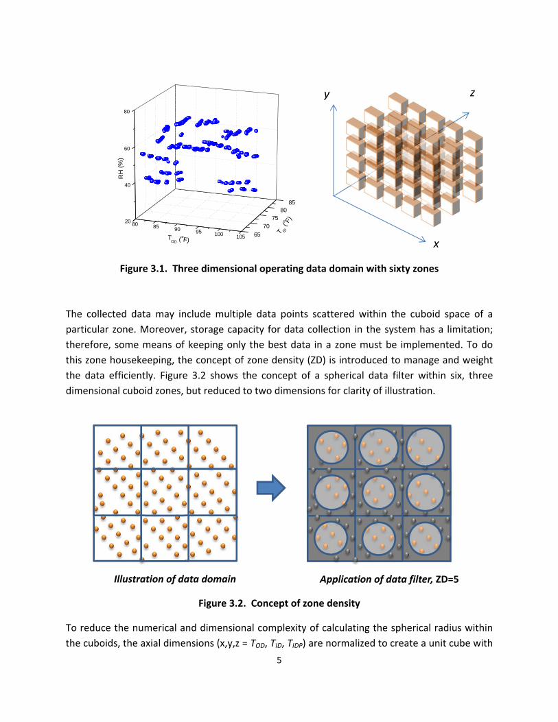
RH
(
)
) F(o
D
T I
TOD (o
F)
y z
80
60
40
85 80
7520 80 7085 90 95 100 65105
x
Figure 31 Three dimensional operating data domain with sixty zones
The collected data may include multiple data points scattered within the cuboid space of a
particular zone Moreover storage capacity for data collection in the system has a limitation
therefore some means of keeping only the best data in a zone must be implemented To do
this zone housekeeping the concept of zone density (ZD) is introduced to manage and weight
the data efficiently Figure 32 shows the concept of a spherical data filter within six three
dimensional cuboid zones but reduced to two dimensions for clarity of illustration
Illustration of data domain Application of data filter ZD=5
Figure 32 Concept of zone density
To reduce the numerical and dimensional complexity of calculating the spherical radius within
the cuboids the axial dimensions (xyz = TOD TID TIDP) are normalized to create a unit cube with
5
each side having unit area (ie 1x1x1) Only data within the sphere are selected and of the
selected data the data closest to the center are ranked as being higher quality and are selected
for storage Data storage demands are reduced by imposing a zone density (ZD) limit which
means that only a specified number of data points closest to the center of each sphere are
kept Figure 32 shows a ZD equal to 5 any new data within a zone will only be accepted if its
distance d is less than the maximum data point distance occurring in that zone The distance
from the center of the sphere to a data point can be easily calculated as shown in Equation 31
and Figure 33a
2 2 2d (05 x) (05 y) (05 z) (31)
The maximum number of data points in a zone can be adjusted using the zone density concept
(Figure 33b) A ZD of m is defined as the selection of the closest m data points from the center
in each zone For example the allowable data number decreases with the decrease of ZD as
shown in Figure 33b In this study a ZD from 100 to 1 was applied and tested in the self
training FDD logic
Center
(x y z)
1 1
d
A single zone (a) (b)
1
Figure 33 Concept of zone density (a) data distance ldquodrdquo from zone center and (b) various
zone densities
32 Domain Coverage Rate
Before a fault‐free dataset is used to develop models for fault‐free features some numerical
criterion needs to be established to assess the quality and extent of the dataset Preferably
each zone should contain data to avoid extrapolation According to Braun and Li (2001) the
predictions in case of extrapolation showed a deviation 3 to 10 times larger than those
predicted by interpolation Ideally each zone should contain the same number of data points
located close to the center
6
For the purpose of rating the extent of the fault‐free dataset the concept of Domain Coverage
Rate (DCR) is introduced which is the ratio of the number of zones with at least one fault‐free
data point to the total number of zones within the operational data domain The calculation of
the DCR is shown by Equations 32 and 33 If all zones contain at least one data point then the
DCR would equal 100
1 if data found in i zoneIndexi
th (32)
0 if data not found in i zone th
DCR 1
n
Indexi (33)n i1
where n is the total number of zones
33 Fault‐Free Models
Once the domain coverage rate reaches a specified maximum level the self training module will
correlate the data within all zones using the chosen fault‐free model form The following
sections evaluate the performance of several fault‐free model forms developed from cooling
mode laboratory test data previously acquired for an air‐source residential heat pump
331 Multivariable Polynomial Regression Models
Multivariable Polynomial Regression (MPR) models have been widely applied as fault‐free
models [(Li and Braun 2003) (Braun and Li 2001) (Kim et al 2008b) (Heo et al 2012)] due to
their simple structure and ease of programming They belong to the ldquoblack‐boxrdquo category of
models which do not consider the physics of the system and require a large dataset to
accurately predict system performance The higher order MPR models offer better accuracy of
prediction however excessive polynomial order for a relatively small database may worsen
data interpolation
Equations 34 35 and 36 show the general form of the regressed equations for features as 1st
2nd and 3rd order MPR models respectively
(1) = a a T a T a T (34)feature 0 1 OD 2 ID 3 IDP
(2) (1) 2 2 2 = a T T a T T a T T a T a T a T (35)feature feature 4 OD ID 5 ID IDP 6 IDP OD 7 OD 8 ID 9 IDP
(3) (2) 3 3 3 2 = a T a T a T a T T T a T Tfeature feature 10 OD 11 ID 12 IDP 13 OD ID IDP 14 OD ID (36)
2 2 2 2 2 a T T a T T a T T a T T a T T15 OD IDP 16 ID OD 17 ID IDP 18 IDP OD 19 IDP ID
7
332 Artificial Neural Network Models
An Artificial Neural Network (ANN) model was developed for the seven dependent features
The relationship between the three independent variables and seven dependent features is
ldquolearnedrdquo by an artificial neural network using a back propagation algorithm The ANN test
module was developed based on the sample code presented by Frenz (2002) The fault‐free
data are used as targets for the back propagation learning
Figure 34 shows the structure of the 3‐layer ANN(3x3x1) which has three input variables (TOD
TID and TIDP) one hidden layer and one output In general a form of the sigmoid function is
used as the activation function in the nodes of the hidden layer The weight coefficients and
offsets (or bias values) are learned using a momentum back propagation algorithm through
more than 10 000 iterations (Frenz 2002)
Figure 34 Artificial neural network structure (3x3x1)
Each hidden layer neuron is connected to every input neuron and each individual hidden layer
neuron receives the sum of the weighted input neuron values as given in Equation 37 Xi represents the input neuron values (TOD TID and TIDP) and wij represents the weights connecting
the input neurons to the hidden layer neurons In a similar way the output layer neurons are
determined as given in Equation 38 Bipolar sigmoid function was applied to layer transfer
function as given in Equation 39
n
h = hin j biasi
X wi ij
j 1
hout j= trans (hinj ) (37)
n
i 1
O =trans(O )outk ink (38)O = Oin k biasj h w jk out j
8
2trans(x) 1 (bipolar sigmoid) (39)
1 e x
The back‐propagation process utilizes a gradient descent algorithm that seeks to minimize the
errors of the values that are output from the neural network The weight and bias update
equations including the learning rate (α) and momentum terms (μ) are given in Equations 310
through 313 The learning rate fragments the weightbias adjustment taken in each training
iteration The smaller the value of alpha the longer a network takes to train but the smaller
alpha reduces fluctuations in the weight variation from iteration to iteration and generally
produces smaller errors Momentum is added to the weight adjustment equations (Equations
310 and 312) which enables the weight to change in response to the current gradient step
Delta (δ) is calculated by multiplying the difference between the target value and output value
by the derivative of the activation function (Equation 314) Here t represents the current set of
weightsbiases t‐1 the previous set and t+1 the new set being calculated
wjk (t 1)= wjk (t) hout j (wjk (t) wjk (t 1)) (310)
O (t 1)=O (t) (O (t) O (t 1)) (311)biask biask biask biask
wij (t 1)= wij (t) Xi (wij (t) wij (t 1)) (312)
hbias j (t 1)= hbias j (t) (hbias j (t) hbias j (t 1)) (313)
= 1 1 trans(O ) 1 trans(O ) (O O ) (314)in in target out2
The standard deviation (σ) of the ANN model was investigated with the variation of the learning
rate alpha (α) momentum (μ) maximum iteration number and number of hidden layers as
shown in Figure 35 The ANN modelrsquos performance was the most sensitive with learning rate (α) and iteration number which were optimized at 0001 and 10 000 respectively The ANN
modelrsquos performance improved with the increase of the momentum term However with the
momentum term greater than 01 the ANN modelrsquos performance decreased due to too large of
a gradient for training If the number of hidden layers increased the total number of variables
for modeling also increased As a result the ANN model with three layers showed the best
performance
9
8 108
7
6 104
5
100
(T
)
(T
)
ee
(T
)
(T
)
ee
4
3
096
1
0
2
092 10-5 10-4 10-3 10-2 10-1 10-3 10-2 10-1100 100
8 104
7
6 102
5
2 098
1
0 096 102 103 104 105 0 1 2 3 4 5 6 7 8 9
Iteration Layer number
Figure 35 Operating factor optimization for the ANN model
333 Combined ANN‐MPR Models
Used alone the ANN model showed good interpolation performance poor extrapolation
performance and relatively long times required for training The low‐order MPR model had
relatively good extrapolation performance low interpolation performance and very fast
training times In order to combine the strengths of the ANN and MPR models a combined
model was designed as illustrated by Braun and Li (2001)
In this study the first and second order MPR models and the ANN (3x3x1) model were applied
in the combined model First the MPR model was regressed with the training data and then
the residuals between the model output and the training data were fit with an ANN This
combined model is calculated as given in Equation 315
Combine=MPR ANN (315)
4 Self Training Implementation
41 Experimental Setup and Fault‐Free Data Collection
To test and validate the self training scheme presented in the previous sections we developed
a fault‐free database with laboratory data taken on an R410A 88 kW split heat pump operating
in the cooling mode The unit had a Seasonal Energy Efficiency Ratio (SEER) of 13 (AHRI 2008)
4 100
3
10
ll
The unit consisted of an indoor fan‐coil section outdoor section with a scroll compressor
cooling and heating mode thermostatic expansion valves (TXV) and connecting tubing Both
the indoor and outdoor air‐to‐refrigerant heat exchangers were of the finned‐tube type The
unit was installed in environmental chambers and charged with refrigerant according to the
manufacturerrsquos specifications Figure 41 shows a schematic of the experimental setup
indicating the measurement locations On the refrigerant side pressure transducers and T‐type
thermocouple probes were attached at the inlet and exit of every component of the system
The refrigerant mass flow rate was measured using a Coriolis flow meter The air enthalpy
method served as the primary measurement of the system capacity and the refrigerant
enthalpy method served as the secondary measurement These two measurements always
agreed within 5 Uncertainties of the major quantities measured during this work are
summarized in Table 41 Detailed specifications of the test rig including indoor ductwork
dimensions data acquisition measurement uncertainty and instrumentation is described in
Kim et al (2006)
IND
OO
RCH
AMBE
R
OU
TDO
OR
CHAM
BER
Evaporator Condenser
Compressor Scro
Mass flow meter
4-way Valve
PP
P
MFR
TDB TDP
SCFM
W
Thermostatic Expansion Valve
T
P T
P T Tsat
P T
P T
P T
TDB
TDB
P T Tsat
P T Tsat
TDB TDP Valves for LL fault
Valve for CMF fault
Figure 41 Schematic diagram of the experimental setup (Kim et al 2006)
To implement the most efficient test procedure outdoor temperature was fixed at one of four
values the addition of steam to the indoor chamber was set at one of several discrete levels by
modulating a steam valve and the indoor dry‐bulb temperature was changed over the desired
operating range by energizing 10 heaters sequentially From the total number of 10 409
recorded data scans 5830 data sets were allowed by the steady‐state detector The data were
recorded every 18 s and filtered through the steady‐state detector which qualified steady‐state
11
data for use in development of the fault‐free models for the seven features In this process
instability of the system due to on‐off transients and rapid load changes was filtered out by the
steady‐state detector From the total number of 10 409 recorded datasets 5830 datasets were
kept by the steady‐state detector
Table 42 shows operating conditions for the fault‐free tests The four outdoor temperatures
were maintained within plusmn05 degF For the indoor conditions the amount of steam introduced to
the indoor chamber was fixed such that the humidity ratio varied from 00037 to 00168 Data
were recorded every 18 s as indoor dry‐bulb temperature varied from 595 degF to 930 degF The
range of operating conditions for which data were collected defines the applicable limits for the
FDD scheme
Table 41 Measurement uncertainties
Measurement Range Uncertainty at a 95 Confidence Level
Individual temperature ‐04 F to 1994 F 054 F
Temperature difference 0 F to 504 F 054 F
Air nozzle pressure drop 0 Pa to 1245 Pa 10 Pa
Refrigerant mass flow rate 0 kgh to 544 kgh 10
Dew point temperature ‐04 F to 1004 F 072 F
Dry‐bulb temperature ‐04 F to 104 F 072 F
Total cooling capacity 3 kW to 11 kW 40
COP 25 to 60 55
Table 42 Operating conditions for fault‐free tests
Outdoor dry‐bulb temp F 82 90 95 100
Indoor dry‐bulb temp F 595 to 93
Indoor humidity ratio 00037 to 00168
If we assume that the data distribution is similar to that of a field‐installed real system the DCR
can be calculated based on the accumulated dataset as introduced in Equations 32 and 33
Figure 42 shows the fault‐free data distribution with increments of the domain coverage rate
DCR of 20 40 60 and 73 were fulfilled when the accumulated data points reached
2104 2830 4211 and 5830 respectively The datasets corresponding to these four DCRs were
used for the self training of different fault‐free models
12
DCR 20 DCR 40 DCR60 DCR73 120
Do
ma
in c
ove
rag
e r
ate
(
) T
em
pe
ratu
re (
o F)
RH
(
)
100
80
60
40
20
0 80
T OD
T ID
RH
60
40
20
0
0 1000 2000 3000 4000 5000 6000
Data no
Figure 42 Test condition data distribution and progression of domain coverage
42 Fault‐Free Model Performance with the Whole Dataset
Six fault‐free model types [MPR(1st order) MPR(2nd order) MPR(3rd order) ANN and two
combined models (MPR(1st order) + ANN MPR(2nd order) + ANN)] were tested and compared
using the entire dataset Each modelrsquos overall performance was evaluated by calculating the
standard error as given in Equation 41 The test standard error (TSE) is calculated from the
square root of the squared summation of residuals divided by the number of data points N
13
x 2 i iFF
TSE= i (41)N
Among the dependent features the TSE of TD and TC were the highest and the lowest
respectively The MPR(3rd order) model showed the lowest prediction error followed by the
MPR(2nd order) combined MPR(2nd order)+ANN combined MPR(1st order)+ANN and ANN
model (Figure 43) Therefore the MPR methods were applied and tested for additional analysis
of the self training method
Figure 43 Fault‐free models performance on the whole dataset
43 Fault‐Free Model Performance with Different Zone Densities
The zone density (ZD) concept was introduced to limit the data needed to generate a model
while collecting data over the predefined range of independent variables In this section the
prediction performance of the fault‐free model was tested with various zone densities In the
process of training fault‐free models were developed based on the data kept at the desired ZD
and then the prediction performance was tested on the filtered dataset in the test range (4627
of the 5830 original points after eliminating repeated tests)
Limiting the zone density produced a smaller dataset of training data the bigger the zone
density number the larger the training dataset for the training process When the zone density
14
d
d
decreased from 100 to 10 the data quantity drastically decreased from 2968 to 426 (Figure 44)
Therefore as the ZD number decreased the training speed and data storage compactness also
improved due to the smaller dataset However too small of a zone density number can
decrease the prediction performance
10
08
06
04
02 Zone density 100 00
2968 data
01 02 03 04 05 06 07 08 09 10 11 12 13 14 15 16 17 18 19 20 21 22 23 24 25 26 27 28 29 30 31 32 33 34 35 36 37 38 39 40 41 42 43 44 45
10
08
06
04
02 426 data Zone density 10 00
01 02 03 04 05 06 07 08 09 10 11 12 13 14 15 16 17 18 19 20 21 22 23 24 25 26 27 28 29 30 31 32 33 34 35 36 37 38 39 40 41 42 43 44 45
Zone number
Figure 44 Data distance to zone center for different zones for two zone densities
Figure 45 shows the standard error of the fault‐free model for the seven dependent features
with different zone densities Whereas the standard error for TE TC ∆TEA ∆TCA was relatively
non‐sensitive to the variation of zone density the standard error for TSH TD and TSC was more
rapidly increased with the decrease of zone density The MPR(3rd order) model was the most
sensitive to zone density variation The MPR(3rd order) model has a relatively large number of
coefficients (20) compared to the first order (4) and the second order (10) MPR models so that
it requires abundant data for stable regression On average the MPR(3rd order) model showed
the lowest standard error followed by the second and the first order MPR models respectively
At a zone density of 100 the standard error remained at a similar level to the models using all
of the data (5830 non‐filtered case) When the zone density was less than 25 the MPR(3rd
order) model showed similar prediction performance to that of the MPR(2nd order) model The
MPR(3rd order) model with zone density of 100 showed the most stable and best prediction
performance
15
06 06
05 05
04
03
TS
E(T
o
F)
TS
E(T
o
F)
TS
E(T
oF
) T
SE
(T
oF
) C
AS
CC
E
TS
E (
Avg
oF
) T
SE(
T
oF
) T
SE(T
oF
) T
SE(
T o
F)
EA
D
SH
MPR (1st)04 MPR (2nd) MPR (3rd) 03
02
01
02 MPR (1st) MPR (2nd)01 MPR (3rd)
00 00All 100 50 25 10 5 1 All 100 50 25 10 5 1
Zone density Zone density
06 10
MPR (1st)05 08 MPR (2nd) MPR (3rd) 04
06
04 03
02 MPR (1st)
0201 MPR (2nd) MPR (3rd)
00 00All 100 50 25 10 5 1 All 100 50 25 10 5 1
Zone density Zone density
06 06 MPR (1st) MPR (2nd)05 05 MPR (3rd)
MPR (1st) MPR (2nd) MPR (3rd)
04 04
03 03
02 02
01 01
00 00 All 100 50 25 10 5 1 All 100 50 25 10 5 1
Zone density Zone density
06 06
MPR (1st)05 05 MPR (2nd) MPR (3rd)
MPR (1st)
04 04
03
02
03
02
MPR (2nd) MPR (3rd)
00
01 01
00All 100 50 25 10 5 1 All 100 50 25 10 5 1
Zone density Zone density
Figure 45 Fault‐free model performance with zone density (Test Standard Error)
16
44 Fault‐Free Model Performance with Different Domain Coverage Rates
Figure 46 shows the domain coverage rate as the size of the fault‐free dataset increases up to
its maximum value of 5380 data points As the number of accumulated fault‐free data points
increases the DCR increases up to 73 The figure shows four training ranges corresponding to
DCR values of 20 40 60 and 73
80Training range DCR 73
Training range DCR 60 60
DC
R (
)
40 Training range DCR 40
20 Training range DCR 20
0
0 1000 2000 3000 4000 5000 6000
Data no
Figure 46 Domain coverage rate for different accumulated data quantity
Figure 47 shows the standard error of the fault‐free models for the seven dependent features
as a function of the domain coverage rate The standard error on all features decreased with an
increase in the DCR The standard error of the MPR(3rd order) model was the most sensitive to
DCR variation In a real system that is collecting training data when the DCR is low each
feature has a higher likelihood of being estimated by extrapolation using the currently
generated fault‐free model In most cases the first and second order MPR models showed the
lowest standard errors at 20 and 40 DCR conditions respectively The MPR(3rd order)
model was the best at 60 and 73 DCR After the DCR reached 40 the standard errors of
all fault‐free feature correlations were less than 1 oF
17
100 100 MPR (1st) MPR (1st) MPR (2nd) MPR (2nd) MPR (3rd) MPR (3rd)
10 T
SE(T
o
F)
TS
E(T
o
F)
TS
E(T
C o
F)
TS
E (
T o
F)
CA
SC
E
TS
E (
Avg
oF
) T
SE(
T
oF
) T
SE(T
oF
) T
SE(
T o
F)
EA
D
SH
10
1 1
01 01 20 40 60 80 20 40 60 80
Domain coverage rate () Domain coverage rate ()
100 100 MPR (1st) MPR (1st) MPR (2nd) MPR (2nd)10 MPR (3rd) MPR (3rd) 10
1
01 1
001 01 20 40 60 80 20 40 60 80
Domain coverage rate () Domain coverage rate ()
100 100 MPR (1st) MPR (1st) MPR (2nd) MPR (2nd) MPR (3rd) MPR (3rd)
10
1
10
1
01 01 20 40 60 80 20 40 60 80
Domain coverage rate () Domain coverage rate ()
100 100
MPR (1st) MPR (1st) MPR (2nd) MPR (2nd)
MPR (3rd) 10 MPR (3rd)
10
1 1
01 01 20 40 60 80 20 40 60 80
Domain coverage rate () Domain coverage rate ()
Figure 47 Fault‐free models performance with domain coverage rate (Test Standard Error)
18
The above standard error results are consistent with Braun and Li (2001) who commented that
the lower the order of the MPR model the better the extrapolation performance in general
When the DCR is low each feature has a higher likelihood of being estimated by extrapolation
For models generated at higher DCRs extrapolation is less likely and higher‐order MPR models
are better where interpolation is required
Figure 48 shows TSE of the MPR models for 20 40 60 and 73 DCR as a function of zone density At a DCR of 20 the TSE of MPR(3rd order) and MPR(2nd order) exceeded 4 oF and 1 oF respectively with steep increases at low ZD values For the higher DCRs the TSE stayed below 1 oF for all models and ZDs except MPR(3rd order) for 40 DCR and ZD less than 25 For 60 and 73 DCR all three models performed in a stable fashion smoothly improving predictions as DCR and ZD values increased
From this analysis the MPR(1st order) and MPR(2nd order) models are recommendable for the intermediate fault‐free models at a DCR of 20 and 40 respectively After the DCR exceeds 60 the MPR(3rd order) model is the most appropriate for the final fault‐free model A ZD between 100 and 50 is recommended for data filtering and storing criteria
40 10 MPR (1st) MPR (2nd) MPR (3rd)
DCR 20
30 20 08
TS
E(
Avg
oF
) T
SE
(A
vg o F
)
TS
E(
Avg
oF
) T
SE(
Avg
oF
)10 8 06
04 6
4 MPR (1st)DCR 4002 MPR (2nd)2 MPR (3rd)
0 00All 100 50 25 10 5 1 All 100 50 25 10 5 1
Zone density Zone density
10 DCR 60 MPR (1st) MPR (1st)DCR 7309
MPR (2nd) MPR (2nd)08 MPR (3rd) 07
MPR (3rd)
06 05
04 03
02 01
00 All 100 50 25 10 5 1 All 100 50 25 10 5 1
Zone density Zone density
Figure 48 Model standard error with zone density at DCR of 20 40 60 and 73
19
5 Validation
We tested and validated the self training method by applying the fault‐free models developed using the self training scheme to an experimental dataset collected by Kim et al (2006) on a heat pump operating in the cooling mode In addition the FDD performance was compared and analyzed considering different zone densities and domain coverage rates Successful diagnosis ratio false alarm missed detection and misdiagnosis were calculated and presented to evaluate the overall FDD performance
51 Validation Dataset and Fault Types
The dataset assembled by Kim et al (2006) includes performance data during fault‐free
operation (72 points) and with seven faults compressor valve leakage improper outdoor air
flow improper indoor air flow liquid line restriction refrigerant undercharge refrigerant
overcharge and non‐condensables (84 points) (Table 51)
Table 51 Definition and range of studied heat pump operational cases
Fault name Symbol Definition of fault Fault
range () Temperature range (oF)
Number of points
Fault‐free (Normal operation)
FF ‐ ‐TOD 80 to 102 TID 65 to 85 TIDP 42 to 85
72
Compressor valve leakage
(4 to way valve leakage)
CMF reduction in refrigerant flow rate from no‐fault
value 3 to 40
TOD 80 to 100 TID 70 to 80 TIDP 50 to 61
16
Reduced outdoor air TOD 80 to 100 flow rate (condenser CF of coil area blocked 10 to 50 TID 70 to 80 13
fouling) TIDP 50 to 61
Improper indoor air flow rate (evaporator
fouling) EF
below specified air flow rate
6 to 35 TOD 80 to 100 TID 70 to 80 TIDP 42 to 61
19
Liquid line restriction LL
change from no‐fault pressure drop from liquid
line service valve to indoor TXV inlet
10 to 32 TOD 80 to 100 TID 70 to 80 TIDP 50 to 61
6
20
Refrigerant undercharge
UC mass below correct
(no‐fault) charge 10 to 30
TOD 80 to 100 TID 70 to 80 TIDP 50 to 61
12
Refrigerant overcharge
OC mass above correct (no‐fault) charge
10 to 30 TOD 80 to 100 TID 70 to 80 TIDP 50 to 61
12
Presence of non‐condensable
gases NC
of pressure in evacuated indoor section and line set due to non‐condensable gas with respect to atmospheric
pressure
10 to 20 TOD 80 to 100 TID 70 to 80 TIDP 50 to 61
6
52 Fault Detection and Diagnostic Method
When the system is operating with a fault it is expected that feature temperatures willdeviate
from their normal fault‐free values An individual featurersquos deviation could be negative
positive or ldquoneutralrdquo (close to the fault‐free value within a pre‐defined threshold) collectively
the featurersquos deviations (or residuals) form a pattern which is unique for a given fault To
detect and diagnose the fault a statistical rule‐based classification is performed by calculating
the probability of the various fault‐types based on the decision rules defined within a rule‐
based chartrsquos predefined fault patterns A set of measurement features can be regarded as a
multi‐dimensional Gaussian probability distribution With the assumption that each dimension
is independent each of the three ldquoclassrdquo problems (negative positive or neutral) can be
represented by a simple normal (Gaussian) distribution rather than a more complicated
distribution with multiple degrees of freedom and dependencies (Rossi et al 1995 Kim et al
2008b) The probability of the kth fault corresponding to the set of m statistically independent
variables (X our features) is given by Equation 51 where P(Cik|Xi) denotes the individual
probability of case variable C (negative positive or neutral) for the ith feature with the kth fault
type Since the features are assumed to be independent the total conditional probability P(Fk|
X) can be obtained by the multiplication of the individual probabilities
m
P(Fk X) P(C1k X ) P(C X 2 ) P(Cik X i ) P(Cik X i ) (51)1 2k i1
21
Figure 51 Probability for three measurement residual cases of positive neutral and negative
In Figure 51 the three differently cross‐hatched areas under the Normal Distribution N(μiFF
σiFF) represents the probability of the current measurement (or predicted value) represented
by a second normal distribution PDF(xi σi) being lower higher or relatively close (neutral) to
the predicted fault‐free modelrsquos value if the conditions are fault‐free the difference in the
measured and predicted value the residual ri = xi ndash μiFF will equal zero In order to locate the
position of the current measurement under the normal distribution we must convert the
currently measured value to its standard form we must represent the current measurement as
some number of fault‐free model standard deviations from the mean value of the fault‐free
normal distribution (the currently predicted value) This standardization is often called the z‐
value Therefore the z‐value for the current measurement zi is defined by our residual and the
standard deviation of the fault‐free model as shown in Equation 52
x ri iFF izi (52) i FF i FF
Using the assumption of independent normally distributed FDD features the area under the
normal distribution N(μiFF σiFF) must be determined in order to place a numerical value on the
probability This integral is represented by the cumulative distribution function Φ(x) Equation
22
53 of the standard normal distribution (a normal distribution with a mean of zero and
standard deviation of 1 N(01))
௫ቀݎଵ
ଶଵଶ
ൌሻݔሺemptyradicଶቁ (53)
The cumulative distribution function describes the probability of a real number value with a
given probability distribution function X ϵ PDF(xi σi) having a value less than or equal to a
given value a This can be re‐stated as Equation 54
(54)ሻሺ ൌሻሺempty
This also leads to the probability of X lying within the semi‐closed interval (a b] or being greater
than some value b Equations 55 and 56 respectively
ሻሺെ emptyሻሺൌ emptyሻ ሺ
ሻሺൌ 1 െ empty ሻ ሺ
(55)
(56)
For the purposes of FDD we would like to know whether the residual ri is positive negative or
insignificant (ie within plusmnεi (neutral threshold) of the FF model predicted value μiFF) In order
to use the cumulative distribution function we must standardize the intervals around the
currently measured value xi plusmn εi as a multiple of the FF model standard deviation therefore we
ldquostandardizerdquo εi as being s number of FF model standard deviations as shown in Equation 57 s
is the ldquostandardizedrdquo width of the neutral threshold (sgt0) The standardized representation of
the residual and three possible cases (positive negative and neutral) are shown in Figure 52
s or ݏ ൌ ఌ
(57)i iFF ఙಷಷ
Now we may use Equation 56 to determine the probability of the residual being greater than
+εi the negative residual case
|
Less than or equal to ‐εi the positive residual case using Equation 54
ሺܥdarr ሻ ൌ ሺݖ ሺݖ ሻሻݏ ൌ 1 െ emptyሺݖ ሻ (58)ݏ
|
Or in the neutral interval of plusmnεi using Equation 55
(510)ሻെ ሺെݖݏ emptyሻ ሺൌݖݏ emptyሻ ሻݏ ሺݖെ ሻݏ ሺൌݖሺݖ ሻ|ܥሺ
ሺܥuarr ሻ ൌ ሺݖ ሺݖ െ ሻሻݏ ൌ emptyሺݖ െ ሻ (59)ݏ
23
Figure 52 Standard normal distribution showing the current measurements z‐value and
standardized neutral threshold s
The summation of probabilities calculated in Equations 58 to 510 equals unity Equation 511
since the integral of any PDFs from ndashinfin to +infin must equal one by definiƟon
P(C X i ) P(C
X i ) P(C X i ) 1 (511)
When the fault level increases the residual between the measured data and predicted data
may increase decrease or remain relatively unchanged Figure 53 shows the residual pattern
analysis results for the seven studied faults which were used to generate a rule‐based chart
Due to the careful selection of the most sensitive (rapidly changing) features for a given fault
type the feature patterns were quite different for all fault types and each pattern (positive
negative and neutral) for a given fault is the template for the calculation of fault probability in
Equation 51 For example the probability of a CMF fault (valve leakage) can be calculated by
the multiplication of the conditional probabilities of the residuals having the following pattern
TE (positive) TSH (neutral) TC (negative) TD (positive) TSC (negative) ∆TEA (negative) and ∆TCA
(negative) as shown in Equation 512
P(FCMF X) P(C TE ) P(C TSH ) P(C TC ) P(C TD ) P(C TSC ) (512)
P(C TEA ) P(C TCA )
24
5
0
-5
0
15 20 CMF CF
10 10
Re
sid
ua
l (oF
) R
esid
ual (
o F)
Re
sid
ua
l (oF
)
Res
idua
l (o F
) R
esid
ual (
o F)
Res
idua
l (o F
)
0
-10 -10
Neutral Positive Negative Neutral Positive Negative
-15 -20 T T T T T T T T T T T T T T
E SH C D SC EA CA E SH C D SC EA CA
8 20EF LL
4
0
-4
10
0
-10
Neutral Positive Negative Neutral Positive Negative -8 -20
T T T T T T T T T T T T T TE SH C D SC EA CA E SH C D SC EA CA
20 UC 20 OC
10
-10
10
0
-10
-20 Neutral Positive Negative -20 Neutral Positive Negative
TE
TSH
TC
TD
T T TSC EA CA
TE
TSH
TC
TD
T T TSC EA CA
20 NC
Re
sid
ua
l (oF
) 10
0
-10
Neutral Positive Negative
-20 T
E T
SH T
C T
D T T T
SC EA CA
Figure 53 Residual patterns for different faults
25
Table 52 Rule‐based FDD chart for air‐to‐air single‐speed heat pump in the cooling mode
Fault type TE TSH TC TD TSC ΔTEA ΔTCA
FF (Fault‐free)
CMF (Compressor valve leakage)
CF (Improper outdoor air flow)
EF (Improper indoor air flow)
LL (Liquid‐line restriction)
UC (Refrigerant undercharge)
OC (Refrigerant overcharge)
NC (Presence of non‐condensable gases)
The value of s must be determined so that it produces a given level of confidence that the
currently measured value is within the neutral threshold (or outside this threshold) The
confidence level is selected by the investigator typical values of α are 001 005 and 010 with
corresponding confidence levels of (1 - α) of 099 095 and 090 (Graybill and Iyer 1994) In
applying the s values the user is determining the alarm thresholds for calling a fault or no‐fault
Table 53 shows standard deviations and thresholds with different zone densities for MPR(3rd
order) models regressed to FDD test data In general if thresholds increase the false alarm rate
(FAR) decreases but missed detections increase and vice versa In this study the threshold for a
95 confidence level was applied to the FDD test data Table 54 summarizes the standard
deviations and thresholds for different domain coverage rates Models with the best fit were
26
selected with respect to the domain coverage rate the standard deviation and threshold
prominently increased with a decrease of DCR
Table 53 Standard deviation (oF) of the fault‐free model for different ZD (DCR=73 all data)
ZD Applied model
σ (TE) σ (TSH) σ (TC) σ (TD) σ (TSC) σ (ΔTEA) σ (ΔTCA)
All 3rd order MPR
0124 0314 0077 0310 0191 0124 0112
100 3rd order MPR
0133 0322 0081 0318 0195 0135 0114
50 3rd order MPR
0147 0388 0093 0521 0219 0156 0117
25 3rd order MPR
0149 0420 0094 0590 0236 0159 0119
10 3rd order MPR
0144 0432 0093 0597 0258 0157 0121
5 3rd order MPR
0141 0433 0097 0589 0258 0158 0125
1 3rd order MPR
0144 0442 0099 0537 0277 0166 0138
ε90 165∙σiFF model
ε95 196∙σiFF model
ε99 258∙σiFF model
Table 54 Standard deviation (oF) of fault‐free model for different DCR (ZD =100)
DCR () Applied model
σ (TE) σ (TSH) σ (TC) σ (TD) σ (TSC) σ (ΔTEA) σ (ΔTCA)
73 3rd order MPR
0133 0322 0081 0318 0195 0135 0114
60 3rd order MPR
0197 0385 0090 0811 0282 0160 0123
40 2nd order MPR
0390 0641 0109 0625 0401 0294 0155
20 1st order MPR
0673 0659 0196 2111 0393 0523 0196
ε90 165∙σiFF model
ε95 196∙σiFF model
ε99 258∙σiFF model
27
53 Procedure for Testing and Rating FDD Performance
The faults summarized in Table 51 were part of the experimental dataset (Kim et al 2006)
applied to test FDD performance For each dataset the fault probability for eight conditions (FF
CMF CF EF LL UC OC and NC) was calculated using Equation 51 and the rule‐based chart
fault patterns as given in Table 52 Among the probabilities of the eight conditions the fault
type with the highest fault probability was selected as the fault type most likely occurring at the
time When the diagnosed fault type was the same as the originally imposed fault type the
diagnostic was considered successful The goodness of the FDD method was further explored by
applying the concepts of FDD performance evaluation as defined by Braun et al (2012)
Successful diagnosis rate SDR () A fault is present The summation of the detected and
successfully diagnosed cases divided by total number of faulty tests equals the SDR for the
particular fault
False alarm rate FAR () No fault is present but the protocol indicates the presence of a
fault The FAR equals the number of false alarm cases divided by the total number of fault‐
free tests
Missed detection rate MDR () A fault is present but the protocol indicates that no fault is
present The MDR equals the number of missed detection cases divided by the total number
of faulty tests
Misdiagnosis rate MSR () A fault is present The protocol detects the fault but
misdiagnoses the fault type The MSR equals the number of misdiagnosis cases divided by
the total number of fault‐free and faulty tests
The above performance indices address that the detection aspect of FDD (FAR and MDR) and
the diagnosis (SDR and MSR)
As recommended in Section 43 the third order MPR model was applied for the fault‐free
model training A zone coverage rate of 73 represented all of the data and was used for this
analysis Figure 54 shows the SDR for the eight conditions with different zone densities In the
cases of FF CMF EF and OC the successful diagnosis rate (SDR ) was relatively high more
than 80 for all zone densities The SDR of CF and UC was between 60 and 80 and that of LL
and NC was less than 50 The feature pattern of the NC fault was very similar to that of OC
which was the reason for the inconsistent FDD performance on this fault (Figure 52) In the
case of the LL fault the fault pattern was unclear and additional fault data for LL was needed
since only six datasets were available for this fault case Overall the SDR gradually decreased
when zone density was less than 100 or 50 due to the increase in the standard deviation of the
fault‐free models and neutral threshold width for a 95 confidence (Figure 46) The average
28
SDR with a zone density of ALL and 100 was 83 and 82 respectively and gradually
decreased from 75 to 71 as the zone density decreased
Suc
cess
ful d
iagn
osis
rat
e (
)
100
90
80
70
60
50
40
30
20
10
0 FF CMF CF EF LL UC OC NC Avg
Zone density All 100 50 25 10 5 1
Fault types
Figure 54 Successful diagnosis rate of various faults for different zone densities
False alarm missed detection misdiagnosis were analyzed with decreasing zone density and
presented in Figure 55 False alarm and missed detection were not observed at the tests with
zone densities of ALL and 100 For zone densities less than 50 the false alarm case increased
from 42 to 56 with decreasing zone density Missed detections also increased from 36
to 95 with decreasing zone density The FAR was less than 6 and the MDR was less than
10 at all zone density conditions A zone density greater than 100 would be the best choice
for a high quality FDD application due to the observed stability and predictive accuracy seen in
our experimental dataset Fault diagnosis performance with zone densities of ALL and 100 was
also superior to cases with zone density less than 100 Misdiagnoses were 77 and 83 at
zone densities of ALL and 100 respectively with misdiagnoses distributed from 135 to 162
at zone densities less than 100
29
40
35
30
25
20
15
10
5
0
Zone density
Figure 55 Fault detection and diagnostic performance for all eight conditions for different zone densities
54 Effect of Domain Coverage Rate on FDD Performance
As recommended in Section 44 the first order and second MPR models were applied for the
fault‐free models at a DCR of 20 and from 40 to 60 respectively When the DCR was
more than 60 the MPR(3rd order) model was applied to the fault‐free model training A zone
density of 100 was applied for this analysis
The successful diagnosis rate SDR for eight fault conditions and varying domain coverage rates
are presented in Figure 56 With a DCR of 73 and 60 the FF CMF EF UC and OC faults
showed an SDR of more than 85 The SDR of CF and NC faults was between 60 and 70
and that of LL was less than 50 Exact diagnosis of FF is very important because it determines
the fault detection performance (false alarm rate FAR) In case of FF operation the SDR
drastically decreased below 65 when the DCR was 20 In cases of CMF EF UC and NC
faults the SDR significantly decreased at a DCR of 40 and 20 due to the increase in the
standard deviation of the FF model and corresponding increase in the neutral threshold The
overall average SDR gradually decreased from 89 to 61 with the decrease of DCR from 73
to 20
Figure 57 shows FAR (false alarm rate) MDR (missed detection rate) and MSR (misdiagnosis
rate) with the decrease of the DCR (domain coverage rate) False alarm and missed detection
were not observed in the tests with zone coverage rate of 73 FAR was 139 and 83 at
FD
D p
erfo
rman
ce (
)
False alarm rate () Missed detection rate () Misdiagnosis rate ()
All 100 50 25 10 5 1
30
DCR 60 and 40 respectively and then drastically increased to 375 at DCR 20 MDR
gradually increased from 714 to 262 with the decrease of DCR from 60 to 20 MSR
remained below 10 at DCR 73 and 60 and then the misdiagnosis rate steeply increased
to 186 and 385 at a DCR of 40 and 20 At a DCR from 73 to 60 FAR MDR and
MSR were all below 10 However FDD performances worsened at DCRs from 40 to 20
From Figures 56 and 57 DCRs greater than 60 were recommendable for a high quality FDD
application due stability and prediction accuracy In addition DCRs greater than 40 might be
acceptable for a lower quality FDD application if the fault detection error less than 15 was
allowable
100
90
80
70
60
50
40
30
20
10
0
Fault types
Figure 56 Successful diagnosis rate of various faults for different domain coverage rates
Suc
cess
ful d
iagn
osi
s ra
te (
)
Domain coverage rate () 73 60 40 20
FF CMF CF EF LL UC OC NC Avg
31
FD
D p
erfo
rman
ce (
)
40
35
30
25
20
15
10
5
0 73 60 40 20
False alarm rate () Missed detection rate () Misdiagnosis rate ()
Model with best fit DCR 73 3rd MPR model DCR 60 3rd MPR model DCR 40 2nd MPR model DCR 20 1st MPR model
Domain coverage rate ()
Figure 57 Fault detection and diagnostic performance for all faults for different domain coverage rates
6 Concluding Remarks
A concept for a self training fault‐free model for residential air conditioner fault detection and
diagnosis was introduced and tested The method of selecting the appropriate temperature
domain for the fault‐free system data was illustrated in order to cover most operating
conditions considering different climate zones in the US The fault‐free system performance
was modeled based upon three independent features (TOD TID TIDP) and seven dependent
features (TE TSH TC TD TSC ΔTEA ΔTCA) The new concept of zone density was introduced to
manage and filter the system data In addition the new concept of domain coverage rate was
also introduced to quantify the number of data needed to produce fault‐free feature models
Various fault‐free models such as the ANN (artificial neural network) the MPR (multivariable
polynomial regression) and a combined ANNMPR were explored for implementing self
training The MPR method was shown to produce very good prediction performance (low
standard errors) compared to the methods using ANNs Therefore MPR models were applied
and tested against previously taken system data for additional analysis of self training
For validation of the self training method the full experimental dataset (72 fault‐free and 84
fault tests) covering eight faultconditions (fault‐free compressor valve leakage outdoor coil
air flow blockage improper indoor air flow liquid‐line restriction refrigerant undercharge
32
refrigerant overcharge and non‐condensable gas contamination) was used to explore self
training performance The statistical rule‐based fault classification method was illustrated
FDD performance was analyzed using the successful detection rate (SDR) false alarm rate (FAR)
missed detection rate (MDR) and misdiagnosis rate (MSR) as zone density (ZD) and domain
coverage rate (DCR) were varied This effort showed that a zone density greater than 100 was
very successful within the experimental dataset In addition a domain coverage rate greater
than 60 produced acceptable FDD performance and good prediction performance (low
standard errors)
This report attempts to document a mathematical and logical technique by which an FDD
technique may be adapted to an air conditioning system with variations in installation details as
would be seen in actual residences It is by no means a perfected technique applicable to
immediate deployment many issues remain that still must be resolved by laboratory
investigation and application to real world problems When considering using an adaptive
technique for FDD in a real application the following questions must be resolved
1) What operating states are suitable for learning Steady state is important but what
about heat pumps operating in frosting conditions for heating What about the effects of
rain on the outdoor unit What about cooling operation at low outdoor temperatures when
the TXV is operating at the edges of its steady control band A key part of the learning
algorithm is developing a filtering algorithm which picks only the data known to be good
2) How does the FDD technique deal with the fact that the unit is aging and changing over
time In a real learning algorithm you must wait for the driving conditions to present
themselves If you install an air‐conditioner in the Fall season it could be 10 months before
you see data for the hottest day Is it fair to assume that the unit is unchanged since its
install What if the home owner tenant keeps their cooling setpoint at 75 degF all of the time
Now a new ownertenant moves in and runs the house at 70 degF can you use the old FDD
model
3) How do you deal withquantify the noise seen in sensors installed in the field Large
transients and noise may be seen in sensor readings A method of quantifying the sensor
noises and creating dynamic error bands need to be developed How does the FDD deal
with a brokenmalfunctioning sensor
The next step is to take this idea to the laboratory and the field and start solving the
outstanding issues
33
References
AHRI (2008) Performance rating of unitary airconditioning and airsource heat pump
equipment AHRI Standard 210240 Arlington VA USA Air‐Conditioning Heating and
Refrigeration Institute
Baechler M Williamson J Gilbride T Cole P Hefty M Love P (2010) High‐performance
home technologies Guide to determining climate regions by county US Department of Energy
PNNL‐19004
Braun J (1999) Automated fault detection and diagnostics for vapor compression cooling
equipment International Journal of Heating Ventilating Air‐Conditioning and Refrigerating
Research 5(2) 85‐86
Braun J amp Li H (2001) Description of FDD modeling approach for normal performance
expectation West Lafayette IN Herrick Labs Purdue University
Braun J Yuill D Cheung H (2012) A method for evaluating diagnostic protocols for
packaged air conditioning equipment CEC‐500‐08‐049 West Lafayette IN USA Purdue
University Herrick Laboratories
Chen B Braun J E (2001) Simple rule‐based methods for fault detection and diagnostics
applied to packaged air conditioners ASHRAE Transactions 107(1) 847‐857
Cho J Heo J Payne W Domanski P (2014) Normalized performances for a residential heat
pump in the cooling mode with single faults imposed Applied Thermal Engineering 67 1‐15
EIA 2013 US Energy Information Agency Residential Energy Consumption Survey
httpwwweiagovelectricitysales_revenue_pricepdftable5_apdf (Accessed April 2015)
EIA 2014 US Energy Information Agency Residential Energy Consumption Survey
httpwwweiagovtoolsfaqsfaqcfmid=96ampt=3 (Accessed April 2015)
Frenz C (2002) Visual basic and visual basicnet for scientists and engineers Apress 1st Edition
February
Graybill F Iyer H (1994) Regression analysis Concepts and applications second ed Belmont
CA USA Duxbury Press
Heo J Payne W Domanski P (2012) FDD CX A fault detection and diagnostic
commissioning tool for residential air conditioners and heat pump NIST TN 1774 Gaithersburg
MD National Institute of Standards and Technology
Kim M Payne W Domanski P Hermes C (2006) Performance of a Residential Air
Conditioner at Single‐Fault and Multiple‐Fault Conditions NISTIR 7350 Gaithersburg MD
National Institute of Standards and Technology
34
Kim M Yoon S Domanski P Payne W (2008a) Design of a steady‐state detector for fault
detection and diagnosis of a residential air conditioner Int J Refrig 31 790‐799
Kim M Yoon S Payne W Domanski P (2008b) Cooling mode fault detection and diagnosis
method for a residential heat pump NIST SP 1087 Gaithersburg MD National Institute of
Standards and Technology
Kim M Yoon S Payne W Domanski P (2010) Development of the reference model for a
residential heat pump system for cooling mode fault detection and diagnosis Journal of
Mechanical Science and Technology 24(7) 1481‐1489
Li H Braun J (2003) An improved method for fault detection and diagnosis applied to
packaged air conditioners ASHRAE Transactions 109(2) 683‐692
Payne W Domanski P Yoon S (2009) Heating mode performance measurements for a
residential heat pump with single‐faults imposed NIST TN 1648 Gaithersburg MD National
Institute of Standards and Technology
Rossi T Braun J E (1997) A statistical rule‐based fault detection and diagnostic method for
vapor compression air conditioners HVACampR Research 3(1) 19‐37
Thornton B Wang W Lane M Rosenberg M Liu B (2009) Technical support document
50 energy savings design technology packages for medium office buildings US Department
of Energy PNNL‐19004
Yoon S Payne W Domanski P (2011) Residential heat pump heating performance with
single faults imposed Applied Thermal Engineering 31 765‐771
Acknowledgements
The authors would like to acknowledge Min Sung Kim (Chief Thermal Energy Conversion Laboratory Korea Institute of Energy Research ndash KIER) Seok Ho Yoon (Korea Institute of Machinery and Materials) Jin Min Cho and Young‐Jin Baik (Engineer Thermal Energy Conversion Laboratory Korea Institute of Energy Research ndash KIER) for their work in developing the background material used in this report Also John Wamsley Glen Glaeser and Art Ellison provided technician support for collecting the data used to develop FDD fault‐free feature correlations We also would like to thank Will Guthrie of the NIST Statistical Engineering Division for reviewing the statistical FDD method section and Dan Veronica of the NIST Energy and Environment Division for reviewing and commenting on the entire document
35
Appendix A Temperature Data Distribution
The temperature domain should be selected in order to cover most of the operating conditions
a residential air conditioner may experience As summarized in Appendix A and Table A1 the
US climate may be divided into seven climate zones based upon certain criteria (Baechler et al
2010) Seven representative cities within these zones were chosen as a source for temperature
and humidity data (Thornton et al 2009) The most recent five year climate data were
investigated as shown in Figure A2 Temperature data domains for outdoor and indoor
temperature with relative humidity were determined using data for these seven cities
Table A1 Temperature domain by climate zone
Temp domain
Hot humid Hot dry Mixed humid
Mixed dry Marine Cold Very cold
TOD
80 to 105 by a step of 5 oF
(5 zones)
80 to 100 by a step of 5 oF
(4 zones)
80 to 105 by a step of 5 oF
(5 zones)
80 to 105 by a step of 5 oF
(5 zones)
80 to 95 by a step of 5 oF
(3 zones)
80 to 100 by a step of 5 oF
(4 zones)
80 to 95 by a step of 5 oF
(3 zones)
TID 65 to 85 by a step of 5 oF
(4 zones)
RH 20 to 80 by a step of 20
(3 zones)
36
Figure A1 Representative cities for seven US climate zones
37
120 120 O
D t
emp
(o F
) O
D t
em
p
(o F)
OD
tem
p
(o F) 100 100
80 80
60 60
40 40
20 20 Los Angeles (Hot dry)Houston (Hot humid)
0 01 2 3 4 5 6 7 8 9 10 11 12 1 2 3 4 5 6 7 8 9 10 11 12
120 120
100 100
80 80
60 60
40 40
20 20Baltimore (Mixed humid) Albuquerque (Mixed dry)
0 01 2 3 4 5 6 7 8 9 10 11 12 1 2 3 4 5 6 7 8 9 10 11 12
120 120
100 100
80 80
60 60
40 40
20
0 1 2 3 4
San Francisco (Marine)
5 6 7 8 9 10 11 12
20
0 1 2 3 4 5 6
Chicago (Cold)
7 8 9 10 11 12
120
O
D t
emp
(o F
) 100
80
60
40
20
0 1 2 3 4
Duluth (Very cold)
5 6 7 8 9 10 11 12
Month
Figure A2 Maximum outdoor temperature distributions in seven climate zones from 2008 to 2012
38
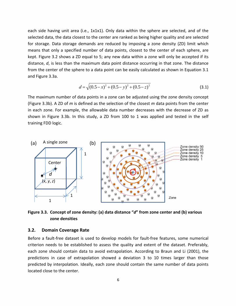
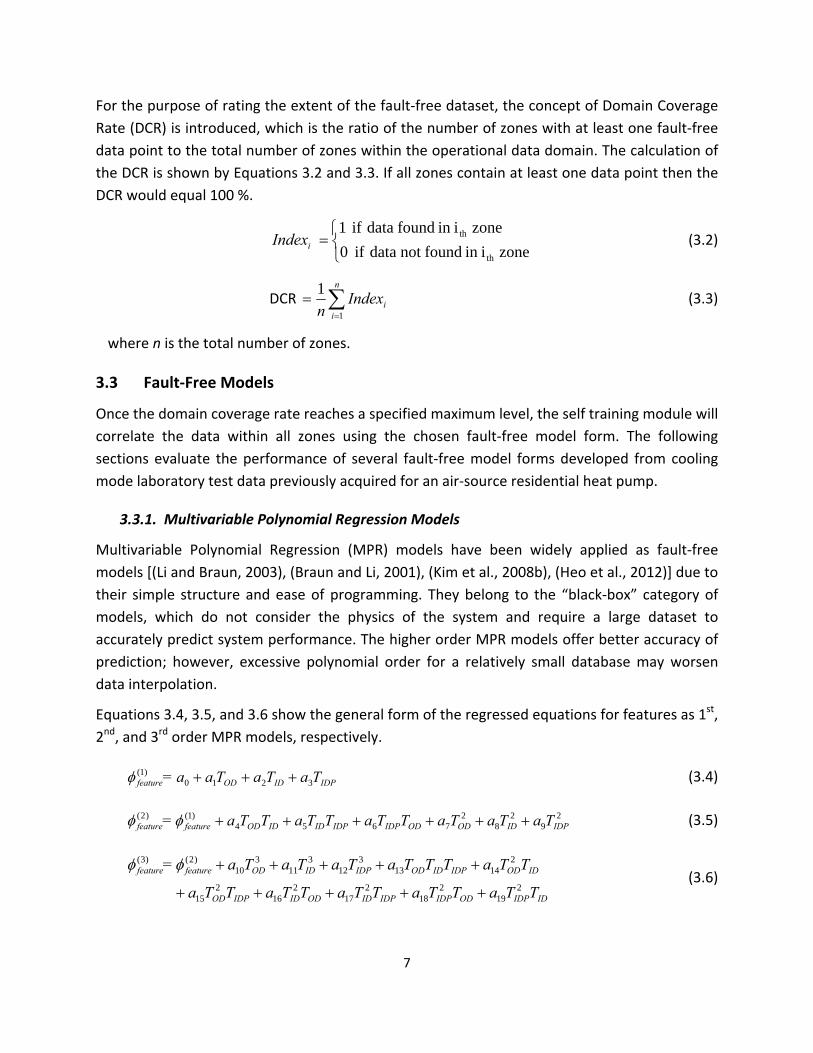

d
d
decreased from 100 to 10 the data quantity drastically decreased from 2968 to 426 (Figure 44)
Therefore as the ZD number decreased the training speed and data storage compactness also
improved due to the smaller dataset However too small of a zone density number can
decrease the prediction performance
10
08
06
04
02 Zone density 100 00
2968 data
01 02 03 04 05 06 07 08 09 10 11 12 13 14 15 16 17 18 19 20 21 22 23 24 25 26 27 28 29 30 31 32 33 34 35 36 37 38 39 40 41 42 43 44 45
10
08
06
04
02 426 data Zone density 10 00
01 02 03 04 05 06 07 08 09 10 11 12 13 14 15 16 17 18 19 20 21 22 23 24 25 26 27 28 29 30 31 32 33 34 35 36 37 38 39 40 41 42 43 44 45
Zone number
Figure 44 Data distance to zone center for different zones for two zone densities
Figure 45 shows the standard error of the fault‐free model for the seven dependent features
with different zone densities Whereas the standard error for TE TC ∆TEA ∆TCA was relatively
non‐sensitive to the variation of zone density the standard error for TSH TD and TSC was more
rapidly increased with the decrease of zone density The MPR(3rd order) model was the most
sensitive to zone density variation The MPR(3rd order) model has a relatively large number of
coefficients (20) compared to the first order (4) and the second order (10) MPR models so that
it requires abundant data for stable regression On average the MPR(3rd order) model showed
the lowest standard error followed by the second and the first order MPR models respectively
At a zone density of 100 the standard error remained at a similar level to the models using all
of the data (5830 non‐filtered case) When the zone density was less than 25 the MPR(3rd
order) model showed similar prediction performance to that of the MPR(2nd order) model The
MPR(3rd order) model with zone density of 100 showed the most stable and best prediction
performance
15
06 06
05 05
04
03
TS
E(T
o
F)
TS
E(T
o
F)
TS
E(T
oF
) T
SE
(T
oF
) C
AS
CC
E
TS
E (
Avg
oF
) T
SE(
T
oF
) T
SE(T
oF
) T
SE(
T o
F)
EA
D
SH
MPR (1st)04 MPR (2nd) MPR (3rd) 03
02
01
02 MPR (1st) MPR (2nd)01 MPR (3rd)
00 00All 100 50 25 10 5 1 All 100 50 25 10 5 1
Zone density Zone density
06 10
MPR (1st)05 08 MPR (2nd) MPR (3rd) 04
06
04 03
02 MPR (1st)
0201 MPR (2nd) MPR (3rd)
00 00All 100 50 25 10 5 1 All 100 50 25 10 5 1
Zone density Zone density
06 06 MPR (1st) MPR (2nd)05 05 MPR (3rd)
MPR (1st) MPR (2nd) MPR (3rd)
04 04
03 03
02 02
01 01
00 00 All 100 50 25 10 5 1 All 100 50 25 10 5 1
Zone density Zone density
06 06
MPR (1st)05 05 MPR (2nd) MPR (3rd)
MPR (1st)
04 04
03
02
03
02
MPR (2nd) MPR (3rd)
00
01 01
00All 100 50 25 10 5 1 All 100 50 25 10 5 1
Zone density Zone density
Figure 45 Fault‐free model performance with zone density (Test Standard Error)
16
44 Fault‐Free Model Performance with Different Domain Coverage Rates
Figure 46 shows the domain coverage rate as the size of the fault‐free dataset increases up to
its maximum value of 5380 data points As the number of accumulated fault‐free data points
increases the DCR increases up to 73 The figure shows four training ranges corresponding to
DCR values of 20 40 60 and 73
80Training range DCR 73
Training range DCR 60 60
DC
R (
)
40 Training range DCR 40
20 Training range DCR 20
0
0 1000 2000 3000 4000 5000 6000
Data no
Figure 46 Domain coverage rate for different accumulated data quantity
Figure 47 shows the standard error of the fault‐free models for the seven dependent features
as a function of the domain coverage rate The standard error on all features decreased with an
increase in the DCR The standard error of the MPR(3rd order) model was the most sensitive to
DCR variation In a real system that is collecting training data when the DCR is low each
feature has a higher likelihood of being estimated by extrapolation using the currently
generated fault‐free model In most cases the first and second order MPR models showed the
lowest standard errors at 20 and 40 DCR conditions respectively The MPR(3rd order)
model was the best at 60 and 73 DCR After the DCR reached 40 the standard errors of
all fault‐free feature correlations were less than 1 oF
17
100 100 MPR (1st) MPR (1st) MPR (2nd) MPR (2nd) MPR (3rd) MPR (3rd)
10 T
SE(T
o
F)
TS
E(T
o
F)
TS
E(T
C o
F)
TS
E (
T o
F)
CA
SC
E
TS
E (
Avg
oF
) T
SE(
T
oF
) T
SE(T
oF
) T
SE(
T o
F)
EA
D
SH
10
1 1
01 01 20 40 60 80 20 40 60 80
Domain coverage rate () Domain coverage rate ()
100 100 MPR (1st) MPR (1st) MPR (2nd) MPR (2nd)10 MPR (3rd) MPR (3rd) 10
1
01 1
001 01 20 40 60 80 20 40 60 80
Domain coverage rate () Domain coverage rate ()
100 100 MPR (1st) MPR (1st) MPR (2nd) MPR (2nd) MPR (3rd) MPR (3rd)
10
1
10
1
01 01 20 40 60 80 20 40 60 80
Domain coverage rate () Domain coverage rate ()
100 100
MPR (1st) MPR (1st) MPR (2nd) MPR (2nd)
MPR (3rd) 10 MPR (3rd)
10
1 1
01 01 20 40 60 80 20 40 60 80
Domain coverage rate () Domain coverage rate ()
Figure 47 Fault‐free models performance with domain coverage rate (Test Standard Error)
18
The above standard error results are consistent with Braun and Li (2001) who commented that
the lower the order of the MPR model the better the extrapolation performance in general
When the DCR is low each feature has a higher likelihood of being estimated by extrapolation
For models generated at higher DCRs extrapolation is less likely and higher‐order MPR models
are better where interpolation is required
Figure 48 shows TSE of the MPR models for 20 40 60 and 73 DCR as a function of zone density At a DCR of 20 the TSE of MPR(3rd order) and MPR(2nd order) exceeded 4 oF and 1 oF respectively with steep increases at low ZD values For the higher DCRs the TSE stayed below 1 oF for all models and ZDs except MPR(3rd order) for 40 DCR and ZD less than 25 For 60 and 73 DCR all three models performed in a stable fashion smoothly improving predictions as DCR and ZD values increased
From this analysis the MPR(1st order) and MPR(2nd order) models are recommendable for the intermediate fault‐free models at a DCR of 20 and 40 respectively After the DCR exceeds 60 the MPR(3rd order) model is the most appropriate for the final fault‐free model A ZD between 100 and 50 is recommended for data filtering and storing criteria
40 10 MPR (1st) MPR (2nd) MPR (3rd)
DCR 20
30 20 08
TS
E(
Avg
oF
) T
SE
(A
vg o F
)
TS
E(
Avg
oF
) T
SE(
Avg
oF
)10 8 06
04 6
4 MPR (1st)DCR 4002 MPR (2nd)2 MPR (3rd)
0 00All 100 50 25 10 5 1 All 100 50 25 10 5 1
Zone density Zone density
10 DCR 60 MPR (1st) MPR (1st)DCR 7309
MPR (2nd) MPR (2nd)08 MPR (3rd) 07
MPR (3rd)
06 05
04 03
02 01
00 All 100 50 25 10 5 1 All 100 50 25 10 5 1
Zone density Zone density
Figure 48 Model standard error with zone density at DCR of 20 40 60 and 73
19
5 Validation
We tested and validated the self training method by applying the fault‐free models developed using the self training scheme to an experimental dataset collected by Kim et al (2006) on a heat pump operating in the cooling mode In addition the FDD performance was compared and analyzed considering different zone densities and domain coverage rates Successful diagnosis ratio false alarm missed detection and misdiagnosis were calculated and presented to evaluate the overall FDD performance
51 Validation Dataset and Fault Types
The dataset assembled by Kim et al (2006) includes performance data during fault‐free
operation (72 points) and with seven faults compressor valve leakage improper outdoor air
flow improper indoor air flow liquid line restriction refrigerant undercharge refrigerant
overcharge and non‐condensables (84 points) (Table 51)
Table 51 Definition and range of studied heat pump operational cases
Fault name Symbol Definition of fault Fault
range () Temperature range (oF)
Number of points
Fault‐free (Normal operation)
FF ‐ ‐TOD 80 to 102 TID 65 to 85 TIDP 42 to 85
72
Compressor valve leakage
(4 to way valve leakage)
CMF reduction in refrigerant flow rate from no‐fault
value 3 to 40
TOD 80 to 100 TID 70 to 80 TIDP 50 to 61
16
Reduced outdoor air TOD 80 to 100 flow rate (condenser CF of coil area blocked 10 to 50 TID 70 to 80 13
fouling) TIDP 50 to 61
Improper indoor air flow rate (evaporator
fouling) EF
below specified air flow rate
6 to 35 TOD 80 to 100 TID 70 to 80 TIDP 42 to 61
19
Liquid line restriction LL
change from no‐fault pressure drop from liquid
line service valve to indoor TXV inlet
10 to 32 TOD 80 to 100 TID 70 to 80 TIDP 50 to 61
6
20
Refrigerant undercharge
UC mass below correct
(no‐fault) charge 10 to 30
TOD 80 to 100 TID 70 to 80 TIDP 50 to 61
12
Refrigerant overcharge
OC mass above correct (no‐fault) charge
10 to 30 TOD 80 to 100 TID 70 to 80 TIDP 50 to 61
12
Presence of non‐condensable
gases NC
of pressure in evacuated indoor section and line set due to non‐condensable gas with respect to atmospheric
pressure
10 to 20 TOD 80 to 100 TID 70 to 80 TIDP 50 to 61
6
52 Fault Detection and Diagnostic Method
When the system is operating with a fault it is expected that feature temperatures willdeviate
from their normal fault‐free values An individual featurersquos deviation could be negative
positive or ldquoneutralrdquo (close to the fault‐free value within a pre‐defined threshold) collectively
the featurersquos deviations (or residuals) form a pattern which is unique for a given fault To
detect and diagnose the fault a statistical rule‐based classification is performed by calculating
the probability of the various fault‐types based on the decision rules defined within a rule‐
based chartrsquos predefined fault patterns A set of measurement features can be regarded as a
multi‐dimensional Gaussian probability distribution With the assumption that each dimension
is independent each of the three ldquoclassrdquo problems (negative positive or neutral) can be
represented by a simple normal (Gaussian) distribution rather than a more complicated
distribution with multiple degrees of freedom and dependencies (Rossi et al 1995 Kim et al
2008b) The probability of the kth fault corresponding to the set of m statistically independent
variables (X our features) is given by Equation 51 where P(Cik|Xi) denotes the individual
probability of case variable C (negative positive or neutral) for the ith feature with the kth fault
type Since the features are assumed to be independent the total conditional probability P(Fk|
X) can be obtained by the multiplication of the individual probabilities
m
P(Fk X) P(C1k X ) P(C X 2 ) P(Cik X i ) P(Cik X i ) (51)1 2k i1
21
Figure 51 Probability for three measurement residual cases of positive neutral and negative
In Figure 51 the three differently cross‐hatched areas under the Normal Distribution N(μiFF
σiFF) represents the probability of the current measurement (or predicted value) represented
by a second normal distribution PDF(xi σi) being lower higher or relatively close (neutral) to
the predicted fault‐free modelrsquos value if the conditions are fault‐free the difference in the
measured and predicted value the residual ri = xi ndash μiFF will equal zero In order to locate the
position of the current measurement under the normal distribution we must convert the
currently measured value to its standard form we must represent the current measurement as
some number of fault‐free model standard deviations from the mean value of the fault‐free
normal distribution (the currently predicted value) This standardization is often called the z‐
value Therefore the z‐value for the current measurement zi is defined by our residual and the
standard deviation of the fault‐free model as shown in Equation 52
x ri iFF izi (52) i FF i FF
Using the assumption of independent normally distributed FDD features the area under the
normal distribution N(μiFF σiFF) must be determined in order to place a numerical value on the
probability This integral is represented by the cumulative distribution function Φ(x) Equation
22
53 of the standard normal distribution (a normal distribution with a mean of zero and
standard deviation of 1 N(01))
௫ቀݎଵ
ଶଵଶ
ൌሻݔሺemptyradicଶቁ (53)
The cumulative distribution function describes the probability of a real number value with a
given probability distribution function X ϵ PDF(xi σi) having a value less than or equal to a
given value a This can be re‐stated as Equation 54
(54)ሻሺ ൌሻሺempty
This also leads to the probability of X lying within the semi‐closed interval (a b] or being greater
than some value b Equations 55 and 56 respectively
ሻሺെ emptyሻሺൌ emptyሻ ሺ
ሻሺൌ 1 െ empty ሻ ሺ
(55)
(56)
For the purposes of FDD we would like to know whether the residual ri is positive negative or
insignificant (ie within plusmnεi (neutral threshold) of the FF model predicted value μiFF) In order
to use the cumulative distribution function we must standardize the intervals around the
currently measured value xi plusmn εi as a multiple of the FF model standard deviation therefore we
ldquostandardizerdquo εi as being s number of FF model standard deviations as shown in Equation 57 s
is the ldquostandardizedrdquo width of the neutral threshold (sgt0) The standardized representation of
the residual and three possible cases (positive negative and neutral) are shown in Figure 52
s or ݏ ൌ ఌ
(57)i iFF ఙಷಷ
Now we may use Equation 56 to determine the probability of the residual being greater than
+εi the negative residual case
|
Less than or equal to ‐εi the positive residual case using Equation 54
ሺܥdarr ሻ ൌ ሺݖ ሺݖ ሻሻݏ ൌ 1 െ emptyሺݖ ሻ (58)ݏ
|
Or in the neutral interval of plusmnεi using Equation 55
(510)ሻെ ሺെݖݏ emptyሻ ሺൌݖݏ emptyሻ ሻݏ ሺݖെ ሻݏ ሺൌݖሺݖ ሻ|ܥሺ
ሺܥuarr ሻ ൌ ሺݖ ሺݖ െ ሻሻݏ ൌ emptyሺݖ െ ሻ (59)ݏ
23
Figure 52 Standard normal distribution showing the current measurements z‐value and
standardized neutral threshold s
The summation of probabilities calculated in Equations 58 to 510 equals unity Equation 511
since the integral of any PDFs from ndashinfin to +infin must equal one by definiƟon
P(C X i ) P(C
X i ) P(C X i ) 1 (511)
When the fault level increases the residual between the measured data and predicted data
may increase decrease or remain relatively unchanged Figure 53 shows the residual pattern
analysis results for the seven studied faults which were used to generate a rule‐based chart
Due to the careful selection of the most sensitive (rapidly changing) features for a given fault
type the feature patterns were quite different for all fault types and each pattern (positive
negative and neutral) for a given fault is the template for the calculation of fault probability in
Equation 51 For example the probability of a CMF fault (valve leakage) can be calculated by
the multiplication of the conditional probabilities of the residuals having the following pattern
TE (positive) TSH (neutral) TC (negative) TD (positive) TSC (negative) ∆TEA (negative) and ∆TCA
(negative) as shown in Equation 512
P(FCMF X) P(C TE ) P(C TSH ) P(C TC ) P(C TD ) P(C TSC ) (512)
P(C TEA ) P(C TCA )
24
5
0
-5
0
15 20 CMF CF
10 10
Re
sid
ua
l (oF
) R
esid
ual (
o F)
Re
sid
ua
l (oF
)
Res
idua
l (o F
) R
esid
ual (
o F)
Res
idua
l (o F
)
0
-10 -10
Neutral Positive Negative Neutral Positive Negative
-15 -20 T T T T T T T T T T T T T T
E SH C D SC EA CA E SH C D SC EA CA
8 20EF LL
4
0
-4
10
0
-10
Neutral Positive Negative Neutral Positive Negative -8 -20
T T T T T T T T T T T T T TE SH C D SC EA CA E SH C D SC EA CA
20 UC 20 OC
10
-10
10
0
-10
-20 Neutral Positive Negative -20 Neutral Positive Negative
TE
TSH
TC
TD
T T TSC EA CA
TE
TSH
TC
TD
T T TSC EA CA
20 NC
Re
sid
ua
l (oF
) 10
0
-10
Neutral Positive Negative
-20 T
E T
SH T
C T
D T T T
SC EA CA
Figure 53 Residual patterns for different faults
25
Table 52 Rule‐based FDD chart for air‐to‐air single‐speed heat pump in the cooling mode
Fault type TE TSH TC TD TSC ΔTEA ΔTCA
FF (Fault‐free)
CMF (Compressor valve leakage)
CF (Improper outdoor air flow)
EF (Improper indoor air flow)
LL (Liquid‐line restriction)
UC (Refrigerant undercharge)
OC (Refrigerant overcharge)
NC (Presence of non‐condensable gases)
The value of s must be determined so that it produces a given level of confidence that the
currently measured value is within the neutral threshold (or outside this threshold) The
confidence level is selected by the investigator typical values of α are 001 005 and 010 with
corresponding confidence levels of (1 - α) of 099 095 and 090 (Graybill and Iyer 1994) In
applying the s values the user is determining the alarm thresholds for calling a fault or no‐fault
Table 53 shows standard deviations and thresholds with different zone densities for MPR(3rd
order) models regressed to FDD test data In general if thresholds increase the false alarm rate
(FAR) decreases but missed detections increase and vice versa In this study the threshold for a
95 confidence level was applied to the FDD test data Table 54 summarizes the standard
deviations and thresholds for different domain coverage rates Models with the best fit were
26
selected with respect to the domain coverage rate the standard deviation and threshold
prominently increased with a decrease of DCR
Table 53 Standard deviation (oF) of the fault‐free model for different ZD (DCR=73 all data)
ZD Applied model
σ (TE) σ (TSH) σ (TC) σ (TD) σ (TSC) σ (ΔTEA) σ (ΔTCA)
All 3rd order MPR
0124 0314 0077 0310 0191 0124 0112
100 3rd order MPR
0133 0322 0081 0318 0195 0135 0114
50 3rd order MPR
0147 0388 0093 0521 0219 0156 0117
25 3rd order MPR
0149 0420 0094 0590 0236 0159 0119
10 3rd order MPR
0144 0432 0093 0597 0258 0157 0121
5 3rd order MPR
0141 0433 0097 0589 0258 0158 0125
1 3rd order MPR
0144 0442 0099 0537 0277 0166 0138
ε90 165∙σiFF model
ε95 196∙σiFF model
ε99 258∙σiFF model
Table 54 Standard deviation (oF) of fault‐free model for different DCR (ZD =100)
DCR () Applied model
σ (TE) σ (TSH) σ (TC) σ (TD) σ (TSC) σ (ΔTEA) σ (ΔTCA)
73 3rd order MPR
0133 0322 0081 0318 0195 0135 0114
60 3rd order MPR
0197 0385 0090 0811 0282 0160 0123
40 2nd order MPR
0390 0641 0109 0625 0401 0294 0155
20 1st order MPR
0673 0659 0196 2111 0393 0523 0196
ε90 165∙σiFF model
ε95 196∙σiFF model
ε99 258∙σiFF model
27
53 Procedure for Testing and Rating FDD Performance
The faults summarized in Table 51 were part of the experimental dataset (Kim et al 2006)
applied to test FDD performance For each dataset the fault probability for eight conditions (FF
CMF CF EF LL UC OC and NC) was calculated using Equation 51 and the rule‐based chart
fault patterns as given in Table 52 Among the probabilities of the eight conditions the fault
type with the highest fault probability was selected as the fault type most likely occurring at the
time When the diagnosed fault type was the same as the originally imposed fault type the
diagnostic was considered successful The goodness of the FDD method was further explored by
applying the concepts of FDD performance evaluation as defined by Braun et al (2012)
Successful diagnosis rate SDR () A fault is present The summation of the detected and
successfully diagnosed cases divided by total number of faulty tests equals the SDR for the
particular fault
False alarm rate FAR () No fault is present but the protocol indicates the presence of a
fault The FAR equals the number of false alarm cases divided by the total number of fault‐
free tests
Missed detection rate MDR () A fault is present but the protocol indicates that no fault is
present The MDR equals the number of missed detection cases divided by the total number
of faulty tests
Misdiagnosis rate MSR () A fault is present The protocol detects the fault but
misdiagnoses the fault type The MSR equals the number of misdiagnosis cases divided by
the total number of fault‐free and faulty tests
The above performance indices address that the detection aspect of FDD (FAR and MDR) and
the diagnosis (SDR and MSR)
As recommended in Section 43 the third order MPR model was applied for the fault‐free
model training A zone coverage rate of 73 represented all of the data and was used for this
analysis Figure 54 shows the SDR for the eight conditions with different zone densities In the
cases of FF CMF EF and OC the successful diagnosis rate (SDR ) was relatively high more
than 80 for all zone densities The SDR of CF and UC was between 60 and 80 and that of LL
and NC was less than 50 The feature pattern of the NC fault was very similar to that of OC
which was the reason for the inconsistent FDD performance on this fault (Figure 52) In the
case of the LL fault the fault pattern was unclear and additional fault data for LL was needed
since only six datasets were available for this fault case Overall the SDR gradually decreased
when zone density was less than 100 or 50 due to the increase in the standard deviation of the
fault‐free models and neutral threshold width for a 95 confidence (Figure 46) The average
28
SDR with a zone density of ALL and 100 was 83 and 82 respectively and gradually
decreased from 75 to 71 as the zone density decreased
Suc
cess
ful d
iagn
osis
rat
e (
)
100
90
80
70
60
50
40
30
20
10
0 FF CMF CF EF LL UC OC NC Avg
Zone density All 100 50 25 10 5 1
Fault types
Figure 54 Successful diagnosis rate of various faults for different zone densities
False alarm missed detection misdiagnosis were analyzed with decreasing zone density and
presented in Figure 55 False alarm and missed detection were not observed at the tests with
zone densities of ALL and 100 For zone densities less than 50 the false alarm case increased
from 42 to 56 with decreasing zone density Missed detections also increased from 36
to 95 with decreasing zone density The FAR was less than 6 and the MDR was less than
10 at all zone density conditions A zone density greater than 100 would be the best choice
for a high quality FDD application due to the observed stability and predictive accuracy seen in
our experimental dataset Fault diagnosis performance with zone densities of ALL and 100 was
also superior to cases with zone density less than 100 Misdiagnoses were 77 and 83 at
zone densities of ALL and 100 respectively with misdiagnoses distributed from 135 to 162
at zone densities less than 100
29
40
35
30
25
20
15
10
5
0
Zone density
Figure 55 Fault detection and diagnostic performance for all eight conditions for different zone densities
54 Effect of Domain Coverage Rate on FDD Performance
As recommended in Section 44 the first order and second MPR models were applied for the
fault‐free models at a DCR of 20 and from 40 to 60 respectively When the DCR was
more than 60 the MPR(3rd order) model was applied to the fault‐free model training A zone
density of 100 was applied for this analysis
The successful diagnosis rate SDR for eight fault conditions and varying domain coverage rates
are presented in Figure 56 With a DCR of 73 and 60 the FF CMF EF UC and OC faults
showed an SDR of more than 85 The SDR of CF and NC faults was between 60 and 70
and that of LL was less than 50 Exact diagnosis of FF is very important because it determines
the fault detection performance (false alarm rate FAR) In case of FF operation the SDR
drastically decreased below 65 when the DCR was 20 In cases of CMF EF UC and NC
faults the SDR significantly decreased at a DCR of 40 and 20 due to the increase in the
standard deviation of the FF model and corresponding increase in the neutral threshold The
overall average SDR gradually decreased from 89 to 61 with the decrease of DCR from 73
to 20
Figure 57 shows FAR (false alarm rate) MDR (missed detection rate) and MSR (misdiagnosis
rate) with the decrease of the DCR (domain coverage rate) False alarm and missed detection
were not observed in the tests with zone coverage rate of 73 FAR was 139 and 83 at
FD
D p
erfo
rman
ce (
)
False alarm rate () Missed detection rate () Misdiagnosis rate ()
All 100 50 25 10 5 1
30
DCR 60 and 40 respectively and then drastically increased to 375 at DCR 20 MDR
gradually increased from 714 to 262 with the decrease of DCR from 60 to 20 MSR
remained below 10 at DCR 73 and 60 and then the misdiagnosis rate steeply increased
to 186 and 385 at a DCR of 40 and 20 At a DCR from 73 to 60 FAR MDR and
MSR were all below 10 However FDD performances worsened at DCRs from 40 to 20
From Figures 56 and 57 DCRs greater than 60 were recommendable for a high quality FDD
application due stability and prediction accuracy In addition DCRs greater than 40 might be
acceptable for a lower quality FDD application if the fault detection error less than 15 was
allowable
100
90
80
70
60
50
40
30
20
10
0
Fault types
Figure 56 Successful diagnosis rate of various faults for different domain coverage rates
Suc
cess
ful d
iagn
osi
s ra
te (
)
Domain coverage rate () 73 60 40 20
FF CMF CF EF LL UC OC NC Avg
31
FD
D p
erfo
rman
ce (
)
40
35
30
25
20
15
10
5
0 73 60 40 20
False alarm rate () Missed detection rate () Misdiagnosis rate ()
Model with best fit DCR 73 3rd MPR model DCR 60 3rd MPR model DCR 40 2nd MPR model DCR 20 1st MPR model
Domain coverage rate ()
Figure 57 Fault detection and diagnostic performance for all faults for different domain coverage rates
6 Concluding Remarks
A concept for a self training fault‐free model for residential air conditioner fault detection and
diagnosis was introduced and tested The method of selecting the appropriate temperature
domain for the fault‐free system data was illustrated in order to cover most operating
conditions considering different climate zones in the US The fault‐free system performance
was modeled based upon three independent features (TOD TID TIDP) and seven dependent
features (TE TSH TC TD TSC ΔTEA ΔTCA) The new concept of zone density was introduced to
manage and filter the system data In addition the new concept of domain coverage rate was
also introduced to quantify the number of data needed to produce fault‐free feature models
Various fault‐free models such as the ANN (artificial neural network) the MPR (multivariable
polynomial regression) and a combined ANNMPR were explored for implementing self
training The MPR method was shown to produce very good prediction performance (low
standard errors) compared to the methods using ANNs Therefore MPR models were applied
and tested against previously taken system data for additional analysis of self training
For validation of the self training method the full experimental dataset (72 fault‐free and 84
fault tests) covering eight faultconditions (fault‐free compressor valve leakage outdoor coil
air flow blockage improper indoor air flow liquid‐line restriction refrigerant undercharge
32
refrigerant overcharge and non‐condensable gas contamination) was used to explore self
training performance The statistical rule‐based fault classification method was illustrated
FDD performance was analyzed using the successful detection rate (SDR) false alarm rate (FAR)
missed detection rate (MDR) and misdiagnosis rate (MSR) as zone density (ZD) and domain
coverage rate (DCR) were varied This effort showed that a zone density greater than 100 was
very successful within the experimental dataset In addition a domain coverage rate greater
than 60 produced acceptable FDD performance and good prediction performance (low
standard errors)
This report attempts to document a mathematical and logical technique by which an FDD
technique may be adapted to an air conditioning system with variations in installation details as
would be seen in actual residences It is by no means a perfected technique applicable to
immediate deployment many issues remain that still must be resolved by laboratory
investigation and application to real world problems When considering using an adaptive
technique for FDD in a real application the following questions must be resolved
1) What operating states are suitable for learning Steady state is important but what
about heat pumps operating in frosting conditions for heating What about the effects of
rain on the outdoor unit What about cooling operation at low outdoor temperatures when
the TXV is operating at the edges of its steady control band A key part of the learning
algorithm is developing a filtering algorithm which picks only the data known to be good
2) How does the FDD technique deal with the fact that the unit is aging and changing over
time In a real learning algorithm you must wait for the driving conditions to present
themselves If you install an air‐conditioner in the Fall season it could be 10 months before
you see data for the hottest day Is it fair to assume that the unit is unchanged since its
install What if the home owner tenant keeps their cooling setpoint at 75 degF all of the time
Now a new ownertenant moves in and runs the house at 70 degF can you use the old FDD
model
3) How do you deal withquantify the noise seen in sensors installed in the field Large
transients and noise may be seen in sensor readings A method of quantifying the sensor
noises and creating dynamic error bands need to be developed How does the FDD deal
with a brokenmalfunctioning sensor
The next step is to take this idea to the laboratory and the field and start solving the
outstanding issues
33
References
AHRI (2008) Performance rating of unitary airconditioning and airsource heat pump
equipment AHRI Standard 210240 Arlington VA USA Air‐Conditioning Heating and
Refrigeration Institute
Baechler M Williamson J Gilbride T Cole P Hefty M Love P (2010) High‐performance
home technologies Guide to determining climate regions by county US Department of Energy
PNNL‐19004
Braun J (1999) Automated fault detection and diagnostics for vapor compression cooling
equipment International Journal of Heating Ventilating Air‐Conditioning and Refrigerating
Research 5(2) 85‐86
Braun J amp Li H (2001) Description of FDD modeling approach for normal performance
expectation West Lafayette IN Herrick Labs Purdue University
Braun J Yuill D Cheung H (2012) A method for evaluating diagnostic protocols for
packaged air conditioning equipment CEC‐500‐08‐049 West Lafayette IN USA Purdue
University Herrick Laboratories
Chen B Braun J E (2001) Simple rule‐based methods for fault detection and diagnostics
applied to packaged air conditioners ASHRAE Transactions 107(1) 847‐857
Cho J Heo J Payne W Domanski P (2014) Normalized performances for a residential heat
pump in the cooling mode with single faults imposed Applied Thermal Engineering 67 1‐15
EIA 2013 US Energy Information Agency Residential Energy Consumption Survey
httpwwweiagovelectricitysales_revenue_pricepdftable5_apdf (Accessed April 2015)
EIA 2014 US Energy Information Agency Residential Energy Consumption Survey
httpwwweiagovtoolsfaqsfaqcfmid=96ampt=3 (Accessed April 2015)
Frenz C (2002) Visual basic and visual basicnet for scientists and engineers Apress 1st Edition
February
Graybill F Iyer H (1994) Regression analysis Concepts and applications second ed Belmont
CA USA Duxbury Press
Heo J Payne W Domanski P (2012) FDD CX A fault detection and diagnostic
commissioning tool for residential air conditioners and heat pump NIST TN 1774 Gaithersburg
MD National Institute of Standards and Technology
Kim M Payne W Domanski P Hermes C (2006) Performance of a Residential Air
Conditioner at Single‐Fault and Multiple‐Fault Conditions NISTIR 7350 Gaithersburg MD
National Institute of Standards and Technology
34
Kim M Yoon S Domanski P Payne W (2008a) Design of a steady‐state detector for fault
detection and diagnosis of a residential air conditioner Int J Refrig 31 790‐799
Kim M Yoon S Payne W Domanski P (2008b) Cooling mode fault detection and diagnosis
method for a residential heat pump NIST SP 1087 Gaithersburg MD National Institute of
Standards and Technology
Kim M Yoon S Payne W Domanski P (2010) Development of the reference model for a
residential heat pump system for cooling mode fault detection and diagnosis Journal of
Mechanical Science and Technology 24(7) 1481‐1489
Li H Braun J (2003) An improved method for fault detection and diagnosis applied to
packaged air conditioners ASHRAE Transactions 109(2) 683‐692
Payne W Domanski P Yoon S (2009) Heating mode performance measurements for a
residential heat pump with single‐faults imposed NIST TN 1648 Gaithersburg MD National
Institute of Standards and Technology
Rossi T Braun J E (1997) A statistical rule‐based fault detection and diagnostic method for
vapor compression air conditioners HVACampR Research 3(1) 19‐37
Thornton B Wang W Lane M Rosenberg M Liu B (2009) Technical support document
50 energy savings design technology packages for medium office buildings US Department
of Energy PNNL‐19004
Yoon S Payne W Domanski P (2011) Residential heat pump heating performance with
single faults imposed Applied Thermal Engineering 31 765‐771
Acknowledgements
The authors would like to acknowledge Min Sung Kim (Chief Thermal Energy Conversion Laboratory Korea Institute of Energy Research ndash KIER) Seok Ho Yoon (Korea Institute of Machinery and Materials) Jin Min Cho and Young‐Jin Baik (Engineer Thermal Energy Conversion Laboratory Korea Institute of Energy Research ndash KIER) for their work in developing the background material used in this report Also John Wamsley Glen Glaeser and Art Ellison provided technician support for collecting the data used to develop FDD fault‐free feature correlations We also would like to thank Will Guthrie of the NIST Statistical Engineering Division for reviewing the statistical FDD method section and Dan Veronica of the NIST Energy and Environment Division for reviewing and commenting on the entire document
35
Appendix A Temperature Data Distribution
The temperature domain should be selected in order to cover most of the operating conditions
a residential air conditioner may experience As summarized in Appendix A and Table A1 the
US climate may be divided into seven climate zones based upon certain criteria (Baechler et al
2010) Seven representative cities within these zones were chosen as a source for temperature
and humidity data (Thornton et al 2009) The most recent five year climate data were
investigated as shown in Figure A2 Temperature data domains for outdoor and indoor
temperature with relative humidity were determined using data for these seven cities
Table A1 Temperature domain by climate zone
Temp domain
Hot humid Hot dry Mixed humid
Mixed dry Marine Cold Very cold
TOD
80 to 105 by a step of 5 oF
(5 zones)
80 to 100 by a step of 5 oF
(4 zones)
80 to 105 by a step of 5 oF
(5 zones)
80 to 105 by a step of 5 oF
(5 zones)
80 to 95 by a step of 5 oF
(3 zones)
80 to 100 by a step of 5 oF
(4 zones)
80 to 95 by a step of 5 oF
(3 zones)
TID 65 to 85 by a step of 5 oF
(4 zones)
RH 20 to 80 by a step of 20
(3 zones)
36
Figure A1 Representative cities for seven US climate zones
37
120 120 O
D t
emp
(o F
) O
D t
em
p
(o F)
OD
tem
p
(o F) 100 100
80 80
60 60
40 40
20 20 Los Angeles (Hot dry)Houston (Hot humid)
0 01 2 3 4 5 6 7 8 9 10 11 12 1 2 3 4 5 6 7 8 9 10 11 12
120 120
100 100
80 80
60 60
40 40
20 20Baltimore (Mixed humid) Albuquerque (Mixed dry)
0 01 2 3 4 5 6 7 8 9 10 11 12 1 2 3 4 5 6 7 8 9 10 11 12
120 120
100 100
80 80
60 60
40 40
20
0 1 2 3 4
San Francisco (Marine)
5 6 7 8 9 10 11 12
20
0 1 2 3 4 5 6
Chicago (Cold)
7 8 9 10 11 12
120
O
D t
emp
(o F
) 100
80
60
40
20
0 1 2 3 4
Duluth (Very cold)
5 6 7 8 9 10 11 12
Month
Figure A2 Maximum outdoor temperature distributions in seven climate zones from 2008 to 2012
38
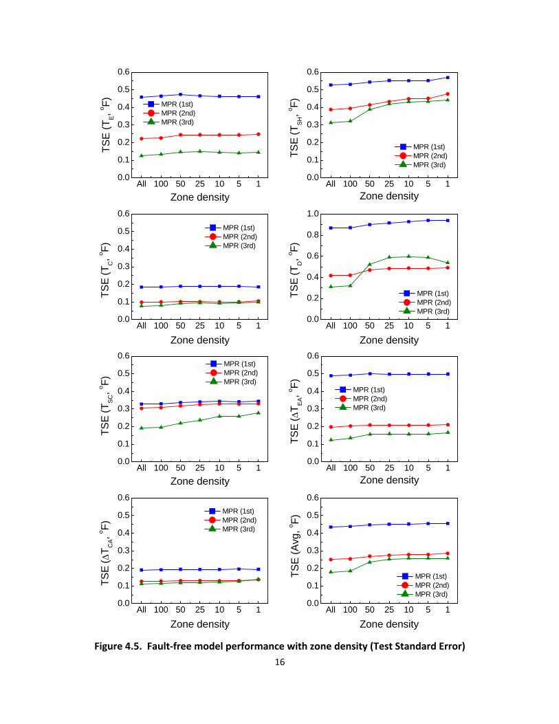
06 06
05 05
04
03
TS
E(T
o
F)
TS
E(T
o
F)
TS
E(T
oF
) T
SE
(T
oF
) C
AS
CC
E
TS
E (
Avg
oF
) T
SE(
T
oF
) T
SE(T
oF
) T
SE(
T o
F)
EA
D
SH
MPR (1st)04 MPR (2nd) MPR (3rd) 03
02
01
02 MPR (1st) MPR (2nd)01 MPR (3rd)
00 00All 100 50 25 10 5 1 All 100 50 25 10 5 1
Zone density Zone density
06 10
MPR (1st)05 08 MPR (2nd) MPR (3rd) 04
06
04 03
02 MPR (1st)
0201 MPR (2nd) MPR (3rd)
00 00All 100 50 25 10 5 1 All 100 50 25 10 5 1
Zone density Zone density
06 06 MPR (1st) MPR (2nd)05 05 MPR (3rd)
MPR (1st) MPR (2nd) MPR (3rd)
04 04
03 03
02 02
01 01
00 00 All 100 50 25 10 5 1 All 100 50 25 10 5 1
Zone density Zone density
06 06
MPR (1st)05 05 MPR (2nd) MPR (3rd)
MPR (1st)
04 04
03
02
03
02
MPR (2nd) MPR (3rd)
00
01 01
00All 100 50 25 10 5 1 All 100 50 25 10 5 1
Zone density Zone density
Figure 45 Fault‐free model performance with zone density (Test Standard Error)
16
44 Fault‐Free Model Performance with Different Domain Coverage Rates
Figure 46 shows the domain coverage rate as the size of the fault‐free dataset increases up to
its maximum value of 5380 data points As the number of accumulated fault‐free data points
increases the DCR increases up to 73 The figure shows four training ranges corresponding to
DCR values of 20 40 60 and 73
80Training range DCR 73
Training range DCR 60 60
DC
R (
)
40 Training range DCR 40
20 Training range DCR 20
0
0 1000 2000 3000 4000 5000 6000
Data no
Figure 46 Domain coverage rate for different accumulated data quantity
Figure 47 shows the standard error of the fault‐free models for the seven dependent features
as a function of the domain coverage rate The standard error on all features decreased with an
increase in the DCR The standard error of the MPR(3rd order) model was the most sensitive to
DCR variation In a real system that is collecting training data when the DCR is low each
feature has a higher likelihood of being estimated by extrapolation using the currently
generated fault‐free model In most cases the first and second order MPR models showed the
lowest standard errors at 20 and 40 DCR conditions respectively The MPR(3rd order)
model was the best at 60 and 73 DCR After the DCR reached 40 the standard errors of
all fault‐free feature correlations were less than 1 oF
17
100 100 MPR (1st) MPR (1st) MPR (2nd) MPR (2nd) MPR (3rd) MPR (3rd)
10 T
SE(T
o
F)
TS
E(T
o
F)
TS
E(T
C o
F)
TS
E (
T o
F)
CA
SC
E
TS
E (
Avg
oF
) T
SE(
T
oF
) T
SE(T
oF
) T
SE(
T o
F)
EA
D
SH
10
1 1
01 01 20 40 60 80 20 40 60 80
Domain coverage rate () Domain coverage rate ()
100 100 MPR (1st) MPR (1st) MPR (2nd) MPR (2nd)10 MPR (3rd) MPR (3rd) 10
1
01 1
001 01 20 40 60 80 20 40 60 80
Domain coverage rate () Domain coverage rate ()
100 100 MPR (1st) MPR (1st) MPR (2nd) MPR (2nd) MPR (3rd) MPR (3rd)
10
1
10
1
01 01 20 40 60 80 20 40 60 80
Domain coverage rate () Domain coverage rate ()
100 100
MPR (1st) MPR (1st) MPR (2nd) MPR (2nd)
MPR (3rd) 10 MPR (3rd)
10
1 1
01 01 20 40 60 80 20 40 60 80
Domain coverage rate () Domain coverage rate ()
Figure 47 Fault‐free models performance with domain coverage rate (Test Standard Error)
18
The above standard error results are consistent with Braun and Li (2001) who commented that
the lower the order of the MPR model the better the extrapolation performance in general
When the DCR is low each feature has a higher likelihood of being estimated by extrapolation
For models generated at higher DCRs extrapolation is less likely and higher‐order MPR models
are better where interpolation is required
Figure 48 shows TSE of the MPR models for 20 40 60 and 73 DCR as a function of zone density At a DCR of 20 the TSE of MPR(3rd order) and MPR(2nd order) exceeded 4 oF and 1 oF respectively with steep increases at low ZD values For the higher DCRs the TSE stayed below 1 oF for all models and ZDs except MPR(3rd order) for 40 DCR and ZD less than 25 For 60 and 73 DCR all three models performed in a stable fashion smoothly improving predictions as DCR and ZD values increased
From this analysis the MPR(1st order) and MPR(2nd order) models are recommendable for the intermediate fault‐free models at a DCR of 20 and 40 respectively After the DCR exceeds 60 the MPR(3rd order) model is the most appropriate for the final fault‐free model A ZD between 100 and 50 is recommended for data filtering and storing criteria
40 10 MPR (1st) MPR (2nd) MPR (3rd)
DCR 20
30 20 08
TS
E(
Avg
oF
) T
SE
(A
vg o F
)
TS
E(
Avg
oF
) T
SE(
Avg
oF
)10 8 06
04 6
4 MPR (1st)DCR 4002 MPR (2nd)2 MPR (3rd)
0 00All 100 50 25 10 5 1 All 100 50 25 10 5 1
Zone density Zone density
10 DCR 60 MPR (1st) MPR (1st)DCR 7309
MPR (2nd) MPR (2nd)08 MPR (3rd) 07
MPR (3rd)
06 05
04 03
02 01
00 All 100 50 25 10 5 1 All 100 50 25 10 5 1
Zone density Zone density
Figure 48 Model standard error with zone density at DCR of 20 40 60 and 73
19
5 Validation
We tested and validated the self training method by applying the fault‐free models developed using the self training scheme to an experimental dataset collected by Kim et al (2006) on a heat pump operating in the cooling mode In addition the FDD performance was compared and analyzed considering different zone densities and domain coverage rates Successful diagnosis ratio false alarm missed detection and misdiagnosis were calculated and presented to evaluate the overall FDD performance
51 Validation Dataset and Fault Types
The dataset assembled by Kim et al (2006) includes performance data during fault‐free
operation (72 points) and with seven faults compressor valve leakage improper outdoor air
flow improper indoor air flow liquid line restriction refrigerant undercharge refrigerant
overcharge and non‐condensables (84 points) (Table 51)
Table 51 Definition and range of studied heat pump operational cases
Fault name Symbol Definition of fault Fault
range () Temperature range (oF)
Number of points
Fault‐free (Normal operation)
FF ‐ ‐TOD 80 to 102 TID 65 to 85 TIDP 42 to 85
72
Compressor valve leakage
(4 to way valve leakage)
CMF reduction in refrigerant flow rate from no‐fault
value 3 to 40
TOD 80 to 100 TID 70 to 80 TIDP 50 to 61
16
Reduced outdoor air TOD 80 to 100 flow rate (condenser CF of coil area blocked 10 to 50 TID 70 to 80 13
fouling) TIDP 50 to 61
Improper indoor air flow rate (evaporator
fouling) EF
below specified air flow rate
6 to 35 TOD 80 to 100 TID 70 to 80 TIDP 42 to 61
19
Liquid line restriction LL
change from no‐fault pressure drop from liquid
line service valve to indoor TXV inlet
10 to 32 TOD 80 to 100 TID 70 to 80 TIDP 50 to 61
6
20
Refrigerant undercharge
UC mass below correct
(no‐fault) charge 10 to 30
TOD 80 to 100 TID 70 to 80 TIDP 50 to 61
12
Refrigerant overcharge
OC mass above correct (no‐fault) charge
10 to 30 TOD 80 to 100 TID 70 to 80 TIDP 50 to 61
12
Presence of non‐condensable
gases NC
of pressure in evacuated indoor section and line set due to non‐condensable gas with respect to atmospheric
pressure
10 to 20 TOD 80 to 100 TID 70 to 80 TIDP 50 to 61
6
52 Fault Detection and Diagnostic Method
When the system is operating with a fault it is expected that feature temperatures willdeviate
from their normal fault‐free values An individual featurersquos deviation could be negative
positive or ldquoneutralrdquo (close to the fault‐free value within a pre‐defined threshold) collectively
the featurersquos deviations (or residuals) form a pattern which is unique for a given fault To
detect and diagnose the fault a statistical rule‐based classification is performed by calculating
the probability of the various fault‐types based on the decision rules defined within a rule‐
based chartrsquos predefined fault patterns A set of measurement features can be regarded as a
multi‐dimensional Gaussian probability distribution With the assumption that each dimension
is independent each of the three ldquoclassrdquo problems (negative positive or neutral) can be
represented by a simple normal (Gaussian) distribution rather than a more complicated
distribution with multiple degrees of freedom and dependencies (Rossi et al 1995 Kim et al
2008b) The probability of the kth fault corresponding to the set of m statistically independent
variables (X our features) is given by Equation 51 where P(Cik|Xi) denotes the individual
probability of case variable C (negative positive or neutral) for the ith feature with the kth fault
type Since the features are assumed to be independent the total conditional probability P(Fk|
X) can be obtained by the multiplication of the individual probabilities
m
P(Fk X) P(C1k X ) P(C X 2 ) P(Cik X i ) P(Cik X i ) (51)1 2k i1
21
Figure 51 Probability for three measurement residual cases of positive neutral and negative
In Figure 51 the three differently cross‐hatched areas under the Normal Distribution N(μiFF
σiFF) represents the probability of the current measurement (or predicted value) represented
by a second normal distribution PDF(xi σi) being lower higher or relatively close (neutral) to
the predicted fault‐free modelrsquos value if the conditions are fault‐free the difference in the
measured and predicted value the residual ri = xi ndash μiFF will equal zero In order to locate the
position of the current measurement under the normal distribution we must convert the
currently measured value to its standard form we must represent the current measurement as
some number of fault‐free model standard deviations from the mean value of the fault‐free
normal distribution (the currently predicted value) This standardization is often called the z‐
value Therefore the z‐value for the current measurement zi is defined by our residual and the
standard deviation of the fault‐free model as shown in Equation 52
x ri iFF izi (52) i FF i FF
Using the assumption of independent normally distributed FDD features the area under the
normal distribution N(μiFF σiFF) must be determined in order to place a numerical value on the
probability This integral is represented by the cumulative distribution function Φ(x) Equation
22
53 of the standard normal distribution (a normal distribution with a mean of zero and
standard deviation of 1 N(01))
௫ቀݎଵ
ଶଵଶ
ൌሻݔሺemptyradicଶቁ (53)
The cumulative distribution function describes the probability of a real number value with a
given probability distribution function X ϵ PDF(xi σi) having a value less than or equal to a
given value a This can be re‐stated as Equation 54
(54)ሻሺ ൌሻሺempty
This also leads to the probability of X lying within the semi‐closed interval (a b] or being greater
than some value b Equations 55 and 56 respectively
ሻሺെ emptyሻሺൌ emptyሻ ሺ
ሻሺൌ 1 െ empty ሻ ሺ
(55)
(56)
For the purposes of FDD we would like to know whether the residual ri is positive negative or
insignificant (ie within plusmnεi (neutral threshold) of the FF model predicted value μiFF) In order
to use the cumulative distribution function we must standardize the intervals around the
currently measured value xi plusmn εi as a multiple of the FF model standard deviation therefore we
ldquostandardizerdquo εi as being s number of FF model standard deviations as shown in Equation 57 s
is the ldquostandardizedrdquo width of the neutral threshold (sgt0) The standardized representation of
the residual and three possible cases (positive negative and neutral) are shown in Figure 52
s or ݏ ൌ ఌ
(57)i iFF ఙಷಷ
Now we may use Equation 56 to determine the probability of the residual being greater than
+εi the negative residual case
|
Less than or equal to ‐εi the positive residual case using Equation 54
ሺܥdarr ሻ ൌ ሺݖ ሺݖ ሻሻݏ ൌ 1 െ emptyሺݖ ሻ (58)ݏ
|
Or in the neutral interval of plusmnεi using Equation 55
(510)ሻെ ሺെݖݏ emptyሻ ሺൌݖݏ emptyሻ ሻݏ ሺݖെ ሻݏ ሺൌݖሺݖ ሻ|ܥሺ
ሺܥuarr ሻ ൌ ሺݖ ሺݖ െ ሻሻݏ ൌ emptyሺݖ െ ሻ (59)ݏ
23
Figure 52 Standard normal distribution showing the current measurements z‐value and
standardized neutral threshold s
The summation of probabilities calculated in Equations 58 to 510 equals unity Equation 511
since the integral of any PDFs from ndashinfin to +infin must equal one by definiƟon
P(C X i ) P(C
X i ) P(C X i ) 1 (511)
When the fault level increases the residual between the measured data and predicted data
may increase decrease or remain relatively unchanged Figure 53 shows the residual pattern
analysis results for the seven studied faults which were used to generate a rule‐based chart
Due to the careful selection of the most sensitive (rapidly changing) features for a given fault
type the feature patterns were quite different for all fault types and each pattern (positive
negative and neutral) for a given fault is the template for the calculation of fault probability in
Equation 51 For example the probability of a CMF fault (valve leakage) can be calculated by
the multiplication of the conditional probabilities of the residuals having the following pattern
TE (positive) TSH (neutral) TC (negative) TD (positive) TSC (negative) ∆TEA (negative) and ∆TCA
(negative) as shown in Equation 512
P(FCMF X) P(C TE ) P(C TSH ) P(C TC ) P(C TD ) P(C TSC ) (512)
P(C TEA ) P(C TCA )
24
5
0
-5
0
15 20 CMF CF
10 10
Re
sid
ua
l (oF
) R
esid
ual (
o F)
Re
sid
ua
l (oF
)
Res
idua
l (o F
) R
esid
ual (
o F)
Res
idua
l (o F
)
0
-10 -10
Neutral Positive Negative Neutral Positive Negative
-15 -20 T T T T T T T T T T T T T T
E SH C D SC EA CA E SH C D SC EA CA
8 20EF LL
4
0
-4
10
0
-10
Neutral Positive Negative Neutral Positive Negative -8 -20
T T T T T T T T T T T T T TE SH C D SC EA CA E SH C D SC EA CA
20 UC 20 OC
10
-10
10
0
-10
-20 Neutral Positive Negative -20 Neutral Positive Negative
TE
TSH
TC
TD
T T TSC EA CA
TE
TSH
TC
TD
T T TSC EA CA
20 NC
Re
sid
ua
l (oF
) 10
0
-10
Neutral Positive Negative
-20 T
E T
SH T
C T
D T T T
SC EA CA
Figure 53 Residual patterns for different faults
25
Table 52 Rule‐based FDD chart for air‐to‐air single‐speed heat pump in the cooling mode
Fault type TE TSH TC TD TSC ΔTEA ΔTCA
FF (Fault‐free)
CMF (Compressor valve leakage)
CF (Improper outdoor air flow)
EF (Improper indoor air flow)
LL (Liquid‐line restriction)
UC (Refrigerant undercharge)
OC (Refrigerant overcharge)
NC (Presence of non‐condensable gases)
The value of s must be determined so that it produces a given level of confidence that the
currently measured value is within the neutral threshold (or outside this threshold) The
confidence level is selected by the investigator typical values of α are 001 005 and 010 with
corresponding confidence levels of (1 - α) of 099 095 and 090 (Graybill and Iyer 1994) In
applying the s values the user is determining the alarm thresholds for calling a fault or no‐fault
Table 53 shows standard deviations and thresholds with different zone densities for MPR(3rd
order) models regressed to FDD test data In general if thresholds increase the false alarm rate
(FAR) decreases but missed detections increase and vice versa In this study the threshold for a
95 confidence level was applied to the FDD test data Table 54 summarizes the standard
deviations and thresholds for different domain coverage rates Models with the best fit were
26
selected with respect to the domain coverage rate the standard deviation and threshold
prominently increased with a decrease of DCR
Table 53 Standard deviation (oF) of the fault‐free model for different ZD (DCR=73 all data)
ZD Applied model
σ (TE) σ (TSH) σ (TC) σ (TD) σ (TSC) σ (ΔTEA) σ (ΔTCA)
All 3rd order MPR
0124 0314 0077 0310 0191 0124 0112
100 3rd order MPR
0133 0322 0081 0318 0195 0135 0114
50 3rd order MPR
0147 0388 0093 0521 0219 0156 0117
25 3rd order MPR
0149 0420 0094 0590 0236 0159 0119
10 3rd order MPR
0144 0432 0093 0597 0258 0157 0121
5 3rd order MPR
0141 0433 0097 0589 0258 0158 0125
1 3rd order MPR
0144 0442 0099 0537 0277 0166 0138
ε90 165∙σiFF model
ε95 196∙σiFF model
ε99 258∙σiFF model
Table 54 Standard deviation (oF) of fault‐free model for different DCR (ZD =100)
DCR () Applied model
σ (TE) σ (TSH) σ (TC) σ (TD) σ (TSC) σ (ΔTEA) σ (ΔTCA)
73 3rd order MPR
0133 0322 0081 0318 0195 0135 0114
60 3rd order MPR
0197 0385 0090 0811 0282 0160 0123
40 2nd order MPR
0390 0641 0109 0625 0401 0294 0155
20 1st order MPR
0673 0659 0196 2111 0393 0523 0196
ε90 165∙σiFF model
ε95 196∙σiFF model
ε99 258∙σiFF model
27
53 Procedure for Testing and Rating FDD Performance
The faults summarized in Table 51 were part of the experimental dataset (Kim et al 2006)
applied to test FDD performance For each dataset the fault probability for eight conditions (FF
CMF CF EF LL UC OC and NC) was calculated using Equation 51 and the rule‐based chart
fault patterns as given in Table 52 Among the probabilities of the eight conditions the fault
type with the highest fault probability was selected as the fault type most likely occurring at the
time When the diagnosed fault type was the same as the originally imposed fault type the
diagnostic was considered successful The goodness of the FDD method was further explored by
applying the concepts of FDD performance evaluation as defined by Braun et al (2012)
Successful diagnosis rate SDR () A fault is present The summation of the detected and
successfully diagnosed cases divided by total number of faulty tests equals the SDR for the
particular fault
False alarm rate FAR () No fault is present but the protocol indicates the presence of a
fault The FAR equals the number of false alarm cases divided by the total number of fault‐
free tests
Missed detection rate MDR () A fault is present but the protocol indicates that no fault is
present The MDR equals the number of missed detection cases divided by the total number
of faulty tests
Misdiagnosis rate MSR () A fault is present The protocol detects the fault but
misdiagnoses the fault type The MSR equals the number of misdiagnosis cases divided by
the total number of fault‐free and faulty tests
The above performance indices address that the detection aspect of FDD (FAR and MDR) and
the diagnosis (SDR and MSR)
As recommended in Section 43 the third order MPR model was applied for the fault‐free
model training A zone coverage rate of 73 represented all of the data and was used for this
analysis Figure 54 shows the SDR for the eight conditions with different zone densities In the
cases of FF CMF EF and OC the successful diagnosis rate (SDR ) was relatively high more
than 80 for all zone densities The SDR of CF and UC was between 60 and 80 and that of LL
and NC was less than 50 The feature pattern of the NC fault was very similar to that of OC
which was the reason for the inconsistent FDD performance on this fault (Figure 52) In the
case of the LL fault the fault pattern was unclear and additional fault data for LL was needed
since only six datasets were available for this fault case Overall the SDR gradually decreased
when zone density was less than 100 or 50 due to the increase in the standard deviation of the
fault‐free models and neutral threshold width for a 95 confidence (Figure 46) The average
28
SDR with a zone density of ALL and 100 was 83 and 82 respectively and gradually
decreased from 75 to 71 as the zone density decreased
Suc
cess
ful d
iagn
osis
rat
e (
)
100
90
80
70
60
50
40
30
20
10
0 FF CMF CF EF LL UC OC NC Avg
Zone density All 100 50 25 10 5 1
Fault types
Figure 54 Successful diagnosis rate of various faults for different zone densities
False alarm missed detection misdiagnosis were analyzed with decreasing zone density and
presented in Figure 55 False alarm and missed detection were not observed at the tests with
zone densities of ALL and 100 For zone densities less than 50 the false alarm case increased
from 42 to 56 with decreasing zone density Missed detections also increased from 36
to 95 with decreasing zone density The FAR was less than 6 and the MDR was less than
10 at all zone density conditions A zone density greater than 100 would be the best choice
for a high quality FDD application due to the observed stability and predictive accuracy seen in
our experimental dataset Fault diagnosis performance with zone densities of ALL and 100 was
also superior to cases with zone density less than 100 Misdiagnoses were 77 and 83 at
zone densities of ALL and 100 respectively with misdiagnoses distributed from 135 to 162
at zone densities less than 100
29
40
35
30
25
20
15
10
5
0
Zone density
Figure 55 Fault detection and diagnostic performance for all eight conditions for different zone densities
54 Effect of Domain Coverage Rate on FDD Performance
As recommended in Section 44 the first order and second MPR models were applied for the
fault‐free models at a DCR of 20 and from 40 to 60 respectively When the DCR was
more than 60 the MPR(3rd order) model was applied to the fault‐free model training A zone
density of 100 was applied for this analysis
The successful diagnosis rate SDR for eight fault conditions and varying domain coverage rates
are presented in Figure 56 With a DCR of 73 and 60 the FF CMF EF UC and OC faults
showed an SDR of more than 85 The SDR of CF and NC faults was between 60 and 70
and that of LL was less than 50 Exact diagnosis of FF is very important because it determines
the fault detection performance (false alarm rate FAR) In case of FF operation the SDR
drastically decreased below 65 when the DCR was 20 In cases of CMF EF UC and NC
faults the SDR significantly decreased at a DCR of 40 and 20 due to the increase in the
standard deviation of the FF model and corresponding increase in the neutral threshold The
overall average SDR gradually decreased from 89 to 61 with the decrease of DCR from 73
to 20
Figure 57 shows FAR (false alarm rate) MDR (missed detection rate) and MSR (misdiagnosis
rate) with the decrease of the DCR (domain coverage rate) False alarm and missed detection
were not observed in the tests with zone coverage rate of 73 FAR was 139 and 83 at
FD
D p
erfo
rman
ce (
)
False alarm rate () Missed detection rate () Misdiagnosis rate ()
All 100 50 25 10 5 1
30
DCR 60 and 40 respectively and then drastically increased to 375 at DCR 20 MDR
gradually increased from 714 to 262 with the decrease of DCR from 60 to 20 MSR
remained below 10 at DCR 73 and 60 and then the misdiagnosis rate steeply increased
to 186 and 385 at a DCR of 40 and 20 At a DCR from 73 to 60 FAR MDR and
MSR were all below 10 However FDD performances worsened at DCRs from 40 to 20
From Figures 56 and 57 DCRs greater than 60 were recommendable for a high quality FDD
application due stability and prediction accuracy In addition DCRs greater than 40 might be
acceptable for a lower quality FDD application if the fault detection error less than 15 was
allowable
100
90
80
70
60
50
40
30
20
10
0
Fault types
Figure 56 Successful diagnosis rate of various faults for different domain coverage rates
Suc
cess
ful d
iagn
osi
s ra
te (
)
Domain coverage rate () 73 60 40 20
FF CMF CF EF LL UC OC NC Avg
31
FD
D p
erfo
rman
ce (
)
40
35
30
25
20
15
10
5
0 73 60 40 20
False alarm rate () Missed detection rate () Misdiagnosis rate ()
Model with best fit DCR 73 3rd MPR model DCR 60 3rd MPR model DCR 40 2nd MPR model DCR 20 1st MPR model
Domain coverage rate ()
Figure 57 Fault detection and diagnostic performance for all faults for different domain coverage rates
6 Concluding Remarks
A concept for a self training fault‐free model for residential air conditioner fault detection and
diagnosis was introduced and tested The method of selecting the appropriate temperature
domain for the fault‐free system data was illustrated in order to cover most operating
conditions considering different climate zones in the US The fault‐free system performance
was modeled based upon three independent features (TOD TID TIDP) and seven dependent
features (TE TSH TC TD TSC ΔTEA ΔTCA) The new concept of zone density was introduced to
manage and filter the system data In addition the new concept of domain coverage rate was
also introduced to quantify the number of data needed to produce fault‐free feature models
Various fault‐free models such as the ANN (artificial neural network) the MPR (multivariable
polynomial regression) and a combined ANNMPR were explored for implementing self
training The MPR method was shown to produce very good prediction performance (low
standard errors) compared to the methods using ANNs Therefore MPR models were applied
and tested against previously taken system data for additional analysis of self training
For validation of the self training method the full experimental dataset (72 fault‐free and 84
fault tests) covering eight faultconditions (fault‐free compressor valve leakage outdoor coil
air flow blockage improper indoor air flow liquid‐line restriction refrigerant undercharge
32
refrigerant overcharge and non‐condensable gas contamination) was used to explore self
training performance The statistical rule‐based fault classification method was illustrated
FDD performance was analyzed using the successful detection rate (SDR) false alarm rate (FAR)
missed detection rate (MDR) and misdiagnosis rate (MSR) as zone density (ZD) and domain
coverage rate (DCR) were varied This effort showed that a zone density greater than 100 was
very successful within the experimental dataset In addition a domain coverage rate greater
than 60 produced acceptable FDD performance and good prediction performance (low
standard errors)
This report attempts to document a mathematical and logical technique by which an FDD
technique may be adapted to an air conditioning system with variations in installation details as
would be seen in actual residences It is by no means a perfected technique applicable to
immediate deployment many issues remain that still must be resolved by laboratory
investigation and application to real world problems When considering using an adaptive
technique for FDD in a real application the following questions must be resolved
1) What operating states are suitable for learning Steady state is important but what
about heat pumps operating in frosting conditions for heating What about the effects of
rain on the outdoor unit What about cooling operation at low outdoor temperatures when
the TXV is operating at the edges of its steady control band A key part of the learning
algorithm is developing a filtering algorithm which picks only the data known to be good
2) How does the FDD technique deal with the fact that the unit is aging and changing over
time In a real learning algorithm you must wait for the driving conditions to present
themselves If you install an air‐conditioner in the Fall season it could be 10 months before
you see data for the hottest day Is it fair to assume that the unit is unchanged since its
install What if the home owner tenant keeps their cooling setpoint at 75 degF all of the time
Now a new ownertenant moves in and runs the house at 70 degF can you use the old FDD
model
3) How do you deal withquantify the noise seen in sensors installed in the field Large
transients and noise may be seen in sensor readings A method of quantifying the sensor
noises and creating dynamic error bands need to be developed How does the FDD deal
with a brokenmalfunctioning sensor
The next step is to take this idea to the laboratory and the field and start solving the
outstanding issues
33
References
AHRI (2008) Performance rating of unitary airconditioning and airsource heat pump
equipment AHRI Standard 210240 Arlington VA USA Air‐Conditioning Heating and
Refrigeration Institute
Baechler M Williamson J Gilbride T Cole P Hefty M Love P (2010) High‐performance
home technologies Guide to determining climate regions by county US Department of Energy
PNNL‐19004
Braun J (1999) Automated fault detection and diagnostics for vapor compression cooling
equipment International Journal of Heating Ventilating Air‐Conditioning and Refrigerating
Research 5(2) 85‐86
Braun J amp Li H (2001) Description of FDD modeling approach for normal performance
expectation West Lafayette IN Herrick Labs Purdue University
Braun J Yuill D Cheung H (2012) A method for evaluating diagnostic protocols for
packaged air conditioning equipment CEC‐500‐08‐049 West Lafayette IN USA Purdue
University Herrick Laboratories
Chen B Braun J E (2001) Simple rule‐based methods for fault detection and diagnostics
applied to packaged air conditioners ASHRAE Transactions 107(1) 847‐857
Cho J Heo J Payne W Domanski P (2014) Normalized performances for a residential heat
pump in the cooling mode with single faults imposed Applied Thermal Engineering 67 1‐15
EIA 2013 US Energy Information Agency Residential Energy Consumption Survey
httpwwweiagovelectricitysales_revenue_pricepdftable5_apdf (Accessed April 2015)
EIA 2014 US Energy Information Agency Residential Energy Consumption Survey
httpwwweiagovtoolsfaqsfaqcfmid=96ampt=3 (Accessed April 2015)
Frenz C (2002) Visual basic and visual basicnet for scientists and engineers Apress 1st Edition
February
Graybill F Iyer H (1994) Regression analysis Concepts and applications second ed Belmont
CA USA Duxbury Press
Heo J Payne W Domanski P (2012) FDD CX A fault detection and diagnostic
commissioning tool for residential air conditioners and heat pump NIST TN 1774 Gaithersburg
MD National Institute of Standards and Technology
Kim M Payne W Domanski P Hermes C (2006) Performance of a Residential Air
Conditioner at Single‐Fault and Multiple‐Fault Conditions NISTIR 7350 Gaithersburg MD
National Institute of Standards and Technology
34
Kim M Yoon S Domanski P Payne W (2008a) Design of a steady‐state detector for fault
detection and diagnosis of a residential air conditioner Int J Refrig 31 790‐799
Kim M Yoon S Payne W Domanski P (2008b) Cooling mode fault detection and diagnosis
method for a residential heat pump NIST SP 1087 Gaithersburg MD National Institute of
Standards and Technology
Kim M Yoon S Payne W Domanski P (2010) Development of the reference model for a
residential heat pump system for cooling mode fault detection and diagnosis Journal of
Mechanical Science and Technology 24(7) 1481‐1489
Li H Braun J (2003) An improved method for fault detection and diagnosis applied to
packaged air conditioners ASHRAE Transactions 109(2) 683‐692
Payne W Domanski P Yoon S (2009) Heating mode performance measurements for a
residential heat pump with single‐faults imposed NIST TN 1648 Gaithersburg MD National
Institute of Standards and Technology
Rossi T Braun J E (1997) A statistical rule‐based fault detection and diagnostic method for
vapor compression air conditioners HVACampR Research 3(1) 19‐37
Thornton B Wang W Lane M Rosenberg M Liu B (2009) Technical support document
50 energy savings design technology packages for medium office buildings US Department
of Energy PNNL‐19004
Yoon S Payne W Domanski P (2011) Residential heat pump heating performance with
single faults imposed Applied Thermal Engineering 31 765‐771
Acknowledgements
The authors would like to acknowledge Min Sung Kim (Chief Thermal Energy Conversion Laboratory Korea Institute of Energy Research ndash KIER) Seok Ho Yoon (Korea Institute of Machinery and Materials) Jin Min Cho and Young‐Jin Baik (Engineer Thermal Energy Conversion Laboratory Korea Institute of Energy Research ndash KIER) for their work in developing the background material used in this report Also John Wamsley Glen Glaeser and Art Ellison provided technician support for collecting the data used to develop FDD fault‐free feature correlations We also would like to thank Will Guthrie of the NIST Statistical Engineering Division for reviewing the statistical FDD method section and Dan Veronica of the NIST Energy and Environment Division for reviewing and commenting on the entire document
35
Appendix A Temperature Data Distribution
The temperature domain should be selected in order to cover most of the operating conditions
a residential air conditioner may experience As summarized in Appendix A and Table A1 the
US climate may be divided into seven climate zones based upon certain criteria (Baechler et al
2010) Seven representative cities within these zones were chosen as a source for temperature
and humidity data (Thornton et al 2009) The most recent five year climate data were
investigated as shown in Figure A2 Temperature data domains for outdoor and indoor
temperature with relative humidity were determined using data for these seven cities
Table A1 Temperature domain by climate zone
Temp domain
Hot humid Hot dry Mixed humid
Mixed dry Marine Cold Very cold
TOD
80 to 105 by a step of 5 oF
(5 zones)
80 to 100 by a step of 5 oF
(4 zones)
80 to 105 by a step of 5 oF
(5 zones)
80 to 105 by a step of 5 oF
(5 zones)
80 to 95 by a step of 5 oF
(3 zones)
80 to 100 by a step of 5 oF
(4 zones)
80 to 95 by a step of 5 oF
(3 zones)
TID 65 to 85 by a step of 5 oF
(4 zones)
RH 20 to 80 by a step of 20
(3 zones)
36
Figure A1 Representative cities for seven US climate zones
37
120 120 O
D t
emp
(o F
) O
D t
em
p
(o F)
OD
tem
p
(o F) 100 100
80 80
60 60
40 40
20 20 Los Angeles (Hot dry)Houston (Hot humid)
0 01 2 3 4 5 6 7 8 9 10 11 12 1 2 3 4 5 6 7 8 9 10 11 12
120 120
100 100
80 80
60 60
40 40
20 20Baltimore (Mixed humid) Albuquerque (Mixed dry)
0 01 2 3 4 5 6 7 8 9 10 11 12 1 2 3 4 5 6 7 8 9 10 11 12
120 120
100 100
80 80
60 60
40 40
20
0 1 2 3 4
San Francisco (Marine)
5 6 7 8 9 10 11 12
20
0 1 2 3 4 5 6
Chicago (Cold)
7 8 9 10 11 12
120
O
D t
emp
(o F
) 100
80
60
40
20
0 1 2 3 4
Duluth (Very cold)
5 6 7 8 9 10 11 12
Month
Figure A2 Maximum outdoor temperature distributions in seven climate zones from 2008 to 2012
38
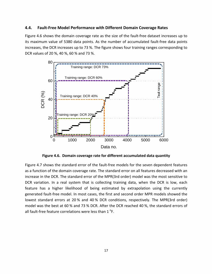
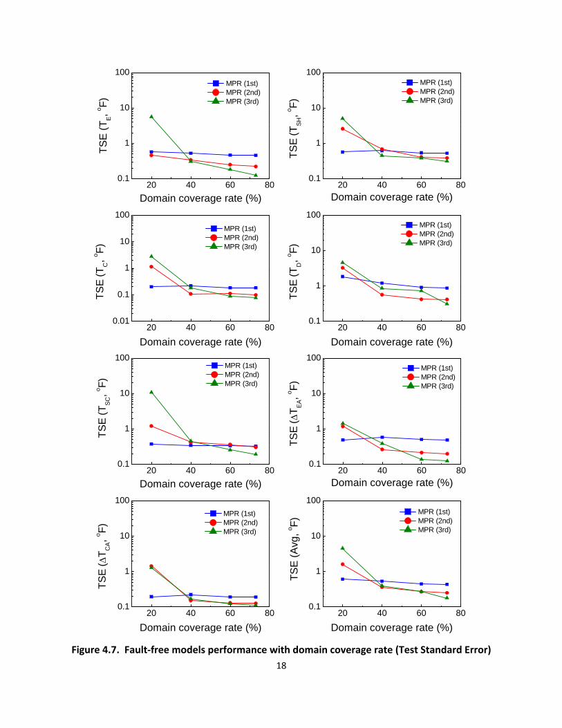
100 100 MPR (1st) MPR (1st) MPR (2nd) MPR (2nd) MPR (3rd) MPR (3rd)
10 T
SE(T
o
F)
TS
E(T
o
F)
TS
E(T
C o
F)
TS
E (
T o
F)
CA
SC
E
TS
E (
Avg
oF
) T
SE(
T
oF
) T
SE(T
oF
) T
SE(
T o
F)
EA
D
SH
10
1 1
01 01 20 40 60 80 20 40 60 80
Domain coverage rate () Domain coverage rate ()
100 100 MPR (1st) MPR (1st) MPR (2nd) MPR (2nd)10 MPR (3rd) MPR (3rd) 10
1
01 1
001 01 20 40 60 80 20 40 60 80
Domain coverage rate () Domain coverage rate ()
100 100 MPR (1st) MPR (1st) MPR (2nd) MPR (2nd) MPR (3rd) MPR (3rd)
10
1
10
1
01 01 20 40 60 80 20 40 60 80
Domain coverage rate () Domain coverage rate ()
100 100
MPR (1st) MPR (1st) MPR (2nd) MPR (2nd)
MPR (3rd) 10 MPR (3rd)
10
1 1
01 01 20 40 60 80 20 40 60 80
Domain coverage rate () Domain coverage rate ()
Figure 47 Fault‐free models performance with domain coverage rate (Test Standard Error)
18
The above standard error results are consistent with Braun and Li (2001) who commented that
the lower the order of the MPR model the better the extrapolation performance in general
When the DCR is low each feature has a higher likelihood of being estimated by extrapolation
For models generated at higher DCRs extrapolation is less likely and higher‐order MPR models
are better where interpolation is required
Figure 48 shows TSE of the MPR models for 20 40 60 and 73 DCR as a function of zone density At a DCR of 20 the TSE of MPR(3rd order) and MPR(2nd order) exceeded 4 oF and 1 oF respectively with steep increases at low ZD values For the higher DCRs the TSE stayed below 1 oF for all models and ZDs except MPR(3rd order) for 40 DCR and ZD less than 25 For 60 and 73 DCR all three models performed in a stable fashion smoothly improving predictions as DCR and ZD values increased
From this analysis the MPR(1st order) and MPR(2nd order) models are recommendable for the intermediate fault‐free models at a DCR of 20 and 40 respectively After the DCR exceeds 60 the MPR(3rd order) model is the most appropriate for the final fault‐free model A ZD between 100 and 50 is recommended for data filtering and storing criteria
40 10 MPR (1st) MPR (2nd) MPR (3rd)
DCR 20
30 20 08
TS
E(
Avg
oF
) T
SE
(A
vg o F
)
TS
E(
Avg
oF
) T
SE(
Avg
oF
)10 8 06
04 6
4 MPR (1st)DCR 4002 MPR (2nd)2 MPR (3rd)
0 00All 100 50 25 10 5 1 All 100 50 25 10 5 1
Zone density Zone density
10 DCR 60 MPR (1st) MPR (1st)DCR 7309
MPR (2nd) MPR (2nd)08 MPR (3rd) 07
MPR (3rd)
06 05
04 03
02 01
00 All 100 50 25 10 5 1 All 100 50 25 10 5 1
Zone density Zone density
Figure 48 Model standard error with zone density at DCR of 20 40 60 and 73
19
5 Validation
We tested and validated the self training method by applying the fault‐free models developed using the self training scheme to an experimental dataset collected by Kim et al (2006) on a heat pump operating in the cooling mode In addition the FDD performance was compared and analyzed considering different zone densities and domain coverage rates Successful diagnosis ratio false alarm missed detection and misdiagnosis were calculated and presented to evaluate the overall FDD performance
51 Validation Dataset and Fault Types
The dataset assembled by Kim et al (2006) includes performance data during fault‐free
operation (72 points) and with seven faults compressor valve leakage improper outdoor air
flow improper indoor air flow liquid line restriction refrigerant undercharge refrigerant
overcharge and non‐condensables (84 points) (Table 51)
Table 51 Definition and range of studied heat pump operational cases
Fault name Symbol Definition of fault Fault
range () Temperature range (oF)
Number of points
Fault‐free (Normal operation)
FF ‐ ‐TOD 80 to 102 TID 65 to 85 TIDP 42 to 85
72
Compressor valve leakage
(4 to way valve leakage)
CMF reduction in refrigerant flow rate from no‐fault
value 3 to 40
TOD 80 to 100 TID 70 to 80 TIDP 50 to 61
16
Reduced outdoor air TOD 80 to 100 flow rate (condenser CF of coil area blocked 10 to 50 TID 70 to 80 13
fouling) TIDP 50 to 61
Improper indoor air flow rate (evaporator
fouling) EF
below specified air flow rate
6 to 35 TOD 80 to 100 TID 70 to 80 TIDP 42 to 61
19
Liquid line restriction LL
change from no‐fault pressure drop from liquid
line service valve to indoor TXV inlet
10 to 32 TOD 80 to 100 TID 70 to 80 TIDP 50 to 61
6
20
Refrigerant undercharge
UC mass below correct
(no‐fault) charge 10 to 30
TOD 80 to 100 TID 70 to 80 TIDP 50 to 61
12
Refrigerant overcharge
OC mass above correct (no‐fault) charge
10 to 30 TOD 80 to 100 TID 70 to 80 TIDP 50 to 61
12
Presence of non‐condensable
gases NC
of pressure in evacuated indoor section and line set due to non‐condensable gas with respect to atmospheric
pressure
10 to 20 TOD 80 to 100 TID 70 to 80 TIDP 50 to 61
6
52 Fault Detection and Diagnostic Method
When the system is operating with a fault it is expected that feature temperatures willdeviate
from their normal fault‐free values An individual featurersquos deviation could be negative
positive or ldquoneutralrdquo (close to the fault‐free value within a pre‐defined threshold) collectively
the featurersquos deviations (or residuals) form a pattern which is unique for a given fault To
detect and diagnose the fault a statistical rule‐based classification is performed by calculating
the probability of the various fault‐types based on the decision rules defined within a rule‐
based chartrsquos predefined fault patterns A set of measurement features can be regarded as a
multi‐dimensional Gaussian probability distribution With the assumption that each dimension
is independent each of the three ldquoclassrdquo problems (negative positive or neutral) can be
represented by a simple normal (Gaussian) distribution rather than a more complicated
distribution with multiple degrees of freedom and dependencies (Rossi et al 1995 Kim et al
2008b) The probability of the kth fault corresponding to the set of m statistically independent
variables (X our features) is given by Equation 51 where P(Cik|Xi) denotes the individual
probability of case variable C (negative positive or neutral) for the ith feature with the kth fault
type Since the features are assumed to be independent the total conditional probability P(Fk|
X) can be obtained by the multiplication of the individual probabilities
m
P(Fk X) P(C1k X ) P(C X 2 ) P(Cik X i ) P(Cik X i ) (51)1 2k i1
21
Figure 51 Probability for three measurement residual cases of positive neutral and negative
In Figure 51 the three differently cross‐hatched areas under the Normal Distribution N(μiFF
σiFF) represents the probability of the current measurement (or predicted value) represented
by a second normal distribution PDF(xi σi) being lower higher or relatively close (neutral) to
the predicted fault‐free modelrsquos value if the conditions are fault‐free the difference in the
measured and predicted value the residual ri = xi ndash μiFF will equal zero In order to locate the
position of the current measurement under the normal distribution we must convert the
currently measured value to its standard form we must represent the current measurement as
some number of fault‐free model standard deviations from the mean value of the fault‐free
normal distribution (the currently predicted value) This standardization is often called the z‐
value Therefore the z‐value for the current measurement zi is defined by our residual and the
standard deviation of the fault‐free model as shown in Equation 52
x ri iFF izi (52) i FF i FF
Using the assumption of independent normally distributed FDD features the area under the
normal distribution N(μiFF σiFF) must be determined in order to place a numerical value on the
probability This integral is represented by the cumulative distribution function Φ(x) Equation
22
53 of the standard normal distribution (a normal distribution with a mean of zero and
standard deviation of 1 N(01))
௫ቀݎଵ
ଶଵଶ
ൌሻݔሺemptyradicଶቁ (53)
The cumulative distribution function describes the probability of a real number value with a
given probability distribution function X ϵ PDF(xi σi) having a value less than or equal to a
given value a This can be re‐stated as Equation 54
(54)ሻሺ ൌሻሺempty
This also leads to the probability of X lying within the semi‐closed interval (a b] or being greater
than some value b Equations 55 and 56 respectively
ሻሺെ emptyሻሺൌ emptyሻ ሺ
ሻሺൌ 1 െ empty ሻ ሺ
(55)
(56)
For the purposes of FDD we would like to know whether the residual ri is positive negative or
insignificant (ie within plusmnεi (neutral threshold) of the FF model predicted value μiFF) In order
to use the cumulative distribution function we must standardize the intervals around the
currently measured value xi plusmn εi as a multiple of the FF model standard deviation therefore we
ldquostandardizerdquo εi as being s number of FF model standard deviations as shown in Equation 57 s
is the ldquostandardizedrdquo width of the neutral threshold (sgt0) The standardized representation of
the residual and three possible cases (positive negative and neutral) are shown in Figure 52
s or ݏ ൌ ఌ
(57)i iFF ఙಷಷ
Now we may use Equation 56 to determine the probability of the residual being greater than
+εi the negative residual case
|
Less than or equal to ‐εi the positive residual case using Equation 54
ሺܥdarr ሻ ൌ ሺݖ ሺݖ ሻሻݏ ൌ 1 െ emptyሺݖ ሻ (58)ݏ
|
Or in the neutral interval of plusmnεi using Equation 55
(510)ሻെ ሺെݖݏ emptyሻ ሺൌݖݏ emptyሻ ሻݏ ሺݖെ ሻݏ ሺൌݖሺݖ ሻ|ܥሺ
ሺܥuarr ሻ ൌ ሺݖ ሺݖ െ ሻሻݏ ൌ emptyሺݖ െ ሻ (59)ݏ
23
Figure 52 Standard normal distribution showing the current measurements z‐value and
standardized neutral threshold s
The summation of probabilities calculated in Equations 58 to 510 equals unity Equation 511
since the integral of any PDFs from ndashinfin to +infin must equal one by definiƟon
P(C X i ) P(C
X i ) P(C X i ) 1 (511)
When the fault level increases the residual between the measured data and predicted data
may increase decrease or remain relatively unchanged Figure 53 shows the residual pattern
analysis results for the seven studied faults which were used to generate a rule‐based chart
Due to the careful selection of the most sensitive (rapidly changing) features for a given fault
type the feature patterns were quite different for all fault types and each pattern (positive
negative and neutral) for a given fault is the template for the calculation of fault probability in
Equation 51 For example the probability of a CMF fault (valve leakage) can be calculated by
the multiplication of the conditional probabilities of the residuals having the following pattern
TE (positive) TSH (neutral) TC (negative) TD (positive) TSC (negative) ∆TEA (negative) and ∆TCA
(negative) as shown in Equation 512
P(FCMF X) P(C TE ) P(C TSH ) P(C TC ) P(C TD ) P(C TSC ) (512)
P(C TEA ) P(C TCA )
24
5
0
-5
0
15 20 CMF CF
10 10
Re
sid
ua
l (oF
) R
esid
ual (
o F)
Re
sid
ua
l (oF
)
Res
idua
l (o F
) R
esid
ual (
o F)
Res
idua
l (o F
)
0
-10 -10
Neutral Positive Negative Neutral Positive Negative
-15 -20 T T T T T T T T T T T T T T
E SH C D SC EA CA E SH C D SC EA CA
8 20EF LL
4
0
-4
10
0
-10
Neutral Positive Negative Neutral Positive Negative -8 -20
T T T T T T T T T T T T T TE SH C D SC EA CA E SH C D SC EA CA
20 UC 20 OC
10
-10
10
0
-10
-20 Neutral Positive Negative -20 Neutral Positive Negative
TE
TSH
TC
TD
T T TSC EA CA
TE
TSH
TC
TD
T T TSC EA CA
20 NC
Re
sid
ua
l (oF
) 10
0
-10
Neutral Positive Negative
-20 T
E T
SH T
C T
D T T T
SC EA CA
Figure 53 Residual patterns for different faults
25
Table 52 Rule‐based FDD chart for air‐to‐air single‐speed heat pump in the cooling mode
Fault type TE TSH TC TD TSC ΔTEA ΔTCA
FF (Fault‐free)
CMF (Compressor valve leakage)
CF (Improper outdoor air flow)
EF (Improper indoor air flow)
LL (Liquid‐line restriction)
UC (Refrigerant undercharge)
OC (Refrigerant overcharge)
NC (Presence of non‐condensable gases)
The value of s must be determined so that it produces a given level of confidence that the
currently measured value is within the neutral threshold (or outside this threshold) The
confidence level is selected by the investigator typical values of α are 001 005 and 010 with
corresponding confidence levels of (1 - α) of 099 095 and 090 (Graybill and Iyer 1994) In
applying the s values the user is determining the alarm thresholds for calling a fault or no‐fault
Table 53 shows standard deviations and thresholds with different zone densities for MPR(3rd
order) models regressed to FDD test data In general if thresholds increase the false alarm rate
(FAR) decreases but missed detections increase and vice versa In this study the threshold for a
95 confidence level was applied to the FDD test data Table 54 summarizes the standard
deviations and thresholds for different domain coverage rates Models with the best fit were
26
selected with respect to the domain coverage rate the standard deviation and threshold
prominently increased with a decrease of DCR
Table 53 Standard deviation (oF) of the fault‐free model for different ZD (DCR=73 all data)
ZD Applied model
σ (TE) σ (TSH) σ (TC) σ (TD) σ (TSC) σ (ΔTEA) σ (ΔTCA)
All 3rd order MPR
0124 0314 0077 0310 0191 0124 0112
100 3rd order MPR
0133 0322 0081 0318 0195 0135 0114
50 3rd order MPR
0147 0388 0093 0521 0219 0156 0117
25 3rd order MPR
0149 0420 0094 0590 0236 0159 0119
10 3rd order MPR
0144 0432 0093 0597 0258 0157 0121
5 3rd order MPR
0141 0433 0097 0589 0258 0158 0125
1 3rd order MPR
0144 0442 0099 0537 0277 0166 0138
ε90 165∙σiFF model
ε95 196∙σiFF model
ε99 258∙σiFF model
Table 54 Standard deviation (oF) of fault‐free model for different DCR (ZD =100)
DCR () Applied model
σ (TE) σ (TSH) σ (TC) σ (TD) σ (TSC) σ (ΔTEA) σ (ΔTCA)
73 3rd order MPR
0133 0322 0081 0318 0195 0135 0114
60 3rd order MPR
0197 0385 0090 0811 0282 0160 0123
40 2nd order MPR
0390 0641 0109 0625 0401 0294 0155
20 1st order MPR
0673 0659 0196 2111 0393 0523 0196
ε90 165∙σiFF model
ε95 196∙σiFF model
ε99 258∙σiFF model
27
53 Procedure for Testing and Rating FDD Performance
The faults summarized in Table 51 were part of the experimental dataset (Kim et al 2006)
applied to test FDD performance For each dataset the fault probability for eight conditions (FF
CMF CF EF LL UC OC and NC) was calculated using Equation 51 and the rule‐based chart
fault patterns as given in Table 52 Among the probabilities of the eight conditions the fault
type with the highest fault probability was selected as the fault type most likely occurring at the
time When the diagnosed fault type was the same as the originally imposed fault type the
diagnostic was considered successful The goodness of the FDD method was further explored by
applying the concepts of FDD performance evaluation as defined by Braun et al (2012)
Successful diagnosis rate SDR () A fault is present The summation of the detected and
successfully diagnosed cases divided by total number of faulty tests equals the SDR for the
particular fault
False alarm rate FAR () No fault is present but the protocol indicates the presence of a
fault The FAR equals the number of false alarm cases divided by the total number of fault‐
free tests
Missed detection rate MDR () A fault is present but the protocol indicates that no fault is
present The MDR equals the number of missed detection cases divided by the total number
of faulty tests
Misdiagnosis rate MSR () A fault is present The protocol detects the fault but
misdiagnoses the fault type The MSR equals the number of misdiagnosis cases divided by
the total number of fault‐free and faulty tests
The above performance indices address that the detection aspect of FDD (FAR and MDR) and
the diagnosis (SDR and MSR)
As recommended in Section 43 the third order MPR model was applied for the fault‐free
model training A zone coverage rate of 73 represented all of the data and was used for this
analysis Figure 54 shows the SDR for the eight conditions with different zone densities In the
cases of FF CMF EF and OC the successful diagnosis rate (SDR ) was relatively high more
than 80 for all zone densities The SDR of CF and UC was between 60 and 80 and that of LL
and NC was less than 50 The feature pattern of the NC fault was very similar to that of OC
which was the reason for the inconsistent FDD performance on this fault (Figure 52) In the
case of the LL fault the fault pattern was unclear and additional fault data for LL was needed
since only six datasets were available for this fault case Overall the SDR gradually decreased
when zone density was less than 100 or 50 due to the increase in the standard deviation of the
fault‐free models and neutral threshold width for a 95 confidence (Figure 46) The average
28
SDR with a zone density of ALL and 100 was 83 and 82 respectively and gradually
decreased from 75 to 71 as the zone density decreased
Suc
cess
ful d
iagn
osis
rat
e (
)
100
90
80
70
60
50
40
30
20
10
0 FF CMF CF EF LL UC OC NC Avg
Zone density All 100 50 25 10 5 1
Fault types
Figure 54 Successful diagnosis rate of various faults for different zone densities
False alarm missed detection misdiagnosis were analyzed with decreasing zone density and
presented in Figure 55 False alarm and missed detection were not observed at the tests with
zone densities of ALL and 100 For zone densities less than 50 the false alarm case increased
from 42 to 56 with decreasing zone density Missed detections also increased from 36
to 95 with decreasing zone density The FAR was less than 6 and the MDR was less than
10 at all zone density conditions A zone density greater than 100 would be the best choice
for a high quality FDD application due to the observed stability and predictive accuracy seen in
our experimental dataset Fault diagnosis performance with zone densities of ALL and 100 was
also superior to cases with zone density less than 100 Misdiagnoses were 77 and 83 at
zone densities of ALL and 100 respectively with misdiagnoses distributed from 135 to 162
at zone densities less than 100
29
40
35
30
25
20
15
10
5
0
Zone density
Figure 55 Fault detection and diagnostic performance for all eight conditions for different zone densities
54 Effect of Domain Coverage Rate on FDD Performance
As recommended in Section 44 the first order and second MPR models were applied for the
fault‐free models at a DCR of 20 and from 40 to 60 respectively When the DCR was
more than 60 the MPR(3rd order) model was applied to the fault‐free model training A zone
density of 100 was applied for this analysis
The successful diagnosis rate SDR for eight fault conditions and varying domain coverage rates
are presented in Figure 56 With a DCR of 73 and 60 the FF CMF EF UC and OC faults
showed an SDR of more than 85 The SDR of CF and NC faults was between 60 and 70
and that of LL was less than 50 Exact diagnosis of FF is very important because it determines
the fault detection performance (false alarm rate FAR) In case of FF operation the SDR
drastically decreased below 65 when the DCR was 20 In cases of CMF EF UC and NC
faults the SDR significantly decreased at a DCR of 40 and 20 due to the increase in the
standard deviation of the FF model and corresponding increase in the neutral threshold The
overall average SDR gradually decreased from 89 to 61 with the decrease of DCR from 73
to 20
Figure 57 shows FAR (false alarm rate) MDR (missed detection rate) and MSR (misdiagnosis
rate) with the decrease of the DCR (domain coverage rate) False alarm and missed detection
were not observed in the tests with zone coverage rate of 73 FAR was 139 and 83 at
FD
D p
erfo
rman
ce (
)
False alarm rate () Missed detection rate () Misdiagnosis rate ()
All 100 50 25 10 5 1
30
DCR 60 and 40 respectively and then drastically increased to 375 at DCR 20 MDR
gradually increased from 714 to 262 with the decrease of DCR from 60 to 20 MSR
remained below 10 at DCR 73 and 60 and then the misdiagnosis rate steeply increased
to 186 and 385 at a DCR of 40 and 20 At a DCR from 73 to 60 FAR MDR and
MSR were all below 10 However FDD performances worsened at DCRs from 40 to 20
From Figures 56 and 57 DCRs greater than 60 were recommendable for a high quality FDD
application due stability and prediction accuracy In addition DCRs greater than 40 might be
acceptable for a lower quality FDD application if the fault detection error less than 15 was
allowable
100
90
80
70
60
50
40
30
20
10
0
Fault types
Figure 56 Successful diagnosis rate of various faults for different domain coverage rates
Suc
cess
ful d
iagn
osi
s ra
te (
)
Domain coverage rate () 73 60 40 20
FF CMF CF EF LL UC OC NC Avg
31
FD
D p
erfo
rman
ce (
)
40
35
30
25
20
15
10
5
0 73 60 40 20
False alarm rate () Missed detection rate () Misdiagnosis rate ()
Model with best fit DCR 73 3rd MPR model DCR 60 3rd MPR model DCR 40 2nd MPR model DCR 20 1st MPR model
Domain coverage rate ()
Figure 57 Fault detection and diagnostic performance for all faults for different domain coverage rates
6 Concluding Remarks
A concept for a self training fault‐free model for residential air conditioner fault detection and
diagnosis was introduced and tested The method of selecting the appropriate temperature
domain for the fault‐free system data was illustrated in order to cover most operating
conditions considering different climate zones in the US The fault‐free system performance
was modeled based upon three independent features (TOD TID TIDP) and seven dependent
features (TE TSH TC TD TSC ΔTEA ΔTCA) The new concept of zone density was introduced to
manage and filter the system data In addition the new concept of domain coverage rate was
also introduced to quantify the number of data needed to produce fault‐free feature models
Various fault‐free models such as the ANN (artificial neural network) the MPR (multivariable
polynomial regression) and a combined ANNMPR were explored for implementing self
training The MPR method was shown to produce very good prediction performance (low
standard errors) compared to the methods using ANNs Therefore MPR models were applied
and tested against previously taken system data for additional analysis of self training
For validation of the self training method the full experimental dataset (72 fault‐free and 84
fault tests) covering eight faultconditions (fault‐free compressor valve leakage outdoor coil
air flow blockage improper indoor air flow liquid‐line restriction refrigerant undercharge
32
refrigerant overcharge and non‐condensable gas contamination) was used to explore self
training performance The statistical rule‐based fault classification method was illustrated
FDD performance was analyzed using the successful detection rate (SDR) false alarm rate (FAR)
missed detection rate (MDR) and misdiagnosis rate (MSR) as zone density (ZD) and domain
coverage rate (DCR) were varied This effort showed that a zone density greater than 100 was
very successful within the experimental dataset In addition a domain coverage rate greater
than 60 produced acceptable FDD performance and good prediction performance (low
standard errors)
This report attempts to document a mathematical and logical technique by which an FDD
technique may be adapted to an air conditioning system with variations in installation details as
would be seen in actual residences It is by no means a perfected technique applicable to
immediate deployment many issues remain that still must be resolved by laboratory
investigation and application to real world problems When considering using an adaptive
technique for FDD in a real application the following questions must be resolved
1) What operating states are suitable for learning Steady state is important but what
about heat pumps operating in frosting conditions for heating What about the effects of
rain on the outdoor unit What about cooling operation at low outdoor temperatures when
the TXV is operating at the edges of its steady control band A key part of the learning
algorithm is developing a filtering algorithm which picks only the data known to be good
2) How does the FDD technique deal with the fact that the unit is aging and changing over
time In a real learning algorithm you must wait for the driving conditions to present
themselves If you install an air‐conditioner in the Fall season it could be 10 months before
you see data for the hottest day Is it fair to assume that the unit is unchanged since its
install What if the home owner tenant keeps their cooling setpoint at 75 degF all of the time
Now a new ownertenant moves in and runs the house at 70 degF can you use the old FDD
model
3) How do you deal withquantify the noise seen in sensors installed in the field Large
transients and noise may be seen in sensor readings A method of quantifying the sensor
noises and creating dynamic error bands need to be developed How does the FDD deal
with a brokenmalfunctioning sensor
The next step is to take this idea to the laboratory and the field and start solving the
outstanding issues
33
References
AHRI (2008) Performance rating of unitary airconditioning and airsource heat pump
equipment AHRI Standard 210240 Arlington VA USA Air‐Conditioning Heating and
Refrigeration Institute
Baechler M Williamson J Gilbride T Cole P Hefty M Love P (2010) High‐performance
home technologies Guide to determining climate regions by county US Department of Energy
PNNL‐19004
Braun J (1999) Automated fault detection and diagnostics for vapor compression cooling
equipment International Journal of Heating Ventilating Air‐Conditioning and Refrigerating
Research 5(2) 85‐86
Braun J amp Li H (2001) Description of FDD modeling approach for normal performance
expectation West Lafayette IN Herrick Labs Purdue University
Braun J Yuill D Cheung H (2012) A method for evaluating diagnostic protocols for
packaged air conditioning equipment CEC‐500‐08‐049 West Lafayette IN USA Purdue
University Herrick Laboratories
Chen B Braun J E (2001) Simple rule‐based methods for fault detection and diagnostics
applied to packaged air conditioners ASHRAE Transactions 107(1) 847‐857
Cho J Heo J Payne W Domanski P (2014) Normalized performances for a residential heat
pump in the cooling mode with single faults imposed Applied Thermal Engineering 67 1‐15
EIA 2013 US Energy Information Agency Residential Energy Consumption Survey
httpwwweiagovelectricitysales_revenue_pricepdftable5_apdf (Accessed April 2015)
EIA 2014 US Energy Information Agency Residential Energy Consumption Survey
httpwwweiagovtoolsfaqsfaqcfmid=96ampt=3 (Accessed April 2015)
Frenz C (2002) Visual basic and visual basicnet for scientists and engineers Apress 1st Edition
February
Graybill F Iyer H (1994) Regression analysis Concepts and applications second ed Belmont
CA USA Duxbury Press
Heo J Payne W Domanski P (2012) FDD CX A fault detection and diagnostic
commissioning tool for residential air conditioners and heat pump NIST TN 1774 Gaithersburg
MD National Institute of Standards and Technology
Kim M Payne W Domanski P Hermes C (2006) Performance of a Residential Air
Conditioner at Single‐Fault and Multiple‐Fault Conditions NISTIR 7350 Gaithersburg MD
National Institute of Standards and Technology
34
Kim M Yoon S Domanski P Payne W (2008a) Design of a steady‐state detector for fault
detection and diagnosis of a residential air conditioner Int J Refrig 31 790‐799
Kim M Yoon S Payne W Domanski P (2008b) Cooling mode fault detection and diagnosis
method for a residential heat pump NIST SP 1087 Gaithersburg MD National Institute of
Standards and Technology
Kim M Yoon S Payne W Domanski P (2010) Development of the reference model for a
residential heat pump system for cooling mode fault detection and diagnosis Journal of
Mechanical Science and Technology 24(7) 1481‐1489
Li H Braun J (2003) An improved method for fault detection and diagnosis applied to
packaged air conditioners ASHRAE Transactions 109(2) 683‐692
Payne W Domanski P Yoon S (2009) Heating mode performance measurements for a
residential heat pump with single‐faults imposed NIST TN 1648 Gaithersburg MD National
Institute of Standards and Technology
Rossi T Braun J E (1997) A statistical rule‐based fault detection and diagnostic method for
vapor compression air conditioners HVACampR Research 3(1) 19‐37
Thornton B Wang W Lane M Rosenberg M Liu B (2009) Technical support document
50 energy savings design technology packages for medium office buildings US Department
of Energy PNNL‐19004
Yoon S Payne W Domanski P (2011) Residential heat pump heating performance with
single faults imposed Applied Thermal Engineering 31 765‐771
Acknowledgements
The authors would like to acknowledge Min Sung Kim (Chief Thermal Energy Conversion Laboratory Korea Institute of Energy Research ndash KIER) Seok Ho Yoon (Korea Institute of Machinery and Materials) Jin Min Cho and Young‐Jin Baik (Engineer Thermal Energy Conversion Laboratory Korea Institute of Energy Research ndash KIER) for their work in developing the background material used in this report Also John Wamsley Glen Glaeser and Art Ellison provided technician support for collecting the data used to develop FDD fault‐free feature correlations We also would like to thank Will Guthrie of the NIST Statistical Engineering Division for reviewing the statistical FDD method section and Dan Veronica of the NIST Energy and Environment Division for reviewing and commenting on the entire document
35
Appendix A Temperature Data Distribution
The temperature domain should be selected in order to cover most of the operating conditions
a residential air conditioner may experience As summarized in Appendix A and Table A1 the
US climate may be divided into seven climate zones based upon certain criteria (Baechler et al
2010) Seven representative cities within these zones were chosen as a source for temperature
and humidity data (Thornton et al 2009) The most recent five year climate data were
investigated as shown in Figure A2 Temperature data domains for outdoor and indoor
temperature with relative humidity were determined using data for these seven cities
Table A1 Temperature domain by climate zone
Temp domain
Hot humid Hot dry Mixed humid
Mixed dry Marine Cold Very cold
TOD
80 to 105 by a step of 5 oF
(5 zones)
80 to 100 by a step of 5 oF
(4 zones)
80 to 105 by a step of 5 oF
(5 zones)
80 to 105 by a step of 5 oF
(5 zones)
80 to 95 by a step of 5 oF
(3 zones)
80 to 100 by a step of 5 oF
(4 zones)
80 to 95 by a step of 5 oF
(3 zones)
TID 65 to 85 by a step of 5 oF
(4 zones)
RH 20 to 80 by a step of 20
(3 zones)
36
Figure A1 Representative cities for seven US climate zones
37
120 120 O
D t
emp
(o F
) O
D t
em
p
(o F)
OD
tem
p
(o F) 100 100
80 80
60 60
40 40
20 20 Los Angeles (Hot dry)Houston (Hot humid)
0 01 2 3 4 5 6 7 8 9 10 11 12 1 2 3 4 5 6 7 8 9 10 11 12
120 120
100 100
80 80
60 60
40 40
20 20Baltimore (Mixed humid) Albuquerque (Mixed dry)
0 01 2 3 4 5 6 7 8 9 10 11 12 1 2 3 4 5 6 7 8 9 10 11 12
120 120
100 100
80 80
60 60
40 40
20
0 1 2 3 4
San Francisco (Marine)
5 6 7 8 9 10 11 12
20
0 1 2 3 4 5 6
Chicago (Cold)
7 8 9 10 11 12
120
O
D t
emp
(o F
) 100
80
60
40
20
0 1 2 3 4
Duluth (Very cold)
5 6 7 8 9 10 11 12
Month
Figure A2 Maximum outdoor temperature distributions in seven climate zones from 2008 to 2012
38
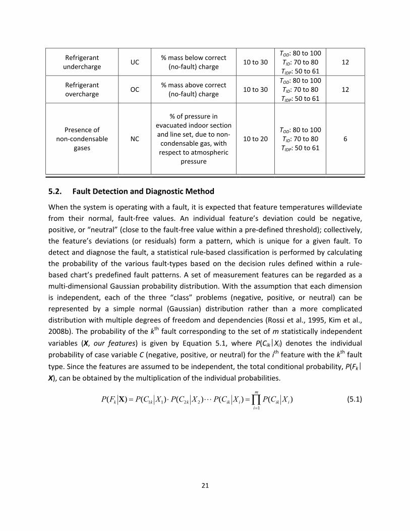
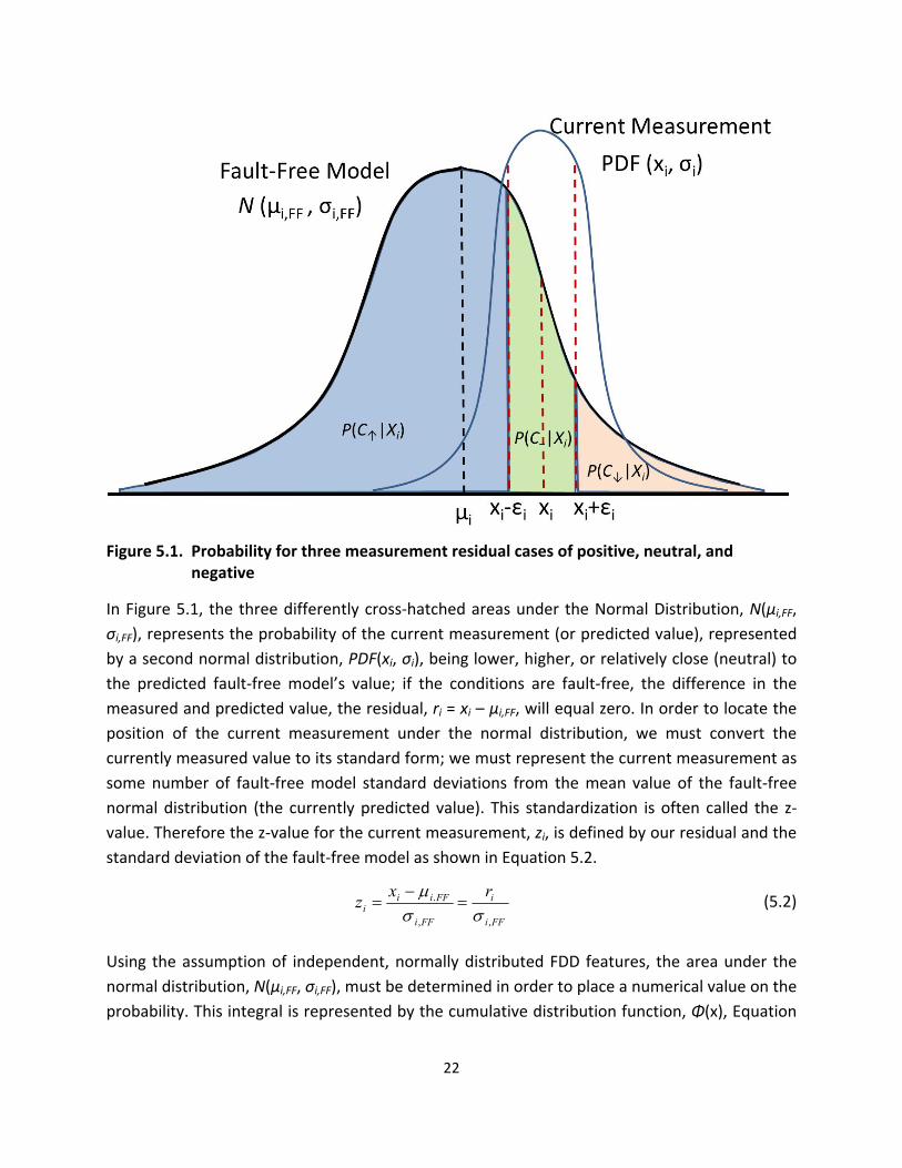

5
0
-5
0
15 20 CMF CF
10 10
Re
sid
ua
l (oF
) R
esid
ual (
o F)
Re
sid
ua
l (oF
)
Res
idua
l (o F
) R
esid
ual (
o F)
Res
idua
l (o F
)
0
-10 -10
Neutral Positive Negative Neutral Positive Negative
-15 -20 T T T T T T T T T T T T T T
E SH C D SC EA CA E SH C D SC EA CA
8 20EF LL
4
0
-4
10
0
-10
Neutral Positive Negative Neutral Positive Negative -8 -20
T T T T T T T T T T T T T TE SH C D SC EA CA E SH C D SC EA CA
20 UC 20 OC
10
-10
10
0
-10
-20 Neutral Positive Negative -20 Neutral Positive Negative
TE
TSH
TC
TD
T T TSC EA CA
TE
TSH
TC
TD
T T TSC EA CA
20 NC
Re
sid
ua
l (oF
) 10
0
-10
Neutral Positive Negative
-20 T
E T
SH T
C T
D T T T
SC EA CA
Figure 53 Residual patterns for different faults
25
Table 52 Rule‐based FDD chart for air‐to‐air single‐speed heat pump in the cooling mode
Fault type TE TSH TC TD TSC ΔTEA ΔTCA
FF (Fault‐free)
CMF (Compressor valve leakage)
CF (Improper outdoor air flow)
EF (Improper indoor air flow)
LL (Liquid‐line restriction)
UC (Refrigerant undercharge)
OC (Refrigerant overcharge)
NC (Presence of non‐condensable gases)
The value of s must be determined so that it produces a given level of confidence that the
currently measured value is within the neutral threshold (or outside this threshold) The
confidence level is selected by the investigator typical values of α are 001 005 and 010 with
corresponding confidence levels of (1 - α) of 099 095 and 090 (Graybill and Iyer 1994) In
applying the s values the user is determining the alarm thresholds for calling a fault or no‐fault
Table 53 shows standard deviations and thresholds with different zone densities for MPR(3rd
order) models regressed to FDD test data In general if thresholds increase the false alarm rate
(FAR) decreases but missed detections increase and vice versa In this study the threshold for a
95 confidence level was applied to the FDD test data Table 54 summarizes the standard
deviations and thresholds for different domain coverage rates Models with the best fit were
26
selected with respect to the domain coverage rate the standard deviation and threshold
prominently increased with a decrease of DCR
Table 53 Standard deviation (oF) of the fault‐free model for different ZD (DCR=73 all data)
ZD Applied model
σ (TE) σ (TSH) σ (TC) σ (TD) σ (TSC) σ (ΔTEA) σ (ΔTCA)
All 3rd order MPR
0124 0314 0077 0310 0191 0124 0112
100 3rd order MPR
0133 0322 0081 0318 0195 0135 0114
50 3rd order MPR
0147 0388 0093 0521 0219 0156 0117
25 3rd order MPR
0149 0420 0094 0590 0236 0159 0119
10 3rd order MPR
0144 0432 0093 0597 0258 0157 0121
5 3rd order MPR
0141 0433 0097 0589 0258 0158 0125
1 3rd order MPR
0144 0442 0099 0537 0277 0166 0138
ε90 165∙σiFF model
ε95 196∙σiFF model
ε99 258∙σiFF model
Table 54 Standard deviation (oF) of fault‐free model for different DCR (ZD =100)
DCR () Applied model
σ (TE) σ (TSH) σ (TC) σ (TD) σ (TSC) σ (ΔTEA) σ (ΔTCA)
73 3rd order MPR
0133 0322 0081 0318 0195 0135 0114
60 3rd order MPR
0197 0385 0090 0811 0282 0160 0123
40 2nd order MPR
0390 0641 0109 0625 0401 0294 0155
20 1st order MPR
0673 0659 0196 2111 0393 0523 0196
ε90 165∙σiFF model
ε95 196∙σiFF model
ε99 258∙σiFF model
27
53 Procedure for Testing and Rating FDD Performance
The faults summarized in Table 51 were part of the experimental dataset (Kim et al 2006)
applied to test FDD performance For each dataset the fault probability for eight conditions (FF
CMF CF EF LL UC OC and NC) was calculated using Equation 51 and the rule‐based chart
fault patterns as given in Table 52 Among the probabilities of the eight conditions the fault
type with the highest fault probability was selected as the fault type most likely occurring at the
time When the diagnosed fault type was the same as the originally imposed fault type the
diagnostic was considered successful The goodness of the FDD method was further explored by
applying the concepts of FDD performance evaluation as defined by Braun et al (2012)
Successful diagnosis rate SDR () A fault is present The summation of the detected and
successfully diagnosed cases divided by total number of faulty tests equals the SDR for the
particular fault
False alarm rate FAR () No fault is present but the protocol indicates the presence of a
fault The FAR equals the number of false alarm cases divided by the total number of fault‐
free tests
Missed detection rate MDR () A fault is present but the protocol indicates that no fault is
present The MDR equals the number of missed detection cases divided by the total number
of faulty tests
Misdiagnosis rate MSR () A fault is present The protocol detects the fault but
misdiagnoses the fault type The MSR equals the number of misdiagnosis cases divided by
the total number of fault‐free and faulty tests
The above performance indices address that the detection aspect of FDD (FAR and MDR) and
the diagnosis (SDR and MSR)
As recommended in Section 43 the third order MPR model was applied for the fault‐free
model training A zone coverage rate of 73 represented all of the data and was used for this
analysis Figure 54 shows the SDR for the eight conditions with different zone densities In the
cases of FF CMF EF and OC the successful diagnosis rate (SDR ) was relatively high more
than 80 for all zone densities The SDR of CF and UC was between 60 and 80 and that of LL
and NC was less than 50 The feature pattern of the NC fault was very similar to that of OC
which was the reason for the inconsistent FDD performance on this fault (Figure 52) In the
case of the LL fault the fault pattern was unclear and additional fault data for LL was needed
since only six datasets were available for this fault case Overall the SDR gradually decreased
when zone density was less than 100 or 50 due to the increase in the standard deviation of the
fault‐free models and neutral threshold width for a 95 confidence (Figure 46) The average
28
SDR with a zone density of ALL and 100 was 83 and 82 respectively and gradually
decreased from 75 to 71 as the zone density decreased
Suc
cess
ful d
iagn
osis
rat
e (
)
100
90
80
70
60
50
40
30
20
10
0 FF CMF CF EF LL UC OC NC Avg
Zone density All 100 50 25 10 5 1
Fault types
Figure 54 Successful diagnosis rate of various faults for different zone densities
False alarm missed detection misdiagnosis were analyzed with decreasing zone density and
presented in Figure 55 False alarm and missed detection were not observed at the tests with
zone densities of ALL and 100 For zone densities less than 50 the false alarm case increased
from 42 to 56 with decreasing zone density Missed detections also increased from 36
to 95 with decreasing zone density The FAR was less than 6 and the MDR was less than
10 at all zone density conditions A zone density greater than 100 would be the best choice
for a high quality FDD application due to the observed stability and predictive accuracy seen in
our experimental dataset Fault diagnosis performance with zone densities of ALL and 100 was
also superior to cases with zone density less than 100 Misdiagnoses were 77 and 83 at
zone densities of ALL and 100 respectively with misdiagnoses distributed from 135 to 162
at zone densities less than 100
29
40
35
30
25
20
15
10
5
0
Zone density
Figure 55 Fault detection and diagnostic performance for all eight conditions for different zone densities
54 Effect of Domain Coverage Rate on FDD Performance
As recommended in Section 44 the first order and second MPR models were applied for the
fault‐free models at a DCR of 20 and from 40 to 60 respectively When the DCR was
more than 60 the MPR(3rd order) model was applied to the fault‐free model training A zone
density of 100 was applied for this analysis
The successful diagnosis rate SDR for eight fault conditions and varying domain coverage rates
are presented in Figure 56 With a DCR of 73 and 60 the FF CMF EF UC and OC faults
showed an SDR of more than 85 The SDR of CF and NC faults was between 60 and 70
and that of LL was less than 50 Exact diagnosis of FF is very important because it determines
the fault detection performance (false alarm rate FAR) In case of FF operation the SDR
drastically decreased below 65 when the DCR was 20 In cases of CMF EF UC and NC
faults the SDR significantly decreased at a DCR of 40 and 20 due to the increase in the
standard deviation of the FF model and corresponding increase in the neutral threshold The
overall average SDR gradually decreased from 89 to 61 with the decrease of DCR from 73
to 20
Figure 57 shows FAR (false alarm rate) MDR (missed detection rate) and MSR (misdiagnosis
rate) with the decrease of the DCR (domain coverage rate) False alarm and missed detection
were not observed in the tests with zone coverage rate of 73 FAR was 139 and 83 at
FD
D p
erfo
rman
ce (
)
False alarm rate () Missed detection rate () Misdiagnosis rate ()
All 100 50 25 10 5 1
30
DCR 60 and 40 respectively and then drastically increased to 375 at DCR 20 MDR
gradually increased from 714 to 262 with the decrease of DCR from 60 to 20 MSR
remained below 10 at DCR 73 and 60 and then the misdiagnosis rate steeply increased
to 186 and 385 at a DCR of 40 and 20 At a DCR from 73 to 60 FAR MDR and
MSR were all below 10 However FDD performances worsened at DCRs from 40 to 20
From Figures 56 and 57 DCRs greater than 60 were recommendable for a high quality FDD
application due stability and prediction accuracy In addition DCRs greater than 40 might be
acceptable for a lower quality FDD application if the fault detection error less than 15 was
allowable
100
90
80
70
60
50
40
30
20
10
0
Fault types
Figure 56 Successful diagnosis rate of various faults for different domain coverage rates
Suc
cess
ful d
iagn
osi
s ra
te (
)
Domain coverage rate () 73 60 40 20
FF CMF CF EF LL UC OC NC Avg
31
FD
D p
erfo
rman
ce (
)
40
35
30
25
20
15
10
5
0 73 60 40 20
False alarm rate () Missed detection rate () Misdiagnosis rate ()
Model with best fit DCR 73 3rd MPR model DCR 60 3rd MPR model DCR 40 2nd MPR model DCR 20 1st MPR model
Domain coverage rate ()
Figure 57 Fault detection and diagnostic performance for all faults for different domain coverage rates
6 Concluding Remarks
A concept for a self training fault‐free model for residential air conditioner fault detection and
diagnosis was introduced and tested The method of selecting the appropriate temperature
domain for the fault‐free system data was illustrated in order to cover most operating
conditions considering different climate zones in the US The fault‐free system performance
was modeled based upon three independent features (TOD TID TIDP) and seven dependent
features (TE TSH TC TD TSC ΔTEA ΔTCA) The new concept of zone density was introduced to
manage and filter the system data In addition the new concept of domain coverage rate was
also introduced to quantify the number of data needed to produce fault‐free feature models
Various fault‐free models such as the ANN (artificial neural network) the MPR (multivariable
polynomial regression) and a combined ANNMPR were explored for implementing self
training The MPR method was shown to produce very good prediction performance (low
standard errors) compared to the methods using ANNs Therefore MPR models were applied
and tested against previously taken system data for additional analysis of self training
For validation of the self training method the full experimental dataset (72 fault‐free and 84
fault tests) covering eight faultconditions (fault‐free compressor valve leakage outdoor coil
air flow blockage improper indoor air flow liquid‐line restriction refrigerant undercharge
32
refrigerant overcharge and non‐condensable gas contamination) was used to explore self
training performance The statistical rule‐based fault classification method was illustrated
FDD performance was analyzed using the successful detection rate (SDR) false alarm rate (FAR)
missed detection rate (MDR) and misdiagnosis rate (MSR) as zone density (ZD) and domain
coverage rate (DCR) were varied This effort showed that a zone density greater than 100 was
very successful within the experimental dataset In addition a domain coverage rate greater
than 60 produced acceptable FDD performance and good prediction performance (low
standard errors)
This report attempts to document a mathematical and logical technique by which an FDD
technique may be adapted to an air conditioning system with variations in installation details as
would be seen in actual residences It is by no means a perfected technique applicable to
immediate deployment many issues remain that still must be resolved by laboratory
investigation and application to real world problems When considering using an adaptive
technique for FDD in a real application the following questions must be resolved
1) What operating states are suitable for learning Steady state is important but what
about heat pumps operating in frosting conditions for heating What about the effects of
rain on the outdoor unit What about cooling operation at low outdoor temperatures when
the TXV is operating at the edges of its steady control band A key part of the learning
algorithm is developing a filtering algorithm which picks only the data known to be good
2) How does the FDD technique deal with the fact that the unit is aging and changing over
time In a real learning algorithm you must wait for the driving conditions to present
themselves If you install an air‐conditioner in the Fall season it could be 10 months before
you see data for the hottest day Is it fair to assume that the unit is unchanged since its
install What if the home owner tenant keeps their cooling setpoint at 75 degF all of the time
Now a new ownertenant moves in and runs the house at 70 degF can you use the old FDD
model
3) How do you deal withquantify the noise seen in sensors installed in the field Large
transients and noise may be seen in sensor readings A method of quantifying the sensor
noises and creating dynamic error bands need to be developed How does the FDD deal
with a brokenmalfunctioning sensor
The next step is to take this idea to the laboratory and the field and start solving the
outstanding issues
33
References
AHRI (2008) Performance rating of unitary airconditioning and airsource heat pump
equipment AHRI Standard 210240 Arlington VA USA Air‐Conditioning Heating and
Refrigeration Institute
Baechler M Williamson J Gilbride T Cole P Hefty M Love P (2010) High‐performance
home technologies Guide to determining climate regions by county US Department of Energy
PNNL‐19004
Braun J (1999) Automated fault detection and diagnostics for vapor compression cooling
equipment International Journal of Heating Ventilating Air‐Conditioning and Refrigerating
Research 5(2) 85‐86
Braun J amp Li H (2001) Description of FDD modeling approach for normal performance
expectation West Lafayette IN Herrick Labs Purdue University
Braun J Yuill D Cheung H (2012) A method for evaluating diagnostic protocols for
packaged air conditioning equipment CEC‐500‐08‐049 West Lafayette IN USA Purdue
University Herrick Laboratories
Chen B Braun J E (2001) Simple rule‐based methods for fault detection and diagnostics
applied to packaged air conditioners ASHRAE Transactions 107(1) 847‐857
Cho J Heo J Payne W Domanski P (2014) Normalized performances for a residential heat
pump in the cooling mode with single faults imposed Applied Thermal Engineering 67 1‐15
EIA 2013 US Energy Information Agency Residential Energy Consumption Survey
httpwwweiagovelectricitysales_revenue_pricepdftable5_apdf (Accessed April 2015)
EIA 2014 US Energy Information Agency Residential Energy Consumption Survey
httpwwweiagovtoolsfaqsfaqcfmid=96ampt=3 (Accessed April 2015)
Frenz C (2002) Visual basic and visual basicnet for scientists and engineers Apress 1st Edition
February
Graybill F Iyer H (1994) Regression analysis Concepts and applications second ed Belmont
CA USA Duxbury Press
Heo J Payne W Domanski P (2012) FDD CX A fault detection and diagnostic
commissioning tool for residential air conditioners and heat pump NIST TN 1774 Gaithersburg
MD National Institute of Standards and Technology
Kim M Payne W Domanski P Hermes C (2006) Performance of a Residential Air
Conditioner at Single‐Fault and Multiple‐Fault Conditions NISTIR 7350 Gaithersburg MD
National Institute of Standards and Technology
34
Kim M Yoon S Domanski P Payne W (2008a) Design of a steady‐state detector for fault
detection and diagnosis of a residential air conditioner Int J Refrig 31 790‐799
Kim M Yoon S Payne W Domanski P (2008b) Cooling mode fault detection and diagnosis
method for a residential heat pump NIST SP 1087 Gaithersburg MD National Institute of
Standards and Technology
Kim M Yoon S Payne W Domanski P (2010) Development of the reference model for a
residential heat pump system for cooling mode fault detection and diagnosis Journal of
Mechanical Science and Technology 24(7) 1481‐1489
Li H Braun J (2003) An improved method for fault detection and diagnosis applied to
packaged air conditioners ASHRAE Transactions 109(2) 683‐692
Payne W Domanski P Yoon S (2009) Heating mode performance measurements for a
residential heat pump with single‐faults imposed NIST TN 1648 Gaithersburg MD National
Institute of Standards and Technology
Rossi T Braun J E (1997) A statistical rule‐based fault detection and diagnostic method for
vapor compression air conditioners HVACampR Research 3(1) 19‐37
Thornton B Wang W Lane M Rosenberg M Liu B (2009) Technical support document
50 energy savings design technology packages for medium office buildings US Department
of Energy PNNL‐19004
Yoon S Payne W Domanski P (2011) Residential heat pump heating performance with
single faults imposed Applied Thermal Engineering 31 765‐771
Acknowledgements
The authors would like to acknowledge Min Sung Kim (Chief Thermal Energy Conversion Laboratory Korea Institute of Energy Research ndash KIER) Seok Ho Yoon (Korea Institute of Machinery and Materials) Jin Min Cho and Young‐Jin Baik (Engineer Thermal Energy Conversion Laboratory Korea Institute of Energy Research ndash KIER) for their work in developing the background material used in this report Also John Wamsley Glen Glaeser and Art Ellison provided technician support for collecting the data used to develop FDD fault‐free feature correlations We also would like to thank Will Guthrie of the NIST Statistical Engineering Division for reviewing the statistical FDD method section and Dan Veronica of the NIST Energy and Environment Division for reviewing and commenting on the entire document
35
Appendix A Temperature Data Distribution
The temperature domain should be selected in order to cover most of the operating conditions
a residential air conditioner may experience As summarized in Appendix A and Table A1 the
US climate may be divided into seven climate zones based upon certain criteria (Baechler et al
2010) Seven representative cities within these zones were chosen as a source for temperature
and humidity data (Thornton et al 2009) The most recent five year climate data were
investigated as shown in Figure A2 Temperature data domains for outdoor and indoor
temperature with relative humidity were determined using data for these seven cities
Table A1 Temperature domain by climate zone
Temp domain
Hot humid Hot dry Mixed humid
Mixed dry Marine Cold Very cold
TOD
80 to 105 by a step of 5 oF
(5 zones)
80 to 100 by a step of 5 oF
(4 zones)
80 to 105 by a step of 5 oF
(5 zones)
80 to 105 by a step of 5 oF
(5 zones)
80 to 95 by a step of 5 oF
(3 zones)
80 to 100 by a step of 5 oF
(4 zones)
80 to 95 by a step of 5 oF
(3 zones)
TID 65 to 85 by a step of 5 oF
(4 zones)
RH 20 to 80 by a step of 20
(3 zones)
36
Figure A1 Representative cities for seven US climate zones
37
120 120 O
D t
emp
(o F
) O
D t
em
p
(o F)
OD
tem
p
(o F) 100 100
80 80
60 60
40 40
20 20 Los Angeles (Hot dry)Houston (Hot humid)
0 01 2 3 4 5 6 7 8 9 10 11 12 1 2 3 4 5 6 7 8 9 10 11 12
120 120
100 100
80 80
60 60
40 40
20 20Baltimore (Mixed humid) Albuquerque (Mixed dry)
0 01 2 3 4 5 6 7 8 9 10 11 12 1 2 3 4 5 6 7 8 9 10 11 12
120 120
100 100
80 80
60 60
40 40
20
0 1 2 3 4
San Francisco (Marine)
5 6 7 8 9 10 11 12
20
0 1 2 3 4 5 6
Chicago (Cold)
7 8 9 10 11 12
120
O
D t
emp
(o F
) 100
80
60
40
20
0 1 2 3 4
Duluth (Very cold)
5 6 7 8 9 10 11 12
Month
Figure A2 Maximum outdoor temperature distributions in seven climate zones from 2008 to 2012
38
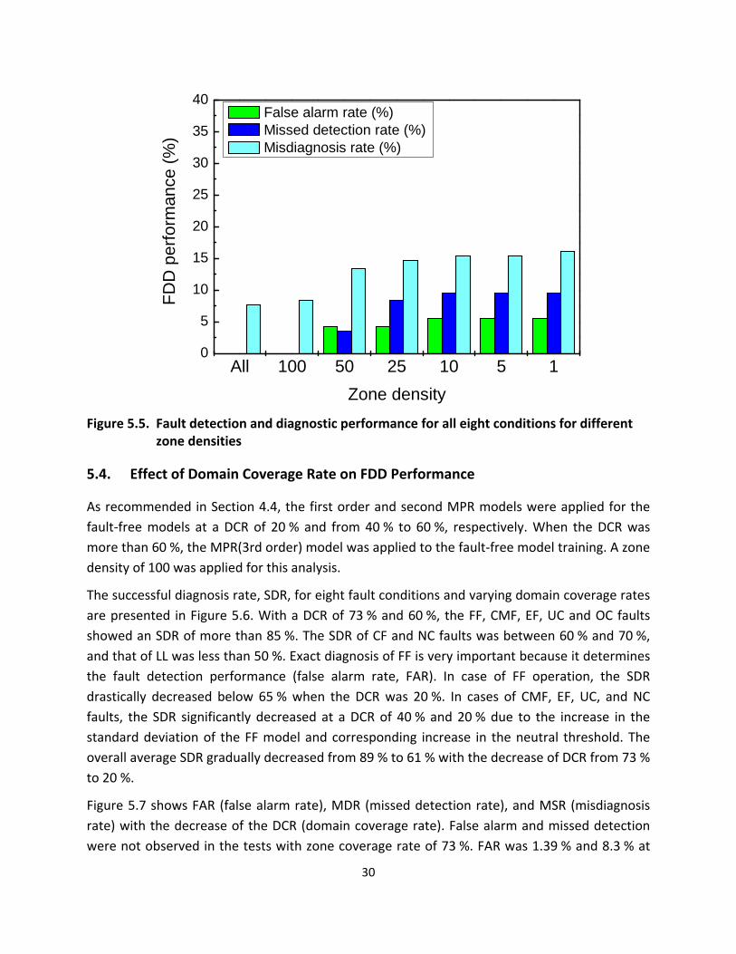
40
35
30
25
20
15
10
5
0
Zone density
Figure 55 Fault detection and diagnostic performance for all eight conditions for different zone densities
54 Effect of Domain Coverage Rate on FDD Performance
As recommended in Section 44 the first order and second MPR models were applied for the
fault‐free models at a DCR of 20 and from 40 to 60 respectively When the DCR was
more than 60 the MPR(3rd order) model was applied to the fault‐free model training A zone
density of 100 was applied for this analysis
The successful diagnosis rate SDR for eight fault conditions and varying domain coverage rates
are presented in Figure 56 With a DCR of 73 and 60 the FF CMF EF UC and OC faults
showed an SDR of more than 85 The SDR of CF and NC faults was between 60 and 70
and that of LL was less than 50 Exact diagnosis of FF is very important because it determines
the fault detection performance (false alarm rate FAR) In case of FF operation the SDR
drastically decreased below 65 when the DCR was 20 In cases of CMF EF UC and NC
faults the SDR significantly decreased at a DCR of 40 and 20 due to the increase in the
standard deviation of the FF model and corresponding increase in the neutral threshold The
overall average SDR gradually decreased from 89 to 61 with the decrease of DCR from 73
to 20
Figure 57 shows FAR (false alarm rate) MDR (missed detection rate) and MSR (misdiagnosis
rate) with the decrease of the DCR (domain coverage rate) False alarm and missed detection
were not observed in the tests with zone coverage rate of 73 FAR was 139 and 83 at
FD
D p
erfo
rman
ce (
)
False alarm rate () Missed detection rate () Misdiagnosis rate ()
All 100 50 25 10 5 1
30
DCR 60 and 40 respectively and then drastically increased to 375 at DCR 20 MDR
gradually increased from 714 to 262 with the decrease of DCR from 60 to 20 MSR
remained below 10 at DCR 73 and 60 and then the misdiagnosis rate steeply increased
to 186 and 385 at a DCR of 40 and 20 At a DCR from 73 to 60 FAR MDR and
MSR were all below 10 However FDD performances worsened at DCRs from 40 to 20
From Figures 56 and 57 DCRs greater than 60 were recommendable for a high quality FDD
application due stability and prediction accuracy In addition DCRs greater than 40 might be
acceptable for a lower quality FDD application if the fault detection error less than 15 was
allowable
100
90
80
70
60
50
40
30
20
10
0
Fault types
Figure 56 Successful diagnosis rate of various faults for different domain coverage rates
Suc
cess
ful d
iagn
osi
s ra
te (
)
Domain coverage rate () 73 60 40 20
FF CMF CF EF LL UC OC NC Avg
31
FD
D p
erfo
rman
ce (
)
40
35
30
25
20
15
10
5
0 73 60 40 20
False alarm rate () Missed detection rate () Misdiagnosis rate ()
Model with best fit DCR 73 3rd MPR model DCR 60 3rd MPR model DCR 40 2nd MPR model DCR 20 1st MPR model
Domain coverage rate ()
Figure 57 Fault detection and diagnostic performance for all faults for different domain coverage rates
6 Concluding Remarks
A concept for a self training fault‐free model for residential air conditioner fault detection and
diagnosis was introduced and tested The method of selecting the appropriate temperature
domain for the fault‐free system data was illustrated in order to cover most operating
conditions considering different climate zones in the US The fault‐free system performance
was modeled based upon three independent features (TOD TID TIDP) and seven dependent
features (TE TSH TC TD TSC ΔTEA ΔTCA) The new concept of zone density was introduced to
manage and filter the system data In addition the new concept of domain coverage rate was
also introduced to quantify the number of data needed to produce fault‐free feature models
Various fault‐free models such as the ANN (artificial neural network) the MPR (multivariable
polynomial regression) and a combined ANNMPR were explored for implementing self
training The MPR method was shown to produce very good prediction performance (low
standard errors) compared to the methods using ANNs Therefore MPR models were applied
and tested against previously taken system data for additional analysis of self training
For validation of the self training method the full experimental dataset (72 fault‐free and 84
fault tests) covering eight faultconditions (fault‐free compressor valve leakage outdoor coil
air flow blockage improper indoor air flow liquid‐line restriction refrigerant undercharge
32
refrigerant overcharge and non‐condensable gas contamination) was used to explore self
training performance The statistical rule‐based fault classification method was illustrated
FDD performance was analyzed using the successful detection rate (SDR) false alarm rate (FAR)
missed detection rate (MDR) and misdiagnosis rate (MSR) as zone density (ZD) and domain
coverage rate (DCR) were varied This effort showed that a zone density greater than 100 was
very successful within the experimental dataset In addition a domain coverage rate greater
than 60 produced acceptable FDD performance and good prediction performance (low
standard errors)
This report attempts to document a mathematical and logical technique by which an FDD
technique may be adapted to an air conditioning system with variations in installation details as
would be seen in actual residences It is by no means a perfected technique applicable to
immediate deployment many issues remain that still must be resolved by laboratory
investigation and application to real world problems When considering using an adaptive
technique for FDD in a real application the following questions must be resolved
1) What operating states are suitable for learning Steady state is important but what
about heat pumps operating in frosting conditions for heating What about the effects of
rain on the outdoor unit What about cooling operation at low outdoor temperatures when
the TXV is operating at the edges of its steady control band A key part of the learning
algorithm is developing a filtering algorithm which picks only the data known to be good
2) How does the FDD technique deal with the fact that the unit is aging and changing over
time In a real learning algorithm you must wait for the driving conditions to present
themselves If you install an air‐conditioner in the Fall season it could be 10 months before
you see data for the hottest day Is it fair to assume that the unit is unchanged since its
install What if the home owner tenant keeps their cooling setpoint at 75 degF all of the time
Now a new ownertenant moves in and runs the house at 70 degF can you use the old FDD
model
3) How do you deal withquantify the noise seen in sensors installed in the field Large
transients and noise may be seen in sensor readings A method of quantifying the sensor
noises and creating dynamic error bands need to be developed How does the FDD deal
with a brokenmalfunctioning sensor
The next step is to take this idea to the laboratory and the field and start solving the
outstanding issues
33
References
AHRI (2008) Performance rating of unitary airconditioning and airsource heat pump
equipment AHRI Standard 210240 Arlington VA USA Air‐Conditioning Heating and
Refrigeration Institute
Baechler M Williamson J Gilbride T Cole P Hefty M Love P (2010) High‐performance
home technologies Guide to determining climate regions by county US Department of Energy
PNNL‐19004
Braun J (1999) Automated fault detection and diagnostics for vapor compression cooling
equipment International Journal of Heating Ventilating Air‐Conditioning and Refrigerating
Research 5(2) 85‐86
Braun J amp Li H (2001) Description of FDD modeling approach for normal performance
expectation West Lafayette IN Herrick Labs Purdue University
Braun J Yuill D Cheung H (2012) A method for evaluating diagnostic protocols for
packaged air conditioning equipment CEC‐500‐08‐049 West Lafayette IN USA Purdue
University Herrick Laboratories
Chen B Braun J E (2001) Simple rule‐based methods for fault detection and diagnostics
applied to packaged air conditioners ASHRAE Transactions 107(1) 847‐857
Cho J Heo J Payne W Domanski P (2014) Normalized performances for a residential heat
pump in the cooling mode with single faults imposed Applied Thermal Engineering 67 1‐15
EIA 2013 US Energy Information Agency Residential Energy Consumption Survey
httpwwweiagovelectricitysales_revenue_pricepdftable5_apdf (Accessed April 2015)
EIA 2014 US Energy Information Agency Residential Energy Consumption Survey
httpwwweiagovtoolsfaqsfaqcfmid=96ampt=3 (Accessed April 2015)
Frenz C (2002) Visual basic and visual basicnet for scientists and engineers Apress 1st Edition
February
Graybill F Iyer H (1994) Regression analysis Concepts and applications second ed Belmont
CA USA Duxbury Press
Heo J Payne W Domanski P (2012) FDD CX A fault detection and diagnostic
commissioning tool for residential air conditioners and heat pump NIST TN 1774 Gaithersburg
MD National Institute of Standards and Technology
Kim M Payne W Domanski P Hermes C (2006) Performance of a Residential Air
Conditioner at Single‐Fault and Multiple‐Fault Conditions NISTIR 7350 Gaithersburg MD
National Institute of Standards and Technology
34
Kim M Yoon S Domanski P Payne W (2008a) Design of a steady‐state detector for fault
detection and diagnosis of a residential air conditioner Int J Refrig 31 790‐799
Kim M Yoon S Payne W Domanski P (2008b) Cooling mode fault detection and diagnosis
method for a residential heat pump NIST SP 1087 Gaithersburg MD National Institute of
Standards and Technology
Kim M Yoon S Payne W Domanski P (2010) Development of the reference model for a
residential heat pump system for cooling mode fault detection and diagnosis Journal of
Mechanical Science and Technology 24(7) 1481‐1489
Li H Braun J (2003) An improved method for fault detection and diagnosis applied to
packaged air conditioners ASHRAE Transactions 109(2) 683‐692
Payne W Domanski P Yoon S (2009) Heating mode performance measurements for a
residential heat pump with single‐faults imposed NIST TN 1648 Gaithersburg MD National
Institute of Standards and Technology
Rossi T Braun J E (1997) A statistical rule‐based fault detection and diagnostic method for
vapor compression air conditioners HVACampR Research 3(1) 19‐37
Thornton B Wang W Lane M Rosenberg M Liu B (2009) Technical support document
50 energy savings design technology packages for medium office buildings US Department
of Energy PNNL‐19004
Yoon S Payne W Domanski P (2011) Residential heat pump heating performance with
single faults imposed Applied Thermal Engineering 31 765‐771
Acknowledgements
The authors would like to acknowledge Min Sung Kim (Chief Thermal Energy Conversion Laboratory Korea Institute of Energy Research ndash KIER) Seok Ho Yoon (Korea Institute of Machinery and Materials) Jin Min Cho and Young‐Jin Baik (Engineer Thermal Energy Conversion Laboratory Korea Institute of Energy Research ndash KIER) for their work in developing the background material used in this report Also John Wamsley Glen Glaeser and Art Ellison provided technician support for collecting the data used to develop FDD fault‐free feature correlations We also would like to thank Will Guthrie of the NIST Statistical Engineering Division for reviewing the statistical FDD method section and Dan Veronica of the NIST Energy and Environment Division for reviewing and commenting on the entire document
35
Appendix A Temperature Data Distribution
The temperature domain should be selected in order to cover most of the operating conditions
a residential air conditioner may experience As summarized in Appendix A and Table A1 the
US climate may be divided into seven climate zones based upon certain criteria (Baechler et al
2010) Seven representative cities within these zones were chosen as a source for temperature
and humidity data (Thornton et al 2009) The most recent five year climate data were
investigated as shown in Figure A2 Temperature data domains for outdoor and indoor
temperature with relative humidity were determined using data for these seven cities
Table A1 Temperature domain by climate zone
Temp domain
Hot humid Hot dry Mixed humid
Mixed dry Marine Cold Very cold
TOD
80 to 105 by a step of 5 oF
(5 zones)
80 to 100 by a step of 5 oF
(4 zones)
80 to 105 by a step of 5 oF
(5 zones)
80 to 105 by a step of 5 oF
(5 zones)
80 to 95 by a step of 5 oF
(3 zones)
80 to 100 by a step of 5 oF
(4 zones)
80 to 95 by a step of 5 oF
(3 zones)
TID 65 to 85 by a step of 5 oF
(4 zones)
RH 20 to 80 by a step of 20
(3 zones)
36
Figure A1 Representative cities for seven US climate zones
37
120 120 O
D t
emp
(o F
) O
D t
em
p
(o F)
OD
tem
p
(o F) 100 100
80 80
60 60
40 40
20 20 Los Angeles (Hot dry)Houston (Hot humid)
0 01 2 3 4 5 6 7 8 9 10 11 12 1 2 3 4 5 6 7 8 9 10 11 12
120 120
100 100
80 80
60 60
40 40
20 20Baltimore (Mixed humid) Albuquerque (Mixed dry)
0 01 2 3 4 5 6 7 8 9 10 11 12 1 2 3 4 5 6 7 8 9 10 11 12
120 120
100 100
80 80
60 60
40 40
20
0 1 2 3 4
San Francisco (Marine)
5 6 7 8 9 10 11 12
20
0 1 2 3 4 5 6
Chicago (Cold)
7 8 9 10 11 12
120
O
D t
emp
(o F
) 100
80
60
40
20
0 1 2 3 4
Duluth (Very cold)
5 6 7 8 9 10 11 12
Month
Figure A2 Maximum outdoor temperature distributions in seven climate zones from 2008 to 2012
38
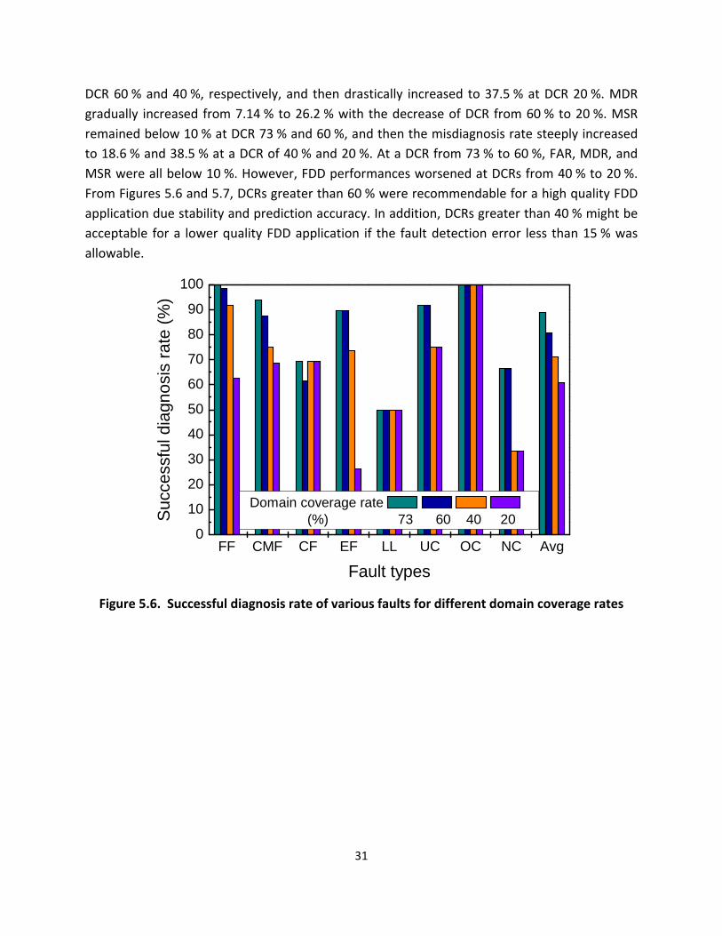
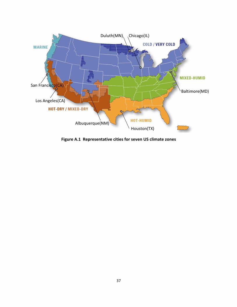
Related Documents


