Self Selection into Credit Markets: Evidence from … Self‐Selection into Credit Markets: Evidence from Agriculture in Mali May 2014 Lori Beaman, Dean Karlan, Bram Thuysbaert, and

1 

Self‐Selection into Credit Markets: Evidence from Agriculture in Mali  

May 2014 

Lori Beaman, Dean Karlan, Bram Thuysbaert, and Christopher Udry1 

Abstract 

We partnered with a micro‐lender in Mali to randomize credit offers at the village level. Then, in no‐loan control villages, we gave cash grants to randomly selected households. These grants led to higher agricultural  investments and profits, thus showing that  liquidity constraints bind with respect to agricultural investment. In loan‐villages, we gave grants to a random subset of farmers  who  (endogenously)  did  not  borrow.  These  farmers  have  lower  –  in  fact  zero  – marginal returns to the grants. Thus we find important heterogeneity in returns to investment and  strong evidence  that  farmers with higher marginal  returns  to  investment  self‐select  into lending programs. 

JEL: D21, D92, O12, O16, Q12, Q14 

Keywords: credit markets; agriculture; returns to capital   

                                                       1 Lori Beaman:  l‐[email protected], Northwestern University; Dean Karlan: [email protected], Yale 

University,  IPA,  J‐PAL,  and  NBER;  [email protected],  Ghent  University;  and  Christopher  Udry: 

[email protected], Yale University. The authors  thank partners Save  the Children and Soro Yiriwaso  for 

their  collaboration.  Thanks  to  Yann Guy,  Pierrick  Judeaux, Henriette Hanicotte, Nicole Mauriello,  and Aissatou 

Ouedraogo for excellent research assistance and to the field staff of Innovations for Poverty Action – Mali office. 

We thank Dale Adams, Alex W. Cohen and audiences at the Columbia University, Dartmouth College, the Federal 

Reserve  Bank  of  Chicago,  the  University  of  California‐Berkeley,  University  of  California‐San  Diego,  and  the 

University of Maryland for helpful comments. All errors and opinions are our own. 

2 

1 Introduction 

Agriculture  sustains  the majority of  the poor  in Mali, as  is  the  case  in most of Africa  (World 

Bank  2000).  The  impact  on  revenue  of  additional  investments  in  agriculture  can  be  high, 

particularly with respect to small investments such as fertilizer and improved seeds (Beaman et 

al. 2013; Duflo, Kremer, and Robinson 2008; Evenson and Gollin 2003; Udry and Anagol 2006). 

We demonstrate that the return to agricultural  investment varies across farmers, farmers are 

aware  of  this  heterogeneity,  and  farmers  with  particularly  high  returns  self‐select  into 

borrowing. 

High average  returns  to agricultural  investment  could emerge when  farmers  lack  capital and 

face credit constraints. Microcredit organizations have attempted to relieve credit constraints, 

but most microcredit  lenders  focus on  small business  financing. The  typical microcredit  loan 

requires  frequent,  small  repayments  and  therefore  does  not  facilitate  investments  in 

agriculture, where  income  comes  as  lump  sums  once  or  twice  a  year. By  contrast,  the  loan 

product studied here is designed for farmers, providing capital at the beginning of the planting 

season and repayment  is done as a lump sum after the harvest. However,  lending may not be 

sufficient  to  induce  investments  in  the  presence  of  other  constraints.2  Farmers  may  be 

constrained  by  a  lack  of  insurance  (Karlan  et  al.  2013),  have  time  inconsistent  preferences 

(Duflo,  Kremer,  and  Robinson  2011),  or  face  high  costs  of  acquiring  inputs  (Suri  2011). We 

investigate whether capital constraints are binding among farmers in Mali, and then, critically, if 

farmers with higher marginal returns to investment are those most likely to borrow.  

We  use  an  experiment  which  offered  some  farmers  access  to  loans  and  other  farmers 

unrestricted cash grants. Out of 198 study villages, our partner microcredit organization, Soro 

Yiriwaso, offered loans in 88 randomly assigned villages. In those “loan” villages, women could 

get loans by joining a local community association. In the remaining “no‐loan” villages, no loans 

were offered. In the no‐loan villages, we randomly selected households to receive grants worth 

40,000 FCFA (US$140).  In  loan villages, we waited until households (and the associations) had 

made  their  loan decisions and  then we gave grants  to a  random  subset of  those households 

who  did  choose  to  borrow. We  can  then  compare  the  average  returns  to  the  grant  in  the 

representative set of farmers in no‐loan villages to the average returns to the grant in the self‐

                                                       2 The evidence from traditional microcredit, targeting micro enterprises, is mixed: some studies find an increase in 

investment  in self‐employment activity (Crepon et al. 2011; Angelucci, Karlan, and Zinman 2013) while others do 

not.  Rarely  (Crepon  et  al.  2011  as  the  exception)  have  evaluations  of  microcredit  found  an  increase  in  the 

profitability of small businesses as a result of access to microcredit, at least at the mean or median (Banerjee et al. 

2013). This is in spite of evidence that the marginal returns to capital can be quite high in micro‐enterprise (de Mel, 

McKenzie, and Woodruff 2008). 

3 

selected sample of households who did not take out loans in loan villages. This allows us to test 

an important question on selection: do those who do not choose to borrow have lower average 

returns than those who choose to borrow?  

The cash grants in no‐loan villages led to a significant increase in investments in cultivation. We 

observe more  land  being  cultivated  (8%), more  fertilizer  use  (14%),  and  overall more  input 

expenditures  (14%).  These  households  also  experienced  an  increase  in  the  value  of  their 

agricultural output and in profits by 13% and 12%, respectively. Thus, we observe a significant 

increase  in  investments  in  cultivation  and  an  increase  in  profits  from  relaxing  capital 

constraints. This  impact on profit even persists after an additional agricultural season. Thus  in 

this environment, capital constraints are limiting investments in cultivation.3 

The impacts of cash grants in the loan villages reveal important selection effects induced by the 

lending process, both on observables and unobservables: the experimental design allows us to 

also ask whether farmers who most productively use capital are more likely to take loans, and 

then whether this composition effect  is predicted by observables.  In  loan villages, households 

given grants did not earn any higher profits from the farm than households not provided grants. 

Yet,  in  the no‐loan villages, households given grants had  large  increases  in profits  relative  to 

those not provided grants. This suggests that households which chose to borrow, and were thus 

self‐selected out of the sample frame  in  loan villages, had higher marginal returns than those 

who did not choose to borrow.   We also  look at other outcomes such as  livestock ownership 

and  small business operations. There  is no evidence  that grant  recipients  in  loan villages are 

investing  the capital  in alternative activities more  than  their counterparts  in no‐loan villages. 

We  conclude  that  there  are  heterogeneous  returns  across  farmers,  and  specifically  that  the 

lending process sorts farmers into higher and lower productivity farmers. 

What aspect of the lending process is creating the positive selection? The experimental design 

itself  does  not  allow  us  to  identify  cleanly whether  farmers  are  positively  self‐selecting  into 

loans  or  whether  the  community,  through  the  group‐lending  process,  is  screening  out 

unproductive farmers. However, two facts suggest that the effect is through self‐selection, not 

                                                       3 The increase in investment contingent upon receipt of the grant is sufficient to reject neoclassical separation, but 

not to demonstrate the existence of binding capital constraints. For example, in models akin to Banerjee and Duflo 

(2012) with an upward‐sloping supply of credit each farmer, a capital grant could completely displace borrowing 

from high‐cost  lenders,  lower  the opportunity cost of capital  to  the  farmer and  induce greater  investment even 

though the farmer could have borrowed more from the high cost lender and thus was not capital constrained in a 

strict sense. However, there is no evidence that these grants lowered total borrowing. Therefore, we refer to the 

range  of  capital market  imperfections  that  could  cause  investment  responses  to  cash  grants  simply  as  credit 

constraints. 

4 

peer selection. First, we  test whether  the differential effect of cash grants  for  farmers  in  the 

loan villages (who chose not to borrow) versus the no‐loan villages is driven by households with 

more socially integrated women. Since the community should have superior information about 

such  households,  communities would  be  able  to more  effectively  screen  out  the  low‐return 

households among those who are socially integrated. Using baseline social integration data, we 

find that the differential effects are not stronger for households with socially integrated women 

and  the  differential  effect  remains  after  controlling  for  heterogeneity  in  baseline  social 

integration,  thus  suggesting  that  peers  are  not  screening  on  expected marginal  returns  to 

capital.  

Second, we look at the distribution of returns. We find that whereas in no‐loan villages there is 

no correlation between baseline profits and marginal returns to the grant, in the loan villages, 

the marginal returns to the grant are close to zero for those with high baseline profits and only 

positive for those with low baseline profits. If the lender or the peers were selecting borrowers, 

they  would  select  based  on  profit  level,  not marginal  profits,  since  profit  levels  are more 

important in determining repayment. Yet the selection effects are occurring only on high‐profit‐

level  farmers.  The  high‐profit,  low‐marginal‐return  farmers  are  those who  are  not  receiving 

loans. This  implies  that even after any bank or peer  selection occurs  (if any) on  the  level of 

profits, a selection effect still occurs, and thus is likely driven by self‐selection.  

We  can  also  estimate  the  intent‐to‐treat  impacts  of  offering  loans  on  a  range  of  outcomes. 

About 21% of households in our sample received loans (in loan villages), which is a take‐up rate 

far  below  that  of  the  grants  ‐  all  households  accepted  the  grants  ‐  but  similar  to  other 

microcredit  contexts.  Like  the  grants,  we  find  that  offering  loans  led  to  an  increase  in 

investments in cultivation, particularly fertilizer, insecticides and herbicides, and an increase in 

agricultural output. We  do  not  detect,  however,  a  statistically  significant  increase  in  profits. 

Therefore we  observe  farmers  investing  in  cultivation when  capital  constraints  are  relaxed 

through credit.  

These  loan  impact  results  are  in  stark  contrast  to  a  long  history  of  failed  agricultural  credit 

programs  (Adams  1971), which  often were  implemented  as  government  programs  and  thus 

plagued by politics (Adams, Graham, and Von Pischke 1984). In the expansion of microcredit in 

the 1980s and onward, we have seen several changes occur at once: a shift from individual to 

group lending processes (although now this trend is reversing (Giné and Karlan 2014; de Quidt, 

Fetzer, and Ghatak 2012)), a shift from balloon payments to high frequency repayment (Field et 

al.  2013  study  a  lending  product  that  partially  reverses  this  trend, with  a  delayed  start  to 

repayments), a shift  from government to nongovernment  (and now to  for‐profit)  institutions, 

and  a  shift  from  agricultural  focus  to  entrepreneurial  focus  (Karlan  and  Morduch  2009; 

5 

Armendariz de Aghion and Morduch 2010). The loan impact component of this study effectively 

returns to this older question, but tests an agricultural lending model that is different than had 

been employed in the past, since there is no government involvement, group liability and also 

little to no subsidy.  

Our  results  on  self‐selection  into  borrowing  also  have  two  important  methodological 

implications.  First,  they  provide  evidence  of  critical  selection  biases  from  non‐experimental 

studies.  For  example,  to  assess  the  impact  of  lending  to  farmers,  had we merely matched 

borrowers to non‐borrowers on observable characteristics, we would have overestimated the 

impact of credit,  since  those who chose  to borrow have higher  returns  to capital  than  those 

who did not choose to borrow. Although the main motivation behind conducting randomized 

trials  is to avoid assumptions regarding selection, the empirical relevance of the bias  is rarely 

estimated (exceptions, for example, exist in the job training literature, LaLonde (1986)). Second, 

the  results  also  highlight  the  pitfalls  of  estimating  treatment‐on‐the‐treated  analysis  in  the 

credit context, given heterogeneous treatment effects with respect to likelihood of borrowing. 

2 The Setting, experimental design and data 

Agriculture  in most of Mali, and  in all of our study area,  is exclusively rainfed. Evidence  from 

nearby  Burkina  Faso  suggests  that  income  shocks  translate  into  consumption  volatility 

(Kazianga  and  Udry  2006),  so  improving  agricultural  output  can  have  important  welfare 

consequences not only on the level of consumption but also the household’s ability to smooth 

consumption within a year. The main crops grown  in the area  include millet/sorghum, maize, 

cotton (mostly grown by men); and rice and groundnuts (mostly grown by women). At baseline, 

about  40%  of  households were  using  fertilizer4,  and  51% were  using  other  chemical  inputs 

(herbicides, insecticide). 

The  loans were marketed,  implemented,  serviced  and  financed  by  Soro  Yiriwaso,  a Malian 

microcredit  organization  (and  an  affiliate  of  Save  the  Children,  an  international 

nongovernmental organization based in the United States). The cash grants were implemented 

by Innovations for Poverty Action. Figure 1 demonstrates the design, and Figure 2 presents the 

timeline.  

                                                       4 The government of Mali introduced heavy fertilizer subsidies in 2008. The price of fertilizer was fixed to 12,500 

FCFA per 50kg of  fertilizer. This constituted a 20%  to 40% subsidy, depending on  the  type of  fertilizer and year. 

Initial usage of the subsidy was  low  in rural areas  initially but grew over time, helping to explain the  increase  in 

input expenses we observe in our data from baseline to endline (Druilhe and Barreiro‐Huré 2012). 

6 

2.1 Experimental design 

The sample frame consisted of 198 villages, located in two cercles (an administrative unit larger 

than  the village but  smaller  than a  region)  in  the Sikasso  region of Mali.5 The  randomization 

consisted of two steps: First, we assigned villages to either loan (88) or no‐loan (110) treatment. 

In  loan villages, anyone could receive a  loan by  joining a women’s association created for the 

purpose.  Second,  after  loan  participation  had  been  decided,  those  households who  did  not 

borrow were  randomly  assigned  to  either  receive  a  grant  or  not.  Below we  describe  each 

component in detail. 

Loans 

Soro Yiriwaso (SY) offered their standard agricultural loan product, called Prêt de Campagne, in 

88  of  the  study  villages  (village‐level  randomization).  This  product  is  given  exclusively  to 

women,  but money  is  fungible within  the  household. Unlike most microloan  products,  it  is 

designed specifically for farmers. Loans are dispersed at the beginning of the agricultural cycle 

in May‐July and repayment occurs after harvest. Administratively the loan is given to groups of 

women organized into village associations, but each individual woman receives a contract with 

the  association.  Repayment  is  tracked  only  at  the  group  level,  and  there  is  nominally  joint 

liability. On  average  there  are  about  30 women  per  group  and  typically  1,  though  up  to  3, 

associations per village. This is a limited liability environment since these households have few 

assets and the  legal environment of Mali would make any  formal recourse on the part of the 

bank  nearly  impossible.  However,  given  that  loans  are  administered  through  community 

associations, the social costs of default could be quite high. In practice we observe no defaults 

over the two agricultural cycles where we were collaborating with Soro Yiriwaso.6  

The annual  interest  rate  is 25% plus 3%  in  fees and a mandatory  savings of 10%. SY offered 

loans in the study villages for the 2010 and 2011 agricultural seasons. The average loan size in 

2010 was 32,000 FCFA (US$113).7  

                                                       5 Bougouni and Yanfolila are  the  two cercles. Both are  in  the northwest portion of  the  region and were chosen 

because  they  were  in  the  expansion  zone  of  the MFI,  Soro  Yiriwaso.  The  sample  frame  was  determined  by 

randomly selecting 198 villages from the 1998 Malian census that met three criteria: (1) were within the planned 

expansion zone of Soro Yiriwaso, (2) were not currently being serviced by Soro Yiriwaso, and (3) had at least 350 

individuals (i.e., sufficient population to generate a lending group). 

6  This  is not  atypical  for  Soro.  In  an  assessment  conducted by  Save  the Children  in 2009, 0% of  Soro’s overall 

portfolio for this loan product was at risk (> 30 days overdue) in years 2004‐2006, rising to only .7% in 2007. 

7 We use the 2011 PPP exchange rate with the Malian FCFA at 284 FCFA per USD throughout the paper. 

7 

Grants 

Grants worth 40,000 FCFA  (US$140) were distributed by  Innovations  for Poverty Action  (with 

no stated relationship to Soro Yiriwaso) to about 1,600 female survey respondents in May and 

June of the agricultural season of 2010‐2011. In the 110 villages not offered loans, households 

were  randomly  selected  to  receive grants and a  female household member –  to parallel  the 

loans – was always the direct recipient. US$140 is a large grant: average input expenses, in the 

absence of the grant, were US$196 and the value of agricultural output was US$522. The size of 

the grant was chosen to closely mimic the size of the average  loan provided by Soro Yiriwaso, 

though  ex  post  the  grant  ended  up  being  slightly  larger  on  average  than  loans.  In  no‐loan 

villages, we also provided some loans to a randomly selected set of men, but we exclude those 

households from the analysis in this paper.8 

In  loan villages, grant  recipients were  randomly  selected among  survey  respondents who did 

not  take  out  a  loan.9 We  attempted  to  deliver  grants  at  the  same  time  in  all  villages,  but 

administrative delays on the  loan side meant that most grants were delivered  first  in no‐loan 

villages, and there is an average 20‐day difference between when no‐loan households received 

their grants from their counterparts in loan villages. We discuss the implications of this delay in 

section 3.2.1. 

In  order  to  minimize  the  possibility  of  dynamic  incentives  to  not  borrow,  we  informed 

recipients that the grants were a one‐time grant, not an ongoing program, and also distributed 

some grants in loan villages to a few borrowers who were not in the survey, so that it was not 

obvious that borrowing precluded someone from being a grant recipient.  

2.2 Data 

Figure 2 shows the timeline of the project. The baseline was conducted in January‐May 2010. A 

first follow‐up survey was conducted after the first year of treatment and the conclusion of the 

                                                       8  These data  are  intended  for  a  separate paper  analyzing household dynamics  and bargaining,  and we do not 

consider them useful for the analysis here since loans were only given to women. 

9 We determined who  took out a  loan by matching names and basic demographic characteristics  from  the  loan 

contracts between  the client and Soro Yiriwaso, which Soro Yiriwaso shared with us on an ongoing basis. There 

were a  few  cases  (67) where Soro Yiriwaso allowed  late applications  for  loans and households  received both a 

grant and a loan. The majority (41 out of 67) of these cases occurred because there were multiple adult women in 

the household, and one took out a loan and another received a grant. We include controls for these households. 

The results are similar if the observations are excluded. 

8 

2010 agricultural season10 in January‐May 2011, and a second follow‐up survey was conducted 

after  the  second  year  of  treatment  and  the  conclusion  of  the  2011  agricultural  season  in 

January‐May  2012.  In  the  three  rounds,  similar  survey  instruments  covered  a  large  set  of 

household characteristics and socioeconomic variables, with a strong focus on agricultural data 

including cultivated area,  input use and production output at  individual and household  levels. 

We also collected data on food and non‐food expenses of the household as well as on financial 

activities (formal and informal loans and savings) and livestock holdings.  

2.3 Randomization, balance check and attrition 

The  randomization was done after  the baseline using a  re‐randomization  technique ensuring 

balance  on  key  variables.11  The  randomization  of  the  provision  of  grants  was  done  at  the 

household  level,  while  the  loan  randomization  was  at  the  village  level. Moreover,  we  did 

separate randomization routines  for  the grant recipients  in  the  loan and no‐loan villages. We 

control  for all village and household‐level variables used  in  the  re‐randomization  routine and 

interactions of the household‐level variables with village type (loan or no‐loan) in all analyses.  

We  conduct  different  tests  to  verify  that  there  are  no  important  observable  differences 

between the different groups in the sample, using variables not included in the randomization 

procedure. Appendix  Table A1  looks  at baseline  characteristics  across  three  comparisons:  (i) 

loan to no‐loan villages;  (ii) grant to no‐grant households  in no‐loan villages; and  (iii) grant to 

no‐grant  households  in  loan  villages.  Few  covariates  are  individually  significantly  different 

                                                       10 We also conducted an “input survey” on a subsample of the sample frame right after planting  in the first year 

(September‐October 2010),  in order  to  collect more accurate data on  inputs  such as  seeds,  fertilizer and other 

chemicals, labor and equipment use. This input survey covered a randomly selected two thirds of our study villages 

(133 villages) and randomly selected half of the households (stratifying by treatment status) to obtain a subsample 

of 2,400 households. We use the input survey if conducted, and if not we use the end of season survey. We also 

control for timing of the collection of the data in all relevant specifications.  

11 First, a loop with a set of number of iterations randomly assigned villages to either loan or no‐loan, and then we 

selected the random draw that minimized the t‐values for all pairwise othorgonality tests. This is done because of 

the difficulties stratifying using a block randomization technique with this many baseline variables. The variables 

used  for  the  loan  randomization were:  village  size,  an  indicator  for whether  the  village was  all  Bambara  (the 

dominant  ethnic  group  in  the  area), distance  to  a paved  road, distance  to  the nearest market,  the percent of 

households having a plough, the percentage of women having a plough, fertilizer use among women in the village, 

average literacy rate, and the distance to the nearest health center. For household‐level randomization we used: 

whether the household was part of an extended family; was polygamous; the primary female respondent’s:  land 

size,  fertilizer use, and whether she had access  to a plough; an  index of  the household’s agricultural assets and 

other assets, and per capita food consumption. See Bruhn and McKenzie (2009) for a more detailed description of 

the randomization procedure. 

9 

across  the  three  comparisons,  and  an  aggregate  test  in  which  we  regress  assignment  to 

treatment on the set of 11 covariates fails to reject orthogonality for each of the 3 comparisons 

(p‐value of 0.26, 0.91 and 0.67, respectively, reported at the bottom of the table).  

Our attrition rate is low: approximately one percent each round. Regardless, Appendix Table A2 

reports tests for differential attrition comparing the same groups as in Table A1, from baseline 

to the  first  follow‐up and to the endline. For each of the three comparisons, we  fail to reject 

that attrition rates are on average the same in the compared groups for both follow up years. In 

a  regression of attrition on  the nine covariates,  treatment status, and  the  interaction of nine 

covariates  and  treatment  status,  a  test  that  the  coefficients  on  treatment  status  and  the 

interaction terms are jointly zero fails to reject for all but one of the six regressions (results on 

bottom row of Appendix Table 2). 

3 Selection into loans 

3.1 Observable characteristics of borrowers versus non‐borrowers 

Take‐up  of  the  loans,  determined  by matching  names  from  administrative  records  of  Soro 

Yiriwaso with our  sample, was 21%  in  the  first agricultural  season  (2010‐11) and 22%  in  the 

second (2011‐2012). Despite the similarity in overall take‐up numbers, there is a lot of turnover 

in clients. Only about 65% of clients who borrowed  in year 1 took out another  loan  in year 2. 

This  overall  take‐up  figure  is  similar  to  other  evaluations  of microcredit  focusing  on  small 

enterprise  (Angelucci, Karlan, and Zinman 2013; Attanasio et al. 2011; Augsburg et al. 2012; 

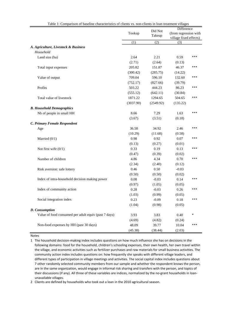
Banerjee et al. 2013; Crepon et al. 2011; Tarozzi, Desai, and  Johnson 2013). Table 1 provides 

descriptive  statistics  from  the baseline on households who  choose  to  take out  loans  in  loan 

villages, compared to non‐clients in those villages. Information on the household as a whole as 

well as  the primary  female  respondent and primary male  respondent  is  reported. There  is a 

striking pattern of selection into loan take‐up: households that invest more in agriculture, have 

higher agricultural output and profits, and have more agricultural assets and livestock, are more 

likely to borrow. Women in households who borrow are also more likely to own a business and 

are more  “empowered” by  three metrics:  they have higher  intra‐household decision‐making 

power,  are  more  socially  integrated  and  are  more  engaged  in  community  decisions.12 

Households that borrow also have higher consumption at baseline than non‐clients. 

                                                       12 All three of these variables are indices, normalized by the no‐grant households in loan‐unavailable villages. The 

household decision‐making index includes questions on how much influence she has on decisions in the following 

domains:  food  for  the  household,  children’s  schooling  expenses,  their  own  health,  her  own  travel within  the 

village,  and economic  activities  such  as  fertilizer purchases  and  raw materials  for  small business  activities. The 

community  action  index  includes  questions  on:  how  frequently  she  speaks with  different  village  leaders,  and 

10 

3.2 Returns to the grant in loan and no‐loan villages 

Panel A of Table 2 shows  the estimates  from  the  following  regression using  the  two years of 

follow up data we have on farm investments and output.  

∙ 2011 ∙ 2011 ∙ ∙ 2012 ∙ 2012 ∙

2012 2012 ∙  

where   indicates individual i received a grant in May‐June 2010, and  indicates that the MFI offered loans in village j.  2011  is an indicator of the data round. We also include 

year  by  village  type  (loan  vs  no‐loan)  controls,  and  additional  baseline  controls  (   which 

include  the  baseline  value  of  the  dependent  variable  13plus  its  interaction with  year  by village type, village fixed effects, and stratification controlsdescribed in section 2.3 and listed in the notes of  the  table, and  indicators  for whether  the household  received both  a grant and 

loan*year  indicators.   and   are the primary coefficients of  interest.    is the effect of the 

cash grant on the outcome   in the non‐loan villages, i.e., the average effect of the cash grant 

among  all  potential  borrowers.    shows  the  differential  impact  of  receiving    grant  on  the 

outcome   for the households that did not borrow (in loan villages) compared to the random, 

representative sample in no‐loan villages. 

Panel  A  of  Table  2  shows  the  estimates  from  this  regression  for  a  variety  of  cultivation 

outcomes  (inputs  along with  harvest  output  and  profits)  and  Panel A  of  Table  3  shows  the 

analogous  estimates  for  other,  non‐cultivation  outcomes  such  as  livestock,  small  business 

ownership, consumption, and female empowerment. 

3.2.1 Agriculture 

Columns (1)‐(6)  look at agricultural inputs. We see  in the first row that  in households who did 

receive  a  grant,  compared  to  those  who  did  not  in  no‐loan  villages,  the  amount  of  land 

cultivated increased (0.18 ha, se=0.065) a small but significant amount. The grant also induced 

an  increased  in  hired  labor  days  (2.7  days,  se=0.80).  2.7  days  is  a  small  number,  but  these 

                                                                                                                                                                               different types of participation in village meetings and activities. The social capital index includes questions about 7 

other randomly selected community members from our sample and whether the respondent knows the person, 

are  in the same organization, would engage  in  informal risk sharing and transfers with the person, and topics of 

their discussions (if any). 

13 In cases where the observation is missing a baseline value, we instead give the lagged variable a value of ‐9 and 

also include an indicator for a missing value. 

11 

households  use  very  little  hired  labor:  the  mean  in  the  control  in  2011  is  only  17  days 

throughout  the  agricultural  season.    Fertilizer  ($11,  se=4.4)  and  other  chemical  inputs  ($9, 

se=2.2) also increased by 14 and 19 percent respectively. Total input expenses (excluding family 

labor and the value of  land, which are challenging to value)  increased to US$28 (se=8.2), a 14 

percent  increase. The grants  therefore  led  to an  increase  in agricultural  investment. Columns 

(7)‐(8)  show  that output and  farm profits  (excluding  the value of  family  labor and  land) also 

went up  significantly. Output went up by 13 percent  ($66,  se=20) and profits by 12 percent 

($40,  se=15). Overall, we  see  significant  increases  in  investments and ultimately profits  from 

relaxing capital constraints. 14 

Table  2  shows  that  the  selected  sample  of  households who  did  not  take  out  a  loan  do  not 

experience  such positive  returns when  capital  constraints are  relaxed. Across  the board,  the 

estimates of the impact of the grant in loan villages in 2011 (year 1) are near zero. Column (1) 

shows  that while households  in no‐loan villages  increased  the amount of  land cultivated as a 

result of the grant, households in loan villages (who did not take out a loan) by contrast did not 

(  is ‐0.16 ha, se=0.09 and the p value of the test that the sum of   and   is zero is 0.85). The 

interaction  term  for  family  labor days  (‐9,  se 6),  fertilizer expenses  (‐$8.8,  se=6.5) and other 

chemical expenses (‐$7, se=3) are all negative, though only the latter is statistically significant. 

Total  input expenses  in  loan villages do  increase  in  response  to  the grant by $17  (p value  is 

0.06), which is not statistically different from the estimate in no‐loan villages of $28. However, 

we  see no  corresponding  increase  in output nor  in profits.  The  interaction  coefficient  for output is similar in magnitude and negative (‐$49.80, se=27.7), offsetting the increase in output 

in no‐loan villages ($66, se=19). The test that the sum of the two coefficients is different from 

zero  is  not  rejected  (p=0.42).  Similarly  for  profits,  the  total  effect  in  loan  villages  is  actually 

negative  (‐$3.78)  and not  significantly different  from  zero  (p=.81).  Thus while  there  is  some 

evidence that among households who did not take out loans, the grant induced some increase 

in inputs, there is no evidence of increases in agricultural output nor profits – in stark contrast 

to the random sample of households in no‐loan villages.  

The analysis  indicates  that households who are screened out of  loans are  those without high 

returns in agriculture to cash transfers. In contrast to the literature on health products, where 

                                                       14 We are not estimating the marginal product of capital as in de Mel, McKenzie, and Woodruff (2008) but instead 

the “total return to capital”– i.e., cash. Beaman et al. (2013) showed in this same area that labor inputs also adjust 

along with agricultural  inputs, making  it  impossible  to  separate  the  returns  to capital  from  the  returns  to  labor 

without  an  additional  instrument  for  labor  inputs. We  are  therefore  capturing  the  total  change  in  profits  and 

investment behavior when capital constraints are  relaxed but will use  the  term “returns” when  referring  to  the 

type of farmers who select into agriculture. 

12 

much of the evidence points towards  limited screening benefits from cost sharing (Cohen and 

Dupas 2010; Tarozzi et al. 2013), we  find  that  the  repayment  liability does  lead  lower  return 

households  to be  screened out.15 The design does not allow us  to experimentally determine 

whether  households  are  self‐selecting  (demand  side)  or  being  screened  by  the  lender  / 

association (supply side).  In section 3.4, we will discuss this further and look at the interaction 

with  respect  to  social  integration, and  the agricultural profits distribution  for each  treatment 

group, to provide us with evidence that the results are driven by self‐selection, not peer or bank 

selection.  

Year 2 

We observe  a persistent  increase  in output  and profits  in  the 2011‐2012  agricultural  season 

(year 2)  from  the  grant  given  in 2010,  as  shown by  the    coefficients  in Table 2: output  is 

higher in grant recipient households by $50 (se=22) in Column (7) of Table 2 and profits by $47 

(se=17). This  is striking since we do not observe grant‐recipient households spending more on 

inputs in Column 6 ($2, se=10). One thing to note, however, is that some of the investments in 

year 1 may benefit year 2 output. There are also changes in agricultural practices which we may 

not  capture  with  our  measure  of  input  expenses.  For  example,  in  2011  grant‐recipient 

households  spend more  on  purchasing  seeds.  In  2012  these  households  spend  no more  on 

seeds  than  control households but  they do use a  larger quantity of  seeds. This  could  reflect 

learning but also could reflect the use of hybrid seeds  in year 2011 which provide some yield 

benefits the  following year, even without re‐purchasing seeds. This highlights that our simple 

accounting of 2011 profits as 2011 output minus 2011 inputs is imperfect, but we have no way 

of constructing a depreciation rate for the various  inputs. We also see a continued  increase  in 

the extensive margin of fertilizer use but not in (average) expenses.  

In year 2, we see a similar negative  interaction term,  , on profits  in Column (8) as  in year 1, 

which is significant at the 10% level (‐$39, se=22.9). The lower profits may be a result of higher 

input use: Column  (6)  shows  that,  in  loan villages, grant‐recipient households  spent more on 

input expenses ($27, se=17.1) than control households in 2012. Although this is not statistically 

significant  compared  to  the  grant  recipients  in  non‐loan  villages,  it  is  statistically  significant 

compared to control (p=0.034). 

                                                       15 However, consistent with the literature on subsidies of health products (Dupas 2013; Kremer and Miguel 2004; 

Ashraf, Berry, and Shapiro 2010), we find demand is dramatically dampened: loan take‐up is around 21% percent 

while all households accepted the grant. 

13 

Timing 

One  concern about our  interpretation of  the  results  is  that on average, households  received 

grants  in  loan  villages  20  days  later  than  in  no‐loan  villages  because  of  delays  in  the 

administration  of  the  loans.  If  farmers  in  no‐loan  villages  received  grants  too  late  in  the 

agricultural cycle to make productive investments, we would erroneously conclude that there is 

positive  selection  into  agricultural  loans  when  in  reality  the  result  is  attributable  to  our 

experimental implementation. This is particularly a concern since we observe farmers increase 

the amount of  land  they  farm, which  is a decision which occurs very early  in  the agricultural 

cycle. In Appendix Table A3, we look at land cultivated (i.e., an investment decision made early 

in the process) and an  index of all the agricultural outcomes and find no relationship with the 

timing of the grant, among the grant‐recipient households in no‐loan villages.16  

3.2.2 Other outcomes 

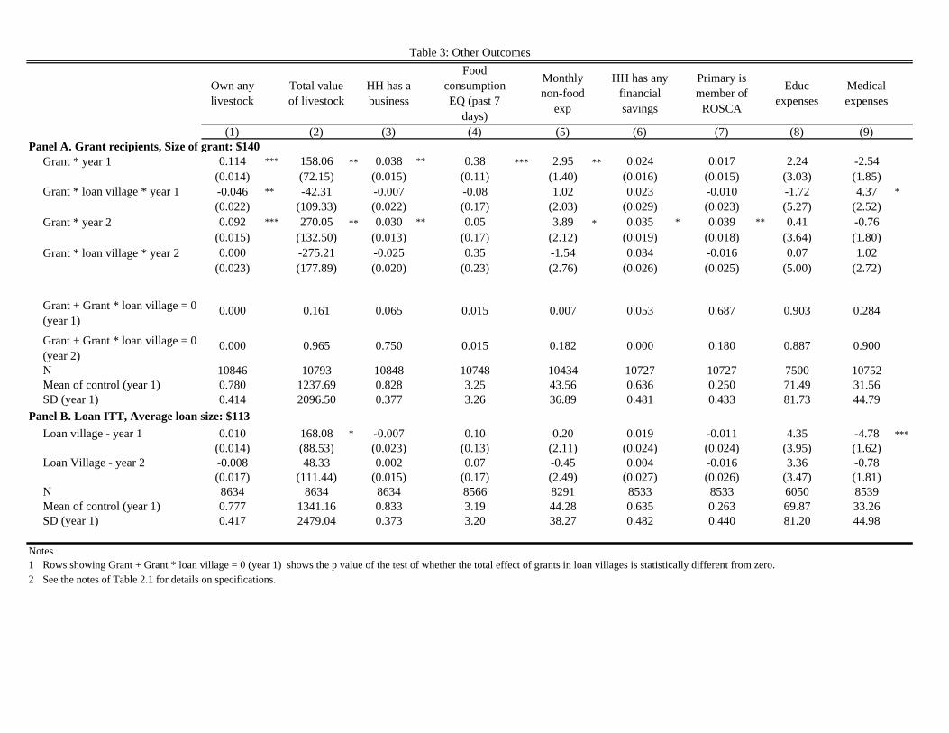
Table 3 shows  the estimates of equation  (1)  looking at outcomes other  than agriculture. The 

most striking result is in Columns (1) and (2): grant‐recipients households in no‐loan villages are 

more  likely  to  own  livestock  (0.11  percentage  points,  se=0.014),  and  there  is  a  large  ($160, 

se=72)  increase  in  the  value  of  total  livestock  compared  to  no‐grant  households.  This 

represents a 10%  increase  in  the value of household  livestock, and  is  slightly  larger  than  the 

value of the grant  itself. Recall we saw  in Table 3 that households also spent an extra $28 on 

cultivation  investments. The  livestock  value  is measured  several months  after harvest;  these 

results may  indicate  that  post‐harvest,  households moved  some  of  their  additional  farming 

profits into livestock.17 We also find evidence that the grant increased the likelihood in no‐loan 

villages  that  a  recipient  household  had  a  small  enterprise  (0.038  percentage  points  higher, 

se=0.015), as shown in Column (3).18 Grant recipient households also consumed more, including 

12% more  food  (Column 4, $0.38 per day  in adult equivalency,  se=0.11) and 6%  in non‐food 

expenditures (Column 5, $2.95 per month, se=1.4). We find the  latter persistent  in year 2 but 

food  consumption  not.  Columns  (6)‐(9)  show  no main  effect  of  the  grant  on  whether  the 

                                                       16 We  look at two main specifications: one  in which we  include date the grant was received  linearly and with  its 

square, and a second which splits the sample into the first half of the grant period and the second half (since most 

of  the  grants  in  the  loan‐available  villages were  distributed  in  the  second  half).  In  both  cases we  control  for 

whether this was the team’s first visit to the village (revisit to village).  

17 We may also over‐value recently‐purchased livestock which may be younger or smaller in treatment households 

since we use village‐level reports of livestock prices to value livestock quantities for all households. 

18 Appendix Table A4 shows  in Column (1) that despite  increasing the extensive margin of small business, we do 

not measure an increase in business profits after year 1. 

14 

household  has  any  financial  savings, membership  in  rotating,  savings  and  loans  associations 

(ROSCAs), education expenses or medical expenses.19 

The investment and spending patterns among grant recipient households in loan villages for the 

most part echo  those described above  in no‐loan villages. Column  (1) shows  that while grant 

recipients  in  loan  villages  were  overall  more  likely  to  own  livestock  than  their  control 

counterparts,  the magnitude  of  the  effect  is  about  half  as  large  as  in  the  no‐loan  villages 

(interaction  term  is  ‐0.046  percentage  points,  se=0.022).  The  remainder  of  the  outcomes 

however shows few differences.20  

Taken together, Panel A of Table 3 shows that the grants benefited households  in a variety of 

ways.  However, we  have  no  strong  evidence  that  households  in  loan  villages, who  did  not 

experience  higher  agricultural  output  and  profits  as  in  no‐loan  villages,  used  their  grants  to 

invest in alternative higher‐return activities other than cultivation. 

Year 2 

In year 2, the coefficients on the  impact of the grants  in no‐loan villages ( ) show persistent 

impacts  for  some  key  outcomes.  Columns  (1)  and  (2)  demonstrate  that  grant‐recipient 

households  are  more  likely  to  own  livestock  (0.09,  se=0.015)  and  continue  to  hold  more 

livestock assets ($270, se=132) than control households in no‐loan villages. They are also more 

likely  to  own  a  business  (3  percentage  points,  se=0.013).21  There  is  no  increase  in  food 

consumption  in  year  2  ($0.05,  se=0.17)  but  an  increase  in  monthly  non‐food  expenditure 

($3.89, se=2.12). Households are also more  likely  to have  financial savings  (0.035 percentage 

points, se=0.019) and be members of rotating savings and  loans associations  (ROSCAs)  (0.039 

                                                       19  Columns  (2)  through  (4)  of  Appendix  Table  A4  also  show  no  impact  in  year  1  on women’s  empowerment, 

involvement in community decisions nor social capital, respectively.  

20  The  only  outcome which  suggests  potential  heterogeneity  in  behavior  upon  receiving  a  grant  between  our 

random,  representative  households  in  no‐loan  villages  and  our  selected  sample  in  loan  villages  is  medical 

expenses, in Column (10). Medical expenses (in the last 30 days) are marginally‐significantly higher in no‐loan grant 

households ($4.37, se=2.52), since medical expenses may have declined (‐$2.54, se=1.85) among grant recipients 

in  loan villages. The  total effect  in  loan villages  is not statistically different  from zero  (p=0.28). This  is a difficult 

outcome to interpret because having more resources could mean a household is more likely to treat illnesses they 

experience but are also more able  to  invest  in preventative care, making  the prediction of  the  treatment effect 

ambiguous. 

21 Appendix Table A4 shows in Column (1) that business profits increase by 18% ($42, se=18.4) in year 2. 

15 

percentage points, se=0.018). Columns (9)‐(10) show that there continues to be no measurable 

impact on educational expenses ($0.41, se=3.64), or medical expenses (‐$0.76, se=1.80).22  

Table 3 shows that, similar to year 1, there  is  little evidence of households  in no‐loan villages 

using grants differently than those in loan villages across this set of non‐agricultural outcomes 

(livestock  ownership,  owning  a  small  business,  and  consumption)  in  year  2.  There  is  an 

alternative hypothesis that the  loan selected  in people with short‐run  investments (i.e., those 

with  payoffs  within  one  year),  and  non‐borrowers  invested  their  grants  in  longer‐term 

investments. However, even by the end of the second year, we do not see profit increases (for 

non‐borrowers  in  loan  villages who  receive  grants)  from  enterprise  investment,  longer‐term 

farm  investments,  or  other  long‐term  investments  such  as  education,  to  support  this 

hypothesis;  nor  does  the  qualitative  information  from  the  field  support  this  alternative 

hypothesis.       

3.3 Unobservable versus observable predictors of marginal returns 

Table 1 demonstrated that  loan‐takers are systematically different at baseline than those who 

do  not  take  out  loans  on  a  number  of  characteristics,  including  those  which  are  surely 

important  in cultivation: they have more  land, spend more  in  inputs, and enjoy higher output 

and  profits.  These  baseline  characteristics  may  be  enough  to  predict  who  could  most 

productively use capital on their farm. Theoretically the prediction is ambiguous: many models 

would predict that those who have the highest returns are households who are the most credit 

constrained. We observe  individuals who  take out  loans have on average more wealth  in  the 

form  of  livestock.  This  could mean  they  have  lower  returns  to  investments  in  cultivation. 

However, they may also have access to better technologies, like a plough, which could increase 

their returns to capital. 

Here we examine whether the marginal returns from grants and the selection effect discussed 

above are predicted  fully by characteristics observed  in  the baseline, or  if  there  is additional 

selection that occurs based on unobservables. We use the same specification as earlier but also 

include baseline characteristics (Z) interacted with an indicator for receiving a grant, for year 1 

and year 2.  

                                                       22  Appendix  table  A4  also  suggests  no  change  in  intra‐household  bargaining  (0.059  of  a  standard  deviation, 

se=0.039) or community action (0.021, se=0.045). The social capital index in column (4) shows a significant rise of 

0.09 of a standard deviation (se=0.017) in year 2. 

16 

∙ 2011 ∙ 2011 ∙

∙ 2012 ∙ 2012 ∙ ∙ ∙ 2011

∙ ∙ 2012 ∙ 2011 ∙ 2012

2012 2012 ∙  

We structure our analysis by sequentially  increasing the controls we  include  in the regression, 

by  first  focusing  on  Z  variables which would  be  fairly  observable  to microcredit  institutions 

(MFI),  then  including  variables  which  would  be  fairly  observable  to  the  community  and 

therefore may be  included  in  screening mechanisms which use  the  community  (as  in group‐

lending), and finally adding in our measure of risk aversion. 

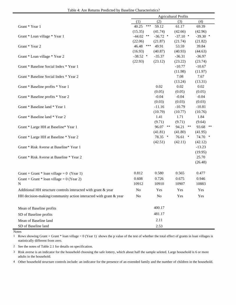
Table  4  shows  our main  empirical  specification with  profits  as  the  outcome, with  different 

baseline  household‐level  controls.  Column  (1)  is  identical  to  Column  (8)  in  Table  2  and  is 

included for ease of comparison. Column (2) adds in Z variables measured at baseline, and their 

interactions,  that  an MFI may  be  able  to  easily  observe:  the  household’s  landholdings  (in 

hectares),  the  value of  their own  livestock,  agricultural profits,  an  indicator  for whether  the 

household  has  six  or more  adults  (the  90th  percentile),  an  indicator  for  the  presence  of  an 

extended  family,  and  the  number  of  children  in  the  household.  Column  (2)  shows  that  the 

estimates of  the differential  effect of  the  grant  in  loan  versus no‐loan  villages  is  reduced  in 

magnitude slightly (‐$36.72, se=21.87 compared to ‐$44 without controls) but continues to be 

significant at the 10%  level. We show the coefficients from the  interactions between some of 

these  Z  variables  and  grant  receipt.  Strikingly,  higher  baseline  profits  do  not  predict  higher 

returns  to  the  grant,  at  least  on  average. We  also  do  not  observe  a  statistically  significant 

relationship between baseline  livestock value or  land size and returns  to  the grant. However, 

larger households do benefit more from the grants in years 1 and 2 than smaller households. 

Column (3) adds in additional information which would likely be known within the community: 

the primary  female  respondent’s  intra‐household decision‐making power, her engagement  in 

community decision‐making and her social capital. Finally, Column (4) also adds in a measure of 

risk aversion. Respondents were asked  to choose between a series of  lotteries, which vary  in 

terms of  their expected value vs  risk. We  include an  indicator  for choosing  the perfectly safe 

lottery,  which  about  half  the  sample  chooses.  In  all  specifications,  the  estimates  on  the 

differential  impacts  of  the  grants  in  loan  versus  no‐loan  villages  are  slightly  smaller  in 

magnitude but still negative and statistically significant at the 10% level. We therefore conclude 

that our estimates of selection effects are not driven by the rich set of observables we measure 

at  the  baseline,  but  by  unobservables,  such  as  land  productivity,  access  to  complementary 

inputs, or farmer skill. In the next section we examine whether the selection  is a demand‐side 

17 

effect  (people  choosing whether  to borrow or not) or  a  supply‐side effect  (lenders or peers 

choosing whether to let a farmer into their lending circle). 

3.4 Is screening driven by supply‐side or demand‐side forces? 

In section 3.1.1 we showed that providing cash grants to households who did not take out loans 

led to lower agricultural returns – and in fact zero returns – compared to households who were 

randomly  selected  in  no‐loan  villages.  The  experimental  design  itself  does  not  allow  us  to 

differentiate how the screening itself occurs: it may be the result of self‐selection on the part of 

farmers  (demand‐side) or due to screening on the part of the MFI or community associations 

(supply‐side). The MFI  itself has  little  to no  information about  loan applicants, so  it  is almost 

impossible that the positive selection  is due to the MFI’s screening process. However, women 

must go through a community association – which has  joint  liability for the  loan –  in order to 

get a contract with the MFI. It is therefore possible that the associations are screening out low‐

return  farmers. Table 1 also  showed  that more connected women and wealthier households 

were  more  likely  to  take  a  loan,  which  would  be  consistent  with  supply‐side  factors  like 

collateral  creating  a  screening  mechanism.  We  conduct  two  tests  to  disentangle  these 

mechanisms, and both are consistent with self‐selection. 

Our first piece of evidence comes from Table 5. We observed in Table 1 that women with more 

social  connections,  as  captured  by  the  social  integration  index,  were  more  likely  to  be 

microcredit clients. Women who are more connected in the community could be more likely to 

be  clients due  to  supply‐side  screening:  for  these women, members  know more  about  their 

activities  and  can  both  better  monitor  and  better  screen  them.  The  highly  integrated 

households who did not receive loans should have low returns to grants. If the association were 

screening households and generating the positive selection we observed  in Table 2, we would 

anticipate households in loan villages with high social integration (who do not borrow) to have 

lower profits than the corresponding households in no‐loan villages. That is, it would precisely 

be  the  low‐return households about whom  the community has good  information  (those who 

are socially  integrated) that would be excluded from receiving  loans. These households would 

then be over‐represented in our sample in loan villages, driving down the returns to the grant. 

This gives us the prediction that Grant * Baseline Social Integration Index * Loan village * year 1 

would be negative: highly  integrated households who do not  receive  loans would experience 

low  returns.  Its  inclusion  would  also  drive  the    coefficient  toward  zero  if  this  screening 

mechanism is driving our results. However, in Column (1) of Table 5 we observe essentially no 

change in the estimate of   compared to Column (1) of Panel A, Table 2 (‐42.82 compared to ‐

44.02, se=22.59). The quadruple  interaction has a positive – not negative – coefficient (16.43, 

se=22.02) and is insignificant. Similarly in Columns (2)‐(4) we see that qualitatively the inclusion 

18 

of  the social  integration  index  interactions changes  little  the estimate of   compared  to  the 

corresponding estimates in Columns (2)‐(4) in Table 4. 

Second, we  look at which  farmers are driving  the selection effect. Figure 3 shows  the CDF of 

profits  in  loan and no‐loan villages.  In each  figure, we show the distribution of profits among 

farmers who received a grant and those who did not. In no‐loan villages, we see that the entire 

distribution  is  pushed  to  the  right  for  grant‐recipient  households  relative  to  control.  By 

contrast, in loan villages, grant‐recipient households at the bottom 70% of the distribution earn 

more profits than their control counterparts. At the top of the distribution, however, we see no 

difference  between  grant  and  control  households.    The  objective  function  of  the MFI,  and 

plausibly the women’s association,  is to maximize repayment.  It  is therefore unlikely that the 

supply‐side would have screened out high profit farmers. Irrespective of their marginal returns, 

high‐profit  farmers would  be  capable  of  repaying  the  loan.  Yet  it  is  among  the  high‐profit 

farmers  in  loan  villages  that  we  find  that  low marginal  return  households  do  not  borrow. 

Therefore, this is evidence of self‐selection.  

Column  (5) of Table 5 echoes  this  finding. We  include additional  interaction  terms  to  look at 

heterogeneity  between  loan  and  no‐loan  villages  in  the  returns  to  the  grants  by  baseline 

profits. Column  (5)  shows  that Grant * Baseline profits *Loan village * Year 1  is  significantly 

correlated  with  profits,  and  the  inclusion  of  these  additional  interaction  terms  erodes  the 

primary selection effect on Grant * Loan village * year 1. Had the effect been driven by supply‐

side screening, we would see the grant * baseline profits * year 1 capture the selection effect 

(because  the  supply‐side  screeners, whether  the  lender or  the peers, would choose only  the 

high profit level, i.e., high baseline profits, farmers as clients). Instead, after controlling for that, 

we observe selection occurring on marginal profits. Thus this supports the conclusion that the 

selection effect is via self‐selection, not supply‐side selection.  

4 Impact of the loans 

We also show our estimates of the intent‐to‐treat (ITT) effects of being offered an agricultural 

loan on the same set of outcomes already discussed in section 3. In this analysis, we exclude all 

grant  recipients,  from  both  loan  and  ineligible  villages.  Panel  B  of  Tables  2  and  3  show  the 

results of the loan intent‐to‐treat analysis. We use the following specification: 

∙ 2011 ∙ 2012  

where (  which  include the baseline value of the dependent variable  , cercle fixed effects, 

and the village stratification controlsdescribed in section 2.3 and listed in the notes of the table 

19 

Table 2. The specification uses probability weights to account for the sampling strategy, which 

depends on take‐up in the loan villages.  

Panel B of Tables 2 and 3 show the  ITT estimates.  In Table 2, we observe an  increase  in  input 

expenditures  on  family  labor  days  (8.7,  se=4.8),  in  fertilizer  expenses  ($10.35,  se=5.09)  and 

other  chemical  expenses  including  insecticides  and  herbicides  ($5.08,  se=2.76)  in  villages 

offered loans. Land cultivated also increases but is only at the margin of statistical significance 

(0.094 ha,  se=0.058). The  value of  the harvest also  increases by $32  (se=19), but we do not 

measure a statistically significant increase in profits ($17, se=15.8). Panel B of Table 3 shows an 

increase  in  the  value  of  livestock  ($168,  se=89)  in  Column  (2)  and  a  reduction  in medical 

expenses (‐$4.78, se=1.62) in Column (10). We do not detect an impact on the other outcomes, 

including  food and non‐food  consumption, whether  the household has a  small business, nor 

educational expenses.23  

These  results on  impact of  loans  stand  in  stark  contrast both  to  the  recent  literature on  the 

impact of entrepreneurially‐focused credit (see Angelucci, Karlan, and Zinman 2013; Attanasio 

et al. 2011; Augsburg et al. 2012; Banerjee et al. 2013; Crepon et al. 2011; Karlan and Zinman 

2011;  Tarozzi,  Desai,  and  Johnson  2013),  and  an  earlier  agricultural  lending  literature  that 

documented consistent institutional failures, typically with high default rates (Adams, Graham, 

and Von Pischke 1984; Adams 1971). The  institutional  results are also promising:  the perfect 

repayment, and the retention to the following year (50%) is on par with typical client retention 

rates  for  sustainable,  entrepreneurially‐focused  microcredit  operations.  The  self‐selection 

results do highlight, however, that estimating the treatment‐on‐the‐treated (TOT) results would 

be  inappropriate,  since  those who  chose  not  to  borrow  have  considerably  lower  returns  to 

capital than those who choose to borrow. 

5 Conclusion 

Capital constraints are a binding constraint for at least some farmers in Southern Mali, and we 

find that agricultural  lending with balloon payments (i.e., with cash flows matched to those of 

the intended productive activity) is a plausible way to increase investments in agriculture. This 

is an important policy lesson since the majority of microcredit has focused on small enterprise 

lending, and the typical microcredit loan contract – where clients must start repayment after a 

                                                       23 Appendix  Table A4  further  shows  no detectable  effect on  business  profits, women’s  decision‐making power 

within the household, women’s involvement in community decisions, nor on women’s social capital. This is similar 

to the existing evaluations of microcredit (Attanasio et al. 2011; Augsburg et al. 2012; Banerjee et al. 2013; Crepon 

et al. 2011; except Angelucci, Karlan, and Zinman 2013). Soro Yiriwaso did not have any explicit component of the 

program emphasizing women’s empowerment. 

20 

few weeks –  is  simply  ill‐suited  for agriculture. Field et. al.  (2013)  find  similar  results merely 

from delaying the onset of high frequency repayment, within the context of microenterprise. In 

Mali,  for example, Soro Yiriwaso  is  the only microcredit organization with a product specially 

designed  for  agriculture,  despite  the  fact  that  the  vast majority  of  households  in  rural Mali 

depend on agriculture for a sizeable part of their livelihood.  

Key to our main purpose, we find that the returns to capital  in cultivation are heterogeneous 

and that higher marginal‐return farmers self‐select into borrowing more so than low marginal‐

return farmers. This has important implications for models of credit markets. In particular, our 

results  provide  rigorous  empirical  evidence  for  optimal  selection  into  contracts,  which  is 

embedded in models like Evans and Jovanovic (1989), Buera (2009) and Moll (2013) but which 

has  lacked  clear  empirical  evidence.  Our  results  also  highlight  the  need  to  incorporate 

heterogeneity of returns in such models, as recognized by Kaboski and Townsend (2011).  

These results are also  important for policy, for example the targeting of social programs. Cash 

transfer  programs  are  often means‐tested  and  recent  work  suggests  that  both  community 

targeting, where community members rank‐order households to  identify the poor, and ordeal 

mechanisms can be an effective way of generating screening on wealth/income  in developing 

countries  (Alatas et al. 2012; Alatas et al. 2013). Price  is the screening mechanism we  look at 

here with  agricultural  loans.  The  literature  on  health  products  in  developing  countries  finds 

mixed evidence on whether positive prices or cost sharing creates a screening effect on usage.24 

Cohen, Dupas, and Schaner (2012) highlight the tradeoff between access and targeting through 

pricing of health products when the benefits are heterogeneous across households, as in their 

case with anti‐malarial medication. Higher subsidies  lead to higher access for households with 

malaria but poor  targeting:  among  adults,  about half of  the  subsidized medications went  to 

people who did not have malaria. We  find  that  in agriculture,  the  lending process generates 

positive  self‐selection  so  farmers who benefit  the most  from  relaxing  capital  constraints  are 

more likely to choose to borrow.  

                                                       24 Cohen and Dupas  (2010) and Tarozzi et al  (2013)  find no evidence households given bednets  for  free are  less 

likely to use them. Ashraf, Berry, and Shapiro (2010), by contrast, find evidence that households who paid higher 

prices were more likely to use a water purification product. Tarozzi et al does find, though, that households who 

have malaria at baseline are more  likely  to take out microloans  for bednets  than  those without malaria.  (Dupas 

2013) provides a summary of the literature.   

21 

References 

Adams,  Dale  W.  1971.  “Agricultural  Credit  in  Latin  America:  A  Critical  Review  of  External Funding Policy.” American Journal of Agricultural Economics 53 (2): 163–72.  

 Adams,  Dale W.,  Douglas  H.  Graham,  and  J.  D.  Von  Pischke,  eds.  1984.  Undermining  Rural 

Development  with  Cheap  Credit.  Westview  Special  Studies  in  Social,  Political,  and Economic Development. Boulder: Westview Press. 

 Alatas, Vivi, Abhijit Banerjee, Rema Hanna, Benjamin A Olken, and Julia Tobias. 2012. “Targeting 

the  Poor:  Evidence  from  a  Field  Experiment  in  Indonesia.”  The  American  Economic Review 102 (4): 1206–40. 

 Alatas, Vivi, Abhijit Banerjee, Rema Hanna, Olken, Benjamin, Ririn Purnamasari, and Matthew 

Wai_Poi. 2013. “Self‐Targeting: Evidence from a Field Experiment in Indonesia.”  Angelucci, Manuela, Dean Karlan, and Jonathan Zinman. 2013. “Microcredit Impacts: Evidence 

from  a  Randomized  Microcredit  Program  Placement  Experiment  by  Compartamos Banco”. Working paper. University of Michigan, Ann Arbor, MI. 

 Armendariz de Aghion, Beatriz, and Jonathan Morduch. 2010. The Economics of Microfinance. 

2nd ed. Cambridge, MA: MIT Press.  Ashraf, Nava,  James Berry, and  Jesse M Shapiro. 2010.  “Can Higher Prices Stimulate Product 

Use? Evidence from a Field Experiment in Zambia.” American Economic Review 100 (5): 2383–2413.  

 Attanasio,  Augsburg,  Britta  Augsburg,  Ralph  de  Haas,  Fitz  Fitzsimons,  and  Heike  Harmgart. 

2011.  “Group  Lending  or  Individual  Lending?  Evidence  from  a  Randomised  Field Experiment in Mongolia.” EBRD Working Paper 136 (December). 

 Augsburg, Britta, Ralph de Haas, Heike Harmgart, and Costas Meghir. 2012. “Microfinance at 

the  Margin:  Experimental  Evidence  from  Bosnia  and  Herzegovina.”  Working  Paper, September. 

 Banerjee,  Abhijit,  and  Esther  Duflo.  2012.  “Do  Firms Want  to  Borrow More?  Testing  Credit 

Constraints Using a Directed Lending Program.” M.I.T. Working Paper.  Banerjee, Abhijit, Esther Duflo, Rachel Glennerster, and Cynthia Kinnan. 2013. “The Miracle of 

Microfinance? Evidence from a Randomized Evaluation”. Working paper.  Bank, World. 2000. “Spurring Agricultural and Rural Development.” 170–207. Can Africa Claim 

the 21st Century? Washington, DC. 

22 

 Beaman,  Lori,  Dean  Karlan,  Bram  Thuysbaert,  and  Christopher  Udry.  2013.  “Profitability  of 

Fertilizer:  Experimental  Evidence  from  Female  Rice  Farmers  in  Mali.”  American Economic Review Papers & Proceedings, May. 

 Bruhn, Miriam, and David McKenzie. 2009. “In Pursuit of Balance: Randomization in Practice in 

Development Field Experiments.” American Economic Journal: Applied Economics 1 (4): 200–232. 

 Buera, Francisco  J. 2009. “A Dynamic Model of Entrepreneurship with Borrowing Constraints: 

Theory and Evidence.” Annals of Finance 5 (3‐4): 443–64.  Cohen, Jessica, and Pascaline Dupas. 2010. “Free Distribution or Cost‐Sharing? Evidence from a 

Randomized Malaria Prevention Experiment.” Quarterly  Journal of Economics 125  (1): 1–45. doi:10.1162/qjec.2010.125.1.1. 

 Cohen,  Jessica,  Pascaline  Dupas,  and  Simone  G  Schaner.  2012.  “Price  Subsidies,  Diagnostic 

Tests,  and  Targeting  of Malaria  Treatment:  Evidence  from  a  Randomized  Controlled Trial.” 

 Crepon,  Bruno,  Florencia  Devoto,  Esther  Duflo,  and  William  Pariente.  2011.  “Impact  of 

Microcredit in Rural Areas of Morocco: Evidence from a Randomized Evaluation.” M.I.T. Working Paper, March. 

 De  Mel,  Suresh,  David  McKenzie,  and  Christopher  Woodruff.  2008.  “Returns  to  Capital  in 

Microenterprises:  Evidence  from  a  Field  Experiment.” Quarterly  Journal  of  Economics 123 (4): 1329–72. 

 De Quidt, Jonathan, Thiemo Fetzer, and Maitreesh Ghatak. 2012. “Group Lending Without Joint 

Liability.” London School of Economics Working Paper.  Druilhe,  Z.,  and  J.  Barreiro‐Huré.  2012.  “Fertilizer  Subsidies  in  sub‐Saharan Africa.”  FAO  ESA 

Working Paper No 12‐04.  Duflo, Esther, Michael Kremer, and Jonathan Robinson. 2008. “How High Are Rates of Return to 

Fertilizer?  Evidence  from  Field  Experiments  in Kenya.” American  Economic Review  98 (2): 482–88. 

 ———.  2011.  “Nudging  Farmers  to  Use  Fertilizer:  Theory  and  Experimental  Evidence  from 

Kenya.” American Economic Review 101 (6): 2350–90.   Dupas, Pascaline. 2013. “Short‐Run Subsidies and Long‐Run Adoption of New Health Products:  

Experimental Evidence from Kenya.” Econometrica forthcoming. 

23 

 Evans, David  S,  and  Boyan  Jovanovic.  1989.  “An  Estimated Model  of  Entrepreneurial  Choice 

Under Liquidity Constraints.” The Journal of Political Economy 97 (4): 808.  Evenson,  R.E.,  and D. Gollin.  2003.  “Assessing  the  Impact  of  the Green  Revolution,  1960  to 

2000.” Science 300 (758): 758–62.  Field, Erica, Rohini Pande,  John Papp, and Natalia Rigol. 2013. “Does the Classic Microfinance 

Model  Discourage  Entrepreneurship  Among  the  Poor?  Experimental  Evidence  from India.” American Economic Review 103 (6): 2196–2226.  

 Giné, Xavier, and Dean S. Karlan. 2014. “Group Versus Individual Liability: Short and Long Term 

Evidence  from  Philippine  Microcredit  Lending  Groups.”  Journal  of  Development Economics 107 (March): 65–83.  

 Kaboski,  Joseph  P,  and Robert M  Townsend.  2011.  “A  Structural  Evaluation  of  a  Large‐Scale 

Quasi‐Experimental Microfinance Initiative.” Econometrica 79 (5): 1357–1406.  Karlan, Dean, and Jonathan Morduch. 2009. “Access to Finance.” In Handbook of Development 

Economics. Vol. 5. Edited by Dani Rodrik Mark Rosenzweig. Elsevier.  Karlan, Dean, Isaac Osei‐Akoto, Robert Darko Osei, and Christopher R. Udry. 2013. “Agricultural 

Decisions  after Relaxing Credit  and Risk Constraints.” Quarterly  Journal of  Economics, Forthcoming.  

 Karlan,  Dean,  and  Jonathan  Zinman.  2011.  “Microcredit  in  Theory  and  Practice:  Using 

Randomized Credit Scoring for Impact Evaluation.” Science 332 (6035): 1278–84.  Kazianga,  Harounan,  and  Christopher  Udry.  2006.  “Consumption  Smoothing?  Livestock, 

Insurance and Drought in Rural Burkina Faso.” Journal of Development Economics 79 (2): 413–46.  

 Kremer,  Michael,  and  Edward  A  Miguel.  2004.  “The  Illusion  of  Sustainability.”  Center  for 

International and Development Economics Research Paper C05‐141.  LaLonde, Robert  J. 1986.  “Evaluating  the  Econometric  Evaluations of  Training Programs with 

Experimental Data.” American Economic Review 76 (4): 604–20.  Moll, Benjamin. Forthcoming. “Productivity Losses  from Financial Frictions: Can Self‐Financing 

Undo Capital Misallocation?” American Economic Review  Suri,  Tavneet.  2011.  “Selection  and  Comparative  Advantage  in  Technology  Adoption.” 

Econometrica 79 (1): 159–209.  

24 

 Tarozzi, Alessandro, Jaikishan Desai, and Kristin Johnson. 2013. “On the Impact of Microcredit: 

Evidence from a Randomized Intervention in Rural Ethiopia.” UPF Working Paper.  Tarozzi, A., Mahajan, A., Blackburn, B., Kopf, D., Krishnan, L., & Yoong,  J. 2013. “Micro‐Loans, 

Bednets  and  Malaria:  Evidence  from  a  Randomized  Controlled  Trial.”  American Economic Review Forthcoming. 

 Udry, C., and S. Anagol. 2006. “The Return to Capital in Ghana.” The American Economic Review 

96 (2): 388–93.  

(1) (2) (3)A. Agriculture, Livestock & Business

Household

Land size (ha) 2.64 2.21 0.59 ***

(2.71) (2.64) (0.13)

Total input expenses 205.82 151.87 46.37 ***

(300.42) (285.75) (14.22)

Value of output 709.04 596.10 132.60 ***

(752.17) (827.66) (39.79)

Profits 503.22 444.23 86.23 ***

(555.12) (642.11) (30.84)

Total value of livestock 1871.22 1294.65 504.65 ***

(3037.90) (2549.92) (135.22)

B. Household Demographics

Nb of people in small HH 8.66 7.29 1.63 ***

(3.67) (3.51) (0.18)

C. Primary Female Respondent

Age 36.58 34.92 2.46 ***

(10.29) (11.68) (0.58)

Married (0/1) 0.98 0.92 0.07 ***

(0.13) (0.27) (0.01)

Not first wife (0/1) 0.33 0.19 0.13 ***

(0.47) (0.39) (0.02)

Number of children 4.86 4.34 0.70 ***

(2.34) (2.40) (0.12)

Risk aversion: safe lottery 0.46 0.50 -0.03

(0.50) (0.50) (0.02)Index of intra-household decision making power 0.08 -0.03 0.14 ***

(0.97) (1.05) (0.05)Index of community action 0.28 -0.03 0.26 ***

(1.03) (0.99) (0.05)Social integration index 0.23 -0.09 0.18 ***

(1.04) (0.98) (0.05)

D. ConsumptionValue of food consumed per adult equiv (past 7 days) 3.93 3.83 0.40 *

(4.69) (4.82) (0.24)Non-food expenses by HH (past 30 days) 48.09 39.77 10.04 ***

(45.38) (38.44) (2.03)

Notes

1

2 Clients are defined by households who took out a loan in the 2010 agricultural season.

Table 1: Comparison of baseline characteristics of clients vs. non-clients in loan treatment villages

TookupDid Not Takeup

Difference(from regression with village fixed effects)

The household decision‐making index includes questions on how much influence she has on decisions in the 

following domains: food for the household, children’s schooling expenses, their own health, her own travel within 

the village, and economic activities such as fertilizer purchases and raw materials for small business activities. The 

community action index includes questions on: how frequently she speaks with different village leaders, and 

different types of participation in village meetings and activities. The social capital index includes questions about 

7 other randomly selected community members from our sample and whether the respondent knows the person, 

are in the same organization, would engage in informal risk sharing and transfers with the person, and topics of 

their discussions (if any). All three of these variables are indices, normalized by the no‐grant households in loan‐

unavailable villages. 

Land cultivated

(ha)

Family labor (days)

Hired labor (days)

Fertilizer expenses

Other chemicals expenses

Total input expenses

Value output

Profits

(1) (2) (3) (4) (5) (6) (7) (8)Panel A. Grant recipients, Size of grant: $140

Grant * year 1 0.175 *** 5.8 2.7 *** 11.07 ** 9.02 *** 28.26 *** 66.17 *** 40.25 *** (0.065) (4.3) (0.8) (4.38) (2.20) (8.23)    (19.05)    (15.35)    

Grant * loan village * year 1 -0.162 * -8.9 0.9 -8.84 -7.02 ** -11.20    -49.79 *   -44.02 **  (0.093) (6.4) (1.4) (6.52) (3.02) (12.15)    (27.70)    (22.06)    Grant * year 2 0.071 -5.5 1.0 -1.59 0.88 2.15    49.65 **  46.48 *** (0.077) (4.0) (0.8) (6.25) (2.77) (10.28)    (22.32)    (16.93)    Grant * loan village * year 2 0.065 9.1 1.0 11.94 7.88 * 26.90    -13.23    -38.52 *   (0.111) (6.1) (1.2) (10.08) (4.27) (17.05)    (32.12)    (22.93)    

Grant + Grant * loan village = 0 (year 1) 0.846 0.505 0.002 0.645 0.333

   0.059 0.417 0.812

   Grant + Grant * loan village = 0 (year 2) 0.091 0.438 0.017 0.192 0.008

   0.034 0.117 0.608

N 11024 11025 11023 11022 11024    11024 11022 10912

Mean of control (year 1) 2.159     137.26 16.84    76.49 48.16    196.36 523.19 328.91    

SD (year 1) 2.278     132.38 22.78    153.11 67.56    262.84 623.53 443.18    Panel B. Loan ITT, Average loan size: $113

Loan village - year 1 0.094 8.66 * -0.83 10.35 **  5.08 *   21.68 **  32.36 *   17.05

(0.058) (4.83) (1.00) (5.09)    (2.76)    (8.80)    (19.46)    (15.80)

Loan Village - year 2 0.017 -1.06 -1.10 2.38    0.07    6.43    15.84    10.48

(0.071) (4.67) (1.02) (6.18)    (3.20)    (11.36)    (23.22)    (15.94)

N 8775 8771 8763 8767    8770 8773 8771 8689    

Mean of control (year 1) 2.083     134.91 17.07    71.52 46.72    186.24    503.37    318.50    

SD (year 1) 2.257     129.66 23.35    144.78 65.92    250.17    599.36    433.60    

Notes1

23

4

5

Rows showing Grant + Grant * loan village = 0 (year 1) shows the p value of the test of whether the total effect of grants in loan villages is statistically different from zero.

Total input expenses includes fertilizer, manuring, herbicide, insecticide, farming equipment and hired labor but excludes the value of family labor.

Table 2: Agriculture

Additional controls include in Panel A include: the baseline value of the dependent variable, village fixed effects, round x village type (loan-village vs no-loan-village) fixed effects, the baselinevalue interacted with round x village type effects, an indicator for whether the baseline value is missing, an indicator for the HH being administered the input survey in 2011, stratification controls(whether the household was part of an extended family; was polygamous; an index of the household’s agricultural assets and other assets; per capita food consumption; and for the primary femalerespondent her baseline: land size, fertilizer use, and whether she had access to a plough), and indicators for whether the household received both a loan and a grant in year 1 and 2. Village-levelstratification controls are not included since there are village fixed effects.

Standard errors are in paranetheses and clustered at the village level in all specifications.

Additional controls in Panel B include: cercle fixed effects; the baseline value of the dependent variable, along with a dummy when missing, interacted with year of survey indicators; and village-level stratification controls: population size, distance to nearest road, distance to nearest paved road, whether the community is all bambara (dominant ethnic group) distance to the nearest market,percentage of households with a plough, percentage of women with access to plough in village, percentage of women in village using fertilizer and the fraction of children enrolled in school. Thespecification uses probability weights to reflect sampling design.

Own any livestock

Total value of livestock

HH has a business

Food consumption EQ (past 7

days)

Monthly non-food

exp

HH has any financial savings

Primary is member of

ROSCA

Educ expenses

Medical expenses

(1) (2) (3) (4) (5) (6) (7) (8) (9)Panel A. Grant recipients, Size of grant: $140

Grant * year 1 0.114 *** 158.06 ** 0.038 ** 0.38 *** 2.95 ** 0.024 0.017 2.24 -2.54

(0.014) (72.15) (0.015) (0.11)     (1.40)     (0.016) (0.015) (3.03) (1.85)

Grant * loan village * year 1 -0.046 ** -42.31 -0.007 -0.08     1.02     0.023 -0.010 -1.72 4.37 *

(0.022) (109.33) (0.022) (0.17)     (2.03)     (0.029) (0.023) (5.27) (2.52)

Grant * year 2 0.092 *** 270.05 ** 0.030 ** 0.05     3.89 * 0.035 * 0.039 ** 0.41 -0.76

(0.015) (132.50)     (0.013) (0.17)     (2.12)     (0.019) (0.018) (3.64) (1.80)

Grant * loan village * year 2 0.000 -275.21     -0.025 0.35     -1.54     0.034 -0.016 0.07 1.02

(0.023) (177.89)     (0.020) (0.23)     (2.76)     (0.026) (0.025) (5.00) (2.72)

Grant + Grant * loan village = 0 (year 1)

0.000 0.161   

0.065 0.015   

0.007   

0.053 0.687 0.903 0.284

Grant + Grant * loan village = 0 (year 2)

0.000 0.965   

0.750 0.015   

0.182   

0.000 0.180 0.887 0.900

N 10846 10793     10848 10748     10434     10727 10727 7500 10752

Mean of control (year 1) 0.780     1237.69     0.828     3.25     43.56     0.636     0.250     71.49 31.56

SD (year 1) 0.414     2096.50     0.377     3.26     36.89     0.481     0.433     81.73 44.79

Loan village - year 1 0.010 168.08 * -0.007 0.10     0.20     0.019 -0.011 4.35     -4.78 ***

(0.014) (88.53) (0.023) (0.13)     (2.11)     (0.024) (0.024) (3.95)     (1.62)    

Loan Village - year 2 -0.008 48.33 0.002 0.07     -0.45     0.004 -0.016 3.36     -0.78    

(0.017) (111.44) (0.015) (0.17)     (2.49)     (0.027) (0.026) (3.47)     (1.81)    

N 8634 8634 8634 8566     8291     8533 8533 6050     8539    

Mean of control (year 1) 0.777     1341.16 0.833     3.19     44.28     0.635     0.263     69.87     33.26    

SD (year 1) 0.417     2479.04 0.373     3.20     38.27     0.482     0.440     81.20     44.98    

Notes12

Table 3: Other Outcomes

Rows showing Grant + Grant * loan village = 0 (year 1) shows the p value of the test of whether the total effect of grants in loan villages is statistically different from zero.See the notes of Table 2.1 for details on specifications.

Panel B. Loan ITT, Average loan size: $113

(1) (2) (3) (4)Grant * Year 1 40.25 *** 59.12     61.17     69.39    

(15.35)     (41.74)     (42.66)     (42.96)    

Grant * Loan village * Year 1 -44.02 **  -36.72 *   -37.10 *   -39.30 *  

(22.06)     (21.87)     (21.74)     (21.82)    

Grant * Year 2 46.48 *** 49.91     53.59     39.84    

(16.93)     (40.87)     (40.93)     (44.63)    

Grant * Loan village * Year 2 -38.52 *   -35.37     -36.31     -36.97    

(22.93)     (23.12)     (23.22)     (23.74)    

Grant * Baseline Social Index * Year 1         -10.77     -10.67    

        (11.98)     (11.97)    

Grant * Baseline Social Index * Year 2         7.08     7.67    

        (13.24)     (13.31)    

Grant * Baseline profits * Year 1             0.02     0.02     0.02    

            (0.05)     (0.05)     (0.05)    

Grant * Baseline profits * Year 2             -0.04     -0.04     -0.04    

            (0.03)     (0.03)     (0.03)    

Grant * Baseline land * Year 1             -11.16     -10.79     -10.81    

            (10.79)     (10.77)     (10.76)    

Grant * Baseline land * Year 2             1.41     1.71     1.84    

            (9.71)     (9.71)     (9.64)    

Grant * Large HH at Baseline* Year 1             96.07 **  94.21 **  93.68 ** 

            (41.81)     (41.80)     (41.95)    

Grant * Large HH at Baseline * Year 2             78.35 *   76.61 *   74.70 *  

            (42.51)     (42.11)     (42.12)    

Grant * Risk Averse at Baseline* Year 1             -13.23             (19.95)Grant * Risk Averse at Baseline * Year 2             25.70             (26.48)

Grant + Grant * loan village = 0 (Year 1) 0.812     0.580 0.565 0.477

Grant + Grant * loan village = 0 (Year 2) 0.608     0.726 0.675 0.946

N 10912 10910 10907 10883    

Additional HH structure controls interacted with grant & year No Yes Yes Yes

HH decision-making/community action interacted with grant & year No No Yes Yes

Mean of Baseline profits 400.17

SD of Baseline profits 481.17

Mean of Baseline land 2.11

SD of Baseline land 2.53

Notes1

2

3

4 Other household structure controls include: an indicator for the presence of an extended family and the number of children in the household.

Table 4: Are Returns Predicted by Baseline Characteristics?

Rows showing Grant + Grant * loan village = 0 (Year 1) shows the p value of the test of whether the total effect of grants in loan villages is statistically different from zero.

See the notes of Table 2.1 for details on specification.

Risk averse is an indicator for the household choosing the safe lottery, which about half the sample seleted. Large household is 6 or more adults in the household.

Agricultural Profits

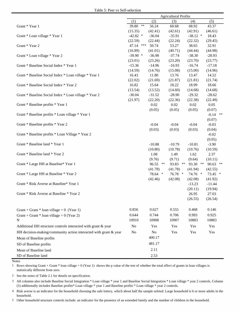
(1) (2) (3) (4) (5)Grant * Year 1 39.80 **  56.24     60.68     68.92     43.37    

(15.35)     (42.41)     (42.61)     (42.91)     (46.61)    

Grant * Loan village * Year 1 -42.82 *   -36.04     -35.91     -38.12 *   18.43    

(22.59)     (22.44)     (22.24)     (22.32)     (29.45)    

Grant * Year 2 47.14 *** 50.74     53.27     38.65     32.91    

(16.89)     (41.01)     (40.71)     (44.44)     (44.98)    

Grant * Loan village * Year 2 -39.90 *   -36.98     -37.74     -38.30     -28.93    

(23.01)     (23.26)     (23.20)     (23.70)     (23.77)    

Grant * Baseline Social Index * Year 1 -15.36     -14.96     -16.93     -16.74     -17.18    

(14.59)     (14.76)     (15.08)     (15.00)     (14.96)    

Grant * Baseline Social Index * Loan village * Year 1 16.43     11.80     13.76     13.47     14.52    

(22.02)     (21.69)     (21.87)     (21.81)     (21.74)    

Grant * Baseline Social Index * Year 2 16.82     15.64     18.22     18.99     18.66    

(13.54)     (13.52)     (14.60)     (14.68)     (14.68)    

Grant * Baseline Social Index * Loan village * Year 2 -30.04     -31.52     -28.90     -29.32     -28.62    

(21.97)     (22.20)     (22.36)     (22.38)     (22.49)    

Grant * Baseline profits * Year 1            0.02     0.02     0.02     0.05    

           (0.05)     (0.05)     (0.05)     (0.07)    

Grant * Baseline profits * Loan village * Year 1                        -0.14 ** 

                       (0.07)    

Grant * Baseline profits * Year 2            -0.04     -0.04     -0.04     -0.03    

           (0.03)     (0.03)     (0.03)     (0.04)    

Grant * Baseline profits * Loan Village * Year 2                        -0.02    

                       (0.05)    

Grant * Baseline land * Year 1            -10.88     -10.79     -10.81     -3.90    

           (10.80)     (10.78)     (10.76)     (10.59)    

Grant * Baseline land * Year 2            1.08     1.49     1.62     2.37    

           (9.76)     (9.71)     (9.64)     (10.11)    

Grant * Large HH at Baseline* Year 1            96.55 **  93.83 **  93.30 **  90.63 ** 

           (41.78)     (41.78)     (41.94)     (42.55)    

Grant * Large HH at Baseline * Year 2            78.64 *   76.78 *   74.76 *   73.45 *  

           (42.46)     (42.08)     (42.08)     (41.92)    

Grant * Risk Averse at Baseline* Year 1 -13.23     -11.44    

(20.11)     (19.94)    

Grant * Risk Averse at Baseline * Year 2 26.95     27.03    

(26.55)     (26.54)    

Grant + Grant * loan village = 0 (Year 1) 0.856 0.627 0.555 0.468 0.146

Grant + Grant * loan village = 0 (Year 2) 0.644 0.744 0.706 0.993     0.925    

N 10910 10908 10907 10883     10883    

Additional HH structure controls interacted with grant & year No Yes Yes Yes Yes

HH decision-making/community action interacted with grant & year No No Yes Yes Yes

Mean of Baseline profits 400.17

SD of Baseline profits 481.17

Mean of Baseline land 2.11

SD of Baseline land 2.53

Notes1

2 See the notes of Table 2.1 for details on specification.

3

4

5 Other household structure controls include: an indicator for the presence of an extended family and the number of children in the household.

Table 5: Peer vs Self-selection

All columns also include Baseline Social Integration * Loan village * year 1 and Baseline Social Integration * Loan village * year 2 controls. Column (5) additionally includes Baseline profits* Loan village * year 1 and Baseline profits * Loan village * year 2 controls.

Rows showing Grant + Grant * loan village = 0 (Year 1) shows the p value of the test of whether the total effect of grants in loan villages is statistically different from zero.

Agricultural Profits

Risk averse is an indicator for the household choosing the safe lottery, which about half the sample seleted. Large household is 6 or more adults in the household.

198 Villages N = 6,807

Randomization

88 Villages Offered loans

N = 2,818

Randomization

Grants N = 1,351

Control N = 2,397

110 Villages No loans offered

N = 3,989

Women who take loan N = 597

Women who do not take loan

N = 2,221

Randomization

No grant N = 1,454

Grant N = 767

Randomization

Grant to female N = 804

Grant to male N = 547

Figure 1: Experimental Design

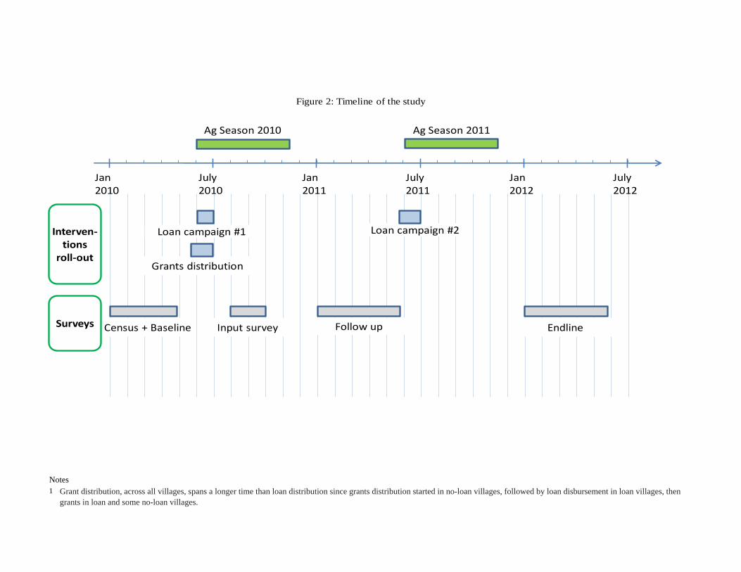
Notes1 Grant distribution, across all villages, spans a longer time than loan distribution since grants distribution started in no-loan villages, followed by loan disbursement in loan villages, then

grants in loan and some no-loan villages.

Figure 2: Timeline of the study

Jan 2010

July 2010

Jan 2011

July 2011

Jan 2012

July 2012

Ag Season 2010 Ag Season 2011

Surveys

Interven‐tions

roll‐out

Census + Baseline Input survey Follow up Endline

Grants distribution

Loan campaign #1 Loan campaign #2

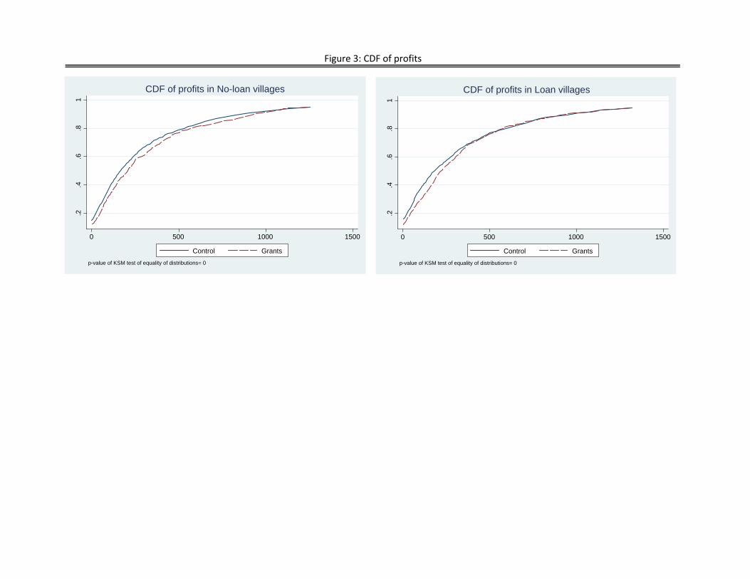
Figure 3: CDF of profits

.2.4

.6.8

1

0 500 1000 1500

Control Grants

p-value of KSM test of equality of distributions= 0

CDF of profits in No-loan villages

.2.4

.6.8

1

0 500 1000 1500

Control Grants

p-value of KSM test of equality of distributions= 0

CDF of profits in Loan villages

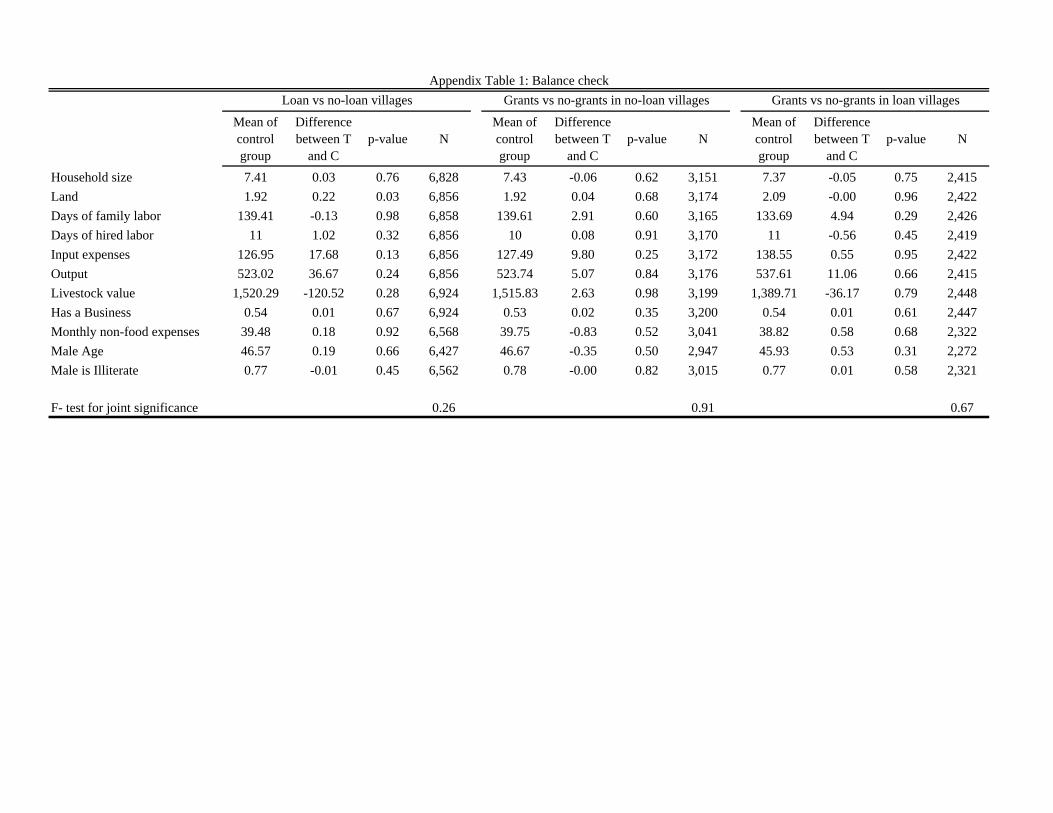
Mean of control group

Difference between T

and Cp-value N

Mean of control group

Difference between T

and Cp-value N

Mean of control group

Difference between T

and Cp-value N

Household size 7.41 0.03 0.76 6,828 7.43 -0.06 0.62 3,151 7.37 -0.05 0.75 2,415

Land 1.92 0.22 0.03 6,856 1.92 0.04 0.68 3,174 2.09 -0.00 0.96 2,422

Days of family labor 139.41 -0.13 0.98 6,858 139.61 2.91 0.60 3,165 133.69 4.94 0.29 2,426

Days of hired labor 11 1.02 0.32 6,856 10 0.08 0.91 3,170 11 -0.56 0.45 2,419

Input expenses 126.95 17.68 0.13 6,856 127.49 9.80 0.25 3,172 138.55 0.55 0.95 2,422

Output 523.02 36.67 0.24 6,856 523.74 5.07 0.84 3,176 537.61 11.06 0.66 2,415

Livestock value 1,520.29 -120.52 0.28 6,924 1,515.83 2.63 0.98 3,199 1,389.71 -36.17 0.79 2,448

Has a Business 0.54 0.01 0.67 6,924 0.53 0.02 0.35 3,200 0.54 0.01 0.61 2,447

Monthly non-food expenses 39.48 0.18 0.92 6,568 39.75 -0.83 0.52 3,041 38.82 0.58 0.68 2,322

Male Age 46.57 0.19 0.66 6,427 46.67 -0.35 0.50 2,947 45.93 0.53 0.31 2,272

Male is Illiterate 0.77 -0.01 0.45 6,562 0.78 -0.00 0.82 3,015 0.77 0.01 0.58 2,321

F- test for joint significance 0.26 0.91 0.67

Appendix Table 1: Balance check

Loan vs no-loan villages Grants vs no-grants in no-loan villages Grants vs no-grants in loan villages

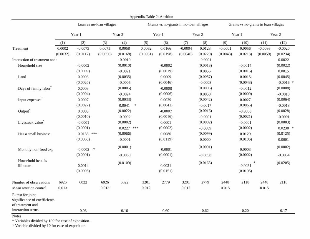
(1) (2) (3) (4) (5) (6) (7) (8) (9) (10) (11) (12)

Treatment 0.0002 -0.0073 0.0075 0.0058 0.0062 0.0166 -0.0004 0.0123 -0.0001 0.0056 -0.0036 -0.0020

(0.0032) (0.0117) (0.0056) (0.0168) (0.0051) (0.0198) (0.0046) (0.0220) (0.0043) (0.0213) (0.0059) (0.0234)

Interaction of treatment and: -0.0010 -0.0001 0.0022

Household size -0.0002 (0.0010) -0.0002 (0.0013) -0.0014 (0.0022)

(0.0009) -0.0021 (0.0019) 0.0056 (0.0016) 0.0015

Land 0.0003 (0.0035) 0.0009 (0.0057) 0.0015 (0.0045)

(0.0026) -0.0005 (0.0046) -0.0008 (0.0043) -0.0016 *

Days of family labor† 0.0003 (0.0005) -0.0008 (0.0005) -0.0012 (0.0008)

(0.0004) -0.0024 (0.0006) 0.0050 (0.0009) -0.0018

Input expenses* 0.0007 (0.0033) 0.0029 (0.0042) 0.0027 (0.0064)

(0.0027) 0.0041 * (0.0041) -0.0017 (0.0065) -0.0018

Output* 0.0003 (0.0022) -0.0007 (0.0016) -0.0008 (0.0028)

(0.0010) -0.0002 (0.0016) -0.0001 (0.0021) -0.0001

Livestock value* -0.0001 (0.0002) 0.0001 (0.0002) -0.0001 (0.0003)

(0.0001) 0.0227 *** (0.0002) -0.0009 (0.0002) 0.0238 *

Has a small business 0.0133 *** (0.0066) 0.0080 (0.0099) 0.0129 (0.0125)

(0.0050) -0.0001 (0.0119) 0.0000 (0.0106) 0.0001

Monthly non-food exp -0.0002 *(0.0001)

-0.0001(0.0001)

0.0003(0.0002)

(0.0001) -0.0068 (0.0001) -0.0058 (0.0002) -0.0054

Household head is illiterate 0.0014

(0.0109)0.0021

(0.0165)-0.0031

* (0.0205)

(0.0095) (0.0151) (0.0195)

Number of observations 6926 6022 6926 6022 3201 2779 3201 2779 2448 2118 2448 2118

Mean attrition control 0.013 0.013 0.012 0.012 0.015 0.015

F- test for joint significance of coefficients of treatment and interaction terms 0.08 0.16 0.60 0.62 0.20 0.17

Notes* Variables divided by 100 for ease of exposition.† Variable divided by 10 for ease of exposition.

Appendix Table 2: Attrition

Year 2

Grants vs no-grants in no-loan villages Grants vs no-grants in loan villages

Year 1 Year 2

Loan vs no-loan villages

Year 1 Year 2 Year 1

(1) (2) (3) (4) (5) (6)

Date (linear) 0.00094 0.00290 0.002 0.005

(0.004) (0.008) (0.011) (0.023)

Date squared -0.00007 -0.00011

(0.000) (0.001)

1 if before June 1st -0.045 -0.176

(0.140) (0.407)

Revisit to Village -0.022 -0.007 -0.034 0.124 0.147 0.051

(0.106) (0.119) (0.121) (0.307) (0.344) (0.351)

Observations 787 787 787 774 774 774

Fixed effects None None None None None None

Notes1

2

Table A3: Timing robustness (No-loan villages)

Index Land Size

Index includes: land area, number of family labor days, number of hired labor days, an indicator for whether fertilizer was used, value of fertilizer expenses, value of other chemical expenses, value of al input expenses, value of harvest, and profits. Sample includes only grant recipients in no-loan villages.

Business Profits: 12

months

Intra HH Decision-making Index

Community

Action Index

Social Capital Index

(1) (2) (3) (4)

Grant - year 1 21.49    -0.0004 0.067 0.031 (13.75)    (0.042) (0.043) (0.039)

Grant * loan village - year 1 -28.87 *   0.076 0.009 0.070 (17.35)    (0.057) (0.059) (0.051) Grant - year 2 42.38 **  0.059 0.021 0.091 *** (18.53)    (0.039) (0.045) (0.034) Grant * loan village - year 2 -18.88    0.007 0.109 * 0.017 (27.01)    (0.057) (0.063) (0.050)

Grant + Grant * loan village = 0 (year 1) 0.486    0.048 0.064 0.002

Grant + Grant * loan village = 0 (year 2) 0.233    0.113 0.004 0.004

N 10740    9942 9985 9813

Mean of control (year 1) 224.57    0.012    -0.027     -0.091   

SD (year 1) 366.80    0.985    0.980     0.936   

Loan village - year 1 2.45 0.000 0.058 -0.001 (19.92) (0.043) (0.053) (0.049) Loan Village - year 2 22.46 0.039 0.065 0.042 (31.37) (0.053) (0.048) (0.042) N 8594    7900 7934 7811

Mean of control (year 1) 230.83    0.035    -0.024     -0.060   

SD (year 1) 371.64    0.958    0.983     0.938   

Notes1

2

Appendix Table 4: Additional Outcomes

Panel A. Grant recipients vs control

Panel B. Loan villages vs control

Rows showing Grant + Grant * loan village = 0 (year 1) shows the p value of the test of whether the total effect of grants in loan villages is statistically different from zero.See the notes of Table 2.1 for details on specification.