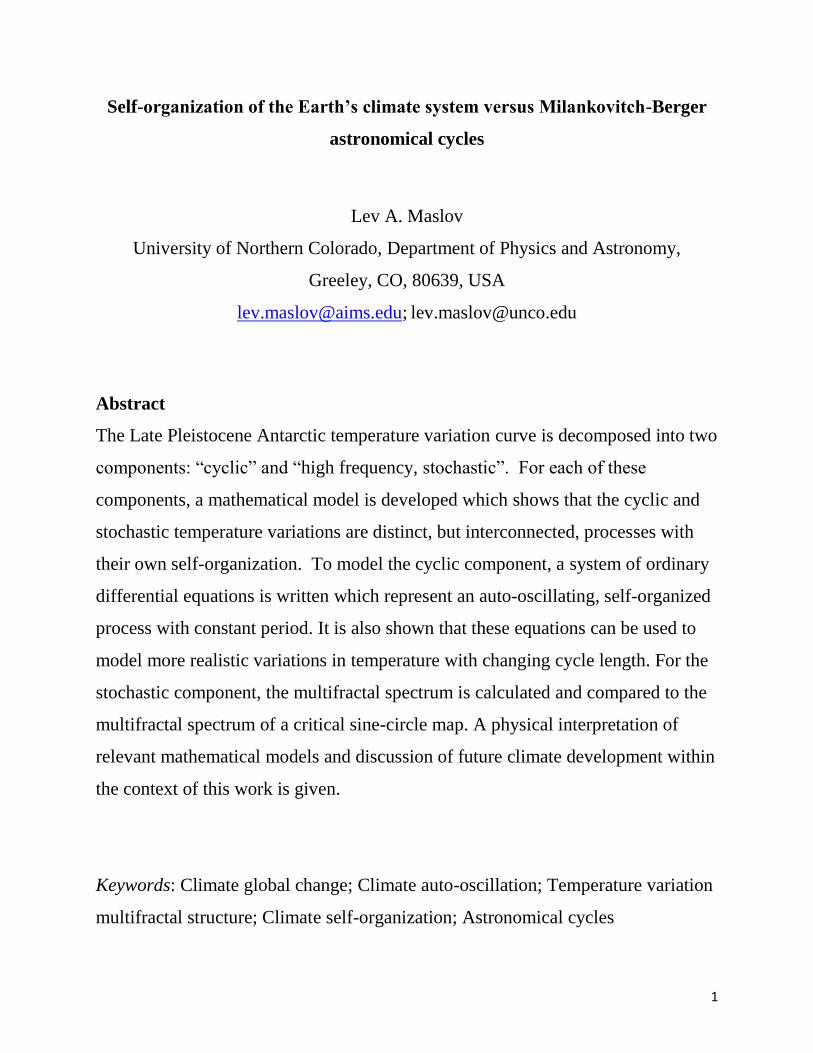
Self-organization of the Earth's climate system versus Milankovitch-Berger astronomical cycles

1

Self-organization of the Earth’s climate system versus Milankovitch-Berger

astronomical cycles

Lev A. Maslov

University of Northern Colorado, Department of Physics and Astronomy,

Greeley, CO, 80639, USA

[email protected]; [email protected]

Abstract

The Late Pleistocene Antarctic temperature variation curve is decomposed into two

components: “cyclic” and “high frequency, stochastic”. For each of these

components, a mathematical model is developed which shows that the cyclic and

stochastic temperature variations are distinct, but interconnected, processes with

their own self-organization. To model the cyclic component, a system of ordinary

differential equations is written which represent an auto-oscillating, self-organized

process with constant period. It is also shown that these equations can be used to

model more realistic variations in temperature with changing cycle length. For the

stochastic component, the multifractal spectrum is calculated and compared to the

multifractal spectrum of a critical sine-circle map. A physical interpretation of

relevant mathematical models and discussion of future climate development within

the context of this work is given.

Keywords: Climate global change; Climate auto-oscillation; Temperature variation

multifractal structure; Climate self-organization; Astronomical cycles

2

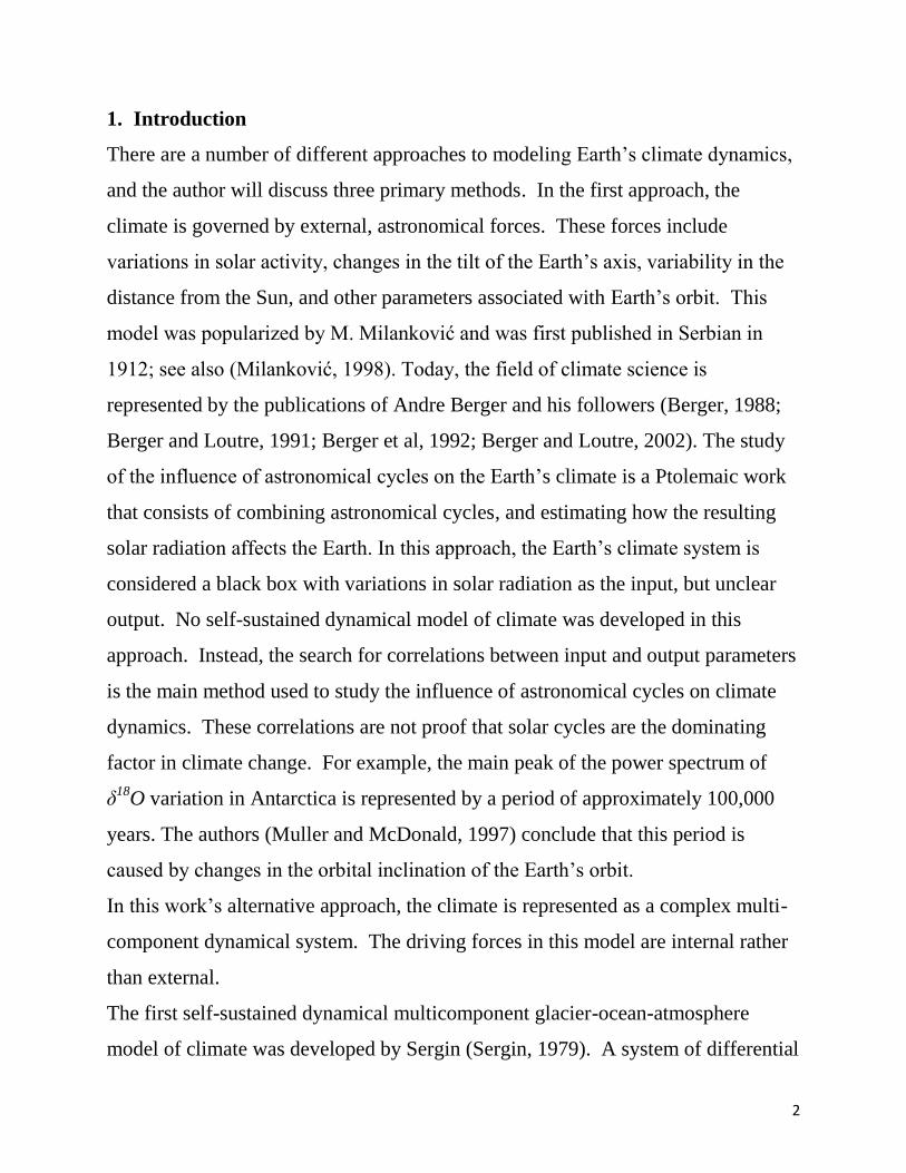
1. Introduction

There are a number of different approaches to modeling Earth’s climate dynamics,

and the author will discuss three primary methods. In the first approach, the

climate is governed by external, astronomical forces. These forces include

variations in solar activity, changes in the tilt of the Earth’s axis, variability in the

distance from the Sun, and other parameters associated with Earth’s orbit. This

model was popularized by M. Milanković and was first published in Serbian in

1912; see also (Milanković, 1998). Today, the field of climate science is

represented by the publications of Andre Berger and his followers (Berger, 1988;

Berger and Loutre, 1991; Berger et al, 1992; Berger and Loutre, 2002). The study

of the influence of astronomical cycles on the Earth’s climate is a Ptolemaic work

that consists of combining astronomical cycles, and estimating how the resulting

solar radiation affects the Earth. In this approach, the Earth’s climate system is

considered a black box with variations in solar radiation as the input, but unclear

output. No self-sustained dynamical model of climate was developed in this

approach. Instead, the search for correlations between input and output parameters

is the main method used to study the influence of astronomical cycles on climate

dynamics. These correlations are not proof that solar cycles are the dominating

factor in climate change. For example, the main peak of the power spectrum of

δ18

O variation in Antarctica is represented by a period of approximately 100,000

years. The authors (Muller and McDonald, 1997) conclude that this period is

caused by changes in the orbital inclination of the Earth’s orbit.

In this work’s alternative approach, the climate is represented as a complex multi-

component dynamical system. The driving forces in this model are internal rather

than external.

The first self-sustained dynamical multicomponent glacier-ocean-atmosphere

model of climate was developed by Sergin (Sergin, 1979). A system of differential

3

equations representing this model were developed and solved numerically. It was

found that characteristic parameters of the climate system auto-oscillate with

periods of 20,000-80,000 years. Another complex self-sustained model of the

interaction between continental ice, ocean and atmosphere was developed in 1993

(Kagan et al, 1993). A system of differential equations representing this model was

written. Given realistic thermodynamic parameters, the authors found a similar

auto-oscillation within this system, with a period of about 100,000 years.

The enormous complexity of climate processes requires the use of methods and

models capable of handling such complexity. Implementing the modern theory of

dynamical systems brought a breakthrough in understanding and modeling climate

dynamics. Thus, the application of multifractal statistics to the study of

temperature variations in Greenland (Schmitt et al, 1995) and Antarctica

(Ashkenazy et al., 2003) allowed the authors to formulate the requirements for

realistic climate models, which must “include both periodic and stochastic

elements of climate change”. The importance of viewing Earth’s climate as a

nonlinear, complex, dynamical system was understood in 2004 (Rial, Pielke,

Beniston, et al., 2004), but no references were made to the earlier publications

(Sergin, 1979; Kagan et al, 1993; Schmitt et al, 1995; Ashkenazy et al., 2003)

which modeled climate as a nonlinear, complex, dynamical system, and no

mathematical, or conceptual models were suggested.

The approach in the current work is based solely on real data. We study the

Antarctic Late Pleistocene temperature record calculated from the hydrogen

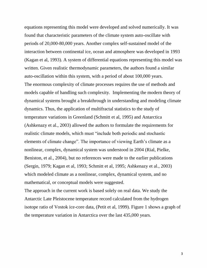
isotope ratio of Vostok ice-core data, (Petit et al, 1999). Figure 1 shows a graph of

the temperature variation in Antarctica over the last 435,000 years.

4

Figure 1

Temperature variations (ΔT) in Antarctica according to Vostok ice-core data.

Our goal is three-fold: a) decomposition of the temperature variations (Figure 1)

into components corresponding to basic processes, b) mathematical modeling of

these processes, c) physical interpretation of these mathematical models and

discussion of a consolidated model of climate cycles.

2. Decomposing the Data

For the last 420 thousand years the planet has experienced four nearly identical

episodes of temperature change. Each episode starts with a sharp increase in

temperature, followed by long gradual cooling. On a conceptual level, this can be

interpreted as a combination of two subsequent processes: a) the release of latent

heat stored in the system and b) dissipation of this heat by thermal convection. To

test the first hypothesis, and to estimate the rise in temperature due to atmospheric

water vapor condensation, suppose the enthalpy H of the atmosphere remains

constant throughout the cycle:

constLqTcH p (1)

5

In this formula cp is the specific heat of dry air, T- temperature, L is the heat of

condensation of water vapor, and q- is the ratio of the total mass of water vapor in

the atmosphere to the total mass of dry air. According to (Trenberth and Smith,

2005) for the current epoch q = 0.00247. Variations in temperature ΔT and of the

ratio of the total mass of water vapor in the atmosphere to the mass of dry air Δq

must compensate each other, such that

0 LqTcp (2)

For cp = 1.006 J/(g oC), L= 2500 J/g, Δq =0.00247 (all the water vapor is

condensed into water), we find ΔT ≈ 6.14 oC. This estimate is reasonably close to

the changes in temperature at the beginning of each interglacial cycle.

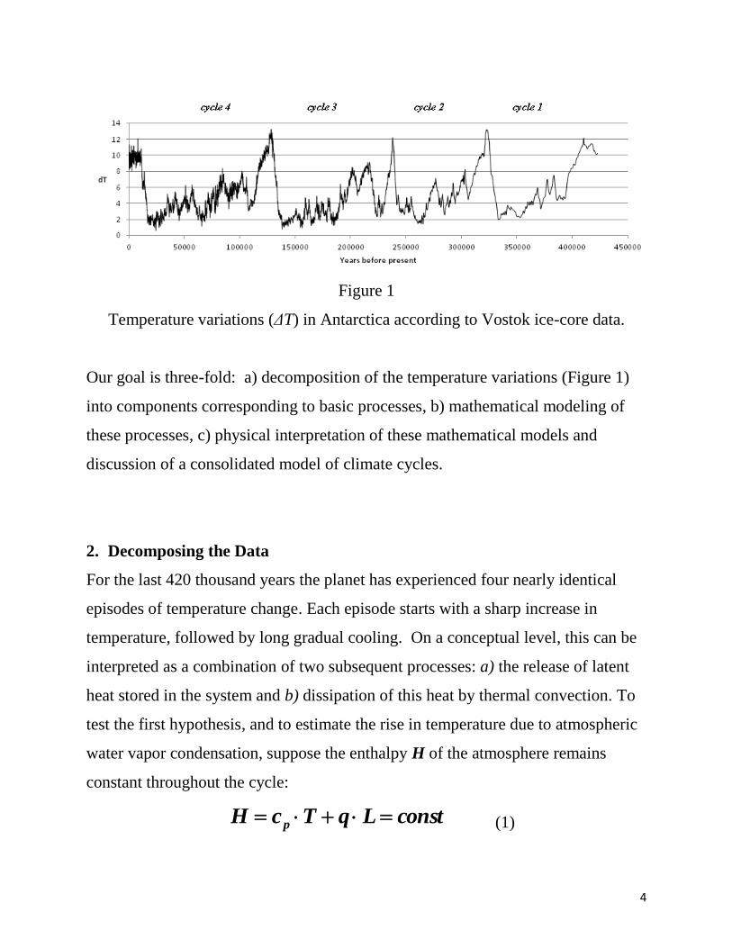
To test the second hypothesis, we use Newton’s Law of Cooling,

0s,sTdt/dT which gives us an exponential decrease in the temperature due

to thermal convection. The natural logarithm of T(t) is plotted in Figure 2.

Figure 2

ln(T) function, and straight line approximations ln(T)=kit+pi within cycles.

Next, the data within each cycle is approximated by ln(T)=kit+pi and four

6

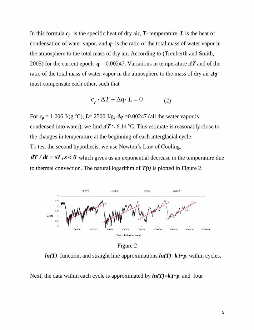
exponential functions Te(t)=exp(kit+pi ) , i=1,2,3,4, are constructed and plotted

against the original temperatures, Figure 3a. Figure 3b shows the difference

between the observed temperature T and Te.

Figure 3

Two components of the temperature variation in Antarctica; a - the original

data superimposed with exponential functions Te(t)=exp(kit+pi ) , i=1,2,3,4,

for each cycle; b – high frequency oscillation components as a difference

between the original data and Te(t).

The coefficient of determination for this approximation was calculated to be R2

=0.624, which is equivalent to a coefficient of correlation r = 0.79.

Thus, the temperature variation in Antarctica can be represented as a sum of two

components: the cyclic, low frequency nonlinear oscillation component, and a high

frequency stochastic oscillation component. For simplicity, we will refer to these

two components as “cyclic” Tc and “high frequency stochastic” Ts; T= Tc+ Ts .

The current approach to decomposing the observed data is based on a physical

principle and is different from methods based on formal frequency filtering of the

data.

7

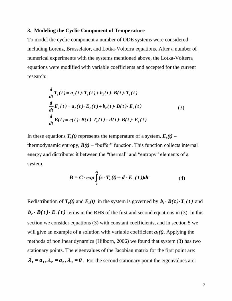
3. Modeling the Cyclic Component of Temperature

To model the cyclic component a number of ODE systems were considered -

including Lorenz, Brusselator, and Lotka-Volterra equations. After a number of

numerical experiments with the systems mentioned above, the Lotka-Volterra

equations were modified with variable coefficients and accepted for the current

research:

)t(E)t(B)t(d)t(T)t(B)t(c)t(Bdt

d

)t(E)t(B)t(b)t(E)t(a)t(Edt

d

)t(T)t(B)t(b)t(T)t(a)t(Tdt

d

cc

c2c2c

c1c1c

(3)

In these equations Tc(t) represents the temperature of a system, Ec(t) –

thermodynamic entropy, B(t) – “buffer” function. This function collects internal

energy and distributes it between the “thermal” and “entropy” elements of a

system.

dt))t(Ed(t)T(cexpC=B c

t

0

c

(4)

Redistribution of Tc(t) and Ec(t) in the system is governed by )t(T)t(Bb c1 and

)t(E)t(Bb c2 terms in the RHS of the first and second equations in (3). In this

section we consider equations (3) with constant coefficients, and in section 5 we

will give an example of a solution with variable coefficient a1(t). Applying the

methods of nonlinear dynamics (Hilborn, 2006) we found that system (3) has two

stationary points. The eigenvalues of the Jacobian matrix for the first point are:

0= ,a= ,a= 32211 . For the second stationary point the eigenvalues are:

8

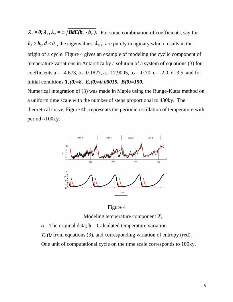
.)b-BdE(b= , 0;= 21321 For some combination of coefficients, say for

0 <d ,b>b 21 , the eigenvalues 2,3 are purely imaginary which results in the

origin of a cycle. Figure 4 gives an example of modeling the cyclic component of

temperature variations in Antarctica by a solution of a system of equations (3) for

coefficients a1= -4.673, b1=0.1827, a2=17.9005, b2= -0.70, c= -2.0, d=3.5, and for

initial conditions Tc(0)=8, Ec(0)=0.00015, B(0)=150.

Numerical integration of (3) was made in Maple using the Runge-Kutta method on

a uniform time scale with the number of steps proportional to 430ky. The

theoretical curve, Figure 4b, represents the periodic oscillation of temperature with

period ≈100ky.

Figure 4

Modeling temperature component Tc.

a – The original data; b – Calculated temperature variation

Tc (t) from equations (3), and corresponding variation of entropy (red).

One unit of computational cycle on the time scale corresponds to 100ky.

9

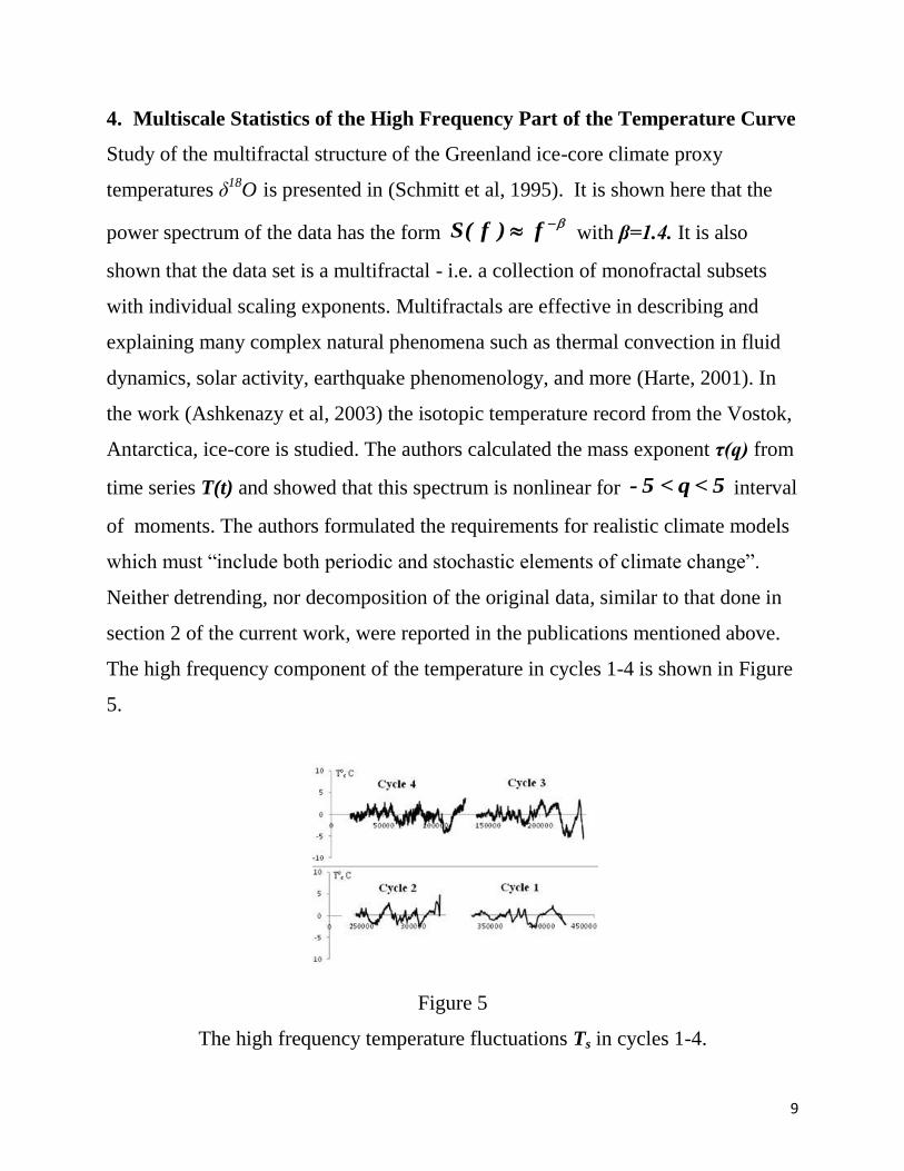
4. Multiscale Statistics of the High Frequency Part of the Temperature Curve

Study of the multifractal structure of the Greenland ice-core climate proxy

temperatures δ18

O is presented in (Schmitt et al, 1995). It is shown here that the

power spectrum of the data has the form f)f(S with β=1.4. It is also

shown that the data set is a multifractal - i.e. a collection of monofractal subsets

with individual scaling exponents. Multifractals are effective in describing and

explaining many complex natural phenomena such as thermal convection in fluid

dynamics, solar activity, earthquake phenomenology, and more (Harte, 2001). In

the work (Ashkenazy et al, 2003) the isotopic temperature record from the Vostok,

Antarctica, ice-core is studied. The authors calculated the mass exponent τ(q) from

time series T(t) and showed that this spectrum is nonlinear for 5 < q< 5- interval

of moments. The authors formulated the requirements for realistic climate models

which must “include both periodic and stochastic elements of climate change”.

Neither detrending, nor decomposition of the original data, similar to that done in

section 2 of the current work, were reported in the publications mentioned above.

The high frequency component of the temperature in cycles 1-4 is shown in Figure

5.

Figure 5

The high frequency temperature fluctuations Ts in cycles 1-4.

10

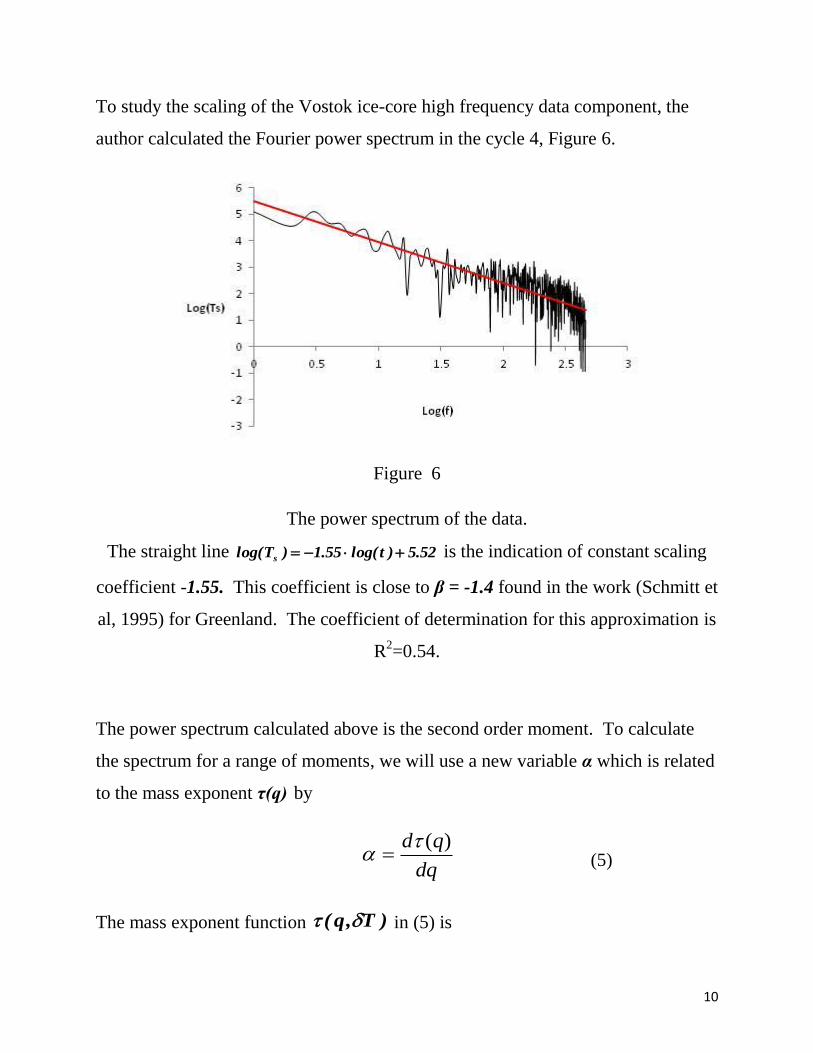
To study the scaling of the Vostok ice-core high frequency data component, the

author calculated the Fourier power spectrum in the cycle 4, Figure 6.

Figure 6

The power spectrum of the data.

The straight line 52.5)tlog(55.1)Tlog( s is the indication of constant scaling

coefficient -1.55. This coefficient is close to β = -1.4 found in the work (Schmitt et

al, 1995) for Greenland. The coefficient of determination for this approximation is

R2=0.54.

The power spectrum calculated above is the second order moment. To calculate

the spectrum for a range of moments, we will use a new variable α which is related

to the mass exponent τ(q) by

dq

qd )( (5)

The mass exponent function )T,q( in (5) is

11

)ln(

),(ln),(

T

TqDTq

, (6)

where )T,q(D is the partition function

N

i

q

inTqD ),( , (7)

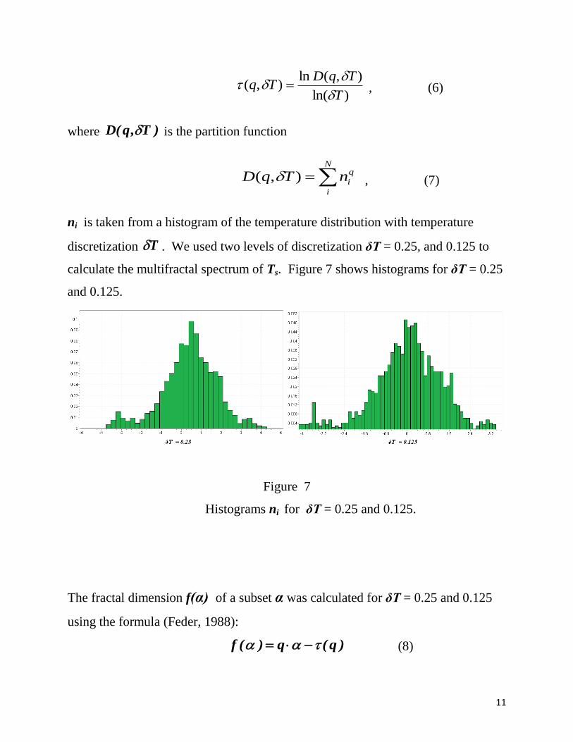
ni is taken from a histogram of the temperature distribution with temperature

discretization T . We used two levels of discretization δT = 0.25, and 0.125 to

calculate the multifractal spectrum of Ts. Figure 7 shows histograms for δT = 0.25

and 0.125.

Figure 7

Histograms ni for δT = 0.25 and 0.125.

The fractal dimension f(α) of a subset α was calculated for δT = 0.25 and 0.125

using the formula (Feder, 1988):

)q(q)(f (8)

12

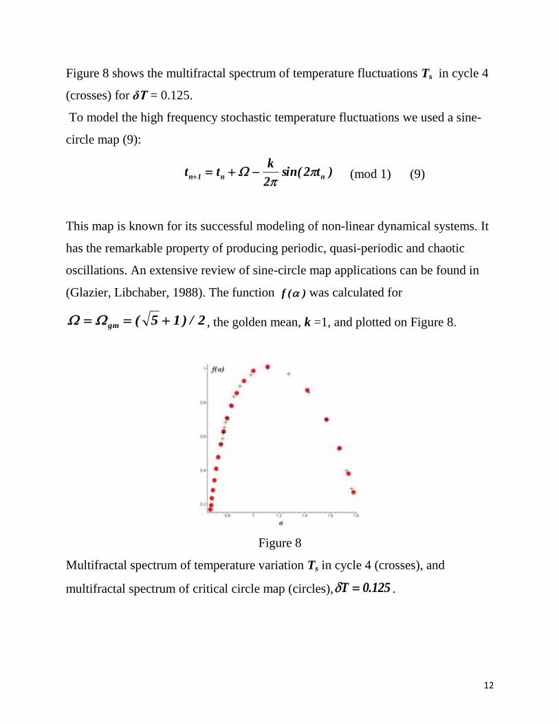
Figure 8 shows the multifractal spectrum of temperature fluctuations Ts in cycle 4

(crosses) for δT = 0.125.

To model the high frequency stochastic temperature fluctuations we used a sine-

circle map (9):

)t2sin(2

ktt nn1n

(mod 1) (9)

This map is known for its successful modeling of non-linear dynamical systems. It

has the remarkable property of producing periodic, quasi-periodic and chaotic

oscillations. An extensive review of sine-circle map applications can be found in

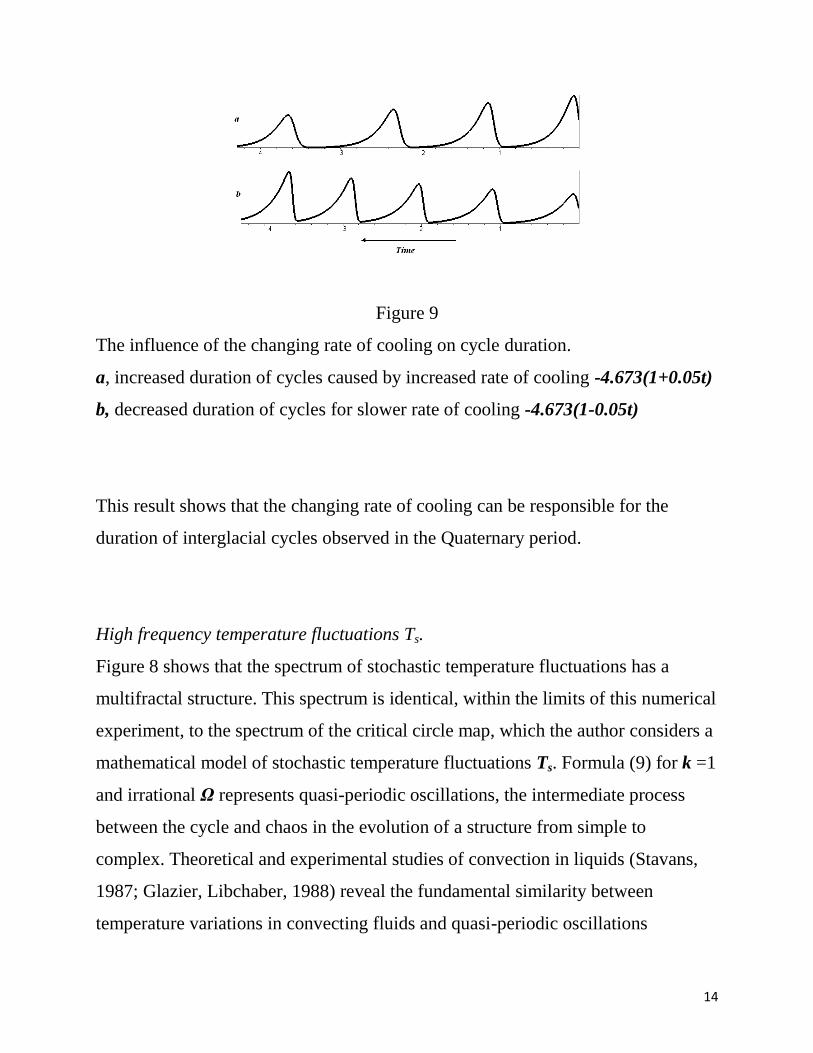
(Glazier, Libchaber, 1988). The function )(f was calculated for

2/)15(gm , the golden mean, k =1, and plotted on Figure 8.

Figure 8

Multifractal spectrum of temperature variation Ts in cycle 4 (crosses), and

multifractal spectrum of critical circle map (circles), 125.0T .

13

5. Conceptual Interpretation of Models

Cyclic temperature variations Tc.

It is show in section 3 that the system of non-linear differential equations (3) has a

cycle. A.Andronov in his work (1929) demonstrated the relation between the limit

cycle and a special form of oscillation which is called auto-oscillation (self-

oscillation, self sustained oscillation). Auto-oscillation is the self-organized

response of a non-linear dynamical system to a constant, non-oscillating, flow of

energy. Thus, dynamical systems, described by non-linear differential equations

(3) can be considered to be a non-linear, dissipative, and self-organized system.

According to Figure 4b, the peak of entropy precedes the peak of the temperature,

and a decrease in entropy is followed by a rapid increase in temperature of about

10oC on the Earth’s surface. Physically, this can be interpreted as a phase

transition, like the condensation of water vapor, and release of latent heat, as

discussed it in section 2. We can see that the duration of observed temperature

cycles, Figure 4a, gradually increases from ≈100ky in cycles 1 and 2, through

≈120ky in cycle 3, and to ≈130ky in cycle 4. This increase in the duration of

temperature cycles can be caused by gradual changes in properties of the system

itself. To model this situation, the original system of equations (3) was modified

by replacing the constant coefficient a1 with coefficient a1(1+αt), t - time.

Calculations were made for a1 = -4.673, and for α = ± 0.05. The case of positive α

corresponds to an increased rate of cooling of the system, and the case of negative

α corresponds to a decreased rate of cooling of the system relative to that rate in a

cycle. The increased rate of cooling of the system caused a gradual increase in the

cycle’s duration, Figure 5a, and, vice versa, for a slower rate of cooling we observe

a decrease in the duration of cycles, Figure 9b.

14

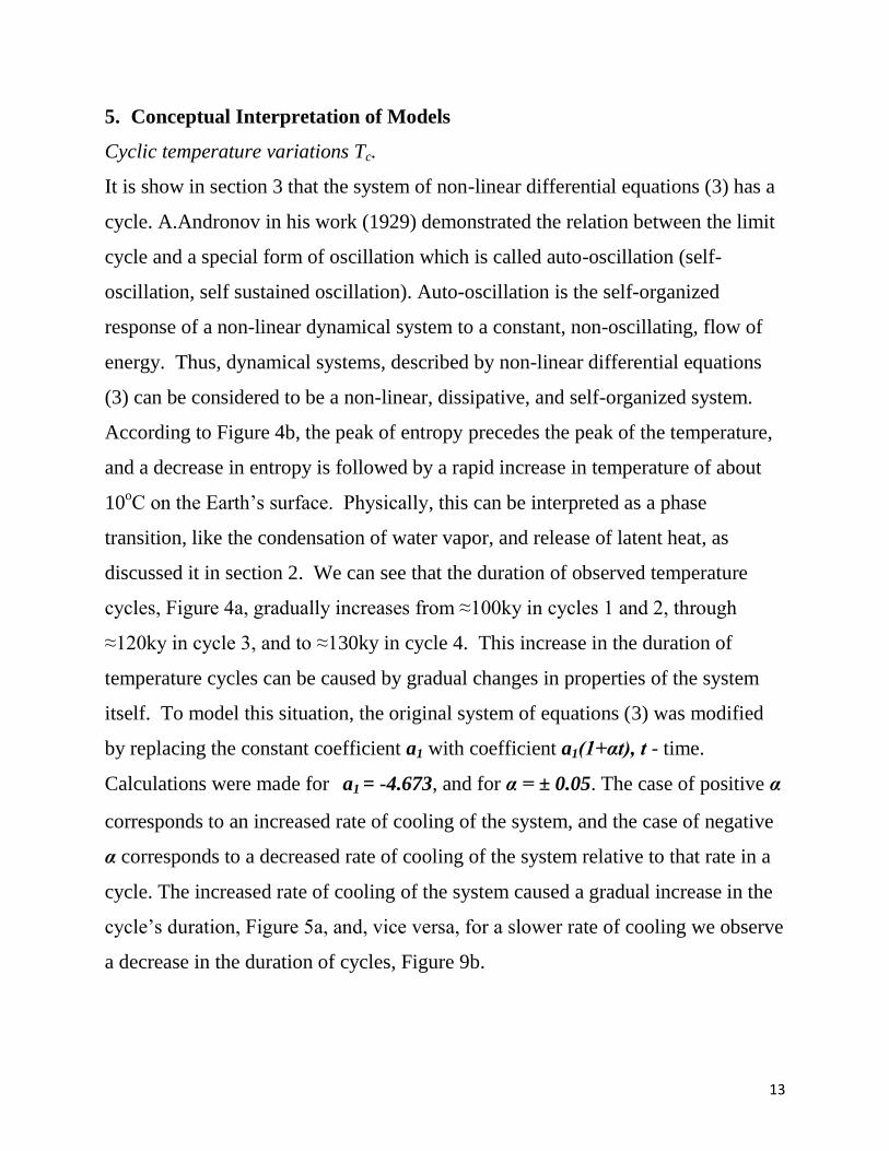
Figure 9

The influence of the changing rate of cooling on cycle duration.

a, increased duration of cycles caused by increased rate of cooling -4.673(1+0.05t)

b, decreased duration of cycles for slower rate of cooling -4.673(1-0.05t)

This result shows that the changing rate of cooling can be responsible for the

duration of interglacial cycles observed in the Quaternary period.

High frequency temperature fluctuations Ts.

Figure 8 shows that the spectrum of stochastic temperature fluctuations has a

multifractal structure. This spectrum is identical, within the limits of this numerical

experiment, to the spectrum of the critical circle map, which the author considers a

mathematical model of stochastic temperature fluctuations Ts. Formula (9) for k =1

and irrational Ω represents quasi-periodic oscillations, the intermediate process

between the cycle and chaos in the evolution of a structure from simple to

complex. Theoretical and experimental studies of convection in liquids (Stavans,

1987; Glazier, Libchaber, 1988) reveal the fundamental similarity between

temperature variations in convecting fluids and quasi-periodic oscillations

15

described by the critical sine circle map (9). Thus, based on the universality of the

critical circle map as a mathematical model, one can suggest that the stochastic

component Ts of temperature fluctuations in Antarctica is caused by convection in

Earth's overheated atmosphere due to global warming. This does not contradict the

hypothesis made in Section 2 for calculating the exponential trend in observed

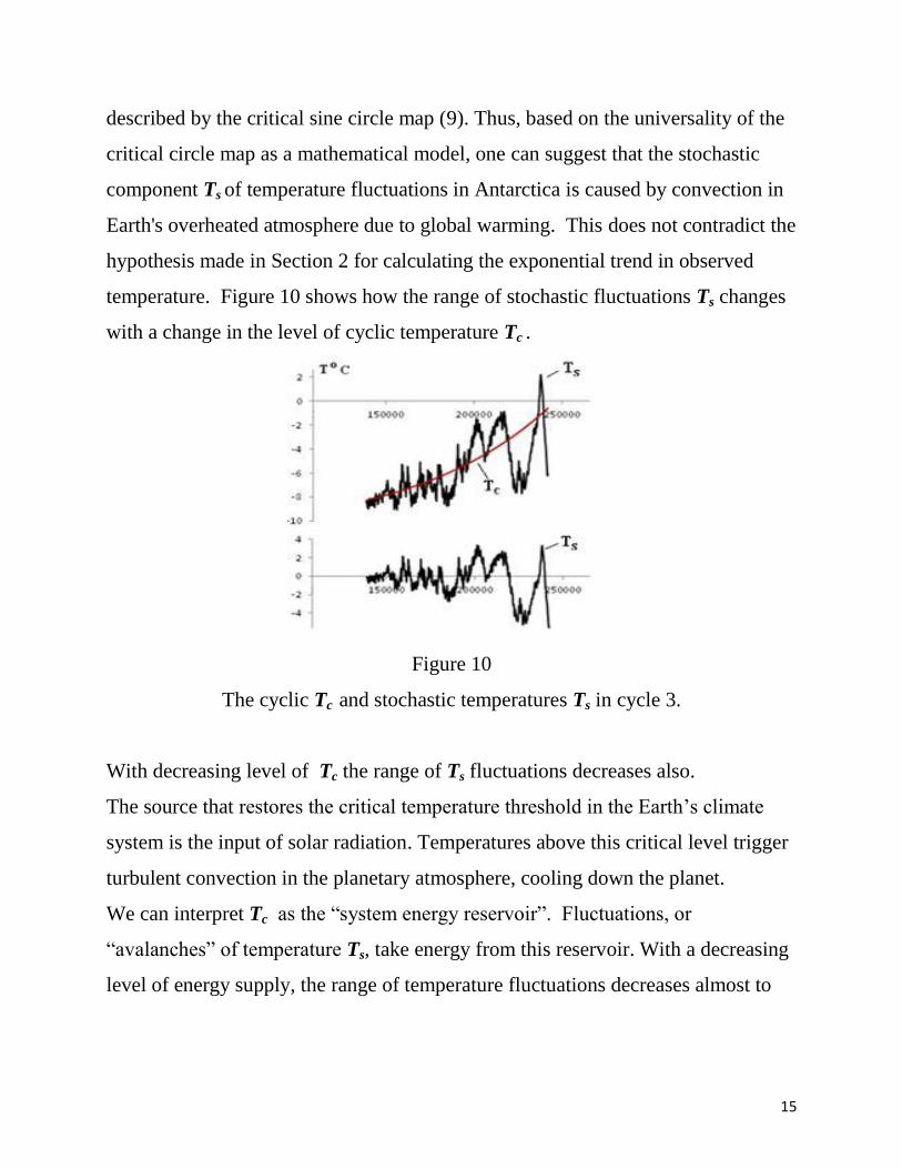
temperature. Figure 10 shows how the range of stochastic fluctuations Ts changes

with a change in the level of cyclic temperature Tc .

Figure 10

The cyclic Tc and stochastic temperatures Ts in cycle 3.

With decreasing level of Tc the range of Ts fluctuations decreases also.

The source that restores the critical temperature threshold in the Earth’s climate

system is the input of solar radiation. Temperatures above this critical level trigger

turbulent convection in the planetary atmosphere, cooling down the planet.

We can interpret Tc as the “system energy reservoir”. Fluctuations, or

“avalanches” of temperature Ts, take energy from this reservoir. With a decreasing

level of energy supply, the range of temperature fluctuations decreases almost to

16

zero. With each sharp rise of temperature in the auto-oscillating component, a

series of temperature “avalanches” continues into the next cycle.

6. Discussion

We will now examine the results of the two processes, cyclic and stochastic, on the

climate system as a whole. Looking at one temperature cycle, and starting at the

interglacial period, we can propose the following conceptual model of climate

evolution: as the atmosphere warms, the permafrost thaws and releases large

quantities of methane. Increasing global temperature also means higher

concentrations of water vapor in the atmosphere. Both of these processes intensify

global warming, which gives rise to turbulent convection in the atmosphere. The

result of this convection is two-fold. On the one hand, the atmosphere will begin

to cool, exhibiting an exponential decay of temperature. At the same time, the

amount of dust in the atmosphere increases. These two processes combine as the

temperature cools enough for water vapor to condense on the dust particles. This

release of latent heat will result in an increase of temperature on the Earth’s

surface, while, at the same time, the atmosphere will clear, and a new cycle will

begin.

7. Conclusion

It is shown that the temperature variation data in Antarctica can be represented as

the sum of two parts, conventionally called the “cyclic” and “high frequency,

stochastic” components. These two components are evidence of two different, but

tightly interconnected, global climate processes. The first one is the sequence of

temperature cycles, with periods gradually increasing from 100,000 years in the

17

first cycle to approximately 130,000 years in the last glacial cycle. The second

process is the high frequency fluctuation of temperature in each cycle. The self-

organization in the auto-oscillation process is the non-linear reaction of the Earth’s

climate system, as a whole, to the input of solar radiation. The self-organization in

the high frequency part is the self-organized nonlinear critical process taking

energy from, and fluctuating around the auto-oscillating part of the temperature

variations. These models characterize the Earth’s climate as an open, complex,

self-organized, dynamical system with nonlinear reaction to the input of solar

radiation. The solar activity and variations in Earth’s orbital parameters are

external factors that can be taken into account as forcing functions in the

dynamical model of climate. To model the actual data as close as possible, we

consider solving the system of equations (3) with time-dependent coefficients and

a forcing function which represents insolation. The second direction of our

continued research is the study of the high-frequency component Ts of temperature

decomposition as a non-stationary multifractal time series.

Acknowledgments

The author would like to thank the anonymous reviewers for their valuable

comments and suggestions.

References

Andronov, A.A., 1929. Les cycles limites de Poincareet la teorie des oscillations

autoentretenues. Comptes Rendus Academie des Sciences. 189, 559-561.

18

Ashkenazy, Y., Baker, D.R., Gildor, H., Havlin, S., 2003. Nonlinearity and

multifractality of climate change in the past 420,000 years. Geophysical Research

Letters. 30, 2146-2149.

Berger, A., 1988. Milankovitch Theory and Climate. Review of Geophysics,

26(4), pp. 624-657.

Berger, A., Loutre M.F., 1991. Insolation values for the climate of the last 10

million years. Quaternary Science Reviews, 10 n°4, pp. 297-317.

Berger, A., Loutre M.F., Laskar J., 1992. Stability of the astronomical frequencies

over the Earth's history for paleoclimate studies. Science, 255, pp. 560-566.

Berger, A., Loutre, M.F. 2002. An Exceptionally long Interglacial Ahead?

Science, 297, pp. 1287-1288.

Feder, J., 1988. Fractals. Plenum Press, New York, London.

Glazier, J.A., Libchaber, A., 1988. Quasi-periodicity and dynamic systems: an

experimentalist’s view. IEEE Transactions on Circuits and Systems.

35 (7), 790-809.

Harte,D., 2001. Multifractals: Theory and Applications. Chapman & Hall, London.

Hilborn, R. C., 2006. Chaos and non-linear dynamics. Oxford Univ. Press,

New York.

Kagan, B.A., Maslova, N.V., Sept, V.V., 1993. Discontinuous auto-oscillations of

the ocean thermohaline circulation and internal variability of the climatic system.

Atmosfera. 6, 199-214.

Milanković, M., 1998. Canon of insolation and the ice-age problem. Alven Global,

Belgrade.

Muller, R.A., MacDonald, G.R., 1997. Spectrum of 100-kr glacial cycle: orbital

inclination, not eccentricity. Proc. Natl. Acad. Sci. USA, 94, 8329-8334.

Petit, J.R., et al., 1999. Climate and atmospheric history of the past 420,000 years

from the Vostok ice core, Antarctica. Nature. 399, 429-436.

19

Petit, J.R., et al., 2001.Vostok ice-core data for 420,000 years, IGBP

PAGES/World Data Center for Paleoclimatology Data Contribution Series #2001-

076. NOAA/NGDC Paleoclimatology Program. Boulder CO, USA.

Rial, J.A., Pielke SR, R.A., Beniston, M., et al., 2004. Nonlinearities, feedbacks,

and critical thresholds within the Earth’s climate system. Climatic Change. 65,

11-38.

Schmitt, F., Lovejoy, S., Schertzer, D., 1995. Multifractal analysis of the

Greenland ice core project climate data. Geophysical Research Letters. 22,

1689-1692.

Sergin, V. Ya., 1979. Numerical modeling of the glaciers-ocean-atmosphere

system. Journal of Geophysical Research. 84, 3191-3204.

Stavans, J., 1987. Experimental study of quasiperiodicity in a hydrodynamical

system. Phys. Rev. A35, 4314-4328.

Trenberth, K. E., Smith, L., 2005. The mass of the atmosphere: A constraint on

global analyses. J. Climate. 18, 864-875.