Self-localization by Laser Scanner and GPS in automated surveys

Seediscussions,stats,andauthorprofilesforthispublicationat:http://www.researchgate.net/publication/280734843

Self-LocalizationbyLaserScannerandGPSinAutomatedSurveys

CHAPTERinLECTURENOTESINELECTRICALENGINEERING·JUNE2014

ImpactFactor:0.11·DOI:10.1007/978-3-319-03967-1

READS

9

2AUTHORS,INCLUDING:

GiulianaBilotta

UniversitàIuavdiVenezia

44PUBLICATIONS21CITATIONS

SEEPROFILE

Availablefrom:GiulianaBilotta

Retrievedon:19October2015

http://www.researchgate.net/publication/280734843_Self-Localization_by_Laser_Scanner_and_GPS_in_Automated_Surveys?enrichId=rgreq-ec482fea-6086-4400-a52f-7018ddb2946f&enrichSource=Y292ZXJQYWdlOzI4MDczNDg0MztBUzoyNjU5NTM1NTY1NjE5MjBAMTQ0MDQxOTY3Nzc5Mg%3D%3D&el=1_x_2

http://www.researchgate.net/publication/280734843_Self-Localization_by_Laser_Scanner_and_GPS_in_Automated_Surveys?enrichId=rgreq-ec482fea-6086-4400-a52f-7018ddb2946f&enrichSource=Y292ZXJQYWdlOzI4MDczNDg0MztBUzoyNjU5NTM1NTY1NjE5MjBAMTQ0MDQxOTY3Nzc5Mg%3D%3D&el=1_x_3

http://www.researchgate.net/?enrichId=rgreq-ec482fea-6086-4400-a52f-7018ddb2946f&enrichSource=Y292ZXJQYWdlOzI4MDczNDg0MztBUzoyNjU5NTM1NTY1NjE5MjBAMTQ0MDQxOTY3Nzc5Mg%3D%3D&el=1_x_1

http://www.researchgate.net/profile/Giuliana_Bilotta3?enrichId=rgreq-ec482fea-6086-4400-a52f-7018ddb2946f&enrichSource=Y292ZXJQYWdlOzI4MDczNDg0MztBUzoyNjU5NTM1NTY1NjE5MjBAMTQ0MDQxOTY3Nzc5Mg%3D%3D&el=1_x_4


http://www.researchgate.net/institution/Universita_Iuav_di_Venezia?enrichId=rgreq-ec482fea-6086-4400-a52f-7018ddb2946f&enrichSource=Y292ZXJQYWdlOzI4MDczNDg0MztBUzoyNjU5NTM1NTY1NjE5MjBAMTQ0MDQxOTY3Nzc5Mg%3D%3D&el=1_x_6


UNCORRECTED PROOF1

23456789101112

13

14

1516171819202122

1

Chapter 23Self-Localization by Laser Scanner and GPS in Automated Surveys

V. Barrile and G. Bilotta

N. Mastorakis, V. Mladenov (eds.), Computational Problems in Engineering, Lecture Notes in Electrical Engineering 307, DOI 10.1007/978-3-319-03967-1_23, © Springer International Publishing Switzerland 2014

V. Barrile ()DICEAM Department, Mediterranean University of Reggio Calabria, via Graziella Feo di Vito, 89100 Reggio Calabria, Italye-mail: [email protected]

G. BilottaPh.D. NT&ITA, Planning Department, IUAV University of Venice, Santa Croce 191 Tolentini, 30135 Venice, Italye-mail: [email protected]

Abstract Our contribution is based on a research aimed to a “quick” resolution of an integrated problem oriented towards the self-localization and perimetration through mobile devices. The adopted methodology is applied on a real case study by using the following surveying tools: a kinematic Global Positioning System (GPS) and a Laser Scanner supporting a “mobile platform”. A GPS receiver provided by Leica Geosystem and a two-dimensional Laser Scanner provided by the Automa-tion and Control Laboratory of the University “Mediteranea” of Reggio Calabria were positioned on an experimental mobile system specifically designed to simulate the behaviour of a future and fully automated platform. The research is aimed to conduct the traditional land surveying through a Laser Scanner alongside with GPS receivers in a three dimensional centimetric resolution within one single system of reference made up of individual scans operated by a “Stop-and-Go” device.

Keywords Laser scanner 3D · Self-localization · GPS · Survey

23.1 Introduction—The Experimental Campaign

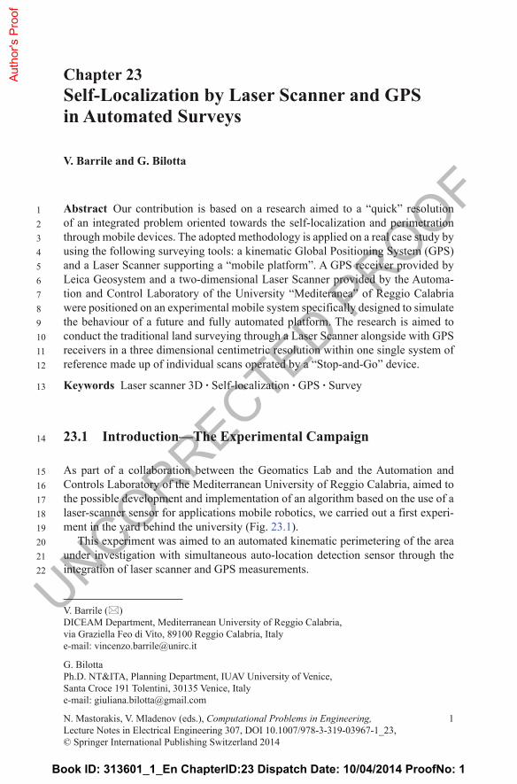
As part of a collaboration between the Geomatics Lab and the Automation and Controls Laboratory of the Mediterranean University of Reggio Calabria, aimed to the possible development and implementation of an algorithm based on the use of a laser-scanner sensor for applications mobile robotics, we carried out a first experi-ment in the yard behind the university (Fig. 23.1).

This experiment was aimed to an automated kinematic perimetering of the area under investigation with simultaneous auto-location detection sensor through the integration of laser scanner and GPS measurements.

Book ID: 313601_1_En ChapterID:23 Dispatch Date: 10/04/2014 ProofNo: 1

Aut

hor's

Pro

of

UNCORRECTED PROOF

2324252627282930313233343536373839

2 V. Barrile and G. Bilotta

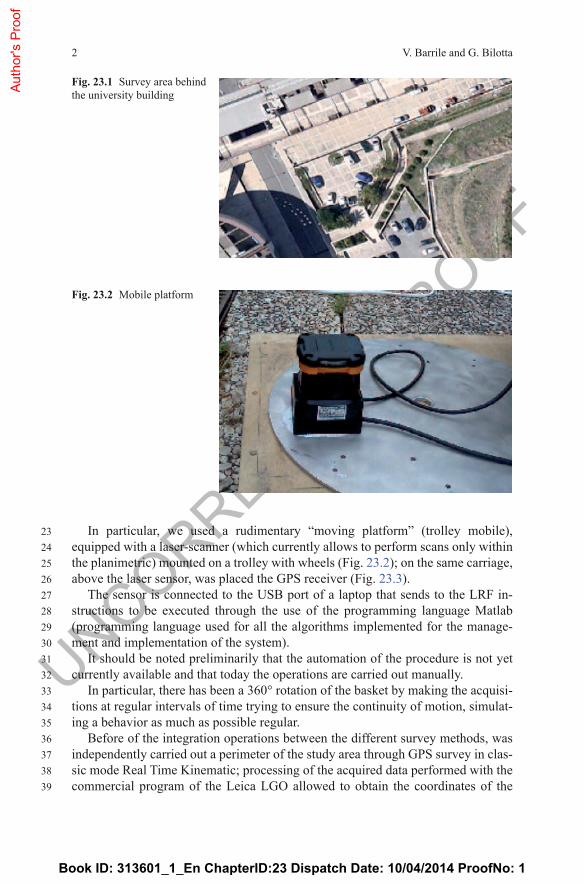
In particular, we used a rudimentary “moving platform” (trolley mobile), equipped with a laser-scanner (which currently allows to perform scans only within the planimetric) mounted on a trolley with wheels (Fig. 23.2); on the same carriage, above the laser sensor, was placed the GPS receiver (Fig. 23.3).

The sensor is connected to the USB port of a laptop that sends to the LRF in-structions to be executed through the use of the programming language Matlab (programming language used for all the algorithms implemented for the manage-ment and implementation of the system).

It should be noted preliminarily that the automation of the procedure is not yet currently available and that today the operations are carried out manually.

In particular, there has been a 360° rotation of the basket by making the acquisi-tions at regular intervals of time trying to ensure the continuity of motion, simulat-ing a behavior as much as possible regular.

Before of the integration operations between the different survey methods, was independently carried out a perimeter of the study area through GPS survey in clas-sic mode Real Time Kinematic; processing of the acquired data performed with the commercial program of the Leica LGO allowed to obtain the coordinates of the

Fig. 23.2 Mobile platform

Fig. 23.1 Survey area behind the university building


Aut

hor's

Pro

of

UNCORRECTED PROOF

404142434445464748

49

505152

323 Self-Localization by Laser Scanner and GPS in Automated Surveys

points shown in the diagram of Fig. 23.4 representing the perimeter of the study area.

The same data were subsequently reported on georeferenced map; these data, con-nected each other, allowed therefore to delimit the perimeter of interest (Fig. 23.5).

These data are considered as data “reliable” to be used for comparison with the survey methods later proposed. In particular, it has been positioned in this regard (integrated laser scanner—GPS—mobile cart) on the platform above the laser scan-ner sensor, a GPS antenna (Fig. 23.6) in such a way to obtain simultaneous mea-surements.

23.2 Measurement by Laser Scanner

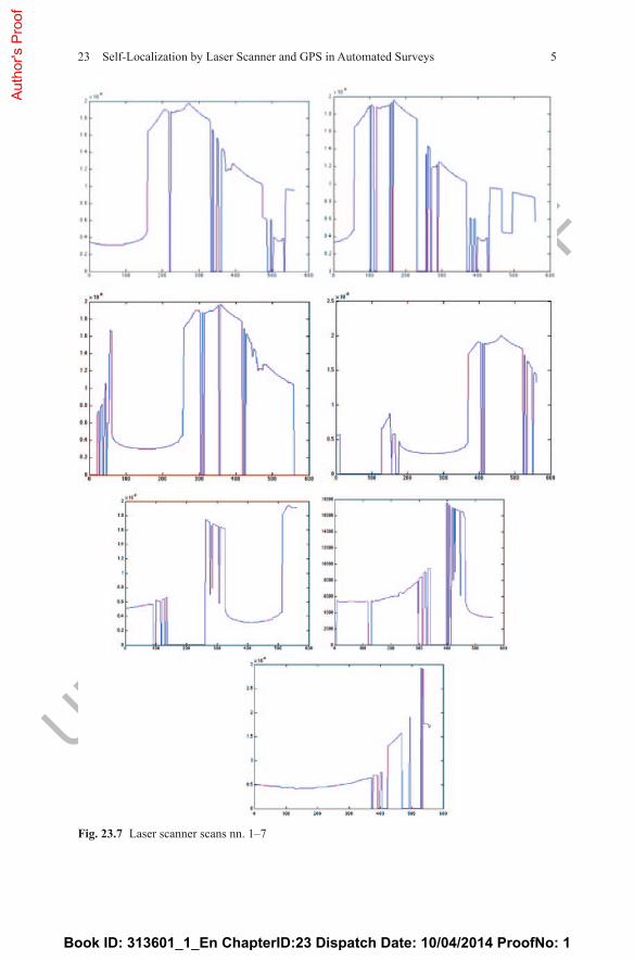
We made seven scans with the “equipped mobile trolley”, manually moving it (360°), with a view to its future and complete automation.

Scans are shown below (Fig. 23.7).

Fig. 23.4 GPS data

Fig. 23.3 Survey operations


Aut

hor's

Pro

of

UNCORRECTED PROOF

53545556575859

60

616263


For each scan was carried out at the same position detected by GPS measure-ments useful for linking the different scans through the measurement of external targets.

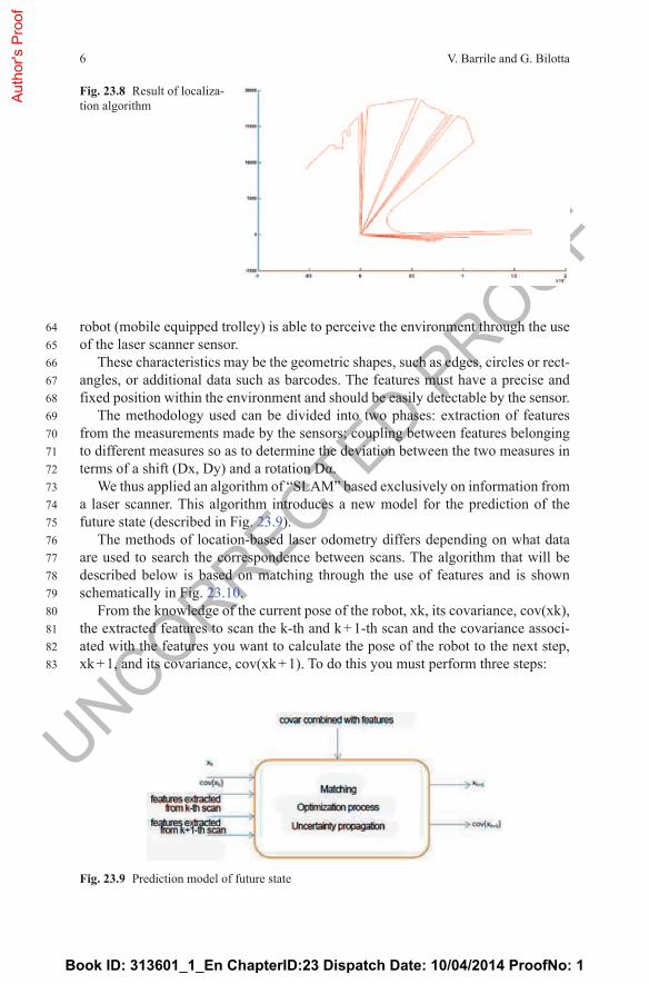
Single scans were processed and linked together by means of an algorithm im-plemented in Matlab (lab AeC), in the testing phase and the subsequent develop-ment by deriving a series of segments that describe, with little margin for error, the geometry of the square (Fig. 23.8).

23.3 The Algorithm

The algorithm implemented in Matlab and used in this experiment does not use the common return target detected externally but makes a connection of several scans through statistical autocorrelation methods by using the distinctive features that the

Fig. 23.6 Simultaneous positioning laser scanner and GPS on “mobile equipped trolley”

Fig. 23.5 GPS data in map


Aut

hor's

Pro

of

UNCORRECTED PROOF


Fig. 23.7 Laser scanner scans nn. 1–7


Aut

hor's

Pro

of

UNCORRECTED PROOF

6465666768697071727374757677787980818283


robot (mobile equipped trolley) is able to perceive the environment through the use of the laser scanner sensor.

These characteristics may be the geometric shapes, such as edges, circles or rect-angles, or additional data such as barcodes. The features must have a precise and fixed position within the environment and should be easily detectable by the sensor.

The methodology used can be divided into two phases: extraction of features from the measurements made by the sensors; coupling between features belonging to different measures so as to determine the deviation between the two measures in terms of a shift (Dx, Dy) and a rotation Dα.

We thus applied an algorithm of “SLAM” based exclusively on information from a laser scanner. This algorithm introduces a new model for the prediction of the future state (described in Fig. 23.9).

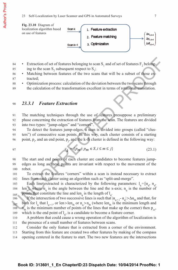
The methods of location-based laser odometry differs depending on what data are used to search the correspondence between scans. The algorithm that will be described below is based on matching through the use of features and is shown schematically in Fig. 23.10.

From the knowledge of the current pose of the robot, xk, its covariance, cov(xk), the extracted features to scan the k-th and k + 1-th scan and the covariance associ-ated with the features you want to calculate the pose of the robot to the next step, xk + 1, and its covariance, cov(xk + 1). To do this you must perform three steps:

Fig. 23.9 Prediction model of future state

Fig. 23.8 Result of localiza-tion algorithm


Aut

hor's

Pro

of

UNCORRECTED PROOF84

8586878889

90

919293949596

97

9899100101102103104

105106

107108109110111112113114


• Extraction of set of features belonging to scan S1 and of set of features F2 belong-ing to the scan S2 subsequent respect to S1;

• Matching between features of the two scans that will be a subset of those ex-tracted;

• Optimization process: calculation of the deviation between the two scans through the calculation of the transformation excellent in terms of rotational translation.

23.3.1 Feature Extraction

The matching techniques through the use of features presuppose a preliminary phase concerning the extraction of features from the scan. The features are divided into two types: “jump-edges” and “corners”.

To detect the features jump-edges, a scan is divided into groups (called “clus-ters”) of consecutive scan points. In this way, each cluster consists of a starting point, pi, and an end point, pj, and the k-th cluster is defined in the following way:

{ | , }c p p S i m jm mk = ∈ ≤ ≤ (23.1)

The start and end points of each cluster are candidates to become features jump-edges as long as these points are invariant with respect to the movement of the robot.

To extract the features “corners” within a scan is instead necessary to extract lines from each cluster using an algorithm such as “split-and-merge”.

Each line extracted is characterized by the following parameters: lq = [αq, nq, lenq], where αq is the angle between the line and the x-axis; nq is the number of points that constitute the line and lenq is the length of lq.

If the intersection of two successive lines is such that |αq + 1- αq| > Δαth and that, for both for lq that lq + 1, or len > lenth or nq > nth (where lenth is the minimum length and nth is the minimum number of points of the lines that make up the corner) then pcc, which is the end point of lq, is a candidate to become a feature corner.

A problem that could cause a wrong operation of the algorithm of localization is the presence of a small number of features between scans.

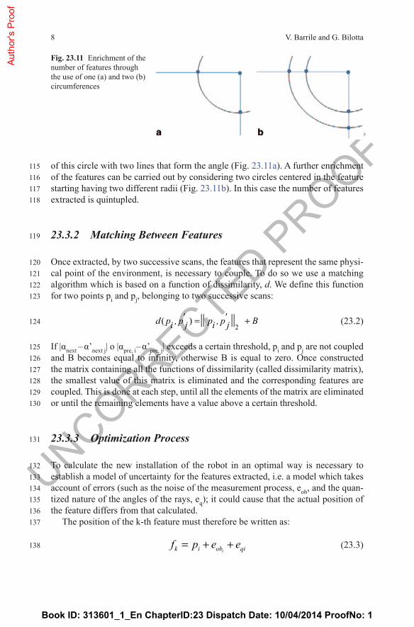
Consider the only feature that is extracted from a corner of the environment. Starting from this feature are created two other features by making of the compass opening centered in the feature to start. The two new features are the intersections

Fig. 23.10 Diagram of localization algorithm based on use of features


Aut

hor's

Pro

of

UNCORRECTED PROOF115

116117118

119

120121122123

124

125126127128129130

131

132133134135136137

138


of this circle with two lines that form the angle (Fig. 23.11a). A further enrichment of the features can be carried out by considering two circles centered in the feature starting having two different radii (Fig. 23.11b). In this case the number of features extracted is quintupled.

23.3.2 Matching Between Features

Once extracted, by two successive scans, the features that represent the same physi-cal point of the environment, is necessary to couple. To do so we use a matching algorithm which is based on a function of dissimilarity, d. We define this function for two points pi and pj, belonging to two successive scans:

2( ) || ||' 'd p , p p , pi i j Bj = + (23.2)

If |αnext – α’next j| o |αpre, i– α’pre, j| exceeds a certain threshold, pi and pj are not coupled and B becomes equal to infinity, otherwise B is equal to zero. Once constructed the matrix containing all the functions of dissimilarity (called dissimilarity matrix), the smallest value of this matrix is eliminated and the corresponding features are coupled. This is done at each step, until all the elements of the matrix are eliminated or until the remaining elements have a value above a certain threshold.

23.3.3 Optimization Process

To calculate the new installation of the robot in an optimal way is necessary to establish a model of uncertainty for the features extracted, i.e. a model which takes account of errors (such as the noise of the measurement process, eob, and the quan-tized nature of the angles of the rays, eq); it could cause that the actual position of the feature differs from that calculated.

The position of the k-th feature must therefore be written as:

ik i ob qif p e e= + + (23.3)

Fig. 23.11 Enrichment of the number of features through the use of one (a) and two (b) circumferences


Aut

hor's

Pro

of

UNCORRECTED PROOF

139

140

141142

143

144145146147

148

149150151152

153

154155

156

157158

159

160161162163164165


And the expected value of the position of features, fk, is given by:

ˆ ( ) (e ) ( )obf E f p E E eqik k= = + + (23.4)

where E(·) is the expected value operator.At this point it is necessary to calculate the covariance of fk:

( ) ( )ˆ ˆ ˆ( ) . ( ) ( )T

Cov f E f f f f Cov e Cov eqk k k k k ob ii

= − − = +

� � (23.5)

Using the measurement of the features and their corresponding covariance, the al-gorithm calculates the displacement (defined in terms of translation, T, and rotation, R) effected by the robot between the two scans. To find the optimal values of T and R the following error function must be minimized:

t 1ˆ ˆ ˆ ˆ( ( + )) ( ( + )), , , ,1

mE f Rf T C f Rf Tj pre j new j j pre j newj

−= − −∑=

(23.6)

Where m is the number of features coupled, fj, pre and fj, new are two new features coupled refer respectively to the previous scan and the current one; vj = (fj.pre– (Rfj, new + T)) is the j-th vector innovation and Cj is its covariance.

Assuming that the errors in the scans are independent, we can write:

cov( ) cov( )pre pre new new tj ob q ob qC e e R e e R= + + + (23.7)

There is the possibility of writing the variables in vector form. In such form, the displacement of the robot can be indicated in the following way:

( )1 21 2X q q t t t= (23.8)

Where t1 and t2 are respectively the translations along the x direction and the y di-rection. The rotation R and translation T matrices become defined as follows:

2 211 2 1 2

2 221 2 1 2

22

tq q q qR T

tq q q q − −

= = − (23.9)

The optimization problem is solved using the SQP method, “Sequential Quadratic Programming”.

Assuming that X* is the deviation between the two scans that minimizes the function E described above, for calculating the covariance of X* should exist Jaco-bian, J, projecting the uncertainty of the features in the uncertainty of X*. If there is an explicit function, g, which relates X* to F, which is the vector of all the features


Aut

hor's

Pro

of

UNCORRECTED PROOF

166167

168

169170

171

172173174

175

176177178179180181

182

183184185

186

187188

189

190191


coupled, we have X* = g(F). The Taylor series expansion of g in the neighborhood of E(F) will be:

** 2ˆ ˆ ˆ( ) ( ) ( )XX g F F F O F F

F∂

= + − + −∂

(23.10)

The last summand represents the higher order terms.The Jacobian between X* and F projects the uncertainty of X* in F, namely:

*cov( ) cov( ) TX J F J= (23.11)

However, there is an explicit relationship between F and X*, then they are related by an implicit function, I(X*,F) = 0, which is derived from ∂E/∂X = 0. You can ob-tain this Jacobian using the equation:

11 2 2

2

E EJ JF F XX X

γ γ−−

∗

∂ ∂ ∂ ∂ = − ⇒ = − ∂ ∂ ∂∂ ∂ (23.12)

with X = X*.Conducting additional steps and substitutions you can get the desired Jacobian

matrix. The independence of the features of a scan brings to obtain a total diagonal covariance matrix.

Furthermore, assuming that the features extracted by two successive scans are independent, the covariance of each pair will be:

( ) ,1

,

cov( ) 0cov( ) 0cov ( ) , cov0 cov( ) 0 cov ( )j

j new

m j pre

fFF FF f

= = (23.13)

Substituting the expressions of J and cov(F) we get cov(X*), i.e. the uncertainty of the deviation.

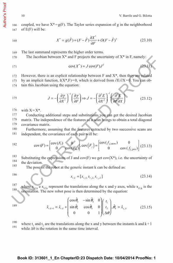
The pose of the robot at the generic instant k can be defined as:

1 2 3, , , ,[ ]r k r k r k r kx x x x= (23.14)

where xr1,k e xr2,k represent the translations along the x and y axes, while xr3,k is the orientation. The new robot pose is then determined by the equation:

3

1

, 1 , 2 ,

ˆ ˆcos sin 0ˆ ˆ ˆˆ ˆ ˆsin cos 0 ,

0 0 1

k k

r k r k k k k r k

tx x t x

θ θ

θ θ θθ

+

− = + = ∆

(23.15)

where t1 and t2 are the translations along the x and y between the instants k and k + 1 while Δθ is the rotation in the same time interval.


Aut

hor's

Pro

of

UNCORRECTED PROOF

192193

194

195196

197

198

199

200201202

203

204

205

206207208209210

211

212213214

215


The calculation of the covariance of Xr, k + 1 requires its differentiation with re-spect to the random parameters of the right side of the equation just written:

, 1

, 1 2 1 2( , , , , )r k

Pr k

xJ

x q q t t+∂

=∂ (23.16)

Given the independence between xr, k and X, the covariance of the parameters of the right side of the equation xr, k + 1 will be:

3 4*

4 3

cov( ) 0'

0 cov( )k x

x

pp

X

= (23.17)

The covariance of xr, k + 1 can be calculated in the following way:

, 1cov( ) tr k P px J P J+ = ′ (23.18)

The state vector xk of the system is composed of the state of the robot, xr, k, and the state of all the features, xf, k. The state vector and its covariance before the predic-tion will be:

, ,

, ,

ˆ cov( ) cov( , )ˆ ,cov( )ˆ cov( , ) cov( )

r k r,k r,k f kk k

f k f,k r,k f k

x x x xx x

x x x x

= = (23.19)

The movement of the robot does not affect the status of the features, so we have:

, 1 1 ,1 1

, ,

ˆ cov( ) cov( , )ˆ ,cov( )ˆ cov( , ) cov( )

Tr k r,k r, k f k P

k kf k P f,k r,k f k

x x x x Jx x

x J x x x+ +

+ +

′ = = ′

(23.20)

J’p is the truncated form of Jp and includes only the differentiation of xr, k + 1 with respect to xr, k.

The next step is the association of the data and update the map. For data bind-ing, the positions of features belonging to the map must be predicted relative to the robot. This is done by a model of the observation that, for the i-th feature, is:

( , )r mapi i r if h x f= (23.21)

The superscript r and map refer respectively to the coordinates of the robot and global ones.

In the present case, the model hi is:

2 21 1 2 2

12

21

( ) ( )

tan

map mapi r i rr

i mapr i

i rmapi

f x f xf

ff af

θ

− − = −

(23.22)


Aut

hor's

Pro

of

UNCORRECTED PROOF

216217218219220221222223

224

225

226

227228229

230

231

232

233

234235236237238239240241242


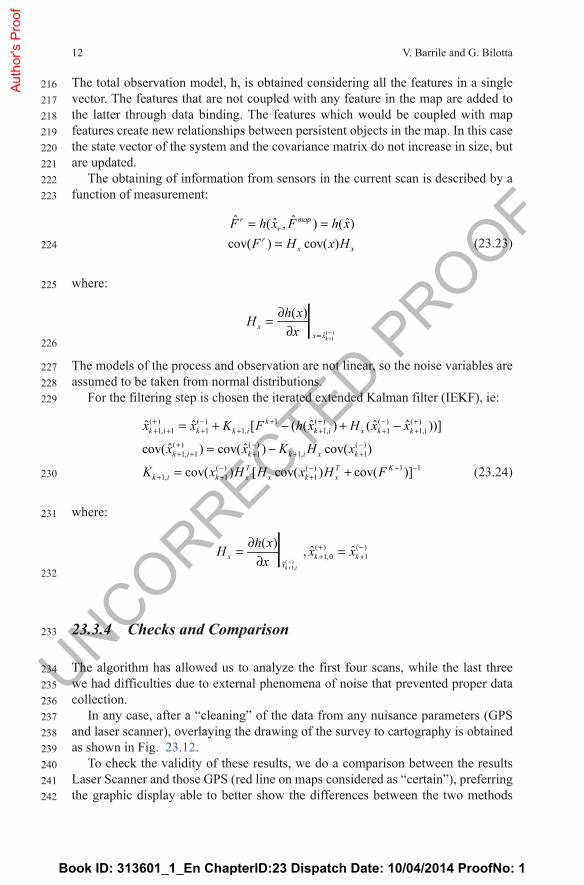
The total observation model, h, is obtained considering all the features in a single vector. The features that are not coupled with any feature in the map are added to the latter through data binding. The features which would be coupled with map features create new relationships between persistent objects in the map. In this case the state vector of the system and the covariance matrix do not increase in size, but are updated.

The obtaining of information from sensors in the current scan is described by a function of measurement:

ˆ ˆˆ ˆ( , ) ( )cov( ) cov( )

r mapr

rx x

F h x F h xF H x H

= == (23.23)

where:

( )1ˆ

( )|k

xx x

h xHx −

+=

∂=

∂

The models of the process and observation are not linear, so the noise variables are assumed to be taken from normal distributions.

For the filtering step is chosen the iterated extended Kalman filter (IEKF), ie:

( ) ( ) 1 ( ) ( ) ( )1,i 1 1 1, 1,i 1 1,i

( ) ( ) ( )1, 1 1 1, 1

( ) ( ) 1 11, 1 1

ˆ ˆ ˆ ˆ ˆ[ ( ( ) ( ))]

ˆ ˆcov( ) cov( ) cov( )

cov( ) [ cov( ) cov( )]

kk k k i k x k k

k i k k i x k

T T Kk i k x x k x

x x K F h x H x x

x x K H x

K x H H x H F

+ − + + − ++ + + + + + +

+ − −+ + + + +

− − + −+ + +

= + − + −

= −

= + (23.24)

where:

( )1,

( ) ( )1,0 1

ˆ

( ) ˆ ˆ,|k i

x k kx

h xH x xx −

+

+ −+ +

∂= =

∂

23.3.4 Checks and Comparison

The algorithm has allowed us to analyze the first four scans, while the last three we had difficulties due to external phenomena of noise that prevented proper data collection.

In any case, after a “cleaning” of the data from any nuisance parameters (GPS and laser scanner), overlaying the drawing of the survey to cartography is obtained as shown in Fig. 23.12.

To check the validity of these results, we do a comparison between the results Laser Scanner and those GPS (red line on maps considered as “certain”), preferring the graphic display able to better show the differences between the two methods


Aut

hor's

Pro

of

UNCORRECTED PROOF

243244245246247248249250

251

252

253254255256


(Fig. 23.13) rather than the creation of complex tables and graphs summarizing and/or various statistical parameters on the accuracy of the processing, because the aim of “expeditious” of this proposal.

Although there is the same precision of the GPS data in terms of return, however, is highlighted as the algorithm proposed for the processing of the given laser scan-ner is able to provide by itself discrete results, as evidenced by the partial planimet-ric correspondence of the two tracks GPS and Laser Scanner shown in Fig. 23.13.

This is a good omen for the continuation of the trial.

23.4 Integration of GPS and Laser Scanner for Connecting Subsequent Scans

As known, the main problem for laser scanner data is the assembly of the scans in order to determine a unique reference system in which “immerse” the obtained model. The acquisition of the scans results in an immediate point cloud ordered in the plane, whose coordinates are known with respect to the center of “taking”.

Fig. 23.12 Overlaying result of algorithm on mapping

Fig. 23.13 Comparison between the two methods


Aut

hor's

Pro

of

UNCORRECTED PROOF

257258259260261262263264265266267268269270271272273274275276277278279280281282283284285286287288289290291292293294295296297298299300301


The scan is then locally oriented with respect to a reference system that derives from the arbitrary choice of the pickup point, which will be taken as the origin of the reference system of the scan. The assembly of multiple scans thus requires the knowledge of the parameters of rototranslation: these parameters can be calculated if the position of the origin of the reference system of each scan with respect to a single system is known through the measurement of the external “target”. Such a problem for geo—topographic applications is solved by having remarkable points (targets), of which the coordinates are known, in all the scans: in this way each scan can be oriented independently of the other. Their georeferencing can be done by using the techniques of GPS tracking.

From the above considerations, the idea of experimenting with a rudimentary expeditious survey able to repeat what has already been experienced with the ve-hicle fully equipped (equipment includes two GPS, a laser scanner and a target all mounted on a vehicle in motion) that, by combining the two receivers GPS with the sensor laser scanner and a target audience, can overcome the issues raised; the whole mounted on a moving body that allows easy movement between the mea-surement sessions.

By performing measurements laser scanner and GPS simultaneously with sta-tionary body is thus ensured a high quality of fit and positioning into a single refer-ence system.

The system is to mount on movable equipped trolley (rigidly and coaxially) the laser scanner surmounted by a GPS and connect the trolley through a rigid arm (adjustable in length) to a “target” coaxially surmounted by other GPS reference (which will serve as the orientation of the scan), left free to rotate anyway so as to guide the laser target to the sensor. In this way, the problem of defining the coordi-nates of the acquisition point (Laser Scanner) and target orientation is overcome by fitting precisely coaxially two GPS receivers, respectively, the Laser Scanner and the target.

The receivers, while the laser sensor scans, acquire measurements from GNSS satellite constellations providing coordinates, both geographic both local coordi-nates of the laser sensor and the target orientation into a single reference system.

Once we have defined the ideal location for the first scan, we must place and stop the mobile equipped trolley at the point defined by performing both those mea-sures GPS and Laser Scanner with the characteristics of density required by the survey. After a few minutes we must close the measures and shall move the trolley equipped cabinet in the next position chosen for the second major station, operating as before and repeating the process until completion of the survey. The processing of GPS data will allow to obtain homogeneous coordinates for all points of outlet (station laser scanner) and for all orientation target with sub-centimeter accuracy. These coordinates are assigned to stations and targets thereby allowing the software used for the management of the scans to unite and georeference all the scans made even in the absence of homologous points or targets positioned on the ground.

In this way, in addition to speed up and facilitate the steps of the survey in the field by eliminating the need of affixed targets and the necessity of their internal vis-ibility between a measurement session and the other, will be easier georeferencing


Aut

hor's

Pro

of

UNCORRECTED PROOF

302303304305306307308309310311312313314315316317318319320


also individual scans with no points in common, decreasing processing time of “point clouds” resulting from the scans.

Taking into account what was said above, namely we have tried to make an initial experimentation in order to achieve “coarse” and “expeditious” what has already been experimented on equipped machine (cf. Leica experiment reported in bibliography).

Specifically, it was built by placing a measuring system on the mobile trolley equipped (rigidly and coaxially) the laser scanner superimposed by a GPS and con-necting the trolley through a rigid arm (simulating the modulation length through the ability to extend and contract) to a “target” coaxially superimposed by other GPS reference.

In particular, measures have been simulated with arms of 3, 2, 1.50, 1, 0.5 m (Fig. 23.14)

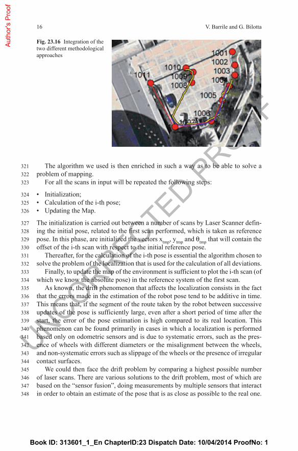
The overall reconstruction of the data, although simulated, is very interesting in particular for the test carried out with the arms of 3 and 2 m (note in this regard the result of the perimeter displayed in color and overlaid on the map as reported in Fig. 23.16). Instead, less accurate appear the results obtained with simulated arm of 1.5 m, while it was not possible to make reliable reconstructions with simulated arm of 1 m or less. (Fig. 23.15).

Fig. 23.15 Variation of the percentage error compared to GPS method (in the test simulated) by varying the arm in question

Fig. 23.14 System with target and dual GPS


Aut

hor's

Pro

of

UNCORRECTED PROOF

321322323

324325326

327328329330331332333334335336337338339340341342343344345346347348


The algorithm we used is then enriched in such a way as to be able to solve a problem of mapping.

For all the scans in input will be repeated the following steps:

• Initialization;• Calculation of the i-th pose;• Updating the Map.

The initialization is carried out between a number of scans by Laser Scanner defin-ing the initial pose, related to the first scan performed, which is taken as reference pose. In this phase, are initialized the vectors xtmp, ytmp and θtmp that will contain the offset of the i-th scan with respect to the initial reference pose.

Thereafter, for the calculation of the i-th pose is essential the algorithm chosen to solve the problem of the localization that is used for the calculation of all deviations.

Finally, to update the map of the environment is sufficient to plot the i-th scan (of which we know the absolute pose) in the reference system of the first scan.

As known, the drift phenomenon that affects the localization consists in the fact that the errors made in the estimation of the robot pose tend to be additive in time. This means that, if the segment of the route taken by the robot between successive updates of the pose is sufficiently large, even after a short period of time after the start, the error of the pose estimation is high compared to its real location. This phenomenon can be found primarily in cases in which a localization is performed based only on odometric sensors and is due to systematic errors, such as the pres-ence of wheels with different diameters or the misalignment between the wheels, and non-systematic errors such as slippage of the wheels or the presence of irregular contact surfaces.

We could then face the drift problem by comparing a highest possible number of laser scans. There are various solutions to the drift problem, most of which are based on the “sensor fusion”, doing measurements by multiple sensors that interact in order to obtain an estimate of the pose that is as close as possible to the real one.

Fig. 23.16 Integration of the two different methodological approaches


Aut

hor's

Pro

of

UNCORRECTED PROOF

349350351352353354355356357358359360361362363364365366367368369370371372373374375376377378379380381382383384385386387


There are several methods to achieve this goal, among which the most popular are the so-called “Bayesian filters” that estimate a state x from noisy sensory mea-surements. This category includes the “Kalman Filter” (with its extensions) and “particle filters”. Looking at the problem from a probabilistic point of view, the robot does not have, instant by instant, the certainty of where he is, but can believe (“belief”) to be in a certain position with a certain uncertainty. On the basis of this statement, the localization problem consists in the estimation of the probability den-sity related to all possible positions, with the aim of obtaining as much knowledge as possible accurate position. Ideally, this occurs when the “belief” has a single peak at the position of the robot and is zero elsewhere.

Returning to the “Kalman Filter”, recursive algorithm that estimates the state of a linear dynamic system affected by noise, this has access to the measurements of sensors which have a linear dependence with the state of the system. It is shown that the Kalman filter converges to the optimal estimation, the one that minimizes the variance of the error of the estimate, assuming the linearity of the system model and measurement, and the corresponding noise is Gaussian with zero mean. There-fore we can say that the Kalman filter calculates the so-called “belief” (which is supposed to have a gaussian) of the state through two phases: the prediction, which calculates the “a priori belief”, i.e. the conditional probability of being in state xk known the measures until the time k-1, while in the correction phase calculates the “belief a posteriori”, i.e. the conditional probability of being in state xk known measures up to the instant k.

We are currently working on “particle filters” that allow to derive the estimate of the state (typically a function of the probability density not Gaussian and multi-modal) in a system characterized by a nonlinear model.

The algorithm of the particle filter is recursive and consists of two phases: the prediction and updating. Following each action performed by the robot starts the prediction phase in which each particle is modified according to the existing model with the addition of noise to the variable of interest. During the upgrade, any weight of each particle is evaluated according to the new measurements from the sensors. The goal yet to be achieved is to get to the implementation of occupancy grid, which involves the construction, starting from the knowledge of the pose of all scans re-ferred to the reference scan, an occupancy grid map.

The method used for the construction of the grid will be the one already de-scribed and the result of this operation will be the partition of the map in a grid in which each element of the grid itself is associated with a probabilistic value of occupancy. By using the occupancy grid more information from different sensors can be integrated in the same representation of the environment, even if they use different methods of data acquisition.


Aut

hor's

Pro

of

UNCORRECTED PROOF

388

389390391392393394395396397

398

399400401402403404405406407408409410411412413414415416417418419420421422423424425426427428429430431


23.5 Conclusions

Of course, although we must emphasize that the results obtained from the integra-tion are to now only been achieved in a “simulated” way and the automation of the procedure is still under study and implementation (having now moved to the cart only by hand), yet the results seem encouraging in view of the realization of a “ex-peditious” process for the auto positioning and perimetering by using mobile and automated tools.

The results certainly push to further study both in terms of actual full realization of the experiment, both in terms of optimization of the algorithms used for the com-pensation of the integrated data.

References

1. Weiß G, Wetzler C, von Puttkamer E (1994) Keeping track of position and orientation of mov-ing indoor systems by correlation of range-finder scans. Proc Intern Conf on Intelligent Robots and Systems, pp 595–601

2. Lu F, Milios E (1997) Robot Pose Estimation in Unknown Environments by Matching 2D Range Scans. J Intelligent and Robotic Systems 18:pp. 249–275

3. Thrun S (2002) Robotic Mapping: A Survey. In: Exploring artificial intelligence in the new millennium. Morgan Kaufmann, Pittsburgh

4. Liu JS, Chen R, Logvinenko T (2001) A theoretical framework for sequential importance sam-pling and resampling. In: Doucet A, de Freitas N, Gordon NJ (eds) Sequential Monte Carlo in Practice. Springer-Verlag, New York

5. Pirjanian P, Karlsson N, Goncalves L, Di Bernardo E (2003) Low-cost visual localization and mapping for consumer robotics. In: Industrial Robot: An International Journal 30:pp 139–144.

6. Rekleitis IM (2004) A particle filter tutorial for mobile robot localization. (Technical Report TR-CIM-04-02)

7. G. Bekey (2005) Autonomous Robots: From Biological Inspiration to Implementation and Control. The MIT Press, Cambridge, MA

8. Lingemann K, Nüchter A, Hertzberg J, Surmann H (2005) High-Speed Laser Localization for Mobile Robots. J Robotics and Autonomous Systems (JRAS), Elsevier Science 51:pp 275–296

9. Garulli A, Giannitrapani A, Rossi A, Vicino A (2005) Simultaneous localization and map building using linear features. In: Proc. 2nd European Conf Mobile Robots, Ancona (Italy)

10. Garulli A, Giannitrapani A, Rossi A, Vicino A (2005) Mobile robot SLAM for line-based en-vironment representation, Decision and Control. 2005 European Control Conference. CDC-ECC ’05, pp 2041–2046

11. Aghamohammadi AA, Taghirad HD, Tamjidi AH, Mihankhah E (2007) Feature-Based Laser Scan Matching For Accurate and High Speed Mobile Robot Localization. In: European Conf on Mobile Robots (ECMR’07)

12. Aghamohammadi AA, Tamjidi AH, Taghirad HD (2008) SLAM Using Single Laser Range Finder. In: Proc. 17th World Congress, The International Federation of Automatic Control, Seoul, Korea

13. Secchia M, Uccelli F (2012) Laser Scanner e GPS -Stop&Go. In: FIG Working Week 2012, Knowing to manage the territory, protect the environment, evaluate the cultural heritage, Rome, Italy

AQ1


Aut

hor's

Pro

of

UNCORRECTED PROOF

432433434435436437438439440441442443444445446447448449450451452453

19

14. Wahde M (2012) Introduction to autonomous robots. Department of Applied Mechanics, Chalmers University of Technology, Goteborg, Sweden

15. Barrile V, Meduri GM, Bilotta G (2009) Laser scanner surveying techniques aiming to the study and the spreading of recent architectural structures. In: Recent advances in signals and systems, Proc 9th WSEAS Intern Conf on Signal, Speech and Image Processing, pp 92–95

16. Barrile V, Meduri GM, Bilotta G (2011) Laser scanner technology for complex surveying structures. In: WSEAS Trans Signal Processing 7:pp 65–74

17. Barrile V, Bilotta G, Meduri GM (2013) Least Squares 3D Algorithm for the Study of De-formations with Terrestrial Laser Scanner. In: Rec Adv in Electronics, Signal Processing and Communication Systems, Proc Intern Conf Electronics, Signal Processing and Communica-tion Systems, Venice, Italy, pp 162–165

18. Bailey T, Nebot E (2001) Localisation in large-scale environments. In: Robotics and Autono-mous Systems, 37:pp 261–281

19. Siegwart R, Nourbakhsh IR (2004) Introduction to Autonomous Mobile Robots. A Bradford Book, The MIT Press, Cambridge, MA, London, England

20. Borenstein J, Everett HR, Feng L, Wehe D (1997) Mobile Robot Positioning—Sensors and Techniques. In: J Robotic Systems, Mobile Robots 14:pp 231–249

21. Barrile V, Cacciola M, Cotroneo F, Morabito FC, Versaci M (2006) TECMeasurements through GPS and Artificial Intelligence. In: J Electromagnetic Waves and Applications 20:pp 1211–1220

22. M. Postorino N, Barrile V (2004) An integrated GPS-GIS surface movement ground control system. In: Management of Information Systems, WIT Press (GBR), pp 3–12



Aut

hor's

Pro

of

Self-localization by Laser Scanner and GPS in automated surveys

Documents