Self Learning Material Managerial Economics (MCOP-201) Course: Masters of Commerce Semester-II Distance Education Programme I.K. Gujral Punjab Technical University Jalandhar

Welcome message from author
This document is posted to help you gain knowledge. Please leave a comment to let me know what you think about it! Share it to your friends and learn new things together.
Transcript

Self Learning Material
Managerial Economics (MCOP-201)
Course: Masters of Commerce
Semester-II
Distance Education Programme
I.K. Gujral Punjab Technical University
Jalandhar

Syllabus
I.K. Gujral Punjab Technical University
MCOP-201 MANAGERIAL ECONOMICS
OBJECTIVE AND EXPECTED OUTCOME OF THE COURSE:
Aims to provide a broader understanding of Managerial Economics and its managerial
applications.
UNIT-I Introduction: Nature and scope of Managerial Economics, Role and Responsibility of Managerial economics in business. Fundamental business concepts – Incremental concept,
Opportunity cost concept, Time perspective, Discounting principle.
UNIT-II Demand analysis and Forecasting for consumer goods and capital goods - use of business indicators - type of elasticity. Demand Forecasting for new products. Test marketing, Opinion
pooling, Life cycle.
UNIT-III Concept and resources allocation - Cost Analysis - Short run and long run Cost functions - production functions - cost price - Output relations.Economics of size and capacity
Utilization - Input - Output analysis - Market Structure - Pricing and output general
equilibrium.
UNIT-IV Pricing Objectives - pricing methods and approaches - price discrimination, Product line pricing and Cost control. Theories of profit, Tools of profit planning. Business Cycles:
Meaning, Causes, Phases, Theories of Business cycles
SUGGESTED READINGS/ BOOKS:
1. Peterson, managerial economics, 4th edition - Pearson education - New Delhi.
2. Sampat Mokherjie, Business and Managerial Economics, New Central Book Agency,
Calcutta.
3. Spencer M.H.Managerial Economics Text, Problems and short cases, Richard D.Inwin
INC.
4. Sankaran.S, Managerial Economics Margham Publications, Chennai.
5. Dwivedi D.N , Managerial Economics, Vikas-New Delhi
6. Mankar & Denkar, Business Economics, Himalaya publishing House, Bombay
7. Joel Dean, Managerial Economics, Prentice Hall of India - New Delhi.
8. R.L. Varshney & K.L. Maheshwari, Managerial Economics-Sultan Chand & Sons, New
Delhi.
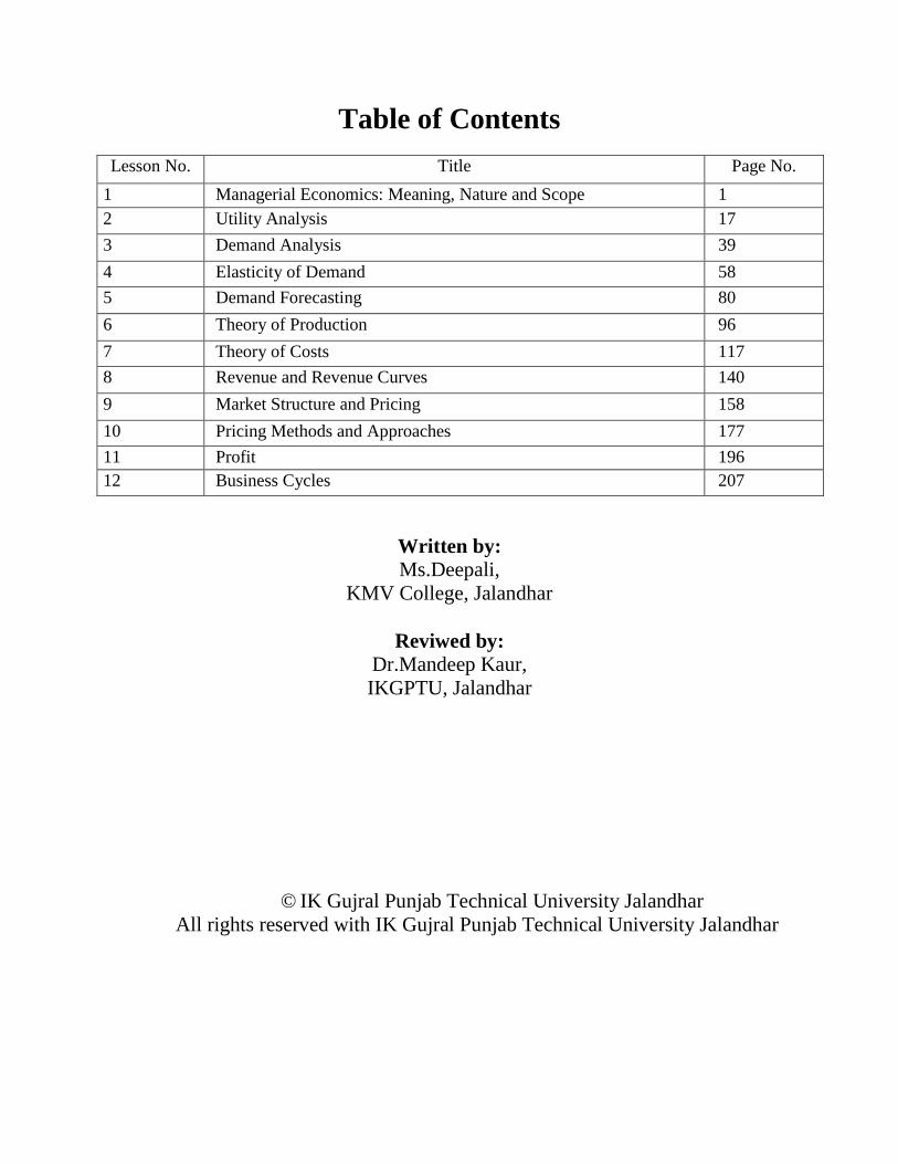
Table of Contents
Lesson No. Title Page No.
1 Managerial Economics: Meaning, Nature and Scope
1
2 Utility Analysis
17
3 Demand Analysis
39
4 Elasticity of Demand
58
5 Demand Forecasting
80
6 Theory of Production
96
7 Theory of Costs
117
8 Revenue and Revenue Curves
140
9 Market Structure and Pricing
158
10 Pricing Methods and Approaches
177
11 Profit
196
12 Business Cycles
207
Written by:
Ms.Deepali,
KMV College, Jalandhar
Reviwed by:
Dr.Mandeep Kaur,
IKGPTU, Jalandhar
© IK Gujral Punjab Technical University Jalandhar
All rights reserved with IK Gujral Punjab Technical University Jalandhar

LESSON – 1
Managerial Economics: Meaning, Nature and Scope
Structure
1.0 Objectives
1.1 Introduction
1.2 Definitions of Managerial Economics
1.3 Nature of Managerial Economics
1.4 Scope of Managerial Economics
1.5 Relationship of Managerial Economics with Other Disciplines
1.6 Role of Managerial Economics in Business Decision-Making
1.7 Summary
1.8 Glossary
1.9 Answer to Check Your Progress
1.10 References
1.11 Suggested Readings
1.12 Terminal and Model Questions

1.0 OBJECTIVES
After reading this lesson, you should be able:
To understand the basic theme of managerial economics.
To bring out the nature and scope of management.
To explain the role of managerial economics in decision-making.
1.1 INTRODUCTION
Business decision making has witnessed an increasing use of economic
concepts, theories and principles, which in turn has led to the development of
managerial economics or business economics as a separate branch of economics.
Managerial economics is an outcome of the close relationship between economics
and management. Management in business firms involves appropriate decision-
making which requires weighing different available alternatives and making the best
possible choice. This involves co-ordination among a group of individuals to help
them perform in an efficient and effective manner in order to attain common
objectives. On the other hand, economics involves the analysis of and solution to the
basic problem i.e. problem of choice. The universal problem of choice stems from
scarcity of resources available to satisfy unlimited human wants. This necessitates a
rational choice both at the individual level (individual as a producer and as a
consumer) as well as at the level of economy as a whole. Thus, economics helps to
study optimal allocation of scarce available resources to maximize gains both at the
micro level (individual) and the macro level (aggregate economy).
Such economic decision-making by firms and managers constitutes the core
of managerial economics. This appropriate decision making has become an
extremely complex task in the light of market imperfections, risk and uncertainties.
Managerial economics or business economics, thus, comes as a useful tool for the
business managers in the process of decision-making for the firms. Hence,
managerial economics is also sometimes referred to as „Economics for Managers‟.
Managerial economics makes use of both of the two very basic branches of
economics- microeconomics as well as macroeconomics. Managerial economics
may be considered as applied microeconomics to a large extent as it relies on the
tools and techniques provided by microeconomic theory to ease managerial
decision-making. However, it draws heavily from macroeconomic theory also as the
macroeconomic environment cannot be ignored in the rational decision-making
process for a firm. However, economic principles in general, make a significant
contribution in improving the performance of business managers. Managers with
some working knowledge of economics can perform their functions more effectively
and efficiently than those without such knowledge. Managerial economics, thus,
enables the managers to find the most efficient way to allocate scarce organizational
resources in order to achieve the given objectives of the firm.
1.2 Definitions of managerial economics

The meaning of managerial economics can be still better understood with the
help of its definition. A large number of eminent economists have defined managerial
economics in different ways. A few important ones are listed below:
“Managerial economics is concerned with the application of economic principles and
methodology to the decision-making process within the firm or organization. It seeks
to establish rules and principles to facilitate the attainment of the desired economic
goals.” -Douglas
“Managerial economics refers to the application of economic theory and the tools of
analysis of decision science to examine how an organization can achieve its
objectives most effectively.” -Salvatore
“Managerial economics applies economic theory and methods to business and
administrative decision-making.” -Pappas and Hirschey
“Managerial economics is concerned with the application of economic concepts and
economics to the problems of formulating rational decision-making.” -Mansfield
“Managerial economics is the study of allocation of limited resources available to a
firm or other unit of management among the various possible activities of that unit.”
-Henry and Haynes
Different definitions of managerial economics make it clear that managerial
economics is the application of economic theories, logic, concepts and tools of
economic analysis to the process of business decision-making in order to help the
business managers in taking best possible decisions. Although no single definition
can claim to be a perfect one, still a study of these different definitions of managerial
economics throw light on its basic nature and meaning.
1.3 Nature of Managerial Economics
The performance of business managers – their duties and responsibilities
relies heavily on a working knowledge of economics. The primary function of the
managers of a business firm is maximization of the given objective subject to the
constraint of limited availability of resources. It is quite obvious that there would not
have been any problem of decision making had there been an unlimited supply of
resources. As we are confronted with scarcity of resources- both natural and man-
made, so the problem of choice is the central problem of any economy or even of the
firm. The typical problems faced by managers in one way or the other can be
categorized as follows:
What to produce?
How to produce?
For whom to produce?
The first major economic decision to be taken for an economy is what to
produce? A choice has to be made between different alternative combinations of
goods and services that can be produced because the resources are limited. Such a
decision at firm level necessitates a review of market demand and the availability of
raw materials and technology. Hence, it leads to the problem of choice.
After this decision is made, the next question confronting the economy is how
to produce, as to what techniques of production should be used which would
maximize production or social benefit. This, again, leads to the problem of choice.
The next basic problem which any economy will face relates to the problem
of distribution of the total national output among the different economic agents.
There again lies a problem of choice as to which principle should be followed in
distribution.
If it were possible to specify the uses to which resources could be put,
perhaps the decision-making process in a situation with resource constraints could
be relatively easy. For instance if you have Rs. 1000 and you are told that out of Rs.
1000, you should spend Rs. 500 on books, Rs. 200 on moves and the remaining on
food, the decision-making would have not been very complicated. However, in
practical reality, resources have alternative uses, Rs. 1000 could be used in
innumerable different ways. Hence, the decision making process becomes complex.
It is here that economic logic, tools and techniques come to the rescue. Hence,
optimization of use of scarce resources is the primary task of managers. Economics
helps the managers in this task of decision-making by providing models, tools and
techniques to achieve the goals of organizations; to reduce the degree of uncertainty
and risk arising due to uncertain market forces, dynamic business environment,
government policy, competitors, impact of international factors, social and political
factors and many others; and to predict future market conditions and business
prospects. Economic theories have, therefore, gained widespread application in
practical problems of business.
Thus, allocation of scarce resources among alternative uses to achieve the
desired objectives is the primary duty of a manager, which is done with the help of
economic tools, techniques and logic. This link between the responsibility of the
managers and economic logic, tools and techniques justifies the name managerial
economics. Highlighting the importance of managerial economics as a separate

discipline, different and distinct from economics in general, Prof. D .M .Mithani has
stated the following characteristics of managerial economics:
Managerial economics involves the application of the working knowledge
of economic theory, especially microeconomics, to solve practical
business problems.
Managerial economics is both a science as well as an art which facilitates
better and rational business decision making. As a science it is both a
positive science (it is a systematic knowledge and answers the question
„what is?‟) as well as a normative science (it involves value judgement
answers the question „what ought to be?‟)
Managerial economics is primarily concerned with optimum allocation of
scarce resources available to a firm which have alternative uses for any
business activity.
These features of managerial economics clearly throw light on its meaning and
nature and form a basis to study the scope of managerial economics or as it is
synonymously called business economics.
Activity A
Managerial economics is the discipline which deals with the application of ‘economic
theory to business management’. Comment.
---------------------------------------------------------------------------------------------------------------
---------------------------------------------------------------------------------------------------------------
---------------------------------------------------------------------------------------------------------------
---------------------------------------------------------------------------------------------------------------
---------------------------------------------------------------------------------------------------------------
---------------------------------------------------------------------------------------------------------------
---------------------------------------------------------------------------------------------------------------
---------------------------------------------------------------------------------------------------------------
---------------------------------------------------------------------------------------------------------------
---------------------------------------------------------------------------------------------------------------
---------------------------------------------------------------------------------------------------------------
---------------------------------------------------------------------------------------------------------------
---------------------------------------------------------------------------------------------------------------
---------------------------------------------------------------------------------------------------------------
---------------------------------------------------------------------------------------------------------------
---------------------------------------------------------------------------------------------------------------
---

1.4 Scope of Managerial Economics
Managerial economics is the study of allocation of scarce resources available
to a firm (financial, human, machines, etc.) among alternative uses in order to realize
the objective of profit maximization or other specified objectives. Managerial
economics comprises of both microeconomic theories and macroeconomic theories
as both of these are applied to business decision-making and analysis in one way or
the other. The scope of managerial economics comprises all the areas of business
issues to which economic theories could be applied in one way or the other. The
important among these can be enlisted as follows.
Allocation of resources: As it has already been discussed earlier in the
context of problem of choice, a business manager has to decide how to
allocate the scarce available resources to their respective uses within the firm
in order to achieve the desired objectives.
Management of Inventory: Inventory problems relate to the issue of holding
an optimum stock of both finished goods and raw materials. Along with it
queuing problems also arise in which decisions have to be taken about
installing new machines or employing extra labour so as to balance the
business requirements.
Pricing and sales promotion: How to fix the prices for the products, how
to face price competition and how to promote sales are important business
decisions to be undertaken with regard to the pricing policy of the firm.
Investment Issues: Decisions regarding investment problems are
crucial to a firm- how to decide on investing in new plants, how much to
invest, how to manage capital and profits, etc.
The above mentioned problems appear in decision-making and forward
planning in any business firm. Micro economics as a part of managerial economics
deals with such operational or internal issues faced by managers of business firms.
The study of the following important microeconomic theories in this context is crucial
in order to make rational business decisions:
Demand Analysis: The theory of demand helps in making the choice of
products, determining their price and optimum level of production.
Product Analysis and cost analysis: The theory of production and
production decisions is very helpful in determining the size of the firm, its total
output & factors of production to be employed in order to attain the given
objectives of the firm.
Pricing Theory and policies: Analysis of market structure and pricing
theory helps in price determination under different market conditions. It also
aids in evaluating the possibility and feasibility of price discrimination and
advertisement for expansion of sales of a given commodity.
Profit Analysis: The theory of profit helps the firms to measure and
manage their profits keeping in view the uncertainties and the risk involved.
Capital Budgeting: The theory of capital and investment decisions helps in
making investment decisions, choice of projects, capital budgeting for
investment decisions, etc for the business firm.
Besides the above mentioned issues, the scope of managerial economics
also includes the general business environment. This general business environment
of the economy relates to the economic, social and political set-up of the country.
These environmental factors include the type of economic system in the country-
socialist, capitalistic or mixed economy; general trends in national income,
employment, output, prices saving and investment etc.; trends in the working of the
financial institutions of the economy; the trends in foreign trade; the extent of
globalization of the economy; political factors, etc. These types of external issues
strongly influence the business and the functioning of the firms. Therefore, business
managers have to give due consideration to these external environmental factors
also in the process of decision making. These external environmental factors may
be broadly classified as follow:
Major Macroeconomic Parameters: Issues concerning the trends in
macroeconomic variables like national income, output, employment, prices,
investment etc. are extremely helpful in forward planning like setting up a new
plant or expanding the existing plant size for business expansion. The study
of these macro economic variables help the firms to make crucial decisions
regarding business expansion keeping in mind the external conditions
prevalent in the eonomy.
Foreign trade: Trade - internal and/or external is an important outcome
all business activity undertaken by the firms. Trade links with the rest of the
world influence the functioning of business firms directly or indirectly. Study of
monetary mechanism and international trade help the managers understand
international trade, prices, exchange rates, fluctuations in the foreign markets,
capital flows, etc.
Government policies: Regulatory government policies have a huge impact
on the working of business undertakings. Government tries to regulate and
control all types of business activities through its policy measures. Any
business activity which goes against the social well being or disturbs the
welfare of the society have to be and are checked by the government through
regulatory policies directed towards the concerned business activities. For
instance government policies to check environment pollution, traffic
congestion in cities etc. affect the concerned firms. Hence, the business
managers need to have complete information about government policies and
their repercussions on business. Their business decisions should be carefully
framed with an effort to not to violate any such government rules and
regulations. In this context the business managers also need to be aware and
sensitive towards the needs of the society so that no business action of theirs
reduces the welfare of the society as a whole or a section of the society.
Besides the above mentioned economic theories, the scope of managerial
economics may include any other issues influencing the working of managers in
business firms. However, these theories largely constitute the scope of
managerial economics with room for further additions.
Check Your Progress 1
1. State whether the following statements are True or False:
(i) Managerial economics is the application of economic tools to business.
(ii) Managerial economics is the study of micro economics only.
(iii) The basic problem of an economy is the problem of choice.
(iv) Managerial economics helps the managers to make efficient use of
scarceresources.
(v) The scope of managerial economics does not include the pricing policy.
1.5 Relationship of Managerial Economics with other disciplines
Essentially managerial economics involves the study of economic tools, logic
and analysis applied to the decision making process of business firms. However,
besides microeconomics and macroeconomics, managerial economics is also
associated with various other disciplines. These related fields of study include the
following:
Operations research: This field of study is an inter disciplinary solution
finding technique used to find an optimum solution to the managerial
problems subject to the given constraints. These problems are solved using
models built with the help of economics, mathematics and statistics. Linear
programming and goal programming are two important techniques studied
under operations research which are useful in business decision making.
Mathematical and Statistical Tools: Mathematical logic and tools are very
helpful in economic analysis as most of the concepts dealt by the managers of
business firms are quantitative in nature like cost, price, demand, profit,
interest, wages, stock etc. Advanced optimization techniques and
mathematical tools, thus, form an integral part of managerial economics.
Similarly statistical tools prove extremely helpful in collecting,
processing and analyzing data for business firms. Regression analysis
probability theory, forecasting techniques, etc. help in forecasting the future
values of economic variables and the probable outcome of the business
decisions undertaken.
Management Theory and Accounting: These disciplines have a close link
with the study of managerial economics. Various management theories make
an attempt to study the behaviour of the business firms which in turn are
working to attain certain desired and pre stated objectives. Hence, a business
manager needs to have sufficient knowledge of management theory in order
to ascertain changes in the behaviour and objectives of the firms with change
in the conditions- internal and/or external. On the other hand accounting data
and statements help in reflecting the working the firm and evaluating its
performance.
Psychology and Organisation Behaviour: Managerial economics helps the
business managers to make rational business decisions by studying the
behaviour of individual buyers and sellers. This involves the study of the
psychological factors influencing the demand and supply patterns, needs,
expectations and aspirations of the market players- the buyers and sellers. In
fact, psychological economics has emerged as recent field of study for the
psychological analysis of the buying behaviour of the consumer. In addition to
the study of individual buyers, various behavioural models studying
organizational psychology have been developed of late to analyse the
economic behaviour of a firm.
Thus, the scope of managerial economics is immensely wide and beyond the
reach of this entire book. However, the above mentioned issues form the basic core
of managerial economics and its scope cannot be complete without the mention of
these issues.
1.6 Role of Managerial Economics in Business Decision-Making
The role of business managers in business decision making is to select
the best possible alternative out of the opportunities available to the business firm.
The process of business decision making primarily comprises of the following
stages:
Stage I : To determine and define the objective(s) to be achieved.
Stage II : To collect and analyse data and information regarding economic,
social, political, and technological environment.
Stage III : To invent, develop and analyse the possible alternatives to achieve
the desired objectives.

Stage IV : To rationally select the best possible alternative.
It is essential to take a note of the fact that stages II and III are very crucial in
order to make the right business decision and involve a need for in depth knowledge
of economic theories and tools, concepts and logic along with individual skills of the
business managers. For example, say a firm plans to launch a new product in the
market and many close substitutes of that product are already available in the
market. The foremost business decision to be taken would whether to launch the
product or not. In order to do so the business manager will have to carefully study
the market; the product and all issues relating to it; and issues relating to the sales.
Here comes the role of the different economic concepts, including demand, supply,
cost, price, etc., that can be and are used by the business managers in business
analysis. Various economic theories, tools, concepts and logic help in arriving at
appropriate and right conclusions as regards the business problem.
The primary responsibility of the manager of a business firm is the attainment
of the desired objectives. A managerial decision can be evaluated only in the context
of its objective. For this the objectives of the firm should be clearly stated which may
be various and conflicting. The conventional theory of firm takes profit maximization
as the primary objective of a business firm. This is defended on the basis of the
argument that making profit is indispensable for the survival of the firm in the long
run. Further, the achievement of alternative objectives of the firm like maximizing
long run growth, maximizing sales revenue, increasing market share and such like
are themselves dependent more or less on the profit objective, as profit is a relatively
more reliable measure of a firm‟s efficiency. Moreover, profit maximization
hypothesis is a time- tested one and is largely used to explain the price and output
decisions of the business firms.
However, whatever may be the objective of a firm, all the business decisions
taken by the managers aim at the attainment of pre determined objective(s).
Traditionally the process of business decision making relied on the rule of thumb
technique. Such a technique evolved out of traditional business practices, serves the
purpose where simple business decisions are involved. However, complex issues in
business decision-making involve the use of some basic economic concepts. A few
important economic concepts and their role in business decision-making are listed
below.:
1.6.1 Principle of opportunity cost
The business manager or as we may call the managerial economist needs to
sacrifice some alternatives against the selected ones in a rational manner in almost
all aspects of business -- the problem of choice. Since human wants are infinite and
means to satisfy them are scarce, it is impossible to satisfy all the wants. In order to
satisfy some wants, it becomes necessary to give up or postpone some other wants.
Similarly resources – natural and man-made are scarce in relation to their demand
but have alternative uses. This scarcity and possible alternative uses of the
resources leads to the concept of opportunity cost.
The opportunity cost or alternative cost is what has been sacrificed to have a
certain thing. It is the benefit foregone of the alternative that has not been chosen.
For example say a worker works in an ice factory and gets a wage of Rs. 4000 per
month. Alternatively if he gets employment in a shoe factory, he might be getting a
wage of Rs. 3000 per month. So the earning in the next best alternative (Rs. 3000) is
the opportunity cost or alternative cost of his services. Similarly a firm has limited
resources at its disposal which can be put to alternative uses. For example a firm
may have different options available to expand its output using a capital of say Rs.
10 million- setting up a new unit having expected annual return of Rs. 2.5 million or
expanding the existing unit having expected annual return of 1.8 million. A rational
business manager would definitely go in for the first alternative other things
remaining the same. This means that the manager will have to sacrifice Rs. 1.8
million- the annual return of second option which is not selected, in order to get an
annual return of Rs. 2.5 million (the selected alternative). Hence, the opportunity cost
of setting up a new unit in this example is the sacrifice involved is not expanding the
existing unit.
Thus, the opportunity cost is the cost of the next best alternative which is
foregone. This concept of alternative or opportunity cost is applicable to all types of
resources involved in business decision where alternative uses are possible.
1.6.2 Marginal Principle and Incremental concept
Marginal analysis is widely used in economic theory -marginal utility in utility
analysis; marginal cost in theory of production and marginal revenue in the theory of
pricing. As regards business decision making, marginal principle is applicable in the
cases where marginal revenue(MR) and marginal cost (MC) can be exactly
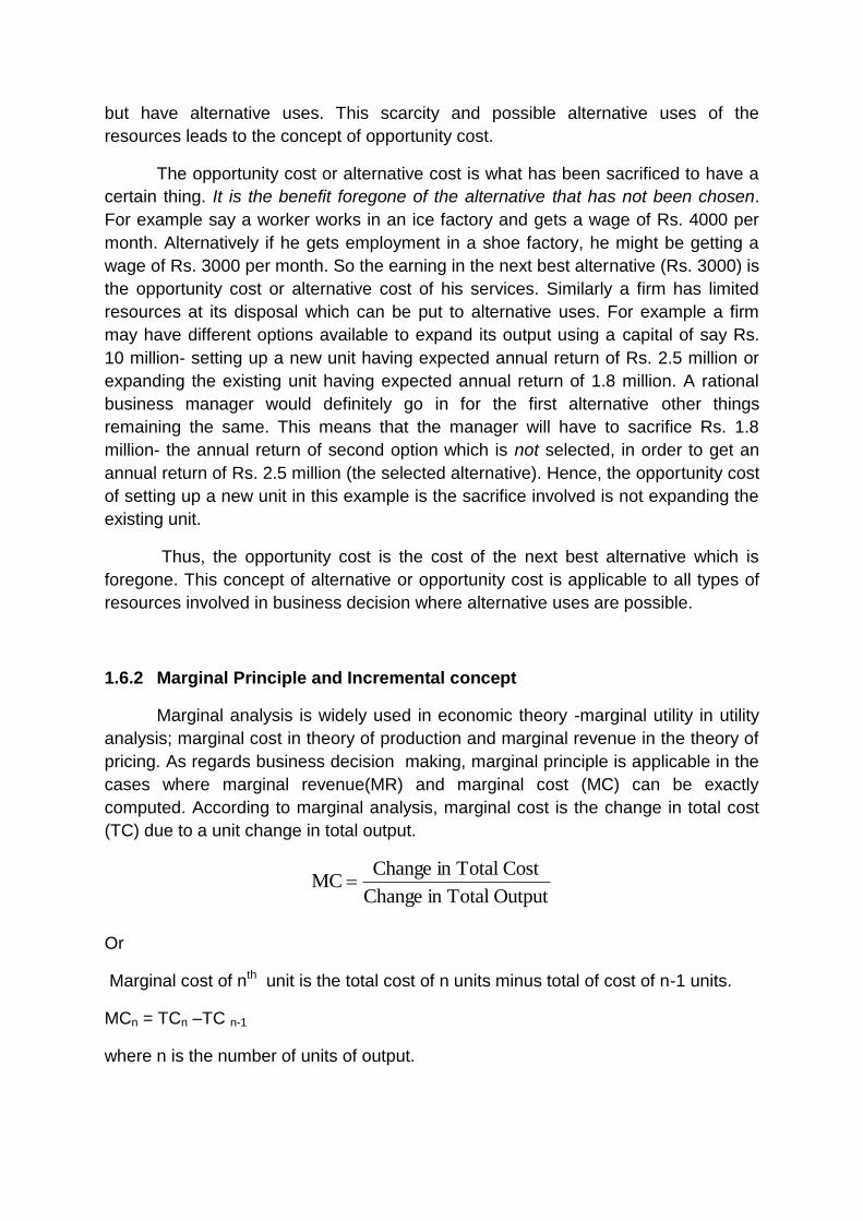
computed. According to marginal analysis, marginal cost is the change in total cost
(TC) due to a unit change in total output.
Or
Marginal cost of nth unit is the total cost of n units minus total of cost of n-1 units.
MCn = TCn –TC n-1
where n is the number of units of output.
MCChange in Total Cost
Change in Total Output
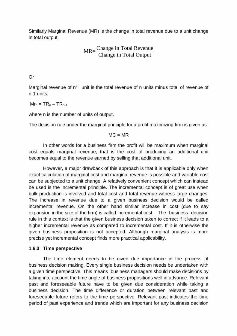
Similarly Marginal Revenue (MR) is the change in total revenue due to a unit change
in total output.
Change in Total RevenueMR=
Change in Total Output
Or
Marginal revenue of nth unit is the total revenue of n units minus total of revenue of
n-1 units.
Mrn = TRn – TRn-1
where n is the number of units of output.
The decision rule under the marginal principle for a profit maximizing firm is given as
MC = MR
In other words for a business firm the profit will be maximum when marginal
cost equals marginal revenue, that is the cost of producing an additional unit
becomes equal to the revenue earned by selling that additional unit.
However, a major drawback of this approach is that it is applicable only when
exact calculation of marginal cost and marginal revenue is possible and variable cost
can be subjected to a unit change. A relatively convenient concept which can instead
be used is the incremental principle. The incremental concept is of great use when
bulk production is involved and total cost and total revenue witness large changes.
The increase in revenue due to a given business decision would be called
incremental revenue. On the other hand similar increase in cost (due to say
expansion in the size of the firm) is called incremental cost. The business decision
rule in this context is that the given business decision taken to correct if it leads to a
higher incremental revenue as compared to incremental cost. If it is otherwise the
given business proposition is not accepted. Although marginal analysis is more
precise yet incremental concept finds more practical applicability.
1.6.3 Time perspective
The time element needs to be given due importance in the process of
business decision making. Every single business decision needs be undertaken with
a given time perspective. This means business managers should make decisions by
taking into account the time angle of business propositions well in advance. Relevant
past and foreseeable future have to be given due consideration while taking a
business decision. The time difference or duration between relevant past and
foreseeable future refers to the time perspective. Relevant past indicates the time
period of past experience and trends which are important for any business decision

in the present. Some of the business decisions involve short run outcome while
others may have long run pay-offs. A certain business decision may be more
profitable in the short-run than in the long-run and vice-versa. For instance say a
business firm decides to increase its expenses on medical facilities along with other
facilities to its workers. Such a decision may escalate costs in the short-run but in the
long run it may lead to increasing revenues by way of enhanced productivity of
workers. Therefore, time perspective is of utmost importance in business decision
making.
1.6.4 Production Possibility Curve
Production Possibility Curve (PPC) is a curve which indicates different
combinations of two commodities that can be produced in an economy at any point
of time with the help of given techniques and resources. Production Possibility Curve
(PPC) is also called Production Possibility Frontier or Transformation Curve. For an
individual consumer, a PPC shows the different combinations of the two
commodities which a consumer can buy given his income and prices of the two
commodities. However, for the economy as a whole, it depicts the opportunity cost or
alternative cost of producing one good in terms of the amount of the other good
sacrificed subject to the limited availability of resources. This concept is also very
important for the business managers for decision making.
Activity B
How does the study of managerial economics help a business manager in decision making?
Illustrate your answer with examples from production and pricing issues.
-------------------------------------------------------------------------------------------------------------------------
-------------------------------------------------------------------------------------------------------------------------
-------------------------------------------------------------------------------------------------------------------------
-------------------------------------------------------------------------------------------------------------------------
-------------------------------------------------------------------------------------------------------------------------
-------------------------------------------------------------------------------------------------------------------------
-------------------------------------------------------------------------------------------------------------------------
-------------------------------------------------------------------------------------------------------------------------
-------------------------------------------------------------------------------------------------------------------------
-------------------------------------------------------------------------------------------------------------------------
-------------------------------------------------------------------------------------------------------------------------
-------------------------------------------------------------------------------------------------------------------------
-------------------------------------------------------------------------------------------------------------------------
-----------------------------------------------------------------------------------------------------------------------

Check Your Progress 2
Fill up the blanks with correct words
(i) Managerial economics is a ………………to an end for managers in any business.
(ii) Marginal concept is applied when …………….calculation of MC and MR is
possible.
(iii) The opportunity cost is the cost of the benefit …………..
(iv) A rational decision involves ……………… incremental revenue as compared to
incremental cost.
1.7 Summary
Managerial economics has emerged as a separated branch of economics due
to increased applicability of economics in business decision-making process by the
managers. Managerial economics helps the business managers in choosing the
most efficient allocation of scarce resources to achieve the given objects. It is micro
as well as macro in nature. Its scope is immensely vast comprising economic
theories and concepts used to analyse business issues and to find practical solutions
to business problems. Managerial economics can thus be referred to as working
knowledge of economics applied to business decision making. It is also linked to
other fields of study, including mathematical tools, statistics, operation management
theory. The role of managerial economics in business decision making is extremely
important for the overall development of business activity. Important decision making
concepts include the principle of opportunity cost, marginal and incremental
principle, time perspective and production possibility curve.
1.8 Glossary
Managerial Economics: The study of economic theories, logic and tools of
economic analysis used in the process of business decision making.
Microeconomics: It attempts to study the economic behaviour of particular small
units of the entire economic system such as a consumer, a producer, a firm, a
worker, price of a particular commodity, etc.
Microeconomics: It attempts to study the economic problems concerning
aggregates in the economic system such as aggregate demand, aggregate supply,
general price level, gross national expenditure, growth rate of the economy, etc.
Opportunity cost: It is cost of the next best alternative which is not selected or
foregone.
Production Possibility Curve: It is a graph showing different combination of two
commodities which can be produced in an economy, given the scarce availability of
resources.
1.9 ANSWERS TO CHECK YOUR PROGRESS
Check Your Progress 1
1) (i) true
(ii) false
(iii) true
(iv) true
(v) false
Check Your Progress 2
1) (i) means
(ii) precise
(iii) foregone/not selected
(iv) higher
1.10 References
1. Spencer, M.H, and Seigelman, L., Managerial Economics, Irwin Illinois
2. Douglas, Evan J., Managerial Economics: Analysis and Strategy, Prentice-
Hall, N.J
3. Baye, Micheal R., Managerial Economics and Business Strategy, McGraw
Hill, Toronto.
4. Mithani D.M. : Managerial Economics, Himalaya Publishing House, Mumbai
5. Dwivedi, D.N. : Managerial Economics, Vikas Publishing House Pvt. Ltd, New
Delhi
1.11 Suggested Readings
1. Dean, Joel, Managerial Economics, Prentice Hall of India, New Delhi.
2. Solvatore, D., Managerial Economics, Mc Graw Hill, New York.
3. Davis, R and S. Chang, Principles of Managerial Economics, Prentice Hall,NJ
1.12 Terminal Questions
1) What do you understand by managerial economics? Explain its nature and
characteristics.
2) Discuss in detail the scope of managerial economics in modern business
environment.
3) Managerial economics is applied economics Discuss
4) Mention the important features of managerial economics.
5) Discuss the link of managerial economics with other disciplines. How do they
contribute to managerial economics?
6) The study of managerial economics helps a business manager in decision
making. Do you agree?
7) What is opportunity cost principle as applied to decision making?
8) How is time perspective important in business decision making?

LESSON – 2
Utility Analysis
Structure
2.0 Objectives
2.1 Introduction
2.2 Utility: Meaning and Features
2.3 Measurement of Utility
2.3.1 Cardinal Utility Analysis
2.3.1.1Assumptions of Cardinal Utility Analysis
2.3.1.2 Law of Diminishing Marginal Utility
2.3.1.3 Law of Equi Marginal Utility
2.3.1.4 Marginal Utility and Demand Curve
2.3.2 Ordinal Utility Analysis
2.3.2.1 Indifference Schedule and Indifference Curve
2.3.2.2 Properties of Indifference Curves
2.3.2.3Marginal Rate of Substitution
2.3.2.4 Price Line
2.3.2.5Consumer’s Equilibrium
2.4 Summary
2.5 Glossary
2.6 Answers to Check Your Progress
2.7References
2.8Suggested Readings
2.9Terminal and Model Questions

2.0 OBJECTIVES
After reading this lesson, you should be able:
To understand the meaning and features of utility
To bring out the difference between cardinal utility analysis and ordinal utility
analysis
To comprehend the concept of consumer’s equilibrium
2.1 INTRODUCTION
An individual as a consumer forms the basis of all production. The individual
consumer has a role to play in two markets in the economy- the factor market and the product
market. The individuals own the productive resources to be used for production and sell these
inputs to the firms in the factor market. On the other hand, as a consumer the individual lays a
demand on goods and services produced by the firms and makes a decision about the quality
and quantity to be bought and at what price. Hence, the force of demand is determined solely
by the behavior of the consumers in the product market. Any change in this force of
consumer demand can altogether change the market solution involving the forces of demand
and supply. Moreover, it is this consumer demand which forms the basis of all production
taking place in the economy. Hence, it is very important rather essentially required for all the
business managers to study the consumer’s behavior in the market. Given his income, prices
of different commodities and other factors, the consumer tries to find optional solutions for
several issues important to him like how much to buy, from whom to buy, what quality to
buy, and at what price to buy. In turn, these issues influence and frame the force of demand
for that particular product in the market.
The producers or sellers also want to know and need to know the preference and
choice of consumers. This insight into the buying behavior of consumers helps the firms in
taking important decisions regarding product type, its pricing, advertisement, new products
and many others. The consumer’s buying behavior or the consumer demand and choice, thus,
is crucial to the process of business decision making. In economic theory the consumer’s
choice and buying behavior have been explained with the help of the concept of utility.
2.2 Utility: Meaning and Features
The entire process of production is guided by the behavior of consumers. The
consumer behavior is explained on the basis of utility. Man by nature is full of desires, all of
which cannot be satisfied as the resources to satisfy them are limited. So the consumer has to
allocate his limited income among unlimited wants in such a way that he gets maximum
possible satisfaction or utility. The term utility owes its original to British philosopher Jeremy
Bentham. It refers to that quality or power in a commodity or service that satisfies a human
want. Every consumer buys several commodities because these commodities can satisfy his
wants. This want satisfying power of a commodity or a service is called utility.
Utility is a psychological or subjective concept, slightly different from satisfaction.
For instance say a consumer wants to buy a chocolate. This shows that chocolate has utility
for the consumer. When the consumer eats it, the good feeling that he gets is satisfaction. Had
he not liked the chocolate he would not have got satisfaction (although it had utility for him,
that is why he bought the chocolate). Thus, utility implies expected satisfaction whereas
satisfaction stands for realized satisfaction. Another feature of utility is its ethical neutrality.
The commodities like liquor, drugs, tobacco and the like too have utility for the consumer but
may be unethical, immoral and even illegal in some cases. Further, utility is a relative term in
the sense that it varies from person to person, place to place and time to time. Cigarettes have
great utility for a chain smoker while no utility for a non-smoker. A person living in a
metropolitan city may have an intense want for a car while a person living in a remote village
may not need it at all. People have greater utility of woollens during winter months than in
summer season. Hence, utility is a relative concept which may vary from person to person,
place to place and even time to time.
2.3 Measurement of Utility
Two different views are found in economic literature regarding the measurement of
utility. The first view point assumes that the utility can be exactly measured in cardinal
numbers and like cardinal numbers the utility from different units of commodities can be
added or subtracted. This approach is called the cardinal utility analysis. On the other hand,
according to the second viewpoint the utility cannot be exactly measured in cardinal
numbers- it can only be ranked just like the ordinal numbers. Hence, this approach is referred
to as the ordinal utility analysis. Both these approaches to utility analysis are discussed
below.
2.3.1 Cardinal Utility Analysis
The cardinal approach to utility analysis is based on the assumption that the utility
derived from a commodity is quantifiable and can be exactly measured in numbers. Based on
the cardinal measurement of utility there are two main concepts of utility.
(i) Total Utility: Total Utility is the sum of utilities derived from the consumption of all
the units of a commodity or service within a given time period. Thus, if a consumer buys five
mangoes, the sum of utilities from all the five units of mangoes is the total utility. Total
utility is a direct function of the quantity purchased. As the quantity purchased increases it
leads to an increase in the total utility. This can be expressed as
TUx = f (Qx)
Where TUx is the total utility derived from x commodity and Qx refers to the units of x
commodity.
(ii) Marginal Utility: Marginal Utility refers to the utility derived from the last or
marginal unit of a given commodity. It is defined as the addition made to total utility by
consuming an additional unit of the commodity within a given period of time. It can be
measured as follows
MUn = TUn – Tun – 1
where MUn is the marginal utility of nth
unit
TUn = Total utility from n units.
TUn-1 = Total utility from (n-1) units
Alternatively marginal utility can also be defined as the rate of change of total utility
due to a unit change in the quantity of given commodity. On the basis of this definition,
marginal utility can be measured as follows:
where MUx is the marginal utility of x commodity
∆ TUX is the change in total utility of x commodity
∆ Qx is the change in quantity of x commodity consumed by one unit.
An important feature of the concept of marginal utility is that it can be either positive
or zero or negative. When total utility increases with purchase of an additional unit of the
commodity marginal utility is positive and marginal utility is negative if purchase of an
additional unit of the given commodity results in a fall in total utility. However, if there is no
change in total utility by purchasing an additional unit of the said commodity, marginal utility
is zero. When marginal utility becomes zero, total utility is maximum. This point of
maximum total utility and zero marginal utility corresponds to the point of maximum
satisfaction and is referred to as the point of saturation. If the consumer still continues to buy
more units of this commodity beyond the point of saturation, total utility begins to decline
and marginal utility becomes negative.
2.3.1.1 Assumptions of Cardinal Utility Analysis
The cardinal utility analysis maintains that utility can be added and subtracted.
However the explanation of consumer’s behavior- choices, tastes and preferences using
cardinal utility approach rests on the following main assumptions:
(i) Utility can be measured in cardinal numbers which means that it can be added or
subtracted.
(ii) Consumption of one commodity is not affected by its related goods. Utility of one
commodity is assumed to be independent of the utilities of other commodities.
(iii) Each unit of the given commodity being consumed should be homogenous or of
uniform quality.
(iv) The size of each unit of the commodity to be consumed should be standard, neither
very small nor very large.
TUxMU = X Qx
(v) The consumption of successive units should be continuous, that is no gap in
consumption of successive units should be there.
(vi) There should be no change either in the income of the consumer or in the price of the
commodity being consumed during the course of consumption.
(vii) There should be no change tastes and preferences of the consumer during the course
of consumption.
(viii) The commodity being consumed should be normal and non addictive in nature.
(ix) The most fundamental assumption in the cardinal utility analysis is that the consumer
is rational and aims to maximize his satisfaction.
The above stated assumptions of the cardinal utility analysis form the basis for the
two fundamental laws of economics- the law of diminishing marginal utility and the law of
equi marginal utility.
2.3.1.2 Law of Diminishing Marginal Utility
The law of diminishing marginal utility states that other things remaining the same, as
the consumer goes on buying more and more units of a commodity, the utility derived from
each successive unit goes on diminishing. This law is one of the basic laws of Economics and
is also called the first law of consumption. This diminishing marginal utility with each
additional unit of the commodity consumed can be attributed to two reasons:
(a) Each particular want is satiable. Inspite of the fact that there are unlimited wants, every
single want can be completely satisfied. Thus, when a consumer goes on consuming more
and more units of a commodity, his want gets fully satisfied and he does not wish to have any
more increase in the commodity. As such his marginal utility starts falling when consumption
increases.
(b) Goods are imperfect substitutes for one another. Satisfaction derived from any two
commodities is not same. Different goods satisfy different wants. If it were possible to
perfectly substitute a good for another good, it would have satisfied all other wants also.
Hence, its marginal utility would not have fallen rather would have increased.
The law of diminishing marginal utility can be explained with the help of a table and diagram
given below:

The above table shows that as the consumer goes on consuming more and more units of
apples, the total utility (TU) derived from the consumption of apples increases but marginal
utility (MU) declines continuously, so much so that it becomes zero when 6th unit of apple is
consumed. At this point TU is maximum corresponding which MU is zero. This is the point
of saturation or satiety or the point of maximum satisfaction. Beyond this point TU begins to
decrease as MU becomes negative. No rational consumer will continue consumption beyond
the point of satiety. The MU curve can be derived from the above schedule as below.
Marginal Utility
In the above figure, marginal utility is measured along Y-axis while units of apples
along X-axis. MU is the marginal utility curve has a negative slope as it falls downwards
from left to right. This is the diminishing MU curve. The above figure clearly shows that
marginal utility is zero when the consumer buys 6th apple. As he consumes more units,
marginal utility becomes negative.
Although the law of diminishing marginal utility is universal in nature yet in some
situations it does not hold true. In certain cases marginal utility from additional consumption
goes on increasing instead of decreasing like goods for display such as diamonds, luxury cars,
etc., rare collections such as rare coins or stamps; accumulation of money, etc. This law does
not hold even in case of abnormal consumer behavior as in the case of misers, drunkards or
even people showing excessive love for music or poetry. Despite these limitations the law
diminishing marginal utility still is a universal law of economics.
Activity A
To test the law of diminishing returns, it is possible to create a factory floor right in your own
classroom. Follow the instructions below to determine whether the law applies to your own
imaginary firm.
Your classroom is about to turn into a factory that manufactures paper chains (to hold paper
anchors for paper boats, of course!). A paper chain is made by taking two long, narrow strips of
paper, folding one into a ring and stapling the ends together, then folding the other into a ring and
connecting it to the first ring to make a chain. Two loops of paper stapled together make a chain.
The longer your chain, the more productive your factory and its workers are. The goal of your
paper chain factory, of course, is to make the longest chain possible in a fixed amount of time
using a fixed amount of land and capital, with labor as your only variable resource. This is
therefore an experiment to test the short-run law of diminishing marginal returns.
----------------------------------------------------------------------------------------------------------------------
----------------------------------------------------------------------------------------------------------------------
----------------------------------------------------------------------------------------------------------------------
----------------------------------------------------------------------------------------------------------------------
----------------------------------------------------------------------------------------------------------------------
----------------------------------------------------------------------------------------------------------------------
----------------------------------------------------------------------------------------------------------------------
----------------------------------------------------------------------------------------------------------------------
2.3.1.3 Law of Equi marginal Utility
The law of diminishing marginal utility is based on the consumption of a single
commodity. However in real life a consumer buys many commodities simultaneously to
maximize his satisfaction. In such a situation, when a consumer spends his limited income on
two or more commodities, the law of equi marginal utility comes into operation. This law of
equi marginal utility is just an extension of the law of diminishing marginal utilityto two or
more than two commodities. This law of equi marginal utility is known by different names :
the Law of Substitution, the Law of Maximum Satisfaction, the Law of Indifference, the
Proportionate Rule and the Gossen’s Second Law. It may be defined as follows:
The household maximizing the utility will so allocate the expenditure between commodities
that the utility of the last penny spent on each item is equal.
--- Lipsey
Every consumer has unlimited wants but limited income. The consumer is, therefore,
faced with a choice among many commodities. The objective of a rational consumer is to
maximize the total utility derived by spending his limited income on two or more
commodities. A rational consumer, in order to get the maximum satisfaction from his limited
income compares (i) the utility of a particular commodity and its price and (ii) the utility of
the other commodities which he can buy with his limited resources. If he finds that a
particular expenditure in a commodity is yielding less utility than another, he will shift the
unit of expenditure from the commodity yielding less marginal utility to a commodity
yielding more marginal utility. The consumer will reach his equilibrium position when it will
not be possible for him to increase the total utility further. The equilibrium will be reached
when the marginal utility of each commodity is in proportion to its price and the ratio of the
prices of all goods is equal to the ratio of their marginal utilities. In other words, the objective
of maximum satisfaction is achieved when the consumer is able to spend his limited income
in such a way that the utility of the last rupee spent on the various commodities is the same.
This can be expressed mathematically as:
MUa / Pa = MUb / Pb = MUc /Pc = …….= MUn / Pn
Where a,b,c,…….,n are different commodities consumed.
In such a situation the consumer becomes indifferent among different commodities
and gets maximum possible satisfaction. Any change in spending pattern against the law of
equi marginal utility results in a loss in satisfaction.
However, in certain cases, the actual behavior of the consumer is found inconsistent
with this law such as change in income, prices, tastes and preferences, ignorance on the part
of the consumer or difficulty in measurement of utility. Still both the law of diminishing
marginal and the law of equi marginal utility are of great practical importance and can also be
used to derive the demand curve for a commodity and hence are crucial importance.
2.3.1.4 Marginal Utility and Demand Curve
Dr. Alfred Marshall derived the demand curve using the law of diminishing marginal
utitlity. The law of diminishing marginal utility states that as the consumer purchases more

and more units of a commodity, he derives lesser utility from each successive unit of the
commodity purchased. Also, as the consumer buys more and more units of one commodity,
he is left with lesser money at his disposal. A rational consumer, therefore, while purchasing
a commodity compares its price with the utility he receives from it. As long as the marginal
utility of a commodity is higher than its price (MUx > Px), the consumer would demand more
units of it till its marginal utility becomes equal to its price (MUx = Px) and the equilibrium
condition is achieved. In other words, as the consumer consumes more and more units of a
commodity, marginal utility derived from the commodity goes on diminishing. Hence, the
consumer would demand more units of a commodity only at a diminishing price.
(a) (b)
Marginal Utility and Demand Curve
The part (a) of the above figure shows that the marginal utility curve of commodity X,say,
being consumed by the consumer is negatively sloped. This shows that as the consumer buys
larger quantities of commodity X, its marginal utility decreases. As a result at diminishing
price, the quantity demanded of the commodity x increases as is shown in part (b) of the
above diagram. When the quantity purchased is X1, the marginal utility of the commodity x
is MU1. By definition, this is equal to P1. The consumer in this case demands OX1 quantity
of the commodity at P1 price. Similarly, X2 quantity of the commodity is equal to price P2 as
at P2 price, the consumer will buy OX2 quantity of commodity. As is clear now, at price P3,
the consumer will buy OX3 quantity and so on. Hence, as the purchase of the units of
commodity X is increased, its marginal utility goes on diminishing. Equivalently, at a
diminishing price, the quantity demanded of good X increases as is clear from the diagram.
The law of demand (to be discussed later) states that, other things remaining the same, when
price of a commodity falls, its quantity demanded increases and vice versa. In other words,
the demand curve, which shows the relation between price of a commodity and its quantity
demanded, has a negative slope. Hence, the marginal utility curve of a commodity depicts its
downward sloping demand curve.(The negative part of marginal utility curve does not form a
part of the demand curve as negative quantities make no sense).
Therefore, the concept of marginal utility enjoys an integral place in utility analysis.
Moreover the utility approach or the cardinal utility analysis is of paramount importance in
explaining the theory consumer behavior, rather the theory consumer behavior remains
incomplete without it.
Check your progress 1
1. _________ is the attribute of a commodity to satisfy a consumer’s wants.
2. The __________________ analysis maintains that utility can be added and subtracted.
3. The utility derived from an additional unit of a commodity is called __________.
4. When marginal utility is zero, the total utility becomes_________.
5. Total utility is the summation of __________________ from all the units of a
commodity.
2.3.2 Ordinal Utility Analysis
The traditional cardinal utility approach suffers from several serious limitations. Out
of these, exact measurement of utility and cardinal measurement of utility were the ones
which received a lot of criticism. In view of the defects in cardinal utility approach, an
alternative theory of consumer behavior known as indifference curve theory or ordinal utility
analysis was developed. This approach of indifference curve analysis was first introduced in
1915 by a Russian economist Slustsky. It was later developed by J.R. Hicks and R.G.D. Allen
in 1928. In contrast to the cardinal utility approach, the indifference curve analysis is based
on the ordinal measurement of utility. It totally ruled out the possibility of cardinal
measurement of utility. This approach emphasized that only ordinal measurements or
comparisons of satisfaction from different combinations of commodities were possible. The
ordinal approach assumes that utilityis purely subjective and cannot be measured. Further, an
individual is interested in a buying a combination of related goods and not in the purchase of
one commodity at a time. So this theory of consumption is based on a scale of preferences or
a list of priorities prepared by the consumer in his mind according to the satisfaction levels
got from different combinations of goods.
In ordinal utility analysis, a consumer’s tastes and equilibrium is shown by
indifference curves. An indifference curve is a curve which shows the various combinations
of two commodities X and Y which yield equal utility or satisfaction to the consumer. An
indifference curve shows an ordinal rather than a cardinal measure of utility. It is also called
an iso-utility curve and all the combinations lying on an indifference curve yield equal
satisfaction.
2.3.2.1 Indifference Schedule and Indifference Curve
In the scale of preferences of the consumer, there are certain combinations which yield
exactly equal satisfaction. The consumer will give equal importance to all such combinations

with no preference to any. He will be indifferent or neutral about these combinations. Such an
indifference on the part of the consumer about thecombinations of two commodities may be
explained with the help of an indifference schedule and indifference curve. An indifference
schedule is the tabular statement which shows the different combinations of two commodities
yielding the same level ofsatisfaction as shown below:
Indifference Schedule
Suppose the consumer is indifferent among the five combinations I, II, III, IV and V
of rice and wheat shown in the indifference schedule above. All these combinationsyield the
same level ofsatisfaction and the consumer gives equal preference to all. The consumer is
ready to give up four units of wheat(Y) to get one more unit of rice(X), only then
combination I and II will yield the same level ofsatisfaction. Similarly in combination III, the
consumer is ready to give up three units of wheat(Y) to get one more unit of rice(X) to get
same level ofsatisfaction, and so on. If a curve is drawn such that each point on the curve
shows a combinations of two commodities which yield the same level ofsatisfaction, such a
curve is called an indifference curve.
In the words of Leftwitch, “A single indifference curve shows the different
combinations of X and Y goods that yield equal satisfaction to the consumer.”
According to Hicks, “An indifference curve is the locus of the points representing
pairs of quantities between which the individual is indifferent.”
On the basis of the different combinations of two commodities yielding the same level
ofsatisfaction, an indifference curve can be shown as follows:

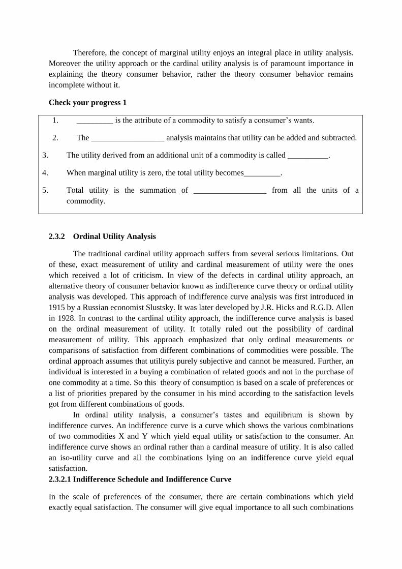
Indifference Curve
The indifference curve IC shown above indicates that the consumer gets equal level
ofsatisfaction from the combinations A, B, C, D, so he is indifferent among them, hence it is
called an indifference curve. Based on indifference curves, an indifference map can be drawn.
A set of indifference curves representing the scale of preference at different levels of
satisfaction is known as indifference map as shown below.
Indifference Map
All combinations lying on indifference curve 1 (IC1) provide the same satisfaction but
the level of satisfaction on Indifference curve 2 (IC2) will be greater than the level of
satisfaction on indifference curve 1 (IC1). Similarly, all combinations lying on indifference
curve 2 (IC2) provide the same satisfaction but the level of satisfaction on Indifference curve
3 (IC3) will be greater than the level of satisfaction on indifference curve 2 (IC2).
2.3.2.2 Properties of Indifference Curves
An indifference curve shows different combinations of two goods about which a
consumer is indifferent. The main properties or of indifference curvesare as follows:
An indifference curve slopes downwards from left to right.This means that when
the quantity of one good in the combination is increased, the quantity of the other
good should be reduced so that the total level of satisfaction remains constant.
However, if the indifference curve is a horizontal straight line parallel to x-axis
(figure (a)), it would mean that the consumer would remain indifferent between
various combinations even if the amount of good X increases while the amount of
good Y remains constant. This is not possible because the consumer always prefers

larger quantity of a good to lesser quantity of that good. Similarly an indifference
curve cannot be a vertical or upward sloping as shown below.
(a) (b) (c)
Higher the indifference curve higher is the level of satisfaction.This means thatthe
combination of commodities which lies on a higher indifference curve will be
preferred by a consumer to the combination which lies on a lower indifference curve.
Indifference Map
Indifference Curves are Convex to the Origin.As the consumer substitutes
commodity X for commodity Y, the marginal rate of substitution of X for Y decreases
along an indifference curve. As the consumer moves from combination A to B to C
to D, he is ready to give up lesser and lesser amounts of Y to get an additional unit of
X. Equivalently, the marginal rate of substitution of X for Y, that is, the quantity of Y
good that the consumer is willing to give up to get an additional unit of X, goes on
diminishing. The slope of IC is negative and it is convex to the origin as shown
below.
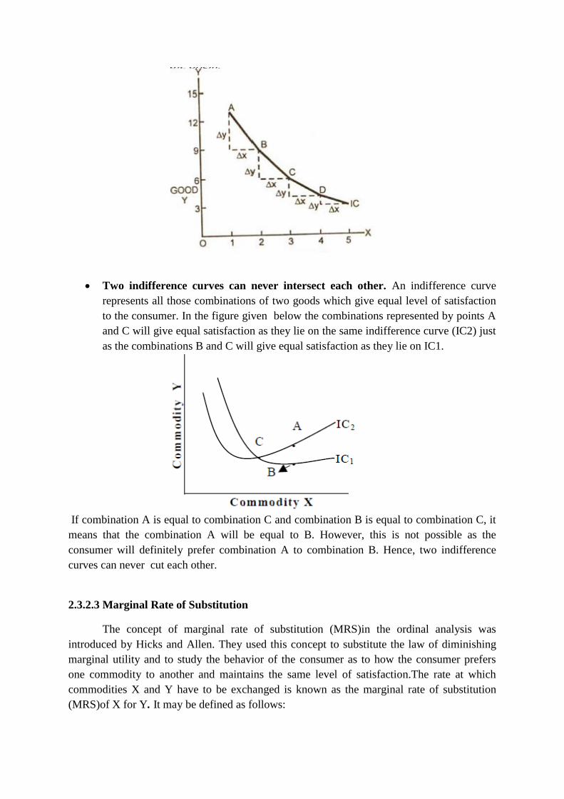
Two indifference curves can never intersect each other. An indifference curve
represents all those combinations of two goods which give equal level of satisfaction
to the consumer. In the figure given below the combinations represented by points A
and C will give equal satisfaction as they lie on the same indifference curve (IC2) just
as the combinations B and C will give equal satisfaction as they lie on IC1.
If combination A is equal to combination C and combination B is equal to combination C, it
means that the combination A will be equal to B. However, this is not possible as the
consumer will definitely prefer combination A to combination B. Hence, two indifference
curves can never cut each other.
2.3.2.3 Marginal Rate of Substitution
The concept of marginal rate of substitution (MRS)in the ordinal analysis was
introduced by Hicks and Allen. They used this concept to substitute the law of diminishing
marginal utility and to study the behavior of the consumer as to how the consumer prefers
one commodity to another and maintains the same level of satisfaction.The rate at which
commodities X and Y have to be exchanged is known as the marginal rate of substitution
(MRS)of X for Y. It may be defined as follows:
The marginal rate of substitution of X for Y measures the number of units of Y that must be
scarified for unit of X gained so as to maintain a constant level of satisfaction.
--- Hicks
Say there are two commodities X and Y which are imperfect substitutes of each other
and the consumer is willing to exchange good X for Y. The rate at which goods X and Y will
be exchanged is known as the marginal rate of substitution of X for Y (MRS
xy).Mathematically, marginal rate of substitution of X for Y (MRS xy) is expressed as
follows:
MRS xy = ∆Y∕∆X
where ∆Y shows change in quantity of Y commodity and ∆X shows change in quantity of X
commodity.
It is important to note that in case of indifference curve analysis the law of
diminishing marginal rate of substitution holds, which means that as the consumer increases
the purchase of X commodity, marginal rate of substitution of X for Y (MRS xy) goes on
diminishing.
Check your progress 2
1. State whether the following statements are True or False:
(i) The demand curve cannot be drawn using the marginal utility curve.
(ii) The ordinal utility approach is based on exact measurement of utility.
(iii) A single indifference curve shows the different combinations of X and Y goods that yield
equal satisfaction to the consumer.
(iv) Higher the indifference curve higher is the level of satisfaction.
(v) An indifference curve is always concave to the origin.
2.3.2.4Price Line
A price line or a budget line shows all those combinations of two commodities which
the consumer can buy given his money income and the prices of two commodities. The price
line is an important element of the theory of consumer behavior and preferences. The
indifference map reflects people’s preferences for different combinations of two goods under
consideration. Every consumer will try to to reach the highest possible indifference curve.
However, the actual choices made will depend on the income of the consumer and prices of
the two commodities. The price line or the budget line defines those combinations of two
goods under consideration which the consumer can actually buy within his income and prices
of the both commodities. Any combination lying outside the price line is beyond the reach of
the consumer and he cannot afford to buy it out of his limited income. The concept of price
line or the budget line can be explained with the help of the following diagram:

Price Line
Suppose a consumer has Rs.100 which he wants to spend on two commodities X and
Y. Let the prices of commodities X and Y be Rs.10 per unit and Rs. 5 per unit respectively. If
the consumer spends his entire income (Rs.100) on X, he would be able to buy 10 units of X,
and if he spends his total income on Y, he would buy 20 units of Y. If a straight line is drawn
joining 10 units of X and 20 units of Y, we get a line which is called the price line or budget
line.
The price line is drawn as a continuous straight line. Its slope is measured as the ratio
of prices of the two commodities. In the above diagram, slope of the price line is measured as
Slope of Price Line = Price of X Commodity/ Price of Y Commodity
If the prices of the two commodities remain the same but the income of the consumer
rises, the slope of price line will remain the same but it shifts its position to the right; and
vice-versa as shown in the figure below. It shows that if prices remain unchanged and income
rises, price line shifts to the right from L1 M1 to L2 M2.
Shift in Price Line
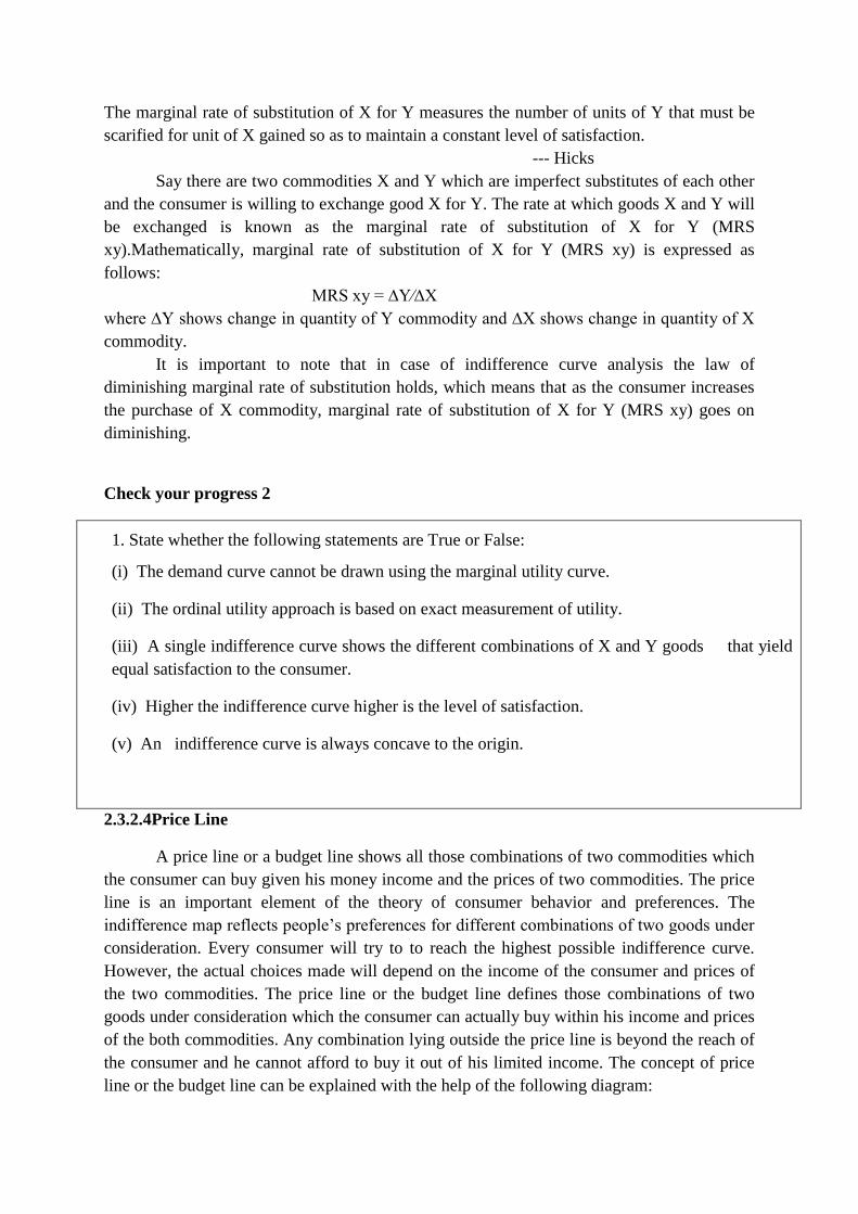
However, if the income of the consumer remains the same but the price of one commodity
say X falls, then the consumer is able to buy more of commodities X. In this situation price
line shifts from LM1 to LM2 as shown below
Shift in Price Line
Hence, various shifts are possible in the position of the price line depending on
whether there is a change in the income of the consumer or change in the price(s) of one or
both the commodities or both.
2.3.2.5 Consumer’s Equilibrium
The aim of a rational consumer is to maximize his satisfaction out of his limited
resources. So long as the consumer feels that he can increase his satisfaction by changing the
purchases of different commodities, he will continue to make adjustments in his purchases. A
situation in which the consumer gets maximum satisfaction and he is neither inclined to
increase or decrease the purchase of any commodity, signifies the equilibrium of the
consumer.
The consumer’s equilibriumindicates the amount of different commodities which the
consumer can buy given his income and given prices of those commodities. Given the price
line and the indifference map, a consumer is said to be in equilibriumat a point where the
price line touches the highest attainable indifference curve from below. Thus, the following
two conditions must be satisfied for consumer’s equilibrium :
(i) The price line should be tangent to some indifference curve, that is, slope of price line
should be equal to the slope of the indifference curve. In other words, the marginal rate of
substitution of X commodity for Y commodity (MRSxy) must
be equal to the price ratio of the two commodities. This condition can be expressed as:
MRSxy = Px / Py
(ii)The second condition is that the indifference curve must be convex to the origin at the
point of tangency which means that the marginal rate of substitution of X for Y (MRS xy)
should be diminishing.
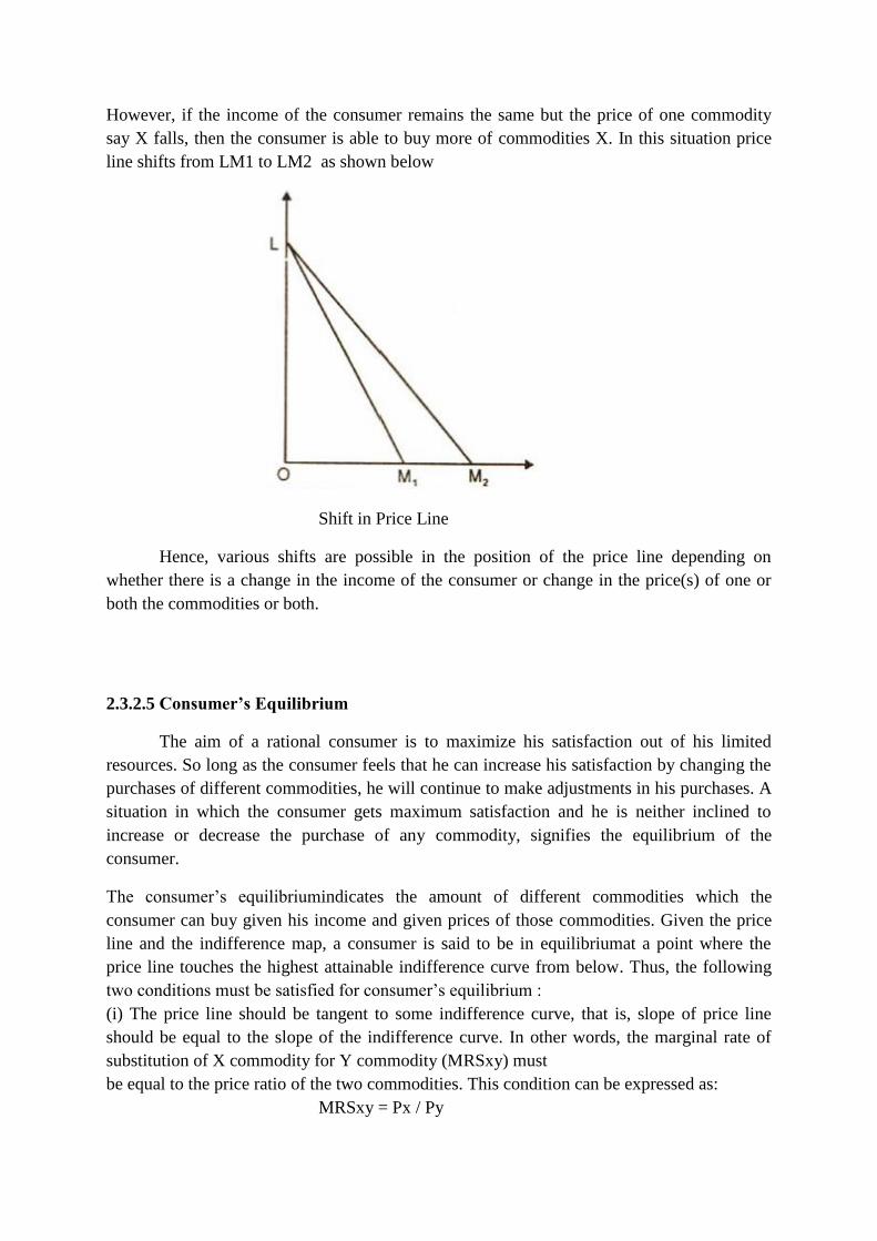
In order to find the consumer’s equilibrium, we superimpose an indifference map on
the price line to get the figure as shown below. Based on the two conditions necessary for
consumer’s equilibrium we find that C is the point of consumer’s equilibrium. The quantity
of good X is measured on the X-axis and that of Y on the Y-axis. PT is the price line and IC1,
IC2, IC3 form the indifference map. The price line
Consumer’s Equilibrium
PT is tangent to the indifference curve IC2 at point C which is the point of maximum
satisfaction. Points R and S do not reflect maximum satisfaction as they lie on a
lowerindifference curve IC1 and lower the indifference curve lower is the level of
satisfaction. Similarly, point U also does not reflect maximum satisfaction level. Although it
lies on a higher indifference curve but it lies outside the price line PT and hence, is beyond
the reach of the consumer.
Therefore, indifference curve analysis explains the concept of consumer’s equilibrium
in a better and realistic way as compared to the cardinal utility approach as it adopts the
ordinal measurement of utility and also uses a practical, measurable concept of marginal rate
of substitution. Moreover, the indifference curve analysis has quite theoretical and extensive
applications in innumerable fields. Almost every aspect of economic analysis and policy has
been explained by the indifference curveapproach in a logical and scientific manner. There
has been a general recognition that ordinal utilityanalysis is superior to the cardinal utility
approach. Even then ordinal utilityanalysis also suffers from some serious limitations:
consumer is not always rational; consumer may buy more than two goods; even absurd
combinations of two commodities are studied; all commodities are not divisible and many
others. Yet no denying the fact that it is better than the traditional theory and occupies an
important place among the theories to analyze the consumer behavior..

Activity B
Critically examine the law of Equi marginal Utility with example:
---------------------------------------------------------------------------------------------------------------------
---------------------------------------------------------------------------------------------------------------------
---------------------------------------------------------------------------------------------------------------------
---------------------------------------------------------------------------------------------------------------------
---------------------------------------------------------------------------------------------------------------------
---------------------------------------------------------------------------------------------------------------------
---------------------------------------------------------------------------------------------------------------------
---------------------------------------------------------------------------------------------------------------------
---------------------------------------------------------------------------------------------------------------------
---------------------------------------------------------------------------------------------------------------------
---------------------------------------------------------------------------------------------------------------------
---------------------------------------------------------------------------------------------------------------------
---------------------------------------------------------------------------------------------------------------------
---------------------------------------------------------------------------------------------------------------------
---------------------------------------------------------------------------------------------------------------------
---------------------------------------------------------------------------------------------------------------------
---------------------------------------------------------------------------------------------------------------------
----------------------------------------------------------------------------------
2.4 Summary
The consumer behavior is explained on the basis of utility. Utility is a psychological or
subjective concept which reflects the want satisfying power of a commodity. There are two
approaches regarding the measurement of utility- cardinal approach and the ordinal approach.
The former assumes that utility can be exactly measured in cardinal numbers while the latter
assumes that utility can only be ranked. Cardinal utility analysis studies the concepts of total
and marginal utility. Based on these concepts there are two basic laws of consumption: the
law of diminishing marginal utility and the law of equi marginal utility. Ordinal utility
analysis studies the consumer behavior using indifference curves. An indifference curve
shows the different combinations of X and Y goods that yield equal satisfaction to the
consumer. Indifference curves slope downwards, are convex to origin, do not intersect and a
higher indifference curve shows higher satisfaction. The rate at which commodities X and Y
are exchanged by the consumer is known as the marginal rate of substitution (MRS)of X for
Y In case of indifference curve analysis the law of diminishing marginal rate of substitution
holds. A price line, on the other hand, shows all the combinations of two commodities which
the consumer can buy given his money income and the prices two commodities. Using these
two concepts of indifference curves and the price line, consumer’s equilibrium, a situation of
maximum satisfaction, can be derived in the ordinal utility analysis.
Check your progress 3
1. Indifference curves ………………. intersect each other.
2. A …………… shows all those combinations of two commodities which the consumer can
buy given his money income and the prices two commodities.
3. For consumer’s equilibrium, marginal rate of substitution of X commodity for Y
commodity (MRSxy) must be equal to the ………….. of the two commodities.
4. The slope is of price line is measured as the ratio of ………………. .
5. The …………… analysis is superior to the cardinal utility approach.
2.5 Glossary
Utility: It is the want satisfying power of a commodity.
Total Utility: Total Utility is the sum of utilities derived from the consumption of all the
units of a commodity.
Marginal Utility: It is the addition made to total utility by consuming an additional unit of
the commodity.
Indifference Curve: It shows the different combinations of two goods that yield equal
satisfaction to the consumer.
Price Line: It shows all the combinations of two commodities which the consumer can
actually buy given his money income and the prices two commodities.
Marginal Rate of Substitution: The rate at which commodities X and Y are exchanged by
the consumer.
Consumer’s Equilibrium: A situation in which the consumer gets maximum satisfaction
given the prices and limited income.
.
2.6 ANSWERS TO CHECK YOUR PROGRESS
Check Your Progress 1
1. Utility
2. Cardinal
3. Marginal
4. Maximum
5. Marginal utilities
Check Your Progress 2
1. False
2. False
3. True
4. True
5. False
Check Your Progress 3
1. Never
2. Price line
3. Price ratio
4. Prices of two commodities
5. Ordinal utility
2.7 References
1. Baumol, K.E., Economic Theory and Operations Analysis, Prentice Hall of India, New
Delhi
2. Dwivedi, D.N., Microeconomic Theory, Pearson Education, New Delhi
3. Koutsoyiannis, A., Modern Microeconomics, Macmillan.
4. Mithani D.M. : Managerial Economics, Himalaya Publishing House, Mumbai
2.8 Suggested Readings
1. Dewett, K.K., Modern Economic Theory, S. Chand Publication
2. Peterson and Lewis, Managerial Economic, Prentice Hall of India
3. Gupta, Managerial Economics, TataMcGraw Hills
4.Geetika, Managerial Economics, Tata McGraw Hills
2.9 Terminal and Model Questions
1. What is utility? Give the difference between total utility and marginal utility?
2. Discuss the law of diminishing marginal utility in detail.
3. Explain the concept of marginal rate of substitution.
4. Define indifference curve. Explain the properties of indifference curves.
5. Give the assumptions of cardinal utility analysis.
6. Explain consumer’s equilibrium with ordinal utility analysis.
7. What is price line?
8. How will you derive demand curve using the concept of marginal utility?
LESSON – 3
Demand Analysis
Structure
3.0 Objectives
3.1 Introduction
3.2 Meaning of Demand
3.3 Types of Demand
3.4 Determinants of Demand
3.5 Law of Demand
3.5.1 Assumptions of Law of Demand
3.5.2 Demand Schedule and Demand Curve
3.5.3 Causes of Application of Law of Demand
3.5.4 Exceptions of Law of Demand
3.6 Changes in Demand
3.7 Summary
3.8 Glossary
3.9 Answer to Check Your Progress
3.10 References
3.11 Suggested Readings
3.12 Terminal and Model Questions
3.0 OBJECTIVES
After reading this lesson, you should be able:
To understand the basics of demand and its importance in decision making
To understand the determinants and types of demand
To comprehend the demand schedule, demand curve and the law of demand
3.1 INTRODUCTION
Demand forms the basis of all economic activities as it is an important economic
decision variable. Economic analysis remains incomplete without understanding the concept
of demand. The analysis of consumer demand for the product being produced by a firm plays
a crucial role in business decision making as demand determines the size and pattern of
market. All the decisions to be taken by the business managers are mostly demand driven, for
instance, decisions relating to the levels of investment and production depend on the market
demand of the products. Even the profit of a firm is influenced by the demand and supply
conditions of its output and inputs. The concept of demand is relevant even if a firm pursues
objectives other than profit maximization objective. It is necessary to evaluate the needs of
customers and social preferences in order to achieve these objectives. All the important
aspects of business decision making, like production planning, sales targeting, profit
targeting, pricing policies, revenue maximizing, inventory management, advertisement
depend on the product demand. The very survival and growth of a firm also depends on the
product demand. Hence, it is very important to understand the various concepts of demand
and then the law of demand.
3.2 Meaning of Demand
Demand refers to the desire to have a commodity backed by enough money to pay for
the good demanded. Thus, in economics demand refers to that desire which is effectively
supported by an adequate purchasing power. In order to understand the concept of demand it
is essential to distinguish between desire and demand. For instance, if a person wishes to buy
a car but does not have the required money, his wish is a desire. On the other hand, if he has
enough money to buy that; then it becomes effective desire or demand. Moreover the demand
is not complete unless the consumer has willingness to buy the commodity. If a person has
the desire to buy a product and also has enough money for it, but at a particular point of time,
he may not have willingness to buy the good, maybe due to a sudden change in his taste or
preference or fashion, etc. For example, when a rich person goes to a showroom to buy an
expensive dress but declines to buy, just because he does not find the colour of his choice.
Moreover, demand for a commodity is always expressed in relation to a particular price and a
particular time. Therefore, the demand for a product has the following five aspects:
(i) Desire to buy
(ii) Ability to pay
(iii) Willingness to spend
(iv) Particular price
(v) Particular time period
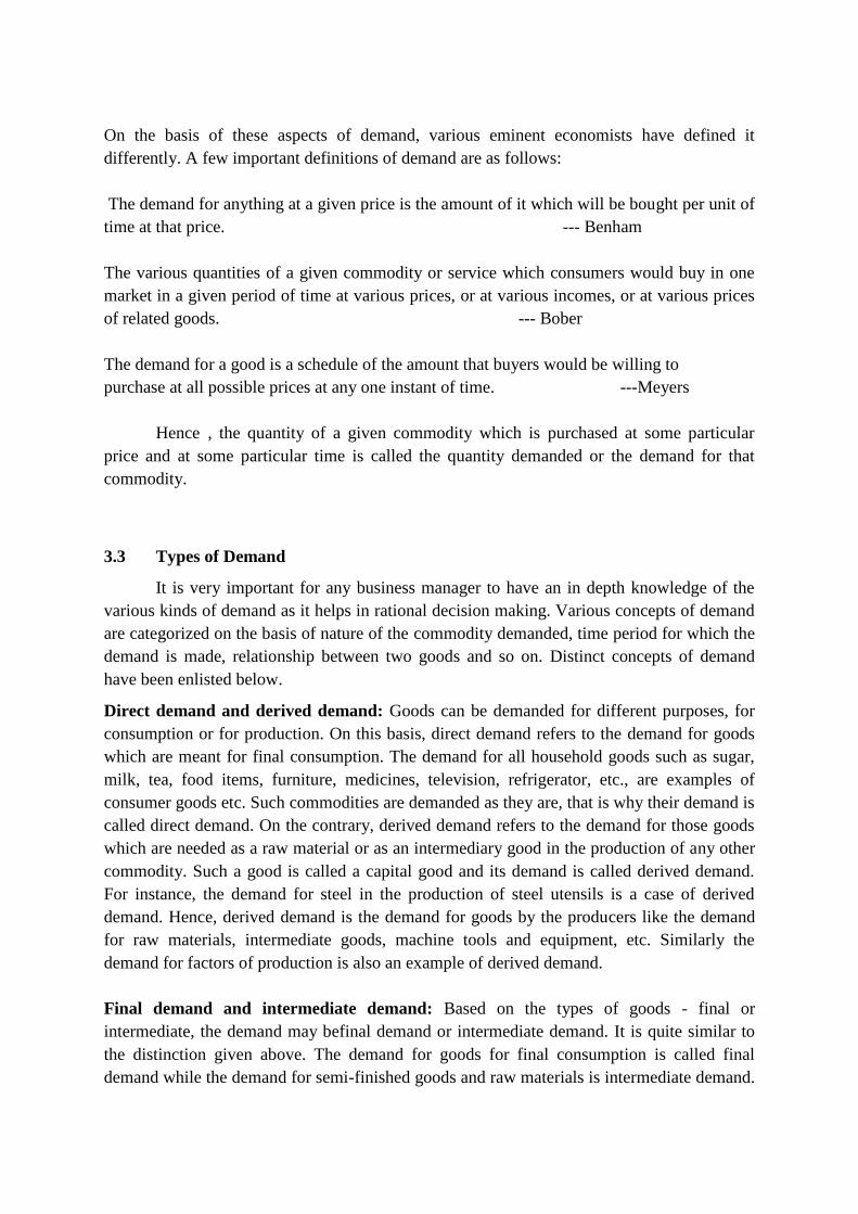
On the basis of these aspects of demand, various eminent economists have defined it
differently. A few important definitions of demand are as follows:
The demand for anything at a given price is the amount of it which will be bought per unit of
time at that price. --- Benham
The various quantities of a given commodity or service which consumers would buy in one
market in a given period of time at various prices, or at various incomes, or at various prices
of related goods. --- Bober
The demand for a good is a schedule of the amount that buyers would be willing to
purchase at all possible prices at any one instant of time. ---Meyers
Hence , the quantity of a given commodity which is purchased at some particular
price and at some particular time is called the quantity demanded or the demand for that
commodity.
3.3 Types of Demand
It is very important for any business manager to have an in depth knowledge of the
various kinds of demand as it helps in rational decision making. Various concepts of demand
are categorized on the basis of nature of the commodity demanded, time period for which the
demand is made, relationship between two goods and so on. Distinct concepts of demand
have been enlisted below.
Direct demand and derived demand: Goods can be demanded for different purposes, for
consumption or for production. On this basis, direct demand refers to the demand for goods
which are meant for final consumption. The demand for all household goods such as sugar,
milk, tea, food items, furniture, medicines, television, refrigerator, etc., are examples of
consumer goods etc. Such commodities are demanded as they are, that is why their demand is
called direct demand. On the contrary, derived demand refers to the demand for those goods
which are needed as a raw material or as an intermediary good in the production of any other
commodity. Such a good is called a capital good and its demand is called derived demand.
For instance, the demand for steel in the production of steel utensils is a case of derived
demand. Hence, derived demand is the demand for goods by the producers like the demand
for raw materials, intermediate goods, machine tools and equipment, etc. Similarly the
demand for factors of production is also an example of derived demand.
Final demand and intermediate demand: Based on the types of goods - final or
intermediate, the demand may befinal demand or intermediate demand. It is quite similar to
the distinction given above. The demand for goods for final consumption is called final
demand while the demand for semi-finished goods and raw materials is intermediate demand.
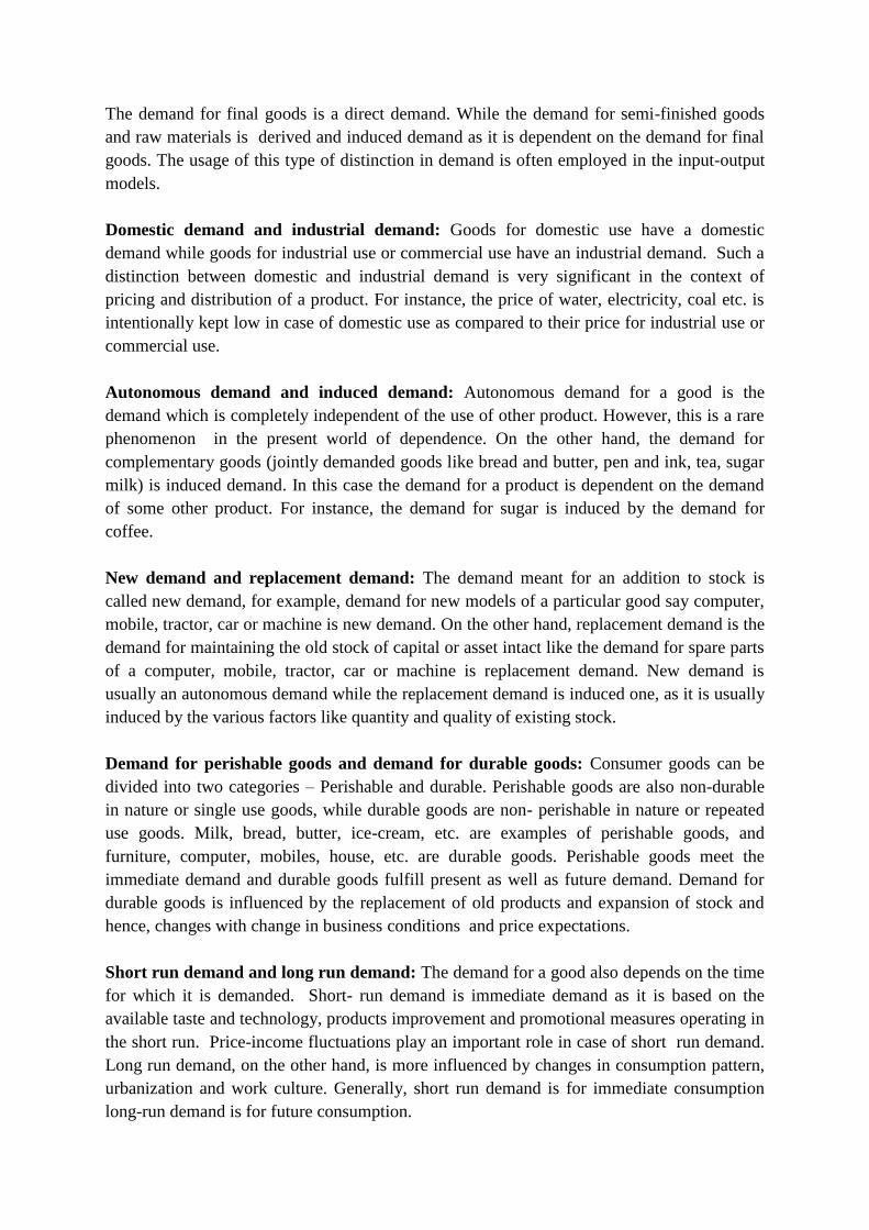
The demand for final goods is a direct demand. While the demand for semi-finished goods
and raw materials is derived and induced demand as it is dependent on the demand for final
goods. The usage of this type of distinction in demand is often employed in the input-output
models.
Domestic demand and industrial demand: Goods for domestic use have a domestic
demand while goods for industrial use or commercial use have an industrial demand. Such a
distinction between domestic and industrial demand is very significant in the context of
pricing and distribution of a product. For instance, the price of water, electricity, coal etc. is
intentionally kept low in case of domestic use as compared to their price for industrial use or
commercial use.
Autonomous demand and induced demand: Autonomous demand for a good is the
demand which is completely independent of the use of other product. However, this is a rare
phenomenon in the present world of dependence. On the other hand, the demand for
complementary goods (jointly demanded goods like bread and butter, pen and ink, tea, sugar
milk) is induced demand. In this case the demand for a product is dependent on the demand
of some other product. For instance, the demand for sugar is induced by the demand for
coffee.
New demand and replacement demand: The demand meant for an addition to stock is
called new demand, for example, demand for new models of a particular good say computer,
mobile, tractor, car or machine is new demand. On the other hand, replacement demand is the
demand for maintaining the old stock of capital or asset intact like the demand for spare parts
of a computer, mobile, tractor, car or machine is replacement demand. New demand is
usually an autonomous demand while the replacement demand is induced one, as it is usually
induced by the various factors like quantity and quality of existing stock.
Demand for perishable goods and demand for durable goods: Consumer goods can be
divided into two categories – Perishable and durable. Perishable goods are also non-durable
in nature or single use goods, while durable goods are non- perishable in nature or repeated
use goods. Milk, bread, butter, ice-cream, etc. are examples of perishable goods, and
furniture, computer, mobiles, house, etc. are durable goods. Perishable goods meet the
immediate demand and durable goods fulfill present as well as future demand. Demand for
durable goods is influenced by the replacement of old products and expansion of stock and
hence, changes with change in business conditions and price expectations.
Short run demand and long run demand: The demand for a good also depends on the time
for which it is demanded. Short- run demand is immediate demand as it is based on the
available taste and technology, products improvement and promotional measures operating in
the short run. Price-income fluctuations play an important role in case of short run demand.
Long run demand, on the other hand, is more influenced by changes in consumption pattern,
urbanization and work culture. Generally, short run demand is for immediate consumption
long-run demand is for future consumption.

Individual demand and market demand: The demand of a consumer for a product over a
period of time is called individual demand, whereas the sum total of demand for a product by
all individual consumers in a market is known as market demand,
Joint demand and Composite demand: When two or more goods together satisfy a
particular want, the demand for such goods is called joint demand. The demand for
complementary goods is a joint demand, like bread and butter or car and petrol. On the other
hand, when a commodity can be put to several uses its total demand in all the uses is called
composite demand. For instance, milk, electricity, etc. can be put to multiple uses.
Company demand and industry demand: Similar to the concept of individual demand and
market demand, is the distinction between company demand and industry demand. The
demand of a company or a single firm involved in the production of a particular product is
company demand. Alternatively, the demand of an industry (group of firms engaged in the
production of the same product) is the industry demand.
3.4 Determinants of Demand
Other than price, the quantity demanded for a particular commodity is influenced by
various other factors also. A mathematical function showing the functional relationship
between the demand for a product and various factors influencing it, is called a demand
function. A demand function may be expressed as follows:
DX = f ( Px, Ps, Pc, Yd, T, A, W, C, E, P, G, U)
where
Dx = Demand for commodity X
Px = Price of commodity X
Ps = Price of substitute of commodity X
Pc = Price of complementary goods of commodity X
Yd = Disposable income of the consumer
T = Taste and preferences of the consumer
A = Advertisement of commodity X
W = Wealth of the consumer
C = Climate
E = Price expectation of the consumer
P = Population
G = Government policies
U = Other unspecified and unidentified factors
The effect of these determinants of demand on the quantity demanded of a particular
commodity under normal circumstances is explained below:

Price of the product: It is the single most important determinant of demand of good.
Normally price has a negative effect on demand. Other things remaining the same, as price
increases, the demand for the good tends to fall and vice-versa. This negative relation
between price and demand is known as the law of demand. This type of demand showing the
effect of changes in price of a commodity on its quantity demanded other things remaining
same, indicates the price effect and is known as price demand.
Income of the consumer: Disposable income of the consumer an important variable
influencing the demand. As income increases, people have a tendency to buy more of
superior or normal goods and less of inferior goods. A normal good is a good whose quantity
demanded increases with increases in income, like higher segment cars. An inferior good is a
good whose quantity demanded decreases with increase in income, like inferior quality
cereal. The income effect changes the quantity demanded by allowing consumers to purchase
goods which they could not afford earlier. This type of demand explains the effect of changes
in the income of the consumer on the demand for a commodity, other things remaining same
and it is called income effect.
Taste and preferences of the consumer: These are important factors which affects the
quantity demanded of a product. The demand for a good will be large if tastes and
preferences are favourable and vice-versa. Many factors play a role in developing the tastes
and preferences like age, gender, professional status, level of education, social and cultural
factors, advertising, to name a few.
Prices of related goods: Related goods are of two types—substitutes and complements and
their prices affect the quantity demanded of a product. Substitutes are those goods which can
be interchangeably used. For example, tea and coffee are substitutes. If price of tea increases
the consumer can use coffee and vice versa. Complementary goods are those goods which are
demanded together and jointly satisfy a demand, like bread and butter or car and petrol. In
case of substitutes, the rise in price of one commodity results in an increase in the quantity
demanded of the other. If the price of substitute (say coffee) rises, the demand for tea
increases. However, in case of complementary goods, the change in the price of any of the
two goods surely affects the demand of the other good. For instance, if price of motor cars
rises, there will be a fall in the demand for motor cars. Along with it, the demand for petrol
also falls.
Consumer’s expectation of future income and prices: The purchases made by a consumer
also depend on future expectations along with present income and prices. If the price for
petrol is expected to rise in the near future, then the demand for petrol will increase now. If
the price for petrol is expected to drop in the near future, then the demand for petrol will
decrease now. Similarly, if a consumer expects a raise in salary in coming times, he will
postpone the demand for some good and buy it later.

Population: Important demographic features of the population like its size, age distribution,
gender ratio, rural urban ratio, etc. have a striking noticeable impact on the level of demand
in the economy.
Advertisement : Publicity measures have a great influence on demand. Sales turnover of
firms increases due to advertisement which is known as the promotional effect on demand.
Climate: The weather and climatic conditions of a region also influence the demand for
different goods. For instance, the demand for coolers and air conditioners increases in
summers, while that of heaters increases in winters.
Government policy: The government policy on taxes and subsidies of different
commodities also influences the demand of different goods differently. An increase in tax
rates or the imposition of new taxes results in a decrease in the demand and an increase in
subsidies increase the demand.
There are many other factors also which may not be specified or identified but
influence demand. Hence, a demand function shows the effect of different factors influencing
the level of demand.
Activity A
Explain the effect of demand for butter in following cases
a)The price of bread rises
-----------------------------------------------------------------------------------------------------------------
b)The price of jam falls
-----------------------------------------------------------------------------------------------------------------
c)The price of butter rises
-----------------------------------------------------------------------------------------------------------------
d)An increase in family income
-------------------------------------------------------------------------------------------------------------------
3.5 Law of Demand
In economics, the law of demand expresses the functional relationship between price
and quantity demanded for a particular commodity. The law states that other things remaining
the same or ceteris paribus, if the price of a commodity falls its quantity demanded will rise
and if price of the good rises quantity demanded will fall. In other words, there is an inverse
relationship between price and quantity demanded. The lawof demand is defined as follows:
People will buy more at lower prices and buy less at higher prices, ceteris paribus or other
things remaining the same. --- Samuelson
Other things being equal, the quantity demanded per unit of time will be greater, the lower
the price and smaller, the higher the price. ---Bilas
The amount demanded increases with a fall in price and diminishes with a rise in price.
---Marshall
Therefore, it can be said that the lawof demand states that other things remaining the
same, demand varies inversely with price.
3.5.1 Assumptions of the Law of Demand
The law of demand is based on the following assumptions:
1. The commodity is normal.
2. There is no change in the incomes of consumers.
3. There is no change in the tastes and preferences of consumers.
4. There is no change in the prices of related goods.
5. The goods are perfectly divisible.
6. There are normal conditions in the economy.
These assumptions refer to the ‘other things remaining the same or ceteris paribus’ clause
of the statement of the law of demand. In other words, assumptions refer to those conditions
which must be met for the law of demand to be valid.
3.5.2 Demand Schedule and Demand Curve
A demand schedule is a tabular representation showing the different quantities of a
commodity that would be demanded at different prices. It shows the quantities of a good that
will be purchased at different possible prices. A demand schedule can be shown as below:
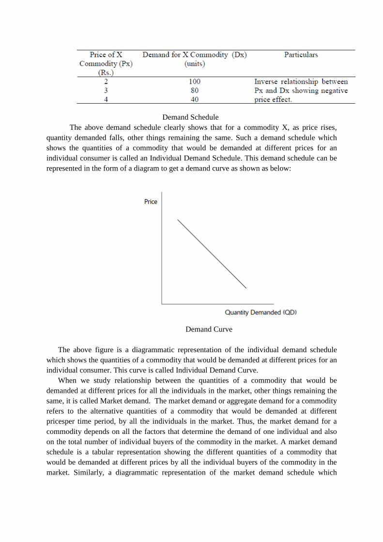
Demand Schedule
The above demand schedule clearly shows that for a commodity X, as price rises,
quantity demanded falls, other things remaining the same. Such a demand schedule which
shows the quantities of a commodity that would be demanded at different prices for an
individual consumer is called an Individual Demand Schedule. This demand schedule can be
represented in the form of a diagram to get a demand curve as shown as below:
Demand Curve
The above figure is a diagrammatic representation of the individual demand schedule
which shows the quantities of a commodity that would be demanded at different prices for an
individual consumer. This curve is called Individual Demand Curve.
When we study relationship between the quantities of a commodity that would be
demanded at different prices for all the individuals in the market, other things remaining the
same, it is called Market demand. The market demand or aggregate demand for a commodity
refers to the alternative quantities of a commodity that would be demanded at different
pricesper time period, by all the individuals in the market. Thus, the market demand for a
commodity depends on all the factors that determine the demand of one individual and also
on the total number of individual buyers of the commodity in the market. A market demand
schedule is a tabular representation showing the different quantities of a commodity that
would be demanded at different prices by all the individual buyers of the commodity in the
market. Similarly, a diagrammatic representation of the market demand schedule which
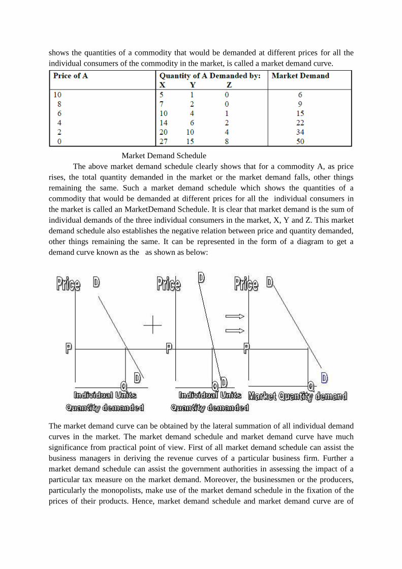
shows the quantities of a commodity that would be demanded at different prices for all the
individual consumers of the commodity in the market, is called a market demand curve.
Market Demand Schedule
The above market demand schedule clearly shows that for a commodity A, as price
rises, the total quantity demanded in the market or the market demand falls, other things
remaining the same. Such a market demand schedule which shows the quantities of a
commodity that would be demanded at different prices for all the individual consumers in
the market is called an MarketDemand Schedule. It is clear that market demand is the sum of
individual demands of the three individual consumers in the market, X, Y and Z. This market
demand schedule also establishes the negative relation between price and quantity demanded,
other things remaining the same. It can be represented in the form of a diagram to get a
demand curve known as the as shown as below:
The market demand curve can be obtained by the lateral summation of all individual demand
curves in the market. The market demand schedule and market demand curve have much
significance from practical point of view. First of all market demand schedule can assist the
business managers in deriving the revenue curves of a particular business firm. Further a
market demand schedule can assist the government authorities in assessing the impact of a
particular tax measure on the market demand. Moreover, the businessmen or the producers,
particularly the monopolists, make use of the market demand schedule in the fixation of the
prices of their products. Hence, market demand schedule and market demand curve are of
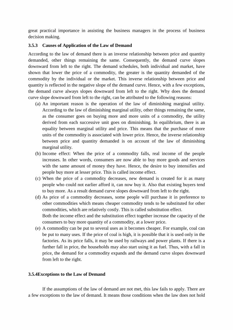
great practical importance in assisting the business managers in the process of business
decision making.
3.5.3 Causes of Application of the Law of Demand
According to the law of demand there is an inverse relationship between price and quantity
demanded, other things remaining the same. Consequently, the demand curve slopes
downward from left to the right. The demand schedules, both individual and market, have
shown that lower the price of a commodity, the greater is the quantity demanded of the
commodity by the individual or the market. This inverse relationship between price and
quantity is reflected in the negative slope of the demand curve. Hence, with a few exceptions,
the demand curve always slopes downward from left to the right. Why does the demand
curve slope downward from left to the right, can be attributed to the following reasons:
(a) An important reason is the operation of the law of diminishing marginal utility.
According to the law of diminishing marginal utility, other things remaining the same,
as the consumer goes on buying more and more units of a commodity, the utility
derived from each successive unit goes on diminishing. In equilibrium, there is an
equality between marginal utility and price. This means that the purchase of more
units of the commodity is associated with lower price. Hence, the inverse relationship
between price and quantity demanded is on account of the law of diminishing
marginal utility.
(b) Income effect: When the price of a commodity falls, real income of the people
increases. In other words, consumers are now able to buy more goods and services
with the same amount of money they have. Hence, the desire to buy intensifies and
people buy more at lesser price. This is called income effect.
(c) When the price of a commodity decreases, new demand is created for it as many
people who could not earlier afford it, can now buy it. Also that existing buyers tend
to buy more. As a result demand curve slopes downward from left to the right.
(d) As price of a commodity decreases, some people will purchase it in preference to
other commodities which means cheaper commodity tends to be substituted for other
commodities, which are relatively costly. This is called substitution effect.
Both the income effect and the substitution effect together increase the capacity of the
consumers to buy more quantity of a commodity, at a lower price.
(e) A commodity can be put to several uses as it becomes cheaper. For example, coal can
be put to many uses. If the price of coal is high, it is possible that it is used only in the
factories. As its price falls, it may be used by railways and power plants. If there is a
further fall in price, the households may also start using it as fuel. Thus, with a fall in
price, the demand for a commodity expands and the demand curve slopes downward
from left to the right.
3.5.4Exceptions to the Law of Demand
If the assumptions of the law of demand are not met, this law fails to apply. There are
a few exceptions to the law of demand. It means those conditions when the law does not hold
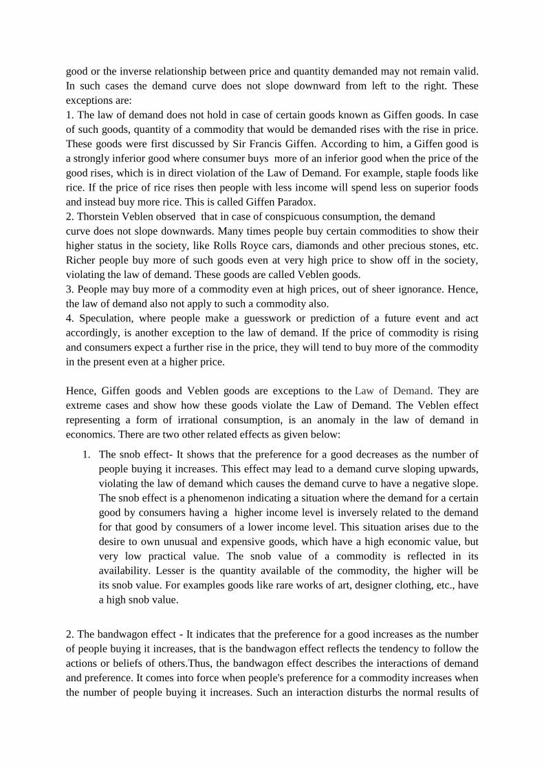
good or the inverse relationship between price and quantity demanded may not remain valid.
In such cases the demand curve does not slope downward from left to the right. These
exceptions are:
1. The law of demand does not hold in case of certain goods known as Giffen goods. In case
of such goods, quantity of a commodity that would be demanded rises with the rise in price.
These goods were first discussed by Sir Francis Giffen. According to him, a Giffen good is
a strongly inferior good where consumer buys more of an inferior good when the price of the
good rises, which is in direct violation of the Law of Demand. For example, staple foods like
rice. If the price of rice rises then people with less income will spend less on superior foods
and instead buy more rice. This is called Giffen Paradox.
2. Thorstein Veblen observed that in case of conspicuous consumption, the demand
curve does not slope downwards. Many times people buy certain commodities to show their
higher status in the society, like Rolls Royce cars, diamonds and other precious stones, etc.
Richer people buy more of such goods even at very high price to show off in the society,
violating the law of demand. These goods are called Veblen goods.
3. People may buy more of a commodity even at high prices, out of sheer ignorance. Hence,
the law of demand also not apply to such a commodity also.
4. Speculation, where people make a guesswork or prediction of a future event and act
accordingly, is another exception to the law of demand. If the price of commodity is rising
and consumers expect a further rise in the price, they will tend to buy more of the commodity
in the present even at a higher price.
Hence, Giffen goods and Veblen goods are exceptions to the Law of Demand. They are
extreme cases and show how these goods violate the Law of Demand. The Veblen effect
representing a form of irrational consumption, is an anomaly in the law of demand in
economics. There are two other related effects as given below:
1. The snob effect- It shows that the preference for a good decreases as the number of
people buying it increases. This effect may lead to a demand curve sloping upwards,
violating the law of demand which causes the demand curve to have a negative slope.
The snob effect is a phenomenon indicating a situation where the demand for a certain
good by consumers having a higher income level is inversely related to the demand
for that good by consumers of a lower income level. This situation arises due to the
desire to own unusual and expensive goods, which have a high economic value, but
very low practical value. The snob value of a commodity is reflected in its
availability. Lesser is the quantity available of the commodity, the higher will be
its snob value. For examples goods like rare works of art, designer clothing, etc., have
a high snob value.
2. The bandwagon effect - It indicates that the preference for a good increases as the number
of people buying it increases, that is the bandwagon effect reflects the tendency to follow the
actions or beliefs of others.Thus, the bandwagon effect describes the interactions of demand
and preference. It comes into force when people's preference for a commodity increases when
the number of people buying it increases. Such an interaction disturbs the normal results of

the theory of supply and demand, which assumes that consumers make buying decisions only
on the basis of price and their own personal preference. The bandwagon effect may be so
strong that it may make the demand curve slope upwards, violating the law of demand. The
bandwagon effect is also known as demonstration effect. In this case, the demand for a
product appears to be determined by consumption pattern of trend setters like cricket stars,
film stars, models, etc., and not by the utility derived from it.
Check Your Progress 1
State whether the following are true or false.
1. Demand refers to the desire to have a commodity.
2. As income increases, people buy more of a given good if it is a normal good.
3. Direct demand refers to the demand for goods which are meant for final consumption.
4. Population structure has no impact on the level of demand in the economy.
5. A demand function shows that quantity demanded for a particular commodity is
influenced by price alone.
3.6 Changes in Demand
In economic analysis, the law of demand expains the changes in demand due to changes
in price. However, sometimes changes in demand are not associated with changes in price but
with certain other non price factors. Based on the factors causing the changes in demand –
price factors or non price factors, the changes in demand can broadly be of two types:
(1) Extension and Contraction in Demand
(2) Increase and Decrease in Demand
Extension and Contraction in demand
When the changes in quantity demanded for a commodity take place on account of
changes in its price, these signify either extension or contraction in demand. Hence,
extension or contraction in demand relates to the law of demand as in this case, changes in
the quantity demanded take place only in response to the own price of the commodity. This
means all the components of the demand function remain unchanged except the price the
commodity under consideration.
If the price of a commodity falls, other things remaining the same, it leads to larger
purchase of this commodity. This is called extension in demand. It signifies more demand at
a lower price. On the other hand, if the price of a commodity rises, other things remaining the
same, it leads to smaller purchase of this commodity.

Extension and Contraction in Demand
Extension and Contraction in Demand may be diagrammatically explained with the help of
the above figure. It is clear from the figure that the changes in quantity demanded are shown
by the movement along the same demand curve. A downward movement from one point to
another on the same demand curve, showing more demand at a lower price, indicates an
extension of demand. On the contrary, an upward movement from one point to another on the
same demand curve implies contraction of demand, showing that lesser quantity is demanded
at higher price.
Increase and Decrease in Demand
When the changes in quantity demanded for a commodity take place not on account
of changes in its price, but due to other non price factors, these signify either increase in
demand or decrease in demand. Hence, increase and decrease in demand do not relate to the
law of demand as in this case other components of the demand function change except the
price the commodity under consideration. Only the non price factors like income, taste and
preferences, price of related goods, climate, population, etc., change while the price the
commodity under consideration remains the same.
Increase or decrease in demand, is graphically represented by a shift in the demand
curve from one position to another. In case of an increase in demand, the demand curve is
shifted to the right in the upward direction as shown below:
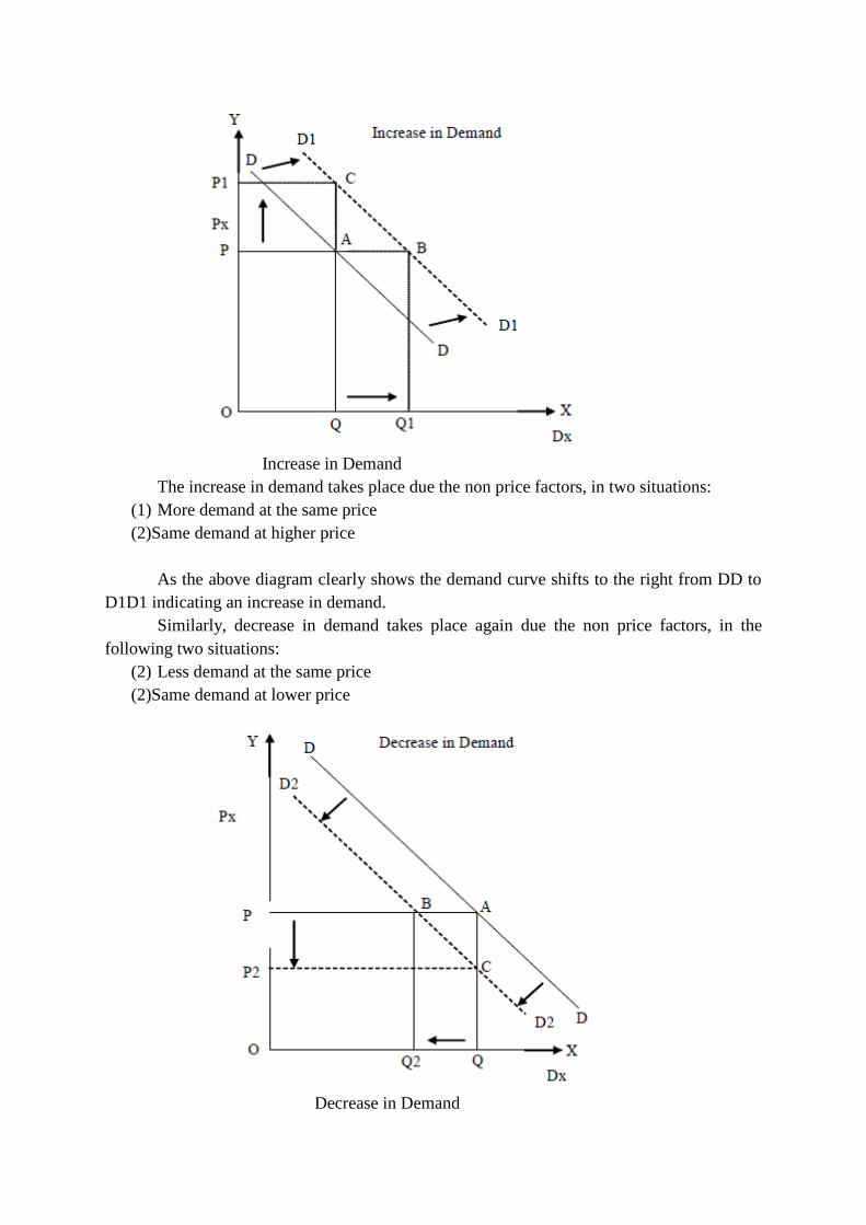
Increase in Demand
The increase in demand takes place due the non price factors, in two situations:
(1) More demand at the same price
(2)Same demand at higher price
As the above diagram clearly shows the demand curve shifts to the right from DD to
D1D1 indicating an increase in demand.
Similarly, decrease in demand takes place again due the non price factors, in the
following two situations:
(2) Less demand at the same price
(2)Same demand at lower price
Decrease in Demand
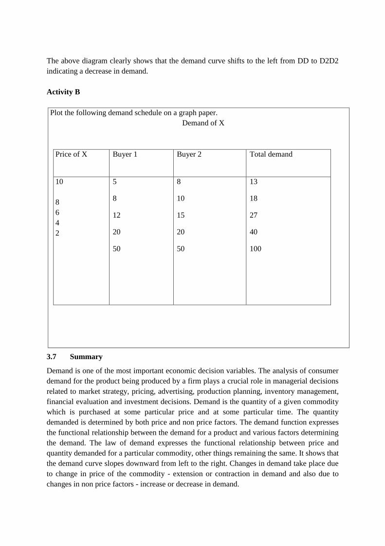
The above diagram clearly shows that the demand curve shifts to the left from DD to D2D2
indicating a decrease in demand.
Activity B
Plot the following demand schedule on a graph paper.
Demand of X
Price of X
Buyer 1
Buyer 2 Total demand
10
8
6
4
2
5
8
12
20
50
8
10
15
20
50
13
18
27
40
100
3.7 Summary
Demand is one of the most important economic decision variables. The analysis of consumer
demand for the product being produced by a firm plays a crucial role in managerial decisions
related to market strategy, pricing, advertising, production planning, inventory management,
financial evaluation and investment decisions. Demand is the quantity of a given commodity
which is purchased at some particular price and at some particular time. The quantity
demanded is determined by both price and non price factors. The demand function expresses
the functional relationship between the demand for a product and various factors determining
the demand. The law of demand expresses the functional relationship between price and
quantity demanded for a particular commodity, other things remaining the same. It shows that
the demand curve slopes downward from left to the right. Changes in demand take place due
to change in price of the commodity - extension or contraction in demand and also due to
changes in non price factors - increase or decrease in demand.

3.8 Glossary
Demand: It refers to the quantity of a commodity which will be purchased at a given price
and at a given time.
Demand function: It expresses functional relationship between the demand for a commodity
and the determinants of demand.
Law of demand: The law of demand expresses the functional relationship between price and
the quantity demanded for a particular commodity, other things remaining the same.
Substitutes :Those goods which can be interchangeably used in place of each other for
satisfying a specific want like tea and coffee.
Complementary goods: When two or more goods together satisfy a particular want, the
demand for such goods is called joint demand and the goods are called complementary goods
like bread and butter or pen and ink.
Giffengoods :Those goods whose demand falls with increase in income of the
consumers, for example, inferior quality cereal.
Check your progress 2
1. The law of demand expresses the functional relationship between ………….. and quantity
demanded for a particular commodity.
2. The law of ……………………….. utility explains why the demand curve slopes downward
from left to the right.
3. The …………. effect shows that the preference for a good decreases as the number of people
buying it increases.
4.……….. goods and ……….. goods are exceptions to the law of demand.
5. The ………… in demand shows that the demand curve shifts outwards to the right.
3.9 ANSWERS TO CHECK YOUR PROGRESS
Check Your Progress 1
1. False
2. True

3. True
4. False
5. False
Check Your Progress 2
1. Price
2. Diminishing marginal
3. Snob
4. Giffen, Veblen
5. increase
3.10References
Koutsoyiannis, A : Modern Microeconomics, The Macmillan Press Ltd.,, London
Dewett, K.K., Modern Economic Theory, S. Chand Publication
.
Geetika, Managerial Economics, Tata McGraw Hills
3.11 Suggested Readings
Mithani D.M. : Managerial Economics, Himalaya Publishing House, Mumbai
Dwivedi, D.N. : Managerial Economics, Vikas Publishing House Pvt. Ltd, New Delhi
Misra&Puri : Economics for Managers, Himalaya Publishing House, Mumbai
Adhikary M. : Managerial Economics, Khosla Educational Publishers, Delhi
3.12 Terminal and Model Questions
1. Define demand.
2. Explain the law of demand. Illustrate your answer with an appropriate diagram.
3. What is the shape of a demand curve?
4. What is demand function?
5. Distinguish between increase in demand and extension in demand.
6. What is market demand?

7. Show the shifts in the demand curve and movement along the demand curve with the help
of diagrams.
8. What do you mean by substitutes and complementary good?
LESSON – 4
Elasticity of Demand
Structure
4.0 Objectives
4.1 Introduction
4.2 Meaning of elasticity of demand
4.3 Types of elasticity of demand
4.3.1 Price elasticity of demand
4.3.1.1 Degrees of price elasticity of demand
4.3.1.2 Measurement of price elasticity of demand
4.3.2 Income elasticity of demand
4.3.3Cross elasticity of demand
4.3.4 Promotional or advertisement elasticity of demand
4.4 Factors determining elasticity of demand
4.5 Importance of elasticity of demand
4.6 Summary
4.7 Glossary
4.8 Answer to Check Your Progress
4.9 References
4.10 Suggested Readings
4.11 Terminal and Model Questions
4.0 OBJECTIVES
After reading this lesson, you should be able:
To understand the meaning of elasticity of demand and its importance in decision
making
To understand the different types of elasticity of demand used in business decisions
To comprehend the degrees of elasticity of demand
To know the methods of measurement of elasticity of demand
4.1 Introduction
Demand plays an important role in economics as well as in the economy as a whole.
The law of demand explains that demand rises with a fall in price and vice-versa, other things
remaining the same. Hence, the law of demand deals only with the direction of change in
demand due to a change in price. However, the law of demand fails to explain what will be
the extent of change in demand due to a given change in price. Thus, the law of demand
makes only a qualitative statement of the relationship between demand and price and does not
consider the quantitative relationship between demand and price. The concept of elasticity of
demand deals with the quantitative aspects regarding the inverse relationship between price
and demand. The knowledge of the nature of relationship between the demand for a product
and the factors determining the quantity demanded (that is, the knowledge of the demand
function) is not sufficient from the point of view of the business managers of a firm. The
degree of responsiveness of demand to changes in its determinants is more important for
rational decision making by the business managers. This degree of responsiveness of demand
to changes in its determinants is referred to as theelasticity of demandfor the product under
consideration. This concept of elasticity of demand is highly significant in the pricing
decisions of the business firms. In rational business decisions making, the firms intend to
shift the increases in cost over to the consumers through price increases. How far this
increase in price due to increasing cost is favourable for the firm, will depend on the elasticity
of demand for that product. Therefore, an in depth study of the concept of elasticity of
demand is extremely essential for the business firms as it helps the firms in making major
business decisions.
4.2 Meaning of Elasticity of Demand
Generally speaking the term elasticity is concerned with the responsiveness of one
variable to changes in another. Specifically, the elasticity of demand indicates the degree of
responsiveness of demand to the changes in its determinants. It shows the response of the
demand of a commodity when there is either increase or decrease in its price. Business
managers of the firms have great advantages by knowing elasticity of the products of the
firm. A greater response in the demand of a commodity indicates greater elasticity and a
smaller response indicates less elasticity. For example, a business manager will definitely be
interested in knowing whether sales will increase by six percent, twelve percent or maybe
more by cutting down price by say, seven percent. Thus, elasticity of demand of a commodity
measures the degree of responsiveness of demand to a change in price of that commodity.

The concept of elasticity of demand in the economic theory was introduced by Prof. Alfred
Marshall. He defined it as:
The elasticity (or responsiveness) of demand in a market is great or small according as the
amount demanded increases much or little for a given fall in price and diminishes much or
little for a given rise in price. -------- Alfred Marshall
Other important definitions of elasticity of demand by eminent economists are listed below.
The elasticity of demand may be defined as the percentage change in the quantity demand
which would result in one percent change in price. ------Boulding
The elasticity of demand at any price or at any output is equal to the proportional change of
amount demanded in response to a small change in price divided by the proportional change
in price. ------Mrs Joan Robinson
Elasticity of demand is the responsiveness of demand to change of prices.
-------Hanson
Thus, elasticity of demand may be defined as the ratio of the percentage change in quantity
demanded to the percentage change in price. Other things remaining the same, if certain
percentage changes in demand of a commodity take place due to certain percentage change in
a price of that commodity, it is known as elasticity of demand. Boulding has given the
following formula to compute the elasticity of demand as follows:
Another formula for calculation of the elasticity of demand has been given by
Robinson which measures elasticity of demand as the ratio of the percentage change in
quantity demanded to the percentage change in price.
Theoretically it is possible to discuss the elasticity of demand for all the different
factors affecting demand, represented in the demand function, but in real practice, broadly
there are four main types of elasticity of demand which can be measured and examined.
These four types of elasticity of demand correspond to four specifically important factors in
the demand function: price of the commodity, income of the consumer, the price of a related
product and promotion or advertisement and are referred to as the price elasticity of demand,
income elasticity of demand, cross elasticity of demand and promotional elasticity of demand
respectively. A detailed analysis of each of these elasticity of demand is given ahead.
4.3 Types of Elasticity of Demand
As mentioned above, depending on the factors influencing the level of quantity
demanded, four main types of elasticity of demand can be listed. Price elasticity of demand
measures the responsiveness of demand of a commodity to change in the price of that
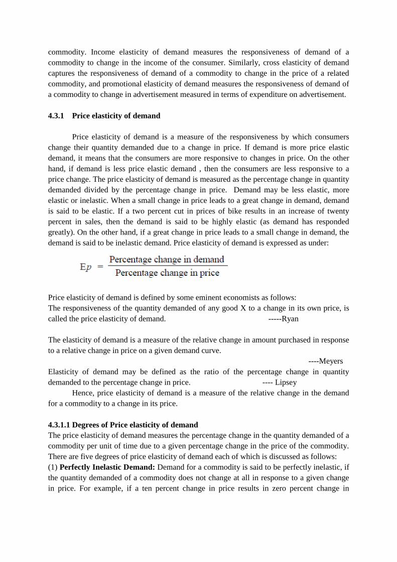
commodity. Income elasticity of demand measures the responsiveness of demand of a
commodity to change in the income of the consumer. Similarly, cross elasticity of demand
captures the responsiveness of demand of a commodity to change in the price of a related
commodity, and promotional elasticity of demand measures the responsiveness of demand of
a commodity to change in advertisement measured in terms of expenditure on advertisement.
4.3.1 Price elasticity of demand
Price elasticity of demand is a measure of the responsiveness by which consumers
change their quantity demanded due to a change in price. If demand is more price elastic
demand, it means that the consumers are more responsive to changes in price. On the other
hand, if demand is less price elastic demand , then the consumers are less responsive to a
price change. The price elasticity of demand is measured as the percentage change in quantity
demanded divided by the percentage change in price. Demand may be less elastic, more
elastic or inelastic. When a small change in price leads to a great change in demand, demand
is said to be elastic. If a two percent cut in prices of bike results in an increase of twenty
percent in sales, then the demand is said to be highly elastic (as demand has responded
greatly). On the other hand, if a great change in price leads to a small change in demand, the
demand is said to be inelastic demand. Price elasticity of demand is expressed as under:
Price elasticity of demand is defined by some eminent economists as follows:
The responsiveness of the quantity demanded of any good X to a change in its own price, is
called the price elasticity of demand. -----Ryan
The elasticity of demand is a measure of the relative change in amount purchased in response
to a relative change in price on a given demand curve.
----Meyers
Elasticity of demand may be defined as the ratio of the percentage change in quantity
demanded to the percentage change in price. ---- Lipsey
Hence, price elasticity of demand is a measure of the relative change in the demand
for a commodity to a change in its price.
4.3.1.1 Degrees of Price elasticity of demand
The price elasticity of demand measures the percentage change in the quantity demanded of a
commodity per unit of time due to a given percentage change in the price of the commodity.
There are five degrees of price elasticity of demand each of which is discussed as follows:
(1) Perfectly Inelastic Demand: Demand for a commodity is said to be perfectly inelastic, if
the quantity demanded of a commodity does not change at all in response to a given change
in price. For example, if a ten percent change in price results in zero percent change in
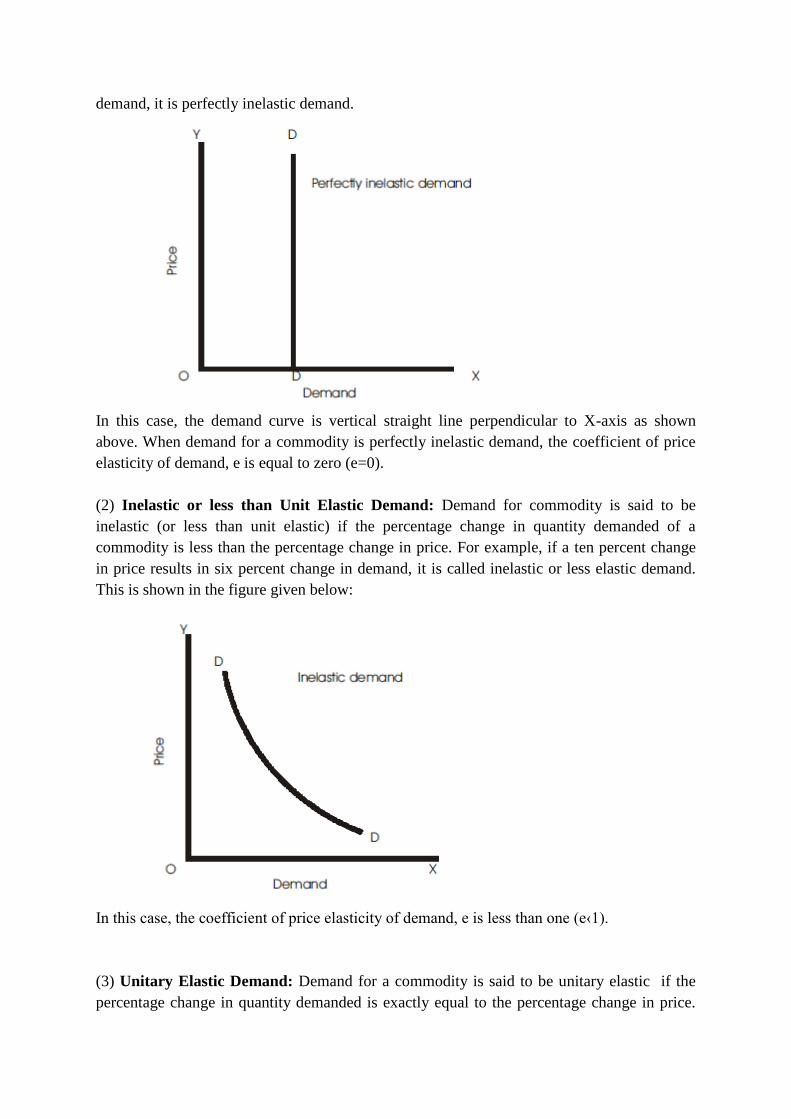
demand, it is perfectly inelastic demand.
In this case, the demand curve is vertical straight line perpendicular to X-axis as shown
above. When demand for a commodity is perfectly inelastic demand, the coefficient of price
elasticity of demand, e is equal to zero (e=0).
(2) Inelastic or less than Unit Elastic Demand: Demand for commodity is said to be
inelastic (or less than unit elastic) if the percentage change in quantity demanded of a
commodity is less than the percentage change in price. For example, if a ten percent change
in price results in six percent change in demand, it is called inelastic or less elastic demand.
This is shown in the figure given below:
In this case, the coefficient of price elasticity of demand, e is less than one (e‹1).
(3) Unitary Elastic Demand: Demand for a commodity is said to be unitary elastic if the
percentage change in quantity demanded is exactly equal to the percentage change in price.

For example, if a ten percent change in price results in ten percent change in demand, it is
called a unitary elastic demand, as shown below:
The demand curve in in case of unitary elastic demand s shown above is called rectangular
hyperbola. In this case, the coefficient of price elasticity of demand, e is equal to one (e=1).
(4) More than Unitary Elastic: Demand for a commodity is said to be more than unitary
elastic demand if a given change in price results in a significant more than proportionate
change in demand for this commodity. For example, if a ten percent change in price results in
a fourteen percent change in demand, it is called more than unitary elastic demand. This can
be shown with the help of the following figure:
In this case, the coefficient of price elasticity of demand, e is more than one (e›1).
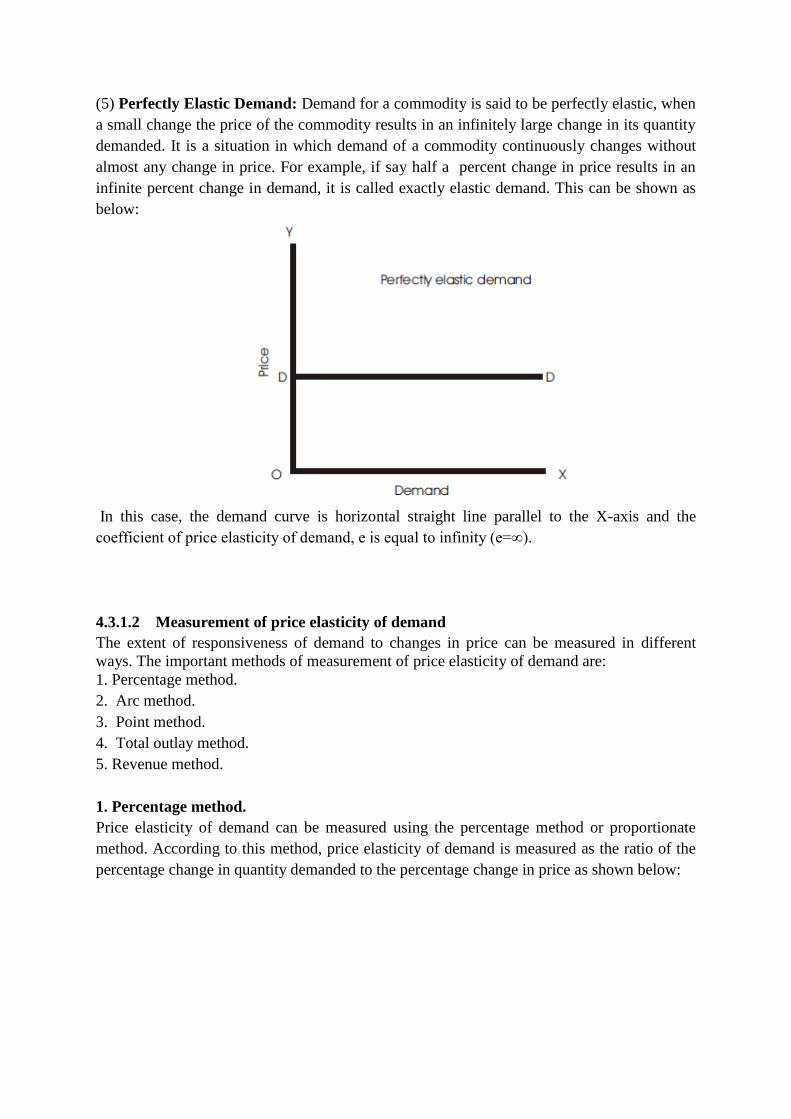
(5) Perfectly Elastic Demand: Demand for a commodity is said to be perfectly elastic, when
a small change the price of the commodity results in an infinitely large change in its quantity
demanded. It is a situation in which demand of a commodity continuously changes without
almost any change in price. For example, if say half a percent change in price results in an
infinite percent change in demand, it is called exactly elastic demand. This can be shown as
below:
In this case, the demand curve is horizontal straight line parallel to the X-axis and the
coefficient of price elasticity of demand, e is equal to infinity (e=∞).
4.3.1.2 Measurement of price elasticity of demand
The extent of responsiveness of demand to changes in price can be measured in different
ways. The important methods of measurement of price elasticity of demand are:
1. Percentage method.
2. Arc method.
3. Point method.
4. Total outlay method.
5. Revenue method.
1. Percentage method.
Price elasticity of demand can be measured using the percentage method or proportionate
method. According to this method, price elasticity of demand is measured as the ratio of the
percentage change in quantity demanded to the percentage change in price as shown below:

Where ep= price elasticity of demand; Δq= change in the quantity demanded and Δp=
change in price. Also p = price of the commodity and q = quantity demanded. It is important
to note thatthe price elasticity of demand is always negative because of the fact that the price
and quantity are, in general, inversely related. By convention the negative sign is dropped.
2. Arc Method
Arc method is another important method to measure the price elasticity of demand. If there
are relatively larger changes in price and demand, the proportionate method does not give
accurate results. In this method, the averages of original and new prices and quantities are
used to measure the price elasticity of demand. Arc method is so called because in measuring
big changes in demand and price, an arc is formed on the demand curve. Price elasticity of
demand, using arc method can be measured by using the formula shown below:
Where, p' = original price; p'' = new price; q' = original quantity; q'' = new quantity.
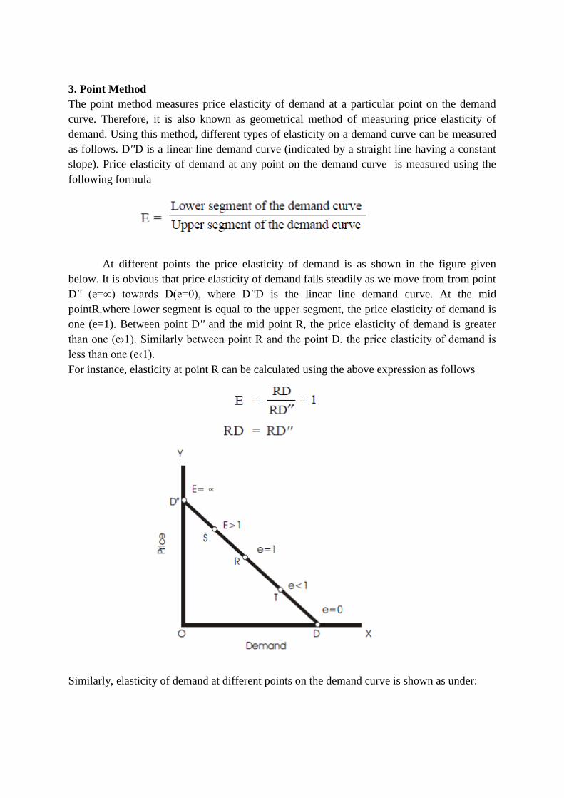
3. Point Method
The point method measures price elasticity of demand at a particular point on the demand
curve. Therefore, it is also known as geometrical method of measuring price elasticity of
demand. Using this method, different types of elasticity on a demand curve can be measured
as follows. D''D is a linear line demand curve (indicated by a straight line having a constant
slope). Price elasticity of demand at any point on the demand curve is measured using the
following formula
At different points the price elasticity of demand is as shown in the figure given
below. It is obvious that price elasticity of demand falls steadily as we move from from point
D'' (e=∞) towards D(e=0), where D''D is the linear line demand curve. At the mid
pointR,where lower segment is equal to the upper segment, the price elasticity of demand is
one (e=1). Between point D'' and the mid point R, the price elasticity of demand is greater
than one (e›1). Similarly between point R and the point D, the price elasticity of demand is
less than one (e‹1).
For instance, elasticity at point R can be calculated using the above expression as follows
Similarly, elasticity of demand at different points on the demand curve is shown as under:
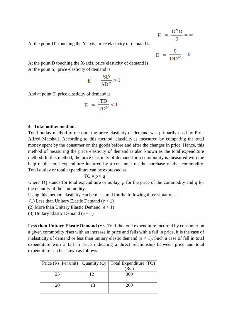
At the point D'' touching the Y-axis, price elasticity of demand is
At the point D touching the X-axis, price elasticity of demand is
At the point S, price elasticity of demand is
And at point T, price elasticity of demand is
4. Total outlay method.
Total outlay method to measure the price elasticity of demand was primarily used by Prof.
Alfred Marshall. According to this method, elasticity is measured by comparing the total
money spent by the consumer on the goods before and after the changes in price. Hence, this
method of measuring the price elasticity of demand is also known as the total expenditure
method. In this method, the price elasticity of demand for a commodity is measured with the
help of the total expenditure incurred by a consumer on the purchase of that commodity.
Total outlay or total expenditure can be expressed as
TQ = p × q
where TQ stands for total expenditure or outlay, p for the price of the commodity and q for
the quantity of the commodity.
Using this method elasticity can be measured for the following three situations:
(1) Less than Unitary Elastic Demand (e < 1)
(2) More than Unitary Elastic Demand (e > 1)
(3) Unitary Elastic Demand (e = 1)
Less than Unitary Elastic Demand (e < 1): If the total expenditure incurred by consumer on
a given commodity rises with an increase in price and falls with a fall in price, it is the case of
inelasticity of demand or less than unitary elastic demand (e < 1). Such a case of fall in total
expenditure with a fall in price indicating a direct relationship between price and total
expenditure can be shown as follows:
Price (Rs. Per unit) Quantity (Q) Total Expenditure (TQ)
(Rs.)
25 12 300
20 13 260
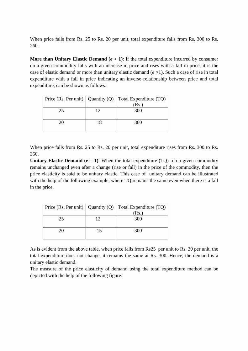
When price falls from Rs. 25 to Rs. 20 per unit, total expenditure falls from Rs. 300 to Rs.
260.
More than Unitary Elastic Demand (e > 1): If the total expenditure incurred by consumer
on a given commodity falls with an increase in price and rises with a fall in price, it is the
case of elastic demand or more than unitary elastic demand (e >1). Such a case of rise in total
expenditure with a fall in price indicating an inverse relationship between price and total
expenditure, can be shown as follows:
Price (Rs. Per unit) Quantity (Q) Total Expenditure (TQ)
(Rs.)
25 12 300
20 18 360
When price falls from Rs. 25 to Rs. 20 per unit, total expenditure rises from Rs. 300 to Rs.
360.
Unitary Elastic Demand (e = 1): When the total expenditure (TQ) on a given commodity
remains unchanged even after a change (rise or fall) in the price of the commodity, then the
price elasticity is said to be unitary elastic. This case of unitary demand can be illustrated
with the help of the following example, where TQ remains the same even when there is a fall
in the price.
Price (Rs. Per unit) Quantity (Q) Total Expenditure (TQ)
(Rs.)
25 12 300
20 15 300
As is evident from the above table, when price falls from Rs25 per unit to Rs. 20 per unit, the
total expenditure does not change, it remains the same at Rs. 300. Hence, the demand is a
unitary elastic demand.
The measure of the price elasticity of demand using the total expenditure method can be
depicted with the help of the following figure:
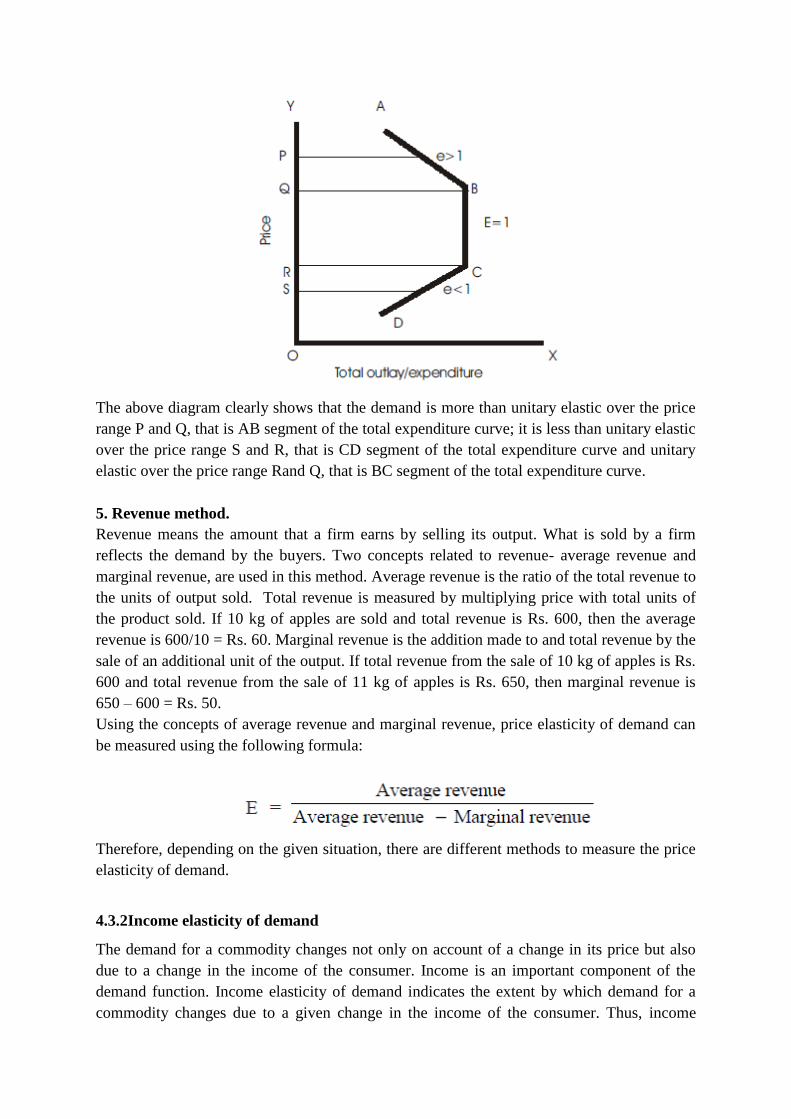
The above diagram clearly shows that the demand is more than unitary elastic over the price
range P and Q, that is AB segment of the total expenditure curve; it is less than unitary elastic
over the price range S and R, that is CD segment of the total expenditure curve and unitary
elastic over the price range Rand Q, that is BC segment of the total expenditure curve.
5. Revenue method.
Revenue means the amount that a firm earns by selling its output. What is sold by a firm
reflects the demand by the buyers. Two concepts related to revenue- average revenue and
marginal revenue, are used in this method. Average revenue is the ratio of the total revenue to
the units of output sold. Total revenue is measured by multiplying price with total units of
the product sold. If 10 kg of apples are sold and total revenue is Rs. 600, then the average
revenue is 600/10 = Rs. 60. Marginal revenue is the addition made to and total revenue by the
sale of an additional unit of the output. If total revenue from the sale of 10 kg of apples is Rs.
600 and total revenue from the sale of 11 kg of apples is Rs. 650, then marginal revenue is
650 – 600 = Rs. 50.
Using the concepts of average revenue and marginal revenue, price elasticity of demand can
be measured using the following formula:
Therefore, depending on the given situation, there are different methods to measure the price
elasticity of demand.
4.3.2Income elasticity of demand
The demand for a commodity changes not only on account of a change in its price but also
due to a change in the income of the consumer. Income is an important component of the
demand function. Income elasticity of demand indicates the extent by which demand for a
commodity changes due to a given change in the income of the consumer. Thus, income
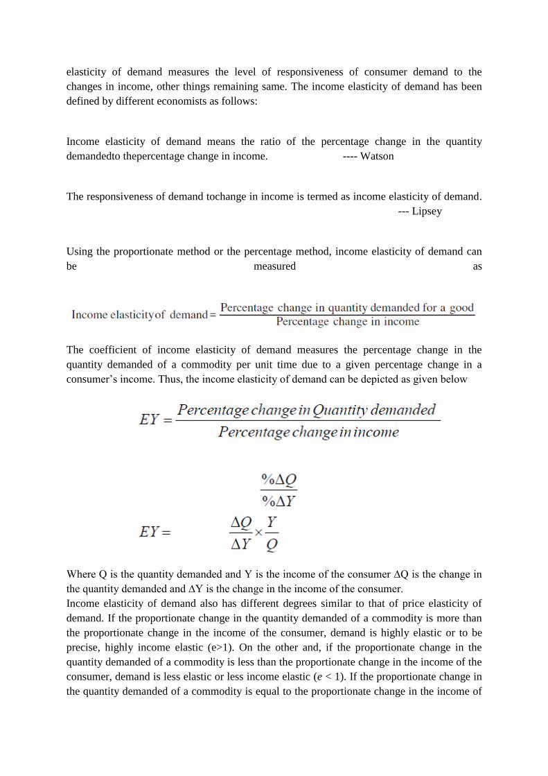
elasticity of demand measures the level of responsiveness of consumer demand to the
changes in income, other things remaining same. The income elasticity of demand has been
defined by different economists as follows:
Income elasticity of demand means the ratio of the percentage change in the quantity
demandedto thepercentage change in income. ---- Watson
The responsiveness of demand tochange in income is termed as income elasticity of demand.
--- Lipsey
Using the proportionate method or the percentage method, income elasticity of demand can
be measured as
The coefficient of income elasticity of demand measures the percentage change in the
quantity demanded of a commodity per unit time due to a given percentage change in a
consumer’s income. Thus, the income elasticity of demand can be depicted as given below
Where Q is the quantity demanded and Y is the income of the consumer ∆Q is the change in
the quantity demanded and ∆Y is the change in the income of the consumer.
Income elasticity of demand also has different degrees similar to that of price elasticity of
demand. If the proportionate change in the quantity demanded of a commodity is more than
the proportionate change in the income of the consumer, demand is highly elastic or to be
precise, highly income elastic (e>1). On the other and, if the proportionate change in the
quantity demanded of a commodity is less than the proportionate change in the income of the
consumer, demand is less elastic or less income elastic (e < 1). If the proportionate change in
the quantity demanded of a commodity is equal to the proportionate change in the income of
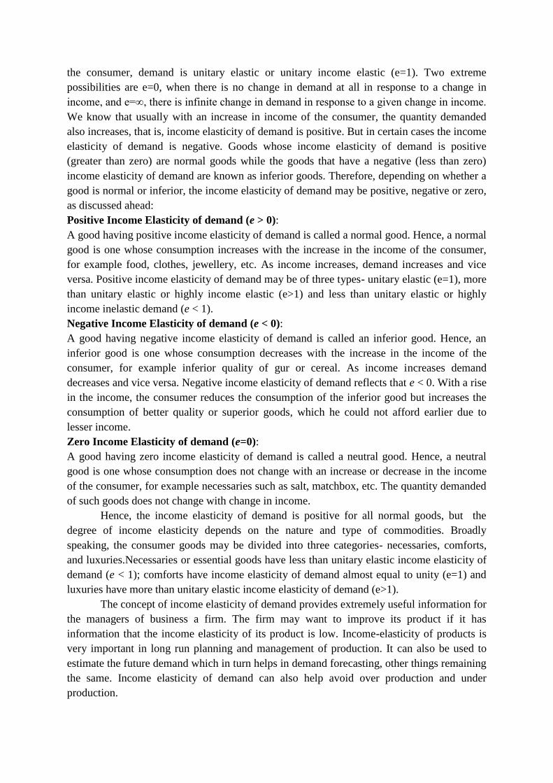
the consumer, demand is unitary elastic or unitary income elastic (e=1). Two extreme
possibilities are e=0, when there is no change in demand at all in response to a change in
income, and e=∞, there is infinite change in demand in response to a given change in income.
We know that usually with an increase in income of the consumer, the quantity demanded
also increases, that is, income elasticity of demand is positive. But in certain cases the income
elasticity of demand is negative. Goods whose income elasticity of demand is positive
(greater than zero) are normal goods while the goods that have a negative (less than zero)
income elasticity of demand are known as inferior goods. Therefore, depending on whether a
good is normal or inferior, the income elasticity of demand may be positive, negative or zero,
as discussed ahead:
Positive Income Elasticity of demand (e > 0):
A good having positive income elasticity of demand is called a normal good. Hence, a normal
good is one whose consumption increases with the increase in the income of the consumer,
for example food, clothes, jewellery, etc. As income increases, demand increases and vice
versa. Positive income elasticity of demand may be of three types- unitary elastic (e=1), more
than unitary elastic or highly income elastic (e>1) and less than unitary elastic or highly
income inelastic demand (e < 1).
Negative Income Elasticity of demand (e < 0):
A good having negative income elasticity of demand is called an inferior good. Hence, an
inferior good is one whose consumption decreases with the increase in the income of the
consumer, for example inferior quality of gur or cereal. As income increases demand
decreases and vice versa. Negative income elasticity of demand reflects that e < 0. With a rise
in the income, the consumer reduces the consumption of the inferior good but increases the
consumption of better quality or superior goods, which he could not afford earlier due to
lesser income.
Zero Income Elasticity of demand (e=0):
A good having zero income elasticity of demand is called a neutral good. Hence, a neutral
good is one whose consumption does not change with an increase or decrease in the income
of the consumer, for example necessaries such as salt, matchbox, etc. The quantity demanded
of such goods does not change with change in income.
Hence, the income elasticity of demand is positive for all normal goods, but the
degree of income elasticity depends on the nature and type of commodities. Broadly
speaking, the consumer goods may be divided into three categories- necessaries, comforts,
and luxuries.Necessaries or essential goods have less than unitary elastic income elasticity of
demand (e < 1); comforts have income elasticity of demand almost equal to unity (e=1) and
luxuries have more than unitary elastic income elasticity of demand (e>1).
The concept of income elasticity of demand provides extremely useful information for
the managers of business a firm. The firm may want to improve its product if it has
information that the income elasticity of its product is low. Income-elasticity of products is
very important in long run planning and management of production. It can also be used to
estimate the future demand which in turn helps in demand forecasting, other things remaining
the same. Income elasticity of demand can also help avoid over production and under
production.

Check Your Progress 1
1. Select the correct statement about price elasticity of demand?
A. It determines the relationship between price and revenue.
B. It determines the relationship between supply and demand.
C. It can be calculated by dividing price by revenue.
D. It is a relationship between price changes and the responsiveness of consumer demand to
these changes.
2. If the price of a good is increased by four percent and in response the quantity demanded
decreases by two percent, then the demand is
A. More elastic.
B. Less elastic.
C. Unitary elastic.
D. The quantity demanded is not affected at all.
3. Select the correct statement relating to price elasticity of demand?
A. It does not study the relationship between complements.
B. It measures the value of total national income.
C. It does not study the relationship between substitutes.
D. It measures the quantitative relationship between changes in price of a good and quantity
demanded.
4. In case of unitary elastic demand, the shape of demand curve is
A. Straight line parallel to X-axis
B. Straight line parallel to Y-axis
C. Rectangular Hyperbola
D. None of the above
5. Price elasticity of demand measures the
A. Quantitative relation between price and demand
B. Qualitative relation between price and demand
C. Psychological relation between price and demand
D. None of the above
4.3.3 Cross elasticity of demand
The demand for a commodity changes also due to a change in the prices of related goods like
substitutes or complements. The demand of tea is affected by the price of its substitute coffee
and also the demand of car is affected by the price of its complement petrol. The cross
elasticity of demand indicates the extent by which demand for a commodity changes due to a
given change in the price of its related good. Hence, the cross elasticity of demand measures
the correlation between a commodity and its substitutes or complements. Or, the
responsiveness of quantity demanded to a change in the prices of related commodities –
substitutes or complements, is called cross elasticity of demand. It is defined as follows:

The responsiveness ofdemand to a change in the prices of other commodities is called cross
elasticity of demand. --- Lipsey
The cross elasticity of demand is a measure of the responsiveness of purchases of Y to
change in the price of X. --- Liebhafsky
The cross elasticity of demand is the proportionate change in the quantity of X demanded
resulting from a given relative change in the price of the related good Y.
--- Ferguson
Using the proportionate method or the percentage method, cross elasticity of demand can be
measured as
Where QX is the quantity demanded of commodity X and PY is the price of the related
commodity Y. ∆QX is the change in the quantity demanded of X and ∆PY is the change in
the price of the related commodity Y.
The cross elasticity of demand also has the following main degrees:
Positive cross elasticity of demand: If a certain percentage increase in the price of X causes
an increase in the quantity demanded of related good Y, the cross elasticity of demand is said
to be positive (e>0). Thus, in case of positive cross elasticity of demand, the demand of Y
moves in the same direction as the price of X. Such goods are known as substitutes, those
goods which can be interchangeably used. Suppose the price of coffee rises by 5 percent and
it causes the demand of tea to rise by 3 percent, the cross elasticity of demand is positive.
Negative cross elasticity of demand: If a certain percentage increase in the price of X
causes a decrease in the quantity demanded of related good Y, the cross elasticity of demand
is said to be negative (e <0). When the goods are complements such as car and petrol, milk
and sugar, paper and pen, bread and butter, the cross elasticity of demand is negative. Thus,
in case of negative cross elasticity of demand, the demand of Y moves in the opposite
direction as the price of X. Such goods are complementary goods which are jointly demanded
to satisfy one want. Suppose the price of petrol rises by 6 percent and it causes the demand of
cars to fall by 4 percent, the cross elasticity of demand is negative.
Zero cross elasticity of demand: If a certain percentage increase in the price of X causes no
change in the quantity demanded of related good Y, the cross elasticity of demand is said to

be zero (e=0). Thus, in case of zero cross elasticity of demand, the demand of Y does not
change at all as the price of X changes. Such goods are not related to each other.
The knowledge of cross elasticity of demand of their products is important for the business
firms in order to assess the pricing and marketing strategies of their competitors. Using the
concept of cross elasticity of demand, the business managers can estimate the impact of their
price changes in relation to substitutes or complements. Hence, the information relating to
cross elasticity of demand is important for the purpose of product planning and forecasting.
4.3.5 Promotional or advertisement elasticity of demand
Advertisements and sales promotion activities are vital for any competitive business firm.
Expenditure on publicity or advertisement brings about different degrees of changes in the
sales of different products. The optimum level of expenditure on advertisement can be
determined using the concept of advertisement elasticity. The advertisement elasticity may be
defined as the degree of responsiveness of sales of a firm to the changes in expenditure on
advertisement. It can be computed by the following formula
where S shows the sales, ΔS indicates the change in sales, A is the initial advertisement cost,
and ΔA represents the increase in advertisement expenditure. The coefficient of
advertisement elasticity lies between zero and infinity (0 ≤ eA ≤ ∞). Normally the
advertisement elasticity is positive as an increase in advertisement expenditure leads to an
increase in sales. However, other factors influencing the advertisement elasticity include the
level of total sales (as total sales increase, the advertisement elasticity decreases);
advertisement by rival firms; change in price and consumer income.
In addition to the above mentioned types, another type of elasticity of demand is the
price expectation elasticity. It studies the impact of price expectations of the consumer on the
demand for a given commodity. The price expectation elasticity is defined as the expected
change in future prices of a commodity due to changes in its current prices. It can be
measured as follows:
where Pc is the current price and Pf is the future price of the given commodity.
If ex > 1 it means that future change in price will be more than the current change in price,
and vice-versa, and ifex = 1, it means that the future change in price will be exactly equal to
the change in current price. This concept of elasticity of price expectation is very useful for
business firms in working out their future pricing policies.
4.4 Factors determining elasticity of demand

The elasticity of demand for a given commodity is different for different types of goods and
different types of markets. It is affected by a number of factors as discussed below:
Nature of commodity: The commodities can be broadly classified as necessaries, comforts
and luxuries. The demand for necessaries like wheat, salt, etc. is inelastic meaning very little
or no change in the quantity demanded due to a given change in price. As regards comforts,
the demand changes in almost the same proportion as the price, that is demand is unitary
elastic. In case of luxuries like gold, diamonds, luxury cars, etc. a small change in price
causes relatively much larger change in the quantity demanded and elasticity of demand is
more than unity.
Existence of substitutes: If a commodity has different substitutes, a slight increase in its
price causes a substantial degree of substitution of other commodities in its place, and the
demand will be more elastic. However, the demand will be inelastic in case of commodities
having no substitutes.
Goods with several uses: If a commodity can be put to many different uses, its demand will
be highly elastic. For instance, in a household, milk can be used for various purposes such as
for making curd, cake, sweets, buttermilk, etc. With a fall in price, demand increases but a
little rise in its price causes the demand to fall greatly.
Possibility of postponement of use: If it is possible to postpone the consumption of a
commodity (like new clothes, new sofa, mobile, computer, etc.) then its demand will be
elastic and if the demand is urgent and cannot be postponed at all (like, electricity) the
demand will be inelastic.
Level of income – At very high and very low levels of income, the overall demand for
commodities tends to be relatively less elastic. On the other hand, in the middle income
range, the demand is relatively more elastic.
Proportion of income spent: The elasticity of demand is also influenced by the percentage
of income spent on a given commodity. If the percentage is very low, like salt, pen, pencil,
etc., then the demand will be inelastic.
Influence of habit, fashion and customs- Those commodities whose consumption is
influenced by conventions, customs or habit, will have an inelastic demand. For example
demand for cigarettes and liquor or some latest brand of clothing. In this case people do not
compromise with price and do not cut demand even if the price is high.
Complementary goods- Those goods which are jointly demanded, such as petrol, ink, etc.
have less elastic demand as their demand depends not only on their respective prices but also
on the demand of other products.
Durability of the commodity- If the commodity is a durable one like a house, the demand is
generally inelastic because consumer buys a house only after a very long period. On the other
hand, in case of perishable commodities, like milk, vegetables, the demand is relatively
elastic.
These factors enable the managers to make an assessment about the greater or lesser
elasticity of demand in case of different commodities.

Activity A
Explain the following term and factor determining each of them.
a)Price elasticity of demand
b)Income elasticity of demand
c)Cross elasticity of demand
------------------------------------------------------------------------------------------------------------
------------------------------------------------------------------------------------------------------------
------------------------------------------------------------------------------------------------------------
------------------------------------------------------------------------------------------------------------
------------------------------------------------------------------------------------------------------------
------------------------------------------------------------------------------------------------------------
------------------------------------------------------------------------------------------------------------
------------------------------------------------------------------------------------------------------------
------------------------------------------------------------------------------------------------------------
------------------------------------------------------------------------------------------------------------
------------------------------------------------------------------------------------------------------------
------------------------------------------------------------------------------------------------------------
------------------------------------------------------------------------------------------------------------
------------------------------------------------------------------------------------------------------------
------------------------------------------------------------------------------------------------------------
------------------------------------------------------------------------------------------------------------
------------------------------------------------------------------------------------------------------------
------------------------------------------------------------------------------------------------------------
------------------------------------------------------------------------------------------------------------
------------------------------------------------------------------------------------------------------------
-------------------------------------------------------------------------------------------------------
4.5 Importance of determining elasticity of demand
The concept of elasticity of demand is of much significance in various situations both from
theoretical and practical viewpoints. The role of elasticity of demand is discussed below:
Importance in taxation policies- The concept of elasticity of demand also proves helpful to
the finance minister in the formulation of taxation policies. He considers the nature of a
commodity and its elasticity of demand before levying a tax on it. If taxes are levied on goods
with more elastic demand, rise in price after tax imposition will cause a large contraction in
demand and tax revenues may fall, and vice-versa.
Price fixation under monopoly: The monopolist has to consider the elasticity of demand for
his product while fixing its price. In case his product has a less elastic demand, he fixes a
higher price and tries to appropriate a larger revenue even if he is selling a limited quantity.
Price discrimination: A monopolist sometimes follows the policy of price discrimination by
charging different prices for the same product in different markets. The basis of price
discrimination is difference of elasticity of demand in different markets. He charges a higher
price in the market where the demand is less elastic and vice-versa.
Price determination in case of joint products: There are many products which are
produced jointly like rice and bran, wheat and straw, sugar and alcohol, etc. The cost of
production in such cases cannot be ascertained separately. In such a situation, the price of the
major product is determined at a higher level if elasticity of demand is low and vice-versa;
while the price of the by-product is fixed keeping in mind the total costs and a reasonable
amount of profit.
Wage determination: If the demand for labour for a particular industry is relatively less
elastic, the employer will have to give in to the demand of trade unions to get their wages
raised. The same applies to other factors of production also with a relatively inelastic
demand.
Determination of terms of trade- Terms of trade between two countries can be calculated
by taking into account the mutual elasticities of demand for the products of each other.
Determination of the Rate of Exchange- The rate of exchange between the currencies of
different countries is determined by the elasticities of demand for the currencies of one
another. Hence, this concept is very important in the field of international trade.
Also the concept of other types of elasticities is very helpful in framing crucial economic and
financial policies.
Activity B
How is demand elasticity is useful for a manager?
-------------------------------------------------------------------------------------------------------------
-------------------------------------------------------------------------------------------------------------
-------------------------------------------------------------------------------------------------------------
------------------------------------------------------------------------------------------------------
-------------------------------------------------------------------------------------------------------------
-----------------------------------------------------------------------------------------------------------
--------------------------------------------------------------------------------------------------------
Check your progress 2
1. In case of luxuries, the elasticity of demand is……………
2. A good having ………… income elasticity of demand is called a normal good.
3. In case of ……….. cross elasticity of demand, the demand of Y does not change at all as the
price of X changes
4. If a commodity has different substitutes, its demand will be ……… elastic.
5. Complementary goods such as petrol, ink, etc. have ……. elastic demand.
4.6 Summary
Elasticity of demand indicates the degree of responsiveness of demand for a
commodity to the changes in its determinants – mainly its own price, income and price of
related goods.Thus, price elasticity of demand may be defined as the ratio of the percentage
change in quantity demanded to the percentage change in price.There are five degrees of
price elasticity of demand depending on the proportionate change in the quantity demanded
in response to a given proportionate change in the price. There are different methods to
measure price elasticity of demand. In percentage method price elasticity of demand is
measured as the ratio of the percentage change in quantity demanded to the percentage
change in price. Arc method measures the price elasticity of demand if there are relatively
larger changes in price and demand.The point method measures price elasticity of demand at
a particular point on the demand curve. In total outlay method the price elasticity of demand
is measured with the help of the total expenditure incurred by a consumer on the purchase of
that commodity. Income elasticity of demand indicates the extent by which demand for a
commodity changes due to a given change in the income of the consumer. It is positive for
normal goods and negative for inferior goods. The cross elasticity of demand refers to the
proportionate change in the quantity of X demanded resulting from a given relative change in
the price of the related good Y. It is positive for substitutes and negative for complements.
4.7 Glossary
Elasticity of demand: It indicates the degree of responsiveness of demand for a commodity
to the changes in its determinants – mainly its own price, income and price of related goods.
Price elasticity of demand: It is defined as the responsiveness of the quantity demanded of
any good X to a change in its own price.
Income elasticity of demand: It is the ratio of the percentage change in the quantity
demandedto thepercentage change in income.
Normal good: A good having positive income elasticity of demand
Inferior good: A good having negative income elasticity of demand
Advertisement elasticity: The degree of responsiveness of sales of a firm to the changes in
expenditure on advertisement.
4.8 Answer to Check Your Progress

Check Your Progress 1
1. D
2. B
3. D
4. C
5. A
Check Your Progress 2
1. more than unity
2. positive
3. zero
4. more
5. less
4.9 References
Koutsoyiannis, A : Modern Microeconomics, The Macmillan Press Ltd.,, London
Dewett, K.K., Modern Economic Theory, S. Chand Publication
.
Geetika, Managerial Economics, Tata McGraw Hills
4.10 Suggested Readings
Mithani D.M. : Managerial Economics, Himalaya Publishing House, Mumbai
Dwivedi, D.N. : Managerial Economics, Vikas Publishing House Pvt. Ltd, New Delhi
Misra&Puri : Economics for Managers, Himalaya Publishing House, Mumbai
Adhikary M. : Managerial Economics, Khosla Educational Publishers, Delhi
4.11 Terminal and Model Questions
1. What is the shape of the perfectly inelastic demand curve?
2. Discuss the degrees of price elasticity of demand with the help of diagrams.
3. Define price elasticity of demand for a commodity and state its importance.
4. When is demand said to be inelastic?
5. How would you measure price elasticity of demand by the total outlay method?
Explain.
6. What is cross elasticity of demand?
7. Discuss the factors which determine the elasticity of demand?
LESSON – 5
Demand Forecasting
Structure
5.0 Objectives
5.1 Introduction
5.2 Meaning of demand forecasting
5.3 Importance of Demand Forecasting
5.4 Scope of Demand Forecasting
5.5 Objectives of Demand Forecasting
5.6 Factors Affecting Demand Forecasting
5.7 Steps in Demand Forecasting
5.8 Check your progress 1
5.9 Demand forecasting Techniques
5.9.1Qualitative Methods
5.9.2 Quantitative Methods
5.10 Methods of Demand Forecasting in case of New Products
5.11 Check your progress 2
5.12 Summary
5.13 Glossary
5.14 Answer to Check Your Progress
5.15 References
5.16 Suggested Readings
5.17 Terminal and Model Questions
5.0 OBJECTIVES
After reading this lesson, you should be able:
To understand the meaning and scope of demand forecasting
To identify the factors that affect demand forecasting
To understand various methods of demand forecasting
5.1 Introduction
In modern business environment, every business firm seems to be operating under the
conditions of uncertainties. Generally, there is risk and uncertainty involved in every decision
making process and almost every business firm or even the government needs to keep in
mind the existing level of demand for a given commodity and estimate the existing gap
between demand and supply. This is essential because uncertainties can be minimised to quite
an extent by planning and forecasting. The ability to forecast future events plays an important
role in the success of a business firm. The business decision maker must not only estimate the
present level of demand but also forecast the future level of demand. Demand forecasting is
also one of the techniques to minimize the risk and uncertainty involved in
business.Generally forecasting refers to knowing the status or nature of an event or variable
before it occurs and it is possible only when we know the status of its respective cause or
causes. In this context, demand forecasting refers to measuring a property of demand and
representing it with a number. The concept of demand forecasting is explained in detail in the
coming sections of this lesson.
5.2 Meaning of Demand Forecasting
Demand forecasting refers to estimating the future demand on the basis of past data.
In fact forecasting of demand is the art of predicting demand for a given commodity or a
service at some future date based on present as well as past behaviour patterns of some
related events. Here it is important to note that demand forecasting is not merely a simple
guess work, rather it refers to scientific and objective estimation made on the basis of some
relevant facts and events. It may be defined as follows
Sales forecasting is an estimate of sales during a specified future period on which
estimates is tied to a proposed marketing plan which assumes a particular set of
uncontrollable and competitive forces. --- Cundif and Still
The company sales forecast is the expected level of company sales based on a chosen
marketing plan and assumed marketing environment. --- Philip Kotler
The above definitions of the concept of demand forecasting help us to know its basic
features. It is clear that the concept of demand forecasting is based on both the past data as
well as the present positions. Also such a demand forecasting may be expressed in monetary
terms or even in physical terms. Moreover, it is demand forecasting which forms the very
basis for future planning and hence, helps to obtain an estimate for the future sales and profit.
As a result, all firms strive to forecast the demand for their goods and services (as demand for
a commodity is a strategically critical variable for every business firm since its very
inception). The term demand in fact refers to a group of three closely associated factors or
variables - the need for the commodity, willingness to buy, and the capacity to buy (the
purchasing power) or
the money income. In this context, forecasting, in general, refers to assigning a value to a
variable at a future point of time, and in particular, demand forecasting refers to measuring
and assigning a specific value represented by a number to the quantity of a given commodity,
say X that will be demanded at a future point of time.
5.3 Importance of Demand Forecasting
Demand forecasting is extremely important for every business firm (whether a
supplier, manufacturer, or retailer) involved in the process of production as forecasts of future
demand help to determine the quantities that should be purchased, produced, and shipped.
The importance of the concept of demandforecasting arises from the fact that the basic
production process from raw materials to finished goods reaching the final consumer involves
a lot of time. Hence, the level of demand needs to be anticipated in advance by the producers
so that they can react immediately to changes in customer demand. The process of production
is based on future planning as the business firms deploy inventories of finished goods into
field locations to immediately cater to a customer order rather than keep the customer waiting
for a long time. A firm which is capable of fulfilling the market order in a short span of time
(that is, having a smaller order cycle) definitely gets an edge over its competitors and will
also indirectly force all competitors in the market to keep finished product inventories so as
to provide fast order cycle times.As a result, almost every business organisation involved will
have to manufacture or at least order parts on the basis of a forecast of future demand. If a
firm develops its expertise in its ability to forecast future levels of demand accurately, it gets
in a relatively commanding position to control costs through leveling its production
quantities, rationalizing its transportation, and generally planning for efficient logistics
operations.
Therefore, generally speaking, accurate demand forecasts of future demand definitely
lead to efficient operations and high levels of customer service. On the other hand, less
efficient forecasts lead to inefficient, high cost operations and/or poor levels of customer
service. Thus, the most important action towards improving the efficiency and efficacy of all
the business processes is paying more attention to and improving the quality of the demand
forecasts.
5.4 Scope of Demand Forecasting
The managerial uses of demand forecasting can be discussed separatele for the
short run and the long run. Demand forecasts for short periods are made on the assumption
that the company has a given production capacity and the time period is too short to change
the existing production capacity. In this context demand forecasting helps in the following
areas:
Production planning: It helps in determining the level of output at various periods and
avoiding under or over production.
Formulating appropriate purchase policy: It helps in better material management, of
buying inputs and control its inventory level which, in turn, cuts down cost of operation.

Appropriate pricing policy: A rational pricing policy can be formulated to suit short run and
seasonal variations in demand.
Sales forecasting: It helps the company to set realistic sales targets for each individual
salesman and for the company as a whole.
Estimating short run financial requirements: It helps the company to plan the finances
required for achieving the production and sales targets. The company will be able to raise the
required finance well in advance at reasonable rates of interest.
Framing a suitable labour policy: A proper sales and production policies help to determine
the exact number of labourers to be employed in the short run.
Further in the long run forecasting of probable demand for a product of a company is
generally for a period of 3 to 5 or 10 years. . This helps in the following areas:
Business planningwhich helps to plan expansion of the existing unit or a new production
unit. Capital budgeting of a firm is based on long run demand forecasting.
Financial planning which helps to plan long run financial requirements and investment
programs by floating shares and debentures in the open market.
5.5 Objectives of Demand Forecasting
The scope of demand forecasting can be confined to a given commodity or service
being supplied by a small business firm in a local area; or even could be extending to the
international level depending upon the area of operation of a given firm. It is also influenced
by the cost and time involved in relation to the benefit of the information acquired through
the study of demand. Besides these factors, the scope of demand forecasting is also
determined by the relevant time period, nature of the commodity, and other miscellaneous
factors like social factors, psychological factors, degree of competition, impact of risk and
uncertainty.
On these grounds, based on the time period, the objectives of demand forecasting, can
be studied under the following two categories
(i) Short Term Objectives: These are the objectives dominating in the short term and
can be listed as follows:
1. Preparing appropriate sales and production policies.
2. Ensuring a regular supply of raw materials required for the production process.
3. Reduction in the cost of purchase and avoiding unnecessary purchases.
4. Best possible or optimum utilisation of machines and other capital equipment.
5. Maintaining suitable labour force and accordingly making arrangements for skilled and
unskilled workers as per requirement.
6. Determination of a suitable price policy.
7. Determination of the financial requirements of the business firm.
8. Preparation of separate sales targets for all the different sales territories.
9. Checking the problem of under production or over production.
(ii) Long Term Objectives: These are the objectives operating in the long term and
can be listed as follows:
1. Planning of the long term production.
2. Planning appropriate plant capacity.
3. Estimating and evaluating the requirements of workers over a long period of time and
making necessary arrangements thus required.
4. Preparing an appropriate dividend policy.
5. Proper capital budgeting.
6. Plan for long term financial requirements of the business firm.
7. Forecasting the future problems of material supplies and energy crisis.
5.6 Factors Affecting Demand Forecasting
Various factors influencing the process of demand forecasting and hence, governing a good
forecast can be listed as follows.
Existing business conditions: The general economic conditions prevalent in the economy
like change in national income, price level, consumption pattern, saving and investment
patterns, employment, etc. strongly influence the demand forecasts.
Conditions within the industry: It is very essential to study the changes in the demand of
the whole industry, number of units within the industry, design and quality of product, price
policy, competition among the firms within the industry etc. as every firm is just a part of a
particular industry.
Conditions within the firm: Internal factors, specific to a given firm like quality and price of
the product, plant capacity of the firm, production policies, financial policies, advertising and
distribution policies, etc. also affect the demand forecast.
Factors affecting exports: These factors include import and export control, terms and
conditions of export, export import policy, export conditions, export finance etc.
Market behaviour: It is essential to study the market behavior also as it, too, brings about
changes in demand.
Sociological factors: Sociological factors relate to size of population, density of population,
changes in age groups, size of family, family life cycle, level of education, family income,
social awareness etc.
Psychological conditions: As the level of demand is strongly influenced by psychological
factors, so it becomes necessary to study changes in factors like changes in consumer tastes,
habits, fashions, life styles, cultural and religious preferences, etc.
All these factors influence the demand forecasts to a large extent.
5.7 Steps in Demand Forecasting
The process of demand forecasting involves the following steps:
1. Determination of the purpose of forecasts.
2. Subdividing the demand forecasting programme into small parts on the basis of
sales territories.
3. Determination of the factors affecting the sale of each product.
4. Selection of appropriate forecasting methods.
5. Analysing the activities of rival firms.
6. Collection of necessary data.
7. Preparation of preliminary sales estimates
8. Analysing the advertisement policies for promoting sales.
9. Estimation and interpretation of the results
9. Evaluation of the demand forecasts
10. Preparation of the final demand forecast on the basis of preliminary forecasts.
5.8 Check your progress 1
1. Generally there is …………….. involved in every decision making process.
2. The concept of demand forecasting is based on both the ……………. as well as ……………..
positions.
3. Demand forecasting is a technique to ……………. the risk and uncertainty involved in
business.
4. The scope of demand forecasting can be confined to a given ………… being supplied by a
small firm in local area; or could be extending to ……………..
5. Estimating the …………… of workers over a …………. and making necessary arrangements is
one of the long term objectives of demand forecasting.
6. ……………........., specific to a given firm tend to affect the demand forecast.
7. The first step in the process of demand forecasting is to determine the …………………
8. Analysing the activities of ………. firms is an important step in demand forecasting.
9. Changes in consumer tastes, habits, fashions, life styles, cultural and religious preferences, etc.
are the ………………. influencing the level of demand.
10. The most important action towards improving the efficiency of all the business processes is
paying more attention to the……………...
5.9 Demand forecasting Techniques
The problem of demand forecasting arises in many economic and managerial
decisions. Numerous forecasting procedures have been developed over the years, for many
different purposes. The performance of most firms depends on the efficient use of accurate,
disaggregated demand forecasts. An important issue for all forecasts is the time horizon for
which the forecast is made. Generally long range forecasts tend to be less accurate that short
range forecasts. The demand forecasting techniques can be broadly divided into two
categories – qualitative methods and the quantitative methods. Each of these can be further
subdivided as shown in following chart.

5.9.1 Qualitative Methods: The qualitative or subjective methods are basically designed to
know the intentions or the willingness of the buyers keeping in view the determinants of
demand. These are judgement based methods and make use of intelligent questions,
interviews or questionnaires (direct or mailed), surveys, etc. for demand forecasting.
Qualitative methods comprise of the following:
Expert Opinion Method: Expert opinion survey method gives a subjective forecast of
demand based on the opinion of experts and not the consumers. The experts make
judgement about the future quantity of demand. If this forecast quantity is reasoned
through an interactive procedure which is justified by the experts, then this method is
called as the reasoned expert survey. On the other hand, if this forecast is not reasoned
out then it is known as the simple expert opinion poll.
Survey Methods: These methods are used for short term forecasting and are based on
information collected from the potential consumers about their plans regarding future
purchases. In survey method, a few consumers are selected and their views are
collected. The sample is considered to be a true representation of the entire
population. The selection of an optimum sample size is a must for this method.
Survey methods can further be of the following types
Complete Enumeration Survey Method: Under this technique all the
consumers are taken into consideration. They may be divided in to several
groups, either on the basis of income, caste, gender, education or any other
variable or even may be divided into groups according to geographical
regions. All the units of observation are studied and data
are collected either through direct interview or by mailing questionnaires or
filling up schedules. The results would be reliable provided the sample is
representative of the population.
Sample Survey Method: Sample survey methodtakes into consideration only a
selected representative sample of the whole population of consumers. The
results so obtained are then logically extended to the whole population. Hence,
a sample of only a few consumers is selected and their opinion on the probable
demand is collected. Such a sample is considered to be a true representation of
the entire population. Sample survey method assumes that demand is based
purely on consumers' opinion and not on the demand-determinants or the end-
use. This method could further take one of the following types:
- Consumers’ interview method: The total demand for the product is
calculated by adding up all individual demands. These individual demands
are obtained on the basis of direct interviews of the consumers. However,
either all the consumers may be interviewed (then it is called complete
enumeration method) or only a selected group of consumers may be
interviewed (then it is called sample survey method). Consumers’
interview method or the consumers’ survey method, as it is also called, is a
relatively simple method because it is not based on past record. It is
suitable for industrial products and can be conveniently used for
forecasting the demand of a new product. However, it may be expensive
and time consuming and may not be for long term forecasting or when the
number of consumer is large. Also the consumers may not divulge correct
buying plans.
- Collective opinion or sales force opinion method: In this method the
salesmen try to estimate the expected sales in their respective territories.
The individual forecasts of the salesmen (on the basis of previous
experience) are then combined to estimate the total demand. This method
enjoys the advantage of first hand knowledge of salesmen who are in close
touch with the market. However, the forecasts may not be reliable if the
salespeople are not trained.
- Experts opinion method: In this method the demand is estimated on the
basis of opinions of skilled and experienced experts rather than salesmen
and consumers. Hence, it is a reliable method and forecast can be made
quickly and economically.
- Consumers’ clinic: In this method the response of the consumers to
changes in prices are observed. Some consumers are selected and are
asked to buy the commodities with certain amount of money at given
prices. Then the prices are changed and change in their purchases is
studied. Thus, the forecast of demand is based on actual consumer
behaviour. Hence, this method provides a reliable and a realistic picture
about future demand and gives useful information to help in the decision
making process. However, it may turn out to be a time consuming and
costly method. Moreover, there is no standard method for the selection of
participating consumers. This method is quite similar to the test market
method which is based on learning about the demand for a product by
actually selling the product or in other words experimenting with the sales
of the given product. The given product is simply introduced in to a test
market; and its demand is observed. This observed behavior of the
consumers is then logically extended to study the behaviour of total
demand in the markets.
End use method: This method is relies on the fact that a product generally has
several uses. So first of all a list of final consumers or the end users is
prepared and then the future demand for the product is found. Total demand
for the product is got by adding the individual demands for all the end users.
5.9.2 Quantitative Methods: The quantitativemethods or the statistical methods are
based on historical (past data) quantitative data as a guide to know the level of future
demand. These methods are generally used for long run forecasting and are based on
the application of a statistical concept to the existing quantitative data. This process
generates a forecast of the demand for the given period. These methods are usually
used for established products rather than for new products. Statistical methods may of
the following types:
Trend projection method or trend method: This method forecasts demand on
the basis of past data analysis. A firm generally does have considerable data
on sales pertaining to different time periods. These data over a period of time
yield time series which also represents the past pattern of effective demand for
a particular product. These time series can be used to project the trend in
future using one of the following methods: free hand method or the graphical
method; least squares method; semi average method; or the moving average
method.
Regression Method:- Under this method a relationship is established between
quantity demanded or sales as the dependent variable and the determinant(s)
of demand (such as price, income, price of the related goods, advertisement
cost etc.) as one or more independent variables . Again this relationship is
based on the past data and is used to project future demand by combining the
economic theory with the statistical techniques of estimation. The regression
and correlation analysis is also called the econometric model building.
The econometric methods of demand forecasting involve the estimation of
demand equation on the basis of influence of the causes (determinants) of
demand. The relationship between demand and its determinants is established
as an equation estimated from their past behavior using the least squares
method.
Simultaneous Equations Method: This method of demand forecasting is also
called the complete system approach to forecasting. It is considered to be one
of the most sophisticated econometric techniques of forecasting. It makes use

of detailed and complicated mathematical as well as statistical tools.
Simultaneous equation method is an improvement over the regression method.
Besides simultaneous equation method, a few more methods are also based
on the causal or the relational approaches to demand forecasting. The basic
assumption is that if we can find relationships between the explanatory
variables (population, income, and so forth) and sales or the quantity
demanded for the firms, then these relationships can be extended also. Data
on the explanatory variables are collected and these relationships are applied
to estimate demand. Mathematical and statistical procedures are then used to
develop and test these explanatory relationships and also to forecast demand
from them. Causal methods generally include the following:
- Econometric models, such as discrete choice models, multiple
regression or more elaborate systems involving sets of simultaneous
regression equations. These are highly advanced and complex models.
- Input-output models which are used to estimate the flow of goods
between markets and industries.
- Life cycle models which examine the various stages in a product's life
from its launch, to its maturity, and to its phasing out. Such models are
used extensively in industries such as high technology, fashion, and some
consumer goods facing short product life cycles.
Graphical Method: This method is used to estimate the trend with the help of
a graph. The past data are plotted on a graph and the trend behaviour so
indentified is extended further in the same pattern to project the demand in
the forecast period. The preparation of such a graph with time & quantity
demanded on both the axes is completely subjective, and may be different for
different persons.
Other statistical methods include
Extrapolation method: Binomial expansion method is used in the extrapolation
method to extrapolate the future demand.
Leading indicator or Barometric method: This method is an improvement over
the trend method. It makes use of an indicator variable or a variable other than
demand to indicate the behavior or direction of the movement of the demand
for the given commodity, that is, the behavior of the demand for the given
commodity is not directly observed but indirectly through a proxy variable.
Indicator variables may be of three types: (i) Leading indicators are those
variables which always lead the demand for given commodity,(ii) Lagging
indicators are those variables that always lag behind the demand variable, and
(iii) Coincidental indicators are those variables that occur along with the
demand variable at the same time along the time scale. According to this
technique the present events can be used to predict the directions of change in
the future. Certain economic and statistical indicators from the selected time
series are used to project future demand. Some of the commonly used
indicators are personal income, gross national income, prices of industrial

materials, wholesale commodity prices, industrial production, bank deposits
etc.
The qualitative or the statistical methods, in general are scientific and relatively less
expensive and relatively more reliable. However, on the flip side, these methods involve
complicated calculations and hence require more of personal skill and experience, the
absence of which may not lead to trustworthy results.
Activity A
A firm uses simple exponential smoothing with 01. to forecast demand. The forecast for the
week of January 1 was 500 units whereas the actual demand turned out to be 450 units. Calculate
the demand forecast for the week of January 8.
---------------------------------------------------------------------------------------------------------------------
---------------------------------------------------------------------------------------------------------------------
---------------------------------------------------------------------------------------------------------------------
---------------------------------------------------------------------------------------------------------------------
---------------------------------------------------------------------------------------------------------------------
---------------------------------------------------------------------------------------------------------------------
---------------------------------------------------------------------------------------------------------------------
---------------------------------------------------------------------------------------------------------------------
---------------------------------------------------------------------------------------------------------------------
---------------------------------------------------------------------------------------------------------------------
---------------------------------------------------------------------------------------------------------------------
---------------------------------------------------------------------------------------------------------------------
---------------------------------------------------------------------------------------------------------------------
---------------------------------------------------------------------------------------------------------------------
---------------------------------------------------------------------------------------------------------------------
---------------------------------------------------------------------------------------------------------------------
---------------------------------------------------------------------------------------------------------------------
---------------------------------------------------------------------------------------------------------------------
---------------------------------------------------------------------------------------------------------------------
---------------------------------------------------------------------------------------------------------------------
---------------------------------------------------------------------------------------------------------------------
---------------------------------------------------------------------------------------------------------------------
---------------------------------------------------------------------------------------------------------------------
---------------------------------------------------------------------------------------------------------------------
---------------------------------------------------------------------------------------------------------------------
--------------------------------------------------------------------------------------------------------------------
5.10 Methods of Demand Forecasting in case of New Products
The methods of demand forecasting mentioned above appear to be more effective,
reliable and trustworthy in case of projecting future demand for the existing products.
However, in case of new products the results may not be perfectly dependable. The
forecasting of demand of new product is more difficult than for an existing product as no past
data are available in this case. In these conditions consumer behavior has to be studied very
carefully and proper thorough research needs to be conducted. It is difficult for the consumer
to give appropriate response for new product as it is not yet available and the consumer has
not yet seen it. Prof. Joel Dean has suggested the following methods for forecasting demand
of new products:
1. Evolutionary approach: This method is based on the assumption that the new product is
actually just an improvement over the old product. The old product has evolved into the new
product gradually. So the demand of the old product is used to forecast the demand for the
new product. For example, the demand for LCDs and now LEDs are viewed as an
improvement over the coloured television.
2. Substitute approach: In the substitute approach, the new product is considered to be
simply a substitute of the existing one. For example, the polythene bags may be considered as
a substitute for the cloth bags.
3. Growth curve approach: The growth rate of the demand of a commodity is used in this
method instead of the quantity demanded of the commodity. Under this method the growth
rate of demand of a new product is estimated on the basis of the growth rate of demand of an
existing product. For example, suppose vim liquid wash for cleaning utensils is in use and a
new product for cleaning utensils is to be introduced in the market. In this case the average
sale of vim liquid wash for cleaning utensils will give an idea as to how the new product for
cleaning utensils will be accepted by the consumers.
4. Opinion poll approach: Under this method the demand for a new product is estimated on
the basis of information collected from the direct interviews (survey) with consumers ( either
all or a sample of consumers may be directly interviewed).
5. Sales Experience approach: Under this method, the new product is offered for sale in a
sample market, i.e. by direct mail or through multiple shop or departmental stores. The total
demand is estimated for the whole market may be estimated from sales experience of this
starter project.
6. Vicarious approach: This method consists of surveying consumers' reactions through the
specialised dealers who are in direct touch with consumers. The dealers are thus able to judge
the reaction of the consumers on the launch and acceptability of the new product and hence,
total future demand can be estimated.
All these methods particularly apply to the case of new products but are quite similar
to the techniques of demand forecasting used usually for the old products. However, these
methods for new products are not mutually exclusive. We can expect better results from these
methods by using a combination of two or more methods based on the given situation and the
nature of study.
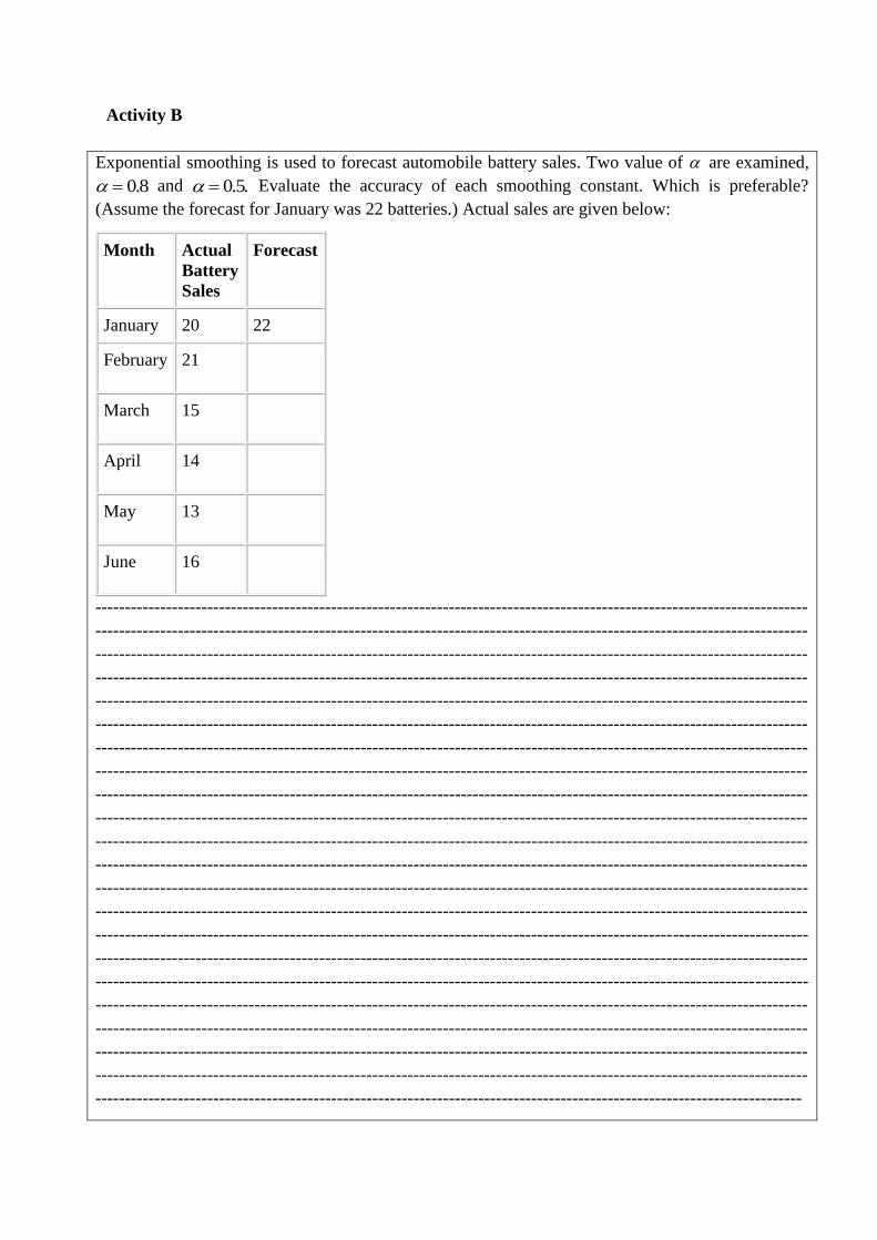
Activity B
Exponential smoothing is used to forecast automobile battery sales. Two value of are examined,
08. and 05. . Evaluate the accuracy of each smoothing constant. Which is preferable?
(Assume the forecast for January was 22 batteries.) Actual sales are given below:
Month Actual
Battery
Sales
Forecast
January 20 22
February 21
March 15
April 14
May 13
June 16
-------------------------------------------------------------------------------------------------------------------------
-------------------------------------------------------------------------------------------------------------------------
-------------------------------------------------------------------------------------------------------------------------
-------------------------------------------------------------------------------------------------------------------------
-------------------------------------------------------------------------------------------------------------------------
-------------------------------------------------------------------------------------------------------------------------
-------------------------------------------------------------------------------------------------------------------------
-------------------------------------------------------------------------------------------------------------------------
-------------------------------------------------------------------------------------------------------------------------
-------------------------------------------------------------------------------------------------------------------------
-------------------------------------------------------------------------------------------------------------------------
-------------------------------------------------------------------------------------------------------------------------
-------------------------------------------------------------------------------------------------------------------------
-------------------------------------------------------------------------------------------------------------------------
-------------------------------------------------------------------------------------------------------------------------
-------------------------------------------------------------------------------------------------------------------------
-------------------------------------------------------------------------------------------------------------------------
-------------------------------------------------------------------------------------------------------------------------
-------------------------------------------------------------------------------------------------------------------------
-------------------------------------------------------------------------------------------------------------------------
-------------------------------------------------------------------------------------------------------------------------
------------------------------------------------------------------------------------------------------------------------

5.11 Check your progress 2
State whether the following are true or false.
1. There are only two methods of demand forecasting.
2. The qualitative or subjective methods are basically same as the econometric methods.
3. Survey Methods are used for long term forecasting of demand.
4. In the complete enumeration method only a selected group of consumers may be
interviewed to collect information on demand.
5. Trend projection method is an improvement over the leading indicator or the barometric
method.
6. Under the experts opinion method the demand is estimated on the basis of opinions of
skilled and experienced experts rather than salesmen and consumers.
7. Under the growth curve approach, the growth rate of demand of a new product is
estimated on the basis of the growth rate of demand of an existing product.
8. Graphical method makes use of the binomial expansion method to forecast demand.
9. End use method is a quantitative method of forecasting of demand.
10. Vicarious approach consists of surveying consumers' reactions through the specialised
dealers who are in direct touch with consumers.
5.12 Summary
There is a lot of uncertainty associated with demand in the present dynamic uncertain
business environment. This uncertainty in demand further generates uncertainty in the
concepts of production, cost, revenue, profit etc. and it is actually possible to reduce these
uncertainties with the help of demand forecasting. Demand forecasting simply refers to
estimating or anticipating future demand on the basis of past data. Demand forecasting is
extremely important for every business firm involved in the process of production. Every
producer must know the present level of demand along with the expected increase in the
demand for his product over time. Demand forecasts are generally useful by the policy
makers and planners; for estimating financial requirements; for determination of sales target
and incentive; for facilitating regular supply of labour and raw material; for production
planning; and also for society researchers and social workers having a futuristic approach.
The objectives of demand forecasting can be studied under two categories: short term
objectives and the long term objectives. Various factors influence the process of demand
forecasting and hence, govern a good forecast. A few important ones include existing
business conditions; conditions within the industryas well as within the firm; factors affecting
exports; market behavior and sociological as well as psychological factors. There are
numerous methods of demand forecasting which may be broadly classified into quantitative
and qualitative methods. The quantitative or the objective methods make use of statistical
methods on the past historical data of the business firm to get an estimate of future demand in
the forecast period. Important quantitative methods include trend method, regression and
correlation method, simultaneous equations method and the graphical method .On the other
hand, the qualitative methods are the subjective methods or the judgementbased methods and

include expert opinion method, survey methods, end use method, to name a few. A separate
list of methods is available for new products.
5.13 Glossary
Demand forecasting: It refers to estimating the value of future demand on the basis of past
data. In fact it is the art of predicting demand for a given commodity or a service at some
future date based on present as well as past behaviour patterns of some related events.
Qualitative Methods for demand forecasting: The qualitative or subjective methods are
judgement based methods used to forecast demand keeping in mind determinants of demand.
Expert Opinion Method: This method gives a subjective forecast of demand based on the
opinion of experts and not the consumers. It may be of two types: reasoned expert survey the
simple expert opinion poll.
Survey Methods: These methods are used for short term forecasting and are based on
information collected from a few consumers or the the potential consumers about their plans
regarding future purchases.
Test market method: The given product is simply introduced in to a test market; and its
demand is observed. This observed behavior of the consumers is then logically extended to
study the behaviour of total demand in the market
Barometric Method: A method used for demand forecasting by analyzing the behavior of
demand indirectly with the help of a proxy or an indicator variable.
Coincidental indicators: Those variables that occur along with the demand variable at the
same time along the time scale and indirectly help to study the behavior of demand.
Growth curve approach: Under this method the growth rate of demand of a new product is
estimated on the basis of the growth rate of demand of an existing product.
5.14 Answer to Check Your Progress
Check Your Progress 1
1. risk and uncertainty
2. past data, present
3. minimize
4. commodity or service, international level
5. requirements, long period
6. Internal factors
7. purpose of forecasts
8. Rival
9. psychological factors
10. quality of the demand forecasts
Check Your Progress 2
1. False
2. False
3. False
4. False
5. False
6. True
7. True
8. False
9. False
10. True
5.15 References
Spencer and Siegeman’s “Managerial Economics.
Sankaran, Business Economics.
Mithani D.M., and Murthy, V.S.R., “Fundamentals of Business Economics.
Mote, V.L., Samule Paula nd G.S. Gupta, Managerial Economics , Concepts
and Cases, Tata McGraw Hill, New Delhi.
5.16 Suggested Readings
Mathur N.D., Managerial Economics, Shivam book House (P.) Limited, Jaipur Mithani, D.M.
: Managerial Economics, Himalaya Publishing House, Mumbai
5.17 Terminal and Model Questions
1. What do you mean by demand forecasting?
2. Explain the scope and importance of demand forecasting.
3. Give the factors influencing demand forecasting.
4. What are the various methods of demand forecasting?
5. Discuss the qualitative and quantitative methods of demand forecasting.
6. Explain the objectives of demand forecasting.
7. Discuss the regression method and graphic method of demand forecasting.
8. Explain the trend method of demand forecasting.

LESSON – 6
Theory of Production
6.0 Objectives
6.1 Introduction
6.2 Production
6.3 Production Function
6.3.1 Short run production function
6.3.2 Law of Variable Proportions
6.3.3 Long run production function
6.3.4 Check Your Progress 1
6.3.5 Isoquants
6.3.6 Properties of Isoquants
6.3.7 Isoquant Map
6.3.8 Isocost Lines
6.3.9 Producer’s Equilibrium
6.3.10 Expansion Path
6.3.11 Returns to Scale
6.4 Check Your Progress 2
6.5 Summary
6.6 Glossary
6.7 Answer to Check Your Progress
6.8 References
6.9 Suggested Readings
6.10 Terminal and Model Questions
6.0 OBJECTIVES
After reading this lesson, you should be able:
To understand the basic concept of production and production function
To bring out the difference between short run production function and long run
production function
To comprehend the law of variable proportions and returns to scale
To know the concept of isoquants in detail
6.1 Introduction
In simple words, production is a process resulting in the creation of goods and
services. However, in economics production refers to the transformation of inputs or the
factors of production, into outputs. Inputs refer to the raw materials or other productive
resources used to produce final product or the output. A producer has to combine the different
inputs such as land, labour, capital and enterprise to turn out the flow of goods and services.
The theory of production is concerned with the ways in which the factor inputs are combined
to secure the maximum return at the least possible cost. The basic knowledge of the theory of
production is very significant for the managers of the business firms.
6.2 Production
The theory of production is defined as follows:
The theory of production consists of how the producer, given the state of technology,
combines various inputs to produce a definite amount of output in an economically efficient
manner. ---- Ferguson
Therefore, production is the process of converting inputs into output. Production of
any commodity or service requires certain quantities of different factors of production, when
the technique of production is given. All inputs used in the process of production are
collectively known as the factors of production. Broadly the factors of production may be
classified as land, labour, capital and organization. Land is a free gift of nature and also
includes all the available natural resources; its remuneration is called rent. Labour indicates
all the physical and mental efforts made by human beings in the process of production; the
reward for labour is called wages. As regards capital, it refers to capital goods, plant
machinery, etc. Apart from the wealth used in the process of production, capital also includes
the human capital, that is, knowledge and skills attained by individuals through specialized
trainings. The capital gets its reward as interest. Finally organization or enterprise bears the
ability to undertake the risk and uncertainty involved in the process of production; its
remuneration is in the form of profit.
On the basis of their variability, these factor inputs can be categorized into two types
– fixed inputs and variable inputs. This classification is based on the two time frames relevant
for the process of production – short run and long run. Short run or the short period is a time
period in which some factors of production remain fixed while others can be varied. On the
other hand, long run or long period refers to a sufficiently large time period in which all the
factors of production can be changed as per the requirement. Hence, the fixed inputs and
variable inputs can be explained on the basis of the distinction between short run and long
run. Thus, fixed inputs are the those which cannot be altered in the short run, for instance,
land, plant and machinery, technique of production, etc. On the other hand, variable inputs
refer to those inputs which may be altered in the short run, for instance, labour, raw material,
etc. Of course in the long run all inputs tend to become variable.
Almost any business decision can be analyzed with managerial economics techniques,
but it is most commonly applied to production analysis - microeconomic techniques are used
to analyze production efficiency, optimum factor allocation costs, and to estimate the firm's
cost function.
6.3 Production Function
Production function expresses the technical relationship between physical inputs and physical
output. It is the relationship between the quantities of inputs and the quantities produced. A
production function may be defined as:
The production function is the name given to the relationship between the rates of input of
productive services and the rate of output of product. It is the economist’s summary of
technological knowledge. ---Stigler
The production function is a purely technical relation which connects factor inputs and
output. --- Koutsoyiannis
The term production function refers to the physical relation between a firm’s inputs of
resources and its output of goods and services per unit of time, leaving prices aside.
--- Leftwitch
Therefore, the production function is a mathematical function showing the output that can be
produced per unit of time for alternative sets of inputs, using the best possible available
technology. A production function for a given commodity can be expressed as follows:
Q = f (a, b, c, d…)
where Q represents the quantity of output produced,
a, b, c, d…. stand for the productive resources or factor inputs, such as land, labour, capital,
raw materials, time, and technology, used in the production process. Thus, a production
function indicates the maximum quantity of output which may be produced from the given
inputs with the given technology.
This leads us to two important types of production functions studied in the theory of
production: short run production function and the long run production function.
6.3.1 Short run production function
Short run or the short period is a time period in which some factors of production
remain fixed while others can be varied. Hence, a production function in which the quantities

of some inputs are kept fixed and the quantity of at least one (or may be a few) input is
variable is called the short run production function. The time period is very small and not
sufficient enough to bring about changes in the factor inputs like plants, equipment,
machinery or the technique of production. Such a production function is also referred to as a
production function with one variable input or even a single variable production function. For
instance, if labour is the only variable factor of production (all other factors remain fixed) in a
given firm producing some commodity, then its production function can be written as:
Q = f (L)
Where Q stands for the level of output and L shows the number of labourers hired by the firm
in the process of production.
Short run production function or a production function with one variable input is governed by
the law of variable proportions. It is also called variable proportion production function as it
indicates a short run production function in which the output of a given commodity is
produced with a single variable input.
6.3.2 Law of Variable Proportions
A short run production function involves the use of some fixed factors along with some
variable factors. If it is supposed that the input of one factor is varied and the inputs of other
factors remain constant, then the output will change in the variable proportions. The
disproportionate changes in the output, when one factor is increased and other inputs remain
constant, indicate that the production is governed by the law of variable proportions. The law
of variable proportions occupies an important place in the economic theory. It examines the
short run production function, that is, a production function with one factor variable, keeping
the quantities of other factors fixed. Eminent economists have defined this law of variable
proportions as follows:
As equal increments of one input are added; the inputs of other productive services being
held constant, beyond a certain point the resulting increments of product will decrease, i.e.,
the marginal products will diminish. --- Stigler
If the input of one resource is increased by equal increments per unit of time while the
inputs of other resources are held constant, total output will increase, but beyond some point,
the resulting output will become smaller and smaller.
--- Leftwitch
The law states that an increase in some inputs relative to other fixed inputs will, in a given
state of technology, cause total output to increase : but after a point, the extra output resulting
from the same additions of extra inputs is likely to become less and less.
---- Samuelson
Thus, according to the law of variable proportions, an increase in the quantities of a variable
factor to a fixed factor results in an increase in the output to a point beyond which it
eventually declines.
Suppose that a farmer employs 15 hectares of land and 4 machines in the production of rice.
These will be the fixed inputs and labour alone is the variable input which is increased one by
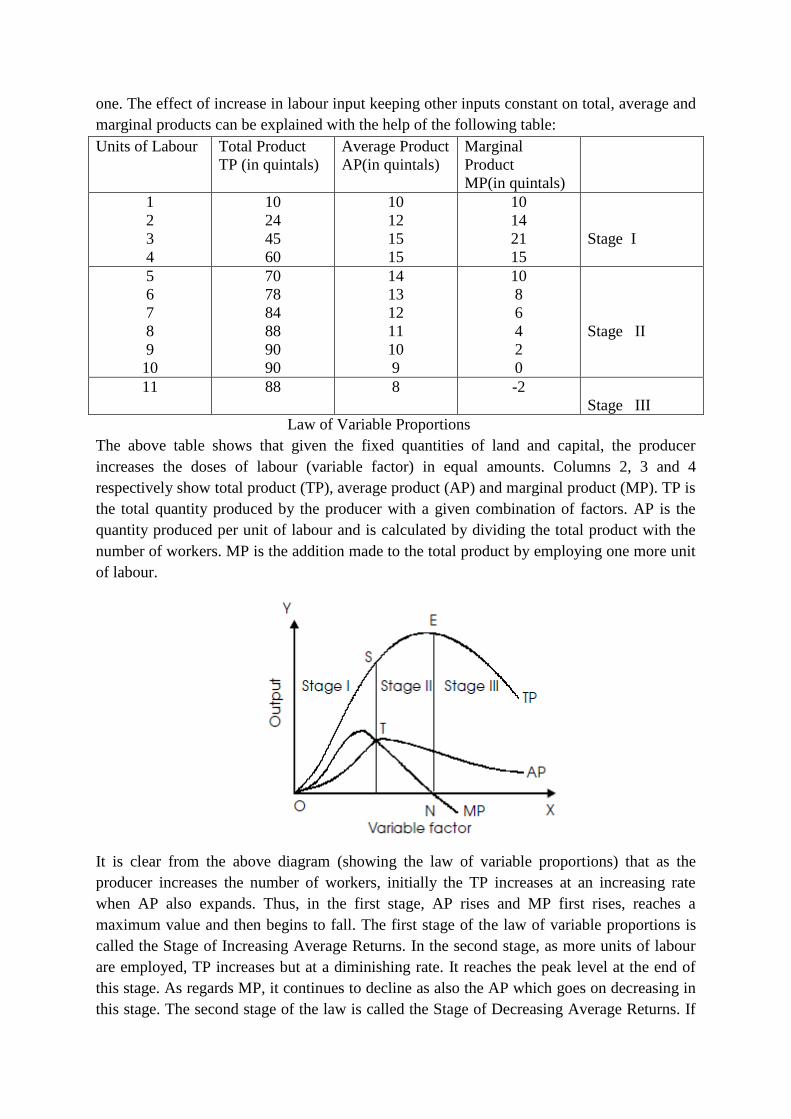
one. The effect of increase in labour input keeping other inputs constant on total, average and
marginal products can be explained with the help of the following table:
Units of Labour
Total Product
TP (in quintals)
Average Product
AP(in quintals)
Marginal
Product
MP(in quintals)
1
2
3
4
10
24
45
60
10
12
15
15
10
14
21
15
Stage I
5
6
7
8
9
10
70
78
84
88
90
90
14
13
12
11
10
9
10
8
6
4
2
0
Stage II
11 88 8 -2
Stage III
Law of Variable Proportions
The above table shows that given the fixed quantities of land and capital, the producer
increases the doses of labour (variable factor) in equal amounts. Columns 2, 3 and 4
respectively show total product (TP), average product (AP) and marginal product (MP). TP is
the total quantity produced by the producer with a given combination of factors. AP is the
quantity produced per unit of labour and is calculated by dividing the total product with the
number of workers. MP is the addition made to the total product by employing one more unit
of labour.
It is clear from the above diagram (showing the law of variable proportions) that as the
producer increases the number of workers, initially the TP increases at an increasing rate
when AP also expands. Thus, in the first stage, AP rises and MP first rises, reaches a
maximum value and then begins to fall. The first stage of the law of variable proportions is
called the Stage of Increasing Average Returns. In the second stage, as more units of labour
are employed, TP increases but at a diminishing rate. It reaches the peak level at the end of
this stage. As regards MP, it continues to decline as also the AP which goes on decreasing in
this stage. The second stage of the law is called the Stage of Decreasing Average Returns. If
the number of workers is still increased beyond this stage, there is a fall in TP. TP continues
to fall along with AP. However, a striking feature about MP is that in the third stage it
becomes negative. So the third stage of the law is called the Stage of Negative Marginal
Returns. The three stages of the law of variable proportions are also known as Increasing
Returns to the Variable Factor, Decreasing Returns to the Variable Factor and Negative
Returns to the Variable Factor respectively because only the variable factor changes and the
returns obtained are actually the returns to the variable factor only.
The main causes of the operation of this law are:
- Indivisibility of the fixed factors: Initially the ratio of the fixed factors to the
variable factors is high as the fixed factors are indivisible. As more units of the
variable factor, labour, are employed, there is better use of indivisible factors.
Thus, AP rises in the first stage. After a point, when the indivisible factor is fully
utilized, the increase in the ratio of variable factors to the fixed factors cause a fall
in AP and MP.
- Scarcity of variable factor: Initially a producer employs the most efficient and
skilled workers who have a higher productivity. As a result the first stage of the
law comes into operation. After a point, the most efficient and skilled workers
become scarce and relatively less efficient and skilled workers have to be
employed which leads to a fall in AP and MP, and TP increases at a diminishing
rate. Ultimately even TP starts falling and MP becomes negative.
- Limited extent of substitution: When only labour units are increased keeping other
factors constant, there is substitution of labour in place of other factors. Upto a
point, the substitution of labour improves the efficiency of the factor combination
leading to more than proportionate increase in total product. But this substitution
is possible only upto a limited extent. After a point, the increased use of the
variable factor makes the factor combination faulty which causes eventual fall in
TP.
- Optimum productive capacity: Each factor of production has a given maximum
productive capacity. If different factor inputs are combined in such a way that
productive capacity of each factor increases, the TP increases more than
proportionately. However, if a factor input is stretched beyond its optimum
productive capacity, the factor combination becomes faulty leading to the second
and third stages of the law of variable proportions.
It is important to note that a typical business firm actually operates only in the second
stage of the law variable proportions. A business firm does not operate in the first stage as in
this stage the increase in the input of the variable factor causes more than proportionate
increase in TP and a consistent rise in AP. Hence, the average cost goes on decreasing and
the producer will continue to expand output by employing more units of the variable factor.
Moreover, the firm does not operate even in the third stage as employing more units of the
variable factor leads to a fall in TP and a negative MP. Hence, a business firm actually
operates only in the second stage of the law variable proportions.
Therefore, it can be said that the law variable proportions is a universal law of
production as production in every sector passes through the different phases of this law.
6.3.3 Long run production function
Long run or the long period is a time period in which all the factors of production can be
varied. Hence, a production function in which the quantities of all inputs are variable is called
the long run production function. The time period is very large and sufficient enough to bring
about changes in those factor inputs also which were fixed in the short period, like plants,
equipment, machinery or the technique of production.
So in the long run all inputs become variable and production may be increased by changing
one or more of the inputs. The firm can make changes in its plant size or the scale of
production.
A long run production function may be represented as follows:
Q = f (L, K)
Where, Q shows the level of output, L represents units of labour and K indicates the units of
capital. Thus, output is a function of both labour and capital which are variable in the long
run. Such a production function is also referred to as a production function with two variable
inputs or even a two variable production function. Given the level of technology, a
combination of the quantities of labour and capital produces a specified level of output. Thus,
a long run production function explains the behavior of output, when all the factor inputs
undergo changes in the same proportion. The law of returns to scale (the technological
relationship between changing scale of inputs and output) helps to describe a long run
production function. Usually in the long run we consider a case where the firm has only two
factors of production, labor and capital, both of which are variable. These two factors inputs
are substitutable with each other to some extent. The isoquants or equal product curves
describe the production function of this type.
Activity A
What do you understand by “cost efficiency”? Draw a long run cost diagram and explain.
--------------------------------------------------------------------------------------------------------------
--------------------------------------------------------------------------------------------------------------
--------------------------------------------------------------------------------------------------------------
--------------------------------------------------------------------------------------------------------------
--------------------------------------------------------------------------------------------------------------
--------------------------------------------------------------------------------------------------------
--------------------------------------------------------------------------------------------------------
--------------------------------------------------------------------------------------------------------
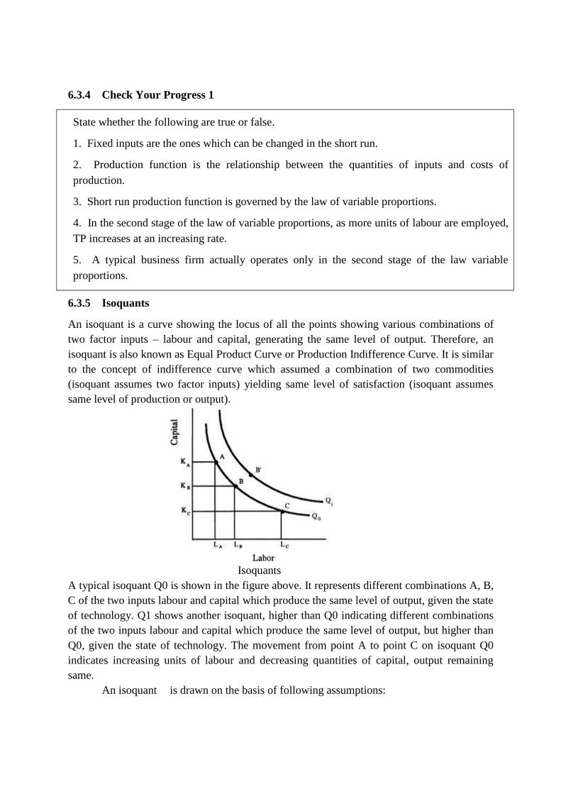
6.3.4 Check Your Progress 1
State whether the following are true or false.
1. Fixed inputs are the ones which can be changed in the short run.
2. Production function is the relationship between the quantities of inputs and costs of
production.
3. Short run production function is governed by the law of variable proportions.
4. In the second stage of the law of variable proportions, as more units of labour are employed,
TP increases at an increasing rate.
5. A typical business firm actually operates only in the second stage of the law variable
proportions.
6.3.5 Isoquants
An isoquant is a curve showing the locus of all the points showing various combinations of
two factor inputs – labour and capital, generating the same level of output. Therefore, an
isoquant is also known as Equal Product Curve or Production Indifference Curve. It is similar
to the concept of indifference curve which assumed a combination of two commodities
(isoquant assumes two factor inputs) yielding same level of satisfaction (isoquant assumes
same level of production or output).
Isoquants
A typical isoquant Q0 is shown in the figure above. It represents different combinations A, B,
C of the two inputs labour and capital which produce the same level of output, given the state
of technology. Q1 shows another isoquant, higher than Q0 indicating different combinations
of the two inputs labour and capital which produce the same level of output, but higher than
Q0, given the state of technology. The movement from point A to point C on isoquant Q0
indicates increasing units of labour and decreasing quantities of capital, output remaining
same.
An isoquant is drawn on the basis of following assumptions:
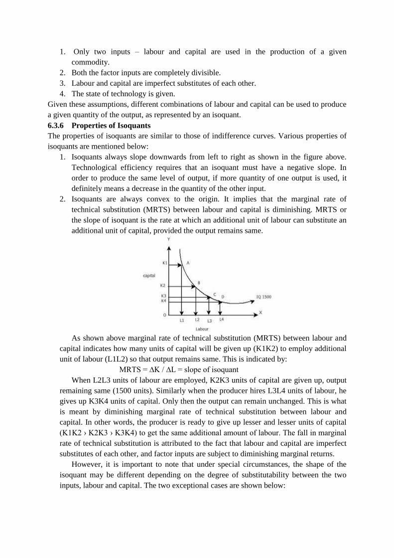
1. Only two inputs – labour and capital are used in the production of a given
commodity.
2. Both the factor inputs are completely divisible.
3. Labour and capital are imperfect substitutes of each other.
4. The state of technology is given.
Given these assumptions, different combinations of labour and capital can be used to produce
a given quantity of the output, as represented by an isoquant.
6.3.6 Properties of Isoquants
The properties of isoquants are similar to those of indifference curves. Various properties of
isoquants are mentioned below:
1. Isoquants always slope downwards from left to right as shown in the figure above.
Technological efficiency requires that an isoquant must have a negative slope. In
order to produce the same level of output, if more quantity of one output is used, it
definitely means a decrease in the quantity of the other input.
2. Isoquants are always convex to the origin. It implies that the marginal rate of
technical substitution (MRTS) between labour and capital is diminishing. MRTS or
the slope of isoquant is the rate at which an additional unit of labour can substitute an
additional unit of capital, provided the output remains same.
As shown above marginal rate of technical substitution (MRTS) between labour and
capital indicates how many units of capital will be given up (K1K2) to employ additional
unit of labour (L1L2) so that output remains same. This is indicated by:
MRTS = ∆K / ∆L = slope of isoquant
When L2L3 units of labour are employed, K2K3 units of capital are given up, output
remaining same (1500 units). Similarly when the producer hires L3L4 units of labour, he
gives up K3K4 units of capital. Only then the output can remain unchanged. This is what
is meant by diminishing marginal rate of technical substitution between labour and
capital. In other words, the producer is ready to give up lesser and lesser units of capital
(K1K2 › K2K3 › K3K4) to get the same additional amount of labour. The fall in marginal
rate of technical substitution is attributed to the fact that labour and capital are imperfect
substitutes of each other, and factor inputs are subject to diminishing marginal returns.
However, it is important to note that under special circumstances, the shape of the
isoquant may be different depending on the degree of substitutability between the two
inputs, labour and capital. The two exceptional cases are shown below:

(a) Linear Isoquant
(b) Right-angled Isoquant
The figure in part (a) shows a linear isoquant. A linear isoquant is formed when the two
inputs are perfect substitutes of each other. In this case, the marginal rate of technical
substitution (MRTS) between labour and capital remains constant, hence, the isoquant is a
straight line.
The other exception to a normal isoquant is shown in part (b) where the isoquant is right
angled or L-shaped. In this case there is zero substitutability between labour and capital. The
two inputs are perfect complements of each other and cannot be used as substitutes at all.
Both the inputs are used in a fixed proportion and the output can be increased only by
increasing both the inputs proportionately.
3. Higher levels of isoquants indicate higher levels of output. A higher isoquant
represents a factor combination with larger quantities of factor inputs. Larger
quantities of factor inputs will definitely generate higher levels of output. This can be
shown with the help of the following figure:
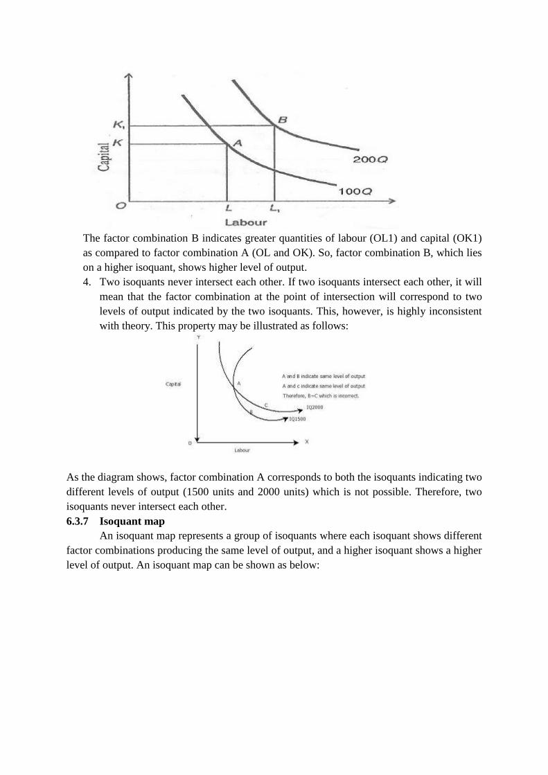
The factor combination B indicates greater quantities of labour (OL1) and capital (OK1)
as compared to factor combination A (OL and OK). So, factor combination B, which lies
on a higher isoquant, shows higher level of output.
4. Two isoquants never intersect each other. If two isoquants intersect each other, it will
mean that the factor combination at the point of intersection will correspond to two
levels of output indicated by the two isoquants. This, however, is highly inconsistent
with theory. This property may be illustrated as follows:
As the diagram shows, factor combination A corresponds to both the isoquants indicating two
different levels of output (1500 units and 2000 units) which is not possible. Therefore, two
isoquants never intersect each other.
6.3.7 Isoquant map
An isoquant map represents a group of isoquants where each isoquant shows different
factor combinations producing the same level of output, and a higher isoquant shows a higher
level of output. An isoquant map can be shown as below:
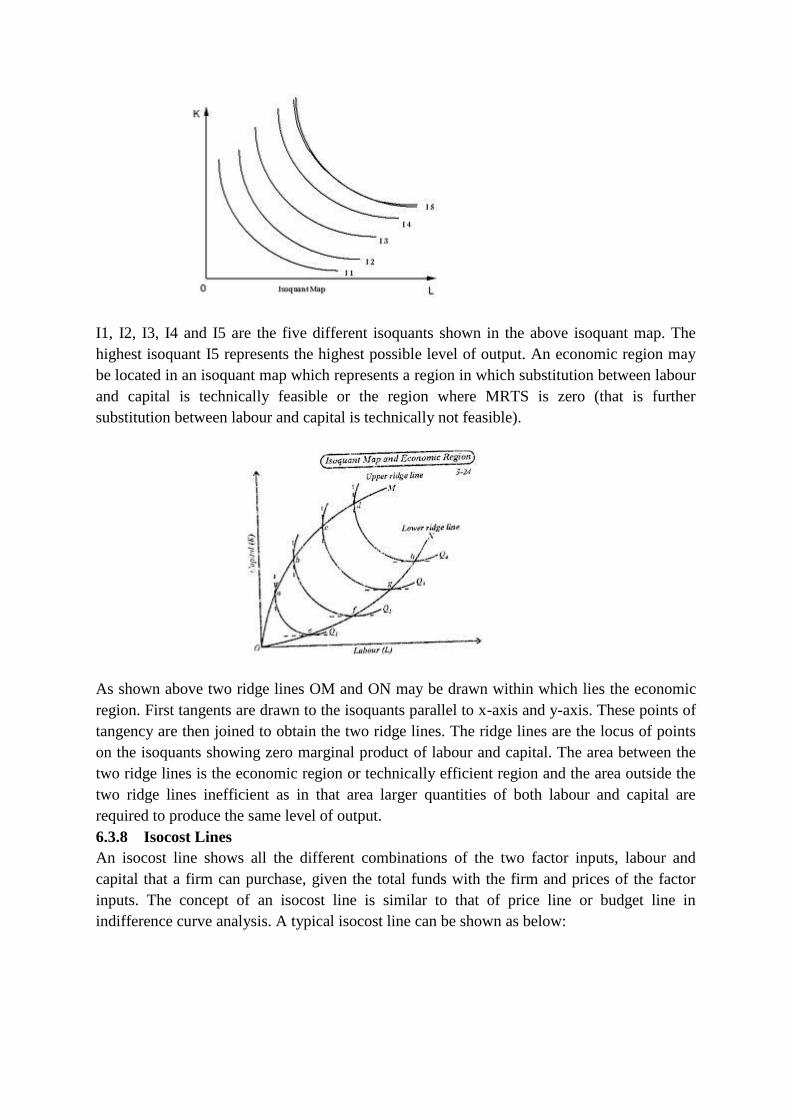
I1, I2, I3, I4 and I5 are the five different isoquants shown in the above isoquant map. The
highest isoquant I5 represents the highest possible level of output. An economic region may
be located in an isoquant map which represents a region in which substitution between labour
and capital is technically feasible or the region where MRTS is zero (that is further
substitution between labour and capital is technically not feasible).
As shown above two ridge lines OM and ON may be drawn within which lies the economic
region. First tangents are drawn to the isoquants parallel to x-axis and y-axis. These points of
tangency are then joined to obtain the two ridge lines. The ridge lines are the locus of points
on the isoquants showing zero marginal product of labour and capital. The area between the
two ridge lines is the economic region or technically efficient region and the area outside the
two ridge lines inefficient as in that area larger quantities of both labour and capital are
required to produce the same level of output.
6.3.8 Isocost Lines
An isocost line shows all the different combinations of the two factor inputs, labour and
capital that a firm can purchase, given the total funds with the firm and prices of the factor
inputs. The concept of an isocost line is similar to that of price line or budget line in
indifference curve analysis. A typical isocost line can be shown as below:
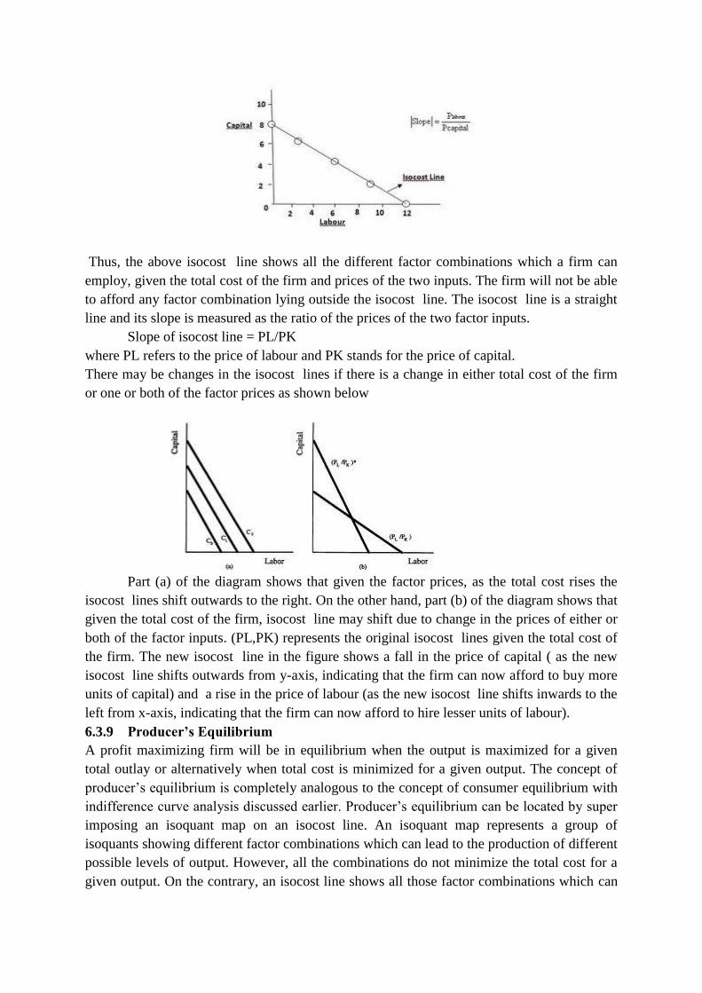
Thus, the above isocost line shows all the different factor combinations which a firm can
employ, given the total cost of the firm and prices of the two inputs. The firm will not be able
to afford any factor combination lying outside the isocost line. The isocost line is a straight
line and its slope is measured as the ratio of the prices of the two factor inputs.
Slope of isocost line = PL/PK
where PL refers to the price of labour and PK stands for the price of capital.
There may be changes in the isocost lines if there is a change in either total cost of the firm
or one or both of the factor prices as shown below
Part (a) of the diagram shows that given the factor prices, as the total cost rises the
isocost lines shift outwards to the right. On the other hand, part (b) of the diagram shows that
given the total cost of the firm, isocost line may shift due to change in the prices of either or
both of the factor inputs. (PL,PK) represents the original isocost lines given the total cost of
the firm. The new isocost line in the figure shows a fall in the price of capital ( as the new
isocost line shifts outwards from y-axis, indicating that the firm can now afford to buy more
units of capital) and a rise in the price of labour (as the new isocost line shifts inwards to the
left from x-axis, indicating that the firm can now afford to hire lesser units of labour).
6.3.9 Producer’s Equilibrium
A profit maximizing firm will be in equilibrium when the output is maximized for a given
total outlay or alternatively when total cost is minimized for a given output. The concept of
producer’s equilibrium is completely analogous to the concept of consumer equilibrium with
indifference curve analysis discussed earlier. Producer’s equilibrium can be located by super
imposing an isoquant map on an isocost line. An isoquant map represents a group of
isoquants showing different factor combinations which can lead to the production of different
possible levels of output. However, all the combinations do not minimize the total cost for a
given output. On the contrary, an isocost line shows all those factor combinations which can
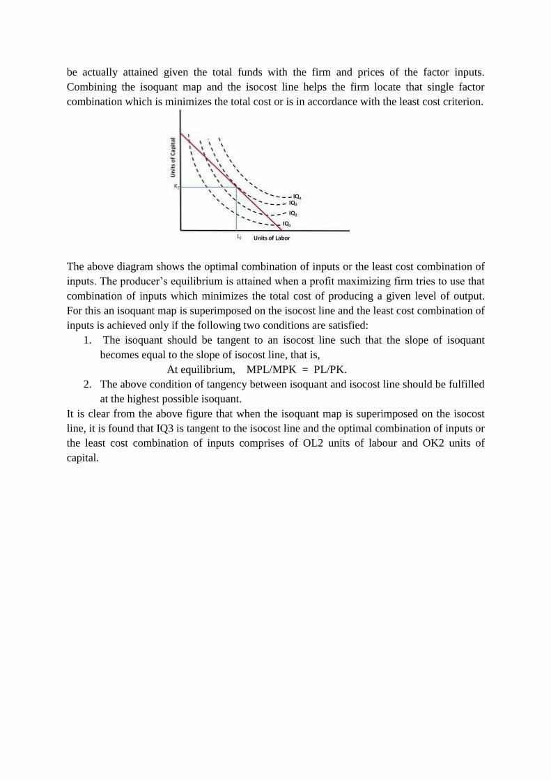
be actually attained given the total funds with the firm and prices of the factor inputs.
Combining the isoquant map and the isocost line helps the firm locate that single factor
combination which is minimizes the total cost or is in accordance with the least cost criterion.
The above diagram shows the optimal combination of inputs or the least cost combination of
inputs. The producer’s equilibrium is attained when a profit maximizing firm tries to use that
combination of inputs which minimizes the total cost of producing a given level of output.
For this an isoquant map is superimposed on the isocost line and the least cost combination of
inputs is achieved only if the following two conditions are satisfied:
1. The isoquant should be tangent to an isocost line such that the slope of isoquant
becomes equal to the slope of isocost line, that is,
At equilibrium, MPL/MPK = PL/PK.
2. The above condition of tangency between isoquant and isocost line should be fulfilled
at the highest possible isoquant.
It is clear from the above figure that when the isoquant map is superimposed on the isocost
line, it is found that IQ3 is tangent to the isocost line and the optimal combination of inputs or
the least cost combination of inputs comprises of OL2 units of labour and OK2 units of
capital.
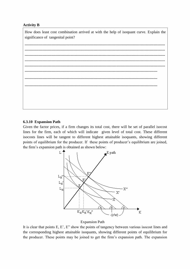
Activity B
How does least cost combination arrived at with the help of isoquant curve. Explain the
significance of tangenital point?
--------------------------------------------------------------------------------------------------------------
--------------------------------------------------------------------------------------------------------------
--------------------------------------------------------------------------------------------------------------
--------------------------------------------------------------------------------------------------------------
--------------------------------------------------------------------------------------------------------------
--------------------------------------------------------------------------------------------------------
--------------------------------------------------------------------------------------------------------
--------------------------------------------------------------------------------------------------------
6.3.10 Expansion Path
Given the factor prices, if a firm changes its total cost, there will be set of parallel isocost
lines for the firm, each of which will indicate given level of total cost. These different
isocosts lines will be tangent to different highest attainable isoquants, showing different
points of equilibrium for the producer. If these points of producer’s equilibrium are joined,
the firm’s expansion path is obtained as shown below:
Expansion Path
It is clear that points E, E’, E” show the points of tangency between various isocost lines and
the corresponding highest attainable isoquants, showing different points of equilibrium for
the producer. These points may be joined to get the firm’s expansion path. The expansion

path may be linear or non linear depending on the ratio of the factor prices of the two inputs –
labour and capital.
6.3.11 Returns to Scale
In the case of short run production function, some factors are assumed to be fixed while
others are variable. However, in the long run all inputs become variable and production may
be increased by changing all the factors of production. Thus, output is a function of both
labour and capital which are variable in the long run. Such a production function is also
referred to as a production function with two variable inputs. In the long run production
function, the returns are varied in the same proportion. For instance, suppose a farmer
employs 20 hectares of land, 8 workers and 4 machines to attain a certain level of output. If
the factor inputs are doubled, say, how will the output increase? This question is answered
by the law of returns to scale. Returns to Scalehas been defined as follows:
The term returns to scale refers to the changes in output as all factors change by the same
proportion. --- Koutsoyiannis
Returns to Scale relates to the behavior of total output as all inputs are varied and is a long
run concept. --- Liebhafasky
The long run production function or returns to scale may be stated as
Q = f (L, K)
Where Q is output, L is labour and K is capital. If the inputs L and K both increase in the
same proportion, say, a, the output may increase to Q1
Q1 = f (aL, aK)
If a is equal to ten percent, say, there can be three different possibilities regarding the change
in the output. The output may increase by more than ten percent (increasing returns to scale),
less than ten percent (decreasing returns to scale), or by exactly ten percent (constant returns
to scale).
Increasing returns to scale : Given the state of technology, when all factors are increased by
a given proportion, the output in response increases by a greater proportion. For example, if
labour and capital are increased by say, 15%, then the increase in output by more than 15% is
known as increasing returns to scale. This may happen due to economies of scale like greater
division of labour and specialization, increase in labor productivity and the like which are
enjoyed by a firm on increasing the scale of production. It can be shown as below:
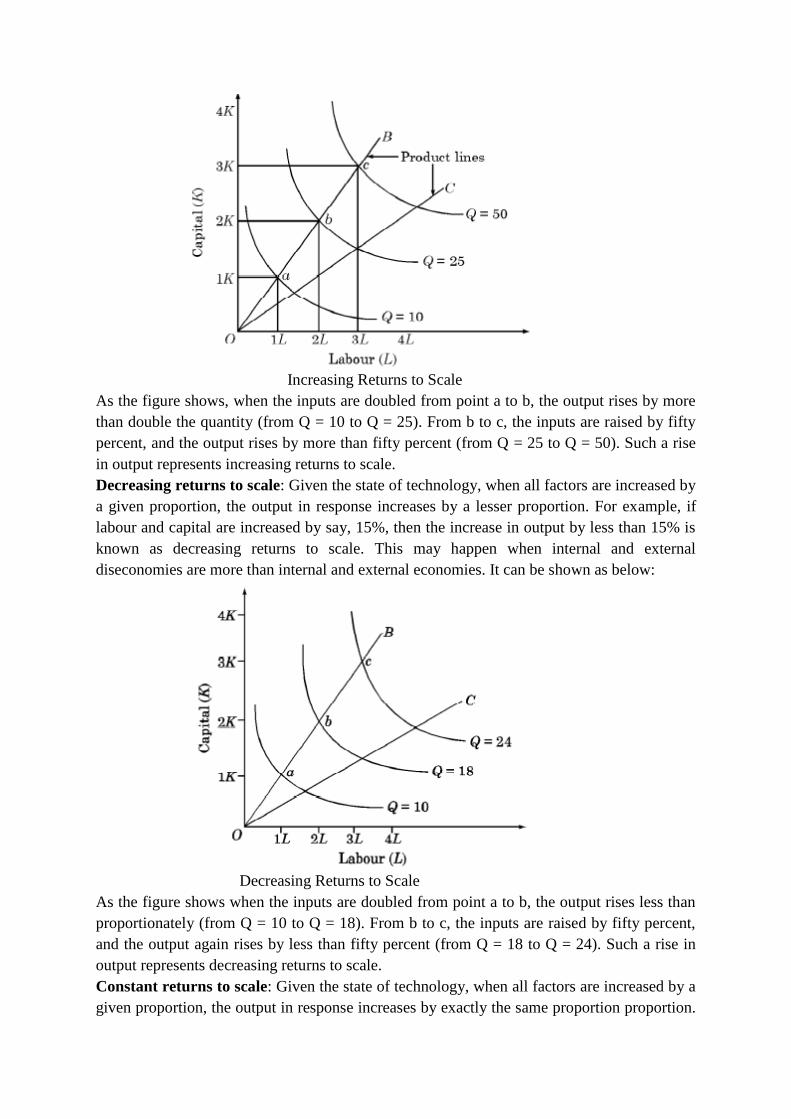
Increasing Returns to Scale
As the figure shows, when the inputs are doubled from point a to b, the output rises by more
than double the quantity (from Q = 10 to Q = 25). From b to c, the inputs are raised by fifty
percent, and the output rises by more than fifty percent (from Q = 25 to Q = 50). Such a rise
in output represents increasing returns to scale.
Decreasing returns to scale: Given the state of technology, when all factors are increased by
a given proportion, the output in response increases by a lesser proportion. For example, if
labour and capital are increased by say, 15%, then the increase in output by less than 15% is
known as decreasing returns to scale. This may happen when internal and external
diseconomies are more than internal and external economies. It can be shown as below:
Decreasing Returns to Scale
As the figure shows when the inputs are doubled from point a to b, the output rises less than
proportionately (from Q = 10 to Q = 18). From b to c, the inputs are raised by fifty percent,
and the output again rises by less than fifty percent (from Q = 18 to Q = 24). Such a rise in
output represents decreasing returns to scale.
Constant returns to scale: Given the state of technology, when all factors are increased by a
given proportion, the output in response increases by exactly the same proportion proportion.

For example, if labour and capital are increased by say, 15%, then the increase in output by
15% is known as constant returns to scale. This happens because initially economies of scale
accrue when the scale of production is expanded. But there is a limit to the extent to which
economies of scale can rise and after a point internal and external economies get fully
matched with internal and external diseconomies. This is where constant returns to scale
come into operation. It can be shown as below:
Constant Returns to Scale
As the figure shows when the inputs are doubled from point a to b, the output rises in
proportion (from Q = 10 to Q = 20). From b to c, the inputs are raised by fifty percent, and
the output again rises by same proportion (from Q = 20 to Q = 30). Such a rise in output
represents constant returns to scale.
Therefore, a production function may change differently with the change in inputs in
the long run and differently in the short run. However, a change in the production function
may also take place due to technical progress. Technical progress means innovation, research
and development undertaken to improve the technical know-how and eventually reduce the
cost of production by helping to produce a higher output with same quantity of inputs. For
example a new and more efficient machinery or research and knowledge may lead to a higher
output with same quantity of inputs. Technical progress shifts the production function
upwards and the isoquant downwards indicating the same level of output but lesser amount of
inputs.

6.4 Check Your Progress 2
1. An isoquant is a curve showing the locus of all the points showing various combinations of
labour and capital producing the same level of …………..
2. Isoquants are always ………… to the origin.
3. A long run production function explains the behavior of output when all the factor inputs
undergo changes in the …………………..
4. A linear isoquant is formed when the two inputs are ……………. of each other.
5. Given the state of technology, when all factors are increased by a given proportion, the output
in response increases by a lesser proportion. This is known as ……………….. returns to scale.
6.5 Summary
The concept of production function is useful in explaining the input output relationship for a
given commodity. It describes the technical quantitative relationship between inputs and
output produced for a given commodity. There are two important types of production
function - short run production function (in which some factors of production remain fixed
and at least one factor input is variable) and the long run production function (in which all the
factors of production become variable). Short run production function is governed by the law
of variable proportions, which states that if the input of one factor is varied and the inputs of
other factors remain constant, then the output will change in the variable proportions. It is a
universal law of production as production in every sector passes through the different phases
of this law. On the other hand, a long run production function explains the behavior of output,
when all the factor inputs undergo changes in the same proportion. It can be explained with
the help of the concept of isoquants. An isoquant is a curve showing the locus of all the
points showing various combinations of two factor inputs – labour and capital, generating the
same level of output. The properties of isoquants are similar to those of indifference curves.
An isoquant map represents a group of isoquants where each isoquant shows different factor
combinations producing the same level of output. The economic region may be located in an
isoquant map which represents a region in which substitution between labour and capital is
technically feasible and it is a technically efficient region. An isocost line shows all the
different combinations of the two factor inputs, labour and capital that a firm can purchase,
given the total funds with the firm and prices of the factor inputs. These two concepts help
locate the producer’s equilibrium or the least cost combination of inputs. Different points of
producer’s equilibrium may be joined to get the firm’s expansion path. In the long run
production function, the returns are varied in the same proportion. The term returns to scale
refers to the changes in output as all factors change by the same proportion in the long run.
The returns to scale may be increasing, constant or decreasing, depending on how the
output changes in response to a proportionate change in the inputs.
6.6 Glossary
Production Function: The technical quantitative relationship between inputs and output
produced for a given commodity.

Short Period:A time period in which some factors of production remain fixed while others
can be varied.
Long Period: A time period in which all the factors of production can be varied.
Law of Variable Proportions: The disproportionate changes in the output, when in the short
run one factor is increased (variable factor) and other inputs remain constant (fixed factors).
Isoquant: A curve showing the locus of various combinations of two factor inputs producing
the same level of output.
Isocost Line: A line showing all the combinations of labour and capital that a firm can
purchase, given the total funds with the firm and prices of the factor inputs.
Producer’s Equilibrium: It is attained when a profit maximizing firm tries to use that
combination of inputs which minimizes the total cost of producing a given level of output.
Expansion Path: A path obtained by the joining the points of tangency between various
isocost lines and the corresponding highest attainable isoquants, showing different points of
equilibrium for the producer.
Returns to Scale:The changes in output when all factors change by the same proportion in
the long run.
6.7 Answer to Check Your Progress
Check Your Progress 1
1. False
2. False
3. True
4. False
5. True
Check Your Progress 2
1. Output
2. Convex
3. Same proportion
4. Perfect substitutes
5. decreasing
6.8 References
Salvatore, Domonick, Managerial Economics, Thompson South-Western.
Ferguson, C. E., Microeconomic Theory, Richard D. Irwin, Homewood.
Douglas, Evan J., Managerial Economics: Theory, Practice and Problems, Prentice Hall Inc.,
NJ.
Koutsoyiannis, A : Modern Microeconomics, The Macmillan Press Ltd.,, London
Dewett, K.K., Modern Economic Theory, S. Chand Publication
.

Geetika, Managerial Economics, Tata McGraw Hills
6.9 Suggested Readings
Mathur N.D., Managerial Economics, Shivam book House (P.) Limited, Jaipur
Mishra &Puri : Managerial Economics, Himalaya Publishing House, Mumbai
Mithani D.M. : Managerial Economics, Himalaya Publishing House, Mumbai
Dwivedi, D.N. : Managerial Economics, Vikas Publishing House Pvt. Ltd, New Delhi
6.10 Terminal and Model Questions
1. What do you mean by production?
2. Explain the law of variable proportions.
3. Define production function.
4. Discuss the producer’s equilibrium.
5. Give the difference between fixed and variable inputs.
6. Explain ridge lines.
7. What is expansion path?
8. Give the properties of isoquants.
9. What is an isocost line?
10. Mention exceptional shapes of isoquants .
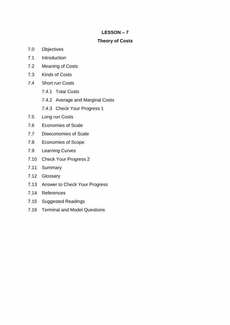
LESSON – 7
Theory of Costs
7.0 Objectives
7.1 Introduction
7.2 Meaning of Costs
7.3 Kinds of Costs
7.4 Short run Costs
7.4.1 Total Costs
7.4.2 Average and Marginal Costs
7.4.3 Check Your Progress 1
7.5 Long run Costs
7.6 Economies of Scale
7.7 Diseconomies of Scale
7.8 Economies of Scope
7.9 Learning Curves
7.10 Check Your Progress 2
7.11 Summary
7.12 Glossary
7.13 Answer to Check Your Progress
7.14 References
7.15 Suggested Readings
7.16 Terminal and Model Questions

7.0 OBJECTIVES
After reading this lesson, you should be able:
To understand the meaning and importance of cost in managerial decision
making
To explain the different concepts of cost.
To comprehend cost behavior in the short run and the long run.
To introduce the concepts of economies of scale and learning curve.
7.1 Introduction
All productive activities of the business firms are guided by the consideration
of maximum profits. The objective of profit maximization can be achieved if the said
firm is able to produce maximum possible output at minimum possible cost. The cost
analysis plays a vital role in every organisation, and hence, in managerial
economics, within the decision making process. The information on costs is of
extreme importance for any business firm because it helps to monitor the other
control systems of the firm like production control, quality control, stock control, etc.
Hence, the business managers must have a complete knowledge of cost concepts
and their role in business, to maximize the value of the firm. The concept of cost is of
great significance in microeconomics as it helps the business managers in making
appropriate business decisions (aiming at reduction of costs) aimed at maximization
of profit. Business firms are responsible for providing the consumers in the market
with a flow of goods and services, in accordance with their tastes and preferences.
The process of production involves various inputs or the factors of production such
as land, labour, capital, raw materials, etc. The factor prices of these inputs, in turn,
affect the price of the final goods and services. All the explicit and implicit payments
made by a firm in the process of production, form the production costs of the firm.
The importance of the relevant time frame is all the more realized in the
context of cost analysis. The major concerns of the business managers of a firm in
the short run are different from those in the long run. In the short run the production
has to be planned keeping in mind that only one factor input is variable while others
are fixed. Hence, the optimum level of output has to be worked out in terms of the
optimal input of the variable factor. However, in the long run all the factor inputs
become variable and the firm is basically concerned with the scale of production, that
is, the pursuit for optimal combination of inputs or the least-cost combination of
inputs. The decision regarding which kind of cost concept should be used in a
specific situation, in turn is influenced by the business decision made by the
manager of a firm. Owing to various definitions and concepts of cost, the cost
analysis has in itself become a complex one. It requires an in depth study of the cost
analysis to decide about the usage of different concepts of cost. This is so because
the cost of production is an important element in almost all the processes of
business decision making. Also, costs can make or break any strategic move in
important decisions involving crucial issues (like expansion or integration or maybe
diversification), which need to be justified on the basis of profitability. Hence, cost

analysis forms the very basis of the economic rationale behind the process of
business decision-making.
7.2 Meaning of Costs
The term cost has different meanings to different users of the term. In economics
the definition of cost is based on the concept of opportunity cost. Every business firm
has to employ different factors of production for producing goods and services for the
consumers in the market. The owners of the factors of production are made
payments in return for the use of their services. In addition to these costs, the
producer also has to give up his time, comfort and opportunity of other sources of
income. Hence, cost also involves sacrifice on the part of the producer as cost leads
to a current or future decrease in cash or other assets. According to Marshall, the
real cost of production includes the real cost of efforts of various qualities and real
cost of waiting. It is also known as alternative sacrificed cost, or transfer cost.
Opportunity cost of a commodity is the alternative sacrificed in order to obtain it.
There are various factors which influence the level of costs, some of which
are uncontrollable while others can be controlled (partially or completely). Out of
these factors, the most significant factor is the factor prices or the prices of the factor
inputs, which largely constitute the total production cost, and which are usually
outside the control of the business firm. Further, the factor costs are related to the
marginal productivity or the efficiency of these factors of production. Other things
remaining the same, a higher level of marginal productivity or efficiency of the factor
inputs leads to a lower factor cost and vice-versa. The other important determinants
of cost are technology (an improvement in technology lowers the cost by increasing
the efficiency, other things remaining the same) and the level of output.
The expenses on production or costs vary directly with the level of output.
Higher the level of output, higher is the cost and vice-versa. The functional
relationship between costs and the level of output is called the cost function. Hence,
the cost function is derived from the production function and is defined as:
Cost functions are derived functions. They are derived from the production function.
--- Koutsoyiannis
Cost is a function of a number of factors- the expenses incurred on all inputs of
production (both factor inputs – land, labour, capital and organisation; and non-factor
inputs - raw materials, fuel, machinery equipment, tools, etc.) form the cost of
production. The cost function can be expressed as:
C = f (Q, T, Pf)
where C is the total cost of production, Q is the level of output; T stands for
technology, and Pf is the prices of factors of production.
7.3 Kinds of Costs
There are various concepts of cost relevant to business operations and the process
of business decision making.Different types of costs are relevant for various kinds of

management decisions.Some important concepts of costs of production are
explained as follows:
Accounting Costs: These costs are the nominal or money costs, that is, costs
expressed in money terms. Accounting costs are so called because these can be
recorded in the books of accounts. Those costs which can be identified and
measured are included in this category, for example, wages and salary, cost of raw
material, interest on capital, electricity expenses, etc.
Real Costs: Real cost of producing a commodity is the exertion, inconvenience, pain
or sacrifice involved in producing it. In the words of Marshall, “Real cost is the
exertion of all the different kinds of labour that are directly or indirectly involved in
making it together with the abstinence or rather waiting required for saving the
capital used in making it.” The producers compensate the owners of factors of
production through the amount of money considered equivalent to exertion,
inconvenience, pain or sacrifice involved in production. However, exertion,
inconvenience, pain or sacrifice are psychological concepts which cannot be exactly
measured in money terms. Hence, real costs are not of much significance for the
accountants but the business decision makers cannot ignore them.
Opportunity Costs: Opportunity cost of a decision is the cost of next best
alternative sacrificed in order to take the current decision. Thus, it is the value of the
next best alternative or opportunity forgone. It is defined as:
The opportunity cost of anything is the next best alternative that could be produced
instead by the same factors or by an equivalent group factors, costing the same
amount of money. --- Benham
The alternative or opportunity cost of producing one unit of commodity X is the
amount of commodity Y that must be sacrificed in order to use resources to produce
X rather than Y. --- Ferguson
Thus, opportunity cost of a particular product is the value of the foregone alternative
products that resources used in its production, could have produced. The concept of
opportunity cost is of special significance for determining the prices of the factors of
production.
Explicit Costs: Explicit costs are the payments made by the producer to the owners
of the factors of production (which do not belong to the employer himself) on account
of the supply of factor services by them.
Explicit costs are those cash payments which firms make to outsiders for their
services and goods. --- Leftwitch
These costs fall under the category of business costs or accounting costs as these
involve cash payments and are entered in the books of accounts. Explicit costs are
also called expenditure costs or out-of-pocket costs, and include payments for raw
materials, fuel, interest on borrowed funds, rent on hired land, wages and salaries,
insurance premium, depreciation charges and taxes paid to the government.
Implicit Costs: Implicit costs of production are the costs of self-owned and self-
employed resources. These costs that do not involve cash payments and hence, are
not entered in the books of accounts. Non-expenditure or implicit costs arise
because of the fact that the entrepreneur himself provides certain services to
production like his own land or capital or managerial services. However, these costs
are not taken into consideration while calculating the loss or gains of the business,
though they form an important consideration in managerial decisions about the
usage of a factor in business operations. Non-expenditure costs are implicit or
internal in character, and hence, they are the imputed costs. Implicit costs are non-
cash costs, like the salary that could have been earned, leisure time foregone and
interest foregone on assets which have to be used in production. These include the
rewards for the entrepreneur’s self-owned land, labour and capital. Expenditure
costs are explicit as they are paid to factors outside the firm while non-expenditure
costs are implicit, hence they are imputed costs. The sum total of the explicit and
implicit costs formseconomic costsor the total cost of production.
Private, External and Social Costs: External costs are not borne by the firm, but
are incurred by others in society. In order to know the social cost or true cost to the
society, we need to know all costs no matter who bears them.
Private costs include the total costs (economic costs) of a firm in involved in the
production of a commodity. For example, the purchase price (offered to the
consumer) of a bike includes the private cost borne by the producer. On the other
hand, the air pollution (and/or other types of pollution) generated in the process of
production of the bike is called an external cost (as these fall not on the firm
producing the bike but on other people in the society). The air pollution from driving
an automobile is also an externality or third party effect. . On the contrary, social cost
is a wider term which is the total of all the costs associated with an economic activity.
It, hence, includes the costs undertaken by the producer as well as the costs on the
society as a whole. Thus, social costs are the sum total of private costs and the
external costs. Therefore, if social costs are greater than private costs, it implies the
presence of a negative externality for example, environmental pollution. However, if
private costs are greater than social costs, this indicates the presence of a positive
externality, for example, education which benefits the society as a whole.
Replacement Costs or Current Costs: Current costs refer to the current price of
buying or replacing any input t under present market conditions. Replacement cost is
the relevant cost for decision-making as it involves the expenditure on replacing an
old machine with a new one on the expiry of its economic life.
Historic Costs and Future Costs: Historical costs are the costs incurred at the time
of the purchase of assets and represent actual cash outlay which is recorded by the
accountants. Historic costs or past costs are the actual costs incurred by a producer
in the past. On the other hand, future costs are those costs which may have to be
incurred in the near future. As this is only a sight into future business actions, future
costs are very important for planning and evaluating of managerial decisions.
However, there is no scope for managerial decision in historic or past costs which
have already been incurred. Relevant feasible action may be taken if the future costs
are high.
Incremental Costs and Sunk Costs: Incremental costs are the changes in costs
caused by a particular decision. This concept is quite similar to the concept of
marginal cost. Incremental cost refers to the total additional cost caused by a change
in the level of production or the nature of activity. It may be associated with the
decision to expand output or to add a new variety of product. Incremental costs may
also arise by adding a new product or changing distribution channel, or adding new
machinery, or replacing worn out plant and machinery, replacing old technique of
production with a new one, etc. Incremental costs are the relevant costs for decision-
making.
Sunk costs are the costs that do not vary according to different decisions.
These costs have already been incurred and cannot be altered in any way.
Investment on machinery, or costs incurred in building a factory, etc. are examples of
sunk cost. All preceding costs are considered to be the sunk costs as they relate to
the prior commitment. It is not possible to reverse or recover these costs when there
is a change in market conditions or a change in business decisions.
The distinction between the sunk cost and the incremental cost is very important in
evaluating different business alternatives. Incremental cost will be different in each
case while sunk cost will remain same. Hence incremental cost is relevant for the
management in decision making.
Controllable Costs and Non-Controllable costs
Controllable costs are those costs that can be controlled by some executive action
on the part of the business management in a firm. These can, hence, improve the
efficiency of the factor inputs. For example, fringe benefits to employees. On the
other hand, non-controllable costs are those that cannot be controlled by way of any
action on the part of the business administration. These costs may lead to wastage
of resources and encourage inefficiency. The factor prices may be regarded as non-
controllable costs as they reflect the external environment and are not in the control
of the producer.
Activity A
Identify types of cost in each case
a)Payment for office stationary
--------------------------------------------------------------------------------------------------------------------
--------------------------------------------------------------------------------------------------------------------
b)Interest cost of owner’s capital----------------------------------------------
--------------------------------------------------------------------------------------------------------------------
c)Salary of the owner of the company
--------------------------------------------------------------------------------------------------------------------
--------------------------------------------------------------------------------------------------------------------
--------------------------------------------------------------------------------------------------------------------
--------------------------------------------------------------------------------------------------------------------

-
7.4 Short run Costs
Short run is a period of time in which some factors are fixed and some are variable.
So in the short period a firm can change its output by changing only the quantity of
the variable factors, such as labour and raw materials etc. The fixed factors like land,
machinery etc, cannot be changed. Hence, based on the fixed factors and variable
factors in the short run, short run costs may be divided into two categories: fixed
costs and variable costs. The concepts related to short run costsare discussed
below:
7.4.1 Total Costs
Total cost is the sum of all the expenses of production that a producer incurs through
the process of production. It is defined as:
The sum of all expenditures incurred in producing a given volume of output.
--- Dooley
Hence, total cost refers to the total expense on the production of goods and services
and it includes both explicit and implicit costs. The explicit costs further comprise of
fixed and variable costs. In the short period, the total cost (TC) is made up of total
fixed cost (TFC) and the total variable costs (TVC).
TC = TFC + TVC
Total Fixed Costs: In the short period, certain factors of production like land,
building, etc. remain fixed. Thus, the expenses incurred by the producer on the fixed
factors also remain constant. So the total fixed costs are related to the fixed factors
and do not vary with output in the short run. For example rent, insurance, interest
payments, depreciation, cost of construction of a building, payment to permanent
staff, expenditure on machinery, property tax, etc.
Fixed costs are those costs which in total do not vary with changes in output.
---- McConnel
Thus, the fixed costs are independent of the level of output and are the costs that
continue even if the firm is temporarily shut down, producing nothing. Fixed costs
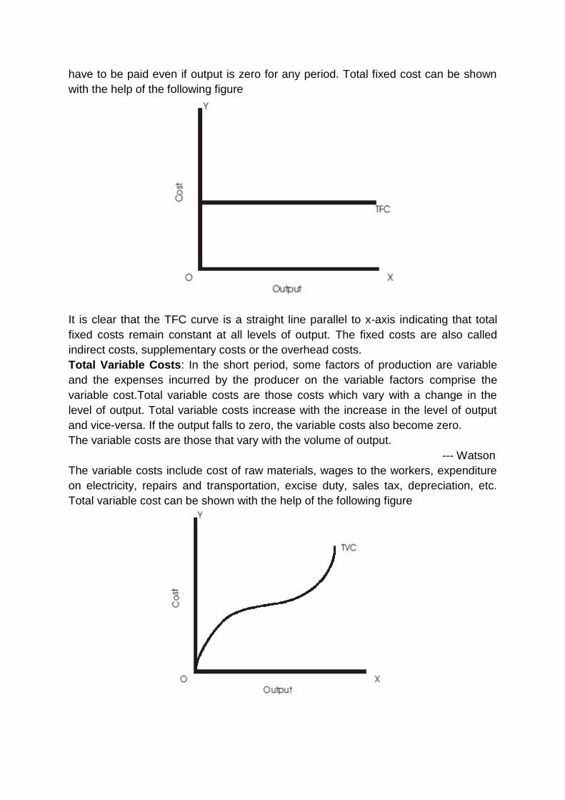
have to be paid even if output is zero for any period. Total fixed cost can be shown
with the help of the following figure
It is clear that the TFC curve is a straight line parallel to x-axis indicating that total
fixed costs remain constant at all levels of output. The fixed costs are also called
indirect costs, supplementary costs or the overhead costs.
Total Variable Costs: In the short period, some factors of production are variable
and the expenses incurred by the producer on the variable factors comprise the
variable cost.Total variable costs are those costs which vary with a change in the
level of output. Total variable costs increase with the increase in the level of output
and vice-versa. If the output falls to zero, the variable costs also become zero.
The variable costs are those that vary with the volume of output.
--- Watson
The variable costs include cost of raw materials, wages to the workers, expenditure
on electricity, repairs and transportation, excise duty, sales tax, depreciation, etc.
Total variable cost can be shown with the help of the following figure
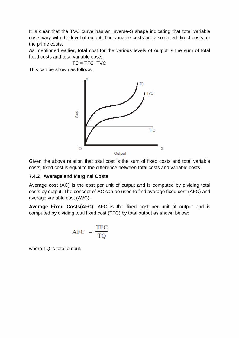
It is clear that the TVC curve has an inverse-S shape indicating that total variable
costs vary with the level of output. The variable costs are also called direct costs, or
the prime costs.
As mentioned earlier, total cost for the various levels of output is the sum of total
fixed costs and total variable costs,
TC = TFC+TVC
This can be shown as follows:
Given the above relation that total cost is the sum of fixed costs and total variable
costs, fixed cost is equal to the difference between total costs and variable costs.
7.4.2 Average and Marginal Costs
Average cost (AC) is the cost per unit of output and is computed by dividing total
costs by output. The concept of AC can be used to find average fixed cost (AFC) and
average variable cost (AVC).
Average Fixed Costs(AFC): AFC is the fixed cost per unit of output and is
computed by dividing total fixed cost (TFC) by total output as shown below:
where TQ is total output.

The above diagram shows AFC curve. The shape of AFC curve is a rectangular
hyperbola, indicating that TFC remains constant throughout.
Average Variable Costs(AVC): AVC is the variable cost per unit of output and is
computed by dividing total variable cost (TVC) by total output as shown below:
where TQ is total output.
It is clear from the above diagram that AVC curve is U-shaped. AVC falls initially,
reaches a minimum when the plant is operated optimally and then starts rising
thereafter showing that AVC is per unit cost of the variable inputs and changes as
the level of output changes.
Average Total Costs or Average Costs(ATC or AC): Average cost (AC) is equal to
total costs divided by the total output. Hence, ATC is per unit cost of both fixed and
variable inputs. Average total cost of production can be calculated by dividing total

cost by the level of output. Moreover, AC is also equals to the sum of AFC and AVC.
This is shown as follows:
The average cost (AC) curve can be shown in the following figure:
Hence, the average cost (AC) curve is U-shaped and its shape is same as that of the
AVC curve.
Marginal Costs
Marginal cost (MC) is the addition to the total cost when the producer produces one
more unit of any commodity. It can be expressed:
MC(N) = TC(N) – TC(N–1)
where, N is any given number of units of output. Alternatively, marginal cost can also
be expressed as follows:
Where, ΔTC and ΔTQ stand for the change in total cost total output respectively.

The MC curve can be diagrammatically shown as above. MC curve represents the
slope of the TC curve, as MC shows the change in TC due to unit change in output.
It is a U-shaped curve. Initially it slopes downwards from left to right because of
negative relation between output and MC. Later the MC curve slopes upwards from
left to right because of positive relation between output and MC. In this connection it
should be noted that MC is independent of fixed cost as the amount of fixed cost has
no impact on the marginal cost. It can be explained as:
MC(N) = TC(N) – TC(N–1)
MC(N) = [FC(N)+VC(N)] – [FC(N–1)+VC(N–1)]
Since FC(N) = FC(N–1)
Hence, MC(N) = VC(N) –VC(N–1)
where, FC and VC are the fixed and variable cost respectively, N is the number of
units of the output.
The relationship among fixed, variable costs, total, average and marginal costs can
be explained with the following table
Thus, total costs are calculated by adding the columns of fixed cost and variable
cost, average fixed cost by dividing fixed costs by output (column 1), average
variable cost by dividing variable costs by output. Average total cost is the sum of
average fixed cost and average variable cost, or alternatively, ratio of total costs to
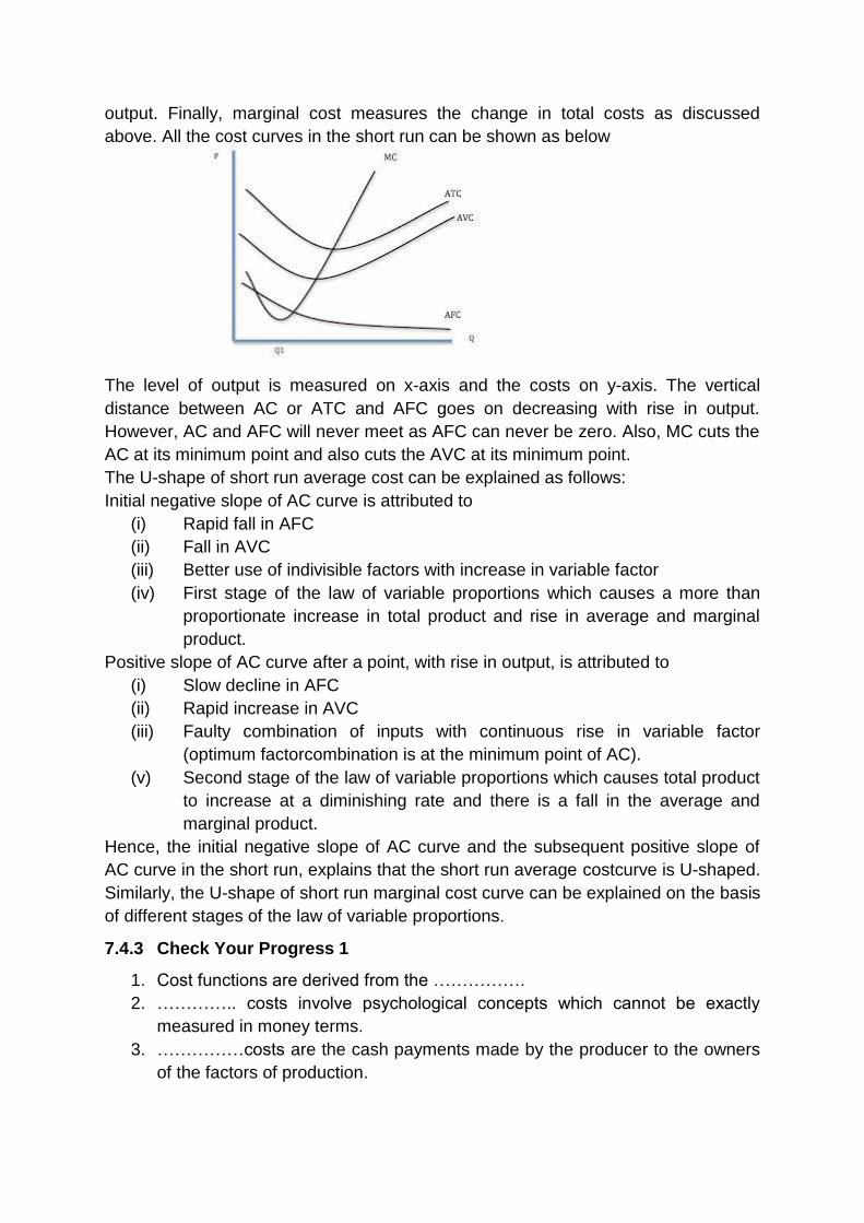
output. Finally, marginal cost measures the change in total costs as discussed
above. All the cost curves in the short run can be shown as below
The level of output is measured on x-axis and the costs on y-axis. The vertical
distance between AC or ATC and AFC goes on decreasing with rise in output.
However, AC and AFC will never meet as AFC can never be zero. Also, MC cuts the
AC at its minimum point and also cuts the AVC at its minimum point.
The U-shape of short run average cost can be explained as follows:
Initial negative slope of AC curve is attributed to
(i) Rapid fall in AFC
(ii) Fall in AVC
(iii) Better use of indivisible factors with increase in variable factor
(iv) First stage of the law of variable proportions which causes a more than
proportionate increase in total product and rise in average and marginal
product.
Positive slope of AC curve after a point, with rise in output, is attributed to
(i) Slow decline in AFC
(ii) Rapid increase in AVC
(iii) Faulty combination of inputs with continuous rise in variable factor
(optimum factorcombination is at the minimum point of AC).
(v) Second stage of the law of variable proportions which causes total product
to increase at a diminishing rate and there is a fall in the average and
marginal product.
Hence, the initial negative slope of AC curve and the subsequent positive slope of
AC curve in the short run, explains that the short run average costcurve is U-shaped.
Similarly, the U-shape of short run marginal cost curve can be explained on the basis
of different stages of the law of variable proportions.
7.4.3 Check Your Progress 1
1. Cost functions are derived from the …………….
2. ………….. costs involve psychological concepts which cannot be exactly
measured in money terms.
3. ……………costs are the cash payments made by the producer to the owners
of the factors of production.
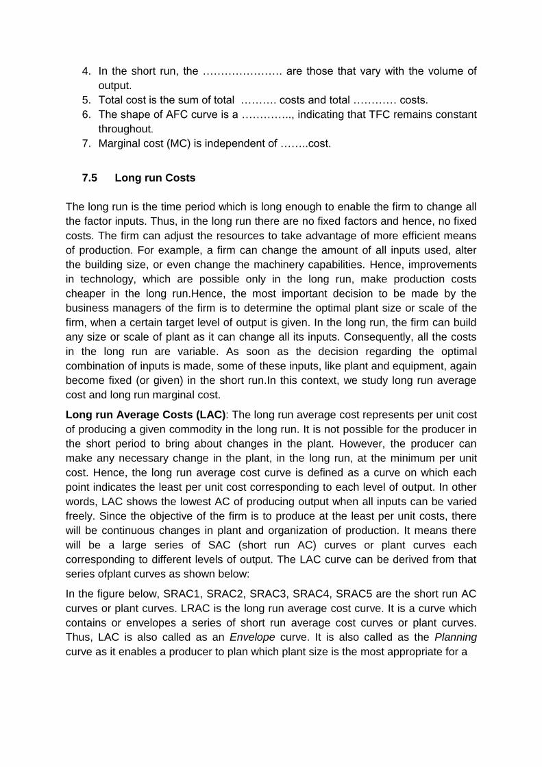
4. In the short run, the …………………. are those that vary with the volume of
output.
5. Total cost is the sum of total ………. costs and total ………… costs.
6. The shape of AFC curve is a ………….., indicating that TFC remains constant
throughout.
7. Marginal cost (MC) is independent of ……..cost.
7.5 Long run Costs
The long run is the time period which is long enough to enable the firm to change all
the factor inputs. Thus, in the long run there are no fixed factors and hence, no fixed
costs. The firm can adjust the resources to take advantage of more efficient means
of production. For example, a firm can change the amount of all inputs used, alter
the building size, or even change the machinery capabilities. Hence, improvements
in technology, which are possible only in the long run, make production costs
cheaper in the long run.Hence, the most important decision to be made by the
business managers of the firm is to determine the optimal plant size or scale of the
firm, when a certain target level of output is given. In the long run, the firm can build
any size or scale of plant as it can change all its inputs. Consequently, all the costs
in the long run are variable. As soon as the decision regarding the optimal
combination of inputs is made, some of these inputs, like plant and equipment, again
become fixed (or given) in the short run.In this context, we study long run average
cost and long run marginal cost.
Long run Average Costs (LAC): The long run average cost represents per unit cost
of producing a given commodity in the long run. It is not possible for the producer in
the short period to bring about changes in the plant. However, the producer can
make any necessary change in the plant, in the long run, at the minimum per unit
cost. Hence, the long run average cost curve is defined as a curve on which each
point indicates the least per unit cost corresponding to each level of output. In other
words, LAC shows the lowest AC of producing output when all inputs can be varied
freely. Since the objective of the firm is to produce at the least per unit costs, there
will be continuous changes in plant and organization of production. It means there
will be a large series of SAC (short run AC) curves or plant curves each
corresponding to different levels of output. The LAC curve can be derived from that
series ofplant curves as shown below:
In the figure below, SRAC1, SRAC2, SRAC3, SRAC4, SRAC5 are the short run AC
curves or plant curves. LRAC is the long run average cost curve. It is a curve which
contains or envelopes a series of short run average cost curves or plant curves.
Thus, LAC is also called as an Envelope curve. It is also called as the Planning
curve as it enables a producer to plan which plant size is the most appropriate for a
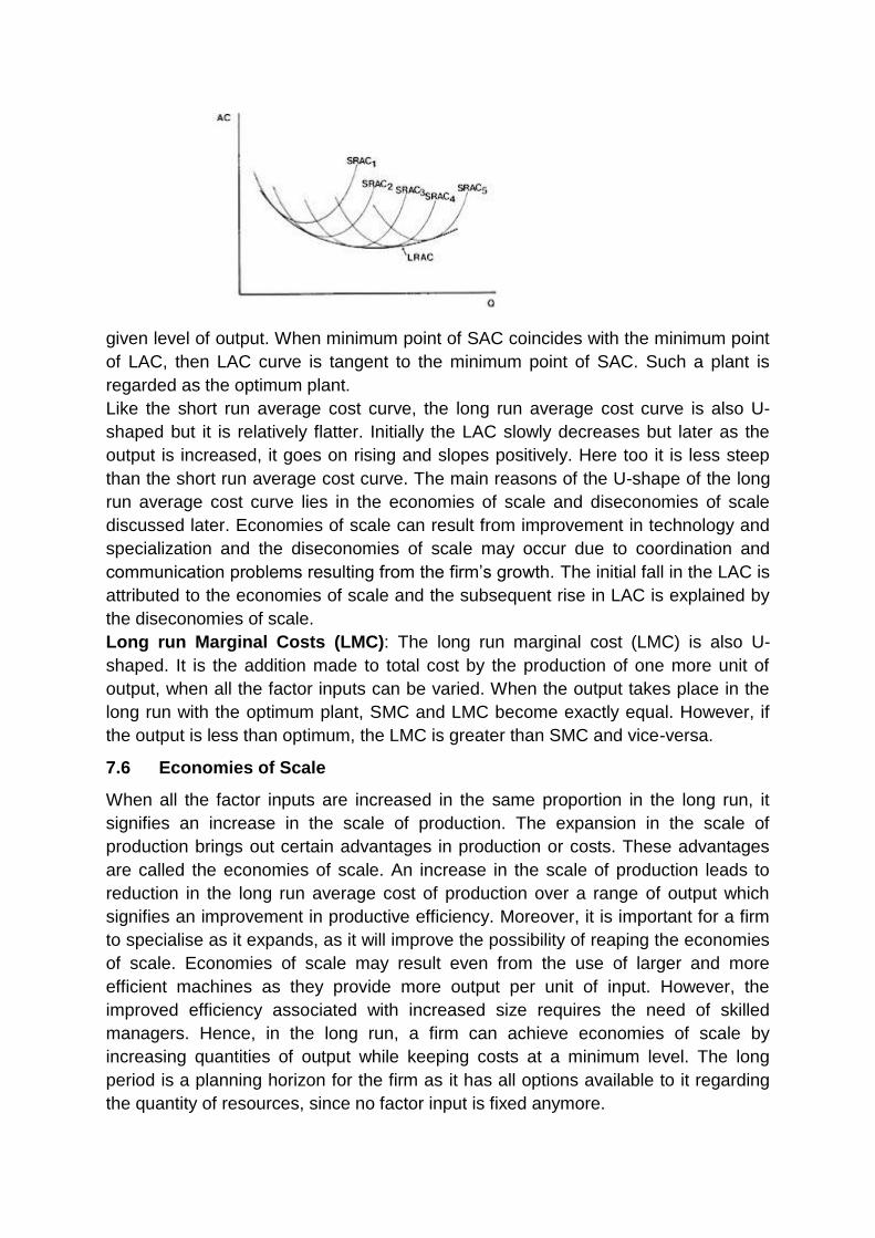
given level of output. When minimum point of SAC coincides with the minimum point
of LAC, then LAC curve is tangent to the minimum point of SAC. Such a plant is
regarded as the optimum plant.
Like the short run average cost curve, the long run average cost curve is also U-
shaped but it is relatively flatter. Initially the LAC slowly decreases but later as the
output is increased, it goes on rising and slopes positively. Here too it is less steep
than the short run average cost curve. The main reasons of the U-shape of the long
run average cost curve lies in the economies of scale and diseconomies of scale
discussed later. Economies of scale can result from improvement in technology and
specialization and the diseconomies of scale may occur due to coordination and
communication problems resulting from the firm’s growth. The initial fall in the LAC is
attributed to the economies of scale and the subsequent rise in LAC is explained by
the diseconomies of scale.
Long run Marginal Costs (LMC): The long run marginal cost (LMC) is also U-
shaped. It is the addition made to total cost by the production of one more unit of
output, when all the factor inputs can be varied. When the output takes place in the
long run with the optimum plant, SMC and LMC become exactly equal. However, if
the output is less than optimum, the LMC is greater than SMC and vice-versa.
7.6 Economies of Scale
When all the factor inputs are increased in the same proportion in the long run, it
signifies an increase in the scale of production. The expansion in the scale of
production brings out certain advantages in production or costs. These advantages
are called the economies of scale. An increase in the scale of production leads to
reduction in the long run average cost of production over a range of output which
signifies an improvement in productive efficiency. Moreover, it is important for a firm
to specialise as it expands, as it will improve the possibility of reaping the economies
of scale. Economies of scale may result even from the use of larger and more
efficient machines as they provide more output per unit of input. However, the
improved efficiency associated with increased size requires the need of skilled
managers. Hence, in the long run, a firm can achieve economies of scale by
increasing quantities of output while keeping costs at a minimum level. The long
period is a planning horizon for the firm as it has all options available to it regarding
the quantity of resources, since no factor input is fixed anymore.
The economies of scale are broadly of two types:
(i) Internal economies
(ii) External Economies
(i) Internal Economies arise from the growth of the firm itself, that is, from the
expansion of the plant size of the firm and are exclusively available to the expanding
firm. These are the advantages resulting from the internal and organization of the
firm. Hence, the internal economies are controllable and under the influence of
business managers. Internal economies are further classified into the following
types:
Technical Economies: The technical economies arise mainly from increased
specialization and indivisibilities. Larger firms are in a position to use more
specialized machinery, equipment and skilled labour in the process of production.
Indivisibilities may also occur in the form of use of more expensive but often more
effective advertising media, and greater expenditure on research and development
activities that small firms cannot afford. Specialisation of the workforce within larger
firms is possible as they split complex production processes into separate tasks. The
division of labour in mass production leads to technical economies of scale.
Other technical economies relate to increased dimensions. The dimensional
economies arise when there is enlargement of plant, machinery or some other
equipment. As the size increases, volume increases more rapidly than surface area.
The unit costs fall as size increases, as volume often determines the output while
surface area determines cost. This is particularly relevant in the transportation and
storage industries. For example, the cost of constructing a double-decker bus is less
than two times the cost of constructing a single-decker bus but its capacity is two
times the capacity of a single-decker bus.
Another type of technical economy relates to economies of linked processes.
Production processes can be linked together with one integrated plant. It is
specifically important in mass production which requires complex manufacturing
processes. Larger firms find it easier to combine equipment or facilities with different
capacities more efficiently. For example, a steel mill having its own iron mines,
transport arrangements and other units involved in different stages of production of
steel, can manufacture steel at a much lesser cost than a small firm not having these
linked processes under its control. These economies are sometimes called multi
plant economies. These technical economies tend to be the most important source
of economies of scale for most of the firms.
Managerial economies: Large scale firms attract and use more specialized, skilled
managers, who are trained and efficient in managerial functions and decision
making. This leads to savings in administrative costs by splitting up jobs (like
specialist buyers, production management). A large firm can afford to employ various
specialist managers to supervise production systems. Hence, better management,
more investment in human resources and use of specialist equipment, all work
towards raising the productivity and reducing unit costs.
Marketing economies: These economies arise from large scale purchase of raw
materials and other inputs, along with large-scale selling of the firm’s own products.
When the firm buys in bulk, larger firms get bulk discounts (if it has monopsony
(buying) power in the market). Economies in marketing the firm’s own product are
associated with the economies in advertisement cost. Expensive advertising
expenditure can be spread over huge volumes of sales which thereby reduces the
marketing costs per unit.
Economies in Transport and Storage costs: These economies arise from full,
efficient and optimum utilisation of the available transport and storage facilities.
Financial economies: Large firms can usually borrow at a lower interest rate due to
higher credit worthiness in the market. So the firms operating at a bigger scale have
access to cheaper sources of finance. Also they have more sources of finance as
compared to smaller firms. They can even use the capital markets to borrow cheaply
through the issue of equities.
Learning Economies: These economies relate to the efficiencies due to the length
of experience in a market and are readily available in high-knowledge industries
which have an edge as they get to learn the tricks of the trade.
Network economies of scale: Some networks and services have huge potential for
economies of scale as they become more valuable to the business that provides
them. For example, networks economies are enjoyed in online auctions, air transport
networks, new phone connections, etc. The marginal cost of adding one more user
to the network is almost negligible but the resulting benefits are huge as each new
user in the network can then interact with all of the existing members.
(ii) External Economies: External economies arise from the growth of the
industry and are independent of the size of the firm. These economies occur outside
of a firm, within an industry. For example, creation of a better transportation network
may increase the scope of expansion of an industry and result in a decrease in cost
for a firm operating within that industry. External economies are also called
economies of concentration because they arise when firms in the same industry are
located close to each other. Development of research and development facilities in
local universitiesmay benefit several business firms in that area. Trade magazines
help firms to advertise cheaply and spread information (economies of information).
Also the relocation of component suppliersand other supporting business firms near
the main centre of production may generate external economies by reducing
transportation costs. Further, external economies of scale exist when the long-term
expansion of an industry leads to the development of ancillary services which benefit
all or the majority of firms in the industry (economies of disintegration).Thus, external
economies justify the tendency for firms to cluster geographically.
Thus, as the internal and external economies create the conditions for
expansion in output and sale along with economy in costs, the profitability of the firm
increases by a large measure.
7.7 Diseconomies of Scale
With the expansion of the scale of production, a firm may eventually experience a
rise in long run average costs caused by diseconomies of scale. Diseconomies of
scale are the disadvantages that arise due to the expansion of scale of production,
thereby leading to a rise in production cost. Diseconomies of scale may be internal
or external.
Internal Diseconomies of Scale: These are the disadvantages that originate within
the firm.Economies of scale reach a limit, when the optimum combination of inputs is
achieved for a given level of output. Then diseconomies appear when the
advantages of division of labour and managerial staff have been fully exploited. For
example, workers doing repetitive jobs may lose motivation to work, which reduces
productivity. It may increase the chance of industrial unrest. Also workers in large
firms may feel a sense of alienation and thus loss of morale. Large firms are more
difficult to manage; monitoring the productivity and the quality of output from
thousands of employees in big corporations could be imperfect and costly. The
suppliers of factor and non factor inputs may start demanding higher prices, raising
the costs. Beyond a point, serious financial difficulties can arise disrupting the whole
process of production.
External Diseconomies of Scale: These are the disadvantages that originate
outside the firm by virtue of being a part of the industry. The diseconomies of scale
lead to rising long-run average costs when the firms expand beyond their optimum
scale. They are often caused by the complex nature of managing large-scale firms.
Increasing demand for inputs also puts pressure on input markets leading to
increase in input prices or even creating serious shortages of raw materials,
machinery, trained labour, power, finance, etc. This further increases production
costs. The expansion of an industry results in an increased intensity of competition
among the firms causing a rise in the cost of material and labour, and also a price-
cut strategy. This in turn leads to a steady erosion of profits for all the firms.
7.8 Economies of Scope
Economies of scope refer to a situation where it is cheaper to produce a range of
products than to produce each individual product on its own.
Economies of scope occur when the total cost of producing two types of outputs
together is less than the total cost of producing each type of output separately.
--- Baye
Economies of scale relate to an increased production of the same commodity being
produced by firm. On the other hand, economies of scope relate to making different
but compatible products. For example, making mango pickle would probably use a
lot of the same equipment as for making lemon pickle, so the firm can save money
per unit because the scope (range of products) is being increased within similar
categories. Economies of scope are relevant to firms that produce more than one
product and obtain production or cost advantages. This concept is a relatively new
business strategy based on high technology. When a firm produces multiple or joint
products, economies of scope can be measured as the ratio of average costs to
marginal costs.
Economies of scope occur when changing the mix of operations leads to cost
benefits as the products may use common processing facilities, especially when
there are joint products or by-products, for example petrochemicals. Thus, the cost
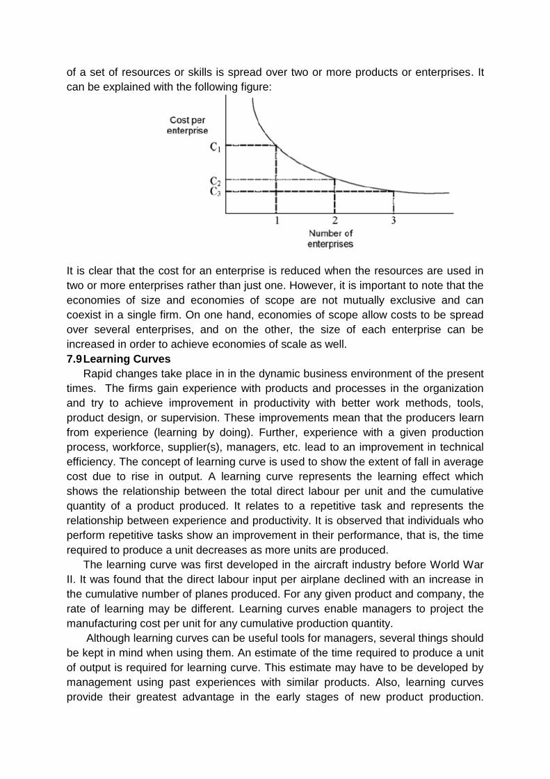
of a set of resources or skills is spread over two or more products or enterprises. It
can be explained with the following figure:
It is clear that the cost for an enterprise is reduced when the resources are used in
two or more enterprises rather than just one. However, it is important to note that the
economies of size and economies of scope are not mutually exclusive and can
coexist in a single firm. On one hand, economies of scope allow costs to be spread
over several enterprises, and on the other, the size of each enterprise can be
increased in order to achieve economies of scale as well.
7.9 Learning Curves
Rapid changes take place in in the dynamic business environment of the present
times. The firms gain experience with products and processes in the organization
and try to achieve improvement in productivity with better work methods, tools,
product design, or supervision. These improvements mean that the producers learn
from experience (learning by doing). Further, experience with a given production
process, workforce, supplier(s), managers, etc. lead to an improvement in technical
efficiency. The concept of learning curve is used to show the extent of fall in average
cost due to rise in output. A learning curve represents the learning effect which
shows the relationship between the total direct labour per unit and the cumulative
quantity of a product produced. It relates to a repetitive task and represents the
relationship between experience and productivity. It is observed that individuals who
perform repetitive tasks show an improvement in their performance, that is, the time
required to produce a unit decreases as more units are produced.
The learning curve was first developed in the aircraft industry before World War
II. It was found that the direct labour input per airplane declined with an increase in
the cumulative number of planes produced. For any given product and company, the
rate of learning may be different. Learning curves enable managers to project the
manufacturing cost per unit for any cumulative production quantity.
Although learning curves can be useful tools for managers, several things should
be kept in mind when using them. An estimate of the time required to produce a unit
of output is required for learning curve. This estimate may have to be developed by
management using past experiences with similar products. Also, learning curves
provide their greatest advantage in the early stages of new product production.

Moreover learning curves are dynamic because they are affected by various factors.
Finally, learning curves are only approximations of actual experience and not the
actual experience.
Activity B
A automobile company recently expanded its annual production from 100 to 150 units and also
diversified its activity. Highlights the economies and diseconomies during expansion.
-------------------------------------------------------------------------------------------------------------------------------
-------------------------------------------------------------------------------------------------------------------------------
-------------------------------------------------------------------------------------------------------------------------------
-------------------------------------------------------------------------------------------------------------------------------
-----------------------------------------------------------------------------------------------------------------------------
7.10 Check Your Progress 2
State whether the following are true or false.
1. The long run average cost represents the lowest average cost of producing output
when all inputs can be varied freely.
2. Economies of scale are the cost advantages that a business firm enjoys by
expanding its scale of production in the short run.
3. External economies arise from the growth of the firm itself and depend on the size
of the firm.
4. Economies of scope refer to a situation where it is cheaper to produce an
individual product rather than a range of products.
5. The external diseconomies of scale originate outside the firm by virtue of being a
part of the industry.
7.12 Summary
The cost analysis plays a vital role in the decision making process. Cost is influenced
by many factors, like factor prices, productivity of the factor, technology and the level
of output. Cost functions are derived from the production function. A firm incurs
different types of costs under different situations. Accounting costs are the costs
which go to the book of accounts. Real costs involve psychological concepts which
cannot be exactly measured in money terms. Opportunity cost of is the cost of the
next best alternative which is foregone.Explicit costs are the payments made by the
producer to the owners of the factors of production (outsiders) on account of the
supply of factor services.Incremental costs are the changes in costs caused by a
particular decision while sunk costs are the costs that do not vary according to
different decisions. Similarly, controllable costs and non-controllable costs reflect the
extent of control of the firm on the costs. Managers must be very careful in using
cost information prepared by the accountants, as it is collected and categorised for
different purposes. On the basis of time frame, costs may be divided into short run
costs and long run costs. Short run costs may be divided into two categories: fixed
costs and variable costs; fixed costs do not vary with output while the variable costs
vary with the volume of output. Average and marginal costs may be derived from the
total costs. The short run average cost and marginal cost curves are U-shaped. In
the long run there are no fixed factors and hence, no fixed costs. The long run
average cost represents per unit cost of producing a given commodity in the long
run.The long run marginal cost is the addition made to total cost by the production of
one more unit of output, in the long run. The economies of scale are the cost
advantages that a business firm enjoys by expanding its scale of production in the
long run. With the expansion of the scale of production, a firm may eventually
experience a rise in long run average costs causing diseconomies of scale. The
concept of learning curve is used to show the extent of fall in average cost due to
rise in output.
7.13 Glossary
Accounting Costs: These costs are the nominal or money costs.
Explicit Costs: The payments made by the producer to the owners of the factors of
production.
Implicit Costs: The costs of self-owned and self-employed resources.
Sunk costs: The costs which do not vary in response to different decisions as they
relate to the prior commitment.
Short run Costs: These costs comprise of fixed costs (of fixed factors) and variable
costs (of variable factors).
Long run Average Costs: The long run average cost represents per unit cost of
producing a given commodity in the long run.
Economies of Scale: The cost advantages that a business firm enjoys by
expanding its scale of production in the long run.
Diseconomies of scale: The disadvantages that arise due to the expansion of
scale of production in the long run.
Learning curve is used to show the extent of fall in average cost due to rise in
output.
7.14 Answers to Check Your Progress
Check Your Progress 1
1. Production function
2. Real
3. Explicit
4. Variable costs
5. Fixed, variable
6. Rectangular hyperbola
7. fixed
Check Your Progress 2
1. true
2. false
3. false
4. false
5. true
7.15 References
Salvatore, Domonick, Managerial Economics, Thompson South-Western.
Ferguson, C. E., Microeconomic Theory, Richard D. Irwin, Homewood.
Douglas, Evan J., Managerial Economics: Theory, Practice and Problems, Prentice
Hall Inc., NJ.
Koutsoyiannis, A : Modern Microeconomics, The Macmillan Press Ltd.,, London
Dewett, K.K., Modern Economic Theory, S. Chand Publication
.
Geetika, Managerial Economics, Tata McGraw Hills
7.16 Suggested Readings
Mathur N.D., Managerial Economics, Shivam book House (P.) Limited, Jaipur
Mishra &Puri : Managerial Economics, Himalaya Publishing House, Mumbai
Mithani D.M. : Managerial Economics, Himalaya Publishing House, Mumbai
Dwivedi, D.N. : Managerial Economics, Vikas Publishing House Pvt. Ltd, New Delhi
7.17 Terminal and Model Questions
1. What is opportunity cost?

2. Explain incremental and sunk costs.
3. Distinguish between fixed and variable costs.
4. Explain various short run cost curves with the help of a diagram.
5. Discuss economies of scope.
6. Why is short run average cost curve U-shaped?
7. What is learning curve?
8. What are internal and external economies of scale?

LESSON – 8
Revenue and Revenue Curves
8.0 Objectives
8.1 Introduction
8.2 Revenue Concepts
8.2.1 Total Revenue
8.2.2 Average Revenue
8.2.3 Marginal Revenue
8.2.4 Relationship between Total Revenue, Average Revenue and Marginal
Revenue
8.3 Revenue Curves under Different Market Situations
8.4 Break even Analysis
8.4.1 Algebraic Method
8.4.2 Graphic Method
8.4.3 Limitations of Break Even Analysis
8.4.4 Examples of Break Even Analysis
8.5 Summary
8.6 Glossary
8.7 Answer to Check Your Progress
8.8 References
8.9 Suggested Readings
8.10 Terminal and Model Questions
8.0 OBJECTIVES
After reading this lesson, you should be able:
To understand the meaning and importance of revenue for a firm
To explain the different concepts of revenue
To explain the revenue curves under different market situations
To comprehend break even analysis
8.1 Introduction
The functions, strategies and managerial decisions of a business firm are basically
determined by the objective of the firm. The traditional theory regarding the objective of the
firm states that the single most important objective of a business firm is maximization of
profits. This idea of profit maximization is justified on the ground that profit is the
remuneration which an entrepreneur expects to get in return for putting on risk his time and
capital. Moreover, profit is extremely essential for the long term survival of a firm. The profit
earned by any business firm is computed as the difference between total revenue and total
cost. However, later several scholars came up with an alternative objective of a business firm
– sales maximization. In this context, Baumol’s theory of sales revenue maximization asserts
that sales play a greater role in market leadership as compared to profits and hence, the firms
constantly try to maximize their total revenue instead of maximizing profits. Still other
objectives of firms have emerged eventually. However, there is no denying the fact that no
matter what is the basic objective of the firm, profits continue to be the main guiding force in
determining the short term and long term perspective of the firm. An in depth study in to the
different concepts of revenue is a pre requisite to ascertain the profits associated with a firm.
8.2 Revenue Concepts
The primary objective of any business firm, by and large, is to secure maximum
profits. The fulfillment of this objective requires production at the least possible cost and the
sale of output bringing in the maximum revenues. In this context, an attempt is made to study
in detail the different concepts of revenue and their inter relationships.
There are three main concepts related to revenues. These are total revenue, average
revenue and marginal revenue.
8.2.1 Total Revenue
Total revenue (TR) is the total amount of money income that a firm receives through
the sale of a specified quantity of its product in the market. Suppose a producer sells 1000
metres of pipes at the price of Rs. 75 per metre, the total money received by him through this
sale in the market is Rs. 75,000. This amount is total revenue. It may be defined as follows
Total revenue is the sum of all sales, receipts or income of a firm. --- Dooley
Total revenue is money received from selling a quantity of a product. --- Holland
Total revenue at any output is equal to price per unit multiplied by quantity sold.
--- Stonier and Hague

If the firm practices single pricing rather than price discrimination, then according to
the above given definition,
TR = total expenditure of the consumer = P x Q
where P stands for the price per unit, and
Q stands for the quantity of the output sold.
Total revenue is the direct function of price of the commodity (P) and the quantity of the
output sold (Q).
TR = f (P, Q)
Given the price, the TR increases with an increases in the quantity of the output sold (Q) and
vice versa. Similarly, if the quantity of the output sold (Q) remains the same but price (P)
rises, the TR will also rise and vice versa. Also, if there is a rise in both P and Q, the TR will
again rise and vice versa.
8.2.2 Average Revenue
Average revenue is the revenue per unit of output. In other words, average revenue
(AR) is the total amount of money income that a firm receives from the sale divided by the
number of units of the commodity sold.
Average revenue is the ratio of the total revenue to the quantity sold of the product.
--- Holland
Average revenue is the per unit revenue received from the sale of one unit of a commodity.
--- Mc Connel
Average revenue (AR) = TR/Q
Since for single pricing practice TR=P x Q, therefore AR = P x Q/Q = P. It signifies that
average revenue (AR) is the technical name for price. This concept of average revenue is very
significant in pricing theory as average revenue along with average cost helps to determine
whether a firm will get normal profits or super normal profits or losses. If average revenue is
more than with average cost, it indicates per unit profit and on the other hand if average
revenue is less than with average cost, it indicates per unit loss. Still another case is possible
where average revenue is just equal to average cost then the firm gets normal profits. Hence,
the study of average revenue is crucial for a firm to ascertain its profits or losses, if any.
8.2.3 Marginal Revenue
Marginal revenue (MR) is the change in total revenue resulting from selling an extra
unit of the commodity. In other words, when a firm sells one more unit of a commodity, the
resultant increase in total revenue is known as marginal revenue.
Marginal revenue, at any level of a firm’s output is the revenue which would be earned from
selling another (marginal) unit of the firm’s product.
--- Stonier and Hague
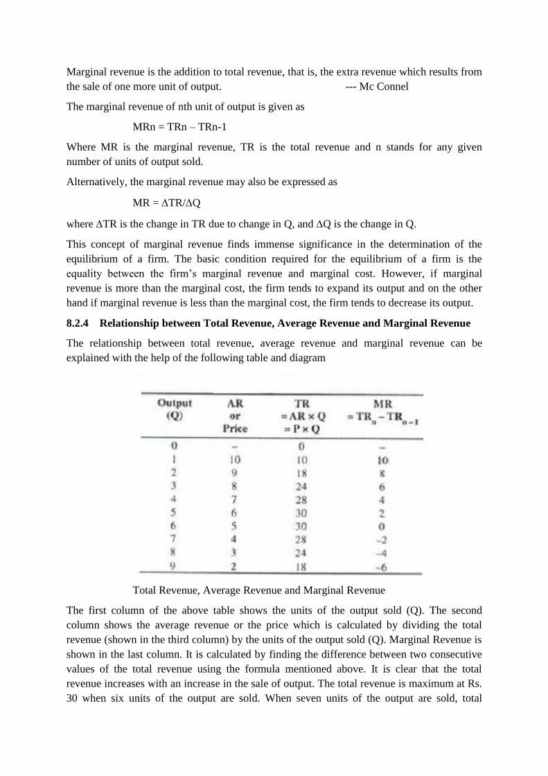
Marginal revenue is the addition to total revenue, that is, the extra revenue which results from
the sale of one more unit of output. --- Mc Connel
The marginal revenue of nth unit of output is given as
MRn = TRn – TRn-1
Where MR is the marginal revenue, TR is the total revenue and n stands for any given
number of units of output sold.
Alternatively, the marginal revenue may also be expressed as
MR = TR/Q
where TR is the change in TR due to change in Q, and Q is the change in Q.
This concept of marginal revenue finds immense significance in the determination of the
equilibrium of a firm. The basic condition required for the equilibrium of a firm is the
equality between the firm’s marginal revenue and marginal cost. However, if marginal
revenue is more than the marginal cost, the firm tends to expand its output and on the other
hand if marginal revenue is less than the marginal cost, the firm tends to decrease its output.
8.2.4 Relationship between Total Revenue, Average Revenue and Marginal Revenue
The relationship between total revenue, average revenue and marginal revenue can be
explained with the help of the following table and diagram
Total Revenue, Average Revenue and Marginal Revenue
The first column of the above table shows the units of the output sold (Q). The second
column shows the average revenue or the price which is calculated by dividing the total
revenue (shown in the third column) by the units of the output sold (Q). Marginal Revenue is
shown in the last column. It is calculated by finding the difference between two consecutive
values of the total revenue using the formula mentioned above. It is clear that the total
revenue increases with an increase in the sale of output. The total revenue is maximum at Rs.
30 when six units of the output are sold. When seven units of the output are sold, total
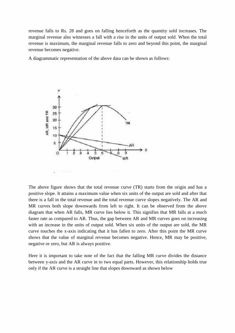
revenue falls to Rs. 28 and goes on falling henceforth as the quantity sold increases. The
marginal revenue also witnesses a fall with a rise in the units of output sold. When the total
revenue is maximum, the marginal revenue falls to zero and beyond this point, the marginal
revenue becomes negative.
A diagrammatic representation of the above data can be shown as follows:
The above figure shows that the total revenue curve (TR) starts from the origin and has a
positive slope. It attains a maximum value when six units of the output are sold and after that
there is a fall in the total revenue and the total revenue curve slopes negatively. The AR and
MR curves both slope downwards from left to right. It can be observed from the above
diagram that when AR falls, MR curve lies below it. This signifies that MR falls at a much
faster rate as compared to AR. Thus, the gap between AR and MR curves goes on increasing
with an increase in the units of output sold. When six units of the output are sold, the MR
curve touches the x-axis indicating that it has fallen to zero. After this point the MR curve
shows that the value of marginal revenue becomes negative. Hence, MR may be positive,
negative or zero, but AR is always positive.
Here it is important to take note of the fact that the falling MR curve divides the distance
between y-axis and the AR curve in to two equal parts. However, this relationship holds true
only if the AR curve is a straight line that slopes downward as shown below

In the above figure MR divides the perpendicular from AR to y-axis (CA) into two equal
parts, that is, AB= BC.
However, when AR is convex to the origin as shown in the figure below
In this case the MR curve is also a falling convex curve, passing at a less than half the
distance between y-axis and the AR curve, that is, AB < BC.
On the other hand, when AR is concave to the origin as shown in the figure below

In this case the MR curve is also a falling concave curve to the origin, passing at a more than
half the distance between y-axis and the AR curve, that is, AB > BC.
Check Your Progress 1
1. The traditional theory about the objective of a firm states that the most important objective of a
business firm is ……………..
2. When AR is concave to the origin, the MR curve passes at a ………..…… the distance
between y-axis and the AR curve.
3. Total revenue at any level of output is equal to the ………… multiplied by the ……………….
4. Average revenue (AR) of a firm is the technical name for …………. of the commodity being
produced and sold.
5. With an increase in the price of the commodity, total revenue …………….
6. When the total revenue attains its maximum value, the marginal revenue falls to
………………. level.
7. The gap between AR and MR curves goes on ………….. with an increase in the units of
output sold.
8. When AR and MR curves are straight lines, the MR curve divides the distance between y-axis
and the AR curve in to ……………
8.3 Revenue Curves under Different Market Situations
The problem of product pricing in different market situations is closely connected to the
shape of the revenue curves. The different possible shapes of the revenue curves in different
market situations are discussed below:
1. Revenue Curves under Perfect Competition: In perfect competition there are large
number of buyers and sellers and the product is homogeneous. Each individual firm
cannot influence the supply or price and the price is given for a firm. As the price
remains constant, the AR curve is perfectly elastic or a straight line parallel to x-axis.
Correspondingly, the MR curve is also a straight line coinciding with the AR curve as
shown below
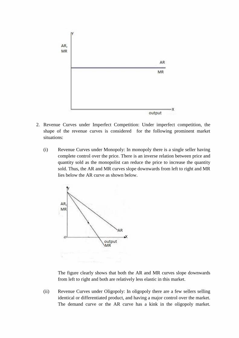
2. Revenue Curves under Imperfect Competition: Under imperfect competition, the
shape of the revenue curves is considered for the following prominent market
situations:
(i) Revenue Curves under Monopoly: In monopoly there is a single seller having
complete control over the price. There is an inverse relation between price and
quantity sold as the monopolist can reduce the price to increase the quantity
sold. Thus, the AR and MR curves slope downwards from left to right and MR
lies below the AR curve as shown below.
The figure clearly shows that both the AR and MR curves slope downwards
from left to right and both are relatively less elastic in this market.
(ii) Revenue Curves under Oligopoly: In oligopoly there are a few sellers selling
identical or differentiated product, and having a major control over the market.
The demand curve or the AR curve has a kink in the oligopoly market.

Beyond a specific price, if one firm raises the price, the rival firm will not do
so. The firm which raises the price, loses buyers to other firms, that is, even a
small rise in price in this situation leads to a big fall in the sale. So beyond a
specific price, the demand curve or the AR curve is more elastic. On the other
hand, if the price is reduced below a specific price, other firms will also do so
and here the demand curve or the AR curve is less elastic. The upper part of
the demand curve is more elastic and the lower part is less elastic and such a
demand curve is called a kinky demand curve as shown below
The kink in the demand curve occurs at point P, the part above P is more
elastic and the part below P is less elastic. Corresponding to the more elastic
part of the demand curve, the MR curve is also more elastic, and
corresponding to the less elastic part of the demand curve, the MR curve is
also less elastic. RT portion shows the discontinuity in the MR curve.
(iii) Revenue Curves under Monopolistic Competition: In this market situation
there are a large number of sellers and the product is differentiated but closely
related. If a firm slightly cuts down its price, it is able to attract the buyers of
the rival firm also, because the products are of substitutable nature. Hence, the
demand curve or the AR curve is relatively more elastic than in monopoly.
Correspondingly the MR curve also slopes downwards from left to right and is
relatively more elastic as shown below

Both the AR and MR curves slope downwards from left to right and both are relatively more
elastic in this market as a small cut in the price leads to a substantial increase in the sale of
output.
8.4 Break Even Analysis
The concept of break even analysis is one of the simplest analytical tools in
management available to the business manager to help in the process of decision making. An
appropriate financial decision making and profit planning are very important for every firm
pursuing the goal of profit maximization. The profit planning involves the study of profit
function which shows the different quantities of output at which the concerned firm makes
profits. For an economist the term profit could refer to two different meanings – normal profit
or super normal profit. The term normal profit indicates the amount of return which an
entrepreneur must definitely earn, only then the entrepreneur will continue that business. The
additional income earned over and above the normal profit is referred to as super normal
profit. In other words, normal profit can be considered to be a part of the total cost while
super normal profit is the excess of total revenue over total cost. The basic condition for the
equilibrium of a profit maximizing firm is the equality between marginal revenue and
marginal cost. A rational firm enjoys maximum profits, and hence, stops further production
when the marginal revenue becomes equal to the marginal cost. However, if marginal
revenue is more than the marginal cost, a rational firm continues with more production and if
marginal revenue is less than the marginal cost, the firm will stop any further production.
Thus, a comparative analysis of cost and revenue of a firm helps the manager to pursue the
objective of profit maximization.
In this context, the break even analysis helps to study the relationship between the
amount of output produced, its cost of production and the revenue generated from the sale of
this output (also known as Volume Cost Profit Analysis). The break even analysis helps a
firm to identify the break even point by determining the levels of profit associated with
different levels of projected sales of the output. A business firm can only make profit when
its total revenue is greater than the total costs. If it is not so, that is, total revenue is less than
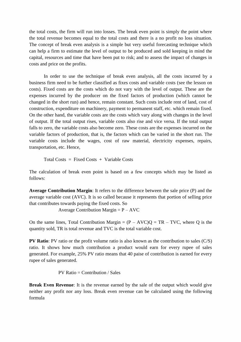
the total costs, the firm will run into losses. The break even point is simply the point where
the total revenue becomes equal to the total costs and there is a no profit no loss situation.
The concept of break even analysis is a simple but very useful forecasting technique which
can help a firm to estimate the level of output to be produced and sold keeping in mind the
capital, resources and time that have been put to risk; and to assess the impact of changes in
costs and price on the profits.
In order to use the technique of break even analysis, all the costs incurred by a
business firm need to be further classified as fixes costs and variable costs (see the lesson on
costs). Fixed costs are the costs which do not vary with the level of output. These are the
expenses incurred by the producer on the fixed factors of production (which cannot be
changed in the short run) and hence, remain constant. Such costs include rent of land, cost of
construction, expenditure on machinery, payment to permanent staff, etc. which remain fixed.
On the other hand, the variable costs are the costs which vary along with changes in the level
of output. If the total output rises, variable costs also rise and vice versa. If the total output
falls to zero, the variable costs also become zero. These costs are the expenses incurred on the
variable factors of production, that is, the factors which can be varied in the short run. The
variable costs include the wages, cost of raw material, electricity expenses, repairs,
transportation, etc. Hence,
Total Costs = Fixed Costs + Variable Costs
The calculation of break even point is based on a few concepts which may be listed as
follows:
Average Contribution Margin: It refers to the difference between the sale price (P) and the
average variable cost (AVC). It is so called because it represents that portion of selling price
that contributes towards paying the fixed costs. So
Average Contribution Margin = P – AVC
On the same lines, Total Contribution Margin = (P – AVC)Q = TR – TVC, where Q is the
quantity sold, TR is total revenue and TVC is the total variable cost.
PV Ratio: PV ratio or the profit volume ratio is also known as the contribution to sales (C/S)
ratio. It shows how much contribution a product would earn for every rupee of sales
generated. For example, 25% PV ratio means that 40 paise of contribution is earned for every
rupee of sales generated.
PV Ratio = Contribution / Sales
Break Even Revenue: It is the revenue earned by the sale of the output which would give
neither any profit nor any loss. Break even revenue can be calculated using the following
formula

Break even revenue = Fixed Costs / PV Ratio
Margin of Safety: It is the difference between the planned or budgeted volume of sales and
the break even volume of sales. Margin of safety measures the sensitivity of the planned sales
in comparison to the break even volume of sales.
Margin of safety = Planned sales – Break even sales
The break even analysis is based on the assumption that sale price, fixed cost and the variable
cost remain constant. On the basis of this assumption, the break even analysis can be
explained using the algebraic method and the graphic method as follows.
8.4.1 Algebraic Method: This method may be explained using the following notations: Let
Q be the quantity of a given commodity being produced and sold; P its price; TFC the total
fixed cost; TVC the total variable cost; AFC the average fixed cost; and AVC the average
variable cost. Let Q’ be the break even volume of sales where total revenue becomes equal to
total cost. It follows that
Total Revenue = P.Q
Total Cost = TFC + TVC = TFC + AVC.Q
Thus, P.Q = TFC + AVC.Q
At break even level, P.Q’ = TFC + AVC.Q’
Or, (P – AVC)Q’ = TFC
Q’ = TFC / (P – AVC)
The above formula for the break even output can be generalised to deal with the situation
where the business firm has determined in advance a target profit. The output volume Q’ that
will yield this target profit is implicitly given by
P.Q’ = Target Profit + TFC + AVC.Q’
Hence, Q’ = (Target Profit + TFC) / (P – AVC)
It is clear from the above formula that changes in TFC, AVC and P affect the break even
output (Q’). If there is a rise in TFC (say cost of equipment, etc.) break even output also rises
and vice versa. Similarly there is a direct relation between AVC (say cost of raw material,
etc.) and the break even output. On the other hand, there is inverse relation between price, P
and Q’. If P increases, Q’ falls and vice versa. It is relatively easy for the firms to calculate
the break even output using the above formula as the data on TFC and AVC are readily
available with the business firms.
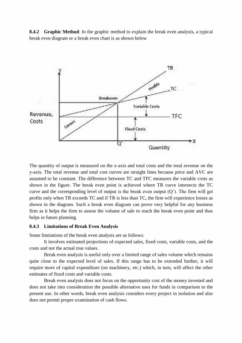
8.4.2 Graphic Method: In the graphic method to explain the break even analysis, a typical
break even diagram or a break even chart is as shown below
The quantity of output is measured on the x-axis and total costs and the total revenue on the
y-axis. The total revenue and total cost curves are straight lines because price and AVC are
assumed to be constant. The difference between TC and TFC measures the variable costs as
shown in the figure. The break even point is achieved where TR curve intersects the TC
curve and the corresponding level of output is the break even output (Q’). The firm will get
profits only when TR exceeds TC and if TR is less than TC, the firm will experience losses as
shown in the diagram. Such a break even diagram can prove very helpful for any business
firm as it helps the firm to assess the volume of sale to reach the break even point and thus
helps in future planning.
8.4.3 Limitations of Break Even Analysis
Some limitations of the break even analysis are as follows:
It involves estimated projections of expected sales, fixed costs, variable costs, and the
costs and not the actual true values.
Break even analysis is useful only over a limited range of sales volume which remains
quite close to the expected level of sales. If this range has to be extended further, it will
require more of capital expenditure (on machinery, etc.) which, in turn, will affect the other
estimates of fixed costs and variable costs.
Break even analysis does not focus on the opportunity cost of the money invested and
does not take into consideration the possible alternative uses for funds in comparison to the
present use. In other words, break even analysis considers every project in isolation and also
does not permit proper examination of cash flows.
Moreover, the break even analysis assumes that the total revenue and total cost curves
are straight lines because price and AVC are assumed to be constant. However, such
restrictive assumptions may not be applicable for every business firm. There is no provision
for the change in price or change in the market conditions or even the changes in the costs
over the time period under consideration.
However, despite its limitations, break even analysis continues to be a very useful tool
in the hand of business managers for appropriate decision making regarding issues like the
costs of expansion, evaluation of sales or profit performance, estimation of the impact of
various expenses on profit, etc. It can even serve as a substitute to estimate an unknown
factor in making project decisions. However, it can not be considered a panacea for all
problems in the financial decision making. Break even analysis is only one of the many tools
available to the business decision maker. The best possible results may be achieved if the
break even analysis is used in combination with the other techniques of financial analysis.
Above all it is very essential for every business firm to be familiar with the break-even
analysis.
8.4.4 Examples of Break Even Analysis: The practical application of the break even
analysis for a business firm can be judged from the following numerical examples.
Example 1:Calculate the break-even output for TFC = Rs. 20,000, P = Rs. 70, and AVC = Rs.
50
Answer: Break even output, Q’ = TFC / (P – AVC)
So Q’ = 20000 / 70 – 50 = 20000 / 20 = 1000
Example 2: Suppose TFC = Rs. 10,000, P = Rs. 50, AVC = Rs. 20. What volume of output is
necessary in order to earn a total profit of Rs. 5000? Also find the average contribution
margin?
Answer:
Q’ = (Target Profit + TFC) / (P – AVC)
So Q’ = (5000 + 10000) / (50 – 20) = 15000 / 30 = 500
Further, Average Contribution Margin = ACM = P – AVC
So ACM = 50 – 20 = 30
Therefore, break even analysis is primarily a planning tool which may be used to examine the
expansion feasibility and other important business decisions.
Activity:
The ABC Credit company incurs the following monthly expenses: Salaries and benefits 3,400
Administration expenses 1,620 Rent and utilities 1,440 Other fixed expenses 800 Interest on debt
@ 12% annual rate per 1,000 10 Interest paid on deposits @ 6% annual rate per 1,000 5 Travel and
transportation per 1,000 loans outstanding 4.5 The ABC Credit company earns a 20% yield on their
loans. Calculate the portfolio size required to break even in a month.
------------------------------------------------------------------------------------------------------------------------

------------------------------------------------------------------------------------------------------------------------
------------------------------------------------------------------------------------------------------------------------
------------------------------------------------------------------------------------------------------------------------
------------------------------------------------------------------------------------------------------------------------
-----------------------------------------------------------------------------
------------------------------------------------------------------------------------------------------------------------
------------------------------------------------------------------------------------------------------------------------
------------------------------------------------------------------------------------------------------------------------
-----------------------------------------------------------------------------------------
------------------------------------------------------------------------------------------------------------------------
------------------------------------------------------------------------------------------------------------------------
------------------------------------------------------------------------------------------------------------------------
-----------------------------------------------------------------------------------------
Check Your Progress 2
State whether the following are true or false.
1. Revenue Curves under monopoly are straight line parallel to x-axis.
2. Break even revenue is the revenue earned by the sale of the output which would give
the target profit.
3. In oligopoly market the demand curve is a kinky demand curve.
4. In the break-even analysis the price and AVC are assumed to be constant.
5. Both the AR and MR curves slope downwards from left to right and both are relatively
more elastic in case of monopolistic competition.
6. Break even analysis involves estimated projections of expected sales, fixed costs, and
the variable costs.
7. In perfect competition each individual firm can influence the supply or price in the
market.
8. The break even point is the point where the total revenue becomes equal to the total
costs and there is a no profit no loss situation.
8.5 Summary
The traditional theory regarding the objective of the firm states that the single most important
objective of a business firm is maximization of profits. Whatever be the basic objective of a
firm, profits continue to be the main guiding force in determining the functions, strategies and
managerial decisions of a business firm. In order to assess the level of profits earned by a
business firm, it is very essential to have an in depth knowledge of the meaning and usage of
the different concepts of revenue. In this context, total revenue (TR) is the total amount of
money income that a firm receives through the sale of a specified quantity of its product in
the market. Average revenue (AR) is the revenue per unit of output sold. Marginal revenue
(MR) is the change in total revenue resulting from selling an extra unit of the commodity. A
study of the relationship between total revenue, average revenue and marginal revenue shows
that total revenue curve (TR) starts from the origin and has a positive slope. On the other
hand, both AR and MR curves both slope downwards from left to right. When TR becomes
maximum, MR becomes zero and when with further increase in sale of output TR starts
falling, then MR becomes negative. However, although AR is also falling all the time with
rise in sale of output but it always remains positive. The revenue curves have different shapes
under different market situations.Break even analysis is an important application of the cost
analysis which is used in business decision making. This concept studies the relation between
total revenue, total costs and total profits of a firm at different levels of output. A break even
point is a point where there are no profits and no losses, that is, where total revenue is just
equal to the total costs. Break even analysis may be explained with the help of algebraic
method as well as the graphic method. Despite its limitations, the study of break even
analysis is very essential for every business firm.
8.6 Glossary
Total revenue: It is the total amount of money income that a firm receives by the sale of a
given quantity of its output in the market.
Average Revenue: It is the revenue per unit of output.
Marginal Revenue: It is the change in total revenue resulting from the sale of an extra unit
of the commodity.
Monopoly: A market situation in which there is a single seller having complete control over
the price.
Perfect Competition: A market situation in which there are large number of buyers and
sellers, the product is and the price remains constant.
Break Even Point: The point where the total revenue becomes just equal to the total costs
and there is a no profit no loss situation.
8.7 Answer to Check Your Progress
Check Your Progress 1
1. Maximization of profits
2. More than half
3. Price per unit, quantity sold
4. Price
5. Also rises
6. Zero
7. Increasing
8. Two equal parts
Check Your Progress 2
1. False
2. False
3. True
4. True
5. True
6. True
7. False
8. True
8.8 References
Blank, L. T., and Tarquin, A.J., Engineering Economy, 5th Edition, McGraw-Hill, USA.

Chandra P., Appraisal Implementation, Tata-McGraw Hill Publishing Company Limited,
New Delhi.
Hampton J.J., Financial Decision Making (4th
edition), Prentice Hall of India Private Limited
Khan M.Y. and Jain P.K., Financial Management (4th
edition), Tata-McGraw Hill Publishing
Company Limited.
Salvatore, Domonick, Managerial Economics, Thompson South-Western.
Douglas, Evan J., Managerial Economics: Theory, Practice and Problems, Prentice Hall Inc.,
NJ.
Dewett, K.K., Modern Economic Theory, S. Chand Publication
.
Geetika, Managerial Economics, Tata McGraw Hills
8.9 Suggested Readings
Mathur N.D., Managerial Economics, Shivam book House (P.) Limited, Jaipur
Mishra & Puri : Managerial Economics, Himalaya Publishing House, Mumbai
Mithani D.M. : Managerial Economics, Himalaya Publishing House, Mumbai
Dwivedi, D.N. : Managerial Economics, Vikas Publishing House Pvt. Ltd, New Delhi
Swarup K., Gupta P.K. and Mohan M., Operations Research, Sultan Chand and Sons, Delhi.
8.10 Terminal and Model Questions
1. Explain the different concepts related to revenue.
2. Explain the relationship between TR, AR and MR.
3. Discuss the shape of the revenue curves under different market situations.
4. What is break even analysis? Discuss its importance for a business firm in decision
making.
5. What do you mean by average contribution margin?
6. How can you calculate break even output using the break even analysis?
7. Explain break even analysis using the graphical method.

LESSON – 9
Market Structure and Pricing
9.0 Objectives
9.1 Introduction
9.2 Meaning of Market
9.3 Market Structure and Pricing Decisions
9.3.1 Price Determination under Perfect Competition
9.3.1.1 Features of Perfect Competition
9.3.1.2 Price and Output under Perfect Competition
9.3.1.3 Price in Market Period
9.3.1.4 Price in Short Period
9.3.1.5 Price in Long Period
9.3.2 Check Your Progress A
9.3.3 Price Determination under Monopoly
9.3.3.1 Price in Short Period
9.3.3.2 Price in Long Period
9.3.4 Price Discrimination under Monopoly
9.3.5 Price Determination under Oligopoly
9.3.5.1 Features of Oligopoly
9.3.5.2 Price Determination
9.3.6 Price Determination under Monopolistic Competition
9.3.6.1 Features of Monopolistic Competition
9.3.6.2 Price in Short Period
9.3.6.3 Price in Long Period
9.4 Check Your Progress B
9.5 Summary
9.6 Glossary
9.7 Answer to Check Your Progress
9.8 References
9.9 Suggested Readings
9.10 Terminal and Model Questions

9.0 OBJECTIVES
After reading this lesson, you should be able:
To understand the meaning of market and its different types
To explain price determination under different market situations
To know the relevance of short run and long run in determination of
equilibrium price and output
9.1 Introduction
In a modern economic system all exchange of goods and services takes place
in the market. Whether the producer will be able to charge a higher or lower price
from the buyers, is determined in an important way by the nature of the market. So
far we have studied that, by and large, maximization of profits remains the primary
objective of any business firm. Besides maximizing output, minimizing cost and
optimizing resource allocation, another important aspect of profit maximization is to
determine the relevant price which is commensurate with the objective of profit
maximization. This profit maximizing price may not always correspond to minimum
cost. Also the level of profit maximizing price is different in different kinds of markets
based on the degree of competition among the sellers in the markets. Hence, it
becomes essential for a firm to give due consideration to the nature of the market
while determining the price of its product.
The market structure plays an important role in determining the ability of a firm
in make pricing decisions, or in other words, the structure of the market helps to find
the extent of freedom (freedom here refers to independence from the rival firm in
determining the product prices) enjoyed by a firm in the determination of product
prices. More is the degree of competition in the market, the firm will enjoy lesser
independence in making decisions about the prices of its products and vice-versa.
Hence, the information about different market forms is very essential for pricing
decisions made by a firm. In simple words, a market is an area over which buyers
and sellers come in close contact with one another and indulge in the process of
buying and selling. However, this is a restricted meaning of market and in economic
sense the word market has a much deeper and elaborate meaning as explained
ahead.
9.2 Meaning of Market
In economics, the word market refers to an effective institutional arrangement which
brings buyers and sellers into contact with one another at a mutually agreed upon
price. In broader sense it is not necessary for the buyers and sellers to be in a face
to face or a direct physical contact with each other. This contact can be through
different means of communication like letters, agents, newspapers, telegraphs,
telephone, e-mail, etc. Thus, the terms market refers to an entire area where buyers
and sellers of a commodity are in such close contact with each other that the price of

the same commodity tends to be the same throughout that area. This can be better
understood with the help of the following definitions of market.
Economists understand by the term market not any particular market place in
which things are bought and sold but the whole of any region in which buyers and
sellers are in such free intercourse with each other that the price of the same goods
tends to uniformity, easily and quickly. ---- Cournot
A market is that mechanism by which buyers and sellers are brought together.
It is not necessarily a fixed place. ---- J.C. Edwards
The term market refers not necessarily to place but always to a commodity
and the buyers and sellers who are in direct competition with one another.
--- Chapman
The structure of the market influences not only the pricing behavior of a firm, but also
its behavior with regard to supply, barrier of entry, efficiency, and competition. It also
enables a firm to control its market plan, to adjust to the changed environment, and
to facilitate the process of strategic decision making.
Hence, it is clear that the term market does not confine to a particular place
but the whole area wherein buyers and sellers of a commodity are spread. For the
existence of the market there must be one commodity like rice, sugar, tea, fruits,
furniture, and utensils, etc. Also there must be healthy and free competition among
the buyers and sellers without any restrictions on them. Generally one price prevails
in a market which is the main feature of a market.
There can be different classifications of markets, on the basis of competition,
commodities transacted (wheat market, rice market, etc.) area or region (local
market, international market, etc.) time period (very short period market, short period
market, long period market, etc.), quantum of transactions (retail market, wholesale
market, etc.), legality of transaction (open market, black market) and so on. We will
basically focus on different market forms based on the degree of competition among
the buyers and sellers. According to this classification of markets, there are three
main types of markets – perfect competition, imperfect competition, and monopolistic
competition. Perfect competition is a market situation in which there are a large
number of buyers and sellers dealing in homogeneous goods such that same price
prevails for a given commodity throughout the market. On the other hand, imperfect
competition is a market situation in which there is some limitation on the number of
buyers and sellers. The goods may be identical or differentiated. The individual firms
may have some degree of control over supply or price of the commodity. The
different forms of market found in imperfect competition are monopoly, duopoly,
oligopoly, monopsony and bilateral monopoly. Monopolistic competition is a market
situation in which there are a large number of buyers and sellers dealing in
differentiated products and is a market situation much close to reality.
9.3 Market Structure and Pricing Decisions
The price level and the level of production of a commodity by a firm depend
upon the market structure in which the firm is operating. The structure of market

tends to influence the possible outcomes of sales, revenues, profits and prices. Also
the demand curve of the firms and the industry (of which the firm is a part) depends
on the number of sellers in the market and the similarity of their products. The
market demand also depends on nature of the commodity (homogeneous or
heterogeneous), number of buyers and sellers of the product in the market and their
mutual inter-dependence. These characteristics of the market structures are likely to
influence the behaviour and performance of a firm. Additional aspects of market
structure that may influence the behaviour and performance of a firm include the
ease with which a firm may enter the industry, nature and size of the buyers of the
firm's products, and the ability of the firm to influence demand by advertising. Broadly
speaking, we will focus on the effect of market structure on a firm’s ability to
determine the price of its product. This power of a firm to fix the price of its product
depends largely on the degree of freedom enjoyed by a firm or its independence
from the rival firms in price fixation. The degree of freedom enjoyed by a firm in turn
depends on the degree of competition among the sellers and buyers in the market.
Higher the degree of competition in the market, lesser is the firm’s control over the
price of its own product. The most important theoretical market structures include
perfect competition, monopoly, oligopoly and monopolistic competition. Each of
these are discussed one by one as follows.
9.3.1 Price Determination under Perfect Competition
Perfect competition is a market situation in which there is an infinitely large number
of buyers and sellers dealing in homogeneous products. The competition among the
buyers and sellers results in the same price of a given commodity throughout the
market. Since each firm contributes a negligible quantity to the total supply, no
individual firm can influence the price of the commodity, it has to accept the given
price and sell its product at the given price only. Perfect competition may be defined
as follows.
Perfect competition is a market in which there are many firms selling identical
product with no firm being large enough relative to the entire market so as to be able
to influence market price. ---- Leftwitch
The perfect competition is characterised by the presence of many firms. They
all sell identical products. The seller is a price taker, not a price maker. ---- Bilas
9.3.1.1 Features of Perfect Competition
Perfect competition is a market structure with the following features
(i) Large number of buyers and sellers: The number of buyers and sellers is
so large that no individual buyer or seller’s independent action can
influence the market price and output. This is so because every buyer and
seller purchases or sells a very negligible amount of the total output.
(ii) Homogeneous products: Perfectly competitive firms produce an identical
or homogeneous product, so consumers will have no preferences for a
particular product or a firm. Perfectly competitive firms do not differentiate
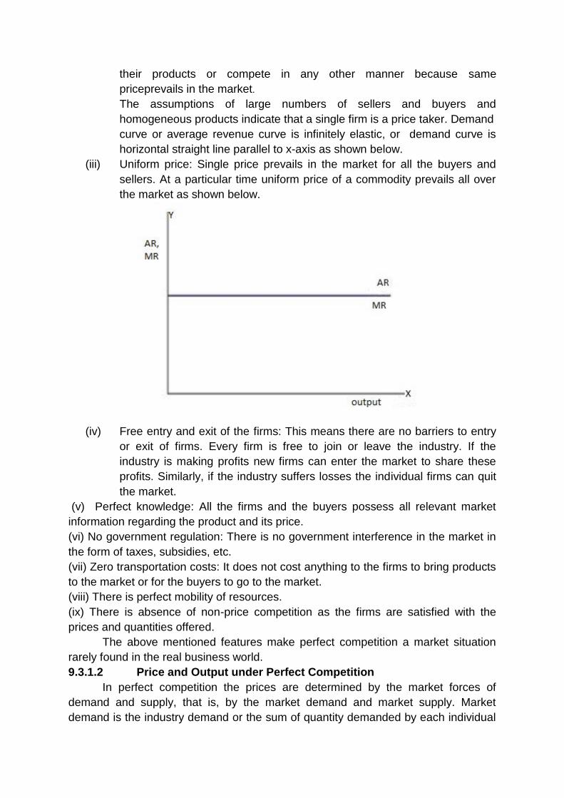
their products or compete in any other manner because same
priceprevails in the market.
The assumptions of large numbers of sellers and buyers and
homogeneous products indicate that a single firm is a price taker. Demand
curve or average revenue curve is infinitely elastic, or demand curve is
horizontal straight line parallel to x-axis as shown below.
(iii) Uniform price: Single price prevails in the market for all the buyers and
sellers. At a particular time uniform price of a commodity prevails all over
the market as shown below.
(iv) Free entry and exit of the firms: This means there are no barriers to entry
or exit of firms. Every firm is free to join or leave the industry. If the
industry is making profits new firms can enter the market to share these
profits. Similarly, if the industry suffers losses the individual firms can quit
the market.
(v) Perfect knowledge: All the firms and the buyers possess all relevant market
information regarding the product and its price.
(vi) No government regulation: There is no government interference in the market in
the form of taxes, subsidies, etc.
(vii) Zero transportation costs: It does not cost anything to the firms to bring products
to the market or for the buyers to go to the market.
(viii) There is perfect mobility of resources.
(ix) There is absence of non-price competition as the firms are satisfied with the
prices and quantities offered.
The above mentioned features make perfect competition a market situation
rarely found in the real business world.
9.3.1.2 Price and Output under Perfect Competition
In perfect competition the prices are determined by the market forces of
demand and supply, that is, by the market demand and market supply. Market
demand is the industry demand or the sum of quantity demanded by each individual

buyer in the market at different prices. Similarly, market supply is the sum of quantity
supplied by individual firms in the industry. The price existing in the market is
determined for the industry and is given for individual firms and buyers. Hence, a firm
is a price taker and not a price maker in perfect competition.
The price determination of commodity under perfectly competition is studied
under three different time periods:
(i) the market period or very short period
(ii) short period and,
(iii) long period.
9.3.1.3 Price in Market Period
The market period, or very short period is the time period in which the market supply
of the commodity remains fixed. In case of perishable commodities in the market
period, costs of production become irrelevant in market price determination the entire
supply of the commodity sold at whatever price it can get.As the supply is fixed, the
supply curve is perfectly inelastic, as shown below and the price is determined solely
by demand. Supply is an inactive agent of price determination as it is fixed at some
level of output,Q.
Even if the demand increases to D2, supply cannot be increased and hence, the
price rises to P2.
9.3.1.4 Price in Short Period
Short period is a time period in which firms cannot change their size or leave
the market. New firms cannot enter the industry. In the market period, supply is
inelastic, but in the short run, supply may be changed by increasing or decreasing
the variable inputs. Hence, in the short run the supply curve is elastic as shown
below

A firm is in equilibrium in short period where marginal cost (MC) is equal to marginal
revenue (MR) and the curve MC cuts MR from below (point E in the figure). The
output corresponding to this point shows the equilibrium or optimum level of output,
q*. Given the industry price, P* (price=AR=MR in perfect competition), the firm’s
profit is maximised where P* equals MC at equilibrium point E. A firm may even
make losses in the short run due to fall in price. However, it may not be desirable for
a firm to shut down in the short run, because if a firm shuts down, the entire amount
of fixed cost will get converted into loss. So it tries to minimise losses by adjusting its
output where it covers atleast some part of AFC. If price falls to such a level that no
part of AFC is covered, there is no further scope of loss minimization and the firm
will decide to close down. So when price becomes equal to minimum AVC in the
short run it is the condition of shut down point. Another possible situation is when
total revenue of a firm is just equal to total cost, in this case the firm gets normal
profits.
9.3.1.5 Price in Long Period
In the long run, all factors of production and all costs are variable and a firm
can adjust its size or leave the industry; new firms are also free to enter the industry.
Thus, in the long run every firm enjoys normal profit. If in long run the firms make
super normal profits then new firms enter the industry which increases the supply
and lowers the price. Hence, there will be normal profits. On the other hand if the
firms are incurring losses then some firms leave the industry, supply decreases,
price increases and the losses disappear. So, normal profits exist in perfect
competition in the long run.

The above figure shows how price and output are determined in the long run in
perfect competition.DL represents long-run demand curve, when short-run supply is
S1, price is determined at P1 (equilibrium point is M as P1 = AR1= MR1 = LMC).
The firms get super-normal profit of MS per unit of output which attracts new firms
into the industry. So, the industry supply curve shifts rightward to S2, and price falls
to P2. At this price, firms cover only the long-run marginal cost (LMC), and will make
losses because AR < LAC. Firms incurring losses will quit the industry decreasing
total industry production causing a leftward shift in the supply curve to S0 with the
corresponding market price P0. The firms adjust their output to q0 and make only
normal profit, where P0 = AR = MR = LMC = LAC. Hence, in the industry equilibrium
position no firm either makes supernormal profit, or losses but only normal profit in
the long run.
9.3.2 Check Your Progress A
State whether the following are true or false.
1. For a market to exist, it is necessary for the buyers and sellers to be in a face to
face or a direct physical contact with each other.
2. The structure of the market does not influence the pricing behavior of a firm.
3. Perfect Competition is a market situation in which there is only a single seller and
a large number of buyers.
4. In perfect competition there are no barriers to entry or exit of firms.
5. Supply of the commodity remains fixed in the very short period.
6. In the short period the supply curve is elastic.
7. At shut down point price equals average fixed cost, AFC.
8. In the long run, under perfect competition all firms enjoy normal profits.
9.3.3 Price Determination under Monopoly
A monopolyis said to exist when a single seller is the market and has no close
substitutes. Pure monopoly is a market structure in which there is a single firm
selling a commodity which has no close substitutes. The cross-elasticity of demand
for a monopolist’s product is either zero or negative. Thus, the firm itself is the
industry facing negatively sloped industry demand curve for the commodity. Hence,

to sell more of the commodity, the monopolist must lower its price of the commodity
being sold. The main features of monopoly are as follows:
(i) There is only one firm in a monopoly. The firm is the single supplier of the
product and it is a case of single-firm industry.
(ii) There are no close substitutes of the product being produced by the
monopolist.
(iii) Monopolist has complete control the prices and the quantity supplied in the
market. So a monopolist is a price maker not a price taker.
(iv) A monopoly firm earns abnormal profits in the long run. (v) Selling costs are negligible. (vi) A monopolist firm is capable of following price discrimination, which means
charging different prices for its products from different buyers. (vii) There are strong barriers to entry into the industry.
Thus, monopoly is a market structure in which a single firm controls the total supply
of a commodity having no close substitutes.
Strong barriers to entry are the main feature of monopoly that allow monopoly
firms to earn supernormal profits in the long run by making it unprofitable for new
firms to enter the industry. These barriers may be of two main types - structural and
strategic. Structural barriers or natural barriers occur due to factors outside the firm’s
control and are of the following types:
(i) Control of essential resources: This may occur due to concentration of
such resources in certain areas. For example, oil, gas, etc. are only found
in limited supplies and locations; certain areas are very advantageous for
the production of quality wines or even the expertise of resource owners
may be included like skilled surgeons or scientists.
(ii) Economies of scale play an important role in a monopoly. A monopolist
may experience economies of scale in the long run due to lack of
competition and hence, can produce more at low costs.
(iii) Brand awareness and image are very important in many industries which
can take time and a heavy cost to develop.
(iv) New firms find it difficult to raise money because of the greater risk they
impose on the lender.
(v) Government regulations like patent laws play a role in preventing entry of
new firms. Many governments deliberately create monopolies through a
licensing system, like public utilities and postal services are legally
protected monopolies in many countries. Foreign trade barriers may also
be imposed by the government to prevent a foreign company to enter the
industry.
Strategic barriers, on the other hand, occur due to deliberate restrictive practices or
strategies to deter entry of new firms. Such strategies include
(i) Limit pricing. It is the practice to discourage entry by charging a low price
before any new firm enters.
(ii) Predatory pricing. It is the practice wherein a firm tries to encourage exit,
by charging a low price after any new firms enter.
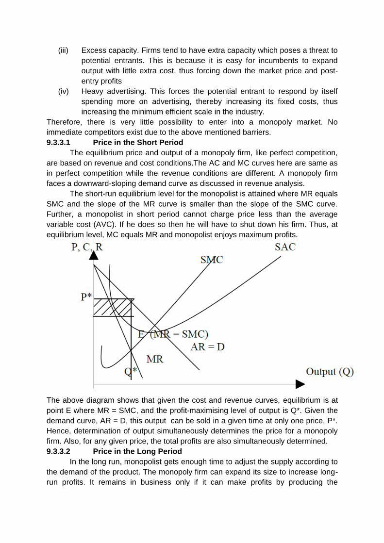
(iii) Excess capacity. Firms tend to have extra capacity which poses a threat to
potential entrants. This is because it is easy for incumbents to expand
output with little extra cost, thus forcing down the market price and post-
entry profits
(iv) Heavy advertising. This forces the potential entrant to respond by itself
spending more on advertising, thereby increasing its fixed costs, thus
increasing the minimum efficient scale in the industry.
Therefore, there is very little possibility to enter into a monopoly market. No
immediate competitors exist due to the above mentioned barriers.
9.3.3.1 Price in the Short Period
The equilibrium price and output of a monopoly firm, like perfect competition,
are based on revenue and cost conditions.The AC and MC curves here are same as
in perfect competition while the revenue conditions are different. A monopoly firm
faces a downward-sloping demand curve as discussed in revenue analysis.
The short-run equilibrium level for the monopolist is attained where MR equals
SMC and the slope of the MR curve is smaller than the slope of the SMC curve.
Further, a monopolist in short period cannot charge price less than the average
variable cost (AVC). If he does so then he will have to shut down his firm. Thus, at
equilibrium level, MC equals MR and monopolist enjoys maximum profits.
The above diagram shows that given the cost and revenue curves, equilibrium is at
point E where MR = SMC, and the profit-maximising level of output is Q*. Given the
demand curve, AR = D, this output can be sold in a given time at only one price, P*.
Hence, determination of output simultaneously determines the price for a monopoly
firm. Also, for any given price, the total profits are also simultaneously determined.
9.3.3.2 Price in the Long Period
In the long run, monopolist gets enough time to adjust the supply according to
the demand of the product. The monopoly firm can expand its size to increase long-
run profits. It remains in business only if it can make profits by producing the

optimum level of output with most appropriate scale of plant. This level of output is
given by the point where the LMC intersects the MR curve from below. In
equilibrium, the most appropriate scale of plant is the one whose SAC curve is
tangent to the LAC curve at the optimum output. The monopolist adjusts the long run
output by adjusting the size of plant depending upon the level and slope of the AR
and MR curves. It is obvious from the diagram given below that in the long run a
monopoly firm always makes super normal profits shown by the shaded area. LMC
and MR intersect at point P, where the equilibrium output is represented as Q* which
is profit-maximising level of output. Given the AR curve, the corresponding
equilibrium price is P*. This output-price combination maximises the long run profit.
9.3.4 Price Discrimination under Monopoly
Price discrimination occurs when a monopolist charges different prices for the same
product from different buyers, different markets or for different uses of the same
product. Price discrimination can take place only when certain conditions are met:
(i) A monopolist must have monopoly power, that is, control over output and
price.
(ii) Separation of market must be attainable. The buyers must be dependent
on monopoly firm’s product even if the elasticities of consumers vary.
(iii) When buyers purchase the product from a monopolist, they must not be
able to resell it.
Monopolists can increase their total revenue and profits for a given level of output
by price discrimination, or, by charging different prices for the same commodity in
different markets in such a way that the last unit of the commodity sold in each
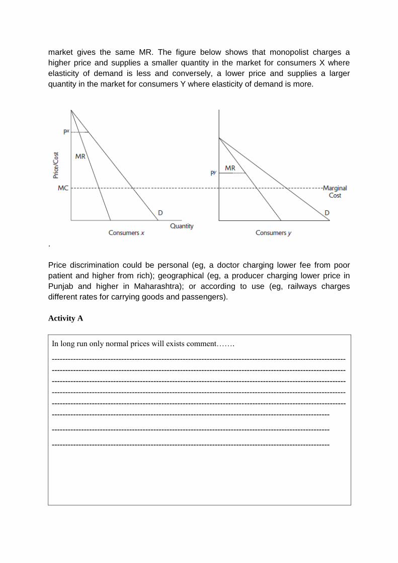
market gives the same MR. The figure below shows that monopolist charges a
higher price and supplies a smaller quantity in the market for consumers X where
elasticity of demand is less and conversely, a lower price and supplies a larger
quantity in the market for consumers Y where elasticity of demand is more.
.
Price discrimination could be personal (eg, a doctor charging lower fee from poor
patient and higher from rich); geographical (eg, a producer charging lower price in
Punjab and higher in Maharashtra); or according to use (eg, railways charges
different rates for carrying goods and passengers).
Activity A
In long run only normal prices will exists comment…….
--------------------------------------------------------------------------------------------------------------
--------------------------------------------------------------------------------------------------------------
--------------------------------------------------------------------------------------------------------------
--------------------------------------------------------------------------------------------------------------
--------------------------------------------------------------------------------------------------------------
--------------------------------------------------------------------------------------------------------
--------------------------------------------------------------------------------------------------------
--------------------------------------------------------------------------------------------------------
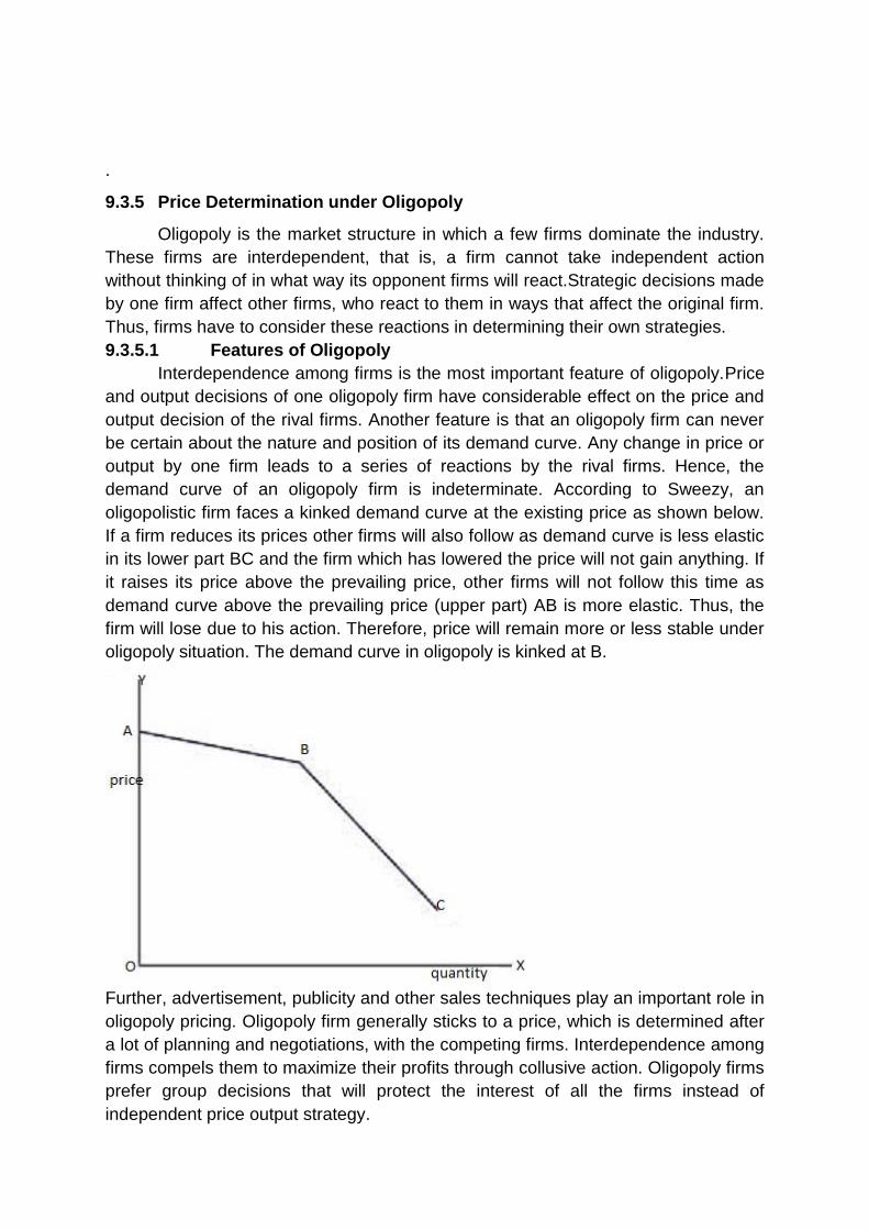
.
9.3.5 Price Determination under Oligopoly
Oligopoly is the market structure in which a few firms dominate the industry.
These firms are interdependent, that is, a firm cannot take independent action
without thinking of in what way its opponent firms will react.Strategic decisions made
by one firm affect other firms, who react to them in ways that affect the original firm.
Thus, firms have to consider these reactions in determining their own strategies.
9.3.5.1 Features of Oligopoly
Interdependence among firms is the most important feature of oligopoly.Price
and output decisions of one oligopoly firm have considerable effect on the price and
output decision of the rival firms. Another feature is that an oligopoly firm can never
be certain about the nature and position of its demand curve. Any change in price or
output by one firm leads to a series of reactions by the rival firms. Hence, the
demand curve of an oligopoly firm is indeterminate. According to Sweezy, an
oligopolistic firm faces a kinked demand curve at the existing price as shown below.
If a firm reduces its prices other firms will also follow as demand curve is less elastic
in its lower part BC and the firm which has lowered the price will not gain anything. If
it raises its price above the prevailing price, other firms will not follow this time as
demand curve above the prevailing price (upper part) AB is more elastic. Thus, the
firm will lose due to his action. Therefore, price will remain more or less stable under
oligopoly situation. The demand curve in oligopoly is kinked at B.
Further, advertisement, publicity and other sales techniques play an important role in
oligopoly pricing. Oligopoly firm generally sticks to a price, which is determined after
a lot of planning and negotiations, with the competing firms. Interdependence among
firms compels them to maximize their profits through collusive action. Oligopoly firms
prefer group decisions that will protect the interest of all the firms instead of
independent price output strategy.
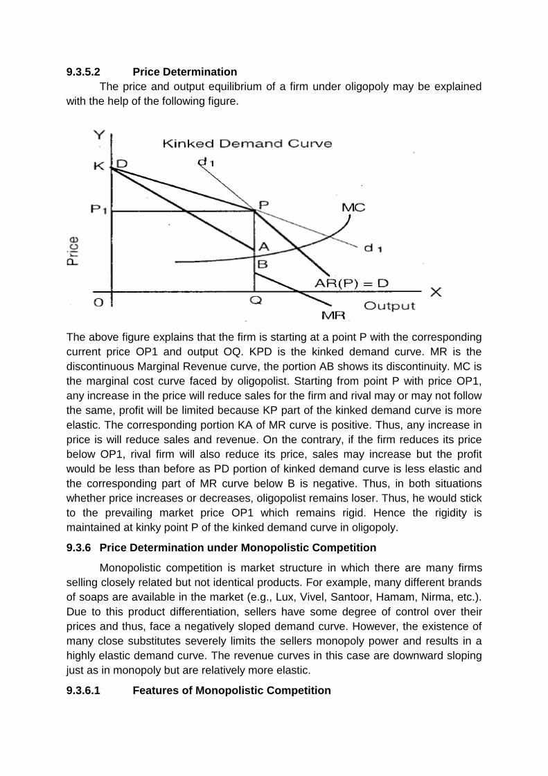
9.3.5.2 Price Determination
The price and output equilibrium of a firm under oligopoly may be explained
with the help of the following figure.
The above figure explains that the firm is starting at a point P with the corresponding
current price OP1 and output OQ. KPD is the kinked demand curve. MR is the
discontinuous Marginal Revenue curve, the portion AB shows its discontinuity. MC is
the marginal cost curve faced by oligopolist. Starting from point P with price OP1,
any increase in the price will reduce sales for the firm and rival may or may not follow
the same, profit will be limited because KP part of the kinked demand curve is more
elastic. The corresponding portion KA of MR curve is positive. Thus, any increase in
price is will reduce sales and revenue. On the contrary, if the firm reduces its price
below OP1, rival firm will also reduce its price, sales may increase but the profit
would be less than before as PD portion of kinked demand curve is less elastic and
the corresponding part of MR curve below B is negative. Thus, in both situations
whether price increases or decreases, oligopolist remains loser. Thus, he would stick
to the prevailing market price OP1 which remains rigid. Hence the rigidity is
maintained at kinky point P of the kinked demand curve in oligopoly.
9.3.6 Price Determination under Monopolistic Competition
Monopolistic competition is market structure in which there are many firms
selling closely related but not identical products. For example, many different brands
of soaps are available in the market (e.g., Lux, Vivel, Santoor, Hamam, Nirma, etc.).
Due to this product differentiation, sellers have some degree of control over their
prices and thus, face a negatively sloped demand curve. However, the existence of
many close substitutes severely limits the sellers monopoly power and results in a
highly elastic demand curve. The revenue curves in this case are downward sloping
just as in monopoly but are relatively more elastic.
9.3.6.1 Features of Monopolistic Competition
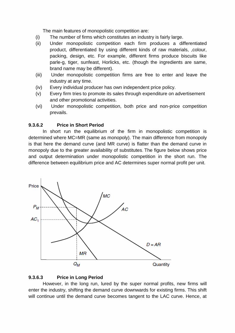
The main features of monopolistic competition are:
(i) The number of firms which constitutes an industry is fairly large.
(ii) Under monopolistic competition each firm produces a differentiated
product, differentiated by using different kinds of raw materials, ,colour,
packing, design, etc. For example, different firms produce biscuits like
parle-g, tiger, sunfeast, Horlicks, etc. (though the ingredients are same,
brand name may be different).
(iii) Under monopolistic competition firms are free to enter and leave the
industry at any time.
(iv) Every individual producer has own independent price policy.
(v) Every firm tries to promote its sales through expenditure on advertisement
and other promotional activities.
(vi) Under monopolistic competition, both price and non-price competition
prevails.
9.3.6.2 Price in Short Period
In short run the equilibrium of the firm in monopolistic competition is
determined where MC=MR (same as monopoly). The main difference from monopoly
is that here the demand curve (and MR curve) is flatter than the demand curve in
monopoly due to the greater availability of substitutes. The figure below shows price
and output determination under monopolistic competition in the short run. The
difference between equilibrium price and AC determines super normal profit per unit.
9.3.6.3 Price in Long Period
However, in the long run, lured by the super normal profits, new firms will
enter the industry, shifting the demand curve downwards for existing firms. This shift
will continue until the demand curve becomes tangent to the LAC curve. Hence, at
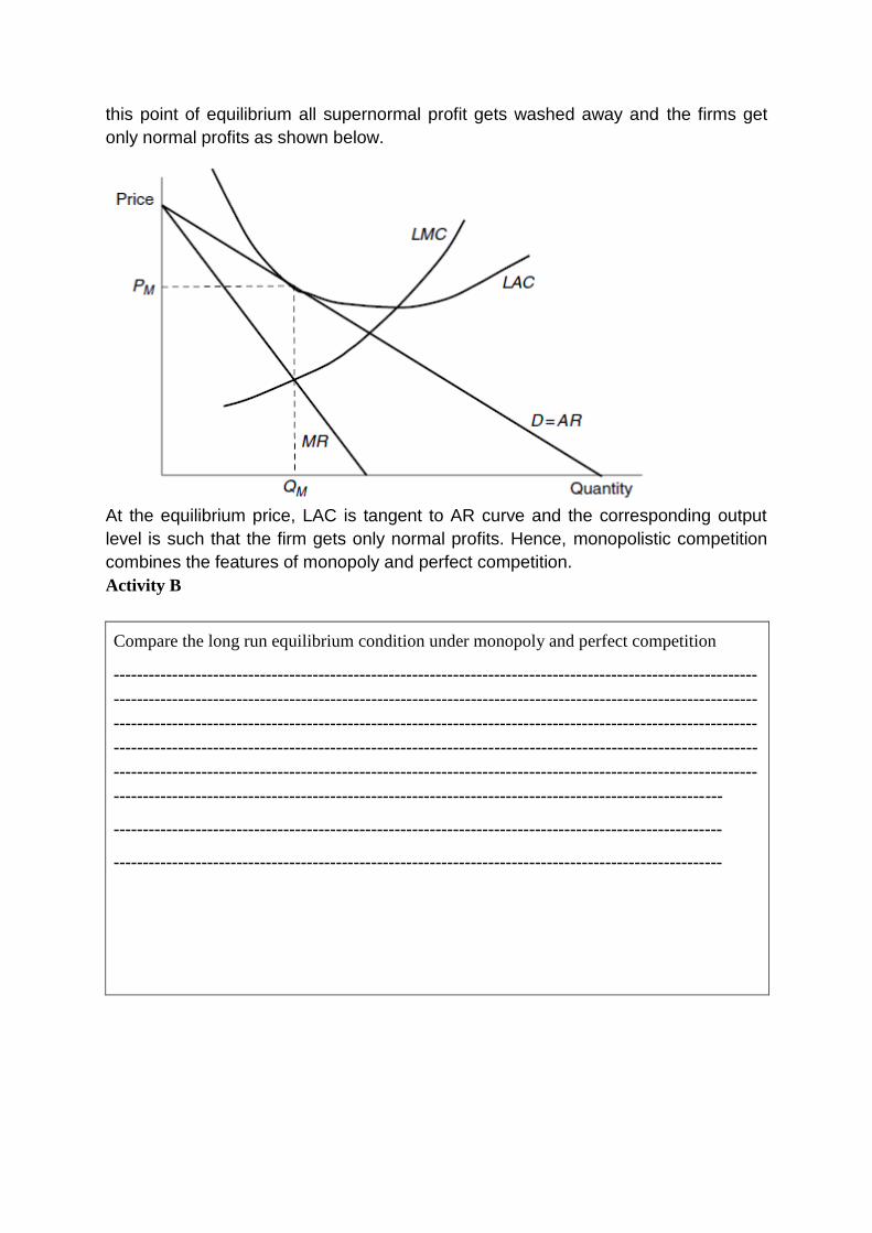
this point of equilibrium all supernormal profit gets washed away and the firms get
only normal profits as shown below.
At the equilibrium price, LAC is tangent to AR curve and the corresponding output
level is such that the firm gets only normal profits. Hence, monopolistic competition
combines the features of monopoly and perfect competition.
Activity B
Compare the long run equilibrium condition under monopoly and perfect competition
--------------------------------------------------------------------------------------------------------------
--------------------------------------------------------------------------------------------------------------
--------------------------------------------------------------------------------------------------------------
--------------------------------------------------------------------------------------------------------------
--------------------------------------------------------------------------------------------------------------
--------------------------------------------------------------------------------------------------------
--------------------------------------------------------------------------------------------------------
--------------------------------------------------------------------------------------------------------
9.4 Check Your Progress B
1. Pure monopoly is a market structure in which there is a ………… firm selling a
commodity which has no ………………….
2. ………………barriers or ………………barriers occur due to factors outside the control
of monopoly firm.
3. In the short period a monopolist cannot charge price less than the …………………
4. In the long run a monopoly firm always makes ……………….. profits.
5. Price discrimination occurs when a monopolist charges ………… prices for the ………
product from different buyers.
6.The demand curve of an oligopoly firm is ……………..
7. Oligopoly firms prefer …………… that will protect the interest of all the firms.
8. Under monopolistic competition firms are free to ……………the industry at any time.
9. In long run a firm under monopolistic competition gets only ……………..
10. In …………………. every firm has its own independent price policy.
9.5 Summary
The word market refers to an effective institutional arrangement which brings
buyers and sellers into contact with one another at a mutually agreed upon price. A
market may be a place (area or region), or a function, or even a process. There can
be different classifications of markets on different basis. However, on the basis of the
degree of competition among the buyers and sellers there are three main types of
markets – perfect competition, imperfect competition, and monopolistic competition.
The market structure plays a crucial role in the pricing decisions made by a firm and
control of a firm over the price of its own product. Perfect competition is a market
situation in which there is an infinitely large number of buyers and sellers dealing in
homogeneous products and single price prevails in the market. The price
determination under perfectly competition is studied under three different time
periods - market period or very short period, short period and, long period. Monopoly
is a market structure in which there is a single firm selling a product which has no
close substitutes.There is virtually no way into a monopoly’s market and no
immediate competitors exist. Strong barriers to entry could be structural and
strategic barriers.Price discrimination occurs when a monopolist charges different
prices for the same product from different buyers, different markets or for different
uses of the same product. Oligopoly is the market structure in which a few firms
dominate the industry. On the other hand, monopolistic competition is market
structure in which there are many firms selling closely related but not identical
products.
9.6 Glossary
Market: An effective institutional arrangement which brings buyers and sellers into
contact with one another at a mutually agreed upon price.
Perfect Competition: A market situation in which there are a large number of
buyers and sellers dealing in homogeneous products and same price prevails in the
market.
Market Period: Market period or very short period is the time period in which the
market supply of the commodity remains fixed.
Monopoly: A market structure in which there is a single firm selling a product which
has no close substitutes.
Oligopoly: A market structure in which a few firms (which are interdependent)
dominate the industry.
Monopolistic Competition: A market structure in which there are many firms selling
closely related but not identical products.
9.7 Answer to Check Your Progress
Check Your Progress A
1. False
2. False
3. False
4. True
5. True
6. True
7. False
8. True
Check Your Progress B
1. Single, close substitutes
2. Structural, natural
3. Average variable cost (AVC).
4. super normal
5. different, same
6. kinked
7. group decisions
8. enter and leave
9. normal profits.
10. monopolistic competition
9.8 References
Mathur N.D., Managerial Economics, Shivam book House (P.) Limited, Jaipur
Mehta P.L. : Managerial Economics-Analysis Problems and Cases: Sultan Chand,
New Delhi.
Salvatore, Domonick, Managerial Economics, Thompson South-Western.
Douglas, Evan J., Managerial Economics: Theory, Practice and Problems, Prentice
Hall Inc., NJ.
Geetika, Managerial Economics, Tata McGraw Hills
9.9 Suggested Readings
Gupta, E.S: Managerial Economics, Tata MC Grow Hill, New Delhi
Dholakiya R.H. and A.H. Ojha: Micro Economics for Management students, Oxford
University Press, Delhi.
Mathur N.D., Managerial Economics, Shivam book House (P.) Limited, Jaipur
Mishra &Puri : Managerial Economics, Himalaya Publishing House, Mumbai
Mithani D.M.: Managerial Economics, Himalaya Publishing House, Mumbai
Dwivedi, D.N: Managerial Economics, Vikas Publishing House Pvt. Ltd, New Delhi
9.10 Terminal and Model Questions
1. What do mean by the term market?
2. Explain the meaning of perfect competition.
3. How is price determined under perfect competition?
4. Why is the demand curve kinky in oligopoly?
5. Discuss in detail price discrimination under monopoly?
6. Give the features of monopolistic competition.
7. How is equilibrium price determined in the long run under monopoly?
8. Why is the study of market structure important?

Chapter 10
Pricing Methods and Approaches
Structure
10.1 Objectives
10.2 Introduction
10.3 Meaning of Price
10.4 Pricing Methods and Approaches
10.5 Pricing Objectives
10.6 Price Discrimination
10.7 Product Line Pricing
10.8 Cost Control
10.9 Conclusion
10.10 Check your Progress
10.11 Glossary
10.12 References
10.13 Suggested Readings
10.14 Model Questions
10.1 Objectives
To study the Pricing Objectives and methods
To study the different types of price discrimination
To understand the concept of product line pricing
To study the ways of cost control.
10.2 Introduction
Given the cost and demand curves, price and output are so determined
that profit is maximized. There are no cut and direct rules for pricing as every
firm has different market situation and are having distinctive features. Thus
every firm follows a variety of pricing rules and methods depending on its
objectives and conditions faced by them.
10.3 Meaning of price
Price can be defined as the exchange of goods or services in terms of
money. Without money, there is no exchange of goods, but without price; there
is no exchange value of a product or service agreed upon in a market
transaction. Thus, What you pay is the price for what you get. Price is the
exchange value of goods or services in terms of money.
10.4 Pricing Methods and Approaches
The method of pricing can be classified into three broad categories. These are:
1. Cost oriented pricing:
(a) Cost plus pricing
(b) Marginal (or incremental pricing)
(c) Target pricing
(d) Programme pricing
2. Competition oriented pricing:
(a) Going rate pricing
(b) loss leaders
(c) Trade association pricing
(d) Customary pricing
(e) Price leadership
(f) Cyclical pricing
(g) Initiative pricing & suggested pricing
h) Multi-Product Pricing
3. Pricing based on other economic considerations:
(a) Administrated pricing
(b) Dual pricing
(c) Price discrimination or differentiated pricing
1. Cost oriented pricing:
a) Cost plus pricing: Cost plus pricing is a most commonly adopted method.
The theory of full cost pricing has been developed by Hall and Mitch.
According to them, under the conditions of oligopoly and monopolistic
competitive markets, business firms do not determine price and output with
the help of the principle of MC = MR.
Price is determined on the basis of full average cost of production AVC +
AFC margin of normal profit.
Under the method, the price is estimated by adding a certain margin to
the cost of the product per unit. Under this method, cost includes production
cost (both variable and fixed) and administrative and selling and distribution
cost (both variable and fixed). This method is also known as margin pricing or
average cost pricing or full cost pricing or mark-up pricing.
Cost-plus Pricing = Cost + Fair Profit.
Advantages
• It is the most easy and convenient method
• It fulfills the objective of profit maximization
• Reduce cost of decision making
• Price considered are fair from point of view of consumers
• More popular and suitable in industries where price leadership prevails
Limitations
• Only consider cost not demand
• It does not accurately take account of competitive forces
• This method cannot provide suitable basis for fixing price
• This method cannot be applied to industries dealing with perishable goods
b) Marginal Cost Pricing: Under the marginal cost pricing, the price is
determined on the basis of marginal or variable cost. In this, fixed cost is
totally excluded and price of product is based on incremental cost of
production. The firm uses those costs that are directly attributed to the output
of a specific product. Pricing decision is basically for the future and as such, it
should be dealt solely with the estimated revenues, expenses and capital
outlays. All type of past outlays, i.e. : historical cost and sunk cost belongs to
the full cost.

Advantages
• It is the most suitable method of short run pricing
• It is useful for pricing over the life cycle of product
• In case of multi-product, multi-process and multi-market firms, marginal
cost pricing seems satisfactory
It is useful at the time of introducing a new product.
Limitations
•It is help only in short period pricing so applied only on a temporary basis
•It does not give guarantee that firm will operate at break even point.
This method leads to cut-throat competition.
c) Target (or Rate of Return) Pricing: It is updated version of cost plus
pricing. When firm revised price, it need to ensure that prices so revised will
allow it to maintain:
Fixed percentage mark up over cost
Profit as a percentage of total sales
Fixed return on existing investment
ROR Price = Full cost + Mark up
FullCost
Earnings
investedCapital
Earnings
tFull
invertedCapitalupMark
cos
d) Programmed pricing: In Programmed pricing, price is related to supply
price. In order to cover own cost and profit margin, a mark-up is put over the
supply price. This supply price may be the wholesale price or that of the goods
at godown. Such practice is popular in wholesale and retail trade.
2) Competition oriented pricing
a) Going rate pricing: It is the price where firm examines the general price
structure prevalling in the industry and accordingly fixes its own price. It is
adopted by those industries which have price leadership characteristic. This
price is the safest policy as it saves the firm from the hazards of price wars.
Moreover, calculations in such pricing are less costly and troublesome for the
business.
b) Loss leader: A loss leader Is an item which produces a less than customary
contribution or a negative contribution to overhead but expected to create
profit on increased future sales or sales of other items. Sometimes, the firms
which deals in multiple products, charge relatively low on some popular
product with the hope that that customer, who come for this product, will also
buy some other products produced and sold by the firm. Such a product is the
firm‟s loss leader. The basic idea of loss leader product is that the profits thus
sacrificed will be made by selling other goods at profit.
c) Trade association pricing: It is used to avoid uncertainties of pricing
decisions and downward pressure on prices which competition exerts. For this,
firms frequently come to express or implied agreements to maintain prices at
similar level.
d) Customary pricing: In case of some commodities prices get fixed because
they have been prevailed over a long period of time. Any change in cost for such
products reflected in its quality and quantity of product rather than its price.
For example: Price of cup of tea in market is customary fixed.
e) Price leadership: When there is one or many big firms in an industry whose
cost of production is low, they dominate the industries. In such a situation,
small firms do not want to enter into the price war and as a result small firms
follow the price fixed by leader.
f) Cylindrical pricing: It is used when pricing by firm is based on assessment
of general economic environment. Such firm has to reduce price in case of

depression and rise price in boom period and ignoring the fact that cost of
production remain unchanged. Price adjustment may be based on:
(1) Cost changes
(2) Price of substitutes
(3) Change in general price level
(4) Market share
(5) Industry‟s other price determinants
g) Suggested prices: It is one in which wholesaler or manufacturer has found
feasible, given the market conditions. It suggests to retailer to charge this price
from customers. This helps the management of retail trade from undertaking
its own assessment of market and cost conditions.
h) Multi-product pricing:
The price theory of price discrimination is based on the assumption that
a firm produces a single, homogenous product. But in actual practice, there is
not a single firm which produces a single homogenous product. Usually, all
firms produce a number of related products at the same time. These are multi
product firms.
For example, the various models of the refrigerators, TV sets, radio are
produced by the same company and set different prices for different products.
Each product has different AR and MR curves and thus firm charging different
prices for all products and this is known as multiproduct pricing strategy. In
multiproduct pricing strategy, the firm considers that the demands for the
various goods are inter-related and thus enjoy a greater cost economy in the
sense that production costs tend to be lower when the goods are produced in a
joint operation. Due to the joint operation, the firm has to look into the cross
— elasticity of demand for the multi-product. Thus, Multi goods produced by
the firm may be in two categories :
• Substitutes/competitive
• Complementary

Complementary products will have negative price Cross-elasticity demand
coefficient where as Substitutes products will have a positive price-cross-
elasticity demand coefficient.
In multiple products, firm considers demand elasticity while deciding
about pricing strategy. The product will be high priced when they are having
inelastic demand While, the product having more elastic demand will be low
priced. In the same way, cost functions will be taken into account. Products
which cost high, will be high priced, with high margin for the make-up.
The multi-product pricing strategy helps in manipulating the
combination of prices for different items, until an optimum or profit
maximising price structure is determined.
3) Prices based on other economic consideration
a) Administrative prices: these are those prices which are statutorily fixed by
government, taking into account cost and stipulated profit per unit. The basic
purpose is to control prices of essential goods and input. This helps weaker
section to have goods at economic prices. Public distribution system, fair price
shops are based on this approach.
b) Dual pricing: A dual market is a market where a commodity is
simultaneously under administrative prices as well as market prices. In such
market, half part of output is subjected to administrative price, while rest is
sold in free market. For example: sugar in India
c) Price discrimination or differentiated pricing: In this, market is
subdivided on some systematic basis, such that it is impossible for buyer to
whom high price is charged to take advantage by shifting to group to which a
low price is quoted.

10.5 Pricing Objectives
Pricing goals or objectives gives direction to the whole pricing process.
The first step in pricing is determining your objectives. For this, one must
consider 1) overall financial, marketing and strategic objectives of the company;
2) the objectives of your product or brand; 3) the availability of resources; and
4) consumer price strategy. After considering the above, one can determine its
pricing objectives.
The basic objective of every pricing strategy is capturing consumer
surplus and converting it into additional profit for the business firm. In figure
11.1, Suppose the firm sold all its output at a single price. To maximize profit,
it would sell at P* and corresponding output at Q*where MC=MR.
Now the managers know that some customers (in region A of the demand
curve) would pay more than P*. But if the firm raises price then it means losing
some customers and hence earning less profits. Similarly, there are other
customers (in region B of the demand curve) who will not pay a price as high as
P*. many of them, however, would pay prices higher than the firm‟s marginal
cost. But by lowering profits, the firm could sell to some of its customers but it
would then lead to earning less revenue from its existing customers and again
profits would shrink.
Now the problem is how can the firm capture the consumer surplus from its
customers in region A and also sell profitably to some of its potential customers
in region B? The solution is price discrimination in which firm might charge
Y
P*
A MC
B
M
D
MR
E
AR
MR
0 Q* x
Output
Co
st/
Rev
enu
e/P
rice
Figure 11.1: Capturing Consumer Surplus

different prices to different customers, according to where the customers are
along the demand curve. The concept of price discrimination is discussed in
the next section. Before this, let us discuss some of the common pricing
objectives are:
1. Pricing for Target Return (on investment) (ROI): Every business needs
capital investment either in the form of various types of assets or working
capital. When a businessman invests capital in a business, he calculates the
expected return on his investment. He aimed to earn a certain rate of return on
investment and accordingly, the price is fixed. This price is seller oriented and
thus includes the predetermined average return.
2. Market Share: The expected volume of sales and the target share of the
market are the most important consideration in pricing the products. Some
firms adopt it as the main pricing objective with a view to maintain or to
improve the market share towards the product. A good market share
symbolizes an indicator of progress. By comparing the present market share
with the past market share, manager can know well whether the market share
is increasing or decreasing. When the market share is decreasing, then firm
can fix low price which discouraged the competitions from entering the market
and hence market share increases.
3. To Meet or Prevent Competition: Another objective of pricing is to meet or
prevent competition. While fixing the price, the price of all products produced
by other firms in the same industry, will have to be considered. At the time of
introduction of products to the market, a low price policy is likely to attract
customers, and can establish a good market share. The low price policy
discourages the competitors.
4. Profit Maximization: All business aims to earn maximum profit and the
situation of profit maximization can be enjoyed where monopolistic situation
exists. The ultimate objective should be to maximize profits on total output,
rather than on every item. Thus every firm fixes the price which generates
maximum profits. But there are government regulations and price control
which check that the price so charged will not exploit the consumers.
5. Stabilize Price: It is a long-time objective and aims at preventing frequent
and violent fluctuations in price. When price remains stable, then price war
amongst the competitors also reduces. The prices are formulated in such a way
that during the depression, the prices are not allowed to fall below a certain
level and in the period of boom, the prices are not allowed to rise beyond a
certain level and hence price remains stable.
6. Customer Ability to Pay: The prices that are charged are according to the
person‟s capacity to pay and hence differ from person to person. For instance,
in government hospitals, doctors charge fees for their services according to the
paying capacity of the patient.
7. Resource Mobilization: This is a pricing objective in which the products are
priced in such a way that sufficient resources are made available to the firms
for their expansion, developmental investment etc.
8. Survival and growth: Another important objective of pricing is survival and
achieving the expected rate of growth. According to P. Drucker, avoidance of
loss and ensuring survival are more important than maximization of profit.
9. Prestige and goodwill: Pricing also aims in maintaining the prestige and
enhancing the goodwill of the firm.
10.6 Price Discrimination
According to Barron's Educational Series (2000), “Price Discrimination is
charging a different price for a different product or to a different buyer without
any true cost differential to justify the different price".
10.6.1 Types/ Methods of price discrimination :
There are various types or methods of price discrimination which are
determined on the basis of the strategy or the policy adopted by the firms.
Following are the main methods or types.
1. Discrimination according to markets: The firm may discriminate between
the whole sale and retail market. Thus a commodity may be sold at a lower
price in the wholesale market and at a higher price in the retail market.
2. Discrimination according to income: Discrimination can also be made on
the basis of incomes of various customers. The financial consultant may charge
higher fees from a big businessman while lower fees from a small
businessman.
3. Discrimination according to time: The time when a commodity or service
is bought may also constitute the basis for price discrimination. The rickshaw
service hired during the night hours costs more fare. Doctors may charge
higher fees for the night visits.
4. Discrimination according to national boundaries: A monopolist may
charge higher price in the protected domestic market but a lower price across
the national boundary. This in other words called as „dumping‟.
5. Discrimination according to utility: Sometimes, different prices are
charged from different customers according to the utilities conferred on them.
Discrimination in first class and second class fares by railways is an example
of this kind. The passenger travelling by first class gets more comforts for
which he pays more.
6. Discrimination according to places: The place where the commodity is
sold is also responsible for price discrimination. The set of „playing cards‟ sold
at railway station shop may cost more than elsewhere.
7. Discrimination according to uses: Sometimes the monopolist may charge
different price for the same service or commodity if used for different purposes.
The electricity charges for example, are more for domestic use than for
industrial use.

10.6.2 Degrees of Price Discrimination
Price discrimination can be divided into three broad forms:
1. 1st Degree Price Discrimination: It refers to charging a different price
based on the customer.
2. 2nd Degree Price Discrimination: It implies charging a different price
based on quantity sold.
3. 3rd Degree Price Discrimination: It refers to charging a different price
based on location of customer segment.
1. First – Degree Price Discrimination: This type of discrimination is also
known as perfect price discrimination. Ideally, a firm would like to charge a
different price to each of its customers. If it could, it would charge each
consumer the maximum price that individual is willing to pay for each unit
bought. This maximum price is the customer„s reservation price. The practice
of charging each customer his or her own reservation price is called first-
degree price discrimination.
This takes out the entire consumer surplus and earns the firms the
maximum possible profits. This method of discrimintation is the most difficult
to adopt as it requires that the company knows each of its customers perfectly
at each level of consumption (Baye, 2006).
2. Second- Degree Price Discrimination: Practice of charging different prices per
unit for diffeeent quantities of the same goods or services is called second-
degree of price discrimination. In this, firm charges separate prices for
different blocks or quantities of the same commodity from the buyers. For
example, Rs 50 per unit for first 10 units, Rs40 per unit for next 10 units and
Rs 30 per unit for another 10 units and so on. This type of discrimination is
usually followed in electricity department.
3. Third- Degree Price Discrimination: Practice of dividing consumers into
two or more sub-markets with separate demand curves and charging
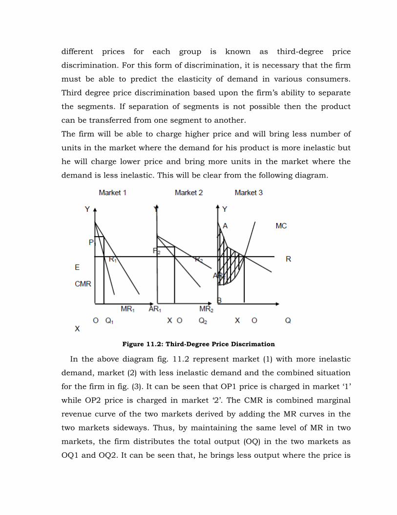
different prices for each group is known as third-degree price
discrimination. For this form of discrimination, it is necessary that the firm
must be able to predict the elasticity of demand in various consumers.
Third degree price discrimination based upon the firm‟s ability to separate
the segments. If separation of segments is not possible then the product
can be transferred from one segment to another.
The firm will be able to charge higher price and will bring less number of
units in the market where the demand for his product is more inelastic but
he will charge lower price and bring more units in the market where the
demand is less inelastic. This will be clear from the following diagram.
Figure 11.2: Third-Degree Price Discrimation
In the above diagram fig. 11.2 represent market (1) with more inelastic
demand, market (2) with less inelastic demand and the combined situation
for the firm in fig. (3). It can be seen that OP1 price is charged in market „1‟
while OP2 price is charged in market „2‟. The CMR is combined marginal
revenue curve of the two markets derived by adding the MR curves in the
two markets sideways. Thus, by maintaining the same level of MR in two
markets, the firm distributes the total output (OQ) in the two markets as
OQ1 and OQ2. It can be seen that, he brings less output where the price is
higher and more output is brought where the price is lower. By doing so, he
can maximize his profits. The total profits earned by him are shown by the
shaded area ARB.
Thus, by dividing the consumers into different sub-markets, the firm can
maximize its profit with the condition that the demand elasticity in both
markets are different and consumers are not able to transfer goods from
one market to another.
10.7 Product Line Pricing
Product line means a group of product items related to each other as
substitutes or compliments. The key economic feature with respect to pricing a
company‟s product line is the cross elasticity of demand.
Pricing of substitute goods: A firm produces substitute goods with a view to
segregate market sectors that have different demand elasticities. Although each
product in the product line competes with similar products of other companies,
they also compete with each other. Pricing policies that push the sales of one
product may consequently hurt the sales of another product of the firm as well
as other firms‟ competing products.
In practice, there are two common methods of product line pricing for
substitute goods. Many producers use mark-up method of pricing on the entire
line of products, with the same margin for all similar products in the line. The
second approach of pricing is to price the product by varying the size of margin
with the level of costs. Thus, more costly the product, higher the product and
vice-versa.
Both of these methods suffer from the defect that they do not considered
the differences in demand, competitive conditions and degree of market
maturity of each product in the line. Moreover, the accounting methods used to
divide joint costs among products of the same firm are whole arbitrary, thus
resulting in prices that reflect the arbitrary allocation of common costs.

Ideally, the optimum price is the one that yields the largest total
contribution margin. The objective of the product-line structure should be that
of exploiting the differences in demand elasticities between market sectors.
Pricing of complimentary goods: The degree of complimentarity can take two
forms:
i) Fixed proportions, like meat and hides; or
ii) Variable proportions, like passenger and freight railway services.
In case of complimentary goods, cross elasticity is negative, i.e, decrease in the
price of one goods leads to an increase in demand for the other goods. The
practical implication is that the sellers may often find it profitable to price an
item low or even sell at loss, in hoping of selling the complementary item at an
above-margin price. But the problem is in the allocation of cost to each
individual output.
1) Fixed Proportion Case: In such case, allocation of cost is not necessary
rather determination of separate price for each product is essential in
order to maximize profits.
2) Varying Proportions Case: In this, the total cost has to be apportioned to
each product because a single MC curve no longer suffices. In such a
case, the optimal price-output combination for the joint products would
require the simultaneous cost and revenue relationships. Linear
Programming approach helps in solving such pricing cases.
10.8 Cost Control
Cost control is defined as the regulation by execution action of the costs
of operating an undertaking. There are the various tools through which
one can execute the technique of cost control. It involves the following
procedure.
1. First of all, plan is set in the form of budgets, standards or estimates,
which serve as a basis for comparing the actual performance with the
planned objectives.

2. After this, communicating the plan to those who is responsible for
execution of this plan.
3. Once the plan executed, evaluation of the performance starts.
4. Comparison is made of the actual performance with the
predetermined targets. Deviations or variances are found out and
reported to the higher officials for further actions.
5. Lastly, the reported variances are reviewed. Either the corrective
actions and remedial measures are taken or the set of the targets is
revised depending upon the management‟s understanding of the
problem.
Thus cost control is a procedure which involves setting standards,
finding deviations which are analysed and reported and hence take the
corrective action. Next area is to know about the major areas in which
cost can be controlled.
10.8.1 Areas of Cost Control
Cost control is essential in following areas:
a) Material Cost: Material cost forms a major part of the total cost of
production. Thus the control and reduction of material cost is extremely
important. Ways of material cost control:
Bulk Buying
Research and Development efforts
Availability of cheaper substitutes
Better utilization of material and inventory control
b) Labour Cost: Reducing labour cost is a very difficult task. Due to the
existence of trade unions and minimum wage legislations, it is not
possible to reduce wage rates. Some other ways of labour cost control
are:
Proper recruitment and training policy
Proper work environment and motivation

Improved methods of production
Proper scheduling of work and materials
c) Overheads Cost: Once the capacity is established, overhead cost is fixed.
A proper selection of capacity, proper layout of plant, a right choice of
equipment and its proper maintenance are likely to keep overheads
down. Some other ways of overheads cost control:
Effective utilization of space and equipment
Reduction in the cost of transportation
Reduction in the cost of energy, i.e. power fuel
Reduction in pilferage, wastage and spoilage
These are the major areas through which cost can be controlled but now the
problem is how one can control these costs. In next section, we will discuss
tools of cost control.
10.8.2 Tools of cost Control
a) Standard cost and budgets: These are those costs that can be obtained
under efficient operations. They are predetermined costs and represent
targets that are considered important for cost control. When comparing
standard performance with the actual performance, one can know about
the area of divergence and the focus area of cost control.
b) Budgetary control: It is a system which used budget as a means of
planning and controlling. It involves the continuous checking and
evaluation of actual performance with the budget goals and hence
helping in taking corrective action.
c) Ratio Analysis: Cost control endeavors can be aided considerably by
using ratio analysis technique. In the ratio analysis, a desirable ratio is
predetermined, the actual performance is compared with this ratio and if
deviation is statistically significant then the corrective action is taken.
d) Value Analysis: It is a method which studies cost in relation to the
product design. It involves the procedure which specifies the functions of

products or components, establishes the appropriate costs, determines
the alternatives and evaluates them.
10.9 Conclusion
There are various methods of pricing. Choosing a particular method of
pricing depends upon the prevailing situations in the economy. Given the lack
of economic training and imperfect knowledge, the business decision makers
decide the simplified pricing method. These methods may be based on cost
considerations, demand conditions or market competitiveness.
10.10 Check your Progress
1. Price- discrimination is possible and profitable, if two markets have
a) Equal Elasticity of Demand c) Different Elasticity of Demand
b) Inelastic Demand d) Highly Elastic Demand
2. Adding a standard markup to the cost of the product refers to:
a) cost-plus pricing c) break-even analysis
b) target profit pricing d) perceived-value pricing
3. When demand elasticity is hard to measure, and firms tend to price
according to the “collective wisdom” of the industry, the pricing method
most likely to be used is called:
a) cost-plus pricing c) break-even pricing
b) sealed-bid pricing d) going-rate pricing.
(Answers: 1c, 2a and 3d)
10.11 Glossary
Consumer Surplus: An economic measure of consumer satisfaction,
which is calculated by analyzing the difference between what consumers
are willing to pay for a good or service relative to its market price. A
consumer surplus occurs when the consumer is willing to pay more for a
given product than the current market price.

Substitute goods: Substitute goods are two goods that could be used for
the same purpose. If the price of one good increases, then demand for the
substitute is likely to rise. Therefore, substitutes have a positive cross
elasticity of demand.
Complimentary goods: A complementary good is a good whose use is
related to the use of an associated or paired good. Two goods (A and B) are
complementary if using more of good A requires the use of more of good B.
For example, the demand for one good (printers) generates demand for the
other (ink cartridges).
10.12 References
Mehta P.L. (2006), Managerial Economics Analysis, Problems and Cases,
Sultan Chand & Sons, New Delhi.
Ahuja H. L. (2005), Advanced Economic Theory, S Chand and Company,
New Delhi.
10.13 Suggested Readings
Dwivedi, D N. (2003), Micro Economics : Theory and Applications;
Pearson Education (Singapore) Pvt. Ltd, Delhi.
Samuelson P.A. & Nordhaus W. D. (1998), Economics, Tata McGraw
Hill, New Delhi.
10.14 Model Questions
1. Explain the method of cost plus pricing. Also state the strength and
weaknesses of this method.
2. Discuss the various pricing objectives.
3. Write short note on
a) Product line pricing
b) Cost Control
Chapter 11
Profit
Structure
11.1Objectives
11.2 Introduction
11.3 Theories of Profit
11.4 Profit Planning
11.5 Break Even Analysis: A technique of profit planning
11.6 Conclusion
11.7 Check your Progress
11.8 Glossary
11.9 References
11.10 Suggested Readings
11.11 Model Questions
11.1 Objectives
To study the various theories of profit
To understand the technique of profit planning
11.2 Introduction
Profits are the fourth factors of production and are the reward for enterprise.
In common language, profit denotes the net income of a businessman. It is
calculated by subtracting total expenditure from the total revenue. In short,
profit is a return to the entrepreneur for the use of his entrepreneurial ability.
There are various hypothesis explaining the emergence and growth of
profits. Thus, there are several theories of profit which explaining the different
views on profit. These theories are discussed in next section.
11.3 Theories of Profit
There are several theories of profit, though none of them is complete in itself to
give a fairly reasonable insight but yet gives partial insight into the process of
emergence of profits. These are:
1. Dynamic Surplus theory of Profit
2. Innovation theory of profit
3. Risk and uncertainty theory of Profit
4. Monopoly Theory of Profit
11.3.1 Dynamic Surplus theory of Profit
This theory is given by the J. B. Clark, who is of the view that there can
be no profit in the static world where size and composition of the population,
the number and variety of human desires and taste, techniques of production,
technical knowledge, commercial organization, etc. remain constant. In a world
like this, everything is certain and is knowable and can be accurately foreseen.
There is no risk, and hence no profit. Costs and selling price remains same,
and hence there can be no profit beyond wages for the routine work of
supervision.
But in the real world, we are not living in a stationary state. Ours is a
dynamic world and some changes are always taking place. The able
entrepreneur foresees these changes and hence makes profits.
Thus According to this theory, profit arises because the world is dynamic
that it is possible for them to keep the lead and reap the profits. In a static
state, there will be no profits, and the entrepreneurs will only earn wages of
management.
Criticism:
Prof. Knight, however, viewed that only those changes which cannot be
foreseen will generate profits and not others. Change may provide a situation
out of which profit will be made, if it brings about ignorance of the future”.
Thus, according to Knight, it is the uncertainty, and not the change, which is
the cause of profit.
11.3.2 Innovation theory of profit
According to the dynamic theory of profits, it is the dynamic changes
which give rise to profits. American economist Joseph Schumpeter viewed that
profit arises because of innovate. As long as entrepreneurs able to hit at one
innovation or another, keeping their business ahead of others and thus making
handsome profits.
According to Schumpeter, the major task of the entrepreneur is to make
innovations and hence profits are a reward for successful innovations.
Schumpeter has given the term „innovation‟ which means that “Discovery of a
new material or a new technique of production”. This innovation helps in
lowering the cost of production or improving the quality of the product.
Innovations may be of two types:
(a) First innovation is changing the production function and hence lowering
the cost of production. This includes the introduction of new machinery, new
production techniques or processes, introduction of a new source of raw
material or a new and better organisational pattern for the firm.
(b) Second innovation is one which stimulate the demand for the product, i.e.,
which change the demand or utility function. This includes introducing a new
product or a new variety of an old product, new and more effective mode of
advertisement, discovery of new markets, etc.
Success of any of these innovations generates a increase in profits.
Profits increase either because of the lowering cost of production or the product
fetches a higher price. It may be noted that profits generated because of
innovations are only temporary and as soon as competitor bring out new
innovation, their profits tend to be competed away.
One must also remember that profits are both the cause and effect of
innovations. Profits serve as a basis for making innovations; hence profits are a

cause of innovations. But since innovations generate profits, thus profits are
the effect of innovations.
Criticism:
Schumpeter‟s innovation theory can be criticised on the following grounds:
(a) Like Clark, Schumpeter also ignores uncertainty as a source of profit.
(b) He also refuses that risk-bearing plays any role in the determination of
profit.
11.3.3 Risk and uncertainty theory of Profit
Risk bearing theory: This theory was developed by the American economist
prof. Hawley in his book Enterprise and productive process published in 1907.
According to this theory profit is a reward for risk bearing. Every
business has some level of risk because all business is more or less
speculative. Thus profit is not reward for differential ability rather it depends
upon the risk taking ability of the entrepreneur. He cannot delegate the
function of risk taking, he alone has to bear the risk and thus profit is the
reward for this risk taking.
The degree of risk affects different business in different way. According
to Prof. Hawley there is a positive relationship between risk and profit - higher
the risk greater is the possibility of profit and vice-versa.
Criticisms:
The risk bearing theory has been criticized on the following grounds.
1) Profit is not the reward for risk bearing but it is the reward for avoiding the
risk.
2) There is never a direct relation between the extent of risk and the amount of
profit.
3) Some risks are 'INSURABLE' and hence shitted over to the insurance
company- the entrepreneur therefore does not bear that risk.
4) The theory overlooks other factors like monopoly, innovation, unexpected,
situation etc which can create profit.
Uncertainty Bearing Theory: Prof. Knignt made a refinement in Hawley‟s risk
bearing theory of profit. According to Prof. knight, pure profit are linked with
uncertainty and risk bearing. For this, he classified risk in the following:
(1) Insurable Risks
(2) Non- Insurable Risks.
Every business has some risk and out of which some risk are predictable while
some are non-predictable. To save business from predictable risk, firms usually
takes insurance. Hence if risk arises, business does not have to bear the risk.
Actual ability of entrepreneur is reflected in bearing non insurable risks. There
risks are uncertain and non-calculable. Such risks being unpredictable, no
insurance company would be willing to cover them. Some examples of non-
insurable risks are fluctuations in demand, depression phase of trade cycle.
Technological changes, changes in degree of competition, changes in govt.
policies etc.
Thus, profit is an exclusive reward for the entrepreneur, for making
business decision under unpredictable and uncertain economic condition. In
short Knight theory implies that uninsurable risks are uncertainty of business
and Profit is the reward for uncertainty bearing.
Criticisms:
The uncertainty bearing theory has been criticized on the following grounds.
1) Uncertainty of business is not only the determinants of profit. There are
other factors also which influence the earning of profit.
2) In fact it is managerial skill rather than uncertainty which leads to higher
profit.
3) The theory dose not focus on the phenomenon of monopoly profit.

11.3.4 Monopoly Theory of Profit
Besides the theories which explain the emergence of profit through dynamic
changes, innovation and uncertainty bearing, there is a strong reason to
believe that monopoly is another source of profit. Monopolistic situation gives
rise to profits both in static and dynamic conditions. Monopolists commands
control over the price of a product and therefore, manages to make profits by
virtue of his monopoly power. He raises price by restricting his level of output
and thereby makes profit.
Criticism:
Monopoly theory of profit is only a partial explanation of the emergence of
profit. If profits had been solely dependent on monopoly power, then a
producer must always create conditions where he can exercise certain
monopoly power to get profits. In real life, this is not always true.
11.4 Profit Planning
Profit planning is a method in which environments affecting an
organisation are analysed, the available resources and internal competence is
identified, agreed objectives are established and plans made to achieve these
objectives. Profit planning is routine job and covers a definite time span.
11.4.1 Need for Profit Planning:
Need for profit planning are as follows:
(i) To improve performance of the management.
(ii) To ensure that the organisation as a whole moves in the right direction.
(iii)To ensure that objectives should be set which will stretch but not overwhelm
managers.
(iv)To encourage strict evaluation of manager‟s performance in monetary terms.
(v) To run a company in a more demanding way.
11.5 Break Even Analysis: A technique of profit planning
The break-even analysis (BEA) has considerable significance for economic
research, business decision-making, company management, investment
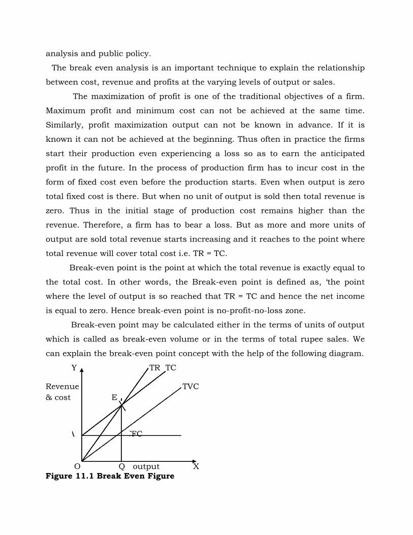
analysis and public policy.
The break even analysis is an important technique to explain the relationship
between cost, revenue and profits at the varying levels of output or sales.
The maximization of profit is one of the traditional objectives of a firm.
Maximum profit and minimum cost can not be achieved at the same time.
Similarly, profit maximization output can not be known in advance. If it is
known it can not be achieved at the beginning. Thus often in practice the firms
start their production even experiencing a loss so as to earn the anticipated
profit in the future. In the process of production firm has to incur cost in the
form of fixed cost even before the production starts. Even when output is zero
total fixed cost is there. But when no unit of output is sold then total revenue is
zero. Thus in the initial stage of production cost remains higher than the
revenue. Therefore, a firm has to bear a loss. But as more and more units of
output are sold total revenue starts increasing and it reaches to the point where
total revenue will cover total cost i.e. TR = TC.
Break-even point is the point at which the total revenue is exactly equal to
the total cost. In other words, the Break-even point is defined as, „the point
where the level of output is so reached that TR = TC and hence the net income
is equal to zero. Hence break-even point is no-profit-no-loss zone.
Break-even point may be calculated either in the terms of units of output
which is called as break-even volume or in the terms of total rupee sales. We
can explain the break-even point concept with the help of the following diagram.
Y TR TC Revenue TVC & cost E
A TFC O Q output X
Figure 11.1 Break Even Figure
In the diagram X axis represents level of output and Y axis represent
revenue & cost. TFC is the total fixed cost curve which is an intercept on Y axis
at point „A‟. TVC is the total variable cost, TC is the total cost which is the sum
of TFC & TVC and TR is the total revenue which starts from origin and slopes
positively upward from left to right shows that TR increases with an increase in
sales. Till OQ output the total cost is more than total revenue and therefore the
area AOE indicates the area of losses. But as output increases to OQ level, TR =
TC at point E. If the output is increased beyond the OQ level TR increases much
faster than TC and hence total profit goes on increasing. Thus the point „E‟ is
called as Break-even point.
Assumptions- Break-even analysis is based on the following assumptions.
1. The cost function and revenue function are linear.
2. The total cost is divided into fixed and variable costs.
3. The selling price is fixed.
4. The volume of sales and production are identical.
5. Prices of factors are remaining constant.
6. Productivity and efficiency remains unchanged.
BEP in terms of total number of units of output/ break even volume – Algebraically, the break even volume is measured by the following formula.
tiableice
tFixedevenvolumeBreak
cosvarPr
cos
Let us explain with the help of following example. Suppose the FC of a firm
is 7,000. Variable cost per unit of output is 15/-. Price per unit is 50/- We can find out the break even level of output with the help of above formula.
1550
7000
BEV
7,000 = ---------
35 = 200 units

BEP in terms of total rupee sales- Total sales value or Total Revenue = P × Q
= 50× 200 =10,000. Total Cost = FC + VC
TFC = 7,000 TVC = VC per unit × Total number of units of output.
= 15 × 200 = 3,000 TFC + TVC = TC 7,000 + 3,000 = 10,000
TR - TC = Net income is equal to zero. TR 10,000 – TC 10,000 = 0 Hence, total profit is zero and thus 200 units is the break-even level output.
Limitations- Break-even analysis has following limitations.
1. Break-even analysis is based on certain assumptions which are assumed to be
constant. This implies a static in nature. It is not applicable to the dynamic
situation.
2. Break-even analysis is unrealistic because it is based on many assumptions.
Linear cost and revenue functions are true only for a limited range of output.
3. It fails to explain the impact of technological change, better management,
division of labour, improved productivity and other factors which influence
profits.
4. It assumes horizontal demand curve with the constant price. It is possible only
in case of perfect competition. But it is not true in case of monopoly.
5. The scope of break even analysis is limited to the short run only.
6. The break even analysis does not consider elements of uncertainty due to tax
structure.
Usefulness of BEA-
1. BEA is useful for decision-making in regards to pricing, cost control, product-
mix, channels of distribution etc.
2. It is a useful tool of managerial planning.
3. It can be used for determining the safety margin.
4. It provides a microscopic view of the profit structure of the firm.
5. It is useful for determining the quantity of output and level of sales of a firm.

6. We can compare the profit margin of different firms with the help of BEA.
7. BEA is useful to understand the relationship between firm‟s cost, revenue,
production, loss and profit.
11.6 Conclusion
Several theories have been formulated to explain how profits arise but
unfortunately none of these theories provide a comprehensive explanation of
the profit. The fact is that, in the real world, there are several factors which
give rise to profit, but the principal factor is uncertainty. It is uncertainty
which is the basic reason of profit. This uncertainty is due to the dynamic
changes of the world. And there is not a single entrepreneur who can foresee
all these changes nor all the circumstances are under his control.
11.7 Check your Progress
1. Which of the following would be considered to be one of the major faults of
break-even analysis and target profit pricing?
a. They do not take into account the price-demand relationship.
b. They are very complicated to calculate.
c. There are serious time lags in the calculations.
d. Most managers do not have confidence in the methods.
2. The following assumptions are made in case of break even analysis, except
a. All fixed costs are fixed
b. All variable costs are fixed
c. The prices of input factors are constant
d. Volume of production and volumes of sales are equal
3. Which theory of profit holds that profit will be higher in industries
characterized by a high degree of variability in their revenues or their costs?
a. Risk-bearing theory
b. Frictional theory
c. Monopoly theory
d. Innovation theory
(Answers: 1a, 2b, 3a)
11.8 Glossary
Fixed Cost: These are defined as expenses that do not change as a
function of the activity of a business, within the relevant period. For
example, a retailer must pay rent and utility bills irrespective of sales.
Variable cost: Variable costs are those costs that vary depending on a
company's production volume; they rise as production increases and fall as
production decreases. Variable costs differ from fixed costs such as rent,
advertising, insurance and office supplies, which tend to remain the same
regardless of production output.
11.9 References
Mehta P.L. (2006), Managerial Economics Analysis, Problems and Cases,
Sultan Chand & Sons, New Delhi.
Dwivedi, D N. (2003), Micro Economics : Theory and Applications;
Pearson Education (Singapore) Pvt. Ltd, Delhi.
11.10 Suggested Readings
Samuelson P.A. & Nordhaus W. D. (1998), Economics, Tata McGraw
Hill, New Delhi.
Ahuja H. L. (2005), Advanced Economic Theory, S Chand and Company,
New Delhi.
11.11 Model Questions
1. Explain briefly the various theories of profit.
2. What is profit planning? Explain the tool of profit planning.
LESSON – 12
Business Cycles
12.0 Objectives
12.1 Introduction
12.2 Meaning and Nature of Trade cycles
12.3 Causes of Trade Cycles
12.4 Check Your Progress A
12.5 Phases of Trade Cycles
12.6 Types of trade Cycles
12.7 Theories of Trade Cycles
12.7.1 Hawtrey’s Pure Monetary Theory
12.7.2 Keynes’ Saving and Investment theory
12.7.3 Hicks’ theory of trade cycle
12.7.4 Over Investment Theory
12.7.5 Under Consumption Theory
12.7.6 Psychological Theory of Trade Cycle
12.8 Control of Trade Cycles
12.9 Check Your Progress B
12.10 Summary
12.11 Glossary
12.12 Answer to Check Your Progress
12.13 References/ Suggested Readings
12.14 Terminal and Model Questions
12.0 OBJECTIVES
After reading this lesson, you should be able:
To understand the meaning and nature of trade cycles
To know the causes and effects of trade cycles
To understand the different phases of trade cycles
To explain different theories of trade cycles
To comprehend controls of trade cycles
12.1Introduction
A glance at economic history reveals that fluctuations in economic conditions
have existed since time immemorial. A prominent feature of modern market-oriented
economies is the existence of economic cycles or fluctuations in the form of the
alternating expansions and contractions that mark cycles in growth. Economic cycles
or business cycles are the recurring fluctuations that occur in real GDP over time.
The business or trade cycles relate to the volatility of economic growth, and the
different periods that the economy goes through. Trade cycles have been closely
connected with the development surges accompanying the economic progress. No
doubt the phases of business cycles are recurring, but their duration, intensity and
scope vary considerably. They have a strong tendency to synchronize industrial,
commercial, and financial processes in the working of an economy. Business cycle
movements often spread from one country to another and sometimes spread to
almost the entire world. A global economic downturn will tend to affect individual
economies. Foreign trade, commodity prices, stock prices, and interest rates play a
vital role in this process of transmission, both directly and indirectly through their
influence on business psychology. Some economists feel that trade cycles cannot be
avoided and so it is not possible for the government to influence and prevent
recessions. However, other economists (prominent among these are Keynes and his
followers) argue that government intervention can definitely help fight and overcome
recessions.
12.2 Meaning and Nature of Trade Cycles
Trade cycles are a type of fluctuation found in the aggregate economic activity
of nations that organize their work mainly in business enterprises: a cycle consists of
expansions occurring at about the same time in many economic activities, followed
by similarly general recessions, contractions and revivals which merge into the
expansion phase of the next cycle; this sequence of changes is recurrent but not
periodic. In other words, business cycle refers to waves of money and economic
activity that forms a regular pattern, defined in terms of periods of expansion or
recession. During expansion, the economy grows in real terms (measured by
indicators like income, output, employment, sales, etc.), after excluding the effects of
inflation. On the other hand, recession is that period when the economy is shrinking
or contracting.
A trade cycle is composed of periods of good trade, characterized by rising prices
and low unemployment percentages, shifting with periods of bad trade characterized
by falling prices and high unemployment percentages. ---Hawtrey
In other words, trade cycles are wave like movements of the economic activity as a
whole, characterised by successive periods of rise and fall. For some years there is
an upward movement extending followed by the downswing for some years and
again followed by an upswing. Usually there is a considerable uniformity in the length
of the cycle (eight or nine years) unless if there are certain exogenous factors
operating such as a war, etc. which might reduce the length of trade cycle to less
than six years or more than eleven years. However, successive cycles differ in
length from each other. This may be attributed to a number of causes including
harvest conditions, domestic politics, changes in monetary and banking systems,
international relations, the conditions of war or peace, the discovery of new industrial
methods, etc. all of which tend to alter the pace of business. The fact however
remains that movements in economic activity are crucial for progress.
During these wavelike movements employment, prices, consumer’s
expenditure, production and investment rise and fall in a successive manner. The
movements in prices and employment moreover also move to and synchronize with
other countries of the world, because in open economies the demand for the
products of various countries is interlinked. Prosperity in one industry creates a
demand for the products of other industries, which, in turn, become prosperous
creating further demand for one still others’ products (psychological factor playing an
important role). Optimism and pessimism in one industry spread to other industries.
However, all industries may be affected by economic fluctuations (depression or a
boom) differently depending on the type if goods being produced. Similarly, the
international character of the trade cycle is strongly influenced by the demands of the
countries for each other’s goods and the psychology of the business class.
Pessimism or even optimism are all the more infectious at the international level,
once started quickly becomes universal. The fluctuations in the business activity,
depressions or booms get easily transmitted from one nation to the rest of the world
if the extent of the international trade is very high, as is prevalent in modern day
economies.
12.3 Causes of Trade Cycles
Various theories to explain the trade cycles share the view that the main
driving force behind the economic fluctuations in an economy (which is also the
original cause of the cycle) is always some sort of shock or disturbance. In addition,
most of the trade cycle theories rest on a propagation mechanism that amplifies
shocks. There exists a need of some propagation mechanism that translates small,
short-lived shocks into large, persistent economic fluctuations if the disturbances are
not big enough by themselves to cause the fluctuations. Some of the possible
shocks and propagation mechanisms are as follows.
Technology shocks: It is a well-known fact that the real world production
functions exhibit a dynamic character and keep changing over time with the
development and introduction of new and improved technologies and
methods of production. Such technical improvements increase the overall
productivity and the production process gets altogether changed. However, on
the other hand, it may be possible that production facilities might break down
or may not work as expected. This may cause the productivity to fall. Hence,
the technological change may not always be smooth as it often comes in the
form of shocks. Improvements in technology may cause a boost in economic
growth while the opposite may also happen.
Weather shocks and natural disasters: Such shocks are faced by those
industries which are dependent on weather conditions, for example,
agriculture or tourism, etc. Fluctuations in the output and productivity of these
sectors is largely influenced by rainfall and sunshine, and even natural
calamities like earthquakes, landslides, floods, cyclones, tsunami, etc. Hence,
weather conditions may act as a potential source of fluctuations in the
economic activity.
Monetary shocks: Real effects of monetary policy may act as monetary
shocks. Therefore, trade cycles or fluctuations in business activity may even
be caused by random changes in money supply or interest rates as also by
other changes in the monetary sector of the economy.
Political shocks: The government influences the working of the economy in
two possible ways - directly through government or public sector enterprises
and indirectly through government regulations and controls influencing
different sectors of the economy. In this context, potential sources of
economic fluctuations may include changes in tax laws, antitrust regulation,
government expenditure and so on. Some economists suggest that there is a
political business cycle especially when politicians try to have a high
economic growth before an election to help win the election.
Taste shocks: Such type of shocks arise from changes or shifts in consumer
tastes, preferences, habits, fashions, etc. (snob effect and bandwagon effect
may introduce taste shocks in the business activity by influencing the
consumer demand patterns). These fluctuations in economic activity are
primarily witnessed in those industries which are strongly influenced by
fashion, style and high fan following, like apparels, music, or movie industries,
foot wears, accessories, etc.
All the above mentioned shocks are present to some degree in every economy but
these may not be potent enough to directly set in trade cycles. There are some
mechanisms present in the economy which perhaps amplify these shocks and
propagate them through time. These may include the following
Sticky prices: The response of market economies to the stimulus of above
mentioned changes or shocks is in the form of price adjustments (both in the
goods market and factor market). For example, in the factor market a negative
productivity shock will lower the marginal productivity of labour, so that the
real wage would have to go down to the demand and supply labour. But as
mentioned in previous chapter, wage cut policy is not very practical and
desirable and hence, the adjustment cannot take place. This in turn leads to
loss of output and unemployment which is much larger than the direct effect of
the shock. Similarly effects arise if prices are sticky in the goods market.
Intertemporal substitution: In continuation with the above example, shocks
having a negative impact on productivity in turn lower the marginal return to
labour along with other factors of production. Fall in marginal products may
reduce the incentive to work, and workers might prefer more of leisure instead
of work. Hence, supply of labour falls further and lowers the output still further.
On the other side, in response to a shock the workers (as consumers) might
cut down their savings to continue smooth consumption. Overall this leads to
lower investment and a lower capital stock in the future, extending the impact
of a shock far into the future.
Frictions in financial sector: Even small shocks can force the directly hit firms
into bankruptcy. This in turn affects other firms and also the banks which gave
credit to these firms. Many a times even banks fail if bad debts rise
excessively, this adversely affects all the creditors and debtors of the bank,
leading to serious economic crises.
On the basis of these causes of trade cycles, business cycle models can be
broadly divided into two categories. On one hand there are some theories which
consider trade cycles as a failure of the economic system. According to these
theories the economy experiences depressions and fails to achieve the efficient level
of output and employment due to frictions (or imperfections of the market mechanism
for example financial frictions, sticky prices, or other adjustment failures. The
Keynesian model of output determination falls into this category where technology
shocks and monetary shocks are considered to be important sources of business
fluctuations. The Great Depression was closely connected to financial sector
disruptions marked by failure of banks and financial instability.
On the other hand, the other category of models that considers trade cycles
as the optimal reaction of the economy to unavoidable shocks. Even if the market
mechanism efficient, the shocks get propagated through intertemporal substitution.
In this case technology shocks are the main cause of economic fluctuations. Such
models are called real business cycle models which can be explained as the optimal
reaction of an efficient market system to economic shocks.

12.4 Check Your Progress A
State True or False
1. A trade cycle is composed of periods of good trade, shifting with periods of bad
trade.
2. Economic fluctuations are country specific and do not extend to other nations of the
world.
3. Trade cycles cannot be caused by technology shocks.
4. A sudden change in fashion may act as a potential source of fluctuation in economic
activity.
5. Real business cycle models are the optimal reaction of an efficient market system to
economic shocks.
6. Sticky prices amplify the effect of shocks to generate trade cycles.
7. The Keynesian model of output determination considers trade cycles as a failure of
the economic system.
12.5 Phases of Trade Cycles
Trade cycle is a wave of economic activity that forms a regular pattern, defined in
terms of periods of expansion (when the economy grows in real terms) or recession
(when the economy shrinks or contracts). A business or a trade cycle has four
phases: expansion- recession-depression-recovery.
Expansion or Prosperity: This is a phase in which there is expansion of
output, income, employment, prices and profits. The standard of living also
rises in this phase. All the macroeconomic parameters witness a substantial
rise. The main features of prosperity are high levels of output and trade,
effective demand, income and employment, rising interest rates, huge
expansion of bank credit, rising prices, high level of marginal efficiency of
capital and investment. The level of production is maximum possible due to
full employment of resources and there is a rise in income. There is a rise in
profits and prices due to a high level of economic activity. There is general
upswing in the economy as the economic activity reaches its peak. The
expansion or prosperity phase is also called boom period.
Recession: This phase is marked by a significant decline in the overall
economic activity. It begins right after the economy reaches a peak of activity
and marks the turning point from prosperity to depression. Due to a fall in
demand there is a decrease in production and future investment and there is
a steady decline in output, income, employment, prices and profits. The wave
of pessimism in the economy reduces investment and hence, halts the
process of business expansion.
Depression: Due to steady and continuous decline in output, income,
employment, prices and profits, there is a fall in the standard of living which
paves way for depression to exist in the economy. The main features of
depression are low levels of output and trade, effective demand, income and
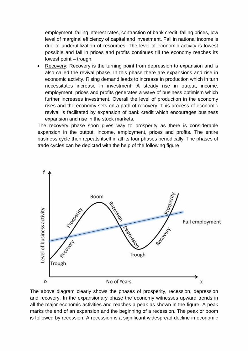
employment, falling interest rates, contraction of bank credit, falling prices, low
level of marginal efficiency of capital and investment. Fall in national income is
due to underutilization of resources. The level of economic activity is lowest
possible and fall in prices and profits continues till the economy reaches its
lowest point – trough.
Recovery: Recovery is the turning point from depression to expansion and is
also called the revival phase. In this phase there are expansions and rise in
economic activity. Rising demand leads to increase in production which in turn
necessitates increase in investment. A steady rise in output, income,
employment, prices and profits generates a wave of business optimism which
further increases investment. Overall the level of production in the economy
rises and the economy sets on a path of recovery. This process of economic
revival is facilitated by expansion of bank credit which encourages business
expansion and rise in the stock markets.
The recovery phase soon gives way to prosperity as there is considerable
expansion in the output, income, employment, prices and profits. The entire
business cycle then repeats itself in all its four phases periodically. The phases of
trade cycles can be depicted with the help of the following figure
The above diagram clearly shows the phases of prosperity, recession, depression
and recovery. In the expansionary phase the economy witnesses upward trends in
all the major economic activities and reaches a peak as shown in the figure. A peak
marks the end of an expansion and the beginning of a recession. The peak or boom
is followed by recession. A recession is a significant widespread decline in economic
activity which begins just after the economy reaches a peak of activity and ends as
the economy reaches its trough. A trough marks the lowermost point of the phase of
depression after which the economy starts showing signs of revival or recovery. A
trough date will mark the end of the recession. Between trough and peak, the
economy is in an expansion phase.
However the length of business cycles is not similar, some cycles are of long
duration while short duration. No matter what is the length of the trade cycle, every
cycle passes through the above mentioned four phases.
Activity A
What is Trade Cycle and describe its various Stages or Phases
-------------------------------------------------------------------------------------------------------------------------------------------------
-------------------------------------------------------------------------------------------------------------------------------------------------
-------------------------------------------------------------------------------------------------------------------------------------------------
-------------------------------------------------------------------------------------------------------------------------------------------------
-------------------------------------------------------------------------------------------------------------------------------------------------
-------------------------------------------------------------------------------------------------------------------------------------------------
-------------------------------------------------------------------------------------------------------------------------------------------------
-------------------------------------------------------------------------------------------------------------------------------------------------
-------------------------------------------------------------------------------------------------------------------------------------------------
-------------------------------------------------------------------------------------------------------------------------------------------------
-------------------------------------------------------------------------------------------------------------------------------------------------
-------------------------------------------------------------------------------------------------------------------------------------------------
-------------------------------------------------------------------------------------------------------------------------------------------------
-----------------------------------------------------------------------------------------------------------------------------------
-------------------------------------------------------------------------------------------------------------------------------------------------
-------------------------------------------------------------------------------------------------------------------------------------------------
-------------------------------------------------------------------------------------------------------------------------------------------------
-------------------------------------------------------------------------------------------------------------------------------------------------
-------------------------------------------------------------------------------------------------------------------------------------------------
------------------------------------------------------------------------------------------------------------------------
-------------------------------------------------------------------------------------------------------------------------------------------------
-------------------------------------------------------------------------------------------------------------------------------------------------
-------------------------------------------------------------------------------------------------------------------------------------------------
-------------------------------------------------------------------------------------------------------------------------------------------------
-------------------------------------------------------------------------------------------------------------------------------------------------
------------------------------------------------------------------------------------------------------------------------
12.6 Types of trade Cycles
According to Schumpeter there are three types of cycles: the major cycles, the minor
cycles and the long waves.
Major Cycles: These type of cycles of economic fluctuations mostly influence the
activities of the businessmen as these basically involve the curse of unemployment
and the wastage of potential wealth. Usually major cycles average between 8 and 9
years from boom to boom but may vary between 6 and 11 years.
Minor Cycles: Such cycles approximately have a duration of forty months. These
cycles have little effect on the day to day operations of most business activities. The
worst hit industries include the ones which are very sensitive to cyclical movement ,
like heavy industries and certain kinds of consumer durables, etc. On the other hand,
firms selling basic foods and low price clothing etc. may not be affected at all. These
minor cycles are superimposed on the major cycles — when the booms and
depressions of the two cycles fall on one another they get intensified.
Long Waves: These cycles have a duration ranging between forty five and sixty
years. They are sometimes also called ―Kondratieff Cycle‖ after the name of the
economist who studied them. Just as the minor cycle is superimposed on the major
cycle, similarly the ―Kondratieff Cycle‖ is superimposed on the major cycle. Good
times during the rising phase of the ―Kondratieff Cycle‖ and bad times during the
falling phase are more prevalent. Hansen found that in each of the long periods of
good times there developed four major recoveries and three major depresssions. In
the downswing of the ―Kondratieff Cycle‖ there developed two major recoveries and
three depressions.
Special Cycles: Besides the above mentioned types of trade cycles, there are
numerous types of special cycles which can be found in particular kinds of economic
series. An important type is the building cycle which seems to have a duration of
about seventeen years. Other examples include cycles in crops, weather, migration
etc.
12.7 Theories of Trade Cycles
There are various theories of trade cycles given by eminent economists to
explain the complex phenomenon of trade cycles but there is no consensus for a
single universal theory accounting for the trade cycles. A trade cycle is a rhythmic
fluctuation in the level of employment, income and output in an economy. Keynesian
theory of output and employment also gives an explanation of the determination of

income, output and employment in an economy at a particular time so in a way,
Keynes also gives and explanation about the cause of trade cycle. Here we discuss
a few important theories of trade cycles including the one by Keynes.
12.7.1 Hawtrey’s Pure Monetary Theory
According to Hawtrey, trade cycle is a purely monetary phenomenon and is
caused by changes in the flow of monetary demand by businessmen in the
economy. The cyclical fluctuations are caused by expansion and contraction of bank
credit which further causes changes in the monetary demand by producers and
traders. The phase of prosperity of trade cycle starts with increase in credit facilities
(by lowering the interest rates or by purchasing securities) by the banks. Cheaper
credit encourages the businessmen to increase their stocks or inventories. Hence,
there is increase in production, employment, and income; again resulting in more
demand. Hence, a circle of cumulative expansion of productive economic activity
sets up leading to higher prices. In turn, traders still further expand their production.
However, this phase of prosperity ends when the banks stop further credit expansion
(due to depletion of their cash funds) and raise the rates of interest. The business
community has to repay their loans for which they need to sell their stocks; as a
result prices start falling and also there is a fall in productive economic activity.
Hence, unemployment may rise due to fall in the demand for the factors of
production, leading to depression – fall in income, output, employment, prices. When
loans are not repaid, banks further contract credit. However, this phase does not
continue endlessly and gradually recovery sets in as the traders try to repay their
loans; cash flows of banks rise. Although pessimism in the economy prevents
traders from borrowing from the banks, central bank plays a key role in initiating
recovery by introducing a cheap monetary policy. Thus, the economy revives and
slowly again expansion starts.
12.7.2 Keynes’ Saving and Investment theory
Although Keynesian theory is not a theory of trade cycle as such, yet it gives a
general explanation for the level of employment by the cyclical nature of changes in
employment. According to Keynes the main cause of trade cycles is the fluctuations
in the rate of investment, which in turn are caused by the marginal efficiency of
capital. Marginal efficiency of capital is the relation between the prospective yield of
capital and the cost of producing the units of output or the expected rate of profit on
new investment or capital goods. The fluctuations in economic activity are attributed
to the expected rate of interest on new investment. Investment is also influenced by
the rate of interest but it is stable in short period (liquidity preference and the quantity
of money which determine the rate of interest do not change significantly in short
period). Hence, fluctuations in investment are mainly due to changes in the marginal
efficiency of capital (as it rises investment will rise leading to expansion). Eventually
there is a decline in the prospective yield on capital due to growing increase of the
capital goods. Fall in marginal efficiency of capital will later result in falling production
and consequent depression. However, a change from depression to recovery is
again due to the revival of the marginal efficiency of capital which pumps in optimism
in the economy by boosting the confidence of the traders. Hence, an increase in
investment is witnessed which causes the income to rise due to the multiplier effect.
Thus, an upward trend or prosperity sets in and hence, the trade cycle operates in
the economy.
12.7.3 Hicks’ theory of trade cycle
Hicks explains the theory of trade cycles on the basis of combination of the
principles of multiplier and accelerator. Investment could be of two possible types -
autonomous investment, and induced investment. Induced investment depends on
the changes in income, output and consumption, whereas autonomous investment is
not at all influenced by the fluctuations in income, output and consumption.
According to Hicks, autonomous investment causes cyclical fluctuations in the
business activity by multiplier effect and induced investment via accelerator effect.
Suppose, initially there is an increase in autonomous investment in the economy. A
multiplier effect will set in and bring about an increase in income and output. This
expansion in the level of income output and employment will increase the induced
investment via the accelerator. Further increases in income are brought about by
multiplier effect and investment by the accelerator principle. This marks the
expansionary phase of the economy which continues till the economy reaches the
upper limit or ceiling determined by full employment. After this upper limit, rate of
expansion in output and income slows down; reducing the amount of induced
investment as the multiplier and accelerator forces start operating in the reverse
direction. This downswing continues till the lower turning point is reached. The
turning point again causes an expansionary phase to set in.
12.7.4 Over Investment Theory
Over investment theory attributes trade cycle to over investment in investment
industries – basic and heavy industries like iron and steel, engineering, building and
construction, etc. This assertion holds true because it is observed that during boom,
capital good industries grow faster than consumption good industries while during
depression capital good industries suffer more than consumption good industries.
There is difference of opinion about the reason of this statement. Some experts
attribute it to banks giving credit at low rates to encourage investment, causing
withdrawal of resources from consumer goods industries to capital goods industries.
The next phase of trade cycle sets in when the banks raise the interest rates to
check credit creation leading to contraction in the economic activity – depression. On
the other hand, some economists feel that the main cause of trade cycle is the
process of production and not the expansion and contraction of bank credit.
12.7.5 Under Consumption Theory
According to Hobson, the main cause of trade cycles is the mal distribution of
national income. During expansion the businessmen amass income with business
activities become richer. Savings also increase as the entire increase in income is
not consumed. Excessive saving during the boom period ultimately leads to
reduction in the level of consumption, hence a fall the demand for consumer goods
Prices begin to fall due to mismatch between demand and supply of consumer
goods. The wave of pessimism initiates a downswing in the economy and leads to
depression. Depression also does continue forever and leads to revival.
12.7.6 Psychological Theory of Trade Cycle
According to Pigou, trade cycles are basically influenced by the psychology of
the businessmen, their optimism and pessimism causes fluctuations in the business
activity. During boom, businessmen earn high profit and expand the investment,
production and employment. There is a wave of optimism in the economy which
leads to prosperity. However, excessive increase in aggregate supply causes prices
and hence profits to fall. Investment, and hence, output and employment also fall.
The wave of pessimism catches up leading to depression.
Activity B
Describe the shocks which are said to cause trade cycles? How are these shocks amplified
in the economy.
-------------------------------------------------------------------------------------------------------------------------------------------------
-------------------------------------------------------------------------------------------------------------------------------------------------
-------------------------------------------------------------------------------------------------------------------------------------------------
-------------------------------------------------------------------------------------------------------------------------------------------------
-------------------------------------------------------------------------------------------------------------------------------------------------
-------------------------------------------------------------------------------------------------------------------------------------------------
-------------------------------------------------------------------------------------------------------------------------------------------------
-------------------------------------------------------------------------------------------------------------------------------------------------
-------------------------------------------------------------------------------------------------------------------------------------------------
-------------------------------------------------------------------------------------------------------------------------------------------------
-------------------------------------------------------------------------------------------------------------------------------------------------
-------------------------------------------------------------------------------------------------------------------------------------------------
-------------------------------------------------------------------------------------------------------------------------------------------------
-----------------------------------------------------------------------------------------------------------------------------------
-------------------------------------------------------------------------------------------------------------------------------------------------
-------------------------------------------------------------------------------------------------------------------------------------------------
-------------------------------------------------------------------------------------------------------------------------------------------------

-------------------------------------------------------------------------------------------------------------------------------------------------
-------------------------------------------------------------------------------------------------------------------------------------------------
------------------------------------------------------------------------------------------------------------------------
-------------------------------------------------------------------------------------------------------------------------------------------------
-------------------------------------------------------------------------------------------------------------------------------------------------
-------------------------------------------------------------------------------------------------------------------------------------------------
-------------------------------------------------------------------------------------------------------------------------------------------------
-------------------------------------------------------------------------------------------------------------------------------------------------
------------------------------------------------------------------------------------------------------------------------
.12.8 Control of Trade Cycles
Although some economists argue that the business cycle is an essential part
of an economy. Even downturns have their role to play in weeding out the inefficient
firms. However, this view is controversial and majority of the economists argue that a
volatile trade cycle may be harmful for the economy. The main measures which have
been suggested for the effective control of trade cycles are as follows:
Monetary Policy: Many economists opine that trade cycle is purely a monetary
phenomenon and hence an effective monetary policy (measures to control the
supply of money and credit). During inflation the central bank can reduce the quantity
of money in circulation by increasing the bank rate, selling of securities in the market,
increasing the reserve ratio of the member banks, by moral persuasion, etc. On the
other hand during depression the quantity of money in circulation can be increased
by appropriate measures. However, monetary policy alone cannot achieve the
desired results (as was seen during Great Depression). The modern economists are
of the opinion that monetary policy can be successful tool to control trade cycles if it
works in coordination with the fiscal policy.
Fiscal Policy: Fiscal policy involves the use of fiscal tools – taxation, government
expenditure, public debt, etc. – to control trade cycles. During inflation, the
government may cut down its own public works programmes, levy heavy taxes,
reduces purchasing power by public debt, etc. On the other hand, during depression,
public works programmes may be increased to increase income, investment and
employment. Fiscal policy is a very sensitive counter cyclical instrument in but needs
to be used in tandem with the monetary policy.
Control of Private Investment: By proper control of private investment in the
economy, the government can help achieve economic stabilization. However, this in
no way means discouraging private investment rather managing it to check
fluctuations.
International Measures: Some economists have suggested the use of measures on
an international scale to check trade cycles as in modern dynamic world business is
an international phenomenon. So business fluctuations should be tackled on an
international level. Important measures in this direction include international
production control, international bill stock control, international investment control,
etc.
12.9 Check Your Progress B
1. The phase of …………. is marked by a significant decline in the overall economic
activity.
2. Hicks theory of trade cycles is based on the combination of the principles
of………………..
3. The best possible way to control trade cycles is to apply ……………. policy in
coordination with the ………….. policy.
4. According to ……….. trade cycle is a purely monetary phenomenon and is
caused by changes in the flow of ……… by businessmen in the economy.
5. The main features of ……. are low levels of output and trade, effective demand,
income and employment, falling interest rates, contraction of bank credit, falling
prices, low level of marginal efficiency of capital and investment.
6. …………. have a duration ranging between forty five and sixty years.
7. Between trough and peak, the economy is in an ……… phase.
8. According to Pigou, trade cycles are basically influenced by ……….. the
businessmen.
12.10 Summary
Trade cycles are wave like movements of the economic activity as a whole,
characterised by successive periods of rise and fall. For some years there is an
upward movement extending followed by the downswing for some years and again
followed by an upswing. The four phases of a trade cycle are expansion, recession,
depression, and recovery and any cycle of whatever duration can be described as
going through these four phases. There is always some sort of shock or disturbance
which causes trade cycle and it is often amplified by some propagation mechanism.
Important ones are technology shocks, monetary shocks, natural shocks or political
shocks. According to Schumpeter there are three types of cycles: the major cycles,
the minor cycles and the long waves. There are various theories of trade cycles
given by eminent economists to explain the complex phenomenon of trade cycles
but there is no consensus for a single universal theory accounting for the trade
cycles. Pure monetary theory by Hawtrey, saving and investment theory by Keynes
are the prominent among these. Other theories by Hicks, Pigou and Hobson are also
important. Trade cycles can be effectively controlled through the judicious and
coordinated use of monetary policy, fiscal policy as well as international measures.
12.11 Glossary
Trade Cycles: Wave like movements of the economic activity as a whole,
characterised by successive periods of rise and fall.
Shocks: Small short-lived disturbances which cause trade cycles.
Expansion or Prosperity: Phase of trade cycle marked by high levels of output and
trade, effective demand, income and employment, rising interest rates, huge
expansion of bank credit, rising prices, and investment.
Depression: When the level of economic activity is lowest possible.
Recovery:Turning point from depression to expansion, also called the revival phase.
Over Investment Theory: Attributes trade cycle to over investment in investment
industries
Pure Monetary Theory: Given by Hawtrey, attributes trade cycles purely to changes
in monetary demand.
Long Waves: Trade cycles having a duration ranging between forty five and sixty
years. They are sometimes also called ―Kondratieff Cycle‖.
12.12 Answers to Check Your Progress
Check Your Progress A
1. True
2. False
3. False
4. True
5. True
6. True
7. True
Check Your Progress B
1. recession
2. multiplier and accelerator
3. monetary, fiscal
4. Hawtrey, monetary demand
5. Depression
6. Long waves
7. Expansion
8. Optimism and pessimism
12.13 References/ Suggested Readings
Dwiwedi, D. N., Macroeconomics: Theory and Policy, Tata McGraw Hill Publishing,
New Delhi.
McConnel , C. R. & H. C. Gupta, Introduction to Macro Economics , Tata McGraw–
Hill, New Delhi
K.K .Dewett, Modern Economic Theory, S. Chand Publication
D.M.Mithani, Managerial Economics Theory and Applications, Himalaya Publication
Peterson and Lewis, Managerial Economic, Prentice Hall of India
Gupta, Managerial Economics, TataMcGraw Hills
Froeb, Managerial Economics, Cengage Learning
12.14 Terminal and Model Questions
1. What do you mean by a trade cycle?
2. Discuss the various phases of business cycles?
3. Explain the causes of trade cycles.
4. Discuss in detail the Hicks’ theory of trade cycles.
5. How can monetary policy be used to tackle fluctuations in the business activity?
Related Documents