Ann´ ee acad´ emique 2007–2008 Th´ ese pr´ esent´ ee en vue de l’obtention du titre de Docteur en Sciences de l’Ing´ enieur Promoteur: Prof. Marco Dorigo Roderich Groß Self-Assembling Robots Universite Libre de Bruxelles Universite d’Europe Facult´ e des Sciences Appliqu´ ees CoDE, Department of Computer & Decision Engineering IRIDIA, Institut de Recherches Interdisciplinaires et de D´ eveloppements en Intelligence Artificielle

Welcome message from author
This document is posted to help you gain knowledge. Please leave a comment to let me know what you think about it! Share it to your friends and learn new things together.
Transcript

Annee academique 2007–2008
These presentee en vue de l’obtention dutitre de Docteur en Sciences de l’Ingenieur
Promoteur:Prof. Marco Dorigo
Roderich Groß
Self-Assembling Robots
Universite Libre de BruxellesUniversite d’Europe
Faculte des Sciences AppliqueesCoDE, Department of Computer & Decision Engineering
IRIDIA, Institut de Recherches Interdisciplinaires
et de Developpements en Intelligence Artificielle


Universite Libre de Bruxelles
Roderich Groß
Self-Assembling Robots


Copyright c© 2007 by Roderich GroßAll rights reserved.
This dissertation was discussed in a public defense held at the Universite Libre deBruxelles, Brussels, Belgium, on October 12, 2007. In this occasion, Roderich Groß wasawarded a European Doctorate title in engineering sciences.
Composition of the jury:
Andre PreumontProfessor, Universite Libre de Bruxelles, Brussels, BelgiumPresident of the jury
Hugues BersiniProfessor, Universite Libre de Bruxelles, Brussels, BelgiumSecretary of the jury
Marco DorigoResearch Director of the Belgian National Fund for Scientific Research (FNRS)Thesis supervisor
Francesco AmigoniAssociate Professor, Politecnico di Milano, Milan, ItalyMember of the jury
Mauro BirattariResearch Associate of the Belgian National Fund for Scientific Research (FNRS)Member of the jury
Hod LipsonAssistant Professor, Cornell University, Ithaca, NYMember of the jury
Ana B. Sendova-FranksSenior Lecturer, University of the West of England, Bristol, UKMember of the jury
Elio TuciSenior Researcher, Universite Libre de Bruxelles, Brussels, BelgiumMember of the jury

Abstract
We look at robotic systems made of separate discrete components that, by self-assembling, can organize into physical structures of growing size. We review 22such systems, exhibiting components ranging from passive mechanical parts to mo-bile robots. We present a taxonomy of the systems, and discuss their design andfunction. We then focus on a particular system, the swarm-bot. In swarm-bot, thecomponents that assemble are self-propelled modules that are fully autonomous inpower, perception, computation, and action.
We examine the additional capabilities and functions self-assembly can offer anautonomous group of modules for the accomplishment of a concrete task: the trans-port of an object. The design of controllers is accomplished in simulation usingtechniques from biologically-inspired computing. We show that self-assembly canoffer adaptive value to groups that compete in an artificial evolution based on theirfitness in task performance. Moreover, we investigate mechanisms that facilitate thedesign of self-assembling systems. The controllers are transferred to the physicalswarm-bot system, and the capabilities of self-assembly and object transport areextensively evaluated in a range of different environments. Additionally, the con-troller for self-assembly is transferred and evaluated on a different robotic system,a super-mechano colony.
Given the breadth and quality of the results obtained, we can say that the swarm-bot qualifies as the current state of the art in self-assembling robots. Our worksupplies some initial evidence (in form of simulations and experiments with theswarm-bot) that self-assembly can offer robotic systems additional capabilities andfunctions useful for the accomplishment of concrete tasks.
vii

viii

Statement
This dissertation describes an original research carried out by the author. It hasnot been previously submitted to the Universite Libre de Bruxelles or to any otheruniversity for the award of any degree. Nevertheless, some chapters of this disser-tation are partially based on articles that, during his doctoral studies, the author,together with a number of co-workers, submitted for publication in the scientificliterature. In the following, the corresponding publications are detailed.
Parts of the related work on self-assembly (Chapter 4) and parts of the furtherwork (Chapter 18) have been already made public in:
• R. Groß and M. Dorigo. Self-assembly at the macroscopic scale. TechnicalReport TR/IRIDIA/2007-007, IRIDIA, Universite Libre de Bruxelles, Brus-sels, Belgium, 2007. Submitted to the Proceedings of the IEEE.
Preliminary versions of the related work on group transport (Chapter 5), of thedescription of the group transport experiments on rough terrain (Section 14.3), andof the description of the group transport experiments with pre-assembled, hetero-geneous groups of robots (Chapter 15) are contained in:
• R. Groß, F. Mondada, and M. Dorigo. Transport of an object by six pre-attached robots interacting via physical links. In Proc. of the 2006 IEEE Int.Conf. on Robotics and Automation (ICRA 2006), pages 1317–1323. IEEEComputer Society Press, Los Alamitos, CA, 2006.
The methods reported in Sections 6.1, 7.1, and 8.1, as well as the related workon the evolutionary design of controllers for multi-robot systems (Section 2.2.1) arepartially based on the following works:
• M. Dorigo, V. Trianni, E. Sahin, R. Groß, T. H. Labella, G. Baldassarre,S. Nolfi, J.–L. Deneubourg, F. Mondada, D. Floreano, and L. M. Gam-bardella. Evolving self-organizing behaviors for a swarm-bot. AutonomousRobots, 17(2–3):223–245, 2004.
• V. Trianni, R. Groß, T.H. Labella, E. Sahin, and M. Dorigo. Evolving ag-gregation behaviors in a swarm of robots. In W. Banzhaf, T. Christaller,P. Dittrich, J. T. Kim, and J. Ziegler, editors, Proc. of the 7th EuropeanConf. on Artificial Life (ECAL 2003), volume 2801 of Lecture Notes in Ar-tificial Intelligence, pages 865–874. Springer Verlag, Berlin, Germany, 2003.
ix
The study of the adaptive value of self-assembly (Chapter 6) and the relatedwork on self-assembly and group transport in social insects (Sections 4.1 and 5.1)are based on:
• R. Groß and M. Dorigo. Evolution of solitary and group transport behav-iors for autonomous robots capable of self-assembling. Adaptive Behavior.Accepted for publication (pending final modifications).
• R. Groß and M. Dorigo. Evolving a cooperative transport behavior for twosimple robots. In P. Liardet, P. Collet, C. Fonlupt, E. Lutton, and M. Schoe-nauer, editors, Artificial Evolution—6th Int. Conf., Evolution Artificielle (EA2003), volume 2936 of Lecture Notes in Computer Science, pages 305–317.Springer Verlag, Berlin, Germany, 2004.
The study of the benefit of biasing the evolution of self-assembly behaviors (Chap-ter 7) is based on:
• R. Groß. Swarm-intelligent robotics in prey retrieval tasks. Memoire de DEA,Universite Libre de Bruxelles, Brussels, Belgium, 2003.
• R. Groß and M. Dorigo. Cooperative transport of objects of different shapesand sizes. In M. Dorigo, M. Birattari, C. Blum, L. M. Gambardella, F. Mon-dada, and T. Stutzle, editors, Proc. of the 4th Int. Workshop on Ant ColonyOptimization and Swarm Intelligence (ANTS 2004), volume 3172 of LectureNotes in Computer Sciences, pages 107–118. Springer Verlag, Berlin, Ger-many, 2004.
The study of self-assembly and group transport in heterogeneous teams of simu-lated robots (Chapter 8) is based on:
• R. Groß and M. Dorigo. Group transport of an object to a target that onlysome group members may sense. In X. Yao, E. Burke, J. A. Lozano, J. Smith,J. J. Merelo–Guervos, J. A. Bullinaria, J. Rowe, P. Tino, A. Kaban, and H.–P.Schwefel, editors, Proc. of the 8th Int. Conf. on Parallel Problem Solving fromNature (PPSN VIII), volume 3242 of Lecture Notes in Computer Sciences,pages 852–861. Springer Verlag, Berlin, Germany, 2004.
A summary of some of the results reported in Chapters 6 to 8 is made public in:
• M. Dorigo, E. Tuci, R. Groß, V. Trianni, T.H. Labella, S. Nouyan, C. Am-patzis, J.–L. Deneubourg, G. Baldassarre, S. Nolfi, F. Mondada, D. Flore-ano, and L.M. Gambardella. The SWARM-BOTS project. In E. Sahin andW. Spears, editors, Proc. of the 1st Int. Workshop on Swarm Robotics atSAB 2004, volume 3342 of Lecture Notes in Computer Science, pages 31–44.Springer Verlag, Berlin, Germany, 2004.
Descriptions of the experiments on self-assembly per se with the swarm-bot sys-tem (Chapters 10 and 11) and of the simulations with 10 to 100 modules (Sec-tion 8.2.2) are based on the following two works:
x
• R. Groß, M. Bonani, F. Mondada, and M. Dorigo. Autonomous self-assemblyin swarm-bots. IEEE Transactions on Robotics, 22(6):1115–1130, 2006.
• R. Groß, M. Bonani, F. Mondada, and M. Dorigo. Autonomous self-assemblyin a swarm-bot. In K. Murase, K. Sekiyama, N. Kubota, T. Naniwa, andJ. Sitte, editors, Proc. of the 3rd Int. Symp. on Autonomous Minirobots forResearch and Edutainment (AMiRE 2005), pages 314–322. Springer Verlag,Berlin, Germany, 2006.
A preliminary version of the description of the experiments on self-assembly perse with the super-mechano colony system (Chapter 12) is contained in:
• R. Groß, M. Dorigo, and M. Yamakita. Self-assembly of mobile robots—fromswarm-bot to super-mechano colony. In T. Arai, R. Pfeifer, T. Balch, andH. Yokoi, editors, Proc. of the 9th Int. Conf. on Intelligent AutonomousSystems (IAS-9), pages 487–496. IOS Press, Amsterdam, 2006.
The description of the experiment on group transport by homogeneous groups ofrobots on flat terrain (Sections 14.2 and 16.1) is based on the following two works:
• E. Tuci, R. Groß, V. Trianni, M. Bonani, F. Mondada, and M. Dorigo. Coop-eration through self-assembling in multi-robot systems. ACM Transactionson Autonomous and Adaptive Systems, 1(2):115–150, 2006.
• R. Groß, E. Tuci, M. Dorigo, M. Bonani, and F. Mondada. Object transportby modular robots that self-assemble. In Proc. of the 2006 IEEE Int. Conf.on Robotics and Automation (ICRA 2006), pages 2558–2564. IEEE ComputerSociety Press, Los Alamitos, CA, 2006.
The experiments on group transport along a self-organized path (Chapter 16.2)are reported in:
• S. Nouyan, R. Groß, M. Bonani, F. Mondada, and M. Dorigo. Group trans-port along a robot chain in a self-organised robot colony. In T. Arai, R. Pfeifer,T. Balch, and H. Yokoi, editors, Proc. of the 9th Int. Conf. on IntelligentAutonomous Systems (IAS-9), pages 433–442. IOS Press, Amsterdam, 2006.
• S. Nouyan, R. Groß, and M. Dorigo. Teamwork in self-organised robotcolonies. In preparation.
A summary of some of the experiments with the swarm-bot has been made publicin:
• M. Dorigo, E. Tuci, V. Trianni, R. Groß, S. Nouyan, C. Ampatzis, T. H.Labella, R. O’Grady, M. Bonani, and F. Mondada. SWARM-BOT: Designand implementation of colonies of self-assembling robots. In G. Y. Yen andD. B. Fogel, editors, Computational Intelligence: Principles and Practice,pages 103–135. IEEE Computer Society Press, Los Alamitos, CA, 2006.
xi

The all-terrain navigation experiments that are briefly summarized in the discus-sions (Chapter 17) are reported in the following two works:
• R. O’Grady, R. Groß, M. Bonani, F. Mondada, and M. Dorigo. Self-assemblyon demand in a group of physical autonomous mobile robots navigating roughterrain. In M. S. Capcarrere, A. A. Freitas, P. J. Bentley, C. G. Johnson, andJ. Timmis, editors, Proc. of the 8th European Conf. on Artificial Life (ECAL2005), volume 3630 of Lecture Notes in Artificial Intelligence, pages 272–281.Springer Verlag, Berlin, Germany, 2005.
• R. O’Grady, R. Groß, A. L. Christensen, F. Mondada, M. Bonani, andM. Dorigo. Performance benefits of self-assembly in a swarm-bot. Tech-nical Report TR/IRIDIA/2007-008, IRIDIA, Universite Libre de Bruxelles,Brussels, Belgium, 2007.
xii

Acknowledgments
I met my Ph.D. supervisor, Marco Dorigo, first in November 2001. Upon the recom-mendation of Wolfgang Banzhaf, he had invited me for a job interview at IRIDIA.By this time, I was in the final stage of my studies in Computer Science at theUniversity of Dortmund, Dortmund, Germany. I owe much to Wolfgang Banzhaf,Hans–Georg Beyer, Peter Dittrich, Ingo Wegener, and others who encouraged myinterest in science. I owe also much to Keno Albrecht who graduated with me atthe University of Dortmund. Without the success of our collaborative final yearproject, which was coordinated by Wolfgang Kantschik and Wolfgang Banzhaf, Iwould certainly not have been offered the opportunity to become part of IRIDIA.
My special thanks go to Marco. I highly appreciated Marco for always being fairand objective. Marco taught me how to conduct research, how to communicateideas and results by presentation or scientific paper, and to some extent how to actas a referee. He also put considerable effort in teaching me to respect deadlines—inthis respect, fortunately, he has been always a very patient teacher. I thank Marcofor always being supportive for my still young research career. For example, I’mvery glad to have received careful advice on how to write research proposals (eventhough I consistently applied for external positions).
I thank my colleagues at IRIDIA, in particular, Erol Sahin, Vito Trianni, ThomasHalva Labella, Shervin Nouyan, and Elio Tuci, for helping me shape central ideasabout many of the topics addressed in this dissertation. I also owe much to HuguesBersini, Thomas Stutzle, Joshua D. Knowles, Mauro Birattari, Tom Lenaerts,Michael Samples, Christos Ampatzis, Rehan O’Grady, Alexandre Campo, An-ders L. Christensen, Francisco C. Santos, Davide Faconti, Max Manfrin, Marco A.Montes de Oca, Krzysztof Socha, Paola Pellegrini, Prasanna Balaprakash, JodelsonSabino, Federico Vicentini, Julia Handl, Christophe Philemotte, Colin Molter, Sal-ihoglu Utku, Christian Blum, Gianni Di Caro, Bruno Marchal, Carlotta Piscopo,Andrea Roli, Stefka Fidanova, Hussain Saleh, Mark Zlochin, Muriel Decreton, andmany others for stimulating discussions and advice. But most importantly, I thankall my colleagues for a really great time together!
Under the coordination by Marco, the SWARM-BOTS project yielded knowl-edge and technology that I could make use of in my Ph.D. studies. In particular, Iwish to thank Francesco Mondada, Michael Bonani, and Andre Guignard for theirenormous effort in developing and maintaining the robot hardware and the experi-mentation environment, Ivo Kwee and Giovanni C. Pettinaro for providing me withthe SWARM-BOT simulator (and advice on how to customize it), and Jean–LouisDeneubourg, Luca M. Gambardella, Stefano Nolfi, and Dario Floreano for sharinginsights on biologically-inspired computing and for general support. I also wish
xiii

to thank all other members of the SWARM-BOTS project: Erkin Bahceci, Gian-luca Baldassarre, Raffaele Calabretta, Sertan Girgin, Stephan Magnenat, DomenicoParisi, Philippe Rasse, Onur Soysal, and Emre Ugur. I thank Mototaka Suzuki,Daniel Roggen, and Markus Waibel for a great time at the Autonomous SystemsLab, Ecole Polytechnique Federale de Lausanne, Lausanne, Switzerland, where Icarried out most of the experiments with the swarm-bot.
I thank Masaki Yamakita for the utmost pleasure of being part of the YamakitaLab at the Department of Control and System Engineering, Tokyo Institute ofTechnology, Tokyo, Japan in 2005. I also thank him for putting considerable ef-fort in arranging visits to leading robotic groups in Japan. I thank his masterstudent Masahiro Saito for providing me with advice and with software to con-trol the super-mechano colony system. I’m grateful to my former colleagues at theYamakita Lab for a wonderful time with many highlights, including the collectiveclimbing up of Fuji-san: Teruyoshi Sadahiro, Norihiro Kamamichi, Gou Nishida,Moko Asada, Mari Kobayashi, Takahiro Kozuki, Junmuk Lee, Naoko Miyashita,Toshihiro Rokusho, Kazuma Sekiguchi, Akio Sera, Ayako Taura, and Atsuo Utano.
I thank Nigel R. Franks for the great opportunity to become part of the AntLab at the School of Biological Sciences, University of Bristol, Bristol, UK in 2006.I’m very grateful that Nigel took always time for discussions and made me feelalmost a biologist. I will keep in good memory, for example, the collection of antcolonies in South England, and Nigel’s patience when he explained to me that thevarious ants and spiders that I collected were not all considered as Temnothoraxalbipennis among biologists. I thank Nigel, as well as Alasdair I. Houston, EdmundJ. Collins, John M. McNamara, and Francois–Xavier Dechaume–Moncharmont forregular discussions that provided me with some flavor of theoretical and practicalstudies of animal behavior. I also owe much to my colleagues at the Ant Lab, Ste-fanie M. Berghoff, Antony Aleksiev, Elizabeth Langridge, Tom Richardson, BrianR. Johnson, Thomas Klimek, Benny Wulf, Elva J. H. Robinson, James W. Hooper,Tamsyn H. Bridger, Mike Gumn, and Ana B. Sendova–Franks, as well as JamesA. R. Marshall, Stephen R. Abolins, Betty Bisdorff, Risha Patel, and others, for agreat time which left me only with good memories.
I thank Curt A. Bererton, Navneet Bhalla, Jarle Breivik, David Duff, ToshioFukuda, Eric Klavins, Haruhisa Kurokawa, Hod Lipson, Kazuhiro Motomura, SatoshiMurata, Kenneth Payne, Michael Rubenstein, Masahiro Saito, Kosuke Sekiyama,Paul J. White, Mark Yim, Ying Zhang, and Victor Zykov, for kindly answeringvarious questions or providing unpublished information.
I thank Keno Albrecht, Christos Ampatzis, Alexandre Campo, Brian R. John-son, Thomas Halva Labella, Shervin Nouyan, Tom Richardson, Feroud Seeparsand,Vito Trianni, and Martin Villwock for providing me with numerous corrections andsuggestions when proof-reading this dissertation.
I thank Melanie for standing by me, even though we lived in different countriesfor more than 5 years.
xiv

I acknowledge financial support from a number of institutions. The main phaseof my Ph.D. studies was carried out at IRIDIA, CoDE, Faculte des Sciences Ap-pliquees, Universite Libre de Bruxelles, Brussels, Belgium while working in SWARM-BOTS, a project funded under the Future and Emerging Technologies program bythe European Community (grant IST-2000-31010), and in ANTS, a project fundedunder the actions de recherche concertees program by the Communaute francaisede Belgique. In 2005, I visited for 4 consecutive months the Yamakita Lab at theTokyo Institute of Technology with support by a fellowship under the FY2005 JSPSPostdoctoral Fellowship (short-term) for North American and European Researchersprogram of the Japan Society for the Promotion of Science. In 2006, I visited for7 consecutive month the Ant Lab at the University of Bristol with support by theBiotechnology and Biological Sciences Research Council (grant E19832). The finalpreparation of the thesis has been accomplished while working at Unilever R&DPort Sunlight, UK, with support of a Marie Curie fellowship for the Transfer ofKnowledge (TOK).
xv

xvi

Contents
1. Introduction 11.1. Problem Statement . . . . . . . . . . . . . . . . . . . . . . . . . . . . 11.2. Preview of Contributions . . . . . . . . . . . . . . . . . . . . . . . . 21.3. Outline . . . . . . . . . . . . . . . . . . . . . . . . . . . . . . . . . . 4
I. Background 7
2. Distributed Robotics 92.1. Brief Historical Account . . . . . . . . . . . . . . . . . . . . . . . . . 92.2. System Architectures . . . . . . . . . . . . . . . . . . . . . . . . . . . 10
2.2.1. Multi-Robot Systems . . . . . . . . . . . . . . . . . . . . . . . 102.2.2. Modular Robot Systems . . . . . . . . . . . . . . . . . . . . . 142.2.3. Swarm-Bot: A Hybrid System . . . . . . . . . . . . . . . . . 15
3. Biologically-Inspired Computing 193.1. Evolutionary Algorithms . . . . . . . . . . . . . . . . . . . . . . . . . 19
3.1.1. Biological Roots . . . . . . . . . . . . . . . . . . . . . . . . . 193.1.2. Overview . . . . . . . . . . . . . . . . . . . . . . . . . . . . . 21
3.2. Swarm Intelligence . . . . . . . . . . . . . . . . . . . . . . . . . . . . 233.2.1. Biological Roots . . . . . . . . . . . . . . . . . . . . . . . . . 233.2.2. Overview . . . . . . . . . . . . . . . . . . . . . . . . . . . . . 26
II. Related Work 27
4. Self-Assembly at the Macroscopic Scale 294.1. A Brief Excursion into Natural Systems . . . . . . . . . . . . . . . . 294.2. Self-Assembly of Externally Propelled Components . . . . . . . . . . 31
4.2.1. Penrose’s Template-Replicating Modules . . . . . . . . . . . . 314.2.2. Hosokawa et al.’s Self-Assembling Hexagons . . . . . . . . . . 324.2.3. Breivik’s Template-Replicating Polymers . . . . . . . . . . . 334.2.4. White et al.’s Self-Assembling Programmable Modules . . . . 334.2.5. Griffith et al.’s Electromechanical Assemblers . . . . . . . . . 334.2.6. White et al.’s Systems for Self-Assembly in 3-D . . . . . . . . 354.2.7. Bishop et al.’s Self-Assembling Hexagons . . . . . . . . . . . 354.2.8. Bhalla & Bentley’s Self-Assembling Special Purpose Modules 36
xvii

Contents
4.3. Self-Assembly of Self-Propelled Components . . . . . . . . . . . . . . 364.3.1. Reproductive Sequence Device (RSD) . . . . . . . . . . . . . 364.3.2. CEBOT . . . . . . . . . . . . . . . . . . . . . . . . . . . . . . 384.3.3. PolyBot . . . . . . . . . . . . . . . . . . . . . . . . . . . . . . 384.3.4. CONRO . . . . . . . . . . . . . . . . . . . . . . . . . . . . . . 394.3.5. Super-Mechano Colony (SMC) . . . . . . . . . . . . . . . . . 394.3.6. Bererton & Khosla’s System for Cooperative Repair . . . . . 404.3.7. Swarm-Bot . . . . . . . . . . . . . . . . . . . . . . . . . . . . 404.3.8. Molecubes . . . . . . . . . . . . . . . . . . . . . . . . . . . . . 414.3.9. M-TRAN . . . . . . . . . . . . . . . . . . . . . . . . . . . . . 42
4.4. Taxonomy and Design Principles . . . . . . . . . . . . . . . . . . . . 424.4.1. Physical and Electrical Design Characteristics . . . . . . . . . 424.4.2. Outcome and Analysis of Self-Assembly Experimentation . . 514.4.3. Process Control . . . . . . . . . . . . . . . . . . . . . . . . . . 514.4.4. Functionality . . . . . . . . . . . . . . . . . . . . . . . . . . . 52
5. Group Transport at the Macroscopic Scale 555.1. A Brief Excursion into Natural Systems . . . . . . . . . . . . . . . . 555.2. Pushing and Caging Strategies . . . . . . . . . . . . . . . . . . . . . 575.3. Grasping and Lifting Strategies . . . . . . . . . . . . . . . . . . . . . 58
III. Self-Assembling Robots: Control and Analysis in Simulation 59
6. The Adaptive Value of Self-Assembly—Evolution of Solitary and GroupTransport 636.1. Methods . . . . . . . . . . . . . . . . . . . . . . . . . . . . . . . . . . 63
6.1.1. Task . . . . . . . . . . . . . . . . . . . . . . . . . . . . . . . . 636.1.2. Simulation Model . . . . . . . . . . . . . . . . . . . . . . . . . 646.1.3. Controller . . . . . . . . . . . . . . . . . . . . . . . . . . . . . 656.1.4. Evolutionary Algorithm . . . . . . . . . . . . . . . . . . . . . 66
6.2. Results . . . . . . . . . . . . . . . . . . . . . . . . . . . . . . . . . . . 686.2.1. Quantitative Analysis . . . . . . . . . . . . . . . . . . . . . . 706.2.2. Behavioral Analysis . . . . . . . . . . . . . . . . . . . . . . . 726.2.3. Scalability . . . . . . . . . . . . . . . . . . . . . . . . . . . . . 77
7. The Benefit of Biasing Self-Assembly—Evolution of Group Transport 797.1. Methods . . . . . . . . . . . . . . . . . . . . . . . . . . . . . . . . . . 79
7.1.1. Simulation Model . . . . . . . . . . . . . . . . . . . . . . . . . 797.1.2. Controller . . . . . . . . . . . . . . . . . . . . . . . . . . . . . 817.1.3. Evolutionary Algorithm . . . . . . . . . . . . . . . . . . . . . 82
7.2. Results . . . . . . . . . . . . . . . . . . . . . . . . . . . . . . . . . . . 837.2.1. Quantitative Analysis . . . . . . . . . . . . . . . . . . . . . . 847.2.2. Scalability . . . . . . . . . . . . . . . . . . . . . . . . . . . . . 86
xviii
Contents
8. An Explicit Task Decomposition—Evolution of Self-Assembly and GroupTransport in Heterogeneous Teams 898.1. Methods . . . . . . . . . . . . . . . . . . . . . . . . . . . . . . . . . . 89
8.1.1. Simulation Model . . . . . . . . . . . . . . . . . . . . . . . . . 908.1.2. Controller . . . . . . . . . . . . . . . . . . . . . . . . . . . . . 908.1.3. Evolutionary Algorithm . . . . . . . . . . . . . . . . . . . . . 95
8.2. Results . . . . . . . . . . . . . . . . . . . . . . . . . . . . . . . . . . . 968.2.1. Quantitative Analysis (Assembly Module) . . . . . . . . . . . 978.2.2. Scalability (Assembly Module) . . . . . . . . . . . . . . . . . 988.2.3. Quantitative Analysis (Transport Module) . . . . . . . . . . . 1038.2.4. Scalability (Transport Module) . . . . . . . . . . . . . . . . . 104
9. Discussion 107
IV. Self-Assembling Robots: Experiments on Self-Assembly Per Se 111
10.Experiments on Flat Terrain 11310.1. Remarks on Transfer from Simulation to Reality . . . . . . . . . . . 11310.2. Autonomous Docking of a Robot to a Prey . . . . . . . . . . . . . . 116
10.2.1. Experimental Setup . . . . . . . . . . . . . . . . . . . . . . . 11710.2.2. Results . . . . . . . . . . . . . . . . . . . . . . . . . . . . . . 117
10.3. Self-Assembly of Two Robots . . . . . . . . . . . . . . . . . . . . . . 11810.3.1. Experimental Setup . . . . . . . . . . . . . . . . . . . . . . . 11810.3.2. Results . . . . . . . . . . . . . . . . . . . . . . . . . . . . . . 119
10.4. Self-Assembly of a Group of Six Robots and a Prey . . . . . . . . . . 12110.4.1. Experimental Setup . . . . . . . . . . . . . . . . . . . . . . . 12110.4.2. Results . . . . . . . . . . . . . . . . . . . . . . . . . . . . . . 121
10.5. Self-Assembly of a Group of 16 Robots . . . . . . . . . . . . . . . . . 12210.5.1. Experimental Setup . . . . . . . . . . . . . . . . . . . . . . . 12210.5.2. Results . . . . . . . . . . . . . . . . . . . . . . . . . . . . . . 123
11.Experiments on Rough Terrain 12511.1. Autonomous Docking of a Robot to a Prey . . . . . . . . . . . . . . 125
11.1.1. Experimental Setup . . . . . . . . . . . . . . . . . . . . . . . 12611.1.2. Results . . . . . . . . . . . . . . . . . . . . . . . . . . . . . . 126
11.2. Self-Assembly of a Group of Six Robots and a Prey . . . . . . . . . . 12711.2.1. Experimental Setup . . . . . . . . . . . . . . . . . . . . . . . 12711.2.2. Results . . . . . . . . . . . . . . . . . . . . . . . . . . . . . . 128
12.Experiments with a Different Modular Robotic Platform 13112.1. Remarks on Transfer from Swarm-Bot to Super-Mechano Colony . . 13112.2. Self-Assembly of Two Robots . . . . . . . . . . . . . . . . . . . . . . 133
12.2.1. Experimental Setup I (Initial Orientation) . . . . . . . . . . . 133
xix

Contents
12.2.2. Results I . . . . . . . . . . . . . . . . . . . . . . . . . . . . . . 13412.2.3. Experimental Setup II (Approaching Angle) . . . . . . . . . . 13412.2.4. Results II . . . . . . . . . . . . . . . . . . . . . . . . . . . . . 13512.2.5. Experimental Setup III (Difficult Starting Positions) . . . . . 13512.2.6. Results III . . . . . . . . . . . . . . . . . . . . . . . . . . . . . 135
12.3. Self-Assembly and Pattern Formation in a Group of Four Robots . . 137
13.Discussion 139
V. Self-Assembling Robots: Experiments in the Context of GroupTransport 143
14.Experiments with Pre-Assembled, Homogeneous Groups of Robots 14514.1. Remarks on Transfer from Simulation to Reality . . . . . . . . . . . 14514.2. Group Transport on Flat Terrain . . . . . . . . . . . . . . . . . . . . 146
14.2.1. Experimental Setup . . . . . . . . . . . . . . . . . . . . . . . 14614.2.2. Results . . . . . . . . . . . . . . . . . . . . . . . . . . . . . . 148
14.3. Group Transport on Rough Terrain . . . . . . . . . . . . . . . . . . . 15114.3.1. Experimental Setup . . . . . . . . . . . . . . . . . . . . . . . 15114.3.2. Results . . . . . . . . . . . . . . . . . . . . . . . . . . . . . . 151
15.Experiments with Pre-Assembled, Heterogeneous Teams of Robots 15315.1. Remarks on Transfer from Simulation to Reality . . . . . . . . . . . 15315.2. Group Transport by a Team of One Blind and One Non-Blind Robot 153
15.2.1. Experimental Setup . . . . . . . . . . . . . . . . . . . . . . . 15415.2.2. Results . . . . . . . . . . . . . . . . . . . . . . . . . . . . . . 155
15.3. Group Transport by a Team of Six (Blind and Non-Blind) Robots . 15715.3.1. Experimental Setup . . . . . . . . . . . . . . . . . . . . . . . 15915.3.2. Results . . . . . . . . . . . . . . . . . . . . . . . . . . . . . . 159
16.Experiments with Robots that Self-Assemble 16316.1. Group Transport Towards a Light Beacon . . . . . . . . . . . . . . . 163
16.1.1. Experimental Setup . . . . . . . . . . . . . . . . . . . . . . . 16316.1.2. Results . . . . . . . . . . . . . . . . . . . . . . . . . . . . . . 164
16.2. Group Transport Along a Self-Organized Path . . . . . . . . . . . . 16716.2.1. Experimental Setup . . . . . . . . . . . . . . . . . . . . . . . 16816.2.2. Results . . . . . . . . . . . . . . . . . . . . . . . . . . . . . . 168
17.Discussion 171
18.Further Work 175
19.Conclusions 177
xx

1. Introduction
In the last few decades, robots have been transforming the way the world works [83].Yet, even the most sophisticated ones are unable to perform everyday tasks we takefor granted [136]. Robots mostly operate under highly controlled conditions andmay depend on human assistance.
One of the grand challenges of robotics is the design of robots that are self-sufficient. This can be crucial for robots exposed to environments that are unstruc-tured or not easily accessible for a human operator, such as the inside of a bloodvessel, a collapsed building, the deep sea, or the surface of another planet.
Among the various types of robots that exist, modular reconfigurable robots arethe most flexible ones. They are made of one or a few types of discrete compo-nent modules which can be connected into many distinct topologies. Therefore,exploring a limited set of modules, a human can set up a robot so that it hasa context-dependent morphology. Self-reconfigurable robots are modular reconfig-urable robots that can autonomously transform between different topologies. Forinstance, they can adapt their locomotion strategy by transforming from a snaketopology to a hexapod topology and vice versa. In many of the current implemen-tations, modular reconfigurable robots are initially manually assembled and onceassembled, they are incapable of assimilating additional component modules with-out external assistance. This lack of autonomy is a severe limitation to the adap-tivity and self-sufficiency of the robotic system. In contrast, in this dissertation weare interested in robotic systems whose components are capable of self-assemblingautonomously to set up modular robots of arbitrary size.
1.1. Problem Statement
Self-assembly is one of the fundamental principles for generating structural organi-zation in natural and artificial systems. Self-assembly can involve components atscales from the molecular (e.g., DNA strands forming a double helix) to the plan-etary (e.g., weather systems). In robotics, self-assembly is of particular interestbecause it may provide modular robots with additional capabilities and functions.An example is that of a modular robot that could change the number or type of itscomponent modules in order to solve a problem that originally it could not solve.We talk in this case of task-oriented self-assembly. Other interesting examples arethose of modular robots that, through self-assembly, could achieve self-replicationby using building blocks provided by the environment, or self-repair by replacingdefective components with new modules available in the environment. Addition-ally, modular robots could also use self-assembly as a way to reproduce capabilities
1

1. Introduction
observed in non self-assembling self-reconfigurable systems. For instance, a mod-ular robot could, by self-assembling, display task-oriented reconfiguration, that is,transform between different topologies so that it can solve a problem it could notsolve in its original configuration.
We believe that the capabilities mentioned above will become more and moreimportant as increasingly complex missions place greater demands on robotic sys-tems.
In this dissertation, we design and study self-assembly processes with the swarm-bot [178]. Swarm-bot is a distributed system composed of autonomous self-propelledrobotic modules that, by establishing physical connections with each other, canorganize into modular robots. We investigate biologically-inspired computing tech-niques to let modules display self-assembly in physics-based computer simulations.In particular, we make use of evolutionary algorithms to synthesize control policies.Thereby, we focus on control policies that let the robotic modules display task-oriented self-assembly, that is, policies that let the modules accomplish a concretetask. We then conduct a series of systematic experiments in order to examine theperformance on the (physical) swarm-bot system under a variety of conditions.
1.2. Preview of Contributions
The main contribution of this thesis is the supply of evidence that self-assemblycan offer robotic systems additional capabilities and functions useful forthe accomplishment of concrete tasks.
In the following, the original contributions of this dissertation are listed.
1. Survey and taxonomy of designed systems that demonstrated self-assemblyat the macroscopic scale. We review 22 such systems, exhibiting componentsranging from passive mechanical parts to mobile robots.
2. Evidence1 that the cooperative transport of a heavy object by a group ofrobotic modules (starting from random locations near the object) does notnecessarily require awareness among the modules to be effective. This sup-ports the hypothesis that in social insects group transport has evolved fromsolitary transport.
3. Evidence1 that robotic modules (although they can neither sense nor com-municate with each other directly) can benefit from behaving differently ingroup transport than in solitary transport.
4. Evidence1 that self-assembly can offer a group of robotic modules adaptivevalue when competing with other groups in an artificial evolution based on thefitness in cooperative transport; in other words, evidence that self-assemblyis useful for robotic systems to accomplish concrete tasks. Moreover, detailedanalyses reveal the proximate mechanisms.
1Based on physics simulations.
2

1.2. Preview of Contributions
5. Evidence1 that a simple recurrent neural network can be an effective solutionfor letting a group of robotic modules display the collective capabilities ofself-assembly and group transport.
6. Design and implementation of a control policy for self-assembly of self-propelledcomponent modules that scales well with group size: on average, a moduleassembled (i) in 98-100% of the trials (with up to 16 physical modules), and(ii) with sub-linear time complexity (as validated with up to 100 modules1).
7. Demonstration of self-assembly with self-propelled component modules thatare fully autonomous in perception, control, action, and power.
8. Systematic quantitative evaluation of the performance of a self-assembly sys-tem composed of more than two self-propelled component modules (up to 16modules).
9. Demonstration (and systematic quantitative evaluation) of a self-assemblysystem composed of self-propelled component modules on rough terrain.
10. Transfer of a control policy for self-assembly from one modular reconfigurablerobotic platform to a different modular reconfigurable robotic platform.
11. Design and implementation of a control policy for group transport by phys-ically connected robotic modules of which some lack knowledge about thetarget location. By physically interacting with those modules that can per-ceive the target location, “blind” modules achieve a performance superior tothat of a passive caster.
12. Design and implementation of an effective group transport mechanism formedium-sized groups of autonomous robotic modules.
13. Demonstration (and systematic quantitative evaluation) of group transportby medium-sized groups of autonomous robotic modules on rough terrain.
14. Demonstration that self-assembly can offer a modular robotic system addi-tional capabilities and functions useful for the accomplishment of the followingtasks:
• Object manipulation: to transport an object that does not provide suf-ficient contact surface for an effective manipulation via direct module-object interactions;
• All-terrain navigation: (i) to overcome a gap too wide for a single moduleto pass; and (ii) to overcome a hill too steep for a single module to pass2.
2This study was accomplished in collaboration with Rehan O’Grady.
3

1. Introduction
15. Evidence3 that a homogeneous group of 12 non-deliberative robotic modulescan solve a task that requires 10 or more robotic modules to cooperate; more-over, the task requires the modules to organize into distinct logical groupsand teams to perform different subtasks concurrently. To the best of ourknowledge, currently this experiment represents the most complex exampleof division of labor in swarm robotics.
1.3. Outline
The remainder of this dissertation is organized into five parts.In Part I, we provide background material that helps put our work into context.
Chapters 2 and 3 give an introduction to the fields of distributed robotics andbiologically-inspired computing, respectively.
In Part II, we survey and critically assess related work. We provide an extensivereview of self-assembling systems at the macroscopic scale (Chapter 4). The reviewis supplemented by an overview of related work in group transport (Chapter 5).The focus of the survey is on designed systems. However, the survey also providesa brief excursion to self-assembly and group transport in natural systems.
In Part III, we look at self-assembly as a mechanism that helps systems of au-tonomous components to accomplish concrete tasks. In particular, we address thetransport of a heavy object by a group of mobile robots. We investigate the designof control policies by evolutionary algorithms. Design and analysis are accomplishedusing physics based simulations. In Chapter 6, we examine whether self-assemblycan offer adaptive value to groups that compete in an artificial evolution based ontheir fitness in task performance. We also look at the relation between solitary andgroup transport. In Chapter 7, we study mechanisms that bias the evolution ofself-assembly in task performance. In Chapter 8, we consider groups of robots withheterogeneous capabilities: some robots are not capable of localizing the targetlocation to which the object has to be transported, while all others can.
In Part IV, we report on a series of experimental works on self-assembly per se.In Chapter 10, we examine the performance and reliability by which modules ofthe swarm-bot system autonomously assemble with each other and/or an object.Moreover, we study self-assembly processes that involve large groups of modules. InChapter 11, we study self-assembly processes in fairly uncontrolled environments.In particular, we detail experiments carried out on two different types of uneventerrain. In Chapter 12, we examine to what extent the self-assembly mechanismis generic, and thus applicable to different modular robotic platforms. We transferand test the control policy on the super-mechano colony (SMC) platform.
In Part V, we report on a series of experimental works on group transport of aheavy object with the swarm-bot system. Firstly, we consider the situation that themodules are physically connected to each other and with the object from the begin-ning of the trial. The modules have no knowledge about their relative positions. In
3This study was accomplished in collaboration with Shervin Nouyan.
4

1.3. Outline
Chapter 14, we examine the performance of homogeneous groups of pre-assembledmodules; all modules are capable of localizing the target location. In Chapter 15,we examine the performance of heterogeneous groups of pre-assembled modules;some modules are capable of localizing the target location while others are not.Secondly, we consider the situation that the modules start from separate locationsin the environment (see Chapter 16). The modules self-organize into assembledstructures which in turn manipulate the object.
Each of Parts III to V is concluded by a summary and critical assessment of thework (Chapters 9, 13, and 17).
Chapter 18 presents further work and highlights possible extensions and futureresearch directions. In Chapter 19, the final conclusions are drawn.
5

1. Introduction
6

Part I.
Background
7


2. Distributed Robotics
In this chapter, we present a brief historical account of the field of distributedrobotics (Section 2.1). We go on to discuss the main system architectures, that is,multi-robot systems and modular robots, as well as a hybrid system called swarm-bot (Section 2.2).
2.1. Brief Historical Account
In the late 1940’s, Walter [250, 123] built two autonomous robots called Machinaspeculatrix (or simply tortoise) that presented behaviors that resembled those ofsimple animals. The robots had each a driving and steering mechanism, a headlight, a photo-receptor, and a bump sensor. The robots were designed to searchcontinuously for light attractors and approach them as long as they are of moderateintensity. If a robot observed such an attractor, its head light was turned off,otherwise, it was turned on. In an experiment, the robots were set up in a darkenvironment. They approached each other exhibiting complex motion patterns.Such “mutual recognition”, allowed “a population of machines” to form “a sortof community”, which broke up once an external attractor was introduced [250,page 129]. This two-robot system can be considered the first example of distributedrobotics. Moreover, a single robot was reported to exhibit complex interactions withitself when facing its mirror image—a behavior, if “observed in an animal, mightbe accepted as evidence of some degree of self-awareness” [250, pages 128–129].
In the 1950’s, the first physical models of self-replication were built. L. S. Penroseand R. Penrose [205] implemented a system in which passive mechanical partsmove on a linear track when the latter is subject to side-to-side agitation. In theirdefault position, the parts do not link under the influence of shaking alone. If aseed object composed of two parts, mechanically linked to each other, is added, itreplicates by physically interacting with the other parts on the track. Jacobson [133]implemented a system in which self-propelled electromechanical parts move on acircular track with several branches. A seed object composed of two parts couldtrigger other parts to assemble into identical objects without human intervention.
From the early 1970’s onwards, Hirose studied a snake-like robot design, later re-ferred to as the Active Cord Mechanism (ACM) [117]. ACM is “a functional bodywhich connects in series joint units which can bend in an animated manner, andwhich forms a cord” (page 1). The study was motivated by the efficiency of snake-like locomotion, and the variety of functions a snake-like mechanism could provide(e.g., in tree-climbing snakes) while retaining a simple form. Hirose modeled a lo-comotion mode common to most snakes, and validated the model using position
9
2. Distributed Robotics
and force measurements taken from in vivo experiments with Elaphe quadrivir-gata. Hirose went on to design a series of physical models and demonstrated theircapabilities.
In the late 1980’s, studies of Fukuda and Nakagawa [86, 88, 87] as well as Beni [17],and Beni and Wang [251] provided an enormous impetus for a field that developedinto distributed robotics. Fukuda and Nakagawa proposed a novel type of roboticsystem, called “dynamically reconfigurable robotic system (DRRS)”, which can“dynamically reorganize its shape and structure . . . for a given task and strategicpurpose”. DRRS is a system made of “several cells”, with built-in intelligence andthe ability to autonomously connect to and detach from one another [87, pages 55–56]. The authors also presented a first prototype of this system, the CEBOT Mark I.Beni and Wang introduced the term “cellular robotic system”, referring to a systemthat can “encode information as patterns of its own structural units” [17, page 59];the units would be structural elements, each with built-in intelligence, able to movein space and act asynchronously under distributed control. Beni and Wang laterused the terms “swarm” and “swarm intelligence” in this context [18, 19].
Early physical implementations of distributed robotic systems are the CEBOTMark I [88] we already mentioned, the CEBOT Mark II [90], ACTRESS [9], andGOFER [38].
2.2. System Architectures
Most distributed robotic systems can be categorized according to their system ar-chitecture into either multi-robot or modular. Multi-robot systems are composedof multiple distinct robots, which typically can perform multiple tasks in parallel.In contrast, modular robot systems are composed of relatively simple componentmodules that are linked together to form a robot. A few hybrid systems exist,sharing properties of both multi-robot and modular systems. A recent example ofsuch a hybrid system is swarm-bot [178]. In the following, we overview researchon multi-robot systems and modular robot systems, as well as the swarm-bot (asan example of a hybrid system). The abundance of publications in this area doesnot allow a thorough review, therefore we only discuss some of the most relevantworks.1
2.2.1. Multi-Robot Systems
Multi-robot systems are composed of multiple distinct robots. In general, twoclasses of multi-robot systems exist: (i) systems composed of stationary robots(e.g., parallel manipulators [46]), and (ii) systems composed of mobile robots.
Multi-robot systems are applicable to a wide range of tasks (see [40, 8]). Mar-tinoli and Mondada [159, page 5] proposed to distinguish between collective non-
1Note that in Part II a review of the literature related to the particular subject of the thesisis given as well.
10
2.2. System Architectures
cooperative tasks that do “not necessarily need cooperation among the individualsto be solved” and collective cooperative tasks “which absolutely need the collab-oration of two or more individuals in order to be carried out, because of somephysical constraints of a single agent”. They report about two experiments. Inone experiment, five mobile robots have to remove relatively long cylinders fromholes in the ground. The removal of each cylinder requires the collaborative effortof two robots. Therefore, the task is considered collective cooperative. In the otherexperiment, the task is to let a group of one to five mobile robots cluster smallcylinders that are scattered arbitrarily in a squared arena. The task is consideredcollective non-cooperative. The use of multiple robots speeds up the cluster build-ing process in absolute terms. However, the relative performance (i.e., the averagesize of constructed clusters per capita) is best in case the group is composed ofonly a single robot—multiple robots would cause an “increasing rate of destructiveinterferences” [159, page 8].
The latter example illustrates that increasing the number of robots of a groupperforming a collective non-cooperative task, can increase the gross benefit for agroup, however, not the benefit per capita (see also [68]). Consequently, tasksthat can be solved super-efficiently—those where the gross benefit increases super-linearly with the number of robots—can be considered collective cooperative tasks.Note, that super-efficiency is possible even for tasks that can be solved already bya single agent (for an example, see Section 5.1).
Mechanisms for Coordination
Several mechanisms can cause coordinated activity in multi-robot systems. Forexample, the experimenter could set up the initial state of the environment sothat the robots’ actions are implicitly coordinated with each other. An example is asystem Parker designed for the study of fault tolerance in multi-robot systems [201].Two mobile robots were required to push a wide box across a room. In the simplestcase that was investigated, the two robots were identical in hardware and leantagainst a same side of the box, but on opposite ends, heading both in the directionof transport. In such a situation the problem is reduced to balancing the extent towhich the two robots move forward and thus push the box.
A-priori knowledge of the environment can also help to achieve coordinatedactivity in multi-robot systems. In a system studied by Wang et al. [252], forinstance, a group of mobile robots used a-priori knowledge of the physical propertiesof an object (center of mass and shape) to ensure that the latter is caged by thesurrounding robots during transport (and therefore can not escape). In the extremecase, robots have an accurate model of their environment and of themselves. Then,all actions can be planned in advance [55]. This is commonly referred to as open loopcontrol, as the robot does not take feedback from the environment into account.Animals often have extensive knowledge of their environment. Such knowledge canbe encoded in the animal’s genes or can be obtained through life-time learning [129].Similarly, coordination in multi-robot systems can be achieved by evolutionary
11

2. Distributed Robotics
algorithms that (implicitly) encode a-priori knowledge of the environment to therobots’ behavioral genes [64, 244]. This is possible even if the robots can neithercommunicate, nor perceive each other directly [109].
In most multi-robot systems, robots coordinate activities by using some formof communication. Dudek et al. [68] presents a detailed taxonomy consideringcommunication range, topology, and bandwidth. In the following, we focus on asimpler classification developed by Cao et al. [40]:
• Interaction via environment refers to the transfer of information mediatedthrough the environment. In the simplest case, a robot manipulates the en-vironment and the manipulation has an immediate effect on other robots.This is the case, for instance, when multiple robots manipulate a single ob-ject simultaneously [1]. By manipulating the environment, robots can alsoleave persistent signs which stimulate the activity of other robots. This kindof indirect communication is also referred to as stigmergy [102]. Stigmergiccommunication is widely used in social insect societies, for example, dur-ing the construction of mounds by termites of Macrotermes bellicosus [39].Stigmergic communication has been implemented in several multi-robot sys-tems [100, 16, 158].
• Interaction via sensing “refers to local interactions that occur between agentsas a result of agents sensing one another, but without explicit communica-tion” [40, page 12]. Kuniyoshi et al. studied autonomous agents observingtheir teammates’ actions to gain useful information about the current situa-tion [151]. They propose a framework, called cooperation by observation thatis based on interactions via action recognition. They introduce the term at-tentive structure to refer to “a set of attentional relations among all membersof a cooperative group and related objects” (page 769). Attentive structuresexist in social animals like monkeys or apes. In some animals, the membersof a group are paying attention to a common leader individual. Their ac-tions can be highly dependent on the observed behavior of the leader, as, forinstance, during an attack of the group [44]. In other animals, no commonleader individual exists. Instead, individuals pay attention to nearby groupmembers. Such attentive structures are typically found in animal groupsshowing herding, flocking, and schooling behaviors [39]. Various types of at-tentive structures, including leader-follower and nearest-neighbor, have beenimplemented in multi-robot systems [162, 163, 95, 233, 255, 64]. In principle,interaction via sensing can be considered an implicit form of communication,in particular, as an observed agent can change action and thereby influencethe behavior of its observers.
• Interaction via communication refers to interactions involving explicit com-munication. Thereby, information is either broadcasted or transferred to spe-cific teammates. Information transfer can take place through direct physicalinteractions, such as touch. This latter form of communication can also be re-
12
2.2. System Architectures
ferred to as direct interaction [242]. Explicit communication can improve theperformance of a multi-robot system. This is typically the case, for instance,if the system benefits from robots being quickly recruited to certain areasof the environment. Balch and Arkin [11] studied such an environment andshowed that it can be sufficient for each robot to signal its state. The transferof more elaborate information would not result in any significant increase intask performance.
Control Algorithms
Over the last two decades, a wide range of algorithms has been investigated for thecontrol of multi-robot systems. One common approach is to decompose the task intoindependent sub-tasks, hierarchical task trees, or roles [202]. “Independent subtasksor roles can be achieved concurrently, while subtasks in task trees are achievedaccording to their interdependence” (page 1302). A prominent algorithm for multi-robot task allocation is ALLIANCE [198, 199, 200, 201]. It is a decentralizedalgorithm that follows a behavior-based approach [34]. ALLIANCE was developedto achieve fault-tolerant action selection. It assumes that robots detect with someprobability the effect of their own actions as well as the actions of other teammembers. The structure among the basic behaviors is hard-coded. Mataric [164,165] proposed an approach based on reinforcement learning [235] to let robots learnhow to collaborate in a “puck” foraging task. Thereby, the robots are provided witha set of hand-coded behaviors, including “avoidance, dispersion, searching for pucks,picking up pucks, homing, and sleeping” (page 197). The robots were required tolearn how “to correlate appropriate conditions for each of these behaviors in orderto optimize the higher-level behavior” (pages 198).
Evolutionary algorithms (see Section 3.1) are another approach that can be usedfor the design of robot controllers [116, 192]. This approach is also applicable tomulti-robot system control. In principle, evolution can bypass both the problem ofdecomposing the task and the problem of implementing basic behaviors that achievethe subtasks [64]. Early studies developed collective behavior such as herding orflocking in simplistic simulation environments [214, 258, 227]. Quinn et al. [210]evolved controllers that let a group of three simulated robots display collective mo-tion, “under the constraint of minimal and ambiguous sensors” (page 2341). Allrobots of the group interpreted an identical controller, an artificial neural network.Following the evolutionary phase, the best-rated network was tested in 100 trialswith a group of three (real) robots. The authors report that “the team successfullycompleted all trials. There was thus no evidence of any degradation of performanceas a result of transferring the controllers to real robots” (page 2332). Trianni,Dorigo, and others [243, 64] evolved neural networks for aggregation behaviors fora group of five robots in a simple, physical simulation environment. As in thesystem of Quinn et al., the control was homogeneous. Several distinct aggregationstrategies were evolved. The best strategies were validated using a more detailed,physical simulation model of the robot. Quantitative measures of the aggregation
13

2. Distributed Robotics
performance were used to confirm that the performance scales well with groupsize. Nelson et al. [190] co-evolved neural networks that control competing teamsof simulated robots playing a game called capture the flag. The controller was thentransferred to a team of real robots called EvBots. The authors report that “thesame basic evolved abilities are observed in simulation and real games” (page 164).The authors systematically measured the performance of the neural network strat-egy when competing with either random or more elaborate, hand-coded strategies.
2.2.2. Modular Robot Systems
Modular robots are composed of multiple standard-type modules, each with built-inintelligence and a connection mechanism through which it can be linked with othermodules. Recently, special attention has been paid to self-reconfigurable robots,that is, modular robots whose components can autonomously transform betweendifferent topologies [279, 218, 278, 183]. Self-reconfigurable robots have potentialadvantages over conventional robots as they are capable of changing their morphol-ogy. Moreover, reconfigurable robots are capable of self-repair, as demonstratedwith Fractum [184, 185]. As reconfigurable robots are very versatile and even flex-ible in size, they can potentially perform a wide range of tasks [186, 240, 265, 43].
Following Yim et al. [279], self-reconfigurable robots can be roughly categorizedaccording to the type of reconfiguration as follows. Chain/Tree-based reconfigurablerobots can change shape “by attaching and detaching chains of modules to and fromthemselves, with each chain always attached to the rest of the modules at one ormore points. Nothing ever moves off on its own.” [279, page 34]. Examples arePolyBot [276] and CONRO [42]. Lattice-based reconfigurable robots can “changeshape by moving into positions on a virtual grid, or lattice. . . . As with chain[-based reconfigurable] robots, all the modules remain attached to the robot” [279,page 34]. Examples are the Crystalline robot [219] and ATRON [197]. Mobilereconfigurable robots are characterized as follows [279]:
[These robots can] change shape by having modules detach themselvesfrom the main body and move independently. They then link up at newlocations to form new configurations. This type of reconfiguration isless explored than the other two because the difficulty of reconfigurationtends to outweigh the gain in functionality. (page 34)
In chain-based, lattice-based, and mobile reconfigurable robots, modules or groupsof them are self-propelled. Modules of stochastic self-reconfigurable robots, in con-trast, are externally propelled. They move “around using statistical processes (likeBrownian motion)” [278, page 44]. Such robots can change shape by having modulesselectively detach themselves from the main body and link up at random locations.Examples are the systems developed in Lipson’s and Klavins’ groups [261, 26].Finally, hybrid systems integrate features of several reconfiguration types. For ex-ample, M-TRAN [187] implements features of both chain-based and lattice-basedreconfigurable systems.
14

2.2. System Architectures
Control Algorithms
Some systematic approaches exist for defining controllers for reconfigurable robots.One class of algorithms addresses the problem of adjusting the relative positions ofmodules without changing the connection topology. Yim [273], for example, studiedthe problem of locomotion using a pre-computed gait control table, which specifiesfor each control cycle and for each module of the robot a basic action to be per-formed. The controller is executed either from a central place or in a distributedfashion. In the latter case, the modules synchronize their actions using internaltimers. Shen et al. [222] proposed “hormone-inspired” communication and con-trol, in which artificial hormones help modules to synchronize actions and discoverchanges in the topology. For example, a set of independent running caterpillar-like robots could be connected into a single entity which would adapt its gait tothe new topology. In a similar experiment, such bigger entity was manually splitinto distinct entities that continued to move as independent caterpillars. Recently,a mathematical framework for hormone-inspired control has been presented [128].Støy [230] proposed a role-based control algorithm to let modular robots displayperiodic locomotion patterns. A module’s role specifies its actions and how tosynchronize them with neighbor modules. Communication uses a parent-child ar-chitecture; thus, modules need to be arranged in acyclic graphs. An extendedversion of the control algorithm can also cope with cycles.
Another class of algorithms addresses the problem of adjusting the relative posi-tions of modules by changing the connection topology. Yoshida et al. [281], for ex-ample, proposed a two-level motion planner for lattice-based reconfigurable robots.A global planner ensures that the robot as a whole follows a predefined 3-D tra-jectory. To do so it specifies several candidate paths that bring individual modulesfrom the tail to the head of the robot. A motion scheme selector chooses a feasiblepath for each module based on a rule database. A range of studies considers decen-tralized controllers, typically implementing cellular automata [37], gradient-basedsystems [127], or combinations of the two [231].
2.2.3. Swarm-Bot: A Hybrid System
Swarm-bot [64, 180, 65, 178, 66] is a distributed robotic system lying at the intersec-tion between multi-robot systems and modular reconfigurable systems. The systemconcept is illustrated in Figure 2.1. The basic components of the system, called s-bots, are fully autonomous mobile robots. Moreover, multiple s-bots, by connectingto each other, can organize into a modular robot that can self-reconfigure its shape.
Figure 2.1(a) shows the physical implementation of the s-bot. The total heightis 19 cm. If the two manipulation arms and the transparent pillar on top of thes-bot are unmounted, the s-bot fits into a cylinder of diameter 12 cm and of height12 cm. The mass of an s-bot is approximately 700 g.
The s-bot has nine degrees of freedom (DOF) all of which are rotational:
• two DOF for the differential treels c© system—a combination of tracks and two
15

2. Distributed Robotics
(a) (b)
Figure 2.1.: The swarm-bot concept: (a) the s-bot, a fully autonomous mobilerobot; (b) three connected s-bots forming a modular robot able tochange its shape, in this case, to climb a step too difficult for a singles-bot.
external wheels [see Figure 2.1(a)],
• one DOF to rotate the s-bot’s upper part (called the turret) with respect tothe lower part (called the chassis),
• one DOF for the grasping mechanism of the rigid gripper (in what we defineto be the s-bot’s front),
• one DOF for the grasping mechanism of the gripper which is fixed on theflexible arm,
• one DOF for elevating the arm to which the rigid gripper is attached (e.g., tolift another s-bot), and
• three DOF for controlling the position of the flexible arm.
Most of these DOF are actuated by DC motors equipped with an incrementalencoder and controlled in torque, position, or speed by a PID controller. Onlytwo DOF (of the flexible arm) are actuated by servo motors. For the purpose ofcommunication, the s-bot is equipped with eight RGB LEDs distributed aroundthe module, and two loudspeakers.
The s-bot is equipped with a variety of sensors:
• 4 proximity sensors fixed underneath (ground sensors),
• 15 proximity sensors distributed around the turret,
• 4 optical barriers integrated in the two grippers,
• 1 force sensor between the turret and the chassis (2-D traction sensor),
16

2.2. System Architectures
• 1 torque sensor on the elevation arm of the rigid gripper,
• 2 humidity and temperature sensors,
• 3 axis inclinometer,
• 8 light sensors distributed around the module,
• 4 omni-directional microphones, and
• 1 VGA omni-directional camera.
Furthermore, proprioceptive sensors provide internal motor information such asthe aperture of the grasping mechanism of the rigid gripper.
When being assembled together in a modular robot, the chassis of each s-bot canbe rotated in any horizontal direction. This allows the s-bots, which are typicallynot aligned with each other, to move in a common direction. Thereby, the 2-Dtraction sensor that is mounted between the s-bot’s turret and the chassis measuresthe mismatch between the direction in which the chassis is trying to move and thedirection in which the modular robot as a whole is trying to move.
In the following, we focus on aspects of the hardware which we consider the mostrelevant to achieve self-assembly. For a more comprehensive description of the s-botsee [178, 180, 177].
Morphology and Mechanics
Mobility The s-bot’s traction system consists of a combination of tracks and twoexternal wheels, called treels c©. The tracks allow the s-bot to navigate on roughterrain. The diameter of the external wheels is slightly bigger than the one of thetracks, thus providing the s-bot with good steering abilities. To ensure a stableposture while enabling teammates to approach and connect from many differentangles, the geometry of the treels c© has been chosen to be roughly cylindrical andof a size comparable to that of the turret.
Connection Mechanism The s-bot is equipped with a surrounding ring matchingthe shape of the gripper (see Figure 2.2). This makes it possible for the s-botto receive connections on more than two thirds of its perimeter. The design ofthe connection mechanism allows for some misalignment in all six DOF duringthe approach phase. A further fine-grained alignment occurs during the graspingphase, favored by the shape of the two teeth at the end of the gripper’s jaws as wellas the relatively high force by which the gripper is closed (15 N). If the jaws arenot completely closed [see Figure 2.2(a)], the s-bots maintain some mobility withrespect to each other. If the grasp is firm [see Figure 2.2(b)], the connection is rigidand can sustain the lifting of another s-bot [see Figure 2.1(b)].
17

2. Distributed Robotics
(a) (b) (c)
Figure 2.2.: Rigid gripper: (a) loose and (b) tight connection of an s-bot with theconnection ring of a teammate. (c) Optical barrier(s) to detect objectsto grasp.
Sensory Systems
The proximity sensors around the turret can perceive other objects up to a distanceof 15 cm. The omni-directional camera can detect s-bots that have activated theirLEDs in different colors.
The rigid gripper is equipped with an internal and an external LED as well as alight sensor [see Figure 2.2(c)]. To test whether an object for grasping is present,two measurements are taken. One with only the external LED being active, andone with no LED being active (ambient light). The difference between the readingvalues indicates whether an object to grasp is present or not.
Once the s-bot has closed the rigid gripper, it can validate the existence of aconnection by monitoring the gripper’s aperture and the optical barriers. In thisway, potential failures in the connection (e.g., no object grasped) can be detected.
By monitoring the torque of the internal motors (e.g., of the treels c©), the s-botgets additional feedback which can be exploited in the control design.
Computational Resources and Handling
The motors and sensors are controlled by 13 microchip PIC processors communicat-ing with the main XScale board via an I2C bus. This board runs a Linux operatingsystem at 400 MHz. The s-bot can be accessed wirelessly to launch programs andfor the purpose of monitoring. The s-bot is equipped with a 10 Wh Lithium-Ionbattery which provides more than two hours of autonomy.
18

3. Biologically-Inspired Computing
Biologically-inspired computing is a general term referring to any form of comput-ing that is inspired by the study of life. In this chapter, we overview two techniquesand their biological counterparts, which we believe are the most relevant to theunderstanding of the thesis. Evolutionary algorithms (see Section 3.1) take in-spiration from natural evolution, and in particular of natural selection, mutation,and recombination. Swarm intelligence (see Section 3.2) draws inspiration fromdecentralized, self-organizing biological systems in general and from the collectivebehavior of social insects in particular.
3.1. Evolutionary Algorithms
This section summarizes the development of the theory of evolution and providesa brief overview of evolutionary algorithms.
3.1.1. Biological Roots
Until modern times, belief in the constancy of species—the division of living thingsinto species that had existed unchanged since time immemorial—was prevalent.The common opinion was that the diversity of nature could be reduced to a limitednumber of sharply defined natural types, each defining a class of identical, constantmembers.
Lamarck realized that species are subject to gradual development. He believedin the inheritance of acquired characteristics that would change according to a tele-ological drive towards greater perfection, triggered by desires or as a result of be-havior influenced by those desires. In his major work ‘Philosophie zoologique’ [152]he proposes that frequently used organs would develop further while rarely usedorgans would recede.
Half a century later, Darwin published his famous work ‘On the origin of speciesby means of natural selection’ [50]. Darwin believed living things changed, andthought that changes occurred in small steps rather than discontinuously. Darwinpostulated that, although it has occurred gradually, all living things descend froma single root. This hypothesis has been supported by the discovery of the universalgenetic code.
In opposition to Lamarck, Darwin stated that the steps of change were not deter-mined by a drive towards greater perfection during life-time, but were the result ofnatural selection - the selection of individuals being adapted best to their environ-ment. He assumed that there would be an excessive amount of offspring, but only
19

3. Biologically-Inspired Computing
a limited amount of available resources in the environment. The offspring wouldbe similar to their parents, but also vary slightly from each other. Individualsbest adapted to the environment would be more likely to produce offspring thanthose less adapted. The familiar term survival of the fittest refers to this process.The continuous interplay of variation and natural selection leads to an evolutionaryprocess.
Although Darwin assumed that characteristics are inherited, he could not explainthe underlying mechanism. The rediscovery of the work of Mendel [170] at thebeginning of the 20th century initially seemed to be incompatible with Darwin’stheory.1 Several critics of Darwin’s Theory of Evolution (Darwinism) stated thatcomplex organisms could arise only by macro mutations rather than by a slow andcontinuous evolutionary process that develops gradually.
Also the key role of natural selection as one of the causal factors influencing evo-lution, was not accepted by several critics. Instead of this, neo-Lamarckian, muta-tionist, or orthogenetic theories had been favored. However, insights, especially inmicrobiology, genetics, paleontology and embryology have led to a falsification ofalmost all of those theories and to support for the theory of natural selection.
Based on Darwin’s Theory of Evolution and the genetic principles primarily ob-served by Mendel, the widely accepted evolutionary synthesis was developed [56,167, 131, 224, 213, 228], including elements of population genetics, systematics,paleontology and botany (for a detailed account, see [168]). The evolutionary syn-thesis rejects the inheritance of acquired characteristics, and instead emphasizesthe step-wise nature of evolution. It assumes that evolutionary phenomena canbe explained as population phenomena and confirms the preeminent importance ofnatural selection.
One of the major evolutionary transitions to stages of higher complexity is thetransition from solitary individuals to animal societies, in particular, to eusocial-ity [266, 29, 209]. Eusociality can be defined as follows:
The key trait of eusociality is that members of the society display areproductive division of labor: some are fertile individuals . . . and someare either completely sterile or show limited fertility . . . . The otherdefining features of eusociality . . . are an overlap of adult generationsin the society, and cooperative brood care, which together mean thatthe workers help raise the young of reproductives in the parental gener-ation. [29, page 10]
Animals with such traits include ants, some bees and wasps, termites, naked molerats, and some snapping shrimp.
Those animals that belong to non-reproducing worker castes show altruistic be-havior at its extreme. From an evolutionary perspective, a behavior is social ifit has consequences for the fitness of both the actor and another individual, the
1This concerns, for instance, Darwin’s belief of continuity in the evolutionary progress and thestrong discontinuity concerning inheritance of characteristics observed by Mendel.
20
3.1. Evolutionary Algorithms
recipient. Selfish behavior is defined as social behavior that increases the fitness ofthe actor at the cost of one or more recipients. Cooperative behavior is defined associal behavior that increases the fitness of one or more recipients. If cooperativebehavior also increases the fitness of the actor it is mutual beneficial. Otherwise,it is altruistic [259]. Inclusive fitness theory [114], also known by the term kinselection, predicts altruism if
rb > c, (3.1)
where c is the costs for the actor, b is the benefit to the recipient, and r ∈ [0, 1]is the relatedness of the actor and the recipient. Costs and benefits are expressedas the lifetime direct fitness of the corresponding individual, that is, its lifetimeproduction of offspring.
Hamilton [114, 115] discusses two potential mechanisms that could favor altruismbased on kin selection:
• altruistic behavior is preferentially directed towards relatives (kin discrimi-nation). This requires individuals to recognize genetic relations among eachother (kin recognition). Kin recognition in eusocial insects, for instance, canrely on odor differences between workers of different colonies. Kin recognitionis also an important factor for mate choice in animals.
• altruistic behavior occurs in a group of relatives of limited dispersal (indis-criminate altruism). Thus, interacting individuals are mostly relatives. Ex-amples are microorganisms such as slime molds where colonies of cell growby cloning in a local area.
It is worth noting that kin selection applies to the evolution of all types of socialactions—mutual benefit, altruism, selfishness, and spite. “However, in practice ithas been mostly used to explain altruism, because this created the greatest puzzlefor individual selection theory” [29, page 13].
There is an ongoing debate on whether kin selection is a consequence of eusocialityor a factor promoting its origin [142, 267, 78].
3.1.2. Overview
The field of evolutionary algorithms unites several fairly independently created anddeveloped research branches started in the 60’s. Certainly the most influencing onesare evolutionary strategies [211, 212, 220, 24] introduced by Rechenberg and Schwe-fel, genetic algorithms [121, 122, 97, 172, 98], founded by Holland, and evolutionaryprogramming [76, 77], proposed by Fogel, Owens and Walsh. Within the field ofgenetic algorithms, the sub-branch of genetic programming [48, 145, 14, 153, 146]was invented by Cramer.
The development of these branches has started in different contexts: evolutionarystrategies have been introduced as an all-purpose technique in experimental opti-mization; genetic algorithms have been proposed to study mechanisms of adaptivesystems and to model classification processes; evolutionary programming has been
21

3. Biologically-Inspired Computing
end
evaluation
initial population
no
?criteria satisfied
termination
and replicationreproduction
yes
selection
Figure 3.1.: Basic evolutionary algorithm
founded to address time series problems with “evolving” finite state machines. Allbranches share the basic inspiration by natural evolution. Therefore, the genericterm evolutionary algorithms has been established to emphasize this common base.
The insight that natural evolution produces new organisms that, over time, arebetter adapted to their highly complex environments, has led to the applicationof the underlying mechanisms in different domains. Fields of application includeartificial life [157], bioinformatics [75], evolvable hardware [225], game playing [45],and robotics [192].
In the following, we detail the basic evolutionary algorithm. It is assumed that anoptimization problem is given. A set of (feasible) solutions—the search space—isdefined. Each solution can be assigned a fitness value reflecting its quality. Theaim is to find a solution of very high quality.
In the context of evolutionary algorithms the term individual is used to refer to asolution. Each individual has a genotype. The genetic material that is coded in thegenotype is subject to genetic operators during reproduction. Apart from that thegenotype itself is immutable, so there are no changes during the lifetime. Dependingon the problem domain and the evolutionary techniques used, individuals can berepresented in different ways.
The genotype contains the information to construct an organism, the phenotype,i.e., the expression of the properties that are coded by the genotype. The genotype-phenotype mapping can be influenced by stochastic processes.
The basic evolutionary algorithm is illustrated in Figure 3.1. In general, evolu-tionary algorithms investigate different search paths at once. Therefore, a popu-lation comprised of several individuals is kept. Usually, a population of unbiasedrandomly initialized individuals serves as starting point. But also individuals offormer evolutions or knowledge in the problem domain can be exploited in order toconstruct a population to start with.
22

3.2. Swarm Intelligence
The quality of each solution is determined by an evaluation procedure. Therefore,a mathematical expression, the result of complex simulations or practical experi-ments might be utilized in order to obtain the fitness value reflecting the solution’squality.
In case a solution of sufficient quality has been found, the algorithm terminates.Otherwise, certain individuals are selected in order to produce the population ofthe next generation. Thereby solutions of higher fitness are more likely to bechosen. The genetic material of the selected individuals will be modified by geneticoperators like mutation or recombination in order to produce offspring that areadmitted to the population of the next generation. Mutation modifies the genotypeof one single individual, whereas recombination combines the genotypes of two ormore individuals. Besides this, some individuals might have the chance to replicatethemselves without any change in the genotype.
The basic evolutionary algorithm is a very simplistic model of natural evolu-tion. Currently much research effort is being directed in producing algorithms thatintegrate current understanding of molecular and evolutionary biology [13].
3.2. Swarm Intelligence
This section provides a brief overview of the biological foundations of swarm intel-ligence. We then go on to discuss artificial swarm intelligent systems, with focuson swarm robotics.
3.2.1. Biological Roots
We now look at three generic principles of biological organization, which are fun-damental to the evolution of complex, “intelligent” systems: self-organization, self-assembly, and division of labor.
Self-Organization
The term self-organization was introduced by Ashby in 1947 [10], and frequentlyredefined in the literature (see [2] and references therein). Camazine et al. [39]write:
Self-organization is a process in which pattern at the global level of asystem emerges solely from numerous interactions among the lower-levelcomponents of the system. Moreover, the rules specifying interactionsamong the system’s components are executed using only local informa-tion, without reference to the global pattern. . . . Pattern is a particular,organized arrangement of objects in space or time. (page 8)
Self-organization processes are responsible for the generation of order in naturaland artifical systems. They occur in chemical and physical systems (molecularself-assembly, reaction-diffusion systems, sand dunes, stars, and galaxies), as well
23
3. Biologically-Inspired Computing
as in artificial systems (cellular automata, robot colonies, societies, economics)and “world of ideas (world views, scientific believes, norm systems)” [12]. In thefollowing, we focus on self-organization in biological systems. Examples include theformation of cell membranes and multi-cellular structures, information processingin brains, the synchronous flashing of fireflies, flocks of birds, and the division oflabor in social insects.
Patterns in self-organized system are generated without external guidance ortemplates [2, 39]. The processes are influenced by the logic of the system’s com-ponents. In biological systems, the component design undergoes evolution as thepatterns that result from the components’ interactions are selected for specific func-tions [41, 221, 7, 248]. The rules specifying interactions among the rather simplelower-level components of the system use only local information. Therefore, com-paratively limited cognitive abilities and knowledge of the environment (if any)are required at the individual level. Without changes in the characteristics of theunderlying lower-level components, self-organized systems may switch between dif-ferent semi-stable states (multi-stability) due to intrinsic factors such as randomfluctuations within the system and due to extrinsic factors such as environmentalchanges [53, 2].
Many self-organized systems are regulated by positive and negative feedback. Pos-itive feedback corresponds to a recurrent influence that amplifies an initial state.This results in growing deviations in a runaway, autocatalytic manner. In contrast,negative feedback stabilizes the system, for instance, if available resources are ex-hausted. In some self-organized processes such as thermoregulation in honeybee(Apis mellifera) positive feedback seems not to be present or the presence is notobvious [2].
Self-Assembly
Following Whitesides and Grzybowski [263], self-assembly can be defined as a pro-cess by which pre-existing discrete components organize into patterns or structureswithout human intervention. In this dissertation, we focus on processes (i) in whichcomponents (physically) bind together, and (ii) that can be controlled by properdesign of the components [263].
Self-assembly processes are governed by information coded in the components.The component design satisfies at least one of the following properties:
• selective binding : components selectively bind to each other and/or selectivelydisband from each other (e.g., based on shape recognition);
• adjustability : once bound into an aggregate, components adjust their positionsrelative to one another.
To illustrate the importance of these properties, we look at some examples fromnature. Selective binding is widely observed, for instance, in the assembly of theDNA double helix. It regulates the replication of genetic information and makes
24

3.2. Swarm Intelligence
the process intrinsically self-correcting [207]. Another example are ants of thespecies Œcophylla longinoda [154, 155] that, if offered two alternative sites to bridgean empty space, typically end up in a single, large aggregate in either one of thetwo sites. This collective choice is triggered by preferences to enter (or leave) aggre-gates of different size. Adjustability is responsible for the well-ordered structure ofcrystals [262], and for the regeneration of functional sponges after a manipulativeisolation of their cells [268].
In molecular chemistry, the terms self-assembly and self-organization are of-ten used interchangeably. At the macroscopic scale, however, the classes of self-assembling and self-organizing systems are not identical (according to the defini-tions we use in this dissertation). On one hand, systems in which the components donot self-assemble (i.e., they do not physically bind together), can be self-organized,such as a school of fish. On the other hand, systems in which the componentsdo not self-organize, can display self-assembly, such as robotic components (withdistinct identities) that are programmed to assemble into a specific arrangement.
Division of Labor
Division of labor is a separation of work into a number of different tasks that areperformed by different workers. The concept became important when Smith studiedhuman societies and economics [226].
Division of labor can render a system more efficient. Typically, this can be at-tributed to the acquisition of skills, spatial efficiency, and mechanical specialization.In biological systems, increase in efficiency can provide adaptive value. Conse-quently, it is not surprising that division of labor occurs at all levels in biologicalsystems, from within a cell to within an insect colony [221].
Several models of the division of labor in social insects have been proposed [23].The models suggest some proximate causes of division of labor. “Two generalpatterns of division of labor are recognized in social insects: temporal polyethism,or age-correlated patterns of task performance, and morphological polyethism, inwhich a worker’s size and/or shape is related to its performance of tasks” [23,page 415].
In an insect colony, various organizational levels can be observed. At one extreme,individual behaviors have been extensively studied. At the other extreme, colony-level behavior has been investigated. “However, between these two extremes, nu-merous functional adaptive units, or ‘parts’ exist” [6, page 291]. These intermediate-level parts comprise groups and teams. Recently, Anderson and Franks [3] rede-fined the concept of groups and teams: a group is a set of individuals that tacklea group task; a team is a set of individuals that tackle a team task. A group taskis a task that “requires multiple individuals to perform the same activity concur-rently”; a team task is a task that “requires different subtasks to be performedconcurrently” (page 535). Anderson and Franks [3, 4] and Anderson and McMil-lan [5] found that this definition, developed primarily from studies of social insects,also applies more generally to societies of other animals (including humans) and
25
3. Biologically-Inspired Computing
robots. Anderson and Franks [4] list a number of misconceptions about teamwork(from their point of view): “groupwork is synonymous with teamwork”, “teamworkrequires interindividual differences”, “teamwork requires individual recognition”,“some tasks are inherently team tasks”, “efficient teamwork requires direct com-munication”, “teams require a leader”, and “team members need to know the stateand goals of other members” (pages 36–39).
3.2.2. Overview
The term “swarm intelligence” was coined by Beni and Wang in the context ofcellular robotic systems [19, page 1], and later extended by Bonabeau, Dorigo, andTheraulaz “to include any attempt to design algorithms or distributed problem-solving devices inspired by the collective behavior of social insect colonies and otheranimal societies” [27, page 7]. In general, swarm intelligence deals with researchdevoted to the study of self-organizing processes in natural and artificial swarmsystems.
The study of swarm intelligence yielded several algorithms for solving optimiza-tion problems. Prominent examples are ant colony optimization [59, 60, 61, 63] andparticle swarm optimization [137, 69, 138].
Swarm robotics deals with swarms of physically embodied agents or robots [54,149, 67, 159, 160, 147]. Dorigo and Sahin [62] identified four criteria to give anapproximate measure of the degree to which a robotic system can be considered aswarm robotic system:
1. The study should be relevant for the coordination of large numbers of robots.
2. The system being studied should consist of relatively few homogeneous groupsof robots, and the number of robots in each group should be large.
3. The robots being used in the study should be relatively simple and incapable,so that the tasks they tackle require the cooperation of the individual robots.
4. The robots being used in the study should only have local and limited sensingand communication abilities.
Swarm robotic systems have potential advantages for the design of self-sufficientrobots. As their are inherently redundant, they would possibly continue to functioneven when faced with a (moderate) reduction of operational units. Swarm roboticsystems are believed to cope well with environmental changes. Their performancepotentially scales well with the number of units. Swarm robotic systems are also ofwide interest because their study may yield new insight into fundamental problemsof fields spanning the social sciences and life sciences [40, 257].
26

Part II.
Related Work
27


4. Self-Assembly at the MacroscopicScale
Following Whitesides and Grzybowski [263], self-assembly can be defined as a pro-cess by which pre-existing discrete components organize into patterns or struc-tures without human intervention. We focus on processes (i) in which components(physically) bind together, and (ii) that can be controlled by proper design of thecomponents [263].
Previous surveys of self-assembling systems provide a general overview of systemsranging from the molecular to the planetary scale [263], treat natural systems [221,7], or focus on systems at the molecular or mesoscopic scale [207, 28]. Instead, wefocus on systems at the macroscopic scale. These systems consist of centimeter-sizedcomponents, which currently are the biggest available in man-made self-assemblingsystems.
Systems at the macroscopic scale present some interesting characteristics: (i) thecomponent design can be precisely controlled, (ii) the logic of existing componentscan be re-programmed by simple means, (iii) components can exhibit complex dy-namic behaviors involving thousands of internal states, (iv) components can beequipped with a range of sensors providing feedback from the environment, (v)components can interact via communication, and (vi) self-assembly processes canbe easily monitored and analyzed (by the components themselves or by externalobservers).
In this chapter, we first present a brief excursion to natural systems for which self-assembly has been observed (Section 4.1). We then go on to present a comprehensivecollection of artificial systems for which self-assembly has been demonstrated. Thediversity of the examples and the present lack of a theoretical framework are partsof the picture that we wish to convey. In general, two distinct classes of systemsexist (Sections 4.2 and 4.3, respectively): (i) systems in which the components (thatassemble) are externally propelled, and (ii) systems in which the components (thatassemble) are self-propelled. Self-propulsion is of particular relevance for systemsat the macroscopic scale. In Section 4.4, we provide a taxonomy that allows toidentify relations among the different systems, and to extract some principles inthe design of self-assembling systems.
4.1. A Brief Excursion into Natural Systems
Self-assembly is a widely observed phenomenon in social insects [221, 7]. Via self-assembly, ants, bees, and wasps can organize into functional units at an interme-
29

4. Self-Assembly at the Macroscopic Scale
Figure 4.1.: Ants of the genus Œcophylla self-assembling into an aggregate thatbridges (vertically) an empty space between two branches. Reprintedwith kind permission from Springer Science and Business Media: J.Insect Behav. [155], copyright (2001).
diate level between the individual and the colony. Anderson et al. [7] identified 18distinct types of self-assembled structures that insects build: “bivouacs, bridges,curtains, droplets, escape droplets, festoons, fills, flanges, ladders, ovens, plugs,pulling chains, queen clusters, rafts, swarms, thermoregulatory clusters, tunnels,and walls” (page 99). In some cases (e.g., an ant raft) the individuals assemble into“a formless random arrangement”, whereas in other cases (e.g., an ant ladder) theindividuals assemble into a “particular (required) arrangement” (page 100). Thefunction of self-assemblages “can be grouped under five broad categories which arenot mutually exclusive: (i) defense, (2) pulling structures, (3) thermoregulation, (4)colony survival under inclement conditions, and (5) ease of passage when crossingan obstacle” (page 99). Anderson et al. [7] claim that in almost all of the observedinstances, the function could not be achieved without self-assembly.
Pulling structures have been observed in a few ant species (e.g., Eciton burchellii)as well as in honey bees (Apis mellifera) [7]. The structures generate torque, forinstance, to fix a large prey to the floor or to bend a leaf during nest construction.Although a pulling structure may only require a few individuals, often a criticaldensity of individuals may be required to initiate self-assembly and growth [7].
Lioni et al. [154, 155] studied mechanisms by which ants of the genus Œcophyllaform living ladders and bridges by linking with each other (see Fig. 4.1). Theyshowed that the ants if offered two alternative sites to bridge an empty space,typically end up in a single, large aggregate in either one of the two sites. They
30

4.2. Self-Assembly of Externally Propelled Components
observed that the process is controlled by the individual probabilities of enteringand leaving the aggregates. The probabilities depend on the number of ants in theaggregate.
Theraulaz et al. [238] modeled self-assembly processes in Linepithema humileusing an agent-based approach. The ants aggregated at the end of a rod andformed droplets containing several assembled ants that eventually fell down. Themodel could be tuned to reproduce some properties of the experimental system,such as the droplet size and the inter-drop interval. The function of this behavioris currently unknown.
At present “virtually nothing is known regarding the rules, signals, and cues usedby individuals in formation [of assembled structures] or the physical constraintsthese structures are under” [7, page 107].
4.2. Self-Assembly of Externally Propelled Components
In this section, we focus on systems in which the components are externally pro-pelled. Components up to the microscopic scale, if suspended in a fluid, exhibit“Brownian motion” as the system is agitated thermally [35, 70]. At the macroscopicscale, however, the underlying thermal effects are irrelevant. Thus, propulsion re-quires external agitation apparatuses. To increase the rate at which componentsencounter each other, the system environment is bounded, and components arerelatively numerous.
In this section, we present 10 systems the components of which are externallypropelled. The components that self-assemble are the system’s building blocks aswell as the intermediate products of the self-assembly process. In the following, weuse the term modules to refer to a system’s basic building blocks.
4.2.1. Penrose’s Template-Replicating Modules
Half a century ago, L. S. Penrose and R. Penrose built the first known physicalmodel of a self-replicating machine [205]. The system, which is of purely mechanicalnature, is detailed in Figure 4.2. It comprises two types of modules that moverandomly on a linear track. Each module has a state, which is expressed by itsorientation relative to the track. A module’s orientation can be horizontal, orinclined to either the left or the right side. The system is capable of replicating twodistinct template structures. The objects it forms equal the template with regardto the number and type of modules, as well as the modules’ state. In a follow-upwork, L. S. Penrose [204] designed a system composed of homogeneous modules.The well thought-out design allowed a seed of two modules to replicate regardlessof the distribution of additional modules on either side of the track. Moreover, thesystem was partially extended to two dimensions.
31

4. Self-Assembly at the Macroscopic Scale
(a) (b)
Figure 4.2.: Illustration of Penrose’s simple model of self-replication. Adapted bypermission from Macmillan Publishers Ltd: Nature [205], copyright(1957). The system comprises two types of modules, A and B. Nu-merous modules of both types are put in random sequence on a lineartrack that is blocked at both ends. The system is subject to side-to-side agitation. In their default position, see (a), modules do not linkunder the influence of shaking alone. If a seed object composed of anA and B module is added, see (b), identical objects will self-assembleat any point on the track where an A module happens to be immedi-ately on the left of a B module. If the experiment is repeated, with theseed object being inclined in the opposite direction, a complementaryaggregate is built.
4.2.2. Hosokawa et al.’s Self-Assembling Hexagons
Hosokawa et al. [126] analyzed the dynamics of self-assembly processes with a sys-tem composed of simple, homogeneous modules. The modules reside in a flat box,which rotates in a vertical plane [see Figure 4.3(a)]. Differently from Penrose’s sys-tem, the modules do not have any state. However, a simple logic is implemented bythe anisotropic binding preferences. The module’s layout is an equilateral trianglewith permanent magnets of opposite polarization in two of its sides. Consequently,at most six modules can bind together, forming this way a hexagon.
The authors describe potential transitions among initial, intermediate, and finalproducts by a system of “chemical” reactions. The state of the system is expressedin the quantities of every product. The system dynamics is described using esti-mates for the reaction probabilities. The yield of hexagons, that is, the amountof hexagons the system produces, is calculated and compared to the average yieldobtained by repeated experiments. The authors report that the equations can besolved numerically within reasonable time for 20 modules.
The authors propose a second design, in which a module can be in either an activeor passive state. Stable bindings between two modules can only occur if at least oneis in the active state. Modules in the passive state get activated once they bind withan active module. Initially, only seed modules (one per desired hexagon) are in theactive state. The yield of hexagons is greater than in the previous system. However,it is not optimal, as multiple seed modules are not prevented from becoming partof a same aggregate.
32

4.2. Self-Assembly of Externally Propelled Components
4.2.3. Breivik’s Template-Replicating Polymers
Breivik [33] developed a system of template-replicating polymers. The system com-prises two types of modules, A and B. Modules can bind in two ways. Binding “:”forms discrete pairs between single A and single B modules (A : B), whereas bind-ing “−” forms continuous polymers of arbitrary sequence (−A−B−B−A−B−).Binding “:” is more probable and less stable than binding “−”. The bindings areimplemented using permanent magnets of different Curie points (i.e., the tempera-ture above which the characteristic ferromagnetic ability disappears). The module’slogic is coded in hardware (i.e., in the particular shape and binding mechanism).
In an experiment, 70 modules (35 of each type) floated freely in an agitatedliquid 2-D environment. The ambient temperature was subject to change to tem-porarily exceed the Curie points of the magnets. Through repetitive thermo-cycles,“polymers formed and acted as templates for the formation of new sequences” [seeFigure 4.3(b)].
4.2.4. White et al.’s Self-Assembling Programmable Modules
White et al. studied two systems in which the module’s binding preferences arecoded in a program executed by an on-board microcontroller, and thus can easilychange in time [261]. The modules float passively on an air table that is fixed to anorbital shaker. In the first system, each module is of cuboid shape and can connectto other modules on four of its faces [see Figure 4.3(c)]. The binding mechanisms areswitchable electromagnets. In the second system, modules are of triangular shapeand equipped with swiveling permanent magnets [see Figure 4.3(d)]. The basicmodules are un-powered. Once they bind with a seed module that is connected toa power supply, they become active.
The systems displayed self-reconfiguring entities, that is, modular entities thatchange structure, in this case, by having modules disband and reunite at differentplaces. Both systems demonstrated self-assembly and subsequent self-reconfigurationwith three modules. Using the first system, further experiments were carried outto determine the mean time until the first binding occurs in an environment witheither two or three modules.
The authors consider an analytical model, which suggests that the number ofmodules in an entity increases quadratically in time, if the growth is unconstrained.A simple computational model of the physical system is presented. It confirms thequadratic order for the unconstrained growth for two different module densities(provided that a sufficient number of modules is available). If modules are pro-grammed to self-assemble into structures of specific shapes, the growth rate largelydepends on the particular algorithm used.
4.2.5. Griffith et al.’s Electromechanical Assemblers
Griffith et al. studied template-replication with a system of programmable modulesthat store state [104, 103]. The modules slide passively on an air table. Each module
33

4. Self-Assembly at the Macroscopic Scale
(a) (b) (c)
(d) (e) (f)
(g) (h) (i)
Figure 4.3.: Systems with externally propelled components: (a) Hosokawa et al.’sself-assembling hexagons; from [126]; (b) Breivik’s template-replicatingpolymers; reprinted by permission from J. Breivik, from [33]; (c)–(d)White et al.’s self-assembling programmable modules; reprinted by per-mission from IEEE: Proc. of ICRA 2004 [261], copyright (2004); (e)Griffith et al.’s electromechanical assemblers; reprinted by permissionfrom Macmillan Publishers Ltd: Nature [103], copyright (2005); (f)White et al.’s first system for self-assembly in 3-D; image courtesy ofP. White and H. Lipson, Cornell Univ.; (g) White et al.’s second sys-tem for self-assembly in 3-D; image courtesy of P. White, V. Zykov,J. Bongard, and H. Lipson, Cornell Univ.; (h) Bishop et al.’s self-assembling hexagons; image courtesy of E. Klavins, Univ. of Wash-ington; (i) Bhalla & Bentley’s self-assembling special purpose modules;image courtesy of N. Bhalla and P. J. Bentley, Univ. College London.
34

4.2. Self-Assembly of Externally Propelled Components
has two active and two passive binding sides [see Figure 4.3(e)]. Each active side isequipped with a physical latch that is activated by an electromagnet once a matingmodule is sufficiently close.
The system demonstrated the self-replication of a 5-module entity (each modulecoding 1 bit of information). Each module executed a finite-state machine. Inanother experiment, modules self-assembled into a 2-D lattice comprising up to 26modules [104].
4.2.6. White et al.’s Systems for Self-Assembly in 3-D
White et al. developed two modular systems and an apparatus containing an agi-tated fluid in which modules are subject to random motion in 3-D [260]. In bothsystems, modules are of cubic shape and with programmable logic. In the first sys-tem, see Figure 4.3(f), modules bind using switchable electromagnets. Self-assemblyof two modules was systematically assessed in fifty trials. One module was manuallyattached to a magnetic plate and thereby connected to an external power supply.The other module could freely move within the apparatus. In 24% of the trials, themodules self-assembled and subsequently self-reconfigured by disconnecting fromeach other and re-assembling into a configuration that was different from the ini-tial one. Communication among connected modules was used to synchronize theactions required for disconnecting. In addition, passive aggregation (i.e., a processby which components stick irreversibly upon random encounter) was demonstratedwith up to four, free moving un-powered modules.
In the second system, see Figure 4.3(g), the fluid of the apparatus flows throughpipelines that are integrated in the modules. Six pipelines—one for each face—joinin the module’s center. Each pipeline is equipped with a valve that can be openedor closed to control the flow. The authors demonstrated the ability of two modulesto form and change configuration by self-assembling. One module was fixed to theapparatus and a pump was connected to the opening of one face. The force of thefluid was directed towards the module and let another module approach and bindwith the previous one. There was no binding force other than the pressure causedby the flow.
4.2.7. Bishop et al.’s Self-Assembling Hexagons
Bishop et al. [26] addressed the problem of controlling a system of programmablemodules to form non-trivial target structures. The modules slide passively on anair table. They are triangular, having a side length of 12 cm [see Figure 4.3(h)].Each side is equipped with a binding mechanism comprising one fixed and twomovable permanent magnets. Power is provided on-board. Once a connection isestablished, modules exchange information on their state and decide whether toremain bound or to detach. The logic is coded in a graph grammar, which is storedon and interpreted by each module.
Equipped with an adequate grammar, N modules can assemble up to bN/6c
35

4. Self-Assembly at the Macroscopic Scale
hexagons autonomously. Experiments were performed with N = 6 modules. Thedesign problem, that is, the problem of finding a grammar that causes the modulesto assemble into a desired product, is further discussed in [140].
4.2.8. Bhalla & Bentley’s Self-Assembling Special Purpose Modules
Bhalla and Bentley [25] studied self-assembly for the formation of objects of pre-defined shape. A module can have an arbitrary concave and/or convex polygonshape, and a single magnetic disk (of arbitrary polarity) attached to an arbitraryposition. The modules are manually designed to assemble an entity of predefinedshape. Typically, some modules are interchangeable, that is, their design is iden-tical. During experimentation, the modules reside on a tray which is subject toagitation. Five systems producing five distinct target shapes have been constructed[e.g., see Figure 4.3(i)]. The authors discuss an automated design approach basedon evolutionary algorithms.
4.3. Self-Assembly of Self-Propelled Components
In this section, we focus on systems with self-propelled components. In these sys-tems, external agitation apparatuses are not required. In nature and technology,self-propulsion is often observed in systems at the macroscopic scale.
In general, two types of modular systems exist in which self-propelled componentsassemble:
1. Systems in which each module is self-propelled, and thus can be a componentthat approaches and assembles with other components. In these systems,modules can be considered mobile robots.
2. Systems in which individual modules have no or highly limited motion abil-ities. Nevertheless, entities comprising multiple assembled modules can beself-propelled, for instance, if the modules change their position or orienta-tion with respect to each other. In these systems, modular entities can beconsidered modular reconfigurable robots [279, 218, 283].
In some systems, modules both with and without self-propulsion coexist.
4.3.1. Reproductive Sequence Device (RSD)
Almost half a century ago, Jacobson [133] designed models for self-replication. TheReproductive Sequence Device One (RSD I) is composed of two types of modules,called heads and tails. The modules move autonomously on a circular track withseveral sidings [see Figure 4.4(a)]. Initially, the modules are arranged in randomsequence. With the help of an operator, a seed object composed of a head and tailmodule assembles in a siding of the track. A reliable connection is established asthe tail car keeps on pushing towards the halted head car. The seed object triggers
36

4.3. Self-Assembly of Self-Propelled Components
(a) (b) (c)
(d) (e) (f)
(g) (h) (i)
(j) (k) (l)
Figure 4.4.: Systems with self-propelled components: (a) Reproductive SequenceDevice (RSD I); from [133]; (b) CEBOT Mark II; (c) CEBOT Mark III;(d) CEBOT Mark IV; (e)–(f) PolyBot G2 and PolyBot G3 (prototype);reprinted with kind permission from Springer Science and Business Me-dia: Auton. Robots [277], copyright (2003); (g) CONRO; image cour-tesy of USC Information Sciences Institute; (h) Super-mechano colony(SMC); (i) Bererton & Khosla’s system for cooperative repair; imagecourtesy of C. Bererton and P. K. Khosla, Carnegie Mellon Univ.; (j)Swarm-bot; (k) Molecubes; image courtesy of V. Zykov, E. Mytilinaios,B. Adams, and H. Lipson, Cornell Univ.; (l) M-TRAN III; printed bypermission from AIST & Tokyo Inst. of Technology, copyright (2005).
37

4. Self-Assembly at the Macroscopic Scale
another head and tail module to assemble into an identical object on the adjacentsiding. This process continues until the system resources (i.e., modules or sidings)get exhausted. The system proved capable of correctly replicating the seed objectin three adjacent sidings [133]. The system operated without human intervention.A considerable amount of functionality resided in the environment.
4.3.2. CEBOT
Fukuda et al. proposed the concept of modular reconfigurable robotics and real-ized the first implementation with CEBOT [86, 92]. CEBOT is a heterogeneoussystem comprised of modules with different functions (e.g., to move, bend, rotate,and slide). A series of prototypes has been implemented. The first prototype, theCEBOT Mark I [87, 88], is of cuboid shape with active and passive connectors onopposite sides. A shape memory alloy (SMA) actuator can cause a latch to catcha lateral groove in a pin from the mating module. It was shown that a module(equipped with two motorized wheels) could approach the back of another mod-ule [87, 88]. However, such a “rough approach” was found ineffective for couplingthe two modules, as the binding mechanism required a very precise alignment. InCEBOT Mark II [89, 90, 84] [see Figure 4.4(b)] and CEBOT Mark IV [91, 94] [seeFigure 4.4(d)], a mechanical hook is used instead for connecting. Additionally, acone-shaped part fixed on the front of each module matches a counterpart on theback of each module to facilitate alignment during approach. In CEBOT MarkIII [93], modules have a hexagonal shape [see Figure 4.4(c)]. The six faces are pro-vided with three active and three passive connectors. The binding mechanism issimilar to the one employed in CEBOT Mark I. The pins of the active connectorsare made of elastic material. The module is equipped with six nozzles providingpropulsion on flat terrain.
Fukuda et al. demonstrated the successful docking of a mobile module with astationary module, using the CEBOT Mark II [90], Mark III [93], and the MarkIV [94] platforms. In each case, coordination was achieved by making use of a set ofinfrared detectors and emitters. Communication among the (connected) modulesof a modular robot was studied to enable it to approach and connect with anadditional module [84].
4.3.3. PolyBot
PolyBot [275, 279, 276, 277, 284] is a chain-based reconfigurable robot that canconfigure its shape with no external mechanical assistance. Each module has onedegree of freedom involving rotation of two opposite binding plates through a +/-90degree range [see Figure 4.4(e)]. A shape memory alloy actuator integrated in eachbinding plate can rotate a latch to catch lateral grooves in the pins from the matingbinding plate. Additional passive cuboid segments with six binding plates can beused to introduce branches to the structure and to connect with an (external) powersupply. Active modules are equipped with IR detectors and emitters integrated in
38
4.3. Self-Assembly of Self-Propelled Components
the binding plates.Yim et al. [280] demonstrated the ability of a modular robot arm composed of six
PolyBot G2 modules to approach and grasp another module on flat terrain. Oneend of this arm was attached to a wall of the arena. To let the other end reacha predetermined position and orientation, the joint angles for each segment werecalculated by an inverse kinematics routine. Further alignment and approach wassupported by making use of the IR detectors and emitters, and by the mechanicalproperties of the binding mechanism (pins sliding into chamfered holes). A similarexperiment was accomplished using PolyBot G3 [280, 284, 277] [see Figure 4.4(f)].A modular arm composed of seven modules approached and docked with anothermodule [274]. The modular arm could operate in 3-D. In the experiment, the armand the target module were set up approximately in a same vertical plane.
4.3.4. CONRO
CONRO is a homogeneous, chain-based reconfigurable robot [43, 42, 203]. Eachmodule comprises a processor, power supply, sensors, and actuators. The basicimplementation consists of three segments connected in a chain [see Figure 4.4(g)]:a passive connector, a body, and an active connector. The connectors can be rotatedwith respect to the body in the pitch and yaw axes by means of two motorized joints.A shape memory alloy actuator integrated in the active connector can rotate a latchto catch lateral grooves in the pins from the plate of the mating passive connector.IR emitters and detectors are integrated in the binding plates to support the dockingand to enable communication between connected modules.
Rubenstein et al. [217] demonstrated the ability of two CONRO robots to self-assemble. Each robot consisted of a chain of two linearly-linked CONRO modules.To ensure that both chains perceive each other, they were set up at distances ofno more than 15 cm, facing each other with an angular displacement not largerthan 45◦. The control was heterogeneous, both at the level of individual moduleswithin each robot and at the level of the modular makeup of both robots. Duringthe experimentation the two modular robots were tethered to an external powersupply.
4.3.5. Super-Mechano Colony (SMC)
Super-mechano colony (SMC) [119, 49, 118] is a modular robotic concept composedof a parent module and several child modules attached to it. Child modules arean integral part of the system’s locomotion. In addition, the child modules candisband to accomplish separate, autonomous missions, and reconnect once the mis-sions are accomplished. Hirose et al. [119, 49] introduced an early prototype of theSMC concept. Two motorized and two passive wheels provide mobility on flat ter-rain. Each module is equipped with a manipulation arm that can be elevated, anda gripper attached to it. The upper body (including the gripper) can be rotatedwith respect to the chassis by means of a motorized vertical axis. For a similar
39

4. Self-Assembly at the Macroscopic Scale
prototype [the child modules are shown in Figure 4.4(h)], a modular robot com-posed of a parent module and three child modules proved capable of task-orientedreconfiguration [272, 270]. The parent module was supposed to move in a straightline. The tracking performance depended on both the speed and the binding struc-ture. Initially, the three child modules were manually arranged into a chain pullingthe parent module. The two child modules at the back of the chain disconnected,followed a predefined path, and reconnected to the parent module directly. Thesystem allowed for an optimal tracking performance at different speeds.
Recently, Groß et al. [111] ported a control algorithm for autonomous self-assemblyfrom the swarm-bot platform to the SMC platform. Although there were substantialdifferences between the two systems, it was shown that it is possible to qualitativelyreproduce the basic functionality of the source platform on the target platform. Thecontroller was capable of letting a child module approach and assemble with anothermodule, for approaching angles up to 150◦ [see Figure 4.4(h)]. In 91 out of 92 trialsthe modules correctly established a connection. In a second experiment with onestatic and three moving child modules, in which the static module was manuallyequipped with specifically designed visual marks to seed the process, it was shownthat, depending on the visual mark present, different formations emerged.
4.3.6. Bererton & Khosla’s System for Cooperative Repair
Bererton and Khosla studied cooperative repair in a team of two autonomous,wheeled modules [21, 20]. Although, the modules cannot establish a firm connectionwith each other, the difficulties encountered in this study are similar to those that weface in self-assembly experimentation. One module (the repair module) is equippedwith a fork-lift mechanism that can be partially inserted into a receptacle of adefective component of its (stationary) teammate [see Figure 4.4(i)]. A black andwhite camera is mounted on top of the approaching module. It is connected toan external PC that processes the images and sends control commands to theapproaching module via an RF link.
A simple state machine proved capable of controlling the repair module to replacea part of its teammate [21]. The module could perform the docking for distancesup to 30 cm, and for angular displacements up to 30◦.
4.3.7. Swarm-Bot
In swarm-bot [179, 178, 64, 66], the basic modules are called s-bots [see Fig-ure 4.4(j)]. A description of the hardware is available in Section 2.2.3. In thefollowing, we summarize work on self-assembly with s-bots. Note that some of thiswork is presented in more detail in the remainder of this dissertation.
Groß and Dorigo [109, 107] showed that self-assembly can offer adaptive value togroups of simulated s-bots that compete in an artificial evolution based on theirfitness in group transport. Using a similar approach, Trianni et al. [244] and Tuci etal. [245] let groups of simulated s-bots display context-dependent switches from
40

4.3. Self-Assembly of Self-Propelled Components
separate to assembled states and vice versa. Groß and Dorigo [110, 105] evolveda neural network for self-assembly and transferred it from simulation to the reals-bots. The modules were manually programmed to signal their assembled or notassembled state. The performance of the system was systematically assessed undera variety of conditions [106]. In 100% of 220 cases, a single module, controlled toconnect with a non-moving seed object (e.g., a stationary teammate), successfullyconnected. In 98% of 204 cases, a module, engaged in a group experiment (withone seed object and six s-bots in total), successfully connected. Self-assembly wasalso systematically examined on different types of rough terrain, all unnavigable formost standard wheeled robots of a similar size. The system performance scaled wellwith the number of modules as experimentally verified with groups of 16 physicalmodules and up to 100 modules in simulation. Given a high density of modules inthe environment, it was shown in simulation that (i) the likelihood of individualmodules to successfully connect to a growing entity remains high regardless of thesize of the group, (ii) the mean time until a module connects to a growing entityincreases sub-linearly with the group size.
The neural-network based controller was applied in a range of more complexscenarios. Groß et al. [105, 106] report on an experiment demonstrating the abilityof seven s-bots to make use of self-assembly in order to cross a hole that cannotbe overcome by less than three s-bots (whether assembled or not). O’Grady etal. [196] conducted a systematic experiment with three physical s-bots showingthat s-bots can benefit from making adaptive use of self-assembly in a concretetask—phototaxis in an uneven terrain. If possible, the s-bots navigated to the lightsource independently. If, however, the terrain proved too difficult for a single s-bot,the group self-assembled into a larger entity and collectively navigated to the lightsource. Another systematic experiment with six physical s-bots confirmed the useof self-assembly in the transport of a heavy object [113, 245]. The weight of theobject was such that a group of four s-bots may not always be sufficient to performthe task. By using the object as a seed for self-assembly, the s-bots organized intomodular entities of up to four s-bots each, that pulled the object to the targetzone. Nouyan et al. [194] integrated this self-assembly and transport strategy inthe broader context of object search and group retrieval.
4.3.8. Molecubes
Molecubes [188] is a homogeneous, lattice-based reconfigurable robot. The basiccomponent module is a 10-cm cube. Each half of it can swivel relative to the otherhalf. Each half can bind with one additional module by using electromagnets.Molecubes are powered through a baseplate and transfer data and power throughtheir faces.
Mytilinaios et al. [188] investigated the use of evolutionary algorithms to designself-replicating morphologies in a 2-D simulation environment. Zykov et al. [285]demonstrated (with the physical system) the self-replication of a 4-module entityprovided with an ordered supply of additional modules [see Figure 4.4(k)]. The
41
4. Self-Assembly at the Macroscopic Scale
system executed a predetermined sequence of actions. To confirm a successfulbinding among modules, communication was employed.
4.3.9. M-TRAN
M-TRAN [187, 282, 135] is a homogeneous modular robotic system that implementsfeatures of both chain-based and lattice-based reconfigurable systems. Each modulecomprises two semicylindrical blocks and a link connecting them. The blocks canrotate through a +/-90 degrees range around two parallel axes. One block of themodule has three active surfaces for connecting, the other block has three passiveones.
Recently, the docking of a mobile modular robot with a stationary modular robothas been demonstrated with the M-TRAN III platform [182]. The docking wassupported by sensory feedback from a dedicated camera module mounted on thestationary robot. Both image processing and control were performed on an exter-nal PC that communicated wirelessly with the modules. To achieve an accuratealignment in the final approach phase, the stationary robot clutched the connect-ing module of the approaching robot [see Figure 4.4(l)]. The procedure provedsuccessful for a variety of initial positions and orientations. Moreover, an inte-grated sequence comprising both self-assembly and self-reconfiguration was demon-strated [182]. Thereby, the entity that assembled changed shape by having modulesmove within its structure.
4.4. Taxonomy and Design Principles
In this section, we classify the information gathered in Sections 4.2 and 4.3 tohelp understand the relations among the different systems and to extract someunderlying design principles. The section is organized into four parts with focusrespectively on physical and electrical design characteristics, outcome and analysisof self-assembly experimentation, process control, and functionality.
4.4.1. Physical and Electrical Design Characteristics
In total, we have identified 22 different modular systems capable of self-assemblingat the macroscopic scale. Tables 4.1 to 4.4 summarize the physical and electricalcharacteristics of the modules of the 22 systems discussed in this chapter. Entriesof the first columns identify each system by its name, if any, or (otherwise) by thename of the authors (abbreviated, if more than two) that reported in the literatureon the system’s implementation. The second column refers to the figure that showscomponent modules of the corresponding system. Table entries that are italicizedhave been obtained directly by contacting one of the authors of the correspondingstudy. All other entries have been obtained from the references specified in the firstcolumns.
42

4.4. Taxonomy and Design Principles
Table 4.1.: Physical characteristics of modules for self-assembly; only systems withexternally propelled components. For details see text.
Sel
f-A
ssem
bly
Syst
em
Fig
ure
#
Sin
gle
Module
Type
Dim
ensi
ons
(L/W
/H
incm
)
Mass
(in
g)
DO
F(F
ull/B
inary
)
Bin
din
gM
echanis
m
Externally Propelled Components
Penrose & Penrose[205]
4.2 - not speci-fied
notspeci-fied
0/0 mechanical interlockingupon collision
Hosokawa et al.[126]
4.3(a) X 2.5 /2.2 /1.0 3.0 0/0 permanent magnets
Breivik [33] 4.3(b) - 6.0 /4.0 /2.0 notspeci-fied
0/0 permanent magnetsa
White et al. [261] 4.3(c) X 6.5 /6.5 /6.5 165 0/4 electromagnets
White et al. [261] 4.3(d) X 6.5 /6.5 /6.5 165 0/4 swiveling permanentmagnets
Griffith et al.[104, 103]
4.3(e) X 5.0 /5.0 /1.5 26 0/2 mechanical latch,regulatedelectromagnetically
White et al. [260] 4.3(f) X 10 /10 /10 895 0/6 electromagnets
White et al. [260] 4.3(g) X 13 /13 /13 1480 0/6 pressure of fluid flow,regulated by valves
Bishop et al. [26] 4.3(h) X 12 /10 /4.2 110 0/3 swiveling permanentmagnets
Bhalla & Bentley[25]
4.3(i) - modulespecific
modulespecific
0/0 permanent magnets
aThe ambient temperature temporarily exceeds the Curie points (i.e., the temperature abovewhich permanent magnets lose their characteristic ferromagnetic ability).
43
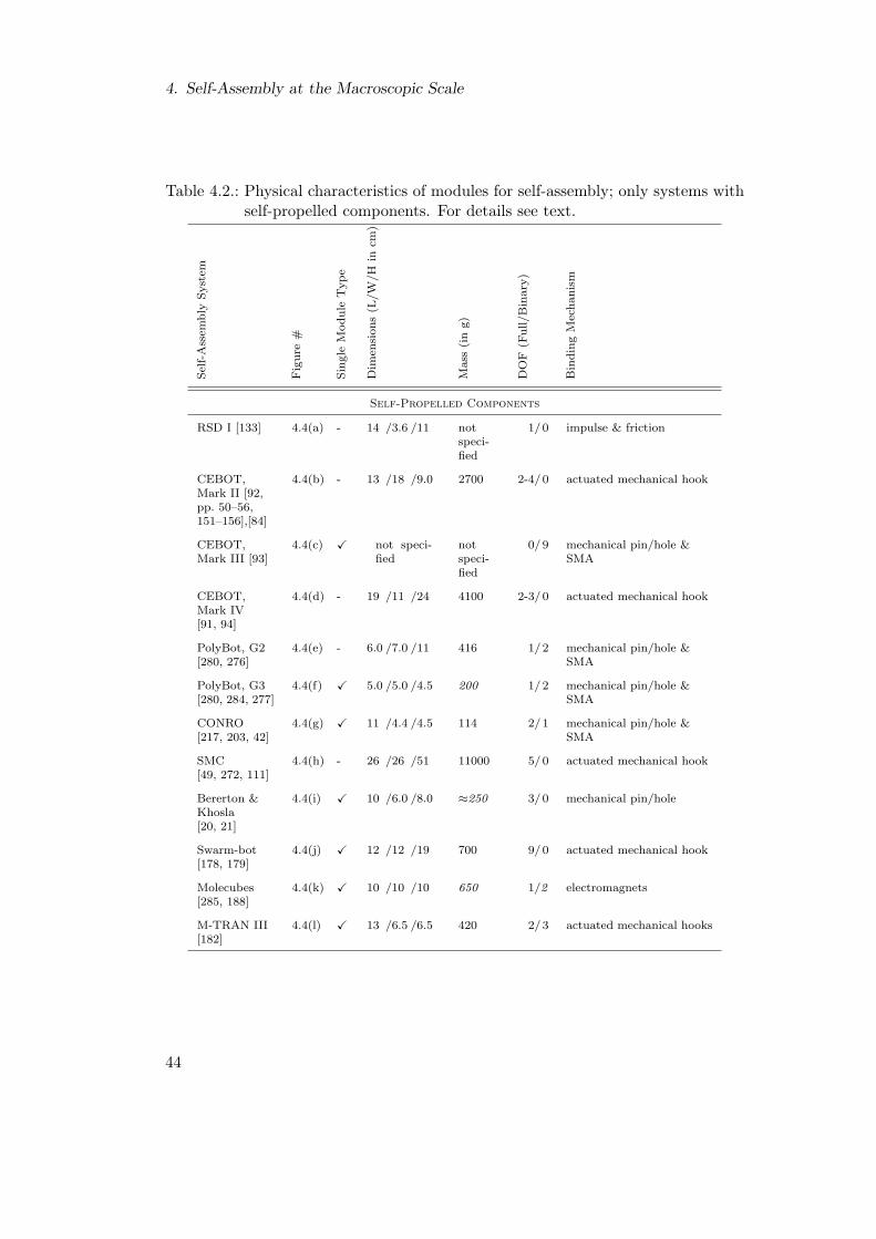
4. Self-Assembly at the Macroscopic Scale
Table 4.2.: Physical characteristics of modules for self-assembly; only systems withself-propelled components. For details see text.
Sel
f-A
ssem
bly
Syst
em
Fig
ure
#
Sin
gle
Module
Type
Dim
ensi
ons
(L/W
/H
incm
)
Mass
(in
g)
DO
F(F
ull/B
inary
)
Bin
din
gM
echanis
m
Self-Propelled Components
RSD I [133] 4.4(a) - 14 /3.6 /11 notspeci-fied
1/0 impulse & friction
CEBOT,Mark II [92,pp. 50–56,151–156],[84]
4.4(b) - 13 /18 /9.0 2700 2-4/0 actuated mechanical hook
CEBOT,Mark III [93]
4.4(c) X not speci-fied
notspeci-fied
0/9 mechanical pin/hole &SMA
CEBOT,Mark IV[91, 94]
4.4(d) - 19 /11 /24 4100 2-3/0 actuated mechanical hook
PolyBot, G2[280, 276]
4.4(e) - 6.0 /7.0 /11 416 1/2 mechanical pin/hole &SMA
PolyBot, G3[280, 284, 277]
4.4(f) X 5.0 /5.0 /4.5 200 1/2 mechanical pin/hole &SMA
CONRO[217, 203, 42]
4.4(g) X 11 /4.4 /4.5 114 2/1 mechanical pin/hole &SMA
SMC[49, 272, 111]
4.4(h) - 26 /26 /51 11000 5/0 actuated mechanical hook
Bererton &Khosla[20, 21]
4.4(i) X 10 /6.0 /8.0 ≈250 3/0 mechanical pin/hole
Swarm-bot[178, 179]
4.4(j) X 12 /12 /19 700 9/0 actuated mechanical hook
Molecubes[285, 188]
4.4(k) X 10 /10 /10 650 1/2 electromagnets
M-TRAN III[182]
4.4(l) X 13 /6.5 /6.5 420 2/3 actuated mechanical hooks
44
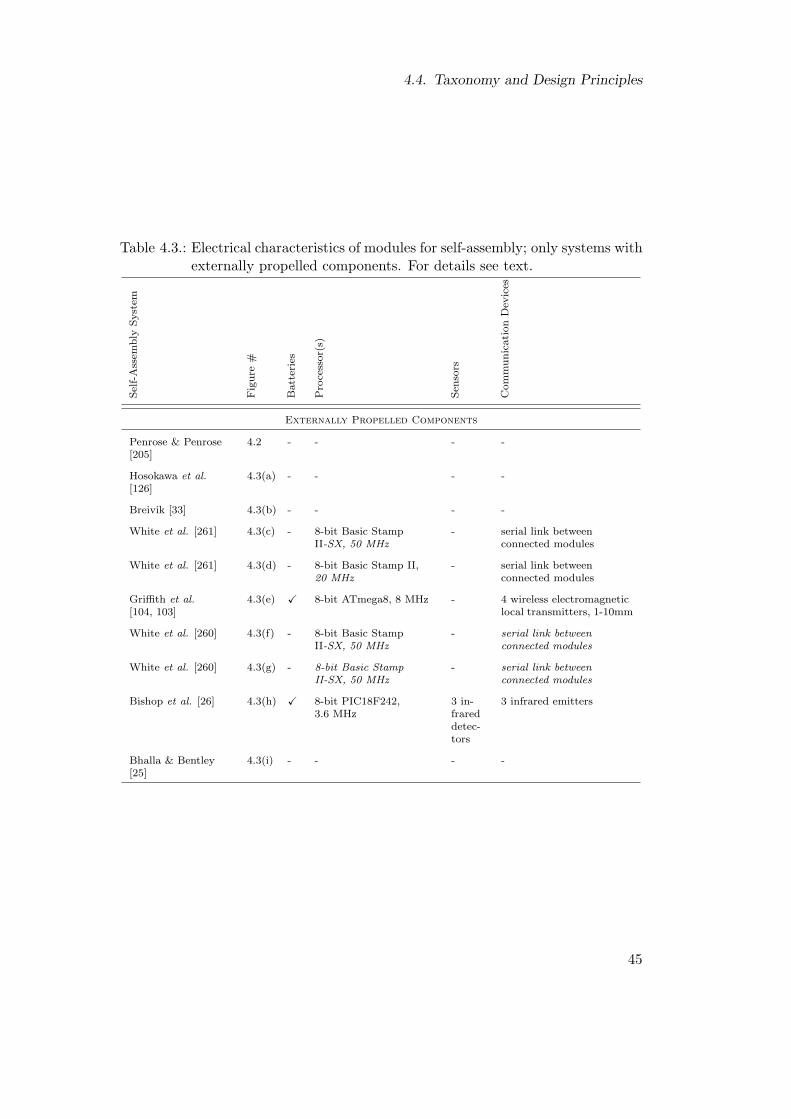
4.4. Taxonomy and Design Principles
Table 4.3.: Electrical characteristics of modules for self-assembly; only systems withexternally propelled components. For details see text.
Sel
f-A
ssem
bly
Syst
em
Fig
ure
#
Batt
erie
s
Pro
cess
or(
s)
Sen
sors
Com
munic
ati
on
Dev
ices
Externally Propelled Components
Penrose & Penrose[205]
4.2 - - - -
Hosokawa et al.[126]
4.3(a) - - - -
Breivik [33] 4.3(b) - - - -
White et al. [261] 4.3(c) - 8-bit Basic StampII-SX, 50 MHz
- serial link betweenconnected modules
White et al. [261] 4.3(d) - 8-bit Basic Stamp II,20 MHz
- serial link betweenconnected modules
Griffith et al.[104, 103]
4.3(e) X 8-bit ATmega8, 8 MHz - 4 wireless electromagneticlocal transmitters, 1-10mm
White et al. [260] 4.3(f) - 8-bit Basic StampII-SX, 50 MHz
- serial link betweenconnected modules
White et al. [260] 4.3(g) - 8-bit Basic StampII-SX, 50 MHz
- serial link betweenconnected modules
Bishop et al. [26] 4.3(h) X 8-bit PIC18F242,3.6 MHz
3 in-frareddetec-tors
3 infrared emitters
Bhalla & Bentley[25]
4.3(i) - - - -
45

4. Self-Assembly at the Macroscopic Scale
Table 4.4.: Electrical characteristics of modules for self-assembly; only systems withself-propelled components. For details see text.
Sel
f-A
ssem
bly
Syst
em
Fig
ure
#
Batt
erie
s
Pro
cess
or(
s)
Sen
sors
Com
munic
ati
on
Dev
ices
Self-Propelled Components
RSD I [133] 4.4(a) - relay (1 head, 2 tail) bump switch (0 head,3 tail)
parallel link betweenconnected modules
CEBOT,Mark II [92,pp. 50–56,151–156],[84]
4.4(b) - sub CPU (+ mainCPU off-board)
4 infrared detectors(3 rigid, 1 rotational),3 ultrasonic distance(1Tx and 2Rx)
9 infrared emitters(8 rigid,1 rotational),parallel link betweenconnected modules
CEBOT,Mark III [93]
4.4(c) - sub CPU (+ mainCPU off-board)
9 infrared detectors,6 ultrasonic distance(3Tx and 3Rx)
9 infrared emitters,link betweenconnected modules
CEBOT,Mark IV[91, 94]
4.4(d) - 16-bit 8086,5-10 MHz
2 infrared detectors 2 infrared emitters,wireless (RS-232C)
PolyBot, G2[280, 276]
4.4(e) - 32-bit PowerPC555(MPC555), 40 MHz
4 infrared detectors 8 infrared emitters,2 CANbus
PolyBot, G3[280, 284, 277]
4.4(f) - 32-bit PowerPC555(MPC555), 40 MHz
8 infrared detectors,2 2-axis inclinometers,8 1-axis force
8 infrared emitters,2 CANbus
CONRO[217, 203, 42]
4.4(g) X 8-bit Basic StampII-SX, 50 MHz
4 infrared detectors 4 infrared emitters
SMC[49, 272, 111]
4.4(h) X 32-bit PentiumMMX, 233 MHz
color camera (2 perparent: 640x416, 2-3per child: 320x240 ),1-axis force
Wi-Fi
Bererton &Khosla [20, 21]
4.4(i) X 8-bit PIC16C73A,20 MHz + off-board
B&W camera(320x240), bump switch
wireless (RF)
Swarm-bot[178, 179]
4.4(j) X 32-bit XScale,400 MHz + 13 8-bitPIC16F876/7,20 MHz
19 infrared proximity,color camera (640x480,omnidirectional), 2-axisforce, torque, 4 micro-phones, 8 light, 3-axisinclinometer, 2 humidi-ty, 4 light barriers
8 RGB LEDschanging body color,2 speakers, Wi-Fi
Molecubes[285, 188]
4.4(k) - 8-bit Basic StampII-SX, 50 MHz
- serial link betweenconnected modules(shared bus)
M-TRAN III[182]
4.4(l) X 32-bit SH7047, 40MHz, 3 16-bit H8,16MHz + off-board
13 infrared detectors,3-axis inclinometer
13 infrared emitters,CANbus, wireless(BlueTooth)
46
4.4. Taxonomy and Design Principles
All tables list only the characteristics of standard modules. Additional modulesmight have been designed for special purposes and could be complementary infunctionality. Tables 4.1 and 4.2 present respectively the physical characteristicsof modules in systems with externally propelled components and in systems withself-propelled components. Entries of the third column indicate whether a systemis composed of homogeneous modules. The dimensions (in cm) listed in the fourthcolumn specify the length, width, and height of a module excluding its bindingmechanism. Typically, it is this measure that is reported. Entries of the fifth columnspecify a module’s mass (in g). For systems in which fluid can enter the module,the module’s net weight is reported. The sixth column details a module’s numberof degrees of freedom (DOF). DOF with two displacements only (e.g., a latch) arereferred to as binary, all others as full. The last column details the principle of themodule’s binding mechanism. Tables 4.3 and 4.4 present respectively the electricalcharacteristics of modules in systems with externally propelled components andin systems with self-propelled components. Entries of the third column specifywhether a module has on-board power or not. The fourth column lists the availableon-board processing resources. It is noted if a module was designed for beingcontrolled remotely. The fifth column summarizes a module’s on-board sensors.These do not include proprioceptive sensors, nor those sensors integrated only onnon-standard modules. The last column lists a module’s devices for inter-modulecommunication. This comprises communication in both the assembled and theseparate state.
Overall, a diverse set of systems has been implemented, with modules rangingfrom a few centimeters to half a meter, and from 3 to 11000 gram. The design of amodule layout is a highly sophisticated task. Typically, it incorporates an enormousamount of human intelligence. Automated design procedures [157, 25] have not yetbeen investigated in much detail.
Most systems are homogeneous, that is, all modules are identical in design. Mod-ules of distinct types (if any) typically are complementary in terms of their bindingmechanisms or functionalities. All systems use only a few distinct types of modules.This could help the fabrication of large quantities of modules. In most systems,however, fabrication still requires a considerable amount of human intervention.
The modules implement a wide range of binding mechanisms, making use ofmechanics (with active or passive inter-locking), magnetism, impulse, friction, andpressure. In all systems, the binding mechanism imposes limits on the relativepositions under which modules can bind to each other. It also imposes limits onthe forces that can be transmitted between assembled modules.
Communication can take place in two distinct situations: between separate mod-ules or modular entities, and within a modular entity. Communication betweenseparate entities (if any) is local unless dedicated global communication channelsare available. Communication within a modular entity can take place through serialor parallel links among all the connected modules.
47
4. Self-Assembly at the Macroscopic Scale
Systems with Externally Propelled Components
In systems with externally propelled components, modules encounter each other atrandom. The modules are designed to operate in a rather limited range of (po-tentially unstructured) environments. The environment imposes constraints on thedesign; for instance, a module’s motion can be affected by its buoyant, frictional,and gravitational forces. Some researchers report difficulties in implementing ran-dom motion without any bias in direction [26, 260].
In the systems of Griffith et al. and Bishop et al., modules are equipped withon-board batteries. Therefore, in principle, any two modules can bind and commu-nicate with each other upon encounter. In White et al.’s systems, a seed modulehas a dedicated link to an external power supply. Modules that bind with the seedstructure receive power through the connection link.
Computing requirements for externally propelled modules are relatively low: inall systems we identified, modules can bind passively upon collision, and if anycomputation is necessary, it reflects the decision whether to stay assembled or not.
Systems with Self-Propelled Components
At the level of individual modules, propulsion can be realized with a differentialdrive, which provides good steering abilities on flat terrain. Tracks on the otherhand allow for good all-terrain navigation. Modules of the swarm-bot system com-bine these two locomotion mechanisms to achieve good mobility on both flat andrough terrain. At the level of modular entities, propulsion requires more elaboratestrategies. This is merely due to the high number of DOF that need to be controlledin a coordinated and often distributed manner, and to the imprecision in actuationthat results in positional errors, which increase with the number of elements insequence.
In most systems with self-propelled modular entities, the latter can change shapeby having modules move within their entity. This capacity is called shape-change—aspecial case of self-reconfiguration—and is typically performed very well by modularreconfigurable robots, such as PolyBot, CONRO, Molecubes, and M-TRAN. Mod-ules of these systems could assemble an arbitrary initial structure, and subsequentlycustomize it by shape-changing.
Modules (in particular, those of modular reconfigurable robots) have a high powerconsumption, which limits their lifetime without external power supply. They typ-ically (i) perceive each other and/or the environment, and (ii) act to selectively en-counter each other. This can put great demands on a module’s design. In fact, manyproblems encountered in the design of self-assembling systems are due to shortcom-ings in the underlying hardware, that is, the modules’ actuation [87, 120, 191],perception [120, 181, 36, 280, 285], and computational resources [120, 181, 21, 36].
48
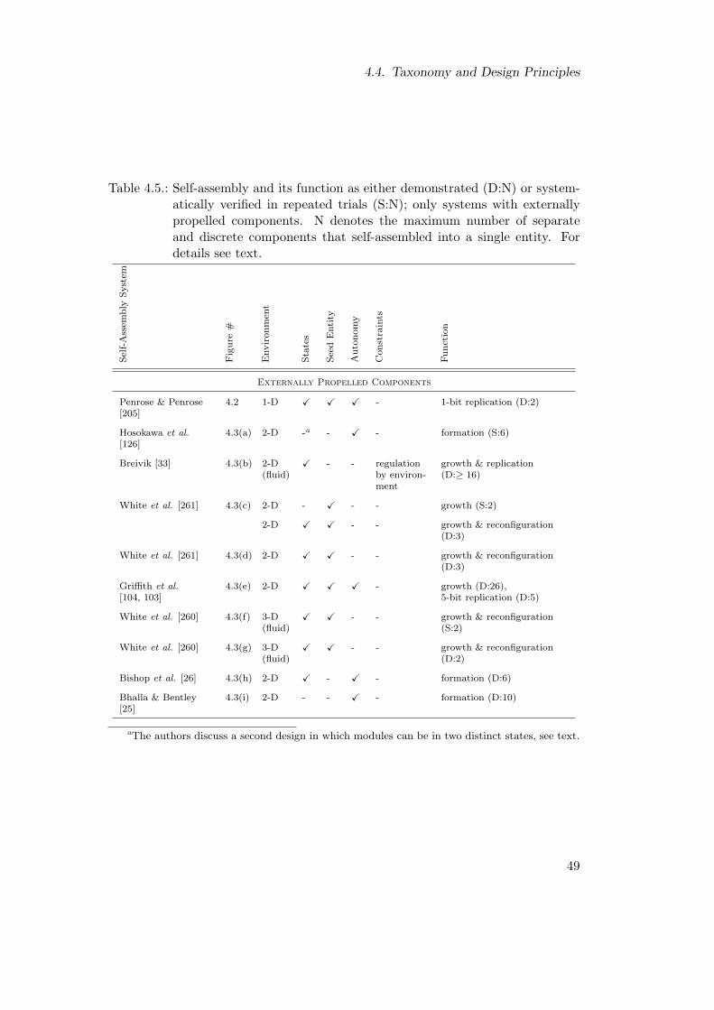
4.4. Taxonomy and Design Principles
Table 4.5.: Self-assembly and its function as either demonstrated (D:N) or system-atically verified in repeated trials (S:N); only systems with externallypropelled components. N denotes the maximum number of separateand discrete components that self-assembled into a single entity. Fordetails see text.
Sel
f-A
ssem
bly
Syst
em
Fig
ure
#
Envir
onm
ent
Sta
tes
See
dE
nti
ty
Auto
nom
y
Const
rain
ts
Funct
ion
Externally Propelled Components
Penrose & Penrose[205]
4.2 1-D X X X - 1-bit replication (D:2)
Hosokawa et al.[126]
4.3(a) 2-D -a - X - formation (S:6)
Breivik [33] 4.3(b) 2-D(fluid)
X - - regulationby environ-ment
growth & replication(D:≥ 16)
White et al. [261] 4.3(c) 2-D - X - - growth (S:2)
2-D X X - - growth & reconfiguration(D:3)
White et al. [261] 4.3(d) 2-D X X - - growth & reconfiguration(D:3)
Griffith et al.[104, 103]
4.3(e) 2-D X X X - growth (D:26),5-bit replication (D:5)
White et al. [260] 4.3(f) 3-D(fluid)
X X - - growth & reconfiguration(S:2)
White et al. [260] 4.3(g) 3-D(fluid)
X X - - growth & reconfiguration(D:2)
Bishop et al. [26] 4.3(h) 2-D X - X - formation (D:6)
Bhalla & Bentley[25]
4.3(i) 2-D - - X - formation (D:10)
aThe authors discuss a second design in which modules can be in two distinct states, see text.
49
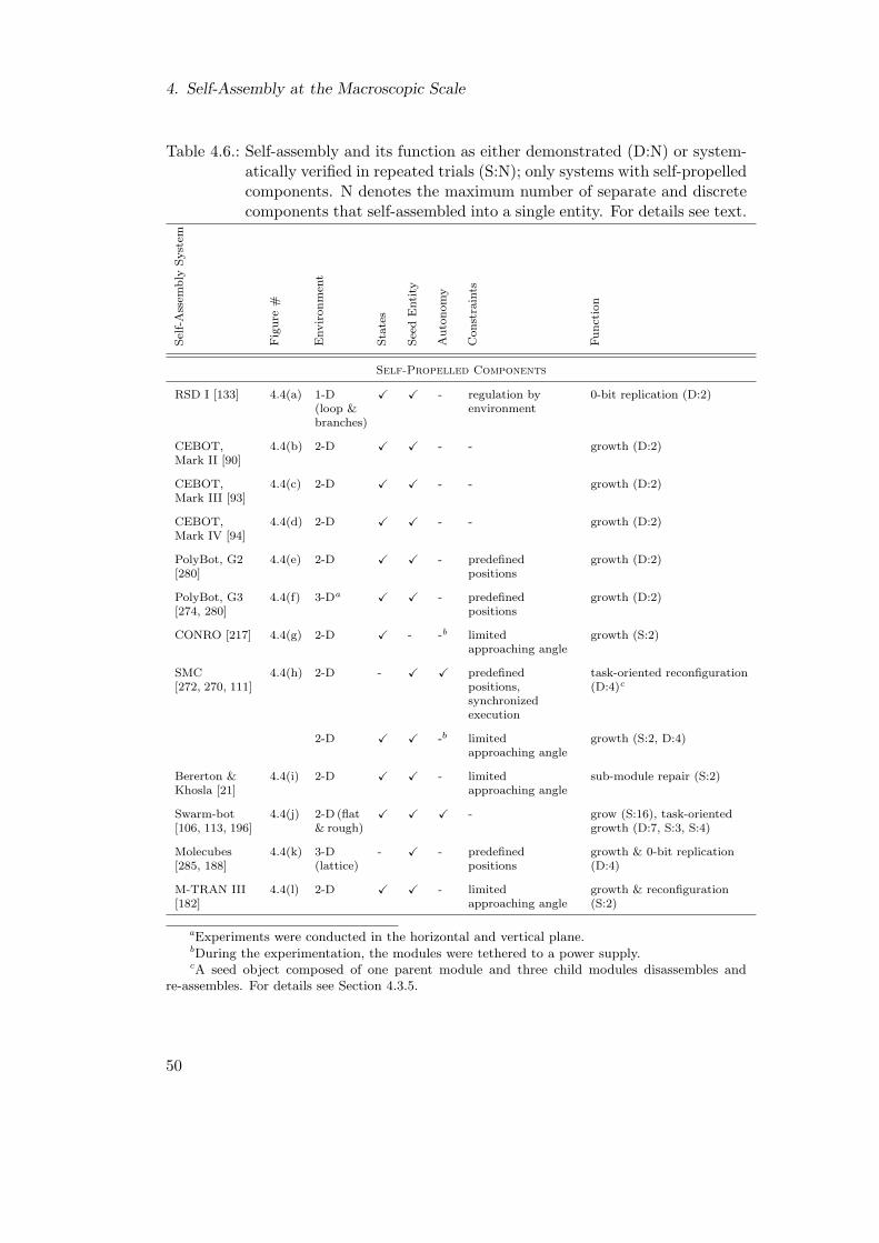
4. Self-Assembly at the Macroscopic Scale
Table 4.6.: Self-assembly and its function as either demonstrated (D:N) or system-atically verified in repeated trials (S:N); only systems with self-propelledcomponents. N denotes the maximum number of separate and discretecomponents that self-assembled into a single entity. For details see text.
Sel
f-A
ssem
bly
Syst
em
Fig
ure
#
Envir
onm
ent
Sta
tes
See
dE
nti
ty
Auto
nom
y
Const
rain
ts
Funct
ion
Self-Propelled Components
RSD I [133] 4.4(a) 1-D(loop &branches)
X X - regulation byenvironment
0-bit replication (D:2)
CEBOT,Mark II [90]
4.4(b) 2-D X X - - growth (D:2)
CEBOT,Mark III [93]
4.4(c) 2-D X X - - growth (D:2)
CEBOT,Mark IV [94]
4.4(d) 2-D X X - - growth (D:2)
PolyBot, G2[280]
4.4(e) 2-D X X - predefinedpositions
growth (D:2)
PolyBot, G3[274, 280]
4.4(f) 3-Da X X - predefinedpositions
growth (D:2)
CONRO [217] 4.4(g) 2-D X - -b limitedapproaching angle
growth (S:2)
SMC[272, 270, 111]
4.4(h) 2-D - X X predefinedpositions,synchronizedexecution
task-oriented reconfiguration(D:4)c
2-D X X -b limitedapproaching angle
growth (S:2, D:4)
Bererton &Khosla [21]
4.4(i) 2-D X X - limitedapproaching angle
sub-module repair (S:2)
Swarm-bot[106, 113, 196]
4.4(j) 2-D (flat& rough)
X X X - grow (S:16), task-orientedgrowth (D:7, S:3, S:4)
Molecubes[285, 188]
4.4(k) 3-D(lattice)
- X - predefinedpositions
growth & 0-bit replication(D:4)
M-TRAN III[182]
4.4(l) 2-D X X - limitedapproaching angle
growth & reconfiguration(S:2)
aExperiments were conducted in the horizontal and vertical plane.bDuring the experimentation, the modules were tethered to a power supply.cA seed object composed of one parent module and three child modules disassembles and
re-assembles. For details see Section 4.3.5.
50

4.4. Taxonomy and Design Principles
4.4.2. Outcome and Analysis of Self-Assembly Experimentation
At present, self-assembly of macroscopic components has been demonstrated for22 different systems. Tables 4.5 and 4.6 provide an overview of the experimentsthat were performed respectively with systems of externally propelled componentsand with systems of self-propelled components. Details on the experimental setupand results can be obtained from the references listed in the first column of eachtable. The second column refers to the figure that shows component modules ofthe corresponding system.
Most of the experiments were carried out in simple environments in which motionwas restricted to 1-D, 2-D, or a lattice structure (see third column). The systemsof White et al. [260], PolyBot [274], and swarm-bot represent the first attempts tostudy self-assembly in more complex situations, such as 3-D environments, high-density environments, and rough terrains.
Most experiments were conducted as proofs of concept. While the number ofcomponents has been large in simulation, physical systems rarely comprised morethan 50 modules, and typically no more than two components self-assembled into asame entity. For 8 out of 22 systems, the self-assembly process was systematicallyexamined using quantitative performance measures and performing multiple trials.To the best of our knowledge, Hosokawa et al.’s system and swarm-bot are the onlysystems for which self-assembly of more than two discrete components has beensystematically examined. Hosokawa et al. analyzed the process dynamics with focuson the yield of desired products (with six discrete components per entity). In swarm-bot, the analysis addressed the reliability and speed by which individual modulesconnect into single entities, as well as the additional capabilities and functions suchprocess may provide (with up to 16 discrete components per entity).
4.4.3. Process Control
The process of self-assembly is governed by the modules’ way to encounter eachother and by the spatially anisotropic binding preferences. In relatively simplesystems, modules are externally propelled and have static binding preferences. Thisis the case for the systems of Hosokawa et al. and Bhalla & Bentley. In all othersystems, a module’s motion and/or binding preferences can depend on its state (seecolumn 4 of Tables 4.5 and 4.6). The state can change in response to interactionswith other modules and/or the environment. In the system of Penrose, for instance,a module’s state changes by mechanical interactions with other modules. In thesystem of Breivik, the state is affected also by the temperature of the environment.In swarm-bot, each module broadcasts its connection state to modules in its vicinity.
In 17 out of 22 systems, self-assembly is seeded by a dedicated component (seecolumn 5 of Tables 4.5 and 4.6). All additional products are formed by havingcomponents interact with the seed entity and/or the products of such interactions.The seed can be a single module or a modular entity; it can be static or mobile.Typically, the seed is explicitly defined by the experimenter. However, systems
51

4. Self-Assembly at the Macroscopic Scale
can also choose autonomously the components by which to seed the process [196].Among systems with self-propelled components, only CONRO demonstrated self-assembly without any seed component.
Seven out of 22 systems were autonomous in perception, control, action, andpower (see column 6 of Tables 4.5 and 4.6).1 In most systems, each module executesa deterministic finite state machine. The logic can be coded in hardware, as in thesystems of Penrose et al. and Breivik, or in software, as in all other state-basedsystems. In Bishop et al.’s system, for instance, each module executes a programthat interprets a graph grammar defining state-dependent binding preferences. Forswarm-bot and Molecubes, evolutionary algorithms have been applied to automatethe control design. Attempts to port a controller from one physical system toanother are still rare and typically require the platforms to share some commonproperties [111].
In some systems self-assembly was reported to take place under constrained con-ditions (see column 7 of Tables 4.5 and 4.6). Examples are a priori assumptionson the components’ initial spatial arrangement and components with knowledgeof their own relative starting positions. Clearly, it is more demanding to realizeself-assembly in a system of disordered components that lack any knowledge abouttheir relative positions.
4.4.4. Functionality
The last column of Tables 4.5 and 4.6 details the basic function of the system thatwas either demonstrated (D:N), or systematically verified in repeated trials (S:N).Thereby, N indicates the maximum number of separate and discrete componentsthat self-assembled into a single entity. The purpose of self-assembling can bemanifold:
• growth: increase of the number and/or type of modules in an entity. To someextent, this capacity is available in all self-assembling systems. However, thecapacity to grow can be limited by the design. In swarm-bot, mobile moduleshave shown to form growing entities that display additional capabilities andfunctions. Examples are (i) transport of objects too heavy for manipulationby the modules when separate, and (ii) locomotion over terrains unnavigablefor individual modules.
• self-reconfiguration: change of an existing entity’s morphology. This capa-bility can be achieved by disassembling and re-assembling (e.g., as in SMC),or by shape-change (e.g., as in M-TRAN). For SMC it was shown that, bydisassembling and re-assembling, a modular entity can solve a problem betterthan it could in its original configuration.
• formation: production of one or more objects of a predefined size and struc-ture. In some systems, the module layout is specifically designed for the
1External agitation apparatuses (if any) are considered as “natural” part of the environment.
52

4.4. Taxonomy and Design Principles
assembly of desired objects. In other systems, the final product is flexible, asit can be defined by re-programming each module (e.g., to execute a differentgraph grammar).
• template replication: replication of a template by producing objects ofidentical size, structure, and state. Templates for replication can be pre-assembled, specific seed entities (e.g., as in RSD I and Molecubes), pre-assembled seed entities with information in the modules’ state (e.g., as inPenrose’s and Griffith et al.’s systems), or products of the self-assembly pro-cess (e.g., as in Breivik’s system).
• self-repair: replacement of an entity’s defective modules with its redundantmodules or other modules available in the environment.
53

4. Self-Assembly at the Macroscopic Scale
54

5. Group Transport at the MacroscopicScale
Group transport can be defined as the “conveyance of a burden by two or moreindividuals” [175, page 227]. In studies of ants, “a similar term, ‘group retrieval’,has usually been applied when ants retrieve food along a common path, regardlessof the occurrence of group transport” (page 227).
Group transport is a widely observed naturally occurring phenomenon. Whencompared to solitary transport, it offers the advantage of being more reliable and inaddition more powerful, as a group may exert higher forces onto an object than eachof its members alone. Such advantages occur, for example, in the transport of cargoparticles by groups of molecular motors in cells of any animal and plant [141, 156].
In this chapter, we focus on group transport at the macroscopic scale. We firstpresent an excursion to group transport in natural systems (Section 5.1). We thensurvey related work on designed systems, that is, physical mobile robots. Thereby,we partition the related work into the two main approaches to solve the task, that is,pushing/caging strategies (Section 5.2) and grasping/lifting strategies (Section 5.3).Note that there are also a few other approaches, for instance, strategies that letrobots make use of tools such as a rope [57, 132], that are not considered here.
5.1. A Brief Excursion into Natural Systems
In the literature, group transport is almost exclusively reported in the context ofants (for an example, see Figure 5.1). In fact, Moffett [175, page 220] claimedthat group transport “is better developed in ants than in any other animal group”.Nevertheless, it “has seldom been recognized as a form of social behavior that isworthy of investigation in its own right” (page 227).
In most ant species, group transport presumably provides adaptive value as re-productive immatures are much bigger than workers, and therefore can not betransported by a single worker alone (e.g., during an emigration). Group transportof “bulky larvae and pupae is probably nearly universal in ants and is likely to havepreceded the transport of food by this method” [175, page 220].
Almost half a century ago, Sudd [232] studied the transport of prey by singleants and by groups of ants of the species Pheidole crassinoda. Sudd reported thatduring transport the ants did not pull steadily but in short successive hauls thatwere generally associated with changes in the arrangement of ants in the group. “Inalmost all series involving groups of ants there was an upward trend of the forceexerted in successive hauls; where only one ant was pulling however the proportion
55
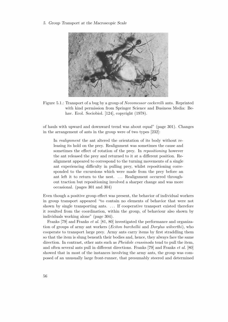
5. Group Transport at the Macroscopic Scale
Figure 5.1.: Transport of a bug by a group of Novomessor cockerelli ants. Reprintedwith kind permission from Springer Science and Business Media: Be-hav. Ecol. Sociobiol. [124], copyright (1978).
of hauls with upward and downward trend was about equal” (page 301). Changesin the arrangement of ants in the group were of two types [232]:
In realignment the ant altered the orientation of its body without re-leasing its hold on the prey. Realignment was sometimes the cause andsometimes the effect of rotation of the prey. In repositioning howeverthe ant released the prey and returned to it at a different position. Re-alignment appeared to correspond to the turning movements of a singleant experiencing difficulty in pulling prey, whilst repositioning corre-sponded to the excursions which were made from the prey before anant left it to return to the nest. . . . Realignment occurred through-out traction but repositioning involved a sharper change and was moreoccasional. (pages 301 and 304)
Even though a positive group effect was present, the behavior of individual workersin group transport appeared “to contain no elements of behavior that were notshown by single transporting ants. . . . If cooperative transport existed thereforeit resulted from the coordination, within the group, of behaviour also shown byindividuals working alone” (page 304).
Franks [79] and Franks et al. [81, 80] investigated the performance and organiza-tion of groups of army ant workers (Eciton burchellii and Dorylus wilverthi), whocooperate to transport large prey. Army ants carry items by first straddling themso that the item is slung beneath their bodies and, hence, they always face the samedirection. In contrast, other ants such as Pheidole crassinoda tend to pull the item,and often several ants pull in different directions. Franks [79] and Franks et al. [80]showed that in most of the instances involving the army ants, the group was com-posed of an unusually large front-runner, that presumably steered and determined
56
5.2. Pushing and Caging Strategies
the direction of transport, and one or more particularly small followers. Andersonand Franks [3] do not consider the front-runner as a leader in any sense. Instead,they hypothesized that “all of the individuals that form a team in army ants are ini-tially using exactly the same rules of thumb” (page 537). Franks [79] reported thatthe performance in the group was much more than the sum of the performances ofits individual members. They could do so probably because by straddling the preybetween them the rotational forces (i.e., forces that occur when lifting the preyin a position aside its barycenter) are balanced and disappear. Super-efficiency ingroup transport has also been observed in other ant species [124, 174]. In the genusPheidologeton, for instance, on average an ant engaged in group transport held atleast 10 times the weight it did as solitary transporter [174]. It was observed thatthe workers that were engaged in group transport behaved differently from thosein solitary transport.
Moffett [175] lists 39 species of ants for which group transport has been reported.He states that “without doubt the group transport of food has arisen independentlyin numerous phylogenetic lines”. “At least with regard to carrying food, those antsspecies capable of group transport are unquestionably in the minority” (page 227).
Group transport of prey has also been observed in a few species of social spi-ders [247]:
During transport, as an aid to the movement of the prey, spiders weavesilk that we named ‘traction silk’, fixed between the prey and the web(in the direction of the shelter) that will permit a slight lifting of theprey. This process will be repeated until the prey has been transportedunder the shelter. (page 765)
Coordination in group transport by social spiders seems to occur through the itemthat is transported [247]:
Movement of one spider engaged in group transport is likely to modifythe stimuli perceived by the other group members (such as vibrationproduced, or indirectly, available site on the prey) possibly producing,in turn, recruitment or departure of individuals. . . . Coordination inspider colonies is based on signals that are made inadvertently as sideproducts of their activities. The communal network, as a means ofinformation, seems to be at the origin of cooperation. This supports thehypothesis of a sudden passage from solitary to social life in spinningspiders [246, 31, 264, 208]. (pages 770–771)
5.2. Pushing and Caging Strategies
Pushing behaviors have the advantage that they allow robots to move objects thatare hard to grasp. In addition, multiple objects can be pushed at the same time [22].On the other hand, it is difficult to predict the motion of the object and of the
57

5. Group Transport at the Macroscopic Scale
robots, especially, if the ground is not uniform.1 Therefore, the control typicallyrequires sensory feedback.
Most studies consider two robots pushing a wide box simultaneously from a singleside [166, 234, 58, 201, 95]. To coordinate the robots’ actions, robots are specificallyarranged [166, 58, 201, 95], control is synchronized [166], relative positions areknown [58, 201], explicit communication is used [166, 201], or the robots’ actionsare planned by a designated leader [95, 234]. Only few systems considered morethan two robots, pushing a wide box simultaneously [149, 269, 150, 148]. In thesesystems, control is homogeneous and decentralized, and robots make no use ofexplicit communication.
Kube et al. [150, 148] reported that if the object is small compared to the sizeof the pushing robots the performance decreases drastically with group size as theobject offers only limited contact surface. A few other studies with multi-robotsystems consider objects of the size of a single robot or less [193, 85]. However, inthese cases the objects were light enough for a single robot to move them alone.
Recently, researchers considered a special case of multi-robot box-pushing inwhich the movable area of the object is bounded by the robots. This condition isreferred to as object closure and the manipulation concept is denoted as caging [74,254, 252, 206]. Typically the object is light enough for a single robot to move italone. In some systems a single robot can constrain the object in several directionsusing multiple contact points [254, 252]. To test and maintain the condition ofobject closure, decentralized control algorithms have been proposed [206, 253].
5.3. Grasping and Lifting Strategies
Many studies considered the transport of an object by multiple, mobile robotsgrasping and/or lifting it [55, 139, 143, 144, 1, 233, 173, 255, 272, 256, 271, 236, 171].
In some systems the trajectories of all robots of a group are planned before thestart of experimentation. Each robot then follows its desired trajectory, for instance,using a controller based on dead-reckoning [55]. In other systems, the manipulationis planned in real-time by an external workstation which communicates with therobots [173, 272, 271]. Often, instead of an external computer, a specific robot calledthe leader knows the desired trajectory or the goal location. The leader robot cansend explicit high- or low-level commands to the followers [233, 255]. However, inmany leader-follower systems explicit communication is not required [143, 144, 1,256, 171, 236]. Typically, this is realized in systems in which the object is lifted bythe robots; the followers simulate the behavior of passive casters [229].
To the best of our knowledge, group transport on rough terrain has only beenreported for teams of two object-lifting robots, as in the works by Huntsberger etal. and Takeda et al. [130, 241, 236].
None of these works considered the transport of an object by groups of more thanfour physical robots.
1For a theory on the mechanics of pushing see Mason [161].
58

Part III.
Self-Assembling Robots:Control and Analysis in Simulation
59


Preface to Part III
During the past 50 years, a variety of systems have demonstrated self-assemblyamong centimeter-scale components (see Chapter 4). The corresponding studiesfocused on self-assembly per se, that is, on the process by which structure formsthrough interactions of specifically designed component modules. Instead, we lookat self-assembly as a mechanism that helps systems of autonomous components toaccomplish concrete tasks. In particular, we address the transport of a heavy objectby a system of self-assembling mobile robots.
In the last decade, group transport of objects has become a canonical task forstudying cooperation in multi-robot systems (see Section 2.2.1). Typically, theobject to be transported cannot be moved by a single robot alone, and thus itstransport requires the coordinated action of multiple robots. Numerous systemshave been developed (see Chapter 5). Yet, even the most sophisticated ones areunable to produce effective coordination for medium-sized or large groups of robots(i.e., five or more robots).
In this third part of the dissertation, we investigate a novel approach to thecoordination of multiple robots in group transport. We consider a system ofself-propelled robots that, by grasping each other, can temporarily organize intoconnected pulling or pushing structures. Such structures could grow in size andstrength as the number of their components increases. They could transport heavyobjects that provide limited contact surface only (see Figure 5.2).
(a) (b)
Figure 5.2.: Transport of an object by a group of six robots organized in an as-sembled structure: (a) pushing the object; (b) physically linked to theobject and pulling/pushing it.
61

The study is accomplished using a simulator, modeling the kinematics, dynamics,and contacts of rigid objects in 3-D. The system comprises a passive object, here-after referred to as prey, and a group of self-propelled, mobile robots. The robotsare endowed with connection mechanisms that allow them to attach to (and detachfrom) each other and the prey. The robot’s model approximates the s-bot of theswarm-bot system (see Section 2.2.3).
We make use of evolutionary algorithms to synthesize control policies (see Sec-tion 3.1). Selection acts at the level of genes [114, 51]. The genotype encodes aneural network controller which is cloned and copied to each robot within a group.Thus, all members of a group are genetically identical. We consider a populationof genotypes, that is, a population of groups. Note that in our setup, selection atthe level of genes is equivalent to between-group selection [142].
62
6. The Adaptive Value of Self-Assembly—Evolution of Solitary and GroupTransport
In this chapter, we address the cooperative transport of prey by a group of tworobots. Initially, the robots are put at random positions near the prey. Their taskis to move the prey in an arbitrary direction (the farther the better). The preycan not be moved by one robot alone. The robots have highly limited capabilities.They can neither communicate nor perceive each other directly.
The aim of the study is two-fold. Firstly, we want to gain some basic understand-ing of the factors that favor self-assembly. Currently, research efforts in biology arebeing directed at giving answers to this question [238, 7]. We study whether theinterplay of variation and selection in an artificial evolutionary process can yieldbehaviors that let robots self-assemble. The self-assembly ability—without be-ing explicitly favored by the fitness function design—can evolve if it provides anadaptive value for the group. If this is the case, we can analyze the proximatemechanisms that cause self-assembly.
Secondly, we want to understand the relationship between the evolution of grouptransport and the evolution of solitary transport. In social insects, group trans-port presumably evolved from solitary transport, without necessarily having themembers of the group recognize each other. We study whether artificial evolutioncan yield robots that, despite not being aware of each other, exhibit effective grouptransport behaviors. Moreover, we examine whether robots engaged in group trans-port can benefit from behaving differently from those engaged in solitary transport.
6.1. Methods
In this section, we detail the task, the simulation model, the robot’s controller, andthe evolutionary algorithm.
6.1.1. Task
We study solitary and group transport of prey. The task is to move the prey in anarbitrary direction (the farther the better). Initially, one or two robots are put atrandom positions near the prey. Each robot is equipped with a gripper that enablesit to establish a physical connection to the other robot or to the prey. Apart fromthat, the robots have highly limited capabilities. They can move autonomously and
63

6. The Adaptive Value of Self-Assembly—Evolution of Solitary and Group Transport
05
1015
Z
05
1015
Z
100 5X
100 5Y
10 05
100
5
X
Y
Figure 6.1.: The simulation model of the robot: front, side, and top view (units incm).
perceive their environment. However, they can neither communicate nor perceiveeach other directly. The environment comprises the prey and a light source. Thelight source represents an environmental cue and as such can be exploited by therobots to coordinate their actions (see Section 2.2.1).
6.1.2. Simulation Model
The simulator models the kinematics and dynamics of rigid, partially constrained,bodies in 3-D. Frictional forces are calculated based on the Coulomb friction law [47].The model of the robot is illustrated in Figure 6.1. It is an approximation of the s-bot, a robot designed and implemented in the context of the SWARM-BOTS project(see Section 2.2.3). The model is composed of five bodies: two spherical wheels,two cylindrical wheels, and a cylindrical torso. The torso is composed of severalparts that are rigidly linked: a cylindrical body, a protruding cuboid (in what wedefine to be the robot’s front), and a pillar fixed on top. The spherical wheels arelinked to the chassis via ball-and-socket joints. The cylindrical wheels are linked tothe chassis via hinge joints.
The robot’s abilities are summarized in Table 6.1. The cylindrical wheels aremotorized, and can be moved both forward and backward at different speeds. Ifthe cuboid heading forward is in contact with either the cylindrical body of anotherrobot or the (cylindrical) prey, a connection can be established. Connections canbe released at any time. In particular, this will happen if the intensity of theforce transmitted by the connection mechanism exceeds a certain threshold. As aconsequence, it is not possible for the robots to form very long pulling chains. Therobot is equipped with an omni-directional camera mounted on a pillar supportthat is fixed at the center of the torso’s top. The camera is able to detect theangular position of the light source. Moreover, it provides the angular position anddistance of the prey, if the latter resides within the sensing range (R = 50 cm). Aconnection sensor enables a robot to perceive whether it is connected to anotherobject or not. The robot is not equipped with any sensor capable of detecting thepresence of a teammate.
64
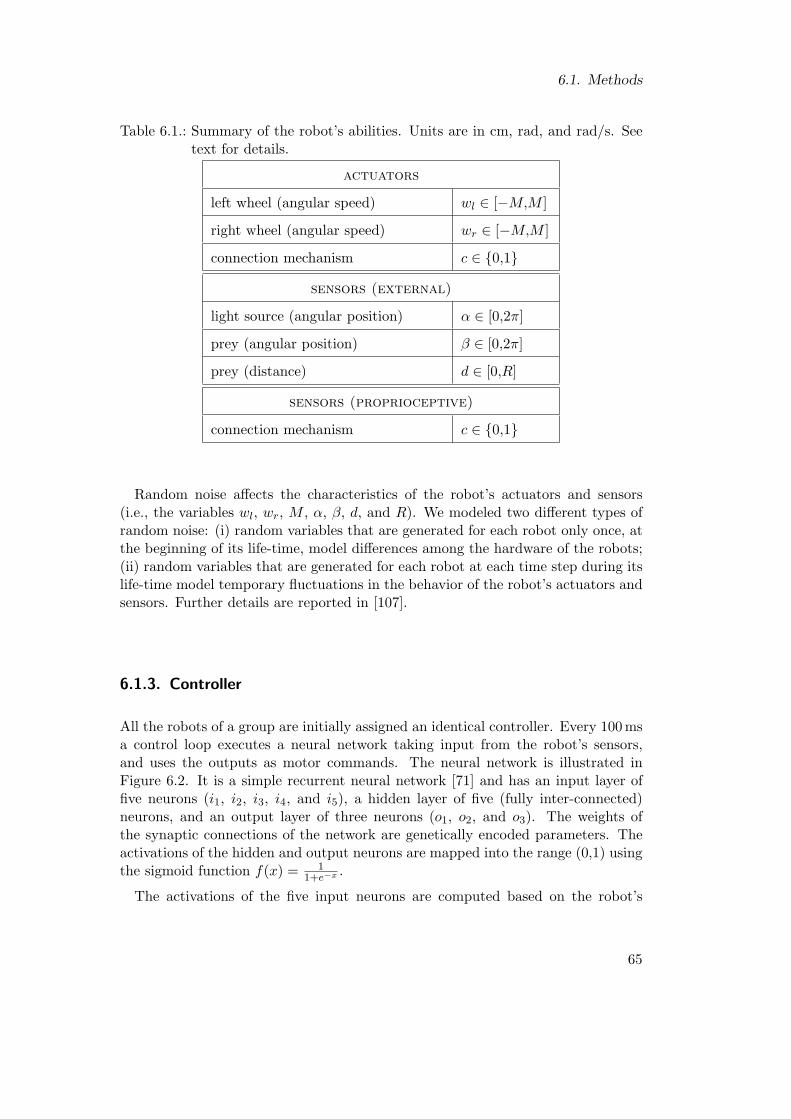
6.1. Methods
Table 6.1.: Summary of the robot’s abilities. Units are in cm, rad, and rad/s. Seetext for details.
actuators
left wheel (angular speed) wl ∈ [−M,M ]
right wheel (angular speed) wr ∈ [−M,M ]
connection mechanism c ∈ {0,1}sensors (external)
light source (angular position) α ∈ [0,2π]
prey (angular position) β ∈ [0,2π]
prey (distance) d ∈ [0,R]
sensors (proprioceptive)
connection mechanism c ∈ {0,1}
Random noise affects the characteristics of the robot’s actuators and sensors(i.e., the variables wl, wr, M , α, β, d, and R). We modeled two different types ofrandom noise: (i) random variables that are generated for each robot only once, atthe beginning of its life-time, model differences among the hardware of the robots;(ii) random variables that are generated for each robot at each time step during itslife-time model temporary fluctuations in the behavior of the robot’s actuators andsensors. Further details are reported in [107].
6.1.3. Controller
All the robots of a group are initially assigned an identical controller. Every 100 msa control loop executes a neural network taking input from the robot’s sensors,and uses the outputs as motor commands. The neural network is illustrated inFigure 6.2. It is a simple recurrent neural network [71] and has an input layer offive neurons (i1, i2, i3, i4, and i5), a hidden layer of five (fully inter-connected)neurons, and an output layer of three neurons (o1, o2, and o3). The weights ofthe synaptic connections of the network are genetically encoded parameters. Theactivations of the hidden and output neurons are mapped into the range (0,1) usingthe sigmoid function f(x) = 1
1+e−x .
The activations of the five input neurons are computed based on the robot’s
65
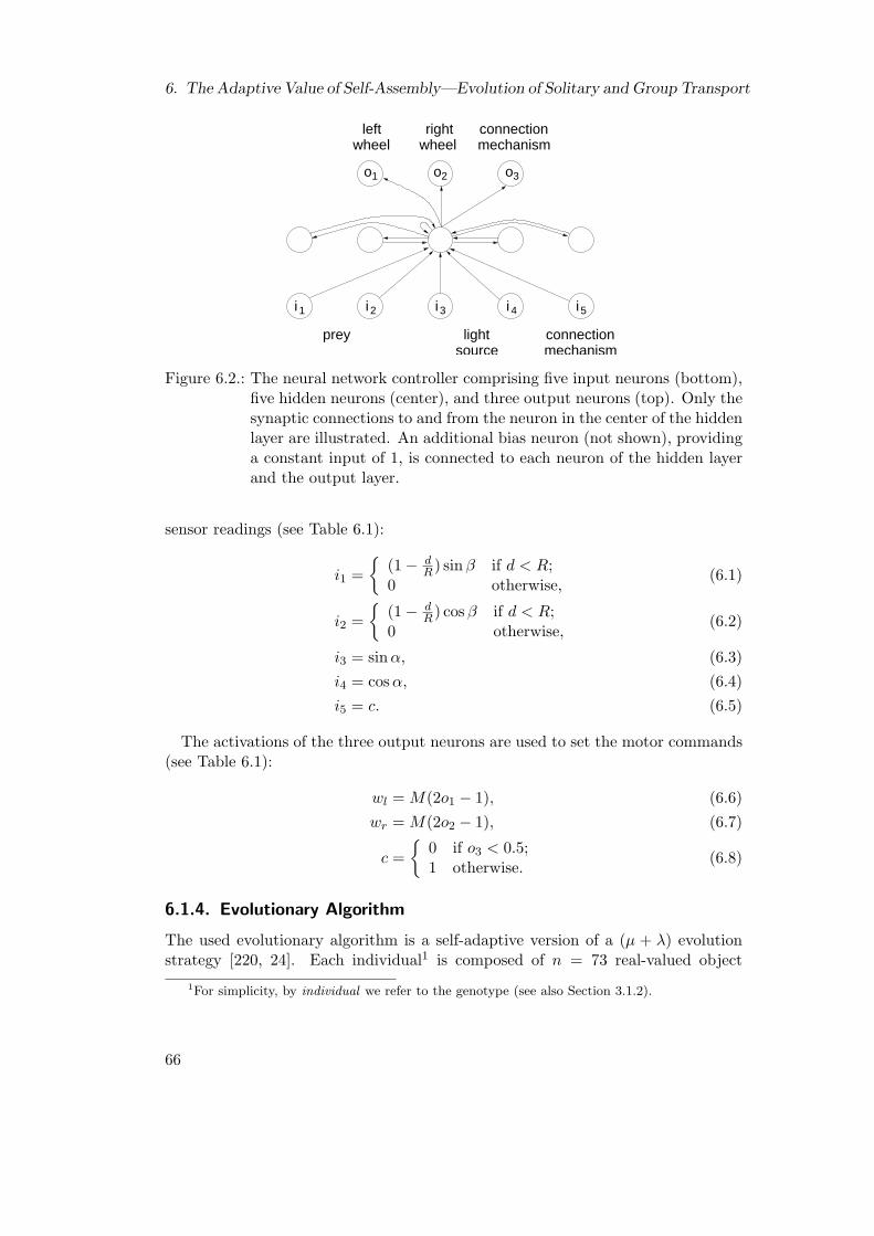
6. The Adaptive Value of Self-Assembly—Evolution of Solitary and Group Transport
wheelright
o1 o2
3i 4i 5i2i
o3
1i
mechanismconnection
sourcelight
mechanismconnection
wheelleft
prey
Figure 6.2.: The neural network controller comprising five input neurons (bottom),five hidden neurons (center), and three output neurons (top). Only thesynaptic connections to and from the neuron in the center of the hiddenlayer are illustrated. An additional bias neuron (not shown), providinga constant input of 1, is connected to each neuron of the hidden layerand the output layer.
sensor readings (see Table 6.1):
i1 ={
(1− dR) sin β if d < R;
0 otherwise,(6.1)
i2 ={
(1− dR) cos β if d < R;
0 otherwise,(6.2)
i3 = sin α, (6.3)i4 = cosα, (6.4)i5 = c. (6.5)
The activations of the three output neurons are used to set the motor commands(see Table 6.1):
wl = M(2o1 − 1), (6.6)wr = M(2o2 − 1), (6.7)
c ={
0 if o3 < 0.5;1 otherwise.
(6.8)
6.1.4. Evolutionary Algorithm
The used evolutionary algorithm is a self-adaptive version of a (µ + λ) evolutionstrategy [220, 24]. Each individual1 is composed of n = 73 real-valued object
1For simplicity, by individual we refer to the genotype (see also Section 3.1.2).
66

6.1. Methods
parameters x1, x2, . . . , xn specifying the connection weights of the neural networkcontroller, and the same number of real-valued strategy parameters s1, s2, . . . , sn
specifying the mutation strength used for each of the n object parameters.The initial population of µ + λ individuals is constructed randomly. In each
generation all individuals are assigned a fitness value. The best-rated µ individualsare selected to create λ offspring. Subsequently, the µ parent individuals and theλ offspring are copied into the population of the next generation. Note that the µparent individuals that are replicated from the previous generation get re-evaluated.We have chosen µ = 20 and λ = 80.
Each offspring is created by mutation with probability 0.8 and by recombinationwith probability 0.2. In either case, the parent individual(s) is selected randomly.If the offspring is created by recombination, the mutation operator is also appliedto it. The object parameter xi is mutated by adding a random variable from thenormal distribution N(0, s2
i ). Beforehand, the mutation strength parameter si ismultiplied by a random variable ξi that follows a log-normal distribution [220, 24].As recombination operators we use intermediate and dominant recombination [24],both with the same probability.
Fitness Computation
The fitness of individuals is assessed using simulations. The simulated environmentconsists of a flat ground, a prey, and a light source. The prey is modeled as acylinder, either 250 g or 500 g in mass, 10 cm in height, and 12 cm in radius. The500 g prey can not be moved by a single robot. A simulation trial lasts T = 20simulated seconds. Initially, the prey is placed in what we refer to as the center ofthe environment. The light source is placed at a random position 300 cm away fromthe prey. This is less than the distance the prey can be moved within the simulationtime T . N ∈ {1, 2} robots are placed at random positions and orientations, but nomore than R
2 = 25 cm away from the perimeter of the prey. This ensures that theprey can initially be detected by each robot.
The quality measure Q accounts for the ability of the individual to let the robotsremain in the vicinity of the prey, and transport it, the farther the better, in anarbitrary direction. It is defined as:
Q ={ C if T = 0;
1 + (1 +√T )Cρ otherwise,
(6.9)
where C ∈ [0,1] reflects the clustering performance, T ∈ [0,∞) reflects the transportperformance, and ρ = 5.
The clustering performance C is defined as
C =1N
N∑
i=1
Ci, with (6.10)
67

6. The Adaptive Value of Self-Assembly—Evolution of Solitary and Group Transport
Ci =
0 if dTi > R;
1 if dTi < R
2 ;R−dT
iR/2 otherwise,
(6.11)
where dTi denotes the distance between robot i and the perimeter of the prey at
time T (see Table 6.1). If the prey at time T is not within the sensing range Rof a robot, the latter receives the lowest possible reward (i.e., 0). Robots that atthe end of the trial are still within the initial range (R
2 = 25 cm) around the preyreceive the maximum reward (i.e., 1). Note that C does not impose any bias on thetransport strategy: any pulling or pushing arrangement of two robots is assignedthe maximum clustering performance.
The transport performance T is defined as
T = ∆(X 0,X T ), (6.12)
where X t denotes the position of the prey at time t, and ∆(·, ·) is the Euclideandistance.
The performance of an individual is evaluated in S = 5 independent trials. Foreach trial, the start configuration (e.g., specifying the initial locations of the robotsand of the light source) is randomly generated. Every individual within the samegeneration is evaluated on the same sample of start configurations. The sample ischanged once at the beginning of each generation. Let Qi be the quality observed intrial i, and φ be a permutation of {1, 2, . . . , S} so that Qφ(1) ≤ Qφ(2) ≤ · · · ≤ Qφ(S).Then the fitness F , which is to be maximized, is defined as
F =2
S(S + 1)
S∑
i=1
(S − i + 1)Qφ(i). (6.13)
Note that in this way the trial resulting in the lowest transport quality value (ifany) has the highest impact on F . Thereby, individuals are penalized for exhibitinghigh performance fluctuations.
6.2. Results
We conducted 30 independent evolutionary runs for 150 generations each. Thiscorresponds to 15 000 fitness evaluations per run. This limit was defined in orderto keep the execution time per run within a time frame of 1–4 days. In 20 runs,the fitness of individuals reflected the performance in solitary transport (i.e., sim-ulations with a single robot and a prey of mass 250 g), while in the other 10 runs,the fitness reflected the performance in group transport (i.e., simulations with tworobots and a prey of mass 500 g).2 Figures 6.3 and 6.4 present the correspondingaverage and maximum fitness time histories. The curves correspond respectively
2Note that the computational costs may increase super-linearly with the number of robotsbeing simulated. This is particularly the case if the robots physically interact with each other.
68
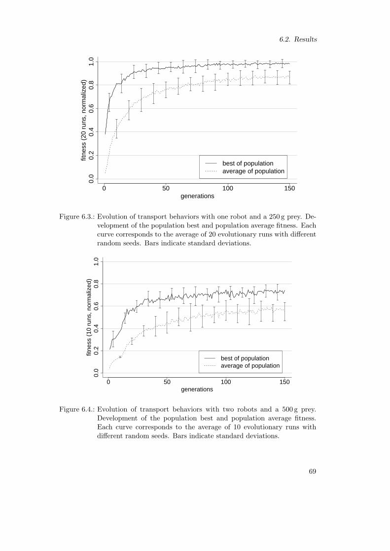
6.2. Results
0 50 100 150
0.0
0.2
0.4
0.6
0.8
1.0
generations
fitne
ss (
20 r
uns,
nor
mal
ized
)
best of populationaverage of population
Figure 6.3.: Evolution of transport behaviors with one robot and a 250 g prey. De-velopment of the population best and population average fitness. Eachcurve corresponds to the average of 20 evolutionary runs with differentrandom seeds. Bars indicate standard deviations.
0 50 100 150
0.0
0.2
0.4
0.6
0.8
1.0
generations
fitne
ss (
10 r
uns,
nor
mal
ized
)
best of populationaverage of population
Figure 6.4.: Evolution of transport behaviors with two robots and a 500 g prey.Development of the population best and population average fitness.Each curve corresponds to the average of 10 evolutionary runs withdifferent random seeds. Bars indicate standard deviations.
69

6. The Adaptive Value of Self-Assembly—Evolution of Solitary and Group Transport
to the average of 20 and 10 runs with different random seeds. The values are nor-malized in the range [0,1]. The lower bound is tight, and represents trials in whichthe prey was not moved and the robots lost visual contact to it (fitness zero). Theupper bound corresponds to the maximum distance a robot that is pre-assembledwith the lighter (250 g) prey can push the latter within T = 20 s. To compute theupper bound, we disabled any random noise affecting the actuators. The upperbound so computed was 152 cm. By comparing the figures, we can see that thefitness values obtained in the one-robot evolutions (see Figure 6.3) are higher thanthe fitness values obtained in the two-robot evolutions (see Figure 6.4).
6.2.1. Quantitative Analysis
The fitness assigned to a group depends not only on the genotype, but also onother factors, including the robots’ initial positions and orientations, the positionof the light source in the environment, and the noise affecting the robots’ sensorsand actuators. Thus, there is a very large number of possible configurations to test.However, the genotype is evaluated only in five trials (per generation) during theevolutionary design phase.
To select the best individual of each evolutionary run, we post-evaluate the µ =20 best-rated (parent) individuals of the final generation on a random sample of500 start configurations. The set of µ parent individuals comprises all geneticmaterial that would be exploited in subsequent generations in case the evolutionwould be resumed. For every evolutionary run, the individual exhibiting the highestaverage performance during the post-evaluation is considered to be the best one.To allow for an unbiased assessment of the performance of the best individual ofeach evolutionary run, we post-evaluate it (for a second time), on a random sampleof 500 start configurations.
Let us first consider the performance of the best individuals from the evolutionaryruns in which a single robot was simulated.
Individuals Evolved for Solitary Transport
Figure 6.5 illustrates the transport performance of individuals evolved for solitarytransport using a box-and-whisker plot [15]. The gray boxes correspond to thedistances (in cm) the 250 g prey was moved by a single robot in the 500 trialsof the post-evaluation. The average distances (in cm) range from 95.0 to 137.9.This is 62.5% to 90.7% of the upper bound. The standard deviations are in therange [9.7,35.3]. Note that the performance in some trials exceeds the upper bound(indicated by the bold horizontal line). This is caused by the random differencesamong the hardware of the robots (e.g., differences in the maximum speed M of awheel). Recall that to compute the upper bound, any form of random noise wasdisabled.
The individuals have been evolved for solitary transport. However, they areapplicable to group transport too. We can examine the ability of a group of robots—
70

6.2. Results
index of evolutionary run
dist
ance
mov
ed (
in c
m)
050
100
150
1 2 3 4 5 6 7 8 9 11 13 15 17 19
Figure 6.5.: Solitary and group transport performance of the best individualsevolved for solitary transport. Box-and-whisker plot of the distance(in cm) the prey was moved for each individual (500 observations perbox). Gray boxes: solitary transport (one robot, 250 g prey); whiteboxes: group transport (two robots, 500 g prey). See Section 6.2.2, forinformation on the order by which the evolutionary runs are presented.
each acting as a solitary worker—to transport a prey that requires cooperation tobe moved. Note that the robots can not perceive each other, nor have they beentrained in situations that involve multiple robots. We assessed the performance ofa group of two robots on 500 start configurations with the 500 g prey. All robotsof the group were initially assigned a copy of the same neural network controller.The results are shown in Figure 6.5 (white boxes). The average distances (in cm)range from 30.4 to 70.1. This is 20.0% to 46.1% of the upper bound. The standarddeviations are in the range [38.3,53.9]. The performance obtained with the two-robot setup is significantly worse than the performance obtained with the one-robotsetup (two-sided Mann-Whitney test, 5% significance level).
Let us now consider the performance of the best individuals from the evolutionaryruns in which two robots were simulated.
Individuals Evolved for Group Transport
Figure 6.6 illustrates the transport performance of the individuals evolved for grouptransport using a box-and-whisker plot [15]. Again, we evaluated both the perfor-mance in solitary transport and the performance in group transport in 500 trialseach. The gray boxes correspond to the distances (in cm) the 250 g prey was movedby a single robot. The average distances (in cm) range from 53.9 to 101.4. Thisis 35.4% to 66.7% of the upper bound. The standard deviations are in the range
71

6. The Adaptive Value of Self-Assembly—Evolution of Solitary and Group Transport
index of evolutionary run
dist
ance
mov
ed (
in c
m)
050
100
150
1 2 3 4 5 6 7 8 9 10
Figure 6.6.: Solitary and group transport performance of the best individualsevolved for group transport. For details, see caption of Figure 6.5.
[15.1,40.9]. For the trials with two robots and a 500 g prey (see white boxes), theaverage distances (in cm) range from 41.6 to 80.9. This is 27.4% to 53.2% of theupper bound. The standard deviations are in the range [12.2,35.6].
Although during evolution only two robots were present, the individuals performconsistently better when tested alone (two-sided Mann-Whitney tests, 5% signifi-cance level). This latter result supports our intuition that group transport is morecomplex than solitary transport. The presence of multiple robots is likely to leadto interferences that cause a decrease in performance. Moreover, group transportrequires a coordinated action as the members of the group have to push or pull theobject in similar directions.
In solitary transport, the individuals that were evolved for solitary transport ex-hibit a higher performance than the individuals that were evolved for group trans-port (one-sided Mann-Whitney test, 5% significance level). For group transport,however, individuals that were evolved for group transport exhibit a higher per-formance than the individuals that were evolved for solitary transport (one-sidedMann-Whitney test, 5% significance level). Thus, even though the robots can nei-ther sense nor communicate with each other directly, they benefit from behavingdifferently in group transport than in solitary transport.
6.2.2. Behavioral Analysis
In the following, we analyze the behaviors of robots when controlled by the neuralnetworks whose parameters are specified by the individuals evolved for solitary andgroup transport, respectively. We identify proximate mechanisms that cause the
72
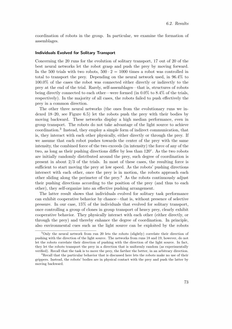
6.2. Results
coordination of robots in the group. In particular, we examine the formation ofassemblages.
Individuals Evolved for Solitary Transport
Concerning the 20 runs for the evolution of solitary transport, 17 out of 20 of thebest neural networks let the robot grasp and push the prey by moving forward.In the 500 trials with two robots, 500 · 2 = 1000 times a robot was controlled intotal to transport the prey. Depending on the neural network used, in 96.4% to100.0% of the cases the robot was connected either directly or indirectly to theprey at the end of the trial. Rarely, self-assemblages—that is, structures of robotsbeing directly connected to each other—were formed (in 0.0% to 8.4% of the trials,respectively). In the majority of all cases, the robots failed to push effectively theprey in a common direction.
The other three neural networks (the ones from the evolutionary runs we in-dexed 18–20, see Figure 6.5) let the robots push the prey with their bodies bymoving backward. These networks display a high median performance, even ingroup transport. The robots do not take advantage of the light source to achievecoordination.3 Instead, they employ a simple form of indirect communication, thatis, they interact with each other physically, either directly or through the prey. Ifwe assume that each robot pushes towards the center of the prey with the sameintensity, the combined force of the two exceeds (in intensity) the force of any of thetwo, as long as their pushing directions differ by less than 120◦. As the two robotsare initially randomly distributed around the prey, such degree of coordination ispresent in about 2/3 of the trials. In most of these cases, the resulting force issufficient to start moving the prey at low speed. As the robots’ pushing directionsintersect with each other, once the prey is in motion, the robots approach eachother sliding along the perimeter of the prey.4 As the robots continuously adjusttheir pushing directions according to the position of the prey (and thus to eachother), they self-organize into an effective pushing arrangement.
The latter result shows that individuals evolved for solitary task performancecan exhibit cooperative behavior by chance—that is, without presence of selectivepressure. In our case, 15% of the individuals that evolved for solitary transport,once controlling a group of clones in group transport of heavy prey, clearly exhibitcooperative behavior. They physically interact with each other (either directly, orthrough the prey) and thereby enhance the degree of coordination. In principle,also environmental cues such as the light source can be exploited by the robots
3Only the neural network from run 20 lets the robots (slightly) correlate their direction ofpushing with the direction of the light source. The networks from runs 18 and 19, however, do notlet the robots correlate their direction of pushing with the direction of the light source. In fact,they let the robots transport the prey in a direction that is uniformly random (as experimentallyverified). Recall that the task is to move the prey, the farther the better, in an arbitrary direction.
4Recall that the particular behavior that is discussed here lets the robots make no use of theirgrippers. Instead, the robots’ bodies are in physical contact with the prey and push the latter bymoving backward.
73

6. The Adaptive Value of Self-Assembly—Evolution of Solitary and Group Transport
to achieve coordination. As we will see in the following, this is the case for theindividuals evolved for group transport.
Individuals Evolved for Group Transport
Concerning the 10 runs for the evolution of group transport, 5 out of 10 of thebest neural networks let the robots display self-assembly behavior (correspondingto the first five pairs of boxes in Figure 6.6). Four out of these five neural networksemploy the strategy depicted in Figure 6.7(a). Each robot cycles (with the gripperheading forward) around the prey to reach a side correlated with the directionof the light source (e.g., the opposite side). Some neural networks let the robotcycle either counter-clockwise or clockwise depending on which path is shorter.During this phase, the robot remains distant from the prey, and thereby, also froma potential teammate that is already connected to the prey. Once the side that iscorrelated with the light source is approximately reached, the robot approaches theprey and potentially the connected teammate, and establishes a connection. Thatis, by exploiting the relative position of both the prey and the light source, the tworobots organize into a dense formation, potentially a linear chain. Each robot keepson moving forward, pushing the prey (e.g., towards the light source). Over the 500trials, 500 · 2 = 1000 times a robot was engaged in group transport. Depending onthe neural network used, in 71.1% to 94.6% of the cases, the robot was connectedeither directly or indirectly to the prey at the end of the trial. Self-assembledstructures were formed in 3.2% to 53.4% of the trials, respectively.
The other five neural networks (corresponding to the five latter pairs of boxesin Figure 6.6) make no use of the gripper element. Their strategy is depicted inFigure 6.7(b). They control the robot to move backward. The robot cycles aroundthe prey to reach a side correlated with the light source. Again, some neuralnetworks let the robot cycle either counter-clockwise or clockwise depending onwhich path is shorter. Differently from the previous behavior, however, the robotgets into physical contact with the prey while cycling around it. In fact, the robottries to push the prey with its body, while at the same time sliding along the prey’sperimeter. If multiple robots are present, their behaviors let them organize into adense, and thus very effective, pushing arrangement [see Figure 6.7(b)].
One neural network was capable of letting the robots display a combination ofboth types of behaviors [see Figure 6.7(c)]. In 28.6% of the cases at the end of thetrial, one robot was pushing the prey with the body by moving backward, whilethe other robot was grasping and pushing the prey by moving forward (recall thatboth robots were controlled by an identical neural network). The performance thegroup achieved in this configuration was significantly higher than the performancethe group could achieve in any other configuration when controlled by the sameneural network (two-sided Mann-Whitney tests, 5% significance level).
74
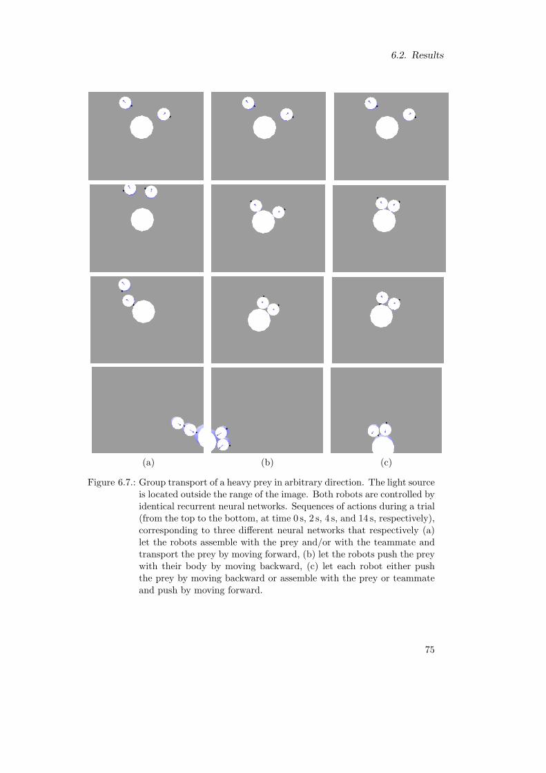
6.2. Results
(a) (b) (c)
Figure 6.7.: Group transport of a heavy prey in arbitrary direction. The light sourceis located outside the range of the image. Both robots are controlled byidentical recurrent neural networks. Sequences of actions during a trial(from the top to the bottom, at time 0 s, 2 s, 4 s, and 14 s, respectively),corresponding to three different neural networks that respectively (a)let the robots assemble with the prey and/or with the teammate andtransport the prey by moving forward, (b) let the robots push the preywith their body by moving backward, (c) let each robot either pushthe prey by moving backward or assemble with the prey or teammateand push by moving forward.
75

6. The Adaptive Value of Self-Assembly—Evolution of Solitary and Group Transport
050
100
150
200
index of evolutionary run
dist
ance
mov
ed (
in c
m)
1 2 3 4 5 6 7 8 9 10
050
100
150
200
index of evolutionary run
dist
ance
mov
ed (
in c
m)
1250g prey, regular size1250g prey, large size
Figure 6.8.: Post-evaluation of the best individuals with groups of five robots trans-porting a 1250 g prey for 30 seconds (200 observations per box). In-dividuals labeled 1–5 are those that let robots self-assemble, all othermake no use of the gripper element. Geometry of the prey: (a) size asduring the two-robot evolutions (i.e., radius 12 cm); (b) size scaled bythe factor the prey’s mass as well as the number of robots has increased(i.e., radius 30 cm).
(a) (b)
Figure 6.9.: Group transport of a 1250 g prey (radius: 12 cm) by five robots. Snap-shots for two different individuals: (a) an individual that let the robotsself-assemble. The group is capable of transporting the prey at lowspeed. (b) An individual that let the robots make no use of the gripperelement. The group is incapable of moving the prey as the latter offersnot enough contact surface for being pushed effectively by more thantwo robots. For a quantitative analysis, see Figure 6.8.
76
6.2. Results
6.2.3. Scalability
We examine to what extent the observed behaviors are scalable, in other words,whether the evolved individuals are able to let robots cooperate in the transport ofa heavier prey when the group size becomes larger. We focus on the best individualsfrom the evolutionary runs with two robots. For each run we take the best individualand evaluate it 200 times using a group of five robots. We keep the geometry ofthe prey identical, but we increase its mass proportionally to the increase in thenumber of robots (1250 g). The gray boxes of the plot in Figure 6.8 show thedistance (in cm) the prey was moved during these trials. The individuals from thefirst five evolutionary runs shown from the left in the figure are those that let therobots make use of the gripper element to solve the task. Self-assemblages occurredin 89.0%, 99.0%, 92.0%, 59.5%, and 46.0% of the trials, respectively. The otherfive individuals do not let the robots make use of the gripper element. Overall,the individuals making use of self-assembly (the average distances are respectively14.4, 18.7, 20.0, 3.7, and 3.4 cm) outperform the other individuals (the averagedistances are respectively, 1.6, 1.8, 1.7, 1.4, and 2.0 cm). The latter individuals areincapable of achieving the task as the prey does not offer enough contact surfacefor being pushed effectively by more than two robots (see Figure 6.9). However, ifthe perimeter of the prey is scaled by the same factor as the mass and the numberof robots has increased, all individuals are able to move the prey, and the ones thatlet the robots not self-assemble exhibit a better performance (see white boxes inFigure 6.8).
77

6. The Adaptive Value of Self-Assembly—Evolution of Solitary and Group Transport
78

7. The Benefit of Biasing Self-Assembly—Evolution of Group Transport
In this chapter, we investigate three mechanisms that promote groups of robots toself-organize into effective pushing and pulling structures:
• The task is simplified by defining a dedicated target location, a light source.
• The fitness function explicitly rewards groups of robots for self-assemblinginto physical structures that are connected with the prey [see Figure 5.2(b)on page 61].
• Each robot features additional acting and cognitive abilities. To make it eas-ier for robots to self-assemble, each robot is equipped with a mechanism toactively scan its surrounding for teammates. To make a robot more flexiblewhen being part of an assembled structure, it is equipped with an additionaldegree of freedom that allows it to rotate its chassis into any horizontal di-rection while its upper part keeps connected to the prey or another robot.
7.1. Methods
In this section, we detail the simulation model, the controller, and the evolutionaryalgorithm.
7.1.1. Simulation Model
The simulation model of the robot is illustrated in Figure 7.1. In contrast to theprevious model (see Section 6.1.2), the robot is composed of an upper part (calledthe turret) that is linked to a lower part (called the chassis) via an actuated hingejoint.
The robot’s abilities are summarized in Table 7.1. The rotating base actuatorenables the robot to align its turret (with respect to its chassis) to any angularoffset (in rad) in [−π, π]. Note that the physical response is delayed: while γ refersto the desired angular position of the base, γ denotes its current angular position.The angular speed (in rad/s) of the rotation is 2. The camera scans for other robotsand for prey on a virtual ray heading in the controllable, horizontal direction β.The scan stops respectively at the first (i.e., the closest) intersection point betweenthe ray and another robot and the first intersection point between the ray and theprey. For both intersection points, the distance can be computed. Perception is
79
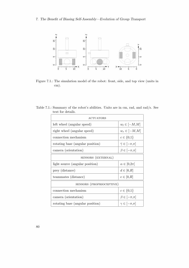
7. The Benefit of Biasing Self-Assembly—Evolution of Group Transport
05
1015
Z
05
1015
Z
100 5X
100 5Y
10 05
100
5
X
Y
Figure 7.1.: The simulation model of the robot: front, side, and top view (units incm).
Table 7.1.: Summary of the robot’s abilities. Units are in cm, rad, and rad/s. Seetext for details.
actuators
left wheel (angular speed) wl ∈ [−M,M ]
right wheel (angular speed) wr ∈ [−M,M ]
connection mechanism c ∈ {0,1}rotating base (angular position) γ ∈ [−π,π]
camera (orientation) β ∈ [−π,π]
sensors (external)
light source (angular position) α ∈ [0,2π]
prey (distance) d ∈ [0,R]
teammates (distance) e ∈ [0,R]
sensors (proprioceptive)
connection mechanism c ∈ {0,1}camera (orientation) β ∈ [−π,π]
rotating base (angular position) γ ∈ [−π,π]
80

7.1. Methods
o6o5o4o3o2o1
1i i2 i3 i4 i5 i6
wheelleft
mechanismrotatingbase base
rotatingconnection
connectionmechanism
wheelright
headingcamera
rotatingbase
light prey teammates cameraheading
Figure 7.2.: The neural network controller. Only connections to and from the thirdneuron of the hidden layer (from the left) are illustrated. Dashed arcsillustrate the feedback loop corresponding to the directional camera.
restricted to objects within range R = 50 cm. In this study, the light source isalways visible for the robots. We also performed a set of experiments in which theprey, due to its size, could shadow the light source [108]. Random noise affects therobot’s sensors (i.e., α, d, e, R, and γ) and actuators (i.e., wl, wr, M , γ, and β).
7.1.2. Controller
We employ the same control architecture as in the previous study (see Section 7.1.2).The simple recurrent neural network [71] is illustrated in Figure 7.2. It has an inputlayer of six neurons (i1, i2, . . . , and i6), a hidden layer of six (fully inter-connected)neurons, and an output layer of six neurons (o1, o2, . . . , and o6).
The activations of the six input neurons are computed based on the robot’s sensorreading (see Table 7.1):
i1 = c, (7.1)
i2 =12π
γ + 0.5, (7.2)
i3 ={
0 if light source not visible;0.5 + 0.5 α
2π otherwise,(7.3)
i4 = 1.0− 0.9d
R, (7.4)
i5 = 1.0− 0.9e
R, (7.5)
i6 =12π
β + 0.5. (7.6)
The activations of the six output neurons are used to set the motor commands(see Table 7.1). Thereby, (o1, o2, o3) defines the speed of the left and the right
81

7. The Benefit of Biasing Self-Assembly—Evolution of Group Transport
10cm
40cm
300cm
nest(i.e., light source)
Figure 7.3.: Example of initial placement: the prey (black disk) has to be trans-ported towards a nest (i.e., a light source). The robots approach theprey from the half space on the side of the nest: they are placed ran-domly within a semi-circle 40 to 50 cm away from the prey.
wheels and the status of the connection mechanism [using Equations (6.6)–(6.8)].The activations of the other three output neurons are used as follows:
γ = (o4 − o5)π, (7.7)
β = β +π
5(o6 − 0.5). (7.8)
To determine the initial heading of the camera (β), the robot scans once its entiresurrounding and chooses the direction with minimum distance to the prey.
7.1.3. Evolutionary Algorithm
The evolutionary algorithm used is the self-adaptive (µ + λ) evolution strategyintroduced in Section 6.1 (with µ = 20 and λ = 60).
Fitness Computation
The simulated environment consists of a flat ground, a prey, and a light source. Theprey is modeled as a cylinder of radius 8 cm and of height 8 cm. The mass of the preychanges across simulation trials. It is chosen uniformly from {500, 625, 750, 875, 1000}(in g). The minimum number of robots necessary to move the prey is either 2 or3 (depending on its mass). A simulation trial lasts T = 20 simulated seconds.Initially, N = 4 robots are put at random positions and orientations in the neigh-borhood of the prey. The placement strategy is illustrated in Figure 7.3.
The quality measure Q is defined as:
Q ={ A if T ≤ 0;
1 + (1 +√T )Aρ otherwise,
(7.9)
where A ∈ [0,1] reflects the assembly performance, T ∈ [0,∞) reflects the transportperformance, and ρ = 2.
82

7.2. Results
Let Z be the set of control steps after T2 = 10 s have elapsed.1 Then, the assembly
performance A can be defined as
A =1|Z|N
∑
t∈Z
N∑
i=1
Ati, (7.10)
where Ati ∈ [0,1] is defined by
Ati =
1 if i ∈Mt;0 if (i /∈Mt) ∧ (dt
i > R);0.75 if (i /∈Mt) ∧ (dt
i < R2 );
0.65R−dti
R/2 + 110 otherwise.
(7.11)
Mt is the set of robots that are physically linked to the prey at time t. It comprisesrobots both directly and indirectly connected to the prey. dt
i is an estimate of theminimum distance of robot i to the prey at time t. If no prey is detected withinthe sensing range, we set dt
i = R + 1.The transport performance measure T reflects the distance the prey has been
moved towards the light source. It is defined as
T = max(0,D0 −DT ), (7.12)
where Dt denotes the distance between the prey and the light source at time t.The performance of an individual is evaluated in S = 5 independent trials. The
sample of test configurations is changed once at the beginning of each generation.Let Qi be the quality observed in trial i. Then, the fitness is given by
F =1S
S∑
i=1
Qi. (7.13)
The fitness values of the individuals have to be maximized.
7.2. Results
The experimental setup described above has been used in 10 independent evolution-ary runs of 750 generations each.2 This corresponds to 60 000 fitness evaluationsper run. In Figure 7.4, the average and the maximum fitness time histories arepresented. Each curve corresponds to the average of 10 runs with different randomseeds. The fitness values are normalized in the range [0,1]; bounds for the perfor-mance were computed as in Section 6.2. Altogether the best and average fitnessvalues continuously increase for about 500 generations. However, the attained fit-ness level drastically varies among the different runs. In fact, only 1 out of 10 runsyielded individuals of very high performance.
1In fact, as the robots start being unconnected and from positions up to R = 50 cm away fromthe prey, some time is required to approach the prey and to establish a connection.
2Initially, the number of generations was set to 300. However, based on the evolutionaryprogress it appeared to be promising to continue the evolution to generation 750.
83

7. The Benefit of Biasing Self-Assembly—Evolution of Group Transport
0 200 400 600
0.0
0.2
0.4
0.6
0.8
1.0
generations
fitne
ss (
10 r
uns,
nor
mal
ized
)
best of populationaverage of population
Figure 7.4.: Evolution of group transport behaviors with four-robot groups: devel-opment of fitness in 10 evolutionary runs.
7.2.1. Quantitative Analysis
To select the best individual of each evolutionary run, we measure the quality ofthe µ = 20 parent individuals of the last generation on a sample of 500 differenttest configurations. The individual exhibiting the highest average performance isconsidered to be best and is post-evaluated for a second time, on a new sample of2500 test configurations.
The average assembly performance A ∈ [0,1] for the best individuals of all 10 runsis in the range [0.72,0.96]. The standard deviations are in the range [0.12,0.25].In the following, we focus on the best individual. Figure 7.5 illustrates the 17topologies in which up to four robots and a prey can be organized. With oneexception, all topologies occurred at least once during the post-evaluation of thebest individual (the frequencies are indicated in the figure). Over the 2500 trials,4 · 2500 = 10 000 times a robot was controlled to transport the prey. In 95.5%of the cases, the robot was connected either directly or indirectly to the prey atthe end of the trial. Thereby, in 37.0% of the cases, the robot was part of anassembled structure. In the majority of the 2500 trials, the robots formed at leastone self-assembled structure (63.6%).
Figure 7.6 plots the distance (in cm) by which prey of different mass approachedthe target location (i.e., D0 − DT ), as observed in the 2500 trials for the bestindividual. Upper bounds are indicated by the bold line. The average distances(in cm) are 109.7, 93.8, 82.2, 69.5, and 57.2. This is respectively 49.2%, 46.1%,44.8%, 42.5%, and 39.8% of the upper bounds for prey of mass (in g) 500, 625,750, 875, and 1000. Note that the upper bounds are not tight; they correspond to
84

7.2. Results
0.48% (12)
27.20% (680)
1.20% (30)
5.76% (144)
0.08% (2)
0.00% (0)
0.08% (2)
0.04% (1)
1.48% (37)
4.48% (112)
0.68% (17)
3.72% (93)
0.92% (23)
0.12% (3)
6.76% (169)
0.12% (3)
46.88% (1172)
15
14
13
12
101
2
3
4
5
6
7
8
9
17
16
11
structureconnection frequency
Figure 7.5.: Topology into which up to four robots (transparent disks) and a prey(gray disks) can be assembled and frequencies by which these topologieshave been observed at the end of a trial (2500 observations in total).
85

7. The Benefit of Biasing Self-Assembly—Evolution of Group Transport
500 625 750 875 1000
050
100
150
200
mass of prey (in g)
appr
oach
of t
arge
t (in
cm
)0
5010
015
020
0
Figure 7.6.: Box-and-whisker plot visualizing the distance (in cm) prey of differ-ent mass was moved by a group of four robots controlled by the bestindividual (500 observations per box).
situations in which the four robots start from an optimal configuration being alreadypre-assembled with each other and the prey. Compared to the results reported inSection 6.2, the standard deviations are astonishingly low; they range from 18.1 to22.0. Recall that fluctuations in performance are partially caused by the nature ofthe task (e.g., differences in the initial placement of the robots).
In the following, we examine the ability of a large group of robots to transportprey of big weight.
7.2.2. Scalability
We consider groups of 4, 8, 12, and 16 robots. Along with the group size, themass of the prey is increased proportionally from 500 to 1000, 1500, and 2000 g,respectively. We evaluate the best individual using these setups 800 times in total.Since large groups of robots might require more time to self-assemble, the simulationperiod T is extended to 30 seconds. To ensure a non-overlapping placement of upto 16 robots, they are initially placed at random positions within a semi-circle ofradius 50 cm away from the prey (similar to Figure 7.3).
Figure 7.7 shows the distance (in cm) the prey was moved in each case. Theaverage distances (in cm) are 167.1, 102.1, 42.3, and 12.9. This is respectively50.2%, 30.6%, 12.7%, and 3.9% of the upper bound. The standard deviations arein the range [21.6,49.0]. Overall, the performance decreases drastically with groupsize and the weight of the prey. We observed that the high density in which the16 robots are initially put in the semi-circle makes it difficult for the robots to
86

7.2. Results
4 8 12 16
010
020
030
0
group size N (mass of prey ~ N)
appr
oach
of t
arge
t (in
cm
)0
100
200
300
Figure 7.7.: Performance of the best evolved individual for groups of 4, 8, 12, and16 robots, randomly arranged in a semi-circle of 50 cm radius aroundthe center, transporting prey of 500 g, 1000 g, 1500 g, and 2000 g, re-spectively, for T = 30 s (200 observations per box).
0 1 2 3 4 5 6 7 8 9 10 11 12
010
020
030
0
size of assembled structure MT (N=16; 2000 g prey; T=30 s)
appr
oach
of t
arge
t (in
cm
)0
100
200
300
Figure 7.8.: Performance of the best evolved individual for groups of 16 robotstransporting prey of 2000 g for T = 30 s; 200 observations, groupedaccording to |MT | (i.e., the number of robots physically linked to eachother and the prey at time T ). Boxes are drawn with widths propor-tional to the square-roots of the number of observations in the groups.
87
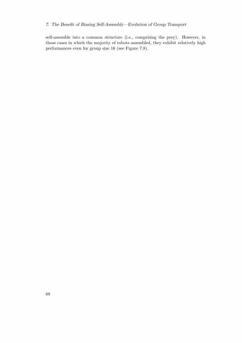
7. The Benefit of Biasing Self-Assembly—Evolution of Group Transport
self-assemble into a common structure (i.e., comprising the prey). However, inthose cases in which the majority of robots assembled, they exhibit relatively highperformances even for group size 16 (see Figure 7.8).
88

8. An Explicit Task Decomposition—Evolution of Self-Assembly and GroupTransport in Heterogeneous Teams
In this chapter, we consider groups of robots with incomplete knowledge about thetask. Some robots (called the blind ones) are not capable of localizing the targetlocation (i.e., a light source), while all others can. Such heterogeneity can, as in ourcase, be designed into a system, but might also arise during task execution if, forinstance, some robots of the group have hardware failures of their sensory system.Or, it might be due to the nature of the environment: for example, the presence ofobstacles, teammates, or of the object being manipulated can make it impossiblefor some of the robots to perceive the target location. In any case, it is importantto consider this problem, as blind robots—being physically assembled with the restof the group—might significantly disrupt the performance of the system.
Given the heterogeneity of the group, the task appears more complex than theone studied in the previous chapter. In fact, the task is a team task (see Sec-tion 3.2.1), because the blind and the non-blind robots are required to performdifferent subtasks concurrently.1 Instead of increasing the computational effort tosolve the task (i.e., the population size and/or the number of generations), we tryto exploit the knowledge gained in the problem domain to effectively constrain thesolution search space. Following a behavior-based approach, we decompose theproblem into sub-problems. Each sub-problem is addressed by a dedicated controlmodule that uses only those sensors and actuators we consider relevant to solve thesub-problem. One control module is in charge of self-assembly, that is, of lettingthe robot connect either directly or indirectly to the prey. As soon as the robot hasconnected, one of two other control modules is in charge of letting the robot pullthe prey towards the target location. Which of the two control modules is useddepends on whether the robot is blind.
8.1. Methods
In this section, we detail the simulation model, the controller, and the evolutionaryalgorithm.
1We use the term group to refer to both, a group and a team (as defined in Section 3.2.1),unless a distinction is important.
89

8. Evolution of Self-Assembly and Group Transport in Heterogeneous Teams
05
1015
Z
05
1015
Z
100 5X
100 5Y
10 05
100
5
X
Y
Figure 8.1.: The simulation model of the robot: front, side, and top view (units incm).
8.1.1. Simulation Model
The simulation model of the robot is illustrated in Figure 8.1. This model closelymatches the basic geometrical properties of a first prototype of the s-bot that wasdesigned and constructed prior to experimentation [179]. The model of the con-nection mechanism comprises a protuding cuboid and a small contact plate in itsfront. A connection can be established if the plate is in contact with the prey orthe body of another robot.
The robot’s abilities are summarized in Table 8.1. Some robots, called the blindones, are not capable of detecting the light source, while all the others can. Arobot can sense whether it is in motion or not. In addition, it can measure thehorizontal angle and the intensity of the traction force acting in between its turretand the chassis (see Section 2.2.3). The turret has two proximity sensors headingin the front-left and front-right direction. Each robot, as well as the prey, has acolored LED ring. The ring can be activated in two colors, and thus be used tocommunicate a binary state. The camera scans for colored objects on a virtual raydirectly ahead of the robot. The scan stops at the first (i.e., the closest) intersectionpoint between the ray and another object, if any. If the first detected object is red,then d refers to the distance to the intersection point (in cm) and β refers to thehorizontal angle (in degrees) to the center of the object.
8.1.2. Controller
We make use of a modular control architecture as illustrated in Figure 8.2. A robotcan be in one of two main states: either its gripper is unconnected or it is connectedto another object. In the first case, the sub-task is self-assembly, in the latter case itis group transport. A control loop executes every 100ms the corresponding controlmodule.
The process of self-assembling is governed by the attraction and the repulsionamong robots, and between robots and a seed (see Figure 8.3). The seed is eitherthe prey or one of the robots. The color ring of the seed is permanently activated
90
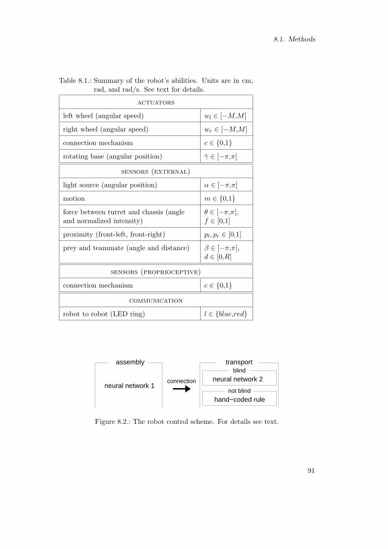
8.1. Methods
Table 8.1.: Summary of the robot’s abilities. Units are in cm,rad, and rad/s. See text for details.
actuators
left wheel (angular speed) wl ∈ [−M,M ]
right wheel (angular speed) wr ∈ [−M,M ]
connection mechanism c ∈ {0,1}rotating base (angular position) γ ∈ [−π,π]
sensors (external)
light source (angular position) α ∈ [−π,π]
motion m ∈ {0,1}force between turret and chassis (angleand normalized intensity)
θ ∈ [−π,π],f ∈ [0,1]
proximity (front-left, front-right) pl, pr ∈ [0,1]
prey and teammate (angle and distance) β ∈ [−π,π],d ∈ [0,R]
sensors (proprioceptive)
connection mechanism c ∈ {0,1}communication
robot to robot (LED ring) l ∈ {blue,red}
neural network 1
assembly
not blind
blind
neural network 2
hand−coded rule
transport
connection
Figure 8.2.: The robot control scheme. For details see text.
91
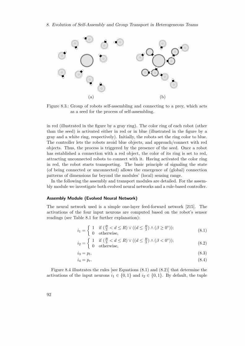
8. Evolution of Self-Assembly and Group Transport in Heterogeneous Teams
(a) (b)
Figure 8.3.: Group of robots self-assembling and connecting to a prey, which actsas a seed for the process of self-assembling.
in red (illustrated in the figure by a gray ring). The color ring of each robot (otherthan the seed) is activated either in red or in blue (illustrated in the figure by agray and a white ring, respectively). Initially, the robots set the ring color to blue.The controller lets the robots avoid blue objects, and approach/connect with redobjects. Thus, the process is triggered by the presence of the seed. Once a robothas established a connection with a red object, the color of its ring is set to red,attracting unconnected robots to connect with it. Having activated the color ringin red, the robot starts transporting. The basic principle of signaling the state(of being connected or unconnected) allows the emergence of (global) connectionpatterns of dimensions far beyond the modules’ (local) sensing range.
In the following the assembly and transport modules are detailed. For the assem-bly module we investigate both evolved neural networks and a rule-based controller.
Assembly Module (Evolved Neural Network)
The neural network used is a simple one-layer feed-forward network [215]. Theactivations of the four input neurons are computed based on the robot’s sensorreadings (see Table 8.1 for further explanation):
i1 ={
1 if (R3 < d ≤ R) ∨ ((d ≤ R
3 ) ∧ (β ≥ 0◦));0 otherwise,
(8.1)
i2 ={
1 if (R3 < d ≤ R) ∨ ((d ≤ R
3 ) ∧ (β < 0◦));0 otherwise,
(8.2)
i3 = pl, (8.3)i4 = pr. (8.4)
Figure 8.4 illustrates the rules [see Equations (8.1) and (8.2)] that determine theactivations of the input neurons i1 ∈ {0, 1} and i2 ∈ {0, 1}. By default, the tuple
92

8.1. Methods
β
Pd
rule conditions i1 i2
1 d > R - 0 0
2 R3
< d ≤ R - 1 1
3 d ≤ R3
β ≥ 0◦ 1 0
4 d ≤ R3
β < 0◦ 0 1
Figure 8.4.: The camera scans for objects on a virtual ray directly ahead of therobot. R = 60 is the sensing range (in cm). The scan stops at thefirst (i.e., the closest) intersection point between the ray and anotherobject, if any. If the first detected object is red, then P, d, and β referto the intersection point, the distance (in cm) to it, and the horizontalangle (in degrees) to the center of the object, respectively. In this case,(i1, i2) is determined by the rule set above. In all other cases, i1 and i2are set to zero. R
3 = 20 is the distance (in cm) between the robot andanother object under which there is high risk of collision.
(i1, i2) is set to (0, 0). As illustrated in Figure 8.4, the camera scans for the firstcolored object in front of the robot. If a red object is detected, (i1, i2) indicates itspresence and coarse orientation.
The network output (o1, o2, o3) defines the speed of the left and the right wheelsand the status of the connection mechanism [using Equations (6.6)–(6.8)]. Therotating base actuator is kept in the default position (γ = 0).
Assembly Module (Rule-Based)
Table 8.2 specifies a parameterized set of rules that map sensory inputs from thevision system (i1 and i2) and the proximity sensors (i3 and i4) to motor commandsto control the speed of the left and the right side of the traction system (o1 ando2, respectively) as well as the connection mechanism (o3). A speed value of 1(0) corresponds to the maximum speed forward (backward) M . The parameters1 ∈ (0.5, 1] specifies the speed with which the robot turns on the spot, if nored object is perceived (rule 1). If a red object is perceived but it is more thanR3 = 20 cm away, the robot moves forward with maximum speed (rule 2). If the redobject is close and more to the left (rule 3) or to the right (rule 4), the parameterss2 ∈ [0.5, 1) and s3 ∈ [s2, 1] specify to what extent the robot turns in the appropriatedirection during approach. In any case, o3 is set to 1, that is, the robot tries toestablish a connection as soon as the grasping requirements are fulfilled.
93

8. Evolution of Self-Assembly and Group Transport in Heterogeneous Teams
Table 8.2.: Rule-based controller for self-assembly with parameters s1, s2, and s3.
rule i1 i2 i3 i4 o1 o2 o3
1 0 0 * * s1 1− s1 1
2 1 1 * * 1 1 1
3 1 0 * * s2 s3 1
4 0 1 * * s3 s2 1
The rule-based controller does not take the inputs from the proximity sensors(i3 and i4) into account. Nevertheless, unconnected robots that reside betweenthe robot itself and the object to approach are perceived as blue objects and thusshadow the presence of the red object (see caption of Figure 8.4).
We assessed the quality of different parameter assignments by performing 200simulation trials in which 2, 4, 6, or 8 robots had to self-assemble with a prey. 1000different assignments to the parameter set (s1, s2, s3) were assessed, and the oneexhibiting the highest average performance was selected (0.85, 0.60, 0.85).
Transport Module
Once the robot is connected, the transport module is activated. We developed twodistinct control modules to control the blind and the non-blind robots, respectively.
The non-blind robot orients its chassis towards the light source. The speed ofthe wheels is set to the maximum value M . This procedure turned out to be veryeffective under the assumptions that the robot (i) is connected either directly orindirectly to the prey, (ii) is equipped with a rotating base actuator, and (iii) canalways perceive the light source.
The controller for the blind robots consists of a simple recurrent neural net-work [71] with four hidden nodes. It is executed in each iteration of the controlloop. The activations of the six input neurons are computed based on the robot’ssensor readings (see Table 8.1):
i1 = f max (0, cos (θ − 0.0π)) , (8.5)i2 = f max (0, cos (θ − 0.5π)) , (8.6)i3 = f max (0, cos (θ − 1.0π)) , (8.7)i4 = f max (0, cos (θ − 1.5π)) , (8.8)i5 = m, (8.9)
i6 =γ
2π+
12. (8.10)
The activations of the three output neurons are used to set the motor commands
94

8.1. Methods
(see Table 8.1):
wl = Mo1, (8.11)wr = Mo1, (8.12)γ = π(2o2 − 1). (8.13)
During transport, the gripper is kept closed (c = 1).
8.1.3. Evolutionary Algorithm
The evolutionary algorithm used is the self-adaptive (µ + λ) evolution strategyintroduced in Section 7.1.3 (with µ = 20 and λ = 80). The object parametersencode the connection weights of the two neural networks. The recombinationoperator combines two genotypes (i) by swapping the parameter sets of either thefirst or the second neural network, (ii) by intermediate recombination, or (iii) bydominant recombination, each with the same probability.
Fitness Computation
The simulated environment consists of a flat ground, a prey, and eight light sources.The prey is modeled as a cylinder. Its radius (in cm) is chosen in the range [5.8, 10];its mass (in grams) is chosen in the range [200N, 300N ], where N ∈ {2, 3, 4, 5}denotes the number of robots used. For each simulation trial, the prey’s radius andmass, the group size N , and the number of blind robots NB ∈ {1, 2, . . . , dN/2e}are chosen randomly according to uniform distributions. A simulation trial lastsT = 35 simulated seconds. The eight light sources are uniformly arranged in acircle at a distance of 500 cm from the prey. At any point in time, there is only onelight source active, and thus indicating the target location. Which one is selectedrandomly according to a uniform distribution once prior and twice during simulation(after 15 and 25 seconds). Doing so, we evaluate the ability of the blind robots toadapt their direction of motion to the rest of the group. All robots are placed atrandom positions and orientations no more than 50 cm all around the prey.
The quality Q exhibited in a trial is defined as
Q = CA+ (1− C)T , (8.14)
where A ∈ [0,1] reflects the assembly performance, T ∈ [0,1] reflects the transportperformance of the blind robots, and C = 1
5 . Q does not account for the perfor-mance of the non-blind robots as their controller is not subject to variation. Q iscomputed based solely on information the robots perceive locally during simula-tion.2
2We assume that during the fitness evaluation, each robot can detect the angular position ofthe light source. The control module of the blind robots is not provided with the correspondinginformation.
95

8. Evolution of Self-Assembly and Group Transport in Heterogeneous Teams
The assembly performance A is defined as
A =1
(T + 1) N
T∑
t=0
N∑
i=1
Ati, (8.15)
where Ati ∈ [0,1] is defined by
Ati =
1 if i ∈Mt;12 + 1
4Oti if (i /∈Mt) ∧ (d ≤ C);
14 if (i /∈Mt) ∧ (C < d ≤ R);0 otherwise,
(8.16)
whereOt
i = 1−min[1,
(|βt
i |/π
6
)]. (8.17)
Mt is the set of robots that are physically linked to the prey at time t (see Sec-tion 7.1.3). Note that i ∈ Mt if and only if robot i is connected to a red object attime t.
Let be B ⊂ {1, 2, . . . , N} the set of blind robots. Let Z be the set of control stepsno more than 6 seconds preceding a change in the target location or the end of thesimulation.3 Then, the transport performance T can be defined as
T =1
|Z| |B|∑
t∈Z
∑
i∈BT t
i , (8.18)
where T ti ∈ [0,1] is defined by
T ti =
{0 ct
i = 0;12 max
(0,Ht
i
)+
(14 + 1
4wt
iMHt
i
)otherwise,
(8.19)
and
Hti =
π − 2∠(αt
i, γti
)
π∈ [−1,1]. (8.20)
Thus, T accounts for the accuracy with which the chassis is aligned towards thetarget location, as well as this accuracy in relation to the speed of the wheelsw = wl = wr ∈ [0,M ].
The fitness value of an individual is calculated based on its performance in fiveindependent trials (see Section 7.1.3). The fitness values have to be maximized.
8.2. Results
The experimental setup has been used in 10 independent evolutionary runs of 300generations each. This corresponds to 30 000 fitness evaluations per run. In Fig-ure 8.5, the average and the maximum fitness time histories are presented. Fitness
3During the other control steps the robots are busy assembling or adapting to the currenttarget location.
96

8.2. Results
0 50 100 150 200 250 300
0.0
0.2
0.4
0.6
0.8
1.0
generations
fitne
ss (
10 r
uns,
nor
mal
ized
)
best of populationaverage of population
Figure 8.5.: Development of fitness values in 10 evolutionary runs. The bold line atfitness level 0.5 marks an upper bound to the average performance ofrobotic systems in which blind robots do not contribute to transport.
values are in the range [0,1]. Each curve corresponds to the average of the 10 runs.The bold line at fitness level 0.5 marks an upper bound to the average performanceof robotic systems in which blind robots do not contribute to transport: once arobot is connected, having its chassis oriented in a random direction and pullingwith maximum speed, the reward the robot receives is 0.5 on average.4
We post-evaluated the µ = 20 best individuals of the final generation of eachevolutionary run on a sample of 200 different test configurations. Thereby, wemeasured the distance by which the prey approached the target location. As thelatter changes twice during each trial, we take as performance measure the sum ofthe corresponding three distances. For each evolution, we consider the individualexhibiting the highest average performance as best. We observed that the bestindividuals of all evolutionary runs exhibit almost the same performance. Theperformance (in cm) of the best individuals is on average 151, the standard deviationis 7.6. In the following, we focus on the assembly and transport performance of thebest individual.
8.2.1. Quantitative Analysis (Assembly Module)
We evaluate the performance of the rule-based and evolved assembly controllersin a group transport task with 4, 8, 12, and 16 robots, none of which is blind.As during evolution, the mass of the prey is proportional to the group size. The
4Q = 15· 1 +
`1− 1
5
´38
= 0.5 [see Equation (8.14)].
97

8. Evolution of Self-Assembly and Group Transport in Heterogeneous Teams
4 8 12 16
010
020
030
040
0
group size N (mass of prey ~ N)
appr
oach
of t
arge
t (in
cm
)0
100
200
300
400
010
020
030
040
0 parameterized, hand−coded controllerevolved controller
Figure 8.6.: Performance of the rule-based and evolved assembly modules (pairedwith the hand-coded transport module) for groups of N = 4, 8, 12,and 16 non-blind robots, randomly arranged in a full circle of 50 cmradius around the center, transporting the prey for 35 seconds (200observations per box). The mass of the prey (in grams) was chosenrandomly from within the range [200N, 300N ].
transport module is the hand-coded controller. Figure 8.6 plots the distance (incm) by which the prey approached the target location in 1600 trials (in total). Foreach group size, the evolved assembly controller performs significantly better thanthe rule-based assembly controller (two-sided Mann-Whitney tests, 5% significancelevel). Moreover, it can be seen that the performance of the evolved controllerscales better with group size. For the rule-based controller, the average distances(in cm) are 199.6, 174.8, 147.0, and 125.4, respectively for the group sizes 4, 8, 12,and 16. This is respectively 55.6%, 48.7%, 41.0%, and 34.9% of the upper bound.The standard deviations are in the range [49.9,59.3]. For the evolved controller, theaverage distances (in cm) are 215.6, 214.9, 213.4, and 203.4, respectively for thegroup sizes 4, 8, 12, and 16. This is respectively 60.1%, 59.9%, 59.5%, and 56.7%of the upper bound. The standard deviations are in the range [35.4,43.1]. Theevolved individual accomplishes the group transport with very high reliability: ineach of the 800 cases, the prey approached the targets in total by at least 100 cm.
8.2.2. Scalability (Assembly Module)
We examine the problem of letting groups of 10 to 100 robots self-assemble witha static prey. The robots are initially placed at random positions and orientationswithin a circular area around the prey. We vary the radius of the initial area tostudy to what extent the behavior is affected by the density of robots. We define
98

8.2. Results
the density of robots as the size of the 2-D area covered by the robots divided bythe size of the available 2-D area. The area size covered by a robot (in simulation)is A = 116 cm2. For each group size we studied densities of 0.050, 0.075, 0.100,0.125, 0.150, 0.175, and 0.200. We could not study densities much higher than thisas it is impossible to find an initial placement in which the robots may turn on thespot without collision.5
Figures 8.7 and 8.8 present the percentage of the group that could successfullyconnect within a time period of 300 seconds for all group sizes and densities in200 trials using the rule-based controller and the neural network based controller,respectively.
In case of the two lowest densities (0.050 and 0.075) the performance for bothcontrollers reduces drastically with group size. We observed that, at such lowdensity, some robots did not have visual contact with any teammates or with theprey. In addition, many robots lost visual contact, since all the teammates lefttheir neighborhood when approaching red objects. For a swarm of robots to self-assemble in a situation in which the robot density is particularly low, it could beof advantage to propagate the presence of the prey using a third color (in additionto blue and red), and to use a rule set to let the robots form a cluster. However, incase the robots start from positions in which visual contact might not be present,the problem of exploration/aggregation has to be addressed.
For all other densities, the neural network based controller has a particularly highsuccess rate. In contrast, the rule-based controller’s success rate drops considerablywhen moving from group size 10 to 20. For increasing group sizes, however, theperformance tends to improve.
We now analyze the relationship between the time needed for a robot to connectand the group size. We measure the average time for a robot to self-assemble ina group of 10 to 100 robots for the different densities (200 trials per situation).Robots that have not established a connection within the predefined timeout of300 s are not taken into account. We do not consider the densities 0.050 and 0.075,as the percentage of connected robots is particularly low.
Figure 8.9 (rule-based controller) and Figure 8.10 (neural network based con-troller) present the average time (over all trials) it took a robot to connect, dividedby the group size and scaled so that the performance for group size 10 equals 1. Forthe neural network based controller, the time grows sub-linearly with the group size.This might be due to the fact that the bigger the structure, the more it providessurface for potential connections.
5To ensure a minimum gap of about 1 cm, the robots are positioned so that a minimum distanceof 20 cm is present between the centers of any two objects. Let us consider the robots and theprey as disks of radius r. To pack 11 congruent disks without over-lapping in a unit circle, thedisk radius may not exceed r = 0.2548485 (for a proof see [169]). This packing would result in a
robot density of 10πr2
π−πr2A
π102 = 0.256. If we consider our additional constraint that one disk (i.e.,the prey) has to be positioned in the center of the unit circle, the highest possible robot density isequal or lower than 0.256.
99

8. Evolution of Self-Assembly and Group Transport in Heterogeneous Teams
1020
3040
5060
7080
9010
0
0 20 40 60 80 100
successful connections (in percentage)
grou
p si
ze
0 20 40 60 80 1000 20 40 60 80 1000 20 40 60 80 1000 20 40 60 80 1000 20 40 60 80 1000 20 40 60 80 100
density 0.200density 0.175density 0.150density 0.125density 0.100density 0.075density 0.050
Figure 8.7.: Rule-based controllers: box-and-whisker plot [15] showing the percent-age of successful connections during self-assembly in a group of 10 to100 robots, for different initial densities (200 observations per box).
100

8.2. Results
1020
3040
5060
7080
9010
0
0 20 40 60 80 100
successful connections (in percentage)
grou
p si
ze
0 20 40 60 80 1000 20 40 60 80 1000 20 40 60 80 1000 20 40 60 80 1000 20 40 60 80 1000 20 40 60 80 100
density 0.200density 0.175density 0.150density 0.125density 0.100density 0.075density 0.050
Figure 8.8.: Neural network based controller: box-and-whisker plot [15] showing thepercentage of successful connections during self-assembly in a group of10 to 100 robots, for different initial densities (200 observations perbox).
101

8. Evolution of Self-Assembly and Group Transport in Heterogeneous Teams
0.0
0.5
1.0
1.5
group size (N)
robo
t com
plet
ion
time
[mea
n, s
cale
d by
θ(1
N)]
10 20 30 40 50 60 70 80 90 100
density 0.100density 0.125
density 0.150density 0.175
density 0.200
Figure 8.9.: Rule-based controller: time complexity (see text for details) for groupsof 10 to 100 robots and different initial densities.
0.0
0.5
1.0
1.5
group size (N)
robo
t com
plet
ion
time
[mea
n, s
cale
d by
θ(1
N)]
10 20 30 40 50 60 70 80 90 100
density 0.100density 0.125
density 0.150density 0.175
density 0.200
Figure 8.10.: Neural network based controller: time complexity (see text for details)for groups of 10 to 100 robots and different initial densities.
102

8.2. Results
010
020
030
040
0ap
proa
ch o
f tar
get (
in c
m)
010
020
030
040
00
100
200
300
400
010
020
030
040
0
N = 2
NB = 1
N = 3
NB = 2
N = 3
NB = 1
N = 4
NB = 2
N = 4
NB = 1
N = 5
NB = 3
N = 5
NB = 2
N = 5
NB = 1
(mass of prey ~ N)
S0: blind robots removedS1: blind robots passive
S2: blind robots with neural networkS3: blind robots replaced
Figure 8.11.: Performance of transport strategies in situations in which NB of agroup of N robots are blind (500 observations per box). For self-assembly, the hand-coded controller is used.
8.2.3. Quantitative Analysis (Transport Module)
In the following, we evaluate the performance of the evolved neural network con-troller for the blind robots with respect to a collection of alternative strategies. Inorder to avoid any bias towards the evolved controller, we use as assembly mod-ule the parameterized hand-coded controller with the most successful parameterset. During transport, non-blind robots are controlled by the standard hand-codedcontroller. For the blind robots, we evaluate the performance of four differentstrategies:
• S0: blind robots are manually removed from experimentation.
• S1: blind robots stop acting once connected; thus, their actuators do notmove, but they remain connected to the prey.
• S2: blind robots are controlled by the neural network based controller forblind robots.
• S3: blind robots are manually replaced by fully operational robots which inturn are controlled by the standard controller for non-blind robots.
Figure 8.11 shows the performance of the transport strategies for those combi-nations of group size N and number of blind robots NB that were used duringevolution (see Section 8.1.3). The first and the last boxes in each group represent
103
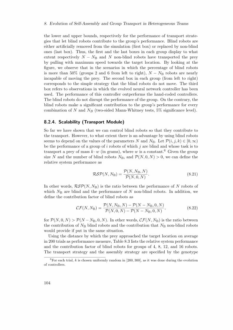
8. Evolution of Self-Assembly and Group Transport in Heterogeneous Teams
the lower and upper bounds, respectively for the performance of transport strate-gies that let blind robots contribute to the group’s performance. Blind robots areeither artificially removed from the simulation (first box) or replaced by non-blindones (last box). Thus, the first and the last boxes in each group display to whatextent respectively N − NB and N non-blind robots have transported the preyby pulling with maximum speed towards the target location. By looking at thefigure, we observe that in the scenarios in which the percentage of blind robotsis more than 50% (groups 2 and 6 from left to right), N − NB robots are nearlyincapable of moving the prey. The second box in each group (from left to right)corresponds to the simple strategy that the blind robots do not move. The thirdbox refers to observations in which the evolved neural network controller has beenused. The performance of this controller outperforms the hand-coded controllers.The blind robots do not disrupt the performance of the group. On the contrary, theblind robots make a significant contribution to the group’s performance for everycombination of N and NB (two-sided Mann-Whitney tests, 5% significance level).
8.2.4. Scalability (Transport Module)
So far we have shown that we can control blind robots so that they contribute tothe transport. However, to what extent there is an advantage by using blind robotsseems to depend on the values of the parameters N and NB. Let P(i, j, k) ∈ [0,∞)be the performance of a group of i robots of which j are blind and whose task is totransport a prey of mass k ·w (in grams), where w is a constant.6 Given the groupsize N and the number of blind robots NB, and P(N, 0, N) > 0, we can define therelative system performance as
RSP(N, NB) =P(N, NB, N)P(N, 0, N)
. (8.21)
In other words, RSP(N,NB) is the ratio between the performance of N robots ofwhich NB are blind and the performance of N non-blind robots. In addition, wedefine the contribution factor of blind robots as
CF(N, NB) =P(N, NB, N)− P(N −NB, 0, N)P(N, 0, N)− P(N −NB, 0, N)
, (8.22)
for P(N, 0, N) > P(N −NB, 0, N). In other words, CF(N,NB) is the ratio betweenthe contribution of NB blind robots and the contribution that NB non-blind robotswould provide if put in the same situation.
Using the distance by which the prey approached the target location on averagein 200 trials as performance measure, Table 8.3 lists the relative system performanceand the contribution factor of blind robots for groups of 4, 8, 12, and 16 robots.The transport strategy and the assembly strategy are specified by the genotype
6For each trial, k is chosen uniformly random in [200, 300], as it was done during the evolutionof controllers.
104
8.2. Results
Table 8.3.: Relative system performance RSP(N, NB) (top value) andcontribution factor of blind robots CF(N, NB) (bottom value),both expressed as percentages, for different group sizes (N)and different numbers of blind robots (NB). The mass of theprey is chosen proportional to group size N.
N/NB 0 1 2 3 14N 2
4N 34N N
4 100.00 80.54 64.53 40.57 80.54 64.53 40.57 0.19
100.00 50.20 57.88 39.14 50.20 57.88 39.14 0.19
8 100.00 93.86 85.01 72.56 85.01 58.91 24.87 -0.43
100.00 60.41 55.66 53.97 55.66 50.93 22.73 -0.43
12 100.00 94.70 89.01 84.48 84.48 56.95 22.09 -0.70
100.00 50.54 46.15 50.45 50.45 48.37 19.14 -0.70
16 100.00 96.90 95.34 91.39 82.88 56.96 20.80 0.10
100.00 51.70 54.29 58.06 40.42 47.41 16.85 0.10
of the best evolved individual. It can be seen that blind robots contribute to thesystem’s performance unless all robots are blind (i.e., NB = N , see last column).In all cases in which no more than half of the robots are blind, the contribution ofthe blind robots is 40 to 60% of the contribution non-blind robots would provide(on average) if put in the same situation.
105

8. Evolution of Self-Assembly and Group Transport in Heterogeneous Teams
106

9. Discussion
In this third part of the dissertation, we investigated whether self-assembly canhelp a system of autonomous robots to accomplish a concrete task—the cooperativetransport of a heavy object called prey. We used a physics-based simulation model,in which the robots are endowed with connection mechanisms that allow them toattach to (and detach from) each other and the prey. We presented a comprehensivestudy on the use of evolutionary algorithms to produce the collective capabilitiesof group transport and self-assembly. The evolved solutions were shown to besuperior to relatively simple hand-coded strategies, and their performance comparedreasonably well with theoretical upper bounds.
In Chapter 6, we evolved neural networks that let a group of two robots performa group transport task. The robots had very limited cognitive abilities, they couldneither communicate nor perceive each other directly. The fitness function of theevolutionary algorithm did neither explicitly reward the robots for self-assembling,nor did it impose any bias concerning the spatial organization of the robots duringtask performance. Nevertheless, in half of the evolutionary runs, the best-ratedneural networks let robots self-assemble. This is a striking result, confirming thatsuch capability—as in social insects—can provide adaptive value to the group. Theanalysis revealed the proximate mechanisms that caused the formation of the self-assemblages. In particular, two visual cues present in the environment (the preyand a light source) were exploited by the robots in the formation of assembledstructures. Moreover, as the assemblages were formed by robots facing approxi-mately in the same (and sometimes the opposite) direction, they were suitable forthe accomplishment of the task (which required all robots to pull/push the prey inapproximately the same direction). This underlines the importance of investigatingself-assembly in the context of its function. When increasing both the group sizeand the weight of the prey, the performance decreased. Groups that self-assembledwere still capable of moving the prey. In contrast, groups that did not make use ofself-assembly were incapable of moving the prey, unless the prey size was increasedproportionally.
We also examined the relation between group transport and solitary transport,with focus on an evolutionary perspective. In fact, we conducted two sets of evolu-tionary runs to synthesize respectively: (i) neural networks to control robots thatcompete at the individual level based on their performance in solitary transport,and (ii) neural networks to control robots that compete at the level of groups intheir performance in group transport. Networks evolved for solitary transport werecapable of letting robots engage also in group transport (with various degree ofsuccess). Networks evolved in group transport were capable of letting robots en-
107

9. Discussion
gage also in solitary transport. However, our results show that group transportand solitary transport impose different demands on the robot. In fact, robots en-gaged in group transport benefit from behaving differently from those engaged insolitary transport. The results support also our intuition that group transport ismore complex than solitary transport. Our study revealed a variety of proximatemechanisms that can cause coordinated behavior. In particular, we observed thatrobots enhance their degree of coordination by physically interacting either directlyor indirectly, that is, via the environment, and by exploiting visual cues of the envi-ronment. This holds for all networks evolved for group transport, but even for 15%of the networks evolved for solitary transport. That is, some “solitary individuals”,when grouped together with a clone, clearly exhibited social behavior (mutual ben-efit). As a result of this, we hypothesize that group transport in social insects hasevolved from situations in which solitary transporters, without being aware of eachother, cooperatively transported a common prey. To the best of our knowledge,although plausible, this hypothesis has not been further investigated by biologists.
In Chapter 7, we investigated mechanisms that facilitate the evolution of neuralnetworks that let robots self-assemble to solve the (transport) task. In particular,we explicitly rewarded robots to self-assemble into physical structures that areconnected to the prey. Moreover, we provided the robots with additional actingand cognitive abilities. Compared to the previous setup, the evolutionary runsrequired increased effort (in terms of fitness evaluations), which is possibly dueto the increased complexity of the solution search space. One of 10 evolutionaryruns performed yielded individuals of very high performance. The best evolvedcontroller lets a group of four robots and the prey self-assemble into a single entityin 89% of the cases. In the group transport of a light (heavy) prey by four robots,it achieved on average 67.7% (58.0%) of the optimal performance. Fluctuations inperformance were surprisingly low.
In Chapter 8, we studied group transport in heterogeneous teams1 of robots.Some robots were capable of localizing the target location in transport, while theothers, the blind ones, were not. Blind robots were equipped with stagnation andforce sensors. We exploited the knowledge we had gained in the problem domainto effectively constrain the solution search space. In particular, the problem wasdecomposed into the sub-problems of self-assembly and transport. Each robot wasprogrammed to signal its state (of being assembled or not), and the robots weretrained to make use of the signals accordingly. This resulted in a positive feedbackmechanism and caused the formation of physical structures that were connectedto the prey (which seeded the assembly process). The structures could attaindimensions far beyond the robots’ (local) sensing range. Ten out of 10 evolutionaryruns yielded controllers of about equally high performance.
The self-assembly performance of the best controller, was examined for groupsizes up to 100 non-blind robots that were initially scattered randomly with differentdensities around a static prey. The controller (a neural network in this case) let
1For a definition of teamwork, see Section 3.2.1.
108
the robots self-assemble reliably into a physical structure comprising the prey. Thetime for a robot to connect grew on average sub-linearly with the group size.
The transport performance for blind robots was examined in teams of up to16 (blind and non-blind) robots. Provided that 25% or more robots were able tolocalize the target location, having blind robots connected to the structure did notdisrupt the performance of the team. On the contrary, the performance with blindrobots in the team was even superior in performance to the alternative of manuallyexcluding them. If no more than half of the robots were blind, the contribution ofthe blind robots was 40 to 60% of the contribution non-blind robots would provide(on average) if put in the same situation.
In social insects, self-assembly processes are widely observed. However, to thebest of our knowledge, self-assembly is not relevant for group transport in ants.Individual limitations might prevent ants from organizing into assemblages movingby their own propulsion. For this to happen, the ants’ pushing and pulling direc-tions must be aligned with each other. Ants of the species Pheidole crassinoda,for example, can alter the orientation of their bodies without releasing their holdon the prey [232] (see Section 5.1). In this case, however, the ants are directlymanipulating the prey. Ants that are part of an assembled structure have fewerdegrees of mobility. In some species, worker ants seem even to become motionlessas a reaction to being stretched (see [7] and references therein). This could explainwhy self-assemblages are virtually non-existing for group transport in ants. In therobotic study presented in Chapter 6, the robots had also very limited degrees ofmobility. In small groups, however, robots could align their pushing and pullingdirections by self-assembling into a fairly regular structure. In the robotic studiespresented in Chapters 7 and 8, the robots could change their pushing and pullingdirections independently of their orientation within the structure. This capacitymight be a key factor for the design of scalable group transport systems.
109

9. Discussion
110
Part IV.
Self-Assembling Robots:Experiments on
Self-Assembly Per Se
111

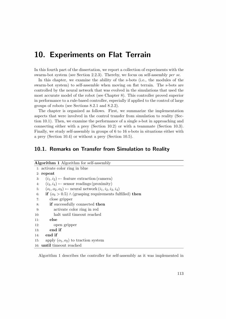
10. Experiments on Flat Terrain
In this fourth part of the dissertation, we report a collection of experiments with theswarm-bot system (see Section 2.2.3). Thereby, we focus on self-assembly per se.
In this chapter, we examine the ability of the s-bots (i.e., the modules of theswarm-bot system) to self-assemble when moving on flat terrain. The s-bots arecontrolled by the neural network that was evolved in the simulations that used themost accurate model of the robot (see Chapter 8). This controller proved superiorin performance to a rule-based controller, especially if applied to the control of largegroups of robots (see Sections 8.2.1 and 8.2.2).
The chapter is organized as follows. First, we summarize the implementationaspects that were involved in the control transfer from simulation to reality (Sec-tion 10.1). Then, we examine the performance of a single s-bot in approaching andconnecting either with a prey (Section 10.2) or with a teammate (Section 10.3).Finally, we study self-assembly in groups of 6 to 16 s-bots in situations either witha prey (Section 10.4) or without a prey (Section 10.5).
10.1. Remarks on Transfer from Simulation to Reality
Algorithm 1 Algorithm for self-assembly1: activate color ring in blue2: repeat3: (i1, i2)← feature extraction (camera)4: (i3, i4)← sensor readings (proximity)5: (o1, o2, o3)← neural network (i1, i2, i3, i4)6: if (o3 > 0.5) ∧ (grasping requirements fulfilled) then7: close gripper8: if successfully connected then9: activate color ring in red
10: halt until timeout reached11: else12: open gripper13: end if14: end if15: apply (o1, o2) to traction system16: until timeout reached
Algorithm 1 describes the controller for self-assembly as it was implemented in
113
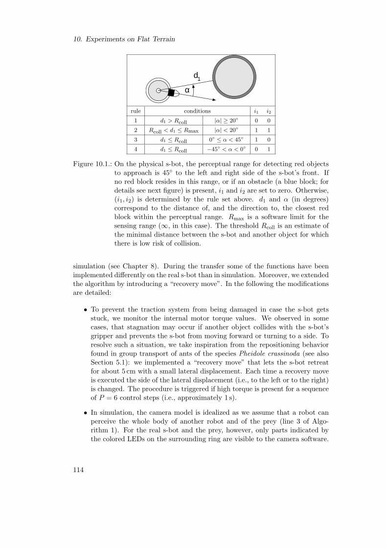
10. Experiments on Flat Terrain
d1
α
rule conditions i1 i2
1 d1 > Rcoll |α| ≥ 20◦ 0 0
2 Rcoll < d1 ≤ Rmax |α| < 20◦ 1 1
3 d1 ≤ Rcoll 0◦ ≤ α < 45◦ 1 0
4 d1 ≤ Rcoll −45◦ < α < 0◦ 0 1
Figure 10.1.: On the physical s-bot, the perceptual range for detecting red objectsto approach is 45◦ to the left and right side of the s-bot’s front. Ifno red block resides in this range, or if an obstacle (a blue block; fordetails see next figure) is present, i1 and i2 are set to zero. Otherwise,(i1, i2) is determined by the rule set above. d1 and α (in degrees)correspond to the distance of, and the direction to, the closest redblock within the perceptual range. Rmax is a software limit for thesensing range (∞, in this case). The threshold Rcoll is an estimate ofthe minimal distance between the s-bot and another object for whichthere is low risk of collision.
simulation (see Chapter 8). During the transfer some of the functions have beenimplemented differently on the real s-bot than in simulation. Moreover, we extendedthe algorithm by introducing a “recovery move”. In the following the modificationsare detailed:
• To prevent the traction system from being damaged in case the s-bot getsstuck, we monitor the internal motor torque values. We observed in somecases, that stagnation may occur if another object collides with the s-bot’sgripper and prevents the s-bot from moving forward or turning to a side. Toresolve such a situation, we take inspiration from the repositioning behaviorfound in group transport of ants of the species Pheidole crassinoda (see alsoSection 5.1): we implemented a “recovery move” that lets the s-bot retreatfor about 5 cm with a small lateral displacement. Each time a recovery moveis executed the side of the lateral displacement (i.e., to the left or to the right)is changed. The procedure is triggered if high torque is present for a sequenceof P = 6 control steps (i.e., approximately 1 s).
• In simulation, the camera model is idealized as we assume that a robot canperceive the whole body of another robot and of the prey (line 3 of Algo-rithm 1). For the real s-bot and the prey, however, only parts indicated bythe colored LEDs on the surrounding ring are visible to the camera software.
114
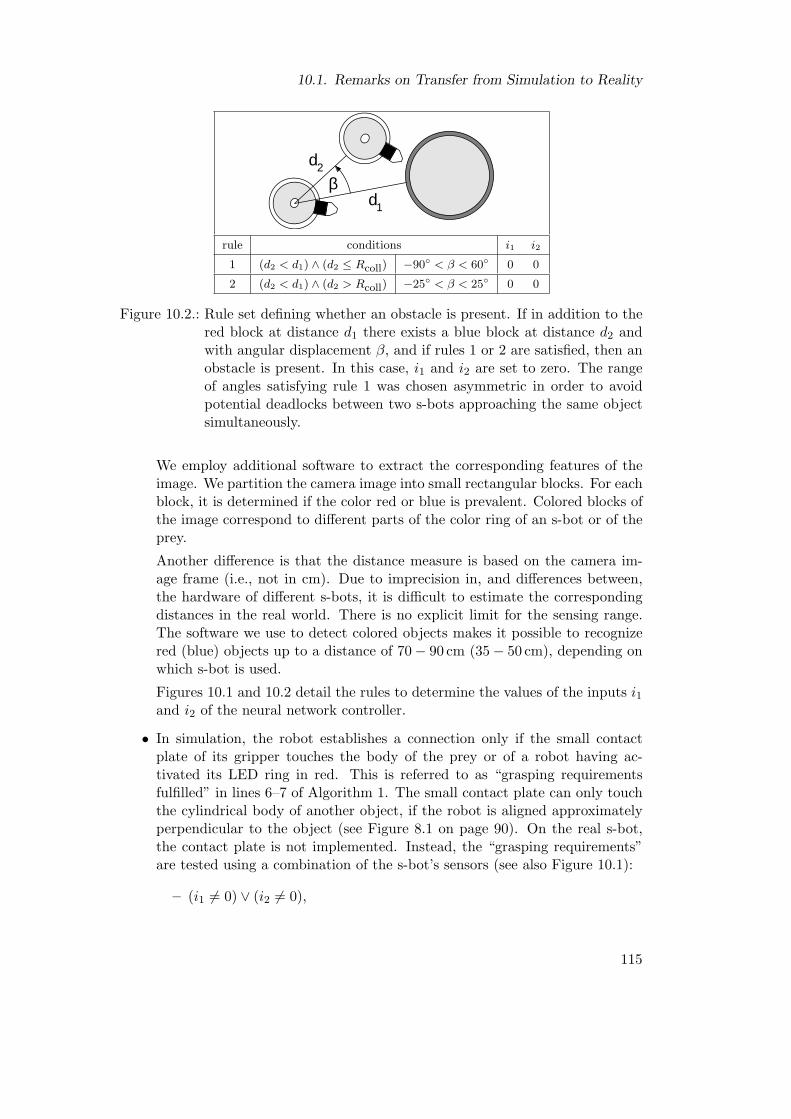
10.1. Remarks on Transfer from Simulation to Reality
d2
d1
β
rule conditions i1 i2
1 (d2 < d1) ∧ (d2 ≤ Rcoll) −90◦ < β < 60◦ 0 0
2 (d2 < d1) ∧ (d2 > Rcoll) −25◦ < β < 25◦ 0 0
Figure 10.2.: Rule set defining whether an obstacle is present. If in addition to thered block at distance d1 there exists a blue block at distance d2 andwith angular displacement β, and if rules 1 or 2 are satisfied, then anobstacle is present. In this case, i1 and i2 are set to zero. The rangeof angles satisfying rule 1 was chosen asymmetric in order to avoidpotential deadlocks between two s-bots approaching the same objectsimultaneously.
We employ additional software to extract the corresponding features of theimage. We partition the camera image into small rectangular blocks. For eachblock, it is determined if the color red or blue is prevalent. Colored blocks ofthe image correspond to different parts of the color ring of an s-bot or of theprey.
Another difference is that the distance measure is based on the camera im-age frame (i.e., not in cm). Due to imprecision in, and differences between,the hardware of different s-bots, it is difficult to estimate the correspondingdistances in the real world. There is no explicit limit for the sensing range.The software we use to detect colored objects makes it possible to recognizered (blue) objects up to a distance of 70− 90 cm (35− 50 cm), depending onwhich s-bot is used.
Figures 10.1 and 10.2 detail the rules to determine the values of the inputs i1and i2 of the neural network controller.
• In simulation, the robot establishes a connection only if the small contactplate of its gripper touches the body of the prey or of a robot having ac-tivated its LED ring in red. This is referred to as “grasping requirementsfulfilled” in lines 6–7 of Algorithm 1. The small contact plate can only touchthe cylindrical body of another object, if the robot is aligned approximatelyperpendicular to the object (see Figure 8.1 on page 90). On the real s-bot,the contact plate is not implemented. Instead, the “grasping requirements”are tested using a combination of the s-bot’s sensors (see also Figure 10.1):
– (i1 6= 0) ∨ (i2 6= 0),
115
10. Experiments on Flat Terrain
– d1 ≤ Rgrasp,1
– |α| ≤ 30◦,
– no connection attempt failed within the last 18 control steps (i.e., ap-proximately 3 s).
If these requirements are fulfilled, the gripper optical barrier is used to de-tect whether an object is present between the two jaws of the gripper (seeSection 2.2.3). If this is the case, the procedure closes the gripper. Whileclosing, the gripper is slightly moved up and down several times to facilitatea tight connection. Failures of the connection procedure can be detected bymonitoring the gripper aperture (line 8 of Algorithm 1).
• For the real s-bot, the time of each control step is on average 0.17 s. This isalmost twice as long as in simulation (0.10 s). In addition, the values of theneural network’s inputs i1 and i2 correspond to an environmental scene thatwas captured more than 0.50 s before. This delay is due to the amount of timerequired to capture, store, and process the image. To ensure that the s-botcan react quickly enough to changes in its environment, we had to reduce thespeed of the traction system (line 15 of Algorithm 1). However, dependingon the situation, increased speed values can yield better performance withoutloss in quality. Therefore, the maximum speed M is set according to thefollowing rule:
M =
M1 if (i1 = 0) ∧ (i2 = 0);M2 if d1 ≤ Rgrasp;M3 if Rgrasp < d1 ≤ Rcoll;M4 if d1 > Rcoll.
(10.1)
After some preliminary experimentation, we have chosen the values M1 = 8,M2 = 5, M3 = 10, and M4 = 20. A value of 20 corresponds to a speed ofapproximately 6.5 cm/s of the s-bot.
Once the speed vector has been scaled accordingly, a moving average functionsmoothes the speed values over time in order to avoid hardware damage bypotentially oscillating speed settings.
10.2. Autonomous Docking of a Robot to a Prey
We examine the ability of a single s-bot to approach and connect with the prey [seeFigure 10.3(a)]. The prey is equipped with a color ring of the same shape as thegrippable ring of the s-bots. The ring has a diameter of 20 cm and is positioned0.5 cm higher than the ring of the s-bots. Its color is set to red.
1Rgrasp is an estimate of the maximum distance to an object that can still be grasped.
116
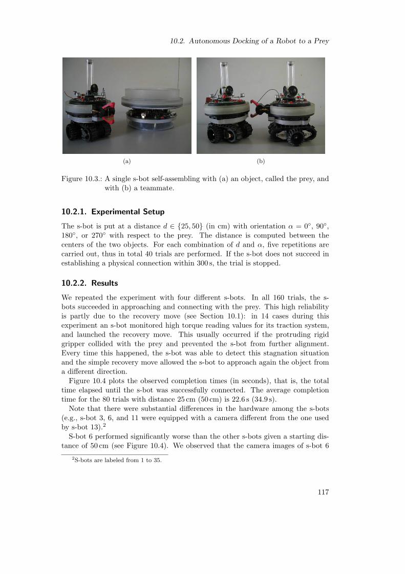
10.2. Autonomous Docking of a Robot to a Prey
(a) (b)
Figure 10.3.: A single s-bot self-assembling with (a) an object, called the prey, andwith (b) a teammate.
10.2.1. Experimental Setup
The s-bot is put at a distance d ∈ {25, 50} (in cm) with orientation α = 0◦, 90◦,180◦, or 270◦ with respect to the prey. The distance is computed between thecenters of the two objects. For each combination of d and α, five repetitions arecarried out, thus in total 40 trials are performed. If the s-bot does not succeed inestablishing a physical connection within 300 s, the trial is stopped.
10.2.2. Results
We repeated the experiment with four different s-bots. In all 160 trials, the s-bots succeeded in approaching and connecting with the prey. This high reliabilityis partly due to the recovery move (see Section 10.1): in 14 cases during thisexperiment an s-bot monitored high torque reading values for its traction system,and launched the recovery move. This usually occurred if the protruding rigidgripper collided with the prey and prevented the s-bot from further alignment.Every time this happened, the s-bot was able to detect this stagnation situationand the simple recovery move allowed the s-bot to approach again the object froma different direction.
Figure 10.4 plots the observed completion times (in seconds), that is, the totaltime elapsed until the s-bot was successfully connected. The average completiontime for the 80 trials with distance 25 cm (50 cm) is 22.6 s (34.9 s).
Note that there were substantial differences in the hardware among the s-bots(e.g., s-bot 3, 6, and 11 were equipped with a camera different from the one usedby s-bot 13).2
S-bot 6 performed significantly worse than the other s-bots given a starting dis-tance of 50 cm (see Figure 10.4). We observed that the camera images of s-bot 6
2S-bots are labeled from 1 to 35.
117
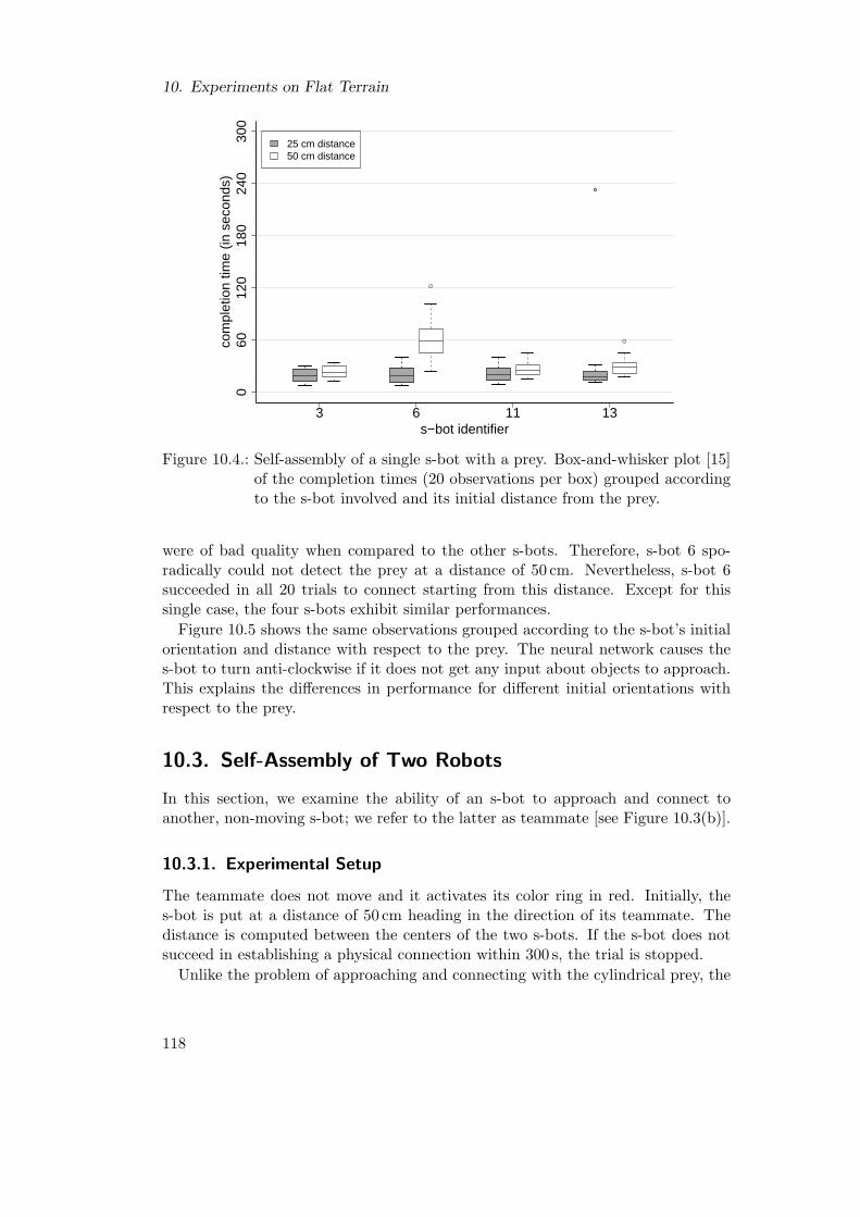
10. Experiments on Flat Terrain
s−bot identifier
com
plet
ion
time
(in s
econ
ds)
3 6 11 13
060
120
180
240
300
25 cm distance50 cm distance
Figure 10.4.: Self-assembly of a single s-bot with a prey. Box-and-whisker plot [15]of the completion times (20 observations per box) grouped accordingto the s-bot involved and its initial distance from the prey.
were of bad quality when compared to the other s-bots. Therefore, s-bot 6 spo-radically could not detect the prey at a distance of 50 cm. Nevertheless, s-bot 6succeeded in all 20 trials to connect starting from this distance. Except for thissingle case, the four s-bots exhibit similar performances.
Figure 10.5 shows the same observations grouped according to the s-bot’s initialorientation and distance with respect to the prey. The neural network causes thes-bot to turn anti-clockwise if it does not get any input about objects to approach.This explains the differences in performance for different initial orientations withrespect to the prey.
10.3. Self-Assembly of Two Robots
In this section, we examine the ability of an s-bot to approach and connect toanother, non-moving s-bot; we refer to the latter as teammate [see Figure 10.3(b)].
10.3.1. Experimental Setup
The teammate does not move and it activates its color ring in red. Initially, thes-bot is put at a distance of 50 cm heading in the direction of its teammate. Thedistance is computed between the centers of the two s-bots. If the s-bot does notsucceed in establishing a physical connection within 300 s, the trial is stopped.
Unlike the problem of approaching and connecting with the cylindrical prey, the
118
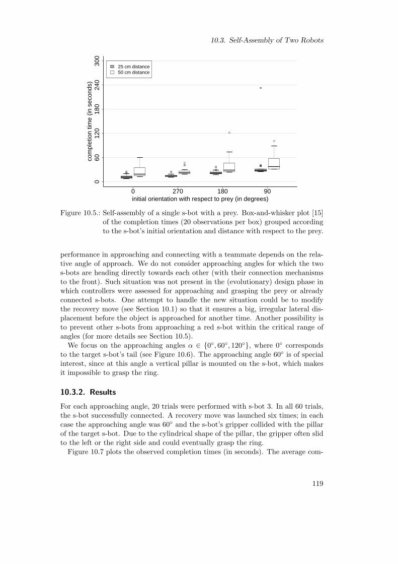
10.3. Self-Assembly of Two Robots
initial orientation with respect to prey (in degrees)
com
plet
ion
time
(in s
econ
ds)
060
120
180
240
300
0 270 180 90
25 cm distance50 cm distance
Figure 10.5.: Self-assembly of a single s-bot with a prey. Box-and-whisker plot [15]of the completion times (20 observations per box) grouped accordingto the s-bot’s initial orientation and distance with respect to the prey.
performance in approaching and connecting with a teammate depends on the rela-tive angle of approach. We do not consider approaching angles for which the twos-bots are heading directly towards each other (with their connection mechanismsto the front). Such situation was not present in the (evolutionary) design phase inwhich controllers were assessed for approaching and grasping the prey or alreadyconnected s-bots. One attempt to handle the new situation could be to modifythe recovery move (see Section 10.1) so that it ensures a big, irregular lateral dis-placement before the object is approached for another time. Another possibility isto prevent other s-bots from approaching a red s-bot within the critical range ofangles (for more details see Section 10.5).
We focus on the approaching angles α ∈ {0◦, 60◦, 120◦}, where 0◦ correspondsto the target s-bot’s tail (see Figure 10.6). The approaching angle 60◦ is of specialinterest, since at this angle a vertical pillar is mounted on the s-bot, which makesit impossible to grasp the ring.
10.3.2. Results
For each approaching angle, 20 trials were performed with s-bot 3. In all 60 trials,the s-bot successfully connected. A recovery move was launched six times; in eachcase the approaching angle was 60◦ and the s-bot’s gripper collided with the pillarof the target s-bot. Due to the cylindrical shape of the pillar, the gripper often slidto the left or the right side and could eventually grasp the ring.
Figure 10.7 plots the observed completion times (in seconds). The average com-
119

10. Experiments on Flat Terrain
(a) (b) (c)
Figure 10.6.: Illustration of angles in which the static teammate is approached inthe two s-bot experiments: (a) 0◦, (b) 60◦, and (c) 120◦.
0 60 120approaching angle (in degrees); distance = 50cm
com
plet
ion
time
(in s
econ
ds)
060
120
180
240
300
0 60 120
Figure 10.7.: Self-assembly of an s-bot with a teammate. Box-and-whisker plot [15]of the completion times (20 observations per box).
120

10.4. Self-Assembly of a Group of Six Robots and a Prey
(a) (b)
Figure 10.8.: Self-assembly of six s-bots with the prey: (a) initial configuration, and(b) final configuration in a typical trial.
pletion times for the 20 trials with approaching angle 0◦, 60◦, and 120◦ (and initialdistance 50 cm) are 17.9, 26.4, and 17.9 s, respectively.
10.4. Self-Assembly of a Group of Six Robots and a Prey
So far, we have studied situations in which a single s-bot is approaching a singleobject for grasping. In this section, we assess the performance of a group of sixs-bots that self-assemble with each other and a prey.
10.4.1. Experimental Setup
The process is seeded by the prey. Each s-bot is driven by an identical controller.This is the same controller as used in the one s-bot experiments.
At the beginning of each trial, the six s-bots are placed at arbitrary positions3 andorientations inside a circle of radius 70 cm around the prey. To favor interactionsamong the s-bots, we limited their initial positions to a 90◦ segment of the circle.The same density could be obtained by putting a swarm of 24 s-bots inside a fullcircle of the same radius. Figure 10.8 shows the initial and the final configurationsin one typical trial. If the s-bots do not succeed within 600 s, the trial is stopped.
10.4.2. Results
Figure 10.9 shows a bar plot of the 34 trials performed. The pattern of each barindicates the number of s-bots that could successfully connect within the time
3As in simulation, the s-bots are positioned in such a way that there is a minimum distance of20 cm between the centers of any two objects. This allows all s-bots to turn on the spot with nocollision of their gripper elements.
121

10. Experiments on Flat Terrain
repetitions
grou
p co
mpl
etio
n tim
e (in
sec
onds
)0
120
240
360
480
600
4 connections5 connections6 connections
Figure 10.9.: Self-assembly of six s-bots with a prey (34 repetitions).
frame. The height of the bar represents the number of elapsed seconds until thelast s-bot completed connection.
In total, 199 times an s-bot succeeded in establishing a connection, while only5 times an s-bot failed. At the end of 30 out of 34 trials, all seven objects werephysically connected; on average this took 96.4 s.
10.5. Self-Assembly of a Group of 16 Robots
In this section, we assess the performance of a group of 16 s-bots to self-assemble.
10.5.1. Experimental Setup
One s-bot acts as a seed, as after 5 seconds it stops moving and activates a patternon its LED ring: the two LEDs in the front are set to blue, while the remainingsix LEDs are set to red. In this way, it attracts teammates to approach from anydirection other than the front.4
The s-bot acting as a seed is put in the center of a circle of radius 50 cm. 15additional s-bots are placed at arbitrary positions and orientations within the samecircle. The s-bots are positioned so that each s-bot can rotate on the spot withoutcolliding with a teammate (i.e., we ensure a minimum distance of 20 cm betweenthe centers of any two s-bots).
4In fact, in its front, the s-bot is unable to passively receive connections from other s-bots dueto the location of its own gripper mechanism.
122
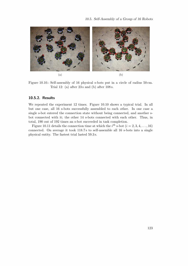
10.5. Self-Assembly of a Group of 16 Robots
(a) (b)
Figure 10.10.: Self-assembly of 16 physical s-bots put in a circle of radius 50 cm.Trial 12: (a) after 23 s and (b) after 108 s.
10.5.2. Results
We repeated the experiment 12 times. Figure 10.10 shows a typical trial. In allbut one case, all 16 s-bots successfully assembled to each other. In one case asingle s-bot entered the connection state without being connected, and another s-bot connected with it; the other 14 s-bots connected with each other. Thus, intotal, 190 out of 192 times an s-bot succeeded in task completion.
Figure 10.11 details the connection time at which the ith s-bot (i = 2, 3, 4, . . . , 16)connected. On average it took 118.7 s to self-assemble all 16 s-bots into a singlephysical entity. The fastest trial lasted 59.3 s.
123

10. Experiments on Flat Terrain
2 3 4 5 6 7 8 9 10 11 12 13 14 15 16connected s−bot (ranked by connection time)
conn
ectio
n tim
e (in
sec
onds
)0
6012
018
024
030
0
Figure 10.11.: Self-assembly of 16 physical s-bots. Box-and-whisker plot [15] show-ing the time at which the ith s-bot connected (observations from the11 out of 12 trials in which all 16 s-bots successfully self-assembled).
124

11. Experiments on Rough Terrain
The s-bot was designed to perform tasks under rough terrain conditions. However,the neural network, which is the main part of our controller, was evolved controllings-bots on flat terrain (see Chapter 8).
In this chapter, we study to what extent the behavior of the robots is disruptedwhen operating on uneven terrain. We consider two types of rough terrain (seeFigure 11.1). Both terrain types are unnavigable for most standard wheeled robotsof a similar size. The first terrain type (here referred to as moderately rough terrain)has a surface with a regular structure. The second terrain type (here referred toas very rough terrain) consists of white plaster bricks providing a very rough, non-uniform surface.
In Section 11.1, we examine the performance of a single s-bot approaching andconnecting with a prey. In Section 11.2, we study groups of six s-bots self-assemblingwith each other and a prey.
11.1. Autonomous Docking of a Robot to a Prey
In this section, we examine the ability of a single s-bot to approach and connectwith the prey.
(a) (b)
Figure 11.1.: Types of rough terrain: (a) moderately rough terrain and (b) veryrough terrain.
125

11. Experiments on Rough Terrain
type of terrain
com
plet
ion
time
(in s
econ
ds)
flat moderately rough very rough
060
120
180
240
300
060
120
180
240
300
25 cm distance50 cm distance
Figure 11.2.: Self-assembly of one s-bot with a prey. Box-and-whisker plot [15]of the completion times on flat terrain (20 observations per box),moderately rough terrain (20 observations per box), and very roughterrain (19 observations per box).
11.1.1. Experimental Setup
Except for the difference in the terrain, the experimental setup and the control arekept unchanged (see Section 10.2).
11.1.2. Results
Figure 11.2 shows the performance of s-bot 13 for the different types of terrain. Foreach terrain, 40 trials were performed. In the 80 trials on the flat terrain and themoderately rough terrain the s-bot successfully connected to the prey. On the veryrough terrain, the s-bot failed once for both initial distances (25 cm and 50 cm). Inthe other 38 trials, the s-bot successfully connected with the prey.
We observed that on the very rough terrain the s-bots often launched the recoverymove during the approach phase. The roughness of the terrain caused a high torqueon the traction system during navigation. Thus, the mechanism to detect stagnationwas erroneously activated. During the recovery move, the s-bot moves backwardswithout recognizing obstacles. In the two cases in which the s-bot failed to completethe task, it got stuck with its back colliding with the prey. A refined version of thecontroller, which takes obstacles into account during recovery, is introduced in thefollowing section.
126
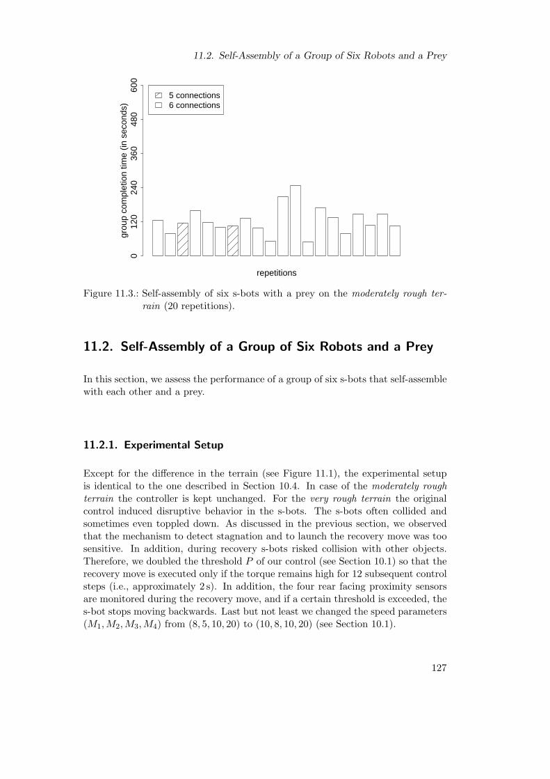
11.2. Self-Assembly of a Group of Six Robots and a Prey
repetitions
grou
p co
mpl
etio
n tim
e (in
sec
onds
)0
120
240
360
480
600
5 connections6 connections
Figure 11.3.: Self-assembly of six s-bots with a prey on the moderately rough ter-rain (20 repetitions).
11.2. Self-Assembly of a Group of Six Robots and a Prey
In this section, we assess the performance of a group of six s-bots that self-assemblewith each other and a prey.
11.2.1. Experimental Setup
Except for the difference in the terrain (see Figure 11.1), the experimental setupis identical to the one described in Section 10.4. In case of the moderately roughterrain the controller is kept unchanged. For the very rough terrain the originalcontrol induced disruptive behavior in the s-bots. The s-bots often collided andsometimes even toppled down. As discussed in the previous section, we observedthat the mechanism to detect stagnation and to launch the recovery move was toosensitive. In addition, during recovery s-bots risked collision with other objects.Therefore, we doubled the threshold P of our control (see Section 10.1) so that therecovery move is executed only if the torque remains high for 12 subsequent controlsteps (i.e., approximately 2 s). In addition, the four rear facing proximity sensorsare monitored during the recovery move, and if a certain threshold is exceeded, thes-bot stops moving backwards. Last but not least we changed the speed parameters(M1,M2,M3,M4) from (8, 5, 10, 20) to (10, 8, 10, 20) (see Section 10.1).
127

11. Experiments on Rough Terrain
repetitions
grou
p co
mpl
etio
n tim
e (in
sec
onds
)0
120
240
360
480
600
3 connections4 connections5 connections6 connections
Figure 11.4.: Self-assembly of six s-bots with a prey on the very rough terrain (20repetitions).
11.2.2. Results
Figure 11.3 shows the results obtained in 20 trials on the moderately rough terrain.In total, 120 times an s-bot was controlled in this experiment. In 118 cases thes-bot successfully connected.
Figure 11.4 shows the results obtained in 20 trials on the very rough terrain. In 12out of 20 trials, all six s-bots connected with the prey. In total, 120 times an s-botwas controlled in order to establish a connection, and in 109 cases it succeeded.
Table 11.1 summarizes the results obtained for the experiments with one s-bot(number 13) and a prey, and those with six s-bots and a prey, for the three differenttypes of terrain. Overall, the reliability of the algorithm which was designed tocontrol s-bots on flat terrain is not affected by the roughness of the moderatelyrough terrain. However, 40% additional time is required (comparing the medianvalues) to connect all seven objects. Even on the very rough terrain, a single s-botconnected in 95% of the cases. Being part of a group of size six, a single s-bot,controlled by the modified controller, connected still in more than 90% of the cases.
The few failures that occurred were mainly due to visual misperceptions of thepresence and/or angular positions of other objects. On the very rough terrain,s-bots also failed to align with their teammates and therefore could not connect.
128

11.2. Self-Assembly of a Group of Six Robots and a Prey
Table 11.1.: Summary of results on self-assembly obtained for the experiments withone s-bot (number 13) and a prey, and those with six s-bots and a prey.Notation: N (group size), D (initial distance in cm), C (percentage ofconnections), T (median group completion time in s; only trials withN connections). Each configuration was tested at least 20 times (seetext for details). Values marked with the *-symbol were obtained withthe modified controller.
N D flat terrain moderately rough t. very rough terrain
C T C T C T
1 25 100.00 18.0 100.00 29.7 95.00 24.9
1 50 100.00 28.7 100.00 36.9 95.00 71.3
6 < 70 97.55 86.7 98.33 121.2 90.83∗ 115.4∗
129

11. Experiments on Rough Terrain
130

12. Experiments with a DifferentModular Robotic Platform
Up to now, a variety of systems comprising self-propelled component modules haveproven capable of self-assembly (see Table 4.6 on page 50). In each case, ad hoccontrol algorithms have been developed. The aim of this chapter is to investigate ifour control algorithm for self-assembly can be ported from the swarm-bot platformto a different modular robotic platform (i.e., a super-mechano colony system (SMC);see Section 4.3.5). Although there are substantial differences between the tworobotic platforms, we try to qualitatively reproduce the functionality of the sourceplatform on the target platform, so that the transfer neither requires modificationsin the hardware nor an extensive redesign of the control.
We first detail the hardware of the target platform and describe the transfer of thecontrol policy (Section 12.1). Then, we present a collection of experiments to studythe performance and reliability of an SMC robot in approaching and connectingwith a teammate (Section 12.2). Finally, we investigate mechanisms to achievescalability and to trigger the formation of distinct patterns with groups of fourSMC robots (Section 12.3).
12.1. Remarks on Transfer from Swarm-Bot toSuper-Mechano Colony
Super-mechano colony (SMC) is a modular robotic concept composed of a parentunit and several child robots attached to it (see Section 4.3.5). Child robots are anintegral part of the system’s locomotion. In addition, the child robots are mobilerobots that can disband to accomplish separate, autonomous missions. Further-more, child robots have the potential to connect to each other. Figure 12.1(a)shows the physical implementation of a child robot of an SMC system [49]. Therobot has a diameter of 26 cm, a total height of 51 cm and weighs 11 kg.
The child robot has five DOF, including two DOF for the traction system, oneDOF to rotate the robots’ upper part with respect to the lower part, one DOF forelevating a manipulation arm (located in what we define to be the robot’s front),and one DOF to open and close a gripper that is attached to the manipulation arm.The traction system consists of two active wheels on the left and the right side, andtwo passive wheels in the front and the back. Each child robot is equipped with acoupling cylinder in its back that allows for receiving connections from a teammate[see Figure 12.1(b)].
131

12. Experiments with a Different Modular Robotic Platform
(a) (b)
Figure 12.1.: Super-mechano colony: (c) a child robot (top view) and (d) two childrobots connecting to each other.
A directional VGA stereo vision system is mounted on top of the robot. Anadditional camera is attached to the manipulation arm. The vision system candetect the relative position of the mark attached to the top of the coupling cylinderof another robot. The control is executed on an on-board Intel Pentium MMXcomputer running a Microsoft Windows operating system at 233 MHz. A batteryprovides full autonomy. In the experiments presented in this section we used anexternal power supply instead.
Algorithm 1 (see page 113) describes the controller for self-assembly with thesource platform, the swarm-bot (see Section 10.1 for modifications made during thetransfer from simulation). In the following, we explain how the sensing and actingfunctions of the source platform were realized on the target platform so that thebasic algorithm could be ported without any change. Some functions (e.g., “neuralnetwork”) remained identical (except for the time required for processing). Manyother functions (e.g., “apply (o1, o2) to traction system”) could be transferred withminor modifications (e.g., by scaling the speed values to an appropriate range). Inthe following, we detail those functions which required a different implementationon the target platform to qualitatively reproduce the original function of the sourceplatform:
• “recovery move”: on the s-bot, the recovery move is triggered if high torqueis present for a sequence of six control steps (i.e., approximately 1 s). For theSMC child robot, we use the camera vision system instead. If there is therisk that the left side of the manipulation arm collides with another robot,the recovery move is executed.1
1Note that the neural network lets the robot approach the object either straight, or by turninganti-clockwise. If the right side of the manipulation arm collides with the object, the neural networklets the robot retreat as a result of the high reading values from the front-right proximity sensor.
132

12.2. Self-Assembly of Two Robots
(a) (b)
Figure 12.2.: Self-assembly of two robots: influence of the initial orientation of theapproaching robot. Examples of (a) initial and (b) final configura-tions.
• “sensor readings (proximity)”: as the target platform is not equipped withproximity sensors, we mimic virtual proximity sensors heading in the front-left and front-right directions by making use of the vision system. The readingvalues of the virtual sensors are computed based on the relative position toother robots.
• “grasping requirements fulfilled”, “successfully connected”: to test if thegrasping requirements are fulfilled, the stereo vision system is used. Thesystem allows for computing the relative position of the coupling cylinder.Consequently, no additional tests must be performed to validate the connec-tion.
• “activate color ring”: as the current prototype of the SMC system is notequipped with communication mechanisms other than wireless network, therobots do not signal their connection state. Therefore, each robot can receiveconnections at any time.
12.2. Self-Assembly of Two Robots
We conducted a series of experiments to examine the ability of a robot to approachand connect with a passive teammate. In all experiments, the robot is driven bythe same controller.
12.2.1. Experimental Setup I (Initial Orientation)
The experimental setup is illustrated in Figure 12.2. The two robots have identicalhardware. The approaching robot is placed at a distance of 100 cm and orientation
133

12. Experiments with a Different Modular Robotic Platform
050
100
150
200
250
300
initial orientation of approaching robot (in degrees)
com
plet
ion
time
(in s
)
0 90 180 270
050
100
150
200
250
300
Figure 12.3.: Self-assembly of two robots, influence of the initial orientation of theapproaching robot. Box-and-whisker plot [15] of the completion times(in s) grouped according to the initial orientation of the approachingrobot (39 observations in total).
α with respect to its teammate. The latter is oriented so that its back with thecoupling cylinder is heading towards the approaching robot. For each initial ori-entation α ∈ {0◦, 90◦, 180◦, 270◦}, 10 repetitions are carried out, thus in total 40trials are performed. If the robots have not established a connection within 300 s,the trial is stopped.
12.2.2. Results I
In 39 out of 40 cases, the robots self-assembled successfully. Figure 12.3 shows theobserved completion times (in s). If no robot to approach is perceived, the neuralnetwork controller lets the robot turn anti-clockwise. This explains the differencesin performance. Overall, it seems that the success rate does not depend on theinitial orientation of the approaching robot.
12.2.3. Experimental Setup II (Approaching Angle)
We examine the ability of a single robot to connect with a passive teammate whenapproaching it from different angles (see Figure 12.4). Due to the mechanical de-sign, the robot cannot connect with the coupling cylinder of the teammate fromevery angle. In fact, if the angular mismatch between the orientations of the tworobots exceeds 85◦, it is impossible to establish a connection. Therefore, potentialapproaching angles for a successful grasp are limited to the range [−85◦, 85◦]. For
134
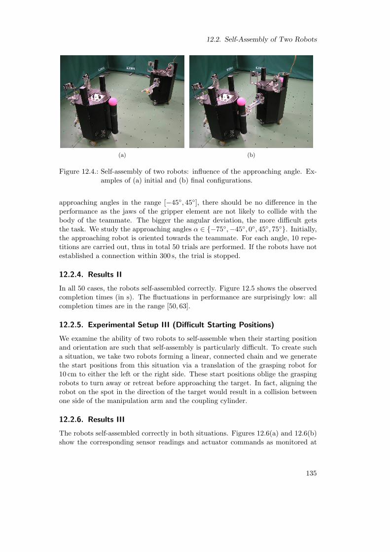
12.2. Self-Assembly of Two Robots
(a) (b)
Figure 12.4.: Self-assembly of two robots: influence of the approaching angle. Ex-amples of (a) initial and (b) final configurations.
approaching angles in the range [−45◦, 45◦], there should be no difference in theperformance as the jaws of the gripper element are not likely to collide with thebody of the teammate. The bigger the angular deviation, the more difficult getsthe task. We study the approaching angles α ∈ {−75◦,−45◦, 0◦, 45◦, 75◦}. Initially,the approaching robot is oriented towards the teammate. For each angle, 10 repe-titions are carried out, thus in total 50 trials are performed. If the robots have notestablished a connection within 300 s, the trial is stopped.
12.2.4. Results II
In all 50 cases, the robots self-assembled correctly. Figure 12.5 shows the observedcompletion times (in s). The fluctuations in performance are surprisingly low: allcompletion times are in the range [50, 63].
12.2.5. Experimental Setup III (Difficult Starting Positions)
We examine the ability of two robots to self-assemble when their starting positionand orientation are such that self-assembly is particularly difficult. To create sucha situation, we take two robots forming a linear, connected chain and we generatethe start positions from this situation via a translation of the grasping robot for10 cm to either the left or the right side. These start positions oblige the graspingrobots to turn away or retreat before approaching the target. In fact, aligning therobot on the spot in the direction of the target would result in a collision betweenone side of the manipulation arm and the coupling cylinder.
12.2.6. Results III
The robots self-assembled correctly in both situations. Figures 12.6(a) and 12.6(b)show the corresponding sensor readings and actuator commands as monitored at
135

12. Experiments with a Different Modular Robotic Platform
050
100
150
200
250
300
approaching angle (in degrees)
com
plet
ion
time
(in s
)
−75 −45 0 45 75
050
100
150
200
250
300
Figure 12.5.: Self-assembly of two robots; influence of the approaching angle. Box-and-whisker plot [15] of the completion times (in s) grouped accordingto the approaching angle (50 observations in total).
target left (i_1)0
1
target right (i_2)0
1
proximity left (i_3)0
1
proximity right (i_4)0
1
left wheel speed
−1
1
right wheel speed
−1
1
gripper (o_3)0
1
0 10 20 30 40 50time (in s)
(a)
target left (i_1)0
1
target right (i_2)0
1
proximity left (i_3)
0
1
proximity right (i_4)0
1
left wheel speed
−1
1
right wheel speed
−1
1
gripper (o_3)0
1
0 10 20 30 40 50time (in s)
(b)
Figure 12.6.: Sensor readings and actuator commands over time (in s) for the twodifficult initial arrangements: translation of the approaching robot (a)to the left and (b) to the right.
136
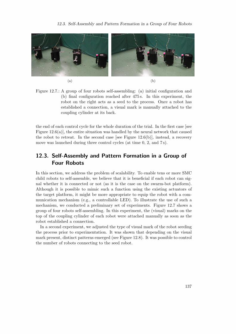
12.3. Self-Assembly and Pattern Formation in a Group of Four Robots
(a) (b)
Figure 12.7.: A group of four robots self-assembling: (a) initial configuration and(b) final configuration reached after 475 s. In this experiment, therobot on the right acts as a seed to the process. Once a robot hasestablished a connection, a visual mark is manually attached to thecoupling cylinder at its back.
the end of each control cycle for the whole duration of the trial. In the first case [seeFigure 12.6(a)], the entire situation was handled by the neural network that causedthe robot to retreat. In the second case [see Figure 12.6(b)], instead, a recoverymove was launched during three control cycles (at time 0, 2, and 7 s).
12.3. Self-Assembly and Pattern Formation in a Group ofFour Robots
In this section, we address the problem of scalability. To enable tens or more SMCchild robots to self-assemble, we believe that it is beneficial if each robot can sig-nal whether it is connected or not (as it is the case on the swarm-bot platform).Although it is possible to mimic such a function using the existing actuators ofthe target platform, it might be more appropriate to equip the robot with a com-munication mechanism (e.g., a controllable LED). To illustrate the use of such amechanism, we conducted a preliminary set of experiments. Figure 12.7 shows agroup of four robots self-assembling. In this experiment, the (visual) marks on thetop of the coupling cylinder of each robot were attached manually as soon as therobot established a connection.
In a second experiment, we adjusted the type of visual mark of the robot seedingthe process prior to experimentation. It was shown that depending on the visualmark present, distinct patterns emerged (see Figure 12.8). It was possible to controlthe number of robots connecting to the seed robot.
137

12. Experiments with a Different Modular Robotic Platform
(a) (b) (c)
Figure 12.8.: Pattern formation: a group of four robots self-assembles starting froma specific initial arrangement, as shown in (a). Depending on the typeof visual mark of the robot seeding the process (i.e., the robot on theright side in the figures), different patterns emerge. The final con-figurations shown in (b) and (c) were reached after 102 s and 207 s,respectively. During the experiments, there was no human interven-tion.
138
13. Discussion
In this fourth part of the dissertation, we presented a comprehensive study of theproblem of self-assembly. In Chapter 10, we have demonstrated the ability of mod-ules of the swarm-bot platform (i.e., the s-bots) to self-assemble under a variety ofconditions. The reliability and the performance in each experiment can be judgedby quantitative results. In 100% of the 220 cases, a single s-bot, controlled to con-nect with a non-moving object (i.e., a stationary teammate or a prey), successfullyconnected. In 98% of the 204 cases, an s-bot, engaged in a group experiment (withsix s-bots and a prey seeding the process), successfully connected. Moreover, wehave shown that the system is scalable, that is, our controller is capable of lettinglarge groups of s-bots self-assemble into a single entity as experimentally verifiedwith groups of 16 physical s-bots (one of which seeded the process).
In Chapter 11, we examined self-assembly on two different types of rough terrain.Both terrain types were unnavigable for most standard wheeled robots of a similarsize. The first terrain type had a surface with a regular structure. Experimentson this terrain type showed no loss in reliability. The second terrain type had anirregular surface, and in more than 90% of the 120 cases, an s-bot, engaged ina group experiment (with six s-bots and a prey seeding the process), successfullyestablished a connection.
In Chapter 12, we have shown that the self-assembly algorithm which we devel-oped for the swarm-bot system can be ported to a different modular robotic plat-form (i.e., a super-mechano colony system). A set of experiments demonstratedthe validity of the approach. A group of two modules self-assembled reliably—in91 out of 92 trials the modules correctly established a connection. The transferdid neither require modifications in the hardware nor an extensive redesign of thecontrol. This suggests that the control algorithm is based on some generic prin-ciples for the design of self-assembling systems. Finally, we studied mechanismsto control the patterns that are formed by autonomous self-assembly. Dependingon the type of visual mark of the module seeding the process, different patternsemerged. Such a mechanism had also been employed in the experiment in which 16s-bots self-assembled (see Section 10.5), to let the s-bots approach each other fromany direction other than the front.
Decisive Design Choices
In view of the very successful results, the swarm-bot system qualifies as the currentstate of the art in autonomous self-assembly. We believe that this success can beattributed to the following critical choices made during the system design:
139

13. Discussion
Mobility
The traction system was designed so that the s-bot is equipped with very goodsteering abilities (due to the external wheels). At the same time it allows for goodall-terrain navigation (due to the tracks). This facilitates approaching a teammateto establish a connection on flat and rough terrain.
Connection Mechanism
The s-bot can receive connections on more than two thirds of its perimeter. More-over, the connection mechanism is designed so that it does not require a specificand accurate alignment of the two s-bots during approach. This property, togetherwith the mobility of the s-bot, is a crucial factor for the design of robotic systemscapable of self-assembling on rough terrain.
Complex Individuals
The s-bot is equipped with a variety of complex sensors that guide it during (i) theapproach of red objects, (ii) the avoidance of blue objects, and (iii) the connectionphase. To some extent, the sensory system also indicates the presence of failures(e.g., in the connection). To preprocess data provided by the sensors, the s-bot isequipped with a considerable amount of computational resources.
The s-bots might, given the current state of the art in mechatronics, currently beconsidered complex artefacts. However, when compared to social insects that self-assemble, the s-bot can be considered as simple. We believe that, in the mediumterm, the use of relatively complex modules and robots is unavoidable in orderto achieve tasks of increasing complexity in the domain of self-reconfigurable andcollective robotics.
Simple Collective Rules
Despite the complexity of the s-bots, their behavior and the interactions amongthem can often be modeled by simple rules. In our control algorithm for self-assembly, for instance, the main part was a simple, reactive neural network with 15connection weights. Nevertheless, the controller proved fairly robust with respectto changes in the s-bots’ initial placements, in the terrain type, and even in therobotic platform. Moreover, the use of sensory feedback was limited to a small setof input variables that seemed indispensable to perform the task. In general, thisapproach enhances the applicability of controllers to different robotic platforms,which potentially provide fewer abilities. In our study, for instance, even thoughthe s-bot has an omni-direction view of the scene, it was sufficient to provide thecontroller only with information concerning objects in the module’s front. This inturn facilitated the transfer of the controller to the super-mechano colony system,which is provided with directional vision only.
140

Scalability
The control is decentralized and homogeneous, that is, the group members haveidentical control. The s-bots are fully autonomous. They make use only of localsensing and acting abilities—no global communication channel exists. Due to theseproperties, the controller can, in principle, be applied to robotic swarms of any(finite) size.
However, these properties by themselves do not ensure that the performancescales well with group size. To improve scalability for our particular task, we in-troduced a simple binary communication mechanism which allowed s-bots to signalwhether or not they were connected. This simple mechanism governed the processof attraction and repulsion, and allowed for the progressive construction of (global)connection patterns of dimensions far beyond the s-bot’s (local) sensing range.
141

13. Discussion
142
Part V.
Self-Assembling Robots:Experiments in the Context
of Group Transport
143


14. Experiments with Pre-Assembled,Homogeneous Groups of Robots
In this fifth part of the dissertation, we report on a series of experimental works oncooperative transport with the swarm-bot system.
In this chapter, we examine the ability of a homogeneous group of non-blind s-bots to transport heavy prey towards a target location. We consider the situationthat the s-bots are physically connected to each other and with the prey from thebeginning of the trial. They have no knowledge about their relative positions. Weuse the controller for the non-blind s-bots that was introduced in Chapter 8.
The chapter is organized as follows. First we summarize the implementationaspects that were involved in the control transfer (Section 14.1). Then, we studycooperative transport by a homogeneous group of non-blind s-bots on flat terrain(Section 14.2). We analyze the impact of the s-bots’ spatial arrangement as wellas of frictional forces on the performance of the system. Finally, we study grouptransport on rough terrain (Section 14.3).
14.1. Remarks on Transfer from Simulation to Reality
Algorithm 2 describes the controller for the non-blind s-bots, that is, the s-bots capable of perceiving the target location (i.e., a light source). The algorithmimplements the same principle as in simulation (see Section 8.1.2): while its turretis connected to another object (e.g., the prey), the s-bot orients its chassis towardsthe light source and moves as fast as possible. In the following the implementationis detailed.
During the transport, the s-bot monitors the magnitude of the torque acting onits traction system and on the turret (see lines 4–5 of Algorithm 2). If the torquereading values exceed a certain threshold, there is stagnation. In this case, a shortrecovery move is performed to prevent the hardware from being damaged.
The transport module uses the camera vision system to detect the direction ofthe light source with respect to the s-bot’s heading. By adjusting the orientationof the chassis with respect to the s-bot’s heading (i.e., the orientation of the tur-ret) the controller sets the direction of motion accordingly. The realignment of thechassis is supported by the motion of the traction system (see lines 7–11 of Algo-rithm 2). We implemented two different types of realignment referred to as “hard”and “soft” alignment. The hard alignment makes the s-bot turn on the spot. Thesoft alignment makes the s-bot turn while moving forward. The hard alignment isexecuted if there is risk of stagnation. This is the case, for instance, if the angular
145
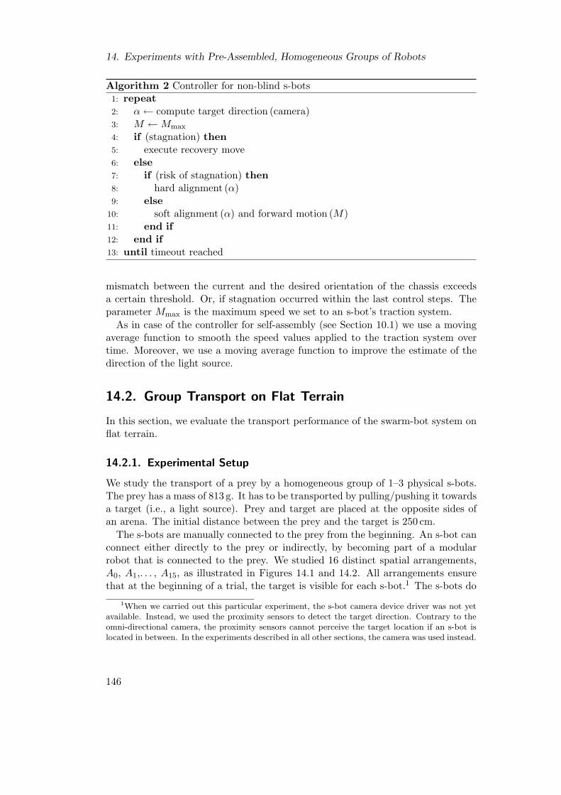
14. Experiments with Pre-Assembled, Homogeneous Groups of Robots
Algorithm 2 Controller for non-blind s-bots1: repeat2: α← compute target direction (camera)3: M ←Mmax
4: if (stagnation) then5: execute recovery move6: else7: if (risk of stagnation) then8: hard alignment (α)9: else
10: soft alignment (α) and forward motion (M)11: end if12: end if13: until timeout reached
mismatch between the current and the desired orientation of the chassis exceedsa certain threshold. Or, if stagnation occurred within the last control steps. Theparameter Mmax is the maximum speed we set to an s-bot’s traction system.
As in case of the controller for self-assembly (see Section 10.1) we use a movingaverage function to smooth the speed values applied to the traction system overtime. Moreover, we use a moving average function to improve the estimate of thedirection of the light source.
14.2. Group Transport on Flat Terrain
In this section, we evaluate the transport performance of the swarm-bot system onflat terrain.
14.2.1. Experimental Setup
We study the transport of a prey by a homogeneous group of 1–3 physical s-bots.The prey has a mass of 813 g. It has to be transported by pulling/pushing it towardsa target (i.e., a light source). Prey and target are placed at the opposite sides ofan arena. The initial distance between the prey and the target is 250 cm.
The s-bots are manually connected to the prey from the beginning. An s-bot canconnect either directly to the prey or indirectly, by becoming part of a modularrobot that is connected to the prey. We studied 16 distinct spatial arrangements,A0, A1,. . . , A15, as illustrated in Figures 14.1 and 14.2. All arrangements ensurethat at the beginning of a trial, the target is visible for each s-bot.1 The s-bots do
1When we carried out this particular experiment, the s-bot camera device driver was not yetavailable. Instead, we used the proximity sensors to detect the target direction. Contrary to theomni-directional camera, the proximity sensors cannot perceive the target location if an s-bot islocated in between. In the experiments described in all other sections, the camera was used instead.
146

14.2. Group Transport on Flat Terrain
A2A0
A4A3 A5 A7 A8
A9
A1
A6
A10 A11 A12 A13 A14 A15
Figure 14.1.: Experimental setup. A prey has to be transported by pulling/pushingit, towards a target (to the right side, not shown). The physical s-botsare manually attached to the prey in one of the spatial arrangementsillustrated in the figure. In each arrangement, every s-bot has visualcontact with the target.
Figure 14.2.: Example of spatial arrangement with two s-bots and the prey (referredto as A5 in Figure 14.1).
147
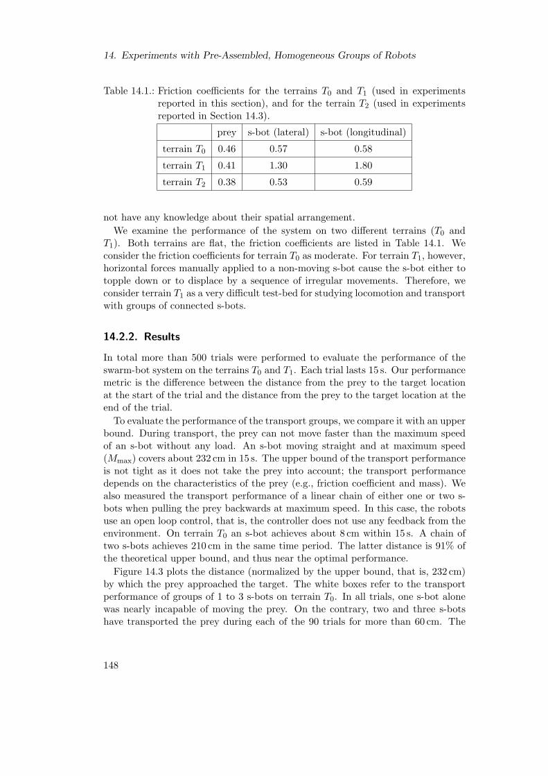
14. Experiments with Pre-Assembled, Homogeneous Groups of Robots
Table 14.1.: Friction coefficients for the terrains T0 and T1 (used in experimentsreported in this section), and for the terrain T2 (used in experimentsreported in Section 14.3).
prey s-bot (lateral) s-bot (longitudinal)
terrain T0 0.46 0.57 0.58
terrain T1 0.41 1.30 1.80
terrain T2 0.38 0.53 0.59
not have any knowledge about their spatial arrangement.We examine the performance of the system on two different terrains (T0 and
T1). Both terrains are flat, the friction coefficients are listed in Table 14.1. Weconsider the friction coefficients for terrain T0 as moderate. For terrain T1, however,horizontal forces manually applied to a non-moving s-bot cause the s-bot either totopple down or to displace by a sequence of irregular movements. Therefore, weconsider terrain T1 as a very difficult test-bed for studying locomotion and transportwith groups of connected s-bots.
14.2.2. Results
In total more than 500 trials were performed to evaluate the performance of theswarm-bot system on the terrains T0 and T1. Each trial lasts 15 s. Our performancemetric is the difference between the distance from the prey to the target locationat the start of the trial and the distance from the prey to the target location at theend of the trial.
To evaluate the performance of the transport groups, we compare it with an upperbound. During transport, the prey can not move faster than the maximum speedof an s-bot without any load. An s-bot moving straight and at maximum speed(Mmax) covers about 232 cm in 15 s. The upper bound of the transport performanceis not tight as it does not take the prey into account; the transport performancedepends on the characteristics of the prey (e.g., friction coefficient and mass). Wealso measured the transport performance of a linear chain of either one or two s-bots when pulling the prey backwards at maximum speed. In this case, the robotsuse an open loop control, that is, the controller does not use any feedback from theenvironment. On terrain T0 an s-bot achieves about 8 cm within 15 s. A chain oftwo s-bots achieves 210 cm in the same time period. The latter distance is 91% ofthe theoretical upper bound, and thus near the optimal performance.
Figure 14.3 plots the distance (normalized by the upper bound, that is, 232 cm)by which the prey approached the target. The white boxes refer to the transportperformance of groups of 1 to 3 s-bots on terrain T0. In all trials, one s-bot alonewas nearly incapable of moving the prey. On the contrary, two and three s-botshave transported the prey during each of the 90 trials for more than 60 cm. The
148
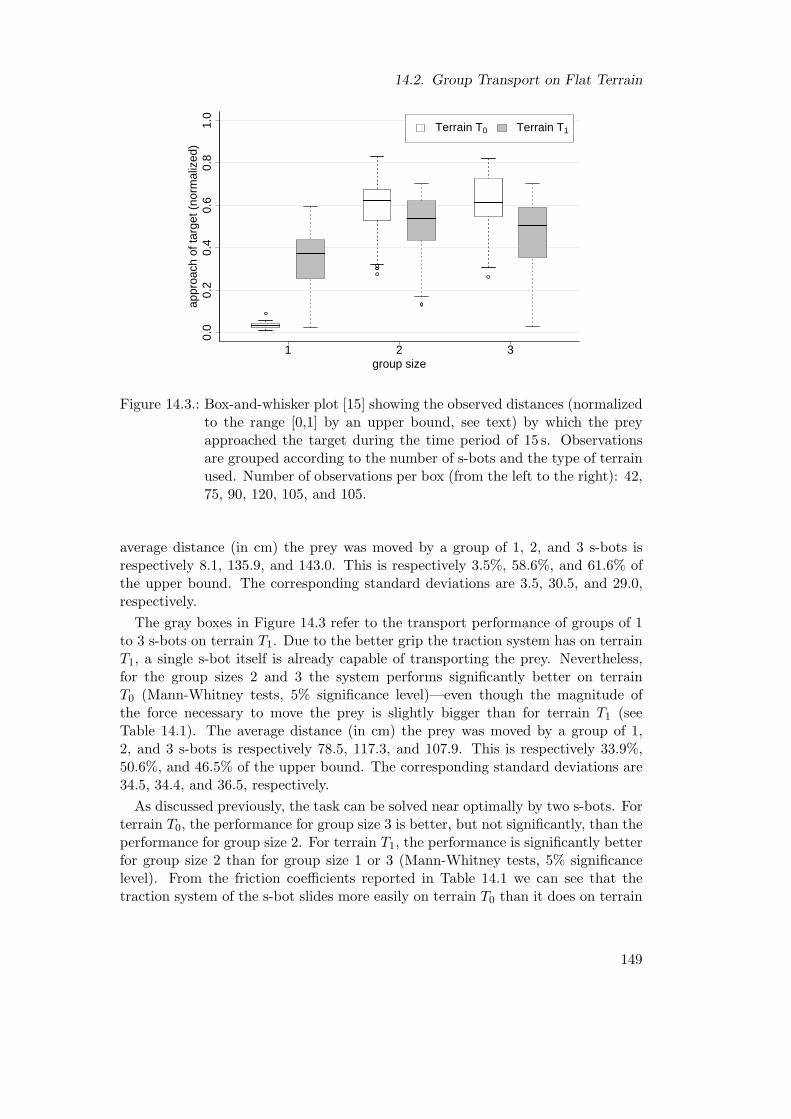
14.2. Group Transport on Flat Terrain
0.0
0.2
0.4
0.6
0.8
1.0
group size
appr
oach
of t
arge
t (no
rmal
ized
)
1 2 3
Terrain T0 Terrain T1
Figure 14.3.: Box-and-whisker plot [15] showing the observed distances (normalizedto the range [0,1] by an upper bound, see text) by which the preyapproached the target during the time period of 15 s. Observationsare grouped according to the number of s-bots and the type of terrainused. Number of observations per box (from the left to the right): 42,75, 90, 120, 105, and 105.
average distance (in cm) the prey was moved by a group of 1, 2, and 3 s-bots isrespectively 8.1, 135.9, and 143.0. This is respectively 3.5%, 58.6%, and 61.6% ofthe upper bound. The corresponding standard deviations are 3.5, 30.5, and 29.0,respectively.
The gray boxes in Figure 14.3 refer to the transport performance of groups of 1to 3 s-bots on terrain T1. Due to the better grip the traction system has on terrainT1, a single s-bot itself is already capable of transporting the prey. Nevertheless,for the group sizes 2 and 3 the system performs significantly better on terrainT0 (Mann-Whitney tests, 5% significance level)—even though the magnitude ofthe force necessary to move the prey is slightly bigger than for terrain T1 (seeTable 14.1). The average distance (in cm) the prey was moved by a group of 1,2, and 3 s-bots is respectively 78.5, 117.3, and 107.9. This is respectively 33.9%,50.6%, and 46.5% of the upper bound. The corresponding standard deviations are34.5, 34.4, and 36.5, respectively.
As discussed previously, the task can be solved near optimally by two s-bots. Forterrain T0, the performance for group size 3 is better, but not significantly, than theperformance for group size 2. For terrain T1, the performance is significantly betterfor group size 2 than for group size 1 or 3 (Mann-Whitney tests, 5% significancelevel). From the friction coefficients reported in Table 14.1 we can see that thetraction system of the s-bot slides more easily on terrain T0 than it does on terrain
149
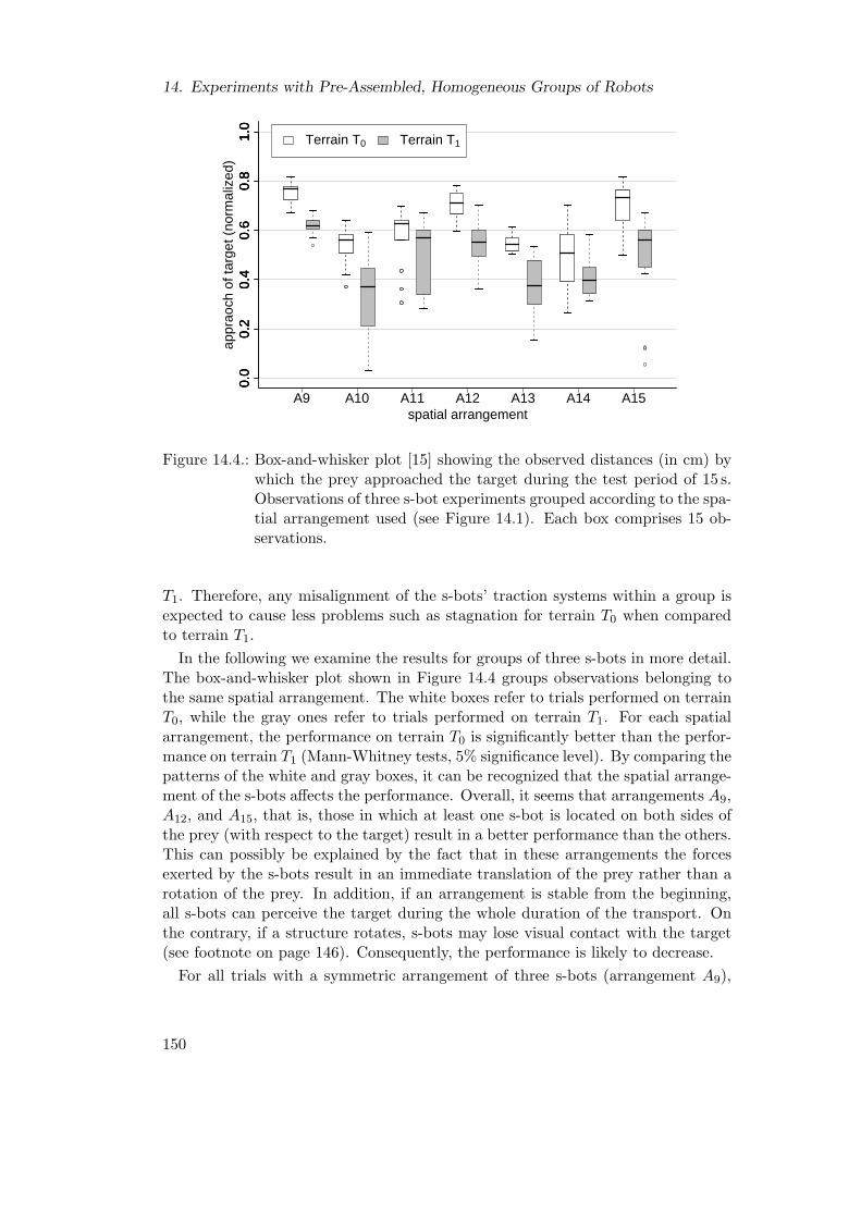
14. Experiments with Pre-Assembled, Homogeneous Groups of Robots
0.0
0.2
0.4
0.6
0.8
1.0
spatial arrangement
appr
aoch
of t
arge
t (no
rmal
ized
)0.
00.
20.
40.
60.
81.
0
A9 A10 A11 A12 A13 A14 A15
0.0
0.2
0.4
0.6
0.8
1.0
Terrain T0 Terrain T1
Figure 14.4.: Box-and-whisker plot [15] showing the observed distances (in cm) bywhich the prey approached the target during the test period of 15 s.Observations of three s-bot experiments grouped according to the spa-tial arrangement used (see Figure 14.1). Each box comprises 15 ob-servations.
T1. Therefore, any misalignment of the s-bots’ traction systems within a group isexpected to cause less problems such as stagnation for terrain T0 when comparedto terrain T1.
In the following we examine the results for groups of three s-bots in more detail.The box-and-whisker plot shown in Figure 14.4 groups observations belonging tothe same spatial arrangement. The white boxes refer to trials performed on terrainT0, while the gray ones refer to trials performed on terrain T1. For each spatialarrangement, the performance on terrain T0 is significantly better than the perfor-mance on terrain T1 (Mann-Whitney tests, 5% significance level). By comparing thepatterns of the white and gray boxes, it can be recognized that the spatial arrange-ment of the s-bots affects the performance. Overall, it seems that arrangements A9,A12, and A15, that is, those in which at least one s-bot is located on both sides ofthe prey (with respect to the target) result in a better performance than the others.This can possibly be explained by the fact that in these arrangements the forcesexerted by the s-bots result in an immediate translation of the prey rather than arotation of the prey. In addition, if an arrangement is stable from the beginning,all s-bots can perceive the target during the whole duration of the transport. Onthe contrary, if a structure rotates, s-bots may lose visual contact with the target(see footnote on page 146). Consequently, the performance is likely to decrease.
For all trials with a symmetric arrangement of three s-bots (arrangement A9),
150

14.3. Group Transport on Rough Terrain
Figure 14.5.: Experimental setup. A group of six s-bots transporting the prey to-wards a target location (indicated by the arrow).
the lowest transport distance observed on terrain T0 (T1) is still 67% (54%) of theupper bound.
14.3. Group Transport on Rough Terrain
In this section, we evaluate the transport performance of the swarm-bot system onterrains of different roughness.
14.3.1. Experimental Setup
We use flat terrain T2, the friction coefficients are listed in Table 14.1. In additionwe use two rough terrains, the moderately rough and the very rough terrains shownin Figure 11.1 on page 125. The rough terrains are unnavigable for most standardwheeled robots of a similar size.
We examine the transport of a prey by a group of six s-bots. The prey weighseither W1 = 2000 g or W2 = 3000 g. The six s-bots are physically connected to theprey at six specific points as shown in Figure 14.5.
14.3.2. Results
Figure 14.6 plots the performance exhibited on the flat and the moderately roughterrain. Using the standard controller for non-blind s-bots, the group is capableof transporting reliably a heavy object on a moderately rough terrain. For thevery rough terrain we observed that the prey can easily get stuck during transport.However, a group of six s-bots could transport a 700 g prey (i.e., the weight of ans-bot) reliably when lifting it for about a centimeter with their elevation arms.
151
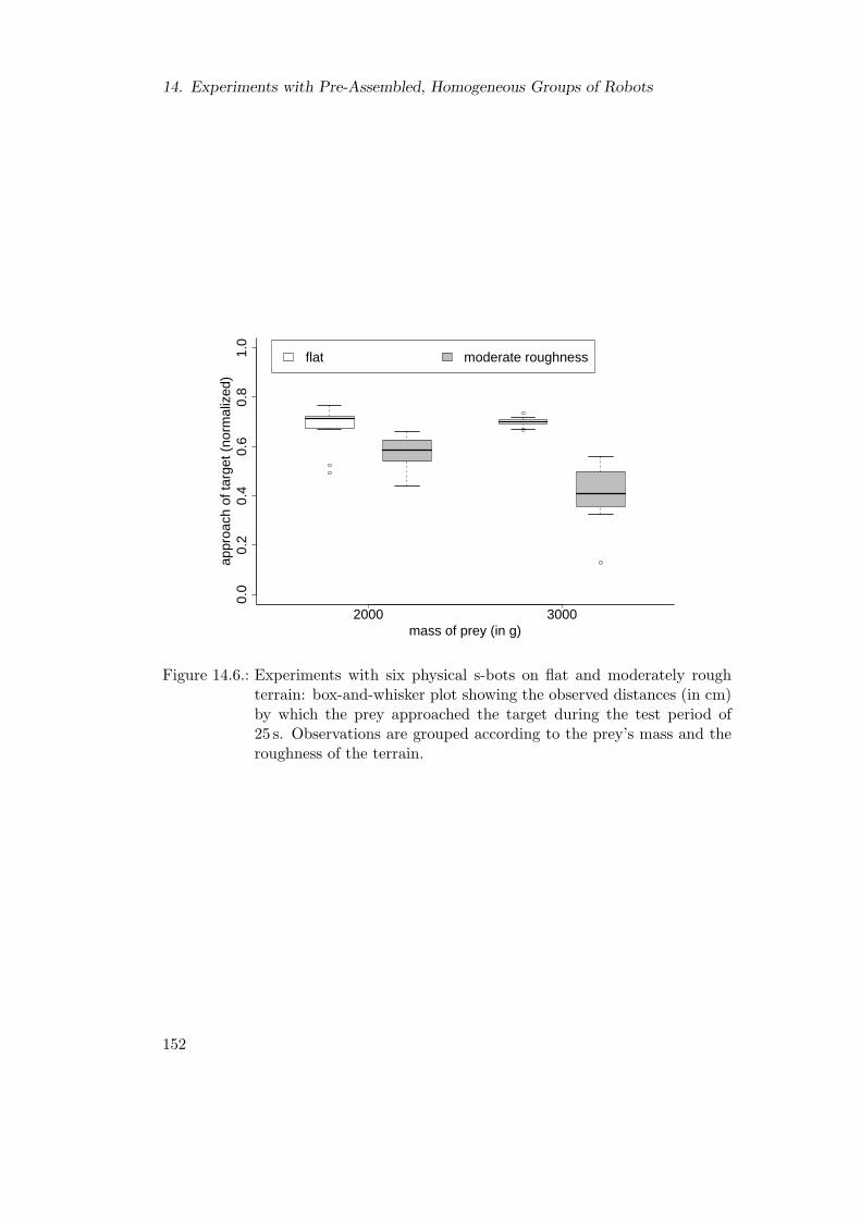
14. Experiments with Pre-Assembled, Homogeneous Groups of Robots
0.0
0.2
0.4
0.6
0.8
1.0
mass of prey (in g)
appr
oach
of t
arge
t (no
rmal
ized
)
2000 3000
flat moderate roughness
Figure 14.6.: Experiments with six physical s-bots on flat and moderately roughterrain: box-and-whisker plot showing the observed distances (in cm)by which the prey approached the target during the test period of25 s. Observations are grouped according to the prey’s mass and theroughness of the terrain.
152

15. Experiments with Pre-Assembled,Heterogeneous Teams of Robots
We present an experiment on cooperative transport in which group members lack-ing knowledge about the target location exploit physical interactions with othermembers of the group that have such knowledge. We use the transport controllersintroduced in Section 8.1.2. Homogeneous groups of non-blind s-bots have beenexamined in Chapter 14. Here we focus on heterogeneous teams comprising bothblind and non-blind s-bots.
In this chapter, first we summarize the implementation aspects that were involvedin the transfer of the controller for the blind s-bots (Section 15.1). In Section 15.2,we show that, in a group of two s-bots, a blind s-bot can physically interact with anon-blind s-bot to achieve a performance superior to that of a passive caster. Thisallows the group to transport an object that cannot be moved by the non-blinds-bot alone. In Section 15.3, we address the problem of scalability. We examine theperformance of a single blind s-bot when being part of a bigger group. Moreover,we investigate whether multiple blind s-bots may display behaviors that contributeto the performance of the group.
15.1. Remarks on Transfer from Simulation to Reality
The controller for blind s-bots is a modified version of the controller for non-blinds-bots (see Algorithm 2 on page 146). The difference is in the lines 2 and 3: weemploy the recurrent neural network previously evolved in simulation to computethe desired orientation α of the chassis (line 2) and the speed M ∈ [0,Mmax] of thetraction system (line 3). The neural network takes four inputs from the 2 DOF forcesensor, one input from a virtual motion sensor, and one input specifying the angularposition of the rotating base. The motion sensor indicates whether stagnation, thatis, high torque readings for the traction system or the turret, was observed in thepast four control cycles. Further details are reported in Section 8.1.2 and in [112].
15.2. Group Transport by a Team of One Blind and OneNon-Blind Robot
In this section, we examine the transport of a prey by a team of one blind andone non-blind s-bot. While the non-blind s-bot is fully operational, the blind s-bot
153

15. Experiments with Pre-Assembled, Heterogeneous Teams of Robots
0A
B
B
1A
B B
2A
B
B
3A
BB
Figure 15.1.: Experimental setup. A prey has to be transported towards a targetlocation (indicated by the arrow). Two s-bots are manually attachedto the prey. While s-bot B is fully operational, s-bot B is not capableof perceiving the target location. The figure illustrates the four spatialarrangements used in the experiments.
has a non-working vision system. Thus, the blind s-bot cannot perceive the targetlocation.
15.2.1. Experimental Setup
The prey weighs 1000 g. It has to be transported towards a light source. Prey andtarget are placed at the opposite sides of an arena of length 500 cm.1 The frictioncoefficients of the terrain (T2) are listed in Table 14.1 on page 148.
The two s-bots are physically connected to the prey from the beginning. They areput in one of four distinct spatial arrangements, A0, A1, A2, and, A3, as illustratedin Figure 15.1.
The non-blind s-bot is always controlled by the standard controller for non-blinds-bots (see Section 14.1). For the blind s-bots, we evaluate the performance ofstrategies S0, S1, S2, and S3 (as already employed in Section 8.2.3):
• S0: blind s-bots are manually removed from experimentation. This is equiv-alent to replacing the blind s-bots by friction-less passive casters.2
• S1: blind s-bots stop acting once connected; thus, their actuators do notmove, but they remain connected to other s-bots and/or the prey.
• S2: blind s-bots are controlled by the neural network based controller forblind s-bots (see Section 15.1).
1The initial distance between the prey and the target is set to 437 cm.2In systems in which robots lift the prey, blind robots simulating a passive caster can facilitate
the transport considerably.
154

15.2. Group Transport by a Team of One Blind and One Non-Blind Robot
−10
00
100
200
300
400
appr
oach
of t
arge
t (in
cm
)
A0 A1 A2 A3arrangement
S0: blind s−bot removedS2: blind s−bot with neural networkS3: blind s−bot replaced
Figure 15.2.: Box-and-whisker plot [15] showing the observed distances (in cm) bywhich the prey approached the target location during the time pe-riod of 25 s. Observations are grouped according to the correspond-ing strategy and spatial arrangement (10 observations per box). Thehorizontal line on top indicates an upper bound for the transport per-formance assuming a weightless prey (for details see text).
• S3: blind s-bots are manually replaced by fully operational s-bots which inturn are controlled by the standard controller for non-blind s-bots (see Sec-tion 14.1).
15.2.2. Results
For each pair (Si, Aj) ∈ {S0, S2, S3} × {A0, A1, A2, A3} 10 trials lasting 25 s wereperformed. We did not evaluate strategy S1, as the non-blind s-bot is not capableof moving both the prey and a passive s-bot.
Figure 15.2 plots the distance (in cm) by which the prey approached the target.By looking at the dark gray boxes (strategy S0) it can be seen that one s-bot alonewas nearly incapable of moving the 1000 g prey when put in one of the spatialarrangements A0, A1, or A3. However, when put in the spatial arrangement A2
the s-bot moved the prey for about 87 cm (median value). It seems that the s-botexerts a higher force while pushing the prey than when pulling it (notwithstandingthe fact that the magnitude of the force applied to the traction system is identicalin both cases).3
3It is worth noting that the controller does not implement a stable pushing strategy. In fact,the s-bot is controlled so that it moves in the direction of the target. Even if the prey could be
155

15. Experiments with Pre-Assembled, Heterogeneous Teams of Robots
As shown by the white boxes in Figure 15.2, a group of two fully operational s-bots, that is, strategy S3, always achieved a better performance than a single s-bot(for each spatial arrangement). An upper bound for the performance is given bythe distance a single s-bot without any load can cover in the same time period (25 s)by moving straight.4 The upper bound is 387 cm (indicated by the horizontal linein the figure). During transport this performance cannot be achieved because thes-bots are slowed down by the load they pull and push. The median performanceof a group of two s-bots is 64%, 70%, 59%, and 69% of this theoretical value forthe spatial arrangements A0, A1, A2, and A3, respectively.
Strategy S2 outperforms strategy S0 in three out of four arrangements. Thisshows that the blind s-bot, when controlled by the neural network based controller,contributes to the performance of the group. To assess the quality of this contri-bution we introduce the following performance measures.
Let the environment of the transport task (i.e., the prey and its initial location,the target and its location, the terrain, etc.) be fixed. Let PA(i, j) ∈ [0,∞) bethe performance (the higher the value, the better) of a group of i s-bots of which jare blind, and that are organized in spatial arrangement A = (A(1), A(2), . . . , A(i)).Thereby, {A(1), A(2), . . . , A(i−j)} is the set of locations (and orientations) of thenon-blind s-bots, while {A(i−j+1), A(i−j+2), . . . , A(i)} is the set of locations (andorientations) of the blind ones.
Given a group of N robots of which NB are blind, spatial arrangement A =(A(1), A(2), . . . , A(N)), and performance PA(N, 0) 6= 0, we can define the relativesystem performance as
RSPA(N, NB) =PA(N, NB)PA(N, 0)
. (15.1)
In other words, RSPA(N, NB) is the ratio between the performance of N s-botsof which NB are blind and the performance of N non-blind s-bots given the spatialarrangement A.
Furthermore, we define the contribution factor of blind s-bots as
CFA(N,NB) =PA(N, NB)− PA∗(N −NB, 0)PA(N, 0)− PA∗(N −NB, 0)
, (15.2)
for PA(N, 0) > PA∗(N−NB, 0), where A∗ is obtained from the spatial arrangementA by removing the locations (and orientations) that correspond to the NB blinds-bots.
placed exactly between the s-bot and the target, imprecision in the s-bot’s sensors and actuatorswould cause the s-bot to turn around the prey and eventually to pull it. This controller might notbe the most effective solution for the transport of a prey by a single s-bot. However, it is a generalsolution applicable to a wide range of scenarios including different group sizes, arbitrary spatialarrangements of s-bots in the group, and terrains with non-uniform friction.
4The speed Mmax is applied to both wheels.
156
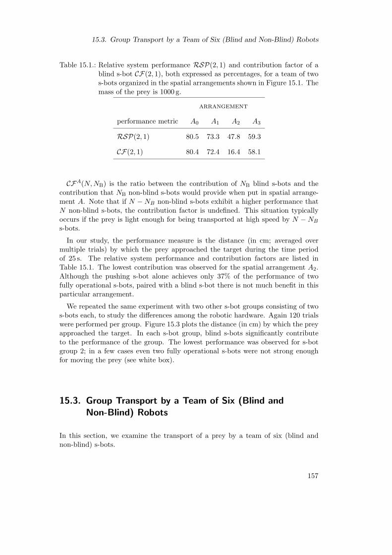
15.3. Group Transport by a Team of Six (Blind and Non-Blind) Robots
Table 15.1.: Relative system performance RSP(2, 1) and contribution factor of ablind s-bot CF(2, 1), both expressed as percentages, for a team of twos-bots organized in the spatial arrangements shown in Figure 15.1. Themass of the prey is 1000 g.
arrangement
performance metric A0 A1 A2 A3
RSP(2, 1) 80.5 73.3 47.8 59.3
CF(2, 1) 80.4 72.4 16.4 58.1
CFA(N, NB) is the ratio between the contribution of NB blind s-bots and thecontribution that NB non-blind s-bots would provide when put in spatial arrange-ment A. Note that if N −NB non-blind s-bots exhibit a higher performance thatN non-blind s-bots, the contribution factor is undefined. This situation typicallyoccurs if the prey is light enough for being transported at high speed by N −NB
s-bots.
In our study, the performance measure is the distance (in cm; averaged overmultiple trials) by which the prey approached the target during the time periodof 25 s. The relative system performance and contribution factors are listed inTable 15.1. The lowest contribution was observed for the spatial arrangement A2.Although the pushing s-bot alone achieves only 37% of the performance of twofully operational s-bots, paired with a blind s-bot there is not much benefit in thisparticular arrangement.
We repeated the same experiment with two other s-bot groups consisting of twos-bots each, to study the differences among the robotic hardware. Again 120 trialswere performed per group. Figure 15.3 plots the distance (in cm) by which the preyapproached the target. In each s-bot group, blind s-bots significantly contributeto the performance of the group. The lowest performance was observed for s-botgroup 2; in a few cases even two fully operational s-bots were not strong enoughfor moving the prey (see white box).
15.3. Group Transport by a Team of Six (Blind andNon-Blind) Robots
In this section, we examine the transport of a prey by a team of six (blind andnon-blind) s-bots.
157

15. Experiments with Pre-Assembled, Heterogeneous Teams of Robots
group 1 group 2 group 3
−10
00
100
200
300
400
appr
oach
of t
arge
t (in
cm
)
S0: blind s−bot removedS2: blind s−bot with neural networkS3: blind s−bot replaced
Figure 15.3.: Box-and-whisker plot showing the observed distances (in cm) groupedaccording to the corresponding strategy and the tested s-bot group (40observations per box, 10 for each configuration). Each group consistsof two s-bots. The three groups differ only in the particular s-botsused. The performance of group 1 is further analyzed in Figure 15.2.
Figure 15.4.: Experimental setup. An object has to be transported towards a target(on the bottom; not shown). Six s-bot are manually attached to theobject. While some s-bots are fully operational, others are not capableof perceiving the target.
158

15.3. Group Transport by a Team of Six (Blind and Non-Blind) Robots
Table 15.2.: Relative system performance RSP(6, NB) and contribution factor ofblind s-bots CF(6, NB), both expressed as percentages, for a team ofsix s-bots of which NB are blind. Average values over all 15 spatialarrangements.
# blind s-bots (NB)
mass of prey performance metric 1 2 3 4
2000 g RSP(6, NB) 101.4 92.4 66.0 18.6
CF(6, NB) -a -40.0 -36.2 15.6
3000 g RSP(6, NB) 92.3 70.5 50.6 9.2
CF(6, NB) 8.7 -53.8 46.5 9.2
aMeasure not well defined. The performance of both the “passive caster” and the neuralnetwork strategies are slightly better than the performance of a fully operational group.
15.3.1. Experimental Setup
The arena is identical to the one used in the previous experiment. The mass of theprey is either W1 = 2000 g or W2 = 3000 g. Thus, the prey is either 2 or 3 timesheavier than it was in the two s-bot experiment. The six s-bots are physicallyconnected to the prey at six specific points as shown in Figure 15.4. The non-blindand blind s-bots are randomly assigned to these points.
Let N be the number of s-bots. NB denotes the number of blind s-bots, whilethe other N −NB s-bots are fully operational.
For the blind s-bot, we evaluate the performance of all four strategies (S0, S1,S2, and S3).
15.3.2. Results
For each situation (Wi, Sj , NB), i ∈ {1, 2}, j ∈ {0, 1, 2, 3}, NB ∈ {1, 2, 3, 4}, 15randomly generated arrangements are tested. The situations for strategy S3 (i.e.,to replace all blind s-bots by non-blind ones) are essentially the same, regardless ofthe number of blind s-bots NB. Therefore, strategy S3 is evaluated only 15 timesfor each prey mass. Each trial lasts 25 s. In total 2 · 3 · 4 · 15 + 2 · 15 = 390 trialswere performed.
Figures 15.5 and 15.6 plot the distance (in cm) by which prey of mass W2 = 2000 gand W3 = 2000 g, respectively, approached the target location. Table 15.2 liststhe relative system performance and the contribution factors, averaged over all 15spatial arrangements.
It is worth noting, that the 2000 g and 3000 g preys can be moved efficientlyby 4 and 5 s-bots, respectively. In case, 1 or 2 s-bots of the group are blind and
159

15. Experiments with Pre-Assembled, Heterogeneous Teams of Robots
1 2 3 4
−10
00
100
200
300
400
number of blind s−bots (NB)
appr
oach
of t
arge
t (in
cm
)
S0: blind s−bot removedS1: blind s−bot passive
S2: blind s−bot with neural networkS3: blind s−bot replaced
Figure 15.5.: Box-and-whisker plot showing the observed distances (in cm) by whicha prey of mass W1 = 2000 g approached the target location duringthe time period of 25 s. Observations are grouped according to NB
(the number of blind s-bots) and the employed strategy. Each boxrepresents 15 observations. The horizontal line on top indicates anupper bound for the transport performance assuming a weightlessprey. For details see text.
1 2 3 4
−10
00
100
200
300
400
number of blind s−bots (NB)
appr
oach
of t
arge
t (in
cm
)
S0: blind s−bot removedS1: blind s−bot passive
S2: blind s−bot with neural networkS3: blind s−bot replaced
Figure 15.6.: Box-and-whisker plot showing the observed distances (in cm) by whicha prey of mass W2 = 3000 g approached the target location during thetime period of 25 s. For details see Figure 15.5.
160

15.3. Group Transport by a Team of Six (Blind and Non-Blind) Robots
controlled by the neural network, there is no major difference in performance (inabsolute terms) with respect to a fully operational group as indicated by the RSPmeasure. The group can compensate for a single s-bot break-down (see boxes forstrategy S1 and NB = 1 in Figures 15.5 and 15.6). However, if two or more s-botsbreak down or do not operate properly, the prey can no longer be moved.
Strategy S2 outperforms strategy S1 for every setup. This shows that the actionsof the blind s-bots, when controlled by the neural network based controller, aremeaningful. In cases in which removing NB non-blind s-bots would cause a decreasein performance of more than 50%, these NB s-bots, when controlled by the neuralnetwork based controller, even contributed (on average) to the performance of thegroup, as indicated by the CF measure.
161

15. Experiments with Pre-Assembled, Heterogeneous Teams of Robots
162

16. Experiments with Robots thatSelf-Assemble
We consider the cooperative transport of prey by a group of s-bots that are initiallyrandomly scattered in the environment. We aim at controlling the s-bots so thatthey autonomously form modular robots, which in turn manipulate the prey. InSection 16.1 we study the transport of a heavy prey by a group of six s-bots thatstart from within the vicinity of the prey and can individually perceive the targetlocation. In Section 16.2 we study the situation where the s-bots start from arbi-trary locations within a bounded environment, and can neither perceive the preynor the target location, unless located in its immediate vicinity.
16.1. Group Transport Towards a Light Beacon
In this section, we study a task that requires a group of s-bots to locate, approach,and grasp the prey—that has to be subsequently transported from its initial locationto a target location. At the level of an s-bot, the task consists of two phases. In thefirst phase, the s-bot is controlled by the standard assembly module (as detailed inSection 10.1). Thus, it tries to establish a connection either directly to the preyor indirectly, via other s-bots. In the second phase, the s-bot is controlled by thestandard transport module (as detailed in Section 14.1). To enable all s-bots toestablish a connection before the prey starts moving, we modified the transportcontroller so that connected s-bots pull or push the prey only when they do notperceive any unconnected teammate. Connected s-bots that do not perceive thetarget location do not start pulling or pushing either.1
16.1.1. Experimental Setup
The experimental setup is shown in Figure 16.1(a). The prey is initially located ata distance of 225 cm from a light source which represents the center of a circulartarget zone. The group is considered to be successful if the s-bots manage to movethe prey inside the target zone within 300 s. If moved in a straight line, the distancecovered by the prey to enter the target zone is 125 cm.
At the beginning of each trial, six s-bots are positioned in the vicinity of theprey. We assume the light source to be strong enough to allow all s-bots to detect
1At this stage of experimentation, we had not yet tested the controller for blind robots on theswarm-bot platform.
163
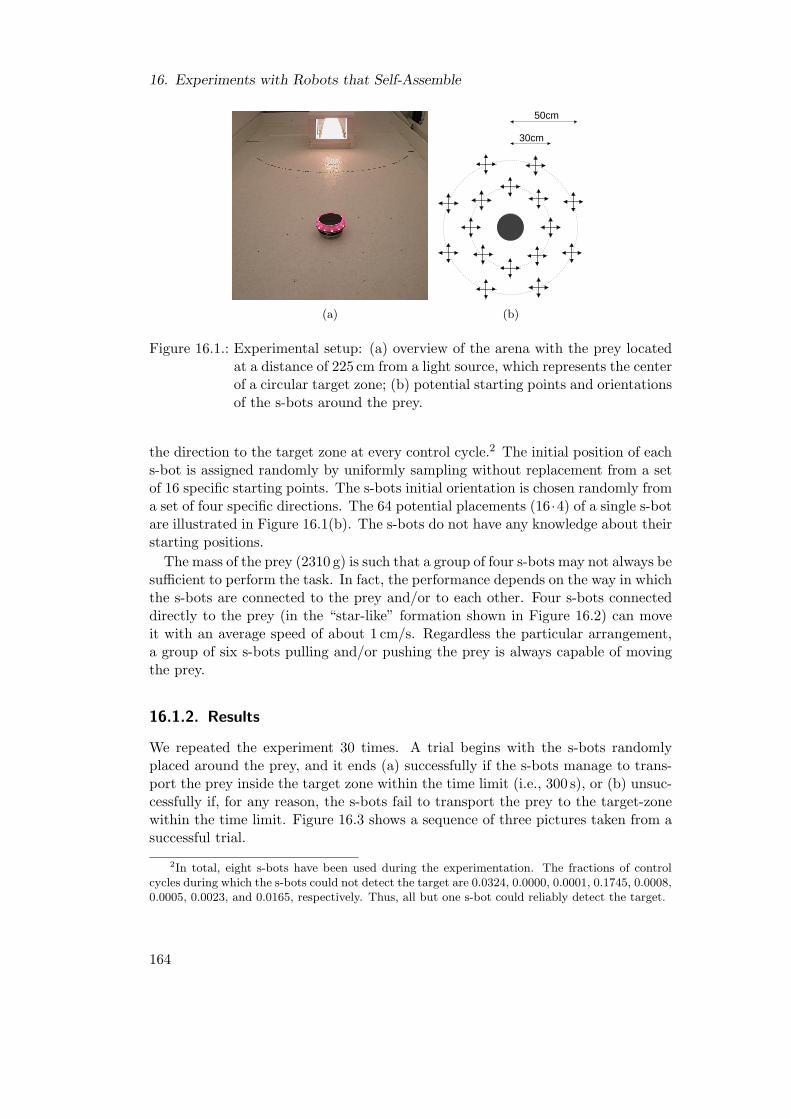
16. Experiments with Robots that Self-Assemble
(a)
30cm
50cm
(b)
Figure 16.1.: Experimental setup: (a) overview of the arena with the prey locatedat a distance of 225 cm from a light source, which represents the centerof a circular target zone; (b) potential starting points and orientationsof the s-bots around the prey.
the direction to the target zone at every control cycle.2 The initial position of eachs-bot is assigned randomly by uniformly sampling without replacement from a setof 16 specific starting points. The s-bots initial orientation is chosen randomly froma set of four specific directions. The 64 potential placements (16 ·4) of a single s-botare illustrated in Figure 16.1(b). The s-bots do not have any knowledge about theirstarting positions.
The mass of the prey (2310 g) is such that a group of four s-bots may not always besufficient to perform the task. In fact, the performance depends on the way in whichthe s-bots are connected to the prey and/or to each other. Four s-bots connecteddirectly to the prey (in the “star-like” formation shown in Figure 16.2) can moveit with an average speed of about 1 cm/s. Regardless the particular arrangement,a group of six s-bots pulling and/or pushing the prey is always capable of movingthe prey.
16.1.2. Results
We repeated the experiment 30 times. A trial begins with the s-bots randomlyplaced around the prey, and it ends (a) successfully if the s-bots manage to trans-port the prey inside the target zone within the time limit (i.e., 300 s), or (b) unsuc-cessfully if, for any reason, the s-bots fail to transport the prey to the target-zonewithin the time limit. Figure 16.3 shows a sequence of three pictures taken from asuccessful trial.
2In total, eight s-bots have been used during the experimentation. The fractions of controlcycles during which the s-bots could not detect the target are 0.0324, 0.0000, 0.0001, 0.1745, 0.0008,0.0005, 0.0023, and 0.0165, respectively. Thus, all but one s-bot could reliably detect the target.
164

16.1. Group Transport Towards a Light Beacon
Figure 16.2.: The prey is heavy and thus it requires the cooperative effort of multiples-bots to be moved. Four s-bots connected in “star-like” formationaround the prey can transport the latter with an average speed ofonly 1 cm/s.
(a) (b) (c)
Figure 16.3.: These pictures show a sequence of actions, during a trial, in whicha group of six s-bots randomly placed around the prey (a), initiallylocates, approaches and connects to the prey (b) and finally, onceassembled, transports the prey to the target zone (c).
165
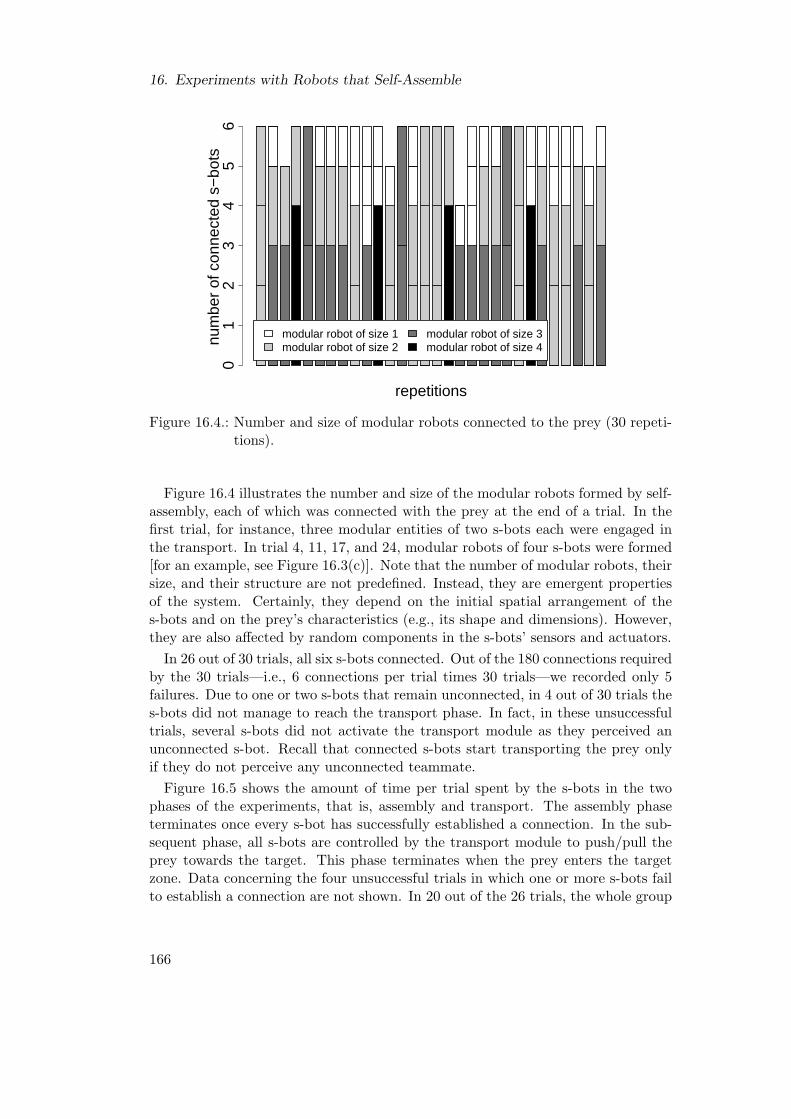
16. Experiments with Robots that Self-Assemble
repetitions
num
ber
of c
onne
cted
s−
bots
01
23
45
6
modular robot of size 1modular robot of size 2
modular robot of size 3modular robot of size 4
Figure 16.4.: Number and size of modular robots connected to the prey (30 repeti-tions).
Figure 16.4 illustrates the number and size of the modular robots formed by self-assembly, each of which was connected with the prey at the end of a trial. In thefirst trial, for instance, three modular entities of two s-bots each were engaged inthe transport. In trial 4, 11, 17, and 24, modular robots of four s-bots were formed[for an example, see Figure 16.3(c)]. Note that the number of modular robots, theirsize, and their structure are not predefined. Instead, they are emergent propertiesof the system. Certainly, they depend on the initial spatial arrangement of thes-bots and on the prey’s characteristics (e.g., its shape and dimensions). However,they are also affected by random components in the s-bots’ sensors and actuators.
In 26 out of 30 trials, all six s-bots connected. Out of the 180 connections requiredby the 30 trials—i.e., 6 connections per trial times 30 trials—we recorded only 5failures. Due to one or two s-bots that remain unconnected, in 4 out of 30 trials thes-bots did not manage to reach the transport phase. In fact, in these unsuccessfultrials, several s-bots did not activate the transport module as they perceived anunconnected s-bot. Recall that connected s-bots start transporting the prey onlyif they do not perceive any unconnected teammate.
Figure 16.5 shows the amount of time per trial spent by the s-bots in the twophases of the experiments, that is, assembly and transport. The assembly phaseterminates once every s-bot has successfully established a connection. In the sub-sequent phase, all s-bots are controlled by the transport module to push/pull theprey towards the target. This phase terminates when the prey enters the targetzone. Data concerning the four unsuccessful trials in which one or more s-bots failto establish a connection are not shown. In 20 out of the 26 trials, the whole group
166

16.2. Group Transport Along a Self-Organized Path
repetitions
com
plet
ion
time
(in s
econ
ds)
060
120
180
240
300
*
self−assemblytransport
* prey did not enter target zone
Figure 16.5.: Time necessary for a group of six s-bots to self-assemble and transportthe prey inside the target zone (only repetitions in which all s-botsassembled).
could successfully self-assemble within 83 s, in the other trials self-assembly wassuccessfully completed within 167 s.
Only in a single case out of those in which the s-bots connected successfully,the group failed to transport the prey entirely inside the target zone. In thisunsuccessful trial, the transport was interrupted in the proximity of the target zone.This failure during the transport phase was probably due to the light reflections inthe immediate vicinity of the light source. In fact, a too high intensity of the lightdisrupts the mechanism used by each s-bot to establish the direction of movement.Therefore, it may happen that, in the immediate vicinity of the target, the entiregroup loses efficiency in moving the prey.
In all other cases, the prey entered the target zone within a short period of time;the average transport speed was 8.20 cm/s, which is about 55% of the maximumspeed of a single s-bot moving without any load. Note that the average trans-port speed is 8 times faster than the speed observed for the group of four s-bots,connected in a “star-like” formation (see Figure 16.2).
16.2. Group Transport Along a Self-Organized Path
In this section, we look at group transport in a wider context. We simulate a rela-tively complex scenario which differs from our previous group transport experimentas follows:
• At the beginning of a trial, the s-bots are randomly scattered in a large arena.
167
16. Experiments with Robots that Self-Assemble
(Previously, the s-bots were randomly scattered around the prey.)
• The s-bots can neither detect the target location nor the prey unless locatedin their immediate vicinity. (Previously, the s-bots could perceive the targetlocation from the entire arena.)
Our hypothesis is that a homogeneous group of non-deliberative physical agentsis capable of performing the task, that is, to transport the prey to the nest. Notethat the task specification has strong implications on the division of labor withinsuch a group. Some s-bots are required to transport the prey, which can be movedonly by a group of two or more s-bots. At the same time, other s-bots are requiredto establish a path that leads those s-bots transporting the prey towards the nest.Depending on the distance between the prey and the nest, such a path requiresdifferent numbers of s-bots to be formed.
This study was accomplished in collaboration with Shervin Nouyan, who alsocontributed the controllers for individual search, collective exploration, and pathformation. These controllers as well as the controllers for self-assembly and trans-port (by non-blind and blind s-bots) were integrated in a behavior-based framework.Transitions between the basic behaviors were triggered based on internal state, (lo-cal) perception, timeouts, or transition probabilities. A comprehensive descriptionof the study is reported in [195, 194].
16.2.1. Experimental Setup
The experiment takes place in a bounded arena of size 500 cm× 300 cm. The nestis positioned in the center. The prey is put at distance D = 60, 90, 120, . . . , 240 (incm) from the nest. The prey requires the cooperative effort of at least two s-botsto be moved. Initially, N = 1, 2, 3, 4, 5, 6, 7, 8, 10, 12 s-bots are positioned on a gridof 60 locations that are uniformly distributed in the arena. S-bots are randomlyassigned to locations by uniformly sampling without replacement. The orientationof each s-bot is chosen randomly from a set of 12 possible directions.
16.2.2. Results
We performed one trial for every combination of distance D and group size N . Thus,in total 7 · 10 = 70 trials were performed. The task was considered to be solved ifeither the prey or an s-bot transporting it touched the nest. Under the assumptionthat all s-bots behave according to specification, we calculated a lower bound forthe number of s-bots that as a group can accomplish the task [195, 194]. In 26 outof the 29 cases, in which the group was sufficiently large to solve the task, the groupsucceeded. The completion of the most difficult setup (i.e., distance D = 240 cm)required the cooperation of at least 10 s-bots—at least 2 s-bots to transport theprey and, at the same time, at least 8 s-bots to establish the path. In this respect,the task required the s-bots to form a team, that is, to accomplish different subtasksconcurrently. Even the group of transporters alone can be considered a team as
168

16.2. Group Transport Along a Self-Organized Path
it happened that some s-bots could not perceive the path to follow while otherscould (see also Chapter 15). Similarly, the path-forming s-bots can be considereda team, composed of the s-bot at the open end of the path (it disbands from thepath with a certain probability), the “inner” s-bots (they remain in the path), andthe explorer s-bots (they follow the existing path and potentially extend it).
It is worth noting that the individual roles of the s-bots are context-dependent.For example, a transporter s-bot (i.e., an s-bot assembled in a pulling structurewith the prey) would be a “leader” (i.e., using the controller developed for non-blind s-bots) or a “follower” (i.e., using the controller developed for blind s-bots),depending on whether it perceives the path or not. Similarly, an explorer s-bot(i.e., an s-bot following the path) might become a transporter s-bot if it encountersthe prey (and succeeds in assembling to it). Thus, the assignment of roles changeswith the context, and so does the organization of s-bots into functional groups andteams.
The system displayed a dynamically changing hierarchy of teamwork in whichcollaboration took place also among high-level entities. The system proved surpris-ingly robust with respect to the inaccurate and sometimes malfunctioning behaviorof its component modules (e.g., parts of s-bots and sometimes entire s-bots brokedown). In some of the trials, even after a long period of time (up to 40 minutes),involving thousands of interactions among the s-bots, the system was still capableof completing the task. We believe this study to have yielded the most complexexample of division of labor in swarm robotics to date.
169

16. Experiments with Robots that Self-Assemble
170

17. Discussion
In this fifth part of the dissertation, we reported on a series of experiments thatpresent a first attempt to perform a manipulation task by a group of self-assemblingrobots. The manipulation consists in the transport of an object (called prey) to-wards a target location.
In Chapter 14, we conducted a series of experiments in which s-bots were man-ually connected to the prey and to each other. Each s-bot was programmed todetect the target, to pull the prey, and to align its traction system accordingly.This simple, homogeneous control strategy does neither require communication norany knowledge about the spatial arrangement of the s-bots and the properties of theterrain. Overall, the strategy proved effective in about 500 trials with one to threes-bots each. We gained some first insights on the impact of the spatial arrangementof s-bots on the performance of the group. We discovered that the transport per-formance is best for terrains on which the traction system has a moderate grip andfor terrains of no or of moderate roughness. High friction coefficients (> 1) andvery rough terrains, however, may cause a significant decrease in the performance.
In Chapter 15, we presented the first system in which group members lackingknowledge about the position of the transport target exploit physical interactionswith other members of the group that have such knowledge to achieve a performancesuperior to that of passive casters. Quantitative results based on 750 trials with upto six s-bots confirmed the effectiveness, reliability, and robustness of the system. Incases in which removing NB s-bots from a group (in which all member can perceivethe target location) would cause a decrease in performance of more than 50%, NB
s-bots without knowledge about the target location would achieve a performancesuperior to that of passive casters (i.e., they contribute to the performance of thegroup). The group could also compensate for a single s-bot break-down within thepushing and pulling structure.
In Chapter 16 we conducted a series of experiments in which the prey was trans-ported by a group of self-assembling s-bots. In a first experiment, six s-bots startedfrom within the vicinity of the prey and self-organized into modular robots, whichin turn transported the prey. The number of modular robots, their size, and theirstructure were emergent properties of the system. Apart from few cases, in whichnot all s-bots correctly assembled, the transport speed was more than half the max-imum speed of a single s-bot without any load. The weight of the prey was suchthat a group of four s-bots may not always be sufficient to perform the task. Over-all, the experiment confirmed that self-assembly is an effective mechanism for thecoordination of s-bots in group transport.
In a second experiment, up to 12 s-bots started from random locations within
171

17. Discussion
Figure 17.1.: Rescue scenario: 19 s-bots organized into four distinct pulling chainstransporting a child. One s-bot was manually removed during exper-imentation as its connection mechanism broke. This work was ac-complished in collaboration with I. Aloisio, M. Bonani, F. Mondada,A. Guignard, and D. Floreano.
the entire arena. The s-bots could neither perceive the prey nor the target lo-cation, unless located in their immediate vicinity. Some s-bots were required totransport the prey, while others were required to establish a path leading thoses-bots transporting the prey towards the target location. The system displayed adynamically changing hierarchy of teamwork in which collaboration took place alsoamong high-level entities. This study shows that teamwork does not fundamentallyrequire interindividual differences (the robots we used were identical both in termsof “morphology” and “brain”), and as such might contribute to the ongoing debateon the role of such differences for the division of labor in social insects [125, 23, 4].
In the literature, group transport by robots has proven successful if the objectcan already be manipulated by a few robots, and if it can provide enough surface forbeing manipulated directly. On the contrary, self-assembly allows s-bots to organizeinto a modular robot of growing size and strength, capable of manipulating a largerange of objects. The author admits, however, that the size of structures is limitedin practice by the s-bots’ physical constraints. In a test, modeling a real worldrescue scenario (see Figure 17.1) with 19 s-bots of approximately 700 g each, pullinga 9 year old child of 20 kg towards a light source, it happened that the connectionmechanism of an s-bot broke.
It is worth noting that the control algorithms for self-assembly and group trans-port can be used to achieve collective motion in a group of connected s-bots, that is,without the prey.1 Self-assembly can then provide a group of s-bots with advancedcapabilities in all-terrain navigation:
1In this case, the self-assembly process needs to be seeded by one of the s-bots.
172

Figure 17.2.: These pictures show a sequence of actions in which seven s-bots self-assemble into a single entity that crosses two holes and navigates overan uneven terrain. The task cannot be completed by a modular robotconsisting of less than three s-bots.
• crossing a hole: we demonstrated the ability of up to seven s-bots to self-assemble into a single entity that crosses a hole (see Figure 17.2). The holewe used is a ditch of width 10 cm from edge to edge. The ditch cannot becrossed by a modular robot consisting of less than three s-bots.2
• navigation over a hill: in a systematic experiment, three s-bots were re-quired to navigate over unknown terrain towards a light source. If the s-bots encountered a moderate hill (or no hill at all), they navigated to thetarget independently. If, however, the s-bots encountered a difficult hill,they self-assembled into a larger entity and collectively navigated to the lightsource [196].
2Theoretical lower bounds for the size of modular robots crossing holes have been derived forthe swarm-bot system in [176].
173

17. Discussion
174

18. Further Work
Macroscopic self-assembly is of wide interest throughout science and technology.Macroscopic systems are increasingly viewed as viable models for the study of pro-cesses at any scale [262]. Table 18.1 gives a broad flavor of potential applicationswithin technical and scientific areas.
We believe that a unifying theory would greatly support the design and study ofself-assembling systems. In particular, it could help develop an understanding ofthe relationship between the logic of components on one side, and the (dynamic orstatic) patterns and structures on the other side. In most studies in the literature,the authors could predict the structures in which the components self-assembled.If underlying generic principles would be uncovered, rules could be generated forexpressing arbitrary patterns, structures, or functions. Some promising first stepshave already been taken by the development of compilers [134, 140, 189] that takeas input a desired pattern or structure and generate a suitable rule set for a sys-tem of simplistic components. However, current compilers are limited in the rangeof patterns and structures they can process. Rothemund [216] views structuresas computations; in fact, all assembled structures can be interpreted as computa-tions, and vice versa. Theory might help to predict the range of structures (i.e.,computations) a given system can produce, as well as the time complexity to do so.
One trend in the design of systems is miniaturization. Among the differentdesigns considered, externally propelled components appear most suited for thispurpose as they do not necessarily require complex computation, actuators, andsensors. A range of studies has addressed the design of millimeter-scale compo-nents for the formation of 2-D arrays, 3-D regular lattices, helixes, and electricalnetworks [30, 237, 239, 32, 101]. Components at this scale can exhibit a similarrange of physical interactions as components at the micro- or even nano-scale (e.g.,capillary forces, hydrodynamic shear, and minimization of interfacial free energy).One challenge is the transfer of knowledge gained with macroscopic systems to thedesign of mesoscopic systems. This could help obtain functional structures thatcope with changes in the environment (e.g., smart materials).
Future designs could greatly benefit from biomimetics. For example, artificialcomponents (or assemblies of those) could, similar to living entities, absorb energyfrom their environment (instead of using dedicated power supplies). Biologicalsystems could also inspire novel approaches to self-propulsion [73].
Systems with self-propelled components have great prospects in autonomousrobotics. Autonomous missions, such as the exploration of the surface of anotherplanet, impose high demands on the flexibility and robustness of a system. Fromtoday’s technology perspective, the component modules of most systems lack ad-
175

18. Further Work
Table 18.1.: Technological and scientific areas that are likely to benefit from thestudy of macroscopic self-assembly.
Scale Enhancing Technology Understanding Nature
macroscopic all-terrain navigation [120]educational toolssearch & rescue [178]self-construction [231]self-repair devices [20]space robotics [223]under water robotics [249]
plant growthsocial insects [238]
mesoscopic 3-D displays [99]computation [216]drug delivery systems [96]manufacturing [72]microelectronics [101]smart materials
origin of life [52]self-replication [82]
vanced on-board computing resources, on-board sensors, or communication abil-ities. These shortcomings limit the practical use of current systems for complexmissions in unstructured terrains. Moreover, the benefit self-assembly provides toautonomous robots is yet poorly understood. Research has to be directed towardsunderstanding the physical constraints of assembled structures [176].
Another promising direction is the study of novel designs of self-assembling sys-tems. Hybrid systems, for instance, could comprise externally propelled compo-nents with actuated degrees of freedom. Components could passively float in anagitated fluid and, upon random encounter, bind to each other to form a struc-ture that changes morphology and/or manipulates the environment. Simulationsindicate potential use of such systems in manufacturing [72]. Innovative designscan also be observed in nature. Some plants grow in groups so that their roots orbranches intertwine with one another. Such self-assembly relies on developmentalprocesses of the participating components. The connectivity potentially providesadaptive value, for instance, to survive harsh condition. Certainly, many moreself-assembly processes can be found in nature, and might inspire next generationdesigns.
176

19. Conclusions
During the last 50 years, a variety of systems were designed displaying self-assemblyof components at the macroscopic scale. We presented an overview of this research.We examined 22 systems with regard to (i) the physical and electrical design char-acteristics of the component modules, (ii) the outcome and analysis of self-assemblyexperimentation, (iii) the mechanisms that control the process of self-assembly, and(iv) the functionality that is provided by self-assembly. Thereby, we identified prin-ciples that are common to the design of such systems.
We then focused on a particular system, the swarm-bot. In swarm-bot, the com-ponents that assemble are self-propelled modules, fully autonomous in power, per-ception, computation, and action. We investigated whether self-assembly can helpa group of modules to accomplish a concrete task—the cooperative transport ofa heavy object. Results from physics-based simulations showed that self-assemblycan offer adaptive value to groups that compete in an artificial evolution basedon their fitness in task performance. The evolutionary process yielded assembledstructures whose shapes and behaviors were optimized for the accomplishment ofthe task. The modules we simulated were very simple in design. They could neithercommunicate nor perceive each other directly. A group of modules could effectivelysolve the task, however, the performance did not scale well as the weight of theobject and the number of modules were increased. In a subsequent study, we sim-ulated modules with additional acting and cognitive abilities. We also exploitedthe knowledge we had gained in the problem domain to effectively constrain thesolution search space. In particular, the problem was decomposed into the sub-problems of self-assembly and transport. Each module was programmed to signalits state (it is either assembling or transporting), and the modules were trained tomake use of the signals accordingly. This simple strategy allowed for the forma-tion of physical structures that were connected with the object, which seeded theassembly process. The structures could attain dimensions far beyond the modules’(local) sensing range.
The control algorithms were then transferred from simulation to the swarm-bot.We examined the self-assembly process under a variety of conditions, such as ondifferent types of rough terrain. We showed that the self-assembly algorithm can beported to a different modular robotic platform, a super-mechano colony. Moreover,the algorithm was shown to be scalable, as it was effective in letting a group of 16modules self-assemble into a single entity.
We examined also the group transport capabilities of the swarm-bot, for bothgroups of pre-assembled modules and groups of self-assembling modules. Our ex-perimental studies confirm the effectiveness, reliability, and robustness of the sys-
177
19. Conclusions
tem. For example, a group of six modules could compensate for a single modulebreak-down within the pushing and pulling structure. We also considered groupsof modules with incomplete knowledge about the task. Group members lackingknowledge about the position of the transport target could exploit physical inter-actions with other members of the group that have such knowledge to achieve aperformance superior to that of passive casters. Consequently, the “blind” modulesactively contributed to the performance of the group. We demonstrated that mod-ules that start from within the vicinity of the object can self-organize into modularrobots which are very effective in transporting the object. Thereby, the number ofmodular robots, their size and structure were emergent properties of the system.Furthermore, in collaboration with Shervin Nouyan the control algorithm was ex-tended to address a transport task, in which the module’s range of perception isparticularly small when compared to the environment. If the distance between theobject and the target location was large, the accomplishment of the task requiredat least 10 modules to cooperate, and it required the modules to organize intoteams and sub-teams, in which multiple distinct roles were performed concurrently.Experiments with up to 12 modules confirmed that such tasks can be solved bya homogeneous group of non-deliberative modules. To the best of our knowledge,currently these experiments represent the most complex example of division of laborin swarm robotics.
Overall, this thesis is a sensible step forward with regard to the understanding ofself-assembling robots, in particular, as it examines self-assembly processes in thecontext of concrete tasks. Thereby, the thesis contributes also to the developmentof state-of-the-art group transport systems. The swarm-bot system could cope, tosome extent, with partial and complete module failure as well as with limited knowl-edge of the environment, and it performed robustly under a variety of conditionsincluding moderately rough terrain.
The research presented in this dissertation is of value not only to robotics, butpotentially for a range of other fields, including biology, chemistry, manufacturing,material science, microelectronics, physics, and sociology. The expertise and varietyof view points in these fields hold great potential to be explored for the design andstudy of artificial and natural self-assembling systems.
178
Bibliography
[1] Y. Aiyama, M. Hara, T. Yabuki, J. Ota, and T. Arai. Cooperative transporta-tion by two four-legged robots with implicit communication. Robot. Auton.Syst., 29(1):13–19, 1999.
[2] C. Anderson. Self-organization in relation to several similar concepts: Arethe boundaries to self-organization indistinct? Biol. Bull., 202(3):247–255,2002.
[3] C. Anderson and N. R. Franks. Teams in animal societies. Behav. Ecol.,12(5):534–540, 2001.
[4] C. Anderson and N. R. Franks. Teamwork in ants, robots and humans. Adv.Stud. Behav., 33:1–48, 2004.
[5] C. Anderson and E. McMillan. Of ants and men: Self-organized teams inhuman and insect organizations. Emergence, 5(2):29–41, 2003.
[6] C. Anderson and D. W. McShea. Intermediate-level parts in insect soci-eties: Adaptive structures that ants build away from the nest. Insectes Soc.,48(4):291–301, 2001.
[7] C. Anderson, G. Theraulaz, and J.-L. Deneubourg. Self-assemblages in insectsocieties. Insectes Soc., 49(2):99–110, 2002.
[8] T. Arai, E. Pagello, and L. E. Parker. Editorial: Advances in multi-robotsystems. IEEE Trans. Robot. Automat., 18(5):655–661, 2002.
[9] H. Asama, A. Matsumoto, and Y. Ishida. Design of an autonomous anddistributed robot system: ACTRESS. In Proc. of the 1989 IEEE/RSJ Int.Workshop on Intelligent Robots and Systems, pages 283–290. IEEE ComputerSociety Press, Los Alamitos, CA, 1989.
[10] W. R. Ashby. Principles of the self-organizing dynamic system. J. Gen.Psychol., 37:125–128, 1947.
[11] T. Balch and R. C. Arkin. Communication in reactive multiagent roboticsystems. Auton. Robots, 1(1):27–52, 1994.
[12] W. Banzhaf. Self-organizing systems. In Encyclopedia of physical science andtechnology, volume 14, pages 589–598. Academic Press, New York, 2002.
179

Bibliography
[13] W. Banzhaf, G. Beslon, S. Christensen, J. A. Foster, F. Kepes, V. Lefort,J. F. Miller, M. Radman, and J. J. Ramsden. From artificial evolution tocomputational evolution: A research agenda. Nat. Rev. Genet., 7(9):729–735, 2006.
[14] W. Banzhaf, P. Nordin, R. Keller, and F. Francone. Genetic programming—An introduction: On the automatic evolution of computer programs and itsapplications. Morgan Kaufmann, San Francisco, 1998.
[15] R. A. Becker, J. M. Chambers, and A. R. Wilks. The new S language. Aprogramming environment for data analysis and graphics. Chapman & Hall,London, 1988.
[16] R. Beckers, O. Holland, and J.-L. Deneubourg. From local actions to globaltasks: Stigmergy and collective robotics. In Proc. of the 4th Int. Workshopon the Synthesis and Simulation of Living Systems (Artificial Life IV), pages181–189. MIT Press, Cambridge, MA, 1994.
[17] G. Beni. The concept of cellular robotic system. In Proc. of 3rd IEEE Int.Symp. on Intelligent Control, pages 57–62. IEEE Computer Society Press,Los Alamitos, CA, 1988.
[18] G. Beni and J. Wang. Swarm intelligence in cellular robotic systems. In Proc.of the NATO Advanced Workshop on Robots and Biological Systems, pages703–712, Il Ciocco, Italy, 1989.
[19] G. Beni and J. Wang. Swarm intelligence (in Japanese). In Proc. of 7th
Annual Meeting of the Robotics Society of Japan, pages 425–428. RSJ Press,Tokyo, 1989.
[20] C. Bererton and P. K. Khosla. Towards a team of robots with reconfigurationand repair capabilities. In Proc. of the 2001 IEEE Int. Conf. on Robotics andAutomation, volume 3, pages 2923–2928. IEEE Computer Society Press, LosAlamitos, CA, 2001.
[21] C. Bererton and P. K. Khosla. Towards a team of robots with repair capabili-ties: A visual docking system. In Proc. of the 7th Int. Symp. on ExperimentalRobotics, volume 271 of Lecture Notes in Control and Information Sciences,pages 333–342. Springer Verlag, Berlin, Germany, 2001.
[22] J. D. Bernheisel and K. M. Lynch. Stable transport of assemblies: Pushingstacked parts. IEEE Trans. Automat. Sci. Eng., 1(2):163–168, 2004.
[23] S. N. Beshers and J. H. Fewell. Models of division of labor in social insects.Annu. Rev. Entomol., 46:413–440, 2001.
[24] H.-G. Beyer. The theory of evolution strategies. Springer Verlag, Berlin,Germany, 2001.
180

Bibliography
[25] N. Bhalla and P. J. Bentley. Working towards self-assembling robots at allscales. In Proc. of the 3rd Int. Conf. on Autonomous Robots and Agents,pages 617–622, Massey Univ., Palmerston North, New Zealand, 2006.
[26] J. Bishop, S. Burden, E. Klavins, R. Kreisberg, W. Malone, N. Napp, andT. Nguyen. Programmable parts: A demonstration of the grammatical ap-proach to self-organization. In Proc. of the 2005 IEEE/RSJ Int. Conf. onIntelligent Robots and Systems, pages 2644–2651. IEEE Computer SocietyPress, Los Alamitos, CA, 2005.
[27] E. Bonabeau, M. Dorigo, and G. Theraulaz. Swarm intelligence: From naturalto artificial systems. Oxford Univ. Press, New York, 1999.
[28] M. Boncheva, D. A. Bruzewicz, and G. M. Whitesides. Millimeter-scale self-assembly and its applications. Pure Appl. Chem., 75(5):621–630, 2003.
[29] A. F. G. Bourke and N. R. Franks. Social evolution in ants. Monographs inbehavior and ecology. Princeton Univ. Press, Princeton, NJ, 1995.
[30] N. Bowden, A. Terfort, J. Carbeck, and G. M. Whitesides. Self-assembly of mesoscale objects into ordered two-dimensional arrays. Science,276(5310):233–235, 1997.
[31] V. Brach. Anelosimus studiosus (Araneae: Theridiidae) and the evolution ofquasisociality in theridiid spiders. Evolution, 31(1):154–161, 1977.
[32] T. L. Breen, J. Tien, S. R. J. Oliver, T. Hadzic, and G. M. Whitesides.Design and self-assembly of open, regular, 3D mesostructures. Science,284(5416):948–951, 1999.
[33] J. Breivik. Self-organization of template-replicating polymers and the spon-taneous rise of genetic information. Entropy, 3(4):273–279, 2001.
[34] R. A. Brooks. Intelligence without representation. Artif. Int., 47(1–3):139–159, 1991.
[35] R. Brown. A brief account of microscopical observations made in the monthsof June, July and August, 1827, on the particles contained in the pollenof plants; and on the general existence of active molecules in organic andinorganic bodies. Phil. Mag., 4:161–173, 1828.
[36] H. B. Brown Jr, J. M. V. Weghe, C. A. Bererton, and P. K. Khosla. Millibottrains for enhanced mobility. IEEE/ASME Trans. Mechatron., 7(4):452–461,2002.
[37] Z. Butler, K. Kotay, D. Rus, and K. Tomita. Generic decentralized control fora class of self-reconfigurable robots. In Proc. of the 2002 IEEE Int. Conf. onRobotics and Automation, volume 1, pages 809–816. IEEE Computer SocietyPress, Los Alamitos, CA, 2002.
181

Bibliography
[38] P. Caloud, W. Choi, J.-C. Latombe, C. Le Pape, and M. Yim. Indoor au-tomation with many mobile robots. In Proc. of the 1990 IEEE Int. Workshopon Intelligent Robots and Systems, volume 1, pages 67–72. IEEE ComputerSociety Press, Los Alamitos, CA, 1990.
[39] S. Camazine, J.-L. Deneubourg, N. R. Franks, J. Sneyd, G. Theraulaz, andE. Bonabeau. Self-organization in biological systems. Princeton Univ. Press,Princeton, NJ, 2001.
[40] Y. U. Cao, A. S. Fukunaga, and A. B. Kahng. Cooperative mobile robotics:Antecedents and directions. Auton. Robots, 4(1):7–27, 1997.
[41] D. L. D. Caspar. Design principles in organized biological structures. InG. E. W. Wolstenholme and M. O’Connor, editors, Principles of BiomolecularOrganization, pages 7–34. J. & A. Churchill Ltd., London, 1966.
[42] A. Castano, A. Behar, and P. M. Will. The Conro modules for reconfigurablerobots. IEEE/ASME Trans. Mechatron., 7(4):403–409, 2002.
[43] A. Castano, W.-M. Shen, and P. M. Will. CONRO: Towards deployablerobots with inter-robots metamorphic capabilities. Auton. Robots, 8(3):309–324, 2000.
[44] M. R. A. Chance and J. J. Clifford. Social groups of monkeys, apes and men.E. P. Dutton, New York, 1970.
[45] K. Chellapilla and D. B. Fogel. Evolution, neural networks, games, and in-telligence. Proc. IEEE, 87(9):1471–1496, 1999.
[46] H. Cheng, Y.-Kuen Yiu, and Z. Li. Dynamics and control of redundantlyactuated parallel manipulators. IEEE/ASME Trans. Mechatron., 8(4):483–491, 2003.
[47] C. A. Coulomb. Theorie des machines simples, en ayant egard au frottementde leurs parties et a la roideur des cordages (in French). Adamant MediaCorporation, Boston, 2001. Reprint of an 1821 edition by Bachelier, Paris.
[48] N. L. Cramer. A representation for the adaptive generation of simple sequen-tial programs. In Proc. of the 1st Int. Conf. on Genetic Algorithms and theirApplications, pages 183–187. Lawrence Erlbaum, Hillsdale, NJ, 1985.
[49] R. Damoto, A. Kawakami, and S. Hirose. Study of super-mechano colony:Concept and basic experimental set-up. Adv. Robot., 15(4):391–408, 2001.
[50] C. Darwin. On the origin of species by means of natural selection, or thepreservation of favoured races in the struggle for life. John Murray, London,1859.
[51] R. Dawkins. The selfish gene. Oxford Univ. Press, New York, 1976.
182
Bibliography
[52] D. Deamer, S. Singaram, S. Rajamani, V. Kompanichenko, and S. Guggen-heim. Self-assembly processes in the prebiotic environment. Phil. Trans. R.Soc. B, 361(1474):1809–1818, 2006.
[53] J.-L. Deneubourg, S. Goss, N. R. Franks, and J. M. Pasteels. The blindleading the blind: Modeling chemically mediated army ant raid patterns. J.Insect Behav., 2(5):719–725, 1989.
[54] J.-L. Deneubourg, S. Goss, G. Sandini, F. Ferrari, and P. Dario. Self-organizing collection and transport of objects in unpredictable environments.In Proc. of Japan–U.S.A Symposium on Flexible Automation, pages 1093–1098. ISCIE, Kyoto, Japan, 1990.
[55] J. Desai, C.-C. Wang, M. Zefran, and V. Kumar. Motion planning for multiplemobile manipulators. In Proc. of the 1996 IEEE Int. Conf. on Robotics andAutomation, volume 3, pages 2073–2078. IEEE Computer Society Press, LosAlamitos, CA, 1996.
[56] T. Dobzhansky. Genetics and the origin of species. Columbia Univ. Press,New York, 1937.
[57] B. Donald, L. Gariepy, and D. Rus. Distributed manipulation of multipleobjects using ropes. In Proc. of the 2000 IEEE Int. Conf. on Robotics andAutomation, volume 1, pages 450–457. IEEE Computer Society Press, LosAlamitos, CA, 2000.
[58] B. R. Donald, J. Jennings, and D. Rus. Information invariants for distributedmanipulation. Int. J. Robot. Res., 16(5):673–702, 1997.
[59] M. Dorigo. Learning and natural algorithms (in Italian). PhD thesis, Dipar-timento di Elettronica, Politecnico di Milano, Milan, 1992.
[60] M. Dorigo, V. Maniezzo, and A. Colorni. Positive feedback as a search strat-egy. Technical Report 91-016, Dipartimento di Elettronica, Politecnico diMilano, Milan, 1991.
[61] M. Dorigo, V. Maniezzo, and A. Colorni. Ant System: Optimization by acolony of cooperating agents. IEEE Trans. Syst., Man, Cybern. B, 26(1):29–41, 1996.
[62] M. Dorigo and E. Sahin. Swarm robotics—special issue editorial. Auton.Robots, 17(2–3):111–113, 2004.
[63] M. Dorigo and T. Stutzle. Ant colony optimization. MIT Press, Cambridge,MA, 2004.
[64] M. Dorigo, V. Trianni, E. Sahin, R. Groß, T. H. Labella, G. Baldassarre,S. Nolfi, J.-L. Deneubourg, F. Mondada, D. Floreano, and L. M. Gambardella.
183

Bibliography
Evolving self-organizing behaviors for a swarm-bot. Auton. Robots, 17(2–3):223–245, 2004.
[65] M. Dorigo, E. Tuci, R. Groß, V. Trianni, T.H. Labella, S. Nouyan, C. Am-patzis, J.-L. Deneubourg, G. Baldassarre, S. Nolfi, F. Mondada, D. Floreano,and L.M. Gambardella. The SWARM-BOTS project. In Proc. of the 1st Int.Workshop on Swarm Robotics at SAB 2004, volume 3342 of Lecture Notes inComputer Science, pages 31–44. Springer Verlag, Berlin, Germany, 2004.
[66] M. Dorigo, E. Tuci, V. Trianni, R. Groß, S. Nouyan, C. Ampatzis, T. H.Labella, R. O’Grady, M. Bonani, and F. Mondada. SWARM-BOT: Designand implementation of colonies of self-assembling robots. In G. Y. Yen andD. B. Fogel, editors, Computational Intelligence: Principles and Practice,pages 103–135. IEEE Computer Society Press, Los Alamitos, CA, 2006.
[67] A. Drogoul and J. Ferber. From tom thumb to the dockers: Some experimentswith foraging robots. In Proc. of the 2nd Int. Conf. on Simulation of AdaptiveBehavior, pages 451–459. MIT Press, Cambridge, MA, 1993.
[68] G. Dudek, M. Jenkin, and E. Milios. A taxonomy of multirobot systems. InT. Balch and L. E. Parker, editors, Robot teams: From diversity to polymor-phism, pages 3–22. A. K. Peters, Ltd., Natick, MA, 2002.
[69] R. Eberhart and J. Kennedy. A new optimizer using particle swarm theory.In Proc. of the 6th Int. Symp. on Micro Machine and Human Science, pages39–43. IEEE Computer Society Press, Los Alamitos, CA, 1995.
[70] A. Einstein. Uber die von der molekularkinetischen Theorie der Warmegeforderte Bewegung von in ruhenden Flussigkeiten suspendierten Teilchen(in German). Ann. Phys., 17(8):549–560, 1905.
[71] J. L. Elman. Finding structure in time. Cognit. Sci., 14(2):179–211, 1990.
[72] R. Ewaschuk and P. D. Turney. Self-replication and self-assembly for manu-facturing. Artif. Life, 12(3):411–433, 2006.
[73] D. J. J. Farnell, T. David, and D. C. Barton. Numerical model of self-propulsion in a fluid. J. R. Soc. Interface, 2(2):79–88, 2005.
[74] R. Fierro, A. Das, J. Spletzer, J. Esposito, V. Kumar, J. P. Ostrowski, G. Pap-pas, C. J. Taylor, Y. Hur, R. Alur, I. Lee, G. Grudic, and B. Sounthall. Aframework and architecture for multi-robot coordination. Int. J. Robot. Res.,21(10–11):977–995, 2002.
[75] G. Fogel and D. Corne, editors. Evolutionary computation in bioinformatics.Morgan Kaufmann, San Francisco, 2002.
184

Bibliography
[76] L. J. Fogel. Toward inductive inference automata. In Proc. of the Int. Fed-eration for Information Processing Congress, pages 395–399. North-HollandPublishing Company, Amsterdam, 1962.
[77] L. J. Fogel, A. J. Owens, and M. J. Walsh. Artificial intelligence throughsimulated evolution. Wiley & Sons, New York, 1966.
[78] K. R. Foster, T. Wenseleers, and F. L. W. Ratnieks. Kin selection is the keyto altruism. TRENDS Ecol. Evol., 21(2):57–60, 2006.
[79] N. R. Franks. Teams in social insects: Group retrieval of prey by armyants (Eciton burchelli, Hymenoptera: Formicidae). Behav. Ecol. Sociobiol.,18(6):425–429, 1986.
[80] N. R. Franks, A. B. Sendova-Franks, and C. Anderson. Division of labourwithin teams of new world and old world army ants. Anim. Behav., 62(4):635–642, 2001.
[81] N. R. Franks, A. B. Sendova-Franks, J. Simmons, and M. Mogie. Convergentevolution, superefficient teams and tempo in Old and New World army ants.Proc. R. Soc. Lond. B, 266(1429):1697–1701, 1999.
[82] R. A. Freitas Jr. and R. C. Merkle. Kinematic self-replicating machines. Landes Bioscience, Georgetown, TX, 2004.http://www.MolecularAssembler.com/KSRM.htm.
[83] O. Friedrich. The robot revolution. TIME Mag. US Edit., 116(23):72–83,1980.
[84] T. Fukuda, M. Buss, H. Hosokai, and Y. Kawauchi. Cell structured roboticsystem CEBOT: Control, planning and communication. Robot. Auton. Syst.,7(2–3):239–248, 1991.
[85] T. Fukuda, H. Mizoguchi, F. Arai, and K. Sekiyama. Micro autonomousrobot systems (MARS): Coordination and control of multiple micro robots.Journal of Micromechatronics, 1(3):239–251, 2002.
[86] T. Fukuda and S. Nakagawa. A dynamically reconfigurable robotic system(concept of a system and optimal configurations). In Proc. of the 1987 IEEEInt. Conf. on Industrial Electronics, Control and Instrumentation, pages 588–595. IEEE Computer Society Press, Los Alamitos, CA, 1987.
[87] T. Fukuda and S. Nakagawa. Approach to the dynamically reconfigurablerobotic system. J. Intell. Robot. Syst., 1(1):55–72, 1988.
[88] T. Fukuda and S. Nakagawa. Dynamically reconfigurable robotic system. InProc. of the 1988 IEEE Int. Conf. on Robotics and Automation, volume 3,pages 1581–1586. IEEE Computer Society Press, Los Alamitos, CA, 1988.
185

Bibliography
[89] T. Fukuda and S. Nakagawa. Method of autonomous approach, docking anddetaching between cells for dynamically reconfigurable robotic system CE-BOT. JSME Int. J. III-VIB. C., 33(2):263–268, 1990.
[90] T. Fukuda, S. Nakagawa, Y. Kawauchi, and M. Buss. Self organizing robotsbased on cell structures—CEBOT. In Proc. of the 1988 IEEE Int. Work-shop on Intelligent Robots, pages 145–150. IEEE Computer Society Press,Los Alamitos, CA, 1988.
[91] T. Fukuda, K. Sekiyama, T. Ueyama, and F. Arai. Efficient communicationmethod in the cellular robotic system. In Proc. of the 1993 IEEE/RSJ Int.Conf. on Intelligent Robots and Systems, volume 2, pages 1091–1096. IEEEComputer Society Press, Los Alamitos, CA, 1993.
[92] T. Fukuda and T. Ueyama. Cellular robotics and micro robotic systems. WorldScientific Publishing, London, 1994.
[93] T. Fukuda, T. Ueyama, and Y. Kawauchi. Self-organization in cellular roboticsystem (CEBOT) for space application with knowledge allocation method. InProc. of the 1990 Int. Symp. on Artificial Intelligence, Robotics and Automa-tion in Space, pages 101–104, Kobe, Japan, 1990.
[94] T. Fukuda, T. Ueyama, and K. Sekiyama. Distributed intelligent systems incellular robotics. In S. G. Tzafestas and H. B. Verbruggen, editors, ArtificialIntelligence in Industrial Decision Making, Control and Automation, pages225–246. Kluwer Academic Publishers, Dordrecht, The Netherlands, 1995.
[95] B. P. Gerkey and M. J. Mataric. Sold!: Auction methods for multirobotcoordination. IEEE Trans. Robot. Automat., 18(5):758–768, 2002.
[96] B. Gimi, T. Leong, Z. Gu, M. Yang, D. Artemov, Z. M. Bhujwalla, and D. H.Gracias. Self-assembled three dimensional radio frequency (RF) shielded con-tainers for cell encapsulation. Biomed. Microdevices, 7(4):341–345, 2005.
[97] D. E. Goldberg. Genetic algorithms in search, optimization, and machinelearning. Addison-Wesley, Reading, MA, 1989.
[98] D. E. Goldberg. The design of innovation: Lessons from and for competentgenetic algorithms. Kluwer Academic Publishers, New York, 2002.
[99] S. C. Goldstein, J. D. Campbell, and T. C. Mowry. Programmable matter.Computer, 38(6):99–101, 2005.
[100] S. Goss and J.-L. Deneubourg. Harvesting by a group of robots. In Proc. of the1st European Conf. on Artificial Life, pages 195–204, MIT Press, Cambridge,MA, 1992.
186

Bibliography
[101] D. H. Gracias, J. Tien, T. L. Breen, C. Hsu, and G. M. Whitesides.Forming electrical networks in three dimensions by self-assembly. Science,289(5482):1170–1172, 2000.
[102] P.-P. Grasse. La reconstruction du nid et les coordinations interindividu-elles chez Bellicositermes natalensis et Cubitermes sp. La theorie de la stig-mergie: Essai d’interpretation du comportement des termites constructeurs(in French). Insectes Soc., 6(1):41–80, 1959.
[103] S. Griffith, D. Goldwater, and J. M. Jacobson. Self-replication from randomparts. Nature, 437(7059):636, 2005.
[104] S. T. Griffith. Growing Machines. PhD thesis, MIT, Cambridge, MA, 2004.
[105] R. Groß, M. Bonani, F. Mondada, and M. Dorigo. Autonomous self-assemblyin a swarm-bot. In Proc. of the 3rd Int. Symp. on Autonomous Minirobots forResearch and Edutainment (AMiRE 2005), pages 314–322. Springer Verlag,Berlin, Germany, 2006.
[106] R. Groß, M. Bonani, F. Mondada, and M. Dorigo. Autonomous self-assemblyin swarm-bots. IEEE Trans. Robot., 22(6):1115–1130, 2006.
[107] R. Groß and M. Dorigo. Evolution of solitary and group transport behaviorsfor autonomous robots capable of self-assembling. Adapt. Behav. Acceptedfor publication (pending final modifications).
[108] R. Groß and M. Dorigo. Cooperative transport of objects of different shapesand sizes. In Proc. of the 4th Int. Workshop on Ant Colony Optimization andSwarm Intelligence (ANTS 2004), volume 3172 of Lecture Notes in ComputerSciences, pages 107–118. Springer Verlag, Berlin, Germany, 2004.
[109] R. Groß and M. Dorigo. Evolving a cooperative transport behavior for twosimple robots. In Artificial Evolution—6th Int. Conf., Evolution Artificielle(EA 2003), volume 2936 of Lecture Notes in Computer Science, pages 305–317. Springer Verlag, Berlin, Germany, 2004.
[110] R. Groß and M. Dorigo. Group transport of an object to a target that onlysome group members may sense. In Proc. of the 8th Int. Conf. on ParallelProblem Solving from Nature (PPSN VIII), volume 3242 of Lecture Notes inComputer Sciences, pages 852–861. Springer Verlag, Berlin, Germany, 2004.
[111] R. Groß, M. Dorigo, and M. Yamakita. Self-assembly of mobile robots—from swarm-bot to super-mechano colony. In Proc. of the 9th Int. Conf.on Intelligent Autonomous Systems, pages 487–496. IOS Press, Amsterdam,2006.
[112] R. Groß, F. Mondada, and M. Dorigo. Transport of an object by six pre-attached robots interacting via physical links. In Proc. of the 2006 IEEE
187

Bibliography
Int. Conf. on Robotics and Automation, pages 1317–1323. IEEE ComputerSociety Press, Los Alamitos, CA, 2006.
[113] R. Groß, E. Tuci, M. Dorigo, M. Bonani, and F. Mondada. Object transportby modular robots that self-assemble. In Proc. of the 2006 IEEE Int. Conf. onRobotics and Automation, pages 2558–2564. IEEE Computer Society Press,Los Alamitos, CA, 2006.
[114] W. D. Hamilton. The genetic evolution of social behaviour. I. J. Theor. Biol.,7(1):1–16, 1964.
[115] W. D. Hamilton. The genetic evolution of social behaviour. II. J. Theor.Biol., 7(1):17–52, 1964.
[116] I. Harvey, P. Husbands, D. Cliff, A. Thompson, and N. Jakobi. Evolutionaryrobotics: The Sussex approach. Robot. Auton. Syst., 20(2–4):205–224, 1997.
[117] S. Hirose. Biologically inspired robots: Snake-like locomotors and manipula-tors. Oxford Univ. Press, New York, 1993.
[118] S. Hirose. Super mechano-system: New perspective for versatile robotic sys-tem. In Proc. of the 7th Int. Symp. on Experimental Robotics, volume 271 ofLecture Notes in Control and Information Sciences, pages 249–258. SpringerVerlag, Berlin, Germany, 2001.
[119] S. Hirose, R. Damoto, and A. Kawakami. Study of super-mechano-colony(concept and basic experimental setup). In Proc. of the 2000 IEEE/RSJ Int.Conf. on Intelligent Robots and Systems, volume 3, pages 1664–1669. IEEEComputer Society Press, Los Alamitos, CA, 2000.
[120] S. Hirose, T. Shirasu, and E. F. Fukushima. Proposal for cooperative robot”Gunryu” composed of autonomous segments. Robot. Auton. Syst., 17(1–2):107–118, 1996.
[121] J. H. Holland. Outline for a logical theory in adaptive systems. Journal ofthe Association for Computing Machinery, 9(3):297–314, 1962.
[122] J. H. Holland. Adaptation in natural and artificial systems. MIT Press,Cambridge, MA, 1975.
[123] O. Holland. The Grey Walter picture archive. Retrieved April 29, 2007, fromhttp://www.ias.uwe.ac.uk/Robots/gwonline/gwarkive.html.
[124] B. Holldobler, R. C. Stanton, and H. Markl. Recruitment and food-retrievingbehavior in Novomessor (Formicidae, Hymenoptera). Behav. Ecol. Sociobiol.,4(2):163–181, 1978.
[125] B. Holldobler and E. O. Wilson. The ants. Harvard Univ. Press, Cambridge,MA, 1990.
188

Bibliography
[126] K. Hosokawa, I. Shimoyama, and H. Miura. Dynamics of self-assemblingsystems: Analogy with chemical kinetics. Artif. Life, 1(4):413–427, 1995.
[127] K. Hosokawa, T. Tsujimori, T. Fujii, H. Kaetsu, H. Asama, Y. Kuroda, andI. Endo. Self-organizing collective robots with morphogenesis in a verticalplane. In Proc. of the 1998 IEEE Int. Conf. on Robotics and Automation,volume 4, pages 2858–2863. IEEE Computer Society Press, Los Alamitos,CA, 1998.
[128] F. Hou and W.-M. Shen. Mathematical foundation for hormone-inspiredcontrol for self-reconfigurable robotic systems. In Proc. of the 2006 IEEEInt. Conf. on Robotics and Automation, pages 1477–1482. IEEE ComputerSociety Press, Los Alamitos, CA, 2006.
[129] A. Houston, A. Kacelnik, and J. McNamara. Some learning rules for acquir-ing information. In D. McFarland, editor, Functional Ontogeny, volume 1of Bioscience research report. Notes in animal behaviour. Pitman AdvancedPublishing Program, Boston, 1982.
[130] T. Huntsberger, P. Pirjanian, A. Trebi-Ollennu, H. D. Nayar, H. Aghazarian,A. Ganino, M. Garret, S. S. Joshi, and P. S. Schenker. CAMPOUT: A controlarchitecture for tightly coupled coordination of multirobot systems for plane-tary surface exploration. IEEE Trans. Syst., Man, Cybern. A, 33(5):550–559,2003.
[131] J. Huxley. Evolution: The modern synthesis. Allen & Unwin, London, 1942.
[132] N. Inou, M. Koseki, and T. Suzuki. Cooperative conveyance of an objectwith tethers by two mobile robots. In Proc. of the 11th World Congress inMechanism and Machine Science, volume 4, pages 1552–1557, China MachinePress, Beijing, China, 2004.
[133] H. Jacobson. On models of reproduction. Am. Sci., 46:255–284, September1958.
[134] C. Jones and M. J. Mataric. From local to global behavior in intelligent self-assembly. In Proc. of the 2003 IEEE Int. Conf. on Robotics and Automation,volume 1, pages 721–726, IEEE Computer Society Press, Los Alamitos, CA,2003.
[135] A. Kamimura, H. Kurokawa, E. Yoshida, S. Murata, K. Tomita, andS. Kokaji. Automatic locomotion design and experiments for a modularrobotic system. IEEE/ASME Trans. Mechatron., 10(3):314–325, 2005.
[136] C. C. Kemp, A. Edsinger, and E. Torres-Jara. Challenges for robot manip-ulation in human environments. IEEE Robot. Automat. Mag., 14(1):20–29,2007.
189

Bibliography
[137] J. Kennedy and R. Eberhart. Particle swarm optimization. In Proc. of theIEEE Int. Conf. on Neural Networks, pages 1942–1948. IEEE Computer So-ciety Press, Los Alamitos, CA, 1995.
[138] J. Kennedy, R. Eberhart, and Y. Shi. Swarm intelligence. Morgan Kaufmann,San Francisco, 2001.
[139] O. Khatib, K. Yokoi, K. Chang, D. Ruspini, R. Holmberg, and A. Casal.Vehicle/arm coordination and multiple mobile manipulator decentralized co-operation. In Proc. of the 1996 IEEE/RSJ Int. Conf. on Intelligent Robotsand Systems, volume 2, pages 546–553. IEEE Computer Society Press, LosAlamitos, CA, 1996.
[140] E. Klavins, R. Ghrist, and D. Lipsky. A grammatical approach to self-organizing robotic systems. IEEE Trans. Automat. Contr., 51(6):949–962,2006.
[141] S. Klumpp and R. Lipowsky. Cooperative cargo transport by several molec-ular motors. Proc. Natl. Acad. Sci. U.S.A., 102(48):17284–17289, 2005.
[142] J. Korb and J. Heinze. Multilevel selection and social evolution of insectsocieties. Naturwissenschaften, 91(6):291–304, 2004.
[143] K. Kosuge and T. Oosumi. Decentralized control of multiple robots handlingan object. In Proc. of the 1996 IEEE/RSJ Int. Conf. on Intelligent Robotsand Systems, volume 1, pages 318–323. IEEE Computer Society Press, LosAlamitos, CA, 1996.
[144] K. Kosuge, T. Oosumi, and K. Chiba. Load sharing of decentralized-controlled multiple mobile robots handling a single object. In Proc. of the1997 IEEE Int. Conf. on Robotics and Automation, volume 4, pages 3373–3378. IEEE Computer Society Press, Los Alamitos, CA, 1997.
[145] J. R. Koza. Genetic programming: On the programming of computers bymeans of natural selection. MIT Press, Cambridge, MA, 1992.
[146] J. R. Koza, A. M. Keane, M. J. Streeter, W. Mydlowec, J. Yu, and G. Lanza.Genetic programming IV: Routine human-competitive machine intelligence.Kluwer Academic Publishers, New York, 2003.
[147] M. J. B. Krieger, J.-B. Billeter, and L. Keller. Ant-like task allocation andrecruitment in cooperative robots. Nature, 406(6799):992–995, 2000.
[148] C. R. Kube and E. Bonabeau. Cooperative transport by ants and robots.Robot. Auton. Syst., 30(1–2):85–101, 2000.
[149] C. R. Kube and H. Zhang. Collective robotics: From social insects to robots.Adapt. Behav., 2(2):189–218, 1993.
190
Bibliography
[150] C. R. Kube and H. Zhang. Task modelling in collective robotics. Auton.Robots, 4(1):53–72, 1997.
[151] Y. Kuniyoshi, N. Kita, S. Rougeaux, S. Sakane, M. Ishii, and M. Kakikura.Cooperation by observation: The framework and basic task patterns. In Proc.of the 1994 IEEE Int. Conf. on Robotics and Automation, pages 767–774.IEEE Computer Society Press, Los Alamitos, CA, 1994.
[152] J. B. Lamarck. Philosophie zoologique ou exposition des considerations rela-tives a l’histoire naturelle des animaux (in French). Dentu, Paris, 1809.
[153] W. B. Langdon and R. Poli. Foundations of genetic programming. SpringerVerlag, Berlin, Germany, 2002.
[154] A. Lioni and J.-L. Deneubourg. Collective decision through self-assembling.Naturwissenschaften, 91(5):237–241, 2004.
[155] A. Lioni, C. Sauwens, G. Theraulaz, and J.-L. Deneubourg. Chain formationin Œcophylla longinoda. J. Insect Behav., 14(5):679–696, 2001.
[156] R. Lipowsky, Y. Chai, S. Klumpp, S. Liepelt, and M. J. I. Muller. Molec-ular motor traffic: From biological nanomachines to macroscopic transport.Physica A, 372(1):34–51, 2006.
[157] H. Lipson and J. B. Pollack. Automatic design and manufacture of roboticlifeforms. Nature, 406(6799):974–978, 2000.
[158] A. Martinoli. Swarm Intelligence in Autonomous Collective Robotics: FromTools to the Analysis and Synthesis of Distributed Control Strategies. PhDthesis, EPFL, Lausanne, Switzerland, 1999.
[159] A. Martinoli and F. Mondada. Collective and cooperative group behaviors:Biologically inspired experiments in robotics. In Proc. of the 4th Int. Symp.on Experimental Robotics, volume 223 of Lecture Notes in Control and Infor-mation Sciences, pages 3–10. Springer Verlag, Berlin, Germany, 1995.
[160] A. Martinoli, M. Yamamoto, and F. Mondada. On the modelling of bio-inspired collective experiments with real robots. In Proc. of the 4th EuropeanConf. on Artificial Life, pages 28–31. MIT Press, Cambridge, MA, 1997.
[161] M. T. Mason. Mechanics and planning of manipulator pushing operations.Int. J. Robot. Res., 5(3):53–71, 1986.
[162] M. J. Mataric. Designing emergent behaviors: From local interactions tocollective intelligence. In Proc. of the 2nd Int. Conf. on Simulation of AdaptiveBehavior, pages 432–441. MIT Press, Cambridge, MA, 1992.
191

Bibliography
[163] M. J. Mataric. Minimizing complexity in controlling a mobile robot popu-lation. In Proc. of the 1992 IEEE Int. Conf. on Robotics and Automation,pages 830–835. IEEE Computer Society Press, Los Alamitos, CA, 1992.
[164] M. J. Mataric. Reward functions for accelerated learning. In Proc. of the11th Int. Conf. on Machine Learning, pages 181–189. Morgan Kaufmann,San Francisco, 1994.
[165] M. J. Mataric. Learning social behavior. Robot. Auton. Syst., 20(2–4):191–204, 1997.
[166] M. J. Mataric, M. Nilsson, and K. T. Simsarian. Cooperative multi-robotbox-pushing. In Proc. of the 1995 IEEE/RSJ Int. Conf. on Intelligent Robotsand Systems, volume 3, pages 556–561. IEEE Computer Society Press, LosAlamitos, CA, 1995.
[167] E. Mayr. Systematics and the origin of species. Columbia Univ. Press, NewYork, 1942.
[168] E. Mayr. One long argument: Charles Darwin and the genesis of modernevolutionary thought. Harvard Univ. Press, Cambridge, MA, 1991.
[169] H. Melissen. Densest packings of eleven congruent circles in a circle. Geome-triae Dedicata, 50(1):15–25, 1994.
[170] G. J. Mendel. Versuche uber Pflanzen-Hybriden (in German). In Ver-handlungen des Naturforschenden Vereines in Brunn, volume 4, pages 3–47,Czechoslovakia, 1866. Natural History Society of Brunn. Engl. title: Experi-ments in Plant Hybridization.
[171] P. E. Meyer. Collective retrieval by autonomous robots. In Proc. of the 2nd
Starting AI Researchers Symp., volume 109 of Frontiers in Artificial Intelli-gence and Applications, pages 199–204. IOS Press, Amsterdam, 2004.
[172] M. Mitchell. An introduction to genetic algorithms. MIT Press/BradfordBooks, Cambridge, MA, 1996.
[173] N. Miyata, J. Ota, T. Arai, and H. Asama. Cooperative transport by multiplemobile robots in unknown static environments associated with real-time taskassignment. IEEE Trans. Robot. Automat., 18(5):769–780, 2002.
[174] M. W. Moffett. Cooperative food transport by an Asiatic ant. Natl. Geogr.Res., 4(3):386–394, 1988.
[175] M. W. Moffett. Ant foraging. Natl. Geogr. Res. Explor., 8(2):220–231, 1992.
[176] F. Mondada, M. Bonani, A. Guignard, S. Magnenat, C. Studer, and D. Flo-reano. Superlinear physical performances in a SWARM-BOT. In Proc. of
192

Bibliography
the 8th European Conf. on Artificial Life, volume 3630 of Lecture Notes inArtificial Intelligence, pages 282–291. Springer Verlag, Berlin, Germany, 2005.
[177] F. Mondada, M. Bonani, S. Magnenat, A. Guignard, and D. Floreano. Phys-ical connections and cooperation in swarm robotics. In Proc. of the 8th Int.Conf. on Intelligent Autonomous Systems, pages 53–60. IOS Press, Amster-dam, 2004.
[178] F. Mondada, L. M. Gambardella, D. Floreano, S. Nolfi, J.-L. Deneubourg,and M. Dorigo. The cooperation of swarm-bots: Physical interactions incollective robotics. IEEE Robot. Automat. Mag., 12(2):21–28, 2005.
[179] F. Mondada, A. Guignard, M. Bonani, D. Bar, M. Lauria, and D. Flore-ano. SWARM-BOT: From concept to implementation. In Proc. of the 2003IEEE/RSJ Int. Conf. on Intelligent Robots and Systems, volume 2, pages1626–1631. IEEE Computer Society Press, Los Alamitos, CA, 2003.
[180] F. Mondada, G. C. Pettinaro, A. Guignard, I. W. Kwee, D. Floreano, J.-L.Deneubourg, S. Nolfi, L. M. Gambardella, and M. Dorigo. Swarm-bot: Anew distributed robotic concept. Auton. Robots, 17(2–3):193–221, 2004.
[181] K. Motomura, A. Kawakami, and S. Hirose. Development of arm equipped sin-gle wheel rover: Effective arm-posture-based steering method. Auton. Robots,18(2):215–229, 2005.
[182] S. Murata, K. Kakomura, and H. Kurokawa. Docking experiments of a mod-ular robot by visual feedback. In Proc. of the 2006 IEEE/RSJ Int. Conf.on Intelligent Robots and Systems, pages 625–630. IEEE Computer SocietyPress, Los Alamitos, CA, 2006.
[183] S. Murata and H. Kurokawa. Self-reconfigurable robots. IEEE Robot. Au-tomat. Mag., 14(1):71–78, 2007.
[184] S. Murata, H. Kurokawa, and S. Kokaji. Self-assembling machine. In Proc.of the 1994 IEEE Int. Conf. on Robotics and Automation, volume 1, pages441–448. IEEE Computer Society Press, Los Alamitos, CA, 1994.
[185] S. Murata, H. Kurokawa, K. Tomita, and S. Kokaji. Self-assembly methodfor mechanical structure. Artif. Life Robotics, 1(3):111–115, 1997.
[186] S. Murata, H. Kurokawa, E. Yoshida, K. Tomita, and S. Kokaji. A 3-D self-reconfigurable structure. In Proc. of the 1998 IEEE Int. Conf. on Roboticsand Automation, volume 1, pages 432–439. IEEE Computer Society Press,Los Alamitos, CA, 1998.
[187] S. Murata, E. Yoshida, A. Kamimura, H. Kurokawa, K. Tomita,and S. Kokaji. M-TRAN: Self-reconfigurable modular robotic system.IEEE/ASME Trans. Mechatron., 7(4):431–441, 2002.
193

Bibliography
[188] E. Mytilinaios, M. Desnoyer, D. Marcus, and H. Lipson. Designed and evolvedblueprints for physical self-replicating machines. In Proc. of the 9th Int. Conf.on the Simulation and Synthesis of Living Systems (Artificial Life IX), pages15–20. MIT Press, Cambridge, MA, 2004.
[189] R. Nagpal. Self-organizing shape and pattern: From cells to robots. IEEEIntell. Syst., 21(2):50–53, 2006.
[190] A. L. Nelson, E. Grant, and T. C. Henderson. Evolution of neural controllersfor competitive game playing with teams of mobile robots. Robot. Auton.Syst., 46(3):135–150, 2004.
[191] J. Nembrini, N. Reeves, E. Poncet, A. Martinoli, and A. Winfield. Mas-carillons: Flying swarm intelligence for architectural research. In Proc. ofthe 2005 IEEE Swarm Intelligence Symp., pages 225–232. IEEE ComputerSociety Press, Los Alamitos, CA, 2005.
[192] S. Nolfi and D. Floreano. Evolutionary robotics—The biology, intelligence,and technology of self-organizing machines. MIT Press, Cambridge, MA,2000.
[193] F. R. Noreils. Toward a robot architecture integrating cooperation betweenmobile robots: Application to indoor environment. Int. J. Robot. Res.,12(1):79–98, 1993.
[194] S. Nouyan, R. Groß, M. Bonani, F. Mondada, and M. Dorigo. Group trans-port along a robot chain in a self-organised robot colony. In Proc. of the9th Int. Conf. on Intelligent Autonomous Systems, pages 433–442. IOS Press,Amsterdam, 2006.
[195] S. Nouyan, R. Groß, and M. Dorigo. Teamwork in self-organised robotcolonies. In preparation.
[196] R. O’Grady, R. Groß, M. Bonani, F. Mondada, and M. Dorigo. Self-assemblyon demand in a group of physical autonomous mobile robots navigating roughterrain. In Proc. of the 8th European Conf. on Artificial Life, volume 3630of Lecture Notes in Artificial Intelligence, pages 272–281. Springer Verlag,Berlin, Germany, 2005.
[197] E. H. Østergaard, K. Kassow, R. Beck, and H. H. Lund. Design of the ATRONlattice-based self-reconfigurable robot. Auton. Robots, 21(2):165–183, 2006.
[198] L. E. Parker. ALLIANCE: An architecture for fault-tolerant, cooperativecontrol of heterogeneous mobile robots. In Proc. of the 1994 IEEE/RSJ/GIInt. Conf. on Intelligent Robots and Systems, volume 2, pages 776–783. IEEEComputer Society Press, Los Alamitos, CA, 1994.
194

Bibliography
[199] L. E. Parker. Task-oriented multi-robot learning in behavior-based systems.In Proc. of the 1996 IEEE/RSJ Int. Conf. on Intelligent Robots and Systems,volume 3, pages 1478–1487. IEEE Computer Society Press, Los Alamitos,CA, 1996.
[200] L. E. Parker. ALLIANCE: An architecture for fault-tolerant multi-robotcooperation. IEEE Trans. Robot. Automat., 14(2):220–240, 1998.
[201] L. E. Parker. Adaptive heterogeneous multi-robot teams. Neurocomputing,28(1–3):75–92, 1999.
[202] L. E. Parker and F. Tang. Building multirobot coalitions through automatedtask solution synthesis. Proc. IEEE, 94(7):1289–1305, 2006.
[203] K. Payne, B. Salemi, P. Will, and W.-M. Shen. Sensor-based distributedcontrol for chain-typed self-reconfiguration. In Proc. of the 2004 IEEE/RSJInt. Conf. on Intelligent Robots and Systems, volume 2, pages 2074–2080.IEEE Computer Society Press, Los Alamitos, CA, 2004.
[204] L. S. Penrose. Self-reproducing machines. Sci. Am., 200:105–114, June 1959.
[205] L. S. Penrose and R. Penrose. A self-reproducing analogue. Nature,179(4571):1183, 1957.
[206] G. A. S. Pereira, M. F. M. Campos, and V. Kumar. Decentralized algorithmsfor multi-robot manipulation via caging. Int. J. Robot. Res., 23(7–8):783–795,2004.
[207] D. Philp and J. F. Stoddart. Self-assembly in natural and unnatural systems.Angew. Chem. Int. Edit., 35(11):1154–1196, 1996.
[208] C. Plateaux-Quenu, A. Horel, and C. Roland. A reflection on social evolu-tion in two different groups of arthropods: halictine bees (Hymenoptera) andspiders (Arachnida). Ethol. Ecol. Evol., 9(2):183–196, 1997.
[209] D. C. Queller and J. E. Strassmann. Eusociality. Curr. Biol., 13(22):R861–R863, 2003.
[210] M. Quinn, L. Smith, G. Mayley, and P. Husbands. Evolving controllers for ahomogeneous system of physical robots: Structured cooperation with minimalsensors. Phil. Trans. R. Soc. A, 361(1811):2321–2343, 2003.
[211] I. Rechenberg. Cybernetic Solution Path of an Experimental Problem.PhD thesis, Royal Aircraft Establishment, Hants Farnborough, UK, 1965.Reprinted in ‘Evolutionary Computation: The fossil record’, D. B. Fogel,Ed., chap. 8, pp. 297–309, IEEE Press 1998.
195

Bibliography
[212] I. Rechenberg. Evolutionsstrategie. Optimierung technischer Systeme nachPrinzipien der biologischen Evolution (in German). Frommann-Holzboog,Stuttgart, Germany, 1973.
[213] B. Rensch. Neuere Probleme der Abstammungslehre (in German). Enke,Stuttgart, Germany, 1947.
[214] C. W. Reynolds. An evolved, vision-based behavioral model of coordinatedgroup motion. In Proc. of the 2nd Int. Conf. on Simulation of AdaptiveBehavior, pages 384–392. MIT Press, Cambridge, MA, 1993.
[215] F. Rosenblatt. The perceptron: A probabilistic model for information storageand organization in the brain. Psychol. Rev., 65(6):386–408, 1958.
[216] P. W. K. Rothemund. From the cover: Using lateral capillary forces to com-pute by self-assembly. Proc. Natl. Acad. Sci. U.S.A., 97(3):984–989, 2007.
[217] M. Rubenstein, K. Payne, P. Will, and W.-M. Shen. Docking among indepen-dent and autonomous CONRO self-reconfigurable robots. In Proc. of the 2004IEEE Int. Conf. on Robotics and Automation, volume 3, pages 2877–2882.IEEE Computer Society Press, Los Alamitos, CA, 2004.
[218] D. Rus, Z. Butler, K. Kotay, and M. Vona. Self-reconfiguring robots. Com-mun. ACM, 45(3):39–45, 2002.
[219] D. Rus and M. Vona. Crystalline robots: Self-reconfiguration with compress-ible unit modules. Auton. Robots, 10(1):107–124, 2001.
[220] H.-P. Schwefel. Evolutionsstrategie und numerische Optimierung (in Ger-man). PhD thesis, Fachbereich Verfahrenstechnik, Technische UniversitatBerlin, Berlin, Germany, 1975.
[221] A. B. Sendova-Franks and N. R. Franks. Self-assembly, self-organization anddivision of labour. Phil. Trans. R. Soc. B, 354(1388):1395–1405, 1999.
[222] W.-M. Shen, B. Salemi, and P. Will. Hormone-inspired adaptive communi-cation and distributed control for CONRO self-reconfigurable robots. IEEETrans. Robot. Automat., 18(5):700–712, 2002.
[223] W.-M. Shen, P. Will, and B. Khoshnevis. Self-assembly in space via self-reconfigurable robots. In Proc. of the 2003 IEEE Int. Conf. on Robotics andAutomation, volume 2, pages 2516–2521. IEEE Computer Society Press, LosAlamitos, CA, 2003.
[224] G. G. Simpson. Tempo and mode in evolution. Columbia Univ. Press, NewYork, 1944.
196

Bibliography
[225] M. Sipper, E. Sanchez, D. Mange, M. Tomassini, A. Perez-Uribe, andA. Stauffer. A phylogenetic, ontogenetic, and epigenetic view of bio-inspiredhardware systems. IEEE Trans. Evol. Comput., 1(1):83–97, 1997.
[226] A. Smith. The wealth of nations. Books I–III. Penguin, Harmondsworth, UK,1776. Reprinted 1986.
[227] L. Spector, J. Klein, C. Perry, and M. Feinstein. Emergence of collectivebehavior in evolving populations of flying agents. Genetic Programming andEvolvable Machines, 6(1):111–125, 2005.
[228] G. L. Stebbins. Variation and evolution in plants. Columbia Univ. Press,New York, 1950.
[229] D. J. Stilwell and J. S. Bay. Toward the development of a material transportsystem using swarms of ant-like robots. In Proc. of the 1993 IEEE Int. Conf.on Robotics and Automation, volume 1, pages 766–771. IEEE Computer So-ciety Press, Los Alamitos, CA, 1993.
[230] K. Støy. Emergent control of self-reconfigurable robots. PhD thesis, TheMaersk Mc-Kinney Moller Institute for Production Technology, Univ. ofSouthern Denmark, Denmark, 2004.
[231] K. Støy. Using cellular automata and gradients to control self-reconfiguration.Robot. Auton. Syst., 54(2):135–141, 2006.
[232] J. H. Sudd. The transport of prey by an ant, Pheidole crassinoda Em. Be-haviour, 16:295–308, 1960.
[233] T. G. Sugar and V. Kumar. Control of cooperating mobile manipulators.IEEE Trans. Robot. Automat., 18(1):94–103, 2002.
[234] H. Sugie, Y. Inagaki, S. Ono, H. Aisu, and T. Unemi. Placing objects withmultiple mobile robots—mutual help using intention inference. In Proc. of the1995 IEEE Int. Conf. on Robotics and Automation, volume 2, pages 2181–2186. IEEE Computer Society Press, Los Alamitos, CA, 1995.
[235] R. S. Sutton and A. G. Barto. Reinforcement learning: An introduction. MITPress, Cambridge, MA, 1998.
[236] H. Takeda, Z.-D. Wang, Y. Hirata, and K. Kosuge. Load sharing algorithmfor transporting an object by two mobile robots in coordination. In Proc.of the 2004 Int. Conf. on Intelligent Mechatronics and Automation, pages374–378. IEEE Computer Society Press, Los Alamitos, CA, 2004.
[237] A. Terfort, N. Bowden, and G. M. Whitesides. Three-dimensional self-assembly of millimetre-scale components. Nature, 386(6621):162–164, 1997.
197
Bibliography
[238] G. Theraulaz, E. Bonabeau, C. Sauwens, J.-L. Deneubourg, A. Lioni, F. Lib-ert, L. Passera, and R. Sole. Model of droplet dynamics in the Argentine antLinepithema humile (Mayr). Bull. Math. Biol., 63(6):1079–1093, 2001.
[239] J. Tien, T. L. Breen, and G. M. Whitesides. Crystallization of millimeter-scaleobjects with use of capillary forces. J. Am. Chem. Soc., 120(48):12670–12671,1998.
[240] K. Tomita, S. Murata, H. Kurokawa, E. Yoshida, and S. Kokaji. Self-assemblyand self-repair method for a distributed mechanical system. IEEE Trans.Robot. Automat., 15(6):1035–1045, 1999.
[241] A. Trebi-Ollennu, H. D. Nayar, H. Aghazarian, A. Ganino, P. Pirjanian,B. Kennedy, T. Huntsberger, and P. Schenker. Mars rover pair coopera-tively transporting a long payload. In Proc. of the 2002 IEEE Int. Conf.on Robotics and Automation, volume 3, pages 3136–3141. IEEE ComputerSociety Press, Los Alamitos, CA, 2002.
[242] V. Trianni and M. Dorigo. Self-organisation and communication in groups ofsimulated and physical robots. Biol. Cybern., 95(3):213–231, 2006.
[243] V. Trianni, R. Groß, T.H. Labella, E. Sahin, and M. Dorigo. Evolving aggre-gation behaviors in a swarm of robots. In Proc. of the 7th European Conf. onArtificial Life, volume 2801 of Lecture Notes in Artificial Intelligence, pages865–874. Springer Verlag, Heidelberg, Germany, 2003.
[244] V. Trianni, E. Tuci, and M. Dorigo. Evolving functional self-assembling in aswarm of autonomous robots. In Proc. of the 8nd Int. Conf. on Simulation ofAdaptive Behavior, pages 405–414. MIT Press, Cambridge, MA, 2004.
[245] E. Tuci, R. Groß, V. Trianni, M. Bonani, F. Mondada, and M. Dorigo. Co-operation through self-assembling in multi-robot systems. ACM Trans. onAutonomous and Adaptive Systems, 1(2):115–150, 2006.
[246] G. Vakanas and B. Krafft. Coordination of behavioral sequences betweenindividuals during prey capture in a social spider, Anelosimus eximius. J.Insect Behav., 14(6):777–798, 2001.
[247] G. Vakanas and B. Krafft. Regulation of the number of spiders participatingin collective prey transport in the social spider Anelosimus eximius (Araneae,Theridiidae). C. R. Biol., 327(8):763–772, 2004.
[248] P. K. Visscher. Animal behaviour: How self-organization evolves. Nature,421(6925):799–800, 2003.
[249] B. von Haller, A. Ijspeert, and D. Floreano. Co-evolution of structures andcontrollers for Neubot underwater modular robots. In Proc. of the 8th Eu-ropean Conf. on Artificial Life, volume 3630 of Lecture Notes in ArtificialIntelligence, pages 189–199. Springer Verlag, Berlin, Germany, 2005.
198

Bibliography
[250] W. G. Walter. The living brain. W. W. Norton & Company, New York, 1953.
[251] J. Wang and G. Beni. Pattern generation in cellular robotic systems. In Proc.of 3rd IEEE Int. Symp. on Intelligent Control, pages 63–69. IEEE ComputerSociety Press, Los Alamitos, CA, 1988.
[252] Z. D. Wang, Y. Hirata, and K. Kosuge. Control multiple mobile robots forobject caging and manipulation. In Proc. of the 2003 IEEE/RSJ Int. Conf. onIntelligent Robots and Systems, volume 2, pages 1751–1756. IEEE ComputerSociety Press, Los Alamitos, CA, 2003.
[253] Z. D. Wang, Y. Hirata, and K. Kosuge. An algorithm for testing object cagingcondition by multiple mobile robots. In Proc. of the 2005 IEEE/RSJ Int.Conf. on Intelligent Robots and Systems, pages 2664–2669. IEEE ComputerSociety Press, Los Alamitos, CA, 2005.
[254] Z. D. Wang, V. Kumar, Y. Hirata, and K. Kosuge. A strategy and a fasttesting algorithm for object caging by multiple cooperative robots. In Proc.of the 2003 IEEE Int. Conf. on Robotics and Automation, volume 2, pages2275–2280. IEEE Computer Society Press, Los Alamitos, CA, 2003.
[255] Z. D. Wang, E. Nakano, and T. Takahashi. Solving function distribution andbehavior design problem for cooperative object handling by multiple mobilerobots. IEEE Trans. Syst., Man, Cybern. A, 33(5):537–549, 2003.
[256] Z. D. Wang, Y. Takano, Y. Hirata, and K. Kosuge. A pushing leader baseddecentralized control method for cooperative object transportation. In Proc.of the 2004 IEEE/RSJ Int. Conf. on Intelligent Robots and Systems, vol-ume 1, pages 1035–1040. IEEE Computer Society Press, Los Alamitos, CA,2004.
[257] B. Webb. What does robotics offer animal behaviour? Anim. Behav.,60(5):545–558, 2000.
[258] G. M. Werner and M. G. Dyer. Evolution of herding behavior in artificialanimals. In Proc. of the 2nd Int. Conf. on Simulation of Adaptive Behavior,pages 393–399. MIT Press, Cambridge, MA, 1993.
[259] S. A. West, A. Gardner, and A. S. Griffin. Altruism. Curr. Biol., 16(13):R482–R483, 2006.
[260] P. White, V. Zykov, J. Bongard, and H. Lipson. Three dimensional stochasticreconfiguration of modular robots. In Proc. of the 2006 Robotics: Science andSystems Conf., pages 161–168. MIT Press, Cambridge, MA, 2005.
[261] P. J. White, K. Kopanski, and H. Lipson. Stochastic self-reconfigurable cel-lular robotics. In Proc. of the 2004 IEEE Int. Conf. on Robotics and Au-tomation, volume 3, pages 2888–2893. IEEE Computer Society Press, LosAlamitos, CA, 2004.
199
Bibliography
[262] G. M. Whitesides and M. Boncheva. Beyond molecules: Self-assembly ofmesoscopic and macroscopic components. Proc. Natl. Acad. Sci. U.S.A.,99(8):4769–4774, 2002.
[263] G. M. Whitesides and B. Grzybowski. Self-assembly at all scales. Science,295(5564):2418–2421, 2002.
[264] W. Wickler and U. Seibt. Pedogenetic sociogenesis via the ‘sibling-route’ andsome consequences for Stegodyphus spiders. Ethology, 95:1–18, 1993.
[265] P. M. Will, A. Castano, and W.-M. Shen. Robot modularity for self-reconfiguration. In Proc. SPIE Sensor Fusion and Decentralized Control inRobotic Systems II, volume 3839, pages 236–245. SPIE Press, Bellingham,WA, 1999.
[266] E. O. Wilson. The insect societies. Harvard Univ. Press, Cambridge, MA,1971.
[267] E. O. Wilson and B. Holldobler. Eusociality: Origin and consequences. Proc.Natl. Acad. Sci. U.S.A., 102(38):13367–13371, 2005.
[268] H. V. Wilson. A new method by which sponges may be artificially reared.Science, 25(649):912–915, 1907.
[269] S. Yamada and J. Saito. Adaptive action selection without explicit commu-nication for multirobot box-pushing. IEEE Trans. Syst., Man, Cybern. C,31(3):398–404, 2001.
[270] M. Yamakita. Formation control. Retrieved October 22, 2004, from http://www.ac.ctrl.titech.ac.jp/~yamakita/coe/smc.html.
[271] M. Yamakita and M. Saito. Formation control of SMC with multiple coordi-nate systems. In Proc. of the 2004 IEEE/RSJ Int. Conf. on Intelligent Robotsand Systems, volume 1, pages 1023–1028. IEEE Computer Society Press, LosAlamitos, CA, 2004.
[272] M. Yamakita, Y. Taniguchi, and Y. Shukuya. Analysis of formation controlof cooperative transportation of mother ship by SMC. In Proc. of the 2003IEEE Int. Conf. on Robotics and Automation, volume 1, pages 951–956. IEEEComputer Society Press, Los Alamitos, CA, 2003.
[273] M. Yim. Locomotion with a unit-modular reconfigurable robot. PhD thesis,Dept. of Mech. Eng., Stanford Univ., Stanford, CA, 1994.
[274] M. Yim. Modular self-reconfigurable robotics: What’s next? presented at theUS-Korea Conf. Sci. Technol. Entrepreneurship, Durham, NC, 2004. [Online]Available: http://www.ksea.org.
200
Bibliography
[275] M. Yim, D. G. Duff, and K. D. Roufas. PolyBot: A modular reconfigurablerobot. In Proc. of the 2000 IEEE Int. Conf. on Robotics and Automation,volume 1, pages 514–520. IEEE Computer Society Press, Los Alamitos, CA,2000.
[276] M. Yim, D. G. Duff, and K. D. Roufas. Walk on the wild side. IEEE Robot.Automat. Mag., 9(4):49–53, 2002.
[277] M. Yim, K. Roufas, D. Duff, Y. Zhang, C. Eldershaw, and S. B. Homans.Modular reconfigurable robots in space applications. Auton. Robots, 14(2–3):225–237, 2003.
[278] M. Yim, W.-M. Shen, B. Salemi, D. Rus, M. Moll, H. Lipson, E. Klavins, andG. S. Chirikjian. Modular self-reconfigurable robot systems. IEEE Robot.Automat. Mag., 14(1):43–52, 2007.
[279] M. Yim, Y. Zhang, and D. Duff. Modular robots. IEEE Spectr., 39(2):30–34,2002.
[280] M. Yim, Y. Zhang, K. Roufas, D. Duff, and C. Eldershaw. Connecting and dis-connecting for chain self-reconfiguration with PolyBot. IEEE/ASME Trans.Mechatron., 7(4):442–451, 2002.
[281] E. Yoshida, S. Murata, A. Kamimura, K. Tomita, H. Kurokawa, andS. Kokaji. A motion planning method for a self-reconfigurable modular robot.In Proc. of the 2001 IEEE/RSJ Int. Conf. on Intelligent Robots and Systems,volume 1, pages 590–597. IEEE Computer Society Press, Los Alamitos, CA,2001.
[282] E. Yoshida, S. Murata, A. Kamimura, K. Tomita, H. Kurokawa, andS. Kokaji. A self-reconfigurable modular robot: Reconfiguration planningand experiments. Int. J. Robot. Res., 21(10–11):903–915, 2002.
[283] E. Yoshida, S. Murata, S. Kokaji, A. Kamimura, K. Tomita, andH. Kurokawa. Get back in shape! IEEE Robot. Automat. Mag., 9(4):54–60, 2002.
[284] Y. Zhang, K. Roufas, C. Eldershaw, M. Yim, and D. Duff. Sensor compu-tations in modular self reconfigurable robots. In Proc. of the 8th Int. Symp.on Experimental Robotics, volume 5 of Springer Tracts in Advanced Robotics,pages 276–286. Springer Verlag, Berlin, Germany, 2003.
[285] V. Zykov, E. Mytilinaios, B. Adams, and H. Lipson. Self-reproducing ma-chines. Nature, 435(7039):163–164, 2005.
201
Related Documents