Self-adaptive and Deterministic Parameter Control in Differential Evolution for Constrained Optimization Efr´ en Mezura-Montes and Ana Gabriela Palomeque-Ortiz Abstract In this Chapter we present the modification of a Differential Evolution algorithm to solve constrained optimization problems. The changes include a deter- ministic and a self-adaptive parameter control in two of the Differential Evolution parameters and also in two parameters related with the constraint-handling mech- anism. The proposed approach is extensively tested by using a set of well-known test problems and performance measures found in the specialized literature. Besides analyzing the final results obtained by the algorithm with respect to its original ver- sion, some interesting findings regarding the behavior found in the approach and in the values observed on each of the parameters controlled are also discussed. 1 Introduction Evolutionary computing (EC) comprises a set of algorithms based on simulating the natural evolution and the survival of the fittest. These algorithms are known as Evolutionary Algorithms (EAs). Three original EAs were proposed in the 1960’s: (1) Genetic Algorithms (GAs) [10], Evolution Strategies (ES) [28] and Evolutionary Programming (EP) [9]. De- spite the fact that they arose from different motivations, all of them have been used to solve complex search tasks [12] providing competitive results [1, 7, 23]. In the 1990’s Storn and Price proposed a novel EA called Differential Evolution (DE) [27]. DE shares similarities with original EAs e.g. DE uses a population of solutions called vectors to sample the search space; DE also uses a recombination and mutation operators to generate new vectors from the current population and, finally, DE has a replacement process to discard the less fit vectors. Like ES, DE Efr´ en Mezura-Montes & Ana Gabriela Palomeque-Ortiz Laboratorio Nacional de Inform´ atica Avanzada (LANIA A.C.), R´ ebsamen 80, Centro, Xalapa, Veracruz, 91000, MEXICO, e-mail: [email protected], [email protected] 1

Welcome message from author
This document is posted to help you gain knowledge. Please leave a comment to let me know what you think about it! Share it to your friends and learn new things together.
Transcript

Self-adaptive and Deterministic ParameterControl in Differential Evolution forConstrained Optimization
Efren Mezura-Montes and Ana Gabriela Palomeque-Ortiz
Abstract In this Chapter we present the modification of a DifferentialEvolutionalgorithm to solve constrained optimization problems. Thechanges include a deter-ministic and a self-adaptive parameter control in two of theDifferential Evolutionparameters and also in two parameters related with the constraint-handling mech-anism. The proposed approach is extensively tested by usinga set of well-knowntest problems and performance measures found in the specialized literature. Besidesanalyzing the final results obtained by the algorithm with respect to its original ver-sion, some interesting findings regarding the behavior found in the approach and inthe values observed on each of the parameters controlled arealso discussed.
1 Introduction
Evolutionary computing (EC) comprises a set of algorithms based on simulatingthe natural evolution and the survival of the fittest. These algorithms are known asEvolutionary Algorithms (EAs).
Three original EAs were proposed in the 1960’s: (1) Genetic Algorithms (GAs)[10], Evolution Strategies (ES) [28] and Evolutionary Programming (EP) [9]. De-spite the fact that they arose from different motivations, all of them have been usedto solve complex search tasks [12] providing competitive results [1, 7, 23].
In the 1990’s Storn and Price proposed a novel EA called Differential Evolution(DE) [27]. DE shares similarities with original EAs e.g. DE uses a population ofsolutions called vectors to sample the search space; DE alsouses a recombinationand mutation operators to generate new vectors from the current population and,finally, DE has a replacement process to discard the less fit vectors. Like ES, DE
Efren Mezura-Montes & Ana Gabriela Palomeque-OrtizLaboratorio Nacional de Informatica Avanzada (LANIA A.C.), Rebsamen 80, Centro, Xalapa,Veracruz, 91000, MEXICO, e-mail: [email protected], [email protected]
1

2 Efren Mezura-Montes and Ana Gabriela Palomeque-Ortiz
uses real-value vectors to represent solutions (no decoding process is necessary asin traditional GAs with binary encoding). Unlike Gaussian distribution used in ES,DE does not use a pre-defined probability distribution for its mutation operator.Instead, DE uses the current distribution of vectors in the population to define thebehavior of the mutation operator, and this seems to be one ofits main advantages.Furthermore DE, in its original version, does not perform self-adaptation process toits parameters as ES does with its mutation operator.
The optimization problem in discrete, continuous or even mixed search spaceshas been solved by using EAs. However, two shortcomings can be identified in thisprocess: (1) A set of parameter values must be defined by the user and the behaviorof the algorithm in the search process depends of these values and (2) in presence ofconstraints, a constraint-handling mechanism must be added to the EA in order toincorporate feasibility information in the selection and replacement processes, andthis mechanism may involve additional parameters to be fine-tuned by the user.
Eiben and Schut [8] proposed a classification of parameter setting techniques: (1)Parameter tuning and (2) parameter control. Besides, parameter control is dividedinto deterministic, adaptive and self-adaptive. Parameter tuning consists on defininggood values for the parameters before the run of an algorithmand then runningit with these values. On the other hand, deterministic parameter control aims tomodify the parameter values by a deterministic rule e.g. a fixed schedule. Adaptiveparameter control aims to modify the parameter values basedon some feedbackfrom the search behavior e.g. diversity measure to update the mutation rate. Finally,self-adaptive parameter control encodes the parameter values into the chromosomeof solutions and they are subject to variation operators. The expected behavior isthat the search process will be able to evolve the solutions of the problems as wellas to find the optimal values for the parameters of the algorithm. Eiben and Schut [8]mention that most of the work related to parameter setting isfocused on variationoperators (mostly on mutation) and population size.
DE, as the remaining EAs, lacks a mechanism to incorporate feasibility informa-tion into the fitness value of a given solution. Hence, the selection of an adequateconstraint-handling technique for a given EA is an open problem. Coello [4] pro-posed a taxonomy of mechanisms: (1) Penalty functions, (2) special representationsand operators, (3) repair algorithms, (4) separation of objectives and constraints and(5) hybrid methods. Penalty functions [25] decrease the fitness of infeasible solu-tions as to prefer feasible solution in the selection process. Special representationsand operators are designed to represent only feasible solutions and the operators areable to preserve the feasibility of the offspring generated. Repair algorithms aimto transform an infeasible solution into a feasible one. Theseparation of objectivesand constraints consists on using these values as separatedcriteria in the selectionprocess of an EA [19]; this is opposed to penalty functions, where the values ofthe objective function and the constraints are joined into one single value. Finally,hybrid methods are a combination of different algorithms and/or mechanisms e.g.fuzzy-logic with EAs, cultural algorithms [15] and immune systems [5].
Research in parameter control for constrained optimization is scarce comparedto unconstrained optimization. Furthermore, the researchefforts do not usually

Parameter control in DE for Constrained Optimization 3
consider, with the exception of penalty-function-based approaches, the parametersadded with the constraint-handling mechanism.
Based on the aforementioned, three main motivations originated this work: (1)to propose parameter control mechanisms in a competitive EAfor constrained op-timization by considering parameters of the constraint-handling mechanism (2) toanalyze the behavior of these controlled parameter values when solving constrainedoptimization problems and (3) to know the on-line behavior of the proposed ap-proach by measuring the evaluations required to reach the feasible region and theimprovement within it.
We use a very competitive approach for constrained optimization known as Di-versity Differential Evolution (DDE) [21] where some of theDE parameter valuesand also those parameter values of its constraint-handlingmechanism are controlledby deterministic and self-adaptive mechanisms. Furthermore, we analyze the be-havior of each parameter during the evolutionary process inorder to provide someinsights about the values they use. A set of 24 test functions[16, 22] and two perfor-mance measures [18] found in the specialized literature areused in the experimentaldesign, where the aims are: (1) to compare the performance ofthe proposed DDEalgorithm with respect to its original version and with respect to state-of-the-art ap-proaches (2) to analyze the behavior of each parameter during the process and (3)to know the on-line behavior of the proposed approach compared with the originalDDE version.
The Chapter is organized as follows: In Section 2 we formallypresent the prob-lem of our interest. Section 3 offers a brief introduction toDE. After that, Section 4presents a review of DE and parameter control in constrainedoptimization. In Sec-tion 5 we detail DDE, the approach which is the base of our study. Then, Section6 introduces our parameter control proposal. The experimental design, the obtainedresults and their corresponding discussions are given in Section 7. Finally, Section8 provides some conclusions and the future work.
2 Statement of the problem
We are interested in the general nonlinear programming problem in which, withoutloss of generality, we want to:
Find x which minimizesf (x) (1)
subject to:
gi(x) ≤ 0, i = 1, . . . ,m (2)
h j(x) = 0, j = 1, . . . , p (3)
wherex is the vector of solutionsx = [x1,x2, . . . ,xn]T , and eachxi ∈ IR, i = 1, . . . ,n
is bounded by lower and upper limitsLi ≤ xi ≤ Ui . These limits define the search

4 Efren Mezura-Montes and Ana Gabriela Palomeque-Ortiz
space of the problem;m is the number of inequality constraints andp is the numberof equality constraints (in both cases, constraints could be linear or nonlinear). If wedenote withF to the feasible region and withS to the whole search space, thenit should be clear thatF ⊆ S . For an inequality constraint that satisfiesgi(x) = 0,then we will say that it is active atx. All equality constraintsh j (regardless of thevalue ofx used) are considered active at all points ofF . Most constraint-handlingapproaches used with EAs tend to deal only with inequality constraints. However,in those cases, equality constraints are transformed into inequality constraints of theform:
|h j(x)|− ε ≤ 0 (4)
whereε is the tolerance allowed (a very small value).
3 Differential Evolution
DE is a simple, but powerful search engine that simulates natural evolution com-bined with a mechanism to generate multiple search directions based on the dis-tribution of solutions in the current population. Each vector i in the population atgenerationG, xi,G, called at this moment of reproduction as the target vector will beable to generate one offspring, called trial vector (ui,G). This trial vector is generatedas follows: First of all, a search direction is defined by calculating the difference be-tween a pair of vectorsr1 andr2, called “differential vectors”, both of them chosenat random from the population. This difference vector is also scaled by using a user-defined parameter called “F ≥ 0” [27]. This scaled difference vector is then added toa third vectorr3, called “base vector”. As a result, a new vector is obtained, knownas the mutation vector. After that, this mutation vector is recombined with the targetvector (also called parent vector) by using discrete recombination (usually binomialcrossover) controlled by a crossover parameter 0≤CR≤ 1 whose value determineshow similar the trial vector will be with respect to the target vector. There are sev-eral DE variants [27]. However, the most known and used is DE/rand/1/bin, wherethe base vector is chosen at random, there is only a pair of differential vectors and abinomial crossover is used. The detailed pseudocode of thisvariant is presented inFigure 1.
4 Related Work
There are previous works on DE for constrained optimization. Lampinen usedDE/rand/1/bin variant to tackle constrained problems [14]by using Pareto domi-nance in the constraints space, Mezura et al. [20] proposed to add Deb’s feasibilityrules [6] into DE to deal with constraints. Kukkonen & Lampinen [13] improved

Parameter control in DE for Constrained Optimization 5
BeginG=0Create a random initial populationxi,G ∀i, i = 1, . . . ,NPEvaluatef (xi,G) ∀i, i = 1, . . . ,NPFor G=1 to MAX GENDo
For i=1 to NPDoSelect randomlyr1 6= r2 6= r3 :jrand = randint(1,D)For j=1 to n Do
If (randj [0,1) < CRor j = jrand) Thenui, j ,G+1 = xr3, j ,G +F(xr1, j ,G−xr2, j ,G)
Elseui, j ,G+1 = xi, j ,G
End IfEnd ForIf ( f (ui,G+1) ≤ f (xi,G)) Then
xi,G+1 = ui,G+1Else
xi,G+1 = xi,G
End IfEnd ForG = G+1
End ForEnd
Fig. 1 “DE/rand/1/bin” pseudocode. rand[0,1) is a function that returns a real number between 0and 1. randint(min,max) is a function that returns an integer number between min and max.NP,MAX GEN, CRandF are user-defined parameters.n is the dimensionality of the problem.
its DE-based approach now to solve constrained multiobjective optimization prob-lems. Zielinsky & Laur also used Deb’s rules [6] in DE to solvesome constrainedoptimization problems.
Other search techniques have been combined with DE. A gradient-based mu-tation with DE by Takahama & Sakai was recently proposed [32]. A combinationof Particle Swarm Optimization and DE (called PESO+), wherethe DE mutationoperator is considered as a turbulence operator, was proposed by Munoz-Zavala etal. [26]. Other authors have proposed novel DE variants for constrained optimization[22] or multi-population DE approaches [33].
On the other hand, there are some studies regarding parameter control in DE forconstrained optimization. Brest et al. [2] proposed an adaptive parameter control totwo DE parameters (F andCR). Huang et al. [11] presented an adaptive approachto choose the most suitable DE variant to generate new trail vectors in constrainedsearch spaces. In this proposal, DE parameters (F, K andCR) were also adapted.Liu & Lampinen [17] proposed to adapt DE parameters by means of Fuzzy Logic.
Besides controlling DE parameters, in this chapter two parameters related withthe constraint-handling mechanism are controlled and analyzed. Furthermore, twoperformance measures help to understand the impact of the control process in theperformance and behavior of the approach.
6 Efren Mezura-Montes and Ana Gabriela Palomeque-Ortiz
5 Diversity Differential Evolution
Based on the very competitive performance shown by DE in global optimizationproblems [3], an adapted version to solve numerical optimization problems in pres-ence of constraints, called Diversity Differential Evolution (DDE) was proposed in[21]. Three simple modifications were made to the original DE/rand/1/bin (detailedin Figure 1):
1. The probability of a target vector to generate a better trial vector is increased byallowing it to generateNO offspring in the same generation.
2. A simple constraint-handling mechanism based on feasibility rules [6] is addedto bias the search to the feasible region of the search space.
a. Between 2 feasible vectors, the one with the highest fitness value wins.b. If one vector is feasible and the other one is infeasible, the feasible vector
wins.c. If both vectors are infeasible, the one with the lowest sumof constraint viola-
tion is preferred(∑m
i=1max(0,gi(x))).
3. A selection ratio parameter 0≤ Sr ≤ 1 is added to control the way vectors will beselected. Based on theSr value the selection will be made based only in the valueof the objective functionf (x) regardless of feasibility. Otherwise, the selectionwill be made based on the feasibility rules described before.
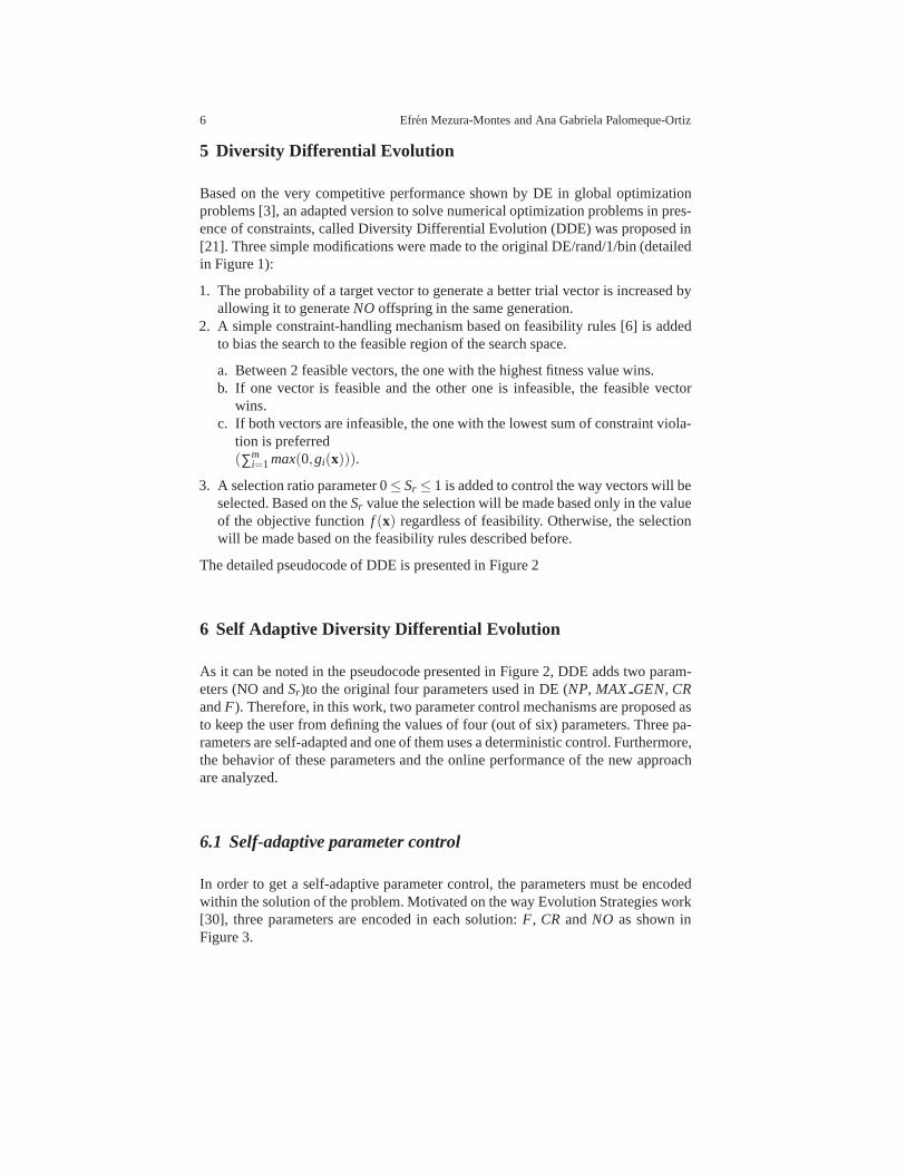
The detailed pseudocode of DDE is presented in Figure 2
6 Self Adaptive Diversity Differential Evolution
As it can be noted in the pseudocode presented in Figure 2, DDEadds two param-eters (NO andSr )to the original four parameters used in DE (NP, MAX GEN, CRandF). Therefore, in this work, two parameter control mechanisms are proposed asto keep the user from defining the values of four (out of six) parameters. Three pa-rameters are self-adapted and one of them uses a deterministic control. Furthermore,the behavior of these parameters and the online performanceof the new approachare analyzed.
6.1 Self-adaptive parameter control
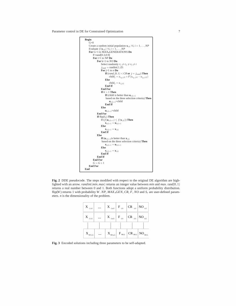
In order to get a self-adaptive parameter control, the parameters must be encodedwithin the solution of the problem. Motivated on the way Evolution Strategies work[30], three parameters are encoded in each solution:F, CR andNO as shown inFigure 3.
Parameter control in DE for Constrained Optimization 7
BeginG=0Create a random initial populationxi,G ∀i, i = 1, . . . ,NPEvaluatef (xi,G) ∀i, i = 1, . . . ,NPFor G=1 to MAX GENERATIONSDo
F=rand[0.3,0.9]For i=1 to NPDo
For k=1 toNODoSelect randomlyr1 6= r2 6= r3 6= ijrand = randint(1,D)For j=1 to n Do
If (randj [0,1) < CRor j = jrand) Thenchildj = xr3, j ,G +F(xr1, j ,G−xr2, j ,G)
Elsechildj = xi, j ,G
End IfEnd ForIf k > 1 Then
If (child is better thanui,G+1
based on the three selection criteria)Thenui,G+1=child
End IfElse
ui,G+1=childEnd ForIf flip(Sr ) Then
If ( f (ui,G+1) ≤ f (xi,G)) Thenxi,G+1 = ui,G+1
Elsexi,G+1 = xi,G
End IfElse
If (ui,G+1is better thanxi,G
based on the three selection criteria)Thenxi,G+1 = ui,G+1
Elsexi,G+1 = xi,G
End IfEnd If
End ForG = G+1
End ForEnd
Fig. 2 DDE pseudocode. The steps modified with respect to the original DE algorithm are high-lighted with an arrow.randint(min,max) returns an integer value betweenminandmax. rand[0,1)returns a real number between 0 and 1. Both functions adopt a uniform probability distribution.flip(W) returns 1 with probabilityW. NP, MAX GEN, CR, F , NO andSr are user-defined param-eters.n is the dimensionality of the problem.
...X X F CR NO1,n,G 1,G 1,G 1,G1,1,G
... NP,n,GXX F NP,G CRNP,G NO
NP,GNP,1,G
...X X F CR NO2,1,G 2,n,G 2,G 2,G 2,G
Fig. 3 Encoded solutions including three parameters to be self-adapted.

8 Efren Mezura-Montes and Ana Gabriela Palomeque-Ortiz
Now, each solution has its ownF , CRandNOvalues and these values are subjectto differential mutation and crossover. The process is explained in Figure 4, wherethe trial vector in Diversity Differential Evolution will inherit the three parametervalues from the target vector if the last decision variable was taken from it . On theother hand, the values for each parameter will be calculatedby using the differentialmutation operator i.e. they will be inherited from the mutation vector. The decisionvariables are handled as in traditional DE, however, theCRparameter value used inthe process is that of the target vector.
If (the last decision variable was inherited from the target vector) Thenchild jF = Fi,G
child jCR= CRi,G
child jNO= NOi,G
Elsechild jF = Fr3,G +Fi,G(Fr1,G−Fr2,G)child jCR= CRr3,G +Fi,G(CRr1,G−CRr2,G)child jNO= NOr3,G +Fi,G(NOr1,G−NOr2,G)
End If
Fig. 4 Differential mutation applied to the self-adapted parameters. Note that theF value for thetarget vectorFi,G is used in all cases where differential mutation is used.
6.2 Deterministic parameter control
Recalling theSRparameter explanation in Section 5, this parameter controls thepercentage of comparisons made between pairs of vectors by only considering theobjective function value, regardless of feasibility information. Therefore, it affectsthe bias in the search [29]. HigherSRvalues keep infeasible solutions located inpromising areas of the search space, whereas lowerSRvalues help to reach thefeasible region by using Deb’s rules [6].
Based on this behavior, theSRparameter is controlled by a fixed schedule. A sim-ple function is used to decrease the value for this parameterin such a way that ini-tial higher values allow DDE to focus on searching promisingregions of the searchspace, regardless of feasibility, with the aim to approach the feasible region froma more convenient area. Later in the process, theSRvalues will be lower, assum-ing the feasible region has been reached and that it is more important to keep goodfeasible solutions. The range withinSRvalues will be considered is the following:[0.45,0.65]. At each generation, theSRvalue will be decreased based on the expres-sion in Equation 5:
SR(t+1) = SRt −∆SR (5)
Parameter control in DE for Constrained Optimization 9
whereSR(t+1) is the new value for this parameter,SRt is the currentSRvalue,∆SRisthe amount decreased from this value at each generation and calculated as indicatedin Equation 6:
∆SR=
(
SR0−SRGmax
Gmax
)
(6)
whereSR0 represents the initial value forSR, andSRGmax its last value in a givenrun.
The detailed pseudocode of Diversity Differential Evolution with the parametercontrol techniques, called Adaptive-DDE (A-DDE) is shown in Figure 5.
7 Experiments and Results
In order to extensively test the A-DDE algorithm, six experiments are conducted.The first experiment compares the final results of A-DDE with respect to the originalDDE (called Static DDE). In order to verify that the self-adaptive mechanism is notequivalent to just generating random values for them withinsuggested ranges, thesecond experiment compares A-DDE with respect a special DDEversion, calledStatic2 DDE, where the values for the four controlled parameters in A-DDE arejust generated at random (by using a uniform distribution) within the same rangesused in A-DDE. The third experiment analyzes the convergence graphs for StaticDDE, Static2 DDE and A-DDE. The fourth experiment includes the graphs for thethree self-adapted parameters (F , CR andNO) in order to know which values arethey taking as to provide competitive results. The fifth experiment compares StaticDDE, Static2 DDE and A-DDE by using two performance measuresfor constrainedoptimization in order to know (1) how fast the feasible region is reached and (2) theability of each DE algorithm to improve inside the feasible region (difficult for mostEAs as analyzed in [18]). The two measures are the following:
1. Evals [14]: The number of evaluations (objective function and constraints) re-quired to generate the first feasible solution are counted. Alower value is pre-ferred because it means a faster approach to the feasible region.
2. Progress Ratio [18]: Originally proposed by Back for unconstrained optimiza-tion [1]. It is a measure of improvement inside the feasible region by using theobjective function values of the first and the best feasible solution reached so far
at the end of the process. The formula is as follows: Pr=
∣
∣
∣
∣
∣
ln
√
fmin(Gf f )fmin(T)
∣
∣
∣
∣
∣
, where
fmin(
Gf f)
is the objective function value of the first feasible solution found andfmin (T) is the objective function value of the best feasible solution found in allthe search so far. A higher value means a better improvement inside the feasibleregion.

10 Efren Mezura-Montes and Ana Gabriela Palomeque-Ortiz
BeginG=0
⇒ Create a random initial populationXi,G ∀i, i = 1, . . . ,NPEvaluatef (Xi,G) ∀i, i = 1, . . . ,NP
⇒ Select randomlySR∈ (0.45,0.65)⇒ Select randomlySRGmax ∈ (0.0,0.5)
For G=1 toGmax DoFor i=1 to NPDo
⇒ For k=1 toNOi,G DoSelect randomlyr1 6= r2 6= r3 :jrand = randint(1,D)For j=1 to D Do
⇒ If (randj [0,1) < CRi,G or j = jrand) Thenchildj ,G = xr3, j ,G +Fi,G(xr1, j ,G−xr2, j ,G)ban=0
Elsechildj ,G = xri , j ,G
ban=1End If
End For⇒ If (ban==1)Then
childF,G = Fi,GchildCR,G = CRi,Gchildn0,G = n0i,G
ElsechildF,G = Fr3,G +Fi,G(Fr1,G−Fr2,G)childCR,G = CRr3,G +Fi,G(CRr1,G−CRr2,G)childNO,G = NOr3,G +Fi,G(NOr1,G−NOr2,G)
End IfIf k > 1 Then
If (child is better thanui,G+1(Based on three selection criteria))Then
ui,G+1 = childEnd If
Elseui,G+1 = child
End IfEnd ForIf flip(SR)
If ( f (ui,G+1) ≤ f (xi,G)) Thenxi,G+1 = ui,G+1
Elsexi,G+1 = xi,G
End IfElse
If (ui,G+1 ≤ xi,G
(Based on three selection criteria))Thenxi,G+1 = ui,G+1
Elsexi,G+1 = xi,G
End IfEnd If
End ForG = G+1
⇒ SR= SR−∆SREnd For
End
Fig. 5 A-DDE pseudocode. Arrows indicate steps where the parameter control mechanisms areinvolved.
Parameter control in DE for Constrained Optimization 11
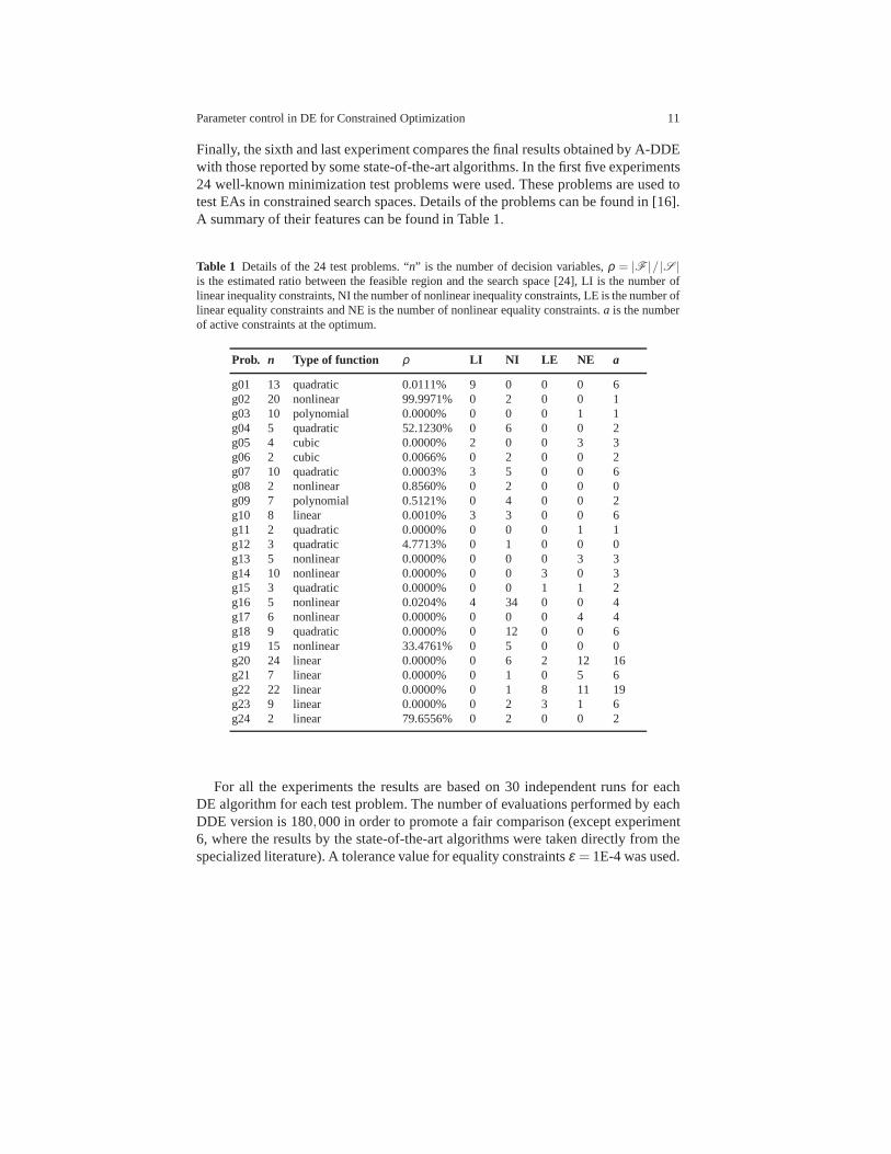
Finally, the sixth and last experiment compares the final results obtained by A-DDEwith those reported by some state-of-the-art algorithms. In the first five experiments24 well-known minimization test problems were used. These problems are used totest EAs in constrained search spaces. Details of the problems can be found in [16].A summary of their features can be found in Table 1.
Table 1 Details of the 24 test problems. “n” is the number of decision variables,ρ = |F |/ |S |is the estimated ratio between the feasible region and the search space [24], LI is the number oflinear inequality constraints, NI the number of nonlinear inequality constraints, LE is the number oflinear equality constraints and NE is the number of nonlinear equality constraints.a is the numberof active constraints at the optimum.
Prob. n Type of function ρ LI NI LE NE a
g01 13 quadratic 0.0111% 9 0 0 0 6g02 20 nonlinear 99.9971% 0 2 0 0 1g03 10 polynomial 0.0000% 0 0 0 1 1g04 5 quadratic 52.1230% 0 6 0 0 2g05 4 cubic 0.0000% 2 0 0 3 3g06 2 cubic 0.0066% 0 2 0 0 2g07 10 quadratic 0.0003% 3 5 0 0 6g08 2 nonlinear 0.8560% 0 2 0 0 0g09 7 polynomial 0.5121% 0 4 0 0 2g10 8 linear 0.0010% 3 3 0 0 6g11 2 quadratic 0.0000% 0 0 0 1 1g12 3 quadratic 4.7713% 0 1 0 0 0g13 5 nonlinear 0.0000% 0 0 0 3 3g14 10 nonlinear 0.0000% 0 0 3 0 3g15 3 quadratic 0.0000% 0 0 1 1 2g16 5 nonlinear 0.0204% 4 34 0 0 4g17 6 nonlinear 0.0000% 0 0 0 4 4g18 9 quadratic 0.0000% 0 12 0 0 6g19 15 nonlinear 33.4761% 0 5 0 0 0g20 24 linear 0.0000% 0 6 2 12 16g21 7 linear 0.0000% 0 1 0 5 6g22 22 linear 0.0000% 0 1 8 11 19g23 9 linear 0.0000% 0 2 3 1 6g24 2 linear 79.6556% 0 2 0 0 2
For all the experiments the results are based on 30 independent runs for eachDE algorithm for each test problem. The number of evaluations performed by eachDDE version is 180,000 in order to promote a fair comparison (except experiment6, where the results by the state-of-the-art algorithms were taken directly from thespecialized literature). A tolerance value for equality constraintsε = 1E-4 was used.

12 Efren Mezura-Montes and Ana Gabriela Palomeque-Ortiz
7.1 Experiment 1
In the first experiment Static DDE and A-DDE are compared. Theparameters usedfor each algorithm were the following:
1. Static DDE
• NP= 60 yGMAX= 600• SR= 0.45• NO= 5,CR= 0.9 andF ∈ (0.3,0.9) generated at random.
2. A-DDE.
• NP= 60 yGMAX= 600• SR∈ (0.45,0.65), SRGmax ∈ (0.0,0.5), randomly generated on each indepen-
dent run and this value is controlled by the deterministic control.• NO∈ (3,7), CR∈ (0.9,1.0) andF ∈ (0.3,0.9) initially generated at random
per each vector in the population and then handled with the self-adaptive con-trol.
The statistical results (best, mean and worst values from a set of 30 independentruns) are summarized in Table 2.
From those results in Table 2, A-DDE was able to maintain the good perfor-mance of the original DDE in fourteen test problems (g01, g03, g04, g05, g06, g07,g08, g09, g11, g12, g15, g16, g18, g24). Furthermore, the statistical values wereimproved in six problems (g10, g14, g17, g19, g21 and g23). Finally, in problemsg02 and g13 the results, mostly in the average and worst values, were not betterthan those provided by Static DDE. Problems g20 and g22 remained unsolved byA-DDE.
7.2 Experiment 2
A-DDE is now compared with respect to Static2 DDE, where the four parameters tobe controlled in A-DDE are just generated at random between the same intervals inStatic2 DDE. The parameter values used in A-DDE were the samereported in ex-periment 1 in Section 7.1. The parameters used in Static2 DDEwere the following:
• Static2 DDE
– NP= 60 yGMAX= 600– SR∈ (0.45,0.65) generated at random instead of using the deterministic pa-
rameter control.– NO∈ (3,7), CR∈ (0.9,1.0) andF ∈ (0.3,0.9) also generated at random in-
stead of using the self-adaptive parameter control.

Parameter control in DE for Constrained Optimization 13
Table 2 Comparison of results obtained with the original DDE version with static parametervalues (named Static DDE) and the proposed Adaptive-DDE (deterministic and self-adaptive pa-rameter control). “-”, means no feasible solution found. Values inboldface mean that the globaloptimum or best know solution was reached, values initalic mean that the obtained result is better(but not the optimal or best known) with respect to the approach compared.
Best Best Mean WorstTest known Adaptive Static Adaptive Static Adaptive Static
problem solution DDE DDE DDE DDE DDE DDE
g01 -15.000 -15.000 -15.000 -15.000 -15.000 -15.000 -15.000g02 -0.803619 -0.803605 -0.803618 -0.771090 -0.789132 -0.609853 -0.747876g03 -1.000 -1.000 -1.000 -1.000 -1.000 -1.000 -1.000g04 -30665.539-30665.539 -30665.539 -30665.539 -30665.539 -30665.539 -30665.539g05 5126.497 5126.497 5126.497 5126.497 5126.497 5126.497 5126.497g06 -6961.814 -6961.814 -6961.814 -6961.814 -6961.814 -6961.814 -6961.814g07 24.306 24.306 24.306 24.306 24.306 24.306 24.306g08 -0.095825 -0.095825 -0.095825 -0.095825 -0.095825 -0.095825 -0.095825g09 680.63 680.63 680.63 680.63 680.63 680.63 680.63g10 7049.248 7049.248 7049.248 7049.248 7049.262 7049.248 7049.503g11 0.75 0.75 0.75 0.75 0.75 0.75 0.75g12 -1.000 -1.000 -1.000 -1.000 -1.000 -1.000 -1.000g13 0.053942 0.053942 0.053942 0.079627 0.053942 0.438803 0.053961g14 -47.765 -47.765 - -47.765 - -47.765 -g15 961.715 961.715 961.715 961.715 961.715 961.715 961.715g16 -1.905 -1.905 -1.905 -1.905 -1.905 -1.905 -1.905g17 8853.540 8853.540 8853.540 8854.664 8854.655 8858.874 8859.413g18 -0.866025 -0.866025 -0.866025 -0.866025 -0.866025 -0.866025 -0.866025g19 32.656 32.656 32.656 32.658 32.666 32.665 32.802g20 0.096700 - - - - - -g21 193.725 193.725 193.725 193.725 193.733 193.726 193.782g22 236.431 - - - - - -g23 -400.055 -400.055 - -391.415 - -367.452 -g24 -5.508 -5.508 -5.508 -5.508 -5.508 -5.508 -5.508
The summary of statistical values from a set of 30 independent runs is shown inTable 3.
The results in Table 3 suggest that the effect of the self-adaptive mechanism isnot equivalent to just generating random values within convenient limits. A-DDEprovided better statistical results (mostly in the mean andworst values from a set of30 independent runs) in thirteen test problems (g01, g02, g04, g06, g07, g10, g13,g14, g16, g17, g19, g21 and g23). In nine problems the performance was similarbetween A-DDE and Static2 DDE (g03, g05, g08, g09, g11, g12, g15, g18 andg24). Finally, Static2 DDE was unable to provide better results in any problem.

14 Efren Mezura-Montes and Ana Gabriela Palomeque-Ortiz
Table 3 Comparison of results obtained with the DDE version with randomly-generated parame-ter values (named Static2 DDE) and the proposed Adaptive-DDE (deterministic and self-adaptiveparameter control). “-”, means no feasible solution found. Values inboldface mean that the globaloptimum or best know solution was reached, values initalic mean that the obtained result is better(but not the optimal or best known) with respect to the approach compared.
Best Best Mean WorstTest known Adaptive Static2 Adaptive Static2 Adaptive Static2
problem solution DDE DDE DDE DDE DDE DDE
g01 -15.000 -15.000 -15.000 -15.000 -14.937 -15.000 -13.917g02 -0.803619 -0.803605 -0.803610 -0.771090 -0.706674 -0.609853 -0.483550g03 -1.000 -1.000 -1.000 -1.000 -1.000 -1.000 -1.000g04 -30665.539-30665.539 -30665.539 -30665.539 -30660.237-30665.539 -30591.889g05 5126.497 5126.497 5126.497 5126.497 5126.497 5126.497 5126.497g06 -6961.814 -6961.814 -6961.814 -6961.814 -6959.015 -6961.814 -6877.840g07 24.306 24.306 24.306 24.306 24.945 24.306 38.903g08 -0.095825 -0.095825 -0.095825 -0.095825 -0.095825 -0.095825 -0.095825g09 680.63 680.63 680.63 680.63 680.63 680.63 680.63g10 7049.248 7049.248 7049.248 7049.248 7073.779 7049.248 7308.826g11 0.75 0.75 0.75 0.75 0.75 0.75 0.75g12 -1.000 -1.000 -1.000 -1.000 -1.000 -1.000 -1.000g13 0.053942 0.053942 0.053942 0.079627 0.131458 0.438803 0.438803g14 -47.765 -47.765 - -47.765 - -47.765 -g15 961.715 961.715 961.715 961.715 961.715 961.715 961.715g16 -1.905 -1.905 -1.905 -1.905 -1.905 -1.905 -1.900g17 8853.540 8853.540 8853.540 8854.664 8855.884 8858.874 8859.693g18 -0.866025 -0.866025 -0.866025 -0.866025 -0.866025 -0.866025 -0.866025g19 32.656 32.656 32.656 32.658 37.785 32.665 65.993g20 - - - - - - -g21 193.725 193.725 193.725 193.725 198.009 193.726 263.444g22 - - - - - - -g23 -400.055 -400.055 -400.011 -391.415 -370.854 -367.452 -165.715g24 -5.508 -5.508 -5.508 -5.508 -5.508 -5.508 -5.508
7.3 Experiment 3
In order to analyze the convergence behavior of each DDE algorithm compared, theconvergence graph of the run located in the median value of the 30 independent runswas plotted for each test problem. The graph starts when the first feasible solution isgenerated. Thex-axis represents the generation number and they-axis is calculatedas follows:log10( f (x)− f (x∗)), where f (x) is the best feasible solution found inthe current generation andf (x∗) is the optimal solution or best known solution forthe problem being solved (see Table 1).
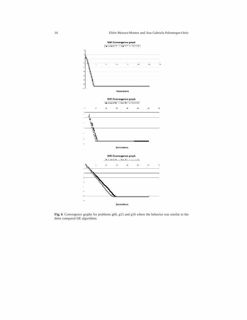
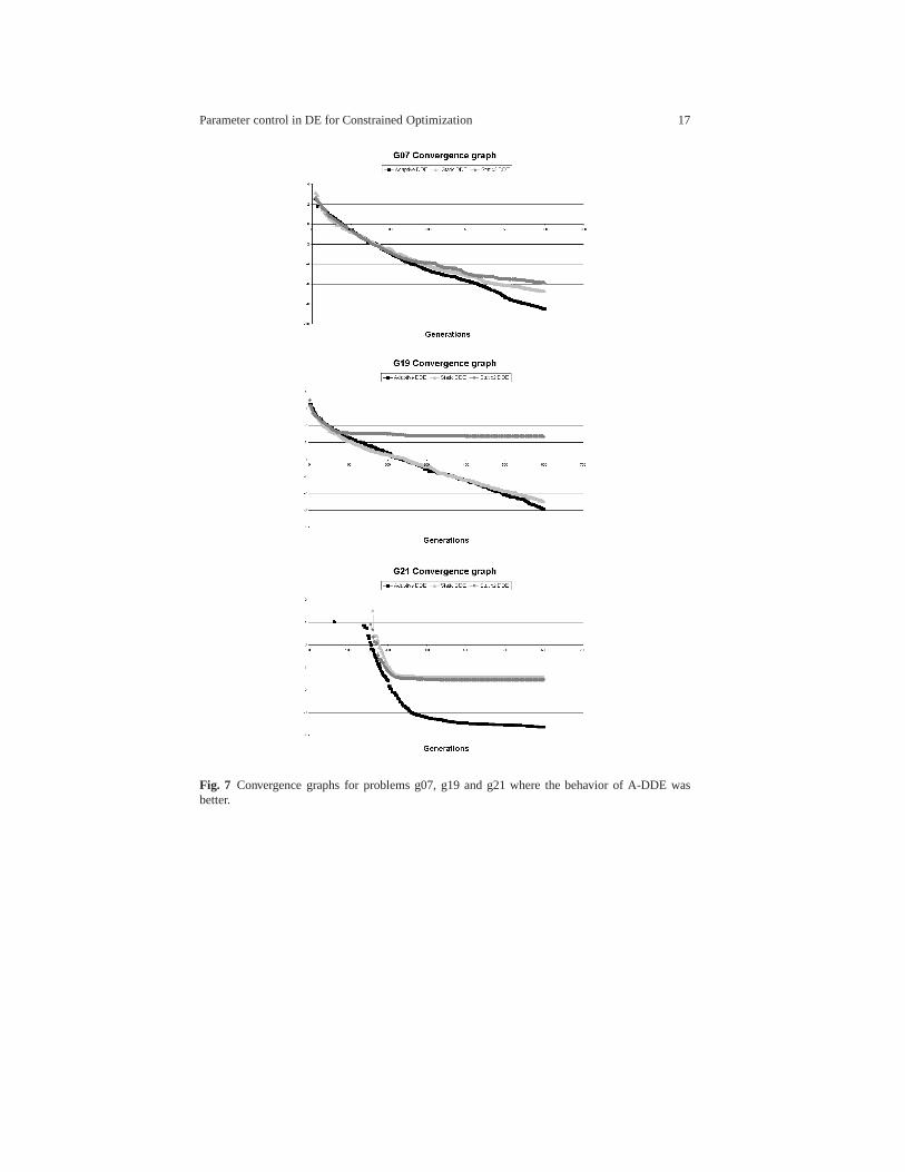
For sake of clarity representative graphs were grouped based on the behaviorobserved: (1) Test problems where the convergence was similar among Static DDE,Static2 DDE and A-DDE in Figure 6, (2) problems where A-DDE converged tobetter solutions faster than the other two approaches in Figure 7 and (3) problemswhere A-DDE got trapped in a local optimum solution in Figure8.

Parameter control in DE for Constrained Optimization 15
Regarding Figure 6, besides problems g06, g15 and g16, the convergence be-havior was similar in other nine problems (g01, g03, g04, g05, g08, g09, g11, g12and g24). A-DDE was able to present a better convergence behavior, besides prob-lems g07, g19 and g21 in Figure 7, in other five problems (g10, g13, g14, g18 andg23). Finally, the two problems presented in Figure 8 (g02 and g17) are those whereA-DDE got trapped in local optima solutions compared to the other two DDE algo-rithms.
There is not a clear pattern between convergence behavior and features of a testproblem. However, the results indeed show that A-DDE mostlymaintained the origi-nal DDE competitive convergence behavior and even was able to skip local optimumsolutions and providing better results in some problems, most of them in presenceof equality constraints (g13, g14, g21 and g23).
7.4 Experiment 4
The results of the experiment to analyze the values taken forthe controlled pa-rameters are reported as follows: Two graphs for representative test problems arepresented. One graph includes the average value for theF andCR parameters ineach generation of the run located in the median value out of 30 independent runs.The other graph presents the average value of theNO parameter of the same run.As in the previous experiment, the graphs are grouped based on the behavior found:(1) Those where the parameter values converged to a specific value in Figure 9,(2) problems where the parameter values oscillated and the final results were betterwith respect to the compared approaches in Figure 10 and finally (3) test problemswhere the parameter values oscillated and the final results where not better thanthose obtained with the other two DDE versions in Figure 11.
It is clear from Figures 9, 10 and 11 that an oscillating behavior was obtained inall cases, This effect was more remarked inF andNO, whereas inCR it is barelynoted. Based on these results, the self-adaptive mechanismis able to find thatCR≈0.9, which means trial vectors more similar to the mutation vector and less similar tothe target vector, is a suitable value on this set of test functions. On the other hand,F ∈ [0.5,0.7] andNO∈ [3,5] are adequate boundaries for the set of constrainedproblems used in the experiments.
Figure 9 includes representative graphs for test problems where the parametervalues reached a single value after converging to an optimum(See Figure 6). Othertest problems where the behavior was similar were g04, g08, g09, g11, g12 and g24.
Figure 10 contains graphs where A-DDE provided a better finalresult (See Fig-ure 7), but required more time to converge. In the same way, the parameter valueskept oscillating, helping the search by varying the values,mostly for F and N0.Other test functions with the same type of results were g01, g03, g05, g10, g14,g17, g18 and g23.
Finally, Figure 11 shows those graphs where the parameter values kept varyingwhile A-DDE got trapped in a local optimum solution (See Figure 8).
16 Efren Mezura-Montes and Ana Gabriela Palomeque-Ortiz
Fig. 6 Convergence graphs for problems g06, g15 and g16 where the behavior was similar in thethree compared DE algorithms.
Parameter control in DE for Constrained Optimization 17
Fig. 7 Convergence graphs for problems g07, g19 and g21 where the behavior of A-DDE wasbetter.

18 Efren Mezura-Montes and Ana Gabriela Palomeque-Ortiz
Fig. 8 Convergence graphs for problems g02 and g17 where the behavior of A-DDE was not betterthan those provided by the compared approaches.
7.5 Experiment 5
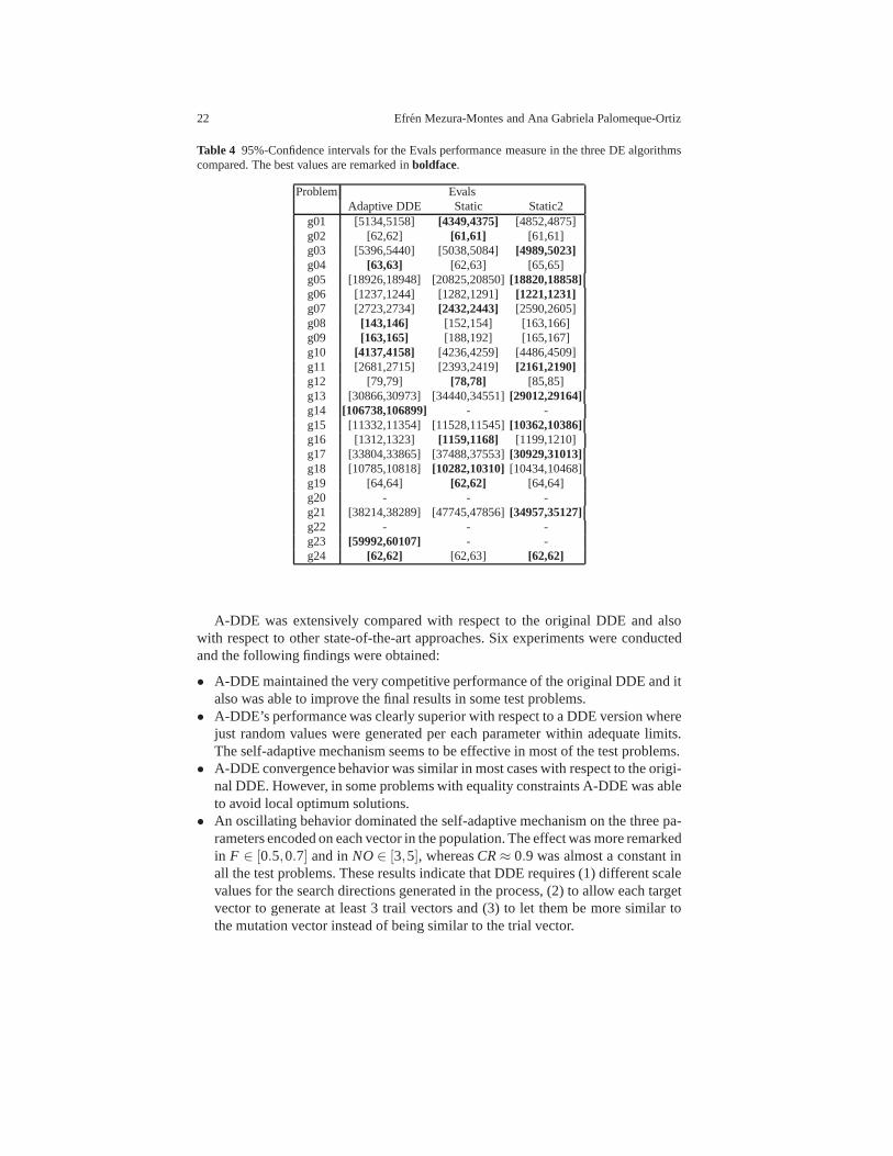
The 95%-confidence intervals for the mean value, out of 30 independent runs arepresented for both performance measures: Evals in Table 4 and Progress Ratio inTable 5. The aim is to analyze the average performance of the three DDE versionsas to establish the effect of the deterministic and self-adaptive control mechanisms.
Regarding the Evals results reported in Table 4, some test problems were notconsidered in the discussion because the feasible region was reached in the initialpopulation or even in the first generation. These problems are g02, g04, g08, g09,g12, g19 and g24. Problems g20 and g22 are also excluded because no feasiblesolutions were found by any algorithm. The confidence intervals for Evals indicatethat Static2 DDE reached the feasible region faster in eightproblems: g03, g05,g06, g11, g13, g15, g17 and g21. Static DDE generated feasible solutions faster infour problems: g01, g07, g16 and g18. A-DDE only found feasible solutions fasterin three problems: g10, g14 and g23. These results point out that the deterministicand self-adaptive mechanisms, despite maintaining or improving the quality and

Parameter control in DE for Constrained Optimization 19
Fig. 9 Average values forF , CR y NO parameters in each generation on the run located in themedian value out of 30 independent runs for problems g06, g15and g16. The parameter valuesconverged to a single value.
consistency of the final results, delayed the arrival to the feasible region with respectto the other two DDE variants.
The results for the Progress Ration in Table 5, where again problems g20 and g22are excluded from discussion because no feasible solutionswere found, show thatA-DDE obtained a better improvement inside the feasible region in ten problems:g02, g04, g09, g10, g14, g15, g16, g17, g21 and g23. Static DDEobtained a betterProgress Ratio interval in eight problems g01, g06, g07, g08, g11, g12, g18 and g19,while Static2 DDE was better in four problems: g03, g05, g13 and g24.
After taking more evaluations to reach the feasible region,A-DDE was ableto improve the fist feasible solution in more problems with respect to Static andStatic2 DDE. This behavior suggests that A-DDE enters the feasible region from amore promising region, based on a better exploration of the search space due to thesuitable parameter values. However, this issue requires further and more detailedresearch.

20 Efren Mezura-Montes and Ana Gabriela Palomeque-Ortiz
Fig. 10 Average values forF , CR y NO parameters in each generation on the run located in themedian value out of 30 independent runs for problems g07, g19and g21. The parameter valueskeep oscillating during all the run and the final results werebetter with respect to both Static DDEversions.
7.6 Experiment 6
In order to compare the final results obtained with A-DDE withrespect to state-of-the-art approaches, a summary of statistical values on the first 13 test problems(the most used for comparison in the specialized literature) are presented in Table6. The approaches used for comparison are: (1) The Generic Framework for con-strained optimization by Venkatraman & Yen [35], where the search is divided intwo phases, one where only the feasibility of solutions is considered and anotherone where the feasibility and the optimization of the objective function are takeninto account, (2) the self-adaptive penalty function by Tessema & Yen [34], wherea parameter-free penalty function is used to deal with the constraints of the problemand (3) a mathematical programming approach combined with amutation operatorby Takahama & Sakai [31]. The comparison shows that A-DDE is indeed very com-

Parameter control in DE for Constrained Optimization 21
Fig. 11 Average values forF , CRy NO parameters in each generation on the median value out of30 independent runs for problems g02 and g17. The parameter values keep oscillating during allthe run and the final results were not better with respect to both Static DDE versions.
petitive with other evolutionary approaches for constrained optimization based onthe quality (best result obtained so far) and consistency (better mean and standarddeviation values) of the final results.
8 Conclusions and Future Work
In this chapter, a deterministic and self-adaptive parameter control mechanisms wereadded to a competitive DE-based approach, called DiversityDifferential Evolution(DDE) to solve constrained optimization problems. The proposed approach, calledAdaptive-DDE (A-DDE) considered the encoding of three parameters per each vec-tor in the population, two from the original DE (F andCR) and one related with theconstraint-handling mechanism (NO, number of trial vectors generated per targetvector). Traditional mutation and crossover DE operators were used to self-adaptthese three values per each vector. Furthermore, other parameter which controlsthe bias in the search to keep infeasible solutions located in promising areas ofthe search space (based on the objective function value, regardless of feasibility),calledSr was deterministically controlled by a decreasing function, focusing first onkeeping good infeasible solutions and, after that, maintaining mostly good feasiblesolutions and discarding those infeasible ones.
22 Efren Mezura-Montes and Ana Gabriela Palomeque-Ortiz
Table 4 95%-Confidence intervals for the Evals performance measurein the three DE algorithmscompared. The best values are remarked inboldface.
Problem EvalsAdaptive DDE Static Static2
g01 [5134,5158] [4349,4375] [4852,4875]g02 [62,62] [61,61] [61,61]g03 [5396,5440] [5038,5084] [4989,5023]g04 [63,63] [62,63] [65,65]g05 [18926,18948] [20825,20850][18820,18858]g06 [1237,1244] [1282,1291] [1221,1231]g07 [2723,2734] [2432,2443] [2590,2605]g08 [143,146] [152,154] [163,166]g09 [163,165] [188,192] [165,167]g10 [4137,4158] [4236,4259] [4486,4509]g11 [2681,2715] [2393,2419] [2161,2190]g12 [79,79] [78,78] [85,85]g13 [30866,30973] [34440,34551][29012,29164]g14 [106738,106899] - -g15 [11332,11354] [11528,11545][10362,10386]g16 [1312,1323] [1159,1168] [1199,1210]g17 [33804,33865] [37488,37553][30929,31013]g18 [10785,10818] [10282,10310] [10434,10468]g19 [64,64] [62,62] [64,64]g20 - - -g21 [38214,38289] [47745,47856][34957,35127]g22 - - -g23 [59992,60107] - -g24 [62,62] [62,63] [62,62]
A-DDE was extensively compared with respect to the originalDDE and alsowith respect to other state-of-the-art approaches. Six experiments were conductedand the following findings were obtained:
• A-DDE maintained the very competitive performance of the original DDE and italso was able to improve the final results in some test problems.
• A-DDE’s performance was clearly superior with respect to a DDE version wherejust random values were generated per each parameter withinadequate limits.The self-adaptive mechanism seems to be effective in most ofthe test problems.
• A-DDE convergence behavior was similar in most cases with respect to the origi-nal DDE. However, in some problems with equality constraints A-DDE was ableto avoid local optimum solutions.
• An oscillating behavior dominated the self-adaptive mechanism on the three pa-rameters encoded on each vector in the population. The effect was more remarkedin F ∈ [0.5,0.7] and inNO∈ [3,5], whereasCR≈ 0.9 was almost a constant inall the test problems. These results indicate that DDE requires (1) different scalevalues for the search directions generated in the process, (2) to allow each targetvector to generate at least 3 trail vectors and (3) to let thembe more similar tothe mutation vector instead of being similar to the trial vector.
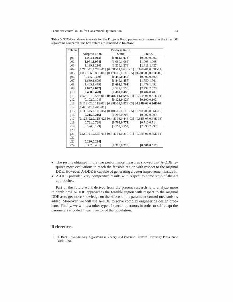
Parameter control in DE for Constrained Optimization 23
Table 5 95%-Confidence intervals for the Progress Ratio performance measure in the three DEalgorithms compared. The best values are remarked inboldface.
Problem Progress RatioAdaptive DDE Static Static2
g01 [1.004,1.013] [1.064,1.073] [0.900,0.906]g02 [1.071,1.074] [1.060,1.062] [1.005,1.008]g03 [1.199,1.216] [1.255,1.273] [1.411,1.427]g04 [0.77E-01,0.78E-01] [0.63E-01,0.63E-01] [0.62E-01,0.63E-01]g05 [0.83E-06,0.85E-06] [0.17E-05,0.18E-05][0.20E-05,0.21E-05]g06 [0.375,0.379] [0.446,0.450] [0.396,0.400]g07 [1.689,1.699] [1.849,1.857] [1.750,1.761]g08 [1.465,1.479] [1.691,1.701] [1.479,1.492]g09 [2.622,2.647] [2.522,2.558] [2.492,2.528]g10 [0.468,0.470] [0.481,0.483] [0.484,0.487]g11 [0.52E-01,0.53E-01][0.58E-01,0.59E-01] [0.30E-01,0.31E-01]g12 [0.102,0.104] [0.123,0.124] [0.100,0.102]g13 [0.11E-02,0.11E-02] [0.89E-03,0.97E-03][0.34E-02,0.36E-02]g14 [0.47E-01,0.47E-01] - -g15 [0.11E-05,0.12E-05] [0.10E-05,0.11E-05] [0.92E-06,0.96E-06]g16 [0.215,0.216] [0.205,0.207] [0.207,0.209]g17 [0.12E-02,0.12E-02] [0.41E-03,0.44E-03] [0.61E-03,0.64E-03]g18 [0.731,0.738] [0.763,0.771] [0.710,0.714]g19 [3.124,3.129] [3.150,3.155] [2.990,2.997]g20 - - -g21 [0.54E-01,0.55E-01] [0.31E-01,0.31E-01] [0.35E-01,0.35E-01]g22 - - -g23 [0.290,0.294] - -g24 [0.397,0.401] [0.310,0.313] [0.506,0.517]
• The results obtained in the two performance measures showedthat A-DDE re-quires more evaluations to reach the feasible region with respect to the originalDDE. However, A-DDE is capable of generating a better improvement inside it.
• A-DDE provided very competitive results with respect to some state-of-the-artapproaches.
Part of the future work derived from the present research is to analyze morein depth how A-DDE approaches the feasible region with respect to the originalDDE as to get more knowledge on the effects of the parameter control mechanismsadded. Moreover, we will use A-DDE to solve complex engineering design prob-lems. Finally, we will test other type of special operators in order to self-adapt theparameters encoded in each vector of the population.
References
1. T. Back. Evolutionary Algorithms in Theory and Practice. Oxford University Press, NewYork, 1996.

24 Efren Mezura-Montes and Ana Gabriela Palomeque-Ortiz
Table 6 Statistical results obtained by A-DDE with respect to thoseprovided by state-of-the-artapproaches on 13 benchmark problems. Values inboldface mean that the global optimum or bestknow solution was reached, values initalic mean that the obtained result is better (but not theoptimal or best known) with respect to the approaches compared. No results reported for problemsg12 andg13 were found in [35]
Problem/BKS Statistic Venkatraman & Yen [35]Tessema & Yen [34]Takahama & Sakai [31] A-DDE
g01 Best -15.000 -15.000 -15.000 -15.000-15.000 Median -15.000 -14.966 -15.000 -15.000
Worst -12.000 -13.097 -15.000 -15.000St. Dev. 8.51E-01 7.00E-01 6.40E-06 7.00E-06
g02 Best -0.803190 -0.803202 -0.803619 -0.803605-0.803619 Median -0.755332 -0.789398 -0.785163 -0.777368
Worst -0.672169 -0.745712 -0.754259 -0.609853St. Dev. 3.27E-02 1.33E-01 1.30E-02 3.66E-02
g03 Best -1.000 -1.000 -1.000 -1.000-1.000 Median -0.949 -0.971 -1.000 -1.000
Worst -1.000 -0.887 -1.000 -1.000St. Dev. 4.89E-02 3.01E-01 8.50E-14 9.30E-12
g04 Best -30665.531 -30665.401 -30665.539 -30665.539-30665.539 Median -30663.364 -30663.921 -30665.539 -30665.539
Worst -30651.960 -30656.471 -30665.539 -30665.539St. Dev. 3.31E+00 2.04E+00 4.20E-11 3.20E-13
g05 Best 5126.510 5126.907 5126.497 5126.4975126.497 Median 5170.529 5208.897 5126.497 5126.497
Worst 6112.223 5564.642 5126.497 5126.497St. Dev. 3.41E+02 2.47E+02 3.50E-11 2.10E-11
g06 Best -6961.179 -6961.046 -6961.814 -6961.814-6961.814 Median -6959.568 -6953.823 -6961.814 -6961.814
Worst -6954.319 -6943.304 -6961.814 -6961.814St. Dev. 1.27E+00 5.88E+00 1.30E-10 2.11E-12
g07 Best 24.411 24.838 24.306 24.30624.306 Median 26.736 25.415 24.306 24.306
Worst 35.882 33.095 24.307 24.306St. Dev. 2.61E+00 2.17E+00 1.30E-04 4.20E-05
g08 Best -0.095825 -0.095825 -0.095825 -0.095825-0.095825 Median -0.095825 -0.095825 -0.095825 -0.095825
Worst -0.095825 -0.092697 -0.095825 -0.095825St. Dev. 0 1.06E-03 3.80E-13 9.10E-10
g09 Best 680.76 680.77 680.63 680.63680.63 Median 681.71 681.24 680.63 680.63
Worst 684.13 682.08 680.63 680.63St. Dev. 7.44E-01 3.22E-01 2.90E-10 1.15E-10
g10 Best 7060.553 7069.981 7049.248 7049.2487049.248 Median 7723.167 7201.017 7049.248 7049.248
Worst 12097.408 7489.406 7049.248 7049.248St. Dev. 7.99E+02 1.38E+02 4.70E-06 3.23E-4
g11 Best 0.75 0.75 0.75 0.750.75 Median 0.75 0.75 0.75 0.75
Worst 0.81 0.76 0.75 0.75St. Dev. 9.30E-03 2.00E-03 4.90E-16 5.35E-15
g12 Best NA -1.000 -1.000 -1.000-1.000 Median NA -1.000 -1.000 -1.000
Worst NA -1.000 -1.000 -1.000St. Dev. NA 1.41E-04 3.90E-10 4.10E-9
g13 Best NA 0.053941 0.053942 0.0539420.053942 Median NA 0.054713 0.053942 0.053942
Worst NA 0.885276 0.438803 0.438803St. Dev. NA 2.75E-01 6.90E-02 9.60E-02
Parameter control in DE for Constrained Optimization 25
2. J. Brest, V.Zumer, and M. S. Maucecc. Control Parameters in Self-Adaptive DifferentialEvolution. In B. Filipic and J.Silc, editors,Bioinspired Optimization Methods and TheirApplications, pages 35–44, Ljubljana, Slovenia, October 2006. Jozef Stefan Institute.
3. U. K. Chakraborty, editor.Advances in Differential Evolution. Studies in ComputationalIntelligence Series. Springer-Verlag, Heidelberg, Germany, 2008.
4. C. A. C. Coello. Theoretical and Numerical Constraint Handling Techniques used with Evolu-tionary Algorithms: A Survey of the State of the Art.Computer Methods in Applied Mechanicsand Engineering, 191(11-12):1245–1287, January 2002.
5. N. Cruz-Cortes, D. Trejo-Perez, and C. A. C. Coello. Handling Constraints in Global Op-timization using an Artificial Immune System. In C. Jacob, M.L. Pilat, P. J. Bentley, andJ. Timmis, editors,Artificial Immune Systems. 4th International Conference, ICARIS 2005,pages 234–247, Banff, Canada, August 2005. Springer. Lecture Notes in Computer ScienceVol. 3627.
6. K. Deb. An Efficient Constraint Handling Method for Genetic Algorithms.Computer Methodsin Applied Mechanics and Engineering, 186(2/4):311–338, 2000.
7. A. Eiben and J. E. Smith.Introduction to Evolutionary Computing. Natural Computing Series.Springer Verlag, 2003.
8. G. Eiben and M. Schut. New Ways to Calibrate Evolutionary Algorithms. In P. Siarry andZ. Michalewicz, editors,Advances in Metaheuristics for Hard Optimization, Natural Comput-ing, pages 153–177. Springer, Heidelberg, Germany, 2008.
9. L. J. Fogel.Intelligence Through Simulated Evolution. Forty years of Evolutionary Program-ming. John Wiley & Sons, New York, 1999.
10. J. H. Holland.Adaptation in Natural and Artificial Systems. An Introductory Analysis withApplications to Biology, Control and Artificial Intelligence. University of Michigan Press,Ann Arbor, Michigan, 1975.
11. V. L. Huang, A. K. Qin, and P. N. Suganthan. Self-adaptative Differential Evolution Algo-rithm for Constrained Real-Parameter Optimization. In2006 IEEE Congress on EvolutionaryComputation (CEC’2006), pages 324–331, Vancouver, BC, Canada, July 2006. IEEE.
12. K. A. D. Jong.Evolutionary Computation. A Unified Approach. MIT Press, 2006.13. S. Kukkonen and J. Lampinen. Constrained Real-Parameter Optimization with Generalized
Differential Evolution. In2006 IEEE Congress on Evolutionary Computation (CEC’2006),pages 911–918, Vancouver, BC, Canada, July 2006. IEEE.
14. J. Lampinen. A Constraint Handling Approach for the Diifferential Evolution Algorithm.In Proceedings of the Congress on Evolutionary Computation 2002 (CEC’2002), volume 2,pages 1468–1473, Piscataway, New Jersey, May 2002. IEEE Service Center.
15. R. Landa-Becerra and C. A. Coello Coello. Optimization with Constraints using a CulturedDifferential Evolution Approach. In H. B. et al., editor,Proceedings of the Genetic and Evo-lutionary Computation Conference (GECCO’2005), volume 1, pages 27–34, New York, June2005. Washington DC, USA, ACM Press. ISBN 1-59593-010-8.
16. J. Liang, T. P. Runarsson, E. Mezura-Montes, M. Clerc, P.Suganthan, C. Coello Coello, andK. Deb. Problem Definitions and Evaluation Criteria for the CEC 2006 Special Session onConstrained Real-Parameter Optimization. Technical report, CEC, March 2006. Available athttp://www.lania.mx/˜emezura/documentos/trcec06.pdf.
17. J. Liu and J. Lampinen. A fuzzy adaptive differential evolution algorithm. Soft Comput.,9(6):448–462, 2005.
18. E. Mezura-Montes and C. A. C. Coello. Identifying On-line Behavior and Some Sourcesof Difficulty in Two Competitive Approaches for ConstrainedOptimization. In2005 IEEECongress on Evolutionary Computation (CEC’2005), volume 2, pages 1477–1484, Edinburgh,Scotland, September 2005. IEEE Press.
19. E. Mezura-Montes and C. A. Coello Coello. Constrained Optimization via MultiobjectiveEvolutionary Algorithms. In J. Knowles, D. Corne, and K. Deb, editors,Multiobjective Prob-lem Solving from Nature, pages 53–75. Springer, Heidelberg, 2008.
20. E. Mezura-Montes, C. A. Coello Coello, and E. I. Tun-Morales. Simple Feasibility Rulesand Differential Evolution for Constrained Optimization.In R. Monroy, G. Arroyo-Figueroa,

26 Efren Mezura-Montes and Ana Gabriela Palomeque-Ortiz
L. E. Sucar, and H. Sossa, editors,Proceedings of the 3rd Mexican International Conferenceon Artificial Intelligence (MICAI’2004), pages 707–716, Heidelberg, Germany, April 2004.Springer Verlag. Lecture Notes in Artificial Intelligence No. 2972.
21. E. Mezura-Montes, J. Velazquez-Reyes, and C. A. C. Coello. Promising Infeasibility andMultiple Offspring Incorporated to Differential Evolution for Constrained Optimization. InH. Beyer and et al., editors,Proceedings of the Genetic and Evolutionary Computation Con-ference (GECCO’2005), volume 1, pages 225–232, New York, June 2005. Washington DC,USA, ACM Press.
22. E. Mezura-Montes, J. Velazquez-Reyes, and C. A. C. Coello. Modified Differential Evolu-tion for Constrained Optimization. In2006 IEEE Congress on Evolutionary Computation(CEC’2006), pages 332–339, Vancouver, BC, Canada, July 2006. IEEE.
23. Z. Michalewicz and D. B. Fogel.How to Solve It: Modern Heuristics. Springer, Germany,2nd edition, 2004.
24. Z. Michalewicz and M. Schoenauer. Evolutionary Algorithms for Constrained Parameter Op-timization Problems.Evolutionary Computation, 4(1):1–32, 1996.
25. K. Miettinen, M. Makela, and J. Toivanen. Numerical comparison of some penalty-based con-straint handling techniques in genetic algorithms.Journal of Global Optimization, 27(4):427–446, December 2003.
26. A. E. Munoz-Zavala, A. Hernandez-Aguirre, E. R. Villa-Diharce, and S. Botello-Rionda.PESO+ for Constrained Optimization. In2006 IEEE Congress on Evolutionary Computa-tion (CEC’2006), pages 935–942, Vancouver, BC, Canada, July 2006. IEEE.
27. K. Price, R. Storn, and J. Lampinen.Differential Evolution: A Practical Approach to GlobalOptimization. Natural Computing Series. Springer-Verlag, 2005.
28. I. Rechenberg.Evolutionsstrategie: Optimierung technischer Systeme nach Prinzipien derbiologischen Evolution. Frommann-Holzboog, Stuttgart, 1973.
29. T. P. Runarsson and X. Yao. Stochastic Ranking for Constrained Evolutionary Optimization.IEEE Transactions on Evolutionary Computation, 4(3):284–294, September 2000.
30. H.-P. Schwefel, editor.Evolution and Optimization Seeking. Wiley, New York, 1995.31. T. Takahama and S. Sakai. Constrained Optimization by Applying theα Constrained Method
to the Nonlinear Simplex Method with Mutations.IEEE Transactions on Evolutionary Com-putation, 9(5):437–451, October 2005.
32. T. Takahama and S. Sakai. Constrained Optimization by the ε Constrained Differential Evo-lution with Gradient-Based Mutation and Feasible Elites. In 2006 IEEE Congress on Evolu-tionary Computation (CEC’2006), pages 308–315, Vancouver, BC, Canada, July 2006. IEEE.
33. M. F. Tasgetiren and P. N. Suganthan. A Multi-Populated Differential Evolution Algorithmfor Solving Constrained Optimization Problem. In2006 IEEE Congress on EvolutionaryComputation (CEC’2006), pages 340–354, Vancouver, BC, Canada, July 2006. IEEE.
34. B. Tessema and G. G. Yen. A Self Adaptative Penalty Function Based Algorithm for Con-strained Optimization. In2006 IEEE Congress on Evolutionary Computation (CEC’2006),pages 950–957, Vancouver, BC, Canada, July 2006. IEEE.
35. S. Venkatraman and G. G. Yen. A Generic Framework for Constrained Optimization UsingGenetic Algorithms.IEEE Transactions on Evolutionary Computation, 9(4):424,435, August2005.
Related Documents


![Deterministic Network Calculus p.2. DNC arrival results Accumulated arrival functions R(t): traffic recieved in [0,t] Arrival function may be constrained:](https://static.cupdf.com/doc/110x72/56649d615503460f94a4252b/deterministic-network-calculus-p2-dnc-arrival-results-accumulated-arrival.jpg)


![How isotropic is the Universe? - arXiv · How isotropic is the Universe? ... curately characterize the deterministic Bianchi pattern across the whole parameter space considered [23].](https://static.cupdf.com/doc/110x72/5b84bcfb7f8b9a784a8ce5d3/how-isotropic-is-the-universe-arxiv-how-isotropic-is-the-universe-curately.jpg)