Self-adaptation of learning rate in XCS working in noisy and dynamic environments

Computers in Human Behavior 27 (2011) 1535–1544

Contents lists available at ScienceDirect

Computers in Human Behavior

journal homepage: www.elsevier .com/locate /comphumbeh

Self-adaptation of learning rate in XCS working in noisy and dynamic environments

Maciej Troc, Olgierd Unold ⇑The Institute of Computer Engineering, Control and Robotics, Wroclaw University of Technology, Wyb. Wyspianskiego 27, 50-370 Wroclaw, Poland

a r t i c l e i n f o

Article history:Available online 16 November 2010

Keywords:Machine learningAdaptationSelf-adaptationXCS

0747-5632/$ - see front matter � 2010 Elsevier Ltd. Adoi:10.1016/j.chb.2010.10.024

⇑ Corresponding author.E-mail addresses: [email protected] (M. Tr

[email protected] (O. Unold).

a b s t r a c t

An extended classifier system (XCS) is an adaptive rule-based technique that uses evolutionary searchand reinforcement learning to evolve complete, accurate, and maximally general payoff map of an envi-ronment. The payoff map is represented by a set of condition-action rules called classifiers. Despite thisinsight, till now parameter-setting problem associated with LCS/XCS has important drawbacks. More-over, the optimal values of some parameters are strongly influenced by properties of the environmentlike its complexity, changeability, and the level of noise. The aim of this paper is to overcome some ofthese difficulties by a self-adaptation of a learning rate parameter, which plays a key role in reinforce-ment learning, since it is used for updates of classifier parameters: prediction, prediction error, fitness,and action set estimation. Self-adaptive control of prediction learning rate is investigated in the XCS,whereas the fitness and error learning rates remain fixed. Simultaneous self-adaptation of predictionlearning rate and mutation rate also undergo experiments. Self-adaptive XCS solves one-step problemsin noisy and dynamic environments.

� 2010 Elsevier Ltd. All rights reserved.

1. Introduction

Learning classifier systems (LCSs) are rule-based systems whichadapt to an environment (Holland, 1992; Goldberg, 1989). Duringeach interaction, learning classifier system: detects the environ-mental state, makes the chosen action (using ‘‘condition-action’’rules) and detects the results (called environmental payoff). Thecollected information are used afterwards for updating the systemknowledge stored in a rule set. In the most popular ‘‘Michigan-style’’ LCS, a rule set is treated as a population ½P�, where each rule(called classifier) is evaluated individually (i.e. based on an averagepayoff caused by the use of the classifier), and genetic algorithm(GA) is applied for discovery new rules. So that, ‘‘Michigan-style’’LCS usually contains: the performance component which selectsan action in respect to the environmental state, the reinforcementcomponent which collects information about usability of rules andthe evolutionary discovery component (GA) which creates newclassifiers (Goldberg, 1989).

Among many varieties of LCS systems, EXtended Classifier Sys-tem (XCS) (Wilson, 1995; Butz, Kovacs, Lanzi, & Wilson, 2004) isprobably still the most advanced and universal one. After detectionof current environmental state, an XCS system tries to predict pay-offs for all action, which can be taken. System adaptation relies oncreating a ‘‘payoff map’’ of the environment, built of classifiers(Wilson, 1995). XCS has shown high performance solving both:

ll rights reserved.

oc), [email protected], olgier-

one-step tasks (where environmental payoff may be detected justafter a single action) and multi-step tasks (where final payoff oc-curs after some number of interactions with an environment).Numerous applications have been proposed for extended classifiersystem, including: solving data-mining problems (i.e. classificationan clustering) (Kharbat, Bull, & Odeh, 2007; Bacardit & Butz, 2005;Tamee, Bull, & Pinngern, 1854) and robot control (Webb, Hart,Ross, & Lawson, 2003). Moreover, many others, more specific mod-els have been based on the basic XCS architecture. Among thesesystems, SUpervised Classifier System (UCS), which applies super-vised learning instead of reinforcement one (Bernad-Mansilla &Garrell-Guiu, 2003; Orriols-Puig, 2008), can be given as anexample.

Despite the huge abilities of XCS, it includes quite complexcomponents controlled by a large number of parameters. The rein-forcement component is controlled among others by parameters: b(the learning rate), a; m. The discovery component is controlled by:v (the crossover rate), l (the mutation rate), hdel (the deletionthreshold) etc. Their influence on system adaptation is analyzedamong other in Butz, Sastry, and Goldberg (2002, 2004). In Butzet al. (2002, 2003), it has been shown that applying a tournamentselection instead of a proportional one during genetic algorithmdecreases significantly parameter sensitivity. Nevertheless theoptimal values of some parameters are still strongly influencedby properties of an environment like its: complexity, changeabilityor the level of noise. That is why, many investigations have beendone for parameter tuning, adaptation or self-adaptation.

Self-adaptation of parameters is widely used to overcomeproblem of parameter settings in evolutionary algorithms

1536 M. Troc, O. Unold / Computers in Human Behavior 27 (2011) 1535–1544

(Meyer-Nieberg & Beyer, 2007; Saravanan, Fogel, & Nelson, 1995;Spears, 1995), particularly in evolutionary strategies and evolu-tionary programming, where the mutation rate is often adapted(Bäck & Schwefel, 1993). One of methods of self-adaptation, whichwas introduced with meta-evolutionary programming (Meta-EP)(Fogel, 1992), has been also successfully applied in scope of learn-ing classifier systems (Hurst & Bull, 2003, 2002). In this method,each individual (or classifier) contains real-value genes which rep-resent parameters controlling operations upon the individual. Likeother methods of self-adaptation, this one also bases on thehypothesis, that the classifiers using more optimal parameter val-ues should be better evaluated and they should be reproducedmore often than the others (Meyer-Nieberg & Beyer, 2007). The re-sults presented in Hurst and Bull (2002) show benefits of the use ofself-adaptive mutation rate in a XCS system solving multi-stepproblems. Self-adaptation of other parameters is much more diffi-cult. Some parameters do not control operations on a single classi-fier, but they control operations on the whole classifier population(deletion threshold hdel is an example). Moreover, some parametersinfluence directly classifier evaluation. The learning rate b controlsfitness updates among others and an inappropriate value of thisparameter makes classifiers overrated. So that, self-adaptation oflearning rate is ‘‘selfish’’ because each inaccurate classifier maybe highly evaluated, if its b gene has some, ‘‘wrong’’ value. In Hurstand Bull (2002) ‘‘enforcement cooperation’’ technique has beenused to overcome this problem in XCS solving multi-steps tasks.

This work describes the new approach to self-adaptation of thelearning rate in the XCS system solving one-step tasks. The pre-sented model has been tested in noisy and dynamic environmentswhich often require other parameter values than taken for solvingsimple, stationary problems. Simultaneous self-adaptation of l andb are also investigated.

The article is structured as follows: next section gives thedescription of XCS model solving single-step tasks, after that theproblem of tuning or adapting the learning rate is described andproposed model is presented. In Section 4 the results of experi-ments are given, and finally summary of the work can be foundin Section 5.

2. EXtended Classifier System (XCS)

From its very beginning (Wilson, 1995), XCS architectureevolves significantly and many varieties of it have been proposed(i.e. XCSR which processes real value inputs (Wilson, 2000)). Themore recent version of basic XCS is described among others in(Butz, 1999), nevertheless in this section we take into account onlythe system which processes binary inputs and solves one-stepproblems. Solving one-step problem relies on simple classificationof input messages (every possible action is a class label).

Like it has been noticed in Section 1, XCS includes the popula-tion (½P�) of constant size linear rules (Goldberg, 1989) called clas-sifiers and it applies procedures to adapt them, both in aparametric and structural way. Classifiers consist of: conditionalparts, action parts and a sets of scalar parameters (Fig. 1). Everycondition C in a condition part is either a symbol belonging to analphabet (in our experimentsjbinary) of input messages or a special‘‘don’t-care’’ symbol #. An action part is a symbolic representationof an action A 2A which can be done in an environment. Threeparameters of classifier are particular important for the learning

Fig. 1. An example of a classifier with an action a and parameters: prediction p,prediction error � and fitness f.

process, that is: prediction p, prediction error � and fitness f.Parameter num (numerosity) of classifier denotes the number ofmicro-classifiers aggregated in it. XCS systems store identical clas-sifiers as a macro-classifier – single individual in ½P�. Parameter expdenotes the experience of a classifier, that is the number of updatesof classifier parameters which have been done. All classifier param-eters will be explained in the following paragraphs.

As the majority of learning classifier systems, in each cycle, XCSchooses an action as an answer for a current environmental state.Nevertheless it may work either in exploit or explore phase everycycle. During exploit cycles, system selects an action which shouldcause the highest payoff (according to the prediction). In explorecycles, system makes a random action to learn more about an envi-ronment (to build a payoff map of it).

At the beginning of each cycle, system detects an environmentalstate and transforms it to a vector (input message s) – see Fig. 2step 1. After that, XCS build a match set ½M� including all classifierswhich match the input (Fig. 2 step 2). Classifier is considered tomatch the input, when its each condition C equals either symbolat the corresponding position of input message or a ‘‘don’t-care’’symbol. Every possible action should be represented by at leastone classifier in the match set. Otherwise, a covering is done forall missing actions. Covering mechanism creates new classifierwith each condition either taken from the input message or setto ‘‘don’t-care’’ symbol (with probability determined by parameterP#). An action part is set to a missing action. After that an action ais selected and done in the environment (Fig. 2 step 5). While in ex-plore cycles the selection is random, in exploit cycles systemchooses the action with the highest value in prediction array PðaÞ(Fig. 2 step 4). The latest includes predictions for all possible ac-tions. The prediction for an action ai 2A is calculated as anweighted average of predictions p of classifiers which have ai intheir action parts. Classifier fitness f is treated as a weight.

After executing the action a, the reaction of environment is de-tected, transformed to the scalar payoff R (Fig. 2 step 6) and rein-forcement learning of classifiers may be done (Fig. 2 step 7).Classifiers are usually learned in explore cycles only, neverthelesssome XCS implementations carry out it also in exploit cycles. Atthe beginning action set ½A� is created including those classifiersfrom ½M�, which have proposed an action a. The experience exp ofall classifiers in ½A� is increased, and an update of parameters ismade. Widrow–Hoff delta rule (Widrow & Hoff, 1960) is used toupdate prediction p, prediction error �, and fitness f. Additionally,the first two parameters are updated with the help of techniqueMAM (Moyenne Adaptive Modifée). The prediction is updated byp pþ bðR� pÞ, where bðb 2 ð0;1�Þ denotes the learning rate.The prediction error is updated by � �þ bðjR� pj � �Þ. The useof MAM causes that, when classifier experience exp is lower then

Fig. 2. A generic overview of XCS solving one-step problem. A structure element isrepresented by a rectangular, a process by a ellipse. Solid arrows represent dataflows between elements as well as between elements and the environment, startingfrom state detection (1) and finishing on payoff detection (6). Dashed arrowsrepresent operations made on classifiers, which are placed in structure elements.

M. Troc, O. Unold / Computers in Human Behavior 27 (2011) 1535–1544 1537

an inversion of learning rate b, the value of 1/exp is used instead ofb. The fitness value of each classifier in ½A� is updated with respectto its current relative accuracy j0:

j ¼ 1 if � < �0

að�=�0Þ�m otherwise

�ð1Þ

j0 ¼ j � numPcl2½A�jcl � numcl

ð2Þ

f f þ bðj0 � f Þ ð3Þ

The parameter �0ð�0 > 0Þ is a minimal considered error of classifier.If � < �0 classifier is treated as an accurate one. Otherwise the accu-racy j is a scaled inversion of an error, controlled by parameters: �0,aða 2 ð0;1ÞÞ and mðm > 0Þ. Set-relative accuracy j0 is counted in re-spect to accuracies of all classifiers in ½A�. Classifier fitness f is up-dated according to Widrow–Hoff delta rule, but without the useof MAM technique. Finally, the action set size estimation as is up-dated (with a help of Widrow–Hoff delta rule and MAM) by current½A� size. Besides the covering mechanism XCS applies steady-stategenetic algorithm for rule discovery. A GA is run if an average timefrom its last invocation in ½A� (counted based on the average timestamp ts parameter of classifiers) is greater than hGA. GA uses a tour-nament selection as it is described in Butz et al. (2002, 2003). Inde-pendent tournaments are created in an action set to select twoparent classifiers. Relative tournament size, denoted as s is a frac-tion of an action set size. After reproduction, offspring classifiersare uniformly crossed (with the probability v) and mutated (withthe probability l). We use simple free mutation (Butz, 1999), wherean action part and each classifier condition can be changed into oneof the remaining possible values. The parameters of offspring clas-sifiers are in majority derived from their parents. At the end timestamps ts of all rules in action set are updated to the current time.

GA subsumption (in version proposed by Butz et al. (2002)) isfired for each offspring classifier. It checks if there exist experi-enced (exp > hsub) and accurate rules in ½A�which logically subsume(in respect to conditional parts) new classifier. If so, numerosity ofthe most general one is increased. Otherwise offspring classifier isinserted into the population. During insertion, the classifier is com-pared with all individuals in ½P�. If exactly identical classifier isfound, its numerosity is increased. If not, new macro-classifier isadded to the population with the numerosity set to 1, experienceset to 0 and fitness divided by 10.

If a population size (in a sense of number of micro-classifiers) isgreater than maximal value N, deletion process in the whole ½P� isdone. Proportional selection is made in respect to two factors: anaction set estimation as of classifier and an inversion of its relativefitness. The second factor is taken into account, if the classifier isexperienced (exp > hdel) and it has very low fitness in relation tothe average fitness in ½P�. After the deletion a new cycle can began.

3. Learning rate and its adaptation in XCS classifier system

As it has been described in the previous section, learning ratecontrols updates of four important classifier estimations (Butzet al., 2004; Orriols-Puig, Bernado-Mansilla, Goldberg, Sastry, &Lanzi, 2009): an estimation of the mean payoff R, called the predic-tion p, an estimation of the standard error of this prediction, calledthe prediction error �, an estimation of the mean relative accuracy(the fitness f) and an estimation of the mean size of an action set, inwhich a classifier is placed (as parameter). We focus on updates offirst three estimations which are strongly correlated.

Widrow–Hoff delta rule (Widrow & Hoff, 1960) has a form sim-ilar exponentially weighted moving average (EWMA) (Roberts,1959) controlled by a smoothing factor b. Therefore, the result ofthe ith update of any parameter is a weighted average of a se-quence of i random values. For example the payoff prediction p is

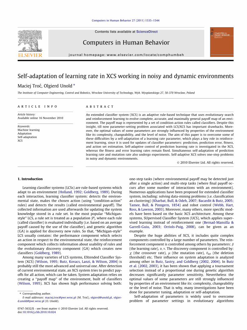
a weighted average of all payoffs, a classifier has been updatedby. If MAM technique is used, the weights of first 1/b elements inthe sequence are equal. The weights of next ones grow geometri-cally (with the common ratio 1/(1�b) for b < 1) and they are thelargest for the last (and most recent) values. Thanks to that, an im-pact of the ‘‘old’’ values is reduced and an updated parameter re-flects on changes in distribution of an updating variable. Fromthe same reason, because only a constant-size part of samplevalues influences an estimation, an updated parameter oscillatesrandomly about its expected value (Butz et al., 2004, 2002;Orriols-Puig et al., 2009). The higher b is set, the larger the oscilla-tions are. So that, the learning rate should be tuned in respect totwo criteria, to speed up the reaction on changes (higher learningrate is recommended) and to reduce the random fluctuations(lower learning rate is recommended). The phenomenon is illus-trated in the plots of Fig. 3. Moreover, this problem is well knownin context of EWMA (Nembhard & Kao, 2003).

The optimal value of b depends on changeability and dispersionof the updating variable. Lets look at some examples of parameteruse. In stationary environments, the lower the learning rate is, thecloser the current payoff prediction is to its expected value, while,in non-stationary ones, classifier predictions should react onchanges in the payoff landscape (higher b is needed). The predic-tion error � should be updated with b� 0, because distributionof variable jR� pj changes in time, even when system learns in sta-tionary environment. Note that the payoff prediction p tends tohave ‘‘wrong’’ values, when classifier is unexperienced (Butzet al., 2004), and the later error estimations � should not base onthem at all. Nevertheless, it is said, that learning rate used for up-dates of the prediction and the prediction error can be very low,when system adapts to the stationary environment (Dam, Lokan,& Abbass, 2007). Among classifier parameters, the fitness f is basedon the most changeable data, because not only prediction errors ofclassifiers change, but also the classifier population itself (via a dis-covery component).

Learning rate of 0.2 is commonly used to solve single-step prob-lems. Nevertheless, applying this value for updates of all parame-ters may cause problems in some cases. In Butz et al. (2002,2003), it has been shown that, XCS system using b ¼ 0:2 cannotadapt effectively, when environmental payoffs are affected byGaussian noise, because of huge parameter fluctuations. On theother hand, too large reduction of b causes problem with classifierevaluation. Classifier fitness changes too slowly, starting from asmall initial value, and the ‘‘young’’ rules cannot compete effec-tively with the experienced ones (Butz et al., 2003). That is why,the use of separated learning rates for updates of different param-eters has been suggested in Butz et al. (2003). The idea has beengiven up, because XCS using: the tournament selection, and thelearning rate of 0.05, adapts effectively for different levels ofGaussian noise (Butz et al., 2002, 2003).

Another example of an ineffective use of the fixed learning rateof 0.2 is an adaptation to an environment with class imbalance. Insuch an environment, some subset (class) of input messages occursmore rarely then the others, during system learning (more detailsin Orriols-Puig et al. (2009)). Classifier estimations are often wrongunder such conditions, because last few updating payoffs (the mostconsidered ones) are not representative for the whole of possiblevalues. Particularly, over-general and inaccurate rules tend to beoverrated. Gradient descent method (originally proposed by Butz,Goldberg, & Lanzi (2005)) has been used in Orriols-Puig et al.(2009) to overcome this phenomenon. The learning rate used forprediction update of the classifier cl is multiplied by the factor

fclPc2½A�

fc, that is by the classifier relative fitness in the action set. It

causes, that predictions of over-general classifiers oscillate less,and prediction errors are not underestimated.

-20

0

20

40

60

80

100

120

140

0 20 40 60 80 100

varia

ble

(xi)

discrete time (i)

xi = i + N(0,20)

time seriesaveraging with β = 0.02

averaging with β = 0.2

Fig. 3. The time series of xiðxi ¼ iþ Nð0;20ÞÞ, where Nðl;rÞ is normally distributed random variable, averaged by means of Widrow–Hoff rule and MAM technique. If learningrate is low (b ¼ 0:02), the estimation of mean xi fluctuates only a little. On the other hand this estimation is very slowly following the trend of xi .

1538 M. Troc, O. Unold / Computers in Human Behavior 27 (2011) 1535–1544

Some adaptive approach to the learning rate has been also pro-posed in Dam et al. (2007), where the XCS system solving dynamicdata mining problems is investigated. The b parameter is thererecalculated in respect to the temporal increase of the predictionerror of the system, that is the difference between the current errorand the previous one (Dam et al., 2007). The large increase meansthat the rapid change has taken place in the environment and thelearning rate should be largely set to speed up estimation updates.Nevertheless, we are not sure, how this mechanism works in anenvironment affected by Gaussian noise, where large error fluctu-ations occur even when the environment does not change.

As it has been noticed, self-adaptive learning rate has beenalready applied in an XCS system solving multi-step problems(Hurst & Bull, 2003, 2002). In such problems, each system actionchanges environmental state and the final payoff is detected afterseveral interactions with an environment. An appropriate mecha-nism is proposed in the XCS system, to update classifier parametersin a chain of action sets which lead to a particular environmentalpayoff (see Wilson (1995, 1999) for more details). Shortly speaking,action sets (of classifiers) created in time tð½A�tÞ and in timet þ 1ð½A�tþ1Þ depend to each other. This fact is used in the ‘‘enforcedco-operation’’ method, where learning rate is taken from classifierselected proportionally in ½A�t to update classifiers in ½A�tþ1 and viceversa. Experiments described in Hurst & Bull (2002) don’t showsupremacy in performance of the self-adaptive b over the fixedone in the XCS solving the Woods problem.

This work focuses on a self-adaptation of the learning rate to alevel of changeability and a level of noise present in a payoff land-scape, where XCS system solves one-step problems. We have ex-tended the range of b by {0}. If the learning rate is 0, we assume,that an updated parameter is counted as a simple average of allprevious updating values (like in MAM technique) during wholeclassifier life. To reduce the risk of selfishness (Hurst & Bull,2003, 2002), only the learning rate used for payoff predictions (de-noted as bp) is self-adapted. Note that both the prediction error �(indirectly) and the fitness f (directly) are the base for classifierevaluation and there exists a big opportunity of manipulating theirupdates to make classifier over-fitted. Like in meta-EP method,prediction learning rate is stored as a real value gene in each clas-sifier and used for its updates. During classifier learning, prediction

update is done just after an error update. If the parameters wereupdated in a reverse order, the prediction error would alwaysequal 0 for bp ¼ 1 and the learning rate adaptation would looseany sense. Like in Hurst & Bull (2002), bp is passed to child classi-fiers during reproduction, and optionally recombined. In our ap-proach bp is mutated as bp ¼ bp þ Nð0; bpÞ. Experiments show,that such wide exploration of the surrounding of the current bp

is effective. The rest of the considered parameters, that is: the pre-diction error �, the fitness f and the action set size estimation as,are updated with the fixed learning rate bðb ¼ 0:2 is used). Theparameter bp is initialized by b/2 in classifiers created by covering.In some experiments described in section below, self-adaptation ofmutation rate has been also performed according to meta-EPmethod (Fogel, 1992; Hurst & Bull, 2003, 2002), i.e. mutation rateis mutated by the formula l ¼ lþ Nð0;lÞ.

The proposed architecture has been compared experimentallywith the XCS using fixed learning rate (b 2 f0:05;0:2g). Moreover,the XCS system using three separated, fixed learning rates: the firstfor prediction updates (denoted as bp), the second for error updates(denoted as b�), the third for updates of the fitness and the actionset size estimation (classically denoted as b), has been investigated.Extreme values of first two rates are set: bp ¼ 0 and b� ¼ 1, while bis of 0.2. The detailed description of experiments and results are gi-ven in following section. Note that our self-adaptive approach isstrongly related to the adaptive models proposed for EWMA, inwhich the smoothing factor is adapted. As reported in Nembhardand Kao (2003), in some of these methods, chosen error measures(based, among others, on the absolute deviation (Chow, 1965)) areused for an evaluation of the smoothing factor values. Similarly, inour approach, prediction error of classifier is used (among others)to evaluate its prediction learning rate.

4. Experiments and results

The experiments have been performed in a modified 20-bit mul-tiplexer environment (MP-20). Interaction with the environmentrelies on making a classification of binary inputs (problems) oflength 20 into one of two classes (A ¼ f0;1g). There are 4 addressbits and 16 data bits in each input. Positions of address bits are ini-tially placed in the beginning of input, but they may be randomly

M. Troc, O. Unold / Computers in Human Behavior 27 (2011) 1535–1544 1539

relocated if a rapid change of an environment occurs. Concatenatedaddress bits code the number of the data bit, and the goal of classi-fication is to point its value. System receives payoffs: 1000 for goodclassifications (RH ¼ 1000) and 0 for bad ones (RL ¼ 0).

The implementation of XCS is based on Butz (1999) and fast rulematching method is applied (Llorà & Sastry, 2006). For the majorityof experiments, XCS parameters are set as follows: b ¼ 0:2, b0

p ¼ 0:1,a ¼ 0:1, m ¼ 5, �0 ¼ 1, pI ¼ 500, �I ¼ 0, FI ¼ 10, hGA ¼ 25, s ¼ 0:4,v ¼ 0:8, l ¼ 0:04 (and l0 ¼ 0:04 for a system with self-adaptivemutation rate), P# ¼ 1:0, hdel ¼ 20, d ¼ 0:1. In Butz et al. (2002)and Kharbat, Bull, & Odeh (2005) similar parameter values are pro-posed. Explore and exploits phases go one after another. Systemslearns during explore phases and exploit phases are only used forrecording results. Performance in all experiments is measured asa moving average of last 50 classifications, where 1 is given forevery good classification and 0 for a bad one. If not stated differ-ently, all results are averaged over 50 independent system runs.

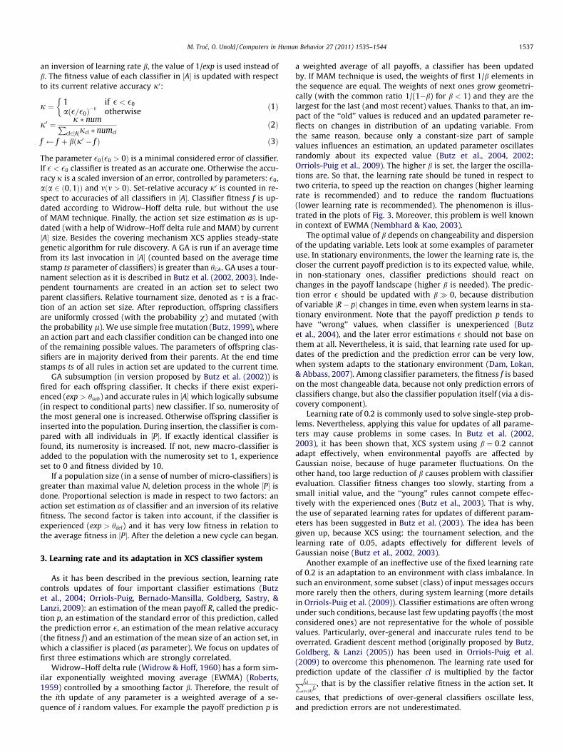
First experiment has been performed in dynamic MP-20 environ-ment, where rapid change occurs in every 50000 explore problem.The change relies on relocation of all four positions of address bits.Fig. 4 presents the performance curves for: a classic XCS(b 2 f0:05; 0:2g), an XCS using separated learning rates (bp ¼ 0,b� ¼ 1, b ¼ 0:2) and a XCS with self-adaptive learning rate. The clas-sic XCS system learns faster for b ¼ 0:2 than for b ¼ 0:05, what hasbeen previously shown in Butz et al. (2002), among others. Surpris-ingly, before change of the environment, the system using separatedlearning rates (bp ¼ 0, b� ¼ 1, b ¼ 0:2) achieves the maximal perfor-mance as the first one. After that, the system learns slower than theXCS using b ¼ 0:2. It is probably caused by the use of a low predic-tion learning rate (classifier predictions cannot be fast updated in re-spect to the new payoff landscape). The system using self-adaptivebp shows slower increase of performance than the XCS withb ¼ 0:2 during whole experiment, but higher than XCS withb ¼ 0:05 after the change. Rapid increase of average bp in ½P� is obser-vable at the beginning of learning process and the slow drop of thisvalue after about the 5000-th exploit (explore) problem. First, we tryto explain behavior of the system using separated learning rates.

To do that, we have created a tiny classifier set which consists ofonly two individuals. The first classifier (the less accurate) is updatedby high payoff RH with probability 0:8ðPH ¼ 0:8Þ, while the secondone (the more accurate) with probability 0.9. Classifiers parametersare initialized as follows: p0 ¼ EðRÞ(where EðRÞ is a mean payoff, a

0

0.2

0.4

0.6

0.8

1

0 20000 40000

perfo

rman

ce /

avg.

βp

exploit

MP-20, mut.

Fig. 4. The performance and average bp in XCS

classifier can receive), �0 ¼ EðjR� EðRÞjÞ, f0 ¼ 0:5, exp0 ¼ 0. Themean payoff can be easily counted as: EðRÞ ¼ RH � PHþRL � ð1� PHÞ,like the standard error of the payoff: EðjR� EðRÞjÞ ¼ 2 � PH�ð1� PHÞ � ðRH � RLÞ (see Butz et al. (2004) for detailed derivations).Note that because classifier experience is initialized by 0 in ourexperiments, in contrary to Butz et al. (2004), where it may be ini-tialized by 1, the initial prediction error does not influence �updates.Classifier numerosity num is set to 1 and it does not change in time.Classifiers are updated by independently randomized payoffs ineach learning episode, nevertheless their fitness values are countedbased on the common accuracies sum (as if they participated thesame action set). Extreme values of prediction and error learningrates (bp 2 f0;1g, b� 2 f0;1g) as the standard values (bp ¼ 0:2,b� ¼ 0:2) are tested during independent experiments. The classifierfitness is updated with b ¼ 0:2 every time and the rest of parametersis like in the description at the beginning of this section.

For the extreme values of learning rates, it is possible to esti-mate parameters of experienced classifiers (assuming, that classi-fier experience exp!1), like: prediction error, accuracy orrelative accuracy. For example, because � converges to the stan-dard error of prediction for b� ¼ 0, a relevant accuracy j of an inac-

curate classifier (� > �0) converges to: a � �02�ðRH�RLÞ�PH�ð1�PHÞ

� �m. Using

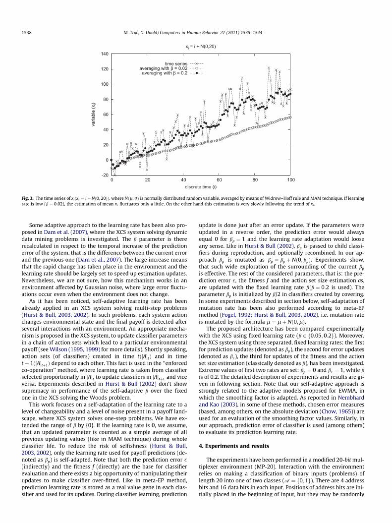
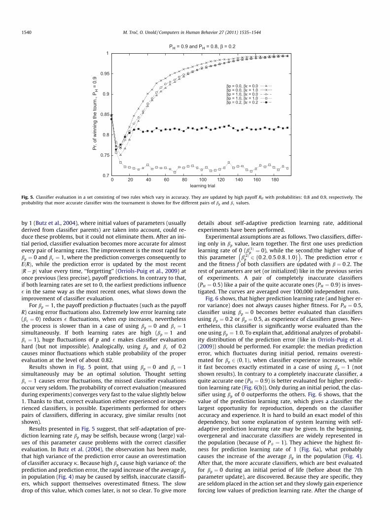
such simple derivations, we can say that, the mean relative accu-racy of the more accurate classifier (PH ¼ 0:9) converges to the va-lue of about 0.95 for b� ¼ 0, while it converges to the value of about0.88, for the pair of rates: bp ¼ 0, b� ¼ 1. It suggests, that using ex-tremely low learning rate for error updates improves the mecha-nism of classifier evaluation. On the other hand, the classifierfitness oscillates (because of learning rate of 0.2) and its distribu-tion changes in time. To decide which values of the learning ratesshould be set, we have to measure for them probabilities, that themore accurate classifier will be better evaluated. Fig. 5 presentsprobability of winning a tournament (of size 2) by classifier withPH ¼ 0:9, in relation to the number of learning trial (classifier expe-rience), for all considered pairs of bp and b�. The curves are aver-aged over 10,000 independent runs. If compared fitness valuesare equal, we assume, that the probability of winning is 0.5.

Proper classifier evaluation is the most difficult at the beginningof each experiment (when both individuals are inexperienced),because of imprecise estimations based on only few payoffs (seeButz et al. (2004) for more details). The policy of initializing exp

60000 80000 100000 problem

rate of 0.04

perf.; β = 0.05perf.; β = 0.2

perf.; βp = 0.0, βε = 1.0perf.; self-adaptive βp, β = 0.2

avg. βp; self-adaptive βp, β = 0.2

working in dynamic MP20 environment.

0.7

0.75

0.8

0.85

0.9

0.95

1

0 20 40 60 80 100 120 140 160 180

Pr. o

f win

ning

the

tour

n., P

H =

0.9

learning trial

PH = 0.9 and PH = 0.8, β = 0.2

βp = 0.0, βε = 0.0βp = 0.0, βε = 1.0βp = 1.0, βε = 0.0βp = 1.0, βε = 1.0βp = 0.2, βε = 0.2

Fig. 5. Classifier evaluation in a set consisting of two rules which vary in accuracy. They are updated by high payoff RH with probabilities: 0.8 and 0.9, respectively. Theprobability that more accurate classifier wins the tournament is shown for five different pairs of bp and b� values.

1540 M. Troc, O. Unold / Computers in Human Behavior 27 (2011) 1535–1544

by 1 (Butz et al., 2004), where initial values of parameters (usuallyderived from classifier parents) are taken into account, could re-duce these problems, but it could not eliminate them. After an ini-tial period, classifier evaluation becomes more accurate for almostevery pair of learning rates. The improvement is the most rapid forbp ¼ 0 and b� ¼ 1, where the prediction converges consequently toEðRÞ, while the prediction error is updated by the most recentjR� pj value every time, ‘‘forgetting’’ (Orriols-Puig et al., 2009) atonce previous (less precise), payoff predictions. In contrary to that,if both learning rates are set to 0, the earliest predictions influence� in the same way as the most recent ones, what slows down theimprovement of classifier evaluation.

For bp ¼ 1, the payoff prediction p fluctuates (such as the payoffR) casing error fluctuations also. Extremely low error learning rate(b� ¼ 0) reduces � fluctuations, when exp increases, neverthelessthe process is slower than in a case of using bp ¼ 0 and b� ¼ 1simultaneously. If both learning rates are high (bp ¼ 1 andb� ¼ 1), huge fluctuations of p and � makes classifier evaluationhard (but not impossible). Analogically, using bp and b� of 0.2causes minor fluctuations which stable probability of the properevaluation at the level of about 0.82.

Results shown in Fig. 5 point, that using bp ¼ 0 and b� ¼ 1simultaneously may be an optimal solution. Thought settingb� ¼ 1 causes error fluctuations, the missed classifier evaluationsoccur very seldom. The probability of correct evaluation (measuredduring experiments) converges very fast to the value slightly below1. Thanks to that, correct evaluation either experienced or inexpe-rienced classifiers, is possible. Experiments performed for otherspairs of classifiers, differing in accuracy, give similar results (notshown).

Results presented in Fig. 5 suggest, that self-adaptation of pre-diction learning rate bp may be selfish, because wrong (large) val-ues of this parameter cause problems with the correct classifierevaluation. In Butz et al. (2004), the observation has been made,that high variance of the prediction error cause an overestimationof classifier accuracy j. Because high bp cause high variance of: theprediction and prediction error, the rapid increase of the average bp

in population (Fig. 4) may be caused by selfish, inaccurate classifi-ers, which support themselves overestimated fitness. The slowdrop of this value, which comes later, is not so clear. To give more

details about self-adaptive prediction learning rate, additionalexperiments have been performed.

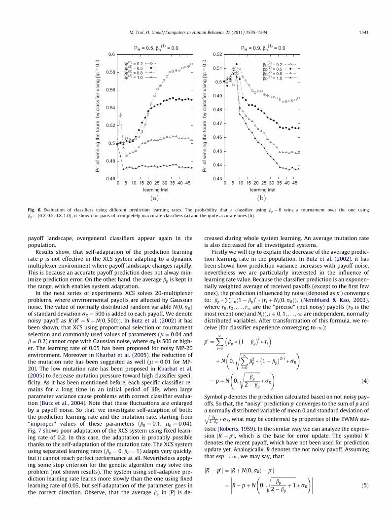
Experimental assumptions are as follows. Two classifiers, differ-ing only in bp value, learn together. The first one uses predictionlearning rate of 0 (bð1Þp ¼ 0), while the secondjthe higher value ofthis parameter bð2Þp 2 f0:2;0:5:0:8;1:0g

� �. The prediction error �

and the fitness f of both classifiers are updated with b ¼ 0:2. Therest of parameters are set (or initialized) like in the previous seriesof experiments. A pair of completely inaccurate classifiers(PH ¼ 0:5) like a pair of the quite accurate ones (PH ¼ 0:9) is inves-tigated. The curves are averaged over 100,000 independent runs.

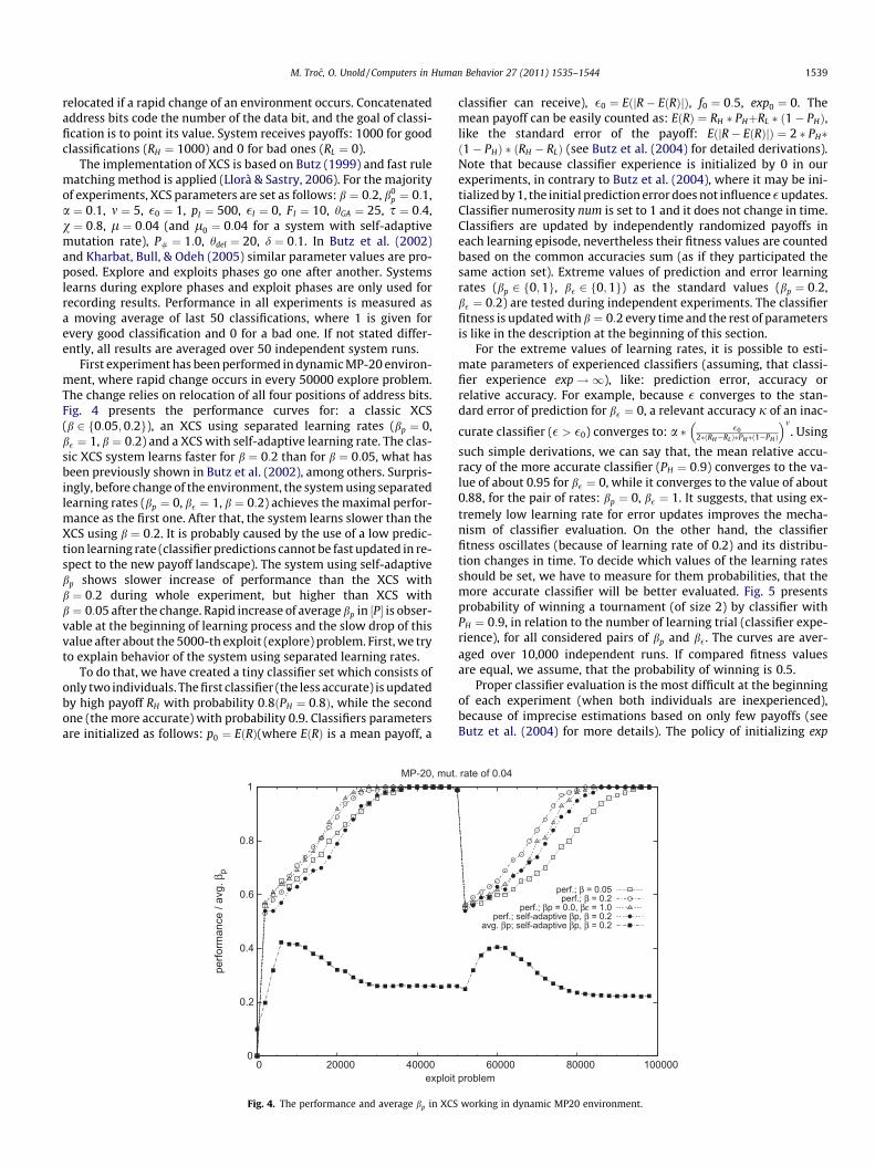
Fig. 6 shows, that higher prediction learning rate (and higher er-ror variance) does not always causes higher fitness. For PH ¼ 0:5,classifier using bp ¼ 0 becomes better evaluated than classifiersusing bp ¼ 0:2 or bp ¼ 0:5, as experience of classifiers grows. Nev-ertheless, this classifier is significantly worse evaluated than theone using bp ¼ 1:0. To explain that, additional analyzes of probabil-ity distribution of the prediction error (like in Orriols-Puig et al.(2009)) should be performed. For example: the median predictionerror, which fluctuates during initial period, remains overesti-mated for bp 2 ð0;1Þ, when classifier experience increases, whileit fast becomes exactly estimated in a case of using bp ¼ 1 (notshown results). In contrary to a completely inaccurate classifier, aquite accurate one (PH ¼ 0:9) is better evaluated for higher predic-tion learning rate (Fig. 6(b)). Only during an initial period, the clas-sifier using bp of 0 outperforms the others. Fig. 6 shows, that thevalue of the prediction learning rate, which gives a classifier thelargest opportunity for reproduction, depends on the classifieraccuracy and experience. It is hard to build an exact model of thisdependency, but some explanation of system learning with self-adaptive prediction learning rate may be given. In the beginning,overgeneral and inaccurate classifiers are widely represented inthe population (because of P# ¼ 1). They achieve the highest fit-ness for prediction learning rate of 1 (Fig. 6a), what probablycauses the increase of the average bp in the population (Fig. 4).After that, the more accurate classifiers, which are best evaluatedfor bp ¼ 0 during an initial period of life (before about the 7thparameter update), are discovered. Because they are specific, theyare seldom placed in the action set and they slowly gain experienceforcing low values of prediction learning rate. After the change of

0.46

0.48

0.5

0.52

0.54

0.56

0.58

0.6

0 5 10 15 20 25 30 35 40 45

Pr. o

f win

ning

the

tour

n. b

y cl

assf

ier u

sing

βp

= 0.

0

learning trial

PH = 0.5, βp(1) = 0.0

βp(2) = 0.2βp(2) = 0.5βp(2) = 0.8βp(2) = 1.0

0.43

0.44

0.45

0.46

0.47

0.48

0.49

0.5

0.51

0.52

0 5 10 15 20 25 30 35 40 45

Pr. o

f win

ning

the

tour

n. b

y cl

assf

ier u

sing

βp

= 0.

0

learning trial

PH = 0.9, βp(1) = 0.0

βp(2) = 0.2βp(2) = 0.5βp(2) = 0.8βp(2) = 1.0

Fig. 6. Evaluation of classifiers using different prediction learning rates. The probability that a classifier using bp ¼ 0 wins a tournament over the one usingbp 2 f0:2;0:5;0:8;1:0g, is shown for pairs of: completely inaccurate classifiers (a) and the quite accurate ones (b).

M. Troc, O. Unold / Computers in Human Behavior 27 (2011) 1535–1544 1541

payoff landscape, overgeneral classifiers appear again in thepopulation.

Results show, that self-adaptation of the prediction learningrate p is not effective in the XCS system adapting to a dynamicmultiplexer environment where payoff landscape changes rapidly.This is because an accurate payoff prediction does not alway min-imize prediction error. On the other hand, the average bp is kept inthe range, which enables system adaptation.

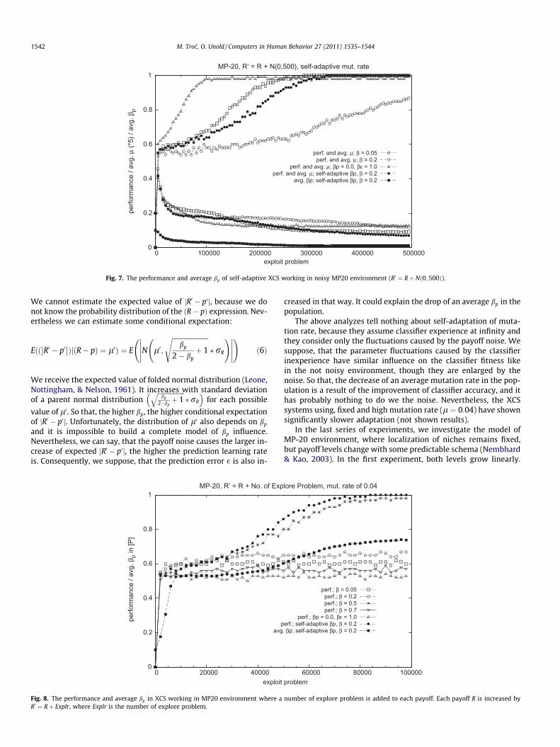
In the next series of experiments XCS solves 20-multiplexerproblems, where environmental payoffs are affected by Gaussiannoise. The value of normally distributed random variable Nð0;rRÞof standard deviation rR ¼ 500 is added to each payoff. We denotenoisy payoff as R0ðR0 ¼ Rþ Nð0;500ÞÞ. In Butz et al. (2002) it hasbeen shown, that XCS using proportional selection or tournamentselection and commonly used values of parameters (l ¼ 0:04 andb ¼ 0:2) cannot cope with Gaussian noise, where rR is 500 or high-er. The learning rate of 0.05 has been proposed for noisy MP-20environment. Moreover in Kharbat et al. (2005), the reduction ofthe mutation rate has been suggested as well (l ¼ 0:01 for MP-20). The low mutation rate has been proposed in Kharbat et al.(2005) to decrease mutation pressure toward high classifier speci-ficity. As it has been mentioned before, each specific classifier re-mains for a long time in an initial period of life, when largeparameter variance cause problems with correct classifier evalua-tion (Butz et al., 2004). Note that these fluctuations are enlargedby a payoff noise. So that, we investigate self-adaption of both:the prediction learning rate and the mutation rate, starting from‘‘improper’’ values of these parameters (b0 ¼ 0:1, l0 ¼ 0:04).Fig. 7 shows poor adaptation of the XCS system using fixed learn-ing rate of 0.2. In this case, the adaptation is probably possiblethanks to the self-adaptation of the mutation rate. The XCS systemusing separated learning rates (bp ¼ 0, b� ¼ 1) adapts very quickly,but it cannot reach perfect performance at all. Nevertheless apply-ing some stop criterion for the genetic algorithm may solve thisproblem (not shown results). The system using self-adaptive pre-diction learning rate learns more slowly than the one using fixedlearning rate of 0.05, but self-adaptation of the parameter goes inthe correct direction. Observe, that the average bp in ½P� is de-

creased during whole system learning. An average mutation rateis also decreased for all investigated systems.

Firstly we will try to explain the decrease of the average predic-tion learning rate in the population. In Butz et al. (2002), it hasbeen shown how prediction variance increases with payoff noise,nevertheless we are particularly interested in the influence oflearning rate value. Because the classifier prediction is an exponen-tially weighted average of received payoffs (except to the first fewones), the prediction influenced by noise (denoted as p0) convergesto: bp �

P1i¼0ð1� bpÞ

i � ðri þ Nið0;rRÞÞ, (Nembhard & Kao, 2003),where r0; r2; . . . ; r1 are the ‘‘precise’’ (not noisy) payoffs (r0 is themost recent one) and NiðÞ; i 2 0;1; . . . ;1 are independent, normallydistributed variables. After transformation of this formula, we re-ceive (for classifier experience converging to 1):

p0 ¼X1i¼0

bp � 1� bp

� �i � ri

� �

þ N 0;

ffiffiffiffiffiffiffiffiffiffiffiffiffiffiffiffiffiffiffiffiffiffiffiffiffiffiffiffiffiffiffiffiffiffiffiffiffiffiffiffiX1i¼0

b2p � 1� bp

� �2�is

� rR

!

¼ pþ N 0;

ffiffiffiffiffiffiffiffiffiffiffiffiffiffibp

2� bp

s� rR

!ð4Þ

Symbol p denotes the prediction calculated based on not noisy pay-offs. So that, the ‘‘noisy’’ prediction p0 converges to the sum of p anda normally distributed variable of mean 0 and standard deviation offfiffiffiffiffiffiffiffi

bp

2�bp

q� rR, what may be confirmed by properties of the EWMA sta-

tistic (Roberts, 1959). In the similar way we can analyze the expres-sion jR0 � p0j, which is the base for error update. The symbol R0

denotes the recent payoff, which have not been used for predictionupdate yet. Analogically, R denotes the not noisy payoff. Assumingthat exp!1, we may say, that:

R0 � p0�� �� ¼ Rþ N 0;rRð Þ � p0j j

¼ R� pþ N 0;

ffiffiffiffiffiffiffiffiffiffiffiffiffiffiffiffiffiffiffiffiffiffibp

2� bpþ 1

s� rR

!���������� ð5Þ

0

0.2

0.4

0.6

0.8

1

0 100000 200000 300000 400000 500000

perfo

rman

ce /

avg.

μ (*

5) /

avg.

βp

exploit problem

MP-20, R’ = R + N(0,500), self-adaptive mut. rate

perf. and avg. μ; β = 0.05perf. and avg. μ; β = 0.2

perf. and avg. μ; βp = 0.0, βε = 1.0perf. and avg. μ; self-adaptive βp, β = 0.2

avg. βp; self-adaptive βp, β = 0.2

Fig. 7. The performance and average bp of self-adaptive XCS working in noisy MP20 environment (R0 ¼ Rþ Nð0;500Þ).

1542 M. Troc, O. Unold / Computers in Human Behavior 27 (2011) 1535–1544

We cannot estimate the expected value of jR0 � p0j, because we donot know the probability distribution of the ðR� pÞ expression. Nev-ertheless we can estimate some conditional expectation:

Eðð R0 � p0�� ��ÞjðR� pÞ ¼ l0Þ ¼ E N l0;

ffiffiffiffiffiffiffiffiffiffiffiffiffiffiffiffiffiffiffiffiffiffibp

2� bpþ 1

s� rR

!����������

!ð6Þ

We receive the expected value of folded normal distribution (Leone,Nottingham, & Nelson, 1961). It increases with standard deviationof a parent normal distribution

ffiffiffiffiffiffiffiffiffiffiffiffiffiffiffiffiffibp

2�bpþ 1

q� rR

� �for each possible

value of l0. So that, the higher bp, the higher conditional expectationof jR0 � p0j. Unfortunately, the distribution of l0 also depends on bp

and it is impossible to build a complete model of bp influence.Nevertheless, we can say, that the payoff noise causes the larger in-crease of expected jR0 � p0j, the higher the prediction learning rateis. Consequently, we suppose, that the prediction error � is also in-

0

0.2

0.4

0.6

0.8

1

0 20000 40000

perfo

rman

ce /

avg.

βp

in [P

]

exploit

MP-20, R’ = R + No. of Exp

pavg

Fig. 8. The performance and average bp in XCS working in MP20 environment where aR0 ¼ Rþ Explr, where Explr is the number of explore problem.

creased in that way. It could explain the drop of an average bp in thepopulation.

The above analyzes tell nothing about self-adaptation of muta-tion rate, because they assume classifier experience at infinity andthey consider only the fluctuations caused by the payoff noise. Wesuppose, that the parameter fluctuations caused by the classifierinexperience have similar influence on the classifier fitness likein the not noisy environment, though they are enlarged by thenoise. So that, the decrease of an average mutation rate in the pop-ulation is a result of the improvement of classifier accuracy, and ithas probably nothing to do we the noise. Nevertheless, the XCSsystems using, fixed and high mutation rate (l ¼ 0:04) have shownsignificantly slower adaptation (not shown results).

In the last series of experiments, we investigate the model ofMP-20 environment, where localization of niches remains fixed,but payoff levels change with some predictable schema (Nembhard& Kao, 2003). In the first experiment, both levels grow linearly.

60000 80000 100000 problem

lore Problem, mut. rate of 0.04

perf.; β = 0.05perf.; β = 0.2perf.; β = 0.5perf.; β = 0.7

perf.; βp = 0.0, βε = 1.0erf.; self-adaptive βp, β = 0.2. βp; self-adaptive βp, β = 0.2

number of explore problem is added to each payoff. Each payoff R is increased by

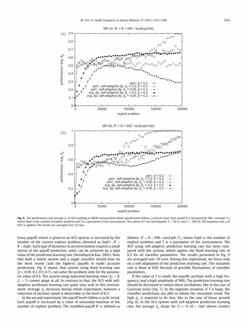
Fig. 9. The performance and average bp in XCS working in MP20 environment where payoff levels follow a cyclical trend. Each payoff R is increased by 500 � sinðExplr=TÞ,where Explr is the number of explore problem and T is a parameter of the environment. Two values of T are investigated: T ¼ 50 (a) and T ¼ 100 (b). The mutation rate l of0.01 is applied. The results are averaged over 10 runs.

M. Troc, O. Unold / Computers in Human Behavior 27 (2011) 1535–1544 1543

Every payoff, which is given to an XCS system, is increased by thenumber of the current explore problem (denoted as ExplrÞ : R0 ¼Rþ Explr. Such type of dynamics in an environment requires a smallinertia of the payoff prediction, what can be achieved by a highvalue of the prediction learning rate (Nembhard & Kao, 2003). Notethat both a whole system and a single classifier should base onthe most recent (and the highest) payoffs to make accuratepredictions. Fig. 8 shows, that system using fixed learning rate(b 2 0:05; 0:2;0:5;0:7), can solve the problem only for the parame-ter value of 0.5. The system using separated learning rates (bp ¼ 0,b� ¼ 1) cannot adapt at all. In contrary to that, the XCS with self-adaptive prediction learning rate gains very well in this environ-ment. Average bp increases during whole experiment, however areduction of increase speed is observable at the level of 0.5.

In the second experiment, the payoff levels follow a cyclic trend.Each payoff is increased by a value of sinusoidal function of thenumber of explore problem. The modified payoff R0 is defined as

follows: R0 ¼ Rþ 500 � sinðExplr=TÞ, where Explr is the number ofexplore problem and T is a parameter of the environment. TheXCS using self-adaptive prediction learning rate has been com-pared with the system, which applies the fixed learning rate of0.2 for all classifier parameters. The results presented in Fig. 9are averaged over 10 runs. During this experiment, we focus onlyon a self-adaptation of the prediction learning rate. The mutationrate is fixed at 0.01 because of possible fluctuations of classifierparameters.

If the value of T is small, the payoffs oscillate with a high fre-quency (and a high amplitude of 500). The prediction learning rateshould be decreased to reduce these oscillations, like in the case ofGaussian noise (Fig. 7). In the opposite situation, if T is large, theclassifier predictions are able to follow the sinusoidal trend. Thehigh bp is required to do that, like in the case of linear growth(Fig. 8). In the XCS system with self-adaptive prediction learningrate, the average bp drops for T 2< 0;10 > (not shown results)

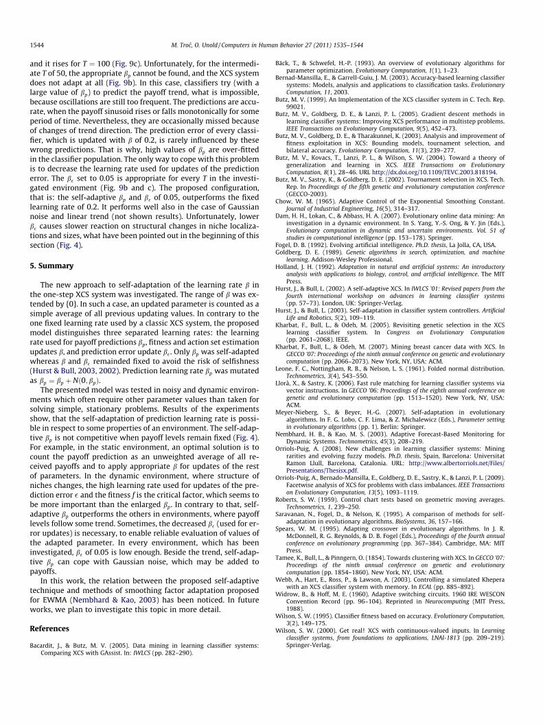
1544 M. Troc, O. Unold / Computers in Human Behavior 27 (2011) 1535–1544

and it rises for T ¼ 100 (Fig. 9c). Unfortunately, for the intermedi-ate T of 50, the appropriate bp cannot be found, and the XCS systemdoes not adapt at all (Fig. 9b). In this case, classifiers try (with alarge value of bp) to predict the payoff trend, what is impossible,because oscillations are still too frequent. The predictions are accu-rate, when the payoff sinusoid rises or falls monotonically for someperiod of time. Nevertheless, they are occasionally missed becauseof changes of trend direction. The prediction error of every classi-fier, which is updated with b of 0.2, is rarely influenced by thesewrong predictions. That is why, high values of bp are over-fittedin the classifier population. The only way to cope with this problemis to decrease the learning rate used for updates of the predictionerror. The b� set to 0.05 is appropriate for every T in the investi-gated environment (Fig. 9b and c). The proposed configuration,that is: the self-adaptive bp and b� of 0.05, outperforms the fixedlearning rate of 0.2. It performs well also in the case of Gaussiannoise and linear trend (not shown results). Unfortunately, lowerb� causes slower reaction on structural changes in niche localiza-tions and sizes, what have been pointed out in the beginning of thissection (Fig. 4).

5. Summary

The new approach to self-adaptation of the learning rate b inthe one-step XCS system was investigated. The range of b was ex-tended by {0}. In such a case, an updated parameter is counted as asimple average of all previous updating values. In contrary to theone fixed learning rate used by a classic XCS system, the proposedmodel distinguishes three separated learning rates: the learningrate used for payoff predictions bp, fitness and action set estimationupdates b, and prediction error update b�. Only bp was self-adaptedwhereas b and b� remainded fixed to avoid the risk of selfishness(Hurst & Bull, 2003, 2002). Prediction learning rate bp was mutatedas bp ¼ bp þ Nð0; bpÞ.

The presented model was tested in noisy and dynamic environ-ments which often require other parameter values than taken forsolving simple, stationary problems. Results of the experimentsshow, that the self-adaptation of prediction learning rate is possi-ble in respect to some properties of an environment. The self-adap-tive bp is not competitive when payoff levels remain fixed (Fig. 4).For example, in the static environment, an optimal solution is tocount the payoff prediction as an unweighted average of all re-ceived payoffs and to apply appropriate b for updates of the restof parameters. In the dynamic environment, where structure ofniches changes, the high learning rate used for updates of the pre-diction error � and the fitness f is the critical factor, which seems tobe more important than the enlarged bp. In contrary to that, self-adaptive bp outperforms the others in environments, where payofflevels follow some trend. Sometimes, the decreased b� (used for er-ror updates) is necessary, to enable reliable evaluation of values ofthe adapted parameter. In every environment, which has beeninvestigated, b� of 0.05 is low enough. Beside the trend, self-adap-tive bp can cope with Gaussian noise, which may be added topayoffs.

In this work, the relation between the proposed self-adaptivetechnique and methods of smoothing factor adaptation proposedfor EWMA (Nembhard & Kao, 2003) has been noticed. In futureworks, we plan to investigate this topic in more detail.

References

Bacardit, J., & Butz, M. V. (2005). Data mining in learning classifier systems:Comparing XCS with GAssist. In: IWLCS (pp. 282–290).

Bäck, T., & Schwefel, H.-P. (1993). An overview of evolutionary algorithms forparameter optimization. Evolutionary Computation, 1(1), 1–23.

Bernad-Mansilla, E., & Garrell-Guiu, J. M. (2003). Accuracy-based learning classifiersystems: Models, analysis and applications to classification tasks. EvolutionaryComputation, 11, 2003.

Butz, M. V. (1999). An Implementation of the XCS classifier system in C. Tech. Rep.99021.

Butz, M. V., Goldberg, D. E., & Lanzi, P. L. (2005). Gradient descent methods inlearning classifier systems: Improving XCS performance in multistep problems.IEEE Transactions on Evolutionary Computation, 9(5), 452–473.

Butz, M. V., Goldberg, D. E., & Tharakunnel, K. (2003). Analysis and improvement offitness exploitation in XCS: Bounding models, tournament selection, andbilateral accuracy. Evolutionary Computation, 11(3), 239–277.

Butz, M. V., Kovacs, T., Lanzi, P. L., & Wilson, S. W. (2004). Toward a theory ofgeneralization and learning in XCS. IEEE Transactions on EvolutionaryComputation, 8(1), 28–46. URL http://dx.doi.org/10.1109/TEVC.2003.818194.

Butz, M. V., Sastry, K., & Goldberg, D. E. (2002). Tournament selection in XCS. Tech.Rep. In Proceedings of the fifth genetic and evolutionary computation conference(GECCO-2003).

Chow, W. M. (1965). Adaptive Control of the Exponential Smoothing Constant.Journal of Industrial Engineering, 16(5), 314–317.

Dam, H. H., Lokan, C., & Abbass, H. A. (2007). Evolutionary online data mining: Aninvestigation in a dynamic environment. In S. Yang, Y.-S. Ong, & Y. Jin (Eds.),Evolutionary computation in dynamic and uncertain environments. Vol. 51 ofstudies in computational intelligence (pp. 153–178). Springer.

Fogel, D. B. (1992). Evolving artificial intelligence. Ph.D. thesis, La Jolla, CA, USA.Goldberg, D. E. (1989). Genetic algorithms in search, optimization, and machine

learning. Addison-Wesley Professional.Holland, J. H. (1992). Adaptation in natural and artificial systems: An introductory

analysis with applications to biology, control, and artificial intelligence. The MITPress.

Hurst, J., & Bull, L. (2002). A self-adaptive XCS. In IWLCS ’01: Revised papers from thefourth international workshop on advances in learning classifier systems(pp. 57–73). London, UK: Springer-Verlag.

Hurst, J., & Bull, L. (2003). Self-adaptation in classifier system controllers. ArtificialLife and Robotics, 5(2), 109–119.

Kharbat, F., Bull, L., & Odeh, M. (2005). Revisiting genetic selection in the XCSlearning classifier system. In Congress on Evolutionary Computation(pp. 2061–2068). IEEE.

Kharbat, F., Bull, L., & Odeh, M. (2007). Mining breast cancer data with XCS. InGECCO ’07: Proceedings of the ninth annual conference on genetic and evolutionarycomputation (pp. 2066–2073). New York, NY, USA: ACM.

Leone, F. C., Nottingham, R. B., & Nelson, L. S. (1961). Folded normal distribution.Technometrics, 3(4), 543–550.

Llorà, X., & Sastry, K. (2006). Fast rule matching for learning classifier systems viavector instructions. In GECCO ’06: Proceedings of the eighth annual conference ongenetic and evolutionary computation (pp. 1513–1520). New York, NY, USA:ACM.

Meyer-Nieberg, S., & Beyer, H.-G. (2007). Self-adaptation in evolutionaryalgorithms. In F. G. Lobo, C. F. Lima, & Z. Michalewicz (Eds.), Parameter settingin evolutionary algorithms (pp. 1). Berlin: Springer.

Nembhard, H. B., & Kao, M. S. (2003). Adaptive Forecast-Based Monitoring forDynamic Systems. Technometrics, 45(3), 208–219.

Orriols-Puig, A. (2008). New challenges in learning classifier systems: Miningrarities and evolving fuzzy models. Ph.D. thesis, Spain, Barcelona: UniversitatRamon Llull, Barcelona, Catalonia. URL: http://www.albertorriols.net/Files/Presentations/Thesisx.pdf.

Orriols-Puig, A., Bernado-Mansilla, E., Goldberg, D. E., Sastry, K., & Lanzi, P. L. (2009).Facetwise analysis of XCS for problems with class imbalances. IEEE Transactionson Evolutionary Computation, 13(5), 1093–1119.

Roberts, S. W. (1959). Control chart tests based on geometric moving averages.Technometrics, 1, 239–250.

Saravanan, N., Fogel, D., & Nelson, K. (1995). A comparison of methods for self-adaptation in evolutionary algorithms. BioSystems, 36, 157–166.

Spears, W. M. (1995). Adapting crossover in evolutionary algorithms. In J. R.McDonnell, R. G. Reynolds, & D. B. Fogel (Eds.), Proceedings of the fourth annualconference on evolutionary programming (pp. 367–384). Cambridge, MA: MITPress.

Tamee, K., Bull, L., & Pinngern, O. (1854). Towards clustering with XCS. In GECCO ’07:Proceedings of the ninth annual conference on genetic and evolutionarycomputation (pp. 1854–1860). New York, NY, USA: ACM.

Webb, A., Hart, E., Ross, P., & Lawson, A. (2003). Controlling a simulated Kheperawith an XCS classifier system with memory. In ECAL (pp. 885–892).

Widrow, B., & Hoff, M. E. (1960). Adaptive switching circuits. 1960 IRE WESCONConvention Record (pp. 96–104). Reprinted in Neurocomputing (MIT Press,1988).

Wilson, S. W. (1995). Classifier fitness based on accuracy. Evolutionary Computation,3(2), 149–175.

Wilson, S. W. (2000). Get real! XCS with continuous-valued inputs. In Learningclassifier systems, from foundations to applications, LNAI-1813 (pp. 209–219).Springer-Verlag.