Selection of Thermotropic Liquid Crystalline Polymers for Rotational Molding Eric Scribben Dissertation submitted to the Faculty of Virginia Polytechnic Institute and State University in partial fulfillment of the requirements for the degree of DOCTOR OF PHILOSOPHY in Chemical Engineering Dr. Donald G. Baird, Chairman Dr. Richey M. Davis Dr. Garth L. Wilkes Dr. Peter Wapperom Dr. Scott Case Dr. Martin Rogers July 19, 2004 Blacksburg, Va Keywords: rotational molding, TLCP, coalescence, sintering

Welcome message from author
This document is posted to help you gain knowledge. Please leave a comment to let me know what you think about it! Share it to your friends and learn new things together.
Transcript
Selection of Thermotropic Liquid Crystalline Polymers for
Rotational Molding
Eric Scribben
Dissertation submitted to the Faculty of
Virginia Polytechnic Institute and State University
in partial fulfillment of the requirements for the degree of
DOCTOR OF PHILOSOPHY
in
Chemical Engineering
Dr. Donald G. Baird, Chairman
Dr. Richey M. Davis
Dr. Garth L. Wilkes
Dr. Peter Wapperom
Dr. Scott Case
Dr. Martin Rogers
July 19, 2004
Blacksburg, Va
Keywords: rotational molding, TLCP, coalescence, sintering
Selection of Thermotropic Liquid Crystalline Polymers for
Rotational Molding
Eric Scribben
(ABSTRACT)
Thermotropic liquid crystalline polymers (TLCPs) possess a number of physical
and mechanical properties such as: excellent chemical resistance, low permeability, low
coefficient of thermal expansion, high tensile strength and modulus, and good impact
resistance, which make them desirable for use in the storage of cryogenic fluids.
Rotational molding was selected as the processing method for these containers because it
is convenient for manufacturing large storage vessels from thermoplastics.
Unfortunately, there are no reports of successful TLCP rotational molding in the
technical literature. The only related work reported involved the static coalescence of
two TLCP powders, where three key results were reported that were expected to present
problems that preclude the rotational molding process. The first result was that
conventional grinding methods produced powders that were composed of high aspect
ratio particles. Secondly, coalescence was observed to be either slow or incomplete and
speculated that the observed difficulties with coalescence may be due to large values of
the shear viscosity at low deformation rates. Finally, complete densification was not
observed for the high aspect ratio particles. However, the nature of these problems were
not evaluated to determine if they did, in fact, create processing difficulties for rotational
molding or if it was possible to develop solutions to the problems to achieve successful
rotational molding.
iii
This work is concerned with developing a resin selection method to identify
viable TLCP candidates and establish processing conditions for successful rotational
molding. This was accomplished by individually investigating each of the
phenomenological steps of rotational molding to determine the requirements for
acceptable performance in, or successful completion of, each step. The fundamental
steps were: the characteristics and behavior of the powder in solids flow, the coalescence
behavior of isolated particles, and the coalescence behavior of the bulk powder. The
conditions identified in each step were then evaluated in a single-axis, laboratory scale,
rotational molding unit. Finally, the rotationally molded product was evaluated by
measuring several physical and mechanical properties to establish the effectiveness of the
selection method.
In addition to the development and verification of the proposed TLCP selection
method, several significant results that pertain to the storage of cryogenic fluids were
identified as the result of this work. The first, and argueably the most significant, was
that the selection method led to the successful extension of the rotational molding process
to include TLCPs. Also, the established mechanical properties were found to be similar
to rotationally molded flexible chain polymers. The biaxial rotationally molded container
was capable of performing to the specified requirements for cryogenic storage: withstand
pressures up to 34 psi at both cryogenic and room temperatures, retain nitrogen as a gas
and as a cryogenic liquid, the mechanical preform retaining nitrogen, as both a gas and as
a cryogenic liquid, and resist the development of micro-cracks during thermal cycling to
cryogenic conditions.

iv
Acknowledgements
The author wishes to express his thanks to Professor Donald G. Baird for the
support and guidance that resulted in the completion of this work. In addition, the author
would also like to thank each member of his research committee (past and present): Dr.
Davis, Dr. Loos, Dr. Rogers, Dr. Wapperom, and Dr. Wilkes.
The author would also wish to acknowledge the following persons:
His parents and brother for their continuous support throughout this process.
John D. Souder for guidance and the infinite wisdom in initiating interest in
engineering and polymer processing.
Professor Kurt Koelling and all of the members of CAPCE at The Ohio State
University for encouragement to pursue a graduate degree.
Vladimir Kogan and all of the members of the Aerosol Science group at Battelle
Memorial Institute for their direction and inspiration to pursue a graduate degree.
All current and past members of the Polymer Processing Lab that he had the
opportunity to serve with: Phil, Mike, Wade, Matt, Quang, Brent, Chris, and
Aaron.
Those members of the department staff who have made this work easier over the
years: Diane, Chris, Riley, Wendell, and Mike.
The group of Buckeyes that have demonstrated unwaivering support throughout
this process.
The following friends for supplying adequate distraction from his research
project: Brooks, John & Jen, Maatha, Doug, Mary, Corey, and too many others to
list.
v
Original Contributions
The following are considered to be significant original contributions of this research:
1. A clearer understanding of the effect of viscoelasticity on polymer coalescence.
Representation of the transient rheological response in the coalescence model is
essential to predicting the coalescence rates for polymeric materials at times that are
less than their characteristic relaxation times. Incorporating the transient rheology
provides a qualitative picture of coalescence that is consistant with reports that
increasing the relaxation time accelerates coalescence.
2. It is demonstrated that TLCPs coalesce faster than is predicted by the Newtonian
coalescence model, which is in agreement with a viscoelastic coalescence model that
uses the transient rheology. However, TLCP coalescence rates cannot be accurately
predicted by the transient model, indicating that an anisotropic liquid crystalline
constitutive model that includes the effect of liquid crystalline structure may be
necessary to accurately model the process.
3. A novel technique is developed to produce spherical TLCP particles for use in
rotational molding. This is used to overcome the low apparent density and
unacceptable powder flow that results when TLCPs powders are prepared by
conventional grinding methods.
vi
4. A selection method is devised to identify viable TLCP candidates and establish
processing conditions for successful rotational molding. In the development of this
method several key results were established. The behavior of the shear viscosity at
low shear rates can be used to determine thermal and environmental conditions where
coalescence occurs. Densification is not possible for TLCPs in the rotational molding
process by extending the molding cycle time, as is standard practice for densifying
flexible chain polymers in rotational molding. However, bubble entrapment is
eliminated during the neck growth process by optimizing the mold rotation rate.
Table of Contents vii
Table of Contents
1 Introduction 1
1.1 Thermotropic Liquid Crystalline Polymers 2
1.2 Rotational Molding 7
1.3 Polymer Sintering 10
1.4 Research Objectives 13
1.5 References 15
2 Literature Review 19
2.1 Rotational Molding 21
2.1.1 Powder Properties 21
2.1.2 Coalescence 37
2.1.3 Processing Considerations 66
2.2 Thermotropic Liquid Crystalline Polymers 76
2.2.1 Mechanical Properties 77
2.2.2 Rheology of Thermotropic Liquid Crystalline Polymers 82
2.3 Research Objectives 94
2.4 References 96
3 Experimental Methods 115
3.1 Materials 116
3.1.1 Polypropylene 117
3.1.2 Thermotropic Liquid Crystalline Polymers 117
3.2 Thermal Analysis 119
3.3 Generation and Characterization of TLCP Powders 119
3.4 Rheological Characterization 122
3.4.1 Polypropylenes 122
Table of Contents viii
3.4.2 TLCPs 123
3.5 Surface Tension Measurement 125
3.5.1 Polypropylenes 125
3.5.2 TLCPs 126
3.6 Coalescence Experiments 128
3.7 Densification Experiments 128
3.8 Single Axis Rotational Molding 130
3.9 Mechanical and Physical Property Testing 131
3.9.1 Testing of Samples from the Densification Study 131
3.9.2 Rotationally Molded Samples 132
3.10 Biaxial Rotational Molding 133
3.11 References 135
4 The Role of Transient Rheology in Polymeric Coalescence 136
4.1 Abstract 137
4.2 Introduction 138
4.3 Experimental 145
4.3.1 Materials 145
4.3.2 Surface Tension Measurement 146
4.3.3 Rheological Characterization 147
4.3.4 Coalescence 148
4.4 Numerical Methods 150
4.4.1 Model Parameter Fitting 150
4.4.2 Solution of the Transient UCM Model 153
4.5 Results and Discussion 155
4.5.1 Newtonian and Steady State UCM Coalescence Models 155
4.5.2 Single Mode Transient UCM Model 160
4.5.3 Multimode Transient UCM Model 162
Table of Contents ix
4.6 Conclusions 164
4.7 Acknowledgements 166
4.8 References 167
5 The Role of Transient Rheology in the Coalescence of Thermotropic
Liquid Crystalline Polymers 169
5.1 Abstract 170
5.2 Introduction 171
5.3 Experimental 174
5.3.1 Materials 174
5.3.2 Differential Scanning Calorimetry 176
5.3.3 Surface Tension Measurement 176
5.3.4 Rheological Characterization 177
5.3.5 Coalescence Experiments 179
5.4 Results and Discussion 180
5.4.1 Rheological Characterization 180
5.4.2 Experimental Coalescence 184
5.4.3 Transient UCM Coalescence Model Predictions 190
5.5 Conclusions 191
5.6 Acknowledgements 192
5.7 References 193
6 The Rotational Molding of a Thermotropic Liquid Crystalline
Polymer 195
6.1 Abstract 196
6.2 Introduction 197
6.3 Analytical Methods 201
Table of Contents x
6.3.1 Material 201
6.3.2 Generation and Characterization of Powders 202
6.3.3 Coalescence Experiments 205
6.3.4 Thermal Behavior 206
6.3.5 Surface Tension 207
6.3.6 Rheology 208
6.3.7 Densification Experiments 209
6.3.8 Properties of Densification Samples 211
6.3.9 Single-Axis Rotational Molding Experiments 211
6.3.10 Properties of the Rotational Molded Samples 212
6.4 Results and Discussion 213
6.4.1 Powder Flow Characteristics 213
6.4.2 Coalescence 218
6.4.3 Densification 223
6.4.4 Single Axis Rotational Molding 227
6.5 Conclusions 233
6.6 Future Work 234
6.7 Acknowledgements 234
6.8 References 235
7 Recommendations 238
Appendix A. Shear Rheological Data 242
A.1 Polypropylene (190k) 243
A.2 Polypropylene (250k) 247
A.3 Polypropylene (340k) 255
A.4 Polypropylene (580k) 263
A.5 Vectra A 950 272
Table of Contents xi
A.6 Vectra B 950 289
Appendix B. Surface Tension 296
B.1 Polypropylene (190k) 297
B.2 Polypropylene (250k) 299
B.3 Polypropylene (340k) 304
B.4 Vectra A 950 307
B.5 Vectra B 950 309
Appendix C. Coalescence 311
C.1 Polypropylene (190k) 312
C.2 Polypropylene (250k) 313
C.3 Polypropylene (340k) 314
C.4 Vectra A 950 315
C.5 Vectra B 950 317
Appendix D. Programs for Coalescence Models 319
D.1 Newtonian Coalescence Model 320
D.2 Single Mode Steady State upper convected Coalescence Model 323
D.3 Single Mode upper convected Maxwell Coalescence Model 326
D.4 Multi-Mode upper convected Maxwell Coalescence Model 330
Appendix E. Physical and Mechanical Properties 336
E.1 Apparent Density 337
E.2 Dynamic Angle of Repose 339
E.3 Average Density 340
Table of Contents xii
E.4 Tensile Modulus 342
E.5 Tensile Strength 344
E.6 Biaxial Rotational Molded Tank 346
Appendix F. Publications 365
Sintering of Thermotropic Liquid Crystalline Polymers 366
Performance of a Rotationally Molded Thermotropic Liquid Crystalline Polymer 374
Vita 382

List of Figures xiii
List of Figures
Figure 1.1. Friedelian Classes: a. Nematic; b. Cholesteric; c. Smectic A; d.
Discotic. 3
Figure 1.2. SEM images of ground: a. TLCP and b. HDPE 12
Figure 1.3. General three region flow curve [33] 13
Figure 2.1. Squared Egg Particle 23
Figure 2.2. Hertz and JKR Predictions 40
Figure 2.3. Shape Evolution 45
Figure 2.4. Two-Particle Sintering Models 46
Figure 2.5. Densification Kinetics 54
Figure 2.6. Rotation Axes 67
Figure 2.7. Comparison of Transient Uniaxial and Shear Viscosities [163] 85
Figure 2.8. Three-Region Flow Curve [163] 88
Figure 2.9. Shear Viscosity Temperature Dependence Near the Nematic-Isotropic
Transition 90
Figure 3.1. Chemical structure and composition of Vectra A 950 and Vectra B
950. 118
Figure 3.2. The dynamic angle of repose of a tumbling powder in steady state
flow. 122
Figure 3.3. Diagram of test fixture used to measure the burst strength. 133
Figure 4.1. Shape evolution during the coalescence of two spherical particles 140
Figure 4.2. Steady and complex shear viscosity master curves for polypropylene
at 180°C. ( ) 190k, ( ) 250k, ( ) 340k. The open symbols
represent small amplitude oscillatory shear measurements; filled
symbols represent steady shear values. 148
Figure 4.3. Optical micrographs from the coalescence of 190k polypropylene
drops 149
Figure 4.4. Single mode UCM model fit to the transient shear viscosity from
stress growth experiments at 180°C. The symbols represent the
experimental data: ( ) 190k, ( ) 250k, ( ) 340k. The lines
represent the single mode UCM fits to the data. 151
List of Figures xiv
Figure 4.5. Multimode fit to the storage and loss moduli for the 340k sample at
180°C. ( ) G', ( ) G". The symbols represent the experimental
data; the lines represent the multimode UCM fit to the data. 152
Figure 4.6. Experimental polypropylene coalescence data, the Newtonian, and
steady state UCM model predictions at 180°C. The symbols
represent the experimental data: ( ) 190k, ( ) 250k, ( ) 340k. The
lines represent the model predictions: (—) Newtonian model, (----)
steady state UCM model. The predictions from the steady state
model obscured because they are nearly identical to the Newtonian
results. 156
Figure 4.7. 340k polypropylene coalescence data, the Newtonian, and steady state
UCM model predictions at short times. The symbols represent the
experimental data: ( ) 340k. The lines represent the model
predictions: (—) Newtonian, steady state UCM model with (----)
λ =1.54 sec, (····) λ =200 sec, (─·─·) λ =400 sec. 157
Figure 4.8. Biaxial extension rate as predicted by the steady state UCM model
during coalescence of the 340k sample where: (—) λ =1.54 sec, (----
) λ =200 sec, (····) λ =400 sec. 159
Figure 4.9. Biaxial extensional viscosity as predicted by the steady state UCM
model during coalescence of the 340k sample where: (—) represents
6ηo that is predicted for Newtonian fluids, and (----) for λ =1.54 sec,
(····) λ =200 sec, (─·─·) λ =400 sec. 160
Figure 4.10. 340k polypropylene coalescence data, the Newtonian, and transient
UCM model predictions. The symbols represent the experimental
data: ( ) 340k. The lines represent the model predictions: (—)
Newtonian, transient UCM model with (----) λ =1.54 sec, (····)
λ =2.0 sec, (─·─·) λ =3.0 sec. 161
Figure 4.11. Transient shear viscosity at 180°C, the single mode UCM model fits,
and the multimode UCM model predictions. The symbols represent
the experimental data: ( ) 190k, ( ) 250k, ( ) 340k. The lines

List of Figures xv
represent the models: (—) single mode fits, (····) multimode
predictions. 163
Figure 4.12. 340k polypropylene coalescence data, the Newtonian, the single
mode transient UCM model, and the multimode transient UCM
model predictions at short times. The symbols represent the
experimental data: ( ) 340k. The lines represent the model
predictions: (—) Newtonian, (----) single mode transient UCM
model, (····) multimode transient model. 164
Figure 5.1. Schematic of the geometric evolution of two coalescing spherical
particles. 172
Figure 5.2. Chemical structure and composition of Vectra A 950 and Vectra B
950. 175
Figure 5.3. Steady and complex shear viscosity master curves for Vectra A 950
( ) and Vectra B 950 ( ) at 320°C. The open symbols represent
small amplitude oscillatory shear measurements, filled symbols
represent steady shear values. 181
Figure 5.4. Steady and complex shear viscosity master curves for Vectra A 950
( ) and Vectra B 950 ( ) at 330°C. The open symbols represent
small amplitude oscillatory shear measurements, filled symbols
represent steady shear values. 182
Figure 5.5. Comparison of the transient shear viscosity for Vectra A 950
measured at a shear rate of 1×10⁻² sec-1 for the two different thermal
and deformation histories. The data was measured using the
prescribed pretest shear and thermal histories: ( ) at 320°C and ( )
at 330°C. The samples measured without the prescribed pretest shear
and thermal histories: ( ) at 320°C and ( ) at 330°C. The lines
represent the UCM fits to the data. 183
Figure 5.6. Optical micrographs from the coalescence experiments of Vectra B
950 at 320°C. 185

List of Figures xvi
Figure 5.7. TLCP coalescence data, where ( ) represents Vectra A 950 and ( )
represents Vectra B 950. Open symbols are used for the data at
320°C and filled symbols represent the data at 330°C. 186
Figure 5.8. Vectra A 950 coalescence data at 330°C and predictions from the
Newtonian, steady state UCM, and transient UCM coalescence
models. The symbols represent the experimental data ( ) and the
lines represent the coalescence model predictions: Newtonian (—),
steady state UCM (----), and the transient UCM (····). 191
Figure 6.1. Chemical structure and composition of Vectra B 950 202
Figure 6.2. The dynamic angle of repose of a tumbling powder in steady state
flow. 205
Figure 6.3. Schematic of the geometric evolution of coalescing spherical particles
during the coalescence experiments. 206
Figure 6.4. Diagram of test fixture used to measure the burst strength. 213
Figure 6.5. Cryogenically ground Vectra B 950 pellets. 214
Figure 6.6. SEM image of a facture surface of the melt blended extrudate. 216
Figure 6.7. Dynamic angle of repose of a sample from sieve number 30. 217
Figure 6.8. DSC thermogram of Vectra B 950 with the peak and end of the melt
transition represented by stars. 218
Figure 6.9. The magnitude of the complex viscosity versus frequency are
represented as for 320°C and for 330°C. The shear viscosity
versus shear rate is represented as for 320°C for 330°C, error
bars represent deviation in the measurements. 219
Figure 6.10. Transient shear viscosity from stress growth experiments at a shear
rate of 0.01 sec-1 and 320°C. The symbol represents the test
conducted in the presence of nitrogen and is in the presence of air. 221
Figure 6.11. Optical micrographs from the coalescence experiments of Vectra B
950 in nitrogen at 320°C. 222
Figure 6.12. Results from the coalescence experiments, where 320°C in nitrogen
is represented as , 320°C in air is , and 330°C in nitrogen is . 223

List of Figures xvii
Figure 6.13. Image of D1 tensile bar fracture surface confirming incomplete
densification. 224
Figure 6.14. Internal surface of the rotationally molded sample D4 in the 1.59 cm
diameter cylindrical mold. 228
Figure 6.15. External surface of rotationally molded sample D4, where the width
image is 50.8 mm. 229
Figure 6.16. Comparison of bubble formation in static bulk powder and in
rotational molding. 231
Figure 6.17. Exterior surface of the cylinder rotationally molded at 3 rpm, where
the width image is 50.8 mm. 233
List of Tables xviii
List of Tables
Table 2.1 Irregular Particle Shape Measurement [24] 27
Table 2.2. Packing Fractions for Commercial Rotational Molding Powders 31
Table 2.3 Scaling Exponents According to Transport Mechanism 44
Table 2.4. McNeil Chart [2] 69
Table 2.5. Parameters Effecting Heating Time 71
Table 2.6. Comparison of Gas Transport Properties at 35°C of Vectra A900 and PAN
[162] 80
Table 3.1. Weight Average Molecular Weight, Polydispersity, and Melt Index 117
Table 3.2. Descriptions of the powder samples used in the densification study. 129
Table 4.1. Weight Average Molecular Weight, Polydispersity, and Melt Index 146
Table 4.2. Single Mode UCM Coalescence Model Parameters and Calculated Values
for the Deborah Number at 180°C. 151
Table 4.3. Multimode Upper Convected Maxwell Model Parameters at 180°C 153
Table 5.1. UCM coalescence model parameters and calculated values for the Deborah
Number. 184
Table 6.1. Descriptions of the powder samples used in the densification study. 210
Table 6.2. Apparent density of the sieved TLCP particles. 216
Table 6.3. The apparent density of the samples used in the densification study. 224
Table 6.4. Results of the density and tensile measurements for the densification study,
S3* represents the results from the extended cycle time. 225
Table 6.5. Comparison of the tensile strength and modulus of sample S3 when molded
in the presence of air. 227
Table 6.6. The average density, tensile strength, and tensile modulus from the
rotationally molded distribution D4 compared the results for the
distribution from the densification study. 230

1 Introduction 1
1 Introduction
1 Introduction 2
1 Introduction
1.1 Thermotropic Liquid Crystalline Polymers
Liquid crystalline behavior was first discovered in 1888 when Reinitzer observed
that upon heating, cholesteryl benzoate melted to form a turbid fluid then appeared to
melt again into a transparent phase at higher temperatures [25]. The first polymeric
liquid crystal† was reported in 1937 when it was observed that above a critical
concentration the tobacco mosaic virus formed two phases, of which one was birefringent
[3]. The first synthetic polymeric system was a poly (γ-benzyl-L-glutamate) solution,
which was reported in 1950 [8]. The first thermotropic LCPs were reported in the mid
70’s [9, 12, 28]. Since then a tremendous amount of research has been done from the
quantumchemical to the macroscopic level on a great number of systems [22]. The result
is that liquid crystalline polymer science has developed into its own discipline.
Liquid crystal (LC) describes a class of materials with long-range molecular order
somewhere between the crystalline state, which exhibits three-dimensional order, and a
disordered isotropic fluid [15]. Four classes have been identified to describe LC order:
nematic, cholesteric, smectic, and discotic [11]. Nematic describes a LC phase with only
one-dimensional long range ordering; it possesses long-range orientational order
(molecular alignment) but only short-range positional order (spatial ordering) [8]. A
cholesteric is very similar to a nematic, but it is periodically twisted along the axis
perpendicular to the long-range order axis. A smectic phase characterizes two-
† Liquid crystal was later renamed mesomorphic phase or mesophase. Mesomorphic is defined: of intermediate form [7]. Friedel found this more appropriate because these materials are not crystalline and may not even be liquids, it is a stable intermediate phase existing between the liquid and crystalline states.
1 Introduction 3
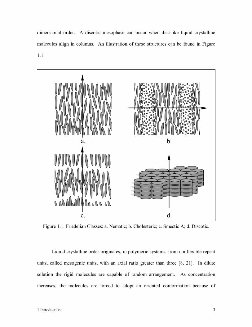
dimensional order. A discotic mesophase can occur when disc-like liquid crystalline
molecules align in columns. An illustration of these structures can be found in Figure
1.1.
Figure 1.1. Friedelian Classes: a. Nematic; b. Cholesteric; c. Smectic A; d. Discotic.
Liquid crystalline order originates, in polymeric systems, from nonflexible repeat
units, called mesogenic units, with an axial ratio greater than three [8, 21]. In dilute
solution the rigid molecules are capable of random arrangement. As concentration
increases, the molecules are forced to adopt an oriented conformation because of
a. b.
c. d.

1 Introduction 4
intermolecular repulsions or excluded volume interactions. Mesogenic units can be either
rod, disc, or lathe-like and may appear within the molecule backbone either randomly or
in a recurring rigid/ flexible structure. These are called main chain LCPs. The other
common type of LCP structure, side chain LCPs, occur as a rigid pendent group to a
flexible polymer backbone with orientation that can range from parallel to perpendicular
to the backbone [21]. Of course another less common possibility would be for the LCP
to contain both main chain and side chain units. This leads to a near infinite number of
possibilities ranging in structure of mesogenic group and arrangement. Most of the
property differences noted between side and main chain LCPs have been related to the
greater mobility of side chain mesogenic units as a result of increased backbone
flexibility [21].
LC order can exist in either solutions or melts. LC transition in solution is a
function of concentration and temperature and is referred to as lyotropic systems [5].
Melts, since concentration is fixed, are only temperature sensitive and are referred to as
thermotropics. The LC phase exists between the crystalline melting point, Tm (or in the
case where no crystalline state exists, the glass transition temperature, Tg), and the upper
transition temperature where the fluid reverts to an isotropic liquid, Tlc→i [20].
Unlike isotropic fluids, orientation is quantified to describe the state and dynamics
of liquid crystals. Molecules are preferentially oriented about an axis, an apolar unit
vector, n, called the director. The direction of the director is typically arbitrary but can
be uniformly aligned through imposing boundaries, applying external magnetic or
1 Introduction 5
electric fields, or inducing viscous flow [20]. Preferential orientation implies that
molecules actually possess a distribution of orientation about the director and therefore a
parameter is needed to describe that distribution. Assuming rigid rod molecules, the
order parameter tensor is defined as [7]:
( )∫
−= iijjiiij duuutufS δ
31, (1.1)
where ui is a unit vector which describes the orientation of a rigid rod molecule, δij is the
Kronecker delta, and f(ui,t) is the orientation distribution function.
The order parameter tensor has a few properties worth noting. It is deviatoric,
therefore its trace is equal to zero and it is symmetric. Its eigenvalues or principal values
(S1, S2, S3) which define the principal axes of orientation must also add to zero. If all
three are equal then S = 0 and the material is isotropic. If two of the eigenvalues are
equal then the system is axially symmetric (as a nematic) and Sij can be represented by:
−= ijjiij nnSS δ
31 (1.2)
where S is a certain scalar equivalent to the Hermans orientation function,
2
1cos3 2 −=
θS (1.3)
ni the projection of the director in the ith direction, while the brackets denote the system
average. Values of S range between, 1 > S > -1/2, with the values 1, 0, and –1/2
representing uniaxial orientation, random orientation, and biaxial orientation.
1 Introduction 6
Valid application of a single order parameter to describe orientation requires that
the material is uniform throughout or a “monodomain” with a single director. It is
possible for elastic distortions to induce slight continuous variation in the director of
monodomain systems [7]. This director variation is typically observed in low molecular
weight materials and becomes less likely as molecular weight increases because of steric
effects [8]. As elastic distortions become more difficult, free energy increases, and
director variation becomes discontinuous, resulting in the formation of defects and
polydomain textures.
Two types of defects have been identified for nematic liquid crystalline polymers
[7]. In thick samples it is possible to observe a system of dark flexible filaments (defined
as disclinations) that correspond to lines of singularity in molecular alignment and result
in the formation of multiple domain texture. The other defect occurs when the imposed
boundary conditions are continuously degenerate (no preferred axis in the plane of the
walls). A system of singular nodes (noyaux) form on the surface and the resulting
general texture is called a Schlieren texture.
Polydomain texture and defects are important to this particular project because of
their influence on rheology. As previously eluded to, the formation of defects is
associated with an increase in free energy. Under quiescent conditions the system
attempts to minimize excess free energy by combining neighboring disclinations with
opposite signs thus eliminating the pair and increasing domain size [13]. However,
mechanical energy can be stored during deformation by an increase in the number of
1 Introduction 7
defects. The development of texture and orientation during deformation can change the
rheological response to imposed stresses and strains.
Liquid crystals have a number of interesting and potentially useful properties.
Optically, the material can be birefringent, although this may be limited to a local scale
[8]. There are also a few polymeric liquid crystals that show nonlinear optical behavior
[29]. Many systems have anisotropic diamagnetic and dielectric properties [20]. The
modulus is often anisotropic, dependant upon the quality of alignment [19, 26]. An
interesting rheological feature is that the nematic phase has a lower viscosity (parallel to
the director) than the isotropic phase [8]. Negative normal stresses have also been
reported for some systems when subjected to steady shear [15]. LCPs also tend to have
low partial entropy of dissolution and therefore have a relatively high resistance to
solvents [8]. Gas transport studies have revealed that they have excellent barrier
properties because of their low gas solubility in their solid state [14]. Another notable
property is that structures can be molded with extremely accurate dimensions because of
their low or negligible coefficient of thermal expansion relative to flexible chain
polymers [5]. They also exhibit high modulus, strength, and impact properties [18].
These properties can be exploited to apply LCPs in applications where flexible chain
polymers perform inadequately.
1.2 Rotational Molding
Rotational molding, also known as rotomolding, is a process used to manufacture
hollow plastic products [6]. This process is comprised of several independent

1 Introduction 8
phenomena: particulate gravitational flow, conductive melting, sintering, and
densification [31]. Particulate gravitational flow, also referred to as granular flow, is
essential for material distribution during mold rotation. A firm understanding of
conductive melting is required because, as long as coalescence is possible, it is the most
time consuming step in the rotational molding cycle. Therefore, an accurate account of
heat transfer to the tumbling powder is required to optimize cycle times. Sintering and
densification are detrimental to the process because incomplete coalescence renders
rotational molding impossible.
The process begins when polymer in either powder, granular, or viscous liquid
form is loaded into a hollow mold which is then simultaneously rotated about two
principal axes. Heat applied to the external surface conducts to the tumbling powder,
which eventually melts and adheres to the mold surface. While heating continues, the
powder sinters into an evenly distributed layer and densifies eliminating trapped air
bubbles from the melt. The mold continues to rotate as it is cooled by water spray, forced
air, or a fog or mist spray before water spray to solidify the product. Once the plastic is
sufficiently rigid, rotation and cooling are halted and the product is removed [6].
Rotational molding has a number of desirable advantages over competing
processes such as blow molding, thermoforming, and injection molding. Parts retain
little residual stress because flow is driven by surface tension and gravity, which
produces much lower deformation rates than the competing processes [6]. Although
weld lines may appear from lack of inter particle diffusion, they are much smaller than
1 Introduction 9
those created by impinging flow fronts because material is continuously distributed
throughout the mold. Material distribution also contributes to uniform wall thickness and
strong corners [30]. Structures can be reinforced by inserts or by multiple wall
construction with multiple resins. Essentially no material is wasted because gates and
sprues are not used. Finishing work is minimized because inserts and high quality
graphics can be incorporated into the molding process [6]. Tooling cost is relatively low
because there is no need to withstand high pressures or manufacture cores to produce
hollow structures. The technique possesses a manufacturing advantage over competing
processes as product dimensions increase, not only because of the ease of physically
forming the product but also because of economics [31].
Rotational molding does have several notable limitations. Manufacturing times
are relatively long; cycles are on the order of minutes to hours while other processing
techniques finish within seconds or minutes. This requires the materials to remain stable
at processing conditions for extended periods of time. Currently, there are a limited
number of materials used in practice, primarily commodity polymers such as
polyethylene, polypropylene, polystyrene, polyvinyl chloride, and nylon 6, 11, and 12
[15]. Very few engineering and high performance polymers have been used [6]. There
also may be an increased material cost due to an added grinding step [30]. Finally,
product design is slightly limited because certain geometrical features, such as ribs, are
difficult to mold.
1 Introduction 10
Two problems have been identified with the rotational molding of TLCPs. As
previously explained, sintering and densification are a part of rotational molding. Any
problem prohibiting their success will, in turn, hinder rotational molding. The second
problem is that rotational molding thermoplastics must be either a powder or granular to
ensure ample material distribution occurs during molding. This implies that materials
must be ground. Grinding of TLCPs generally returns particulate with large aspect ratios
that clump together bearing low bulk density, poor granular flow, and insufficient
material distribution. Incomplete coalescence (ie. porous product) results and is the
primary obstacle preventing the application of TLCPs to rotational molding. However, if
this is overcome, TLCPs have the potential to deliver a level of chemical resistance and
structural integrity unavailable from current materials.
1.3 Polymer Sintering
The term ‘sintering’ refers to the process of forming a homogeneous mass from
particulate without melting [31]. The material processing community utilizes this term
interchangeably with coalescence despite the fact that coalescence is intended for use in
processes where material often exceeds the glass transition temperature, Tg, for
amorphous materials and the melt temperature, Tm, for semicrystalline materials. With
this in mind, when applied to the simplest system, sintering describes the process where
two particles or fluid drops are driven by surface tension (and resisted by viscous
dissipation) to coalesce into a single drop [4]. Frenkel [10] was the first to explain this
behavior for Newtonian fluids, he derived the following expression for growth of the
normalized neck radius:
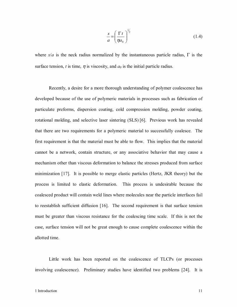
1 Introduction 11
21
0
Γ=at
ax
η (1.4)
where x/a is the neck radius normalized by the instantaneous particle radius, Γ is the
surface tension, t is time, η is viscosity, and a0 is the initial particle radius.
Recently, a desire for a more thorough understanding of polymer coalescence has
developed because of the use of polymeric materials in processes such as fabrication of
particulate preforms, dispersion coating, cold compression molding, powder coating,
rotational molding, and selective laser sintering (SLS) [6]. Previous work has revealed
that there are two requirements for a polymeric material to successfully coalesce. The
first requirement is that the material must be able to flow. This implies that the material
cannot be a network, contain structure, or any associative behavior that may cause a
mechanism other than viscous deformation to balance the stresses produced from surface
minimization [17]. It is possible to merge elastic particles (Hertz, JKR theory) but the
process is limited to elastic deformation. This process is undesirable because the
coalesced product will contain weld lines where molecules near the particle interfaces fail
to reestablish sufficient diffusion [16]. The second requirement is that surface tension
must be greater than viscous resistance for the coalescing time scale. If this is not the
case, surface tension will not be great enough to cause complete coalescence within the
allotted time.
Little work has been reported on the coalescence of TLCPs (or processes
involving coalescence). Preliminary studies have identified two problems [24]. It is

1 Introduction 12
difficult to produce TLCP particles from pellets. Grinding TLCPs, even at cryogenic
temperatures, results in high aspect ratio particles that aggregate and create a bulk
material with low bulk density [24]. Low bulk density translates to large voids, which
make it difficult to consolidate. An example of particle shape differences between
ground TLCP and polyethylene is shown in Figure 1.2.
a. b.
Figure 1.2. SEM images of ground: a. TLCP and b. HDPE
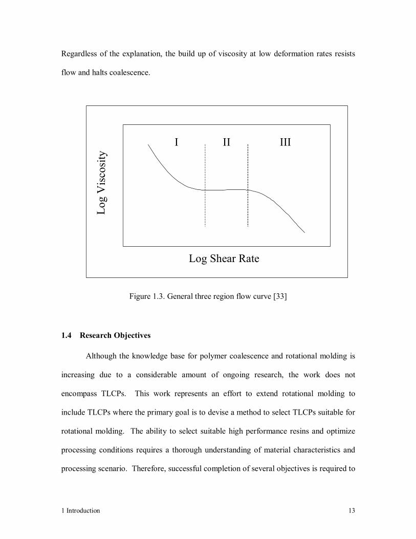
The second problem is that some TLCPs exhibit a three-region flow curve. This
three-region behavior is important because viscosity, and viscous resistance, tends to be
too high at the low deformation rates observed during coalescence [32, 34]. A schematic
of the proposed three-region flow curve is shown in Figure 1.3. Originally this behavior
was thought to be the result of LCP structure, and therefore inherent to all liquid crystals
[23]. However, further evidence has shown that this is not a common feature and is more
likely the product of residual crystallinity or interaction between domains [1, 2, 13].
1 Introduction 13
Regardless of the explanation, the build up of viscosity at low deformation rates resists
flow and halts coalescence.
I II III
Log Shear Rate
Log
Vis
c osi
ty
Figure 1.3. General three region flow curve [33]
1.4 Research Objectives
Although the knowledge base for polymer coalescence and rotational molding is
increasing due to a considerable amount of ongoing research, the work does not
encompass TLCPs. This work represents an effort to extend rotational molding to
include TLCPs where the primary goal is to devise a method to select TLCPs suitable for
rotational molding. The ability to select suitable high performance resins and optimize
processing conditions requires a thorough understanding of material characteristics and
processing scenario. Therefore, successful completion of several objectives is required to
1 Introduction 14
accomplish the primary goal. The first objective is to develop a method to identify
conditions necessary for successful TLCP coalescence. The second objective is to
determine if the identified coalescence conditions can be effectively translated to a lab
scale rotational molding device. The final objective is to establish rotational molding
conditions that optimize the physical and mechanical properties. The results from each of
these objectives should provide a method of screening TLCPs for effective use in
rotational molding.

1 Introduction 15
1.5 References
1. Baird, D.G., Ballman, R.L., “Comparison of the Rheological Properties of
Concentrated solutions of a Rodlike and a Flexible Chain Polyamide,” Journal
of Rheology, 23, 4, 505 (1979)
2. Baird, D.G., “Rheological Properties of Liquid Crystalline Solutions of Poly-
P-Phenyleneterephthalamide in Sulfuric Acid,” Journal of Rheology, 24, 4,
465 (1980)
3. Bawden, F.C., Pirie, N.W., Bernal, J.D., and Fankuchen, I., “Liquid
Crystalline Substances from Virus Infected Plants,” Nature, 138, 1051 (1936)
4. Bellehumeur, C.T., Kontopoulou, M., Vlachopoulos, J., “The Role of
Viscoelasticity in Polymer Sintering,” Rheologica Acta, 37, 3, 270 (1998)
5. Brostow, W., Chapter 1, “An Introduction to Liquid Crystallinity” in Liquid
Crystal Polymers: From Structures to Applications, edited by Collyer, A.A.,
Elsevier Applied Science, New York (1992)
6. Crawford, R.J., Throne, J.L., Rotational Molding Technology, William
Andrew Publishing, Norwich, New York (2002)
7. De Gennes, P.G., Prost, J., The Physics of Liquid Crystals 2cnd ed., Oxford
University Press, New York (1993)
8. Donald, A.M., Windle, A.H., Liquid Crystalline Polymers, Cambridge
University Press (1992)
9. Elliot, A., Ambrose, E.J., “Evidence of Chain Folding in Polypeptides and
Proteins,” Discussions of the Faraday Society, 9, 246 (1950)

1 Introduction 16
10. Frenkel, J.F., “Viscous Flow of Crystalline Bodies Under the Action of
Surface Tension,” Journal of Physics, (Moscow), 9, 5, 385 (1945)
11. Friedel, G., Annales de Physique, 18, 273 (1922)
12. Jackson, W.J., Kuhfuss, H.F., “Liquid Crystal Polymers Em Dash 1.
Preparation and Properties of p-Hydroxybenzoic Acid Copolyesters,” Journal
of Polymer Science. Part A-1: Polymer Chemistry, 14, 8, 2043 (1976)
13. Larson, R.G., The Structure and Rheology of Complex Fluids, Oxford
University Press, New York (1999)
14. MacDonald, W.A., Chapter 8, “Thermotropic Main Chain Liquid Crystal
Polymers” in Liquid Crystal Polymers: From Structures to Applications,
edited by Collyer, A.A., Elsevier Applied Science, New York (1992)
15. Marrucci, G., Chapter 11, “Rheology of Nematic Polymers” in Liquid
Crystallinity in Polymers: Principles and Fundamental Properties, edited by
Ciferri, A. VCH Publishers, New York (1991)
16. Mazur, S., Beckerbauer, R., Buckholz, J., “Particle Size Limits for Sintering
Polymer Colloids without Viscous Flow,” Langmuir, 13, 4287 (1997)
17. Misev, T.A., Powder Coatings, Chemistry and Technology, John Wiley &
Sons, New York (1991)
18. Nguyen, T.N., Geiger, K., Walther, T.H., “Flow Behavior od LCP Melts and
Its Influence on Morphology and Mechanical Properties of Injection Molded
Parts,” Polymer Engineering and Science, 40, 7, 1643 (2000)

1 Introduction 17
19. Noël, C., Laupretre, F., Friedrich, C., Fayolle, B., Bosio, L., “Synthesis and
Mesomorphic Properties of a New Thermotropic Liquid-Crystalline
‘Backbone’ Copolyester,” Polymer, 25, 6, 808 (1984)
20. Noël, C., Chapter 2, “Characterization of Mesophases” in Liquid Crystal
Polymers: From Structures to Applications, edited by Collyer, A.A., Elsevier
Applied Science, New York (1992)
21. Ober, C.K., Weiss, R.A., Chapter 1, “Current Topics in Liquid Crystalline
Polymers” in Liquid-Crystalline Polymers, edited by Ober, C.K., Weiss, R.A.,
American Chemical Society, Washington DC (1990)
22. Odijk, T., Liquid Crystallinity in Polymers: Principles and Fundamental
Properties, edited by Ciferri, A., VCH Publishers, Inc. New York (1991)
23. Onogi, S., Asada, T., Rheology, Vol.1, edited by Astarita, G., Marrucci, G.,
Nicolias, L., Plenum Press, New York, 1980.
24. Rangarajan, P., Huang, J., Baird, D.G., “Rotational Molding of TLCPs,” SPE
ANTEC, 47 (2000)
25. Reinitzer, F., Monatsh. Chem., 9, 421 (1888)
26. Ronca, G., Yoon, D.Y., “Theory of Nematic Systems of Semiflexible
Polymers. I. Jigh Molecular Weight Limit,” Journal of Chemical Physics, 76,
3295 (1982)
27. Rosenzweig, N., Chapter 1, “Introduction” in Polymer Powder Technology,
edited by Narkis, M., Rosenzweig, N., John Wiley & Sons, New York (1995)
28. Roviello, A., Sirigu, A., “Mesophasic Structures in Polymers. A Preliminary
Account on the Mesophases of Some poly-Alkanoates of p,p’-Di-Hydroxy-
1 Introduction 18
α,α’-Di-Methy Benzalazine,” Journal of Polymer Science: Polymer Letters,
13, 455 (1975)
29. Simmonds, D.J., Chapter 7, “Thermotropic Side Chain Liquid Crystal
Polymers” in Liquid Crystal Polymers: From Structures to Applications,
edited by Collyer, A.A., Elsevier Applied Science, New York (1992)
30. Throne, J.L., Chapter 11, “Rotational Molding” in Polymer Powder
Technology, edited by Narkis, M., Rosenzweig, N., John Wiley & Sons, New
York (1995)
31. Tadmor, Z., Gogos, C.G., Principles of Polymer Processing, John Wiley &
Sons, New York (1979)
32. Viola, G.G., “RheologicalCharacterizaton, and the Development of Molecular
Orientation and Texture During Flow for a Liquid Crystalline Copolymer of
Para-Hydroxybenzoic Acid and Polyethylene Terephthalate”, PhD
Dissertation, Department of Chemical Engineering, Virginia Polytechnic
Institute and State University, Blacksburg, Va, 24061 (1985)
33. Wilson, T.S., “The Rheology and Structure of Thermotropic Liquid
Crystalline Polymers in Extensional Flow,” Ph.D. Dissertation, Department of
Chemical Engineering, Virginia Polytechnic Institute and State University,
Blacksburg, Va. 24061 (1991)
34. Wissbrun, K.F, “Rheology of Rod-like Polymers in the Liquid Crystalline
State,” Journal of Rheology, 25, 6, 619 (1981)
35. Webster’s 3rd International Dictionary
2 Literature Review 19
2 Literature Review
Preface
This chapter provides a review of literature pertinent to this research project. The
key topics discussed in this chapter include: rotational molding, how material properties
and processing parameters may affect moldablility, and the important properties and
behavior of thermotropic liquid crystalline polymers.
2 Literature Review 20
2 Literature Review
This chapter contains a review of research that is relevant to the selection of
TLCPs for rotational molding. In section 2.1, phenomena associated with rotational
molding such as powder properties, sintering and densification, and processing
parameters are examined. In section 2.2, the aspects of TLCPs that are pertinent to
rotational molding are detailed: their rheological response to various types of flow, and
their mechanical properties. The review concludes with a restatement of research
objectives in section 2.3, with an emphasis on tying together the previous work found in
the literature review with the objectives for this work.

2 Literature Review 21
2.1 Rotational Molding
The success of rotational molding depends upon a number of variables that
include everything from the behavior and properties of the powder to the material’s
response under suface driven flow and processing variables. The importance of each of
these areas is examined in the following sections.
2.1.1 Powder Properties
Powder quality is a rather vague term that is typically related to powder physical
properties such as shape, size, and density [145]. It may be more accurate to associate
quality with the powder’s ability to perform as desired; a characteristic which varies with
application. Regardless of the definition of quality, powder properties are important
because they have been connected to the quality of rotational molded products through
phenomena such as: powder distribution during mold rotation, heat transfer, material
densification, surface quality, and mechanical performance [24]. Relationships between
the physical properties of powder and their behavior are explored in the following section
with an underlying attempt to identify what is desirable for rotational molding.
2.1.1.1 Particle Size
Selection of powder size is typically dependant upon melting rate and can range
from fine (<100µm) to coarse (>500µm) [87]. Including a portion of small particulate in
the powder can increase melting rate and improve surface finish. Melting rate will
2 Literature Review 22
increase because small particles have a larger surface area to volume ratio than larger
particles [24]. Also, the powder is naturally sieved as it tumbles in the mold, filtering
finer particles to the mold surface [87]. Finer powders produce bulk samples that contain
less void and melt relatively quickly leading to an improvement in surface quality.
A large mass fraction of fine particulate can create problems for rotational
molding. The large mass fraction of fines decreases the average particle size, which is
accompanied by an increase in the overall powder melting rate because it increases heat
flux by increasing the surface area to volume ratio. If the molding cycle is not adjusted to
compensate for this change, the melt is in jeopardy of rapid thermal oxidation [87]. Fine
powders are easily fluidized, which may lead to excessive material loss as dust. Small
particles are also more susceptible to elactrostatic forces, which can cause agglomeration
and prematurely melt in the surrounding powder [132]. As mentioned, coarse particles
move away from the mold surface and may cause irregular, matte internal surfaces with
an excessive amount of pinholes [24]. They may also extend the heating cycle, cause
larger bubbles, and possibly poor interparticle adhesion [133].
A desirable particle size distribution should possess the highest bulk density
possible because it leads to fewer voids, reducing the amount of air that is capable of
becoming trapped on the surface or within the melt [24]. While this does not completely
eliminate the formation of bubbles, those that are formed are rather small and readily
disappear, as explained by the Laplace equation, which states that the pressure inside a
bubble is proportional to 1/R [88]. Pressure within the bubble increases as the bubble

2 Literature Review 23
radius decreases; the increased pressure accelerates gas diffusion. In practice, experience
has shown that the most desirable rotational molding grade powders are typically in the
range of 75 to 420 microns with a Gaussian distribution [24]. Additional discussion of
the importance of size distribution will be presented later in relation to bulk density.
2.1.1.2 Particle Shape
The most desirable shape for a rotational molding particle is a “squared egg”
[133]. The squared egg has an ovoid side projection and a rectangular or square end
projection, as shown in Figure 2.1. This shape has optimum packing density and particle
contact, while retaining free powder flow properties.
Figure 2.1. Squared Egg Particle
2 Literature Review 24
Unfortunately, rotational molding powders are not typically the “squared egg”
shape, but vary from spherical to fiberous. Spherical particles have lower packing
density than the squared egg and interparticle contacts are points rather than extended
surfaces [24]. Low packing density is undesirable because it can lead to the formation of
an excessive number of voids and make densification difficult. Fibrous particles, also
referred to as acicular, are produced when shredding or tearing occurs during grinding
[87]. This shape can be seen clearly, even at low magnifications, 10-20x. These particles
can have a fibrous tail that can be two or three times the length of the particle itself. Tails
prevent the powders from flowing freely and cause porosity when molded. The particles
bridge, their tails interlock to block narrow cavities and prevent other particles from
continuing into narrow recesses within the mold cavity. Once the bridge forms it remains
as an internal surface imperfection and can even prevent complete fusion at the outer
(mold) surface. Fibrous particles may also collect into fluffy balls that tumble about on
the surface of the powder. Once the distributed powder has melted, the balls become
anchored to the surface and form irregular shaped lumps. The defect is referred to as
“scrambled eggs” because of the resulting appearance of the molded surface [87].
Particle shape can dramatically affect heat transfer of the powder mass. Rao and
Throne [133] compared the surface area to volume ratios of various shapes as a measure
of the efficiency for heat transfer into the particle interior. For surface convective heating
of a flat sheet with thickness R, the ratio is 1/R. For a cube with side dimension R it is
6/R, and for a sphere it is 3/R. For contact conduction, assuming only one portion of the
particle is in contact with the heated surface the ratios become; 1/2R for the flat sheet,
2 Literature Review 25
1/R for a cube, and zero for a sphere. As particles become more spherical the contact
area for conductive heat transfer decreases, increasing the importance of convective
heating.
There are number of ways to classify particle shape [98, 127]. Historically, such
quantities as length to diameter ratios and inscribed or circumscribed circles were used
along with verbal descriptions. Although these methods are simplistic, they still have a
place in both laboratory and industry [115]. Possibly the most commonly used method is
a shape factor, the ratio of the surface areas between the particle and a sphere with equal
volume. Other common quantities are given in
2 Literature Review 26
Table 2.1. One potential pitfall is that many of these quantities rely on particle
symmetry because dimensions are obtained from a two-dimensional projection, a practice
referred to as stereology or morphometry [24]. Despite this, it has become apparent that
image analysis is the quickest and most cost effective way to get particle information
[115].

2 Literature Review 27
Table 2.1 Irregular Particle Shape Measurement [24]
Average Thickness The average diameter between the upper and lower surfaces of a particle at its most stable position of rest.
Average Length The average diameter of the longest chords measured along the upper surface of a particle in the position of rest.
Average Breadth The average diameter at right angles to the diameter of average length along the upper surface of a particle in its position of rest.
Chunkiness Reciprocal of elongational ratio.
Circularity Ratio of circumference of a circle with the same projected area to the actual circumference of the projected area.
Elongational Ratio The largest particle length to its largest breadth when the particle is in a position of rest.
External Compactness The square of the diameter of equal area to that of the profile, divided by the square of the diameter of an embracing circle.
Feret’s Diameter The diameter between the tangents at right angles to the direction of scan, which touch the two extremities of the particle in its position of rest.
Martin’s Diameter The diameter which divides the particle profile into two equal areas measured in the direction of scan when the particle is in a position of rest.
Projected Area Diameter The diameter of a sphere having the same projected area as the particle profile in the position of rest.
Roundness Factor Ratio of the radius of the sharpest corner to the most round corner with the particle in a position of rest.
Specific Surface Diameter The diameter of a sphere having the same ratio of external surface area to volume as the particle.
Surface Diameter The diameter of a sphere having the same surface area as the particle.
Stokes Diameter The diameter of a sphere having the same terminal velocity as the particle.
Volume Diameter The diameter of a sphere having the same volume as the particle.
The quantities in

2 Literature Review 28
Table 2.1 as well several additional measures have been applied to image analysis
algorithms. Of these additional measures, the most notable has been the use of Fourier
analysis. The length of the radius vector from the particle’s center to its surface is
measured as a function of the angle between the radius and reference vectors [116]. This
function of radius length is then plotted against the angle and analyzed by the Fourier
cosine series to obtain a power spectrum for the particle. This technique is capable of
regenerating the original particle’s silhouette with a great degree of accuracy, providing
that the phase angle data are conserved. Unfortunately, extending the technique to the
prediction of behavioral aspects has proven to be extremely difficult [98].
An effective system for image analysis has not been identified because it is
unclear exactly what information is needed to describe powder behavior. Should a
general shape description be determined or only a measurement of shape features relevant
to a specific problem? Since particle-particle interaction is desired, the mixture of shapes
in the powder may be more relevant than individual particle shape. Ultimately, a
connection between shape and interaction must be developed. Presently, this feat cannot
be seriously considered because the state of particle characterization is still limited to
providing an effective means of shape identification [116].
Three philosophies are currently being explored in image analysis of particle
shapes [116]. The first pertains to quantifying only the relevant shape features (RSF) for
a given process or problem, but this assumes that the relevant features are known. The
second is to quantify particles according to a formation system because the formation
2 Literature Review 29
mechanism inherently places constraints upon particle shape. For example, roundness
can be used for particles formed from a shot tower, crystal shape can be used for particles
formed by crystal growth, and angularity for particles formed from brittle fracture. This
approach is the most fundamental and shows the most promise [115]. The third is to
generate a comparison particle from a given set of measured parameters (dimensions).
This approach is the most extensively used because data can be easily generated to
evaluate new particle characterizing algorithms.
2.1.1.3 Bulk Density
Bulk density is a measure of powder packing efficiency. Packing efficiency is
important because it governs the number of contact points between particles as well as
the number and size of voids between them. Typically, bulk density is inversely related
to powder flow. An increase in bulk density increases the flow rate, which indicates
better flow.
Bulk density is dependent upon particle shape, size, and size distribution.
Gaussian distributions tend to produce high packing density and intimate particle-to-
particle contact during the coalescence step of particle adhesion. The relationship
between distribution and density is more universally described by measuring the packing
fraction, defined as the ratio of the density of the powder bed to the material density.
Sometimes, void fraction is used, which is one minus the packing fraction. Packing
fraction can be understood by considering a powder composed of spheres having equal
diameter. If the spheres are packed in a body centered cubic mode the packing fraction

2 Literature Review 30
would be 0.534 [32]. Upon melting, assuming complete densification, the material will
occupy nearly half the volume of the original powder. There are numerous packing
arrangements (and accompanying packing fractions) that these spheres could take:
orthorhombic (0.605), tetragonal-spherical (0.698), and rhombohedral (0.740).
The coordination number is another way to describe packing. It represents the
number of contact points each particle has with neighboring particles. The previously
mentioned packing arrangements have the following coordination numbers: cubic 6,
orthorhombic 8, tetragonal-spherical 10, rhombohedral 12.
Unfortunately, rotational molding powders are not normally spherical and do not
have a uniform diameter. The result is that packing fractions differ from theoretical
values. Values for real particles may deviate either above or below depending on the size
distribution and shape but little is known about the effect of shape except for highly
anisotropic structures like fibers or plates, which are not typically molded [24]. It has
been shown that coordination numbers range from 10 to 20 for mixed particle sizes with
irregular shape and in respect to coalescence the coordination number should be as large
as possible.
The amount of fine particles in the size distribution can influence bulk density. In
Gaussian distributions fine particles fill in the gaps between coarse particles acting to
increase bulk density. But if the mass fraction of fines surpasses three times that of the
coarse particles they drive coarse particles apart and reduce density [32]. It has been
2 Literature Review 31
shown theoretically that a packing fraction of 0.85 can be obtained for a distribution
regardless of average particle size. The limitation is that five successive sizes are
selected, each being 70% of the previous dimension [24]. Interestingly, if the 70% rule is
not followed then for the same distribution, packing fraction will decrease as the mean
particle size decreases. This is due to arching and bridging because fine particles have a
higher surface area to volume ratio and thus the effect of surface interactions like friction
and static are increased.
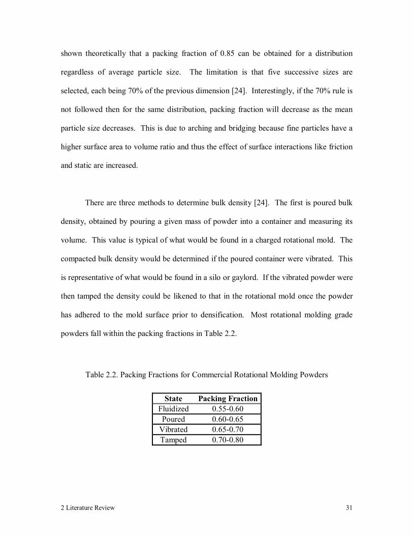
There are three methods to determine bulk density [24]. The first is poured bulk
density, obtained by pouring a given mass of powder into a container and measuring its
volume. This value is typical of what would be found in a charged rotational mold. The
compacted bulk density would be determined if the poured container were vibrated. This
is representative of what would be found in a silo or gaylord. If the vibrated powder were
then tamped the density could be likened to that in the rotational mold once the powder
has adhered to the mold surface prior to densification. Most rotational molding grade
powders fall within the packing fractions in Table 2.2.
Table 2.2. Packing Fractions for Commercial Rotational Molding Powders
State Packing FractionFluidized 0.55-0.60 Poured 0.60-0.65
Vibrated 0.65-0.70 Tamped 0.70-0.80
2 Literature Review 32
2.1.1.4 Powder Flow
Dry powder flow properties are important because they determine how well the
polymer will distribute during rotation and if the powder is capable of entering into small
cavities and complex shapes [24]. This is a combination of particles interacting with
each other and with the mold surface. It should be noted that this review of powder flow
is restricted to identifying general flow behavior and does not explore the enormous and
complex field of modeling granular flow.
Powder flow characteristics depend upon particle size and shape [1]. Flat
particles, such as flakes and cubes, will alternately slip and stick. Particles with large
aspect ratios tend to agglomerate and distribute poorly, while spheres produce the best
possible flow properties. These different flow behaviors have allowed powders to be
classified into two groups [134, 146]. The first group is referred to as Coulomb flow
powders or non-segregating (cohesive) powders with behavior that is dictated by contact
forces. Neighboring particles remain in constant contact, acting more like a cohesive
solid than a freely flowing powder. The second group is viscous flow powder or
segregating (freely-flowing) powder. Their behavior is the result of competition between
contact forces and momentum transfer, allowing particles free movement relative to each
other.
Three types of powder motion have been identified for these powders: steady state
circulation, avalanche flow, and slip flow [147]. In steady state circulation, the powder at
the mold surface moves with the mold until it exceeds the dynamic angle of repose,

2 Literature Review 33
which is illustrated in Error! Reference source not found. and lies between 25° and 50°
above horizontal for most powders [24]. At that point the powder breaks away from the
mold and cascades across the static surface of the bulk powder. Flow is continuous and
flow rate is altered only by mold geometry. The powder may be either cohesive or free
flowing and is typically either spherical or square-egg shaped. The mold surface needs to
be fairly rough, particle sizes are rather large, and powder volume is moderate in
comparison to the mold volume. This flow is considered an ideal flow in that it offers the
maximum amount of mixing and the best heat transfer.
In avalanche flow the powder bed is initially static in reference to the mold
surface. The entire bed moves until it surpasses the dynamic angle of repose. Then the
top portion of the bed breaks away from the mold and tumbles across the lower portion of
the bed, returning to a static state with respect to the mold. Avalanche flow cannot truly
be classified as Coulombic or viscous flow since it does not reach steady state [24]. The
particulate typically belong to the cohesive group and may be squared egg, acicular, or
disk-like. Aside from occurring initially, avalanche flow can develop as the bed depletes
during coalescence. Although not as desirable as steady state circulation, it does provide
acceptable distribution, mixing, and heat transfer.
Slip flow is a Coulomb flow that occurs when particles can pack well and have a
low coefficient of friction with the mold surface [24]. The powders are cohesive, acicular
or disk-like, and continuously slides along the mold. A variant of this flow, slip-stick, is
actually more common. The static bed rises with the mold surface until friction between

2 Literature Review 34
the powder and the mold wall can no longer stop movement, then the entire mass slides
to the bottom of the mold. Both variations provide poor distribution, mixing, and heat
transfer.
There are several common ways of obtaining information about powder flow for
rotational molding. A general measure of flow can be acquired according to ASTM D-
1875. Flowability is reported as the time it takes for 100 grams of powder to flow
through a standard funnel into a cup. While this test may work well at evaluating flow
behavior in funnel, care must be taken in extrapolating the results to other geometries. A
simple rotating unit, composed of a rotating 1000mL graduated glass cylinder, is
commonly used to evaluate the flow behavior of new rotational molding powders. It is
useful in determining the effect of mold fill level on bed motion as well as particle
motion during dry flow and melting [24].
2.1.1.5 Powder Heating
Predicting heat transfer in powders has been approached from two perspectives:
by treating the bed as a continuum and by transient heating of an individual particle [24].
Considering the case of an individual particle, the traditional solution for temperature
gradient through a sphere is [61, 90]:
∂∂+
∂∂=
∂∂
rT
rrT
tT 2
2
2
α (2.1)
where α is thermal diffusivity and the initial condition is:
2 Literature Review 35
( ) 00, TtrT == (2.2)
It is then assumed that the contact area with the mold, or other particles, is relatively
small when compared to the total surface area so convective heat transfer dominates the
heating process. An energy balance at the surface of the particle leads to the boundary
condition:
( )( )tRTThrTk air
Rr
,−=∂∂−
=
(2.3)
where k is the thermal conductivity of the polymer sphere and h is the heat transfer
coefficient of quiescent air. The exact solution for this system is in the form of a
dimensionless infinite series. Except for very small values of the Fourier number (Fo <
0.2) the series solution can be approximated by a single term and the graphical solution is
available in a number of heat transfer references [90].
There is a problem with applying this approach to rotational molding powders.
Time dependency is retained in the Fourier number, and since particle radii are very
small, the Fourier number becomes extremely large even at short times. Perhaps a more
convenient approach is to equate the total thermal energy in the sphere to the convective
transfer [24]:
( )dtTThAVdTc airp −=ρ (2.4)
where V is the particle volume, A is the surface area, and cp is the polymer’s heat
capacity. Under the assumption that air temperature is constant, which is not rigorously
correct in rotational molding because it is more uniform than constant, the solution is:
2 Literature Review 36
tVchA
air
air peTTTT
=−− ρ
0
(2.5)
This solution does not assume a particle shape, so it is equally applicable to spheres as
well as cubes and cylinders. Shape is accounted for by the ratio of surface area to
volume, which is possible because the solution requires that the particles have small
dimensions (less than approximately 420µm). Incidentally, this requirement implies that
the temperature throughout the particle is uniform.
Precise heat transfer modeling of a flowing powder is not possible because
powder flow itself is not adequately characterized [24]. Therefore, it is assumed that
powder flow is either steady-state circulation or slip flow. In both cases heat is
transferred into the powder bed (continuum) through conduction from the wall. An
effective thermal diffusivity is used to correct for reduced conductive flux due to voids
within the bed. The effective thermal diffusity is defined as:
ppowderpowdereffective ck ×= ρα (2.6)
The thermal diffusivity of static powders can be considered as only weakly
dependent on bulk density as a first approximation [24]. This is only the case for static
beds; values can decrease by up to ten times for steady state circulation or avalanche
flow.
Values for the thermal conductivity of untamped powders range from 20 to 50%
of the polymer [24]. The thermal conductivity of the powder consists of contributions
from air and polymer through the Lewis-Nielsen equation [131]:
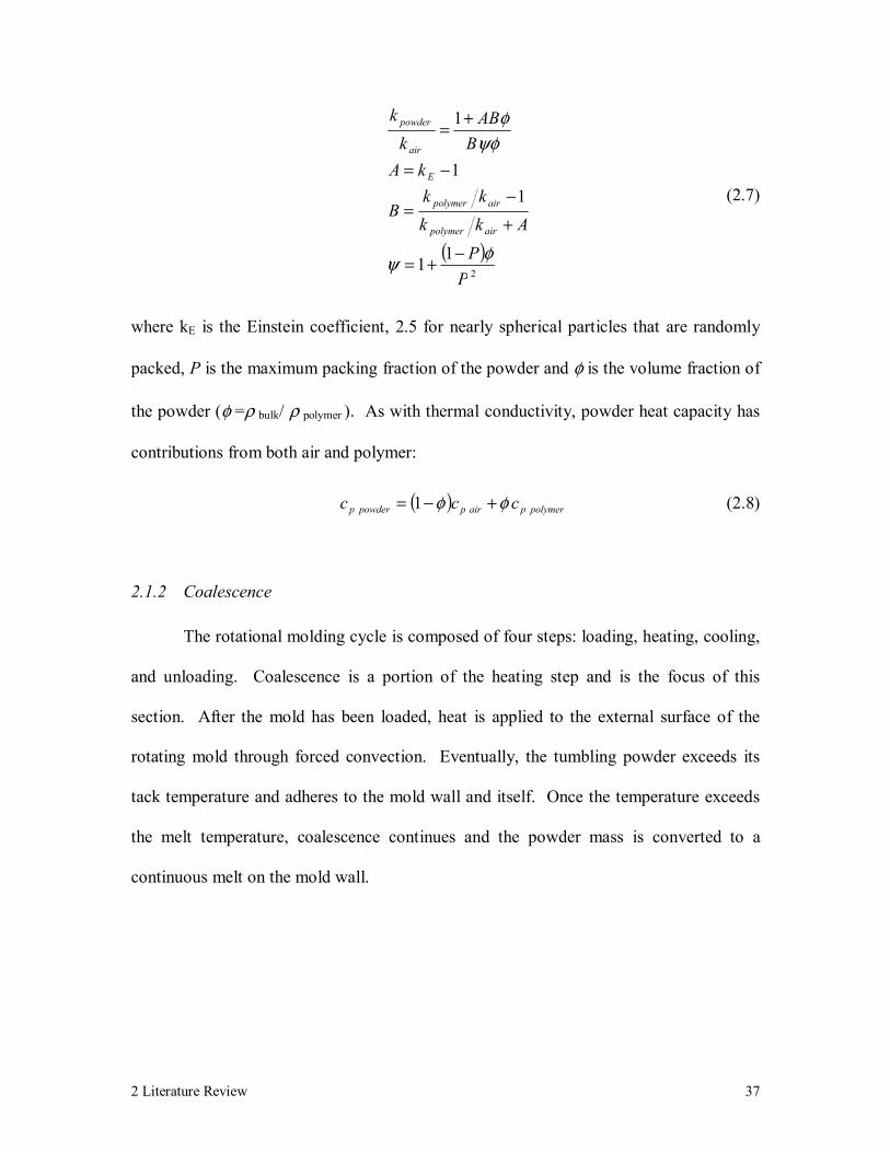
2 Literature Review 37
( )2
11
11
1
PP
Akkkk
B
kAB
ABk
k
airpolymer
airpolymer
E
air
powder
φψ
ψφφ
−+=
+−
=
−=
+=
(2.7)
where kE is the Einstein coefficient, 2.5 for nearly spherical particles that are randomly
packed, P is the maximum packing fraction of the powder and φ is the volume fraction of
the powder (φ =ρ bulk/ ρ polymer ). As with thermal conductivity, powder heat capacity has
contributions from both air and polymer:
( ) polymerpairppowderp ccc φφ +−= 1 (2.8)
2.1.2 Coalescence
The rotational molding cycle is composed of four steps: loading, heating, cooling,
and unloading. Coalescence is a portion of the heating step and is the focus of this
section. After the mold has been loaded, heat is applied to the external surface of the
rotating mold through forced convection. Eventually, the tumbling powder exceeds its
tack temperature and adheres to the mold wall and itself. Once the temperature exceeds
the melt temperature, coalescence continues and the powder mass is converted to a
continuous melt on the mold wall.
2 Literature Review 38
2.1.2.1 Elastic Deformation
Polymeric coalescence can be categorized into three stages: elastic deformation,
neck growth and pore formation (particle sintering), and densification. When two
particles are brought into contact there is an immediate elastic deformation and the
particles adhere. Further coalescence proceeds via neck growth during this process
particles retain their individuality and neck growth is not influenced by neighboring
contacts. The neck dimension continues to grow until a network of pores form, which
has been handled as a bulk phenomenon due to interactions between neighboring
particles. At this stage the packing geometry is significant because it dictates where
pores form. Also, most shrinkage occurs during this stage, introducing complexities
involved with particle rearrangement. Eventually, the pores become spherical in shape
and densification occurs, which is dependent upon gas dissolution.
The mechanism proposed for elastic deformation (also referred to as adhesive
contact) is fundamentally different from viscous sintering. van der Waals forces have
been identified as the driving force for this growth mode. More generally they are
referred to as adhesive traction forces and act to “zip” the particle contact together [70].
Unlike with curvature based surface tractions observed during viscous flow that act
normal to the surface, adhesive traction forces act normal to the contact plane to draw
opposing surface elements together and may remain active as long as the gap between the
two surfaces is within the fixed length scale characterizing those adhesive forces [100].
They completely neglect radial stretching, whereas viscous sintering models account for
the deformation by radial stretching only. Also, elastic growth kinetics do not scale with
2 Literature Review 39
particle size as sintering does [91, 111]. The fraction of neck growth contributed by
elasticity increases with decreasing particle size; sufficiently small particles can
completely coalesce (geometrically) through elastic deformation [70].
The original analysis of elastic contacts by Hertz was for two identical elastic
spheres, brought into contact with each other by applying a compressive load. This
appeared reasonable for the glass sphere system considered. In fact, it predicts elastic
collisions surprisingly well for highly elastic solids. However, Johnson, Kendall, and
Roberts [73] considered adhesive contact force of elastic solids in order to address
evidence of adhesive forces between two particles in contact. The preexisting Hertz
theory for elastic contact underestimated the contact area in the low load limit because it
neglected surface tension forces, predicting a point contact when no load was applied.
The JKR theory establishes a balance between stored elastic energy and minimized
surface energy to produce finite contact area without an applied load.
In the absence of an applied load, equilibrium is established between potential
energy lost from decreasing external surface area and potential energy stored in the form
of residual elastic stresses near the contact area [73]. These stresses are predicted as
tensile near contact boundary and compressive near the center of the neck [111]. It also
proposes a noticeably different neck shape; JKR predicts a rounded shape whereas Hertz
is sharp. Figure 2.2 shows neck contours and pressure distributions as predicted by Hertz
and JKR theories. The Hertz illustration is for identical spheres under an applied load
while the JKR is for the same geometry but without an applied load. As can be seen in

2 Literature Review 40
the figure, JKR theory is not completely realistic since pressure distribution near the
contact periphery is actually continuous. It does however provide interesting insight into
the nature of elastic contacts.
Compression
Tension
p (x)
Hertz JKR
Compression
Tension
p (x)
Hertz JKR
Compression
Tension
p (x)
Compression
Tension
p (x)
HertzHertz JKRJKR
Figure 2.2. Hertz and JKR Predictions
It has been experimentally demonstrated that the kinetics during the early stage of
polymeric coalescence can often be completely described by considering only elastic
deformation [111]. In addition, JKR theory has been used to predict the amount of neck
growth (equilibrium) that can be expected from purely elastic effects.
( ) 31
00 819
−Γ=
aJ
ax nνπ
(2.9)
where v is Poisson’s ratio and Jn is creep compliance in the plateau region.

2 Literature Review 41
Similarly, size limits have been determined for viscoelastic particles in the elastic
limit [112]. The maximum particle radius that will allow elastic deformation to fill all
packing voids was determined as a function of surface energy, elastic compliance, and
packing fraction.
( ) 23
31
max
147.0
i
nJr
Φ−
Γ= (2.10)
In determining the relationship, experiments verified that viscous sintering is indeed
preceded by elastic deformation since sufficiently small particles completely sinter in
much less time than the characteristic relaxation time (the longest relaxation time
obtained from stress growth and relaxation experiments).
2.1.2.2 Particle Sintering
Transport Mechanisms
Several mechanisms have been identified for material transport during sintering:
surface migration, viscous flow, evaporation and condensation, volume diffusion, and
grain boundary diffusion [155]. It should be noted that these mechanisms were originally
identified for sintering non-polymeric materials and the nature of polymeric materials
eliminate the possibility of several of these mechanisms. Despite this, all mechanisms
are presented for completeness. The reader is referred to the description by Thümmler
[155] for an illustration of these transport mechanisms.
2 Literature Review 42
Surface migration exists in most sintering processes [155], especially at low
temperatures, in fine powders, and in the first stages of sintering while there is a large
amount of surface area. The activation energy is lower with this mechanism than other
forms of diffusion [155]. It governs all surface related activity such as surface smoothing
and pore rounding and has the ability to contribute to neck growth. If surface mobility is
hindered it can account for a reduction in the growth rate of the neck dimension. It
cannot contribute to pore shrinkage and densification. Surface atoms have greatest
mobility in convex geometries and can become immobilized on concave surfaces such as
in necks with sharp curvatures [155].
Grain boundaries act as paths for atoms to move along. The diffusion rate is
dependent upon boundary uniformity and the angle between the adjacent grains. Grain
boundaries are capable of acting as sinks for directed vacancy flow during volume
diffusion from pores, which becomes important during pore shrinkage in the intermediate
and later stages of coalescence [155]. This mechanism is unlikely to allow transport of
polymeric fluids where molecules may be much larger than the grain boundary.
In the volume diffusion transport mechanism, it is proposed that the contact
region during neck evolution becomes deprived of interstitial atoms. This generates a
gradient in chemical potential that drives atoms to flow from other parts of the system to
the junction, which decreases the overall surface area. While this may occur in polymeric
systems, it is limited by the molecular diffusivity of the polymer molecule.
2 Literature Review 43
Evaporation and condensation is responsible for external transport to and from the
surface. Molecules at the fluid/ gas interface evaporate to establish phase equilibrium.
Once the vapor phase becomes saturated, molecules must condense back into the liquid
phase in order to maintain equilibrium. Kinetic theory has been used to explain
evaporation and condensation rates [93, 85]. However, evaporation of polymeric
materials is unlikely.
The viscous flow mechanism accounts for coalescence by equating energy from
the reduction of surface area to that dissipated by the resisting viscous flow. It has been
established as the governing transport mechanism in polymer coalescence and will be
discussed in more detail in section 2.1.2.2.
Scaling Relations
The various transport mechanisms each have a unique scaling relation.
Kuczynski provided a series of scaling relations between the neck radius xn, internal
particle radius ao, and time t [92]. The scaling relations are represented by the following
form with exponents given in Table 2.3. Scaling for elastic deformation has been
included as determined by Johnson et al [73]. The coefficient k is a function of material
properties and the exponents depend only upon the transport mechanism.
βαtkax on = (2.11)
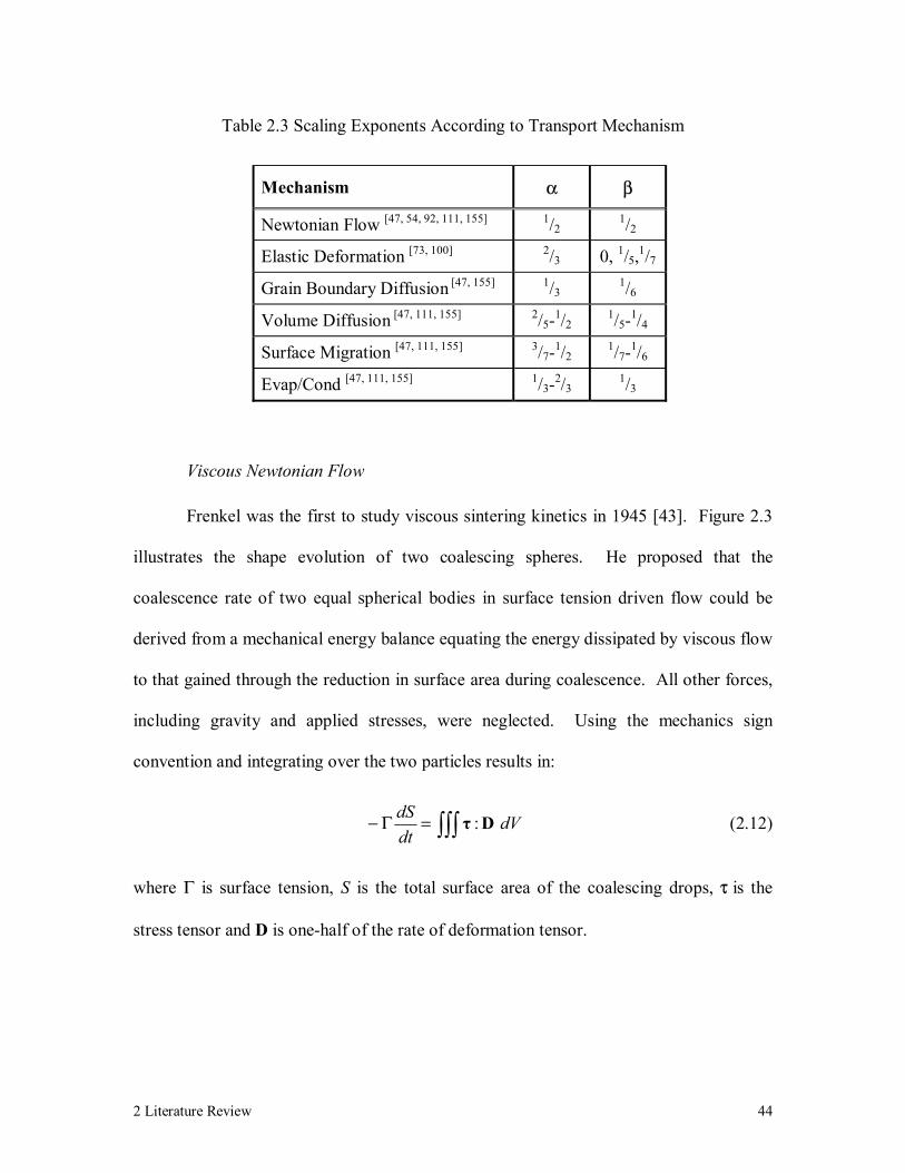
2 Literature Review 44
Table 2.3 Scaling Exponents According to Transport Mechanism
Mechanism α β
Newtonian Flow [47, 54, 92, 111, 155] 1/2 1/2
Elastic Deformation [73, 100] 2/3 0, 1/5,1/7
Grain Boundary Diffusion [47, 155] 1/3 1/6
Volume Diffusion [47, 111, 155] 2/5-1/2 1/5-1/4
Surface Migration [47, 111, 155] 3/7-1/2 1/7-1/6
Evap/Cond [47, 111, 155] 1/3-2/3 1/3
Viscous Newtonian Flow
Frenkel was the first to study viscous sintering kinetics in 1945 [43]. Figure 2.3
illustrates the shape evolution of two coalescing spheres. He proposed that the
coalescence rate of two equal spherical bodies in surface tension driven flow could be
derived from a mechanical energy balance equating the energy dissipated by viscous flow
to that gained through the reduction in surface area during coalescence. All other forces,
including gravity and applied stresses, were neglected. Using the mechanics sign
convention and integrating over the two particles results in:
∫∫∫=Γ− dVdtdS Dτ : (2.12)
where Γ is surface tension, S is the total surface area of the coalescing drops, τ is the
stress tensor and D is one-half of the rate of deformation tensor.

2 Literature Review 45
ao
y θ
a
x
aoao
y θ
a
x
y θ
a
x
Figure 2.3. Shape Evolution
The flow field is assumed to be equibiaxial extensional flow with the rate of
deformation tensor given as:
−=
εε
ε
&
&
&
0002000
2D (2.13)
The mechanical energy balance for a Newtonian fluid in the limit of small angles
(small neck radii), where particle radius remains undisturbed by deformation, results in
the following (corrected) expression:
21
023
Γ=a
tax
η (2.14)
where a0 is the initial particle radius, η is the viscosity, Γ is surface tension, t is time, and
x is the neck radius. A comparison of Frenkel’s model with several other particle
sintering models, which will be presented later, can be found in Figure 2.4. Frenkel’s
neck growth expression in equation 2.14 has been used to generate the following equation

2 Literature Review 46
describing the approach of the centers of two spheres or the linear shrinkage rate of an
array of spherical particles.
Rt
LL
η83
0
Γ=∆ (2.15)
Several experimental studies are in good agreement with these predictions while another
showed notable deviation for compacts of non-spherical particles [34,91,85]. The
presence of asymmetric neck growth and formation of new contacts during sintering
makes extension of quantitative models derived for two particles to irregular packings
unlikely [41].
0
0.2
0.4
0.6
0.8
1
1.2
0 0.5 1 1.5 2 2.5
Dimensionless Time (γt/a oη)
Dim
ensi
onle
ss N
eck
Rad
ius
(x/ a
)
Frenkel
Modified Frenkel
UCM
Model Parameters η = 1000 Pa sec γ = 0.01 N/m a o = 2.5x10⁻⁴ m λ = 100 sec
Figure 2.4. Two-Particle Sintering Models†
† Data in graph were acquired from solving the appropriate models with the given parameters.
2 Literature Review 47
The Frenkel model was later extended to apply beyond the initial stages of
sintering by developing the following expression for the time dependent radius [129].
( )( )[ ] ( )[ ]
31
2 cos2cos14
−+=
θθoata (2.16)
θ , referred to as the sintering angle, is shown in Figure 2.3 and defined below.
( )θsin=ax (2.17)
By applying the transient radius expression in the Frenkel derivation, the following
expression for the evolution of the sintering angle can be obtained.
( ) ( ) ( )[ ]( )[ ] ( )[ ] 3
1
313
5
cos1cos1
cos2sincos2
θθθθθ
ηθ
+−
−Γ=−
oadtd (2.18)
The modified model produces lower coalescence rates than predicted from the
Frenkel model, which is reasonable because the Frenkel model is strictly limited to the
early stages of sintering and therefore progresses from those high initial rates in an
unbounded fashion. Predictions are included in Figure 2.4 as the Modified Frenkel
Model.
There have been concerns expressed about the stability of coalescing systems. It
is well known that surface tension has the ability to induce the breakup of liquid streams,
referred to as Rayleigh instability [143]. Is it possible that this could impede
coalescence? If so, what are the requirements for instability? Rayleigh showed that the
2 Literature Review 48
amplitude of a disturbance, A, of wavelength, λ, on a viscous cylinder of radius, a, would
grow according to:
( ) ( )
−
Γ= 2
22416
exp0λ
πη
aat
AtA (2.19)
This predicts that disturbance growth is limited to cases where a/λ is less than 1/2π. The
largest possible disturbances occur in the case of adjoining spheres, which have a
wavelength of λ = 2a so they would be stable. It was predicted that a viscous system
would have to posses an initial bulk density less than 0.001 kg.m-3 to be unstable [143].
The first numerical attempts had difficulty with correctly handling the moving
boundary. The first to have even remote success was an analytical approach that applied
complex variable theory of biharmonic functions (time dependent conformal mapping) to
describe shape evolution during sintering [55, 56, 57, 58]. No mathematical
approximations were made although it considered only viscous and capillary forces.
The method does have severe limitations. The approach is quite involved and
limited to cases where conformal mapping functions are previously known or intuitively
determined. Since there is no way to back out the function it is impossible for this
method to elucidate another form of greater generality that would be applicable to bulk
systems. The mapping function also predetermines the sintering kinetics and different
materials could not be accounted for because there is only one adjustable parameter,
which is not related to material properties.
2 Literature Review 49
Difficulties with computing surface curvature and repairing mesh were overcome
and an FEM was developed for the sintering problem [65]. The solution detailed the
evolution of the neck geometry in the early stages for viscous sintering of two particles.
The numerical solution was formulated by using the weak forms of the equations for
equilibrium and conservation of mass then forming the finite element discretization using
Galerkin’s method. Flow was assumed to be quasi-Lagrangian, once velocity and
pressure were solved for a given time step the boundary was advanced by Euler
integration of the velocity field. Results were qualitatively similar to Frenkel’s model but
the growth rate was overestimated relative to Frenkel’s model by a factor of
approximately 1.5.
A boundary element method based on the stream and vorticity functions for the
two-dimensional Stokes flow was used to solve the two-dimensional system with more
neck curvature than could be handled with the previous FEM [94]. The method also
appeared to work better than FEM because only the velocities of boundary points were
needed for a solution and remeshing a boundary curve is much easier than remeshing the
entire two-dimensional grid. Unfortunately it was still incapable of converging on a
solution for extremely sharp or large curvatures. Small disturbances in surface curvature
were shown to decay exponentially. However, it required an initial smoothing step
before the particles began to coalesce. The simulations were not realistic in that they
were incapable of maintaining constant density, which was estimated by checking for
constant area [144]. The source of the error was identified as the loss of the free rotation
condition during discretization.
2 Literature Review 50
An FEM was used for three-dimensional axisymmetrical particles [102]. Again,
two spheres were modeled but not only of equal but also different sizes. A balance was
drawn between surface tension and fluid traction forces normal to the particle surface;
tangential stresses on the fluid surface were neglected. Simulations showed that material
moves through the particle interior and that the stream function increases, proceeding
through a maximum then decreasing due to shape evolution and disappearance of surface
curvature. For the case where one of the spheres had a radius four times that of the other,
the mass of the smaller particle was absorbed but remained confined to a localized
region. This suggests that viscous flow alone is incapable of effectively mixing
coalescing particles, which has important implications to mixing particles with different
composition. The work was followed up with a three-dimensional FEM analysis of three
particles adjoined in a right angle [171]. The simulation revealed that the two adjacent
particles approached one another. This was the first simulation to demonstrate the
importance of particle rearrangement during multiple particle sintering.
Viscoelastic Flow
Viscoelasticity in sintering has had a somewhat confusing history. Viscoelastic
response was first applied to sintering by introducing an exponentially increasing
viscosity into Frenkel’s original model [102]. This approximation proved to be too
simplistic to accurately illustrate true viscoelasticity. The term (viscoelasticity) has also
been used to describe the combination of elastic contact with viscous flow [110]. It is
important to not confuse the two formulations. Preceding viscous neck growth with the
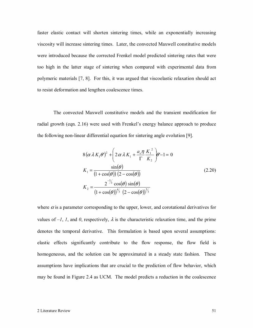
2 Literature Review 51
faster elastic contact will shorten sintering times, while an exponentially increasing
viscosity will increase sintering times. Later, the convected Maxwell constitutive models
were introduced because the corrected Frenkel model predicted sintering rates that were
too high in the latter stage of sintering when compared with experimental data from
polymeric materials [7, 8]. For this, it was argued that viscoelastic relaxation should act
to resist deformation and lengthen coalescence times.
The convected Maxwell constitutive models and the transient modification for
radial growth (eqn. 2.16) were used with Frenkel’s energy balance approach to produce
the following non-linear differential equation for sintering angle evolution [9].
( )
( )( )( ) ( )( )
( ) ( )( )( ) ( )( ) 3
53
4
35
2
1
2
21
12
1
cos2cos1
sincos2
cos2cos1sin
01'2'8
θθθθ
θθθ
θηλαθλα
−+=
−+=
=−
Γ++
−
K
K
KKa
KK o
(2.20)
where α is a parameter corresponding to the upper, lower, and corotational derivatives for
values of –1, 1, and 0, respectively, λ is the characteristic relaxation time, and the prime
denotes the temporal derivative. This formulation is based upon several assumptions:
elastic effects significantly contribute to the flow response, the flow field is
homogeneous, and the solution can be approximated in a steady state fashion. These
assumptions have implications that are crucial to the prediction of flow behavior, which
may be found in Figure 2.4 as UCM. The model predicts a reduction in the coalescence
2 Literature Review 52
rate with increasing relaxation times, which appears to agree with the experimental data
used to validate the model.
Another approach to evaluate viscoelastic effects was to solve the momentum
balance and the continuity equation by using the upper convected Maxwell equation for
the extra stress tensor. The results were consistent with the coupling of elastic
deformation and viscous flow [55]. The predictions demonstrated that stress fields in
viscoelastic particles are dramatically different from those in purely viscous particles
during intermediate stage sintering. Stresses in the neck region of viscous particles were
shown to decay monotonically while viscoelastic stresses progress through a maximum
before decay. The method was unable to resolve the regime where purely elastic neck
growth succumbs to viscous flow. It was suggested that inclusion of multiple modes with
additional relaxation times might facilitate extending the model to the elastic-viscous
transition.
It was also suggested that the history dependence of viscoelastic fluids requires
that even the earliest stages of sintering be accurately described. Therefore, models
based solely on viscoelastic flow descriptions, like the previously described UCM model
in equation 2.20, cannot realistically describe the behavior of such systems. Realistic
models must describe the essential physics of the earliest particle contact and allow for
transitions between growth mechanisms.
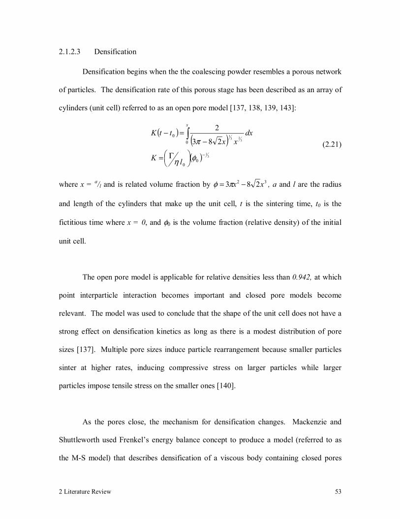
2 Literature Review 53
2.1.2.3 Densification
Densification begins when the the coalescing powder resembles a porous network
of particles. The densification rate of this porous stage has been described as an array of
cylinders (unit cell) referred to as an open pore model [137, 138, 139, 143]:
( ) ( )( ) 3
1
323
1
00
00
283
2
−
Γ=
−=− ∫
φη
π
lK
dxxx
ttKx
(2.21)
where x = a/l and is related volume fraction by 32 283 xx −= πφ , a and l are the radius
and length of the cylinders that make up the unit cell, t is the sintering time, t0 is the
fictitious time where x = 0, and φ0 is the volume fraction (relative density) of the initial
unit cell.
The open pore model is applicable for relative densities less than 0.942, at which
point interparticle interaction becomes important and closed pore models become
relevant. The model was used to conclude that the shape of the unit cell does not have a
strong effect on densification kinetics as long as there is a modest distribution of pore
sizes [137]. Multiple pore sizes induce particle rearrangement because smaller particles
sinter at higher rates, inducing compressive stress on larger particles while larger
particles impose tensile stress on the smaller ones [140].
As the pores close, the mechanism for densification changes. Mackenzie and
Shuttleworth used Frenkel’s energy balance concept to produce a model (referred to as
the M-S model) that describes densification of a viscous body containing closed pores
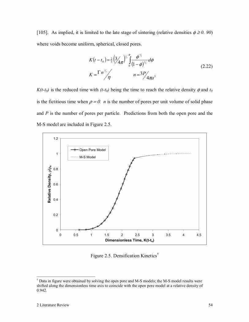
2 Literature Review 54
[105]. As implied, it is limited to the late stage of sintering (relative densities φ ≥ 0. 90)
where voids become uniform, spherical, closed pores.
( ) ( )( )
3
032
0
43
143
31
32
31
31
aPnnK
dttK
πη
φφ
φπ
φ
=Γ=
−=− ∫
(2.22)
K(t-t0) is the reduced time with (t-t0) being the time to reach the relative density φ and t0
is the fictitious time when ρ = 0. n is the number of pores per unit volume of solid phase
and P is the number of pores per particle. Predictions from both the open pore and the
M-S model are included in Figure 2.5.
0
0.2
0.4
0.6
0.8
1
1.2
0 0.5 1 1.5 2 2.5 3 3.5 4 4.5Dimensionless Time, K(t-to)
Rel
ativ
e D
ensi
ty, ρ
/ ρs
Open Pore Model
M-S Model
Figure 2.5. Densification Kinetics†
† Data in figure were obtained by solving the open pore and M-S models; the M-S model results were shifted along the dimensionless time axis to coincide with the open pore model at a relative density of 0.942.
2 Literature Review 55
It was found that the closed pore model over predicts densification rate once pores
close. The result was attributed to the shrinkage of bubbles contained in a polymer melt
ceased to be controlled by viscous and surface free energy but by dissolution of air from
the bubble through the surrounding melt [79,88]. It was shown from a force balance on a
typical bubble in molten polymer that buoyancy forces can be neglected because the
apparent viscosity is so large [23]. A diffusion model was developed to predict
densification by simultaneously solving diffusion, conservation of momentum, and
continuity equations through a force balance around the encapsulated bubble [89]. For an
ideal gas bubble surrounded by a Newtonian fluid the shrinkage of the bubble radius is
given by:
( )[ ]
0
23 3
241
ar
g
fg
drdcDaa
RTP
dtd
aPPdtda
=
=
Γ−−=η
(2.23)
where a is the time dependant radius of the gas bubble, a0 is the initial bubble diameter, r
is radial position, Pg is the pressure inside the bubble, Pf is the system pressure, R is the
universal gas constant, T is the system temperature, D is the diffusion coefficient, and c is
gas concentration. The model was evaluated for several linear low density polyethylenes,
ethylene butyl acrylate, and ethylene vinyl acetate. Results were in good agreement with
experiment for relative densities above 0.942 and could be used in conjunction with open
pore models to describe the entire densification of a polymer melt.
Densification theory was extended to include composite systems of non-sintering
particles in a packing of sintering particles in two and three dimensions [68, 69]. For

2 Literature Review 56
example, a few percent of elastic material can greatly alter the viscosity and sintering rate
of the composite packing. Also, it is generally known that the geometrical arrangement
of the inclusions plays a crucial role in determining the effective properties of the
composite [67, 142]. One of the most interesting experimental results is the existence of
an inclusion volume fraction threshold where sintering is incapable of proceeding. This
cessation is thought to coincide with the formation of a percolating cluster of hard
particles. The model uses a network of points (representing particle centers) as well as
links connecting these points (representing contacts between particles) to replace the
packing. Sintering mechanics and packing densification are then inferred by observing
the deformation of the network.
Two models were devised for network deformation: the truss and the beam
models. The truss model imposed only force equilibrium on each particle while the beam
model required equilibrium of both forces and moments. The beam model appeared to
do a better job because the truss model does not contain particle rotation in predicting
deformation and rearrangement. The method was compared to several of the previously
mentioned constitutive models, which apply a mean field assumption implying that the
macroscopic deformation field gives the relative motion of two particles [65, 70]. The
assumption results in predicted properties that actually represent the upper bound of the
true properties [65]. The constitutive models suffice at low concentrations but fail to
capture clustered inclusion behavior.

2 Literature Review 57
BEM was applied to the two-dimensional multiply connected domains including
shrinking pores [158]. Various aggregate arrangements were considered: circular hole
centered and not centered in a circular disk, elliptic hole, three to six cylinders stacked
systematically, such that center to center distances were minimized, and several 4 x 4
arrays of cylinders with different contact radii. From the series of regular particle
packings it was concluded that cylinder sintering could be reasonably described by the
coalescence of two equal cylinders thus supporting the use of unit problems in the theory
of sintering. The cylindrical arrays were used to study interior pore formation and
evolution in truly multiply connected systems. For the various initial neck radii the pores
proceed towards the interior of the fluid as time progresses. Interestingly, the final pore
location for initial neck radii of 0.095 and 0.3 are approximately the same, meaning the
pores move faster in the latter case. This also implies that pore location in non-composite
powders is dependent upon geometrical features, not viscosity and surface free energy.
The main limitation was that it was computationally demanding, although it was also
incapable of handling cases where boundaries of neighboring particles, not initially in
contact, touch during simulation. In a later publication the BEM was reformulated to
handle axisymmetric three-dimensional objects such as opposing cones, stacked rings,
sphere and ring, and coupled spheres [159]. Results look promising from a geometrical
progression point of view but no experimental evidence is available for confirmation.
Coupling compaction and sintering by combining unit problems has been used to
describe densification [63, 64, 65, 66]. The two unit problems were external traction
induced compaction of an infinite line of spheres and two spheres with surface tension
2 Literature Review 58
driven sintering, which was computed by using the previously discussed FEM solution
for viscous flow. The approach assumed that the contact area alone was sufficient to
describe the kinetic part of the constitutive response. Predictions for a two dimensional
packing of mono sized particles compared well with experiment as long as the wetting
factor (introduced in the compaction unit problem) was arbitrarily chosen properly.
Interestingly, some of the voids grew while others shrank. It was found that the wetting
factor accounting for interaction with the surface could completely change the nature of
the velocity field. Friction with the surface introduces a dissipation term that depends on
the absolute velocity, which leads to length scale dependence in the energy balance. So
defects larger than a certain size will dilate even though the entire packing will shrink.
2.1.2.4 Equilibration
Equilibration refers to the relaxation of molecular structure at the contact
interface. A body formed from the coalescence of smaller particles must experience
various molecular relaxation processes to become a fully homogeneous, history
independent material. Often, neck growth and densification may occur faster than these
relaxation processes. This can become exaggerated by compositional inhomogeneity at
particle interfaces as with the breakdown of hydrophilic bilayers at interfaces between
densely packed latex particles [111]. Still, the contribution of molecular interdiffusion
and stress relaxation at compositionally homogeneous interfaces may be equally
dramatic.
2 Literature Review 59
Perera and Vanden Eynde [125, 126] displayed the extent that stress relaxation in
bulk polymer may lag behind the deformation by examining the development of
mechanical stresses in latex paints during and after film formation. It was shown that
without coalescing aids stresses reached a maximum of approximately 1 MPa but took
several weeks to relax to approximately 0.2 MPa, even with the addition of coalescing
aids. Although the magnitude of the peak was suppressed, the residual stresses continued
to remain after many days.
Interfacial Strength
From a number of observations (i.e. the dependence of peel strength on time,
temperature, molecular weight, and plasticizers) it was hypothesized that the diffusion of
polymer chains across an interface should be the critical step for the development of
homogeneous bulk mechanical strength when two surfaces of the same polymer are
brought into contact. Advances in chain dynamics and recent developments in
experimental methods to measure polymer diffusion and mechanical properties have
stimulated studies examining the relationship between interfacial diffusion and
mechanical properties [78]. One such study was of the fracture toughness of PMMA and
poly(styrene-co-acrylonitrile) in tension. Samples were fractured below Tg then the crack
interface was allowed to ‘heal’ for various periods at temperatures from 5 to 15° above
Tg. The critical stress intensity factor for crack propagation, KIC, was measured below
Tg. It was observed that KIC increased with 41
t until the time to produce a monolithic
molded specimen was surpassed. The same rate law was observed in lamination of
2 Literature Review 60
polished surfaces. It was also found that molecular weight has little effect on the initial
equilibration rate [74, 75].
Another study demonstrated that correlations exist between molecular structure,
diffusion, and the development of strength by measuring changes in the tensile properties
of annealed poly(n-butyl methacrylate) latex films that were crosslinked with varying
amounts of methallyl methacrylate [172]. All of the films fabricated at 23°C, noting that
the material’s Tg is 29°C, showed brittle fracture in tension at strains less than 0.5. A
series of films with up to 2% crosslinking agent were formed at 90°C for a various times.
Samples with less than 2% of the crosslinking agent displayed plastic yielding behavior
and an increase in ultimate strain to approximately 3. Those same samples showed that
the annealing time required to produce ductile failure increased as the crosslink density
increased. The 2% samples all showed brittle behavior regardless of processing
conditions. The fracture energies (integrated area of stress vs. strain curve) increased by
more than 10 times over the transition from brittle to plastic failure. It was also found
that additional annealing time, after ductile fracture developed, could only increase
fracture energy up to 1.5 times. The diffusion rate was measured between the
uncrosslinked deuterated and protonated latex particles by SANS. The penetration depth
at the interface grew linearly with 21
t . It was shown that the time required to equilibrate
the fracture energy corresponded to penetration depths of 40 nm, which was comparable
to the radius of gyration for the selected chains (Mw ~ 5x10⁵) [52]. It was concluded that
brittle fracture reflected the interfacial energy of densely packed domains without
polymer chains diffused across the interface and ductile facture was indicative of chains

2 Literature Review 61
crossing the interface, which could be restricted to a negligible sol fraction and free ends
of the gel. When the mean length of the sol fraction and end segments were greater than
the length necessary for entanglements ductile fracture occurred, otherwise brittle
fracture was produced. This was supported by observing that the crosslink density for the
network chain lengths to become equivalent was about 2%, and therefore sol fraction and
end segments at that density were too short.
Diffusion
There have been considerable advances in understanding the conformation and
motion of chains confined at an interface. Conventional Fickian diffusion in liquids
corresponds to a three-dimensional random walk with a mean square displacement,
2r∆ , that is proportional to time. The entanglements found in polymer melts act as
intermolecular conformational constraints that reduce the rate of diffusion. It has been
suggested that at short times chain segment motion is localized and corresponds to Rouse
modes which predicts 212 tr ∝∆ . Rouse behavior eventually yields to a one-
dimensional random walk along a contour defined by its entanglements as predicted by
reptation theory 412 tr ∝∆ . At some longer time, dτ , after gRr ∝∆ 2 (where Rg is
the radius of gyration) the chain will have disengaged from its initial entanglements.
After disengagement normal Fickian diffusion is restored. There is also a possibility that
the chains will begin to relax at some time before dτ , which restricts the length of the
reptation regime and introduces 212 tr ∝∆ at intermediate times.
2 Literature Review 62
A number of experiments have been performed to test the validity of these
predictions at interfaces. One such experiment was performed on deuterated polystyrene,
where their concentration near the interface was measured as a function of annealing time
[135]. Results confirmed that Fickian diffusion occurred at long times but, even though
the time exponent was less than one, experimental uncertainty made it impossible to
validate theory at shorter times. Another study used selective deuteration of polystyrene
chains to enable the middle of the chains to be distinguished from the ends [136]. The
redistribution of labels during annealing time was measured by secondary ion mass
spectrometry (SIMS). The experiment was able to confirm that end segments cross the
interface before the middle segments as would be expected from reptation theory. SANS
was used to measure the amount of interdiffusion that occurs in two systems, one having
a weight average molecular weight, Mw, of 250,000 and the other being 2,000,000 [170].
It was found that the radial penetration distance was greater than the radius of gyration
for the lower molecular weight sample with a time dependence of 21
t . The radial
penetration distance of the high molecular weight sample was less than the Rg and the
exponent for time dependence was slightly less than ½. A correlation between tensile
strength and annealing time was also attempted. The lower molecular weight sample
appeared to increase with 41
t while the higher molecular weight increased with 32
t . The
time dependence for the higher molecular weight sample is questionable since the particle
radius was actually less than Rg so the entropic driving force to expand the coil
dimensions should accelerate chain transport.
2 Literature Review 63
Actually, various methods have been proposed to relate mechanical strength of a
partially equilibrated interface with interfacial diffusion [111]. Griffith’s model for
fracture mechanics states that a crack will propagate when the imposed mechanical
energy per unit crack area equals the nominal energy per unit area, Gc, of crack surface.
For polymeric materials Gc includes a significant contribution from energy that is
dissipated by plastic deformation away from the surface. One method proposed that Gc is
proportional to the average distance, x∆ , the chains have diffused across the interface
and to establish equilibrium, the entanglement density at the interface must become equal
to that of the homogeneous melt. If diffusion is Fickian, it can be shown that the kinetics
for critical stress intensity scale as [74, 75]:
43
41
21
21 −
∝∆∝∝ MtxGK cIc (2.24)
which is consistent with experiments. For a particular polystyrene system it was
estimated that at complete equilibration nmx 2≅∆ , much less than Rg for the weight
average component but comparable to the Re (Rg for the chain segments between
entanglements.) While eRx ≤∆ applying reptation theory produces the following
kinetics.
81
21
txK Ic ∝∆∝ (2.25)
A second method suggested that Gc is proportional to the number of chains that
cross the interface per unit area instead of the number of entanglements per unit volume.
It was found that the predicted growth of Gc according to reptation theory depends
strongly on the initial arrangement of chain ends near the interface [37, 38]. For

2 Literature Review 64
randomly distributed chain ends it was found that 23
21 −
∝ MtGc and for chain ends
initially concentrated at the interface 41
41 −
∝ MtGc . The randomly distributed case
appeared to agree with experiments because 21
cIc GK ∝ .
In a third model it was assumed that xK Ic ∆∝ and the kinetics were determined
by applying reptation theory along with two initial conditions [84, 167, 168]. Chains
adjacent to the interface were restricted to nongaussian conformations and there were no
conformational restraints imposed on end segments at the interface. The result was that
the critical stress intensity is proportional to 41
41 −
Mt . All three models predict the same
time dependence, 41
t , but each has a unique description of the dependence on molecular
weight. Even with their agreement upon time dependence there is still doubt about its
generality because some experiments have shown 21
t [111].
Stress Relaxation
At least a fraction of the driving force for elastic or quasi-elastic neck growth is
retained as residual stress after coalescence has occurred. The relaxation of these stresses
may have either a direct (weaken interface) or indirect (influence diffusion properties
across interface) effect on material properties. Despite its importance, the quest for
complete understanding has been neglected by both theorists and experimentalists. This
is primarily because the effects of residual stress can be difficult to isolate and quantify.
In the case of amorphous polymers, residual stresses are the result of non-equilibrium
2 Literature Review 65
chain conformations, and therefore stress relaxation and diffusion may not be separable
events. This is one of the benefits of accurately simulating viscoelastic neck growth; it
could provide much needed insight into the evolution of stress fields.
Observations have been made on the development of strength and failure
morphology for neck growth of a sphere coalescing with a slab of the same material
(Lucite-40 acrylic). The spheres were partially coalesced with the previously annealed
slab for various times and at several temperatures, after which they were cooled below
their Tg. The sphere was then broken off and the structure and properties of the
remaining ‘stump’ were examined.
Two extremes are anticipated, elastic and viscous recovery. When only elastic
neck growth occurs, failure is expected as brittle fracture along the interface where axial
stresses have concentrated (JKR, compressive in the center and tensile around the
periphery) and leave a shallow crater. Residual axial stresses are distributed along the
failure surface and can remain indefinitely while gTT < . If the temperature surpasses the
glass transition temperature elastic compliance will increase enough for elastic recovery
to occur, which should manifest as a purely axial stump recovery. Residual stresses do
not develop during viscous neck growth and failure can occur either along the contact
interface or at some other point. If failure occurs along the contact interface (brittle),
then the remaining stump should be relatively stress free. Otherwise ductile fracture will
transpire, generating stresses along the fracture surface. Heating to above Tg should
allow surface forces concentrated at the periphery to induce viscous flow, spreading the
2 Literature Review 66
stump out on the slab. Both of these responses were observed with the Lucite system,
with evidence of contributions from both mechanisms at intermediate times. This
suggests that the time required for ductile failure to develop is comparable to the time for
viscous flow to occur, times greater than the terminal relaxation time.
2.1.3 Processing Considerations
In this section, the various processing variables associated with rotational molding
equipment are identified and their potential impact upon the product is discussed.
2.1.3.1 Mold Rotation
A common feature of rotational molding is that the mold is rotated about two
perpendicular axes [24]. An illustration of the two axes is shown in Figure 2.6. A
number of labels have been used to identify these axes. The major axis is also referred to
as the primary, arm, or polar axis. The minor or secondary axis may also be called the
plate or equatorial axis.
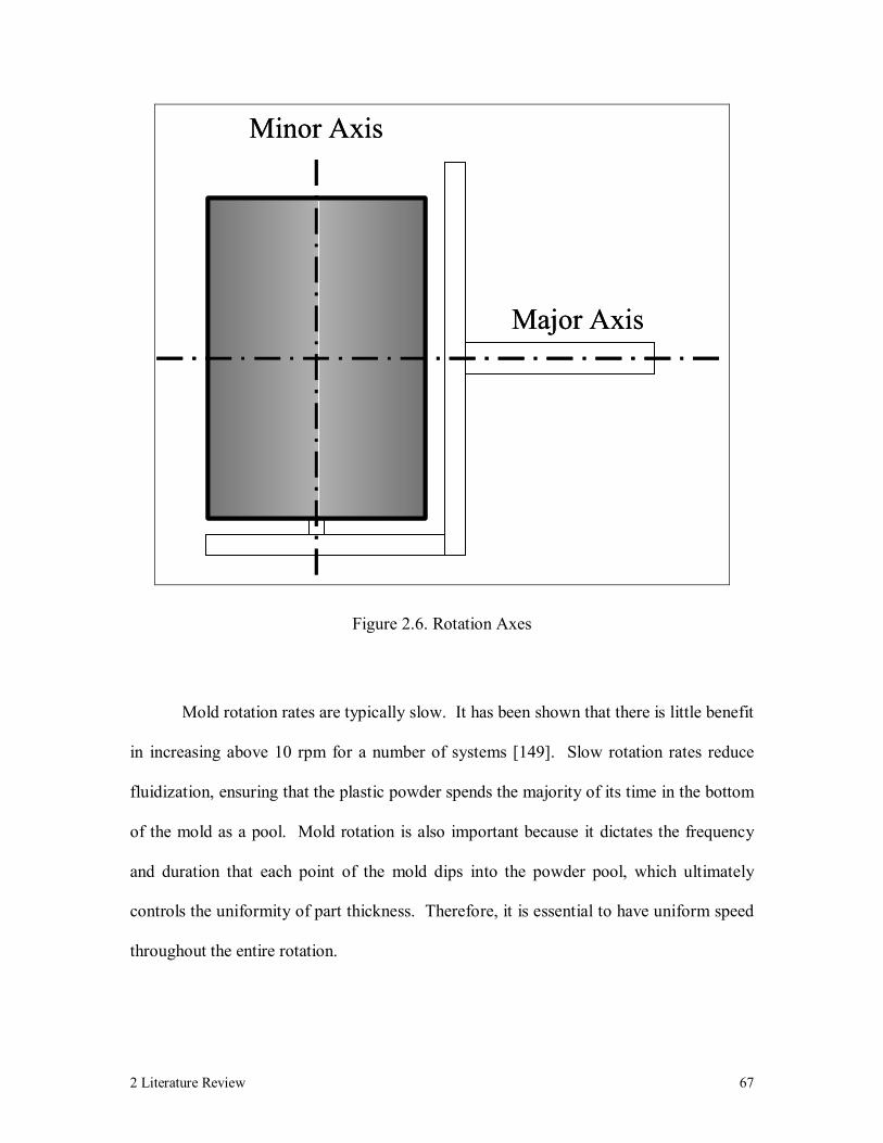
2 Literature Review 67
Major Axis
Minor Axis
Major Axis
Minor Axis
Figure 2.6. Rotation Axes
Mold rotation rates are typically slow. It has been shown that there is little benefit
in increasing above 10 rpm for a number of systems [149]. Slow rotation rates reduce
fluidization, ensuring that the plastic powder spends the majority of its time in the bottom
of the mold as a pool. Mold rotation is also important because it dictates the frequency
and duration that each point of the mold dips into the powder pool, which ultimately
controls the uniformity of part thickness. Therefore, it is essential to have uniform speed
throughout the entire rotation.

2 Literature Review 68
Mold position relative to the axes is important because it is possible that rotation
can induce differential acceleration of powder as it passes over the mold surface. So, it is
suggested not to orient the mold such that the mold surface is on the centerline of the
minor axis of rotation [133]. Along the centerline, material is only affected by major axis
rotation with maximum acceleration occurring at the ends of the mold. Because minor
axis speeds are relatively slow, variation in radial acceleration across the mold can be
great enough to have a significant effect on the distribution of thickness. As this
suggests, the distribution of thickness throughout the part is dependent upon not only the
speed but also the ratio of the major/ minor axes speeds. Originally, the machines had a
fixed major-minor rotation rate ratio of 4:1, which is still used as a starting point for
preliminary trials with new molds [132]. Modern machines allow independent control of
the major and minor axes to accommodate molding odd shaped parts.
It is important to recognize that the ratios of rotation speeds are often given in
terms of a speed ratio. Rotation speeds are obtained from tachometers located on the
major and minor drive shafts. Since the minor drive shaft is located inside the major
shaft, the measured minor rotation speeds are actually the total of the major and minor
rotation rates. The speed ratio is defined as:
rpmMajorrpmMinorrpmMajor
RatioSpeed−
= (2.26)
Selecting an appropriate speed is not a precise science. Actual values are
typically determined, to a large extent, by trial-and-error. The main reference for setting
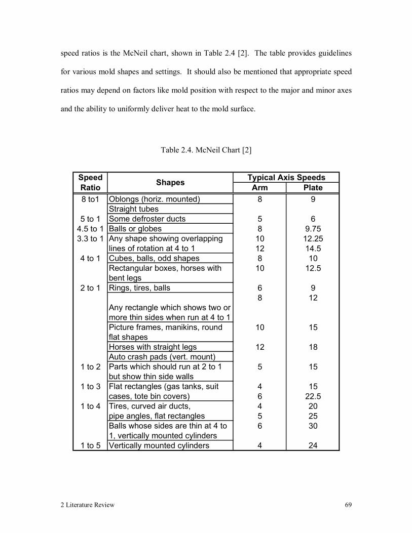
2 Literature Review 69
speed ratios is the McNeil chart, shown in Table 2.4 [2]. The table provides guidelines
for various mold shapes and settings. It should also be mentioned that appropriate speed
ratios may depend on factors like mold position with respect to the major and minor axes
and the ability to uniformly deliver heat to the mold surface.
Table 2.4. McNeil Chart [2]
Arm Plate8 to1 8 9
5 to 1 5 64.5 to 1 8 9.753.3 to 1 10 12.25
12 14.54 to 1 8 10
10 12.5
2 to 1 6 98 12
10 15
12 18
1 to 2 5 15
1 to 3 4 156 22.5
1 to 4 4 205 256 30
1 to 5 4 24
ShapesSpeed Ratio
Typical Axis Speeds
Any shape showing overlapping lines of rotation at 4 to 1
Rectangular boxes, horses with bent legs
Oblongs (horiz. mounted)Straight tubesSome defroster ductsBalls or globes
Cubes, balls, odd shapes
Rings, tires, balls
Any rectangle which shows two or more thin sides when run at 4 to 1Picture frames, manikins, round flat shapesHorses with straight legs
Balls whose sides are thin at 4 to 1, vertically mounted cylindersVertically mounted cylinders
Auto crash pads (vert. mount)Parts which should run at 2 to 1 but show thin side wallsFlat rectangles (gas tanks, suit cases, tote bin covers)Tires, curved air ducts,pipe angles, flat rectangles

2 Literature Review 70
2.1.3.2 Molding Cycle Time
For rotational molding to remain competitive against industrial blow molding and
emerging technologies such as twin sheet thermoforming and gas assisted injection
molding, cycle times must be reduced to a fraction of what they are today [24]. The
length of the molding cycle depends on each of the four cycle stages: loading, heating,
cooling, and unloading. Cycle times vary according to how the rotational molding
machine performs each of these steps [30]. Some machines have multiple arms, each
possessing a mold and occupying a step. If this is the case, each stage will require the
same amount of time, which is dictated by the longest step (typically the heating stage).
Although this is the most continuous approach to molding, it does not provide the most
control over each stage and large amounts of dead time are inherent in the shorter steps.
A single arm machine allows for the optimization of each stage. However, each stage is
not being used simultaneously, so production rates are lower. Industry’s solution was to
develop an independent arm machine that was capable of combining stage controllability
of a single arm unit with the more continuous operation of a multiple arm machine by
incorporating independent arm control and several holding areas.
Heating
The heating time can be divided into three parts: induction, fusion, and
densification [1]. Induction time refers to the time it takes the mold, from the onset of
heating, to reach the tack temperature. The tack temperature is identified as the
temperature where particles begin to adhere to the mold surface and therefore, nearly
coincides with the melt temperature. There are a number of parameters, listed in order of
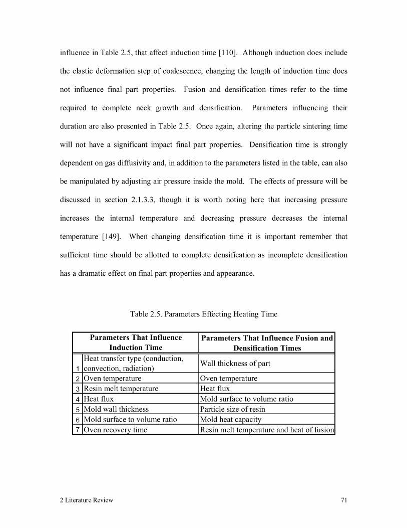
2 Literature Review 71
influence in Table 2.5, that affect induction time [110]. Although induction does include
the elastic deformation step of coalescence, changing the length of induction time does
not influence final part properties. Fusion and densification times refer to the time
required to complete neck growth and densification. Parameters influencing their
duration are also presented in Table 2.5. Once again, altering the particle sintering time
will not have a significant impact final part properties. Densification time is strongly
dependent on gas diffusivity and, in addition to the parameters listed in the table, can also
be manipulated by adjusting air pressure inside the mold. The effects of pressure will be
discussed in section 2.1.3.3, though it is worth noting here that increasing pressure
increases the internal temperature and decreasing pressure decreases the internal
temperature [149]. When changing densification time it is important remember that
sufficient time should be allotted to complete densification as incomplete densification
has a dramatic effect on final part properties and appearance.
Table 2.5. Parameters Effecting Heating Time
Parameters That Influence Fusion and Densification Times
1Heat transfer type (conduction, convection, radiation) Wall thickness of part
2 Oven temperature Oven temperature3 Resin melt temperature Heat flux4 Heat flux Mold surface to volume ratio5 Mold wall thickness Particle size of resin6 Mold surface to volume ratio Mold heat capacity7 Oven recovery time Resin melt temperature and heat of fusion
Parameters That Influence Induction Time

2 Literature Review 72
The heating cycle can be monitored by recording the temperatures of the oven, the
exterior and interior wall of the mold, and the air temperature inside the mold. These
data have a characteristic shape, unique to the rotational molding process. The oven
temperature is important because it provides a means of assessing the ability of the oven
to deliver heat. The thermal traces for the mold walls provide a measure of how heat is
received from the oven and transferred to the powder. The internal air temperature
provides perhaps the most interesting information. After the cycle begins, the internal air
temperature increases steadily (constant slope in plot) until it surpasses its tack
temperature [24]. This is sometimes referred to as the “kink” temperature and is
identified as the temperature at which the powder begins to melt and adhere to the mold
surface [24]. The heating rate slows as the cycle proceeds, indicating particle adhesion.
The plastic acts as a heat sink against the inner surface of the mold by absorbing energy
as it melts and retarding the rate of energy transfer to the cavity air. Once all the material
has melted, the temperature trace resumes a higher heating rate, often being very similar
to what was originally witnessed at the beginning of the cycle. There is generally a lag
between the internal mold thermal trace and the cavity air trace. This lag can be
increased further if there is either a large amount of powder or the powder has low
thermal conductivity [24].
Cooling
A thermal gradient remains after heating, with the mold’s external surface being
the hottest and the internal cavity air being the coolest parts of the system. The system is
typically cooled from the outside, which can be done by forced air, water mist, or water

2 Literature Review 73
shower. External cooling causes the maximum temperature to shift from the external
surface, through the mold and densified polymer, towards the mold cavity. This process
is referred to as thermal inversion. The rate of thermal inversion is dependent upon
relative thermal properties and the thickness of both the mold and polymer.
The rate of thermal inversion is important because it can adversely influence final
part properties by developing residual stresses [114]. Rapid cooling can freeze molecular
structure in a metastable state and eventually, chains move to increase stability, resulting
in warpage and distortion. High cooling rates can also reduce part density in
semicrystalline materials by increasing the amorphous content, which increases impact
strength and flexibility [114, 132]. In extreme cases the molding can develop surface
distortions and even collapse from the rapid change of internal pressure if a vent is not
present to equalize pressure [24]. The cavity may be pressurized to reduce shrinkage
ensure that the molding does not pull away from the mold because that dramatically
reduces the effectiveness of heat transfer. Therefore, water cooling must be applied
judiciously, typically only after thermal inversion and recrystallization has occurred. On
the other hand, slow cooling increases the crystalline content and density, while reducing
impact strength.
A number of techniques have been used to determine the most effective cooling
rate. Initially, cooling rates were selected by trial-and-error. Molders soon discovered
that it was a difficult and inefficient method to optimize cycle time and part performance.
An obvious addition to the selection process was the differential scanning calorimeter
2 Literature Review 74
(DSC). DSCs quickly and accurately provide valuable information about melting and
recrystallization by subjecting samples to various heating and cooling rates. As their
accuracy improves, process simulation has become a more common method of screening
process conditions. With the advent of portable multiplexed thermocouple platforms, the
most promising conditions can be quickly verified before being scaled to the larger, more
expensive equipment.
2.1.3.3 Vacuum and Pressure
Vacuum or additional pressure within the mold can produce a number of effects
depending on how it is applied. In general, introducing a small positive pressure (5 to 10
psi) during densification decreases both the frequency and size of entrapped bubbles [24].
Pressure compresses the trapped bubbles, acting to increase the solubility in the bulk
polymer by increasing the concentration gradient in the dissolving bubble and
accelerating bubble extinction. The majority of pinholes can be completely removed in
as little as thirty seconds [149]. It has been shown to increase properties like tensile
strength, modulus, and impact strength, but improvement may be limited to cosmetic
quality, which can be as important as mechanical properties. If pressure is applied before
bubble formation the air concentration is increased but as long as the pressure is
maintained there will be no net effect because there is no compressive force on the
bubbles (the pressure inside the bubbles is equivalent to that inside the mold). Of course
applying pressure prior to bubble formation then releasing it during densification will
cause bubbles to expand.
2 Literature Review 75
If a vacuum is introduced prior to bubble formation the effect is very similar to
applying pressure during densification. However, this method should produce better
results, especially in polymers with low gas permeability, because the concentration of air
is decreased [24]. By removing the air at the onset bubble extinction does not depend on
gas dissolution into the polymer. It is not necessary to hold the vacuum during the entire
heating cycle, just until bubbles form. At that point, releasing the vacuum will cause the
bubbles to disappear almost immediately. Since this process occurs while the mold
temperature is increasing, additional heating after bubble formation will cause bubbles to
grow. Applying a vacuum after bubble formation will cause bubble growth.
2.1.3.4 Mold Release Agent
Mold release agents are used because, even in the simplest geometries, moldings
stick to the mold surfaces. Mold release agents are designed to interfere with polymer
adhesion to the mold surface by reducing the mold’s surface energy [149]. Over 250
types of mold releases exist, varying from having to be applied each cycle to permanent
alteration of both internal and external surfaces.
Molten polymer will wet a mold surface if the surface energy of the mold is
greater than that of the polymer. Mold surface energies are typically an order of
magnitude greater than polymers so, in theory, they should spread easily without many
defects [3, 53]. In practice, bare metal surfaces are not as good as theory suggests
because an oxidative layer forms that reduces surface energy. Oxidation rates increase
with temperature and coincidentally, the polymer is exposed to the highest temperatures

2 Literature Review 76
during rotational molding at the mold/polymer interface [87]. In the most extreme cases,
like with polyethylene, oxidation causes the formation of chemical bonds between the
polymer and the mold surface. This escalates the sticking problem and introduces an
increased need for release agents. Unfortunately, mold release agents act by reducing
surface energy to impair adhesion and that reduction inherently, by reducing the
polymers affinity to wet the surface, increases the number of pinholes in the surface.
2.2 Thermotropic Liquid Crystalline Polymers
The purpose of this section is to review various aspects of main chain TLCP
rheology and mechanical properties that pertain to rotational molding. In fact, their
unique performance and rheological behavior inspired their selection for rotational
molding because they may extend the processing technique to higher performance
applications where conventional rotational molding polymers are insufficient.
The section begins with the review of TLCP mechanical properties in section
2.2.1. As some mechanical properties are dependent on the processing technique, it
should be stated that reported values might not be representative of what may be obtained
from rotational molding. This is especially true in properties that are strongly dependent
on the degree of molecular orientation. Section 2.2.2 focuses on various rheological
aspects of TLCPs.

2 Literature Review 77
2.2.1 Mechanical Properties
Strength and Modulus
Mechanical properties, especially tensile strength and modulus, depend upon the
degree of orientation achieved. This is limited by the fabrication method and geometry
of the manufactured item. A compression molded unoriented LCP has mechanical
properties similar to that of a conventional isotropic polymer [104]. Injection molding
imposes higher deformation rates that increase the degree of orientation, especially in the
skin, which makes the major contribution to stiffness [31]. Injection molded main chain
TLCPs show superior tensile moduli to those molded from conventional glass fiber
reinforced isotropic polymers. As the degree of orientation increases in the testing
direction, the mechanical properties approach those of main chain TLCP fibers [21, 130].
Simplistically, the layered structure of injection molded TLCP can be viewed as a
microcomposite composed of layers with varying directional orientation [104]. Each
layer contributes in an integral manner to the mechanical properties of the entire molding.
Modulus is dependent upon layer thickness and the direction and degree of orientation of
polymer chains in those layers. Each of these factors depends on the processing
conditions and the fluid’s rheological response to the imposed flow conditions. Stiffness
can also be varied through manipulation of the chemical composition. The flexural
modulus of injection molded tensile bars with varying HBA content was studied. As
HBA content increases and becomes great enough for the polymer to transition to a liquid
crystalline phase, the modulus monotonically increases [14]. Orientation was measured
as a function of depth through the moldings. Despite the obvious skin-core effects, it was

2 Literature Review 78
found that an increase in molecular orientation was mainly responsible for the increase in
modulus [13]. From this, it was concluded that simply creating a liquid crystal
mesophase is not sufficient to acquire a system with high, self-reinforcing modulus; the
mesophase must become sufficiently oriented. However, if this is done effectively,
TLCPs can exhibit exceptionally high strength and modulus. Moldings may retain these
properties at elevated temperatures (>200°C), which make them suitable for high
temperature applications.
TLCP articles possess some degree of anisotropy, a difference in properties when
tested parallel and perpendicular to the flow direction, which is reported as the anisotropy
ratio. The anisotropy ratio increases with the degree of orientation and is therefore
greatest in fibers. The anisotropy ratio for injection molded TLCP has been shown to fall
somewhere between 4:1 to 10:1, increasing with decreasing thickness as the proportion of
skin and core increases [118, 62, 29]. Introducing fillers tends to increase the anisotropy
ratio of conventional isotropic polymers, but disrupts molecular alignment and reduces
the ratio for TLCPs [118]. Although not typically desirable, this is one way of improving
the cross flow properties.
Dimensional Stability
TLCPs are used for high precision components that require close tolerances on
dimensional quantities. There is very little difference in molecular configuration, and
therefore a negligible density change between the melt and solid states for TLCPs. They
also typically possess little elastic recovery. This means that when molded, they exhibit

2 Literature Review 79
very low mold shrinkage and warpage when compared with isotropic polymers. Once
molded, they retain their molded dimensions well. One reason for this is that TLCPs
absorb very small quantities of water (typically less than 0.2% when immersed in water),
which makes the effects of swelling from moisture absorption negligible [104]. The
coefficient of linear thermal expansion is much lower for TLCPs than for conventional
polymers, even when conventional polymers have been reinforced with glass fibers [31].
Incidentally, they are quite similar to values for metals (TLCPs < 1, 1< Metals < 3
cm/cm/°Cx10-5). This similarity results in good integrity and minimal strain during
thermal cycling of components including both materials [104].
Barrier Properties and Chemical Resistance
TLCPs act as excellent barriers to gases, with permeability coefficients for He,
H2, Ar, N2, CO2 comparable to or smaller than those for polyacrylonitrile, one of the least
permeable polymers known [26]. See Table 2.6 for a comparison between Vectra A900
and PAN. They also have exceptionally low oxygen and water vapor permeabilities. The
low permeability seems to be more of a result of low gas solubility rather than low gas
diffusion, though it has been shown that diffusion can be greatly reduced by thermal
treatment in systems that are crystallizable [22]. It was calculated that crystalline content
would have to be near 90% or more to explain the solubility. However, crystallinity is
often below 20% for an unannealed sample so it seems that liquid crystalline order is
responsible [104].

2 Literature Review 80
Table 2.6. Comparison of Gas Transport Properties at 35°C of Vectra A900 and PAN
[162]
LCP PAN LCP PAN LCP PANHe 17,700 71,000 6,600 2,700 2.0 200N2 3.0 2.9 1.4 0.042 1.6 52Ar 10 18 1.5 0.042 5.4 330
CO2 70 280 0.96 0.023 51 9200
P x 1015 D x 1010 S x 103
Gas ( )
⋅⋅
⋅Hgcmcm
cmSTPcmsec2
3
( )sec2cm ( )[ ]atmcmSTPcm ⋅33
A precise explanation for the low solubility observed in TLCPs has not been
determined. Two explanations have been proposed. The liquid crystalline phase is the
only viable region for gas sorption, but solubility is orders of magnitudes less than in
amorphous polymers because of efficient chain packing. Another explanation is that the
polydomain structure of the mesophase is responsible [162]. It was suggested that
domain boundaries are separated by a material having gas solubility and diffusion
characteristics similar to flexible chain polymers. If this boundary material accounts for
only a few percent of the total volume, it would explain the behavior. This two phase
depiction of permeability was used with reasonable success to estimate the values for
Vectra type materials [162].
TLCPs have excellent resistance to a wide range of organic solvents and exhibit
good hydrolysis resistance. Retention of properties in both acidic and basic environments
is also very good [21]. As with gas barrier properties, it is likely that liquid crystalline
2 Literature Review 81
order is somewhat responsible; it is possible to decrease chemical resistance in TLCPs by
increasing backbone flexibility [21].
Interfacial Strength
A major problem identified during the injection molding of TLCPs is poor weld-
line strength. Adjoining flow fronts have difficulty reestablishing equilibrium molecular
structure across the interface. This can dramatically reduce tensile strength as
demonstrated by the injection molded tensile bar study, where tensile strength is reduced
to roughly 10% of the continuous sample [104]. It has also been shown that fillers may
improve strength, but not significantly. The current approach to handle this issue is to
manipulate weld line position to areas where they will have the least effect on properties.
A detailed study of the adhesion mechanism, or lack thereof, in TLCPs has not
been completed. Flexible chain polymers that are void of ionic interactions mend by
molecular diffusion to establish equilibrium across the interface. The study of molecular
diffusion in TLCPs has neglected interfacial or domain effects. It has revealed that the
rigid nature of the LC molecule requires the combination of both rotation and translation.
Diffusion is anisotropic, dependent on molecular dimensions and the degree of
orientational order [161]. Incidentally, it has been shown that orientation can be strongly
influenced at fluid boundaries, even at free surfaces [148]. This may imply that boundary
induced orientation inhibits diffusion across an interface.
Miscellaneous
2 Literature Review 82
Main chain TLCPs possess several other notable properties. They are rather
tough materials that typically do not fail in a brittle or ductile fashion upon impact.
Instead, their failure is more benign, similar to that of long fiber reinforced polymers or
natural wood [104]. Moldings also show extremely low flammability, without the need
for flame retardant additives. They tend to have low dielectric constants (less than 3.0)
and high dielectric strength (greater than 7000 V/ 25µm).
2.2.2 Rheology of Thermotropic Liquid Crystalline Polymers
TLCPs exhibit strong interdependence between morphology, rheology, and
processing [119]. This makes attempting to characterize the fluid’s rheology difficult. In
fact, the flow behavior of these materials is so sensitive to temperature and deformation
history that sample preparation and loading procedures change the initial morphology
(initial conditions) and alter rheological results, especially the transient response. One
way to reduce response fluctuation is to impose reproducible initial conditions by heating
the melt into the isotropic state to erase nematic texture. This eliminates any previously
induced preferential orientation due to deformation or temperature, thus generating a
randomly oriented (no bulk orientation) polydomain structure upon quenching back into
the LC phase [157]. This is common practice for main chain TLCPs with flexible
spacers, and it is partially responsible for why they are referred to as model nematic
TLCP systems (the other reason is their lack of residual crystallinity in the melt state and
subsequent aversion of biphasic influences) [51, 157]. However, the procedure does not
apply to more rigid main chain TLCPs because the nematic-isotropic transition is usually
above degradation temperatures, making it inaccessible. Also, in those systems,
2 Literature Review 83
recrystallization or transesterification may occur at melt temperatures, leading to time
dependent material properties [99, 113]. It is also possible to obtain reproducible data by
following identical sample loading protocols and applying a flow field to introduce
repeatable initial conditions prior to the rheological measurement. Unfortunately, the
initial morphological state is still unknown, making interpretation of start-up transients
difficult and inhibits meaningful comparisons between studies [6, 157].
To familiarize the reader with the current state of TLCP rheological
characterization, a review of TLCP rheology is contained in this section. This review is
not meant to encompass all TLCP rheology. Instead, emphasis has been placed upon the
responses important to the rotational molding process. This includes behavior common,
and particular, to main chain thermotropic systems with nematic mesophases.
Observations of the LCP response to shear and shearfree flows are summarized in the two
sections that compose this chaper, 2.2.2.1 and 2.2.2.2.
2.2.2.1 TLCP Response to Shearfree Flow
It was shown in the review on particle sintering that the deformation kinematics
for coalescence are equibiaxial extension. For this reason the rheological response of
TLCPs in extensional flow is reviewed.
Despite inherent difficulties involved with extensional rheometry, several
experimental studies exist on the extensional behavior of TLCPs. In a lyotropic system
of HPC in acetic acid, it has been shown that the transient uniaxial elongational viscosity,

2 Literature Review 84
ae+, was independent of extension rate over the range 0.02 to 10 sec-1 [117]. It was also
demonstrated that the Trouton ratio was approximately 9, three times greater than the
linear visoelastic limit observed in flexible chain polymers. The generality of these
results are somewhat questionable. Experiments were performed with a gravity spinning
apparatus, where the applied deformation rate is not constant and the results for flexible
chain polymers do not agree with homogeneous extensional flows.
Experiments have been performed on HPC as a thermotropic system [25]. A
single rotary clamp device was used to measure uniaxial shearfree stress growth with
extension rates from 0.005 to 0.05 sec-1 under isothermal conditions (180°C). At short
times, ae+ was independent of rate but showed rate thinning with increasing time. The
curves also passed through a maximum at strains around 0.2 strain units, which is lower
than what would be anticipated for a steady state linear viscoelastic fluid. The generality
of the results from this study are also limited because yield stresses have been reported in
HPC melts at 180°C, which could explain the rate thinning behavior [44, 152].
Another series of thermotropic extensional tests were performed with HPC and
also included Vectra A 900 [164]. Extension was applied with a rotary clamp device that
could be operated as either a single clamp or a twin clamp. In both materials, the
transient uniaxial elongational viscosity was found to respond similarly to that of
isotropic melts of linear polyolefins. At small strains linear viscoelastic behavior was
observed, which progressed to strain hardening as strains increased, see Figure 2.7. The
HPC was tested in both the isotropic and anisotropic states. It was concluded that the
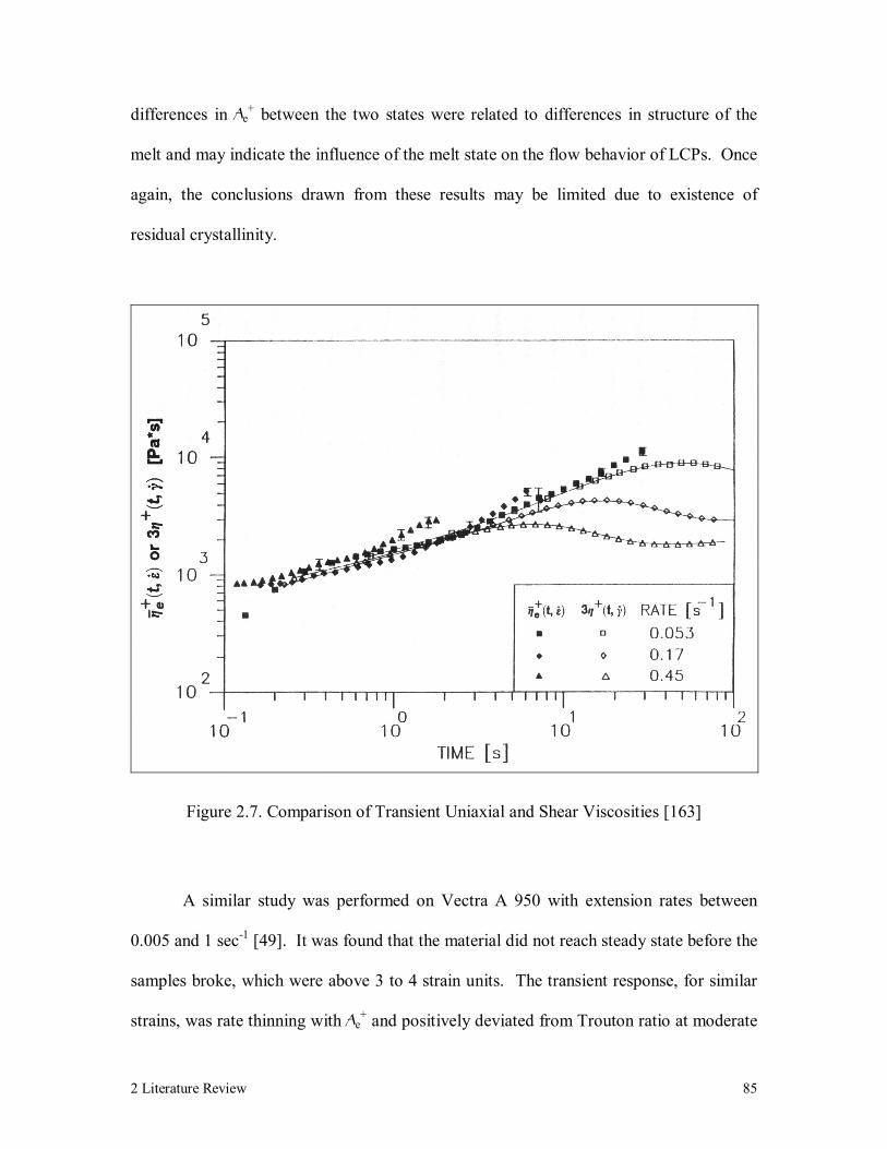
2 Literature Review 85
differences in ae+ between the two states were related to differences in structure of the
melt and may indicate the influence of the melt state on the flow behavior of LCPs. Once
again, the conclusions drawn from these results may be limited due to existence of
residual crystallinity.
Figure 2.7. Comparison of Transient Uniaxial and Shear Viscosities [163]
A similar study was performed on Vectra A 950 with extension rates between
0.005 and 1 sec-1 [49]. It was found that the material did not reach steady state before the
samples broke, which were above 3 to 4 strain units. The transient response, for similar
strains, was rate thinning with ae+ and positively deviated from Trouton ratio at moderate
2 Literature Review 86
strains. Also, samples that were injection molded consistently demonstrated greater
values for viscosity than compression molded counterparts. It was determined that the
results from injection molded samples were strongly influenced by skin-core effects. The
samples did not melt uniformly and the skin often separated from the core as a result.
Experimental studies of TLCP extensional flow properties has not been limited to
uniaxial flow. A series of thermotropic copolyesters (60 HBA/ 40 PET, 80 HBA/ 20
PET, and 73 HBA/ 23 HNA) were studied in equibiaxial extensional flow [36].
Lubricated squeezing flow was performed to measure the transient biaxial extensional
viscosity. Results showed that ab+ was slightly lower at small strains than 6h+. At
greater strains the transient biaxial elongational viscosity exceeded the Trouton ratio
because of strain hardening. The results of the study were limited to relatively small
strains because the equibiaxial response becomes contaminated with shear effects when
proceeding through larger strains due to the loss of lubrication effectiveness.
2.2.2.2 TLCP Response to Shear Flow
The previous discussion of the rheological response of TLCPs in shearfree flows
alluded to the use of the Trouton ratio to establish a correlation between shear and
shearfree flows for linear viscoelastic materials. From the experimental results reviewed
in the previous section, this relationship is expected to remain valid for TLCPs
throughout the coalescence process because it is limited to low rates and small strains.
Therefore, the viscosity behavior at low shear rates is of particular interest because of its
role in coalescence.

2 Literature Review 87
Steady Response
Onogi and Asada proposed an explanation for a well documented feature of the
steady shear viscosity [122]. They suggested that a general, three-region flow curve
could be used to describe the viscous behavior of LCPs in response to steady shear flow,
as shown in Figure 2.8. In addition, by introducing the concept of domains and
polydomain structure, with individual molecular orientation in each domain, they were
able to relate each of the three-regions to different stages of destruction of polydomain
texture to form a single nematic phase [10, 119]. Region I occurs at low rates and has
shear-thinning behavior that suggests the existence of a yield stress. The mesophase is
dominated by defects that result in polydomain texture [108]. Region II exists at
moderate rates where shear-thinning transitions to a Newtonian plateau as a dynamic
balance of shear induced texture [119]. The polydomain texture becomes more refined as
the directors in the various domains begin to align [10]. Region III occurs at even higher
rates and is another shear-thinning region. If rates are great enough, the polydomain
texture is fully reduced to a monodomain [10, 49].

2 Literature Review 88
I II III
Log Shear Rate
Log
Vis
cosi
tyI II III
Log Shear Rate
Log
Vis
cosi
tyI II III
Log Shear Rate
Log
Vis
cosi
ty
Figure 2.8. Three-Region Flow Curve [163]
Several studies have confirmed the existence of the three-region concept in both
lyotropic and thermotropic systems [49, 119, 165]. Still, others have shown some
systems have well defined zero shear viscosities proving that region I is not an essential
characteristic of all LCPs [80, 163]. There is evidence from a number of studies on
thermotropic copolyesters that region I behavior can be removed by an elevated thermal
treatment, suggesting the presence of residual higher melting temperature crystallites
were responsible for that behavior [76, 77, 106, 156, 163].
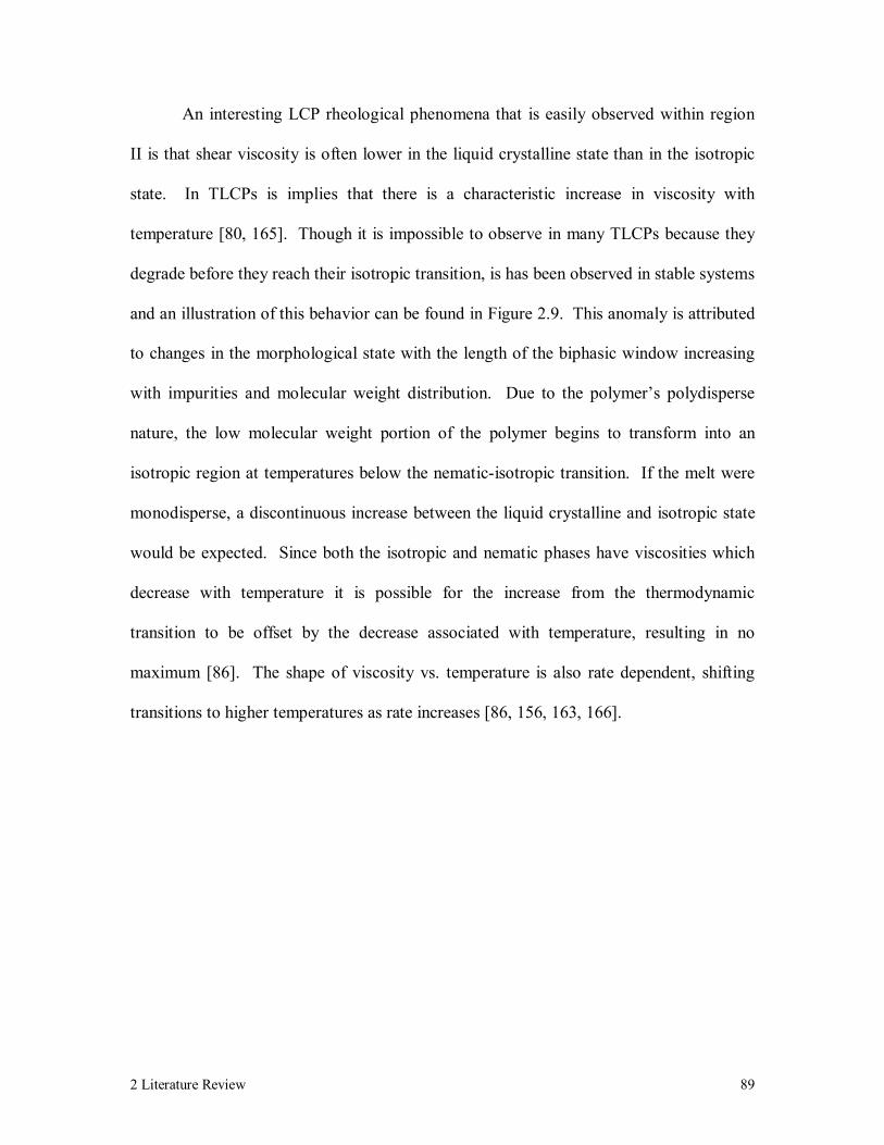
2 Literature Review 89
An interesting LCP rheological phenomena that is easily observed within region
II is that shear viscosity is often lower in the liquid crystalline state than in the isotropic
state. In TLCPs is implies that there is a characteristic increase in viscosity with
temperature [80, 165]. Though it is impossible to observe in many TLCPs because they
degrade before they reach their isotropic transition, is has been observed in stable systems
and an illustration of this behavior can be found in Figure 2.9. This anomaly is attributed
to changes in the morphological state with the length of the biphasic window increasing
with impurities and molecular weight distribution. Due to the polymer’s polydisperse
nature, the low molecular weight portion of the polymer begins to transform into an
isotropic region at temperatures below the nematic-isotropic transition. If the melt were
monodisperse, a discontinuous increase between the liquid crystalline and isotropic state
would be expected. Since both the isotropic and nematic phases have viscosities which
decrease with temperature it is possible for the increase from the thermodynamic
transition to be offset by the decrease associated with temperature, resulting in no
maximum [86]. The shape of viscosity vs. temperature is also rate dependent, shifting
transitions to higher temperatures as rate increases [86, 156, 163, 166].
2 Literature Review 90
Temperature
Shea
r Vis
cosi
ty
Nematic
Isotropic
Biphasic
Temperature
Shea
r Vis
cosi
ty
Nematic
Isotropic
Biphasic
Figure 2.9. Shear Viscosity Temperature Dependence Near the Nematic-Isotropic
Transition
The onset and extent of region III shear-thinning is an important aspect of
rheological behavior that is related to a characteristic relaxation time for the polymer
[11]. A rule of thumb for the rate that shear-thinning begins is the reciprocal of the
longest characteristic relaxation time, implying that onset at lower rates translates to
longer relaxation times. By measuring the shear-thinning behavior of the isotropic and
liquid crystalline states a comparison of relaxation can be made between those states.
With that stated, it has been found that shear thinning tends to occur at lower rates and
possess stronger shear-thinning behavior than in the isotropic phase [12, 156, 166]. It
2 Literature Review 91
was also observed that either the isotropic or the LC phase may behave as a Newtonian
fluid [163]. Factors that determine shear-thinning have not been well established, but
should be related to various characteristics specific to each system, such as molecular
weight, molecular weight distribution, chain stiffness, etc. A study with a well
fractionated TLCP showed that polydisperse samples possess a higher degree of shear-
thinning than fractionated samples [12].
The three-region flow curve does not generally apply to LCPs. It has been shown
that only one or two of the regions may exist in some LCPs. Still, it has experienced
continued use in literature as a framework for the description of the viscosity behavior of
LCPs and for comparison with the isotropic state.
Negative values for steady primary normal stress difference have been reported in
several studies on lyotropic systems. Its origin has been attributed to a condition known
as director tumbling. Although it was first predicted with the Doi model, it has been
experimentally confirmed in various monodomain lyotropes [18, 150, 169]. Nematics
may respond to shear flow in two distinct ways, while within the linear limit. The first is
referred to as flow aligning, where hydrodynamic torques on the director disappear
because the director rotates to a characteristic alignment angle in reference to the flow
field. The second response is director tumbling. The hydrodynamic torques in these
materials remain unbalanced, which leads to indefinite director rotation and negative
normal stresses.
2 Literature Review 92
There have been no reproducible reports of a steady negative first normal stress
difference in TLCPS [28]. Early reports of such behavior in commercial copolyesters
appear to have been undermined by residual normal stresses associated with sample
loading [28, 50]. In model systems, where the isotropic phase provides a means of
erasing those influences, only positive N1 values have been observed. However, the lack
of negative N1 values does not prove that tumbling is absent. A series of studies on
hydroxypropylcellulose (HPC) solutions over a wide range of temperatures and
concentrations have suggested that the semiflexible molecules may continue to exhibit
tumbling in their thermotropic phase [4, 60, 96].
As previously mentioned, LCP rheology is further complicated because it can be
influenced by prior deformation and thermal states. This is because thermal and shear
histories induce change in the anisotropic polydomain structure; by changing the
morphology the rheological response is changed [51, 82, 83, 166]. Although the majority
of these effects are observed in the transient response, it may influence steady shear
behavior. Preshearing, imposing a shear deformation history to stabilize the morphology,
has been found to shift the transition from region I to region II to lower shear rates [28,
46, 51]. It can also narrow the range of shear rates and decrease the viscosity of region II
[119]. Imposing a particular thermal history is capable of altering the behavior in an
entire region.
Transient Response
2 Literature Review 93
Oscillations in the response to stress growth have been observed in the low shear
rate, linear regime of some lyotropic systems [157]. The oscillations are slowly damped
by elastic effects associated with spatial distortions of the director field, which are
induced by director tumbling. This distortional elasticity also provides the driving force
for large strain recovery [17, 97]. Also during stress growth, N1 may pass through a
negative value before settling into a positive steady value. This has been established as a
nonlinear viscoelastic effect that is a signature of a transition from tumbling to flow
aligning behavior [71, 96, 109].
Stress growth experiments have been performed on a number of TLCP systems
with varying results. Monodomain experiments on a semiflexible main chain TLCPs
show that flow alignment was confirmed near the nematic-isotropic transition and
tumbling was found close to the nematic-smectic transition [151]. Other studies have
only shown indirect evidence of either flow aligning or tumbling. PSHQ10
(poly[(phenylenesulfonyl)-p-phenylene 1,10-decamethylenebis(4-oxybenzoate)]), a
thermotropic polyester with flexible spacers, shows a large stress overshoot and weak
negative N1 undershoots followed by more pronounced overshoots. A very similar
relative, PSHQ6-12 (random copolyester with two spacer lengths) does not show
negative N1 transients [25]. At low temperatures and high rates, multiple N1 overshoots
are observed as well as multiple shear stress overshoots [39, 81]. Multiple overshoots
could indicate tumbling, but have been attributed to the transient response at different
structural levels [6, 39]. Reproducible tumbling-like behavior in transients has also been
reported in the commercial thermotrope Vectra B 950, but only under certain preshear
2 Literature Review 94
conditions [6]. TLCPs generally do not exhibit the characteristic damped oscillations that
are taken as a clear indication of tumbling. When they do occur, oscillations in TLCPs
are not as pronounced and are damped much more quickly than those observed in
lyotropic systems.
2.3 Research Objectives
The previous sections of this chapter have outlined the rotational molding
processs and how it is understood. Current limitations in rotational molding were also
discussed to explain why high performance rotational molding resins are not currently
being used, although there is a strong desire to apply such technology if it were
developed.
Thermotropic liquid crystal polymers are a class of materials that provide a
number of properties that are desirable to the rotational molder. However, the current
state of understanding of the coalescence process and TLCP behavior under such flow
conditions is inadequate to effectively apply these materials to rotational molding.
Developing this technology will not only advance the field of rotational molding
but it can also be applied to other areas. For example, this would extend the application
of TLCPs, and possibly other high performance polymers, to powder coating operations
such as fluidized bed and flame spray, allow the fabrication of particulate performs,
dispersion coating, and selective laser sintering.
2 Literature Review 95
This research is intended to provide a better understanding of what material
properties are necessary for successful rotational molding and to develop a method to
establish if TLCPs possess those properties. To accomplish this, the following three
objectives have been identified:
I. Develop a method for identifying conditions that generate TLCP behavior
necessary for successful coalescence.
II. Determine if the identified coalescence conditions can be effectively translated
to a lab scale rotational molding device.
III. Establish rotational molding conditions that optimize mechanical properties.
A review of the literature relevant to the rotational molding of thermotropic liquid
crystalline polymers has been presented in this chapter. The subsequent chapter contains
a detailed account of the experimental design and procedures devised to address the
stated research objectives.

2 Literature Review 96
2.4 References
1. Anon., “Sclair Polyethylene Resins for Rotational Moulding: Powder
Characteristics’, Sclair Manual, Dupont, Canada, Mar. (1980)
2. Anon., “Graph of Ratio of Rotation,” McNeil Akron, Akron, Ohio, undated.
3. “Metals Handbook 9th Edition,” edited by Boyer, H.E., Gall, T.L., Metals Park,
Ohio: American Society of Metals (1985)
4. Baek, S.G., Magda, J.J., Larson, R.G., Hudson, S.D., “Rheological Differences
Among Liquid-Crystalline Polymers. II. Disappearance of Negative N1 in Densely
Packed Lyotropes and Thermotropes,” Journal of Rheology, 38, 5, 1473 (1994)
5. Barnetson, A., Hornsby, P.R., “Observations on the Sintering of Ultra-High
Molecular Weight Polyethylene (UHMWPE) Powders,” Journal of Materials
Science Letters, 14, 80 (1995)
6. Beekmans, F., Gotsis, A.D., Norder, B., “Influence of Flow History on Stress
Growth and Structure Changes in the Thermotropic Liquid Crystalline Polymer
Vectra B950,” Rheologica Acta, 36, 82 (1997)
7. Bellehumeur, C.T., Bisaria, M.K., Vlachopoulos, “An Experimental Study and
Model Assessment of Polymer Sintering,” Polymer Engineering and Science, 36,
17, 2198 (1996)
8. Bellehumeur, C.T., Vlachopoulos, J., “Polymer Sintering and its Role in
Rotational Molding,” SPE ANTEC, 44 (1998)
9. Bellehumeur, C.T., Kontopoulou, M., Vlachopoulos, J., “The Role of
Viscoelasticity in Polymer Sintering,” Rheoogica. Acta, 37, 3, 270 (1998)
2 Literature Review 97
10. Berghausen, J., Fuchs, J., Richtering, W., “Rheology and Shear Orientation of a
Nematic Liquid Crystalline Side-Group Polymer with Laterally Attached
Mesogenic Units,” Macromolecules, 30, 24, 7574 (1997)
11. Bird, R.B., Armstrong, R.C., Hassager, O., Dynamics of Polymeric Liquids.
Volume 1: Fluid Mechanics, 2cnd Edition, John Wiley & Sons, New York (1987)
12. Blumstein, A., Thomas, O., Kumar, S., “Rheological Behavior of Thermotropic
Flexible Main-Chain Polyesters Based on 4,4’-Dioxy-2,2’-Dimethyl
Azoxybenzene Mesogens, I. Oscillating Shear Behavior,” Journal of Polymer
Science: Polymer Physics Ed., 24, 27 (1986)
13. Blundell, D.J., Chivers, R.A., Curson, A.D., Love, J.C., MacDonald, W.A., “The
Relationship of Chain Linearity of Aromatic Liquid-Crystal Polyesters to
Molecular Orientation and Stiffnessof Moldings,” Polymer, 29, 1459 (1988)
14. Blundell, D.J., Chivers, R.A., MacDonald, W.A., High Performance Polymer, 1,
97 (1989)
15. Brostow, W., “An Introduction to Liquid Crystallinity” in Liquid Crystalline
Polymers: From Structures to Applications, edited by Collyer, A.A., Elsevier
Applied Science, New York (1992)
16. Brown, R.L., Richards, J.C., Principles of Powder Mechanics: Essays on the
Packing and Flow of Powder and Bulk Solids, Pergamon Press, Oxford, (1970)
17. Burghardt, W.R., Fuller, G.G., “Transient Shear Flow of Nematic Liquid Crystals:
Manifestations of Director Tumbling,” Journal of Rheology, 34, 959 (1990)
18. Burghardt, W.R., Fuller, G.G., “Role of Director Tumbling in the Rheology of
Polymer Liquid Crystal Solutions,” Macromolecules, 24, 9, 2546 (1991)

2 Literature Review 98
19. Calundann, G.W., US Patent 4161470, Celanese Co. (1979)
20. Calundann, G.W., US Patent 4188996, Celanese Co. (1980)
21. Calundann, G.W., Jaffe, M., Robert A. Welch Conferences in Chemical Research
Proc. Synth. Polymers Houston, Texas, Nov., 247 (1982)
22. Cantrell, G.R., Freeman, B.D., Hopfenberg, H.B., Makhija, S., Haider, I., Jaffe,
M., Chapter 20, “The Influence of Thermal Annealing on Organic Vapor Sorption
and Transport in a Nematogenic Copolyester,” in Liquid Crystalline Polymers:
Proceedings of the International Workshop on Liquid Crystalline Polymers,
WLCP93, Capri, Italy, June 1-4 1993, edited by Carfagna, C., Elsevier Science
Inc. (1994)
23. Crawford, R.J., Scott, J.A., “The Formation and Removal of Gas Bubbles in a
Rotational Moulding Grade of PE,” Plastics and Rubber Processing and
Applications, 7, 2, 85 (1987)
24. Crawford, R.J., Throne, J.L., Rotational Molding Technology, Plastics Design
Library, William Andrew Publishing, New York (2002)
25. Chang, S., Han, C.D., “A Thermotropic Main-Chain Random Copolyester
Containing Flexible Spacers of Differing Lengths. 2. Rheological Behavior,”
Macromolecules, 30, 6, 1656 (1997)
26. Chiou, J.S., Paul, D.R., “Gas Transport in a Thermotropic Liquid-Crystalline
Polymer,” Journal of Polymer Science Part B: Polymer Physics, 25, 1699 (1987)
27. Chung, T.S., Cheng, S.X., Jaffe, M., Chapter 1 “Introduction of Liquid Crystalline
Materials,” in Thermotropic Liquid Crystal Polymers: Thin-film Polymerization,
2 Literature Review 99
Characterization, Blends, and Applications, edited by Chung, T.S., Technomic
Publ. Co., Inc., Lancaster, Pa (2001)
28. Cocchini, F., Nobile, M.R., Acierno, D., “Letter: About Negative First Normal
Stress Differences in a Thermotropic Liquid Crystalline Polymer,” Journal of
Rheology, 36, 7, 1307 (1992)
29. Cogswell, F.N., Part III: Characterization, “Observations on the Rheology of
Thermotropic Polymer Liquid Crystals,” in Recent Advances in Liquid Crystalline
Polymers, edited by Chapoy, L.L., Elsevier Science, New York, 165 (1985)
30. Covington, W.H., Jr., Chapter 4 “Rotational Moulding Machines,” in Rotational
Moulding of Plastics second edition, edited by Crawford, R.J., Research Studies
Press, John Wiley & Sons, New York (1996)
31. Cox, M.K., “The Application of Liquid Crystal Polymer Properties,” Molecular
Crystals and Liquid Crystals, 153, 415 (1987)
32. Cumberland, D., Crawford, R.J., The Packing of Particles, Elsevier Publishers,
Oxford, U.K. (1987)
33. Cundall, P.A., Jenkins, J.T., Ishibashi, I., “Evolution of Elastic Moduli in a
Deforming Granular Assembly,” in Powders and Grains, A.A. Balkema,
Rotterdam, Netherlands, 319 (1989)
34. Cutler, I.B., Hendrichsen, R.E., Journal of the American Ceramic Society, 51, 10,
604 (1968)
35. Donald, A.M., Windle, A.H., Liquid Crystalline Polymers, Cambridge University
Press (1992)

2 Literature Review 100
36. Done, D.D., “Studies on the Rheology and Morphology of Thermotropic Liquid
Crystalline Polymers,” Ph.D. Dissertation, Virginia Polytechnic Institute and State
University, Blacksburg, Va, 24061 (1987)
37. DeGennes, P.G., C.R. Acad. Sci. Paris, 291, 219, (1980)
38. DeGennes, P.G., Physics of Polymer Surfaces and Interfaces, ed. Sanchez, I.C.,
Butterworth-Heinemann, Boston, 55 (1992)
39. Driscoll, P., Masuda, T., Fujiwara, K., “Rheological Properties of a Homogeneous
Thermotropic Liquid-Crystalline Polyester: Dynamic Viscoelastic and
Interrupted-Flow Measurements,” Macromolecules, 24, 7, 1567 (1991)
40. Eshelby, J.D., Discussion in Paper by Shaler AJ, “Seminar on the Kinetics of
Sintering,” Transactions of AIME, 185, 11, 806 (1949)
41. Exner, H.E., Petzow, G., Sintering and Catalysis, edited by Kuczynski, G.C.,
Plenum Press, New York, 279 (1975)
42. Flory, P.J., Part II, Theory, “Theoretical Basis for Liquid Crystallinity in
Polymers,” in Recent Advances in Liquid Crystalline Polymers, edited by Chapoy,
L.L., Elsevier Science, New York, 99 (1985)
43. Frenkel, J.F., “Viscous Flow of Crystalline Bodies Under the Action of Surface
Tension,” Journal of Physics, (Moscow), 9, 5, 385 (1945)
44. Fuyiyama, M., “Capillary Flow Properties of Thermotropic
Hydroxypropylcelluloses,” Journal of Applied Polymer Science, 40, 67 (1990)
45. Garabedian, R.S., Helble, J.J., “A Model for the Coalescence of Amorphous
Particles,” Journal of Colloid and Interface Science, 234, 248 (2001)
2 Literature Review 101
46. Geiger, K., “Mechanical/ Thermal Pretreatment of LCP Melts and its Influence on
the Rheological Behavior of These Polymers,” in Processing and Properties of
Liquid Crystalline Polymers and LCP Based Blends, edited by Acierno, D., La
Mantia, F.P., ChemTec Publishing, Canada (1993)
47. German, R. M., Powder Metallurgy Science second edition, Metal Powder
Industries Federation, Princeton, New Jersey, (1994)
48. Giordano, M., Leporini, D., Chiellini, E., Galli, G., Structure and Transport
Properties in Organized Polymeric Materials, edited by Chiellini, E., Giordanao,
M., Leporini, D., World Scientific, Singapore (1997)
49. Gotsis, A.D., Odriozola, M.A., “Extensional Viscosity of a Thermotropic Liquid
Crystalline Polymer,” Journal of Rheology, 44, 5, 1205 (2000)
50. Han, C.D., Chang, S., “Note: On the First Normal Stress Difference of the
Thermotropis Copolyester 73/27 HBA/HNA,” Journal of Rheology, 38, 2, 241
(1994)
51. Han, C.D., Chang, S., Kim, S.S., “Rheological Behavior of Thermotropic Liquid
Crystalline Polymers: Effects of Thermal and Deformation Histories,” Molecular
Crystals and Liquid Crystals, 254, 335 (1994)
52. Han, K., Ley, G., Schuller, H., Oberthur, R., “On Particle Coalescence in Latex
Films,” Colloid Polymer Science, 264, 1092 (1986)
53. Heath, R.J., “A Review of the Surface Coating of Polymeric Substrates,”
Progress in Rubber and Plastics Technology, 6, 369 (1990)
54. Herring, C., “Effect of Change of Scale on Sintering Phenomena,” Journal of
Applied Physics, 21, 301 (1950)
2 Literature Review 102
55. Hooper, R., Macosko, C.W., Derby, J.J., “Assessing Flow-Based Finite Elements
Model for the Sintering of Viscoelastic Particles,” Chemical Engineering Science,
55, 5733 (2000)
56. Hopper, R.W., “Coalescence of Two Equal Cylinders: Exact Results for Creeping
Viscous Flow Driven by Capillarity,” Communications of the American Ceramic
Society, C-262 (1984)
57. Hopper, R.W., “Plane Stokes Flow Driven by Capillarity on a Free Surface,”
Journal of Fluid Mechanics, 213, 349 (1990)
58. Hopper, R.W., “Plane Stokes Flow Driven by Capillarity on a Free Surface. Part 2
Further Developments,” Journal of Fluid Mechanics, 230, 355 (1991)
59. Hopper, R.W., “Stokes Flow of a Cylinder and Half-Space Driven by Capillarity,”
Journal of Fluid Mechanics, 243, 171 (1992)
60. Huang, C.M., Magda, J.J., Larson, R.G., “The Effect of Temperature and
Concentration on N1 and Tumbling in a Liquid Crystal Polymer,” Journal of
Rheology, 43, 1, 31 (1999)
61. Incropera, F.P., DeWitt, D.P., Introduction to Heat Transfer third edition, John
Wiley & Sons, New York, (1996)
62. Jackson, W.J., Kuhfuss, H.F., “Liquid Crystal Polymer. I. Preparation and
Properties of p-Hydroxybenzoic Acid Copolyesters,” Journal of Polymer Science.
Polymer Chemistry Edition, 14, 2043 (1976)
63. Jagota, A., Dawson, P.R., “Micormechanical Modeling of Powder Compacts-I.
Unit Problems for Sintering and Traction Induced Deformation,” Acta
Metallurgica, 36, 9, 2551 (1988)
2 Literature Review 103
64. Jagota, A., Dawson, P.R., “Micormechanical Modeling of Powder Compacts-II.
Truss Formulation of Discrete Packings,” Acta Metallurgica, 36, 9, 2563 (1988)
65. Jagota, A., Dawson, P.R., “Simulation of the Viscous Sintering of Two Particles,”
Journal of the American Ceramic Society, 73, 1, 173 (1990)
66. Jagota, A., Mikeska, K.R., Bordia, R.K., “Isotropic Constitutive Model for
Sintering Particle Packings,” Journal of the American Ceramic Society, 73 [8],
2266-2273 (1990)
67. Jagota, A., Boyes, E.D., Bordia, R.K., “Sintering of Glass Powder Packings with
Metal Inclusions,” Materials Research Society Symposia Proceedings, 249, 475
(1991)
68. Jagota, A., Scherer, G.W., “Viscosities and Sintering Rates of a Two-Dimensional
Granular Composite,” Journal of the American Ceramic Society, 76, 12, 3123
(1993)
69. Jagota, A., Scherer, G.W., “Viscosities and Sintering Rates of Composite
Packings of Spheres,” Journal of the American Ceramic Society, 78, 3, 521
(1995)
70. Jagota, A., Argento, C., Mazur, S., “Growth of Adhesive Contacts for Maxwell
Viscoelastic Spheres,” Journal of Appied Physics, 83, 1, 250 (1998)
71. Jamieson, A.M., Gu, D., Chen, F.L., Smith, S., “Viscoelastic Behavior of Nematic
Monodomains Containing Liquid Crystal Polymers,” Progress in Polymer
Science, 21, 981 (1996)
72. Jenkins, J.T., Modern Theory of Elasticity and Applications, Society for industrial
and applied mathematics, Philadelphia, Pa. 368 (1991)

2 Literature Review 104
73. Johnson, K.L., Kendall, K., Roberts, A.D., “Surface Energy and the Contact of
Elastic Solids,” Proceedings of the Royal Society of London. Series A, 324, 301
(1971)
74. Jud, K., Kausch, H.H., “Load Transfer Through Chain Molecules After
Interpenetration at the Interfaces,” Polymer Bulletin, 1, 697 (1979)
75. Jud, K., Kausch, H.H., Williams, J.G., “Fracture Mechanics Studies of Crack
Healing and Welding of Polymers,” Journal of Material Science, 16, 204 (1981)
76. Kalika, D.S., Nuel, L., Denn, M.M., “Gap Dependence of the Viscosity of a
Thermotropic Liquid Crystalline Copolymer,” Journal of Rheology, 33, 7, 1059
(1989)
77. Kalika, D.S., Nuel, L., Denn, M.M., “Shear and Time Dependent Rheology of a
Fully Nematic Thermotropic Liquid Crystalline Copolymer,” Journal of
Rheology, 34, 2, 139 (1990)
78. Kausch, H.H., Tirrell, M., “Polymer Interdiffusion,” in Annual Reviews of
Materials Science, 19, 341 (1989)
79. Kelly, P.Y., “A Microscopic Examination of Rotomoulded Polyethylene,”
DuPont, Canada, undated.
80. Kim, D.O., Han, C.D., “ Effect of Bulkiness of Pendent Side Groups on the
Rheology of Semiflexible Main Chain Thermotropic Liquid Crystalline
Polymers,” Macromolecules, 33, 3349 (2000)
81. Kim, S.S., Han, C.D., “Transient Rheological Behavior of a Thermotropic Liquid-
Crystalline Polymer. I. The Startup of Shear Flow,” Journal of Rheology, 37, 5,
847 (1993)

2 Literature Review 105
82. Kim, S.S., Han, C.D., “Effect of Thermal History on the Rheological Behavior of
a Thermotropic Liquid-Crystalline Polymer,” Macromolecules, 26, 12, 3176
(1993)
83. Kim, S.S., Han, C.D., “Oscillatory Shear Flow Behavior of a Thermotropic
Liquid-Crystalline Polymer,” Polymer, 35, 93 (1994)
84. Kim, Y.H., Wool, R.P., “A Theory of Healing at a Polymer-Polymer Interface,”
Macromolecules, 16, 1115 (1983)
85. Kingery, W.D., Berg, M., “Study of the Initial Stage of Sintering Solids by
Viscous Flow, Evaporation-Condensation, and Self-Diffusion,” Journal of
Applied Physics, 26, 10, 1205 (1955)
86. Kiss, G., “Anomalous Temperature Dependence of Viscosity of Thermotropic
Polyesters,” Journal of Rheology, 30, 3, 585 (1986)
87. Kliene, R.I., Chapter 2 “Rotational Moulding of Polyethylene” in Rotational
Moulding of Plastics second edition, edited by Crawford, R.J., Research Studies
Press, John Wiley & Sons, New York (1996)
88. Kontopoulou, M., Vlachopoulos, J. “Bubble Dissolution in Molten Polymers and
its Role in Rotational Molding,” Polymer Engineering and Science, 39, 7, 1189
(1999)
89. Kontopoulou, M., Vlachopoulos, J., “Melting and Densification of Thermoplastic
Powders,” Polymer Engineering and Science, 41, 2, 155 (2001)
90. Kreith, F., Principles of Heat Transfer, 2cnd ed., International Textbook Co.,
Scranton, Pa (1965)

2 Literature Review 106
91. Kuczynski, G.C., “Study of the Sintering of Glass,” Journal of Applied Physics,
20, 12, 1160 (1949)
92. Kuczynski, G.C., “ Self-Diffusion in Sintering of Metallic Particles,”
Transactions of AIME, 185, 2, 169 (1949)
93. Kuczynski, G.C., “Physics and Chemistry of Sintering,” Advances in Colloid and
Interface Science, 3, 275, (1972)
94. Kuiken, H.K., “Viscous Sintering: the Surface-Tension-Driven Flow of a Liquid
Form Under the Influence of Curvature Gradients in its Surface,” Journal of Fluid
Mechanics, 214, 503 (1990)
95. Kwolek, S.L., British Patent 1283064, E.I. DuPont de Nemours and Co., (1968)
96. Larson, R.G., “Arrested Tumbling in Shearing Flows of Liquid-Crystal
Polymers,” Macromolecules, 23, 17, 3983 (1990)
97. Larson, R.G., Doi, M., “Mesoscopic Domain Theory for Textured Liquid
Crystalline Polymers,” Journal of Rheology, 35, 4, 539 (1991)
98. Leurkins, D.W., Abstracts of 15th Fine Particle Society Meeting, Orlando, 75
(1984)
99. Lin, Y.G., Winter, H.H., “High-Temperature Recrystallization and Rheology of a
Thermotropic Liquid Crystalline Polymer,” Macromolecules, 24, 10, 2877 (1991)
100. Lin, Y.Y., Hui, C.Y., Jagota, A., “The Role of Viscoelastic Adhesive Contact in
the Sintering of Polymeric Particles,” Journal of Colloid and Interface Science,
237, 267 (2001)
101. Linoya,K., Gotoh, K., Higashitanti, K., eds., Powder Technology Handbook,
Marcell Dekker, New York (1991)

2 Literature Review 107
102. Lontz, J.F., “Sintering of Polymeric Material” in Fundamental Phenomena in the
Materials Sciences Vol. 1., edited by L.F.Bonis, H.H. Hausner, Plenum Press,
New York (1964)
103. Lusignea, R.W., Chapter 11 “LCP Extrusion and Applications,” in Thermotropic
Liquid Crystalline Polymers: Thin-film Polymerization, Characterization, Blends,
and Applications, edited by Chung, T.S., Technomic Publ. Co., Inc., Lancaster, Pa
(2001)
104. MacDonald, W.A., Chapter 8, “Thermotropic Main Chain Liquid Crystal
Polymers,” in Liquid Crystal Polyners: From Structures to Applications, edited
by Collyer, A.A., Elsevier Applied Science, NewYork (1992)
105. Mackenzie, J.K., Shuttleworth, R., “Phenomenological Theory of Sintering,”
Proceedings of the Physical Society of London, 62, 12-B, 833 (1949)
106. Mackley, M.R., “The Rheology and Micro-Structure of Flowing Thermotropic
Liquid Crystal Polymers,” Molecular Crystals and Liquid Crystals, 153, 249
(1987)
107. Martínez-Herrera, J.I., Derby, J.J., “Viscous Sintering of Spherical Particles via
Finite Element Analysis,” Journal of the American Ceramic Society, 78, 3, 645
(1995)
108. Marrucci, G., Greco, F., “Flow Behavior of Liquid Crystalline Polymers,”
Advances in Chemical Physics, 86, 331 (1993)
109. Marrucci, G., Maffetone, P.L., “A Description of the Liquid-Crystalline Phase of
Rodlike Polymers at High Shear Rates,” Macromolecules, 22, 10, 4076 (1989)
2 Literature Review 108
110. Mazur, S., Plazek, D.J., “Viscoelastic Effects in the Coalescence of Polymer
Particles,” Progress in Organic Coatings, 24, 225 (1994)
111. Mazur, S., Chapter 8, “Coalescence of Polymer Particles” in Polymer Powder
Technology, edited by Narkis, M., Rosenzweig, N., John Wiley & Sons, New
York (1995)
112. Mazur, S., Beckerbauer, R., Buckholz, J., “Particle Size Limits for Sintering
Polymer Colloids without Viscous Flow,” Langmuir, 13, 4287 (1997)
113. McCullagh, C.M., Blackwell, J., Jamieson, A.M., “Tranesterification in Blends of
Wholly Aromatic Thermotropic Copolyesters,” Macromolecules, 27, 11, 2996
(1994)
114. McDonagh, J.M., “Process Variables in Rotational Molding,” in Basic Principles
of Rotational Moulding, edited by Bruins, P.F., Gordon and Breach (1971)
115. Meloy, T.P., “Geometry for Characterizing Fractured Particle-Shape,” Powder
Technology, 55, 4, 285 (1988)
116. Meloy, T.P., Williams, M.C., Chapter 3, “Particle Characterization” in Polymer
Powder Technology, edited by Narkis, M., Rosenzweig, N., John Wiley & Sons,
New York (1995)
117. Metzner, A.B., Prilutski, G.M., “Rheological Properties of Polymeric Liquid
Crystals,” Journal of Rheology, 30, 3, 661 (1986)
118. Naitove, M.N., Plastics Technology, 31, 35 (1985)
119. Nguyen, T.N., Geiger, K., Walther, T.H., “Flow Behavior of LCP Melts and Its
Influence on Morphology and Mechanical Properties of Injection Molded Parts,”
Polymer Engineering and Science, 40, 7, 1643 (2000)

2 Literature Review 109
120. Noël, C., Chapter 2, “Characterization of Mesophases” in Liquid Crystal
Polymers: From Structures to Applications, edited by Collyer, A.A., Elsevier
Applied Science, New York (1992)
121. Ober, C.K., Weiss, R.A., Chapter 1, “Current Topics in Liquid Crystalline
Polymers” in Liquid-Crystalline Polymers, edited by Ober, C.K., Weiss, R.A.,
American Chemical Society, Washington DC (1990)
122. Onogi, S., Asada, T., “Rheology and Rheo-Optics of Polymer Liquid Crystal,” in
Rheology, Vol. 1., edited by Astarita, G., Marrucci, G., Nicolais, L., Plenum Press,
New York (1980)
123. Orgaz-Orgaz, F., “Gel to Glass Conversion: Densification Kinetics and
Controlling Mechanisms,” Journal of Non-Crystalline Solids, 100, 115 (1988)
124. Payet, C.R., German Patent 2751653, E.I DuPont de Nemoursand Co. (1978)
125. Perera, D.Y., Vanden Eynde, D., “Effect of Organic Solvents on Internal Stress in
Latex Coatings,” Journal of Coatings Technology, 56, 718, 69 (1984)
126. Perera, D.Y., “Internal Stress in Latex Coatings,” Journal of Coatings
Technology, 56, 716, 111 (1984)
127. Pietsch, W., Size Enlargement by Agglomeration, John Wiley & Sons, Inc., Ltd.,
Chichester, U.K. (1991)
128. Pletcher, T.C., US Patent 3991013 and 3091014, E.I DuPont de Nemoursand Co.
(1976)
129. Pokluda, O., Bellehumeur, C.T., Vlachopoulos, J., “Modification of Frenkel’s
Model for Sintering,” AIChE Journal, 43, 12, 3253 (1997)
2 Literature Review 110
130. Prevorsek, D.C., “Recent Advances in High-Strength Fibers and Composites,” in
Polymer Liquid Crystals, edited by Ciferri, A., Krigbaum, W.R., Meyer, R.B.,
Academic Press, New York (1982)
131. Progelhof, R.C, Throne, J.L., Ruetsch, R.R., “Methods for Predicting the Thermal
Conductivity of Composite Systems,” Polymer Engineering and Science, 16, 615
(1976)
132. Ramazotti, D., Rotational Molding, Plastics Products Design Handbook. Ed.
Miller, E., Marcel Dekker, New York (1983)
133. Rao, M.A., Throne, J.L., “Principles of Rotational Molding,” Polymer
Engineering and Science, 12, 7, 237 (1972)
134. Rauwendaal, C., Extrusion, Carl Hanser Verlag, Munich, (1986)
135. Reiter, G., Steiner, U., “Short-Time Dynamics of Polymer Diffusion Across an
Interface,” Progress in Colloid and Polymer Science, 91, 93 (1993)
136. Russell, T.P., Deline, V.R., Dozier, W.D., Felcher, G.P., Agarwal, G., Wool, R.P.,
Mays, J.W., “Direct Observation of Reptation at Polymer Interfaces,” Nature,
365, 235 (1993)
137. Scherer, G.W., “Sintering of Low-Density Glasses: I , Theory,” Journal of the
American Ceramic Society, 60, 5-6, 236 (1977)
138. Scherer, G.W., Bachman, D.L., “Sintering of Low-Density Glasses: II ,
Experimental Study,” Journal of the American Ceramic Society, 60 [5-6], 239
(1977)
139. Scherer, G.W., “Sintering of Low-Density Glasses: III, Effect of a Distribution of
Pore Sizes,” Journal of the American Ceramic Society, 60 [5-6], 243 (1977)

2 Literature Review 111
140. Scherer, G.W., “Viscous Sintering of a Bimodal Pore-Size Distribution,” Journal
of the American Ceramic Society, 67, 11, 709 (1984)
141. Scherer, G.W., Garino, T., “Viscous Sintering on a Rigid Substrate,” Journal of
the American Ceramic Society, 68, 4, 216 (1985)
142. Scherer, G.W., “Viscous Sintering with a Pore-Size Distribution and Rigid
Inclusions,” Journal of the American Ceramic Society, 70, 10, 719 (1988)
143. Scherer, G.W., “Cell Models for Viscous Sintering,” Journal of the American
Ceramic Society, 74, 7, 1523 (1991)
144. Siegmann, A., Raiter, I., Narkis, M., Eyerer, P., “Effect of Powder Particle
Morphology on the Sintering Behaviour of Polymers,” Journal of Materials
Science, 21, 1180 (1986)
145. Smit, T., de Bruin, W., “ The Production of High Quality Powders for Rotational
Molding,” Rotation, 6, 1, 10 (1996)
146. Snow, R.H., Allen, T., Ennis, B.J., Litster, J.D., Section 20 “Size Reduction and
Size Enlargement,” in Perry’s Chemical Engineers’ Handbook 7th Ed., McGraw-
Hill, New York, 20-5 (1997)
147. Sohn, M.-S., “Characterization of Rotational Molding Resin Powders and Study
of Structure-Property of Rotationally Molded Sample,” Master of Science Thesis,
Department of Polymer Engineering, University of Akron, Akron, OH. 44325
(1989)
148. Sonin, A.A., The Surface Physics of Liquid Crystals, Gordon and Breach
Publishers, US (1995)
2 Literature Review 112
149. Spence, A.G., Crawford, R.J., Chapter 10, “Pin-holes and Bubbles in Rotationally
Moulded Products,” in Rotational Moulding of Plastics second ed., edited by
Crawford, R.J., Research Studies Press LTD., Tauton, Somerset, England (1996)
150. Srinivasarao, M., Berry, G.C., “Rheo-optical Studies on Aligned Nematic
Solutions of a Rodlike Polymer,” Journal of Rheology, 35, 3, 379 (1991)
151. Srinivasarao, M., Garay, R.O., Winter, H.H., Stein, R.S., “Rheo Optical
Properties of a Thermotropic Liquid Crystalline Polymer,” Molecular Crystals
and Liquid Crystals, 223, 29 (1992)
152. Suto, S., White, J.L., Fellers, J.F., “A Comparative Study of the Thermotropic
Mesomorphic Tendencies and Rheological Characteristics of Three Cellulose
Derivatives: Ethylene and Propylene Oxide Ethers and an Acetate Butyrate
Ester,” Rheologica Acta, 21, 62 (1982)
153. Throne, J.L., “Powder Characteristics in Rotational Molding,” SPE ANTEC, 43
(1997)
154. Thümmler, F., Thomma W., “The Sintering Process,” Metallurgical Review, 12,
69 (1967)
155. Thümmler, F., Oberacker, R., Introduction to Powder Metallurgy, edited by
Jenkins, I., Wood, J.V., Institute of Materials, Cambridge, Great Britain (1993)
156. Tuttle, J.R., Barthony, H.E., Lenz, R.W., “The Rheological Characterization of a
Series of Thermotropic Liquid Crystalline Polymers,” Polymer Engineering and
Science, 27, 15, 1156 (1987)

2 Literature Review 113
157. Ugaz, V.M., Burghardt, W.R., “In Situ X-ray Scattering Study of a Model
Thermotropic Copolyester under Shear: Evidence and Consequences of Flow-
Aligning Behavior,” Macromolecules, 31, 24, 8474 (1998)
158. Van De Vorst, G.A.L., Mattheij, R.M.M., Kuiken, H.K., “A Boundary Element
Solution for Two-Dimensional Viscous Sintering,” Journal of Computational
Physics, 100, 50 (1992)
159. Van De Vorst, G.A.L., “Integral Method for a Two-Dimensional Stokes Flow
with Shrinking Holes Applied to Viscous Sintering,” Journal of Fluid Mechanics,
257, 667 (1993)
160. Van De Vorst, G.A.L., “Numerical Simulation of Axisymmetric Viscous
Sintering,” Engineering Analysis with BoundaryElements, 14, 193 (1994)
161. Vertogen, G., de Jeu, W.H., Thermotropic Liquid Crystals, Fundamentals,
Springer-Verlag, New York (1987)
162. Weinkauf, D.H., Paul, D.R., Chapter 19, “Gas Transport in Liquid Crystalline
Polymers,” in Liquid Crystalline Polymers: Proceedings of the International
Workshop on Liquid Crystalline Polymers, WLCP93, Capri, Italy, June 1-4 1993,
edited by Carfagna, C., Elsevier Science Inc. (1994)
163. Wilson, T.S., “The Rheology and Structure of Thermotropic Liquid Crystalline
Polymers in Extensional Flow,” Ph.D. Dissertation, Department of Chemical
Engineering, Virginia Polytechnic Institute and State University, Blacksburg, Va.
24061 (1991)
2 Literature Review 114
164. Wilson, T.S., Baird, D.G., “Transient Elongational Flow Behavior of
Thermotropic Liquid Crystalline Polymers,” Journal of Non-Newtonian Fluid
Mechanics, 44, 85 (1992)
165. Wissbrun, K.F., “Rheology of Rod-Like Polymers in the Liquid Crystalline
State,” Journal of Rheology, 25, 6, 619 (1981)
166. Wissbrun, K.F., Griffin, A.C., “Rheology of a Thermotropic Polyester in the
Nematic and Isotropic States,” Journal of Polymer Science: Polymer Physics
Edition, 20, 1835 (1982)
167. Wool, R.P., O’Conner, K.M., “A Theory of Crack Healing in Polymers,” Journal
of Applied Physics, 52, 5953 (1981)
168. Wool, R.P., O’Conner, K.M., “Time Dependence of Crack Healing,” Journal of
Polymer Science. Polymer Letters Edition, 20, 7 (1982)
169. Yang, I.K., Shine, A.D., “Electrorheology of a Nematic Poly(n-hexyl isocyanate)
Solution,” Journal of Rheology, 36, 6, 1079 (1992)
170. Yoo, J.N., Sperling, L.H., Glinka, C.J., Klein, A., “Characterization of Film
Formation From Polystyrene Latex Particles via SANS [small angle neutron
scattering]. 1. Moderate Molecular Weight,” Macromolecules, 23, 17, 3962
(1990)
171. Zhou, H., Derby, J.J., “Three-Dimensional Finite-Element Analysis of Viscous
Sintering,” Journal of the American Ceramic Society, 81, 3, 533 (1998)
172. Zosel, A., Ley, G., “Influence of Crosslinking on Structure, Mechanical
Properties, and Strength of Latex Films,” Macromolecules, 26, 9, 2222 (1993)
3 Experimental and Numerical Methods 115
3 Experimental Methods
Preface
This chapter provides additional information regarding the experimental methods
used in this research. This is meant to supplement the brief descriptions provided in later
chapters (manuscripts) and provide a guide for future Polymer Processing Laboratory
personnel.
3 Experimental and Numerical Methods 116
3 Experimental and Numerical Methods
This chapter contains a description of the selected materials, the experimental
apparatus and procedures, and the numerical methods used to accomplish the specified
research objectives. The materials used throughout this project are identified in section
3.1. The thermal analysis used to identify potential operating temperatures is described
in section 3.2. The powder generation technique and powder characterization methods
are described in 3.3. The rheological test methods used to characterize each of tested
materials is presented in section 3.4. Section 3.5 reports the process used to determine
the surface tension of the melt. Explanations of the two particle and bulk coalescence
experiments are included in sections 3.6 and 3.7. Sections 3.8 and 3.9 present
information pertaining to the single and biaxial rotational molding studies. Finally,
section 3.10 contains a description of the experimental apparatus and test methods used to
quantify the mechanical properties such as the tensile strength and modulus.
3.1 Materials
The materials that are selected for this research can be separated into two groups.
The first group is a series of polypropylenes that are used to investigate the effect of
transient rheology on polymeric coalescence. The second group consists of two TLCPs
that are used for two purposes. The first purpose is to investigate the relationship
between TLCP material functions and behavior during coalescence. The second purpose
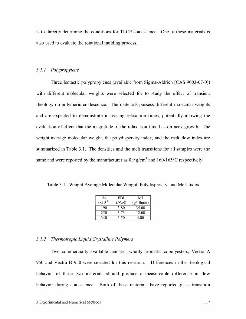
3 Experimental and Numerical Methods 117
is to directly determine the conditions for TLCP coalescence. One of these materials is
also used to evaluate the rotational molding process.
3.1.1 Polypropylene
Three Isotactic polypropylenes (available from Sigma-Aldrich [CAS 9003-07-0])
with different molecular weights were selected for to study the effect of transient
rheology on polymeric coalescence. The materials possess different molecular weights
and are expected to demonstrate increasing relaxation times, potentially allowing the
evaluation of effect that the magnitude of the relaxation time has on neck growth. The
weight average molecular weight, the polydispersity index, and the melt flow index are
summarized in Table 3.1. The densities and the melt transitions for all samples were the
same and were reported by the manufacturer as 0.9 g/cm3 and 160-165°C respectively.
Table 3.1. Weight Average Molecular Weight, Polydispersity, and Melt Index
M (x10-3)
PDI (M/N)
MI (g/10min)
190 3.80 35.00 250 3.73 12.00 340 3.50 4.00
3.1.2 Thermotropic Liquid Crystalline Polymers
Two commercially available nematic, wholly aromatic copolyesters, Vectra A
950 and Vectra B 950 were selected for this research. Differences in the rheological
behavior of these two materials should produce a measureable difference in flow
behavior during coalescence. Both of these materials have reported glass transition
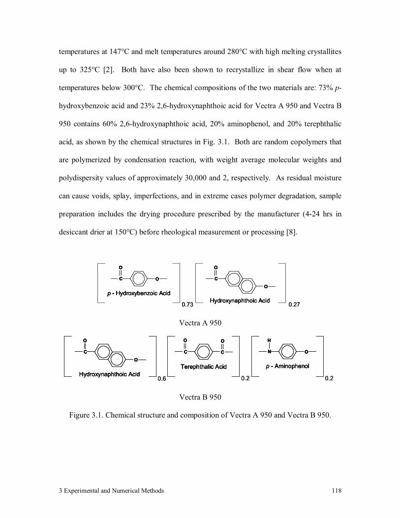
3 Experimental and Numerical Methods 118
temperatures at 147°C and melt temperatures around 280°C with high melting crystallites
up to 325°C [2]. Both have also been shown to recrystallize in shear flow when at
temperatures below 300°C. The chemical compositions of the two materials are: 73% p-
hydroxybenzoic acid and 23% 2,6-hydroxynaphthoic acid for Vectra A 950 and Vectra B
950 contains 60% 2,6-hydroxynaphthoic acid, 20% aminophenol, and 20% terephthalic
acid, as shown by the chemical structures in Fig. 3.1. Both are random copolymers that
are polymerized by condensation reaction, with weight average molecular weights and
polydispersity values of approximately 30,000 and 2, respectively. As residual moisture
can cause voids, splay, imperfections, and in extreme cases polymer degradation, sample
preparation includes the drying procedure prescribed by the manufacturer (4-24 hrs in
desiccant drier at 150°C) before rheological measurement or processing [8].
C O
O
p - Hydroxybenzoic Acid
C
O
O
Hydroxynaphthoic Acid 0.73 0.27
C O
O
p - Hydroxybenzoic Acid
C O
O
p - Hydroxybenzoic Acid
C O
O
C O
OO
p - Hydroxybenzoic Acid
C
O
O
Hydroxynaphthoic Acid
C
O
O
Hydroxynaphthoic Acid
C
O
OC
O
C
OO
OO
Hydroxynaphthoic Acid 0.73 0.27
Vectra A 950
C
O
O
Hydroxynaphthoic Acid
N
H
O
p - Aminophenol
C C
O O
Terephthalic Acid
0.6 0.2 0.2
C
O
O
Hydroxynaphthoic Acid
C
O
O
Hydroxynaphthoic Acid
C
O
OC
O
C
OO
OO
Hydroxynaphthoic Acid
N
H
O
p - Aminophenol
N
H
O
p - Aminophenol
N
H
ON
H
N
H
OO
p - Aminophenol
C C
O O
Terephthalic Acid
C C
O O
Terephthalic Acid
C C
O O
C C
OO OO
Terephthalic Acid
0.6 0.2 0.2
Vectra B 950
Figure 3.1. Chemical structure and composition of Vectra A 950 and Vectra B 950.
3 Experimental and Numerical Methods 119
3.2 Thermal Analysis
Differential scanning calorimetry (DSC) is used to identify a potential minimum
temperature for the neck growth experiments by measuring the end of the melt transition.
The thermal analysis was performed with a heating rate of 10°C/ minute with a Seiko
Instruments SSC/5200 series auto cooling DSC-220C. The sample was exposed to both a
heating and a cooling cycle before the recorded measurement to ensure the material had
been properly dried and to impose a known thermal history.
3.3 Generation and Characterization of TLCP Powders
Vectra B 950 is available as a pellet, which is too large for rotational molding and
conventional grinding methods produce unacceptable powders. A novel powder
generation technique is developed to overcome this obstacle. The technique is based on
the melt blending of a TLCP with an incompatible polymer in a 1” Killion single screw
extruder. When two immiscible phases are mixed, the minor phase is dispersed with a
droplet size determined by its properties (i.e. viscosity and interfacial tension) and the
shear stress [9]. The TLCP is blended at up to 40 weight percent with a low molecular
weight polypropylene at 340°C. The resin is available from Exxon as product number
PD3505G E1. The resin is a free-flowing low dusting granule with a typical particle size
between a 25-35 mesh and has a melt index of 400. The extruder temperatures are: 150,
300, 340, 340, 295°C for zones 1-4 and the die, respectively. The screw speed is set at 15
rpm and the die diameter is 1.59 mm. The extruded blend is quenched below the melt

3 Experimental and Numerical Methods 120
temperature of both components, effectively freezing the dispersed blend morphology.
The cooling rate played an important role in determining the size of the dispersed TLCP
phase. If the mixture is not quenched quickly enough the TLCP phase would continue to
separate from the continuous phase and coalesce with itself, increasing the dimensions of
the TLCP phase. The dispersed TLCP phase is retrieved by fracturing the polypropylene
matrix with a mill and separating the components in water (the specific gravity of
polypropylene is approximately 0.9 and will float in water, while the TLCP has a specific
gravity of 1.4 and sinks). Residual polypropylene on the TLCP particles (less than 1
weight percent as measured by thermal gravimetric analysis) is removed by dissolving it
in light mineral oil at 170°C. The mineral oil mixture is then washed from the TLCP
particles using a biodegradable degreaser and water. The TLCP powder is then dried in
accordance to manufacturer specifications in vacuum oven at 150°C for between 12 and
24 hours [8].
After the particles are retrieved from the polypropylene matrix, they are separated
into discrete groups according to their size with a series of U.S. standard sieves and a
Rotap shaker. Separation is performed not only to measure the size distribution of the
accumulated powder but also to allow for the evaluation of particular sizes and
distributions in later experiments. The procedure for separating the powder is to sift 100
gram samples for 10 minutes as described in ASTM test D 3451 for testing polymeric
powder and powder coatings. Shaking for 10 minutes delivered consistent results while
minimizing static charge build-up in the extremely fine particles (less than 149 micron).
3 Experimental and Numerical Methods 121
The apparent density of all powders is measured according to ASTM test D 1895,
which describes powder property measurements for plastic materials. Test method A is
used for the particles obtained from the melt blending process and test method C is used
for the powder acquired from the milling process. Test method A is designed for fine
granular materials that can be readily poured through a standardized funnel. Test method
C is applicable to materials that cannot be poured through the funnel because they are
compressible, usually composed of coarse flakes, chips, cut fibers, or strands. Two
values are reported for the apparent density measured according to test method C: one for
the initial density of loosely packed material and one with the powder under a prescribed
compressive load.
The dynamic angle of repose is the angle of the surface of a flowing powder
relative to horizontal, as shown in Fig. 3.2. It was measured in a 100 mL graduated
cylinder. 50 mL of the powder is poured into the cylinder. The open end of the cylinder
is plugged with a rubber stopper that had been placed on a shaft, driven by a variable
speed motor. The cylinder is supported at the opposite end so that it would remain
horizontal during rotation. Rotation rates from approximately 1 to 10 rpm are used
during the measurement of each sample. The rates are selected because they are
comparable to what is introduced to the powder during rotational molding. A digital
image of the tumbling powder is taken at each rotation rate and the angle is determined
by analyzing the image in Adobe Photoshop.
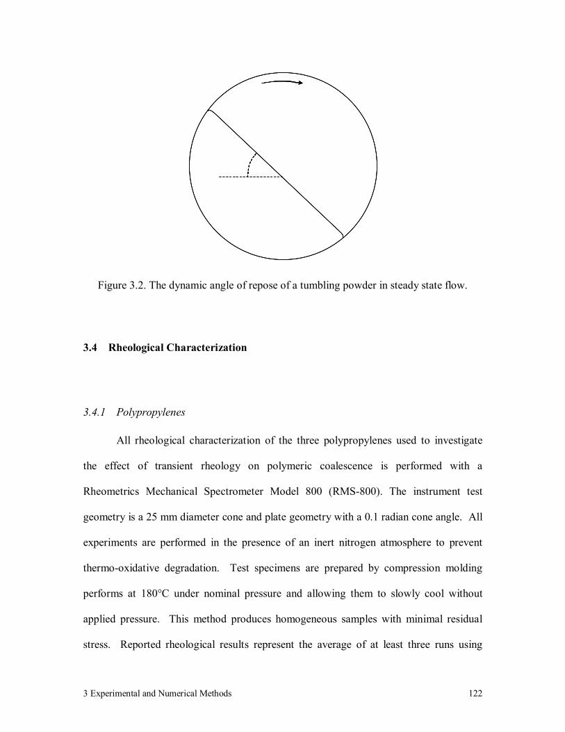
3 Experimental and Numerical Methods 122
Figure 3.2. The dynamic angle of repose of a tumbling powder in steady state flow.
3.4 Rheological Characterization
3.4.1 Polypropylenes
All rheological characterization of the three polypropylenes used to investigate
the effect of transient rheology on polymeric coalescence is performed with a
Rheometrics Mechanical Spectrometer Model 800 (RMS-800). The instrument test
geometry is a 25 mm diameter cone and plate geometry with a 0.1 radian cone angle. All
experiments are performed in the presence of an inert nitrogen atmosphere to prevent
thermo-oxidative degradation. Test specimens are prepared by compression molding
performs at 180°C under nominal pressure and allowing them to slowly cool without
applied pressure. This method produces homogeneous samples with minimal residual
stress. Reported rheological results represent the average of at least three runs using

3 Experimental and Numerical Methods 123
different samples for each run. Stress growth upon inception of steady shear flow
experiments were conducted to obtain single mode UCM model parameters. These
experiments are performed at shear rates in the zero shear viscosity limit at 180°C (steady
values from 0.01 to 0.1 sec-1). Small amplitude dynamic oscillatory shear measurements
are performed to determine parameters for the multimode UCM model. The tests
encompassed frequencies from 0.1 to 100 rad/sec at 180, 220, and 260°C. The
experiments performed at 220 and 260°C are shifted to the coalescence temperature
(180°C) by applying time-temperature superposition to include frequencies lower than
could be obtained by direct measurement.
3.4.2 TLCPs
All rheological characterization of the TLCPs is performed with a Rheometrics
Mechanical Spectrometer Model 800 (RMS-800). The instrument test geometry is a 25
mm diameter cone and plate with a 0.1 radian cone angle. The magnitude of the complex
shear viscosity, |η*|, versus angular frequency, ω, and shear viscosity, η, versus shear
rate, g, data are measured in the presence of an inert nitrogen atmosphere to prevent
thermo-oxidative degradation. Test specimens are prepared by compression molding
preforms at 320°C under nominal pressure and allowing them to quiescently cool without
applied pressure. This method produces homogeneous samples with minimal residual
stress that are the dimensions desired for the test geometry. Reported rheological results
represent the average of at least three runs using different samples for each run. Small
amplitude dynamic oscillatory shear measurements are performed for angular frequencies
between 0.1 to 100 rad/sec at 10% strain for both 320 and 330°C. The steady shear
3 Experimental and Numerical Methods 124
viscosity is measured at low shear rates by recording the steady state value of a stress
growth upon inception of steady shear flow experiment. The stress growth experiments
are performed because of the lengthy times required to obtain data at low angular
frequencies from dynamic oscillatory measurements. Transient viscosity values at shear
rates less than 0.01 sec-1 are thought to be the most pertinent to the coalescence process
and are used to obtain parameters for the UCM constitutive model by minimizing the sum
of the squared difference between the predicted and experimental viscosity values. To
represent the transient response, fitting was performed at 0.5 second intervals from
inception of flow until steady state is achieved.
Two procedures are used during rheological characterization because the
measured rheological response of TLCPs can be strongly dependent upon thermal and
deformation history. The first procedure is devised to introduce reproducible shear and
thermal histories to minimize variation in rheological data and is used for both the stress
growth and the dynamic oscillatory measurements. The cone and plate preform is placed
in the rheometer and the cone is brought to 0.05 mm from the plate while the sample is
heated to 340°C. Once the temperature reaches 340°C, a steady shear deformation is
applied at a shear rate of 0.1 sec-1 for 10 seconds. After the preshear is complete the
sample is cooled to the test temperature where it is given five minutes to reach a stress
free state before beginning the test. The 340°C preheat temperature is used because the
sample will not relax to a stress-free state within the allotted time if lower temperatures
are used. The second procedure is designed to mimic the thermal and deformation
histories of the samples used in the neck growth experiments. This procedure is used
3 Experimental and Numerical Methods 125
only for repeating the stress growth experiments. The cone and plate perform is placed in
the rheometer and the cone is brought to 0.05 mm from the plate while the sample is
heated directly to the test temperature. Once the set point is reached, the test is
performed.
3.5 Surface Tension Measurement
3.5.1 Polypropylenes
The surface tension of each of the polypropylenes is determined by fitting the
Bashforth and Adams equation to the sessile drop profile of the molten polymer in an
inert atmosphere at 180°C [4,5]. Sessile drops were prepared by first extruding
polypropylene fibers with a Göttfert Rheograph 2001 capillary rheometer equipped with
a 0.5 mm capillary die (L/D = 10). Pellets, with a diameter of approximately 500 µm and
an aspect ratio of approximately one, were cut from the fibers. A single pellet was placed
vertically, standing on its cut end, on a glass slide in a Linkham hot stage set at 180°C,
where it was melted into a sessile drop. The sample was quenched and the glass slide
was rotated to allow a profile view of the drop. The sample was reheated to 180°C and a
digital image of the profile was recorded with an optical microscope equipped with a
miniDV camcorder. The accuracy of this technique (0.1% error) demands that the
particle radii must be small so that gravitational forces cannot influence the shape of the
profile. This was verified by calculating the Bond numbers Γ
= grBo2ρ (Bo190k=0.063,
3 Experimental and Numerical Methods 126
Bo250k=0.125, Bo340k=0.063) and supported by the observation that the profile shape did
not change when the glass slide was rotated.
3.5.2 TLCPs
Surface tension of TLCPs is dependent upon the phase of the measured material.
The solid phase surface energy is different than that of the melt phase and, for many
materials, it is dependent on temperature. Therefore, the surface tension must be
measured with the TLCP as a melt and over a range of possible processing temperatures.
There are a number of methods available to measure surface tension in fluids.
However, the majority of these methods such as capillary rise, Wilhelmy plate, ring, drop
volume or weight, and oscillating jet do not easily allow access to high melt temperatures
or produce results that are not influenced by the high viscosities of polymeric materials.
It is also important to note that the surface tension of nematic TLCPs can be affected by
bulk elastic distortions (splay, twist, and bend) [7]. Therefore, obtrusive methods such as
the Wilhelmy plate method may introduce a bulk elastic contribution in addition to the
underlying temperature dependence [7]. This makes measurement of TLCP surface
tension a nontrivial task.
There is a technique that makes accurate surface tension measurement of TLCPs
possible. The profile shape of axially symmetric menisci, such as that of a sessile drop
on a surface, can be correlated to surface tension. Its unobtrusive nature allows the use of
samples that have the same geometry as those used in coalescence experiments.

3 Experimental and Numerical Methods 127
Distortional elastic effects or a different deformation history are not imposed so it should
prove to be very representative of what is observed during coalescence. Specific details
about the derivation and application of the measurement method can be found in several
references [4,5].
The surface tension of each of the materials is determined by fitting the Bashforth
and Adams equation to the sessile drop profile of the molten polymer in an inert
atmosphere at 320 and 330°C [4,5]. This method is used because it presents a
noninvasive means of measuring the surface tension of the TLCP as a melt with the
identical geometry, thermal history, and deformation history of the particles used in the
neck growth experiments. A single, 500 µm diameter sphere, identical to those used in
the neck growth experiments, is placed on a glass slide in the hot stage, where it is melted
into a sessile drop. The sample is quenched and the glass slide is rotated to allow a
profile view of the drop from above. The sample is reheated to the test temperature and a
digital image of the profile is recorded by an optical microscope equipped with a miniDV
camcorder. The Bashforth and Adams equation is fit to data points representing the
profile shape that are extracted from the digital image of the profile with Scion Image, an
image analysis software available from Scion Corporation. The accuracy of this
technique (0.1%) demands that the particle radii must be small so that gravitational forces
cannot influence the shape of the profile. The absence of gravitational forces is verified
by calculating the Bond number Γ
= grBo2ρ (0.027 for Vectra A 950 and 0.030 for
Vectra B 950) and is supported by the observation that the profile shape does not change
upon rotating the glass slide.
3 Experimental and Numerical Methods 128
3.6 Coalescence Experiments
The sample preparation for the coalescence experiments is identical to the
procedure used to generate sessile drops for each material. Two of the particles are
placed next to each other in the hot stage at 180°C. The hot stage is capable of achieving
a heating rate of 90°C per minute and could maintain the temperature within 0.1°C,
which assisted in providing nearly isothermal conditions. An inert, nitrogen atmosphere
is used to help eliminate thermo-oxidative degradation throughout the experiment. For
the polypropylene samples, the cylinders adopted a spherical shape before coalescence
began. The entire coalescence process is recorded on high resolution video. Still images
are extracted at prescribed intervals, and the neck and particle radii are measured using
Scion Image, a digital image analysis software available from Scion Corporation.
Coalescence experiments with the polypropylene samples are performed both with and
without a lubricant, in order to explore the importance of surface contact with the glass
slide, but no difference is observed. Each coalescence experiment is conducted three
times to ensure reproducibility, and the reported neck radius versus time data is the
average of the three runs. The standard deviation in the dimensionless neck radius
between the repeated runs was 0.01 for the polypropylene samples and 0.02 for the
Vectra samples.
3.7 Densification Experiments

3 Experimental and Numerical Methods 129
Eight samples of the spherical particles are used to evaluate particle size and size
distribution, each sample is described in Table 3.2. The first four samples, identified as
S1 through S4, represent particular sizes and samples D1 through D4 represent various
distributions. D1 is skewed towards smaller particles, D2 is skewed towards larger
particles, D3 is a normal distribution, and D4 represents a traditional rotational molding
distribution, where the majority of its content is between approximately 300 and 600
micron and contains a small fraction of fine particles. The samples are poured into a 1.27
cm x 6.35 cm rectangular bar mold with an exposed top surface and a thermocouple fixed
in the center of one of the sides of the mold. A nitrogen purge (powders are not under
pressure) is supplied through a chamber that covered the mold. The entire unit is placed
on a pre-heated hot plate that simulated conductive heating from one side as occurs in
rotational molding. The total heating time is 40 minutes and began once the set
temperature, as measured at the mold, is reached. After 40 minutes the apparatus is
removed from the hot plate and allowed to cool in ambient with continued nitrogen
purge.
Table 3.2. Descriptions of the powder samples used in the densification study.
S1 S2 S3 S4 D1 D2 D3 D4
20 840 1.0 - - - 0.07 0.53 0.10 -30 595 - 1.0 - - 0.13 0.27 0.40 0.0840 420 - - 1.0 - 0.27 0.13 0.40 0.4850 297 - - - 1.0 0.53 0.07 0.10 0.3960 250 - - - - - - - 0.0270 210 - - - - - - - 0.02100 149 - - - - - - - 0.01
Size and Distribution Mass FractionsU.S. Standard
Sieve No.Opening (micron)
3 Experimental and Numerical Methods 130
In addition to the 40 minute experiments, sample S3 is used in three other tests. In
the first test, the heating time is extended to 80 minutes to check for improved
densification with increased time. The other two tests are to evaluate the possibility of
increasing strength by an oxidative effect that had been observed during the coalescence
tests. The first heating cycle for those experiments is designed to determine if
introducing air to the sample at the end of the formerly described 40 minute cycle could
improve properties. For this case, the sample is exposed to 20 minutes of heating in
nitrogen followed by 20 minutes in air. The last test is to verify that any differences
observed in the 20/20 test are not due to reducing the time the sample is heated in
nitrogen. For this, the sample is exposed to an additional 20 minute of heating in air
after spending 40 minutes heating in nitrogen.
3.8 Single Axis Rotational Molding
The laboratory-scale rotational molding device consisted of a cylindrical, stainless
steel mold, with an inside diameter of 1.59 cm and 7.62 cm in length, is used as the
rotational mold. For each test, the mold is filled with 30 grams of D4 powder, this
distribution is used because it produces the greatest average density during the
densification study. Both ends of the mold are capped. One cap is threaded onto a shaft
that is driven by a variable speed motor. A fitting is installed in the center of the opposite
cap so that a nitrogen purge can be delivered directly into the mold cavity. The mold is
placed in a forced convection oven that could heat at up to 60°C per minute and maintain
the set temperature to within 1°C. The heating cycle is designed to mimic the conditions

3 Experimental and Numerical Methods 131
used in the densification experiments. The heating stage began once the mold reached
the set temperature and after 40 minutes, the heat is stopped and the oven is opened.
Rotation and nitrogen purge continued as the mold is allowed to cool to room
temperature with the assistance of the oven fan.
3.9 Mechanical and Physical Property Testing
3.9.1 Testing of Samples from the Densification Study
Several properties of the bars molded in the densification experiments are
evaluated. The density of the molded specimen, which is defined as the average density
and differs from the material density by the amount of voids in the molded sample, is
measured to determine the extent of densification. The average density is measured
according to method A in ASTM test D 792, for testing solid plastics by displacement in
water. It should be noted that the average density measured by this method is not
affected by surface porosity, but only by differences in the amount of encapsulated gas.
The test also requires the results to be corrected for variation in the test temperature and
reported at 23°C.
Tensile tests are performed on the molded bars with a model 4202 Instron tensile
testing machine to determine the ultimate tensile strength and Young’s modulus. The
crosshead speed is 1.27mm/min and the gauge length is 30.5 mm according to ASTM test
D 638. The samples fracture surfaces are inspected for uniform pore distribution and
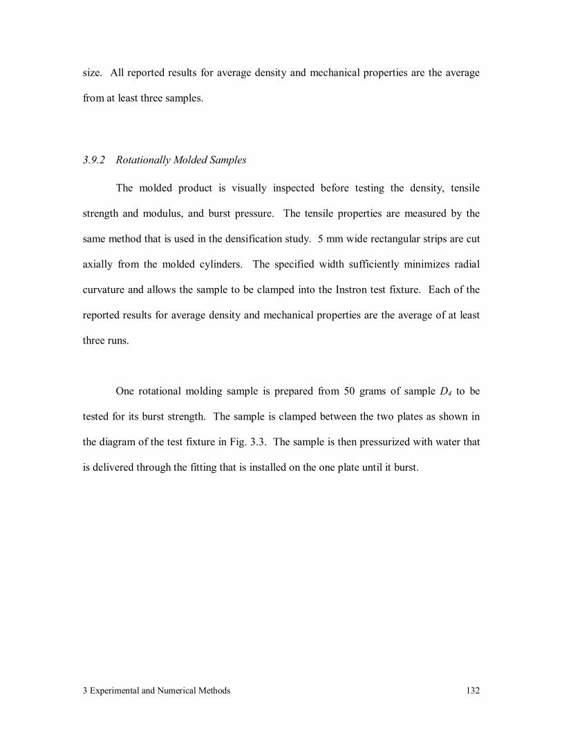
3 Experimental and Numerical Methods 132
size. All reported results for average density and mechanical properties are the average
from at least three samples.
3.9.2 Rotationally Molded Samples
The molded product is visually inspected before testing the density, tensile
strength and modulus, and burst pressure. The tensile properties are measured by the
same method that is used in the densification study. 5 mm wide rectangular strips are cut
axially from the molded cylinders. The specified width sufficiently minimizes radial
curvature and allows the sample to be clamped into the Instron test fixture. Each of the
reported results for average density and mechanical properties are the average of at least
three runs.
One rotational molding sample is prepared from 50 grams of sample D4 to be
tested for its burst strength. The sample is clamped between the two plates as shown in
the diagram of the test fixture in Fig. 3.3. The sample is then pressurized with water that
is delivered through the fitting that is installed on the one plate until it burst.
3 Experimental and Numerical Methods 133
Figure 3.3. Diagram of test fixture used to measure the burst strength.
3.10 Biaxial Rotational Molding
The conditions identified by the selection process developed in this research are
used in biaxial rotational molding experiments performed by the PolyProcessing
Company, a rotational molding company located in French Camp, Ca. The specifics of
the rotational molding cycle are proprietary and cannot be disclosed in this document,
although it may be stated that the conditions used in their molding cycle are in close
agreement with the conditions identified in this work. However, several containers are
tested for use as cryogenic storage and publication of the results of those tests is
permitted.
3 Experimental and Numerical Methods 134
To determine the container’s ability to perform as a cryogenic storage vessel the
container is sealed in a device similar to that used to pressurize the rotationally molded
tube. The container is subjected to 34 psi, the suggested target value specified by Nasa,
with nitrogen to determine if the container is capable of handling the generated forces at
room temperature. A similar experiment is performed only the container is filled with
liquid nitrogen to determine if the container is capable of handling the generated forces at
cryogenic temperatures. The rotational molded structure is evaluated for its ability to
contain the gas by sealing the container with nitrogen, as a gas at 34 psi, then monitoring
the pressure over an extended period of time. Finally a rectangular sample from the wall
of the container is tested to determine its ability to withstand thermal cycling. The
sample is cycled from liquid nitrogen to room temperatures in excess of 1000 times then
evaluated by inspecting the surface for the development of micro-cracks with a scanning
electron microscope. The results from these tests are summarized in the appendix, and
not in the body of this text, because the tanks were molded by PolyProcessing using
powders that were generated from micropelletization and the specifics of the molding
cycle are proprietary.

3 Experimental and Numerical Methods 135
3.11 References
1. Beekmans, F., Gotsis, A.D., Norder, B., “Transient and Steady State Rheological
Behavior of the Thermotropic Liquid Crystalline Polymer Vectra B950,” Journal
of Rheology, 40, 5, 947 (1996)
2. Beekmans, F., Gotsis, A.D., Norder, B., “Influence of the Flow History on Stress
Growth and Structure Changes in the Thermotropic Liquid Crystalline Polymer
Vectra B950,” Rheologica Acta, 36, 82 (1997)
3. Chang, S., Han, C., “A Thermotropic Main-Chain Random Copolyester
Containing Flexible Spacers of Differing Lengths. 1. Synthesis and
Characterization,” Macromolecules, 29, 7, 2383 (1996)
4. Padday, J.F., “Part II. The Measurement of Surface Tension,” in Surface and
Colloid Science, Vol.1, edited by Matijević, E., Wiley Interscience, New York
(1969)
5. Hiemenz, P.C., Rajagopalan, R., Principles of Colloid and Surface Chemistry
Third Edition, Marcel Dekker, New York (1997)
6. Kim, S.S., Han, C.D., “Oscillatory Shear Flow Behavior of a Thermotropic
Liquid-Crystalline Polymer,” Polymer, 35, 1, 93 (1994)
7. Rey, A.D., “Modelling the Wilhelmy Surface Tension for Nematic Liquid
Crystals,” Langmuir, 16, 845 (2000)
8. Ticona, Vectra Liquid Crystal Polymer Global Brochure (VC-7), Product
Literature (2000)
9. Baird, D.G., Collias, D.I., Polymer Processing: Principles and Design, John Wiley
& Sons, New York, (1998)
4 The Role of Transient Rheology in Polymeric Coalescence
136
4 The Role of Transient Rheology in Polymeric Coalescence
Preface
The work presented in this chapter partially addresses the first objective of this
research, as it represents the first step towards understanding the coalescence of TLCPs.
Specifically, the effect that transient rheology has on the coalescence of polymeric
materials. It was discovered during the review of the literature that a clear, consistent
understanding of the role that viscoelasticity plays in polymer coalescence was not
available but is required to understand the behavior observed for TLCPs. This chapter is
organized as a manuscript for future publication.
4 The Role of Transient Rheology in Polymeric Coalescence
137
The Role of Transient Rheology in Polymeric Coalescence
Eric Scribben†, Donald Baird†, and Peter Wapperom‡
†Department of Chemical Engineering, Virginia Polytechnic Institute and State University, Blacksburg, Va 24061
‡Department of Mathematics, Virginia Polytechnic Institute and State University, Blacksburg, Va 24061
4.1 Abstract
Polymeric coalescence is the process by which surface tension drives two small
drops to merge into a single uniform, homogeneous drop. In this work a coalescence
model, which equates the work of surface tension to the work done by viscous forces
while assuming biaxial extensional flow kinematics, is evaluated to determine its ability
to accurately predict the coalescence rates of three isotactic polypropylene resins with
increasing weight average molecular weight (M = 190k, 250k, 340k). There were three
variations of the model: one used a Newtonian constitutive model, another used the upper
convected Maxwell (UCM) constitutive model with the assumption of steady state stress
behavior, and the last used the UCM model with time dependent material functions.
Coalescence model predictions from each of these formulations were compared to
experimental data at 180°C. The surface tension was obtained by fitting the Bashforth
and Adams equation to a sessile drop profile and the constitutive equations were fit to
rheological data to obtain the viscosity and relaxation spectra. The coalescence rates
predicted by the Newtonian model were slower than those of the experimental data,
indicating that viscoelastic effects were significant even for the case of relatively low
Deborah numbers. The results from the steady state UCM model predict that

4 The Role of Transient Rheology in Polymeric Coalescence
138
viscoelasticity (as quantified by the relaxation time) acts to slow coalescence relative to
the Newtonian model and, therefore, was less accurate than the Newtonian model at
representing the experimental coalescence data. It was shown that the reduction in
coalescence rate with increasing relaxation time was due to the UCM model predicting
that the biaxial extensional viscosity approaches infinity at a critical extension rate. A
numerical algorithm was developed to treat the increased complexity that was introduced
by the transient UCM formulation. The solution demonstrated that coalescence was
accelerated by increasing the relaxation time, the opposite relationship of what was
predicted by the steady state UCM formulation. It was also found that the transient UCM
formulation was capable of quantitatively predicting the coalescence rates of the
polypropylenes at short times where viscoelasticity was important. This work illustrates
that the effective viscosity, over a range of times where the viscosity had not reached
steady state, was lower than the steady state value and lead to the acceleration of
coalescence.
4.2 Introduction
Coalescence refers to the process where, in an attempt to minimize surface area,
surface tension drives a collection of fluid drops to merge into a single, homogeneous
body. Coalescence begins when drops are brought into contact, and they instantaneously
deform in an elastic manner to create finite contact surfaces [1]. It is important to
emphasize that elastic contact scales with surface tension, creep compliance, and particle
radius but not time [2]. Elastic contact may also be referred to as neck formation,
4 The Role of Transient Rheology in Polymeric Coalescence
139
because it defines the formation of a bridge at the interface between particles.
Coalescence continues with the radial growth of the neck region. At this stage, the
particles retain their individuality because coalescence is not influenced by other contacts
from neighboring drops. In addition, there is no appreciable change in density of the
multi-particle structure [2]. The neck dimensions grow until a network of pores form and
eventually become entrapped bubbles. The process of eliminating the entrapped bubbles
is referred to as densification, and the densification rate depends upon gas permeability in
the molten material [2]. A complete description of the coalescence of multiple drops
must represent at least three stages: elastic contact, neck growth, and densification.
However, the neck growth process is the focus of this work because it embodies most of
the geometrical change experienced by a particle during coalescence.
Frenkel [3] first modeled viscous (Newtonian) coalescence by proposing an
expression for the coalescence rate of this system that was later corrected for continuity
by Eshelby [4]. They suggested that coalescence could be modeled by evaluating two
isolated particles, which they represented by the idealized system of spherical drops as
depicted in Fig. 4.1. In the figure ao is the initial particle radius, x is the neck radius, y is
the distance from the particle center to the contact plane, and θ is the angle between the
axial plane of symmetry and the line from the particle center to the neck radius.

4 The Role of Transient Rheology in Polymeric Coalescence
140
ao
y θ
a
x
aoao
y θ
a
x
y θ
a
x
Figure 4.1. Shape evolution during the coalescence of two spherical particles
Their model was derived from the mechanical energy balance by equating the work of
surface tension to the work done by the rheological stresses, which is referred to as
viscous dissipation for a purely viscous fluid [5],
∫∫∫=Γ− dVdtdS Dτ : (1)
where τ is the deviatoric stress tensor, D is one-half the rate of strain tensor,
( )TvvD ∇+∇=21 (2)
S is surface area, and V is the volume of both spheres. The presence of external stresses
and gravitational effects were neglected. The flow kinematics were assumed to be biaxial
stretching flow, with the components of the velocity gradient tensor given by,
−=∇
εε
ε
&
&
&
0002000
v (3)
4 The Role of Transient Rheology in Polymeric Coalescence
141
where ε& is the extension rate. The rheological stresses in Eq. 1 were assumed to be
described in terms of the Newtonian constitutive equation. They solved Eqs. 1 through 3
for the early stages of coalescence when the particle radius remained constant to give,
21
23
Γ=oo a
tax
η (4)
where t is time, Γ is the surface tension, and ηo is viscosity. Despite its simplicity by
assuming a Newtonian fluid and a constant particle radius, the Frenkel model defines a
relationship between material properties, particle size, and the rate of viscous
coalescence. It has been used as a qualitative benchmark for experimental data,
demonstrating good agreement between measured values of the dimensionless neck
radius (x/a) and the predicted exponent of ½ on time [6].
Pokluda et al. improved the accuracy of Eq. 4 by applying the conservation of
mass with constant density to account for the time dependence of the particle radius [7],
3/122 )
)](cos2[)](cos1[4()(
ttata o θθ −+
= (5)
where θ is referred to as the coalescence angle, θsin=ax , as shown in Fig. 1. This time
dependent radius was incorporated into the mechanical energy balance, Eq. 1, through the
definition for the surface area of the two spheres:
( )θπ cos14 2 += aS (7)
As outlined in reference [7] this system of equations can be rewritten as the following
homogeneous, first-order differential equation:

4 The Role of Transient Rheology in Polymeric Coalescence
142
( ) ( )( )[ ] ( )[ ] 3
43
521
35
cos1cos2sincos2
θθθθ
ηθ
+−Γ=
−
Kadtd
oo
(8)
where K1 arises from the definition of the extension rate,
dtdK
yvy θε 12
1 =∂∂
−=& (9)
and is defined by:
( ) ( )( )( )
−+
++−−=θθ
θθθθcos2cos1
cos1cos226
sin2
tan1K (10)
It should be added that K1 presented here is a slightly different form than was defined in
the original derivation, which was an approximation in the limit of small coalescence
angles. The K1 defined here is valid over all coalescence angles during the coalescence
process and is used because it represents an improvement in model accuracy.
In addition to the energy balance approach for modeling coalescence first
introduced by Frenkel [3], a complete flow description of coalescence was derived from
the equations for the conservation of mass and momentum, a constitutive equation
describing the development of stress with deformation, initial conditions, and boundary
conditions describing the movement of the free surface has been used [8]. The latter
approach provides greater resolution of stresses, and its complexity requires a numerical
simulation technique such as finite element method (FEM). This approach has been used
to explore numerous factors that pertain to the viscous coalescence problem
[8,9,10,11,12]. It was demonstrated that the complete flow description is capable of
accurately predicting the relative density for a packing of glass spheres, at least up to
densities where the kinetics are no longer controlled by neck growth [13]. When
4 The Role of Transient Rheology in Polymeric Coalescence
143
compared to the Newtonian model, Eq. 8, the coalescence predictions were in reasonable
agreement, which was not surprising because the predicted streamlines from the
numerical solution confirm the assumed biaxial extensional flow kinematics [7,8,11].
Bellehumeur et al. evaluated the Newtonian coalescence model, Eq. 8, for several
polyethylenes and found that the model over predicted the coalescence rates [6]. They
proposed a variation of the Newtonian coalescence model to incorporate viscoelasticity
by using the upper convected Maxwell (UCM) constitutive equation for the extra stress
tensor,
Dττ oηλ 2=+∇
(11)
where λ is the characteristic relaxation time, ∇τ is the convected derivative,
vττvττ ∇⋅−⋅∇−=∇
T
DtD (12)
and DtDτ is the substantial derivative. By assuming that the flow field is homogeneous,
and that at any instant the stresses are at steady state (though the stresses may change
with the extension rate throughout the process) the constitutive equation was simplified to
the following expression [5]:
[ ] Dvττvτ oT ηλ 2=∇⋅−⋅∇−+ (13)
After Eqs. 3, 5, 7, 9, and 13 were substituted into Eq. 1 and the integration was
performed, the model was rearranged into the following differential equation for the
steady state representation of coalescence:

4 The Role of Transient Rheology in Polymeric Coalescence
144
01282
21
1
2
1 =−
Γ+−+
dtd
KKaK
dtdK oo θηλθλ (14)
where K1 is defined as before, Eq. 10, and
( ) ( ) 35
34
35
2cos2cos1
sincos2θθ
θθ−+
=−
K (15)
Eq. 14 predicts that the coalescence rate decreases with an increase in the
relaxation time. The predicted behavior was used to suggest that viscoelasticity was
responsible for the observation that two propylene ethylene copolymers coalesced at a
slower rate than predicted by the Newtonian model [6]. This is interesting because
reported coalescence times for polytetrafluoroethylene (PTFE) and several acrylic resins
were significantly shorter than what was predicted by the Newtonian model [2,16].
Furthermore, the relaxation times were not measured experimentally. Instead, they were
adjusted to produce better agreement with data, and these values were unrealistically
large. Therefore, it was unclear if it was possible to accurately predict coalescence using
a viscoelastic constitutive equation with experimentally measured relaxation times.
The complete flow description with a FEM has also been extended to include the
viscoelastic representation of stresses. As with other cases where viscoelastic behavior
has been modeled with a FEM, the inability to achieve convergence with increasing
relaxation times limit the simulations to cases with relatively low Deborah numbers [14].
Although the complete flow description provides increased resolution of the stresses
relative to the energy balance approach, it appears that the flow kinematics are
predominately biaxial extension, as assumed in Frenkel’s Newtonian model [15].
4 The Role of Transient Rheology in Polymeric Coalescence
145
The objective of this work is to extend the approach devised by Frenkel to
describe the coalescence of two particles to the transient viscoelastic case by using the
upper convected Maxwell constitutive equation without the assumption of steady state
stress behavior. The ability of the model to predict coalescence is assessed by comparing
the measured coalescence values of three polymers with different relaxation times to the
predicted values. The significance of this work rests partially on the fact that all of the
material parameters in the UCM model are obtained directly from rheological data rather
than arbitrarily adjusted for the model to accurately predict coalescence data. Finally, the
results presented here are used to explain the predictions of a previous model presented
by others concerning the role of viscoelasticity in polymer coalescence.
4.3 Experimental
4.3.1 Materials
Isotactic polypropylenes (available from Sigma-Aldrich [CAS 9003-07-0]) of
three different molecular weights were selected for this study. Because the materials
possess different molecular weights, they are expected to demonstrate increasing
relaxation times, potentially allowing the evaluation of effect that the magnitude of the
relaxation time has on coalescence. The weight average molecular weight, the
polydispersity index, and the melt flow index are summarized in Table 4.1. The densities

4 The Role of Transient Rheology in Polymeric Coalescence
146
and the melt transitions for all samples were the same and were reported by the
manufacturer as 0.9 g/cm3 and 160-165°C respectively.
Table 4.1. Weight Average Molecular Weight, Polydispersity, and Melt Index
M (x10-3)
PDI (M/N)
MI (g/10min)
190 3.80 35.00 250 3.73 12.00 340 3.50 4.00
4.3.2 Surface Tension Measurement
The surface tension of each of the materials was determined by fitting the
Bashforth and Adams equation to the sessile drop profile of the molten polymer in an
inert atmosphere at 180°C [17]. Sessile drops were prepared by first extruding
polypropylene fibers with a Göttfert Rheograph 2001 capillary rheometer equipped with
a 0.5 mm capillary die (L/D = 10). Pellets, with a diameter of approximately 500 µm and
an aspect ratio of approximately one, were cut from the fibers. A single pellet was placed
vertically, standing on its cut end, on a glass slide in a Linkham hot stage set at 180°C,
where it was melted into a sessile drop. The sample was quenched and the glass slide
was rotated to allow a profile view of the drop. The sample was reheated to 180°C and a
digital image of the profile was recorded with an optical microscope equipped with a
miniDV camcorder. The accuracy of this technique (0.1% error) demands that the
particle radii must be small so that gravitational forces cannot influence the shape of the
profile. This was verified by calculating the Bond numbers Γ
= grBo2ρ (Bo190k=0.063,
4 The Role of Transient Rheology in Polymeric Coalescence
147
Bo250k=0.125, Bo340k=0.063) and supported by the observation that the profile shape did
not change when the glass slide was rotated.
4.3.3 Rheological Characterization
All rheological characterization was performed with a Rheometrics Mechanical
Spectrometer Model 800 (RMS-800). The instrument test geometry was a 25 mm
diameter cone and plate geometry with a 0.1 radian cone angle. All experiments were
performed in the presence of an inert nitrogen atmosphere to prevent thermo-oxidative
degradation. Test specimens were prepared by compression molding performs at 180°C
under nominal pressure and allowing them to slowly cool without applied pressure. This
method produces homogeneous samples with minimal residual stress. Reported
rheological results represent the average of at least three runs using different samples for
each run. Stress growth upon inception of steady shear flow experiments were conducted
to obtain single mode UCM model parameters. These experiments were performed at
shear rates in the zero shear viscosity limit at 180°C (steady values from 0.01 to 0.1 sec-1
are shown in Fig. 2). Small amplitude dynamic oscillatory shear measurements were
performed to determine parameters for the multimode UCM model. The tests
encompassed frequencies from 0.1 to 100 rad/sec at 180, 220, and 260°C. The
experiments performed at 220 and 260°C were then shifted to the coalescence
temperature (180°C, the master curves are shown in Fig. 4.2) by applying time-
temperature superposition to include frequencies lower than could be obtained by direct
measurement. The calculated errors for the stress growth and dynamic oscillatory
measurements were found to be ±10 and ±5%, respectively.
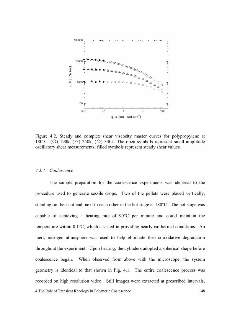
4 The Role of Transient Rheology in Polymeric Coalescence
148
0.01 0.1 1 10 100
100
1000
10000
100000
η, |k
| (P
a se
c)
g, ω (sec-1, rad sec-1)
Figure 4.2. Steady and complex shear viscosity master curves for polypropylene at 180°C. ( ) 190k, ( ) 250k, ( ) 340k. The open symbols represent small amplitude oscillatory shear measurements; filled symbols represent steady shear values.
4.3.4 Coalescence
The sample preparation for the coalescence experiments was identical to the
procedure used to generate sessile drops. Two of the pellets were placed vertically,
standing on their cut end, next to each other in the hot stage at 180°C. The hot stage was
capable of achieving a heating rate of 90°C per minute and could maintain the
temperature within 0.1°C, which assisted in providing nearly isothermal conditions. An
inert, nitrogen atmosphere was used to help eliminate thermo-oxidative degradation
throughout the experiment. Upon heating, the cylinders adopted a spherical shape before
coalescence began. When observed from above with the microscope, the system
geometry is identical to that shown in Fig. 4.1. The entire coalescence process was
recorded on high resolution video. Still images were extracted at prescribed intervals,

4 The Role of Transient Rheology in Polymeric Coalescence
149
and the neck and particle radii were measured using Scion Image, a digital image analysis
software available from Scion Corporation. Coalescence experiments were performed
both with and without a lubricant, in order to explore the importance of surface contact
with the glass slide, but no difference was observed. Each coalescence experiment was
conducted three times to ensure reproducibility, and the reported neck radius versus time
data is the average of the three runs. The standard deviation in the dimensionless neck
radius between the repeated runs was 0.01. A representative example of the recorded
images is shown in Fig. 4.3, where there is initially a finite contact area and the neck
radius increases with time until the two drops converge. In the example, the two particles
nearly reach a dimensionless neck radius of 1 within thirty seconds. Although the test is
stopped a few seconds later because the magnitude of the change in the dimensionless
neck radius becomes comparable to the magnitude of the error in the measurement, the
two particles do appear to continue to coalesce towards a single, nearly spherical drop.
Figure 4.3. Optical micrographs from the coalescence of 190k polypropylene drops

4 The Role of Transient Rheology in Polymeric Coalescence
150
4.4 Numerical Methods
4.4.1 Model Parameter Fitting
The single mode UCM model parameters were obtained from stress growth data
by minimizing the sum of the squared difference between the predicted and experimental
transient viscosity. To represent the transient response, fitting was performed at 0.5
second intervals from inception of flow until steady state was achieved. The single mode
UCM model fits to data at a shear rate of 0.01 sec-1 are shown in Fig. 4.4, where it is
shown that the model fits well at long times but not as well at short times. A summary of
the coalescence model parameters and calculated Deborah numbers (as defined for
coalescence,ooa
DeηλΓ= ) is provided in Table 2.

4 The Role of Transient Rheology in Polymeric Coalescence
151
0 2 4 6 8 10 12 14
1000
10000
h+ (Pa
sec)
t (sec)
Figure 4.4. Single mode UCM model fit to the transient shear viscosity from stress growth experiments at 180°C. The symbols represent the experimental data: ( ) 190k, ( ) 250k, ( ) 340k. The lines represent the single mode UCM fits to the data.
Table 4.2. Single Mode UCM Coalescence Model Parameters and Calculated Values for the Deborah Number at 180°C.
λ (sec)
ηo (Pa sec)
Γ ±0.002 (J/m2)
ao ± 1(µm)
De (λΓ/ηo ao)
190k 0.18 1097.2 0.024 232 0.017 250k 0.73 3986.8 0.015 232 0.012 340k 1.54 11128.9 0.028 274 0.014
Multimode UCM model parameters were obtained by simultaneously fitting Eqs.
16 and 17, using a nonlinear regression method to storage (G') and loss (G") modulus
data as outlined in Bird et al. [5]:
( ) ( )∑= +
=′N
k kj
jkkjG
12
2
1 λωωλη
ω (16)
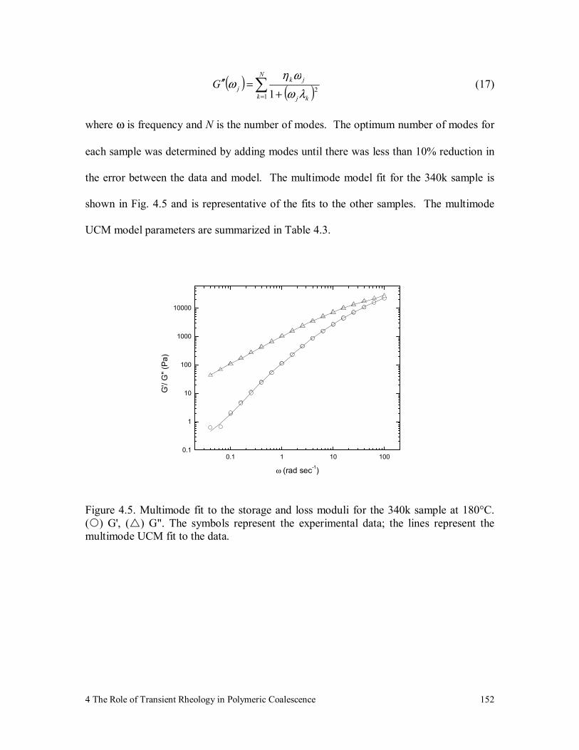
4 The Role of Transient Rheology in Polymeric Coalescence
152
( ) ( )∑= +
=′′N
k kj
jkjG
121 λω
ωηω (17)
where ω is frequency and N is the number of modes. The optimum number of modes for
each sample was determined by adding modes until there was less than 10% reduction in
the error between the data and model. The multimode model fit for the 340k sample is
shown in Fig. 4.5 and is representative of the fits to the other samples. The multimode
UCM model parameters are summarized in Table 4.3.
0.1 1 10 1000.1
1
10
100
1000
10000
G'/
G" (
Pa)
ω (rad sec-1)
Figure 4.5. Multimode fit to the storage and loss moduli for the 340k sample at 180°C. ( ) G', ( ) G". The symbols represent the experimental data; the lines represent the multimode UCM fit to the data.
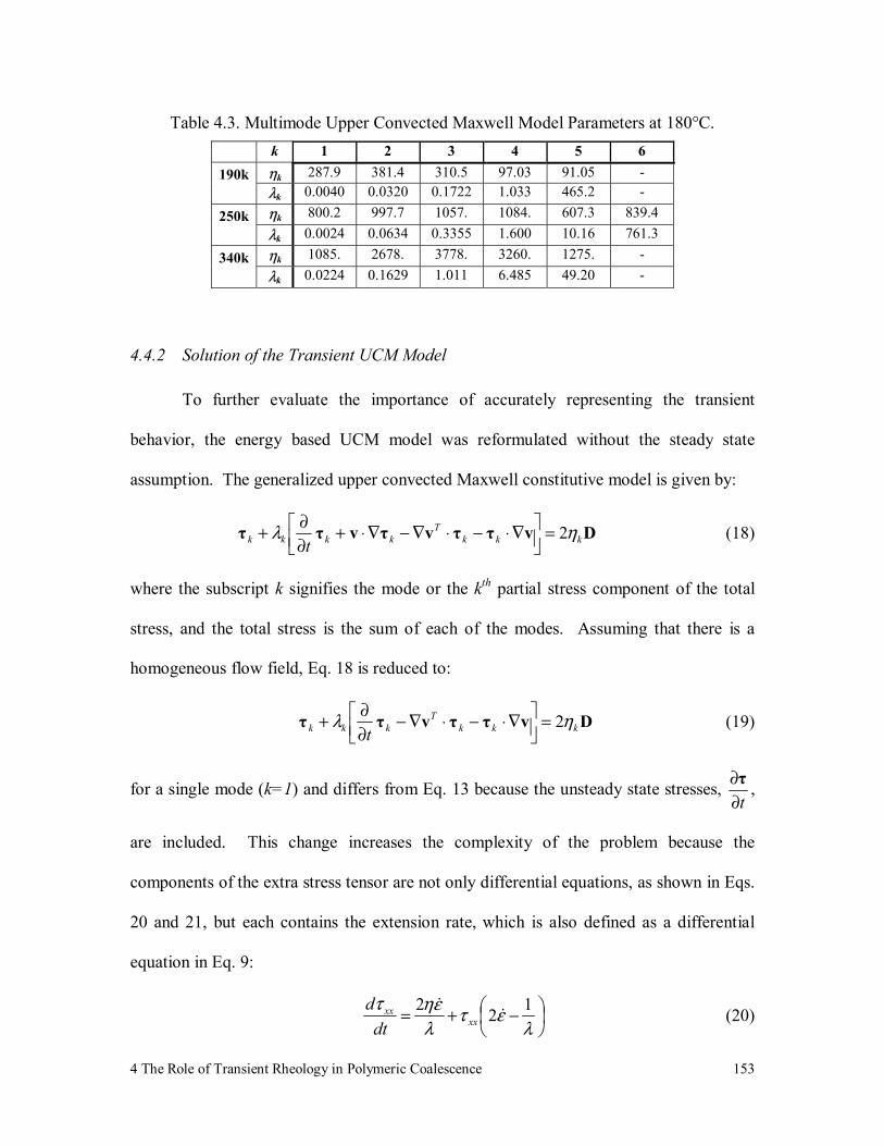
4 The Role of Transient Rheology in Polymeric Coalescence
153
Table 4.3. Multimode Upper Convected Maxwell Model Parameters at 180°C. k 1 2 3 4 5 6
ηk 287.9 381.4 310.5 97.03 91.05 - 190k λk 0.0040 0.0320 0.1722 1.033 465.2 - ηk 800.2 997.7 1057. 1084. 607.3 839.4 250k λk 0.0024 0.0634 0.3355 1.600 10.16 761.3 ηk 1085. 2678. 3778. 3260. 1275. - 340k λk 0.0224 0.1629 1.011 6.485 49.20 -
4.4.2 Solution of the Transient UCM Model
To further evaluate the importance of accurately representing the transient
behavior, the energy based UCM model was reformulated without the steady state
assumption. The generalized upper convected Maxwell constitutive model is given by:
Dvττvτvττ kkkT
kkkk tηλ 2=
∇⋅−⋅∇−∇⋅+∂∂+ (18)
where the subscript k signifies the mode or the kth partial stress component of the total
stress, and the total stress is the sum of each of the modes. Assuming that there is a
homogeneous flow field, Eq. 18 is reduced to:
Dvττvττ kkkT
kkk tηλ 2=
∇⋅−⋅∇−∂∂+ (19)
for a single mode (k=1) and differs from Eq. 13 because the unsteady state stresses, t∂
∂τ ,
are included. This change increases the complexity of the problem because the
components of the extra stress tensor are not only differential equations, as shown in Eqs.
20 and 21, but each contains the extension rate, which is also defined as a differential
equation in Eq. 9:
−+=
λετ
λεητ 122
&&
xxxx
dtd
(20)

4 The Role of Transient Rheology in Polymeric Coalescence
154
++−=
λετ
λεητ 144
&&
yyyy
dtd
(21)
xxzz ττ = (22)
This requires the development of an alternative numerical approach to what was applied
to the steady state model. By assuming that the extension rate is constant over a given
time step, which is valid if discretization is sufficiently refined, and the initial condition
that the stresses are zero at t = 0, the differential equations for stress may be solved
analytically to give:
( )( )
( ) ( )
−
−+−
=−
−
−
−
−−
ελεητ
ελεητ
ελ
ελ
ελ
&
&
&
& &&&
212
212
1
1212121
n
n
xx
ttt
xx eee (23)
( )( )
( ) ( )
+
+++−=
−
−
+
+
+−
ελεητ
ελεητ
ελ
ελ
ελ
&
&
&
& &&&
414
414
1
1414141
n
n
yy
ttt
yy eee (24)
These equations for stress (Eqs. 23 and 24) may then be substituted into the energy
balance, Eq. 1, and integrated to give the following equation:
( ) ( ) ( ) 01sincos
cos2cos132 3
53
41
32
=−−+−Γ θθ
θθττ yyxxo Ka
(25)
Eqs. 9, 10, 23, 24, and 25 may be solved by determining the root, dtdθ , at a given time
and θ by using Müller’s method [18]. Convergence was achieved when there was less
than 1% difference in each predicted value of dimensionless coalescence between
successive reductions of the time step, dt. The accuracy of the numerical scheme was
evaluated by applying it to the steady state model and comparing the results to those
produced by the numerical integration of Eq. 15.
4 The Role of Transient Rheology in Polymeric Coalescence
155
4.5 Results and Discussion
4.5.1 Newtonian and Steady State UCM Coalescence Models
The results from the coalescence experiments are shown in Fig. 4.6 along with
predictions from the Newtonian and steady state UCM models using experimentally
measured parameters. The coalescence data are in qualitative agreement with what the
Frenkel model suggests; coalescence rates decrease with increasing viscosity. The
Newtonian model predicts slower coalescence rates than what were experimentally
measured. This result is consistent with the previously mentioned reports on PTFE and
acrylic resins in which it was concluded that the experimental coalescence was faster than
predicted by the Newtonian model [2,16].
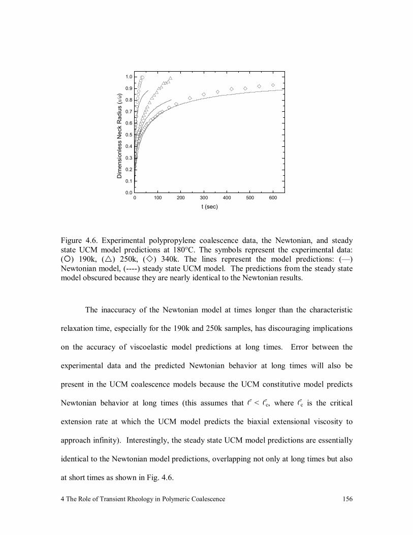
4 The Role of Transient Rheology in Polymeric Coalescence
156
0 100 200 300 400 500 6000.0
0.1
0.2
0.3
0.4
0.5
0.6
0.7
0.8
0.9
1.0
Dim
ensi
onle
ss N
eck
Rad
ius
(x/a
)
t (sec)
Figure 4.6. Experimental polypropylene coalescence data, the Newtonian, and steady state UCM model predictions at 180°C. The symbols represent the experimental data: ( ) 190k, ( ) 250k, ( ) 340k. The lines represent the model predictions: (—) Newtonian model, (----) steady state UCM model. The predictions from the steady state model obscured because they are nearly identical to the Newtonian results.
The inaccuracy of the Newtonian model at times longer than the characteristic
relaxation time, especially for the 190k and 250k samples, has discouraging implications
on the accuracy of viscoelastic model predictions at long times. Error between the
experimental data and the predicted Newtonian behavior at long times will also be
present in the UCM coalescence models because the UCM constitutive model predicts
Newtonian behavior at long times (this assumes that f < fc, where fc is the critical
extension rate at which the UCM model predicts the biaxial extensional viscosity to
approach infinity). Interestingly, the steady state UCM model predictions are essentially
identical to the Newtonian model predictions, overlapping not only at long times but also
at short times as shown in Fig. 4.6.

4 The Role of Transient Rheology in Polymeric Coalescence
157
Following the approach by Bellehumeur et al. [6], the relaxation time was
arbitrarily increased in an attempt to improve the accuracy of the predictions. As
illustrated in Fig. 4.7, the coalescence rates decrease at short times with large changes in
the relaxation time. However, this only decreases the accuracy of the predictions by
slowing coalescence rates relative to the predicted Newtonian limit. The facts that the
steady state UCM model predictions are the same as the Newtonian predictions for the
experimentally measured relaxation times, the magnitude of the relaxation times need to
be relatively large to observe a difference from the Newtonian model, and increasing the
relaxation time decreases accuracy suggest that the behavior predicted by the steady state
model may not be representative of the response of viscoelastic materials.
0 1000.0
0.1
0.2
0.3
0.4
0.5
0.6
0.7
Dim
ensi
onle
ss N
eck
Rad
ius
(x/a
)
t (sec)
Figure 4.7. 340k polypropylene coalescence data, the Newtonian, and steady state UCM model predictions at short times. The symbols represent the experimental data: ( ) 340k. The lines represent the model predictions: (—) Newtonian, steady state UCM model with (----) λ =1.54 sec, (····) λ =200 sec, (─·─·) λ =400 sec.
4 The Role of Transient Rheology in Polymeric Coalescence
158
The reason that the coalescence rate of the steady state model is predicted to slow
as the relaxation time is increased can be determined by considering the magnitude of the
biaxial extension rates and the implications it has on the nature of the biaxial viscosity.
The evolution of the biaxial extension rates during coalescence, as predicted by the
steady state UCM model for the three evaluated relaxation times, are shown in Fig. 4.8.
The extension rates pass through a maximum then decay monotonically. The UCM
model predicts that the biaxial extensional viscosity approaches infinity at the critical
extension rate, λ
ε21=c& . It is reasonable to suspect that the enhanced viscosity, which
simulates a rate hardening behavior, excessively slows coalescence. The magnitude of
the extension rates for the large relaxation times of 200 and 400 sec do not exceed the
predicted critical extension rates of 0.0025 and 0.00125 sec-1, respectively, but they are
close enough to cause the biaxial viscosity to increase beyond 6ηo, as shown in Fig. 4.9.
The biaxial viscosity predicted for the experimentally measured relaxation time (λ = 1.54
sec) is practically identical to 6ηo and explains the similarity in coalescence rates for the
steady state UCM and Newtonian cases. By increasing the relaxation time, the biaxial
extensional viscosity significantly surpasses 6ηo leading to a decrease in the coalescence
rate relative to the Newtonian model. This explains why the steady state model predicts a
decrease in the coalescence rate as the relaxation time is increased.
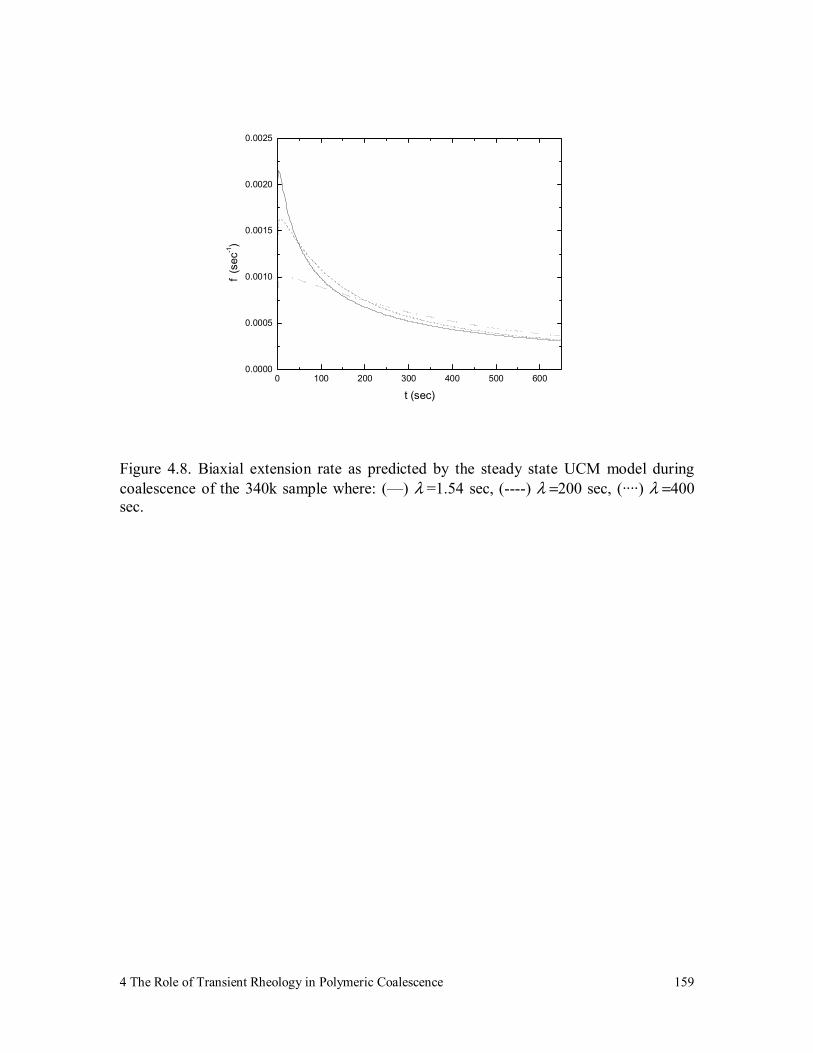
4 The Role of Transient Rheology in Polymeric Coalescence
159
0 100 200 300 400 500 6000.0000
0.0005
0.0010
0.0015
0.0020
0.0025
f (s
ec-1)
t (sec)
Figure 4.8. Biaxial extension rate as predicted by the steady state UCM model during coalescence of the 340k sample where: (—) λ =1.54 sec, (----) λ =200 sec, (····) λ =400 sec.
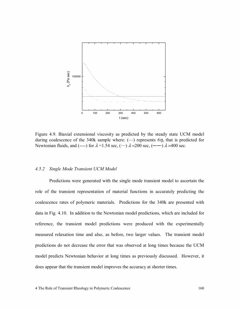
4 The Role of Transient Rheology in Polymeric Coalescence
160
0 100 200 300 400 500 600
100000
h b (Pa
sec)
t (sec)
Figure 4.9. Biaxial extensional viscosity as predicted by the steady state UCM model during coalescence of the 340k sample where: (—) represents 6ηo that is predicted for Newtonian fluids, and (----) for λ =1.54 sec, (····) λ =200 sec, (─·─·) λ =400 sec.
4.5.2 Single Mode Transient UCM Model
Predictions were generated with the single mode transient model to ascertain the
role of the transient representation of material functions in accurately predicting the
coalescence rates of polymeric materials. Predictions for the 340k are presented with
data in Fig. 4.10. In addition to the Newtonian model predictions, which are included for
reference, the transient model predictions were produced with the experimentally
measured relaxation time and also, as before, two larger values. The transient model
predictions do not decrease the error that was observed at long times because the UCM
model predicts Newtonian behavior at long times as previously discussed. However, it
does appear that the transient model improves the accuracy at shorter times.
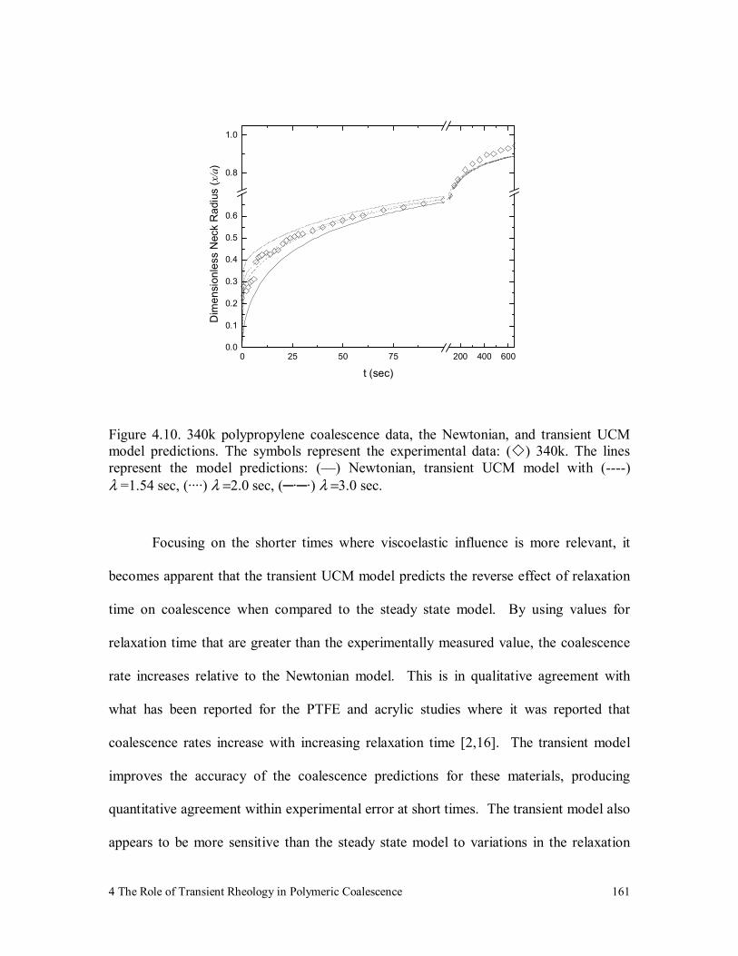
4 The Role of Transient Rheology in Polymeric Coalescence
161
0 25 50 75 200 400 6000.0
0.1
0.2
0.3
0.4
0.5
0.6
0.8
1.0
Dim
ensi
onle
ss N
eck
Rad
ius
(x/a
)
t (sec)
Figure 4.10. 340k polypropylene coalescence data, the Newtonian, and transient UCM model predictions. The symbols represent the experimental data: ( ) 340k. The lines represent the model predictions: (—) Newtonian, transient UCM model with (----) λ =1.54 sec, (····) λ =2.0 sec, (─·─·) λ =3.0 sec.
Focusing on the shorter times where viscoelastic influence is more relevant, it
becomes apparent that the transient UCM model predicts the reverse effect of relaxation
time on coalescence when compared to the steady state model. By using values for
relaxation time that are greater than the experimentally measured value, the coalescence
rate increases relative to the Newtonian model. This is in qualitative agreement with
what has been reported for the PTFE and acrylic studies where it was reported that
coalescence rates increase with increasing relaxation time [2,16]. The transient model
improves the accuracy of the coalescence predictions for these materials, producing
quantitative agreement within experimental error at short times. The transient model also
appears to be more sensitive than the steady state model to variations in the relaxation

4 The Role of Transient Rheology in Polymeric Coalescence
162
time and does not require unrealistically large values to affect the coalescence rate.
Furthermore, the biaxial extensional viscosity approaches but does not exceed 6ηo, thus
eliminating the rate hardening behavior predicted by the steady state model.
4.5.3 Multimode Transient UCM Model
The previous results, shown in Fig. 4.10, were based on calculations using a
single relaxation time. The multimode UCM model was used next to further examine the
importance of accurately representing the transient viscosity during coalescence. The
first step is to establish the significance of using a relaxation spectrum by evaluating the
shear stress growth predictions with model parameters obtained from the small amplitude
dynamic oscillatory shear data. These predictions are compared to the single mode fits
and experimental data in Fig. 4.11. The multimode model appears to be more accurate
than the single mode UCM model fits to the stress growth data, especially at short times,
and for the highest molecular weight sample. In general, it is expected that the
magnitude of the difference in predicted stress growth behavior between the single mode
and multimode will increase in materials possessing greater relaxation times or broader
relaxation spectra and, therefore, will become more important in the coalescence
predictions for those cases.
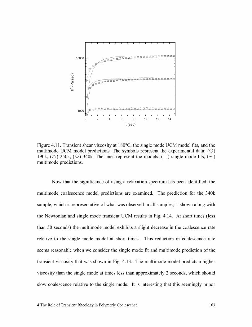
4 The Role of Transient Rheology in Polymeric Coalescence
163
0 2 4 6 8 10 12 14
1000
10000
h+ (Pa
sec)
t (sec)
Figure 4.11. Transient shear viscosity at 180°C, the single mode UCM model fits, and the multimode UCM model predictions. The symbols represent the experimental data: ( ) 190k, ( ) 250k, ( ) 340k. The lines represent the models: (—) single mode fits, (····) multimode predictions.
Now that the significance of using a relaxation spectrum has been identified, the
multimode coalescence model predictions are examined. The prediction for the 340k
sample, which is representative of what was observed in all samples, is shown along with
the Newtonian and single mode transient UCM results in Fig. 4.14. At short times (less
than 50 seconds) the multimode model exhibits a slight decrease in the coalescence rate
relative to the single mode model at short times. This reduction in coalescence rate
seems reasonable when we consider the single mode fit and multimode prediction of the
transient viscosity that was shown in Fig. 4.13. The multimode model predicts a higher
viscosity than the single mode at times less than approximately 2 seconds, which should
slow coalescence relative to the single mode. It is interesting that this seemingly minor
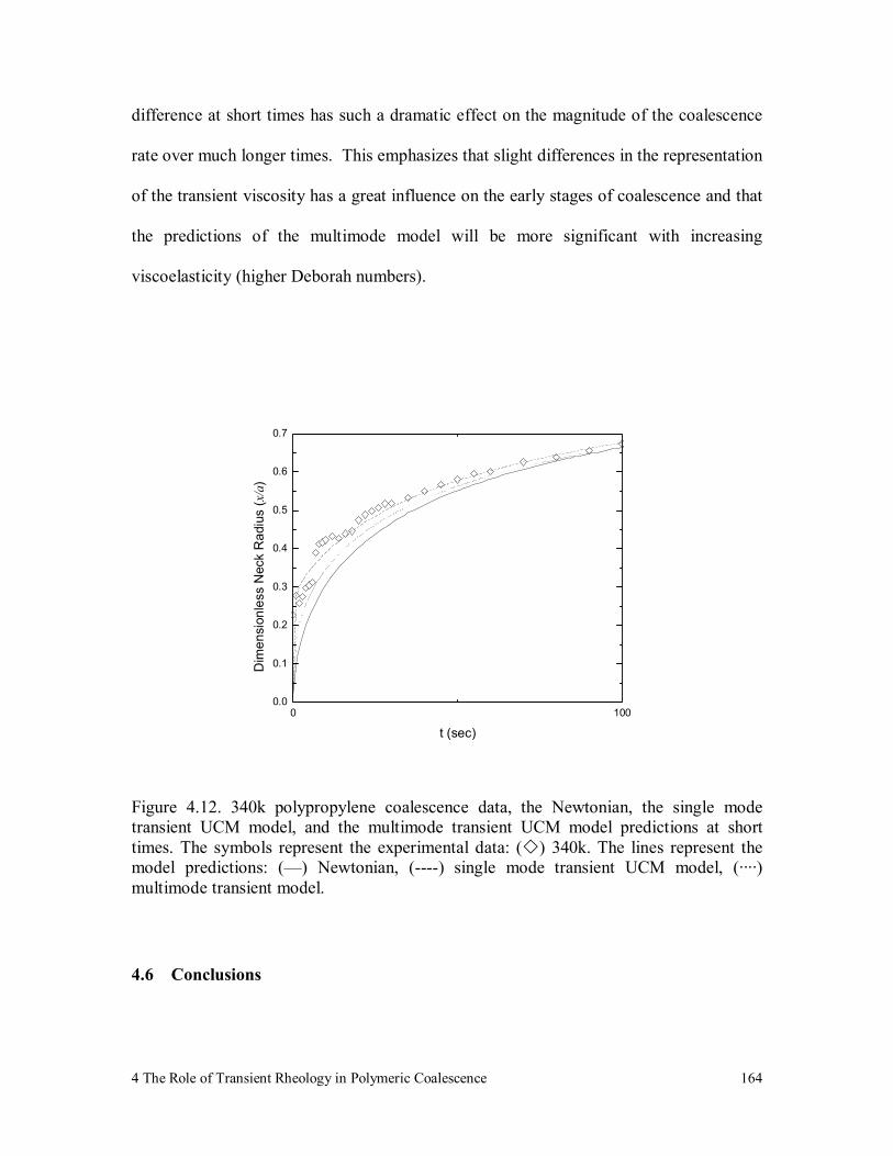
4 The Role of Transient Rheology in Polymeric Coalescence
164
difference at short times has such a dramatic effect on the magnitude of the coalescence
rate over much longer times. This emphasizes that slight differences in the representation
of the transient viscosity has a great influence on the early stages of coalescence and that
the predictions of the multimode model will be more significant with increasing
viscoelasticity (higher Deborah numbers).
0 1000.0
0.1
0.2
0.3
0.4
0.5
0.6
0.7
Dim
ensi
onle
ss N
eck
Rad
ius
(x/a
)
t (sec)
Figure 4.12. 340k polypropylene coalescence data, the Newtonian, the single mode transient UCM model, and the multimode transient UCM model predictions at short times. The symbols represent the experimental data: ( ) 340k. The lines represent the model predictions: (—) Newtonian, (----) single mode transient UCM model, (····) multimode transient model.
4.6 Conclusions
4 The Role of Transient Rheology in Polymeric Coalescence
165
Three energy balance derived coalescence models, one with a Newtonian
constitutive equation while the other two utilized two different forms of the upper
convected Maxwell constitutive model, were evaluated to determine their ability to
predict coalescence rates of three polypropylenes with experimentally measured model
parameters. Rheological characterization of the selected polypropylenes showed that the
measured relaxation times were short relative to the coalescence times, and the Deborah
numbers were small. In spite of this, the experimental data indicated faster coalescence
rates than were predicted by the Newonian model. This suggests that modeling the
coalescence of viscoelastic materials requires the inclusion of viscoelasticity to accurately
predict coalescence rates, even for materials with small Deborah numbers. Predictions
from the steady state UCM coalescence model using the experimentally measured
parameters did not produce a significant change in the predicted coalescence rates. Upon
varying the relaxation time it was found that the model was insensitive to the magnitude
of the relaxation time and required unrealistically large values to observe a change in
behavior. The change that was observed did not improve the accuracy of the predictions
because increasing relaxation time slowed coalescence. It was determined that the source
of this behavior was that the UCM constitutive model predicts infinite viscosity at a
critical extension rate. By increasing the relaxation time the critical extension rate is
effectively lowered, causing the viscosity to increase beyond 6ηo and coalescence to slow
relative to the Newtonian case.
The viscoelastic coalescence model was solved without the steady state
approximation. This transient model was evaluated with a single and multiple modes.
4 The Role of Transient Rheology in Polymeric Coalescence
166
The single mode transient coalescence model demonstrated that the influence of
viscoelasticity is limited to short times and at long times it converges with the Newtonian
solution. This formulation was able to improve the model accuracy at short times by
predicting an increase in coalescence rate with an increase in relaxation time and in doing
so illustrates the importance of representing the transient viscosity. The model was also
more sensitive to the magnitude of the relaxation time, producing significant changes in
coalescence rates with only small changes in the magnitude of the relaxation time. While
the multimode transient UCM model more accurately represented the transient
rheological response it was unable improve the accuracy of the model predictions for
these materials but will likely be more important for fluids possessing a broader
relaxation spectrum.
4.7 Acknowledgements
This work was financially supported by a phase II SBIR grant from NASA, grant
number NAS-2S-4018-285, managed by Luna Innovations.
4 The Role of Transient Rheology in Polymeric Coalescence
167
4.8 References
1 K.L. Johnson, K. Kendall, and A.D. Roberts, Surface Energy and the Contact of
Elastic Solids, Proceedings of the Royal Society of London. Series A, 324, 1558
(1971) 301.
2 S. Mazur, Coalescence of Polymer Particles, in M. Narkis and N. Rosenzweig
(Eds.), Polymer Powder Technology, John Wiley & Sons, New York, 1995,
Chapter 8.
3 J. Frenkel, Viscous Flow of Crystalline Bodies Under the Action of Surface
Tension, Journal of Physics, (Moscow), 9, 5 (1945) 385.
4 J.D. Eshelby, Discussion in Paper by A.J. Shaler, Seminar on the Kinetics of
Sintering, Transactions of AIME, 185, 11 (1949) 806.
5 R.B. Bird, R.C. Armstrong, and O. Hassager, Dynamics of Polymeric Liquids,
Vol. 1., second edition, John Wiley & Sons, New York, 1987, Chapter 5.
6 C.T. Bellehumeur, M. Kontopoulou, and J. Vlachopoulos, The Role of
Viscoelasticity in Polymer Sintering, Rheologica Acta, 37, 3 (1998) 270.
7 O. Pokluda, C.T. Bellehumeur, and J. Vlachopoulos, Modification of Frenkel’s
Model for Sintering, AICHE Journal, 43, 12 (1997) 3253.
8 A. Jagota, P.R. Dawson, and J.T. Jenkins, An Anisotropic Continuum Model for
the Sintering and Compaction of Powder Packings, Mechanics of Materials, 7, 3
(1988) 255.
9 R.S. Garabedian and J.J. Helble, A Model for the Viscous Coalescence of
Amorphous Particles, Journal of Colloid and Interface Science, 234 (2001) 248.

4 The Role of Transient Rheology in Polymeric Coalescence
168
10 A. Jagota and P.R. Dawson, Micromechanical Modeling of Powder Compacts – I.
Unit Problems for Sintering and Traction Induced Deformation, Acta
Metallurgica, 36, 9 (1988) 2551.
11 J.I. Martinez-Herrera and J.J. Derby, Viscous Sintering of Spherical Particles via
Finite Element Analysis, Journal of the American Ceramic Society, 78, 3 (1995)
645.
12 H. Zhou and J.J. Derby, Three-Dimensional Finite-Element Analysis of Viscous
Sintering, Journal of the American Ceramic Society, 81, 3 (1998) 533.
13 A. Jagota, K.R. Mikeska, and R.K. Bordia, Isotropic Constitutive Model for
Sintering Particle Packings, Journal of the American Ceramic Society, 73, 8
(1990) 2266.
14 P.J. Doerpinghaus and D.G. Baird, Pressure Profiles along an Abrupt 4:1 Planar
Contraction, AICHE Journal, 49, 10 (2003) 2487.
15 R. Hooper, C.W. Macosko, and J.J. Derby, Assessing Flow-Based Finite Element
Model for the Sintering of Viscoelastic Particles, Chemical Engineering Science,
55 (2000) 5733.
16 S. Mazur and D.J. Plazek, Viscoelastic Effects in the Coalescence of Polymer
Particles, Progress in Organic Coatings, 24 (1994) 225.
17 J.F. Padday, in Matijević, E. (Ed.), Surface and Colloid Science, Vol.1, Wiley
Interscience, New York, 1969, Part II., 104.
18 IMSL Fortran Subroutines for Mathematical Applications, Math/Library, Vol. 1.,
Visual Numerics, 1997, Chapter 7, 846.

5 The Role of Transient Rheology in the Coalescence of Thermotropic Liquid Crystalline Polymers
169
5 The Role of Transient Rheology in the Coalescence of Thermotropic
Liquid Crystalline Polymers
Preface
The work presented in this chapter addresses the first objective of the research.
Specifically, the coalescence of TLCPs is investigated to determine if their behavior may
be explained solely by their viscoelastic character. This chapter is organized as a
manuscript for future publication.

5 The Role of Transient Rheology in the Coalescence of Thermotropic Liquid Crystalline Polymers
170
The Role of Transient Rheology in the Coalescence of Thermotropic Liquid Crystalline Polymers
Eric Scribben and Donald Baird
Department of Chemical Engineering , Virginia Polytechnic Institute and State University, Blacksburg, Va 24061
5.1 Abstract
Polymeric coalescence is the process by which surface tension drives two small
drops to merge into a single uniform, homogeneous drop. In this work a coalescence
model, which equates the work of surface tension to the work done by viscous forces
while assuming biaxial extensional flow kinematics, is evaluated to determine its ability
to accurately predict the coalescence rates of two TLCPs. Results from two variations of
the model (one used a Newtonian constitutive model and the other used the upper
convected Maxwell (UCM) constitutive model with the assumption of steady state stress
behavior) that had previously been reported were explained according to their predicted
viscosity behavior. The analysis suggested the importance of using the transient viscosity
in the model. The model employing unsteady stresses that was described elsewhere was
evaluated to determine its ability to accurately predict coalescence rates when using
experimentally quantified coalescence model parameters. This model represents a
qualitative improvement to the previous models because it predicted that coalescence
would occur at a higher rate than predicted by the Newtonian model, which was observed
experimentally. However, the model was unable to quantitatively predict the
experimental coalescence rates, as it over predicted the acceleration of coalescence that

5 The Role of Transient Rheology in the Coalescence of Thermotropic Liquid Crystalline Polymers
171
arises due to the transient viscosity. The origin of the disagreement is not known, but
could be due to the use of a constitutive relation designed for flexible chain polymers.
5.2 Introduction
Polymer coalescence is the basis of a number of polymer processing operations
such as: the fabrication of particulate performs, cold compression molding, dispersion
coating, powder coating, rotational molding, and selective laser sintering [1].
Coalescence refers to the process where, in an attempt to minimize surface area, surface
tension drives a collection of fluid drops to merge into a single, homogeneous body.
When drops are brought in contact, they instantaneously deform to create finite contact
surface [2]. This is also referred to as neck formation because it describes the formation
of a bridge at the interface between drops. Coalescence continues with the radial growth
of the neck radius, x, as is shown by the schematic in Fig. 5.1, where the drops are
represented by identical spheres.

5 The Role of Transient Rheology in the Coalescence of Thermotropic Liquid Crystalline Polymers
172
xx
Figure 5.1. Schematic of the geometric evolution of two coalescing spherical particles.
Thermotropic liquid crystalline polymers (TLCPs) exhibit a number of
mechanical and physical properties that are desirable for products manufactured by
techniques involving coalescence. TLCPs have demonstrated exceptionally high values
of tensile strength and modulus (strengths in excess of 1000 MPa and moduli near 100
GPa from fiber spinning and approaching 200 MPa and 20 GPa, respectively, in injection
molding) [3]. They retain their mechanical properties over a wide range of temperatures.
They have permeability coefficients for gases such as: He, H2, Ar, N2, CO2 that are
comparable to or less than those for polyacrylonitrile (PAN), one of the least permeable
polymers known [4]. They exhibit excellent resistance to acidic or basic environments
and a wide range of organic solvents [5]. Finally, they have low coefficients of linear
thermal expansion (CLTE), which are less than 1 cm/cm/°Cx10-5 [3].
5 The Role of Transient Rheology in the Coalescence of Thermotropic Liquid Crystalline Polymers
173
In our initial work, the coalescence behavior of two commercial TLCPs was
reported [6]. It was observed that coalescence was possible if the material exhibits a
well-defined zero shear viscosity. It was also demonstrated that TLCP coalescence rates
could not be predicted by either a Newtonian or a viscoelastic coalescence model. The
viscoelastic coalescence model incorporated viscoelastic effects by using the upper
convected Maxwell (UCM) constitutive equation to describe the extra stress tensor and is
referred to as steady state because it was assumed that the stresses, at any instant, were at
steady state. The reader is referred to the original papers for details on the complete
derivation of the Newtonian and the steady state UCM coalescence models [7,6]. The
cause for the inability of the models to accurately predict the coalescence rates of the
TLCPs was not known, but it was suggested that it could be due to the fact that the
transient viscosity was not represented in either of the evaluated coalescence models and
the time required for the viscosity to reach steady state was the same order of magnitude
as the time required for coalescence [6].
The UCM coalescence model was evaluated for several polypropylenes without
the steady state assumption to determine the effect that transient viscosity had on
predicting coalescence rates [9]. This model is hereafter referred to as the transient UCM
coalescence model because of its transient description of the rheological stresses. As
with both the Newtonian and steady state UCM coalescence models, the transient UCM
model predicted that the coalescence rate was proportional to the surface tension an
inversely proportional to viscosity. However, it was demonstrated the transient UCM
coalescence model was more sensitive to relaxation time than the steady state formulation
5 The Role of Transient Rheology in the Coalescence of Thermotropic Liquid Crystalline Polymers
174
and, in contrast to the steady state UCM model, the coalescence rate was accelerated by
increasing the relaxation time. The model also quantitatively predicted the coalescence
rates of the selected polypropylenes, using measured relaxation times, at short times
where the transient biaxial extensional viscosity had not reached steady state.
The objective of this work is to determine if the transient UCM coalescence
model can accurately predict coalescence rate of coalescing TLCPs. To accomplish this
objective, two TLCPs with markedly different rheological behavior are used. The
Newtonian and steady state UCM coalescence models are analyzed with respect to the
coalescence data to provide an explanation for their inablity to predict the measured
coalescence data. The UCM constitutive model is fit to transient shear viscosity data to
obtain UCM model parameters. Finally, predictions from the Newtonian, steady state
UCM, and the transient UCM coalescence models are compared to experimental data to
determine if the transient UCM model can improve the accuracy of the predictions.
5.3 Experimental
5.3.1 Materials
Two nematic TLCPs, Vectra A 950 and Vectra B 950, available from Ticona
(Summit, NJ), were selected for this evaluation. Both materials are randomly
copolymerized wholly aromatic copolyesters: Vectra A is composed of hydroxybenzoic
acid and hydroxynaphthoic acid, and Vectra B is composed of hydroxynaphthoic acid,
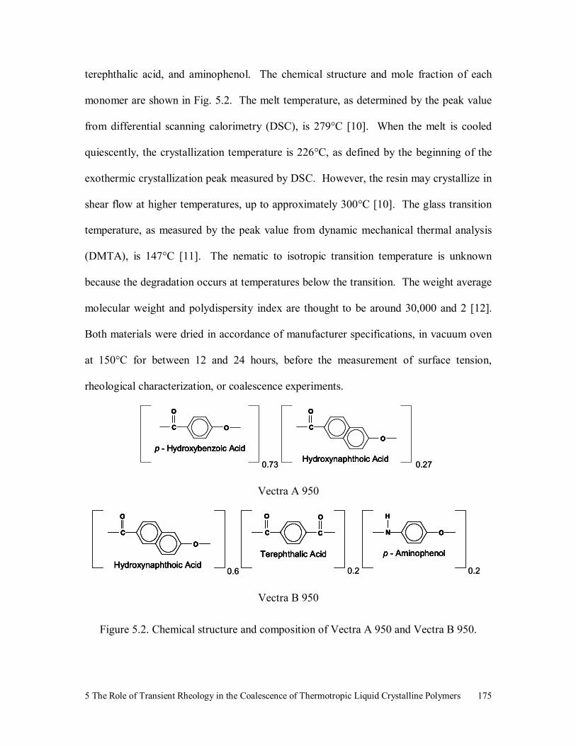
5 The Role of Transient Rheology in the Coalescence of Thermotropic Liquid Crystalline Polymers
175
terephthalic acid, and aminophenol. The chemical structure and mole fraction of each
monomer are shown in Fig. 5.2. The melt temperature, as determined by the peak value
from differential scanning calorimetry (DSC), is 279°C [10]. When the melt is cooled
quiescently, the crystallization temperature is 226°C, as defined by the beginning of the
exothermic crystallization peak measured by DSC. However, the resin may crystallize in
shear flow at higher temperatures, up to approximately 300°C [10]. The glass transition
temperature, as measured by the peak value from dynamic mechanical thermal analysis
(DMTA), is 147°C [11]. The nematic to isotropic transition temperature is unknown
because the degradation occurs at temperatures below the transition. The weight average
molecular weight and polydispersity index are thought to be around 30,000 and 2 [12].
Both materials were dried in accordance of manufacturer specifications, in vacuum oven
at 150°C for between 12 and 24 hours, before the measurement of surface tension,
rheological characterization, or coalescence experiments.
C O
O
p - Hydroxybenzoic Acid
C
O
O
Hydroxynaphthoic Acid 0.73 0.27
C O
O
p - Hydroxybenzoic Acid
C O
O
p - Hydroxybenzoic Acid
C O
O
C O
OO
p - Hydroxybenzoic Acid
C
O
O
Hydroxynaphthoic Acid
C
O
O
Hydroxynaphthoic Acid
C
O
OC
O
C
OO
OO
Hydroxynaphthoic Acid 0.73 0.27
Vectra A 950
C
O
O
Hydroxynaphthoic Acid
N
H
O
p - Aminophenol
C C
O O
Terephthalic Acid
0.6 0.2 0.2
C
O
O
Hydroxynaphthoic Acid
C
O
O
Hydroxynaphthoic Acid
C
O
OC
O
C
OO
OO
Hydroxynaphthoic Acid
N
H
O
p - Aminophenol
N
H
O
p - Aminophenol
N
H
ON
H
N
H
OO
p - Aminophenol
C C
O O
Terephthalic Acid
C C
O O
Terephthalic Acid
C C
O O
C C
OO OO
Terephthalic Acid
0.6 0.2 0.2
Vectra B 950
Figure 5.2. Chemical structure and composition of Vectra A 950 and Vectra B 950.
5 The Role of Transient Rheology in the Coalescence of Thermotropic Liquid Crystalline Polymers
176
5.3.2 Differential Scanning Calorimetry
Differential scanning calorimetry (DSC) was used to identify a potential
minimum temperature for the coalescence experiments by measuring the end of the melt
transition. The thermal analysis was performed with a heating rate of 10°C/ minute with
a Seiko Instruments SSC/5200 series auto cooling DSC-220C. The sample was exposed
to both a heating and a cooling cycle before the recorded measurement to ensure the
material had been properly dried and to impose a known thermal history. 320 and 330°C
were selected for the coalescence experiments because they were at least 10 to 15°
greater than the end of the melt transitions.
5.3.3 Surface Tension Measurement
The surface tension of each of the materials was determined by fitting the
Bashforth and Adams equation to the sessile drop profile of the molten polymer in an
inert atmosphere at 320 and 330°C [17]. This method was selected because it presents a
noninvasive means of measuring the surface tension of the TLCP as a melt with the
identical geometry, thermal history, and deformation history of the particles used in the
coalescence experiments. A single, 500 µm diameter sphere, identical to those used in
the coalescence experiments, was placed on a glass slide in the hot stage, where it was
melted into a sessile drop. A description of the procedure used to generate the spherical
particles is provided elsewhere [14]. The sample was quenched and the glass slide was
rotated to allow a profile view of the drop from above. The sample was reheated to the
test temperature and a digital image of the profile was recorded by an optical microscope
equipped with a miniDV camcorder. The Bashforth and Adams equation was fit to data
5 The Role of Transient Rheology in the Coalescence of Thermotropic Liquid Crystalline Polymers
177
points representing the profile shape that were extracted from the digital image of the
profile with Scion Image, an image analysis software available from Scion Corporation.
The accuracy of this technique (0.1%) demands that the particle radii must be small so
that gravitational forces cannot influence the shape of the profile. The absence of
gravitational forces was verified by calculating the Bond number Γ
= grBo2ρ (0.027 for
Vectra A 950 and 0.030 for Vectra B 950) and was supported by the observation that the
profile shape did not change upon rotating the glass slide.
5.3.4 Rheological Characterization
All rheological characterization was performed with a Rheometrics Mechanical
Spectrometer Model 800 (RMS-800). The instrument test geometry was a 25 mm
diameter cone and plate with a 0.1 radian cone angle. The magnitude of the complex
viscosity, |η*|, versus angular frequency, ω, and shear viscosity, η, versus shear rate, g,
data were measured in the presence of an inert nitrogen atmosphere to prevent thermo-
oxidative degradation. Test specimens were prepared by compression molding preforms
at 320°C under nominal pressure and allowing them to quiescently cool without applied
pressure. This method produces homogeneous samples with minimal residual stress that
were the dimensions desired for the test geometry. Reported rheological results represent
the average of at least three runs using different samples for each run. Small amplitude
dynamic oscillatory shear measurements were performed for angular frequencies between
0.1 to 100 rad/sec at 10% strain for both 320 and 330°C. The steady shear viscosity was
measured at low shear rates by recording the steady state value of a stress growth upon
5 The Role of Transient Rheology in the Coalescence of Thermotropic Liquid Crystalline Polymers
178
inception of steady shear flow experiment. The stress growth experiments were
performed because of the lengthy times required to obtain data at low angular frequencies
from dynamic oscillatory measurements. Transient viscosity values at shear rates less
than 0.01 sec-1 were thought to be the most pertinent to the coalescence process and were
used to obtain parameters for the UCM constitutive model by minimizing the sum of the
squared difference between the predicted and experimental viscosity values. To represent
the transient response, fitting was performed at 0.5 second intervals from inception of
flow until steady state was achieved.
Two procedures were used during rheological characterization because the
measured rheological response of TLCPs can be strongly dependent upon thermal and
deformation history. The first procedure was devised to introduce reproducible shear and
thermal histories to minimize variation in rheological data and was used for both the
stress growth and the dynamic oscillatory measurements. The cone and plate preform
was placed in the rheometer and the cone was brought to 0.05 mm from the plate while
the sample was heated to 340°C. Once the temperature reached 340°C, a steady shear
deformation was applied at a shear rate of 0.1 sec-1 for 10 seconds. After the preshear
was complete the sample was cooled to the test temperature where it was given five
minutes to reach a stress free state before beginning the test. The 340°C preheat
temperature was selected because the sample would not relax to a stress-free state within
the allotted time if lower temperatures were used. The second procedure was designed to
mimic the thermal and deformation histories of the samples used in the coalescence
experiments. This procedure was used only for repeating the stress growth experiments.

5 The Role of Transient Rheology in the Coalescence of Thermotropic Liquid Crystalline Polymers
179
The cone and plate perform was placed in the rheometer and the cone was brought to
0.05 mm from the plate while the sample was heated directly to the test temperature.
Once the set point was reached, the test was performed.
5.3.5 Coalescence Experiments
Coalescence measurements were conducted to determine the coalescence rates for
the TLCP particles at two temperatures, 320 and 330°C. Two spherical particles with a
diameter of 500 µm were placed in contact inside a Linkam THM 600 hot stage set at one
of two operating temperatures, as identified by the DSC and shear viscosity
measurements. The tests were performed in an inert, nitrogen atmosphere to assist in
eliminating thermo-oxidative degradation during the experiment. The heating rate for the
coalescence experiments was 90°C per minute and the test temperature was maintained at
the set point to within 0.1°C, which provided nearly isothermal conditions. The
coalescence process was observed in the hot stage with a Zeiss Axioskop equipped with a
color CCD camera. The video feed was recorded to high resolution digital video. The
coalescence between the two particles was identical to that shown in Fig. 5.1. Still
images from the digital video were extracted at prescribed intervals, and the neck and
particle radii were measured using Scion Image, a digital image analysis software
available from Scion Corporation. Each coalescence experiment was conducted three
times to ensure reproducibility, and the reported neck radius versus time data is the
average of the three runs.
5 The Role of Transient Rheology in the Coalescence of Thermotropic Liquid Crystalline Polymers
180
5.4 Results and Discussion
5.4.1 Rheological Characterization
The results from steady shear and small amplitude dynamic oscillatory
measurements are shown in Figures 5.3 and 5.4. Vectra A 950 at 320°C did not exhibit a
zero shear viscosity over the measured range of deformation rates tested. The measured
steady shear viscosity at low deformation rates exhibited yield-like flow behavior. A
well defined zero shear viscosity was observed for Vectra B 950 at 320°C for shear rates
below 1×10⁻² sec-1 and the magnitude of the viscosity was approximately an order of
magnitude less than was measured for Vectra A 950. At 330°C, both materials exhibited
a zero shear viscosity at shear rates below approximately 1×10⁻² sec-1. This represented a
dramatic change in the shape of the shear flow curve for Vectra A 950 relative to the
measurement at 320°C. At 330°C, the magnitude of the zero shear viscosity of Vectra A
950 was approximately an order of magnitude greater than the zero shear viscosity of
Vectra B 950.
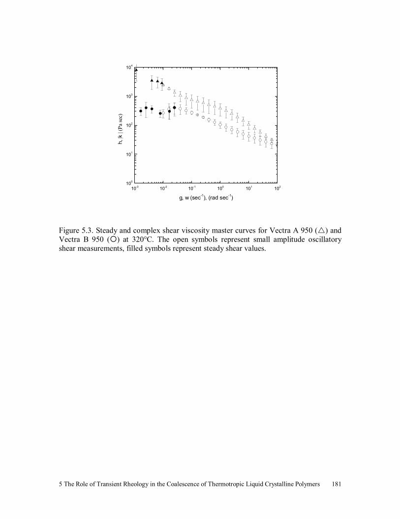
5 The Role of Transient Rheology in the Coalescence of Thermotropic Liquid Crystalline Polymers
181
10-3 10-2 10-1 100 101 102100
101
102
103
104
h, |k
| (Pa
sec)
g, w (sec-1), (rad sec-1)
Figure 5.3. Steady and complex shear viscosity master curves for Vectra A 950 ( ) and Vectra B 950 ( ) at 320°C. The open symbols represent small amplitude oscillatory shear measurements, filled symbols represent steady shear values.
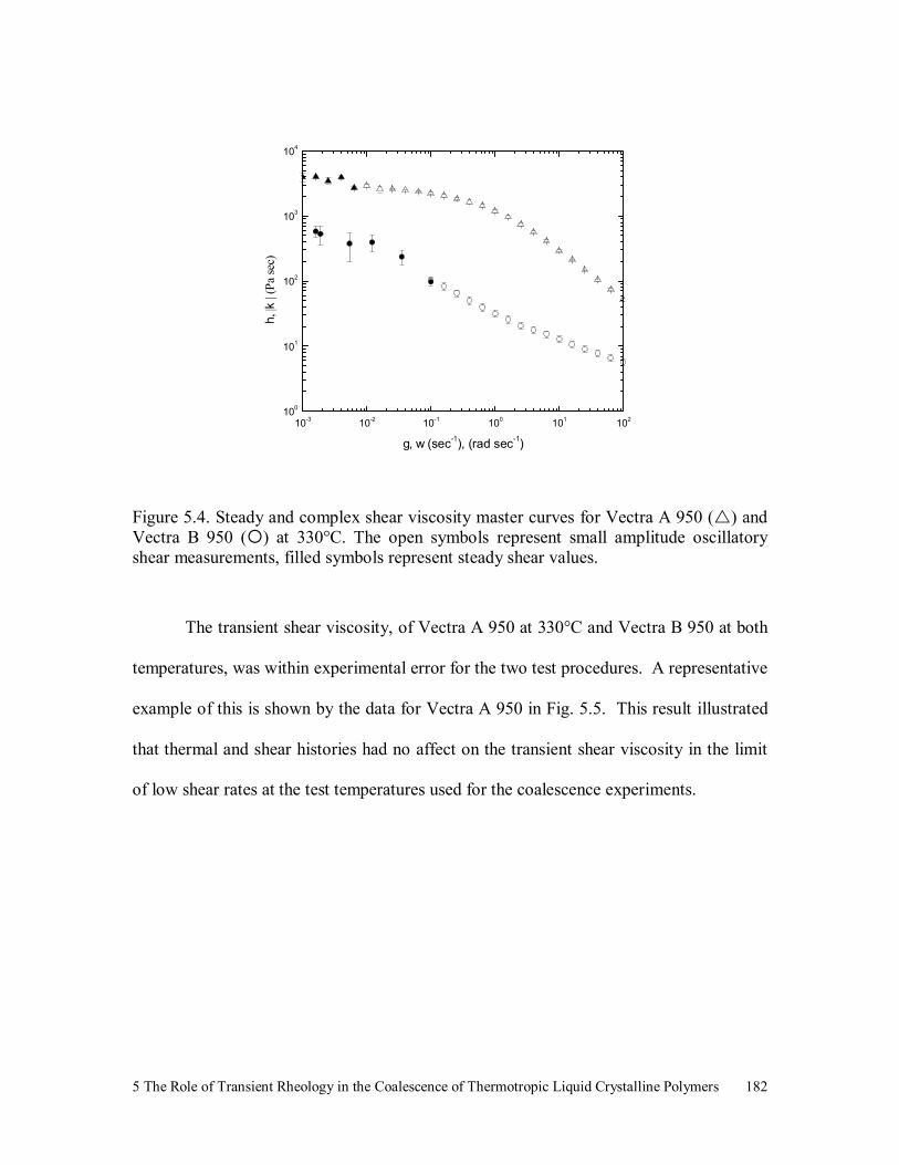
5 The Role of Transient Rheology in the Coalescence of Thermotropic Liquid Crystalline Polymers
182
10-3 10-2 10-1 100 101 102100
101
102
103
104
h, |k
| (Pa
sec)
g, w (sec-1), (rad sec-1)
Figure 5.4. Steady and complex shear viscosity master curves for Vectra A 950 ( ) and Vectra B 950 ( ) at 330°C. The open symbols represent small amplitude oscillatory shear measurements, filled symbols represent steady shear values.
The transient shear viscosity, of Vectra A 950 at 330°C and Vectra B 950 at both
temperatures, was within experimental error for the two test procedures. A representative
example of this is shown by the data for Vectra A 950 in Fig. 5.5. This result illustrated
that thermal and shear histories had no affect on the transient shear viscosity in the limit
of low shear rates at the test temperatures used for the coalescence experiments.
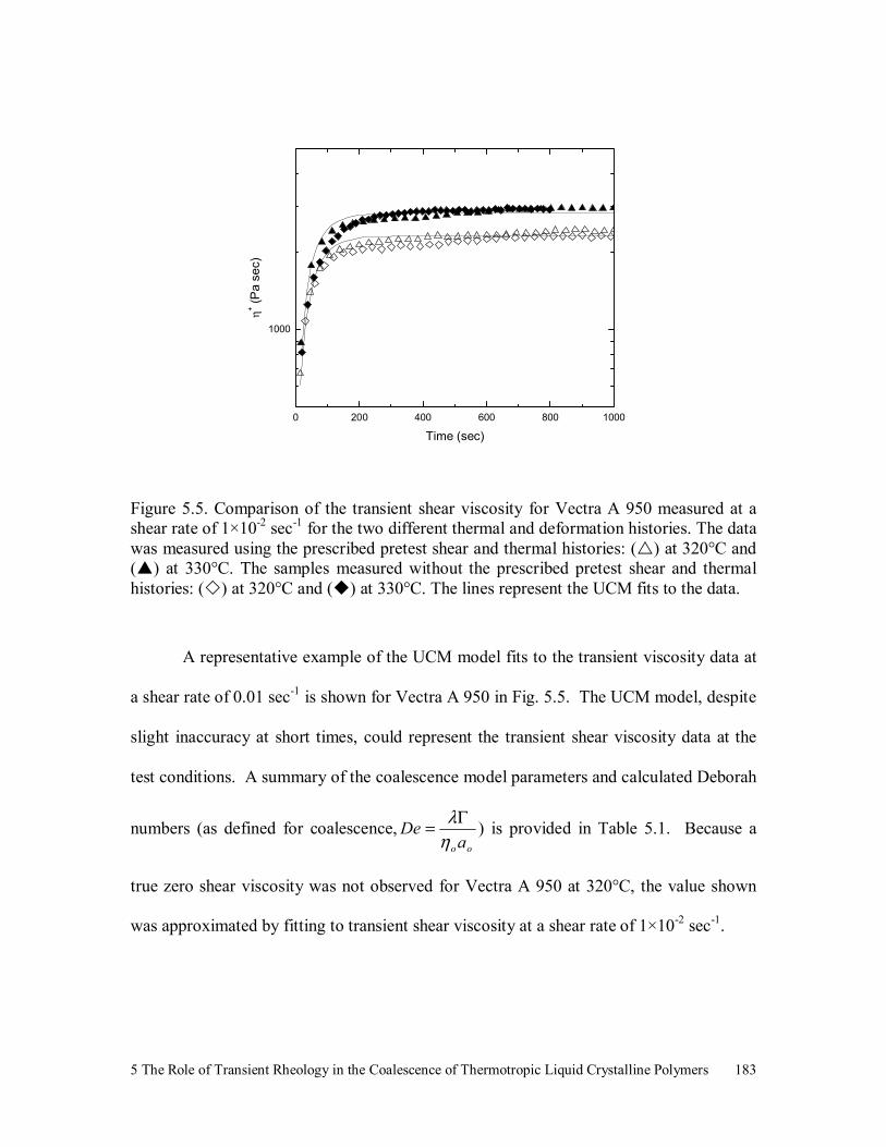
5 The Role of Transient Rheology in the Coalescence of Thermotropic Liquid Crystalline Polymers
183
0 200 400 600 800 1000
1000
η+ (Pa
sec)
Time (sec)
Figure 5.5. Comparison of the transient shear viscosity for Vectra A 950 measured at a shear rate of 1×10⁻² sec-1 for the two different thermal and deformation histories. The data was measured using the prescribed pretest shear and thermal histories: ( ) at 320°C and ( ) at 330°C. The samples measured without the prescribed pretest shear and thermal histories: ( ) at 320°C and ( ) at 330°C. The lines represent the UCM fits to the data.
A representative example of the UCM model fits to the transient viscosity data at
a shear rate of 0.01 sec-1 is shown for Vectra A 950 in Fig. 5.5. The UCM model, despite
slight inaccuracy at short times, could represent the transient shear viscosity data at the
test conditions. A summary of the coalescence model parameters and calculated Deborah
numbers (as defined for coalescence,ooa
DeηλΓ= ) is provided in Table 5.1. Because a
true zero shear viscosity was not observed for Vectra A 950 at 320°C, the value shown
was approximated by fitting to transient shear viscosity at a shear rate of 1×10⁻² sec-1.

5 The Role of Transient Rheology in the Coalescence of Thermotropic Liquid Crystalline Polymers
184
Table 5.1. UCM coalescence model parameters and calculated values for the Deborah Number.
Temperature (°C)
Relaxation Time λ
(sec)
Viscosityηo
(Pa sec)
Surface Tension Γ
±0.002 (J/m2)
Particle Radius ao
± 1(µm)
De (λΓ/ηo ao)
320 50.8 2301.1 0.031 250 2.7 Vectra A 950 330 49.3 2809.2 0.031 250 2.2
320 3.04 257.4 0.029 250 1.4 Vectra B 950 330 2.97 384.2 0.029 250 0.9
5.4.2 Experimental Coalescence
A representative example of the micrographs recorded during coalescence is
shown in Fig. 5.6 for Vectra B 950, where there is initially a finite contact area and the
neck radius increases with time until the two drops converge. In the example, the two
particles nearly reached a dimensionless neck radius of 1 within thirty seconds. Although
the test was stopped a few seconds later because the magnitude of the change in the
dimensionless neck radius becomes comparable to the magnitude of the error in the
measurement, the two particles did appear to continue to coalesce towards a single,
nearly spherical drop.

5 The Role of Transient Rheology in the Coalescence of Thermotropic Liquid Crystalline Polymers
185
Figure 5.6. Optical micrographs from the coalescence experiments of Vectra B 950 at 320°C.
Coalescence data is shown in Fig. 5.7 for Vectra A 950 and Vectra B 950 at both
temperatures. The coalescence rate for Vectra A 950 at 320°C was slower than for
Vectra A 950 at 330°C and Vectra B 950 at both temperatures. It was also observed that
Vectra A 950 failed completely coalesce at 320°C, which may be explained by the
presence of the yield-like shear viscosity behavior at low shear rates at that temperature.
The yield-like behavior may be the explained by the presence of residual crystallites.
Wilson et al. [12] showed that residual crystallites were present in the melt at 320°C, but
were completely melted by 330°C for a series of Vectra A 950 thin films. If residual
crystallites were present in Vectra A 950 at 320°C, they may act as physical cross links,
effectively increasing the viscosity and, hence, slowing coalescence.
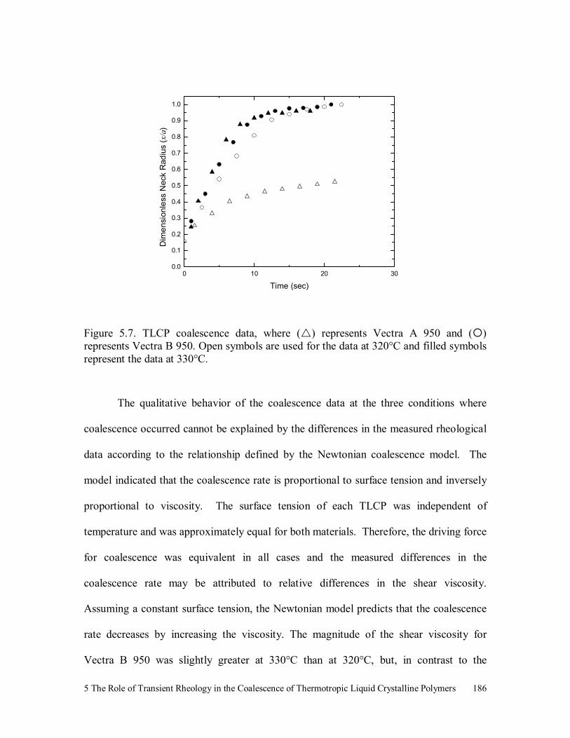
5 The Role of Transient Rheology in the Coalescence of Thermotropic Liquid Crystalline Polymers
186
0 10 20 300.0
0.1
0.2
0.3
0.4
0.5
0.6
0.7
0.8
0.9
1.0
Dim
ensi
onle
ss N
eck
Rad
ius
(x/a
)
Time (sec)
Figure 5.7. TLCP coalescence data, where ( ) represents Vectra A 950 and ( ) represents Vectra B 950. Open symbols are used for the data at 320°C and filled symbols represent the data at 330°C.
The qualitative behavior of the coalescence data at the three conditions where
coalescence occurred cannot be explained by the differences in the measured rheological
data according to the relationship defined by the Newtonian coalescence model. The
model indicated that the coalescence rate is proportional to surface tension and inversely
proportional to viscosity. The surface tension of each TLCP was independent of
temperature and was approximately equal for both materials. Therefore, the driving force
for coalescence was equivalent in all cases and the measured differences in the
coalescence rate may be attributed to relative differences in the shear viscosity.
Assuming a constant surface tension, the Newtonian model predicts that the coalescence
rate decreases by increasing the viscosity. The magnitude of the shear viscosity for
Vectra B 950 was slightly greater at 330°C than at 320°C, but, in contrast to the
5 The Role of Transient Rheology in the Coalescence of Thermotropic Liquid Crystalline Polymers
187
Newtonian model predictions, coalescence occurred faster at 330°C. In addition, the zero
shear viscosity of Vectra A 950 at 330°C was approximately an order of magnitude
greater than for Vectra B 950 at either temperature, yet Vectra A 950 coalesced faster.
The steady state UCM coalescence model is also incapable of explaining the
qualitative behavior of the coalescence data. This model was derived by substituting the
UCM constitutive model into the Newtonian derivation to introduce the effects of
viscoelasticity. As a first approximation the steady state assumption was imposed, which
effectively eliminates the time dependence of the biaxial extensional viscosity, as is
shown by Eq. 1.
ελη
εληη
&& 414
212
++
−= oo
b (1)
The same biaxial extensional viscosity is predicted, at small values of λ or f, for
both the Newtonian and the steady state UCM coalescence models, ηb= 6ηo. Under these
conditions, the steady state UCM coalescence model is expected to predict nearly the
same coalescence rate as the Newtonian coalescence model, which was shown could not
qualitatively explain the experimental data. As the biaxial extension rate is increased the
biaxial extensional viscosity passes through a slight minimum before beginning its
increase towards infinity. Increasing viscosity by will only act to further reduce the
coalescence rate relative to the Newtonian model. This effect does not assist in
explaining the relative differences in the coalescence data because, as reported in Table
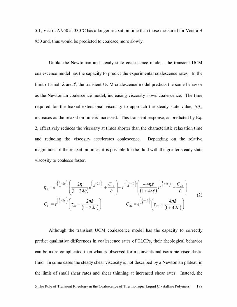
5 The Role of Transient Rheology in the Coalescence of Thermotropic Liquid Crystalline Polymers
188
5.1, Vectra A 950 at 330°C has a longer relaxation time than those measured for Vectra B
950 and, thus would be predicted to coalesce more slowly.
Unlike the Newtonian and steady state coalescence models, the transient UCM
coalescence model has the capacity to predict the experimental coalescence rates. In the
limit of small λ and f, the transient UCM coalescence model predicts the same behavior
as the Newtonian coalescence model, increasing viscosity slows coalescence. The time
required for the biaxial extensional viscosity to approach the steady state value, 6ηo,
increases as the relaxation time is increased. This transient response, as predicted by Eq.
2, effectively reduces the viscosity at times shorter than the characteristic relaxation time
and reducing the viscosity accelerates coalescence. Depending on the relative
magnitudes of the relaxation times, it is possible for the fluid with the greater steady state
viscosity to coalesce faster.
( ) ( )
( ) ( )
+
+=
−
−=
+
+−−
+
−=
+
−
+
+−
−
−−
ελεητ
ελεητ
εελεη
εεληη
ελ
ελ
ελ
ελ
ελ
ελ
&
&
&
&
&&
&
&&
&&
&&&&
414
212
414
212
41
22
21
11
224141
112121
yy
t
xx
t
tttt
b
eCeC
Cee
Cee
(2)
Although the transient UCM coalescence model has the capacity to correctly
predict qualitative differences in coalescence rates of TLCPs, their rheological behavior
can be more complicated than what is observed for a conventional isotropic viscoelastic
fluid. In some cases the steady shear viscosity is not described by a Newtonian plateau in
the limit of small shear rates and shear thinning at increased shear rates. Instead, the
5 The Role of Transient Rheology in the Coalescence of Thermotropic Liquid Crystalline Polymers
189
measured viscosity exhibits a yield-like behavior that is referred to as a three-region flow
curve, where the magnitude of the steady shear viscosity is related to different stages of
the destruction of polydomain liquid crystalline texture into a single nematic phase by the
imposed shear deformation [15]. Also the rheological stresses can be unique functions of
the deformation rate, strain, time, and may also be strongly dependent on the sample’s
thermal and deformation histories. Furthermore, there have been reports of oscillations
of the shear stresses during start-up of steady shear flow [16]. There have also been
reports of interesting behavior in the normal stress differences, such as negative values at
steady state or local minima before reaching steady state.
Despite the complex behavior exhibited by some TLCPs that suggests a complex
constitutive equation may need to be considered, it is possible that the rheological
behavior of TLCPs during coalescence can be sufficiently described by a more
conventional viscoelastic constitutive model. The dimension of liquid crystalline
domains for the materials evaluated in this study is on the order of 1 µm, while the
particle diameter is approximately 500 µm [17]. The particles were prepared in such a
manner that the liquid crystalline domains were not preferentially oriented, a description
of the process is provided elsewhere [14]. Therefore, without preferential orientation of
the domains, a random distribution of orientation exists and the particle is effectively
isotropic on the 500 µm scale. The magnitudes of the deformation rates and strains are
small during the coalescence of two particles. The deformation rates predicted by the
Newtonian model, using a value for the viscosity that is comparable to the zero shear
viscosity of the TLCPs used in this work, exhibit a maximum value during coalescence
5 The Role of Transient Rheology in the Coalescence of Thermotropic Liquid Crystalline Polymers
190
that is less than 1×10⁻² sec-1. Also, the predicted strain for two identical spherical
particles is limited to one strain unit. Possible influence of negative values of the normal
stress differences should not be factor because the flow kinematics for coalescence are
biaxial extension. In addition, the transient biaxial extensional viscosity can be
approximated by the transient shear viscosity, using the relationship, ηb+ = 6ηo
+, which
was verified for these materials for deformation rates (g, f) up to 0.1 sec-1 [18].
5.4.3 Transient UCM Coalescence Model Predictions
Predictions from the transient UCM, Newtonian, and steady state coalescence
models are shown for Vectra A 950 at 330°C in Fig. 5.8. Similar results were observed
for Vectra A 950 and Vectra B 950 at 320°C. As shown in the figure, the Newtonian
coalescence model predictions began to deviate from the experimental data within the
first few seconds and, afterwards, under predicted the coalescence rates. The steady state
UCM coalescence model predicted slower coalescence than was predicted by the
Newtonian model and, in doing so, was less accurate than the Newtonian model. The
transient UCM coalescence model predicted greater coalescence rates than the Newtonian
model, which was in qualitative agreement with the experimental data. Unfortunately,
the model grossly over predicted the coalescence rate, which was nearly instantaneous
and was almost identical for the three experimental conditions. Also, the transient UCM
coalescence model was unable to correctly predict the order of coalescence times for
Vectra A 950 at 330°C and Vectra B at 320 and 330°C. The experimental coalescence
times were tVA330°C < tVB330°C < tVB320°C, as was shown in Fig. 5.7 and the model predicted
tVA330°C < tVB320°C < tVB330°C. Although the predicted results are not shown, the predicted

5 The Role of Transient Rheology in the Coalescence of Thermotropic Liquid Crystalline Polymers
191
order of coalescence times was consistent with the calculated Deborah number, the
samples with larger Deborah numbers coalesced faster.
0 10 20 300.0
0.2
0.4
0.6
0.8
1.0
D
imen
sion
less
Nec
k R
adiu
s (x
/a)
Time (sec)
Figure 5.8. Vectra A 950 coalescence data at 330°C and predictions from the Newtonian, steady state UCM, and transient UCM coalescence models. The symbols represent the experimental data ( ) and the lines represent the coalescence model predictions: Newtonian (—), steady state UCM (----), and the transient UCM (····).
5.5 Conclusions
The coalescence of two TLCPs was studied by comparing experimentally
measured values of the dimensionless neck radius with predicted values from the
Newtonian, steady state, and the transient UCM coalescence models. Several significant
conclusions can be drawn from this work. The first is that the behavior of the shear
viscosity at low shear rates can be used to identify conditions where successful

5 The Role of Transient Rheology in the Coalescence of Thermotropic Liquid Crystalline Polymers
192
coalescence will occur. It was shown that the measured rheological behavior, specifically
the transient viscosity in the limit of small shear rates, can be accurately represented by
the UCM constitutive model. The biaxial extensional viscosities, as predicted by the
Newtonian and steady state coalescence models, were analyzed to explain why those
models were incapable of qualitatively predicting the experimental coalescence data.
Finally, it was shown that the transient UCM coalescence model predicted faster
coalescence than the Newtonian model, which was in qualitative agreement with the
experimental data, but much faster.
5.6 Acknowledgements
This work was financially supported by a phase II SBIR grant from NASA, grant
number NAS-2S-4018-285, managed by Luna Innovations.
5 The Role of Transient Rheology in the Coalescence of Thermotropic Liquid Crystalline Polymers
193
5.7 References
1. Crawford, R.J., Throne, J.L., Rotational Molding Technology, Plastics Design
Library, William Andrew Publishing, Norwich, New York (2002)
2. K.L. Johnson, K. Kendall, and A.D. Roberts, Surface Energy and the Contact of
Elastic Solids, Proceedings of the Royal Society of London. Series A, 324, 1558
301 (1971)
3. MacDonald, W.A., Chapter 8, “Thermotropic Main Chain Liquid Crystal
Polymers,” in Liquid Crystal Polyners: From Structures to Applications, edited by
Collyer, A.A., Elsevier Applied Science, NewYork (1992)
4. Chiou, J.S., Paul, D.R., “Gas Transport in a Thermotropic Liquid-Crystalline
Polymer,” Journal of Polymer Science Part B: Polymer Physics, 25, 1699 (1987)
5. Cox, M.K., “The Application of Liquid Crystal Polymer Properties,” Molecular
Crystals and Liquid Crystals, 153, 415 (1987)
6. Scribben, E., Baird, D.G., “Sintering of Thermotropic Liquid Crystalline
Polymers,” SPE ANTEC, 48 (2002)
7. O. Pokluda, C.T. Bellehumeur, and J. Vlachopoulos, Modification of Frenkel’s
Model for Sintering, AICHE Journal, 43, 12 (1997) 3253.
8. C.T. Bellehumeur, M. Kontopoulou, and J. Vlachopoulos, The Role of
Viscoelasticity in Polymer Sintering, Rheologica Acta, 37, 3 (1998) 270.
9. Scribben, E., Baird, D.G., Wapperom, P., “The Role of Transient Rheology in
Polymeric Coalescence,” Journal of Non-Newtonian Fluid Mechanics, submitted.

5 The Role of Transient Rheology in the Coalescence of Thermotropic Liquid Crystalline Polymers
194
10. Beekmans, F., Gotsis, A.D., Norder, B., “Influence of the Flow History on Stress
Growth and Structure Changes in the Thermotropic Liquid Crystalline Polymer
Vectra B950,” Rheologica Acta, 36, 82 (1997)
11. Product Literature from Ticona, Vectra® liquid crystal polymer (LCP)
12. Wilson, T.S., “The Rheology and Structure of Thermotropic Liquid Crystalline
Polymers in Extensional Flow,” Ph.D. Dissertation, Department of Chemical
Engineering, Virginia Polytechnic Institute and State University, Blacksburg, Va.
24061 (1991)
13. J.F. Padday, in Matijević, E. (Ed.), Surface and Colloid Science, Vol.1, Wiley
Interscience, New York, 1969, Part II., 104.
14. Scribben, E., Baird, D.G., “The Rotational Molding of a Thermotropic Liquid
Crystalline Polymer,” Polymer Engineering and Science, submitted.
15. Onogi, S., Asada, T., “Rheology and Rheo-Optics of Polymer Liquid Crystal,” in
Rheology, Vol. 1., edited by Astarita, G., Marrucci, G., Nicholais, L., Plenum
Press, New York (1980)
16. Ternet, D.J., Larson, R.G., Leal, L.G., “Transient director patterns upon start-up
of nematic liquid crystals (an explanation for stress oscillation damping),”
Rheologica Acta, 40, 307-316 (2001)
17. Gotsis, A.D., Odriozola, M.A., “Extensional viscosity of a thermotropic liquid
crystalline polymer,” Journal of Rheology, 44, 5, 1205-1223 (2000)
18. Done, D.D., “Studies on the Rheology and Morphology of Thermotropic Liquid
Crystalline Polymers,” Ph.D. Dissertation, Virginia Polytechnic Institute and State
University, Blacksburg, Va, 24061 (1987)

6 The Rotational Molding of a Thermotropic Liquid Crystalline Polymer
195
6 The Rotational Molding of a Thermotropic Liquid Crystalline
Polymer
Preface
This chapter addresses the second and third objectives of this research.
Specifically, the adaptation of the conditions identified by studying the coalescence of the
selected TLCP to the rotational molding process and establishing rotational molding
conditions that optimize the physical and mechanical properties. This chapter is
organized as a manuscript for future publication.
6 The Rotational Molding of a Thermotropic Liquid Crystalline Polymer
196
The Rotational Molding of a Thermotropic Liquid Crystalline Polymer
Eric Scribben and Donald Baird
Department of Chemical Engineering, Virginia Polytechnic Institute and State University, Blacksburg, Va 24061
6.1 Abstract
Thermotropic liquid crystalline polymers (TLCPs) exhibit a number of
mechanical and physical properties such as excellent chemical resistance, low
permeability, low coefficient of thermal expansion, high tensile strength and modulus,
and good impact resistance, which make them desirable as a rotationally molded storage
vessel. However, there are no reports in the technical literature of the successful
rotational molding of TLCPs. In this paper conditions are identified that lead to the
successful rotational molding of a TLCP, Vectra B 950. First, a technique was developed
to produce particles suitable for rotational molding because TLCP’s cannot be ground
into a free flowing powder. Second, because the viscosity at low shear rates can be
detrimental to the sintering process, coalescence experiments with isolated particles were
carried out to determine the thermal and environmental conditions where sintering should
occur. These conditions were then applied to static sintering experiments to determine
whether coalescence and densification of the bulk powder would occur. Finally, the
powders were successfully rotationally molded into tubular structures in a single axis,
lab-scale device. The density of the molded structure was essentially equivalent to the
material density and the tensile strength and modulus were approximately 18 MPa and 2
GPa, respectively.
6 The Rotational Molding of a Thermotropic Liquid Crystalline Polymer
197
6.2 Introduction
Thermotropic liquid crystalline polymers (TLCPs) exhibit a number of
mechanical and physical properties that make them desirable for use in storage vessels
for cryogenic or corrosive fluids. TLCPs have demonstrated exceptionally high values of
tensile strength and modulus (strengths in excess of 1000 MPa and moduli near 100 GPa
from fiber spinning and approaching 200 MPa and 20 GPa, respectively, in injection
molding) [1]. They possess low permeability to gases, which is essential for the
containment of gases [2]. They exhibit excellent resistance to acidic or basic
environments and a wide range of organic solvents, prerequisites for storing corrosive
fluids [3]. Finally, they have low coefficients of linear thermal expansion (CLTE) and,
therefore, may be useful for storage of cryogenic fluids such as liquid hydrogen and
oxygen as they may be less prone to failure due to thermally induced stresses [1].
Rotational molding is a convenient processing method for manufacturing large
storage vessels from thermoplastics [4]. In the process polymer powder is loaded into a
hollow mold that is simultaneously rotated about two principal axes. Heat is applied to
the external surface of the mold and is conducted to the tumbling powder, which melts
and adheres to the mold surface. As heating continues, the powder coalesces as a result
of the surface tension and densifies into an evenly distributed layer that coats the internal
surface of the mold. The mold is cooled, and once the plastic has solidified, the product
is removed [5].
6 The Rotational Molding of a Thermotropic Liquid Crystalline Polymer
198
Unfortunately, there are no reports in the technical literature on the rotational
molding of TLCPs. The only work that was presented involved the static coalescence of
two TLCP powders [6]. Three key results were reported. The first result was that
powder generated by cryogenically grinding TLCP pellets was composed of high aspect
ratio particles. Secondly, it was reported that coalescence was either slow or incomplete
and speculated that the observed difficulties with coalescence may be due to large values
of the shear viscosity at low deformation rates. Finally, complete densification was not
observed for the high aspect ratio particles. Hence, it is most likely that the problems
encountered in the static coalescence of TLCPs would preclude rotational molding of
these materials.
High aspect ratio particles are not desirable for rotational molding because they
typically have low apparent (or bulk) densities and tend to agglomerate. Free flow of
granular solids, also referred to as powder flow, is essential for material distribution
during mold rotation and is greatly dependent upon powder properties such as size,
shape, and density [4]. In general, a desirable powder for rotational molding is one with
a diameter that is approximately between 150 to 500 µm, gives good packing density,
possesses reasonable surface area to volume ratio, and are not fibrous or thread-like [7].
Therefore, it is expected that a free flowing powder is not readily available for use in the
rotational molding process.
6 The Rotational Molding of a Thermotropic Liquid Crystalline Polymer
199
Complete coalescence is crucial for successful rotational molding. In its simplest
form, coalescence describes the merging of two particles into a single, homogeneous
drop. When two fluid-like particles are brought into contact, surface tension, being
opposed by the fluid’s viscosity, acts to minimize surface area by expanding the contact
interface between the particles. It has been shown that the rate of interfacial growth is
proportional to surface tension and inversely proportional to the shear viscosity [8,9].
Unlike Newtonian fluids, the viscosity of a polymeric fluid is dependent on the rate of
deformation. The deformation rates that occur during coalescence are estimated to be
less than approximately 1×10⁻² sec-1 [10]. These low deformation rates suggest that the
zero shear viscosity of a polymer melt represents the resistance to flow during this
process. It has been shown that some TLCPs do not have a well defined zero shear
viscosity [11]. Instead they exhibit a yield stress-like behavior that is part of what is
referred to as a three-region flow curve, where the magnitude of the steady shear
viscosity is related to different stages of the destruction of a polydomain texture into a
single nematic phase by the imposed shear deformation [11]. If the selected TLCP
exhibits this behavior, the large value of viscosity at low deformation rates may inhibit
coalescence. Hence, identifying conditions (i.e. temperature and environmental) where
the zero shear viscosity behavior is conducive to coalescence is a prerequisite for
successful rotational molding.
Densification refers to the stage in rotational molding by which the coalescing
powder bed consolidates into a homogeneous pore-free layer. Once the contact interfaces
between coalescing particles become large enough, the structure of the powder bed

6 The Rotational Molding of a Thermotropic Liquid Crystalline Polymer
200
begins to resemble a continuous, three-dimensional lattice [7]. As the particles continue
to melt, the height of the powder bed decreases and the lattice gradually collapses upon
itself. Unfortunately, not all of the air that was once surrounding the lattice structure is
immediately expelled during the collapse and, a portion becomes encapsulated within the
melt. The encapsulated bubbles are not drawn to the free surface by buoyancy or
capillary forces [12]. Instead, the gas in the bubbles is removed by dissolution into and
diffusion through the surrounding polymer melt [13,14]. Hence, the same factor that
makes TLCPs useful for gas storage vessels may also hinder the densification process. It
is noted that TLCPs have permeability coefficients for gases such as He, H2, Ar, N2, and
CO2 that are comparable to or less than those for polyacrylonitrile (PAN), one of the least
permeable polymers known [2].
As there are no reports of successful rotational molding of TCLPs, obviously, the
mechanical properties of rotational molded TLCP structures have not been reported.
While TLCPs have demonstrated exceptionally high values of tensile strength and
modulus, the magnitude of these quantities is dependent upon the degree of mesophase
orientation introduced during processing [1]. Processing methods that introduce high
deformation rates increase orientation and produce structures with higher values of
tensile strength and modulus. Compression molding, which generates deformation
similar to those that occur during rotational molding, produces an unoriented TLCP that
has mechanical properties similar to those of a conventional isotropic polymer [1].
Furthermore, the strength may also be limited by the presence of weld lines, which form
at the contact interface between coalescing particles [1]. Hence, it is unknown as to the
6 The Rotational Molding of a Thermotropic Liquid Crystalline Polymer
201
order of magnitude of mechanical properties that might be possible in the rotational
molding of TLCPs.
Based on the fact that rotational molding of TLCPs may beset by several
problems, the objectives of this work are to: 1) develop a method to generate free flowing
powders; 2) establish the thermal and environmental conditions required for the
successful coalescence of TLCP particles; 3) determine if the conditions for coalescence
can be translated to appropriate conditions for rotational molding of the bulk powder; 4)
evaluate the mechanical properties of a rotationally molded tube.
6.3 Analytical Methods
6.3.1 Material
Vectra B 950, a nematic TLCP available from Ticona (Summit, NJ), was selected
for this evaluation. The primary motivation for selecting this particular material is
because it has demonstrated superior mechanical properties when compared to other
commercial TLCPs [15]. Vectra B is a wholly aromatic polyesteramide, randomly
copolymerized from 60 mole percent hydroxynaphthoic acid, 20 mole percent
terephthalic acid, and 20 mole percent aminophenol. The chemical structure is shown in
Fig. 5.3. The melt temperature, as determined by the peak value from differential
scanning calorimetry (DSC), is 279°C [16]. When the melt is cooled quiescently, the
crystallization temperature is 226°C, as defined by the beginning of the exothermic
crystallization peak measured by DSC. However, the resin may crystallize in shear flow

6 The Rotational Molding of a Thermotropic Liquid Crystalline Polymer
202
at higher temperatures, up to approximately 300°C [16]. The glass transition
temperature, as measured by the peak value from dynamic mechanical thermal analysis
(DMTA), is 147°C [17]. The nematic to isotropic transition temperature is unknown
because the degradation occurs at temperatures below the transition. The weight average
molecular weight and polydispersity index are thought to be around 30,000 and 2,
respectively [18].
C
O
O
Hydroxynaphthoic Acid
N
H
O
p - Aminophenol
C C
O O
Terephthalic Acid
0.6 0.2 0.2
C
O
O
Hydroxynaphthoic Acid
C
O
O
Hydroxynaphthoic Acid
C
O
OC
O
C
OO
OO
Hydroxynaphthoic Acid
N
H
O
p - Aminophenol
N
H
O
p - Aminophenol
N
H
ON
H
N
H
OO
p - Aminophenol
C C
O O
Terephthalic Acid
C C
O O
Terephthalic Acid
C C
O O
C C
OO OO
Terephthalic Acid
0.6 0.2 0.2
Figure 6.1. Chemical structure and composition of Vectra B 950
6.3.2 Generation and Characterization of Powders
Vectra B 950 is available as a pellet, which is too large for rotational molding.
Thus two powder generation methods were evaluated. The first method was the approach
used to make powders from conventional rotational molding polymers. The pellets were
milled with a Vortec M-1 impact mill at room temperatures and under cryogenic
conditions by combining liquid nitrogen to the feed. The second method for generating
powders was based on the blending of a TLCP with an incompatible polymer in a 1”
Killion single screw extruder. When two immiscible phases are mixed, the minor phase
is dispersed with a droplet size determined by its properties (i.e. viscosity and interfacial
tension) and the shear stress [5]. The TLCP was blended at up to 40 weight percent with
a low molecular weight polypropylene (melt index = 400) at 340°C. The extruded blend

6 The Rotational Molding of a Thermotropic Liquid Crystalline Polymer
203
was quenched below the melt temperature of both components, effectively freezing the
dispersed blend morphology. The cooling rate played an important role in determining
the size of the dispersed TLCP phase. If the mixture was not quenched quickly enough
the TLCP phase would continue to separate from the continuous phase and coalesce with
itself, increasing the dimensions of the TLCP phase. The dispersed TLCP phase was
retrieved by fracturing the polypropylene matrix with a mill and separating the
components in water (the specific gravity of polypropylene is approximately 0.9 and will
float in water, while the TLCP has a specific gravity of 1.4 and sinks). Residual
polypropylene on the TLCP particles (less than 1 weight percent as measured by thermal
gravimetric analysis) was removed by dissolving it in light mineral oil at 170°C. The
mineral oil mixture was then washed from the TLCP particles using a biodegradable
degreaser and water. The TLCP powder was then dried in accordance to manufacturer
specifications in vacuum oven at 150°C for between 12 and 24 hours [17].
After the particles were retrieved from the polypropylene matrix, they were
separated into discrete groups according to their size with a series of U.S. standard sieves
and a Rotap shaker. Separation was performed not only to measure the size distribution
of the accumulated powder but also to allow for the evaluation of particular sizes and
distributions in later experiments. The procedure for separating the powder was to sift
100 gram samples for 10 minutes as described in ASTM test D 3451 for testing
polymeric powder and powder coatings. Shaking for 10 minutes delivered consistent
results while minimizing static charge build-up in the extremely fine particles (less than
149 micron).
6 The Rotational Molding of a Thermotropic Liquid Crystalline Polymer
204
The apparent density of all powders was measured according to ASTM test D
1895, which describes powder property measurements for plastic materials. Test method
A was used for the particles obtained from the melt blending process and test method C
was used for the powder acquired from the milling process. Test method A was designed
for fine granular materials that can be readily poured through a standardized funnel. Test
method C was applicable to materials that cannot be poured through the funnel because
they are compressible, usually composed of coarse flakes, chips, cut fibers, or strands.
Two values are reported for the apparent density measured according to test method C:
one for the initial density of loosely packed material and one with the powder under a
prescribed compressive load.
The dynamic angle of repose is the angle of the surface of a flowing powder
relative to horizontal, as shown in Fig. 6.2. It was measured in a 100 mL graduated
cylinder. 50 mL of the powder was poured into the cylinder. The open end of the
cylinder was plugged with a rubber stopper that had been placed on a shaft, driven by a
variable speed motor. The cylinder was supported at the opposite end so that it would
remain horizontal during rotation. Rotation rates from approximately 1 to 10 rpm were
used during the measurement of each sample. The rates were selected because they were
comparable to what was introduced to the powder during rotational molding. A digital
image of the tumbling powder was taken at each rotation rate and the angle was
determined by analyzing the image in Adobe Photoshop.
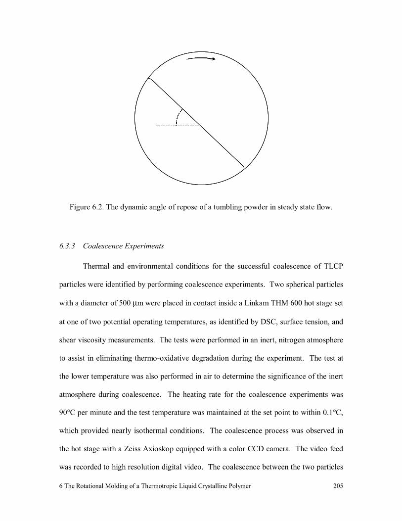
6 The Rotational Molding of a Thermotropic Liquid Crystalline Polymer
205
Figure 6.2. The dynamic angle of repose of a tumbling powder in steady state flow.
6.3.3 Coalescence Experiments
Thermal and environmental conditions for the successful coalescence of TLCP
particles were identified by performing coalescence experiments. Two spherical particles
with a diameter of 500 µm were placed in contact inside a Linkam THM 600 hot stage set
at one of two potential operating temperatures, as identified by DSC, surface tension, and
shear viscosity measurements. The tests were performed in an inert, nitrogen atmosphere
to assist in eliminating thermo-oxidative degradation during the experiment. The test at
the lower temperature was also performed in air to determine the significance of the inert
atmosphere during coalescence. The heating rate for the coalescence experiments was
90°C per minute and the test temperature was maintained at the set point to within 0.1°C,
which provided nearly isothermal conditions. The coalescence process was observed in
the hot stage with a Zeiss Axioskop equipped with a color CCD camera. The video feed
was recorded to high resolution digital video. The coalescence between the two particles

6 The Rotational Molding of a Thermotropic Liquid Crystalline Polymer
206
was identical to that shown in Fig. 6.3. Still images from the digital video were extracted
at prescribed intervals, and the neck and particle radii, x and a, were measured using
Scion Image, a digital image analysis software available from Scion Corporation. Each
coalescence experiment was conducted three times to ensure reproducibility, and the
reported neck radius versus time data were the average of the three runs.
ao a
x
aoao a
x
a
x
Figure 6.3. Schematic of the geometric evolution of coalescing spherical particles during the coalescence experiments.
6.3.4 Thermal Behavior
Dynamic scanning calorimetry (DSC) was used to identify a potential minimum
temperature for the coalescence experiments by measuring the end of the melt transition.
This analysis can only identify a potential minimum temperature because it has been
shown that TLCPs can recrystallize at temperatures above their melt point [19]. Also, the
presence of a small amount of crystallinity, undetectable by DSC, can still greatly affect
the viscosity [18]. In both of these cases care should be taken in assuming that complete
melting has occurred. The thermal analysis was performed at a heating rate of 10°C/
minute with a Seiko Instruments SSC/5200 series auto cooling DSC-220C. The sample
6 The Rotational Molding of a Thermotropic Liquid Crystalline Polymer
207
was exposed to both a heating and a cooling cycle before the reported measurement to
ensure the material had been properly dried and to impose a known thermal history.
6.3.5 Surface Tension
The surface tension was measured at two potential operating temperatures to
determine the magnitude of the driving force during coalescence. The surface tension
was determined by fitting the Bashforth and Adams equation to a sessile drop profile of
the molten polymer at the particular test conditions [20]. This method was selected
because it presents a noninvasive means of measuring the surface tension of the TLCP as
a melt with the identical geometry, thermal history, and deformation history used in the
coalescence experiments. A single, 500 µm diameter sphere, identical to those used in
the coalescence experiments, was placed on a glass slide in the hot stage, where it was
melted into a sessile drop. The sample was quenched and the glass slide was rotated to
allow a profile view of the drop from above. The sample was reheated to the test
temperature and a digital image of the profile was recorded with an optical microscope
equipped with a miniDV camcorder. The Bashforth and Adams equation was fit to data
points representing the profile shape that were extracted from the digital image of the
profile with Scion Image. The accuracy of this technique (0.1%) demands that the
particle radii must be small so that gravitational forces cannot influence the shape of the
profile. The absence of gravitational forces was verified by calculating the Bond number
Γ= grBo
2ρ (Bo=0.030) and was supported by the observation that the profile shape did
not change upon rotating the glass slide.
6 The Rotational Molding of a Thermotropic Liquid Crystalline Polymer
208
6.3.6 Rheology
The shear viscosity was measured at the two potential operating temperatures to
determine the magnitude during coalescence and to verify the absence of the three-region
viscosity behavior. All rheological characterization was performed with a Rheometrics
Mechanical Spectrometer Model 800 (RMS-800). The instrument test geometry was a 25
mm diameter cone and plate with a 0.1 radian cone angle. The magnitude of the complex
viscosity, |η*| versus angular frequency, ω, and shear viscosity, η, versus shear rate, g,
data were measured in the presence of an inert nitrogen atmosphere to prevent thermo-
oxidative degradation. Test specimens were prepared by compression molding preforms
at 320°C under nominal pressure and allowing them to quiescently cool without applied
pressure. This method produces homogeneous samples with minimal residual stress that
were the desired dimensions for the test geometry. Reported rheological results represent
the average of at least three runs using different samples for each run. Small amplitude
dynamic oscillatory shear measurements were performed for frequencies between 0.1 to
100 rad/sec at 10% strain for both 320 and 330°C. The steady shear viscosity was
measured by recording the steady state value of a stress growth upon inception of steady
shear flow experiment. The stress growth experiments were performed at low shear rates
because of the lengthy times required to obtain data at low angular frequencies from
dynamic oscillatory measurements. Viscosity values at shear rates less than 0.1 sec-1
were thought to be the most pertinent to the coalescence process.
6 The Rotational Molding of a Thermotropic Liquid Crystalline Polymer
209
The measured rheological response of TLCPs is strongly dependent upon thermal
and deformation history. Therefore, a pretest procedure was devised to introduce
reproducible shear and thermal histories to minimize variation in rheological data. The
cone and plate preform was placed in the rheometer and while the sample was heated to
340°C, the cone was brought to 0.05 mm from the plate. Once the temperature reached
340°C, a steady shear deformation was applied at a shear rate of 0.1 sec-1 for 10 seconds.
After the preshear was complete the sample was cooled to the test temperature where it
was given five minutes to reach a stress free state before beginning the test. The 340°C
preheat temperature was selected because the sample would not relax to a stress-free state
within the allotted time if lower temperatures were used.
6.3.7 Densification Experiments
Eight samples of the spherical particles were used to evaluate particle size and
size distribution, each sample is described in Table 6.1. The first four samples, identified
as S1 through S4, represent particular sizes and samples D1 through D4 represent various
distributions. D1 is skewed towards smaller particles, D2 is skewed towards larger
particles, D3 is a normal distribution, and D4 represents a traditional rotational molding
distribution, where the majority of its content is between approximately 300 and 600
micron and contains a small fraction of fine particles. The samples were poured into a
1.27 cm x 6.35 cm rectangular bar mold with an exposed top surface and a thermocouple
fixed in the center of one of the sides of the mold. A nitrogen purge (powders were not
under pressure) was supplied through a chamber that covered the mold. The entire unit
was placed on a pre-heated hot plate that simulated conductive heating from one side as

6 The Rotational Molding of a Thermotropic Liquid Crystalline Polymer
210
occurs in rotational molding. The total heating time was 40 minutes and began once the
set temperature, as measured at the mold, was reached. After 40 minutes the apparatus
was removed from the hot plate and allowed to cool in ambient with continued nitrogen
purge.
Table 6.1. Descriptions of the powder samples used in the densification study.
S1 S2 S3 S4 D1 D2 D3 D4
20 840 1.0 - - - 0.07 0.53 0.10 -30 595 - 1.0 - - 0.13 0.27 0.40 0.0840 420 - - 1.0 - 0.27 0.13 0.40 0.4850 297 - - - 1.0 0.53 0.07 0.10 0.3960 250 - - - - - - - 0.0270 210 - - - - - - - 0.02100 149 - - - - - - - 0.01
Size and Distribution Mass FractionsU.S. Standard
Sieve No.Opening (micron)
In addition to the 40 minute experiments, sample S3 was used in three other tests.
In the first test, the heating time was extended to 80 minutes to check for improved
densification with increased time. The other two tests were to evaluate the possibility of
increasing strength by an oxidative effect that had been observed during the coalescence
tests. The first heating cycle for those experiments was designed to determine if
introducing air to the sample at the end of the formerly described 40 minute cycle could
improve properties. For this case, the sample was exposed to 20 minutes of heating in
nitrogen followed by 20 minutes in air. The last test was to verify that any differences
observed in the 20/20 test were not due to reducing the time the sample was heated in
nitrogen. For this, the sample was exposed to an additional 20 minute of heating in air
after spending 40 minutes heating in nitrogen.
6 The Rotational Molding of a Thermotropic Liquid Crystalline Polymer
211
6.3.8 Properties of Densification Samples
Several properties of the bars molded in the densification experiments were
evaluated. The density of the molded specimen, which is defined as the average density
and differs from the material density by the amount of voids in the molded sample, was
measured to determine the extent of densification. The average density was measured
according to method A in ASTM test D 792, for testing solid plastics by displacement in
water. It should be noted that the average density measured by this method is not
affected by surface porosity, but only by differences in the amount of encapsulated gas.
The test also requires that the results to be corrected for variation in the test temperature
and reported at 23°C.
Tensile tests were performed on the molded bars with a model 4202 Instron
tensile testing machine to determine the ultimate tensile strength and Young’s modulus.
The crosshead speed was 1.27mm/min and the gauge length was 30.5 mm according to
ASTM test D 638. The samples fracture surfaces were inspected for uniform pore
distribution and size. All reported results for average density and mechanical properties
were the average from at least three samples.
6.3.9 Single-Axis Rotational Molding Experiments
The laboratory-scale rotational molding device consisted of a cylindrical, stainless
steel mold, with an inside diameter of 1.59 cm and 7.62 cm in length, was used as the

6 The Rotational Molding of a Thermotropic Liquid Crystalline Polymer
212
rotational mold. For each test, the mold was filled with 30 grams of D4 powder, this
distribution was selected because it produced the greatest average density during the
densification study. Both ends of the mold were capped. One cap was threaded onto a
shaft that was driven by a variable speed motor. A fitting was installed in the center of
the opposite cap so that a nitrogen purge could be delivered directly into the mold cavity.
The mold was placed in a forced convection oven that could heat at up to 60°C per
minute and maintain the set temperature to within 1°C. The heating cycle was designed
to mimic the conditions used in the densification experiments. The heating stage began
once the mold reached the set temperature and after 40 minutes, the heat was stopped and
the oven was opened. Rotation and nitrogen purge continued as the mold was allowed to
cool to room temperature with the assistance of the oven fan.
6.3.10 Properties of the Rotational Molded Samples
The molded product was visually inspected before testing the density, tensile
strength and modulus, and burst pressure. The tensile properties were measured by the
same method that was used in the densification study. 5 mm wide rectangular strips were
cut axially from the molded cylinders. The specified width was found to sufficiently
minimize radial curvature and allow the sample to be clamped into the Instron test
fixture. Each of the reported results for average density and mechanical properties were
the average of at least three runs.
One rotational molding sample was prepared from 50 grams of sample D4 to be
tested for its bust strength. The sample was clamped between the two plates as shown in

6 The Rotational Molding of a Thermotropic Liquid Crystalline Polymer
213
the diagram of the test fixture in Fig. 6.4. The sample was then pressurized with water
that was delivered through the fitting that was installed on the one plate until it burst.
Figure 6.4. Diagram of test fixture used to measure the burst strength.
6.4 Results and Discussion
6.4.1 Powder Flow Characteristics
Vectra B 950 was obtained in pellet form, which was too large to successfully use
in the rotational molding process. An attempt was made to generate powder by methods
used for conventional polymers. Visual evaluation showed that the milled TLCP was
composed of high aspect ratio particles that agglomerate, which is illustrated in Fig. 6.5.
The fibrillar particles obtained from the milled pellets arise from the unique morphology
generated during the extrusion of TLCPs. Shear deformation introduced during extrusion
orients the liquid crystalline domains into a hierarchal fibrillar texture [21]. The
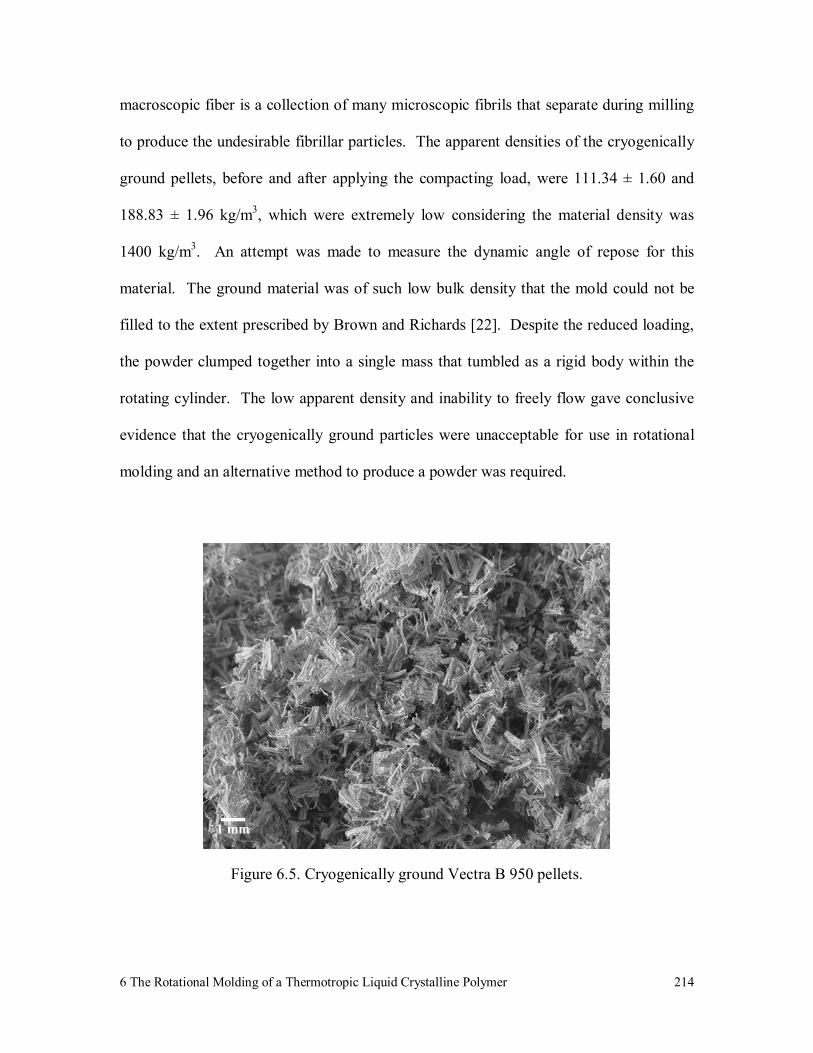
6 The Rotational Molding of a Thermotropic Liquid Crystalline Polymer
214
macroscopic fiber is a collection of many microscopic fibrils that separate during milling
to produce the undesirable fibrillar particles. The apparent densities of the cryogenically
ground pellets, before and after applying the compacting load, were 111.34 ± 1.60 and
188.83 ± 1.96 kg/m3, which were extremely low considering the material density was
1400 kg/m3. An attempt was made to measure the dynamic angle of repose for this
material. The ground material was of such low bulk density that the mold could not be
filled to the extent prescribed by Brown and Richards [22]. Despite the reduced loading,
the powder clumped together into a single mass that tumbled as a rigid body within the
rotating cylinder. The low apparent density and inability to freely flow gave conclusive
evidence that the cryogenically ground particles were unacceptable for use in rotational
molding and an alternative method to produce a powder was required.
Figure 6.5. Cryogenically ground Vectra B 950 pellets.
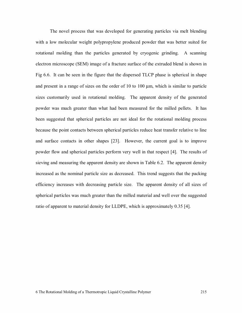
6 The Rotational Molding of a Thermotropic Liquid Crystalline Polymer
215
The novel process that was developed for generating particles via melt blending
with a low molecular weight polypropylene produced powder that was better suited for
rotational molding than the particles generated by cryogenic grinding. A scanning
electron microscope (SEM) image of a fracture surface of the extruded blend is shown in
Fig 6.6. It can be seen in the figure that the dispersed TLCP phase is spherical in shape
and present in a range of sizes on the order of 10 to 100 µm, which is similar to particle
sizes customarily used in rotational molding. The apparent density of the generated
powder was much greater than what had been measured for the milled pellets. It has
been suggested that spherical particles are not ideal for the rotational molding process
because the point contacts between spherical particles reduce heat transfer relative to line
and surface contacts in other shapes [23]. However, the current goal is to improve
powder flow and spherical particles perform very well in that respect [4]. The results of
sieving and measuring the apparent density are shown in Table 6.2. The apparent density
increased as the nominal particle size as decreased. This trend suggests that the packing
efficiency increases with decreasing particle size. The apparent density of all sizes of
spherical particles was much greater than the milled material and well over the suggested
ratio of apparent to material density for LLDPE, which is approximately 0.35 [4].
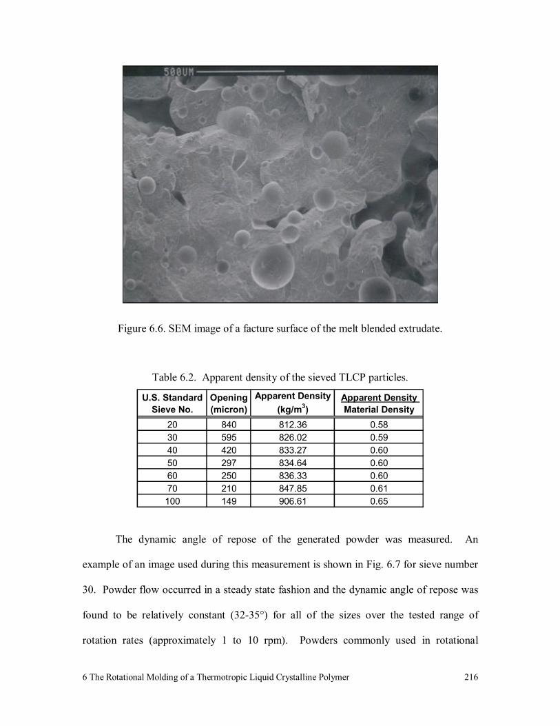
6 The Rotational Molding of a Thermotropic Liquid Crystalline Polymer
216
Figure 6.6. SEM image of a facture surface of the melt blended extrudate.
Table 6.2. Apparent density of the sieved TLCP particles.
U.S. Standard Sieve No.
Opening (micron)
Apparent Density (kg/m3)
Apparent Density Material Density
20 840 812.36 0.5830 595 826.02 0.5940 420 833.27 0.6050 297 834.64 0.6060 250 836.33 0.6070 210 847.85 0.61100 149 906.61 0.65
The dynamic angle of repose of the generated powder was measured. An
example of an image used during this measurement is shown in Fig. 6.7 for sieve number
30. Powder flow occurred in a steady state fashion and the dynamic angle of repose was
found to be relatively constant (32-35°) for all of the sizes over the tested range of
rotation rates (approximately 1 to 10 rpm). Powders commonly used in rotational
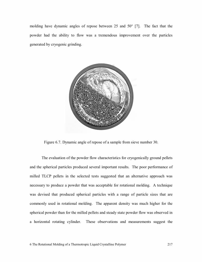
6 The Rotational Molding of a Thermotropic Liquid Crystalline Polymer
217
molding have dynamic angles of repose between 25 and 50° [7]. The fact that the
powder had the ability to flow was a tremendous improvement over the particles
generated by cryogenic grinding.
Figure 6.7. Dynamic angle of repose of a sample from sieve number 30.
The evaluation of the powder flow characteristics for cryogenically ground pellets
and the spherical particles produced several important results. The poor performance of
milled TLCP pellets in the selected tests suggested that an alternative approach was
necessary to produce a powder that was acceptable for rotational molding. A technique
was devised that produced spherical particles with a range of particle sizes that are
commonly used in rotational molding. The apparent density was much higher for the
spherical powder than for the milled pellets and steady state powder flow was observed in
a horizontal rotating cylinder. These observations and measurements suggest the

6 The Rotational Molding of a Thermotropic Liquid Crystalline Polymer
218
generated powder should possess acceptable powder flow characteristics for the
rotational molding process.
6.4.2 Coalescence
DSC was used to identify the end of the melt transition, and the measured DSC
thermogram is shown in Fig. 6.8. The peak of the melt transition occurred at 284°C and
the melt transition was complete by 310°C, both are represented as stars in the figure. In
an attempt to ensure that complete melting would occur, 320 and 330°C were selected for
the coalescence experiments.
0 50 100 150 200 250 300 350
260
280
300
320
340
360
380
Endo
ther
m (µ
W/m
g)
Temperature (°C)
Figure 6.8. DSC thermogram of Vectra B 950 with the peak and end of the melt transition represented by stars.

6 The Rotational Molding of a Thermotropic Liquid Crystalline Polymer
219
The surface tension and shear viscosity were measured at 320 and 330°C, to
verify their relative magnitudes and the absence of a three-region viscosity behavior. The
surface tension was measured as 0.029 ± 0.002 J/m2 and was independent of temperature
and the surrounding atmospheric composition. This demonstrates that the driving force
for coalescence is constant for the two temperatures. The shear flow curves at the two
temperatures in nitrogen are shown in Fig. 6.9. As shown in the figure, the material does
not exhibit three-region viscosity behavior at either temperature, but, instead, a well
defined zero shear viscosity that is similar in magnitude at both two temperatures. With
the driving force and the resistance to flow equal at the two temperatures, coalescence
was expected to progress at similar rates.
10-3 10-2 10-1 100 101 102100
101
102
103
104
h, |k
| (Pa
sec)
g, w (sec-1), (rad sec-1)
Figure 6.9. The magnitude of the complex viscosity versus frequency are represented as for 320°C and for 330°C. The shear viscosity versus shear rate is represented as
for 320°C for 330°C, error bars represent deviation in the measurements.
6 The Rotational Molding of a Thermotropic Liquid Crystalline Polymer
220
In addition to the complex and steady shear viscosity values, two stress growth
upon inception of steady shear flow experiments were conducted in the zero shear limit
(0.01 sec-1) at 320°C, one in the presence of nitrogen the other in air, the results are
shown in Fig. 6.10. The transient viscosity of the sample measured in nitrogen reaches a
steady state value while the sample that was measured in the presence of air increases in
an unbounded fashion. It is doubtful that this behavior is the result of recrystallization
during shear because it did not occur in the sample measured in nitrogen at the same
temperature. However, a possible explanation is that the molecular weight was
increasing, as has been reported for a similar wholly aromatic TLCP, Vectra A 950. It
was shown, for Vectra A, that the melt was polymerized by interchain transesterification
that begins at temperatures approximately 35°C above the melt temperature [24].
Polymerization increases the molecular weight by one liquid crystal molecule forming a
convalent bond with one of its neighbors. Regardless of the reason for the increase in
viscosity, the measured behavior suggests that the presence of an inert atmosphere will be
essential to obtaining complete coalescence.

6 The Rotational Molding of a Thermotropic Liquid Crystalline Polymer
221
0 100 200 300 400 500 6000
1000
2000
3000
4000
5000
6000
7000
h+ (Pa
sec)
Time (sec)
Figure 6.10. Transient shear viscosity from stress growth experiments at a shear rate of 0.01 sec-1 and 320°C. The symbol represents the test conducted in the presence of nitrogen and is in the presence of air.
Coalescence experiments were carried out to confirm that the conditions
identified by rheological characterization were appropriate. A representative example of
the images recorded during the coalescence experiments is shown in Fig. 6.11. Initially,
there was a finite contact area and the neck radius increased with time until the two drops
converged. In the figure, the two particles nearly reached a dimensionless neck radius,
ax , of 1 within 20 seconds. Although the test was stopped shortly thereafter because the
magnitude of the change in the dimensionless neck radius becomes comparable to the
magnitude of the error in the measurement, the two particles do appear to continue to
coalesce towards a single, nearly spherical drop.
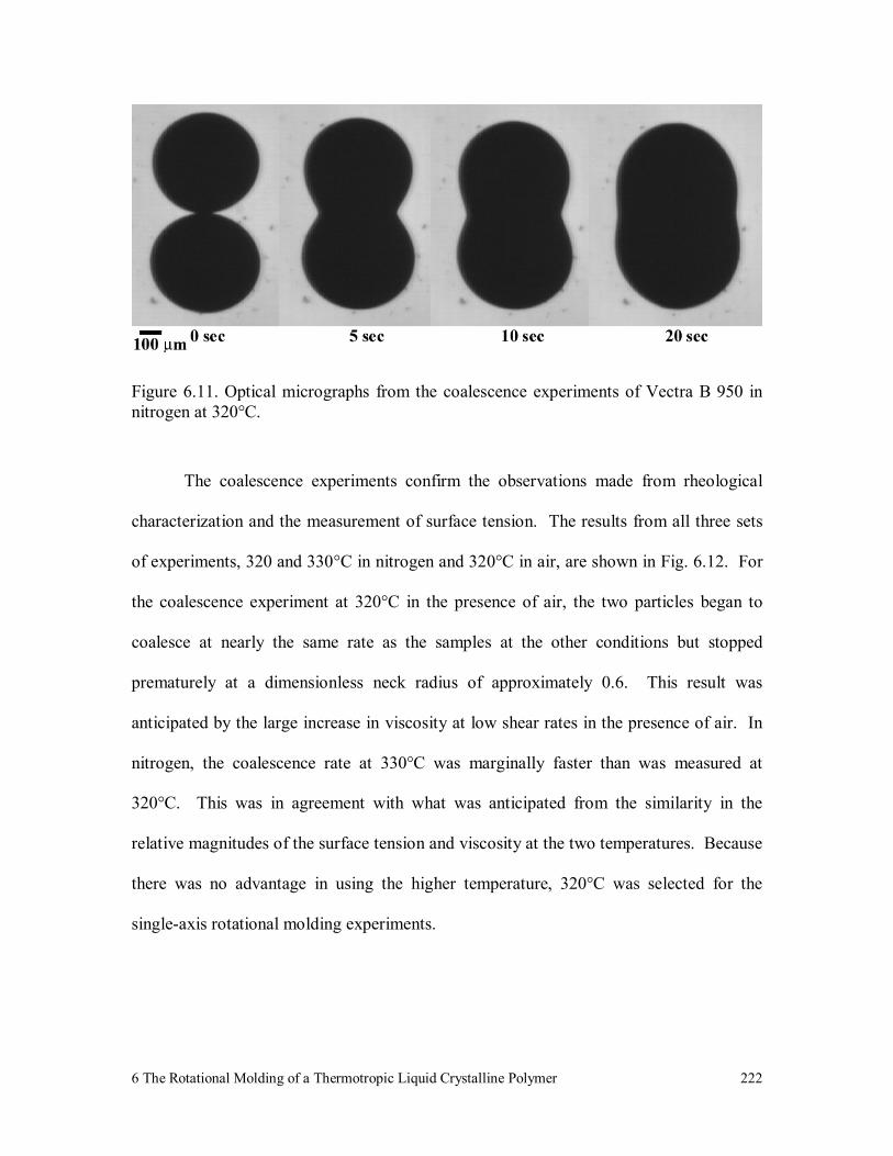
6 The Rotational Molding of a Thermotropic Liquid Crystalline Polymer
222
Figure 6.11. Optical micrographs from the coalescence experiments of Vectra B 950 in nitrogen at 320°C.
The coalescence experiments confirm the observations made from rheological
characterization and the measurement of surface tension. The results from all three sets
of experiments, 320 and 330°C in nitrogen and 320°C in air, are shown in Fig. 6.12. For
the coalescence experiment at 320°C in the presence of air, the two particles began to
coalesce at nearly the same rate as the samples at the other conditions but stopped
prematurely at a dimensionless neck radius of approximately 0.6. This result was
anticipated by the large increase in viscosity at low shear rates in the presence of air. In
nitrogen, the coalescence rate at 330°C was marginally faster than was measured at
320°C. This was in agreement with what was anticipated from the similarity in the
relative magnitudes of the surface tension and viscosity at the two temperatures. Because
there was no advantage in using the higher temperature, 320°C was selected for the
single-axis rotational molding experiments.
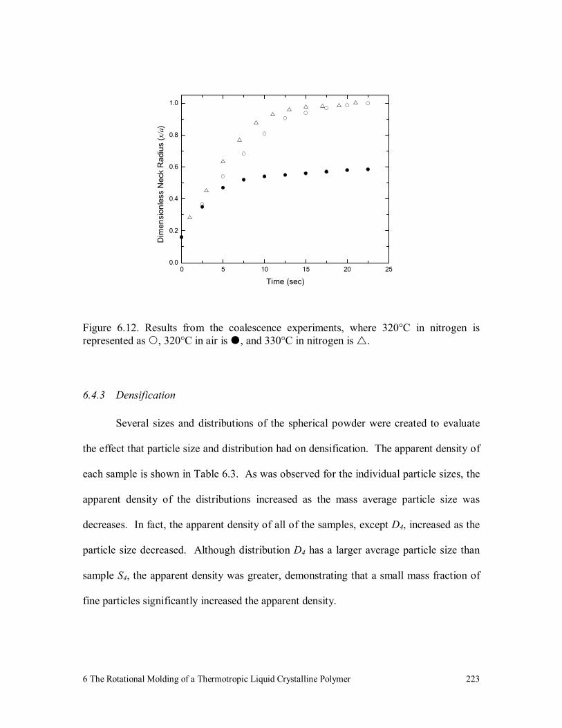
6 The Rotational Molding of a Thermotropic Liquid Crystalline Polymer
223
0 5 10 15 20 250.0
0.2
0.4
0.6
0.8
1.0
Dim
ensi
onle
ss N
eck
Rad
ius
(x/a
)
Time (sec)
Figure 6.12. Results from the coalescence experiments, where 320°C in nitrogen is represented as , 320°C in air is , and 330°C in nitrogen is .
6.4.3 Densification
Several sizes and distributions of the spherical powder were created to evaluate
the effect that particle size and distribution had on densification. The apparent density of
each sample is shown in Table 6.3. As was observed for the individual particle sizes, the
apparent density of the distributions increased as the mass average particle size was
decreases. In fact, the apparent density of all of the samples, except D4, increased as the
particle size decreased. Although distribution D4 has a larger average particle size than
sample S4, the apparent density was greater, demonstrating that a small mass fraction of
fine particles significantly increased the apparent density.
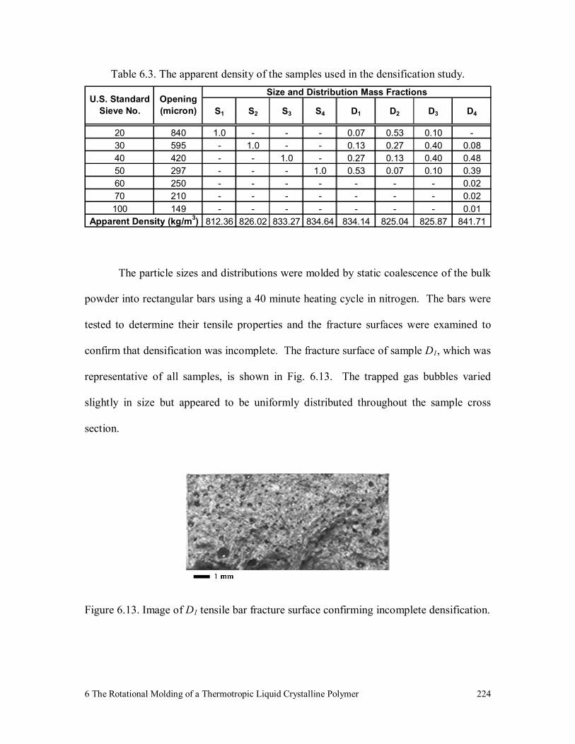
6 The Rotational Molding of a Thermotropic Liquid Crystalline Polymer
224
Table 6.3. The apparent density of the samples used in the densification study.
S1 S2 S3 S4 D1 D2 D3 D4
20 840 1.0 - - - 0.07 0.53 0.10 -30 595 - 1.0 - - 0.13 0.27 0.40 0.0840 420 - - 1.0 - 0.27 0.13 0.40 0.4850 297 - - - 1.0 0.53 0.07 0.10 0.3960 250 - - - - - - - 0.0270 210 - - - - - - - 0.02100 149 - - - - - - - 0.01
812.36 826.02 833.27 834.64 834.14 825.04 825.87 841.71
Size and Distribution Mass Fractions
Apparent Density (kg/m3)
U.S. Standard Sieve No.
Opening (micron)
The particle sizes and distributions were molded by static coalescence of the bulk
powder into rectangular bars using a 40 minute heating cycle in nitrogen. The bars were
tested to determine their tensile properties and the fracture surfaces were examined to
confirm that densification was incomplete. The fracture surface of sample D1, which was
representative of all samples, is shown in Fig. 6.13. The trapped gas bubbles varied
slightly in size but appeared to be uniformly distributed throughout the sample cross
section.
Figure 6.13. Image of D1 tensile bar fracture surface confirming incomplete densification.

6 The Rotational Molding of a Thermotropic Liquid Crystalline Polymer
225
The measured values of the average density at 23°C, tensile modulus, and the
ultimate tensile strength are all reported in Table 6.4. Of the molded samples that consist
of a particular particle size (S1-S4), it is shown that the gas content in the molded sample,
as determined by measuring the average density, was slightly reduced as the apparent
density of the powder was increased. This trend was also observed by the increase in the
ratio of average to apparent density for these samples. It was also found that the
extended 80 minute heating cycle was ineffective at increasing the average density of
sample S3, proving that densification could not be increased by simply increasing the
cycle time, as is usually done in rotational molding. A similar relationship to that
observed for samples S1 through S4 was found for the distributions, D1 through D4. The
average density of the molded samples increased as the apparent density of the powder
increased. Although the extent of densification appears to be correlated to the apparent
density, complete densification was not attained by increasing the apparent density.
Table 6.4. Results of the density and tensile measurements for the densification study, S3*
represents the results from the extended cycle time.
ρ/ρappUltimate Tensile Strength normalized by D23°C (MPa)
S1 1022 ± 7 1.26 0.598 ± 0.008 7.18 ± 0.10 9.84S2 1148 ± 8 1.39 1.093 ± 0.015 10.08 ± 0.14 12.29S3 1189 ± 8 1.43 1.140 ± 0.015 11.00 ± 0.15 12.96S3
* 1175 ± 8 1.41 1.147 ± 0.015 10.92 ± 0.15 13.01S4 1193 ± 8 1.43 0.964 ± 0.013 12.78 ± 0.17 15.00D1 1176 ± 8 1.41 1.040 ± 0.014 13.48 ± 0.18 16.05D2 1106 ± 7 1.34 1.008 ± 0.014 9.61 ± 0.13 12.16D3 1155 ± 8 1.40 1.066 ± 0.014 9.11 ± 0.12 11.04D4 1218 ± 8 1.45 0.930 ± 0.012 10.51 ± 0.14 12.08
Tensile Modulus (GPa)
Ultimate Tensile Strength (MPa)
Average Density D23°C (kg/m3)
Several interesting results were shown by the measured tensile properties. The
tensile modulus was near 1 GPa for all samples except S1. It is possible that the results
6 The Rotational Molding of a Thermotropic Liquid Crystalline Polymer
226
for S1 were not representative because of the low average density in that sample. The
ultimate tensile strength of samples S1 through S4 increased with the average density,
indicating that strength was dependent on the extent of densification. The values for
strength were normalized for differences in their average density to determine if the
relationship between strength and average density was solely due to variation in the
extent of densification or if there was also a change in adhesion between particles.
Because the strength of the normalized results was not all equal it was concluded that
adhesion had been increased. A clear relationship between tensile strength and average
density was not observed for the sample distributions. Sample D1 delivered the highest
tensile strength, but D4 possessed the highest average density. Perhaps the small fraction
of extremely fine powders in distribution D4 actually reduces the strength. If this were
true, it could be rationalized by the distribution possessing a greater number of particles,
and, therefore particle interfaces.
The two trials that were used to evaluate the possibility of increasing the strength
by introducing the oxidative effect were unsuccessful. The results are shown in Table 6.5
with the results for the sample molded in nitrogen. It was found that the strength of the
samples that were exposed to air was less than the sample molded in nitrogen. Not only
does this imply that the speculated molecular weight increase by transesterification was
not occurring, it also demonstrates the importance of supplying an inert atmosphere
throughout the entire molding process and not only during the initial stages when
coalescence occurs.
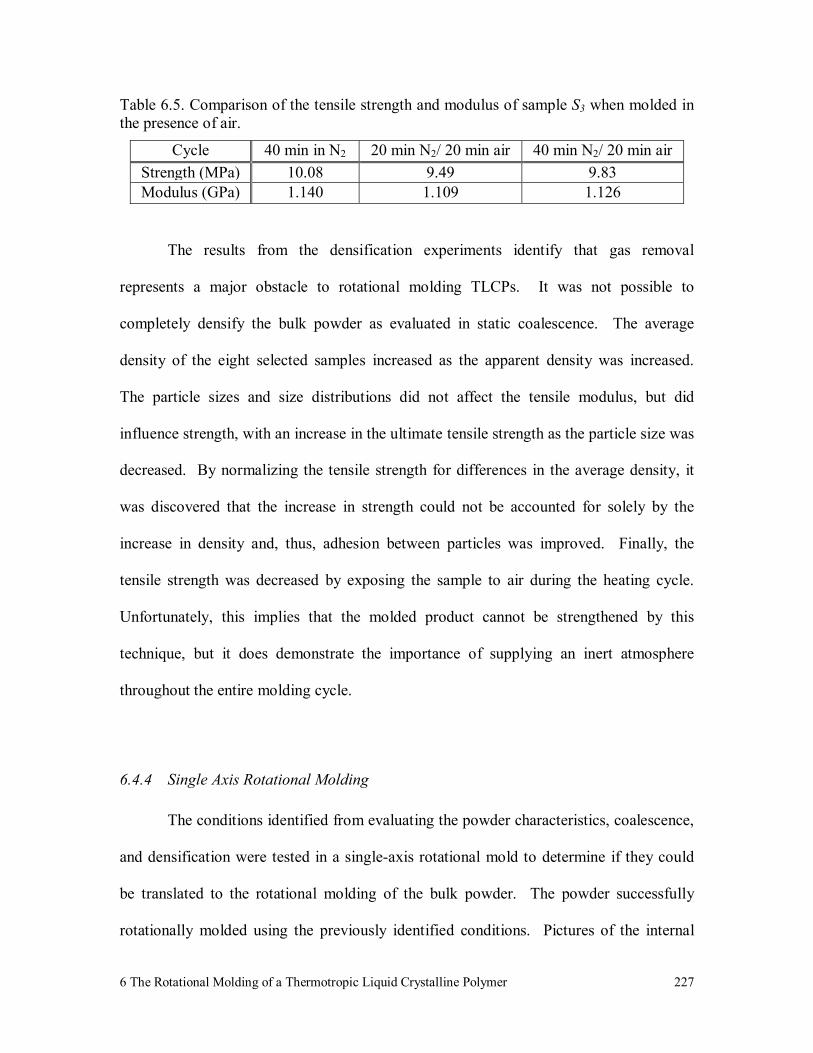
6 The Rotational Molding of a Thermotropic Liquid Crystalline Polymer
227
Table 6.5. Comparison of the tensile strength and modulus of sample S3 when molded in the presence of air.
Cycle 40 min in N2 20 min N2/ 20 min air 40 min N2/ 20 min air Strength (MPa) 10.08 9.49 9.83 Modulus (GPa) 1.140 1.109 1.126
The results from the densification experiments identify that gas removal
represents a major obstacle to rotational molding TLCPs. It was not possible to
completely densify the bulk powder as evaluated in static coalescence. The average
density of the eight selected samples increased as the apparent density was increased.
The particle sizes and size distributions did not affect the tensile modulus, but did
influence strength, with an increase in the ultimate tensile strength as the particle size was
decreased. By normalizing the tensile strength for differences in the average density, it
was discovered that the increase in strength could not be accounted for solely by the
increase in density and, thus, adhesion between particles was improved. Finally, the
tensile strength was decreased by exposing the sample to air during the heating cycle.
Unfortunately, this implies that the molded product cannot be strengthened by this
technique, but it does demonstrate the importance of supplying an inert atmosphere
throughout the entire molding cycle.
6.4.4 Single Axis Rotational Molding
The conditions identified from evaluating the powder characteristics, coalescence,
and densification were tested in a single-axis rotational mold to determine if they could
be translated to the rotational molding of the bulk powder. The powder successfully
rotationally molded using the previously identified conditions. Pictures of the internal
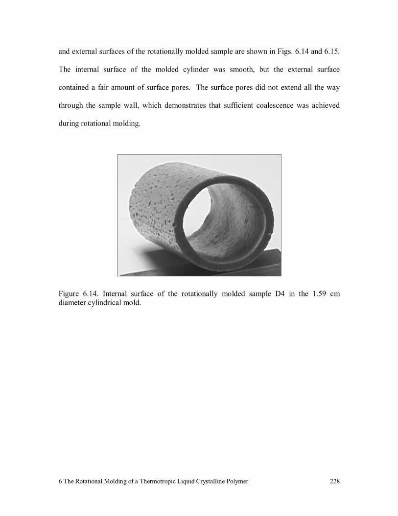
6 The Rotational Molding of a Thermotropic Liquid Crystalline Polymer
228
and external surfaces of the rotationally molded sample are shown in Figs. 6.14 and 6.15.
The internal surface of the molded cylinder was smooth, but the external surface
contained a fair amount of surface pores. The surface pores did not extend all the way
through the sample wall, which demonstrates that sufficient coalescence was achieved
during rotational molding.
Figure 6.14. Internal surface of the rotationally molded sample D4 in the 1.59 cm diameter cylindrical mold.

6 The Rotational Molding of a Thermotropic Liquid Crystalline Polymer
229
Figure 6.15. External surface of rotationally molded sample D4, where the width image is 50.8 mm.
The results from the measured average density, ultimate tensile strength, and
tensile modulus for the rotationally molded cylinder are shown in Table 6.6. The results
for the same distribution from the densification study are included for comparison.
Surprisingly, all quantities were increased relative to what had been measured for static
coalescence. The increase in density suggests that further improvement may be possible
in the rotational molding experiment. Although the tensile modulus was over twice that
measured in the densification study, it was still only a fraction of the 20 GPa that can be
obtained with proper molecular alignment and implies that further increase may still be
possible. The measured increase in the tensile strength was quite significant because it is
very close to the nominal strength (17.9 MPa) required for industrial cross-linked high
density polyethylene tanks [25]. This was sufficient to pressurize the molded sample to
1.59 MPa before rupture occurred (50 gram sample with 3.8 mm wall thickness).

6 The Rotational Molding of a Thermotropic Liquid Crystalline Polymer
230
Table 6.6. The average density, tensile strength, and tensile modulus from the rotationally molded distribution D4 compared the results for the distribution from the densification study.
0.012 2.022 ± 0.013
0.14 17.49 0.16±Ultimate Tensile Strength (MPa)
Tensile Modulus (GPa)
1218 ±
10.51 ±
0.930 ±
Sample D 4 Results from the Densification Study
Sample D 4 Results from Rotational Molding
Average Density (kg/m3)
8 1288 ± 7
When comparing the results from the densification study with the results from
rotational molding, it appears that the dynamics introduced by rotation increased the
average density. The increase must occur by reducing the amount of gas that initially
gets trapped during coalescence because it was demonstrated in the densification study
that once gas is encapsulated, it cannot be removed. Understanding the mechanism that
controls the relationship between rotation and the amount of gas that is encapsulated
during coalescence may lead to a method to optimize the rotation rate.
To explain the increased density the static densification and dynamic rotational
molding processes were reconsidered. The encapsulation of bubbles in the static scenario
may be described as shown in Fig. 6.16. The powder is heated by conduction from the
mold wall. As the powder melts, coalescence occurs and a network of connected
particles is formed. Eventually the network collapses, and bubbles are encapsulated,
which are removed by dissolving and diffusing through the surrounding melt. However,
the permeability of a gas in the TLCP is extremely low so any bubbles that are formed
remain in the melt, as in stage two of the figure.
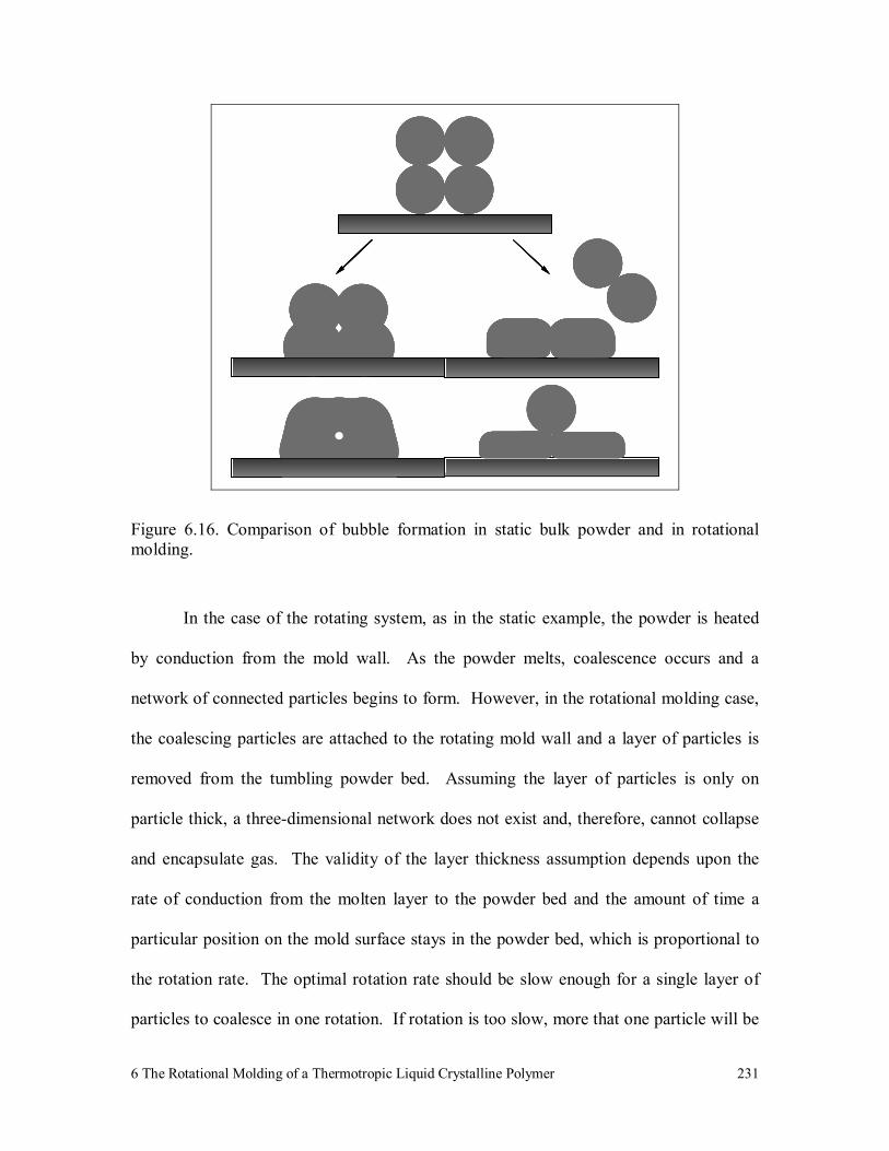
6 The Rotational Molding of a Thermotropic Liquid Crystalline Polymer
231
Figure 6.16. Comparison of bubble formation in static bulk powder and in rotational molding.
In the case of the rotating system, as in the static example, the powder is heated
by conduction from the mold wall. As the powder melts, coalescence occurs and a
network of connected particles begins to form. However, in the rotational molding case,
the coalescing particles are attached to the rotating mold wall and a layer of particles is
removed from the tumbling powder bed. Assuming the layer of particles is only on
particle thick, a three-dimensional network does not exist and, therefore, cannot collapse
and encapsulate gas. The validity of the layer thickness assumption depends upon the
rate of conduction from the molten layer to the powder bed and the amount of time a
particular position on the mold surface stays in the powder bed, which is proportional to
the rotation rate. The optimal rotation rate should be slow enough for a single layer of
particles to coalesce in one rotation. If rotation is too slow, more that one particle will be

6 The Rotational Molding of a Thermotropic Liquid Crystalline Polymer
232
attached to the mold wall as it passes through the powder bed. If it is too fast, the layer
will not completely coalesce before the next layer of particles attach.
The single axis rotational molding experiment was repeated to test the proposed
explanation of the observed difference in average density between the static and dynamic
cases. The rotation rate used in this experiment was determined by using the coalescence
time measured in the coalescence experiments. The particles coalesced at 320°C within
approximately 20 seconds. To promote the formation of a single particle layer, the
rotation rate was set at 20 seconds per revolution or 3 rpm.
Several of the measured properties were improved by reducing the rotation rate.
The density of the sample that was rotationally molded at 3 rpm was increased to 1392 ±
6 kg/m3. This is a significant improvement because it is essentially the material density
and, therefore, complete densification was achieved by the reduction in rotation rate.
Unfortunately, an increase comparable to what was measured in density was not
measured in the ultimate tensile strength and tensile modulus. The measured values were
17.63 ± 0.019 MPa and 2.010 ± 0.014 GPa for strength and modulus, respectively, which
were within the experimental error of the sample molded at 10 rpm. The surface pores in
the exterior surface were reduced as shown in Fig. 6.18. Although some surface pores
still exist, this represents a dramatic improvement over what had been found at 10 rpm,
shown in Fig. 6.17.
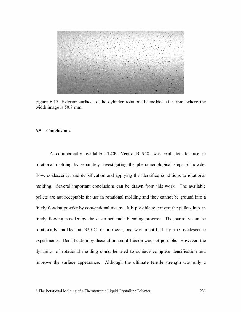
6 The Rotational Molding of a Thermotropic Liquid Crystalline Polymer
233
Figure 6.17. Exterior surface of the cylinder rotationally molded at 3 rpm, where the width image is 50.8 mm.
6.5 Conclusions
A commercially available TLCP, Vectra B 950, was evaluated for use in
rotational molding by separately investigating the phenomenological steps of powder
flow, coalescence, and densification and applying the identified conditions to rotational
molding. Several important conclusions can be drawn from this work. The available
pellets are not acceptable for use in rotational molding and they cannot be ground into a
freely flowing powder by conventional means. It is possible to convert the pellets into an
freely flowing powder by the described melt blending process. The particles can be
rotationally molded at 320°C in nitrogen, as was identified by the coalescence
experiments. Densification by dissolution and diffusion was not possible. However, the
dynamics of rotational molding could be used to achieve complete densification and
improve the surface appearance. Although the ultimate tensile strength was only a
6 The Rotational Molding of a Thermotropic Liquid Crystalline Polymer
234
fraction of what can be obtained by this material it still exhibited a value that was
approximately equal to the requirements for cross-linked high density polyethylene.
6.6 Future Work
Although this work has answered several questions about the rotational molding
of TLCPs in a single axis rotational mold, further assessment of the performance such as:
the structural integrity during thermal cycling, the mechanical performance at cryogenic
conditions, and permeability to a variety of gases, would be invaluable in evaluating the
molded structure for potential use as a cryogenic storage vessel. It would also be
beneficial to rotational mold the material in a larger, possibly more complex, mold with
biaxial rotation. Such an investigation would address the ability to effectively fill corners
and allow for the evaluation of their mechanical performance. Finally, an investigation
should be performed to address the possibility of increasing the limited strength values by
altering the TLCP chemical structure with the addition of telechelic ionomeric groups to
increase the interfacial adhesion between particles.
6.7 Acknowledgements
This work was financially supported by a phase II SBIR grant from NASA, grant
number NAS-2S-4018-285, managed by Luna Innovations.
6 The Rotational Molding of a Thermotropic Liquid Crystalline Polymer
235
6.8 References
1 MacDonald, W.A., Chapter 8, “Thermotropic Main Chain Liquid Crystal
Polymers,” in Liquid Crystal Polyners: From Structures to Applications, edited by
Collyer, A.A., Elsevier Applied Science, NewYork (1992)
2 Chiou, J.S., Paul, D.R., “Gas Transport in a Thermotropic Liquid-Crystalline
Polymer,” Journal of Polymer Science Part B: Polymer Physics, 25, 1699 (1987)
3 Cox, M.K., “The Application of Liquid Crystal Polymer Properties,” Molecular
Crystals and Liquid Crystals, 153, 415 (1987)
4 Crawford, R.J., Throne, J.L., Rotational Molding Technology, Plastics Design
Library, William Andrew Publishing, Norwich, New York (2002)
5 Kliene, R.I., “Rotational Moulding of Polyethylene” in Rotational Moulding of
Plastics second edition, ed. Crawford, R.J., John Wiley & Sons inc. New York,
1996, pp.32-61.
6 Rangarajan, P., Huang, J., Baird, D., “Rotational Molding of TLCPs,” SPE
ANTEC, 47 (2000)
7 Throne, J.L., “Rotational Molding,” Chapter 11 in Polymer Powder Technology,
Narkis, M., Rosenzweig, N., eds., John Wiley & Sons, New York (1995)
8 Frenkel, J.F., “Viscous Flow of Crystalline Bodies Under the Action of Surface
Tension,” Journal of Physics, (Moscow), 9, 5, 385 (1945)
9 Eshelby, J.D., Discussion in Paper by Shaler AJ, “Seminar on the Kinetics of
Sintering,” Transactions of AIME, 185, 11, 806 (1949)
10 O. Pokluda, C.T. Bellehumeur, and J. Vlachopoulos, Modification of Frenkel’s
Model for Sintering, AICHE Journal, 43, 12 (1997) 3253.
6 The Rotational Molding of a Thermotropic Liquid Crystalline Polymer
236
11 Onogi, S., Asada, T., “Rheology and Rheo-Optics of Polymer Liquid Crystal,” in
Rheology, Vol. 1., edited by Astarita, G., Marrucci, G., Nicholais, L., Plenum
Press, New York (1980)
12 Xu, L., Crawford, R.J., Analysis of the formation and removal of gas bubbles in
rotationally molded thermoplastics, Journal of Material Science, 28, 2067-2074
(1993)
13 Kontopoulou, M., Vlachopoulos, J. “Bubble Dissolution in Molten Polymers and
its Role in Rotational Molding,” Polymer Engineering and Science, 39, 7, 1189
(1999)
14 Kontopoulou, M., Vlachopoulos, J., “Melting and Densification of Thermoplastic
Powders,” Polymer Engineering and Science, 41, 2, 155 (2001)
15 Gray, R.W., Baird, D.G.,, Bohn, J.H., “Thermoplastic composites reinforced with
long fiber thermotropic liquid crystalline polymers for fused deposition
modeling,” Polymer Composites, 19, 4, 383 (1998)
16 Beekmans, F., Gotsis, A.D., Norder, B., “Influence of the Flow History on Stress
Growth and Structure Changes in the Thermotropic Liquid Crystalline Polymer
Vectra B950,” Rheologica Acta, 36, 82 (1997)
17 Product Literature from Ticona, Vectra® liquid crystal polymer (LCP)
18 Wilson, T.S., “The Rheology and Structure of Thermotropic Liquid Crystalline
Polymers in Extensional Flow,” Ph.D. Dissertation, Department of Chemical
Engineering, Virginia Polytechnic Institute and State University, Blacksburg, Va.
24061 (1991)
6 The Rotational Molding of a Thermotropic Liquid Crystalline Polymer
237
19 Gotsis, A.D., Odriozola, M.A., “Extensional Viscosity of a Thermotropic Liquid
Crystalline Polymer,” Journal of Rheology, 44, 5, 1205 (2000)
20 Padday, J.F., in Matijević, E. (Ed.), Surface and Colloid Science, Vol.1, Wiley
Interscience, New York, Part II., 104, (1969)
21 Sawyer, L.C., Jaffe, M., “The Structure of Thermotropic Copolyesters,” Journal
of Materials Science, 21, 1897 (1986)
22 Brown, R.L., Richards, J.C., Principles of Powder Mechanics: Essays on the
Packing and Flow of Powder and Bulk Solids, Pergamon Press, Oxford, (1970)
23 Rao, M.A., Throne, J.L., “Principles of Rotational Molding,” Polymer
Engineering and Science, 12, 7, 237 (1972)
24 Mühlebach, A., Economy, J., Johnson, R.D., Karis, T., Lyerla, J., “Direct
Evidence for Transesterification and Randomization in a Mixture of
Homopolyesters of Poly(HBA) and Poly(HNA) above 450C,” Macromolecules,
23, 6, 1803 (1990)
25 High Density Crosslinked Polyethylene (HDXLPE) Storage Tanks, [Online],
Available: http://www.polyprocessing.com/updates/GenSpecrev2-HDXLPE.pdf

7 Recommendations
238
7 Recommendations
7 Recommendations
239
Recomendations Coalescence of Isotropic Polymers
The unsteady state rheological response was incorporated into the coalescence
model that used the upper convected Maxwell model and was evaluated for several
isotropic polymers. Two observations were made that may require further investigation.
1. It was shown that the model predicted the coalescence rates accurately at short
times. However, the model under predicted the rate at long times where the
viscosity had reached steady state. Because deviation occurs for steady state
values of viscosity, this implies that a source of error exists in the Newtonian
model. A closer investigation of the assumptions used in the derivation of the
Newtonian model would be useful in increasing the accuracy of both the
Newtonian and the UCM coalescence models.
2. The transient UCM coalescence model was evaluated with three isotactic
polypropylenes. Although the characteristic relaxation times for the three resins
possess vary, the relative effect of viscoelasticity on coalescence is approximately
equal from all three samples, as was shown by their calculated Deborah numbers.
It would be useful to determine the accuracy of the transient UCM coalescence
model for several materials with greater Deborah numbers.

7 Recommendations
240
Coalescence of Thermotropic Liquid Crystalline Polymers
It was shown that the transient UCM coalescence model could not accurately
predict the coalescence rates for the selected TLCPs. However, the cause for the
descrepency between the model and the experimental data was not identified. Additional
work is required to clarify the effect that several other material properties have on the
coalescence of TLCPs.
1. Little is known about the relationship between domain structure and surface
tension. It is possible that liquid crystalline domains preferentially orient at the
free surface of the coalescing particles and this orientation can affect surface
tension. In addition, if domain orientation is a function of the free surface
curvature, then the experimentally measured values of surface tension may not be
representative of the values that occur at the contact interface because the surface
curvature in that region changes throughout coalescence.
2. Domain orientation may also affect the viscosity. To incorporate this behavior,
the coalescence model would require the addition of an anisotropic constitutive
model such as the Leslie Ericksen or Doi constitutive models. Therefore, it would
be necessary to determine how domain structure evolves during coalescence of
the identical spherical particles and how it affects the viscosity.
3. It would also be useful to investigate the effect of highly oriented domains
parallel to the contact interface to obtain a better understanding of the coalescence
process in highly oriented fibers.

7 Recommendations
241
Rotational Molding of Thermotropic Liquid Crystalline Polymers
A number of questions an problems pertaining to the rotational modling of TLCPs
were addressed in this research. Despite this, several other questions and problems still
exist.
1. The scale-up of the rotational molding of TLCPs still remains in order to produce
a larger structure for the evaluation of liquid oxygen containment.
2. In addition, interest has been expressed concerning the potential for these
structures to be used for the containment of liquid hydrogen. This requires an
investigation to determine the compatibility of the raw material, as well as the
rotationally molded structure, with liquid hydrogen.
3. Finally, a study should be performed to investigate the possibility of increasing
the limited strength values by altering the TLCP chemical structure with the
addition of telechelic ionomeric groups to increase the interfacial adhesion
between particles.

Appendix A. Shear Rheological Data
242
Appendix A. Shear Rheological Data
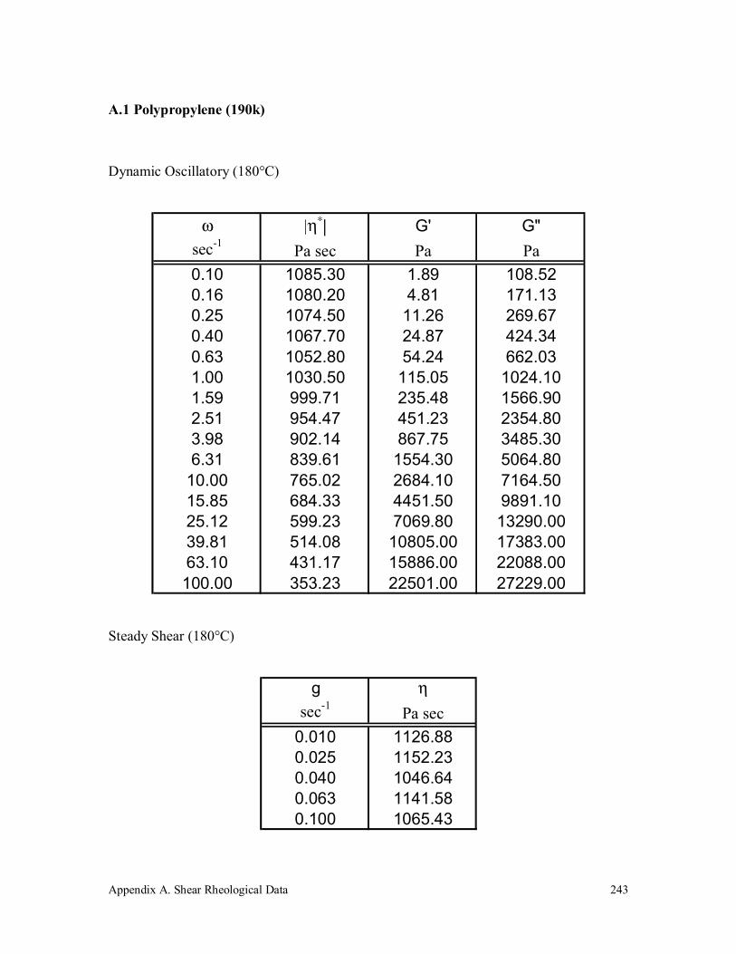
Appendix A. Shear Rheological Data
243
A.1 Polypropylene (190k)
Dynamic Oscillatory (180°C)
ω |η∗| G' G"sec-1 Pa sec Pa Pa0.10 1085.30 1.89 108.520.16 1080.20 4.81 171.130.25 1074.50 11.26 269.670.40 1067.70 24.87 424.340.63 1052.80 54.24 662.031.00 1030.50 115.05 1024.101.59 999.71 235.48 1566.902.51 954.47 451.23 2354.803.98 902.14 867.75 3485.306.31 839.61 1554.30 5064.80
10.00 765.02 2684.10 7164.5015.85 684.33 4451.50 9891.1025.12 599.23 7069.80 13290.0039.81 514.08 10805.00 17383.0063.10 431.17 15886.00 22088.00100.00 353.23 22501.00 27229.00
Steady Shear (180°C)
g ηsec-1 Pa sec
0.010 1126.880.025 1152.230.040 1046.640.063 1141.580.100 1065.43
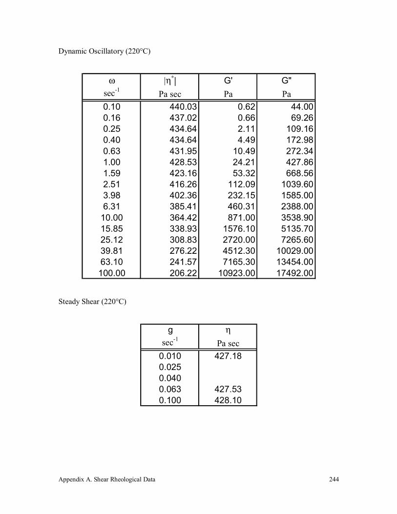
Appendix A. Shear Rheological Data
244
Dynamic Oscillatory (220°C)
ω |η∗| G' G"sec-1 Pa sec Pa Pa0.10 440.03 0.62 44.000.16 437.02 0.66 69.260.25 434.64 2.11 109.160.40 434.64 4.49 172.980.63 431.95 10.49 272.341.00 428.53 24.21 427.861.59 423.16 53.32 668.562.51 416.26 112.09 1039.603.98 402.36 232.15 1585.006.31 385.41 460.31 2388.00
10.00 364.42 871.00 3538.9015.85 338.93 1576.10 5135.7025.12 308.83 2720.00 7265.6039.81 276.22 4512.30 10029.0063.10 241.57 7165.30 13454.00100.00 206.22 10923.00 17492.00
Steady Shear (220°C)
g ηsec-1 Pa sec
0.010 427.180.0250.0400.063 427.530.100 428.10

Appendix A. Shear Rheological Data
245
Dynamic Oscillatory (Master Curve - 180°C)
ω |η∗| G' G"sec-1 Pa sec Pa Pa
0.040 1093.24 0.62 44.000.064 1085.76 0.66 69.260.100 1085.30 1.89 108.520.101 1079.85 2.11 109.160.158 1080.20 4.81 171.130.160 1079.85 4.49 172.980.251 1074.50 11.26 269.670.254 1073.17 10.49 272.340.398 1067.70 24.87 424.340.403 1064.67 24.21 427.860.631 1052.80 54.24 662.030.638 1051.33 53.32 668.561.000 1030.50 115.05 1024.101.011 1034.19 112.09 1039.601.585 999.71 235.48 1566.901.602 999.65 232.15 1585.002.512 954.47 451.23 2354.802.540 957.54 460.31 2388.003.981 902.14 867.75 3485.304.025 905.39 871.00 3538.906.310 839.61 1554.30 5064.806.380 842.06 1576.10 5135.7010.001 765.02 2684.10 7164.5010.111 767.28 2720.00 7265.6015.850 684.33 4451.50 9891.1016.025 686.26 4512.30 10029.0025.121 599.23 7069.80 13290.0025.398 600.17 7165.30 13454.0039.813 514.08 10805.00 17383.0040.250 512.35 10923.00 17492.0063.101 431.17 15886.00 22088.00
100.000 353.23 22501.00 27229.00

Appendix A. Shear Rheological Data
246
Transient Shear (0.01 sec-1 - 180°C)
t η+
sec Pa sec0.25 834.720.75 1043.201.25 1060.501.75 1075.702.25 1082.302.75 1083.503.25 1099.303.75 1086.304.25 1108.204.75 1092.705.25 1098.405.75 1113.106.25 1094.706.75 1106.907.25 1092.607.75 1108.908.25 1090.408.75 1100.109.25 1110.409.75 1110.80
10.25 1127.6010.75 1103.8011.25 1117.0011.75 1096.6012.25 1098.9012.75 1102.7013.25 1087.6013.75 1102.7014.25 1094.4014.75 1105.80
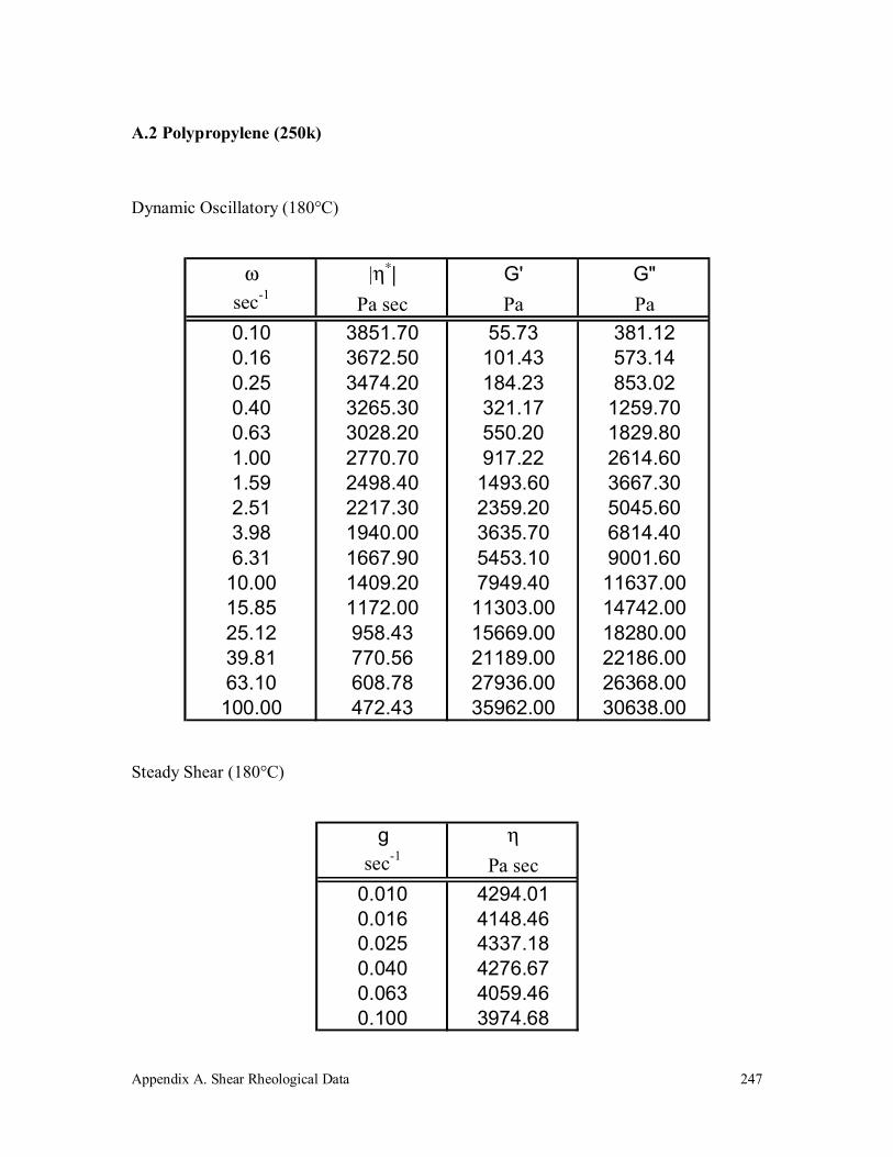
Appendix A. Shear Rheological Data
247
A.2 Polypropylene (250k)
Dynamic Oscillatory (180°C)
ω |η∗| G' G"sec-1 Pa sec Pa Pa0.10 3851.70 55.73 381.120.16 3672.50 101.43 573.140.25 3474.20 184.23 853.020.40 3265.30 321.17 1259.700.63 3028.20 550.20 1829.801.00 2770.70 917.22 2614.601.59 2498.40 1493.60 3667.302.51 2217.30 2359.20 5045.603.98 1940.00 3635.70 6814.406.31 1667.90 5453.10 9001.60
10.00 1409.20 7949.40 11637.0015.85 1172.00 11303.00 14742.0025.12 958.43 15669.00 18280.0039.81 770.56 21189.00 22186.0063.10 608.78 27936.00 26368.00100.00 472.43 35962.00 30638.00
Steady Shear (180°C)
g ηsec-1 Pa sec
0.010 4294.010.016 4148.460.025 4337.180.040 4276.670.063 4059.460.100 3974.68
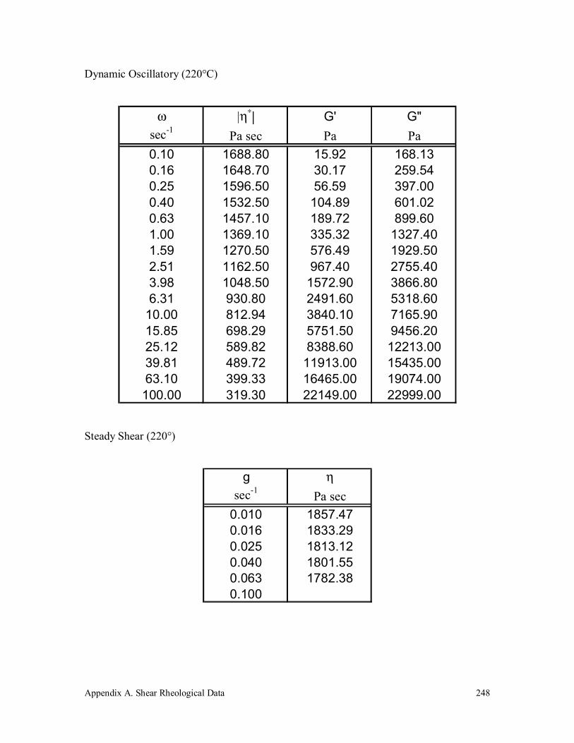
Appendix A. Shear Rheological Data
248
Dynamic Oscillatory (220°C)
ω |η∗| G' G"sec-1 Pa sec Pa Pa0.10 1688.80 15.92 168.130.16 1648.70 30.17 259.540.25 1596.50 56.59 397.000.40 1532.50 104.89 601.020.63 1457.10 189.72 899.601.00 1369.10 335.32 1327.401.59 1270.50 576.49 1929.502.51 1162.50 967.40 2755.403.98 1048.50 1572.90 3866.806.31 930.80 2491.60 5318.60
10.00 812.94 3840.10 7165.9015.85 698.29 5751.50 9456.2025.12 589.82 8388.60 12213.0039.81 489.72 11913.00 15435.0063.10 399.33 16465.00 19074.00100.00 319.30 22149.00 22999.00
Steady Shear (220°)
g ηsec-1 Pa sec
0.010 1857.470.016 1833.290.025 1813.120.040 1801.550.063 1782.380.100

Appendix A. Shear Rheological Data
249
Dynamic Oscillatory (260°C)
ω |η∗| G' G"sec-1 Pa sec Pa Pa0.10 716.83 2.87 71.630.16 687.12 5.86 108.740.25 666.99 11.35 167.160.40 648.18 22.61 257.050.63 626.34 44.86 392.641.00 604.13 86.45 597.931.59 578.44 162.42 902.302.51 548.81 293.41 1347.003.98 512.36 526.02 1970.906.31 472.79 908.56 2841.60
10.00 430.00 1515.90 4024.3015.85 383.79 2453.40 5566.4025.12 337.15 3845.10 7546.2039.81 291.14 5854.00 10005.0063.10 246.58 8630.10 12947.00100.00 204.47 12333.00 16309.00

Appendix A. Shear Rheological Data
250
Dynamic Oscillatory (Master Curve – 180°C)
ω |η∗| G' G"sec-1 Pa sec Pa Pa
0.015 4778.87 2.87 71.630.024 4580.80 5.86 108.740.038 4446.60 11.35 167.160.043 3973.65 15.92 168.130.060 4321.20 22.61 257.050.067 3879.29 30.17 259.540.095 4175.60 44.86 392.640.100 3851.70 55.73 381.120.107 3756.47 56.59 397.000.150 4027.53 86.45 597.930.158 3672.50 101.43 573.140.169 3605.88 104.89 601.020.238 3856.27 162.42 902.300.251 3474.20 184.23 853.020.268 3428.47 189.72 899.600.377 3658.73 293.41 1347.000.398 3265.30 321.17 1259.700.425 3221.41 335.32 1327.400.597 3415.73 526.02 1970.900.631 3028.20 550.20 1829.800.674 2989.41 576.49 1929.500.947 3151.93 908.56 2841.601.000 2770.70 917.22 2614.60
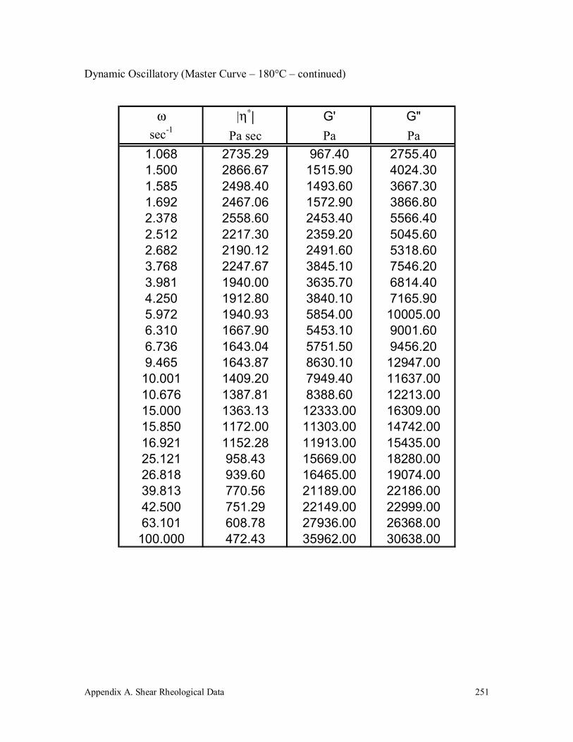
Appendix A. Shear Rheological Data
251
Dynamic Oscillatory (Master Curve – 180°C – continued)
ω |η∗| G' G"sec-1 Pa sec Pa Pa
1.068 2735.29 967.40 2755.401.500 2866.67 1515.90 4024.301.585 2498.40 1493.60 3667.301.692 2467.06 1572.90 3866.802.378 2558.60 2453.40 5566.402.512 2217.30 2359.20 5045.602.682 2190.12 2491.60 5318.603.768 2247.67 3845.10 7546.203.981 1940.00 3635.70 6814.404.250 1912.80 3840.10 7165.905.972 1940.93 5854.00 10005.006.310 1667.90 5453.10 9001.606.736 1643.04 5751.50 9456.209.465 1643.87 8630.10 12947.0010.001 1409.20 7949.40 11637.0010.676 1387.81 8388.60 12213.0015.000 1363.13 12333.00 16309.0015.850 1172.00 11303.00 14742.0016.921 1152.28 11913.00 15435.0025.121 958.43 15669.00 18280.0026.818 939.60 16465.00 19074.0039.813 770.56 21189.00 22186.0042.500 751.29 22149.00 22999.0063.101 608.78 27936.00 26368.00
100.000 472.43 35962.00 30638.00
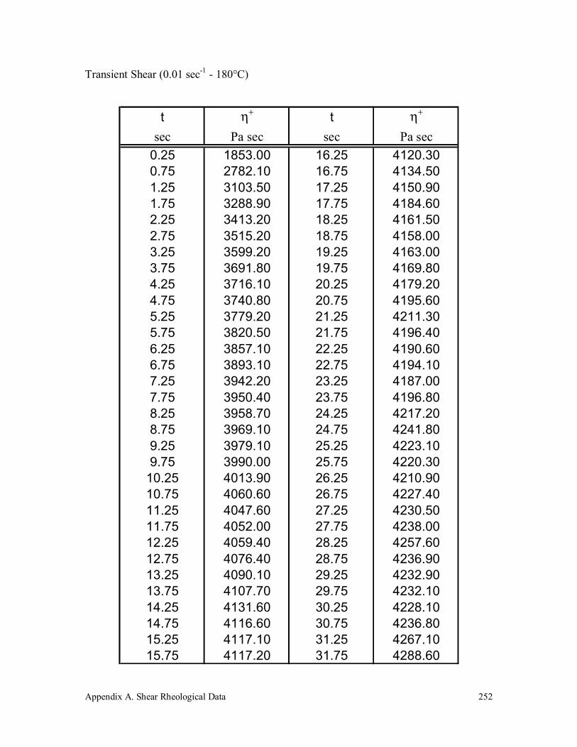
Appendix A. Shear Rheological Data
252
Transient Shear (0.01 sec-1 - 180°C)
t η+ t η+
sec Pa sec sec Pa sec0.25 1853.00 16.25 4120.300.75 2782.10 16.75 4134.501.25 3103.50 17.25 4150.901.75 3288.90 17.75 4184.602.25 3413.20 18.25 4161.502.75 3515.20 18.75 4158.003.25 3599.20 19.25 4163.003.75 3691.80 19.75 4169.804.25 3716.10 20.25 4179.204.75 3740.80 20.75 4195.605.25 3779.20 21.25 4211.305.75 3820.50 21.75 4196.406.25 3857.10 22.25 4190.606.75 3893.10 22.75 4194.107.25 3942.20 23.25 4187.007.75 3950.40 23.75 4196.808.25 3958.70 24.25 4217.208.75 3969.10 24.75 4241.809.25 3979.10 25.25 4223.109.75 3990.00 25.75 4220.30
10.25 4013.90 26.25 4210.9010.75 4060.60 26.75 4227.4011.25 4047.60 27.25 4230.5011.75 4052.00 27.75 4238.0012.25 4059.40 28.25 4257.6012.75 4076.40 28.75 4236.9013.25 4090.10 29.25 4232.9013.75 4107.70 29.75 4232.1014.25 4131.60 30.25 4228.1014.75 4116.60 30.75 4236.8015.25 4117.10 31.25 4267.1015.75 4117.20 31.75 4288.60
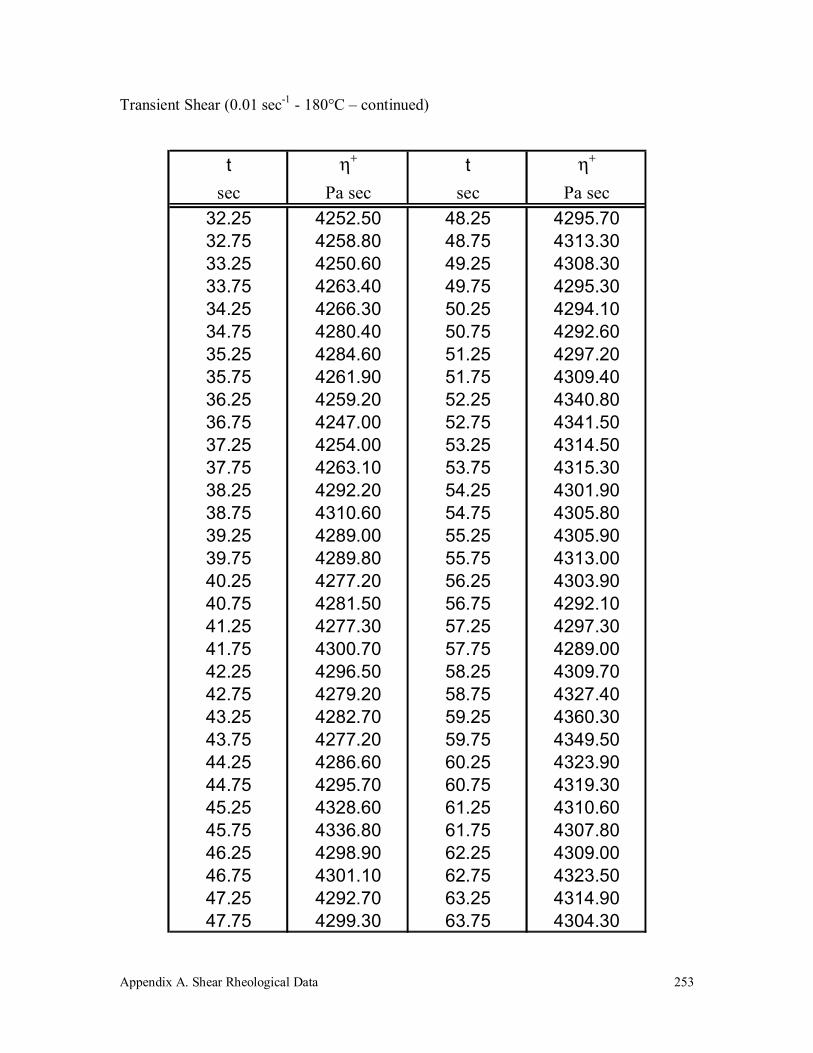
Appendix A. Shear Rheological Data
253
Transient Shear (0.01 sec-1 - 180°C – continued)
t η+ t η+
sec Pa sec sec Pa sec32.25 4252.50 48.25 4295.7032.75 4258.80 48.75 4313.3033.25 4250.60 49.25 4308.3033.75 4263.40 49.75 4295.3034.25 4266.30 50.25 4294.1034.75 4280.40 50.75 4292.6035.25 4284.60 51.25 4297.2035.75 4261.90 51.75 4309.4036.25 4259.20 52.25 4340.8036.75 4247.00 52.75 4341.5037.25 4254.00 53.25 4314.5037.75 4263.10 53.75 4315.3038.25 4292.20 54.25 4301.9038.75 4310.60 54.75 4305.8039.25 4289.00 55.25 4305.9039.75 4289.80 55.75 4313.0040.25 4277.20 56.25 4303.9040.75 4281.50 56.75 4292.1041.25 4277.30 57.25 4297.3041.75 4300.70 57.75 4289.0042.25 4296.50 58.25 4309.7042.75 4279.20 58.75 4327.4043.25 4282.70 59.25 4360.3043.75 4277.20 59.75 4349.5044.25 4286.60 60.25 4323.9044.75 4295.70 60.75 4319.3045.25 4328.60 61.25 4310.6045.75 4336.80 61.75 4307.8046.25 4298.90 62.25 4309.0046.75 4301.10 62.75 4323.5047.25 4292.70 63.25 4314.9047.75 4299.30 63.75 4304.30
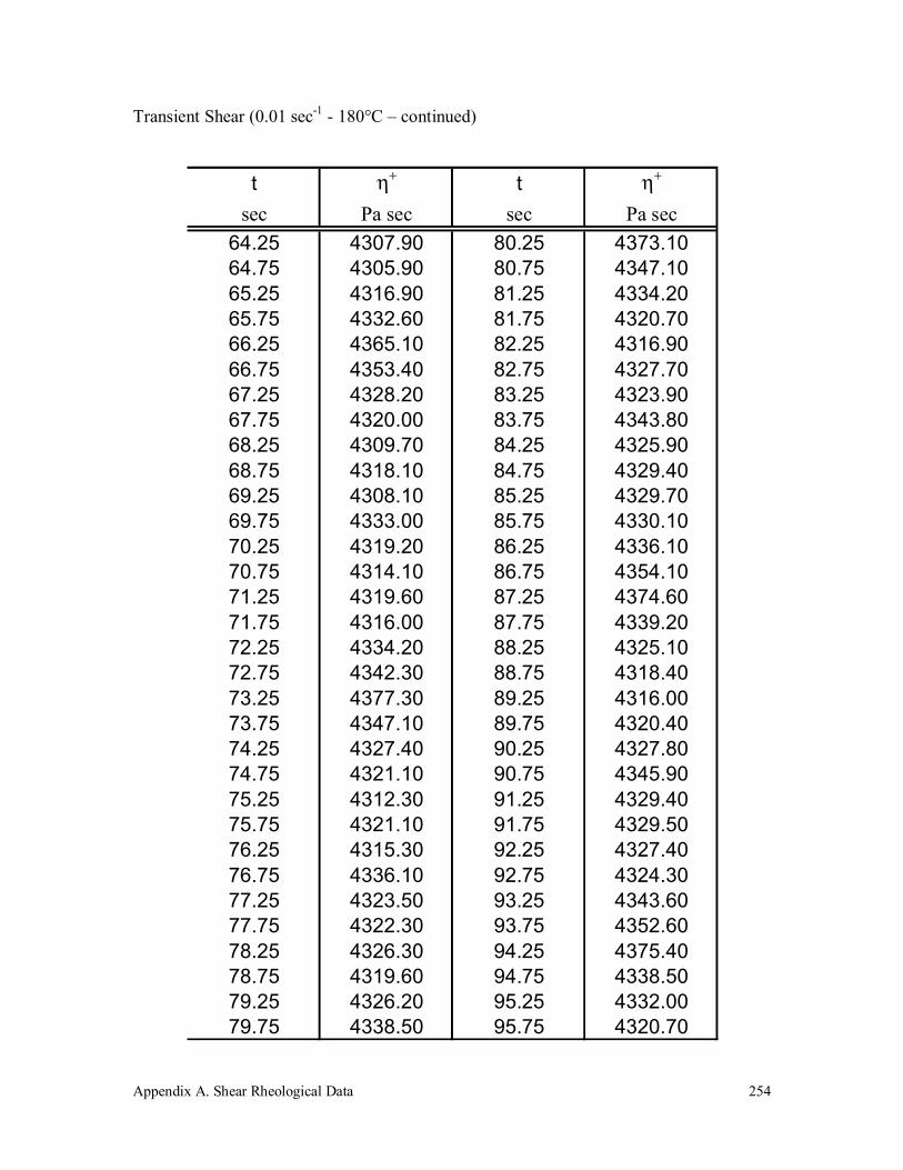
Appendix A. Shear Rheological Data
254
Transient Shear (0.01 sec-1 - 180°C – continued)
t η+ t η+
sec Pa sec sec Pa sec64.25 4307.90 80.25 4373.1064.75 4305.90 80.75 4347.1065.25 4316.90 81.25 4334.2065.75 4332.60 81.75 4320.7066.25 4365.10 82.25 4316.9066.75 4353.40 82.75 4327.7067.25 4328.20 83.25 4323.9067.75 4320.00 83.75 4343.8068.25 4309.70 84.25 4325.9068.75 4318.10 84.75 4329.4069.25 4308.10 85.25 4329.7069.75 4333.00 85.75 4330.1070.25 4319.20 86.25 4336.1070.75 4314.10 86.75 4354.1071.25 4319.60 87.25 4374.6071.75 4316.00 87.75 4339.2072.25 4334.20 88.25 4325.1072.75 4342.30 88.75 4318.4073.25 4377.30 89.25 4316.0073.75 4347.10 89.75 4320.4074.25 4327.40 90.25 4327.8074.75 4321.10 90.75 4345.9075.25 4312.30 91.25 4329.4075.75 4321.10 91.75 4329.5076.25 4315.30 92.25 4327.4076.75 4336.10 92.75 4324.3077.25 4323.50 93.25 4343.6077.75 4322.30 93.75 4352.6078.25 4326.30 94.25 4375.4078.75 4319.60 94.75 4338.5079.25 4326.20 95.25 4332.0079.75 4338.50 95.75 4320.70

Appendix A. Shear Rheological Data
255
A.3 Polypropylene (340k)
Dynamic Oscillatory (180°C)
ω |η∗| G' G"sec-1 Pa sec Pa Pa0.10 10377.00 236.51 1010.400.16 9700.60 407.12 1482.600.25 8927.40 689.81 2133.800.40 8132.30 1132.50 3033.000.63 7290.30 1816.50 4226.101.00 6436.30 2834.50 5778.701.59 5596.00 4319.50 7746.602.51 4786.90 6409.10 10174.003.98 4026.30 9263.60 13082.006.31 3331.70 13070.00 16467.00
10.00 2712.80 17994.00 20304.0015.85 2170.90 24161.00 24500.0025.12 1710.20 31708.00 28986.0039.81 1326.30 40728.00 33610.0063.10 1012.10 51156.00 38228.00100.00 758.77 62821.00 42553.00
Steady Shear (180°C)
g ηsec-1 Pa sec
0.010 12411.130.016 12309.570.025 12355.610.040 11800.900.063 11495.550.100 10935.25

Appendix A. Shear Rheological Data
256
Dynamic Oscillatory (220°C)
ω |η∗| G' G"sec-1 Pa sec Pa Pa0.10 4610.10 71.34 455.460.16 4401.50 129.57 685.440.25 4156.50 230.89 1018.200.40 3886.10 401.15 1494.200.63 3588.90 681.57 2159.501.00 3269.30 1126.60 3069.201.59 2935.20 1815.40 4283.302.51 2595.30 2851.40 5862.703.98 2257.30 4351.90 7863.106.31 1931.50 6472.00 10327.00
10.00 1626.20 9377.30 13287.0015.85 1345.70 13244.00 16719.0025.12 1095.00 18231.00 20599.0039.81 876.28 24498.00 24839.0063.10 689.06 32109.00 29318.00
Steady Shear (220°C)
g ηsec-1 Pa sec
0.010 4714.570.016 5080.360.025 4956.760.040 4895.500.063 4730.170.100

Appendix A. Shear Rheological Data
257
Dynamic Oscillatory (260°C)
ω |η∗| G' G"sec-1 Pa sec Pa Pa0.10 1710.40 13.08 170.540.16 1619.50 23.01 255.640.25 1531.60 43.44 382.270.40 1469.80 81.37 579.450.63 1395.00 150.07 867.291.00 1318.60 272.50 1290.201.59 1235.00 484.37 1896.502.51 1140.50 841.88 2738.603.98 1040.80 1409.90 3896.506.31 934.59 2303.50 5428.80
10.00 825.95 3643.20 7413.2015.85 715.54 5595.10 9865.1025.12 609.12 8329.60 12836.0039.81 509.32 12034.00 16321.0063.10 417.47 16871.00 20232.00100.00 335.11 22951.00 24417.00
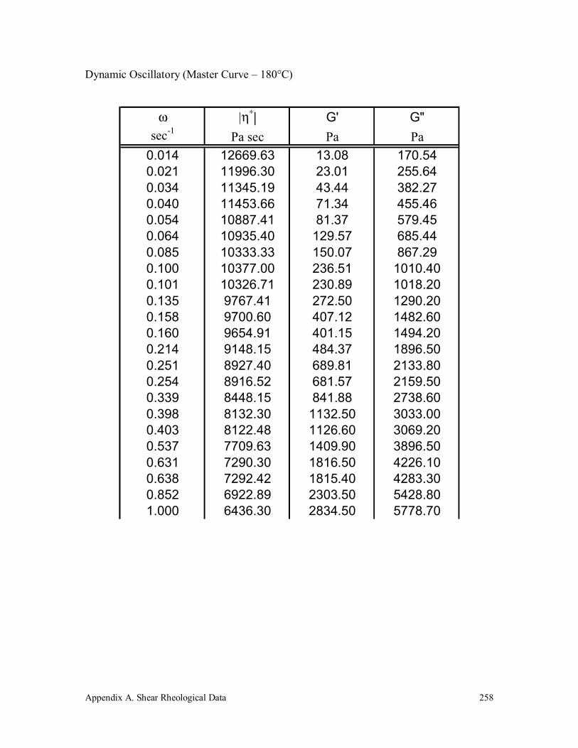
Appendix A. Shear Rheological Data
258
Dynamic Oscillatory (Master Curve – 180°C)
ω |η∗| G' G"sec-1 Pa sec Pa Pa
0.014 12669.63 13.08 170.540.021 11996.30 23.01 255.640.034 11345.19 43.44 382.270.040 11453.66 71.34 455.460.054 10887.41 81.37 579.450.064 10935.40 129.57 685.440.085 10333.33 150.07 867.290.100 10377.00 236.51 1010.400.101 10326.71 230.89 1018.200.135 9767.41 272.50 1290.200.158 9700.60 407.12 1482.600.160 9654.91 401.15 1494.200.214 9148.15 484.37 1896.500.251 8927.40 689.81 2133.800.254 8916.52 681.57 2159.500.339 8448.15 841.88 2738.600.398 8132.30 1132.50 3033.000.403 8122.48 1126.60 3069.200.537 7709.63 1409.90 3896.500.631 7290.30 1816.50 4226.100.638 7292.42 1815.40 4283.300.852 6922.89 2303.50 5428.801.000 6436.30 2834.50 5778.70

Appendix A. Shear Rheological Data
259
Dynamic Oscillatory (Master Curve – 180°C – continued)
ω |η∗| G' G"sec-1 Pa sec Pa Pa
1.011 6447.95 2851.40 5862.701.350 6118.15 3643.20 7413.201.585 5596.00 4319.50 7746.601.602 5608.20 4351.90 7863.102.140 5300.30 5595.10 9865.102.512 4786.90 6409.10 10174.002.540 4798.76 6472.00 10327.003.391 4512.00 8329.60 12836.003.981 4026.30 9263.60 13082.004.025 4040.25 9377.30 13287.005.375 3772.74 12034.00 16321.006.310 3331.70 13070.00 16467.006.380 3343.35 13244.00 16719.008.519 3092.37 16871.00 20232.0010.001 2712.80 17994.00 20304.0010.111 2720.50 18231.00 20599.0013.500 2482.30 22951.00 24417.0015.850 2170.90 24161.00 24500.0016.025 2177.09 24498.00 24839.0025.121 1710.20 31708.00 28986.0025.398 1711.95 32109.00 29318.0039.813 1326.30 40728.00 33610.0063.101 1012.10 51156.00 38228.00
100.000 758.77 62821.00 42553.00
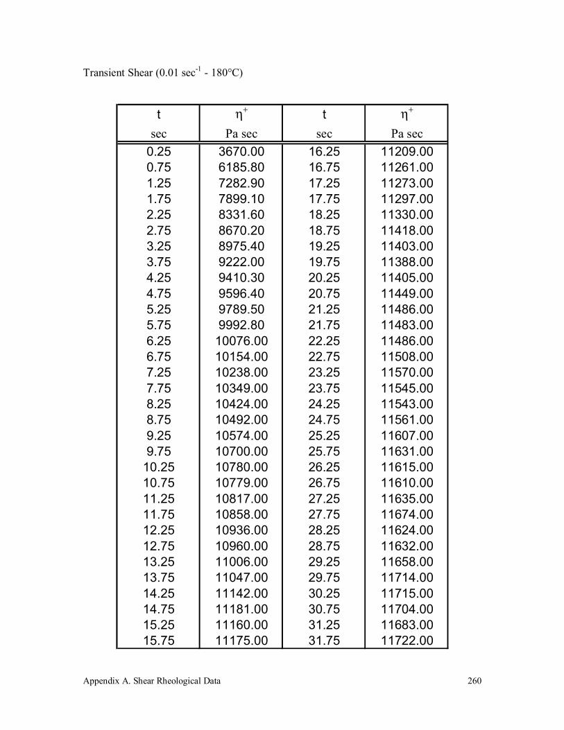
Appendix A. Shear Rheological Data
260
Transient Shear (0.01 sec-1 - 180°C)
t η+ t η+
sec Pa sec sec Pa sec0.25 3670.00 16.25 11209.000.75 6185.80 16.75 11261.001.25 7282.90 17.25 11273.001.75 7899.10 17.75 11297.002.25 8331.60 18.25 11330.002.75 8670.20 18.75 11418.003.25 8975.40 19.25 11403.003.75 9222.00 19.75 11388.004.25 9410.30 20.25 11405.004.75 9596.40 20.75 11449.005.25 9789.50 21.25 11486.005.75 9992.80 21.75 11483.006.25 10076.00 22.25 11486.006.75 10154.00 22.75 11508.007.25 10238.00 23.25 11570.007.75 10349.00 23.75 11545.008.25 10424.00 24.25 11543.008.75 10492.00 24.75 11561.009.25 10574.00 25.25 11607.009.75 10700.00 25.75 11631.00
10.25 10780.00 26.25 11615.0010.75 10779.00 26.75 11610.0011.25 10817.00 27.25 11635.0011.75 10858.00 27.75 11674.0012.25 10936.00 28.25 11624.0012.75 10960.00 28.75 11632.0013.25 11006.00 29.25 11658.0013.75 11047.00 29.75 11714.0014.25 11142.00 30.25 11715.0014.75 11181.00 30.75 11704.0015.25 11160.00 31.25 11683.0015.75 11175.00 31.75 11722.00
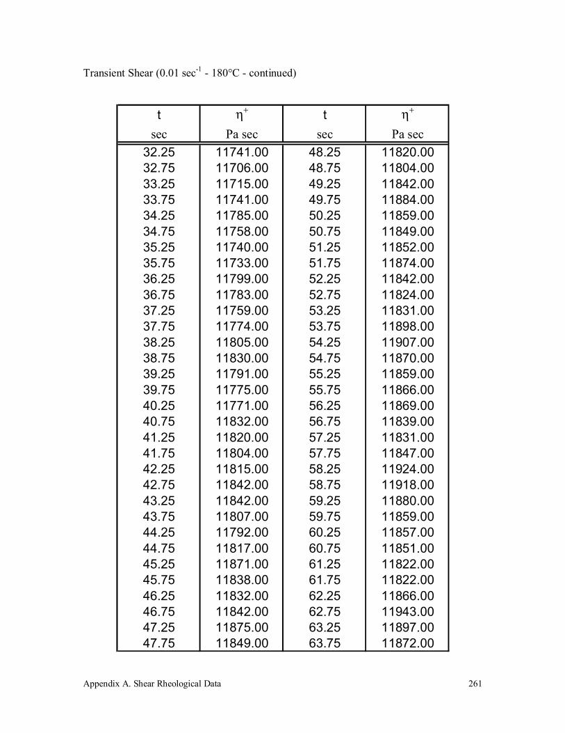
Appendix A. Shear Rheological Data
261
Transient Shear (0.01 sec-1 - 180°C - continued)
t η+ t η+
sec Pa sec sec Pa sec32.25 11741.00 48.25 11820.0032.75 11706.00 48.75 11804.0033.25 11715.00 49.25 11842.0033.75 11741.00 49.75 11884.0034.25 11785.00 50.25 11859.0034.75 11758.00 50.75 11849.0035.25 11740.00 51.25 11852.0035.75 11733.00 51.75 11874.0036.25 11799.00 52.25 11842.0036.75 11783.00 52.75 11824.0037.25 11759.00 53.25 11831.0037.75 11774.00 53.75 11898.0038.25 11805.00 54.25 11907.0038.75 11830.00 54.75 11870.0039.25 11791.00 55.25 11859.0039.75 11775.00 55.75 11866.0040.25 11771.00 56.25 11869.0040.75 11832.00 56.75 11839.0041.25 11820.00 57.25 11831.0041.75 11804.00 57.75 11847.0042.25 11815.00 58.25 11924.0042.75 11842.00 58.75 11918.0043.25 11842.00 59.25 11880.0043.75 11807.00 59.75 11859.0044.25 11792.00 60.25 11857.0044.75 11817.00 60.75 11851.0045.25 11871.00 61.25 11822.0045.75 11838.00 61.75 11822.0046.25 11832.00 62.25 11866.0046.75 11842.00 62.75 11943.0047.25 11875.00 63.25 11897.0047.75 11849.00 63.75 11872.00
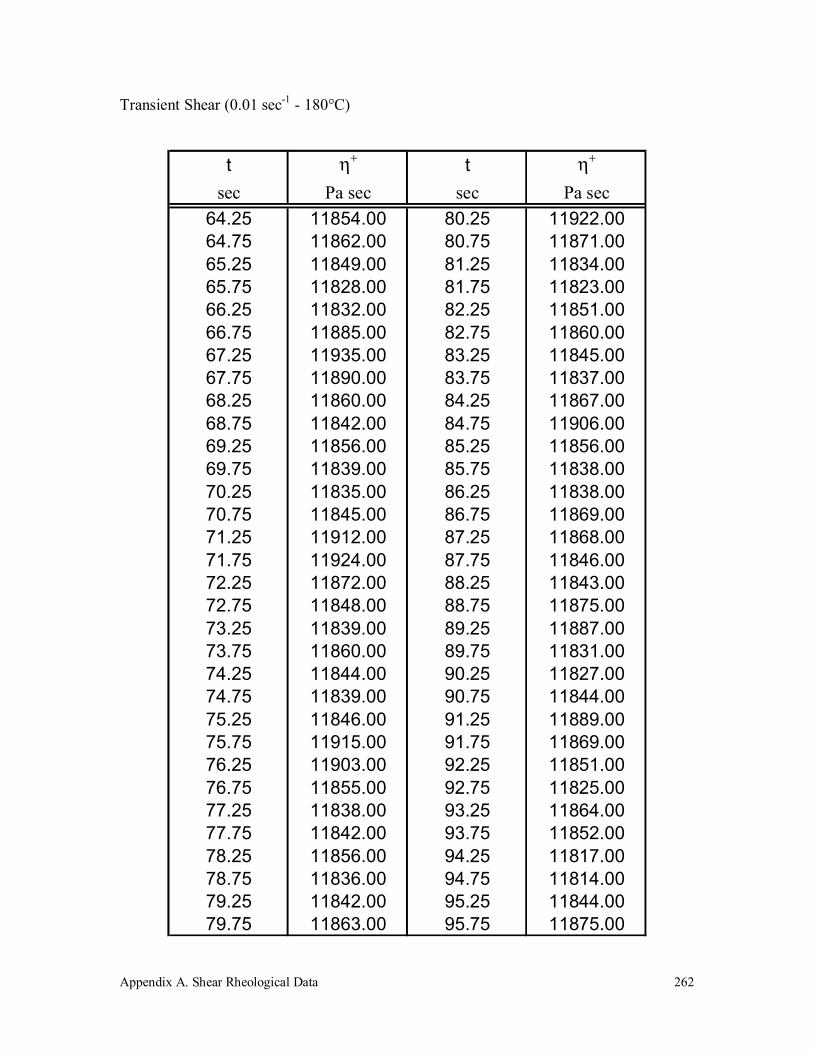
Appendix A. Shear Rheological Data
262
Transient Shear (0.01 sec-1 - 180°C)
t η+ t η+
sec Pa sec sec Pa sec64.25 11854.00 80.25 11922.0064.75 11862.00 80.75 11871.0065.25 11849.00 81.25 11834.0065.75 11828.00 81.75 11823.0066.25 11832.00 82.25 11851.0066.75 11885.00 82.75 11860.0067.25 11935.00 83.25 11845.0067.75 11890.00 83.75 11837.0068.25 11860.00 84.25 11867.0068.75 11842.00 84.75 11906.0069.25 11856.00 85.25 11856.0069.75 11839.00 85.75 11838.0070.25 11835.00 86.25 11838.0070.75 11845.00 86.75 11869.0071.25 11912.00 87.25 11868.0071.75 11924.00 87.75 11846.0072.25 11872.00 88.25 11843.0072.75 11848.00 88.75 11875.0073.25 11839.00 89.25 11887.0073.75 11860.00 89.75 11831.0074.25 11844.00 90.25 11827.0074.75 11839.00 90.75 11844.0075.25 11846.00 91.25 11889.0075.75 11915.00 91.75 11869.0076.25 11903.00 92.25 11851.0076.75 11855.00 92.75 11825.0077.25 11838.00 93.25 11864.0077.75 11842.00 93.75 11852.0078.25 11856.00 94.25 11817.0078.75 11836.00 94.75 11814.0079.25 11842.00 95.25 11844.0079.75 11863.00 95.75 11875.00

Appendix A. Shear Rheological Data
263
A.4 Polypropylene (580k)
Dynamic Oscillatory (180°C)
ω |η∗| G' G"sec-1 Pa sec Pa Pa0.10 52249.00 2309.50 4686.800.16 45667.00 3528.20 6319.500.25 39177.00 5246.10 8325.900.40 33069.00 7623.80 10733.000.63 27377.00 10787.00 13492.001.00 22283.00 14883.00 16585.001.59 17814.00 19965.00 19965.002.51 14011.00 26225.00 23474.003.98 10837.00 33606.00 27057.006.31 8254.90 42165.00 30583.00
10.00 6193.70 51832.00 33915.0015.85 4584.00 62540.00 36985.0025.12 3347.30 74133.00 39685.0039.81 2413.50 86458.00 41935.0063.10 1718.80 99260.00 43716.00100.00 1208.30 112140.00 44990.00
Steady Shear (180°C)
g ηsec-1 Pa sec
0.010 121733.500.016 114388.500.025 105532.000.040 48975.700.063 75098.25
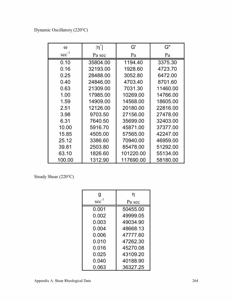
Appendix A. Shear Rheological Data
264
Dynamic Oscillatory (220°C)
ω |η∗| G' G"sec-1 Pa sec Pa Pa0.10 35804.00 1194.40 3375.300.16 32193.00 1928.60 4723.700.25 28488.00 3052.80 6472.000.40 24846.00 4703.40 8701.600.63 21309.00 7031.30 11460.001.00 17985.00 10269.00 14766.001.59 14909.00 14568.00 18605.002.51 12126.00 20180.00 22816.003.98 9703.50 27156.00 27478.006.31 7640.50 35699.00 32403.00
10.00 5916.70 45871.00 37377.0015.85 4505.00 57565.00 42247.0025.12 3386.60 70940.00 46959.0039.81 2503.80 85478.00 51292.0063.10 1826.60 101220.00 55134.00100.00 1312.90 117690.00 58180.00
Steady Shear (220°C)
g ηsec-1 Pa sec
0.001 50455.000.002 49999.050.003 49034.900.004 48668.130.006 47777.600.010 47262.300.016 45270.080.025 43109.200.040 40188.900.063 36327.25

Appendix A. Shear Rheological Data
265
Dynamic Oscillatory (Master Curve – 180°C)
ω |η∗| G' G"sec-1 Pa sec Pa Pa0.08 47738.67 1194.40 3375.300.10 52249.00 2309.50 4686.800.12 42924.00 1928.60 4723.700.16 45667.00 3528.20 6319.500.19 37984.00 3052.80 6472.000.25 39177.00 5246.10 8325.900.30 33128.00 4703.40 8701.600.40 33069.00 7623.80 10733.000.47 28412.00 7031.30 11460.000.63 27377.00 10787.00 13492.000.75 23980.00 10269.00 14766.001.00 22283.00 14883.00 16585.001.19 19878.67 14568.00 18605.001.59 17814.00 19965.00 19965.001.88 16168.00 20180.00 22816.002.51 14011.00 26225.00 23474.002.99 12938.00 27156.00 27478.003.98 10837.00 33606.00 27057.004.73 10187.33 35699.00 32403.006.31 8254.90 42165.00 30583.007.50 7888.93 45871.00 37377.00
10.00 6193.70 51832.00 33915.0011.89 6006.67 57565.00 42247.0015.85 4584.00 62540.00 36985.0018.84 4515.47 70940.00 46959.0025.12 3347.30 74133.00 39685.0029.86 3338.40 85478.00 51292.0039.81 2413.50 86458.00 41935.0047.33 2435.47 101220.00 55134.0063.10 1718.80 99260.00 43716.0075.00 1750.53 117690.00 58180.00100.00 1208.30 112140.00 44990.00
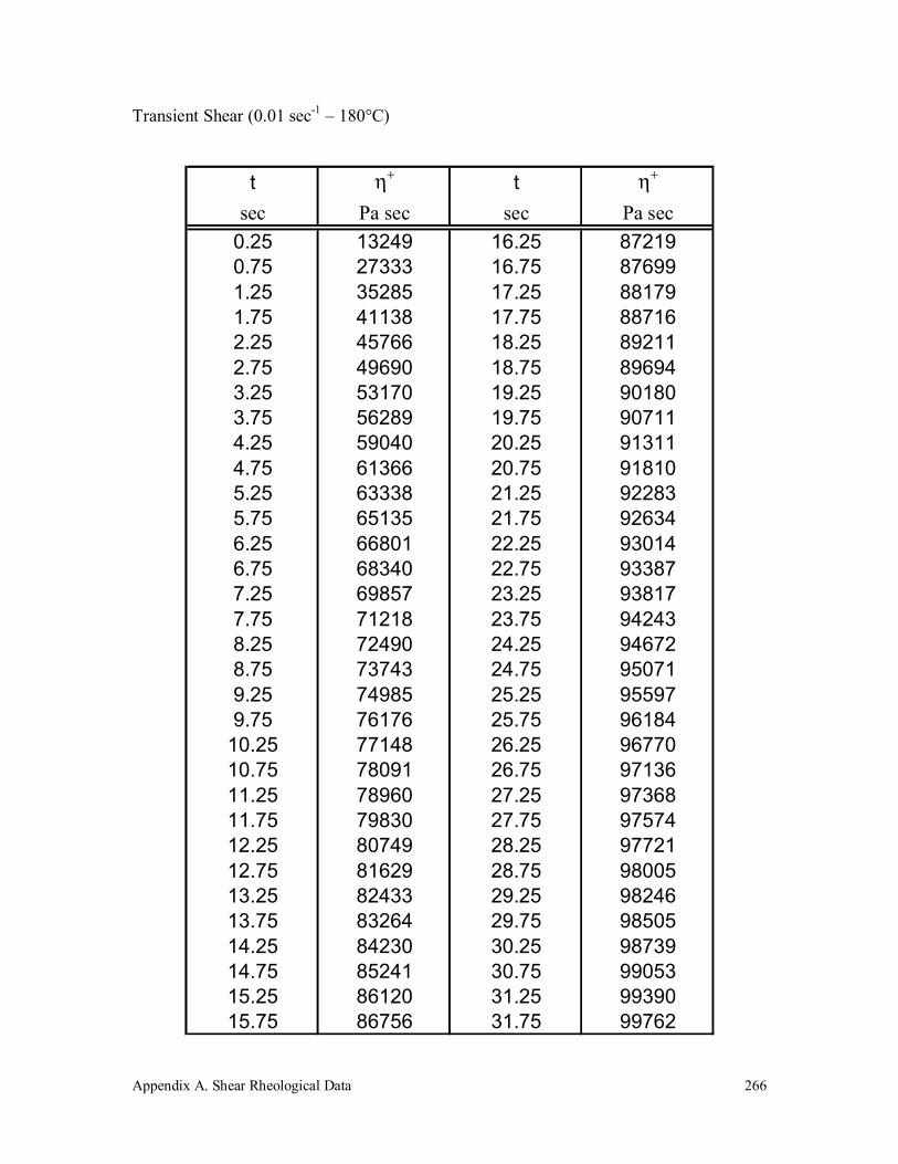
Appendix A. Shear Rheological Data
266
Transient Shear (0.01 sec-1 – 180°C)
t η+ t η+
sec Pa sec sec Pa sec0.25 13249 16.25 872190.75 27333 16.75 876991.25 35285 17.25 881791.75 41138 17.75 887162.25 45766 18.25 892112.75 49690 18.75 896943.25 53170 19.25 901803.75 56289 19.75 907114.25 59040 20.25 913114.75 61366 20.75 918105.25 63338 21.25 922835.75 65135 21.75 926346.25 66801 22.25 930146.75 68340 22.75 933877.25 69857 23.25 938177.75 71218 23.75 942438.25 72490 24.25 946728.75 73743 24.75 950719.25 74985 25.25 955979.75 76176 25.75 96184
10.25 77148 26.25 9677010.75 78091 26.75 9713611.25 78960 27.25 9736811.75 79830 27.75 9757412.25 80749 28.25 9772112.75 81629 28.75 9800513.25 82433 29.25 9824613.75 83264 29.75 9850514.25 84230 30.25 9873914.75 85241 30.75 9905315.25 86120 31.25 9939015.75 86756 31.75 99762

Appendix A. Shear Rheological Data
267
Transient Shear (0.01 sec-1 – 180°C - continued)
t η+ t η+
sec Pa sec sec Pa sec32.25 100040 48.25 10680032.75 100270 48.75 10700033.25 100440 49.25 10704033.75 100690 49.75 10697034.25 100950 50.25 10697034.75 101190 50.75 10704035.25 101470 51.25 10713035.75 101760 51.75 10719036.25 102100 52.25 10730036.75 102580 52.75 10742037.25 102960 53.25 10764037.75 103220 53.75 10787038.25 103260 54.25 10802038.75 103240 54.75 10811039.25 103350 55.25 10815039.75 103490 55.75 10822040.25 103620 56.25 10835040.75 103740 56.75 10847041.25 103920 57.25 10857041.75 104120 57.75 10864042.25 104420 58.25 10887042.75 104650 58.75 10912043.25 104830 59.25 10946043.75 104990 59.75 10961044.25 105070 60.25 10956044.75 105240 60.75 10943045.25 105360 61.25 10938045.75 105570 61.75 10938046.25 105710 62.25 10946046.75 105880 62.75 10953047.25 106090 63.25 10958047.75 106470 63.75 109690
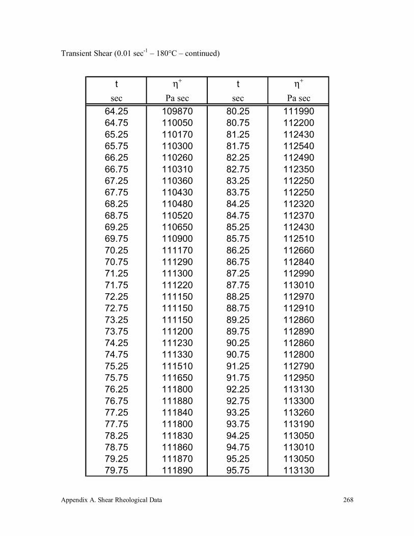
Appendix A. Shear Rheological Data
268
Transient Shear (0.01 sec-1 – 180°C – continued)
t η+ t η+
sec Pa sec sec Pa sec64.25 109870 80.25 11199064.75 110050 80.75 11220065.25 110170 81.25 11243065.75 110300 81.75 11254066.25 110260 82.25 11249066.75 110310 82.75 11235067.25 110360 83.25 11225067.75 110430 83.75 11225068.25 110480 84.25 11232068.75 110520 84.75 11237069.25 110650 85.25 11243069.75 110900 85.75 11251070.25 111170 86.25 11266070.75 111290 86.75 11284071.25 111300 87.25 11299071.75 111220 87.75 11301072.25 111150 88.25 11297072.75 111150 88.75 11291073.25 111150 89.25 11286073.75 111200 89.75 11289074.25 111230 90.25 11286074.75 111330 90.75 11280075.25 111510 91.25 11279075.75 111650 91.75 11295076.25 111800 92.25 11313076.75 111880 92.75 11330077.25 111840 93.25 11326077.75 111800 93.75 11319078.25 111830 94.25 11305078.75 111860 94.75 11301079.25 111870 95.25 11305079.75 111890 95.75 113130

Appendix A. Shear Rheological Data
269
Transient Shear (0.01 sec-1 – 180°C – continued)
t η+ t η+
sec Pa sec sec Pa sec96.25 113160 112.25 11382096.75 113240 112.75 11378097.25 113350 113.25 11374097.75 113530 113.75 11385098.25 113620 114.25 11405098.75 113640 114.75 11419099.25 113620 115.25 11427099.75 113550 115.75 114150100.25 113510 116.25 114070100.75 113480 116.75 114050101.25 113440 117.25 114070101.75 113400 117.75 114050102.25 113400 118.25 114120102.75 113560 118.75 114120103.25 113760 119.25 114240103.75 113920 119.75 114360104.25 113870 120.25 114440104.75 113690 120.75 114410105.25 113620 121.25 114350105.75 113560 121.75 114250106.25 113650 122.25 114150106.75 113620 122.75 114120107.25 113700 123.25 114060107.75 113760 123.75 114040108.25 113860 124.25 114010108.75 114010 124.75 114140109.25 114110 125.25 114340109.75 114120 125.75 114530110.25 114050 126.25 114540110.75 113950 126.75 114430111.25 113900 127.25 114290111.75 113870 127.75 114250
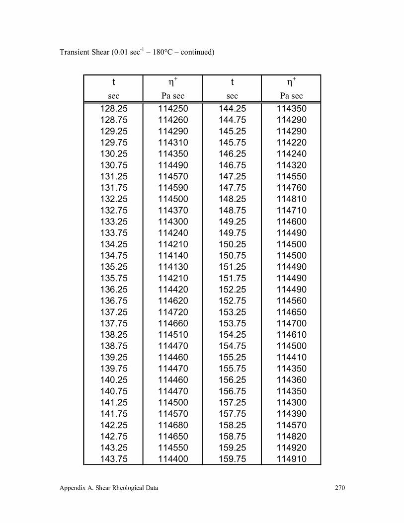
Appendix A. Shear Rheological Data
270
Transient Shear (0.01 sec-1 – 180°C – continued)
t η+ t η+
sec Pa sec sec Pa sec128.25 114250 144.25 114350128.75 114260 144.75 114290129.25 114290 145.25 114290129.75 114310 145.75 114220130.25 114350 146.25 114240130.75 114490 146.75 114320131.25 114570 147.25 114550131.75 114590 147.75 114760132.25 114500 148.25 114810132.75 114370 148.75 114710133.25 114300 149.25 114600133.75 114240 149.75 114490134.25 114210 150.25 114500134.75 114140 150.75 114500135.25 114130 151.25 114490135.75 114210 151.75 114490136.25 114420 152.25 114490136.75 114620 152.75 114560137.25 114720 153.25 114650137.75 114660 153.75 114700138.25 114510 154.25 114610138.75 114470 154.75 114500139.25 114460 155.25 114410139.75 114470 155.75 114350140.25 114460 156.25 114360140.75 114470 156.75 114350141.25 114500 157.25 114300141.75 114570 157.75 114390142.25 114680 158.25 114570142.75 114650 158.75 114820143.25 114550 159.25 114920143.75 114400 159.75 114910
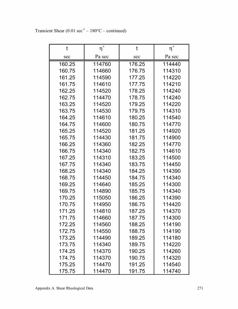
Appendix A. Shear Rheological Data
271
Transient Shear (0.01 sec-1 – 180°C – continued)
t η+ t η+
sec Pa sec sec Pa sec160.25 114760 176.25 114440160.75 114660 176.75 114310161.25 114590 177.25 114220161.75 114610 177.75 114210162.25 114520 178.25 114240162.75 114470 178.75 114240163.25 114520 179.25 114220163.75 114530 179.75 114310164.25 114610 180.25 114540164.75 114600 180.75 114770165.25 114520 181.25 114920165.75 114430 181.75 114900166.25 114360 182.25 114770166.75 114340 182.75 114610167.25 114310 183.25 114500167.75 114340 183.75 114450168.25 114340 184.25 114390168.75 114450 184.75 114340169.25 114640 185.25 114300169.75 114890 185.75 114340170.25 115050 186.25 114390170.75 114950 186.75 114420171.25 114810 187.25 114370171.75 114660 187.75 114300172.25 114560 188.25 114190172.75 114550 188.75 114190173.25 114490 189.25 114180173.75 114340 189.75 114220174.25 114370 190.25 114260174.75 114370 190.75 114320175.25 114470 191.25 114540175.75 114470 191.75 114740
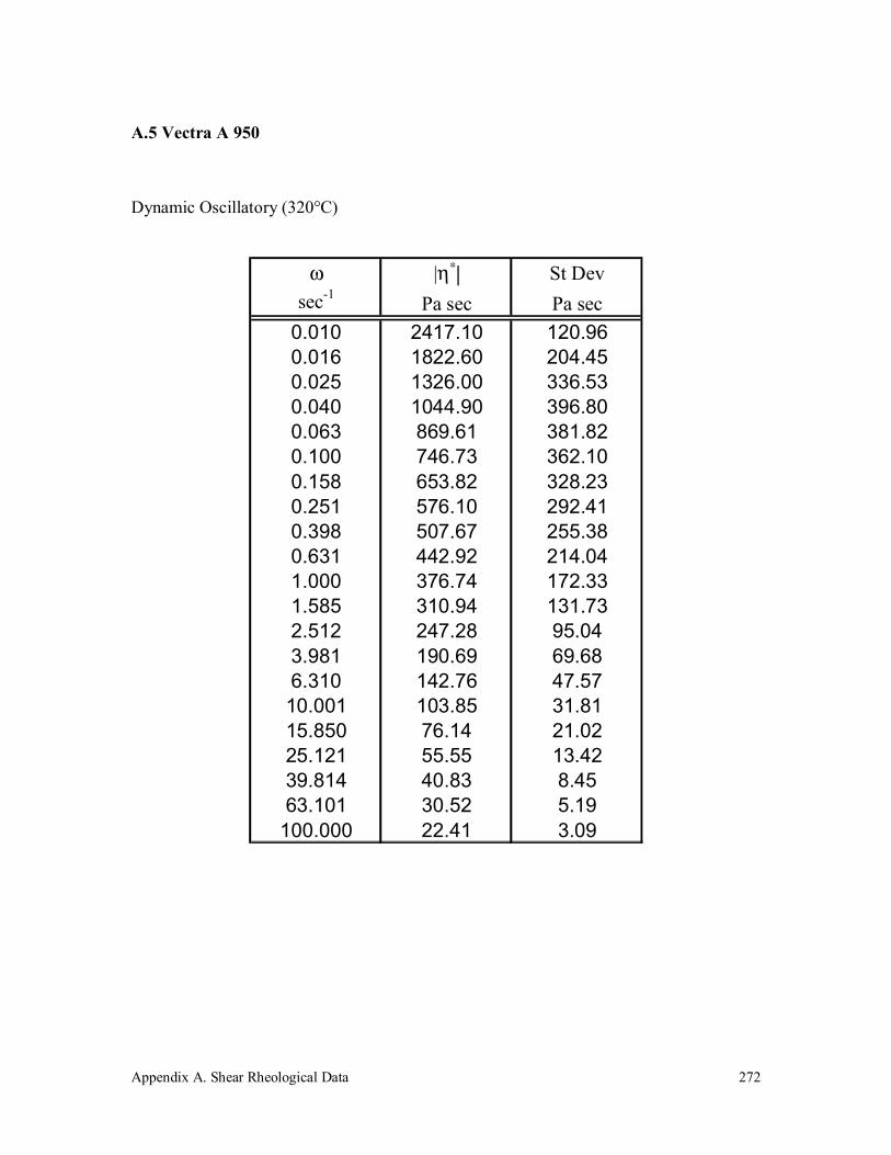
Appendix A. Shear Rheological Data
272
A.5 Vectra A 950
Dynamic Oscillatory (320°C)
ω |η∗| St Devsec-1 Pa sec Pa sec
0.010 2417.10 120.960.016 1822.60 204.450.025 1326.00 336.530.040 1044.90 396.800.063 869.61 381.820.100 746.73 362.100.158 653.82 328.230.251 576.10 292.410.398 507.67 255.380.631 442.92 214.041.000 376.74 172.331.585 310.94 131.732.512 247.28 95.043.981 190.69 69.686.310 142.76 47.5710.001 103.85 31.8115.850 76.14 21.0225.121 55.55 13.4239.814 40.83 8.4563.101 30.52 5.19
100.000 22.41 3.09
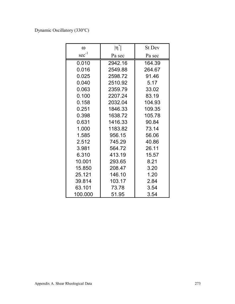
Appendix A. Shear Rheological Data
273
Dynamic Oscillatory (330°C)
ω |η∗| St Devsec-1 Pa sec Pa sec
0.010 2942.16 164.390.016 2549.88 264.670.025 2598.72 91.460.040 2510.92 5.170.063 2359.79 33.020.100 2207.24 83.190.158 2032.04 104.930.251 1846.33 109.350.398 1638.72 105.780.631 1416.33 90.841.000 1183.82 73.141.585 956.15 56.062.512 745.29 40.863.981 564.72 26.116.310 413.19 15.5710.001 293.65 8.2115.850 208.47 3.2025.121 146.10 1.2039.814 103.17 2.8463.101 73.78 3.54
100.000 51.95 3.54
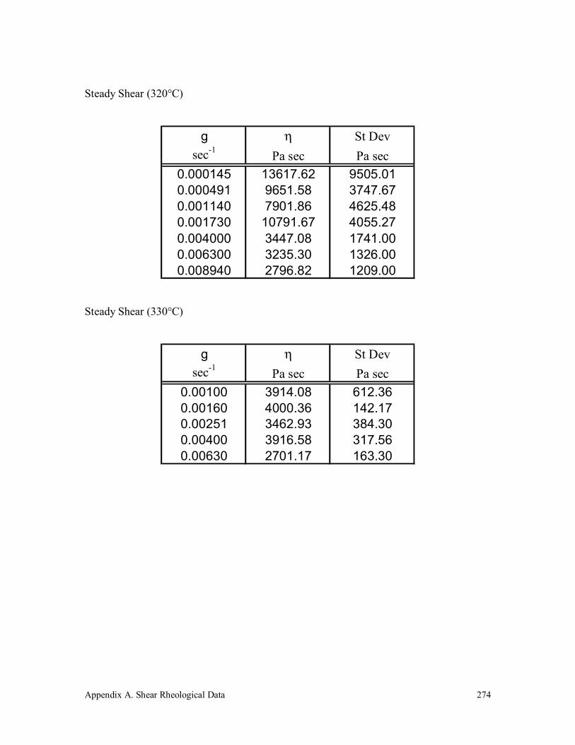
Appendix A. Shear Rheological Data
274
Steady Shear (320°C)
g η St Devsec-1 Pa sec Pa sec
0.000145 13617.62 9505.010.000491 9651.58 3747.670.001140 7901.86 4625.480.001730 10791.67 4055.270.004000 3447.08 1741.000.006300 3235.30 1326.000.008940 2796.82 1209.00
Steady Shear (330°C)
g η St Devsec-1 Pa sec Pa sec
0.00100 3914.08 612.360.00160 4000.36 142.170.00251 3462.93 384.300.00400 3916.58 317.560.00630 2701.17 163.30

Appendix A. Shear Rheological Data
275
Transient Shear (0.01 sec-1 – 320°C)
t η+ t η+
sec Pa sec sec Pa sec15.50 673.81 524.50 2306.7331.50 1109.09 540.00 2305.8746.50 1390.24 555.50 2314.2362.00 1594.27 570.50 2302.9877.50 1720.92 586.00 2311.5093.00 1826.46 601.50 2307.58108.00 1929.09 617.00 2318.83123.50 1992.86 632.50 2313.72139.00 2026.27 648.00 2318.66154.50 2067.36 663.00 2328.21170.00 2076.74 678.50 2337.76185.50 2091.91 694.00 2355.49200.50 2115.27 709.50 2339.97216.00 2139.14 725.00 2350.71231.50 2167.61 740.50 2362.14247.00 2181.93 756.00 2360.94262.50 2179.03 771.00 2370.32278.00 2172.21 786.50 2389.07293.00 2202.39 802.00 2395.89308.50 2215.17 817.50 2421.30324.00 2223.53 833.00 2418.74339.50 2246.03 848.50 2411.58355.00 2233.76 863.50 2433.06370.50 2226.09 879.00 2430.84385.50 2233.08 894.50 2425.39401.00 2257.29 910.00 2427.43416.50 2279.96 925.50 2394.19432.00 2283.03 941.00 2391.80447.50 2301.61 956.00 2400.50463.00 2306.56 971.50 2404.93478.00 2277.40 987.00 2430.84493.50 2266.83 1002.50 2431.01509.00 2281.84
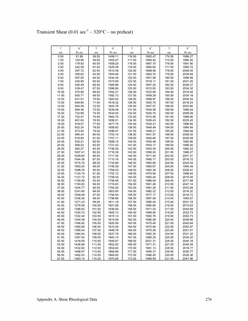
Appendix A. Shear Rheological Data
276
Transient Shear (0.01 sec-1 – 320°C – no preheat)
t η+ t η+ t η+ t η+
sec Pa sec sec Pa sec sec Pa sec sec Pa sec0.50 51.99 58.50 1499.11 116.50 1883.47 174.50 1996.271.50 120.90 59.50 1503.47 117.50 1884.42 175.50 1985.352.50 179.92 60.50 1508.25 118.50 1887.70 176.50 1991.903.50 242.59 61.50 1529.39 119.50 1864.65 177.50 1995.724.50 297.72 62.50 1514.38 120.50 1898.06 178.50 2008.405.50 355.62 63.50 1544.94 121.50 1883.74 179.50 2030.646.50 407.50 64.50 1544.39 122.50 1901.06 180.50 1998.997.50 430.95 65.50 1573.99 123.50 1918.11 181.50 2031.058.50 505.49 66.50 1585.86 124.50 1907.20 182.50 2026.279.50 539.47 67.50 1596.90 125.50 1912.93 183.50 2034.3210.50 570.95 68.50 1592.27 126.50 1923.84 184.50 2019.0411.50 605.71 69.50 1592.13 127.50 1908.29 185.50 2034.1812.50 631.91 70.50 1583.54 128.50 1899.97 186.50 2008.5413.50 646.85 71.50 1618.32 129.50 1920.70 187.50 2018.2314.50 654.09 72.50 1644.78 130.50 1947.57 188.50 2003.9015.50 694.46 73.50 1639.46 131.50 1934.48 189.50 1996.5416.50 733.69 74.50 1634.55 132.50 1920.70 190.50 2009.0917.50 752.57 75.50 1663.74 133.50 1910.06 191.50 1988.9018.50 801.63 76.50 1656.51 134.50 1926.43 192.50 2025.4519.50 818.07 77.50 1677.79 135.50 1934.21 193.50 1996.9520.50 832.24 78.50 1658.83 136.50 1949.48 194.50 1984.9421.50 873.40 79.50 1696.47 137.50 1949.21 195.50 1984.9422.50 895.24 80.50 1703.15 138.50 1941.57 196.50 2008.0023.50 916.80 81.50 1707.11 139.50 1945.66 197.50 2000.4924.50 932.21 82.50 1688.15 140.50 1955.48 198.50 1982.9025.50 958.02 83.50 1721.43 141.50 1953.17 199.50 1996.4026.50 992.27 84.50 1746.26 142.50 1953.30 200.50 1982.2227.50 1007.41 85.50 1716.38 143.50 1956.03 201.50 1996.2728.50 1029.60 86.50 1717.34 144.50 1971.44 202.50 2001.3129.50 1044.36 87.50 1715.16 145.50 1980.17 203.50 2016.7230.50 1075.70 88.50 1732.89 146.50 1965.85 204.50 2020.5431.50 1083.20 89.50 1749.39 147.50 1960.67 205.50 1994.4932.50 1098.25 90.50 1764.53 148.50 1963.39 206.50 2026.4133.50 1124.19 91.50 1752.12 149.50 1970.90 207.50 1998.4534.50 1127.72 92.50 1759.35 150.50 1983.44 208.50 2015.5035.50 1159.26 93.50 1756.48 151.50 1986.04 209.50 2017.6836.50 1193.83 94.50 1774.63 152.50 1961.49 210.50 2047.1437.50 1204.77 95.50 1764.26 153.50 1981.26 211.50 2033.0938.50 1241.60 96.50 1803.95 154.50 1982.22 212.50 2016.3239.50 1259.49 97.50 1794.54 155.50 1977.17 213.50 2016.7240.50 1246.26 98.50 1796.86 156.50 1997.08 214.50 1993.6741.50 1271.23 99.50 1811.18 157.50 1980.44 215.50 2031.1842.50 1278.38 100.50 1821.68 158.50 1980.85 216.50 2015.6343.50 1286.63 101.50 1836.00 159.50 1971.03 217.50 2044.6944.50 1330.73 102.50 1800.13 160.50 1999.95 218.50 2022.7345.50 1332.44 103.50 1815.13 161.50 1982.76 219.50 2040.7346.50 1344.38 104.50 1814.59 162.50 1986.58 220.50 2038.9647.50 1346.92 105.50 1820.59 163.50 1975.40 221.50 2042.6448.50 1360.08 106.50 1810.09 164.50 1972.94 222.50 2052.8749.50 1390.54 107.50 1846.78 165.50 1975.26 223.50 2051.5150.50 1384.54 108.50 1837.78 166.50 1982.35 224.50 2031.3251.50 1387.54 109.50 1842.14 167.50 1985.35 225.50 2034.3252.50 1418.09 110.50 1844.87 168.50 2001.31 226.50 2040.1853.50 1426.96 111.50 1852.92 169.50 1971.31 227.50 2045.0954.50 1432.82 112.50 1854.82 170.50 1981.13 228.50 2018.7755.50 1468.97 113.50 1869.96 171.50 1995.31 229.50 2030.7756.50 1492.43 114.50 1864.92 172.50 1986.45 230.50 2024.3657.50 1483.15 115.50 1875.69 173.50 1989.99 231.50 2047.96
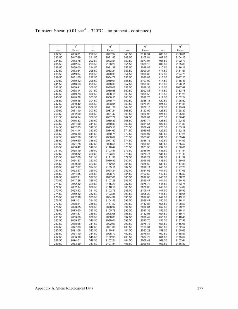
Appendix A. Shear Rheological Data
277
Transient Shear (0.01 sec-1 – 320°C – no preheat - continued)
t η+ t η+ t η+ t η+
sec Pa sec sec Pa sec sec Pa sec sec Pa sec232.50 2056.01 290.50 2077.97 348.50 2112.34 406.50 2106.61233.50 2047.69 291.50 2071.83 349.50 2107.84 407.50 2104.15234.50 2063.78 292.50 2093.51 350.50 2077.01 408.50 2102.79235.50 2042.64 293.50 2106.20 351.50 2089.15 409.50 2135.80236.50 2050.00 294.50 2081.38 352.50 2089.83 410.50 2146.16237.50 2033.64 295.50 2063.24 353.50 2090.24 411.50 2131.57238.50 2019.04 296.50 2070.33 354.50 2098.83 412.50 2124.75239.50 2031.05 297.50 2054.78 355.50 2080.83 413.50 2097.20240.50 2080.42 298.50 2059.01 356.50 2107.02 414.50 2116.43241.50 2048.23 299.50 2076.33 357.50 2099.38 415.50 2126.11242.50 2050.41 300.50 2085.06 358.50 2088.33 416.50 2097.47243.50 2038.14 301.50 2050.55 359.50 2092.83 417.50 2133.75244.50 2049.73 302.50 2068.15 360.50 2095.56 418.50 2111.25245.50 2048.78 303.50 2056.55 361.50 2092.70 419.50 2102.24246.50 2070.46 304.50 2070.74 362.50 2086.15 420.50 2126.52247.50 2059.42 305.50 2053.01 363.50 2074.28 421.50 2111.38248.50 2053.96 306.50 2071.28 364.50 2077.15 422.50 2115.07249.50 2051.10 307.50 2087.24 365.50 2122.02 423.50 2128.30250.50 2082.60 308.50 2091.47 366.50 2062.96 424.50 2125.98251.50 2066.24 309.50 2087.79 367.50 2089.01 425.50 2130.48252.50 2076.33 310.50 2080.83 368.50 2067.74 426.50 2122.43253.50 2061.60 311.50 2079.33 369.50 2081.51 427.50 2151.89254.50 2062.83 312.50 2093.51 370.50 2088.47 428.50 2135.52255.50 2044.14 313.50 2064.60 371.50 2069.65 429.50 2122.16256.50 2046.19 314.50 2070.74 372.50 2089.97 430.50 2117.25257.50 2092.29 315.50 2068.69 373.50 2085.60 431.50 2109.47258.50 2079.60 316.50 2077.42 374.50 2086.15 432.50 2114.93259.50 2071.28 317.50 2098.56 375.50 2090.65 433.50 2135.52260.50 2056.42 318.50 2118.47 376.50 2071.96 434.50 2130.61261.50 2058.19 319.50 2103.47 377.50 2086.97 435.50 2131.84262.50 2050.82 320.50 2103.20 378.50 2079.74 436.50 2131.43263.50 2047.00 321.50 2111.38 379.50 2090.24 437.50 2141.39264.50 2054.37 322.50 2089.83 380.50 2095.56 438.50 2139.07265.50 2039.50 323.50 2112.61 381.50 2085.60 439.50 2147.80266.50 2067.87 324.50 2105.11 382.50 2099.11 440.50 2127.20267.50 2052.87 325.50 2093.24 383.50 2084.65 441.50 2147.66268.50 2044.55 326.50 2098.70 384.50 2102.52 442.50 2135.52269.50 2042.91 327.50 2097.61 385.50 2097.06 443.50 2136.21270.50 2047.28 328.50 2107.29 386.50 2085.47 444.50 2160.35271.50 2052.32 329.50 2115.20 387.50 2075.78 445.50 2133.75272.50 2062.14 330.50 2116.16 388.50 2076.06 446.50 2154.89273.50 2053.82 331.50 2102.79 389.50 2106.47 447.50 2138.93274.50 2059.42 332.50 2103.88 390.50 2095.29 448.50 2138.66275.50 2062.96 333.50 2084.92 391.50 2097.88 449.50 2143.16276.50 2071.01 334.50 2104.56 392.50 2088.47 450.50 2126.11277.50 2078.51 335.50 2117.52 393.50 2112.88 451.50 2128.57278.50 2090.65 336.50 2098.97 394.50 2092.01 452.50 2129.25279.50 2073.60 337.50 2105.79 395.50 2097.33 453.50 2129.11280.50 2064.87 338.50 2096.65 396.50 2112.06 454.50 2149.71281.50 2053.69 339.50 2080.83 397.50 2098.42 455.50 2148.48282.50 2069.37 340.50 2089.01 398.50 2095.70 456.50 2137.98283.50 2078.65 341.50 2092.97 399.50 2078.78 457.50 2146.98284.50 2077.83 342.50 2091.06 400.50 2103.34 458.50 2152.57285.50 2091.06 343.50 2110.84 401.50 2083.29 459.50 2160.62286.50 2081.10 344.50 2098.70 402.50 2078.51 460.50 2158.57287.50 2066.10 345.50 2102.93 403.50 2087.79 461.50 2175.62288.50 2074.01 346.50 2102.24 404.50 2068.42 462.50 2152.44289.50 2083.29 347.50 2107.84 405.50 2099.65 463.50 2156.80

Appendix A. Shear Rheological Data
278
Transient Shear (0.01 sec-1 – 320°C – no preheat - continued)
t η+ t η+ t η+ t η+
sec Pa sec sec Pa sec sec Pa sec sec Pa sec464.50 2174.53 522.50 2197.72 580.50 2229.36 638.50 2227.59465.50 2143.57 523.50 2208.22 581.50 2219.68 639.50 2274.51466.50 2161.85 524.50 2201.54 582.50 2206.86 640.50 2283.10467.50 2158.57 525.50 2191.17 583.50 2201.40 641.50 2231.41468.50 2163.21 526.50 2194.86 584.50 2198.40 642.50 2239.05469.50 2166.49 527.50 2194.04 585.50 2243.82 643.50 2266.33470.50 2165.67 528.50 2199.08 586.50 2225.27 644.50 2270.69471.50 2153.39 529.50 2196.63 587.50 2227.04 645.50 2279.56472.50 2148.62 530.50 2213.27 588.50 2206.86 646.50 2248.19473.50 2156.12 531.50 2178.76 589.50 2226.77 647.50 2252.28474.50 2155.03 532.50 2207.81 590.50 2197.86 648.50 2254.46475.50 2166.76 533.50 2191.04 591.50 2207.54 649.50 2265.92476.50 2151.21 534.50 2175.76 592.50 2217.63 650.50 2262.64477.50 2162.26 535.50 2170.85 593.50 2220.50 651.50 2271.92478.50 2173.44 536.50 2170.58 594.50 2213.68 652.50 2274.24479.50 2157.07 537.50 2186.40 595.50 2216.13 653.50 2276.96480.50 2185.04 538.50 2209.18 596.50 2222.82 654.50 2283.10481.50 2193.49 539.50 2202.77 597.50 2223.50 655.50 2278.33482.50 2174.81 540.50 2208.22 598.50 2248.59 656.50 2305.47483.50 2177.53 541.50 2197.04 599.50 2228.41 657.50 2284.06484.50 2152.85 542.50 2201.40 600.50 2239.46 658.50 2270.28485.50 2161.58 543.50 2205.09 601.50 2231.14 659.50 2300.02486.50 2146.16 544.50 2192.81 602.50 2254.32 660.50 2288.97487.50 2173.03 545.50 2205.90 603.50 2239.46 661.50 2278.87488.50 2149.57 546.50 2213.41 604.50 2227.04 662.50 2248.73489.50 2163.21 547.50 2206.18 605.50 2214.77 663.50 2271.51490.50 2168.12 548.50 2187.63 606.50 2213.54 664.50 2261.28491.50 2170.58 549.50 2196.77 607.50 2218.59 665.50 2280.37492.50 2183.94 550.50 2181.63 608.50 2219.68 666.50 2262.10493.50 2161.85 551.50 2197.86 609.50 2195.26 667.50 2263.60494.50 2193.49 552.50 2190.08 610.50 2216.82 668.50 2264.55495.50 2170.03 553.50 2193.63 611.50 2208.09 669.50 2276.42496.50 2172.21 554.50 2193.22 612.50 2193.08 670.50 2259.92497.50 2206.99 555.50 2186.26 613.50 2219.82 671.50 2280.51498.50 2188.85 556.50 2193.49 614.50 2227.18 672.50 2273.28499.50 2200.45 557.50 2186.81 615.50 2204.68 673.50 2270.01500.50 2222.41 558.50 2211.50 616.50 2232.50 674.50 2273.83501.50 2199.63 559.50 2157.62 617.50 2228.41 675.50 2264.42502.50 2202.63 560.50 2177.12 618.50 2234.82 676.50 2259.92503.50 2167.71 561.50 2198.27 619.50 2200.31 677.50 2281.19504.50 2194.17 562.50 2209.59 620.50 2204.27 678.50 2263.46505.50 2168.67 563.50 2197.45 621.50 2211.09 679.50 2258.14506.50 2175.62 564.50 2198.27 622.50 2233.46 680.50 2263.33507.50 2173.85 565.50 2182.99 623.50 2252.96 681.50 2279.97508.50 2182.72 566.50 2182.85 624.50 2229.23 682.50 2267.14509.50 2194.58 567.50 2189.54 625.50 2243.96 683.50 2260.87510.50 2189.13 568.50 2189.26 626.50 2225.00 684.50 2271.24511.50 2203.72 569.50 2187.90 627.50 2246.96 685.50 2272.46512.50 2201.13 570.50 2204.68 628.50 2245.46 686.50 2271.10513.50 2176.31 571.50 2178.90 629.50 2252.41 687.50 2263.87514.50 2169.90 572.50 2184.63 630.50 2252.69 688.50 2313.11515.50 2198.81 573.50 2196.77 631.50 2249.28 689.50 2276.28516.50 2159.53 574.50 2208.22 632.50 2251.32 690.50 2261.83517.50 2202.08 575.50 2182.58 633.50 2228.14 691.50 2272.74518.50 2193.08 576.50 2204.68 634.50 2253.23 692.50 2289.79519.50 2211.50 577.50 2181.63 635.50 2252.69 693.50 2260.73520.50 2222.41 578.50 2218.18 636.50 2253.78 694.50 2268.37521.50 2206.31 579.50 2227.45 637.50 2252.00 695.50 2266.33

Appendix A. Shear Rheological Data
279
Transient Shear (0.01 sec-1 – 320°C – no preheat - continued)
t η+ t η+ t η+ t η+
sec Pa sec sec Pa sec sec Pa sec sec Pa sec696.50 2258.82 754.50 2248.73 812.50 2306.97 870.50 2285.83697.50 2252.41 755.50 2258.55 813.50 2310.65 871.50 2278.87698.50 2256.92 756.50 2257.73 814.50 2297.83 872.50 2270.55699.50 2249.82 757.50 2272.46 815.50 2287.06 873.50 2292.51700.50 2272.05 758.50 2261.28 816.50 2295.38 874.50 2306.97701.50 2283.92 759.50 2263.60 817.50 2279.97 875.50 2298.11702.50 2282.56 760.50 2252.14 818.50 2276.28 876.50 2307.11703.50 2279.83 761.50 2281.47 819.50 2280.65 877.50 2303.29704.50 2275.60 762.50 2287.88 820.50 2286.51 878.50 2294.29705.50 2276.01 763.50 2264.69 821.50 2272.60 879.50 2292.79706.50 2264.42 764.50 2249.14 822.50 2256.92 880.50 2310.65707.50 2276.96 765.50 2269.33 823.50 2274.92 881.50 2298.92708.50 2277.24 766.50 2284.60 824.50 2271.37 882.50 2292.24709.50 2262.10 767.50 2267.42 825.50 2272.05 883.50 2311.61710.50 2248.32 768.50 2285.15 826.50 2284.74 884.50 2307.93711.50 2289.10 769.50 2290.47 827.50 2287.60 885.50 2277.24712.50 2301.79 770.50 2292.92 828.50 2282.69 886.50 2288.83713.50 2262.64 771.50 2291.15 829.50 2289.24 887.50 2300.70714.50 2269.60 772.50 2297.01 830.50 2288.29 888.50 2302.20715.50 2274.92 773.50 2279.69 831.50 2293.33 889.50 2288.69716.50 2286.38 774.50 2295.51 832.50 2301.24 890.50 2288.56717.50 2272.33 775.50 2284.60 833.50 2283.51 891.50 2285.97718.50 2259.78 776.50 2271.65 834.50 2289.38 892.50 2297.01719.50 2259.23 777.50 2282.01 835.50 2297.56 893.50 2319.79720.50 2274.10 778.50 2292.79 836.50 2329.61 894.50 2326.89721.50 2258.14 779.50 2277.65 837.50 2299.88 895.50 2316.79722.50 2246.96 780.50 2297.15 838.50 2313.65 896.50 2315.29723.50 2249.96 781.50 2265.78 839.50 2311.06 897.50 2311.47724.50 2265.92 782.50 2254.60 840.50 2296.74 898.50 2306.29725.50 2266.19 783.50 2258.82 841.50 2303.70 899.50 2307.65726.50 2278.19 784.50 2265.64 842.50 2294.01 900.50 2317.20727.50 2260.46 785.50 2287.06 843.50 2294.70 901.50 2318.43728.50 2265.37 786.50 2292.65 844.50 2300.83 902.50 2307.93729.50 2266.87 787.50 2280.37 845.50 2298.38 903.50 2271.37730.50 2269.33 788.50 2304.11 846.50 2311.88 904.50 2243.14731.50 2289.79 789.50 2277.10 847.50 2299.61 905.50 2264.96732.50 2282.83 790.50 2290.74 848.50 2295.24 906.50 2279.83733.50 2262.64 791.50 2315.43 849.50 2303.02 907.50 2283.38734.50 2229.91 792.50 2309.84 850.50 2299.88 908.50 2302.88735.50 2257.46 793.50 2286.38 851.50 2280.92 909.50 2280.51736.50 2264.28 794.50 2279.97 852.50 2294.83 910.50 2272.05737.50 2248.46 795.50 2291.97 853.50 2298.11 911.50 2284.06738.50 2255.41 796.50 2293.47 854.50 2329.34 912.50 2268.24739.50 2260.19 797.50 2305.06 855.50 2294.29 913.50 2293.61740.50 2287.47 798.50 2282.42 856.50 2312.97 914.50 2317.61741.50 2269.60 799.50 2256.64 857.50 2299.47 915.50 2303.56742.50 2271.24 800.50 2268.64 858.50 2310.93 916.50 2290.47743.50 2258.55 801.50 2264.83 859.50 2303.29 917.50 2291.83744.50 2282.56 802.50 2250.78 860.50 2292.38 918.50 2298.92745.50 2261.28 803.50 2274.65 861.50 2277.51 919.50 2291.83746.50 2258.42 804.50 2289.79 862.50 2282.01 920.50 2293.06747.50 2281.88 805.50 2285.29 863.50 2292.65 921.50 2256.92748.50 2277.78 806.50 2276.28 864.50 2276.42 922.50 2256.37749.50 2291.01 807.50 2297.83 865.50 2299.88 923.50 2280.78750.50 2279.83 808.50 2312.84 866.50 2286.79 924.50 2274.78751.50 2290.33 809.50 2296.06 867.50 2257.46 925.50 2305.20752.50 2258.82 810.50 2295.51 868.50 2285.42 926.50 2234.96753.50 2281.33 811.50 2305.74 869.50 2286.24 927.50 2266.74
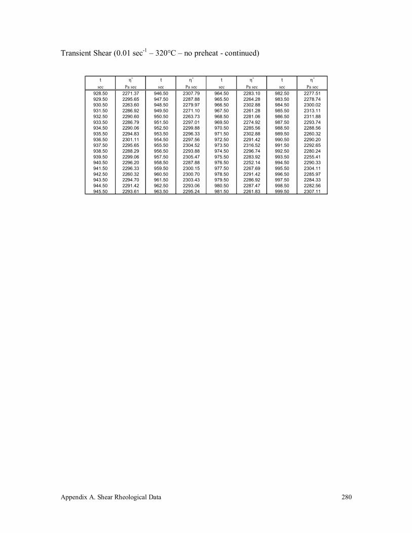
Appendix A. Shear Rheological Data
280
Transient Shear (0.01 sec-1 – 320°C – no preheat - continued)
t η+ t η+ t η+ t η+
sec Pa sec sec Pa sec sec Pa sec sec Pa sec928.50 2271.37 946.50 2307.79 964.50 2283.10 982.50 2277.51929.50 2295.65 947.50 2287.88 965.50 2264.28 983.50 2278.74930.50 2263.60 948.50 2279.97 966.50 2302.88 984.50 2300.02931.50 2286.92 949.50 2271.10 967.50 2261.28 985.50 2313.11932.50 2290.60 950.50 2263.73 968.50 2281.06 986.50 2311.88933.50 2286.79 951.50 2297.01 969.50 2274.92 987.50 2293.74934.50 2290.06 952.50 2299.88 970.50 2285.56 988.50 2288.56935.50 2294.83 953.50 2296.33 971.50 2302.88 989.50 2260.32936.50 2301.11 954.50 2297.56 972.50 2291.42 990.50 2290.20937.50 2295.65 955.50 2304.52 973.50 2316.52 991.50 2292.65938.50 2288.29 956.50 2293.88 974.50 2296.74 992.50 2280.24939.50 2299.06 957.50 2305.47 975.50 2283.92 993.50 2255.41940.50 2296.20 958.50 2287.88 976.50 2252.14 994.50 2290.33941.50 2296.33 959.50 2300.15 977.50 2267.69 995.50 2304.11942.50 2260.32 960.50 2300.70 978.50 2291.42 996.50 2285.97943.50 2294.70 961.50 2303.43 979.50 2286.92 997.50 2284.33944.50 2291.42 962.50 2293.06 980.50 2287.47 998.50 2282.56945.50 2293.61 963.50 2295.24 981.50 2261.83 999.50 2307.11
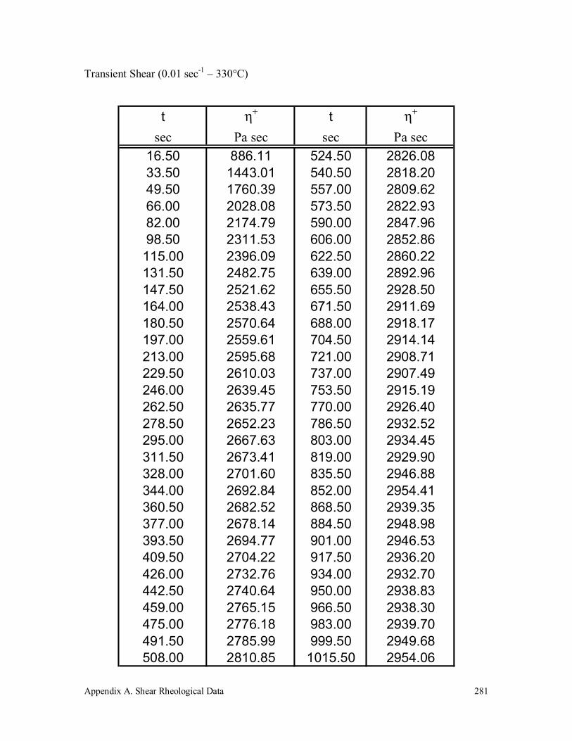
Appendix A. Shear Rheological Data
281
Transient Shear (0.01 sec-1 – 330°C)
t η+ t η+
sec Pa sec sec Pa sec16.50 886.11 524.50 2826.0833.50 1443.01 540.50 2818.2049.50 1760.39 557.00 2809.6266.00 2028.08 573.50 2822.9382.00 2174.79 590.00 2847.9698.50 2311.53 606.00 2852.86115.00 2396.09 622.50 2860.22131.50 2482.75 639.00 2892.96147.50 2521.62 655.50 2928.50164.00 2538.43 671.50 2911.69180.50 2570.64 688.00 2918.17197.00 2559.61 704.50 2914.14213.00 2595.68 721.00 2908.71229.50 2610.03 737.00 2907.49246.00 2639.45 753.50 2915.19262.50 2635.77 770.00 2926.40278.50 2652.23 786.50 2932.52295.00 2667.63 803.00 2934.45311.50 2673.41 819.00 2929.90328.00 2701.60 835.50 2946.88344.00 2692.84 852.00 2954.41360.50 2682.52 868.50 2939.35377.00 2678.14 884.50 2948.98393.50 2694.77 901.00 2946.53409.50 2704.22 917.50 2936.20426.00 2732.76 934.00 2932.70442.50 2740.64 950.00 2938.83459.00 2765.15 966.50 2938.30475.00 2776.18 983.00 2939.70491.50 2785.99 999.50 2949.68508.00 2810.85 1015.50 2954.06

Appendix A. Shear Rheological Data
282
Transient Shear (0.01 sec-1 – 330°C – no preheat - continued)
t η+ t η+ t η+ t η+
sec Pa sec sec Pa sec sec Pa sec sec Pa sec0.25 51.56 29.25 1050.70 58.25 1620.92 87.25 1937.650.75 99.30 29.75 1066.46 58.75 1593.84 87.75 1923.271.25 118.15 30.25 1077.74 59.25 1598.64 88.25 1947.471.75 173.65 30.75 1101.00 59.75 1603.79 88.75 1942.322.25 185.87 31.25 1096.91 60.25 1611.57 89.25 1938.132.75 224.41 31.75 1131.44 60.75 1629.18 89.75 1947.713.25 257.18 32.25 1110.28 61.25 1622.12 90.25 1963.643.75 270.13 32.75 1122.16 61.75 1664.04 90.75 1967.484.25 290.37 33.25 1131.10 62.25 1646.07 91.25 1970.474.75 303.57 33.75 1154.36 62.75 1654.82 91.75 1982.815.25 344.52 34.25 1158.37 63.25 1647.39 92.25 1975.035.75 354.46 34.75 1166.10 63.75 1671.35 92.75 1986.766.25 398.95 35.25 1170.69 64.25 1672.19 93.25 1995.876.75 419.25 35.75 1169.29 64.75 1669.19 93.75 1976.107.25 425.66 36.25 1203.08 65.25 1712.68 94.25 2005.337.75 462.04 36.75 1233.51 65.75 1678.06 94.75 1999.108.25 450.58 37.25 1233.15 66.25 1693.63 95.25 2016.478.75 474.04 37.75 1244.89 66.75 1715.67 95.75 2004.379.25 504.99 38.25 1246.09 67.25 1726.22 96.25 2024.509.75 530.02 38.75 1267.89 67.75 1732.92 96.75 2043.55
10.25 543.34 39.25 1249.32 68.25 1714.72 97.25 2030.8510.75 551.27 39.75 1276.75 68.75 1738.19 97.75 2044.8611.25 582.10 40.25 1290.89 69.25 1724.66 98.25 2029.0511.75 573.62 40.75 1287.89 69.75 1755.56 98.75 2061.9912.25 627.63 41.25 1308.50 70.25 1755.09 99.25 2044.9812.75 609.00 41.75 1296.40 70.75 1771.26 99.75 2044.6213.25 649.25 42.25 1326.71 71.25 1765.75 100.25 2056.7213.75 644.77 42.75 1322.27 71.75 1772.81 100.75 2056.3614.25 665.92 43.25 1345.15 72.25 1779.40 101.25 2086.1914.75 676.11 43.75 1351.14 72.75 1788.75 101.75 2054.9315.25 702.50 44.25 1351.50 73.25 1802.28 102.25 2100.4515.75 730.77 44.75 1359.65 73.75 1788.75 102.75 2065.4716.25 715.93 45.25 1374.86 74.25 1791.74 103.25 2106.2016.75 747.63 45.75 1382.41 74.75 1813.66 103.75 2097.8117.25 751.34 46.25 1386.48 75.25 1816.18 104.25 2101.4117.75 777.08 46.75 1403.85 75.75 1830.32 104.75 2122.1318.25 779.86 47.25 1405.53 76.25 1821.69 105.25 2095.3018.75 788.15 47.75 1434.04 76.75 1840.38 105.75 2129.6819.25 813.49 48.25 1434.76 77.25 1836.07 106.25 2118.7819.75 801.89 48.75 1430.21 77.75 1850.44 106.75 2142.6220.25 854.31 49.25 1453.69 78.25 1828.52 107.25 2136.9920.75 844.78 49.75 1447.94 78.75 1845.05 107.75 2131.9521.25 871.55 50.25 1459.92 79.25 1860.98 108.25 2154.0021.75 868.80 50.75 1465.31 79.75 1853.20 108.75 2133.3922.25 880.93 51.25 1504.84 80.25 1868.05 109.25 2171.0122.75 930.84 51.75 1503.88 80.75 1861.46 109.75 2135.5523.25 921.18 52.25 1499.93 81.25 1875.48 110.25 2177.1223.75 950.20 52.75 1509.03 81.75 1874.16 110.75 2158.5524.25 933.41 53.25 1508.07 82.25 1895.48 111.25 2152.9224.75 967.50 53.75 1524.84 82.75 1890.81 111.75 2172.4425.25 952.20 54.25 1508.07 83.25 1885.66 112.25 2170.0525.75 967.72 54.75 1546.05 83.75 1908.66 112.75 2174.6026.25 989.09 55.25 1538.02 84.25 1891.77 113.25 2178.7926.75 990.87 55.75 1541.14 84.75 1902.31 113.75 2196.6427.25 1010.63 56.25 1561.74 85.25 1903.75 114.25 2188.6227.75 995.23 56.75 1570.84 85.75 1906.26 114.75 2209.3428.25 1015.78 57.25 1586.78 86.25 1915.25 115.25 2208.8628.75 1036.70 57.75 1589.53 86.75 1906.26 115.75 2204.19
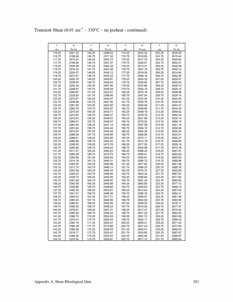
Appendix A. Shear Rheological Data
283
Transient Shear (0.01 sec-1 – 330°C – no preheat - continued)
t η+ t η+ t η+ t η+
sec Pa sec sec Pa sec sec Pa sec sec Pa sec116.25 2221.32 145.25 2389.03 174.25 2523.32 203.25 2635.92116.75 2198.08 145.75 2371.30 174.75 2518.65 203.75 2615.44117.25 2215.93 146.25 2404.72 175.25 2517.33 204.25 2626.82117.75 2198.68 146.75 2391.07 175.75 2526.91 204.75 2642.51118.25 2226.95 147.25 2382.32 176.25 2514.21 205.25 2630.29118.75 2218.32 147.75 2407.48 176.75 2547.16 205.75 2640.12119.25 2224.07 148.25 2404.12 177.25 2519.36 206.25 2614.84119.75 2237.97 148.75 2405.32 177.75 2558.18 206.75 2652.09120.25 2224.19 149.25 2409.87 178.25 2520.32 207.25 2629.57120.75 2238.93 149.75 2428.44 178.75 2545.60 207.75 2655.93121.25 2244.20 150.25 2407.00 179.25 2537.69 208.25 2649.10121.75 2248.87 150.75 2409.39 179.75 2554.10 208.75 2625.14122.25 2250.67 151.25 2422.57 180.25 2570.16 209.25 2656.89122.75 2235.93 151.75 2396.46 180.75 2547.04 209.75 2626.10123.25 2273.91 152.25 2445.57 181.25 2572.55 210.25 2640.00123.75 2248.99 152.75 2427.00 181.75 2535.78 210.75 2636.40124.25 2281.69 153.25 2442.82 182.25 2555.06 211.25 2643.47124.75 2265.76 153.75 2432.87 182.75 2558.66 211.75 2634.25125.25 2275.83 154.25 2433.71 183.25 2558.18 212.25 2648.62125.75 2272.83 154.75 2444.37 183.75 2578.78 212.75 2662.04126.25 2270.91 155.25 2448.57 184.25 2541.89 213.25 2625.14126.75 2284.81 155.75 2448.57 184.75 2579.02 213.75 2668.15127.25 2264.56 156.25 2427.12 185.25 2557.58 214.25 2641.19127.75 2291.64 156.75 2454.44 185.75 2590.16 214.75 2658.08128.25 2274.87 157.25 2445.45 186.25 2564.29 215.25 2650.30128.75 2288.28 157.75 2458.99 186.75 2566.68 215.75 2654.01129.25 2286.61 158.25 2463.90 187.25 2574.11 216.25 2665.27129.75 2289.48 158.75 2463.42 187.75 2572.19 216.75 2656.65130.25 2308.05 159.25 2472.76 188.25 2577.58 217.25 2659.16130.75 2290.68 159.75 2454.44 188.75 2554.58 217.75 2670.78131.25 2317.27 160.25 2482.23 189.25 2588.24 218.25 2667.91131.75 2284.09 160.75 2472.76 189.75 2588.01 218.75 2662.28132.25 2306.85 161.25 2482.83 190.25 2582.61 219.25 2665.63132.75 2314.16 161.75 2480.31 190.75 2585.73 219.75 2668.99133.25 2295.59 162.25 2484.86 191.25 2577.82 220.25 2661.56133.75 2317.75 162.75 2490.13 191.75 2586.33 220.75 2685.76134.25 2303.38 163.25 2465.34 192.25 2576.74 221.25 2653.65134.75 2325.42 163.75 2488.94 192.75 2603.22 221.75 2667.67135.25 2329.73 164.25 2482.95 193.25 2588.84 222.25 2671.62135.75 2351.06 164.75 2490.97 193.75 2591.24 222.75 2660.60136.25 2362.08 165.25 2495.88 194.25 2605.85 223.25 2677.73136.75 2346.86 165.75 2498.88 194.75 2594.83 223.75 2668.15137.25 2352.25 166.25 2503.67 195.25 2613.64 224.25 2691.03137.75 2341.47 166.75 2496.36 195.75 2586.33 224.75 2664.31138.25 2363.03 167.25 2517.21 196.25 2598.67 225.25 2681.08138.75 2365.43 167.75 2482.95 196.75 2602.62 225.75 2665.99139.25 2365.91 168.25 2500.08 197.25 2608.25 226.25 2676.17139.75 2390.35 168.75 2496.24 197.75 2615.32 226.75 2677.37140.25 2378.61 169.25 2491.21 198.25 2617.47 227.25 2670.42140.75 2395.50 169.75 2508.34 198.75 2631.25 227.75 2693.54141.25 2366.75 170.25 2502.83 199.25 2591.72 228.25 2663.59141.75 2375.01 170.75 2526.43 199.75 2620.11 228.75 2696.42142.25 2365.19 171.25 2504.27 200.25 2609.21 229.25 2671.02142.75 2386.39 171.75 2510.86 200.75 2621.43 229.75 2673.90143.25 2385.08 172.25 2509.54 201.25 2642.51 230.25 2685.04143.75 2374.77 172.75 2505.47 201.75 2630.65 230.75 2667.67144.25 2390.35 173.25 2520.20 202.25 2643.95 231.25 2688.87144.75 2370.34 173.75 2503.67 202.75 2617.12 231.75 2685.64
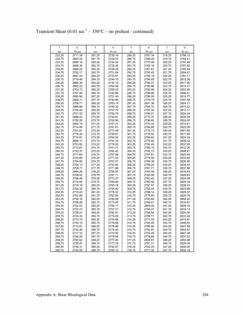
Appendix A. Shear Rheological Data
284
Transient Shear (0.01 sec-1 – 330°C – no preheat - continued)
t η+ t η+ t η+ t η+
sec Pa sec sec Pa sec sec Pa sec sec Pa sec232.25 2711.39 261.25 2739.18 290.25 2787.34 319.25 2798.12232.75 2683.24 261.75 2725.53 290.75 2769.49 319.75 2794.41233.25 2696.18 262.25 2744.34 291.25 2775.48 320.25 2797.40233.75 2696.30 262.75 2735.35 291.75 2785.18 320.75 2787.82234.25 2686.24 263.25 2726.25 292.25 2767.81 321.25 2785.54234.75 2702.17 263.75 2751.64 292.75 2793.45 321.75 2804.47235.25 2687.43 264.25 2723.97 293.25 2782.19 322.25 2781.71235.75 2718.46 264.75 2744.10 293.75 2794.65 322.75 2812.26236.25 2696.30 265.25 2734.15 294.25 2780.27 323.25 2811.90236.75 2692.23 265.75 2764.58 294.75 2785.66 323.75 2814.77237.25 2703.73 266.25 2769.25 295.25 2780.99 324.25 2803.99237.75 2707.20 266.75 2740.98 295.75 2766.86 324.75 2806.51238.25 2695.94 267.25 2751.40 296.25 2796.09 325.25 2814.77238.75 2689.11 267.75 2740.86 296.75 2779.79 325.75 2787.58239.25 2709.71 268.25 2763.14 297.25 2801.36 326.25 2804.71239.75 2699.89 268.75 2750.32 297.75 2764.70 326.75 2813.22240.25 2705.04 269.25 2757.75 298.25 2787.34 327.25 2817.17240.75 2721.93 269.75 2759.79 298.75 2796.21 327.75 2824.24241.25 2696.42 270.25 2744.81 299.25 2772.37 328.25 2830.59241.75 2702.29 270.75 2762.90 299.75 2798.60 328.75 2824.00242.25 2694.74 271.25 2747.21 300.25 2770.33 329.25 2814.41242.75 2714.99 271.75 2767.81 300.75 2794.89 329.75 2823.28243.25 2701.81 272.25 2772.49 301.25 2772.73 330.25 2801.60243.75 2716.30 272.75 2749.97 301.75 2776.92 330.75 2817.89244.25 2710.91 273.25 2764.94 302.25 2789.62 331.25 2824.24244.75 2699.17 273.75 2754.16 302.75 2775.60 331.75 2808.42245.25 2723.85 274.25 2776.92 303.25 2792.49 332.25 2837.65245.75 2710.67 274.75 2761.71 303.75 2780.15 332.75 2812.26246.25 2723.37 275.25 2765.42 304.25 2792.73 333.25 2848.91246.75 2711.63 275.75 2757.99 304.75 2767.81 333.75 2823.04247.25 2723.85 276.25 2771.53 305.25 2779.55 334.25 2833.82247.75 2704.80 276.75 2767.57 305.75 2786.38 334.75 2826.99248.25 2709.12 277.25 2752.84 306.25 2769.25 335.25 2839.45248.75 2709.71 277.75 2771.89 306.75 2781.71 335.75 2837.89249.25 2694.26 278.25 2756.07 307.25 2764.58 336.25 2816.93249.75 2708.52 278.75 2781.71 307.75 2780.99 336.75 2829.63250.25 2706.48 279.25 2772.37 308.25 2762.42 337.25 2824.48250.75 2715.94 279.75 2769.85 308.75 2790.46 337.75 2829.39251.25 2719.18 280.25 2765.78 309.25 2767.57 338.25 2828.43251.75 2704.32 280.75 2754.40 309.75 2753.44 338.75 2823.88252.25 2710.43 281.25 2776.32 310.25 2786.14 339.25 2828.07252.75 2702.89 281.75 2762.06 310.75 2778.60 339.75 2820.76253.25 2728.16 282.25 2785.66 311.25 2793.69 340.25 2848.20253.75 2708.28 282.75 2773.92 311.75 2769.01 340.75 2816.81254.25 2722.53 283.25 2794.17 312.25 2800.04 341.25 2828.19254.75 2723.73 283.75 2757.51 312.75 2783.27 341.75 2818.13255.25 2726.01 284.25 2782.91 313.25 2784.94 342.25 2824.00255.75 2724.33 284.75 2774.40 313.75 2784.11 342.75 2833.22256.25 2715.70 285.25 2774.88 314.25 2771.53 343.25 2815.97256.75 2734.15 285.75 2776.68 314.75 2793.45 343.75 2846.64257.25 2713.91 286.25 2778.96 315.25 2785.90 344.25 2847.48257.75 2732.48 286.75 2774.40 315.75 2792.97 344.75 2852.87258.25 2717.14 287.25 2773.92 316.25 2792.49 345.25 2847.48258.75 2745.29 287.75 2778.84 316.75 2776.68 345.75 2837.53259.25 2740.62 288.25 2777.40 317.25 2804.47 346.25 2855.98259.75 2726.97 288.75 2777.76 317.75 2781.71 346.75 2829.39260.25 2756.31 289.25 2792.97 318.25 2792.25 347.25 2840.05260.75 2724.09 289.75 2755.12 318.75 2771.05 347.75 2834.18
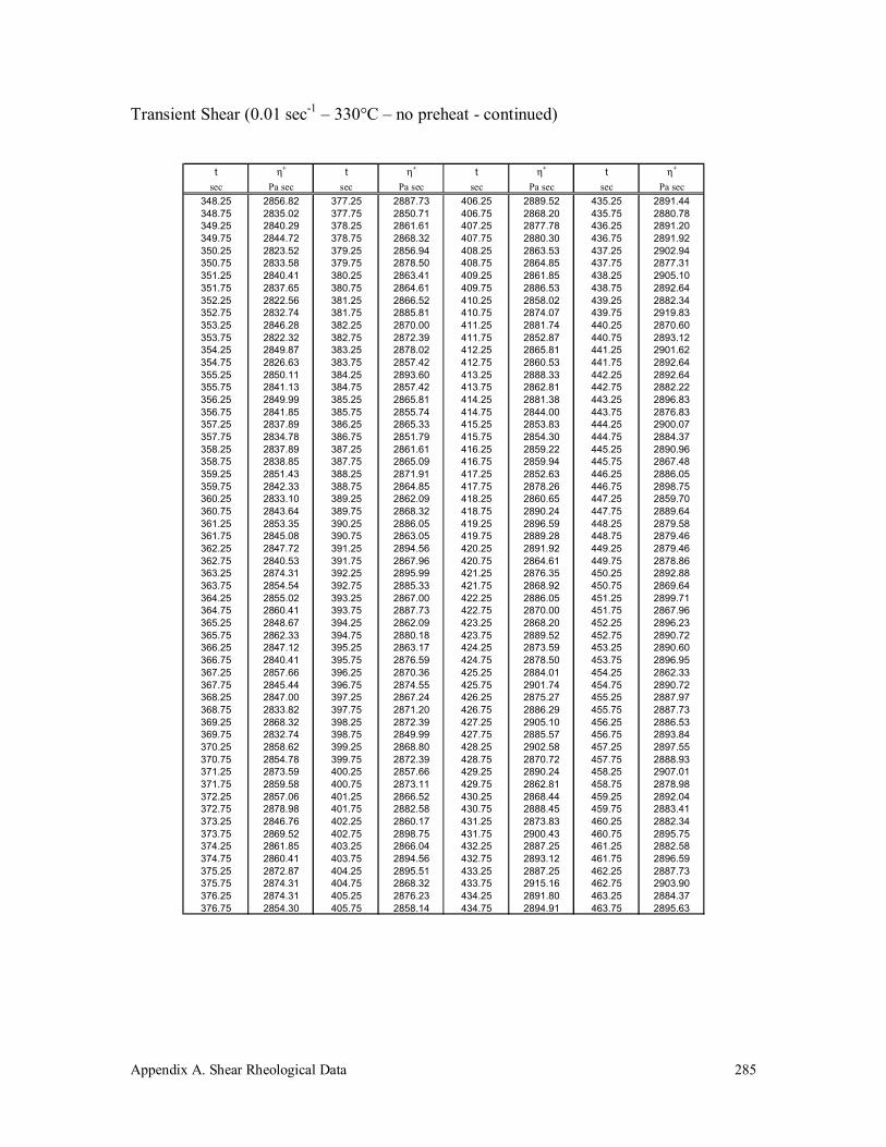
Appendix A. Shear Rheological Data
285
Transient Shear (0.01 sec-1 – 330°C – no preheat - continued)
t η+ t η+ t η+ t η+
sec Pa sec sec Pa sec sec Pa sec sec Pa sec348.25 2856.82 377.25 2887.73 406.25 2889.52 435.25 2891.44348.75 2835.02 377.75 2850.71 406.75 2868.20 435.75 2880.78349.25 2840.29 378.25 2861.61 407.25 2877.78 436.25 2891.20349.75 2844.72 378.75 2868.32 407.75 2880.30 436.75 2891.92350.25 2823.52 379.25 2856.94 408.25 2863.53 437.25 2902.94350.75 2833.58 379.75 2878.50 408.75 2864.85 437.75 2877.31351.25 2840.41 380.25 2863.41 409.25 2861.85 438.25 2905.10351.75 2837.65 380.75 2864.61 409.75 2886.53 438.75 2892.64352.25 2822.56 381.25 2866.52 410.25 2858.02 439.25 2882.34352.75 2832.74 381.75 2885.81 410.75 2874.07 439.75 2919.83353.25 2846.28 382.25 2870.00 411.25 2881.74 440.25 2870.60353.75 2822.32 382.75 2872.39 411.75 2852.87 440.75 2893.12354.25 2849.87 383.25 2878.02 412.25 2865.81 441.25 2901.62354.75 2826.63 383.75 2857.42 412.75 2860.53 441.75 2892.64355.25 2850.11 384.25 2893.60 413.25 2888.33 442.25 2892.64355.75 2841.13 384.75 2857.42 413.75 2862.81 442.75 2882.22356.25 2849.99 385.25 2865.81 414.25 2881.38 443.25 2896.83356.75 2841.85 385.75 2855.74 414.75 2844.00 443.75 2876.83357.25 2837.89 386.25 2865.33 415.25 2853.83 444.25 2900.07357.75 2834.78 386.75 2851.79 415.75 2854.30 444.75 2884.37358.25 2837.89 387.25 2861.61 416.25 2859.22 445.25 2890.96358.75 2838.85 387.75 2865.09 416.75 2859.94 445.75 2867.48359.25 2851.43 388.25 2871.91 417.25 2852.63 446.25 2886.05359.75 2842.33 388.75 2864.85 417.75 2878.26 446.75 2898.75360.25 2833.10 389.25 2862.09 418.25 2860.65 447.25 2859.70360.75 2843.64 389.75 2868.32 418.75 2890.24 447.75 2889.64361.25 2853.35 390.25 2886.05 419.25 2896.59 448.25 2879.58361.75 2845.08 390.75 2863.05 419.75 2889.28 448.75 2879.46362.25 2847.72 391.25 2894.56 420.25 2891.92 449.25 2879.46362.75 2840.53 391.75 2867.96 420.75 2864.61 449.75 2878.86363.25 2874.31 392.25 2895.99 421.25 2876.35 450.25 2892.88363.75 2854.54 392.75 2885.33 421.75 2868.92 450.75 2869.64364.25 2855.02 393.25 2867.00 422.25 2886.05 451.25 2899.71364.75 2860.41 393.75 2887.73 422.75 2870.00 451.75 2867.96365.25 2848.67 394.25 2862.09 423.25 2868.20 452.25 2896.23365.75 2862.33 394.75 2880.18 423.75 2889.52 452.75 2890.72366.25 2847.12 395.25 2863.17 424.25 2873.59 453.25 2890.60366.75 2840.41 395.75 2876.59 424.75 2878.50 453.75 2896.95367.25 2857.66 396.25 2870.36 425.25 2884.01 454.25 2862.33367.75 2845.44 396.75 2874.55 425.75 2901.74 454.75 2890.72368.25 2847.00 397.25 2867.24 426.25 2875.27 455.25 2887.97368.75 2833.82 397.75 2871.20 426.75 2886.29 455.75 2887.73369.25 2868.32 398.25 2872.39 427.25 2905.10 456.25 2886.53369.75 2832.74 398.75 2849.99 427.75 2885.57 456.75 2893.84370.25 2858.62 399.25 2868.80 428.25 2902.58 457.25 2897.55370.75 2854.78 399.75 2872.39 428.75 2870.72 457.75 2888.93371.25 2873.59 400.25 2857.66 429.25 2890.24 458.25 2907.01371.75 2859.58 400.75 2873.11 429.75 2862.81 458.75 2878.98372.25 2857.06 401.25 2866.52 430.25 2868.44 459.25 2892.04372.75 2878.98 401.75 2882.58 430.75 2888.45 459.75 2883.41373.25 2846.76 402.25 2860.17 431.25 2873.83 460.25 2882.34373.75 2869.52 402.75 2898.75 431.75 2900.43 460.75 2895.75374.25 2861.85 403.25 2866.04 432.25 2887.25 461.25 2882.58374.75 2860.41 403.75 2894.56 432.75 2893.12 461.75 2896.59375.25 2872.87 404.25 2895.51 433.25 2887.25 462.25 2887.73375.75 2874.31 404.75 2868.32 433.75 2915.16 462.75 2903.90376.25 2874.31 405.25 2876.23 434.25 2891.80 463.25 2884.37376.75 2854.30 405.75 2858.14 434.75 2894.91 463.75 2895.63

Appendix A. Shear Rheological Data
286
Transient Shear (0.01 sec-1 – 330°C – no preheat - continued)
t η+ t η+ t η+ t η+
sec Pa sec sec Pa sec sec Pa sec sec Pa sec464.25 2906.77 493.25 2866.04 522.25 2907.25 551.25 2862.09464.75 2891.20 493.75 2875.51 522.75 2890.24 551.75 2847.12465.25 2896.11 494.25 2875.03 523.25 2898.03 552.25 2868.20465.75 2888.69 494.75 2858.50 523.75 2892.88 552.75 2858.38466.25 2911.45 495.25 2881.50 524.25 2902.70 553.25 2863.77466.75 2878.50 495.75 2885.09 524.75 2887.49 553.75 2858.50467.25 2884.37 496.25 2901.38 525.25 2899.23 554.25 2858.74467.75 2902.22 496.75 2884.13 525.75 2893.12 554.75 2849.87468.25 2885.09 497.25 2909.77 526.25 2893.60 555.25 2862.81468.75 2906.30 497.75 2888.69 526.75 2901.62 555.75 2874.67469.25 2893.84 498.25 2885.81 527.25 2902.94 556.25 2865.81469.75 2885.45 498.75 2915.88 527.75 2916.36 556.75 2878.26470.25 2874.31 499.25 2891.68 528.25 2895.99 557.25 2865.57470.75 2881.74 499.75 2901.14 528.75 2905.58 557.75 2879.46471.25 2895.15 500.25 2897.31 529.25 2907.01 558.25 2872.87471.75 2887.97 500.75 2896.35 529.75 2906.53 558.75 2870.72472.25 2894.68 501.25 2892.16 530.25 2905.58 559.25 2862.57472.75 2877.42 501.75 2879.70 530.75 2891.20 559.75 2859.46473.25 2890.00 502.25 2890.48 531.25 2915.28 560.25 2869.28473.75 2886.05 502.75 2878.74 531.75 2889.76 560.75 2852.03474.25 2902.70 503.25 2899.47 532.25 2904.14 561.25 2884.61474.75 2892.16 503.75 2863.77 532.75 2893.60 561.75 2870.24475.25 2883.29 504.25 2882.58 533.25 2879.46 562.25 2869.16475.75 2894.56 504.75 2900.90 533.75 2897.55 562.75 2868.20476.25 2875.75 505.25 2875.27 534.25 2898.75 563.25 2863.65476.75 2887.97 505.75 2886.77 534.75 2904.26 563.75 2881.38477.25 2874.07 506.25 2873.83 535.25 2885.81 564.25 2856.82477.75 2899.23 506.75 2898.27 535.75 2888.81 564.75 2882.70478.25 2882.34 507.25 2878.86 536.25 2880.42 565.25 2878.98478.75 2872.39 507.75 2894.91 536.75 2901.74 565.75 2891.68479.25 2881.62 508.25 2908.21 537.25 2877.78 566.25 2864.13479.75 2861.13 508.75 2899.23 537.75 2896.59 566.75 2882.82480.25 2882.58 509.25 2911.45 538.25 2888.69 567.25 2895.51480.75 2854.30 509.75 2890.72 538.75 2871.91 567.75 2889.52481.25 2874.91 510.25 2903.18 539.25 2891.56 568.25 2905.10481.75 2876.83 510.75 2905.58 539.75 2869.28 568.75 2868.92482.25 2866.28 511.25 2900.90 540.25 2881.38 569.25 2874.55482.75 2881.86 511.75 2916.60 540.75 2863.05 569.75 2869.16483.25 2867.24 512.25 2894.20 541.25 2885.09 570.25 2886.53483.75 2893.84 512.75 2925.82 541.75 2877.31 570.75 2877.54484.25 2867.00 513.25 2902.58 542.25 2875.03 571.25 2877.31484.75 2876.23 513.75 2903.66 542.75 2895.39 571.75 2881.86485.25 2869.76 514.25 2895.03 543.25 2875.99 572.25 2871.32485.75 2879.70 514.75 2919.23 543.75 2902.94 572.75 2894.32486.25 2885.57 515.25 2898.99 544.25 2890.48 573.25 2879.94486.75 2864.85 515.75 2893.12 544.75 2881.38 573.75 2885.09487.25 2880.66 516.25 2916.36 545.25 2876.35 574.25 2890.72487.75 2856.46 516.75 2899.95 545.75 2870.72 574.75 2898.63488.25 2884.25 517.25 2926.90 546.25 2878.02 575.25 2896.35488.75 2870.00 517.75 2894.44 546.75 2867.12 575.75 2883.41489.25 2876.83 518.25 2931.57 547.25 2884.61 576.25 2899.47489.75 2878.62 518.75 2909.17 547.75 2869.76 576.75 2897.31490.25 2908.69 519.25 2907.25 548.25 2874.07 577.25 2906.41490.75 2893.36 519.75 2918.03 548.75 2884.73 577.75 2895.63491.25 2875.03 520.25 2909.05 549.25 2870.96 578.25 2890.72491.75 2888.93 520.75 2924.38 549.75 2875.51 578.75 2880.42492.25 2890.72 521.25 2900.43 550.25 2860.17 579.25 2884.85492.75 2876.95 521.75 2909.05 550.75 2877.19 579.75 2915.28
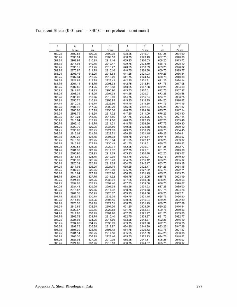
Appendix A. Shear Rheological Data
287
Transient Shear (0.01 sec-1 – 330°C – no preheat - continued)
t η+ t η+ t η+ t η+
sec Pa sec sec Pa sec sec Pa sec sec Pa sec580.25 2892.88 609.25 2899.95 638.25 2910.01 667.25 2934.69580.75 2898.51 609.75 2909.53 638.75 2923.43 667.75 2940.80581.25 2902.94 610.25 2914.44 639.25 2906.53 668.25 2913.72581.75 2914.08 610.75 2919.47 639.75 2933.49 668.75 2928.10582.25 2895.15 611.25 2918.27 640.25 2918.99 669.25 2928.82582.75 2875.87 611.75 2915.16 640.75 2924.38 669.75 2929.77583.25 2905.46 612.25 2918.63 641.25 2921.03 670.25 2936.84583.75 2882.34 612.75 2910.49 641.75 2924.14 670.75 2940.80584.25 2921.63 613.25 2923.43 642.25 2931.81 671.25 2924.14584.75 2901.14 613.75 2908.33 642.75 2913.84 671.75 2917.08585.25 2907.85 614.25 2915.88 643.25 2947.86 672.25 2934.69585.75 2914.68 614.75 2900.90 643.75 2907.61 672.75 2907.97586.25 2905.34 615.25 2904.38 644.25 2920.91 673.25 2928.58586.75 2908.09 615.75 2912.40 644.75 2915.64 673.75 2933.25587.25 2895.75 616.25 2908.93 645.25 2918.75 674.25 2926.42587.75 2910.25 616.75 2926.66 645.75 2915.88 674.75 2944.15588.25 2887.49 617.25 2909.29 646.25 2892.64 675.25 2921.87588.75 2900.90 617.75 2936.36 646.75 2924.98 675.75 2947.14589.25 2898.75 618.25 2917.32 647.25 2911.09 676.25 2923.90589.75 2913.24 618.75 2917.56 647.75 2933.25 676.75 2927.14590.25 2916.84 619.25 2914.80 648.25 2922.23 677.25 2933.49590.75 2905.10 619.75 2911.21 648.75 2903.90 677.75 2929.30591.25 2920.79 620.25 2937.80 649.25 2924.38 678.25 2939.12591.75 2895.63 620.75 2921.03 649.75 2910.73 678.75 2934.45592.25 2915.04 621.25 2922.71 650.25 2931.45 679.25 2956.61592.75 2909.29 621.75 2904.38 650.75 2916.84 679.75 2933.97593.25 2916.36 622.25 2916.84 651.25 2922.47 680.25 2933.37593.75 2915.88 622.75 2930.49 651.75 2918.51 680.75 2928.82594.25 2902.58 623.25 2922.71 652.25 2930.97 681.25 2932.77594.75 2901.38 623.75 2917.32 652.75 2921.51 681.75 2943.19595.25 2880.90 624.25 2911.69 653.25 2905.10 682.25 2923.67595.75 2915.64 624.75 2919.95 653.75 2930.01 682.75 2949.30596.25 2895.39 625.25 2910.73 654.25 2916.12 683.25 2935.17596.75 2920.31 625.75 2911.69 654.75 2942.47 683.75 2949.18597.25 2917.08 626.25 2921.75 655.25 2922.47 684.25 2934.45597.75 2907.49 626.75 2916.60 655.75 2927.62 684.75 2922.71598.25 2913.84 627.25 2923.90 656.25 2931.45 685.25 2933.73598.75 2904.38 627.75 2914.32 656.75 2912.05 685.75 2923.19599.25 2921.03 628.25 2933.01 657.25 2940.56 686.25 2929.53599.75 2894.08 628.75 2892.40 657.75 2939.00 686.75 2920.67600.25 2934.45 629.25 2904.38 658.25 2934.93 687.25 2939.00600.75 2918.87 629.75 2917.32 658.75 2910.73 687.75 2924.26601.25 2901.50 630.25 2920.07 659.25 2924.38 688.25 2922.71601.75 2926.78 630.75 2935.05 659.75 2931.45 688.75 2926.90602.25 2914.80 631.25 2895.15 660.25 2915.04 689.25 2932.89602.75 2923.55 631.75 2921.51 660.75 2931.45 689.75 2957.69603.25 2915.88 632.25 2901.26 661.25 2928.58 690.25 2916.84603.75 2923.67 632.75 2928.58 661.75 2952.54 690.75 2950.26604.25 2917.80 633.25 2901.26 662.25 2921.27 691.25 2939.60604.75 2903.78 633.75 2915.40 662.75 2933.37 691.75 2932.77605.25 2921.03 634.25 2911.69 663.25 2943.67 692.25 2946.19605.75 2894.08 634.75 2898.99 663.75 2923.90 692.75 2930.25606.25 2898.75 635.25 2918.87 664.25 2944.39 693.25 2947.86606.75 2898.39 635.75 2893.12 664.75 2920.43 693.75 2921.27607.25 2901.14 636.25 2917.56 665.25 2957.09 694.25 2960.08607.75 2906.30 636.75 2928.46 665.75 2922.23 694.75 2948.82608.25 2887.01 637.25 2919.95 666.25 2941.51 695.25 2946.07608.75 2924.86 637.75 2910.13 666.75 2944.87 695.75 2958.17
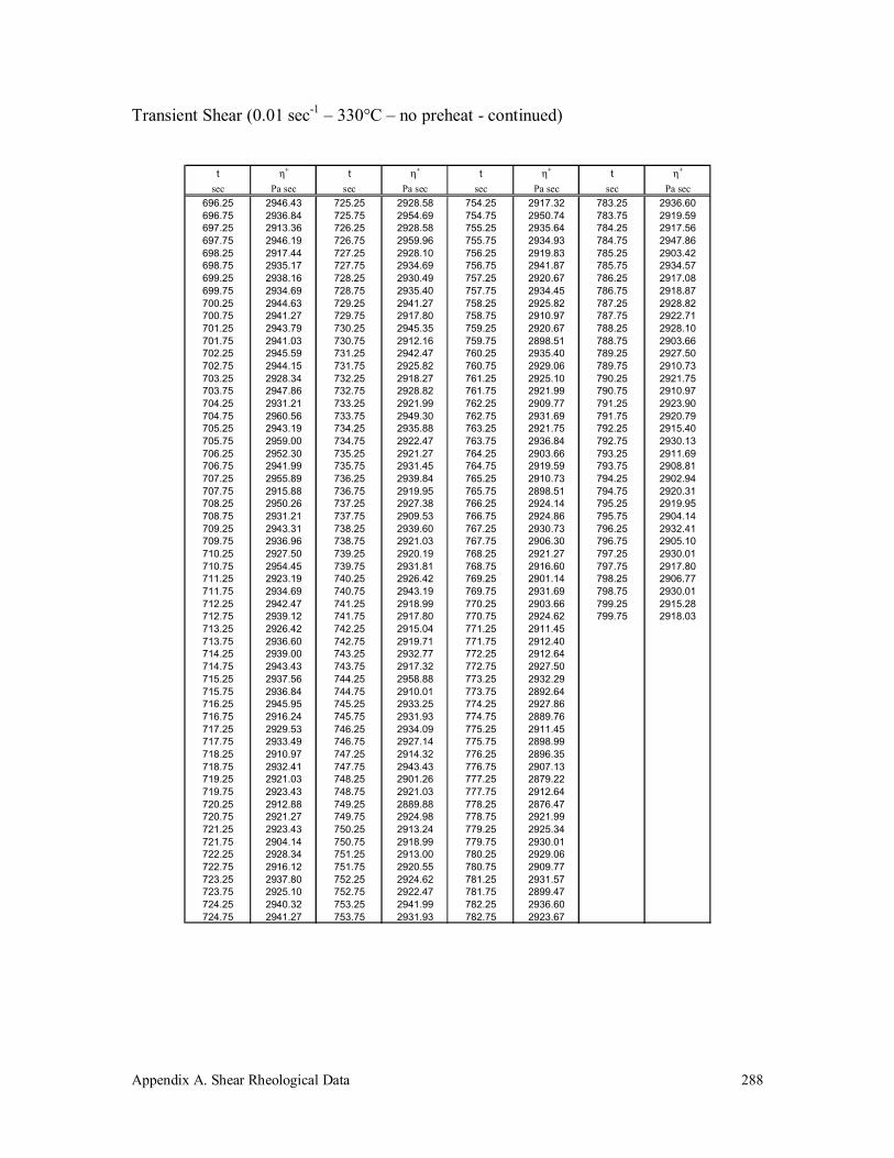
Appendix A. Shear Rheological Data
288
Transient Shear (0.01 sec-1 – 330°C – no preheat - continued)
t η+ t η+ t η+ t η+
sec Pa sec sec Pa sec sec Pa sec sec Pa sec696.25 2946.43 725.25 2928.58 754.25 2917.32 783.25 2936.60696.75 2936.84 725.75 2954.69 754.75 2950.74 783.75 2919.59697.25 2913.36 726.25 2928.58 755.25 2935.64 784.25 2917.56697.75 2946.19 726.75 2959.96 755.75 2934.93 784.75 2947.86698.25 2917.44 727.25 2928.10 756.25 2919.83 785.25 2903.42698.75 2935.17 727.75 2934.69 756.75 2941.87 785.75 2934.57699.25 2938.16 728.25 2930.49 757.25 2920.67 786.25 2917.08699.75 2934.69 728.75 2935.40 757.75 2934.45 786.75 2918.87700.25 2944.63 729.25 2941.27 758.25 2925.82 787.25 2928.82700.75 2941.27 729.75 2917.80 758.75 2910.97 787.75 2922.71701.25 2943.79 730.25 2945.35 759.25 2920.67 788.25 2928.10701.75 2941.03 730.75 2912.16 759.75 2898.51 788.75 2903.66702.25 2945.59 731.25 2942.47 760.25 2935.40 789.25 2927.50702.75 2944.15 731.75 2925.82 760.75 2929.06 789.75 2910.73703.25 2928.34 732.25 2918.27 761.25 2925.10 790.25 2921.75703.75 2947.86 732.75 2928.82 761.75 2921.99 790.75 2910.97704.25 2931.21 733.25 2921.99 762.25 2909.77 791.25 2923.90704.75 2960.56 733.75 2949.30 762.75 2931.69 791.75 2920.79705.25 2943.19 734.25 2935.88 763.25 2921.75 792.25 2915.40705.75 2959.00 734.75 2922.47 763.75 2936.84 792.75 2930.13706.25 2952.30 735.25 2921.27 764.25 2903.66 793.25 2911.69706.75 2941.99 735.75 2931.45 764.75 2919.59 793.75 2908.81707.25 2955.89 736.25 2939.84 765.25 2910.73 794.25 2902.94707.75 2915.88 736.75 2919.95 765.75 2898.51 794.75 2920.31708.25 2950.26 737.25 2927.38 766.25 2924.14 795.25 2919.95708.75 2931.21 737.75 2909.53 766.75 2924.86 795.75 2904.14709.25 2943.31 738.25 2939.60 767.25 2930.73 796.25 2932.41709.75 2936.96 738.75 2921.03 767.75 2906.30 796.75 2905.10710.25 2927.50 739.25 2920.19 768.25 2921.27 797.25 2930.01710.75 2954.45 739.75 2931.81 768.75 2916.60 797.75 2917.80711.25 2923.19 740.25 2926.42 769.25 2901.14 798.25 2906.77711.75 2934.69 740.75 2943.19 769.75 2931.69 798.75 2930.01712.25 2942.47 741.25 2918.99 770.25 2903.66 799.25 2915.28712.75 2939.12 741.75 2917.80 770.75 2924.62 799.75 2918.03713.25 2926.42 742.25 2915.04 771.25 2911.45713.75 2936.60 742.75 2919.71 771.75 2912.40714.25 2939.00 743.25 2932.77 772.25 2912.64714.75 2943.43 743.75 2917.32 772.75 2927.50715.25 2937.56 744.25 2958.88 773.25 2932.29715.75 2936.84 744.75 2910.01 773.75 2892.64716.25 2945.95 745.25 2933.25 774.25 2927.86716.75 2916.24 745.75 2931.93 774.75 2889.76717.25 2929.53 746.25 2934.09 775.25 2911.45717.75 2933.49 746.75 2927.14 775.75 2898.99718.25 2910.97 747.25 2914.32 776.25 2896.35718.75 2932.41 747.75 2943.43 776.75 2907.13719.25 2921.03 748.25 2901.26 777.25 2879.22719.75 2923.43 748.75 2921.03 777.75 2912.64720.25 2912.88 749.25 2889.88 778.25 2876.47720.75 2921.27 749.75 2924.98 778.75 2921.99721.25 2923.43 750.25 2913.24 779.25 2925.34721.75 2904.14 750.75 2918.99 779.75 2930.01722.25 2928.34 751.25 2913.00 780.25 2929.06722.75 2916.12 751.75 2920.55 780.75 2909.77723.25 2937.80 752.25 2924.62 781.25 2931.57723.75 2925.10 752.75 2922.47 781.75 2899.47724.25 2940.32 753.25 2941.99 782.25 2936.60724.75 2941.27 753.75 2931.93 782.75 2923.67

Appendix A. Shear Rheological Data
289
A.6 Vectra B 950
Dynamic Oscillatory (320°C)
ω |η∗| St Devsec-1 Pa sec Pa sec
0.010 263.69 84.900.016 358.67 194.260.025 396.63 191.890.063 322.92 78.360.100 268.99 33.350.158 225.21 4.770.251 186.70 13.990.398 154.15 23.640.631 126.62 27.481.000 103.77 27.251.585 85.40 24.892.512 69.61 19.973.981 59.09 19.306.310 49.29 16.7610.001 42.15 14.3815.850 35.95 12.3425.121 30.86 10.6639.814 26.89 9.1563.101 23.30 7.91
100.000 19.63 6.61

Appendix A. Shear Rheological Data
290
Dynamic Oscillatory (330°C)
ω |η∗| St Devsec-1 Pa sec Pa sec
0.100 103.40 12.700.158 82.81 10.200.251 65.12 8.000.398 49.54 6.100.631 39.37 4.801.000 31.40 3.901.585 25.35 3.102.512 20.51 2.503.981 17.73 2.206.310 15.12 1.9010.001 12.78 1.6015.850 10.49 1.3025.121 8.95 1.1039.814 7.72 0.9063.101 6.59 0.80
100.000 5.67 0.70

Appendix A. Shear Rheological Data
291
Steady Shear (320°C)
g η St Devsec-1 Pa sec Pa sec
0.00163 306.00 87.900.00251 400.00 215.000.00400 364.00 98.000.00787 254.00 72.100.01660 301.00 143.000.02470 406.00 166.00
Steady Shear (330°C)
g η St Devsec-1 Pa sec Pa sec
0.00160 579.00 105.630.00189 530.00 166.910.00534 375.00 178.000.01210 393.00 110.520.03500 236.00 58.000.10000 97.30 12.70

Appendix A. Shear Rheological Data
292
Transient Shear (0.01 sec-1 – 320°C)
t η+ t η+ t η+ t η+
sec Pa sec sec Pa sec sec Pa sec sec Pa sec0.07 77.02 8.78 215.70 17.48 244.76 26.18 251.840.23 111.39 8.93 219.36 17.63 248.78 26.33 254.990.38 122.24 9.08 224.37 17.78 249.56 26.48 255.110.53 129.49 9.23 223.56 17.93 246.01 26.63 255.700.68 135.63 9.38 226.27 18.08 250.74 26.78 258.320.83 139.25 9.53 226.41 18.23 248.53 26.93 257.980.98 143.45 9.68 225.17 18.38 251.39 27.08 259.881.13 151.57 9.83 228.33 18.53 249.02 27.23 254.781.28 146.28 9.98 229.94 18.68 248.34 27.38 256.431.43 157.30 10.13 225.03 18.83 245.43 27.53 256.331.58 154.79 10.28 228.96 18.98 251.15 27.68 256.251.73 160.35 10.43 230.78 19.13 251.66 27.83 253.001.88 159.56 10.58 234.35 19.28 250.18 27.98 261.232.03 164.22 10.73 236.61 19.43 249.11 28.13 260.252.18 165.43 10.88 233.03 19.58 250.90 28.28 262.702.33 172.19 11.03 227.96 19.73 249.19 28.43 261.112.48 173.80 11.18 231.13 19.88 251.64 28.58 256.742.63 172.90 11.33 233.07 20.03 247.70 28.73 258.312.78 179.80 11.48 235.45 20.18 247.87 28.88 258.432.93 182.13 11.63 232.99 20.33 248.62 29.03 259.443.08 180.41 11.78 231.41 20.48 250.56 29.18 266.173.23 183.59 11.93 228.57 20.63 248.60 29.33 258.913.38 182.94 12.08 233.96 20.78 246.53 29.48 256.063.53 184.12 12.23 232.23 20.93 251.50 29.63 259.643.68 187.88 12.38 232.62 21.08 251.85 29.78 256.563.83 190.64 12.53 234.29 21.23 252.64 29.93 253.073.98 191.75 12.68 237.39 21.38 251.43 30.08 262.944.13 190.67 12.83 237.97 21.53 250.52 30.23 260.014.28 192.76 12.98 237.15 21.68 253.42 30.38 256.804.43 197.29 13.13 237.48 21.83 250.45 30.53 261.034.58 197.84 13.28 237.62 21.98 252.15 30.68 259.744.73 200.78 13.43 236.27 22.13 248.16 30.83 261.194.88 200.12 13.58 236.17 22.28 249.42 30.98 265.295.03 199.88 13.73 240.54 22.43 250.25 31.13 261.815.18 199.53 13.88 239.70 22.58 254.97 31.28 258.275.33 202.88 14.03 241.62 22.73 250.47 31.43 264.525.48 203.70 14.18 236.61 22.88 250.21 31.58 259.195.63 205.35 14.33 242.66 23.03 254.92 31.73 264.445.78 205.37 14.48 242.23 23.18 258.02 31.88 261.375.93 211.60 14.63 241.33 23.33 255.31 32.03 264.806.08 206.80 14.78 244.08 23.48 254.13 32.18 260.456.23 208.85 14.93 242.42 23.63 255.21 32.33 261.036.38 206.48 15.08 242.63 23.78 252.04 32.48 260.116.53 209.86 15.23 244.15 23.93 255.92 32.63 262.786.68 207.45 15.38 243.97 24.08 259.62 32.78 258.446.83 213.64 15.53 236.88 24.23 254.56 32.93 261.296.98 209.19 15.68 243.67 24.38 254.23 33.08 263.527.13 207.88 15.83 248.86 24.53 257.29 33.23 260.417.28 213.39 15.98 240.92 24.68 256.11 33.38 263.587.43 215.29 16.13 246.89 24.83 258.50 33.53 259.667.58 217.01 16.28 243.76 24.98 256.23 33.68 258.057.73 218.14 16.43 248.59 25.13 256.27 33.83 261.867.88 218.47 16.58 246.09 25.28 254.09 33.98 264.588.03 219.05 16.73 243.84 25.43 252.68 34.13 257.508.18 220.52 16.88 243.73 25.58 260.42 34.28 263.468.33 224.58 17.03 245.88 25.73 257.11 34.43 265.938.48 219.53 17.18 246.03 25.88 255.84 34.58 260.978.63 220.01 17.33 243.60 26.03 252.68 34.73 260.21
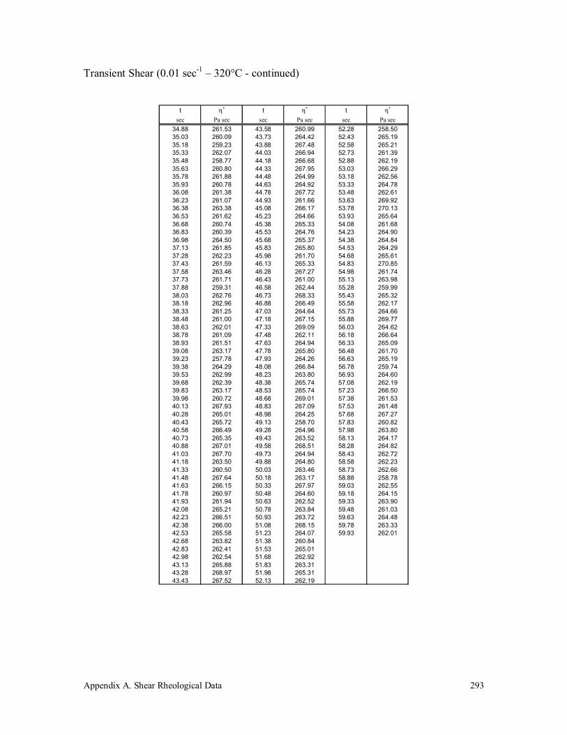
Appendix A. Shear Rheological Data
293
Transient Shear (0.01 sec-1 – 320°C - continued)
t η+ t η+ t η+
sec Pa sec sec Pa sec sec Pa sec34.88 261.53 43.58 260.99 52.28 258.5035.03 260.09 43.73 264.42 52.43 265.1935.18 259.23 43.88 267.48 52.58 265.2135.33 262.07 44.03 266.94 52.73 261.3935.48 258.77 44.18 266.68 52.88 262.1935.63 260.80 44.33 267.95 53.03 266.2935.78 261.88 44.48 264.99 53.18 262.5635.93 260.78 44.63 264.92 53.33 264.7836.08 261.38 44.78 267.72 53.48 262.6136.23 261.07 44.93 261.66 53.63 269.9236.38 263.38 45.08 266.17 53.78 270.1336.53 261.62 45.23 264.66 53.93 265.6436.68 260.74 45.38 265.33 54.08 261.6836.83 260.39 45.53 264.76 54.23 264.9036.98 264.50 45.68 265.37 54.38 264.8437.13 261.85 45.83 265.80 54.53 264.2937.28 262.23 45.98 261.70 54.68 265.6137.43 261.59 46.13 265.33 54.83 270.8537.58 263.46 46.28 267.27 54.98 261.7437.73 261.71 46.43 261.00 55.13 263.9837.88 259.31 46.58 262.44 55.28 259.9938.03 262.76 46.73 268.33 55.43 265.3238.18 262.96 46.88 266.49 55.58 262.1738.33 261.25 47.03 264.64 55.73 264.6638.48 261.00 47.18 267.15 55.88 269.7738.63 262.01 47.33 269.09 56.03 264.6238.78 261.09 47.48 262.11 56.18 266.6438.93 261.51 47.63 264.94 56.33 265.0939.08 263.17 47.78 265.80 56.48 261.7039.23 257.78 47.93 264.26 56.63 265.1939.38 264.29 48.08 266.84 56.78 259.7439.53 262.99 48.23 263.80 56.93 264.6039.68 262.39 48.38 265.74 57.08 262.1939.83 263.17 48.53 265.74 57.23 266.5039.98 260.72 48.68 269.01 57.38 261.5340.13 267.93 48.83 267.09 57.53 261.4840.28 265.01 48.98 264.25 57.68 267.2740.43 265.72 49.13 258.70 57.83 260.8240.58 266.49 49.28 264.96 57.98 263.8040.73 265.35 49.43 263.52 58.13 264.1740.88 267.01 49.58 268.51 58.28 264.8241.03 267.70 49.73 264.94 58.43 262.7241.18 263.50 49.88 264.80 58.58 262.2341.33 260.50 50.03 263.46 58.73 262.6641.48 267.64 50.18 263.17 58.88 258.7841.63 266.15 50.33 267.97 59.03 262.5541.78 260.97 50.48 264.60 59.18 264.1541.93 261.94 50.63 262.52 59.33 263.9042.08 265.21 50.78 263.84 59.48 261.0342.23 266.51 50.93 263.72 59.63 264.4842.38 266.00 51.08 268.15 59.78 263.3342.53 265.58 51.23 264.07 59.93 262.0142.68 263.82 51.38 260.8442.83 262.41 51.53 265.0142.98 262.54 51.68 262.9243.13 265.88 51.83 263.3143.28 268.97 51.98 265.3143.43 267.52 52.13 262.19

Appendix A. Shear Rheological Data
294
Transient Shear (0.01 sec-1 – 330°C)
t η+ t η+ t η+ t η+
sec Pa sec sec Pa sec sec Pa sec sec Pa sec0.07 78.52 8.78 342.53 17.48 378.27 26.18 383.170.23 121.31 8.93 337.84 17.63 374.64 26.33 381.910.38 151.71 9.08 342.62 17.78 379.61 26.48 386.490.53 165.22 9.23 344.26 17.93 380.68 26.63 383.420.68 178.38 9.38 342.62 18.08 380.00 26.78 375.850.83 186.49 9.53 341.28 18.23 377.12 26.93 380.740.98 199.10 9.68 341.44 18.38 381.09 27.08 379.011.13 200.85 9.83 345.53 18.53 377.32 27.23 382.521.28 217.23 9.98 338.16 18.68 374.95 27.38 382.201.43 219.03 10.13 343.33 18.83 374.44 27.53 382.891.58 223.68 10.28 344.55 18.98 381.50 27.68 377.341.73 228.33 10.43 347.35 19.13 377.86 27.83 380.671.88 240.37 10.58 349.97 19.28 378.43 27.98 390.412.03 238.85 10.73 348.96 19.43 375.59 28.13 381.852.18 241.98 10.88 346.20 19.58 371.79 28.28 386.622.33 250.56 11.03 348.98 19.73 377.58 28.43 387.062.48 255.33 11.18 348.44 19.88 380.64 28.58 387.442.63 255.45 11.33 350.71 20.03 381.54 28.73 391.572.78 264.02 11.48 347.00 20.18 380.29 28.88 397.082.93 271.52 11.63 346.88 20.33 380.42 29.03 390.483.08 266.73 11.78 348.95 20.48 376.05 29.18 384.123.23 271.58 11.93 350.92 20.63 373.93 29.33 385.593.38 276.79 12.08 360.93 20.78 378.24 29.48 389.423.53 287.21 12.23 352.34 20.93 380.23 29.63 388.553.68 283.08 12.38 359.97 21.08 377.13 29.78 387.443.83 280.69 12.53 362.95 21.23 381.06 29.93 393.383.98 284.01 12.68 357.42 21.38 382.94 30.08 390.254.13 290.75 12.83 356.37 21.53 379.51 30.23 384.224.28 293.24 12.98 354.74 21.68 384.24 30.38 392.304.43 290.30 13.13 361.06 21.83 377.77 30.53 393.804.58 295.82 13.28 365.66 21.98 381.81 30.68 389.524.73 293.85 13.43 366.56 22.13 382.34 30.83 394.844.88 300.65 13.58 360.38 22.28 375.94 30.98 390.735.03 299.98 13.73 365.53 22.43 379.20 31.13 387.445.18 306.72 13.88 364.19 22.58 373.01 31.28 385.685.33 307.71 14.03 363.36 22.73 374.93 31.43 389.525.48 308.23 14.18 360.55 22.88 375.94 31.58 395.435.63 310.87 14.33 357.95 23.03 374.70 31.73 393.575.78 316.94 14.48 360.65 23.18 375.09 31.88 391.725.93 309.35 14.63 359.33 23.33 385.24 32.03 386.386.08 315.12 14.78 364.16 23.48 380.51 32.18 394.186.23 312.95 14.93 361.63 23.63 385.24 32.33 388.816.38 318.86 15.08 359.28 23.78 381.97 32.48 392.496.53 318.09 15.23 365.90 23.93 377.45 32.63 382.216.68 317.78 15.38 364.22 24.08 379.02 32.78 386.896.83 322.76 15.53 367.37 24.23 377.41 32.93 386.396.98 327.93 15.68 370.77 24.38 381.18 33.08 387.467.13 327.96 15.83 375.08 24.53 382.91 33.23 390.077.28 332.15 15.98 372.59 24.68 379.49 33.38 386.127.43 329.20 16.13 369.97 24.83 379.08 33.53 388.247.58 334.16 16.28 373.19 24.98 384.06 33.68 389.047.73 327.01 16.43 374.19 25.13 379.39 33.83 392.817.88 333.20 16.58 367.29 25.28 374.66 33.98 389.558.03 332.25 16.73 364.57 25.43 382.98 34.13 393.238.18 341.06 16.88 366.84 25.58 381.38 34.28 384.988.33 334.12 17.03 371.41 25.73 385.21 34.43 382.948.48 339.98 17.18 374.70 25.88 380.29 34.58 388.668.63 337.67 17.33 375.20 26.03 384.72 34.73 389.14
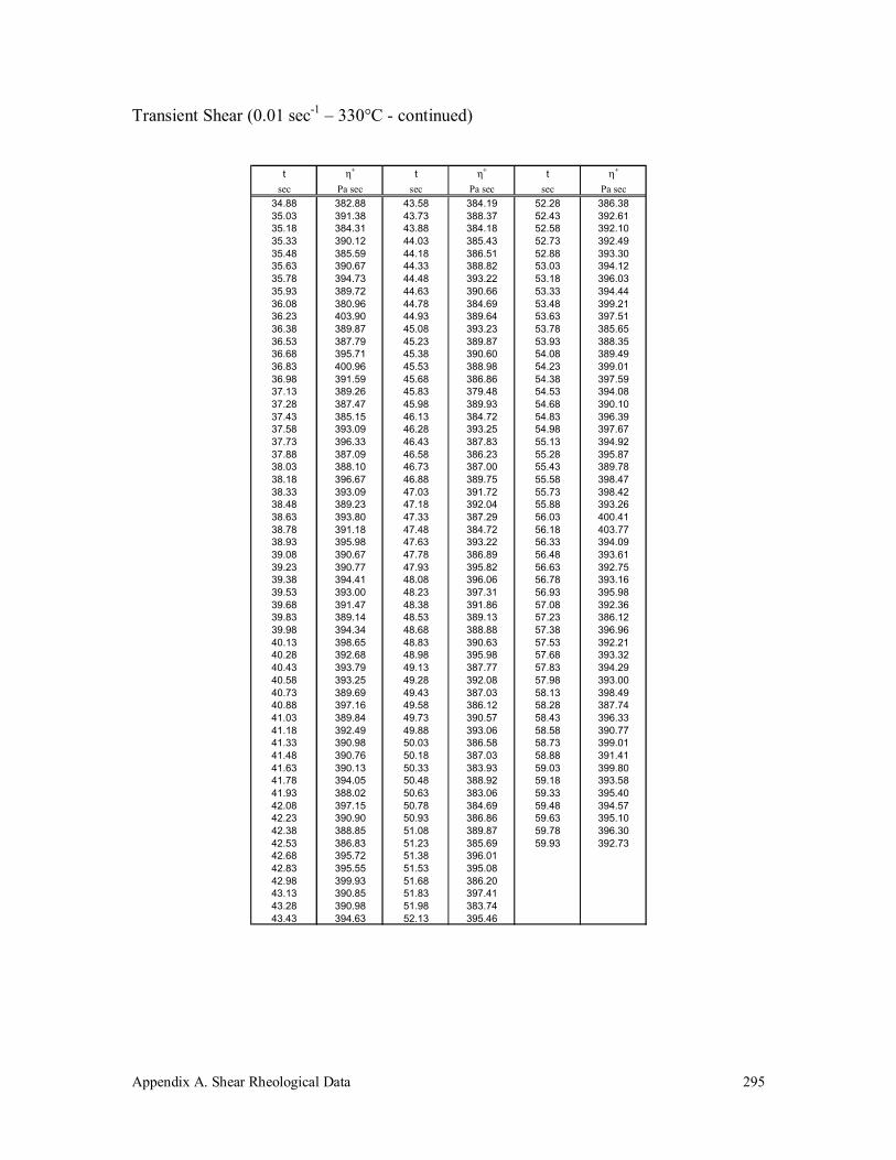
Appendix A. Shear Rheological Data
295
Transient Shear (0.01 sec-1 – 330°C - continued)
t η+ t η+ t η+
sec Pa sec sec Pa sec sec Pa sec34.88 382.88 43.58 384.19 52.28 386.3835.03 391.38 43.73 388.37 52.43 392.6135.18 384.31 43.88 384.18 52.58 392.1035.33 390.12 44.03 385.43 52.73 392.4935.48 385.59 44.18 386.51 52.88 393.3035.63 390.67 44.33 388.82 53.03 394.1235.78 394.73 44.48 393.22 53.18 396.0335.93 389.72 44.63 390.66 53.33 394.4436.08 380.96 44.78 384.69 53.48 399.2136.23 403.90 44.93 389.64 53.63 397.5136.38 389.87 45.08 393.23 53.78 385.6536.53 387.79 45.23 389.87 53.93 388.3536.68 395.71 45.38 390.60 54.08 389.4936.83 400.96 45.53 388.98 54.23 399.0136.98 391.59 45.68 386.86 54.38 397.5937.13 389.26 45.83 379.48 54.53 394.0837.28 387.47 45.98 389.93 54.68 390.1037.43 385.15 46.13 384.72 54.83 396.3937.58 393.09 46.28 393.25 54.98 397.6737.73 396.33 46.43 387.83 55.13 394.9237.88 387.09 46.58 386.23 55.28 395.8738.03 388.10 46.73 387.00 55.43 389.7838.18 396.67 46.88 389.75 55.58 398.4738.33 393.09 47.03 391.72 55.73 398.4238.48 389.23 47.18 392.04 55.88 393.2638.63 393.80 47.33 387.29 56.03 400.4138.78 391.18 47.48 384.72 56.18 403.7738.93 395.98 47.63 393.22 56.33 394.0939.08 390.67 47.78 386.89 56.48 393.6139.23 390.77 47.93 395.82 56.63 392.7539.38 394.41 48.08 396.06 56.78 393.1639.53 393.00 48.23 397.31 56.93 395.9839.68 391.47 48.38 391.86 57.08 392.3639.83 389.14 48.53 389.13 57.23 386.1239.98 394.34 48.68 388.88 57.38 396.9640.13 398.65 48.83 390.63 57.53 392.2140.28 392.68 48.98 395.98 57.68 393.3240.43 393.79 49.13 387.77 57.83 394.2940.58 393.25 49.28 392.08 57.98 393.0040.73 389.69 49.43 387.03 58.13 398.4940.88 397.16 49.58 386.12 58.28 387.7441.03 389.84 49.73 390.57 58.43 396.3341.18 392.49 49.88 393.06 58.58 390.7741.33 390.98 50.03 386.58 58.73 399.0141.48 390.76 50.18 387.03 58.88 391.4141.63 390.13 50.33 383.93 59.03 399.8041.78 394.05 50.48 388.92 59.18 393.5841.93 388.02 50.63 383.06 59.33 395.4042.08 397.15 50.78 384.69 59.48 394.5742.23 390.90 50.93 386.86 59.63 395.1042.38 388.85 51.08 389.87 59.78 396.3042.53 386.83 51.23 385.69 59.93 392.7342.68 395.72 51.38 396.0142.83 395.55 51.53 395.0842.98 399.93 51.68 386.2043.13 390.85 51.83 397.4143.28 390.98 51.98 383.7443.43 394.63 52.13 395.46
Appendix B.Surface Ternsion
296
Appendix B. Surface Tension
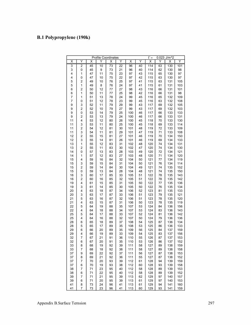
Appendix B.Surface Ternsion
297
B.1 Polypropylene (190k)
Γ = 0.023
X Y X Y X Y X Y X Y X Y3 2 45 10 73 22 96 40 114 63 130 1013 0 45 9 73 21 96 40 114 62 130 984 1 47 11 75 23 97 43 115 65 130 974 0 47 10 75 22 97 42 115 63 130 975 2 49 10 76 25 97 41 115 63 131 1055 1 49 8 76 24 97 41 115 61 131 1036 2 50 12 77 27 98 43 116 66 131 1016 1 50 11 77 25 98 42 116 66 131 987 1 51 13 78 24 99 45 116 65 132 1097 0 51 12 78 23 99 45 116 63 132 1089 3 52 11 79 29 99 43 117 69 132 1059 2 52 10 79 27 99 43 117 69 132 1039 0 53 14 79 25 100 46 117 66 133 1339 2 53 13 79 24 100 46 117 66 133 131
11 4 53 12 80 26 100 45 118 70 133 13011 3 53 11 80 25 100 45 118 69 133 11411 2 54 12 81 30 101 48 119 72 133 10911 3 54 11 81 29 101 47 119 71 133 10812 2 55 15 81 27 101 46 119 70 134 15012 3 55 14 81 26 101 46 119 69 134 13313 1 55 12 83 31 102 48 120 74 134 13113 2 55 11 83 30 102 47 120 74 134 13014 0 57 13 83 28 103 49 120 72 134 12114 1 57 12 83 27 103 48 120 71 134 12015 4 59 16 84 32 104 50 121 77 134 11915 3 59 15 84 31 104 50 121 76 134 11415 2 59 14 84 30 104 49 121 74 135 15215 0 59 13 84 28 104 48 121 74 135 15016 3 60 17 85 33 105 51 122 78 135 14316 2 60 16 85 32 105 51 122 78 135 14219 4 61 15 85 31 105 50 122 77 135 13619 3 61 14 85 30 105 50 122 76 135 13420 4 63 18 87 34 106 52 123 81 135 13320 3 63 17 87 33 106 51 123 79 135 12121 5 63 16 87 32 106 51 123 78 135 12021 4 63 15 87 31 106 50 123 78 135 11922 5 64 19 88 35 107 53 124 84 136 15622 4 64 18 88 34 107 53 124 83 136 14325 5 64 17 88 33 107 52 124 81 136 14225 4 64 16 88 32 107 50 124 79 136 13628 6 65 18 89 37 108 54 125 87 136 13428 5 65 17 89 35 108 53 125 86 136 13329 6 66 20 89 35 109 56 125 84 137 15929 4 66 19 89 33 109 54 125 83 137 15632 7 67 21 91 36 110 55 126 87 137 15332 6 67 20 91 35 110 53 126 86 137 15233 8 68 19 92 39 111 58 127 89 138 15933 7 68 18 92 38 111 58 127 89 138 15837 9 69 22 92 37 111 56 127 87 138 15337 8 69 21 92 36 111 55 127 87 138 15237 7 70 20 93 39 112 61 128 94 139 15937 6 70 19 93 38 112 60 128 93 139 15838 7 71 23 95 40 112 58 128 89 139 15338 6 71 22 95 40 112 58 128 89 139 15239 7 71 21 95 39 113 62 129 97 140 15739 6 71 20 95 39 113 61 129 97 140 15341 8 73 24 96 41 113 61 129 94 141 16041 7 73 23 96 41 113 60 129 93 141 159
J/m^2Profile Coordinates
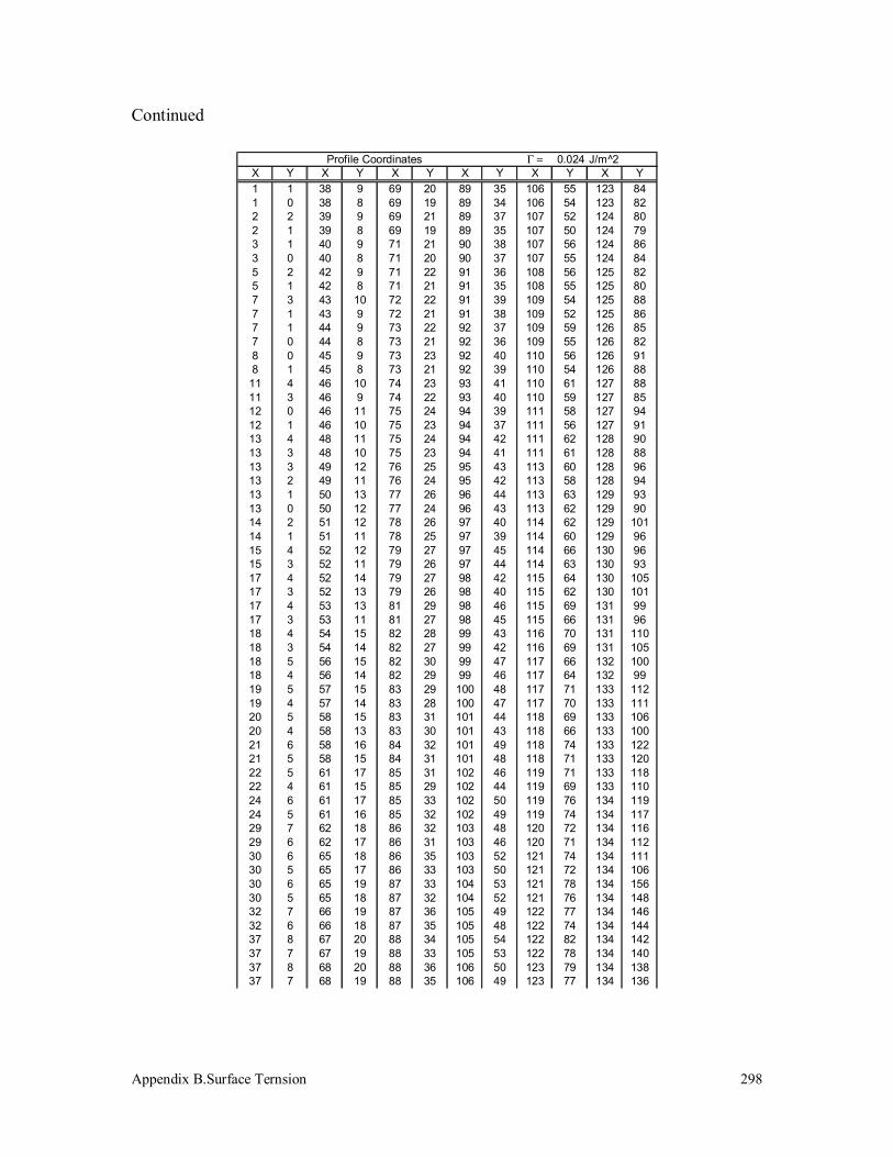
Appendix B.Surface Ternsion
298
Continued
Γ = 0.024X Y X Y X Y X Y X Y X Y1 1 38 9 69 20 89 35 106 55 123 841 0 38 8 69 19 89 34 106 54 123 822 2 39 9 69 21 89 37 107 52 124 802 1 39 8 69 19 89 35 107 50 124 793 1 40 9 71 21 90 38 107 56 124 863 0 40 8 71 20 90 37 107 55 124 845 2 42 9 71 22 91 36 108 56 125 825 1 42 8 71 21 91 35 108 55 125 807 3 43 10 72 22 91 39 109 54 125 887 1 43 9 72 21 91 38 109 52 125 867 1 44 9 73 22 92 37 109 59 126 857 0 44 8 73 21 92 36 109 55 126 828 0 45 9 73 23 92 40 110 56 126 918 1 45 8 73 21 92 39 110 54 126 88
11 4 46 10 74 23 93 41 110 61 127 8811 3 46 9 74 22 93 40 110 59 127 8512 0 46 11 75 24 94 39 111 58 127 9412 1 46 10 75 23 94 37 111 56 127 9113 4 48 11 75 24 94 42 111 62 128 9013 3 48 10 75 23 94 41 111 61 128 8813 3 49 12 76 25 95 43 113 60 128 9613 2 49 11 76 24 95 42 113 58 128 9413 1 50 13 77 26 96 44 113 63 129 9313 0 50 12 77 24 96 43 113 62 129 9014 2 51 12 78 26 97 40 114 62 129 10114 1 51 11 78 25 97 39 114 60 129 9615 4 52 12 79 27 97 45 114 66 130 9615 3 52 11 79 26 97 44 114 63 130 9317 4 52 14 79 27 98 42 115 64 130 10517 3 52 13 79 26 98 40 115 62 130 10117 4 53 13 81 29 98 46 115 69 131 9917 3 53 11 81 27 98 45 115 66 131 9618 4 54 15 82 28 99 43 116 70 131 11018 3 54 14 82 27 99 42 116 69 131 10518 5 56 15 82 30 99 47 117 66 132 10018 4 56 14 82 29 99 46 117 64 132 9919 5 57 15 83 29 100 48 117 71 133 11219 4 57 14 83 28 100 47 117 70 133 11120 5 58 15 83 31 101 44 118 69 133 10620 4 58 13 83 30 101 43 118 66 133 10021 6 58 16 84 32 101 49 118 74 133 12221 5 58 15 84 31 101 48 118 71 133 12022 5 61 17 85 31 102 46 119 71 133 11822 4 61 15 85 29 102 44 119 69 133 11024 6 61 17 85 33 102 50 119 76 134 11924 5 61 16 85 32 102 49 119 74 134 11729 7 62 18 86 32 103 48 120 72 134 11629 6 62 17 86 31 103 46 120 71 134 11230 6 65 18 86 35 103 52 121 74 134 11130 5 65 17 86 33 103 50 121 72 134 10630 6 65 19 87 33 104 53 121 78 134 15630 5 65 18 87 32 104 52 121 76 134 14832 7 66 19 87 36 105 49 122 77 134 14632 6 66 18 87 35 105 48 122 74 134 14437 8 67 20 88 34 105 54 122 82 134 14237 7 67 19 88 33 105 53 122 78 134 14037 8 68 20 88 36 106 50 123 79 134 13837 7 68 19 88 35 106 49 123 77 134 136
J/m^2Profile Coordinates

Appendix B.Surface Ternsion
299
B.2 Polypropylene (250k)
Γ = 0.012X Y X Y X Y X Y X Y X Y
137.5 138 126.5 100 115.5 82 100.5 43 78.5 25 57.5 10137.5 137 126.5 97 115.5 79 98.5 43 78.5 23 56.5 10136.5 131 126.5 96 115.5 75 98.5 42 77.5 23 56.5 9136.5 130 125.5 100 115.5 73 97.5 42 77.5 22 55.5 10134.5 130 125.5 97 114.5 75 97.5 41 76.5 22 55.5 9134.5 124 125.5 96 114.5 74 96.5 41 76.5 21 54.5 10133.5 137 125.5 94 113.5 74 96.5 39 74.5 21 54.5 9133.5 135 124.5 94 113.5 69 94.5 39 74.5 20 51.5 10133.5 124 124.5 92 112.5 69 94.5 37 73.5 20 51.5 9133.5 119 124.5 91 112.5 63 93.5 37 73.5 19 50.5 10132.5 119 124.5 90 110.5 63 93.5 36 72.5 19 50.5 9132.5 117 123.5 92 110.5 61 92.5 36 72.5 18 50.5 8132.5 116 123.5 91 109.5 61 92.5 35 69.5 18 50.5 7132.5 114 123.5 91 109.5 58 91.5 35 69.5 17 49.5 9131.5 117 123.5 90 108.5 58 91.5 34 66.5 17 49.5 8131.5 116 122.5 91 108.5 56 90.5 34 66.5 15 48.5 7131.5 114 122.5 87 107.5 56 90.5 32 65.5 15 48.5 6131.5 113 121.5 87 107.5 55 89.5 32 65.5 14 47.5 7130.5 113 121.5 82 106.5 55 89.5 30 64.5 14 47.5 6130.5 110 120.5 82 106.5 53 88.5 30 64.5 13 45.5 7129.5 135 120.5 81 105.5 53 88.5 29 63.5 14 45.5 6129.5 133 118.5 84 105.5 50 86.5 29 63.5 13 44.5 6129.5 110 118.5 81 104.5 50 86.5 28 62.5 14 44.5 5129.5 103 117.5 84 104.5 49 85.5 28 62.5 13 43.5 6128.5 133 117.5 83 102.5 49 85.5 27 61.5 13 43.5 5128.5 131 116.5 83 102.5 46 81.5 27 61.5 12 42.5 6128.5 103 116.5 82 101.5 46 81.5 26 60.5 12 42.5 5128.5 102 116.5 79 101.5 45 80.5 26 60.5 11 37.5 5126.5 102 116.5 73 100.5 45 80.5 25 57.5 11 37.5 3
J/m^2Profile Coordinates

Appendix B.Surface Ternsion
300
Continued
Γ = 0.016
X Y X Y X Y X Y X Y X Y2 1 60 14 85 27 106 40 122 60 139 932 0 60 13 85 26 106 38 122 59 139 885 2 60 12 86 29 107 41 123 62 139 875 1 60 11 86 27 107 40 123 61 139 85
15 1 61 14 86 26 108 37 123 61 140 9315 0 61 13 86 24 108 36 123 60 140 9016 2 62 12 87 30 109 42 124 63 140 8916 1 62 11 87 29 109 41 124 62 140 8721 2 63 15 87 27 109 37 125 65 141 9321 0 63 14 87 26 109 36 125 63 141 9022 4 64 13 88 30 110 45 126 67 141 9222 3 64 12 88 29 110 42 126 65 141 8923 3 65 16 89 30 110 38 126 63 142 9723 2 65 15 89 29 110 37 126 61 142 9326 2 65 14 89 28 111 48 127 69 142 9626 1 65 13 89 27 111 45 127 67 142 9227 5 66 17 90 31 111 39 127 64 143 9927 4 66 16 90 30 111 38 127 63 143 9727 1 67 18 90 30 112 49 128 70 143 9927 0 67 17 90 28 112 48 128 69 143 9630 3 67 15 91 31 112 40 128 66 144 9930 2 67 14 91 30 112 39 128 64 144 9832 3 68 18 92 32 113 50 129 71 145 10132 2 68 17 92 31 113 49 129 70 145 9833 6 68 15 92 31 113 46 129 67 145 10433 5 68 14 92 28 113 44 129 66 145 9933 3 69 18 93 33 113 43 130 73 146 11233 2 69 17 93 32 113 40 130 71 146 10139 8 69 16 93 29 114 52 130 70 146 10939 6 69 14 93 28 114 50 130 67 146 10839 4 71 19 94 30 114 48 131 77 146 10739 3 71 18 94 29 114 46 131 73 146 10443 5 71 18 96 34 114 44 131 71 147 11743 4 71 16 96 33 114 43 131 70 147 11244 8 73 20 96 32 115 53 132 77 147 11144 7 73 19 96 30 115 52 132 75 147 10944 5 74 22 98 35 115 51 132 73 147 10844 4 74 20 98 34 115 48 132 71 147 10745 8 75 19 98 34 117 54 133 77 148 11345 7 75 18 98 32 117 53 133 75 148 11145 6 76 19 100 35 117 53 133 75 149 12145 4 76 18 100 34 117 51 133 73 149 11750 7 77 20 100 34 118 56 134 80 149 11750 6 77 18 100 33 118 54 134 77 149 11351 8 78 23 101 35 118 55 134 77 150 12551 7 78 22 101 34 118 53 134 75 150 12152 10 79 24 101 34 119 57 135 81 150 12252 8 79 23 101 33 119 56 135 80 150 11755 13 79 22 102 37 119 56 135 79 151 12655 10 79 20 102 35 119 55 135 77 151 12555 10 80 22 102 35 120 58 137 84 151 12655 8 80 21 102 34 120 57 137 81 151 12258 14 82 26 103 36 120 58 137 82 152 12758 13 82 24 103 35 120 56 137 79 152 12658 11 82 23 105 38 121 61 138 88 153 12858 10 82 21 105 37 121 58 138 84 153 12659 12 84 24 105 37 121 59 138 85 153 13159 11 84 23 105 36 121 58 138 82 153 127
J/m^2Profile Coordinates

Appendix B.Surface Ternsion
301
Continued
Γ = 0.015
X Y X Y X Y X Y X Y X Y1.5 1 41.5 7 69.5 17 99.5 33 117.5 55 134.5 731.5 0 41.5 6 69.5 16 99.5 32 117.5 53 135.5 792.5 1 42.5 7 71.5 17 99.5 33 117.5 52 135.5 782.5 0 42.5 6 71.5 16 99.5 32 117.5 51 135.5 783.5 1 43.5 6 72.5 18 100.5 34 118.5 53 135.5 763.5 0 43.5 4 72.5 17 100.5 33 118.5 52 136.5 846.5 1 44.5 7 73.5 19 100.5 34 119.5 57 136.5 796.5 0 44.5 6 73.5 18 100.5 33 119.5 56 136.5 817.5 1 45.5 8 75.5 20 101.5 35 119.5 57 136.5 787.5 0 45.5 7 75.5 19 101.5 34 119.5 53 137.5 8710.5 1 46.5 8 75.5 18 102.5 35 120.5 58 137.5 8410.5 0 46.5 6 75.5 17 102.5 34 120.5 57 137.5 8216.5 1 47.5 8 76.5 21 102.5 36 120.5 56 137.5 8116.5 0 47.5 7 76.5 20 102.5 34 120.5 55 138.5 9017.5 0 48.5 7 77.5 22 103.5 35 120.5 58 138.5 8817.5 1 48.5 6 77.5 21 103.5 34 120.5 57 138.5 8419.5 0 49.5 7 79.5 23 103.5 37 121.5 59 138.5 8219.5 1 49.5 6 79.5 22 103.5 36 121.5 58 139.5 9121.5 2 50.5 7 79.5 20 104.5 36 121.5 58 139.5 9021.5 1 50.5 6 79.5 18 104.5 35 121.5 57 139.5 8822.5 1 50.5 9 80.5 24 104.5 38 122.5 58 139.5 8722.5 0 50.5 8 80.5 23 104.5 37 122.5 57 139.5 8624.5 4 51.5 7 82.5 22 105.5 38 123.5 61 139.5 8424.5 2 51.5 6 82.5 20 105.5 36 123.5 59 140.5 9525.5 4 52.5 8 83.5 26 107.5 40 123.5 59 140.5 9125.5 3 52.5 7 83.5 24 107.5 38 123.5 58 140.5 8925.5 1 53.5 9 84.5 27 108.5 41 124.5 63 140.5 8625.5 0 53.5 8 84.5 26 108.5 40 124.5 61 141.5 9726.5 3 54.5 10 84.5 23 109.5 43 124.5 61 141.5 9526.5 2 54.5 9 84.5 22 109.5 41 124.5 59 141.5 9027.5 3 54.5 10 86.5 25 109.5 38 125.5 65 141.5 8927.5 2 54.5 9 86.5 23 109.5 36 125.5 63 142.5 9327.5 1 55.5 11 87.5 28 110.5 44 126.5 62 142.5 9027.5 0 55.5 10 87.5 27 110.5 43 126.5 61 143.5 9828.5 4 56.5 12 89.5 30 110.5 37 127.5 66 143.5 9728.5 3 56.5 10 89.5 28 110.5 36 127.5 65 143.5 9729.5 4 57.5 11 90.5 26 111.5 46 127.5 65 143.5 9329.5 3 57.5 10 90.5 25 111.5 44 127.5 62 144.5 10029.5 1 58.5 12 91.5 31 111.5 41 128.5 68 144.5 9829.5 0 58.5 10 91.5 30 111.5 37 128.5 66 144.5 10130.5 4 60.5 14 92.5 28 112.5 47 128.5 66 144.5 9730.5 3 60.5 12 92.5 26 112.5 46 128.5 65 145.5 11030.5 1 61.5 14 93.5 32 112.5 42 129.5 71 145.5 10430.5 0 61.5 12 93.5 31 112.5 41 129.5 68 145.5 10131.5 2 61.5 14 94.5 29 113.5 49 130.5 68 145.5 10031.5 1 61.5 12 94.5 28 113.5 47 130.5 66 146.5 10236.5 4 62.5 14 95.5 30 113.5 44 131.5 74 146.5 10136.5 3 62.5 12 95.5 29 113.5 42 131.5 71 146.5 10637.5 6 62.5 14 96.5 32 114.5 45 131.5 68 146.5 10137.5 4 62.5 12 96.5 30 114.5 44 132.5 76 147.5 11538.5 6 63.5 14 97.5 33 115.5 51 132.5 74 147.5 11038.5 4 63.5 12 97.5 32 115.5 49 132.5 73 147.5 10438.5 3 65.5 15 97.5 32 115.5 49 132.5 70 147.5 10238.5 2 65.5 14 97.5 30 115.5 45 133.5 79 147.5 11039.5 6 66.5 16 98.5 33 116.5 53 133.5 76 147.5 10639.5 5 66.5 14 98.5 32 116.5 51 134.5 79 148.5 12040.5 5 67.5 16 98.5 32 116.5 51 134.5 78 148.5 11540.5 4 67.5 15 98.5 30 116.5 49 134.5 76 148.5 115
J/m^2Profile Coordinates

Appendix B.Surface Ternsion
302
Continued
Γ = 0.016
X Y X Y X Y X Y X Y X Y0 0 55 10 80 23 104 40 123 62 141 910 2 58 10 80 24 104 41 123 63 142 91
27 0 58 11 82 23 105 40 125 63 142 9427 2 61 11 82 24 105 41 125 65 143 9428 1 61 12 83 24 106 41 126 65 143 9628 2 62 12 83 25 106 43 126 67 145 9628 5 62 13 85 25 107 43 127 67 145 9828 6 63 13 85 26 107 45 127 69 146 9829 1 63 14 86 26 110 45 129 69 146 10129 2 65 15 86 27 110 46 129 71 147 10131 2 65 16 88 27 111 41 130 71 147 10531 4 66 14 88 28 111 46 130 73 149 10534 4 66 15 89 28 111 48 131 73 149 10934 5 70 16 89 29 113 48 131 75 150 10944 4 70 18 91 29 113 50 133 75 150 11344 5 73 18 91 30 114 50 133 77 151 11345 4 73 20 92 29 114 52 134 77 151 11745 5 74 20 92 30 115 52 134 79 152 11745 5 74 21 97 29 115 53 135 79 152 11845 6 75 21 97 34 117 53 135 81 153 11846 5 75 22 98 34 117 54 137 81 153 12246 6 76 21 98 36 118 54 137 84 154 12251 6 76 22 99 36 118 56 138 84 154 12651 7 77 21 99 37 119 56 138 85 155 12652 7 77 22 101 37 119 58 139 85 155 13052 8 78 22 101 38 121 58 139 87 157 13054 8 78 23 102 38 121 61 140 87 157 13454 9 79 23 102 39 122 61 140 89 157 13555 9 79 24 103 39 122 62 141 89 157 136
J/m^2Profile Coordinates

Appendix B.Surface Ternsion
303
Continued
Γ = 0.015
X Y X Y X Y X Y X Y X Y4 1 57 10 89 28 114 50 136 91 145 1234 0 57 9 89 27 114 49 136 90 145 1226 1 58 11 90 29 115 52 137 95 145 1216 0 58 10 90 28 115 50 137 93 145 1209 1 61 12 91 30 117 53 137 92 146 1329 0 61 11 91 29 117 52 137 91 146 130
11 1 63 13 93 31 118 54 138 111 146 12811 0 63 12 93 30 118 53 138 110 146 12720 1 66 15 94 32 119 56 138 108 146 12620 0 66 13 94 31 119 54 138 102 146 12321 1 70 16 95 33 120 57 138 100 146 12221 0 70 15 95 32 120 56 138 95 146 12124 1 71 18 97 34 121 60 138 93 147 13424 0 71 16 97 33 121 57 138 92 147 13225 1 72 18 98 35 122 63 139 113 147 13025 0 72 17 98 34 122 60 139 111 147 12828 3 73 18 99 36 123 67 139 110 148 13428 2 73 17 99 35 123 63 139 108 148 13130 2 74 19 101 38 124 67 139 102 149 13530 1 74 18 101 36 124 66 139 100 149 13335 4 75 20 102 39 125 68 140 113 149 13235 3 75 19 102 38 125 66 140 111 149 13136 4 76 20 103 40 126 69 141 115 150 13836 3 76 19 103 39 126 68 141 114 150 13537 4 77 20 105 41 127 71 141 112 150 13337 3 77 19 105 40 127 69 141 111 150 13240 4 78 21 106 42 128 73 142 120 151 14340 3 78 20 106 41 128 71 142 119 151 14241 5 81 23 107 43 129 75 142 117 151 14141 3 81 21 107 42 129 73 142 115 151 14046 7 82 24 108 44 130 79 142 114 151 13946 6 82 23 108 43 130 75 142 112 151 13850 6 84 24 109 45 131 81 143 121 152 14450 5 84 23 109 44 131 79 143 120 152 14351 9 85 25 110 46 133 84 143 119 152 14251 7 85 23 110 45 133 81 143 117 152 14152 9 86 26 111 47 134 88 144 121 152 14052 8 86 25 111 46 134 84 144 120 152 13955 9 87 27 113 49 135 90 145 127 153 14555 8 87 26 113 47 135 88 145 126 153 144
J/m^2Profile Coordinates
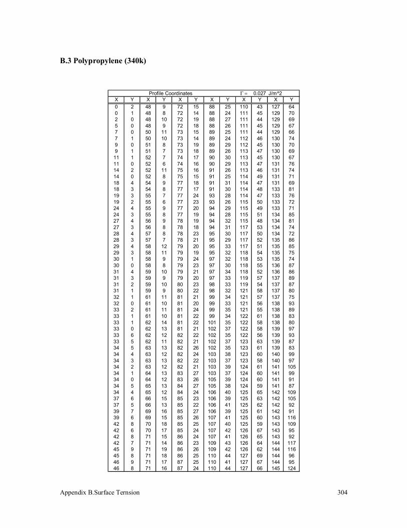
Appendix B.Surface Ternsion
304
B.3 Polypropylene (340k)
Γ = 0.027
X Y X Y X Y X Y X Y X Y0 2 48 9 72 15 88 25 110 43 127 640 1 48 8 72 14 88 24 111 45 129 702 0 48 10 72 19 88 27 111 44 129 695 0 48 9 72 18 88 26 111 45 129 677 0 50 11 73 15 89 25 111 44 129 667 1 50 10 73 14 89 24 112 46 130 749 0 51 8 73 19 89 29 112 45 130 709 1 51 7 73 18 89 26 113 47 130 69
11 1 52 7 74 17 90 30 113 45 130 6711 0 52 6 74 16 90 29 113 47 131 7614 2 52 11 75 16 91 26 113 46 131 7414 0 52 8 75 15 91 25 114 49 131 7118 4 54 9 77 18 91 31 114 47 131 6918 3 54 8 77 17 91 30 114 48 133 8119 3 55 7 77 24 93 28 114 47 133 7619 2 55 6 77 23 93 26 115 50 133 7224 4 55 9 77 20 94 29 115 49 133 7124 3 55 8 77 19 94 28 115 51 134 8527 4 56 9 78 19 94 32 115 48 134 8127 3 56 8 78 18 94 31 117 53 134 7428 4 57 8 78 23 95 30 117 50 134 7228 3 57 7 78 21 95 29 117 52 135 8629 4 58 12 79 20 95 33 117 51 135 8529 3 58 11 79 19 95 32 118 54 135 7530 1 58 9 79 24 97 32 118 53 135 7430 0 58 8 79 23 97 30 118 55 136 8731 4 59 10 79 21 97 34 118 52 136 8631 3 59 9 79 20 97 33 119 57 137 8931 2 59 10 80 23 98 33 119 54 137 8731 1 59 9 80 22 98 32 121 58 137 8032 1 61 11 81 21 99 34 121 57 137 7532 0 61 10 81 20 99 33 121 56 138 9333 2 61 11 81 24 99 35 121 55 138 8933 1 61 10 81 22 99 34 122 61 138 8333 1 62 14 81 22 101 35 122 58 138 8033 0 62 13 81 21 102 37 122 58 139 9733 6 62 12 82 22 102 35 122 56 139 9333 5 62 11 82 21 102 37 123 63 139 8734 5 63 13 82 26 102 35 123 61 139 8334 4 63 12 82 24 103 38 123 60 140 9934 3 63 13 82 22 103 37 123 58 140 9734 2 63 12 82 21 103 39 124 61 141 10534 1 64 13 83 27 103 37 124 60 141 9934 0 64 12 83 26 105 39 124 60 141 9134 5 65 13 84 27 105 38 124 59 141 8734 4 65 12 84 24 106 40 125 65 142 10937 6 66 15 85 23 106 39 125 63 142 10537 5 66 13 85 22 106 41 125 62 142 9239 7 69 16 85 27 106 39 125 61 142 9139 6 69 15 85 26 107 41 125 60 143 11642 8 70 18 85 25 107 40 125 59 143 10942 6 70 17 85 24 107 42 126 67 143 9542 8 71 15 86 24 107 41 126 65 143 9242 7 71 14 86 23 109 43 126 64 144 11745 9 71 19 86 26 109 42 126 62 144 11645 8 71 18 86 25 110 44 127 69 144 9646 9 71 17 87 25 110 41 127 67 144 9546 8 71 16 87 24 110 44 127 66 145 124
J/m^2Profile Coordinates
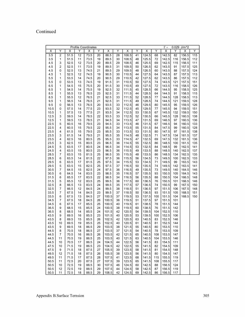
Appendix B.Surface Ternsion
305
Continued
Γ = 0.029
X Y X Y X Y X Y X Y X Y X Y X Y3.5 2 51.5 12 73.5 20 88.5 28 108.5 41 124.5 68 142.5 82 156.5 1153.5 1 51.5 11 73.5 19 89.5 30 108.5 48 125.5 72 142.5 116 156.5 1124.5 3 52.5 12 73.5 20 89.5 29 108.5 46 125.5 69 142.5 115 156.5 1114.5 2 52.5 11 73.5 19 89.5 31 109.5 50 126.5 62 143.5 91 157.5 1254.5 0 52.5 13 74.5 21 89.5 29 109.5 48 126.5 60 143.5 88 157.5 1244.5 1 52.5 12 74.5 19 90.5 30 110.5 44 127.5 64 143.5 87 157.5 1135.5 1 53.5 14 74.5 20 90.5 29 110.5 42 127.5 62 143.5 86 157.5 1125.5 0 53.5 13 74.5 19 91.5 31 110.5 50 127.5 74 143.5 121 157.5 1516.5 1 54.5 15 75.5 20 91.5 30 110.5 49 127.5 72 143.5 116 158.5 1266.5 1 54.5 14 75.5 19 92.5 32 111.5 45 128.5 66 144.5 95 158.5 1258.5 1 55.5 13 76.5 23 92.5 31 111.5 44 128.5 64 144.5 91 158.5 1158.5 1 55.5 12 76.5 21 92.5 33 111.5 52 128.5 77 144.5 128 158.5 1139.5 1 56.5 14 76.5 21 92.5 31 111.5 49 128.5 74 144.5 121 159.5 1289.5 0 56.5 13 76.5 20 93.5 33 112.5 46 129.5 80 145.5 95 159.5 12610.5 0 57.5 14 77.5 23 93.5 32 112.5 45 129.5 77 145.5 94 159.5 15110.5 1 57.5 13 77.5 21 93.5 34 112.5 53 130.5 67 145.5 132 159.5 15012.5 3 59.5 14 78.5 22 93.5 33 112.5 52 130.5 66 145.5 128 160.5 13812.5 1 59.5 13 78.5 21 94.5 34 113.5 47 131.5 69 146.5 97 160.5 13622.5 5 60.5 16 79.5 23 94.5 33 113.5 46 131.5 67 146.5 94 160.5 13322.5 4 60.5 15 79.5 22 95.5 34 113.5 55 131.5 84 147.5 99 160.5 12823.5 4 61.5 15 79.5 23 95.5 33 113.5 53 131.5 80 147.5 97 161.5 13823.5 3 61.5 14 79.5 21 95.5 35 114.5 48 132.5 71 147.5 134 161.5 13723.5 4 62.5 16 80.5 25 95.5 33 114.5 47 132.5 69 147.5 132 161.5 13623.5 3 62.5 15 80.5 23 96.5 36 114.5 55 132.5 86 148.5 100 161.5 13524.5 5 63.5 17 80.5 24 96.5 34 114.5 53 132.5 84 148.5 99 162.5 14124.5 4 63.5 15 80.5 23 96.5 36 115.5 49 133.5 88 148.5 140 162.5 13728.5 7 63.5 15 81.5 25 96.5 35 115.5 48 133.5 86 148.5 134 162.5 13528.5 6 63.5 14 81.5 22 97.5 36 115.5 56 134.5 73 149.5 100 162.5 13329.5 6 63.5 17 81.5 25 97.5 34 115.5 53 134.5 71 149.5 99 163.5 14329.5 5 63.5 15 82.5 25 97.5 37 116.5 50 135.5 74 149.5 142 163.5 14130.5 7 64.5 15 82.5 24 97.5 36 116.5 49 135.5 73 149.5 140 164.5 14630.5 6 64.5 14 83.5 23 98.5 35 116.5 57 135.5 93 150.5 105 164.5 14331.5 6 65.5 17 83.5 22 98.5 34 116.5 56 135.5 88 150.5 104 166.5 14831.5 5 65.5 12 83.5 25 99.5 36 117.5 60 136.5 76 150.5 101 166.5 14632.5 8 66.5 13 83.5 24 99.5 35 117.5 57 136.5 74 150.5 99 167.5 15032.5 7 66.5 12 84.5 24 99.5 38 118.5 51 136.5 97 151.5 106 167.5 14833.5 7 67.5 14 84.5 23 99.5 37 118.5 50 136.5 93 151.5 105 168.5 15133.5 6 67.5 13 84.5 27 100.5 37 119.5 53 137.5 100 151.5 104 168.5 15034.5 7 67.5 18 84.5 26 100.5 36 119.5 51 137.5 97 151.5 10134.5 6 67.5 17 85.5 25 100.5 40 119.5 61 138.5 78 151.5 14436.5 9 68.5 15 85.5 24 100.5 38 119.5 60 138.5 76 151.5 14236.5 8 68.5 14 85.5 24 101.5 42 120.5 54 139.5 104 152.5 11043.5 9 69.5 16 85.5 23 101.5 40 120.5 53 139.5 100 152.5 10643.5 8 69.5 15 85.5 26 102.5 42 120.5 63 140.5 83 152.5 14643.5 10 69.5 19 85.5 25 102.5 40 120.5 61 140.5 81 152.5 14443.5 9 69.5 18 86.5 29 103.5 38 121.5 55 140.5 80 153.5 11044.5 8 70.5 18 86.5 27 103.5 37 121.5 54 140.5 78 153.5 10944.5 7 70.5 16 86.5 26 103.5 42 121.5 65 140.5 108 153.5 14744.5 11 70.5 19 86.5 25 103.5 40 121.5 63 140.5 104 153.5 14644.5 10 70.5 17 86.5 24 104.5 44 122.5 56 141.5 83 154.5 11147.5 10 71.5 19 86.5 23 104.5 42 122.5 55 141.5 82 154.5 10947.5 9 71.5 18 87.5 27 105.5 39 123.5 58 141.5 81 154.5 14849.5 12 71.5 18 87.5 26 105.5 38 123.5 56 141.5 80 154.5 14749.5 11 71.5 17 87.5 28 107.5 41 123.5 68 141.5 115 155.5 11950.5 11 72.5 20 87.5 27 107.5 39 123.5 65 141.5 108 155.5 11750.5 10 72.5 19 88.5 30 107.5 46 124.5 60 142.5 88 156.5 12450.5 12 72.5 19 88.5 29 107.5 44 124.5 58 142.5 87 156.5 11950.5 11 72.5 18 88.5 29 108.5 42 124.5 69 142.5 86 156.5 117
J/m^2Profile Coordinates
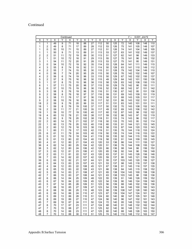
Appendix B.Surface Ternsion
306
Continued
Γ = 0.031
X Y X Y X Y X Y X Y X Y X Y X Y1 1 49 9 71 18 88 27 112 50 125 72 140 108 148 1101 2 49 8 71 17 89 28 112 53 126 75 141 105 148 1071 0 50 10 71 15 89 27 112 51 126 74 141 104 148 1051 1 50 9 71 13 89 31 113 53 127 63 141 102 149 1372 2 51 11 72 19 89 30 113 51 127 62 141 98 149 1332 1 51 10 72 18 91 29 113 55 127 76 141 96 149 1323 1 54 11 72 20 91 28 113 53 127 75 141 95 149 1313 0 54 10 72 19 92 35 114 53 128 64 141 111 149 1154 3 55 8 74 19 92 31 114 50 128 63 141 110 149 1124 2 55 7 74 15 95 30 115 51 128 79 142 104 149 1104 0 56 7 74 20 95 29 115 50 128 76 142 102 149 1074 2 56 6 74 19 96 33 115 50 129 67 142 102 150 1375 2 57 9 75 16 96 30 115 49 129 64 142 101 150 1365 1 57 8 75 15 96 38 115 58 129 83 142 106 150 1156 1 57 11 75 20 96 37 115 55 129 79 142 98 150 1116 0 57 10 75 19 96 36 116 52 130 68 142 97 151 1429 3 58 9 76 19 96 35 116 51 130 67 142 95 151 1369 2 58 8 76 18 97 37 116 59 131 69 143 109 151 1199 3 58 11 76 17 97 36 116 58 131 68 143 105 151 1179 2 58 10 76 16 99 35 117 52 131 86 143 102 151 114
18 2 59 9 76 20 99 33 117 51 131 83 143 101 151 11118 1 59 8 76 19 100 37 117 50 132 70 143 108 152 14319 2 59 11 77 21 100 35 117 49 132 69 143 106 152 14219 1 59 10 77 19 100 40 117 60 132 87 143 98 152 12219 4 60 10 78 21 100 38 117 59 132 86 143 97 152 11919 3 60 9 78 20 102 38 118 51 133 74 143 96 152 11722 2 60 14 79 21 102 37 118 50 133 70 143 95 152 11422 1 60 13 79 20 103 40 118 60 133 91 144 121 153 14523 2 60 12 79 18 103 38 118 58 133 87 144 120 153 14323 1 60 11 79 17 103 42 119 51 135 76 144 118 153 12425 6 61 11 79 24 103 40 119 50 135 74 144 116 153 12225 5 61 10 79 19 104 41 119 59 135 92 144 115 155 14630 5 61 13 80 22 104 40 119 58 135 91 144 109 155 14530 4 61 12 80 21 104 43 120 53 136 86 144 111 155 12736 4 62 14 80 25 104 42 120 51 136 76 144 108 155 12436 3 62 12 80 24 106 42 120 66 136 98 144 98 156 15237 3 63 12 81 23 106 41 120 65 136 92 144 96 156 14837 2 63 11 81 22 107 43 120 63 137 91 145 126 156 14639 7 63 14 82 22 107 42 120 59 137 86 145 121 156 13539 6 63 12 82 21 107 44 121 55 137 103 145 120 156 12740 5 64 13 83 23 107 43 121 53 137 98 145 118 157 13840 4 64 12 83 22 108 45 121 67 138 91 145 116 157 13542 6 65 15 83 22 108 43 121 66 138 84 145 115 158 15242 5 65 14 83 21 108 47 121 65 138 104 145 100 158 13842 7 66 15 83 27 108 44 121 63 138 103 145 98 158 13642 6 66 14 84 25 109 48 122 55 139 91 146 126 159 15243 6 67 16 84 22 109 45 122 54 139 90 146 124 159 14043 5 67 14 85 28 109 51 123 56 139 88 146 102 159 13643 7 68 18 85 27 109 47 123 54 139 84 146 100 160 14343 6 68 16 86 25 110 48 123 68 139 108 147 126 160 14045 6 69 14 86 24 110 47 123 67 139 104 147 124 161 15245 5 69 13 86 28 110 51 124 60 140 98 147 105 161 14645 8 69 19 86 27 110 47 124 56 140 96 147 102 161 14345 7 69 18 87 24 111 50 124 72 140 95 148 133 162 14647 8 70 17 87 23 111 47 124 68 140 91 148 132 162 14447 7 70 15 88 27 111 51 125 62 140 90 148 131 163 15248 8 70 14 88 23 111 47 125 60 140 88 148 126 163 15048 7 70 13 88 30 112 51 125 74 140 110 148 112 163 147
J/m^2Continued
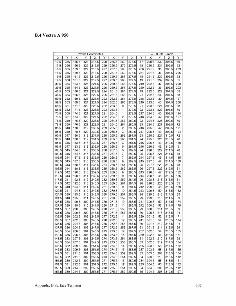
Appendix B.Surface Ternsion
307
B.4 Vectra A 950
Γ = 0.031 J/m^2
X Y X Y X Y X Y X Y X Y X Y17.5 355 156.5 328 216.5 298 256.5 269 276.5 17 290.5 232 305.5 6017.5 356 156.5 329 216.5 299 256.5 270 276.5 18 290.5 234 305.5 6318.5 355 159.5 327 218.5 297 257.5 268 276.5 250 291.5 35 305.5 20318.5 356 159.5 328 218.5 298 257.5 269 276.5 251 291.5 37 305.5 20519.5 355 161.5 326 219.5 296 259.5 267 277.5 18 291.5 230 306.5 6319.5 356 161.5 327 219.5 297 259.5 268 277.5 19 291.5 232 306.5 6539.5 354 164.5 325 221.5 295 260.5 266 277.5 249 292.5 37 306.5 20039.5 355 164.5 326 221.5 296 260.5 267 277.5 250 292.5 39 306.5 20346.5 353 166.5 324 222.5 294 261.5 265 278.5 19 292.5 229 307.5 6546.5 354 166.5 325 222.5 295 261.5 266 278.5 21 292.5 230 307.5 6859.5 352 169.5 323 224.5 293 262.5 264 278.5 248 293.5 39 307.5 19759.5 353 169.5 324 224.5 294 262.5 265 278.5 249 293.5 40 307.5 20065.5 351 171.5 322 226.5 292 263.5 0 279.5 21 293.5 227 308.5 6865.5 352 171.5 323 226.5 293 263.5 1 279.5 22 293.5 229 308.5 7073.5 350 174.5 321 227.5 291 264.5 1 279.5 247 294.5 40 308.5 19473.5 351 174.5 322 227.5 292 264.5 2 279.5 248 294.5 42 308.5 19778.5 349 176.5 320 228.5 290 264.5 263 280.5 22 294.5 225 309.5 7078.5 350 176.5 321 228.5 291 264.5 264 280.5 23 294.5 227 309.5 7285.5 348 178.5 319 230.5 289 265.5 2 280.5 246 295.5 42 309.5 19185.5 349 178.5 320 230.5 290 265.5 3 280.5 247 295.5 43 309.5 19490.5 347 180.5 318 231.5 288 265.5 262 281.5 23 295.5 224 310.5 7290.5 348 180.5 319 231.5 289 265.5 263 281.5 24 295.5 225 310.5 7695.5 346 183.5 317 232.5 287 266.5 3 281.5 245 296.5 43 310.5 18995.5 347 183.5 318 232.5 288 266.5 5 281.5 246 296.5 45 310.5 191
100.5 345 184.5 316 233.5 286 267.5 5 282.5 24 296.5 222 311.5 76100.5 346 184.5 317 233.5 287 267.5 7 282.5 25 296.5 224 311.5 78105.5 344 187.5 315 235.5 285 268.5 7 282.5 244 297.5 45 311.5 185105.5 345 187.5 316 235.5 286 268.5 8 282.5 245 297.5 47 311.5 189108.5 343 188.5 314 236.5 284 268.5 261 283.5 25 297.5 220 312.5 78108.5 344 188.5 315 236.5 285 268.5 262 283.5 26 297.5 222 312.5 81112.5 342 190.5 313 239.5 283 269.5 8 283.5 243 298.5 47 312.5 182112.5 343 190.5 314 239.5 284 269.5 9 283.5 244 298.5 48 312.5 185117.5 341 192.5 312 240.5 282 269.5 259 284.5 26 298.5 218 313.5 81117.5 342 192.5 313 240.5 283 269.5 261 284.5 28 298.5 220 313.5 85120.5 340 194.5 311 242.5 281 270.5 9 284.5 242 299.5 48 313.5 179120.5 341 194.5 312 242.5 282 270.5 10 284.5 243 299.5 50 313.5 182124.5 339 195.5 310 243.5 280 270.5 257 285.5 28 299.5 216 314.5 85124.5 340 195.5 311 243.5 281 270.5 259 285.5 29 299.5 218 314.5 89127.5 338 199.5 309 244.5 279 271.5 10 285.5 241 300.5 50 314.5 174127.5 339 199.5 310 244.5 280 271.5 11 285.5 242 300.5 52 314.5 179131.5 337 200.5 308 245.5 278 271.5 256 286.5 29 300.5 214 315.5 89131.5 338 200.5 309 245.5 279 271.5 257 286.5 30 300.5 216 315.5 94133.5 336 202.5 306 246.5 277 272.5 11 286.5 239 301.5 52 315.5 171133.5 337 202.5 308 246.5 278 272.5 12 286.5 241 301.5 54 315.5 174137.5 335 204.5 305 247.5 276 272.5 255 287.5 30 301.5 212 316.5 94137.5 336 204.5 306 247.5 277 272.5 256 287.5 31 301.5 214 316.5 98140.5 334 206.5 304 248.5 275 273.5 12 287.5 237 302.5 54 316.5 165140.5 335 206.5 305 248.5 276 273.5 14 287.5 239 302.5 56 316.5 171143.5 333 207.5 303 249.5 274 273.5 254 288.5 31 302.5 210 317.5 98143.5 334 207.5 304 249.5 275 273.5 255 288.5 33 302.5 212 317.5 104145.5 332 209.5 302 251.5 273 274.5 14 288.5 235 303.5 56 317.5 162145.5 333 209.5 303 251.5 274 274.5 15 288.5 237 303.5 58 317.5 165149.5 331 211.5 301 253.5 272 274.5 252 289.5 33 303.5 208 318.5 104149.5 332 211.5 302 253.5 273 274.5 254 289.5 34 303.5 210 318.5 112151.5 330 212.5 300 254.5 271 275.5 15 289.5 234 304.5 58 318.5 151151.5 331 212.5 301 254.5 272 275.5 17 289.5 235 304.5 60 318.5 162155.5 329 214.5 299 255.5 270 275.5 251 290.5 34 304.5 205 319.5 112155.5 330 214.5 300 255.5 271 275.5 252 290.5 35 304.5 208 319.5 127
Profile Coordinates

Appendix B.Surface Ternsion
308
Continued
Γ = 0.031
X Y X Y X Y X Y X Y X Y3 0 94 21 132 45 161 72 184 104 203 1473 1 94 22 132 46 161 74 184 105 203 1504 0 96 22 134 46 163 74 185 105 203 2894 1 96 23 134 47 163 76 185 107 203 297
15 1 97 23 135 47 164 76 186 107 204 15015 2 97 24 135 48 164 77 186 108 204 15326 2 100 24 137 48 165 77 187 108 204 28626 3 100 25 137 50 165 78 187 111 204 28930 3 101 25 139 50 166 78 188 111 205 15330 4 101 26 139 52 166 79 188 113 205 15738 4 103 26 141 52 167 79 189 113 205 27938 5 103 27 141 53 167 81 189 115 205 28642 5 105 27 142 53 168 81 190 115 206 15742 6 105 28 142 54 168 82 190 117 206 16049 6 107 28 143 54 169 82 191 117 206 27249 7 107 29 143 55 169 84 191 120 206 27951 7 109 29 144 55 170 84 192 120 207 16051 8 109 30 144 56 170 85 192 122 207 16657 8 111 30 145 56 171 85 193 122 207 26457 9 111 32 145 57 171 87 193 124 207 27259 9 114 32 147 57 172 87 194 124 208 16659 10 114 33 147 59 172 88 194 125 208 16963 10 115 33 149 59 173 88 195 125 208 25963 11 115 34 149 61 173 89 195 129 208 26466 11 117 34 151 61 174 89 196 129 209 16966 12 117 35 151 63 174 90 196 130 209 17671 12 118 35 152 63 175 90 197 130 209 25371 13 118 36 152 64 175 92 197 133 209 25974 13 121 36 153 64 176 92 198 133 210 17674 14 121 38 153 65 176 93 198 136 210 18178 14 123 38 154 65 177 93 199 136 210 24878 15 123 39 154 66 177 95 199 139 210 25379 15 124 39 155 66 178 95 200 139 211 18179 16 124 40 155 67 178 96 200 141 211 19283 16 126 40 156 67 179 96 200 302 211 23883 17 126 41 156 68 179 98 200 303 211 24884 17 127 41 157 68 180 98 201 141 212 19284 18 127 42 157 69 180 100 201 144 212 20487 18 129 42 158 69 181 100 201 298 212 22487 19 129 43 158 70 181 101 201 302 212 23889 19 130 43 159 70 182 101 202 144 213 20489 20 130 44 159 71 182 102 202 147 213 22493 20 131 44 160 71 183 102 202 29793 21 131 45 160 72 183 104 202 298
J/m^2Profile Coordinates

Appendix B.Surface Ternsion
309
B.5 Vectra B 950
Γ = 0.029 J/m^2
X Y X Y X Y X Y X Y X Y X Y X Y12.5 0 174.5 28 233.5 57 278.5 86 314.5 115 344.5 146 373.5 185 401.5 25012.5 1 174.5 29 233.5 58 278.5 87 314.5 116 344.5 147 373.5 187 401.5 25933.5 1 178.5 29 234.5 58 279.5 87 315.5 116 345.5 147 374.5 187 401.5 32033.5 2 178.5 30 234.5 59 279.5 88 315.5 117 345.5 148 374.5 188 401.5 32346.5 2 179.5 30 236.5 59 281.5 88 316.5 117 346.5 148 375.5 188 401.5 34046.5 3 179.5 31 236.5 60 281.5 89 316.5 118 346.5 149 375.5 190 401.5 34251.5 3 181.5 31 238.5 60 282.5 89 317.5 118 347.5 149 376.5 190 402.5 25951.5 4 181.5 32 238.5 61 282.5 90 317.5 119 347.5 151 376.5 192 402.5 26864.5 4 182.5 32 240.5 61 283.5 90 318.5 119 348.5 151 377.5 192 402.5 31564.5 5 182.5 33 240.5 62 283.5 91 318.5 120 348.5 152 377.5 193 402.5 32071.5 5 184.5 33 241.5 62 285.5 91 319.5 120 349.5 152 378.5 193 402.5 34271.5 6 184.5 34 241.5 63 285.5 92 319.5 121 349.5 153 378.5 195 402.5 34375.5 6 186.5 34 243.5 63 286.5 92 320.5 121 350.5 153 379.5 195 403.5 26875.5 7 186.5 35 243.5 64 286.5 93 320.5 122 350.5 154 379.5 197 403.5 27283.5 7 189.5 35 244.5 64 287.5 93 322.5 122 351.5 154 380.5 197 403.5 31083.5 8 189.5 36 244.5 65 287.5 94 322.5 123 351.5 155 380.5 199 403.5 31590.5 8 192.5 36 247.5 65 289.5 94 323.5 123 352.5 155 381.5 199 403.5 34390.5 9 192.5 37 247.5 66 289.5 95 323.5 124 352.5 157 381.5 201 403.5 34497.5 9 194.5 37 248.5 66 290.5 95 324.5 124 353.5 157 382.5 201 404.5 27297.5 10 194.5 38 248.5 67 290.5 96 324.5 125 353.5 158 382.5 203 404.5 280
105.5 10 196.5 38 250.5 67 291.5 96 325.5 125 354.5 158 383.5 203 404.5 307105.5 11 196.5 39 250.5 68 291.5 97 325.5 126 354.5 159 383.5 205 404.5 310107.5 11 198.5 39 251.5 68 292.5 97 326.5 126 355.5 159 384.5 205 405.5 280107.5 12 198.5 40 251.5 69 292.5 98 326.5 127 355.5 161 384.5 207 405.5 289113.5 12 199.5 40 253.5 69 294.5 98 327.5 127 356.5 161 385.5 207 405.5 306113.5 13 199.5 41 253.5 70 294.5 99 327.5 128 356.5 162 385.5 210 405.5 307118.5 13 201.5 41 255.5 70 295.5 99 328.5 128 357.5 162 386.5 210 406.5 289118.5 14 201.5 42 255.5 71 295.5 100 328.5 129 357.5 163 386.5 212 406.5 295127.5 14 203.5 42 256.5 71 296.5 100 329.5 129 358.5 163 387.5 212 406.5 304127.5 15 203.5 43 256.5 72 296.5 101 329.5 130 358.5 165 387.5 214 406.5 306129.5 15 206.5 43 258.5 72 297.5 101 330.5 130 359.5 165 388.5 214 407.5 295129.5 16 206.5 44 258.5 73 297.5 102 330.5 131 359.5 166 388.5 218 407.5 296130.5 16 208.5 44 259.5 73 299.5 102 331.5 131 360.5 166 389.5 218 407.5 302130.5 17 208.5 45 259.5 74 299.5 103 331.5 133 360.5 167 389.5 219 407.5 304134.5 17 209.5 45 261.5 74 300.5 103 332.5 133 361.5 167 390.5 219 408.5 299134.5 18 209.5 46 261.5 75 300.5 104 332.5 134 361.5 168 390.5 220 408.5 302138.5 18 212.5 46 263.5 75 301.5 104 333.5 134 362.5 168 391.5 220 409.5 296138.5 19 212.5 47 263.5 76 301.5 105 333.5 135 362.5 169 391.5 223 409.5 299142.5 19 214.5 47 264.5 76 302.5 105 334.5 135 363.5 169 392.5 223142.5 20 214.5 48 264.5 77 302.5 106 334.5 136 363.5 171 392.5 226145.5 20 216.5 48 266.5 77 303.5 106 335.5 136 364.5 171 393.5 226145.5 21 216.5 49 266.5 78 303.5 107 335.5 137 364.5 172 393.5 227147.5 21 217.5 49 267.5 78 304.5 107 336.5 137 365.5 172 394.5 227147.5 22 217.5 50 267.5 79 304.5 108 336.5 138 365.5 174 394.5 232153.5 22 220.5 50 268.5 79 305.5 108 337.5 138 366.5 174 395.5 232153.5 23 220.5 51 268.5 80 305.5 109 337.5 139 366.5 175 395.5 236155.5 23 221.5 51 270.5 80 308.5 109 338.5 139 367.5 175 396.5 236155.5 24 221.5 52 270.5 81 308.5 110 338.5 140 367.5 177 396.5 241159.5 24 224.5 52 271.5 81 309.5 110 339.5 140 368.5 177 397.5 241159.5 25 224.5 53 271.5 82 309.5 111 339.5 142 368.5 179 397.5 244163.5 25 226.5 53 273.5 82 310.5 111 340.5 142 369.5 179 398.5 244163.5 26 226.5 54 273.5 83 310.5 112 340.5 143 369.5 180 398.5 246168.5 25 227.5 54 275.5 83 311.5 112 341.5 143 370.5 180 399.5 246168.5 26 227.5 55 275.5 84 311.5 113 341.5 144 370.5 182 399.5 248170.5 25 228.5 55 276.5 84 312.5 113 342.5 144 371.5 182 400.5 248170.5 26 228.5 56 276.5 85 312.5 114 342.5 145 371.5 183 400.5 250172.5 26 231.5 56 277.5 85 313.5 114 343.5 145 372.5 183 400.5 323172.5 28 231.5 57 277.5 86 313.5 115 343.5 146 372.5 185 400.5 340
Profile Coordinates

Appendix B.Surface Ternsion
310
Conxtinued
Γ = 0.029 J/m^2
X Y X Y X Y X Y X Y X Y194 300 203 178 179 114 152 76 122 48 83 22193 300 202 178 178 114 150 76 121 48 80 22195 293 202 170 178 112 150 74 121 47 80 21194 293 201 170 177 112 149 74 120 47 79 21196 290 201 167 177 111 149 73 120 46 79 20195 290 200 167 176 111 148 73 118 46 76 20197 286 200 164 176 108 148 72 118 44 76 19196 286 199 164 174 108 147 72 116 44 75 19198 284 199 160 174 105 147 71 116 43 75 18197 284 198 160 173 105 146 71 114 43 72 18199 280 198 157 173 104 146 70 114 42 72 17198 280 197 157 172 104 145 70 113 42 71 17200 278 197 155 172 102 145 69 113 41 71 16199 278 196 155 170 102 144 69 112 41 68 16201 274 196 151 170 100 144 68 112 40 68 15200 274 195 151 169 100 142 68 110 40 66 15202 272 195 149 169 99 142 66 110 39 66 14201 272 194 149 168 99 141 66 109 39 63 14203 265 194 146 168 97 141 65 109 38 63 13202 265 193 146 167 97 140 65 106 38 62 13204 261 193 143 167 96 140 64 106 36 62 12203 261 192 143 166 96 139 64 104 36 58 12205 252 192 140 166 94 139 63 104 35 58 11204 252 191 140 164 94 138 63 103 35 56 11206 247 191 138 164 92 138 62 103 34 56 10205 247 190 138 163 92 137 62 100 34 52 10206 244 190 135 163 91 137 61 100 32 52 9205 244 189 135 162 91 136 61 98 32 49 9206 243 189 134 162 89 136 60 98 31 49 8205 243 188 134 161 89 134 60 97 31 44 8207 234 188 130 161 88 134 58 97 30 44 7206 234 186 130 160 88 132 58 94 30 43 7207 216 186 126 160 86 132 56 94 28 43 6206 216 184 126 158 86 130 56 91 28 38 6207 214 184 123 158 84 130 54 91 27 38 5206 214 183 123 157 84 128 54 90 27 36 5207 213 183 121 157 83 128 52 90 26 36 4206 213 182 121 156 83 126 52 88 26 30 4206 200 182 119 156 81 126 51 88 25 30 3205 200 181 119 155 81 125 51 86 25 21 3205 194 181 118 155 80 125 50 86 24 21 2204 194 180 118 154 80 123 50 84 24204 184 180 116 154 78 123 49 84 23203 184 179 116 152 78 122 49 83 23
Profile Coordinates

Appendix C. Neck Growth
311
Appendix C. Coalescence
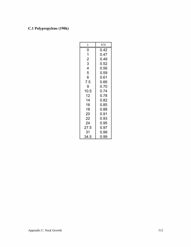
Appendix C. Neck Growth
312
C.1 Polypropylene (190k)
t x/a0 0.421 0.472 0.493 0.524 0.565 0.596 0.61
7.5 0.669 0.70
10.5 0.7412 0.7814 0.8216 0.8518 0.8820 0.9122 0.9324 0.95
27.5 0.9731 0.99
34.5 0.99

Appendix C. Neck Growth
313
C.2 Polypropylene (250k)
t x/a0.5 0.311.5 0.342.5 0.343.5 0.374.5 0.395.5 0.407.5 0.439.5 0.44
11.5 0.4713.5 0.4915.5 0.5117.5 0.5219.5 0.5421.5 0.5423.5 0.5725.5 0.5930.5 0.6135.5 0.6440.5 0.6745.5 0.6950.5 0.7155.5 0.7465.5 0.7875.5 0.8185.5 0.8495.5 0.87
105.5 0.90115.5 0.91125.5 0.94135.5 0.95145.5 0.96155.5 0.99

Appendix C. Neck Growth
314
C.3 Polypropylene (340k)
t x/a0 0.462 0.47
3.5 0.485.5 0.497.5 0.4913 0.51
17.5 0.5323 0.5428 0.5633 0.5838 0.5948 0.61
55.5 0.6265.5 0.6475.5 0.6685.5 0.6895.5 0.69
120.5 0.72150.5 0.75180.5 0.78225.5 0.82285.5 0.85345.5 0.87405.5 0.90465.5 0.90525.5 0.92585.5 0.93645.5 0.94

Appendix C. Neck Growth
315
C.4 Vectra A 950
320°C
t x/a1.5 0.254 0.33
6.5 0.409 0.43
11.5 0.4614 0.48
16.5 0.4919 0.51
21.5 0.5238 0.58
51.5 0.63
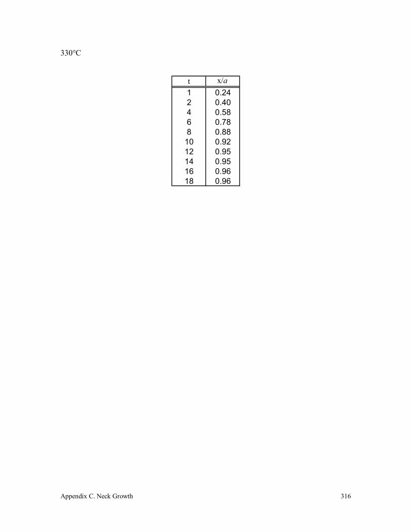
Appendix C. Neck Growth
316
330°C
t x/a1 0.242 0.404 0.586 0.788 0.88
10 0.9212 0.9514 0.9516 0.9618 0.96

Appendix C. Neck Growth
317
C.5 Vectra B 950
320°C
t x/a0 0.16
2.5 0.375 0.54
7.5 0.6810 0.81
12.5 0.9115 0.94
17.5 0.9720 0.99
22.5 1.00

Appendix C. Neck Growth
318
330°C
t x/a1 0.283 0.455 0.637 0.779 0.88
11 0.9313 0.9615 0.9817 0.9819 0.9821 1.00
Appendix D. Programs for the Neck Growth Model
319
Appendix D. Programs for Coalescence Models
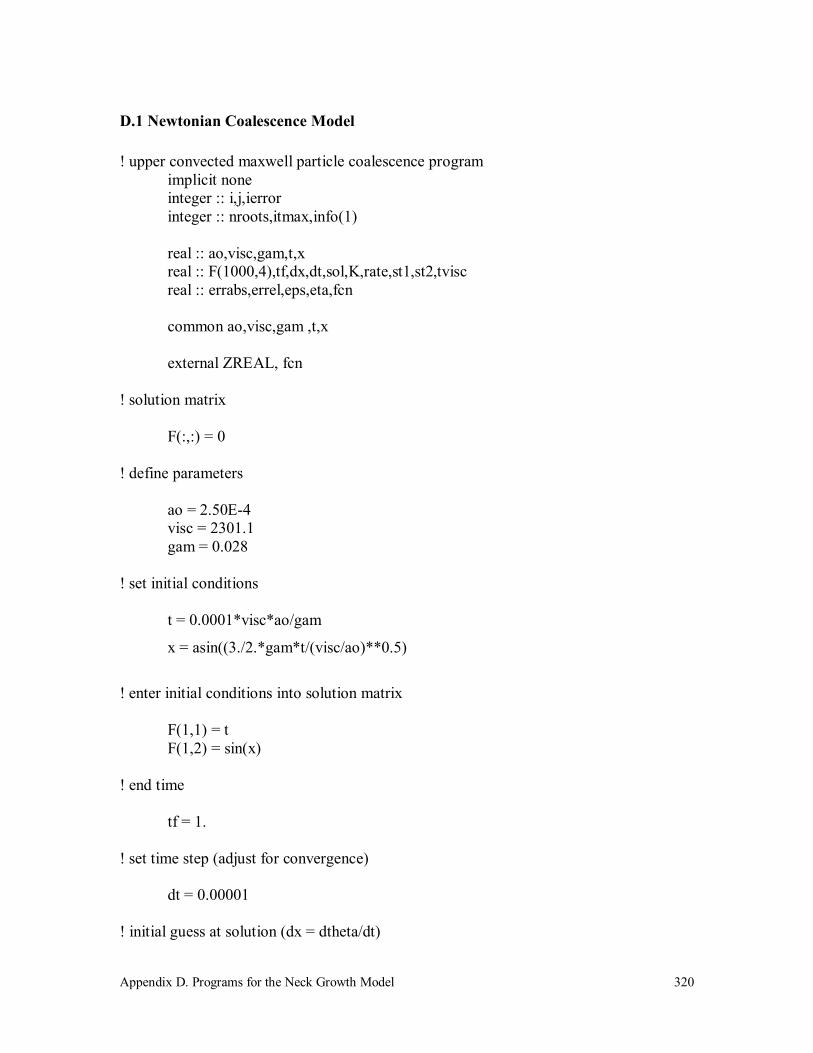
Appendix D. Programs for the Neck Growth Model
320
D.1 Newtonian Coalescence Model
! upper convected maxwell particle coalescence program implicit none integer :: i,j,ierror integer :: nroots,itmax,info(1) real :: ao,visc,gam,t,x real :: F(1000,4),tf,dx,dt,sol,K,rate,st1,st2,tvisc real :: errabs,errel,eps,eta,fcn common ao,visc,gam ,t,x external ZREAL, fcn ! solution matrix F(:,:) = 0 ! define parameters ao = 2.50E-4 visc = 2301.1 gam = 0.028 ! set initial conditions t = 0.0001*visc*ao/gam
x = asin((3./2.*gam*t/(visc/ao)**0.5)
! enter initial conditions into solution matrix F(1,1) = t F(1,2) = sin(x) ! end time tf = 1. ! set time step (adjust for convergence) dt = 0.00001 ! initial guess at solution (dx = dtheta/dt)
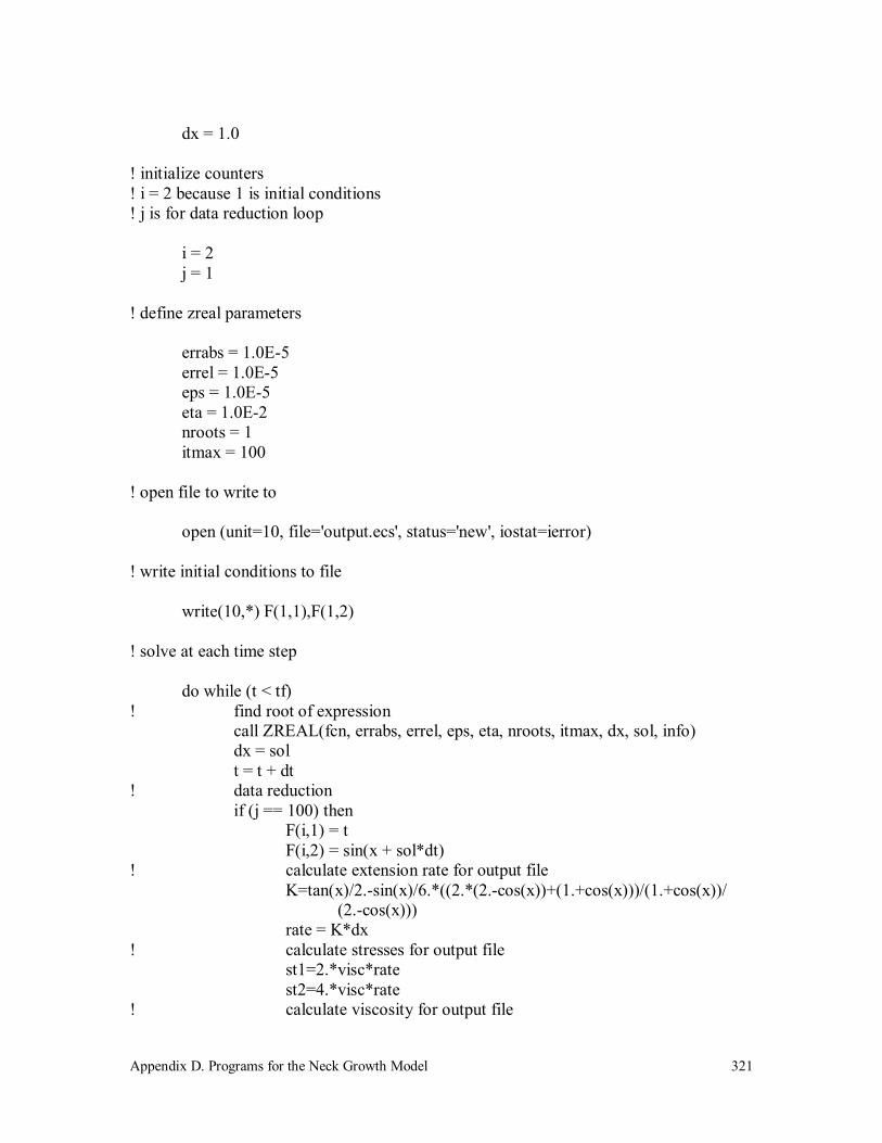
Appendix D. Programs for the Neck Growth Model
321
dx = 1.0 ! initialize counters ! i = 2 because 1 is initial conditions ! j is for data reduction loop i = 2 j = 1 ! define zreal parameters errabs = 1.0E-5 errel = 1.0E-5 eps = 1.0E-5 eta = 1.0E-2 nroots = 1 itmax = 100 ! open file to write to open (unit=10, file='output.ecs', status='new', iostat=ierror) ! write initial conditions to file write(10,*) F(1,1),F(1,2) ! solve at each time step do while (t < tf) ! find root of expression call ZREAL(fcn, errabs, errel, eps, eta, nroots, itmax, dx, sol, info) dx = sol t = t + dt ! data reduction if (j == 100) then F(i,1) = t F(i,2) = sin(x + sol*dt) ! calculate extension rate for output file K=tan(x)/2.-sin(x)/6.*((2.*(2.-cos(x))+(1.+cos(x)))/(1.+cos(x))/ (2.-cos(x))) rate = K*dx ! calculate stresses for output file st1=2.*visc*rate st2=4.*visc*rate ! calculate viscosity for output file
Appendix D. Programs for the Neck Growth Model
322
tvisc = (st1+st2)/rate F(i,3) = rate F(i,4) = tvisc ! write solution to file write(10,*) F(i,1),F(i,2),F(i,3), F(i,4) i = i + 1 j = 0 end if j = j +1 x = x + sol*dt end do end program !- supporting function ----------------------------------------- real function fcn(dx) implicit none real :: ao,visc,gam,t,x,dx real :: K,T1,T2 common ao,visc,gam,t,x ! for small angles (use only for angle approximation) ! K = sin(x)/(1+cos(x))/(2-cos(x)) ! full expression K = tan(x)/2.-sin(x)/6.*((2.*(2.-cos(x))+(1.+cos(x)))/(1.+cos(x))/(2.-cos(x))) ! 1st normal stress (growth) Tau11 T1=2.*visc*K*dx ! 2cnd normal stress (growth) Tau22 T2=-4.*visc*Kdx ! define energy balance equation fcn=2.**(2./3.)*ao*K/3./gam*(T1-T2)*(1.+cos(x))**(4./3.)* (2.-cos(x))**(5./3.)/cos(x)/sin(x)-1. return end
Appendix D. Programs for the Neck Growth Model
323
D.2 Single Mode Steady State upper convected Coalescence Model
! upper convected maxwell particle coalescence program implicit none integer :: i,j,ierror integer :: nroots,itmax,info(1) real :: ao,visc,gam,lam,t,x real :: F(1000,4),tf,dx,dt,sol,K,rate,st1,st2,tvisc real :: errabs,errel,eps,eta,fcn common ao,visc,gam,lam,t,x external ZREAL, fcn ! solution matrix F(:,:) = 0 ! define parameters ao = 2.50E-4 visc = 2301.1 gam = 0.028 lam = 50.80 ! set initial conditions t = 0.0001*visc*ao/gam
x = asin((3./2.*gam*t/(visc/ao)**0.5)
! enter initial conditions into solution matrix F(1,1) = t F(1,2) = sin(x) ! end time tf = 1. ! set time step (adjust for convergence) dt = 0.00001
Appendix D. Programs for the Neck Growth Model
324
! initial guess at solution (dx = dtheta/dt) dx = 1. ! initialize counters ! i = 2 because 1 is initial conditions ! j is for data reduction loop i = 2 j = 1 ! define zreal parameters errabs = 1.0E-5 errel = 1.0E-5 eps = 1.0E-5 eta = 1.0E-2 nroots = 1 itmax = 100 ! open file to write to open (unit=10, file='output.ecs', status='new', iostat=ierror) ! write initial conditions to file write(10,*) F(1,1),F(1,2) ! solve at each time step do while (t < tf) ! find root of expression call ZREAL(fcn, errabs, errel, eps, eta, nroots, itmax, dx, sol, info) dx = sol t = t + dt ! data reduction if (j == 100) then F(i,1) = t F(i,2) = sin(x + sol*dt) ! calculate extension rate for output file K=tan(x)/2.-sin(x)/6.*((2.*(2.-cos(x))+(1.+cos(x)))/(1.+cos(x))/ (2.-cos(x))) rate = K*dx ! calculate stresses for output file st1=2.*visc/(1.-2.*lam*rate)*rate st2=4.*visc/(1.+4.*lam*rate)*rate
Appendix D. Programs for the Neck Growth Model
325
! calculate viscosity for output file tvisc = (st1+st2)/rate F(i,3) = rate F(i,4) = tvisc ! write solution to file write(10,*) F(i,1),F(i,2),F(i,3), F(i,4) i = i + 1 j = 0 end if j = j +1 x = x + sol*dt end do end program !- supporting function ----------------------------------------- real function fcn(dx) implicit none real :: ao,visc,gam,lam,t,x,dx real :: K,T1,T2 common ao,visc,gam,lam,t,x ! for small angles (use only for angle approximation) ! K = sin(x)/(1+cos(x))/(2-cos(x)) ! full expression K = tan(x)/2.-sin(x)/6.*((2.*(2.-cos(x))+(1.+cos(x)))/(1.+cos(x))/(2.-cos(x))) ! 1st normal stress (growth) Tau11 T1=2.*visc*K*dx/(1.-2.*lam*K*dx) ! 2cnd normal stress (growth) Tau22 T2=-4.*visc*K*dx/(1.+4.*lam*K*dx) ! define energy balance equation fcn=2.**(2./3.)*ao*K/3./gam*(T1-T2)*(1.+cos(x))**(4./3.)* (2.-cos(x))**(5./3.)/cos(x)/sin(x)-1. return end
Appendix D. Programs for the Neck Growth Model
326
D.3 Single Mode upper convected Maxwell Coalescence Model
! upper convected maxwell particle coalescence program ! this is the program for the transient upper convected maxwell coalescence model with 1 ! mode. implicit none integer :: i,j,ierror integer :: nroots,itmax,info(1) real :: ao,visc,gam,lam,t,x,C11,C22 real :: F(1000,6),tf,dx,dt,sol,K,tvisc real :: errabs,errel,eps,eta,fcn,fcn1,T1,T2 common ao,visc,gam,lam,t,x,C11,C22,T1,T2 external ZREAL, fcn, fcn1 ! solution matrix F(:,:) = 0 ! define parameters ao = 2.74E-4 visc = 11128.9 gam = 0.028 lam = 1.54 ! set initial conditions t = 0.0001*visc*ao/gam x = asin((3./2.*gam*t/visc/ao)**0.5) ! enter initial conditions into solution matrix F(1,1) = t F(1,2) = sin(x) ! end time tf = 650. ! set time step (adjust for convergence) dt = 0.001 ! initial guess at solution (dx = dtheta/dt) dx = 1. ! initialize counters ! i = 2 because 1 is initial conditions
Appendix D. Programs for the Neck Growth Model
327
! j is for data reduction loop i = 2 j = 1 ! define zreal parameters errabs = 1.0E-5 errel = 1.0E-5 eps = 1.0E-5 eta = 1.0E-2 nroots = 1 itmax = 1000 ! open file to write to open (unit=10, file='output.ecs', status='new', iostat=ierror) ! write initial conditions to file write(10,*) F(1,1),F(1,2) do while (t < tf) ! find root of expression if (i == 2) then call ZREAL(fcn, errabs, errel, eps, eta, nroots, itmax, dx, sol, info) dx = sol t = t + dt F(i,1) = t F(i,2) = sin(x + sol*dt) ! calculate extension rate and viscosity for file K = tan(x)/2.-sin(x)/6.*((2.*(2.-cos(x))+ (1.+cos(x)))/(1.+cos(x))/(2.-cos(x))) tvisc = (T1-T2)/K/dx !biaxial extensional viscosity F(i,3) = K*dx !biaxial extension rate F(i,4) = tvisc F(i,5) = T1 !normal stress 11 F(i,6) = T2 !normal stress 22 ! write solution to file write(10,*) F(i,1),F(i,2),F(i,3),F(i,4),F(i,5),F(i,6) else if (i > 2) then call ZREAL(fcn1, errabs, errel, eps, eta, nroots, itmax, dx, sol, info) dx = sol t = t + dt K = tan(x)/2.-sin(x)/6.*((2.*(2.-cos(x))+ (1.+cos(x)))/(1.+cos(x))/(2.-cos(x))) ! data reduction if (j == 100) then F(i,1) = t

Appendix D. Programs for the Neck Growth Model
328
F(i,2) = sin(x + sol*dt) ! calculate extension rate and viscosity for file tvisc = (T1-T2)/K/dx !biaxial extensional viscosity F(i,3) = K*dx !biaxial extension rate F(i,4) = tvisc F(i,5) = T1 !normal stress 11 F(i,6) = T2 !normal stress 22 ! write solution to file write(10,*) F(i,1),F(i,2),F(i,3),F(i,4),F(i,5),F(i,6) j = 0 end if end if ! calculate stress constants for next time step C11 = exp((1./lam-2.*K*dx)*t)*(T1-2.*visc*K*dx/(1.-2.*lam*K*dx)) C22 = exp((1./lam+4.*K*dx)*t)*(T2+4.*visc*K*dx/(1.-2.*lam*K*dx)) ! step forward x (theta) x = x + sol*dt ! advance counters i = i + 1 j = j + 1 end do end program !- supporting function ----------------------------------------- ! fcn is a function that is called by zreal to find dtheta/dt. It is only used for the first time ! step to initiate the program by using integration constants for the stress expressions that ! are determined from the conditions: t=0 Tau11 = Tau22 = 0. !------------------------------------------------------------------- real function fcn(dx) implicit none real :: ao,visc,gam,lam,t,x,dx real :: K,C11,C22,T1,T2 common ao,visc,gam,lam,t,x,C11,C22,T1,T2 ! for small angles (approximation) ! K = sin(x)/(1+cos(x))/(2-cos(x)) ! full expression K = tan(x)/2.-sin(x)/6.*((2.*(2.-cos(x))+(1.+cos(x)))/(1.+cos(x))/(2.-cos(x))) ! 1st normal stress (growth) Tau11 T1 = 2.*visc*K*dx/(1.-2.*lam*K*dx)*exp(-(1./lam-2.*K*dx)*t)* (exp((1./lam-2.*K*dx)*t)-1.)

Appendix D. Programs for the Neck Growth Model
329
! 2cnd normal stress (growth) Tau22 T2 = -4.*visc*K*dx/(1.+4.*lam*K*dx)*exp(-(1./lam+4.*K*dx)*t)* (exp((1./lam+4.*K*dx)*t)-1.) ! define energy balance fcn1 = 2.**(2./3.)*ao*K/3./gam*(T1-T2)*(1.+cos(x))**(4./3.)* (2.-cos(x))**(5./3.)/cos(x)/sin(x)-1. return end !- supporting function ----------------------------------------- ! fcn1 is a function that is called by zreal to find dtheta/dt. It is used for all time steps ! after the first iteration. The integration constant for the stress expressions are !determined using Tau11 & Tau22 from the previous time step. !------------------------------------------------------------------- real function fcn1(dx) implicit none real :: ao,visc,gam,lam,t,x,dx real :: K,C11,C22,T1,T2 common ao,visc,gam,lam,t,x,C11,C22,T1,T2 ! for small angles (approximation) ! K = sin(x)/(1+cos(x))/(2-cos(x)) ! full expression K = tan(x)/2-sin(x)/6.*((2.*(2.-cos(x))+(1.+cos(x)))/(1.+cos(x))/(2.-cos(x))) ! 1st normal stress (growth) Tau11 T1 = exp(-(1./lam-2.*K*dx)*t)*(2.*visc*K*dx/(1.-2.*lam*K*dx)* exp((1./lam-2.*K*dx)*t)+C11) ! 2cnd normal stress (growth) Tau22 T2 = exp(-(1./lam+4.*K*dx)*t)*(-4.*visc*K*dx/(1.+4.*lam*K*dx)* exp((1./lam+4.*K*dx)*t)+C22) ! define energy balance fcn = 2.**(2./3.)*ao*K/3./gam*(T1-T2)*(1.+cos(x))**(4./3.)* (2.-cos(x))**(5./3.)/cos(x)/sin(x)-1. return end

Appendix D. Programs for the Neck Growth Model
330
D.4 Multi-Mode upper convected Maxwell Coalescence Model
! upper convected maxwell particle coalescence program ! this is the program for the transient upper convected maxwell coalescence model with 1 ! mode. implicit none integer :: i,j,n,modes,ierror integer :: nroots,itmax,info(1) ! set # of modes parameter (modes = 5) integer, dimension(1:modes,1:2) :: L real :: ao,visc(modes),gam,lam(modes),t,x real :: C11,C22,T1(1:modes),T2(1:modes) real :: F(1000,6),tf,dx,dt,sol real :: errabs,errel,eps,eta,fcn common n,ao,visc,gam,lam,t,x,L,C11,C22,T1,T2 external ZREAL, fcn ! set n = modes n = 5 L(:,:) = 0 F(:,:) = 0 ! define parameters ao = 2.74E-4 visc(1) = 1084.603559 visc(2) = 2677.551217 visc(3) = 3778.27556 visc(4) = 3259.505989 visc(5) = 1274.613484 gam = 0.02832 lam(1) = 0.02243756 lam(2) = 0.162908159 lam(3) = 1.010652684 lam(4) = 6.48507642 lam(5) = 49.20180938 ! set initial conditions t = 0.0001*(sum(visc))*ao/gam x = asin((3./2.*gam*t/(sum(visc))/ao)**0.5)
Appendix D. Programs for the Neck Growth Model
331
! enter initial conditions into solution matrix F(1,1) = t F(1,2) = sin(x) ! end time tf = 650. ! set time step (adjust for convergence) dt = 0.001 ! initial guess at solution dx = 1. ! initialize counters ! i = 2 because 1 is initial conditions ! j is for data reduction loop i = 2 j = 1 errabs = 1.0E-5 errel = 1.0E-5 eps = 1.0E-5 eta = 1.0E-2 nroots = 1 itmax = 1000 ! open file to write to open (unit=10, file='output.ecs', status='new', iostat=ierror) write(10,*) F(1,1),F(1,2) do while (t < tf) ! find root of expression if (i == 2) then call ZREAL(fcn, errabs, errel, eps, eta, nroots, itmax, dx, sol, info) dx = sol t = t + dt F(i,1) = t F(i,2) = sin(x + sol*dt) ! calculate extension rate and viscosity for file K = tan(x)/2.-sin(x)/6.*((2.*(2.-cos(x))+(1.+cos(x)))/ (1.+cos(x))/(2.-cos(x))) tvisc = (sum(T1)-sum(T2))/K/dx !biaxial extensional viscosity F(i,3) = K*dx !biaxial extension rate F(i,4) = tvisc F(i,5) = sum(T1) !normal stress 11
Appendix D. Programs for the Neck Growth Model
332
F(i,6) = sum(T2) !normal stress 22 ! write solution to file write(10,*) F(i,1),F(i,2),F(i,3),F(i,4),F(i,5),F(i,6) else if (i > 2) call ZREAL(fcn1, errabs, errel, eps, eta, nroots, itmax, dx, sol, info) dx = sol t = t + dt K = tan(x)/2.-sin(x)/6.*((2.*(2.-cos(x))+(1.+cos(x)))/ (1.+cos(x))/(2.-cos(x))) if (j == 1000) then F(i,1) = t F(i,2) = sin(x + sol*dt) ! calculate extension rate and viscosity for file ! biaxial extensional viscosity tvisc = (sum(T1)-sum(T2))/K/dx F(i,3) = K*dx !biaxial extension rate F(i,4) = tvisc F(i,5) = sum(T1) !normal stress 11 F(i,6) = sum(T2) !normal stress 22 ! write data to file write(10,*) F(i,1),F(i,2),F(i,3),F(i,4),F(i,5),F(i,6) j = 0 end if end if ! calculate stress constants for next time step C11 = exp((1./lam-2.*K*dx)*t)*(sum(T1)-2.*visc*K*dx/ (1.-2.*lam*K*dx)) C22 = exp((1./lam+4.*K*dx)*t)*(sum(T2)+4.*visc*K*dx/ (1.-2.*lam*K*dx)) ! step forward x (theta) x = x + sol*dt ! advance counters i = i + 1 j = j + 1 end do end program !- supporting function ----------------------------------------- ! fcn is a function that is called by zreal to find dtheta/dt. It is only used for the first time ! step to initiate the program by using integration constants for the stress expressions that ! are determined from the conditions: t=0 Tau11 = Tau22 = 0. !------------------------------------------------------------------- real function fcn(dx)
Appendix D. Programs for the Neck Growth Model
333
implicit none integer :: i,j,n,modes parameter(modes = 5) integer, dimension(1:modes,1:2) :: L real :: ao,visc(modes),gam,lam(modes),t,x,dx real :: K,C11,C22,T1(1:modes),T2(1:modes) common n,ao,visc,gam,lam,t,x,L,C11,C22,T1,T2 ! for small angles (approximation) ! K = sin(x)/(1+cos(x))/(2-cos(x)) ! full expression K = tan(x)/2.-sin(x)/6.*((2.*(2.-cos(x))+(1.+cos(x)))/(1.+cos(x))/(2.-cos(x))) i = 1 j = 1 ! multimode 1st normal stress (Tau11) ! loop to determine each mode's contribution to stress ! conditions to simplify the stress equation once steady state has been reached do while (i <= n) if (L(i,1) == 1) then T1(i) = 2.*visc(i)*K*dx/(1.-2.*lam(i)*K*dx) !steady state else if (exp(-(1./lam(i)-2.*K*dx)*t)*(exp((1./lam(i)-2.*K*dx)*t)-1.) == 1.) ` then T1(i) = 2.*visc(i)*K*dx/(1.-2.*lam(i)*K*dx) L(i,1) = 1 else T1(i) = 2.*visc(i)*K*dx/(1.-2.*lam(i)*K*dx)* exp(-(1./lam(i)-2.*K*dx)*t)*(exp((1./lam(i)-2.*K*dx)*t)-1.) end if i = i+1 end do ! multimode 2cnd normal stress (Tau22) do while (j <= n) if (L(j,2) == 1) then T2(j) = -4.*visc(j)*K*dx/(1.+4.*lam(j)*K*dx) else if (exp(-(1./lam(j)+4.*K*dx)*t)*(exp((1./lam(j)+4.*K*dx)*t)-1.) == 1.) then T2(j) = -4.*visc(j)*K*dx/(1.+4.*lam(j)*K*dx) L(j,2) = 1 else
Appendix D. Programs for the Neck Growth Model
334
T2(j) = -4.*visc(j)*K*dx/(1.+4.*lam(j)*K*dx)* exp(-(1./lam(j)+4.*K*dx)*t)*(exp((1./lam(j)+4.*K*dx)*t)-1.) end if j = j+1 end do ! define energy balance fcn = 2.**(2./3.)*ao*K/3./gam*(sum(T1)-sum(T2))*(1.+cos(x))**(4./3.)* (2.-cos(x))**(5./3.)/cos(x)/sin(x)-1. return end !- supporting function ----------------------------------------- ! fcn1 is a function that is called by zreal to find dtheta/dt. It is used for all time steps ! after the first iteration. The integration constant for the stress expressions are !determined using Tau11 & Tau22 from the previous time step. !------------------------------------------------------------------- real function fcn1(dx) implicit none integer :: i,j,n,modes parameter(modes = 5) integer, dimension(1:modes,1:2) :: L real :: ao,visc(modes),gam,lam(modes),t,x,dx,C11,C22 real :: K,C11,C22,T1(1:modes),T2(1:modes) common n,ao,visc,gam,lam,t,x,L,C11,C22,T1,T2 ! for small angles (approximation) ! K = sin(x)/(1+cos(x))/(2-cos(x)) ! full expression K = tan(x)/2.-sin(x)/6.*((2.*(2.-cos(x))+(1.+cos(x)))/(1.+cos(x))/(2.-cos(x))) i = 1 j = 1 ! loop to determine each mode's contribution to stress ! conditions to simplify the stress equation once steady state has been reached ! multimode 1st normal stress (Tau11) do while (i <= n) if (L(i,1) == 1) then T1(i) = 2.*visc(i)*K*dx/(1.-2.*lam(i)*K*dx) !steady state else if (exp(-(1./lam(i)-2.*K*dx)*t)*(exp((1./lam(i)-2.*K*dx)*t)+C11) == 1.) then T1(i) = 2.*visc(i)*K*dx/(1.-2.*lam(i)*K*dx) !steady state
Appendix D. Programs for the Neck Growth Model
335
L(i,1) = 1 else T1(i) = exp(-(1./lam(i)-2.*K*dx)*t)*(2.*visc(i)*K*dx/ (1.-2.*lam(i)*K*dx)*exp((1./lam(i)-2.*K*dx)*t)+C11)!transient end if i = i+1 end do ! multimode 2cnd normal stress (Tau22) do while (j <= n) if (L(j,2) == 1) then T2(j) = -4.*visc(j)*K*dx/(1.+4.*lam(j)*K*dx) !steady state else if (exp(-(1./lam(j)+4.*K*dx)*t)*(exp((1./lam(j)+4.*K*dx)*t)+C22.) == 1.) then T2(j) = -4.*visc(j)*K*dx/(1.+4.*lam(j)*K*dx) !steady state L(j,2) = 1 else T2(j) = exp(-(1./lam(j)+4.*K*dx)*t)*(-4.*visc(j)*K*dx/ (1.+4.*lam(j)*K*dx)*exp((1./lam(j)+4.*K*dx)*t)+C22)!transient end if j = j+1 end do ! define energy balance fcn = 2.**(2./3.)*ao*K/3./gam*(sum(T1)-sum(T2))*(1.+cos(x))**(4./3.)* (2.-cos(x))**(5./3.)/cos(x)/sin(x)-1. return end
Appendix E. Physical and Mechanical Properties
336
Appendix E. Physical and Mechanical Properties
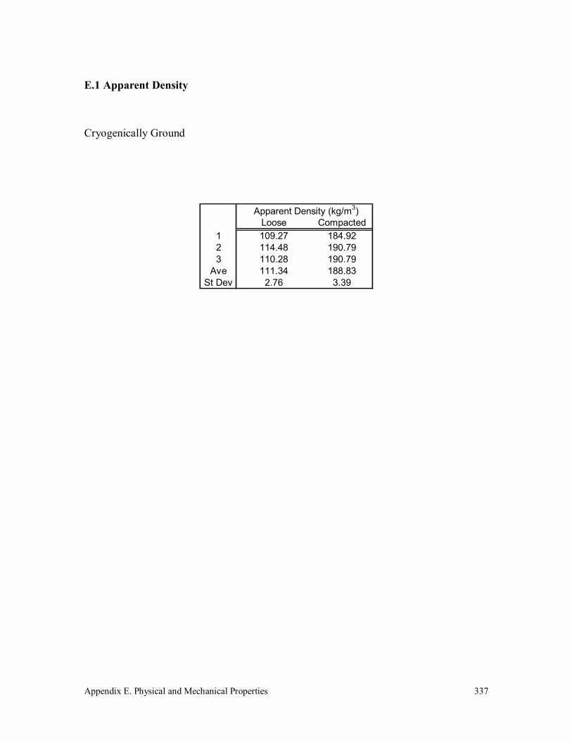
Appendix E. Physical and Mechanical Properties
337
E.1 Apparent Density
Cryogenically Ground
Loose Compacted1 109.27 184.922 114.48 190.793 110.28 190.79
Ave 111.34 188.83St Dev 2.76 3.39
Apparent Density (kg/m3)

Appendix E. Physical and Mechanical Properties
338
Spherical Particles
1 2 3 Ave St Dev20 812.21 811.51 813.37 812.36 0.9430 826.68 826.28 825.11 826.02 0.8240 834.64 831.55 833.64 833.27 1.5850 835.96 833.19 834.77 834.64 1.3960 836.81 835.94 836.25 836.33 0.4470 847.19 847.77 848.58 847.85 0.70100 908.50 905.17 906.17 906.61 1.71
Apparent Density (kg/m3)

Appendix E. Physical and Mechanical Properties
339
E.2 Dynamic Angle of Repose
20 301 35.48 33.832 34.93 32.783 35.14 31.164 34.685 32.63
Ave 35.18 33.01St Dev 0.28 1.33
Degrees
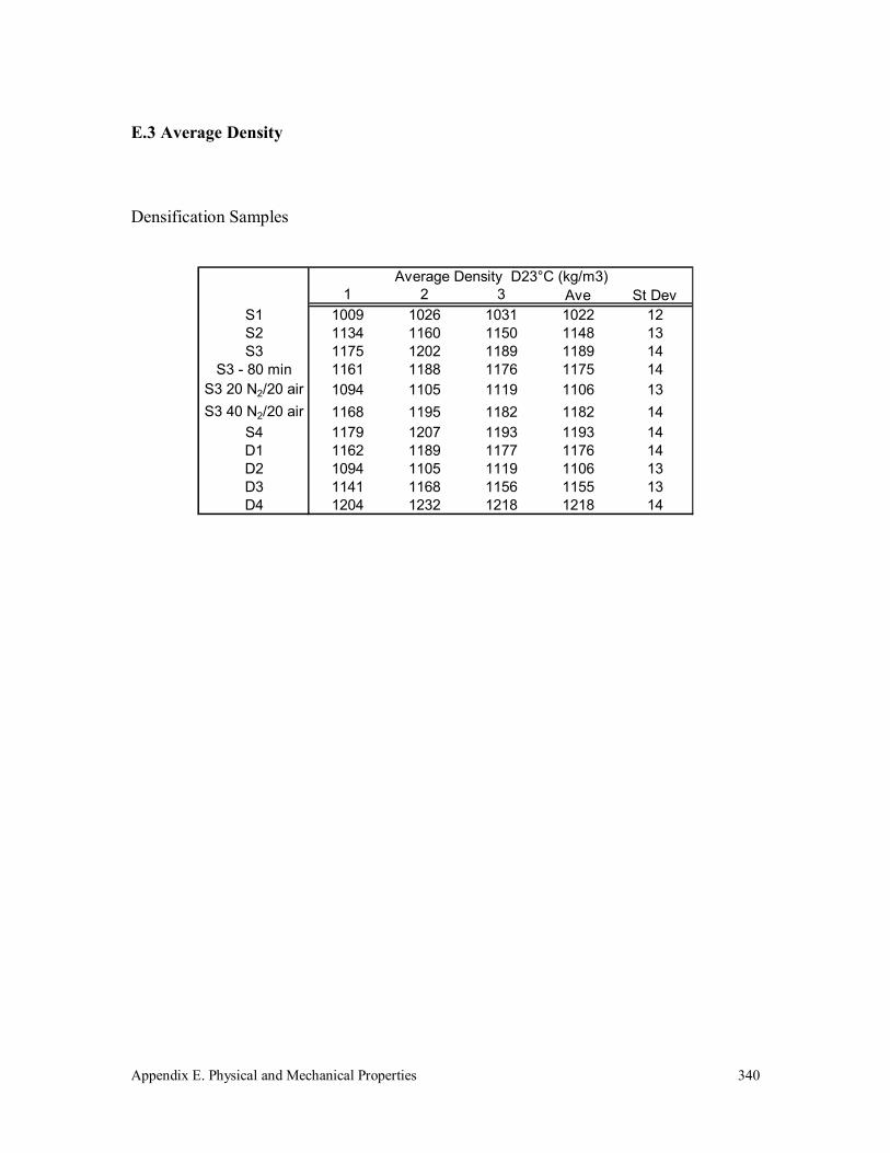
Appendix E. Physical and Mechanical Properties
340
E.3 Average Density
Densification Samples
1 2 3 Ave St DevS1 1009 1026 1031 1022 12S2 1134 1160 1150 1148 13S3 1175 1202 1189 1189 14
S3 - 80 min 1161 1188 1176 1175 14S3 20 N2/20 air 1094 1105 1119 1106 13S3 40 N2/20 air 1168 1195 1182 1182 14
S4 1179 1207 1193 1193 14D1 1162 1189 1177 1176 14D2 1094 1105 1119 1106 13D3 1141 1168 1156 1155 13D4 1204 1232 1218 1218 14
Average Density D23°C (kg/m3)
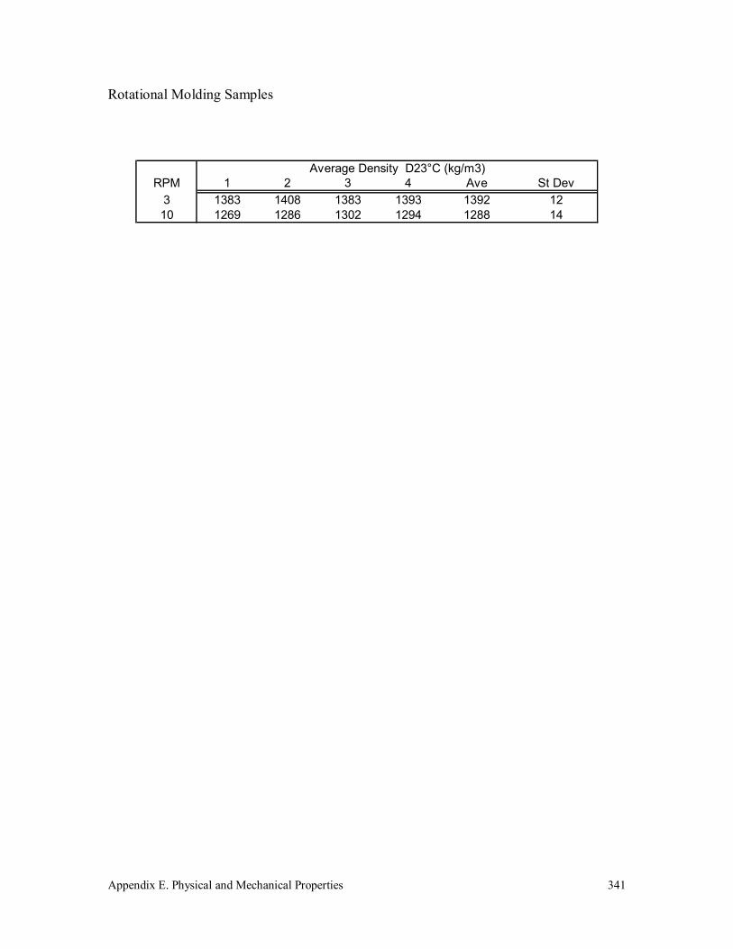
Appendix E. Physical and Mechanical Properties
341
Rotational Molding Samples
RPM 1 2 3 4 Ave St Dev3 1383 1408 1383 1393 1392 1210 1269 1286 1302 1294 1288 14
Average Density D23°C (kg/m3)
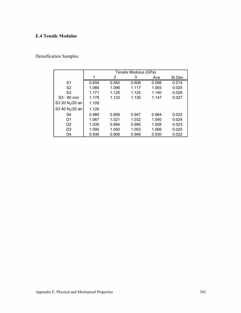
Appendix E. Physical and Mechanical Properties
342
E.4 Tensile Modulus
Densification Samples
1 2 3 Ave St DevS1 0.604 0.582 0.608 0.598 0.014S2 1.066 1.096 1.117 1.093 0.025S3 1.171 1.125 1.124 1.140 0.026
S3 - 80 min 1.178 1.133 1.130 1.147 0.027S3 20 N2/20 air 1.109S3 40 N2/20 air 1.126
S4 0.989 0.956 0.947 0.964 0.022D1 1.067 1.021 1.032 1.040 0.024D2 1.035 0.994 0.995 1.008 0.023D3 1.095 1.050 1.053 1.066 0.025D4 0.936 0.906 0.948 0.930 0.022
Tensile Modulus (GPa)

Appendix E. Physical and Mechanical Properties
343
Rotational Molding Samples
RPM 1 2 3 4 Ave St Dev3 1.97 2.03 2.02 2.01 2.01 0.0110 1.98 2.04 2.03 2.03 2.02 0.01
Tensile Modulus (GPa)
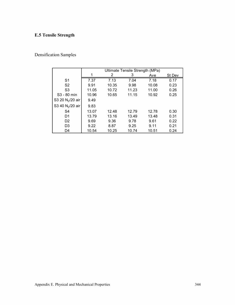
Appendix E. Physical and Mechanical Properties
344
E.5 Tensile Strength
Densification Samples
1 2 3 Ave St DevS1 7.37 7.13 7.04 7.18 0.17S2 9.91 10.35 9.98 10.08 0.23S3 11.05 10.72 11.23 11.00 0.26
S3 - 80 min 10.96 10.65 11.15 10.92 0.25S3 20 N2/20 air 9.49S3 40 N2/20 air 9.83
S4 13.07 12.48 12.79 12.78 0.30D1 13.79 13.16 13.49 13.48 0.31D2 9.69 9.36 9.78 9.61 0.22D3 9.22 8.87 9.25 9.11 0.21D4 10.54 10.25 10.74 10.51 0.24
Ultimate Tensile Strength (MPa)
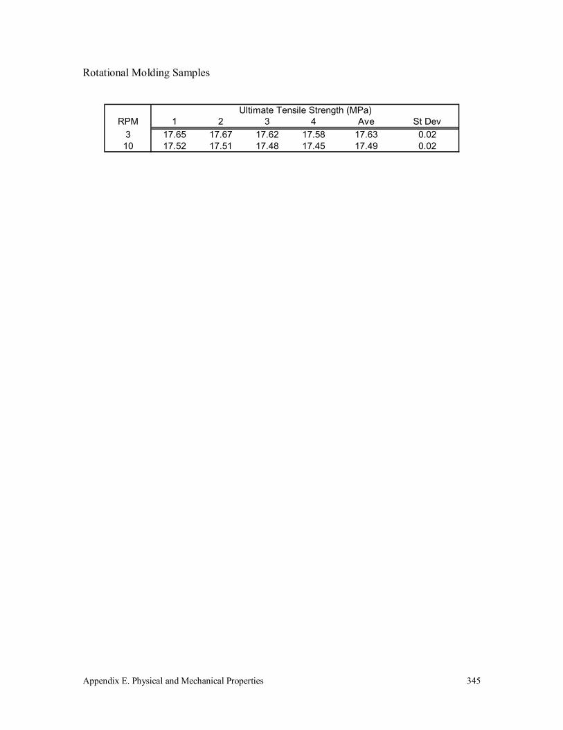
Appendix E. Physical and Mechanical Properties
345
Rotational Molding Samples
RPM 1 2 3 4 Ave St Dev3 17.65 17.67 17.62 17.58 17.63 0.0210 17.52 17.51 17.48 17.45 17.49 0.02
Ultimate Tensile Strength (MPa)

Appendix E. Physical and Mechanical Properties
346
E.6 Biaxial Rotational Molded Tank
Extended Pressurization with N2
Day Pressure (psi) Day Pressure (psi) Day Pressure (psi)
1 34.5 16 34.5 31 34.52 34 17 34.5 32 34.53 34.5 18 34 334 34.5 19 34 345 34.5 20 35 346 21 34 36 347 34 22 34 37 34.58 34.5 23 34.5 38 34.59 34.5 24 34.5 39 34.5
10 34 25 34.5 40 3411 34.5 26 41 34.512 34.5 27 4213 28 34.5 4314 34 29 34.5 44 3415 34.5 30 34.5 45 34.5
Miscellaneous Cryogenic Test Results
Pressurization with N2
Pressurization with LN2
Thermal Cycling (1000x +)
34 psi34 psino crack formation
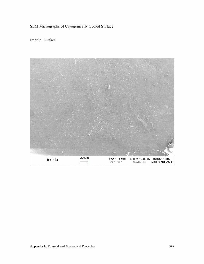
Appendix E. Physical and Mechanical Properties
347
SEM Micrographs of Cryogenically Cycled Surface
Internal Surface
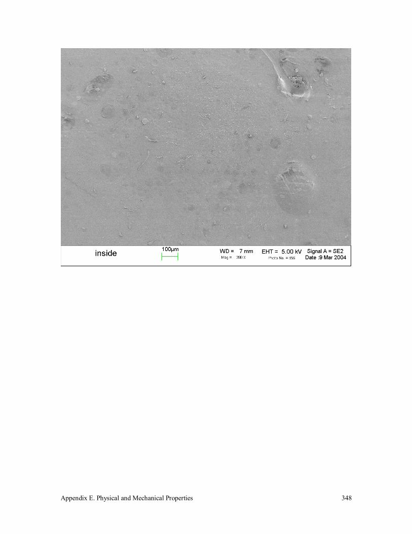
Appendix E. Physical and Mechanical Properties
348

Appendix E. Physical and Mechanical Properties
349

Appendix E. Physical and Mechanical Properties
350

Appendix E. Physical and Mechanical Properties
351
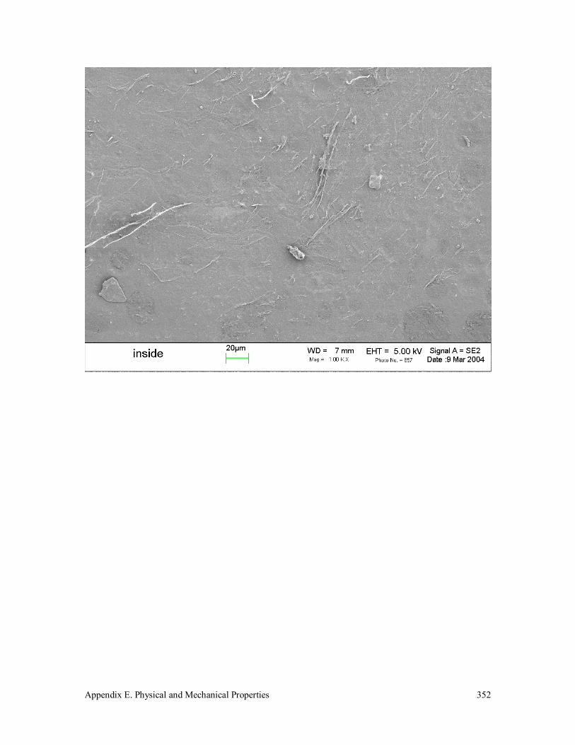
Appendix E. Physical and Mechanical Properties
352

Appendix E. Physical and Mechanical Properties
353
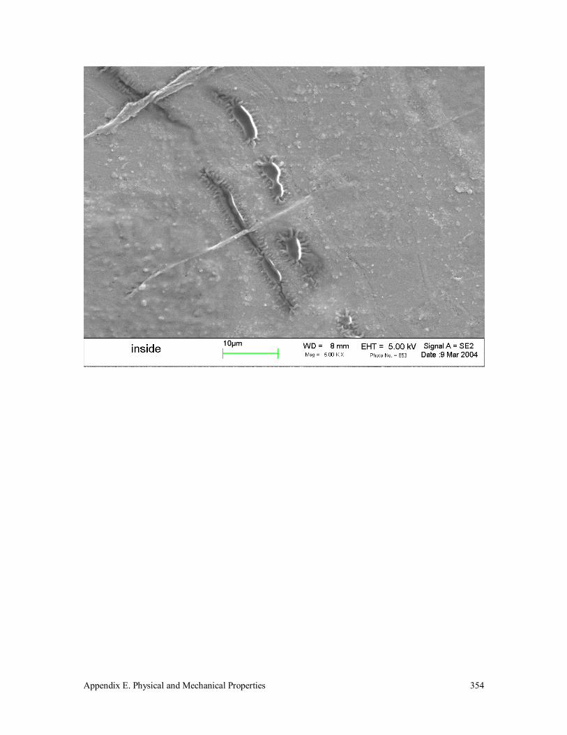
Appendix E. Physical and Mechanical Properties
354

Appendix E. Physical and Mechanical Properties
355
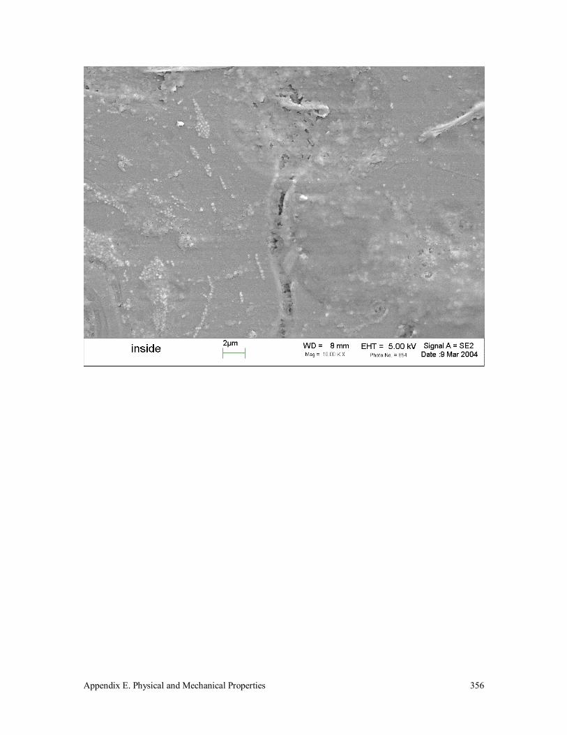
Appendix E. Physical and Mechanical Properties
356
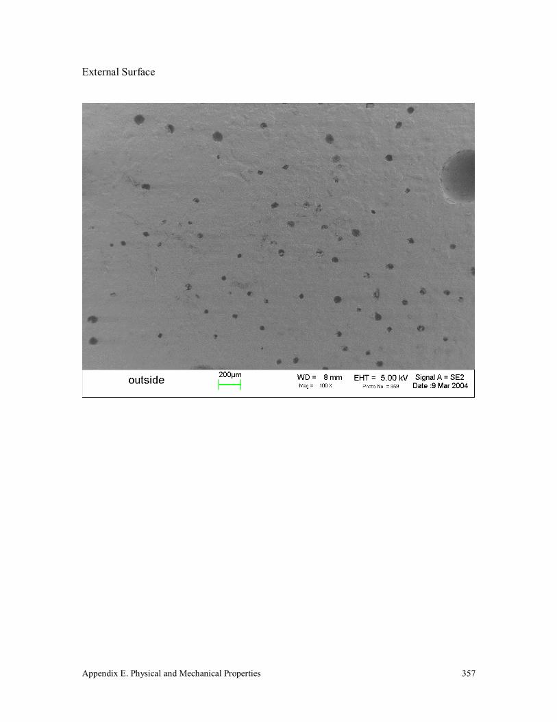
Appendix E. Physical and Mechanical Properties
357
External Surface

Appendix E. Physical and Mechanical Properties
358

Appendix E. Physical and Mechanical Properties
359
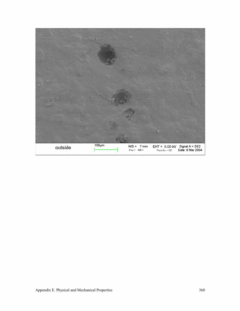
Appendix E. Physical and Mechanical Properties
360
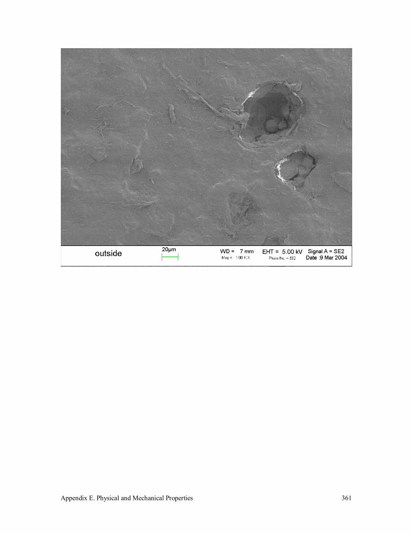
Appendix E. Physical and Mechanical Properties
361

Appendix E. Physical and Mechanical Properties
362
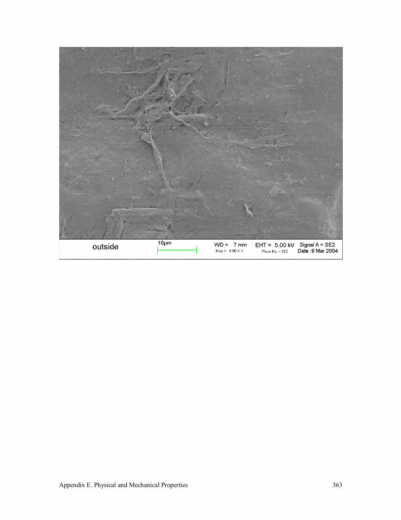
Appendix E. Physical and Mechanical Properties
363
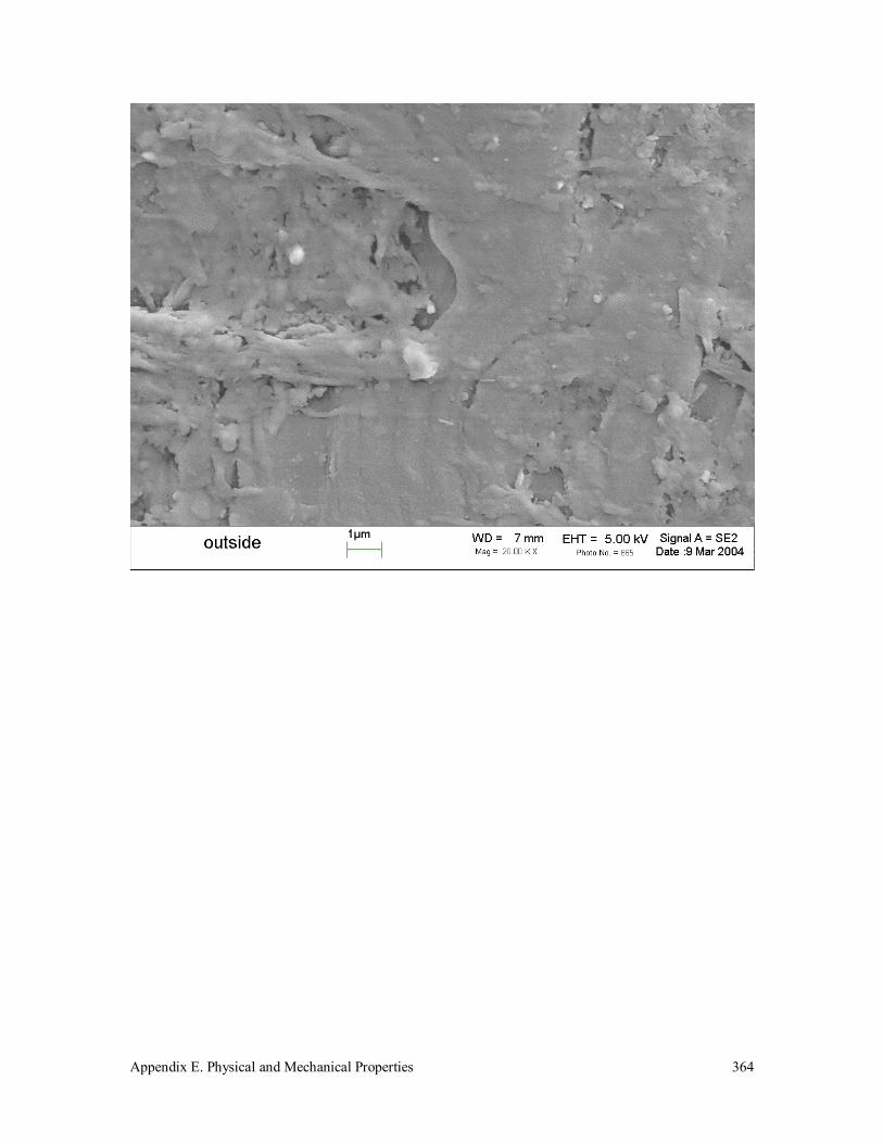
Appendix E. Physical and Mechanical Properties
364

Appendix F. Publications
365
Appendix F. Publications

Appendix F. Publications
366
Sintering of Thermotropic Liquid Crystalline Polymers
Eric Scribben and Donald Baird, Department of Chemical Engineering, Virginia Tech
Abstract
Two thermotropic liquid crystalline polymers were
evaluated for use in rotational molding: Vectra A 950 and
Vectra B 950. Material is typically prepared by grinding.
When ground, even under cryogenic conditions, TLCPs
tend to yield particles of high aspect ratio translating to
low bulk density, poor granular flow, and incomplete
densification. A process was developed to generate
spherical particles of controlled size and distribution.
Particle coalescence and densification characteristics were
determined and compared against model predictions.
Introduction and Background
Rotational molding is composed of four distinct
steps. First the material is ground then mixed to ensure a
homogenous powder exists. Next the powder is loaded
into a mold, which is rotated biaxially. In this phase, a
solid granular flow problem exists. As the material
tumbles, the mold is heated eventually causing the
particles to coalesce and adhere to the mold wall. Finally,
once densification is complete, the mold is cooled and the
solidified part is removed.
Coalescence can be divided into two steps: initial
interface bridge formation between particles, where there
is little or no change in density, and densification in
which the inter-particle cavities are eliminated [1].
Densification is a bulk effect and is modeled to account
for pore closing. Neck formation is not dependent on the
bulk powder because individual necks do not influence
each other until pores form. Hence, it is typically
modeled as the coalescence of two particles. This will be
referred to as sintering in this paper, although it is
technically the sintering of two particles.
Frenkel [2] first explored viscous sintering by
deriving an expression for the coalescence rate of two
identical spherical particles, which was corrected for
continuity by Eshelby [3]. Their model, Eq. 1, is limited
to Newtonian materials at the beginning of sintering
where the particle radius has not changed due to neck
growth. It is the result of a mechanical energy balance
between the work done by viscous forces to that presented
by the reduction of surface area due to surface tension
(see equations 2 and 3).
2
1
023
=
at
ax
ηΓ
(1)

Appendix F. Publications
367
where x is the radius of the neck between the drops, a is
the drop radius, t is time, Γ is the surface tension, and η is
the zero shear viscosity.
∫∫∫=V
v dVW γτ &: (2)
dtdSWs Γ−= (3)
where t is stress, g is the rate of strain tensor, S is surface area, and V is volume.
Some progress has been made since Frenkel proposed
his viscous sintering model. Pokluda [4] extended
Frenkel’s expression to apply to the entire sintering
process by using geometrical arguments and applying the
conservation of mass with constant density to account for
changing drop radius. Bellehumeur [5] used those
geometrical arguments and adopted the upper convected
Maxwell constitutive model (UCM) to incorporate
viscoelastic effects. However, it is doubtful that this
could capture the anisotropic nature of TLCPs.
TLCPs have numerous benefits over traditional
polymers used in processes involving sintering. They
typically possess superior mechanical properties, are
chemically resistant to corrosive liquids, and have good
barrier properties. Exploiting these advantages could
result in high performance products capable of new
applications.
Unfortunately there are several disadvantages
inhibiting their processing via sintering. Generally
sintered materials are first ground into a powder to reduce
particle size thereby increasing the driving force for
coalescence and decreasing the void fraction. Grinding
TLCPs, even under cryogenic conditions, results in high
aspect ratio particles with low bulk density. This material
cannot completely sinter under pressureless sintering
conditions. Fig. 1 is an SEM of cryogenically ground
Vectra B 950. These particles tend to aggregate causing
poor solid granular flow, which makes it nearly
impossible to rotationally mold them.
Typical deformation rates obtained from sintering
experiments are in the range of 10-2 s-1, during the early
stages, down to approximately 10-4 s-1, nearing complete
densification. This implies that the zero shear viscosity is
the relevant viscosity in this process. Some TLCPs under
appropriate conditions have been observed to contain a
viscosity increase at low deformation rates that could
effectively slow or even halt sintering prematurely.
In this paper the sintering problems associated with
TLCPs are addressed for the two selected resins. The low
shear rate rheology was evaluated to ensure that a zero
shear viscosity exists. A drop deformation technique was
used to generate spherical particles to eliminate the low
bulk density problem. These spheres were sintered and
compared to several models to assess their applicability to
the TLCP sintering process.
Experimental
Materials
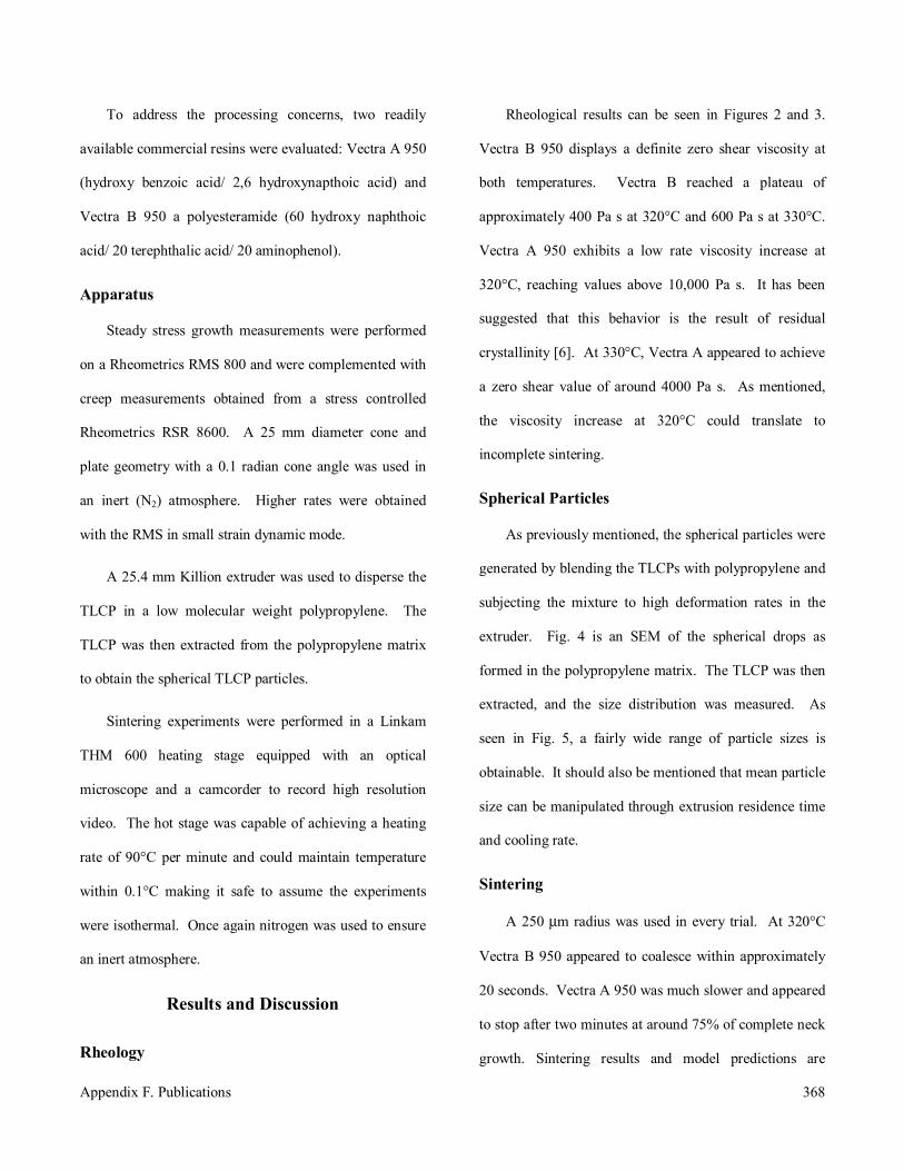
Appendix F. Publications
368
To address the processing concerns, two readily
available commercial resins were evaluated: Vectra A 950
(hydroxy benzoic acid/ 2,6 hydroxynapthoic acid) and
Vectra B 950 a polyesteramide (60 hydroxy naphthoic
acid/ 20 terephthalic acid/ 20 aminophenol).
Apparatus
Steady stress growth measurements were performed
on a Rheometrics RMS 800 and were complemented with
creep measurements obtained from a stress controlled
Rheometrics RSR 8600. A 25 mm diameter cone and
plate geometry with a 0.1 radian cone angle was used in
an inert (N2) atmosphere. Higher rates were obtained
with the RMS in small strain dynamic mode.
A 25.4 mm Killion extruder was used to disperse the
TLCP in a low molecular weight polypropylene. The
TLCP was then extracted from the polypropylene matrix
to obtain the spherical TLCP particles.
Sintering experiments were performed in a Linkam
THM 600 heating stage equipped with an optical
microscope and a camcorder to record high resolution
video. The hot stage was capable of achieving a heating
rate of 90°C per minute and could maintain temperature
within 0.1°C making it safe to assume the experiments
were isothermal. Once again nitrogen was used to ensure
an inert atmosphere.
Results and Discussion
Rheology
Rheological results can be seen in Figures 2 and 3.
Vectra B 950 displays a definite zero shear viscosity at
both temperatures. Vectra B reached a plateau of
approximately 400 Pa s at 320°C and 600 Pa s at 330°C.
Vectra A 950 exhibits a low rate viscosity increase at
320°C, reaching values above 10,000 Pa s. It has been
suggested that this behavior is the result of residual
crystallinity [6]. At 330°C, Vectra A appeared to achieve
a zero shear value of around 4000 Pa s. As mentioned,
the viscosity increase at 320°C could translate to
incomplete sintering.
Spherical Particles
As previously mentioned, the spherical particles were
generated by blending the TLCPs with polypropylene and
subjecting the mixture to high deformation rates in the
extruder. Fig. 4 is an SEM of the spherical drops as
formed in the polypropylene matrix. The TLCP was then
extracted, and the size distribution was measured. As
seen in Fig. 5, a fairly wide range of particle sizes is
obtainable. It should also be mentioned that mean particle
size can be manipulated through extrusion residence time
and cooling rate.
Sintering
A 250 µm radius was used in every trial. At 320°C
Vectra B 950 appeared to coalesce within approximately
20 seconds. Vectra A 950 was much slower and appeared
to stop after two minutes at around 75% of complete neck
growth. Sintering results and model predictions are
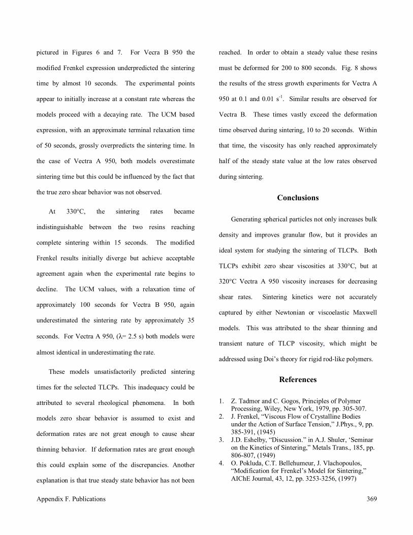
Appendix F. Publications
369
pictured in Figures 6 and 7. For Vecra B 950 the
modified Frenkel expression underpredicted the sintering
time by almost 10 seconds. The experimental points
appear to initially increase at a constant rate whereas the
models proceed with a decaying rate. The UCM based
expression, with an approximate terminal relaxation time
of 50 seconds, grossly overpredicts the sintering time. In
the case of Vectra A 950, both models overestimate
sintering time but this could be influenced by the fact that
the true zero shear behavior was not observed.
At 330°C, the sintering rates became
indistinguishable between the two resins reaching
complete sintering within 15 seconds. The modified
Frenkel results initially diverge but achieve acceptable
agreement again when the experimental rate begins to
decline. The UCM values, with a relaxation time of
approximately 100 seconds for Vectra B 950, again
underestimated the sintering rate by approximately 35
seconds. For Vectra A 950, (λ= 2.5 s) both models were
almost identical in underestimating the rate.
These models unsatisfactorily predicted sintering
times for the selected TLCPs. This inadequacy could be
attributed to several rheological phenomena. In both
models zero shear behavior is assumed to exist and
deformation rates are not great enough to cause shear
thinning behavior. If deformation rates are great enough
this could explain some of the discrepancies. Another
explanation is that true steady state behavior has not been
reached. In order to obtain a steady value these resins
must be deformed for 200 to 800 seconds. Fig. 8 shows
the results of the stress growth experiments for Vectra A
950 at 0.1 and 0.01 s-1. Similar results are observed for
Vectra B. These times vastly exceed the deformation
time observed during sintering, 10 to 20 seconds. Within
that time, the viscosity has only reached approximately
half of the steady state value at the low rates observed
during sintering.
Conclusions
Generating spherical particles not only increases bulk
density and improves granular flow, but it provides an
ideal system for studying the sintering of TLCPs. Both
TLCPs exhibit zero shear viscosities at 330°C, but at
320°C Vectra A 950 viscosity increases for decreasing
shear rates. Sintering kinetics were not accurately
captured by either Newtonian or viscoelastic Maxwell
models. This was attributed to the shear thinning and
transient nature of TLCP viscosity, which might be
addressed using Doi’s theory for rigid rod-like polymers.
References
1. Z. Tadmor and C. Gogos, Principles of Polymer
Processing, Wiley, New York, 1979, pp. 305-307. 2. J. Frenkel, “Viscous Flow of Crystalline Bodies
under the Action of Surface Tension,” J.Phys., 9, pp. 385-391, (1945)
3. J.D. Eshelby, “Discussion.” in A.J. Shuler, ‘Seminar on the Kinetics of Sintering,” Metals Trans., 185, pp. 806-807, (1949)
4. O. Pokluda, C.T. Bellehumeur, J. Vlachopoulos, “Modification for Frenkel’s Model for Sintering,” AIChE Journal, 43, 12, pp. 3253-3256, (1997)
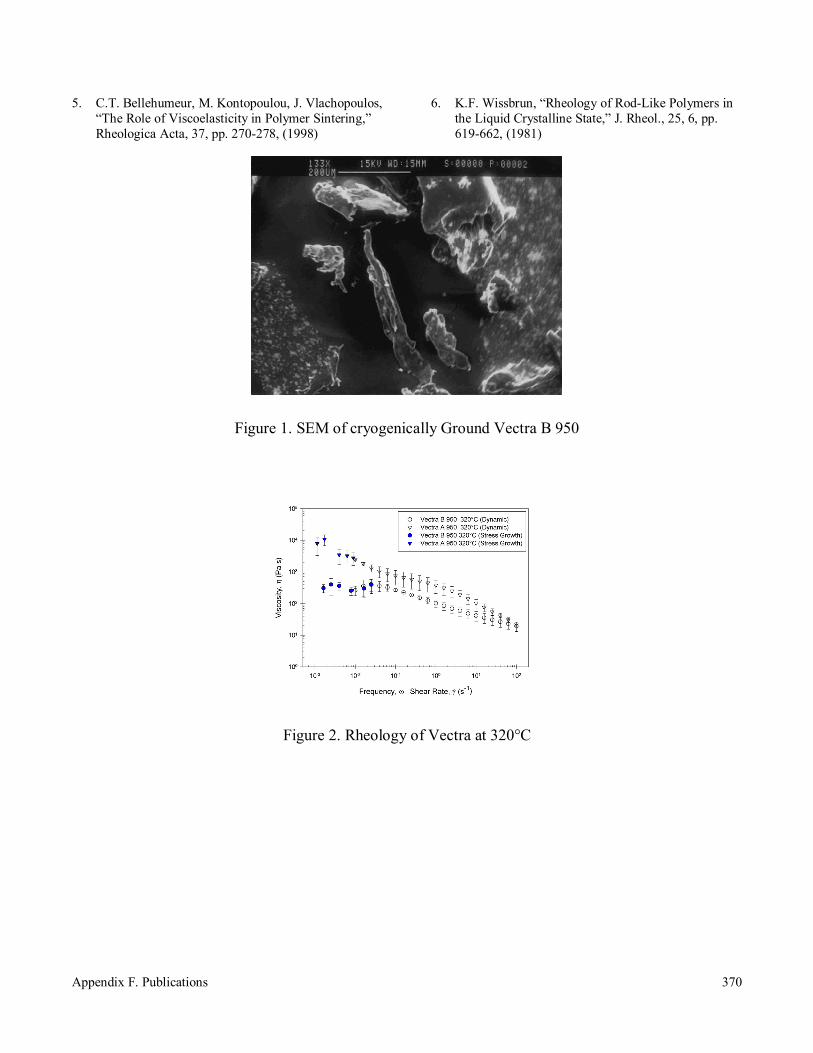
Appendix F. Publications
370
5. C.T. Bellehumeur, M. Kontopoulou, J. Vlachopoulos, “The Role of Viscoelasticity in Polymer Sintering,” Rheologica Acta, 37, pp. 270-278, (1998)
6. K.F. Wissbrun, “Rheology of Rod-Like Polymers in the Liquid Crystalline State,” J. Rheol., 25, 6, pp. 619-662, (1981)
Figure 1. SEM of cryogenically Ground Vectra B 950
Figure 2. Rheology of Vectra at 320°C
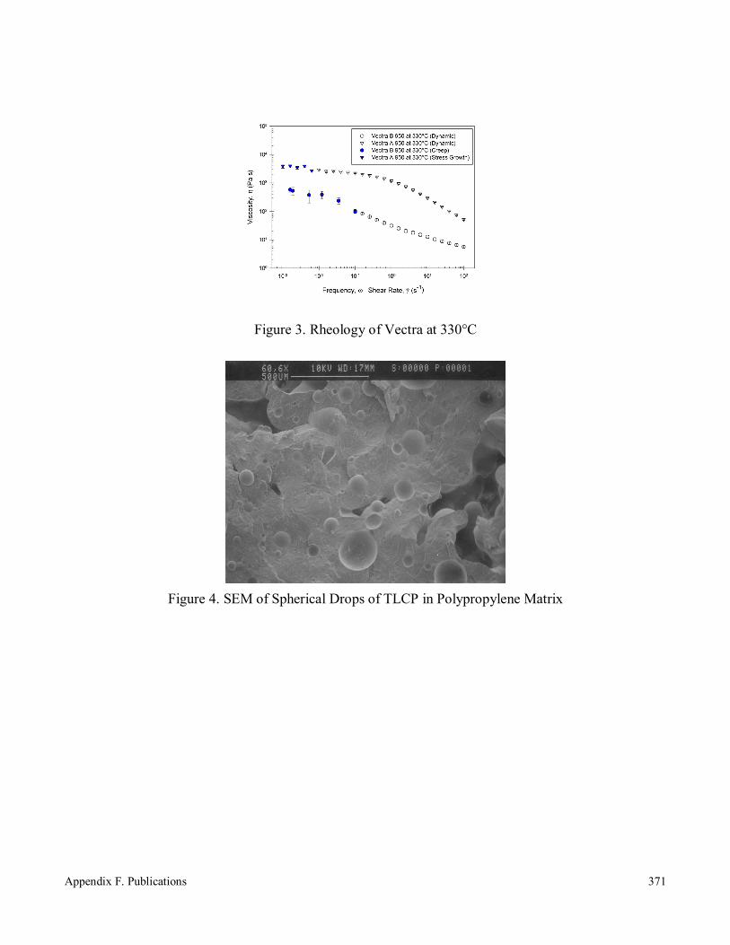
Appendix F. Publications
371
Figure 3. Rheology of Vectra at 330°C
Figure 4. SEM of Spherical Drops of TLCP in Polypropylene Matrix
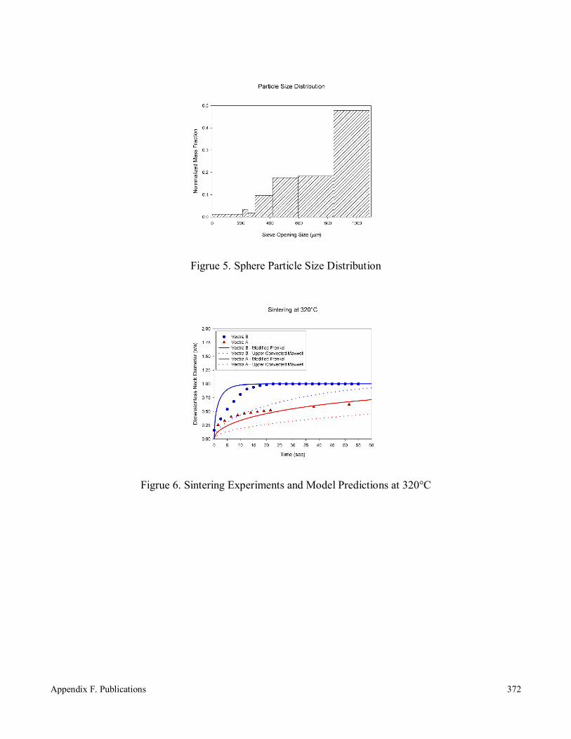
Appendix F. Publications
372
Figrue 5. Sphere Particle Size Distribution
Figrue 6. Sintering Experiments and Model Predictions at 320°C
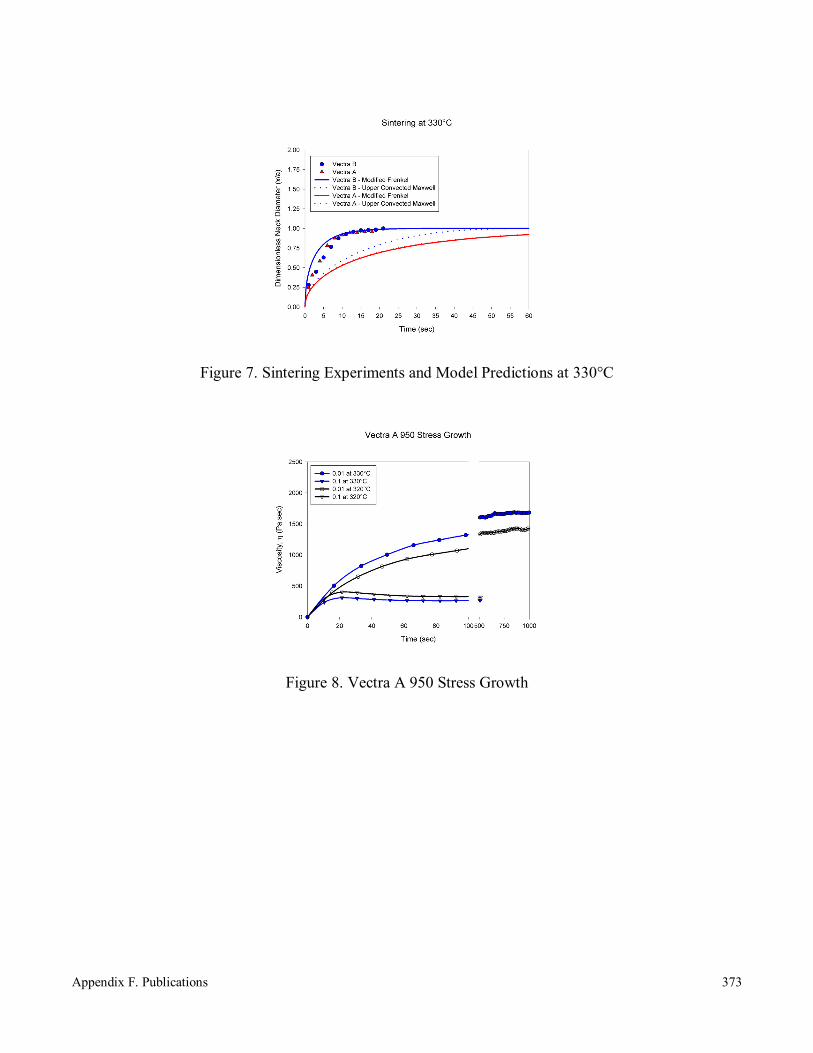
Appendix F. Publications
373
Figure 7. Sintering Experiments and Model Predictions at 330°C
Figure 8. Vectra A 950 Stress Growth

Appendix F. Publications
374
Performance of a Rotationally Molded Thermotropic Liquid Crystalline Polymer
Eric Scribben and Donald Baird, Department of Chemical Engineering, Virginia Tech
Abstract
Thermotropic liquid crystalline polymers (TLCPs)
have a number of potentially useful physical properties
for rotational molding: excellent chemical resistance,
good barrier properties, low coefficient of thermal
expansion, high tensile strength and modulus, and good
impact resistance. However, it is possible that the nature
of the molding process is such that full advantage of these
properties cannot be obtained. To determine how well
TLCPs perform when rotationally molded a commercially
available TLCP, Vectra B 950, was studied under static
conditions as well as with a single axis rotational molding
unit capable of measuring the internal air temperature.
The processing temperature was determined by measuring
shear viscosity at several temperatures. The tensile
strength and modulus of both statically molded and
rotationally molded samples were measured. Samples
were evaluated for complete densification by inspecting
the fractured surface.
Introduction and Background
Rotational molding is a process used to manufacture
hollow plastic products [1]. The process begins by
loading polymer powder into a hollow mold and then
simultaneously rotating it about two principal axes. Heat
applied to the external surface conducts to the tumbling
powder, which eventually exceeds its tack temperature
and adheres to the mold surface. While heating
continues, the powder sinters into an evenly distributed
layer and densifies as the trapped air bubbles diffuse
through the melt. The mold continues to rotate as it is
cooled, and once the plastic is sufficiently rigid the
product is removed [2].
Thermotropic liquid crystalline polymers (TLCPs)
are a class of engineering resins that offer some unique
and potentially useful properties to rotational molding.
They can have a relatively high resistance to solvents and
excellent barrier properties because of their low gas
solubility. They may be molded into structures with
extremely accurate dimensions because of their low or
negligible coefficient of thermal expansion. They are also
capable of providing high tensile strength and modulus,
which are on the order of 102MPa and 101GPa
respectively [3].
Unfortunately, some of these properties may become
a disadvantage in rotational molding. For example low
gas solubility may inhibit bubble dissolution and a
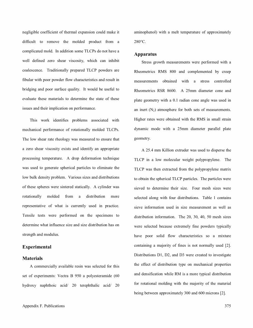
Appendix F. Publications
375
negligible coefficient of thermal expansion could make it
difficult to remove the molded product from a
complicated mold. In addition some TLCPs do not have a
well defined zero shear viscosity, which can inhibit
coalescence. Traditionally prepared TLCP powders are
fibular with poor powder flow characteristics and result in
bridging and poor surface quality. It would be useful to
evaluate these materials to determine the state of these
issues and their implication on performance.
This work identifies problems associated with
mechanical performance of rotationally molded TLCPs.
The low shear rate rheology was measured to ensure that
a zero shear viscosity exists and identify an appropriate
processing temperature. A drop deformation technique
was used to generate spherical particles to eliminate the
low bulk density problem. Various sizes and distributions
of these spheres were sintered statically. A cylinder was
rotationally molded from a distribution more
representative of what is currently used in practice.
Tensile tests were performed on the specimens to
determine what influence size and size distribution has on
strength and modulus.
Experimental
Materials
A commercially available resin was selected for this
set of experiments: Vectra B 950 a polyesteramide (60
hydroxy naphthoic acid/ 20 terephthalic acid/ 20
aminophenol) with a melt temperature of approximately
280°C.
Apparatus
Stress growth measurements were performed with a
Rheometrics RMS 800 and complemented by creep
measurements obtained with a stress controlled
Rheometrics RSR 8600. A 25mm diameter cone and
plate geometry with a 0.1 radian cone angle was used in
an inert (N2) atmosphere for both sets of measurements.
Higher rates were obtained with the RMS in small strain
dynamic mode with a 25mm diameter parallel plate
geometry.
A 25.4 mm Killion extruder was used to disperse the
TLCP in a low molecular weight polypropylene. The
TLCP was then extracted from the polypropylene matrix
to obtain the spherical TLCP particles. The particles were
sieved to determine their size. Four mesh sizes were
selected along with four distributions. Table 1 contains
sieve information used in size measurement as well as
distribution information. The 20, 30, 40, 50 mesh sizes
were selected because extremely fine powders typically
have poor solid flow characteristics so a mixture
containing a majority of fines is not normally used [2].
Distributions D1, D2, and D3 were created to investigate
the effect of distribution type on mechanical properties
and densification while RM is a more typical distribution
for rotational molding with the majority of the material
being between approximately 300 and 600 microns [2].

Appendix F. Publications
376
The eight samples were statically sintered into tensile
bars and tested. All tensile bars were sintered in a 1.27cm
× 6.35cm mold with an exposed top surface and a
thermocouple fixed in the center of the side wall.
Nitrogen was supplied through a chamber that covered the
mold. The entire unit was placed in a pre-heated hot
press. The heating soak time was 40 minutes and began
once the maximum temperature (320°C) was reached.
The sintered bars were tested with an Instron 4202 using a
crosshead speed of 1.27mm/min and a 30.5mm gauge
length to determine strength and Young’s modulus
according to ASTM Standard D638-01.
Rotational molding was done using the distribution
RM with a single axis lab scale device. The mold was a
stainless steel cylinder with a 3.81cm diameter and
7.62cm long. Both ends were capped. One end was fixed
to a shaft that was driven by an electric motor rotating at
10rpm. The other cap had an opening so that a
thermocouple could be installed to monitor the air
temperature within the mold. Heat was provided by a
convection oven equipped with a nitrogen purge and
capable of heating rates up to 60°C per minute. The
heating cycle was designed to mimic the static sintering
conditions. The molded product was then sectioned and
strips were used for tensile measurements.
Results and Discussion Rheology
Results from the rheological tests are shown in
Figure 1. Vectra B 950 displays a zero shear viscosity at
both temperatures, but rate independence occurs at 400 Pa
sec at 320°C and 600 Pa sec at 330°C. Results for
temperatures below 320°C are not reproducible, behavior
that can be attributed to varying amounts of residual
crystallinity [4]. Since the viscosity at 320°C is less than
at 330°C and lower temperatures contain residual
crystallinity 320°C was selected as the processing
temperature.
Statically Sintered Tensile Properties
The results from the tensile measurements are
summarized in Table 2. No clear relationship between
size or size distribution and modulus was found.
Excluding the 20 mesh sample, all moduli were within
standard deviation of each other. Therefore, it is
reasonable to assume that the modulus remained constant
with a mean of 1.03GPa. The 20 mesh sample should not
be completely disregarded. It would be useful to
understand why its modulus is almost half of the other
samples. The 1.03GPa mean is also significantly below
the 20GPa that is possible with good molecular alignment
[3].
Possible causes for these discouraging results could
be insufficient global molecular alignment. Although this
may be part of the reason, it cannot completely account
for the problem, since poorly oriented samples have
moduli around 2.5GPa [3]. It could possibly be attributed
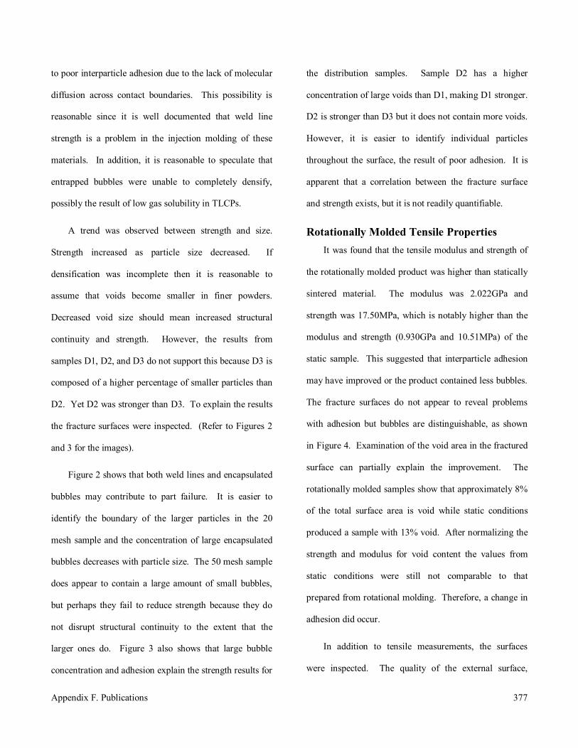
Appendix F. Publications
377
to poor interparticle adhesion due to the lack of molecular
diffusion across contact boundaries. This possibility is
reasonable since it is well documented that weld line
strength is a problem in the injection molding of these
materials. In addition, it is reasonable to speculate that
entrapped bubbles were unable to completely densify,
possibly the result of low gas solubility in TLCPs.
A trend was observed between strength and size.
Strength increased as particle size decreased. If
densification was incomplete then it is reasonable to
assume that voids become smaller in finer powders.
Decreased void size should mean increased structural
continuity and strength. However, the results from
samples D1, D2, and D3 do not support this because D3 is
composed of a higher percentage of smaller particles than
D2. Yet D2 was stronger than D3. To explain the results
the fracture surfaces were inspected. (Refer to Figures 2
and 3 for the images).
Figure 2 shows that both weld lines and encapsulated
bubbles may contribute to part failure. It is easier to
identify the boundary of the larger particles in the 20
mesh sample and the concentration of large encapsulated
bubbles decreases with particle size. The 50 mesh sample
does appear to contain a large amount of small bubbles,
but perhaps they fail to reduce strength because they do
not disrupt structural continuity to the extent that the
larger ones do. Figure 3 also shows that large bubble
concentration and adhesion explain the strength results for
the distribution samples. Sample D2 has a higher
concentration of large voids than D1, making D1 stronger.
D2 is stronger than D3 but it does not contain more voids.
However, it is easier to identify individual particles
throughout the surface, the result of poor adhesion. It is
apparent that a correlation between the fracture surface
and strength exists, but it is not readily quantifiable.
Rotationally Molded Tensile Properties
It was found that the tensile modulus and strength of
the rotationally molded product was higher than statically
sintered material. The modulus was 2.022GPa and
strength was 17.50MPa, which is notably higher than the
modulus and strength (0.930GPa and 10.51MPa) of the
static sample. This suggested that interparticle adhesion
may have improved or the product contained less bubbles.
The fracture surfaces do not appear to reveal problems
with adhesion but bubbles are distinguishable, as shown
in Figure 4. Examination of the void area in the fractured
surface can partially explain the improvement. The
rotationally molded samples show that approximately 8%
of the total surface area is void while static conditions
produced a sample with 13% void. After normalizing the
strength and modulus for void content the values from
static conditions were still not comparable to that
prepared from rotational molding. Therefore, a change in
adhesion did occur.
In addition to tensile measurements, the surfaces
were inspected. The quality of the external surface,

Appendix F. Publications
378
surface in contact with the mold, was much worse than
the internal surface. Pitholes were not found on the
internal surface but the external surface did contain a
significant amount of them. This undesirable defect can
be seen in Figure 5. The size of the pitholes could be
decreased by reducing particle size, but it was unable to
completely eliminate them.
Despite the bubbles reducing the strength and
modulus and the pitholes being a cosmetic deterrent to
rotational molding, the rotationally molded LCP did
exhibit notable mechanical properties. The tensile
modulus was comparable to that of crosslinked high
density polyethylene, which is nominally 17.9 MPa for
industrially produced tanks [5].
Conclusions
It was found that modulus was not affected by
particle size or size distribution under static conditions.
The modulus was higher when the material was
rotationally molded. Strength decreased with increasing
particle size and was also improved when rotationally
molded. Although these results can be explained by
interparticle adhesion and bubble content, precisely how
much each contributed could not be determined. It was
also found that porosity decreased and adhesion
increased, in comparison to static results, when the
material was rotationally molded. The surface of the
cylinder contained a significant amount of pitholes.
References 7. Crawford, R.J., Throne, J.L., Rotational Molding
Technology, Plastics Design Library, William Andrew Publishing, Norwich, New York, 2002.
8. Kliene, R.I.,‘Rotational Moulding of Polyethylene’ in Rotational Moulding of Plastics second edition, ed. Crawford, R.J., John Wiley & Sons inc. New York, 1996, pp.32-61.
9. Sawyer, L., Shepherd, J., Kaslusky, A., Knudsen, R., Tech Spotlight: Unfilled liquid crystalline polymers, [Online], Available: http://www.ticona-us.com/literature/documents/LCP_Article_01_351res72dpi.PDF, June, 2001.
10. Wissbrun, K.F., “Rheology of Rod-Like Polymers in the Liquid Crystalline State,” J. Rheol., 25, 6, 1981, pp. 619-662.
11. High Density Crosslinked Polyethylene (HDXLPE) Storage Tanks, [Online], Available: http://www.polyprocessing.com/updates/GenSpecrev2-HDXLPE.pdf
Key Words Rotational molding, LCP, mechanical properties
Table 1. Sieve and Distribution Sizes
Sieve Size Gap Opening (microns) D1 D2 D3 RM20 840 0.07 0.53 0.10 0.00330 595 0.13 0.27 0.40 0.07640 420 0.27 0.13 0.40 0.47650 297 0.53 0.07 0.10 0.39360 250 - - - 0.01670 210 - - - 0.019
100 149 - - - 0.012Pan - - - - 0.004
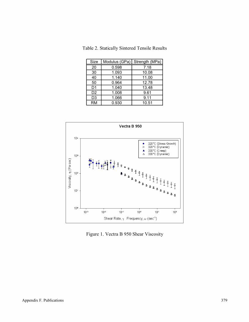
Appendix F. Publications
379
Table 2. Statically Sintered Tensile Results
Size Modulus (GPa) Strength (MPa)20 0.598 7.1830 1.093 10.0840 1.140 11.0050 0.964 12.78D1 1.040 13.48D2 1.008 9.61D3 1.066 9.11RM 0.930 10.51
Figure 1. Vectra B 950 Shear Viscosity

Appendix F. Publications
380
Figure 2. Fracture Surfaces of 20, 30, 40, and 50 Mesh Tensile Bars
Figure 3. Fracture Surfaces of Tensile Bars

Appendix F. Publications
381
Figure 4. Fracture Surfaces of Rotationally Molded Cylinder
Figure 5. External Surface of RM Cylinder

Vita
382
Vita
The author was born in Ashtabula, Ohio on August 23, 1976. After graduating from
Pymatuning Valley High School (Andover, Ohio) in the Spring of 1994, he attended The Ohio
State University to pursue a Bachelor of Science degree in Chemical Engineering. His
undergraduate education was supplemented with work experiences at Koch Materials, Kohler
Company, Battelle Memorial Institute, and an undergraduate honors research project in polymer
processing under the direction of Dr. Kurt Koelling. Upon graduation, the author to begin his
gradute studies at Virginia Polytechnic Institute and State University in August, 1999. Presently,
he is a candidate for the Doctor of Philosphy degree in Chemical Engineering under the direction
of Dr. Donald G. Baird.
Eric Scribben
Related Documents