Selection between models through multi-step-ahead forecasting

Report Issued: January 28, 2010 Disclaimer: This report is released to inform interested parties of research and to encourage discussion. The views expressed are those of the authors and not necessarily those of the U.S. Census Bureau

RESEARCH REPORT SERIES (Statistics #2010-01)

Selection Between Models Through

Multi-Step-Ahead Forecasting

Tucker S. McElroy David F. Findley

Statistical Research Division U.S. Census Bureau

Washington, D.C. 20233

Selection Between Models Through Multi-Step-Ahead Forecasting

Tucker S. McElroya and David F. Findleya,b

U.S. Census Bureau

Abstract

We present and show applications of two new test statistics for deciding if one ARIMA model

provides significantly better h -step-ahead forecasts than another, as measured by the difference

of approximations to their asymptotic mean square forecast errors. The two statistics differ in

the variance estimate whose square root is the statistic’s denominator. Both variance estimates

are consistent even when the ARMA components of the models considered are incorrect. Our

principal statistic’s variance estimate accounts for parameter estimation. Our simpler statistic’s

variance estimate treats parameters as fixed. The broad consistency properties of these estimates

yield improvements to what are known as tests of Diebold and Mariano (1995) type. These are

tests whose variance estimates treat parameters as fixed and are generally not consistent in our

context.

We describe how the new test statistics can be calculated algebraically for any pair of ARIMA

models with the same differencing operator. Our size and power studies demonstrate their

superiority over the Diebold-Mariano statistic. The power study and the empirical study also

reveal that, in comparison to treating estimated parameters as fixed, accounting for parameter

estimation can increase power and can yield more plausible model selections for some time series

in standard textbooks.

a Statistical Research Division, U.S. Census Bureau, 4600 Silver Hill Road, Washington, D.C.

20233-9100b Corresponding author. E-mail address: [email protected]

Keywords. ARIMA models; Diebold-Mariano tests; Incorrect models; Misspecified models;

Model selection; Parameter estimation effects; Time series

Disclaimer. This paper is released to inform about ongoing research and to encourage discussion.

The views expressed are those of the authors and not necessarily those of the U.S. Census Bureau.

1 Introduction

In this article, we make several contributions to the technology of testing whether two not necessarily

correct time series models for an observed series have equal or differing h-step-ahead forecasting

1

ability as assessed by estimates of mean square h-step forecast error. This work is in the tradition of

Meese and Rogoff (1988), Findley (1990, 1991a), Diebold and Mariano (1995) and Rivers and Vuong

(2002). Our focus is on nonstationary ARIMA models, a type of model not considered in this earlier

work. Our specific approach is derived from the goodness-of-fit testing methodology of McElroy and

Holan (2009) with modifications to account for the consideration of more than one model and other

features of the forecast comparison setting. We account for effects of parameter estimation, which

only Rivers and Vuong (2002) do among the forecasting papers cited. In contrast to Rivers and

Vuong, we provide explicit formulas for the asymptotic variance of our statistic (corresponding to

the σ2n quantity of their Assumption 7), as well as an explicit consistent estimator of this variance.

Also, our assumptions are more basic and therefore more transparent. These same advantages

apply in relation to the results of West (1996), which also account for parameter estimation but are

focused on out-of-sample forecasting, from a perspective more connected with regression models.

Our tests, like those of the papers other than West’s, are tests of in-sample forecast performance.

The approximation relation between our measure of model forecast performance (8) and the

more customary average of squared forecast errors over the sample is derived in Section 2.1, after

a review of some relevant aspects of ARIMA model forecasting. The central theoretical results

of the paper are presented in Section 2.3, whose Theorem 1 provides the CLT and consistent

estimator of its variance needed for our main test statistic (12). Section 2.4 presents results for the

situation in which parameter estimation uncertainty is ignored, i.e., when estimated parameters

are treated as constant. Here our consistent variance estimate simplifies, becoming reasonably

straightforward to calculate for all ARIMA models, and is also applicable to the ARIMA model

case of the test commonly referred to as the test of Diebold and Mariano (1995). For this test, it

provides a consistent alternative to the customary variance estimate, which is consistent only in

effectively correct model situations. With h = 1, it also provides a consistent variance estimate,

which had been lacking, for the time series generalization in Findley (1990) of the non-nested model

comparison test statistic of Vuong (1989).

In Section 3, after explaining why the size study of Diebold and Mariano (1995) is invalid, we

present size and power studies of our test statistics and the Diebold-Mariano statistic together with

an empirical study of the application of all three statistics to competing models for series from Box,

Jenkins and Reinsel (1994) and Brockwell and Davis (2002). The size and power studies favor

both of our new test statistics over the Diebold-Mariano statistic. All of the studies favor most our

statistic that accounts for parameter estimation.

The Appendix contains proofs and the derivations of some formulas, including auxiliary formulas

for algebraically computing the variance estimate that accounts for parameter uncertainty.

2

2 Methodology

We are interested in comparing two competing models’ h-step-ahead forecasts of data from a time

series Yt which, if nonstationary, can be made stationary by application of a differencing operator,

i.e., a backshift operator polynomial δ (B) whose zeroes have unit magnitude. As usual, B denotes

the backshift (or lag) operator, with BXt = Xt−1. To simplify the exposition, the stationary series

Wt = δ (B)Yt is assumed to be Gaussian, an assumption that can be weakened moderately. It is also

assumed to be purely nondeterministic. Thus its spectral density f is log integrable and generates

its autocovariances via γj(f) = (2π)−1 ∫ π−π f(λ)eijλ dλ, a formula that shows our convention with

the constant 2π. The matrix of autocovariances is denoted Γ(f), i.e. Γjk(f) = γj−k(f). The

dimension of Γ(f) is equal to the number of Wt = δ (B) Yt calculable from the observed Yt.

2.1 Multi-Step-Ahead Forecasting

We start by reviewing some basic forecasting results for nonstationary Yt. Beyond basic formulas,

the key results obtained are two concerning asymptotic properties of forecast error measures, (6)

and (7).

Let δ(z) = 1 +∑d

j=1 δjzj be the differencing operator such that Wt = δ(B)Yt and let Yt,

1 − d ≤ t ≤ n denote the available data. Set τ(z) = 1/δ(z) expressed as a power series in |z| < 1

with coefficients τj . Thus τj = 1 for j = 0 and τj = −∑j−1i=0 τiδj−i for j > 0. For any 1 ≤ h < n

and any 1 ≤ t ≤ n− h, we have Yt+h = [τ ]h−10 (B)Wt+h +

∑d−1j=0 cj,hYt−j , where the coefficients cj,h

depend only on the coefficients of δ (z), see Bell (1984, p. 650). The bracket notation means that

the power series is truncated to powers of B between zero and h− 1. Forecasts Yt+h|t of Yt+h from

Ys, 1−d ≤ s ≤ t are obtained from forecasts Wt+h−j|t, 0 ≤ j ≤ h−1 of Wt+h−j from Ws, 1 ≤ s ≤ t

by way of

Yt+h|t =h−1∑

j=0

τjWt+h−j|t +d−1∑

j=0

cj,hYt−j . (1)

Consequently, the forecast errors are given by Yt+h − Yt+h|t =∑h−1

j=0 τj

(Wt+h−j − Wt+h−j|t

).

To motivate our performance measure, we will use the forecast Wt+h|t obtained by truncating

the filter for the forecast Wt+h|t of Wt+h from the infinite past Ws, −∞ < s ≤ t. The latter

forecast is given by Wt+h|t =∑

j≥0 ψj+hBjΨ(B)−1Wt, where Ψ(z) =∑

j≥0 ψjzj with ψ0 = 1

has the coefficients of the innovations (Wold, MA(∞)) representation Wt =∑

j≥0 ψjεt−j with εt

the error of the mean square optimal forecast of Wt from Ws, s < t. Since Wt+h − Wt+h|t =

[Ψ]h−10 (B)Ψ−1(B)Wt+h = [Ψ]h−1

0 (B)εt+h, this forecast error is a moving average process of order

3

(at most) h−1, as is also the error process of the forecasts Yt+h|t =∑h−1

j=0 τjWt+h−j|t+∑d−1

j=0 cj,hYt−j ,

Yt+h − Yt+h|t =h−1∑

j=0

τj

(Wt+h−j −Wt+h−j|t

)

=h−1∑

j=0

τjBj [Ψ]h−1−j

0 (B)Ψ−1(B)Wt+h (2)

=h−1∑

j=0

τjBj [Ψ]h−1−j

0 (B)εt+h,

where the backshift operators Bj operate on the t index.

The truncated filter forecast Wt+h|t and its error Wt+h − Wt+h|t are obtained from the infinite

past formulas given above by setting Wt−j = 0 for j ≥ t. Denoting the filter in (2) by

η(h) (B) =

h−1∑

j=0

τjBj [Ψ]h−1−j

0 (B)

Ψ−1(B), (3)

it follows that, for the associated forecast Yt|t−h of Yt, the error process ε(h)t = Yt− Yt|t−h is given by

ε(h)t = η(h) (B) Wt, Wt−j = 0, j ≥ t

=t−1∑

j=0

η(h)j Wt−j , t ≥ 1. (4)

Now we generalize the notation to let Ψ (B) in (3) denote the innovations filter of a not nec-

essarily correct model for Wt, the log of whose continuous spectral density is integrable. This

condition guarantees the existence of a (unique) continuous Ψ(e−iλ

)= 1 +

∑∞j=1 ψje

−ijλ satisfy-

ing∫ π−π log

∣∣Ψ (e−iλ

)∣∣ dλ = 0 and such that the model spectral density is equal to σ2∣∣Ψ (

e−iλ)∣∣2

for some σ2 > 0, see Theorem VII of Pourahmadi (2001, p. 68). (For an ARMA model con-

sidered for Wt, Ψ(B) has the form Ψ(B) = Ω (B) Ξ−1 (B), where Ξ (B) is the AR polynomial

and Ω (B) is the MA polynomial with no zeroes of magnitude less than one.) The only fur-

ther requirement on the model is∫ π−π |Ψ(e−iλ)|−2

f (λ) dλ < ∞, to ensure that its infinite past

(quasi)innovations εt = Ψ (B)−1 Wt for Wt are defined. Unless the true spectral density is given by

f (λ) = σ2∣∣Ψ (

e−iλ)∣∣2 for some σ2 > 0, then the series εt will not be white noise and

∑h−1j=0 τjB

jεt

will generally not be a moving average process of order h− 1.

One measure commonly used to evaluate the h-step forecast performance of a model is the

average of squared forecast errors n−1∑n

t=1 [ε(h)t ]

2, where now we let ε

(h)t denote the forecast error

either from the truncated predictor or from the standard finite-past predictor discussed, for example,

in Section 3.3.1 of Findley, Potscher and Wei (2004). With either predictor, for an invertible ARIMA

model, Proposition 4.1 of Findley (1991a) shows, under the assumption∞∑

j=−∞

(21/2 + |j|1/2

) ∣∣∣γj(f)∣∣∣ < ∞. (5)

4

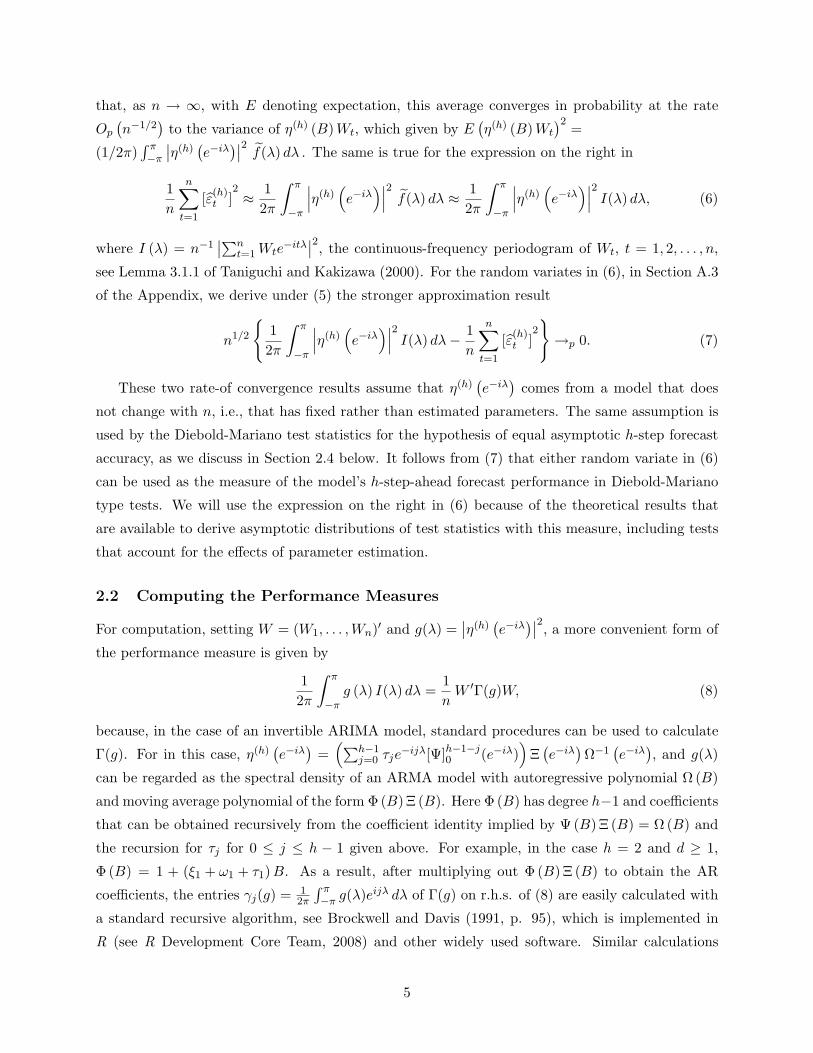
that, as n → ∞, with E denoting expectation, this average converges in probability at the rate

Op

(n−1/2

)to the variance of η(h) (B) Wt, which given by E

(η(h) (B) Wt

)2=

(1/2π)∫ π−π

∣∣η(h)(e−iλ

)∣∣2 f(λ) dλ . The same is true for the expression on the right in

1n

n∑

t=1

[ε(h)t ]

2 ≈ 12π

∫ π

−π

∣∣∣η(h)(e−iλ

)∣∣∣2

f(λ) dλ ≈ 12π

∫ π

−π

∣∣∣η(h)(e−iλ

)∣∣∣2I(λ) dλ, (6)

where I (λ) = n−1∣∣∑n

t=1 Wte−itλ

∣∣2, the continuous-frequency periodogram of Wt, t = 1, 2, . . . , n,

see Lemma 3.1.1 of Taniguchi and Kakizawa (2000). For the random variates in (6), in Section A.3

of the Appendix, we derive under (5) the stronger approximation result

n1/2

12π

∫ π

−π

∣∣∣η(h)(e−iλ

)∣∣∣2I(λ) dλ− 1

n

n∑

t=1

[ε(h)t ]

2

→p 0. (7)

These two rate-of convergence results assume that η(h)(e−iλ

)comes from a model that does

not change with n, i.e., that has fixed rather than estimated parameters. The same assumption is

used by the Diebold-Mariano test statistics for the hypothesis of equal asymptotic h-step forecast

accuracy, as we discuss in Section 2.4 below. It follows from (7) that either random variate in (6)

can be used as the measure of the model’s h-step-ahead forecast performance in Diebold-Mariano

type tests. We will use the expression on the right in (6) because of the theoretical results that

are available to derive asymptotic distributions of test statistics with this measure, including tests

that account for the effects of parameter estimation.

2.2 Computing the Performance Measures

For computation, setting W = (W1, . . . , Wn)′ and g(λ) =∣∣η(h)

(e−iλ

)∣∣2, a more convenient form of

the performance measure is given by

12π

∫ π

−πg (λ) I(λ) dλ =

1n

W ′Γ(g)W, (8)

because, in the case of an invertible ARIMA model, standard procedures can be used to calculate

Γ(g). For in this case, η(h)(e−iλ

)=

(∑h−1j=0 τje

−ijλ[Ψ]h−1−j0 (e−iλ)

)Ξ

(e−iλ

)Ω−1

(e−iλ

), and g(λ)

can be regarded as the spectral density of an ARMA model with autoregressive polynomial Ω (B)

and moving average polynomial of the form Φ (B) Ξ (B). Here Φ (B) has degree h−1 and coefficients

that can be obtained recursively from the coefficient identity implied by Ψ (B) Ξ (B) = Ω (B) and

the recursion for τj for 0 ≤ j ≤ h − 1 given above. For example, in the case h = 2 and d ≥ 1,

Φ (B) = 1 + (ξ1 + ω1 + τ1) B. As a result, after multiplying out Φ (B) Ξ (B) to obtain the AR

coefficients, the entries γj(g) = 12π

∫ π−π g(λ)eijλ dλ of Γ(g) on r.h.s. of (8) are easily calculated with

a standard recursive algorithm, see Brockwell and Davis (1991, p. 95), which is implemented in

R (see R Development Core Team, 2008) and other widely used software. Similar calculations

5

are used to compute our consistent variance alternative for Diebold-Mariano statistics derived in

Section 2.4 and the asymptotic variances used to analyze the power study results in Section 3.2.

For the finite-past forecasts, n−1∑n

t=1 [ε(h)t ]

2can be computed from τj , 0 ≤ j ≤ h − 1 and the

covariance matrix of the ARMA model, see (3.13)–(3.15) of Findley, Potscher and Wei (2004).

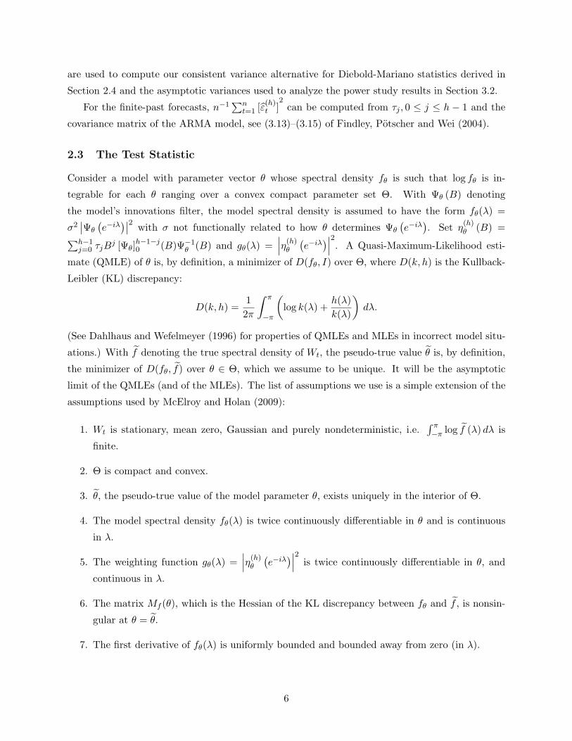
2.3 The Test Statistic

Consider a model with parameter vector θ whose spectral density fθ is such that log fθ is in-

tegrable for each θ ranging over a convex compact parameter set Θ. With Ψθ (B) denoting

the model’s innovations filter, the model spectral density is assumed to have the form fθ(λ) =

σ2∣∣Ψθ

(e−iλ

)∣∣2 with σ not functionally related to how θ determines Ψθ

(e−iλ

). Set η

(h)θ (B) =

∑h−1j=0 τjB

j [Ψθ]h−1−j0 (B)Ψ−1

θ (B) and gθ(λ) =∣∣∣η(h)

θ

(e−iλ

)∣∣∣2. A Quasi-Maximum-Likelihood esti-

mate (QMLE) of θ is, by definition, a minimizer of D(fθ, I) over Θ, where D(k, h) is the Kullback-

Leibler (KL) discrepancy:

D(k, h) =12π

∫ π

−π

(log k(λ) +

h(λ)k(λ)

)dλ.

(See Dahlhaus and Wefelmeyer (1996) for properties of QMLEs and MLEs in incorrect model situ-

ations.) With f denoting the true spectral density of Wt, the pseudo-true value θ is, by definition,

the minimizer of D(fθ, f) over θ ∈ Θ, which we assume to be unique. It will be the asymptotic

limit of the QMLEs (and of the MLEs). The list of assumptions we use is a simple extension of the

assumptions used by McElroy and Holan (2009):

1. Wt is stationary, mean zero, Gaussian and purely nondeterministic, i.e.∫ π−π log f (λ) dλ is

finite.

2. Θ is compact and convex.

3. θ, the pseudo-true value of the model parameter θ, exists uniquely in the interior of Θ.

4. The model spectral density fθ(λ) is twice continuously differentiable in θ and is continuous

in λ.

5. The weighting function gθ(λ) =∣∣∣η(h)

θ

(e−iλ

)∣∣∣2

is twice continuously differentiable in θ, and

continuous in λ.

6. The matrix Mf (θ), which is the Hessian of the KL discrepancy between fθ and f , is nonsin-

gular at θ = θ.

7. The first derivative of fθ(λ) is uniformly bounded and bounded away from zero (in λ).

6

Apart from the Gausssian requirement, these assumptions are typical for the literature on this

topic. The Gaussian assumption is needed for the theory to cover MLEs, as discussed in Dahlhaus

and Wefelmeyer (1996); if only QMLEs are of interest, Gaussianity can be relaxed. If Θ specifies

only invertible ARIMA models whose AR and MA polynomials have no common zeroes, then 4 and

5 hold. If, in addition, the correct model is specified by an interior point of Θ, then 3 and 6 also

hold, see §10.8 of Brockwell and Davis (1991). Further, when there is only a pseudo-true model in

the interior of Θ, then 3 and 6 will continue to hold if its spectral density is sufficiently close to the

true spectral density in the Kullback-Leibler sense, – see Ploberger (1982). More generally, when

3 holds, it seems reasonable to expect that 6 usually will, too. Our goal is to compare the h-step-

ahead forecast performance of two fitted models with the correct differencing operator for the data

that have parameters θ(i) in Θ(i) and unique pseudo-true values θ(i), i = 1, 2. (The forecast lead

h is the same for both models – otherwise we would not be evaluating them on the same footing.)

For i = 1, 2, we define gi = gθ(i) and gi = gθ(i) , i = 1, 2. In the Appendix we establish the following

result.

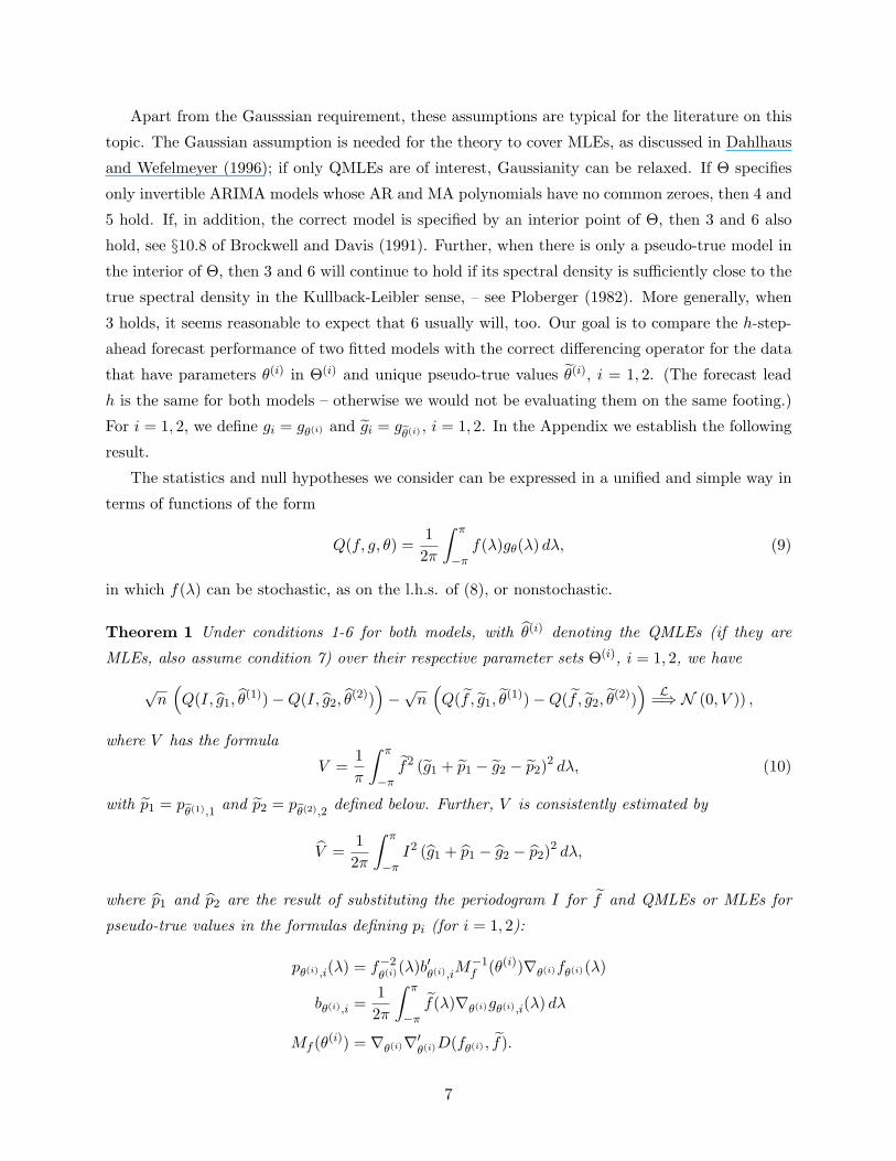
The statistics and null hypotheses we consider can be expressed in a unified and simple way in

terms of functions of the form

Q(f, g, θ) =12π

∫ π

−πf(λ)gθ(λ) dλ, (9)

in which f(λ) can be stochastic, as on the l.h.s. of (8), or nonstochastic.

Theorem 1 Under conditions 1-6 for both models, with θ(i) denoting the QMLEs (if they are

MLEs, also assume condition 7) over their respective parameter sets Θ(i), i = 1, 2, we have

√n

(Q(I, g1, θ

(1))−Q(I, g2, θ(2))

)−√n

(Q(f , g1, θ

(1))−Q(f , g2, θ(2))

) L=⇒ N (0, V )) ,

where V has the formula

V =1π

∫ π

−πf2 (g1 + p1 − g2 − p2)

2 dλ, (10)

with p1 = pθ(1),1

and p2 = pθ(2),2

defined below. Further, V is consistently estimated by

V =12π

∫ π

−πI2 (g1 + p1 − g2 − p2)

2 dλ,

where p1 and p2 are the result of substituting the periodogram I for f and QMLEs or MLEs for

pseudo-true values in the formulas defining pi (for i = 1, 2):

pθ(i),i(λ) = f−2θ(i)(λ)b′

θ(i),iM−1

f (θ(i))∇θ(i)fθ(i)(λ)

bθ(i),i =12π

∫ π

−πf(λ)∇θ(i)gθ(i),i(λ) dλ

Mf (θ(i)) = ∇θ(i)∇′θ(i)D(fθ(i) , f).

7

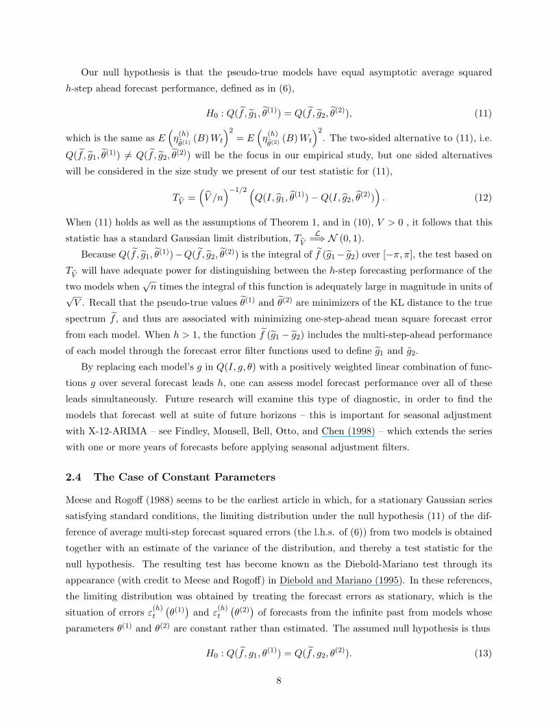
Our null hypothesis is that the pseudo-true models have equal asymptotic average squared

h-step ahead forecast performance, defined as in (6),

H0 : Q(f , g1, θ(1)) = Q(f , g2, θ

(2)), (11)

which is the same as E(η

(h)

θ(1)(B) Wt

)2= E

(η

(h)

θ(2)(B)Wt

)2. The two-sided alternative to (11), i.e.

Q(f , g1, θ(1)) 6= Q(f , g2, θ

(2)) will be the focus in our empirical study, but one sided alternatives

will be considered in the size study we present of our test statistic for (11),

TV

=(V /n

)−1/2 (Q(I, g1, θ

(1))−Q(I, g2, θ(2))

). (12)

When (11) holds as well as the assumptions of Theorem 1, and in (10), V > 0 , it follows that this

statistic has a standard Gaussian limit distribution, TV

L=⇒ N (0, 1).

Because Q(f , g1, θ(1))−Q(f , g2, θ

(2)) is the integral of f (g1− g2) over [−π, π], the test based on

TV

will have adequate power for distinguishing between the h-step forecasting performance of the

two models when√

n times the integral of this function is adequately large in magnitude in units of√V . Recall that the pseudo-true values θ(1) and θ(2) are minimizers of the KL distance to the true

spectrum f , and thus are associated with minimizing one-step-ahead mean square forecast error

from each model. When h > 1, the function f (g1 − g2) includes the multi-step-ahead performance

of each model through the forecast error filter functions used to define g1 and g2.

By replacing each model’s g in Q(I, g, θ) with a positively weighted linear combination of func-

tions g over several forecast leads h, one can assess model forecast performance over all of these

leads simultaneously. Future research will examine this type of diagnostic, in order to find the

models that forecast well at suite of future horizons – this is important for seasonal adjustment

with X-12-ARIMA – see Findley, Monsell, Bell, Otto, and Chen (1998) – which extends the series

with one or more years of forecasts before applying seasonal adjustment filters.

2.4 The Case of Constant Parameters

Meese and Rogoff (1988) seems to be the earliest article in which, for a stationary Gaussian series

satisfying standard conditions, the limiting distribution under the null hypothesis (11) of the dif-

ference of average multi-step forecast squared errors (the l.h.s. of (6)) from two models is obtained

together with an estimate of the variance of the distribution, and thereby a test statistic for the

null hypothesis. The resulting test has become known as the Diebold-Mariano test through its

appearance (with credit to Meese and Rogoff) in Diebold and Mariano (1995). In these references,

the limiting distribution was obtained by treating the forecast errors as stationary, which is the

situation of errors ε(h)t

(θ(1)

)and ε

(h)t

(θ(2)

)of forecasts from the infinite past from models whose

parameters θ(1) and θ(2) are constant rather than estimated. The assumed null hypothesis is thus

H0 : Q(f , g1, θ(1)) = Q(f , g2, θ

(2)). (13)

8

Unaware of the work of Meese and Rogoff, for the null hypothesis (13) and for a large class of

stationary time series models, Findley (1991a) obtained a limiting distribution equivalent to theirs

for the errors ε(h)t

(θ(i)

)from the standard finite-past predictors defined by constant parameters

θ(i), i = 1, 2,

n−1/2

(n−h∑

t=1

[ε(h)t (θ(1))]2 −

n−h∑

t=1

[ε(h)t (θ(2))]2

)L=⇒ N (0, Vc) ,

but provided no estimator for the limiting variance, which we denote by Vc, where the subscript c

indicates the treatment of the parameters as constant. Meese and Rogoff’s formula for Vc will be

presented below in (17) and shown to have the value

Vc =1π

∫ π

−πf2 (g1 − g2)

2 dλ. (14)

This is the variance that Theorem 1 yields for the constant parameter case under (13),

√n

(Q(I, g1, θ

(1))−Q(I, g2, θ(2))

) L=⇒ N (0, Vc) ,

because the terms in (10) involving derivatives with respect to the parameters drop out. Theorem

1 provides a consistent estimate of Vc,

Vc =12π

∫ π

−πI2 (g1 − g2)

2 dλ

=n−1∑

j,k=−n+1

γj γk

γj−k(g2

1) + γj−k(g22)− 2 γj−k(g1g2)

, (15)

with γj = n−1∑n

t=|j|+1 WtWt−|j|,−n + 1 ≤ j ≤ n− 1. Thus we have a test statistic

TVc

=(Vc/n

)−1/2 (Q(I, g1, θ

(1))−Q(I, g2, θ(2))

). (16)

The simplifications of the proof of Theorem 1 that result from using constant parameters show

that TVc

has an N (0, 1) limiting distribution when, along with conditions 1–3 of Theorem 1, the

model spectral density and weighting functions are continuous functions of their parameters and

also g1 6= g2 holds, so that Vc > 0. The same is true for the time series generalization of the

non-nested model comparison test statistic of Vuong (1989) in Findley (1990) if the h = 1 instance

of Vc replaces the robust estimate of asymptotic variance used in this report’s applications, which

was not shown to be consistent.

In the case of competing ARIMA models, the model autocovariances on the right in (15) can

be calculated by identifying the coefficients of the ARMA models whose spectral densities are g21,

g22 and g1g2 and from these coefficients obtaining the autocovariances, as in Section 2.2. In the

numerical studies below, the parameters treated as constant are Maximum Likelihood estimates

from W1, . . . , Wn. The calculation of V is much more complex because of its terms that involve

derivatives.

9

To present Meese and Rogoff’s formula for Vc and their estimate VDM as described for general

h by Diebold and Mariano (1995), set vt = ε(h)t

(θ(1)

)+ ε

(h)t

(θ(2)

)and wt = ε

(h)t

(θ(1)

)− ε(h)t

(θ(2)

)

and observe that [ε(h)t

(θ(1)

)]2 − [ε(h)

t

(θ(2)

)]2 = vtwt. Thus, the null hypothesis (11) is equivalent

to Evtwt = 0, and n−1/2 times the difference of the average squared forecast errors is equal to

n−1/2∑n

t=1 vtwt, whose normal limiting distribution under the null has the well-known variance

formula

Vc,MR =∞∑

r=−∞[γvv (r) γww (r) + γvw (r) γvw (−r)] , (17)

in the Gaussian case. In Section A.4 of the Appendix, we verify that

Vc,MR = Vc. (18)

Motivated by the fact discussed above that with correct models, the h-step-ahead forecast errors

ε(h)t form a moving average process of order h − 1, Meese and Rogoff (1988) and Diebold and

Mariano (1995, p. 257) propose the estimator of Vc,MR = Vc defined by

VDM =h−1∑

r=−h+1

(1− |r|

n

)[γvv (r) γww (r) + γvw (r) γvw (−r)] , (19)

with sample cross-covariance estimates γvv (r), γww (r), γvw (r) γvw (−r) defined by the observed

in-sample forecast errors from the estimated models. This VDM converges to

VDM =h−1∑

r=−h+1

[γvv (r) γww (r) + γvw (r) γvw (−r)] , (20)

which is to be regarded, and judged, as an approximation to Vc. The equality VDM = Vc

holds only in very special situations. For example, it holds when the series being modeled is

a moving average process of order less than h, or when both models being compared contain

the correct model as a special case. However, in this correct model situation, at the asymp-

totic (true) parameter values, wt = 0 and VDM = Vc = 0, a situation in which the test statistic

proposed by these authors has not been shown to have a limiting distribution1. In the empir-

ical results of the next section, for uniformity, the Diebold-Mariano test statistic is taken as

TDM =(VDM/n

)−1/2 (Q(I, g1, θ

(1))−Q(I, g2, θ(2))

), which differs from their actual statistic to

the extent of the effect of the approximation errors in (7) for both models. However, it has the

same N (0, Vc/VDM ) limit distribution when VDM 6= 0.

Remark. In the important case h = 1, which is also relevant for likelihood-ratio-based model se-

lection, see Findley (1990), we have V = Vc because, for each model family, the vector b(θ) of Theo-

rem 1 is zero. This happens because in this case, b(θ) is the gradient of (1/2π)∫ π−π f(λ)

∣∣Ψθ

(e−iλ

)∣∣−2dλ

1Clark and McCracken (2001, 2005) have obtained limiting distributions in this situation for related encompassing

statistics comparing out-of-sample forecasting performance of competing regression models with jointly stationary

variables. The distributions are determined by the limit of the ratio of the number of data held out of sample to the

number of in-sample data used to forecast the withheld data.

10

and the pseudo-true value θ minimizes this integral and lies in the interior of Θ by Assumption 3.

Thus, when h = 1, we can expect similar results from TV

and TVc

with large enough samples.

3 Numerical Studies

First we report a size study of the statistics TV

, TVc

, and TVDM

obtained from the only kind of exam-

ples known to us of pairs of incorrect models for which the null hypothesis (11) is satisfied, namely

pairs of autoregressive models like those described in Section 3 of Findley (1991b) involving models

with coefficient gaps. For a misspecified autoregressive model, the pseudo-true coefficient vector and

its associated Asymptotic Mean Square Forecast Error (AMSFE) Q(f , g, θ) = E(η

(h)

θ(B) Wt

)2for

the case h = 1 both have simple general formulas. These facilitate finding non-nested pairs of incor-

rect autoregressive models with g1 6= g2 such that for h = 1, the null hypothesis of equal AMSFEs

holds, Q(f , g1, θ(1)) = Q(f , g2, θ

(2)), and also V > 0. After the size study, we present simulation-

based power studies, some of which involve nonstationary series and values h > 1. Pseudo-true

coefficients are used in the evaluation of AMSFEs and asymptotic variances Vc and VDM as well as

V , because estimated rather than fixed coefficient are used with each simulation and series length,

and the pseudo-true coefficients are the theoretical limit of the estimates from each data generat-

ing process (DGP). Therefore, the statistics TV

, TVc

, and TVDM

differ only in their denominators,

which converge to the asymptotic standard errors√

V ,√

Vc, and√

VDM , respectively. These limit

quantities will be shown to be good indicators of the relative power properties of the three statistics

in finite samples. After the simulation studies (done with R), we present the results of applying

TV

, TVc

, and TVDM

to recommended and alternative models for some published time series.

Remark. The simulation results presented as size studies of TVDM

in Section 3 of Diebold and

Mariano (1995) are not valid for this purpose. They assume a series Wt can exist that has two

incorrect models with |ψ1| < 1 whose 2-step-ahead forecast errors processes are distinct invertible

MA(1) processes with the same MA coefficient. There is no such Wt: For models with |ψ1| < 1,

for a given MA(1) forecast error polynomial Ω (B) = 1 + ω1B with |ω1| < 1, the MA(1) process is

unique, being given by Ω (B) εt where εt is the innovations process of Wt. Indeed, more generally,

for any h ≥ 1, if the zeroes of [Ψ]h−10 (z) and Ω (z) lie in |z| > 1, then from η(h) (B) Wt =

[Ψ]h−10 (B)Ψ−1(B)Wt = Ω (B) et, we have Wt = Ψ (B) et for Ψ (B) = Ψ (B)

([Ψ]h−1

0 (B))−1

Ω (B).

Because Ψ−1 (B) = Ω−1 (B) [Ψ]h−10 (B)Ψ−1(B) is causal, if et = Ψ−1 (B) Wt is white noise, then

Ψ (B) is the innovations filter of Wt and et = εt .

3.1 Size Studies

We use the easily verified fact that when fitting a possibly incorrect AR(p) model to the time series

Wt, the pseudo-true coefficient vector ξ =(ξ1, . . . , ξp

)′has the entries that minimize

11

E(Wt −

∑pj=1 ξjWt−j

)2. Thus ξ is the solution to the Yule-Walker equation defined by Wt’s

true autocovariances, Γ(f)ξ = γ, where the covariance matrix is p − 1 dimensional and γ =(γ1(f), · · · , γp(f)

)′. Hence, when h = 1 the AMSFE is equal to E

(Wt −

∑pj=1 ξjWt−j

)2= γ0(f)−

γ′Γ−1(f)γ.

For an AR(1) model, ξ1 = γ1(f)/γ0(f), the lag one autocorrelation of Wt. For the null hy-

pothesis, we must find two different models such that the corresponding AMSFEs are equal, but

without their spectra and weighting functions (evaluated at pseudo-true values) being equal – this

excludes nested models, for example. Let an AR(1) be the first model, and let an AR(2) model with

AR polynomial of the constrained form Ξ (B) = 1− ξ2B be the second. This model’s pseudo-true

coefficient, the minimizer of E (Wt − ξ2Wt−2)2, is ξ2 = γ2(f)/γ0(f), the lag two autocorrelation of

Wt, and the AMSFE for h = 1 is γ0(f)− γ22(f)/γ0(f).

The two AMSFEs will be equal when Wt is such that γ1(f) = γ2(f). An MA(2) process of the

form Wt = (1 + 1/3B + 1/2B2)εt has this property and, with Gaussian white noise, will be the

“Null DGP” for our size study (its innovation variance is irrelevant for our purposes). It is easy

to see that g1 6= g2 at the pseudo-true values, so the asymptotic variances of the test statistics are

non-zero. We will generate data from the Null DGP in order to assess the size properties of the

statistics, for h = 1. Another choice of h, or a model with δ(B) 6= 1, would have different AMSFE

formulas and would thereby require other constraints on f .

For the size study, we simulated 1,000 Gaussian time series from the Null DGP described above,

with sample sizes n = 50, 100, 200. The three test statistics TV

, TVc

, and TVDM

(for h = 1) were

then applied and the coverage was computed. Nominal coverage was α = .05, .10; in Table 1 we

give empirical coverage for each method, for both the left and right tails (the tests are considered

as if one-sided, so the table entries should be compared against the limiting values of α = .05, .10

for each tail). There is very similar under-coverage for TV

and TVc

at n = 50 with some asymmetry,

which disappears as the data length increases. The similarity is expected because h = 1, so the

statistics’ denominators coincide asymptotically,√

V =√

Vc(= 1.239). (The calculation of the

asymptotic variances is discussed at the end of Section 3.2.) Except at n = 50 and α = .05, TVDM

has over-coverage throughout. The fact that TVDM

consistently made more Type I errors is what

one might expect from√

VDM = 1.020, and the fact that TVDM

is asymptotically equivalent to TVc

multiplied by√

Vc/√

VDm = 1.215. (Thus√

VDM is not a good approximation√

Vc in this case.)

None of the tests is grossly mis-sized, but the correctly normalized test statistic TV

performs best.

3.2 Power Studies

We now present the results of simulation experiments to determine the probabilities that one-sided

tests with the three test statistics reject the null hypothesis in favor of the model with smaller

AMSFE in various stationary and nonstationary situations. Consider first the fitting of an AR(1)

12

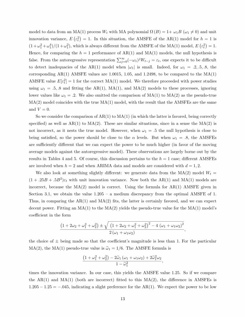
model to data from an MA(1) process Wt with MA polynomial Ω (B) = 1+ ω1B (ω1 6= 0) and unit

innovation variance, E(ε2t

)= 1. In this situation, the AMSFE of the AR(1) model for h = 1 is

(1+ω21 +ω4

1)/(1+ω21), which is always different from the AMSFE of the MA(1) model, E

(ε2t

)= 1.

Hence, for comparing the h = 1 performance of AR(1) and MA(1) models, the null hypothesis is

false. From the autoregressive representation∑∞

j=0(−ω1)jWt−j = εt, one expects it to be difficult

to detect inadequacies of the AR(1) model when |ω1| is small. Indeed, for ω1 = .2, .5, .8, the

corresponding AR(1) AMSFE values are 1.0015, 1.05, and 1.2498, to be compared to the MA(1)

AMSFE value E[ε2t ] = 1 for the correct MA(1) model. We therefore proceeded with power studies

using ω1 = .5, .8 and fitting the AR(1), MA(1), and MA(2) models to these processes, ignoring

lower values like ω1 = .2. We also omitted the comparison of MA(1) to MA(2) as the pseudo-true

MA(2) model coincides with the true MA(1) model, with the result that the AMSFEs are the same

and V = 0.

So we consider the comparison of AR(1) to MA(1) (in which the latter is favored, being correctly

specified) as well as AR(1) to MA(2). These are similar situations, since in a sense the MA(2) is

not incorrect, as it nests the true model. However, when ω1 = .5 the null hypothesis is close to

being satisfied, so the power should be close to the α levels. But when ω1 = .8, the AMSFEs

are sufficiently different that we can expect the power to be much higher (in favor of the moving

average models against the autoregressive model). These observations are largely borne out by the

results in Tables 4 and 5. Of course, this discussion pertains to the h = 1 case; different AMSFEs

are involved when h = 2 and when ARIMA data and models are considered with d = 1, 2.

We also look at something slightly different: we generate data from the MA(2) model Wt =

(1 + .25B + .5B2)εt with unit innovation variance. Now both the AR(1) and MA(1) models are

incorrect, because the MA(2) model is correct. Using the formula for AR(1) AMSFE given in

Section 3.1, we obtain the value 1.205 – a medium discrepancy from the optimal AMSFE of 1.

Thus, in comparing the AR(1) and MA(2) fits, the latter is certainly favored, and we can expect

decent power. Fitting an MA(1) to the MA(2) yields the pseudo-true value for the MA(1) model’s

coefficient in the form

(1 + 2ω2 + ω2

1 + ω22

)±√ (

1 + 2ω2 + ω21 + ω2

2

)2 − 4 (ω1 + ω1ω2)2

2 (ω1 + ω1ω2),

the choice of ± being made so that the coefficient’s magnitude is less than 1. For the particular

MA(2), the MA(1) pseudo-true value is ω1 = 1/6. The AMSFE formula is(1 + ω2

1 + ω22

)− 2ω1 (ω1 + ω1ω2) + 2ω21ω2

1− ω21

,

times the innovation variance. In our case, this yields the AMSFE value 1.25. So if we compare

the AR(1) and MA(1) (both are incorrect) fitted to this MA(2), the difference in AMSFEs is

1.205− 1.25 = −.045, indicating a slight preference for the AR(1). We expect the power to be low

13

– perhaps even close to the nominal size for small samples – in this case. This is borne out by

the results in Table 6 for d = 0. Note that we could also do comparisons of MA(1) to MA(2) fits

(they are not nested in this case, since their AMSFEs differ), but this is omitted for uniformity of

presentation.

For the power studies, we simulate from these DGPs and fit three models, making two compar-

isons as discussed above. We examine the sample sizes n = 50, 100, 200 and the α levels .05, .10 just

as in the size study. We restrict the power calculation for the three statistics to the relevant tail

(either left or right, depending on which model is favored), since if there is power in the positive

direction there should be negligible power in the negative direction, and vice versa. When h = 1,

the differencing order is irrelevant, but for h = 2 we consider d = 0, 1, 2.

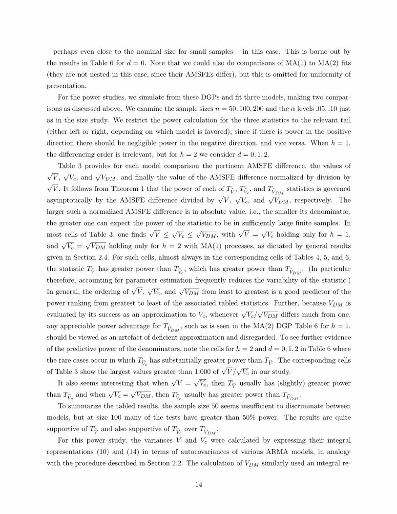
Table 3 provides for each model comparison the pertinent AMSFE difference, the values of√V ,

√Vc, and

√VDM , and finally the value of the AMSFE difference normalized by division by√

V . It follows from Theorem 1 that the power of each of TV

, TVc

, and TVDM

statistics is governed

asymptotically by the AMSFE difference divided by√

V ,√

Vc, and√

VDM , respectively. The

larger such a normalized AMSFE difference is in absolute value, i.e., the smaller its denominator,

the greater one can expect the power of the statistic to be in sufficiently large finite samples. In

most cells of Table 3, one finds√

V ≤ √Vc ≤

√VDM , with

√V =

√Vc holding only for h = 1,

and√

Vc =√

VDM holding only for h = 2 with MA(1) processes, as dictated by general results

given in Section 2.4. For such cells, almost always in the corresponding cells of Tables 4, 5, and 6,

the statistic TV

has greater power than TVc

, which has greater power than TVDM

. (In particular

therefore, accounting for parameter estimation frequently reduces the variability of the statistic.)

In general, the ordering of√

V ,√

Vc, and√

VDM from least to greatest is a good predictor of the

power ranking from greatest to least of the associated tabled statistics. Further, because VDM is

evaluated by its success as an approximation to Vc, whenever√

Vc/√

VDM differs much from one,

any appreciable power advantage for TVDM

, such as is seen in the MA(2) DGP Table 6 for h = 1,

should be viewed as an artefact of deficient approximation and disregarded. To see further evidence

of the predictive power of the denominators, note the cells for h = 2 and d = 0, 1, 2 in Table 6 where

the rare cases occur in which TVc

has substantially greater power than TV

. The corresponding cells

of Table 3 show the largest values greater than 1.000 of√

V /√

Vc in our study.

It also seems interesting that when√

V =√

Vc, then TV

usually has (slightly) greater power

than TVc

and when√

Vc =√

VDM , then TVc

usually has greater power than TVDM

.

To summarize the tabled results, the sample size 50 seems insufficient to discriminate between

models, but at size 100 many of the tests have greater than 50% power. The results are quite

supportive of TV

and also supportive of TVc

over TVDM

.

For this power study, the variances V and Vc were calculated by expressing their integral

representations (10) and (14) in terms of autocovariances of various ARMA models, in analogy

with the procedure described in Section 2.2. The calculation of VDM similarly used an integral re-

14

expression of the r.h.s. of (20) obtained with certain algebraic simplifications. Details are omitted

for brevity.

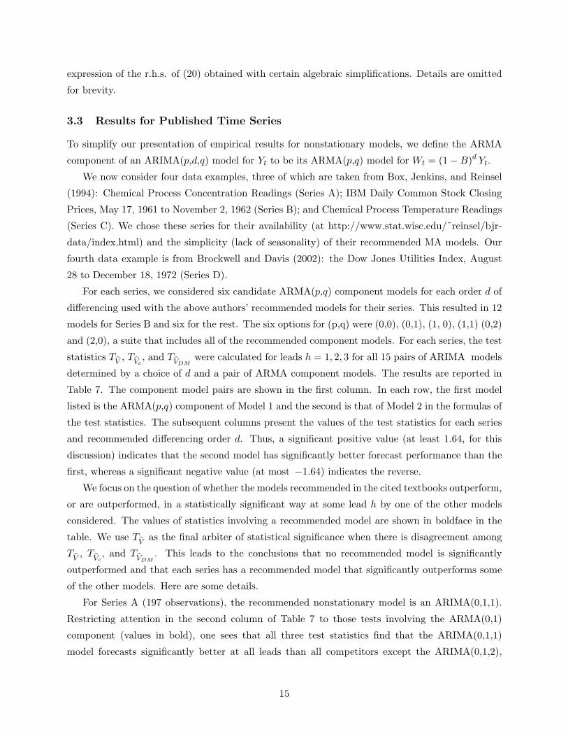
3.3 Results for Published Time Series

To simplify our presentation of empirical results for nonstationary models, we define the ARMA

component of an ARIMA(p,d,q) model for Yt to be its ARMA(p,q) model for Wt = (1−B)d Yt.

We now consider four data examples, three of which are taken from Box, Jenkins, and Reinsel

(1994): Chemical Process Concentration Readings (Series A); IBM Daily Common Stock Closing

Prices, May 17, 1961 to November 2, 1962 (Series B); and Chemical Process Temperature Readings

(Series C). We chose these series for their availability (at http://www.stat.wisc.edu/˜reinsel/bjr-

data/index.html) and the simplicity (lack of seasonality) of their recommended MA models. Our

fourth data example is from Brockwell and Davis (2002): the Dow Jones Utilities Index, August

28 to December 18, 1972 (Series D).

For each series, we considered six candidate ARMA(p,q) component models for each order d of

differencing used with the above authors’ recommended models for their series. This resulted in 12

models for Series B and six for the rest. The six options for (p,q) were (0,0), (0,1), (1, 0), (1,1) (0,2)

and (2,0), a suite that includes all of the recommended component models. For each series, the test

statistics TV

, TVc

, and TVDM

were calculated for leads h = 1, 2, 3 for all 15 pairs of ARIMA models

determined by a choice of d and a pair of ARMA component models. The results are reported in

Table 7. The component model pairs are shown in the first column. In each row, the first model

listed is the ARMA(p,q) component of Model 1 and the second is that of Model 2 in the formulas of

the test statistics. The subsequent columns present the values of the test statistics for each series

and recommended differencing order d. Thus, a significant positive value (at least 1.64, for this

discussion) indicates that the second model has significantly better forecast performance than the

first, whereas a significant negative value (at most −1.64) indicates the reverse.

We focus on the question of whether the models recommended in the cited textbooks outperform,

or are outperformed, in a statistically significant way at some lead h by one of the other models

considered. The values of statistics involving a recommended model are shown in boldface in the

table. We use TV

as the final arbiter of statistical significance when there is disagreement among

TV

, TVc

, and TVDM

. This leads to the conclusions that no recommended model is significantly

outperformed and that each series has a recommended model that significantly outperforms some

of the other models. Here are some details.

For Series A (197 observations), the recommended nonstationary model is an ARIMA(0,1,1).

Restricting attention in the second column of Table 7 to those tests involving the ARMA(0,1)

component (values in bold), one sees that all three test statistics find that the ARIMA(0,1,1)

model forecasts significantly better at all leads than all competitors except the ARIMA(0,1,2),

15

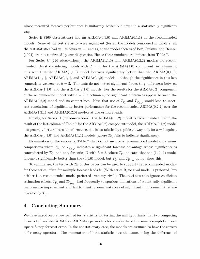
whose measured forecast performance is uniformly better but never in a statistically significant

way.

Series B (369 observations) had an ARIMA(0,1,0) and ARIMA(0,1,1) as the recommended

models. None of the test statistics were significant (for all the models considered in Table 7, all

the test statistics had values between −1 and 1), so the model choices of Box, Jenkins, and Reinsel

(1994) are not confirmed by our diagnostics. Hence these numbers are omitted from Table 7.

For Series C (226 observations), the ARIMA(1,1,0) and ARIMA(0,2,2) models are recom-

mended. First considering models with d = 1, for the ARMA(1,0) component, in column 4,

it is seen that the ARIMA(1,1,0) model forecasts significantly better than the ARIMA(0,1,0),

ARIMA(1,1,1), ARIMA(0,1,1), and ARIMA(0,1,2) models – although the significance in this last

comparison weakens at h = 3. The tests do not detect significant forecasting differences between

the ARIMA(1,1,0) and the ARIMA(2,1,0) models. For the results for the ARMA(0,2) component

of the recommended model with d = 2 in column 5, no significant differences appear between the

ARIMA(0,2,2) model and its competitors. Note that use of TVc

and TVDM

would lead to incor-

rect conclusions of significantly better performance for the recommended ARIMA(0,2,2) over the

ARIMA(1,2,1) and ARIMA(0,2,0) models at one or more leads.

Finally, for Series D (78 observations), the ARIMA(0,1,2) model is recommended. From the

result of the last column of Table 7 for the ARMA(0,2) component model, the ARIMA(0,1,2) model

has generally better forecast performance, but in a statistically significant way only for h = 1 against

the ARIMA(0,1,0) and ARIMA(1,1,1) models (where TVc

fails to indicate significance).

Examination of the entries of Table 7 that do not involve a recommended model show many

comparisons where TVc

or TVDM

indicates a significant forecast advantage whose significance is

contradicted by TV

, and one, for series D with h = 3, where TV

indicates that the (1, 1, 1) model

forecasts significantly better than the (0,1,0) model, but TVc

and TVDM

do not show this.

To summarize, the test with TV

of this paper can be used to support the recommended models

for these series, often for multiple forecast leads h. (With series B, no rival model is preferred, but

neither is a recommended model preferred over any rival.) The statistics that ignore coefficient

estimation effects, TVc

and TVDM

, lead frequently to spurious indications of statistically significant

performance improvement and fail to identify some instances of significant improvement that are

revealed by TV

.

4 Concluding Summary

We have introduced a new pair of test statistics for testing the null hypothesis that two competing

incorrect, invertible ARMA or ARIMA-type models for a series have the same asymptotic mean

square h-step forecast error. In the nonstationary case, the models are assumed to have the correct

differencing operator. The numerators of both statistics are the same, being the difference of

16

the mean square forecast error measures of the models. But they are conceptually different in

that the models’ parameters are treated as fixed in the simpler statistic TVc

and as sample-size-

dependent (Quasi-)Maximum Likelihood estimates in the statistic TV

, which the more complex

standard deviation estimate in its denominator to account for parameter estimation. The simpler

statistic improves the well-known Diebold-Mariano statistic, equivalent to TVDM

in our notation,

by providing a denominator that leads to a standard normal limiting distribution when the null

hypothesis of equal asymptotic mean square forecast error is satisfied, as happens with the series

of our size study. No series is known to exist for which for which TVDM

has this property (see the

Remark of Section 3). Regarding our more comprehensive statistic, its superior finite-sample and

asymptotic results in our power study clearly reveal that accepting the parameters in the numerator

of these statistics as estimates, and accounting for this fact appropriately in the denominator, often

yields a statistic with smaller variability both asymptotically and in samples of moderate size.

R code is available from the first author (McElroy) for calculating the statistics for the general

ARIMA case, including exact calculation of the first and second derivatives of functions of the

model spectral densities required to account for parameter estimation as shown in formulas in the

Appendix.

For the size study, we provided an example of an MA(2) series and simple pair of non-nested

incorrect AR models for which the null hypothesis of equal asymptotic mean squared one-step-ahead

forecast error holds in a non-degenerate way. In the study, the worst results were obtained for the

Diebold-Mariano statistic, which was often quite oversized, whereas the new statistics showed a

tendency to be moderately undersized.

Our empirical study of models for four published time series provided further evidence of the

superior performance of TV

over TVc

and TVDM

. Our test with TV

of models for four published time

series formally justified the use of one or more of the models recommended by experts for these

series in the application to forecasting at lead one and often at higher leads.

Acknowledgements. The communicating author (Findley) was stimulated to change fields from

functional analysis to statistical time series analysis by a one-day time series workshop at the

University of Cincinnati in 1973 presented by Manny Parzen and his distinguished former student

Grace Wahba. He is most grateful for this influential workshop and is further grateful to Manny for

subsequent acts of support and collaboration. The authors are indebted to two anonymous referees

and to Michael McCracken for comments and questions that led to significant improvements. They

also thank Brian Monsell for his careful reading of the manuscript.

17

Appendix

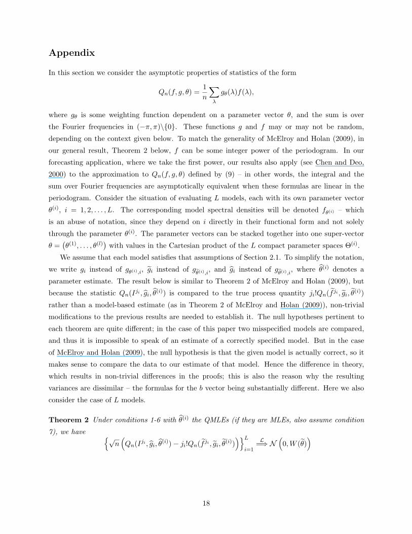
In this section we consider the asymptotic properties of statistics of the form

Qn(f, g, θ) =1n

∑

λ

gθ(λ)f(λ),

where gθ is some weighting function dependent on a parameter vector θ, and the sum is over

the Fourier frequencies in (−π, π)\0. These functions g and f may or may not be random,

depending on the context given below. To match the generality of McElroy and Holan (2009), in

our general result, Theorem 2 below, f can be some integer power of the periodogram. In our

forecasting application, where we take the first power, our results also apply (see Chen and Deo,

2000) to the approximation to Qn(f, g, θ) defined by (9) – in other words, the integral and the

sum over Fourier frequencies are asymptotically equivalent when these formulas are linear in the

periodogram. Consider the situation of evaluating L models, each with its own parameter vector

θ(i), i = 1, 2, . . . , L. The corresponding model spectral densities will be denoted fθ(i) – which

is an abuse of notation, since they depend on i directly in their functional form and not solely

through the parameter θ(i). The parameter vectors can be stacked together into one super-vector

θ =(θ(1), . . . , θ(l)

)with values in the Cartesian product of the L compact parameter spaces Θ(i).

We assume that each model satisfies that assumptions of Section 2.1. To simplify the notation,

we write gi instead of gθ(i),i, gi instead of gθ(i),i

, and gi instead of gθ(i),i

, where θ(i) denotes a

parameter estimate. The result below is similar to Theorem 2 of McElroy and Holan (2009), but

because the statistic Qn(Iji , gi, θ(i)) is compared to the true process quantity ji!Qn(f ji , gi, θ

(i))

rather than a model-based estimate (as in Theorem 2 of McElroy and Holan (2009)), non-trivial

modifications to the previous results are needed to establish it. The null hypotheses pertinent to

each theorem are quite different; in the case of this paper two misspecified models are compared,

and thus it is impossible to speak of an estimate of a correctly specified model. But in the case

of McElroy and Holan (2009), the null hypothesis is that the given model is actually correct, so it

makes sense to compare the data to our estimate of that model. Hence the difference in theory,

which results in non-trivial differences in the proofs; this is also the reason why the resulting

variances are dissimilar – the formulas for the b vector being substantially different. Here we also

consider the case of L models.

Theorem 2 Under conditions 1-6 with θ(i) the QMLEs (if they are MLEs, also assume condition

7), we have √n

(Qn(Iji , gi, θ

(i))− ji!Qn(f ji , gi, θ(i))

)L

i=1

L=⇒ N(0,W (θ)

)

18

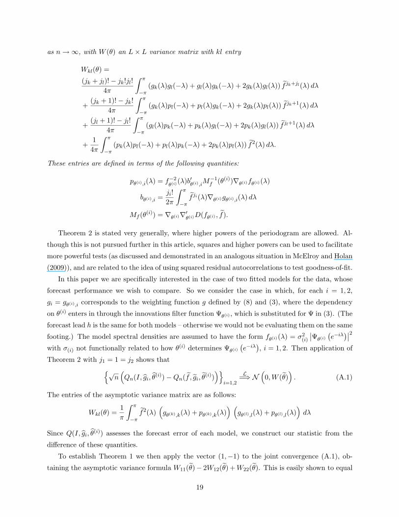
as n →∞, with W (θ) an L× L variance matrix with kl entry

Wkl(θ) =

(jk + jl)!− jk!jl!4π

∫ π

−π(gk(λ)gl(−λ) + gl(λ)gk(−λ) + 2gk(λ)gl(λ)) f jk+jl(λ) dλ

+(jk + 1)!− jk!

4π

∫ π

−π(gk(λ)pl(−λ) + pl(λ)gk(−λ) + 2gk(λ)pl(λ)) f jk+1(λ) dλ

+(jl + 1)!− jl!

4π

∫ π

−π(gl(λ)pk(−λ) + pk(λ)gl(−λ) + 2pk(λ)gl(λ)) f jl+1(λ) dλ

+14π

∫ π

−π(pk(λ)pl(−λ) + pl(λ)pk(−λ) + 2pk(λ)pl(λ)) f2(λ) dλ.

These entries are defined in terms of the following quantities:

pθ(i),i(λ) = f−2θ(i)(λ)b′

θ(i),iM−1

f (θ(i))∇θ(i)fθ(i)(λ)

bθ(i),i =ji!2π

∫ π

−πf ji(λ)∇θ(i)gθ(i),i(λ) dλ

Mf (θ(i)) = ∇θ(i)∇′θ(i)D(fθ(i) , f).

Theorem 2 is stated very generally, where higher powers of the periodogram are allowed. Al-

though this is not pursued further in this article, squares and higher powers can be used to facilitate

more powerful tests (as discussed and demonstrated in an analogous situation in McElroy and Holan

(2009)), and are related to the idea of using squared residual autocorrelations to test goodness-of-fit.

In this paper we are specifically interested in the case of two fitted models for the data, whose

forecast performance we wish to compare. So we consider the case in which, for each i = 1, 2,

gi = gθ(i),i corresponds to the weighting function g defined by (8) and (3), where the dependency

on θ(i) enters in through the innovations filter function Ψθ(i) , which is substituted for Ψ in (3). (The

forecast lead h is the same for both models – otherwise we would not be evaluating them on the same

footing.) The model spectral densities are assumed to have the form fθ(i)(λ) = σ2(i)

∣∣Ψθ(i)

(e−iλ

)∣∣2

with σ(i) not functionally related to how θ(i) determines Ψθ(i)

(e−iλ

), i = 1, 2. Then application of

Theorem 2 with j1 = 1 = j2 shows that√

n(Qn(I, gi, θ

(i))−Qn(f , gi, θ(i))

)i=1,2

L=⇒ N(0,W (θ)

). (A.1)

The entries of the asymptotic variance matrix are as follows:

Wkl(θ) =1π

∫ π

−πf2(λ)

(gθ(k),k(λ) + pθ(k),k(λ)

) (gθ(l),l(λ) + pθ(l),l(λ)

)dλ

Since Q(I, gi, θ(i)) assesses the forecast error of each model, we construct our statistic from the

difference of these quantities.

To establish Theorem 1 we then apply the vector (1,−1) to the joint convergence (A.1), ob-

taining the asymptotic variance formula W11(θ)− 2W12(θ) + W22(θ). This is easily shown to equal

19

the limiting variance V of Theorem 1. The consistency of V – independent of whether the null

or alternative hypothesis is true – then follows from conditions 2, 3, 4, 5, and 6 (as well as condi-

tion 7 if we are considering MLEs instead of QMLs), together with Lemma 3.1.1 of Taniguchi and

Kakizawa (2000). This concludes the derivation.

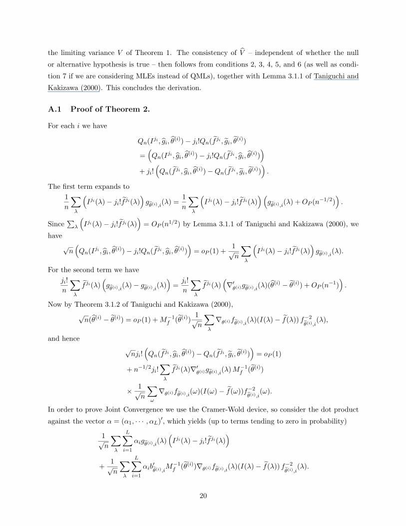
A.1 Proof of Theorem 2.

For each i we have

Qn(Iji , gi, θ(i))− ji!Qn(f ji , gi, θ

(i))

=(Qn(Iji , gi, θ

(i))− ji!Qn(f ji , gi, θ(i))

)

+ ji!(Qn(f ji , gi, θ

(i))−Qn(f ji , gi, θ(i))

).

The first term expands to1n

∑

λ

(Iji(λ)− ji!f ji(λ)

)gθ(i),i

(λ) =1n

∑

λ

(Iji(λ)− ji!f ji(λ)

)(gθ(i),i

(λ) + OP (n−1/2))

.

Since∑

λ

(Iji(λ)− ji!f ji(λ)

)= OP (n1/2) by Lemma 3.1.1 of Taniguchi and Kakizawa (2000), we

have√

n(Qn(Iji , gi, θ

(i))− ji!Qn(f ji , gi, θ(i))

)= oP (1) +

1√n

∑

λ

(Iji(λ)− ji!f ji(λ)

)gθ(i),i

(λ).

For the second term we haveji!n

∑

λ

f ji(λ)(gθ(i),i

(λ)− gθ(i),i

(λ))

=ji!n

∑

λ

f ji(λ)(∇′

θ(i)gθ(i),i(λ)(θ(i) − θ(i)) + OP (n−1)

).

Now by Theorem 3.1.2 of Taniguchi and Kakizawa (2000),√

n(θ(i) − θ(i)) = oP (1) + M−1f (θ(i))

1√n

∑

λ

∇θ(i)fθ(i),i(λ)(I(λ)− f(λ)) f−2

θ(i),i(λ),

and hence√

nji!(Qn(f ji , gi, θ

(i))−Qn(f ji , gi, θ(i))

)= oP (1)

+ n−1/2ji!∑

λ

f ji(λ)∇′θ(i)gθ(i),i

(λ) M−1f (θ(i))

× 1√n

∑ω

∇θ(i)fθ(i),i(ω)(I(ω)− f(ω))f−2

θ(i),i(ω).

In order to prove Joint Convergence we use the Cramer-Wold device, so consider the dot product

against the vector α = (α1, · · · , αL)′, which yields (up to terms tending to zero in probability)

1√n

∑

λ

L∑

i=1

αigθ(i),i(λ)

(Iji(λ)− ji!f ji(λ)

)

+1√n

∑

λ

L∑

i=1

αib′θ(i),i

M−1f (θ(i))∇θ(i)fθ(i),i

(λ)(I(λ)− f(λ)) f−2

θ(i),i(λ).

20

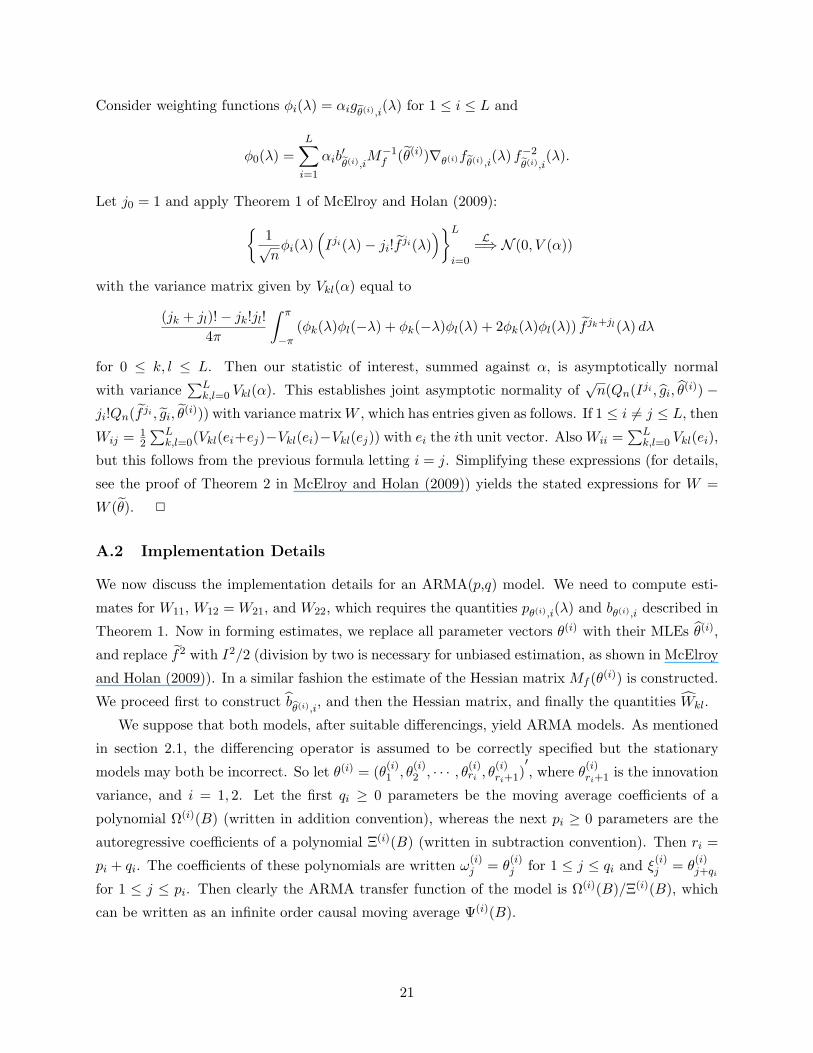
Consider weighting functions φi(λ) = αigθ(i),i(λ) for 1 ≤ i ≤ L and

φ0(λ) =L∑

i=1

αib′θ(i),i

M−1f (θ(i))∇θ(i)fθ(i),i

(λ) f−2

θ(i),i(λ).

Let j0 = 1 and apply Theorem 1 of McElroy and Holan (2009):

1√n

φi(λ)(Iji(λ)− ji!f ji(λ)

)L

i=0

L=⇒ N (0, V (α))

with the variance matrix given by Vkl(α) equal to

(jk + jl)!− jk!jl!4π

∫ π

−π(φk(λ)φl(−λ) + φk(−λ)φl(λ) + 2φk(λ)φl(λ)) f jk+jl(λ) dλ

for 0 ≤ k, l ≤ L. Then our statistic of interest, summed against α, is asymptotically normal

with variance∑L

k,l=0 Vkl(α). This establishes joint asymptotic normality of√

n(Qn(Iji , gi, θ(i)) −

ji!Qn(f ji , gi, θ(i))) with variance matrix W , which has entries given as follows. If 1 ≤ i 6= j ≤ L, then

Wij = 12

∑Lk,l=0(Vkl(ei+ej)−Vkl(ei)−Vkl(ej)) with ei the ith unit vector. Also Wii =

∑Lk,l=0 Vkl(ei),

but this follows from the previous formula letting i = j. Simplifying these expressions (for details,

see the proof of Theorem 2 in McElroy and Holan (2009)) yields the stated expressions for W =

W (θ). 2

A.2 Implementation Details

We now discuss the implementation details for an ARMA(p,q) model. We need to compute esti-

mates for W11, W12 = W21, and W22, which requires the quantities pθ(i),i(λ) and bθ(i),i described in

Theorem 1. Now in forming estimates, we replace all parameter vectors θ(i) with their MLEs θ(i),

and replace f2 with I2/2 (division by two is necessary for unbiased estimation, as shown in McElroy

and Holan (2009)). In a similar fashion the estimate of the Hessian matrix Mf (θ(i)) is constructed.

We proceed first to construct bθ(i),i

, and then the Hessian matrix, and finally the quantities Wkl.

We suppose that both models, after suitable differencings, yield ARMA models. As mentioned

in section 2.1, the differencing operator is assumed to be correctly specified but the stationary

models may both be incorrect. So let θ(i) = (θ(i)1 , θ

(i)2 , · · · , θ

(i)ri , θ

(i)ri+1)

′, where θ

(i)ri+1 is the innovation

variance, and i = 1, 2. Let the first qi ≥ 0 parameters be the moving average coefficients of a

polynomial Ω(i)(B) (written in addition convention), whereas the next pi ≥ 0 parameters are the

autoregressive coefficients of a polynomial Ξ(i)(B) (written in subtraction convention). Then ri =

pi + qi. The coefficients of these polynomials are written ω(i)j = θ

(i)j for 1 ≤ j ≤ qi and ξ

(i)j = θ

(i)j+qi

for 1 ≤ j ≤ pi. Then clearly the ARMA transfer function of the model is Ω(i)(B)/Ξ(i)(B), which

can be written as an infinite order causal moving average Ψ(i)(B).

21

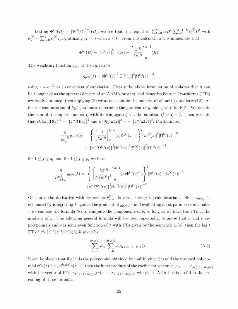
Letting Φ(i)(B) = [Ψ(i)/δ]h−1

0 (B), we see that it is equal to∑h−1

k=0 τkBk∑h−1−k

l=0 ψ(i)l Bl with

φ(i)k =

∑kl=0 ψ

(i)l τk−l, utilizing τk = 0 when k < 0. From this calculation it is immediate that

Φ(i)(B) = [Ψ(i)/δ]h−1

0 (B) =

[Ω(i)

δΞ(i)

]h−1

0

(B).

The weighting function gθ(i) is then given by

gθ(i)(λ) = |Φ(i)(z)|2|Ξ(i)(z)|2|Ω(i)(z)|−2,

using z = e−iλ as a convenient abbreviation. Clearly the above formulation of g shows that it can

be thought of as the spectral density of an ARMA process, and hence its Fourier Transforms (FTs)

are easily obtained; then applying (8) we at once obtain the numerator of our test statistic (12). As

for the computation of bθ(i),i

we must determine the gradient of g, along with its FTs. We denote

the sum of a complex number ζ with its conjugate ζ via the notation ζ] = ζ + ζ. Then we note

that ∂/∂ωj |Ω(z)|2 = z−jΩ(z)] and ∂/∂ξj |Ξ(z)|2 = − z−jΞ(z)]. Furthermore,

∂

∂θ(i)j

gθ(i)(λ) =

[ ·jδΞ(i)

]h−1

0

(z)Φ(i)(z−1)

]

|Ξ(i)(z)|2|Ω(i)(z)|−2

− z−jΩ(i)(z)]|Φ(i)(z)|2|Ξ(i)(z)|2|Ω(i)(z)|−4

for 1 ≤ j ≤ qi, and for 1 ≤ j ≤ pi we have

∂

∂θ(i)j+qi

gθ(i)(λ) =

[·jΩ(i)

δ(Ξ(i)

)2

]h−1

0

(z)Φ(i)(z−1)

]

|Ξ(i)(z)|2|Ω(i)(z)|−2

− z−jΞ(i)(z)]|Φ(i)(z)|2|Ω(i)(z)|−2.

Of course the derivative with respect to θ(i)ri+1 is zero, since g is scale-invariant. Since bθ(i),i is

estimated by integrating I against the gradient of gθ(i),i – and evaluating all at parameter estimates

– we can use the formula (8) to compute the components of b, so long as we have the FTs of the

gradient of g. The following general formula will be used repeatedly: suppose that a and c are

polynomials and s is some even function of λ with FTs given by the sequence γk(s); then the lag t

FT of zka(z−1)z−lc(z)s(λ) is given by

deg(a)∑

m=0

am

deg(c)∑

n=0

cnγt+m−n−k+l(s). (A.2)

It can be shown that if e(z) is the polynomial obtained by multiplying c(z) and the reversed polyno-

mial of a(z), i.e., zdeg(a)a(z−1), then the inner product of the coefficient vector [e0, e1, · · · , edeg(a)+deg(c)]

with the vector of FTs [γt−k+l+deg(a)(s), · · · , γt−k+l−deg(c)] will yield (A.2); this is useful in the en-

coding of these formulas.

22

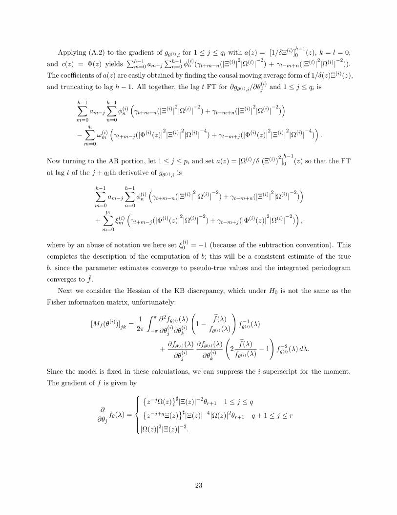
Applying (A.2) to the gradient of gθ(i),i for 1 ≤ j ≤ qi with a(z) = [1/δΞ(i)]h−1

0 (z), k = l = 0,

and c(z) = Φ(z) yields∑h−1

m=0 am−j∑h−1

n=0 φ(i)n (γt+m−n(|Ξ(i)|2|Ω(i)|−2

) + γt−m+n(|Ξ(i)|2|Ω(i)|−2)).

The coefficients of a(z) are easily obtained by finding the causal moving average form of 1/δ(z)Ξ(i)(z),

and truncating to lag h− 1. All together, the lag t FT for ∂gθ(i),i/∂θ(i)j and 1 ≤ j ≤ qi is

h−1∑

m=0

am−j

h−1∑

n=0

φ(i)n

(γt+m−n(|Ξ(i)|2|Ω(i)|−2

) + γt−m+n(|Ξ(i)|2|Ω(i)|−2))

−qi∑

m=0

ω(i)m

(γt+m−j(|Φ(i)(z)|2|Ξ(i)|2|Ω(i)|−4

) + γt−m+j(|Φ(i)(z)|2|Ξ(i)|2|Ω(i)|−4))

.

Now turning to the AR portion, let 1 ≤ j ≤ pi and set a(z) = [Ω(i)/δ (Ξ(i))2]h−1

0 (z) so that the FT

at lag t of the j + qith derivative of gθ(i),i is

h−1∑

m=0

am−j

h−1∑

n=0

φ(i)n

(γt+m−n(|Ξ(i)|2|Ω(i)|−2

) + γt−m+n(|Ξ(i)|2|Ω(i)|−2))

+pi∑

m=0

ξ(i)m

(γt+m−j(|Φ(i)(z)|2|Ω(i)|−2

) + γt−m+j(|Φ(i)(z)|2|Ω(i)|−2))

,

where by an abuse of notation we here set ξ(i)0 = −1 (because of the subtraction convention). This

completes the description of the computation of b; this will be a consistent estimate of the true

b, since the parameter estimates converge to pseudo-true values and the integrated periodogram

converges to f .

Next we consider the Hessian of the KB discrepancy, which under H0 is not the same as the

Fisher information matrix, unfortunately:

[Mf (θ(i))]jk =12π

∫ π

−π

∂2fθ(i)(λ)

∂θ(i)j ∂θ

(i)k

(1− f(λ)

fθ(i)(λ)

)f−1

θ(i)(λ)

+∂fθ(i)(λ)

∂θ(i)j

∂fθ(i)(λ)

∂θ(i)k

(2

f(λ)fθ(i)(λ)

− 1

)f−2

θ(i)(λ) dλ.

Since the model is fixed in these calculations, we can suppress the i superscript for the moment.

The gradient of f is given by

∂

∂θjfθ(λ) =

z−jΩ(z)

]|Ξ(z)|−2θr+1 1 ≤ j ≤ qz−j+qΞ(z)

]|Ξ(z)|−4|Ω(z)|2θr+1 q + 1 ≤ j ≤ r

|Ω(z)|2|Ξ(z)|−2.

23

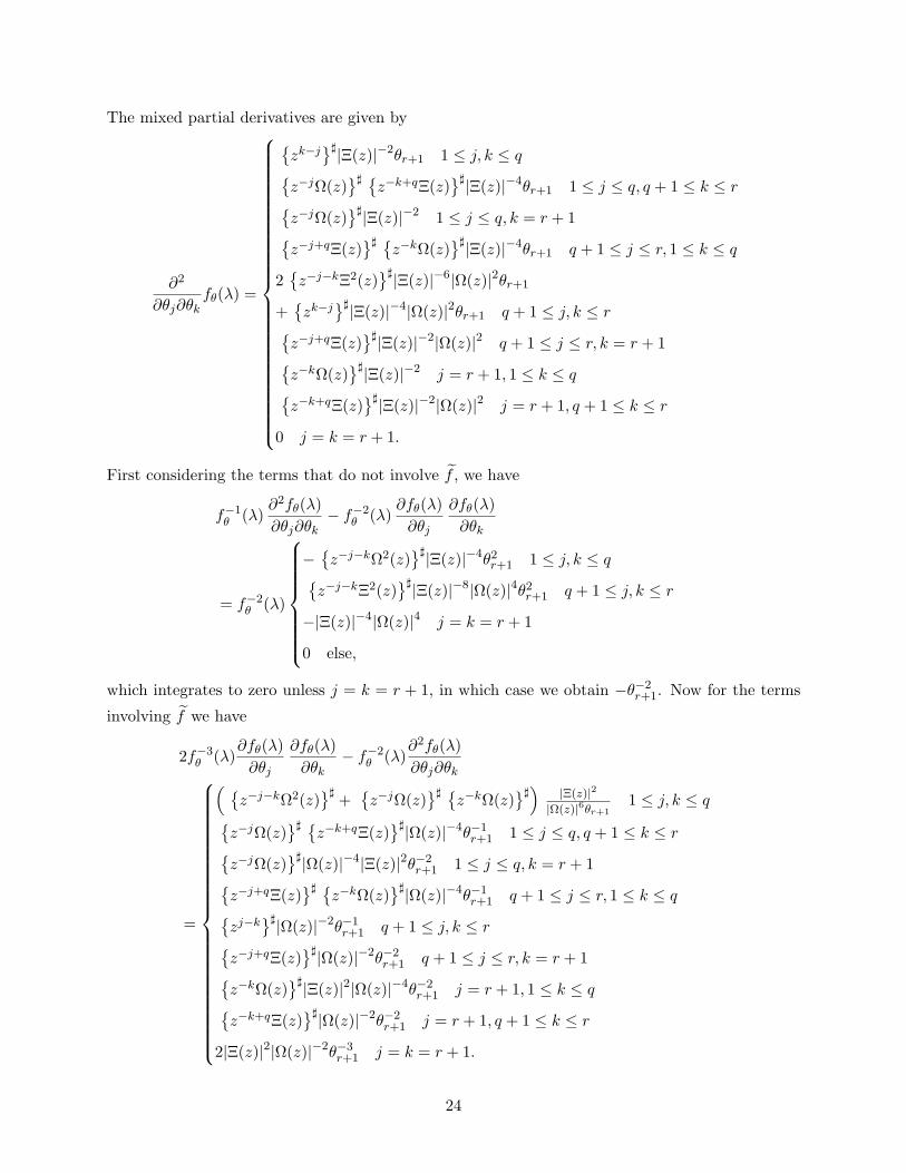
The mixed partial derivatives are given by

∂2

∂θj∂θkfθ(λ) =

zk−j

]|Ξ(z)|−2θr+1 1 ≤ j, k ≤ qz−jΩ(z)

] z−k+qΞ(z)

]|Ξ(z)|−4θr+1 1 ≤ j ≤ q, q + 1 ≤ k ≤ rz−jΩ(z)

]|Ξ(z)|−2 1 ≤ j ≤ q, k = r + 1z−j+qΞ(z)

] z−kΩ(z)

]|Ξ(z)|−4θr+1 q + 1 ≤ j ≤ r, 1 ≤ k ≤ q

2z−j−kΞ2(z)

]|Ξ(z)|−6|Ω(z)|2θr+1

+zk−j

]|Ξ(z)|−4|Ω(z)|2θr+1 q + 1 ≤ j, k ≤ rz−j+qΞ(z)

]|Ξ(z)|−2|Ω(z)|2 q + 1 ≤ j ≤ r, k = r + 1z−kΩ(z)

]|Ξ(z)|−2 j = r + 1, 1 ≤ k ≤ qz−k+qΞ(z)

]|Ξ(z)|−2|Ω(z)|2 j = r + 1, q + 1 ≤ k ≤ r

0 j = k = r + 1.

First considering the terms that do not involve f , we have

f−1θ (λ)

∂2fθ(λ)∂θj∂θk

− f−2θ (λ)

∂fθ(λ)∂θj

∂fθ(λ)∂θk

= f−2θ (λ)

− z−j−kΩ2(z)

]|Ξ(z)|−4θ2r+1 1 ≤ j, k ≤ q

z−j−kΞ2(z)

]|Ξ(z)|−8|Ω(z)|4θ2r+1 q + 1 ≤ j, k ≤ r

−|Ξ(z)|−4|Ω(z)|4 j = k = r + 1

0 else,

which integrates to zero unless j = k = r + 1, in which case we obtain −θ−2r+1. Now for the terms

involving f we have

2f−3θ (λ)

∂fθ(λ)∂θj

∂fθ(λ)∂θk

− f−2θ (λ)

∂2fθ(λ)∂θj∂θk

=

( z−j−kΩ2(z)

] +z−jΩ(z)

] z−kΩ(z)

]) |Ξ(z)|2|Ω(z)|6θr+1

1 ≤ j, k ≤ qz−jΩ(z)

] z−k+qΞ(z)

]|Ω(z)|−4θ−1r+1 1 ≤ j ≤ q, q + 1 ≤ k ≤ r

z−jΩ(z)

]|Ω(z)|−4|Ξ(z)|2θ−2r+1 1 ≤ j ≤ q, k = r + 1

z−j+qΞ(z)

] z−kΩ(z)

]|Ω(z)|−4θ−1r+1 q + 1 ≤ j ≤ r, 1 ≤ k ≤ q

zj−k

]|Ω(z)|−2θ−1r+1 q + 1 ≤ j, k ≤ r

z−j+qΞ(z)

]|Ω(z)|−2θ−2r+1 q + 1 ≤ j ≤ r, k = r + 1

z−kΩ(z)

]|Ξ(z)|2|Ω(z)|−4θ−2r+1 j = r + 1, 1 ≤ k ≤ q

z−k+qΞ(z)

]|Ω(z)|−2θ−2r+1 j = r + 1, q + 1 ≤ k ≤ r

2|Ξ(z)|2|Ω(z)|−2θ−3r+1 j = k = r + 1.

24

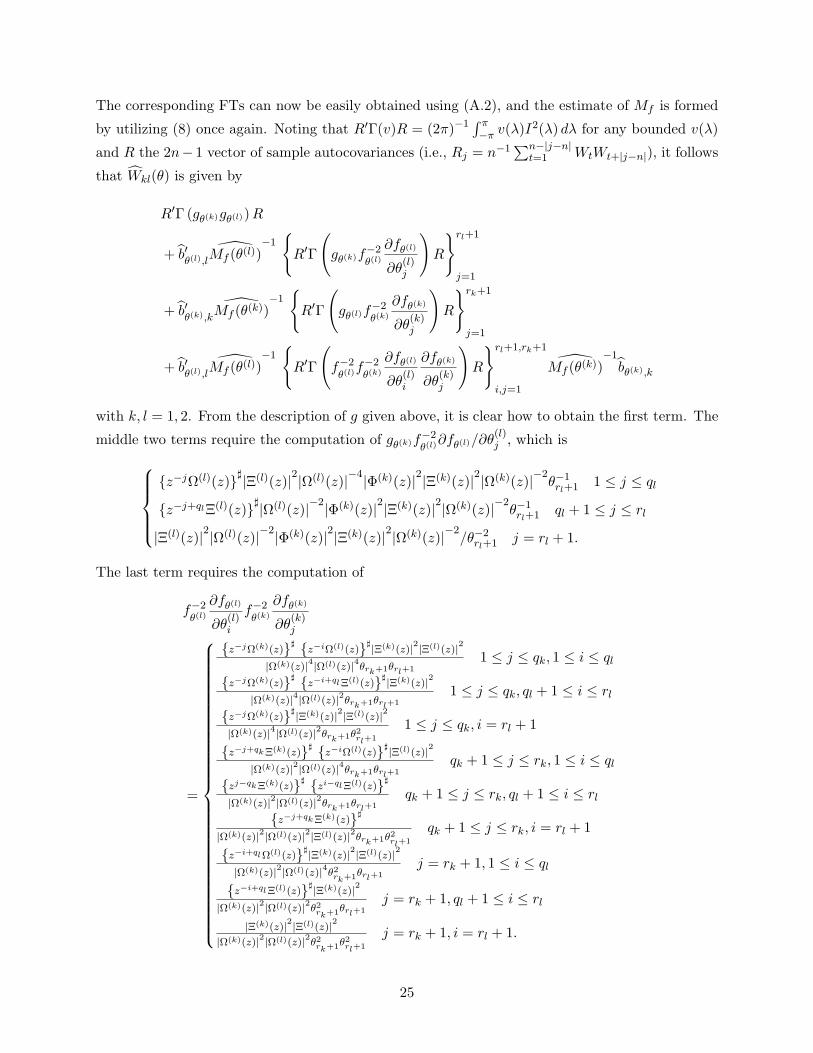
The corresponding FTs can now be easily obtained using (A.2), and the estimate of Mf is formed

by utilizing (8) once again. Noting that R′Γ(v)R = (2π)−1 ∫ π−π v(λ)I2(λ) dλ for any bounded v(λ)

and R the 2n− 1 vector of sample autocovariances (i.e., Rj = n−1∑n−|j−n|

t=1 WtWt+|j−n|), it follows

that Wkl(θ) is given by

R′Γ (gθ(k)gθ(l)) R

+ b′θ(l),l

Mf (θ(l))−1

R′Γ

(gθ(k)f−2

θ(l)

∂fθ(l)

∂θ(l)j

)R

rl+1

j=1

+ b′θ(k),k

Mf (θ(k))−1

R′Γ

(gθ(l)f−2

θ(k)

∂fθ(k)

∂θ(k)j

)R

rk+1

j=1

+ b′θ(l),l

Mf (θ(l))−1

R′Γ

(f−2

θ(l)f−2θ(k)

∂fθ(l)

∂θ(l)i

∂fθ(k)

∂θ(k)j

)R

rl+1,rk+1

i,j=1

Mf (θ(k))−1

bθ(k),k

with k, l = 1, 2. From the description of g given above, it is clear how to obtain the first term. The

middle two terms require the computation of gθ(k)f−2θ(l)∂fθ(l)/∂θ

(l)j , which is

z−jΩ(l)(z)]|Ξ(l)(z)|2|Ω(l)(z)|−4|Φ(k)(z)|2|Ξ(k)(z)|2|Ω(k)(z)|−2θ−1rl+1 1 ≤ j ≤ ql

z−j+qlΞ(l)(z)]|Ω(l)(z)|−2|Φ(k)(z)|2|Ξ(k)(z)|2|Ω(k)(z)|−2θ−1rl+1 ql + 1 ≤ j ≤ rl

|Ξ(l)(z)|2|Ω(l)(z)|−2|Φ(k)(z)|2|Ξ(k)(z)|2|Ω(k)(z)|−2/θ−2

rl+1 j = rl + 1.

The last term requires the computation of

f−2θ(l)

∂fθ(l)

∂θ(l)i

f−2θ(k)

∂fθ(k)

∂θ(k)j

=

z−jΩ(k)(z)] z−iΩ(l)(z)]|Ξ(k)(z)|2|Ξ(l)(z)|2

|Ω(k)(z)|4|Ω(l)(z)|4θrk+1θrl+11 ≤ j ≤ qk, 1 ≤ i ≤ ql

z−jΩ(k)(z)] z−i+qlΞ(l)(z)]|Ξ(k)(z)|2

|Ω(k)(z)|4|Ω(l)(z)|2θrk+1θrl+11 ≤ j ≤ qk, ql + 1 ≤ i ≤ rl

z−jΩ(k)(z)]|Ξ(k)(z)|2|Ξ(l)(z)|2

|Ω(k)(z)|4|Ω(l)(z)|2θrk+1θ2rl+1

1 ≤ j ≤ qk, i = rl + 1

z−j+qkΞ(k)(z)] z−iΩ(l)(z)]|Ξ(l)(z)|2

|Ω(k)(z)|2|Ω(l)(z)|4θrk+1θrl+1qk + 1 ≤ j ≤ rk, 1 ≤ i ≤ ql

zj−qkΞ(k)(z)] zi−qlΞ(l)(z)]

|Ω(k)(z)|2|Ω(l)(z)|2θrk+1θrl+1qk + 1 ≤ j ≤ rk, ql + 1 ≤ i ≤ rl

z−j+qkΞ(k)(z)]

|Ω(k)(z)|2|Ω(l)(z)|2|Ξ(l)(z)|2θrk+1θ2rl+1

qk + 1 ≤ j ≤ rk, i = rl + 1

z−i+qlΩ(l)(z)]|Ξ(k)(z)|2|Ξ(l)(z)|2

|Ω(k)(z)|2|Ω(l)(z)|4θ2rk+1θrl+1

j = rk + 1, 1 ≤ i ≤ ql

z−i+qlΞ(l)(z)]|Ξ(k)(z)|2

|Ω(k)(z)|2|Ω(l)(z)|2θ2rk+1θrl+1

j = rk + 1, ql + 1 ≤ i ≤ rl

|Ξ(k)(z)|2|Ξ(l)(z)|2|Ω(k)(z)|2|Ω(l)(z)|2θ2

rk+1θ2rl+1

j = rk + 1, i = rl + 1.

25

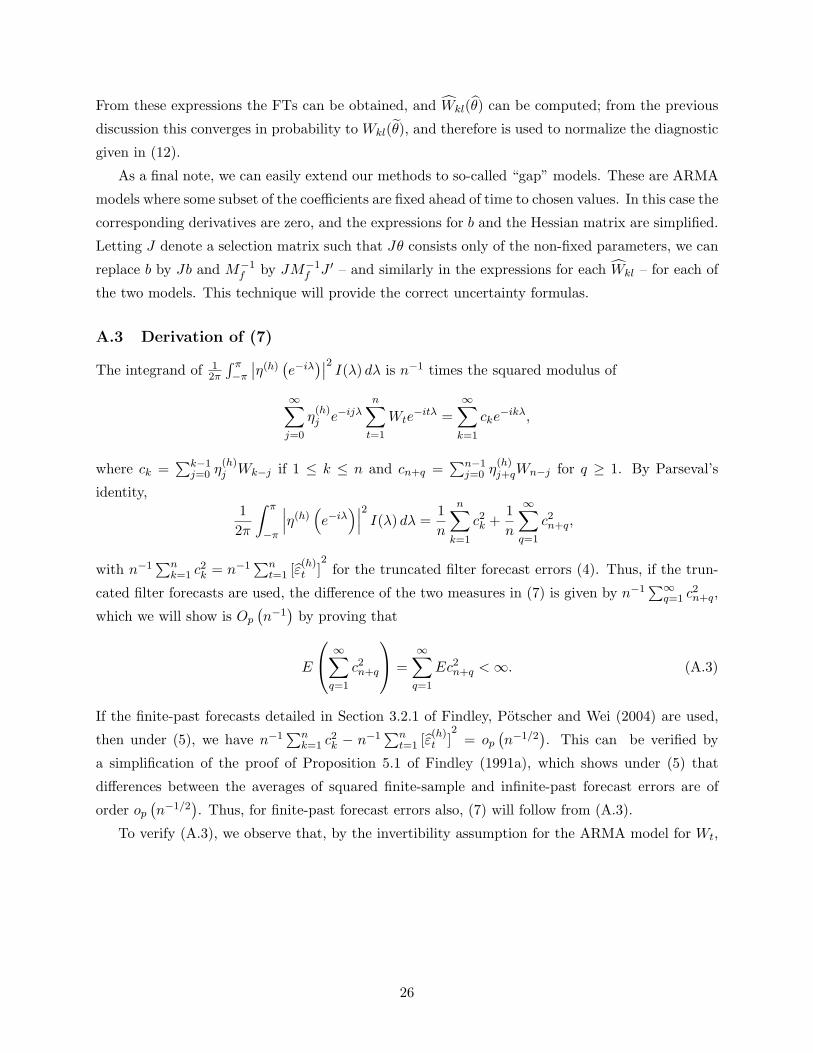
From these expressions the FTs can be obtained, and Wkl(θ) can be computed; from the previous

discussion this converges in probability to Wkl(θ), and therefore is used to normalize the diagnostic

given in (12).

As a final note, we can easily extend our methods to so-called “gap” models. These are ARMA

models where some subset of the coefficients are fixed ahead of time to chosen values. In this case the

corresponding derivatives are zero, and the expressions for b and the Hessian matrix are simplified.

Letting J denote a selection matrix such that Jθ consists only of the non-fixed parameters, we can

replace b by Jb and M−1f by JM−1

f J ′ – and similarly in the expressions for each Wkl – for each of

the two models. This technique will provide the correct uncertainty formulas.

A.3 Derivation of (7)

The integrand of 12π

∫ π−π

∣∣η(h)(e−iλ

)∣∣2 I(λ) dλ is n−1 times the squared modulus of

∞∑

j=0

η(h)j e−ijλ

n∑

t=1

Wte−itλ =

∞∑

k=1

cke−ikλ,

where ck =∑k−1

j=0 η(h)j Wk−j if 1 ≤ k ≤ n and cn+q =

∑n−1j=0 η

(h)j+qWn−j for q ≥ 1. By Parseval’s

identity,12π

∫ π

−π

∣∣∣η(h)(e−iλ

)∣∣∣2I(λ) dλ =

1n

n∑

k=1

c2k +

1n

∞∑

q=1

c2n+q,

with n−1∑n

k=1 c2k = n−1

∑nt=1 [ε(h)

t ]2

for the truncated filter forecast errors (4). Thus, if the trun-

cated filter forecasts are used, the difference of the two measures in (7) is given by n−1∑∞

q=1 c2n+q,

which we will show is Op

(n−1

)by proving that

E

∞∑

q=1

c2n+q

=

∞∑

q=1

Ec2n+q < ∞. (A.3)

If the finite-past forecasts detailed in Section 3.2.1 of Findley, Potscher and Wei (2004) are used,

then under (5), we have n−1∑n

k=1 c2k − n−1

∑nt=1 [ε(h)

t ]2

= op

(n−1/2

). This can be verified by

a simplification of the proof of Proposition 5.1 of Findley (1991a), which shows under (5) that

differences between the averages of squared finite-sample and infinite-past forecast errors are of

order op

(n−1/2

). Thus, for finite-past forecast errors also, (7) will follow from (A.3).

To verify (A.3), we observe that, by the invertibility assumption for the ARMA model for Wt,

26

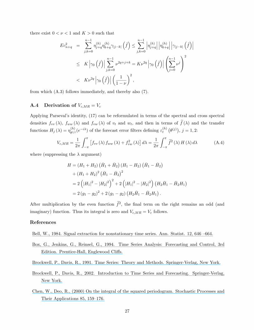
there exist 0 < ν < 1 and K > 0 such that

Ec2n+q =

n−1∑

j,k=0

η(h)j+qη

(h)k+qγ|j−k|

(f)≤

n−1∑

j,k=0

∣∣∣η(h)j+q

∣∣∣∣∣∣η(h)

k+q

∣∣∣∣∣∣γ|j−k|

(f)∣∣∣

≤ K∣∣∣γ0

(f)∣∣∣

n−1∑

j,k=0

ν2q+j+k = Kν2q∣∣∣γ0

(f)∣∣∣

n−1∑

j=0

νj

2

< Kν2q∣∣∣γ0

(f)∣∣∣

(1

1− ν

)2

,

from which (A.3) follows immediately, and thereby also (7).

A.4 Derivation of Vc,MR = Vc

Applying Parseval’s identity, (17) can be reformulated in terms of the spectral and cross spectral

densities fvv (λ), fww (λ) and fvw (λ) of vt and wt, and then in terms of f (λ) and the transfer

functions Hj (λ) = η(h)

θ(j)(e−iλ) of the forecast error filters defining ε(h)t

(θ(j)

), j = 1, 2:

Vc,MR =12π

∫ π

−π

[fvv (λ) fww (λ) + f2

vw (λ)]dλ =

12π

∫ π

−πf2 (λ) H (λ) dλ (A.4)

where (suppressing the λ argument)

H = (H1 + H2)(H1 + H2

)(H1 −H2)

(H1 − H2

)

+ (H1 + H2)2 (

H1 − H2

)2

= 2(|H1|2 − |H2|2

)2+ 2

(|H1|2 − |H2|2

) (H2H1 − H2H1

)

= 2 (g1 − g2)2 + 2 (g1 − g2)

(H2H1 − H2H1

).

After multiplication by the even function f2, the final term on the right remains an odd (and

imaginary) function. Thus its integral is zero and Vc,MR = Vc follows.

References

Bell, W., 1984. Signal extraction for nonstationary time series. Ann. Statist. 12, 646 –664.

Box, G., Jenkins, G., Reinsel, G., 1994. Time Series Analysis: Forecasting and Control, 3rd

Edition. Prentice-Hall, Englewood Cliffs.

Brockwell, P., Davis, R., 1991. Time Series: Theory and Methods. Springer-Verlag, New York.

Brockwell, P., Davis, R., 2002. Introduction to Time Series and Forecasting. Springer-Verlag,

New York.

Chen, W., Deo, R., (2000) On the integral of the squared periodogram. Stochastic Processes and

Their Applications 85, 159–176.

27

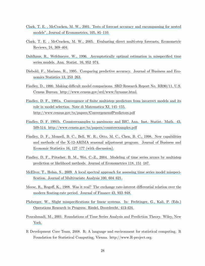
Clark, T. E. , McCracken, M. W., 2001. Tests of forecast accuracy and encompassing for nested

models”, Journal of Econometrics, 105, 85–110.

Clark, T. E. , McCracken, M. W., 2005. Evaluating direct multi-step forecasts, Econometric

Reviews, 24, 369–404.

Dahlhaus, R., Wefelmeyer, W., 1996. Asymptotically optimal estimation in misspecified time

series models. Ann. Statist. 16, 952–974.

Diebold, F., Mariano, R., 1995. Comparing predictive accuracy. Journal of Business and Eco-

nomics Statistics 13, 253–263.

Findley, D., 1990. Making difficult model comparisons. SRD Research Report No. RR90/11, U.S.

Census Bureau. http://www.census.gov/srd/www/byname.html.

Findley, D. F., 1991a. Convergence of finite multistep predictors from incorrect models and its

role in model selection. Note di Matematica XI, 145–155.

http://www.census.gov/ts/papers/ConvergenceofPredictors.pdf

Findley, D. F. 1991b. Counterexamples to parsimony and BIC, Ann. Inst. Statist. Math. 43,

509-514. http://www.census.gov/ts/papers/counterexamples.pdf

Findley, D. F., Monsell, B. C., Bell, W. R., Otto, M. C., Chen, B. C., 1998. New capabilities

and methods of the X-12-ARIMA seasonal adjustment program. Journal of Business and

Economic Statistics 16, 127–177 (with discussion).

Findley, D. F., Potscher, B. M., Wei, C.-Z., 2004. Modeling of time series arrays by multistep

prediction or likelihood methods. Journal of Econometrics 118, 151–187.

McElroy, T., Holan, S., 2009. A local spectral approach for assessing time series model misspeci-

fication. Journal of Multivariate Analysis 100, 604–621.

Meese, R., Rogoff, K., 1988. Was it real? The exchange rate-interest differential relation over the

modern floating-rate period. Journal of Finance 43, 933–948.

Ploberger, W., Slight misspecifications for linear systems. In: Fechtinger, G., Kali, P. (Eds.)

Operations Research in Progress. Riedel, Doordrecht, 413-424.

Pourahmadi, M., 2001. Foundations of Time Series Analysis and Prediction Theory. Wiley, New

York.

R Development Core Team, 2008. R: A language and environment for statistical computing. R

Foundation for Statistical Computing, Vienna. http://www.R-project.org.

28

Rivers, D., Vuong, Q., 2002. Model selection tests for nonlinear dynamic models. Econometrics

Journal 5, 1–39.

Taniguchi, M., Kakizawa, Y., 2000. Asymptotic Theory of Statistical Inference for Time Series.

Springer-Verlag, New York.

Vuong, Q., 1989. Likelihood ratio tests for model selection and non-nested hypotheses. Econo-

metrica 57, 307-333.

West, K., 1996. Asymptotic inference about predictive ability. Econometrica 64, 1067–1084.

29

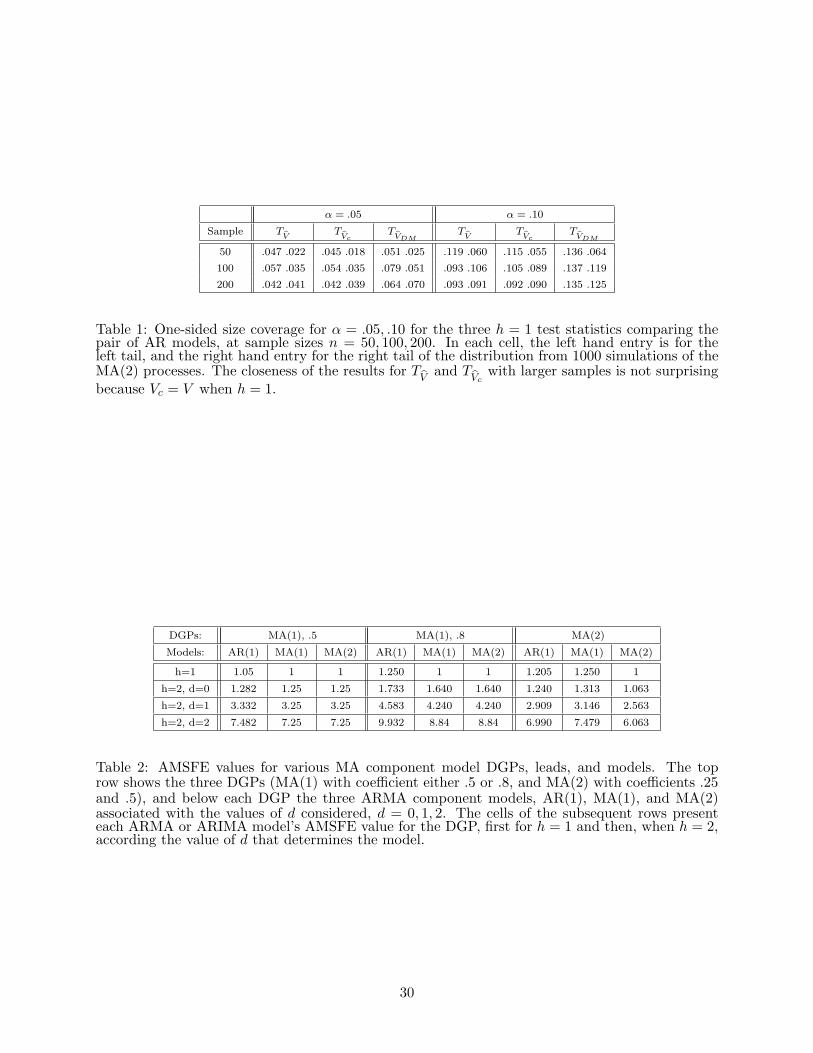
α = .05 α = .10

Sample TV

TVc

TVDM

TV

TVc

TVDM

50 .047 .022 .045 .018 .051 .025 .119 .060 .115 .055 .136 .064

100 .057 .035 .054 .035 .079 .051 .093 .106 .105 .089 .137 .119

200 .042 .041 .042 .039 .064 .070 .093 .091 .092 .090 .135 .125

Table 1: One-sided size coverage for α = .05, .10 for the three h = 1 test statistics comparing thepair of AR models, at sample sizes n = 50, 100, 200. In each cell, the left hand entry is for theleft tail, and the right hand entry for the right tail of the distribution from 1000 simulations of theMA(2) processes. The closeness of the results for T

Vand T

Vcwith larger samples is not surprising

because Vc = V when h = 1.

DGPs: MA(1), .5 MA(1), .8 MA(2)

Models: AR(1) MA(1) MA(2) AR(1) MA(1) MA(2) AR(1) MA(1) MA(2)

h=1 1.05 1 1 1.250 1 1 1.205 1.250 1

h=2, d=0 1.282 1.25 1.25 1.733 1.640 1.640 1.240 1.313 1.063

h=2, d=1 3.332 3.25 3.25 4.583 4.240 4.240 2.909 3.146 2.563

h=2, d=2 7.482 7.25 7.25 9.932 8.84 8.84 6.990 7.479 6.063

Table 2: AMSFE values for various MA component model DGPs, leads, and models. The toprow shows the three DGPs (MA(1) with coefficient either .5 or .8, and MA(2) with coefficients .25and .5), and below each DGP the three ARMA component models, AR(1), MA(1), and MA(2)associated with the values of d considered, d = 0, 1, 2. The cells of the subsequent rows presenteach ARMA or ARIMA model’s AMSFE value for the DGP, first for h = 1 and then, when h = 2,according the value of d that determines the model.

30

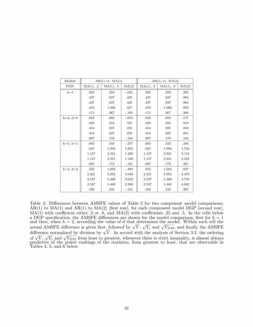
Models: AR(1) vs. MA(1) AR(1) vs. MA(2)

DGP: MA(1), .5 MA(1), .8 MA(2) MA(1), .5 MA(1), .8 MA(2)

h=1 .050 .250 -.045 .050 .250 .205

.437 .937 .429 .437 .937 .984

.437 .937 .429 .437 .937 .984

.453 1.060 .327 .453 1.060 .952

.115 .267 -.105 .115 .267 .208

h=2, d=0 .032 .093 -.073 .032 .093 .177

.329 .584 .701 .329 .584 .910

.454 .925 .259 .454 .925 .859

.454 .925 .238 .454 .925 .891

.097 .159 -.104 .097 .159 .194

h=2, d=1 .082 .343 -.237 .082 .343 .346

.947 1.994 1.955 .947 1.994 1.724

1.127 2.321 1.209 1.127 2.321 2.112

1.127 2.321 1.166 1.127 2.321 2.224

.087 .172 -.121 .087 .172 .201

h=2, d=2 .232 1.092 -.489 .232 1.092 .927

2.321 5.054 4.048 2.321 5.054 4.470

2.537 5.469 3.022 2.537 5.469 4.759

2.537 5.469 2.909 2.537 5.469 4.962

.100 .216 -.121 .100 .216 .207

Table 3: Differences between AMSFE values of Table 2 for two component model comparisons,AR(1) to MA(1) and AR(1) to MA(2) [first row], for each component model DGP [second row],MA(1) with coefficient either .5 or .8, and MA(2) with coefficients .25 and .5. In the cells belowa DGP specification, the AMSFE differences are shown for the model comparison, first for h = 1and then, when h = 2, according the value of d that determines the model. Within each cell theactual AMSFE difference is given first, followed by

√V ,

√Vc and

√VDM , and finally the AMSFE

difference normalized by division by√

V . In accord with the analysis of Section 3.2, the orderingof√

V ,√

Vc and√

VDM from least to greatest, whenever there is strict inequality, is almost alwayspredictive of the power rankings of the statistics, from greatest to least, that are observable inTables 4, 5, and 6 below.

31

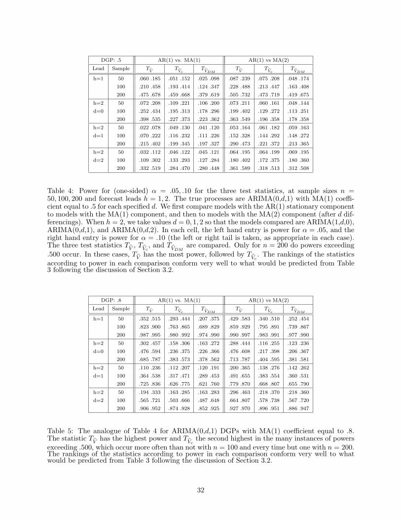
DGP: .5 AR(1) vs. MA(1) AR(1) vs MA(2)

Lead Sample TV

TVc

TVDM

TV

TVc

TVDM

h=1 50 .060 .185 .051 .152 .025 .098 .087 .239 .075 .208 .048 .174

100 .210 .458 .193 .414 .124 .347 .228 .488 .213 .447 .163 .408

200 .475 .678 .459 .668 .379 .619 .505 .732 .473 .719 .419 .675

h=2 50 .072 .208 .109 .221 .106 .200 .073 .211 .060 .161 .048 .144

d=0 100 .252 .434 .195 .313 .178 .296 .199 .402 .129 .272 .113 .251

200 .398 .535 .227 .373 .223 .362 .363 .549 .196 .358 .178 .358

h=2 50 .022 .078 .049 .130 .041 .120 .053 .164 .061 .182 .059 .163

d=1 100 .070 .222 .116 .232 .111 .226 .152 .328 .144 .292 .148 .272

200 .215 .402 .199 .345 .197 .327 .290 .473 .221 .372 .213 .365

h=2 50 .032 .112 .046 .122 .045 .121 .064 .195 .064 .199 .069 .195

d=2 100 .109 .302 .133 .293 .127 .284 .180 .402 .172 .375 .180 .360

200 .332 .519 .284 .470 .280 .448 .361 .589 .318 .513 .312 .508

Table 4: Power for (one-sided) α = .05, .10 for the three test statistics, at sample sizes n =50, 100, 200 and forecast leads h = 1, 2. The true processes are ARIMA(0,d,1) with MA(1) coeffi-cient equal to .5 for each specified d. We first compare models with the AR(1) stationary componentto models with the MA(1) component, and then to models with the MA(2) component (after d dif-ferencings). When h = 2, we take values d = 0, 1, 2 so that the models compared are ARIMA(1,d,0),ARIMA(0,d,1), and ARIMA(0,d,2). In each cell, the left hand entry is power for α = .05, and theright hand entry is power for α = .10 (the left or right tail is taken, as appropriate in each case).The three test statistics T

V, T

Vc, and T

VDMare compared. Only for n = 200 do powers exceeding

.500 occur. In these cases, TV

has the most power, followed by TVc

. The rankings of the statisticsaccording to power in each comparison conform very well to what would be predicted from Table3 following the discussion of Section 3.2.

DGP: .8 AR(1) vs. MA(1) AR(1) vs MA(2)

Lead Sample TV

TVc

TVDM

TV

TVc

TVDM

h=1 50 .352 .515 .293 .444 .207 .375 .429 .583 .340 .510 .252 .454

100 .823 .900 .763 .865 .689 .829 .859 .929 .795 .891 .739 .867

200 .987 .995 .980 .992 .974 .990 .990 .997 .983 .991 .977 .990

h=2 50 .302 .457 .158 .306 .163 .272 .288 .444 .116 .255 .123 .236

d=0 100 .476 .594 .236 .375 .226 .366 .476 .608 .217 .398 .206 .367

200 .685 .787 .383 .573 .378 .562 .713 .787 .404 .595 .381 .581

h=2 50 .110 .236 .112 .207 .120 .191 .200 .365 .138 .276 .142 .262

d=1 100 .364 .538 .317 .471 .289 .453 .491 .655 .383 .554 .360 .531

200 .725 .836 .626 .775 .621 .760 .779 .870 .668 .807 .655 .790

h=2 50 .194 .333 .163 .285 .163 .283 .296 .463 .218 .370 .218 .360

d=2 100 .565 .721 .503 .666 .487 .648 .664 .807 .578 .738 .567 .720

200 .906 .952 .874 .928 .852 .925 .927 .970 .896 .951 .886 .947

Table 5: The analogue of Table 4 for ARIMA(0,d,1) DGPs with MA(1) coefficient equal to .8.The statistic T

Vhas the highest power and T

Vcthe second highest in the many instances of powers

exceeding .500, which occur more often than not with n = 100 and every time but one with n = 200.The rankings of the statistics according to power in each comparison conform very well to whatwould be predicted from Table 3 following the discussion of Section 3.2.

32

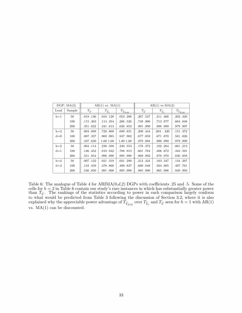
DGP: MA(2) AR(1) vs. MA(1) AR(1) vs MA(2)

Lead Sample TV

TVc

TVDM

TV

TVc

TVDM

h=1 50 .018 .136 .018 .128 .052 .206 .267 .527 .211 .466 .202 .420

100 .115 .363 .114 .354 .266 .526 .749 .906 .713 .877 .664 .848

200 .351 .622 .341 .613 .626 .852 .991 .999 .988 .999 .979 .997

h=2 50 .004 .088 .729 .868 .689 .831 .209 .444 .204 . 420 .151 .372

d=0 100 .087 .337 .969 .985 .947 .982 .677 .859 .671 .870 .581 .826

200 .337 .630 1.00 1.00 1.00 1.00 .979 .994 .990 .999 .979 .999

h=2 50 .004 .114 .230 .598 .230 .553 .178 .372 .102 .264 .061 .213

d=1 100 .126 .452 .810 .942 .788 .913 .601 .784 .406 .672 .343 .591

200 .551 .854 .996 .998 .995 .998 .969 .992 .878 .970 .830 .958

h=2 50 .007 .122 .021 .319 .021 .290 .212 .424 .163 .347 .134 .297

d=2 100 .134 .459 .478 .866 .499 .837 .680 .848 .564 .805 .497 .761

200 .546 .850 .991 .998 .995 .998 .985 .996 .965 .996 .949 .993

Table 6: The analogue of Table 4 for ARIMA(0,d,2) DGPs with coefficients .25 and .5. Some of thecells for h = 2 in Table 6 contain our study’s rare instances in which has substantially greater powerthan T

V. The rankings of the statistics according to power in each comparison largely conform

to what would be predicted from Table 3 following the discussion of Section 3.2, where it is alsoexplained why the appreciable power advantage of T

VDMover T

Vcand T

Vseen for h = 1 with AR(1)

vs. MA(1) can be discounted.

33

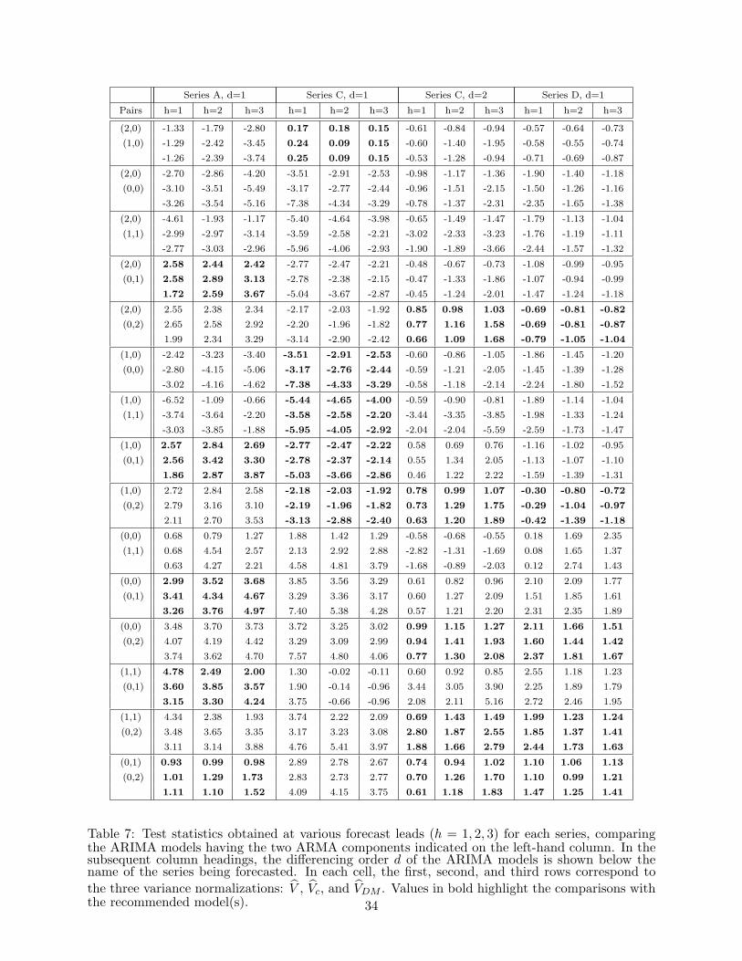
Series A, d=1 Series C, d=1 Series C, d=2 Series D, d=1

Pairs h=1 h=2 h=3 h=1 h=2 h=3 h=1 h=2 h=3 h=1 h=2 h=3

(2,0) -1.33 -1.79 -2.80 0.17 0.18 0.15 -0.61 -0.84 -0.94 -0.57 -0.64 -0.73

(1,0) -1.29 -2.42 -3.45 0.24 0.09 0.15 -0.60 -1.40 -1.95 -0.58 -0.55 -0.74

-1.26 -2.39 -3.74 0.25 0.09 0.15 -0.53 -1.28 -0.94 -0.71 -0.69 -0.87

(2,0) -2.70 -2.86 -4.20 -3.51 -2.91 -2.53 -0.98 -1.17 -1.36 -1.90 -1.40 -1.18

(0,0) -3.10 -3.51 -5.49 -3.17 -2.77 -2.44 -0.96 -1.51 -2.15 -1.50 -1.26 -1.16

-3.26 -3.54 -5.16 -7.38 -4.34 -3.29 -0.78 -1.37 -2.31 -2.35 -1.65 -1.38

(2,0) -4.61 -1.93 -1.17 -5.40 -4.64 -3.98 -0.65 -1.49 -1.47 -1.79 -1.13 -1.04

(1,1) -2.99 -2.97 -3.14 -3.59 -2.58 -2.21 -3.02 -2.33 -3.23 -1.76 -1.19 -1.11

-2.77 -3.03 -2.96 -5.96 -4.06 -2.93 -1.90 -1.89 -3.66 -2.44 -1.57 -1.32

(2,0) 2.58 2.44 2.42 -2.77 -2.47 -2.21 -0.48 -0.67 -0.73 -1.08 -0.99 -0.95

(0,1) 2.58 2.89 3.13 -2.78 -2.38 -2.15 -0.47 -1.33 -1.86 -1.07 -0.94 -0.99

1.72 2.59 3.67 -5.04 -3.67 -2.87 -0.45 -1.24 -2.01 -1.47 -1.24 -1.18

(2,0) 2.55 2.38 2.34 -2.17 -2.03 -1.92 0.85 0.98 1.03 -0.69 -0.81 -0.82

(0,2) 2.65 2.58 2.92 -2.20 -1.96 -1.82 0.77 1.16 1.58 -0.69 -0.81 -0.87

1.99 2.34 3.29 -3.14 -2.90 -2.42 0.66 1.09 1.68 -0.79 -1.05 -1.04

(1,0) -2.42 -3.23 -3.40 -3.51 -2.91 -2.53 -0.60 -0.86 -1.05 -1.86 -1.45 -1.20

(0,0) -2.80 -4.15 -5.06 -3.17 -2.76 -2.44 -0.59 -1.21 -2.05 -1.45 -1.39 -1.28

-3.02 -4.16 -4.62 -7.38 -4.33 -3.29 -0.58 -1.18 -2.14 -2.24 -1.80 -1.52

(1,0) -6.52 -1.09 -0.66 -5.44 -4.65 -4.00 -0.59 -0.90 -0.81 -1.89 -1.14 -1.04

(1,1) -3.74 -3.64 -2.20 -3.58 -2.58 -2.20 -3.44 -3.35 -3.85 -1.98 -1.33 -1.24

-3.03 -3.85 -1.88 -5.95 -4.05 -2.92 -2.04 -2.04 -5.59 -2.59 -1.73 -1.47

(1,0) 2.57 2.84 2.69 -2.77 -2.47 -2.22 0.58 0.69 0.76 -1.16 -1.02 -0.95

(0,1) 2.56 3.42 3.30 -2.78 -2.37 -2.14 0.55 1.34 2.05 -1.13 -1.07 -1.10

1.86 2.87 3.87 -5.03 -3.66 -2.86 0.46 1.22 2.22 -1.59 -1.39 -1.31

(1,0) 2.72 2.84 2.58 -2.18 -2.03 -1.92 0.78 0.99 1.07 -0.30 -0.80 -0.72

(0,2) 2.79 3.16 3.10 -2.19 -1.96 -1.82 0.73 1.29 1.75 -0.29 -1.04 -0.97

2.11 2.70 3.53 -3.13 -2.88 -2.40 0.63 1.20 1.89 -0.42 -1.39 -1.18

(0,0) 0.68 0.79 1.27 1.88 1.42 1.29 -0.58 -0.68 -0.55 0.18 1.69 2.35

(1,1) 0.68 4.54 2.57 2.13 2.92 2.88 -2.82 -1.31 -1.69 0.08 1.65 1.37

0.63 4.27 2.21 4.58 4.81 3.79 -1.68 -0.89 -2.03 0.12 2.74 1.43

(0,0) 2.99 3.52 3.68 3.85 3.56 3.29 0.61 0.82 0.96 2.10 2.09 1.77

(0,1) 3.41 4.34 4.67 3.29 3.36 3.17 0.60 1.27 2.09 1.51 1.85 1.61

3.26 3.76 4.97 7.40 5.38 4.28 0.57 1.21 2.20 2.31 2.35 1.89

(0,0) 3.48 3.70 3.73 3.72 3.25 3.02 0.99 1.15 1.27 2.11 1.66 1.51

(0,2) 4.07 4.19 4.42 3.29 3.09 2.99 0.94 1.41 1.93 1.60 1.44 1.42

3.74 3.62 4.70 7.57 4.80 4.06 0.77 1.30 2.08 2.37 1.81 1.67

(1,1) 4.78 2.49 2.00 1.30 -0.02 -0.11 0.60 0.92 0.85 2.55 1.18 1.23

(0,1) 3.60 3.85 3.57 1.90 -0.14 -0.96 3.44 3.05 3.90 2.25 1.89 1.79

3.15 3.30 4.24 3.75 -0.66 -0.96 2.08 2.11 5.16 2.72 2.46 1.95

(1,1) 4.34 2.38 1.93 3.74 2.22 2.09 0.69 1.43 1.49 1.99 1.23 1.24

(0,2) 3.48 3.65 3.35 3.17 3.23 3.08 2.80 1.87 2.55 1.85 1.37 1.41

3.11 3.14 3.88 4.76 5.41 3.97 1.88 1.66 2.79 2.44 1.73 1.63

(0,1) 0.93 0.99 0.98 2.89 2.78 2.67 0.74 0.94 1.02 1.10 1.06 1.13

(0,2) 1.01 1.29 1.73 2.83 2.73 2.77 0.70 1.26 1.70 1.10 0.99 1.21

1.11 1.10 1.52 4.09 4.15 3.75 0.61 1.18 1.83 1.47 1.25 1.41

Table 7: Test statistics obtained at various forecast leads (h = 1, 2, 3) for each series, comparingthe ARIMA models having the two ARMA components indicated on the left-hand column. In thesubsequent column headings, the differencing order d of the ARIMA models is shown below thename of the series being forecasted. In each cell, the first, second, and third rows correspond tothe three variance normalizations: V , Vc, and VDM . Values in bold highlight the comparisons withthe recommended model(s). 34