Selected Papers from IIKII 2019 conferences in Symmetry

Selected Papers from IIKII 2019 conferences in Sym

metry • Teen H

ang Meen, Charles Tijus and Jih-Fu Tu

Selected Papers from IIKII 2019 conferences in Symmetry

Printed Edition of the Special Issue Published in Symmetry

www.mdpi.com/journal/symmetry

Teen Hang Meen, Charles Tijus and Jih-Fu TuEdited by

Selected Papers from IIKII 2019conferences in Symmetry

Selected Papers from IIKII 2019conferences in Symmetry

Special Issue Editors

TeenHang Meen

Charles Tijus

Jih-Fu Tu

MDPI • Basel • Beijing • Wuhan • Barcelona • Belgrade • Manchester • Tokyo • Cluj • Tianjin

Special Issue Editors

TeenHang Meen

National Formosa University

Taiwan

Charles Tijus

Universite Paris 8

France

Jih-Fu Tu

St. John’s University

Taiwan

Editorial Office

MDPI

St. Alban-Anlage 66

4052 Basel, Switzerland

This is a reprint of articles from the Special Issue published online in the open access journal Symmetry

(ISSN 2073-8994) (available at: https://www.mdpi.com/journal/symmetry/special issues/IIKII

2019 conferences).

For citation purposes, cite each article independently as indicated on the article page online and as

indicated below:

LastName, A.A.; LastName, B.B.; LastName, C.C. Article Title. Journal Name Year, Article Number,

Page Range.

ISBN 978-3-03936-240-0 (Hbk) ISBN 978-3-03936-241-7 (PDF)

c© 2020 by the authors. Articles in this book are Open Access and distributed under the Creative

Commons Attribution (CC BY) license, which allows users to download, copy and build upon

published articles, as long as the author and publisher are properly credited, which ensures maximum

dissemination and a wider impact of our publications.

The book as a whole is distributed by MDPI under the terms and conditions of the Creative Commons

license CC BY-NC-ND.

Contents

About the Special Issue Editors . . . . . . . . . . . . . . . . . . . . . . . . . . . . . . . . . . . . . vii

Teen-Hang Meen, Charles Tijus and Jih-Fu Tu

Selected Papers from IIKII 2019 Conferences in SymmetryReprinted from: Symmetry 2020, 12, 684, doi:10.3390/sym12050684 . . . . . . . . . . . . . . . . . 1

Xianghu Liu, Chia-Hui Liu and Yang Li

The Effects of Computer-Assisted Learning Based on Dual Coding TheoryReprinted from: Symmetry 2020, 12, 701, doi:10.3390/sym12050701 . . . . . . . . . . . . . . . . . 11

Pavel Kubıcek, Dalibor Bartonek, Jirı Bures and Otakar Svabensky

Proposal of Technological GIS Support as Part of Resident Parking in Large Cities–Case Study,City of BrnoReprinted from: Symmetry 2020, 12, 542, doi:10.3390/sym12040542 . . . . . . . . . . . . . . . . . 25

Hwi-Ho Lee, Jung-Hyok Kwon and Eui-Jik Kim

Design and Implementation of Virtual Private Storage Framework Using Internet of ThingsLocal NetworksReprinted from: Symmetry 2020, 12, 489, doi:10.3390/sym12030489 . . . . . . . . . . . . . . . . . 47

Jung-Hyok Kwon and Eui-Jik Kim

Failure Prediction Model Using Iterative Feature Selection for Industrial Internet of ThingsReprinted from: Symmetry 2020, 12, 454, doi:10.3390/sym12030454 . . . . . . . . . . . . . . . . . 59

Tian-Syung Lan, Kai-Chi Chuang, Hai-Xia Li, Jih-Fu Tu and Huei-Sheng Huang

Symmetric Modeling of Communication Effectiveness and Satisfaction for CommunicationSoftware on Job PerformanceReprinted from: Symmetry 2020, 12, 418, doi:10.3390/sym12050684 . . . . . . . . . . . . . . . . . 71

Li Li, Shengxian Wang, Shanqing Zhang, Ting Luo and Ching-Chun Chang

Homomorphic Encryption-Based Robust Reversible Watermarking for 3D ModelReprinted from: Symmetry 2020, 12, 347, doi:10.3390/sym12030347 . . . . . . . . . . . . . . . . . 85

Hanfei Zhang, Shungen Xiao and Ping Zhou

A Matching Pursuit Algorithm for Backtracking Regularization Based on Energy SortingReprinted from: Symmetry 2020, 12, 231, doi:10.3390/sym12020231 . . . . . . . . . . . . . . . . . 103

Fu-Lan Ye, Chou-Yuan Lee, Zne-Jung Lee, Jian-Qiong Huang and Jih-Fu Tu

Incorporating Particle Swarm Optimization into Improved Bacterial Foraging OptimizationAlgorithm Applied to Classify Imbalanced DataReprinted from: Symmetry 2020, 12, 229, doi:10.3390/sym12020229 . . . . . . . . . . . . . . . . . 115

Hsin-Hung Lin, Jui-Hung Cheng and Chi-Hsiung Chen

Application of Gray Relational Analysis and Computational Fluid Dynamics to the StatisticalTechniques of Product DesignsReprinted from: Symmetry 2020, 12, 227, doi:10.3390/sym12020227 . . . . . . . . . . . . . . . . . 131

Hui-Chun Hung, I-Fan Liu, Che-Tien Liang and Yu-Sheng Su

Applying Educational Data Mining to Explore Students’ Learning Patterns in the FlippedLearning Approach for Coding EducationReprinted from: Symmetry 2020, 12, 213, doi:10.3390/sym12020213 . . . . . . . . . . . . . . . . . 151

v

Dalibor Bartonek and Michal Buday

Problems of Creation and Usage of 3D Model of Structures and Theirs Possible SolutionReprinted from: Symmetry 2020, 12, 181, doi:10.3390/sym12010181 . . . . . . . . . . . . . . . . . 165

Fu-Hsien Chen and Sheng-Yuan Yang

A Balance Interface Design and Instant Image-based Traffic Assistant Agent Based on GPS andLinked Open Data TechnologyReprinted from: Symmetry 2020, 12, 1, doi:10.3390/sym12010001 . . . . . . . . . . . . . . . . . . . 179

Yan-Hong Fan, Ling-Hui Wang, You Jia, Xing-Guo Li, Xue-Xia Yang and Chih-Cheng Chen

Investigation of High-Efficiency Iterative ILU Preconditioner Algorithm for Partial-DifferentialEquation SystemsReprinted from: Symmetry 2020, 12, 1461, doi:10.3390/sym11121461 . . . . . . . . . . . . . . . . . 203

Kai-Chi Chuang, Tian-Syung Lan, Lie-Ping Zhang, Yee-Ming Chen and Xuan-Jun Dai

Parameter Optimization for Computer Numerical Controlled Machining Using Fuzzy andGame TheoryReprinted from: Symmetry 2020, 12, 1450, doi:10.3390/sym11121450 . . . . . . . . . . . . . . . . . 219

Jing-Jing Bao, Chun-Liang Hsu and Jih-Fu Tu

An Efficient Data Transmission with GSM-MPAPM Modulation for an Indoor VLC SystemReprinted from: Symmetry 2019, 11, 1232, doi:10.3390/sym11101232 . . . . . . . . . . . . . . . . . 237

Yu-Min Hsueh, Veeresh Ramesh Ittangihal, Wei-Bin Wu, Hong-Chan Chang and

Cheng-Chien Kuo

Fault Diagnosis System for Induction Motors by CNN Using Empirical Wavelet TransformReprinted from: Symmetry 2019, 11, 1212, doi:10.3390/sym11101212 . . . . . . . . . . . . . . . . . 251

Horng-Lin Shieh and Fu-Hsien Chen

Forecasting for Ultra-Short-Term Electric Power Load Based on Integrated Artificial NeuralNetworksReprinted from: Symmetry 2019, 11, 1063, doi:10.3390/sym11081063 . . . . . . . . . . . . . . . . . 267

Shiow-Luan Wang, Yung-Tsung Hou and Sarawut Kankham

Behavior Modality of Internet Technology on Reliability Analysis and Trust Perception forInternational Purchase BehaviorReprinted from: Symmetry 2019, 11, 989, doi:10.3390/sym11080989 . . . . . . . . . . . . . . . . . 283

Hsin-Hung Lin and Jui-Hung Cheng

Application of the Symmetric Model to the Design Optimization of Fan Outlet GrillsReprinted from: Symmetry 2019, 11, 959, doi:10.3390/sym11080959 . . . . . . . . . . . . . . . . . 297

Yu-Tung Chen, Eduardo Piedad Jr. and Cheng-Chien Kuo

Energy Consumption Load Forecasting Using a Level-Based Random Forest ClassifierReprinted from: Symmetry 2019, 11, 956, doi:10.3390/sym11080956 . . . . . . . . . . . . . . . . . 319

Ru-Yan Chen and Jih-Fu Tu

The Computer Course Correlation between Learning Satisfaction and Learning Effectiveness ofVocational College in TaiwanReprinted from: Symmetry 2019, 11, 822, doi:10.3390/sym11060822 . . . . . . . . . . . . . . . . . 329

Yun-Long Gao, Si-Zhe Luo, Zhi-Hao Wang, Chih-Cheng Chen and Jin-Yan Pan

Locality Sensitive Discriminative Unsupervised Dimensionality ReductionyReprinted from: Symmetry 2019, 11, 1036, doi:10.3390/sym11081036 . . . . . . . . . . . . . . . . . 339

vi

About the Special Issue Editors

Teen-Hang Meen, Dr., was born in Tainan, Taiwan on August 1, 1967. He received his BS degree from

Department of Electrical Engineering, National Cheng Kung University (NCKU), Tainan, Taiwan

in 1989, his MS degree and PhD from Institute of Electrical Engineering, National Sun Yat-Sen

University (NSYSU), Kaohsiung, Taiwan in 1991 and 1994, respectively. He was Chairman of the

Department of Electronic Engineering from 2005 to 2011 at National Formosa University, Yunlin,

Taiwan. He received prestigious research awards from National Formosa University in both 2008

and 2014. Currently, he is a distinguished professor at the Department of Electronic Engineering,

National Formosa University, Yunlin, Taiwan. He is also the president of the International Institute

of Knowledge Innovation and Invention (IIKII) and the Chair of the IEEE Tainan Section Sensors

Council. He has published more than 100 SCI, SSCI and EI papers in recent years.

Charles Tijus, Dr., has worked on visual perception for two years, with Adam Reeves (Vision Lab,

Northeastern University, Boston, USA) as a research assistant. Charles Tijus is the Director of the

Cognitions Humaine et Artificielle Laboratory, founded with M. Bui and F. Jouen, the CHArt, a

cognitive science laboratory (problem solving, understanding, robotics and cognitive ergonomics),

and “Laboratoire des Usages des Techniques d’Information Numeriques”, with D. Boullier; a

new cognitive ergonomics living LAB laboratory, (LUTIN), which is a “USERLAB” (something

like the Audience Research Facility, Boston), located at the “Cite des Sciences et de l’Industrie”,

La Villette. LUTIN is a platform for usability observations and experiments. LUTIN owns most of

the analytical equipment required for its work. It provides access to various shared equipment, such

as eye-tracking systems, evoked potentials systems, physiological recording systems, video recording

and analysi. The advantages of LUTIN are participants for observations, technologies for observation

and experimentation, cognitive simulation, interface between disciplines, and links with industries.

LUTIN has close relationships with hospitals, industries, and professional teams and users. It offers

services and advice for the adequate conception and use of information technologies. Charles Tijus

develops a contextual categorization-based approach in order to study the cognitive processes of

understanding: thinking, reasoning, decision-making and learning in early child development and

adults. How people develop abilities and competencies is the major concern when it comes to

adaptive behavior. The methods comprise empirical research, eye-tracking, event-related potentials

(ERPs): N400, and computer models for cognitive simulations. The current interdisciplinary and

collaborative research (cognitive psychology, neuroscience and computer science) is on problem

solving and operative language, as well as figurative language understanding, and on cognitive

robotics and other smart cognitive technologies. Charles Tijus was one of the 2014 IBM Faculty Award

recipients.

Jih-Fu Tu, Dr., received his PhD in Computer Science from Preston University, USA. He is also

the professor of the Industrial Engineering and Management Department at St. John’s University

in Taiwan. He was a technology consultant for WanWell Cop. He is interested in the computer

architecture of multiprocessor systems and multithreaded processors, discrete event systems (DES),

VLSI design, the I/O devices design of a computer, and AIoT. He was also the peer reviewer of The

Journal of Supercomputing, Computers and Electrical Engineering, Microsystem Technologies, and

the Committee of International Conference, etc. He has published over 20 journal papers, 5 authored

books, 7 edited books, and 30 papers in international conference proceedings.

vii

Symmetry 2020, 12, 684; doi:10.3390/sym12050684 www.mdpi.com/journal/symmetry

Editorial

Selected Papers from IIKII 2019 Conferences in Symmetry Teen-Hang Meen 1,*, Charles Tijus 2 and Jih-Fu Tu 3,*

1 Department of Electronic Engineering, National Formosa University, Yunlin 632, Taiwan 2 Director of the Cognitions Director of the Cognitions Humaine et Artificielle Laboratory,

University Paris 8, 93526 Paris, France; [email protected] 3 Department of Industrial Engineering and Management, St. John’s University,

New Taipei City 25135, Taiwan * Correspondence: [email protected] (T.-H.M.); [email protected] (J.-F.T.)

Received: 21 April 2020; Accepted: 21 April 2020; Published: 26 April 2020

Abstract: The International Institute of Knowledge Innovation and Invention (IIKII) is an institute that promotes the exchange of innovations and inventions, and establishes a communication platform for international innovations and researches. In 2019, IIKII cooperated with the Institute of Electrical and Electronics Engineers (IEEE) Tainan Section Sensors Council to hold IEEE conferences such as IEEE ICIASE 2019, IEEE ECBIOS 2019, IEEE ICKII 2019, ICUSA-GAME 2019, and IEEE ECICE 2019. This Special Issue entitled “Selected Papers from IIKII 2019 conferences” aims to select excellent papers from IIKII 2019 conferences, including symmetry in physics, chemistry, biology, mathematics, and computer science, etc. It selected 21 excellent papers from 750 papers presented in IIKII 2019 conferences on the topic of symmetry. The main goals of this Special Issue are to encourage scientists to publish their experimental and theoretical results in as much detail as possible, and to discover new scientific knowledge relevant to the topic of symmetry.

Keywords: physics symmetry; mathematics symmetry; computer Science

1. Introduction

Symmetry in language refers to a sense of harmonious and beautiful proportion and balance. In mathematics, “symmetry” has a more precise definition, where an object is invariant to any of the various transformations, including reflection, rotation, or scaling. Mathematical symmetry may be observed with respect to the passage of time; as a spatial relationship; through geometric transformations; through other kinds of functional transformations; and as an aspect of abstract objects, theoretic models, and even knowledge itself. Recently, the symmetry theorem and simulation have been widely applied in engineering to improve the developments of new technologies.

In addition, the International Institute of Knowledge Innovation and Invention (IIKII, ) is an institute that promotes the exchange of innovations and inventions, and

establishes a communication platform for international innovations and researches. In 2019, IIKII cooperated with the Institute of Electrical and Electronics Engineers (IEEE) Tainan Section Sensors Council to hold IEEE conferences such as IEEE ICIASE 2019, IEEE ECBIOS 2019, IEEE ICKII 2019, ICUSA-GAME 2019, and IEEE ECICE 2019. This Special Issue entitled “Selected Papers from IIKII 2019 conferences” aims to select excellent papers from IIKII 2019 conferences, including symmetry in physics, chemistry, biology, mathematics, and computer science, etc. It selected 21 excellent papers from 750 papers presented in IIKII 2019 conferences on the topic of symmetry. The main goals of this Special Issue are to encourage scientists to publish their experimental and theoretical results in as much detail as possible, and to discover new scientific knowledge relevant to the topic of symmetry.

1

Symmetry 2020, 12, 684

2. The Topic of Symmetry

This special issue selected 21 excellent papers from 750 papers presented in IIKII 2019 conferences on the topic of symmetry. The published papers are introduced as follows: Kubí cek et al. reported “Proposal of Technological Geographic Information System (GIS) Support as Part of Resident Parking in Large Cities–Case Study, City of Brno” [1]. The aim of this study is to design and optimize the integrated collection of image data localized by satellite Global Satellite Navigation Systems (GNSS) technologies in the GIS environment to support the resident parking system, including an evaluation of its effectiveness. To achieve this goal, a residential parking monitoring system was designed and implemented, based on dynamic monitoring of the parking state using a vehicle equipped with a digital camera system and Global Satellite Navigation Systems (GNSS) technology for measuring the vehicle position, controlled by spatial and attribute data flow from static and dynamic spatial databases in the Geographic Information System (GIS), which integrate the whole monitoring system. The control algorithm of a vehicle passing through the street network works on the basis of graph theory with a defined recurrence interval for the same route, taking into account other parameters such as the throughput of the street network at a given time, its traffic signs, and the usual level of traffic density. Statistics after one year of operation show that the proposed system significantly increased the economic yield from parking areas from the original 30% to 90% and reduced the overall violation of parking rules to only 10%. It further increased turnover and, thus, the possibility of short-term parking for visitors, and it also ensured availability of parking for residents in the historical center of Brno and surrounding monitored areas.

Lee et al. reported the “Design and Implementation of Virtual Private Storage Framework Using Internet of Things Local Networks” [2]. This paper presents a virtual private storage framework (VPSF) using Internet of Things (IoT) local networks. The VPSF uses the extra storage space of sensor devices in an IoT local network to store users’ private data, while guaranteeing expected network lifetime, by partitioning the storage space of a sensor device into data and system volumes and, if necessary, logically integrating the extra data volumes of the multiple sensor devices to virtually build a single storage space. When user data need to be stored, the VPSF gateway divides the original data into several blocks and selects the sensor devices in which the blocks will be stored based on their residual energy. The blocks are transmitted to the selected devices using the modified speedy block-wise transfer (BlockS) option of the constrained application protocol (CoAP), which reduces communication overhead by retransmitting lost blocks without a retransmission request message. To verify the feasibility of the VPSF, an experimental implementation was conducted using the open-source software libcoap. The results demonstrate that the VPSF is an energy-efficient solution for virtual private storage because it averages the residual energy amounts for sensor devices within an IoT local network and reduces their communication overhead.

Kwon et al. reported “Failure Prediction Model Using Iterative Feature Selection for Industrial Internet of Thing” [3]. This paper presents a failure prediction model using iterative feature selection, which aims to accurately predict the failure occurrences in industrial Internet of Things (IIoT) environments. In general, vast amounts of data are collected from various sensors in an IIoT environment, and they are analyzed to prevent failures by predicting their occurrence. However, the collected data may include data irrelevant to failures and thereby decrease the prediction accuracy. To address this problem, the authors propose a failure prediction model using iterative feature selection. To build the model, the relevancy between each feature (i.e., each sensor) and the failure was analyzed using the random forest algorithm, to obtain the importance of the features. Then, feature selection and model building were conducted iteratively. In each iteration, a new feature was selected considering the importance and added to the selected feature set. The failure prediction model was built for each iteration via the support vector machine (SVM). Finally, the failure prediction model having the highest prediction accuracy was selected. The experimental implementation was conducted using open-source R. The results showed that the proposed failure prediction model achieved high prediction accuracy.

Lan et al. reported “Symmetric Modeling of Communication Effectiveness and Satisfaction for Communication Software on Job Performance” [4]. Users in the Taiwanese community send

2

Symmetry 2020, 12, 684

messages or share information through communication software that leads to more dependence from business. Various business problems have been solved and job performance has increased through the diversified functions on communication software. Thus, this research supposed that staff are willing to continuously use communication software LINE (a new communication app that allows one to make FREE voice calls and send FREE messages), and they agree that the varied functions of the communication software would mean that information delivery more symmetrically affects their job performance. According to the research outcomes, communication effectiveness significantly influenced communication satisfaction and job performance, and communication satisfaction significantly influenced job performance. As organizational communication must be conducted through media that disseminate information, and different media have different communication effects, the relationship between communication effectiveness and job performance was completely mediated by communication satisfaction. The research suggested companies or organizations use LINE as a symmetric communication method to not only help employees improve their job performance, but also help enterprises achieve their goals or raise their profit, or even steady development for enterprises.

Li et al. reported “Homomorphic Encryption-Based Robust Reversible Watermarking for 3D Model” [5]. Robust reversible watermarking in an encrypted domain is a technique that preserves privacy and protects copyright for multimedia transmission in the cloud. In general, most models of buildings and medical organs are constructed by three-dimensional (3D) models. A 3D model shared through the internet can be easily modified by an unauthorized user, and in order to protect the security of 3D models, a robust reversible 3D models watermarking method based on homomorphic encryption is necessary. In this study, a 3D model is divided into non-overlapping patches, and the vertex in each patch is encrypted by using the Paillier cryptosystem. On the cloud side, in order to utilize the addition and multiplication homomorphism of the Paillier cryptosystem, three direction values of each patch are computed for constructing the corresponding histogram, which is shifted to embed the watermark. For obtaining watermarking robustness, the robust interval is designed in the process of histogram shifting. The watermark can be extracted from the symmetrical direction histogram, and the original encrypted model can be restored by histogram shifting. Moreover, the process of watermark embedding and extraction are symmetric. Experimental results show that compared to the existing watermarking methods in encrypted 3D models, the quality of the decrypted model is improved. Moreover, the proposed method is robust to common attacks, such as translation, scaling, and Gaussian noise.

Zhang et al. reported “A Matching Pursuit Algorithm for Backtracking Regularization Based on Energy Sorting” [6]. This paper proposes a matching pursuit algorithm for backtracking regularization based on energy sorting. This algorithm uses energy sorting for secondary atom screening to delete individual wrong atoms through the regularized orthogonal matching pursuit (ROMP) algorithm backtracking. The support set is continuously updated and expanded during each iteration. While the signal energy distribution is not uniform, or the energy distribution is in an extreme state, the reconstructive performance of the ROMP algorithm becomes unstable if the maximum energy is still taken as the selection criterion. The proposed method for the regularized orthogonal matching pursuit algorithm can be adopted to improve those drawbacks in signal reconstruction due to its high reconstruction efficiency. The experimental results show that the algorithm has a proper reconstruction.

Ye et al. reported “Incorporating Particle Swarm Optimization into Improved Bacterial Foraging Optimization Algorithm Applied to Classify Imbalanced Data” [7]. In this paper, particle swarm optimization is incorporated into an improved bacterial foraging optimization algorithm, which is applied to classify imbalanced data to solve the problem of how original bacterial foraging optimization easily falls into local optimization. In this study, the borderline synthetic minority oversampling technique (Borderline-SMOTE) and Tomek link are used to pre-process imbalanced data. Then, the proposed algorithm is used to classify the imbalanced data. In the proposed algorithm, the chemotaxis process is first improved. The particle swarm optimization (PSO) algorithm is used to search first and then treat the result as bacteria, improving the global searching

3

Symmetry 2020, 12, 684

ability of bacterial foraging optimization (BFO). Secondly, the reproduction operation is improved and the selection standard of survival of the cost is improved. Finally, the authors improve elimination and dispersal operation, and the population evolution factor is introduced to prevent the population from stagnating and falling into a local optimum. In this paper, three data sets are used to test the performance of the proposed algorithm. The simulation results show that the classification accuracy of the proposed algorithm is better than the existing approaches.

Lin et al. reported “Application of Gray Relational Analysis and Computational Fluid Dynamics to the Statistical Techniques of Product Designs” [8]. During the development of fan products, designers often encounter gray areas when creating new designs. Without clear design goals, development efficiency is usually reduced, and fans are the best solution for studying symmetry or asymmetry. Therefore, fan designers need to figure out an optimization approach that can simplify the fan development process and reduce associated costs. This study provides a new statistical approach using gray relational analysis (GRA) to analyze and optimize the parameters of a particular fan design. During the research, it was found that the single fan uses an asymmetry concept with a single blade as the design, while the operation of double fans is a symmetry concept. The results indicated that the proposed mechanical operations could enhance the variety of product designs and reduce costs. Moreover, this approach can relieve designers from unnecessary effort during the development process and also effectively reduce the product development time.

Hung et al. reported “Applying Educational Data Mining to Explore Students’ Learning Patterns in the Flipped Learning Approach for Coding Education” [9]. In this study, the authors applied educational data mining to explore the learning behaviors in data generated by students in a blended learning course. The experimental data were collected from two classes of Python programming-related courses for first-year students in a university in northern Taiwan. During the semester, high-risk learners could be predicted accurately by data generated from the blended educational environment. The f1-score of the random forest model was 0.83, which was higher than the f1-score of logistic regression and decision tree. The model built in this study could be extrapolated to other courses to predict students’ learning performance, where the F1-score was 0.77. Furthermore, the authors used machine learning and symmetry-based learning algorithms to explore learning behaviors. By using the hierarchical clustering heat map, this study could define the students’ learning patterns including the positive interactive group, stable learning group, positive teaching material group, and negative learning group. These groups also corresponded to the student conscious questionnaire. With the results of this research, teachers can use the mid-term forecasting system to find high-risk groups during the semester and remedy their learning behaviors in the future.

Bartonek et al. reported “Problems of Creation and Usage of 3D Model of Structures and Theirs Possible Solution” [10]. This paper describes problems that occur when creating three-dimensional (3D) building models. The first problem is geometric accuracy; the next is the quality of visualization of the resulting model. The main cause of this situation is that current computer-aided design (CAD) software does not have the sufficient means to precision mapping the measured data of a given object in the field. Therefore, the process of 3D model creation is mainly a relatively high proportion of manual work when connecting individual points, approximating curves and surfaces, or laying textures on surfaces. In some cases, it is necessary to generalize the model in the CAD system, which degrades the accuracy and quality of field data. The paper analyzes these problems and then recommends several variants for their solution. There are two basic methods described: Using topological codes in the list of coordinate points and creating new special CAD features while using Python scripts. These problems are demonstrated on examples of 3D models in practice. These are mainly historical buildings in different locations and different designs (brick or wooden structures). These are four sacral buildings in the Czech Republic (CR): The church of saints Johns of Brno-Bystrc, the Church of St. Paraskiva in Blansko, the Strejc’s Church in Židlochovice, and the Church of St. Peter in Alcantara in Karviná city. All of the buildings were geodetically surveyed by the terrestrial method while using the total station. The 3D model was created in both cases in the program AUTOCAD v. 18 and MicroStation.

4

Symmetry 2020, 12, 684

Chen et al. reported “A Balance Interface Design and Instant Image-based Traffic Assistant Agent Based on GPS and Linked Open Data Technology” [11]. This paper aims to integrate government open data and global positioning system (GPS) technology to build an instant image-based traffic assistant agent with user-friendly interfaces, thus providing more convenient real-time traffic information for users and relevant government units. The proposed system is expected to overcome the difficulty of accurately distinguishing traffic information and to solve the problem of some road sections not providing instant information. Taking the New Taipei City Government traffic open data as an example, the proposed system can display information pages at an optimal size on smartphones and other computer devices, and integrate database analysis to instantly view traffic information. Users can enter the system without downloading the application and can access the cross-platform services using device browsers. The proposed system also provides a user reporting mechanism, which informs vehicle drivers on congested road sections about road conditions. Comparison and analysis of the system with similar applications show that although they have similar functions, the proposed system offers more practicability, better information accessibility, excellent user experience, and an approximately optimal balance (a kind of symmetry) of the important items of the interface design.

Fan et al. reported “Investigation of High-Efficiency Iterative ILU Preconditioner Algorithm for Partial-Differential Equation Systems” [12]. In this paper, the authors investigate an iterative incomplete lower and upper (ILU) factorization preconditioner for partial-differential equation systems. The authors discretize the partial-differential equations into linear equation systems. An iterative scheme of linear systems is used. ILU preconditioners of linear systems are performed on the different computation nodes of multi-central processing unit (CPU) cores. First, the preconditioner of general tridiagonal matrix equations is tested on supercomputers. Then, the effects of partial-differential equation systems on the speedup of parallel multiprocessors are examined. The numerical results estimate that the parallel efficiency is higher than in other algorithms.

Chuang et al. reported “Parameter Optimization for Computer Numerical Controlled Machining Using Fuzzy and Game Theory” [13]. In this study, the precision computerized numerically controlled (CNC) cutting process was chosen as an example, while tool wear and cutting noise were chosen as the research objectives of CNC cutting quality. The effects of quality optimization were verified using the depth of cut, cutting speed, feed rate, and tool nose runoff as control parameters, and actual cutting on a CNC lathe was performed. Further, the relationships between Fuzzy theory and control parameters, as well as quality objectives, were used to define semantic rules to perform fuzzy quantification. The quantified output value was introduced into game theory to carry out the multi-quality bargaining game. Through the statistics of strategic probability, the strategy with the highest total probability was selected to obtain the optimum plan of multi-quality and multi-strategy. Under the multi-quality optimum parameter combination, the tool wear and cutting noise, compared to the parameter combination recommended by the cutting manual, was reduced by 23% and 1%, respectively. This research can indeed ameliorate the multi-quality cutting problem. The results of the research provided the technicians with a set of all-purpose economic prospective parameter analysis methods in the manufacturing process to enhance the international competitiveness of the automated CNC industry.

Bao et al. reported “An Efficient Data Transmission with GSM-MPAPM Modulation for an Indoor VLC System” [14]. The objective of this study was to put forward an efficient and theoretical scheme that is based on generalized spatial modulation to reduce the bit error ratio in indoor short-distance visible light communication. The scheme was implemented while using two steps in parallel: (1) The multi-pulse amplitude and the position modulation signal were generated by combiningmulti-pulse amplitude modulation with multi-pulse position modulation using transmittedinformation, and (2) certain light-emitting diodes were activated by employing the idea ofgeneralized spatial modulation to convey the generated multi-pulse amplitude and positionmodulation optical signals. Furthermore, pulse width modulation was introduced to achievedimming control in order to improve the anti-interference ability to the ambient light of the system.The two steps above involved the information theory of communication. An embedded hardware

5

Symmetry 2020, 12, 684

system, which was based on the C8051F330 microcomputer and included a transmitter and a receiver, was designed to verify the performance of this new scheme. Subsequently, the verifiability experiment was carried out. The results of this experiment demonstrated that the proposed theoretical scheme of transmission was feasible and could lower the bit error ratio (BER) in indoor short-distance visible light communication while guaranteeing indoor light quality.

Hsueh et al. reported “Fault Diagnosis System for Induction Motors by CNN Using Empirical Wavelet Transform” [15]. In this paper, a novel methodology is demonstrated to detect the working condition of a three-phase induction motor and classify it as a faulty or healthy motor. The electrical current signal data are collected for five different types of fault and one normal operating condition of the induction motors. The first part of the methodology illustrates a pattern recognition technique based on the empirical wavelet transform, to transform the raw current signal into two-dimensional (2-D) grayscale images comprising the information related to the faults. Second, a deep convolutional neural network (CNN) model is proposed to automatically extract robust features from the grayscale images to diagnose the faults in the induction motors. The experimental results show that the proposed methodology achieves a competitive accuracy in the fault diagnosis of the induction motors and that it outperformed the traditional statistical and other deep learning methods.

Shieh et al. reported “Forecasting for Ultra-Short-Term Electric Power Load Based on Integrated Artificial Neural Networks” [16]. In order to improve power production efficiency, an integrated solution regarding the issue of electric power load forecasting was proposed in this study. The solution proposed was to, in combination with persistence and search algorithms, establish a new integrated ultra-short-term electric power load forecasting method based on the adaptive-network-based fuzzy inference system (ANFIS) and back-propagation neural network (BPN), which can be applied in forecasting electric power load in Taiwan. The research methodology used in this paper was mainly to acquire and process the all-day electric power load data of Taiwan Power and execute preliminary forecasting values of the electric power load by applying ANFIS, BPN, and persistence. The preliminary forecasting values of the electric power load obtained therefrom were called suboptimal solutions and the optimal weighted value was finally determined by applying a search algorithm through integrating the above three methods by weighting. In this paper, the optimal electric power load value was forecasted based on the weighted value obtained therefrom. It was proven through experimental results that the solution proposed in this paper can be used to accurately forecast electric power load, with minimal error.

Wang et al. reported “Behavior Modality of Internet Technology on Reliability Analysis and Trust Perception for International Purchase Behavior” [17]. The main research question that this study intends to answer is, “What do users do when a YouTube advertisement appears? Do they avoid or confront them?” The aim of this study is to explore the perceptions and related behaviors of international purchasing and consumers’ trust of YouTube advertisements. Statistical analyses focus on the demographics of a sample population in Thailand. The findings are based on data obtained by a questionnaire, the results of which were analyzed by t-test and multiple regression. The results indicate that YouTube advertising has a significant effect on behavioral trends. Moreover, the subjects in the sample reported that they are more likely to avoid YouTube ads than confront them. The study subjects have a low satisfaction with YouTube advertising, and males have a significantly lower satisfaction than females. This study also analyzes the reliability of trust perception toward purchasing. The results indicate that the reliability is greater than 90% at an level of 5% and a 95% confidence interval.

Lin et al. reported “Application of the Symmetric Model to the Design Optimization of Fan Outlet Grills” [18]. In this study, different designs of the opening pattern of computer fan grills were investigated. The objective of this study was to propose a simulation analysis and compare it to the experimental results for a set of optimized fan designs. The FLUENT computational fluid dynamics (CFD) simulation software was used to analyze the fan blade flow. The experimental results obtained by the simulation analysis of the optimized fan designs were analyzed and compared. The effect of different opening pattern designs on the resulting airflow rate was investigated. Six types of fans with different grills were analyzed. The airflow velocity distribution in the simulated flow channel

6

Symmetry 2020, 12, 684

indicated that the wind speed efficiency of the fan and its influence were comparable to the experimental model. The air was forced by the fan into the air duct. The flow path was separately measured by analog instruments. The three-dimensional flow field was determined by performing a wind speed comparison on nine planes containing the mainstream velocity vector. Moreover, the three-dimensional curved surface flow field at the outlet position and the highest fan rotation speed were investigated. The air velocity distribution at the inlet and the outlet of the fan indicated that among the air outlet opening designs, the honeycomb-shaped air outlet displayed the optimal performance by investigating the fan characteristics and the estimated wind speed efficiency. These optimized designs were the most ideal configurations to compare these results. The air flow rate was evenly distributed at the fan inlet.

Chen et al. reported “Energy Consumption Load Forecasting Using a Level-Based Random Forest Classifier” [19]. In this study, a conventional method of level prediction with a pattern recognition approach was performed by first predicting the actual numerical values using typical pattern-based regression models, and then classifying them into pattern levels (e.g., low, average, and high). A proposed prediction with a pattern recognition scheme was developed to directly predict the desired levels using simpler classifier models without undergoing regression. The proposed pattern recognition classifier was compared to its regression method using a similar algorithm applied to a real-world energy dataset. A random forest (RF) algorithm, which outperformed other widely used machine learning (ML) techniques in previous research, was used in both methods. Both schemes used similar parameters for training and testing simulations. After 10 cross-training validations and five averaged repeated runs with random permutations per data splitting, the proposed classifier shows better computation speed and higher classification accuracy than the conventional method. However, when the number of its desired levels increases, its prediction accuracy seems to decrease and approaches the accuracy of the conventional method. The developed energy level prediction, which is computationally inexpensive and has a good classification performance, can serve as an alternative forecasting scheme.

Chen et al. reported “The Computer Course Correlation between Learning Satisfaction and Learning Effectiveness of Vocational College in Taiwan” [20]. In this paper, the authors surveyed the influence of learning effectiveness in a computer course under the factors of learning attitude and learning problems for students in senior-high school. The authors followed the formula for a regression line as R = A + BX + and simulated it on a Statistical Product and Service Solutions (SPSS) platform with symmetry to obtain the results as follows: (1) In learning attitude, both the cognitive-level and behavior-level are positively correlated with satisfaction. This means the students have a cognitive-level and behavior-level more positively correlated with satisfaction in computer subjects and have a high degree of self-learning effectiveness. (2) In learning problems, the female students had a higher learning effectiveness than male students, and the students who practiced on the computer on their own initiative long-term each week had a higher learning effectiveness.

Gao et al. reported “Locality Sensitive Discriminative Unsupervised Dimensionality Reduction” [21]. Graph-based embedding methods receive much attention due to the use of graph and manifold information. However, conventional graph-based embedding methods may not always be effective if the data have high dimensions and have complex distributions. First, the similarity matrix only considers local distance measurement in the original space, which cannot reflect a wide variety of data structures. Second, the separation of graph construction and dimensionality reduction leads to the similarity matrix not being fully relied on because the original data usually contain lots of noise samples and features. In this paper, the authors address these problems by constructing two adjacency graphs to stand for the original structure featuring similarity and diversity of the data, and then impose a rank constraint on the corresponding Laplacian matrix to build a novel adaptive graph learning method, namely locality sensitive discriminative unsupervised dimensionality reduction (LSDUDR). As a result, the learned graph shows a clear block diagonal structure so that the clustering structure of data can be preserved. Experimental results on synthetic datasets and real-world benchmark data sets demonstrate the effectiveness of our approach.

7

Symmetry 2020, 12, 684

Author Contributions: Writing and reviewing all papers, T.-H.M.; English editing, C.T.; Checking and correcting manuscript, J.-F.T. All authors have read and agreed to the published version of the manuscript.

Funding: This research received no external funding.

Acknowledgments: The guest editors would like to thank the authors for their contributions to this special issue and all the reviewers for their constructive reviews. We are also grateful to Dr. Dalia Su, the Managing Editor of Symmetry, for her time and efforts on the publication of this special issue for Symmetry.

Conflicts of Interest: The authors declare no conflicts of interest.

References

1. Kubí ek, P.; Barton k, D.; Bureš, J.; Švábenský, O. Proposal of Technological GIS Support as Part ofResident Parking in Large Cities–Case Study, City of Brno. Symmetry 2020, 12, 542,doi:10.3390/sym12040542.

2. Lee, H.-H.; Kwon, J.-H.; Kim, E.-J. Design and Implementation of Virtual Private Storage Framework Using Internet of Things Local Networks. Symmetry 2020, 12, 489, doi:10.3390/sym12030489.

3. Kwon, J.-H.; Kim, E.-J. Failure Prediction Model Using Iterative Feature Selection for Industrial Internet ofThings. Symmetry 2020, 12, 454, doi:10.3390/sym12030454.

4. Lan, T.-S.; Chuang, K.-C.; Li, H.-X.; Tu, J.-F.; Huang, H.-S. Symmetric Modeling of CommunicationEffectiveness and Satisfaction for Communication Software on Job Performance. Symmetry 2020, 12, 418,doi:10.3390/sym12030418.

5. Li, L.; Wang, S.; Zhang, S.; Luo, T.; Chang, C.-C. Homomorphic Encryption-Based Robust ReversibleWatermarking for 3D Model. Symmetry 2020, 12, 347, doi:10.3390/sym12030347.

6. Zhang, H.; Xiao, S.; Zhou, P. A Matching Pursuit Algorithm for Backtracking Regularization Based onEnergy Sorting. Symmetry 2020, 12, 231, doi:10.3390/sym12020231.

7. Ye, F.-L.; Lee, C.-Y.; Lee, Z.-J.; Huang, J.-Q.; Tu, J.-F. Incorporating Particle Swarm Optimization intoImproved Bacterial Foraging Optimization Algorithm Applied to Classify Imbalanced Data. Symmetry 2020,12, 229, doi:10.3390/sym12020229.

8. Lin, H.-H.; Cheng, J.-H.; Chen, C.-H. Application of Gray Relational Analysis and Computational FluidDynamics to the Statistical Techniques of Product Designs. Symmetry 2020, 12, 227,doi:10.3390/sym12020227.

9. Hung, H.-C.; Liu, I.-F.; Liang, C.-T.; Su, Y.-S. Applying Educational Data Mining to Explore Students’Learning Patterns in the Flipped Learning Approach for Coding Education. Symmetry 2020, 12, 213,doi:10.3390/sym12020213.

10. Barton k, D.; Buday, M. Problems of Creation and Usage of 3D Model of Structures and Theirs PossibleSolution. Symmetry 2020, 12, 181, doi:10.3390/sym12010181.

11. Chen, F.-H.; Yang, S.-Y. A Balance Interface Design and Instant Image-based Traffic Assistant Agent Based on GPS and Linked Open Data Technology. Symmetry 2019, 12, 1, doi:10.3390/sym12010001.

12. Fan, Y.-H.; Wang, L.-H.; Jia, Y.; Li, X.-G.; Yang, X.-X.; Chen, C.-C. Investigation of High-Efficiency IterativeILU Preconditioner Algorithm for Partial-Differential Equation Systems. Symmetry 2019, 11, 1461,doi:10.3390/sym11121461.

13. Chuang, K.-C.; Lan, T.-S.; Zhang, L.; Chen, Y.-M.; Dai, X.-J. Parameter Optimization for ComputerNumerical Controlled Machining Using Fuzzy and Game Theory. Symmetry 2019, 11, 1450,doi:10.3390/sym11121450.

14. Bao, J.-J.; Hsu, C.-L.; Tu, J.-F. An Efficient Data Transmission with GSM-MPAPM Modulation for an IndoorVLC System. Symmetry 2019, 11, 1232, doi:10.3390/sym11101232.

15. Hsueh, Y.-M.; Ittangihal, V.R.; Wu, W.-B.; Chang, H.-C.; Kuo, C.-C. Fault Diagnosis System for InductionMotors by CNN Using Empirical Wavelet Transform. Symmetry 2019, 11, 1212, doi:10.3390/sym11101212.

16. Shieh, H.-L.; Chen, F.-H. Forecasting for Ultra-Short-Term Electric Power Load Based on IntegratedArtificial Neural Networks. Symmetry 2019, 11, 1063, doi:10.3390/sym11081063.

17. Wang, S.-L.; Hou, Y.-T.; Kankham, S. Behavior Modality of Internet Technology on Reliability Analysis and Trust Perception for International Purchase Behavior. Symmetry 2019, 11, 989, doi:10.3390/sym11080989.

18. Lin, H.-H.; Cheng, J.-H. Application of the Symmetric Model to the Design Optimization of Fan OutletGrills. Symmetry 2019, 11, 959, doi:10.3390/sym11080959.

8

Symmetry 2020, 12, 684

19. Chen, Y.-T.; Piedad, E., Jr.; Kuo, C.-C. Energy Consumption Load Forecasting Using a Level-Based Random Forest Classifier. Symmetry 2019, 11, 956, doi:10.3390/sym11080956.

20. Chen, R.-Y.; Tu, J.-F. The Computer Course Correlation between Learning Satisfaction and LearningEffectiveness of Vocational College in Taiwan. Symmetry 2019, 11, 822, doi:10.3390/sym11060822.

21. Gao, Y.-L.; Luo, S.-Z.; Wang, Z.-H.; Chen, C.-C.; Pan, J.-Y. Locality Sensitive Discriminative UnsupervisedDimensionality Reduction. Symmetry 2019, 11, 1036, doi:10.3390/sym11081036.

© 2020 by the authors. Licensee MDPI, Basel, Switzerland. This article is an open access

article distributed under the terms and conditions of the Creative Commons

Attribution (CC BY) license (http://creativecommons.org/licenses/by/4.0/).

9

Symmetry 2020, 12, 701; doi:10.3390/sym12050701 www.mdpi.com/journal/symmetry

Article

The Effects of Computer-Assisted Learning Based on Dual Coding Theory Xianghu Liu 1, Chia-Hui Liu 2,* and Yang Li 3

1 College of Foreign Languages, Bohai University, Jinzhou City 121013, China; [email protected]

2 Department of Industrial Management and Business Administration, St. John’s University, New Taipei City 25135, Taiwan

3 Qingyang No. 1 Primary School, Wensheng District, Liaoyang City 111000, China; [email protected]

* Correspondence: [email protected]

Received: 30 January 2020; Accepted: 13 April 2020; Published: 1 May 2020

Abstract: This research explored the integration of dual coding theory and modern computer technology with symmetry into a vocabulary class to improve students’ learning attitude and effectiveness. Three research questions are addressed in this research on the effects of computer-assisted learning based on dual coding theory (DCT). This experimental research was carried out in a high school in a remote rural area in China. The study was conducted in two parallel classes (the experimental and the control) in Grade 8 with a total of 88 students. Our research methods included pre- and post-test, questionnaires, and an interview with symmetry as the focus to obtain the results as follows: (1) Using the integration of computer assisted language learning (CALL) and DCT to effectively improve students’ learning attitude, (2) transforming students’ traditional learning methods into the dual coding method, and (3) enhancing students’ vocabulary learning effectiveness.

Keywords: dual coding theory; computer assisted language learning; learning attitude; learning effectiveness

1. Introduction

With the rapid development and popularization of network computer technology, how to apply the new technology to education has become a hot topic of general concern to educational scholars. There have been many studies using CALL (Computer Assisted Language Learning) in teaching, and in the process of computer-assisted teaching, many pictures and visual effects are bound to be used to present the language teaching content. As one of the three major elements of language, vocabulary is the material that constitutes the heart of language. Without adequate vocabulary, language loses its meaning [1]. Therefore, vocabulary acquisition is one of the most important parts of language learning. However, teachers often adopt traditional vocabulary teaching methods due to factors such as tight schedules and heavy tasks. Students recite words by themselves, frequently using the rehearsal strategy to memorize words [2]. In order to improve students’ vocabulary learning ability, more attention should be paid to exploring correct vocabulary teaching methods. The dual coding theory (DCT), proposed by Paivio in the 1970s, was one of the most important principles at that time [3]. The DCT was first put forward by Paivio [3]. The theory is a description of human cognitive process, including two distinct but interconnected input channels: verbal and non-verbal systems. During the cognitive process, both language generators—logogen—and image generators—imagens—(visual, auditory) were used to activate stimuli. Compared with unitary coding, Paivio strongly believes that using both two systems is

11

Symmetry 2020, 12, 701

more effective than one. The theory attempts to put visual and verbal cognition in equally important positions. By using the visual and verbal system with symmetry in both the left and right hemispheres of the brain, students’ learning situations can be improved. This paper aims to investigate the effect of applying computer-assisted dual coding theory (DCT) (a theory about processing by the human cognitive system) to vocabulary teaching, especially in a high school. This research is conducted on the symmetry subject of vocabulary involved in two parallel classes in Grade 8 in a high school in China. The number of research participants was 88 students around 15 years old who had studied English for at least five years. Class one was the control class (CC), which included 43 students (21 girls and 22 boys), and class two was the experiment class (EC), which included 45 students (22 girls and 23 boys). In this research, we investigated the effectiveness of applying the integration of computer assisted language learning (CALL) and DCT. Moreover, we aimed to explore students’ attitudes towards visual assisted vocabulary learning based on dual coding theory. This paper is also devoted to researching the changes in the learning method of high school students using dual coding theory and computer-assisted instruction. Finally, this paper discusses to what extent the computer-assisted dual coding theory improved student’s vocabulary learning in a high school.

2. Related Work

2.1. Dual Coding Theory

The dual coding theory (DCT) was first put forward by Allan Urho Paivio, a Canadian psychologist from the University of Western Ontario, in 1970s. The theory is a description of the human cognitive process, including two distinct but interconnected input channels: the imagery system and the verbal system. The verbal system deals with modality-specific verbal codes, which are visual, auditory, etc. (e.g., words and book, teacher and study). Verbal system is specialized for processing verbal information (language); it deals with linguistic input and stores linguistic information. The nonverbal system is specialized for the processing of nonverbal objects and events like mental imagery; it deals with visual images and emotional reactions. It has been found that the left hemisphere of the human brain is good at processing verbal information, while the right hemisphere is good at processing representation information [4], which is in line with the DCT’s belief that the human cognitive system is composed of two coding systems. Figure 1 is a schematic diagram of the main elements of dual coding theory; it clearly explains the process of the human cognitive system. The model includes the internal organization and connections of the two systems: verbal and nonverbal, and the three levels of processing: representational processing, referential processing, and associative processing.

Figure 1. General model of the dual coding theory (DCT) [5].

12

Symmetry 2020, 12, 701

Figure 1 explains the processing of our cognitive system, which involves the organization of the two coding systems mentioned above: the verbal and nonverbal systems, and the three levels of processing: representational processing, referential processing, and associative processing. The top of the model shows that the cognitive process begins with the sensory system’s initial detection of verbal and nonverbal stimuli from the real environment. As vividly shown in Figure 1, the organization of the verbal system is sequential and hierarchical, which indicates that it is modeled like a network. On the other hand, the imagens in the nonverbal system are constructed in an overlapping and nested way. Representation processing is the direct activation of sensory systems and the activation of logogens in a verbal system and imagens in a nonverbal system. For example, when we see a picture of a monkey, the image stimuli will trigger our visual system, while on seeing or hearing the word panda, the verbal stimuli will also activate our verbal system and form logogens. There are two factors to decide which representations are to be activated: the stimulus situation and the individual differences. When “l” occurs in the context of the word “love”, it means the letter “l”. However, if “l” is put in a series of numbers, it will more likely to be considered as the number “one” [6]. With the application of multimedia in the field of education, the traditional teaching mode can be updated and reformed. Thus, it enhances students’ interest and helps the understanding and memory of language. Computer assisted language learning (CALL) refers to the use of computers as the main media to help foreign language teachers in education activities. More specifically, teachers use computer screen-displayed text, pictures, sound, calculations, control, storage, and other functions to improve the quality of their teaching. Levy defines CALL as finding and studying how to apply computers in language teaching [7].

CALL has a history of more than 40 years. The development of CALL can be divided into three stages: behaviorist CALL, communicative CALL, and integrative CALL. Behaviorist CALL started in the late 1950s, and was based on the behaviorist learning model and consisted of drill-and-practice materials. Based on the increasingly prominent communicative approach, communicative CALL became popular in the 1980s. From the early 1990s to the present, integrative CALL has been very popular.

2.2. Vocabulary Learning and Dual Code

In contrast to dual coding theory, the context-availability method denies that the faster identification of concrete and abstract nouns is determined by different types of information processing systems; this theory explains that specific nouns have greater context support [8]. Compared with abstract words, concrete words have stronger or broader associations with context materials. Similarly, Schwanenflugel and Stowe also agree with this explanation and believe that concrete nouns activate more associative information, thereby hastening the process of recognition [9]. However, if the context of the abstract word is meaningful and there is enough verbal information to support it, the abstract word will be recognized as quickly as the concrete word. The difference between context-availability and dual-coding theory lies in the process and place where the information is stored and processed [10]. Many studies have proven and compared the two rival theories’ effectiveness in vocabulary learning. By comparing this two theories, Sadoski, Goetz, and Avila concluded that their results were more consistent with the dual coding theory. The results of previous research [11] also showed that pre-teaching with visual aids has a positive effect on vocabulary acquisition compared with pre-teaching with only written context. They believe that this multi-modal approach improves learners’ ability to pay attention to vocabulary items and thus increase their vocabulary learning. However, one study [12] concluded that both dual-coding theory and the situational availability method are effective for vocabulary learning, and no one effective vocabulary teaching method is superior to the other. Therefore, it is thought that the dual-coding theory and the context-availability method can be combined or used independently, depending on the subject-matter; it is suggested that interesting pictures should be carefully chosen and used for word recall, and that various techniques should be used to avoid boredom. Research proves there is a link between rote memory and dual coding theory [13]. The authors studied the effects of rote memorization, background, keywords, and keyword methods on the long-term retention of

13

Symmetry 2020, 12, 701

vocabulary by studying 160 ninth-grade students from two schools in Trujillo, Venezuela [14]. The results show that in both long-term and short-term memory, the effects of other methods are lower than that of the context method. Rodríguez and Sadoski claim this result can be explained by DCT [5], and that the information processed through both the verbal system and image system will obtain stronger memory traces and more retrieval paths, thus enhancing vocabulary memory. Context method or rote method primarily activates the verbal system, whose effect is lower than the context method, which is activated in both the verbal and the image system. As more elaboration is offered in the context approach, it is also superior to the keyword approach by which both systems are also activated.

2.3. The Application of Dual Coding Theory to Vocabulary Teaching

The application of dual coding theory in vocabulary teaching in a multimedia situation offers many benefits. In the first place, multimodal input like text, graphics, sound, animation, video, etc., can be provided by computer technology. According to dual coding theory, visual, verbal, and sound sensory stimuli carried out at the same time maximally help foreign language learners to understand the learning materials and master the language forms [15]. Effective vocabulary teaching should be a combination of pronunciation, spelling, word meaning, grammar rules, collocation, internal relations, external relations, and pragmatic rules of words. In this way, with the use of multimedia courseware, students are able to imagine imagens to link the new words with existing knowledge, emotional experience, or real life experience to help them understand and enjoy longer retention of new vocabulary [16]. Mayer explained the concept of cognitive overload in multimedia learning theory [17] and implied that learners should not process too much information which exceeds their available cognitive capacity. Too many pictures can attract students’ attention to them but not to the words. The dual coding theory can be used to shape the diversified education samples. The combination of specificity, image, and language has a profound influence in different fields of education: the characterization and understanding of knowledge, the retained memory and learning of school textbooks, effective guidance, individual differences, and the motivation to realize achievements, overcome test anxiety, and master motor skills. Dual coding also has an impact on educational psychology, especially educational research and teacher education [18]. Additionally, one study [19] maintains that the theory of dual coding not only provides a unified interpretation of different topics in education, but its framework can also be applied to other high-level psychological processes. The theory of dual coding provides a concrete model for the behavior and experience of students, teachers, and educational psychologists, and can strengthen the understanding of educational phenomena and teaching practice. Other research [20] investigated the aspect of computer-assisted learning more specifically. The participants were Japanese college science freshmen. The study showed that with online learning, those learning English phrasal verbs with pictures processed information faster and associated non-verbal codes with concepts better. However, the study also found that only relying on picture media is insufficient; other media should also be put into use, reminding us to carefully select pictures, phrasal verbs, and problem formats.

3. Research Method

According to the theory presented in a literature review, compared with the traditional approach, students who accepted dual coding and image creation interventions attained a higher level of vocabulary acquisition. This paper investigates the effectiveness of computer assisted learning based on DCT as the novel teaching method. The proposed research architecture is shown in Figure 2. A framework is used to analyze the influence of computer assisted learning based on DCT teaching effectiveness on the students' studying vocabulary. Furthermore, a questionnaire was designed to investigate the symmetric relationship between variables and statistical methods for analyzing empirical data and verification for answering the research questions. Both quantitative and qualitative research approaches were applied in this study to analyze the data more effectively and reliably. The main research instruments (methods) included: the same pre- and

14

Symmetry 2020, 12, 701

post-questionnaire on students’ attitudes, a pretest and a post-test, an interview, and SPSS program version 19.0.

These research questions are stated below:

1. What are students’ attitudes towards visual assisted vocabulary learning based on dual codingtheory?

2. What are students’ opinions of computer-assisted dual coding theory instruction?3. To what extent does computer-assisted dual coding theory improve student’s vocabulary

learning in high school?

Figure 2. The research architecture.

3.1. Research Participants

The research participants were 88 students around 15 years old selected randomly from two parallel Grade 8 classes in a high school who had studied English for at least five years. During the four months of vocabulary instruction, the teaching method of dual coding theory was consciously applied to teach vocabulary in the experimental class (EC) with the aid of multimedia. Table 1 shows the background information of the participants.

Table 1. Background information of the participants.

Class Experimental Class Control Class

Student Number Boys 23 Boys 22Girls 22 Girls 21

Total Students 45 43Teaching Method DCT-based Instruction Traditional Method

The choice of these students was reasonable because the number of samples was consistent with the results of Gay’s research [21]. They claimed that when performing correlation analysis, the scale of the sample should exceed 30 in a group. Additionally, the students were all teenagers whose learning methods were easy to form. They did not previously develop a stable learning habit, even though they had an English learning experience for nearly five years [22]. The specific data analysis is conducted in Section 4. Two tests were given to the participants. One was the pre-test which was completed by all the participants before the experiment to examine their level of vocabulary. The other, a post-test, was administrated after the experiment to verify their achievements. The pre-test was a vocabulary test conducted in the first semester in the second grade of junior school (i.e., Grade 8). All the students, including 45 students in the experimental class (EC) and 43 students in the control class (CC), participated in the pre-test. The vocabulary covered in the test was selected from key words in the word list. The structure of the test included English–Chinese translations and Chinese–English translations, each accounting for 20 points, including both concrete and abstract words [22]. In order to increase the validity of the test, the third type of questions was derived from the city high school entrance examination test from recent years. The aim was to test students’ mastery of spelling and meaning of words.

15

Symmetry 2020, 12, 701

3.2. Questionnaires and Interview

Students were reassured the questionnaires were collected anonymously in order to ensure that the data were true and reliable to garner first-hand information about the effect of vocabulary teaching. The questionnaire was distributed to 88 Grade 8 high school students. After a four- month experiment, two questionnaires (Questionnaires I and II) were designed to answer Research Questions 1 and 2. The questionnaires were designed to elicit: students’ basic views on learning vocabulary; their own main use of the word memory method normally used; and their views of the teaching methods used by teachers in the classroom. The questionnaire investigated the main attitudes and means of students when encountering difficulties in memorizing words; the last part investigated the teaching methods that students hope to see in the classroom. In order to understand their changes in terms of vocabulary learning methods after the experiment, the researcher handed out the same questionnaire again to all the students in the EC.

The questionnaires in this study were designed based on the research architecture (see Figure 2). Meanwhile, the design of the questionnaires referred to the references related to this research, whose questionnaires have higher reliability and validity (see Table 3). Additionally, the adaption and revision of these questionnaires matched the aims of this study, mentioned above. Furthermore, all questionnaire items were designed by the use of multiple-choice questions because they can be rapidly coded and speedily accumulated to present frequencies of response (Cohen, Manion, and Morrison, 2007) [23]. Such a kind of questionnaires is very easy and convenient to analyze for researchers. In this study, Likert’s five-scale is also adopted in this questionnaire. Regarding five degrees from “strongly disagree” to “strongly agree”, “1” stands for “strongly disagree”, “2” means “disagree”, “3” represents “neutral”, “4” refers to “agree”, and 5 shows “strongly agree”. Because there was only one choice for each question, answers to the questions are easier and more convenient for calculation and statistical analysis so that attitudes and opinions of participants can be tested. Finally, the questionnaires (Questionnaires I and II) were to address Research Questions 1 and 2 respectively, along with some interview questions. The statistical results from both indicated the findings or the conclusion of the two research questions. On the whole, the design of the questionnaires was closely related to the research design so that the objectives of this study could be reached smoothly. In order to collect the attitudes and opinions of students in terms of vocabulary learning methods more directly, the researchers surveyed 10 interviewees in the experimental class. The interview questions were divided into eight questions to investigate respondents’ views on the teaching methods. Throughout the interview, the interviewees could express their opinions and share their experiences to ensure that the results of the interview would be meaningful. The interview questions were conducted in Chinese throughout, ensuring that every issue could be accurately communicated. The interviewees’ answers underwent a truthful translation and analysis in English.

3.3. Research Procedures

The study was carried out in 2018. Eighty-eight high school students participated in the experiment altogether. One of the authors used computer-assisted dual coding theory to improve students’ attitude and memory in the EC, while using traditional vocabulary teaching method in the CC. The research procedures included a pilot study, pre-questionnaire, pre-test, vocabularyteaching, post-questionnaire, post-test, and interview. In brief, tests and questionnaires were used todetermine the extent to which the computer-assisted dual coding theory could improve students’vocabulary learning. The detailed research procedures have shown in Table 2.

Table 2. Detailed research procedures.

Steps Procedures Participants 1 Pilot study 30 selected randomly 2 Pre-questionnaire EC and CC 3 Pre-test EC and CC4 Vocabulary teaching EC and CC 5 Post-questionnaire EC and CC 6 Post-test EC and CC

16

Symmetry 2020, 12, 701

7 Interview EC

Cohen [23] pointed out that a pilot study is needed in order to prove the reliability of questionnaires. The questionnaires used in the experiment were administered as a pilot study among 30 students in Grade 8 but not in the EC and CC. Questionnaire I and Questionnaire II were adapted from Zhang [24] and Gu and Johnson [2]. According to the reliability analysis of SPSS shown in Table 3, the reliability coefficients Cronbach’s values were 0.80 and 0.76, respectively, which was relatively high, showing that the questionnaires were reliable enough.

Table 3. Reliability statistics of questionnaires.

Questionnaire Cronbach’s Alpha N of Items I 0.80 20II 0.76 20

4. Results and Discussion

In this research, both qualitative and quantitative analyses were used to address the three research questions. The data from vocabulary tests, questionnaires, and interviews were arranged for analysis and discussion.

4.1. Data Analysis and Discussion of Research Question 1 (RQ1)

Research Question 1 is about students’ attitude towards visually assisted vocabulary learning based on dual coding theory (DCT). The first questionnaire included two parts: the students’ attitude regarding vocabulary learning and their attitude regarding the teaching method. It was distributed to the EC students before and after the experiment in order to find out if the students’ attitude changed with the help of DCT teaching. The first and second questionnaires (Questionnaires I and II) consisted of 20 questions each. There are five scales of choice to reveal the degree of affective responses. Before the experiment, the participants’ total average values of attitude on vocabulary learning between EC and CC were similar, indicating similar initial attitude levels regarding vocabulary learning. After the experiment, the total average of EC students reached 3.76, while the total average of CC was 2.99. With the help of dual coding theory, the students’ attitude towards vocabulary improved significantly in EC. In addition, the independent sample t-test between EC and CC was used to test whether the attitude towards English vocabulary had changed. T-test scores of independent samples from pre-questionnaires in EC and CC on vocabulary attitudes showed that students from EC did not significantly differ from the students from CC about vocabulary attitudes (t (86) = 0.211, p > 0.05). Inspections of both groups’ means indicated that the average vocabulary attitudes of EC were similar to CC. The difference between the means was 0.21395 points. The results are shown in Table 4.

Table 4. Results of Research Question 1.

Class N Mean Std. Deviation Std. Error Mean

Pre-questionnaire EC 45 59.4000 3.99659 0.59578CC 43 59.1860 5.43908 0.82945

Post-questionnaire EC 45 75.2444 3.16340 0.47157CC 43 59.7907 4.38373 0.66851

The two groups had the same level before the experiment. With the help of DCT in the experiment, students from EC significantly differed from to those in CC in vocabulary learning attitudes (t (86) = 19.027, p < 0.05). Inspections of the two groups’ means indicate that the average of EC (75.2444) was significantly higher than the score of CC (59.7907). The difference between the means was 15.45375 points. Therefore, the students in EC significantly improved in their vocabulary learning attitude with the help of DCT. To sum up, the analysis of Questionnaire I and the follow-up interview addressed Research Question 1. EC students’ attitudes improved after 4 months of teaching based on computer-assisted dual coding theory, which was in line with many other

17

Symmetry 2020, 12, 701

researchers’ claims. They held positive attitudes to pictures, which make the learning process more pleasant and memorable.


In order to verify the change of students’ learning method after the research, the questionnaire on students’ English vocabulary learning and the interview were designed. The mean values of the EC and CC students’ use of traditional learning methods were 3.36 and 3.35, respectively, with only 0.01 difference. Nevertheless, change resulted after the use of the DCT. In the post-questionnaire, the total mean value of the students in EC was 2.37, while the total mean value of the CC students on use of traditional method was 3.34. In the post-questionnaire, the mean difference of EC was 0.08 points lower than that of CC. Through these results, we can see that this experiment made the EC students use the traditional vocabulary learning method less compared to the CC students. Students from EC were not significantly different from CC students regarding the use of traditional learning methods (t (86) = 0.171, p > 0.05). Inspections of the two groups’ means indicated that the average score for students’ use of traditional learning method in EC (33.6222) was similar in that in CC (33.4651). It was obvious that the two groups had the same level before the experiment. The difference between the means was 0.15711 points.

The data statistics show that students from EC significantly improved compared to those in CC regarding vocabulary learning attitudes (t (86) = 11.462, p < 0.05). Inspections of the two groups’ means indicated that the average score on students’ use of traditional learning methods in EC (23.6889) was significantly lower than that in CC (4.18628). It was obvious that the two groups had the same level before the experiment. The difference between the means was 9.68320 points. Therefore, the students in EC used traditional methods less after the vocabulary teaching based on DCT. The mean values of the students in EC and CC on the application of traditional learning method only differed by 0.01. It can be deduced that before this experiment, the students in EC and CC were at similar levels in using the DCT method. The total mean value of EC students in the post-questionnaire increased to 3.24 through the experiment, while the total mean value of the CC students in the post-questionnaire was 2.25, nearly the same as in the pre-questionnaire. The mean difference of the EC in the post-questionnaire was 0.09 points higher than that of the CC in post-questionnaire. These results showed that through this experiment, the EC students used the DCT vocabulary learning method more than the CC students did. The data statistics indicate that students from EC did not significantly differ from CC students on the use of the DCT learning method (t (86) = 0.160, p > 0.05). Inspections of the two groups’ means indicated that the average score of EC students using the DCT learning method was similar to the score of the CC students. The difference between the means was 0.13798 points. The two groups were at the same level before the experiment. This showed that students from EC differed significantly from those in CC regarding vocabulary learning attitudes (t (86) = 11.076, p < 0.05). Inspections of the two groups’ means indicated that the average score of students’ use of DCT learning method in the EC (32.3778) was significantly higher than that in the CC (22.5349). The difference between the means was 9.84289 points. Table 5 shows that the students in EC used the DCT learning method more with the training of DCT.

Table 5. Results of the students’ use of the DCT learning method.




It can be concluded from the results of Questionnaire II and the follow-up interview that the students were fully aware of the benefits of DCT and that most of them used this strategy to learn vocabulary. After a period, the participants improved their traditional learning methods including transcription and mnemonics. They began to learn words through visual, auditory, tactile, or

18

Symmetry 2020, 12, 701

emotional means, for example, watching English movies and animations. In this way, they were more interested in vocabulary learning and became more confident regarding English study, which had a positive and deep influence on English vocabulary learning.


In the research procedures, a pre-test and a post-test were conducted before and after implementing the DCT-based instruction. The pre-test was designed to find out whether the EC and CC students were at the same English level, while the post-test aimed to verify whether the application of DCT in junior high school was beneficial in improving students’ achievement in terms of their English vocabulary level. The pre-test in the EC and CC on vocabulary was designed to find out whether the students were at the same vocabulary learning level. The mean values of the students in the EC and CC were 25.9333 and 25.9302, respectively, with the mean difference of 0.0031 between them from the students’ vocabulary achievements in the pre-test result. Furthermore, the standard deviations of the EC and CC were 1.59716 and 1.67563, respectively. Therefore, the students’ scores in these two classes were similar. It seems that the students in EC and CC were generally at the same level in terms of vocabulary learning level. From the results of the independent samples T-test for scores of the pre-test in EC and CC on vocabulary, the EC and CC students’ vocabulary achievements in the pre-test were almost at the same level. The significance value was 0.999, which was higher than 0.05, indicating no significant difference between the EC and CC subjects’ vocabulary achievements. The post-test was designed to investigate the difference between the EC and CC students after the research. The data show that the mean value of the students in EC on vocabulary was 31.6667, while the mean value of the students in CC was 25.8837 in the post-test. From the mean value, the EC students got higher scores than the CC students did after this experiment; the difference of scores was 5.78295. Regarding the independent samples t-test of students’ vocabulary achievements between the students in EC and CC, the significance (2-tailed) value was 0.015, which was lower than 0.05. Thus, we can conclude that through the experiment, the EC and CC students significantly differed in vocabulary achievements. In order to verify that the EC students made significant improvement in vocabulary learning, a paired samples t-test was used. The data reveal that the mean value of EC students’ vocabulary score increased from 25.9333 in the pre-test to 31.6667 in the post-test. The students’ mean score increased by 8.2245, indicating that by applying dual coding theory to vocabulary teaching in a high school, students’ vocabulary achievements can be greatly improved. We also compared the EC students’ vocabulary achievements in the pre-test and post-test. It showed t (44) = 5.387, p < 0.05. The output of the paired sample t-test showed that EC students’ vocabulary achievement in the post-test significantly differed from that in the pre-test. Therefore, we can say that to some extent, applying computer assisted DCT to vocabulary learning can greatly improve students’ vocabulary learning. The CC students’ vocabulary scores in the pre-test and post-test were also analyzed in this part to further verify the effectiveness of applying DCT to vocabulary learning. We showed that the CC students’ mean value of pre-test on vocabulary was 25.9302. Comparatively, in the post-test, the mean value was 25.8837. The CC students before and after the research were approximately at the same level in terms of vocabulary achievement. The results of the pre- and post-tests for the CC students on vocabulary learning can be seen in Table 6, the t (42) score was 0.61 and p > 0.05; they did not make significant progress in vocabulary learning, which was different from the result of students in EC.

Table 6. Result of the students’ use of the DCT learning method.




To sum up, through qualitative and quantitative analysis, it can be concluded that appropriate visual materials have a positive effect on vocabulary teaching. When students learn vocabulary

19

Symmetry 2020, 12, 701

through text such as sentences and translation, compared with through visual materials, they may forget them more easily. In addition, it should be noted that the pictures are more attractive, and the students will be more interested in vocabulary learning; therefore, this method improves the learning effect of students, which is consistent with the results of Hashemi and Pourgharib [25].

4.4. Summary

In this paper, quantitative and qualitative data including a questionnaire, interview, and test were collected, analyzed, and discussed based on the three research questions; Table 7 summarizes the research results related to the three research questions.

Table 7. Summary of the results for the three research questions.

Research Question (RQ) Research Instrument Major Finding

RQ 1: What are students’ attitudes towards visual assisted vocabulary learning based on dual coding theory?

Questionnaire I (Q1–Q20) and interview (Q1–Q3)

After receiving vocabulary teaching based on DCT, the EC students have a more positive attitude towards vocabulary learning, which is conducive to vocabulary learning.

RQ 2: What are students’ opinions of computer-assisted dual coding theory instruction?

Questionnaire II (Q1–Q20) and interview (Q4–Q6)

The EC students tend to use traditional rote learning less but more DCT strategies to remember words. They also offered new suggestions on new vocabulary teaching method.

RQ 3: To what extent does the computer-assisted dual coding theory improve students’ vocabulary learning in junior high school?

Pre-test and post-test and interview (Q7–Q8)

With the help of DCT training, EC students’ performance in the post-test of vocabulary was significantly better than that in the pre-test.

This paper shows that EC students made great progress in this experiment. First of all, the computer assisted DCT vocabulary learning strategy training has a positive effect on constructing positive vocabulary learning attitudes. Secondly, through training, students use the DCT learning method more than the traditional method in vocabulary learning. They offer more new suggestions about vocabulary learning methods. Finally, applying DCT vocabulary learning has greatly enhanced students’ vocabulary achievement. By combining both qualitative and quantitative analysis, some findings of the experiment are concluded:

• Major findings on Research Question 1: The results of Questionnaire I and the follow-upinterview indicate that the computer-assisted dual coding teaching method can improveparticipants’ attitudes towards vocabulary learning. Through the experimental process,students can acquire visual and audio information via pictures, video, audio, and multimedia,so that they experience higher interest in learning. This finding supports the idea of Cohen andJohnson [26] that students were more interested and paid more attention to vocabularyteaching. In addition, through the process of group discussion and image formation,participants were more willing to engage in learning activities, which increased their learningenthusiasm. To recap the findings of Research Question 1, EC students’ attitudes wereimproved after four months of teaching based on computer-assisted dual coding theory. Inother words, they held a positive attitude to pictures, which made the learning process morepleasant, meaningful, and memorable. This finding is in line with Kim and Gilman [20].Compared with their study, a more detailed analysis process was conducted by the researcher;for example, the study adopted both quantitative and qualitative analysis methods.

• Major findings on Research Question 2: In this study, the results of Questionnaire II and theinterview show that the interviewees are fully aware of the benefits of DCT and used thisstrategy more frequently to learn vocabulary, which is consistent with the study ofYanasugondha [18]. After the experiment, the participants improved their traditional learningmethods including transcription and mnemonics. Through the training of image formation,students can understand and memorize words with the help of visual, auditory, haptics,feelings, and other aspects, combined with the student's own experience in daily life. Theresearcher introduced the DCT method at the beginning of the experiment, and then gradually

20

Symmetry 2020, 12, 701

combined this method with technology to present pictures or videos related to new words in each class. After that, some practice instructions were given to help consolidate students’ memory. After a period of time, the participants improved the original method of rote learning. They liked to use visual, auditory, tactile, or emotional tools to learn more words, for example, by watching English movies and animations. In this way, they became more interested in vocabulary learning and more confident in English study, which has a positive and deep influence on vocabulary learning. Furthermore, they can think of other new methods for learning vocabulary, which is in line with Cohen and Johnson [26].

• Major findings on Research Question 3: From the pre- and post-test results, it can be proven thatthe computer-assisted dual coding theory is beneficial to vocabulary teaching in school. Itimproved students’ vocabulary scores to a large extent. In the comparison with pre- andpost-test results, EC students’ scores greatly improved, and it is not difficult to imagine thatstudents will improve their vocabulary level in their future studies by using this methodeffectively. Compared with traditional teaching, the students can shape their own images in thememory process. Additionally, students can not only improve their memory accuracy, but alsoreduce the burden of learning as well as avoid bad learning habits such as rote learning. Theyfeel that vocabulary learning has become easier for them. After using the vocabulary teachingmethod, these students have formed an effective and self-disciplined new vocabulary learningmethod. Therefore, the vocabulary teaching method based on DCT plays a very vital role inimproving students’ vocabulary proficiency, which is consistent with the results of Hashemiand Pourgharib [25].

5. Conclusions

Based on the symmetry approach, this research proposed the integration of dual coding theory and modern computer technology into vocabulary classes to improve students’ learning attitudes and effectiveness. According to the research results summarized above, the implications are as follows: firstly, visual aids like pictures or videos should be presented to help students learn vocabulary. It is proven that teaching vocabulary with vivid pictures and images and can be more meaningful, while also attracting the attention of students. Through the integration of CALL and DCT, students will be more positive concerning learning words, which will deeply influence their future studies. It was shown herein that the integrated method can effectively improve the learning attitude of students. Moreover, during the DCT vocabulary teaching process, instead of being forced to accept this learning method, the students in the experimental class were guided to develop the habit of forming images gradually and naturally. They found this method more effective and interesting, which makes them prefer using this new method. This study helps prove that dual code theory enhances students’ learning methods. Outside of using image formation, teachers should also give feedback and evaluation of a student’s or group's answers in a timely manner. In order to help students have a deeper understanding of vocabulary, the teacher’s own image examples can also be presented to them when necessary. Finally, students will improve their attitude towards learning, consciously associate words with images to remember words, and effectively improve their academic performance. The most significant implication in this research is applying modern technology into the field of education with the advanced DCT concepts to maximally improve the quality of education. To conclude, there is no doubt that the innovative vocabulary teaching approach based on DCT plays a very significant part in enhancing EFL (English as a foreign language) students’ vocabulary achievements and language teachers’ teaching quality. Meanwhile, the present research enlightens educators regarding future language teaching and research.

Author Contributions: X.L. and Y.L. contributed equally to the conception of the idea, implementing and analyzing the experimental results, writing the manuscript and so on. C.-H.L. contributed to the research design, revision and proofreading of the manuscript and so on. X.L. plays a leading role in completing the article. All authors have read and agreed to the published version of the manuscript.

21

Symmetry 2020, 12, 701

Funding: This research was partly funded by the Scientific Research Funding Programme for PhD-Staff of Bohai University, China. Grant Number: 0518bs005.

Conflicts of Interest: The authors declare no conflict of interest.

References

1. Wilkins, D.A. Linguistics in Language Teaching; Edward Arnold: London, UK, 1972.2. Gu, Y.Q.; Johnson, R.K. Vocabulary Learning Strategies and Language Learning Outcomes. Lang. Learn.

1996, 4, 643–679.3. Paivio, A. Imagery and Verbal Processes; Holt, Rinehart and Winston (HRW): New York, NY, USA, 1971.4. Rizzolatti, G.; Umilta, C.; Berlucchi, G. Opposite Superiorities of the Right and Left Cerebral Hemispheres

in Discriminative Reaction Time to Physiognomical and Alphabetical Material. Brain: A J. Neurol. 1971, 94,431–442.

5. Paivio, A. Mental Representations: A Dual Coding Approach; Oxford Psychology Series: New York, NY, USA, 1986. 6. Nuramah, H. The Effects of Using Dual-Coding Theory in Teaching English Reading Comprehension

among Vocational Students at Narathiwat Technical College. Int. J. Arts Humanit. Soc. Sci. Stud. 2019, 4, 1–6.7. Levy, M. CALL: Context and Conceptualization; Oxford University Press: New Yourk, USA, 1997.8. Schwanenflugel, P.J.; Shoben, E.J. Differential Context Effects in the Comprehension of Abstract and

Concrete Verbal Materials. J. Exp. Psychol. Learn. Mem. Cogn. 1983, 9, 82–102.9. Schwanenflugel, P.; Stowe, R.W. Context Availability and the Processing of Concrete and Abstract Words

in Sentences. Read. Res. Q. 1989, 24, 114–126.10. Alam, Y.S.; Oe, Y. E-Learning of English Phrasal Verbs via Pictorial Elucidation and L1 Glosses. In

Proceedings of the 12th IEEE International Conference on Advanced Learning Technologies, Rome, Italy,4–6 July 2012.

11. Alamri, K.; Rogers, V. The Effectiveness of Different Explicit Vocabulary-Teaching Strategies on Learners’Retention of Technical and Academic Words. Lang. Learn. J. 2018, 46, 622–633.

12. Soylu, B.A.; Yelken, T.Y. Dual-coding Versus Context-availability: Quantitative and QualitativeDimensions of Concreteness Effect. Procedia Soc. Behav. Sci. 2014, 116, 4814–4818.

13. Sadoski, M.; Goetz, E.T.; Avila, E. Concreteness Effects in Text Recall: Dual Coding or Context Availability?Read. Res. Q. 1995, 30, 278–88.

14. Rodriguez, M.; Sadoski, M. Effects of rote, Context, keyword, and Context/keyword Methods onRetention of Vocabulary in EFL Classrooms. Lang. Learn. 2000, 50, 385–412.

15. Kanellopoulou, C.; Kermanidis, K.L.; Giannakoulopoulos, A. The Dual-Coding and Multimedia LearningTheories: Film Subtitles as a Vocabulary Teaching Tool. Educ. Sci. 2019, 9, 1–13.https://doi.org/10.3390/educsci9030210

16. Moody, S.; Hu, X.; Kuo, L.-J.; Jouhar, M.; Xu, Z.; Lee, S. Vocabulary Instruction: A Critical Analysis ofTheories, Research, and Practice. Educ. Sci. 2018, 8, 180, 1–22. https://doi.org/10.3390/educsci8040180

17. Mayer, R.E. Multimedia Learning; Cambridge University: Cambridge, UK, 2003.18. Yanasugondha, V. A Study of English Vocabulary Learning Using the Dual Codling Learning Theory;

Thammasat University: Bangkok, Thailand, 2016.19. Clark, J.M.; Paivio, A. A Dual Coding Theory and Education. Educ. Psychol. Rev. 1991, 33, 149–210.20. Kim, D.; Gilman, D. A. Effects of Text, Audio, and Graphic Aids in Multimedia Instruction for

Vocabulary Learning. Educ. Technol. Soc. 2008, 11, 114–126.21. Gay, L.R. Educational Research: Competences for Analysis and Application; Merrill: New York, NY, USA, 1992. 22. Paivio, A. Dual Coding Theory, Word Abstractness, and Emotion: A Critical Review of Kousta et al. J. Exp.

Psychol. Gen. 2013, 142, 282–287.23. Cohen, L.; Manion, L.; Morrison, K. Research Methods in Education; Routledge: London, UK, 2007.24. Zhang, L. A Study of the Application of Dual Coding Theory to English Vocabulary Instruction in Junior Middle

School; Shenyang Normal University: Shenyang, China, 2016.

22

Symmetry 2020, 12, 701

25. Hashemi, M.; Pourgharib, B. The Effect of Visual Instruction on New Vocabularies Learning. Int. J. BasicSci. Appl. Res. 2013, 2, 623–627.

26. Cohen, M.T.; Johnson, H.L. Improving the Acquisition and Retention of Science Material by Fifth GradeStudents through the Use of Imagery Interventions. Instr. Sci. 2012, 40, 925–955.

© 2020 by the authors. Licensee MDPI, Basel, Switzerland. This article is an open access article distributed under the terms and conditions of the Creative Commons Attribution (CC BY) license (http://creativecommons.org/licenses/by/4.0/).

23

symmetryS S

Article

Proposal of Technological GIS Support as Part ofResident Parking in Large Cities–Case Study,City of Brno

Pavel Kubícek 1, Dalibor Bartonek 2,* , Jirí Bureš 2 and Otakar Švábenský 2

1 Bc. Brnenské komunikace a.s., Renneska trída 787/1a, 639 00 Brno, Czech Republic; [email protected] Civil Engineering, Brno University of Technology, Veverí 331/95, 602 00 Brno, Czech Republic;

[email protected] (J.B.); [email protected] (O.Š.)* Correspondence: [email protected]

Received: 2 February 2020; Accepted: 31 March 2020; Published: 3 April 2020

Abstract: Over the last few years, there has been a significant increase in people’s dependence onpassenger and freight transport. As a result, traffic infrastructure is congested, especially in big citycenters and, at critical times, this is to the point of traffic collapse. This has led to the need to addressthis situation by the progressive deployment of Intelligent Transport Systems (ITS), which are usedto optimize traffic, to increase traffic flow, and to improve transport safety, including reduction ofadverse environmental impacts. In 2018, the first results of the C-Roads Platform which is a jointinitiative of European Member States and road operators for testing and implementing C-ITS servicesin light of cross-border harmonization and interoperability (C-ROADS) Czech Republic project wereput into operation in Brno, closely related to the international initiative to support the data structurefor future communication between vehicles and intelligent transport infrastructure. A system oftransport organization and safety was introduced in the city of Brno, which manages key informationand ensures central management of partial systems of transport organization and safety. The mostimportant part of this system is the parking organization system discussed in this article. The mainobjective was to streamline the parking system in the city center of Brno and in the immediate vicinityby preventing unauthorized long-term parking, ensuring an increased number of parking places forresidents and visitors by increasing the turnover of parking. The aim of the research was to investigate(i) the possibility and optimal use of Geographic Information System (GIS) technology for residentparking system solutions, (ii) the integration of Global Satellite Navigation Systems (GNSS) satellitedata and image data collected by cameras on the move and (iii) the possibility of using networkalgorithms to optimize mobile data collection planning. The aim of our study is to design and optimizethe integrated collection of image data localized by satellite GNSS technologies in the GIS environmentto support the resident parking system, including an evaluation of its effectiveness. To achieve thisgoal, a residential parking monitoring system was designed and implemented, based on dynamicmonitoring of the parking state using a vehicle equipped with a digital camera system and GlobalSatellite Navigation Systems (GNSS) technology for measuring the vehicle position, controlled byspatial and attribute data flow from static and dynamic spatial databases in the Geographic InformationSystem (GIS), which integrate the whole monitoring system. The control algorithm of a vehicle passingthrough the street network works on the basis of graph theory with a defined recurrence interval forthe same route, taking into account other parameters such as the throughput of the street network at agiven time, its traffic signs and the usual level of traffic density. Statistics after one year of operationshow that the proposed system significantly increased the economic yield from parking areas from theoriginal 30% to 90%, and reduced the overall violation of parking rules to only 10%. It further increasedturnover and thus the possibility of short-term parking for visitors and also ensured availability ofparking for residents in the historical center of Brno and surrounding monitored areas.

Keywords: GIS; monitoring; resident parking; transport

Symmetry 2020, 12, 542; doi:10.3390/sym12040542 www.mdpi.com/journal/symmetry25

Symmetry 2020, 12, 542

1. Introduction

Brno is the second largest city in the Czech Republic and has about 500,000 inhabitants. Every majormetropolis faces the challenges of security, housing, cleanliness and transport. Modern informationtechnology, smartphones and other devices are already an essential part of the daily life of citizens andcan contribute to the optimization and streamlining of many processes affecting urban life. Brno is alsoa university city with a strong support for science, research and development, represented by morethan 100 scientific research institutions. The most important are, for example, medical and researchcenters covered by Masaryk University or technical research centers under the auspices of the BrnoUniversity of Technology. Brno has the ambition to be a modern city that uses modern technologyand thus applies information technology to many areas of social life. The map portal [1] provides anon-line basic map of the city, as well as many thematically oriented map sets, such as, in the area ofspatial planning, price maps, 3D building models, temperature maps, maps of water resources, georiskmaps, etc. The basic maps relating to the city of Brno can also be found at the geoportal [2].

In the last few years, there has been a significant increase in people’s dependence on passengerand freight transport. Increasing traffic has a negative impact on the environment and is also energyintensive. Due to the increase in traffic intensity and density, communications are often very close tocapacity. The mobility of people and things is now in the process of fundamental changes, triggeredby the rapid development of information and communication technologies and services supportingmobile connectivity. The rapid deployment of mobile digital technologies is also changing the waywe provide traffic information or current changes that affect traffic. Intelligent Transport Systems(ITS) are used to optimize transport, increase traffic flow and improve transport safety and reduce itsimpacts. [3]. Transport in Brno is provided by trams, buses, trolleybuses and trains. Brno has a publicinternational civil airport providing flights to 25 countries across the world, capable of handling up to557,000 passengers per year.

The proposed system of parking regulation in the center and adjacent parts of the city of Brnois designed to be conceptually consistent with a higher project Transport Organization and SecuritySystem (SOBD) supported by a project of the European Union [4]. The subject matter of the informationsystem is the management of key information and central management of future sub-systems oftransport organization and safety. Such sub-systems include, e.g., parking regulation systems in thehistorical center of Brno, parking (for residents, visitor parking, parking lot on the outskirts of thecity with good connection to public transport, parking houses, barrier systems), speed measurement,junction control, vehicle weighing and parking systems with payment terminals. The softwarepart of the information system supports activities and manages data in the areas of informationmanagement and rules related to transport organization and security, authorization management (e.g.,parking privileges), management of information provided by sub-systems (e.g., measurement results),compliance assessment, detection and reporting suspected violations, billing and statistics.

The sharp increase in traffic density, especially in large cities, causes problems with parkingof vehicles both in historical centers and in adjacent areas. This situation can no longer be solvedextensively, i.e., by increasing the number of parking spaces, or even in a classic way, e.g., by regulatingparking via members of the municipal police. Therefore, methods were sought to make the parkingsystem in Brno more efficient using modern technologies.

The main objective of this project is:

1. To prevent long-term (in many cases unauthorized) parking of vehicles in the city center, thusblocking parking capacity;

2. To ensure a sufficient number of parking places for residents and visitors of Brno by increasingthe turnover of parking.

The result of the project is a system that automatically monitors the situation of parking in Brnobased on a suitable planning algorithm, and automatically evaluates data from the field based onparking rules, and creates and sends offense documentation to the police for further investigation.

26

Symmetry 2020, 12, 542

Prior to the launch of the parking monitoring system addressed in this article, no similar automatedor semi-automated system was in operation to meet the above objectives.

The aim of the research was to investigate (i) the possibility and optimal use of GeographicInformation System (GIS) technology for resident parking system solution, (ii) the integration of GlobalSatellite Navigation Systems (GNSS) satellite data and image data collected by cameras on the moveand (iii) the possibility of using network algorithms to optimize mobile data collection planning. Theaim of our study is to design and optimize the integrated collection of image data localized by satelliteGNSS technologies in the GIS environment to support the resident parking system, including anevaluation of its effectiveness.

Integrated collection of satellite positioning data and image data to deal with parking regulationin large cities due to high traffic density is a topical issue. It is common to use information technologyand to collect and evaluate image data acquired mainly by static cameras. The use of satellite-basedcollection of photographic data in larger areas by mobile cameras, their integration with GIS technologyand subsequent evaluation of data as a basis for regulation of parking by authorities is not yet acommonly used technology. Moreover, it has its pitfalls, which were the subjects of our solution.

The system was expected to significantly increase the economic yield from parking areas, reducethe overall rate of parking violations, increase turnover and thus the availability of short-term parkingfor visitors and residents in the historical center of Brno and the monitored surrounding areas.

The introduction of the parking monitoring system has completed the construction of the StaticObject Base Data (SOBD) system as a partial important data structure contributing to the futurepossibility of using smart communication between vehicles, which is the subject of the transnationalproject C-ROADS.

2. Related Concepts and Works

The massive development of the automotive industry causes complications not only in transportbut also in the possibilities of vehicle parking. The situation is particularly critical in large cities anddensely populated conurbations. Extensive solutions to this problem, i.e., by extending parking areas,have been exhausted in many cases. Therefore, an intensive approach to vehicle parking is currentlybeing promoted, which is based on the establishment of appropriate rules for the efficient use ofexisting parking capacities in a given location. This method belongs to the wider issue of developedcities (Smart Cities). It is a highly topical subject concerning all cities in developed countries aroundthe world.

There are a number of publications in world databases dealing with similar issues and usingmathematical, GIS and other tools that inspired the authors to generate ideas for solving the givenissue. The topics of improving the organization of transport and increasing the safety and fluidityof transport in the central parts of various cities were monitored. Another monitored topic was therespect of already implemented regulatory measures in transport related to the issue of illegally parkedvehicles, reducing congestion, searching for free parking spaces and also the issue of reducing energyconsumption and emissions. In terms of technical tools working with spatial location data, the use ofGIS tools proved to be the most suitable.

The publications were selected according to the objective defined in the previous chapter, andaccording to criteria that specifies the wider aspects of the objective. The categories of topics are:

1. Improving the organization of transport, i.e., increasing the safety and flow of traffic in the centralpart of the city;

2. Increasing respect for regulatory measures in transport and reducing the number of illegallyparked vehicles;

3. Reducing congestion by reducing parking space and thereby reducing energy consumptionand emissions;

4. Increasing safety and ensuring sufficient parking space for residents and visitors;

27

Symmetry 2020, 12, 542

5. Use of GIS technology to organize parking in the city.

For each of these categories, the methods used were evaluated and the possibilities of their use inour project were analyzed.

In [5], the authors provide a search character and deal with works aimed at optimizing trafficroutes, parking problems and the detection and prevention of traffic accidents. The most widely usedmethods for the solution were machine learning (ML) and the Internet of Things (IoT). In paper [6],the problem of parking has been addressed by proposing an architecture to automate the parkingprocess using the internet of things, artificial intelligence and multi agent systems. The authors in [7]offer a review of the literature that deals with a wider field of transport problems and its results areuseful for solving general transport issues. The study in [8] deals with traffic management based onfog computing. The method is based on cloud computing and is used to control smart city traffic inreal time. The paper in [9] presents a machine learning method for traffic management. These includeparking monitoring, 5G communications and more. The study in [10] focuses on the design of newroad signs for the use of wireless communication technologies. The principle of the proposed solutionis the digitization of road signs and their display on the driver’s desk of vehicles.

In our project, we used the principles of the machine learning method in the design of the controlalgorithm for the calculation of the optimized route of the monitoring vehicle and for the search forfree parking places. The use of IoT is foreseen only in the C-ROADS project, when the vehicles willbe equipped with the appropriate technology to participate in solving situations in an intelligenttransport system.

A new parking model for cost and time optimization is described in [11]. Performance is measuredby a special parameter. The work in [12] proposes a distributed system that informs drivers about freeparking spaces in real time. The detection of vacant places works on the principles of computer visionand machine learning. The study in [13] proposes an intelligent, fully automated parking managementsystem. It informs the driver about the number of free parking spaces in the immediate vicinity andsaves fuel.

From these schematics, it was possible to use common computer vision algorithms to recognizeimages of the license plates of parked vehicles. Localization of a visitor’s vehicle is realized by theGNSS method or by their location in the mobile operator’s network using the on-board computer in thecar or the driver’s smartphone. Based on its current location, the web application or the smartphoneapplication of the Brno parking system [14] searches for free parking places in the immediate vicinity,including the possibility of vehicle registration into the system. An evolutionary algorithm was usedfor a similar function in [15]. Another localization task based on the intelligent algorithm solved in [16]was to find the nearest place for charging electric vehicles. In our project, it was necessary to solve theintegration of static and dynamic data from multiple sources. The use of data from static cameras incombination with IoT has been dealt with in [17–19].

The authors in [15] deal with a system for the allocation of free parking spaces—a system ofavailable mathematical models that works on the basis of a genetic algorithm. The advantage of thesystem is the speed and efficiency of searching.

In [17], the authors present a system for data mining from independent sources, which are storedin city computers. Their system is designed to obtain more information for Smart Cities.

A new Smart City Network Design Tool is described in [18]. The system is based on humanmachine communication, monitors network traffic and optimizes network services.

In [19] there is an intelligent management system for managing a large number of IoT devices.The system is based on cloud computing and aims to optimize services within a Smart City.

Article [16] shows a case study for charging electric vehicles. The principle is an intelligent conceptwith the possibility of an ecosystem with a user interface for mobile applications. The project is part ofthe EU Horizon 2020.

One possible way of relieving traffic and reducing the number of vehicles is their sharing, assolved in [20]. In a study [21], the authors try to solve the problem of parking by introducing a bicycle

28

Symmetry 2020, 12, 542

sharing system where supply and demand are realized using smartphones. An important part of theactual parking space capacity monitoring system is the interoperability addressed in [22] by IoT. Interms of enforceability of offenses when parking vehicles, legal conditions are also important. Thework in [23] addresses an analysis of the legal framework for smart city services including transportand parking.

The study in [20] discusses a car sharing system based on the use of cars in 10 different Europeancities. The knowledge can be used to design a system that allows car sharing based on prediction,usage and other parameters.

The work in [22] describes the Global IoT Services system, which enables interoperability withinIoT between cities. The application has been verified in Smart Cities in Spain and South Korea.

The authors in [23] deal with IoT classification within a Smart City. It discusses four IoT cases: anintelligent parking system, intelligent street lighting, intelligent monitoring system and intelligentsensors. Each of these systems is analyzed in this work and their optimization is recommended.

The work in [21] discusses a bicycle sharing system in China. The system was introduced in 2008and is based on empirical analysis. The result is the design of a new bicycle sharing system calledDockless bikeshare. This system has proved its worth and supports the Chinese Republic.

Most of the above work solves the problem of parking using modern methods from the field ofinformation technology, web applications and multi-criteria decision making. Surprisingly, very fewprojects use GIS as an integrating element between static and dynamic spatial data. It is this principlethat the authors chose as the basic element of the concept presented in the next chapter.

The authors in [24] use a web GIS in combination with multicriterial analysis (MCDA) to findparking spaces. The principle of the solution is group decision-making, which leads to a decrease inthe share of information retrieval, average time spent gathering individual information and variabilityof information retrieval per attribute in the context of parking space selection.

The work in [25] uses GIS technology to select the optimal places for parking and charging electriccars in Germany. The system evaluates demand near points of interest.

The study in [26] presents the use of GIS to monitor traffic density and free parking spaces inVilnius (Lithuania).

The issue of changing the standards of parking space dimensions in the context of the trend forpurchasing and manufacturing larger vehicles that provide the best possible comfort is addressedin [27]. Parking space projects tend to design parking spaces for a representative set of vehicle types,but the effort is to minimize the dimensions of parking spaces. The article evaluates an analysis ofvehicles from different countries and with different dimensions that are comparable to the dimensionsof parking spaces.

3. The Concept of Transport Organization and Security System in the Historical Center of Brno

The Residential Parking Project in Brno is part of the Transport Organization and Security System(SOBD) [4], which contains:

• A parking regulation system in the historical center of Brno;• Speed measurement;• Checking drivers who drive through red traffic lights;• Vehicle weighing;• Parking organization (resident parking (R), visitor parking (P), R and P parking, parking houses,

barrier systems);• Parking systems with payment terminals.

In 2018, the first results of the C-ROADS Czech Republic project [28], which is closely linked to theC-ROADS international initiative, which was the result of joint activities of the Czech Republic, Austriaand Germany, were put into operation in Brno. The C-ROADS Czech Republic project is co-funded bythe EU under the Connecting Europe Facility program (CEF). The main objective of the project was, in

29

Symmetry 2020, 12, 542

cooperation with other European countries, to harmonize the provision of data communication servicesbetween vehicles and to allow communication between vehicles and intelligent transport infrastructure,thus creating an environment for the emergence of cooperative intelligent transport systems (C-ITS)including the possibility of using autonomous vehicles. The use of new technologies will contributeto greater safety for road users and smoother and more efficient transport, including achieving theeffect of reducing emissions in the atmosphere. C-ITS systems inform drivers in a timely and accurateway about traffic conditions and warn of dangerous locations and other problems around them. Inaddition, traffic control and information centers receive accurate and comprehensive information onthe current traffic situation directly from vehicles. As a result, it is possible to efficiently influence trafficflow and thereby increase traffic flow and safety and reduce its negative environmental impact [28].The most important part of the traffic management in Brno is the Central Technical Control Center(CTD), which provides dispatching activity, remote supervision of traffic lights, evaluates informationfrom the city surveillance system, monitors public transport preferences, operates a traffic informationcenter [29], manages the parking system, home and paid parking in the city of Brno and cooperateswith authorities, police and integrated rescue systems [30].

Citizens can also contribute to improving the quality of road maintenance through a mobileapplication to report defects on urban roads under the management of the Brno CommunicationCompany [31]. In order to reduce the number of towing vehicles in the block cleaning of public roads,the application is in operation with their clear terms and locations [32].

Partial goals of optimization of the parking system:

1. Improving the organization of transport, i.e., increasing the safety and fluidity of transport in thecentral part of the city;

2. Increasing respect for traffic-regulatory measures and reducing the number of illegallyparked vehicles;

3. Reducing congestion by reducing parking space and thus reducing energy consumptionand emissions;

4. Increasing security and ensuring adequate parking space for residents and visitors.

Transport organization is generally a complex issue that cannot be solved without the support ofnew information technologies. Since it is a method that requires spatial information (position-relatedinformation in the reference coordinate system), it is possible to use GIS technologies.

There are four areas currently operating in the system. The central area—Brno center—which hasspecific rules and entrance to the historical city center is guided by the entry permissions. The otherthree resident parking areas are linked to the Central District in the northern part and are definedby specific streets. The resident parking system has been phased in. The first stage was launched in2018. In March 2019, a new concept for residential parking in the city of Brno was approved. Moreinformation can be found in [4].

The principle of the proposed solution is based on the use of static (parking areas) and dynamic(monitoring data) spatial data processed in the geographical information system (GIS).

The parking monitoring system is based on the use of a mobile camera system for a large numberof parking spaces located in the city of Brno. This technology is original in the Czech Republic. Themobile system is more efficient than the system of a large number of static cameras due to the limitedpossibilities for their installation, including the necessity of solving the problem of the necessaryimage quality.

The resident parking areas are shown in Figure 1, together with the types of traffic signs displayed.The red zone A (center of the city) is the entrance restricted zone (resident mode), the green zone B(central area of the city) is without entry restriction (subscription and visitor mode), blue zone C (edgezone) is not controlled during the day. The zones differ in the price of parking, the most expensivebeing the central zone. Examples of traffic signs illustrate how a car parking area in a given street zoneis marked.

30

Symmetry 2020, 12, 542

Figure 1. Residential parking areas map [14].

In Figure 1, areas with authorized parking are enclosed in red. Area 1-01 is the central area; areas1-02, 1-13 and 1-14 are named after the area’s most important street. Road signs in partial areas alwaysinclude a supplementary table that identifies the area, e.g., 1-01, and specifies its restriction.

Resident parking space (Residents) it is intended for a natural resident in a demarcated area or fora property owner in a demarcated area.

Subscription parking place (Subscribers) it is intended for an entrepreneurial natural or legalperson established in the demarcated area or for an entrepreneurial natural or legal person with anestablishment in the demarcated area.

Visiting persons (Visitors) are neither subscribers nor residents. In the areas of the new parkingsystem, which are marked with an orange band mark, short-term parking is free (60 or 30 min by priceband, once every 24 h), then paid via parking meters or mobile app. Another solution is the use ofparking houses or parking places. Persons going to visit a particular resident can ask for a temporaryparking permit. Each resident (including children and non-residents) can split up to 150 parking hoursa year.

Parking houses are buildings for toll parking in the center. Currently, there are eight parkinghouses with a capacity of 1310 parking spaces.

4. Materials and Methods

The parking system model is based on control data, which consists of three parts.

1. Static spatial data locate parking spaces, arising from the project or geodetic survey, and areformed by:

• Parking area polygons;

31

Symmetry 2020, 12, 542

• The position of vertical traffic signs;• Residential parking area boundaries.

Horizontal road markings are represented by polygons, and vertical markings are represented bypoints. In addition to the position, the data includes other attributes such as identification codes,types of stall, Zones of Parking Stages (ZPS) capacity, operating hours, etc.

2. Dynamical spatial data consist of data generated by mobile integrated data collection usingcamera recordings of localized Global Navigation Satellite Systems (GNSS) technologies. Dataare captured on the basis of attributes, which are used to start the camera in place of triggers.These data are comprised of:

• Monitor triggers;• Links;• Routes and waypoints;• The street network.

3. Attribute data are used for the parametric settings of the camera system based on the orientationof the parking lot to the monitoring vehicle (perpendicular or inclined position of the vehicles,left, right). The data contain these items:

• Vehicle identifiers;• Driver identifiers;• Track identifiers.

Figure 2 is a diagram of the data flow between components of the parking system.The basic pillar of control data is the existence of the polygons of pay stall areas and vertical

traffic signs in vector form. The basis for creating polygons is a geodetic survey or project. The resultis then a digital map with the polygons of parking areas within the paid parking zone. The BrnoCommunication Center uses GIS software from City Data Software, Ltd. (CDSw), in which it recordsthe passport data of roads and their features in the city of Brno. One of the applications of this GISsoftware is Transport, where both horizontal and vertical traffic signs are recorded.

These polygons represent surfaces in individual layers:

• Residential parking areas;• License plate parking for disabled people;• Parking for disabled people;• Prohibited areas—entrances, green areas, obstacles;• Supply (with authorization);• Reserved parking spaces—doctors, restaurants, shops, etc.;• Reserved parking space for a contract/state administration institutions—courts, police, etc.;• Turn parking;• Turn parking with time limitation and authorization (visits);• For motorcycles;• Closure to residential parking–block cleaning, closing off, etc.

32

Symmetry 2020, 12, 542

Figure 2. Scheme of data flow between parking system components.

Each base layer polygon has its attribute table, which contains the object identification, timevalidity, city area, zone type, standing type (longitudinal, perpendicular, oblique), paid parking areadesignation, street network location, operating time according to the vertical road sign, parking spaces,editing history, etc. These polygons represent the entire parking space, which is usually a few parkingspaces. Figure 3 shows an excerpt from a GIS Transport section designed by CDSw in the GISServer onthe NexusDB platform.

There are sections of residential parking (fully green), forbidden areas, greenery, etc. (filler—browngrid), disabled places for a specific license plate (green grid), reserved parking places for doctors,restaurants, shops, etc. (purple hatch).

Figure 4 shows a view of the GIS Transport section with additional vertical traffic signs (traffic signsymbols) and a photograph of the parking meter and a vertical traffic sign indicating the parking areain the terrain that is part of the data stored in the database. There is also an example of a photographof a border of a parking area in the terrain with blue lines. The vertical traffic sign is registered inthe Transport application by a point element, with the cell displayed according to the created stylein its actual form. An important item of traffic sign attributes is the validity that uniquely links thesign with the resident parking system. Sign attributes, like parking meters, contain a link to photodocumentation of the sign in the field. Taking photo documentation, an essential part of the controldata, is facilitated by the mobile application from CDSw company (San Diego, CA, USA), Praha, CR.This allows you to take photos of traffic signs through smart phones and assign them to the appropriatepoint in the Traffic app, so the operator will record the change and can respond to the change. If a newsign is taken, its photo can be assigned to a photo-point with coordinates found by the mobile, andthe operator at the PC then assigns photo documentation to point attributes after creating the tag’sdata point.

33

Symmetry 2020, 12, 542

Figure 3. Sections of residential parking in the Transport application.

Figure 4. Sections of resident parking with traffic signs.

An example showing how to locate the control data is shown in Figure 5. This illustration showsstreet polygons, control points, vertical traffic signs, and triggers. Paid parking areas are highlightedin pink.

34

Symmetry 2020, 12, 542

Figure 5. Monitoring control data—sample from the Monitoring Data (MONDATA) database.

Monitoring control data includes so-called monitoring triggers, links between triggers and trafficsigns, routes and points, including a street network. Monitoring control data is an important part of theentire system. Monitoring triggers are points with certain coordinates that trigger and stop monitoringwhen the monitoring car is in the same position. The trigger also contains parameters for a particularsection of the pay-per-area section, for example, the type of parking. This allows the recognitionprocess to estimate the angle of rotation of the registration number of the parked cars relative to themonitoring vehicle, thereby increasing the chance of it being correctly recognized from the cameraimage taken by the camera. The monitoring trigger also includes a preset azimuth under which thevehicle must be moved to trigger the monitoring. Triggers also stop monitoring at the end of the streetto avoid recording vehicles outside the pay zone. Links between triggers and traffic signs give a moreaccurate pairing of road marking documentation and parked vehicle documentation. These are thelines between the trigger and the polygon, representing the parking space in the paid parking area orbetween the trigger and the vertical traffic sign.

The background data (signs and sections of paid parking) prepared in this way enter the GISsystem SOBD, which uses two PostgreSQL™ databases. This is the SOBD database and the MonitoringData (MONDATA) database. Data management is then performed through the open source geographicinformation system QGIS™. Data embedded in the SOBD database is synchronized with the MONDATAdatabase data and vice versa, with set rules for editing. The MONDATA database is designed to createand edit triggers, links, waypoints, and street network lines. Some data, such as the attributes ofmonitoring cars, the drivers of these cars and routes, are without geometry. All this data is necessaryand after connecting the monitoring car in the garage to the computer network, this data is insertedinto the server in the car.

35

Symmetry 2020, 12, 542

4.1. Field Data Collection

Figure 6 shows a monitoring vehicle equipped with a camera system. It is a hybrid car equippedwith a camera system with control and storage equipment. Control monitoring is performed overdefined routes. The number of vehicle plates in residential parking spaces are also recorded, as aretraffic signs defining or specifying parking in these parking areas. The result of this recording systemis documentation, i.e., photographs in digital form with a mark containing the date and time of theacquisition. Photos are taken five times per second. Stop and start monitoring is automated thanks tothe parameters specified for each route.

Figure 6. Monitoring car.

The data is generated as the output from the GIS data base of the Brnenské komunikace (BKOM)data manager. All control data is managed in the QGIS geographic information system. Spatial staticdata is stored in the SOBD database; spatial dynamic and attribute data is stored in the MONDATAdatabase to monitor parking rules. A field monitoring unit is a monitoring car equipped with camerasand a software server. Field data and documentation is sent to the server and evaluated. In additionto the monitoring vehicle, data from parking meters are transferred to the database. If a violation ofthe parking rules is found in the evaluation, the documentation together with the data is sent to thedatabase of potential offenses and the municipal police then deal with the offense. Acquired data aresubject to regulation by the EU General Data Protection Regulations (GDPR).

The data server is accessed by data from parking meters (number plates of parking cars andpaid parking time) and is used to update the control data of the monitoring vehicle. The SOBDdatabase generates potential offenses data, which is evaluated by the Municipal Police. Police evaluateoffenses on the basis of registration plate number (RZ) and other parameters (color, etc.) obtained fromimage and text recognition and evaluate the quality of the recording material in terms of the legalenforceability of the offense.

An example for displaying the saved track of the monitoring vehicle in the form of TrackPoints inthe GIS is shown in Figure 7; an example for displaying TrackPoint attributes from a database is shownin Figure 8.

36

Symmetry 2020, 12, 542

Figure 7. View of saved car positions as TrackPoints—sample from the MONDATA database.

Figure 8. TrackPoints attribute listing from MONDATA database via QGIS.

Routes are used to ensure complete coverage of the site. Each route consists of waypoints whoseserial numbers provide navigation to the driver as they drive through the streets. The waypoints, aswell as triggers, are registered by the system using GNSS positioning. Occasionally, it is necessary totravel several times so that the monitoring vehicle passes through all the streets with parking areaswithin the paid parking area. This is especially true for one-way streets. The data also includes a streetnetwork, which is represented by line elements that contain topographic information. Monitoringtriggers and waypoints are designed to lie directly on the line.

TrackPoints are snapped onto lines representing a street network using an algorithm to obtaininformation from a monitoring trigger or a waypoint. Therefore, if there is a trigger or a waypoint atthe origin of the TrackPoint, this information is also written to the TrackPoint. Once identified in theGIS software, you can view the point attributes. It is essential to have an existing unique attribute itemwithin the point (record) identifier.

Data generated during operation of the monitoring vehicle are generated in addition to thecamera records and so-called “Tracks” and “TrackPoints”, vehicle position records and other data.Individual tracks (rides) contain a set of TrackPoints, i.e., records of the monitoring car’s GNSS

37

Symmetry 2020, 12, 542

position. Furthermore, the track stores information about the driver, the monitoring car, the definedroute, the time of the journey, the number of registered registration plates of parked vehicles andmore. TrackPoints—that is, individual points—store a specific driving identifier and obtain detailedinformation that is stored five times per second. This information includes the position, direction ofmovement, speed, time, and more.

The monitoring vehicle carries out monitoring and documentation based on control data. Thedata is stored in a database on a server located inside the car. The database can be managed directly onthe car’s server via remote access, but a database located on the local server of Brno’s communicationnetwork is used by default and data synchronization of both servers is started after the monitoring caris connected in the garage.

The functionality of the parking system is ensured by checking its compliance with the set rules.These are based on traffic signs and the public decree of the city of Brno. Random checks are carried outby the Municipal Police on the basis of patrols or on the basis of a notice. The systematic technologicalcontrol is then carried out by the monitoring car, which passes through the streets, falling into the areasof resident parking several times a day.

4.2. Analysis and Methods of Data Evaluation

The passage of the monitoring vehicle is controlled by an algorithm based on graph theory. It isa modified Chinese postman algorithm (The Chinese Postman Problem) with restrictive conditionsresulting from traffic signs, with a required time interval of 30 min to capture repeated data, andnormal traffic density parameters.

The output of data evaluation is the identification of an offense against parking rules and generationof the necessary documentation on the offense for administrative proceedings via the municipal police.A general mathematical model for evaluating the parking rule is applied for evaluating the data andidentifying the offense. The last two items are the subject of this article. The model concept is basedon a set of rules on parking that have been approved by the competent administrative authority.Mathematically, we can express the model by function P. It is a Boolean function that depends on thespecific area (grounds) A and looks like this:

PA(r, l, t) = R x (L ∩ T) (1)

where

r ∈ R is the vehicle registration plate number,l ∈ L is the parking area (parking place),t ∈ T is the date and time of parking.

Index A of function P in Equation (1) means that there are different parking rules in each area. Ifthe PA function is True, then the vehicle with the registration plate r is parked at l at a given time t inaccordance with the rules, If the PA is False, then a rule violation is suspected. The aim is to addressthe control of the established parking rules in the given areas A and their localities L. The checks willbe in two ways:

1. Systematically (by automation), using a monitoring system whose data and documents will beevaluated in appropriate software;

2. Randomly, by the city police lineman.

The monitoring is then carried out on the basis of this data. They determine at which pointwhich camera starts recording and navigate the driver’s route. The monitoring results (trackingand TrackPoint records) are transferred to the MONDATA database after connecting the control carin the garage to the computer network. At the same time, the process of automated evaluation ofscanned photographic documentation is performed by means of scripts, which ensure the comparison

38

Symmetry 2020, 12, 542

between the individual parking places on the traversed route and attributes of polygons from theSOBD database at the time of scanning. During this process, the photographic documentation showingparking spaces that were not regulated by the resident parking system at the time the monitoring carpassed by, i.e., outside the time stamp on the traffic sign indicating the residential parking area, willbe deleted. These are mainly parking places where the reserved parking regime is valid for a part ofthe day, and parking places for disabled people, places of entry, sections of block cleaning, etc. Theevaluation uses the position and time of the control vehicle at the time of recording. This informationis part of the scanned data (TrackPoints).

5. Results

After completing this data evaluation process, the next phase of comparison is followed, wherethe remaining photo documentation is subjected to the automated license plate recognition of theparked vehicles, and then these license plates are compared with the SOBD database, which includesinformation on vehicle registrations parked in regulated resident parking lots. The insertion oftheir car’s license plate into the system is done by drivers when parking in a parking meter ormobile application.

The documentation (in which the registration number of the parked car is not stored) in the SOBDdatabase, together with the identification data of the record and photographic documentation of thetraffic sign to which the potential offense was related, is submitted to the Municipal Police for review.If it is found to be a misdemeanor, it is sent to the Department of Transport Administration Activitiesof the City of Brno (MMB). The time between two consecutive passes of the monitoring vehicle is aminimum of 30 min. If the same parked vehicle is identified on both records, it is subject to analysis onthe legitimacy of its parking.

Technical support of the system (service of monitoring vehicles and data server administration) isprovided by Eltodo, Praha, CR, the stock company.

In Figure 9a–e is an example of the output of the web documentation of suspected offensesagainst residential parking generated from the SOBD system for the municipal police. Some data areanonymized for privacy reasons (GDPR). The key part is the photo documentation (Figure 9d) andtext with image analysis of the identified license plate (Figure 9b) of the vehicle during the first andsecond passage. The Municipal Police can choose from more photographs than the specified ones tobe included in the offense report. It has a similar structure to this document, but is supplemented byvehicle data obtained from the vehicle register and its owner and specification of the legal provision ofthe offense. This protocol shall be sent to the owner of the vehicle through the competent authority.

For undeniable image documentation, it is important that in both series of photographs taken aftera minimum of 30 min of each pass, a traffic sign indicating the parking area (Figure 9c) is identifiedbased on the satellite location of the route with the marker kept in that place in the SOBD database. Interms of GNSS localization requiring a free horizon for satellite signal reception, it has often been thecase in dense urban areas that localization accuracy has been reduced or even GNSS signal receptionhas been interrupted, causing problems with mobile camera recording. The incompleteness of theimage data requires a repeated pass of the same street. In Figure 9d is an example of an incompleteimage sequence at the first pass (lack of a traffic sign image) that has necessitated a subsequent secondpass, and a subsequent third pass after an offense was identified 30 min later.

39

Symmetry 2020, 12, 542

(a)

(b)

(c)

(d)

Figure 9. Cont.

40

Symmetry 2020, 12, 542

(e)

Figure 9. (a) Documentation of suspected offense (header). (b) Documentation of suspectedoffense—identification of vehicle registration number (anonymized). (c) Documentation of suspectedoffense—identification of the parking area traffic sign from the traffic sign catalog in SOBD. (d)Documentation of suspected violation—video sequences of transit records. (e) Documentation ofsuspected violation—localization of parking area (purple), parking area traffic signs (black dot) andvehicles suspected of offense (short black line) from QGIS.

At the same time, the parking area is identified, and in the map section (Figure 9e), the specificlocation of the standing vehicle suspected of a parking violation (short black line) and the correspondingtraffic sign indicating the parking area (black dot) is marked.

In the initial phase of trial operation, the system showed up to 60%, in terms of legal enforceability,unrecognizable offenses. This high percentage was subjected to reverse analysis and was found to bedue to several factors:

- The need to calibrate the system;- The illegibility of the registration plate;- Reduced visibility (snow, rain, fog, night);- As a result of temporary traffic signs which are not part of the control data (temporary mobile

road signs).

The need for system calibration was triggered by the uncertainty of the starting trigger locationresulting from the uncertainty of vehicle positioning by GNSS due to the considerable obscurity of thehorizon in dense buildings. This resulted in a shift in the image sequence in which not all the necessaryobjects were recorded for correct image evaluation (e.g., missing an appropriate vertical traffic sign orinappropriate camera angle). The problem was solved by changing the position of the trigger points inthe control data by adjusting the orientation of the cameras on the vehicle, and refining the positionwas solved by using an Inertial Measurement Unit (IMU).

In Table 1, the statistics document the benefits of system calibration by comparing the percentageof qualitative data improvement by the offense demonstrability parameter. After the calibration of thesystem, the quality of the monitored data was improved by 25% in terms of demonstrable offenses.

Table 1. Statistics of evaluation of qualitative improvement in the provability of the offense.

Period Provability of Offense [%] Range of the Sample

Before calibration—from Apr. to Aug. 2019 28 13,251

After calibration—Oct. 2019 35 1695

41

Symmetry 2020, 12, 542

Table 2 shows in detail the structure of the percentage of the individual parameters in the proportionof data excluded due to the non-verifiability of the offense, which are still subject to improvement.

Table 2. Structure of data discarded by the system due to the non-verifiability of the offense.

Reason for Non-Demonstrable Offense Before Calibration [%] After Calibration [%]

Poorly captured vertical road sign (fromwrong position) 2 2

Hidden vehicle registration number 3 1

Bad vehicle photo 3 6

Missing street name 18 3

Wrong type of parking 3 2

Bad section type 3 7

Wrong section code 0 0

Wrong time interval 2 1

Incorrectly recognized vehicle registrationplate 14 14

Missing catalog photo of road sign 3 4

Hidden road sign 2 1

Missing road sign 11 12

Night shot 7 10

Other 14 19

Temporary traffic sign 7 4

Unreadable road sign 2 1

Vehicle out of section 5 9

ZTP card holder 1 4

Duplicate offense 0 0

Non-sendability of data 0 0

The seemingly high percentage of inadequate documentation for offense proceedings is due to alarge number of limiting factors regarding the legal unquestionability of the offense. Failure to complywith any of them makes the offense ineligible.

6. Discussion

The main objectives of this project were to prevent long-term (in many cases unauthorized)parking of vehicles in the center of Brno city, thus blocking the parking capacity, and ensuring asufficient number of parking spaces for Brno residents and visitors by increasing the turnover ofparking, which was accomplished by the introduction of the parking system.

The whole technology is fully automated; the human factor enters the process in the initial phaseof setting and modifying the parameters and then at the end in evaluating offenses in administrativeproceedings. The benefit of the technology lies in the automated processing of a large number ofrecords that could not be evaluated manually. Another benefit is to free the city center from long-termparked vehicles and increase parking availability.

Our solution utilizes the integration of image data referencing position and time by GNSS satellitetechnology, while utilizing database resources and Open Source GIS. The methods of graph theory andimage recognition were used in algorithmization. In related works (Chapter 2), the methods of theInternet of Things (IoT) [5,22], were used in particular, while Machine Learning (ML) [9,12], and image

42

Symmetry 2020, 12, 542

processing were used [11,12], in other contexts than in our solution. The use of a modified Chinesepostman algorithm (The Chinese Postman Problem) has proved to work best for our project.

From the perspective of those interested in parking, information is available on the website or inthe mobile application about the availability of parking spaces at the place of need. The availability ofparking information is now a frequently used IoT-based application.

The system of static cameras is used for the evaluation of vehicle entrances to the center through amechanical barrier. For monitoring barrier-free parking spaces in urban conditions, the method ofmobile monitoring has clearly proved its worth. The use of static cameras requires multi-angle shots,generating increased demands on the number and installation of cameras, but the success rate of imagerecognition is high and is up to 89% [33–35].

The illegibility of the license plate is due to multiple factors, e.g., a dirty or missing license plateor one scanned at an unfavorable angle. The technology has only been operational for one year and isconstantly being evaluated and improved. The main aim of the system is to force drivers to respect theparking rules.

Through the calibration process of the mobile parking monitoring system, the quality of data wasimproved from 28% to 35% in terms of provable offenses. We note that this percentage is made up ofexcellent data in terms of meeting all the necessary conditions for successful enforcement of offenses.In [11], a similar improved success rate from 24% to 43% is reported. The error rate is very individualand depends on local conditions.

Brnenské Komunikace company, Brno, CR is the operator of the resident parking system, butthe evaluation is automated and camera records are only available to the municipal police. Thiscomplicates the correct setting of control data, as GIS operators cannot access the monitoring cardocumentation for privacy reasons (according to GDPR), and the municipal police initiative is the onlyresponse for correcting settings.

The electronic availability of parking rule information via smart communication devices, whichmost people use, contributes to the acceptance of the whole system and its increasing popularity. Asimilar system of regulated parking also operates in the capital of the Czech Republic, Prague.

7. Conclusions

The article introduced a system for the intensive use of parking spaces. It is an automatedsystem based on monitoring the situation in parking places using a mobile camera set equipped withdata storage and means for data transfer to the central database. The data is evaluated in a suitableGIS-based software according to parking rules. It is this evaluation that is a critical part of the wholesystem. In practice, there have been cases where a complaint was sent to municipal police on parkingrules violation, which was not fully justified. Therefore, the further development of the describedsystem will be aimed at improving the evaluation process in order to minimize unauthorized cases.Detailed information about the parking system is very well presented on the web or in the form of asmartphone application [36], which lists all the possible parking situations in Brno.

Prior to the introduction of the system, the parking yield was around 30% compared to the currentsituation after the introduction of the parking system.

In the city center, where the entrances are regulated by a bolt system, the use of static cameras iseffective, while for the control of parking in the street network it is cheaper and more flexible in termsof video recording to use a mobile camera system on a vehicle.

The main benefit of the technical solution was the integration of image, location and timedata acquired by a moving vehicle equipped with a camera system in combination with GNSSnavigation technology.

After the introduction of a monitored parking system, the overall rate of violations of parkingrules assessed from the records of offenses in the monitored areas decreased. The statistics of themunicipal police show that, in 2019, parking was unjustified, on average, 10% of the time, with amonthly variability of 17% to 7%. Mobile data collection has a number of disturbances affecting the

43

Symmetry 2020, 12, 542

quality of data, and for the correct evaluation of offenses it is necessary to have flawless data. Allformulated research goals were fulfilled and the GIS environment proved to be usable both for dataintegration and for their subsequent analysis and efficient distribution of purpose outputs.

The continuation of the research will consist of improving the data quality in statistically identifiedproblematic parameters, especially license plate recognition, the problem of changes resulting fromtemporary traffic signs, and traffic in reduced visibility.

The introduction of a regulated parking system in the center of Brno and in the surrounding areascontributed significantly to improving the availability of parking for residents, subscribers and visitors.The system of parking houses and car parks will be gradually extended in the city of Brno, along withthe modernization of the transport network. The new parking system offers many advantages. Thegoal is not to collect money purposefully, but to achieve effective renewal of parking, thus allowingmore people to park and deal with the necessary issues. The limitation makes sense where residentshave a problem with parking or where there is a day-to-day overpressure. In most of Brno, where anew system was introduced, regulation is only introduced at night. In the most critical places (the firsttwo zones), there is regulation even during the day.

The City of Brno is working to make the most of the use of information technology in conjunctionwith smart communication devices and smart applications to improve city life.

With the introduction of the automated parking system in the city of Brno as the last part of theSOBD system, one of the important databases for the future possibility of intelligent communicationbetween vehicles, solved in the project C-ROADS Czech Republic, was created.

Author Contributions: P.K. provided support materials and is the administrator of the BKOM company parkingsystem, D.B. elaborated the literature review and system model, J.B. wrote the introductory section, a chapter onexperimental results, discussion and conclusion, O.Š. conducted the overall editing of the article the a professionaltranslation. The roles of D.B. and J.B. are in the professional consultancy of GIS technology in support of BKOM.All authors have read and agreed to the published version of the manuscript.

Funding: This paper was elaborated with the support of European project C-ROADS and with the theoreticalcooperation of Brno University of Technology, Specific Research Project FAST-S-18-5324 and FAST-J-20-6374.

Acknowledgments: Thanks to all reviewers for their suggestive comments.


References

1. Map Portal of the City of Brno. Available online: https://gis.brno.cz/portal/ (accessed on 31 March 2020).(In Czech).

2. Geoportal State Administration of Land Surveying and Cadastre. Available online: https://geoportal.cuzk.cz(accessed on 31 March 2020).

3. Czech Space Portal. Available online: http://www.czechspaceportal.cz/3-sekce/its-inteligentni-dopravni-systemy/ (accessed on 31 March 2020). (In Czech).

4. Project Parking System Operational Program Transport, 2.3—Improving Traffic Management and IncreasingTraffic Safety. Call Number 27. European Union, European Structural and Investment Funds. 2015–2020.Available online: https://ec.europa.eu/transport/sites/transport/files/2019-transport-in-the-eu-current-trends-and-issues.pdf (accessed on 1 April 2020).

5. Zantalis, F.; Koulouras, G.; Karabetsos, S.; Kandris, D. A Review of Machine Learning and IoT in SmartTransportation. Future Internet 2019, 11, 94. [CrossRef]

6. Belkhala, S.; Benhadou, S.; Boukhdir, K.; Medromi, H. Smart Parking Architecture based on Multi AgentSystem. Int. J. Adv. Comput. Sci. Appl. 2019, 10, 378–382. [CrossRef]

7. Fiore, U.; Florea, A.; Lechuga, G.P. An Interdisciplinary Review of Smart Vehicular Traffic and Its Applicationsand Challenges. J. Sens. Actuator Netw. 2019, 8, 13. [CrossRef]

8. Ning, Z.L.; Huang, J.; Wang, X.J. Vehicular Fog Computing: Enabling Real-Time Traffic Management forSmart Cities. IEEE Wirel. Commun. 2019, 26, 87–93. [CrossRef]

44

Symmetry 2020, 12, 542

9. Pawlowicz, B.; Salach, M.; Trybus, B. Smart City Traffic Monitoring System Based on 5G Cellular Network,RFID and Machine Learning. In Engineering Software Systems: Research and Praxis; Kosiuczenko, P.,Zielinski, Z., Eds.; Advances in Intelligent Systems and Computing; Springer International Publishing: Basel,Switzerland, 2018; Volume 830, pp. 151–165. [CrossRef]

10. Toh, C.K.; Cano, J.C.; Fernandez-Laguia, C.; Manzoni, P.; Calafate, C.T. Wireless digital traffic signs of thefuture. IET Netw. 2019, 8, 74–78. [CrossRef]

11. Hung, F.H.; Tsang, K.F.; Wu, C.K.; Wei, Y.; Liu, Y.C.; Hao, W. Cost and Time-Integrated Road-to-Park CruisingPrevention Scheme in Smart Transportation. IEEE Access 2019, 7, 54497–54507. [CrossRef]

12. Avalos, H.; Gomez, E.; Guzman, D.; Ordonez-Camachol, D.; Roman, J.; Taipe, O. Where to park? Architectureand implementation of an empty parking lot, automatic recognition system. Enfoque UTE 2019, 10, 54–64.[CrossRef]

13. Al Maruf, M.A.; Ahmed, S.; Ahmed, M.T.; Roy, A.; Nitu, Z.F. A Proposed Model of Integrated Smart ParkingSolution for a city. In Proceedings of the 1st International Conference on Robotics, Electrical and SignalProcessing Techniques (ICREST), Dhaka, Bangladesh, 10–12 January 2019; pp. 340–345.

14. Parking System in Brno. Available online: https://www.parkovanivbrne.cz/ (accessed on 31 March 2020).(In Czech).

15. Arellano-Verdejo, J.; Alonso-Pecina, F.; Alba, E.; Arenas, A.G. Optimal allocation of public parking spots in asmart city: Problem characterisation and first algorithms. J. Exp. Theor. Artif. Intell. 2019. [CrossRef]

16. Karpenko, A.; Kinnunen, T.; Madhikermi, M.; Robert, J.; Framling, K.; Dave, B.; Nurminen, A. Data ExchangeInteroperability in IoT Ecosystem for Smart Parking and EV Charging. Sensors 2018, 18, 4404. [CrossRef]

17. Honarvar, A.R.; Sami, A. Multi-source dataset for urban computing in a Smart City. Data Brief 2019, 22,222–226. [CrossRef]

18. Rodriguez-Hernandez, M.A.; Gomez-Sacristan, A.; Gomez-Cuadrado, D. SimulCity: PlanningCommunications in Smart Cities. IEEE Access 2019, 7, 46870–46884. [CrossRef]

19. Al-Hamadi, H.; Chen, I.R.; Cho, J.H. Trust Management of Smart Service Communities. IEEE Access 2019, 7,26362–26378. [CrossRef]

20. Boldrini, C.; Bruno, R.; Laarabi, M.H. Weak signals in the mobility landscape: Car sharing in ten Europeancities. EPJ Data Sci. 2019, 8, 7. [CrossRef]

21. Gu, T.Q.; Kim, I.; Currie, G. To be or not to be dockless: Empirical analysis of dockless bikeshare developmentin China. Transp. Res. Part A-Policy Pract. 2019, 119, 122–147. [CrossRef]

22. Sotres, P.; Lanza, J.; Sanchez, L.; Santana, J.R.; Lopez, C.; Munoz, L. Breaking Vendors and City Locks througha Semantic-enabled Global Interoperable Internet-of-Things System: A Smart Parking Case. Sensors 2019, 19,229. [CrossRef] [PubMed]

23. Weber, M.; Zarko, I.P. A Regulatory View on Smart City Services. Sensors 2019, 19, 415. [CrossRef] [PubMed]24. Mohammadreza, J.-N. Exploring the effect of group decision on information search behaviour in web-based

collaborative GIS-MCDA. J. Decis. Syst. 2019, 28, 261–285. [CrossRef]25. Pagany, R.; Marquardt, A.; Zink, R. Electric Charging Demand Location ModelA User- and Destination-Based

Locating Approach for Electric Vehicle Charging Stations. Sustainability 2019, 11, 2301. [CrossRef]26. Jakimavicius, M.; Burinskiene, M. A Gis and Multi-Criteria-Based Analysis and Ranking of Transportation

Zones of Vilnius City. Technol. Econ. Dev. Econ. 2009, 15, 39–48. [CrossRef]27. Matuszková, R.; Heczko, M.; Radimský, M.; Kozák, P. The Comparison of the Parking space dimensions

to the modern car fleet of the selected european countries. In International Conference on Traffic andTransport Engineering; City Net Scientific Research Center Ltd.: Belgrade, Serbia, 2016; pp. 924–928.ISBN 978-86-916153-3-8.

28. Portal C-Roads. Available online: https://c-roads.cz/ (accessed on 31 March 2020). (In Czech).29. Traffic Information Center. Available online: https://www.doprava-brno.cz/ (accessed on 31 March 2020).

(In Czech).30. Brnenské Komunikace Portal. Available online: https://www.bkom.cz (accessed on 31 March 2020).

(In Czech).31. Application for Traffic Error Reporting. Available online: https://www.brnaciprobrno.cz (accessed on 31

March 2020). (In Czech).32. Application of Block Cleaning of Public Roads. Available online: https://cisteni.bkom.cz/ (accessed on 31

March 2020). (In Czech).

45

Symmetry 2020, 12, 542

33. State Administration of Land Surveying and Cadastre. Available online: www.cuzk.cz (accessed on 31March 2020).

34. Kubicek, P. GSI support for resident parking monitoring in Brno. In Proceedings of the International SeminarXX. Transportation-Engineering Days-Mobility and Logistics in Cities and Regions of the Future, Mikulov,Czech Republic, 20 March 2019; pp. 58–67, ISBN 978-80-270-5551-7. (In Czech).

35. De Almeida, P.R.; Oliveira, L.S.; Britto, A.S., Jr.; Silva, E.J., Jr.; Koerich, A.L. PKLot—A robust dataset forparking lot classification. Expert Syst. Appl. 2015, 42, 4937–4949. [CrossRef]

36. Eltodo, A.S. Mobile Control Mechanism—Control Data. Ver. 1.0/2018. (In Czech). Available online:www.eltodo.cz (accessed on 1 April 2020).

© 2020 by the authors. Licensee MDPI, Basel, Switzerland. This article is an open accessarticle distributed under the terms and conditions of the Creative Commons Attribution(CC BY) license (http://creativecommons.org/licenses/by/4.0/).

46

symmetryS S

Article

Design and Implementation of Virtual Private StorageFramework Using Internet of Things Local Networks

Hwi-Ho Lee 1, Jung-Hyok Kwon 2,* and Eui-Jik Kim 1,*

1 School of Software, Hallym University, 1 Hallymdaehak-gil, Chuncheon, Gangwon-do 24252, Korea;[email protected]

2 Smart Computing Laboratory, Hallym University, 1 Hallymdaehak-gil, Chuncheon,Gangwon-do 24252, Korea

* Correspondence: [email protected] (J.-H.K.); [email protected] (E.-J.K.); Tel.: +82-33-248-2333;Fax: +82-33-242-2524

Received: 30 January 2020; Accepted: 18 March 2020; Published: 24 March 2020

Abstract: This paper presents a virtual private storage framework (VPSF) using Internet of Things(IoT) local networks. The VPSF uses the extra storage space of sensor devices in an IoT local networkto store users’ private data, while guaranteeing expected network lifetime, by partitioning the storagespace of a sensor device into data and system volumes and, if necessary, logically integrating theextra data volumes of the multiple sensor devices to virtually build a single storage space. When userdata need to be stored, the VPSF gateway divides the original data into several blocks and selectsthe sensor devices in which the blocks will be stored based on their residual energy. The blocksare transmitted to the selected devices using the modified speedy block-wise transfer (BlockS)option of the constrained application protocol (CoAP), which reduces communication overheadby retransmitting lost blocks without a retransmission request message. To verify the feasibility ofthe VPSF, an experimental implementation was conducted using the open-source software libcoap.The results demonstrate that the VPSF is an energy-efficient solution for virtual private storagebecause it averages the residual energy amounts for sensor devices within an IoT local network andreduces their communication overhead.

Keywords: constrained application protocol; Internet of Things local network; sensor device; speedyblock-wise transfer; virtual private storage

1. Introduction

As the amount of data produced by individuals has increased explosively in recent years, sohas the demand for storage solutions for efficiently storing, accessing, and managing user data [1–4].Two representative storage solutions are typically considered for storing user data: cloud storage andon-premises storage. Cloud storage stores user data on remote servers maintained by third-partyservice providers such as Google Drive, Apple iCloud, and Dropbox [5–7]. On-premises storage storesuser data on local servers dedicated to specific users such as network-attached storage (NAS) [8].Cloud storage does not require hardware installation at a personal site but is vulnerable to data leakagebecause it can be accessed by anyone over the Internet [9–11]. Consequently, users are reluctant to storecritical data using cloud storage. In contrast, on-premises storage can help to prevent data leakagebecause the user can set the security policy of the local server to control how the data are storedand who has access [12,13]. However, local storage demands a high cost to install and maintain thehardware, with the risk that all data can become inaccessible due to a local server failure [14].

Meanwhile, with the spread of the Internet of Things (IoT), embedded sensor devices interactingeach other over an IoT local network have been deployed in real-world applications [15–18]. As therequirements for IoT applications become more complex, sensor devices tend to be designed with


Symmetry 2020, 12, 489

sufficient storage space (e.g., on-board memory and external memory) to perform specific operationsreliably [19]. Accordingly, to solve the problems of existing storage solutions, the extra storage spaceof sensor devices can be merged to build local storage virtually (virtual storage) that does not requireadditional hardware installation costs and effectively prevents data leakage. Moreover, even whensome sensor devices fail, user data stored in the other sensor devices are accessible. Even though thevirtual storage is often too small due to the limited number of sensor devices or extra storage size,it can be very useful for storing various kinds of data that require privacy, but are only up to kilobytein size, such as personal health and financial data. However, sensor devices have physical resourcesthat are inherently limited, such as batteries and microcontroller units (MCUs) [20]. Consequently,the following must be considered when designing virtual storage using such sensor devices.

• Long lifetime: The most important role of storage solutions is to guarantee seamless and reliabledata access. However, with virtual storage, some data may not be accessible due to the energydepletion of sensor devices. Each sensor device may have different residual energies—a sensorwith low residual energy is discharged before other sensor devices if it is frequently used forstoring data. Therefore, before storing data, the virtual storage should be able to select the sensordevice based on its residual energy.

• Lightweight data transfer: For storing a large amount of data, the virtual storage must divide thedata into multiple blocks and transmit the data to sensor devices in a constrained IoT environment.This causes the sensor devices to suffer from high communication overhead, which leads to a longdelay and high energy consumption.

In order to build the storage using sensor devices within an IoT local network, the distributed filesystem (DFS) solutions such as Ceph, Lustre, Hadoop Distributed File System (HDFS), and Google FileSystem (GFS) can be used [21–24]. The DFS makes it possible to divide a data file into several parts andstore them in multiple different devices. To this end, the DFS maintains the list and information of allstored files as metadata (i.e., type, size, attributes, etc.) via name nodes or meta-servers. However, theexisting DFS solutions do not consider the limited physical resources of sensor devices composing theIoT local network. Thus, DFS-based storage is highly likely to suffer from unreliable data access dueto the energy-depleted sensor devices and the high communication overhead. The recent paradigmof fog computing (a.k.a., edge computing) seems to be an ideal solution to build virtual storageusing sensor devices in the IoT local network, because it is expected to benefit an IoT local networkby reducing energy consumption, increasing bandwidth utilization, and enhancing security/privacycompared to cloud computing [25–27]. However, when it comes to implementing virtual data storagebased on the fog computing paradigm, the research on its implementation technology is still in itsinfancy. In order to implement virtual data storage based on fog computing, the technologies capableof logically integrating and managing the storage space of edge devices are required, and in addition,various aspects of the data storage system, such as energy consumption, bandwidth, fault tolerance,scalability, and security, should be considered. However, only a few research efforts have been put intofog computing-based virtual data storage [28,29].

This paper presents a virtual private storage framework (VPSF) using Internet of Things (IoT) localnetworks. The VPSF uses the extra storage space of sensor devices in an IoT local network to store users’private data, while guaranteeing expected network lifetime, by partitioning the storage space of a sensordevice into data and system volumes, and, if necessary, logically integrating the extra data volumes ofthe multiple sensor devices to virtually build a single storage space. When user data need to be stored,the VPSF gateway divides the original data into several blocks and selects the sensor devices in which theblocks will be stored based on their residual energy. The blocks are transmitted to the selected devicesusing the modified speedy block-wise transfer (BlockS) option of the constrained application protocol(CoAP), which reduces communication overhead by retransmitting lost blocks without a retransmissionrequest message [30–32]. To verify the feasibility of the VPSF, an experimental implementation wasconducted using the open-source software libcoap [33,34]. The results demonstrate that the VPSF is an

48

Symmetry 2020, 12, 489

energy-efficient solution for virtual private storage because it averages the residual energy amountsfor sensor devices within an IoT local network and reduces their communication overhead.

The rest of this paper is organized as follows. Section 2 describes the VPSF design in detail.Section 3 presents the results of the implementation and performance evaluation. Finally, Section 4concludes the paper.

2. VPSF Design

The VPSF stores user data in the extra storage space of sensor devices while guaranteeing theexpected network lifetime of the IoT local network. Accordingly, the VPSF averages the remainingenergy of the sensor devices across the IoT local network by building virtual private storage consistingof a specific group of sensor devices, and reduces communication overhead by using the modifiedBlockS of the CoAP. In this section, the VPSF design is described in detail.

2.1. VPSF Architecture

Figure 1 illustrates the VPSF architecture consisting of the user device, VPSF gateway, and sensordevices. It is assumed that VPSF gateway and sensor devices are static and all sensor devices arewithin the transmission range of the VPSF gateway. The user device is responsible for the request fordata storing and retrieval. In the figure, the user device requests to store the user data. If the userdevice has the data that need to be stored, it transmits both the storing request message and the data tothe VPSF gateway. In contrast, it transmits only the retrieval request message to the VPSF gatewaywhen data retrieval is needed. The storing and retrieval request messages are identified by the VPSFgateway through a message type field in the header of each message.

Figure 1. Virtual private storage framework (VPSF) architecture.

The VPSF gateway builds virtual storage by logically integrating the extra data volumes of themultiple sensor devices and manages it by maintaining a virtual storage table (VST) containing thetotal amount of extra data volumes of all sensor devices in the network and the information of eachsensor device (device ID, extra data volume size, and residual energy). For storing data, the VPSFgateway divides the user data into several blocks and selects the sensor devices in which the blockswill be stored based on their residual energy. Then, the VPSF gateway forwards the blocks to theselected sensor devices and maintains a block information table (BIT) containing the information ofthe stored blocks (original user data identifier, block sequence number, block size, and device ID ofthe sensor device where the block is stored). The selected sensor device stores only the information

49

Symmetry 2020, 12, 489

contained in the payload of the blocks in binary format. For data retrieval, upon receiving the retrievalrequest message, the VPSF gateway checks the identifier of the requested data and then searches theBIT to find the device ID of sensor devices where the blocks for the requested data are stored. It thenrequests the blocks of the corresponding sensor devices in order of sequence number. After the VPSFgateway obtains all blocks, it integrates them into a single data set and transmits the integrated data tothe user device.

Each sensor device serves as storage for the blocks. The storage space of a sensor device is dividedinto data and system volumes by the VPSF gateway—each sensor device separately maintains twovolumes. The data volume is a part of the sensor device’s storage space that is used to build virtualstorage, and the system volume is a storage space required to perform the sensor device’s uniqueoperations (e.g., sensor and actuator control). Therefore, upon receiving the blocks from the VPSFgateway, the sensor device stores them in the data volume within its storage space. For data retrieval,it transmits the requested blocks to the VPSF gateway.

The VPSF can have a variety of use cases, such as healthcare, financial, and multimedia datastorage, in which it is necessary to consider the physical resources of sensor devices running VPSFsuch as battery capacity and storage space. One of the potential use cases for VPSF is the personalhealthcare data storage. In this use case, the wearable or mobile user devices periodically collect users’health information and generate the healthcare data files. The generated files are transmitted to theVPSF gateway. Then, the VPSF gateway divides the files into multiple blocks and store them in theextra storage space of the sensor devices. In the use case, users maintain personal health informationvia their own local storage, which is logically created by merging the extra storage space of sensordevices. Therefore, VPSF eliminates the need for users to store sensitive health information in storagemanaged by third-party service providers, and allows users to maintain it by themselves withoutadditional hardware installation.

2.2. Operations of VPSF Gateway

The VPSF gateway performs three operations: (1) virtual storage building, (2) sensor deviceselection, and (3) consecutive block retransmission. In the following subsections, the operations of theVPSF gateway are described in detail.

2.2.1. Virtual Storage Building

In a virtual storage building, the VPSF gateway first partitions the storage space of a sensor deviceinto two volumes: system and data. The storage space of the system volume should be sufficientto store the system data needed for installing and running the operating system (OS), applications,and task data generated by processing specific tasks. It is difficult to determine the storage space forthe system volume because each sensor device may use a different OS and applications. Consequently,we consider two assumptions to determine the storage space for the system volume. First, the storagespace required to store system data is determined by examining the filled storage space when thesensor device does not perform any task, provided as a constant value in VPSF. Second, the sensordevice generates task data of the same size at periodic intervals (task data generation interval) andtemporally accumulates the data in the storage space. The sensor device transmits the accumulatedtask data to the intended destination and removes it from the storage space at specific intervals (taskdata removal interval). The storage space for the data volume (extra storage space) for the i-th sensordevice (DVi) is given by

DVi = Ti − Sysi − Taski = Ti − Sysi − SizeTaskiRemTaskiGenTaski

(1)

where Ti, Sysi, Taski, SizeTaski, GenTaski, and RemTaski are the total storage space, the storage spacerequired to store system data, the storage space required to store task data, the task data size, the taskdata generation interval, and the task data removal interval for the i-th sensor device, respectively.

50

Symmetry 2020, 12, 489

The VPSF gateway then logically integrates the data volume of all sensor devices to build virtualprivate storage. The total storage space of virtual storage is equal to the sum of the storage space of thedata volumes. The total storage space of the virtual private storage and the storage space of the datavolume for each sensor device are listed in the VST. The VST is updated when a new sensor device isadded or the existing sensor device is depleted.

2.2.2. Sensor Device Selection

The purpose of sensor device selection is to guarantee the expected lifetime of the IoT local networkby averaging the residual energy of sensor devices, which may differ for each device. Accordingly,when building virtual private storage, the VPSF gateway examines the residual energy of each sensordevice and maintains it using the VST. The residual energy values of all sensor devices are representedby E = [e0, e2, . . . , en−1], where n is the number of sensor devices. Sensor device selection is initiatedwhen the VPSF gateway receives the storing request message, which contains the size of the user data,from the user device. Algorithm 1 defines the sensor device selection procedure. In the algorithm,the VPSF gateway iteratively performs sensor device selection. Before initiating sensor device selection,the VPSF gateway initializes variables to zero: the number of iterations (k), the device ID of the sensordevice selected in the k-th iteration (SSDk), and the sum of the data volume of the selected sensordevices (SDS). It then calls the list of residual energy for each sensor device from the VST and initiatessensor device selection. During sensor device selection, the VPSF gateway selects a sensor device withthe highest residual energy (based on the VST) and verifies whether the data volume of the selectedsensor device is large enough to store the user data; if it is not, the sensor device with the next highestresidual energy is selected from the remaining list. The VPSF gateway then sums the data volumesof all selected sensor devices and compares the result with the size of the user data. This operationrepeats until the sum of the data volumes of the selected sensor devices becomes larger than the sizeof the user data (SizeUsr). After terminating sensor device selection, the VPSF gateway divides theuser data into multiple identically-sized blocks and sequentially transmits the blocks to the selectedsensor devices.

Algorithm 1. Sensor device selection procedure

1: INITIALIZE k to 0, SSDk to 0, SDS to 0 // Initialize variables2: Call E from VST3: REPEAT // Initiate sensor device selection4: maxE←max(E) // Find the highest residual energy5: FOR each sensor device, i, i ∈ [0, n− 1]6: IF E[i] == maxE // Find the device ID of the sensor device with the highest residual energy7: SSDk ← i // Select a sensor device8: ENDIF

9: ENDFOR

10: SSD[k]← SSDk // List the selected sensor devices11: E[SSDk]← 0 // Remove the residual energy of the selected sensor device from E

12: SDS← SDS+ DVi // Sum the data volumes of the selected sensor devices13: k← k + 1 // Increment the number of iterations by one14: UNTIL SizeUsr ≤ SDS // Terminate sensor device selection15: RETURN SED // Return the device ID of the selected sensor devices

2.2.3. Consecutive Block Retransmission

Consecutive block retransmission aims to reduce communication overhead in the VPSF.Accordingly, the BlockS option of the CoAP is modified to retransmit lost blocks without anyrequest message and then applied to the VPSF. The existing BlockS option of the CoAP uses thenon-confirmable (NON) message, which does not require acknowledgment when transmitting theblocks. This allows the server to transmit multiple blocks consecutively. For the existing BlockS option,

51

Symmetry 2020, 12, 489

the confirmable (CON) message that requires acknowledgment is regularly transmitted to verify theclient’s state. The server transmits the CON message when the number of consecutive transmissionsreaches the maximum window size (SPDYWND), which is predefined based on the client’s capacitylimit. The number of blocks transmitted consecutively is equal to the value of SPDYWND. However,for retransmission, the existing BlockS option only uses the CON message, causing unnecessaryretransmission request messages to be transmitted repeatedly.

To solve this problem, in VPSF, the existing protocol is modified to inform the server of thesequence number of the lost blocks. Upon receiving the blocks, the client identifies the lost blocks byexamining the gap between their sequence numbers and maintains the sequence number of the lostblocks as a list. The client then piggybacks the list to the acknowledgment and transmits it to the server,thereby providing the server with the sequence number of the lost blocks. Consequently, the serverconsecutively transmits the lost blocks as NON messages without any retransmission request messages.

Figure 2 illustrates an operational example of the existing and modified BlockS option of the CoAP.MID is the message ID, T is the token, and S is the value of the BlockS option (the sequence number ofthe blocks, whether more blocks are following, the size of the block, and SPDYWND). In the example,the size of the block is set to 64 B, and SPDYWND is set to 4. The example demonstrates that themodified protocol reduces communication overhead by eliminating retransmission request messages.

(a)

Figure 2. Cont.

52

Symmetry 2020, 12, 489

(b)

Figure 2. Comparison of two operational examples: (a) existing speedy block-wise transfer in CoAP;(b) modified speedy block-wise transfer in CoAP.

3. Implementation and Performance Evaluation

The VPSF performance was evaluated through implementation and extensive experiments.The user device was implemented using a personal computer running the Windows 10 OS, and theVPSF gateway and sensor devices were implemented using the open-source hardware Raspberry Pi 3Model B+ running the Linux-based Raspbian OS.

Figure 3 depicts the VPSF implementation structure. The VPSF gateway was placed between theuser device and multiple sensor devices. It communicates with the user device using the hypertexttransfer protocol (HTTP) and communicates with the sensor devices using the CoAP. To implementthe CoAP for the VPSF, we used the open-source software libcoap, a C-implementation of CoAP.We developed a monitoring application running on the VPSF gateway to examine the residual energy ofeach sensor device and the delay required to successfully store blocks. Each device was equipped witha wireless interface supporting IEEE 802.11 b/g/n and used a 100 Mbps data rate for data transmission.

For the experiment, we implemented four sensor devices, each initially set to have a differentresidual energy. Table 1 lists the initial settings for the residual energy of each sensor device. In theexperiment, the size of user data varied from 100 MB to 1 GB. The block size was fixed as 1000 B, so thenumber of blocks per user data varied from 105 to 106. Each sensor device was equipped with a 32 GBSD card, and the storage space of each data volume was set equally to 20 GB. SPDYWND was set to100 to consecutively transmit 100 blocks. To evaluate the VPSF performance, the VPSF experimentresults were compared to legacy virtual private storage (legacy VPS), in which the gateway transmitsthe same number of blocks to each sensor device using the existing BlockS option of the CoAP.

53

Symmetry 2020, 12, 489

Figure 3. VPSF implementation structure.

Table 1. Initial setting for residual energy of each sensor device.

Sensor Device 1 Sensor Device 2 Sensor Device 3 Sensor Device 4

Residual energy 8.14 Wh 16.28 Wh 24.42 Wh 32.56 Wh

Figure 4 depicts the changes in the lifetime of the sensor device with the lowest residual energy(Sensor Device 1) when the size of user data increases. The lifetime of the IoT local network isdetermined by the lifetime of the sensor device with the lowest residual energy. In this experiment,the user device was set to transmit user data continuously until the energy of Sensor Device 1 wasdepleted. Moreover, the sensor devices were set to overwrite user data to prevent the storage space ofits data volume from filling up completely.

Figure 4. Lifetime of sensor device with the lowest residual energy.

54

Symmetry 2020, 12, 489

The VPSF exhibited a longer lifetime than legacy VPS, owing to the VPSF’s support of sensordevice selection and the modified BlockS option. Specifically, Sensor Device 1 was used to storethe blocks only after the residual energy of the other sensor devices reached that of Sensor Device1. Furthermore, the lost blocks were retransmitted without any retransmission request messages inthe VPSF. In contrast, in legacy VPS, the same number of blocks were stored in each sensor devicewhenever the user data were transmitted from the user device, and the retransmission was conductedwith the retransmission request messages. In both cases, as the size of user data increased, the lifetimedecreased; if the size of user data increased, the sensor device received and stored more blocks becausethe communication overhead caused by the transmission interval and the user data header decreased.On average, the VPSF exhibited a 65.85% longer lifetime than that of legacy VPS.

Figure 5 depicts the residual energy of each sensor device. In the experiment, the user device wasconfigured to transmit 100 times to the VPSF gateway. Two sizes of user data (500 MB and 1 GB) wereconsidered. In both cases, VPSF had a smaller difference in residual energy among sensor devicescompared to legacy VPS because, unlike legacy VPS, the VPSF selected and used some of the sensordevices to store the blocks. Only Sensor Device 4 was used in the 500 MB case, and Sensor Devices3 and 4 were used in the 1 GB case. The difference in residual energy among sensor devices can bemathematically represented by the fairness index F [35]. The fairness index is calculated as

F =

(∑ni=1 ei

)2

n∑n

i=1 ei2(2)

Figure 5. Residual energy of each sensor device.

The higher the fairness index, the smaller the difference in residual energy. Table 2 lists the fairnessindex of the VPSF and legacy VPS for each case. For 500 MB and 1 GB, respectively, the VPSF exhibited7.58% and 19.77% higher fairness indexes than legacy VPS.

55

Symmetry 2020, 12, 489

Table 2. Fairness index.

VPSF (500MB)

Legacy VPS(500 MB)

VPSF(1 GB)

Legacy VPS(1 GB)

Fairness index 0.83 0.77 0.82 0.68

Figure 6 depicts the variance in retransmission delay per user data when the size of user datachanges. During the experiment, the block delivery ratio was 92.1%, on average, and 7.9% of blockswere lost and retransmitted. The VPSF employed the modified BlockS option, which enabled the server(VPSF gateway) to consecutively retransmit the lost blocks. The retransmission delay of the VPSF was25.6% shorter than that of legacy VPS, on average. During the experiment, the retransmission delayincreased as the size of user data increased—the larger the size of the user data, the higher the numberof lost blocks.

Figure 6. Retransmission delay based on size of user data.

4. Conclusions

In this paper, we presented a VPSF that uses the extra storage space of sensor devices in an IoTlocal network to store user data while guaranteeing the expected network lifetime. The VPSF gatewayperforms three operations to build and maintain virtual private storage: (1) virtual storage building,(2) sensor device selection, and (3) consecutive block retransmission. The first operation builds virtualprivate storage by integrating the extra storage space of sensor devices. The second operation selects asensor device to store blocks based on the device’s residual energy to guarantee the expected lifetimeof the IoT local network. The third operation enables the VPSF gateway to retransmit the lost blockswithout retransmission request messages to reduce communication overhead. To verify the feasibilityof the VPSF, an experiment was performed using a specific implementation and the results werecompared with legacy VPS. The results demonstrate that the VPSF exhibited a 65.85% longer lifetimeand 25.6% shorter retransmission delay than those of legacy VPS.

Author Contributions: E.-J.K. conceived and designed the overall framework; H.-H.L. performed the opensource-based implementation and experiment; J.-H.K. interpreted and analyzed the data; H.-H.L., J.-H.K., andE.-J.K. wrote the paper; E.-J.K. guided the research direction and supervised the entire research process. All authorshave read and agreed to the published version of the manuscript.

56

Symmetry 2020, 12, 489

Funding: This research was supported by Basic Science Research Program through the National ResearchFoundation of Korea (NRF) funded by the Ministry of Education (NRF-2019R1I1A1A01059787).


References

1. Siddiqa, A.; Karim, A.; Gani, A. Big data storage technologies: A survey. Front. Inf. Techol. Electron. 2017, 18,1040–1070. [CrossRef]

2. Dai, H.-N.; Wang, H.; Xu, G.; Wan, J.; Imran, M. Big data analytics for manufacturing internet of things:Opportunities, challenges and enabling technologies. Enterp. Inf. Syst. 2019, 1–25. [CrossRef]

3. Kobusinska, A.; Leung, C.; Hsu, C.-H.; Raghavendra, S.; Chang, V. Emerging trends, issues and challenges inInternet of Things, Big Data and cloud computing. Future Gener. Compt. Syst. 2018, 87, 416–419. [CrossRef]

4. Yang, C.-T.; Chen, S.-T.; Cheng, W.-H.; Chan, Y.-W.; Kristiani, E. A Heterogeneous Cloud Storage Platform WithUniform Data Distribution by Software-Defined Storage Technologies. IEEE Access 2019, 7, 147672–147682.[CrossRef]

5. Google Drive. Available online: https://www.google.com/drive/ (accessed on 28 January 2020).6. iCloud. Available online: https://www.icloud.com (accessed on 28 January 2020).7. Dropbox. Available online: https://www.dropbox.com (accessed on 28 January 2020).8. Park, J.K.; Kim, J. Big data storage configuration and performance evaluation utilizing NDAS storage systems.

AKCE Int. J. Graphs Comb. 2018, 15, 197–201. [CrossRef]9. Nachiappan, R.; Javadi, B.; Calheiros, R.N.; Matawie, K.M. Cloud storage reliability for big data applications:

A state of the art survey. J. Netw. Comput. Appl. 2017, 97, 35–47. [CrossRef]10. Singh, A.; Chatterjee, K. Cloud security issues and challenges: A survey. J. Netw. Comput. Appl. 2017, 79,

88–115. [CrossRef]11. Mansouri, Y.; Toosi, A.N.; Buyya, R. Data storage management in cloud environments: Taxonomy, survey,

and future directions. ACM Comput. Surv. 2017, 50, 1–51. [CrossRef]12. Kishani, M.; Tahoori, M.; Asadi, H. Dependability analysis of data storage systems in presence of soft errors.

IEEE Trans. Reliab. 2019, 68, 201–215. [CrossRef]13. Xing, L.; Tannous, M.; Vokkarane, V.M.; Wang, H.; Guo, J. Reliability modeling of mesh storage area networks

for Internet of Things. IEEE Internet Things 2017, 4, 2047–2057. [CrossRef]14. Wu, Y.; Wang, F.; Hua, Y.; Feng, D.; Hu, Y.; Tong, W.; Liu, J.; He, D. I/O Stack Optimization for Efficient and

Scalable Access in FCoE-Based SAN Storage. IEEE Trans. Parallel Distrib. 2017, 28, 2514–2526. [CrossRef]15. Ammar, M.; Russello, G.; Crispo, B. Internet of Things: A survey on the security of IoT frameworks. J. Inf.

Secur. Appl. 2018, 38, 8–27. [CrossRef]16. Sheng, Z.; Tian, D.; Leung, V.C.M. Toward an energy and resource efficient internet of things: A design

principle combining computation, communications, and protocols. IEEE Commun. Mag. 2018, 56, 89–95.[CrossRef]

17. Musaddiq, A.; Zikria, Y.B.; Hahm, O.; Yu, H.; Bashir, A.K.; Kim, S.W. A survey on resource management inIoT operating systems. IEEE Access 2018, 6, 8459–8482. [CrossRef]

18. Tang, J.; Sun, D.; Liu, S.; Gaudiot, J.-L. Enabling deep learning on IoT devices. Computer 2017, 50, 92–96.[CrossRef]

19. Ren, J.; Guo, H.; Xu, C.; Zhang, Y. Serving at the edge: A scalable IoT architecture based on transparentcomputing. IEEE Netw. 2017, 31, 96–105. [CrossRef]

20. Kurunathan, H.; Severino, R.; Koubaa, A.; Tovar, E. IEEE 802.15. 4e in a nutshell: Survey and performanceevaluation. IEEE Commun. Surv. Tutor. 2018, 20, 1989–2010. [CrossRef]

21. Ceph. Available online: https://ceph.io/ (accessed on 28 January 2020).22. Lustre. Available online: http://lustre.org/ (accessed on 28 January 2020).23. Apache Hadoop. Available online: https://hadoop.apache.org/ (accessed on 28 January 2020).24. Ghemawat, S.; Gobioff, H.; Leung, S.-T. The Google file system. In Proceedings of the 19th ACM Symposium

on Operating Systems Principles, Bolton Landing, NY, USA, 19–22 October 2003; pp. 29–43.25. Hu, P.; Dhelim, S.; Ning, H.; Qiu, T. Survey on fog computing: Architecture, key technologies, applications

and open issues. J. Netw. Comput. Appl. 2017, 98, 27–42. [CrossRef]

57

Symmetry 2020, 12, 489

26. Yousefpour, A.; Fung, C.; Nguyen, T.; Kadiyala, K.; Jalali, F.; Niakanlahiji, A.; Kong, J.; Jue, J.P. All one needsto know about fog computing and related edge computing paradigms: A complete survey. J. Syst. Archit.2019, 98. [CrossRef]

27. Wang, T.; Zhou, J.; Chen, X.; Wang, G.; Liu, A.; Liu, Y. A three-layer privacy preserving cloud storage schemebased on computational intelligence in fog computing. IEEE Trans. Emerg. 2018, 2, 3–12. [CrossRef]

28. Moysiadis, V.; Sarigiannidis, P.; Moscholios, I. Towards distributed data management in fog computing.Wirel. Commun. Mob. Comput. 2018, 2018. [CrossRef]

29. Hao, Z.; Novak, E.; Yi, S.; Li, Q. Challenges and software architecture for fog computing. IEEE InternetComput. 2017, 21, 44–53. [CrossRef]

30. Shelby, Z.; Hartke, K.; Bormann, C.; Frank, B. The Constrained Application Protocol (CoAP) (RFC 7252).Available online: https://tools.ietf.org/html/rfc7252 (accessed on 28 January 2020).

31. Bormann, C.; Shelby, Z. Block-Wise Transfers in the Constrained Application Protocol (CoAP) (RFC 7959).Available online: https://tools.ietf.org/html/rfc7959 (accessed on 28 January 2020).

32. Cao, Z.; Jin, K.; Fu, B.; Zhang, D. Speeding Up CoAP Block-wise Transfer. Available online: https://tools.ietf.org/id/draft-zcao-core-speedy-blocktran-00.html (accessed on 28 January 2020).

33. Libcoap. Available online: https://libcoap.net (accessed on 28 January 2020).34. Libcoap Open Source. Available online: https://github.com/obgm/libcoap (accessed on 28 January 2020).35. Kwon, J.-H.; Kim, E.-J. Asymmetric Directional Multicast for Capillary Machine-to-Machine Using mmWave

Communications. Sensors 2016, 16, 515. [CrossRef] [PubMed]


58

symmetryS S

Article

Failure Prediction Model Using Iterative FeatureSelection for Industrial Internet of Things

Jung-Hyok Kwon 1 and Eui-Jik Kim 2,*

1 Smart Computing Laboratory, Hallym University, 1 Hallymdaehak-gil, Chuncheon, Gangwon-do 24252,Korea; [email protected]

2 School of Software, Hallym University, 1 Hallymdaehak-gil, Chuncheon, Gangwon-do 24252, Korea* Correspondence: [email protected]; Tel.: +82-33-248-2333; Fax: +82-33-242-2524

Received: 30 January 2020; Accepted: 8 March 2020; Published: 12 March 2020

Abstract: This paper presents a failure prediction model using iterative feature selection, which aimsto accurately predict the failure occurrences in industrial Internet of Things (IIoT) environments.In general, vast amounts of data are collected from various sensors in an IIoT environment, and theyare analyzed to prevent failures by predicting their occurrence. However, the collected data mayinclude data irrelevant to failures and thereby decrease the prediction accuracy. To address thisproblem, we propose a failure prediction model using iterative feature selection. To build the model,the relevancy between each feature (i.e., each sensor) and the failure was analyzed using the randomforest algorithm, to obtain the importance of the features. Then, feature selection and model buildingwere conducted iteratively. In each iteration, a new feature was selected considering the importanceand added to the selected feature set. The failure prediction model was built for each iteration via thesupport vector machine (SVM). Finally, the failure prediction model having the highest predictionaccuracy was selected. The experimental implementation was conducted using open-source R.The results showed that the proposed failure prediction model achieved high prediction accuracy.

Keywords: failure prediction model; industrial Internet of Things; iterative feature selection; machinelearning; manufacturing

1. Introduction

Recently, the industrial Internet of Things (IIoT) has been widely adopted by various companies,as it provides connectivity and analysis capabilities, which are the key technologies for advancedmanufacturing [1–4]. In IIoT, a large number of sensors are used to periodically detect changes inmachine health, manufacturing process, industrial environment, etc. [5–10]. Hence, a huge amount ofdata is collected from the sensors used in IIoT. In general, the collected data are analyzed to provideuseful information for productivity improvement [11]. In particular, failure prediction through dataanalysis is considered one of the most important issues in IIoT [12]. The failure, such as executionerror, long delay, and defective product, leads to a fatal system malfunction and huge maintenancecost, resulting in productivity degradation of enterprises in industrial fields [13]. Therefore, manyenterprises have endeavored to predict when and why failures occur for improving their capabilitiesof failure prevention and recovery, also known as resilience capacity [14]. Especially, the accuracy offailure prediction is an important factor that determines the resilience capacity of enterprises; thus,its improvement is crucial in the IIoT.

To predict failures, we need to build a failure prediction model that determines whether or not afailure occurs [15–17]. In order to build such a failure prediction model, most of the existing studieshave used machine learning techniques. Abu-Samah et al. built the failure prediction model on thebasis of a Bayesian network, and Kwon and Kim (i.e., our previous work) used the nearest centroid


Symmetry 2020, 12, 454

classification to predict machine failures [18,19]. The results of both the studies showed that the builtfailure prediction model achieved approximately 80% prediction accuracy. However, they did notconduct the feature selection. In other words, they used all the data in the dataset when building themodel. Accordingly, in a real IIoT context where a very large number of sensors are used, the predictionaccuracy might be significantly degraded because of the impact of the data irrelevant to the failures.

Therefore, feature selection has been considered one of the most important steps in buildinga failure prediction model. There have been many studies to build the failure prediction modelusing feature selection, most of which have selected features considering the importance of eachfeature [20–22]. Moldovan et al. built a failure prediction model using the selected features toimprove prediction accuracy and performed feature selection using three algorithms (i.e., randomforest, regression analysis, and orthogonal linear transformation) to compare the prediction accuracyof each for the comparative study [20]. Mahadevan and Shah used a support vector machine recursivefeature elimination (SVM-RFE) algorithm to rank the features by their importance [21]. The SVM-RFEalgorithm was used to compute the norm of the weights of each feature (i.e., the importance of eachfeature). For feature selection, the authors determined a threshold value specified by the limit of thenumber of selected features, and then selected the features considering their importance until thenumber of selected features reached the threshold. The selected features were used for failure detectionand diagnosis. Hasan et al. focused on a two-step approach of random forest based-feature selection,which consists of the feature importance measurement and feature selection [22]. In the first step,the importance of each feature was measured using average permutation importance (APIM) score.APIM score is obtained by calculating the mean decreases in the forest’s classification accuracy when aspecific feature is not available. In the second step, the features with an APIM score greater than athreshold were selected. However, in the existing feature selection methods, the optimal predictionaccuracy cannot be obtained because the number of selected features is fixed or all the features inwhich the importance is greater than a predefined threshold are selected. Specifically, the number ofselected features might be too large to obtain optimal prediction accuracy or vice versa.

In this paper, we propose a novel failure prediction model using iterative feature selection, whichaims to accurately predict the occurrence of failures. To build the model, the collected data areprocessed and analyzed using the following steps: (1) preprocessing, (2) importance measurement,(3) feature selection, (4) model building, and (5) model selection. The preprocessing step includesfeature elimination, missing data imputation, normalization, and data division. In the importancemeasurement step, to measure the importance of each feature, the relevancy between each featureand the failure is analyzed using the random forest algorithm [23–26]. Then, the feature selectionand model building steps are conducted iteratively. In particular, in the feature selection step, a newfeature is selected considering its importance in each iteration and is added to the selected featureset. In the model building step, the failure prediction model is built via the SVM on the basis of theselected feature set updated in each iteration [27–30]. Finally, one of the failure prediction models isselected considering the prediction accuracy in the model selection step. To evaluate the performanceof the proposed model, we conducted an experimental implementation using open-source R. We usedthe semiconductor manufacturing (SECOM) dataset provided by the University of California Irvine(UCI) repository [31]. The results showed that the proposed failure prediction model achieved highprediction accuracy.

The rest of this paper is organized as follows. Section 2 describes the proposed failure predictionmodel in detail. In Section 3, the results of the implementation and performance evaluation arepresented. Finally, Section 4 concludes this paper.

2. Failure Prediction Model Using Iterative Feature Selection

In this section, we present the design of the failure prediction model using iterative featureselection in detail. It is assumed that sensors with unique identification (ID) employed in an IIoTenvironment periodically generate data, and the data is collected by a data analysis server. In this paper,

60

Symmetry 2020, 12, 454

the sensor device is represented as a feature, and its ID is represented by a feature index. The dataanalysis server collects data from sensor devices and builds and evaluates the failure prediction model.The data is represented in the form of a matrix format (i.e., dataset) in which each column and rowmeans the feature and data collection time, respectively.

We built the failure prediction model on the basis of the features selected to maximize theprediction accuracy. To this end, feature selection was iteratively conducted, and multiple failureprediction models were built on the basis of the features selected in each iteration. Then, the failureprediction model with the highest prediction accuracy was selected. To build the failure predictionmodel, we considered five steps, namely preprocessing, importance measurement, feature selection,model building, and model selection. In this section, each step for building the failure predictionmodel is described in detail.

Figure 1 shows the overall procedure for building the failure prediction model. In the figure,the white square indicates each step, and the grey square indicates the input or output of each step.In the preprocessing step, feature elimination, missing data imputation, normalization, and datadivision are sequentially conducted. To eliminate invalid features from the input dataset (i.e., collecteddata), the not applicable (NA) data of each feature are searched, and the variance of each feature iscalculated. If the ratio of the NA data of a specific feature is greater than the predefined validityfactor determined in the range [0, 1], the corresponding feature is eliminated from the input dataset.Moreover, if the variance of a certain feature is close to zero, the corresponding feature is eliminatedfrom the input dataset. This is because the closer the variance of a certain feature is to zero, the moresimilar is the value of all the data. In particular, if the variance of a certain feature is zero, all the dataof this feature have the same value, which means that the feature is meaningless for the data analysis.To replace the remaining missing data with the appropriate data, an average of the non-missing data ofeach feature is calculated and imputed. Then, normalization is conducted to match the data scale ofeach feature. To this end, the standard score is used, which calculates the normalized data of eachfeature according to Equation (1):

x′i = (xi − μ)/σ, (1)

where x′i is the (i + 1)-th normalized data of the feature, xi is the (i + 1)-th data of the feature, μ isthe average of the feature, and σ is the standard deviation of the feature [32]. The μ and σ values arecalculated using Equations (2) and (3), respectively [33].

μ =1m

m−1∑i=0

xi (2)

σ =

√√√1m

m−1∑i=0

(xi − μ)2 (3)

where m is the amount of data of the feature. Finally, the normalized dataset is divided into trainingand test datasets, which are used to build the failure prediction model and to evaluate the performanceof the prediction model, respectively.

61

Symmetry 2020, 12, 454

Figure 1. Overall procedure for building failure prediction model.

To measure the importance of each feature, the training dataset (i.e., a part of the preprocesseddataset) is analyzed using the random forest algorithm, which is one of the machine learning techniquesfor importance measurement. In particular, via the random forest, multiple decision trees are built,and the relevancy between each feature and the failure is analyzed considering the built decision treescomprehensively. In the random forest, multiple subsets of the training dataset are created to buildeach decision tree differently. Note that each subset consists of different data and features. For this,n data (i.e., n rows) and mtry features (i.e., mtry columns) are randomly selected from the trainingdataset. This operation repeats until the number of created subsets reaches the number of decisiontrees predefined as ntree. Then, each decision tree is built separately using one of the created subsets.After building ntree decision trees, the importance of each feature is measured through the meandecrease Gini, which indicates the extent to which each feature affects the correct prediction results.More specifically, in each decision tree, the sum of the difference for Gini impurities between the parentnodes using a particular feature and their child nodes is calculated. Then, the average of the results ofall the decision trees is calculated. Note that the decision tree consists of multiple nodes that makedecisions using the threshold of a specific feature. In addition, each node has a Gini impurity that is ameasurement of the likelihood of an incorrect decision.

Then, the feature selection and model building steps are conducted iteratively. Algorithm 1 showsthe overall operation of both the steps. In the algorithm, the set of the importance of features and theset of features are represented by Equations (4) and (5), respectively.

IMP = [imp0, · · · , impj, · · · , impn f−1] (4)

F = [ f0, · · · , f j, · · · , fn f−1] (5)

where n f is the number of features and impj is the importance of the ( j + 1)-th feature. The index ofeach element in IMP and F (i.e., index of each importance and feature) denotes the sequence numberof each feature. At the beginning of the algorithm, the variables are initialized: the selected featureat the (cnt + 1)-th iteration (s fcnt), the prediction accuracy for the built model at the (cnt + 1)-thiteration (pacnt), and the iteration counter (cnt). Then, the feature selection and model buildingsteps are repeated until the importance of a newly selected feature is smaller than the importancethreshold. In the algorithm, the maximum number of iterations (max) is equal to the number of featureswhose importance is greater than the importance threshold. Therefore, the iteration terminates whencnt reaches max. In each iteration, the feature selection step selects a new feature with the highestimportance and adds it to the selected feature set represented by Equation (6).

SF = [s f0, s f1, · · · , s fcnt], cnt ∈ [0, max− 1] (6)

62

Symmetry 2020, 12, 454

Consequently, the number of features included in is incremented by one as the number of iterationincreases. Once SF is updated, the model building step builds the failure prediction model throughSVM on the basis of SF. Then, it evaluates the prediction accuracy to update the prediction accuracyset that is expressed by Equation (7).

PA = [pa0, pa1, · · · , pacnt], cnt ∈ [0, max− 1] (7)

Note that the index of each element in SF and PA (i.e., index of each selected feature and predictionaccuracy) refers to the number of iterations. In the algorithm, modelBuildEvalFunction() is a function tobuild and evaluate the prediction model. It derives the prediction accuracy by taking SF he predictionmodel. It derives the prediction accuracy by taking SF as the input. For example, if cnt = 2 (i.e., thethird iteration) and the selected feature set is equal to the SF = [ f39, f12, f19] (i.e., s f0 = f39, s f1 = f12,and s f2 = f19), modelBuildEvalFunction() first builds the failure prediction model using the trainingdata of the features in the SF. Then, it derives pa2 by evaluating the built model using the test dataof the features and updates the prediction accuracy set from PA = [pa0, pa1] to PA = [pa0, pa1, pa2].In the example, the number of elements in PA increases from two to three. When cnt reaches max, theoperation is terminated. The outputs of this operation are shown in Equations (8) and (9).

SF = [s f0, s f1, · · · , s fmax−1] (8)

PA = [pa0, pa1, · · · , pamax−1] (9)

Algorithm 1: Operation of feature selection and model building steps.

1: INITIALIZE s fcnt to NULL, pacnt to 0, and cnt to 0 //Initialize variables2: REPEAT //Start iteration3: /* ========== Feature Selection Step ========== */4: maxImp←max(IMP) //Find the highest importance from IMP

5: FOR each feature index, j, j ∈ [0, n f − 1]6: IF IMP[ j] == maxImp //Find feature index with the highest importance7: s fcnt ← F[ j] //Select a new feature8: F[ j], IMP[ j]← 0 //Remove the selected feature from IMP and F

9: ENDIF

10: ENDFOR

11: SF[cnt]← s fcnt //Update the selected feature set12: /* ==========Model Building Step ========== */13: pacnt ←modelBuildEvalFunction(SF) //Build and evaluate model14: PA[cnt]← pacnt //Update the prediction accuracy set15: cnt← cnt + 1 //Increment iteration counter by one16: UNTIL cnt ≥ max //Terminate iteration if condition becomes TRUE17: RETURN SF and PA //Return selected feature set and prediction accuracy set

The model selection step selects the failure prediction model having the highest predictionaccuracy, referring to PA and SF. In particular, this step first searches for the highest predictionaccuracy in PA by using max(PA), where max() is the function that searches the element having themaximum value in a given set. Then, it derives the index of max(PA) from PA. For this, each elementin PA is compared with max(PA), and the index of the element that is equal to max(PA) is derivedfrom PA. Finally, a failure prediction model is selected, taking into account the index of max(PA) andSF. More specifically, the elements (i.e., selected features) in which the index is less than or equal to theindex of max(PA) are extracted from SF. Then, one of the failure prediction models built in the model

63

Symmetry 2020, 12, 454

building step is selected by comparing the features used in the model building step and the extractedfeatures from SF.

3. Implementation and Performance Evaluation

An experimental implementation was conducted to verify the feasibility of the proposed failureprediction model by using the open-source R version 3.4.3. For this, the SECOM dataset provided bythe UCI repository was used. This dataset consists of 1567 data elements and 591 features, and thedata were collected from a semiconductor manufacturing process by monitoring the sensors and theprocess measurement point. The data of 590 features were measured from different sensors, and thedata of the remaining feature were the results of the house line test represented by Pass and Fail.

For feature elimination, we set the validity factor to 0.1, which was empirically determined tomaximize the prediction accuracy. Thus, features with more than 10% NA data and features havingzero variance were eliminated from the dataset. Through feature elimination, the number of featuresreduced from 591 to 393. The ratio of the training dataset and the test dataset was set to 7:3. To measurethe importance of each feature, we used the randomForest and caret packages. We set n, mtry, and ntreeto 1000, 19, and 500, respectively. Through this setting, 500 decision trees were built using the randomlycreated 1000 × 19 matrix. The importance of each feature was measured through the mean decreaseGini. Figure 2 shows the importance of the top 30 features. The x-axis and the y-axis denote the meandecrease Gini and the feature, respectively. In the figure, F60 has the highest mean decrease Gini (i.e.,1.52) among all the features.

Figure 2. Importance of each feature.

For iterative feature selection, we set the importance threshold to 0.7, which was chosen inthe range of [0.1, 1], taking into account the feature selection results of the existing research for thecomparative study. Therefore, max was determined as 24. This implied that the number of iterationswas 24. The training dataset contained 70 fails and 1038 passes. This imbalance of the trainingdataset made it difficult for the failure prediction model to predict a fail case. To address this problem,the sampling was conducted before building the failure prediction model. In particular, some of thepass data were removed to have less effect on the model building. With the results of feature selectionand the sampled training dataset, the failure prediction model was built using the SVM. To this end,

64

Symmetry 2020, 12, 454

we used the e1071 package in R. Table 1 lists the obtained SF and PA. In the table, max(PA) is 0.72,and its index is 7. As a result, the failure prediction model that was built using eight features (i.e., F60,F349, F41, F289, F427, F65, F66, and F154) was selected.

Table 1. Selected feature set and prediction accuracy set.

Index 0 1 2 3 4 5 6 7 8 9 10 11

SF F60 F349 F41 F289 F427 F65 F66 F154 F39 F104 F461 F461PA 0.69 0.64 0.66 0.7 0.7 0.69 0.71 0.72 0.71 0.7 0.67 0.71

Index 12 11 13 14 15 16 17 18 19 20 21 22

SF F211 F26 F495 F442 F351 F268 F578 F540 F223 F27 F213 F64PA 0.66 0.7 0.69 0.64 0.68 0.65 0.64 0.6 0.56 0.64 0.65 0.63

For the performance evaluation, the prediction accuracy of the proposed model was comparedto that of the existing models. We considered three existing models, which were built on the basisof a fixed number of features (i.e., 12 and 24 features) and all the features, respectively. Figures 3–6show the receiver operating characteristic (ROC) curve for the three failure prediction models thatused different numbers of features. The ROC curve is a performance measure of the prediction modeland presents the relationship between the true positive rate (TPR) and the false positive rate (FPR) [34].The TPR and FPR values were calculated using Equations (10) and (11), respectively.

TPR =TP

TP + FN(10)

FPR =FP

FP + TN(11)

where TP, FN, FP, and TN are the true positive, false negative, false positive, and true negative,respectively. With the ROC curve, the area under the curve (AUC) was used to evaluate the predictionaccuracy of the model. In particular, the greater the AUC was, the higher was the prediction accuracy.In Figure 3, the failure prediction model that was built on the basis of iterative feature selection has thegreatest AUC among the considered models. This was because the model was iteratively built using adifferent number of features; one of the models, i.e., the one with the highest prediction accuracy, wasselected. As shown in Figures 4 and 5, if a fixed number of features are used for building the model,the prediction accuracy might be relatively degraded. The reason was that irrelevant features made itdifficult to build accurate prediction models. If more features irrelevant to the failure were used tobuild the model, the prediction accuracy of the model decreased. Therefore, in the case that all thefeatures in the dataset were used as shown in Figure 6, the AUC decreased significantly. Quantitatively,the proposed model achieved 14.3% and 22.0% higher AUC than in the fixed number of features andthe all features cases, respectively.

65

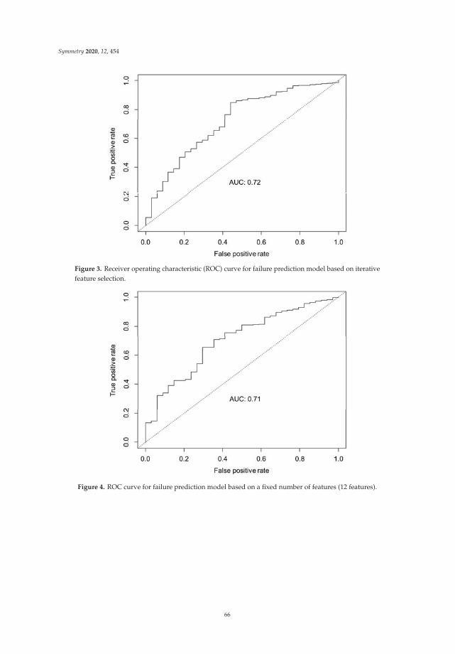
Symmetry 2020, 12, 454

Figure 3. Receiver operating characteristic (ROC) curve for failure prediction model based on iterativefeature selection.

Figure 4. ROC curve for failure prediction model based on a fixed number of features (12 features).

66

Symmetry 2020, 12, 454

Figure 5. ROC curve for failure prediction model based on a fixed number of features (24 features).

Figure 6. ROC curve for failure prediction model based on all features.

4. Conclusions

In this paper, we proposed a failure prediction model using iterative feature selection with theaim of predicting the failure occurrences. The procedure for building the failure prediction modelconsisted of the following five steps: (1) preprocessing, (2) importance measurement, (3) featureselection, (4) model building, and (5) model selection. In the first step, feature elimination, missing dataimputation, normalization, and data division are sequentially conducted. The importance measurementstep is to measure the importance of each feature by using the random forest. The third and the fourthsteps were iteratively performed to build the failure prediction models using the various selectedfeature sets and to obtain the prediction accuracy of the built models. In the last step, the failureprediction model with the highest prediction accuracy was selected. The experimental implementation

67

Symmetry 2020, 12, 454

was conducted to evaluate the performance of the proposed model using the open-source R and theSECOM dataset given by the UCI repository. Through the experimental implementation, we obtainedthe importance of features representing the relevancy between each feature and failure. Moreover,we obtained the selected feature set and prediction accuracy set, each of which contains twenty-fourfeatures and prediction accuracy measurements. In the experiments, the proposed failure predictionmodel was built with eight features, and we compared the prediction accuracy of the proposed modelwith that of the failure prediction model built based on 12 features, 24 features, and all features.The results showed that the proposed model achieved 1.4%, 14.3%, and 22.0% higher AUC than that ofother models. Comprehensively, the contributions of this paper are as follows. (1) We presented anddiscussed the problems of the existing failure prediction models for IIoT. (2) Through the importancemeasurement and iterative feature selection, we derived the feature index and the number of featuresthat maximize the prediction accuracy of the failure prediction model. (3) We verified the feasibilityof our work by conducting open-source-based implementation and extensive experiments. In ourwork, the proposed failure prediction model was implemented using only a limited dataset. Therefore,future work involves performing additional experiments with extended datasets to assess whether theproposed model is useful for various IIoT applications.

Author Contributions: E.-J.K. conceived and designed the failure prediction model; J.-H.K. performed theimplementation and experiment; E.-J.K. interpreted and analyzed the data; J.-H.K. and E.-J.K. wrote the paper;E.-J.K. guided the research direction and supervised the entire research process. All authors have read and agreeto the published version of the manuscript.

Funding: This research was supported by Hallym University Research Fund, 2019 (HRF-201911-010).


References

1. Cheng, J.; Chen, W.; Tao, F.; Lin, C.-L. Industrial IoT in 5G environment towards smart manufacturing. J. Ind.Inf. Integr. 2018, 10, 10–19. [CrossRef]

2. Kaur, K.; Garg, S.; Aujla, G.S.; Kumar, N.; Rodrigues, J.J.; Guizani, M. Edge Computing in the IndustrialInternet of Things Environment: Software-Defined-Networks-Based Edge-Cloud Interplay. IEEE Commun.Mag. 2018, 56, 44–51. [CrossRef]

3. Zhu, C.; Rodrigues, J.J.; Leung, V.C.; Shu, L.; Yang, L.T. Trust-based Communication for the IndustrialInternet of Things. IEEE Commun. Mag. 2018, 56, 16–22. [CrossRef]

4. Talavera, J.M.; Tobon, L.E.; Gomez, J.A.; Culman, M.A.; Aranda, J.M.; Parra, D.T.; Quiroz, L.A.; Hoyos, A.;Garreta, L.E. Review of IoT applications in agro-industrial and environmental fields. Comput. Electron. Agric.2017, 42, 283–297. [CrossRef]

5. Lee, H.-H.; Kwon, J.-H.; Kim, E.-J. FS-IIoTSim: A flexible and scalable simulation framework for performanceevaluation of industrial Internet of things systems. J. Supercomput. 2018, 74, 4385–4402. [CrossRef]

6. Liao, Y.; Loures, E.D.F.R.; Deschamps, F. Industrial Internet of Things: A Systematic Literature Review andInsights. IEEE Internet Things J. 2018, 5, 4515–4525. [CrossRef]

7. Ometov, A.; Bezzateev, S.; Voloshina, N.; Masek, P.; Komarov, M. Environmental Monitoring with DistributedMesh Networks: An Overview and Practical Implementation Perspective for Urban Scenario. Sensors 2019,19, 5548. [CrossRef]

8. Kontogiannis, S. An Internet of Things-Based Low-Power Integrated Beekeeping Safety and ConditionsMonitoring System. Inventions 2019, 4, 52. [CrossRef]

9. Haseeb, K.; Almogren, A.; Islam, N.; Din, I.U.; Jan, Z. An Energy-Efficient and Secure Routing Protocol forIntrusion Avoidance in IoT-Based WSN. Energies 2019, 12, 4174. [CrossRef]

10. Nguyen, D.T.; Le, D.-T.; Kim, M.; Choo, H. Delay-Aware Reverse Approach for Data Aggregation Schedulingin Wireless Sensor Networks. Sensors 2019, 19, 4511. [CrossRef]

68

Symmetry 2020, 12, 454

11. Lade, P.; Ghosh, R.; Srinivasan, S. Manufacturing Analytics and Industrial Internet of Things. IEEE Intell.Syst. 2017, 32, 74–79. [CrossRef]

12. Kammerer, K.; Hoppenstedt, B.; Pryss, R.; Stökler, S.; Allgaier, J.; Reichert, M. Anomaly Detections forManufacturing Systems Based on Sensor Data—Insights into Two Challenging Real-World ProductionSettings. Sensors 2019, 19, 5370. [CrossRef] [PubMed]

13. Lim, H.K.; Kim, Y.; Kim, M.-K. Failure Prediction Using Sequential Pattern Mining in the Wire BondingProcess. IEEE Trans. Semicond. Manuf. 2017, 30, 285–292. [CrossRef]

14. Sanchis, R.; Canetta, L.; Poler, R. A Conceptual Reference Framework for Enterprise Resilience Enhancement.Sustainability 2020, 12, 1464. [CrossRef]

15. Wang, J.; Yao, Y. An Entropy-Based Failure Prediction Model for the Creep and Fatigue of Metallic Materials.Entropy 2019, 21, 1104. [CrossRef]

16. Hamadache, M.; Dutta, S.; Olaby, O.; Ambur, R.; Stewart, E.; Dixon, R. On the Fault Detection and Diagnosisof Railway Switch and Crossing Systems: An Overview. Appl. Sci. 2019, 9, 5129. [CrossRef]

17. Nam, K.; Ifaei, P.; Heo, S.; Rhee, G.; Lee, S.; Yoo, C. An Efficient Burst Detection and Isolation MonitoringSystem for Water Distribution Networks Using Multivariate Statistical Techniques. Sustainability 2019, 11,2970. [CrossRef]

18. Abu-Samah, A.; Shahzad, M.K.; Zamai, E.; Said, A.B. Failure Prediction Methodology for Improved ProactiveMaintenance using Bayesian Approach. IFAC Pap. Online 2015, 48, 844–851. [CrossRef]

19. Kwon, J.-H.; Kim, E.-J. Machine Failure Analysis Using Nearest Centroid Classification for Industrial Internetof Things. Sens. Mater. 2019, 31, 1751–1757. [CrossRef]

20. Moldovan, D.; Cioara, T.; Anghel, I.; Salomie, I. Machine learning for sensor-based manufacturing processes.In Proceedings of the 2017 IEEE 13th International Conference on Intelligent Computer Communication andProcessing (ICCP), Cluj-Napoca, Romania, 7–9 September 2017; pp. 147–154. [CrossRef]

21. Mahadevan, S.; Shah, S.L. Fault detection and diagnosis in process data using one-class support vectormachines. J. Process Control 2009, 19, 1627–1639. [CrossRef]

22. Hasan, M.A.M.; Nasser, M.; Ahmad, S.; Molla, K.I. Feature Selection for Intrusion Detection Using RandomForest. J. Inf. Secur. 2016, 7, 129–140. [CrossRef]

23. Wu, D.; Jennings, C.; Terpenny, J.; Gao, R.X.; Kumara, S. A Comparative Study on Machine LearningAlgorithms for Smart Manufacturing: Tool Wear Prediction Using Random Forests. J. Manuf. Sci. Eng. 2017,139, 071018-1–071018-2. [CrossRef]

24. Awan, F.M.; Saleem, Y.; Minerva, R.; Crespi, N. A Comparative Analysis of Machine/Deep Learning Modelsfor Parking Space Availability Prediction. Sensors 2020, 20, 322. [CrossRef] [PubMed]

25. Wu, D.J.; Feng, T.; Naehrig, M.; Lauter, K. Privately evaluating decision trees and random forests. Proc. Priv.Enhancing Technol. 2016, 2016, 335–355. [CrossRef]

26. Garg, R.; Aggarwal, H.; Centobelli, P.; Cerchione, R. Extracting Knowledge from Big Data for Sustainability:A Comparison of Machine Learning Techniques. Sustainability 2019, 11, 6669. [CrossRef]

27. Lin, X.; Li, C.; Zhang, Y.; Su, B.; Fan, M.; Wei, H. Selecting Feature Subsets Based on SVM-RFE and theOverlapping Ratio with Applications in Bioinformatics. Molecules 2018, 23, 52. [CrossRef]

28. Liao, C.H.; Wen, C.H.-P. SVM-Based Dynamic Voltage Prediction for Online Thermally Constrained TaskScheduling in 3-D Multicore Processors. IEEE Embed. Syst. Lett. 2017, 10, 49–52. [CrossRef]

29. Shen, Y.; Wu, C.; Liu, C.; Wu, Y.; Xiong, N. Oriented Feature Selection SVM Applied to Cancer Prediction inPrecision Medicine. IEEE Access 2018, 6, 48510–48521. [CrossRef]

30. Li, Z.; Wang, N.; Li, Y.; Sun, X.; Huo, M.; Zhang, H. Collective Efficacy of Support Vector Regression withSmoothness Priority in Marine Sensor Data Prediction. IEEE Access 2019, 7, 10308–10317. [CrossRef]

31. SECOM Data Set in University of California Irvine (UCI) Machine Learning Repository. Available online:https://archive.ics.uci.edu/ml/datasets/secom (accessed on 30 January 2020).

32. Schenatto, K.; de Souza, E.G.; Bazzi, C.L.; Gavioli, A.; Betzek, N.M.; Beneduzzi, H.M. Normalization of datafor delineating management zones. Comput. Electron. Agric. 2017, 143, 238–248. [CrossRef]

69

Symmetry 2020, 12, 454

33. Singh, D.; Singh, B. Investigating the impact of data normalization on classification performance. Appl. SoftComput. 2019, in press. [CrossRef]

34. Ali, L.; Niamat, A.; Khan, J.A.; Golilarz, N.A.; Xingzhong, X.; Noor, A.; Nour, R. An Optimized StackedSupport Vector Machines Based Expert System for the Effective Prediction of Heart Failure. IEEE Access 2019,7, 54007–54014. [CrossRef]


70

symmetryS S

Article

Symmetric Modeling of CommunicationEffectiveness and Satisfaction for CommunicationSoftware on Job Performance

Tian-Syung Lan 1,2, Kai-Chi Chuang 1 , Hai-Xia Li 1,*, Jih-Fu Tu 3 and Huei-Sheng Huang 2

1 College of Mechanical and Control Engineering, Guilin University of Technology, Guilin 541004, China;[email protected] (T.-S.L.); [email protected] (K.-C.C.)

2 Department of Information Management, Yu Da University, Miaoli County 36143, Taiwan;[email protected]

3 Department of Industrial Management and Business Administration, St. John’s University, Tamsui District,New Taipei City 25135, Taiwan; [email protected]

* Correspondence: [email protected]; Tel.: +86-1373-738-1010

Received: 14 February 2020; Accepted: 3 March 2020; Published: 5 March 2020

Abstract: Job performance is an issue highly related to the repetition of one enterprise. Because of thepopularity of the Internet, consumer electronics have boomed rapidly and remove the space limitationstems. Users in the Taiwanese community send messages or share information through communicationsoftware that leads to more dependence from business. Various business problems have been solvedand job performance has increased through the diversified functions on communication software.Thus, this research supposed that staff are willing to continuously use communication softwareLINE(a new communication app which allows one to make FREE voice calls and send FREE messages),and they agree that the varied functions of communication software would mean that informationdelivery more symmetrically affects their job performance. According to the research outcomes,communication effectiveness significantly influenced communication satisfaction and job performance,and communication satisfaction significantly influenced job performance. As organizationalcommunication must be conducted through media that disseminate information, and different mediahave different communication effects, the relationship between communication effectiveness andjob performance was completely mediated by communication satisfaction. The research suggestedcompanies or organizations use LINE as a symmetric communication method to not only helpemployees improve their job performance, but also help enterprises achieve their goals or raise theprofit, or even steady development for enterprises.

Keywords: symmetric model; communication effectiveness; communication satisfaction; job performance

1. Introduction

Exchanging information by multiple roles connects the social activities in our daily life, such ascommercial activities, academic activities, and personal activities. This information or messageexchanges often relay thoughts and emotions, and this kind of behavior is called communication.The way of information exchange is quite diverse; formal ways of exchanging information includethrough writing or language. Since the Internet network has been developed, electronic communicationbegan to prevail, breaking the limitation of time and distance, which means both sides can performinformation exchange without time and place limitations. Mobile devices have become more andmore popular and broken through the limitation of space. With the use of the network, users cantransmit instant messages anywhere using applications. The transmission methods of informationhave also become more diverse, such as multi-person consultations or discussions, instant image or


Symmetry 2020, 12, 418

video transmissions, and even paying function that has been extra added on some communicationsoftware. As the public displays increasing reliance on mobile devices, using instant communicationapplications as the pipeline in commercial applications can not only solve many business problems inan instant, but also help enterprises improve their business performance.

A team of Taiwan Institute for Information Industry (FIND) surveyed and analyzed the usagebehavior on a Taiwanese community website. The survey found that the top two most frequently usedby Taiwan people were LINE and Facebook [1], as shown in Figure 1.

Figure 1. Frequency of using communication application more than three times a week [1].

As the most frequently used communication application, another survey about LINE, which wasdone by The Nielsen Company, found that LINE is a combination of communications, payments,entertainment, and other features [2]. Making calls or sending instant messages is the users’ primarybehavior, as shown in Figure 2.

Figure 2. Most frequently used features of LINE [2].

LINE is a mobile application that can be used in mobile devices like smart phone, tablet, oreven computer. LINE was first developed for individual users, which means individuals can send

72

Symmetry 2020, 12, 418

texts, stickers, or pictures to each other. With the development of the program, users can also makereal-time video and set up a group. Group members can send messages, stickers, pictures, videos,audios, or even files; make audio or video calls with other members; and create albums or noteswithin the group. Many companies or organizations, thus, set up groups for different departments orunits. They even set up groups for business partners or cooperators. The main intention is to facilitatecommunication and to reduce misunderstanding or mistakes.

According to the 2016 survey from Taiwan Institute for Information Industry, the applicationmost people visit weekly was LINE, whereas Nielsen’s 2016 survey also found that 91% of Taiwanpeople had used LINE in the last seven days, which means LINE was the most used communicationapplication in Taiwan. At the same time, according to the same Nielsen’s 2016 survey mentioned above,two of the most engaged behavior on LINE was to communicate with family and friends (94%) and todiscuss work (71%). Unlike the traditional phone or application with text-only messaging, LINE hasbecome the first choice to make contact with people in Taiwan. Therefore, it is worth exploring whetherLINE’s competence in communication effectiveness and for commercial communication can positivelyaffect job performance.

As LINE is a new and recent software that has just appeared in Taiwan since 2012 [3], there isno other research discuss about the communication effectiveness, communication satisfaction, or jobperformance about LINE. Due to the lack of previous research, this research held that the morewilling the workers from different levels of enterprises of different occupations, such as educationorganization, vehicle industry, and financial industry are to continuously use LINE as communication,the more they can use LINE’s diversified function of information transmission, and certainly theyare satisfied with the results of the information transmission, thereby continuously improving theirjob performance. Symmetrically, if the communication effectiveness is high enough to accuratelyand smoothly transmit messages, people within the company will be satisfied with the results ofcommunication, and ultimately lead to improved job performance.

2. Literature Review

2.1. Communication Effectiveness

Carl Rogers, an American psychologist, said that active listeners not only listened to whatthe other person was saying, they also tried to understand and respond to the feelings behindthose words, and would place themselves in the speaker’s position to understand the messagedeeply [4]. Whether expressing one’s opinions or ideas, or consulting or discussing with others at work,effective communication is essential, and effective communication can not only bring the membershipcloser, but also help members build a commitment to the organization, willing to contribute to theorganization [5]. According to the Sproull and Kiesler’s study of the situation about users self-exposingon the Internet, the Internet did help users expose themselves faster and deeper [6]. Yang believedthat language cues can compensate for the lack of non-verbal cues, and that both parties could useonline communication to subtly arrange the meaning of language and words. As people interacton the Internet over time, intimacy can also be created between the parties and help people exposethemselves [7]. Levinger suggested that the transition in self-disclosure relationships begins with a shiftfrom superficial revelations to intimate revelations, which means that the longer people communicatewith friends on the Internet, the more intimate they feel [8].

Effective organizational communication depends on appropriate communication mechanismsand media [9]. As organizational communication must be conducted through media that disseminateinformation, and different media have different communication effects, the communication mediachosen to be used by the organization affects their ability to process information, to learn, and determinesthe results of communication. In addition, the medium and methods of communication used byorganizations also influence their behavior patterns [10]. Comparing to an environment with a high

73

Symmetry 2020, 12, 418

social presence, there is usually more information hiding and untrustworthy behavior in a low socialpresence environment [11].

In addition to exploring people’s feelings of the existence of other participating individualsthrough digital media, in recent years, social presence has also begun to study the social cues containedby the digital media itself through interactive forms, so that people can produce a presence of a socialactor. This social perception does not come from others involved in the media, but from the social cuesprovided by the media itself [12]. Instant messaging tools are mostly used in text-based communication,but there are also emoticons (emojis) available to users. Social context cues can be divided into twocategories: dynamic and static. Emoticons (emojis) are dynamic and a substitute for facial expressions,it should be able to achieve more communication help at the social context level. Ambler believed thatcommunication effectiveness could be assessed from the degree to which the sender can select andmatch the appropriate communication medium according to the situation and the extent to which therecipient correctly understands the message [13]. Gray believed that only by mastering the goal ofcommunication can it be able to further measure the effectiveness of communication, and if the senderis not clear enough about the communication objectives, then there is no basis for measurement ofcommunication effectiveness [14].

The key to successful communication is the correctness of information transmission, which wasnot easy to occur if there are different perceptions between the sender and the recipient.Successful communication can also be called effective communication. Effective communicationcan help deliver the correct message between employees, solve problems, and successfully achieveorganizational goals.

2.2. Communication Satisfaction

Hargie and Dickson clearly pointed out that communication was the process of conveyinga message that allowed two parties to understand and influence each other through sharing andbuilding common perspectives [15]. Li and Tsai defined communication satisfaction as the differentcommunication levels and forms in an organization, and the satisfaction levels of the individualmembers with their perception of quality and quantity [16]. Communication satisfaction relays a levelof recognition. Communication was also a marketing process, marketing itself in the workplace togive cognitive subjective feelings. Communication helped employees to improve their productivity,the main purpose not only was meant to increase mutual understanding, avoiding misunderstandingbetween superiors and colleagues but also let one’s professional ability to be found and one’s jobperformance was able to be seen. Communication in the modern workplace symbolized as a positiveimage. Hecht defined communication satisfaction as an emotional response to the achievement ofcommunication goals and expectations [17,18].

Krone, Jablin, and Putnam believed that there are four characteristics of communication:communication frequency, communication mode, communication content, and communicationdirection [19]. Communication frequency refers to the number of contacts between members ofthe organization. The more frequent communication involves between supervisors, volunteers, andfull-time personnel; the closer the relationship between the members of the organization and theorganization will perform. Communication mode refers to the channel used to convey information,that is, how the supervisor delivers the information to the members of the organization. According tothe organizational structure, organizational communication can be divided into two categories,formal communication and informal communication. Formal mode refers to non-private pipelines,such as memos, group meetings, and other communication pipeline and methods that the supervisorstrust or depend on. In contrast, the informal mode is very private, and it is often like a verbal,face-to-face individual teaching, and a temporary and improvisational communication pipeline [20].The communication content is not referring to actual messages conveyed, but is related to theextent of direct communication to which the sender used in order to change the recipient’s actions.Further, command-style information is direct communication, and vice versa. The communication

74

Symmetry 2020, 12, 418

direction refers to the change or flow of information horizontally and vertically within an organization.The communication flow between supervisor and subordinate initially occurs in a single direction,but the current human management environment has changed a lot. Schmuck and Runkel believedthat the direction of communication has changed to be a loop with feedback, and communication israrely one-way, it should be two-way.

Robertson pointed out that ideal communication can establish a good connection betweenmanagers and employees, but not only for sharing information and ideas [21]. Therefore, the levelof leadership communication behavior was different comparing with other organizations. If theleader could understand the leadership’s organizational communication characteristics, along with thecommunication technology, communication would be easier to succeed naturally.

After the employees started to use the communication software as the communication channel,they were able to produce a sense of satisfaction in communication when they achieved a communicationsmoothly and completed the tasks delivered by the organization, which was the main purpose ofcommunication as they were able to gain satisfaction through the effectiveness of message transmissionin communication.

2.3. Job Performance

Job performance results from the actions of the members in the organization and is expectedby the organization and its members to be achieved with minimal resources [22]. According toCampbell’s research structure, Borman and Motowidlo proposed that job performance is dividedinto task performance and contextual performance [23]. Task performance refers to the outcomeof an individual’s work that directly relates to the organization expects, and is judged by whetherit meets the requirements of a formal role [24]. Contextual performance refers to the actions of anindividual who voluntarily performs informal activities; adheres to complete the task; is willing tocooperate with others; follows rules and procedures; and is able to endorse, support, and defend theorganization’s goals.

Wright and Boswell measured job performance in five perspectives, which are support,goal Emphasis, team building, workshop facilitation, and global rating [25]. Castro, Dounlas,Hochwasser, Ferris, and Frink represented employees’ performance with eight characteristics:work habits, planning and analytical skills, job knowledge, management skills, communicationskills, developments in other aspects, interpersonal relationships, and overall assessment [26]. If aperformance assessment could be performed properly, it would not only enable the employees tounderstand the benefit of executing it, but also affect the work efficiency and the mission direction inthe future [27].

The pursuit of an enterprise is to maximize job performance with limited resources. Under suchconditions, the joint efforts of all members are necessary. Therefore, it is necessary for all members tostay together and achieve their goals.

3. Research Design

3.1. Research Assumptions

As discussed in the previous section, Levinger [8] suggested that the longer people communicatewith friends on the Internet, the more intimate they feel. Krone, Jablin, and Putnam [19] believed thatthe more frequent communication occurs between supervisors, volunteers, and full-time personnel,the closer the relationship between the members of the organization and the organization will perform,meaning higher communication satisfaction, and both Borman and Motowidlo [23] and Wright andBoswell [25] pointed out that job performance was mostly resulted from different communication form.

Based on the research purposes and the framework presented in Figure 3, the following hypothesesare developed.

75

Symmetry 2020, 12, 418

Communication

Effectiveness

Communication

Satisfaction (H4)

Job Performance

H1

H2

H3

Figure 3. Research framework.

Hypothesis 1 (H1). Communication effectiveness has significant effects on communication satisfaction.

Hypothesis 2 (H2). Communication effectiveness has significant effects on job performance.

Hypothesis 3 (H3). Communication satisfaction has significant effects on job performance.

Hypothesis 4 (H4). Communication satisfaction has a mediation effect between communication effectivenessand job performance.

3.2. Sample of Research

The subjects of this research are the members who have used communication software toexplain, distribute, and communicate at work in different levels of enterprises from all occupations.The convenience sampling method was used and conducted for the qualified anonymous samples.The questionnaires were used to collect data, and to understand the respondents’ views on the researchissues and to analyze their behaviors. The questionnaires were distributed in paper and the number ofdistributed questionnaires in detail as shown in Table 1.

Table 1. Detail of distributed questionnaires.

Distributed Response Valid Invalid Valid Response Rate

Paper Questionnaires 480 455 445 10 92.7%

3.3. Instrument and Procedures

Based on the aforementioned research purpose and structure, the research questionnaire wasdivided into four parts: basic data, using behavior, communication satisfaction, and job performance.A 5-point Likert Scale was used to score and quantify, on a scale of 1–5, respectively, in five categories:strongly disagree, disagree, no opinion, agree, and strongly agree. The first part of the questionnairewas basic data, including four basic questions: age, gender, the amount of salary, and work area.The second part was the using communication effectiveness scale, the third part was the communicationsatisfaction scale, and the fourth part was the job performance scale.

Yan suggested that effective communication in an organization refers to the ability ofcommunication showed within an organization, and that communication effectiveness can beexplained from two aspects, “people” and “things”, respectively. “People” refers to communicationsatisfaction and communication harmony, and “things” refers to the effectiveness and correctness ofthe messages. The purpose of communication within an organization is to enhance understanding,build consensus, coordinate actions, brainstorm ideas, meet the needs of members, and thus achievepredetermined objectives. The achievement of the above objectives can be used as a judgment oneffective communication [28].

76

Symmetry 2020, 12, 418

There were many pieces of research on communication effectiveness, and the factors of it in thisresearch were based on the findings of Yan [29], which measured communication effectiveness in fourfactors, communication satisfaction, communication harmony, messages effectiveness, and messagestimeliness (correctness). The findings had been revised to develop suitable dimensions and questionsfor the purposes and subjects of this research, as shown in Table 2.

Table 2. Dimensions and questions of communication effectiveness.

Dimensions Questions

Harmony 1. I am satisfied with the overall harmonious communication in my department.Effectiveness 2. I am satisfied with the overall effective communication in my organization.

Timeliness 3. I am satisfied with the overall timely communication in my organization.Satisfaction 4. I am satisfied with the overall communication in my organization.

Communication satisfaction is a degree of awareness, defined by Price as a kind of emotionalorientation that members of society produced towards their group [30]. Crino and White definedcommunication satisfaction as “one individual’s perception of different forms of communication andits respective satisfactions in the organization” [31]. According to the previous literature of variousstudies, the communication satisfaction scale had been revised and developed as shown in Table 3.

Table 3. Dimensions and questions of communication satisfaction.


CommunicationSatisfaction

1. I am satisfied with the information from LINE about my job compared to my colleagues’ job.2. I am satisfied with the information from LINE about the judgment of me from

my supervisors.3. My supervisors know about my effort from LINE.4. I am satisfied with the report on how my work problems were handled.5. The extent to which my supervisors know and understand the problems the staff is facing

through LINE.6. The extent to which my supervisors can listen and pay attention to me7. My supervisors are able to provide guidance on solving work-related issues.8. The extent to which my supervisors are willing to listen with an open mind.9. The extent of correct and fluent communication with my colleagues though LINE.10. Using communication software (LINE) can achieve smooth communication.11. Using communication software (LINE) can clearly deliver information about work.12. Using communication software (LINE) can clearly deliver company policies and goals.13. Because of organizational communication, I feel that I am a very important part of

the organization.14. Conflict can usually be resolved through an appropriate communication pipe (LINE).15. Communication through LINE is very important for productivity.

Edwards integrated the views of several scholars and argued that individual job performance canbe studied in terms of demand and ability, and demand and supply [32]. Demand and ability refer tothe fit between the abilities the work demanded and an individual’s abilities, whereas demand andsupply refer to the fit between an individual’s needs and the job attributes. Based on the above studies,this research defined job performance as individual job performance, which measures the behavior ofmembers and the results of their work. According to the relevant researches and previous literature,this research revised Robbins [33], Liu, and Liao’s questionnaires [34] to measure job performance, anddeveloped the questions of the job performance scale, as shown in Table 4.

77

Symmetry 2020, 12, 418

Table 4. Factors and questions of job performance.


Job Performance

1. I appreciate the results of the members’ work.2. I can continuously improve my work quality and efficiency by using LINE.3. I am willing to assist my colleagues in the extra work and strive for

organizational performance.4. I can comply with the organization’s rules through LINE.5. I can carry out orders or works through LINE.6. I have many skills to handle works.7. I can offer specific proposals for my job through LINE.8. I can solve work problems alone.9. I can handle emergent works through LINE.10. I can participate in organizing affairs or meetings with a positive attitude.11. I understand my job and responsibility through LINE.12. I value my job.13. I offer my help to my colleagues through LINE.

To increase the stability and reliability of the questionnaire, a reliability analysis was used to identifythe Cronbach’s α coefficient in each dimension. The Cronbach’s α of the variable communicationeffectiveness was 0.791. The Cronbach’s α of the variable communication satisfaction was 0.815.The Cronbach’s α of the variable job performance as 0.758. The reliability of each variable was passed.


This research used regression analysis to explore the explanation and relationship amongthe variables. One independent variable was used to explain or predict another variable bybuilding and testing the regression equation. Therefore, this research used regression analysisto examine whether communication effectiveness influenced communication satisfaction and jobperformance, to examine whether communication satisfaction influenced job performance, and toexamine whether communication satisfaction had an intermediary effect in communication effectivenessand job performance.

To explore whether there was a correlation between two variables—communication effectivenessand communication satisfaction—regression analysis was carried out with communication effectivenessas independent variable and communication satisfaction as the dependent variable. Through regressionanalysis, it could be found that the coefficient of the independent variable was 0.711. The p-valuewas 0.021, which was less than 0.05, so the result was significant, indicating that communicationeffectiveness had a positive effect on communication satisfaction. The coefficient of determinationwas 0.601, which meant 60.1% of communication satisfaction could be explained by communicationeffectiveness. The date was shown in Table 5.

Table 5. Regression analysis of communication satisfaction on communication effectiveness.

Mode

UnstandardizedCoefficients

StandardizedCoefficients t Sig.

B Std. Error Beta

1.(Constant) 1.011 0.093 10.881 0.000

CE 0.711 0.027 0.775 25.853 0.021

R R2 Adjusted R2 Std. Error of the Estimate

0.775 a 0.601 0.600 0.32125

Coefficients (a) a. Dependent variable: CS

78

Symmetry 2020, 12, 418

Next, we discuss whether communication effectiveness is related to job performance by, first,taking communication effectiveness as the independent variable and job performance as the dependentvariable for regression analysis. The coefficient of the independent variable was 0.753. Its p-valuewas 0.005, which was less than 0.05, so the result was significant, indicating that communicationeffectiveness had a positive effect on job performance. The coefficient of determination was 0.665,which meant 66.5% of job performance could be explained by communication effectiveness. The datewas shown in Table 6.

Table 6. Regression analysis of job performance on communication effectiveness.

Mode

UnstandardizedCoefficients

StandardizedCoefficients t Sig.

B Std. Error Beta

1.(Constant) 0.815 0.086 9.504 0.000

CE 0.753 0.025 0.816 29.660 0.005

R R2 Adjusted R2 Std. Error of the Estimate

0.816 a 0.665 0.664 0.29670

Coefficients (a) a. Predictors: (Constant), CE.

According to Baron and Kenny’s view of defining the mediator [35], as shown in Figure 4, there arethree conditions for meeting the mediator. The first is that the variation of the independent variablecan significantly explain the variation of the mediator, which means path a is significant. The secondone is that the variation of the mediator can significantly explain the variation of the dependentvariable, which means path b is significant. The last one is when controlling independent variables andmediators are being considered at the same time, the relationship effect of the independent variable forthe dependent variable (path c) is less significant, and in the case, the mediation effect of the mediatorbecomes strongest which c = 0. In other words, the independent variable can significantly explainthe variation of the dependent variable, which means path c is significant. However, when both theindependent variable and mediator are considered, the effect of the previous argument is reduced.As a result, the mediation effect of the mediator can be examined by four regression patterns.

Figure 4. Defining the mediator [35].

Model 1: The effect of the independent variable on the mediator is significant.Model 2: The effect of the independent variable on the dependent variable is significant.Model 3: The effect of the mediator on the dependent variable is significant.Model 4: Examine the effect of the mediator and the independent variable on the dependent

variable at the same time, and compare the result of model 2, at which point the independent variableof model 4 should have less effect on the dependent. There should be two scenarios:

1. Complete mediation: If only the effect of the mediator is still significant, the effect of theindependent variable is no longer significant, and then the mediator has a complete mediationeffect between the relationship of the independent variable and the dependent variable.

79

Symmetry 2020, 12, 418

2. Partial mediation: If the effect of the mediator and the independent variable are both stillsignificant, then the mediator has a partial mediation effect between the relationship of theindependent variable and the dependent variable.

In this section, to explore the mediation effect of communication satisfaction on communicationeffectiveness and job performance, regression analysis was taken to verify the hypotheses, and thecommunication satisfaction was used as a mediator to analyze to understand whether communicationsatisfaction has an impact on communication effectiveness and job performance.

To examine the mediation effect of communication satisfaction between communicationeffectiveness and job performance, four steps were carried out. The first step was the regressionanalysis of communication effectiveness on communication satisfaction. The p-value was 0.021, and thecoefficient was 0.711, which had reached a significant level. The second step was the regressionanalysis of communication effectiveness on job performance. The p-value was 0.005, and the coefficientwas 0.753, which had also reached a significant level. The third step was the regression analysis ofcommunication satisfaction on job performance. The p-value was 0.000, and the coefficient was 0.922,which had reached a significant level. The last step was the regression analysis of communicationeffectiveness and communication satisfaction on job performance. The p-values were 0.182 and 0.002,and the coefficient was 0.245 and 0.715, which meant only communication satisfaction had reached asignificant level. Based on the above four-step analysis results, the research found that communicationsatisfaction had a complete mediation effect between communication effectiveness and job performance.The analysis result can be found in Table 7.

Table 7. Mediation effect analysis.

DependentVariable

CommunicationSatisfaction

Job Performance Job Performance Job Performance

Model 1 Model 2 Model 3 Model 4

DependentVariable

Coe. Sig. Coe. Sig. Coe. Sig. Coe. Sig.

CommunicationEffectiveness 0.711 0.021 0.753 0.005 — — 0.245 0.182

CommunicationSatisfaction — — — — 0.922 0.000 0.715 0.002

According to the above-mentioned analysis, the analysis results were used to review the researchhypotheses and were explained. This research contained four research hypotheses, which weresummarized and verified, as shown in Table 8.

Table 8. The result of hypotheses verification.

Hypothesis Result

H1: Communication effectiveness has significant effects on communication satisfaction. valid

H2: Communication effectiveness has significant effects on job performance. valid

H3: Communication satisfaction has significant effects on job performance. valid

H4: Communication satisfaction has a mediation effect between communicationeffectiveness and job performance.

Completemediation

According to the research result, three hypotheses developed by this research were valid.As pointed out by Levinger [8], communication effectiveness can make people feel more or less intimatewith each other and lead to a level of communication satisfaction. As job performance was mostlyaffected by different kind of communication, as mentioned by Borman and Motowidlo [23] and Wright

80

Symmetry 2020, 12, 418

and Boswell [25], this research assumed that both communication effectiveness and communicationsatisfaction would affect job performance, which was later proved by the research result as valid.

5. Conclusions and Discussion

Because of the popularity of the Internet, consumer electronics have boomed rapidly and breakthe space limitation stems. Users send messages or share information by communication software thatleads to more dependence from businessmen. Various business problems have been solved and jobperformance has been risen up through the diversified functions on communication software.

In this study, the communication effectiveness is validated by the results of communication andled to the improvement of one’s job performance by our proposed symmetric model. This researchheld that the more willing the workers are to use LINE as communication, the more they can useLINE’s diversified function of information transmission, and certainly, they are satisfied with theresults of the information transmission, thereby improving their job performance. Relatively, if thecommunication effectiveness is high enough to accurately and smoothly transmit messages, peoplewithin the company will be satisfied with the results of communication, which ultimately leads to animprovement in job performance. Therefore, the researchers believed that communication effectivenesshas significant effects on communication satisfaction and job performance.

5.1. Conclusions

The results showed that communication effectiveness had a positive effect on communicationsatisfaction, and its explanatory power was 60.1%. Communication effectiveness had a positiveeffect on job performance, and its explanatory power was 66.5%. As communication effectivenesshad significant positive effects on both communication satisfaction and job performance, and theexplanatory power was both higher than 60%, when organizations or enterprises use communicationsoftware to communicate, they should pay attention to and strengthen the effectiveness of using LINE orother communication software to strengthen workers’ communication satisfaction and job performance.

As there was only the variable communication satisfaction remained significant after the four-stepregression analysis for the mediation effect, it was proved that communication satisfaction had acomplete mediation effect between communication effectiveness and job performance, which meantthe satisfaction of using LINE as a communication software would affect communication effectivenessand job performance. Therefore, organizations or companies should pay more attention of the usage ofLINE, or even consider the utilization of communication software as the primary communication pipe,such as how their employees think about using LINE as the major communication pipe. As mentionedin the above chapters, LINE users can send texts, stickers, or pictures to each other. They can also makereal-time video and set up a group. Group members can send messages, stickers, pictures, videos,audios, or even files; make audio or video calls with other members; and create albums or noteswithin the group. Many companies or organizations, thus, set up groups for different departmentsor units. They even set up groups for business partners or cooperators. The main intention is tofacilitate communication and to reduce misunderstanding or mistakes. As the results of this researchshowed that employees were satisfied with using LINE as a major communication pipe in work place,it was suggested that employers can make good use of LINE continuously to improve employees’communication effectiveness and job performance. Communication software often improve theirusefulness by updating their software functions, employers or supervisors can always make good useof the updated functions to assign tasks, establish to-do lists, establish personal memo, or any othersways to improve communication satisfaction, communication effectiveness, and job performance.As every company or organization must have the needs of communication to keep their work ongoingor keep their business developing, the results of this research (using communication software likeLINE could ultimately improve job performance) could even help companies or organizations for theirsteady development.

81

Symmetry 2020, 12, 418

5.2. Discussions

According to the findings of the research, future researchers could further the research byconducting follow-up discussions on the above phenomena and exploring other variables that canaffect job performance. In addition, this research suggested that future researchers could continue toexpand the sample size or add some new influence variables, or adjust the causal sequence betweenthe variables in the framework or re-establish the research structure for re-discussion. It is also possibleto lock in the comparison of industry differences, such as high-tech and traditional industries, it mightresult in giving some professional advice on work communication. Finally, future researchers canintroduce more updated variables into the research structure, such as salary, benefits, and so on. It isbelieved that these future research results could provide some valuable information and the strategicdirection of implementation.

Future research is suggested to explore the negative effect on employees of continuously usingcommunication software as the major communication methodology in the work place, such as privacyissues, messiness of information, taking up non-working hours, etc.

5.3. Limitation

Although the results of the research were satisfied and the findings could contribute to help steadydevelopment of companies, there were two major limitations should be noted: First, the number ofsamples could be larger to strengthen the persuasiveness of the research or be more widespread todifferent levels of position or areas of industry to ensure the credibility of the results. Second, theresearch also limited to the users of communication software in Taiwan. The results of other countriesmight different from Taiwan’s.

Author Contributions: Conceptualization, T.-S.L.; Data curation, K.-C.C. and H.-X.L.; Methodology, T.-S.L.and J.-F.T.; Project administration, T.-S.L.; Software, H.-X.L.; Validation, H.-S.H.; Visualization, K.-C.C. andH.-S.H.ng; Writing—original draft, T.-S.L. and J.-F.T. All authors have read and agreed to the published version ofthe manuscript.



References

1. Institute for Information Industry. Service System Drives Research and Development Plans for EmergingBusinesses. 2017. Available online: https://www.iii.org.tw/ (accessed on 20 September 2019).

2. LINE. LINE Annual Seminar. 2016. Available online: https://meet.bnext.com.tw/articles/view/38786 (accessedon 20 September 2019).

3. Watchinese. App “LINE” is Booming! 2012. Available online: https://www.watchinese.com/article/2012/4402(accessed on 25 November 2019).

4. Dessler, G. Human Resource Management; Prentic-Hall: Upper Saddle River, NJ, USA, 2005.5. Rollinson, D. Organizational Behavior and Analysis, 2nd ed.; Prentice-Hall: New Upper Saddle River, NJ, USA,

2002; pp. 627–631.6. Sproull, L.; Kiesler, S. Computers, Networks and Work. Sci. Am. 1991, 265, 116–127. [CrossRef]7. Yang, C.C. Developing intimacy in computer-mediated communication: A study of the functions of verbal

and non-verbal cues. J. World Press Coll. 1995, 5, 19–38.8. Levinger, G. Toward the analysis of close relationships. J. Exp. Soc. Psychol. 1980, 16, 510–544. [CrossRef]9. Shiang, J. Preconditions of digital democracy. RDEC Bimon. 2004, 28, 52–66.10. Lu, W.S. The principle and practicality of organizational learning: The viewpoint of organization

communication. Pers. Mon. 1996, 23, 24–43.11. Hassanein, K.; Head, M. Manipulating social presence through the web interface and its impact on attitude

towards online shopping. Int. J. Hum. Comp. Stu. 2007, 65, 689–708. [CrossRef]12. Tung, F.W.; Deng, Y.S. Social cues in human-computer interaction-speech and interactivity effects on children

in E-learning. J. Des. 2006, 11, 81–97.

82

Symmetry 2020, 12, 418

13. Ambler, S. Agile Modeling: Effective Practices for Extreme Programming and the Unified Process, 1st ed.; John Wiley& Sons, Inc.: New York, NY, USA, 2002.

14. Gray, D. How to Measure Your Communication Effectiveness. Unpublished Work. 2005. Available online:http://communicationnation.blogspot.com/ (accessed on 14 October 2019).

15. Hargie, O.; Dickson, D. Skilled Interpersonal Communication: Research, Theory, and Practice; Routledge: London,UK, 2004.

16. Lee, Y.D.; Tsai, W.Y. A study on the construction of communication satisfaction inventory for the businessemployees in Taiwan. J. Natl. Cheng-Kung Univ. 1998, 33, 257–283.

17. Hecht, M.L. Measures of communication satisfaction. Hum. Commun. Res. 1978, 4, 350–368. [CrossRef]18. Hsu, L.L.; Lai, S.Q.; Hsu, C.S.; Li, C.Y. The effect of blog and MSN usage on the interpersonal communication:

A social presence theory perspective. Chaoyang Bus. Manag. Rev. 2011, 10, 19–48.19. Krone, K.J.; Jablin, F.M.; Putnam, L.L. Communication theory and organizational communication:

Multiple perspectives. In Handbook of Organizational Communication; Sage Publications: Los Angeles,CA, USA, 1987; pp. 18–40.

20. Schmuck, R.A.; Runkel, P.J. Handbook of Organization Development in Schools; National Press Books: LosAngeles, CA, USA, 1972.

21. Robertson, E. Using leadership to improve the communication climate. Strateg. Commun. Manag. 2002, 7,24–27.

22. Liang, H.Y.; Wu, C.F.; Chang, S.C. Apply the balanced scorecard to measure strategic performance inhealthcare system. Tzu Chi Nurs. J. 2005, 4, 26–31.

23. Borman, W.C.; Motowidlo, S.J. Expanding the Criterion Domain to Include Elements of Contextual Performance;Jossey-Bass: Los Angeles, CA, USA, 1993; pp. 71–98.

24. Motowidlo, S.J.; Van Scotter, J.R. Evidence that task performance should be distinguished from contextualperformance. J. Appl. Psychol. 1994, 79, 475–480. [CrossRef]

25. Wright, P.M.; Boswell, W.R. Desegregating HRM: A review and synthesis of micro and macro human resourcemanagement research. J. Manag. 2002, 28, 247–276. [CrossRef]

26. Castro, S.L.; Douglas, C.; Hochwarter, W.A.; Ferris, G.R.; Frink, D.D. The effects of positive affect and genderon the influence tactics-job performance relationship. J. Leadersh. Organ. 2003, 10, 1–18. [CrossRef]

27. Lee, M.L.; Chou, P.F. Discussion on employee’s cognitive attitude and job performance. J. Far East Coll. 2003,20, 869–882.

28. Yan, C.H. A Study on Relations of Communication Capability, Attitude and Communication Effectiveness.Master’s Thesis. 1999. Available online: https://ndltd.ncl.edu.tw/ (accessed on 10 October 2019).

29. Yen, C.C.; Wei, W.L. The effects of the key factors of organizational communication on organizationalcommunication effectiveness and design performance. J. Des. 2011, 16, 61–85.

30. Price, J.H. Handbook of Organization Measurement; Health & Company: Washington, DC, USA, 1972;pp. 156–157.

31. Crino, M.D.; White, M.C. Satisfaction in communication: an examination of the Downs-Hazen measure.Psychol. Rep. 1981, 49, 831–838. [CrossRef]

32. Edwards, J.R. Person-job fit: A conceptual integration, literature review, and methodological critique.In International Review of Industrial and Organizational Psychology; Cooper, C.L., Robertson, I., Eds.; John Wiley& Sons, Inc.: New York, NY, USA, 1991; pp. 283–357.

33. Robbins, S.P. Organizational Behavior, 11th ed.; Prentice-Hall: New Upper Saddle River, NJ, USA, 2006.34. Liou, J.C.; Liao, W.T. The Relationships among Knowledge Continuity Management, Job capability and

Personal Work Performance. In Proceedings of the 2010 The 13th Conference on Interdisciplinary andMultifunctional Business Management, Taipei, Taiwan, 26 June 2010; pp. 189–202.

35. Baron, R.; Kenny, D. The moderator-mediator variable distinction in social psychological research: Conceptual,strategic, and statistical considerations. J. Personal. Soc. Psychol. 1986, 51, 1173–1182. [CrossRef]


83

symmetryS S

Article

Homomorphic Encryption-Based Robust ReversibleWatermarking for 3D Model

Li Li 1, Shengxian Wang 1, Shanqing Zhang 1,*, Ting Luo 2 and Ching-Chun Chang 3

1 Department of Computer Science, Hangzhou Dianzi University, Hangzhou 330018, China;[email protected] (L.L.); [email protected] (S.W.)

2 Collage of Science and Technology, Ningbo University, Ningbo 315000, China; [email protected] Department of Computer Science, University of Warwick, Coventry CV47AL, UK;

[email protected]* Correspondence: [email protected]; Tel.: +86-130-7360-1029

Received: 31 January 2020; Accepted: 21 February 2020; Published: 1 March 2020

Abstract: Robust reversible watermarking in an encrypted domain is a technique that preservesprivacy and protects copyright for multimedia transmission in the cloud. In general, most models ofbuildings and medical organs are constructed by three-dimensional (3D) models. A 3D model sharedthrough the internet can be easily modified by an unauthorized user, and in order to protect thesecurity of 3D models, a robust reversible 3D models watermarking method based on homomorphicencryption is necessary. In the proposed method, a 3D model is divided into non-overlapping patches,and the vertex in each patch is encrypted by using the Paillier cryptosystem. On the cloud side,in order to utilize addition and multiplication homomorphism of the Paillier cryptosystem, threedirection values of each patch are computed for constructing the corresponding histogram, which isshifted to embed watermark. For obtaining watermarking robustness, the robust interval is designedin the process of histogram shifting. The watermark can be extracted from the symmetrical directionhistogram, and the original encrypted model can be restored by histogram shifting. Moreover, theprocess of watermark embedding and extraction are symmetric. Experimental results show thatcompared with the existing watermarking methods in encrypted 3D models, the quality of thedecrypted model is improved. Moreover, the proposed method is robust to common attacks, such astranslation, scaling, and Gaussian noise.

Keywords: three-dimensional models; cloud computing; histogram shifting; encrypted model;decrypted model

1. Introduction

Due to the development of outsourced storage in the cloud, reversible watermarking in anencrypted domain has been developed for security in the cloud [1–4]. However, the cloud cannotintroduce distortion of original content during watermark embedding. Therefore, the reversiblewatermarking method is required [5,6]. In addition, the watermark carrier is vulnerable duringtransmission, and the embedded watermark is expected to resist common attacks [7,8]. Therefore,robust reversible watermarking in an encrypted domain has greatly attracted researchers forpotential applications.

In general, watermarking can be divided into robust and fragile watermarking methods in termsof their robustness. Robust watermarking [9] is used to protect security and resist attacks, while fragilewatermarking [10,11] is used to provide integrity authentication. For the occasions with high datasecurity requirements, such as judicial authentication, medical images, etc., more researchers focus onfragile watermarking in the encrypted domain.


Symmetry 2020, 12, 347

Reversible watermarking in the encrypted domain can be divided into reserving room beforeencryption (RRBE) and vacating room after encryption (VRAE). The RRBE method reserves embeddingroom before encrypting the original image [12–15]. For example, the vacated bits, which are reservedby self-embedding before encryption, can be substituted by the watermark in the encrypted domain [4].With the development of reversible watermarking [16,17], the original image can be restored absolutelyafter extracting the watermark. The second type directly implements watermark embedding bymodified the encrypted image [18,19] after encryption. For instance, Xiang divided the original imageinto patches to be encrypted, and then the histogram of statistical values was calculated in the encrypteddomain for shifting to embed watermark [20].

However, these methods are only applied to images, and cannot be used in 3D models directlydue to different structures between images and 3D models. Ke et al. proposed a robust watermarkingmethod on the basis of self-similarity [21]. In that method, a 3D model is divided into patches, andwatermark bits were embedded by changing the local vector length of a point in each patch. Feng et al.divided a 3D model into patches, then embedded a watermark into each patch by modulating anglequantization [22]. However, those methods are not reversible. Jiang et al. proposed a 3D modelwatermarking method on the basis of stream cipher encryption [1]. The watermark was embedded byflipping the least significant bits (LSBs) of the vertex coordinates. Since the original 3D models havehigh spatial correlation, the watermark can be extracted successfully. Shah proposed a watermarkingmethod based on the homomorphic Paillier cryptosystem, which used VRAE framework to vacate spacebefore encryption [2]. However, those methods are fragile to attacks and cannot protect their copyrights.

To our best of knowledge, although the aforementioned watermarking methods on encrypted 3Dmodels have been developed, the research on robustness for encrypted 3D models is rarely reported.In this paper, in order to protect the security of a 3D model in the cloud, we proposed a homomorphicencryption-based robust reversible watermarking method. In this method, the original model isfirst divided into patches to facilitate patch encryption using the Paillier cryptosystem. Then, thewatermark is embedded by constructing the symmetrical direction histogram and shifting histogramin the encrypted domain, and the robust interval is reserved during the histogram shifting. Last, thereceiver extracts the watermark in the encrypted model or the decrypted model by constructing adirection histogram of patches, and restores the original model through the method of histogramshifting which is the opposite to the embedding process. The contributions of the paper are organizedas follows.

(1) The proposed method can directly construct direction histogram in the encrypted modelso that the watermark can be extracted and the original encrypted model can be restored in theencrypted domain.

(2) The proposed method is robust to several common attacks by reserving the robust intervalduring the histogram shifting for watermark embedding.

(3) The proposed method not only has higher security and capacity, but also has less distortioncompared with the original model.

The rest of this paper is organized as follows. In the second part, the Paillier cryptosystem is brieflyintroduced. In the third part, the related robust reversible watermarking method flow is proposed. Theexperimental results are shown in Section 4. The conclusions of the thesis are discussed in Section 5.

2. Paillier Cryptosystem

The Paillier cryptosystem [23], which was proposed by Paillier Pascal in 1999, has homomorphismand probability. Homomorphism means that one arithmetic operation of two ciphertexts are equalto another arithmetic operation of two corresponding plaintext. Moreover, homomorphism includesaddition and multiplication homomorphism. Probability means that different ciphertexts, which areobtained by encrypting the same plaintext with different parameters, can be decrypted to the sameplaintext. The following describes the processes of key generation, encryption, and decryption, twoproperties, and the application of modular multiplication inverse (MMI) [24] in the Paillier cryptosystem.

86

Symmetry 2020, 12, 347

• Key Generation

Randomly pick up two large primes numbers p and q. Calculate N = pq and λ = lcm(p −1, q− 1), where lcm(·) stand for the lowest common multiple. Afterwards, select g ∈ Z∗

N2 randomly,which satisfies

gcd(L(gλmodN2), N) = 1 (1)

where L(u) = (u − 1)/N, and gcd(·) means the greatest common divisor of two inputs. ZN2 ={0, 1, 2, . . . , N2 − 1

}and Z∗

N2 are the numbers in ZN2 which prime with N2. Finally, we get the publickey (N, g) and corresponding private key λ.

• Encryption

Select a parameter r ∈ Z∗N2 randomly. The plaintext m ∈ ZN can be encrypted to the corresponding

ciphertext c byc = E[m, r] = gm · rNmodN2 (2)

where E[·] denotes the encryption function. Due to the nature of the Paillier cryptosystem, for the sameplaintext m, different ciphertexts c can be obtained by choosing different r. After decryption, differentciphertexts can be restored to the same plaintext m, which ensures the security of the ciphertext.

• Decryption

The original plaintext m can be obtained by

m = D[c] =L(cλmodN2)

L(gλmodN2)modN (3)

Moreover, two important characteristics are described as follows (which has been applied in theproposed method).

• Lemma One

For two plaintexts m1, m2 ∈ ZN, compute corresponding ciphertexts c1, c2 with r1, r2 according toEquation (1), respectively. The Equation c1 = c2 holds if and only if m1 = m2 and r1 = r2.

• Homomorphic Multiplication

For ∀r1, r2 ∈ Z∗N, two plaintexts m1, m2 ∈ ZN and corresponding ciphertexts E[m1, r1], E[m2, r2] ∈Z∗

N2 satisfy

c1 · c2 = E[m1, r1] · E[m2, r2] = gm1+m2 · (r1 · r2)NmodN2 (4)

D[c1 · c2] = D[E[m1, r1] · E[m2, r2]modN2] = m1 + m2modN (5)

The original Paillier cryptosystem only has addition homomorphism and multiplicationhomomorphism. The subtraction homomorphism can be achieved through modular multiplicationinverse (MMI).

• Modular Multiplication Inverse (MMI)

For two coprime integers y and z, the existence of an integer θ satisfies

θ · y = 1modz (6)

where θ is called the modular multiplicative inverse of y, and θ can be obtained according to theextended Euclidean method [25].

87

Symmetry 2020, 12, 347

3. The Proposed Method

In order to protect the security of 3D model in the cloud, a homomorphic encryption-based robustreversible watermarking method is proposed. Figure 1 shows the flowchart of the proposed method.Firstly, the original model is divided into patches, and vertices in each patch are encrypted usingthe Paillier cryptosystem. In the cloud, three direction values of each patch are computed, and thedirection histogram is constructed for shifting to embed the watermark. At last, the watermark can beextracted from direction histogram, and the original 3D model can be restored by histogram shifting.

Figure 1. Flowchart of the proposed method.

3.1. Preprocessing

Because the input of the Paillier cryptosystem should be a positive integer, the vertex coordinatesfirstly are converted from decimal to positive integer.

3D models are consisted of vertex data and connectivity data. The vertex data includes thecoordinates of each vertex in the spatial domain. The connectivity data reflects the connectionrelationship between vertices. A 3D model devil and its local region are illustrated in Figure 2. Eachvertex and each face of the 3D model have a corresponding index number, respectively. For a 3D modelM, let {vi}NV

i=0 represents the sequence of vertices, where vi = (vi,x, vi,y, vi,z) and NV is the number ofvertices. Note that each coordinate

∣∣∣vi, j∣∣∣< 1, j ∈ {

x, y, z}, and the significant digit of each coordinate is 6.

88

Symmetry 2020, 12, 347

(a) (b)

Figure 2. A 3D model devil; (a) original model, (b) local region.

Normally, uncompressed vertices are 32-bit floating point numbers with a precision of 6 digits.The first four significant digits of vertex coordinates can accurately display the 3D model. Therefore,the vertex coordinates are converted into an integer with four significant digits by using Equation (7).

v′i, j =⌊vi, j · 104

⌋, j ∈ {

x, y, z}

(7)

Moreover, all vertex coordinates should be converted to positive integers for encryption byusing Equation (8).

v′i, j = v′i, j + 10000, j ∈ {x, y, z

}(8)

After preprocessing, the pre-processed 3D model is computed, and denoted as M′.

3.2. Patch Dividing and Patch Encryption

The section describes how to divide the model into several non-overlapping patches and performencryption by using the Paillier cryptosystem.

3.2.1. Patch Dividing

For the vertex of the 3D model, if two vertices vi and vk are connected by a edge, vk is a neighborof vi. All neighbors of vi constitute the 1-ring neighborhood of vi, and all 1-ring neighborhood of theneighbors of the vertex vi constitute its 2-ring neighborhood. N(vi) is the 2-ring neighborhood of thevertex vi, and N(vi) is computed by

N(vi) = {vk|0 ≤|vivk|≤ 2, k = 0, 1, . . . , NV} (9)

where NV are the number of the vertices of the 3D model, and |vivk| represents the number of verticesbetween vi and vk. As illustrated in Figure 2, the blue vertices are the 1-ring neighborhood of the redvertex, and the green vertices are the 2-ring neighborhood of the red vertex.

When the 3D model is divided into patches, it is necessary to ensure patches do not overlap eachother. Suppose that the unclassified and classified sets are SY and SN, respectively. SY = {vi}NV

i=0 and SN

are initially empty. Suppose that the lth patch is denoted as P(l). A 3D model is divided into patches bythe following rules, and initially l = 1.

Step 1: The first vertex vi is selected according to the order of vertex index, and vi and its 1-ringneighborhood are used as the P(l). Vertices in P(l) are sorted by

P(l)(p) ={

vi, p = 1vk, p = 2, 3, . . .Nl

(10)

where Nl is the number of vertices in P(l).

89

Symmetry 2020, 12, 347

Step 2: Update the unclassified set and the classified set by using Equation (11).

SN = SN ∪N(vi), SY = SY −N(vi) (11)

where SN ∪N(vi) is the union of two sets, and SY −N(vi) is the vertex set that exist in SY but not inN(vi). N(vi) is put into the classified set for ensuring patches do not overlap each other.

Step 3: Determine whether the unclassified set SY is empty. If SY is empty, then the divisionof patches ends. If SY is not empty, then continue to select the (l + 1)th patch from Step 1, until SYis empty.

As illustrated in Figure 3, the local region of 3D model devil can be divided into five patches, andeach color in Figure 3 represents a patch.

Figure 3. Patch dividing of 3D model devil.

3.2.2. Patch Encryption

Let P(l)(p, j), j ∈ {x, y, z

}be the j-axis coordinates of the pth vertex in P(l). Referring to Equation (2),

an integer r1(l) ∈ Z∗N can be randomly selected to encrypt P(l)(p, j) with the public key (N, g).

C(l)(p, j) = E[P(l)(p, j), r1(l)] = gP(l)(p, j) · r1(l)N mod N2 (12)

where p ∈ [1, Nl], j ∈ {x, y, z

}, C(l) denotes the encrypted vertex coordinates, and E[M′] represents the

encrypted model.

3.3. Watermark Embedding

Firstly, three direction values of each patch in ciphertext are computed. Then, according to thepossible values of the direction in ciphertext, the mapping table is constructed to map the directionvalues in ciphertext to the direction values in plaintext. The direction histogram is constructed bycounting the direction values of all patches. Lastly, the watermark is embedded by histogram shifting.

3.3.1. Three Direction Values Calculation of Each Patch

In order to calculate three direction values of each patch, a vector M(p) is defined by usingEquation (13).

M(p) ={

1 i f p = 2, 3, . . .Nl−1 i f p = 1

(13)

Suppose that d(l)( j), j ∈ {x, y, z

}denotes the j-axis direction value of the lth patch P(l), which is

calculated by Equation (14).

d(l)( j) =Nl∑

p=2

[P(l)(p, j) ·M(p) + P(l)(1, j) ·M(1)] (14)

90

Symmetry 2020, 12, 347

In the encrypted domain, without the private key λ, the encrypted vertex coordinates cannot bydecrypted to obtain the vertex coordinate in plaintext, so the direction value d(l)( j) cannot be directlycalculated. In the proposed method, the direction value in ciphertext can be calculated using theMMI method. C(l) represents the encrypted patch corresponding to the original patch P(l). In orderto calculate the direction value in ciphertext, the modular multiplicative inverse θC(l)(p, j) of C(l)(p, j)should be calculated through the extended Euclidean method. θC(l)(p, j) satisfies

θC(l)(p, j) ·C(l)(p, j) = 1modN2 (15)

For the lth patch, the vectors M(l)1 and M(l)

2 are defined by using Equations (16) and (17), respectively.

M(l)1 (p, j) =

⎧⎪⎪⎨⎪⎪⎩ C(l)(p, j) i f p = 2, 3, . . .NlθC(l)(p, j) i f p = 1 (16)

M(l)2 (p, j) =

⎧⎪⎪⎨⎪⎪⎩ θC(l)(p, j) i f p = 2, 3, . . .Nl

C(l)(p, j) i f p = 1(17)

Since the direction value d(l)( j) may be negative, two direction values c(l)d1 ( j) and c(l)d2 ( j) are

re-defined. If d(l)( j) is positive, c(l)d1 ( j) is the ciphertext corresponding to d(l)( j). If d(l)( j) is negative,

c(l)d2 ( j) is the ciphertext corresponding to d(l)( j). c(l)d1 ( j) and c(l)d2 ( j) can be calculated by Equation (18).

⎧⎪⎪⎪⎪⎪⎪⎨⎪⎪⎪⎪⎪⎪⎩c(l)d1 ( j) = M(l)

1 (1, j)3Nl∏

p=2M(l)

1 (p, j)modN2

c(l)d2 ( j) = M(l)2 (1, j)3

Nl∏p=2

M(l)2 (p, j)modN2

(18)

After c(l)d1 ( j) and c(l)d2 ( j) are calculated, d(l)( j) is obtained by querying the mapping table. Thefollowing is the corresponding equation derivation and proof. To facilitate understanding, a patchconsisting of four vertices is used as an example. Suppose that P1, P2, P3, P4 denote the j-axis coordinateof the pth vertex as illustrated in Figure 4, and c1, c2, c3, c4 is the ciphertext corresponding to P1, P2, P3, P4.θ1,θ2,θ3,θ4 is the modular multiplicative inverses corresponding to c1, c2, c3, c4, which satisfies

⎧⎪⎪⎪⎪⎪⎪⎨⎪⎪⎪⎪⎪⎪⎩θ1 · c1 = θ1 · gP1 · r1

N = 1modN2

θ2 · c2 = θ2 · gP2 · r1N = 1modN2

θ3 · c3 = θ3 · gP3 · r1N = 1modN2

θ4 · c4 = θ4 · gP4 · r1N = 1modN2

(19)

(a) (b)

Figure 4. The patch with four vertices. (a) M(p) correspond to the vertex. (b) The encrypted coordinate.

91

Symmetry 2020, 12, 347

Then the direction value in ciphertext can be calculated by using Equation (20).

⎧⎪⎪⎪⎪⎪⎪⎨⎪⎪⎪⎪⎪⎪⎩cd1( j) = M1(1, j)3

Nl∏p=2

M1(p, j)modN2 = θ13 · c2 · c3 · c4

cd2( j) = M2(1, j)3Nl∏

p=2M2(p, j)modN2 = c1

3 · θ2 · θ3 · θ4

(20)

It can be derived to the following equation.

⎧⎪⎪⎨⎪⎪⎩ c(l)d1 ( j) = gP2+P3+P4 · r13N · θ1modN2

c(l)d2 ( j) = g3P1 · r13N · θ1 · θ2 · θ3modN2

(21)

According to Carmichael theory, the following equation holds.

{gNλ = 1modN2

r1Nλ = 1modN2 (22)

Hence, the following equation holds.

gNλ · r1Nλ = 1modN2 (23)

According to Equations (19) and (23), Equation (24) can be derived.

⎧⎪⎪⎪⎪⎪⎪⎨⎪⎪⎪⎪⎪⎪⎩θ1 = gNλ−P1 ·r1

N(λ−1)modN2

θ2 = gNλ−P2 ·r1N(λ−1)modN2



(24)

According to Equations (22) and (24), Equation (20) can be simplified as

⎧⎪⎪⎨⎪⎪⎩ c(l)d1 ( j) = g3Nλ+P2+P3+P4−3P1modN2

c(l)d2 ( j) = g3Nλ+3P1−P2−P3−P4modN2(25)

3.3.2. Constructing the Mapping Table

Due to the spatial correlation of the 3D model, the vertex coordinates are relatively close in space.According to the experiments on multiple 3D model, the direction values are usually in a certainrange, and the maximum direction value is usually related to the number of vertices in the patch.As illustrated in Figure 5, the blue line shows the change in the maximum direction value when thenumber of vertices in the patch changes. The red line is the fitted curve of the blue line, and its fittingfunction F(Nl) satisfies

F(Nl) = 1.925 · (Nl − 1)3 − 60.6 · (Nl − 1)2 + 528 · (Nl − 1) − 609 (26)

Therefore, the direction values are all within a certain range. When the number of vertices of thepatch changes, the direction values does not exceed F(Nl). Moreover, in order to obtain robustness, therobust interval T(Nl) is designed in the process of histogram shifting. The robust interval T(Nl) isrelated to the number of the patch, which is defined by

T(Nl) = t · (Nl − 1) (27)

where t represents the strength of robustness. Hence, the change of direction values is F(Nl) + T(Nl)

at most.

92

Symmetry 2020, 12, 347

Suppose that dp denotes the absolute of direction values, then dp ∈ [0, 2F(Nl) + T(Nl)]. With thepublic key, and the ciphertext cdp corresponding to dp can be calculated by

cdp = gdpmodN2, dp = 0, 1, 2, . . . , 2F(Nl) + T(Nl) (28)

Figure 5. The blue line represents relationship between the maximum direction value and the numberof vertices of the patch, and the red line is the fitted curve of the blue line.

Hence, the mapping table can be constructed as illustrated in Figure 6, and the direction valuesin ciphertext can be mapped to the direction values in plaintext through the mapping table cdp . Themapping method is described as follows: cdp is a ciphertext set obtained by encrypting all possible

values dp. When c(l)d1 ( j) matches the value cdp [m] in cdp , it indicates d(l)( j) ≥ 0, and d(l)( j) = dp[m].

When c(l)d2 ( j) matches the value cdp [m] in cdp , it indicates d(l)( j) < 0, and d(l)( j) = −dp[m], wherem ∈ [0, 2F(Nl) + T(Nl)), and dp[m] represents the mth value in the mapping table. Therefore, withoutthe private key, the direction values in plaintext can be obtained by querying the mapping table.

Figure 6. The mapping table.

3.3.3. Constructing the Symmetrical Direction Histogram

In the proposed method, the direction values in ciphertext are first calculated using the MMImethod. Then, according to all possible direction values, the mapping table can be constructed, so

93

Symmetry 2020, 12, 347

the direction values in ciphertext can be mapped to direction values in plaintext. Last, the directionhistogram can be constructed by counting all direction values. The direction histogram of all patcheswith six vertices is shown as Figure 7. It is found that most direction values are concentrated in thecentral area, and only a small part of the direction values are beyond the central area. Moreover, thedirection histogram is symmetrical visually.

Figure 7. The direction histogram of patches with seven vertices.

3.3.4. Embedding Watermark by Histogram Shifting

In the proposed method, the watermark is embedded by shifting the direction histogram. In orderto embed the watermark, the changed direction values should exceed the range of original histogram.Using F(Nl) and T(Nl) as embedding keys, the embedded function B(Nl) is defined by Equation (29)to change the direction values.

B(Nl) =

⌈F(Nl) + T(Nl)

Nl − 1

⌉= t + 528 + ϕ(Nl − 1) (29)

where ϕ(Nl − 1) is the function about Nl − 1, ϕ(Nl − 1) will not change, and �·� means to round up.Suppose that β = t + 528, and B(Nl) can be changed by modifying β. Moreover, three bits can beembedded by changing three direction values of a patch. Suppose that C(l)

w denotes the encryptedpatch with watermark. If the watermark bit ‘0′ needs to be embedded, the vertex coordinate is notchanged, which means C(l)

w = C(l). If the bit ‘1′ needs to be embedded, the ciphertext C(l)(p, j) in thepatch C(l)

w is changed by Equation (30) to obtain C(l)w (p, j).

C(l)w (p, j) =

⎧⎪⎪⎨⎪⎪⎩ C(l)(p, j) · gB(Nl) = gP(l)(p, j)+B(Nl) · r1(k)NmodN, i f d(l)( j) ∈ [0, f (Nl) ) and p = 2, 3, . . . , N

C(l)(p, j) · gB(Nl) = gP(l)(p, j)+B(Nl) · r1(k)NmodN, i f d(l)( j) ∈ (− f (Nl), 0) and p = 1

(30)

where C(l)w (p, j) is the encrypted patch with watermark. Suppose that P(l)

w (p, j) denotes the decryptedpatch with watermark. The operation in ciphertext is equivalent to change the coordinates P(l)(p, j) toP(l)

w (p, j) in plaintext.

P(l)w (p, j) =

{P(l)(p, j) + B(Nl), i f d(l)( j) ∈ [0, F(Nl) ) and p = 2, 3, . . . , NP(l)(p, j) + B(Nl), i f d(l)( j) ∈ (−F(Nl), 0) and p = 1

(31)

Suppose that d(l)w ( j) denotes the direction value with watermark. After embedding the bit ‘0′,d(l)w ( j) is still in the range (−F(Nl), F(Nl) ), so (−F(Nl), F(Nl) ) is called the 0-bit area. After embeddingthe bit ‘1′, d(l)( j) will be changed by the size of F(Nl) + T(Nl) for making d(l)w ( j) within the range(−2F(Nl) − T(Nl),−F(Nl) − T(Nl)] or [F(Nl) + T(Nl), 2F(Nl) + T(Nl)). (−2F(Nl) − T(Nl),−F(Nl) −T(Nl)] and [F(Nl) + T(Nl), 2F(Nl) + T(Nl)) are called the 1-bit area. Finally, the encrypted model with

94

Symmetry 2020, 12, 347

watermark can be obtained. For example, after embedding 1000 bits, the direction histogram is shownin Figure 8. When embedding the bit ‘0′, the direction values are still in the 0-bit area. When embeddingthe bit ‘1′, the direction values will be shifted into the 1-bit area. Moreover, the 0-bit area and the 1-areaare separated by the robust interval of size T(Nl). Hence, the watermark is embedded successfully.

Figure 8. The watermarked histogram. After embedding the watermark, the original directionhistogram can be divided into 0-bit area and 1-bit area. The 0-bit area and 1-bit area are separated bythe robust interval of size T(Nl).

3.4. Watermark Extraction

Watermark extraction includes extracting the watermark in the encrypted model and extractingthe watermark in the decrypted model.

3.4.1. Extracting Watermark in an Encrypted Domain and Restore the Original Encrypted Model

The watermarked model is firstly divided into patches, and the direction values in ciphertext iscalculated and mapped to the direction values in plaintext using the MMI method and the mappingtable. Then, the direction histogram is constructed, and the watermark is extracted from directionhistogram. Finally, with the embedding key (F(Nl), T(Nl)), the embedding function B(Nl) can beobtained to restore the original encrypted model. Let w(l)( j) be the watermark embedded in the j-axisof the lth patch, and w(l)( j) is extracted by Equation (32).

w(l)( j) ={

0, i f d(l)( j) ∈ (−F(Nl), F(Nl) )

1, else(32)

The original encrypted model can be restored by histogram shifting, which is reverse to theembedding process. In order to restore the original encrypted model, the modular multiplicativeinverse θgB(Nl) of gB(Nl) need to be calculated through the extended Euclidean method.

θgB(Nl) · gB(Nl) = 1modN2 (33)

Therefore, the original encrypted vertex coordinate C(l)(p, j) can be obtained by Equation (34).

C(l)(p, j) =

⎧⎪⎪⎪⎪⎪⎪⎪⎪⎪⎪⎪⎪⎪⎨⎪⎪⎪⎪⎪⎪⎪⎪⎪⎪⎪⎪⎪⎩

C(l)w (p, j)· θgB(Nl) = C(l)(p, j) · gB(Nl) · θgB(Nl)modN2

i f d(l)( j) ∈ [F(Nl) + T(Nl), 2F(Nl) + T(Nl)) and p = 2, .., NC(l)

w (p, j)· θgB(Nl) = C(l)(p, j) · gB(Nl) · θgB(Nl)modN2

i f d(l)( j) ∈ (−2F(Nl) − T(Nl),−F(Nl) − T(Nl)] and p = 1

C(l)w (p, j)

i f d(l)( j) ∈ (−F(Nl), F(Nl) )

(34)

95

Symmetry 2020, 12, 347

where C(l)w (p, j) is the vertex coordinate with watermark in the patch C(l)

w , and the processing inciphertext is equivalent to the change in plaintext by using Equation (35).

P(l)(p, j) =

⎧⎪⎪⎪⎪⎨⎪⎪⎪⎪⎩P(l)

w (p, j) − B(Nl), i f d(l)( j) ∈ [F(Nl) + T(Nl), 2F(Nl) + T(Nl)) and p = 2, .., NP(l)

w (p, j) − B(Nl), i f d(l)( j) ∈ (−2F(Nl) − T(Nl),−F(Nl) − T(Nl)] and p = 1

P(l)w (p, j), i f d(l)( j) ∈ (−F(Nl), F(Nl) )

(35)

After the above process, d(l)w is restored to d(l), and the original encrypted model can be obtained.

3.4.2. Extracting Watermark in Decrypted Model

With the private key, the watermarked model can be decrypted. With the embedding key,the watermark can be extracted and the original 3D model can be restored. Firstly, the watermarkedmodel is divided into patches and the direction values of each patch are calculated by using Equation (14).Then, the direction histogram is constructed and the watermark is extracted from direction histogramby using Equation (32). Finally, with the embedding key, the original model can be restored byusing Equation (35).

The decrypted model with watermark may be vulnerable to some common attacks such as noiseinterference during transmission. Since the robust interval during histogram shifting is reserved, theproposed method is robust to common attacks, such as Gaussian noise, translation, scaling, etc. Asillustrated in Figure 8, the 0-bit area and the 1-bit area are separated by the robust interval of size T(Nl).After the decrypted watermarked model is attacked slightly, it will cause a small range fluctuation ofthe direction values. However, if the direction values do not enter the error area, the receiver can stillcorrectly extract the watermark. In order to improve the accuracy of watermark extraction after beingdisturbed, the watermark is extracted by using

w(l)( j) ={

0, i f d(l)( j) ∈ (−F(Nl) − T(Nl)/3, F(Nl) + T(Nl)/3 )1, else

(36)

4. Experimental Results and Discussion

The proposed method processed 3D model and implemented the watermark method in MATLABR2016b under Window 7. We implemented the following experiment on 40 3D models and calculatedthe average of 40 3D models. Figure 9 shows six models used in the experiment.

The quality of the decrypted watermarked model is evaluated by the signal-to-noise ratio (SNR).The higher the value SNR, the better the imperceptibility after embedding watermark. SNR iscomputed as

SNR = 10lg

NV∑i=1

[(vi,x − vx)2 + (vi,y − vy)

2 + (vi,z − vz)2]

NV∑i=1

[(gi,x − vi,x)2 + (gi,y − vi,y)

2 + (gi,z − vi,z)2]

(37)

where vx, vy, vz are the mean of vertex coordinates, vi(vi,x, vi,y, vi,z) are the original coordinates, andgi(gi,x, gi,y, gi,z) are the coordinates of the watermarked model Mw.

In addition, the bit error rate (BER) is used to measure the error rate of the extracted watermark.The lower the value, the higher the accuracy of the extracted watermark.

4.1. The Value of β

According to Equation (29), B(Nl) = β+ϕ(Nl − 1), and the embedding function B(Nl) is changedby changing the value of β. According to Equation (31), if the value of β is large, the distortion of thedecrypted model is high and the accuracy of watermark extracting is high, and vice versa. In orderto observe the effect of β on the quality of decrypted model and the bit error rate of the extracted

96

Symmetry 2020, 12, 347

watermark, we changed the value of β to perform on 40 tested models and calculated their average. Therelationship between the value of β and the distortion SNR is illustrated in Figure 10a. As β increases,SNR gradually decreases. When β = 588, SNR of the decrypted model is slightly greater than 30 dB.Based on imperceptible considerations, in order to obtain better model quality, the value of β cannotexceed 588. The relationship between the value of β and BER is shown in Figure 10b. When β ≥ 528,the watermark was correctly extracted without being attacked. Therefore, the value of b cannot be lessthan 528.

(a) (b) (c)

(d) (e) (f)

Figure 9. Six tested 3D models. (a) Fairy. (b) Boss. (c) Solider. (d) Devil. (e) Thing. (f) Lord.

(a) (b)

Figure 10. The effect of β on the distortion of decrypted model and the bit error rate of the extractedwatermark. (a) β is related to signal-to-noise ratio (SNR ). (b) β is related to bit error rate (BER).

97

Symmetry 2020, 12, 347

4.2. The Value of t

As shown in Figure 7, the 0-bit area and 1-bit area are separated by the robust interval of sizet · (Nl − 1). If the robust interval is large, the robustness is high. However, as t increases, the quality ofthe decrypted model is reduced. Therefore, t needs to be adjusted according to the actual applicationscenario. If higher robustness is required, a greater value of t can be assigned. If better quality ofdecrypted model is required, a smaller value of t is set. In order to choose a suitable value, experimentswere conducted on 40 models to test the robustness with different values of t.

As illustrated in Figure 11, the BER of watermark extraction is low under Gaussian noise (0.01).By increasing t, the BER could be reduced. When t = 50, the watermark could be extracted correctly.Therefore, when higher robustness is required, the value of t can be assigned to be 50.

Figure 11. The BER under Gaussian attacks (the strength is 0.01).

4.3. Feasibility of the Watermarking

In order to show the feasibility of the proposed watermarking method, the 3D model devil with30,000 vertices was tested, and other models had similar results. The watermark was a 1024-bitpseudo-random sequence. Firstly, the original model was divided into patches and the encryptedmodel was obtained by encrypting the 3D model with the public key as illustrated in Figure 12.Secondly, with the embedding key, the watermark was embedded to obtain the watermarked model asillustrated in Figure 12c. Then, the directly decrypted model (as shown in Figure 12d) is obtained bydecrypting the encrypted model; SNR of the decrypted model was 30.93. Lastly, the watermark wasextracted and the model was restored (as shown in Figure 12e), and the SNR of the restored modelapproaches infinity, which shows that the restored model was exactly the same as the original model.Figure 12f shows that all watermark bits were correctly extracted. The experimental results showed thatthe proposed method achieved reversibility of embedding and extraction, and the restoration of theoriginal model. Figure 13 shows five decrypted 3D models had less distortion compared to the original3D model, and Figure 13f shows the SNR of the decrypted models were close to 30, which denotes theproposed method can obtain good quality.

98

Symmetry 2020, 12, 347

(a) (b) (c)

(d) (e) (f)

Figure 12. Experiment with 3D model ‘devil’ (a) The original model; (b) the encrypted model; (c) thewatermarked model; (d) the decrypted model. After decryption, the SNR was 30.93. (e) The restoredmodel. After restoration, the SNR approached infinity. (f) The bit error rate after watermark extraction.

(a) (b) (c)

(d) (e) (f)

Figure 13. Five watermarked 3D models. (a) The watermarked “Fairy”; (b) the watermarked “Boss”;(c) the watermarked “Solider”; (d) the watermarked “Thing”; (e) the watermarked “Lord”; (f) SNR ofthe five watermarked models.

99

Symmetry 2020, 12, 347

4.4. Robustness Analysis

In order to compare the robustness under attacks, several attacks were performed on the decrypted3D model. Table 1 shows the bit error rate of watermark extraction under different attacks.

Table 1. The BER under several common attacks.

Model t SNRGaussian

TranslationScaling

(0.005) (0.01) (0.02) 0.8 1.2 1.5

Fairy 40 30.96 1.75% 2.63% 6.15% 1 0.21 0.073 0.18Boss 40 30.96 1.24% 1.52% 6.26% 1 0.17 0.064 0.19

Solider 35 31.44 1.98% 2.67% 5.98% 1 0.13 0.053 0.15Devil 30 31.44 2.06% 2.41% 6.74% 1 0.16 0.069 0.19Thing 30 31.44 1.68% 2.47% 6.45% 1 0.18 0.057 0.21Lord 25 32.1 2.28% 3.24% 8.64% 1 0.23 0.071 0.24

4.4.1. Robustness Against Translation Attacks

The robustness against the translation attacks was tested. As shown in Table 1, the methodperfectly resisted translation attacks. When the model was subjected to a translation attack, the vertexcoordinates of the patch increased by a certain value at the same time. According to Equation (14),when the vertex coordinates in a patch are changed by the same size, it can be known that its directionvalues will not change. Therefore, the watermark can be extracted correctly.

4.4.2. Robustness Against Scaling Attacks

The robustness against scaling attacks was tested by different levels (0.8, 1.2, 1.5) on the decrypted3D model. As shown in Table 1, the proposed method was robust to scaling attacks. When the modelwas attacked, the vertex coordinates of the patch were multiplied by a certain coefficient at the sametime. According to Equation (14), its direction values also increased or decreased accordingly. Asillustrated in Figure 7, the direction values of most patches were concentrated in the central area.Therefore, when the scaling size was increased, most of the vertices were still in the original area,and only a small number of vertices were offset. On this condition, the robustness was high. Whenthe scaling size was decreased, the 1-bit area was easily shifted to the 0-bit area, which affected theaccuracy of extracting the watermark. Therefore, the robustness was much higher when the 3D modelwas amplified compared with other levels of attacks.

4.4.3. Robustness to Gaussian Noise Attacks

The robustness against Gaussian noise attacks was tested by performing different degrees (0.005,0.01, 0.02) on the decrypted 3D model. As shown in Table 1, the robustness against Gaussian noiseattacks was high. When the model was attacked by Gaussian noise, the vertex coordinates were slightlydisturbed. According to Equation (14), its direction values were also slightly modified. As illustratedin Figure 7, the direction values of most patches were concentrated in the central area, and only a fewvertices were in the non-central area. Therefore, when the model was slightly disturbed, the directionvalues of the central area were slightly disturbed, and only a few direction values of non-central areawere shifted.

However, the proposed method cannot resist the attacks of cropping and simplification, it isbecause those attacks will influence the order of the vertices. Moreover, the proposed methodcannot resist salt and pepper noise, mainly because the attack obviously changes the relative positionbetween vertices.

100

Symmetry 2020, 12, 347

4.5. Compared with the Existing Watermark Method in an Encrypted Domain

To our knowledge, few effective robust reversible watermarking methods for 3D model in theencryption domain has been reported in the literature. In order to show the effectiveness of theproposed method, Jiang [1] is extended to the encrypted 3D model. From Table 2, the proposed methodhas a slightly higher embedding capacity compared with the Jiang [1], and it is mainly because a patchhas three coordinate axes and three bits can be embedded. To sum up, the proposed method has goodsecurity and robustness, and the decrypted 3D model has low distortion.

Table 2. Compared to the method of Jiang [1].

Capability Robustness SecuritySNR of

Decrypted ModelSNR of

Restored ModelBER

The proposed method 0.396 yes high 30.08 +∞ 0Method of Jiang [1] 0.365 no low 5.35 31.97 4.22%

5. Conclusions

In this paper, a robust reversible three-dimensional (3D) model watermarking method basedon homomorphic encryption is presented for protecting the copyright of 3D models. The 3D modelis divided into non-overlapping patches, and the vertex in each patch is encrypted by using thePaillier cryptosystem. On the cloud side, three direction values of each patch are computed, and thesymmetrical direction histogram is constructed for shifting to embed watermark. In order to obtainrobustness, the robust interval is designed in the process of histogram shifting. The watermark can beextracted from the direction histogram, and the original encrypted model can be restored by histogramshifting. Experimental results show that the decrypted 3D models have less distortion comparedwith the existing methods, which denotes the proposed method can embed more secret data withoutincreasing the 3D models distortion. Moreover, the proposed method can resist a series of attackscompared to the existing watermarking methods on encrypted 3D model. Thus, the proposed methodis efficient to protect copyright of 3D models in the cloud when the cloud administrator does not knowthe content of the 3D models, but the existing methods have no ability.

In the future, we will investigate the following two possible research directions. (1) Reduce thedistortion of the directly decrypted 3D model. (2) Further improve the robustness against more kindsof attacks, such as cropping and salt and pepper noise.

Author Contributions: Conceptualization and funding acquisition are credited to L.L. Methodology andwriting—original draft are due to S.W. Conceptualization and supervision are credited to S.Z. Writing—review &editing is credited to T.L. Formal analysis and investigation are originated by C.-C.C. All authors have read andagreed to the published version of the manuscript.

Funding: This work was partially supported by National Natural Science Foundation of China (No. 61370218, No.61971247), Public Welfare Technology and Industry Project of Zhejiang Provincial Science Technology Department(No. LGG19F020016), and Ningbo Natural Science Foundation (No. 2019A610100).


References

1. Jiang, R.Q.; Zhou, H.; Zhang, W.M. Reversible Data Hiding in Encrypted Three-Dimensional Mesh Models.IEEE Trans. Multimed. 2018, 20, 55–67. [CrossRef]

2. Shah, M.; Zhang, W.M.; Hu, H.G. Homomorphic Encryption-Based Reversible Data Hiding for 3D MeshModels. Arab. J. Sci. Eng. 2018, 43, 8145–8157. [CrossRef]

3. Wu, H.T.; Cheung, Y.M.; Tang, S.H. A high-capacity reversible data hiding method for homomorphicencrypted images. J. Vis. Commun. Image Represent. 2019, 62, 87–96. [CrossRef]

4. Xiang, S.J.; Luo, X.R. Reversible Data Hiding in Homomorphic Encrypted Domain by Mirroring CiphertextGroup. IEEE Trans. Circuits Syst. Video Technol. 2018, 28, 3099–3110. [CrossRef]

101

Symmetry 2020, 12, 347

5. Liu, J.; Wang, Y.; Li, Y. A robust and blind 3D watermarking algorithm using multiresolution adaptiveparameterization of surface. Neurocomputing 2017, 237, 304–315. [CrossRef]

6. Weng, S.; Zhao, Y.; Pan, J.S. Reversible watermarking based on invariability and adjustment on pixel pairs.IEEE Signal Process. Lett. 2008, 15, 721–724. [CrossRef]

7. Amini, M.; Ahmad, M.; Swamy, M. A Robust multibit multiplicative watermark decoder using vector-basedhidden markov model in wavelet domain. IEEE Trans. Circuits Syst. Video Technol. 2016, 1, 402–413.[CrossRef]

8. Benedens, X.; Busch, C. Towards blind detection of robust watermarks in polygonal models. Comput. Graph.Forum 2000, 19, 199–208. [CrossRef]

9. Malvar, H.S.; Florencio, D.A. Improved spread spectrum: A new modulation technique for robustwatermarking. IEEE Trans. Signal Process 2003, 51, 898–905. [CrossRef]

10. Coltuc, D. Low distortion transform for reversible watermarking. IEEE Trans. Image Process. 2012, 21, 412–417.[CrossRef]

11. Wu, Q.L.; Wu, M. Adaptive and blind audio watermarking algorithm based on chaotic encryption in hybriddomain. Symmetry 2018, 10, 284. [CrossRef]

12. Feng, J.B.; Lin, I.C.; Tasi, C.S. Reversible watermarking: Current status and key issues. Int. J. Netw. Secur.2006, 2, 161–171.

13. Ma, K.W.; Zhang, X.; Zhao, N. Reversible data hiding in encrypted images by reserving room beforeencryption. IEEE Trans. Inf. Forensics Secur. 2013, 8, 553–562. [CrossRef]

14. Zhang, W.; Ma, K.; Yu, N. Reversibility improved data hiding in encrypted images. Signal Process. 2014, 94,118–127. [CrossRef]

15. Shiu, C.-W.; Chen, Y.C.; Hong, W. Encrypted image-based reversible data hiding with public key cryptographyfrom difference expansion. Signal Process. Image Commun. 2015, 39, 226–233. [CrossRef]

16. Ni, Z.; Shi, Y.Q.; Ansari, N. Reversible data hiding. IEEE Trans. Circuits Syst. Video Technol. 2006, 16, 354–362.17. Wu, H.T.; Cheung, Y.-M. Reversible watermarking by modulation and security enhancement. IEEE Trans.

Instrum. Meas. 2010, 59, 221–228.18. Zhang, X. Separable reversible data hiding in encrypted image. IEEE Trans. Inf. Forensics Secur. 2012, 16,

826–832. [CrossRef]19. Zhang, X.; Qian, Z.; Feng, G. Efficient reversible data hiding in encrypted images. J. Vis. Commun. Image

Represent. 2015, 25, 322–328. [CrossRef]20. Xiang, S.J.; Yang, L. Robust and reversible image watermarking algorithm in homomorphic encrypted

domain. Ruan Jian Xue Bao/J. Softw. 2018, 29, 957–972. (In Chinese)21. Ke, Q.; Xie, D.Q. A self-similarity based robust watermarking scheme for 3D point cloud models. Inf. Jpn.

2010, 16, 287–291.22. Feng, X. A new watermarking algorithm for point model using angle quantization index modulation. In

Proceeding of the National Conference on Electrical Electronics and Computer Engineering, Xi’an, China,12–13 December 2015; pp. 962–968.

23. Paillier, P. Public-key cryptosystems based on composite degree residuosity classes. In International Conferenceon the Theory and Applications of Cryptographic Techniques; Springer: Berlin/Heidelberg, Germany, 1999;pp. 223–238.

24. Zheng, P.J.; Huang, J.W. Discrete wavelet transform and data expansion reduction in homomorphic encrypteddomain. IEEE Trans. Image Process. 2013, 22, 2455–2468. [CrossRef] [PubMed]

25. Donald, K. The Art of Computer Programming, 3rd ed.; Addison-Wesley: Boston, MA, USA, 1997; pp. 325–515.


102

symmetryS S

Article

A Matching Pursuit Algorithm for BacktrackingRegularization Based on Energy Sorting

Hanfei Zhang 1,*, Shungen Xiao 2,* and Ping Zhou 1

1 Information service and Information Research Center, Huaiyin Normal University, Huai’an 223700, China;[email protected]

2 School of Information Mechanical and Electrical Engineering, Ningde Normal University,Ningde 352100, China

* Correspondence: [email protected] (H.Z.); [email protected] (S.X.)

Received: 9 December 2019; Accepted: 29 January 2020; Published: 3 February 2020

Abstract: The signal reconstruction quality has become a critical factor in compressed sensing atpresent. This paper proposes a matching pursuit algorithm for backtracking regularization based onenergy sorting. This algorithm uses energy sorting for secondary atom screening to delete individualwrong atoms through the regularized orthogonal matching pursuit (ROMP) algorithm backtracking.The support set is continuously updated and expanded during each iteration. While the signalenergy distribution is not uniform, or the energy distribution is in an extreme state, the reconstructiveperformance of the ROMP algorithm becomes unstable if the maximum energy is still taken as theselection criterion. The proposed method for the regularized orthogonal matching pursuit algorithmcan be adopted to improve those drawbacks in signal reconstruction due to its high reconstructionefficiency. The experimental results show that the algorithm has a proper reconstruction.

Keywords: backtracking; energy sorting; atom screening

1. Introduction

Magnetic resonance (MR) image reconstruction technology has been long-established in clinicalmedical detection with the rapid development of medical image processing technology. It has becomean essential means of medical diagnosis [1–3]. In practical medical applications, the traditionalapproach is to sample data according to the Shannon–Nyquist sampling technique. The data collectedin this way can adequately represent the original signal, but they have massive amounts of redundancy.Therefore, these methods often lead to the overflow of acquisition data and the waste of sensors. It isof considerable significance to reduce the amount of data. The method of extracting a sinusoidal signalfrom the noise has attracted many scientists and using the compressibility of the signal to sample datais a new subject. It originates from the study of the acquisition of a finite-rate-of-innovation signal.Fixed deterministic sampling kernels are used to double the innovation rate instead of acquiringcontinuous signals at twice the Nyquist sampling frequency.

The compressed sensing (CS) [4–7] based on sparse representation has attracted significantattention as a new sampling theory in recent years. It breaks the limitation of Nyquist’s samplingtheorem, compresses signal sampling simultaneously, saves a lot of time and storage space, andhas become a new research direction in the field of signal processing [8–10]. CS theory has beenwidely used in many biomedical imaging systems and physical imaging systems, such as computedtomography, ultrasound medical imaging, and single-pixel camera imaging. Compressed sensingmagnetic resonance imaging (CS-MRI) based on CS can reconstruct high-quality MR images through asmall amount of sample data, which significantly shortens the scanning time, speeds up the processingof MR images, and improves work efficiency. The compressed sensing mainly includes two aspects: thefirst is the sampling and compression of the signal, and the second is the reconstruction of the original


Symmetry 2020, 12, 231

signal. The former is for sparse or compressible high-dimensional signals to acquire low dimensionalmeasurement values through a measurement matrix. At the same time, the latter uses these lowdimensional measurement data to restore the original signal as much as possible. However, how todesign a recovery algorithm with fewer observation times, excellent reconstruction performance, andlow complexity are essential challenges in the study of CS.

The basic pursuit manner [11–14] has been put forward by some scholars for this problem.The convex optimization process has a good reconstruction effect, but it is often disadvantageous topractical applications because it takes an excessively long time to run. For this reason, the greedyiterative algorithm [15–18] has been favored by the vast majority of researchers because of its lowcomplexity and simple geometric principle. Among all the kinds of reconstruction algorithms studiedat present, the greedy algorithm is the most widely used. However, in greedy algorithms, moreattention is paid to a sparse unknown reconstruction algorithm, which does not need the preconditionof known signal sparseness. The representative algorithms are the sparsity adaptive matching pursuitand the regularized adaptive matching pursuit algorithms. They approximate sparsity by setting aninitial step and expanding the support set step by step, while the backtracking adaptive orthogonalmatching pursuit uses backtracking detection to reconstruct the unknown sparseness signal. In recentyears, a forward–backward pursuit (forward–backward pursuit) algorithm was proposed to estimatesparsity by iteratively accumulating the difference between the front and back steps.

An energy-based adaptive matching pursuit algorithm increases the sparsity level graduallyaccording to the increase of the iteration residual energy. Furthermore, the adaptive matching-pursuit-based difference reconstruction algorithm uses the rate of change between the measurement matrixand the residual inner product elements to approximate the sparsity adaptively. The proposed BRAMPalgorithm is also an adaptive algorithm for compressed sensing reconstruction.

The orthogonal matching pursuit algorithm (OMP) [19–21], the regularized orthogonal matchingpursuit algorithm (ROMP) [22,23], uses each atom and the residual value of the measurement matrixfor the inner product. Then, the atom that is most matched with the residual is placed in the supportset using some principles. Once the atom is selected, it will not be deleted until the end of the iteration.The other is a class of compressive sampling matching pursuit algorithm (CoSaMP) [24,25], the subspacetracking algorithm (SP) [26,27]. After selecting the matched atoms, they added a backtracking functionto delete unstable atoms to better guarantee the quality of the reconstructed signal. The OMP algorithmcontinues the principle of atom selection in a matching pursuit algorithm. Although the signal canbe accurately reconstructed with only one atom being selected in each iteration, the efficiency ofthe algorithm is low. The ROMP algorithm, stagewise orthogonal matching pursuit algorithm, andgeneralized orthogonal matching pursuit algorithm can select more than one atom in each iteration,which speeds up the convergence of the algorithm. However, they cannot guarantee that the selectedatoms in each iteration are correct. If the wrong atoms are selected in the previous iteration, the choiceof atoms in the next iteration will be affected. The CoSaMP algorithm and the SP algorithm can selectmore than one atom at each iteration.

Meanwhile, the backtracking procedure is introduced to improve the reconstruction accuracy.The above algorithms increase the number of atoms to candidate sets to improve the performance ofthe algorithm. Due to the influence of noise observation, the performance of reconstructing signalsby the above algorithms is not ideal. A regularized orthogonal matching pursuit algorithm usesregularization criteria as atomic screening rules. It can ensure that the energy of selected atoms ismuch larger than that of non-selected atoms, and its reconstruction performance is better than othergreedy algorithms.

In this research, the regularization method was adopted to select the atomic advantage effectively,and the ROMP and SP algorithms were used to screen the atomic backtracking strategy. Further,a matching pursuit algorithm for regular backtracking based on the energy ranking (ESBRMP) wasproposed. The experimental results show that this algorithm had a better reconstruction effect.

104

Symmetry 2020, 12, 231

2. Compressed Sensing Theory

Let x be the N length of the original signal, y is the M length of the observed signal, ΦM×N(M < N)

is the measurement matrix, and they meet with y = Φx. If x includes K sparse signals and M ≥ K× lg(N)

between K, M, and N, x could achieve the accurate reconstruction. The problem to be solved in thispaper is how to reconstruct the signal x from the observed signal y, which is usually solved using thefollowing optimization problem:

min‖x‖0, s.t. y = Φx. (1)

In practice, a certain degree of error is allowed. Therefore, the original optimization problem canbe transformed into a simpler approximate solution. δ is a minimal constant:

min‖x‖0, s.t. ‖y−Φx‖22 ≤ δ. (2)

The minimum norm problem is an NP difficult problem, and it is challenging to solve the problemdirectly. The matching pursuit algorithm provides a powerful tool for the approximate solution, andTropp and Gilbert [18] pointed out that the methods for sparse signal reconstruction have a specificstability. Furthermore, the OMP algorithm continues the selection rule of atoms in the matchingpursuit algorithm and realizes the orthogonalization of the selected atom set recursively to ensurethe optimization of the iteration, thus reducing the number of iterations. Needell and Vershynin [22],based on the OMP algorithm, proposed the ROMP algorithm, where the regularization process is usedin the OMP algorithm for a known sparsity. The difference between the ROMP algorithm and the OMPalgorithm is that, first, the algorithm selects multiple atoms as a candidate set based on the relevantprinciples, and second, some atoms are selected by the regularization principle from the candidate set,and then incorporated into the final support set to realize the rapid and effective selection of the atom.The SP and CoSaMP algorithms use the idea of back-stepping filtering. The reconstruction quality andthe reconstruction complexity of these algorithms are similar to that of linear programming (LP).

3. Reconstruction Processes

The ROMP algorithm can accurately reconstruct all the matrices and all sparse signals that satisfythe restricted isometry property (RIP) [28], and the reconstruction speed is fast. The ROMP algorithmfirst selects the atoms according to the correlation principle and calculates the correlation coefficientby calculating the absolute value of the inner product between the residual and each atom in themeasurement matrix Φ:

u ={uj

∣∣∣uj =∣∣∣< r,ϕ j >

∣∣∣, j = 1, 2, 3 · · · , N}. (3)

The ROMP algorithm uses the regularization process to carry out the two filters of the atom.Through Equation (4), the correlation coefficients of the atoms corresponding to the index value setare divided into several groups. That is, the correlation coefficient of the atom corresponding to themedium index is divided into several groups according to Equation (4):∣∣∣u(i)∣∣∣ ≤ 2

∣∣∣u( j)∣∣∣, i, j ∈ J0; J0 ∈ J (4)

The key to the regularization process is to select a set of atomic index values corresponding to themost significant energy correlation coefficients from the perception matrix, store them in the updatedsupport set, and complete the secondary selection. Then, the atomic index value corresponding to agroup of correlation coefficients with the maximum energy is deposited into J0. The regularizationprocess allows the ROMP algorithm to obtain the support set |Λ| with a lower atomic number than ΦΛ

to reconstruct the signal accurately for most iterations. For the atoms that have not been selected intothe support set, the regularization process can ensure that their energy is much smaller than the energyof the selected atoms, which is a simple and effective way of undertaking atomic screening. It couldimprove the stability of the signal reconstruction. After a particular iteration to get the support set for

105

Symmetry 2020, 12, 231

the reconstruction of the signal, the least squares method is used for the signal approximation and theremainder update. The flow chart of the ROMP algorithm is shown in Figure 1. It can be expressed as:

x = arg min‖y−ΦΛx‖2, (5)

rnew = y−ΦΛx. (6)

t ju r −=< Φ >

J

Figure 1. The flow chart of the regularized orthogonal matching pursuit (ROMP) algorithm.

The ROMP algorithm is represented as follows:(1) Initialization: r0 = y, Λ = φ, iterating t = 1, repeating the following steps K times or until

|Λ| ≥ 2K.(2) Calculation: u =< rt−1, Φ j >.(3) The set of the largest non-zero coordinates of K or all its non-zero coordinates, and the small

one is set to J.(4) Regularization: In all subsets with comparable coordinates J0 ∈ J, where

∣∣∣u(i)∣∣∣ ≤ 2∣∣∣u( j)

∣∣∣, i, j ∈J0 J0 ∈ J, select the maximum energy for reconstructing the original signal.

(5) Update: Add J0 to the index set Λ = Λ ∪ J0, x = argmin‖y = ΦΛx‖2, r = y−Φx.The ROMP algorithm selects the atom through a regularization criterion in a reasonable condition.

When the signal energy distribution is uniform or showing the distribution of an extreme energy state,i.e., the maximum total energy as the selection criteria, the algorithm may not accurately choose therequired columns, and therefore the ROMP algorithm performance becomes unstable. The ROMPalgorithm for energy sorting is proposed to solve the unstable problem, which is combined with theadvantages of the ROMP algorithm and the SP algorithm. For the selection principle, first, a screening

106

Symmetry 2020, 12, 231

is carried out using the correlation criterion to select the column vector with the maximum innerproduct of the column and the iterative error vector. Then, the set of column vectors with the energyratio less than two is selected in the selected column vector based on the regularization criterion. Lastly,the algorithm selects the set of columns that meet the requirements in all the column sets through theenergy screening criteria.

The steps of the energy sorting are as follows:(1) The correlation criterion and regularization standard selects a set of all columns:

Σi, i = 1, 2, 3, · · · L.(2) For the Σi set of all columns, the energy Ei, the number of column vectors Numi, and the energy

average Evei are counted, where i = 1, 2, 3, · · · L.(3) Select the maximum n energy set Ej by setting the energy threshold, j = 1, 2, · · · n.(4) Select a column El from Ej that is lower than the threshold.(5) Find the descending order of El through energy values, and select the set of energy averages

not less than k (0 < k < 1) times of later from the maximum energy value. This is the set of columnsthat are screened.

In the above steps, the purpose of step 3 is to ensure that the selected set energy is more significantthan most of the sets. The purpose of steps 4 and 5 is to ensure that the selected set energy distributionis more reasonable than others. The set of columns that are filtered can contain more useful signalinformation. The flow chart of the ESBRMP algorithm is shown in Figure 2.

t ju r −=< Φ >

J

Figure 2. The flow chart of the matching pursuit algorithm for regular backtracking based on theenergy ranking (ESBRMP).

The steps of the ESBRMP algorithm are as follows:

(1) Initialization: Set the residual r0 = y, Λ = φ.(2) Calculate the inner product between the residuals ri−1 and the atoms of the observation matrix.(3) Set the threshold value, select the value larger than the threshold value Th from u, and make up

the set J of the sequence number j corresponding to these values.(4) Energy sorting and finding subsets J0 ∈ J.(5) Update the index set Λi = Λi−1 ∪ J0 and update the support set Γi = Γi−1 ∪ J0.(6) Solve the least squares problem θ = argmin‖y−Atθt‖.

107

Symmetry 2020, 12, 231

(7) Backtracking update support set: Based on the backtracking idea, a new support set is made upof the larger aL elements (0 < a < 1, A is the number of B)

(8) Update the residual rt = y−Atθ.(9) Judge whether ‖rt‖2 ≤ ‖rt−1‖2 is established. If it is established, stop iterating; if it is not established,

determine whether the number of initial stages s can be reached. If it is reached, the iteration isstopped; if it is not reached, return to the second step and continue to iterate.


The one-dimensional Gaussian random signal with an original signal length was reconstructedunder different numbers of sparsity and measurement. The measurement matrix was a Gaussianrandom matrix. The length, sparsity, compression ratio, and the reconstruction performance of theobserved signal are shown in Figures 3 and 4. Figure 3 shows the ESBRMP algorithm’s reconstructionsignal and residual. Figure 4 is the traditional OMP algorithm’s reconstruction signal and residual.

Figure 3. ESBRMP algorithm’s reconstruction result.

Figure 4. OMP algorithm’s reconstruction result.

108

Symmetry 2020, 12, 231

From the above experiments, it can be seen that the ESBRMP algorithm had a better effect on thereconstruction of the one-dimensional signal, and the residual of reconstruction was small. The relatedexperiments were carried out on the reconfiguration rate, sparsity, and measurement of the signal,as shown in Figures 5 and 6. Under different sparsities, the relationship between the measurementand the signal reconstruction rate is shown in Figure 5. When the sparsity was low, the original signalcould be restored with a lower number of measurements, and the lower number of measurementsproduced a lower signal reconstruction rate when the sparsity was high.

Figure 5. The ESBRMP algorithm’s relationship between the signal reconfiguration rate and the numberof measurements.

Figure 6. The ESBRMP algorithm’s relationship between the signal reconfiguration rate and the sparsity.

Under different numbers of measurements, the relation between the sparsity and the signalreconstruction rate is shown in Figure 6. When the number of measurements was low, the original

109

Symmetry 2020, 12, 231

signal could be restored with a lower sparsity, and the lower sparsity produced a lower signalreconstruction rate when the number of measurements was higher. Overall, regarding the signalreconstruction rate, the size of the sparsity was directly proportional to the number of measurements.The sparsity was more significant than usual, and the more measurements we needed to ensure thatthe signal had a high reconstruction rate.

The performance of the ESBRMP algorithm was compared to other typical greedy pursuitalgorithms, such as the OMP, ROMP, SP, and CoSaMP algorithms. Moreover, the comparison betweenthe exact reconstruction probability and reconstruction accuracy was verified.

The accurate reconstruction probability of the signal was compared with other algorithms.The accurate reconstruction of the signal was defined as the actual signal, which gives the same positionof the non-zero elements in the recovery signal in the ideal condition without noise. The accuratereconstruction rate of the signal for different measurements M is given in Figures 7 and 8. From Figure 7,for all reconstruction algorithms, the exact reconstruction probability of the first signal increased withthe increase of the number of measurements M. For this algorithm, when the number of measurementswas more significant than 35, the reconstruction probability of the ESBRMP algorithm was close to 1.When the number of measurements was greater than 25, the reconstruction probability of the ESBRMPalgorithm was more than the OMP, ROMP, and SP algorithms. Overall, for the same signal, the numberof measurements required to stabilize the reconstructed signal using the ESBRMP algorithm was lessthan the OMP, ROMP, and SP algorithms.

Figure 7. The relationship between the signal recovery rate and measurement.

110

Symmetry 2020, 12, 231

Figure 8. The relationship between the signal recovery rate and sparsity.

When the sparsity is greater than 60 in Figure 8, the reconstruction probability was close to 0.When the number of measurements was between 25 and 60, the reconstruction probability of theESBRMP algorithm was higher than the other algorithms. Overall, for the same signal, the sparsityrequired to stabilize the reconstructed signal using the ESBRMP algorithm was higher than the otheralgorithms. The accurate reconstruction rate of all kinds of algorithms decreased gradually with theincrease of sparsity, which was because the amount of information contained in the signal was relatedto the sparsity K of the signal. The sparsity K was more extensive than others, which meant there wasmore meaningful information. In the signal reconstruction, the atoms contained in the observationmatrix were determined. More atoms were needed for the reconstruction of the signal with a largersparsity K, while the number of atoms needed to satisfy the dictionary, the possibility of representingthe signal, and the precision reconstruction rate was lower than others. On the contrary, for signals witha smaller sparsity K, the number of atoms used to represent the reconstruction was smaller. Moreover,there were many kinds of atom combinations satisfied in the dictionary, which made it possible torepresent the signal and it had a higher precision reconstruction rate.

In order to further illustrate the performance of the ESBRMP algorithm, Lena images with the sizeof 256 × 256 were selected to compare the peak signal to noise ratio (PSNR) and the reconstruction timeof the reconstructed images. First, an orthogonal wavelet transform (coif3) was used for the transform,then each column of the transformed matrix was reconstructed, and finally, the reconstructed imagewas obtained using the inverse wavelet transform. The measurement matrix was an orthogonalobservation matrix. Table 1 compares the average PSNR and reconstruction time of the reconstructedimages with different compression ratios. Under the same conditions, the larger the PSNR, the higherthe quality of the reconstructed images.

111

Symmetry 2020, 12, 231

Table 1. Qualities of images reconstructed and running time by different algorithms. PSNR: Peak signalto noise ratio.

AlgorithmsM/N = 0.3 M/N = 0.4 M/N = 0.5

PSNR (dB) T (s) PSNR (dB) T (s) PSNR (dB) T (s)

OMP 23.7848 16.3249 26.3581 35.4372 29.6349 62.9146ROMP 19.3325 2.8873 22.6383 3.0273 26.8823 3.5338

CoSaMP 22.1336 4.1558 24.0518 6.3511 25.8473 9.2915ESBRMP 26.2538 3.2903 28.6912 5.1083 31.2703 8.9474

From Table 1, it can be seen that the PSNR value of the reconstructed image of the ESBRMPalgorithm was higher than that of other algorithms, and even in the case of a low sampling rate, it stillhad a better reconstruction effect. The reconstruction time of the ESBRMP algorithm was higher thanthe ROMP algorithm and less than the other algorithms.

Table 2 shows the reconstruction effects of different images at the same sampling rate. It can still beseen that the ESBRMP algorithm also had a strong reconstruction ability and reasonable reconstructiontime for other images, which shows that the ESBRMP algorithm had better applicability than others.

Table 2. PSNR of the different images using different algorithms.

Algorithms Lena Fruits Cameraman Pepers

OMP 29.6349 30.9803 28.0214 29.1471ROMP 26.8921 28.8023 24.0257 25.7125

CoSaMP 25.8473 27.2755 24.1903 25.0361ESBRMP 31.2703 33.4108 29.1827 30.5297

The reconstruction time was related to the number of atoms needed for the signal reconstruction;the more atoms used for reconstruction, the longer the reconstruction time. Through the analysis ofthe accurate reconstruction rate of signal reconstruction, the results show that the larger the signalsparsity, the more atoms that were needed, and the longer the reconstruction time. On the contrary, thesmaller the signal sparsity, the fewer atoms that were needed, and the shorter the reconstruction time.The reconstruction probability of the ESBRMP algorithm in the environment without noise was morethan for the OMP, ROMP, and SP algorithms, and had a high probability of signal reconstruction.

5. Conclusions

In this paper, a matching pursuit algorithm for backtracking regularization based on energy sorting(ESBRMP) was proposed. The algorithm uses energy sorting to carry out two atomic screening anduses backtracking to delete individual unreliable atoms. Experimental results showed that the ESBRMPalgorithm could reconstruct sparse signals with a high probability and had a high reconstructionaccuracy without a noisy environment.

Author Contributions: H.Z. proposed the framework of this work and carried out all of the experiments, and S.X.drafted the manuscript. P.Z. offered useful suggestions and helped to modify the manuscript. All authors haveread and agreed to the published version of the manuscript.

Funding: This study was funded by the Huaian Natural Science Research Project (Grant No. HABZ201919), theproject of application research and science and technology of Huaian (industrial and agricultural) (Grant Nos.HAGZ2014009), Young excellent talent support program of Huaiyin Normal University (Grant No. 13HSQNZ01),Science and Technology Guiding Project of Fujian Province, China (2019Y0046), Natural Science Foundation ofFujian Province of China (No. 2019J01846, No. 2018J01555, No. 2017J01773), Special subject of Ningde normaluniversity serving local enterprises (Grant Nos. 2019ZX403 and 2018ZX409).

Conflicts of Interest: This study is for academic research and submission purposes only. The authors in this studydeclare that they have no competing interests.

112

Symmetry 2020, 12, 231

Abbreviations

ESBRMP backtracking regularization matching pursuit algorithm based on energy sortingMR magnetic resonanceCS compressed sensingCS-MRI compressed sensing magnetic resonance imagingOMP orthogonal matching pursuit algorithmROMP regularized orthogonal matching pursuit algorithmCoSaMP compressive sampling matching pursuit algorithmSP subspace trackingLP linear programmingRIP restricted isometry propertyBRAMP Backtracking Regularized Adaptive Matching Pursuit

References

1. Yahyazadeh, S.; Mehraeen, R. A Comparison of the Diagnostic Value of Magetic Resonance MammographyVersus Ultrasound Mammography in Moderate-and High-risk Breast Cancer Patients. J. Evolut. Med. Dent.Sci. 2018, 7, 5629–5633. [CrossRef]

2. Afsar, J.; Khazaei, A.; Zolfigol, M.A. A novel nano perfluoro ionic liquid as an efficient catalyst in the synthesisof chromenes under mild and solvent-free conditions. Iran. J. Catal. 2018, 9, 37–49.

3. Nasiriavanaki, M.; Xia, J.; Wan, H.; Bauer, A.Q.; Culver, J.P.; Wang, L.V. High-resolution photoacoustictomography of resting-state functional connectivity in the mouse brain. Proc. Natl. Acad. Sci. USA 2014, 111,21–26. [CrossRef] [PubMed]

4. Chkifa, A.; Dexter, N.; Hoang, T.; Webster, C.G. Polynmial approximation via compressed sensing ofhigh-dimensional functions on lower sets. Math. Comput. 2018, 87, 1415–1450. [CrossRef]

5. Donoho, D.L. Compressed Sensing. IEEE Trans. Inf. Theory 2006, 52, 1289–1306. [CrossRef]6. Baraniuk, R. Compressive sensing. IEEE Signal Process. Mag. 2007, 24, 118–121. [CrossRef]7. Saha, T.; Srivastava, S.; Khare, S.; Stanimirovic, P.S.; Petkovic, M.D. An improved algorithm for basis pursuit

problem and its applications. Appl. Math. Comput. 2019, 355, 385–398. [CrossRef]8. Wei, Y.; Liu, S. Numerical analysis of the dynamic behavior of a rotor-bearing-brush seal system with bristle

interference. J. Mech. Sci. Tech. 2019, 33, 3895–3903. [CrossRef]9. Xiao, S.; Liu, S.; Song, M.; Ang, N.; Zhang, H. Coupling rub-impact dynamics of double translational joints

with subsidence for time-varying load in a planar mechanical system. Multibody Syst. Dyn. 2019. [CrossRef]10. Xiao, S.; Liu, S.; Jiang, F.; Song, M.; Cheng, S. Nonlinear dynamic response of reciprocating compressor

system with rub-impact fault caused by subsidence. J. Vib. Control 2019, 25, 1737–1751. [CrossRef]11. Chen, S.S.; Donoho, D.L.; Saunders, M.A. Atomic decomposition by basis pursuit. SIAM Rev. 2001, 43,

129–159. [CrossRef]12. Chi-Duran, R.; Comte, D.; Diaz, M.; Silva, J.F. Automatic detection of P- and S-wave arrival times: new

strategies based on the modified fractal method and basic matching pursuit. J. Seismol. 2017, 21, 1171–1184.[CrossRef]

13. Zhang, F.; Jin, Z.; Sheng, X.; Li, X.; Shi, J.; Liu, X. A direct inversion for brittleness index based on GLI withbasic-pursuit decomposition. Chin. J. Geophys. 2017, 60, 3954–3968.

14. Cui, L.; Yao, T.; Zhang, Y.; Gong, X.; Kang, C. Application of pattern recognition in gear faults based on thematching pursuit of characteristic waveform. Measurement 2017, 104, 212–222. [CrossRef]

15. Nam, N.; Needell, D.; Woolf, T. Linear Convergence of Stochastic Iterative Greedy Algorithms with SparseConstraints. IEEE Trans. Inf. Theory 2017, 63, 6869–6895.

16. Tkacenko, A.; Vaidyanathan, P.P. Iterative greedy algorithm for solving the FIR paraunitary approximationproblem. IEEE Trans. Signal Process. 2006, 54, 146–160. [CrossRef]

17. Mallat, S.G.; Zhang, Z. Matching pursuits with time-frequency dictionaries. IEEE Trans. Signal Process. 1993,41, 3397–3415. [CrossRef]

18. Tropp, J.A.; Gilbert, A.C. Signal Recovery from Random Measurements Via Orthogonal Matching Pursuit.IEEE Trans. Inf. Theory 2007, 53, 4655–4666. [CrossRef]

113

Symmetry 2020, 12, 231

19. Li, H.; Ma, Y.; Fu, Y. An Improved RIP-Based Performance Guarantee for Sparse Signal Recovery viaSimultaneous Orthogonal Matching Pursuit. Signal Process. 2017, 144, 29–35. [CrossRef]

20. Michel, V.; Telschow, R. The Regularized Orthogonal Functional Matching Pursuit for Ill-Posed InverseProblems. Siam J. Numer. Anal. 2016, 54, 262–287. [CrossRef]

21. Needell, D.; Vershynin, R. Greedy signal recovery and uncertainty principles. Proc. SPIE Int. Soc. Opt. Eng.2008, 6806, 1–12.

22. Needell, D.; Vershynin, R. Uniform Uncertainty Principle and Signal Recovery via Regularized OrthogonalMatching Pursuit. Found. Comput. Math. 2007, 9, 317–334. [CrossRef]

23. Needell, D.; Tropp, J.A. CoSaMP: Iterative signal recovery from incomplete and inaccurate samples.Appl. Comput. Harmon. Anal. 2008, 26, 301–321. [CrossRef]

24. Rao, M.S.; Naik, K.K.; Reddy, K.M. Radar Signal Recovery using Compressive Sampling Matching PursuitAlgorithm. Def. Sci. J. 2016, 67, 94–99. [CrossRef]

25. Dai, W.; Milenkovic, O. Subspace pursuit for compressive sensing signal reconstruction. IEEE Trans.Inf. Theory 2009, 55, 2230–2249. [CrossRef]

26. Satpathi, S.; Chakraborty, M. On the Number of Iterations for Convergence of CoSaMP and Subspace PursuitAlgorithms. Appl. Comput. Harmon. Anal. 2017, 43, 568–576. [CrossRef]

27. Candes, E.; Tao, T. Decoding by linear programming. IEEE Trans. Inf. Theory 2005, 51, 4203–4215. [CrossRef]28. Candes, E.; Romberg, J.; Tao, T. Robust uncertainty principles: Exact signal reconstruction from highly

incomplete frequency information. IEEE Trans. Inf. Theory. 2006, 52, 489–509. [CrossRef]


114

symmetryS S

Article

Incorporating Particle Swarm Optimization intoImproved Bacterial Foraging Optimization AlgorithmApplied to Classify Imbalanced Data

Fu-Lan Ye 1, Chou-Yuan Lee 1,* , Zne-Jung Lee 1, Jian-Qiong Huang 1 and Jih-Fu Tu 2,*

1 School of Technology, Fuzhou University of International Studies and Trade, Fuzhou 350202, China;[email protected] (F.-L.Y.); [email protected] (Z.-J.L.); [email protected] (J.-Q.H.)

2 Department of Industrial Engineering and Management, St. John’s University,New Taipei City 25135, Taiwan

* Correspondence: [email protected] (C.-Y.L.); [email protected] (J.-F.T.)


Abstract: In this paper, particle swarm optimization is incorporated into an improved bacterialforaging optimization algorithm, which is applied to classifying imbalanced data to solve the problemof how original bacterial foraging optimization easily falls into local optimization. In this study,the borderline synthetic minority oversampling technique (Borderline-SMOTE) and Tomek link areused to pre-process imbalanced data. Then, the proposed algorithm is used to classify the imbalanceddata. In the proposed algorithm, firstly, the chemotaxis process is improved. The particle swarmoptimization (PSO) algorithm is used to search first and then treat the result as bacteria, improving theglobal searching ability of bacterial foraging optimization (BFO). Secondly, the reproduction operationis improved and the selection standard of survival of the cost is improved. Finally, we improveelimination and dispersal operation, and the population evolution factor is introduced to prevent thepopulation from stagnating and falling into a local optimum. In this paper, three data sets are used totest the performance of the proposed algorithm. The simulation results show that the classificationaccuracy of the proposed algorithm is better than the existing approaches.

Keywords: particle swarm optimization; improved bacterial foraging optimization; imbalanced data

1. Introduction

In machine learning the imbalanced distribution of categories is called an imbalanced problem.When conventional algorithms are directly applied to this problem, the classification results tend to bebiased towards most classes, resulting in a few classes not being correctly identified. Moreover, most ofthe traditional algorithms train classifiers based on the maximization of overall accuracy, meaningthey ignore the misclassification of a few samples, thus affecting the classification results of traditionalclassifiers [1–3]. However, in many practical applications, a few samples are often more valuable thanmost samples, such as in bank fraud user identification, medical cancer diagnosis, and network hackerintrusion [4–9].

Imbalanced data mining is an important problem in data mining. Various algorithms, including knearest neighbor (KNN), decision tree (DT), artificial neural network (ANN), and the genetic algorithm(GA), have been recommended for data mining [10–17]. However, these algorithms usually assumethat datasets are distributed evenly among different classes and that some classes may be ignored.In the literature, some methods for dealing with imbalanced data have been proposed. These methodsinclude adjusting the size of training datasets, cost-sensitive classifiers, and snowball methods [18–20].These methods may result in the loss of information in general rules and the incorrect classification ofadditional classes. Ultimately, they can lead to an over-matching of data and poor performance due to


Symmetry 2020, 12, 229

having too many specific rules. Traditional optimization methods can no longer solve the complexproblems faced by many datasets. In recent years, people have proposed a hybrid intelligent system toimprove the accuracy of data mining rather than use a separate method. The hybrid method combinesthe best results of various systems to improve the accuracy [21–23].

Particle swarm optimization (PSO) was first invented by Dr. Eberhart and Dr. Kennedy [24,25].It is a population-based heuristic algorithm used for simulating social behavior, such as birds clusteringto promising locations, in order to find accurate targets in multi-dimensional space. PSO uses groupsof individuals (called particles) to perform searches as with evolutionary algorithms, and particlescan be updated from each iteration to the other [26–30]. In order to find the optimal solution, eachparticle changes its search direction based on two factors: its best previous location (pbest) and all othermembers’ best locations (gbest) [31–34]. Shi et al. called pbest the cognitive part and gbest the socialpart [35].

The bacterial foraging optimization (BFO) algorithm is a bionic intelligent algorithm which wasproposed by Passino in 2002 according to Escherichia coli in the human intestine [36,37]. The bacterialforaging chemotaxis process makes its local search ability stronger, but the global search ability ofbacteria foraging can only be achieved by elimination and dispersal, and the global search ability isnot strong enough to be limited by elimination and dispersal probability; thus it easily to falls into alocal search optimal problem. In this paper, the incorporation of particle swarm optimization into animproved bacterial foraging optimization algorithm applied to the classification of imbalanced data isproposed. The borderline synthetic minority oversampling technique (Borderline-SMOTE) and Tomeklink are used to pre-process imbalanced data. Thereafter, the proposed algorithm is used to classifyimbalanced data.

Because PSO has a strong global search ability, individual effect, and group effect, PSO isincorporated into the improvement of the chemotaxis process of the improved BFO algorithm.The proposed algorithm improves the global searching ability and efficiency through the strongglobal search ability of PSO. In addition to embedding PSO into the BFO algorithm’s chemotaxisprocess to improve the BFO algorithm’s vulnerability to local optimization, in the improved replicationoperation, the crossover operator is introduced into the replication parent to increase the diversityof the population, while retaining the best individual. In the improved elimination and dispersionoperation, the population evolution factor fevo is proposed, and (1 − fevo) is introduced to replace thePed in the original BFO algorithm so as to prevent the population from falling into a local optimum andachieving evolution stagnation. The purpose of this study was to improve the classification accuracyof ovarian cancer microarray data and to improve the practicability and accuracy of doctors’ judgmentof ovarian cancer microarray data.

This paper is organized as follows: Section 2 reviews PSO and BFO. Section 3 shows the proposedalgorithms. Section 4 presents the experimental results and discussion. This section also describes anin-depth comparison of the proposed algorithm with other methods. Finally, a conclusion is given.

2. A Brief Description of Bacterial Foraging Optimization and Particle Swarm Optimization

In this paper, the bacterial foraging optimization algorithm is improved. Firstly, PSO is incorporatedinto the BFO chemotaxis process to improve the chemotaxis process. For this reason, this sectionintroduces the basic concepts of bacterial foraging optimization and particle swarm optimization.

2.1. Bacterial Foraging Optimization

Passino introduced bacteria foraging optimization as a solution to distributed optimization andcontrol problems. It is an evolutionary algorithm and a global random search algorithm. The BFOalgorithm mainly solves the optimization problem by using four process iterative calculations:chemotaxis, swarming, reproduction, elimination, and dispersal [38]. In the chemotaxis process,there are two basic movements of E. coli in the process of foraging, namely, swimming and tumbling.Usually, in areas with poor environmental conditions (for example, toxic areas), bacteria may tumble

116

Symmetry 2020, 12, 229

more frequently, and in areas with a good environment, they will swim more often. Let P( j, k, l) ={θi( j, k, l)

∣∣∣i = 1, 2, . . . S}

indicate the ith bacterium in the population of the S bacteria at the jth chemotaxisprocess, kth reproduction process, and lth elimination and dispersal process. Let L(i, j, k, l) be the costat the location θ( j, k, l) of the ith bacterium. When the bacterial population size is S and Nc is the lengthof the bacteria in one direction of the chemotactic operation, the chemotaxis operation of each step ofthe ith bacterium is expressed as

θi( j + 1, k, l) = θi( j, k, l) + α(i)δ(i)√δT(i)δ(i)

(1)

where α(i) > 0 represents the step unit of the forward swimming and δ(i) represents a unit vector inthe random direction vector after the tumbling. In the swarming process, in addition to searching forfood in their own way, each bacterial individual receives an appeal signal from other individuals inthe population; that is, the individual will swim to the center of the population and will also receivea repulsive force signal from nearby individuals to maintain a safe distance between it and otherindividuals. Hence, the decision-making behavior of each bacterial individual in BFO which findsfood is affected by two factors. The first is its own information, that is, the purpose of individualforaging to maximize the energy acquired by the individual in unit time, and the other is informationfrom other individuals, that is, foraging information transmitted by other bacteria in the population.The mathematical expression is described as

Lcc(θ, P( j, k, l)) =s∑

i=1Li

cc

(θ, θi( j, k, l)

)=

s∑i=1

[−xattract exp(−yattract

p∑m=1

(θm − θi

m

)2]

+s∑

i=1

[−xrepellent exp(−yrepellent

p∑m=1

(θmθi

m

)2] (2)

where Lcc(θ, P( j, k, l)) denotes the penalty for the actual cost function, S is the number of bacteria, θm isthe location of the fittest bacterium, and xattract, xrepellent, yattract, and yrepellent are different coefficients.The swarming process is minimized mathematically.

Lsw(i, j, k, l) = L(i, j, k, l) + Lcc(θ, P( j, k, l)) (3)

In the swarming process, the number of biologically-motivated choices is expressed as Ns. In thereproduction process, according to the strength of the foraging ability of the bacteria, the appropriatecost L is selected; that is, L ranks the sum of the cost of all the locations experienced by the ith bacteriain the chemotaxis operation, and the elimination ranks 50% later. The number of bacteria in thepopulation, the reproduction process of the remaining bacteria, and the new individuals generated bythemselves which are identical to themselves have the same foraging ability and the same location,and the replication operation maintains the invariance of the population size. After Nre reproductionsteps the elimination and dispersal process occurs, where Ned is the number of steps of eliminationand dispersal. These operations occur with a certain probability Ped. When the individual bacteriameet the probability Ped of elimination and dispersal, the individual dies and randomly generates anew individual at any location in the solution space. These new bacteria may have different bacterialforaging capabilities than the original bacteria, conducive to jumping out of the local optimal solution.A flow diagram of bacteria foraging optimization is presented in Figure 1.

117

Symmetry 2020, 12, 229

Start

Initialize parameters

For elimination and dispersal process (l)

Yes

End

l<Ned ?

k<Nre ?

j<Nc ?

l=l+1

For reproduction

process (k)

For chemotaxis process (j)

k=k+1 j=j+1

Yes

No

No

No

Yes

Figure 1. A flow diagram of bacterial foraging optimization (BFO).

2.2. Particle Swarm Optimization

PSO is a bionic algorithm used for the study of birds searching for food in nature. It regards birdsas a particle in space, and a bird swarm is subject to PSO [39,40]. A single particle carries correspondinginformation—i.e., its own velocity and location—and determines the distance and direction of itsmotion according to the corresponding information of the particle itself. The PSO is used to initializea group of particles which are randomly distributed into a solution space to be searched and theniterated according to a given equation. The equation of the mature particle swarm optimizationalgorithm includes two optimum concepts. The first is the local optimum pbest and the other is theglobal optimum gbest. The local optimum is the best solution obtained by each particle in the search,and the global optimum is the best solution obtained by this particle swarm. The PSO algorithm hasthe characteristics of memory, using positive feedback adjustment; the principle of the algorithm issimple, the parameters are few, and the applicability is good. The formulae of PSO are Equations (4)and (5), as described.

vt+1i = wvt

i + c1 × randt1 ×

(xpbest

i − xti

)+ c2 × randt

2 ×(xgbest − xt

i

)(4)

xt+1i = xt

i + vt+1i (5)

118

Symmetry 2020, 12, 229

In Equation (4), vti and vt+1

i denote the velocity of the ith particle in iterations t and t + 1, w is theinertia weight, c1 and c2 are learning factors, randt

1 and randt2 are random numbers between [0, 1] in

iteration t, xpbesti is the best location of the ith particle, and xgbest is the best location of fitness found by

all particles in the population. In Equation (5), xti and xt+1

i denote the location of the ith particle initerations t and t + 1. A flow chart of PSO is shown in Figure 2.

Start

Initialize parameters and generate initial location and velocity of each particle

End

Maximum number of PSO’s iterations is met?

No

Yes

Find the best location of the ith particle as well as the best location of fitness for all particles in the

population

Update the velocity and the location

Update the and

Output the results

Figure 2. A flow chart of the particle swarm optimization (PSO) algorithm.

3. The Proposed Algorithm

In this paper, the incorporation of particle swarm optimization into an improved bacterial foragingoptimization algorithm applied to the classification of imbalanced data is proposed. Three datasets areused for testing the performance of the proposed algorithm. One consists of ovarian cancer microarraydata, and the other two, obtained from the UCI repository, are a spam email dataset and zoo dataset.The ovarian cancer microarray data were obtained from Taiwan’s university. There are 9600 features inthe microarray data of ovarian cancer, which were collected from China Medical University Hospital,with an imbalance ratio of about 1:20 [41,42]. The instances of microarray data we used included

119

Symmetry 2020, 12, 229

ovarian tissue, vaginal tissue, cervical tissue, and myometrium, including six benign ovarian tumors(BOT), 10 ovarian tumors (OVT), and 25 ovarian cancers (OVCA). The spam email dataset and zoodataset were obtained from the UCI repository [43]. For the spam email dataset, there were 4601 emailswith 58 features, as shown in Table 1, and the imbalance ratio was about 1:1.54. For the zoo dataset,there were 101 instances with 17 features, as shown in Table 2, and the imbalance ratio was about 1:25.

Table 1. The 58 features of the spam email dataset.

Number Meaning Range Maximum Value

1–48 Frequency of occurrence of a particular word [0, 100] <10049–54 Frequency of occurrence of a particular character [0, 100] <10055 Travel length of capital letters [1, . . . ] 1102.556 Longest capital travel [1, . . . ] 998957 Total travel length of capital letters [1, . . . ] 15,84158 Spam ID (1 for spam) [0, 1] 1

Table 2. The 17 features of the zoo dataset.

Number Feature Name Data Type

1 Animal name Continuous2 Hair Nominal3 Feathers Continuous4 Eggs Nominal5 Milk Nominal6 Airborne Nominal7 Aquatic Nominal8 Predator Nominal9 Toothed Nominal10 Backbone Nominal11 Breathes Nominal12 Venomous Nominal13 Fins Nominal14 Legs Nominal15 Tail Nominal16 Domestic Nominal17 Catsize Nominal

Figure 3 shows a flow chart of the proposed algorithm. In Figure 3, the used parameters areset first. The approaches of the Borderline-SMOTE and Tomek link are used for pre-process data.Thereafter, the improved BFO algorithm is applied to classify imbalanced data so as to solve theshortcoming of falling into a local optimum in the original BFO algorithm.

In order to over-sample the minority instances, the Borderline-SMOTE is designed in the proposedalgorithm; the main idea of SMOTE is to balance classes by generating synthetic instances from theminority class [44]. For the subset of minority instances mi, k nearest neighbors are obtained bysearching. The k nearest neighbors are defined as the smallest distance between the Euclidean distanceand mi, and n synthetic instances are randomly selected from them which are recorded as Yj, j = 1, 2,. . . , n. This is done to create a new minority instance as in Equation (6) as described, where rand is therandom number between [0, 1].

mnew = mi + rand ∗(

Yj −mi)

(6)

In the proposed algorithm, as a data cleaning technology, the Tomek link is effectively applied toeliminate the overlap in the sampling method [45]. The Tomek link is used to remove unnecessaryoverlaps between classes until the nearest neighbor pairs at the minimum distance belong to the sameclass. Suppose that the nearest neighbors (mi, mj) of a pair of minimal Euclidean distances belong to

120

Symmetry 2020, 12, 229

different classes. d(mi, mj) represents the Euclidean distance between mi and mj. If there is no instanceml satisfying Equation (7), we call (mi, mj) a pair of Tomek link.

d( mi, ml) < d(mi, mj

)or d

(mj, ml

)< d

(mi, mj

)(7)

Pre-process dataset, initialize parameters, and generate initial solution

Incorporate PSO into improvement of chemotaxis process, j=j+1, obtain new , and compute

Apply improvement of reproduction process, k=k+1

Update and

Apply improvement of elimination and dispersal

process, l= l+1

Maximum number of BFO’s iterations is

met?

Output the results

Yes

Yes

No

No

Start

End

Figure 3. A flow diagram of the proposed algorithm.

121

Symmetry 2020, 12, 229

In this paper, the parameter k used for SMOTE was set to k = 3. After preprocessing data,the solution of location θi was generated. Thereafter, the improved BFO algorithm was performed.Aiming at the BFO algorithm shortcoming of falling into a local optimum, we propose the incorporationof particle swarm optimization into an improved bacterial foraging optimization to solve theseproblems. An improved BFO proposed algorithm improves the chemotaxis process, reproductionprocess, and the elimination and dispersal process.

3.1. Improvement of Chemotaxis Process

The original BFO algorithm mainly searches within the process of chemotaxis. When thechemotaxis searches the target area, the swimming and tumbling operation of the chemotaxis processdirectly affects the effect of the algorithm. While a large swimming step makes the global search abilitystrong, a small swimming step makes the local search ability strong. Because of the characteristicsof chemotaxis, the BFO algorithm has good local search ability because it can change direction inchemotaxis, meaning the local search accuracy is very good. However, the global search ability ofbacteria can only rely on the elimination and dispersal operation process, and its global search abilityis not good.

Because PSO has strong memory and global search ability, individual effect, and group effect,in this paper, the PSO is incorporated into the chemotaxis process of the original BFO so as to solve theproblem of how the original BFO algorithm easily falls into local optimization. By using particles tosearch first and then treat particles as bacteria, the global search ability of the original BFO algorithm isimproved. The purpose of this study is to find an effective algorithm which combines the advantagesof PSO, including fast convergence speed, strong search ability, and the good classification effect of theBFO algorithm, to improve the accuracy of imbalanced data.

3.2. Improvement of Reproduction Process

In the reproduction process of the original BFO algorithm, half of the good bacteria (S/2) arereplicated using the current bacterial position generation cost L as the basis for good or bad arrangementin the bacterial population with a population size of S, and the sub-population generated by replicationreplaces the other half of the bad bacteria in the original bacterial population.

Because each parent has one of the same offspring in the bacterial population with size S afterreplication, the diversity of the population is reduced. In this paper, the cost of the current bacteriallocation is used to rank the values as good and bad, and half of the excellent bacteria S/2 are reproduced.The reproduced sub-population replaces the worse S/2 bacteria in the original bacterial population.In order to increase the diversity of the population and prevent the loss of the best individual, a hybridoperator is introduced into the parent individual (excluding the best parent individual) to cross withthe best individual. The hybrid equation is [46]

σ = σ+ rand ∗ (σbest − σ) (8)

where σ is the parent individual (excluding the best parent individual), σbest is the best parent individual,and rand is the random number with entries on [0, 1].

3.3. Improvement of Elimination and Dispersal Process

The elimination–dispersal operation helps the BFO algorithm jump out of the local optimalsolution and find the global optimal solution. In the elimination–dispersal process of the originalBFO, elimination and dispersal is carried out according to the given fixed probability Ped withoutconsidering the evolution of the population.

122

Symmetry 2020, 12, 229

In this paper, the elimination–dispersal operation is improved by introducing the populationevolution factor and elimination–dispersal is carried out according to the evolution of the population,which is conducive to the effectiveness of the algorithm and prevents the population from falling into alocal optimum due to slow evolution. The formula of the population evolution factor fevo is

fevo =Lgen − Lgen−1

Lgen−1 − Lgen−2 + rand(9)

where Lgen represents the optimal generation cost at the iteration gen and rand prevents the denominatorfrom being 0. In this paper, (1 − fevo) is used to replace Ped as in the original BFO algorithm. Whenfevo > 1, the evolution is accelerated. At this time, the evolution degree of the population is fasterand the population is in a fast and effective optimization state. Elimination–dispersal with a lowerelimination–dispersal probability (1 − fevo) can retain the current favorable location information. When0 ≤ fevo < 1, the evolution slows down. When the evolution degree of the population is slow, thepopulation falls into a local optimum to a large extent. It is necessary for elimination–dispersal with ahigh elimination–dispersal probability (1 − fevo) to jump out of the local optimum solution so as toprevent the population from not evolving.

In order to overcome the shortcoming of the BFO algorithm easily falling into a local optimum anduncertain orientation during the chemotaxis process, PSO is incorporated into the BFO algorithm inthis paper, that is to say, PSO is added to the chemotaxis process of each individual bacterium, which isthe cost of each bacterium according to PSO. For the improved chemotaxis process, PSO is performedto obtain the updated location of the θi. The procedure of the proposed algorithm is detailed as follows.

(1) The particle swarm population of size S is initialized. Here, PSO is added to the chemotaxisprocess of each individual bacterium, and the swarm population size S of PSO is the sameas that of the BFO algorithm. The initial velocity and position of each particle is randomlygenerated. The maximum number of PSO iterations is T. The BFO algorithm parametersNc, Ns, Nre, Ned, xattract, xrepellent, yattract, and yrepellent are set. The number of BFO iterations isNc × Nre ×Ned .

(2) The cost L, defined as the classification accuracy of each particle, is calculated. The best locationof the ith particle xpbest

i and the best location of the cost xgbest for all particles in the population arefound. xpbest

i is updated and xgbest if xpbesti and xgbest are improved.

(3) Equation (4) is applied to update the velocity vt+1i and Equation (5) is applied to update the

location xt+1i . In Equation (4), the velocity of each particle must be limited to the range of the set

maximum velocity vmax. If the velocity of each particle exceeds the limit, the velocity is expressedas vmax.

(4) If the set termination condition is met, it will stop; otherwise, the process goes back to step 2.The termination condition is usually to reach the best location xgbest of the cost for all particles inthe population, or to exceed the set PSO’s maximum number of iterations T. Through Equation(4) and Equation (5) particles treated as bacteria, PSO is completed to obtain the updated positionxt+1

i . In other words, the PSO is performed to obtain the updated location of θi in the improvedchemotaxis process.

(5) In the swarming process, the cost of Lsw is evaluated by Equation (3).(6) In the improved reproduction process, Equation (8) is performed to increase the diversity of the

population and avoid losing the best individual; in other words, the parent individual (excludingthe best parent individual) crosses the best individual.

(7) In the improved elimination–dispersal process, the population evolution factor fevo is used inEquation (9). The new θi by PSO is generated according to (1 − fevo). In the improved BFOalgorithm, Ped is replaced with (1 − fevo).

123

Symmetry 2020, 12, 229

(8) If the maximum number of BFO iterations is met, the algorithm is over. Finally, we output theclassification accuracy results in this implementation.

The proposed algorithm is performed and cost L is defined as the classification accuracy. Thisexperiment used a classification accuracy based on the confusion matrix, which can test the performanceof the classification method. The confusion matrix is shown in Table 3.

Table 3. The confusion matrix.

ActualPredicted

Actual Positive Active Negative

Predicted positive TP (true positive) FP (false positive)Predicted negative FN(false negative) TN (true negative)

TP and FP represent the true positive class and the false positive class, respectively; FN and TNrepresent the false negative class and the true negative class, respectively. When the predicted value isa positive example, it is recorded as P (positive). When the predicted value is a negative example, it isis recorded as N (negative). When the predicted value is the same as the actual value, it is recordedas T (true). Finally, when the predicted value is opposite to the actual value, it is is recorded as F(false). The four results of defining examples in the data set after model classification are TP: predictedpositive, actual positive actual; FP: predicted positive, actual negative; TN: predicted negative, actualnegative; and FN: predicted negative, actual positive. The classification accuracy calculation formula is

Classification accuracy = (TP + TN)/(TP + FN + FP + TN) × 100% (10)

The receiver operating characteristic curve (ROC curve) and area under the curve (AUC) cantest the performance of the classification results. This is because the ROC curve has a favorablecharacteristic: when the distribution of positive and negative instances in the test dataset changes, theROC curve can remain unchanged. Class imbalance often occurs in the actual data set, i.e., there aremany more negative instances than positive instances (or vice versa) and the distribution of positive andnegative instances in the test data may change with time. The area under the ROC curve is calculatedas the evaluation method of imbalanced data. It can comprehensively describe the performance ofclassifiers under different decision thresholds. The AUC calculation formula is

Area Under the Curve (AUC) =1 +

(TP

FP + FN

)−

(FP

TN + FP

)2

(11)

4. Simulation Results and Discussion

In this study, our purpose was to obtain an effective algorithm with which to improve theaccuracy of imbalanced data. In order to verify the performance of the proposed algorithm, ovariancancer microarray data, a spam email dataset and a zoo dataset are used for simulation experiments.The Borderline-SMOTE and Tomek link approaches are used for preprocess data to increase thenumbers of minority classes until they are the same number as the majority class. In the simulationexperiment, some parameters of the algorithm need to be determined. In this experiment, the BFOalgorithm parameters were set as S = 50, Nc = 100, Ns = 4, Nre = 4, Ned = 2, Ped = 0.25, xattract = 0.05,xrepellent= 0.05, yattract = 0.05, yrepellent = 0.05, α(i) = 0.1, and i = 1, 2, . . . S. The number of BFO iterationswas Nc ×Nre ×Ned = 100× 4× 2 = 800. This study evaluated the results when adopting 10-fold crossvalidation with random partitions. The maximum number of PSO iterations was set to 5000 and theother parameters were set as inertia weight w = 0.6, learning factors c1 = c2 = 1.5, and maximumvelocity of each particle vmax= 2 [47].

124

Symmetry 2020, 12, 229

The parameter value of the algorithm is the key to the performance and efficiency of the algorithm.In evolutionary algorithms there are no general methods for determining the optimal parameters ofthe algorithm. Most parameters are selected by experience. There are many BFO and PSO parameters.Knowing how to determine the optimal BFO and PSO parameters to optimize the performance ofthe algorithm is a very complex optimization problem. In the parameter setting of PSO and BFO,in order to jump off the local solution to find the global solution without spending a lot of calculationtime, we used empirical values.

4.1. Comparing and Analyzing the Classification Accuracy of the Proposed Algorithm and Other Methods

(1) In addition to the proposed algorithm, we also employ other existing approaches for comparison.The approaches used include the support vector machine (SVM), DT, random forest (RF), KNN,and BFO. The SVM is a learning system that uses a hypothesis space of linear function ina high-dimensional feature space. DT uses partition information entropy minimization torecursively partition the dataset into smaller subdivisions and then generate a tree structure. RF isan ensemble learning method for classification that constructs multiple decision trees duringtraining time and outputs the class that depends on the majority of the classes. KNN is a methodused to classify objects based on the closest training examples in an n-dimensional pattern space.The BFO algorithm is described in Section 2.1.

(2) Tables 4–6 list the classification performances of the ovarian cancer microarray data, spam emaildataset, and zoo dataset, respectively. From Table 4, the average classification accuracy in theproposed algorithm for the ovarian cancer microarray data can be seen to be 93.47%. From Table 5,the average classification accuracy of the proposed algorithm for the spam email dataset can beseen to be 96.42%. As shown in Table 6, the average classification accuracy for the zoo dataset ofthe proposed algorithm is 99.54%. From Tables 4–6, it is clearly evident that the proposed approachhas the best classification results given a fair comparison for all compared approaches. This isbecause the performance of the classification for the three tested datasets can be found basedon intelligent information. In fact, the proposed approach has similar performance, meaning itperforms well in classification accuracy.

(3) In the comparison results it can be found that the classification accuracy of the original BFOmethod in Table 4 was 89.93%, which is not better than the proposed algorithm classificationaccuracy of 93.47%. In Table 5, the classification accuracy of the original BFO method can beseen to be 94.27%, which is not better than the proposed algorithm classification accuracy of96.42%. In Table 6, the classification accuracy of the original BFO method can be seen to be 94.38%,which is not better than the proposed algorithm classification accuracy of 99.54%. Because theoriginal BFO algorithm can change direction in the chemotaxis operation, its local search ability isbetter; the global search, however, can only rely on elimination and dispersal operation, and theglobal search ability is not very good. Hence, the classification accuracy is not better than theproposed algorithm.

(4) The proposed algorithm provides a better classification effect because PSO is incorporated intothe improved chemotaxis process. PSO has memory and global search abilities, so we first usedparticles for global search and then treat these particles as bacteria, and the chemotaxis operationimproved the global search ability. The PSO algorithm introduced in this paper only uses its globaloperation and uses the memory of PSO to improve the bacterial search ability. In the improvedreproduction operation, the crossover operator is introduced to the replica parent to increase thediversity of the population while the best individual is retained. In the improved elimination anddispersal operation, the (1 − fevo) replaces Ped in the original BFO, and is introduced to preventthe population from dying and falling into a local optimum.

125

Symmetry 2020, 12, 229

Table 4. The classification accuracy for microarray data of ovarian cancer. Legend: RF, random forest;SVM, support vector machine; DT, decision tree; KNN, k nearest neighbor.

Approaches Classification Accuracy

SVM 88.45%DT 85.71%RF 83.66%

KNN 80.88%BFO 89.93%

The proposed algorithm 93.47%

Table 5. The classification accuracy for the spam email dataset.


SVM 93.51%DT 90.83%RF 91.68%

KNN 90.64%BFO 94.27%


Table 6. The classification accuracy for the zoo dataset.


SVM 93.55%DT 92.71%RF 90.32%

KNN 91.46%BFO 94.38%


4.2. Analysis of ROC and AUC

In this experiment, the area below the ROC is also called the AUC and is used to evaluate theperformance of the proposed approach. The value of the AUC is from 0 to 1.0, and the closer to1.0, the better the effect of the model classifier. The value of the AUC is 0.979 for the ovarian cancermicroarray data, as shown in Figure 4. The value of the AUC is 0.987 for the spam email dataset, asshown in Figure 5. The value of the AUC is 0.995 for the zoo data, as shown in Figure 6. Hence, theexperimental results show that the proposed algorithm has good classification performance.

Figure 4. The receiver operating characteristic (ROC) and the area under the curve (AUC) for themicroarray data of ovarian cancer.

126

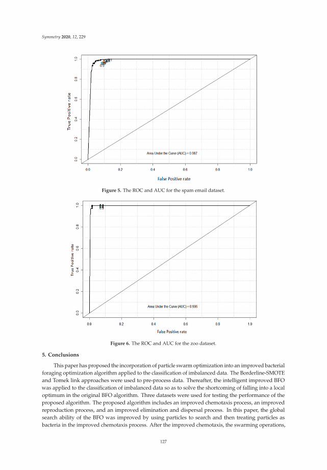
Symmetry 2020, 12, 229

Figure 5. The ROC and AUC for the spam email dataset.

Figure 6. The ROC and AUC for the zoo dataset.

5. Conclusions

This paper has proposed the incorporation of particle swarm optimization into an improved bacterialforaging optimization algorithm applied to the classification of imbalanced data. The Borderline-SMOTEand Tomek link approaches were used to pre-process data. Thereafter, the intelligent improved BFOwas applied to the classification of imbalanced data so as to solve the shortcoming of falling into a localoptimum in the original BFO algorithm. Three datasets were used for testing the performance of theproposed algorithm. The proposed algorithm includes an improved chemotaxis process, an improvedreproduction process, and an improved elimination and dispersal process. In this paper, the globalsearch ability of the BFO was improved by using particles to search and then treating particles asbacteria in the improved chemotaxis process. After the improved chemotaxis, the swarming operations,

127

Symmetry 2020, 12, 229

improved reproduction operations, and improved elimination and dispersal operations were performed.The average classification accuracy of the proposed algorithm for the ovarian cancer microarray datawas 93.47%. The average classification accuracies of the spam email dataset and the zoo dataset ofthe proposed algorithm were 96.42% and 99.54%, respectively. The value of the AUC was 0.979 forthe ovarian cancer microarray data, 0.987 for the spam email dataset, and 0.995 for the zoo dataset.The experimental results showed that the proposed algorithm in this research can achieve the bestaccuracy in the classification of imbalanced data compared with existing approaches.

In this paper, PSO was introduced into an improved bacterial foraging optimization algorithmand applied to the classification of imbalanced data. Based on the research results, we put forward thefollowing suggestions:

(1) Improvement of the algorithm’s operation: The key to implementing the optimization is theoperation of the algorithm. Designing an excellent operation plays an important role in improvingthe performance and efficiency of the algorithm. In BFO, this will become a key area of research intoBFO to improve chemotaxis and reproduction and the elimination and dispersal operation process,and to coordinate the local mining ability and global exploring ability of the processing algorithm.

(2) Selection of algorithm parameters: The parameter value of the algorithm is key to the performanceand efficiency of the algorithm. In evolutionary algorithms, there is no general method todetermine the optimal parameters of the algorithm. At present, there are many BFO parameters.Determining the optimal parameters of BFO to optimize the performance of the algorithm itself isa complex optimization problem.

(3) Combining with other algorithms: Combining the advantages of BFO and other algorithms topropose more efficient algorithms is a valuable topic in BFO research.

Author Contributions: Methodology, F.-L.Y. and C.-Y.L.; software, F.-L.Y., J.-Q.H., and J.-F.T.; formal analysis,F.-L.Y., C.-Y.L., and Z.-J.L.; investigation, F.-L.Y., C.-Y.L., and J.-F.T.; resources, C.-Y.L. and Z.-J.L.; data curation,F.-L.Y., J.-Q.H., and J.-F.T.; original draft preparation, F.-L.Y., C.-Y.L., and J.-F.T.; review and editing, F.-L.Y., C.-Y.L.,and J.-F.T. All authors have read and agreed to the published version of the manuscript.


Acknowledgments: This research was supported by the Major Education and Teaching Reform Projects in FujianUndergraduate Colleges and Universities in 2019 under grant FBJG20190284. This work was also supported byprojects under 2019-G-083.

Conflicts of Interest: The authors declare no conflict of interest. The funders had no role in the design of thestudy; in the collection, analyses, or interpretation of data; in the writing of the manuscript; or in the decision topublish the results.

References

1. Hu, J.J.; Yang, H.Q.; Lyu, M.R.; King, I.R.; So, A.M.C. Online Nonlinear AUC Maximization for ImbalancedData Sets. IEEE Trans. Neural Netw. Learn. Syst. 2018, 29, 882–895. [CrossRef]

2. Huang, X.L.; Zou, Y.X.; Wang, Y. Cost-sensitive sparse linear regression for crowd counting with imbalancedtraining data. In Proceedings of the 2016 IEEE International Conference on Multimedia and Expo (ICME),Seattle, WA, USA, 11–15 July 2016.

3. Padmaja, T.M.; Dhulipalla, N.; Bapi, R.S.; Krishna, P.R. Imbalanced data classification using extreme outlierelimination and sampling techniques for fraud detection. In Proceedings of the International Conference onAdvanced Computing and Communications, Guwahati, India, 18–21 December 2007; pp. 511–516.

4. Lin, S.W.; Ying, K.C.; Lee, C.Y.; Lee, Z.J. An intelligent algorithm with feature selection and decision rulesapplied to anomaly intrusion detection. Appl. Soft Comput. 2012, 12, 3285–3290. [CrossRef]

5. Lee, C.Y.; Lee, Z.J. A Novel Algorithm Applied to Classify Unbalanced Data. Appl. Soft Comput. 2012, 12,2481–2485. [CrossRef]

6. Zhang, Y.; Wu, L. Stock market prediction of S&P 500 via combination of improved BCO approach and BPneural network. Expert Syst. Appl. 2009, 36, 8849–8854.

128

Symmetry 2020, 12, 229

7. Xia, C.Q.; Han, K.; Qi, Y.; Zhang, Y.; Yu, D.J. A Self-Training Subspace Clustering Algorithm under Low-RankRepresentation for Cancer Classification on Gene Expression Data. IEEE/ACM Trans. Comput. Biol. Bioinform.2018, 15, 1315–1324. [CrossRef] [PubMed]

8. Esfahani, M.S.; Dougherty, E.R. Incorporation of Biological Pathway Knowledge in the Construction of Priorsfor Optimal Bayesian Classification. IEEE/ACM Trans. Comput. Biol. Bioinform. 2014, 11, 202–218. [CrossRef][PubMed]

9. Sadreazami, H.; Mohammadi, A.; Asif, A.; Plataniotis, K.N. Distributed-Graph-Based Statistical Approachfor Intrusion Detection in Cyber-Physical Systems. IEEE Trans. Signal Inform. Process. Netw. 2018, 4, 137–147.[CrossRef]

10. Mathew, J.; Pang, C.K.; Luo, M.; Leong, W.H. Classification of imbalanced data by oversampling in kernelspace of support vector machines. IEEE Trans. Neural Netw. Learn. Syst. 2018, 29, 4065–4076. [CrossRef]

11. Zhang, J.; Bloedorn, E.; Rosen, L.; Venese, D. Learning rules from highly imbalanced data sets. In Proceedingsof the Fourth IEEE International Conference on Data Mining, ICDM’04, Brighton, UK, 1–4 November 2004;Volume 1, pp. 571–574.

12. Jiang, Y.; Zhou, Z.H. Editing training data for kNN classifiers with neural network ensemble. In Proceedings ofthe International Symposium on Neural Networks, Dalian, China, 19–21 August 2004; Volume 1, pp. 356–361.

13. Tao, Q.; Wu, G.W.; Wang, F.Y.; Wang, J. Posterior probability support vector Machines for imbalanced data.IEEE Trans. Neural Netw. 2005, 16, 1561–1573. [CrossRef]

14. Zhang, J.; Mani, I. kNN approach to imbalanced data distributions: A case study involving informationextraction. In Proceedings of the ICML’2003 Workshop on Learning from Imbalanced Datasets, Washington,DC, USA, 21 August 2003.

15. Elaidi, H.; Elhaddar, Y.; Benabbou, Z.; Abbar, H. An idea of a clustering algorithm using support vectormachines based on binary decision tree. In Proceedings of the 2018 International Conference on IntelligentSystems and Computer Vision (ISCV), Fez, Morocco, 2–4 April 2018; pp. 1–5.

16. Ye, D.; Chen, Z. A rough set based minority class oriented learning algorithm for highly imbalanced datasets. In Proceedings of the IEEE International Conference on Granular Computing, Hangzhou, China,26–28 August 2008; pp. 736–739.

17. Yang, X.; Song, Q.; Cao, A. Clustering nonlinearly separable and imbalanced data set. In Proceedings of the2004 2nd International IEEE Conference on Intelligent Systems, Varna, Bulgaria, 22–24 June 2004; Volume 2,pp. 491–496.

18. Lu, Y.; Guo, H.; Feldkamp, L. Robust neural learning from imbalanced data samples. In Proceedings ofthe 1998 IEEE International Joint Conference on Neural Networks, Anchorage, AK, USA, 4–9 May 1998;Volume 3, pp. 1816–1821.

19. Wang, J.; Jean, J. Resolve multifont character confusion with neural network. Pattern Recognit. 1993, 26,173–187. [CrossRef]

20. Searle, S.R. Linear Models for Unbalanced Data; Wiley: New York, NY, USA, 1987.21. Wang, J.; Miyazaki, M.; Kameda, H.; Li, J. Improving performance of parallel transaction processing systems

by balancing data load on line. In Proceedings of the Seventh International Conference on Parallel andDistributed Systems, Taipei, Taiwan, 4–7 December 2000; pp. 331–338.

22. Crepinsek, M.; Liu, S.H.; Mernik, M. Replication and comparison of computational experiments in appliedevolutionary computing: Common pitfalls and guidelines to avoid them. Appl. Soft Comput. 2014, 19,161–170. [CrossRef]

23. De Corte, A.; Sörensen, K. Optimisation of gravity-fed water distribution network design: A critical review.Eur. J. Oper. Res. 2013, 228, 1–10. [CrossRef]

24. Kennedy, J.; Eberhart, R.C. A discrete binary version of the particle swarm algorithm. In Proceedings of the1997 IEEE International Conference on Systems, Man, and Cybernetics. Computational Cybernetics andSimulation, Orlando, FL, USA, 12–15 October 1997; Volume 5.

25. Eberhart, R.; Kennedy, J. A new optimizer using particle swarm theory. In Proceedings of the SixthInternational Symposium on Micro Machine and Human Science (MHS’ 95), Nagoya, Japan, 4–6 October 1995.

26. Jia, J.Y.; Zhao, A.W.; Guan, S.A. Forecasting Based on High-Order Fuzzy-Fluctuation Trends and ParticleSwarm Optimization Machine Learning. Symmetry 2017, 9, 124. [CrossRef]

27. Xue, H.X.; Bai, Y.P.; Hu, H.P.; Xu, T.; Liang, H.J. A Novel Hybrid Model Based on TVIW-PSO-GSA Algorithmand Support Vector Machine for Classification Problems. IEEE Access 2019, 7, 27789–27801. [CrossRef]

129

Symmetry 2020, 12, 229

28. Kim, J.J.; Lee, J.J. Trajectory Optimization with Particle Swarm Optimization for Manipulator MotionPlanning. IEEE Trans. Ind. Inform. 2015, 11, 620–631. [CrossRef]

29. Liu, H.M.; Yan, X.S.; Wu, Q.H. An Improved Pigeon-Inspired Optimisation Algorithm and Its Application inParameter Inversion. Symmetry 2019, 11, 1291. [CrossRef]

30. Salleh, I.; Belkourchia, Y.; Azrar, L. Optimization of the shape parameter of RBF based on the PSO algorithmto solve nonlinear stochastic differential equation. In Proceedings of the 2019 5th International Conferenceon Optimization and Applications (ICOA), Kenitra, Morocco, 25–26 April 2019.

31. Medoued, A.; Lebaroud, A.; Laifa, A.; Sayad, D. Feature form extraction and optimization of inductionmachine faults using PSO technique. In Proceedings of the 2013 3rd International Conference on ElectricPower and Energy Conversion Systems, Istanbul, Turkey, 2–4 October 2013.

32. Yeom, C.U.; Kwak, K.C. Incremental Granular Model Improvement Using Particle Swarm Optimization.Symmetry 2019, 11, 390. [CrossRef]

33. Lee, J.H.; Kim, J.W.; Song, J.Y. Distance-Based Intelligent Particle Swarm Optimization for Optimal Design ofPermanent Magnet Synchronous Machine. IEEE Trans. Magn. 2017, 53, 1–4. [CrossRef]

34. Yu, X.; Chen, W.N.; Gu, T.L. Set-Based Discrete Particle Swarm Optimization Based on Decomposition forPermutation-Based Multiobjective Combinatorial Optimization Problems. IEEE Trans. Cybern. 2018, 48,2139–2153. [CrossRef]

35. Shi, Y.; Eberhart, R. A modified particle swarm optimizer. Proceeding of the 1998 IEEE InternationalConference on Evolutionary Computation, World Congress on Computational Intelligence, Anchorage, AK,USA, 4–9 May 1998.

36. Passino, K.M. Biomimicry of bacterial foraging for distributed optimization and control. IEEE Control Syst.Mag. 2002, 22, 52–67.

37. Abraham, A.; Biswas, A.; Dasgupta, S. Analysis of reproduction operator in bacterial foraging optimizationalgorithm. In Proceedings of the IEEE World Congress on Computational Intelligence, Hong Kong, China,1–6 June 2008; pp. 1476–1483.

38. Bidyadhar, S.I.; Raseswari, P. Bacterial Foraging Optimization Approach to Parameter Extraction of aPhotovoltaic Module. IEEE Trans. Sustain. Energy 2018, 9, 381–389.

39. Noguchi, T.; Togashi, S.; Nakamoto, R. Based maximum power point tracking method for multiplephotovoltaic and converter module system. IEEE Trans. Ind. Electron. 2002, 49, 217–222. [CrossRef]

40. Raza, A.; Yousaf, Z.; Jamil, M. Multi-Objective Optimization of VSC Stations in Multi-Terminal VSC-HVdcGrids, Based on PSO. IEEE Access 2018, 6, 62995–63004. [CrossRef]

41. Lu, S.J. Gene Expression Analysis and Regulator Pathway Exploration with the Use of Microarray Data forOvarian Cancer. Master’s Thesis, National Taiwan University of Science and Technology, Taipei, Taiwan, 2006.

42. Lee, Z.J. An integrated algorithm for gene selection and classification applied to microarray data of ovariancancer. Int. J. Artif. Intell. Med. 2008, 42, 81–93. [CrossRef] [PubMed]

43. Blake, C.; Keogh, E.; Merz, C.J. UCI Repository of Machine learning Databases; Department of Information andComputer Science, University of California: Irvine, CA, USA, 1998; Available online: https://archive.ics.uci.edu/ml/datasets.php (accessed on 24 December 2019).

44. Gosain, A.; Sardana, S. Farthest SMOTE: A modified SMOTE approach. In Computational Intelligence in DataMining; Springer: Singapore, 2019; pp. 309–320.

45. Devi, D.; Purkayastha, B. Redundancy-driven modified Tomek link based undersampling: A solution toclass imbalance. Pattern Recogn. Lett. 2017, 93, 3–12. [CrossRef]

46. Liu, L.; Shan, L.; Yan, J.H. An Improved BFO Algorithm for Optimising the PID Parameters of Servo System.In Proceedings of the IEEE the 30th Chinese Control and Decision Conference (2018 CCDC), Shenyang,China, 9–11 June 2018; pp. 3831–3836.

47. Abd-Elazim, S.M.; Ali, E.S. A hybrid particle swarm optimization and bacterial foraging for power systemstability enhancement. Complexity 2015, 21, 245–255. [CrossRef]


130

symmetryS S

Article

Application of Gray Relational Analysis andComputational Fluid Dynamics to the StatisticalTechniques of Product Designs

Hsin-Hung Lin 1,2,* , Jui-Hung Cheng 3 and Chi-Hsiung Chen 1

1 Department of Creative Product Design, Asia University, Taichung City 41354, Taiwan2 Department of Medical Research, China Medical University Hospital, China Medical University,

Taichung 404, Taiwan3 Department of Mold and Die Engineering, National Kaohsiung University of Science and Technology,

Kaohsiung 80778, Taiwan* Correspondence: [email protected] or [email protected]; Tel.: +886-04-2332-3456-1051

Received: 27 September 2019; Accepted: 20 January 2020; Published: 3 February 2020

Abstract: During the development of fan products, designers often encounter gray areas whencreating new designs. Without clear design goals, development efficiency is usually reduced, andfans are the best solution for studying symmetry or asymmetry. Therefore, fan designers need tofigure out an optimization approach that can simplify the fan development process and reduceassociated costs. This study provides a new statistical approach using gray relational analysis (GRA)to analyze and optimize the parameters of a particular fan design. During the research, it was foundthat the single fan uses an asymmetry concept with a single blade as the design, while the operationof double fans is a symmetry concept. The results indicated that the proposed mechanical operationscould enhance the variety of product designs and reduce costs. Moreover, this approach can relievedesigners from unnecessary effort during the development process and also effectively reduce theproduct development time.

Keywords: gray relational analysis; flow-field analysis; fan design; CFD; product designevaluation; symmetry

1. Introduction

During the development of new fan products, it is necessary to repeatedly experiment and test tooptimize the product. However, the conventional design and development of a fan is usually limitedby standard methods, and the fan is the best solution to study symmetry or asymmetry. This methodconsists of multiple rounds of simulations and experiments. When a designer comes up with a newidea, it takes a long time to test and verify the parameters of the impeller profile. During the research,the single fan uses an asymmetry concept and the singular blade is used as the design, while thedouble fans constitute an asymmetry concept. In order to optimize the best method of symmetry orasymmetry regarding the mechanical principle of the blades, a new statistical method of gray relationalanalysis (GRA) analysis and the optimization of specific fan design parameters are required. In 2012,Kim et al. [1] suggested that a detailed blade design and optimized tip clearance is important forperformance, and the geometric parameters of a blade were calculated and the results served as theflow criteria. The geometric parameters of a blade were also determined by calculations and verifiedby the simulation results of Computational Fluid Dynamics (CFD) and experiments. In 2010, Huraultet al. [2] studied the impact of the turbulence in axial-flow fans, and the fans that had been studiedwere provided with radial, swept-forward, and swept-backward blades. He compared the results ofexperiments and CFD with those obtained by Rhee et al. [3]. However, there are many gray zones


Symmetry 2020, 12, 227

for the blade parameters during the process of development, and therefore most of the parametersare difficult to determine. In 2009, Lai et al. [4] applied the method of gray relational analysis (GRA)to product design evaluation (PDE) models when designing new product models. The final resultssolved the problem of complicated probabilities in the application of ergonomics to human comfort. In2011, Wei et al. [5] proposed an optimal alternative solution package with the concept of the largestgray correlation degree, and the package was used to determine the negative ideal solution with aminimal degree of gray relation. The method is simple and effective, and it is also easy to calculate. In2012, Qiu et al. [6] applied GRA to the verification of simulation models and simulation techniques formodeling, and improved the technique of GRA by considering data curves’ geometrical shape. Therationality and effectiveness of GRA have been further verified by case studies. Li et al. [7] proposedthat the important achievements by the continuous and diverse values of the gray system theory can bepredictable and controllable. Under indeterminate conditions, he applied GRA to typical gray matrixproblems and solved the problem of indeterminate and gray zones. The theory of GRA is one of themost mature and most broadly utilized gray system theories. During the analysis, the calculationswere conducted on the basis of value comparisons, and in general, the comparison of parameters wasalso an important index for the analysis. Gray relational analysis supplies a simple way of analyzing asequence of relationships or behaviors of a system. The analysis has the characteristics of quantitativeand sequential analysis, and it can be applied to a random sequence of major and minor factors. Thisapproach can analyze and confirm the factors affecting the target factors or the factors’ degrees ofimprovement. It substantially affects the quantitative analysis of the factors of a system with a trend ofdynamic development [8].

Li’s work aims to investigate the possibility of using tip nozzles on ducted fans under conditionsof large blade pitch angles and high ruggedness. The aerodynamic performance and flow field of thehovering ducted fan are studied numerically at a certain range of blade pitch angles at three operatingspeeds. Numerical experiments were performed using a shear stress transfer k-ω turbulence modeland a fine, high-quality structured grid. The maximum thrust, peak efficiency, and stall margin ofa ducted fan with a sharp jet are the main objectives of this study. The results show that under thecondition of stall margin, the thrust of the fan with the tip nozzle increased by 30%. The improvementin aerodynamics seems to increase with increasing blade pitch angle because the separation flow at thefront of the blade becomes uniform and reattaches to the blade surface due to the entrainment of thetip jet. The nozzles that are angled in the downward flushing direction can increase the nozzle ejectionefficiency at larger blade pitch angles. Tip nozzles are suitable for fans with large pitch angles andhigh ruggedness [9]. Wang research proposed an integrated device called a wind energy fan (WEF),which uses wind energy to directly drive a fan connected to a wind turbine through a drive shaft.This vertical wind turbine can achieve underground ventilation. A test platform was established totest the WEF performance, considering three transmission ratios and two wind turbines with threeand five blades. The results show that the transmission ratio has a significant effect on the fan airvolume and should be selected to obtain the rated air volume. A wind turbine with three blades iseasier to start, and its air volume is 5.43–17.85% higher than a wind turbine with five blades. Basedon the aerodynamic characteristics of vertical fans and axial fans, a method of matching power andspeed was proposed. This scheme is an effective wind energy technology, which can realize the activeutilization of wind energy [10]. Wu used CFD simulations to study the transient characteristics of bladeforces in fans with uneven blade spacing. Based on this, a “[T] -h” model for predicting blade forceswas developed, and then a prediction based on simulation results and CFD research was developedbased on the Lowson model [11]. David evaluated the performance of these underground fan systemsin four different deep gold mines in South Africa. Of the six systems, the overall efficiency of theauxiliary fan system was 5%, with an average fan efficiency of 33% of the 33 fans. The results show thatthese fans deviate significantly from the design operating point. Therefore, current underground fanpractices have significant shortcomings. Our detailed studies have concluded that the combination ofunderground auxiliary fan systems can lead to significant energy inefficiencies. Therefore, maintaining

132

Symmetry 2020, 12, 227

good underground fan operation (such as optimal fan selection, pipe design, and maintenance) iscritical to the efficiency of the mine ventilation network [12].

It is clear from the above analysis that no one has yet attempted to apply GRA to fan design.Based on this observation, a new concept of applying GRA to fan design is proposed in this study.After the relationship between parameters of a fan design is determined by GRA, the performanceof new fan designs can be improved by the optimization of parameters. To verify the performanceimprovement, the CFD software, FLUENT, is used to obtain numerical results of the fan’s performance,including flow rate and static pressure [1].

2. Model for Investigation

2.1. Development of the Model

Gray relational analysis is utilized in this study to establish the relationship between theindeterminate and gray zones of parameters for fan products. From the results of related methods, theoptimal approach for the parameter analysis of a product can be determined by the results obtained.The flow chart of this study is shown in Figure 1. It includes the principles for the calculation of GRA.When using GRA to assess each of the fan parameters, a value is considered valid if it surpasses thethreshold value of 0.7, which is recommended.

Figure 1. Framework of the development procedure.

For the evaluation of design parameters, it is usually difficult to predict the performance gain dueto design optimization without making prototypes for measurement. However, the cost of makingprototypes can be huge when the design optimization is based on a large number of design parameters.Therefore, simulation by CFD software is an important tool for a designer to predict the performance

133

Symmetry 2020, 12, 227

indicators of a new fan design, including air-flow rate and static pressure. By comparing theseindicators, which are available from CFD simulation, the flow-field characteristics can be captured,and the optimal design can be determined among several candidates. The CFD simulation results arealso compared with the experiment results in this study for the validation of this method.

2.2. Fan Model for Investigation

A schematic diagram of a symmetrical dual-impeller fan model in a case study is shown inFigure 2a, in which the initial impeller diameter is 80 mm. The main components, including theimpellers, motors, and the base, are shown in Figure 2b, which is an exploded view of the fan model.

(a)

(b)

Figure 2. Fan parameters: (a) assembled dual-impeller fan; (b) exploded view of dual-impeller fan.

134

Symmetry 2020, 12, 227

The operational principle of fans is mostly by means of the rotation of blades causing the pressuredifference between the fore and aft ends to happen, driving the rapid flow of the surrounding air. Thistakes away the heat of the heat-dissipating body and results in a temperature decrease. For a typicaldesign, after the design of a cooling element is shaped, the impedance curve of the element is fixed [13].Therefore, it is the most often used approach in the typical cooling element design process to changethe design of a fan to match the cooling element and enhance the overall cooling efficiency [14,15].Therefore, it is rather important to find out and know the performance curves of different fans whendesigning cooling elements [16,17].

2.3. Fan Parameters Affecting the Performance Curve

1. Blade pitch angle: The larger the pitch angle, the larger the pressure difference between the blade’supper and lower surfaces. Under the same rotation speed, the air pressure is also larger with alarger pitch angle. However, when the pressure of the lower surface is too large, the phenomenonof recirculation may occur, and this instead reduces the fan’s performance. Therefore, the bladepitch angle should also be increased to a certain extent.

2. Blade spacing: When the distance between the blades is too small, this leads to air-flowdisturbance, which increases the friction on the blade surfaces and reduces fan efficiency. Whenthe distance between blades is too large, this leads to an increase of pressure loss and insufficientair pressure [18].

3. The number of blades: This affects other specifications of fan blades, such as the sectional curveand pitch angle. The width of each blade usually depends on its height. To guarantee that bladespacing will not affect the air pressure, the approach of increasing the number of blades is usuallyadopted as a remedy in comparatively thinner fans.

3. Research Methods

3.1. Gray Relational Theory

Assuming a space in relation to the gray information as

{Q(X), R

}(1)

where Q(X) is the factor set in relation to the gray information, and R is the relation of mutual influence.The factor subset X0(k) is taken as the reference sequence, and Xi (k), i� 0 is the comparison sequence [8]:

X0 = [x0(1), x0(2), · · · , xi(k)] (2)

Xi = [xi(1), xi(2), · · · , xi(k)], i ∈ I, k ∈ N (3)

The correlation coefficient in relation to the gray information for Xi(k) on X0(k) is defined as

ri(k) = r[X0(k), Xi(k)] (4)

The correlation degree in relation to the gray information for Xi on X0 is

r(X0, Xi) =1n

n∑k=1

r[X0(k), Xi(k)] =1n

n∑k=1

ri(k) (5)

where the quantitative model of the correlation coefficient of gray information relationship for Xi(k) onX0(k) is defined as

ri(k) = r[X0(k), Xi(k)] =Δmin + ζΔmaxΔ0,i(k) + ζΔmax

(6)

135

Symmetry 2020, 12, 227

In the equation, Δ0,i =∣∣∣X0(k) −Xi(k)

∣∣∣ is the absolute difference of two comparison sequences,Δmin = min

i∈Imin

k

∣∣∣X0(k) −Xi(k)∣∣∣ is the minimum of the absolute differences of all comparison

sequences [19], Δmax = maxi∈I

maxk

∣∣∣X0(k) −Xi(k)∣∣∣ is the maximum of the absolute differences of

all comparison sequences, and ζ is the distinguishing coefficient. Its value is adjusted according to thepractical demands of the system. Typically, its value is between 0 and 1, and is usually assigned as 0.5.

From the analysis mentioned above, four major equations of GRA and the quantitative model ofthe correlation degree are employed to establish the analysis model in relation to the gray information.The procedure is as follows.

Step 1: The initialization of the original sequence.Step 2: Obtain the difference sequence, Δ0,i =

∣∣∣X0(k) −Xi(k)∣∣∣.

Step 3: Obtain the minimum of the absolute differences of all comparison sequences Δmin andthe maximum value Δmax.

Step 4: Calculate the gray correlation degree ri(k). The distinguishing coefficient is assigned as0.5. Substitute the difference sequence, the minimum, and the maximum of the absolute differencesinto the quantitative model of the correlation degree in relation to the gray information to obtain thegray correlation degree ri(k).

Step 5: Calculate the correlation degree in relation to the gray information Xi on X0.Step 6: Sort the degree of relationship between the major factor and all other factors in the

gray system.

3.2. Governing Equations

In three-dimensional Cartesian coordinates, the governing equations are as follows (FLUENTUser’s Guide) [1,20].

(1) Continuity equation:∂u∂x

+∂v∂y

+∂w∂z

= 0 (7)

(2) Momentum equations:X direction:

∂u∂t

+∂(u2)

∂x+∂(uv)∂y

+∂(uw)

∂z= − 1ρ∂P∂x

+ v[∂2u∂x2 +

∂2u∂y2 +

∂2u∂z2

](8)

Y direction:

∂v∂t

+∂(uv)∂x

+∂(v2)

∂y+∂(vw)

∂z= − 1ρ

∂(P− P0)

∂z+ v

[∂2v∂x2 +

∂2v∂y2 +

∂2v∂z2

](9)

Z direction:

∂w∂t

+∂(uw)

∂x+∂(vw)

∂y+∂(w2)

∂z= − 1ρ∂P∂z

+ v[∂2w∂x2 +

∂2w∂y2 +

∂2w∂z2

](10)

(3) Energy equation:

∂T∂t

+∂(uT)∂x

+∂(vT)∂y

+∂(wT)∂z

= α(∂2T∂x2 +

∂2T∂y2 +

∂2T∂z2 ) +

qpCP

(11)

(4) Governing equations can be represented by the general equations as follows:

∂(ρϕ)

∂t+∂(ρϕu)∂x

+∂(ρϕv)∂y

+∂(ρϕw)

∂z=∂∂x

(Γ∂ϕ

∂x

)+∂∂y

(Γ∂ϕ

∂y

)+∂∂z

(Γ∂ϕ

∂z

)+ s (12)

136

Symmetry 2020, 12, 227

where ∂(ρϕu)∂x +

∂(ρϕv)∂y +

∂(ρϕw)∂z is the convective term, ∂∂x

(Γ ∂ϕ∂x

)+ ∂∂y

(Γ ∂ϕ∂y

)+ ∂∂z

(Γ ∂ϕ∂z

)is the diffusive

term, S is the source term, and ∂(ρϕ)∂t is the unsteady term and is not considered when the system

is in steady state. Symbol ∅ represents physical variables such as u, v, w, k, ε, and T (Table 1). Thevelocity components in the x, y, and z directions are u, v, and w, respectively; Γ is the correspondingdiffusivity of each physical variable. Since we are looking for a steady-state solution, the variablesare independent of time. Therefore, the partial derivatives of u, v, w, and T with respect to t are equalto zero.

Table 1. Symbols of independent variables.

Continuity 1

X-momentum u

Y-momentum v

Z-momentum w

3.3. Standard k−ε Turbulence Model

Due to its extensive range of applications and reasonable precision, the standard k−εmodel hasbecome one of the main tools that are used for the calculation of turbulent flow fields. The standardk−ε turbulence model is a type of semi-empirical turbulence mode. Based on the fundamental physicalcontrol equations, the model can be used to derive the transport equations for the turbulence kineticenergy (k) and the rate of dissipation of turbulence energy (ε) as follows.

Turbulence kinetic energy equation (k)

∂∂t(ρk) +

∂∂xi

(ρkui) =∂∂xj

[(μ+μt

σk

)∂k∂xj

]+ Gk + Gb − ρε−YM (13)

(1) Equation of the rate of dissipation (ε)

∂∂t(ρε) +

∂∂xi

(ρεui) =∂∂xj

[(μ+μt

σε

)∂ε∂xj

]+ C1s

εk(Gk + C3εGb) −C2gρ

ε2

k(14)

(2) Coefficient of turbulent viscosity (μt)

μt = ρCμk2

ε(15)

where Gk indicates the turbulence kinetic energy that is generated by the laminar velocity gradient, Gbindicates the turbulence kinetic energy that is generated by buoyancy, YM indicates the fluctuationthat is generated by the excessive diffusion in compressible turbulent flows, and σk and σε are theturbulence Prandtl number of kinetic energy and dissipation, respectively. Further, C1ε, C2ε, and C3ε

are empirical numbers, and their recommended numbers are shown in Table 2.

Table 2. Coefficients of standard k–ε turbulence model.

C1ε C2ε Cu Ck Cε

1.44 1.92 0.09 1.0 1.3

The k−εmodel is based on the assumption that the flow field is fully turbulent and the molecularviscosity is negligible. Therefore, better results will be obtained from the calculation of fully turbulentflow fields.

137

Symmetry 2020, 12, 227

3.4. Performance Testing Equipment for Wind Turbines

The main device of the performance testing equipment for fans is an outlet-chamber wind tunnelthat conforms to AMCA 210-99. The principal parts include flow setting means, multiple nuzzles,flow-rate regulating devices, etc. The major function is to supply a good and stable flow field formeasurement and acquire the complete performance curves [21].

3.5. Calculation of Flow Rates

Regarding the measured pressure difference between the nozzle outlet and inlet (PL5 and PL6), theflow rates on the cross-sections of nozzles shown in Figure 3 can be obtained by the nozzle coefficients.For the calculation of the outlet flow rate of the fan under test, the effect of density variations mustbe considered.

Figure 3. Schematic of measurement planes.

The equation for the calculation of flow rates in a test chamber with multiple nuzzles [22,23] is

Q5 = 265.7Y√

ΔP/ρ5

∑n(CnA6n) (16)

whereQ5 the total flow rate measured by a bank of nozzles, CMMΔP the pressure difference across the nozzles, mm-Aqρ5 the air density upstream of the nozzles, kg/m3

Y expansion factorCn the discharge coefficient of the nth nozzle (Nozzle Discharge CoefficientA6n the cross-sectional area of the nth nozzle’s throat, m2

3.6. Method of Measurements

(a) Start the measurement from the point of the maximum flow rate (i.e., the point at which thestatic pressure of a fan is zero). Pay attention to the pressure difference across the nozzles, whichshould be between 0.5 inch-Aq and 2.5 inch-Aq. If the differential pressure reading is not within thisrange, this indicates that the flow rate measured for the time being is incorrect. It is required to adjustthe nozzle switch to respond to the variations in flow rate accordingly.

(b) After the completion of the data acquisition on the point of maximum flow rate, adjust thepressure to adequate values by means of the shutter of the auxiliary fan and inverter.

(c) Increase the pressure sequentially; the nozzle switch, the shutter of the auxiliary fan, and theinverter must be adjusted during each of the changes. After the system turns stable, then acquire agroup of data by the data acquisition system [24,25].

(d) Store 10 sets of data in 10 different files, and use a computer program to calculate the values ofair flow rate (Q), pressure (ΔP), and efficiency (η).

(e) Import the calculation results into CAD software to draw the performance curves of the fans

138

Symmetry 2020, 12, 227

This section expatiates on the procedures of the performance–curve measurement of fans basedon the experience acquired after many rounds of measurements.

Ps = Pt − Pv (17)

Pt = Pt2 − Pt1 (18)

where Ps is the static pressure of the fan under test;Pt is the total pressure of the fan under test;Pv is the dynamic pressure of the fan under test;Pt2 is the total pressure at the fan’s outlet (or plane PL2);Pt1 is the total pressure at the fan’s inlet (or plane PL1).Since in this experiment there was no duct at the inlet of the fan under test, therefore Pt1 = 0 On

the other hand, the measured static pressure at the outlet is the same as the static pressures measuredat the measuring plane PL7. Therefore, Ps2 = Ps7 .

Pt2 = Ps7 + Pv (19)

Ps = Ps7 (20)

It is concluded from the above equation that the static pressure of the fan under test happens tobe equal to the static pressure obtained at the outlet test chamber Pt7. The calculation of dynamicpressures is

Pv2 =ρ2V2

2

19.6(21)

where Pv2 is the outlet dynamic pressure of the fan under test, mm-Aq;V2 is the outlet air velocity of the fan under test, m/s;ρ2 is the outlet air density of the fan under test, kg/m3;and V2 = Q2

60A2= Q

60A2· ρρ2

= Q50ρ2A2

where Q2 is the outlet flow rate of the fan under test, CMM;Q is the standard flow rate of the fan under test, CMM;A2 is the outlet cross-sectional area of the fan under test, m2;ρ is the density of air at STP (1.2 kg/m3).

Pt = Ps + Pv = Ps + Pv2 .

Pt = Ps +ρ2V2

2

19.6(22)

3.7. Method of Measuring the Performance Curves of Fans

With a fixed amount of power, the flow rate varies inversely proportional to the output air pressure.Since the efficiency of fans changes as the flow rate varies, a non-linear relationship between the flowrate and the air pressure exists, and this forms the performance curve of fans [26]. The measurementprocess is shown in Figure 4.

139

Symmetry 2020, 12, 227

Figure 4. Operational flow chart of fan performance measurements.

3.8. Fan Performance Test Equipment

In terms of performance measurement, the detailed installation and operation of measurementequipment and instruments are described as follows. Regarding the fan performance measurementequipment, the fan performance test body used in this paper uses the AMCA 210-99 standard exportwind tunnel, mainly including the main body. The main functions of the rectifier plate, multi-nozzle,

140

Symmetry 2020, 12, 227

and air volume adjustment device are to simulate the air flow conditions downstream of various fans,and to provide a good and stable measurement flow field, so that a complete performance curve canbe obtained.

The test platform includes the body, rectifier plate, multiple nozzles, and auxiliary fans (seeFigures 4–9) to provide an ideal measurement benchmark; with the air volume adjustment device, itcan simulate the outlet of the fan to be tested for various system impedances and even use in free air.The details are as follows:

1. Test fan 12. Thermocouple 2. Auxiliary fan 13. Fiber Optic Tachometer 3. Air volume adjustment device 14. Multi-function capture interface card 4. Rectifier 15. Multi-function signal conversion card 5. Multi-nozzle 16. personal computers 6. Static pressure hole in front of nozzle 17. Laser printer 7. Static pressure hole behind nozzle 18. Thermometer and hygrometer 8. Air inlet static pressure hole 19. Barometer 9. No. 1 pressure converter 20. Digital inverter

10. No. 2 pressure converter 21. Power Supplier 11. Optical fiber tachometer adjustment device 22. Hand hole

Figure 5. Main specifications of fan performance test.

141

Symmetry 2020, 12, 227

Figure 6. Model of the dual-impeller fan.

Figure 7. Structure of the numerical model of the dual-impeller fan for the case study.

142

Symmetry 2020, 12, 227

(a) No. 1 (b) No. 2 (c) No. 3

Figure 8. Contours of velocity on the centerline section.

Figure 9. Fan performance curves.

(1) The bodyThe cross-sectional area of the outlet wind tunnel should be designed to be more than 16 times the

maximum measurable area of the air outlet of the axial flow fan (because the test surface required bythe axial flow fan is large, the wind tunnel is designed in this way).

(2) RectifierThere is one set consisting of a front and one back box, with three pieces in each group. The area

opening rate should be maintained at 50–60%. It is used to stabilize the fluid flow and ensure thereliability of measurement. Since the measurement of Sections 6 and 7 downstream of the nozzle andthe static pressure of the fan are located upstream of the rectifier plate, in order to avoid the design ofthe rectifier plate affecting the measurement of these two sections, the maximum bounce velocity ofthe rectifier plate must be maintained at Sections 2 and 6 within 10% of the flow rate. Meanwhile, themeasurement section (upstream of the nozzle) is also encountered downstream of the rectifier, so itspecifies a local maximum speed of 0.1 M downstream of the rectifier unless the local maximum speedis less than 2 m/s; otherwise, it must not exceed 25% of the average flow rate.

143

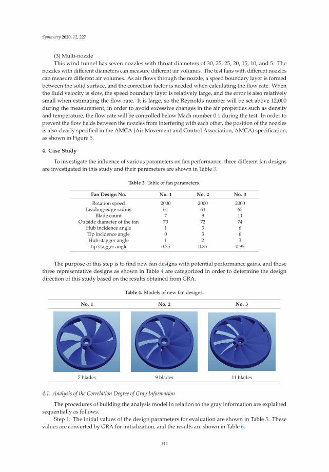
Symmetry 2020, 12, 227

(3) Multi-nozzleThis wind tunnel has seven nozzles with throat diameters of 30, 25, 25, 20, 15, 10, and 5. The

nozzles with different diameters can measure different air volumes. The test fans with different nozzlescan measure different air volumes. As air flows through the nozzle, a speed boundary layer is formedbetween the solid surface, and the correction factor is needed when calculating the flow rate. Whenthe fluid velocity is slow, the speed boundary layer is relatively large, and the error is also relativelysmall when estimating the flow rate. It is large, so the Reynolds number will be set above 12,000during the measurement; in order to avoid excessive changes in the air properties such as densityand temperature, the flow rate will be controlled below Mach number 0.1 during the test. In order toprevent the flow fields between the nozzles from interfering with each other, the position of the nozzlesis also clearly specified in the AMCA (Air Movement and Control Association, AMCA) specification,as shown in Figure 5.

4. Case Study

To investigate the influence of various parameters on fan performance, three different fan designsare investigated in this study and their parameters are shown in Table 3.

Table 3. Table of fan parameters.

Fan Design No. No. 1 No. 2 No. 3

Rotation speed 2000 2000 2000Leading-edge radius 61 63 65

Blade count 7 9 11Outside diameter of the fan 70 72 74

Hub incidence angle 1 3 6Tip incidence angle 0 3 6Hub stagger angle 1 2 3Tip stagger angle 0.75 0.85 0.95

The purpose of this step is to find new fan designs with potential performance gains, and thosethree representative designs as shown in Table 4 are categorized in order to determine the designdirection of this study based on the results obtained from GRA.

Table 4. Models of new fan designs.

No. 1 No. 2 No. 3

7 blades 9 blades 11 blades

4.1. Analysis of the Correlation Degree of Gray Information

The procedures of building the analysis model in relation to the gray information are explainedsequentially as follows.

Step 1: The initial values of the design parameters for evaluation are shown in Table 5. Thesevalues are converted by GRA for initialization, and the results are shown in Table 6.

144

Symmetry 2020, 12, 227

Table 5. Initial values of design parameters.

Fan Design No. 1 2 3

Rotation speed X0 2000 2000 2000Leading-edge radius X1 61 63 65

Blade count X2 7 9 11Outside diameter of the fan X3 70 72 74

Hub incidence angle X4 1 3 6Tip incidence angle X5 1 3 6Hub stagger angle X6 1 2 3Tip stagger angle X7 0.75 0.85 0.95

Table 6. Initialization of design parameters for gray relational analysis (GRA) X0 =

[x0(1), x0(2), · · · , xi(k)].


Rotation speed X0 0.3333 0.3333 0.3333Leading-edge radius X1 0.3228 0.3333 0.3439

Blade count X2 0.2593 0.333 0.4074Outside diameter of the fan X3 0.3241 0.333 0.3426

Hub incidence angle X4 0.1 0.3 0.6Tip incidence angle X5 0.1 0.3 0.6Hub stagger angle X6 0.1667 0.3333 0.5Tip stagger angle X7 0.2941 0.3333 0.3725

Step 2: Obtain the difference sequence,Δ0,i =∣∣∣X0(k) −Xi(k)

∣∣∣, as shown in Table 7.

Table 7. Difference sequence Δ0,i =∣∣∣X0(k) −Xi(k)

∣∣∣.Fan Design No. 1 2 3

Leading-edge radius X1 0.0106 0.0000 0.0106Blade count X2 0.0741 0.0000 0.0741

Outside diameter of the fan X3 0.0093 0.0000 0.0093Hub incidence angle X4 0.2333 0.0333 0.2667Tip incidence angle X5 0.2333 0.0333 0.2667Hub stagger angle X6 0.1667 0.0000 0.1667Tip stagger angle X7 0.0392 0.0000 0.0392

Step 3: From Table 7, the maximum and minimum values of the difference sequence can bedetermined as Δmin = Δ1,1(2) = 0.0000 and Δmax = Δ4,3(1) = 0.2667, respectively.

Step 4: Set the threshold value for gray correlation degrees at 0.5. The gray correlation degrees ofvarious variance factors can be obtained as shown in Table 8.

Table 8. Gray correlation degree ri(k).


Leading-edge radius X1 0.9265 1.0000 0.9265Blade count X2 0.6429 1.0000 0.6429

Outside diameter of the fan X3 0.9351 1.0000 0.9351Hub incidence angle X4 0.3637 0.8000 0.3334Tip incidence angle X5 0.3637 0.8000 0.3334Hub stagger angle X6 0.4445 1.0000 0.4445Tip stagger angle X7 0.7727 1.0000 0.7727

145

Symmetry 2020, 12, 227

Step 5: Calculate each variance factor Xi for its average difference in the design parameters X0 ofthe correlation degree in relation to the gray information r(X0, Xi). The resulting correlation degrees inrelation to the gray information are shown in Table 9.

Table 9. Correlation degrees in relation to the gray information r(X0, Xi).

Factor Correlation Degree

Leading-edge radius X1 0.9510Blade count X2 0.7619

Outside diameter of the fan X3 0.9567Hub incidence angle X4 0.4990Tip incidence angle X5 0.4990Hub stagger angle X6 0.6297Tip stagger angle X7 0.8485

4.2. Configuration of the Numerical Model

As shown in Figure 6, a numerical model of the dual-impeller fan was built for the case study.The dimensions of the inlet and outlet zones were determined based on the recommended values inorder to reflect a real scenario of no impedance to the air flow into the ambient.

4.3. Settings of Model Parameters

A. Settings of boundary conditionsThe main consideration of the settings of boundary conditions is to reflect the physical phenomena

of the surrounding environment and objects around the target model. It is critical to meet the physicalphenomena or else the calculation result of the simulation might be affected. A designer might also bemisguided into making a wrong decision. In this case study, the boundary conditions include the inletboundary condition, outlet boundary condition, and wall boundary condition, which are describedas follows.

1. Inlet boundary condition: The inlet condition is for the initial calculation. In order to simulatethe condition of a fan in an infinite domain, a normal atmospheric pressure of P0 is set at the inlet.

2. Outlet boundary condition: In order to simulation the air flow that is generated by the rotatingimpellers into the ambient, a normal atmospheric pressure of P0 is also set at the outlet.

3. Wall boundary condition: For a fluid flow passing along a wall, it needs to satisfy not only thenon-permeable condition but also the no-slip condition.

In addition to the above-mentioned conditions, this case study includes the following assumptionsin order to simplify the complexity of the flow field calculation.

1. The flow field is at a steady state and the fluid is non-compressible air.2. The turbulence model that is used in this case study is k–εwith an eddy correction.3. The influence of gravitation is neglected.4. Relevant fluid properties, including the viscosity coefficient, density, and specific heat,

are constants.5. A rotation speed of 2000 RPM is set for the fluid in the rotating zone.6. The fluid velocity at the surface of a solid is zero, and this is the no-slip condition.7. The heat radiation term and the buoyancy term are neglected, while physical properties are

independent of temperature. This is because when the temperature of fluid is different at differentlocations, the buoyancy force is generated due to the variation in its density. However, air isdriven by fans under forced convection while the natural convective effect is much less effective;therefore, the buoyance term can be neglected. On the other hand, the heat convective termdue to the fluid’s sensible heat and latent heat is much larger than the heat radiation term, andtherefore the radiation term can be neglected.

146

Symmetry 2020, 12, 227

B. Mesh settingsAs shown in Figure 7, the total number of cells is 1,957,013 for the dual impellers and 2,659,498 for

the entire system, including the inlet and the outlet. As the mesh for the inlet and the outlet is used forthe analysis of the upstream and downstream flow fields and for the boundary conditions, more cellsare required at the locations that are closer to the dual impellers in order to simulate the complicatedflow field locally. For the domain that is upstream to the dual impellers, the size of a cell is the largestat the inlet. Similarly, the size of a cell is the largest at the outlet for the domain that is downstream tothe impellers. This is because no complex geometry exists at either the inlet or the outlet.

4.4. Simulation Results of Fans

The results of numerical simulation make it easy to understand the aerodynamic characteristicsand the flow field of fans, which serve as the foundation for further investigation, analysis, andimprovement. The contours of pressure, as shown in Figure 8, allow us to better understand theinfluence of pressure on the entire system in the flow field being analyzed as well as the velocitydistribution of the fluid at the centerline section.

Lastly, the one to be compared is the resulting flow rate by numerical calculations. Based on thepredicted flow rates of Table 10 by simulation at the outlet, it is known that the flow rate of 40.4 CFMin No. 2 is the maximum, whereas the change of incidence angle still has the effect of increasing theflow rate, but for the phenomenon of recirculation occurring along the upper edge of the impeller andbetween the blades, no big improvement is observed.

Table 10. Predicted flow rates by simulation.


Rotation speed when the maximum flow rate occurs (RPM) 2000 2000 2000Maximum static pressure Ps (mm-Aq) 1.75 1.92 1.83

Maximum flow rate Q (CFM, Cubic feet per minute) 37.3 40.4 38.2

The weighted averages of the correlation degrees x1~xn are determined by the following equation.By applying the weighted averages to the flow rate and the static pressure of each fan design, theresulting values of maximum flow rate and maximum static pressure are shown in Table 11.

Table 11. Weighted averages of the maximum flow rate and the maximum static pressure.


Maximum static pressure Ps (mm-Aq) 0.3182 0.3491 0.3327Maximum flow rate Q (CFM) 0.3218 0.3486 0.3296

In this study, simulation of three kinds of different fan designs designated as No. 1, No. 2, andNo. 3 was conducted separately. Verifications of the various results obtained, including flow rates andair pressures, were also conducted by the simulation. With the simulation results obtained, consistencyverification was further conducted on these results by the correlation degree of gray information.Observation and comparison were conducted both on the maximum static pressure and the maximumflow rate. It can be found in the simulation results that the maximum flow rate of No. 2 is apparently9% higher than that of No. 1, whereas the maximum static pressure of No. 2 is also about 8% higherthan that of No. 1, as shown in Figure 6.

4.5. Comparison Between the Results of Simulation and Experiment

Method of measuring the performance curve of a fanThe testing of fan characteristics is accomplished on a wind tunnel, as shown in Figure 9. The

performance of a fan is usually determined by several operating points instead of a single point of

147

Symmetry 2020, 12, 227

static pressure versus air flow rate, because it is typically not considered as a stable system. Moreover,when a fan operates under a constant input power, the resulting flow rate varies inversely proportionalto the output air pressure. In this study, the procedure of measuring fan performance is as follows.

1. Preparatory work for measurements

A. Turn on the thermometer, hygrometer, barometer, fiber-optic tachometer, and inverter onehour before measurement. Make sure the equipment operates at a stable state. A testingworkbench with a wind tunnel is shown in Figure 10a. The fan to be tested is mounted onthe front plate of the main chamber. Care should be taken to ensure that the fan is sealedadequately to prevent leakage.

B. Turn on the test fan and the auxiliary blower for several minutes until both of them runstably. Adjust the blast gate from fully open to fully closed and check the air flow throughthe chamber. Check the readings of each of the equipment.

C. Measure the pressure difference between the free-flow condition (free deliver) and theno-flow condition (shut off). Divide the pressure difference into nine segments fordetermining the pressure increment and the data acquisition points.

(a) Testing workbench with a wind tunnel (b) Specimen under wind-tunnel testing

Figure 10. Wind-tunnel testing.

2. Measurement procedure

A. Start the measurement from the free-flow condition with a static pressure of 0. Pay attentionto the pressure difference between the nozzle array. The pressure difference needs to bein the range of 0.5–2.5 mm-Aq or the measured air-flow rate could be incorrect. In thiscase, it is required to select another nozzle from the nozzle array for a different range ofair-flow rates.

B. After the data under the free-flow condition are determined, use the blast gate and theinverter of the auxiliary blower to adjust the pressure to a desired range.

C. Increase the pressure to the next range of these nine segments by swapping the nozzle andadjusting the blast gate and the inverter. Use the data-acquisition system to take data ofsystem readings after it has been stabilized. Repeat this step for all of these nine segments.

D. Pull out the data that are recorded in files and calculate the air-flow rate, air pressure, andefficiency of the computer program.

E. Summarize the calculation results in the performance curve of the fan.

The performance improvement that is predicted by the numerical simulation is further comparedto the result that is obtained from the wind-tunnel testing, as shown in Table 12. Both the difference

148

Symmetry 2020, 12, 227

in the pressure drop and that in the air-flow rate are within 5%, which indicates a small differencebetween the simulation and the experiment results.

Table 12. Comparison between results from the simulation and the experiment.

Results from the Simulation Results from the Experiment

Rotation speed at the maximum flow rate (RPM) 2000Maximum static pressure Ps (mm-Aq) 1.92 1.75Maximum flow rate Q (CFM) 40.4 38.3


In this study, the gray design GRA was used to determine the important design parameters forimproving the design performance of the fan with the best solution for symmetry or asymmetry. Basedon the results obtained by GRA, the priority of design parameters for improving performance wasdetermined, and GRA stated that the second design can provide better performance than the other twodesigns. The effects of these design parameters are further studied through numerical simulationsand experiments. The simulation results also showed that the static pressure of the No. 2 design was1.92 mm-Aq, and its flow rate was 40.4 CFM. Compared to the other two designs, it was obvious thatperformance-wise, No. 2 was the best of the three fan designs. By taking the weighted averages of thecorrelation degrees for the design parameters, the resulting maximum static pressures were No. 1:0.3182, No. 2: 0.3491, and No. 3: 0.3327. Moreover, the maximum flow rates were No. 1: 0.3218, No. 2:0.3486, and No. 3: 0.3296. It is clear that the maximum flow rate of No. 2 was the largest among thesethree designs. The most important design parameters can be determined by GRA at an earlier stage offan design.

The results of the case study indicated that among fan parameters, the one with the greatestinfluence was the leading-edge radius. The outside diameter is another design parameter that shows ahigher correlation degree. However, it is already known that an oversized fan could cause a stall, whichleads to the phenomenon of rapidly deteriorating fan performance. Moreover, in space-constrainedapplications, the outside diameter is typically not selected as one of the design variables, becauseincreasing the outside diameter leads to a bigger fan, which might fail to fit into the available space.

Author Contributions: The author contributed to the paper. H.-H.L. collected and organized the data and acts asthe corresponding author, J.-H.C. and C.-H.C. proposed the methods. All authors have read and agreed to thepublished version of the manuscript.

Funding: This work was supported by the Ministry of Science and Technology of the Republic of China undergrant MOST-108-2221-E-468-003.

Conflicts of Interest: The author declares no conflict of interest.

References

1. Bredell, J.R.; KrÃÃger, D.G.; Thiart, G.D. Numerical investigation of fan performance in a forced draftair-cooled steam condenser. Appl. Therm. Eng. 2006, 26, 846–852. [CrossRef]

2. Hurault, J.; Kouidri, S.; Bakir, F.; Rey, R. Experimental and numerical study of the sweep effect onthree-dimensional flow downstream of axial flow fans. Flow Meas. Instrum. 2010, 21, 155–165. [CrossRef]

3. Rhee, D.H.; Cho, H.H. Effect of vane/blade relative position on heat transfer characteristics in a stationaryturbine blade: Part 2. Blade surface. Int. J. Therm. Sci. 2008, 47, 1544–1554. [CrossRef]

4. Lai, H.H.; Chen, C.H.; Chen, Y.C.; Yeh, J.W.; Lai, C.F. Product design evaluation model of child car seat usinggray relational analysis. Adv. Eng. Inform. 2009, 23, 165–173. [CrossRef]

5. Wei, G.W. Grey relational analysis method for 2-tuple linguistic multiple attribute group decision makingwith incomplete weight information. Expert Syst. Appl. 2011, 38, 4824–4828. [CrossRef]

6. Qiu, B.; Wang, F.; Li, Y.; Zuo, W. Research on Method of Simulation Model Validation Based on ImprovedGrey Relational Analysis. Phys. Procedia 2012, 25, 1118–1125. [CrossRef]

7. Li, Q.X. Grey dynamic input–output analysis. J. Math. Anal. Appl. 2009, 359, 514–526. [CrossRef]

149

Symmetry 2020, 12, 227

8. Trivedi, H.V.; Singh, J.K. Application of Grey System Theory in the Development of a Runoff PredictionModel. Biosyst. Eng. 2005, 92, 521–526. [CrossRef]

9. Li, L.; Huang, G.; Chen, J. Aerodynamic characteristics of a tip-jet fan with a large blade pitch angle. Aerosp.Sci. Technol. 2019, 91, 49–58. [CrossRef]

10. Wang, Z.; Wu, Y.; Lu, S.; Meng, X.; Zhang, J. A study on model experiment and aerodynamic match of WindEnergy Fan. Sustain. Cities Soc. 2019, 49, 101618. [CrossRef]

11. Wu, Y.; Pan, D.; Peng, Z.; Hua, O. Blade force model for calculating the axial noise of fans with unevenlyspaced blades. Appl. Acoust. 2019, 146, 429–436. [CrossRef]

12. Villiers, D.J.; Mathews, M.J.; Maré, P.; Kleingeld, M.; Arndt, D. Evaluating the impact of auxiliary fan practiceson localised subsurface ventilation. Int. J. Min. Sci. Technol. 2019, 29, 933–941. [CrossRef]

13. Tournier, J.M.; El-Genk, M.S. Axial flow, multi-stage turbine and compressor models. Energy Convers. Manag.2009, 51, 16–29. [CrossRef]

14. Qian, X.; Deba, D. Design of heterogeneous turbine blade. Comput. Aided Des. 2003, 35, 319–329. [CrossRef]15. Lin, H.H. Application of Fuzzy Decision Model to the Design of a Pillbox for Medical Treatment of Chronic

Diseases. Appl. Sci. 2019, 9, 4909. [CrossRef]16. Lin, S.C.; Huang, C.L. An integrated experimental and numerical study of forward–curved centrifugal fan.

Exp. Therm. Fluid Sci. 2002, 26, 421–434. [CrossRef]17. Li, Y.L.; Liu, J.; Ou, H.; Du, Z.H. Internal flow mechanism and experimental research of low pressure axial

fan with forward-skewed blades. J. Hydrodyn. Ser. B 2008, 20, 299–305. [CrossRef]18. Niu, M.; Zang, S. Experimental and numerical investigations of tip injection on tip clearance flow in an axial

turbine cascade. Exp. Therm. Fluid Sci. 2011, 35, 1214–1222. [CrossRef]19. Yao, C. Application of Gray Relational Analysis Method in Comprehensive Evaluation on the Customer

Satisfaction of Automobile 4S Enterprises. Phys. Procedia 2012, 33, 1184–1189.20. FLUENT User’s Guide. Available online: https://www.ansys.com/products/fluids/ansys-fluent (accessed on

1 January 2019).21. Lin, H.H.; Huang, Y.Y. Application of ergonomics to the design of suction fans. In Proceedings of the 1st

IEEE International Conference on Knowledge Innovation and Invention, Jeju Island, South Korea, 23–27 July2018; pp. 203–206.

22. Hsiao, S.W.; Lin, H.H.; Lo, C.H.; Ko, Y.C. Automobile shape formation and simulation by a computer-aidedsystematic method. Concurr. Eng. Res. Appl. 2016, 24, 290–301. [CrossRef]

23. Lin, H.H. Improvement of Human Thermal Comfort by Optimizing the Airflow Induced by a Ceiling Fan.Sustainability 2019, 11, 3370. [CrossRef]

24. Lin, H.H.; Hsiao, S.W. A Study of the Evaluation of Products by Industrial Design Students. Eurasia J. Math.Sci. Technol. Educ. 2018, 14, 239–254. [CrossRef]

25. Hsiao, S.W.; Lin, H.H.; Lo, C.H. A study of thermal comfort enhancement by the optimization of airflowinduced by a ceiling fan. J. Interdiscip. Math. 2016, 19, 859–891. [CrossRef]

26. Lin, H.H.; Cheng, J.H. Application of the Symmetric Model to the Design Optimization of Fan Outlet Grills.Symmetry 2019, 11, 959. [CrossRef]


150

symmetryS S

Article

Applying Educational Data Mining to ExploreStudents’ Learning Patterns in the Flipped LearningApproach for Coding Education

Hui-Chun Hung 1, I-Fan Liu 2, Che-Tien Liang 3 and Yu-Sheng Su 4,*1 Graduate Institute of Network Learning Technology, National Central University, Taoyuan City 320, Taiwan;

[email protected] Center for General Education, Taipei Medical University, Taipei City 110, Taiwan; [email protected] Graduate Institute of Data Science, Taipei Medical University, Taipei City 110, Taiwan;

[email protected] Department of Computer Science and Engineering, National Taiwan Ocean University,

Keelung City 202, Taiwan* Correspondence: [email protected]


Abstract: From traditional face-to-face courses, asynchronous distance learning, synchronous livelearning, to even blended learning approaches, the learning approach can be more learner-centralized,enabling students to learn anytime and anywhere. In this study, we applied educational datamining to explore the learning behaviors in data generated by students in a blended learning course.The experimental data were collected from two classes of Python programming related coursesfor first-year students in a university in northern Taiwan. During the semester, high-risk learnerscould be predicted accurately by data generated from the blended educational environment. Thef1-score of the random forest model was 0.83, which was higher than the f1-score of logistic regressionand decision tree. The model built in this study could be extrapolated to other courses to predictstudents’ learning performance, where the F1-score was 0.77. Furthermore, we used machine learningand symmetry-based learning algorithms to explore learning behaviors. By using the hierarchicalclustering heat map, this study could define the students’ learning patterns including the positiveinteractive group, stable learning group, positive teaching material group, and negative learninggroup. These groups also corresponded with the student conscious questionnaire. With the results ofthis research, teachers can use the mid-term forecasting system to find high-risk groups during thesemester and remedy their learning behaviors in the future.

Keywords: blended learning; learning behaviors; learning performance; machine learning; onlineprogramming course

1. Introduction

With the development of the Internet, emerging forms of distance education can eliminate thegeographical and temporal separation between two learners, and the knowledge can be transmitted toall corners of the world through the teaching environment of the online platform. Furthermore, anothersignificant advantage of the Internet is that the teaching will be transformed from teacher-centeredto learner-centered [1]. Distance learning enables learners to more flexibly manage their time andprogress, and choose the time and place to learn. Therefore, it also improves the shortcomings of thetraditional educational environment such as a lack of flexibility, limited delivery distance, and inabilityto repeat learning [2].

However, traditional asynchronized distance teaching has its disadvantages. For example,the learner’s problem can be answered by message or by mail, however, it takes a longer time


Symmetry 2020, 12, 213

when compared to the face-to-face environment where learners can ask questions and obtainanswers immediately, as the teacher cannot grasp it instantly. With the advancement of technology,the synchronous distance learning (live) environment has become another choice for the teachingenvironment. The advantages of the live broadcast environment include providing innovative learningmodels, motivating learners, providing formal multi-learning materials, and making the learnerreflect [3]. In the live broadcast environment, learners can ask questions to the instructor promptlyunder the live broadcast, and the instructor can respond promptly. Compared with asynchronouslearning, students can ask questions more freely. Discussing the teaching content of the teacher withother students does not affect the learning quality of other students, and the students can respond tothe teaching content of the teacher so that the instructor can immediately see whether the teachingcontent is correctly transmitted. Immediate response is unattainable in traditional face-to-face andnon-synchronous distance learning [4].

Additionally, a chat box in the learning management system can become a conduit forcommunication between learners. The live environment breaks this gap, and learners can instantlyexchange ideas and explain questions with others in the chat box. This is followed by the possibilityof learners chatting with each other [5]. The advantages and disadvantages of synchronous andasynchronous learning are different, so the blended learning environment has become one of thechoices of today’s learning approaches. The blended learning environment proposed by this studyintegrates traditional face-to-face courses, asynchronous, and synchronized online learning. Therefore,it can provide students with the most flexible learning environment. In the literature review ofblended learning, there have been few studies on the learning approach integrated with Facebook live.Therefore, this study hopes to explore the learner’s learning experience and learning achievement withthe use of educational data mining through traditional distance education, face-to-face teaching, andlearning via Facebook live.

This study aims to use machine learning and symmetry-based learning algorithms to explore therelationship between the data generated by the learning process in a blended learning environmentand learning achievement. The research questions in this study are as follows:

1. In the blended learning environment, can we use the data generated in the learning process toforecast learners’ performances?

2. Can we apply the generated model to predict the data of the other class?3. Can we find a specific learning model from the learner’s learning behavior? How can the learning

group be defined and which variables should they be based on?

To solve these research questions, this paper explored which variables were related to the learner’slearning performance in a mixed-education environment of mixed face-to-face courses. This studycollected the learning records generated by students in a blended learning environment such asthe degree of synchronous and asynchronous participation, the submission of assignments, and thediscussion in the online forum. Through educational data exploration, predictions can be made in theinterim period so that the instructors are in the second half of the semester. Personalized guidancecould then be given to high-risk students. Therefore, this study is able to predict learners’ learningperformance and provide personalized guidance or reminders for high-risk learners to enhance theefficiency and effectiveness of future teaching.


2.1. Blending Learning Environment

In the last few decades, information and communication technology has revolutionized theprocesses of learning. The blending learning environment can be defined as the combination oftraditional face-to-face courses and online learning environments that can complement each other’sshortcomings [2]. The implementation is complicated and challenging as the proportion of face-to-face

152

Symmetry 2020, 12, 213

and online learning will lead to an unlimited number of combinations [6]. The definition andclassification of the blended learning environment mainly include two aspects: one is the transmissionmethod (offline and online), and the other is the learning method (educator-oriented and learnercenter) [7]. Therefore, from these two aspects, there are four possible blended learning environments:(1) Mostly face-to-face courses and significant online interactions; (2) mostly online courses and offlinegroup discussions; (3) mostly face-to-face courses and online resources provided; and (4) mostlyonline courses and optional face-to-face discussions. The blended learning environment of this studywas similar to the fourth type. Most of the online courses and online assignments, discussions,quizzes, and live online courses were synchronized, while the remaining few face-to-face courses weremainly for the start of course introduction, environment building, follow-up question discussions,and examinations. Furthermore, Francis, and Raftery [8] also proposed three digital learning modelsusing hybrid education: (1) Basic course management and helping learners; (2) Hybrid learningbrings significant improvements in the teaching and learning process; and (3) The first two modesachieve personalized guidance through multiple online courses and modules. Based on the abovethree stages, it is recommended that the academic management staff of the university should havesufficient awareness of the strategies, structure, and support of each stage in order to improve thehigher education and learning environment [6]. The course in this study was the blended learningenvironment of online courses, live online interactions, and face-to-face courses. To bring aboutsignificant improvement in learning to learners, this research established a mid-term prediction model,so that teachers could find high-risk groups of learners in the mid-term, and provide personalizedguidance and reminders to them, in order to achieve the process of improving the learning effectiveness.

Moreover, thematic research on the blended learning environment has pointed out that 41% of theresearch in the past decade has raised questions about education design including education models,strategies, best practices, learning environments, and curriculum [9,10]. Sikder, Herold, Meinel, andLorenzen-Zabel [10] combined theoretical knowledge and practice-oriented education to presente-Learning platforms, which included lectures, tests, and practical exercises aside from short teasersand technical tutorials as the major learning modules components. Keržic, Tomaževic, Aristovnik, andUmek [11] explored the critical factors of blended learning for higher education students and indicatedthat e-learning was positively perceived when the teacher was engaged in an e-course and students’attitude to the subject had a direct impact.

2.2. Educational Data Mining

In the field of educational data mining, predicting the performance of learners is one of themost practical applications. According to the definition of the Educational Data Mining Communitywebsite [12], educational data mining is “a rapidly emerging discipline that focuses on developingmethods that can explore specific information in the educational environment and uses its methods togain a deeper understanding for students’ learning performance and set the goals for them.” In addition,many leading experts in educational data exploration divide educational data exploration into thefollowing sections: statistics and visualization, prediction (classification, regression, and densityestimation), clustering, correlation analysis, outlier detection, and semantic analysis [5,12–14]. The goalis to understand learners’ learning behaviors and predict their knowledge absorption [14]. However,predicting learner performance is not easy, and a large number of factors or personal characteristicsmay affect learner performance. Factor characteristics include the learner’s background, pastlearning performance, and interactions between learners and educators [15]. When predicting learnerperformance, the method used will vary depending on the predictive variables [16]. The application ofeducational data mining in student learning performance is improving the learning process and guidinglearners to learn, providing feedback suggestions based on learner learning behavior, evaluatinglearning materials and course equipment, early detection of abnormal learning behaviors and problems,and overall a deeper understanding of the learning environment [14,17].

153

Symmetry 2020, 12, 213

In recent years, the application of predicting the performance of learners is mostly in highereducation [18,19]. The main reasons are the popularity of learning management systems (LMS) such asMoodle, Claroline, and Blackboard. The reason why such a learning management system can be quicklypopularized is mainly because it can effectively, flexibly, and merely manage the experience of onlinecourses. In addition, the learning management system can accumulate a large amount of informationincluding the number of times the learner visits the webpage, the time, the time and number of viewingthe resources, the status and performance of the assignment, and even the interaction record withothers in the chat room and discussion area. Therefore, this kind of information is crucial for analyzingthe learner’s behavior and predicting the learner’s performance. This allows the teacher to find anyinappropriate parts in the course, or the deficiency to improve, so that future teaching will be bettersuited [17,20].

In supervised learning, random forest (RF) is one of the statistical learning theories, and theapproach is applied to make predictions with multiple decision trees and uses voting to obtain the finalprediction results. To effectively train the random forest model, the number of trees in the randomforest needs to be reduced [21]. Scholars currently compare various decision trees and random forestalgorithms for performance predictions. Random forests have been proven to demonstrate the bestpossible performances when all of the features are included in the model [22].

In unsupervised learning, the clustering approach is a basic exploratory tool in data mining.The clustering approach attempts to classify data when the actual group membership classification isnot known. There are also cases in which the clustering approach is applied to educational data miningsuch as while using the clustering and sequential approach to simulate learner behavior patterns ingames [23].

With the learning management system, the data collection of learners becomes more and moreconvenient, but the information is more complicated. Therefore, it is difficult to analyze the currentlearning behaviors using traditional research methods. This study applies classification, grouping,data visualization, and other educational data exploration methods to analyze the learning behavior ofcomplex learners, and hopes to explore the variables that affect the learners’ learning performance andthus help the overall learning efficiency.

2.3. Visual Analysis

Data visualization is an emerging field that aims to address a growing database of scale andcomplexity. The visualization of data developed from the fields of statistics, probability, and datapresentation is to understand the large datasets that exist in the database. Moreover, data visualizationtechniques are mathematical tools that aggregate large datasets into a single representation or numericalvalue. Such models include time-series graphs, heat maps, etc. [24]. In the era when computers werestill not widespread, there was already data visualization [25], like the weather map of Francis-Galtonin the 1980s. There are many complicated technologies used in data nowadays. Data visualization ismainly used in business and science. Unlike data mining, data visualization usually deals with rawmaterials such as numbers or letters [26], which makes the process of visualizing data consume a lot ofcomputing energy and time. Large database management systems often encounter such problems.

The use of data visualization is part of the critical trend of educational data mining [27]. Researchershave pointed out the representative power of data visualization. Data visualization is not a neutralpresentation, but magnifies the meaning or persuasiveness of data so that it can be used to generatediscourse and opinions. Additionally, it can persuade others to make the same belief in others’opinions [27]. Therefore, Beer [28] indicates that researchers need to examine the process of datavisualization in detail so that everyone can take these visual effects seriously.

154

Symmetry 2020, 12, 213

3. Method

3.1. Participants

In this study, we present an exploratory study to conduct practical teaching experimental researchin universities. This study plans to conduct empirical evidence-based research on a compulsory course.The study was conducted in the Python programming course at a university in northern Taiwan(from now on referred to as Class A). This course is a general education course with a total of 38students that come from many various departments. To protect the personal information of students,the data was coded. This course utilizes a the blended learning education approach that includes aweekly online lecture available on the learning management system. Students are required to watchinstructional videos. In addition, there are face-to-face courses, which allow students to interact withtheir peers in person, the online quiz, test, and the Facebook live class twice in the semester. Toextrapolate our research model, this study also collected the data from another Python course in thesame university (hereinafter referred to as Class B). The total number of students in this course was 34.Its weekly learning approach was the same as Class A.

3.2. Data Collection

The collection of course materials analyzed in this study included (1) the students’ asynchronousonline learning behavior; (2) the students’ synchronous online learning behavior; and (3) thestudents’ self-evaluation.

(1) The source of the students’ asynchronous online learning behavior was obtained from the learningmanagement system log file.

The information included the student’s necessary information (student number, department,name), the results of 11 regular homework assignments, the order of payment, the time of payment,whether to submit late, the results of the final report, three times the average test scores, and theusual class interaction scores. In this study, the data were collected from the learning managementsystem including the total score of the semester, the grades of the students, the 11 assignment scores,the number of unsubmitted assignments, and the number of delayed submitted assignments. Therewere 38 rows of data, each with 80 fields. The teaching log file showed what teaching content eachstudent clicked at any time, so the variables were courseID, userID, click content ID, logTime, exitTime,and account. There were a total of 4575 items (clicks).

(2) The source of the students’ synchronous learning behavior was from the Facebook live platform.

Using the Facebook Graph API (Application Programming Interface) to obtain the platforminformation as Creat_time (message generation time), live_broadcast_timestamp (message generatedat the time of the broadcast), message (message content), and NAME (message publisher). There weretwo live sessions with 275 responses for the first session and 125 responses for the second session.Therefore, there were a total of 400 articles and four fields each after the merger.

(3) The source of the students’ course evaluation was from the learner questionnaire.

This questionnaire was submitted to the students after the semester finished. There were fourmajor themes, namely, personal background, teaching platform and curriculum design planning, actualplatform usage, and open questions.

155

Symmetry 2020, 12, 213

3.3. Research Tools

The tools used in this research environment included the learning management system (My2TMU),Facebook live platform, Facebook Graph API, as follows:

(1) Learning Management System

The Learning Management System collects the learner’s course of study in this course for onesemester including basic materials, weekly work assignments, quiz results, and click on the content onthe platform.

(2) Facebook Live Platform, Facebook Graph API

Using the Facebook live platform provides an environment for learners to do distance learning,as learners can enjoy the advantages of distance learning and the advantages of instant interaction,so that learners can use the communication device to learn and interact with the teacher at any place,and also interact with their peers.

The Facebook Graph API is the primary method for applications to read and write Facebooksocial relationships by using Python to connect to the Facebook Graph API to obtain the informationgenerated by learners on Facebook live and organize them appropriately. The version used in thisstudy was v2.12. This study used Facebook graph API to obtain live platform information includingcreat_time (message generated time), live_broadcast_timestamp (message generated time), message(message content), and NAME (message publisher).

(3) Final learner questionnaire

At the end of the semester, the student was asked to fill out a questionnaire, which was an onlinetest with a total of 23 questions.

3.4. Data Analysis

After the environment was built, Python was used to analyze the data in this study. The mainversion of Python used in this study was 3.6, with the following kits: Pandas, the Numpy suite fordata collation, Matplotlib, Seaborn, the SciPy kit for data visualization, and the Scikit-learn kit for dataanalysis. This study used Python to obtain the learner’s answer data during Facebook live teachingand to analyze the data including machine learning methods such as classification and clustering.The original data were preprocessed and standardized as Z-scores , which had a mean of zero and astandard deviation of 1.

In supervised learning, we explored the learner’s learning outcomes at the end of the term, andthe target variable was whether the final grade was passed or not. Three algorithms were used, namelylogistic regression, decision trees, and random forests. This study first applied these three models tomake mid-term predictions and find the best one. After that, to evaluate the model, this study appliedthe best model of the three models to another class.

In unsupervised learning, we used the clustering approach to find learners with different learningbehaviors. This study applied Euclidean distance (European distance) and the hierarchical groupingmethod to generate the tree diagram. Euclidean distance is the most common distance measureand is suitable to measure the distance of individuals in space. The hierarchical grouping methodis a hierarchical structure, which repeatedly splits the data or aggregation, and finally becomes atree structure.

156

Symmetry 2020, 12, 213

4. Results

In this study, the curriculum with flipped learning for the programming course wasproposed. Moreover, an 18-week Python programming online course was designed in the generaleducation curriculum.

4.1. Mid-Term Forecast

This study applied the following machine learning classification methods: (1) logistic regression,(2) decision tree, and (3) random forest to make mid-term predictions and applied the best model toanother class. Among the three models that evaluate the y variable scores, the f1-score of the randomforest model was 0.83, which was higher than the f1-score of the logistic-regression and decision trees,as shown in Table 1. Therefore, the best model in this study was the random forest model.

Table 1. Model evaluation and comparison between the three models.

DataLabel

Logistic Regression Decision Tree Random Forest

Precision Recall F1-Score Precision Recall F1-Score Precision Recall F1-Score

0/Fail 0.33 0.50 0.40 0.33 0.50 0.40 0.53 0.50 0.501/Pass 0.89 0.80 0.84 0.89 0.80 0.84 0.90 0.90 0.90

Avg/Total 0.80 0.75 0.77 0.80 0.75 0.77 0.83 0.83 0.83

To evaluate the predicting model trained by Class A, we further applied the model to Class B.The time of the B class data was also processed the same as Class A. This study further used this modelto predict Class B. The results indicate that the F1-score was 0.77, as shown in Table 2. Therefore, thismodel also had a successful interim prediction for Class B.

Table 2. Model evaluation for Class B.

Data Label Precision Recall F1-Score

0/Fail 0.33 0.50 0.401/Pass 0.89 0.80 0.84

Avg/Total 0.80 0.75 0.77

4.2. Learning Behavior Grouping

To further explore the different learning behaviors, this study applied hierarchical clustering tomeasure the distance of individuals in space. Moreover, to have a closer understanding of the treestructure, the tree diagram was added to the group heat map to generate a hierarchical clustering heatmap, as shown in Figure 1. The closer the distance, the smaller the difference between the individuals.

The color depth of the heat map represents the original value. Since the data were standardized, themaximum value was about 4.5, and the minimum value was about −1.5. From the hierarchical structureon the left, we can see the learner’s grouping and understand which learners’ learning behaviors weresimilar. Moreover, the relationship between the variables can be seen from the hierarchical structureabove; so we can understand the degree of association between the variables. The correlation betweenthe variables is one of the links that the instructor wants to explore. Therefore, the variable hierarchyabove the hierarchical group heat map is represented separately from the disguised name below,as shown in Figure 2.

157

Symmetry 2020, 12, 213

Figure 1. Hierarchical group heat map.

Figure 2. Hierarchical group heat map variable group.

158

Symmetry 2020, 12, 213

In Figure 2, there are four variables on the left: Dropout (Drop), the number of unsubmittedassignments (NUA), the number of late submissions (NLA), and the assignment submission rank(ASR). In this part, the higher these features are, the more negative the students are. The features in themiddle section of Figure 2 are the behaviors on the learning management server including the firstexam score (ES1), the log clicks on others (LCO), the total log click (LCT), the log clicks on video (LCV),final project score (FPS), course scores (CS), the third exam score (ES3), the exam score average (ESM),the assignment score average (ASM), and the second exam score (ES2). Most of the features in theright section of Figure 2 are the interaction of learners including online time (OT), post on forum (PoF),second FB live comments (FBL2), first FB live comment (FBL1), and FB live interaction (FBLA). FromFigure 3, the hierarchical group heat map can further explore the similarity of learning behavior amonglearners. From the left part, the first order is divided into green and red groups.

The learning behavior of these two groups of students is very different. The color of CS and ASMin group R is lighter than that in group G. The learning participation of group G such as log clicks,reading time, and live response was much better than group R. Then, the red group and the greengroup were divided into the next level, as shown in Figure 3. It can be seen that the green group couldbe further divided into three groups: upper (G1), middle (G2), and lower (G3), while the red groupcould be divided into the upper group (R1) and the lower group (R2).

Figure 3. Fine grouping of the hierarchical group heat map.

The upper group (R1) and the lower group (R2) of the red groups showed that the learningperformance of the two groups was quite shallow in the part of the log click and the part of the liveresponse. The difference is that the three students of R1 were divided into a group. The number ofnon-delivery assignments, late submissions, and total payment priorities was particularly deep, asshown in Figure 3, and the learning performance was the lowest. From the CoI theory proposed by

159

Symmetry 2020, 12, 213

Garrison, Anderson, and Archer [29], it can be seen that the R1 and R2 students had a low degreeof social presence, teaching presence, and cognitive presence. For learners in these groups, theirinteractive performance, teaching content clicks, small test scores, and assignments were quite weak.Therefore, we can define red groups as learning negative groups based on their learning behavior.

The green group can be divided into three groups: upper (G1), middle (G2), and lower (G3). G1was relatively light in the part of the log clicks, but the color of the live answer was quite dark. Fromthe CoI theory proposed by Garrison, Anderson, and Archer [29], it can be seen that the G1 group oflearners had a higher degree of social and emotional connection with others. Therefore, we can definethis group as synchronized interactive active groups, according to their learning behavior.

4.3. Discussion on Conscious Learning Attitude

In the questionnaire, the question “I think my learning model for this semester” had four options,as shown in Table 3, namely “Active learning”, “Regular learning”, “On-demand learning”, and“Negative learning”. Active learners are not only able to learn the learning content uploaded by theteacher, but also actively learn additional knowledge and can actively ask questions or actively helpstudents to answer questions. Regular learners learn the learning materials weekly and submit theirassignments on time; on-demand learners are unable to complete the learning content on time everyweek, and negative learning refers to students who are too busy to undertaken this course. We thencross-analyzed the four types of student self-identified learning patterns and hierarchical group heatmaps, as shown in Figure 4.

Figure 4. Self-conscious learning mode and hierarchy cross-analysis of the group heat map.

160

Symmetry 2020, 12, 213

Table 3. Learning mode questionnaire.

QuestionActive

LearningRegular

LearningOn-Demand

LearningNegativeLearning

I think my learning modefor this course 1 (4%) 19 (73%) 6 (23%) 0 (0%)

As shown in Figure 4, the four conscious learning modes are represented by yellow, green, blue,and red, respectively. The invalid questionnaires are indicated by blanks. We received 17 questionnairesfor the 23 students in the green group (G) where one was an active learner, up to 15 students wereregular quantitative learners, and one was a demand-based learner. In the red group (R), there were15 students from whom we obtained seven valid questionnaires, among which two students wereregular quantitative learners, and five students were demand-based learners. It can be seen fromthe learner’s conscious learning model that there were roughly the same conclusions as this study.The green group (G) had better scores among the 17 valid questionnaires, up to 16 were regularquantitative or active learners. Therefore, this study believes that learners who have a stable learningpace can have a better learning performance in a mixed education environment. In contrast, the redgroup (R) with poor grades consisted of only two of the seven valid questionnaires. The other fivewere demand-based learners, that is, learners who do not have a stable learning pace, and cannotcomplete the learning content provided by the teacher on time every week.

5. Conclusions and Discussion

In this paper, we explored which variables were related to the learner’s learning performance in amixed-education environment of mixed face-to-face courses and live-action real-time teaching in atraditional online learning environment through educational data exploration, and which could makepredictions in the interim period so instructors could be present in the second half of the semester forpersonalized guidance to be given to high-risk students. The pace of learning, synchronization, andnon-synchronization activity had a significant impact on learning performance, and then methodsof logistic regression, decision tree, and other methods were used to train the mid-term predictionmodel. The class also had a high accuracy rate. Finally, the content of the self-conscious questionnairewas discussed. The learner’s thoughts also had complementary effects on the overall research.The conclusions can be divided into the following three major points:

5.1. Explore the Impact of Overall Learning Behavior on Learning Performance in a MixedLearning Environment

(1) Synchronous/non-synchronized participants have better learning performance.

The study found that active students in an online education environment will have a betterlearning performance. Since this mixed education environment included traditional online coursesand live teaching, the activity level included the clicks of online teaching content and the live broadcastenvironment. Under the interaction with others, high-score learners had at least one of these twovariables relatively prominent, and even some high-score learners were prominent at the same time.

(2) Learners with stable pace have better learning performance.

The learning pace also plays a very important relationship for end-of-term learning performance.In the online teaching environment, the learning step changes discussed in this study included thefrequency of clicks on the teaching content, and whether the click-through teaching content was stablefrom the beginning of the semester to the end of the semester. Moreover, from the submission of theassignment including the time of late submission, it could be found that the high-score learners wererelatively unsuccessful in their clicks of teaching content, were stable learners, and often handed intheir assignments on time.

161

Symmetry 2020, 12, 213

5.2. Use Machine Learning to Establish an Interim Warning System to Predict High-risk Group Learners

(1) Using a mixed education environment to generate data can accurately predict high-risk grouplearners during the period

After understanding the impact of learning behavior on learning performance, this study hopesto develop a mid-term warning model so that teachers can know which learners are high-risk groupsduring the study period. Compared to logistic regression and decision trees, the random forest modelhad a 0.83 f1-score and 0.83 accuracy in predicting learner pass or fail variables, which shows that themodel in the study was more accurate than the other two models. This study contributes empiricalevidence to support the study results of Osmanbegovic, Suljic, and Agic [22], who used classificationalgorithms to determine dominant factors for the students’ performance prediction and found thatrandom forest had better accuracy.

(2) The model trained in this study can be extrapolated and applied to other courses to predictlearner performance.

In order to understand whether it is possible to extrapolate the model, this study built the modelfor other courses, so that the same pedagogic could also be applied in the other class (B class). When weextrapolated the model to the data collected from Class B to make predictions, there was a 0.90 f1-scoreand 0.91 model accuracy. In the mid-term, students can explore their learning behaviors for thepredicted high-risk groups, improve their learning pace and lack of activity, and thus improve theirlearning performance.

5.3. Model Analysis Definitions for Learner Learning Behavior

(1) Using the clustering method can explore the fixed learning mode for the learner’s learning behavior.

Through the hierarchical group heat map, it is possible to understand the learner’s learningbehavior at a glance and see that different groups of learners have different learning modes, some beingrelatively prominent in the teaching content click, and some active in the live teaching environment.This result supports the research findings of Hou [23], which addressed the analysis of learners’potential clusters and the behavioral patterns of each cluster. Moreover, this study addressed a morein-depth analysis integrating clustering and the heat map.

(2) Using hierarchical clustering and heat map can further define learning mode grouping frommulti-dimensional user data variables.

According to the hierarchical group heat map, according to the synchronous teaching participationdegree, the teaching content click degree and the homework paying situation, it can be seen that thelearner is roughly divided into a green group with better scores that could be further subdivided, anda red group with poor scores. The three subdivisions in the green group were the “Interactive ActiveGroup”, “Stable Learning Group”, and “Teaching Content Active Group”, while the red group wasthe “Learning Negative Group”. In the future, the instructor may be advised to provide differentreminders and guidance for different groups of learners such as being able to set additional remindersfor groups that have been promising their assignments, or for those who have been less engagedin face-to-face classes. The additional interaction is believed to have a significant improvement inlearning performance and learning.

5.4. Limitations of This Study

While this study adds new insights into the application of educational data mining to explorestudents’ learning patterns in the flipped learning approach, some limitations may be the subjectof future research. The questionnaires relied on self-reporting, which may not have been answeredaccurately, so the sample could be biased [30]. Another limitation is that the use of a digital solution

162

Symmetry 2020, 12, 213

for collecting data might have led to a selection bias for students. Finally, this study was carried outin specific higher education environments that use a particular LMS. The behavior data of students’learning activities were acquired and limited from the LMS student log files and Facebook GraphAPI. Thus, further generalizations to other blended learning environments must be made with care.Therefore, based on the results we obtained in this study, in the future, educators will be able to use themid-term forecasting system to find high-risk groups during the semester.

With the advancement of technology and the development of social media, the possibility oflearning environments has become more diverse, which also brings different benefits to learners andeducators as learners can access the content at their own pace. Future research can refer to the coursedesign of this study and make more use of the interactive advantages of synchronous/asynchronousonline teaching. In addition, qualitative data can be collected and analyzed. For example, futurework will explore whether the interactive data of the learner is related to learning. Moreover, a largersample data and the addition of new data exploration clusters and classification algorithms might beconducted to provide additional evidence.

Author Contributions: Conceptualization, methodology and writing-original manuscript, H.-C.H., C.-T.L. andY.-S.S. Review and editing, I-F.L. Furthermore, Y.-S.S. acted as a corresponding author. All authors have read andagreed to the published version of the manuscript.

Funding: This work was supported by the Ministry of Science and Technology of Taiwan under contract numbersMOST 106-2511-S-038-009-, MOST 108-2511-H-019-002, MOST 108-2511-H-019-003, and MOST 108-2511-H-008-017-.The authors would like to thank all the people who took part in this study.

Conflicts of Interest: The authors no conflicts of interest.

References

1. Ni, A.Y. Comparing the effectiveness of classroom and online learning: Teaching research methods. J. PublicAff. Educ. 2013, 19, 199–215. [CrossRef]

2. Graham, C.R.; Woodfield, W.; Harrison, J.B. A framework for institutional adoption and implementation ofblended learning in higher education. Internet High. Educ. 2013, 18, 4–14. [CrossRef]

3. Wang, Q.Y. A generic model for guiding the integration of ICT into teaching and learning. Innov. Educ.Teach. Int. 2008, 45, 411–419. [CrossRef]

4. He, W. Examining students’ online interaction in a live video streaming environment using data mining andtext mining. Comput. Hum. Behav. 2013, 29, 90–102. [CrossRef]

5. Romero, C.; López, M.-I.; Luna, J.-M.; Ventura, S. Predicting students’ final performance from participationin on-line discussion forums. Comput. Educ. 2013, 68, 458–472. [CrossRef]

6. Garrison, D.R.; Kanuka, H. Blended learning: Uncovering its transformative potential in higher education.Internet High. Educ. 2004, 7, 95–105. [CrossRef]

7. Park, Y.; Yu, J.H.; Jo, I.H. Clustering blended learning courses by online behavior data case study in a Koreanhigher education institute. Internet High. Educ 2016, 29, 1–11. [CrossRef]

8. Francis, R.; Raftery, J. Blended learning landscapes. Brookes Ejournal Learn. Teach. 2005, 1, 1–5.9. Halverson, L.R.; Graham, C.R.; Spring, K.J.; Drysdale, J.S.; Henrie, C.R. A thematic analysis of the most

highly cited scholarship in the first decade of blended learning research. Internet High. Educ. 2014, 20, 20–34.[CrossRef]

10. Sikder, S.; Herold, H.; Meinel, G.; Lorenzen-Zabel, A. Blessings of open data and technology: E-learningexamples on land use monitoring and e-mobility. In Proceeding of the STS Conference, Graz, Austria, 6–7May 2019.

11. Keržic, D.; Tomaževic, N.; Aristovnik, A.; Umek, L. Exploring critical factors of the perceived usefulness ofblended learning for higher education students. PLoS ONE 2019, 14, e0223767. [CrossRef] [PubMed]

12. Baker, R.; Yacef, K. The State of educational data mining in 2009: A review and future visions. J. Educ.Data Min. 2009, 1, 3–17. [CrossRef]

13. Baker, R. Data Mining for Education. In International Encyclopedia of Education, 3rd ed.; Peterson, P., Baker, E.,Mcgaw, B., Eds.; Elsevier: Oxford, UK, 2012; pp. 112–118. [CrossRef]

163

Symmetry 2020, 12, 213

14. Romero, C.; Ventura, S. Educational data mining: A review of the state of the art. IEEE Trans. Syst. ManCybern.Part C Appl. Rev. 2010, 40, 601–618. [CrossRef]

15. Araque, F.; Roldan, C.; Salguero, A. Factors influencing university drop out rates. Comput. Educ. 2019, 53,563–574. [CrossRef]

16. Hämäläinen, W.; Vinni, M. Classifiers for Educational Data Mining; Chapman & Hall/CRC: London, UK, 2011.[CrossRef]

17. Romero, C.; Ventura, S.; Garcia, E. Data mining in course management systems: Moodle case study andtutorial. Comput. Educ. 2008, 51, 368–384. [CrossRef]

18. Romero, C.; Ventura, S. Data mining in education. Wiley Interdiscip. Rev. Data Min. Knowl. Discov. 2013, 3,12–27. [CrossRef]

19. Romero, C.; Espejo, P.; Romero, R.; Ventura, S. Web usage mining for predicting final marks of students thatuse Moodle courses. Comput. Appl. Eng. 2013, 21, 135–146. [CrossRef]

20. Romero, C.; Ventura, S.; Espejo, P.; Hervás, C. Data mining algorithms to classify students. In Proceedings ofthe Educational Data Mining, Montréal, QC, Canada, 20–21 June 2008; pp. 20–21.

21. Kulkarni, V.Y.; Sinha, P.K. Pruning of random forest classifiers: A survey and future directions. In Proceedingsof the 2012 International Conference on Data Science & Engineering (ICDSE 2012), Cochin, Kerala, India,18–20 July 2012; pp. 64–68.

22. Osmanbegovic, E.; Suljic, M.; Agic, H. Determing dominant factors for students performance prediction byusing data mining classification algorithms. Tranzicija 2015, 16, 147–158.

23. Hou, H.-T. Computers in human behavior integrating cluster and sequential analysis to explore learners’flow and behavioral patterns in a simulation game with situated-learning context for science courses:A video-based process exploration. Comput. Hum. Behav. 2015, 48, 424–435. [CrossRef]

24. Friendly, M. A Brief History of Data Visualization. In Handbook of Data Visualization; Springer HandbooksComp. Statistics; Springer: Berlin/Heidelberg, Germany, 2008. [CrossRef]

25. Tufte, E.R. The visual display of quantitative information. Am. J. Phys. 1986, 53, 1117. [CrossRef]26. Kochevar, P. Database Management for Data Visualization. In Database Issues for Data Visualization; Lee, J.P.,

Grinstein, G.G., Eds.; Springer Lecture Notes in Computer Science: Berlin/Heidelberg, Germany, 1994;Volume 871. [CrossRef]

27. Gitelman, L.; Jackson, V. Introduction. In Raw data. Is an Oxymoron; Gitelman, L., Ed.; MIT Press: Cambridge,MA, USA, 2013.

28. Beer, D. Popular Culture and New Media: The Politics of Circulation; Palgrave: London, UK, 2013.29. Garrison, D.; Anderson, R.T.; Archer, W. Critical inquiry in a text-based environment: Computer conferencing

in higher education. Internet High. Educ. 2000, 2, 87–105. [CrossRef]30. Shaw, R.S. A study of the relationships among learning styles, participation types, and performance in

programming language learning supported by online forums. Comput. Educ. 2012, 58, 111–120. [CrossRef]


164

symmetryS S

Article

Problems of Creation and Usage of 3D Model ofStructures and Theirs Possible Solution

Dalibor Bartonek * and Michal Buday

Institute of Geodesy, Faculty of Civil Engineering, Brno University of Technology, Veveri 95,602 00 Brno, Czech Republic; [email protected]* Correspondence: [email protected]; Tel.: +420-605-912-767

Received: 29 November 2019; Accepted: 13 January 2020; Published: 20 January 2020

Abstract: This article describes problems that occur when creating three-dimensional (3D) buildingmodels. The first problem is geometric accuracy; the next is the quality of visualization of the resultingmodel. The main cause of this situation is that current Computer-Aided Design (CAD) softwaredoes not have sufficient means to precision mapping the measured data of a given object in field.Therefore the process of 3D model creation is mainly a relatively high proportion of manual workwhen connecting individual points, approximating curves and surfaces, or laying textures on surfaces.In some cases, it is necessary to generalize the model in the CAD system, which degrades the accuracyand quality of field data. The article analyzes these problems and then recommends several variantsfor their solution. There are described two basic methods: using topological codes in the list ofcoordinates points and creating new special CAD features while using Python scripts. These problemsare demonstrated on examples of 3D models in practice. These are mainly historical buildings indifferent locations and different designs (brick or wooden structures). These are four sacral buildingsin the Czech Republic (CR): the church of saints Johns of Brno-Bystrc, the Church of St. Paraskiva inBlansko, further the Strejc’s Church in Židlochovice, and Church of St. Peter in Alcantara in Karvinácity. All of the buildings were geodetically surveyed by terrestrial method while using total station.The 3D model was created in both cases in the program AUTOCAD v. 18 and MicroStation.

Keywords: structure surveying; 3D model; reverse engineering; CAD

1. Introduction

A geodetic survey of buildings and other construction is one of the common activities in the fieldof surveying. Satellite methods, photogrammetry, or currently popular laser scanning are also used inaddition to classical terrestrial measurements. Very often, three-dimensional (3D) models of buildingsand structures are created from the measured data for the purpose of reconstruction, evaluation of thecurrent state or just visualization.

A number of technologies have been developed for this activity. [1,2] using the latest knowledgeof related fields. There are still problems that have not yet been satisfactorily resolved, despite thefacts in the flow chart (Figure 1). The article tries to identify, analyze, present, and try to propose anacceptable solution. These problems can be divided into two basic categories:

1. display geometry (position and height accuracy) of the geographic object (GO) in the terrain intoappropriate software, and

2. visualization of the created 3D model in suitable software.

Problem ad (1) is related to obtaining the data by measurement. Today’s geodesy data collectiontechnologies enable the user to focus the selected object with the required accuracy. These technologiesintegrate many features and provide high user comfort. The next step in the processing chain (Figure 1)


Symmetry 2020, 12, 181

poses a problem. It is a creation of a 3D model from a list of coordinates of detailed points, which isbased on connecting points with general lines being selected from the element libraries in the software.In many cases, it is necessary to generalize the model to make interconnection possible. In fact,this means degrading the geodesist’s work in the field while locating the object.

Figure 1. Flow chart of three-dimensional (3D) model creation.

The problem ad (2) mainly depends on the supply of surface materials in selected softwarethat represent the surface of a focused GO in the field. Basically, it is about surface textures or theimplementation of photographs on the partial surfaces of an object. The essence of the problem, inthis case, is that the real surfaces of the object are in general not planar, which, in current applications,is solved by decomposing the general surface into a system of planar surfaces. As a result, the resultingimage is rendered when the object is visualized.

This paper presents the problems encountered in the creation of 3D models that the authors haveencountered in solving projects in [3–6]. These are mainly historical church buildings, in the case of [3]wooden buildings. The text also contains a solution proposal in the context of current possibilities ofavailable applications.

The paper is organized, as follows. In Section 2, we mention some related work for 3D models.In Section 3, we describe problems regarding 3D model creation and propose the method of a possiblesolution. Section 4 demonstrates the experiments. Section 5 contains discussion of the given topic.Section 6 addresses the conclusions.

2. Related Works

A number of papers have been published on this topic, of which only those are directly related toour article are described, as follows. Previous publications can be divided into the following categories:

1. Building information modelling (BIM).2. Reverse engineering.3. New technologies for data processing from TLS (Terrestrial Laser Scanning).4. New methods for 3D models creation.5. Visualization of 3D objects.

2.1. BIM

The topic of the paper [1] is the integration of BIM with the issue of reverse engineering. It isabout improving the sub-phases of the information flow throughout the entire project cycle. The aim isto reduce the errors and increase efficiency by supporting technologies, such as prefabrication, virtualreality, 3D printing, etc. The proposed methodology also includes tools for managing and organizingthe entire workflow. The results can be used in projects for the renewal of towns and municipalities.The article [7] deals with Historic Building Information Modeling (HBIM). It is special library ofhistorical architectural elements, from which it is possible to reconstruct entire historical buildingsand complexes. The library was created in ArchiCAD GDL (Geometric Description Language). Theseare parametric elements whose specific geometry is defined by the user. The resulting model iscomposed of laser scanning surveying or photogrammetric data and is completed with elements fromlibrary. The resulting model serves for conservation purposes. The publication [8] is a continuation

166

Symmetry 2020, 12, 181

of the research that was presented in the previous paper [7]. The method for HBIM creation wassupplemented by algorithms of data segmentation from point clouds that were obtained by groundlaser scanning of buildings. This is a difficult task to be solved by algorithm, therefore a heuristicmethod was used.

2.2. Reverse Engineering

Article [2] deals with reverse engineering technology. The topic is terrestrial 3D laser scanning.There are latest technologies of point cloud processing by powerful technical and software toolsdescribed. The work [9] proposes a special procedure for laser scanning of buildings. The methodconsists in optimizing the arrangement of devices in the space by means of a telecommunicationdevice located on the roofs of buildings. It is a virtual simulation of antenna sites, which generatesa 3D scenario of the process. The method was verified at a project at the Technical University ofMadrid. [10] is another work that belongs to the field of reverse engineering. It proposes an algorithmfor comparing the actual state of the pipe design with the state in the Computer-Aided Design (CAD)system. 3D model is obtained from laser scanning. The method is used for reconstruction of buildingsor verification of quality in construction. In the work [11] is described a new method of reverseengineering combined with knowledge engineering of construction. It deals with a definition of inverseCAD process while using topology and tree structure of design process. A specific geometry of themodel is then created from this general concept.

2.3. Terrestrial Laser Scanning

The study [12] presents a new methodology for creating a 3D model of wooden structures. This isa quick procedure based on generative algorithms. Terrain data are obtained while using TerrestrialLaser Scanning. The method was verified in the framework of a research project of wooden roofstructures in Bologna. A new algorithm for transforming point clouds into a 3D model while usingparametric tools was developed. The model is created, in general, and other building elements can bemodeled by changing of input parameters. The work [13] deals with the creation of a 3D model of thechurch that was obtained by Terrestrial Laser Scanning. There are described methods of point cloudanalysis and digitization in CAD system.

2.4. New Methods for 3D Models Creation

In the paper [14] is proposed a method for reconstruction of geometry of 3D object and itscomponents. The object is surveyed by geodetic terrestrial methods and obtained list of points isprocessed by object methods. The paper describes strategies for recognizing elements in objects anddevelops new algorithms that improve existing methods. The article [15] describes the method ofreconstruction of reinforced concrete arch bridge. The technology is based on the smallest elementmethod. The aim is to identify the structure of the building and create a 3D model of its actual execution.The work also presents an analysis of the accuracy of the geometric method that was used in objectsurveying. The content of the article [16] is a new technology for the surveying of historical buildingsin hard to reach places. It is a photogrammetric method that uses fish-eye lenses. The advantage of themethod is the speed of data acquisition and optimization of the data volume. It is an alternative methodto Unmanned Aerial Vehicles (UAV). The paper [17] describes the monitoring of buildings by using ofthe methods of engineering geodesy. Buildings are geodetically surveyed and 2D or 3D models can beobtained from the data. The models are also used for the stage of structure protection and safety ofbuildings. The method of laser scanning of buildings is described in detail. It is also possible to createdrawings, which include views and sections, from the data. Close-range photogrammetry can alsobe used to create orthoimage and linear drawing. This method is particularly suitable for surveyinghistorical buildings that do not have building documentation.

Ref. [18] describes a special approach to 3D modeling. It is a new method of hybrid 3Dreconstruction of objects, which is a combination of building elements, and computer graphics methods.

167

Symmetry 2020, 12, 181

This integrated method takes advantage of the geometry, topology, and visualization of buildingobjects in the process of 3D model creation.

2.5. Visualization of 3D Objects

The paper [19] deals with the analysis of 3D objects visualization. A new method that is basedon the analysis of topology and time series of the object is proposed. The method does not need itsown 3D model; the information is directly obtained from the data. Visualization is used to obtain newfunctional relationships within an object. The method is verified on a case study. Article [20] deals withthe reconstruction of architectural elements of historical buildings from a cloud of points that wereobtained by laser scanning. It is a high resolution 3D model in Triangular Irregular Network (TIN)format. The benefit is the high speed of algorithm and realistic visualization of the object. The methodis used in architecture for the reconstruction of historical buildings. The paper [21] describes a methodfor approximating the surface of 3D models in CAD software. The method allows for creating a surfacefrom suitably randomly selected points that were obtained from reverse engineering or from the designprocess. Geodesy algorithms motivated the technology, e.g., the creation of a digital terrain model.The paper [22] presents a design of an algorithm based on Gaussian map. It is a procedure that issuitable for visualization of ancient architecture. Technology has been proven during archaeologicalresearch of ancient cities. Experiments show that the method is accurate enough, with minimum noise,and no need for user intervention.

3. Materials and Methods

3.1. Problems Description

The process of creating a 3D model of a geographic object (GO) is simplified according to thediagram presented in Figure 1. The GO can represent any real object of interest (e.g., building or otherconstruction). A general and not yet fully solved problem is to create a 3D model in suitable software(SW) with given accuracy.

Let I = {(xi, yi, zi)|i = 1, 2, . . . , n} is a set of vectors (input) that represent the points of the GO in thereal world, O = {(xo, yo, zo)|o = 1, 2, . . . , n} is a set of vectors (output), describing the points in a digitaldatabase of a 3D model in suitable software. Subsequently, mapping function f from real space to thedigital database of 3D model

O = f(I) (1)

must fulfill the following conditions:

1. The mapping f must be homomorphism for capturing the topology of GO.2. f must satisfy the level of geometric accuracy that was reached with surveying the GO.

After generalization in software (Figure 1) the mapping function can be described withfollowing equation:

O’ = g(I) (2)

where O’ = U(O) and U represents neighborhood of vectors that display the input vectors of GO fromthe real space to the digital database. The neighborhood size of U then represents the true accuracy ofthe 3D model in used SW. This accuracy is less, and then the a priori accuracy of the geodetic survey ofGO in field. The mapping function g then describes the functional repository of the used SW (CAD,GIS), while g ⊂ f is valid.

A closed set of functions g though to describe the topology of GO, but it is necessary to generalizethe 3D model in many cases. That means O’ ⊂ O ⊆ I. In fact, we lose not only the accuracy of theposition of points, but also some details of GO, which is a big disadvantage for further use of 3Dmodels in engineering practice.

168

Symmetry 2020, 12, 181

Another problem when creating a 3D model is the visualization of the results. This mainlyinvolves rendering surfaces that represent the surface of an object. The problem can be divided intotwo categories:

1. Texture mapping onto surface areas,2. The quality of the appearance of texture.

3.2. Posibility of Solutions

Replacing complex elements with simple entities where there is no further need for generalizationcan solve the problem of the geometric accuracy of a 3D model in suitable software. E.g. compositearcs or larger degree curves can be replaced with polyline elements. For the model [6], the authorsused the method of topological coding [23]. The main principle consists in adding special codes intolist of coordinates of points, according to field sketch:topological code: L/x,y or S/x

where,

L refers to lineS refers to surface (polygon),x is unique identifier of the line (integer), andy is order number of the point in the line segment.

Format of the list of coordinates is following:Point ID, Y, X, Z [, code1, code2, . . . , coden]

Every attribute is separated by comma, while topological codes in square brackets are optional.The application in the form of the script in Python language was created for points input into graphiceditors. This script offers automatic creation of topologically correct drawing in CAD or GIS-basedsoftware. The script also checks duplicities of entities and provides full topology of the drawing.Figure 2 presents the chart diagram.

Figure 2. Flow chart of Python script for topological drawing in Quantum GIS.

The problem of visualization of the produced 3D model can be solved in two ways:

169

Symmetry 2020, 12, 181

1. Using available visualization tools in commonly available CAD products (e.g., AUTOCAD,MicroStation, etc.). In this case, there are two options:

(a) used build-in modules with customary texture models in given software, and(b) create your own set of textures and import them into the software (if the program product

has the appropriate features for this purpose).

2. Placing the textures on 3D surfaces of given GO while using the special applications—see [24,25].

In models [3–5], variant 1 (a) was used to represent the surface, in model [6] variant 1 (b).

3.3. Transformation of Point Cloud into 3D Model

Creating a 3D model by terrestrial laser scanning technology has several phases:

1. Data acquisition. Scanning an object in the field results in a raw point cloud, which, in manycases, is made up of several partial clouds.

2. Transformation of individual measured point clouds from the coordinate system of the scannerinto a project system to create a homogeneous spatial model. Subsequently, transformation fromthe project system to a global coordinate system—national grids and an altimetry system. In theCzech Republic, it is S-JTSK (Datum of Uniform Trigonometric Cadastral Network) and Bpv(Baltic Vertical Datum After Adjustment).

3. Subsequent levelling of measured data using the ICP (iterative closest point) technology correlationof mutual position of individual clouds.

4. Create a 3D/BIM (Building Information Modelling) model. The core of this phase is to detectobjects (edges, faces) in the point cloud and link these elements to the resulting model. Generally,it is necessary that modelling complied with agreed standards. The phase of focusing and plottingof the 3D/BIM model of the current state should be part of the so-called BIM Execution Plan if thewhole project will be processed by the BIM methodology. LOD (Level of Detail), i.e., the level ofdetail and detail that the 3D/BIM model will carry from the phase of surveying the current state.

4. Results

The problems that are described in the previous chapter, the authors encountered in the practicalimplementation of 3D models of existing GO. These are four sacral buildings in the Czech Republic(CR): the church of saints Johns of Brno-Bystrc (Figures 3 and 4), the Church of St. Paraskiva in Blansko(Figures 4 and 5), further the Strejc’s Church in Židlochovice and Church of St. Peter in Alcantara inKarviná city. All of the buildings were geodetically surveyed by the terrestrial method while using totalstation. The 3D model was created in both cases in the program AUTOCAD v. 18 and MicroStation.

170

Symmetry 2020, 12, 181

Figure 3. Photo of Church of St. Jonh the Baptist and John the Apostle in Brno-Bystrc district (CR)-zoom.

Figure 4. Three-dimensional (3D) model of Church of St. Jonh the Baptist and John the Apostle inBrno-Bystrc district (CR).

171

Symmetry 2020, 12, 181

Figure 5. Photo of wooden Church of St. Paraskiva in Blansko (CR)–zoom.

Geometric inaccuracy became evident when transforming the measured points from the terraininto suitable software (AUTOCAD) in several details. Of all cases, we will show as a demonstrationexample in Figures 3 and 4 during the 3D model creation of church of St. Jonh the Baptist and Johnthe Apostle in Brno-Bystrc district (CR). Figure 3 shows a detail of the rotunda with the upper andlower arches indicated. Both arcs actually have different radii of curvature. When creating a wireframe,it was not possible to connect these arcs with vertical edges in AUTOCAD. The connection of the sameedge to the lower arc was disconnected and vice versa when joining an edge to the upper arc. It wasnecessary to generalize the model in order to connect both arcs with vertical edges. The result aftergeneralization is evident in Figure 4. The disadvantage is that similar inaccuracies limit the furtherpractical use of the 3D model, e.g., making sections for the purpose of object reconstruction etc.

Problems with visualization are demonstrated on the 3D model of the Church of St. Paraskiva inBlansko (CR). In general, it involves laying textures or patterns with the real appearance of the buildingmaterial used (e.g., roof tiles or shingles) on 3D model surfaces. In existing programs, this is onlypossible when the surfaces are planar. However, for real objects, the surfaces of buildings rarely meetthat requirement. Most of these are general areas in space—see Figure 5. In this case, it is very difficultto apply realistic textures to these surfaces. Usually, it is necessary to decompose the surface intoa numerous of planar patterns and then cover them with textures or photographs. Usually, triangles orplanar quadrilaterals are used. However, this process is very time-consuming and laborious and inmany cases the result does not correspond to the exerted effort. Figures 5 and 6 show the difference.

172

Symmetry 2020, 12, 181

Figure 6. Visualization of 3D model of wooden Church of St. Paraskiva in Blansko (CR).

A similar situation can be seen in the models Strejc Church in Židlochovice—Figures 7 and 8—andthe Church of St. Peter of Alcantara in Karviná (CZE)—Figures 9 and 10. The visualization of the StrejcChurch (Figure 8) was done while using standard tools in the AUTOCAD program. The differencebetween the actual situation (Figure 7) and the display in AutoCAD (Figure 8) of the two imagesis obvious. For another 3D model of the Church of St. Peter of Alcantara in Karviná—Figures 9and 10—visualization was performed while using own set of textures. The result is evident fromthe comparison of Figures 9 and 10. The visualization quality of the 3D model is many times higherthan that of the Strejc’s Church (Figures 7 and 8). However, the bases of both visualizations arethe same—the textures in both models were placed on generalized (planar) surfaces. If we left themodel without generalization, one of the methods described in [24] or [25] would have to be usedfor visualization.

Figure 7. Real view of Strejc’s Church in Židlochovice (CR).

173

Symmetry 2020, 12, 181

Figure 8. Visualization of 3D model of Strejc’s Church in Židlochovice (CR).

Figure 9. Photo of Church of St. Peter of Alcantara in Karviná (CR).

Figure 10. Visualization of 3D model Church of St. Peter of Alcantara in Karviná (CR).

The described problems occur in all of the 3D models of real objects that the authors haveencountered. These examples are only selected typical demonstration examples.

5. Discussion

Practically, the above-mentioned problems manifested in two aspects:

1. geometric accuracy of the model, and2. quality of model visualization.

The solution of the above problems is dealt with in several works, of which the most importantones are mentioned.

The Geometric accuracy of the model is further explained in publications [11,18,23]. In paper [11]the geometry of the 3D model is complemented by a knowledge database that was obtained from a real

174

Symmetry 2020, 12, 181

object. It includes, for example, a tree that captures the GO topology. The article [18] is dealing withthe problem of the precision issue with hybrid modeling. The elements of the building are extractedand then formally saved to the library as an object for further use. Another solution is presentedin [23]. It is a complement of the list of coordinates with topological codes directly when surveying theobject in the field. From the list of point coordinates, the exact drawing in the CAD program is thenautomatically displayed while using a Python script.

Visualization quality is discussed in [16,21,24,25]. The article [16] presents a visualization ofhistorical objects that were captured by photogrammetrically special fish-eye camera. The objectis measured by laser scanning. An interesting approach to surface modeling is described in [21].The object’s surface is approximated by curves that are defined by randomly selected points from thepoint cloud from laser scanning. Curves are created by special VB.NET applications in the AUTOCADprogram. The work [24] proposes a method of classification of the surface of a 3D object that is basedon the skeleton metric of this object. The result of the classification is a set of classes of segmentsthat can be used for the whole surface. The most appropriate display method is then selected foreach class. The publication [25] presents a design of the CatSurf system for displaying 3D objects inCAD (Computer-Aided Design). It is the surface texture information system, which is a part of theintegrated CAD surface texture platform. The disadvantage of the latter two applications is that theyare highly specialized systems that are difficult for ordinary users available.

6. Conclusions and Future Work

The main problems for creating 3D models of existing GOs were identified and described.The experimental results show that the currently used CAD programs are relatively outdated in itsrepertoire when compared to the quality and possibilities of geodetic surveying of real objects. Currentmethods of data acquisition in the field use modern technologies that allow for surveying the objectwith high accuracy. In addition, data collection devices have a number of built-in features, which allowfor people with basic training to use them.

The authors proposed a solution concerning the first part of the problem mentioned in Section 4,namely the geometric accuracy of the 3D model. A Python application was created to producea wireframe 3D model from a list of coordinate points with topological codes in suitable software.This procedure will significantly speed up the whole process-see Figure 1 and make the work easier forusers. The script can be added as a plug-in to CAD software.

Further research in this area will be focused on solving the problem of quality visualization of the3D model of GO.

Author Contributions: D.B. has provided support materials, elaborated literature review and create systemmodel, M.B. conducted an overall editorial of the whole article and a professional translation. All authors haveread and agreed to the published version of the manuscript.

Funding: This research was funded by the Grant No. FAST-J-19-5994 of the Brno University of Technology,Czech Republic.

Acknowledgments: We greatly appreciate the careful reviews and thoughtful suggestions by reviewers.


References

1. Ding, Z.; Liu, S.; Liao, L.; Zhang, L. A digital construction framework integrating building information modelingand reverse engineering technologies for renovation projects. Autom. Constr. 2019, 102, 45–58. [CrossRef]

2. Mesaros, P.; Kozlovska, M.; Hruby, K. Potential of IT Based Reverse Engineering in Civil Engineeringand architecture. In Proceedings of the 3rd International Multidisciplinary Scientific Conference on SocialSciences and Arts SGEM 2016, Vienna, Austria, 6–9 April 2016; pp. 765–772.

3. Michalková, J. 3D Model Dreveného Kostela sv. Paraskivy v Blansku (3D Model of Wooden Church of st.Paraskiva in Blansko). Master’s Thesis, Brno University of Technology, Brno, Czech Republic, 2018; p. 49.

175

Symmetry 2020, 12, 181

4. Vilceková, L. 3D Model Kostela sv. Janu v Brne—Bystrci (3D Model of st John’s Church in Brno-Bystrc).Master’s Thesis, Brno University of Technology, Brno, Czech Republic, 2018; p. 46.

5. Kaliciaková, J. 3D Model Objektu Strejcuv sbor v Židlochovicích. (3D Model of Strejc’s Church in Židlochovice).Master’s Thesis, Brno University of Technology, Brno, Czech Republic, 2018; p. 45.

6. Giemza, L. 3D model kostela sv. Petra z Alkantary v Karviné (3D model of church of st. Peter of Alkantarain Karviná). Master’s Thesis, Brno University of Technology, Brno, Czech Republic, 2019; p. 45.

7. Prati, D.; Zuppella, G.; Mochi, G.; Guardigli, L.; Gulli, R. Wooden trusses reconstruction and analysis throughparametric 3d modeling. In Proceedings of the 8th International Workshop on 3D Virtual Reconstructionand Visualization of Complex Architectures (3D-ARCH), Bergamo, Italy, 6–8 February 2019; Volume 42-2,pp. 623–629.

8. Nieves-Chinchilla, J.; Martinez, R.; Farjas, M.; Tubio-Pardavila, R.; Cruz, D.; Gallego, M. Reverse engineeringtechniques to optimize facility location of satellite ground stations on building roofs. Autom. Constr. 2018, 90,156–165. [CrossRef]

9. Meidow, J.; Uslaender, T.; Schulz, K. Obtaining as-built models of manufacturing plants from point clouds.Automatisierungstechnik 2018, 66, 397–405. [CrossRef]

10. Lee, M.; Lee, S.; Kwon, S.; Chin, S. A Study on Scan Data Matching for Reverse Engineering of Pipes in PlantConstruction. KSCE J. Civ. Eng. 2017, 21, 2027–2036. [CrossRef]

11. Perkins, M.; Daniels, K. Visualizing Dynamic Gene Interactions to Reverse Engineer Gene RegulatoryNetworks using Topological Data Analysis. In Proceedings of the 21st International Conference onInformation Visualisation (IV), London, UK, 11–14 July 2017; pp. 384–389.

12. Pawlowicz, J.A. Importance of Laser Scanning Resolution in the Process of Recreating the Architectural Detailsof Historical Buildings. In Proceedings of the World Multidisciplinary Civil Engineering-Architecture-UrbanPlanning Symposium (WMCAUS), Prague, Czech Republic, 12–16 June 2017.

13. Pawlowicz, J.A.; Szafranko, E. Application of reverse engineering in modelling of rural buildings of religiousworship. In Proceedings of the 15th International Scientific Conference on Engineering for Rural Development,Jelgava, Latvia, 25–27 May 2016; pp. 762–766.

14. Artese, S.; Lerma, J.L.; Zagari, G.; Zinno, R. The survey, the representation and the structural modelingof a dated bridge. In Proceedings of the 8th International Congress on Archaeology, Computer Graphics,Cultural Heritage and Innovation (ARQUEOLOGICA), Valencia, Spain, 5–7 September 2016; pp. 162–168.

15. Covas, J.; Ferreira, V.; Mateus, L. 3D Reconstruction with Fisheye Images Strategies to Survey ComplexHeritage Buildings. In Proceedings of the Digital Heritage International Congress, Granada, Spain, 28September–2 October 2015; pp. 123–126.

16. Cazacu, R.; Grama, L. Constructing 3D Surfaces from Random Sets of Points by Means of Level Curves.In Proceedings of the 17th International Conference on Innovative Manufacturing Engineering, Iasi, Romania,23–24 May 2013; Volume 371, pp. 483–487.

17. Dore, C.; Murphy, M. Semi-automatic modelling of building facades with shape grammars using historicbuilding information modelling. In Proceedings of the Conference on 3D Virtual Reconstruction andVisualization of Complex Architectures (3D-ARCH), Trento, Italy, 25–26 February 2013; Volume 40-5-W1,pp. 57–64.

18. Musat, C.C.; Herban, I.S. Study on Reverse Engineering of Historical Architecture in Timisoara BASED on3D Laser Point Technologies. J. Environ. Prot. Ecol. 2012, 13, 1107–1116.

19. Murphy, M.; McGovern, E.; Pavia, S. Historic building information modelling—Adding intelligence to laserand image based surveys. In Proceedings of the 4th ISPRS International Workshop 3D-ARCH—3D VirtualReconstruction and Visualization of Complex Architectures, Trento, Italy, 2–4 March 2011; Volume 38-5,pp. 1–7.

20. Zhao, J.; Wu, J.; Wang, Y. Ancient Architecture Point Cloud Data Segmentation Based on Gauss Map.In Proceedings of the International Conference on Ecological Protection of Lakes-Wetlands-Watershed andApplication of 3S Technology (EPLWW3S 2011), Nanchang, China, 25–26 June 2011; Volume 3, pp. 402–405.

21. Durupt, A.; Remy, S.; Ducellier, G.; Guyot, E. A new reverse engineering process, the combination betweenthe knowledge extraction and the geometrical recognition techniques. In Proceedings of the InternationalConference on Computers and Industrial Engineering (CIE39), Troyes, France, 6–9 July 2009; Volume 1–3,pp. 1367–1372.

176

Symmetry 2020, 12, 181

22. De Luca, L.; Veron, P.; Florenzano, M. Reverse engineering of architectural buildings based on a hybridmodeling approach. Comput. Graph. UK 2006, 30, 160–176. [CrossRef]

23. Bartonek, D.; Bureš, J.; Ježek, J.; Vacková, E. Automatic creation of field survey sketch by using of topologicalcodes. In Proceedings of the 19th International Multidisciplinary Scientific GeoConference SGEM 2019,Albena, Bulgaria, 28 June–9 July 2019; Volume 19, pp. 777–784, ISBN 978-619-7408-79-9. [CrossRef]

24. Beynea, T.B.; Morina, G.; Leonardb, K.; Hahmann, S.; Carliera, A. A salience measure for 3D shapedecomposition and sub-parts classification. Graph. Models 2018, 99, 22–30. [CrossRef]

25. Qi, Q.; Scott, P.J.; Jiang, X.; Lu, W. Design and implementation of an integrated surface texture informationsystem for design, manufacture and measurement. Comput. Aided Des. 2014, 50, 41–53. [CrossRef]


177

symmetryS S

Article

A Balance Interface Design and Instant Image-basedTraffic Assistant Agent Based on GPS and LinkedOpen Data Technology

Fu-Hsien Chen 1 and Sheng-Yuan Yang 2,*

1 Department of Electrical Engineering, St. John’s University, New Taipei City 25135, Taiwan;[email protected]

2 Department of Information and Communication, St. John’s University, New Taipei City 25135, Taiwan* Correspondence: [email protected]; Tel.: +886-2-2801-3131 (ext. 6396)

Received: 16 October 2019; Accepted: 15 December 2019; Published: 18 December 2019

Abstract: Taiwan is a highly informational country, and a robust traffic network is not only critical tothe national economy, but is also an important infrastructure for economic development. This paperaims to integrate government open data and global positioning system (GPS) technology to buildan instant image-based traffic assistant agent with user-friendly interfaces, thus providing moreconvenient real-time traffic information for users and relevant government units. The proposedsystem is expected to overcome the difficulty of accurately distinguishing traffic information and tosolve the problem of some road sections not providing instant information. Taking the New TaipeiCity Government traffic open data as an example, the proposed system can display information pagesat an optimal size on smartphones and other computer devices, and integrate database analysis toinstantly view traffic information. Users can enter the system without downloading the applicationand can access the cross-platform services using device browsers. The proposed system also providesa user reporting mechanism, which informs vehicle drivers on congested road sections about roadconditions. Comparison and analysis of the system with similar applications shows that althoughthey have similar functions, the proposed system offers more practicability, better informationaccessibility, excellent user experience, and approximately the optimal balance (a kind of symmetry)of the important items of the interface design.

Keywords: linked open data; GPS; traffic assistant agents; balance interface design

1. Introduction

Within the context of the artificial intelligence, big data, and cloud computing (ABC) era, 2019is the first year to have fifth generation (5G) mobile Internet service, meaning big data based on thecloud computing environment must rely on artificial intelligence technology for processing. Withoutsolutions for the volume, velocity, variety, and veracity (4V) data characteristics, the problem of garbagein, garbage out (GIGO), which is often mentioned in computer science, would continue to occur.Therefore, open data can be a valuable tool to solve this problem. Taiwan is a densely-populatedcountry with heavy traffic, especially in metropolitan areas; thus, an open traffic database provided bygovernment units is very important. This study aims to solve the problem of “true” and “false” in bigdata floods, which are commonly found in cloud information systems, by using the linked open data(LOD) technology of government units.

Smart mobile devices have become prevalent in recent years. According to the eMarketer surveydata of 2016 [1], Taiwan has the highest penetration rate of smartphones, as compared with Singaporeand South Korea. According to the 2018 Household Digital Opportunity Survey Report of the NationalDevelopment Council [2], the mobile Internet usage rate among Taiwanese grew from 41.9% in 2009 to


Symmetry 2020, 12, 1

98.2% in 2018, and mobile Internet usage has long been the main trend of Taiwanese Internet usage.The survey also pointed out that 84.9% of Taiwanese people over 12 years old use mobile Internet,while more than 60% of Taiwanese people under sixty-five years old use mobile Internet; therefore,the use of information systems or applications on various mobile devices by Taiwanese people via theInternet is undoubtedly a fairly mature digital skill. Thus, appropriate, convenient, and correct mobileor cloud information systems or applications are in great demand.

Taiwan is a highly informational country, and transportation is one of the most important issuesrelated to people on a daily basis. The transportation network is critical to the national economy, and isthe benchmark index of public construction. Building a sound, smooth traffic network is an importantinfrastructure for the country’s economic development, while traffic has a negative association with alarge influx of vehicles, road construction, and traffic accidents [3–6], which are the reasons for roadcongestion. However, Taiwan is a country with dense population and heavy traffic, which is one of themain causes of road congestion. Therefore, there is a growing demand for information systems thatcan facilitate real-time and dynamic queries, and present current traffic information, especially formobile application users.

With the prevalence of smartphones, people have easy access to communication applications,such as LINE, WeChat, Telegram, and Skype. As of March 9, 2018, the monthly active users of LINEreached nineteen million in Taiwan, with an opening rate of about twenty times a day [7], whichalso represents the dependence of users on smartphones. In addition, the Taiwanese have a largenumber of private cars [8], and self-help travel is a common mode of transport [9]. Therefore, most ofthem rely on car navigation systems, resulting in a higher probability of road congestion [10], such asthe problem mentioned by the Waze system—because there is no car owner feedback mechanism,this leads to a dilemma in avoiding the “A” road section, crowding drivers into the “B” road section,just like the problem caused by using only Google Maps [11]. For this reason, if users can use mobiledevices to access the real-time traffic information on communication applications, they can be updatedon the latest road conditions, and thus avoid traffic congestions. This study aims to develop a trafficassistant agent with a simplified reporting procedure on an intuition-based graphical interface forsmartphone use.

Therefore, this study used LOD and global positioning system (GPS) technology to develop anintelligent traffic assistant agent with user-friendly interfaces and a user reporting mechanism toinstantly check traffic flow. This study further explored the feasibility of developing a traffic assistantagent that does not require users to download the application, provides cross-platform services, savessystem development costs, and has practicability, accessibility of information, excellent user experience,and approximately optimal balance of the important interface design.

2. Literature Review and Development Technologies

This study first reviewed the various traffic assistant information systems available in Taiwan,including Road Condition Autotoll [12], Real-Time Traffic Image—RoadCam [13], Police BroadcastReal-time Traffic [14], and New Taipei City Advanced Traveler Information System [15], as shown inTable 1. In summary, although those systems can use the responsive web design (RWD) technologyto present the information page with the most suitable size and can automatically retrieve the users’position, they still need improvement on providing the correct corresponding information, and mostof them lack the user reporting function.

180


Ta

ble

1.

Four

traffi

cas

sist

anti

nfor

mat

ion

syst

ems

expl

ored

inth

isst

udy.

No

Sy

stem

Nam

eS

yst

em

Pic

ture

Ad

van

tag

es

Dis

ad

van

tag

es

1R

oad

Con

diti

onA

utot

oll(

capt

ure

tim

e:D

ecem

ber

19,2

018)

Prov

ide

com

preh

ensi

veap

plic

atio

nsfo

rna

tion

alex

pres

sway

s,ho

tspo

tare

as,

road

sto

and

from

airp

orts

,im

port

ant

urba

nro

ads,

and

scen

icsp

ots.

GPS

func

tion

isst

illno

tper

fect

;oft

enun

able

tore

adlo

cati

onin

form

atio

n.La

ckof

user

repo

rtin

gfu

ncti

onin

this

stud

y.

2R

eal-

Tim

eTr

affic

Imag

e(c

aptu

reti

me:

Oct

ober

19,2

018)

Prov

ide

real

-tim

eim

age

appl

icat

ion

prog

ram

for

road

cond

itio

nsin

the

coun

ties

and

citi

esof

Taiw

an,w

hich

ispr

acti

cal.

Lack

ofus

erre

port

ing

func

tion

inth

isst

udy.

3Po

lice

Broa

dcas

tRea

l-Ti

me

Roa

dC

ondi

tion

s(c

aptu

reti

me:

Oct

ober

18,2

018)

The

web

site

disp

lay

incl

udes

date

,tim

e,ro

adse

ctio

nde

scri

ptio

n,ca

tego

ry,e

tc.

Att

his

stag

e,it

isst

illne

cess

ary

tore

port

road

cond

itio

nin

form

atio

nby

tele

phon

eor

retr

ieve

rele

vant

gove

rnm

entd

ata

topr

esen

trel

evan

ttr

affic

info

rmat

ion.

Lack

ofus

erre

port

ing

func

tion

inth

isst

udy.

4N

ewTa

ipei

City

Adv

ance

dTr

avel

erIn

form

atio

nSy

stem

(cap

ture

tim

e:D

ecem

ber

24,2

018)

The

web

site

uses

resp

onsi

vew

ebde

sign

tech

nolo

gyan

dca

nvi

ewre

leva

ntin

form

atio

npa

ges

inan

optim

alsi

zeon

anin

telli

gent

hand

held

devi

ce.

The

user

posi

tion

cann

otbe

auto

mat

ical

lyob

tain

ed,a

ndon

lyth

elo

ngit

ude

and

lati

tude

posi

tion

sor

igin

ally

setb

yth

em

apar

epr

esen

ted.

Furt

herm

ore,

ente

ring

the

web

site

still

need

sto

bech

ecke

dm

anua

lly.

Lack

ofus

erre

port

ing

func

tion

inth

isst

udy.

181


Open data, especially government open data, is a huge resource that has not been fully developed.Since 2011, Taiwan’s government has also started to actively promote open government and open dataplatforms to provide public access. The JavaScript Object Notation (JSON) format is most commonlyused on the government open data platform, which can store and transmit data in plain text. For morecomplex types of data, transmission can be achieved through objects or arrays [16]. LOD is an appliedopen database that organizes the data set according to the principle of linked data, and there are manyresearch studies related to open data or LOD in the literature. For example, Wang [17] combinedcommon classification methods, K nearest neighbor (KNN), support vector machines (SVM), anddecision trees to explore and link open data in order to achieve automatic classification of news articles.Yan [18] took the government open data platform as the database, and explored the technologiesrelated to building the resource description framework (RDF) based on a prototype platform. Yu [19]studied Taipei City’s open data platform’s traffic parking lot, smiling bicycle (a public bicycle rentalsystem in Taipei), and mass rapid transit (MRT, a rapid transit system in Taipei) data to explore relevanttechnologies for LOD applications. Albert et al. [20] presented the research project census data openlinked (CEDAR) data set, which is the historical census of the Netherlands in LOD format, to explorea more accessible, better connected, and history-related integration technology. Alobaidi et al. [21]used LOD to enrich the query content to improve search effectiveness and ranking. Selvam et al. [22]proposed a systematic approach using ontology and LOD with significance to semantic links inthe social event detection (SED) task. Pourhomayoun et al. [23] proposed an effective end-to-endsystem for traffic vision, detection, and counting on real-time traffic open data. Most of the aboveliterature used LOD support to add and evaluate subsequent information services. This study usedthe Azure cloud platform support to extract appropriate corresponding LOD information (as detailedin Sections 3.2 and 3.3) after referencing GPS position capture and conversion comparison, whichsupports the operation of the overall information system and enhances the correctness, authenticity,and integrity of location-based service (LBS) information service provision.

GPS is a satellite network that can measure satellite distance to accurately capture the positionon earth by continuously transmitting coded information to satellites, thus providing correspondinginformation services. The GPS information is free and open to users around the world. There aremany research studies on the GPS architecture and information systems in literature. For example,Juan [24] quoted GPS signals from mobile devices to explore relevant technologies to analyze thespace–time data of office workers’ lives. Liou [25] integrated the GPS and Beidou satellite navigationsystem, put forward an adaptive multitime algorithm, and explored relevant technologies to achievesingle-frequency, real-time, precise single-point positioning. Tu [26] connected the electronic collarsof pets to smartphones as an invisible dog leash, and used the BLE (Bluetooth Low Energy) receivedsignal strength indicator with GPS to explore the relevant technologies of real-time pet tracking.Fridman et al. [27] used styles, applications, web browsing, and GPS positioning to realize the relatedtechnologies of active authentication on mobile devices. Based on the survey of GPS-assisted travelin Beijing suburbs, Ta et al. [28] studied the related technologies of personal commuting efficiencyaccording to the difference in commuting distance and route selection efficiency between the morningand evening peak traffic hours. Aliprantis et al. [29] described a concept with image identification andmatching from the Europeana platform, which can link the LOD cloud from cultural institutes aroundEurope and mobile augmented reality applications for cultural heritage without accurate geo-basedlocations. Khaghani et al. [30] proposed a platform for dynamic performance assessment of roadwaynetworks, leveraging coarse GPS data from probe vehicles, such as taxis, to quantify the resilience ofroad networks using a multidimensional approach. As discussed above, it is a development trendof contemporary information systems to quote GPS to explore corresponding information services(as detailed in Section 3.2). This study used GPS location acquisition and conversion to explorehow to quote appropriate LOD and related technologies to provide corresponding value-added LBSinformation services.

182


In the age of the Internet, mobile devices have been widely used to deliver personalized services.For example, LBS can be integrated with various technologies, such as GPS positioning and mobiledata, to provide comprehensive applications for services related to spatial location. In fact, LBS wasfirst provided as a rescue service by an American operator in 1996, then called E911 [31]. Syu [32] usedthe message queuing telemetry transport protocol (MQTT) to carry out data transmission and realizemobile phone application push and broadcast function. They applied relevant technologies to calculatethe value of taxi drivers’ LBS in the Taoyuan area of Taiwan. Chou [33] combined the Internet of Things(IoT) and LBS, using Arduino and mobile devices to identify the common causes of accidents in China,including not paying attention while driving, not keeping a safe distance, careless driving, drunkdriving, etc. They also implemented various technologies to integrate sensors with government publicdata to provide suitable services. Sun et al. [34] used the location label to mark the sensitive and normallocations of mobile users, and designed an algorithm based on the location label to explore relevanttechnologies to protect users’ location privacy. Wang et al. [35] discussed the issues of location awarenessand privacy protection, and explored technologies related to location-based services according tousers’ requirements, as based on different locations. Ukrit et al. [36] proposed an LBS architecturePROFILER (a framework for constructing location centric profiles), which was centered on the discretelocations visited by users, and explored the related application technologies. Lin et al. [37] described themethods for efficiently finding the links across maps, converting the data into RDF, and querying theresulting knowledge graphs to solve the problem of how to convert vector data extracted from multiplehistorical maps into linked data. Sansonetti et al. [38] proposed a research study on integrating therecommendation process of nearby points of artistic and cultural interest (POIs) with related multimediacontent, exploiting the potential offered by LOD by following semantic links in the LOD graph with thespecific POI to provide personalized suggestions. As discussed above, location-based services, mobilepositioning services, and location services can obtain the location information (geographic coordinates)of mobile users through the mobile operator’s radio communication network (e.g., GSM—GlobalSystem for Mobile Communications, network, CDMA—Code Division Multiple Access, network) orexternal location method (e.g., GPS). With the support of the back-end geographic information system(GIS) platform, it provides corresponding value-added information services. This study utilized theAzure cloud platform to explore how to intercept appropriate LOD information after referencing localGPS location acquisition and conversion to support the overall system operation, thus effectivelyadding value to the quality of cloud information consultation and the sharing function of this system.

Microsoft Azure [39,40] is Microsoft’s public cloud service platform. At present, Microsoft Azurecan support up to 30 kinds of service contents, including computing, storage, analysis, network,management, and identification services. In addition, Microsoft Azure has data centers around theworld, which have tens of thousands of servers to provide users with applications and research.If one server suddenly fails, another server can take its place to operate in real time to ensure thesustainability of website services. Many studies have used Azure as the research tool. Liou [41]proposed a set of air quality index (AQI) deterioration real-time early warning systems, as based onthe Azure cloud computing platform, including a prediction model, evaluation model, and othersystem operation modules. Ho [42] used the decision tree model on the Microsoft Azure platform toanalyze data, and produced a customer recommendation list with high purchase probability. Lin [43]developed an integrated entrance guard system using a face recognition system and Raspberry Pi 3 incombination with Microsoft Azure cloud services. Richard [44] introduced all information servicesprovided on Microsoft Azure. Diaz and Freato [45] mentioned that Microsoft Azure has supporteddata administrators and developers to provide a rich platform for big data workloads, such as linkedservices with Azure data and Azure storage. Färber [46] presented the Microsoft Academic KnowledgeGraph (MAKG), a large RDF data set with over eight billion triples with information about scientificpublications and related entities, used to solve problems in the LOD cloud. Based on the abovesystems, and with the support of the Azure cloud platform, this study explored and developed relevant

183


technologies for cloud information consultation and sharing in order to automatically balance systemoperation efficiency and corresponding system stability.

The Google Maps API (Application Programming Interface) is a copyrighted and chargeabledevelopment kit developed by the Google company. Users can use the application functions providedby Google Maps (e.g., JavaScript API) by typing the kit and serial key into the webpage program.The users receive the data through the mobile client or the webpage, which presents the map andpositioning information. The use of Google Maps API as a map in the literature is quite extensive.Chang [47] combined Google Maps API with a generic algorithm to generate an approximate optimalsolution, explored the mathematical vehicle route model, and provided an effective route guidanceplan, thereby greatly shortening drive time. Wang [48] analyzed the data of the old 119 systemand the new 119 system, explored the related issues and research, and developed technologies forshortening emergency rescue response time after the emergency rescue service data was imported intothe geographic information system. Rahmi et al. [49] consolidated MySQL as the main data storagespace, and used Firebase to store additional data, where Firebase’s real-time database processes chatdata to provide corresponding notifications, along with Google Maps API to support GIS to exploreand construct relevant technologies to meet the needs of mobile Android and web applications betweendoctors and patients. Xia et al. [50] introduced population grid data into a new gravity radiationmodel, used Google Maps API to obtain grid-level travel costs, and explored relevant technologiesfor population flow estimation. Tan et al. [51] adopted SPARQL (SPARQL Protocol and RDF QueryLanguage) to query useful data from the DBpedia LOD database to acquire related data nodes andused the page rank algorithm to calculate the importance of each data node in order to build a conceptmap for awareness training in cybersecurity. Nyo and Hein [52] presented a technique for guiding andcontrolling autonomous vehicles by using the Google Maps API with GPS for localization of the vehicleon the Google Maps application via WiFi module. As mentioned above, the system also used GoogleGeolocation API to display the converted address information on the system page according to thelocation reported by the users’ device and WiFi signal. Furthermore, Google Traffic [53] was used toindicate color stratification as the congestion degree of road sections, thus presenting the authenticityof the proposed system by verifying road condition information in multiple ways.

In summary, this study used a service-oriented information service system, which integratesLOD and GPS to achieve a mobile information service system, with the aim of solving all of theaforementioned problems. The proposed system serves no borders and uses a cross-platform approach,meaning users do not have to repeat learning for different programs. With the integration of GoogleMaps, the proposed system allows users to obtain the current real-time traffic information accordingto their current location. In the case of traffic emergencies, they can also inform rear road users topay special attention, suggesting diversions through the system’s registration form. The real-timeinformation can be sent to the police units so the appropriate manpower can be deployed or othermeasures could be taken to reduce road congestion. In addition, the proposed system can facilitateuser reporting of traffic conditions and can quickly check the nearest intersection monitor and sensors,so as to present the information on the most suitable page. Moreover, it can access cloud resourcesmore quickly, and use and combine the open data provided by the government units to obtain theusers’ first-hand information regarding traffic conditions. In summary, the proposed system hasthe advantages of real-time information, simple and convenient usage, cross-platform use-relatedinformation services, and optimal balance of the important items of the interface design, without theneed to update applications,

3. Proposed System Architecture

This study used Visual Studio and ASP.NET to develop the web applications. The MicrosoftSQL server was used as the system data storage space, and Microsoft Azure was especially used toset up the cloud servers. Government open data was screened and analyzed according to specificconditions by using the circulation method of R language, and then traffic monitoring data content

184


was built in the corresponding cloud database. The R & D of hardware equipment included an ASUSMD710 computer mainframe and ACER E5-572G notebook computer, which were used for informationsystem development and testing. Finally, the receiver was tested on an ASUS ZenFone 3 intelligenthandheld device.

3.1. Overall System Architecture

The intelligent traffic assistant agent is a comprehensive application with a location-based serviceas the main body, which includes a front-end agent web application (web app), a back-end database(SQL Server), and a corresponding cloud database (Azure SQL Database). The system architectureis shown in detail in Figure 1. The web application can present all of the operating functions of theproposed system: real-time information, endpoint information, and historical analysis. When a useropens the system through an intelligent networking handheld device, the system reads the longitudeand latitude of the user’s location through the GPS function of the device and presents it on the map,which can display the current road condition data in color; for example, green means smooth andred means congestion. Drivers are reminded to obtain the latest road condition information throughthe graphical interface in advance. The user reporting subsystem provides up-to-date road conditioninformation, including member verification, addition of reports, and report records.

Figure 1. Overall system architecture.

3.2. LOD

The dynamic vehicle information of the proposed system is retrieved via the API of the NewTaipei City Government open data platform through R language. The API updates data once everyfive minutes, randomly returns a record with eight fields of real traffic data once at a single sensingpoint, and transmits data in the JSON format, as shown in Figure 2. Each field has the followingcorresponding meanings.

1. vdid: endpoint number;2. datacollecttime: collection time;3. status: endpoint status;4. vsrid: road number;5. vsrdir: road direction;6. speed: detect the current speed;7. carid: detect the types;8. volume: detect the number of vehicles.

185


Figure 2. Dynamic vehicle data (Origin URL: https://data.ntpc.gov.tw/od/detail?oid=875D5555-A881-4561-8E9D-93B96C959384).

This study only stored the relatively important dynamic vehicle data. Figure 3 shows the trafficdata extraction concept, as developed for the proposed LOD subsystem. It is mainly based on roaddirection (vsrdir) as the water shed, access to a single kind of vehicle (carid), and a single road (vsrid).The corresponding cloud database stores the LOD, based on the principle of low host load and savingdatabase space. Figure 4 shows the open data captured by the subsystem at random time intervals.Based on the error message, meaning that the sensors cannot frequently read the traffic flow that occurson the open data platform, the subsystem filters and analyzes the data through the program loop ofR language, which captures and links the vdid, longitude, and latitude of the vehicle static data ofthe traffic sensing endpoint. Figure 5 illustrates the linked data content. The LOD are captured bythe vehicle static information of the open information platform through R language and stored in thecloud database. Figure 6 shows the fragment program. The API updates data once a day. The webapplication automatically retrieves the database every five minutes and presents it on the webpage,thus greatly improving the real-time accuracy of the proposed system.

Figure 3. Vehicle dynamic data capture program segment.

Figure 4. Example of reading real open data at a single time.

186


Figure 5. Linked static vehicle data. “雙向” is two-way; “單向” is one-way; The rest of the Chinesecharacters are the addresses of the corresponding road sections.

Figure 6. Fragment program for storing linked open data (LOD) in the cloud database.

3.3. Establishment of Cloud Server and Corresponding Databases

The proposed system uses Microsoft Azure cloud services to set up a web server, as installation inthe cloud can reduce the consumption of physical equipment. The system service can be diversified andopen, and the website server is not restricted by physical attacks, such as a power failure in the computerroom, network interruption, etc. In the case of power failure and network interruption, it can alsoquickly switch to hosts in other regions through cloud services to continuously maintain the adequacyrate of this cloud system, thus improving the practicability and sustainability of the cloud system.The cloud database stores the data of the New Taipei City Government, including open information,report status information, reporter information, and related information used by the correspondingsubsystem, such as web applications and the user road condition reporting subsystem. When the usersopen the system, the system displays their longitude and latitude, as obtained through the GoogleGeolocation API on the system webpage, and converts it to the corresponding physical address. Whenusers want to report new road condition information, such as information regarding congestion status,they can log the current situation information through the user road condition reporting subsystem,and other drivers and police units can know the situation and take follow-up actions. The positioningfunction used in this subsystem adopts HTML 5 to obtain the position longitude and latitude. Table 2presents the description of the main parameters of GetPosition. However, as a cloud database hasthe advantage of flexibility, it can select the most suitable service content according to the currentrequirements, thereby reducing costs. The disadvantage lies in the safety problem; however, as trafficinformation is not personal data and is part of public information, the information service can be takenas the first priority.

187


Table 2. Description of main parameters and functions of GetPosition.

Parameter Function Description

Coords.Latitude Latitude

Coords.Longitude Longitude

Accuracy Accuracy (error range between detected position and actual position)

Maximum Age Time to reacquire location information

3.4. User Reporting Mechanism on Road Conditions

At present, when traffic-related information systems in Taiwan are confronted with trafficemergencies, most people would call the police broadcast hotline, while people on the nationalhighway would call the 1968 traffic voice service line for traffic inquiries, traffic notifications, roadrescues, and other services. In addition, some road users often use the Google Maps applicationto check traffic information. However, neither the system nor the mobile phone application has areal-time information user reporting function for traffic emergencies. The establishment of the roadcondition user reporting mechanism requires users to enter the member mode in order to check theidentity of the reporter and ensure the accuracy of the reported data. This can improve the system’sability to present the comprehensive real-time traffic data to other road users, and further improve thereal-time information deficiency faced by government units in making decisions when consideringroad condition assessment. Figure 7a shows the operating flow of the road condition user reportingmechanism of the proposed system. First, member registration is required to ensure that the users areroad users. As mentioned above, when users encounter road congestion (e.g., accidents, heavy traffic,processions, control, etc.) while driving on a road section and their path is blocked, the users can openthe road condition reporting function of the system to add report information (e.g., congestion typeand current situation). After completing the corresponding report form, the report form can be sent outand stored in the cloud database of the system. The processing flow of the added report information isshown in Figure 7b. Subsequent responsible units, such as police units and their related responsibleunits, receive the report information and then dispatch manpower to the location for road conditionelimination in a more real-time and accurate manner, thereby solving the problems efficiently.

(a) (b)

Figure 7. Road condition user reporting mechanism and processing flow chart: (a) operation processof road condition user reporting mechanism; (b) processing flow chart of newly added information.

188


4. System Presentation and Efficiency Analysis

4.1. System Presentation

As mentioned above, the proposed system uses intelligent handheld devices and computerdevices to present an intelligent traffic assistant agent using GPS and LOD technology with the optimalpage size. The real-time display images include real-time information, a real-time image list, endpointanalysis information, and real-time reporting, which are listed and explained as follows. The webapplication of the agent presents all the operational functions of the proposed system. When the usersturn on the system, the system takes the longitude and latitude of the users’ location and presents it ona map through the GPS function of the intelligent handheld device held by the users, and then displaysthe “real-time status” data, such as the green color indicating smooth conditions and red indicatingcongested road conditions. Figure 8 shows the system execution screens, as opened by a computer anda handheld device, respectively.

(a) (b)

Figure 8. Real-time traffic information displays for a (a) computer and (b) mobile phone. In this step wetake the longitude and latitude of the user’s location and present it on a map through the GPS functionof the intelligent handheld device held by the user, and then, display the “real-time status” data, such asthe green color indicating the smooth conditions and red indicating congested road conditions.

Regarding the traffic “real-time image” function, the proposed system combines many supportedGoogle Chrome browsers and Apple Safari browsers and matches RWD web page technology forseamless connection to achieve a cross-platform and diversified traffic assistant agency system. Whenthe users open this system, the system uses the GPS function of the intelligent handheld device held bythe user, which reads the users’ location and displays the nearby monitor screen, and then verifies theroad section. Figure 9 shows the execution screens of a computer and a handheld device, respectively;users can click the “view” hyperlink to display the real-time image of the endpoint; users can alsoclick endpoint number 3 to show the real-time image of Zhongzheng Road and Zhongshan Road.The computer and handheld device displays are shown in Figure 10 (capture time: 7 April 2019).

189


(a) (b)

Figure 9. Real-time traffic image (Take the Tamsui District, New Taipei City, Taiwan as an example)displays for a (a) computer and (b) mobile phone. In this step we use the GPS function of the intelligenthandheld device held by the user, which will read the user’s location and display the nearby monitorscreen, and then, look at the road section.

(a) (b)

Figure 10. Real-time traffic image displays for endpoint number 3 for a (a) computer and (b)mobile phone. In this step we Click the “View” hyperlink to display the real-time image of theendpoint; for example, click endpoint number 3 to show the real-time image of Zhongzheng Road andZhongshan Road.

As mentioned above, the “endpoint information” of this system is extracted from the dynamicvehicle information of the New Taipei City open data platform as the real-time data of the sensingendpoint. Due to the poor contact of the reported data of some sensing endpoints, the inability tosense data, and other reasons, the data is incomplete. In this study, JSON is retrieved through Rlanguage and the data content required for screening is automatically retrieved and stored in the clouddatabase, which is then presented through the traffic assistance agent web application. Users canuse the intelligent handheld devices to view the most real-time endpoint road condition information(including speed and vehicle detection). Figure 11 shows the execution screens of a computer andhandheld device, respectively.

190


(a) (b)

Figure 11. Real-time data displays of endpoint information for a (a) computer and (b) mobile phone.The “endpoint information” of this system is extracted from the dynamic vehicle information of theNew Taipei City Open Data Platform as the real-time data of the sensing endpoint, including forwardand reverse road information.

Based on the above, as sensing endpoints often fail to sense data and report error messages,the proposed system uses the longitude and latitude positions of the endpoints of the vehiclesnot in motion and the vdid of the sensing endpoints on the New Taipei City open data platform.The obtained data are filtered through R language, and the data of each sensing endpoint is updatedin the system’s cloud database. If there are additional sensors, the system stores them in the clouddatabase. The users can view the “sensing endpoint information” of each sensed endpoint throughthe system, so that government information can be openly and transparently displayed. At thattime, the users or government work units can use a smart handheld device to view and attend tothe endpoint to carry out relevant work services, such as inspection and repair. Figure 12 shows theexecution screen of the system opened by a computer and a handheld device, respectively. Users clickthe “navigation” hyperlink to open the icon of the Google Maps display endpoint. Taking endpointnumber 65000V008130 as an example, the displays of the computer and handheld devices are shownin Figure 13.

Regarding the “road condition reporting function”, after logging into the system, when usersarrive at an accident emergency site, their intelligent handheld device can read the longitude andlatitude of their location through the built-in GPS function and present it in real time on the reportingpage. If the users click on the relevant information (e.g., category, event, date, and time) of theemergency site, the system will immediately store it in the cloud database, and road users behind themcan see the information. The police and public works units can arrive at the site promptly to eliminatethe reported traffic condition, thus shortening the congestion time of the traffic section. Figure 14shows the execution screens opened for a computer and a mobile phone, respectively, to complete the“add road condition reporting information”.

191


(a) (b)

Figure 12. Sensing information displays of endpoints for a (a) computer and (b) mobile phone. Theuser will view the “sensing endpoint information” of each sensed end through the system, at that time,the user or government work unit will hold an intelligent handheld device to view and attend theendpoint to carry out relevant work services.

(a) (b)

Figure 13. Navigating to endpoint number 65000V008130. Displays for a (a) computer-side and (b)mobile phone. The user will click the “navigation” hyperlink to open the icon of the Google Mapdisplay endpoint. Taking endpoint number 65000V008130 as an example.

After being verified as a member and completing the “add road condition reporting information”,the “history analysis” page of the system obtains that reporting information through the cloud database,as shown in Figure 15; that is, clicking on the navigation function of the page will open the icon of theGoogle Maps display endpoint.

The proposed system establishes a back-end management system for user reporting information,which is mainly responsible for management, such as report information resolution, membermanagement, real-time image settings, etc. The identities of users are visitors, registered members, andadministrators. The hierarchical information of relevant identities is detailed in Table 3. Visitors onlyhave the function of viewing information, and cannot use any of the reporting functions. Registeredmembers can enter the member area to add new reporting information. Administrators can enter themanagement area, browse and modify all member data, and delete members. Figure 16 shows thepage of the back-end system management.

192


(a) (b)

Figure 14. Road condition user reporting function displays for a (a) computer and (b) mobile phone.After logging into the system, when a user arrives at an accident emergency site, their intelligenthandheld device can read the longitude and latitude of their location through the built-in GPS function,and present it in real time on the reporting page to complete add road condition reporting information.

(a) (b)

Figure 15. History analysis page displays map distribution of road reporting information and popularcongestion locations for a (a) computer and (b) mobile phone. History analysis page of the system willobtain the return information through the cloud database; that is, clicking on the navigation function ofthe page will open the icon of the Google Maps display endpoint and go there.

Table 3. Hierarchical authority list for system members.

Authority Items Visitor Registered Member Administrator

View real-time information � � �

View live images � � �

View reporting information � � �

Add reporting information � � �

Modify reporting information � � �

Real-time image setting � � �

Membership management � � �

Legend: “�” means to have this function; while “�” means none.

193


Figure 16. Back-end system management page.

The reason for the hierarchical management of the system’s modification of report informationis that different authorities and responsible units (e.g., police units, public works units, etc.) haveslightly different authority. For example, the real-time image setting is within the jurisdiction of policeunits. Table 4 and Figure 17 present the hierarchical authority table of power and the responsibleunits, the page of power, and responsible unit management area in the system. In addition, the publicworks unit, police unit, and back-end management can add and modify the information related to theroad condition report. Police units and back-end management can add and modify settings related toreal-time imaging devices. Finally, back-end management has all the rights of the system, and candelete additional settings, such as members.

Table 4. Hierarchical authority list of power and responsible units.

Administrative Rights Items Public Works Unit Police Unit Back-end Management

Add reporting information � � �

Modify reporting information � � �

Real-time image setting � � �

Membership management � � �

Legend: “�” means to have this function; while “�” means none.

194


Figure 17. Authority unit management page.

4.2. Performance Analysis

The following comparisons and experiments involved users from related departments (Departmentof Information and Communication Engineering), unrelated departments (Department of BusinessManagement), and users from the middle–high age group (over 45 years old). There were ten personsin each group, and the three groups were used as a reference frame for analysis. All comparisons andevaluation results were based on opinions, for which there was 75% or greater agreement in the threegroups, showing that the majority of the subjects were in agreement.

The main comparison objects of this system are four traffic information systems relatedapplications, namely Police Broadcast Real-Time Traffic, Road Condition Autotoll, Real-time TrafficImage—RoadCam, and New Taipei City Advanced Traveler Information System. The followingexperiment presents the analysis of data accessibility and system performance. This is the firstcondition for a user-friendly interface of information systems—rapid response information accessibility.The content of the first experiment is to explore the data accessibility analysis of the system, as well asits related systems. This study compared the following items: open real-time information, real-timeimages, road condition reporting, real-time weather, and other information for analysis and comparison.Table 5 presents the comparison between the proposed system and its related applications for thecorresponding information, as obtained by the number of clicks with the same target. The “X” inthe table indicates that the system does not have this function, while the numbers in the table meansthe number of clicks for the corresponding data. This study performed the click count experimentin real time, and recorded the data for analysis and comparison with other applications. This studydeveloped a total of eight comparison items for the average number of clicks to perform experiments,and developed Equation (1), where S is the comparison system, K is the comparison system number,n is the number of system comparison items, Click is the number of clicks of the comparison item,x denotes that the comparison item of the system has no such function and is not included in thecalculation, and Nx is the number of such functions available. In the end, the data acquisition clicks of

195


the proposed system averaged 1.6 times, while both the RoadCam and New Taipei City AdvancedTraveler Information System averaged 1.8 times, and the remaining Police Broadcast Real-Time Trafficand Autotoll both averaged more than 2 times. It is obvious that the proposed system exhibits excellentperformance in the accessibility of the information acquisition interface, which is the first condition forbuilding an effective information system with user-friendly interfaces.

AverageS =KS1

⎛⎜⎜⎜⎜⎜⎜⎜⎜⎜⎜⎜⎜⎝n∑

i�xClicki

n−Nx

⎞⎟⎟⎟⎟⎟⎟⎟⎟⎟⎟⎟⎟⎠ (1)

The second experiment is the content of system operating environment and user experienceanalysis. This is also one of the important topics for constructing contemporary information systemswith user-friendly interfaces. In order to explore the function test of this system, three categoriesare planned: positioning, multiplatform, and user experience, including eight items for functioncomparison (see Table 6 for details). The comparison objects of this experiment are the four systemsmentioned above. Through experimental tests, the proposed system can accurately obtain the currentlocation, both indoors and outdoors, with a handheld device with the GPS function, and the othertwo can also obtain the current location. The system can be used normally in multiplatform browsers.At present, there are only IOS and Android platforms in Autotoll, and there is no computer version.Finally, the user experience part of the comparison system is discussed. The proposed system uses theMicrosoft Azure web server and database applications. The traffic can be automatically allocated tooptimize the operation of the system, and the multiplatform RWD responsive webpage technology [54]is adopted. Thus, users do not have to repeatedly learn the webpage version or the mobile phoneversion of the proposed system.

The third experiment is the content and function balance of the important items of the interfacedesign. The design preference to importance ratio (DIR) (Equation (2)), as proposed by Ha [55], is takenas the design principle of the human–machine interface (HMI) of this system. The HMI is ideal whencombined with the balancing index (BI) (see Equation (3)) to define the user interface. In short, if BI iszero, all the HMI elements in the interface design are balanced and perfect. Its physical meaning isthat the HMI design satisfies the principle of the design preference for importance, and the interfaceoperation of the system is more consistent with user demand:

DIRijk =

DPij∑ni=1 DPij

Iik∑ni=1 Iik

(2)

BIjk =

∣∣∣∑ni=1 log10 DIRijk

∣∣∣n

(3)

where DIRijk is the DIR of design attribute j and importance attribute k of HMI interface element i. DPij

is the design preference of design attribute j of HMI interface element i. Iik denotes design importancek of the importance attribute of HMI interface element i. BIjk is the balance index of design attribute jand importance attribute k, while n is the total number of HMI interface elements.

196


Ta

ble

5.

Ana

lysi

sre

sult

sof

data

acqu

isit

ion

acce

ssib

ility

.

Cli

ckT

he

Pro

po

sed

Sy

ste

mP

oli

ceB

roa

dca

stR

ea

l-T

ime

Traffi

cR

oa

dC

on

dit

ion

sA

uto

toll

Re

al-

Tim

eT

raffi

cIm

ag

e:

Ro

ad

Ca

mN

ew

Ta

ipe

iC

ity

Ad

va

nce

dT

rav

ele

rIn

form

ati

on

Sy

ste

m

Ope

nre

al-t

ime

info

rmat

ion

12

32

1

Ope

nre

al-t

ime

imag

e1

23

22

Ope

ntr

affic

repo

rt4

6X

XX

Roa

dco

ndit

ions

repo

rtin

gco

nten

t1

2X

XX

Rea

l-ti

me

wea

ther

info

rmat

ion

X1

X2

2

Pers

onal

ized

subs

crip

tion

info

rmat

ion

XX

1X

X

Dis

aste

rpr

even

tion

mon

itor

ing

info

rmat

ion

XX

X2

3

Oth

erin

form

atio

nlin

ks1

11

11

Av

era

ge

info

rma

tio

na

cqu

isit

ion

1.6

2.3

21

.81

.8

Ta

ble

6.

Ana

lysi

sre

sult

sof

syst

empe

rfor

man

ce.

Co

mp

ari

son

Ite

ms

Co

mp

ari

son

Ite

ms

Th

ep

rop

ose

dS

yst

em

Po

lice

Bro

ad

cast

Re

al-

Tim

eT

raffi

cR

oa

dC

on

dit

ion

sA

uto

toll

Re

al-

Tim

eT

raffi

cIm

ag

e:

Ro

ad

Ca

mN

ew

Ta

ipe

iC

ity

Ad

va

nce

dT

rav

ele

rIn

form

ati

on

Sy

ste

m

Posi

tion

ing

Con

tinu

ous

posi

tion

ing

��

��

�

Out

door

posi

tion

ing

��

��

�

Cro

sspl

atfo

rmA

ndro

id�

��

��

iOS

��

��

�

Chr

ome/

Safa

ri�

��

��

Use

rex

peri

ence

Easy

toup

date

��

��

�

Easy

toop

erat

e�

��

��

Gra

phic

alin

terf

ace

��

��

�

Lege

nd:“

�”

mea

nsto

have

this

func

tion

;whi

le“�

”m

eans

none

.

197


A five-scale evaluation scheme is used to evaluate each design preference (DPij). The designpreferences include very good, good, moderate, weak, and very weak, and their corresponding valuesare five, four, three, two, and one, respectively. Table 7 displays the evaluation of the HMI elements inour design attributes, as well as the corresponding informational importance of the proposed agents,as evaluated using the analytic hierarchy process [55]. Table 8 illustrates the evaluation results of DIRwith average BI = 0.012534 (BI should approach zero for the best balance) of the proposed agents.“Needs to improve a little bit” means that the proposed system interface design must be slightlyadjusted, but will not affect the operations of the proposed system. The verification results show thatthe human-machine interfaces of our proposed agents can meet important design preferences andprovide approximately optimal balance.

Table 7. Evaluation of human–machine interface (HMI) elements and their corresponding importance.

HMI Elements DescriptionDesign

PreferenceInformational

ImportanceRemarks

RTILL Real-time information label 5 0.204082 Label in Text

ARTILT A real-time image list 3 0.265306 List in Text

EAILL Endpoint analysis information label 3 0.265306 Label in Text

RTTLL Real-time reporting label 3 0.265306 Label in Text

Table 8. Evaluation results of design preference to importance ratio (DIR) where balancing index (BI) =0.012534.

HMI Elements DIR Description BI

RTILL 1.228055 Needs to improve a little bit

0.012534ARTILT 0.939958 Needs to improve a little bit

EAILL 0.944658 Needs to improve a little bit

RTTLL 0.939958 Needs to improve a little bit

Finally, this study did not analyze the correctness and satisfaction of the information provided bythe proposed system because it adopted the LOD of government units, which provide accurate andreliable information. Moreover, this study developed an instant image-based information system thatis user-friendly and offers nearly perfect design interfaces to present the LOD of government units.The answer to the above question is, hence, self-evident.

5. Conclusions and Discussions

Based on GPS and LOD technology, this study developed a multiplatform, cloud-based, and instantimage-based traffic assistance agent with user-friendly interfaces, which provides various functions,including real-time information, real-time images, endpoint analysis information, and real-time userreporting. It also has quite good user experience in the system interface design, and the system filesand required databases are cloud-based. On a smart handheld device with Internet connection, userscan access the proposed system and the condition reporting system. The proposed system does nothave any demand on the device capacity, as all systems are developed on a cloud-based smart trafficassistance system. The comprehensive system operation and presentation to performance comparisonconfirmed that the proposed system has excellent accessibility to the information acquisition interfaceand approximately optimal balance of the important items of the interface design. Moreover, due tothe application of the Microsoft Azure web server and database, traffic can be automatically allocatedto optimize system operation. In addition, this study adopted RWD responsive webpage technology,which makes it easier for users to use various devices without having to learn the relevant interfaces ofthe proposed system.

198


Although the proposed system has been successfully combined with Microsoft Azure cloudservices to achieve cloud-based, instant image-based, and traffic LOD of government units, there arestill many unfinished, missing, and yet to be improved areas, which are listed and described as follows:

1. At present, the time for reporting road conditions is modified manually. In the future, a newsystem can be added to automatically judge the subsequent elimination time or cooperate withrelevant government units, so that such units can carry out linked modification actions.

2. Future studies can strengthen the introduction of the data analysis function, and present periodicanalysis charts to facilitate exploration, planning, and overall review of traffic flows before beingupdated by cities in the future;

3. Future studies can add an automatic reporting function for endpoint maintenance, where userscan report sensor endpoint failures to relevant units;

4. Multiple accounts (e.g., LINE login, Google login, etc.) can be authorized to save users’ logintime before reporting road conditions.

5. As mentioned above, Taiwan is narrow and crowded with people and cars. Depending onthe navigation system, it is prone to the dilemma of avoiding road section “A” and enteringthe congested road section “B”. Therefore, the introduction of the proposed system is unique;however, Taiwan (including its capital city, Taipei) is an international tourist destination, and theinterface version of future applications should adopt a multilingual model. In addition, futurestudies could explore how combining the proposed system with international traffic databases,such as a NoSQL database approach for processing traffic-related big data [56] and a real approachon open data and databases in analysis of traffic accidents [57]. Finally, further research can targetthe setting up of traffic information-related urban development strategies, data privacy rights,and urban data plans (e.g., four data-driven algorithms extracting useful information from highresolution traffic data [58], providing another level of automation in processing mechanisms anddeserve more attention.

Author Contributions: The research article was completed by two authors, F.-H.C. and S.-Y.Y. F.-H.C. and S.-Y.Y.jointly designed the overall architecture and related algorithms, and also conceived and designed the experiments,however S.-Y.Y. coordinated the overall plan and direction of the experiments and related skills. F.-H.C. and S.-Y.Y.contributed analysis tools and also analyzed the data. F.-H.C. performed the experiments, and S.-Y.Y. wrote thispaper and the related reply. All authors have read and agreed to the published version of the manuscript.

Funding: This research is partly sponsored under grants 106-2221-E-129-008 and 107-2632-E-129-001 by theMinistry of Science and Technology, Taiwan.

Acknowledgments: The authors would like to thank Yu-Wei Wu for his assistance in earlier system implementationand preliminary experiments. The authors feel deeply indebted to the Department of Electrical Engineeringand Department of Information and Communication, St. John’s University, Taiwan, for all aspects of assistanceprovided. All authors have read and agreed to the published version of the manuscript.


References

1. Sodano, D. Mobile Taiwan: A Look at a Highly Mobile Market. 2016. Available online: https://www.emarketer.com/Article/Mobile-Taiwan-Look-Highly-Mobile-Market/1014877 (accessed on 11 July 2019).

2. National Development Council, Taiwan. Investigation Report on Individual and Household DigitalOpportunity in 2018. Available online: https://ws.ndc.gov.tw/Download.ashx?u=LzAwMS9hZG1pbmlzdHJhdG9yLzEwL2NrZmlsZS81NzQyMWI3YS0xMjhmLTRmMzAtYTY0ZC04MzdiYTkzNmRkZDUucGRm&n=MTA35bm05YCL5Lq65a625oi25pW45L2N5qmf5pyD6Kq%2f5p%2bl5aCx5ZGKLnBkZg%3d%3d&icon=.pdf (accessed on 26 March 2019).

3. He, W.Z. Taichung City Government Transcends Data Framework and Discovers Hidden Emotions to MakeTraffic Management No Longer a Problem. 2017. Available online: https://www.ithome.com.tw/news/117280(accessed on 11 July 2019).

199


4. Ministry of the Interior Police Department, Taiwan. Traffic Accident Main Data Inquiry. 2018. Availableonline: http://stat.motc.gov.tw/mocdb/stmain.jsp?sys=100&funid=b3303 (accessed on 8 April 2018).

5. Works Bureau of New Construction Office of the Taipei Municipal Government, Taiwan. Taipei CityRoad Management Center Promotes Road Construction Management Innovation Measures have AchievedRemarkable Results. 2018. Available online: https://nco.gov.taipei/News_Content.aspx?n=BB8CF6F431E10630&s=6F5661BD113EBD54 (accessed on 8 April 2018).

6. New Taipei City Tourism Bureau, Taiwan. Annual Report of Tourism Bureau in 2017; New Taipei CityGovernment: Taiwan, China, 2017. Available online: http://cdn.tour-ntpc.com/site/a3be84a9-7283-40a3-b4c7-758bf39c7828/Content/Upload/ContentPageFile/d4aebfd7-72ea-40d8-b87e-40c7e277e524.pdf (accessed on26 March 2019).

7. Su, W.B. The Number of Monthly Active Users in Line has Grown to 19 Million, and the Service Data hasbeen Revealed! 2018. Available online: https://www.ithome.com.tw/news/121717 (accessed on 10 March2018).

8. Taiwan Ministry of Communications, China. Self-Use Passenger Car Usage Survey. 2019. Available online:http://ipgod.nchc.org.tw/dataset/315000000h-000004 (accessed on 24 November 2019).

9. Taiwan Tourism Bureau, Ministry of Communications, China. Survey of Taiwanese Tourists in 2018. Availableonline: https://admin.taiwan.net.tw/FileUploadCategoryListC003340.aspx?CategoryID=7b8dffa9-3b9c-4b18-bf05-0ab402789d59&appname=FileUploadCategoryListC003340 (accessed on 24 November 2019).

10. National Police Agency, Taiwan Ministry of Interior, China. Interior Information Open Platform: HistoricalTraffic Accident Information. 2019. Available online: https://data.moi.gov.tw/MoiOD/Data/DataDetail.aspx?oid=67781E29-8AAD-46A9-A2C8-C3F339592C27 (accessed on 24 November 2019).

11. Flynn, D.B.; Gilmore, M.M.; Sudderth, E.A. Estimating Traffic Crash Counts Using Crowdsourced Data: PilotAnalysis of 2017 Waze Data and Police Accident Reports in Maryland; Technical Report: DOT-VNTSC-BTS-19-01;Bureau of Transportation Statistics: Washington, DC, USA, 2018.

12. Chunghwa Telecom, Taiwan. Road Condition Quick Easy Pass Plus. 2018. Available online: https://play.google.com/store/apps/details?id=com.chttl.android.traffic.plus (accessed on 19 December 2018).

13. Antyi, Taiwan. Real-Time Image of Traffic. 2018. Available online: https://play.google.com/store/apps/details?id=com.sy.twcctv (accessed on 19 October 2018).

14. Lin, Z.Y. Police New. 2018. Available online: https://play.google.com/store/apps/details?id=tw.myself.oceanlin.newsbroadcast (accessed on 19 December 2018).

15. New Taipei City Government, Taiwan. New Taipei City Instant Traffic Information Network. 2018. Availableonline: http://atis.ntpc.gov.tw/ (accessed on 9 November 2018).

16. Cai, Y.H. Development of an Omni-Restaurant Information Consultation & Sharing Agent System withGPS & Linked Open Data Technologies. Master’s Thesis, Department of Information and CommunicationEngineering, St. John’s University, New Taipei City, Taiwan, 2015.

17. Wang, Y.C. Automatic News Classification Using Machine Learning and Linked Open Data. Master’s Thesis,Department of Information Management, National University of Kaohsiung, Kaohsiung, Taiwan, 2018.

18. Yan, Y.H. Building a Prototyping Platform of Open Government Linked Data. Master’s Thesis, Institute ofInformation Management, Chung Yuan Christian University, Taoyuan, Taiwan, 2018.

19. Yu, C.Y. Research on Linked Open Data Applications Using Dynamic Context Data Analysis. Master’sThesis, Department of Computer Science and Information Engineering, National Taiwan Normal University,Taipei, Taiwan, 2016.

20. Albert, M.P.; Ashkan, A.; Christophe, G.; Stefan, S. CEDAR: The Dutch historical censuses as Linked OpenData. Semant. Web 2017, 8, 297–310.

21. Alobaidi, M.; Mahmood, K.; Sabra, S. Semantic Enrichment for Local Search Engine using Linked Open Data.In Proceedings of the 25th International Conference Companion on World Wide Web, Montreal, QC, Canada,11–15 April 2016; pp. 631–634.

22. Selvam, S.; Balakrishnan, R.; Ramakrishnan, B. Social Event Detection-A Systematic Approach using Ontologyand Linked Open Data with Significance to Semantic Links. Int. Arab J. Inf. Technol. 2018, 15, 729–738.

23. Pourhomayoun, M.; Wang, H.; Vahedi, M.; Mazari, M.; Smith, J.; Owens, H.; Chernicoff, W. Real-Time BigData Analytics for Traffic Monitoring and Management for Pedestrian and Cyclist Safety. In Proceedings ofthe Fifth International Conference on Big Data, Small Data, Linked Data and Open Data, Valencia, Spain,24–28 March 2019; p. 33.

200


24. Juan, Y.C. Analysis of Spatio-temporal Data of Office Workers Based on GPS Signals Collected from MobileDevice. Master’s Thesis, Department of Computer Science and Information Engineering, Feng ChiaUniversity, Taichung, Taiwan, 2018.

25. Liou, G.T. A Multi-Epoch Algorithm for GPS/BDS Single Frequency Precise Point Positioning. Master’sThesis, Institute of Applied Mechanics, National Taiwan University, Taipei, Taiwan, 2016.

26. Tu, T.Y. Method of Monitoring and Locating Pets by GPS and BLE. Master’s Thesis, Institute of ElectricalEngineering and Computer Science Master’s In-service Program, National Taipei University of Technology,Taipei, Taiwan, 2016.

27. Fridman, L.; Weber, S.; Greenstadt, R.; Kam, M. Active Authentication on Mobile Devices via Stylometry,Application Usage, Web Browsing, and GPS Location. IEEE Syst. J. 2017, 11, 513–521. [CrossRef]

28. Ta, N.; Zhao, Y.; Chai, Y. Built environment, peak hours and route choice efficiency: An investigation ofcommuting efficiency using GPS data. J. Transp. Geogr. 2016, 57, 161–170. [CrossRef]

29. Aliprantis, J.; Kalatha, E.; Konstantakis, M.; Michalakis, K.; Caridakis, G. Linked Open Data as UniversalMarkers for Mobile Augmented Reality Applications in Cultural Heritage. Digit. Cult. Herit. Lect. NotesComput. Sci. 2018, 10605, 79–90.

30. Khaghani, F.; Rahimi-Golkhandan, A.; Jazizadeh, F.; Garvin, M.J. Urban Transportation System Resilienceand Diversity Coupling Using Large-scale Taxicab GPS Data. In Proceedings of the 6th ACM InternationalConference on Systems for Energy-Efficient Buildings, Cities, and Transportation, New York, NY, USA, 13–14November 2019; pp. 165–168.

31. Bellavista, P.; Kupper, A.; Helal, S. Location-based services: Back to the Future. IEEE Pervasive Comput. 2008,7, 85–89. [CrossRef]

32. Syu, Y.C. The Framework of Location Based Service Using IoT Subscription Agreement—Taxi Service inTaoyuan Area as a Case. Master’s Thesis, Department of Computer Science and Information Engineering,Yuan Ze University, Taoyuan, Taiwan, 2018.

33. Chou, C.C. The Study of Driving Safety Enhancement based on IoT and LBS. Master’s Thesis, Department ofInformation Communication, Chinese Culture University, Taipei, Taiwan, 2017.

34. Sun, G.; Liao, D.; Li, H.; Yu, H.; Chang, V. L2P2: A location-label based approach for privacy preserving inLBS. Future Gener. Comput. Syst. 2017, 74, 375–384. [CrossRef]

35. Wang, Y.; Xu, D.; Li, F. Providing Location-Aware Location Privacy Protection for Mobile Location-BasedServices. Tsinghua Sci. Technol. 2016, 21, 243–259. [CrossRef]

36. Ukrit, M.F.; Venkatesh, B.; Suman, S. Location Based Services with Location Centric Profiles. Int. J. Electr.Comput. Eng. 2016, 6, 3001–3005.

37. Lin, C.; Su, H.; Knoblock, C.A.; Chiang, Y.Y.; Duan, W.; Leyk, S.; Uhl, J.H. Building Linked Data fromHistorical Maps. In Proceedings of the Second Workshop on Enabling Open Semantic Science Co-Locatedwith 17th International Semantic Web Conference, Monterey, CA, USA, 8–12 October 2018; pp. 59–67.

38. Sansonetti, G.; Gasparetti, F.; Micarelli, A. Cross-Domain Recommendation for Enhancing Cultural HeritageExperience. In Proceedings of the 27th Conference on User Modeling, Adaptation and Personalization,New York, NY, USA, 9–12 June 2019; pp. 413–415.

39. Microsoft. The Developer’s Guide to Azure. 2018. Available online: https://go.microsoft.com/fwlink/?LinkId=862819&clcid=0x409 (accessed on 20 December 2018).

40. Wikipedia. Microsoft Azure. 2018. Available online: https://en.wikipedia.org/wiki/Microsoft_Azure(accessed on 20 December 2018).

41. Liou, W.X. An Azure ACES System for Air Quality Index Deteriorating Real-Time Early Warning. Master’sThesis, Department of Information Management, National Yunlin University of Science and Technology,Yunlin, Taiwan, 2018.

42. Ho, Y.C. A Case Study on Machine Learning for Customer Relationship Management in Service Industry.Master’s Thesis, Department of Management Information Systems, National Chengchi University, Taipei,Taiwan, 2018.

43. Lin, Y.Z. Implementation of an Access Control System by Using Raspberry PI and Cloud Face RecognitionServices. Master’s Thesis, Department of M-Commerce and Multimedia Applications, Asia University,Taichung, Taiwan, 2017.

201


44. Richard, H. Check Out This Interactive Map of Azure Platform Services. 2016. Available online: https://www.itprotoday.com/microsoft-azure/check-out-interactive-map-azure-platform-services (accessed on24 November 2018).

45. Diaz, F.; Freato, R. Azure Data Lake Store and Azure Data Lake Analytics. In Cloud Data Design, Orchestration,and Management Using Microsoft Azure; Apress: Berkeley, CA, USA, 2018; pp. 327–392.

46. Färber, M. The Microsoft Academic Knowledge Graph: A Linked Data Source with 8 Billion Triples ofScholarly Data. In Proceedings of the 18th International Semantic Web Conference, Auckland, New Zealand,26–30 October 2019; pp. 113–129.

47. Chang, W.C. Integration of Google Map API and Evolutionary Algorithm for Route Planning in RoadFlatness Inspection. Master’s Thesis, Department of Civil Engineering, National Chung Hsing University,Taichung, Taiwan, 2016.

48. Wang, J.W. Using Google Maps in Ambulance Dispatch—A Case Study of the 119 Emergency System ofthe New Taipei City Fire Department. Master’s Thesis, Department of Computer Science, National TaipeiUniversity of Education, Taipei, Taiwan, 2018.

49. Rahmi, A.; Piarsa, I.N.; Buana, P.W. FinDoctor-Interactive Android Clinic Geographical Information SystemUsing Firebase and Google Maps API. Int. J. New Technol. Res. 2017, 3, 8–12.

50. Xia, N.; Cheng, L.; Chen, S.; Wei, X.; Zong, W.; Li, M. Accessibility based on Gravity-Radiation model andGoogle Maps API: A case study in Australia. J. Transp. Geogr. 2018, 72, 178–190. [CrossRef]

51. Tan, Z.; Hasegawa, S.; Beuran, R. Concept Map Building from Linked Open Data for Cybersecurity AwarenessTraining. In Proceedings of the Japanese Society for Artificial Intelligence Special Interest Group on AdvancedLearning Science and Technology Workshop, Ishikawa, Japan, 14 July 2018; pp. 1–6.

52. Nyo, M.T.H.; Hein, W.Z. Design and Construction of Navigation Based Auto Self-Driving Vehicle usingGoogle Map API with GPS. Int. J. Trend Sci. Res. Dev. 2019, 3, 65–68.

53. Wikipedia. Google Traffic. 2018. Available online: https://en.wikipedia.org/wiki/Google_Traffic (accessed on21 December 2018).

54. Ryan, B. Responsive Web Design vs. Mobile App Development. 2013. Available online: https://www.techrepublic.com/blog/web-designer/responsive-web-design-vs-mobile-app-development/ (accessed on15 December 2018).

55. Ha, J.S. A Human-machine Interface Evaluation Method Based on Balancing Principles. Procedia Eng. 2014,69, 13–19. [CrossRef]

56. Kaur, M.; Singh, S.; Aggarwal, N. Study of NoSQL Databases for Storing and Analyzing Traffic Data.In Proceedings of the 2nd International Conference on Communication, Computing and Networking,NITTTR, Chandigarh, India, 29–30 March 2018; pp. 577–587.

57. Gladovic, P.V.; Deretic, N.N. Open data and databases in analysis of traffic accidents in Belgrade. Tehnika2018, 73, 247–253. [CrossRef]

58. Amini, Z. Data-Driven Approaches for Robust Signal Plans in Urban Transportation Networks. Ph.D. Thesis,Engineering-Civil and Environmental Engineering, Graduate Division, University of California, Berkeley,CA, USA, 2018.


202

symmetryS S

Article

Investigation of High-Efficiency Iterative ILUPreconditioner Algorithm for Partial-DifferentialEquation Systems

Yan-Hong Fan 1 , Ling-Hui Wang 1,*, You Jia 1, Xing-Guo Li 1, Xue-Xia Yang 1 and

Chih-Cheng Chen 2,*

1 Department of Mechanics, School of Applied Science, Taiyuan University of Science and Technology,Taiyuan 030024, China; [email protected] (Y.-H.F.); [email protected] (Y.J.);[email protected] (X.-G.L.); [email protected] (X.-X.Y.)

2 Information and Engineering College, Jimei University, Xiamen 361021, Fujian, China* Correspondence: [email protected] (L.-H.W.); [email protected] (C.-C.C.)

Received: 14 October 2019; Accepted: 21 November 2019; Published: 28 November 2019

Abstract: In this paper, we investigate an iterative incomplete lower and upper (ILU) factorizationpreconditioner for partial-differential equation systems. We discretize the partial-differential equationsinto linear equation systems. An iterative scheme of linear systems is used. The ILU preconditionersof linear systems are performed on the different computation nodes of multi-central processingunit (CPU) cores. Firstly, the preconditioner of general tridiagonal matrix equations is tested onsupercomputers. Then, the effects of partial-differential equation systems on the speedup of parallelmultiprocessors are examined. The numerical results estimate that the parallel efficiency is higherthan in other algorithms.

Keywords: iterative ILU; preconditioner; partial-differential equations; parallel computation

1. Introduction

In applied sciences, such as computational electromagnetics, the solving of partial-differentialequation systems is usually touched upon. Many variables need to be sought for solving engineeringproblems. These often need to be transformed into a solution of partial differential equations. Whensolving partial differential equations, the equations need to be discretized. When discretizing partialdifferential equations, symmetric systems of equations are usually gotten. Hence, it is necessary touse the idea of symmetry to solve partial differential equations. Several studies on multi-computershave appeared. For instance, Eric Polizzi and Ahmed H. Sameh [1] contributed a spike algorithm as aparallel solution to hybrid banded equations. The algorithm firstly decomposes banded equationsinto block-tridiagonal form and then makes full use of the divide and conquer technique. However,by increasing the bandwidth, the parallel computation becomes much more complex, leading to adecrease in the parallel efficiency. Obviously, the highly efficient parallelism of banded systems is ofgreat importance. Methods for block-tridiagonal linear equations contain iterative algorithms suchas the multi-splitting algorithm [2,3]. The multi-splitting algorithm (MPA) [2] can be used to solvelarge band linear systems of equations; however, it sometimes has lower parallel efficiency. In [4], amethod for working out block-tridiagonal equations is provided by the authors. Any incomplete typepreconditioner will be appropriate for the algorithm. Based on the Galerkin principle, the parallelismsolution for large-scale banded equations is investigated in [5]. In [6], a parallel direct algorithm isused on multi-computers. In [7], a parallel direct method for large banded equations is presented.A preconditioner of large-scale banded equations is discovered in [8–14]. The block successiveover-relaxation method (BSOR) [10] can be adopted to solve large-scale systems of equations, but


Symmetry 2019, 11, 1461

different parallel efficiencies will be presented because of the different optimal relaxation factors. Thesealgorithms use parallelism to solve banded equations but they cannot contain solving partial differentialequations. From better provision of a computing environment, a highly efficient preconditioner canbe carried out on multi-computers [15–23]. Simultaneously, Krylov subspace solvers [24–30] andpreconditioners [31–38] for large-scale banded equations are commonly used, including the generalizedminimal residual (GMRES) [39]. The pseudo-elimination method with parameter k (PEk) [40] can beapplied on multi-processors; however, the setting of parameter k will influent the speedup and parallelefficiency. These are mostly preconditioners for sparse linear systems or partial differential equationproblems in Graphics Processing Unit (GPU) computation. However, these methods consume greatcomputational effort. The development of a new algorithm which needs less calculation among everyiteration and has more speedup and higher parallel efficiency is required. This paper is based on thesymmetry subject of solving partial differential equation systems. The systems of equations are usuallysymmetric. In the process of solving them, the systems of equations need to be divided into blocks. Theblock equations may be symmetric or asymmetric, so this paper considers the general form of blockequations. Of course, for symmetric block equations, the incomplete lower and upper factorizationpreconditioner (ILUP) algorithm is suitable. This paper is concerned with partial-differential equationsystems of the form Ax = b. The associated iterative form Mx(k+1) = Nx(k) + b is used. The lineartridiagonal special form is tested on multi-processors. Then, the iterative ILUP for partial differentialequation systems is used to examine multi central processing unit (CPU) cores.

The outline is as mentioned hereunder. Section 2 describes a decomposition strategy of a parallelalgorithm. Section 3 documents the analysis of convergence. Section 4 introduces the parallelimplementation of this algorithm. The analysis of results computations with numerical examplesincluding a large-scale system of equations and partial-differential equations are presented in Section 5.Finally, we conclude the paper in Section 6.

2. Decomposition Strategy

Consider large-scale band equationsAx = b (1)

that is ⎛⎜⎜⎜⎜⎜⎜⎜⎜⎜⎜⎜⎜⎜⎜⎜⎜⎜⎜⎜⎝

A1 B1

C2 A2 B2. . . . . . . . .

Cn−1 An−1 Bn−1

Cn An

⎞⎟⎟⎟⎟⎟⎟⎟⎟⎟⎟⎟⎟⎟⎟⎟⎟⎟⎟⎟⎠

⎛⎜⎜⎜⎜⎜⎜⎜⎜⎜⎜⎜⎜⎜⎜⎜⎜⎜⎜⎜⎝

x1

x2...

xn−1

xn

⎞⎟⎟⎟⎟⎟⎟⎟⎟⎟⎟⎟⎟⎟⎟⎟⎟⎟⎟⎟⎠=

⎛⎜⎜⎜⎜⎜⎜⎜⎜⎜⎜⎜⎜⎜⎜⎜⎜⎜⎜⎜⎝

b1

b2...

bn−1

bn

⎞⎟⎟⎟⎟⎟⎟⎟⎟⎟⎟⎟⎟⎟⎟⎟⎟⎟⎟⎟⎠where Ai, Bi, and Ci are di × di, di × di+1, and di × di−1, and xi, bi are the di− vectors of the unknownsand the right–hand side,

The coefficient matrix A can be approximately decomposed as

A ≈ GH (2)

Generally, supposing n = pm(m ≥ 2, m ∈ Z), where p represents the processors, let

M = GH

204

Symmetry 2019, 11, 1461

where

G =

⎛⎜⎜⎜⎜⎜⎜⎜⎜⎜⎜⎜⎜⎜⎜⎜⎜⎜⎜⎜⎜⎜⎜⎜⎜⎜⎜⎜⎜⎜⎜⎜⎜⎜⎜⎜⎜⎜⎜⎜⎜⎜⎜⎜⎜⎜⎜⎜⎜⎜⎜⎜⎜⎜⎜⎜⎜⎜⎜⎜⎜⎜⎜⎜⎝

I1

L2 I2. . . . . .

Lm Im Sm

Im+1

Lm+2 Im+2. . . . . .

L2m I2m S2m

I2m+1

L2m+2 I2m+2

. . . . . .Ln In

⎞⎟⎟⎟⎟⎟⎟⎟⎟⎟⎟⎟⎟⎟⎟⎟⎟⎟⎟⎟⎟⎟⎟⎟⎟⎟⎟⎟⎟⎟⎟⎟⎟⎟⎟⎟⎟⎟⎟⎟⎟⎟⎟⎟⎟⎟⎟⎟⎟⎟⎟⎟⎟⎟⎟⎟⎟⎟⎟⎟⎟⎟⎟⎟⎠

H =

⎛⎜⎜⎜⎜⎜⎜⎜⎜⎜⎜⎜⎜⎜⎜⎜⎜⎜⎜⎜⎜⎜⎜⎜⎜⎜⎜⎜⎜⎜⎜⎜⎜⎜⎜⎜⎜⎜⎜⎜⎜⎜⎜⎜⎜⎜⎜⎜⎜⎜⎜⎜⎜⎜⎜⎜⎜⎜⎜⎜⎜⎜⎜⎜⎝

U1 S1. . . . . .

Um−1 Sm−1

Um

Lm+1 Um+1 Sm+1. . . . . .

U2m−1 S2m−1

U2m

L2m+1 U2m+1 S2m+1

. . . . . .Un−1 Sn−1

Un

⎞⎟⎟⎟⎟⎟⎟⎟⎟⎟⎟⎟⎟⎟⎟⎟⎟⎟⎟⎟⎟⎟⎟⎟⎟⎟⎟⎟⎟⎟⎟⎟⎟⎟⎟⎟⎟⎟⎟⎟⎟⎟⎟⎟⎟⎟⎟⎟⎟⎟⎟⎟⎟⎟⎟⎟⎟⎟⎟⎟⎟⎟⎟⎟⎠

(3)

in which

Si = Bi, i = m(q− 1) + 1, · · · , m(q− 1) + m− 1, q = 1, · · · , pSi = BiA−1

i+1, i = mq, q = 1, 2 · · · , p− 1

Li = Ci, i = m(q− 1) + 1, q = 2, 3, · · · , pLi = CiU−1

i−1, i = m(q− 1) + 2, · · · , m(q− 1) + m, q = 1, · · · , pUi = Ai, i = m(q− 1) + 1, q = 1, · · · , pUi = Ai − LiSi−1, i = mq + 2, · · · , mq + m− 1, q = 0, · · · , p− 1; i = mq + m, q = p− 1Ui = Ai − LiSi−1 − SiLi+1, i = m(q− 1) + m, q = 1, · · · , p− 1and Ii is a di × di unit matrix, i = 1, · · · , n.

Then

N = M−A

205

Symmetry 2019, 11, 1461

that is

N =

⎛⎜⎜⎜⎜⎜⎜⎜⎜⎜⎜⎜⎜⎜⎜⎜⎜⎜⎜⎜⎜⎜⎜⎜⎜⎜⎜⎜⎜⎜⎜⎜⎜⎜⎜⎜⎜⎜⎜⎜⎜⎜⎜⎜⎜⎜⎜⎜⎜⎜⎜⎜⎜⎜⎜⎜⎜⎜⎜⎜⎝

(O)

O SmSm+1

OLm+2Lm+1

(O)

O S2mS2m+1. . .

OL(p−1)m+2L(p−1)m+1

(O)

⎞⎟⎟⎟⎟⎟⎟⎟⎟⎟⎟⎟⎟⎟⎟⎟⎟⎟⎟⎟⎟⎟⎟⎟⎟⎟⎟⎟⎟⎟⎟⎟⎟⎟⎟⎟⎟⎟⎟⎟⎟⎟⎟⎟⎟⎟⎟⎟⎟⎟⎟⎟⎟⎟⎟⎟⎟⎟⎟⎟⎠where (O) is the

m∑i=1

di ×m∑

i=1di zero matrix. Therefore, the new iterative scheme for the large-scale band

system of equations isGHx(k+1) = Nx(k) + b (4)

where the iterative matrix isT = H−1G−1N

Obviously, GH is nonsingular, which is the necessary condition that the algorithm holds. In termsof the structure of G and H, the parallelism of the iterative algorithm is preferable.

The strategy is an ILUP algorithm. Compared with published algorithms [2,10,40], the ILUPalgorithm requires less multiplication and adds calculation among every iteration, meaning thisalgorithm has more speedup and higher parallel efficiency. It is appropriate for solving the large-scalesystem of equations and partial-differential equations for multi-core processors.

3. Analysis of Convergence

3.1. Preliminary

Here, some notations are introduced. Two definitions and one lemma are mentioned.

Definition 1. ([39]) A real n× n matrix A = (ai, j) with ai, j ≤ 0 for all i � j is an M-matrix if A is nonsingularand A−1 ≥ O.

Definition 2. ([39]) The matrix A, M, N, A = M−N is a regular splitting of A if M is nonsingular, M−1 ≥ O,N ≥ O.

Lemma 1. ([39]) Presume A = M−N is a regular splitting of A. Then, A is nonsingular and A−1 ≥ O, if andonly if ρ(M−1N) < 1.

3.2. Proposition and Theorem

Note that the inverse matrix of the following matrix is gained by the algorithm of the Gaussianelimination. Firstly, from the definitions and lemma, a proposition is obtained as follows.

Proposition 1. If A is an M-matrix, in this way, the matrices Ui (i = 1, 2, 3, · · · , n) defined by Expression (3)satisfy U−1

i ≥ O.

206

Symmetry 2019, 11, 1461

Proof. From Expression (3), in terms of the contracture of A, G, H and M = GH, N = M−A, we have

Ui = Ai, i = m(q− 1) + 1, q = 1, · · · , pUi = Ai − LiSi−1 = Ai −CiU−1

i−1Bi−1, i = m(q− 1) + 2, · · · , m(q− 1) + m− 1, q = 1, · · · , p− 1;i = n−m + 1, · · · , n, q = p;Ui = Ai − LiSi−1 − SiLi+1, i = m(q− 1) + m, q = 1, · · · , p− 1.

As A is an M-matrix, then U−1i ≥ O for i = m(q− 1) + 1 , q = 1, · · · , p

Let Wi =

⎛⎜⎜⎜⎜⎜⎜⎜⎜⎜⎜⎜⎜⎜⎜⎜⎜⎜⎝

A(i−1)m+1 B(i−1)m+1

C(i−1)m+2 A(i−1)m+2. . .

. . . . . . Bim−1

Cim Aim

⎞⎟⎟⎟⎟⎟⎟⎟⎟⎟⎟⎟⎟⎟⎟⎟⎟⎟⎠, then W−1

i ≥ O.

Since the block on the m-th row and m-th column of W−1i is U−1

i for i = m(q− 1) + 2 , · · · , m(q−1) + m− 1 and q = 1, · · · , p− 1;

Hence, U−1i ≥ O for i = m(q− 1) + 2 , · · · , m(q− 1) + m− 1 and q = 1, · · · , p− 1;

Furthermore,

Vi =

⎛⎜⎜⎜⎜⎜⎜⎜⎜⎜⎜⎜⎜⎜⎜⎜⎜⎜⎝

A(i−1)m+1 B(i−1)m+1

C(i−1)m+2 A(i−1)m+2. . .

. . . . . . B(i−1)m+mC(i−1)m+m+1 A(i−1)m+m+1

⎞⎟⎟⎟⎟⎟⎟⎟⎟⎟⎟⎟⎟⎟⎟⎟⎟⎟⎠,

Similarly, the block on the m-th row and m-th column of V−1i is U−1

i for i = m(q − 1) + m , q =

1, · · · , p − 1 by inducing. Therefore, U−1i ≥ O for i = m(q − 1) + m , q = 1, · · · , p − 1. Then, we have

U−1i ≥ O (i = 1, · · · , n).

Secondly, taking advantage of the above lemma and proposition, a theorem is given. �

Theorem 1. If A is an M-matrix, then the approximate factorization of matrix A can be represented byExpression (2), and the iterative scheme Algorithm (4) converges to X∗ = A−1b.

Proof. From the above proposition, the approximate factorization of matrix A can be represented byExpression (2).

Firstly, prove N ≥ O.As A is an M-matrix, then A−1

im+1 ≥ O, Bim+1 ≤ O, Bim ≤ O, Cim+1 ≤ O, Cim+2 ≤ O, fori = 1, · · · , p − 1. Hence, BimA−1

im+1Bim+1 ≥ O, Cim+2A−1im+1Cim+1 ≥ O, for i = 1, · · · , p − 1. Therefore,

N ≥ O.Secondly, prove M−1 ≥ O.

Since M−1 =~U−1 ~

L−1

, provided~L−1

=

⎛⎜⎜⎜⎜⎜⎜⎜⎜⎜⎜⎜⎜⎜⎜⎜⎜⎜⎜⎜⎜⎜⎜⎜⎜⎜⎝

�L1 −�S1

�L2 −�S2

. . . . . .�Lp−1 −�Sp−1

�Lp

⎞⎟⎟⎟⎟⎟⎟⎟⎟⎟⎟⎟⎟⎟⎟⎟⎟⎟⎟⎟⎟⎟⎟⎟⎟⎟⎠,

where

�L i =

⎛⎜⎜⎜⎜⎜⎜⎜⎜⎜⎜⎜⎜⎜⎜⎜⎝

I(i−1)m+1−L(i−1)m+2 I(i−1)m+2

. . . . . .−Lim Iim

⎞⎟⎟⎟⎟⎟⎟⎟⎟⎟⎟⎟⎟⎟⎟⎟⎠, i = 1, · · · , p,−�S i =

⎛⎜⎜⎜⎜⎜⎜⎜⎜⎜⎜⎜⎜⎜⎜⎝

O...

O−Sim

⎞⎟⎟⎟⎟⎟⎟⎟⎟⎟⎟⎟⎟⎟⎟⎠, i = 1, · · · , p− 1,

and

207

Symmetry 2019, 11, 1461

~U−1

=

⎛⎜⎜⎜⎜⎜⎜⎜⎜⎜⎜⎜⎜⎜⎜⎜⎜⎜⎜⎜⎜⎜⎜⎜⎜⎜⎝

�U1�C2

�U2. . . . . .

�Cp−1

�Up−1�Cp

�Up

⎞⎟⎟⎟⎟⎟⎟⎟⎟⎟⎟⎟⎟⎟⎟⎟⎟⎟⎟⎟⎟⎟⎟⎟⎟⎟⎠,

where

�Ui =

⎛⎜⎜⎜⎜⎜⎜⎜⎜⎜⎜⎜⎜⎜⎜⎜⎜⎜⎜⎜⎜⎝

U−1(i−1)m+1 −U−1

(i−1)m+1B(i−1)m+1U−1(i−1)m+2 · · · (−1)m−1m−1∏

j=1U−1

j B jU−1im

. . . . . ....

U−1(i−1)m+m−1 −U−1

(i−1)m+m−1B(i−1)m+m−1U−1im

U−1im

⎞⎟⎟⎟⎟⎟⎟⎟⎟⎟⎟⎟⎟⎟⎟⎟⎟⎟⎟⎟⎟⎠,

�Ci =

⎛⎜⎜⎜⎜⎜⎜⎜⎜⎜⎜⎜⎜⎜⎜⎜⎝

−C(i−1)m+1U−1(i−1)m

...OO

⎞⎟⎟⎟⎟⎟⎟⎟⎟⎟⎟⎟⎟⎟⎟⎟⎠. i = 2, · · · , p.

According to the proposition, U−1i ≥ O(i = 1, · · · , n). Since

L(i−1)m+ j = C(i−1)m+ jU−1(i−1)m+ j−1 , j = 2 , · · · , m, i = 1, · · · , p

we have −L(i−1)m+ j ≥ O, i = 1, · · · , p, j = 2, · · · , m. Therefore,~L−1 ≥ O,

~U−1 ≥ O M−1 ≥ O.

Finally, based on M−1 ≥ O, N ≥ O and Lemma 1, we conclude that ρ(M−1N) < 1. That is, thisalgorithm converges. �

This section shows that the condition in the theorem is a sufficient condition for convergence ofthe algorithm. If A is not an M-matrix, Algorithm (4) is sometimes convergent, as is shown in thefollowing section (Example 1).

4. Parallel Implementations

4.1. Storage Method

For the i-th processor Pi(i = 1, · · · , p), allocate A(i−1)m+ j, B(i−1)m+ j, C(i−1)m+ j (i � p, j =

1, · · · , m, m + 1; i = p, j = 1, · · · , m), b(i−1)m+ j ( j = 1, · · · , m), the initial vector x(0)(i−1)m+ j

, and theconvergence tolerance ε.

4.2. Circulating

(1) Gy = b + Nx(k) is solved to obtain y.

Pi (i = 1, · · · , p − 1) acquires x(k)(i+1)m+2

from Pi+1 and then computes to obtain

y(i−1)m+q, q = 1, · · · , m − 1, i = 1, · · · , p and yn. Pi (i = 1, · · · , p − 1) gains y(i+1)m+1 from Pi+1

and then obtains yim, i = 1, · · · , p− 1.

(2) Hx(k+1) = y is solved to obtain x(k+1).

Pi (i = 1, · · · , p) computes to obtain x(k+1)(i−1)m+q

(q = 2, · · · , m, i = 1, · · · , p) and x(k+1)1 . The -ith

processor Pi (i = 2, · · · , p) gains x(k+1)im from Pi−1 and then computes to obtain x(k+1)

(i−1)m+1, i = 2, · · · , p.

208

Symmetry 2019, 11, 1461

(3) On Pi(i = 1, · · · , p), judge ‖x(k+1)(i−1)m+ j

− x(k)(i−1)m+ j

‖ ≤ ε. Following this, stop if correct, or otherwise,go back to step (1).

5. Results Analysis of Numerical Examples

For testing the new algorithm, some results on the Inspur TS10000 cluster have been given bythe new algorithm and order 2 multi-splitting algorithm [2], which is a well-known parallel iterativealgorithm. The PEk method [40] is used on the inner iteration of the order 2 multi-splitting algorithm.Suppose di = di−1 = di+1 = t, x(0)i = (0, · · · , 0)T

t×1, ‖x(k+1) − x(k)‖∞ < ε, ε = 10−10.In the tables, P is the number of processors, l is the inner iteration time, k is the parameter of the

PEk method, T is the run time (in seconds), I is the iterative time, S is the speedup and E is the parallelefficiency (E = S/P). In the following figures, ILUP, BSOR, PEk, and MPA, respectively, denote theiterative incomplete lower and upper factorization preconditioner, the block successive over-relaxationmethod, the PEk method, and the multi-splitting algorithm.

5.1. Results Analysis of the Large-Scale System of Equations

Example 1. A in Expression (1) represents

Ai =

⎡⎢⎢⎢⎢⎢⎢⎢⎢⎢⎢⎢⎢⎢⎢⎢⎢⎢⎢⎢⎣

12 −2−3 12 −2

. . . . . . . . .−3 12 −2

−3 12

⎤⎥⎥⎥⎥⎥⎥⎥⎥⎥⎥⎥⎥⎥⎥⎥⎥⎥⎥⎥⎦t×t

, Bi =

⎡⎢⎢⎢⎢⎢⎢⎢⎢⎢⎢⎢⎢⎢⎢⎢⎢⎢⎢⎢⎣

2.2 −1.3−3 2.2 −1.3

. . . . . . . . .−3 2.2 −1.3

−3 2.2

⎤⎥⎥⎥⎥⎥⎥⎥⎥⎥⎥⎥⎥⎥⎥⎥⎥⎥⎥⎥⎦t×t

,

Ci =

⎡⎢⎢⎢⎢⎢⎢⎢⎢⎢⎢⎢⎢⎢⎢⎢⎢⎢⎢⎢⎣

2 2−1 2 2

. . . . . . . . .−1 2 2

−1 2

⎤⎥⎥⎥⎥⎥⎥⎥⎥⎥⎥⎥⎥⎥⎥⎥⎥⎥⎥⎥⎦t×t

, bi =

⎡⎢⎢⎢⎢⎢⎢⎢⎢⎢⎢⎢⎢⎢⎢⎢⎢⎢⎢⎢⎣

(i− 1)k + 1(i− 1)k + 2

...ik− 1

ik

⎤⎥⎥⎥⎥⎥⎥⎥⎥⎥⎥⎥⎥⎥⎥⎥⎥⎥⎥⎥⎦t×1...

, and(i = 1, 2, · · · , n),

where Bn = C1 = O, n = 300, and t = 300. The numerical results are shown in Tables 1–5, and inFigures 1 and 2.

The first example is not a numerical simulation regarding any partial differential equations (PDE);we use this example in order to test the correctness of the iterative incomplete lower and upperfactorization preconditioner algorithm. The first example can build a good foundation for the secondexample regarding PDE. The solutions to the large-scale system of equations for Example 1 by the ILUPare shown in Table 1 and the details of these are as follows: This problem requires solving with morethan eight processors and the number of iterations is 238. When increasing the number of processors,time and parallel efficiency all decrease. The number of processors for solving Example 1 transformsfrom 4 to 64 and the parallel efficiency changes from 91.14% to 73.80%. All of the parallel efficiencyvalues are higher than those in published works, including Cui et al.’s [10], Zhang et al.’s [40], andYun et al.’s [2] methods, with the values being above 73%. No matter how many processors are used tocalculate the problem, the error tolerance of this example is the same: 6.897 × 10−11.

209

Symmetry 2019, 11, 1461

Table 1. The iterative incomplete lower and upper factorization preconditioner (ILUP) for Example 1.

P 1 4 8 16 32 64

T 119.1036 32.6697 17.5870 9.6202 4.8371 2.5217I 233 237 238 238 238 238S 3.6457 6.7723 12.3806 24.6231 47.2324E 0.9114 0.8465 0.7738 0.7695 0.7380Δ 6.897× 10−11 6.897× 10−11 6.897× 10−11 6.897× 10−11 6.897× 10−11 6.897× 10−11

The results of Example 1 when using the BSOR method [10] are listed in Table 2. When more thanfour processors are used to resolve the problem of Example 1, the number of iterations is 216. Whenincreasing the number of processors, the time and parallel efficiency decrease. The cost of the time ofevery iteration and communication is more than that found when using the ILUP algorithm for thelarge-scale system of equations. Hence, the speedup, which is less than that found when using theILUP algorithm, decreases. Thus the parallel efficiency is not better than that found when using theILUP algorithm for the large-scale system of equations. When the number of processors for solvingExample 1 is four, the parallel efficiency is 59.56%; however, the parallel efficiency is 91.14% for fourprocessors when using the ILUP algorithm. When increasing the number of processors, the parallelefficiency decreases to 44.81%, which is lower than that found when using the ILUP algorithm.

Table 2. The key to the block successive over relaxation method (BSOR) method for Example 1 (ω = 2.0).

P 1 4 8 16 32 64

T 112.0383 47.0284 25.0183 14.0130 7.5833 3.9065I 211 216 216 216 216 216S 2.3824 4.4783 7.9953 14.7743 28.6800E 0.5956 0.5598 0.4997 0.4617 0.4481

The results of Example 1 when using the PEk method published by Zhang et al. [40] are describedas Table 3. When more than four processors are used to resolve the problem of Example 1, the numberof iterations is 227. When increasing the number of processors, the time and parallel efficiency decrease.The cost of the time of every iteration and communication is more than that when using the ILUPalgorithm for the large-scale system of equations. Hence, the speedup, which is less than that foundwhen using the ILUP algorithm, decreases. Therefore, the parallel efficiency is poorer than that foundwhen using the ILUP algorithm for the large-scale system of equations. When the number of processorsused when solving Example 1 is four, the parallel efficiency is 64.08%; however, the parallel efficiency is91.14% for four processors when using the ILUP algorithm. When increasing the number of processors,the parallel efficiency decreases to 44.79%, corresponding to the parallel efficiency when using theBSOR method, which is lower than that found when using the ILUP algorithm, 73.80%.

Table 3. Answers for the pseudo-elimination method with parameter k (PEk) for Example 1 (k = 1.6).

P 1 4 8 16 32 64

T 114.3098 44.5992 24.7489 14.2286 7.6159 3.9878I 224 227 227 227 227 227S 2.5630 4.6188 8.0338 15.0094 28.6649E 0.6408 0.5773 0.5021 0.4690 0.4479

The results of Example 1 when using the multi-splitting algorithm (MPA) published by Yun et al. [2]are introduced in Table 4. As seen in Table 4, when more than four processors are used to solve theproblem of Example 1, the number of iterations is 174. When increasing the number of processors, thetime and parallel efficiency decrease. The cost of the time of every iteration and communication is

210

Symmetry 2019, 11, 1461

more than that when using the ILUP algorithm for the large-scale system of equations. Hence, thespeedup, which is less than that found when using the ILUP algorithm, decreases. Thus, the parallelefficiency is poorer than when using the ILUP algorithm for the large-scale system of equations. Whenthe number of processors for solving Example 1 is four, the parallel efficiency is 55.64%, 33.50% lessthan that that found when using the ILUP algorithm. When increasing the number of processors, theparallel efficiency decreases to 40.82%, about 4% less than the parallel efficiency obtained with theBSOR method, which is 23% lower than that that found when using the ILUP algorithm.

Table 4. The solutions to the multi-splitting algorithm (MPA) used for Example 1.

P 1 4 8 16 32 64

T 103.597 46.547 24.716 13.717 7.472 3.9564I 172 174 174 174 174 174S 2.2256 4.1915 7.5525 13.8647 26.1254E 0.5564 0.5239 0.4720 0.4333 0.4082

This section compares the speedup and parallel efficiency performance of the ILUP algorithmwith methods in other recently published works, including Cui et al.’s [10], Zhang et al.’s [40], andYun et al.’s [2] methods. Table 5 introduces a summary and comparison of the speedup and parallelefficiency with the different methods used for Example 1 on 64 CPU cores, which is better than otherworks [2,10,40]. As seen in Table 5, the speedup obtained with our method for Example 1 on 64 CPUcores is 47.2324, and the parallel efficiency is 73.80%. The parallel efficiency obtained with the ILUPalgorithm is about 29% higher than that obtained using the BSOR method. The parallel efficiency is29.01% more than that obtained using the PEk method. The parallel efficiency obtained with the BSORmethod corresponds to the parallel efficiency obtained with the PEk method. The parallel efficiency is23% higher than that obtained using the MPA algorithm.

Table 5. Comparison speedup and parallel efficiency with the different methods used for Example 1 on64 central processing unit (CPU) cores.

Compared ListILUP

Algorithm

Block Successiveover Relaxation

Method [10]

Pseudo-EliminationMethod with

Parameter k [40]

Multi-SplittingAlgorithm [2]

Speedup 47.2324 28.6800 28.6649 26.1254

Parallel Efficiency 0.7380 0.4481 0.4479 0.4082

Figure 1 illustrates the speedup performances obtained with the ILUP algorithm and the otherthree methods for Example 1 at different CPU cores. As seen from Figure 1, when increasing thenumber of processors, the speedup obtained using all the methods increases. No matter how greatthe number of processors, the speedup obtained using the ILUP algorithm is significantly higherthan that obtained using the other three methods, especially when the number of processors is more.Regardless of the number of processors, the speedup values obtained using the BSOR method, the PEkmethod, and the MPA algorithm are close, particularly those obtained with the BSOR method and thePEk method.

Figure 2 shows the parallel efficiency performance of the ILUP algorithm and the other threemethods for Example 1 at different CPU cores. As seen from Figure 2, when increasing the numberof processors, the parallel efficiency obtained using all the methods decreases. Regardless of thenumber of processors, the parallel efficiency obtained using the ILUP algorithm is much higher thanthat found using the other three methods, maintaining a value of more than 70%. No matter thenumber of processors, the parallel efficiency values obtained using the PEk method, the BSOR method,and the MPA algorithm are lower and nearer, especially those found using the BSOR method andthe PEk method. In particular, when the number of processors is 64, the parallel efficiency obtained

211

Symmetry 2019, 11, 1461

using the ILUP algorithm rises above 73%; however, the parallel efficiencies obtained using the BSORmethod, the PEk method, and the MPA algorithm are only about 40%. The ILUP algorithm has theclear superiority of producing exceedingly higher parallel efficiency values.

Figure 1. The speedup values for Example 1.

Figure 2. The parallel efficiency values for Example 1.

212

Symmetry 2019, 11, 1461

5.2. Results Analysis of the Partial-Differential Equations

Example 2. Given the equations

Cx∂2u∂x2 + Cy

∂2u∂y2 + (C1 sin 2πx + C2)

∂u∂x + (D1 sin 2πy + D2)

∂u∂y + Eu = 0

0 ≤ x ≤ 1, 0 ≤ y ≤ 1andu∣∣∣x=0 = u

∣∣∣x=1 = 10 + cosπyu∣∣∣y=0 = u

∣∣∣y=1 = 10 + cosπx ,

Cx, Cy, C1, C2, D1, D2 and E are invariants. Let Cx = Cy = E = 1, C1 = C2 = D1 = D2 = 0 andh = 1/101. The results are given in Tables 6–10 and in Figures 3 and 4.

The finite difference method is used to discretize Example 2 in the tests. We adopt second-ordercentral difference schemes to discretize Example 2 and then converse the format for numericalsimulation; lastly, we test the iterative incomplete lower and upper factorization preconditioneralgorithm on different processors. The results to the partial-differential equations for Example 2obtained using the ILUP are listed in Table 6. The details are thus: This problem was solved with morethan four CPU cores and the number of iterations was 560. When increasing the number of processors,the time and the parallel efficiency can be seen to all decrease. When the number of processors usedfor solving Example 2 changes from 4 to 64 the parallel efficiency changes from 89.48% to 71.64%.All of the parallel efficiency values are higher than in the published works [2,10,40], being above71%. Regardless of how many processors are used to compute Example 2, the error allowance of thisproblem can be seen to be equally 3.158 × 10−11.

Table 6. The iterative incomplete lower and upper factorization preconditioner for Example 2.

P 1 4 8 16 32 64

T 121.7960 34.0280 19.6270 10.2140 5.1830 2.6565I 578 560 560 560 560 560S 3.5793 6.2055 11.9244 23.4991 45.8483E 0.8948 0.7757 0.7453 0.7343 0.7164Δ 3.158× 10−10 3.158× 10−10 3.158× 10−10 3.158× 10−10 3.158× 10−10 3.158× 10−10

The results for Example 2 obtained with the BSOR method [10] are listed in Table 7. When morethan four processors are used to resolve the problem of Example 2, the number of iterations is 793.When increasing the number of processors, the time and parallel efficiency decrease. The cost of thetime of every iteration and communication is more than that obtained using the ILUP algorithm forthe large-scale system of equations. Hence, the speedup, which is less than that found when usingthe ILUP algorithm, decreases. Thus, the parallel efficiency is not as good as that found using theILUP algorithm for the partial-differential equations. When the number of processors used for solvingExample 2 is four, the parallel efficiency is 86.24%, 3.24% lower than that found when using the ILUPalgorithm for the partial-differential equations. With increasing the number of processors, the parallelefficiency decreases to 52.42%, which is less than that obtained using the ILUP algorithm, 71.64%.

Table 7. The key to the BSOR method for Example 2 (ω = 2.0).

P 1 4 8 16 32 64

T 144.8230 41.9830 26.6220 14.1590 7.6370 4.3165I 779 793 793 793 793 793S 3.4496 5.4400 10.2283 18.9633 33.5510E 0.8624 0.6800 0.6393 0.5926 0.5242

213

Symmetry 2019, 11, 1461

The results obtained for Example 2 using the PEk method [40] are given in Table 8. When morethan four processors are used to resolve the problem of Example 2, the number of iterations is 798.When increasing the number of processors, the time and parallel efficiency decrease. The cost of thetime of every iteration and communication is more than that obtained using the ILUP algorithm forthe large-scale system of equations. Hence, the speedup, which is less than that obtained when usingthe ILUP algorithm, decreases. Thus, the parallel efficiency is poorer than that found when using theILUP algorithm for the partial-differential equations. When the number of processors used for solvingExample 2 is four, the parallel efficiency is 80.59%, which is 8.89% lower than that found when usingthe ILUP algorithm. When increasing the number of processors, the parallel efficiency decreases to48.40%, which is 23.24% lower than that obtained with the ILUP algorithm.

Table 8. Answers to the PEk method for Example 2 (k = 2.7).

P 1 4 8 16 32 64

T 157.7210 48.9280 29.4860 16.0790 9.3640 5.0917I 786 798 798 798 798 798S 3.2235 5.3490 9.8091 16.8433 30.9764E 0.8059 0.6686 0.6131 0.5264 0.4840

The results for Example 2 obtained with the multi-splitting algorithm [2] are introduced in Table 9.As seen in Table 9, when more than four processors are used to solve the problem of Example 2, thenumber of iterations is 838. When increasing the number of processors, the time and parallel efficiencydecrease. The cost of the time of every iteration and communication is more than that found whenusing the ILUP algorithm for the partial-differential equations. Hence, the speedup, which is lessthan that found using the ILUP algorithm, decreases. Thus, the parallel efficiency is poorer thanthat obtained using the ILUP algorithm for the large-scale system of equations. When the number ofprocessors used for solving Example 2 is four, the parallel efficiency is 78.25%, 11.23% less than thatobtained using the ILUP algorithm. When increasing the number of processors, the parallel efficiencydecreases to 46.34%, about 6% less than the parallel efficiency obtained with with the BSOR method,corresponding to the parallel efficiency obtained with the PEk technique, which is 25.3% lower thanthat found using the ILUP algorithm.

Table 9. The solutions to the multi-splitting algorithm for Example 2.

P 1 4 8 16 32 64

T 180.6459 57.7139 32.2524 17.7462 10.9967 6.0917I 824 838 838 838 838 838S 3.1300 5.6010 10.1794 16.4273 29.6547E 0.7825 0.7001 0.6362 0.5134 0.4634

This section compares the speedup and parallel efficiency performance of the ILUP algorithmwith methods in other recently published works, including Cui et al.’s [10], Zhang et al.’s [40], andYun et al.’s [2] methods. Table 10 provides a summary and comparisons of speedup and parallelefficiency obtained using the different methods for Example 2 on 64 CPU cores, which is better thanother published works. As seen in Table 10, the speedup in our method for Example 2 on 64 CPUcores is 45.8483 and the parallel efficiency is 71.64%. The parallel efficiency obtained using the ILUPalgorithm is 19.22% higher than found using the BSOR method. The parallel efficiency is 23.24% morethan that found using the PEk method. The parallel efficiency is 25.3% higher than that obtained usingthe MPA algorithm.

214

Symmetry 2019, 11, 1461

Table 10. Comparison of speedup and parallel efficiency values obtained using the different methodsfor Example 2 on 64 CPU cores.

Compared ListILUP

Algorithm

Block Successiveover Relaxation

Method [10]

Pseudo-EliminationMethod with

Parameter k [40]

Multi-SplittingAlgorithm [2]

Speedup 45.8483 33.5510 30.9764 29.6547Parallel Efficiency 0.7164 0.5242 0.4840 0.4634

Figure 3 compares the speedup performance of ILUP algorithm and the other three methods forExample 2 at different CPU cores. As seen from Figure 3, when increasing the number of processors,the speedup values of all the methods increase. Regardless of the number of processors, the speedupobtained using the ILUP algorithm is much higher than that found using the other three methods, inparticular when the number of processors is greater. No matter the number of processors, the speedupvalues found using the BSOR method, the PEk method, and the MPA algorithm are close, especiallyfor those found using the PEk technique and the MPA algorithm. For example, when the number ofprocessors is 64, the speedup found using the ILUP algorithm rises above 45; however, the speedupvalues obtained using the BSOR method, the PEk method, and the MPA algorithm are only about 30.Obviously, the ILUP algorithm has the advantage of producing higher speedup values.

Figure 3. The speedup values for Example 2.

Figure 4 shows the parallel efficiency performance of the ILUP algorithm and the other threemethods for Example 2 at different CPU cores. As seen from Figure 4, when increasing the number ofprocessors, the parallel efficiency of all the methods decreases. Regardless of the number of processors,the parallel efficiency obtained using the ILUP algorithm is much higher than that found using the otherthree methods, maintaining a value of more than 70%. When increasing the number of processors, theparallel efficiency values obtained using the BSOR method, the PEk method, and the MPA algorithmare lower and sustain a descent, especially for those found using the MPA algorithm. In particular,when the number of processors is 64, the parallel efficiency obtained using the ILUP algorithm rises

215

Symmetry 2019, 11, 1461

above 71%; however, the parallel efficiency values found using the BSOR method, the PEk method,and the MPA algorithm are only about 50%. The ILUP algorithm is clearly beneficial in its productionof exceedingly high parallel efficiency values.

Figure 4. The parallel efficiency values for Example 2.

6. Conclusions

In this work, an iterative incomplete LU factorization preconditioner for partial-differentialequation systems has been presented. The partial-differential equations were discretized into linearequations with the form Ax = b. An iterative scheme of linear systems was used. The iterativeILU preconditioners of linear systems and partial-differential equations systems were performed ondifferent computation nodes of multi-CPU cores. From the above numerical results in the tables andfigures, we can obtain the following conclusions:

1. The ILUP algorithm for the large-scale system of equations and partial-differential equationsystems was performed on different multi-CPU cores. The numerical results show that thesolutions are consistent with the theory.

2. From Example 1, when A is neither positive nor an M-matrix, the ILUP algorithm still converges.3. At any multi-CPU cores, the speedup of the ILUP algorithm for the system of equations is far higher

than that found using the BSOR method [10], the PEk method [40], and the MPA algorithm [2].Evidently, the ILUP algorithm has the advantage of producing higher speedup values.

4. No matter the number of processors, the parallel efficiency of the ILUP algorithm is preferable.The parallel efficiency of the ILUP algorithm is higher than that of the other three algorithms. Forexample, the parallel efficiency of the ILUP algorithm achieves a value of above 73.8% (as seen inTable 5), which is higher than that for any other algorithm, including the BSOR method [10], thePEk method [40], and the MPA algorithm [2]. Obviously, the ILUP algorithm has the superiorityof producing exceedingly high parallel efficiency values.

216

Symmetry 2019, 11, 1461

Author Contributions: Conceptualization, Y.-H.F. and L.-H.W.; methodology, L.-H.W.; software, Y.J.; validation,Y.J., X.-G.L., and X.-X.Y.; formal analysis, Y.-H.F.; investigation, Y.-H.F.; resources, L.-H.W.; data curation, Y.J.;writing—original draft preparation, X.-G.L. and C.-C.C.; writing—review and editing, Y.-H.F.; visualization,Y.-H.F.; supervision, Y.-H.F.; project administration, L.-H.W. and C.-C.C.; funding acquisition, X.-X.Y.

Funding: This research was funded by the Natural Science Foundation of Shanxi Province, China (201801D221118),the National Natural Science Foundation of China (grant nos. 11802194 and 11602157) and the Taiyuan Universityof Science and Technology Scientific Research Initial Funding (TYUST SRIF. 20152027, 20162037).

Conflicts of Interest: The authors declare no conflict of interest. We confirm that the manuscript has been readand approved by all named authors and that there are no other persons who satisfied the criteria for authorshipbut are not listed. We further confirm that the order of authors listed in the manuscript has been approved by allof us. We confirm that we have given due consideration to the protection of intellectual property associated withthis work and that there are no impediments to publication, including the timing of publication, with respect tointellectual property. In so doing we confirm that we have followed the regulations of our institutions concerningintellectual property.

References

1. Polizzi, E.; Sameh, A.H. A parallel hybrid banded system solver: The spike algorithm. Parallel Comput. 2006,32, 177–194. [CrossRef]

2. Yun, J.H. Convergence of nonstationary multi-splitting methods using ILU factorizations. J. Comput.Appl. Math. 2005, 180, 245–263. [CrossRef]

3. Zhang, B.L.; Gu, T.X. Numerical Parallel Computational Theory and Method; Defense Industry Press: Beijing,China, 1999; pp. 161–168.

4. Wu, J.; Song, J.; Zhang, W.; Li, X. Parallel incomplete factorization pre-conditioning of block-tridiagonallinear systems with 2-D domain decomposition. Chin. J. Comput. Phys. 2009, 26, 191–199.

5. Duan, Z.; Yang, Y.; Lv, Q.; Ma, X. Parallel strategy for solving block-tridiagonal linear systems. Comput. Eng.Appl. 2011, 47, 46–49.

6. Fan, Y.; Lv, Q. The parallel iterative algorithms for solving the block-tridiagonal linear systems. J. Basic Sci.Text. Coll. 2010, 23, 174–179.

7. El-Sayed, S.M. A direct method for solving circulant tridiagonal block systems of linear equations. Appl. Math.Comput. 2005, 165, 23–30. [CrossRef]

8. Bai, Z. A class of parallel decomposition-type relaxation methods for sparse systems of linear equations.Linear Algebra Appl. 1998, 282, 1–24.

9. Cui, X.; Lv, Q. A parallel algorithm for block-tridiagonal linear systems. Appl. Math. Comput. 2006, 173,1107–1114. [CrossRef]

10. Cui, X.; Lv, Q. A parallel algorithm for band linear systems. Appl. Math. Comput. 2006, 181, 40–47.11. Akimova, E.; Belousov, D. Parallel algorithms for solving linear systems with block-tridiagonal matrices on

multi-core CPU with GPU. J. Comput. Sci. 2012, 3, 445–449. [CrossRef]12. Terekhov, A.V. A fast parallel algorithm for solving block-tridiagonal systems of linear equations including

the domain decomposition method. Parallel Comput. 2013, 39, 245–258. [CrossRef]13. Ma, X.; Liu, S.; Xiao, M.; Xie, G. Parallel algorithm with parameters based on alternating direction for solving

banded linear systems. Math. Probl. Eng. 2014, 2014, 752651. [CrossRef]14. Terekhov, A. A highly scalable parallel algorithm for solving Toeplitz tridiagonal systems of linear equations.

J. Parallel Distrib. Comput. 2016, 87, 102–108. [CrossRef]15. Gu, B.; Sun, X.; Sheng, V.S. Structural minimax probability machine. IEEE Trans. Neural Netw. Learn. Syst.

2017, 28, 1646–1656. [CrossRef]16. Zhou, Z.; Yang, C.N.; Chen, B.; Sun, X.; Liu, Q.; Wu, Q.M.J. Effective and efficient image copy detection with

resistance to arbitrary rotation. IEICE Trans. Inf. Syst. 2016, E99, 1531–1540. [CrossRef]17. Deng, W.; Zhao, H.; Liu, J.; Yan, X.; Li, Y.; Yin, L.; Ding, C. An improved CACO algorithm based on adaptive

method and multi-variant strategies. Soft Comput. 2015, 19, 701–713. [CrossRef]18. Deng, W.; Zhao, H.; Zou, L.; Li, G.; Yang, X.; Wu, D. A novel collaborative optimization algorithm in solving

complex optimization problems. Soft Comput. 2016, 21, 4387–4398. [CrossRef]19. Tian, Q.; Chen, S. Cross-heterogeneous-database age estimation through correlation representation learning.

Neurocomputing 2017, 238, 286–295. [CrossRef]

217

Symmetry 2019, 11, 1461

20. Xue, Y.; Jiang, J.; Zhao, B.; Ma, T. A self-adaptive artificial bee colony algorithm based on global best forglobal optimization. Soft Comput. 2018, 22, 2935–2952. [CrossRef]

21. Yuan, C.; Xia, Z.; Sun, X. Coverless image steganography based on SIFT and BOF. J. Internet Technol. 2017, 18,435–442.

22. Qu, Z.; Keeney, J.; Robitzsch, S.; Zaman, F.; Wang, X. Multilevel pattern mining architecture for automaticnetwork monitoring in heterogeneous wireless communication networks. China Commun. 2016, 13, 108–116.

23. Chen, Z.; Ewing, R.E.; Lazarov, R.D.; Maliassov, S.; Kuznetsov, Y.A. Multilevel preconditioners for mixedmethods for second order elliptic problems. Numer. Linear Algebra Appl. 1996, 3, 427–453. [CrossRef]

24. Liu, H.; Yu, S.; Chen, Z.; Hsieh, B.; Shao, L. Sparse matrix-vector multiplication on NVIDIA GPU. Int. J.Numer. Anal. Model. Ser. B 2012, 2, 185–191.

25. Liu, H.; Chen, Z.; Yu, S.; Hsieh, B.; Shao, L. Development of a restricted additive Schwarz preconditioner forsparse linear systems on NVIDIA GPU. Int. J. Numer. Anal. Model. Ser. B 2014, 5, 13–20.

26. Chen, Z.; Liu, H.; Yang, B. Parallel triangular solvers on GPU. In Proceedings of the International Workshopon Data-Intensive Scientific Discovery (DISD), Shanghai, China, 2–4 June 2013.

27. Yang, B.; Liu, H.; Chen, Z. GPU-accelerated preconditioned GMRES solver. In Proceedings of the 2nd IEEEInternational Conference on High Performance and Smart Computing (IEEE HPSC), Columbia University,New York, NY, USA, 8–10 April 2016.

28. Liu, H.; Yang, B.; Chen, Z. Accelerating the GMRES solver with block ILU (K) preconditioner on GPUs inreservoir simulation. J. Geol. Geosci. 2015, 4, 1–7.

29. Barrett, R.; Berry, M.; Chan, T.F.; Demmel, J.; Donato, J.; Dongarra, J.; Eijkhout, V.; Pozo, R.; Romine, C.;Vander, V.H. Templates for the Solution of Linear Systems: Building Blocks for Iterative Methods, 2nd ed.; SIAM:Philadelphia, PA, USA, 1994.

30. Saad, Y. Iterative Methods for Sparse Linear Systems, 2nd ed.; SIAM: Philadelphia, PA, USA, 2003.31. Cai, X.C.; Sarkis, M.A. restricted additive Schwarz preconditioner for general sparse linear systems. Math. Sci.

Fac. Publ. 1999, 21, 792–797. [CrossRef]32. Ascher, U.M.; Greif, C. Computational methods for multiphase flows in porous media. Math. Comput. 2006,

76, 2253–2255.33. Hu, X.; Liu, W.; Qin, G.; Xu, J.; Yan, Y.; Zhang, C. Development of a fast auxiliary subspace pre-conditioner

for numerical reservoir simulators. In Proceedings of the Society of Petroleum Engineers SPE ReservoirCharacterisation and Simulation Conference and Exhibition, Abu Dhabi, UAE, 9–11 October 2011.

34. Cao, H.; Tchelepi, H.A.; Wallis, J.R.; Yardumian, H.E. Parallel scalable unstructured CPR-type linear solverfor reservoir simulation. In Proceedings of the SPE Annual Technical Conference and Exhibition, Dallas, TX,USA, 9–12 October 2005.

35. NVIDIA Corporation. CUSP: Generic Parallel Algorithms for Sparse Matrix and Graph. Available online:http://code.google.com/p/cusp-library (accessed on 25 December 2008).

36. Chen, Z.; Zhang, Y. Development, analysis and numerical tests of a compositional reservoir simulator. Int. J.Numer. Anal. Mode. 2009, 5, 86–100.

37. Klie, H.; Sudan, H.; Li, R.; Saad, Y. Exploiting capabilities of many core platforms in reservoir simulation.In Proceedings of the SPE RSS Reservoir Simulation Symposium, Bali, Indonesia, 21–23 February 2011.

38. Chen, Y.; Tian, X.; Liu, H.; Chen, Z.; Yang, B.; Liao, W.; Zhang, P.; He, R.; Yang, M. Parallel ILU preconditionersin GPU computation. Soft Comput. 2018, 22, 8187–8205. [CrossRef]

39. Varga, R.S. Matrix Iterative Analysis; Science Press: Beijing, China, 2006; pp. 91–96.40. Zhang, K.; Zhong, X. Numerical Algebra; Science Press: Beijing, China, 2006; pp. 70–77.


218

symmetryS S

Article

Parameter Optimization for Computer NumericalControlled Machining Using Fuzzy and Game Theory

Kai-Chi Chuang 1, Tian-Syung Lan 1,2, Lie-Ping Zhang 1,*, Yee-Ming Chen 3 and Xuan-Jun Dai 1

1 College of Mechanical and Control Engineering, Guilin University of Technology,Guilin 541004, Guangxi, China; [email protected] (K.-C.C.); [email protected] (T.-S.L.);[email protected] (X.-J.D.)

2 Department of Information Management, Yu Da University, Miaoli County 36143, Taiwan3 Department of Industrial Engineering and Management, Yuan Ze University, Taoyuan City 32003, Taiwan;

[email protected]* Correspondence: [email protected]

Received: 20 October 2019; Accepted: 21 November 2019; Published: 25 November 2019

Abstract: Under the strict restrictions of international environmental regulations, how to reduceenvironmental hazards at the production stage has become an important issue in the practice ofautomated production. The precision computerized numerical-controlled (CNC) cutting processwas chosen as an example of this, while tool wear and cutting noise were chosen as the researchobjectives of CNC cutting quality. The effects of quality optimizing were verified using the depthof cut, cutting speed, feed rate, and tool nose runoff as control parameters and actual cuttingon a CNC lathe was performed. Further, the relationships between Fuzzy theory and controlparameters as well as quality objectives were used to define semantic rules to perform fuzzyquantification. The quantified output value was introduced into game theory to carry out themulti-quality bargaining game. Through the statistics of strategic probability, the strategy with thehighest total probability was selected to obtain the optimum plan of multi-quality and multi-strategy.Under the multi-quality optimum parameter combination, the tool wear and cutting noise, comparedto the parameter combination recommended by the cutting manual, was reduced by 23% and 1%,respectively. This research can indeed ameliorate the multi-quality cutting problem. The results of theresearch provided the technicians with a set of all-purpose economic prospective parameter analysismethods in the manufacturing process to enhance the international competitiveness of the automatedCNC industry.

Keywords: CNC machining; semantic rules; fuzzy quantification; fuzzy inference; Game theory

1. Introduction

Under strict international environmental regulations, although there are various cutting conditionsrelated to environmental protection quality, tool wear and cutting noise are always consideredpreferentially as because of their green environmental protection quality in the practice of machining ofcutting. There are often sophisticated nonlinear relationships in the problem of parameter optimizationin multi-quality precision CNC production. The industry often selects appropriate machiningparameters that rely on the program of the numerically controlled machine tool or the technicians’experience, but the results are not necessarily optimal and are not guaranteed to be optimal undermulti-quality (more than two target qualities). Most of the cutting parameter optimization literatureobviously does not meet the needs of the industry as it either considers only a single quality (only onetarget quality) or has overly costly research.

According to the research on cutting parameters, using Analytic Hierarchy Process (AHP) tocombine the innovative thinking model of Teoriya Resheniya Izobretatelskikh Zadatch (TRIZ) and


Symmetry 2019, 11, 1450

the concept of green production reduces the impact on the environment [1]. The optimal turningparameters obtained by using fuzzy semantic quantification can indeed be used as a method ofanalyzing parameters for practical cutting operations under environmental and cost considerations [2].Considering the problem of cutting noise, Lan, Chuang, and Chen analyzed the combination of theoptimal factor level with the Taguchi method [3]. However, the research only explored the noise targetand thus was research of a single quality. Zhang et al. analyzed the influence of cutting parameterson noise with the variance. The cutting cost model was proposed after the analysis results showedthat the cutting depth was the main factor affecting the cutting noise. However, the results of thestudy also applied only to a single quality material [4]. Hossein and Kops’s research showed thatthe cutting temperature increases under larger cutting depth and higher cutting speed, which inturn shortens the tool life. However, the research took time to carry out the cutting work andbelonged solely to the research of a single quality and not a multi-quality research [5]. The researchof Schultheiss et al. which pointed out that reducing the tool wear can shorten the time of theproduction cycle and reduce energy consumption, was also a single quality research and not amulti-quality research [6]. Weng obtained the optimal cutting parameters by using fuzzy quantification.The parameters can reach 10% of the level prior the whole experiment under the Technique for OrderPreference by Similarity to Ideal Solution (TOPSIS) arrangement. This proved that the experimentis unnecessary in reaching this level and can result in cost and labor savings. While this researchobtained optimized combinations of multi-quality parameters, it did not take into account the conflictof quality objectives [7]. Li et al. established a multi-quality optimization model scheme by applyinggame theory to machining cutting parameters. The research showed that game theory was suitable formulti-quality optimization design, but failed to obtain the best combination [8]. Zhou et al. reducedand optimized the carbon footprint of the cutting process through game theory, but multi-quality wasnot taken into account [9]. Tian et al. considered the tool wear conditions and optimized the cuttingparameters through game theory. The research discussed the conditions of tool wear, which wasalso a single-quality optimization research [10]. The above-mentioned local or abroad researches oncutting parameters are either discussions of only a single quality or optimization plans with specificconditions. Not only is there no further explanation and analysis of the conflict between the productionqualities, but there is a need to be achieved through the actual operation of the cutting equipment,which is a waste of material resources, time, and labor and has an influence on the surroundingenvironment. Different control parameters are required when the processing conditions (materials,equipment, and tools) are different, which troubles the CNC industry. Therefore, developing a set ofgeneral production optimal mechanisms with green innovation by analyzing the inference methodof green product design without equipment operation will be positive for the competitiveness anddevelopment of the precision CNC turning industry.

Based on the shortcomings of the above-mentioned researches, this research integrate fuzzy theoryand game theory. Through the method of semantic quantification, a set all-purpose prediction modelsprovides the fuzzy value of each goal for the selection of cutting parameters without actual cuttingby the machine. The research also resolves the conflict problem between production qualities andcontrol parameters by using game theory. The best quality strategy was obtained through statistic tohelp improve the understanding of engineering science by technicians as a consideration in the designor manufacture of future products. Through the result of this research, a set of optimal, all-purposeeconomic prospective parameter analysis methods could be provided to the technicians to enhance theoverall competitiveness of the automated CNC cutting industry.

2. Research Background

2.1. Tool Wear

From Taylor’s tool life formula, the wear of high-speed steel tools refers to the use time in theupper limit of the low wear rate area, which was used to record the characteristics of High Speed Steel

220

Symmetry 2019, 11, 1450

(HSS) tools and to obtain Formula (1) after rearrangement [11]. The relationship between feed rate andcutting speed must be properly matched during cutting. For instance, friction phenomenon instead ofcutting might occur with overly slow speed. However, unexpected high-speed might break the cuttingedge or roughen the transient surface.

TV1/n f 1/md1/l = C′ (1)

T: tool function.V: cutting speed.f : feed rate.D: diameter of milling cutter.n, m: constant of tool material properties (acquired by experiment or experience).l: cutting length.C′: cutting speed of tool life in 1 minute (supplied by tool manufacturer).

(1) According to the formula, a larger depth of cut and higher cutting speed lead to less tool wear.(2) From expert experience, higher cutting speed and feed rate lead to less tool wear.(3) According to the formula, lower cutting speed and feed rate lead to less tool wear.

2.2. Cutting Noise

All the noise values produced by the measurement experiment, including the noise valuesproduced by motor idling and cutting experiments, were substituted in the formula, since theirdifferences are lower than three Decibels, as shown in Formula (2) [12].

LPC = 10 log[10

LPB10 − 10

LPA10

](2)

LPB: the measured value of motor running with no cutting.LPA: the measured value of motor running with cutting.

(1) Smaller depth of cut, less noise.(2) Slower cutting speed, less noise.(3) Improving the pressure of the tool, less noise.

2.3. Fuzzy Theory

In 1965, Professor Zadeh of the University of California, Berkeley proposed fuzzy theory, which isa kind of fuzzy concept quantification based on fuzzy sets. It is mainly focused on making a correctjudgment without going through complicated calculation processes of the fuzzy message of the humanbrain or incomplete information [13]. The language ‘IF . . . THEN . . . ’ is used in fuzzy theory torepresent the fuzzy relationship. A language represents a qualitative conditional sentence and anuncertain rule, which is quantified by fuzzy mathematical tools. Fuzzy logic control was used toconvert the input language to a fuzzy set. The fuzzy logic control architecture included the fuzzificationinterface, interface engine, defuzzification interface, and the fuzzy rule-based system, as shown inFigure 1 [14].

221

Symmetry 2019, 11, 1450

Figure 1. Architecture of fuzzy logic control.

2.4. Game Theory

Game theory was proposed in 1928 [15,16] before being promoted by the economist John Nash.Von Neumann and Oskar Morgenstern co-authored The Theory of Games and Economic Behavior in1944, which analyzed game theory and economic behavior in detail and explained zero-sum games,the league, and the cooperative game, which further laid the theoretical foundation of game theory.Shapley contributed significantly to the development of core theory in game theory through thedevelopment of a prisoner’s dilemma game [17]. Nash proved the Nash equilibrium existence theoremin 1953, which set a milestone for the current non-cooperative game theory.

Game theory is a state of confrontation for two or more contestants in a rational situation, with thepursuit of their own interests as the greatest goal. The conflict and cooperative relationship betweenrational contestants, using mathematical model simulation, has been widely used in various typesof study.

2.4.1. Elements of a Game

The setting of contestants is rational in a game; however, the result could be quite the contraryor could have a Pareto principle, which is just in line with the current economic development trendsince the smart contestant sits first in the best strategy of others to greater their own payoff function.Therefore, the result of the game is not necessarily rational or efficient but is closer to the economicsituation. The main elements of the game are:

1. Player: The actor who makes decisions with the greatest goal of pursuing his own interest.2. Nature: If not a contestant, the action taken is determined by a well-known probability.3. Action set: A collection of all possible actions taken by a contestant.4. Payoff Function: The remuneration that a contestant receives when the results of a game are

shown, which is generally affected by all participants.

2.4.2. Information Structure

The information structure was divided into four types by Rasmusen, which are perfect information,complete information, certain information, and symmetric information [18]. Within a game withperfect information, each information set is a single node, which means that the players are clear aboutat which decision point the decision is made. If not, the game is called an imperfect information game.A game in which the players sit aware of the following three situations is called a complete informationgame. If not, the game is called an incomplete information game.

1. The identities of the players.2. The moves could be taken by all players.3. The utility function of all players.

Within a game with certain information, players will not act naturally after acting. If not, the gameis called an uncertain information game. In a game with symmetric information, the information a

222

Symmetry 2019, 11, 1450

player gets at the move node or at the end is the same with other players. If not, the game is called anasymmetric information game. Based on the player’s simultaneous move (static game) or sequentialmove (dynamic game), and prior information (strategy and playoff) a player has or does not have,the game is divided into four types, as shown in Table 1.

Table 1. Four main types of game.

Perfect Information Imperfect Information

Static Nash Equilibrium Bayesian Nash EquilibriumDynamic Sub-dame Perfect Nash Equilibrium Perfect Bayesian Nash Equilibrium

2.4.3. Bargaining Games

The largest difference between bargaining game theory and decision theory is that the problemsfaced by a group of decision makers in a given situation can solve many economic problems. Therefore,game theory, which is widely used by economic, political, and financial experts, not only has the rigorof a mathematical model, but also simplifies the complex interaction phenomena in a real environment,and provides the strategic behavior analysis method for decision makers. In 1950, Nash assumed thata group of axioms would only get a solution to a set of bargaining models based on a non-cooperativegame, which was divided into four parts [19,20].

1. Pareto efficiency

The outcome of the contestants’ bargaining is beneficial to both parties; in other words, there is noother bargaining outcome that can increase the interests of all participants at the same time.

2. Independence of the irrelevant alternatives

Add things that do not matter in the game, and the outcome of the bargain is not affected.

3. Symmetry

If there is symmetry in the contestants’ negotiation questions, the two contestants will receive anequal result.

4. Invariance under strategically equivalent representations

The utility function after the monotonic transformation still indicates that the participants have thesame preference, and the monotonic transformed utility function does not affect the bargaining result.

Nash’s suggestion, as shown in Formula (3), proved that the bargaining solution exists and isunique if these four axioms are satisfied.

max(S1 − d1)s1s2

(S2 − d2) (3)

d1, d2: the payoff that both players can get when there is no agreement of the bargain.S1, S2: the payoff that both players can get when there is a agreement of the bargain.

Only if the result of the bargain is better than the one before the bargain can the players bemotivated to bargain, so that (d1, d2) ≤ (s1, s2).

Bargaining game theory has been used universally in economics, international relationships,calculator science, military strategy, and other disciplines. Some general topics that had used bargaininggame theory are about the efficiency and rationality of solving supplier selection problems [21],the demand-response resource allocation between distribution networks [22], the reduction ofenvironmental risks to enterprises in production processes [23], the solutions to the upload transmissionpower optimization problems in the multilateral bargaining model [24], and more.

223

Symmetry 2019, 11, 1450

3. Research Design

Precision CNC cutting was taken as an example in this research, while tool wear and cuttingnoise were selected as the green production quality of CNC cutting. The depth of cut, cutting speed,feed rate, and tool nose runoff were taken as control parameters. Fuzzy theory was used to define thesemantic rules of the relationship of control parameters and production quality to carry out the fuzzyquantification. The quantified output values were introduced into game theory to resolve the conflictamong the two production qualities and four control parameters. The strategy probability statistics ofthe game result and the strategy option with the highest sum of probability as the best strategy of thatproduction quality were taken.

3.1. Fuzzy Rules Establishment

In the selection of the fuzzy membership function, different membership functions, based oneach rule, were compared by entering the three factors: Cutting speed, cutting depth, and feed rate.The minimum membership function was calculated by the intersection, and the maximum value ofthe union was selected as the output part of the set to calculate the value of the center of gravity ofthe largest area in order to obtain the fuzzy value. The triangular membership function was usedas the fuzzy pattern and the defuzzification was calculated by the center of gravity. Tool wear andcutting noise were chosen as the production qualities in this research. According to the literature,relevant cutting experience level range, and the suggestion of cutting parameters from tool manuals,was determined as low, medium, or high. The cutting characteristics of the target were obtainedby using semantic quantification and were divided into five levels: Greatest, large, moderate, small,and minimal.

3.1.1. Tool Wear

Tool wear is a vital factor affecting cutting quality in precision machining. Changing the cuttingtool before the end of the tool’s life may result in higher production cost, lower production efficiency,and many disposals of tool inserts, which cause environmental pollution. Therefore, this studyestablished fuzzy rules using cutting speed, cutting depth, and feed rate to minimize the tool wear,as shown in Table 2.

Table 2. Tool wear fuzzy rule table.

RuleParameter Cutting Speed Cutting Depth Feed Rate Tool Wear Rate

1 low low low high

2 low low moderate maximum

3 low low high high

4 low moderate low moderate

5 low moderate moderate high

6 low moderate high high

7 low high low minimum

8 low high moderate minimum

9 low high high low

10 moderate low low maximum

11 moderate low moderate maximum

12 moderate low high maximum

13 moderate moderate low moderate

224

Symmetry 2019, 11, 1450

Table 2. Cont.

RuleParameter Cutting Speed Cutting Depth Feed Rate Tool Wear Rate

14 moderate moderate moderate moderate

15 moderate moderate high high

16 moderate high low low

17 moderate high moderate minimum

18 moderate high high low

19 high low low high

20 high low moderate maximum

21 high low high maximum

22 high moderate low moderate

23 high moderate moderate low

24 high moderate high low

25 high high low low

26 high high moderate minimum

27 high high high low

3.1.2. Cutting Noise

The noise during the cutting process is mainly caused by the vibration phenomenon, which notonly interferes with the entire cutting process, but also seriously influences the quality of the workpiece. The noise might even influence the mood of the technicians during work, which has a certainnegative impact on production quality. In order to reduce the vibration frequency, it is necessary toreduce the cutting speed, depth of cutting, and feed rate of the tool, which in turn reduces productivity.Therefore, the fuzzy rules were established with cutting speed, depth of cutting, and feed rate as thefactors based on the semantic considerations, as shown in Table 3.

Table 3. Cutting noise fuzzy rule table.

RuleParameter Cutting Speed Cutting Depth Feed Rate Cutting Noise

1 low low low minimum

2 low low moderate minimum

3 low low high low

4 low moderate low minimum

5 low moderate moderate low

6 low moderate high moderate

7 low high low low

8 low high moderate low

9 low high high low

10 moderate low low moderate

11 moderate low moderate moderate

12 moderate low high moderate

13 moderate moderate low low

14 moderate moderate moderate high

15 moderate moderate high high

225

Symmetry 2019, 11, 1450

Table 3. Cont.

RuleParameter Cutting Speed Cutting Depth Feed Rate Cutting Noise

16 moderate high low moderate

17 moderate high moderate moderate

18 moderate high high moderate

19 high low low maximum

20 high low moderate maximum

21 high low high maximum

22 high moderate low maximum

23 high moderate moderate maximum

24 high moderate high maximum

25 high high low maximum

26 high high moderate maximum

27 high high high maximum

3.2. Variability of the Input and Output Domains

The operation had three inputs and one output. The input target was the control factor, and theoutput target was the default result. The input domain of the variables was in the interval [0,5] andwas divided into five equal parts. The output domain of the variables was in the interval [0,40] andwas divided into 40 equal parts.

1. Input target (1): The degree of membership of cutting speed as the control factor (Figure 2).

Figure 2. Degree of membership of the cutting speed.

Fuzzy terms: The degree of membership presented in Figure 2 is listed in Table 4.

Table 4. Input membership values of cutting speed.

Fuzzy Term 0 1.25 2.5 3.75 5Low 1 0.5 0 0 0

Medium 0 0.5 1 0.5 0High 0 0 0 0.5 1

2. Input target (2): The degree of membership of cutting depth as the control factor (Figure 3).

226

Symmetry 2019, 11, 1450

Figure 3. Degree of membership of the cutting depth.


Table 5. Input membership values of cutting depth.

Fuzzy Term 0 1.25 2.5 3.75 5Low 1 0.5 0 0 0

Medium 0 0.5 1 0.5 0High 0 0 0 0.5 1

3. Input target (3): The degree of membership of feed rate as the control factor (Figure 4).

Figure 4. Degree of membership of the feed rate.


Table 6. Input membership values of feed rate.

Fuzzy Term 0 1.25 2.5 3.75 5Low 1 0.5 0 0 0

Medium 0 0.5 1 0.5 0High 0 0 0 0.5 1

4. Output target: Membership functions of the output variable (Figure 5).

227

Symmetry 2019, 11, 1450

Figure 5. Degree of membership of output variables.

Fuzzy terms: The degree of membership presented in Figure 5 is detailed in Table 7.

Table 7. Output membership values.

No. Minimal Small Moderate Large Greatest

0 1 0 0 0 01 0.84 0 0 0 02 0.68 0 0 0 03 0.52 0 0 0 04 0.36 0 0 0 05 0.2 0.04 0 0 06 0.04 0.2 0 0 07 0 0.36 0 0 08 0 0.52 0 0 09 0 0.84 0 0 010 0 1 0 0 011 0 0.68 0 0 012 0 0.52 0 0 013 0 0.36 0 0 014 0 0.2 0.04 0 015 0 0.04 0.2 0 016 0 0 0.36 0 017 0 0 0.52 0 018 0 0 0.68 0 019 0 0 0.84 0 020 0 0 1 0 021 0 0 0.84 0 022 0 0 0.68 0 023 0 0 0.52 0 024 0 0 0.36 0 025 0 0 0.2 0 026 0 0 0.04 0.04 027 0 0 0 0.2 028 0 0 0 0.36 029 0 0 0 0.52 030 0 0 0 0.68 031 0 0 0 0.84 032 0 0 0 1 033 0 0 0 0.84 034 0 0 0 0.68 0.0435 0 0 0 0.52 0.236 0 0 0 0.36 0.3637 0 0 0 0.2 0.5238 0 0 0 0.04 0.6839 0 0 0 0 0.8440 0 0 0 0 1

228

Symmetry 2019, 11, 1450

3.3. Combination of Rules and Fuzzy Operation

According to the level range (low, medium, and high), the corresponding membership functionswere the highest point of each fuzzy area, and the membership functions of input targets weredetermined by way of the intersection. The fuzzy operations of each target-preset result are shown below.

1. When the fuzzy region denotes “minimal” tool wear:

Average value =1× 0.84 + 2× 0.68 + 3× 0.52 + 4× 0.36 + 5× 0.2 + 6× 0.04

1 + 0.84 + 0.68 + 0.52 + 0.36 + 0.2 + 0.04= 1.1769

2. When the fuzzy region denotes “small” tool wear:

Average value= 5×0.04+6×0.2+7×0.36+8×0.52+9×0.84+10×1+11×0.68+12×0.52+13×0.36+14×0.2+15×0.04

0.04+0.2+0.36+0.52+0.84+1+0.68+0.52+0.36+0.2+0.04= 9.966

3. When the fuzzy region denotes “moderate” tool wear:

Average value= 14×0.04+15×0.2+16×0.36+17×0.52+18×0.68+19×0.84+20×1+21×0.84+22×0.68+23×0.52+24×0.36+25×0.2+26×0.04

0.04+0.2+0.36+0.52+0.68+0.84+1+0.84+0.68+0.52+0.36+0.2+0.04= 20

4. When the fuzzy region denotes “large” tool wear:

Average value= 26×0.04+27×0.2+28×0.36+29×0.52+30×0.68+31×0.84+32×1+33×0.84+34×0.68+35×0.52+36×0.36+37×0.2+38×0.04

0.04+0.2+0.36+0.52+0.68+0.84+1+0.84+0.68+0.52+0.36+0.2+0.04= 32

5. When the fuzzy region denotes “greatest” tool wear

Average value= 34×0.04+35×0.2+36×0.36+37×0.52+38×0.68+39×0.84+40×1

0.04+0.2+0.36+0.52+0.68+0.84+1= 38.23

3.4. Optimal Strategies of Games

A bargaining game for the two production qualities that are often considered in precision machiningof cutting, tool wear, and cutting noise was conducted, and an innovative optimal mechanism wasdevelopment afterward. The conflict among two production qualities and four control parameterswas resolved through the perfect Bayesian equilibrium of game theory with one production qualityas one individual player. The main strategy was chosen according to different production qualities.The probability value of strategies generated by the game was calculated to select the one with thehighest sum of probability as the optimal strategy of each production quality. The optimal strategychosen was also used to obtain the optimal plan of multi-quality and multi-strategy.

3.4.1. Establishment of the Game Model

1. Player (target)

Tool wear and cutting noise were set as players. The experimental data of the qualities are shownin Tables 8 and 9. Player A is referred to as the tool wear (the smaller, the better) and player B as thecutting noise (the smaller, the better) in the following.

229

Symmetry 2019, 11, 1450

Table 8. Test data of tool wear.

Cutting Speed(m/min)

Depth of Cut(mm)

Feed Rate(mm/rev)

Tool Nose Runoff(mm)

Tool Wear(μm−2)

2 2 2 2 4.383 2 2 1 4.133 2 2 2 3.871 2 2 1 4.212 3 2 2 2.971 2 2 3 4.132 2 1 1 4.382 2 2 1 4.042 1 3 3 4.131 2 1 3 4.551 3 3 2 3.38

Table 9. Test data of cutting noise.


Depth of Cut(mm)

Feed Rate(mm/rev)


Cutting Noise(dB)

2 2 2 2 82.831 2 2 2 81.733 2 2 2 85.972 1 2 2 82.612 3 2 2 82.912 2 1 2 82.552 2 3 2 82.932 2 2 1 82.792 2 2 3 82.811 1 1 1 81.51 3 3 2 81.94

2. Strategic planning (control parameter)

(1) Cutting speed(2) Depth of cut(3) Feed rate(4) Tool nose runoff

3.4.2. Target of Bargaining Games

The overall optimal improvement strategy was prioritized to obtain important control parametersconsidered preferentially by each production quality and was used to improve the turning process toobtain the best multi-quality and multi-strategy optimization. In order to take both the productionqualities into account to develop a multi-quality and multi-strategy optimization, the numbers ofthe appearance of each strategy of the production qualities were counted. Four main strategies wereselected, and the output values of their corresponding semantic rules after quantification were importedinto game theory. The initial payoffmatrix (Z1) was constructed under consideration of the strategiesof the two production qualities, as shown in Table 10.

Table 10. Initial payoffmatrix Z1.

B

B-1 B-2 B-3 B-4

A

A-1

A-2

A-3

A-4

230

Symmetry 2019, 11, 1450

3.4.3. Mixed Strategies Game

In the initial payoffmatrix initially established, the payoff value of all strategic combinations werefilled in the corresponding spaces, resulting in the two-player multi-strategy game payoffmatrix Z2,as shown in Table 11. Matrix Z2 was analyzed to establish whether the dominant strategy (one player’sstrategies are always better than the other player’s strategies) existed. If positive, the matrix mustfirst be simplified, as shown in Table 12. Finally, the probability values generated by all the gameswere statistically analyzed with their strategy probability, and the strategy with the highest probabilitysum was chosen to be the optimal strategy of that production quality. The optimal strategy of eachproduction quality and its adoption probability are listed in Table 13 to obtain the optimal multi-qualityand multi-strategy strategies.

Table 11. Payoffmatrix Z2.

B

B-1 B-2 B-3 B-4

A

A-1 (Pa1,Pb1) (Pa2,Pb2) (Pa3,Pb3) (Pa4,Pb4)A-2 (Pa5,Pb5) (Pa6,Pb6) (Pa7,Pb7) (Pa8,Pb8)A-3 (Pa9,Pb9) (Pa10,Pb10) (Pa11,Pb11) (Pa12,Pb12)A-4 (Pa13,Pb13) (Pa14,Pb14) (Pa15,Pb15) (Pa16,Pb16)

Pa: the payoff value of quality A under different situation; Pb: the payoff value of quality B under different situation.

Table 12. Simplified payoffmatrix Z3.

B

B-1 B-2

AA-1 (Pa1,Pb1) (Pa2,Pb2)A-2 (Pa3,Pb3) (Pa4,Pb4)

Table 13. Optimal multi-quality and multi-strategy strategies.

Player Optimal Strategy Adoption Probability (%)

Tool wear (S)Cutting noise (Z)

4. Experimental Verification

4.1. Experimental Condition

As a precision turning experiment, medium-carbon steel S45C with ∅45 mm × 250 mm, 100 mmclamping length, and a disposable tool were, respectively, used as the research targets and the cuttingtool. The cutting blade was model NX2525, manufactured by Mitsubishi, and the tool holder wasmodel WTJNR2020K16, manufactured by Toshiba. With the control parameter range recommendedby the blade manufacturer, the cutting speed was between 150–300 m per minute, the cutting depthwas 1–4.5 mm, and the feed rate was 0.17–0.45 mm per revolution, the experiment setting was listedin below.

1. Cutting depth: 0.5 mm, 1 mm, and 1.5 mm.2. Cutting speed: The highest CNC lathe rotational speed of the tool was 3000 rpm, the diameter of

the medium-carbon steel S45C used in the turning experiment was ∅45 mm, and its highest cuttingspeed was 339.292 m per minute. The cutting speed was set as 250 m per minute, 200 m perminute, and 150 m per minute, according to the recommendations given by the disposable blade.

3. Feed rate: The feed rate of the precision turning experiment was 0.02 mm per revolution, 0.06 mmper revolution, and 0.1 mm per revolution.

231

Symmetry 2019, 11, 1450

The cutting parameters, according to the above, are shown in Table 14.

Table 14. Cutting parameters.

Control Parameter Level 1 Level 2 Level 3

A: Depth of cut (mm) 0.5 1 1.5B: Cutting speed (m/min) 150 200 250C: Feed rate (mm/rev) 0.02 0.06 0.1D: Tool nose runoff (mm) −0.1 ±0.03 0.1

4.2. Result of Single Target Production Quality Verification

The median of the experimental results was used for comparative analysis. The median of the toolwear was 4.38 μm−2, as shown in Table 15. The median of the cutting noise was 82.83 dB, as shownin Table 16. According to the median and the comparative analysis of the two production qualities,the data obtained in this research was better than the median, which showed that the innovativestrategies of both production qualities were optimized, as shown in Table 17.

Table 15. Median values of tool wear.


Depth of Cut(mm)

Feed Rate(mm/rev)


Tool Wear(μm−2)

200 1 0.06 ±0.03 4.38

Table 16. Median values of cutting noise.


Depth of Cut(mm)

Feed Rate(mm/rev)


Cutting Noise(dB)

200 1 0.06 ±0.03 82.83

Table 17. Data of single quality optimization.

Tool WearCutting Speed

(m/min)Depth of Cut

(mm)Feed Rate(mm/rev)


(μm−2)

Cutting speed 250 1 0.06 ±0.03 3.87Depth of cut 200 1.5 0.06 ±0.03 2.97

Feed rate 200 1 0.02 ±0.03 4.55Median 200 1 0.06 ±0.03 4.38

Cutting NoiseCutting Speed

(m/min)Depth of Cut

(mm)Feed Rate(mm/rev)


(dB)

Cutting speed 150 1 0.06 ±0.03 81.73Depth of cut 200 0.5 0.06 ±0.03 82.61

Feed rate 200 1 0.02 ±0.03 82.55Median 200 1 0.06 ±0.03 82.83

4.3. Multi-Quality Optimal Strategy

4.3.1. Establish Initial PayoffMatrix Z2

Four preferred groups of the strategy were chosen through the experimental combination andfuzzy quantified. The output values were input into matrix Z2, as shown in Table 18. The parametersof the matrix were defined as follows.

232

Symmetry 2019, 11, 1450

Table 18. Multi-quality payoffmatrix Z2.

B

B-1 B-2 B-3 B-4

A

A-1 (9.966,9.966) (9.966,9.966) (9.966,20) (9.966,20)A-2 (20,9.966) (20,9.966) (20,20) (20,20)A-3 (9.966,9.966) (9.966,9.966) (9.966,20) (9.966,20)A-4 (1.769,9.966) (1.769,9.966) (1.769,20) (1.769,20)

Player (target)

A: Tool wearB: Cutting noise

Strategy planning

A-1: Cutting speed is “low”, cutting depth is “high”, and feed rate is “high”. (Rule9)A-2: Cutting speed is “medium”, cutting depth is “medium”, and feed rate is “low”. (Rule13)A-3: Cutting speed is “medium”, cutting depth is “high”, and feed rate is “low”. (Rule16)A-4: Cutting speed is “medium”, cutting depth is “high”, and feed rate is “high”. (Rule18)B-1: Cutting speed is “low”, cutting depth is “high”, and feed rate is “high”. (Rule9)B-2: Cutting speed is “medium”, cutting depth is “medium”, and feed rate is “low”. (Rule13)B-3: Cutting speed is “medium”, cutting depth is “high”, and feed rate is “low”. (Rule16)B-4: Cutting speed is “medium”, cutting depth is “high”, and feed rate is “high”. (Rule18)

4.3.2. Mixed Strategy as the Problem Solver

Since the initial payoff matrix Z2 cannot obtain the equilibrium solution or the approximateequilibrium solution, the cycle repeated continuously in some strategy combinations and a mixedstrategy was needed for problem solving. As shown in the simplified payoff matrix Z3 (Table 19),two strategies remained, respectively, in both production quality A and B. However, the values of thestrategies were output after fuzzy quantification, the differences of the values couldn’t be distinguishedclearly. To solve the problem, the strategy values were restored to the corresponding experimentalvalues, as shown in Table 20. The optimal strategy combination was A1 and B1, as shown in Table 20.The optimal strategy of the two production qualities and its adoption probability are shown in Table 21.

Table 19. Simplified multi-quality payoffmatrix Z3.

B

B-1 B-2

AA-1 (9.966,9.966) (9.966,9.966)A-3 (9.966,9.966) (9.966,9.966)

Table 20. Restored data of simplified payoffmatrix Z3.

B

B-1 B-2

AA-1 (3.38,81.94) (3.38,82.55)A-3 (4.38,81.94) (4.38,82.55)

233

Symmetry 2019, 11, 1450

Table 21. Multi-quality optimization.

Player Optimal Strategy Adoption Probability (%)

Tool wear (S) Increasing the cutting depth 100Cutting noise (Z) Reducing the cutting speed 100

4.3.3. Analysis of the Results of Multi-Quality Optimization

The conflict between production qualities and control parameters was aimed to be solved throughthe game matrix with the green production issue, which was internationally concerned and was selectedas the research target. Multi-quality optimization was obtained through game theory. The optimalstrategies of tool wear and cutting noise were, respectively, increasing the cutting depth and decreasingthe cutting speed. The optimization obtained was further compared to the median commonly used inthe industry, as shown in Table 22. The results of the comparison show that the improvement of themulti-quality cutting problem can indeed be achieved even without the operation of the equipment,and further develop a set of universal green innovative production optimization mechanism, which canprovide technical personnel with a set of all-purpose economic prospective parameter analysis methodsto stimulate alternative, innovative considerations of the industry.

Table 22. Comparison of multi-quality optimization and median data.


Depth of Cut(mm)

Feed Rate(mm/rev)


Comparison

Multi-QualityOptimization

150 1.5 0.1 ±0.03Tool wear 3.38 (μm−2)

Cutting noise 81.94 (dB)

Median 200 1 0.06 ±0.03Tool wear 4.38 (μm−2)

Cutting noise 82.83 (dB)

5. Conclusions

Nowadays, the industrial production design is getting more and more complicated, and with theincreasingly demanding machining requirements, the setting of cutting parameters must be extremelystrict to prevent changes to some parameters that could influence other production qualities. The mostdifficult breakthrough of CNC turning was the difficulty in setting the turning parameter. Due to theconsiderations of cost and time, the quality characteristics were judged by expert experience with a trialand error method, which might cause the doubts of improper use of quality measurement indicators.

Coupled with the environmental awareness and international regulation in recent years, reducingenvironmental harm in the product design stage avoids being labeled as a high pollution industryand prevents being forced to move or even close down factories. It is necessary for the automatedCNC turning industry to use an easy-to-use quality-improving analysis program. In view of theinability of the operators to optimize the turning quality, fuzzy theory was used in the research todefine the semantic rule of the relationship between control parameters and production qualities forfuzzy quantification. The output value after quantification was input into game theory to resolve theconflict between control parameters and production qualities for carrying out the game of multi-quality.With the statistic of the strategy probability, the strategy with the highest sum of probability wasselected to obtain the multi-quality and multi-strategy optimization.

The results show that, within the parameter combination of multi-quality optimization, comparedwith the parameter combination recommended in the cutting manual, the tool wear reduced by 23%and the cutting noise reduced by 1%. The cutting problem of multi-quality is indeed improved by theresearch. In order to enhance the international competitiveness of the automated CNC cutting industry,the method used in the research can further be promoted and applied to the process or other industries.

234

Symmetry 2019, 11, 1450

Author Contributions: Conceptualization, T.-S.L.; Formal Analysis, K.-C.C., T.-S.L., L.-P.Z. and X.-J.D.;Investigation, L.-P.Z., Y.-M.C. and X.-J.D.; Methodology, K.-C.C. and T.-S.L.; Project administration, K.-C.C.;Software, K.-C.C., L.-P.Z. and Y.-M.C.; Validation, K.-C.C. and X.-J.D.; Visualization, Y.-M.C.; Writing-OriginalDraft, T.-S.L., L.-P.Z. and X.-J.D; Writing-Review & Editing, K.-C.C. and Y.-M.C.


Acknowledgments: The authors would like to thank for the comments from many reviewers to improve this work.


References

1. Lan, T.S.; Chuang, K.C.; Chen, Y.M. Automated Green Innovation for CNC Machining Design. J. Adv.Mech. Eng. 2018, 10, 1–11.

2. Lan, T.S.; Chuang, K.C.; Chen, Y.M. Optimization of Machining Parameters Using Fuzzy Taguchi Method forReducing Tool Wear. J. Appl. Sci. 2018, 8, 1011. [CrossRef]

3. Lan, T.S.; Chuang, K.C.; Chen, Y.M. Optimal Production Parameters under Considerations of Noise UsingFuzzy Taguchi Method. In Proceedings of the 4th IEEE International Conference on Applied SystemInnovation, Chiba, Japan, 13–17 April 2018; pp. 354–357.

4. Zhang, L.; Zhang, B.; Hong, B.; Huang, H.H. Optimization of Cutting Parameters for MinimizingEnvironmental Impact: Considering Energy Efficiency, Noise Emission and Economic Dimension. J. Precis.Eng. Manuf. 2018, 19, 613–624. [CrossRef]

5. Hossein, K.A.E.; Kops, N. Investigation on the use of cutting temperature and tool wear in the turning ofmild steel bars. J. Mech. Eng. Sci. 2017, 11, 3038–3045. [CrossRef]

6. Schultheiss, F.; Zhou, J.; Gröntoft, E.; Ståhl, J.E. Sustainable machining through increasing the cutting toolutilization. J. Clean. Prod. 2013, 59, 298–307. [CrossRef]

7. Weng, Y.Z. Multi-Objective Optimization of CNC Turning Parameters Using Fuzzy Analysis. Master’s Thesis,Tatung University, Taipei City, Taiwan, 2007.

8. Li, Y.; Wang, H.P.; Wang, F.Y. Multi-objective Design of Process Parameter Based On Game Theory. J. Appl.Mech. Mater. 2011, 121–126, 964–967. [CrossRef]

9. Zhou, G.; Lu, Q.; Xiao, Z.; Zhou, C.; Tian, C. Cutting parameter optimization for machining operationsconsidering carbon emissions. J. Clean. Prod. 2019, 208, 937–950. [CrossRef]

10. Tian, C.; Zhou, G.; Zhang, J.; Zhang, C. Optimization of cutting parameters considering tool wear conditionsin low-carbon manufacturing environment. J. Clean. Prod. 2019, 226, 706–719. [CrossRef]

11. Hung, L.T. Cutting Tool Science (Revised Edition); Chuan-Hwa Book Co., Ltd.: Taipei City, Taiwan, 2016.12. Chiu, M.C.; Lan, T.S. Noise control Theory and engineering design; Wu-Nan Book Inc.: Taipei City, Taiwan, 2014.13. Zadeh, L.A. Fuzzy sets. Inf. Control. 1965, 8, 338–353. [CrossRef]14. Chiu, T.Y. Micro-environment Control by Using Fuzzy Theory. Master’s Thesis, National Chung Hsing

University, Taichung City, Taiwan, 2015.15. Chen, S.Y. A Comparative Study of Allocation of Projects Benefit with Cooperative Game Theory.

Master’s Thesis, National UNITED University, Miaoli County, Taiwan, 2015.16. Lan, C.H. Construction of Deduction Fuzzy Optimization System for Multiple-quality Production Using

TRIZ and Game Theory. Master’s Thesis, Yu Da University, Miaoli County, Taiwan, 2008.17. Shapley, L.S. A Value for n-Person Games. Contributions to the Theory of Games Volume II; Kuhn, H.W.,

Tucker, A.W., Eds.; Princeton University Press: Princeton, NJ, USA, 1953.18. Gao, Y.; Li, Z.; Wang, F.; Wang, F.; Tan, R.R.; Bi, J.; Jia, X. A game theory approach for corporate environmental

risk mitigation. J. Resour. Conserv. Recycl. 2018, 130, 240–247. [CrossRef]19. Nash, J. The Bargaining Problem. J. Econom. 1950, 18, 155–162. [CrossRef]20. Rubinstein, A. Perfect Equilibrium in a Bargaining Model. J. Econom. 1982, 50, 97–109. [CrossRef]21. Liu, T.; Deng, Y.; Chan, F. Evidential Supplier Selection Based on DEMATEL and Game Theory. J. Fuzzy Syst.

2018, 20, 1321–1333. [CrossRef]22. Marzband, M.; Javadi, M.; Pourmousavi, S.A.; Lightbody, G. An advanced retail electricity market for active

distribution systems and home microgrid interoperability based on game theory. J. Electr. Power Syst. Res.2018, 157, 187–199. [CrossRef]

235

Symmetry 2019, 11, 1450

23. Rasmusen, E. Games and Information: An Introduction to Game Theory; Blackwell Publishers: Hoboken, NJ,USA, 1989.

24. Tsiropoulou, E.E.; Kapoukakis, A.; Papavassiliou, S.J. Energy-efficient subcarrier allocation in SC-FDMAwireless networks based on multilateral model of bargaining. In Proceedings of the 2013 IFIP NetworkingConference, Brooklyn, NY, USA, 22–24 May 2013.


236

symmetryS S

Article

An Efficient Data Transmission with GSM-MPAPMModulation for an Indoor VLC System

Jing-Jing Bao 1,*, Chun-Liang Hsu 2 and Jih-Fu Tu 3

1 School of Electronics and Electrical Engineering, Dong Guan Polytechnic, No. 3, University Road,Songshan Lake District, Dongguan 523808, Guangdong, China

2 Department of Electrical Engineering, St. John’s University, New Taipei City 25135, Taiwan;[email protected]

3 Department of Industrial Engineering and Management, St. John’s University, New Taipei City 25135,Taiwan; [email protected]

* Correspondence: [email protected]; Tel.: +86-135-807-597-29 or +86-076-923-306-282

Received: 31 July 2019; Accepted: 16 September 2019; Published: 2 October 2019

Abstract: As an emerging wireless communication technique, visible light communication isexperiencing a boom in the global communication field, and the dream of accessing to the Internetwith light is fast becoming a reality. The objective of this study was to put forward an efficientand theoretical scheme that is based on generalized spatial modulation to reduce the bit errorratio in indoor short-distance visible light communication. The scheme was implemented whileusing two steps in parallel: (1) The multi-pulse amplitude and the position modulation signal weregenerated by combining multi-pulse amplitude modulation with multi-pulse position modulationusing transmitted information, and (2) certain light-emitting diodes were activated by employingthe idea of generalized spatial modulation to convey the generated multi-pulse amplitude andposition modulation optical signals. Furthermore, pulse width modulation was introduced to achievedimming control in order to improve anti-interference ability to the ambient light of the system.The two steps above involved the information theory of communication. An embedded hardwaresystem, which was based on the C8051F330 microcomputer and included a transmitter and a receiver,was designed to verify the performance of this new scheme. Subsequently, the verifiability experimentwas carried out. The results of this experiment demonstrated that the proposed theoretical scheme oftransmission was feasible and could lower the bit error ratio (BER) in indoor short-distance visiblelight communication while guaranteeing indoor light quality.

Keywords: generalized spatial modulation; indoor visible light communication; multi-pulseamplitude and position modulation; dimming control

1. Introduction

The white light-emitting diode (LED), which is known as the future star of green lighting, isreplacing traditional lighting lamps and is widely used in indoor lighting applications. A promisingcharacteristic of LEDs is their ability to rapidly flash on or off, which makes it possible to conveyinformation; this is called visible light communication (VLC) and it is receiving global attention [1,2].As VLC has advantages that traditional radio frequency (RF) communication lacks, it is considered tobe a mutual enhancement to RF, especially for indoor applications. However, VLC also has flaws in itscurrent development, such as the limitation of emission power using existing LEDs, which increasesthe bit error ratio (BER) and lowers the transmission rate of the system. Furthermore, using visiblelight to convey information is very susceptible to ambient light. Some solutions were proposed toaddress this, including the adoption of key technologies or algorithms in existing RF communication


Symmetry 2019, 11, 1232

into the VLC system, so long as the structure or circuit involving the transmitter and receiver wasslightly modified or upgraded.

One solution was to introduce effective modulations. In recent years, many modulations wereput forward to achieve excellent communication and illumination performances regarding indoorVLC. In [3], multi-pulse position modulation (M-PPM), with the joint purpose of dimming andcommunication, was proposed to increase the spectrum efficiency and dimming control for VLC. In [4],an adaptive M-ary pulse amplitude modulation (M-PAM) for an indoor VLC system coordinatedmultiple LED lamps to provide users with the highest rate of data transmission. In [5], an optical spatialmultiple pulse position modulation, which combined a high spectral efficiency space shift setting withhigh energy efficiency multiple pulse position modulation, was proposed to provide a balance betweencomplexity, achievable spectral efficiency, and energy efficiency in an indoor VLC system. In [6],a VLC system that is based on the offset pulse position modulation (Offset-PPM) was demonstratedusing a single commercial highpower white LED (30 W) and a new coding scheme; the results ofthis experiment showed that this modulation attained good performance regarding the BER withina certain distance. In [7], a multi-LED phaseshifted on-off keying (OOK) modulation was designedto overcome the two key challenges of the limited modulation bandwidth and the non-linearitynature of LEDs in VLC. In [8], an asymmetric frequency shift keying (FSK) modulation technique wasproposed to mitigate flickering and dimming in square and rectified waves in a VLC system. In [9],an optical software-defined radio VLC system was introduced, with variable pulse position modulationbeing considered at the transmitter. This system attained a better data transmission rate through thesimulation. In addition to the single carrier modulation above, many multi-carrier modulations wereproposed. In [10], a DC-biased optical orthogonal frequency division multiplexing (DCO-OFDM) wasused for optical wireless communication, which reduced the complexity of the conventional OFDMand improved the BER. However, the DCO-OFDM signal needed to be clipped at zero power andat peak power of the LED, which distorted the signal. In [11], an asymmetrically clipped opticalOFDM (ACO-OFDM) was used to reduce the peak to average power ratio (PAPR) when only the oddsubcarriers were modulated, resulting in low bandwidth utilization efficiency. The OFDM, which is amulti-carrier modulation, was very promising regarding its resistance to inter-symbol interference andits high spectral efficiency. However, due to the nonlinear response of the LED, when the OFDM wasapplied to the VLC, it caused a higher BER and PAPR than the single carrier modulation. Single carriermodulation might be a better alternative due to the requirements for the BER and PAPR in an indoorVLC system. Generally speaking, indoor LED lamps consist of multiple wicks, so the spatial dimensionoffered by these wicks to convey information can be utilized. Over the past 10 years, generalized spatialmodulation (GSM) has received worldwide attention due to its better performance in the reduction ofthe BER than traditional spatial modulation [12,13].

The main objective of this paper was to put forward an efficient and theoretical scheme thatis based on generalized spatial modulation with multi-pulse amplitude and position modulation(GSM-MPAPM) for an indoor VLC system to achieve a lower BER and pulse width modulation (PWM)dimming. This scheme was implemented on an embedded hardware system, which was based on theC8051F330 microcomputer.

The main contributions of this paper are as follows:

(1) An efficient GSM-MPAPM modulation with PWM dimming for an indoor VLC system.(2) An embedded hardware system, including a transmitter and a receiver, which were both based

on the C8051F330 microcomputer. The key innovation of this paper was to employ the idea ofGSM to convey MPAPM optical signals. Moreover, an embedded hardware system was designedto achieve the theoretical scheme.

Firstly, theoretical and mathematical models for the VLC system were set up, which were mainlyrelated to the information theory of communication. Secondly, the experiment was carried out withthe help of computers and the embedded hardware that was designed for this purpose. This paper is

238

Symmetry 2019, 11, 1232

organized, as follows. Section 2 presents related knowledge and the theory regarding MPAPM andGSM. Section 3 describes a typical VLC system and introduces the proposed modulation. Section 4details the scheme implementation. Analysis of the experimental results is found in Section 5. Finally,the conclusions of this paper are summarized in Section 6.

2. Related Knowledge and Theory

2.1. MPAPM

The MPAPM is a compound modulation and it combines two basic modulations that are commonlyemployed in a VLC system, namely, MPPM and MPAM. For MPPM, the L continuous signals of thebinary are modulated in a time period consisting of Q time-slots and optical pulses that appear inP time slots. Moreover, the P optical pulses are arranged according to a certain regularity, so it isgenerally recorded as (Q,P)MPPM. The relationship of Q, P, and L are expressed in Equation (1), whereCP

Q means the gain of MPPM [14].

CPQ = Q!/P!(Q− P)! ≥ 2L (1)

According to the definition of MPPM, it can be derived that the information that every symbolof MPPM can transmit is log2cP

Q bits. Hence, the capability of the data transmission increases asthe number of time-slots increases, which means that MPPM has a significant advantage regardingbandwidth utilization, as demonstrated in multiple analyses. MPPM is better than PPM in thesetwo aspects.

For MPAM, all of the information is encoded into the amplitude of the signal; the amplitude ofthe transmitted signal takes M different values, which implies that each pulse conveys log2M bits persymbol time [15]. MPAM is superior to the other modulations when it comes to the data transmissionrate and implementation complexity.

In this study, we designed a modulation method where the data transmission rate was theproduct of MPPM and MPAM, namely MPAPM. For analysis and comparison, it was expressed as(Q,P,M)MPAPM.

2.2. Generalized Spatial Modulation

As a special form of spatial modulation, GSM is receiving increased attention. Similarly to themultiple input and multiple output (MIMO) method, GSM activates multiple transmitting LEDs at thesame time to simultaneously transmit the same information. The BER and the transmission rate bothhave thresholds because the number of LEDs cannot infinitely increase, which ultimately affects theperformance of the system. However, unlike MIMO, GSM conveys transmitted information whileusing the activated combination of the transmitting LEDs, which are selected from a regular table.As a result, the number of transmitting LEDs required to achieve a certain spectral efficiency or BER isreduced as compared to MIMO. Transmitting the same information from more than one LED at a timenot only retains the core advantage of MIMO, but also offers an increase in spatial diversity. Moreover,GSM completely avoids inter-carrier interference (ICI) at the receiver, which improves the reliability ofthe communication system [16,17]. Figure 1 depicts the GSM system model.

GSM employs multiple transmitting LEDs, which are activated to send the same information.Hence, a cluster of LEDs needs to be defined as the spatial constellation points. The combinationnumber of LEDs is N = CNs

Nt, theoretically, where Nt is the number of transmitting LEDs and Ns is

the number of LEDs activated at one time. However, the combination number of LEDs that can beconsidered for transmission must be a power of two, which removes doubles. Finally, the combinationnumber is reduced to Nx = 2n, where n =

⌊log2CNs

Nt

⌋and �•� is the floor operation.

239

Symmetry 2019, 11, 1232

Figure 1. The generalized spatial modulation (GSM) system model.

3. The VLC System Based on GSM-MPAPM

3.1. GSM-MPAPM

Figure 2 depicts the indoor VLC system model based on GSM-MPAPM; an example of the datamapping and transmission for every time slot is also shown. For simplicity, eight information bits aretransmitted for every time slot. Hence, in every time slot, eight bits are first selected from the inputdata. Subsequently, they are divided into two groups, i.e., the group consisting of the combinationof transmitting LEDs and the group consisting of the information bits. Finally, the two groups areseparately mapped according to mapping tables. For simplicity, Nt = 5 and Ns = 2 are assumed.The mapping procedure modulates the first five bits while using MPAPM, and the remaining three bitsare mapped according to the activated combination of LEDs.

Figure 2. The indoor visible light communication (VLC) system model based on generalized spatialmodulation with multi-pulse amplitude and position modulation (GSM-MPAPM).

The resultant combinations of the transmitting LEDs are listed in Table 1 and the MPAPM mappingrules are listed in Table 2. Table 1 shows that eight combinations of transmitting LEDs were obtainedwith the last three bits at one time. In Table 2, every time period is divided into 16 time slots, with thefirst four information bits are conveyed in one of the 16 time slots. The remaining bit is used to indicatethe level of transmission power. Figure 3 shows the function of each bit in a time slot. For instance,if the eight information bits transmitted at one time are [10011001], then five information bits aretransmitted from LED 1 and LED 3 in time slot 10 with a transmission power of U2. In each time slot,the information bits are transmitted from the exiting five transmitting LEDs, while only two LEDs areactivated at any given time. If MIMO is used instead of this modulation, the number of transmittingLEDs is increased to eight to maintain the same BER and spectral efficiency.

240

Symmetry 2019, 11, 1232

Table 1. Light-emitting diode (LED) combinations.

Grouped Bits LED Combinations

000 (1,2)001 (1,3)010 (1,4)011 (1,5)100 (2,3)101 (2,4)110 (2,5)111 (3,4)

Table 2. The MPAPM mapping rules.

Information Bits Mapping Rules Information Bits Mapping Rules

Front_4bits

0000 Transmit in time slot 1

Front_4bits

1000 Transmit in time slot 90001 Transmit in time slot 2 1001 Transmit in time slot 100010 Transmit in time slot 3 1010 Transmit in time slot 110011 Transmit in time slot 4 1011 Transmit in time slot 120100 Transmit in time slot 5 1100 Transmit in time slot 130101 Transmit in time slot 6 1101 Transmit in time slot 140110 Transmit in time slot 7 1110 Transmit in time slot 150111 Transmit in time slot 8 1111 Transmit in time slot 16

Middle_1bit0 The amplitude is U11 The amplitude is U2

Figure 3. The function of each bit in a time slot.

3.2. Information Bits Transmitted per Symbol

In Section 2, MPAPM modulation is expressed as (Q,P,M)MPAPM, where Q is the total number oftime slots in a time period, P is the time slot that is used to convey the information bits, and M is thelevel number of amplitude. Therefore, in the proposed GSM-MPAPM, the information bits transmittedper symbol are represented by log2

(CP

Q ×M×CNsNt

). GSM-MPAPM conveys more information bits per

symbol and has a higher transmission rate when compared to the other modulations. Table 3 lists theinformation bits transmitted per symbol according to the different modulations.

Table 3. Comparison of information bits per symbol.

Modulation Schemes Bits Transmitted per Symbol (bits)

MPAM log2M

MPPM log2CPQ

VPAPM log2(Q×M)

VMPAPM log2

(CP

Q ×M)

GSM-MPAPM log2

(CP

Q ×M×CNsNt

)

241

Symmetry 2019, 11, 1232

3.3. Dimming Strategy

In the proposed GSM-MPAPM, the dimming mechanism is implemented while using the principlethat is presented in Table 4. The PWM dimming strategy is employed to change the intensity of LEDillumination according to the duty cycle ratio of the pulse signals transmitted in time slot i. This isexpressed as the differentiated dimming. In Table 4, pi (i = 1, 2, 3, 4) is the dimming coefficient, whichhas four different values throughout the 16 time slots. When p1 = 0.2, the information bits are conveyedin time slot 1, time slot 5, time slot 9, and time slot 13. When p2 = 0.4, the information bits are conveyedin time slot 2, time slot 6, time slot 10, and time slot 14. When p3 = 0.6, the information bits areconveyed in time slot 3, time slot 7, time slot 11, and time slot 15. When p4 = 0.8, the information bitsare conveyed in time slot 4, time slot 8, time slot 12, and time slot 16. The dimming is implemented bychoosing different coefficients. T represents a time period, including 16 time slots, while U representsthe dimming voltage that is responsible for transmitting the information bits. In the actual system, ifthe dimming resolution of the PWM is k, the value increases four-fold in the innovative differentiateddimming. Undoubtedly, a more precise dimming is implemented with this strategy.

Table 4. The dimming strategy.

The Dimming Coefficients The Principle of Dimming Control

p1 = 0.2

p2 = 0.4

p3 = 0.6

p4 = 0.8

4. System Design and Implementation

An embedded hardware system was designed in order to test the performance of the proposedGSM-MPAPM in indoor VLC system. The overall system architecture includes two parts, the transmitterand the receiver. The optical signals of the information bits are conveyed in the free space. Figure 4shows the overall VLC system architecture in detail.

Figure 4. The overall VLC system architecture.

242

Symmetry 2019, 11, 1232

4.1. Design of the Transmitter

The main modules of the transmitter circuit are the GSM-MPAPM modulator, the power amplifier,the LED driver, and the array of LED wicks. All of the modules work normally under the controlof the C8051F330 microcomputer, which was designed by Silicon Labs. Although it is an 8-bitmicrocomputer, the C8051F330 has a high-speed core of CIP-51, which is fully compatible with the8051. This microcomputer was our first choice for communication design.

The input data processed by the transmitter are firstly generated by the Tera_Term, which isusually used to produce serial data in a communication system. Secondly, the serial data is separatedinto two data stream groups, namely, the LED combinations and the information bits. The bits areprocessed according to mapping tables. This procedure is performed while using the GSM-MPAPMmodulator, of which the C8051F330 plays a key role.

A power amplifier is set as the primary amplification before the driver circuit to improve the drivecapability of the transmitter to the wicks since the power of the white LED wicks used in the system is2 W. The corresponding circuit is shown in Figure 5. In the power amplifier, the LM386 is chosen as anamplifier due to its low power consumption and weak harmonic distortion. By adding an externalcapacitor between pin 1 and pin 8, the voltage gain can be adjusted to any value up to 200. The powerconsumption of the LM386 at a static state is only 24 mW at the supply voltage of 5 V.

Figure 5. The power amplifier circuit.

The triode S9013 is employed to form a common-shot amplification and drive circuit in the singleLED driver circuit, which is shown as Figure 6. The output signals from the power amplifier areinputted into the circuit through the SEND pin. When there is high input, the S9013 is turned on andthe corresponding LED is activated to light up. When there is low input, there is no current flowingthrough the S9013 and the LED is off.

Figure 6. The single LED driver circuit.4.2. Design of the Receiver.

The receiver circuit mainly consists of three parts, i.e., the photodetector, the amplifier, andthe GSM-MPAPM demodulator. Figure 7 shows that the resistance value of the photodiode LED1decreases if it detects optical signals, which thereby forces the positive input voltage of the dual voltagecomparator LM393 to decrease; the inverted input voltage is determined by the variable resistanceR2. Therefore, when the photosensitive detector detects obvious optical signals, the voltage of thepositive input is less than that of the inverted input, the output of LM393 is low, and LED2 is on. If the

243

Symmetry 2019, 11, 1232

photosensitive detector does not detect obvious optical signals, then the voltage of pin 3 is more thanthat of pin 2, the output is high, and LED2 is off. The sensitivity of the whole photodetector system canbe changed by adjusting the value of R2, according to indoor light interference.

Figure 7. The photodetector.

The amplitude of the photodetector’s output signals cannot be satisfied with the demodulationthreshold; therefore, the signals must be amplified. In Figure 8, The high frequency triode 2SC1815 isintroduced to form a secondary amplifier circuit, which is not only cost-effective, but it also obtainsbetter gain than the operational amplifier.

Figure 8. The signal amplifier.

4.2. Frame Format

Figure 9 shows the frame format of the information bits, which consists of four parts:The synchronization header of the frame, the training level, the information bits, and the terminator.The synchronization header of the frame uses a high level of six time slots and a low level of one timeslot. To eliminate the effects of ambient light, the training levels are added before the information bits.Finally, the signal 0 × 0D is used to represent the end of a frame.

Figure 9. The frame format of the information bits.

The character sent by the serial debugging assistant at the transmitter is displayed in an ASCIIformat. The eight information bits are conveyed with (16,1,2)GSM-MPAPM. Figure 10 shows theprocesses for generating and receiving information bits at the transmitter and receiver.

244

Symmetry 2019, 11, 1232

Figure 10. The process for the generation and reception of information bits (a) at the transmitter; and,(b) at the receiver.

5. Results and Analysis

Measurements were made in a laboratory that was 4 m long, 3 m wide, and 4 m high, in thepresence of other light sources in an indoor environment. It was supposed that the light emittingfrom the LEDs was on line of sight. At the transmitter, there were five LEDs, each with 2 W of power.The maximum output current of the pins on the C8051f330 was 25 mA, and the drive capability ofthe designed LED drive circuit was limited; the luminous power in the measurement was only 1.5 W.Furthermore, the C8051f330 clock influenced signal generation at the transmitter. Thus, 25 kb/s waschosen as the transmission rate of the information bits in the experiment.

This experiment firstly analyzed two activated LEDs which transmitted eight information bits ata time in the system. The different peak values of the voltage were obtained by changing the distancebetween the photodetector and the LEDs. The photodetector faced LED1, but all LEDs were at thesame level and each was a different distance from the photodetector. Therefore, the different valueswere obtained according to LED combinations. In Figures 11–14 seven high-level synchronizationheaders were followed by three training levels. The measured peak value of the voltage decreased from4.15 V, 2.30 V, 1.40 V, to 0.8 V when the distance between the photodetector and the LEDs increasedfrom 10 cm, 20 cm, 30 cm, to 40 cm. It could be seen clearly that in Figure 14, when the distancebetween the photodetector and the LEDs was 40 cm, the measured peak value of the voltage wasalmost close to that of the noise. The received signals were drowned in the noise at this moment.The BER performance was also analyzed in this experiment. Figure 15 shows that the BER remainedbelow the value of 1.5 × 10−4 when the distance was within 40 cm. However, when the distanceexceeded 40 cm, the value rapidly increased. The results of the peak value of the voltage and the BERperformance of the received signals both demonstrated that the distance between the photodetectorand the LEDs was a very crucial parameter for the proposed scheme in the indoor short-distance VLC.This was mainly due to the use of a single photodetector for the intensity modulation/direct detectiondemodulation at the receiver. The illumination intensity decreased as the distance increased. Once thedistance exceeded a threshold that guaranteed normal communication, multiple levels of interference

245

Symmetry 2019, 11, 1232

appeared in the received signals. From the five figures above, it was drawn that the threshold ofthe distance was 40 cm. Ultimately, the aliasing signals prevented the original signals from beingmodulated. Furthermore, the luminous power of 1.5 W in this experiment might have been a factorthat influenced the BER performance.

Figure 11. The amplified waveform of the received signals (10 cm).




246

Symmetry 2019, 11, 1232

Figure 15. The relationship between the BER (%�) and the distance.

When the string of the information bits with the value of 10100101110000110011110011100110was transmitted by Tera_Term at the transmitter, the receiver correctly received the string. In thistest, the BER performances of GSM-MPAPM, V-MPAPM, MPAPM, and ACO-OFDM were compared.Among them, the latter three were mentioned in [5,9,11], respectively. Figure 16 shows that, within therange of the observation distance that was set between 15 cm and 23 cm, as the distance increased,the proposed (16,1,2)GSM-MPAPM, V-MPAPM, and MPAPM all had a stable performance in the BER,while the BER of ACO-OFDM gradually raised. This was because when the OFDM was applied tothe VLC, due to the nonlinear response of the LED, it caused a higher BER than the single carriermodulation, such as GSM-MPAPM, V-MPAPM, and MPAPM, which were compared in Figure 16.At the same time, the (16,1,2)GSM-MPAPM had a better BER performance as compared to V-MPAPMand MPAPM obviously. That is because, as the distance increased, the channel fading was getting moreand more serious, the (16,1,2)MPAPM provided an increase in spatial diversity via the two activatedLEDs, which causes an improvement in the BER.

Figure 16. Comparisons of the bit error ratios (BERs) of different modulations.

Three dimming coefficients were chosen and an illuminance curve was drawn throughmeasurements in Figure 17 to verify the relationship between the illuminance and the distanceof the (16,1,2)MPAPM. It can be seen from the curve that the illuminance decreased as the distanceincreased over the three different dimming coefficients. This caused a decrease in the peak value of thevoltage and an increase in the BER. For p1, the system had a stable dimming effect when it was keptwithin the measurement distance, but the illuminances of all of the distances were slightly lower thanthe other two values. For p2 and p3, there were sudden changes at some values, i.e., 14 cm, 20 cm.Therefore, p1 was the best choice when a stable dimming was considered.

247

Symmetry 2019, 11, 1232

Figure 17. The relationship between the illuminance and the distance under three dimming coefficients.

6. Conclusions

In this paper, an efficient data transmission scheme was successfully implemented in a designedindoor VLC system. The experiments demonstrated that the proposed GSM-MPAPM modulationworked normally so long as the distance between a transmitter and a receiver was within 40 cm,and the BER performance was inversely proportional to the distance. Furthermore, GSM-MPAPM hada better BER performance than VMPAPM, MPAPM, and ACO-OFDM when the same distance wasused. This was because activated LEDs, of which there are usually multiple, provide an increase inspatial diversity to resist communication fading. Additionally, the differentiated dimming strategycaused a stable dimming effect on the variety of light in the environment.

Author Contributions: This research article contains three authors, including J.-J.B., who graduated fromCommunication and Information System, was responsible for conceiving and designing the modulation algorithm,designing the embedded hardware system together with C.-L.H., doing the experiments, and writing the paperand the replies. C.-L.H., was charged of analyzing the data and designing the embedded hardware systemtogether with J.-J.B., J.-F.T., who was charged for proposing many helpful suggestions on the conception, formatand writing of this paper. With the author’s help, this study can be completed as schedule.

Funding: This research was funded by [Social Science and Technology Development of Dongguan Science andTechnology Bureau] grant number [2019507156746], [School-Enterprise Cooperation Horizontal Research ofDongguan Polytechnic] grant number [2018H64], [Technical R&D and service team of Dongguan Polytechnic]grant number [CXTD201802].


References

1. Elgala, H.; Mesleh, R.; Haas, H. Indoor Optical Wireless Communication: Potential and State-of-Art.IEEE Commun. Mag. 2011, 49, 56–62. [CrossRef]

2. Grubor, J.; Randel, S.; Langer, K.D. Broadband Information Broadcasting Using LED-Based Interior Lighting.J. Light. Technol. 2008, 26, 3883–3892. [CrossRef]

3. Lou, S.; Gong, C.; Wu, N. Joint Dimming and Communication Design for Visible Light Communication.IEEE Commun. Lett. 2017, 21, 1043–1046. [CrossRef]

4. Jie, L.; Maite, B. Adaptive M-PAM for Multiuser MISO Indoor VLC Systems. In Proceedings of the 2016 IEEEGlobal Communications Conference, Washington, DC, USA, 4–8 December 2016; pp. 1–6.

5. Thai-Chien, B.; Mauro, B.; Suwit, K. Theoretical Analysis of Optical Spatial Multiple Pulse Position Modulation.In Proceedings of the 2018 Global Communications Conference, Abu Dhabi, UAE, 9–13 December 2018;pp. 112–120.

6. Mostafa, H.; Martin, J.; Peter, J. Visible Light Communication based on Offset Pulse Position Modulation UsingHigh Power. In Proceedings of the 32nd General Assembly and Scientific Symposium of the InternationalUnion of Radio Science, Montreal, QC, Canada, 19–26 August 2017; pp. 223–228.

7. Zhang, D.-F.; Zhu, Y.-J.; Zhang, Y.-Y. Multi-LED Phase-Shifted OOK Modulation Based Visible LightCommunication Systems. IEEE Photonics Technol. Lett. 2013, 25, 2251–2254. [CrossRef]

248

Symmetry 2019, 11, 1232

8. Yamga, G.M.; Ndjionge, A.R.; Ouahada, K. Low Complexity Clipped Frequency Shift Keying for VisibleLight Communications. In Proceedings of the IEEE 7th International Conference on Adaptive Science &Technology, Accra, Ghana, 22–24 August 2018; pp. 62–70.

9. Chumchewkul, D. Performance Evaluation of VPPM Visible Light Communications based on Simulationwith Experiment’s Parameters. In Proceedings of the 15th International Conference on ElectricalEngineering, Electronics, Computer, Telecommunications and Information Technology, Chiang Rai, Thailand,18–21 July 2018; pp. 26–35.

10. Zhang, M.; Zhang, Z. An optimum DC-Biasing for DCO-OFDM system. IEEE Commun. Lett. 2014, 18,1351–1354. [CrossRef]

11. Armstrong, J.; Lowery, A.J. Power efficient optical OFDM. Electron. Lett. 2006, 42, 370–372. [CrossRef]12. Su, S.; Chung, W.; Wu, C. Exploiting Entire GSSK Antenna Combinations in MIMO Systems.

IEEE Commun. Lett. 2015, 19, 719–722. [CrossRef]13. Olanrewaju, H.; Thompson, J.; Popoola, W. Generalized Spatial Pulse Position Modulation for Optical

Wireless Communications. In Proceedings of the 2016 IEEE 84th Vehicular Technology Conference, Montreal,QC, Canada, 18–21 September 2016; pp. 245–249.

14. Qin, Y.L. Performance Analysis of MPPM Based Wireless Optical Communication System. Master’s Thesis,Xidian University of Electronic Technology, Xi’an, China, 2018.

15. Effros, M.; Goldsmith, A.; Liang, Y. Generalizing Capacity: New Definitions and Capacity Theorems forComposite Channels. IEEE Trans. Inf. Theory 2010, 56, 3069–3087. [CrossRef]

16. Younis, A.; Serafimovski, N.; Mesleh, R. Generalised Spatial Modulation. In Proceedings of the 44th AsilomarConference on Signals, Systems and Computers, Pacific Grove, CA, USA, 7–11 November 2010; pp. 1498–1502.

17. Younis, A.; Basnayaka, D.A.; Hass, H. Performance Analysis for Generalised Spatial Modulation. Eur. Wirel.2014, 45, 1–6.


249

symmetryS S

Article

Fault Diagnosis System for Induction Motors by CNNUsing Empirical Wavelet Transform

Yu-Min Hsueh, Veeresh Ramesh Ittangihal, Wei-Bin Wu, Hong-Chan Chang

and Cheng-Chien Kuo *

Department of Electrical Engineering, National Taiwan University of Science and Technology,Taipei 10607, Taiwan; [email protected] (Y.-M.H.); [email protected] (V.R.I.);[email protected] (W.-B.W); [email protected] (H.-C.C.)* Correspondence: [email protected]

Received: 5 August 2019; Accepted: 27 September 2019; Published: 29 September 2019

Abstract: Detecting the faults related to the operating condition of induction motors is a veryimportant task for avoiding system failure. In this paper, a novel methodology is demonstratedto detect the working condition of a three-phase induction motor and classify it as a faulty orhealthy motor. The electrical current signal data is collected for five different types of fault and onenormal operating condition of the induction motors. The first part of the methodology illustratesa pattern recognition technique based on the empirical wavelet transform, to transform the rawcurrent signal into two dimensional (2-D) grayscale images comprising the information related to thefaults. Second, a deep CNN (Convolutional Neural Network) model is proposed to automaticallyextract robust features from the grayscale images to diagnose the faults in the induction motors.The experimental results show that the proposed methodology achieves a competitive accuracy inthe fault diagnosis of the induction motors and that it outperformed the traditional statistical andother deep learning methods.

Keywords: empirical mode decomposition; pattern recognition; wavelet; empirical wavelet transform;convolutional neural network; induction motor; fourier transform; fault diagnosis

1. Introduction

Because of the simple design, low cost, low maintenance, and easy operation, induction motorsare one of the most commonly used rotating machines in the industry. In spite of the fact that thesemachines are more reliable and robust in nature, failure of induction motors is expected, due tothe various stresses they encounter during their operating conditions. The most responsible factorsbehind such failure conditions could be either from mechanical or electrical forces. Different types ofmachinery faults, like broken bars, bearing faults, an unbalanced rotor, and stator faults and windingfaults, have been discussed in the literature [1,2]. Many studies have been conducted on fault diagnosisin recent years. Early detections of the problems are vital to save time and costs, so as to take remedialmeasures to avoid an entire system failure [3]. The fault diagnosis methods can be classified widely intosignal-based, model-based, active/hybrid and knowledge-based methods [4,5]. The knowledge-basedmethods, also called data-driven methods, require a huge amount of historical data to find the signalpatterns for the fault diagnosis of the system.

The predictive maintenance and the data-driven methods are commonly used to analyze signalssuch as the current, temperature, electrical tension and vibrations, which are captured by the use ofsensors [6,7]. The signal-based features are extracted for the fault diagnosis. However, the extractedfeatures need to undergo the feature selection techniques to avoid repeated information and also tosignificantly reduce the feature dimensions, which can improve the performance by retaining importantfeatures [8]. Finally, the selected features are used for the fault diagnosis via various methods based on


Symmetry 2019, 11, 1212

traditional statistical and machine learning models. [9–11]. The traditional methods have achievedsignificant results. However, the feature selection for the methods depends heavily on the knowledgeand expertise of signal processing methods with respect to the diagnosis. Furthermore, the traditionalmachine learning methods are not capable enough to produce distinguishable features of original dataand constantly require a process of feature extraction from the signal [10,12–15].

Apart from the significant development in machine learning, deep learning has emerged asan effective study that can overcome the above-mentioned drawbacks in fault diagnosis. It canavoid manual feature extraction and automatically learn the abstract features from the raw data [12].Various deep learning methods have been studied and applied to fault diagnosis, such as thestacked sparse auto-encoder [13], sparse auto-encoder [15], deep belief network (DBN) [16], denoisingauto-encoder [17], and sparse filtering [18]. Deep learning has achieved significant results in comparisonto traditional machine learning methods. The convolutional neural network (CNN), known as one ofthe proven deep learning models, has delivered promising results in learning useful features [14,19].However, there are still many studies to be done on the application of deep learning on fault diagnosis.

In the real world, most of the pattern recognition tasks deal with time-series data. Weather andforecasting, video processing, biomedical signal processing, stock and currency exchange rate dataprocessing have been studied with time-series data [20–22]. Similarly, electrical industry devices suchas induction motors also often deal with time-series data like the current, voltage, temperature andvibration signals. Since machinery data signals belong to time-domain signals, a one-dimensional(1-D) CNN is studied to diagnose motor faults [23]. However, in a few cases, the machinery data canbe viewed in two dimensions (2-D), such as the time-frequency domain, to avoid redundant data,representing the data as 2-D images using the empirical wavelet transform [24].

As part of this study, the current signals from 3 phase induction motors are considered for a faultdiagnosis. All three currents are the same with a difference in the phase, and each phase current wasused as one sample for representation in empirical wavelet transform. The main contributions ofthis work are summarized as follows. First, we propose a well-defined data preprocessing method,in which 2-D features are extracted and represented as an image from the current signal. Second,an effective CNN model is proposed to extract and learn the features automatically from the images.Finally, the proposed CNN-based method achieves promising results compared to other deep learningand traditional methods.

The remainder of this paper is structured as follows: Section 2 reviews the related works. Section 3introduces the proposed framework, in which the data preprocessing and proposed CNN model arediscussed. Section 4 presents the experimental results. Finally, the conclusion and future researchworks are presented in Section 5.

2. Related Works

In recent years, many signal processing techniques have been studied in the frequency domain,time domain, and time-frequency domain to extract the full features and detect the machine operatingcondition using classification methods. Time-frequency domain methods are preferred, among others,to analyze and extract the features from the non-stationary signals. Wang et al. [25] applied waveletscalogram images as an input to CNN to learn the features and detect the faults. Lee et al. [26] analyzeda corrupted raw signal and the effect of the noise on training the CNN model. Ge et al. [27] studiedand theoretically analyzed the empirical mode decomposition (EMD) method. Lei et al. [28] usedthe EMD method to extract features from vibration signals and discussed a kurtosis-based methodfor fault diagnosis. Pandya et al. [11] constructed an efficient KNN classifier using an asymmetricproximity function for fault diagnosis. Yang et al. [10] proposed an SVM-based method to diagnose thefault patterns of roller bearings. Ngaopitakkul et al. [9] proposed a decision algorithm based on ANNfor a fault diagnosis using discrete wavelet transform (DWT) and backpropagation neural networks.The high-frequency component of the current signals is decomposed by using a mother waveletcalled Daubechies (db4). The DWT extracts the high-frequency component from the fault current

252

Symmetry 2019, 11, 1212

signals and the coefficients of the first scale from the DWT are used to detect the fault. Ma et al. [29]proposed a method to extract the features of bearing faults based on the complete ensemble EMD(CEEMD) by enhancing the mode characteristic and via the introduction of adaptive noise to diagnosethe bearing faults of rotatory machines. Ge et al. [30] proposed a fault diagnosis method based onan empirical wavelet transform sub modal hypothesis test and ambiguity correlation classification todiagnose the rolling bearing faults using vibration signals. However, the authors concentrated onlyon rolling bearing faults. Deng et al. [31] studied a fault diagnosis method to extract a new featureby combining Hilbert transform coefficients, the correlation coefficients and the ensemble empiricalmode decomposition (EEMD). The vibration signal is decomposed into a list of multiple intrinsicmode functions (IMFs) with distinct frequencies using the EEMD. Agarawal et al. [32] presenteda comparative study of ANN and SVM using continuous wavelet transforms and energy entropymethods to diagnose and classify the rolling element bearing faults. Mother base wavelet is selectedfrom four real-valued base wavelets based on the entropy criterions and the energy. The statisticalfeatures are extracted from the wavelet coefficients of real signals. The extracted statistical features areprovided to ANN and SVM as input for the classification of the bearing faults. These comparativeresults show SVM giving a better performance than ANN. Jayaswal et al. [33] provided a brief reviewof recent studies on ANN, fuzzy logic and wavelet transform, used to diagnose rotating machineryfaults using raw vibration signals. However, special attention is only given to rolling element bearingfaults. Bin et al. [34] studied a method using wavelet coefficients and empirical mode decompositionto extract features and classify faults using a multi-layer perceptron network. However, the ANNstudy found two main concerns: (1) A large dependency on a prior knowledge of signal processingmethods and an expertise in the diagnostic process; and (2) the ANNs studied for the fault diagnosisof induction motors might be limited in their learning capacity from learning complex and nonlinearrelationships because of the large information on motor currents. Thus, it is essential to study the deeparchitecture network for fault diagnosis.

Deep learning is more advanced when compared to traditional machine learning methodology.Due to its potential ways of featuring representation, it has been extensively used in machine healthmonitoring systems [35]. Jia et al. [36] proposed a neural network-based method to diagnose faultsusing an auto-encoder. Cho et al. [37] used recurrent neural networks and dynamic Bayesian modelingfor fault detection in induction motors. However, with RNN, the information flows via the hiddenstates and is much slower than with CNN. Deep learning models like deep auto-encoders (DAE), deepbelief networks (DBN) and CNNs have been studied for fault diagnosis [13,14,16]. Ince et al. [20] useda one-dimensional (1-D) CNN for a real-time motor fault diagnosis. Xu et al. [38] proposed a study basedon the Gabor wavelet and the neural network to detect the image intelligence. The authors employedthe Gabor wavelet transform to extract the features of information from images. Abdeljaber et al. [39]proposed a 1-D CNN for real-time structural damage detection. Furthermore, there are various waysto represent machinery data in the 2-D format. Chong [40] proposed an effective way to extract thefeatures by converting 1-D vibration signals into 2-D grayscale images. Gaowei et al. [41] proposeda method based on deep CNN and random forest ensemble learning with a remarkable performance;however, they only focused the bearing fault diagnosis. Lu et al. [42] used a probabilistic neuralnetwork as an image classifier by converting signals to images using a bispectrum. Kang et al. [43] used2-D greyscale images created using Shannon wavelets for an induction motor fault diagnosis. However,an expert’s knowledge is necessary for these conversion methods. Although methods such as neuralnetworks, using raw data signals, are considered in many studies in order to diagnose and classifyfaults, data preprocessing is a highly important action in deep learning. Processing huge quantities ofdata and examining several qualities of parameters leads to a lot of troubles in data preprocessing. Datawith distinct characteristics need distinct methods to extract their characteristics. Many studies usefrequency, time-frequency, and histograms to convert signals into images for classification. Similarly, inthe proposed study, a two-dimensional matrix generated from wavelet coefficient values is representedas an image. The benefit of presenting an image instead of the raw one-dimensional current signal is

253

Symmetry 2019, 11, 1212

that the image can provide spatial and temporal dependencies. Moreover, CNN has been a populardeep learning algorithm for working with image datasets, and traditionally it is two dimensional.The benefit of using CNN over a neural network is its ability to develop an internal representation ofa two-dimensional image or a matrix of values. It helps the model to learn the position and scale ofdifferent structures in the image data or in the two-dimensional matrix data. It also helps to reducethe number of parameters involved by learning high-level features and via the reusability of weights.In this study, an efficient 1-D signal to 2-D greyscale image representation is proposed by usingan empirical wavelet transform. This method is free of any predefined parameters and eliminates theexpert’s interference.

3. Proposed Methodology

This section describes the proposed EWT-CNN-based fault diagnosis methodology. As part ofdata preprocessing, the raw current signal is converted into images using EWT modes. Then, a deepCNN model is presented to extract and learn the features for the fault diagnosis.

3.1. Pattern Recognition Technique

As the most common data-driven methods are unable to deal with direct original signals forthe fault diagnosis, preprocessing the raw signal is necessary. In recent years, an empirical modedecomposition (EMD) algorithm proposed by Huang et al. [44], and has gained a great interest insignal analysis due to its ability to separate stationary and non-stationary components from a signal.However, although its adaptability seems appreciable, the lack of a mathematical theory is the mainissue with this approach. To deal with this problem, an Ensemble EMD (EEMD) is proposed to computeseveral EMD decompositions of the original signal, averaging the decompositions to get a final EEMD.This method seems appreciable, but it increases the computational cost [45].

Currently, wavelet analysis is classified as one of the most used tools to analyze signals.An extensive literature about wavelet theory [46–48] can be referenced for further details. In thetemporal domain, with a scaling factor s > 0 and a translation factor u ∈ R, the wavelet dictionary{ψu,s} is defined as:

ψu,s(t) =1√

sψ( t− u

s

)(1)

The scaling factor s is used to stretch or compress the wavelet function in order to change theoscillating frequency, and the translation facto u is used to change the position of the time window.The wavelet functions define the focal features and time-frequency properties, which can effectivelycapture the non-stationary characteristics of the signal. There are many wavelets functions that arestudied, such as Morlet, Meyer, Symlet, Gabor, Coiflet, and Haar [49–52]. All these methods use eithera prescribed scale subdivision or use the output of the classic wavelet output smartly. However, theyfailed to build a full adaptive wavelet transform. Thus, the proposed method uses a new approachcalled empirical wavelet transform (EWT) to build a family of wavelets adapted to the processedsignal [24,30]. The empirical wavelet transform is defined in a step-by-step manner rather than ina single mathematical formulation as is the case of the classic wavelet transform. The main idea behindthe EWT is to extract the different modes of a signal based on Fourier supports detected from thespectrum information of the processed signal.

The following steps summarize the empirical wavelet transform proposed in [24]:

Step 1: Find the Fourier transform of the processed input signal.Step 2: Segment the Fourier spectrum by detecting the local maxima in the spectrum.Step 3: Sort the local maxima in decreasing orderStep 4: Define the boundaries of every segment as the center between two successive maxima.Step 5: Follow the construction idea of Meyer’s wavelet to obtain a tight framesetStep 6: Obtain the corresponding signal filters (modes as defined in [24]).

254

Symmetry 2019, 11, 1212

The proposed empirical wavelets correspond to the dilated version of a single mother wavelet inthe temporal domain. However, the corresponding dilatation factors do not follow a prescribed schemebut are detected empirically. For further details on the EWT, we refer the reader to the literature [24].A three-phase current signal from the induction motor is collected. Ten cycles (one full cycle having167 data points) for each phase current signal, i.e., 1670 continuous points, are sampled.

Then, the 1670 points are converted into a 1670 × N time-frequency spectrum, which consistsof the coefficient matrices via the empirical wavelet transform. N stands for the number of modes,and the sufficient raw signal characteristics can be obtained by choosing the appropriate value. Finally,the grayscale image is represented from the time-frequency spectrum.

The raw current signals collected from the different induction motors working at differentfaulty/healthy condition and operating on the same load condition are shown in Figure 1. However,they are non-distinguishable, and it is almost impossible to diagnose the fault condition of the motorsby using the raw current signals. Figure 2 shows the same set of raw signals that are processed by EWT,and they look absolutely distinguishable from each other. Hence, it is indeed necessary to preprocessthe raw current signals by EWT in order to find the distinguishable patterns.

Figure 1. The induction motor current signals: 10 cycles of current signals for each fault and healthyconditions motors (non-distinguishable patterns).

255

Symmetry 2019, 11, 1212

Figure 2. The EWT modes of the current signals: The EWT modes plot for the respective fault andhealthy conditions (distinguishable patterns).

The CNN model training will be difficult with the 1670 × N image, as the latter results incomputational complexity. A simple image resizing method based on scikit-image processing [53]is used to decrease the image size. Figure 3 illustrates the entire workflow of the proposed method.Figure 4 shows the distinguishable grayscale resized (32 × 32) images for each fault type and thehealthy type of motors data.

Figure 3. The architecture of the proposed methodology.

256

Symmetry 2019, 11, 1212

Figure 4. Grayscale images (32 × 32) for the EWT modes of each fault and the healthy conditions ofthe motor.

3.2. Proposed Deep Convolutional Neural Network

After converting the raw current signals into grayscale images, a deep CNN model is designedand pre-trained for feature learning. The proposed deep CNN has a three-stage structure. Each stagerepresents a feature learning stage with a different feature-level, which includes convolution, activation,and pooling layers.

Figure 5 illustrates the architecture of the proposed CNN model, which consists of threeconvolutional layers with filters 32–3 × 3, 64–3 × 3 and 128–3 × 3, respectively. In addition tothat, there are three max-pooling layers of size 2 × 2. The most commonly-used activation functionsare the hyperbolic tangent, softmax, ReLU, and sigmoid function [54]. Among them, ReLU has provento be more effective than the others. However, during the training, ReLU units can die, and this couldoccur when a large gradient flows through a ReLU neuron. This causes the weights to update, so

257

Symmetry 2019, 11, 1212

that the neuron will never activate again on any data point. A leaky ReLU is an attempt to solve thisproblem [55,56]; thus, the leaky ReLU (Rectified Linear Units) is applied as an activation function tointroduce non-linearity into each stage, allowing the CNN to learn complex models. Pooling is used toreduce the resolution of the input image via the process of subsampling, and Max Pooling is used inthe proposed model.

Figure 5. The proposed 3-stage Convolutional Neural Network Architecture diagram. 32 × 32 sizegrayscale images are fed into the CNN model. The architecture consists of three convolutions layersfollowed by pooling layers and two fully connected layers.

Training the CNN model involves learning all the weights and biases, and it is important tooptimize these parameters for an efficient feature learning. Apart from the training parameters, the CNNalso needs to optimize the hyperparameters, such as the learning rate and dropout. The dropout isan important property of CNN, which can greatly help in preventing the overfitting by generalizing themodel [57]. A dropout of size 0.4 is used for a better regularization in the proposed CNN. The adaptedmoment estimation (ADAM), which is a backpropagation algorithm, is used to optimize the learningrate and other hyperparameters. The ADAM adapts the learning rate scale through different layers andavoids the manual assignment for choosing the best learning rate [58]. At the end of the three stages,the feature maps are flattened and classified via a fully connected layer for 6 types of classifications.


To assess the performance of the proposed methodology, the raw current signal data froman experimental setup involving a total of six induction motors with the same specifications are used.This includes one healthy and five fault types of raw current data signals, which are collected fromthe experimental setup. The six types of current signals are studied and analyzed for the healthycondition of the motor, as well as for the following five faulty conditions of the motor [59]. The datapreprocessing and the CNN model are written in Python 3.6 with TensorFlow and run on the Windows64 bit operating system.

4.1. Faults in Induction Motors

The motors undergo various types of failure modes, mostly due to electrical and mechanicalforces. These failure modes eventually break the entire system from its normal working condition.This section deals mainly with the five types of faults, namely: bearing axis deviation, stator and rotorfriction, rotor aluminum end ring break, bearing noise and poor insulation.

1. Bearing Axis Deviation: The structure of the bearing is precise. If it is disturbed by some externalforces, the structure of the bearing may be affected. After connecting the motor to the load,an earthquake, collision, and the assembly process may introduce an offset of midpoints on bothends of the connection, which causes heating problems and unwanted noise. A normal motorwith a full load is used, and, for this experiment, the coupling is shifted 0.5 mm upward to imitatethe deviation condition. The experimental motor model is shown in Figure 6d.

258

Symmetry 2019, 11, 1212

2. Stator and Rotor Friction and Poor Insulation: Because of friction, overheating, insulation aging,dampness and corona, the stator or rotor coil is short-circuited, and hence it will break down ifnot diagnosed. The insulation of the adjacent turns in the stator coil will be damaged, causinga short circuit, as shown in the Figure 6a. When the motor is started, the short-circuit currentvalue will be high due to the difference in excessive voltage caused by different wound turns inthe stator, and the motor will be burnt. The experimental motor model is shown in Figure 6a.

3. Rotor Aluminum End Ring Break: The outer ring damage is one of the most common faults.If the starting frequency is very high and/or the motor is overloaded, the rotor bar will break dueto the excessive current. For this experiment, a hole with a diameter of 7 mm and a depth of30 mm is made on the rotor bar to simulate the fault condition. The experimental motor model isshown in Figure 6b.

4. Bearing Noise: Damage to the bearing’s outer race is considered one of the constant faultsobserved in bearings. The structure of the bearing is always kept precise. However, if thestructure is disturbed by an external force or some other structures of bearing, this causes messyand numerous harmonics in the measured spectrum. A hole with a diameter and depth of 1 mmis made in the outer race to simulate the fault condition for this experiment. The experimentalmotor model is shown in Figure 6c.

The proposed method uses the motor raw current signal values to analyze and find patterns forthe fault diagnosis of the above-listed motor faults.

Figure 6. The experimental motor model: (a) stator and rotor friction and poor insulation; (b) rotoraluminum end ring break; (c) bearing noise; and (d) bearing axis deviation.

259

Symmetry 2019, 11, 1212

4.2. Dataset

The collected dataset from the experiment consists of 900 samples [60]. 50 samples from thehealthy condition motor and 50 samples from each kind of faulty condition motor on a 100% load(full load) are collected and analyzed. As three-phase induction motors are used in this study, thereare three current signals, with differences in the phase, and each phase current is considered whenpreparing the dataset. Hence, a total of 150 raw current data samples are prepared for the healthymotor and for each of the five faulty motors, as described in Table 1.

Table 1. The dataset samples used for the evaluation.

Bearing AxisDeviation

Stator andRotor Friction

Rotor AluminumEnd Ring Break

BearingNoise

PoorInsulation

Healthy Total

150 150 150 150 150 150 900

The data set is divided into three parts, as described in Table 2. 70% of the dataset (630 samplesfor training) and 15% of the dataset (135 samples for validation) are used simultaneously to trainthe CNN model. The remaining 15% (135 image samples) are used to test the trained CNN model.Cross-validation techniques are often used for simple models having few trainable parameters likelinear regression, logistic regression, small neural networks and support vector machines. A CNNmodel having many parameters will lead to too many possible changes in the architecture. However,in this study, the proposed CNN model is trained and evaluated using a k-fold cross-validation withthe data split ratio shown in Table 2.

Table 2. The dataset samples used for the evaluation.

Data Split Ratio

Training 70% 630Validation 15% 135

Test 15% 135

4.3. CNN Performance Evaluation Results

The proposed CNN model is trained over 150 epochs to learn the robust features for each type offaulty condition motor and one normal operating condition motor. A k-fold cross-validation techniquewith five folds is applied manually to evaluate the model training and testing. The CNN model istrained to extract and learn the features from 630 samples of the training dataset, simultaneouslyvalidated against 135 samples of the validation dataset during each iteration for the five folds of thedataset split. The trained CNN model is evaluated against 135 samples of the test-dataset. The modelis cross-validated over five folds with the dataset split ratio being described in Table 2, after whichthe averages of all the accuracies and losses during each fold are collected in order to observe theaccuracies and losses during the training, as shown in Figure 7.

The proposed CNN model is trained and tested with batch sizes of 16, 32 and 64, and we foundthe best results to be with a size of 32. The CNN model is trained over 50 to 200 epochs to learn therobust features and analyze the classification performance, in order to choose the number of epochs.The average accuracies and losses (training and validation) are collected at each iteration while trainingthe CNN model with a k-fold cross-validation technique and are then plotted, as shown in Figure 7.The CNN model hit the training accuracy by almost 100% with a validation accuracy of around 91%.Over the 150 epochs, the proposed CNN model was able to learn the robust and generalized featuresof the EWT grayscale images, in order to diagnose the motor faults and classify them into faulty orhealthy categories.

260

Symmetry 2019, 11, 1212

Figure 7. The accuracy and loss curves over 150 epochs of the CNN training.

To evaluate the performance of the trained CNN model, 135 samples of the test dataset are used.The performance result of the trained CNN model looks interesting, with an average accuracy of97% on the test dataset, as described in the classification report (Table 3). From the classificationreport, it can be clearly seen that the proposed CNN model is capable of extracting and learning thefeatures from the test dataset and of classifying the features for the respective faulty and healthyconditions. The proposed model is able to classify the healthy condition, bearing axis deviation fault,rotor aluminum end ring break fault and bearing noise fault more effectively than the other faults.However, the model needs to be tuned in the case of the motor with poor insulation faulty condition.Poor insulation can also be observed due to stator and rotor friction and bearing axis deviation. Hence,there are some misclassifications with other types. Figure 8 illustrates the confusion matrix, whichexplains the classification results on the test dataset (135 samples) using the well-trained CNN model.Almost all the test samples are correctly classified, with a few misclassifications involving the poorinsulation condition and other faulty conditions.

Figure 8. The confusion matrix for the test dataset. (Fault 0: Healthy, Fault 1: Bearing Axis Deviation,Fault 2: Stator and Rotor Friction, Fault 3: Rotor Aluminum End Ring Break, Fault 4: Bearing Noise,Fault 5: Poor Insulation).

In order to assess the performance metrics of the proposed deep CNN model, a few of the otherstatistical and deep learning models are chosen to compare them with the proposed deep CNN model.The experiment of comparing this model with the traditional methodologies is conducted with thesame dataset that was considered to evaluate the proposed model. The collected dataset is used to

261

Symmetry 2019, 11, 1212

evaluate the traditional and other deep learning models listed in Table 4. The proposed methodology iscompared with the deep belief network (DBN) [16], SVM [61], sparse filter [18], ANN [16] and adaptivedeep convolutional neural network (ADCNN) [62]. Similar to the proposed CNN model, a k-foldcross-validation technique with five folds is used to train these methods. The test data (135) samplesare used to evaluate these models. The prediction accuracy for the test dataset is collected for each ofthese methods and presented in Table 4.

Table 3. The classification report of the test dataset.

Classification Report

CLASS Precision Recall F1-Score Support

Healthy 1.00 1.00 1.00 23

Bearing Axis Deviation 0.97 0.96 0.94 22

Stator and Rotor Friction 0.95 0.97 0.96 22

Rotor Aluminum End Ring Break 1.00 1.00 1.00 23

Bearing Noise 0.93 1.00 0.96 22

Poor Insulation 0.96 0.89 0.95 23

Accuracy 0.97 135

Macro avg 0.97 0.97 0.97 135

Weighted avg 0.97 0.97 0.97 135

Table 4. The comparison results.

Methods Accuracy (%)

DBN 92.2

SVM 89.8

Sparse filter 96.4

ANN 81.8

ADCNN 96.2

Proposed CNN 97.37

The comparison results explain that the proposed deep CNN model attains a prominent resultwhen compared to the other methods. The prediction accuracy is 97.37%, which is better than all theother methods; this shows the significant performance of the proposed deep CNN model.

5. Conclusions and Future Work

An effective methodology was presented to diagnose the faults in a three-phase induction motorbased on EWT and deep CNN. The main contributions of this study are that we propose a method toconvert time-series data, such as current signals, into grayscale images, using EWT and applying theproposed deep CNN model to classify the EWT grayscale images for a fault diagnosis. The proposedmethodology was tested for five fault types of the induction motor, including bearing axis deviation,stator and rotor friction, rotor aluminum end ring break, bearing noise and poor insulation, and itachieved a significant accuracy of 97.37%. The proposed methodology performed better than the othertraditional and deep learning methods. We demonstrated that the proposed methodology, whichtook into account a single variable as the input feature, yielded promising results when compared torule-based diagnosis systems that take into account multiple features for a fault diagnosis.

The limitations of the proposed methodology are as follows. First, the dataset that was consideredfor the experiment was comparatively small, and a huge number of data samples need to be collected

262

Symmetry 2019, 11, 1212

for different load conditions, such as no load, half load or full load. Second, data from motors withdifferent specifications need to be collected in order to learn more generalized features. Third, the mostcommon faults in induction motors need to be detected in order to avoid misclassifications. Basedon the limitations described above, our future work is focused on collecting more data samples frominduction motors having different specifications and working at different loads, as well as investingin collecting information on the most common fault types in induction motors in order to avoidmisclassification. Furthermore, CNN-based transfer learning can be studied to reduce training costs.

Author Contributions: Y.-M.H. has generated the data and analyzed the faults in induction motors. W.-B.W.validated the data for each kind of fault. V.R.I. performed data preprocessing to train the CNN model andevaluated the trained model for fault diagnosis. Y.-M.H. and V.R.I. analyzed the experimental results withguidance from C.-C.K.; C.-C.K. and H.-C.C. revised the manuscript for submission.



References

1. Albrecht, P.F.; Appiarius, J.C.; McCoy, R.M.; Owen, E.L.; Sharma, D.K. Assessment of the Reliability ofMotors in Utility Applications—Updated. IEEE Trans. Energy Convers. 1986, EC-1, 39–46. [CrossRef]

2. Bonnett, A.H.; Soukup, G.C. Cause and Analysis of Stator and Rotor Failures in Three-Phase Squirrel-CageInduction Motors. IEEE Trans. Ind. Appl. 1992, 28, 921–937. [CrossRef]

3. Dai, X.; Gao, Z. From model signal to knowledge: A data-driven perspective of fault detection and diagnosis.IEEE Trans. Ind. Inform. 2013, 9, 2226–2238. [CrossRef]

4. Gao, Z.; Cecati, C.; Ding, S.X. A survey of fault diagnosis and fault-tolerant techniques-Part I: Fault diagnosiswith model-based and signal-based approaches. IEEE Trans. Ind. Electron. 2015, 62, 3757–3767. [CrossRef]

5. Cecati, C. A survey of fault diagnosis and fault-tolerant techniques-Part II: Fault diagnosis withknowledge-based and hybrid/active approaches. IEEE Trans. Ind. Electron. 2015, 62, 3768–3774.

6. Lee, J.; Wu, F.; Zhao, W.; Ghaffari, M.; Liao, L.; Siegel, D. Prognostics and health management design forrotary machinery systems—Reviews, methodology and applications. Mech. Syst. Signal Process. 2014, 42,314–334. [CrossRef]

7. Lamim Filho, P.C.M.; Pederiva, R.; Brito, J.N. Detection of stator winding faults in induction machines usingflux and vibration analysis. Mech. Syst. Signal Process. 2014, 42, 377–387. [CrossRef]

8. Sun, W.; Chen, J.; Li, J. Decision tree and PCA-based fault diagnosis of rotating machinery. Noise Vib. Worldw.2007, 21, 1300–1317. [CrossRef]

9. Ngaopitakkul, A.; Bunjongjit, S. An application of a discrete wavelet transform and a back-propagationneural network algorithm for fault diagnosis on single-circuit transmission line. Int. J. Syst. Sci. 2013, 44,1745–1761. [CrossRef]

10. Yang, Y.; Yu, D.; Cheng, J. A fault diagnosis approach for roller bearing based on IMF envelope spectrum andSVM. Measurement 2007, 40, 943–950. [CrossRef]

11. Pandya, D.H.; Upadhyay, S.H.; Harsha, S.P. Fault diagnosis of rolling element bearing with intrinsic modefunction of acoustic emission data using APF-KNN. Expert Syst. Appl. 2013, 40, 4137–4145. [CrossRef]

12. Lecun, Y.; Bengio, Y.; Hinton, G. Deep learning. Nature 2015, 521, 436–444. [CrossRef] [PubMed]13. Qi, Y.; Shen, C.; Wang, D.; Shi, J.; Jiang, X.; Zhu, Z. Stacked Sparse Autoencoder-Based Deep Network for

Fault Diagnosis of Rotating Machinery. IEEE Access 2017, 5, 15066–15079. [CrossRef]14. Xia, M.; Li, T.; Xu, L.; Liu, L.; Silva, C.W. Fault Diagnosis for Rotating Machinery Using Multiple Sensors and

Convolutional Neural Networks. IEEE/ASME Trans. Mechatron. 2018, 23, 101–110. [CrossRef]15. Wen, L.; Gao, L.; Li, X. A New Deep Transfer Learning Based on Sparse Auto-Encoder for Fault Diagnosis.

IEEE Trans. Syst. Man Cybern. Syst. 2017, 99, 1–9. [CrossRef]16. Shao, H.; Jiang, H.; Zhang, X.; Niu, M. Rolling bearing fault diagnosis using an optimization deep belief

network. Meas. Sci. Technol. 2015, 26, 115002. [CrossRef]17. Shao, H.; Jiang, H.; Wang, F.; Zhao, H. An enhancement deep feature fusion method for rotating machinery

fault diagnosis. Knowl. Based Syst. 2017, 119, 200–220. [CrossRef]

263

Symmetry 2019, 11, 1212

18. Lei, Y.; Jia, F.; Lin, J.; Xing, S.; Ding, S.X. An intelligent fault diagnosis method using unsupervised featurelearning towards mechanical big data. IEEE Trans. Ind. Electron. 2016, 63, 3137–3147. [CrossRef]

19. Lee, K.B.; Cheon, S.; Chang, O.K. A Convolutional Neural Network for Fault Classification and Diagnosis inSemiconductor Manufacturing Processes. IEEE Trans. Semicond. Manuf. 2017, 30, 135–142. [CrossRef]

20. Wang, J.; Liu, P.; She, M.; Nahavandi, S.; Kouzani, A. Bag-of-words representation for biomedical time seriesclassification. Biomed. Signal Process. Control 2016, 8, 634–644. [CrossRef]

21. Hatami, N.; Chira, C. Classifiers with a reject option for early time-series classification. In Proceedings ofthe 2013 IEEE Symposium on Computational Intelligence and Ensemble Learning (CIEL), Singapore, 16–19April 2013; pp. 9–16.

22. Wang, Z.; Oates, T. Pooling sax-bop approaches with boosting to classify multivariate synchronousphysio-logical time series data. In Proceedings of the 28th International FLAIRS Conference, Hollywood, FL,USA, 18–20 May 2015; pp. 335–341.

23. Ince, T.; Kiranyaz, S.; Eren, L.; Askar, M.; Gabbouj, M. Real-time motor fault detection by 1-D convolutionalneural networks. IEEE Trans. Ind. Electron. 2016, 63, 7067–7075. [CrossRef]

24. Jerome, G. Empirical Wavelet Transform. IEEE Trans. Signal Process. 2013, 61, 3999–4010.25. Wang, J.; Zhuang, J.; Duan, L.; Cheng, W. A multi-scale convolution neural network for featureless fault

diagnosis. In Proceedings of the International Symposium on Flexible Automation (ISFA′16), Cleveland,OH, USA, 1–3 August 2016.

26. Lee, D.; Siu, V.; Cruz, R.; Yetman, C. Convolutional neural net and bearing fault analysis. In Proceedings ofthe International Conference on Data Mining Series (ICDM) Barcelona, San Diego, CA, USA, 12–15 December2016; pp. 194–200.

27. Ge, H.; Chen, G.; Yu, H.; Chen, H.; An, F. Theoretical Analysis of Empirical Mode Decomposition. Symmetry2018, 10, 623. [CrossRef]

28. Lei, Y.; He, Z.; Zi, Y. EEMD method and WNN for fault diagnosis of locomotive roller bearings. Expert Syst.Appl. 2011, 38, 7334–7341. [CrossRef]

29. Ma, F.; Zhan, L.; Li, C.; Li, Z.; Wang, T. Self-Adaptive Fault Feature Extraction of Rolling Bearings Basedon Enhancing Mode Characteristic of Complete Ensemble Empirical Mode Decomposition with AdaptiveNoise. Symmetry 2019, 11, 513. [CrossRef]

30. Ge, M.; Wang, J.; Xu, Y.; Zhang, F.; Bai, K.; Ren, X. Rolling Bearing Fault Diagnosis Based on EWT Sub-ModalHypothesis Test and Ambiguity Correlation Classification. Symmetry 2018, 10, 730. [CrossRef]

31. Deng, W.; Zhao, H.; Yang, X.; Dong, C. A Fault Feature Extraction Method for Motor Bearing and TransmissionAnalysis. Symmetry 2017, 9, 60. [CrossRef]

32. Agrawal, P.; Jayaswal, P. Diagnosis and Classifications of Bearing Faults Using Artificial Neural Networkand Support Vector Machine. J. Inst. Eng. India Ser. C 2019, 1–12. [CrossRef]

33. Jayaswal, P.; Wadhwani, A.K. Application of artificial neural networks, fuzzy logic and wavelet transform infault diagnosis via vibration signal analysis: A review. Aust. J. Mech. Eng. 2015, 7, 157–171. [CrossRef]

34. Bin, G.F.; Gao, J.J.; Li, X.J.; Dhillon, B.S. Early fault diagnosis of rotating machinery based on waveletpackets-Empirical mode decomposition feature extraction and neural network. Mech. Syst. Signal Process.2012, 27, 696–711. [CrossRef]

35. Zhao, R.; Yan, R.; Chen, Z.; Mao, K.; Wang, P.; Gao, R.X. Deep learning and its applications to machine healthmonitoring: A survey. arXiv 2016, arXiv:1612.07640. [CrossRef]

36. Jia, F.; Lei, Y.; Lin, J.; Zhou, X.; Lu, N. Deep neural networks: A promising tool for fault characteristic miningand intelligent diagnosis of rotating machinery with massive data. Mech. Syst. Signal Process. 2016, 72,303–315. [CrossRef]

37. Cho, H.C.; Knowles, J.; Fadali, M.S.; Lee, K.S. Fault detection and isolation of induction motors usingrecurrent neural networks and dynamic Bayesian modeling. IEEE Trans. Control Syst. Technol. 2009, 18,430–437. [CrossRef]

38. Xu, Y.; Liang, F.; Zhang, G.; Xu, H. Image Intelligent Detection Based on the Gabor Wavelet and the NeuralNetwork. Symmetry 2016, 8, 130. [CrossRef]

39. OAbdeljaber; Avci, O.; Kiranyaz, S.; Gabbouj, M.; Inman, D.J. Real-time vibration-based structural damagedetection using one-dimensional convolutional neural networks. J. Sound Vib. 2017, 388, 154–170. [CrossRef]

40. Chong, U.P. Signal model-based fault detection and diagnosis for induction motors using features of vibrationsignal in two-dimension domain. Stroj. Vestn. J. Mech. Eng. 2011, 57, 655–666.

264

Symmetry 2019, 11, 1212

41. Xu, G.; Liu, M.; Jiang, Z.; Söffker, D.; Shen, W. Bearing fault diagnosis method based on deep convolutionalneural network and random forest ensemble learning. Sensors 2019, 19, 1088. [CrossRef] [PubMed]

42. Lu, C.; Wang, Y.; Ragulskis, M.; Cheng, Y. Fault diagnosis for rotating machinery: A method based on imageprocessing. PLoS ONE 2016, 11, e0164111. [CrossRef]

43. Kang, M.; Kim, J.M. Reliable fault diagnosis of multiple induction motor defects using a 2-D representationof Shannon wavelets. IEEE Trans. Magn. 2014, 50, 1–13. [CrossRef]

44. Huang, N.E.; Shen, Z.; Long, S.R.; Wu, M.C.; Shih, H.H.; Zheng, Q.; Yen, N.-C.; Tung, C.C.; Liu, H.H.The empirical mode decomposition and the Hilbert spectrum for nonlinear and non-stationary time seriesanalysis. Proc. R. Soc. Lond. Ser. A Math. Phys. Eng. Sci. 1971, 454, 903–995. [CrossRef]

45. Torres, M.E.; Colominas, M.A.; Schlotthauer, G.; Flandrin, P. A complete ensemble empirical modedecomposition with adaptive noise. In Proceedings of the 2011 IEEE International Conference on Acoustics,Speech and Signal Processing (ICASSP), Prague, Czech Republic, 22–27 May 2011; pp. 4144–4147.

46. Daubechies, I. Ten Lectures on Wavelets; ser. CBMS-NSF Regional Conference Series in Applied Mathematics;SIAM: Philadelphia, PA, USA, 1992.

47. Jaffard, S.; Meyer, Y.; Ryan, R.D. Wavelets: Tools for Science and Technology; SIAM: Philadelphia, PA, USA, 2001.48. Mallat, S. A Wavelet Tour of Signal Processing: The Sparse Way, 3rd ed.; Elsevier/Academic: New York, NY,

USA, 2009.49. Huang, S.J.; Hsieh, C.T. High-impedance fault detection utilizing a Morlet wavelet transform approach. IEEE

Trans. Power Deliv. 1999, 14, 1401–1410. [CrossRef]50. Lin, J.; Qu, L. Feature extraction based on morlet wavelet and its application for mechanical fault diagnosis.

J. Sound Vib. 2000, 234, 135–148. [CrossRef]51. Peng, Z.K.; Chu, F.L. Application of the wavelet transform in machine condition monitoring and fault

diagnostics: A review with bibliography. Mech. Syst. Signal Process. 2004, 18, 199–221. [CrossRef]52. Verstraete, D.; Ferrada, A.; Droguett, E.L.; Meruane, V.; Modarres, M. Deep Learning Enabled Fault Diagnosis

Using Time-Frequency Image Analysis of Rolling Element Bearings. Shock Vib. 2017, 2017, 5067651.[CrossRef]

53. Image Processing in Python. Available online: http://scikit-image.org/docs/dev/auto_examples/transform/plot_rescale.html (accessed on 12 May 2019).

54. Nwankpa, C.; Ijomah, W.; Gachagan, A.; Marshall, S. Activation Functions: Comparison of Trends in Practiceand Research for Deep Learning. arXiv 2018, arXiv:1811.03378.

55. Krizhevsky, A.; Sutskever, I.; Hinton, G.E. ImageNet classification with deep convolutional neural networks.In Proceedings of the Conference on Neural Information Processing Systems (NIPS12), Lake Tahoe, NV, USA,3–6 December 2012; pp. 1097–1105.

56. Xu, B.; Wang, N.; Chen, T.; Li, M. Empirical Evaluation of Rectified Activations in Convolutional Network.arXiv 2015, arXiv:1505.00853.

57. Park, S.; Kwak, N. Analysis on the Dropout Effect in Convolutional Neural Networks. In ComputerVision—ACCV 2016; Lecture Notes in Computer Science; Lai, S.H., Lepetit, V., Nishino, K., Sato, Y., Eds.;Springer: Cham, Switzerland, 2017; Volume 10112, pp. 189–204.

58. Kingma, D.P.; Ba, J. Adam: A method for stochastic optimization. arXiv 2014, arXiv:1412.6980.59. Chang, H.; Kuo, C.; Hsueh, Y.; Wang, Y.; Hsieh, C. Fuzzy-Based Fault Diagnosis System for Induction

Motors on Smart Grid Structures. In Proceedings of the IEEE International Conference on Smart EnergyGrid Engineering, Oshawa, ON, Canada, 14–17 August 2017.

60. The Dataset Used for This Study. Available online: https://drive.google.com/drive/u/0/folders/1Cvs-1LYagNmEQcj-s395dZflh3L4JWTO (accessed on 12 May 2019).

61. Zhang, X.; Liang, Y.; Zhou, J. A novel bearing fault diagnosis model integrated permutation entropy ensembleempirical mode decomposition and optimized SVM. Measurement 2015, 69, 164–179. [CrossRef]

62. Guo, X.; Chen, L.; Shen, C. Hierarchical adaptive deep convolution neural network and its application tobearing fault diagnosis. Measurement 2016, 93, 490–502. [CrossRef]


265

symmetryS S

Article

Forecasting for Ultra-Short-Term Electric Power LoadBased on Integrated Artificial Neural Networks

Horng-Lin Shieh * and Fu-Hsien Chen

St. John’s University, 499, Sec. 4, Tam King Road, Tamsui District, New Taipei City 25135, Taiwan* Correspondence: [email protected]

Received: 25 July 2019; Accepted: 14 August 2019; Published: 20 August 2019

Abstract: Energy efficiency and renewable energy are the two main research topics for sustainableenergy. In the past ten years, countries around the world have invested a lot of manpower into newenergy research. However, in addition to new energy development, energy efficiency technologiesneed to be emphasized to promote production efficiency and reduce environmental pollution. In orderto improve power production efficiency, an integrated solution regarding the issue of electric powerload forecasting was proposed in this study. The solution proposed was to, in combination withpersistence and search algorithms, establish a new integrated ultra-short-term electric power loadforecasting method based on the adaptive-network-based fuzzy inference system (ANFIS) andback-propagation neural network (BPN), which can be applied in forecasting electric power load inTaiwan. The research methodology used in this paper was mainly to acquire and process the all-dayelectric power load data of Taiwan Power and execute preliminary forecasting values of the electricpower load by applying ANFIS, BPN and persistence. The preliminary forecasting values of theelectric power load obtained therefrom were called suboptimal solutions and finally the optimalweighted value was determined by applying a search algorithm through integrating the above threemethods by weighting. In this paper, the optimal electric power load value was forecasted based onthe weighted value obtained therefrom. It was proven through experimental results that the solutionproposed in this paper can be used to accurately forecast electric power load, with a minimal error.

Keywords: sustainable energy; power load forecasting; adaptive-network-based fuzzy inferencesystem (ANFIS); back-propagation neural network (BPN); persistence; search algorithm

1. Introduction

Due to human over-exploitation, the global warming and energy crisis is a challenge that humanbeings must face. In order to achieve sustainable energy goals, developing renewable energy andimproving energy efficiency are principal research methods. Power forecasting is important for powercompanies to improve energy efficiency. Power companies must closely monitor the supply anddemand of electricity. Otherwise, whether the load demand is greater than the power supply capacitycaused by a power jump, or the energy waste caused by an oversupply of electricity, the power cost forthe power company will increase.

In recent years, the demand for electric power has been growing steadily along with boomingeconomic growth in Taiwan. A stable electric power supply should be the basis for national economicdevelopment. A noticeable increase in demand for industrial and civil electricity has also been observeddue to rapid economic development. A stable and sufficient electric power supply is most crucialto electric power companies. Electric power companies can reduce electric power operation costsand further improve the quality and stability of the electric power supply if the future load can beaccurately forecasted.

Electric power load forecasting is of great importance. Therefore, electric power companies needto control the distribution of electric power. Excessive electric power supply will also cause grievous


Symmetry 2019, 11, 1063

waste of energy, and on the other hand, a power trip will be caused if the load demand is greaterthan the electric power supply. In both cases, the electric power costs of electric power companieswill be increased, such that civil electricity charges will be increased accordingly. The increase in civilelectricity charges will lead to a rise in the costs of all things.

In view of the above reasons, it is necessary that effective electric power supply and maintenanceof the appropriate reserve capacity and appropriate electric power distribution and dispatching areundertaken to determine the electric power demand increase due to various uncertainty factors.Moreover, reasonable electric power dispatching and distribution must be based on accurateload forecasting.

The quality of an electric power supply has a great influence on industrial development and livingconditions. For the purpose of a stable electric power supply and eliminating heavy economic lossescaused by power shortage, additional load increased by the demand for industrial development andcivil electricity must be satisfied and an appropriate reserve capacity must be maintained. As a result,accurate load forecasting is extremely important.

Electric power load forecasting constitutes a part of an electric power system. Load forecastingcan be classified into four categories according to time [1]: Long-term, mid-term, short-term andultra-short-term, as set out below, respectively:

• Ultra-short-term load forecasting: The forecasting unit ranges from several minutes to severalhours. Such a model is often used in flow control and used for detecting the stability of an electricpower system and forecasting its reserve capacity, so as to prevent the occurrence of insufficientelectric power dispatching.

• Short-term load forecasting: The forecasting unit ranges from 1 h to several weeks. Such a modelis often used for adjusting the economic dispatching of electric power, analyzing electric powerdemand and supply and power flow, forecasting crisis in the case of accidents, and for corporateoperations and equipment maintenance.

• Mid-term load forecasting: the forecasting unit ranges from several days to 1 month. Such amodel is often used for estimating the peak electric power consumption and maintenance ofpower equipment. It can be used for detecting the time for maintenance and shutdown of powergenerators and is mainly used for decision making on energy management, such as electricitypricing and procurement of fuels used in power generation.

• Long-term load forecasting: The forecasting unit ranges from 1 year to several years. Such a modelis often used for research on electric power policies. New generator sets can be developed orconstructed thereby for the future electric power planning of power industry, planning of powertransmission and distribution system, procurement of fuels, signing contracts on outsourcedelectricity, electricity pricing and price structure analysis, corporate operation management andearnings estimation, load management, etc. This load forecasting considers the economic growth,energy proportion planning, industrial structure, construction of electric power development,electric power demand management and other conditions, such as population, temperature,power saving effect of research organizations or government agencies.


In [2], Kuster et al. present a systematic review of electric power load forecasting. This paperreveals that regression methods are still popularity adopted and very efficient for long and verylong-term electrical load forecasting. The machine-learning algorithms, such as artificial neuralnetworks (ANN), support vector machines (SVM), and time series analysis are widely used for shortand very short-term prediction.

Mi et al. [3] propose a short-term power load forecasting method based on the improved exponentialsmoothing grey model. Authors used grey correlation analysis to determine the importance factoraffecting the power load, then conducted power load forecasting using the improved multivariable

268

Symmetry 2019, 11, 1063

grey model. The results showed that proposed method has a satisfactory prediction effect and meetsthe requirements of short-term power load forecasting.

Minhas et al. [4] forecasted short-term electric power load based on the adaptive fuzzy neuralsystem. In the ANN database, temperature and power load were used as a training model. The data ofelectric power load and temperature in 2015 were used for forecasting the electric power demand overthe next few hours, and a fuzzy system was used for establishing membership functions. Subsequently,the probabilistic and stochastic hybrid adaptive fuzzy neural system was used for reducing the errorin electric power load forecasting, in particular, the error on the weekend was much lower than thaton weekdays.

Yin et al. [5] proposed the ultra-short-term load forecasting method based on the weighted averageoptimal local shape similarity model which was used for acquiring the preliminary forecasting valuesof ultra-short term load and rectifying the preliminary forecasting values of the ultra-short termload. Computation methods for various influence factors were proposed after analyzing other factorsinfluencing the accuracy of ultra-short-term load forecasting. Human comfort and other influencefactors were improved based on the impact of the improved air quality index on human behaviors.The second rectification was carried out on the forecasting value of the ultra-short-term load byapplying the Super-Stable Adaptive Control Theory, based on the deviation value of actual data fromthe forecasting data. Such a method features a very good adaptability to the computation speedand the accuracy of large-scale ultra-short term load forecasting and satisfies the actual demands ofsite engineering.

Din and Marnerides [6] implemented applicability and comparison to the performance of thefeed-forward deep neural network and recurrent deep neural network by leveraging the accuracyand computation capability of short-term forecasting. In that study, the data of 4 years were usedfor forecasting the load in several days or several weeks. The use of certain different input sourcescan accurately forecast the consumption of the short-term load. Such inputs included weather, time,official holidays and festivals. In addition, a higher accuracy can be obtained through feature analysisof the time frequency of collaborative use of the deep neural network.

Chen et al. [7] proposed a kind of nonlinear issue of partially connected neural network to beused for short-term load forecasting and have developed the group-based chaos genetic algorithmto produce various effective neural networks. In that study, a new pruning method was utilizedto develop partially connected neural networks. In order to further improve forecasting accuracy,a non-linear partially connected neural network predictor based on the neural network has beendeveloped in the paper. As a result of the application of this research, results in a PJM market datasetand an ISO New England dataset with errors of 1.76% and 1.29% have been obtained, respectively,which has proven that the network is an effective predictor.

Eljazzar et al. [8] introduced the main factors to short-term load forecasting, such as temperature,wind and humidity. They studied the relationship between inputs and peak load and measured theaccuracy through comparison between actual value and forecasting value, residual error and thefitted model. Selection of correct parameters affecting forecasting was very important. Additionalcomputation time would be required, and forecasting accuracy may not be improved if irrelevantparameters were selected. They introduced the impact of electric power load factors on short-termload forecasting, and applied certain factors (temperature, required temperature, wind and humidity)in ANN, so as to understand their impact on electric power load forecasting in the north of Cairo.The experimental results showed that MAPE, RMSE and MAE were reduced by more than a half as aresult of the application of the model proposed.

López et al. [9] proposed the application of a linear hybrid model in short-term load forecasting.That study was in relation to load forecasting of a current Spanish Transport System Operator based onlinear autoregressive techniques and neural networks. At present, the forecasting system forecasts loadin each area in Spain respectively, to enable the load behaviors in each area to be subject to the effectsof the same factors. Subsequently, certain areas have been integrated as a linear hybrid model, so as

269

Symmetry 2019, 11, 1063

to utilize the information from other areas to understand the general behaviors of all areas, as wellas to determine the individual deviation of each area. Such a technique is particularly useful for themodeling of impact of special days without sufficient information. Such a model has been applied inthe three most relevant areas in the system, to collect the data of several years for the training of themodel and forecast the demand load for the whole year. The proposed model provided a powerfuldatabase and average error was reduced by 4% through comparison between the experimental resultand the original autoregressive model.

Tian et al. [10] proposed a hybrid deep learning model that integrates the hidden feature ofthe convolutional neural network (CNN) model and the long short-term memory (LSTM) model toimprove the forecasting accuracy. The CNN extracts the local trend and captures the same pattern,and the LSTM learns the relationship in time steps. The performances of the hybrid model proposedby this paper were compared with the LSTM model and the CNN model; the experimental resultsshowed that the proposed method can achieve a better and a more stable performance than either theCNN, or LSTM modes.

Semero et al. [11] proposed a hybrid technique for very short-term load forecasting in microgrids.The proposed method integrated genetic algorithm (GA), particle swarm optimization (PSO),and adaptive neuro fuzzy inference systems (ANFIS). The GA selects important predictors thatsignificantly influence the load pattern among a number of candidate input variables. The PSO is usedto optimize an ANFIS model for very short-term forecasting of load.

3. Proposed Method

In this study, preliminary forecasting values of electric power load were executed by integratingANFIS and BPN and persistence. The preliminary forecasting values of the electric power load obtainedtherefrom were called suboptimal solutions and finally the optimal weighted value was determined byapplying the search algorithm through integrating the above three methods into a forecast formula byweighting, in order to effectively improve forecasting accuracy.

3.1. Adaptive-Network-Based Fuzzy Inference System (ANFIS)

In this study, the IF-THEN rules of fuzzy system were developed systematically through inputand output data by applying an artificial neural algorithm to adjust the parameters of ANFIS with theSugeno model, as shown in Figure 1. In this paper, the architecture of ANFIS was utilized to forecastthe electric power load value. A common IF-THEN rule of the Sugeno model is the flowing:

Ri: If x1 is Ai1 and x2 is Ai

2 and . . . xk is Aik

Then f i = aikxk + ai

k−1xk−1 + . . . + ai0

Figure 1. Architecture of the adaptive-network-based fuzzy inference system (ANFIS).

270

Symmetry 2019, 11, 1063

In this study, the ANFIS was applied with three input nodes and an output node. Let X= (x1, x2,x3,) be input load data; from x1 to x3 in sequence, x1 was the load value for the first period of timeprior to the forecasting time point, x2 was the load value for the second period of time; x3 was the loadvalue for the third period of time. The node at the output layer was the forecasting value of electricpower load at the forecasting time point.

ANFIS was a five-layer artificial neural node. Set out below are the functions of each layer [12]:Layer 1: In the architecture of ANFIS as shown in Figure 1, each node at the layer 1 was represented

with i to indicate the membership function of antecedent input variables. Node function outputwas as shown in Equation (1), indicating the membership grade of output to its correspondingfuzzy set. The membership function could be any appropriate function, such as the Bell Function orGaussian Function.

O1,ij= μAi

j

(xj), j = 1, 2, . . . , k, (1)

where xj is the j-th input, O1,ijis the output of Layer 1 and the μAi

j

(xj)

is the membership grade of a

fuzzy set Aij.

Layer 2: Each node at the layer was marked with i to indicate that each node implementedarithmetic product computation to incoming signal. The node output was as shown in Equation (2),indicating the output of each rule.

O2,i = βi =

∏k

j=1μAi

j

(xj), (2)

where μAij(xj) is the membership grade of the input xj that is fed to node i of Layer 2. The output of

each node of layer 2 represents the firing strength of a rule.Layer 3: Each node at the layer was marked with i to calculate the ratio of the output of the ith

rule to the sum of outputs of all rules. It was called normalized fulfillment, as shown in Equation (3).

O3,i = wi =βi∑c

j=1 βj , i = 1, 2, . . . , c, (3)

where c is the number of rules.Layer 4: Each adaptive node, marked with i, at the layer represented an output variable of

consequent explicit function and was used for completing the computation as shown in Equation (4);where, c was the number of rules.

O4,i = yi = wi f i = wi(ai

2x2 + ai1x1 + ai

0

), i = 1, 2, . . . , c, (4)

where wi is the output of layer 3 and aij is the parameter of rule.

Layer 5: Only a single node at the layer was used for calculating the sum of outputs of all rules,as shown in Equation (5).

O5 = y =∑c

i=1yi =

∑c

i=1wi f i =

∑ci=1 β

i f i∑ci=1 β

i , (5)

3.2. Ultra-Short Term Load Forecasting Based on Back-Propagation Neural Network

Operation of the BPN consisted of two parts: learning and recalling. Supervised learning wasused in the learning part. Supervised learning acquired training data and target output value from theproblem and imported training value into the system, and repeatedly adjusted the weighted valueand bias through the Steepest slope method. In terms of the recalling part, through classification andforecasting, the network would inform us of the most possible forecasting result when a value has

271

Symmetry 2019, 11, 1063

been imported. The BPN was applied to forecast electric power load value in this paper, as shown inFigure 2.

.

.

.

.

.

.

Figure 2. Architecture of the back-propagation neural network.

In this paper, the architecture of the BPN for electric power load forecasting used three inputnodes and one output node. Nodes x1 to x3 at the input layer were the actual values of electric powerload for the three periods of time prior to forecasting. The gradient descent approach is adopted foradjusting the parameters of the BPN. The node at the output layer was the forecasting value of theelectric power load in the forecasting period of time.

3.3. Persistence

In terms of persistence, it was assumed that the future load was as the same as the load duringforecasting [13]. In short-term load forecasting, persistence showed a higher accuracy than other loadforecasting methods. The forecasting accuracy of persistence, however, reduced along with the increaseof forecasting time [14].

Figure 3 is the curve graph of persistence. La is the current actual load value; Lf is forecastingvalue. As seen, the value of Lf was forecasted from the first period of time on the first day prior tothe actual load value to the next period of time in sequence. However, in the case of bad weatheror hot weather, such external conditions would lead to dramatic changes in the load line and henceforecasting based on persistence would not be so accurate. If the weather conditions and other externalfactors on that day are the same as that on the previous day, the forecasting based on the method willbe quite accurate. Persistence is one of the most efficient methods in some cases.

Figure 3. Curve graph of persistence.

272

Symmetry 2019, 11, 1063

Persistence was a method for forecasting the reference value and was applicable when there wasa stable environment during electric power load forecasting, without any factor which would causedramatic changes of load. In this case, persistence would be significantly useful. In the applicationof persistence in electric power load forecasting, a set of data of actual load values per 10 min in theprevious period of time was regarded as the forecasting value of electric power load in the next periodof time. Such a method is the traditional method for forecasting the reference value, as shown inEquation (6):

L f (t + 1) = La, (6)

where, Lf (t + 1) is the forecasting value of time t+1, La is the actual value of time t.

3.4. Integrated Search Method

Figure 4 shows the diagram of the proposed predictor for an ultra-short-term power loadforecasting. In Figure 4, this paper integrated three methods, ANFIS, BPN and persistence, into thepredictor. Each method was a suboptimal solution, attached with a weight (0 ≤ wi ≤ 1, i = 1,2,3);w1 + w2 + w3 = 1; and the output yes was evaluated as Equation (7).

yes = w1y1 + w2y2 + w3y3, (7)

where y1, y2; y3 are the outputs of ANFIS; BPN; and persistence, respectively. The optimal weightvalue was determined by applying the search algorithm, as shown in Algorithm 1.

Figure 4. The diagram of proposed method.

In order to determine the best weighted value, Equation (8) was regarded as the criterion forevaluating weight in this paper.

minwi

∑n

t=1

∣∣∣(w1y1(t) + w2y2(t) + w3y3(t) − y′(t))∣∣∣, (8)

where, the restriction was 0 ≤ wi ≤ 1, i = 1,2,3, and w1+w2+w3 = 1. y′ was actual load value; n was datavolume. In Equation (8), all training data were used for calculating the difference between the weightof load estimates of the three methods and the actual load value, and obtaining the wi at the time of theminimal error value as the weight of training model.

273

Symmetry 2019, 11, 1063

Algorithm 1. Integrated search algorithm

Input: ANFIS, BPN, Persistence model, load dataset (X, y′)Output: w1,opt, w2,opt, w3,opt

Step 1: Input X, calculate ANFIS, BPN, Persistence output: y1, y2, y3.Step 2: Emin =∞Step 3: For w1 = 0: 1: step 0.01Step 4: For w2 = 0: (1 − w1): step 0.01Step 5: w3 = 1 − (w1+w2)Step 6: Enew =

∑nt=1

∣∣∣(w1y1(t) + w2y2(t) + w3y3(t) − y′(t))∣∣∣

Step 7: If (Emin > Enew) ThenStep 8 Emin = Enew; w1,opt = w1;w2,opt = w2; w3,opt = w3;Step 9 End ifStep 10 Next w2Step 11 Next w1Step 12 End

4. Experimental Results

4.1. The Data Set

In this paper, electric power consumption in workdays and non-workdays in Taiwan wasforecasted. Generally, work and rest hours in weekdays are roughly the same, therefore, the electricpower load is stable. In holidays, the rest of certain industries causes a load different from that inweekdays. Therefore, forecasting was carried out in respect of two periods of time respectively, i.e.,workdays and non-workdays, in this paper. Sample data derived from the daily electric power supplyof the Taiwan Power Company. A set of data was acquired per 10 min, and a total of 144 sets of datawere collected each day. In this paper, a total of seven modes were established on a weekly basis,and the simulation was implemented in one model on each day of each week. In the phase of modeltraining, data on the same day in three consecutive weeks were used for training. For example, sampledata on 31 May 2017, 7 June 2017 and 14 June 2017 were used as model training data. Upon thecompletion of model training, the model was used for forecasting the electric power consumption onthe same day in the next week, i.e., 21 June 2017. There were three inputs for each model training, i.e.,x1, x2, x3. x1 was the load value for the first period of time prior to the forecasting time point; x2 wasthe load value for the second period of time, and x3 was the load value for the third period of time.Output yi(t), i = 1, 2, 3 was the load at the forecasting time point, t; y′(t) was the actual load. In modeltraining, define ε(t) = y(t)− y′(t) as the error value. For adjustment of parameters, please refer to [15].

Four methods were used in this study for ultra-short-term electric power load forecasting. The firstmethod was ANFIS, the second method was BPN, the third method was persistence, and the fourthmethod was integrated search. In respect of all the four methods, actual values of electric power loadwere used as test data and error values were used to compare and judge the forecasting accuracy of thefour methods.

4.2. Ultra-Short Term Electric Power Load Forecasting

In this paper, ANFIS used three input nodes and one output node. Inputs were the electric powerload values for the first three periods of time prior to forecasting. Generally, load forecasting startedfrom 00:00 each day to 23:55 next day. Data from Taiwan Power per 10 min were used as a set oftraining data. Therefore, data of the three periods of time prior to forecasting, i.e., the actual loadvalues in the first period of time as at 11:50, the second period of time as at 11:40 and the third periodof time as at 11:30, were used as training data.

Three input nodes and one output node were used in the architecture of BPN. The output layerwas the forecasting value of electric power load during forecasting period of time.

274

Symmetry 2019, 11, 1063

In terms of persistence, a set of data of actual load values per 10 min in the previous period oftime were used as the forecasting value of electric power load during forecasting period of time.

The integrated search has integrated the above three methods, i.e., BPN, ANFIS and persistence.Preliminary forecasting values of electric power load from the above three methods were calledsuboptimal solutions and the optimal weighted value was determined through search by integratingthe three forecasting methods.

In order to express the error of each method, Mean Absolute Percentage Error (MAPE) andMaximum Absolute Percentage Error (MaxAPE) were used in this paper to calculate and compareerror values, as shown below:

(1) Mean Absolute Percentage Error (MAPE, Eave):

Eave =1n

⎛⎜⎜⎜⎜⎜⎝∑n

t=1

∣∣∣p f (t) − pL(t)∣∣∣

PL(t)

⎞⎟⎟⎟⎟⎟⎠× 100%, (9)

where: PL was the actual load value at the time t, Pf was the forecasting load value at the time t.

(2) Maximum Absolute Percentage Error (MaxAPE, Emax):

Emax = max

⎛⎜⎜⎜⎜⎜⎝∣∣∣p f (t) − pL(t)

∣∣∣PL(t)

⎞⎟⎟⎟⎟⎟⎠× 100% , t = 1, 2, . . . , n, (10)

4.2.1. Workday Ultra-Short-Term Electric Power Load Forecasting Experiment

In the experiment, forecasting object was the ultra-short-term electric power load in northernTaiwan on Wednesday, 21 June 2017. Comparison between the forecasting values of ultra-short-termelectric power load by applying ANFIS, BPN, persistence, and integrated search and the actual loadvalues are as shown in Figure 5. In Figure 5, the blue line represents the actual values; the red linerepresents the forecasting values of ANFIS; the yellow line represents the forecasting values of BPN,the purple line represents the forecasting values of persistence, and the green line represents theforecasting values of the integrated search. Table 1 sets out the comparison of errors in forecastingworkday electric power load in northern Taiwan from 20 June to 26 June. Table 2 sets out the comparisonof MAPE and MaxAPE in five workdays. As seen, the average error of the solution proposed in the fivedays, no matter absolute error or maximum error, is lower than that of ANFIS, BPN and persistence.

Figure 5. Ultra-short-term electric power load forecasting chart in northern Taiwan on 21 June.

275

Symmetry 2019, 11, 1063

Table 1. Table of forecasting errors in workdays in northern Taiwan in June.

Date Method Eave (%) Emax (%)

20

ANFIS 0.78 4.73BPN 2.33 12.79

Persistence 0.95 6.03Proposed Method 0.75 4.7

21

ANFIS 0.74 3.19BPN 2.3 12.56


22ANFIS 0.79 3.67BPN 2.17 13.4

22Persistence 0.94 5.69

Proposed Method 0.74 3.63

23

ANFIS 0.66 3.26BPN 2.22 12.08


26

ANFIS 0.68 3.65BPN 2.31 15.8


Table 2. Comparison of average forecasting errors in workdays in northern Taiwan in June.

Methods Eave (%) Emax (%)

ANFIS 0.73 3.70BPN 2.27 13.32


4.2.2. Non-workday Ultra-Short-Term Electric Power Load Forecasting Experiment

Figure 6 shows the comparison of load forecasting in northern Taiwan on a non-workday, i.e.,Saturday, 24 June 2017.

Figure 6. Ultra-Short-Term electric power load forecasting chart in northern Taiwan on 24 June.

276

Symmetry 2019, 11, 1063

In Figure 6, the blue line represents the actual values; the red line represents the forecasting valuesof ANFIS; the yellow line represents the forecasting values of BPN, the purple line represents theforecasting values of persistence, and the green line represents the forecasting values of integratedsearch. Table 3 sets out the comparison of load forecasting errors in non-workdays in northern Taiwanon 24 June and 24 June. Table 4 shows the comparison of MAPE and MaxAPE in non-workdays.As seen, the average error of the solution proposed in non-workdays, no matter absolute error ormaximum error, is lower than that of ANFIS, BPN and persistence.

Table 3. Table of forecasting errors in non-workdays in northern Taiwan on 24 June and 25 June.

Date Methods Eave (%) Emax (%)

24 June

ANFIS 0.72 3.12BPN 1.73 8.69


25 June

ANFIS 0.81 3.54BPN 1.94 6.99


Table 4. Comparison of average forecasting errors in non-workdays in northern Taiwan in June.

Methods Eave (%) Emax(%)

ANFIS 0.77 3.33

BPN 2.18 7.84

Persistence 0.86 3.32


4.2.3. National Workday Ultra-Short-Term Electric Power Load Forecasting Experiment

In order to forecast workday ultra-short-term electric power load across Taiwan, ANFIS, BPN andpersistence, and integrated search were used in this paper to forecast electric power consumption loadacross Taiwan on 20 June 2017. Comparison results are as shown in Figure 7. The representation oflines in Figure 7 is the same as that in above experiments.

Figure 7. National workday ultra-short-term electric power load forecasting chart on 20 June.

277

Symmetry 2019, 11, 1063

Table 5 sets out the comparison between the solution proposed and the other three methods inworkdays across Taiwan. Table 6 sets out average errors. As seen, the average error of the solutionproposed is lower than that of the other three methods.

Table 5. Table of forecasting errors in workdays across Taiwan.

Date Method Eave (%) Emax (%)

20

ANFIS 0.61 5.4BPN 1.74 11.63


21

ANFIS 0.58 2.86BPN 1.76 12.44


22

ANFIS 0.66 3.53BPN 1.87 1.87


23

ANFIS 0.51 2.2BPN 1.78 10.82


26

ANFIS 0.51 2.15BPN 1.86 12.05


Table 6. Comparison of average forecasting errors in workdays across Taiwan.


ANFIS 0.57 3.17

BPN 1.80 9.76



4.2.4. National Non-Workday Ultra-Short-Term Electric Power Load Forecasting Experiment

Non-workday electric power load across Taiwan was also forecasted in this paper. Figure 8 showsthe comparison of ultra-short-term electric power load forecasting on 24 June 2017 between the solutionproposed in this paper and the other three methods. The representation of lines in Figure 7 is the sameas that in above experiments.

Table 7 sets out forecasting errors in non-workdays across Taiwan in June.

Table 7. Table of forecasting errors in non-workdays across Taiwan on 24 June and 25 June.

Date Methods Eave (%) Emax (%)

24 June

ANFIS 0.59 2.05BPN 1.44 4.24


25 June

ANFIS 0.63 2.48BPN 1.27 4.65


278

Symmetry 2019, 11, 1063

Figure 8. National non-workday ultra-short-term electric power load forecasting chart on 24 June.

Table 8 sets out average errors in non-workdays across Taiwan. As seen, the average error of thesolution proposed is lower than that of the other three methods.

Table 8. Comparison of average forecasting errors in non-workdays across Taiwan on 24 June and25 June.


ANFIS 0.61 2.27

BPN 1.36 4.45



5. Discussion

An integrated electric power load forecasting method was proposed in this paper. ANFIS, BPNand persistence were integrated by weighting, and the optimal weighted value was determined byapplying the search algorithm. The MAPE and MaxAPE analysis of experimental results indicatedthat among the three methods of ANFIS, BPN and persistence, ANFIS features a better forecastingaccuracy. But the result through the weighted integrated search proposed in this paper showed thatthe solution proposed in this paper showed a better forecasting accuracy than ANFIS. The optimalweighted value can be determined by applying integrated search. In addition, significant effect will beobserved if integrating more efficient forecasting methods in the future. It can be effectively applied bypractitioners in certain relevant fields.

In this paper, actual load data in the three periods of time prior to forecasting were used to forecastelectric power load. Such a practice is relatively not subject to the great influence of weather or otherfactors. In the future, data in relation to load, such as temperature, weather, apparent temperature,relative humidity, wind force and daylight hours can be utilized to increase the accuracy of the systemin forecasting. In this paper, the search algorithm was employed to determine the optimal weightedvalue. In future study, the genetic algorithm, bee colony algorithm and other optimization theories canbe used to determine the optimal weighted portfolio, so as to achieve better forecasting performance.

The search algorithm determines the w1, w2, and w3 parameter values. Since there are only threeparameters to decide, using the search algorithm can find the best value in a short time. Since thecurrent load value is estimated using the power load values of the previous three 10-min periods,the experimental results show that the predicted value of this paper is more accurate than the other

279

Symmetry 2019, 11, 1063

three methods. When future research considers long-term or mid-term electric power load forecasting,the search algorithm requires more calculation time because of the longer estimation time and the needto consider the weather and temperature. In future research, gene algorithms, bee colony algorithms,and PSO algorithms can be used to estimate parameters for long-term or mid-term electric powerload forecasting.

Author Contributions: This research article contains two authors, including H.L.S. and F.H.C. F.H.C. and H.L.S.jointly design the overall architecture and related algorithms, and also conceived and designed the experiments,however, H.L.S. coordinated the overall plan and direction of the experiments and related skills; F.H.C. and H.L.S.not only contributed analysis tools, but also analyzed the data; F.H.C. performed the experiments; and H.L.S.wrote this paper and related reply.

Funding: This research was funded by Ministry of Science and Technology, Taiwan, grant number “MOST107-2622-E-129 -003 -CC3” and “MOST 107-2632-E-129 -001”.


References

1. Luis, H.; Carlos, B.; Javier, M.A.; Belen, C.; Antonio, J.S.-E.; Jaime, L.; Joaquim, M. A Survey on ElectricPower Demand Forecasting: Future Trends in Smart Grids, Microgrids and Smart Buildings. IEEE Commun.Surv. Tutor. 2014, 16, 1460–1495.

2. Kuster, C.; Rezgui, Y.; Mourshed, M. Electrical load forecasting models: A critical systematic review.Sustain. Cities Soc. 2017, 35, 257–270. [CrossRef]

3. Jianwei, M.; Libin, F.; Xuechao, D.; Yuanying, Q. Short-Term Power Load Forecasting Method Based onImproved Exponential Smoothing Grey Model. Math. Probl. Eng. 2018, 2018, 1–11.

4. Daud, M.M.; Raja, R.K.; Georg, F. Short term load forecasting using hybrid adaptive fuzzy neural system:The performance evaluation. In Proceedings of the 2017 IEEE PES PowerAfrica, Accra, Ghana, 27–30 June2017; pp. 468–473.

5. Yin, Z.; Chen, Y.; Zhang, W.; Li, J. An ultra-short term load forecasting method based on improvedhuman comfort index. In Proceedings of the 2017 4th International Conference on Electrical and ElectronicEngineering (ICEEE), Ankara, Turkey, 8–10 April 2017; pp. 468–473.

6. Ghulam, M.U.D.; Angelos, K.M. Short term power load forecasting using Deep Neural Networks.In Proceedings of the 2017 International Conference on Computing, Networking and Communications(ICNC), Santa Clara, CA, USA, 26–29 January 2017; pp. 594–598.

7. Chen, L.-G.; Chiang, H.-D.; Dong, N.; Liu, R.-P. Group-based chaos genetic algorithm and non-linearensemble of neural networks for short-term load forecasting. IET Gener. Transm. Distrib. 2016, 10, 1440–1447.[CrossRef]

8. Maged, M.E.; Elsayed, E.H. Feature selection and optimization of artificial neural network for short termload forecasting. In Proceedings of the 2016 Eighteenth International Middle East Power Systems Conference(MEPCON), Cairo, Egypt, 27–29 December 2016; pp. 827–831.

9. López, M.; Valero, S.; Senabre, C. Short-Term Load Forecasting of Multiregion Systems Using Mixed EffectsModels. In Proceedings of the 2017 14th International Conference on the European Energy Market (EEM),Dresden, Germany, 6–9 June 2017; pp. 1–5.

10. Tian, C.; Ma, J.; Zhang, C.; Zhan, P. A Deep Neural Network Model for Short-Term Load Forecast Based onLong Short-Term Memory Network and Convolutional Neural Network. Energies 2018, 11, 3493. [CrossRef]

11. Yordanos, K.S.; Zhang, J.; Zheng, D.; Wei, D. An Accurate Very Short-Term Electric Load ForecastingModel with Binary Genetic Algorithm Based Feature Selection for Microgrid Applications. Electr. PowerCompon. Syst. 2018, 46, 1570–1579. [CrossRef]

12. Wayan, S.; Kemal Maulana, A. A comparison of ANFIS and MLP models for the prediction of precipitablewater vapor. In Proceedings of the 2013 IEEE International Conference on Space Science and Communication(IconSpace), Melaka, Malaysia, 1–3 July 2013; pp. 243–248.

13. Zhao, X.; Wang, S.; Li, T. Review of Evaluation Criteria and Main Methods of Wind Power Forecasting.Energy Procedia 2011, 12, 761–769. [CrossRef]

280

Symmetry 2019, 11, 1063

14. Wu, Y.-K.; Hong, J.-S. A Literature Review of Wind Forecasting Technology in the World. In Proceedings ofthe IEEE Conference on Power Tech, Lausanne, Switzerland, 1–5 July 2007; pp. 504–509.

15. Jang, J.-S.R.; Sun, C.-T.; Mizutani, E. Neruo-Fuzzy and Soft Computing; Prentice Hall: Englewood Cliffs, NJ,USA, 1997.


281

symmetryS S

Article

Behavior Modality of Internet Technology onReliability Analysis and Trust Perception forInternational Purchase Behavior

Shiow-Luan Wang *, Yung-Tsung Hou and Sarawut Kankham

Department of Information Management, National Formosa University, Yunlin 632, Taiwan* Correspondence: [email protected]; Tel.: +886-933-173-886

Received: 17 July 2019; Accepted: 29 July 2019; Published: 2 August 2019

Abstract: The proliferation of Internet technology and balance of composition in major feature ofmany visual products have been advantageous for businesses and changed the distribution channelsthrough which industries reach their consumers. The intensive development of Internet technologyand the increasing popularity of online shopping have further changed customers’ purchasingbehaviors and the methods by which companies disseminate their video advertisements. Themain research question that this study intends to answer is, “What do users do when a YouTubeadvertisement appears? Do they avoid or confront them?” The aim of this study is to explore theperceptions and related behaviors of international purchasing and consumers’ trust of YouTubeadvertisements. Statistical analyses focus on the demographics of a sample population in Thailand.The findings are based on data obtained by a questionnaire, the results of which were analyzed byt-test and multiple regression. The results indicate that YouTube advertising has a significant effecton behavioral trends. Moreover, the subjects in the sample reported that they are more likely to avoidYouTube ads than confront them. The study subjects have low satisfaction with YouTube advertising,and males have significantly lower satisfaction than females. This study also analyzes the reliabilityof trust perception toward purchasing. The results indicate that the reliability is greater than 90% atan α level of 5% and a 95% confidence interval.

Keywords: YouTube advertising; uses and gratifications approach; demographic characteristics;behavioral modality; reliability

1. Introduction

Since its appearance, the Internet has become increasingly influential by facilitating the connectionof people all over the world. In particular, the introduction of the World Wide Web (www) has allowedpeople to easily discover information about any topic by simply searching and clicking. Symmetry’sexpertise in connecting engineers to the technology allows consumers to save time and money bygetting their design products of complex interactions among various stimuli and perceptions. TheInternet revolution has led to the advancement of online business all over the world [1]. Users relyon websites to serve their practical demands, such as finding entertainment, enjoying social media,making or chatting with friends, watching movies, doing business, receiving news updates, readingarticles, checking on product stock in stores, and so on.

Nevertheless, nothing in this world is free, including the Internet. Users generally pay monthlyfees for Internet access through their smartphones or computers. Many highly popular websites arefree to users but include many advertisements. By profiting from advertisers who purchase ad space onthese websites, website creators are able to maintain the quality of their websites while keeping themup to date. The development of computer technology has accelerated economic development while


Symmetry 2019, 11, 989

creating new opportunities and sectors of activity amidst an increasingly competitive environmentand easily accessible information could greatly affect the online consumption decision [2,3].

Im2market [4] explained that advertisers focus on providing information that generates orencourages customers’ enjoyment. Advertising media can be a tool that promotes a company’s productto customers and target groups, and its success is dependent on the chosen media type.

The Digital Advertising Association in Thailand (DAAT) [5] has shown that Facebook (www.facebook.com) has continued to be a predominant platform preferred by companies for advertisingand communicating their brand to customers. Advertising on Facebook was valued at 4084 millionbaht (Thai monetary unit) or one third of digital media advertising revenue in 2017. YouTube(www.youtube.com) was in second place in advertising revenue, which amounted to 2105 million baht,and the third highest was attributed to the display of advertising banners or website banners, with avalue of 1340 million baht.

YouTube is a website for watching videos that users can easily upload and share with peoplearound the world. The website is a collection of countless video types of different topics and variouscontent. Globally, more than 1000 million people per day watch videos on YouTube, with hundreds ofmillions of hours watched per day [6].

Marketers insert advertising into regular media in an attempt to deploy attention-grabbing factsabout their goods or services. Consequently, customers are increasingly shunning such advertising.Customers can avoid advertisements on television using a range of actions, such as changing channelsor muting the TV when advertising appears. Internet users tend to avoid advertisements in onlinemedia as well; for example, users can close banners and pop-up ads that appear on websites by clickingthe window cross-box.

In this study, we concentrate on the behavioral trends of Thai individuals to investigate theeffects of YouTube advertising, with a particular focus on the “uses and gratifications” approach andthe demographic characteristics of Thai people. We used these methods to determine whether thebehavioral trend of Thai Internet users is toward avoiding or confronting YouTube advertisements.


2.1. YouTube Website

Sanook [7] suggested that YouTube could serve as an effective video-sharing website on whichusers upload videos, view existing videos, and share videos. These videos are available free of chargeto anybody on the YouTube website, although much of the content includes advertising. The types ofvideo content include short film clips, TV shows, music videos, video blogs, and so on. Videos onYouTube are mostly short clips with a duration that ranges from about one minute to more than onehour, and they are recorded by the people in the general public or content creators. The videos aresorted by the website under categories such as recent videos, most viewed videos, most liked videos,and so on. YouTube is available on various platforms: such as a website on PCs or as an application onsmartphones, smart TVs, and tablets. In this study, we focus on the PC platform because YouTubestarted as a website that is accessible through browsers, such as Google Chrome, Internet Explorer,Opera, Safari, and so on.

2.2. Types of Advertising on the Desktop Version of YouTube

Nuttaputch [8] explained that the desktop version of YouTube has six types of advertisements.(1) Mastheads (Scheme 1) are oversized banners that appear at the top of YouTube’s homepage.

The standard banner size is 970 × 250 pixels or 970 × 500 pixels as an expandable size. It has multipleformats (schemes or video advertising) and is a fixed banner that is viewed multiple times every day.

284

Symmetry 2019, 11, 989

Scheme 1. Mastheads.

(2) Display ads (Scheme 2) are banner ads that are displayed as slides or animated gifs. They aretypically 300 × 250 pixels and appear on the right side of the playing video.

Scheme 2. Display ads.

(3) Overlay-in-video ads (Scheme 3) are banner ads beneath the video content to discourage theaudience from hiding it.

Scheme 3. Overlay-in-video ads

The next two types of ads are forms of TrueView advertising. TrueView is advertising forwhich YouTube can only charge the advertiser who placed the ad once users view the ad. TrueViewadvertisements can automatically find their target audiences through the system.

(4) TrueView in-stream ads (Scheme 4) are video ads that play before the main video that the userintends to watch. The cost of advertising to the ad owner depends on whether the video is watcheduntil the end without the user skipping it. However, users who want to skip it can only do so fiveseconds after the advertisement appears.

Scheme 4. TrueView in-stream ads.

(5) TrueView in-search ads (Scheme 5) are recommended video clips at the top of YouTube’s searchresults. The ad owner is charged once a link is clicked to view the ad.

285

Symmetry 2019, 11, 989

Scheme 5. TrueView in-search ads.

(6) Non-skippable in-stream ads (Scheme 6) are also called reserve videos. They are mostly videoclips similar to TrueView in-stream ads, but this type of ad forces the user to view the video until theend before they can access the main video. The video ad is no longer than 20 s. The ad owner is onlycharged per 1000 views.

Scheme 6. Non-skippable in-stream ads.

2.3. Demographic Characteristics

Bryant, and Oliver, [9] indicated that because of the influential role the mass media play in society,understanding the psychosocial mechanisms through which symbolic communication influenceshuman thought, affect, and action is of considerable import. To disseminate information (such as news,advertising, and so on), advertisers apply market segmentation to define their target market usingdemographic characteristics such as gender, age, occupation, social and economic status, education,and so on.

2.4. Uses and Gratifications Approach

When mass society theory was first proposed, it claimed that humanity is the victim of influentialmedia. Later, the credibility of this theory decreased as a result of social studies and observations thatillustrated that advertising media do not have a direct effect on everybody or affect everyone in thesame way.

Pira Jirasopon [10] recommended the “uses and gratifications theory” as a potential social andpsychological theory that views human communication activities as being driven by wants andmotivations. By this theory, the receiver looks for specific media and content to satisfy their wants andmotivations to obtain self-satisfaction.

Dainton and Zelley [11] asserted that communication constitutes giving and receiving meaningand includes the concept of interaction followed by sharing with others. The media are considered toplay a role in the production and dissemination of content that corresponds to the wants of the receiver.

Hence, the uses and gratification approach is based on the view that receivers are enthusiasticallyactive rather than passive in their search for media that is in line with their wants and needs.

2.5. Exit-Voice

As described by Albert O. Hirschman [12], Exit-Voice Theory pertains to the response of customersto the product or service of a company when they feel dissatisfied with that product or service.For instance, dissatisfaction can arise if a product’s quality deteriorates but still sells at its originalprice or if the quality of the item does not match what is advertised. Consumers react to this situationin two major ways:

286

Symmetry 2019, 11, 989

(1) The “exit option” is an expression of consumer dissatisfaction with a product or service in theform of behaviors such as no longer purchasing that product or service, changing brands, andso on.

(2) Consumers who exercise the “voice option” continue to purchase such products or services andemploy other expressions of dissatisfaction that are either direct or indirect. An example is issuinga complaint to the company by writing an e-mail, criticizing the company on social media, andso on.

In cases of the voice option, consumers are likely to spend time or money to express theirdissatisfaction to others, such as the time spent writing e-mails to complain to the company. Therefore,the exit option is often a simpler and more convenient expression of dissatisfaction than the voice option.

The theoretical exit-voice concepts are applied to this research to study the behavioral trends ofThai people in response to YouTube advertising. Their possible responses are divided into two types ofexpression:

(1) Avoidance behavior is the use of measures to avoid viewing the ad on the YouTube website.There are many ways in which advertising can be avoided: closing the YouTube website, refreshingthe page (reloading the YouTube website), returning to a previous page, waiting for five secondsto skip the advertisement, watching other videos, installing Web browser extensions (such asAdBlock), and so on.

(2) Confrontation behavior is viewing the ad on YouTube rather than avoiding it, and the video isallowed to play to completion. Such confrontation actions include watching the advertisement,leaving the YouTube ad open, and so on.

3. The Conceptual Framework of Trust Perception-Based Purchasing Behavior

This study analyzes the international purchasing behavior by Thai individuals. The structure ofperception-based behavior is shown in Figure 1.

Figure 1. Conceptual framework and hypothesis.

The four hypotheses in this study are as follows:

Hypothesis 1. Thai subjects have low satisfaction with YouTube advertising.

Hypothesis 2. Male subjects have lower satisfaction with YouTube advertising than Female subjects.

287

Symmetry 2019, 11, 989

Hypothesis 3. The behavioral trend of Thai subjects in response to YouTube advertising is that of avoidancerather than confrontation.

Hypothesis 4. YouTube advertising has a significant effect on behavioral trends.

4. Research Methodology and Behavioral Modality Establishment

This research used a quantitative approach through the collection of data from Thai subjects usinga questionnaire and sample population are presented on Table 1.

Table 1. Sample Thai population.

Population Details

Thai Individuals

- Equal number of males and females.- Age range of 11–60 years old.- Living in Chiang Mai, Thailand.- Used the YouTube website for at least one

month via laptop or personal computer.

4.1. Sample Selection

There are roughly 960,906 individuals living in Chiang Mai, Thailand [13]. Therefore, wedetermined the sample size for a precision level defined by a 95% confidence level and a degree ofaccuracy of 0.05. Thus [14],

Size =X2NP (1−P)

d2 (N−1)+X2P (1−P) ,

Size =3.84×1,728,242×0.50×(1− 0.50)

0.052 (1,728,242−1)+3.84 ∗ 0.50 ∗ (1− 0.50) ,

Size = 384,

(1)

where X2 is the Chi-Square value for df (degrees of freedom) = 1 for the desired confidence level of95%, i.e., X2 = 3.84; N is the population size; P is the population proportion (defined as 0.50); and d isthe degree of accuracy (expressed as a proportion), these are shown on Table 1.

According to the above formula and the desired confidence level and accuracy, the sample Thaipopulation size for this study was 384 Thai subjects. For easier analysis, we added 16 more subjects.Therefore, there were 400 subjects in the sample.

4.2. Random Sampling

We used probability sampling by multi-stage sampling. The steps were:Step 1: From Thai sample (400 subjects, these data are presented as Table 2), we conducted

non-probability sampling by using quota sampling with respect to the age of Thai subjects.

Table 2. Sample population of Thai subjects.

Group Gender Number (Samples)

1 Male 2002 Female 200

Step 2: We used non-probability sampling, accident sampling, snowball sampling, and conveniencesampling to distribute the questionnaire until the number of completed questionnaires was that of thecalculated sample size.

288

Symmetry 2019, 11, 989

4.3. The Study Instrument

The questionnaire was written in two languages, English and Thai, and consisted of three parts.

• Part 1: Information about the demographic characteristics of the study subjects. The requestedinformation included gender, age, education, and occupation. There were four questions inthis part.

• Part 2: Information about Thai subjects’ application of the uses and gratification approach toYouTube advertising. This part of the questionnaire consisted of closed-ended questions sothat subjects could choose a certain answer from six scaled-response questions, which askedabout satisfaction with six types of YouTube advertising: mastheads, display ads (banners),overlay-in-video ads, TrueView in-stream ads, TrueView in-search ads, and non-skippablein-stream ads. Table 3 shows the five possible responses on the importance scale.

• Part 3: Behavioral trend of Thai subjects in response to YouTube advertising. This part of thequestionnaire had one closed-ended question, with more than one possible answer (i.e., checklistquestion), as well as one open-ended question, the answer to which respondents could writewhatever they chose. Importance scale are presented here as Table 3.

Table 3. Importance scale.

Number Meaning

(Number) 5 Most(Number) 4 More(Number) 3 Moderate(Number) 2 Low(Number) 1 Very Low

4.4. Data Analysis and Statistics for Analyzing Data

Data analysis for analyzing data and classification of satisfaction are presented here as Tables 4and 5. We used the standardized satisfaction of subjects by following the formula below [15]:

Class Interval =Upper Class Limit − Lower Class Limit

Amount of Class=

5− 15

= 0.80. (2)

Table 4. Data Analysis Statistics for Analyzing Data

Data Scale Variable Statistic

DemographicCharacteristics

Nominal Gender, Occupation number, percentage,t-testOrdinal Age, Education

uses and gratificationsApproach to Media of

Thai Subjects inResponse to YouTube

Advertising

Internal

- Mastheads- Display ads (banner)- Overlay-in-video ads- TrueView in-stream ads- TrueView in-search ads- Non-Skippable in-stream ads

percentage, mean,standard deviation

The Behavioral Trend ofThai Subjects in

Response to YouTubeAdvertising

Internal

Avoidance

- Return to a previous page- Wait for 5 s to skip the advertising- Watch other videos- Install Web browser extensions (such

as AdBlock)

Confrontation

- Watch advertising- Leave the YouTube advertising open

number, percentage,multiple regression

289

Symmetry 2019, 11, 989

Table 5. Average range of points for classification of satisfaction.

Average Points Meaning

4.21–5.00 Most Satisfaction3.41–4.20 More Satisfaction2.61–3.40 Moderate Satisfaction1.81–2.60 Low Satisfaction1.00–1.80 Very Low Satisfaction

4.5. Perception-Based Behavior toward Purchasing: Reliability Analysis

This study analyzed the purchaser’s perception-based behavior and the reliability of purchasingperception for relevant purchases in the future. Reliability is defined as the probability that an element(that is, a component, subsystem, or full system) will accomplish its assigned task within a specifiedtime, which is designated by the interval t = [0, tM] [16]. Reliability is closely related to the followingfour factors: (1) probability value; (2) predetermined function; (3) predetermined life; and (4) prescribedenvironment. The probability function of reliability allocation is defined in the next subsection.

4.6. Exponential Distribution

Hazard rate:h(x) = (f(x))/(R(x)), (3)

where f(x) is the probability density function of exponential distribution,

f (x) = λ e−λx, x ≥ 0 (4)

where λ is the failure rate.The mean time between failures (MTTF) is calculated by the following calculations.Let X be a random variable that indicates the expiration time. Then, the probability of the product

failing at a specific time x isP(X ≤ x) = F(x), x ≥ 0, (5)

where F(x) is the failure distribution function.If the product still functions as intended at time x, then

R(x) = P(X > x) = 1 − F(x). (6)

4.7. Weibull Distribution Probability Density Function

The probability density function of a Weibull is

f (x) =β

λ

( xλ

)β−1exp

[−( xλ

)β], x ≥ 0 (7)

The cumulative distribution function is:

F(x) = 1− exp[−( xλ

)β], x ≥ 0 (8)

Reliability is:

R(x) = 1− F(x) = exp[−( xλ

)β], x ≥ 0 (9)

The average time to failure is:

MTTF = λΓ(1 +

1β

)(10)

290

Symmetry 2019, 11, 989

The failure rate function is:

h(x) =β

λ

( xλ

)β−1, x ≥ 0 (11)

where the conditions are as follows: when β < 1, the failure rate decreases with time (early stage);when β = 1, the failure rate is constant (opportunity period); when β > 1, the failure rate increases withtime (loss period).

Reliability defines the reliability of a product or system. This study had two key computations: theinternal series calculation and the Internet of Things (IOT) system. The RA is the A-system reliability,RB is the B-system reliability, RC is the C-system reliability, and RD is the D-system reliability.

RS = (RA)(RB)(RC)(RD) (12)

In the internal parallel calculation, the internal components of the system are connected in series,and the Internet of Things (IoT) system is also connected in series. The parallel equation is as follows:

RP = 1 − (1 − RA)(1 − RB)(1 − RC)(1 − RD) (13)

The above scenario and calculations were applied in this experiment by using 400 subjects fromThailand, as shown in Table 6.

Table 6. Thai sample population.

Group Gender Number (Samples)

1 Male 2002 Female 200

From the Thai sample population (400 subjects), we conducted non-probability sampling by usingquota sampling with respect to the age of Thai subjects.

The purpose of this study was to determine the reliability of using perception-based behaviorto predict an individual’s final decision on their willingness to purchase the product. The results areshown in Table 7. The reliability of the predicted purchasing behavior (i.e., whether the individual willpurchase) was low when it was based on a single use of YouTube. With multiple uses of YouTube, thepredicted purchasing behavior was highly reliable. Overall, the reliability of determining purchasingbehavior on the basis of YouTube use was greater than 90%.

Table 7. Statistical analysis of reliability on purchaser and abandonment purchase behavior.

GroupPurchaser Abandonment Purchaser

Reliability ofPurchasing Behavior

(R = RA ∗ RB ∗ RC ∗ RD)

Single Use ofYouTube

Multiple Usesof YouTube

Single Use ofYouTube

Multiple Usesof YouTube

Male (200 subjects) 0.86 0.96 0.88 0.98 0.712

Female (200 subjects) 0.84 0.97 0.96 0.94 0.735

Reliability of purchasingbehavior R = 1−(1 – R1) ∗

(1 − R2)0.923

5. Summary of Findings

The data from the sample population are summarized in Table 8.

291

Symmetry 2019, 11, 989

Table 8. Demographic characteristics of sample population.

Demographic Characteristics Number (Subjects) Percentage

GenderMale 200 50%Female 200 50%

Age11–20 years old 56 14%21–30 years old 328 82%31–40 years old 12 3%41–50 years old 4 1%51–60 years old 0 0%

OccupationSelf-Employed 8 2%Bureaucrat 8 2%Student 344 86%Unemployed/Retirement 8 2%Other (includes Professor and Librarian) 32 8%

EducationJunior high school 12 3%Senior high school 24 6%Bachelor’s degree 348 87%Higher than bachelor’s degree 16 4%

The results indicate that most of the Thai subjects were students with a bachelor’s degree, and theage range of the majority was 21–30 years old.

6. Hypothesis Testing

6.1. Hypothesis 1: Thai Subjects Have Low Satisfaction with YouTube Advertising

Table 9 reports the satisfaction of the subjects with the six types of YouTube advertising. The resultsreveal that Thai subjects had a moderate satisfaction with mastheads, display ads (banners), andTrueView in-search ads. Overlay-in-video ads and TrueView in-stream ads were scored as lowsatisfaction, and Thai subjects had very low satisfaction with non-skippable in-stream ads.

Table 9. Satisfaction with types of YouTube advertising.

Variable Mean St. Dev. Description

Mastheads 2.96 1.132 Moderate SatisfactionDisplay ads/banners 3.08 1.145 Moderate SatisfactionOverlay-in-video ads 2.20 1.218 Low Satisfaction

TrueView in-stream ads 2.37 1.455 Low SatisfactionTrueView in-search ads 3.03 1.139 Moderate Satisfaction

Non-skippable in-stream ads 1.72 1.195 Very Low Satisfaction

Total 2.54 0.835 Low Satisfaction

We next used the ranges of average points to classify satisfaction, as specified in Table 5. Theresults reveal that Thai subjects have low satisfaction with YouTube advertising, with a mean scoreof 2.54.

6.2. Hypothesis 2: Male Subjects Have Lower Satisfaction with YouTube Advertising than Female Subjects

Table 10 compares the mean scores given by male and female subjects. These results demonstratethat the difference in satisfaction with YouTube advertising between genders was not significant at the0.05 level, which means that males and females had the same opinion toward YouTube advertising.

292

Symmetry 2019, 11, 989

Table 10. Satisfaction with YouTube advertising according to the gender of Thai subjects (independentsamples t-test).

Gender N x S.D. t df Sig. (Two-Tailed) p

Male 200 2.48 0.825 1.519 398 0.129 * 0.098Female 200 2.60 0.842

* Significant at the 0.05 level.

The mean satisfaction score given by male subjects was 2.48, which was lower than that given byfemale subjects, whose mean was 2.60. In other words, male samples have lower satisfaction withYouTube advertising than female samples.

6.3. Hypothesis 3: The Behavioral Trend of Thai Subjects in Response to YouTube Advertising Is that ofAvoidance Rather Than Confrontation

The results show that most Thai subjects engaged in Avoidance behavior toward YouTubeadvertising. This option was selected 564 times, which was 76.2% of the total. The most commonavoidance behavior was waiting for five seconds and then skipping the ad. This behavior was selected328 times, which is 44.3% of the total.

Confrontation behavior was reported 176 times (23.8% of the total). The most commonconfrontation behavior was leaving the YouTube advertisement open, which was selected 124 times,which was 16.8% of the total.

This implies that the behavioral trend of Thai subjects was more avoidance than confrontation inresponse to YouTube advertising. These data are presented here as Table 11.

Table 11. The number and percentage of behaviors toward YouTube advertising reported byThai subjects.

Behavioral Trend of Subjects toward YouTube Advertising Number Percentage

Avoidance 564 76.2%Close YouTube website 56 7.6%Refresh the page (reload the YouTube website) 72 9.7%Return to a previous page 28 3.8%Wait for 5 s to skip the advertisement 328 44.3%Watch other videos 64 8.6%Install Web browser extensions (such as AdBlock) 16 2.2%

Confrontation 176 23.8%Watch advertising 52 7%Leave the YouTube advertisement open 124 16.8%

Total 740 100%

6.4. Hypothesis 4: YouTube Advertising Has a Significant Effect on Behavioral Trends

Table 12 provides the regression results with avoidance as the dependent variable. The resultindicates that variation in masthead ads and display ads (banner) explained 4.2% of the variation in theavoidance behavior of Thai subjects at a significance level of 0.01 for these two independent variables.Thus, the independent variables that led to the most variation in avoidance behavior were display ads(banner) and mastheads.

293

Symmetry 2019, 11, 989

Table 12. Regression results (dependent variable = avoidance).

Independent Variable B S.E. Beta

Mastheads −0.024 0.007 −0.201 **Display ads (Banner) 0.026 0.007 0.227 **Overlay-in-video ads 00.001 0.007 0.005

TrueView in-stream ads 0.006 0.006 0.066TrueView in-search ads 0.003 0.007 0.024

Non-skippable in-stream ads 0.002 0.008 0.021

R2 = 0.042 SEE = 0.130 F = 3.851 **

** Significant at the 0.01 level.

This result shows that Thai subjects tended to avoid mastheads and display ads (banners) themost among all types of YouTube advertising. The results for the remaining independent variablesimply that Thai subjects were consistent in their accepted level of advertising.

Table 13 reports the regression results with confrontation as the dependent variable. The resultindicates that variation in mastheads, TrueView in-search ads, and non-skippable ads explained 5.9% ofthe variation in the confrontation behavior of Thai subjects at the 0.05 significance level for mastheadsand at the 0.01 level for the two other independent variables. Thus, the independent variables that ledto the most variation were TrueView in-search ads, non-skippable in-stream ads, and mastheads, fromhighest to lowest significance.

Table 13. Regression results (dependent variable = confrontation).

Independent Variable B S.E. Beta

Mastheads −0.035 0.015 −0.142 *Display ads (banners) 0.005 0.014 0.021Overlay-in-video ads 0.020 0.015 0.089

TrueView in-stream ads −0.017 0.012 −0.086TrueView in-search ads 0.060 0.014 0.244 **

Non-skippable in-stream ads −0.041 0.016 −0.174 **

R2 = 0.059 SEE = 0.270 F = 5.048 **

** Significant at the 0.01 level; * Significant at 0.05 level.

The result implies that Thai subjects tended to confront mastheads, TrueView in-search ads, andnon-skippable in-stream ads. This means that they accepted watching these types of YouTube ads.

Note that mastheads were a special case: Thai subjects tended to both confront and avoid them.However, comparing significance levels revealed that Thai subjects tended to avoid more than confrontmastheads since the former behavior was associated with a significance level of 0.01. These data arepresented here as Table 14.

Table 14. Summary of the hypotheses.

Hypothesis Result

H1: Thai subjects have low satisfaction with YouTube advertising. SupportedH2: Male subjects have lower satisfaction with YouTube advertising thanfemale subjects. Supported

H3: The behavioral trend of Thai subjects in response to YouTube advertising isthat of avoidance rather than confrontation. Supported

H4: YouTube advertising has a significant effect on behavioral trends. Supported

294

Symmetry 2019, 11, 989

7. Conclusions

The results indicate that Thai subjects using the desktop version of YouTube had low satisfactionwith YouTube advertising, and the YouTube advertising type that subjects felt the most displeasureencountering was non-skippable in-stream ads. This was likely because it is the only kind of YouTubeadvertising on the desktop version of the website that users cannot avoid unless they install specificWeb browser adds-on (i.e., extensions, such as AdBlock). Further, male subjects had lower satisfactionwith YouTube advertising than female subjects. Demographic characteristic theories [6] argue thatindividuals with different demographic characteristics (such as gender, age, occupation, education,and so on) behave differently.

Avoidance or confrontation? In fact, the presented results indicated that subjects were more likelyto avoid YouTube advertising than confront it. The most common way to avoid ads was waiting for fiveseconds and then skipping the ad, which is applicable to TrueView in-stream ads (video ads that playbefore the main video that the user intends to watch). Research on why people avoid advertising onthe Internet has been conducted, and it was suggested in Reference [17] that the more that advertisinginterrupts the Internet user’s activity, the more they avoid the advertising website. Some comments insubjects’ responses to the questionnaire included, “I do not like YouTube advertising that waste[s] mytime”, “we can install an extension to block advertising”, “advertising should be suitable with video”,“YouTube advertising should not have non-skip[p]able in-stream ads because I cannot skip”, and so on.

Riedl and Kenning’s study found that perceived trustworthiness of Internet offers is affectedby neurobiology [18]. Organizational trust can be divided into intra- and inter-organizational trust.Inter-organizational trust refers to the extent to which organizational members have a collectively heldtrust orientation towards the partner firm [19]. We have to emphasis on this point in the future study.

What should YouTube do? Understanding how IT impacts consumer behavior can serve asa critical foundation for businesses to identify and develop effective and sustainable marketingcommunication strategies [20]. To enhance user satisfaction, YouTube ought to improve its advertisingformat by providing a choice to users, such as monthly or yearly subscriptions to the website for anad-free experience, or reducing non-skippable advertising on the website. Future work may need toconsider other countries and apply a similar method for comparison with Thailand, as well as studyavoidance behavior for other social media platforms, such as Instagram, Line, and Facebook.

Author Contributions: Conceptualization, all authors; methodology, S.K.; software, Y.-T.H.; formal analysis anddata extraction, S.K., Y.-T.H.; writing—original draft preparation, S.K.; writing—review and editing, S.-L.W.;visualization, Y.-T.H.; supervision, S.-L.W.



References

1. Oláh, J.; Kitukutha, N.; Haddad, H.; Pakurár, M.; Máté, D.; Popp, J. Achieving sustainable e-Commerce inenvironmental, social and economic dimensions by taking possible trade-offs. Sustainability 2018, 11, 89.[CrossRef]

2. Chin, A.J.; Wafa, S.A.; Ooi, A.Y. The effect of internet trust and social influence towards willingness topurchase online in Labuan, Malaysia. Int. Bus. Res. 2009, 2, 72–81. [CrossRef]

3. Cheung, C.M.; Lee, M.K.; Rabjohn, N. The impact of electronic word-of-mouth: The adoption of onlineopinions in online customer communities. Internet Res. 2008, 18, 229–247. [CrossRef]

4. Im2market. Advertisement. Available online: https://www.im2market.com/2017/02/11/4290 (accessed on7 August 2018).

5. Digital Advertising Association (Thailand). Available online: www.daat.in.th/index.php/thailand-digital-advertising-spend-by-daat2018/ (accessed on 7 August 2018).

6. Pudpong Woradech. Media Exposure, Attitudes and Advertising Avoidance Behaviors in YouTube of ThaiTeenagers. Master’s Thesis, Burapha University, Chon Buri, Thailand, 2015.

295

Symmetry 2019, 11, 989

7. Sanook. YouTube. Available online: https://guru.sanook.com/2292/ (accessed on 7 August 2018).8. Nuttaputch. Six Ad Formats on YouTube that Marketers and Viewers Should Know. Available online:

https://www.nuttaputch.com/5-major-youtube-ad-types/ (accessed on 10 August 2018).9. Bryant, J.; Oliver, M.B. Media Effects: Advances in Theory and Research, 3rd ed.; Routledge: New York, NY,

USA, 2009; p. 31.10. Pira Jirasopon. Paradigm about the Theory of Results from Mass Communication (Instructor’s Handbook: Strategic

Communication Theory); Bangkok: Bangkok, Thailand, 2013.11. Dainton, M.; Zelley, E.D. Applying Communication Theory for Professional Life: A Practical Introduction, 2nd ed.;

Sage: Singapore, 2011; p. 167.12. Hirschman, A.O. Exit, Voice, and Loyalty: Responses to Decline in Firms, Organizations, and States; Harvard

University Press: Cambridge, MA, USA, 1970.13. Wikipedia. Chiang Mai Province. Available online: https://en.wikipedia.org/wiki/Chiang_Mai_Province

(accessed on 10 September 2018).14. Krejcie, R.V.; Morgan, D.W. Determining sample size for research activities. Educ. Psychol. Meas. 1970, 30,

607–610. [CrossRef]15. Suta Phachareeya. Perception and Attitude of Consumers towards Goods Purchasing through QR Code

Payment in Bangkok Metropolitan Area. Master’s Thesis, Rajamangala University of Technology Thanyaburi,Pathum Thani, Thailand, 2012.

16. Myers, A. Complex System Reliability: Multichannel Systems with Imperfect Fault Coverage, 2nd ed.; Springer:London, UK, 2010.

17. Cho, C.H.; Cheon, H.J. Why Do People Avoid Advertising on the Internet? J. Advert. 2004, 33, 89–97.[CrossRef]

18. Riedl, R.; Hubert, M.; Kenning, P. Are there neural gender differences in online trust? An fMRI study on theperceived trustworthiness of eBay offers. MIS Q. 2010, 34, 397428. [CrossRef]

19. Oláh, J.; Karmazin, G.; Fekete, M.F.; Popp, J. An examination of trust as a strategical factor of success inlogistical firms. Bus. Theory Pract. 2017, 18, 171–177. [CrossRef]

20. Xiang, Z.; Magnini, V.P.; Fesenmaier, D.R. Information technology and consumer behavior in travel andtourism: Insights from travel planning using the internet. J. Retail. Consum. Serv. 2015, 22, 244–249.[CrossRef]


296

symmetryS S

Article

Application of the Symmetric Model to the DesignOptimization of Fan Outlet Grills

Hsin-Hung Lin 1,2,* and Jui-Hung Cheng 3

1 Department of Creative Product Design, Asia University, Taichung City 41354, Taiwan2 Department of Medical Research, China Medical University Hospital, China Medical University,

Taichung 404, Taiwan3 Department of Mold and Die Engineering, National Kaohsiung University of Science and Technology,

Kaohsiung 80778, Taiwan* Correspondence: [email protected] or [email protected]; Tel.: +886-04-2332-3456-1051

Received: 1 July 2019; Accepted: 21 July 2019; Published: 30 July 2019

Abstract: In this study, different designs of the opening pattern of computer fan grills were investigated.The objective of this study was to propose a simulation analysis and compare it to the experimentalresults for a set of optimized fan designs. The FLUENT computational fluid dynamics (CFD)simulation software was used to analyze the fan blade flow. The experimental results obtainedby the simulation analysis of the optimized fan designs were analyzed and compared. The effectof different opening pattern designs on the resulting airflow rate was investigated. Six types offans with different grills were analyzed. The airflow velocity distribution in the simulated flowchannel indicated that the wind speed efficiency of the fan and its influence were comparable withthe experimental model. The air was forced by the fan into the air duct. The flow path was separatelymeasured by analog instruments. The three-dimensional flow field was determined by performinga wind speed comparison on nine planes containing the mainstream velocity vector. Moreover,the three-dimensional curved surface flow field at the outlet position and the highest fan rotationspeed were investigated. The air velocity distribution at the inlet and the outlet of the fan indicatedthat among the air outlet opening designs, the honeycomb shaped air outlet displayed the optimalperformance by investigating the fan characteristics and the estimated wind speed efficiency. Theseoptimized designs were the most ideal configurations to compare these results. The air flow rate wasevenly distributed at the fan inlet.

Keywords: fan design; numerical simulation; fan experiments; axial flow fan; electronics cooling

1. Introduction

The opening pattern of an axial fan grill is one of the most important factors of the resulting airflowrate. The fan grill is provided with a number of significant characteristics. From the standpoint ofaerodynamic performance, the pressure rise will decrease depending on the different types of openingpatterns on the axial fan grill. The increased density of the boundary layer of the fan grill openingpattern affects the exhaust flow of an axial. The resulting phenomenon is the influence of the flowingvortex when the airflow passes the fan grill. On the other hand, the style of the fan grill also affectsthe overall efficiency of the intake airflow when the blade design remains unchanged. A smalleraspect ratio and a higher opening ratio allow for an axial fan to generate better outflow performance.The overall airflow rate can be increased by optimizing the opening pattern of the outflow whenconsidering the complex aerodynamic parameters [1].

The influence of different fan grill patterns on the resulting airflow velocity has been investigated.In the simulation, the airflow velocity distribution indicated the efficiency of the air velocity. Thethree-dimensional flow field of the experimental model was also verified from the verification of the


Symmetry 2019, 11, 959

airflow velocity. One of the most important factors that affect the resulting airflow velocity of an axialfan grill is its characteristics. Sergio Marinetti et al. 2001 carried out the investigation of the rotationalspeed of a fan by forcing airflow through an evaporator and two fans. The three-dimensional flowfield was investigated by measuring the airflow distribution at different elevations at the evaporatorinlet and outlet. The results indicated a uniform air velocity distribution at the evaporator inlet [1].Gebrehiwot et al. 2010 applied the CFD approach to the investigation of the performance of a cross-flowfan by using three fans with similar geometry at the cross-flow opening. The fan load can be determinedfrom the impedance curve of the perforated plates with different openings. The results of the windtunnel testing indicated that the non-uniform airflow distribution at the air inlet along the width ofa cross-flow fan was an important factor for the CFD simulation [2]. The findings from Chen’s et al.2009 investigation indicated that the design of a distorted stator of a transonic fan presented betteraerodynamic characteristics [3]. Betta et al. 2010 studied the fluid dynamic performance by comparingit to the conventional axial ventilation system and by applying the CFD analysis to the system by the k–emodel [4]. Li et al. 2008 carried out the analysis and experimental investigation of the aerodynamics offorward inclined impellers and radial low pressure axial impellers. The design of the forward-inclinedblades was optimized by CFD techniques and by measuring the aerodynamics and aeroacoustics ofthe two blades. In comparison to typical radial blades, a forward-inclined blade was proven to be ableto improve the efficiency by carrying out a detailed flow rate measurement and the calculated exhaustflow field. The results indicated that a forward-inclined blade could trigger the redistribution alongthe radial direction and reduce the tip overload [5]. Delele et al. 2005 A CFD model was developedfor the investigation of the three-dimensional airflow pattern of the ground velocity of the cross-flowair sprayer. The researchers conducted a simulation of the rotational speed of two different fans, andthe results of the instant cross-sectional velocity distribution and simulation of the maximum verticalexhaust velocity and the change in directions indicated good consistency. This is due to the fact that themagnitude of the exhaust velocity of the jet flow is larger and the change in direction is greater [6]. Theflow allocation and performance investigation were carried out by CFD approaches and anemometersin order to determine the effect of the balanced split vortex walls between two grid points. The resultsindicated that a two-dimensional CFD model could be used to predict fan performance to an acceptablelevel, especially at the portion between two outlets. The modification indicated a more uniform airvortex distribution at the walls and the mass flow rate between the two outlets affected the rotorexhaust air to a greater extent [7]. Li et al. 2011 carried out the comparison between two impellers withdiameters 5% and 10% larger than the original impeller by both numerical analysis and experimentalstudy. The numerical simulation of the internal characteristics indicated that the flow speed andtotal pressure increased, so the axial power and sound pressure also increased. When the efficiencydecreased, the impeller needed to have a larger diameter for a better operating point [8]. The fanassembly could keep the average level of the components of the heat transfer coefficient. The resultsindicated that if a fan design could resolve the problem of cross-flow environment, the heat transferefficiency could be improved by 30% [9]. Other studies have implemented CFD approaches in the flowfield of axial fans and their performance and characteristics. The deviation of the fan performance curveobtained by experimental results reached the horizontal DFR method, and the use of static meshesand moving meshes was less than 3% and 1.5%, respectively. This presents significant improvementto the conventional approach, which has a significant deviation of 26% [10,11]. Hu et al. 2013 thecalculation includes three steps: firstly, the unsteady viscous flow around the blades is calculated usingthe CFD method to acquire the noise source information; secondly, the radiated sound pressure iscalculated using the acoustic analogy Curle equation in the frequency domain; lastly, the scatteringeffect of the duct wall on the propagation of the sound wave is expressed using the thin-body BEMmethod [12]. Owen 2013 a comparison of test data collected at an existing ACC (cooling performance ofan air-cooled condenser) and numerical data generated in a CFD analysis of the flow around the sameACC shows a discrepancy in the predicted effects of wind on fan inlet temperature. Careful analysis ofthe test data indicates the potential involvement of atmospheric temperature distributions in fan inlet

298

Symmetry 2019, 11, 959

temperature deviations. A numerical case study is conducted considering four differing atmospherictemperature distributions [13]. Detailed flow measurement and computation were performed foroutlet flow field for investigating the responsible flow mechanisms. Yang et al. 2008 The results showthe forward-skewed blade can cause a spanwise redistribution of flow toward the blade mid-spanand reduce tip loading [14]. Carolus et al. 2007 In the limits of the necessary assumptions the SEM(a simple semi-empirical noise prediction model) predicts the noise spectra and the overall soundpower surprisingly well without any further tuning of parameters; the influence of the fan operatingpoint and the nature of the inflow is obtained. Naturally, the predicted spectra appear unrealistically“smooth”, since the empirical input data are averaged and modeled in the frequency domain. By wayof contrast the LES (The numerical large eddy simulation) yields the fluctuating forces on the blades inthe time domain. Details of the source characteristics and their origin are obtained rather clearly. Thepredicted effects of the ingested turbulence on the fluctuating blade forces and the fan noise comparefavorably with experiments [15].

The objective of this study is to investigate the performance of different gap designs of fan grills.The flow field of an axial fan was investigated by CFD simulation and the result was compared toexperimental one. The airflow velocity of the resulting airflow was determined in the three-dimensionalflow field. The maximum rotating speed at the fan outlet was also measured. The distribution of theairflow velocity at the fan inlet and outlet was analyzed in order to determine the effect of differentgap designs. The objective is to generate uniform airflow velocity at the fan inlet so that an optimalconfiguration can be created.

2. Research Model

Configuration of Model Parameters

The dimension of the target fan model was 35 mm (L) × 95 mm (W) × 146 mm (H), as shown inFigure 1. The main components of the external structure included a casing or housing, impeller, andexhaust housing. A fan operates by creating a pressure difference by the rotating blades so that thesurrounding fluid is forced to move. Therefore, its energy is transferred to the surrounding fluid in adynamic way. The main effect is to overcome the system impedance by the air pressure that is createdby the fan.

Figure 1. New fan model.

Typically, when designing an impeller, various parameters and equations that affect the fanperformance need to be considered since the geometry of the impeller deals with three-dimensionalsurfaces. A fan designer is required to design based on the criteria of geometrical form design andneeds to carry out the design process again if a resulting impeller does not meet the performancecriteria. Axial fan parameters were collected for the investigation in this study with the relevanttheories and equations summarized for further review to determine the optimal impeller designand parameters such as the inner and outer diameters. With further configuration of other detailed

299

Symmetry 2019, 11, 959

parameters, a designer can quickly generate the required impeller without much effort in the calculationand modification. The final impeller design can be determined by the curve-fitting results and itsgeometric parameters, as shown in Table 1.

Table 1. Configuration parameters of the new fan model.

Airfoil Type Airfoil Name Blade No. Radius of Hub Tip of Blade Radius of Shroud

NACA65 NACA65-Parabolic 7 8 36 40

Thickness ofhub Section No. Tip clearance

Incidence angleof the blade at

the hub

Incidence angleof the blade at

the tip

Blade width at thehub

23.5 31 0.75 50 35 11

One of the most important factors that affect the flow rate of a fan is the opening pattern. In orderto make the overall evaluation framework more complete, the parameters and curve equations thataffect the fan performance should be considered when designing the blade profile. The conditions ofthe geometric shapes were listed, and the simulation results of the new fan models were comparedwith the real test results as shown in Figure 1. Therefore, after analyzing the fans that are available onthe market, a variety of new fan grill designs were created in this study. These new grill designs werescreened out according to the ergonomic design principle that human fingers do not penetrate the grillgaps. Moreover, the qualified designs need to present symmetric and regular curve patterns. A total ofsix grill patterns were determined to be the qualified ones and were analyzed by CFD simulation inorder to determine the most optimal fan grill design. The geometric parameters of the new fan bladedesigns are shown in Table 1. Of all the new opening pattern designs, six were selected for furthersimulation. The six different opening pattern designs are shown in Figure 2 as follows.

COVER-A COVER-B COVER-C

COVER-D COVER-E COVER-F

Figure 2. The six different opening patterns.

The purpose of this study was to investigate the design of the opening patterns. A fan rotatesto move air to the opening, and the domain of the upstream and downstream of the fan should beincluded into the numerical simulation to obtain more accurate numerical results. The symmetric airvelocity measurement points on the fan model is shown in Figure 3. Along the centerline of the fan

300

Symmetry 2019, 11, 959

model, there were a total of nine measurement points marked as Points A to I, among which Points Cto F were the points located within the fan itself. Points A and I were located at the inlet and outlet ofthis flow field to determine the flow pattern of the region close to the opening. The velocity componentV can be determined as these points are located at the boundary of this solution domain. The velocityalong the vertical axis can be obtained from the numerical analysis and can be later compared to thereal measurement results. The numerical model was based on the standard k–εmodel. The verticalcomponent V indicates a larger difference than the component along the flow direction. This is themain purpose of optimizing the opening pattern design in order to obtain satisfactory results.

Figure 3. Symmetric air velocity measurement points on the model.

3. Research Methodology

3.1. Numerical Analysis

When a numerical method is used for the simulation and analysis, some fundamental andreasonable assumptions need to be made in order to simplify the complexity of the numericalsimulation. These assumptions are described as follows.

3.1.1. Governing Equations

In the 3D Cartesian coordinate system, the governing equations are as follows [16–18].Continuity equation:

∂u∂x

+∂v∂y

+∂w∂z

= 0 (1)

Momentum equation:X direction:

∂u∂t

+∂(u2)

∂x+∂(uv)∂y

+∂(uw)

∂z= − 1ρ∂P∂x

+ v[∂2u∂x2 +

∂2u∂y2 +

∂2u∂z2

](2)

Y direction:

∂v∂t

+∂(uv)∂x

+∂(v2)

∂y+∂(vw)

∂z= − 1ρ∂P∂y

+ v[∂2v∂x2 +

∂2v∂y2 +

∂2v∂z2

](3)

301

Symmetry 2019, 11, 959

Z direction:

∂w∂t

+∂(uw)

∂x+∂(vw)

∂y+∂(w2)

∂z= − 1ρ∂P∂z

+ v[∂2w∂x2 +

∂2w∂y2 +

∂2w∂z2

](4)

Energy equation:

∂T∂t

+∂(uT)∂x

+∂(vT)∂y

+∂(wT)∂z

= α(∂2T∂x2 +

∂2T∂y2 +

∂2T∂z2 ) +

qpCP

. (5)

The governing equations can be represented by the general equations as follows:

∂(ρφ)

∂t+∂(ρφu)∂x

+∂(ρφv)∂y

+∂(ρφw)

∂z=∂∂x

(Γ∂φ

∂x

)+∂∂y

(Γ∂φ

∂y

)+∂∂z

(Γ∂φ

∂z

)+ s. (6)

∂(ρφu)∂x

+∂(ρφv)∂y

+∂(ρφw)

∂z

is the convective term;∂∂x

(Γ∂φ

∂x

)+∂∂y

(Γ∂φ

∂y

)+∂∂z

(Γ∂φ

∂z

)

is the diffusive term; S is the source term; and ∂(ρφ)∂t is the unsteady term [19]. This term is not

considered under the steady-state assumption. The symbol ϕ represents dependent variables such asu, v, w, k, ε, and T in Table 2 [20]. Γ is the corresponding diffusivity of each physical variable [12]. u, v,and w are the velocity components in the x, y, and z directions, respectively.

Table 2. List of independent variables.

Equation ψ

Continuity 1

X-momentum u

Y-momentum v

Z-momentum w

Energy I or T

Based on the fundamentals of the finite-volume method, the computational domain must bepartitioned into many small control volumes. After a volume integral, the equations of the mass,energy, and momentum of fluids can then be transformed into algebraic equations as follows:

∂∂t

∫v(ρϕ)dV +

∫A

⇀n ·

(ρϕ⇀V)dA =

∮A

⇀n ·

(Γϕ∇ϕ

)dA +

∫V

Sϕ · dV. (7)

where∮

A⇀n · (ρϕ⇀V)dA is the convective term;

∮A⇀n · (Γϕ∇ϕ)dA is the diffusive term;

∮V Sϕ · dV is

the generation term; and ∂∂t

∫v(ρϕ)dV is the unsteady term. This term is not considered under the

steady-state assumption.

3.1.2. Theory of Turbulence Model

Since turbulence causes the exchange of momentum, energy, and concentration variations betweenthe fluid medium, it causes quite a few fluctuations. Such fluctuations are of a small scale and withhigh frequency. Therefore, for real engineering calculations, a direct simulation requires very high-endcomputer hardware [13]. Therefore, when simulating turbulent flows, manipulations of the controlequations are required to filter out turbulence components that are at an extremely high frequency or

302

Symmetry 2019, 11, 959

of extremely small scale. However, the modified equations may comprise variables that are unknownto us, while the turbulence model requires the use of known variables to confirm these variables [21].

3.1.3. Standard k–ε Turbulence Model

The standard k–ε is a type of semi-empirical turbulence model. It is mostly based on basic physicalequations to derive the transport equations that describe the turbulent flow transmission of turbulencekinetic energy (k) and dissipation (ε) [22]. These equations are as follows [23]:

Turbulence kinetic energy equation (k):

∂∂t(ρk) +

∂∂xi

(ρkui) =∂∂xj

[(μ+μt

σk

)∂k∂xj

]+ Gk + Gb − ρε−YM; (8)

Dissipation equation (ε):

∂∂t(ρε) +

∂∂xi

(ρεui) =∂∂xj

[(μ+μt

σε

)∂ε∂xj

]+ C1s

εk(Gk + C3εGb) −C2gρ

ε2

k; (9)

(3) Coefficient of turbulent viscosity (μt):

μt = ρCμk2

ε. (10)

In the equation, Gk indicates the turbulence kinetic energy generated by the velocity gradient oflaminar flow. Gb is the turbulence kinetic energy generated by the buoyancy. In compressible turbulentflows, YM is the fluctuation generated by the excessive diffusion. σk and σε are the turbulent Prandtlnumbers of turbulence kinetic energy and turbulent dissipation; and C1ε, C2ε, and C3ε are the empiricalconstants. The recommended values of these coefficients are shown in Table 3 [24].

Table 3. Coefficients of the standard k–ε turbulence model.

C1ε C2ε Cμ Ck C3ε

1.44 1.92 0.09 1.0 1.3

The k–εmodel is based on the resulting equations by assuming that the flow field is completely atthe turbulence state and the condition in which the molecular viscosity is negligible. Therefore, thestandard k–εmodel provided a better result for calculating the fully turbulent flow fields [25].

3.1.4. RNG k−ε Turbulence Model

The RNG k−ε model is derived from the mathematical method of renormalization group incombination with the transient Navier-Stokes equations (N-S equations). This model is similar tothe standard model and its analytical characteristics directly evolved from the standard model. Themain difference between the RNG model and the standard one is due to the consideration of theturbulent vortex by the RNG model. This consideration enhances the calculation precision on thevortex. Moreover, the turbulent Prandtl number also provides a comprehensive analytical equation. Acondition is also included into the turbulent diffusion equation in order to improve the precision ofthe standard model. The flow field can be presented in a more precise way. The equation of the RNGmodel is described as follows [18].

Equation of turbulence kinetic energy (k)

∂∂t(ρk) +

∂∂xi

(ρkui) =∂∂xj

(αkμe f f

∂k∂xj

)+ Ck + Gb − ρε−YM (11)

303

Symmetry 2019, 11, 959

Equation of diffusivity (ε)

∂∂t(ρε) +

∂∂xi

(ρεui) =∂∂xj

(αkμe f f

∂ε∂xj

)+ C1ε

εk+ (Gk + C3εGb) −C2ερ

ε2

k−Rε (12)

where αK and αε are the turbulence Prandtl number of the turbulence kinetic energy and the turbulencediffusivity, μe f f is the coefficient of equivalent turbulence viscosity, Rε is the parameter of the modifiedturbulence viscosity, the constants are C1ε = 1.42, C2ε = 1.68 respectively.

The main difference between the RNG model and the standard model is described as follows. TheRNG model is used to build up a new equation based on the condition of low Reynolds number. Theequation is as follows.

d(ρ2k√εμ

)= 1.72

∩v

∩3v − 1 + CV

(13)

where CV ≈ 100,∩v =

μe f fμ .

The equation depicts how the Reynolds number affects the coefficient of equivalent turbulenceviscosity so that a model could perform better at a low Reynolds number. At conditions with a higherReynolds number, the turbulence velocity equation of the standard model is still used, except that theCμ parameter is set as 0.0845 according to the RNG theoretical calculation.

Moreover, since the turbulence in a uniform flow is also affected by the vortex, the turbulenceviscosity is also modified to compensate for this influence. The equation is as follows.

μt = μt0 f(αs, Ω,

kε

)(14)

Here μt0 is the quantity that is not modified from the original equation of the turbulence viscositycoefficient. Ω is a characteristic parameter that is used by the FLUENT software. αs is a vortex constantand its value is determined form the vortex intensity of the flow condition. For a moderate vortex flowstate, αs is set as 0.05. For a stronger vortex flow, a larger value can be used.

For the turbulence Prandtl number, the RNG theory supplies a comprehensive analytical equationthat can be used to calculate αk and αε as follows.

∣∣∣∣∣ α− 1.3929α0 − 1.3929

∣∣∣∣∣0.6321∣∣∣∣∣α+ 2.3929α+ 2.3929

∣∣∣∣∣0.3679=μmol

μe f f(15)

where α0 = 1.0 and αk = αε ≈ 1.393 for a larger Reynolds number.Finally, the conditional parameter of Rε is also included into the diffusivity equation. This

parameter leads to the main difference from the standard model and the equation is as follows.

Rε =Cμρη3(1− η/η0)

1 + βη3ε2

k(16)

where η = Skε , η0 = 4.38, β = 0.0 = 0.012.

Since the RNG model provides a comprehensive definition and correction to several parameters,the RNG model can react to the flow field with immediate changes and curved streamlines. This isalso the reason why the RNG can present better performance in this type of flow field.

3.2. Performance Testing Equipment for Fans

From the aspect of performance measurements in this experiment, the detailed configuration ofthe measuring equipment and apparatus and the corresponding operations were described separatelyas shown in Figure 4. The main device of the performance testing equipment for the fans used adoptedthe outlet-chamber wind tunnel according to the AMCA 210-99 standard. This type of wind tunnel is

304

Symmetry 2019, 11, 959

composed of a main body, flow setting means, multiple nuzzles, and a flow-rate regulating device [14].Its major function is to simulate various types of the air-flow condition downstream of the fan andsupply a good and stable flow field for measurement in order to obtain the complete performancecurves [26].

1 Test fan 12 Thermocouple 2 Auxiliary fan 13 Fiber-optic tachometer 3 Flow-rate adjusting device 14 Multi-functional interface card for extraction 4 Flow setting means 15 Multi-functional signal converter card 5 Multiple nuzzles 16 Desktop computer 6 Pressure tap upstream of the nozzle plate 17 Laser printer 7 Pressure tap downstream of the nozzle plate 18 Thermometer and hygrometer 8 Pressure tap at the inlet 19 Barometer 9 Pressure transducer #1 20 Digital inverter

10 Pressure transducer #2 21 Power supply 11 Adjusting device for fiber-optic tachometer 22 Access hole

Figure 4. Configuration of the fan performance testing system and specifications of themajor instruments.

3.2.1. Calculation of Flow Rates

According to the calculation by the standard equations and flow-rate measurements by theNational Laboratory, the errors can be obtained through a comparison with the measurement readings.The standard equations are as follows [27].

The pressure difference between the nozzle outlet and inlet PL5 and PL6 can be obtained. Theflow rates on the cross-sections of the nozzles can be determined with varying nozzle coefficients as

305

Symmetry 2019, 11, 959

shown in Figure 5. If there is a need to calculate the outlet flow rate of the fan under test, then theeffect of density variations must be considered, the measurement of which is as follows [28].

Figure 5. Definition of various measurement planes.

The equation for the calculation of flow rates in a test chamber with multiple nuzzles is

Q5 = 265.7Y√

ΔP/ρ5

∑n(CnA6n) (17)

where Q5 is the total flow rate measured by a bank of nozzles, CMM; ΔP is the pressure differenceacross the nozzles, mm-Aq; ρ5 is the air density upstream of the nozzles, kg/m3; is the expansion factor;Cn is the discharge coefficient of the nth nozzle; and A6n is the cross-sectional area of the nth nozzle’sthroat, m2.

3.2.2. Calculation of Air Pressures

Typical pressure readings can be directly measured by instruments, but requires understandingthe definition of a fan’s static pressure (ΔPs) and total pressure (ΔPt). The static pressure, defined asthe difference between the fan’s static pressure at typical pressure readings, can be directly measuredby instruments, but understanding (Ps2 ) and the static pressure at inlet (Ps1 ) is required. The totalpressure is the difference between the fan’s total pressure at outlet (Pt2 ) and the total pressure at inlet(Pt1 ). The equations for measurement and calculation are explained respectively as follows.

Since the outlet and inlet planes of the fan under test are PL2 and PL1, respectively, they can bedefined as follows [29]:

Ps = Pt − Pv (18)

Pt = Pt2 − Pt1 (19)

where Ps is the static pressure of the fan under test; Pt is the total pressure of the fan under test; Pν isthe dynamic pressure of the fan under test; Pt2 is the total pressure at the fan’s outlet (or plane PL2);and Pt1 is the total pressure at the fan’s inlet (or plane PL1).

Since in this experiment there was no duct at the inlet of the fan under test, therefore Pt1 = 0. Onthe other hand, the measured static pressure at the outlet is the same as the static pressures measuredat the measuring plane PL7. Therefore, Ps2 = Ps7 .

Pt2 = Ps7 + Pv (20)

Ps = Ps7 (21)

It can be concluded from the above equation that the static pressure of the fan under test happenedto be equal to the static pressure obtained at the outlet test chamber Pt7 . The Type A method (a testmethod with no duct at either the outlet or the inlet) that was carried out at the outlet test box is aspecial case of testing. When carrying out different types of tests or different equipment, the equation of

306

Symmetry 2019, 11, 959

the static pressure of the fan under test is thus more complicated. The calculation of dynamic pressureis as follows [30]:

Pv2 =ρ2V2

2

19.6(22)

where Pν2 is the outlet dynamic pressure of the fan under test, mm-Aq; V2 is the outlet airvelocity of the fan under test, m/s; ρ2 is the outlet air density of the fan under test, kg/m3; andV2 = Q2

60A2= Q

60A2· ρρ2

= Q50ρ2A2

where Q2 is the outlet flow rate of the fan under test, CMM; Q is thestandard flow rate of the fan under test, CMM; A2 is the outlet cross-sectional area of the fan undertest, m2; ρ is the density of air at STP (1.2 kg/m3); and Pt = Ps + Pv = Ps + Pv2 .

Pt = Ps +ρ2V2

2

19.6(23)

3.2.3. Fan Performance Power and Efficiency

The calculation of power can be obtained from torque and rotation speed. By measuring thetorque of a fan by a torque gauge and measuring the rotation speed by a fiber-optic tachometer, the faninput power (W) can be obtained. The fan efficiency can also be obtained from the air pressure and theflow rate. It can be estimated by the equations as follows:

W =2π× T × n

33, 000× 12(24)

ηs =Ps ·Q

4500W(25)

ηt =Pt ·Q

4500W. (26)

4. Numerical Simulation

The flow passage of the numerical model of the target axial fan is shown in Figure 6. Within theentire range of the flow rate, the model was composed of not only one flow passage. It is known thatthe flow field behavior follows the continuity equation and the momentum equation. The axial fanis composed of the inlet cone, impeller, and the fan housing. The resulting mesh structure containsstructured meshes as the majority and unstructured meshes as the minority. After further meshrefinement and coupling, the final number of the mesh contained 750,000 cells as shown in Figure 7.The mesh structure contained a rotating mesh system between the inlet and the outlet. The outletboundary had a uniform pressure of 1 atm. The rotation speed of the rotating mesh was 2000 RPM. Thepressure and velocity coupling wind-facing difference method was selected as the simple algorithm.The maximum residual was defined as <10−3 for convergence.

Since this is a problem for rotating machinery, the commercial CFD software FLUENT6.3 wasused for the simulation. The selected region was configured to rotate against an axis so the momentumequation could be rectified automatically. The source terms were automatically added into the relevantequations for calculation. The configuration of the boundary conditions needs to consider the operatingcondition of a real object, i.e., to comply with the physical phenomenon. Otherwise, the accuracy ofthe calculated result might be affected. The boundary conditions of this simulation include the inletboundary condition, outlet boundary condition, and wall boundary condition. Their descriptions arelisted in Table 4 as follows as shown in Figure 8 [15,28,31].

307

Symmetry 2019, 11, 959

Figure 6. Numerical model of the target axial fan.

Figure 7. Mesh structure along the cross-section of the numerical model of the axial fan.

Table 4. Boundary conditions of the fan model for simulation.

Inlet boundary condition [9,32]The inlet condition is for the initial calculation, this research simulates the fan inan infinite domain condition, therefore, at the inlet, it selects and adopts normal

atmospheric pressure P0.

Outlet boundary condition [33]The flow generated by the rotation of the fan is the simulated flow toward theambient atmosphere. Therefore, the outlet boundary condition of the normal

atmospheric pressure P0 is also adopted.

Wall boundary conditionExcept for the non-permeable condition to be satisfied when a fluid flows

through a wall, it also needs to satisfy the no-slip condition), i.e., u = v = w = 0.k and ε are determined by the near-wall model.

Assumption that is made toreduce the complexity of flow

field calculation [34]

The flow field is at the steady state and the fluid is incompressible air.The turbulence model is the standard k–εmodel with eddy rectification.

The influence of gravity is neglected.Related fluid properties such as viscosity, density, and specific heat are

all constants.A rotation speed of 2000 RPM is set for the MRF fluid rotating region.

The relative velocity between the solid surface and the fluid is zero, which is theno-slip condition.

The influence of radiation and buoyancy is neglected. Moreover, physicalproperties do not vary with temperature.

Rotating speed of the fan Configured to be 2000 RPM.

308

Symmetry 2019, 11, 959

Figure 8. Boundary conditions.

5. Verification of the Case Study and Numerical Analysis

5.1. Verification between Numerical Simulation and Experiment Testing

After the completion of the numerical simulation, we compared the results to the experiment inorder to determine whether the trend corresponded to each other. Furthermore, the accuracy of thenumerical simulation in this study was also verified as shown in Figure 9. First, to verify the accuracy ofthe numerical simulation, it is known from the comparison of the numerical results to the experimentalones in Table 5 that the numerical results were on average 3% smaller than the experimental ones.After exploring the reason, it was found that the deviations occurred most from the difference betweenthe configuration of the real test environment and that of the simulated environment. This is due tothe fact that when testing a real fan, the air impedance varies according to different operating points. Itis also known from the experimental results that the average fan speed during the real tests was 3%larger than the design fan speed, so that it could be closer to the real test result [34].

Table 5. Comparison of the numerical simulation result and the experimental result.

Numerical Simulation Experimental Result Deviation

Air flow rate 16.8CFM 16.3CFM 3%Static pressure 1.75 mm-H2O 1.71 mm-H2O 2%

By comparing the numerical simulation results to the experimental results, the non-dimensionalair velocity at the inlet, as shown in Figure 10, served as a good reference for analyzing the flow fielddistribution of these six opening patterns. From the average value at the inlet and the pulse velocitydistribution, the correct air velocity can be determined from Figure 10. The results indicated that thedeviation of the non-dimensional velocity at the inlet 4H was the same for the six opening patterns onthe boundary. Therefore, the mesh structure was valid for the simulation in this study.

309

Symmetry 2019, 11, 959

(a)

(b)

(c)

Figure 9. Cont.

310

Symmetry 2019, 11, 959

(d)

(e)

Figure 9. Resulting plots of CFD simulation for the numerical fan model. (a) Pressure distribution on topand bottom covers; (b) pressure distribution on the fan; (c) distribution of stream lines; (d) distributionfor flow field; and (e) program convergence plot.

Figure 11 indicates the non-dimensional velocity V along the vertical direction from A to I. Sincethe air flow rate of a fan is affected by the gaps at the outlet, the relative location of the intake channelis different according to its air velocity. The velocity component of the six curves on 4H in Figure 11was consistent with those in Figure 10. The velocity component V at 10 mm in front of the fan wasalmost uniform. The variation in the air velocity was due to the interference of the direction of the reargaps. At a distance of −1H, the velocity started to vary and the change in the air velocity was in thesame direction. A similar trend could be observed at the eight vertical lines at the rear end of −3H.The V component was larger at both the left and right sides and was negative at the centerline of thefan. It is known that the magnitude of the velocity component at −5H is relatively smaller than theleft and right sides. The results also indicated that the velocity component of the Idea-D magnituderemained at the highest air velocity from the measurement line between E and I. Under this condition,the boundary layer effect of the velocity component could be clearly observed. The magnitude of thevelocity component was gradually increased and the Idea-D can be viewed as the optimal factor of theopening pattern design.

311

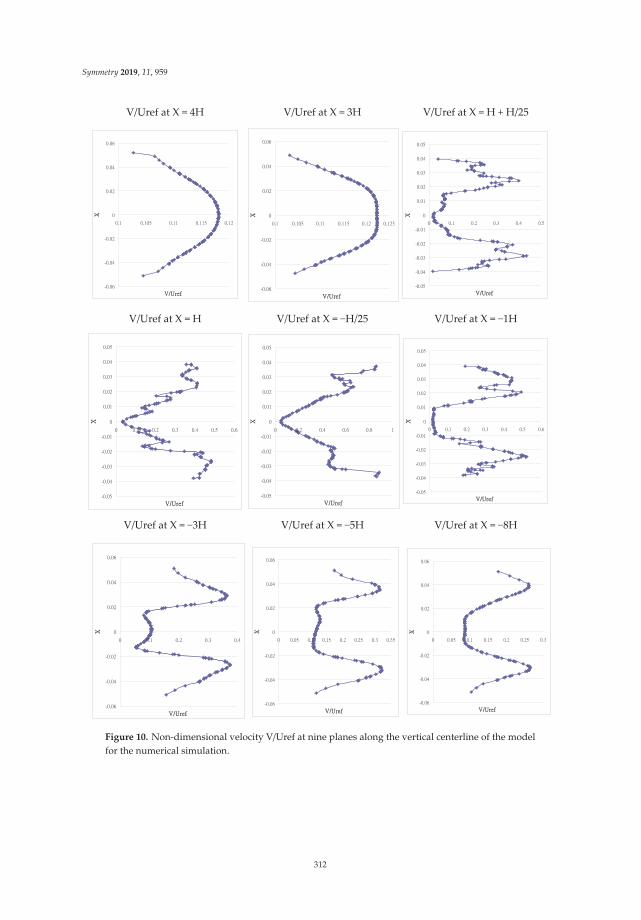
Symmetry 2019, 11, 959

V/Uref at X = 4H V/Uref at X = 3H V/Uref at X = H + H/25

V/Uref at X = H V/Uref at X = H/25 V/Uref at X = 1H

V/Uref at X = 3H V/Uref at X = 5H V/Uref at X = 8H

Figure 10. Non-dimensional velocity V/Uref at nine planes along the vertical centerline of the modelfor the numerical simulation.

312

Symmetry 2019, 11, 959

V/Uref at X = 4H V/Uref at X = 3H V/Uref at X = H + H/25

V/Uref at X = H V/Uref at X = H/25 V/Uref at X = 1H

V/Uref at X = 3H V/Uref at X = 5H V/Uref at X = 8H

Figure 11. Non-dimensional velocity V/Uref at nine planes along the vertical centerline of the modelfor the numerical simulation for these six opening patterns.

5.2. Design Cases and Comparison between Simulation Results

Figure 12 indicates the qualitative velocity distribution on the three-dimensional plane at locationF of the outlet opening. The purpose of this figure is to understand the velocity pattern on these sixplanar regions. As the results clearly indicated a cone-shaped distribution, the velocity distributionat the outlet region was the most apparent. Moreover, Figure 12 also indicates that the out ring ofthe distribution of Idea-C revealed a low air velocity. In contrast, the air velocity at the peak was thehighest. The Idea-D had the largest number of peaks and this indicates that this region was the regionwith the highest air velocity and the distribution had a more focused region in the central region. Forthe velocity distribution of Idea-B, E, and F, since they were affected by the non-uniform gaps, the airflow velocity was reduced. When the fan was rotating, the air layers also rotated. The air at the centralregion was affected by the viscosity and molecular attraction, so the rotating effect was transferred tothe air on the out ring of the flow field.

313

Symmetry 2019, 11, 959

Idea-A Idea-B Idea-C

Idea-D Idea-E Idea-F

Velocity-magnitude: m/s

Figure 12. Three-dimensional distribution of the air velocity at the outlet.

The results of the simulation for the six opening patterns are shown in Table 6. The effect ofdifferent opening patterns can be evaluated by a comparison of the numerical results. The variation inthe flow field of six different opening patterns and the change in the performance were reviewed fromthe inlet and outlet of each streamline. Table 6 reveals that the high velocity regions were on the left andright sides of the flow field. This phenomenon also directly affected the outflow of the air between theblades. This is the same phenomenon that reduced the range of higher air velocity on the downstreamof the fan. For Idea-A, the expansion of the opening pattern provided some improvement and becamemore and more apparent. The region of low air velocity extended inward so that the velocity along theinner diameter increased gradually. For Idea-B and E, the region of the highest air velocity at the outletreduced gradually. The region of low air velocity also expanded along the downstream direction. Thedownstream flow field of the Idea-D honeycomb type opening still remained smooth, but not affected

314

Symmetry 2019, 11, 959

by the opening gap. The flow field revealed high velocity at the middle portion and downstreamportion. On the overall distribution, the outlet of the impeller still remained at the high air velocity.

Table 6. Comparison of the numerical simulation results for six different cases.

Idea-A (a) Idea-B (b)

1(a) Pressure distributionon the fan

1(b) Pressuredistribution on the outer

cover



cover

1(c) Velocity distribution 1(d) Streamlinedistribution 2(c) Velocity distribution 2(d) Streamline

distribution

Idea-C (c) Idea-D (d)



cover



3(c) Velocity distribution 3(d) Streamlinedistribution 4(c) Velocity distribution 4(c) Flow field

distribution

Idea-E (e) Idea-F (f)



cover



cover

5(c) Velocity distribution 5(d) Streamlinedistribution 6(c) Velocity distribution 6(d) Streamline

distribution

315

Symmetry 2019, 11, 959

Moreover, the flow field of those six opening patterns indicated a trend of moving downstreamtoward the outlet. A non-ideal velocity distribution at the outlet could severely affect the total air flowrate. It is known from Table 6 that Idea-B presented a very non-uniform velocity distribution. Mostof the fluid aggregated to the left and right sides of the circular region. Reverse airflow and low airvelocity can be found at the central region. The total air flow rate of the fan was not greatly affected bythis phenomenon, and therefore this portion could be excluded.

The comparison of the resulting flow rate of the six opening patterns is shown in Figure 13. At theoutlet of Idea-D with the honeycomb shape, the flow rate obtained from the numerical simulation was18CFM. Similarly, the resulting flow rate of Idea-A was 16CFM. Figure 13 also reveals that the air flowrate of Idea-D was 2CFM larger than Idea-A. For the static pressure, the A4 model had the highest staticpressure of 1.87 mm-H2O. The result static pressure of Idea-A was 1.74 mm-H2O. From the aspect ofoverall air flow rate, the simulation results indicated that Idea-D had the largest air flow rate.

Figure 13. Comparison of air flow rate and static pressure of new fan designs by simulation.

6. Conclusions

In this study, the aerodynamic performance of axial fans was investigated to determine theeffect of different opening patterns. As the air flow rate decreases with increasing pressure, the fan’saerodynamic performance is affected if the density of the opening pattern is increased, so the boundarylayer is affected. The cross-sectional flow field of an axial fan was reviewed and investigated. The flowfield could be improved by making the streamlines smoother. Some reverse flows were also observedat the outlet of the fan. Conclusions of the investigation of the flow field along the radial direction andat the outlet are as follows.

1. The distribution at the inlet can be smoother.2. After passing through the inlet, the air pressure will increase at some portions about 1/2 of the

impeller height.3. The maximum velocity at each cross-sectional plane occurs closer to the outlet.4. The change in the outlet location makes the air velocity increase and move toward the

outlet direction.5. At the outlet plane of Idea-B, C, and E, many regions were found to have a low air velocity and

recirculation. This phenomenon indicates inferior outlet conditions.6. Idea-D, with the honeycomb shape, had the most uniform air velocity among the six opening

patterns. From the aspect of the leaving flow rate, it was also the most optimal opening pattern.7. If a fan is not improved by the airfoil design, the assessment can be carried out on the design

factors of the outlet pattern.

316

Symmetry 2019, 11, 959

There are many design parameters when desigrning the opening patterns of a fan outlet. Theanalysis in this study investigated six factors in order to provide future fan designs with a goodreference for the optimization of the opening pattern. The results indicate that the honeycomb-shapedopening pattern can be beneficial to the performance enhancement of an axial fan. The parameters ofthe inlet design can also be included for further investigation on design optimization.

Author Contributions: The author contributed to the paper. H.-H.L. Collects and organizes data and acts as thecorresponding author, J.-H.C. and the authors propose methods.



References

1. Marinetti, S.; Cavazzini, G.; Fedele, L.; De Zan, F.; Schiesaro, P. Air velocity distribution analysis in the airduct of a display cabinet by PIV technique. Int. J. Refrig. 2012, 35, 2321–2331. [CrossRef]

2. Gebrehiwot, M.G.; De Baerdemaeker, J.; Baelmans, M. Effect of a cross-flow opening on the performance ofa centrifugal fan in a combine harvester: Computational and experimental study. Biosyst. Eng. 2010, 105,247–256. [CrossRef]

3. Chen, F.; Li, S.; Su, J.; Wang, Z. Experimental Study of Bowed-twisted Stators in an Axial Transonic Fan Stage.Chin. J. Aeronaut. 2009, 22, 364–370.

4. Betta, V.; Cascetta, F.; Musto, M.; Rotondo, G. Fluid dynamic performances of traditional and alternative jetfans in tunnel longitudinal ventilation systems. Tunn. Undergr. Space Technol. 2010, 25, 415–422. [CrossRef]

5. Li, Y.; Liu, J.; Ouyang, H.; Du, Z.-H. Internal flow Mechanism and Experimental Research of low PressureAxial fan with Forward-Skewed Blades. J. Hydrodyn. 2008, 20, 299–305. [CrossRef]

6. Delele, M.; De Moor, A.; Sonck, B.; Ramon, H.; Nicolaï, B.; Verboven, P. Modelling and Validation of the AirFlow generated by a Cross Flow Air Sprayer as affected by Travel Speed and Fan Speed. Biosyst. Eng. 2005,92, 165–174. [CrossRef]

7. Gebrehiwot, M.G.; De Baerdemaeker, J.; Baelmans, M. Numerical and experimental study of a cross-flow fanfor combine cleaning shoes. Biosyst. Eng. 2010, 106, 448–457. [CrossRef]

8. Chunxi, L.; Ling, W.S.; Yakui, J. The performance of a centrifugal fan with enlarged impeller. Energy Convers.Manag. 2011, 52, 2902–2910. [CrossRef]

9. Stafford, J.; Walsh, E.; Egan, V. The effect of global cross flows on the flow field and local heat transferperformance of miniature centrifugal fans. Int. J. Heat Mass Transf. 2012, 55, 1970–1985. [CrossRef]

10. Liu, S.H.; Huang, R.F.; Lin, C.A. Computational and experimental investigations of performance curve of anaxial flow fan using downstream flow resistance method. Exp. Therm. Fluid Sci. 2010, 34, 827–837. [CrossRef]

11. Zhao, X.; Sun, J.; Zhang, Z. Prediction and measurement of axial flow fan aerodynamic and aeroacousticperformance in a split-type air-conditioner outdoor unit. Int. J. Refrig. 2013, 36, 1098–1108. [CrossRef]

12. Hu, B.-B.; Ouyang, H.; Wu, Y.-D.; Jin, G.-Y.; Qiang, X.-Q.; Du, Z.-H. Numerical prediction of the interactionnoise radiated from an axial fan. Appl. Acoust. 2013, 74, 544–552. [CrossRef]

13. Owen, M.; Kröger, D.G. Contributors to increased fan inlet temperature at an air-cooled steam condenser.Appl. Ther. Eng. 2013, 50, 1149–1156. [CrossRef]

14. Moonen, P.; Blocken, B.; Roels, S.; Carmeliet, J. Numerical modeling of the flow conditions in a closed-circuitlow-speed wind tunnel. J. Wind Eng. Ind. Aerodyn. 2006, 94, 699–723. [CrossRef]

15. Carolus, T.; Schneider, M.; Reese, H. Axial flow fan broad-band noise and prediction. J. Sound Vib. 2007, 300,50–70. [CrossRef]

16. Bredell, J.; Kröger, D.; Thiart, G. Numerical investigation of fan performance in a forced draft air-cooledsteam condenser. Appl. Eng. 2006, 26, 846–852. [CrossRef]

17. Hsiao, S.-W.; Lin, H.-H.; Lo, C.-H. A study of thermal comfort enhancement by the optimization of airflowinduced by a ceiling fan. J. Interdiscip. Math. 2016, 19, 859–891. [CrossRef]

18. Hsiao, S.W.; Lin, H.H.; Lo, C.H.; Ko, Y.C. Automobile shape formation and simulation by a computer-aidedsystematic method. Concurr. Eng. Res. Appl. 2016, 24, 290–301. [CrossRef]

317

Symmetry 2019, 11, 959

19. Lin, H.H.; Huang, Y.Y. Application of ergonomics to the design of suction fans. In Proceedings of the 1st IEEEInternational Conference on Knowledge Innovation and Invention, Jeju Island, South Korea, 23–27 July 2018;pp. 203–206.

20. Andrea, T. On the theoretical link between design parameters and performance in cross-flow fans. A numericaland experimental study. Comput. Fluids 2005, 34, 49–66.

21. Hurault, J.; Kouidri, S.; Bakir, F. Experimental investigations on the wall pressure measurement on the bladeof axial flow fans. Exp. Fluid Sci. 2012, 40, 29–37. [CrossRef]

22. Lin, H.H.; Hsiao, S.W. A Study of the Evaluation of Products by Industrial Design Students. Eurasia J. Math.Sci. Technol. Educ. 2018, 14, 239–254. [CrossRef]

23. Shih, Y.-C.; Hou, H.-C.; Chiang, H. On similitude of the cross flow fan in a split-type air-conditioner. Appl. Eng.2008, 28, 1853–1864. [CrossRef]

24. Kim, J.-H.; Hur, N.; Kim, W. Development of algorithm based on the coupling method with CFD and motortest results to predict performance and efficiency of a fuel cell air fan. Renew. Energy 2012, 42, 157–162.[CrossRef]

25. Jason, S.; Walsh, E.; Egan, V.; Grimes, R. Flat plate heat transfer with impinging axial fan flows. Int. J. HeatMass Transfer. 2010, 53, 5629–5638.

26. Greenblatt, D.; Avraham, T.; Golan, M. Computer fan performance enhancement via acoustic perturbations.Int. J. Heat Fluid Flow 2012, 34, 28–35. [CrossRef]

27. Lin, H.-H. Improvement of Human Thermal Comfort by Optimizing the Airflow Induced by a Ceiling Fan.Sustainability 2019, 11, 3370. [CrossRef]

28. Lin, S.-C.; Tsai, M.-L. An integrated performance analysis for a backward-inclined centrifugal fan.Comput. Fluids 2012, 56, 24–38. [CrossRef]

29. Stinnes, W.H. Effect of cross-flow on the performance of air-cooled heat exchanger fans. Appl. Ther. Eng.2002, 22, 1403–1415. [CrossRef]

30. Casarsa, L.; Giannattasio, P. Experimental study of the three-dimensional flow field in cross-flow fans.Exp. Fluid Sci. 2011, 35, 948–959. [CrossRef]

31. Liu, G.; Liu, M. Development of simplified in-situ fan curve measurement method using the manufacturersfan curve. Build. Environ. 2013, 48, 77–83. [CrossRef]

32. Hurault, J.; Kouidri, S.; Bakir, F.; Rey, R. Experimental and numerical study of the sweep effect onthree-dimensional flow downstream of axial flow fans. Flow Meas. Instrum. 2010, 21, 155–165. [CrossRef]

33. Chen, T.Y.; Shu, H.T. Flow structures and heat transfer characteristics in fan flows with and without delta-wingvortex generators. Exp. Ther. Fluid Sci. 2004, 28, 273–282. [CrossRef]

34. Stafford, J.; Walsh, E.; Egan, V. Local heat transfer performance and exit flow characteristics of a miniatureaxial fan. Int. J. Heat Fluid Flow 2010, 31, 952–960. [CrossRef]


318

symmetryS S

Article

Energy Consumption Load Forecasting Usinga Level-Based Random Forest Classifier

Yu-Tung Chen 1, Eduardo Piedad Jr. 2 and Cheng-Chien Kuo 1,*

1 Department of Electrical Engineering, National Taiwan University of Science and Technology,Taipei City 10607, Taiwan

2 Department of Electrical Engineering, University of San Jose-Recoletos, Cebu City 6000, Philippines* Correspondence: [email protected]; Tel.: +886-02-27333141 (ext. 7710)

Received: 1 June 2019; Accepted: 13 July 2019; Published: 29 July 2019

Abstract: Energy consumers may not know whether their next-hour forecasted load is either highor low based on the actual value predicted from their historical data. A conventional method oflevel prediction with a pattern recognition approach was performed by first predicting the actualnumerical values using typical pattern-based regression models, hen classifying them into patternlevels (e.g., low, average, and high). A proposed prediction with pattern recognition scheme wasdeveloped to directly predict the desired levels using simpler classifier models without undergoingregression. The proposed pattern recognition classifier was compared to its regression methodusing a similar algorithm applied to a real-world energy dataset. A random forest (RF) algorithmwhich outperformed other widely used machine learning (ML) techniques in previous research wasused in both methods. Both schemes used similar parameters for training and testing simulations.After 10-time cross training validation and five averaged repeated runs with random permutationper data splitting, the proposed classifier shows better computation speed and higher classificationaccuracy than the conventional method. However, when the number of its desired levels increases,its prediction accuracy seems to decrease and approaches the accuracy of the conventional method.The developed energy level prediction, which is computationally inexpensive and has a goodclassification performance, can serve as an alternative forecasting scheme.

Keywords: energy level consumption; pattern recognition; random forest; machine learning; loadforecasting; level classification

1. Introduction

Energy load forecasting is becoming one of the latest trends due to advancements in energy andpower systems and management. As a result, emerging techniques in the field of artificial intelligence(AI) have recently come into play. One particular study reviews various prediction techniques forenergy consumption prediction in buildings [1]. Energy regression models are studied in [2]. Machinelearning (ML) techniques such as artificial neural networks (ANNs) and support vector machines(SVMs) are employed to predict energy consumption and draw energy-saving mechanisms [3]. Anotherstudy reviews the use of a probabilistic approach in load forecasting [4]. Other studies analyze theeffectiveness of AI tools applied in smart grid and commercial buildings [5–7]. Most of the studied AItools focus primarily on actual value forecasting. For example, consumers may not know whetherthe next-hour forecasted load value based on these models is either high or low. The conventionalway is to categorize the forecasted value into reasonable levels, such as low, average, or high, whichconsumers can understand. This study proposes an alternative method which can be applied whenestimated levels instead of actual values are already sufficient for a load forecasting application.

Short-term forecasting of energy consumption load uses the most important historical data rangingfrom a few hours even up to a number of weeks before the forecasted day. Recently, short-term load


Symmetry 2019, 11, 956

forecasting research studies employed advance machine learning such as artificial neural networks [8],fuzzy logic algorithms and wavelet transform techniques integrated in a neural network system [9],and an extreme learning machine [10]. Studies on short-term forecasting also cover various settingssuch as residential [11], non-residential [12], and micro-grid [13] buildings.

In residential houses, a typical energy consumption forecasting is driven by data generated fromhumidity and temperature sensors [14]. Occupant behavior assessment can also predict buildingconsumption [15]. A number of research papers study short- and long-term energy consumption bothin residential and small commercial establishments. The emergence of algorithms and an increasingcomputational capability have encouraged the development of different prediction models. Stochasticmodels can reliably predict the energy consumption of buildings and identify areas of possible energywaste [15–17]. Standard engineering regression and a statistical approach still have good predictionresults [1,7,14]. A combination with genetic programming is also effective [18]. Various machinelearning tools such as support vector machines and neural network algorithms provide an acceptableenergy prediction performance [19,20]. Random forest outperforms other widely used classifiers suchas artificial neural networks and support vector machines in energy consumption forecasting [21].

2. Machine Learning Methodology

This section introduces the machine learning models and presents their implementation.This covers two parts—the pipeline and implementation of ML models, and the random forestclassifier as the ML model used in this study.

2.1. Machine Learning Pipeline and Implementation

Figure 1 shows the typical implementation flow of machine learning (ML) algorithms. Two mainstages of an ML algorithm are the training and testing phases. First, the training phase creates the MLmodel using a training dataset based on the chosen ML classifier models. The three most commonlyknown ML models, namely, artificial neural network (ANN), support vector machine (SVM), andrandom forest (RF), are employed. The performance validation of the training stage guarantees thegeneral performance of the classifier model and is used to avoid the overfitting issue. Then, verificationis performed on the trained model in the testing stage using the testing dataset as input to the trainedclassifier. This testing dataset is the other partitioned data from the original dataset; therefore, it hasidentical characteristics to the training dataset. The original dataset is partitioned into 70% and 30% fortraining and testing, respectively. Performance metrics are used to evaluate both stages. By comparingthe performance of both training and testing, any overfitting issue can be determined. It occurs whenthe training performance is relatively higher than the testing performance.

Figure 1. Pseudocode of a usual machine learning implementation with training and testing phases,and final evaluation stage.

320

Symmetry 2019, 11, 956

Algorithm 1 presents the implemented program ML classifier similar to the pseudocode of [21].A k number of times of cross-validation was performed. In this study, 10-time cross-validationwas used. This cycle was repeated for another 10 times. The overall average performance andrandom data shuffling were taken. This verification helped avoid any overfitting issue. This wasperformed by taking the loss function of random forest present the difference between the trainingand testing results. For the evaluation of the conventional method, which is a regression-typeproblem, the root-mean-square error (RMSE) function in Equation (1) is used. F-score, classificationaccuracy, and confusion matrix are the metrics used for the proposed classifier. F-score accuracymetrics in Equation (2) weigh the significance of both precision and recall performance of the MLmodel. Precision measures its positive predictive value, whereas recall measures its sensitivity.

Algorithm 1. Machine Learning Implementation

# InitializationIn the initialization stage, data pre-processing is performed such as the loading and shuffle-splitting of the dataset intofeature X and predictor y, and the importation of the necessary python-based libraries.# Repeat n times the training and testing of the modelfor i=1:nShuffle-splitting of dataset into training, validation, and testing datasets# k-time Training Cross-Validationfor j=1:k-timeTraining of the model using an ML algorithm using the training datasetPerformance evaluation of the trained model using the validation dataset# Testing the modelTesting of the trained model using the testing datasetPerformance evaluation of the tested model# Display Performance ResultsCompute classification accuracy and F-scoreCompute classification confusion matrix

Another measure, classification accuracy in (3), was also taken. This metric is the percent ofcorrectly classified levels over the total number of taken levels.

RMSE =

√∑n

i=1

(wTx(i) − y(i))2

n(1)

F score =2∗Precision ∗RecallPrecision ∗Recall

(2)

Accuracy =No. of correctly classified energy levelsTotal number of classified energy levels

(3)

Finally, a confusion matrix normalized between zero and one helps visualize the classificationperformance of the model. scikit-learn in [22] is an open source platform that provides Python librariesand support. This was used to implement the three ML model classifiers—ANN, SVM, and RF.

2.2. Random Forest Classifier

A decision tree was used as the predictive model. The model predicts from the subject observationsup to the model decision on which the subject’s target value is based. The subject observations arealso called branches while subject’s target values are also known as leaves. Bagging is a technique ofestimated prediction by reducing its variance which is suitable for decision trees [23]. For its regressionapplication, a recursive fit of a similar regression tree was performed to produce bootstrap-sampledversions of training data taking its mean value. For classification, a predicted class was chosen by themajority vote from each committee of trees. Random forest (RF) is a modified bagging that produces a

321

Symmetry 2019, 11, 956

large collection of independent trees and averages their results [24]. Each of the trees generated frombagging is identically distributed, making it hard to improve other than achieving variance reduction.RF performs the tree-growing process by random input variable selection, thereby improving baggingby the correlation reduction between trees without an excessive variance increase.

3. Energy Data Processing

This section presents the implementation of the proposed machine learning classifier using a realenergy dataset. The dataset was processed according to the state-of-the-art data class interval method.It was then compared with the conventional forecasting technique.

A 12-month energy dataset of [25] from a large hypermarket was used in this study. An hourlyenergy consumption collected via a smart metering device and hourly temperature records retrievedfrom meteorological sensors are shown in Figures 2 and 3, respectively. During the sunny days of theyear between June to September, the energy load consumption is relatively high due to the prevalentuse of air conditioning units in response to the high temperature.

Figure 2. Whole-year time series energy consumption data of a commercial entity.

Figure 3. Whole-year time series temperature data of a commercial entity.

The conventional method and the new proposed scheme of predicting energy level are shown inFigure 4. The conventional method of energy level prediction is performed by first predicting the actualnumerical values using typical regression models and then classifying them into consumer-preferredlevels (e.g., low, average, and high). Since the regression model becomes computationally expensive as

322

Symmetry 2019, 11, 956

its model becomes more complicated, a proposed prediction scheme was developed to directly predictthe desired levels using simpler classifier models without undergoing regression.

Figure 4. Methodology and comparison of the conventional and the proposed time series machinelearning classifiers (source: authors’ own conception).

In the proposed scheme, the energy consumption values are classified into ordinal bins usinga general percentile statistic. Ordinal bin partitioning has an approximately equal number of datapoints as shown. For example, five bins representing five energy levels (very low, low, mid, high, veryhigh) can be created using five even percentile ranges of the energy consumption data resulting in the[0.174, 0.366), [0.366, 0.634), [0.634, 0.782), [0.782, 0.874), [0.874, 1.36] energy value ranges, respectively.For prediction implementation, energy levels were converted into their respective ordinal values (1, 2,3, 4, 5) for the machine learning implementation. The dataset contains three energy level cases—three,five and seven classes, as shown in Table 1. The modified dataset can be found in [26]. With these,three prediction cases were conducted using a machine learning random forest classifier.

Table 1. Three n-level cases for a real dataset.

n-Level Cases Interval Data Points

3-level[0, 0.525) 2927

[0.525, 0.807) 2917[0.807, 1.36] 2940

5-level

[0, 0.366) 1755[0.366, 0.634) 1756[0.634, 0.7816) 1759[0.7816, 0.874) 1752[0.874, 1.36] 1762

7-level

[0, 0.3366) 1255[0.3366, 0.427) 1249[0.427, 0.675) 1260[0.675, 0.771) 1236[0.771, 0.827) 1271[0.827, 0.935) 1257[0.935, 1.36] 1256

323

Symmetry 2019, 11, 956


This section presents the implementation results of the previous proposed random forest classifierwith the previous preprocessed energy data. The results were compared with those of the conventionalforecasting classifier.

A brute-force simulation was performed to tune the hyperparameters of both the conventionalclassifier and the proposed random forest classifier. The training and testing loss function differencesof both the conventional and the proposed classifiers are shown in Figure 5. Based on three-level cases,it can be observed that, most of the time, the proposed RF classifier has a lower train–test difference,indicating a better model performance to avoid overfitting compared to the conventional classifier.In addition, the proposed method tends to converge in less than 2% train–test loss function differenceas the parameters increase, whereas the conventional method deviates. Furthermore, the averagestandard deviation on the classification accuracy of the proposed method is lower than the conventionalone in all three cases, as shown in Table 2. Accordingly, the lower minimum and maximum standarddeviations of the proposed method suggest a more precise prediction than the performance of theconventional method.

Figure 5. Training and testing difference from the loss function graph of the random forest (RF) classifiers.

Table 2. Classification performance of the conventional and proposed methods in three cases.

Classifier ModelsClassification Accuracy

std_min std_ave std_max

3-levelconventional 0.0032 0.0106 0.9131

proposed 0.0012 0.0048 0.0100


proposed 0.0023 0.0068 0.0148


proposed 0.0033 0.0070 0.0123

The proposed RF classifier tends to perform better with a lower number of energy levels andcompared with the conventional method. Based on the F-score in Table 3, the proposed classifierdeviates further as the number of levels increases. For example, seven-energy level prediction suggeststwo times deviation as compared with the three-energy level prediction.

324

Symmetry 2019, 11, 956

Table 3. F-score performance of the proposed method in three cases.

ProposedF Score

min std_ave max std

3-level 0.0054 0.6491 3.3674 0.6388

5-level 0.0085 1.0993 7.1509 0.9413

7-level 0.0058 1.3333 5.2442 1.1107

Parameter simulations of both the conventional and the proposed classifiers in three cases arecompared in Figure 6a–c. This was conducted to determine the classification performance and theexecution time of both methods as the respective parameters become more complicated. Both classifiersseem to perform better with lower energy levels. Both classifiers converge to a classification accuracyaround 90% in three-level prediction in Figure 6a, while reaching around 83% and 75% for five- andseven-level predictions in Figure 6b,c, respectively. However, the proposed classifier is observed tooutperform the conventional classifier based on a higher classification accuracy performance and alower execution time in all three cases. Initially, the execution time of the proposed model takes almostthe same time as the conventional one using simpler parameters. With the increasing complexity of theparameters, the former does not change significantly, whereas the latter changes abruptly. It seemsthat this is due to the fact that the conventional method has a regression model structure which ismore complicated than the classification model of the proposed method. The performance of theconventional method approaches that of the proposed method in terms of classification accuracy at theexpense of computation time.

(a)

(b)

Figure 6. Cont.

325

Symmetry 2019, 11, 956

(c)

Figure 6. Parameter simulation of three cases, using (a) three-energy level, (b) five-energy level,and (c) seven-energy level prediction of both methods.

5. Conclusions

Energy level prediction was performed using a developed random forest classifier. Insteadof undergoing regression-based load forecasting from the conventional method, the developedclassifier preprocessed the numerical-valued data into levels and then later predicted them using asimpler classification process. Both classifiers perform better with a lower number of energy levels.The developed classifier outperforms the conventional classifier based on its classification accuracyand execution time when simulating 3, 5 and 7 level cases –. However, the performance of theconventional classifier approaches that of the proposed method in terms of classification accuracy butat the expense of computation time. The proposed random forest classifier serves as an alternativeto regression-based problems not only for energy consumption forecasting but also for other similarapplications. This study was limited to only a single real dataset. Further studies can use otherreal datasets.

Author Contributions: Conceptualization, C.-C.K.; Data curation, Y.-T.C.; Formal analysis, Y.-T.C. and E.P.J.;Investigation, E.P.J.; Methodology, E.P.J. and C.-C.K.; Project administration, C.-C.K.; Software, Y.-T.C.; Supervision,C.-C.K.


References

1. Zhao, H.X.; Magoulès, F. A review on the prediction of building energy consumption. Renew. Sustain.Energy Rev. 2012, 16, 3586–3592. [CrossRef]

2. Fumo, N.; Rafe Biswas, M.A. Regression analysis for prediction of residential energy consumption.Renew. Sustain. Energy Rev. 2015, 47, 332–343. [CrossRef]

3. Ahmad, A.S.; Hassan, M.Y.; Abdullah, M.P.; Rahman, H.A.; Hussin, F.; Abdullah, H.; Saidur, R. A reviewon applications of ANN and SVM for building electrical energy consumption forecasting. Renew. Sustain.Energy Rev. 2014, 33, 102–109. [CrossRef]

4. Hong, T.; Fan, S. Probabilistic electric load forecasting: A tutorial review. Int. J. Forecast. 2016, 32, 914–938.[CrossRef]

5. Raza, M.Q.; Khosravi, A. A review on artificial intelligence based load demand forecasting techniques forsmart grid and buildings. Renew. Sustain. Energy Rev. 2015, 50, 1352–1372. [CrossRef]

6. Yildiz, B.; Bilbao, J.I.; Sproul, A.B. A review and analysis of regression and machine learning models oncommercial building electricity load forecasting. Renew. Sustain. Energy Rev. 2017, 73, 1104–1122. [CrossRef]

7. Menezes, A.C.; Cripps, A.; Buswell, R.A.; Wright, J.; Bouchlaghem, D. Estimating the energy consumptionand power demand of small power equipment in office buildings. Energy Build. 2014, 75, 199–209. [CrossRef]

326

Symmetry 2019, 11, 956

8. Tsekouras, G.J.; Kanellos, F.D.; Mastorakis, N. Short term load forecasting in electric power systems withartificial neural networks. In Computational Problems in Science and Engineering; Springer: Berlin, Germany,2015; pp. 19–58.

9. Chaturvedi, D.K.; Sinha, A.P.; Malik, O.P. Short term load forecast using fuzzy logic and wavelet transformintegrated generalized neural network. Int. J. Electr. Power Energy Syst. 2015, 67, 230–237. [CrossRef]

10. Li, S.; Wang, P.; Goel, L. Short-term load forecasting by wavelet transform and evolutionary extreme learningmachine. Electr. Power Syst. Res. 2015, 122, 96–103. [CrossRef]

11. Jain, R.K.; Smith, K.M.; Culligan, P.J.; Taylor, J.E. Forecasting energy consumption of multi-family residentialbuildings using support vector regression: Investigating the impact of temporal and spatial monitoringgranularity on performance accuracy. Appl. Energy 2014, 123, 168–178. [CrossRef]

12. Massana, J.; Pous, C.; Burgas, L.; Melendez, J.; Colomer, J. Short-term load forecasting in a non-residentialbuilding contrasting models and attributes. Energy Build. 2015, 92, 322–330. [CrossRef]

13. Chitsaz, H.; Shaker, H.; Zareipour, H.; Wood, D.; Amjady, N. Short-term electricity load forecasting ofbuildings in microgrids. Energy Build. 2015, 99, 50–60. [CrossRef]

14. Candanedo, L.M.; Feldheim, V.; Deramaix, D. Data driven prediction models of energy use of appliances in alow-energy house. Energy Build. 2017, 140, 81–97. [CrossRef]

15. Virote, J.; Neves-Silva, R. Stochastic models for building energy prediction based on occupant behaviorassessment. Energy Build. 2012, 53, 183–193. [CrossRef]

16. Oldewurtel, F.; Parisio, A.; Jones, C.N.; Morari, M.; Gyalistras, D.; Gwerder, M.; Stauch, V.; Lehmann, B.;Wirth, K. Energy efficient building climate control using Stochastic Model Predictive Control andweather predictions. In Proceedings of the 2010 American Control Conference, Baltimore, MD, USA,30 June–2 July 2010; pp. 5100–5105.

17. Arghira, N.; Hawarah, L.; Ploix, S.; Jacomino, M. Prediction of appliances energy use in smart homes. Energy2012, 48, 128–134. [CrossRef]

18. Castelli, M.; Trujillo, L.; Vanneschi, L. Prediction of energy performance of residential buildings: A geneticprogramming approach. Energy Build. 2015, 102, 67–74. [CrossRef]

19. Tsanas, A.; Xifara, A. Accurate quantitative estimation of energy performance of residential buildings usingstatistical machine learning tools. Energy Build. 2012, 49, 560–567. [CrossRef]

20. Li, K.; Su, H.; Chu, J. Forecasting building energy consumption using neural networks and hybrid neuro-fuzzysystem: A comparative study. Energy Build. 2011, 43, 2893–2899. [CrossRef]

21. Chang, H.-C.; Kuo, C.-C.; Chen, Y.-T.; Wu, W.-B.; Piedad, E.J. Energy Consumption Level Prediction Basedon Classification Approach with Machine Learning Technique. In Proceedings of the 4th World Congress onNew Technologies (NewTech’18), Madrid, Spain, 19–21 August 2018; pp. 1–8.

22. Pedregosa, F.; Varoquaux, G.; Gramfort, A.; Michel, V.; Thirion, B.; Grisel, O.; Blondel, M.; Müller, A.;Nothman, J.; Louppe, G.; et al. Scikit-learn: Machine Learning in Python. J. Mach. Learn. Res. 2011,12, 2825–2830.

23. Bickel, P.; Diggle, P.; Fienberg, S.; Gather, U.; Olkin, I.; Zeger, S. Springer Series in Statistics; Springer:New York, NY, USA, 2009.

24. Breiman, L. Random forests. Mach. Learn. 2001, 45, 5–32. [CrossRef]25. Pîrjan, A.; Oprea, S.V.; Carutasu, G.; Petrosanu, D.M.; Bâra, A.; Coculescu, C. Devising hourly forecasting

solutions regarding electricity consumption in the case of commercial center type consumers. Energies 2017,10, 1727.

26. Piedad, E.J.; Kuo, C.-C. A 12-Month Data of Hourly Energy Consumption Levels from a Commercial-TypeConsumer. Available online: https://data.mendeley.com/datasets/n85kwcgt7t/1/files/6cfc7434-315c-4a2d-8d8c-ce6a2bb80a01/energy_consumption_levels.csv?dl=1 (accessed on 25 June 2018).


327

symmetryS S

Article

The Computer Course Correlation between LearningSatisfaction and Learning Effectiveness of VocationalCollege in Taiwan

Ru-Yan Chen 1 and Jih-Fu Tu 2,*

1 Department of Computer Science and Information Engineering, Vanung University, ZhongliDist.,Taoyuan City 32061, Taiwan; [email protected]

2 Department of Industrial Management, St. John’s University, Tamsui District, New Taipei 25135, Taiwan* Correspondence: [email protected]; Tel.: +886-930038679

Received: 20 May 2019; Accepted: 10 June 2019; Published: 21 June 2019

Abstract: In this paper, we surveyed the influence of learn effectiveness in a computer courseunder the factors of learning attitude and learning problems for students in senior-high school.We followed the formula for a regression line as R = A + BX +ε and simulated on SPSS platform withsymmetry to obtained the results as follows: (1) In learning attitude, both the cognitive-level andbehavior-level, are positively correlated with satisfaction. This means the students have cognitive-leveland behavior-level more positively correlated with satisfaction in computer subjects and have ahigh degree of self-learning effectiveness. (2) In learning problems, the female students had higherlearning effectiveness than male students, and the students who practiced on the computer on theirown initiative long-term each week had higher learning effectiveness.

Keywords: learning attitude; computer subject; learning effectiveness

1. Introduction

Education should focus on cultivating professional skills and combining practice with practice toenable students to have the ability to work in response to the rapid changes in the current industrialstructure. Therefore, in addition to paying attention to students’ professional and practical abilities,students should also have professional abilities in order to improve their graduation employment rateand employment competitiveness [1].

The ultimate goal of school is to assist students in acquiring the skills of employment. Therefore,the content of the curriculum should complement the workplace and assist students in obtainingprofessional skills related to their work [2].

How to make students have the motivation to learn, and then generate interest in active learning isan important question. A teacher should understand the behavioral motivation of students in a timelymanner while teaching [3], as well as the learning attitude (including cognition, emotion, and behavior)that students hold while studying computer courses, and the troubles encountered in learning.

We also analyze the “learning attitude” and “learning problems” of the learning effectivenessframe for high vocational students to understand the student’s personal background variables forlearning attitude, learning problems, and learning effectiveness, and the relationship between learningattitude, learning problems, and learning effectiveness [4,5].

This paper is based on the symmetry subject of computer courses with students of the InformationProcess Department and International Trade Department to survey student learning attitudes andlearning problems in the subject of computers. This paper aims to analyze the learning effectiveness andrelated issues of computer courses for higher vocational students through the questionnaire approach.


Symmetry 2019, 11, 822

The rest of this paper is structured as follows. Section 2 describes the design structure andprogress of the research. Section 3 presents the implemented research. Section 4 documents symmetryregressing on analysis between learning attitude and learning effectiveness. The regression analysis oflearning problems to learning effectiveness is described in Section 5. Finally, we conclude the paper inSection 6.

2. Research Design and Progress

In this paper, we use a frame work to measure learning attitudes and learning problems foranalyzing the learning effectiveness influences on students studying a computer course. In orderto implement the above framework, firstly, we used a questionnaire survey to search the symmetryrelationship between variables, and statistical methods for analyzing empirical data and verificationthe hypothesis.

2.1. Research Object and QuestionnaireResponse

The research objects of this paper were aimed at the three degree students of the InformationProcess Department and the International Trade Department. We issued in total 219 questionnairesthrough on-site distribution to students. The number of responses of valid questionnaires was 196(89.49% response rate).

2.2. Research Tools

The measurement tool was a questionnaire of “learning attitudes and learning problems forlearning effectiveness influences of computer courses”, which included the following four categories:learning attitude, learning problems, learning effectiveness, and personal basic information. They aredescribed as follows.

(1) Personal basic information includes sex, age, department, and practice computer time every week.(2) Learning effectiveness factors include the learning attitude frame and the learning problems frame.

The learning attitude frame has three parts as cognitive, emotional, and behavioral. The learningproblems frame has four parts: personal, family, school, and course content. The learningeffectiveness frame has four parts: class schedule, teacher teaching, learning environment, andlearning results.

2.3. Assessment Method of Questionnaire

The questionnaire used a scale from 1 to 4, with “4” indicating very much agree, “3” indicatingagree, “2” indicating disagree, and “1” indicating very much disagree. For the questionnaire, we setsome reverse test questions, which meant that the sampled students had the attention item contentwhen answering “not applicable”.

2.4. Questionnaire Pretest

The pretest questionnaire was processed by random to 25 third grade students of high vocationaleducation school. The main purpose of this pretest was to test the internal consistency and consistencywhen answering the questionnaire questions. We found α coefficient with high reliability for valueslarger than 0.898. The results of α coefficient are listed as Table 1.

330

Symmetry 2019, 11, 822

Table 1. Questionnaire Cronbach α reliability analysis.

Frame Classification Numbers Cronbach α Coefficient

Learning attitude-cognitive 8 0.877Learning attitude-emotional 8 0.805Learning attitude-behavioral 11 0.871

Learning problems frame 14 0.887Learning effectiveness-class schedule 3 0.755

Learning effectiveness-teacher teaching 8 0.929Learning effectiveness-learning environment 5 0.850

Learning effectiveness-learning results 4 0.791Total Reliability 61 0.898

3. Research Implementation

The samples of this questionnaire were third grade students of the International Trade Departmentand Information Process Department. As for the initial issued samples, the number was 219 and thenumber of valid questionnaires was 196. The details of these are shown in Table 2.

Table 2. Questionnaire response information.

Items Issues SortResponse

QuestionnaireRatio of UsefulQuestionnaire

International Trade Dept. A 45valid 43

95.56%invalid 2

International Trade Dept. B 36valid 30

83.33%invalid 6

Information Process Dept. A 34valid 30

88.24%invalid 4

Information Process Dept. B 34valid 33

97.06%invalid 1

Information Process Dept. C 35valid 33

94.29%invalid 2

Information Process Dept. D 35valid 27

77.14%invalid 8

Total 219valid 196

89.49%invalid 23

3.1. Data Analysis and Results

After administering the response questionnaires, we deleted the invalid questionnaire, and thencarried out statistics and analyzed the valid questionnaire using SPSS 15.0. The methods of statisticalanalysis are described as follows.

(1) Narrative statistics was used to organize and present the characteristics of the existing data usingstatistical description groups. The methods used in this paper were: average, standard deviation,number of times, and percentage to understand the situation of the subject [6].

(2) Variance analysis was used to test whether there was a difference in the average of the maternalgroup. If there was a significant difference in variance analysis, then carried out a T-test to confirmwhether there was a difference in the average of each selected group. In this paper, single factorvariance analysis was used to test whether the student’s personal background variables had asignificant level of learning attitude, learning problems, and learning effectiveness [7,8].

(3) Regression analysis (RA) was used as a symmetry statistical method for analyzing data, mainlyto determine specific relationships between the survey data.

Regression analysis is a relation model that was used to create the symmetry dependent variableY and independent variable X. In this paper, we exploited multi regression analysis to create the frame

331

Symmetry 2019, 11, 822

of learning attitude and learning problems to use as a pre-prediction model for learning effectiveness,and then survey the influence level between those two frames and learning effectiveness [9].

3.2. Learning Attitude and Learning Problems for Learning Effectiveness

For the learning attitude, if a higher score was obtained, the more positive the learning attitudewas than if a lower score was obtained, and vices versa. The average score of the fourth-order scalewas 2.5 points. However, for learning problems, if the average scale was lower than 2.5 points whichindicated those had less learning and those who had higher learning.

For learning effectiveness, an average scores for each question higher than 2.5 indicated that thetraining effectiveness was slightly positive. We found that if the teacher patiently guided studentsthrough computer related issues, the average score was 3.01 points. This meant students had satiablefaction of learning because the teacher was able to patiently teach the students and the students weremore satisfied.

4. Regression Analysis between Learning Attitude and Learning Effectiveness

In this paper, we used the symmetry regression analysis (R), coefficient of determination (R2),adjusted R2, and F test. Regression analysis is a powerful statistical method that allows the examinationof the relationship between two or more variables of interest. The formula for a regression line can begiven as R =A + BX +ε, where A and B are coefficients (also are constants). X and R are the independentand dependent variables, and ε is the error term [10].

We also showed the p value, which referred to the probability that the statistical symmetrysummary (such as the difference between the two groups of samples) was the same as the actualobservation data, or even larger, in a probability model.

4.1. Learning Attitude and Learning Effectiveness under Class Schedule

Table 3 shows the regression analysis of computer subject for learning attitude to learningeffectiveness under class schedule. For the class schedule relation, the cognitive coefficient of learningattitude to learning effectiveness was 0.578 and was significantly positively correlated. This meant thatwith students in computer courses, the learning attitude was higher and more positive, and the activestudents had more satisfaction with the class schedule.

Table 3. Attitude to class schedule regression analysis.

Item Value

Regression factor (R) 0.656R2 0.430

AdjustedR2 0.421F-test 48.36

Class scheduleLearning attitude Cognitive Emotion Behavior

Coefficient 0.578 0.205 0.327p value <0.000*** 0.144 <0.01**

For the class schedule correlation, the coefficient of learning attitude behavior to learningeffectiveness was 0.327 and was also significantly positively correlated. This indicated that thecomputer course students had a higher number and more positive learning attitude, and the positivestudents were more satisfied with the class schedule.

The learning effectiveness correlation coefficient of the emotion of learning attitude was 0.205, butthe p value was 0.144, which indicted that there was no significant difference. Inferred from the above,the possible reasons may be that the students were just beginning to experience the computer subject

332

Symmetry 2019, 11, 822

or if just contact with the course was not enough to influence class schedule satisfaction by the aspectof learning emotion.

4.2. Regression Analysis between Learning Attitude and Teacher Teaching

Table 4 shows the symmetry regression analysis of teacher teaching under the computer subject oflearning attitude cognitive to learning effectiveness with a p value <0.000***, so the equation was valid.As seen in Table 4, we found the correlative coefficient between cognitive of learning attitude cognitiveand teacher teaching of learning effectiveness was 0.287 and had a positive correlation (P < 0.005**).

Table 4. Subject of learning attitude to teacher teaching regression analysis.

Item Value



Teacher teachingLearning attitude Cognitive Emotion Behavior

Coefficient 0.287 0.041 0.406p value <0.005** 0.717 <0.000***

Based on the above results, if the learning attitude of students in the computer course was higherand more positive, the positive students had higher satisfaction with teacher teaching.

Regression analysis of teacher teaching of the computer subject of learning attitude behavior tolearning effectiveness had a p value <0.000***, so the equation was also valid. As seen in Table 4, thecorrelation coefficient between cognitive of learning attitude cognitive and teacher teaching of learningeffectiveness was 0.406 and had appositive correlation. This indicated that the students’ learningbehavior in the computer course was higher and more positive, and the positive students were moresatisfied with teacher teaching.

Finally, we conducted symmetry regression analysis of teacher teaching under the computersubject of learning attitude emotion to learning effectiveness. We found the correlation coefficientbetween emotion of learning attitude cognitive and teacher teaching of learning effectiveness was 0.041,but the p value was 0.717, which meant there was no significant difference. The possible reason wasthat students were beginning to understand the computer subject, and they had a preliminary feelingabout learning emotion in the course. There were not enough factors to influence their satisfactionwith teacher teaching.

4.3. Regression Analysis between Learning Attitude and Learning Environment

Table 5 shows the regression analysis of learning attitude to learning environment in the computercourse. As seen in Table 5, we found the correlation coefficient between cognitive of learning attitudecognitive and learning environment of learning effectiveness to be 0.390, which was a positive correlation.This indicates that the computer course students’ subject of learning attitude cognitive was higher andmore positive, and the positive students had higher satisfaction with the learning environment.

The symmetry correlation coefficient between emotion of learning attitude cognitive and learningenvironment of learning effectiveness was 0.326, which was a positive correlation. This indicatesthat the computer course students’ learning attitude emotion was higher and more positive, and thepositive students were more satisfied with the learning environment.

Furthermore, the symmetry correlative coefficient between behavior of learning attitude cognitiveand learning environment of learning effectiveness was 0.446 and had a positive correlation. Thisindicated that the computer course students’ learning attitude behavior was higher and more positive,and the positive students had higher satisfaction with the learning environment.

333

Symmetry 2019, 11, 822

Table 5. Subject of learning attitude to learning environment regression analysis.

Item Value



Learning environmentLearning attitude Cognitive Emotional Behavioral

Coefficient 0.390 0.326 0.446p value <0.001*** <0.01** <0.000***

4.4. Regression Analysis between Learning Attitude and Learning Results

Table 6 shows the regression question for the computer subject of learning attitude to learningresults. As seen in Table 6, we found the correlation coefficient between cognitive of learning attitudecognitive and learning environment of learning effectiveness to be 0.573 with a positive correlative.This indicates that the computer course students’ learning attitude cognitive was higher and morepositive, and the positive students had higher satisfaction with the learning results.

The correlative coefficient between emotions of learning attitude cognitive and learningenvironment of learning effectiveness was 0.126, but the p value was 0.717, which meant that there wasno significant difference. The results may indicate that students were beginning to understand thecomputer subject, and they had a preliminary feeling about learning emotion in the course. Therewere not enough factors to influence their satisfaction with learning results.

Furthermore, the correlative coefficient between behavior of learning attitude cognitive andlearning environment of learning effectiveness was 0.382 and was appositive correlation. This indicatesthe computer course students’ learning attitude behaviors were higher and more positive, and thepositive students had the higher satisfaction with the learning results.

Table 6. Subject of learning attitude to learning results regression analysis.

Item Value


AdjustedR2 0.420

Learning resultsLearning attitude Cognitive Emotional Behavioral

Coefficient 0.573 0.126 0.382p value <0.000*** 0.360 <0.000***

5. Regression Analysis of Learning Problems to Learning Effectiveness

5.1. Regression Analysis of Class Schedule between Learning Problems and Learning Effectiveness

As seen in Table 7, which shows the regression question between the computer subject of learningproblems and class schedule, we also found the p value <0.000***, which indicated the regressionquestion was valid. We also found the correlation coefficient between learning problems and learningeffectiveness of class schedule was –0.479, which was a negative correlation. This represents the lowerdegree of computer subject learning problems of student with higher satisfaction in the class schedule.

334

Symmetry 2019, 11, 822

Table 7. Computer subject of learning problems to class schedule regression analysis.

Item Value



Coefficient –0.479

5.2. Regression Analysis between Learning Problems and Teacher Teaching

As seen Table 8, which shows the regression question between the computer subject of learningproblems and teacher teaching, we also found the p value <0.000***, which indicated the regressionquestion was valid. We also found the correlation coefficient between learning problems and learningeffectiveness was –0.309, which was a negative correlation. This represents the lower the degree ofcomputer subject learning problems of student with higher satisfaction in teacher teaching.

Table 8. Computer subject of learning problems to teacher teaching.

Item Value




5.3. Regression Analysis between Learning Problems and Learning Environment

As seen in Table 9, which shows the regression question between the computer subject of learningproblems and learning environment, we also found the p value<0.000***, which indicated the regressionquestion was valid. We also found the correlation coefficient between learning problems and learningeffectiveness was −0.510, which was a negative correlation. This represents the lower the degree ofcomputer subject learning problems of students with higher satisfaction in the learning environment.

Table 9. Computer subject of learning problems to learning environment.

Item Value



Coefficient -0.510

5.4. Regression Analysis of Learning Problems to Learning Results

In Table 10, which shows the regression question (=0.465) between the computer subject of learningproblems and learning results, we also found the p value <0.000***, which indicated the regressionquestion was valid. We also found a negative correlation coefficient between learning problems andlearning effectiveness of –0.580. It represents the lower degree of computer subject learning problemsof student with higher satisfaction in learning results.

335

Symmetry 2019, 11, 822

Table 10. Computer subject of learning problems to learning results regression analysis.

Item Value




6. Conclusions

In this paper, symmetry we surveyed a computer course of learning attitudes and learningproblems to learning effectiveness as influences. We summarized the results as follows.

1. For students in computer course, learning attitude to learning effectiveness had a higher difference.However, for the level of cognitive and behavioral with positive correlative satisfaction resultsshowed students with more positive learning attitude cognitive and learning behavior than withhigher satisfaction of class schedule, teacher teaching, teaching environment, and learning results.

2. For the emotion of learning attitude to learning effectiveness, there are significant differencesin learning environment. The most students had more approval in the learning environmentin emotion.

3. For the computer course analysis of learning problems to learning effectiveness, the learningproblems to learning effectiveness symmetry as class schedule, teacher teaching, teachingenvironment, and learning had results with negative correlations. If they have higher satisfactionof class schedule, teacher teaching learning environment, and learning results.

Author Contributions: The authors contributed equally to the conception of the idea, implementing and analyzingthe experimental results, and writing the manuscript.



References

1. Campos, A.M. Analyzing the Effectiveness of Learning Objects and Designs. In Proceedings of the 2011IEEE 11th International Conference on Advanced Learning Technologies, Athens, GA, USA, 6–8 July 2011;pp. 650–651.

2. Chatzara, K.; Karagiannidis, C.; Stamatis, D. Students Attitude and Learning Effectiveness of EmotionalAgents. In Proceedings of the 2010 10th IEEE International Conference on Advanced Learning Technologies,Sousse, Tunisia, 5–7 July 2010; pp. 558–559.

3. Yang, Y.; Wang, Y.; Yuan, X. Bidirectional Extreme Learning Machine for Regression Problem and Its LearningEffectiveness. IEEE Trans. Neural Netw. Learn. Syst. 2012, 23, 1498–1505. [CrossRef] [PubMed]

4. Mishra, N.R.; Chavhan, R.K. Effectiveness of mobile learning on awareness about learning disability amongstudent teachers. In Proceedings of the 2012 IEEE International Conference on Technology EnhancedEducation (ICTEE), Kerala, India, 3–5 January 2012; pp. 1–6.

5. Krikun, I. Applying learning analytics methods to enhance learning quality and effectiveness in virtuallearning environments. In Proceedings of the 2017 5th IEEE Workshop on Advances in Information, Electronicand Electrical Engineering (AIEEE), Riga, Latvia, 24–25 November 2017; pp. 1–6.

6. Shadiev, R.; Hwang, W.; Huang, Y.; Liu, A. Cognitive Diffusion Model: Facilitating EFL Learning in anAuthentic Environment. 2017. Available online: https://ieeexplore.ieee.org/abstract/document/7497494(accessed on 17 June 2019).

7. Joseph, N.; Pradeesh, N.; Chatterjee, S.; Bijlani, K. A novel approach for group formation in collaborativelearning using learner preferences. In Proceedings of the 2017 International Conference on Advancesin Computing, Communications and Informatics (ICACCI), Karnataka, India, 13–16 September 2017;pp. 1564–1568.

336

Symmetry 2019, 11, 822

8. Boicu, C.; Tecuci, G.; Boicu, M. Learning complex problem solving expertise from failures. In Proceedings ofthe Sixth International Conference on Machine Learning and Applications (ICMLA 2007), Cincinnati, OH,USA, 13–15 December 2007.

9. Dehghani-Pilehvarani, A.; Karimaghaee, P.; Khayatian, A. Combined gradient and Iterative Learning Controlmethod for magnetostatic inverse problem. In Proceedings of the 3rd International Conference on Control,Instrumentation, and Automation, Tehran, Iran, 28–30 December 2013; pp. 334–339.

10. Krishnan, M.; Muhammad, R.; Ruhizan, Y. Problem based learning in Engineering Education at Malaysianpolytechnics: A proposal. In Proceedings of the 2009 International Conference on Engineering Education(ICEED), Kuala Lumpur, Malaysia, 7–8 December 2009; pp. 122–124.


337

symmetryS S

Review

Locality Sensitive Discriminative UnsupervisedDimensionality Reduction

Yun-Long Gao 1, Si-Zhe Luo 1 , Zhi-Hao Wang 1, Chih-Cheng Chen 2,* and Jin-Yan Pan 2,*

1 Department of Automation, Xiamen University, Xiamen 361005, China2 School of Information Engineering, Jimei University, Xiamen 361021, China* Correspondence: [email protected] (C.-C.C.); [email protected] (J.-Y.P.)

Received: 15 July 2019; Accepted: 7 August 2019; Published: 12 August 2019

Abstract: Graph-based embedding methods receive much attention due to the use of graph andmanifold information. However, conventional graph-based embedding methods may not always beeffective if the data have high dimensions and have complex distributions. First, the similarity matrixonly considers local distance measurement in the original space, which cannot reflect a wide varietyof data structures. Second, separation of graph construction and dimensionality reduction leads tothe similarity matrix not being fully relied on because the original data usually contain lots of noisesamples and features. In this paper, we address these problems by constructing two adjacency graphsto stand for the original structure featuring similarity and diversity of the data, and then imposea rank constraint on the corresponding Laplacian matrix to build a novel adaptive graph learningmethod, namely locality sensitive discriminative unsupervised dimensionality reduction (LSDUDR).As a result, the learned graph shows a clear block diagonal structure so that the clustering structureof data can be preserved. Experimental results on synthetic datasets and real-world benchmark datasets demonstrate the effectiveness of our approach.

Keywords: machine learning; graph embedding method; dimensionality reduction; diversitylearning; adaptive neighbors

1. Introduction

Due to the large number of data generated by the advancements of science and technology,dimensionality reduction has become an important task in data mining and machine learning researchwith many applications [1–4]. These data have such characteristics as high dimensionality, nonlinearity,and extreme complexity, which bring a lot of problems to the subsequent data processing. However,the intrinsic structure of data are often suspected to be much lower due to the redundant informationhidden in the original space [5]. Therefore, revealing the potential low-dimensional representationinvolved in the corresponding high-dimensional structure is an essential preprocessing step for variousapplications. Under the background, a lot of supervised and unsupervised dimensionality reductionmethods are proposed, such as principal component analysis (PCA) [6], linear discriminant analysis(LDA) [7], Laplacian embedding(LE) [8–10], local linear embedding (LLE) [11], locality preservingprojections (LPP) [12], neighborhood minmax projections (NMMP) [13], isometric feature mapping(IsoMAP) [14], discriminant sparsity neighborhood preserving embedding (DSNPE) [15], and multipleempirical kernel learning with locality preserving constraint (MEKL-LPC) [16], etc. Obviously,the unsupervised dimensionality reduction method is more challenging than other methods dueto the lack of label information. Among them, the graph embedding method exhibits significantperformance because it captures the structural information of high-dimensional space. The graphembedding method is built on the basis of manifold assumption, which means the data are formedaccording to a certain manifold structure and the nearby data points tend to have the same labels.


Symmetry 2019, 11, 1036

The commonly used graph-based algorithms, such as LPP [12], IsoMAP [14], local graph basedcorrelation clustering (LGBACC) [17], and locality weighted sparse representation (LWSR) [18]generally have the same steps—for instance, (1) build adjacency graph for each neighborhood;(2) construct pairwise feature (similarity) for each neighborhood to describe the intrinsic manifoldstructure; and (3) convert the problem into an eigenvalue problem. Thus, we can find the traditionalgraph-based algorithms mentioned above are all established independently of the subsequentprocesses, i.e., cluster indicators need to be extracted through post-processing, such dimensionalityreduction results are highly dependent on the input pairwise feature matrix [19]. For graph-basedalgorithms taken, only local distances’ account in the original space cannot adequately eliminate noiseand capture the underlying manifold structure [20], in that it is an insufficient description for datasimilarity. Moreover, it is usually difficult to explicitly capture the intrinsic structure of data only byusing pairwise data during the graph construction process [21]. In fact, for pairwise data, the similarityis dependent on the adjacency graph constructed by a pair of data individually, without considerationfor the local environment of pairwise data. It can be seen from Figure 1, though the distance betweenA and B is shorter than that between A and C in the original space, and, clearly, S(A, B) is calleda similarity, one pairwise feature is bigger than S(A, C), hence point A and point C should be sortedout to one class, and B to the other class. However, point A and point C could get more similar inregular classification or clustering tasks because there exists a dense distribution of many points whichlink A and C, resulting from a big gap between A and B, which are regarded as less similar in sometraditional methods with two more manifold and consequently divided into different class. Therefore,the traditional definition of similarity does not sufficiently describe the structure.

Figure 1. A data point map (point A and point B are closer, but point A and point C get bigger similarityin two more manifold structures.)

In recent years, there has been a lot of research devoted to solving these problems. For example,the constrained Laplacian rank (CLR) method [22] learns a block diagonal similarity matrix so that theclustering indicators can be immediately extracted. For Cauchy graph embedding [23], a new objectiveis proposed to preserve the similarity between the original data for the embedded space, and emphasizethe closer two nodes in the embedding space, those that are more similar. Projected clustering withadaptive neighbors (PCAN) [24] designs a similarity matrix and is assigned adaptive and optimalneighbors to every piece of data on the basis of the local distances to learn instead of learninga probabilistic affinity matrix before dimensionality reduction. Stable semi-supervised discriminantlearning (SSDL) [25] is worked out to learn the intrinsic structure of a constructed adjacency graphswhich could extract the local topology characteristics, and get the geometrical properties as well.Nonetheless, these methods only focus on parts of the problems mentioned above, and the challenge

340

Symmetry 2019, 11, 1036

in reasonably representing underlying data structure or adaptively adjusting the similarity graph stillexists. As a consequence, it is quite necessary and challenging to develop an algorithm to addressthese problems.

In this paper, we propose a novel adaptive graph learning method, namely locality sensitivediscriminative unsupervised dimensionality reduction (LSDUDR), which aims to uncover the intrinsictopology structures of data by proposing two objective functions. In the first step, one of the objectivefunctions is aimed at guaranteeing the mapping of all points close to each other in the subspace,while the other one is with the purpose of excluding points with a large distance from the subspace.Furthermore, a data similarity matrix is learned to adaptively adjust the initial input data graphaccording to the basis of the projected local distances, that is to say, we adjust the projection jointly withgraph learning. Moreover, we constrain the similarity matrix by imposing a rank constraint to make itcontain more explicit data structure information. It is worthwhile to emphasize the main contributionsof our method: (1) LSDUDR can construct a discriminative linear embedded representation that candeal with high-dimensional data and characterize the intrinsic geometrical structure among data;(2) compared with traditional two-stage graph embedding methods, which need an independentaffinity graph to be constructed in advance in LSDUDR, and a clustering-oriented graph can belearned and the clustering indicators are extracted with no post-processing needed for the graph; (3)comprehensive experiments were performed on both synthetic data sets and real world benchmarkdata sets and better effectiveness of the proposed LSDUDR was demonstrated.

2. Related Work

2.1. Principal Component Analysis (PCA)

PCA is one of the most representative unsupervised dimensionality reduction methods. The mainidea of PCA is to seek a projection transformation to maximise the variance of data. Assume thatwe have a data matrix X ∈ Rd×n, where xi ∈ Rd×1 denotes the i-th sample. For better generality,

the samples in the data set are centralized, i.e.,n∑

i=1xi = 0. PCA aims to solve the following problem:

maxWTW=I

n∑

i,j=1

∥∥WTxi − WTxj∥∥2

2, (1)

where W ∈ Rd×m is the projection matrix, and m is the dimensionality of the linear subspace.When data points lie in a low-dimensional manifold and the manifold is linear or nearly-linear,the low-dimensional structure of data can be effectively captured by a linear subspace spanned by theprincipal PCA directions; the property provides a basis for utilizing the global scatter of samples asregularization in many applications.

2.2. Locality Preserving Projections (LPP)

LPP is very popular to substitute algorithms in linear manifold learning in which the data areprojected responding to the direction of maximal variance, and the adjacent graph was employed toextract the structure properties of high-dimensional data, and structure properties were transplantedinto low-dimensional subspace. The objective function of LPP is

minWTW=I

n∑

i,j=1


2 sij, (2)

where sij is defined as the similarity between samples xi and xj. As we can see, LPP is a linear versionof Laplacian Eigenmaps that uses linear model approximation to nonlinear dimensionality reduction,Thus, it shares many of the data representation properties of nonlinear techniques such as Laplacianeigenmaps or locally linear embedding.

341

Symmetry 2019, 11, 1036

2.3. Clustering and Projected Clustering with Adaptive Neighbors (PCAN)

The PCAN algorithm performs subspace learning and clustering simultaneously instead oflearning an initial pairwise feature matrix that is constructed before dimensionality reduction. The goalof PCAN is to assign the optimal and adaptive neighbors for each data point according to the localdistances so that it can learn a new data similarity matrix. Therefore, it can be used as a clusteringmethod, and can also be used as a unsupervised dimensionality reduction method. Denote the totalscatter matrix by St = XHXT , where H is the centering matrix defined as H = I − 1

n 11T , and 1 isa column vector whose elements are all 1. PCAN constrains the subspace with WTStW = I so that thedata in the subspace has no statistical correlation. In [24], the definition of PCAN is:

minS,W

n∑

i,j=1

(∥∥WTxi − WTxj∥∥2

2 sij + θs2ij

)s.t.∀i, sT

i 1 = 1, 0 ≤ sij ≤ 1, WTStW = I,rank(L) = n − c,

(3)

where L = D − (S + ST)/2 is called Laplacian matrix in graph theory, and the i-th diagonal element ofthe degree matrix D ∈ Rn×n is ∑

j(sij + sji)/2. Then, by assigning the adaptive neighbors according

to the local distances, the neighbors assignment divides the data points into c clusters based on thelearned similarity matrix S, which can be directly used for clustering without having to perform otherpost-procedures.

3. Locality Sensitive Discriminative Unsupervised Dimensionality Reduction

3.1. Intrinsic Structure Representation

The proposed method needs a pre-defined affinity matrix S as the initial graph. While learningthe affinity values of S, we get a smaller distance by adopting the the square of Euclidean distance∥∥xi − xj

∥∥22, which is related to a larger affinity value sij. Thus, determining the value of sij can be seen

as solving the following problem:

minsT

i 1=1,si≥0,sii=0

n∑

j=1

(∥∥xi − xj∥∥2

2 sij + θs2ij

), (4)

where θ is the regularization parameter. The affinities are learned using a suitable θ in formula (4) sothat we can get the optimal solution si with k nonzero values, i.e., the number of neighbors k. Let usdefine eij =

∥∥xi − xj∥∥2

2 and denote ei as a vector and eij as j-th element; formula (4) can be simplified as

minsT

i 1=1,si≥0,sii=0

12

∥∥∥si +12θ ei

∥∥∥2

2. (5)

According to [22], we can get the optimal affinities sij as follows:

sij =

{ ei,k+1−eij

kei,k+1−∑ kh=1eih

, j ≤ k,

0, j > k.(6)

Next, we define two adjacency graphs Ms = {X, S} and Md = {X, V} in order to characterize theintrinsic structure of data. Among them, the elements in matrix S represent the similarity betweennearby points, and the elements in matrix V represent the diversity between nearby points. We definethe elements vij in V as follows:

vij =

{1 − sij, j ≤ k,

0, j > k.(7)

342

Symmetry 2019, 11, 1036

Following the above work, we still did not get a clear and simple intrinsic structure if only usingsimilarity or diversity. Therefore, two objective functions simultaneously proposed to emphasizethe local intrinsic structure. One objective function is proposed to guarantee that nearby data pointsshould be embedded to be close to each other in the subspace and mainly focuses on preserving thesimilarity relationships among nearby data; the other objective function mainly focuses on the shape ofa manifold and guarantees that nearby data with large distance are not embedding to be very close toeach other in the subspace and effectively preserves the diversity relationships of data. By integratingthis two objective functions, the local topology are guaranteed, that is to say, similarity property anddiversity property of the data can be perfectly preserved. Based on the above conclusions, we employthe following objective functions to capture the local intrinsic structure:

minWTW=I

n∑

i,j=1


2 sij, (8)

maxWTW=I

n∑

i,j=1


2 vij. (9)

By simple algebra, we have:

n∑

i,j=1


2 sij = tr(WTXLSXTW

), (10)

n∑

i,j=1


2 vij = tr(WTXLV XTW

), (11)

where LS = D − (S + ST)/2 and LV = P − (V + VT)/2, P ∈ Rn×n is a diagonal matrix and its entriesare column sum of V. Furthermore, in order to consider the global geometric structure information ofdata, we introduce the third objective function, i.e., preserving as much information as possible bymaximizing overall variance of the input data. Then, inspired by LDA, we can construct a concisediscriminant criterion by combining the three objective functions, which contain both local and globalgeometrical structures information for dimensionality reduction:

minW

tr(WTX (LS − βLV) XTW

)tr (WTXHXTW)

,

s.t.WTW = I.(12)

Bringing the definitions of LS and LV into Equation (12), we have:


)=

n∑

i,j=1


2 sij − βn∑

i,j=1


2 vij

= (1 + β)n∑

i,j=1


2 sij − βn∑

i=1

k∑

j=1


2.(13)

According to the definition of sij, when j > k, we have sij = 0. Therefore,n∑

i,j=1


2 sij

models the local geometric structure, whilen∑

i=1

k∑

j=1


2 represents the total scatter

in the local region. Thus, we call this model locality sensitive discriminative unsuperviseddimensionality reduction.

3.2. Analysis of Optimal Graph Learning

When the data contain a large number of noise samples, the similarity matrix S obtained byEquation (6) is virtually impossible to be the ideal state. The desired situation is that we map thedata to a low-dimensional subspace in which the elements of similarity matrix within a cluster is

343

Symmetry 2019, 11, 1036

nonzero and evenly distributed while the values of elements between clusters are zero. Based theabove considerations, we adopt a novel and feasible way to achieve the desired state:

minW,S


)tr (WTXHXTW)

+ θ ‖S‖2F

s.t.∀i, sTi 1 = 1, 0 ≤ sij ≤ 1, WTW = I, rank(LS) = n − c.

(14)

In order to exclude the situation of trivial solution, we add the regularization term θ ‖S‖2F. The first

and second constraints are added according to the definition of graph weights, which is defined fora vertex as the sum of the distance between one vertex and the members and is non-negative. Inaddition, we also add the rank constraint to the problem. If S is non-negative, the Laplacian matrix hasa significant property:

Theorem 1. A graph S with sij ≥ 0(∀i, j) has c connected components if and only if the algebraic multiplicityof eigenvalue 0 for the corresponding Laplacian matrix LS is c [26].

Theorem 1 reveals that, when rank(LS) = n − c, the obtained graph could distinctly divide thedata set into exactly c clusters based on the block diagonal structure of similarity matrix S. It isworth mentioning that Equation (14) can simultaneously learn the projection matrix W and thesimilarity matrix S, which is significantly different from previous works. However, it is hard to tackle itdirectly, especially when there are several strict constraints. In order to solve the question, an iterativeoptimization algorithm is proposed.

4. Optimization

4.1. Determine the Value of S, W, F

Without loss of generality, suppose σi(LS) is the i-th smallest eigenvalue of LS. It is clearly seenthat σi(LS) ≥ 0 since LS is positive semi-definite. Then, if λ is big enough, Equation (14) can berewritten as:

minW,S


)tr (WTXHXTW)

+ θ ‖S‖2F + 2λ

c

∑i=1

σi (LS)

s.t.∀i, sTi 1 = 1, 0 ≤ sij ≤ 1, WTW = I.

(15)

Hyperparameter λ here can be used to trade balance between the rank of the graph Laplacian andconsistency of the data structure. The rank constraint of the graph Laplacian is usually satisfied witha large enough λ. Meanwhile, given a rank-enforcing matrix F ∈ Rn×c, suppose that node i is assigneda function value as fi ∈ R1×c. According to the Ky Fan’s Theorem [27], the rank constraint term inEquation (15) can be seen as the optimization of the smallest c eigenvalues of the Laplacian matrix.Thus, we can transform Equation (15) into the following form:

minW,S,F


)tr (WTXHXTW)

+ θ ‖S‖2F + 2λtr

(FT LSF

),

s.t.∀i, sTi 1 = 1, 0 ≤ si ≤ 1, WTW = I, FT F = I.

(16)

When S and F are fixed, problem (16) can be rewritten as:

minW


)tr (WTXHXTW)

s.t.WTW = I.(17)

344

Symmetry 2019, 11, 1036

We can use the iterative method introduced in [28] to solve W from Equation (17), and the Lagrangianfunction is constructed according to Equation (17):

L (W, η) =tr

(WTX (LS − βLV) XTW

)tr (WTXHXTW)

− ηtr(

WTW − I)

, (18)

where η is a scalar. Then, taking the derivative of W and letting the result be zero, we have

(X (LS − βLV) XT − tr


)tr (WTXHXTW)

XHXT

)W = ηW, (19)

where η=ηtr(WTXHXTW

). The optimal solution of W in Equation (19) is formed by the m

eigenvectors corresponding to the m smallest eigenvalues of the matrix:

(X (LS − βLV) XT − tr


)tr (WTXHXTW)

XHXT

). (20)

When W and S are fixed, problem (16) becomes

minF

2λtr(FT LSF)

s.t.FT F = I.(21)

Since λ is a constant, the optimal solution of rank-enforcing matrix F in Equation (21) is composed of ceigenvectors, which are derived from c smallest eigenvalues of Laplacian matrix LS.

When we fix W and F, problem (16) was written as:

minS

n

∑i,j=1

⎛⎝ (1 + β)


2 sij

tr (WTXHXTW)+ θs2

ij + λ∥∥fi − fj

∥∥22 sij

⎞⎠

s.t.∀i, sTi 1 = 1, 0 ≤ sij ≤ 1.

(22)

Note that problem (22) can be solved independently for different si, so that the following problem canbe solved separately for each i:

minsi

n

∑i=1

(Γijsij + θs2ij + λΨijsij)

s.t.∀i, sTi 1 = 1, 0 ≤ sij ≤ 1,

(23)

where Γij =(1+β)‖WT xi−WT xj‖2

2tr(WT XHXTW)

and Ψij =∥∥fi − fj

∥∥22. Then, Equation (23) can be rewritten as:

minsi

∥∥∥∥si +12θ

(Γi + λΨi)

∥∥∥∥2

2s.t.∀i, sT

i 1 = 1, 0 ≤ sij ≤ 1.(24)

Thus, Equation (24) can be solved easily with a close form solution. Denote vector di ∈ Rn×1 withdij = Γij + λΨij. For each i, Lagrange functions can be obtained:

L(W, ς, γi) =12

∥∥∥si +12θ di

∥∥∥2

2− ς(sT

i 1 − 1)− γTi si, (25)

345

Symmetry 2019, 11, 1036

where ς and γTi ≥ 0 are the Lagrangian multipliers. Take a partial derivative for each si and set it to

zero; then, according to K.K.T. conditions:

(si)j − (di)j + ς − γi = 0,(si)j ≥ 0,γi ≥ 0,(si)jγi ≥ 0,sT

i 1 − 1 = 0.

(26)

Then, we can obtain si that should be:

sij = [− 12θi

di + ς]+

. (27)

4.2. Approach to Determine the Initial Value of θ, λ

In actual experiments, regularization parameters are difficult to tune because their values mayrange from zero to infinity. In this section, we propose an efficient way to determine the regularizationparameter θ and λ as follows:

λ = θ = 1n

n∑

j=1[ k

2 di,k+1 − 12

k∑

j=1dij]. (28)

k is a pre-defined parameter. In this way, we only need to set the number of neighbors we preferrather than setting two hyper-parameters of θ and λ. The number of neighbors is usually easy toset according to the number of samples and locality of the data set. The rationality of deciding θ

and λ using the distance gaps between k-th neighbor and (k + 1)-th neighbor lies in the fact that, toachieve a desired similarity where the top k-neighbor similarities are kept and the rest are set to zeros,we should approximately achieve

k2 dik − 1

2

k∑

j=1dij < θi ≤ k

2 di,k+1 − 12

k∑

j=1dij, (29)

where di1, di2, ..., din are sorted in ascending order. If we set the inequality to equality, we can getan estimation of θ:

θ ∼ 1n

n∑

j=1[ k

2 di,k+1 − 12

k∑

j=1dij]. (30)

Similarly, λ is set to be equal to θ as follows:

λ = θ ∼ 1n

n∑

j=1[ k

2 di,k+1 − 12

k∑

j=1dij]. (31)

Since these two parameters control the regularization strength, we adaptively update the parametersduring each iteration:

1. When the connected components are insufficient, i.e., the number of zero eigenvalues is smallerthan c, we multiply λ by 2.

2. The number of connected components could be overrun, i.e., the number of zero eigenvalues islarger than c. We divide λ by 2.

3. If the graph has exact c connected components, then we stop the algorithm in this case and returnthe result.

The detailed steps are summarized in Algorithm 1.

346

Symmetry 2019, 11, 1036

Algorithm 1 Framework of the LSDUDR method.

Require: Data X ∈ Rd×n, cluster number c, projection dimension m.Initialize S and V according to Equations (6) and (7). Initialize parameter θ and λ by the Equation (28).If algorithm 1 not converge:

repeat1. Construct the Laplacian matrix LS = D − (S + ST)/2 and LV = P − (V + VT)/2.2. Calculate F, columns of F are c eigenvectors of LS and are derived from the c samllesteigenvalues.3. Calculate the projection matrix W by the m eigenvectors corresponding to the m smallesteigenvalues of the matrix:(

X (LS − βLV) XT − tr(WTX (LS − βLV) XTW

)tr (WTXHXTW)

XHXT

).

4. Compute S by updating si according to Equation (27).5. Calculate the number of connected components of the graph, if it is smaller than c, then multiplyλ by 2; if larger than c, then divide λ by 2.

until Convergence

End if

return

Projection matrix W ∈ Rd×m and similarity matrix S ∈ Rn×n.

5. Discussion

5.1. Analysis

As previously discussed, LSDUDR represents the local intrinsic structure of data set based onEquations (8) and (9). Then, we integrate the two objective functions as follows:

n∑

i,j=1


2 sij − βn∑

i,j=1


2 vij

=n∑

i=1

k∑

j=1


2

(sij + βsij − 1

)=

n∑

i,j=1


2 zij,

(32)

where the elements zij are defined as follows:

zij =

{sij + βsij − 1, j ≤ k,

0, j > k.(33)

It is easy to see that Equation (32) is very similar to Equation (8). However, they are completelydifferent when they express the intrinsic geometrical structure of the data. Without loss of generality,we set the weight elements sij in Equation (8) as a heat kernel function. Figure 2 shows their weightchange process with a distance between two points xi and xj.

347

Symmetry 2019, 11, 1036

Figure 2. Difference between sij and zij.

As we know, the real-world data are usually unbalanced and complex, thus some points maybe distributed in sparse areas while other data points are distributed in compact areas. As shown inFigure 2, zij is positive for data points in compact regions, thus Equation (32) maps these data pointsto be very close in the subspace, and mainly preserves the similarity of data. If data points lie insparse regions, zij is negative, and Equation (32) mainly characterizes diversity of data in this case,i.e., the shape of a manifold structure. However, the difference among points in a neighborhood is notconsidered in Equation (8), and always projects the neighborhood points to be close into subspace,which ignores the intrinsic geometrical structure of data.

It is noteworthy that three updating rules are included in the proposed algorithm,which are computationally efficient. In fact, [29] has already proven the convergence of thealternative optimization method. In our algorithm, the main cost lies in each iteration being theeigen-decomposition step for Equations (7) and (21). The time computational complex of the proposedmethod is O((d2m + n2c)t), where t is the number of iterations.

5.2. Convergence Study

The method proposed by Algorithm 1 can be used to find a locally optimal solution of problem (14).The convergence of Algorithm 1 is given through Theorem (2).

Theorem 2. The alternate updating rules in Algorithm 1 monotonically decrease the objective function value ofoptimization problem (14) in each iteration until convergence.

Proof. In the procedure of iteration, we get the global optimal selective matrix Wt+1 by

solving optimization problem Wt+1 = arg minWTW=I

tr(WT X(LS−βLV )XTW)tr(WT XHXTW)

. As a result, we have the

following inequality:

tr(WTt+1X(LS−βLV)XTWT

t+1)tr(WT

t+1XHXTWTt+1)

≤ tr(WTt X(LS−βLV)XTWT

t )tr(WT

t XHXTWTt )

. (34)

Since variable Ft+1 is updated by solving problem FTt+1 = arg min

FT F=I2λtr(FT

t LFTt ), we obtain the

following inequality:tr(FT

t+1LFTt+1) ≤ tr(FT

t LFTt ). (35)

Consequently, we have the following inequality:

tr(WTt+1X(LS−βLV )XTWT

t+1)tr(WT

t+1XHXTWTt+1)

+ tr(FTt+1LFT

t+1) ≤tr(WT

t X(LS−βLV)XTWTt )

tr(WTt XHXTWT

t )+ tr(FT

t LFTt ). (36)

348

Symmetry 2019, 11, 1036

In addition, K.K.T. conditions (26) illustrate that the converged solution of Algorithm 1 is at leasta stationary point of Equation (25). Because the updating of weights matrix St+1 ∈ Rn×n can be dividedinto n independently sub-optimization problem with respect to n-dimensional vector. Consequently,the objective function value of optimization problem (14) decreases monotonically in each iterationuntil the algorithm convergence.

6. Experiment

In the experiment, the following two metrics are used to evaluate the performance of the proposedLSDUDR algorithm: Accuracy (ACC) and Normalized Mutual Information (NMI) [30]. Accuracy isdefined as

ACC =

n∑

i=1δ(ti ,map(tg

i ))

n ,(37)

where ti is the label of the clustering result and tgi is the known label of xi. map

(tgi

)is the optimal

mapping function that permutes the label set of the clustering results and the known label set ofsamples. δ

(ti, map

(tgi

))is an indicator function. Normalized Mutual Information is defined as

NMI =

c∑

i,j=1tij log

n×tijti tj√√√√(

c∑

i=1ti log ti

n

)(c∑

j=1tj log

tjn

) , (38)

where ti is the number of samples in the i-th cluster Ci according to clustering results and tj is thenumber of samples in the j-th ground truth class Gj. tij is the number of overlap between Ci and Gj.

We compare the performance of LSDUDR with K-Means [31], Ratio Cut [32], Normalized Cut [33]and PCAN methods, since they are closely related to LSDUDR, i.e., the information contained inthe eigenvectors of an affinity matrix is used to detect the similarity. We made comparisons withRatio Cut, Normalized Cut to show that LSDUDR can effectively mitigate the influence of outliersby inducing robustness and adaptive neighbors. To emphasize the importance of describing theintrinsic manifold structure, we compared the results of PCAN with LSDUDR which concatenates touncover the intrinsic topology structures of data by proposing two objective functions and performsdiscriminatively embedded K-Means clustering.

6.1. Experiment on the Synthetic Data Sets

To verify the robust performances and strong discriminating power of the proposed LSDUDR,two simple synthetic examples (two-Gaussian and multi-cluster data) are given in this experiment.

In this first synthetic data set, we deliberately set a point away from the two-Gaussian distributionas an outlier so that a one-dimensional linear manifold representation was obtained to clearly dividetwo clusters. LSDUDR and PCAN were demonstrated on the synthetic examples respectively and theresults are shown in Figure 3. It is clear that one cluster shown in pink almost submerges in another oneas blue in the one-dimensional representation using PCAN, while it is separated distinctly out usingLSDUDR, so we can conclude that LSDUDR has more discriminating power than PCAN. Furthermore,LSDUDR is less sensitive to outliers than PCAN because the objective function of LSDUDR will bringa heavy penalty to two points when they are embedded to be close in the subspace but with largedistance in the origin space.

349

Symmetry 2019, 11, 1036

(a) (b) (c)

Figure 3. (a) two-Gaussian synthetic data projection results; (b) one-dimensional representationobtained by Projected clustering with adaptive neighbors. (PCAN); (c) one-dimensional representationobtained by Locality Sensitive Discriminative Unsupervised Dimensionality Reduction. (LSDUDR).

The second synthetic data set is a multi-cluster data, which contains 196 randomly generatedclusters that are distributed in a spherical manner. We compared LSDUDR with K-means and PCAN.Due to the fact that K-means is sensitive to initialization [34], we repeatedly run K-means 100 timesand use the minimal K-means objective value as the result. To be fair, the parameters of PCAN areadjusted to report the best performance of PCAN. As for LSDUDR, we run LSDUDR once to generatea clustering result and use it as initialization for K-means and report the best performance. Table 1and Figure 4 show the experiment results of LSDUDR and other two algorithms on multi-clusterdata. As can be seen from Table 1, LSDUDR obtained better performance than those of other methodsaccording to the the minimal K-means objective value and clustering accuracy. Thus, LSDUDR hasstronger discriminating power than PCAN and K-means especially when the data distribution iscomplex.

Table 1. Compare results on multi-cluster synthetic data sets.

Methods ACC% Minimal K-Means Objective

K-Means 66.94 336.46PCAN 98.62 107.33

LSDUDR 99.49 106.21

(a) K-means (b) PCAN (c) LSDUDR

Figure 4. Clustering results of three algorithms.

6.2. Experiment on Low-Dimensional Benchmark Data Sets

In this subsection, we evaluate the performance of the proposed LSDUDR on ten low-dimensionalbenchmark data sets with comparison to four related methods, including K-Means, Ratio Cut,Normalized Cut and PCAN methods. Description of these data sets is summarized in Table 2, includingfour synthetic data sets and six University of CaliforniaIrvine (UCI) datasets [35]. In low-dimensional

350

Symmetry 2019, 11, 1036

data, we set the projection dimension in PCAN and LSDUDR to be c − 1. For the methods that requirea fixed input data graph, we use the self-turn Gaussian method [34,36] to build the graph. For themethods involving K-Means to extract the clustering labels, we repeatedly ran K-Means 100 timeswith the same settings and chose the best performance. As for PCAN and LSDUDR, we only ran itonce and reported the result directly from the learned graph. The experimental results are shown inTables 3 and 4.

Table 2. Specifications of the data sets.

Data Set #Classes (c) #Data Points (n) #Dimensions (d)

Spiral 3 312 2Pathbased 3 300 2

Compound 6 399 2Movements 15 360 90

Iris 3 150 4Cars 3 392 8Glass 6 214 9Vote 2 435 16

Diabetes 2 768 8Dermatology 6 366 34

Table 3. ACC(%) on low-dimensional benchmark data sets.

ACC% K-Means RatioCut NormalizedCut PCAN LSDUDR

Spiral 33.97 99.68 99.68 100 100Pathbased 74.33 77.33 76.67 87.00 87.00

Compound 80.20 76.69 65.91 78.95 88.22Movements 10.56 5.83 10.56 56.11 55.56

Iris 66.67 68.00 66.39 77.33 92.00Cars 44.90 53.27 47.70 48.98 58.42Glass 52.21 36.45 51.87 49.07 52.80Vote 83.45 61.61 83.68 67.36 85.75

Diabetes 56.02 64.71 61.98 58.46 65.10Dermatology 85.25 54.92 93.72 94.81 95.90

Table 4. NMI(%) on low-dimensional benchmark data sets.

NMI% K-Means RatioCut NormalizedCut PCAN LSDUDR

Spiral 12.52 98.35 98.35 100 100Pathbased 51.33 54.96 53.10 75.63 79.27

Compound 79.74 71.60 66.32 77.48 85.16Movements 44.11 15.85 44.91 84.95 84.17

Iris 61.68 61.3 59.05 61.85 77.52Cars 39.10 21.61 39.06 39.03 39.39Glass 35.83 35.33 34.88 35.76 35.90Vote 36.58 30.17 35.66 35.23 39.37

Diabetes 52.67 50.02 61.98 64.01 68.10Dermatology 85.20 41.24 88.43 91.83 93.53

In this experiment, we can observe that PCAN and LSDUDR are much better than those offixed graph-based methods. This observation confirms that separation of graph construction anddimensionality reduction leads the similarity matrix to not being able to be fully relied on and theexperimental results will seriously deteriorate. In addition, LSDUDR outperforms other methods innine data sets on account of preserving locality structure among data.

351

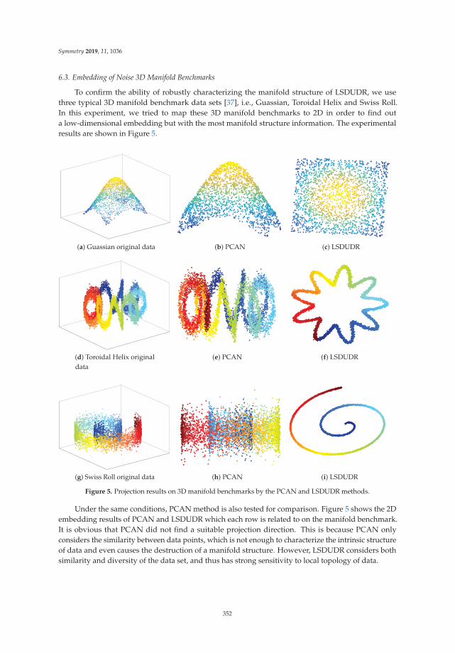
Symmetry 2019, 11, 1036

6.3. Embedding of Noise 3D Manifold Benchmarks

To confirm the ability of robustly characterizing the manifold structure of LSDUDR, we usethree typical 3D manifold benchmark data sets [37], i.e., Guassian, Toroidal Helix and Swiss Roll.In this experiment, we tried to map these 3D manifold benchmarks to 2D in order to find outa low-dimensional embedding but with the most manifold structure information. The experimentalresults are shown in Figure 5.

(a) Guassian original data (b) PCAN (c) LSDUDR

(d) Toroidal Helix originaldata

(e) PCAN (f) LSDUDR

(g) Swiss Roll original data (h) PCAN (i) LSDUDR

Figure 5. Projection results on 3D manifold benchmarks by the PCAN and LSDUDR methods.

Under the same conditions, PCAN method is also tested for comparison. Figure 5 shows the 2Dembedding results of PCAN and LSDUDR which each row is related to on the manifold benchmark.It is obvious that PCAN did not find a suitable projection direction. This is because PCAN onlyconsiders the similarity between data points, which is not enough to characterize the intrinsic structureof data and even causes the destruction of a manifold structure. However, LSDUDR considers bothsimilarity and diversity of the data set, and thus has strong sensitivity to local topology of data.

352

Symmetry 2019, 11, 1036

6.4. Experiment on the Image Data Sets

6.4.1. Visualization for Handwritten Digits

To further test the low-dimensional embedding applicability of the proposed LSDUDR algorithm,another experiment is carried out on a Binary Alphadigits data set [38], as shown in Figure 6. We selectfour letters (“C”, “P”, “X”, “Z”) and four digits (“0”, “3”, “6”, “9”) from the Binary Alphadigits dataset, which comprises binary digits from “0” to “9” and capital “A” to “Z”. The embedding results aredrawn in Figure 7.

Figure 6. Some image samples of the handwritten digits.

(a) PCA (b) LPP (c) PCAN (d) LSDUDR

Figure 7. Experiment on the Alphadigits data set.

It can be seen from Figure 7a,b that there are overlaps in clusters of “C”, “P” and “Z”, digits “0”and “6” when we use PCA and LPP. In addition, worse results are obtained from PCAN and it isshown in Figure 7c that almost all points are tangled for all clusters. However, for LSDUDR, results inFigure 7d show that classes are separated clearly, which reflects that diversity plays an important rolein representing the intrinsic structure of data.

6.4.2. Face Benchmark Data Sets

We use four image benchmark data sets in this section for experiments on projection, since thesedata typically have high dimensionality. We summarize the four face image benchmark data sets inTable 5. To study the data-adaptiveness and noise-robustness of the proposed LSDUDR algorithm,we use a range of data sets contaminated by different kinds of noise based on the face data sets,as shown in Figure 8. Similar to the above-mentioned experiment, three algorithms, including PCAN,PCA and LPP, are used for comparison.

353

Symmetry 2019, 11, 1036

Table 5. The description of the face image benchmark data sets.

Data Sets #Classes (c) #Data Points (n) #Dimensions (d)

YaleA 15 165 3456Jaffe 10 213 1024CBCI 120 840 7668

UMIST 120 840 768

(a) Original image (b) Image with Gaussian noise

(c) Image with multiplicative noise (d) Image with salt-and-pepper noise

Figure 8. Some image samples of the data sets with different kinds of noise.

The experimental results about face benchmark data sets are shown in Figure 9, from whichwe get a convincing observation that the experimental results obtained by adaptive graph learningalgorithms are usually more outstanding, especially when the dimensionality of projection spaceincreases. This is because adaptive graph learning algorithms can use the embedded informationthat are obtained in the previous step to update the similarity matrix, hence the dimensionalityreduction results are more accurate. In addition, we observe that PCA and LPP are more sensitiveto the dimensionality of embedded space while the curve of LSDUDR is basically stable with thechange of dimensionality. Furthermore, LSDUDR is capable of projecting the data into a subspace witha relatively small dimension c − 1; such subspace with low dimensionality obtained by our methodwould be even better than the subspaces obtained by PCA and LPP with higher dimensionality.It indicates that local topology and geometrical properties were taken into account for the similarityand diversity of data when using LSDUDR, and thus have better performance and achieved higheraccuracy than PCAN when the images reserve sufficient spatial information.

(a) yale with Gaussiannoise

(b) yale withmultiplicative noise

(c) yale withsalt-and-peppernoise

Figure 9. Cont.

354

Symmetry 2019, 11, 1036

(d) jaffe with Gaussiannoise

(e) jaffe withmultiplicative noise

(f) jaffe withsalt-and-peppernoise

(g) CBCL withGaussian noise

(h) CBCL withmultiplicative noise

(i) CBCL withsalt-and-peppernoise

(j) UMIST withGaussian noise

(k) UMIST withmultiplicative noise

(l) UMIST withsalt-and-pepper noise

Figure 9. Projection results on face image benchmark data sets with different kinds of noise.

7. Conclusions

In this paper, a novel adaptive graph learning method (LSDUDR) is proposed from a newperspective by integrating a similarity graph and diversity graph to learn a discriminative subspacewhere data can be easily separated. Meanwhile, LSDUDR performs dimensionality reduction andlocal structure learning simultaneously based on the high quality Laplacian matrix. Different fromprevious graph-based models, LSDUDR constructs two adjacency graphs that could represent theintrinsic structure of data well in learning the local sensitivity of the data. Furthermore, LSDUDRdoesn’t require other clustering methods to obtain cluster indicators but extracts label informationfrom a similarity graph or diversity graph, which adaptively updates in a reconstruction manner.We also discuss the convergence of the proposed algorithm as well as the value of trade-off parameters.Experimental results on the synthetic data, face image databases and several benchmark data illustratethe effectiveness and superiority of the proposed method.

In this paper, we focus on the scenario of construction of two adjacency graphs to represent theoriginal structure with data similarity and diversity. Our method can be used to remove irrelevantand correlated features involved in high-dimensional feature space and convert data represented in

355

Symmetry 2019, 11, 1036

subspaces [39]. In our future work, it is potentially interesting to extend the proposed methods tounsupervised feature selection of data points with multiview and multitask.

Author Contributions: Y-L.G. and S-Z.L. conceived and designed the experiments; S-Z.L. performed theexperiments; C-C.C. and Z-H.W. analyzed the data; J-Y.P. contributed analysis tools.

Funding: This research was funded by [National Natural Science Foundation of China] grant number [61203176]and [Fujian Provincial Natural Science Foundation] grant number [2013J05098, 2016J01756].


References

1. Everitt, B.S.; Dunn, G.; Everitt, B.S.; Dunn, G. Cluster Analysis; Wiley: Hoboken, NJ, USA, 2011; pp. 115–136.2. Xu, R.; Wunsch, D. Survey of clustering algorithms. IEEE Trans. Neural Netw. 2005, 16, 645–678. [CrossRef]

[PubMed]3. Cheng, Q.; Zhou, H.; Cheng, J. The Fisher-Markov Selector: Fast Selecting Maximally Separable Feature

Subset for Multiclass Classification with Applications to High-Dimensional Data. IEEE Trans. Pattern Anal.Mach. Intell. 2011, 33, 1217–1233. [CrossRef] [PubMed]

4. Dash, M.; Liu, H. Feature selection for clustering. In Proceedings of the Pacific-Asia Conference onKnowledge Discovery and Data Mining, Keihanna Plaza, Japan, 17–20 April 2000; pp. 110–121.

5. Ben-Bassat, M. Pattern recognition and reduction of dimensionality. Handb. Stat. 1982, 2, 773–910.6. Wold, S.; Esbensen, K.; Geladi, P. Principal component analysis. Chemom. Intell. Lab. Syst. 1987, 2, 37–52.

[CrossRef]7. FISHER, R.A. The use of multiple measurements in taxonomic problems. Ann. Eugen. 1936, 7, 179–188.

[CrossRef]8. Hall, K.M. Anr-Dimensional Quadratic Placement Algorithm. Manag. Sci. 1970, 17, 219–229. [CrossRef]9. Belkin, M.; Niyogi, P. Laplacian Eigenmaps for Dimensionality Reduction and Data Representation.

Neural Comput. 2003, 15, 1373–1396. [CrossRef]10. Luo, D.; Ding, C.; Huang, H.; Li, T. Non-negative Laplacian Embedding. In Proceedings of the 2009 Ninth

IEEE International Conference on Data Mining, Miami, FL, USA, 6–9 December 2009. [CrossRef]11. Roweis, S.T. Nonlinear Dimensionality Reduction by Locally Linear Embedding. Science 2000, 290, 2323–2326.

[CrossRef]12. He, X.; Niyogi, P. Locality preserving projections. In Advances in Neural Information Processing Systems;

MIT Press: Vancouver, BC, Canada, 2004; pp. 153–160.13. Nie, F.; Xiang, S.; Zhang, C. Neighborhood MinMax Projections. In Proceedings of the International Joint

Conference on Artificial Intelligence (IJCAI), Hyderabad, India, 8 January 2007; pp. 993–998.14. Tenenbaum, J.B. A Global Geometric Framework for Nonlinear Dimensionality Reduction. Science

2000, 290, 2319–2323. [CrossRef]15. Lu, G.F.; Jin, Z.; Zou, J. Face recognition using discriminant sparsity neighborhood preserving embedding.

Knowl.-Based Syst. 2012, 31, 119–127. [CrossRef]16. Fan, Q.; Gao, D.; Wang, Z. Multiple empirical kernel learning with locality preserving constraint.

Knowl.-Based Syst. 2016, 105, 107–118. [CrossRef]17. Pandove, D.; Rani, R.; Goel, S. Local graph based correlation clustering. Knowl.-Based Syst. 2017, 138, 155–175.

[CrossRef]18. Feng, X.; Wu, S.; Zhou, W.; Min, Q. Efficient Locality Weighted Sparse Representation for Graph-Based

Learning. Knowl.-Based Syst. 2017, 121, 129–141. [CrossRef]19. Du, L.; Shen, Y.D. Unsupervised feature selection with adaptive structure learning. In Proceedings of the

21th ACM SIGKDD International Conference on Knowledge Discovery and Data Mining, Sydney, Australia,10–13 August 2015; pp. 209–218. [CrossRef]

20. Nie, F.; Wang, H.; Huang, H.; Ding, C. Unsupervised and semi-supervised learning via L1-norm graph.In Proceedings of the 2011 International Conference on Computer Vision, Barcelona, Spain, 6–13 November2011. [CrossRef]

21. Gao, Q.; Liu, J.; Zhang, H.; Gao, X.; Li, K. Joint Global and Local Structure Discriminant Analysis. IEEE Trans.Inf. Forensics Secur. 2013, 8, 626–635. [CrossRef]

356

Symmetry 2019, 11, 1036

22. Nie, F.; Wang, X.; Jordan, M.I.; Huang, H. The Constrained Laplacian Rank Algorithm for Graph-BasedClustering. In Proceedings of the Thirtieth AAAI Conference on Artificial Intelligence, Phoenix, AZ, USA,12–17 February 2016; pp. 1969–1976.

23. Luo, D.; Nie, F.; Huang, H.; Ding, C.H. Cauchy graph embedding. In Proceedings of the 28th InternationalConference on Machine Learning (ICML-11), Bellevue, WA, USA, 28 June–2 July 2011; pp. 553–560.

24. Nie, F.; Wang, X.; Huang, H. Clustering and projected clustering with adaptive neighbors. In Proceedings ofthe 20th ACM SIGKDD international conference on Knowledge discovery and data mining, New York, NY,USA, 24–27 August 2014; pp. 977–986. [CrossRef]

25. Gao, Q.; Huang, Y.; Gao, X.; Shen, W.; Zhang, H. A novel semi-supervised learning for face recognition.Neurocomputing 2015, 152, 69–76. [CrossRef]

26. Mohar, B.; Alavi, Y.; Chartrand, G.; Oellermann, O. The Laplacian spectrum of graphs. Graph TheoryComb. Appl. 1991, 2, 12.

27. Fan, K. On a Theorem of Weyl Concerning Eigenvalues of Linear Transformations I. Proc. Natl. Acad.Sci. USA 1949, 35, 652–655. [CrossRef]

28. Nie, F.; Xiang, S.; Jia, Y.; Zhang, C. Semi-supervised orthogonal discriminant analysis via label propagation.Pattern Recognit. 2009, 42, 2615–2627. [CrossRef]

29. Bezdek, J.C.; Hathaway, R.J. Convergence of alternating optimization. Neural Parallel Sci. Comput.2003, 11, 351–368.

30. Chen, W.; Feng, G. Spectral clustering: A semi-supervised approach. Neurocomputing 2012, 77, 229–242.[CrossRef]

31. Macqueen, J. Some Methods for Classification and Analysis of MultiVariate Observations. In Proceedingsof the Fifth Berkeley Symposium on Mathematical Statistics and Probability, Oakland, CA, USA,21 June–18 July 1965; pp. 281–297.

32. Hagen, L.; Kahng, A. New spectral methods for ratio cut partitioning and clustering. IEEE Trans.Comput.-Aided Des. Integr. Circuits Syst. 1992, 11, 1074–1085. [CrossRef]

33. Shi, J.; Malik, J. Normalized cuts and image segmentation. IEEE Trans. Pattern Anal. Mach. Intell.2000, 22, 888–905.

34. Nie, F.; Xu, D.; Li, X. Initialization Independent Clustering With Actively Self-Training Method. IEEE Trans.Syst. Man Cybern. Part B Cybern. 2012, 42, 17–27. [CrossRef]

35. Dua, D.; Graff, C. UCI Machine Learning Repository. 2017. Available online: http://archive.ics.uci.edu/ml(accessed on 1 August 2018).

36. Zelnik-Manor, L.; Perona, P. Self-tuning spectral clustering. In Advances in Neural Information ProcessingSystems; MIT Press: Vancouver, BC, Canada, 2005; pp. 1601–1608.

37. Chen, S.B.; Ding, C.H.; Luo, B. Similarity learning of manifold data. IEEE Trans. Cybern. 2015, 45, 1744–1756.[CrossRef]

38. Roweis, S. Binary Alphadigits. Available online: https://cs.nyu.edu/~roweis/data.html (accessed on1 August 2018).

39. Har, M.T.; Conrad, S.; Shirazi, S.; Lovell, B.C. Graph embedding discriminant analysis on Grassmannianmanifolds for improved image set matching. In Proceedings of the IEEE Conference on Computer Visionand Pattern Recognition, Colorado Springs, CO, USA, 20–25 June 2011.

c© 2019 by the authors. Licensee MDPI, Basel, Switzerland. This article is an open accessarticle distributed under the terms and conditions of the Creative Commons Attribution(CC BY) license (http://creativecommons.org/licenses/by/4.0/).

357

MDPISt. Alban-Anlage 66

4052 BaselSwitzerland

Tel. +41 61 683 77 34Fax +41 61 302 89 18

www.mdpi.com

Symmetry Editorial OfficeE-mail: [email protected]

www.mdpi.com/journal/symmetry

MDPI St. Alban-Anlage 66 4052 Basel Switzerland

Tel: +41 61 683 77 34 Fax: +41 61 302 89 18

www.mdpi.com ISBN 978-3-03936-241-7

Selected Papers from IIKII 2019 conferences in Symmetry

Documents