STiCM Select / Special Topics in Classical Mechanics P. C. Deshmukh Department of Physics Indian Institute of Technology Madras Chennai 600036 [email protected] STiCM Lecture 02: Unit 1 Equations of Motion (i) 1 PCD_STiCM

Welcome message from author
This document is posted to help you gain knowledge. Please leave a comment to let me know what you think about it! Share it to your friends and learn new things together.
Transcript

STiCM
Select / Special Topics in Classical Mechanics
P. C. Deshmukh
Department of Physics
Indian Institute of Technology Madras
Chennai 600036
STiCM Lecture 02: Unit 1 Equations of Motion (i) 1 PCD_STiCM

2
Unit 1: Equations of Motion
Equations of Motion. Principle of Causality and
Newton’s I & II Laws. Interpretation of Newton’s
3rd Law as ‘conservation of momentum’ and its
determination from translational symmetry.
Alternative formulation of Mechanics via
‘Principle of Variation’. Determination of
Physical Laws from Symmetry Principles,
Symmetry and Conservation Laws.
Lagrangian/Hamiltonian formulation.
Application to SHO.
PCD-10
PCD_STiCM

3
Learning goals:
‘Mechanical system’ is described by (position,
velocity) or (position, momentum) or some well
defined function thereof.
How is an ‘inertial frame of reference’ identified?
What is the meaning of ‘equilibrium’?
What causes departure from equilibrium?
Can we ‘derive’ I law from the II by putting
0 in .F F ma
PCD-10
PCD_STiCM

4
……. Learning goals:
Learn about the ‘principle of variation’ and how it
provides us an alternative and more powerful
approach to solve mechanical problems.
Introduction to Lagrangian and Hamiltonian
methods which illustrate this relationship and apply
the technique to solve the problem of the simple
harmonic oscillator.
PCD-10
PCD_STiCM

5
The mechanical state of a
system is characterized by
its position and velocity,
or, position and momentum,
Why ‘position’ and ‘velocity’ are both needed to specify the
mechanical state of a system?
They are independent parameters that specify the ‘state’.
Central problem in ‘Mechanics’: How is the ‘mechanical
state’ of a system described, and how does this ‘state’
evolve with time? Formulations due to Galileo/Newton,
Lagrange and Hamilton.
( , ) :( , ) :
L q q LagrangianH q p Hamiltonian
,( )q q
Or, equivalently by their
well-defined functions:
,( )q p
PCD-10
PCD_STiCM
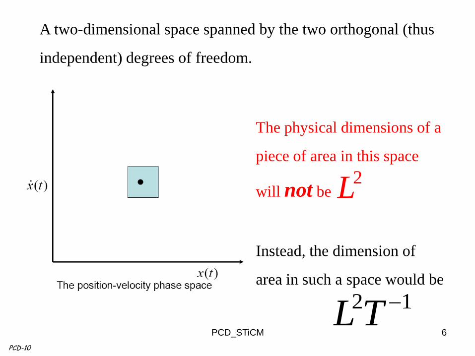
The physical dimensions of a
piece of area in this space
will not be
Instead, the dimension of
area in such a space would be
6
2L
2 1L T
A two-dimensional space spanned by the two orthogonal (thus
independent) degrees of freedom.
PCD-10
PCD_STiCM

7
position-momentum phase space
PCD-10
( )p t
( )q t
Dimensions?
Depends on [q], [p]
[area] : angular momentum
2 1
Accordingly, dimensions
of the position-velocity
phase will also
not always be L T
PCD_STiCM
8
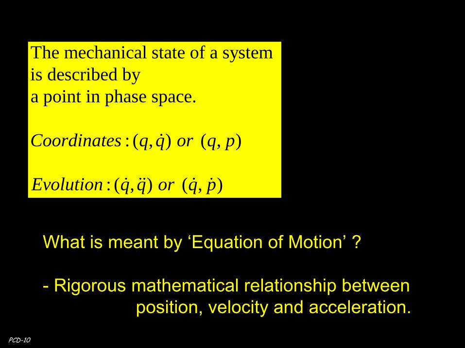
The mechanical state of a system
is described by
a point in phase space.
: ( , ) ( , )
: ( , ) ( , )
Coordinates q q or q p
Evolution q q or q p
What is meant by ‘Equation of Motion’ ?
- Rigorous mathematical relationship between
position, velocity and acceleration.
PCD-10
PCD_STiCM
9
PCD-10
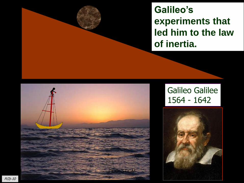
Galileo Galilee 1564 - 1642
Galileo’s
experiments that
led him to the law
of inertia.
PCD_STiCM

10
Galileo Galilei 1564 - 1642
Isaac Newton (1642-1727)
What is ‘equilibrium’?
What causes departure from ‘equilibrium’?
is proportional to the C .
Linear Response. Principle of causality.
F ma Effect ause
PCD-10
Causality
&
Determinism
I Law II Law
PCD_STiCM
11
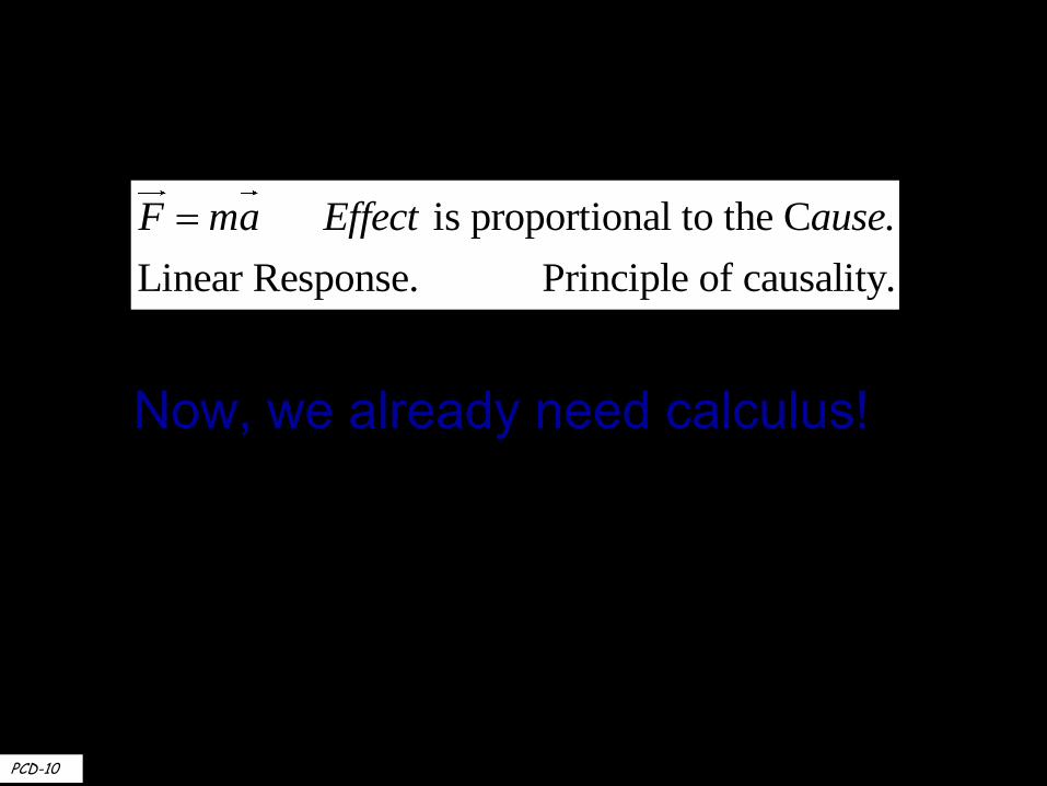
is proportional to the C .
Linear Response. Principle of causality.
F ma Effect ause
Now, we already need calculus!
PCD-10
PCD_STiCM
12
From Carl Sagan’s ‘Cosmos’:
“Like Kepler, he (Newton) was not immune to the
superstitions of his day… in 1663, at his age of twenty, he
purchased a book on astrology, …. he read it until he came
to an illustration which he could not understand, because
he was ignorant of trigonometry. So he purchased a book
on trigonometry but soon found himself unable to follow
the geometrical arguments, So he found a copy of Euclid’s
Elements of Geometry, and began to read.
Two years later he invented the differential calculus.”
PCD-10
PCD_STiCM
13
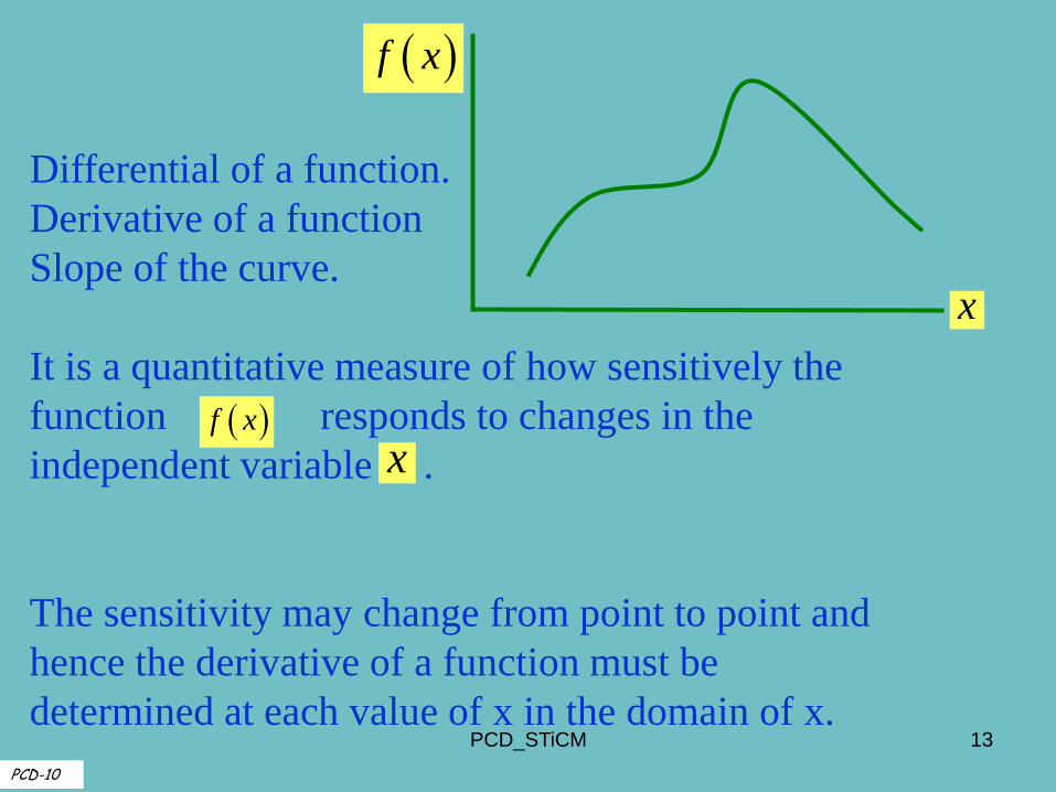
Differential of a function.
Derivative of a function
Slope of the curve.
It is a quantitative measure of how sensitively the
function f(x) responds to changes in the
independent variable x .
The sensitivity may change from point to point and
hence the derivative of a function must be
determined at each value of x in the domain of x.
f x
x
f x
x
PCD-10
PCD_STiCM

14
x
f
0x
0 0
0 0
0 0
( ) ( )2 2lim lim
x x
x x
x xf x f x
df f
dx x x
0f x
f x
x
0
x
dff x
dx
PCD-10
Tangent to the curve.
Dimensions of the derivative of the function: [f][x]-1 PCD_STiCM
15
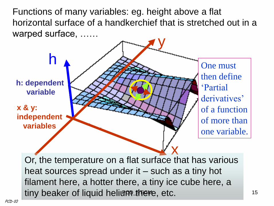
y h
h: dependent
variable
x & y:
independent
variables
One must
then define
‘Partial
derivatives’
of a function
of more than
one variable.
PCD-10
x
Functions of many variables: eg. height above a flat
horizontal surface of a handkerchief that is stretched out in a
warped surface, ……
Or, the temperature on a flat surface that has various
heat sources spread under it – such as a tiny hot
filament here, a hotter there, a tiny ice cube here, a
tiny beaker of liquid helium there, etc. PCD_STiCM

16
0 0 0
0 0 0 0
0 0( , )
( , ) ( , )2 2lim lim
x xx y y
x xh x y h x y
h h
x x x
y
h
h: dependent
variable
x & y:
independent
variables
0 0 0
0 0 0 0
0 0( , )
( , ) ( , )2 2lim lim
y yx y x
y yh x y h x y
h h
y y y
Partial
derivatives of a
function of
more than one
variable.
PCD-10
x
PCD_STiCM
17
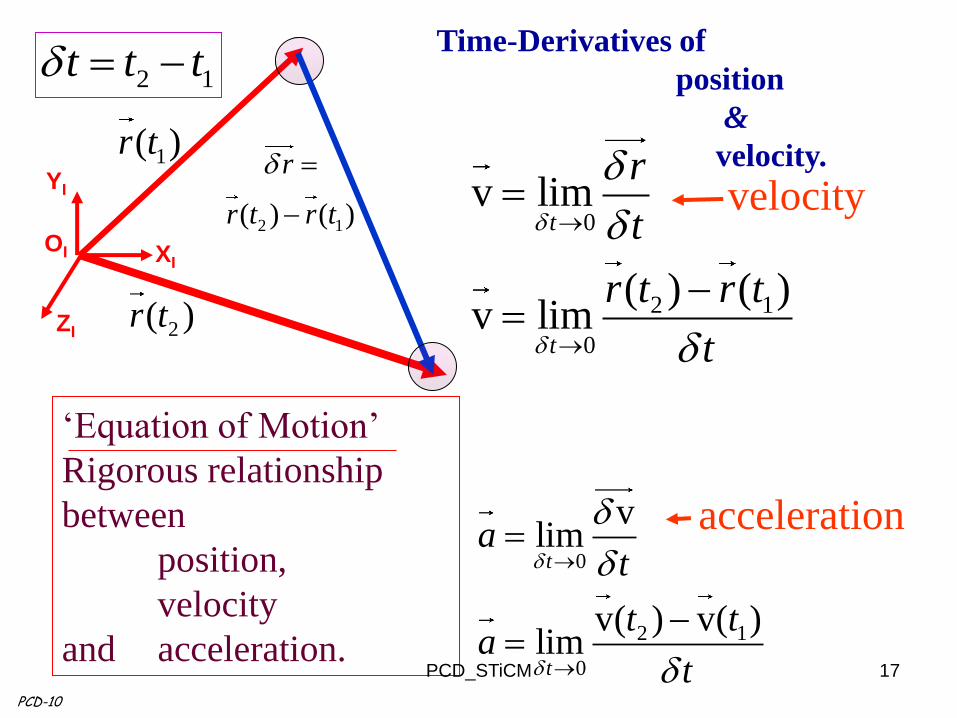
0
2 1
0
vlim
v( ) v( )lim
t
t
at
t ta
t
1( )r t
2 1
( ) ( )
r
r t r t
2( )r t
OI XI
ZI
YI
0
2 1
0
v lim
( ) ( )v lim
t
t
r
t
r t r t
t
2 1 t t t
velocity
acceleration
‘Equation of Motion’
Rigorous relationship
between
position,
velocity
and acceleration.
Time-Derivatives of
position
&
velocity.
PCD-10
PCD_STiCM
18
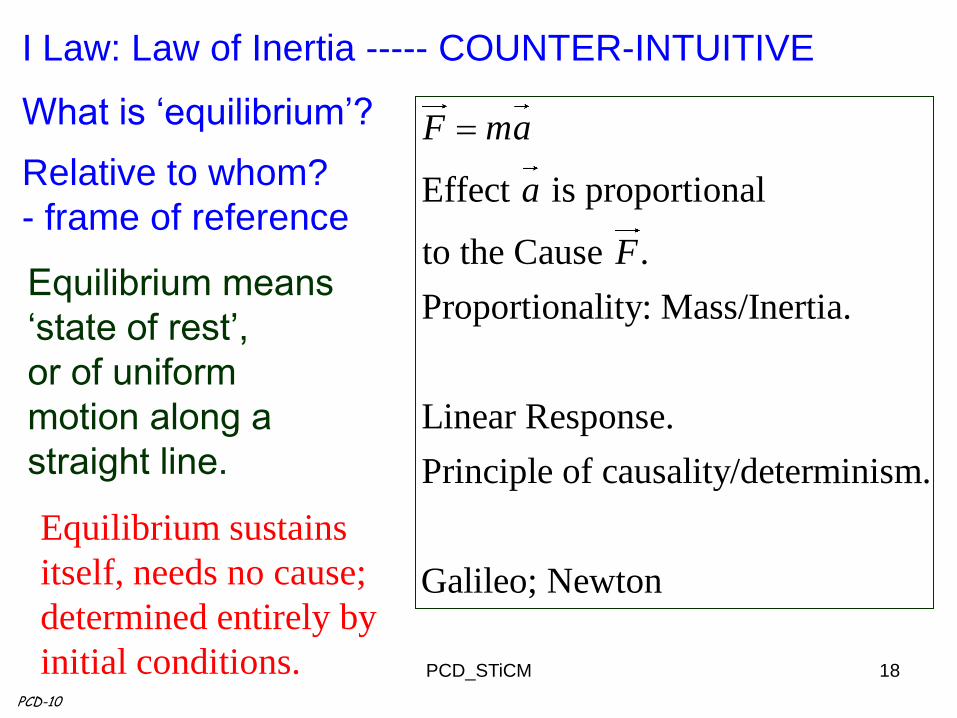
I Law: Law of Inertia ----- COUNTER-INTUITIVE
What is ‘equilibrium’?
Relative to whom?
- frame of reference
Equilibrium means
‘state of rest’,
or of uniform
motion along a
straight line.
Equilibrium sustains
itself, needs no cause;
determined entirely by
initial conditions. PCD-10
Effect is proportional
to the Cause .
Proportionality: Mass/Inertia.
Linear Response.
Principle of causality/determinism.
Galileo; Newton
F ma
a
F
PCD_STiCM
19
PCD-10
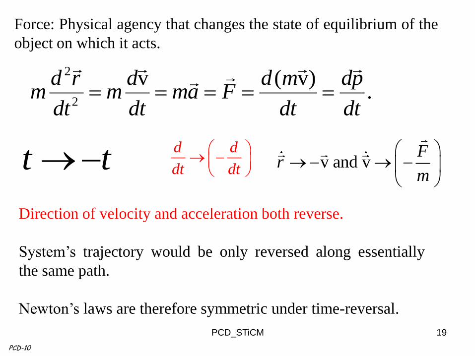
2
2
v ( v).
d r d d m dpm m ma F
dt dt dt dt
Force: Physical agency that changes the state of equilibrium of the
object on which it acts.
d d
dt dt
t t v and v
Fr
m
Direction of velocity and acceleration both reverse.
System’s trajectory would be only reversed along essentially
the same path.
Newton’s laws are therefore symmetric under time-reversal.
PCD_STiCM
20
PCD-10
Newton’s laws: ‘fundamental’ principles
– laws of nature.
Did we derive Newton’s laws from anything?
We got the first law from Galileo’s brilliant experiments.
We got the second law from Newton’s explanation of departure
from equilibrium in terms of the linear-response cause-effect
relationship.
No violation of these predictions was ever found.
- especially elevated status: ‘laws of nature’;
- universal in character since no mechanical phenomenon
seemed to be in its range of applicability. PCD_STiCM
21
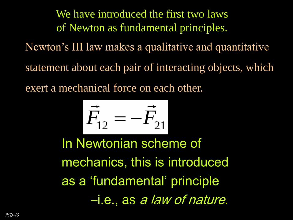
We have introduced the first two laws
of Newton as fundamental principles.
PCD-10
In Newtonian scheme of
mechanics, this is introduced
as a ‘fundamental’ principle
–i.e., as a law of nature.
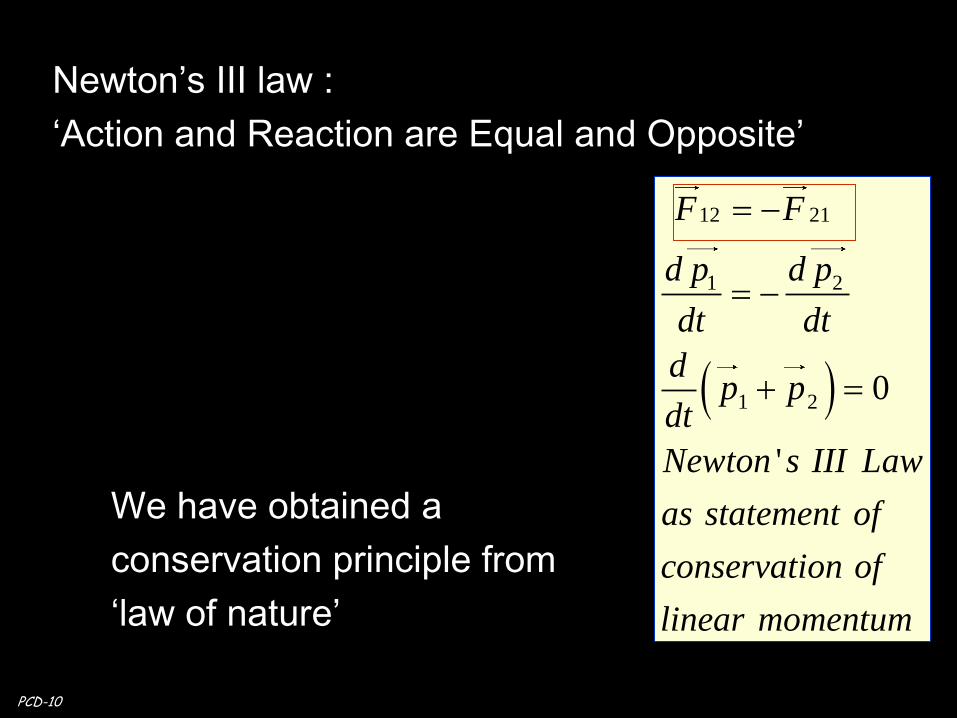
12 21F F
Newton’s III law makes a qualitative and quantitative
statement about each pair of interacting objects, which
exert a mechanical force on each other.
PCD_STiCM
22
12 21
1 2
1 2 0
'
F F
d p d p
dt dt
dp p
dt
Newton s III Law
as statement of
conservation of
linear momentum
Newton’s III law :
‘Action and Reaction are Equal and Opposite’
PCD-10
We have obtained a
conservation principle from
‘law of nature’
PCD_STiCM
23
Are the conservation principles consequences of the laws of
nature? Or, are the laws of nature the consequences of the
symmetry principles that govern them?
Until Einstein's special theory of relativity,
it was believed that
conservation principles are the result of the laws of nature.
Since Einstein's work, however, physicists began to analyze
the conservation principles as consequences of certain
underlying symmetry considerations,
enabling the laws of nature to be revealed from this analysis.
PCD-10
PCD_STiCM
24
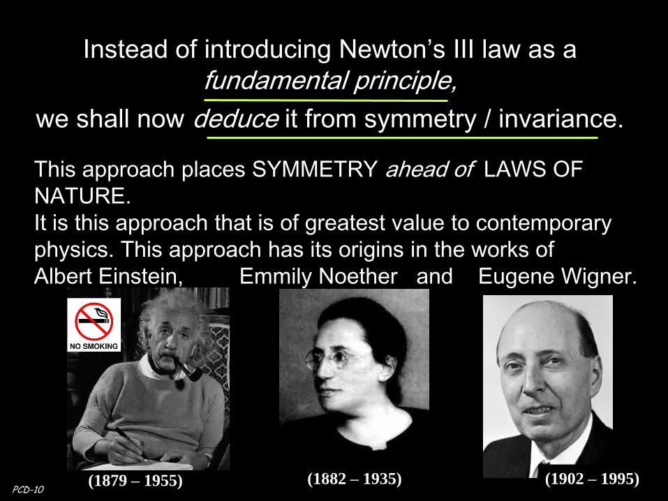
Instead of introducing Newton’s III law as a
fundamental principle,
we shall now deduce it from symmetry / invariance.
This approach places SYMMETRY ahead of LAWS OF
NATURE.
It is this approach that is of greatest value to contemporary
physics. This approach has its origins in the works of
Albert Einstein, Emmily Noether and Eugene Wigner.
(1882 – 1935) (1902 – 1995) (1879 – 1955) PCD-10
PCD_STiCM

STiCM
Select / Special Topics in Classical Mechanics
PCD-10
NEXT CLASS:
STiCM Lecture 03: Unit 1 Equations of Motion (ii)
25 PCD_STiCM

STiCM
Select / Special Topics in Classical Mechanics
PCD-L03
P. C. Deshmukh
Department of Physics
Indian Institute of Technology Madras
Chennai 600036
STiCM Lecture 03: Unit 1 Equations of Motion (ii) 26 PCD_STiCM
27
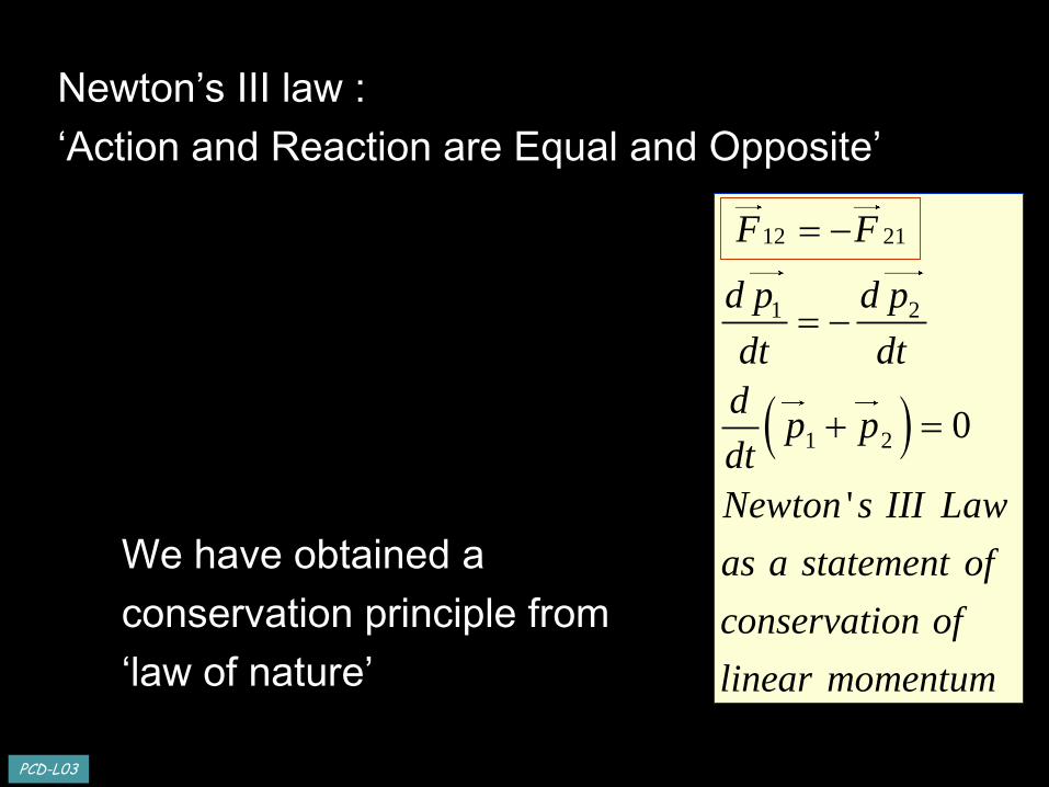
12 21
1 2
1 2 0
'
F F
d p d p
dt dt
dp p
dt
Newton s III Law
as a statement of
conservation of
linear momentum
Newton’s III law :
‘Action and Reaction are Equal and Opposite’
PCD-L03
We have obtained a
conservation principle from
‘law of nature’
PCD_STiCM

28
Are the conservation principles consequences of the laws of
nature?
Or, are the laws of nature the consequences of the symmetry
principles that govern them?
Until Einstein's special theory of relativity,
it was believed that
conservation principles are the result of the laws of nature.
Since Einstein's work, however, physicists began to analyze
the conservation principles as consequences of certain
underlying symmetry considerations,
enabling the laws of nature to be revealed from this analysis.
PCD-L03
PCD_STiCM
29
PCD-L03
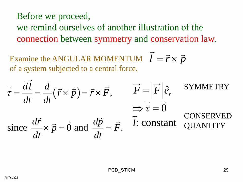
,
since 0 and .
dl dr p r F
dt dt
dr dpp F
dt dt
l r p Examine the ANGULAR MOMENTUM
of a system subjected to a central force.
Before we proceed,
we remind ourselves of another illustration of the
connection between symmetry and conservation law.
ˆ
0
: constant
rF F e
l
SYMMETRY
CONSERVED
QUANTITY
PCD_STiCM
Consider a system of N particles in a medium that is homogenous.
A displacement of the entire N-particle system through in this
medium would result in a new configuration that would find itself in
an environment that is completely indistinguishable from the
previous one.
30
S
Begin with a symmetry principle:
translational invariance in homogenous space.
PCD-L03
The connection between ‘symmetry’ and ‘conservation law’ is so
intimate, that we can actually derive Newton’s III law using
‘symmetry’.
This invariance of the environment of the entire N
particle system following a translational displacement is
a result of translational symmetry in homogenous space. PCD_STiCM
31
FOUR essential considerations:
1. Each particle of the system is under the influence only of all the
remaining particles;
the system is isolated: no external forces act on any of its
particles.
2 The entire N-particle system is deemed to have undergone
simultaneous identical displacement;
all inter-particle separations and relative orientations remain
invariant.
3 Entire medium: essentially homogeneous;
- spanning the entire system both
before and after the displacement.
PCD-L03
4. The displacement the entire system under consideration
is deemed to take place at a certain instant of time. PCD_STiCM
32
The implication of these FOUR considerations:
“Displacement considered is only a virtual displacement.”
- only a mental thought process;
- real physical displacements would require a certain time
interval over which the displacements would occur
- virtual displacements can be thought of to occur at an
instant of time and subject to the specific four features
mentioned.
PCD-L03
PCD_STiCM

33
PCD-L03
Displacement being virtual,
it is redundant to ask
“what agency has caused it”
PCD_STiCM
34
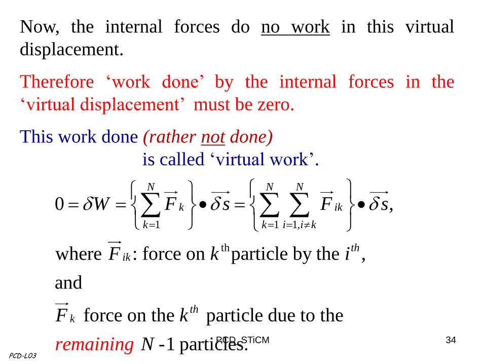
Now, the internal forces do no work in this virtual
displacement.
Therefore ‘work done’ by the internal forces in the
‘virtual displacement’ must be zero.
This work done (rather not done)
is called ‘virtual work’.
1 1 1,
th
0 ,
where : force on particle by the ,
and
force on the particle due to the
-1 particles.
N N N
k ik
k k i i k
thik
thk
remai
W F s F s
F k i
F k
ng Nni
PCD-L03
PCD_STiCM
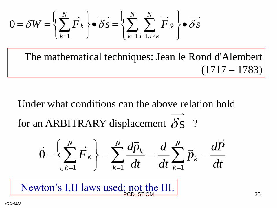
Under what conditions can the above relation hold
for an ARBITRARY displacement ?
35
s
The mathematical techniques: Jean le Rond d'Alembert
(1717 – 1783)
1 1 1
0N N N
kk k
k k k
dp d dPF p
dt dt dt
PCD-L03
1 1 1,
0N N N
k ik
k k i i k
W F s F s
Newton’s I,II laws used; not the III. PCD_STiCM

36
is obtained from the properties of translational symmetry
in homogenous space.
2 1
12 21
0,
. ., ,
which gives ,
the .
d P
dt
d p d pi e
dt dt
F F
III law of Newton
Amazing!
- since it suggests a path to
discover the laws of physics
by exploiting the connection
between symmetry and
conservation laws!
PCD-10
For just two particles:
1 1 1
0N N N
kk k
k k k
dp d dPF p
dt dt dt
The relation
PCD_STiCM

37
Newton’s III law need not be introduced as a
fundamental principle/law;
we deduced it from symmetry / invariance.
SYMMETRY placed ahead of LAWS OF NATURE.
Albert Einstein, Emmily Noether and Eugene Wigner.
(1882 – 1935) (1879 – 1955) PCD-L03 (1902 – 1995)
PCD_STiCM
38
Emilly Noether: Symmetry Conservation Laws
Eugene Wigner's profound impact on physics:
symmetry considerations using `group theory' resulted
in a change in the very perception of just what is most
fundamental.
`symmetry' : the most fundamental entity whose form
would govern the physical laws.
PCD-10
PCD_STiCM

39
The connection between SYMMETRY and
CONSERVATION PRINCIPLES brought out in
the previous example,
becomes even more transparent in an
alternative scheme of MECHANICS.
While Newtonian scheme rests on the principle
of causality (effect is linearly proportional to the
cause), this alternative principle does not
invoke the notion of ‘force’ as the ‘cause’ that
must be invoked to explain a system’s evolution.
PCD-10
PCD_STiCM
40
This alternative principle also begins by the
fact that the mechanical system is
characterized by its position and velocity
(or equivalently by position and momentum),
…… but with a very slight difference!
PCD-10
PCD_STiCM

41
The mechanical system is determined by
a well-defined function of position and
velocity/momentum.
The functions that are employed are the
Lagrangian and the Hamiltonian . ( , )L q q ( , )H q p
PCD-10
The primary principle on which this
alternative formulation rests is known as the
Principle of Variation. PCD_STiCM

42
We shall now introduce the
‘Principle of Variation’,
often referred to as the
‘Principle of Least (extremum) Action’.
PCD-10
PCD_STiCM
43
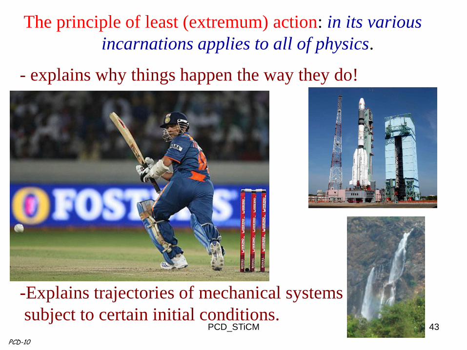
The principle of least (extremum) action: in its various
incarnations applies to all of physics.
- explains why things happen the way they do!
-Explains trajectories of mechanical systems
subject to certain initial conditions.
PCD-10
PCD_STiCM
44
The principle of least action has for its precursor what is
known as Fermat's principle - explains why light takes
the path it does when it meets a boundary of a medium.
Common knowledge: when a ray of light meets the edge
of a medium, it usually does not travel along the direction
of incidence - gets reflected and refracted.
Fermat's principle explains this by stating that light travels
from one point to another along a path over which it
would need the ‘least’ time. PCD-10
PCD_STiCM

45
Pierre de Fermat (1601(?)-1665) : French lawyer who pursued
mathematics as an active hobby.
Best known for what has come to be known as Fermat's last theorem,
namely that the equation xⁿ+yⁿ=zⁿ has no non-zero integer solutions
for x,y and z for any value of n>2.
"To divide a cube into two other
cubes, a fourth power or in general
any power whatever into two
powers of the same denomination
above the second is impossible, and
I have assuredly found an
admirable proof of this, but the
margin is too narrow to contain it."
-- Pierre de Fermat
It took about 350
years for this
theorem to be
proved (by Andrew
J. Wiles, in 1993).
PCD-10
PCD_STiCM
46
Actually, the time taken by light is not necessarily a
minimum.
More correctly, the principle that we are talking about
is stated in terms of an ‘extremum’,
and even more correctly as
‘The actual ray path between two points is the one for
which the optical path length is stationary with respect
to variations of the path’.
…………………. Usually it is a minimum:
Light travels along a path that takes the least time.
PCD-10
PCD_STiCM
STiCM
Select / Special Topics in Classical Mechanics
PCD-L04
P. C. Deshmukh
Department of Physics
Indian Institute of Technology Madras
Chennai 600036
STiCM Lecture 04: Unit 1 Equations of Motion (iii) 47 PCD_STiCM
48
We shall now introduce the
‘Principle of Variation’,
often referred to as the
‘Principle of Least (extremum) Action’.
PCD-10
PCD_STiCM

49
Hamilton’s principle
‘principle of least (rather, extremum) action’
Hamilton's principle of least action thus has an
interesting development, beginning with Fermat's
principle about how light travels between two points, and
rich contributions made by Pierre Louis Maupertuis
(1698 -- 1759), Leonhard Paul Euler (1707 - 1783), and
Lagrange himself.
PCD_STiCM

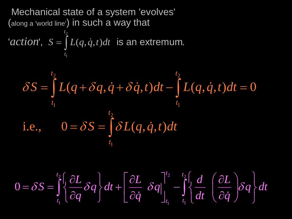
50
2
1
( , , ) .
t
t
S L q q t dtaction
Mechanical state of a system 'evolves' (along a 'world line') in such a way that
' ', is an extremum
Hamilton’s principle
‘principle of least (rather, extremum) action’
...and now, we need ‘action’,
- ‘integral’ of the ‘Lagrangian’!
PCD_STiCM
51
0t 2t1t
2
1
( ) t
t
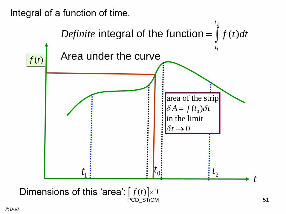
Definite f t dt integral of the function
Area under the curve
t
Integral of a function of time.
0
area of the strip
( )
in the limit
0
A f t t
t
( )f t
PCD-10
Dimensions of this ‘area’: ( )f t TPCD_STiCM
52
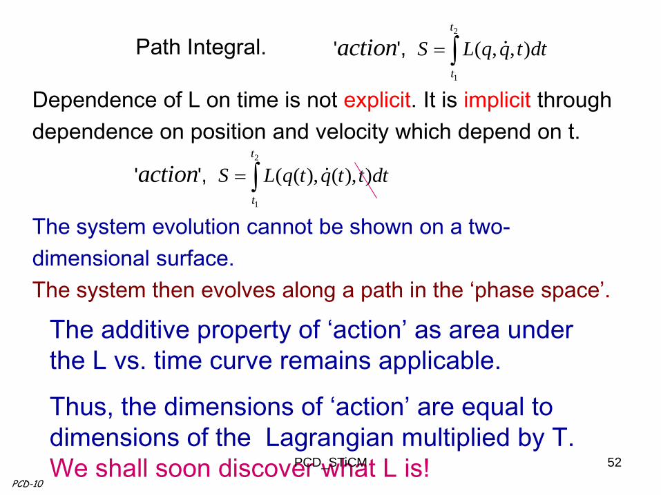
Path Integral.
Dependence of L on time is not explicit. It is implicit through
dependence on position and velocity which depend on t.
The system evolution cannot be shown on a two-
dimensional surface.
The system then evolves along a path in the ‘phase space’.
The additive property of ‘action’ as area under
the L vs. time curve remains applicable.
Thus, the dimensions of ‘action’ are equal to
dimensions of the Lagrangian multiplied by T.
We shall soon discover what L is!
2
1
( , , ) t
t
S L q q t dtaction' ',
2
1
( ( ), ( ), ) ' ',
t
t
S L q t q t t dtaction
PCD-10
PCD_STiCM

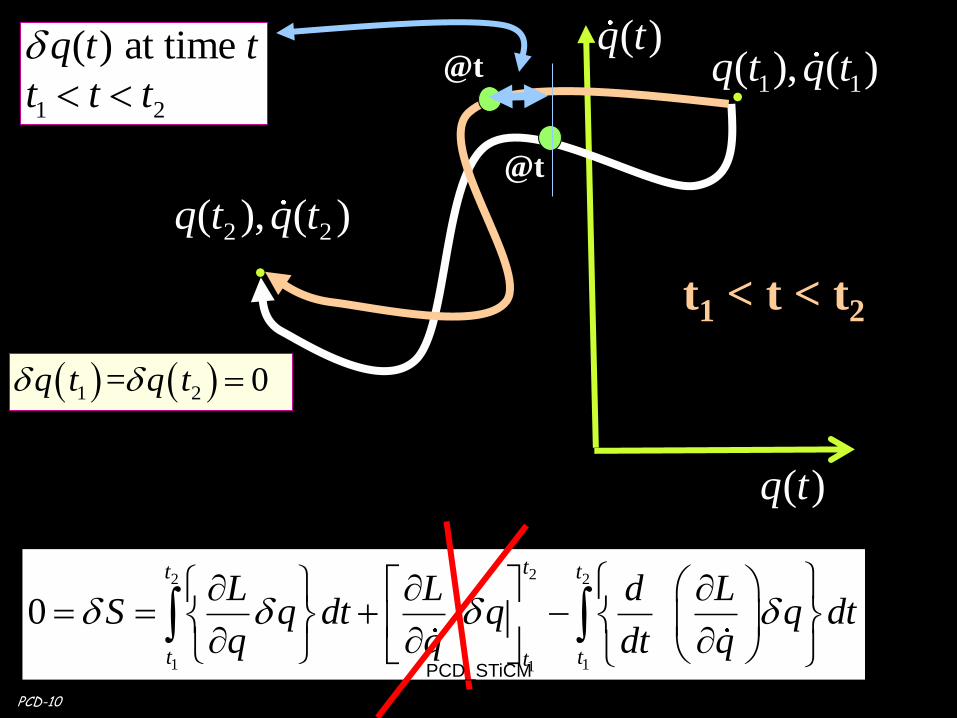
53
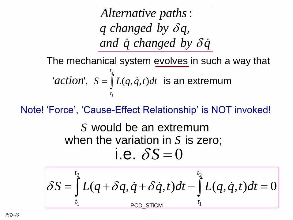
Consider alternative paths
along which the mechanical state
of the system may evolve in the
phase space :
,
q changed by q
and q changed by qPCD-10
.
. 1 1( ), ( )q t q t
2 2( ), ( )q t q t
( )q t
( )q t
PCD_STiCM
54
0
SS
S
would be an extremum when the variation in is zero;
i.e.
2
1
( , , )
The mechanical system evolves in such a way that
' ', is an extremum
t
t
S L q q t dtaction
2 2
1 1
( , , ) ( , , ) 0
t t
t t
S L q q q q t dt L q q t dt
:
,
Alternative paths
q changed by q
and q changed by q
Note! ‘Force’, ‘Cause-Effect Relationship’ is NOT invoked!
PCD-10
PCD_STiCM
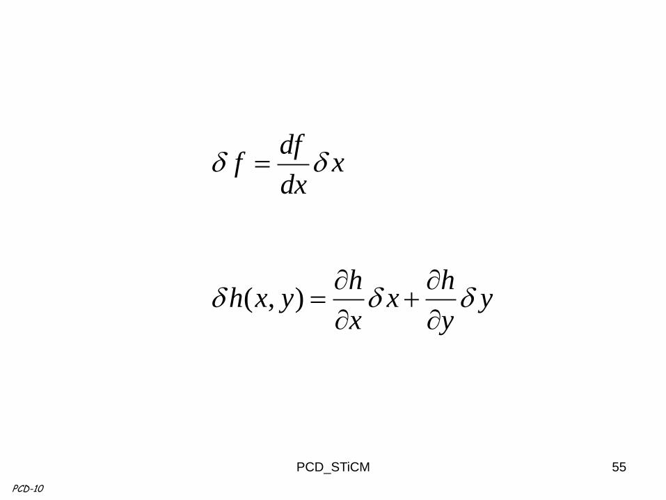
55
( , )
dff x
dx
h hh x y x y
x y
PCD-10
PCD_STiCM

56
0 0 0
0 0 0 0
0 0( , )
( , ) ( , )2 2lim lim
x xx y y
x xh x y h x y
h h
x x x
y
h
h: dependent
variable
x & y:
independent
variables
0 0 0
0 0 0 0
0 0( , )
( , ) ( , )2 2lim lim
y yx y x
y yh x y h x y
h h
y y y
Partial
derivatives of a
function of
more than one
variable.
PCD-10
x
PCD_STiCM
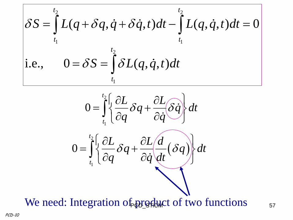
57
2 2
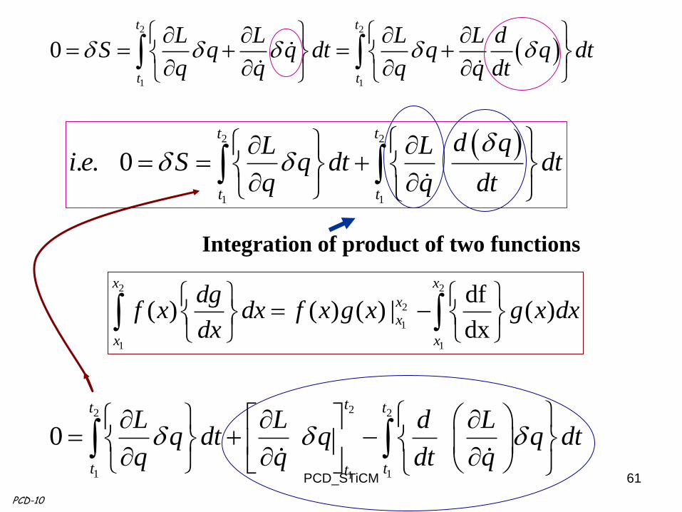
1 1
2
1
( , , ) ( , , ) 0
i.e., 0 ( , , )
t t
t t
t
t
S L q q q q t dt L q q t dt
S L q q t dt
2
1
0
t
t
L Lq q dt
q q
We need: Integration of product of two functions PCD-10
2
1
0
t
t
L L dq q dt
q q dt
PCD_STiCM
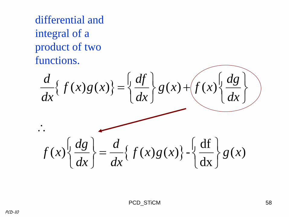
58
( ) ( ) ( ) ( )
df ( ) ( ) ( ) - ( )
dx
d df dgf x g x g x f x
dx dx dx
dg df x f x g x g x
dx dx
differential and
integral of a
product of two
functions.
PCD-10
PCD_STiCM
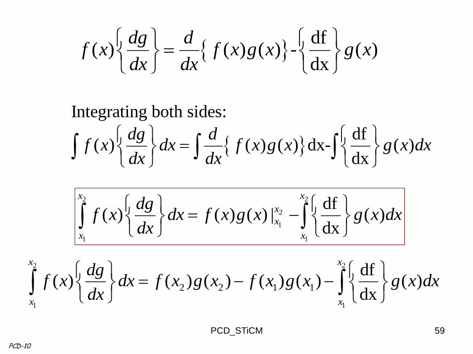
59
df
( ) ( ) ( ) - ( )dx
dg df x f x g x g x
dx dx
Integrating both sides:
df( ) ( ) ( ) dx- ( )
dx
dg df x dx f x g x g x dx
dx dx
2 2
2
1
1 1
df( ) ( ) ( ) | ( )
dx
x x
x
x
x x
dgf x dx f x g x g x dx
dx
2 2
1 1
2 2 1 1
df( ) ( ) ( ) ( ) ( ) ( )
dx
x x
x x
dgf x dx f x g x f x g x g x dx
dx
PCD-10
PCD_STiCM

60
22 2
1 11
0
tt t
t tt
L L d Lq dt q q dt
q q dt q
2 2
1 1
0
t t
t t
L L L L dS q q dt q q dt
q q q q dt
2 2
1 1
. . 0
t t
t t
d qL Li e S q dt dt
q q dt
Integration of product of two functions
2 2
2
1
1 1
df( ) ( ) ( ) | ( )
dx
x x
x
x
x x
dgf x dx f x g x g x dx
dx
PCD-10
PCD_STiCM
61
22 2
1 11
0
tt t
t tt
L L d Lq dt q q dt
q q dt q
2 2
1 1
0
t t
t t
L L L L dS q q dt q q dt
q q q q dt
2 2
1 1
. . 0
t t
t t
d qL Li e S q dt dt
q q dt
Integration of product of two functions
2 2
2
1
1 1
df( ) ( ) ( ) | ( )
dx
x x
x
x
x x
dgf x dx f x g x g x dx
dx
PCD-10
PCD_STiCM
62
PCD-10
.
. 1 1( ), ( )q t q t
2 2( ), ( )q t q t
( )q t
( )q t
@t
@t
1 2
( ) at time
q t t
t t t
1 2= 0 q t q t
t1 < t < t2
22 2
1 11
0
tt t
t tt
L L d LS q dt q q dt
q q dt q
PCD_STiCM

STiCM
Select / Special Topics in Classical Mechanics
PCD-L05
P. C. Deshmukh
Department of Physics
Indian Institute of Technology Madras
Chennai 600036
STiCM Lecture 05: Unit 1 Equations of Motion (iv) 63 PCD_STiCM
64
2
1
( , , ) .
t
t
S L q q t dtaction
along a 'world line'
Mechanical state of a system 'evolves' ( ) in such a way that
' ', is an extremum
2 2
1 1
2
1
( , , ) ( , , ) 0
i.e., 0 ( , , )
t t
t t
t
t
S L q q q q t dt L q q t dt
S L q q t dt
22 2
1 11
0
tt t
t tt
L L d LS q dt q q dt
q q dt q
PCD_STiCM

65
.
. 1 1( ), ( )q t q t
2 2( ), ( )q t q t
( )q t
( )q t
@t
@t
1 2
( ) at time q t t
t t t
1 2= 0 q t q t
t1 < t < t2
22 2
1 11
0
tt t
t tt
L L d LS q dt q q dt
q q dt q
PCD_STiCM
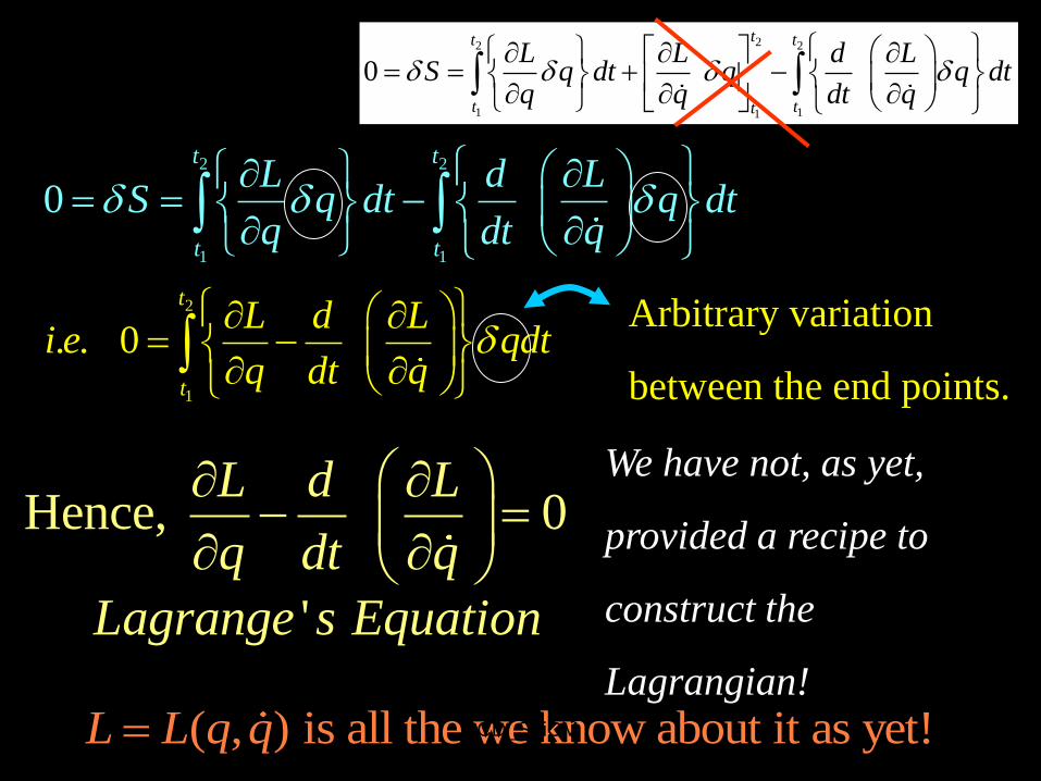
66
2
1
. . 0
t
t
L d Li e qdt
q dt q
Arbitrary variation
between the end points.
2 2
1 1
0
t t
t t
L d LS q dt q dt
q dt q
Hence, 0
'
L d L
q dt q
Lagrange s Equation
We have not, as yet,
provided a recipe to
construct the
Lagrangian!
( , ) is all the we know about it as yet!L L q q
22 2
1 11
0
tt t
t tt
L L d LS q dt q q dt
q q dt q
PCD_STiCM

67
2
1 2( , , ) ( ) ( )L q q t f q f q
0 ' L d L d L L
Lagrange s Equationq dt q dt q q
Homogeneity & Isotropy of space
L can only be quadratic function of the velocity.
2( , , ) ( )2
mL q q t q V q
T V
PCD_STiCM
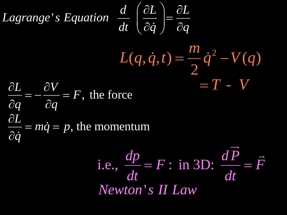
68
' d L L
Lagrange s Equationdt q q
i.e., : in 3D:
'
dp d PF F
dt dtNewton s II Law
, the force
, the momentum
L VF
q q
Lmq p
q
2( , , ) ( )2
-
mL q q t q V q
T V
PCD_STiCM
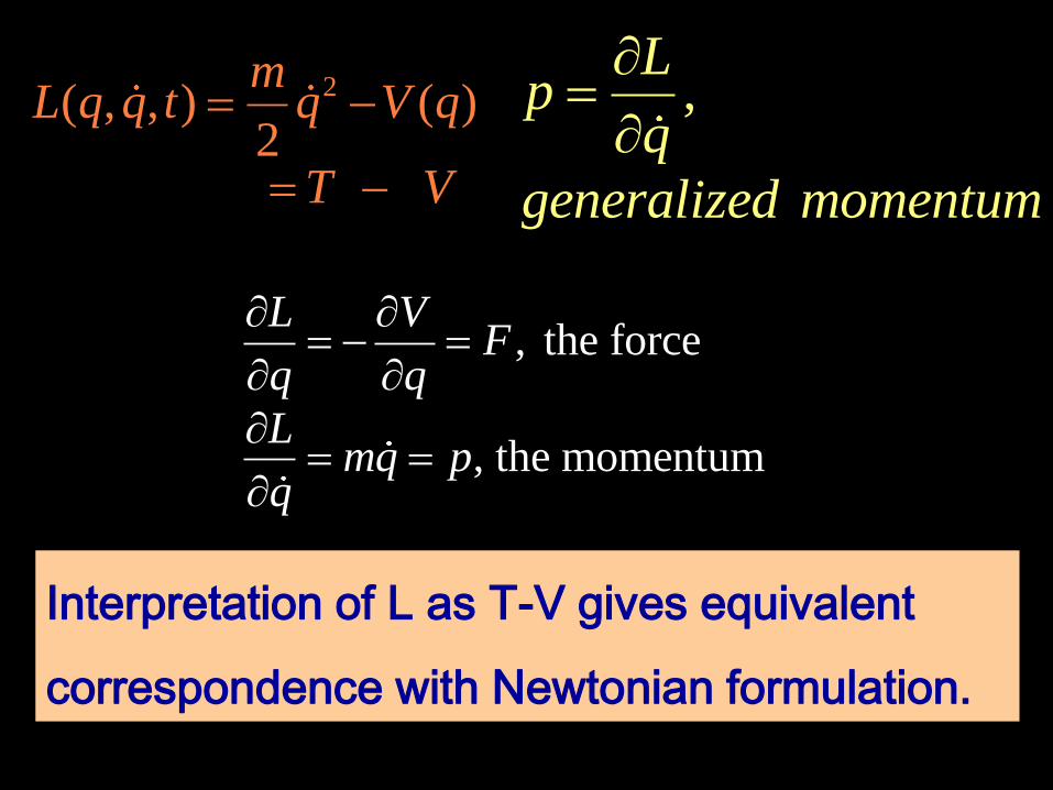
69
Interpretation of L as T-V gives equivalent
correspondence with Newtonian formulation.
,
Lp
q
generalized momentum
, the force
, the momentum
L VF
q q
Lmq p
q
2( , , ) ( )2
mL q q t q V q
T V
PCD_STiCM

70
( , , )
dL +
dt
L L q q t
L L Lq q
q q t
d +
dt
dL L L Lq q
dt q q t
d L Lq
dt q t
d0
dt
d
dt
L L
q q
L L
q q
Lq L
q
d L
dt t
0?L
What ift
PCD_STiCM
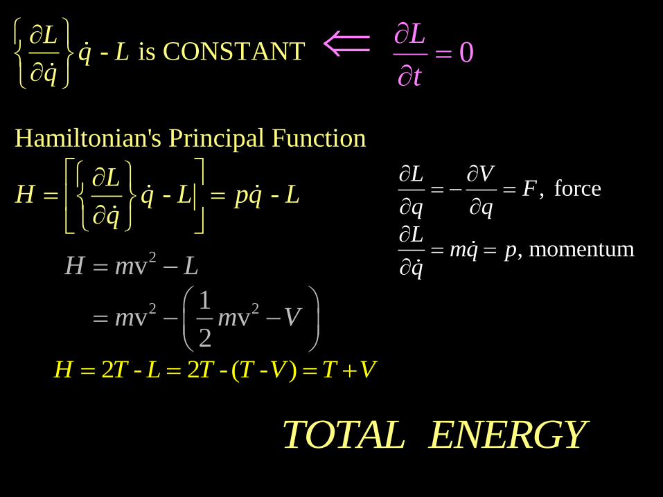
71
- is CONSTANT
Hamiltonian's Principal Function
- -
Lq L
q
LH q L pq L
q
2
2 2
v
1v v
2
H m L
m m V
TOTAL ENERGY
2 - 2 - ( - )H T L T T V T V
, force
, momentum
L VF
q q
Lmq p
q
0L
t
PCD_STiCM
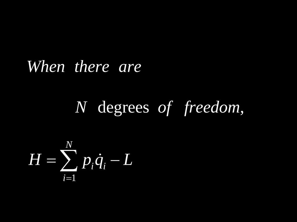
72
1
degrees ,
N
i i
i
When there are
N of freedom
H p q L
PCD_STiCM
73
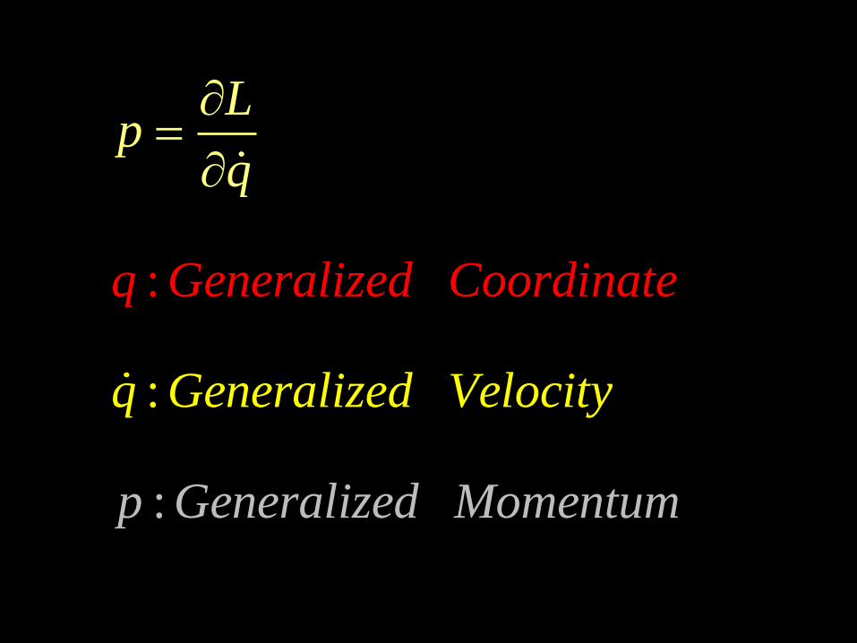
:
:
:q Generalize
q Ge
d
neraliz
Vel
ed Coordi
ocit
p
y
Generalized Momen
na
tu
Lp
q
t
m
e
PCD_STiCM

74
( )
Symmetry Conservation Laws
Noether
PCD_STiCM
75
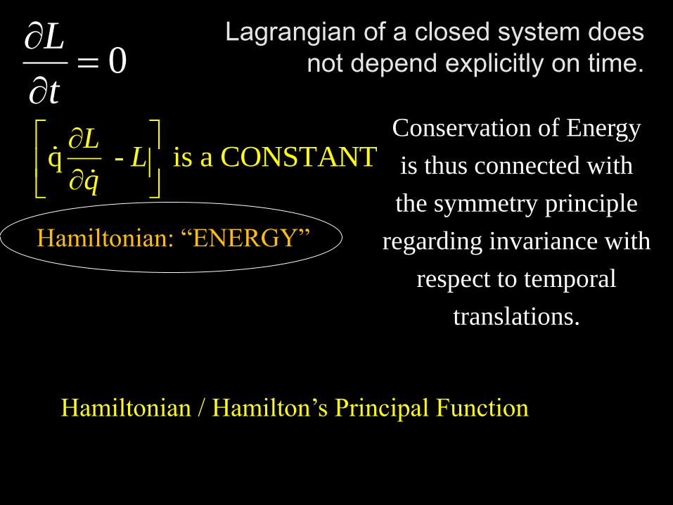
Lagrangian of a closed system does
not depend explicitly on time.
Hamiltonian / Hamilton’s Principal Function
q - is a CONSTANTL
Lq
Conservation of Energy
is thus connected with
the symmetry principle
regarding invariance with
respect to temporal
translations.
Hamiltonian: “ENERGY”
0L
t
PCD_STiCM
76
since 0, this means . . is conserved.
. ., is independent of time, is a constant of motion
L d L Li e p
q dt q q
i e
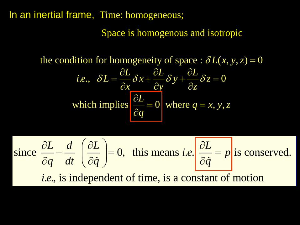
In an inertial frame, Time: homogeneous;
Space is homogenous and isotropic
the condition for homogeneity of space : ( , , ) 0
. ., 0
which implies 0 where , ,
L x y z
L L Li e L x y z
x y z
Lq x y z
q
PCD_STiCM
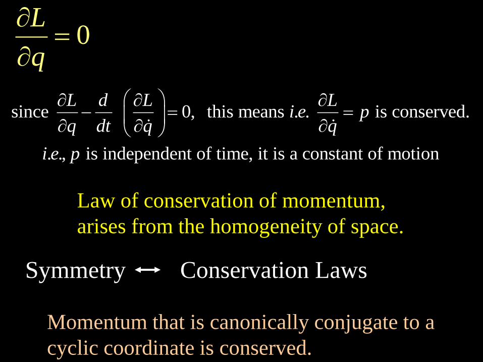
77
since 0, this means . . is conserved.
. ., is independent of time, it is a constant of motion
L d L Li e p
q dt q q
i e p
Law of conservation of momentum,
arises from the homogeneity of space.
Symmetry Conservation Laws
Momentum that is canonically conjugate to a
cyclic coordinate is conserved.
0L
q
PCD_STiCM

k k k
k k k
k k k k
k k
LdH q dp dq
q
q dp p dq
78
( , )k k k k
k
H q p L q q Many degrees of freedom:
Hamiltonian (Hamilton’s Principal Function) of a system
k k k k k k
k k k kk k
L LdH p dq q dp dq dq
q q
PCD_STiCM

79
k k k k
k k
dH q dp p dq
, ( , )k k
k k
k kk k
But H H p q
H Hso dH dp dq
p q
Hamilton’s equations of motion
: k k
k k
H HHence k q and p
p q
PCD_STiCM

80
Hamilton’s Equations
( , )
:
k k
k k
k k
H H p q
H Hk q and p
p q
( , )k k k k
k
H q p L q q
Hamilton’s Equations of Motion :
Describe how a mechanical state of a system
characterized by (q,p) ‘evolves’ with time. PCD_STiCM

81 PCD_STiCM

82
[1] Subhankar Ray and J Shamanna,
On virtual displacement and virtual work in Lagrangian dynamics
Eur. J. Phys. 27 (2006) 311--329
[2] Moore, Thomas A., (2004)
`Getting the most action out of least action: A proposal'
Am. J. Phys. 72:4 p522-527
[3] Hanca, J.,Taylor, E.F. and Tulejac, S. (2004)
`Deriving Lagrange's equations using elementary calculus'
Am. J. Phys. 72:4, p510-513
[4] Hanca, J. and Taylor, E.F. (2004) `From conservation of energy to the principle of least action:
A story line'
Am. J. Phys. 72:4, p.514-521
REFERENCES
NEXT CLASS: STiCM Lecture 06: Unit 1 Equations of Motion (v) PCD_STiCM

STiCM
Select / Special Topics in Classical Mechanics
P. C. Deshmukh
Department of Physics
Indian Institute of Technology Madras
Chennai 600036
STiCM Lecture 06: Unit 1 Equations of Motion (v) 83 PCD_STiCM
84
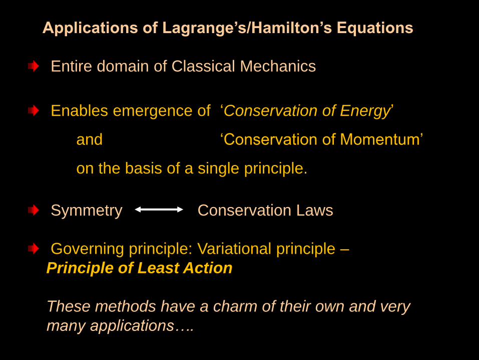
Applications of Lagrange’s/Hamilton’s Equations
Entire domain of Classical Mechanics
Enables emergence of ‘Conservation of Energy’
and ‘Conservation of Momentum’
on the basis of a single principle.
Symmetry Conservation Laws
Governing principle: Variational principle –
Principle of Least Action
These methods have a charm of their own and very
many applications…. PCD_STiCM

85
Applications of Lagrange’s/Hamilton’s
Equations
• Constraints / Degrees of Freedom
- offers great convenience!
• ‘Action’ : dimensions
‘angular momentum’ :
: :h Max Planckfundamental quantityin Quantum Mechanics
Illustrations: use of Lagrange’s / Hamilton’s equations
to solve simple problems in Mechanics PCD_STiCM

86
Manifestation of simple
phenomena in different
unrelated situations
radiation oscillators,
molecular vibrations,
atomic, molecular, solid
state, nuclear physics,
Dynamics of
spring–mass systems,
pendulum,
oscillatory electromagnetic circuits,
bio rhythms,
share market fluctuations … electrical engineering,
mechanical
engineering …
Musical instruments PCD_STiCM

87
SMALL OSCILLATIONS
1581:
Observations on the
swaying chandeliers
at the Pisa cathedral.
http://www.daviddarling.info/images/Pisa_cathedral_chandelier.jp
http://roselli.org/tour/10_2000/102.htmlg
Galileo (when only 17
years old) recognized
the constancy of the
periodic time for
small oscillations. PCD_STiCM
88
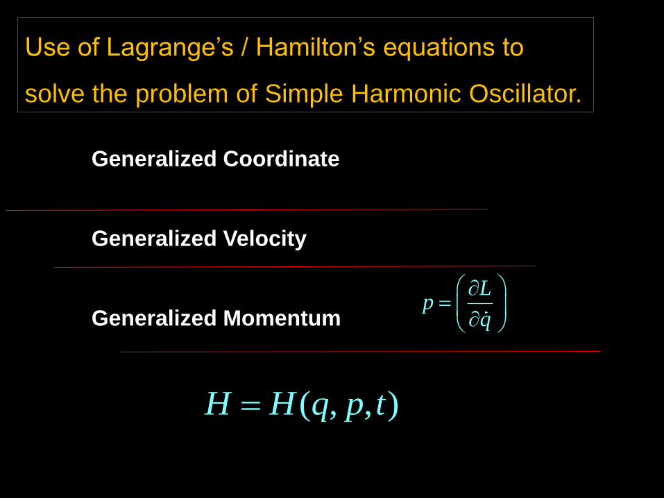
:
:
:
q
q
p
( , , )L L q q t
( , , )H H q p t
Generalized Coordinate
Generalized Velocity
Generalized Momentum
Lp
q
Use of Lagrange’s / Hamilton’s equations to
solve the problem of Simple Harmonic Oscillator.
PCD_STiCM

89
( , , )
0 '
L L q q t Lagrangian
L d LLagrange s Equation
q dt q
( , , )
'
k k
k
k k
k k
H q p L
H H q p t Hamiltonian
H Hq p
p q
Hamilton s Equations
k: and
2nd order
differential
equation
TWO
1st order
differential
equations PCD_STiCM
90
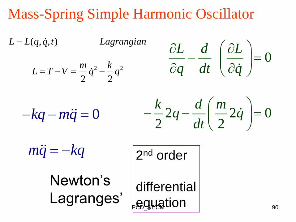
2 2
( , , )
2 2
L L q q t Lagrangian
m kL T V q q
2nd order
differential
equation
Newton’s
Lagranges’
Mass-Spring Simple Harmonic Oscillator
0
2 2 02 2
L d L
q dt q
k d mq q
dt
0
kq mq
mq kq
PCD_STiCM

91
kx x
m
http://www-groups.dcs.st-and.ac.uk/~history/PictDisplay/Hooke.html
k
mq kq q qm
Robert Hooke (1635-1703),
(contemporary of Newton),
empirically discovered this
relation for several elastic
materials in 1678.
Linear relation between restoring force and
displacement for spring-mass system:
PCD_STiCM
92
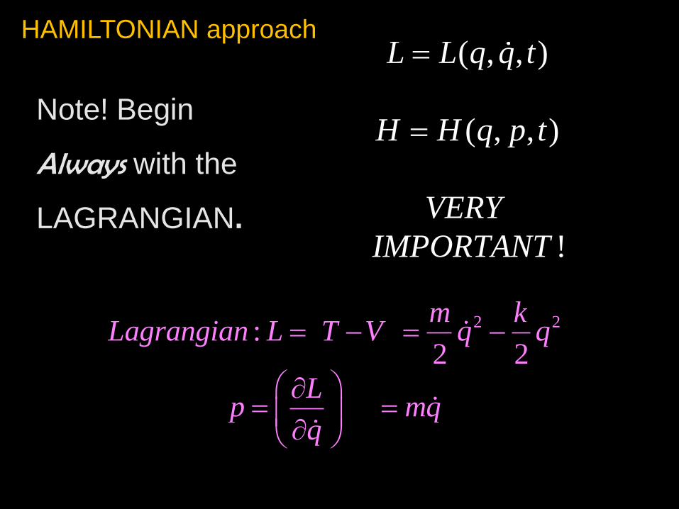
2 2: 2 2
m kLagrangian L T V q q
Lp mq
q
( , , )
( , , )
!
L L q q t
H H q p t
VERY
IMPORTANT
HAMILTONIAN approach
Note! Begin
Always with the
LAGRANGIAN.
PCD_STiCM

93
2 2: 2 2
m kLagrangian L T V q q
Lp mq
q
Mass-Spring
2 2 2
2 2
m kH pq L mq q q
22
2 2
p kH q
m
PCD_STiCM
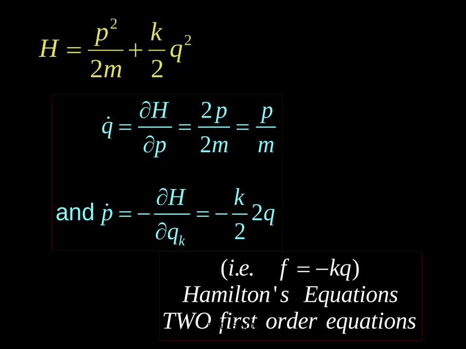
94
22
2 2
p kH q
m
2
2
22k
H p pq
p m m
H kp q
q
and
( . . )'
i e f kqHamilton s Equations
TWO first order equations
PCD_STiCM

95
2 2
22
:2 2
2
2
m kLagrangian L T V q q
Lp mq
q
p kH q
m
( , , )
( , , )
!
L L q q t
H H q p t
VERY
IMPORTANT
Generalized Momentum is interpreted
only as , and not a product of mass with velocity Lp
q
Be careful about how you write the Lagrangian and
the Hamiltonian for the Harmonic oscillator!
PCD_STiCM
96
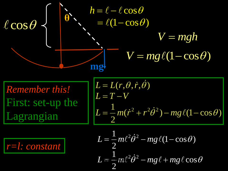
l : length
E: equilibrium
S: support
θ
mg
coscos
(1 cos )
h
2 2 2
( , , , )
1( ) (1 cos )
2
L L r r
L T V
L m r r mg
(1 cos )V mg
Remember this!
First: set-up the
Lagrangian
2 2
2 2
1(1 cos )
21
cos2
L m mg
L m mg mg
V mgh
r=l: constant
PCD_STiCM

97
2 21cos
2L m mg mg
2
=0r
Lp
rL
p ml
Now, we can find the
generalized
momentum for each
degree of freedom.
: fixed lengthr
0 L d L
q dt q
PCD-10
PCD_STiCM

98
2 21cos
2L m mg mg
0.
sin
L
rL
mgl mgl
2
=0r
Lp
rL
p ml
0 L d L
q dt q
2
2
( ) 0d
mgl mldt
mgl ml
g
l
Simple pendulum
PCD_STiCM
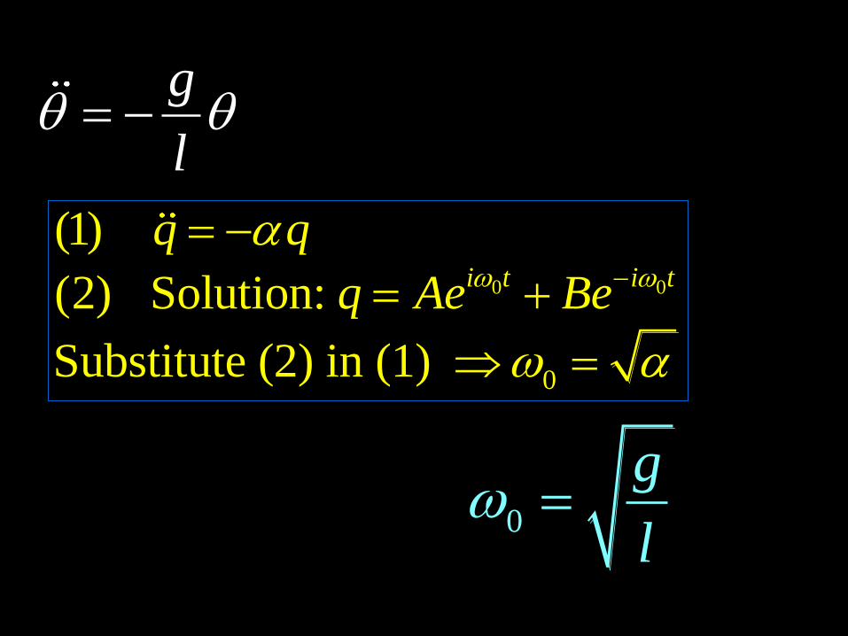
99
0 0
0
(1)
(2) Solution:
Substitute (2) in (1)
i t i t
q q
q Ae Be
0
g
l
g
l
PCD_STiCM

100
(1) Newtonian
(2) Lagrangian
g
l
0
g
l
Note! We have not used
‘force’, ‘tension in the
string’ etc. in the
Lagrangian and
Hamiltonian approach!
PCD_STiCM
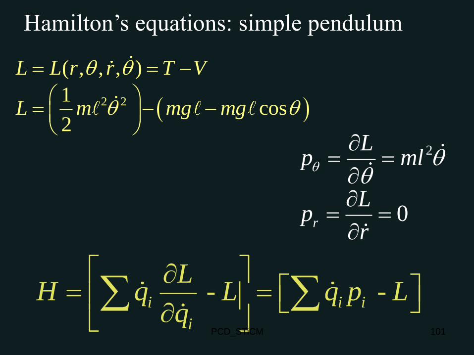
101
- - i i i
i
LH q L q p L
q
Hamilton’s equations: simple pendulum
2 2
( , , , )
1cos
2
L L r r T V
L m mg mg
2
0r
Lp ml
Lp
r
PCD_STiCM
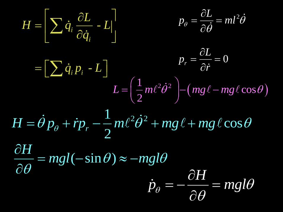
102
-
-
i
i
i i
LH q L
q
q p L
2 21cos
2rH p rp m mg mg
2
0r
Lp ml
Lp
r
2 21cos
2L m mg mg
( sin )H
mgl mgl
Hp mgl
PCD_STiCM
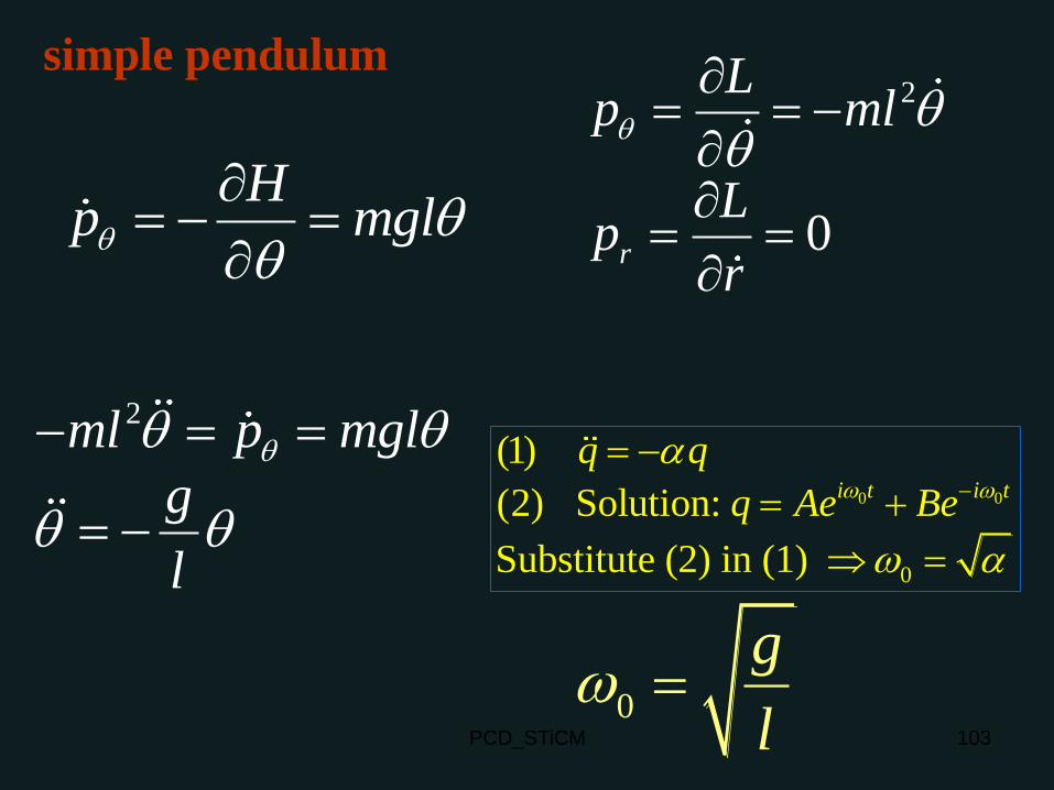
103
2ml p mgl
g
l
Hp mgl
0
g
l
simple pendulum
0 0
0
(1)
(2) Solution:
Substitute (2) in (1)
i t i t
q q
q Ae Be
2
0r
Lp ml
Lp
r
PCD_STiCM
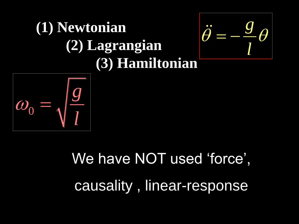
We have NOT used ‘force’,
causality , linear-response 104
(1) Newtonian
(2) Lagrangian
(3) Hamiltonian
g
l
0
g
l
PCD_STiCM

105
Lagrangian and Hamiltonian
Mechanics has very many
applications.
All problems in ‘classical
mechanics’ can be addressed using
these techniques. PCD_STiCM
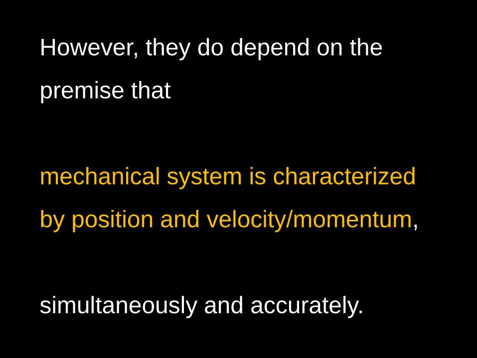
106
However, they do depend on the
premise that
mechanical system is characterized
by position and velocity/momentum,
simultaneously and accurately. PCD_STiCM
107
Central problem in ‘Mechanics’:
How is the ‘mechanical state’ of a system
described, and how does this ‘state’ evolve
with time?
- Formulations due to Galileo/Newton,
- Lagrange and Hamilton. PCD_STiCM

108
(q,p) : How do we get these?
Heisenberg’s
principle of uncertainty
New approach required !
PCD_STiCM

109
‘New approach’ is not required on account of
the Heisenberg principle!
Rather,
the measurements of q and p are not compatible….
….. so how could one describe the
mechanical state of a system by (q,p) ?
PCD_STiCM
110
Heisenberg principle comes into play as a
result of the fact that simultaneous
measurements of q and p do not provide
consistent accurate values on repeated
measurements. ….
….. so how could one describe the
mechanical state of a system by (q,p) ? PCD_STiCM
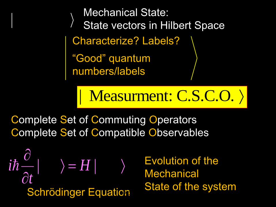
111
| Mechanical State:
State vectors in Hilbert Space
| Measurment: C.S.C.O.
| | i Ht
Evolution of the
Mechanical
State of the system
Complete Set of Commuting Operators
Complete Set of Compatible Observables
Schrödinger Equation
Characterize? Labels?
“Good” quantum
numbers/labels
PCD_STiCM

112
Galileo Galilei 1564 - 1642
Galileo Newton
Lagrange
Hamilton
( , )
Linear Response.
Principle of causality.
Principle of
Variation
( , )
( , )
q q
F ma
L q q
H q p
0L d L
q dt q
,k
H Hq p
p q
PCD_STiCM
Related Documents