Seismic tomography shows that upwelling beneath Iceland is confined to the upper mantle G. R. Foulger, 1 M. J. Pritchard, 1 B. R. Julian, 2 J. R. Evans, 2 R. M. Allen, 3 G. Nolet, 3 W. J. Morgan, 3 B. H. Bergsson, 4 P. Erlendsson, 4 S. Jakobsdottir, 4 S. Ragnarsson, 4 R. Stefansson 4 and K. Vogfjo ¨rd 5 1 Department of Geological Sciences, University of Durham, Durham, DH1 3LE, UK. E-mail: [email protected] 2 US Geological Survey, 345 Middlefield Road., Menlo Park, CA 94025, USA 3 Department of Geological and Geophysical Sciences, Guyot Hall, Princeton University, Princeton, NJ 08544–5807, USA 4 Meteorological Office of Iceland, Bustadavegi 9, Reykjavik, Iceland 5 National Energy Authority, Grensasvegi 9, Reykjavik, Iceland Accepted 2001 April 3. Received 2001 March 19; in original form 2000 August 1 SUMMARY We report the results of the highest-resolution teleseismic tomography study yet performed of the upper mantle beneath Iceland. The experiment used data gathered by the Iceland Hotspot Project, which operated a 35-station network of continuously recording, digital, broad-band seismometers over all of Iceland 1996–1998. The structure of the upper mantle was determined using the ACH damped least-squares method and involved 42 stations, 3159 P-wave, and 1338 S-wave arrival times, including the phases P, pP, sP, PP, SP, PcP, PKIKP, pPKIKP, S, sS, SS, SKS and Sdiff. Artefacts, both perceptual and parametric, were minimized by well-tested smoothing techniques involving layer thinning and offset-and-averaging. Resolution is good beneath most of Iceland from y60 km depth to a maximum of y450 km depth and beneath the Tjornes Fracture Zone and near-shore parts of the Reykjanes ridge. The results reveal a coherent, negative wave-speed anomaly with a diameter of 200–250 km and anomalies in P-wave speed, V P , as strong as x2.7 per cent and in S-wave speed, V S , as strong as x4.9 per cent. The anomaly extends from the surface to the limit of good resolution at y450 km depth. In the upper y250 km it is centred beneath the eastern part of the Middle Volcanic Zone, coincident with the centre of the y100 mGal Bouguer gravity low over Iceland, and a lower crustal low-velocity zone identified by receiver functions. This is probably the true centre of the Iceland hotspot. In the upper y200 km, the low- wave-speed body extends along the Reykjanes ridge but is sharply truncated beneath the Tjornes Fracture Zone. This suggests that material may flow unimpeded along the Reykjanes ridge from beneath Iceland but is blocked beneath the Tjornes Fracture Zone. The magnitudes of the V P , V S and V P /V S anomalies cannot be explained by elevated temperature alone, but favour a model of maximum temperature anomalies <200 K, along with up to y2 per cent of partial melt in the depth range y100–300 km beneath east-central Iceland. The anomalous body is approximately cylindrical in the top 250 km but tabular in shape at greater depth, elongated north–south and generally underlying the spreading plate boundary. Such a morphological change and its relationship to surface rift zones are predicted to occur in convective upwellings driven by basal heating, passive upwelling in response to plate separation and lateral temperature gradients. Although we cannot resolve structure deeper than y450 km, and do not detect a bottom to the anomaly, these models suggest that it extends no deeper than the mantle transition zone. Such models thus suggest a shallow origin for the Iceland hotspot rather than a deep mantle plume, and imply that the hotspot has been located on the spreading ridge in the centre of the north Atlantic for its entire history, and is not fixed relative to other Atlantic hotspots. The results are consistent with recent, regional full-thickness mantle tomography and whole-mantle tomography images that show a strong, low- wave-speed anomaly beneath the Iceland region that is confined to the upper mantle and Geophys. J. Int. (2001) 146, 504–530 504 # 2001 RAS

Welcome message from author
This document is posted to help you gain knowledge. Please leave a comment to let me know what you think about it! Share it to your friends and learn new things together.
Transcript

Seismic tomography shows that upwelling beneath Iceland isconfined to the upper mantle
G. R. Foulger,1 M. J. Pritchard,1 B. R. Julian,2 J. R. Evans,2 R. M. Allen,3
G. Nolet,3 W. J. Morgan,3 B. H. Bergsson,4 P. Erlendsson,4 S. Jakobsdottir,4
S. Ragnarsson,4 R. Stefansson4 and K. Vogfjord5
1 Department of Geological Sciences, University of Durham, Durham, DH1 3LE, UK. E-mail: [email protected] US Geological Survey, 345 Middlefield Road., Menlo Park, CA 94025, USA3 Department of Geological and Geophysical Sciences, Guyot Hall, Princeton University, Princeton, NJ 08544–5807, USA4 Meteorological Office of Iceland, Bustadavegi 9, Reykjavik, Iceland5 National Energy Authority, Grensasvegi 9, Reykjavik, Iceland
Accepted 2001 April 3. Received 2001 March 19; in original form 2000 August 1
SUMMARY
We report the results of the highest-resolution teleseismic tomography study yetperformed of the upper mantle beneath Iceland. The experiment used data gatheredby the Iceland Hotspot Project, which operated a 35-station network of continuouslyrecording, digital, broad-band seismometers over all of Iceland 1996–1998. Thestructure of the upper mantle was determined using the ACH damped least-squaresmethod and involved 42 stations, 3159 P-wave, and 1338 S-wave arrival times, includingthe phases P, pP, sP, PP, SP, PcP, PKIKP, pPKIKP, S, sS, SS, SKS and Sdiff.Artefacts, both perceptual and parametric, were minimized by well-tested smoothingtechniques involving layer thinning and offset-and-averaging. Resolution is good beneathmost of Iceland from y60 km depth to a maximum of y450 km depth and beneath theTjornes Fracture Zone and near-shore parts of the Reykjanes ridge. The results reveal acoherent, negative wave-speed anomaly with a diameter of 200–250 km and anomaliesin P-wave speed, VP, as strong as x2.7 per cent and in S-wave speed, VS, as strong asx4.9 per cent. The anomaly extends from the surface to the limit of good resolution aty450 km depth. In the upper y250 km it is centred beneath the eastern part of theMiddle Volcanic Zone, coincident with the centre of the y100 mGal Bouguer gravitylow over Iceland, and a lower crustal low-velocity zone identified by receiver functions.This is probably the true centre of the Iceland hotspot. In the upper y200 km, the low-wave-speed body extends along the Reykjanes ridge but is sharply truncated beneath theTjornes Fracture Zone. This suggests that material may flow unimpeded along theReykjanes ridge from beneath Iceland but is blocked beneath the Tjornes Fracture Zone.The magnitudes of the VP, VS and VP /VS anomalies cannot be explained by elevatedtemperature alone, but favour a model of maximum temperature anomalies <200 K,along with up to y2 per cent of partial melt in the depth range y100–300 km beneatheast-central Iceland. The anomalous body is approximately cylindrical in the top 250 kmbut tabular in shape at greater depth, elongated north–south and generally underlyingthe spreading plate boundary. Such a morphological change and its relationship tosurface rift zones are predicted to occur in convective upwellings driven by basal heating,passive upwelling in response to plate separation and lateral temperature gradients.Although we cannot resolve structure deeper than y450 km, and do not detect abottom to the anomaly, these models suggest that it extends no deeper than the mantletransition zone. Such models thus suggest a shallow origin for the Iceland hotspot ratherthan a deep mantle plume, and imply that the hotspot has been located on the spreadingridge in the centre of the north Atlantic for its entire history, and is not fixed relative toother Atlantic hotspots. The results are consistent with recent, regional full-thicknessmantle tomography and whole-mantle tomography images that show a strong, low-wave-speed anomaly beneath the Iceland region that is confined to the upper mantle and
Geophys. J. Int. (2001) 146, 504–530
504 # 2001 RAS
thus do not require a plume in the lower mantle. Seismic and geochemical observationsthat are interpreted as indicating a lower mantle, or core–mantle boundary origin forthe North Atlantic Igneous Province and the Iceland hotspot should be re-examined toconsider whether they are consistent with upper mantle processes.
Key words: hotspot, Iceland, seismic tomography, upper mantle, plume.
I N T R O D U C T I O N
Arthur Holmes was the first influential advocate of convection
within the Earth, a process that later became generally accepted
as the physical basis for Wegener’s theory of continental drift
(Holmes 1931). Very early, the convection hypothesis was
accepted by German geodesists, who surmised that the rift zones
of Iceland might overlie upwelling limbs and be widening, with
magma rising passively to fill the space created (Bernauer 1943).
It is now accepted that subducting slabs comprise the descending
limbs of a convecting system, but the nature of the ascending
flow at spreading ridges and hotspots, and the depths from
which material rises, are still poorly understood.
Magmas at spreading ridges are thought to be of relatively
shallow origin, perhaps no deeper than y100 km (e.g. Shen
& Forsyth 1995). Subducted slabs, however, are known from
earthquake activity and full-thickness mantle tomography
to extend much deeper (Grand 1994). Spreading ridges thus
appear not to involve upwellings on the same depth scale as
downgoing slabs. It was originally suggested by Wilson (1963)
and Morgan (1971, 1972) that hot material rises from the
deep mantle to the surface of the Earth in jets or vertical, cylin-
drical ‘plumes’. This hypothesis has gained wide acceptance,
and has been invoked to explain large-scale geological and
geophysical features such as large igneous provinces and geoid,
topographic and geochemical anomalies. However, few obser-
vations require that magma rises in plumes from great depth.
Whole-mantle tomography, for example, suggests that deep
upwellings are very broad and diffuse, although the spatial
resolution of those models cannot rule out narrow structures.
Alternatives to the plume model that involve only relatively
shallow processes have been proposed (e.g. King & Anderson
1998). The plume hypothesis is an elegant tenet that has achieved
widespread acceptance, but it is unproven. It should thus not
go unchallenged. Alternative models should be considered.
Seismic studies seeking mantle plumes include whole-mantle
tomography, regional full-thickness mantle tomography, tele-
seismic tomography involving regional-scale seismic networks,
and experiments focusing on specific plume markers. Tabular,
high-wave-speed lithospheric slabs have been imaged beneath
major subduction zones (e.g. van der Hilst et al. 1997; Fukao
et al. 1992). However, negative wave-speed anomalies with
the vertical, cylindrical morphology traditionally expected of
plumes have not been detected. Three candidate bodies have
been reported to date, one y2000 km wide arising from the
core–mantle boundary beneath the South Atlantic and extend-
ing obliquely to the Earth’s surface beneath East Africa, and
two beneath the Pacific ocean (e.g. Ritsema et al. 1999; Megnin
& Romanowicz 2000). However, none has a simple, traditional
plume shape, width or geometry or can be explained as a
thermal plume (Tackley 1998; van der Hilst & Karason 1999;
Megnin & Romanowicz 2000).
For most hotspots there is no seismic evidence for a deep-
seated origin. The best studied is the Iceland hotspot. Several
independent, regional full-thickness mantle tomography and
whole-mantle tomography studies have imaged a strong, broad,
low-wave-speed upper mantle anomaly that occupies most of
the north Atlantic at the latitude of Iceland (Hager & Clayton
1989; Zhou 1996; Bijwaard & Spakman 1999; Ritsema et al.
1999; Megnin & Romanowicz 2000; Karason & van der Hilst
2001a,b). In contrast, the lower mantle is characterized by
anomalies at least an order of magnitude weaker, with poor
repeatability of the details of individual features. The maxi-
mum depth of good resolution of land-based, regional seismic
experiments in Iceland is limited to y450 km by the size of
the island, and thus such studies can only image reliably the
upper mantle above the transition zone. A strong, negative
wave-speed anomaly is invariably detected. Allen et al. (1999)
reported that the attenuation pattern of teleseismic waves pass-
ing beneath Iceland indicates a body no more than y200 km
wide and with an anomaly in VS of up to x12 per cent. This
is considerably narrower and stronger than anomalies found
in earlier teleseismic tomography experiments, which report
bodies with diameters of 200–400 km and VP anomalies of up
to yx4 per cent (Tryggvason et al. 1983; Wolfe et al. 1997).
Interpretations of these regional experiments did not consider
alternative, non-plume hypotheses.
We report here the results of the largest teleseismic tomo-
graphy study yet performed of the upper mantle beneath
Iceland. Our study involves more stations and several times
more arrival times than have been used before, and includes
diverse seismic phases that improve resolving power. The results
confirm the presence of a negative wave-speed anomaly in the
upper mantle, but show additionally that its gross morphology
varies with depth. The body is centred beneath east-central
Iceland and is consistent with elevated temperature and partial
melting. It extends beneath the Reykjanes ridge southwest
of Iceland in the upper y200 km but terminates laterally
at shallow depth beneath the Tjornes Fracture Zone north of
Iceland. The body is roughly cylindrical in the upper y250 km,
but at greater depth assumes a vertical, tabular morphology
underlying and approximately parallel to the spreading plate
boundary. Such a change in shape is expected near the bottom
of rising, buoyant bodies, and our observations thus suggest
that the negative wave-speed anomaly in the upper mantle
beneath Iceland does not extend into the lower mantle (Foulger
et al. 2000).
T E C T O N I C S T R U C T U R E O F I C E L A N D
Iceland has east–west and north–south dimensions of y500
and 350 km and lies on the spreading plate boundary in the
north Atlantic. Over 30 spreading segments are exposed on
land and comprise four major volcanic zones: the Northern,
Eastern, Western and Middle Volcanic Zones (NVZ, EVZ, WVZ
and MVZ; Fig. 1; Saemundsson 1979). The currently active
spreading zone is represented by the NVZ, which developed
at y7 Ma with the abandonment of a zone 150 km further
Upwelling beneath Iceland confined to upper mantle 505
# 2001 RAS, GJI 146, 504–530

to the west (Saemundsson et al. 1980). The NVZ is linked to
the offshore Kolbeinsey ridge by the y120 km long, right-
lateral Tjornes Fracture Zone (TFZ). The EVZ, a southward-
propagating rift, is currently growing at the expense of the
dwindling WVZ (Sigmundsson et al. 1994). The WVZ is con-
nected to the offshore spreading plate boundary, the Reykjanes
ridge, via the Reykjanes peninsula in southwest Iceland.
The Iceland hotspot is popularly thought, on the basis of
geochemistry and volcanic production rates, to be currently
centred beneath the northwest part of the Vatnajokull ice-cap
(Schilling 1973; Sigvaldason et al. 1974). It has been suggested
that the hotspot has migrated east with respect to the oceanic
plate boundary at a rate of y1 cm yrx1 over the last 55 Myr
(Vink 1984), and that recently the spreading plate boundary in
Iceland has migrated with it. However, these models are based
on the assumption that the Iceland hotspot has remained fixed
relative to other Atlantic hotspots. Furthermore, the shape of
the edge of the Iceland plateau is consistent with the centre
of volcanism having been relatively stationary with respect to
the plate boundary over the last 26 Myr (Bott 1985).
D A T A A C Q U I S I T I O N
The objective of the Iceland Hotspot Project is to study the crust
and upper mantle beneath Iceland. A network of 35 digital
broad-band seismic stations was operated from June 1996 to
August 1998—the largest deployment of such instruments ever
in Iceland (Fig. 1). A primary objective was to perform tele-
seismic tomography of the highest quality practical. The greatest
depth that may be imaged using this method is approxi-
mately equal to the network aperture, and we maximized this
by deploying sensors from coast to coast, including one on
the island of Grimsey north of Iceland. The network comple-
mented the permanent Icelandic SIL (South Iceland Lowland)
network (Stefansson et al. 1993), from which data were also
drawn. Particularly challenging was the deployment of station
23 at Grimsfjall, a nunatak on the caldera rim of the Grimsvotn
volcano, within the Vatnajokull icecap. Bedrock is exposed
there because the ground is warmed by geothermal heat from
the Grimsvotn volcano. This station was deployed two months
prior to, and at a distance of 5 km from, the eruption of
the subglacial volcano Gjalp in September and October 1996
(Gudmundsson et al. 1997), and resulted in the serendipitous
acquisition of an excellent seismic data set of volcanic earthquakes
and tremor.
The equipment used was supplied by the IRIS–PASSCAL
consortium. We used 24-bit REFTEK 72 A-08 data loggers
recording a continuous data stream at 20 samples sx1 on
0.66–1.2 Gbyte disks. A triggered data stream was also recorded
at 100 samples sx1 to enhance recordings of large local earth-
quakes. The sensors were Guralp three-component broad-
band seismometers of type CMG-3T, which has a bandwidth
25ûW
25ûW
24ûW
24ûW
23ûW
23ûW
22ûW
22ûW
21ûW
21ûW
20ûW
20ûW
19ûW
19ûW
18ûW
18ûW
17ûW
17ûW
16ûW
16ûW
15ûW
15ûW
14ûW
14ûW
13ûW
13ûW
63ûN 63ûN
64ûN 64ûN
65ûN 65ûN
66ûN 66ûN
67ûN 67ûN
0 50 100
km
RR
TFZ
KR
WVZ
EVZ
NVZ
N W Fjords
MVZ
Vatnajökull
Hofsjökull
1
2
3
45
678
910
11
12 13
14
15
16
1718
19
20
2122
23
24
2526
27
28
29
30
Seismic station
Glacier
Volcanic centre
Figure 1. Map of Iceland showing the major tectonic elements. NVZ, EVZ, WVZ and MVZ: Northern, Eastern, Western and Middle Volcanic
Zones; TFZ: Tjornes Fracture Zone; RR: Reykjanes ridge; KR: Kolbeinsey ridge. Grey areas: major ice-caps; black dots: broad-band seismic stations
in operation 1996– 1998 that were used for this study; numbered dots: temporary stations of the Iceland Hotspot Project. Station 23 was deployed on a
nunatak in the Vatnajokull ice-cap. It, along with stations 24, 25, 26 and 28, was battery-powered and deployed in mountain huts. Dots without
numbers: permanent stations of the Icelandic SIL network with broad-band sensors, the five in southwest and central Iceland being supplied by the
Iceland Hotspot Project.
506 G. R. Foulger et al.
# 2001 RAS, GJI 146, 504–530
of 0.01–50 Hz, and types CMG-3ESP and CMG-40T, which
have bandwidths of 0.03–50 Hz. The CMG-40T sensors are
compact and suitable for outdoors deployments where vaults
have to be excavated. Microseisms are strong in Iceland, and
dominated the noise compared to instrumental effects. Timing
and station locations were provided by GPS clocks.
Most of the coastal zone in Iceland is populated, so we were
able to deploy most of the stations in buildings, either on bed-
rock exposed in basements or on concrete floors laid directly
onto bedrock. At these sites, mains power was used, and backup
power was provided by trickle-charged batteries. Five broad-
band sensors were deployed in existing vaults of the Icelandic
SIL network. Those data were sampled at 100 samples sx1 and
stored in a ring buffer from which earthquakes of interest
were extracted on a daily basis. The SIL data were resampled
at 20 samples sx1 for this study. The interior of Iceland is
unpopulated and not served by mains electricity, but in order to
achieve uniform coverage, five stations were deployed there.
We deployed the recorders in mountain huts that were selected
for regularity of spacing and suitability for winter maintenance
visits by a team of field workers in specially equipped snow jeeps.
Winter-time power was the limiting factor at those stations, and
banks of eight 150 amp hr batteries were used, trickle charged
by four to eight 30 W solar panels.
All stations were visited at 6–12 week intervals. Data
were dumped from field disks and archived in Reykjavik.
Earthquakes were extracted on a monthly basis using event
lists from the National Earthquake Information Centre (NEIC)
and the Meteorological Office of Iceland, which operates the
SIL network. We achieved an average of 86 per cent uptime for
our stations. The most serious causes of data loss were lack of
power at the interior stations, and malfunctioning of elements
in outdoor excavated pits that were inaccessible throughout the
winter because of frozen ground. The final data archive comprises
y200 Gbytes of data compressed with the Steim algorithm
(Halbert et al. 1988), and is publicly available over the inter-
net from the IRIS–PASSCAL Consortium Data Management
Center.
D A T A P R O C E S S I N G
Teleseismic earthquake arrival times were measured on rotated
seismograms using the interactive computer program dbpick
(Harvey & Quinlan 1996). The signal-to-noise ratio of seismic
recordings in Iceland is degraded by microseismic and wind-
generated noise, but the 2 yr deployment period was sufficient
to gather excellent recordings of more than 120 teleseisms. Using
preliminary arrival times computed using the IASP91 earth
model (Kennett & Engdahl 1991) and NEIC final locations,
traces were time-shifted to align the first-arriving P phase to
facilitate waveform comparison. Phases picked were P, pP, sP,
PP, SP, PcP, PKIKP, pPKIKP, S, sS, SS, SKS and Sdiff.
(Table 1). For the final inversion we selected picks made in
the frequency band 0.5–2.0 Hz for P waves and 0.05–0.1 Hz
for S waves. We picked by hand for consistency, since initial
trials with numerical cross-correlation revealed that frequent
cycle misidentification occurred. Furthermore, algorithms that
correlate several cycles of waveforms introduce systematic
errors, since later cycles include crustal reverberations and
multipathing, which vary across a large network deployed in an
inhomogeneous region. Such errors may distort final models
more seriously than the slightly larger but random errors in
hand picks. We measured times of the first trough or peak
relative to the phase of interest, with an estimated accuracy of
y0.05 s for P phases and y0.5 s for S phases. Weights were
assigned to picks on the basis of qualitative judgement of the
clarity of the phases. Traveltime residuals were calculated by
subtracting the arrival times predicted by the IASP91 model
from each observed time.
The surface-reflected phases PP and SS are particularly
valuable because, for a given epicentral distance, they have
larger slownesses than most other teleseismic body phases and
can therefore help to increase vertical resolution where earth-
quakes at small epicentral distances are sparse, as is the case
for Iceland. In particular, use of PP and SS phases can reduce
vertical smearing, and help to distinguish true vertical structures
from artefacts of poor resolution. The results of previous
studies of mantle structure beneath Iceland are open to question,
partly because of failure to use such phases (Keller et al. 2000).
At the same time, however, surface-reflected phases introduce
their own problems because their rays are not minimum-time
paths. Reflections from points on the surface other than the
geometrical ray bounce-point can arrive before the geometrical
arrival, so signals tend to have emergent beginnings whose
absolute onset times are difficult to measure. Relative arrival
times must thus be measured for peaks or troughs later in the
waveform, which are more subject to contamination by crustal
structure variations and multipathing. In this study, we used
PP phases from 33 earthquakes and SS phases from 14. To
minimize the errors discussed above, we used only phases with
high signal-to-noise ratios and waveforms that were coherent
from station to station.
In a data set of this size, some measurements inevitably have
large errors, caused, for example, by comparing different peaks
or troughs at different stations, and it is important to identify
and remove such outliers. This can be done by comparing the
patterns of arrival-time anomalies at different stations for earth-
quakes with similar locations. For such a collection of events,
the ray paths beneath the network are similar, and therefore, in
the absence of errors, the pattern of arrival-time anomalies is
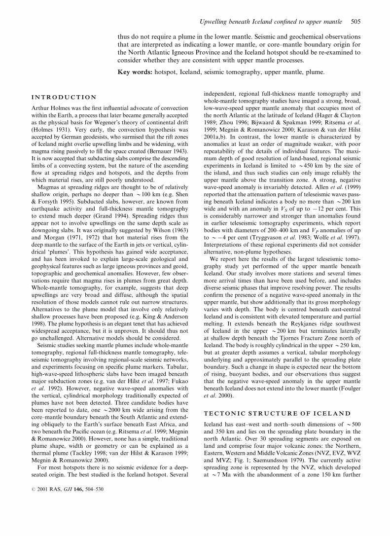
also similar. We divided the phases into 10 azimuth–slowness
bins for P and nine for S (Fig. 2) and analysed each bin
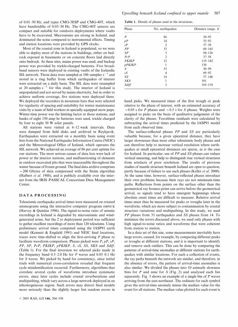
separately. Fig. 3 shows an example of a single bin of P waves
arriving from the east-northeast. The ordinate for each symbol
gives the arrival-time anomaly minus the median value for the
event for all stations. The median value plotted for each event is
Table 1. Details of phases used in the inversions.
Phase No. earthquakes Distance range, Du
P 86 30–95
pP 14 35–92
sP 2 57–58
PP 33 69–145
SP 3 94–126
PcP 2 37–58
PKIKP 12 119–142
pPKIKP 1 130
S 52 30–99
sS 4 69–92
SS 14 57–146
SKS 1 101
Sdiff 3 103–118
Upwelling beneath Iceland confined to upper mantle 507
# 2001 RAS, GJI 146, 504–530
thus zero. Data on plots such as this that deviated from
the median value for the station by more than t0.6 s for P
or t1.5 s for S were assumed to contain large errors and
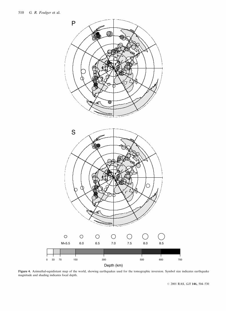
eliminated. The final data set contains 3159 P arrivals from
160 phases and 113 earthquakes, and 1338 S arrivals from 73
phases and 66 earthquakes (Fig. 4). The peak magnitudes of
the mean arrival-time anomalies at a station were about 1 s for
P waves and 3 s for S waves.
2
000°
00 ∞
180∞
0 °
3
2
4
8
000∞
00 °
180°
0 °
P
S
Figure 2. Azimuth–slowness bins into which phases were divided for outlier identification (Fig. 3). Double dividing lines indicate overlapping bins.
Upper panel: P phases; lower panel: S phases.
508 G. R. Foulger et al.
# 2001 RAS, GJI 146, 504–530
T O M O G R A P H Y M E T H O D
To invert the arrival-time anomalies and determine 3-D
structure, we used the ‘ACH’ damped-least-squares method
of Aki et al. (1977). In particular, we used a version of the
computer program thrd that had been modified to correct a
geometrical error that is important at high latitudes (Julian
et al. 2001). A comprehensive description of the method and
application is given by Evans & Achauer (1993). The ACH
method uses data from a network of seismic stations whose
aperture is small compared with the distances to the sources.
The 3-D structure is represented as a stack of layers, each
divided into homogeneous rectangular blocks. The optimum
block size depends on the station spacing. Blocks should have
horizontal dimensions of approximately the average station
spacing, and layers should initially have thicknesses about 1.5
times this width. The method requires that all rays enter the
study volume through its base, so the model cannot extend
deeper than the turning point of the shallowest incoming ray.
Well-conditioned experiments involve rays distributed widely
in azimuth–slowness space, and thus the study volume is a
truncated cone that broadens downwards.
The ACH method perturbs an initial 1-D wave-speed model
to minimize the arrival-time anomalies in the least-squares
sense. Only in those places where there are many crossing rays,
well distributed in azimuth and slowness, is the structure well
resolved. The near surface, where there are no crossing rays, is
treated differently, by solving for a single wave-speed anomaly
in a cone beneath each station (a ‘special first layer’). A key
assumption is that delays caused by structure outside the study
volume are the same for all stations for a particular event
and phase. Clearly this is only an approximation, and hetero-
geneities outside the study volume can introduce spurious
anomalies into peripheral parts of the final images (Evans &
Achauer 1993). These parts must thus be viewed with caution.
Furthermore, the method computes the effects of changing
wave speeds in the blocks by applying Fermat’s Principle
to ray paths appropriate to the initial 1-D, layered structure,
and thus ignores the second-order effect of refraction of rays
by horizontal variations in wave speed. The severity of this
approximation depends on both the magnitude of the wave-
speed anomalies and their geometry. Because the rays follow
minimum-time paths, regions of high wave speed are sampled
most heavily, and the wave speeds in the derived models tend to
be overestimated. In practice, the errors introduced have been
found to be negligible if wave-speed anomalies are less than
y5 per cent (Steck & Prothero 1991), which is the case for the
upper mantle beneath Iceland.
To choose optimum block sizes and damping parameters, we
performed trial inversions using layers 100 km thick and blocks
100, 75 and 50 km wide (Pritchard 2000). In all cases, the
homogeneous cones used to approximate variations in crustal
structure beneath the stations were taken to be 10 km high.
As a starting model, we used a layered approximation to the
IASP91 wave-speed model. We performed a suite of inversions
varying only the damping parameter, and studied the trade-
off between residual variance and the square of the Euclidean
length of the model vector m. A damping-parameter value of
400 s2 per centx2 provided a reasonable trade-off between data
fit and model complexity.
-2
-1
0
1
2Relativeresidual(s)
1 1
1
1
1
11 1
11
1
1
1
1
1
11
1
1
1
11
1
1
1
1
1
11
2 2
2
22
2
2
2
2
2
2
2
2 2
2 22
2
2
2
2
2 2
2
2
2
2
2
22
3
33 3 3 3
33
3
3
3
33
3 3
3
3 3
3
33
44
4
44 4
4 4
4
44
4 44
4 44
5
5
5
55 5
5
5
5
5
5
5
5
55
5
5
55
5 5
5
5
5 55
55
5
5
6
66
6
6
6
6
6
6
6
6
6
66
6
66
6
6
7
7
8
8 8
8
8
8
8
8 8
88
8
8 8
8 88
88
8
8
9
99
9 9
9 9
9
9 9
9
9
9
9
99
9
99
99
9
1010 10
10
10
101010
101010
1010 10
101010
10
1010
1111
11 1111
11
11 1111
1111
11
11
11
11
1111
11
11
11
11
1111
11
11
11 1111
1212
12 1212
12
1212
12
12 12
12
12
12
12
12
1212
12
1212 12 1212
12
12 12 1212
1313
1313
13
13 1313
1313
13
13 13 13
13
13
1313
131313
13
13
1313
13
1313 13 1313
1313
131313
14
14
1414 14
14
1414
14
14 14
14
14
14
1414
1414
14
14
1414
141414
1414
15
15
15
1515
15
15
15
15
1515
15
15
15
15
15
1515
15
151515
1515
1515
15 1515
1616
16
16
16
1616
161616
1616
16
1616
1717
1717
17
17
17
17
17
17
17
17
1717
17
1717 17 1717
17 17
1717
18
19
20
20
20
20
20
20
20
20
20
2020
202020
2020
20
20
2020
21
21
21
2121
21
21
21
21
21
21
21
21 2121
2121
212121
2121
21
21
2121
22
22
22
22
22 22
2222
2222
22
2222
2222 22
22
22
22 222223
23
23 23
23
23 23 23
23
23
23
2323
23
2323 23 23
2323
232323
2323
23
23
23
23 23 2323
24
24 24
24
24 24
24
24
2424
2424 24
24 2424
2424 24 2424
24
24
24
2424 2424
2525
25 25
25
25 25 25
2525
25
25
25
2525
25
25 2525
2525
25
25
252525
2525
25
2525
26 26
2626
26
26
26 26 26
2626
26
2626
26
26
26
2626 2626
26
2626
262626
2626
2626
2626
HOT08
HOT09
HOT10
HOT07
HOT06
HOT04
HOT11
HOT03
HOT02
ASB
HOT05
HOT01
HOT30
VOG
KRO
HOT28
HVE
SKR
HOT26
HOT27
HOT14
HOT13
HOT12
SIG
GRI
GRA
REN
KRA
GIL
HOT15
HOT29
GRS
HOT16
HOT17
HOT18
HOT24
HOT25
HOT19
HOT23
HOT20
HOT21
HOT22
Figure 3. Example of a plot used to identify outliers, for P waves from events in the outer bin between y50uE and 90uE (Fig. 2, upper panel). Each
dot corresponds to an observation. Its ordinate is the arrival-time anomaly minus the median anomaly for the event. Circled dots: observations
identified as outliers.
Upwelling beneath Iceland confined to upper mantle 509
# 2001 RAS, GJI 146, 504–530
M=5.5 6.0 6.5 7.0 7.5 8.0 8.5
P
S
0 33 70 150 300 500 600 700
Depth (km)
Figure 4. Azimuthal-equidistant map of the world, showing earthquakes used for the tomographic inversion. Symbol size indicates earthquake
magnitude and shading indicates focal depth.
510 G. R. Foulger et al.
# 2001 RAS, GJI 146, 504–530

The ACH method is prone to non-linear effects that can
introduce distortion into 3-D models. The effect whereby the
sensitivity of the method to features smaller than the block size
depends on their position with respect to the block boundaries
is known as the ‘disappearing anomaly’ effect. An anomaly
near the centre of a block can be resolved more easily than one
near a block corner. We dealt with this problem by applying the
‘offset-and-averaging’ procedure of Evans & Achauer (1993).
The original grid is offset by 1/n times the block size along each
horizontal axis, where n is a small integer, and an additional
n2x1 offset models are computed. The final model is the
average of all n2 models. This averaging also smoothes the
model horizontally.
In order to smooth the model vertically, to remove visual
artefacts, we used ‘layer thinning’ (Evans & Achauer 1993).
This procedure involves performing a final inversion with
layers thinner by a factor of m, a small integer, than the initial
value used (which in the case of this study was 100 km). The
damping parameter must simultaneously be reduced by about
a factor of m to compensate for the increased number of
blocks in the model. For our layer-thinned inversions we used
m=2 and a damping value of 225 s2 per centx2. Increasing
the number of blocks reduces the number of rays per block,
and thus reduces formal statistical resolution. However, using
synthetic tests, Evans & Achauer (1993) showed that layer
thinning yields vertical smoothing without loss of ability to
retrieve true Earth structure, so that the equivalent spatial
resolution of the layer-thinned models is the same as that of
full-thickness layer models.
We performed a suite of inversions with block widths of 100,
75 or 50 km and layer thicknesses of 100, 50 or 33 km, both
with and without offset-and-averaging, for n=2 (Pritchard
2000). Agreement of the overall results between inversions was
good for the first-order features we interpret in this paper.
Pritchard (2000) showed additionally models with 100 km wide
blocks and 100 km thick layers that yielded smooth, averaged
structures, and models with 50 km wide blocks and 33 km
thick layers that yielded noisier results. Our preferred final VP
and VS models used offset-and-averaging with n=2, blocks
75 km wide and layers 50 km thick (Fig. 5), a compromise
between under-modelling the data and over-modelling noise.
For the original models, the initial and final rms arrival-time
anomalies for P waves are 0.49 and 0.19 s, and for S waves 3.27
and 1.08 s. The 3-D models thus give data variance reductions
of 84 per cent for P and 89 per cent for S. Values for the offset-
and-averaged models are expected to be approximately the
same.
We studied four measures of inversion quality. The hit-count
(the number of rays sampling each block) is shown for P and S
waves in Figs 6 and 7 for the model with 75 km wide blocks
and 100 km thick layers. The whole of Iceland is well sampled
from the surface down to y450 km depth. Below this, the
best-sampled areas are to the north of Iceland, where blocks
down to over 600 km depth are sampled by >100 P waves and
>50 S waves, and to the southwest of Iceland.
Hit-count is a poor indicator of resolving power because
the locations of anomalies can be determined well only if the
structure is sampled by crossing rays. Arrival times measured
from a bundle of quasi-parallel rays can detect the existence
a wave-speed anomaly but are insensitive to its position along
the ray bundle. More detailed information is provided by the
resolution matrix R (Evans & Achauer 1993, eq. 13.18), which
specifies the mapping between the ‘true’ Earth m and the
inversion result m,
m ¼ Rm : (1)
R is based on assumptions, most notably that the true Earth
consists of homogeneous blocks and that ray theory accurately
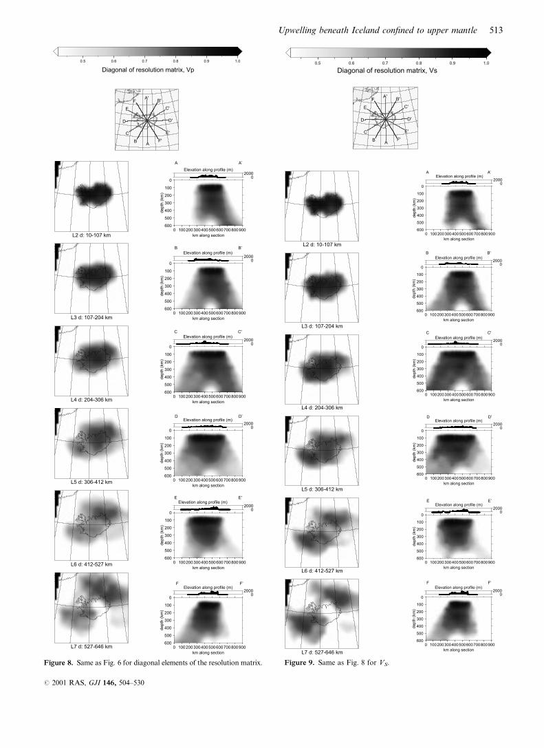
describes the paths of seismic waves. The diagonal elements of
the resolution matrix provide relative measures of the ability
of the data set to detect anomalies in different locations. Figs 8
and 9 show the diagonal elements of R for VP and VS for 75 km
wide blocks and 100 km thick layers. These are good indicators
of the quality of our preferred models with 50 km thick layers
(Evans & Achauer 1993). The pictures are broadly similar
for VP and VS. Resolution greater than y0.8, which exists
throughout much of our models, is unusually good for studies
of this kind. There is no resolution in the top y60 km of
the model since there are no crossing rays there. In the depth
range y60–450 km, resolution is high beneath most of Iceland
except in the upper 100 km beneath a small area in south
Iceland. Below 450 km, resolution decreases, and at great depth
resolution is poor, the incoming rays diverge strongly and
smearing is strong.
The diagonal elements of the resolution matrix do not
describe the tendency of an anomaly to be imaged in the wrong
location along a ray bundle, i.e. the degree of smearing. Such
information is contained in the off-diagonal elements of R, and
by examining these columns for blocks at key locations we
can assess the reliability of the shapes and sizes of features
of interest. A useful quantity for this purpose is the ‘volume
metric’ of a diagonal element Rij defined as the volume within
which the largest positive off-diagonal elements of column i sum
to some value d (Evans & Achauer 1993). Figs 10 and 11 show
the ‘volume metrics’ of selected blocks for the final VP and VS
models, computed for d=0.95, a high (pessimistic) value com-
pared with the values of 0.5–0.7 usually used (Evans & Achauer
1993).
Smearing in the central part of the study volume is minor,
and confined to a few vertically adjacent blocks. Smearing on
the north, south, east and west peripheries of the study volume
-600-500-400-300-200-100
0
depth
(km)
-1275 0 1275
km along W-E axis
-600-500-400-300-200-100
0
depth
(km)
0 5 10
velocity km/s
VpVs
Iasp91
Figure 5. West–east cross-section of the block structure used for the final inversion, which uses blocks 75 km wide and layers 50 km thick.
Wave-speed profiles at right show initial VP and VS models obtained from the IASP91 model (Kennett & Engdahl 1991).
Upwelling beneath Iceland confined to upper mantle 511
# 2001 RAS, GJI 146, 504–530

-25
o
-20
o
-15
o
64o
66o
L1 (special) d: 0-10 km
0 50 100 150 200 250 300
No. of hits per block, P
L2 d: 10-107 km
L3 d: 107-204 km
L4 d: 204-306 km
L5 d: 306-412 km
L6 d: 412-527 km
L7 d: 527-646 km
0
100
200
300
400
500
600
de
pth
(km
)
0 100200300400500600700800900
km along section
02000
Elevation along profile (m)A A'
0
100
200
300
400
500
600
de
pth
(km
)
0 100200300400500600700800900
km along section
02000
Elevation along profile (m)B
C
D
E
B'
C’
D’
E’
0
100
200
300
400
500
600
de
pth
(km
)
0 100200300400500600700800900
km along section
02000
Elevation along profile (m)
0
100
200
300
400
500
600
de
pth
(km
)
0 100200300400500600700800900
km along section
02000
Elevation along profile (m)
0
100
200
300
400
500
600
de
pth
(km
)
0 100200300400500600700800900
km along section
02000
Elevation along profile (m)
0
100
200
300
400
500
600
de
pth
(km
)
0 100200300400500600700800900
km along section
02000
Elevation along profile (m)F F'
Figure 6. Horizontal (left column) and vertical (right column) sections
showing the hit-count for P waves for the model with 75 km wide blocks
and 100 km thick layers. Top left panel shows hit-counts for individual
stations. Top right panel shows lines of vertical cross-sections.
-25
o
-20
o
-15
o
64o
66o
L1 (special) d: 0-10 km
0 50 100
No. of hits per block, S
L2 d: 10-107 km
L3 d: 107-204 km
L4 d: 204-306 km
L5 d: 306-412 km
L6 d: 412-527 km
L7 d: 527-646 km
0
100
200
300
400
500
600
depth
(km
)
0 100200300400500600700800900
km along section
02000
Elevation along profile (m)
0
100
200
300
400
500
600
depth
(km
)
0 100200300400500600700800900
km along section
02000
Elevation along profile (m)
0
100
200
300
400
500
600
depth
(km
)
0 100200300400500600700800900
km along section
02000
Elevation along profile (m)
0
100
200
300
400
500
600
depth
(km
)
0 100200300400500600700800900
km along section
02000
Elevation along profile (m)
0
100
200
300
400
500
600
depth
(km
)
0 100200300400500600700800900
km along section
02000
Elevation along profile (m)E
D
C
B
A
F
E'
D’
C’
B’
A’
F’
0
100
200
300
400
500
600
depth
(km
)
0 100200300400500600700800900
km along section
02000
Elevation along profile (m)
Figure 7. Same as Fig. 6 for S waves. Note the different greyscale.
512 G. R. Foulger et al.
# 2001 RAS, GJI 146, 504–530
0.5 0.6 0.7 0.8 0.9 1.0
Diagonal of resolution matrix, Vp
L2 d: 10-107 km
L3 d: 107-204 km
L4 d: 204-306 km
L5 d: 306-412 km
L6 d: 412-527 km
L7 d: 527-646 km
0
100
200
300
400
500
600
depth
(km
)
0 100200300400500600700800900
km along section
02000
Elevation along profile (m)
0
100
200
300
400
500
600
de
pth
(km
)
0 100200300400500600700800900
km along section
02000
Elevation along profile (m)
0
100
200
300
400
500
600
de
pth
(km
)
0 100200300400500600700800900
km along section
02000
Elevation along profile (m)C
F
D
A
B
C'
F’
D’
A’
B’
0
100
200
300
400
500
600
de
pth
(km
)
0 100200300400500600700800900
km along section
02000
Elevation along profile (m)
0
100
200
300
400
500
600
de
pth
(km
)
0 100200300400500600700800900
km along section
02000
Elevation along profile (m)E E'
0
100
200
300
400
500
600
depth
(km
)
0 100200300400500600700800900
km along section
02000
Elevation along profile (m)
Figure 8. Same as Fig. 6 for diagonal elements of the resolution matrix.
0.5 0.6 0.7 0.8 0.9 1.0
Diagonal of resolution matrix, Vs
L2 d: 10-107 km
L3 d: 107-204 km
L4 d: 204-306 km
L5 d: 306-412 km
L6 d: 412-527 km
L7 d: 527-646 km
0
100
200
300
400
500
600
depth
(km
)
0 100200300400500600700800900
km along section
02000
Elevation along profile (m)
0
100
200
300
400
500
600
depth
(km
)
0 100200300400500600700800900
km along section
02000
Elevation along profile (m)
B
A
B'
A’
0
100
200
300
400
500
600
depth
(km
)
0 100200300400500600700800900
km along section
02000
Elevation along profile (m)
C
D
E
F
C'
D’
E’
F’
0
100
200
300
400
500
600
depth
(km
)
0 100200300400500600700800900
km along section
02000
Elevation along profile (m)
0
100
200
300
400
500
600
depth
(km
)
0 100200300400500600700800900
km along section
02000
Elevation along profile (m)
0
100
200
300
400
500
600
depth
(km
)
0 100200300400500600700800900
km along section
02000
Elevation along profile (m)
Figure 9. Same as Fig. 8 for VS.
Upwelling beneath Iceland confined to upper mantle 513
# 2001 RAS, GJI 146, 504–530

is always radial and outwards plunging. Because there are no
outlying seismic stations at which to record waves traversing
the study volume, deep, peripheral blocks on the edges are
sampled only by rays approaching from outside the study
volume. It is significant to our results that the radial smearing
at the periphery is similar in all areas, and not greater in one
quadrant than in another. Below y450 km the tendency for
downward smearing, and for structure outside the imaged
volume to map into the model, is strong. Thus, despite the
relatively high hit-counts and resolutions in some deeper areas,
we consider our models to be unreliable at depths >y450 km.
In order to increase our confidence in the large-scale first-
order features of our models, we performed a fourth resolution
test for both VP and VS. We generated models containing hypo-
thetical wave-speed anomalies, expressed in the block structure
used in our inversions, and multiplied the models by the
computed resolution matrices R (eq. 1) for 100 km thick layers
without offset-and-averaging. The results show how hypo-
thetical anomalies would be distorted in the tomographic
inversion because of uneven sampling by the available seismic
rays. This test is more powerful than one based only on the
diagonal elements of R, because it measures not only the
sensitivity to an anomaly at a particular location, but also the
tendency to generate spurious images in the wrong locations.
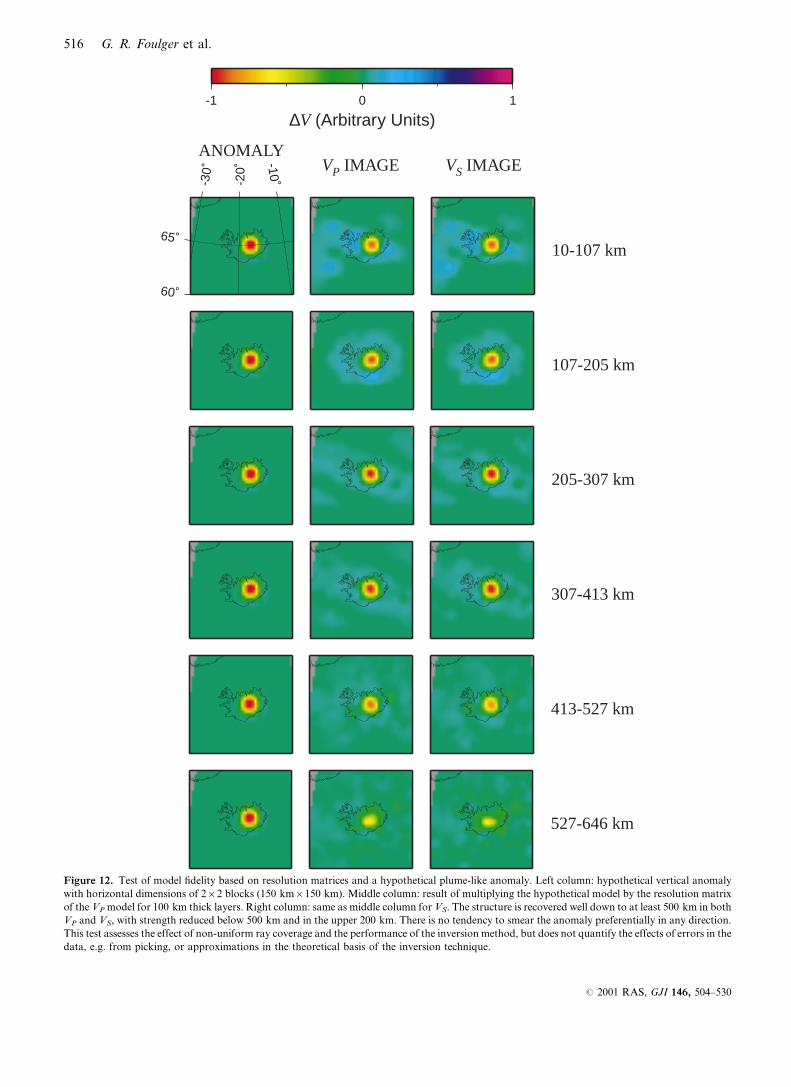
We tested whether we could faithfully image a simple,
vertical, cylindrical, plume-like anomaly with constant wave
speeds inside and outside. Fig. 12 shows the results of such
a test for an anomaly with horizontal dimensions of 2r2
blocks (150 kmr150 km) underlying central Iceland. The
result indicates that good resolution extends to depths of about
500 km in both VP and VS, and that there is little tendency
to distort the shape of the anomaly in any systematic way.
We performed tests of many such anomalies with different
diameters and locations, all of which confirm this conclusion.
-25Ê-20Ê
-15Ê-10Ê
60Ê62Ê
64Ê66Ê
68Ê
-500-
400-
300-
200-
100
0
-25Ê-20Ê
-15Ê-10Ê
60Ê62Ê
64Ê66Ê
68Ê
-500-
400-
300-
200-
100
0-5
00-
400-
300-
200-
100
0
-25Ê-20Ê
-15Ê-10Ê
60Ê62Ê
64Ê66Ê
68Ê
-500-
400-
300-
200-
100
0-5
00-
400-
300-
200-
100
0
-25Ê-20Ê
-15Ê-10Ê
60Ê62Ê
64Ê66Ê
68Ê
-500-
400-
300-
200-
100
0-5
00-
400-
300-
200-
100
0
-25Ê-20Ê
-15Ê-10Ê
60Ê62Ê
64Ê66Ê
68Ê
-500-
400-
300-
200-
100
0-5
00-
400-
300-
200-
100
0
-25Ê-20Ê
-15Ê-10Ê
60Ê62Ê
64Ê66Ê
68Ê
-500-
400-
300-
200-
100
0-5
00-
400-
300-
200-
100
0
Vp
Figure 10. ‘Volume metrics’ for five blocks from the final VP model (75 km wide blocks, 50 km thick layers), as seen looking downwards from the
southwest. Top: locations of the five blocks, which lie in the layer at about 250–300 km depth. The five lower boxes show how anomalies located in
the five black blocks are smeared (grey blocks) in the final model as a result of the ray distribution and the inversion method. The off-diagonal elements
of the resolution matrix corresponding to the grey blocks sum to 0.95.
514 G. R. Foulger et al.
# 2001 RAS, GJI 146, 504–530
We also tested the ability of our method to resolve structure
beneath the Tjornes Fracture Zone to the north of Iceland. We
found that such structure in the upper 100–300 km could be
resolved clearly to a distance of y50 km north of Iceland. There
was no tendency for computed anomalies to be terminated
artificially beneath the fracture zone.
R E S U L T S
Our final VP model is shown in Fig. 13. The most significant
feature is a coherent, low-VP body extending vertically down-
wards beneath east-central Iceland. This anomaly has a strength
of up to x2.7 per cent in the top layer (Fig. 13, layer L2), and
up to x2.1 per cent in deeper layers.
Wave-speed variations in the special first layer are as strong
as t5.5 per cent for VP and t8 per cent for VS, with little
spatial coherence in their values (Fig. 13, layer L1). Recent
explosion seismology, surface wave and receiver function work
suggests that the crust is thickest (up to about 40 km) in central
Iceland and thinner (around 25 km) beneath coastal areas
(Darbyshire et al. 1998; Allen et al. 1999; Du & Foulger 1999,
2001; Du et al. 2001). The wave-speed perturbations in the special
first layer show only very broadly such a trend, suggesting that
they reflect mostly the very shallow structure of the upper
10 km only. Crustal structure below this contributes to the top
layer of the tomographic image and to the strong VP anomalies
imaged there. It is a common problem in teleseismic tomo-
graphy that few rays cross at shallow depths and shallow
structure is thus poorly resolved. When an independently
determined model for the seismic structure of the crust over all
of Iceland becomes available, it will be possible to overcome
this limitation by explicitly correcting for the crust in our model.
There are no crossing rays in the upper y60 km of the
model, which includes layer 2. In this layer, the structure
determined is thus the smoothed perturbation field obtained
independently for each station. The low-wave-speed anomaly is
sharply truncated to the north, at the TFZ. It underlies the
NVZ, EVZ and MVZ, and is centred easterly within the MVZ,
-25Ê-20Ê
-15Ê-10Ê
60Ê62Ê
64Ê66Ê
68Ê
-500-
400-
300-
200-
100
0
-25Ê-20Ê
-15Ê-10Ê
60Ê62Ê
64Ê66Ê
68Ê
-500-
400-
300-
200-
100
0-5
00-
400-
300-
200-
100
0
-25Ê-20Ê
-15Ê-10Ê
60Ê62Ê
64Ê66Ê
68Ê
-500-
400-
300-
200-
100
0-5
00-
400-
300-
200-
100
0
-25Ê-20Ê
-15Ê-10Ê
60Ê62Ê
64Ê66Ê
68Ê
-500-
400-
300-
200-
100
0-5
00-
400-
300-
200-
100
0
-25Ê-20Ê
-15Ê-10Ê
60Ê62Ê
64Ê66Ê
68Ê
-500-
400-
300-
200-
100
0-5
00-
400-
300-
200-
100
0
-25Ê-20Ê
-15Ê-10Ê
60Ê62Ê
64Ê66Ê
68Ê
-500-
400-
300-
200-
100
0-5
00-
400-
300-
200-
100
0
Vs
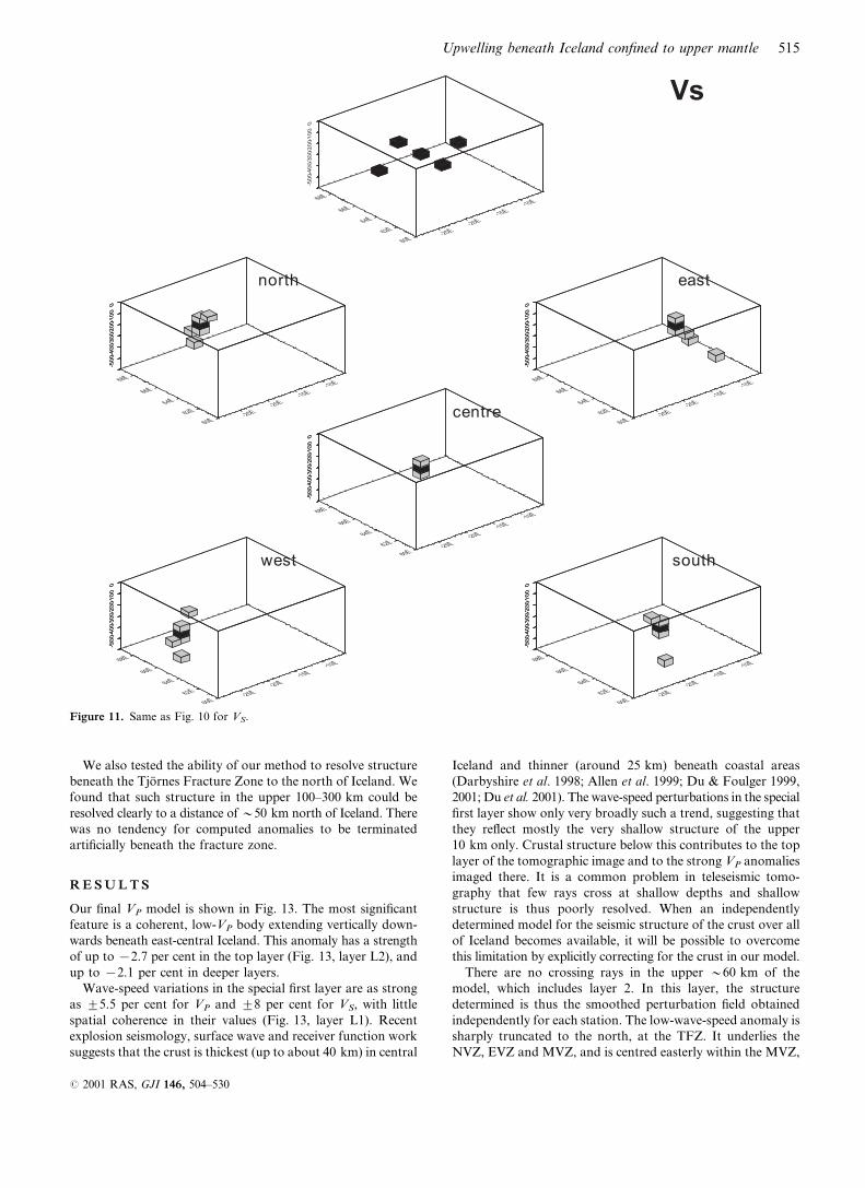
Figure 11. Same as Fig. 10 for VS.
Upwelling beneath Iceland confined to upper mantle 515
# 2001 RAS, GJI 146, 504–530
-1 0 1
∆V (Arbitrary Units)
ANOMALYVP IMAGE VS IMAGE
-30˚
-20˚
-10˚
60˚
65˚10-107 km
107-205 km
205-307 km
307-413 km
413-527 km
527-646 km
Figure 12. Test of model fidelity based on resolution matrices and a hypothetical plume-like anomaly. Left column: hypothetical vertical anomaly
with horizontal dimensions of 2r2 blocks (150 kmr150 km). Middle column: result of multiplying the hypothetical model by the resolution matrix
of the VP model for 100 km thick layers. Right column: same as middle column for VS. The structure is recovered well down to at least 500 km in both
VP and VS, with strength reduced below 500 km and in the upper 200 km. There is no tendency to smear the anomaly preferentially in any direction.
This test assesses the effect of non-uniform ray coverage and the performance of the inversion method, but does not quantify the effects of errors in the
data, e.g. from picking, or approximations in the theoretical basis of the inversion technique.
516 G. R. Foulger et al.
# 2001 RAS, GJI 146, 504–530

-25
o
-20
o
-15
o
64o
66o
L1 (special) vp=5.8 kms-1 d: 0-10 km
-2 -1 0 1 2
P velocity perturbation (%)
L2 vp=8.04 kms-1 d: 10-58 km
L3 vp=8.05 kms-1 d: 58-106 km
L4 vp=8.08 kms-1 d: 106-155 km
L5 vp=8.22 kms-1 d: 155-204 km
L6 vp=8.37 kms-1 d: 204-255 km
L7 vp=8.56 kms-1 d: 255-306 km
L8 vp=8.75 kms-1 d: 306-359 km
L9 vp=8.94 kms-1 d: 359-412 km
L10 vp=9.46 kms-1 d: 412-469 km
L11 vp=9.66 kms-1 d: 469-526 km
L12 vp=9.85 kms-1 d: 526-586 km
L13 vp=10.06 kms-1 d: 586-646 km
0
100
200
300
400
500
600
de
pth
(km
)
0 100200300400500600700800900
km along section
02000
Elevation along profile (m)
0
100
200
300
400
500
600
de
pth
(km
)
0 100200300400500600700800900
km along section
02000
Elevation along profile (m)
0
100
200
300
400
500
600
de
pth
(km
)
0 100200300400500600700800900
km along section
02000
Elevation along profile (m)D
E
F
B
C
D'
E’
F’
0
100
200
300
400
500
600
de
pth
(km
)
0 100200300400500600700800900
km along section
02000
Elevation along profile (m)A A’
B’
C’
0
0
100
100
200
200
300
300
400
400
500
500
600
600
de
pth
(km
)d
ep
th(k
m)
0
0
100
100
200
200
300
300
400
400
500
500
600
600
700
700
800
800
900
900
km along section
km along section
0
0
2000
2000
Elevation along profile (m)
Elevation along profile (m)
Figure 13. Horizontal (left and middle columns) and vertical (right column) sections through the final VP model, which uses 75 km wide blocks and
50 km thick layers and was computed using the offset-and-averaging technique with n=2. The colour scale shows the percentage difference from VP at
the corresponding depth in the initial (IASP91) wave-speed model. The starting wave speed and the depth range are given beneath each horizontal
section. Dotted black lines show the region within which resolution (the diagonal element of R) is i 0.7. Maps are plotted in azimuthal-equidistant
projection. Unmodelled areas are pale green or white. Top left: wave-speed perturbations in the ‘special first layer’; top right: map showing lines of
vertical sections.
Upwelling beneath Iceland confined to upper mantle 517
# 2001 RAS, GJI 146, 504–530
between the glaciers Vatnajokull and Hofsjokull. A small, local,
low-VP anomaly occurs beneath the Northwest Fjords area.
The area where VP is depressed by more than 1 per cent relative
to the surrounding areas has a diameter of 200–250 km.
In the depth interval y50–250 km, the low-VP anomaly
underlies northwest Vatnajokull, the NVZ, EVZ and MVZ
(Fig. 13, layers L3–L6). It extends beneath all of the MVZ at all
depths, but is not everywhere continuous beneath the NVZ and
EVZ. As a result, it is elongated east–west in some layers, most
notably at depths of y50–100 and y150–200 km. A weak
low-VP anomaly underlies the Reykjanes ridge, southwest of
Iceland, at all depths (Fig. 13, Section CCk). This part of our
image is peripheral and the least reliable. The TFZ, in contrast,
is well resolved in the upper y450 km because of the presence
of the station Grimsey off the north coast of the mainland
(Fig. 1). The TFZ is underlain by relatively high-VP material in
the upper y100 km (Fig. 13, section AAk), but beneath this VP
is low.
Beneath y250 km, the morphology of the low-VP anomaly
changes systematically. Instead of being cylindrical, with a
quasi-circular or east–west elongated shape in map view, it
becomes elongated north–south. This is clear in all horizontal
sections below this depth, down to the limit of moderate
resolution at y450 km (Fig. 13, layers L7–L10). This change
from cylindrical to tabular morphology is particularly clear
in cross-section. Section AAk of Fig. 13 runs south–north and
clearly shows the anomaly widening with depth, whereas the
west–east section DDk shows the anomaly narrowing with depth.
The volume metrics show an equal tendency for the inversion
to smear anomalies radially outwards and downwards in all
directions, which suggests that this anomaly shape is not a result
of smearing. Furthermore, images of hypothetical anomalies
(Fig. 12) show no tendency to elongate real anomalies north–
south. This supports our inference that the azimuthally
asymmetric morphology we observe is real.
Because the maximum aperture of our array is y450 km,
structure imaged at depths greater than this is poorly resolved,
and heavily influenced by downward smearing. This is a conse-
quence of the inherent geometric weakness of teleseismic tomo-
graphy, and stems from the fact that there are few crossing rays
at great depth. Thus, despite the fact that the formal resolution
is good in some parts of our model at greater depth, we do not
attach significance to those parts of our model deeper than
y450 km, but show these results for information only. The
low-wave-speed anomaly we image persists from the surface
down to at least y450 km depth, and thus our experiment does
not image the base of the anomaly.
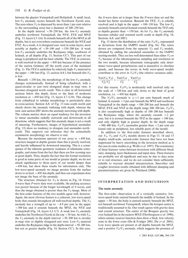
The structure obtained for VS is shown in Fig. 14. Fewer
S-wave than P-wave data were available, the picking accuracy
was poorer because of the longer wavelength of S waves, and
thus the image obtained is poorer than the VP image. Most of
the first-order features of the two models agree well, however.
Again, the most obvious feature is a coherent, low-wave-speed
body that extends throughout all well-resolved depths. The VS
anomaly has a strength of up to x4.9 per cent in the upper
y300 km and it extends beneath the MVZ, the NVZ and
Vatnajokull (Fig. 14, layers L2–L7). A weak low-VS anomaly
underlies the Northwest Fjords in the top y50 km. As with VP,
the VS anomaly in the depth interval y50–200 km is circular
in map view or slightly elongated east–west. Low-VS material
underlies the Reykjanes ridge in the depth interval y50–200 km,
but not at greater depths (Fig. 14, Section CCk). In this area,
the S-wave data set is larger than the P-wave data set and the
model has better resolution. Beneath the TFZ, VS is reliably
resolved and is high in the upper y100–150 km. The low-VS
anomaly beneath central Iceland extends beneath the TFZ only
at depths greater than y150 km. As for VP, the VS anomaly
becomes tabular and oriented north–south at depth (Fig. 14,
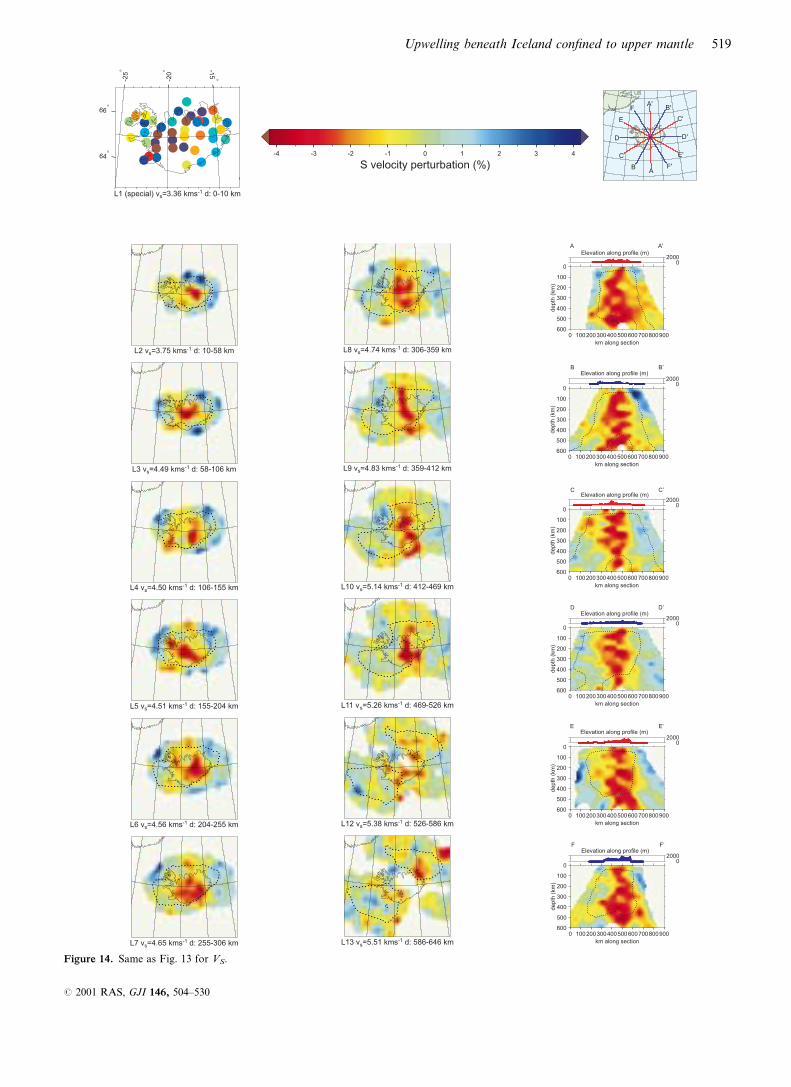
Sections AAk and DDk).Fig. 15 shows the distribution of the ratio VP/VS, represented
as deviations from the IASP91 model (Fig. 16). The ratios
shown are computed from the separate VP and VS models,
obtained by adding the calculated anomalies to the IASP91
starting models. They are less well determined than either VP or
VS because of the inhomogeneous sampling and resolution in
the two models, because teleseismic tomography only deter-
mines wave-speed perturbations and is insensitive to absolute
speeds, and because the errors in both wave-speed models
contribute to the error in VP /VS (the relative variances add),
Var(VP=VS)V2
P=V2S
~Var(VP)
V2P
zVar(VS)
V2S
:
For this reason, VP /VS is moderately well resolved only on
the scale of y100 km and only down to the limit of good
resolution, i.e. y450 km depth.
The VP /VS anomaly is i+1 per cent beneath much of
Iceland. It exceeds +3 per cent beneath the MVZ and northwest
Vatnajokull in the depth range y100–200 km and beneath the
MVZ, EVZ and NVZ in the depth range 200–300 km. VP/VS
is also exceptionally high at depths of 100–200 km beneath
the Reykjanes ridge, where the anomaly exceeds +2 per
cent, but it is normal beneath the TFZ in the upper y100 km,
and only slightly high at greater depth. In the depth range
y300–400 km, VP/VS anomalies greater than +2 per cent are
found only in peripheral, less reliable parts of the model.
In addition to the first-order features described above,
our VP, VS and VP/VS models shown in Figs 13, 14 and 15
display small-scale, second-order features that have not been
suppressed by heavy smoothing in the inversion method as is
the case in some studies (e.g. Wolfe et al. 1997). The consistency
of these features varies between inversions with different block
sizes, damping, layer thicknesses and input data. These features
are probably not all significant and may be due to data noise
or to real structure, and we do not consider them sufficiently
reliable to warrant detailed interpretation. Smoother and
rougher inversion results obtained with different damping and
parametrizations are given by Pritchard (2000).
I N T E R P R E T A T I O N A N D D I S C U S S I O N
The main anomaly
The first-order observation is of a vertically extensive, low-
wave-speed body centred beneath the middle of Iceland. In the
upper y50 km, the body is centred easterly beneath the MVZ,
not beneath northwest Vatnajokull, where the hotspot centre is
traditionally assumed to lie. Our result agrees with gravity data
and crustal structure. The centre of the Bouguer gravity low
over Iceland lies in the eastern MVZ (Thorbergsson et al. 1990),
where seismic receiver-function data show a thick, low-velocity
zone in the lower crust (Du & Foulger 2001; Du et al. 2001).
Low wave speeds are present at all depths beneath the MVZ,
and a positive VP /VS anomaly, which suggests the presence of
518 G. R. Foulger et al.
# 2001 RAS, GJI 146, 504–530
-25
o
-20
o
-15
o
64o
66o
L1 (special) vs=3.36 kms-1 d: 0-10 km
-4 -3 -2 -1 0 1 2 3 4
S velocity perturbation (%)
L2 vs=3.75 kms-1 d: 10-58 km
L3 vs=4.49 kms-1 d: 58-106 km
L4 vs=4.50 kms-1 d: 106-155 km
L5 vs=4.51 kms-1 d: 155-204 km
L6 vs=4.56 kms-1 d: 204-255 km
L7 vs=4.65 kms-1 d: 255-306 km
L8 vs=4.74 kms-1 d: 306-359 km
L9 vs=4.83 kms-1 d: 359-412 km
L10 vs=5.14 kms-1 d: 412-469 km
L11 vs=5.26 kms-1 d: 469-526 km
L12 vs=5.38 kms-1 d: 526-586 km
L13 vs=5.51 kms-1 d: 586-646 km
0
100
200
300
400
500
600
depth
(km
)
0 100200300400500600700800900
km along section
02000
Elevation along profile (m)
A
B
C
D
A'
B’
C’
D’
0
100
200
300
400
500
600
depth
(km
)
0 100200300400500600700800900
km along section
02000
Elevation along profile (m)
0
100
200
300
400
500
600
depth
(km
)
0 100200300400500600700800900
km along section
02000
Elevation along profile (m)
0
100
200
300
400
500
600
depth
(km
)
0 100200300400500600700800900
km along section
02000
Elevation along profile (m)
0
100
200
300
400
500
600
depth
(km
)
0 100200300400500600700800900
km along section
02000
Elevation along profile (m)E
F
E'
F’
0
100
200
300
400
500
600
depth
(km
)
0 100200300400500600700800900
km along section
02000
Elevation along profile (m)
Figure 14. Same as Fig. 13 for VS.
Upwelling beneath Iceland confined to upper mantle 519
# 2001 RAS, GJI 146, 504–530
partial melt, occupies the depth range y100–200 km. In con-
trast, the anomaly is discontinuous beneath the NVZ and EVZ,
suggesting that these linear zones may be fed laterally by a
central upwelling. The WVZ is peripheral to the main, low-
wave-speed body at most depths, in keeping with the view that
it is a declining rift (Sigmundsson et al. 1994). A subsidiary,
15 mGal Bouguer gravity low is associated with the Northwest
Fjords area, where we image local low VP and VS anomalies in
the upper y50 km.
A number of factors affect seismic wave speeds. High
temperature reduces VP by y0.9 per cent per 100 K and VS by
1.2–1.8 times this (Anderson 1989; Faul et al. 1994; Ito et al.
1996; Goes et al. 2000). Numerical plume models for Iceland
predict temperature anomalies of 70 to 250 K (e.g. Sleep 1990;
Feighner & Kellogg 1995; Ribe et al. 1995; White et al. 1995),
which correspond to anomalies in VP of 0.6–2.2 per cent and in
VP /VS of up to 2.1 per cent. The anomalies we observe are
locally up to about x2 per cent in VP and +3.7 per cent in VP /
VS, although the bulk of the low-wave-speed body has an
anomaly in VP of 0.5–1.5 per cent and in VP/VS of y1 per cent
(Figs 13 and 15).
The wave-speed anomalies cannot be caused solely by
elevated temperatures, since VS anomalies of up to 4.9 per
cent would imply temperature anomalies of up to y300 K,
thought to be an unrealistically high value. Furthermore, VP/VS
-25
o
-20
o
-15
o
64o
66o
L1 (special) vp/vs=1.73 d: 0-10 km
-5 -4 -3 -2 -1 0 1 2 3 4 5
Vp/Vs perturbation (%)
L2 vp/vs=1.80 d: 10-107 km
L3 vp/vs=1.81 d: 107-204 km
L4 vp/vs=1.84 d: 204-306 km
L5 vp/vs=1.85 d: 306-412 km
L6 vp/vs=1.84 d: 412-527 km
L7 vp/vs=1.83 d: 527-646 km
0
100
200
300
400
500
600
depth
(km
)
0 100200300400500600700800900
km along section
02000
Elevation along profile (m)
0
100
200
300
400
500
600
depth
(km
)
0 100200300400500600700800900
km along section
02000
Elevation along profile (m)
0
100
200
300
400
500
600
depth
(km
)
0 100200300400500600700800900
km along section
02000
Elevation along profile (m)C
B
A
C'
B’
A’
0
100
200
300
400
500
600
depth
(km
)
0 100200300400500600700800900
km along section
02000
Elevation along profile (m)D
E
F
D'
E’
F’
0
100
200
300
400
500
600
depth
(km
)
0 100200300400500600700800900
km along section
02000
Elevation along profile (m)
0
100
200
300
400
500
600
depth
(km
)
0 100200300400500600700800900
km along section
02000
Elevation along profile (m)
Figure 15. Same as Fig. 13 for VP/VS, for the offset-and-averaged
model with 75 km wide blocks and layers 100 km thick.
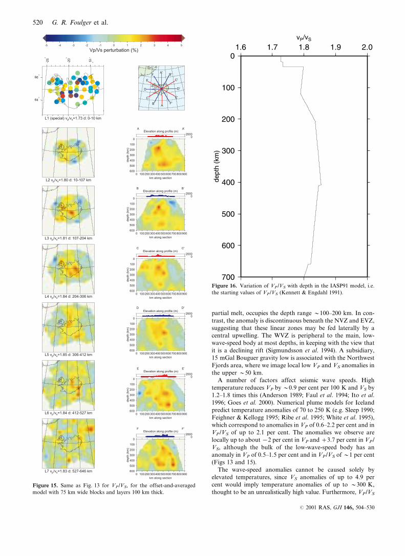
Figure 16. Variation of VP/VS with depth in the IASP91 model, i.e.
the starting values of VP/VS (Kennett & Engdahl 1991).
520 G. R. Foulger et al.
# 2001 RAS, GJI 146, 504–530

anomalies of only up to y2.5 per cent would be expected.
Partial melt is a candidate explanation for the observations, as
it depresses VS more strongly than VP (Anderson 1989; Karato
1993). The effect of melt on seismic wave speeds is difficult to
assess quantitatively, because it depends strongly on the geo-
metry of the melt bodies, with tabular shapes such as dykes,
sills and thin films having about twice the effect of tubular
shapes (Spetzler & Anderson 1968; Anderson & Sammis 1970;
Faul et al. 1994). Melt may form at grain boundaries as both
films and pockets (Faul et al. 1994). Under these circumstances,
a decrease of y3.4 per cent in VP and 7.8 per cent in VS for
each 1 per cent increase in melt is a reasonable estimate (Goes
et al. 2000). In the upper y300 km of the central core of the
body, where the VP/VS anomaly is strong, the observations are
most readily explained by temperature anomalies significantly
lower than 200 K and a few tenths of a per cent partial melt.
Such an amount is insufficient for percolation to take place
(Faul et al. 1994; Schmeling 2000). The outer parts of the body
can be explained by lower temperature anomalies and per cent
partial melt. Regions where VP /VS is highest and VP lowest are
the most likely sites for partial melt. These underlie the MVZ
and northwest Vatnajokull in the depth range y100–200 km,
and the NVZ and EVZ in the depth range y200–300 km.
The degree of partial melting suggested by our observations
is smaller, and the depth range greater, than predicted for
spreading plate boundaries and plumes. Melt fractions up to
y20 per cent are predicted to occupy zones a few tens of kilo-
metres high in the upper y70 km beneath ridges and y120 km
of plumes (Iwamori et al. 1995; Shen & Forsyth 1995; White &
McKenzie 1995; Ito et al. 1996; Schmeling 2000). Such zones
are too small to be resolved by teleseismic tomography, which
will, at best, average them over a large volume. However, the
distribution of low-concentration partial melt beneath hotspots
and ridges is not strongly constrained by physical plume models
(McKenzie & Bickle 1988). Our observations are consistent
with Iceland being underlain by an extensive volume of low-
degree partial melt that extends at least throughout the sub-
lithospheric low-velocity zone in the depth interval 190–250 km
(Gutenberg 1959; Anderson & Bass 1984; Anderson 1989).
Other factors expected to affect seismic wave speeds in a
volcanic environment are chemical heterogeneity, including
chemical depletion, and anisotropy. The possibility that com-
positional variation might contribute to the observed anomalies
cannot be ruled out. Depletion is the removal of basalt from
the parent rock. VP increases by y0.5 per cent per 10 per cent
depletion (Goes et al. 2000), and partial melting levels of up
to y20 per cent are predicted locally beneath Iceland (White &
McKenzie 1995). However, the parent volume must be con-
tinuously replenished by flow from deeper levels if erupted
lavas are not to become progressively depleted with time, and if
melt production is not eventually to dwindle and cease, trends
that are not observed. The degree of depletion beneath Iceland
is thus not certain, nor is its expected effect on seismic wave
speeds.
Anisotropy is expected at mid-ocean ridges because flow
aligns olivine crystals so that the crystallographic a-axes [100]
lie parallel to the flow direction. This causes VP and VS to be
higher for waves propagating parallel to the direction of flow
than normal to it. Such anisotropy might be as strong as +7 per
cent (e.g. Anderson 1989; Kendall 1994). A simplistic model for
a plume beneath Iceland would predict vertical upward flow
within a central core and radially outward flow in the upper
50–100 km. Superimposed on the shallow, radial flow pattern
might be bilaterally symmetric flow away from the spreading
plate boundary. Such a pattern of flow might increase vertical
wave speeds in the plume core, where rays are subvertical. Thus
the negative wave-speed anomalies we observe there, of up to
x2.1 per cent in VP and x4.9 per cent in VS, if corrected for
anisotropy, might be as strong as x9 and x12 per cent. In the
topmost y100 km, dykes and flow-induced anisotropy might
strengthen the negative anomalies observed, since horizontal
flow aligns the slow b-axis vertically. However, the few obser-
vations of upper mantle anisotropy currently available for
Iceland fail to support the simple flow model described above
(Bjarnason et al. 1996), so this effect cannot yet be assessed
quantitatively.
Structure beneath the Reykjanes ridge and the TjornesFracture Zone
We observe a negative VP anomaly of up to yx0.5 per cent
at all depths beneath the Reykjanes ridge close to Iceland.
Resolution in VS is superior in this part of the model, and
shows an anomaly of up to yx2.5 per cent in the depth range
y50–200 km. In this region, the VP/VS anomaly is up to
+2.4 per cent, which is consistent with the presence of up to a
few tenths of a per cent of partial melt. The Reykjanes ridge is
peripheral to our study volume and is poorly imaged. However,
the structure imaged beneath it contrasts with that observed
beneath other seaward parts of our study volume, for example,
to the west and east of Iceland (Figs 13 and 14, section DDk).This structure is also expected on geological grounds, and is
thus probably real.
The structure found beneath the TFZ to the north is well
resolved and contrasts sharply with that beneath the Reykjanes
ridge. Both VP and VS are normal or high in the upper
100–200 km. At greater depths, the low-wave-speed body imaged
beneath central Iceland extends to the north of the TFZ. The
positive VP /VS anomaly is, however, no stronger than y+1 per
cent anywhere beneath this region, and thus partial melting is
not required to explain the observations.
The structures we observe beneath the Reykjanes ridge and
the TFZ agree with predictions that melt may be channelled
beneath ridges and blocked by fracture zones (e.g. Vogt 1976;
Schilling et al. 1985; Schilling 1991; Ribe et al. 1995; Sleep
1996, 1997). Material is thought to flow unimpeded from
beneath central Iceland southwestwards along the Reykjanes
ridge at shallow depth, and to cause the topographic uplift and
enhanced on-ridge volcanism observed there. The structure
we observe beneath the TFZ supports the prediction that this
fracture zone blocks the lateral flow of melt. This close agree-
ment with geological ground truth in peripheral parts of our
study volume strengthens confidence in our results in general.
Nature of the anomaly beneath Iceland
The most significant feature of the anomaly is its change
in shape from cylindrical to tabular at about 250 km depth
beneath Iceland. Several geodynamic models predict such a
change in morphology, including buoyant upwelling, passive
infilling of a widening rift, convection resulting from lateral
temperature gradients, heating from below or cooling from
above. All these models imply that the anomaly is caused by
a buoyant upwelling whose origin is approached at the depth
Upwelling beneath Iceland confined to upper mantle 521
# 2001 RAS, GJI 146, 504–530
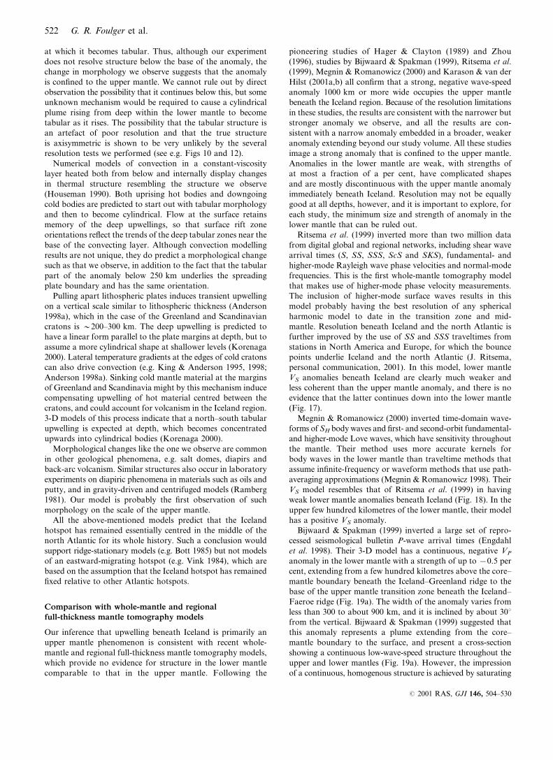
at which it becomes tabular. Thus, although our experiment
does not resolve structure below the base of the anomaly, the
change in morphology we observe suggests that the anomaly
is confined to the upper mantle. We cannot rule out by direct
observation the possibility that it continues below this, but some
unknown mechanism would be required to cause a cylindrical
plume rising from deep within the lower mantle to become
tabular as it rises. The possibility that the tabular structure is
an artefact of poor resolution and that the true structure
is axisymmetric is shown to be very unlikely by the several
resolution tests we performed (see e.g. Figs 10 and 12).
Numerical models of convection in a constant-viscosity
layer heated both from below and internally display changes
in thermal structure resembling the structure we observe
(Houseman 1990). Both uprising hot bodies and downgoing
cold bodies are predicted to start out with tabular morphology
and then to become cylindrical. Flow at the surface retains
memory of the deep upwellings, so that surface rift zone
orientations reflect the trends of the deep tabular zones near the
base of the convecting layer. Although convection modelling
results are not unique, they do predict a morphological change
such as that we observe, in addition to the fact that the tabular
part of the anomaly below 250 km underlies the spreading
plate boundary and has the same orientation.
Pulling apart lithospheric plates induces transient upwelling
on a vertical scale similar to lithospheric thickness (Anderson
1998a), which in the case of the Greenland and Scandinavian
cratons is y200–300 km. The deep upwelling is predicted to
have a linear form parallel to the plate margins at depth, but to
assume a more cylindrical shape at shallower levels (Korenaga
2000). Lateral temperature gradients at the edges of cold cratons
can also drive convection (e.g. King & Anderson 1995, 1998;
Anderson 1998a). Sinking cold mantle material at the margins
of Greenland and Scandinavia might by this mechanism induce
compensating upwelling of hot material centred between the
cratons, and could account for volcanism in the Iceland region.
3-D models of this process indicate that a north–south tabular
upwelling is expected at depth, which becomes concentrated
upwards into cylindrical bodies (Korenaga 2000).
Morphological changes like the one we observe are common
in other geological phenomena, e.g. salt domes, diapirs and
back-arc volcanism. Similar structures also occur in laboratory
experiments on diapiric phenomena in materials such as oils and
putty, and in gravity-driven and centrifuged models (Ramberg
1981). Our model is probably the first observation of such
morphology on the scale of the upper mantle.
All the above-mentioned models predict that the Iceland
hotspot has remained essentially centred in the middle of the
north Atlantic for its whole history. Such a conclusion would
support ridge-stationary models (e.g. Bott 1985) but not models
of an eastward-migrating hotspot (e.g. Vink 1984), which are
based on the assumption that the Iceland hotspot has remained
fixed relative to other Atlantic hotspots.
Comparison with whole-mantle and regionalfull-thickness mantle tomography models
Our inference that upwelling beneath Iceland is primarily an
upper mantle phenomenon is consistent with recent whole-
mantle and regional full-thickness mantle tomography models,
which provide no evidence for structure in the lower mantle
comparable to that in the upper mantle. Following the
pioneering studies of Hager & Clayton (1989) and Zhou
(1996), studies by Bijwaard & Spakman (1999), Ritsema et al.
(1999), Megnin & Romanowicz (2000) and Karason & van der
Hilst (2001a,b) all confirm that a strong, negative wave-speed
anomaly 1000 km or more wide occupies the upper mantle
beneath the Iceland region. Because of the resolution limitations
in these studies, the results are consistent with the narrower but
stronger anomaly we observe, and all the results are con-
sistent with a narrow anomaly embedded in a broader, weaker
anomaly extending beyond our study volume. All these studies
image a strong anomaly that is confined to the upper mantle.
Anomalies in the lower mantle are weak, with strengths of
at most a fraction of a per cent, have complicated shapes
and are mostly discontinuous with the upper mantle anomaly
immediately beneath Iceland. Resolution may not be equally
good at all depths, however, and it is important to explore, for
each study, the minimum size and strength of anomaly in the
lower mantle that can be ruled out.
Ritsema et al. (1999) inverted more than two million data
from digital global and regional networks, including shear wave
arrival times (S, SS, SSS, ScS and SKS), fundamental- and
higher-mode Rayleigh wave phase velocities and normal-mode
frequencies. This is the first whole-mantle tomography model
that makes use of higher-mode phase velocity measurements.
The inclusion of higher-mode surface waves results in this
model probably having the best resolution of any spherical
harmonic model to date in the transition zone and mid-
mantle. Resolution beneath Iceland and the north Atlantic is
further improved by the use of SS and SSS traveltimes from
stations in North America and Europe, for which the bounce
points underlie Iceland and the north Atlantic (J. Ritsema,
personal communication, 2001). In this model, lower mantle
VS anomalies beneath Iceland are clearly much weaker and
less coherent than the upper mantle anomaly, and there is no
evidence that the latter continues down into the lower mantle
(Fig. 17).
Megnin & Romanowicz (2000) inverted time-domain wave-
forms of SH body waves and first- and second-orbit fundamental-
and higher-mode Love waves, which have sensitivity throughout
the mantle. Their method uses more accurate kernels for
body waves in the lower mantle than traveltime methods that
assume infinite-frequency or waveform methods that use path-
averaging approximations (Megnin & Romanowicz 1998). Their
VS model resembles that of Ritsema et al. (1999) in having
weak lower mantle anomalies beneath Iceland (Fig. 18). In the
upper few hundred kilometres of the lower mantle, their model
has a positive VS anomaly.
Bijwaard & Spakman (1999) inverted a large set of repro-
cessed seismological bulletin P-wave arrival times (Engdahl
et al. 1998). Their 3-D model has a continuous, negative VP
anomaly in the lower mantle with a strength of up to x0.5 per
cent, extending from a few hundred kilometres above the core–
mantle boundary beneath the Iceland–Greenland ridge to the
base of the upper mantle transition zone beneath the Iceland–
Faeroe ridge (Fig. 19a). The width of the anomaly varies from
less than 300 to about 900 km, and it is inclined by about 30ufrom the vertical. Bijwaard & Spakman (1999) suggested that
this anomaly represents a plume extending from the core–
mantle boundary to the surface, and present a cross-section
showing a continuous low-wave-speed structure throughout the
upper and lower mantles (Fig. 19a). However, the impression
of a continuous, homogenous structure is achieved by saturating
522 G. R. Foulger et al.
# 2001 RAS, GJI 146, 504–530
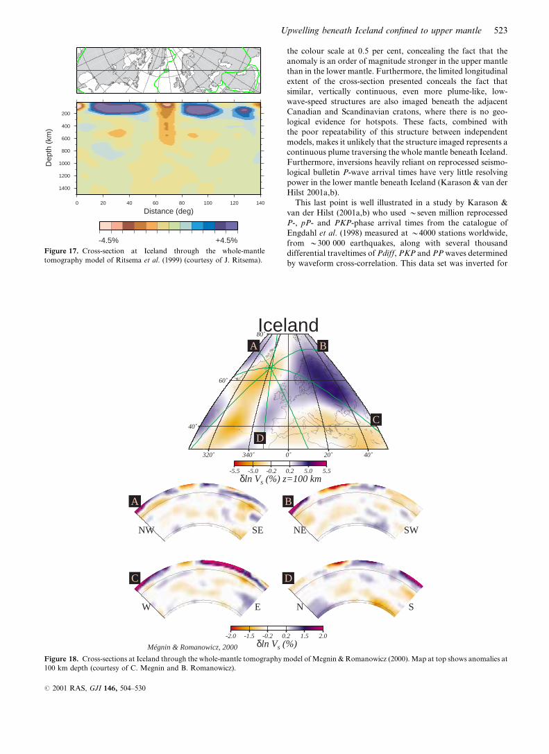
the colour scale at 0.5 per cent, concealing the fact that the
anomaly is an order of magnitude stronger in the upper mantle
than in the lower mantle. Furthermore, the limited longitudinal
extent of the cross-section presented conceals the fact that
similar, vertically continuous, even more plume-like, low-
wave-speed structures are also imaged beneath the adjacent
Canadian and Scandinavian cratons, where there is no geo-
logical evidence for hotspots. These facts, combined with
the poor repeatability of this structure between independent
models, makes it unlikely that the structure imaged represents a
continuous plume traversing the whole mantle beneath Iceland.
Furthermore, inversions heavily reliant on reprocessed seismo-
logical bulletin P-wave arrival times have very little resolving
power in the lower mantle beneath Iceland (Karason & van der
Hilst 2001a,b).
This last point is well illustrated in a study by Karason &
van der Hilst (2001a,b) who used yseven million reprocessed
P-, pP- and PKP-phase arrival times from the catalogue of
Engdahl et al. (1998) measured at y4000 stations worldwide,
from y300 000 earthquakes, along with several thousand
differential traveltimes of Pdiff, PKP and PP waves determined
by waveform cross-correlation. This data set was inverted for
200
400
600
800
1000
1200
1400
0 20 40 60 80 100 120 140
Dep
th (
km)
Distance (deg)
-4.5% +4.5%Figure 17. Cross-section at Iceland through the whole-mantle
tomography model of Ritsema et al. (1999) (courtesy of J. Ritsema).
320 340˚ 0˚ 20˚ 40˚
40˚
60˚
80˚
A B
C
D
Iceland
-5.5 -5.0 -0.2 0.2 5.0 5.5δln Vs (%) z=100 km
NW SE
A
NE SW
B
W E
C
N S
D
-2.0 -1.5 -0.2 0.2 1.5 2.0δln Vs (%)Mégnin & Romanowicz, 2000
Figure 18. Cross-sections at Iceland through the whole-mantle tomography model of Megnin & Romanowicz (2000). Map at top shows anomalies at
100 km depth (courtesy of C. Megnin and B. Romanowicz).
Upwelling beneath Iceland confined to upper mantle 523
# 2001 RAS, GJI 146, 504–530

global mantle structure using 3-D sensitivity kernels and local
basis functions of variable size (Fig. 19b). Beneath Iceland, a
low-wave-speed anomaly of up to 2 per cent is detected that
extends from the surface down to the base of the upper mantle
and no deeper (Fig. 19b, cross-section at lower left). In order to
study the variation in resolution in the mantle beneath Iceland,
and specifically to investigate if a deeper structure could be
detected if it existed, rays were traced through a theoretical
plume-like structure (Fig. 19b, cross-section at lower middle)
to generate synthetic data. The theoretical structure extends
from the surface to 1500 km depth, and has a wave-speed
anomaly of 2 per cent in the upper mantle and 1 per cent in
the lower mantle. The synthetic data were inverted to test
for anomaly retrieval (Fig. 19b, cross-section at lower right).
Retrieval of the anomaly is good above y400 km, partial in
the transition zone, but poor in the lower mantle. Inversion
parameters can perhaps be found that would recover better this
particular theoretical structure, but this example (H. Karason
& R. D. van der Hilst, personal communication, 2001) illustrates
that, with this data set, and that of Bijwaard & Spakman
(1999) because of the paucity of rays sampling the lower mantle
beneath Iceland, resolution there is very poor. This analysis
illustrates the non-uniformity of data coverage, and thus
resolution, in mantle tomography images, and the importance
of assessing resolution prior to interpreting the results.
Presently available tomography models using spherical
harmonic basis functions cannot resolve the sizes of bodies
smaller than y1000 km in diameter. Smaller bodies can be
detected if they are strong, but they become smeared over
broad regions. For example, low-wave-speed bodies underlying
the mid-Atlantic ridge are imaged, but smeared over distances
of y1000 km, although regional and local-scale studies show
them to be much narrower. Models that use local rather than
spherical harmonic basis functions can resolve the sizes of
smaller bodies. In addition, low-wave-speed bodies are more
difficult to detect using tomography than high-wave-speed
bodies because rays passing through a low-wave-speed body
may not arrive first at stations. Beneath Iceland, ray coverage
in the lower mantle is sparse for direct P waves, compared with
the upper mantle, and the use of additional phases and higher-
mode surface waves is necessary to achieve good resolution in
the transition zone and uppermost lower mantle. Mindful of
these caveats, it remains the case that none of the presently
available tomographic models of the whole mantle shows
evidence of continuation into the lower mantle of the structure
imaged in the upper mantle beneath Iceland.
Depth 410 km
I II
0
410 660
2000
I II I II0
410 660
2000
I II
(−1.0%) slow fast (+1.0%)
(a)
(b)
Figure 19. (a) Cross section through the Iceland region showing
the full-thickness mantle P-wave tomographic model of Bijwaard &
Spakman (1999). Upper panel shows line of cross section and lower
panel shows cross section through the mantle. The impression of a
uniform structure that is continuous from the surface to the core-
mantle boundary is achieved by saturating the colour scale at y10%
of the maximum anomaly in the upper mantle. The limited lateral
extent of the cross section conceals the fact that anomalies of a similar
strength in the lower mantle underlie the adjacent Scandinavian
and Canadian cratons (adapted from Bijwaard & Spakman, 1999).
(b) Cross-sections at Iceland through the full-thickness mantle tomo-
graphy model of Karason & van der Hilst (2001a,b). Map at top shows
anomalies at 410 km depth. Row of cross-sections shows (left) inversion
results and (middle) model of a theoretical plume-like anomaly extend-
ing from the surface to 1500 km depth, with wave speed 2 per cent low
in the upper mantle and 1 per cent low in the lower mantle. Rays were
traced through this model. Right: model retrieved from inversion of
rays traced through the theoretical model shown in the middle cross-
section. The same inversion parameters were used as for the model
shown in the left cross-section (figure courtesy of Hrafnkell Karason).
524 G. R. Foulger et al.
# 2001 RAS, GJI 146, 504–530
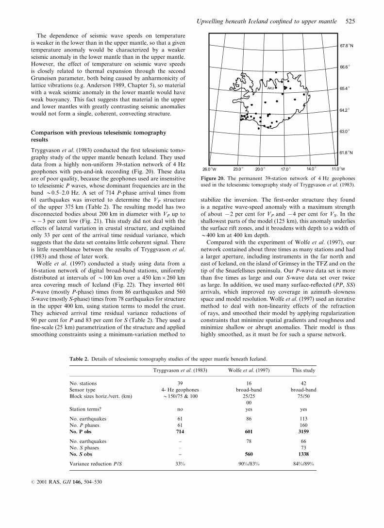
The dependence of seismic wave speeds on temperature
is weaker in the lower than in the upper mantle, so that a given
temperature anomaly would be characterized by a weaker
seismic anomaly in the lower mantle than in the upper mantle.
However, the effect of temperature on seismic wave speeds
is closely related to thermal expansion through the second
Gruneisen parameter, both being caused by anharmonicity of
lattice vibrations (e.g. Anderson 1989, Chapter 5), so material
with a weak seismic anomaly in the lower mantle would have
weak buoyancy. This fact suggests that material in the upper
and lower mantles with greatly contrasting seismic anomalies
would not form a single, coherent, convecting structure.
Comparison with previous teleseismic tomographyresults
Tryggvason et al. (1983) conducted the first teleseismic tomo-
graphy study of the upper mantle beneath Iceland. They used
data from a highly non-uniform 39-station network of 4 Hz
geophones with pen-and-ink recording (Fig. 20). These data
are of poor quality, because the geophones used are insensitive
to teleseismic P waves, whose dominant frequencies are in the
band y0.5–2.0 Hz. A set of 714 P-phase arrival times from
61 earthquakes was inverted to determine the VP structure
of the upper 375 km (Table 2). The resulting model has two
disconnected bodies about 200 km in diameter with VP up to
yx3 per cent low (Fig. 21). This study did not deal with the
effects of lateral variation in crustal structure, and explained
only 33 per cent of the arrival time residual variance, which
suggests that the data set contains little coherent signal. There
is little resemblance between the results of Tryggvason et al.
(1983) and those of later work.
Wolfe et al. (1997) conducted a study using data from a
16-station network of digital broad-band stations, uniformly
distributed at intervals of y100 km over a 450 kmr260 km
area covering much of Iceland (Fig. 22). They inverted 601
P-wave (mostly P-phase) times from 86 earthquakes and 560
S-wave (mostly S-phase) times from 78 earthquakes for structure
in the upper 400 km, using station terms to model the crust.
They achieved arrival time residual variance reductions of
90 per cent for P and 83 per cent for S (Table 2). They used a
fine-scale (25 km) parametrization of the structure and applied
smoothing constraints using a minimum-variation method to
stabilize the inversion. The first-order structure they found
is a negative wave-speed anomaly with a maximum strength
of about x2 per cent for VP and x4 per cent for VS. In the
shallowest parts of the model (125 km), this anomaly underlies
the surface rift zones, and it broadens with depth to a width of
y400 km at 400 km depth.
Compared with the experiment of Wolfe et al. (1997), our
network contained about three times as many stations and had
a larger aperture, including instruments in the far north and
east of Iceland, on the island of Grimsey in the TFZ and on the
tip of the Snaefellsnes peninsula. Our P-wave data set is more
than five times as large and our S-wave data set over twice
as large. In addition, we used many surface-reflected (PP, SS)
arrivals, which improved ray coverage in azimuth–slowness
space and model resolution. Wolfe et al. (1997) used an iterative
method to deal with non-linearity effects of the refraction
of rays, and smoothed their model by applying regularization
constraints that minimize spatial gradients and roughness and
minimize shallow or abrupt anomalies. Their model is thus
highly smoothed, as it must be for such a sparse network.
Table 2. Details of teleseismic tomography studies of the upper mantle beneath Iceland.
Tryggvason et al. (1983) Wolfe et al. (1997) This study
No. stations 39 16 42
Sensor type 4- Hz geophones broad-band broad-band
Block sizes horiz./vert. (km) y150/75 & 100 25/25 75/50
00
Station terms? no yes yes
No. earthquakes 61 86 113
No. P phases 61 160
No. P obs 714 601 3159
No. earthquakes – 78 66
No. S phases – 73
No. S obs – 560 1338
Variance reduction P/S 33% 90%/83% 84%/89%
AKU
67.8 NO
66.6O
65.4O
64.2O
63.0O
61.8 NO
11.0 WO
14.0O
17.0O
20.0O
23.0O
26.0 WO
Figure 20. The permanent 39-station network of 4 Hz geophones
used in the teleseismic tomography study of Tryggvason et al. (1983).
Upwelling beneath Iceland confined to upper mantle 525
# 2001 RAS, GJI 146, 504–530

The dominant feature of both our study and that of Wolfe
et al. (1997) is a negative wave-speed anomaly, with a diameter
of about 200 km and strengths of up to 2–3 and 4–5 per cent
in VP and VS, extending continuously to a depth of at least
400 km. The anomalies imaged by Wolfe et al. (1997) differ
from ours in widening with depth in all directions. Keller et al.
(2000) pointed out that the shape of the anomaly of Wolfe et al.
(1997) closely resembles that of the incoming ray bundle, and
questioned the resolution of the model at depths greater than
about 200 km. They argued that the experiment cannot resolve
structure deeper than y200 km, and that structure imaged
below this depth could simply result from the downward
smearing of shallow anomalies. The anomaly in our model also
widens with depth in the north–south direction, but narrows in
the east–west direction. By virtue of our wider array aperture,
denser station distribution and larger and more diverse data
set, our resolution is superior at all depths. The criticisms
of Keller et al. (2000) are thus probably valid, and the east–
west widening of the anomaly of Wolfe et al. (1997) is artificial.
Clearly, the problem of resolution is of critical importance to
using teleseismic tomography to seek plume-like structures
because this type of experiment is prone to systematic dis-
tortions that can produce artificial anomalies of precisely the
kind being sought.
Although Wolfe et al. (1997) did not point it out, except for
VP around 125 km, the anomaly in their model is centred on
the eastern MVZ as it is in our model. Some tendency is also
discernible for their anomaly, especially for VP, to be elongated
in the NNW direction at depths of about 300 km, in agreement
with the systematic morphological change that we find. Wolfe
et al. (1997) also found a positive VP/VS anomaly of up to
y+2 per cent, which agrees with our result. The sparseness
of the network used by Wolfe et al. (1997) resulted in a lack of
crossing rays in the upper y100 km and a lack of resolution
beneath the near-shore Reykjanes ridge. Thus neither the high
wave speeds we image beneath the TFZ at shallow depths
-2 -1 0 1 2
P velocity perturbation (%)
L1 d: 0-75 km
L2 d: 75-175 km
L3 d: 175-275 km
L4 d: 275-375 km
0
100
200
300de
pth
(km
)
0 100200300400
km along section
02000
Elevation (m)
0
100
200
300depth
(km
)
0 100200300400500600
km along section
02000
Elevation (m)BA B'A’
Figure 21. VP model of Tryggvason et al. (1983), re-drawn using the same plotting conventions and colour scale as used for Fig. 13.
526 G. R. Foulger et al.
# 2001 RAS, GJI 146, 504–530

nor the low wave speeds beneath the Reykjanes ridge can be
confirmed by that experiment.
Concluding remarks
Our results suggest that:
(i) central Iceland is underlain by a low-wave-speed anomaly
consistent with a temperature anomaly of less than 200 K,
whose width is 200–250 km and which extends to at least
450 km depth;
(ii) this anomaly is centred beneath the eastern MVZ rather
than Vatnajokull;
(iii) low-degree partial melting is extensive beneath Iceland
in the upper y300 km;
(iv) material rising beneath Iceland flows along the
Reykjanes ridge but is blocked beneath the TFZ in the upper
100–200 km;
(v) the morphology of the anomaly changes from roughly
cylindrical to tabular below about 250 km depth, in the manner
expected for an upwelling from the transition zone, induced
either by buoyancy or by passive upwelling; and
-5 -15 1.25 .5-.25 -.5
-2.1 -4.2-1.4 -2.9-0.7 -1.40 00.7 1.4
P-wave % velocity anomaly S-wave % velocity anomaly
station terms (s) station terms (s)
depth = 125 km
depth = 300 km depth = 300 km
depth = 125 km
67
67
6767
66
66
6666
65
65
6565
64
64
6464
63
63
6363
-12 -12
-12-12
-13 -13
-13-13
-14 -14
-14-14
-15 -15
-15-15
-16 -16
-16-16
-17 -17
-17-17
-18 -18
-18-18
-19 -19
-19-19
-20 -20
-20-20
-21 -21
-21-21
-22 -22
-22-22
-23 -23
-23-23
-24 -24
-24-24
-25 -25
-25-25
Longitude Longitude
LongitudeLongitude
La
titu
de
La
titu
de
La
titu
de
La
titu
de
0 0
100 100
200 200
300 300
400 400
S-wave modelP-wave model
Figure 22. The VP and VS models of Wolfe et al. (1997) (figure adapted). White boxes in middle panels: seismic stations used; symbols in top panels:
wave-speed perturbations in the ‘special first layer’.
Upwelling beneath Iceland confined to upper mantle 527
# 2001 RAS, GJI 146, 504–530

(vi) these observations are consistent with models that imply
that the volcanic province currently associated with Iceland
has been centred in the middle of the north Atlantic since its
inception at y54 Ma, and is thus not fixed relative to other
Atlantic hotspots.
None of the tomography images currently available requires
convective upwelling from the lower mantle beneath Iceland.
The simplest model consistent with currently existing seismic
data thus does not require a lower mantle plume, and the added
constraint we have provided in the morphology of the anomaly
is more consistent with a no-plume than a plume model.
Alternative hypotheses should be considered to theories whose
essential features lack observational support.
Some observations are consistent with a plume originating in
the lower mantle. The thickness of the transition zone (that is,
the separation of the 400 and 650 km discontinuities) is smaller
beneath south Iceland than the global average. This is con-
sistent with elevated temperatures, and Shen et al. (1998, 2001)
interpreted it as evidence for a plume rising from the lower
mantle. However, similar thickness variations have been detected
elsewhere and there is no global correlation between these
variations and hotspots (e.g. Chevrot et al. 1999), although this
might be explained by a lack of resolution in the global studies.
Ultra-low-wave-speed anomalies have been detected in a dome-
shaped volume 250 km wide and 40 km high in region Da just
above the core–mantle boundary southwest of Iceland and
interpreted as a partial melt body that could be the source
of a lower mantle plume beneath Iceland (Helmberger et al.
1998). However, this anomaly may have nothing to do with the
Iceland volcanic province, because region Da is exceptionally
heterogeneous everywhere and evidence for structural con-
nection with the surface is absent. Observations of seismic
anomalies for waves passing beneath the Iceland region and
arriving at the Norwegian Seismic Array (NORSAR) are con-
sistent with a weak negative VP anomaly beneath the Iceland–
Faeroes ridge, similar to that found by Bijwaard & Spakman
(1999), but this interpretation is highly non-unique (Pritchard
et al. 2000). The NORSAR data do not support an extension
into the mid-lower mantle of the broader plume hypothesized
by Shen et al. (1998, 2001) to underlie Iceland.
Much of the seismic evidence for a plume in the lower mantle
beneath Iceland consists of observations of types that either
are found elsewhere unaccompanied by hotspots or are not
found beneath known hotspots. Many studies specifically seek
a narrow, vertical, cylindrical body with a relatively strong
anomaly, and the results tend to be interpreted in these terms if
possible, although the observations may be consistent with
other hypotheses.
Non-seismic data interpreted in support of plumes in the
lower mantle include the broad geoid highs associated with hot-
spots, which indicate major low-density anomalies in the lower
mantle (Richards & Hager 1988). Global surface heat flow
requires the extraction of heat from the lower mantle and core
(Davies 1988; Sleep 1990). Trace element and isotopic anomalies
have been attributed variously to lower mantle plumes, the upper
mantle or upper mantle sources with entrained lower mantle
material (e.g. Fitton et al. 1997). In particular, high 3He/4He
isotope ratios in some hotspot rocks (e.g. Hilton et al. 1999) are
commonly attributed to excess 3He from a primordial, little-
degassed lower mantle (e.g. O’Nions & Tolstikhin 1994). This
theory has recently been brought into question, however, and
instead these observations may reflect an upper mantle source
depleted in 4He (e.g. Anderson 1998c,b; Graham et al. 1998;
Foulger & Pearson 2001).
The deep structure beneath hotspots varies greatly. The
East African rift is underlain by a strong negative VP anomaly
that plunges to the southwest, is y2000 km wide and extends
throughout the whole mantle to the core–mantle boundary
(Woodhouse & Dziewonski 1984; Ritsema et al. 1999). This
contrasts radically with the Iceland hotspot, where the strong
seismic anomaly is confined to the upper mantle. Where clear,
low-wave-speed, lower mantle bodies are detected by full-
thickness mantle tomography beneath surface hotspots, they
are far from having classical plume morphology. The simplistic
model of tall, narrow, relatively simple, vertical, cylindrical
pipe-like structures delivering hot material from deep within
the lower mantle, or even transporting material within the upper
mantle to the surface, is gaining little observational support,
while that of shallow-seated phenomena is becoming increasingly
viable.
A C K N O W L E D G M E N T S
We are indebted to Jeroen Ritsema, Barbara Romanowicz,
Charles Megnin, Rob van der Hilst and Hrafnkell Karason,
who generously provided cross-sections through their mantle
tomography models in the Iceland region (Figs 17, 18 and 19).
This research was funded by Natural Environment Research
Council (NERC) grants GST/02/1238 and GR3/10727, and
NSF grant EAR 9417918. We thank the IRIS–PASSCAL
instrument centre for lending the field equipment and providing
technical assistance. MJP was supported by NERC studentship
GT4/95/76E. Careful and painstaking reviews by R. van der
Hilst, who straightened some of us out on whole-mantle
tomography, and an anonymous reviewer greatly improved
the manuscript. We were enlightened by discussions with
D. L. Anderson.
R E F E R E N C E S
Aki, K., Christoffersson, A. & Husebye, E., 1977. Determination of the
three-dimensional seismic structure of the lithosphere, J. geophys.
Res., 82, 277–296.
Allen, R.M. et al., 1999. The thin hot plume beneath Iceland, Geophys.
J. Int., 137, 51–63.
Anderson, D.L., 1989. Theory of the Earth, Blackwell Scientific
Publications, Boston.
Anderson, D.L., 1998a. The EDGES of the mantle, in The
Core–Mantle Boundary Region, pp. 255–271, eds Gurnis, M.E.,
Wysession, E.K. & Buffett, B.A., AGU, Washington, DC.
Anderson, D.L., 1998b. The helium paradoxes, Proc. Nat. Acad. Sci.,
95, 4822–4827.
Anderson, D.L., 1998c. A model to explain the various paradoxes
associated with mantle noble gas geochemistry, Proc. Nat. Acad. Sci.,
95, 9087–9092.
Anderson, D.L. & Bass, J.D., 1984. Mineralogy and composition of the
upper mantle, Geophys. Res. Lett., 11, 637–640.
Anderson, D.L. & Sammis, C., 1970. Partial melting in the upper
mantle, Phys. Earth planet. Inter., 3, 41–50.
Bernauer, F., 1943. Junge Tektonik Auf Island und Ihre Ursachen, in
Spalten Auf Island—Geologische, Geodaetische und Geophysikalische
Forschungsarbeiten der Deutschen Island-Expedition Des Jahres 1938,
ed. Niemczyk, O., Verlag von Konrad Wittwer, Stuttgart.
528 G. R. Foulger et al.
# 2001 RAS, GJI 146, 504–530
Bijwaard, H. & Spakman, W., 1999. Tomographic evidence for a
narrow whole mantle plume below Iceland, Earth planet. Sci. Lett.,
166, 121–126.
Bjarnason, I.T., Wolfe, C.J., Solomon, S.C. & Gudmundson, G., 1996.
Initial results from the ICEMELT experiment: body-wave delay
times and shear-wave splitting across Iceland, Geophys. Res. Lett.,
23, 459–462.
Bott, M.H.P., 1985. Plate tectonic evolution of the Icelandic transverse
ridge and adjacent regions, J. geophys. Res., 90, 9953–9960.
Chevrot, S., Vinnik, L. & Montagner, J.P., 1999. Global-scale analysis
of the mantle Pds phases, J. geophys. Res., 104, 20 203–20 219.
Darbyshire, F.A., Bjarnason, I.T., White, R.S. & Flovenz, O.G., 1998.
Crustal structure above the Iceland mantle plume imaged by the
ICEMELT refraction profile, Geophys. J. Int., 135, 1131–1149.
Davies, G.F., 1988. Ocean bathymetry and mantle convection 1, Large-
scale flow and hotspots, J. geophys. Res., 93, 10 467–10 480.
Du, Z.J. & Foulger, G.R., 1999. The crustal structure beneath
the Northwest Fjords, Iceland, from receiver functions and surface
waves, Geophys. J. Int., 139, 419–432.
Du, Z. & Foulger, G.R., 2001. Variation in the crustal structure across
central Iceland, Geophys. J. Int., 145, 246–264.
Du, Z. et al., 2001. Crustal structure beneath western and eastern
Iceland from surface waves and receiver functions, Geophys. J. Int.,
submitted.
Engdahl, E.R., van der Hilst, R.D. & Buland, R.P., 1998. Global
teleseismic earthquake relocation from improved travel times and
procedures for depth determination, Bull. seism. Soc. Am., 88, 722–743.
Evans, J.R. & Achauer, U., 1993. Teleseismic velocity tomography
using the ACH method: theory and application to continental-
scale studies, in Seismic Tomography: Theory and Applications,
pp. 319–360, eds Iyer, H.M. & Hirahara, K., Chapman & Hall,
London.
Faul, U.H., Toomey, D.R. & Waff, H.S., 1994. Intergranular basaltic
melt is distributed in thin, elongated inclusions, Geophys. Res. Lett.,
21, 29–32.
Feighner, M.A. & Kellogg, L.H., 1995. Numerical modeling of
chemically buoyant mantle plumes at spreading ridges, Geophys.
Res. Lett., 22, 715–718.
Fitton, J.G., Saunders, A.D., Norry, M.J., Hardarson, B.S. &
Taylor, R.N., 1997. Thermal and chemical structure of the Iceland
plume, Earth planet. Sci. Lett., 153, 197–208.
Foulger, G.R. & Pearson, D.G., 2001. Is Iceland underlain by a plume
in the lower mantle? Seismology and helium isotopes, Geophys. J.
Int., 145, F1–F5.
Foulger, G.R. et al., 2000. The seismic anomaly beneath Iceland
extends down to the mantle transition zone and no deeper, Geophys.
J. Int., 142, F1–F5.
Fukao, Y., Obayashi, M., Inoue, H. & Nenbai, M., 1992. Subducting
slabs stagnate in the mantle transition zone, J. geophys. Res., 97,
4809–4822.
Goes, S., Govers, R. & Vacher, P., 2000. Shallow mantle temperatures
under Europe from P and S wave tomography, J. geophys. Res., 105,
11 153–11 169.
Graham, D.W., Larsen, L.M., Hanan, B.B., Storey, M., Pedersen, A.K.
& Lupton, J.E., 1998. Helium isotope composition of the early
Iceland mantle plume inferred from Tertiary picrites of west
Greenland, Earth planet. Sci. Lett., 160, 241–255.
Grand, S.P., 1994. Mantle shear structure beneath the Americas and
surrounding oceans, J. geophys. Res., 99, 11 591–11 621.
Gudmundsson, M.T., Sigmundsson, F. & Bjornsson, H., 1997.
Ice–volcano interaction of the 1996 Gjalp subglacial eruption,
Vatnajokull, Iceland, Nature, 389, 954–957.
Gutenberg, B., 1959. The asthenosphere low-velocity layer, Ann.
Geofis., 12, 439–460.
Hager, B.H. & Clayton, R.W., 1989. Constraints on the structure of
mantle convection using seismic observations, flow models, and the
geoid, in Mantle Convection, Plate Tectonics and Global Dynamics,
pp. 657–764, ed. Peltier, W.R., Gordon & Breach, New York.
Halbert, S.E., Buland, R. & Hutt, C.R., 1988. Standard for the
Exchange of Earthquake Data (SEED), Version V2.0, USGS,
Albuquerque Seismological Laboratory, NM.
Harvey, D. & Quinlan, D., 1996. Datascope Seismic Application
Package (DSAP), Rept Joint Seismic Processing Center, University
of Colorado, CO.
Helmberger, D.V., Wen, L. & Ding, X., 1998. Seismic evidence that the
source of the Iceland hotspot lies at the core–mantle boundary,
Nature, 396, 251–255.
Hilton, D.R., Gronvold, K., Macpherson, C.G. & Castillo, P.R.,
1999. Extreme 3He/4He ratios in northwest Iceland: constraining the
common component in mantle plumes, Earth planet. Sci. Lett., 173,
53–60.
Holmes, A., 1931. Radioactvity and Earth movements, Trans. geol.
Soc. Glasgow 1928–29, 18, 559–606.
Houseman, G.A., 1990. The thermal structure of mantle plumes:
axisymmetric or triple-junction?, Geophys. J. Int., 102, 15–24.
Ito, G., Lin, J. & Gable, C.W., 1996. Dynamics of mantle flow and
melting at a ridge-centered hotspot: Iceland and the mid-Atlantic
ridge, Earth planet. Sci. Lett., 144, 53–74.
Iwamori, H., McKenzie, D. & Takahashi, E., 1995. Melt generation
by isentropic mantle upwelling, Earth planet. Sci. Lett., 134,
253–266.
Julian, B.R., Evans, J.R., Pritchard, M.J. & Foulger, G.R., 2001. A
geometrical error in some versions of the ACH method of teleseismic
tomography, Bull. seism. Soc. Am., 90, 1554–1558.
Karason, H. & van der Hilst, R.D., 2001a. Tomographic imaging of the
lowermost mantle with differential times of refracted and diffracted
core phases (PKP, Pdiff), J. geophys. Res., 106, 6569–6587.
Karason, H. & van der Hilst, R.D., 2001b. Mantle P-wave speed from
seismic tomography: advances in methodology and data integration,
J. geophys. Res., submitted.
Karato, S., 1993. Importance of anelasticity in the interpretation of
seismic tomography, Geophys. Res. Lett., 20, 1623–1626.
Keller, W.R., Anderson, D.L. & Clayton, R.W., 2000. Difficulties in
seismically imaging the Icelandic hotspot, Geophys. Res. Lett., 27,
3993–3996.
Kendall, J.-M., 1994. Teleseismic arrivals at a mid-ocean ridge: effects
of mantle melt and anisotropy, Geophys. Res. Lett., 21, 301–304.
Kennett, B.L.N. & Engdahl, E.R., 1991. Travel times for global
earthquake location and phase identification, Geophys. J. Int., 105,
429–466.
King, S.D. & Anderson, D.L., 1995. An alternative mechanism of flood
basalt formation, Earth planet. Sci. Lett., 136, 269–279.
King, S.D. & Anderson, D.L., 1998. Edge-driven convection, Earth
planet. Sci. Lett., 160, 289–296.
Korenaga, J., 2000. Magmatism and dynamics of continental breakup
in the presence of a mantle plume, PhD thesis, MIT, Cambridge, MA.
McKenzie, D. & Bickle, M.J., 1988. The volume and composition of
melt generated by extension of the lithosphere, J. Petrol., 29, 625–679.
Megnin, C. & Romanowicz, B., 1998. The effect of theoretical
formalism and data selection scheme on mantle models derived
from waveform tomography, Geophys. J. Int., 138, 366–380.
Megnin, C. & Romanowicz, B., 2000. The three-dimensional velocity
structure of the mantle from the inversion of body, surface and
higher-mode waveforms, Geophys. J. Int., 143, 709–728.
Morgan, W.J., 1971. Convection plumes in the lower mantle, Nature,
230, 42–43.
Morgan, W.J., 1972. Plate motions and deep mantle convection, Geol.
Soc. Am. Bull., 132, 7–22.
O’Nions, R.K. & Tolstikhin, I.N., 1994. Behaviour and residence times
of lithophile and rare gas tracers in the upper mantle, Earth planet.
Sci. Lett., 124, 131–138.
Pritchard, M.J., 2000. A seismological study of the mantle beneath
Iceland, PhD thesis, University of Durham, Durham.
Pritchard, M.J., Foulger, G.R., Julian, B.R. & Fyen, J., 2000.
Constraints on a plume in the mid-mantle beneath the Iceland
region from seismic-array data, Geophys. J. Int., 143, 119–128.
Upwelling beneath Iceland confined to upper mantle 529
# 2001 RAS, GJI 146, 504–530

Ramberg, H., 1981. Gravity, Deformation and the Earth’s Crust,
Academic Press, London.
Ribe, N.M., Christensen, U.R. & Theissing, J., 1995. The dynamics of
plume–ridge interaction, 1: Ridge-centered plumes, Earth planet. Sci.
Lett., 134, 155–168.
Richards, M.A. & Hager, B.H., 1988. Dynamically supported geoid
highs over hotspots: observations and theory, J. geophys. Res., 93,
7690–7708.
Ritsema, J., van Heijst, H.J. & Woodhouse, J.H., 1999. Complex shear
wave velocity structure imaged beneath Africa and Iceland, Science,
286, 1925–1928.
Saemundsson, K., 1979. Outline of the geology of Iceland, Jokull, 29,
7–28.
Saemundsson, K., Kristjansson, L., McDougall, I. & Watkins, N.D.,
1980. K-Ar dating, geological and paleomagnetic study of a 5-km
lava succession in northern Iceland, J. geophys. Res., 85, 3628–3646.
Schilling, J.-G., 1973. Iceland mantle plume: geochemical study of
Reykjanes ridge, Nature, 242, 565–571.
Schilling, J.-G., 1991. Fluxes and excess temperatures of mantle plumes
inferred from their interaction with migrating mid-ocean ridges,
Nature, 352, 397–403.
Schilling, J.-G., Thompson, G., Kingsley, R. & Humphris, S., 1985.
Hotspot–migrating ridge interaction in the south Atlantic, Nature,
313, 187–191.
Schmeling, H., 2000. Partial melting and melt segregation in a con-
vecting mantle, in Physics and Chemistry of Partially Molten Rocks,
pp. 141–178, eds Bagdassarov, N., Laporte, D. & Thompson, A.B.,
Kluwer, Dordrecht.
Shen, Y. & Forsyth, D.W., 1995. Geochemical constraints on initial
and final depths of melting beneath mid-ocean ridges, J. geophys.
Res., 100, 2211–2237.
Shen, Y., Solomon, S.C., Bjarnason, I.T. & Wolfe, C.J., 1998. Seismic
evidence for a lower-mantle origin of the Iceland plume, Nature, 395,
62–65.
Shen, Y. et al., 2001. Seismic evidence for a tilted mantle plume and
north–south mantle flow beneath Iceland, Science, submitted.
Sigmundsson, F., Einarsson, P., Bilham, R. & Sturkell, E., 1994. Rift-
transform kinematics in south Iceland: deformation from GPS
measurements 1986–1992, J. geophys. Res., 100, 6235–6248.
Sigvaldason, G.E., Steinthorsson, S., Oskarsson, N. & Imsland, P.,
1974. Compositional variation in recent Icelandic tholeiites and the
Kverkfjoll hot spot, Nature, 251, 579–582.
Sleep, N.H., 1990. Hotspots and mantle plumes: some phenomenology,
J. geophys. Res., 95, 6715–6736.
Sleep, N.H., 1996. Lateral flow of hot plume material ponded at
sublithospheric depths, J. geophys. Res., 101, 28 065–28 083.
Sleep, N.H., 1997. Lateral flow and ponding of starting plume material,
J. geophys. Res., 102, 10 001–10 012.
Spetzler, H. & Anderson, D.L., 1968. The effect of temperature and
partial melting on velocity and attenuation in a simple binary system,
J. geophys. Res., 73, 6051–6060.
Steck, L.K. & Prothero, W.A., 1991. A 3-D raytracer for teleseismic
body-wave arrival times, Bull. seism. Soc. Am., 81, 1332–1339.
Stefansson, R. et al., 1993. Earthquake prediction research in the south
Iceland seismic zone and the SIL project, Bull. seism. Soc. Am., 83,
696–716.
Tackley, P.J., 1998. Self-consistent generation of tectonic plates
in three-dimensional mantle convection, Earth planet. Sci. Lett.,
157, 9–22.
Thorbergsson, G., Magnusson, I.T. & Palmason, G., 1990. Gravity
Data and Gravity Map of Iceland, Rept OS-90001/JHD-01, National
Energy Authority, Reykjavik.
Tryggvason, K., Husebye, E.S. & Stefansson, R., 1983. Seismic
image of the hypothesized Icelandic hot spot, Tectonophysics, 100,
94–118.
van der Hilst, R. & Karason, H., 1999. Compositional heterogeneity
in the bottom 1000 kilometers of Earth’s mantle: toward a hybrid
convection model, Science, 283, 1885–1888.
van der Hilst, R., Widiyantoro, S. & Engdahl, E.R., 1997. Evidence for
deep mantle circulation from global tomography, Nature, 353, 37–42.
Vink, G.E., 1984. A hotspot model for Iceland and the Voring Plateau,
J. geophys. Res., 89, 9949–9959.
Vogt, P.R., 1976. Plumes, sub-axial pipe flow, and topography along
mid-oceanic ridges, Earth planet. Sci. Lett., 29, 309–325.
White, R.S. & McKenzie, D.P., 1995. Mantle plumes and flood basalts,
J. geophys. Res., 100, 17 543–17 585.
White, R.S., Bown, J.W. & Smallwood, J.R., 1995. The temperature
of the Iceland plume and origin of outward-propagating V-shaped
ridges, J. Geol. Soc. Lond., 152, 1039–1045.
Wilson, J.T., 1963. A possible origin of the Hawaiian Islands, Can. J.
Phys., 41, 863–870.
Wolfe, C.J., Bjarnason, I.T., VanDecar, J.C. & Solomon, S.C., 1997.
Seismic structure of the Iceland mantle plume, Nature, 385, 245–247.
Woodhouse, J.H. & Dziewonski, A.M., 1984. Mapping the upper
mantle—3-dimensional modeling of Earth structure by inversion of
seismic waveforms, J. geophys. Res., 89, 5953–5984.
Zhou, H.W., 1996. A high resolution P-wave model for the top
1200 km of the mantle, J. geophys. Res., 101, 27 791–27 810.
530 G. R. Foulger et al.
# 2001 RAS, GJI 146, 504–530
Related Documents


![UPWELLING, EKMAN MASS TRANSPORT AND EL NIÑO, ENS O & …ocw.umb.edu/environmental-earth-and-ocean-sciences/eeos-630-biol… · on Ekman transport and upwelling.] Comments on upwelling](https://static.cupdf.com/doc/110x72/606d25ba60c7861ff966b665/upwelling-ekman-mass-transport-and-el-nio-ens-o-ocwumbeduenvironmental-earth-and-ocean-scienceseeos-630-biol.jpg)