Seismic characterization of geothermal reservoirs by application of the common-reflection-surface method and attribute analysis Pussak Marcin Institute of Earth and Environmental Science Potsdam University A thesis submitted for the degree of PhilosophiæDoctor (PhD) Potsdam, Juli 2014

Welcome message from author
This document is posted to help you gain knowledge. Please leave a comment to let me know what you think about it! Share it to your friends and learn new things together.
Transcript
Seismic characterization of
geothermal reservoirs by
application of the
common-reflection-surface method
and attribute analysis
Pussak Marcin
Institute of Earth and Environmental Science
Potsdam University
A thesis submitted for the degree of
PhilosophiæDoctor (PhD)
Potsdam, Juli 2014

This work is licensed under a Creative Commons License: Attribution – Noncommercial – NoDerivatives 4.0 International To view a copy of this license visit http://creativecommons.org/licenses/by-nc-nd/4.0/ Published online at the Institutional Repository of the University of Potsdam: URN urn:nbn:de:kobv:517-opus4-77565 http://nbn-resolving.de/urn:nbn:de:kobv:517-opus4-77565

Abstract
An important contribution of geosciences to the renewable energy produc-
tion portfolio is the exploration and utilization of geothermal resources. For
the development of a geothermal project at great depths a detailed geologi-
cal and geophysical exploration program is required in the first phase. With
the help of active seismic methods high-resolution images of the geothermal
reservoir can be delivered. This allows potential transport routes for fluids
to be identified as well as regions with high potential of heat extraction to be
mapped, which indicates favorable conditions for geothermal exploitation.
The presented work investigates the extent to which an improved charac-
terization of geothermal reservoirs can be achieved with the new methods
of seismic data processing. The summations of traces (stacking) is a crucial
step in the processing of seismic reflection data. The common-reflection-
surface (CRS) stacking method can be applied as an alternative for the
conventional normal moveout (NMO) or the dip moveout (DMO) stack.
The advantages of the CRS stack beside an automatic determination of
stacking operator parameters include an adequate imaging of arbitrarily
curved geological boundaries, and a significant increase in signal-to-noise
(S/N) ratio by stacking far more traces than used in a conventional stack.
A major innovation I have shown in this work is that the quality of signal at-
tributes that characterize the seismic images can be significantly improved
by this modified type of stacking in particular. Imporoved attribute analy-
sis facilitates the interpretation of seismic images and plays a significant role
in the characterization of reservoirs. Variations of lithological and petro-
physical properties are reflected by fluctuations of specific signal attributes
(eg. frequency or amplitude characteristics). Its further interpretation can
provide quality assessment of the geothermal reservoir with respect to the
capacity of fluids within a hydrological system that can be extracted and
utilized.

The proposed methodological approach is demonstrated on the basis on two
case studies. In the first example, I analyzed a series of 2D seismic profile
sections through the Alberta sedimentary basin on the eastern edge of the
Canadian Rocky Mountains. In the second application, a 3D seismic volume
is characterized in the surroundings of a geothermal borehole, located in
the central part of the Polish basin. Both sites were investigated with the
modified and improved stacking attribute analyses. The results provide
recommendations for the planning of future geothermal plants in both study
areas.

Contents
List of Figures iii
List of Tables vii
1 Introduction 1
2 Geophysical methods in geothermal exploration 7
2.1 Geothermal environments . . . . . . . . . . . . . . . . . . . . . . . . . 7
2.2 Active and passive seismic methods . . . . . . . . . . . . . . . . . . . . 10
2.3 Electrical methods . . . . . . . . . . . . . . . . . . . . . . . . . . . . . 13
2.4 Potential methods . . . . . . . . . . . . . . . . . . . . . . . . . . . . . . 15
3 CRS method 17
3.1 Seismic reflection data stacking . . . . . . . . . . . . . . . . . . . . . . 17
3.2 CMP stack method . . . . . . . . . . . . . . . . . . . . . . . . . . . . . 18
3.3 CRS stack method . . . . . . . . . . . . . . . . . . . . . . . . . . . . . 21
4 Application to 2D reflection seismic data from the Alberta basin 33
4.1 Geological overview . . . . . . . . . . . . . . . . . . . . . . . . . . . . . 33
4.2 Experiment and data . . . . . . . . . . . . . . . . . . . . . . . . . . . . 39
4.3 CMP Processing . . . . . . . . . . . . . . . . . . . . . . . . . . . . . . 42
4.4 CRS Processing . . . . . . . . . . . . . . . . . . . . . . . . . . . . . . . 47
4.5 Results of stacking . . . . . . . . . . . . . . . . . . . . . . . . . . . . . 50
4.6 Analysis of seismic signal attributes . . . . . . . . . . . . . . . . . . . . 59
5 Application to 3D data from Polish basin 65
5.1 Geological overview . . . . . . . . . . . . . . . . . . . . . . . . . . . . . 65
5.2 Experiment description and data assessment . . . . . . . . . . . . . . . 72
i

CONTENTS
5.3 CMP Processing . . . . . . . . . . . . . . . . . . . . . . . . . . . . . . 76
5.4 CRS Processing . . . . . . . . . . . . . . . . . . . . . . . . . . . . . . . 81
5.5 Analysis of seismic signal attributes . . . . . . . . . . . . . . . . . . . . 89
6 Discussion and conclusions 97
6.1 Improvements of stack images . . . . . . . . . . . . . . . . . . . . . . . 98
6.2 Improvements of attributes and interpretation . . . . . . . . . . . . . . 104
6.3 Outlook . . . . . . . . . . . . . . . . . . . . . . . . . . . . . . . . . . . 114
References 117
ii

List of Figures
3.1 Theoretical reflection response from a flat reflector in homogeneous and
inhomogeneous medium. . . . . . . . . . . . . . . . . . . . . . . . . . . 19
3.2 The concept of CMP stacking and velocity analysis in a CMP gather . 20
3.3 Sketch of theoretical aspects of NIP wave and normal wave. . . . . . . 23
3.4 Comparison of normal moveout velocities obtained with the CMP and
CRS method . . . . . . . . . . . . . . . . . . . . . . . . . . . . . . . . . 25
3.5 Visual representation of the CRS apertures . . . . . . . . . . . . . . . . 28
4.1 Lithoprobe’s seismic acquisition lines over the main tectonic unit . . . . 34
4.2 The geological cross-section of the Alberta basin east of Rocky Mountains 35
4.3 Common-shot gathers from the Central Alberta Transect recorded on
line 4, 6 and 8 (see the line locations on fig. 4.1) . . . . . . . . . . . . . 41
4.4 Comparison of the processing parameters applied to the LITHOPROBE
Central Alberta Transect surveys (see line locations on fig. 4.1) . . . . 43
4.5 Deconvolution parameter tests applied to typical shot gather . . . . . . 45
4.6 Results of the application of selected processing steps performed on typ-
ical shot gathers . . . . . . . . . . . . . . . . . . . . . . . . . . . . . . . 46
4.7 Results of parameter tests applied to the CRS data set from Line 4 –
coherency and emergency angle α . . . . . . . . . . . . . . . . . . . . . 48
4.8 Results of parameter tests applied to the CRS data set from Line 4 –
normal ray KN and radius of RNIP wave . . . . . . . . . . . . . . . . . 50
4.9 CMP and CRS processed section of CAT Line 2 . . . . . . . . . . . . . 53
4.10 CMP and CRS processed section of CAT Line 3 . . . . . . . . . . . . . 54
4.11 CMP and CRS processed section of CAT Line 4 . . . . . . . . . . . . . 55
4.12 CMP and CRS processed section of CAT Line 5 . . . . . . . . . . . . . 56
4.13 CMP and CRS processed section of CAT Line 6 . . . . . . . . . . . . . 56
iii
LIST OF FIGURES
4.14 CMP and CRS processed section of CAT Line 8 . . . . . . . . . . . . . 57
4.15 CMP and CRS processed section of CAT line 9 . . . . . . . . . . . . . 58
4.16 Waveform of the Precambrian and Pika horizons . . . . . . . . . . . . . 61
4.17 RMS amplitude attribute obtained along CMP and CRS stack of line 6 62
4.18 Instantaneous frequency attribute obtained along CMP and CRS stack
of line 6 . . . . . . . . . . . . . . . . . . . . . . . . . . . . . . . . . . . 63
5.1 Geological map of main structural and tectonic units of the study area
in central Poland . . . . . . . . . . . . . . . . . . . . . . . . . . . . . . 66
5.2 Regional geological cross-section across Polish Basin . . . . . . . . . . . 67
5.3 Well log curves for Kompina-2 well . . . . . . . . . . . . . . . . . . . . 70
5.4 A sparse 3D seismic survey in Skierniewice site plotted onto CMP fold
coverage map . . . . . . . . . . . . . . . . . . . . . . . . . . . . . . . . 75
5.5 Raw shot gathers from the shot 58 . . . . . . . . . . . . . . . . . . . . 77
5.6 Processing flow of 3D seismic reflection data from Skierniewice site . . 78
5.7 Example of processing steps performed on shot records from Skierniewice
site . . . . . . . . . . . . . . . . . . . . . . . . . . . . . . . . . . . . . . 81
5.8 Distribution of the zero-offset two way-time from the Skierniewice site
obtained in terms of coverage . . . . . . . . . . . . . . . . . . . . . . . 85
5.9 Results of CMP hyperbolic search and linear ZO search derived along
the Ja1 horizon . . . . . . . . . . . . . . . . . . . . . . . . . . . . . . . 87
5.10 Seismic cross section of the CRS stack and corresponding distribution
of coherency attribute . . . . . . . . . . . . . . . . . . . . . . . . . . . 88
5.11 Distribution of the zero-offset two-way-time for the Ja1 horizon obtained
within the study area . . . . . . . . . . . . . . . . . . . . . . . . . . . . 91
5.12 Window length used to determine seismic attributes along Ja1 horizon 92
5.13 Comparison of RMS amplitude attribute performed on Ja1 horizon ac-
quired from CMP and CRS stacked seismic volume . . . . . . . . . . . 93
5.14 Comparison of instantaneous frequency attribute performed on Ja1 hori-
zon acquired from CMP and CRS stacked seismic volume . . . . . . . 94
6.1 Examples of CAT profiles showing improvements in the CRS stack over
CMP counterpart. . . . . . . . . . . . . . . . . . . . . . . . . . . . . . . 100
6.2 Comparison of seismic volumes obtained from stacked data processed
with CMP and CRS methods . . . . . . . . . . . . . . . . . . . . . . . 102
iv

LIST OF FIGURES
6.3 The lower Paleozoic structural features identified from seismic experiment104
6.4 A composite profile of the seismic attributes calculated along CAT lines 108
6.5 Seismic attribute computed for ”Seismic anomaly” from the figure 6.3 . 109
6.6 Attribute crossplot analysis performed for 3 selected horizons . . . . . . 110
6.7 Simplified cluster analysis obtained from cross correlation of seismic at-
tributes determined along Ja1 horizon . . . . . . . . . . . . . . . . . . . 112
v

LIST OF FIGURES
vi
List of Tables
4.1 Acquisition parameters of the LITHOPROBE Central Alberta Transect
survey (see the location of lines on fig. 4.1)) performed by Veritas Geo-
physical Ltd. of Calgary in July, 1992 (after Eaton et al. (1995)) . . . . 40
5.1 Acquisition parameters of the Skierniewice 3D seismic survey, 2008 . . 74
5.2 CRS processing parameters applied for 3D land seismic data from Skierniewice 83
vii

LIST OF TABLES
viii
1
Introduction
The main message of this thesis concentrates on the methods that can significantly im-
prove imaging of seismic reflection data acquired from sedimentary environments that
may host hydrocarbon or geothermal resources. Since many years, reflection seismics
is the most valuable technique for revealing the geological information contained in
the subsurface. With the use of non-destructive surface measurements it provides the
details of the Earths interior allowing geologists to make comprehensive and rational
choices concerning exploration and exploitation.
The geothermal applications which make use of earths heat, can be applied almost
anywhere. However, under certain circumstances related to physical properties, even
less productive reservoirs can be accessed with economic use. The most important
parameters describing the geothermal reservoir are based on rock physical properties
that host geothermal resources. Thus, the conceptual model of a geothermal system
and its characteristics can be determined by different geophysical methods whose ap-
plication strongly depends on the local geological conditions. It is worth to note that
the drilling operations are the most expensive part of geothermal projects, therefore
special attention is necessary to minimize the risk by providing the most reliable model
of the subsurface.
The conceptual model of a geothermal reservoir can be acquired by the integra-
tion of geophysical methods that have capabilities to determine reservoir parameters
influencing further exploitation. Such a model is most valuable when fully described
by geostructural elements with stress information and characterized by porosity and
permeability of the rocks formations. So far, the most successful geothermal projects
were preceded by the application of electrical, seismic and potential field methods or
1

1. INTRODUCTION
their combination. Although electrical methods, and magnetotellurics especially, were
mostly used in conventional exploration programs, since about a dozen years the seismic
imaging method has taken the leading role in geothermal projects.
In order to ensure the effectiveness of geothermal productivity a complete geostruc-
tural identification of the prospective horizons and nearby structures is required. Such
information is provided by seismic investigations and is usually based on reprocessing
of old data and new 2D or more often 3D surveys, depending on the budget. In con-
trast to 2D lines, 3D volumes allow for the identification and mapping of structural
features such as fault zones and seismic compartments within target horizons. The
latter can be used in combination with other data from geology and borehole analysis
to constrain numerical simulations of geothermal production. Additionally, they may
help to discover new possible targets for geothermal exploration i.e fractured zones of
high permeability or sinkholes.
In simply terms, seismic measurements are focused to record the signal generated by
the source, that propagates in the form of elastic waves. Differences in elastic properties
of the adjacent geological formations cause that the wave will be partially transmitted
and reflected. The reflected events are then recorded in the form of seismograms by
receivers arranged in special layouts at the surface.
In the next step, the acquired data are processed in sophisticated processing rou-
tine flows in order to increase the signal to noise ratio (S/N) and thus transform the
recorded events into high quality images of the subsurface. The recorded signals travel
from the source to the receivers illuminating structures encountered along the way and
significantly increasing the amount of recorded data. This so-called redundant infor-
mation is later used in the summation process the result of which is a stacked section.
Summation of traces that illuminate the same reflection point enhance the amplitude
of the recorded signal while the unwanted information is attenuated. This procedure
allows to obtain a section where location of both source and receivers match each-other
producing a zero-offset (ZO) section.
In general, a successful stacking operation demands an accurate velocity model. The
common midpoint (CMP) stacking method was originally developed for horizontally
layered media (Mayne, 1962). Thus, providing an accurate solution also for dipping
reflectors makes the stacking procedure challenging due to reflectionpoint dispersal.
Later on Yilmaz & Clearbout (1980) proposed a method called dip moveout (DMO) to
overcome this effect. Utilizing this solution, traces that are spread around a common
2
reflection point (CRP) create a more accurate ZO section than the conventional CMP
stack.
The significant increase of computing power in the last decades has allowed for
development and application to a real dataset of modern methods that overcome the
problem of dipping reflector. Two methods appeared almost at the same time, namely
the Common Reflection Surface (CRS) stack (Jager et al., 2001; Mann, 2002; Mann
et al., 1999) and Multifocusing (Berkovitch et al., 2008; Landa et al., 1999, 2010). Both
methods have raised the quality of the stacked section to a much higher level. The
methods aim at defining the reflector by an accurate determination of its position, dip
and curvature by the selection of parameters in two measurement planes (offset and
CMP). An additional contribution of a large amount of traces improves the stacking
results and drastically increases the S/N ratio, and thus the approximation of travel–
times is more accurate than the NMO/DMO stack. It is worth to note that the CRS
method has been developed for both 2D and 3D media as a fully automatic process and
only requires a limited user assistance. Moreover the stack can be obtained without
explicit knowledge of the velocity model (Muller, 1999).
As can be expected, dynamic development of the CRS method has created ex-
ceptional accompanying work. For example, the kinematic attributes obtained during
traveltime approximation were used to determine laterally inhomogeneous 2D/3D ve-
locity models Duveneck (2004). The velocity models obtained from Normal Incidence
Point – NIP-wave tomography can be applied for further processing, i.e. depth imaging
(conversion of the data from time to depth domain) as has been shown by Dummong
et al. (2007). he partial CRS stacking method, proposed by Baykulov et al. (2009)
allows to obtain a regular and uniform stacked seismic section/volume and addition-
ally can be used to fill in the gaps between traces within a sparse dataset. Besides
the data infill and overall S/N improvement, the partial CRS stack assumes amplitude
preservation that allows the method to be widely applied (Baykulov & Gajewski, 2009).
A method to derive the migration velocities based on the CRS kinematic attributes
was proposed by Mann (2002). It is based on the assumption that the diffraction
response can be obtained by the CRS operator, thus mapping the diffraction apex.
Recent developments of the CRS technique focused on structural imaging associated
with fractured or pinch-out structures with thickness of less than half a wavelength.
Dell (2012) made use of the CRS method to separate diffraction from primary reflection
events in the time domain by using the CRS attributes to attenuate the reflection events
3
1. INTRODUCTION
in the poststack domain while making a simultaneously summing the diffraction events
in the way of partial CRS stacking.
Seismic attributes analysis is another important step in reservoir engineering as well
as in the development of a geothermal project and can be used for quantitative and
qualitative interpretation. Information extracted from seismic data allows to highlight
the particularly useful features at different scales and resolution. In thesis, I applied
the seismic attributes to reflection data obtained from the CRS stack method in order
to perform a lithological interpretation, as the attributes can be qualitatively corre-
lated to borehole data.
In order to check whether the combination of the CRS stack method with seismic
attributes can be used as an extended tool in geothermal exploration, I compiled the
structure of the thesis as follows:
In chapter 1, I describe the thesis content and the general overview of its struc-
ture. The basic ideas of a geothermal experiment and definitions with respect to the
exploration techniques are provided.
A brief description of the geophysical methods that are particularly useful in geother-
mal exploration is given in chapter 2. However, depending on the target and the specific
geothermal project, the application of a single or multiple method approach may be
required. Three main groups of geophysical methods, namely electrical, seismic and
potential field provide considerable information that is essential for the construction of
a hydrogeological model of a geothermal reservoir.
Chapter 3, summarizes the state of the art in the seismic data processing empha-
sizing the roles of conventional and newly developed methods. It describes CMP and
CRS stack methods used in time imaging. In particular, it provides the information
concerning the CRS stack method that is required to significantly improve the S/N
ratio of the prestack dataset obtained from a reflection seismic experiment.
In chapter 4, I show the results of reprocessing 2D reflection seismic data obtained
within the frame of the Lithoprobe project (Eaton et al., 1995) aimed at crustal iden-
tification in the Western Canadian Sedimentary Basin. While in the first part the
conventional the CMP stack was used to derive the geological image of the subsurface,
the second part shows the improvement acquired by the use of the CRS method for the
4
same dataset. In the last sub-section, the trace attributes were used to verify the im-
provements in the CRS stack and provide additional lithological information contained
within the selected horizons.
Chapter 5 describes a low-fold 3D seismic reflection survey performed within the
6th EU Framework Programme at the Skierniewice site located in the Polish basin.
The conventional CMP and CRS stacks were acquired to demonstrate the significant
improvements of the CRS method in structural imaging of the fault system that was
essential for geothermal exploration of the investigated area. Moreover, the trace at-
tributes performed along the target horizon on both stacks were used to indicate a
prospective zone for a drilling location or direct exploitation.
Chapter 6 contains a summary of the results obtained from the two previous chap-
ters supported by the cluster analysis that can provide more specific characteristics of
the reflected horizons. It was used in large-scale identification of lithological variations
along 2D cross-sections from the Alberta basin and in a 3D horizon analysis performed
in the Polish basin. In addition, it gives an outlook for prospective fields of work that
can be identified with the combination of the CRS stack method and the trace attribute
analysis.
5

1. INTRODUCTION
6

2
Geophysical methods in geothermal
exploration
The main aim of geothermal exploration is to detect and provide detailed information
of highly permeable reservoirs which contain steam or hot water resources that can
be used for sustainable and efficient energy production. Geophysical methods used in
geothermal exploration derive great benefits from hydrocarbon exploration since many
of these methods have evolved from approaches and solutions used to characterize oil
and gas reservoirs. Although, the overall cost in hydrocarbon exploration are enormous
in comparison to the geothermal developments, which can lead to the easy technology
transfer, direct method application is often limited due to different geological char-
acteristics of geothermal reservoirs. From the exploration and further imaging point
of view the following aspects influence the exploration methods: application cost in
respect to the site specifics and possibilities; the geological structure of the reservoir
and identification of water-bearing/fractured zones; physical properties of geothermal
media and possibilities of its extraction.
2.1 Geothermal environments
Geothermal energy is an energy source accumulated within the Earths interior as heat
that in transferred to the surface. Scientific investigation of geothermal activity and
Earths heat flow distribution is crucial to better understand interactions of plate tec-
tonics and mantle dynamics at the global scale (Houseman & McKenzie, 1982; Jaupart
& Parsons, 1985; Yuen & Fleitout, 1984). Some of these thermal processes can be ex-
7
2. GEOPHYSICAL METHODS IN GEOTHERMAL EXPLORATION
plained by convection models towards deeper parts of the Earth, which is in agreement
with the seismic observations and geochemical properties of mantle minerals (Turcotte
& Schubert, 2002). Although the thermal processes within mantle and crust are im-
portant to estimate heat transfer and energy balance the more important are media
circulation within the system thus making the operation cycle within time frame more
accurate and predictable (Jaupart, 1981). Thus, the shallower systems accessible by
the borehole are of special interest and may bring the geothermal energy to the surface
that can be used for power and heat generation.
Geothermal systems are driven by heat transport processes that must be consid-
ered in advance of geothermal development. The knowledge about the heat transfer
within the system provides an indicator for the economic of a geothermal project since
the heat source can be characterized by its transition nature or permanent state (Bar-
bier, 1997; Huenges, 2010). Transition state dominates for sedimentary aquifers which
are characterized by smaller thickness that tends to cold down faster and decrease of
production performance due to negative influence of cold water reinjection. The ac-
curate estimation of geothermal energy transfer mechanism, however, is not the only
parameter that has to be considered in the development of geothermal system as rock
permeability may facilitate or attenuate fluid circulation within the system.
Geothermal resources can be found in different geological environments creating
geothermal systems based on either the temperature or amount of thermal fluids.
Huenges (2010) distinguished three main environments based on rocks type occurrence
that host geothermal media where sedimentary, metamorphic and magmatic rocks in-
fluence the further utilization parameters. In most common situations, low enthalpy
systems (< 150 ◦C) dominate within sedimentary environments composing aquifers at
shallower depths. On the other side, the high enthalpy reservoirs (> 150 ◦C) are typical
for metamorphic or magmatic rocks which form high pressure reservoirs suited for elec-
tricity production. Sedimentary reservoirs are composed from sandstone or carbonate
rocks, while good reservoir parameters are achieved by high porosity and permeability
value.
Drilling operation forms the obvious connection between underground geothermal
system and surface installation where thermal energy is utilized for heating or elec-
tricity production purposes. Geothermal system characteristics differ substantially
from typical hydrocarbon with respect to the drilling parameters, mostly due to high
pressure and temperature. Thus detailed risk evaluation is necessary to successfully
8

2.1 Geothermal environments
complete the drilling operation at projected costs. Huenges (2010) indicated two main
factors influencing the drilling operation: The first one corresponds to the technical
aspects of the geothermal fluid extraction. The aggressive composition of geothermal
fluids can cause corrosion or scaling (Corsi, 1986; Gallup, 1998), necessitating the use
of other than standard materials or extraction techniques such as coatings, acidification
or thicker than standard side walls, etc Criaud & Fouillac (1989); Hirowatari (1996);
Sugama & Gawlik (2002). The second aspects is connected to the production quanti-
ties, as the flow rates are much higher to those known from hydrocarbon exploitation.
This requires the application of of large diameters of the casing and special drilling
techniques to perform large holes. In the consequence, the access to the reservoir to
exploit the geothermal system makes the drilling operation the most essential and ex-
pensive part for geothermal projects. Cost reduction during this phase is therefore a
main aspect that should be considered in order the make benefits from the geothermal
energy usage in the most economic way.
Beside technical aspects of the drilling the most cost reductions can be acquired
from the geological knowledge before drilling. The reliable imaging of the subsurface
structures minimizes costs significantly since 50 % of the capital costs are accumulated
within drilling operation Huenges (2010); Legarth (2008); Sanyal (2007); Sigfusson
(2012). Moreover, the careful arrangement of borehole location and design of geother-
mal well performed in respect to existing structural features and specific of geologic
conditions not only allow to minimize drilling risk but also to keep the sustainability
of geothermal exploitation in terms of long-term operation.
Based on these requirements and in order to solve the target specific problems
the existing surface exploration methods can be distinguish in three major categories
(Barbier, 2002; Bruhn et al., 2010; Buntebarth, 1984; Majer, 2003). These methods -
seismic, magnetic and potential fields – have to be adopted independently to resolve the
geothermal target. High imaging capabilities of geophysical methods allow to provide
physical and structural parameters of the geothermal environment and its surroundings.
Although, type of events as their parameters or even lack of information are individual
for every geothermal system under consideration, however some specific operation can
be unify in order to create geological model (Moeck et al., 2010).
9
2. GEOPHYSICAL METHODS IN GEOTHERMAL EXPLORATION
2.2 Active and passive seismic methods
Seismic methods are used to provide a detailed subsurface image of the geothermal
reservoir highlighting the structural information and reflector imaging (Lees, 2004;
Matsushima et al., 2003; Sausse et al., 2010; Unruh et al., 2008), the location of frac-
tured and tectonically changed systems with faults (Cuenot et al., 2006) or extensional
shear zones (Brogi et al., 2003). Such an image is necessary to define the geothermal
target area and in consequence to select the best borehole location, thus minimizing
the drilling risk. It should be noted that the drilling costs account for half the capi-
tal investments costs(Brogi et al., 2003). The corrosive effect of chemical components
within the geothermal water and the larger size of the borehole ensure the effective
fluid transfer puts the drilling operations at the top of an investment costs.
Seismic investigations include many sophisticated engineering processes and en-
gaged significant computing power but generally based on three physical laws, derived
in mathematically equivalent form within the last four centuries (Yilmaz, 2001). These
laws – Huygens Principle, Fermat’s Principle and Snell’s law – are used mainly to
structural identification, mapping of subsurface discontinuities or other targets of high
impedance contrasts, imaging steeply dipping tectonic features and others. Different
aspects of the site characteristic, its exploitation scenarios in correspondence to the
limits of seismic imaging were discussed by Liberty (1998); Majer (2003); Niitsuma
et al. (1999); Weber et al. (2005).
With respect to the source of seismic signals, exploration of geothermal systems
can gain from both active or passive seismic techniques. In both variants the impulse
response is measured in the form of an elastic wave, induced by an artificial or a natural
source, respectively. Besides structural information obtained from reflected or refracted
seismic waves, velocity values or their mutual relationship allows an interpretation to
the physical characteristics of the reservoir rocks. With such an interpretation it is
possible to derive porosity of rocks that host the geothermal reservoir by the application
of the Gassmann-Domenico relationship (Berryman et al., 2000; De Matteis et al.,
2008), moreover, when results from other methods are added it is possible to determine
lithological characteristics of larger complexes (Bauer et al., 2010, 2012; von Hartmann
et al., 2012).
General information concerns reflection seismic, its acquisition and processing I will
present in chapter 3.1, while target oriented description of surveys and their data pro-
10
2.2 Active and passive seismic methods
cessing are presented in chapter 4.2 and chapter 5.2.
Active seismic
Different seismic sources are used during acquisition processes to generate a seismic
wave, however, explosive techniques and Vibroseis technology are the most often used
in geothermal projects. Generated waves are recorded by geophones (or other seismic
sensors) deployed in specially arranged layouts that are spread across the study site.
Most surveys in the geothermal prospect used 2-D seismic reflection acquisition (Majer,
2003; Yilmaz, 2001), mainly focused on the imaging of P- wave reflections in order
to create the subsurface image composed of the structural elements for exploitation
horizons and faults located within sedimentary reservoirs. The application of 2-D
reflection seismic is quite common and characteristics of many geothermal targets were
defined that way (Batini & Nicolich, 1985; Casini et al., 2010; Henrys & Hochstein,
1990; Lamarche, 1992; Moeck et al., 2010; Soma & Niitsuma, 1997).
Originating from the hydrocarbon industry, the reflection seismic method is the
most expensive among all geothermal exploration methods. However, with the pro-
gressive decline in prices of seismic surveys, even high resolution measurements can be
adopted by the tight budget demands of geothermal projects allowing to takeover its
knowledge and high-quality results. Nevertheless, the application of 3D seismic surveys
in geothermal exploration is still rare and number of geothermal targets developed with
the use of high resolution seismic is limited to a few places over the world (Bujakowski
et al., 2010; Casini et al., 2010; Echols et al., 2011; Luschen et al., 2011, 2014).
Seismic measurements may also provide valuable information when performed within
existing boreholes. In the Kakkonda geothermal field, Japan, a reflection seismic mea-
surement together with a technique called vertical seismic profiling (VSP) were used
to provide detailed characteristics of the reservoir with special emphasis on fracture
zone identification (Nakagome et al., 1998). VSP is the technique of seismic measure-
ments performed within a wellbore. While it exists in many variants, generally the
source of the signal is located at the surface while the receiver or group of receivers are
deployed inside wellbore. In the processing, VSP uses the reflected energy of seismic
signals to correlate surface measurements to well data and additionally distinguish pri-
mary reflections (Hardage, 2000). Fractured reservoirs are common in areas affected
by intensive geological processes and strong tectonic activities producing a complicated
and attenuated seismic response. In such a situation, it is particularly important to
11

2. GEOPHYSICAL METHODS IN GEOTHERMAL EXPLORATION
differentiate the origin of attenuated signals, therefore VSP measurements may cor-
rect primary reflection events, providing more detailed image of the subsurface geology
in the borehole surroundings. Similar measurements and results were also obtained in
the well-known geothermal sites - Soultz-sous-Forets, France (Place et al., 2010; Sausse
et al., 2010) or Mt. Amiata area, Italy (Brogi, 2004).
Similar to the VSP, results obtained from seismic surveys may also serve as the in-
put data for integrated interpretation in conjunction with other geophysical methods.
The quite common solution is to obtain the velocity structure coupled with electrical
resistivity models. Such a joint interpretation based on results obtained from pas-
sive/active seismic measurements combined with MT/TEM electromagnetic surveys
to indicate areas of high velocity contrast supplemented by low resistivity places, that
may serve as a direct indicator of location of the main heat source within geother-
mal system. Many aspects of such a joint interpretation allowed to perform extensive
studies and relationship between structural features, seismic manifestation and fluid
content in respect to different geothermal systems, for example in volcanic (Jousset
et al., 2011) or sedimentary sites (Bujakowski et al., 2010; Munoz et al., 2010a).
The tomography method is used to obtain the velocity structure along a measured
profile (2D) or within an investigated volume (3D). An additional Vp and Vs differ-
entiation allows to distinguish physical properties of reservoirs rocks due to their fluid
content and porosity, i.e. Larderello, Italy (De Matteis et al., 2008; Vanorio et al.,
2004) or Groß Schoeneback, Germany (Bauer et al., 2006). Although the tomography
algorithms are applied in order to resolve the velocity distribution, the method can de-
liver even a fourth dimension to the resultant model. Charlety et al. (2006) successfully
applied the tomographic algorithm for data acquired at Soultz-sous-Forets, France, to
derive velocity model changes under constrained conditions by hydraulic stimulation
spread over a long period of time. Such an analysis is particularly useful not only in
differentiation of areas affected by hydraulic stimulation of the reservoir but also to
determine the possible scenario of water circulation inside a target horizon.
Another technique of geothermal exploration that use seismic measurements is
shear-wave splitting (SWS) that is particularly useful in the characterization of reser-
voirs that are already fractured (Rabbel & Luschen, 1996; Rial et al., 2005; Wuestefeld
et al., 2010). SWS can gain structural information based on induced or natural seismic
events recorded by three component seismic sensors. It is based on the characteristic
of the seismic wave that splits into two counterparts on the fractures edge. As the
12
2.3 Electrical methods
consequence, the two resultant waves will differ with propagation speed, and the faster
wave can be used to determine the cracks orientation due to its parallel polarization.
Additionally, it is possible to estimate the fracture density as the velocity difference
exhibited by the time delay of split waves. The effectiveness of the method strongly
depends on the reservoir rocks where reservoirs of higher degree of homogeneity may
provide results of higher accuracy (Rial et al., 2005; Tang et al., 2008).
Passive seismic
The passive seismic is well established in geothermal exploration, since micro-
earthquakes (MEQ) have been observed in the close vicinity of many geothermal sites
worldwide (Foulger, 1982; Ward, 1972). The mutual conjunction between seismic and
geothermal activities allowed to highlight structural features like active fault zones that
may indicate fluid pathways of geothermal fluids. Moreover, the constant monitoring
of seismicity produced by hydraulic stimulation allows to verify the exploitation pa-
rameters of already established geothermal systems (Mayr et al., 2011; Shapiro et al.,
2011). Development and practical consideration concerning the passive seismic and
MEQ monitoring has been presented by many authors Duncan & Eisner (2010); Legaz
et al. (2009); Wuestefeld et al. (2010). Its is also worth to note that such a stimulation
and resultant micro-earthquake activity can enhance or even collapse the flow system
of thermal fluids or even suspend the geothermal project due to civil protests (Haring
et al., 2008).
Although the application of passive seismic methods in geothermal exploration is
addressed to visualize the distribution of micro-earthquake emission in respect to the
production, it can be used in wider scale. For example, the velocity distribution ac-
quired from earthquake monitoring in seismically active areas can provide lithological
parameters by the application of the tomography method Muksin et al. (2013). Anal-
ysis of tomography results based velocities obtained from earthquake monitoring can
be used in wider context, i.e Simmons et al. (2006) use the tomographic reconstruction
to resolve the convective flow occurring in the mantle.
2.3 Electrical methods
Electrical methods can be applied due to Maxwell’s equation making the rock’s electro-
magnetic features achievable by the measurements of electrical resistivity in the subsur-
13
2. GEOPHYSICAL METHODS IN GEOTHERMAL EXPLORATION
face (Simpson & Bahr., 2005). Depending on target, electrical methods can be selected
based on the electrical potential methods and those that measure an electromagnetic
field. Another division selects the source type which distinguish natural or induced
actively. Modern methods (Barbier, 2002; Bruhn et al., 2010; Pellerin et al., 1996),
however, aimed at deriving 3-D models based on the following classification: magne-
totellurics (MT), controlled-source audio magnetotellurics (CSAMT), long-offset time-
domain EM (LOTEM), and short-offset time-domain EM (TEM). CSAMT method
uses the active electric field, and when used with TEM measurements can be applied
for shallow targets or clay cap delineation at the maximum depth of 2000 m since reli-
able identification of deeper reservoir are disturbed by the transmitter effects (Pellerin
et al., 1996). Its long-offset equivalent is still in the development phase and the appro-
priate interpretation tools are expected to derive solution for geothermal exploration.
Deeper targets has profited greatly due to potential of naturally occurring elec-
tromagnetic waves. The electrical properties of these waves can be imaged by the
magnetotelluric method (MT) that is based on the continuous measurement of total
electromagnetic filed. Magnetotellurics has become the competitive geophysical meth-
ods since its formulation in the 50’ last century by Tikhonov (Tikhonov, 1950) and
(Cagniard, 1953). Generally, it based on the relationship between electric and mag-
netic filed components which modulates daily in magnitude and orientation. Such a
ratio of electromagnetic components endorsed by their relative phases allows to de-
termine the resistivity distribution in the earth interior. Moreover, due to a close
relationship the electrical conductivity may serve as indirect temperature estimator
that allows rejection of an inappropriate site locations (Spichak et al., 2011).
The unique composition of both measurement fields makes benefits where magnetic
field is enhanced by an electric counterpart on one side, however, the subtle anomaly
due to boundary charges will be evident only for those sites providing the high-quality
data obtained within optimally distributed measurements layout. It is worth to note
that MT can reach targets as deep as several or hundreds of km and reveal their
resistivity depending on the recorded frequency spectrum (Simpson & Bahr., 2005).
MT has enjoyed a big success in the geothermal exploration due to prominent imaging of
resistivity anomalies and temperature distributions associated with structural elements
of geothermal sites worldwide. It has provided valuable characteristics of geothermal
systems in correspondence to all geological environments, i.e. Beowawe (Garg et al.,
2007) or Coso (Newman et al., 2008) in the USA, Kayabe area in Japan (Tan et al.,
14

2.4 Potential methods
2003), Hengill in Iceland (Arnason et al., 2010; Gasperikova et al., 2011), Mt. Amiata
in Italy (Volpi et al., 2003), Soultz-sous-Forets in France (Geiermann & Schill, 2010),
Taupo Volcanic Zone, New Zealand (Bertrand et al., 2012), Bishkek in Kyrgyzstan
(Spichak et al., 2011) or Gross Schonebeck in Germany (Munoz et al., 2010b).
2.4 Potential methods
Potential field methods consist of gravity or geomagnetic measurements which based
on the physical properties of reservoir rocks and provide data at considerably low
resolution. Both methods provide usually good overall data quality in regional scale
which makes the results appropriate estimation of the geothermal system borders,
however, the resolution and penetration depth allows to identify only those structures
of uncomplicated geometries located at shallower depth (Barbier, 2002; Bruhn et al.,
2010). Nevertheless both methods are attractive due complementary role and short
acquisition time. Wide application spectrum emphasizes the importance of potential
methods whereas their interpretation capabilities allows to better understand the con-
nection between hydrothermal manifestation observed within sedimentary formations
and adjacent geology.
Among wide spectrum of usage an interesting application of potential methods has
been presented by Sugihara & Ishido (2008) and Yahara & Tokita (2010) in order
to determine the fluid recharge volume with the application of a high-precision ab-
solute/relative hybrid gravity-measurement technique. The microgravity monitoring
measurements using an absolute gravimeter allowed to observe the gravity changes
associated with geothermal exploitation. Within the accuracy range of a few micro-
gals it was possible to observe the long term trends caused by fluid withdrawal in
the Okuaizu and Hatchobaru geothermal power stations in Japan. Gravity data can
also be used for delineating structural features in regional scale revealing a complex
fault system. The interpretation the low-enthalpy geothermal system in Northern
Portugal was performed by Represas et al. (2013) with correspondence to imaging of its
structural features within the tectonically conditioned hydrothermal basin composed of
fractured rocks. The 3D inversion model acquired from gravity measurements endorsed
by gradient maps highlighted the presence of main fault zone and the location of gravity
anomaly identified as a granite intrusion body. Many similar application of regional
15
2. GEOPHYSICAL METHODS IN GEOTHERMAL EXPLORATION
scale delineation regarding to the basin environments modeling study were performed
in Walker Valley, Nevada (Shoffner et al., 2010) and Sydney basin (Danis et al., 2011).
16

3
CRS method
The common-reflection-surface (CRS) stack method (Jager et al., 2001; Mann et al.,
1999) allows to obtain simulated zero-offset (ZO) stacked section with significantly im-
proved signal-to-noise (S/N) ratio compared to the classical common-midpoint (CMP)
stack method. The CRS stack can be treated as extended form of the CMP stack
technique. It is based on a second-order traveltime approximation and on extracting
the traveltime information that have a form of so-called kinematic wavefield attributes.
3.1 Seismic reflection data stacking
In seismics, reflection data are obtained in the form of multiple recordings with varying
source-receiver separation (offset) that allows for illumination of subsurface reflectors.
Such a way of data gathering provides redundant information on subsurface structures
and can be later used for a number of purposes. The main parameter, the S/N ratio
can be improved by summing (stacking) seismic signal traces recorded with varying
offsets. Additionally, the traveltime variation of reflection events defined as a function
of source-receiver offset contains information on the distribution of seismic velocities in
the subsurface. Beside borehole data and other geological knowledge, such dependency
of offset and reflection traveltimes is the only information available for the construction
of a velocity model. A good control of the velocity model is required for the transfor-
mation of measured data in time domain into a structural image of the subsurface in
depth. Since the location of the signals originating from a common reflection point is
initially unknown, a sophisticated data processing must be applied to find its location
within the data. It is performed during a number of approximations and assumption
17
3. CRS METHOD
bringing a closer definition of subsurface structures. The standard method based on
such a simplifications is called common-midpoint (CMP) stack technique and is widely
used in seismic reflection data processing.
For the best performance of a comparison purpose between CMP and CRS seismic
stack section it is necessary to establish the same coordinate system in which data are
presented. Based on the notation proposed by Hocht et al. (1999) the measurement
surface is defined by two vectors and spans in the midpoint and half-offset directions.
The midpoint vector ξm and half-offset h vector become scalars in 2D case and are as
follows
h = (ξg − ξs)/2 and ξm = (ξg + ξs)/2 . (3.1)
3.2 CMP stack method
The multicoverage data stacking technique has been introduced by Mayne (1962) in
the 60ies of the last century. In the CMP stack, seismic traces are subdivided into en-
sambles of the same midpoint location and different offsets. Such a collection of traces,
called CMP gather, is designated to perform a summation (stacking) along specific
stacking curves. The result of this process is a seismic section image of stacked CMP
traces with improved S/N ratio. The method was originally designed for horizontally
layered media where reflection events measured on different traces within the same
CMP gather are focused in a common reflection point located directly below the CMP
location. In nature, the structural image of the subsurface is more complicated and the
common reflection point is shifted from the CMP point due to dipping of the reflector,
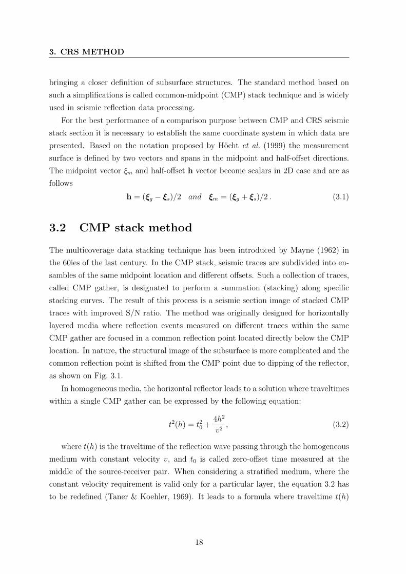
as shown on Fig. 3.1.
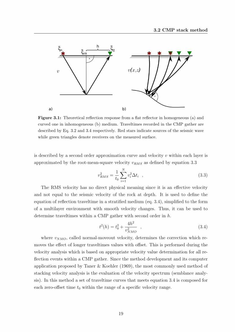
In homogeneous media, the horizontal reflector leads to a solution where traveltimes
within a single CMP gather can be expressed by the following equation:
t2(h) = t20 +4h2
v2, (3.2)
where t(h) is the traveltime of the reflection wave passing through the homogeneous
medium with constant velocity v, and t0 is called zero-offset time measured at the
middle of the source-receiver pair. When considering a stratified medium, where the
constant velocity requirement is valid only for a particular layer, the equation 3.2 has
to be redefined (Taner & Koehler, 1969). It leads to a formula where traveltime t(h)
18
3.2 CMP stack method
Figure 3.1: Theoretical reflection response from a flat reflector in homogeneous (a) and
curved one in inhomogeneous (b) medium. Traveltimes recorded in the CMP gather are
described by Eq. 3.2 and 3.4 respectively. Red stars indicate sources of the seismic wave
while green triangles denote receivers on the measured surface.
is described by a second order approximation curve and velocity v within each layer is
approximated by the root-mean-square velocity vRMS as defined by equation 3.3
v2RMS =1
t0
N∑i=1
v2i∆ti , (3.3)
The RMS velocity has no direct physical meaning since it is an effective velocity
and not equal to the seismic velocity of the rock at depth. It is used to define the
equation of reflection traveltime in a stratified medium (eq. 3.4), simplified to the form
of a multilayer environment with smooth velocity changes. Thus, it can be used to
determine traveltimes within a CMP gather with second order in h.
t2(h) = t20 +4h2
v2NMO
, (3.4)
where vNMO, called normal-moveout velocity, determines the correction which re-
moves the effect of longer traveltimes values with offset. This is performed during the
velocity analysis which is based on appropriate velocity value determination for all re-
flection events within a CMP gather. Since the method development and its computer
application proposed by Taner & Koehler (1969), the most commonly used method of
stacking velocity analysis is the evaluation of the velocity spectrum (semblance analy-
sis). In this method a set of traveltime curves that meets equation 3.4 is composed for
each zero-offset time t0 within the range of a specific velocity range.
19
3. CRS METHOD
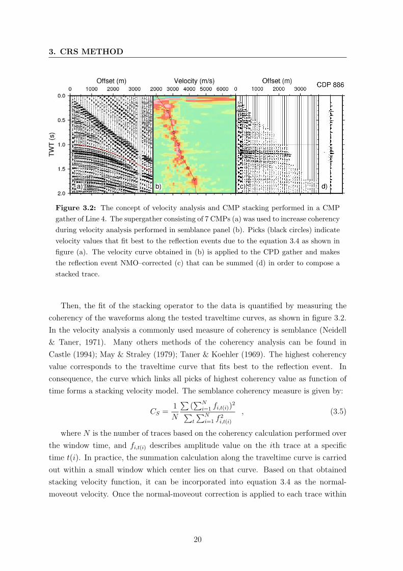
Figure 3.2: The concept of velocity analysis and CMP stacking performed in a CMP
gather of Line 4. The supergather consisting of 7 CMPs (a) was used to increase coherency
during velocity analysis performed in semblance panel (b). Picks (black circles) indicate
velocity values that fit best to the reflection events due to the equation 3.4 as shown in
figure (a). The velocity curve obtained in (b) is applied to the CPD gather and makes
the reflection event NMO–corrected (c) that can be summed (d) in order to compose a
stacked trace.
Then, the fit of the stacking operator to the data is quantified by measuring the
coherency of the waveforms along the tested traveltime curves, as shown in figure 3.2.
In the velocity analysis a commonly used measure of coherency is semblance (Neidell
& Taner, 1971). Many others methods of the coherency analysis can be found in
Castle (1994); May & Straley (1979); Taner & Koehler (1969). The highest coherency
value corresponds to the traveltime curve that fits best to the reflection event. In
consequence, the curve which links all picks of highest coherency value as function of
time forms a stacking velocity model. The semblance coherency measure is given by:
CS =1
N
∑(∑N
i=1 fi,t(i))2
∑t
∑Ni=1 f
2i,t(i)
, (3.5)
where N is the number of traces based on the coherency calculation performed over
the window time, and fi,t(i) describes amplitude value on the ith trace at a specific
time t(i). In practice, the summation calculation along the traveltime curve is carried
out within a small window which center lies on that curve. Based on that obtained
stacking velocity function, it can be incorporated into equation 3.4 as the normal-
moveout velocity. Once the normal-moveout correction is applied to each trace within
20
3.3 CRS stack method
a CMP gather traces can be stacked along the offset axis. The equation 3.6 describes
the NMO time correction
∆tNMO = t0
(√1 +
4h2
v2NMOt
20
− 1
). (3.6)
Practical consideration of the velocity analysis presented by Al-Chalabi (1973) or
Hubral & Krey (1980) show the misfit between stacking velocity curve and second-
order traveltime approximation. This effect, called spread-length bias, is caused by
many factors but mainly due to lateral inhomogeneities recorded along the offset in
the subsurface and the finite offset aperture. The offset factor plays a significant
role on the resultant stacked image section as well as in tomography and inversion
technique (Duveneck, 2004; Zhang & McMechan, 2011), where its maximum value
must be selected with care.
Although the NMO technique fits well to all aspects of horizontally layered media,
it fails for dipping layered media acquired in the CMP stack, by enhancing reflections
with a particular slope and simultaneously attenuating reflections with another slope.
An additional correction can be applied to minimize the effect of dipping reflector.
The method called dip moveout (DMO) allows horizontal and dipping reflectors to be
stacked with the same NMO velocity. Further readings concerning DMO technique
can be found in Hale (1984), Deregowski (1986) or Notfors & Godfrey (1987) but the
method will not be more discussed through this thesis.
3.3 CRS stack method
As described in secion 3.2, the CMP stack defined as a second order traveltime ap-
proximation is determined in the offset domain. With additional domain, oriented
in the midpoint direction, the stacking operator becomes a stacking surface defined
in the 3–dimensional time–midpoint–half–offset space. This assumption leads to the
determination of a reflection response from the subsurface, spanning through several
neighborhood traces in midpoint direction.
The CRS stack method (Jager et al., 2001; Mann et al., 1999) is considered as
the new concept of the reflection seismic method which is aimed to use a stacking
operator determined as a second order traveltime approximation. It is used to perform
a simulated zero-offset stacking procedure of reflection events in the neighborhood of
21

3. CRS METHOD
each zero-offset sample trace (t0, ξ0). To include an additional domain, the trajectory
of the stacking operator determined by equation 3.6 must be then redefined, and the
new traveltime approximation in the vicinity of the zero-offset point (t0, ξ0) has the
following form (Schleicher et al., 1993):
t2(ξm, h) =(t0 + 2p(ξ)∆ξ
)2+ 2t0
(M
(ξ)N ∆ξ2 +M
(ξ)NIPh
2)
. (3.7)
To make full usage of the CRS stacking method, the traveltime approximation
from equation 3.7, which is defined in the 3–dimensional time–midpoint–half–offset
space, must be described by three independent parameters. Those parameters p(ξ),
M(ξ)N , and M
(ξ)NIP are responsible for creating the stacking surface and are calculated
for each sample trace independently. Their detailed description is given in the next
paragraph. After the three parameters are calculated, the stack is performed in the
way of the coherency analysis. Thus, the CRS stack technique can be treated as an
extended form of the common-midpoint stack technique as described in the previous
section, and it relies on traveltime information that has the form of so-called kinematic
wavefield attributes.
When considering an inhomogeneous medium with a curved reflector as shown in
Figure 3.1b, it can be seen that the reflection event is not limited to a single midpoint
location. Each individual location is named common-reflection point (CRP) and when
linked to the surface, it creates the CRP trajectory which defines the locations of all
primary reflection events. Hence, its value is initially unknown, however, it can be re-
solved by a second-order traveltime approximation which determines the corresponding
CRS stacking operator. As proved by Hocht et al. (1999) the conjunction of the de-
termined kinematic wavefield attributes p(ξ), M(ξ)N , and M
(ξ)NIP together with additional
near-surface velocity information allows to calculate CRP trajectory approximation for
a given zero-offset sample (t0, ξ0). Physically, the attributes can be seen as a two hypo-
thetical wavefronts of Normal Incidence Point (NIP) and Normal (N) waves emerging
at the surface as shown on Figure 3.3.
There are big advantages when using the CRS stacking surface instead of stacking
trajectories known from the CMP stacking method. The biggest improvement is due
to the significantly larger number of traces contributing to the stack at each zero-offset
location. In consequence, the stacked sample trace is characterized by an improved
S/N ratio in comparison to the same trace obtained with conventional CMP stacking
technique as described in section 3.2. Especially, in case of low fold data sets, when
22

3.3 CRS stack method
Figure 3.3: Sketch of theoretical aspects of NIP wave and normal wave, with hypo-
thetical waves emerging at location ξ0 on the surface due to a point source (a) and an
exploding reflector (b). Quantities KN and KNIP describe the wavefront curvature of
the normal and NIP wave, respectively. Additional thicker black lines indicate the radius
of the curvature. More details and parameter description is given in the text below.
the number of traces is not sufficient to perform a reliable velocity analysis, the CRS
may fulfill all stacking demands.
The application of kinematic wavefield attributes can be used in different ways
and has a long history of usage in many seismic data processing techniques. The
first attempt to make benefits of it was conducted by Hubral (1983) by means of a
geometrical spreading correction. Another application was proposed by Mann (2002)
to determine parameters of the projected Fresnel zone. Significant studies has been
conducted by Duveneck (2004), who developed the idea of tomographic inversion based
on the velocity data extracted from the kinematic wavefield attributes.
A similar solution of using a different stacking operator where the characterization
of wavefront is determined by traveltime, radius of curvature and angle of incidence
(Shah (1973), Hubral & Krey (1980)) has been proposed by (Gelchinsky, 1988) in the
method called common reflecting element (CRE). Its further implementation named
multifocusing homeomorphic imaging (MHI) was developed by Gelchinsky et al. (1999)
and Landa et al. (1999, 2010) and Berkovitch et al. (2008).
Kinematic wavefield attributes
The three coefficients of the hyperbolic second-order traveltime approximation de-
23
3. CRS METHOD
fined by equation 3.7 characterize the hypothetical wavefronts that are emerging at
the surface location ξ0. Its quantities are determined as the spatial derivatives of the
hypothetical wavefronts related to the NIP and normal wave experiment. As shown
in Figure 3.3, the meaning of the normal radius of curvature is related to the reflector
curvature, while the NIP-wave radius of curvature to its depth.
As the CMP reflection coincides with the reflection that passes through the NIP
point and is equal to the second order derivative in the offset domain (Chernyak &
Gritsenko, 1979; Hubral, 1983) it is allowed to assign the M(ξ)NIP parameter to the
NIP wave second spatial derivative. When considering a normal wave experiment, the
quantity of M(ξ)NIP can be explained as the second horizontal traveltime derivative of
its wavefront when the source is placed at NIP point on the reflector (see Fig. 3.3a).
On the other hand, the part of the reflector in the vicinity of the NIP point location,
interpreted as the exploding reflector, is normal to the wavefront emerging at the ξ0
location of the zero–offset ray (see Fig. 3.3b). Thus, its quantities p(ξ) and M(ξ)N can
be explained as the first and second spatial traveltime derivatives respectively.
For the considered quantities that are used to determine NIP and normal wave
emerging at ξ0 surface location along the seismic line, the parameters M(ξ)NIP , p(ξ) and
M(ξ)N can be written (Duveneck, 2004) in the following form (under the assumption
that the near-surface velocity v0 is constant locally and subsurface velocity differs only
along the seismic line):
M(ξ)NIP =
cos2 α
v0
KNIP (3.8)
p(ξ) =sinα
v0
(3.9)
M(ξ)N =
cos2 α
v0
KN , (3.10)
where KNIP describes the wavefront curvature of the emerging NIP wave at surface
ξ0 location, while KN refers to its normal wave counterpart. Emergence angle α denotes
the relative angle of the normal ray at ξ0 to the measurements surface. Those three
parameters, defined as the traveltime derivatives related to an emerging wavefront, can
be incorporated to equation 3.7 in order to obtain the 2D CRS operator:
t2(ξm, h) =
(t0 +
2sinα
v0
(ξm − ξ0)
)2
+2t0cos
2α
v0
((ξm − ξ0)2
RN
+h2
RNIP
). (3.11)
24
3.3 CRS stack method
Instead of the wavefront curvature parameters KNIP and KN , the radius of wave-
front can be used to preserve conformity of equation 3.11 with the one originally pro-
posed by Mann et al. (1999). Thus, the radii of wavefront have the reciprocal value
of the curvature parameters KNIP and KN that describe NIP and normal wave, re-
spectively. Although the true values of curvature and depth of a reflector in complex
media are not equal to the measured values of RNIP and RN , their real values can be
recovered with a seismic inversion method by the use of NIP-wave tomography, as has
been proposed by Duveneck (2004). Under the additional assumption, that ∆ξ = 0
and by comparison to equation 3.4 the normal-moveout velocity can be expressed by
the use of the kinematic wavefield attributes RNIP and α and expressed in the following
form:
v2NMO =2v0RNIP
t0 cos2 α. (3.12)
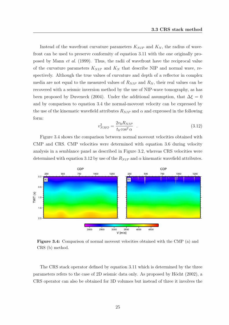
Figure 3.4 shows the comparison between normal moveout velocities obtained with
CMP and CRS. CMP velocities were determined with equation 3.6 during velocity
analysis in a semblance panel as described in Figure 3.2, whereas CRS velocities were
determined with equation 3.12 by use of the RNIP and α kinematic wavefield attributes.
Figure 3.4: Comparison of normal moveout velocities obtained with the CMP (a) and
CRS (b) method.
The CRS stack operator defined by equation 3.11 which is determined by the three
parameters refers to the case of 2D seismic data only. As proposed by Hocht (2002), a
CRS operator can also be obtained for 3D volumes but instead of three it involves the
25
3. CRS METHOD
assistance of eight parameters as shown in the equation below:
t2(ξ0 + ∆ξ,h) =(t0 + 2p(ξ)∆ξ
)2+ 2t0
(∆ξTM
(ξ)N ∆ξ + hTM
(ξ)NIPh
). (3.13)
As already denoted by the equation 3.1 the coordinates of midpoint-half-offset space
are determined by ξm and h vectors. The quantity of parameter p(ξ) is defined by a
two-component vector, while M(ξ)N and M
(ξ)NIP are two symmetric 2×2 matrices.
By the translation from the case of 2D seismic data to a 3D seismic volume, the
CRS operator parameters can be assigned with the same kinematic characteristics to
the NIP and normal waves. Thus, the vector p(ξ) is determined by the first horizon-
tal traveltime derivatives, whereas the matrices M(ξ)N and M
(ξ)NIP are second traveltime
derivatives of emerging normal and NIP waves respectively.
Processing and practical consideration
CRS data processing makes use of kinematic wavefield attributes to determine an
optimum stacking operator for each zero–offset sample trace. Since the attributes can
be obtained only for existing reflection events within a multicoverage dataset they
give measurable benefits by providing additional sections/volumes. Such results are
the basis for a qualitative assessment of the NIP and normal wave parameters, where
detected reflection events are characterized by high coherency values. Additionally, the
assessment provides information concerning reliability of acquired kinematic attributes.
It is worth to mention that the coherency value measured for a reflection event can
be influenced by other factors i.e its overall S/N ratio, the number of traces used
for processing and the shape of the second-order hyperbolic traveltime approximation
defined by equation 3.7 and 3.13.
At the end of the CRS processing chain one can obtain a zero-offset stacked section
and three additional sections of wavefield kinematic attributes and a coherency section
obtained at each step. When applied to a 3D multicoverage dataset, the number of
kinematic attributes increase up to eight instead of three obtained during 2D data
processing. The results of a CRS processing example sequence for multicoverage 2D
and 3D datasets are presented on Figure 4.7-4.8 and Fig. 5.8.
Simultaneous determination of three kinematic wavefield attributes defined for each
zero-offset sample trace involves a great deal of time, even for modern computers. This
is especially the case, when a 3D multicoverage dataset is processed and up to eight
parameters need to be found. Depending on the overall quality of a dataset which
26
3.3 CRS stack method
is related to the acquisition technique, the wavefield attribute determination can be
divided into singular step-by-step search processes.
In the 2D CRS data processing flow, originally proposed by Mann et al. (1999),
Mann (2002), the first step consists of CMP stacking in each CMP gather under the
assumptions that the parameter of wavefield attribute obtained from equation 3.7 for
the 2D case and equation 3.11 is limited to ∆ξ = 0. In the result, due to an automatic
velocity analysis, a stacking velocity is obtained and can be incorporated to equation
3.9 in order to obtain RNIP and α. As the stacked section is acquired from the previous
step, it can be used to perform a search for the first–order traveltime derivative from
equation 3.9 defined by the parameter α under the restriction of h = 0 and RN =∞.
The last parameter search for the second–order travelitime derivative RN requires the
assumption of h = 0 for the CRS operator. After all three wavefield attributes are
obtained, the last processing step is based on a local optimization, where each of
the wavefield attributes can be calculated to obtain a stable CRS operator for the
considered multicoverage dataset. The success of this operation relies on the sufficient
S/N of the reflection events and an adequate number of traces.
Optimum results acquired during the parameter search procedures as defined with
equation 3.7 and 3.13 strongly depend on the quality of dataset. Concerning reflection
traveltimes, they decrease especially with distance from the ZO sample trace position
in both midpoint and offset directions. Therefore, both the values of aperture selected
in three parameter searches and the final CRS stacking step should be selected with
special care to obtain appropriate results. The initial aperture estimation relies on the
geologic information, however, its further values depend on the projected Fresnel zone.
Its size is based on the intersection between first Fresnel volume and the reflector, thus
it can be treated as a good indicator to determine ∆ξ. More accurate width values
of the projected Fresnel zone are provided through the processing sequence due to an
automatic parameter search. The size of the projected Fresnel zone can be determined
by the following equation:
FHW =1
cosα
√√√√ V0
2ω∣∣∣ 1RN− 1
RNIP
∣∣∣ , (3.14)
where ω denotes the dominant frequency of the recorded seismic signal. Again,
by limiting the maximum displacement ∆ξ = 0, the stacking surface changes to the
classical CMP form, known from equation 3.6 with one CMP gather only.
27
3. CRS METHOD
If the selected aperture is too small at larger offset, it will reduce the confidence
level for the attribute determination. The same effect can be observed in conventional
NMO stacking procedure, as the offset space is the common for both methods. On
the other hand, if the selected aperture is too large, the parameter determined for the
stacking operator might not satisfy the condition at the ZO sample trace location but
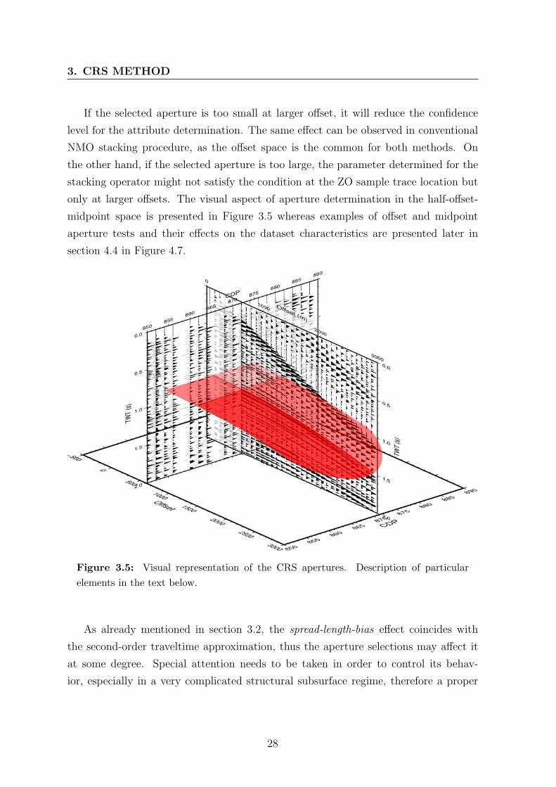
only at larger offsets. The visual aspect of aperture determination in the half-offset-
midpoint space is presented in Figure 3.5 whereas examples of offset and midpoint
aperture tests and their effects on the dataset characteristics are presented later in
section 4.4 in Figure 4.7.
Figure 3.5: Visual representation of the CRS apertures. Description of particular
elements in the text below.
As already mentioned in section 3.2, the spread-length-bias effect coincides with
the second-order traveltime approximation, thus the aperture selections may affect it
at some degree. Special attention needs to be taken in order to control its behav-
ior, especially in a very complicated structural subsurface regime, therefore a proper
28
3.3 CRS stack method
determination of optimum wavefield attributes may encounter major obstacles.
The general approach in conventional NMO analysis involves that the velocity val-
ues are picked at certain traveltimes only due to their high coherency. The remaining
values are interpolated to make the velocity curve complete. In consequence, due to the
interpolation at short offsets, the wavelet characteristics become distorted and a loss of
temporal resolution can be observed. This effect, known as NMO stretch (Buchholtz,
1972; Yilmaz, 2001; Zhang et al., 2011) must be removed in the further processing
chain. Since the second-order approximation in CRS processing allows the operator to
be determined independently for each ZO sample trace, such an effect does not appear
for the considered ZO location.
Although the interpolation between highly coherent values of the stacking NMO
velocity leads to a stretching effect, the sample-by-sample CRS processing may also
cause small irregularities within determined attributes, thus the criteria for a stable
operator calculation may not be fulfilled and these fluctuations can occur with all
calculated attributes affecting further methods that are based on the CRS results.
It is worth to mention that the derivatives of traveltimes, as the kinematic wavefield
attributes, keep the wavelet characteristics invariant of the recording time. Moreover,
as the CRS stack meets the criteria of the paraxial ray theory, the variations of the kine-
matic wavefield attributes, that are proportional to the traveltime derivatives, remain
smooth along the reflection event. The above statements allow to apply smoothing
procedures to kinematic wavefield attributes before the final stacking to enhance its
result. Different smoothing procedures were selected by the authors in order to meet
a particular demands, i.e. Duveneck (2004) proposed an event-consistent smoothing
algorithm to speed up the computation time in order to prepare the attribute sections
for the tomography, Mann et al. (1999) originally proposed a local optimization algo-
rithm and this algorithm was also used in this thesis.
Advanced techniques and new developments in the CRS
Kinematic attributes obtained during second-order traveltime approximation by
means of the CRS stack can be used to determine laterally inhomogeneous 2D/3D
velocity models that can be applied for further processing, i.e. depth imaging. The
NIP-wave tomography method has been originally developed by Duveneck (2004) and
applied by Dummong et al. (2007) and Baykulov et al. (2009). It assumes the use of
provided attribute sections/volumes serving as input data while their values are selected
29
3. CRS METHOD
by the number of pick locations in the CRS stacked zero-offset sections/volumes. Since
the NIP-wave tomography is based on smooth model and reflection points assumed to
be independent, only a few picks are necessary. The forward quantities are obtained
by iteratively determined dynamic ray tracing along normal rays, while the calulation
of Frechet derivatives is based on perturbation theory.
The CRS method has become the starting point for many other more sophisticated
and advance processing methods. One of these is the partial CRS stacking method,
originally proposed by Baykulov & Gajewski (2009). It allows to obtain regular and
uniform seismic section/volume and can be used to fill in the gaps between traces within
a sparse dataset. The idea of partial CRS stack is based on the summation of stacking
surface that coincidences locally with the specific point defined in half-offset–midpoint
domain of a chosen CMP location. In the results, the CRS supergather is obtained
that consists of desired points determined by the summation surface. That surface is
consistent to the surface of the CRS stack but smaller in size. Beside the data infill and
overall S/N improvement, the partial CRS stack assumes the amplitude preservation
that allows a method to be applied in wider spectrum (Baykulov et al., 2009).
In the time migration methods, the velocities defined at the apex of migration op-
erator are usually obtained in the iterative way from a stacking velocities. Another
method to derive the migration velocities based on the CRS kinematic attributes was
proposed by Mann (2002) and Mann et al. (2003). It based on the assumption that
diffraction response can be obtained by the CRS operator, thus mapping the diffrac-
tion apex. Although, the method has limitation due to the selective characteristics
based on points mapping, however it can be used as first approximation of the sub-
surface. Another solution to use the CRS attributes for Kirchoff depth migration was
proposed by Jager (2005). With the CRS attributes it was possible to estimate the
minimum migration aperture and thus enhance the resultant seismic image, mainly by
attenuating the migration artifacts and preventing an aliasing of migration operator.
Spinner & Mann (2005) and later Spinner (2007) has used the CRS attributes and the
idea of minimum–aperture in time migration. The main aim of this approach was to
gain the stability of migration aperture and in consequence to lower the dependency
from velocity model errors, that was considered as limitation of depth counterpart.
A general approach of minimum time migration focused on accurate determination of
location and size of migration aperture. Determined, with the assumption of straight
30
3.3 CRS stack method
ray, the migration operator makes it possible to obtain the improved migrated image
and preserved amplitude.
The latest developments of CRS technique focused on the structural imaging within
the resolution beyond a half of wavelength. Such a structural details are usually asso-
ciated with karst and fractured or pinch-out structures that are important in further
interpretation. Landa et al. (1987) proved the useability of diffracted waves to image
and highlight such a small structures. Dell & Gajewski (2011) make a usage of the CRS
method to separate diffraction from reflection primary events in time domain, whereas
the previous works of Krey (1952) and Kunz (1960) suggest the relationship between
faults and diffracted waves. Generally, the key target of the algorithm is based on such
a usage of CRS attributes, that makes the possible to attenuate the reflection events
in the poststack domain while make a simultaneously summation of diffraction ones in
the way of partial CRS stacking. Taking those processes together a new CRS-based
workflow of seismic data processing can be established.
31

3. CRS METHOD
32
4
Application to 2D reflection seismic
data from the Alberta basin
4.1 Geological overview
The Western Canadian Sedimentary Basin (WCSB) is an extensive basin in Western
Canada covering an area of 1.4 x 10⁶ km2 , similar in size to the area of Germany, France
and Spain taken together. It is bounded by the Rocky Mountain Fold and Thrust Belt
in the Southwest and the Canadian Shield in the Northeast (Fig. 4.1). It extends from
the southwestern part of the Northwest Territories, to the southwestern part of the
Manitoba province. The main deposition axis of the WCSB, called the Alberta Basin,
has the form of northeastward-tapering wedge composed of supracrustal rocks covering
the crystalline basement. The thickness of the wedge decreases gradually from about
6 km in the center of the main deposition axis in front of the Rocky Mountain fold and
Thrust Belt (RMFTB), before completely tapering out close to the northeastern part
of the Canadian Shield margin.
The origin and evolution of the WCSB is directly linked to the process that influ-
enced the tectonic evolution of the Cordilliera as a result of North American craton
interaction with lithospheric units to the west (Monger & Price, 1979) and its later
orogenic deformation process (Porter et al., 1982). Bally et al. (1966) and Price &
Mountjoy (1970) proposed two stages of the WCSB development based on changes in
the composition and origin of the clastic rocks within the sedimentary layers. The first,
a Late Proterozoic to Late Jurassic stage, correlated with the rifting that initiated the
Cordilleran margin, its nearby ocean basin and the continental terrace wedge. The
33
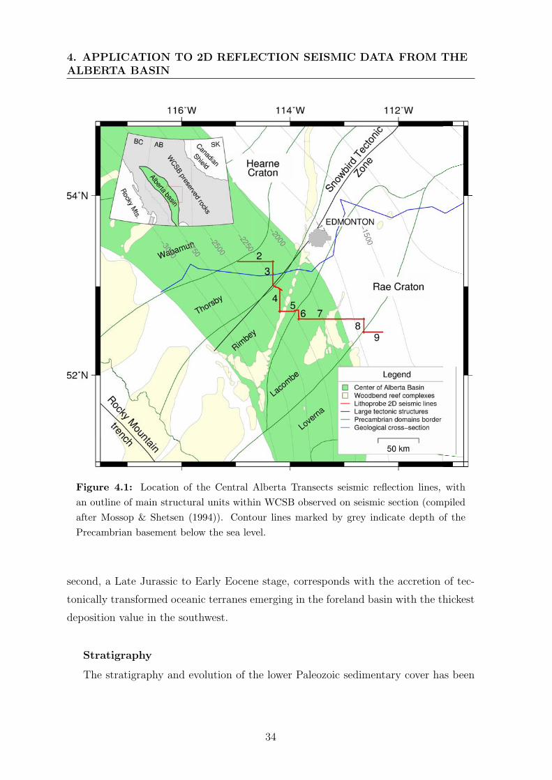
4. APPLICATION TO 2D REFLECTION SEISMIC DATA FROM THEALBERTA BASIN
Figure 4.1: Location of the Central Alberta Transects seismic reflection lines, with
an outline of main structural units within WCSB observed on seismic section (compiled
after Mossop & Shetsen (1994)). Contour lines marked by grey indicate depth of the
Precambrian basement below the sea level.
second, a Late Jurassic to Early Eocene stage, corresponds with the accretion of tec-
tonically transformed oceanic terranes emerging in the foreland basin with the thickest
deposition value in the southwest.
Stratigraphy
The stratigraphy and evolution of the lower Paleozoic sedimentary cover has been
34

4.1 Geological overview
investigated by Stott & Aitken (1993) and Kent (1994) and Slind et al. (1994). Within
the study area, the sedimentary succession above the basement collage consist of 500 to
800m deposits from the Cambrian to the Lower Middle Devonian period. The thickest
Cambrian succession of about 500m, consisting of Basal Sandstone, shallow marine
carbonates of the Cathedral, Eldon and Pika formations, shows northwest alignment
to the continental margin. Clastic sedimentary rocks of the Upper Cambrian strata
are overlain unconformably by the 70m thick Upper Ordovician carbonates of the Red
River Formation. The Devonian Elk Point sediments consist of Ashern clastic units
while Winnipegosis and Prairie formations are mostly carbonate and salt with a total
thickness of 150 to 180m. These strata unconformably overlay the older Ordovican-
Cambrian formation.
Figure 4.2: The geological cross-section of the Alberta basin east of Rocky Mountains.
The section shows the general trend of southeast dipping and the reef structure (sim-
plified after Mossop & Shetsen (1994)). For the line orientation see Fig. 4.1. Vertical
exaggeration is approximately 40.
Target horizons
There are others sedimentary layers of particular interest for geothermal exploration
due to their unique features. These were selected based on physical rock properties
35
4. APPLICATION TO 2D REFLECTION SEISMIC DATA FROM THEALBERTA BASIN
acquired from boreholes.
The Nisku Formation found in B.A. Pyrcz No. 1 well between 1,496.3 and 1,548.8 m
is surrounded by two dolomitic complexes – the Woodbend Group on top which partly
contains shales, and the Winterburn Group at the bottom also containing shales and
additionally anhydrites. It varies between 40 to 60 m in thickness throughout central
Alberta plains and exceeds 100 m in western part within the Winterburn Basin, while
it thins slightly over the Leduc Formation (Stoakes, 1987; Watts, 1987). The layer of
crystalline dolomite with minor admixture of shales and anhydrite whose exact contents
depend on the environment in which they were formed. Leduc reefs are usually devel-
oped in pinnacle forms. The porosity of limestone rocks occurring in Nisku Fm. varies
between 9.7 to 10.4 % while their relative permeability within CO22-brine system varies
between 21.0 to 45.9 mD (Bachu & Bennion, 2008). The Leduc formation of Frasnian
age occurs as reefal buildups developed in shallow water environment and platform
complex with the thickness of 180 to 300 m. It consists of a mixture of shallow water
reef facies, mostly stromatoporoids and skeletal mudstones, which are mainly dolomi-
tized. This process usually creates a natural pit-like cavity in the rocks, hence the
vuggy porosity in the Leduc formation varies between 2 and 14 % while permeability
depends on the pore orientation and reaches the maximum value of 26.7 mD (Stoakes,
1980). The Cooking Lake formation covers the area of central Alberta and is limited
in the south by the Woodbend shelf. Its thickness varies from 60 to 90 m at a depth
of about 1,900 m. The formation occurs as the carbonate platform of limestone and
their dolomitized counterparts including mudstones and wackestones. It is overlain by
the Leduc Formation reefs and overlies the Beaverhill Lake Formation. Measurements
performed by Bachu & Bennion (2008) for the drainage cycle in CO2-brine systems
provide permeability values up to 65.3 mD and a porosity as high as 9.9 %. The Keg
River formation covers the area from the Precambrian shield to the north- east corner
of British Columbia. Among different sub-basins, it occurs as a vuggy or cryptocrys-
talline limestone with minor admixture of dolomite, those thickness varies from 10 to
300 m.
Structural features within the Basin
The Central Alberta Transect crosses the boundary between the Rae province and
the western part of the Archean Hearne Craton, called Snowbird Tectonic Zone, a
structural discontinuity that can be traced from the Canadian Cordillera to the shore
36
4.1 Geological overview
of the Hudson Bay. The Snowbird Tectonic Zone can be distinguished on potential
field images giving the strong pattern on both Bouger and magnetic anomaly images
(Ross et al., 1991; Villeneuve et al., 1993).
In contrast to the sedimentary layers, structural features of the basement have not
been widely investigated. One of the reasons for that is an insignificant number of
boreholes that penetrate the basement rocks. In consequence, this limits the structural
analysis to the borehole surroundings or large scale regional analysis. Nonetheless,
based on that sparse information a large tectonic unit crossing through the central
part of Alberta of about 2000 km long and with a general NE orientation called Snow-
bird Tectonic Zone (STZ), can be distinguished. The presence of the STZ was also
confirmed by the analysis of potential field measurements performed by Ross et al.
(1991); Sharpton et al. (1987) and Villeneuve et al. (1993). Results from these mea-
surements helped to characterize the regional setting of the STZ from Alberta to the
Hudson Bay, where it can be observed as clearly visible signatures on magnetic and
Bouger anomaly maps. It is worth to note that a few anomalies are not directly corre-
lated with dipping basement observed on seismic sections. These additional patterns
were investigated by Ross et al. (1995) and seem to represent mid-crustal thrust faults.
There are some minor disturbances in the basement topography, most likely caused
by the local tectonic activity linked to the basement faulting. In other cases, the sur-
face of the crystalline basement appears to be smooth. Detailed investigations based
on Lithoprobe seismic reflection profiles did not provide more details due to its limited
resolution, which is 20 m. Nevertheless, the detailed analysis of available cores from
the boreholes that penetrate the basement outcrop investigated in the Lower Paleozoic
Project, provides the tectonic evidence on small scale basement faulting existence (Hein
& Nowlan, 1998). This evidence for existence of fault zones oriented NE and located
in central Alberta has been documented during the 3D seismic measurements near
Joffre Field, where hydrocarbons have been found within the Nisku formation. Earlier
measurements and data acquired in South Alberta proved the NE to NNE faulting
orientation in post Leduc period Haites (1960).
Natural resources within the WCSB
The Western Canada Sedimentary Basin is considered one of the worlds largest
reservoirs of hydrocarbons. It contains vast reserves of oil, natural gas and also has
37
4. APPLICATION TO 2D REFLECTION SEISMIC DATA FROM THEALBERTA BASIN
huge reserves of coal. The bulk of the oil and gas resources of Canada and nearly all
of its oil sands lie in the Alberta province (Stringham, 2012).
Although, the Alberta province contains most of the reserves of crude oil within the
WCSB, its production will decline of about 40 % from 2006 to 2016 whereas its pools
have been almost depleted (Davidson & Elsner, 2005). Light and heavy crude oil types
are mostly accumulated in the Devonian reefal, while the Cretaceous ones occur mainly
in porous sands, reaching 50.7 and 26.6 % in recoverable oil reserves in Western Canada
respectively. Pool size and its numbers also depend on intervals age, i.e. Beaverhill
Lake pools are dozen times larger than the shallower Upper Cretaceous pools. The av-
erage size of the Elk Point pools appears to be smaller, through the number of pools is
large due to pinnacle reef type. Within the group of 14 largest oil pools, the 11 largest
occur within Paleozoic formations. There are three important areas in Alberta accu-
mulating oil sands which contain about 260 x 109 m3 initial oil-in-place reserves. The
major oil sand areas are located in the region of Athabasca, Cold Lake and Peace River
and the reserves mostly occur in the Upper and Lower Mannville and some amounts
in the Devonian Grosmont. Since 2005, the number of projects related to the oil sands
exploration and exploitation rapidly increased gathering the total capital expenditures
of about $125 billion. Canada is a leading country in production and exporting of
natural gas with large quantities coming from the WCSB. The overall reserves within
the WCSB are estimated at 4000 km3 of natural gas whose peak production occurred
in 2001 at around 0.45 km3 per day. However, most of the discovered gas pools have
been depleted and new discoveries give less gas with each new well indicating decline
in production (Davidson & Elsner, 2005). The large portion of gas comes from the four
Devonian intervals and five Cretaceous, 23.0 and 48.1 % of marketable gas reserves re-
spectively. The WCSB contains almost the whole of Canadas coal resources ranging in
age from Early Carboniferous (Mississippian) to Paleocene (Cameron & Smith, 1991).
Large quantities of the coal resources found in Alberta are lignite to semianthracite.
These flat-lying beds reach the average thickness of about a dozen meters and due to
low sulfur contents and moderate ash level are mined for power generation purpose or
coking feedstocks.
Geothermal analysis
The geothermal analysis in sedimentary basins is defined by mutual interactions
between different heat sources and its transport methods towards the surface (Chap-
38
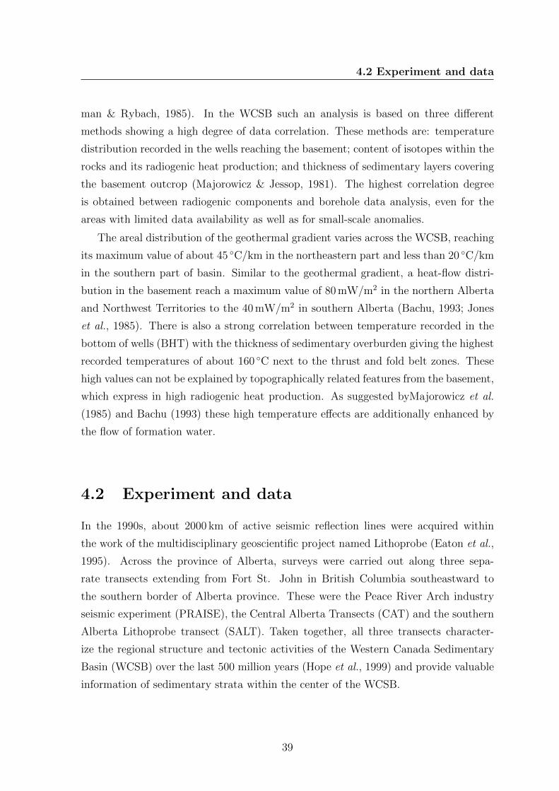
4.2 Experiment and data
man & Rybach, 1985). In the WCSB such an analysis is based on three different
methods showing a high degree of data correlation. These methods are: temperature
distribution recorded in the wells reaching the basement; content of isotopes within the
rocks and its radiogenic heat production; and thickness of sedimentary layers covering
the basement outcrop (Majorowicz & Jessop, 1981). The highest correlation degree
is obtained between radiogenic components and borehole data analysis, even for the
areas with limited data availability as well as for small-scale anomalies.
The areal distribution of the geothermal gradient varies across the WCSB, reaching
its maximum value of about 45 ◦C/km in the northeastern part and less than 20 ◦C/km
in the southern part of basin. Similar to the geothermal gradient, a heat-flow distri-
bution in the basement reach a maximum value of 80 mW/m2 in the northern Alberta
and Northwest Territories to the 40 mW/m2 in southern Alberta (Bachu, 1993; Jones
et al., 1985). There is also a strong correlation between temperature recorded in the
bottom of wells (BHT) with the thickness of sedimentary overburden giving the highest
recorded temperatures of about 160 ◦C next to the thrust and fold belt zones. These
high values can not be explained by topographically related features from the basement,
which express in high radiogenic heat production. As suggested byMajorowicz et al.
(1985) and Bachu (1993) these high temperature effects are additionally enhanced by
the flow of formation water.
4.2 Experiment and data
In the 1990s, about 2000 km of active seismic reflection lines were acquired within
the work of the multidisciplinary geoscientific project named Lithoprobe (Eaton et al.,
1995). Across the province of Alberta, surveys were carried out along three sepa-
rate transects extending from Fort St. John in British Columbia southeastward to
the southern border of Alberta province. These were the Peace River Arch industry
seismic experiment (PRAISE), the Central Alberta Transects (CAT) and the southern
Alberta Lithoprobe transect (SALT). Taken together, all three transects character-
ize the regional structure and tectonic activities of the Western Canada Sedimentary
Basin (WCSB) over the last 500 million years (Hope et al., 1999) and provide valuable
information of sedimentary strata within the center of the WCSB.
39

4. APPLICATION TO 2D REFLECTION SEISMIC DATA FROM THEALBERTA BASIN
Table 4.1: Acquisition parameters of the LITHOPROBE Central Alberta Transect
survey (see the location of lines on fig. 4.1)) performed by Veritas Geophysical Ltd. of
Calgary in July, 1992 (after Eaton et al. (1995))
SURVEY PARAMETERS
Source Vibroseis c©, 4 vibrators over 50 m
Source interval 100 m
Sweep linear, 10–56 Hz, 8 sweeps per VP
Sweep length 14 s
Receiver group interval 50 m
Receiver group spacing 9 over 42 m
Recording system I/O System One
Record length 18 s
Sampling rate 4 ms
Spread asymmetric split–spread
3000 – 150 – VP – 150 – 9000 m
Coverage 60
The Lithoprobe seismic reflection data from the Central Alberta Transects are
composed of 10 seismic profiles with a total length of 520 km. The localization of the
profiles extends from 60 km west of Edmonton, eastward to the Alberta-Saskatchewan
border (Figure 4.1). Data were acquired in the summer of 1992 by Veritas Geophysical
Ltd, mainly along the road grid of the Alberta province with overshooting at line
intersections. Lines 2, 5, 7 and 9 were oriented in east-west direction, whereas Lines
3, 4, 6, and 8 were predominantly running north-south. The line location and their
orientation was chosen to cross the basement domain borders perpendicular to the
strike (Ross et al., 1991).
Acquisition parameters originally focused to highlight features of deep crystalline
basement and were described in details by Eaton et al. (1995). The research target
of the Lithoprobe project required the application of a field geometry different from
the common industry standards, i.e. the source signal was acquired from a group
of four larger then usual Vibroseis units spaced at 100 m to ensure its penetration at
greater depths, quite low frequency range of the sweep (5-56 Hz) to avoid too fast signal
attenuation, larger spacing of receivers groups (50 m) placed in half of source position
and very long offsets - up to 12 km obtained by the use of 240 channels recording system.
Acquisition geometry was a combination of asymmetric split–spread with short offset
up to 3000 m and long offset up to 9000 m. The main acquisition parameters are
presented in Table 4.1.
In general, the quality of recorded seismic data was good along all lines with strong
continuous reflections from the sedimentary layers (Figure 4.3) as well as all three
40
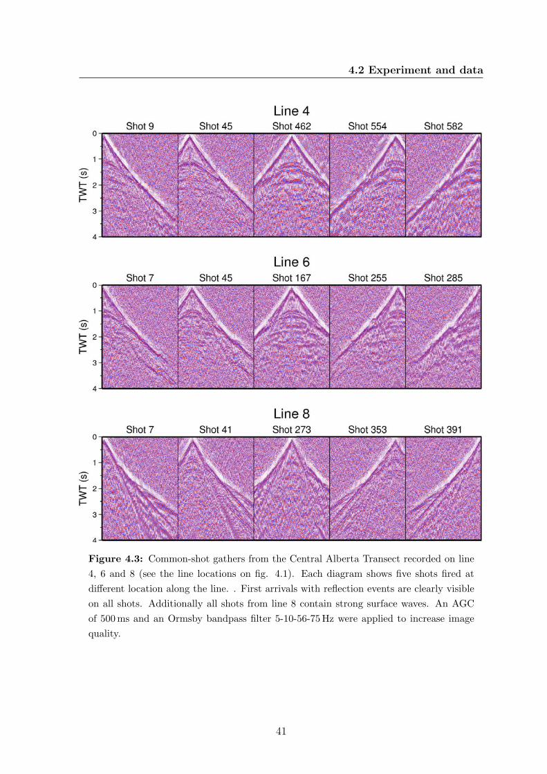
4.2 Experiment and data
Figure 4.3: Common-shot gathers from the Central Alberta Transect recorded on line
4, 6 and 8 (see the line locations on fig. 4.1). Each diagram shows five shots fired at
different location along the line. . First arrivals with reflection events are clearly visible
on all shots. Additionally all shots from line 8 contain strong surface waves. An AGC
of 500ms and an Ormsby bandpass filter 5-10-56-75Hz were applied to increase image
quality.
41
4. APPLICATION TO 2D REFLECTION SEISMIC DATA FROM THEALBERTA BASIN
transects throughout the crust due to 18 s of data recording (Hope et al., 1999). Sed-
imentary succession and its interface with the basement surface were recorded within
the first 2 seconds of TWT as shown later in section 4.3. Additionally, the real-time
noise elimination and precise monitoring of vibrator synchronization allowed to recover
much more high quality seismic data.
The presence of high lateral reflectivity from sedimentary layers largely helped to
compute residual static correction and assisted in the calculation of crustal velocities
Eaton et al. (1995). A noticeable loss of reflectivity was observed at the first half of
Line 1, probably caused by too high power energy output from the vibroseis trucks.
Due to low quality of recordings along Line 1 and too complicated crooked geometry
along Line 10, these two lines were excluded from the further CMP and CRS processing.
4.3 CMP Processing
The Central Alberta Transect 2D reflection seismic project was recorded in 1992 by
Vertias Geophysical Ltd. and then processed by Pulsonic Geophysical Ltd. of Calgary.
The original data processing scheme has been presented by Eaton et al. (1995) and
the major steps are shown in Table 4.4. Originally, the Lithoprobe reflection project
aimed at imaging the deep part of the crust due to 18 s of data recording which allowed
to penetrate the subsurface down to 40 km. Since the target horizons presented in this
study are located between 3 and 4 km depth, the data processing scheme demonstrated
here slightly differs from that performed by the contractor and will concentrate on the
first 2.5 s of TWT.
Since 1995, when first Lithoprobe results have been published, several new acqui-
sition and processing innovations have become available to improve the data quality.
Beside migration algorithms, dominant flows of the seismic data processing at that time
focused on noise attenuation and removal of multiple reflections and application of f-k
filtering. The processed data demonstrated here slightly differ from that described
in Eaton et al. (1995), mostly by the application of other than original deconvolu-
tion method and filtration method focused to highlight the reflection events from the
first 2.5 s TWT. All further processing steps have been carried out with PROMAX c©
software.
The original records provided by Natural Resources Canada (NRC) were stored
in SEG-P format. As part of this thesis noise test files as well as corrupted shots
42
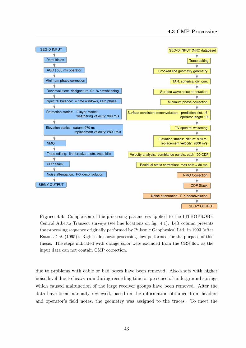
4.3 CMP Processing
Figure 4.4: Comparison of the processing parameters applied to the LITHOPROBE
Central Alberta Transect surveys (see line locations on fig. 4.1). Left column presents
the processing sequence originally performed by Pulsonic Geophysical Ltd. in 1993 (after
Eaton et al. (1995)). Right side shows processing flow performed for the purpose of this
thesis. The steps indicated with orange color were excluded from the CRS flow as the
input data can not contain CMP correction.
due to problems with cable or bad boxes have been removed. Also shots with higher
noise level due to heavy rain during recording time or presence of underground springs
which caused malfunction of the large receiver groups have been removed. After the
data have been manually reviewed, based on the information obtained from headers
and operator’s field notes, the geometry was assigned to the traces. To meet the
43
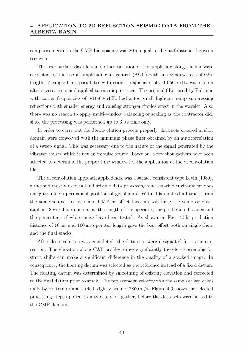
4. APPLICATION TO 2D REFLECTION SEISMIC DATA FROM THEALBERTA BASIN
comparison criteria the CMP bin spacing was 20 m equal to the half-distance between
receivers.
The near surface disorders and other variation of the amplitude along the line were
corrected by the use of amplitude gain control (AGC) with one window gate of 0.5 s
length. A single band-pass filter with corner frequencies of 5-10-56-75 Hz was chosen
after several tests and applied to each input trace. The original filter used by Pulsonic
with corner frequencies of 5-10-60-64 Hz had a too small high-cut ramp suppressing
reflections with smaller energy and causing stronger ripples effect in the wavelet. Also
there was no reason to apply multi-window balancing or scaling as the contractor did,
since the processing was performed up to 3.0 s time only.
In order to carry out the deconvolution process properly, data sets ordered in shot
domain were convolved with the minimum phase filter obtained by an autocorrelation
of a sweep signal. This was necessary due to the nature of the signal generated by the
vibrator source which is not an impulse source. Later on, a few shot gathers have been
selected to determine the proper time window for the application of the deconvolution
filer.
The deconvolution approach applied here was a surface consistent type Levin (1989),
a method mostly used in land seismic data processing since marine environment does
not guarantee a permanent position of geophones. With this method all traces from
the same source, receiver and CMP or offset location will have the same operator
applied. Several parameters, as the length of the operator, the prediction distance and
the percentage of white noise have been tested. As shown on Fig. 4.5b, prediction
distance of 16 ms and 100 ms operator length gave the best effect both on single shots
and the final stacks.
After deconvolution was completed, the data sets were designated for static cor-
rection. The elevation along CAT profiles varies significantly therefore correcting for
static shifts can make a significant difference in the quality of a stacked image. In
consequence, the floating datum was selected as the reference instead of a fixed datum.
The floating datum was determined by smoothing of existing elevation and corrected
to the final datum prior to stack. The replacement velocity was the same as used origi-
nally by contractor and varied slightly around 2800 m/s. Figure 4.6 shows the selected
processing steps applied to a typical shot gather, before the data sets were sorted to
the CMP domain.
44
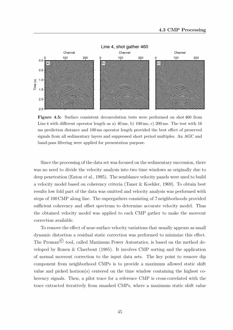
4.3 CMP Processing
Figure 4.5: Surface consistent deconvolution tests were performed on shot 460 from
Line 4 with different operator length as a) 40ms, b) 100ms, c) 200ms. The test with 16
ms prediction distance and 100ms operator length provided the best effect of preserved
signals from all sedimentary layers and suppressed short period multiples. An AGC and
band-pass filtering were applied for presentation purpose.
Since the processing of the data set was focused on the sedimentary succession, there
was no need to divide the velocity analysis into two time windows as originally due to
deep penetration (Eaton et al., 1995). The semblance velocity panels were used to build
a velocity model based on coherency criteria (Taner & Koehler, 1969). To obtain best
results low fold part of the data was omitted and velocity analysis was performed with
steps of 100CMP along line. The supergathers consisting of 7 neighborhoods provided
sufficient coherency and offset spectrum to determine accurate velocity model. Thus
the obtained velocity model was applied to each CMP gather to make the moveout
correction available.
To remove the effect of near-surface velocity variations that usually appears as small
dynamic distortion a residual static correction was performed to minimize this effect.
The Promax c© tool, called Maximum Power Autostatics, is based on the method de-
veloped by Ronen & Claerbout (1985). It involves CMP sorting and the application
of normal moveout correction to the input data sets. The key point to remove dip
component from neighborhood CMPs is to provide a maximum allowed static shift
value and picked horizon(s) centered on the time window containing the highest co-
herency signals. Then, a pilot trace for a reference CMP is cross-correlated with the
trace extracted iteratively from smashed CMPs, where a maximum static shift value
45
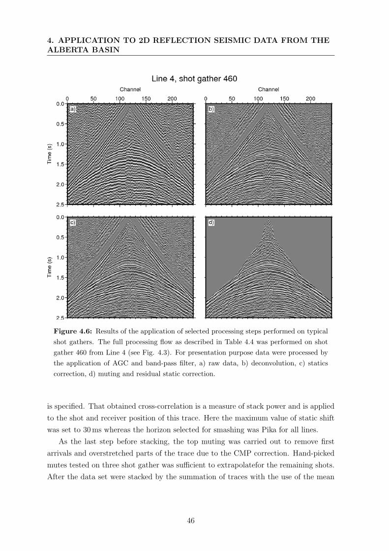
4. APPLICATION TO 2D REFLECTION SEISMIC DATA FROM THEALBERTA BASIN
Figure 4.6: Results of the application of selected processing steps performed on typical
shot gathers. The full processing flow as described in Table 4.4 was performed on shot
gather 460 from Line 4 (see Fig. 4.3). For presentation purpose data were processed by
the application of AGC and band-pass filter, a) raw data, b) deconvolution, c) statics
correction, d) muting and residual static correction.
is specified. That obtained cross-correlation is a measure of stack power and is applied
to the shot and receiver position of this trace. Here the maximum value of static shift
was set to 30ms whereas the horizon selected for smashing was Pika for all lines.
As the last step before stacking, the top muting was carried out to remove first
arrivals and overstretched parts of the trace due to the CMP correction. Hand-picked
mutes tested on three shot gather was sufficient to extrapolatefor the remaining shots.
After the data set were stacked by the summation of traces with the use of the mean
46

4.4 CRS Processing
stack algorithm, F-X deconvolution was applied to enhance lateral resolution of the
reflection events and to restore high frequency attenuated during CMP correction and
stacking. Before exporting to SEG-Y format an automatic gain control scaling with a
window length of 500 ms has been applied to enhance image quality.
Later on, to compile a joint section from the individual CAT profiles it was necessary
to apply static corrections with a floating datum and fixed replacement velocity slightly
different between lines in order to resolve significant mis-ties. The large extent of
the resulting composite section enables the attribute analysis of regional reflection
characteristics spanning several basement tectonic domains, as well as interregional
comparisons of key structural elements in the Alberta basin.
4.4 CRS Processing
As mentioned in the section 3.3, the CRS processing is aimed to provide the stacking
operator for each zero-offset trace sample in order to obtain a simulated zero-offset
stack section. In consequence, three of the CRS kinematic attributes obtained during
the processing provide additional sections and can be utilized in other techniques, i.e.
NIP-wave tomography (Duveneck, 2004). These attributes bring up their potential
only where associated with the reflection event highlighted by a high coherence value.
Thus, the coherency section is the first evaluator of reflection event occurrence and
reliability of the obtained CRS attributes. The quality of coherency section depends
on the number of contributing traces and S/N ratio of the event.
Since the simultaneous parameter selection is not efficient in the sense of computa-
tion time, an additional simplification steps are highly desired. In the 2D case, where
three of the CRS attributes must be provided to obtain the final CRS stack such a
simplification proposed by Mann et al. (1999) decrease the computation time signifi-
cantly. As already defined by 3.7, the idea is to determine single attribute separately
one after the other, under the assumption that the rest will be zeroed. As soon as the
νNMO value is computed under the ∆ξ = 0 assumption it can be used to search for α
parameter by setting h = 0 and RN = ∞. Consequently, RN is obtained with h = 0
assumption which leads to the last step - an optimization of the all CRS attributes. As
the alternative to local optimization an event consistent smoothing method is applied
to determine a proper parameter values.
47

4. APPLICATION TO 2D REFLECTION SEISMIC DATA FROM THEALBERTA BASIN
0.0
0.5
1.0
1.5
2.0
TW
T (
s)
250 500 750 1000 1250
CDP
a)
0.0
0.5
1.0
1.5
2.0
TW
T (
s)
b)
0.0
0.5
1.0
1.5
2.0
TW
T (
s)
c)
0.5 0.6 0.7 0.8 0.9 1.0
Coherency
0.0
0.5
1.0
1.5
2.0
TW
T (
s)
250 500 750 1000 1250
CDP
d)
e)
f)
−10 −8 −6 −4 −2 0 2 4 6 8 10
Angle dip [°]
Figure 4.7: Results of parameter tests applied to the CRS data set from Line 4. Images
show the consecutive steps in CRS stack data processing applied to the CMP sorted
dataset along Line 4. (a) to (c) Coherency section , (d) to (f) emergency angle α search
results. Low coherency values are masked in gray. Further description is given in the
text below.
The travel time approximations defined by equation 3.9 are dependent on distance
in the midpoint and offset directions and generally, its quality decrease with distance
from the zero-offset location. Thus, the proper aperture selection, both in midpoint and
48
4.4 CRS Processing
offset direction, applied during the parameter search, needs to be selected with special
attention to obtain good quality results. Also, if the main aim is the determination of
CRS attributes for further applications needs, i.e. tomography, controlling of spread-
length-bias effect has to be undertaken with special care. For example when a large
apertures is selected, the second order approximation may fit to the reflection not at
the considered zero-offset location (see Fig. 4.7c and f). While too small, apertures will
decrease the resolution and lead to inefficient number of parameters to determine the
CRS attribute (see Fig. 4.7a and d). The efficient aperture selection mainly depends
on differences between the traveltime moveout function and its theoretical hyperbolic
shape. The larger the difference the less reliable is the CRS attribute determination.
The search for CRS parameters is performed on the preprocessed CMP data sets
without normal moveout correction, as mentioned in CMP processing flow description
(see Fig. 4.4). In order to make the full imaging available different apertures in offsets
and midpoint direction were tested. During the first phase, the aperture estimation
based on the test performed along selected shot gather with CMP corrected reflection
events. These kind of tests make use of large number of traces increasing the coherency
analysis and improve the spread-length bias effect. After several tests, the offset aper-
ture was determined between 300 m for near surface times to 2500 m at 3.0 s TWT (see
Fig. 4.7c) and interpolated linearly in between. The midpoint aperture was determined
between 75 m for near surface times to 300 m at 3.0 s TWT. Figure 4.7 and 4.8 show
example aperture search performed on Line 4.
The ZO section acquired during CMP processing is used as the input model in order
to perform emergency angle α search. The emergency angle section presented on Fig.
4.7e shows gentle dipping to the south (see Fig. 4.1 for line orientation) which does not
exceed 10 ◦ in agreement with the general tendency of the local geological framework
that is proved by high coherency values 4.7b along the package of reflection events.
This also indicates that the subsurface structure can be treated as 1D medium where
the lateral velocity variations are expected to be relatively small.
Further steps of the CRS processing incorporate the constrains of the ZO searches
that are more connected to the geological condition of the sedimentary basin.
49
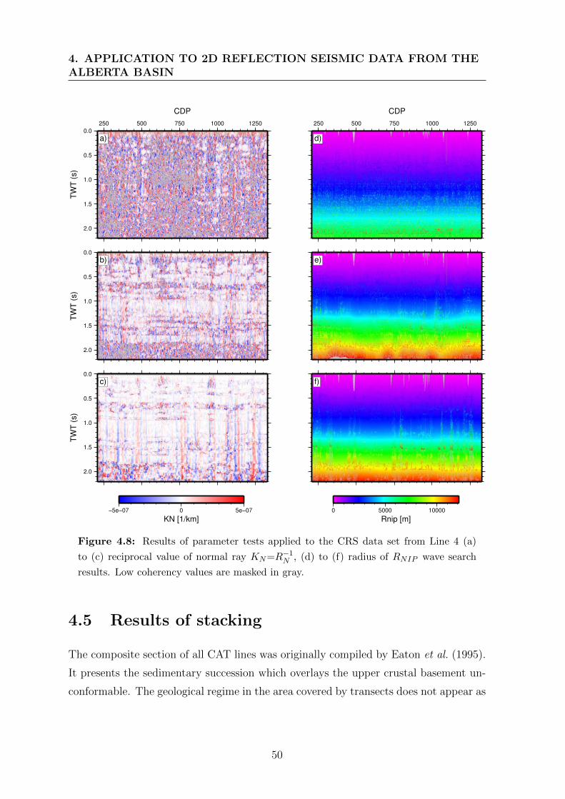
4. APPLICATION TO 2D REFLECTION SEISMIC DATA FROM THEALBERTA BASIN
0.0
0.5
1.0
1.5
2.0
TW
T (
s)
250 500 750 1000 1250
CDP
a)
0.0
0.5
1.0
1.5
2.0
TW
T (
s)
b)
0.0
0.5
1.0
1.5
2.0
TW
T (
s)
c)
−5e−07 0 5e−07
KN [1/km]
250 500 750 1000 1250
CDP
d)
e)
f)
0 5000 10000
Rnip [m]
Figure 4.8: Results of parameter tests applied to the CRS data set from Line 4 (a)
to (c) reciprocal value of normal ray KN=R−1N , (d) to (f) radius of RNIP wave search
results. Low coherency values are masked in gray.
4.5 Results of stacking
The composite section of all CAT lines was originally compiled by Eaton et al. (1995).
It presents the sedimentary succession which overlays the upper crustal basement un-
conformable. The geological regime in the area covered by transects does not appear as
50
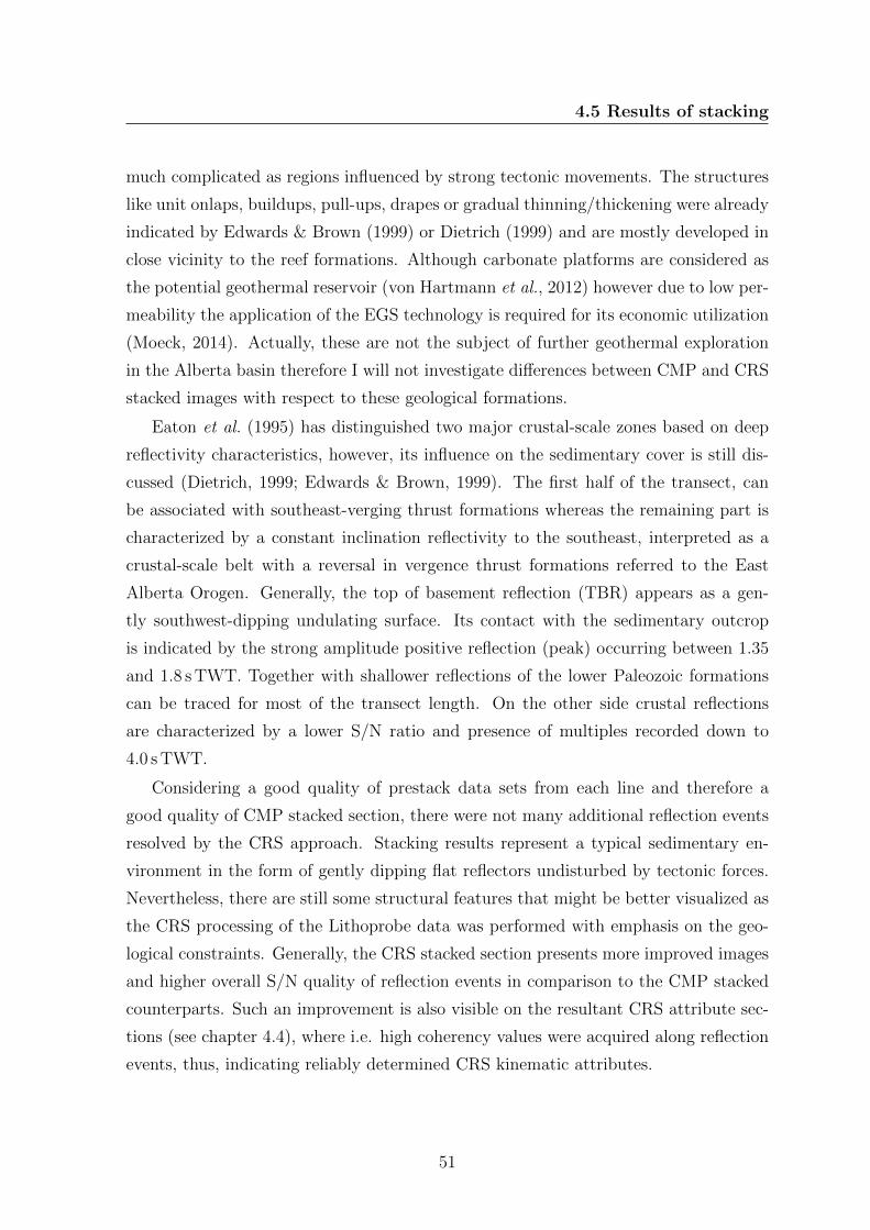
4.5 Results of stacking
much complicated as regions influenced by strong tectonic movements. The structures
like unit onlaps, buildups, pull-ups, drapes or gradual thinning/thickening were already
indicated by Edwards & Brown (1999) or Dietrich (1999) and are mostly developed in
close vicinity to the reef formations. Although carbonate platforms are considered as
the potential geothermal reservoir (von Hartmann et al., 2012) however due to low per-
meability the application of the EGS technology is required for its economic utilization
(Moeck, 2014). Actually, these are not the subject of further geothermal exploration
in the Alberta basin therefore I will not investigate differences between CMP and CRS
stacked images with respect to these geological formations.
Eaton et al. (1995) has distinguished two major crustal-scale zones based on deep
reflectivity characteristics, however, its influence on the sedimentary cover is still dis-
cussed (Dietrich, 1999; Edwards & Brown, 1999). The first half of the transect, can
be associated with southeast-verging thrust formations whereas the remaining part is
characterized by a constant inclination reflectivity to the southeast, interpreted as a
crustal-scale belt with a reversal in vergence thrust formations referred to the East
Alberta Orogen. Generally, the top of basement reflection (TBR) appears as a gen-
tly southwest-dipping undulating surface. Its contact with the sedimentary outcrop
is indicated by the strong amplitude positive reflection (peak) occurring between 1.35
and 1.8 s TWT. Together with shallower reflections of the lower Paleozoic formations
can be traced for most of the transect length. On the other side crustal reflections
are characterized by a lower S/N ratio and presence of multiples recorded down to
4.0 s TWT.
Considering a good quality of prestack data sets from each line and therefore a
good quality of CMP stacked section, there were not many additional reflection events
resolved by the CRS approach. Stacking results represent a typical sedimentary en-
vironment in the form of gently dipping flat reflectors undisturbed by tectonic forces.
Nevertheless, there are still some structural features that might be better visualized as
the CRS processing of the Lithoprobe data was performed with emphasis on the geo-
logical constraints. Generally, the CRS stacked section presents more improved images
and higher overall S/N quality of reflection events in comparison to the CMP stacked
counterparts. Such an improvement is also visible on the resultant CRS attribute sec-
tions (see chapter 4.4), where i.e. high coherency values were acquired along reflection
events, thus, indicating reliably determined CRS kinematic attributes.
51

4. APPLICATION TO 2D REFLECTION SEISMIC DATA FROM THEALBERTA BASIN
Also significant improvement can be observed close to the surface, where reflections
from shallow strata recorded at 0.2 s are better imaged by the CRS stack due to in-
creased continuity of the recorded reflections. On the other side, insufficient number
of traces within the CMP counterpart makes the identification of shallow horizons
unclear. A sample set of final results of CMP and CRS stacked sections from the
Central Alberta Transects are presented on figures 4.9 - 4.15.
Figure 4.9 and figure 4.10 show images of the CMP and CRS stacked sections
acquired from Line 2 and Line 3 respectively located at the beginning of the Central
Alberta Transect. The overall quality presented on the CRS image is higher than
obtained from the CMP counterpart. The continuity of reflection events from the
lower Paleozoic formations recorded between 1.0 and 1.8 s TWT are highlighted with
more details. Most of horizons obtained from CMP stack are presented noisy whereas
the same reflectors imaged by the CRS stack show better continuity and can be clearly
identified. Especially the reflection event located between CMP 1050 and 1250 at
1.2 s TWT along Line 2 has been resolved at higher confidence level than the CMP
counterpart.
The Mesozoic succession visible above 1.0 s TWT shows similar signal characteristic
on both, the CMP and CRS stacked images, and allows the horizons to be clearly
identified. The partial identification of the horizon recorded at 0.9 s TWT has been
improved by the CRS stack where it shows reflection events with higher S/N ratio and
better continuity. Due to irregular acquisition and limited amount of available shots,
traces visible between CMP 1300 and 1400 on Line 2 were not resolved sufficiently on
both stack producing noisy and disturbed stacked image.
Figure 4.11 presents the stacking results obtained by the application of the CMP and
the CRS technique to dataset acquired from Line 4 located at the end of the southeast-
verging thrust formations. The whole sedimentary succession is horizontally arranged
due to perpendicular orientation of the profile in respect to the main axis of the basin
subsidence. The CMP and the CRS sections show imaged horizons consisting of similar
S/N ratio and similar reflection continuity. The Precambrian basement formation has
been imaged with a weak amplitude reflection events recorded at 1.8 s TWT, while the
Pika horizon at 1.6 s TWT. The reflection event from the basement which is observed
along Line 4 (some influence is also visible on neighborhood Lines 3 and 5) shows a
’seismic anomaly’ which is associated with precambrian Rimbey domain and the high
amplitude Middle Cambrian reflection event. Initially it was defined by Eaton et al.
52
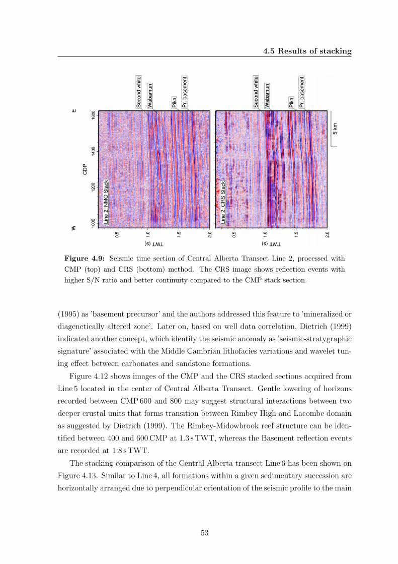
4.5 Results of stacking
Figure 4.9: Seismic time section of Central Alberta Transect Line 2, processed with
CMP (top) and CRS (bottom) method. The CRS image shows reflection events with
higher S/N ratio and better continuity compared to the CMP stack section.
(1995) as ’basement precursor’ and the authors addressed this feature to ’mineralized or
diagenetically altered zone’. Later on, based on well data correlation, Dietrich (1999)
indicated another concept, which identify the seismic anomaly as ’seismic-stratygraphic
signature’ associated with the Middle Cambrian lithofacies variations and wavelet tun-
ing effect between carbonates and sandstone formations.
Figure 4.12 shows images of the CMP and the CRS stacked sections acquired from
Line 5 located in the center of Central Alberta Transect. Gentle lowering of horizons
recorded between CMP600 and 800 may suggest structural interactions between two
deeper crustal units that forms transition between Rimbey High and Lacombe domain
as suggested by Dietrich (1999). The Rimbey-Midowbrook reef structure can be iden-
tified between 400 and 600CMP at 1.3 sTWT, whereas the Basement reflection events
are recorded at 1.8 sTWT.
The stacking comparison of the Central Alberta transect Line 6 has been shown on
Figure 4.13. Similar to Line 4, all formations within a given sedimentary succession are
horizontally arranged due to perpendicular orientation of the seismic profile to the main
53
4. APPLICATION TO 2D REFLECTION SEISMIC DATA FROM THEALBERTA BASIN
Figure 4.10: Seismic time section of Central Alberta Transect Line 3, processed with
CMP (top) and CRS (bottom) method. The CMP and the CRS stacked sections show
similar quality image.
subsidence axis of the Alberta Basin. The deepest Basement formation is recorded at
1.7 sTWT, whereas the Second White Speckled at 0.9 sTWT. Missing traces in the
CRS image are caused by the crooked geometry layout.
Beside the general quality improvement, a better continuity and clearly visible
reflectors are dominate on the CRS image. Acquired horizons allowed to be imaged
more precisely within tested apertures, thus ensure reliable picking of target horizons.
Interesting results were acquired between 0.45-0.65 sTWT at the beginning of profile
where complicated structural image of the shallow succession could be interpreted by
a violent sedimentation or local tectonic processes.
Figure 4.14 shows the comparison between the CMP and the CRS stacked image
from the Line 8 located at the end of Central Alberta Transect. The overall quality of
both processed sections are similar, however, there are some details less visible in the
CMP stack section. Reflection events of Pika horizon recorded at 1.35 sTWT between
CMP 400 and 500 show better continuity and are clearly identified. Also large package
of reflections between CMP 550 and 700 at 1.0 to 1.25 sTWT disturbed due the higher
located pull-up are better resolved.
The final part of Central Alberta Transect presented in Figure 4.15 shows stacked
54
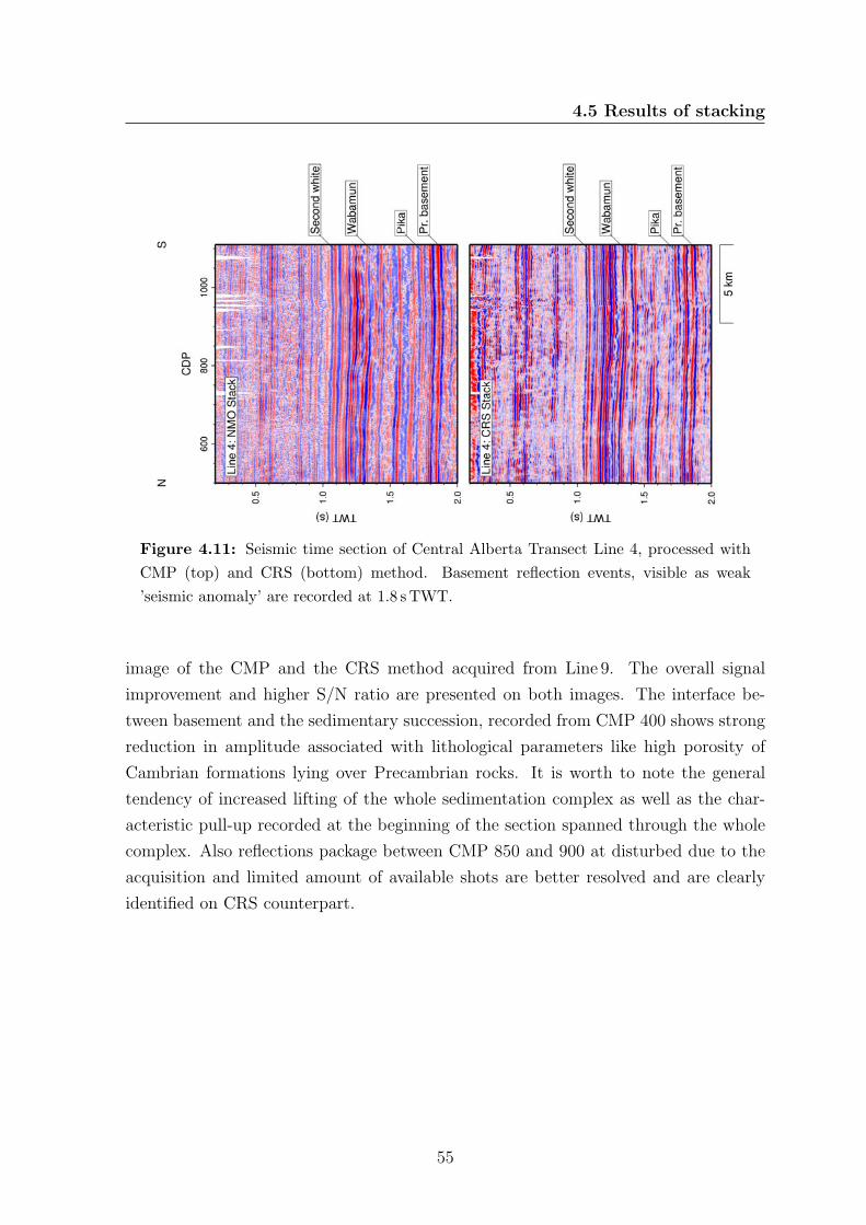
4.5 Results of stacking
Figure 4.11: Seismic time section of Central Alberta Transect Line 4, processed with
CMP (top) and CRS (bottom) method. Basement reflection events, visible as weak
’seismic anomaly’ are recorded at 1.8 sTWT.
image of the CMP and the CRS method acquired from Line 9. The overall signal
improvement and higher S/N ratio are presented on both images. The interface be-
tween basement and the sedimentary succession, recorded from CMP 400 shows strong
reduction in amplitude associated with lithological parameters like high porosity of
Cambrian formations lying over Precambrian rocks. It is worth to note the general
tendency of increased lifting of the whole sedimentation complex as well as the char-
acteristic pull-up recorded at the beginning of the section spanned through the whole
complex. Also reflections package between CMP 850 and 900 at disturbed due to the
acquisition and limited amount of available shots are better resolved and are clearly
identified on CRS counterpart.
55
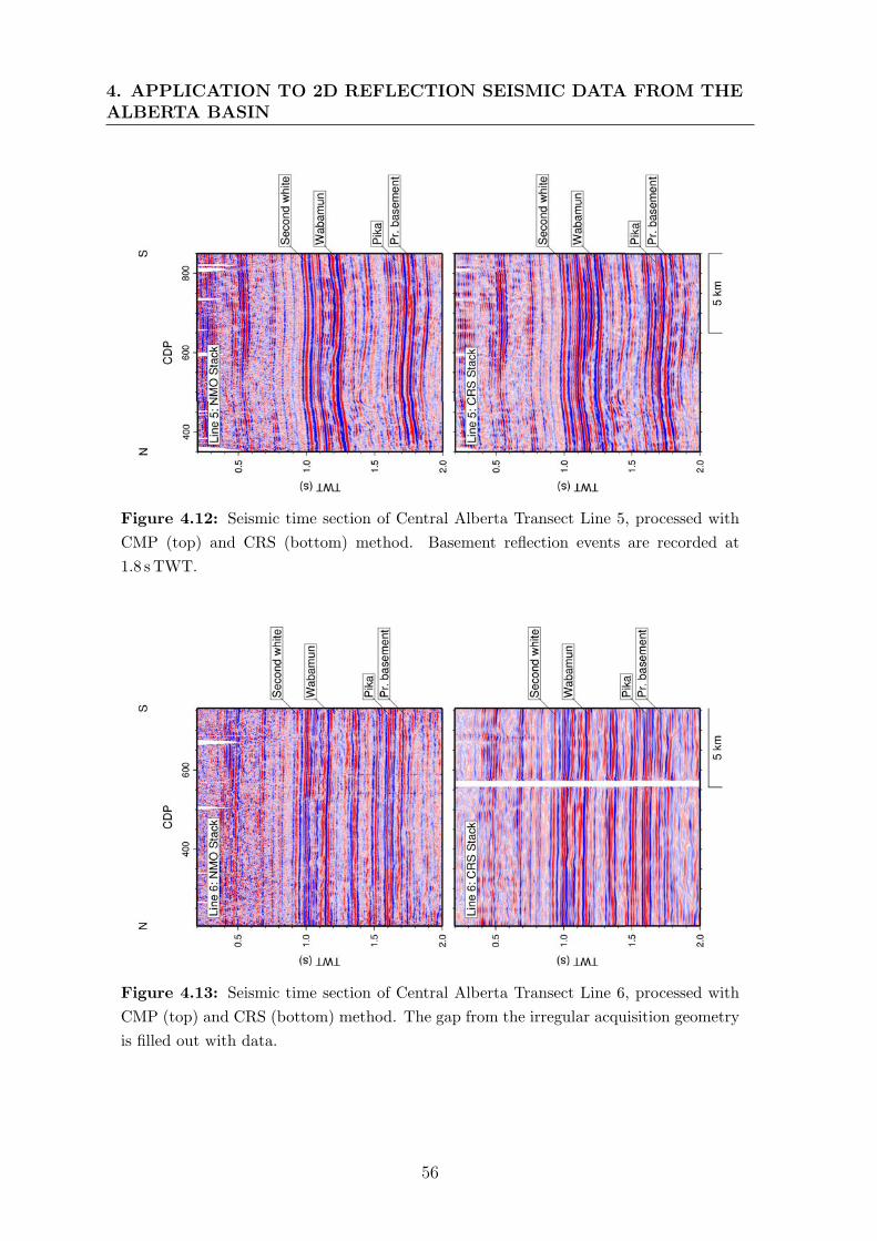
4. APPLICATION TO 2D REFLECTION SEISMIC DATA FROM THEALBERTA BASIN
Figure 4.12: Seismic time section of Central Alberta Transect Line 5, processed with
CMP (top) and CRS (bottom) method. Basement reflection events are recorded at
1.8 sTWT.
Figure 4.13: Seismic time section of Central Alberta Transect Line 6, processed with
CMP (top) and CRS (bottom) method. The gap from the irregular acquisition geometry
is filled out with data.
56
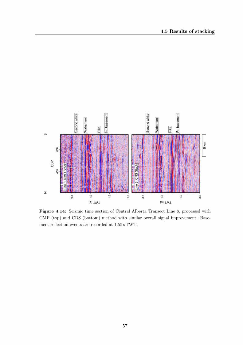
4.5 Results of stacking
Figure 4.14: Seismic time section of Central Alberta Transect Line 8, processed with
CMP (top) and CRS (bottom) method with similar overall signal improvement. Base-
ment reflection events are recorded at 1.55 sTWT.
57

4. APPLICATION TO 2D REFLECTION SEISMIC DATA FROM THEALBERTA BASIN
Figure 4.15: Seismic time section of Central Alberta Transect line 9, processed with
CMP (top) and CRS (bottom) method. The termination characteristics of basement
reflections are recorded at 1.4 s TWT.
58
4.6 Analysis of seismic signal attributes
4.6 Analysis of seismic signal attributes
The composite section of about 500 km length assembled from a 2D seismic lines and
acquired within the Lithoprobe project (Eaton et al., 1995) were used to facilitate
differentiation of structural and tectonic units that spans over Western Canada Sedi-
mentary Basin. In the previous chapter, Central Alberta Transect line’s of the Litho-
probe project, serve as the input data to perform comparison between CMP and the
CRS stack. Here, I used the resultant stack sections in order to calculate seismic
trace attribute acquired along specific horizons and represented by attributes of RMS
amplitude and instantaneous frequency. Both stack composite sections as well as the
attributes image provide valuable information and can be used to show the interactions
between the crystaline basement and sedimentary strata of the Paleozoic succession.
While the reflection seismic image based on CRS stack allowed the structural iden-
tification of the horizon more clear, the seismic attribute analysis along the horizon
obtained from that stack offer the possibility to distinguish the tectonic domains with
higher order of confidence.
Seismic attributes were calculated to indicate the variations in lithology and thick-
ness of the stratigraphic units that build the sedimentary package above the basement
reflection event. Additionally, attributes were used to determine in more detail the loca-
tion of lithofacies transition, structural features such as faults, alignments, lithological
edges etc. visible between basement and sedimentary layers contact or directly within
sedimentary formations. These structures were depicted in figure 6.3 and although
their structural manifestation were presented on the seismic crosss-section however its
representation in the form of seismic attribute also plays significant role, in geothermal
exploration especially.
I used RMS amplitude and instantaneous frequency attributes as they are particu-
larly useful for reservoir analysis within the basin environment. Both attributes belong
to the primary group of seismic trace attributes and additionally may serve as the
background for many others sophisticated or sometimes redundant attributes (Barnes,
2007; Taner, 2001). The RMS amplitude is computed as reflectivity within time win-
dow and can be treated as hydrocarbon or facies changes discriminator (Hammond,
1974). The higher values can also indicate intensive compaction of sediments due to
a direct relationship with reflectivity (Chopra & Marfurt, 2011; Yilmaz, 2001). The
instantaneous frequency attribute belongs to the group of instantaneous attributes that
are derived from Hilbert transformation of the seismic trace and by definition is time
59
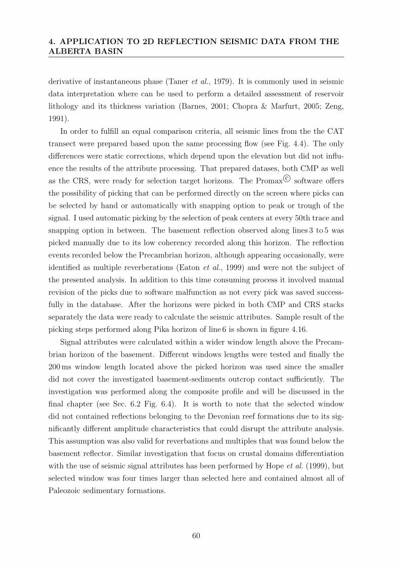
4. APPLICATION TO 2D REFLECTION SEISMIC DATA FROM THEALBERTA BASIN
derivative of instantaneous phase (Taner et al., 1979). It is commonly used in seismic
data interpretation where can be used to perform a detailed assessment of reservoir
lithology and its thickness variation (Barnes, 2001; Chopra & Marfurt, 2005; Zeng,
1991).
In order to fulfill an equal comparison criteria, all seismic lines from the the CAT
transect were prepared based upon the same processing flow (see Fig. 4.4). The only
differences were static corrections, which depend upon the elevation but did not influ-
ence the results of the attribute processing. That prepared datases, both CMP as well
as the CRS, were ready for selection target horizons. The Promax c© software offers
the possibility of picking that can be performed directly on the screen where picks can
be selected by hand or automatically with snapping option to peak or trough of the
signal. I used automatic picking by the selection of peak centers at every 50th trace and
snapping option in between. The basement reflection observed along lines 3 to 5 was
picked manually due to its low coherency recorded along this horizon. The reflection
events recorded below the Precambrian horizon, although appearing occasionally, were
identified as multiple reverberations (Eaton et al., 1999) and were not the subject of
the presented analysis. In addition to this time consuming process it involved manual
revision of the picks due to software malfunction as not every pick was saved success-
fully in the database. After the horizons were picked in both CMP and CRS stacks
separately the data were ready to calculate the seismic attributes. Sample result of the
picking steps performed along Pika horizon of line 6 is shown in figure 4.16.
Signal attributes were calculated within a wider window length above the Precam-
brian horizon of the basement. Different windows lengths were tested and finally the
200 ms window length located above the picked horizon was used since the smaller
did not cover the investigated basement-sediments outcrop contact sufficiently. The
investigation was performed along the composite profile and will be discussed in the
final chapter (see Sec. 6.2 Fig. 6.4). It is worth to note that the selected window
did not contained reflections belonging to the Devonian reef formations due to its sig-
nificantly different amplitude characteristics that could disrupt the attribute analysis.
This assumption was also valid for reverbations and multiples that was found below the
basement reflector. Similar investigation that focus on crustal domains differentiation
with the use of seismic signal attributes has been performed by Hope et al. (1999), but
selected window was four times larger than selected here and contained almost all of
Paleozoic sedimentary formations.
60
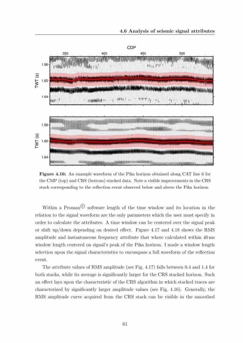
4.6 Analysis of seismic signal attributes
Figure 4.16: An example waveform of the Pika horizon obtained along CAT line 6 for
the CMP (top) and CRS (bottom) stacked data. Note a visible improvements in the CRS
stack corresponding to the reflection event observed below and above the Pika horizon.
Within a Promax c© software length of the time window and its location in the
relation to the signal waveform are the only parameters which the user must specify in
order to calculate the attributes. A time window can be centered over the signal peak
or shift up/down depending on desired effect. Figure 4.17 and 4.18 shows the RMS
amplitude and instantaneous frequency attribute that where calculated within 40ms
window length centered on signal’s peak of the Pika horizon. I made a window length
selection upon the signal characteristics to encompass a full waveform of the reflection
event.
The attribute values of RMS amplitude (see Fig. 4.17) falls between 0.4 and 1.4 for
both stacks, while its average is significantly larger for the CRS stacked horizon. Such
an effect lays upon the characteristic of the CRS algorithm in which stacked traces are
characterized by significantly larger amplitude values (see Fig. 4.16). Generally, the
RMS amplitude curve acquired from the CRS stack can be visible in the smoothed
61

4. APPLICATION TO 2D REFLECTION SEISMIC DATA FROM THEALBERTA BASIN
Figure 4.17: The result from a seismic signal attribute calculation obtained for both
CMP (middle) and CRS (bottom) stacks acquired along Line 6 of the Lithoprobe transect.
The attributes of RMS amplitude was calculated within ±20ms window length (top).
form, leaving out noisy or other fine–scale structures that are typically observed within
the CMP stacked dataset. Although the number of anomalies detected on both stacks
shows high compliance in respect to the calculated values, however one anomaly did not
62
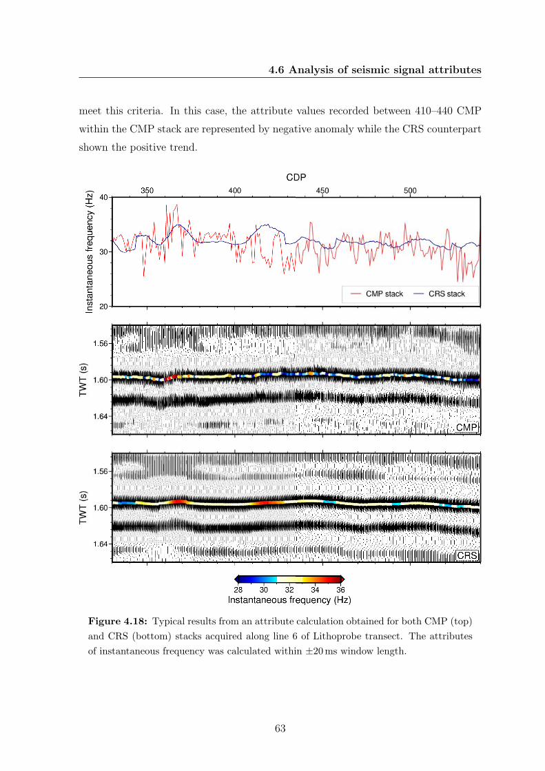
4.6 Analysis of seismic signal attributes
meet this criteria. In this case, the attribute values recorded between 410–440 CMP
within the CMP stack are represented by negative anomaly while the CRS counterpart
shown the positive trend.
Figure 4.18: Typical results from an attribute calculation obtained for both CMP (top)
and CRS (bottom) stacks acquired along line 6 of Lithoprobe transect. The attributes
of instantaneous frequency was calculated within ±20ms window length.
63
4. APPLICATION TO 2D REFLECTION SEISMIC DATA FROM THEALBERTA BASIN
The attribute of instantaneous frequency calculated for the same sample profile of
CMP and the CRS stack is presented on Figure 4.18. As can be seen, both profiles
are dominated by an average frequency of 34 Hz showing anomaly peaks ranging from
20 to almost 40 Hz. Similar to the RMS amplitude acquired from CMP stack, the
distribution of instantaneous frequency attribute is presented in the form of noisy curve
dominated by a small–scale structures, however a three significant minimum anomalies
can be clearly distinguished in the subset. Different results were obtained for the
second curve, where as might be expected, a similar smooth effect is accompanied by
the results obtained for the CRS stack. Even due to a considerable small variance
values in the frequency distribution, which makes the detailed observation less visible,
the same anomalies observed in the CMP stacked dataset were represented as the rapid
phenomena of increased/decreased values.
Although a significant diversity in the frequency distribution makes the differen-
tiation between CMP and the CRS method complicated, nevertheless it shows some
specific correlation, especially those related to the CRS stacked data. For example, the
effect of rapid phenomenons consisting of positive/negative pairs within amplitude and
frequency can be easily identified at the CMPs 345, 430 and 460 suggesting the struc-
tural relationship. On the other side, there are positive amplitude anomalies recorded
through the profile that are not correlated with frequency anomalies. Such an effect
can be observed at CMP 390 and 470. Unfortunately, direct explanation of this effect
can not be achieved by the simple signal comparison and other techniques or advance
modeling studies should be incorporated. Therefore, more details concerning CMP and
CRS stack comparisons as well as the detailed attribute interpretation I will present
in the Chapter 6.2.
64
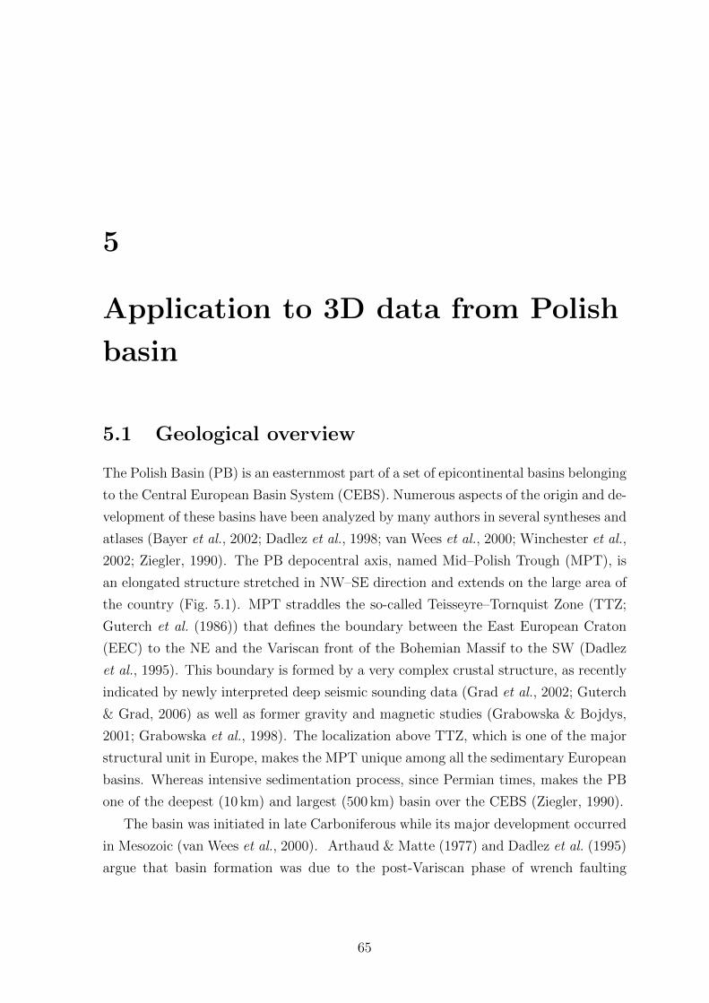
5
Application to 3D data from Polish
basin
5.1 Geological overview
The Polish Basin (PB) is an easternmost part of a set of epicontinental basins belonging
to the Central European Basin System (CEBS). Numerous aspects of the origin and de-
velopment of these basins have been analyzed by many authors in several syntheses and
atlases (Bayer et al., 2002; Dadlez et al., 1998; van Wees et al., 2000; Winchester et al.,
2002; Ziegler, 1990). The PB depocentral axis, named Mid–Polish Trough (MPT), is
an elongated structure stretched in NW–SE direction and extends on the large area of
the country (Fig. 5.1). MPT straddles the so-called Teisseyre–Tornquist Zone (TTZ;
Guterch et al. (1986)) that defines the boundary between the East European Craton
(EEC) to the NE and the Variscan front of the Bohemian Massif to the SW (Dadlez
et al., 1995). This boundary is formed by a very complex crustal structure, as recently
indicated by newly interpreted deep seismic sounding data (Grad et al., 2002; Guterch
& Grad, 2006) as well as former gravity and magnetic studies (Grabowska & Bojdys,
2001; Grabowska et al., 1998). The localization above TTZ, which is one of the major
structural unit in Europe, makes the MPT unique among all the sedimentary European
basins. Whereas intensive sedimentation process, since Permian times, makes the PB
one of the deepest (10 km) and largest (500 km) basin over the CEBS (Ziegler, 1990).
The basin was initiated in late Carboniferous while its major development occurred
in Mesozoic (van Wees et al., 2000). Arthaud & Matte (1977) and Dadlez et al. (1995)
argue that basin formation was due to the post-Variscan phase of wrench faulting
65
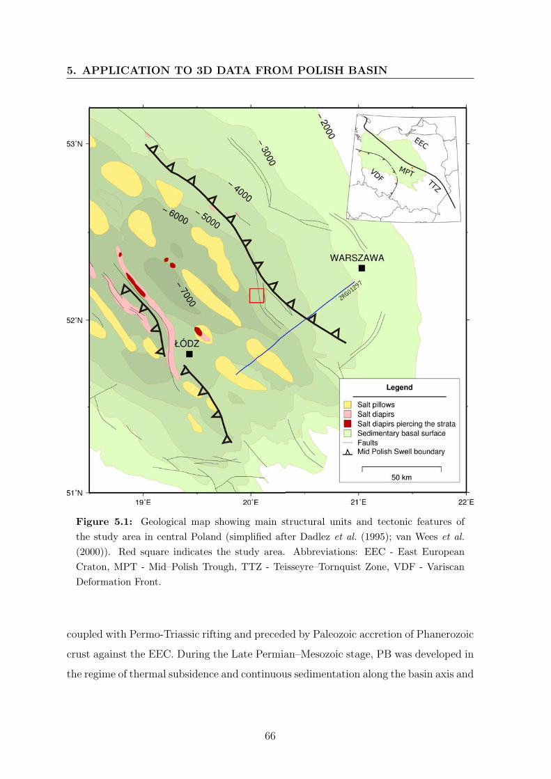
5. APPLICATION TO 3D DATA FROM POLISH BASIN
Figure 5.1: Geological map showing main structural units and tectonic features of
the study area in central Poland (simplified after Dadlez et al. (1995); van Wees et al.
(2000)). Red square indicates the study area. Abbreviations: EEC - East European
Craton, MPT - Mid–Polish Trough, TTZ - Teisseyre–Tornquist Zone, VDF - Variscan
Deformation Front.
coupled with Permo-Triassic rifting and preceded by Paleozoic accretion of Phanerozoic
crust against the EEC. During the Late Permian–Mesozoic stage, PB was developed in
the regime of thermal subsidence and continuous sedimentation along the basin axis and
66
5.1 Geological overview
interrupted by three tectonic subsidence pulses (Dadlez et al., 1995; Karnkowski, 1999;
Stephenson et al., 2003; Ziegler, 1990). Those pulses of accelerated basin subsidence
occurred in the Zechstein–Scythian, Oxfordian–Kimmeridgian and early Cenomanian
can be explained by thermal attenuation of lithosphere (Dadlez et al., 1995; van Wees
et al., 2000).
Structural trend of this complex is characterized by NW–SE-oriented syn-sedimentary
and transversal faulting (Marek & Znosko, 1972). The remains of the subsidence pro-
cess are several kilometers of sediments, interleaved by thick Zechstein salts layers
(Dadlez et al., 1998; Marek & Pajchlowa, 1997). In a later stage, from the Triassic to
the Quaternary, syn-sedimentary salt movements caused the development of a complex
system of salt structures (see Fig. 5.2). Various tectonics aspects as well as the heat
transfer model have been analyzed by numerous authors (Bujakowski, 2003; Burliga,
1996; Krzywiec, 2004; Majorowicz et al., 2003; Resak et al., 2008). Later, during the
Laramian orogenic event in the Late Cretaceous–Paleocene, sedimentary cover was
inverted due to NE–SW-oriented intra-continental compression (Dadlez et al., 1995)
linked to a change of the convergence between Africa and Eurasia (Albarello et al.,
1995; Pichon et al., 1988). This gave rise to the formation of regional tectonic unit
called Mid–Polish Swell (MPS, Dadlez et al. (1998); Kutek & Glazek (1972)), inten-
sively eroded in the Tertiary and covered by Paleogene sediments (Dadlez, 2003).
Figure 5.2: Regional geological cross-section illustrating the general geology of the
Polish Basin, simplified after Gorecki (1995). The locations of cross-sections is shown on
the insert.
Natural resources of MPT
67
5. APPLICATION TO 3D DATA FROM POLISH BASIN
The Mid–Polish Through is the major reservoir of natural gas in Poland. The gas
deposits are accumulated in the southeastern part of MPT within the Permian horizons
while in the northern part within the Carboniferous and Permian. The economic
reserves within the MPT consist of 78.5 x 10⁹ m3 and represent of about 70 % of the
total exploitable resources in Poland (Szuflicki et al., 2013). The biggest gas fields
located in southeastern part of MPT, Barnowko–Mostno–Buszow (BMB) that was
discovered in 1993, has proved resources of around 9.9 x 10⁹ m3 (Mamczur & Radecki,
1998) accumulated within a dolomite reef structure.
In 2012, the crude oil resources that are hosted in Permian, Carboniferous and
Cambrian formations stored within MPT represented 75 % of total Polish oil resources
while the economic reserves within MPT consists of about 18.8 x 10⁶ t crude oil (Szu-
flicki et al., 2013). Similar to the gas field, the biggest oil field is BMB (Mamczur
& Radecki, 1998), that has proved resources of around 7.8 x 10⁶ t crude oil (double of
the total reserves before its discovery). Another of great importance is the Lubiatow–
Midzychod–Grotow (LMG) oil field, that was discovered in 1993 and has proven re-
sources of 5.4 x 10⁶ t (Papiernik et al., 2009). The resources of the LMG oil field are
stored in the Main Dolomite strata of the Zechstein cycloterm PZ2.
The major source of salt resources located within the area of MPT are Zechstein
salts, that stretch over the late epicontinental basin and consist of the evaporates with
the salt sediments, reaching 1000 m in thickness. Salt formations have structures of pil-
lows and diapirs that have elongated form, stretched parallel to the general subsidence
axis of MPT, as depicted on Figure 5.1. Although, the total exploitable resources
consist of about 85 x 109 t (Szuflicki et al., 2013), the exploitation is currently per-
formed with limited scale (about 3.9 x 10⁶ t) but these structures are in great interest
for petroleum industry due to storage capabilities.
Geothermal regime
The Polish basin belong to a group of three main geothermal provinces in Poland
(Sokolowski, 1993) that are selected based on geostructural units division. Basins
formations host numerous geothermal aquifers developed by extensive sedimentation
processes between the Triassic and the Cretaceous period. Relatively large thickness
(from 7 to 12 km) of sedimentary succession dominated by the presence of sandstones
and carbonates rocks makes it possible to distinguish six aquifers, reach in occurrence of
geothermal resources (Gorecki, 1995). Generally, the mesozoic formations are charac-
terized with good hydrogeological and reservoir parameters. The heat flow rate values
68
5.1 Geological overview
vary from 20 to 90 mW/m2 (Szewczyk & Gientka, 2009), while the reservoir tempera-
tures that can be found at depths down to 4 km vary from 30 to 130 ◦ C. Water reserves
differ between the horizons from several to 150 l/s, whereas total dissolved solids (TDS)
of the water varies from several to 300 g/l (Gorecki, 2006; Gorecki et al., 2003).
Determination of recovered geothermal heat in the manner of economic performance
can be carried out in order to classify the perspective zones from which the geothermal
heat can be commercially produced. Gorecki (2006) applied the so-called ”power fac-
tor” method (Gosk, 1982) to perform the economic evaluation of the Paleozoic aquifers
in a simplified way. Based on such evaluation it was possible to indicate that the Lower
Jurassic aquifer has the largest disposable resources among all geothermal aquifers of
the Polish Basin and can produce 1.88 x 10¹⁸ J/year of geothermal energy. On the other
side, relatively low disposable resources occur in the Upper Jurassic aquifer. Its poor
reservoir properties due to average permeability about 90 mD and low production rates
from the boreholes allow to obtain 2.54 x 10¹⁷ J/year of geothermal energy.
Currently, there are four plants using the geothermal water for heat production
while another five are in realization phase (Kepinska, 2010). Two geothermal plants n
are operated next to the site, which utilize the heat of underground waters for district
heating. Since 1999, geothermal heat plant in Mszczonow, located 40 km southeast of
the test site, utilizes water with a temperature of approx. 40 ◦C from the Cretaceous
sandstones. The very low mineralization of the exploited water (TDS 0.5 g/l) makes
it possible to use it both for heating and drinking. In Uniejow, 80 km west of the test
site, since 2001 a heat plant exploits geothermal waters hosted in the same Cretaceous
sandstones with temperature about 60 ◦ C and TDS about 5 g/l (Kepinska, 2003).
Target horizon
Within the study area, the basin is filled with sedimentary rocks ranging in age
from Early Permian to Maastrichtian and its sedimentary succession is about 6000 m
thick. Tectonic patterns are related to the Polish Basin general development stages
and the layers lying below are the Permian–Mesozoic complex, however, the former
seismic image indicates two zones, separated by a major N–S normal fault (Fig. 5.1).
The eastern part presents a complex system of normal and reverse faults, striking
predominantly in NW–SE direction. The western part is a basin with a sedimentary
thickness that varies from 600 m near its borders to 2300 m at its center.
Three horizons, the most perspective for the geothermal usage, were found in the
well Kompina-2 (Fig. 5.3) located in the central place of the site. Generally, Lower
69

5. APPLICATION TO 3D DATA FROM POLISH BASIN
Cretaceous horizon and Lower Jurassic are more productive and the temperature of
geothermal medium reach below 100 ◦C. On the other side, the deepest reservoir, Upper
Triassic found at depth of 4100m, provides water with temperature about 110 ◦C but
its production capabilities is fairly low.
Figure 5.3: Well log curves for Kompina-2 well. From left a) Gamma, Temperature
and Caliper, b) Lithology and c) Porosity profile where the brine outflow of 40m3/h was
recorded from J1 horizon.
Three horizons, the most perspective for the geothermal usage, were found in the
well Kompina-2 (Fig. 5.3) located in the central place of the site. Generally, Lower
Cretaceous horizon and Lower Jurassic are more productive and the temperature of
70
5.1 Geological overview
the geothermal medium reaches below 100 ◦C. On the other side, the deepest reservoir,
Upper Triassic found at depth of 4100 m, provides water with a temperature about
110 ◦C but its production capabilities is fairly low. The Lower Cretaceous aquifer
spans over about 128 000 km2 whereas its total thickness varies from several to over
400 m (Leszczynski, 2012; Marek, 1988a). Lower Cretaceous water saturated beds
are composed mainly from permeable sands, sandy-marly and sandy-muddy sediments
which forms a common water-bearing layer. Temperature distribution varies from 20
to 40 ◦C while in the survey area the temperature rises to over 50 ◦C which is related
to the higher thickness of sediments in the axial zone. Among the Lower Cretaceous
groundwaters, the lowest TDS was found in the survey area, where its value equals sev-
eral g/dm3 . Pumping tests performed in 60 water wells showed an average hydraulic
conductivity value of about 7.8 x 10⁵ m/s (Gorecki, 1995). The Lower Cretaceous sedi-
mentary succession reveals a higher permeability and occur at smaller depths but show
comparable pressures in comparison with Lower Jurassic aquifer. Chemical contami-
nation of the Lower Cretaceous groundwater is dominated by HCO3 and Ca, whereas
a salinity over 10 g/dm3 is mostly due to the Cl–Na type brine (Gorecki, 2006). Addi-
tionally, bromide and iodine ions within the geothermal waters of the Lower Cretaceous
formation allow their balneological and recreational utilization.
The rocks, that build the Lower Jurassic aquifer, are composed of sandstones, inter-
bedded with semi- or impermeable claystones, mudstones. Variable thickness of sand-
stone rocks, locally cracked due to tectonic activities, creates a typical artesian to
subartesian aquifer (Bojarski et al., 1979). In the survey area its thickness equals
about 600 m whereas the permeable rocks build 50 % of its total thickness. Although,
the Lower Jurassic sediments show vertical variability and facies changes, it may be
suggested that reservoir waters developed as a continuous aquifer (Gorecki, 2006). The
hydrogeological parameters were obtained mostly from an old petroleum borehole and
are sufficient to determine the complex storage efficiency values in limited accuracy.
The chemical composition of the Lower Jurassic waters depends on geostructural fac-
tors that are characterized mainly by increased mineralization with depth. Its value
varies from 0.2 to 174 g/dm3 due to recharge areas fed with fresh, infiltrational waters,
while its composition is dominated by CO3–Ca, HCO3–Na–Ca, HCO3–SO4–Ca types
(Bojarski et al., 1979; Gorecki, 1995). Similar to the Lower Cretaceous aquifer, high
concentration of iodine and bromine components make the geothermal water of the
Lower Jurassic suitable for balneological purposes. Within the survey area the salinity
71
5. APPLICATION TO 3D DATA FROM POLISH BASIN
value is more than 100 g/dm3 which is typical for that exceeding below 1500 m due to
slow exchange rate of waters in the deeper parts of the Lower Jurassic aquifer (Bojarski
& Sadurski, 2000). Since, the water discharge factor strongly depends on thickness of
water bearing layer the discharge rate of about 250–350 m3/h can be expected in the
survey area. High intensity of exchange rate also affects the temperature distribution
that makes from those typical of shallow fresh waters to 120 ◦C in the deeper part
(Gorecki, 2006).
Based on the production test carried out in well Kompina-2 and the quality of
obtained data, the Lower Jurassic (J1) horizon was selected for further investigation.
It is composed by the alternating layers of sandstone and claystone with total thickness
in the 400-900 m range. In Kompina-2 they yield more than 150 m3/h of about 80 ◦C
water that has a TDS between 80 and 120 g/l (see Fig. 5.3).
Sediments of the Lower Triassic formations were developed within the marine en-
vironment of hot and dry climate (Marek & Znosko, 1972) that results in claystone–
siltstone rocks with isolated patches of sandstone lithofacies. Although, the total thick-
ness of the formation varies between a dozen meters up to 1600 m in the center of the
basin axis, the aquifer thickness does not exceed 400 m in the central part and is less
than 200 m in the remaining areas ((Marek, 1988b; Nawrocki et al., 2013). The lower
temperatures of a few degrees were measured at the edge of the structures, mostly on
the eastern side, whereas the rising tendency was observed towards the basin center,
where temperatures over 140 ◦C were observed. Similar trends characterize the distri-
bution of mineralization, where values of a few g/dm3 were measured at the marginal
part whereas values up to 350 g/dm3 dominate in the center (Gorecki, 1995, 2006).
Within survey area a temperature as high as 100 ◦C was observed and the mineraliza-
tion of the geothermal medium was 250 g/dm3. The whole area of the Lower Triassic
aquifer is characterized by low hydraulic conductivity values (1-3 x 10⁻⁴ cm/s) that
qualify it as poor aquifer. Its capabilities of discharges do not exceed 50 m3/h over
50 % of the aquifer volume (Gorecki, 2006).
5.2 Experiment description and data assessment
Several 2D seismic reflection surveys were acquired near the investigation area in the
1970s (Cianciara, 1975; Cianciara & Piech, 1977). Although, the measurements were
performed by the use of 12-channel digital recording, however, in the results it was
72
5.2 Experiment description and data assessment
possible to trace strong reflections from the formations of the Lower Cretaceous and
Jurassic. The weaker reflections were obtained from the Triassic, mainly from disloca-
tion zones and salt pillows in the Zechstein formations. Additionally to the seismics,
there were semi-detailed magnetic survey and regional scale gravity measurements that
indicate the presence of a big anomaly which is directly linked with the TTZ tectonic
zone that crosses the entire country (Grabowska & Bojdys, 2001; Majorowicz, 2004).
The reprocessing of the old seismic surveys performed in 2006 (Borowska, 2006)
showed the presence of three clearly visible structural levels, (1) the Dogger–Cretaceous
level, characterized by gentle tectonics and the quite intensive subsidence that occurred
during the Cretaceous; (2) the Upper Permian–Triassic–Lias level, mainly marine sedi-
mentary rocks locally perturbed by salt tectonics; (3) the Precambrian–Lower Permian
level, characterized by weak reflections and hard to identify without the borehole data.
The new experiment, a 3D reflection seismic survey was carried out in November
2007. Project was conducted within the scope of 6th Framework European Programme
titled ”Integrated Geophysical Exploration Technologies for deep fractured geothermal
systems - I–GET” (Contract No. 518378 SES6) and operated at the site by Mineral
and Energy Economy Research Institute of Polish Academy of Sciences in Krakow
(MEERI PAS). The main target of the project was to use the combination of seismic
and magnetotelluric (MT) methods as the integrated tool to improve the detection of
geothermal deposits and thus minimize the geological risk prior to drilling operation.
The Polish site, named Skierniewice, was treated as the test site selected due to
low and intermediate enthalpy of geothermal deposits occurring in sedimentary rocks
of the Cretaceous, Jurassic and Triassic formations (Bujakowski et al., 2010; Cumming
& Bruhn, 2010). Within the I–GET project similar formations were tested at Gross
Schonebeck site, Germany (Bauer et al., 2006). Based on that surveys experience,
star–like arrangement for seismic layout was considered insufficient and was replaced
with a grid seismic layout presented below.
The study region (Fig. 5.1) covered an area of about 30 km2 and is located 70 km
west of Warsaw, central Poland. The acquisition was carried out on an agricultural area
that is crossed by a dense network of drainage channels which increased the acquisition
time due to many bypasses. The land relief is characterized by a weak diversity in
terms of topography and elevation along the individual profiles varying from about
95 m in the NW to about 85 m in the SE part of the survey. The complete survey took
73
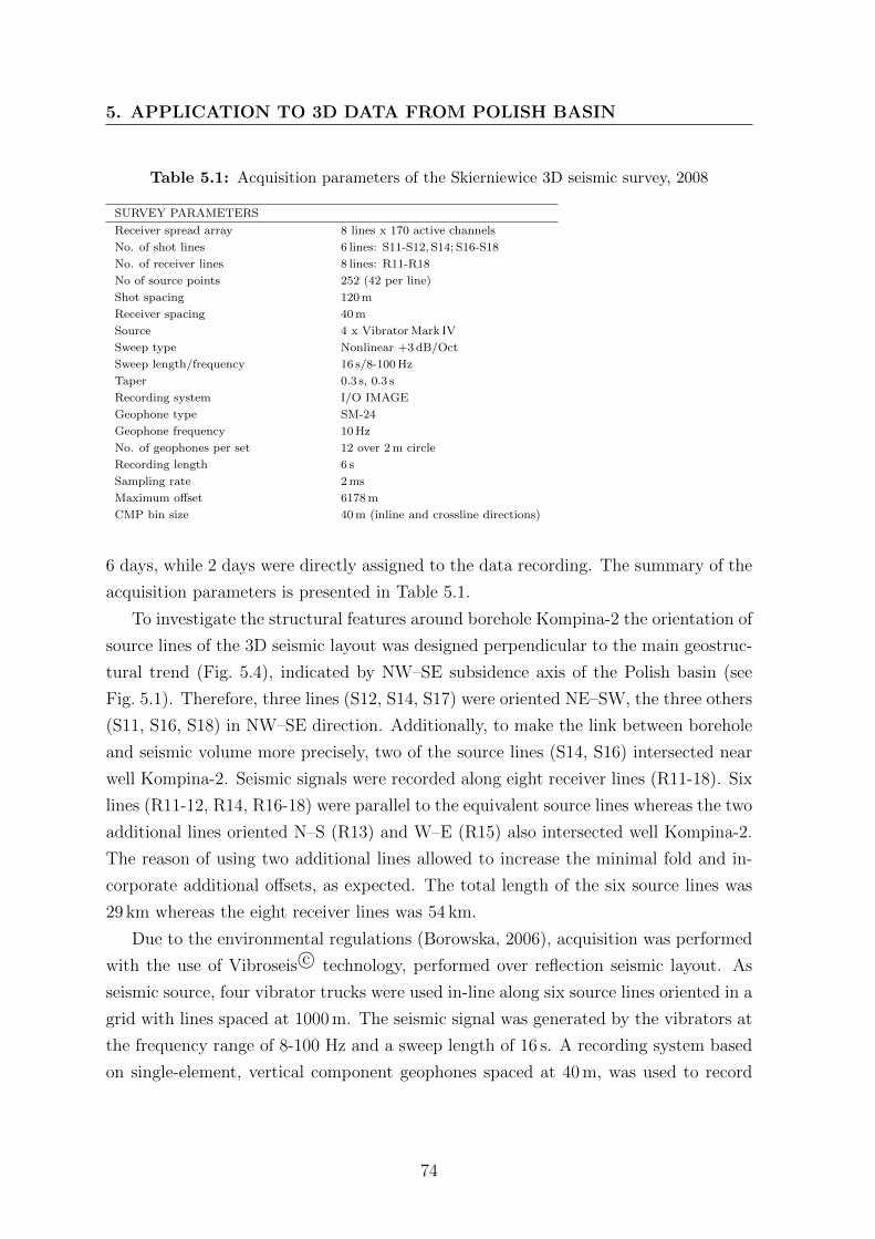
5. APPLICATION TO 3D DATA FROM POLISH BASIN
Table 5.1: Acquisition parameters of the Skierniewice 3D seismic survey, 2008
SURVEY PARAMETERS
Receiver spread array 8 lines x 170 active channels
No. of shot lines 6 lines: S11-S12, S14; S16-S18
No. of receiver lines 8 lines: R11-R18
No of source points 252 (42 per line)
Shot spacing 120 m
Receiver spacing 40 m
Source 4 x Vibrator Mark IV
Sweep type Nonlinear +3 dB/Oct
Sweep length/frequency 16 s/8-100 Hz
Taper 0.3 s, 0.3 s
Recording system I/O IMAGE
Geophone type SM-24
Geophone frequency 10 Hz
No. of geophones per set 12 over 2 m circle
Recording length 6 s
Sampling rate 2 ms
Maximum offset 6178 m
CMP bin size 40 m (inline and crossline directions)
6 days, while 2 days were directly assigned to the data recording. The summary of the
acquisition parameters is presented in Table 5.1.
To investigate the structural features around borehole Kompina-2 the orientation of
source lines of the 3D seismic layout was designed perpendicular to the main geostruc-
tural trend (Fig. 5.4), indicated by NW–SE subsidence axis of the Polish basin (see
Fig. 5.1). Therefore, three lines (S12, S14, S17) were oriented NE–SW, the three others
(S11, S16, S18) in NW–SE direction. Additionally, to make the link between borehole
and seismic volume more precisely, two of the source lines (S14, S16) intersected near
well Kompina-2. Seismic signals were recorded along eight receiver lines (R11-18). Six
lines (R11-12, R14, R16-18) were parallel to the equivalent source lines whereas the two
additional lines oriented N–S (R13) and W–E (R15) also intersected well Kompina-2.
The reason of using two additional lines allowed to increase the minimal fold and in-
corporate additional offsets, as expected. The total length of the six source lines was
29 km whereas the eight receiver lines was 54 km.
Due to the environmental regulations (Borowska, 2006), acquisition was performed
with the use of Vibroseis c© technology, performed over reflection seismic layout. As
seismic source, four vibrator trucks were used in-line along six source lines oriented in a
grid with lines spaced at 1000 m. The seismic signal was generated by the vibrators at
the frequency range of 8-100 Hz and a sweep length of 16 s. A recording system based
on single-element, vertical component geophones spaced at 40 m, was used to record
74

5.2 Experiment description and data assessment
the signals during the time of 6.0 s at sampling rate of 2ms. With differential GPS
technology and GPS devices mounted on the vibrator trucks the recording sites and
shot localizations reached the accuracy of about 0.01m. Recorded signals were stored
on 4mm tape in SEG-D format (Barry et al., 1975) whereas survey parameters in SPS
format (SEG, 1995).
Shallow refraction measurements were performed in addition to the reflection survey
in order to investigate the low velocity zone (LVZ). A hammer source was used to
generate seismic signals along five short profiles (not indicated on Fig. 5.4) over a
spread of 180m length with various receivers spacing. The velocity obtained below
the LVZ from refraction measurements varies between 1700 and 2200m/s and was
interpolated over the whole layout (Borowska, 2006).
Figure 5.4: The layout of a sparse 3D reflection seismic survey acquired in Skierniewice
site. (a) Acquisition geometry plotted onto CMP fold coverage map obtained for a CMP
bin size of 40x40m. The sources are indicated by white stars, receivers by black triangles
and Kompina-2 borehole is located in the middle b) Azimuth distribution form the survey
(grouped together into sector for display purposes), c) histogram of Source-Receiver offset
distribution.
Seismic reflection data were acquired at 252 source localization, spaced at 120m
75

5. APPLICATION TO 3D DATA FROM POLISH BASIN
intervals over a grid with 1360 channels used simultaneously. In the results, about
342 000 seismic traces were collected during the data acquisition. Although, a max-
imum obtained offset of 6188.78 m (see Fig. 5.4c) ensured the identification of the
deepest Permian horizon within the survey area, however, due to limited number of
traces with such long offsets, the penetration depth was rather limited to 4000 m depth.
Overall dynamic range and continuity of recorded signal was good and allowed to
trace the reflections from the sedimentary succession of the Cretaceous, Jurassic and
Triassic formation. The seismic reflection events from deeper parts are characterized
with less quality of recorded signals, however the lower Triassic formation expected
at 2.5 s TWT are still observed. Figure 5.5 shows typical raw shot gathers with high
quality of recorded signals and clearly visible first arrivals. Also several distinct re-
flections can be found deeper along all receiver lines, however its number and quality
decrease with distance from the source. Analysis of the amplitude spectrum indicates
that dominant frequency ranges vary between 40-50 Hz and the low-frequency noise is
mostly associated with ground roll, typically below 30 Hz.
5.3 CMP Processing
Within the frame of this thesis, simultaneous recordings from 1360 active channels
were processed as a sparse low fold 3D survey with a 2.44 km2 homogeneous fold area
in the center of the survey. Such a sparse survey becomes widely accepted and allows
to reduce acquisition cost while achieving imaging objectives with sufficient resolution
(Eisenberg-Klein et al., 2008; Trappe et al., 2005). It is worth to note that the survey,
however, was designed as a sparse 3D measurement that also allows to process the
dataset in the form of six independent 2D lines, composed of 170 channels each (with
28 CMP fold).
The review of original processing sequence performed in 2008 (Bujakowski et al.,
2010) followed the setting of new processing parameters. This allowed to identify crucial
steps that were applied to solve some key data or noise issues occurring within the
dataset. The original processing sequence was based on the standard procedure for land
seismic reflection data (i.e. (Yilmaz, 2001)), although special attention was given due
to non uniform offset and fold distribution within bins. Table 5.6 shows the parameters
of principal steps applied during the processing. Generally, it based on the assumption
that the flat sediment deposits with different acoustic impedance found in the study
76

5.3 CMP Processing
Figure 5.5: Raw shot gather from the shot number 58 recorded onto receiver lines
R11-R18. Reflection from the sedimentary successions are still visible down to 2.0 s.
In addition to the very good signal quality of the several primary reflections, note the
ground roll visible on line R13-15 and R18.
area, should produce strong reflections. The original data were provided as a single file
in SEG-Y format. An additional file, containing the survey information stored in SPS
format, was used to set up the geometry within the Promax c© processing software.
Provided records had already been demultiplexed and correlated with vibrator signal.
In the first step, data were loaded into the processing software and changed to its
internal format which increases the speed up the whole processing.
An important question for further processing was the appropriate CMP binning.
Typically, bin size equals half of the receiver group spacing, however this produced
a very low CMP fold value of around 6. Such a low value covered a large part of
the grid which caused a high disproportion in fold distribution, and allowed credible
77

5. APPLICATION TO 3D DATA FROM POLISH BASIN
Figure 5.6: Processing flow of 3D seismic reflection data from Skierniewice site, Poland.
On left side, processing sequence performed by Geofizyka Krakow (Bujakowski et al.,
2010). Right column contains the steps of processing adapted for the comparison purpose.
On white are the matched the steps not included within the CRS processing method.
interpretation only along source lines. Based on tests with various bin sizes that may
increase heterogeneous value of the coverage factor, I decided to choose a CMP bin size
of 40 m by 40 m, which is equal to the group spacing along receiver lines. I followed the
equation proposed by Yilmaz (2001) which defines the relationship between the bin size
78
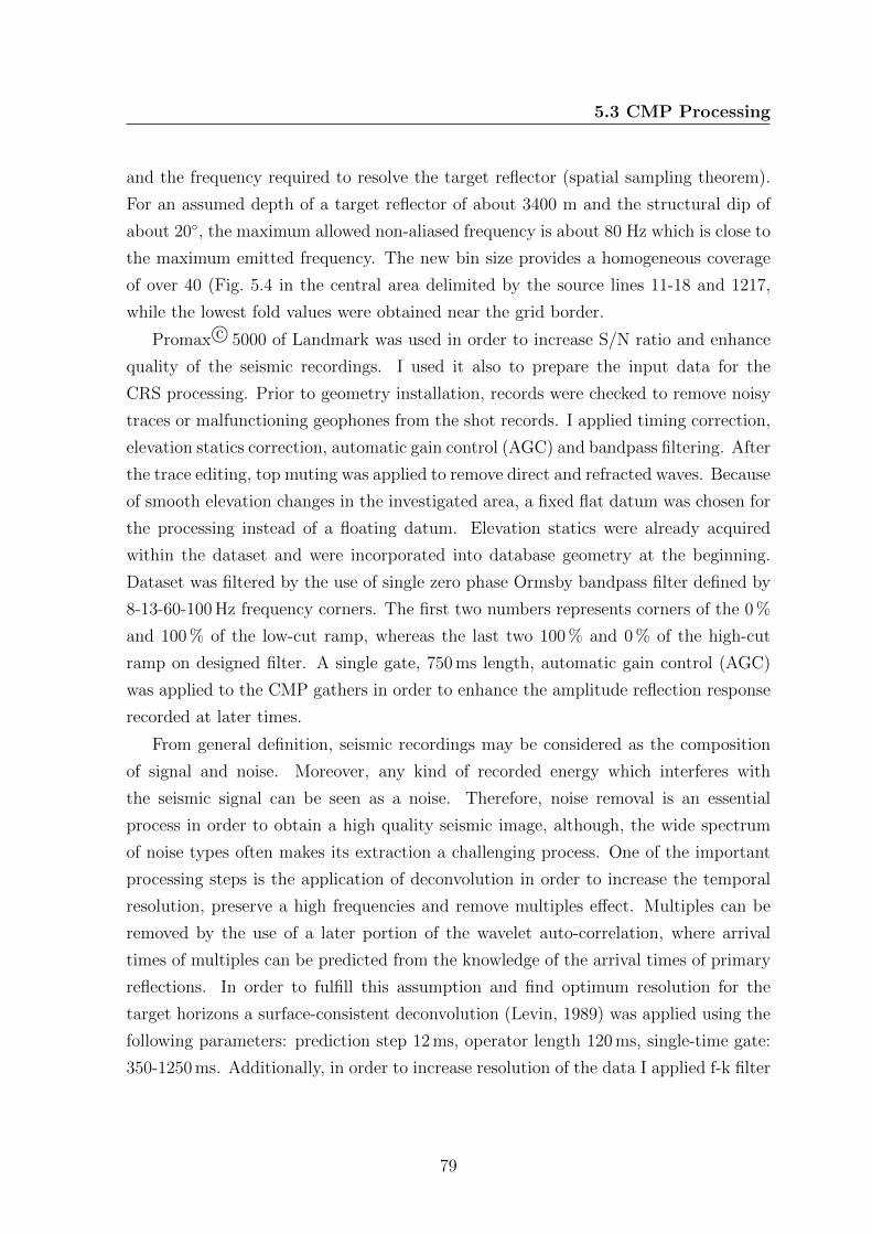
5.3 CMP Processing
and the frequency required to resolve the target reflector (spatial sampling theorem).
For an assumed depth of a target reflector of about 3400 m and the structural dip of
about 20◦, the maximum allowed non-aliased frequency is about 80 Hz which is close to
the maximum emitted frequency. The new bin size provides a homogeneous coverage
of over 40 (Fig. 5.4 in the central area delimited by the source lines 11-18 and 1217,
while the lowest fold values were obtained near the grid border.
Promax c© 5000 of Landmark was used in order to increase S/N ratio and enhance
quality of the seismic recordings. I used it also to prepare the input data for the
CRS processing. Prior to geometry installation, records were checked to remove noisy
traces or malfunctioning geophones from the shot records. I applied timing correction,
elevation statics correction, automatic gain control (AGC) and bandpass filtering. After
the trace editing, top muting was applied to remove direct and refracted waves. Because
of smooth elevation changes in the investigated area, a fixed flat datum was chosen for
the processing instead of a floating datum. Elevation statics were already acquired
within the dataset and were incorporated into database geometry at the beginning.
Dataset was filtered by the use of single zero phase Ormsby bandpass filter defined by
8-13-60-100 Hz frequency corners. The first two numbers represents corners of the 0 %
and 100 % of the low-cut ramp, whereas the last two 100 % and 0 % of the high-cut
ramp on designed filter. A single gate, 750 ms length, automatic gain control (AGC)
was applied to the CMP gathers in order to enhance the amplitude reflection response
recorded at later times.
From general definition, seismic recordings may be considered as the composition
of signal and noise. Moreover, any kind of recorded energy which interferes with
the seismic signal can be seen as a noise. Therefore, noise removal is an essential
process in order to obtain a high quality seismic image, although, the wide spectrum
of noise types often makes its extraction a challenging process. One of the important
processing steps is the application of deconvolution in order to increase the temporal
resolution, preserve a high frequencies and remove multiples effect. Multiples can be
removed by the use of a later portion of the wavelet auto-correlation, where arrival
times of multiples can be predicted from the knowledge of the arrival times of primary
reflections. In order to fulfill this assumption and find optimum resolution for the
target horizons a surface-consistent deconvolution (Levin, 1989) was applied using the
following parameters: prediction step 12 ms, operator length 120 ms, single-time gate:
350-1250 ms. Additionally, in order to increase resolution of the data I applied f-k filter
79

5. APPLICATION TO 3D DATA FROM POLISH BASIN
(Yilmaz, 2001) to remove acoustic and surface waves. The step helped also to remove
high-amplitude disturbance and to suppress steep amplitude variations. Figure 5.7
presents sample shot gathers with the influence of various processing steps and their
impact on signal to noise ratio (S/N) reduction.
Until now, the seismic dataset was stored as shot gathers, however further pro-
cessing steps i.e velocity analysis requires additional CMP sorting that includes CMP
bin location beside existing information of source and receiver locations, field record
numbers, etc. Determination of NMO velocities was performed by the use of semblance
analysis on a subset of the in-line and cross-line CMP positions. These locations over-
lapped with high fold lines source lines and between. Then, velocities were interpolated
for all CMPs in the 3D volume. There were no significant velocity variations lateral
nor vertical observed throughout the volume that could indicate the presence of salt
structures in the region characterized by strong velocity variations compared to the
surrounding sediments. Relatively continuous distribution of reflections over the vol-
ume allowed stacking velocities of the topmost reflection to be picked and determined
reliably.
As the final stage data were stacked by the use of common-mid-point stacking
procedure (see Fig. 5.8a,d). In consequence, an increase in reflection continuity and
reduction of the refracted energy were observed along all control lines. Despite a non-
uniform offset distribution and fold area inside bins, the final stack image is comparable
with the processing results obtained from standard 3D seismic surveys. Good quality
of the seismic reflections from the Cretaceous, Jurassic, Middle and Lower Triassic
horizons allows to recognize the geological formation in the study area. Even the seismic
horizons with lower quality signals (i.e. Upper Triassic) can be discerned. Within the
structural interpretation, it can be seen that investigated area is represented in the
form of a complex structure formed under the influence of uplift and salt tectonics
(Borowska, 2006). Although, CMP stacked volume was ready to compare with CRS
counterparts its further analysis was expanded to include lithofacial interpretation
based on the application of seismic attributes i.e. root-mean-square (RMS) amplitude
and instantaneous frequency (see section 6.2).
80
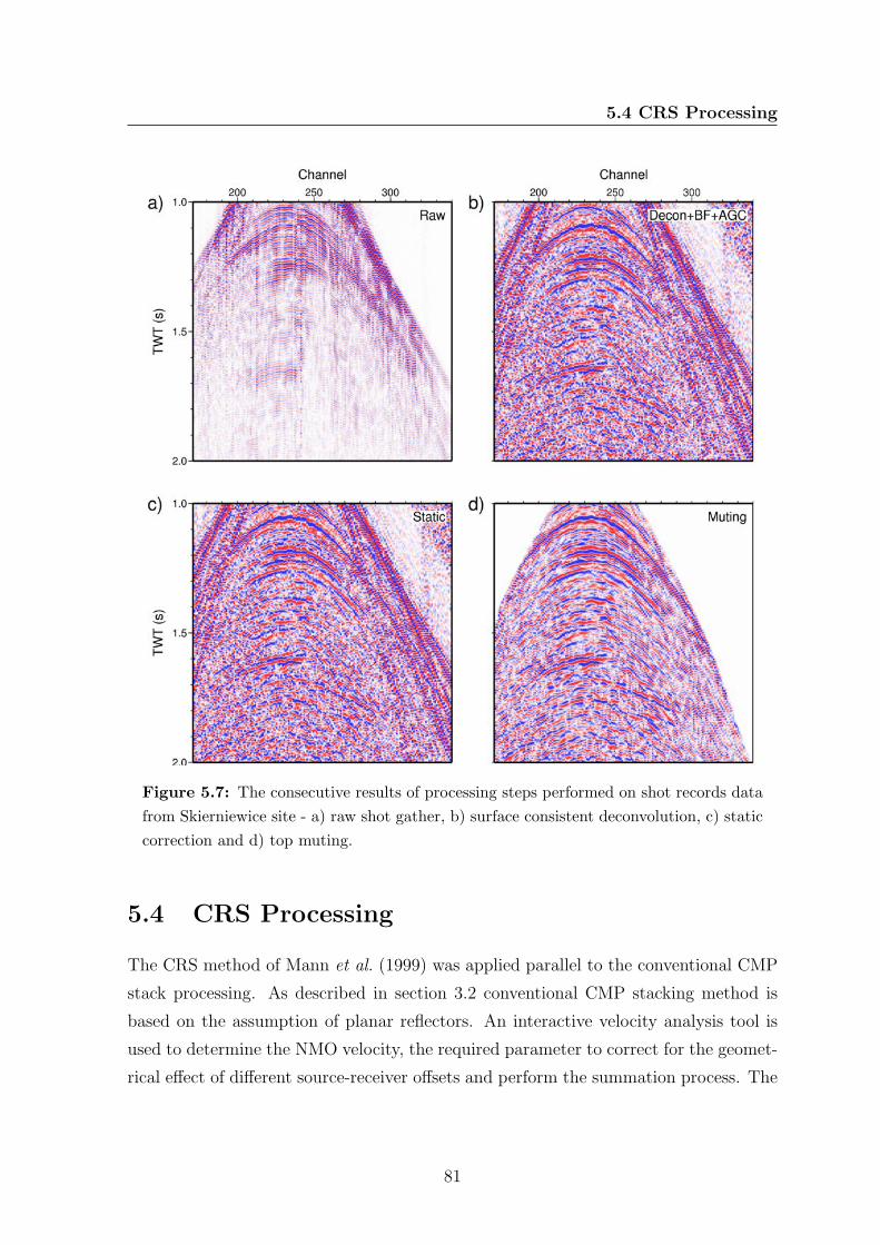
5.4 CRS Processing
Figure 5.7: The consecutive results of processing steps performed on shot records data
from Skierniewice site - a) raw shot gather, b) surface consistent deconvolution, c) static
correction and d) top muting.
5.4 CRS Processing
The CRS method of Mann et al. (1999) was applied parallel to the conventional CMP
stack processing. As described in section 3.2 conventional CMP stacking method is
based on the assumption of planar reflectors. An interactive velocity analysis tool is
used to determine the NMO velocity, the required parameter to correct for the geomet-
rical effect of different source-receiver offsets and perform the summation process. The
81
5. APPLICATION TO 3D DATA FROM POLISH BASIN
CRS stack represents a more generalized approach in which the assumed correction is
defined by the location, orientation and curvature Mann et al. (1999) of an assigned
surface. As a consequence, parametrization of the CRS stack operator allowed the
CRS method to be applied without a known macro-velocity model, which means no an
additional velocity analysis is required in principle. Within the general data processing
work flow the CRS method can be used as a substitute for the NMO velocity analysis,
and subsequent stack of the NMO corrected traces. The processing steps applied to the
data before the CRS stack are identical with the conventional processing. Practically
this means the data were processed in the conventional way as described in section 5.3
(Fig. 5.6), but were exported without the following application of the NMO correc-
tion. The subsequent CRS processing includes the determination of the CRS stacking
operator and the application of this operator during stacking (see Sect. 3.3). As men-
tioned, the CRS stacking operator is based on the concept of so-called eigenwaves
(Hubral, 1983). These hypothetical waves include (1) an up-going Normal Incidence
Point (NIP) wave generated from a point source at the reflector, and (2) an up-going
normal N wave generated from an exploding reflector. Following this proposed idea,
the reflected wave field measured at the surface can be described by three parameters
forming the CRS stacking operator (Mann et al., 1999): (1) the common emergent
angle α, (2) the curvature radius RN of the N wave front, and (3) the curvature radius
RNIP of the NIP wave front. These quantities are used in a parametric description of
the wave field at the surface based on par-axial ray theory (Schleicher et al., 1993). In
the implementation of Mann et al. (1999), the three parameters are determined for each
sample of a simulated zero-offset section by fitting the measured data with maximum
coherency (Neidell & Taner, 1971).
The CRS parameter estimation is carried out by subsequent solution of single-
parameter determination (Mann et al., 1999; Muller, 2007). Recent developments by
Garabito et al. (2012) make use of global optimization approaches instead of the single-
parameter estimation concept, but this method is established in 2D but not yet in 3D
so far. The data are first processed in the offset-domain similar to the CMP processing,
where a NMO velocity is determined automatically based on the maximal coherency
fitting of the data. This automatic NMO velocity implicitly depends on a combination
of the CRS parameters curvature radius RNIP and the emergent angle α. All three CRS
components are subsequently determined in the zero-offset-domain, with additional
consideration of the previously derived automatic NMO velocity values. More details
82
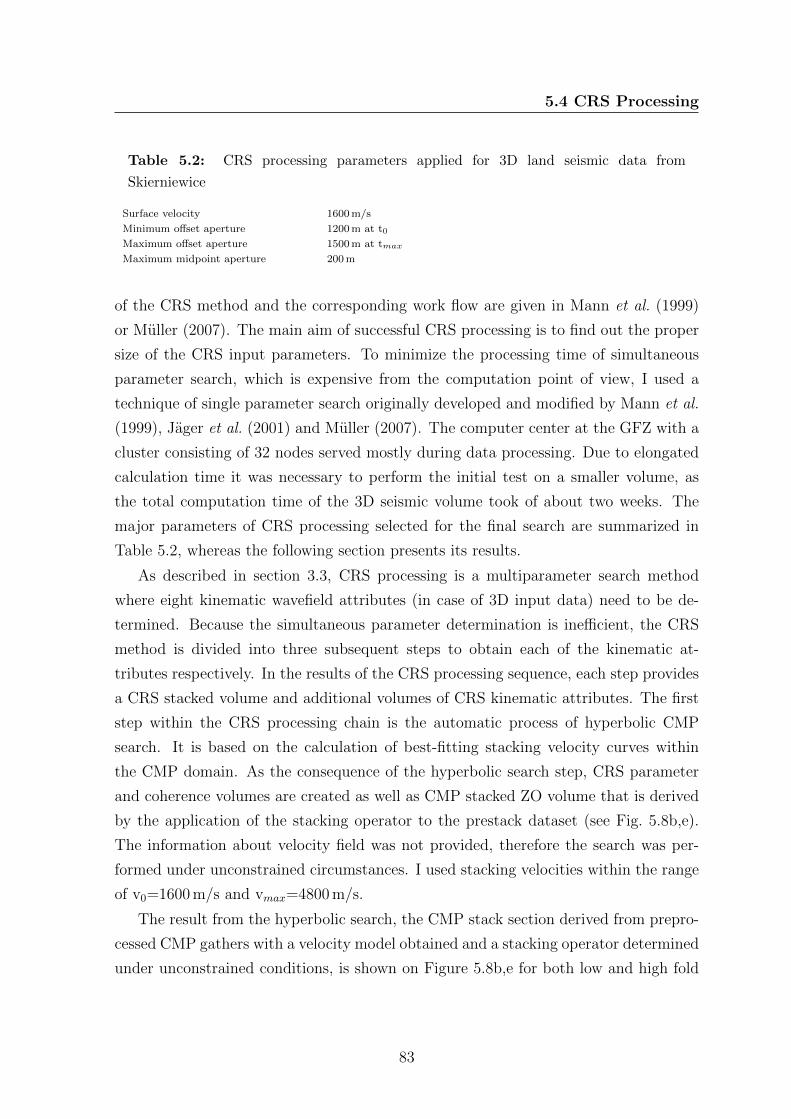
5.4 CRS Processing
Table 5.2: CRS processing parameters applied for 3D land seismic data from
Skierniewice
Surface velocity 1600 m/s
Minimum offset aperture 1200 m at t0
Maximum offset aperture 1500 m at tmax
Maximum midpoint aperture 200 m
of the CRS method and the corresponding work flow are given in Mann et al. (1999)
or Muller (2007). The main aim of successful CRS processing is to find out the proper
size of the CRS input parameters. To minimize the processing time of simultaneous
parameter search, which is expensive from the computation point of view, I used a
technique of single parameter search originally developed and modified by Mann et al.
(1999), Jager et al. (2001) and Muller (2007). The computer center at the GFZ with a
cluster consisting of 32 nodes served mostly during data processing. Due to elongated
calculation time it was necessary to perform the initial test on a smaller volume, as
the total computation time of the 3D seismic volume took of about two weeks. The
major parameters of CRS processing selected for the final search are summarized in
Table 5.2, whereas the following section presents its results.
As described in section 3.3, CRS processing is a multiparameter search method
where eight kinematic wavefield attributes (in case of 3D input data) need to be de-
termined. Because the simultaneous parameter determination is inefficient, the CRS
method is divided into three subsequent steps to obtain each of the kinematic at-
tributes respectively. In the results of the CRS processing sequence, each step provides
a CRS stacked volume and additional volumes of CRS kinematic attributes. The first
step within the CRS processing chain is the automatic process of hyperbolic CMP
search. It is based on the calculation of best-fitting stacking velocity curves within
the CMP domain. As the consequence of the hyperbolic search step, CRS parameter
and coherence volumes are created as well as CMP stacked ZO volume that is derived
by the application of the stacking operator to the prestack dataset (see Fig. 5.8b,e).
The information about velocity field was not provided, therefore the search was per-
formed under unconstrained circumstances. I used stacking velocities within the range
of v0=1600 m/s and vmax=4800 m/s.
The result from the hyperbolic search, the CMP stack section derived from prepro-
cessed CMP gathers with a velocity model obtained and a stacking operator determined
under unconstrained conditions, is shown on Figure 5.8b,e for both low and high fold
83

5. APPLICATION TO 3D DATA FROM POLISH BASIN
cross sections. An AGC of 500 ms window was applied to enhance the image resolution
and improve the visibility of deeper reflections. The obtained image shows that the
reflection events can be identified as deep as 2.0 s TWT. Furthermore, the CMP search
brings out a some more improvements when compared to the standard CMP stacked
section. The reflection events show a better continuity along the horizons as well as
from the target reflector recorded at 1.8 s TWT and deeper one. The improvements on
the low fold section (Fig. 5.8b) are not significant and the noise level is comparable to
the low fold section obtained from CMP stacking (Fig. 5.8a). This fact is important
due to an AGC filter enhances both the amplitude of seismic signal and the noise,
therefore its further interpretation should be performed with special care. The initial
comparison of the conventional CMP stack (Fig. 5.8a,d) with the results obtained by
the automatic CMP stack (Fig. 5.8b,e) shows already that minor improvements can be
achieved in the first step of the CRS processing. The proper selection of the aperture
size in the offset-domain is the most influential parameter at this step. Based on the
many tests I used the aperture size within the range of 200 m at 0.0 s and 2000 m at 3.0 s
of recording time that allowed to include as much reflection wave forms as possible.
Generally, the automatic CMP stacked volume is characterized by good quality re-
flections that have been recorded in the time window of 0.1-2.0 s TWT. In particular,
the gently dipping sedimentary succession of the Cenozoic, the Cretaceous and the Up-
per Jurassic is depicted in form of good continuity events with a noticeably impedance
contrast visible at 0.8-1.4 s TWT. The Lower Jurassic formations package, significant
due its geothermal potential, is visible down to 1.8 s TWT. Within the Lower Jurassic
package, the most productive horizon Ja1 has been imaged with high impedance con-
trast (marked by gray arrow). The differences between low fold and high fold images
(b,e), however similar to the standard CMP stack, present little more improvements.
These are visible mostly within younger formations up to 1.5 s TWT on both cross-
sections. Although the reflections from deeper horizons are not resolved ultimately,
and can be seen as disturbed and without continuity, some improvement is observed,
especially on the high-fold cross-section.
The Ja1 horizon recorded at 1.65 s TWT is very well imaged and allows for highly
reliable correlation, both in inline and cross-line direction. Moreover, the remaining
horizons show similar structural engagement, repeating the tectonic features between
neighborhood units located below and above. Conflicting dip situations often appear-
ing within sedimentary environments due to the presence of salt structures, were not
84
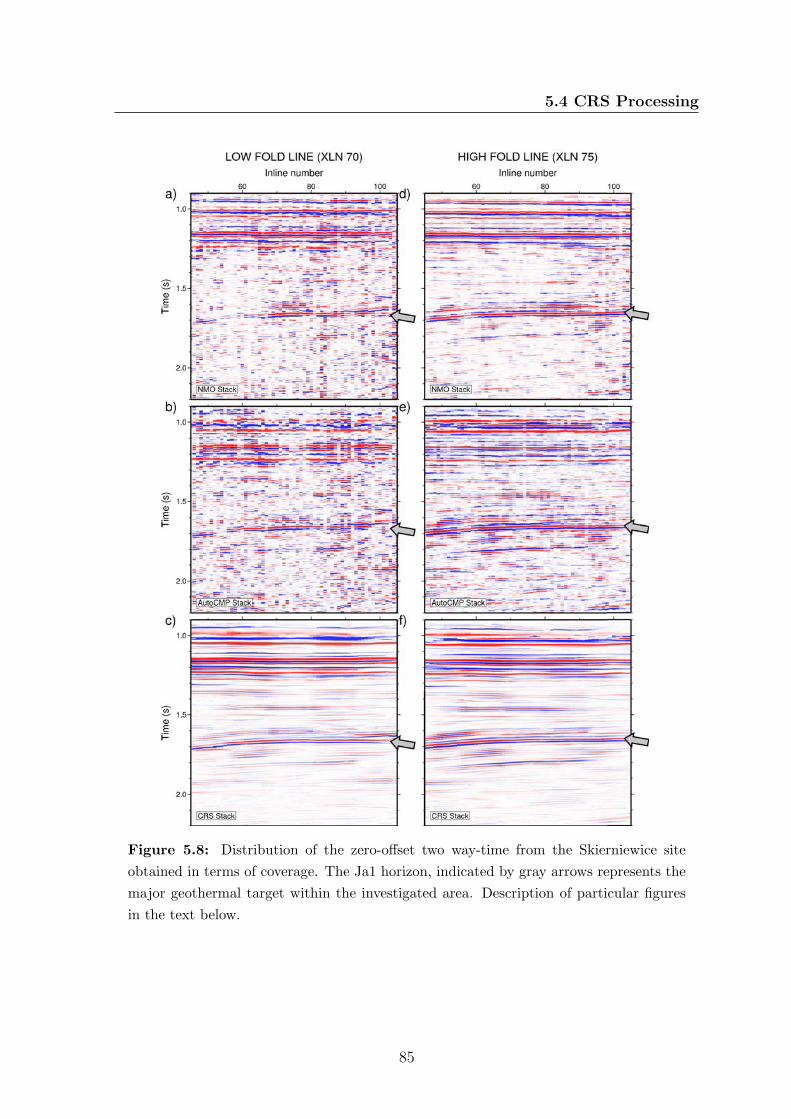
5.4 CRS Processing
Figure 5.8: Distribution of the zero-offset two way-time from the Skierniewice site
obtained in terms of coverage. The Ja1 horizon, indicated by gray arrows represents the
major geothermal target within the investigated area. Description of particular figures
in the text below.
85
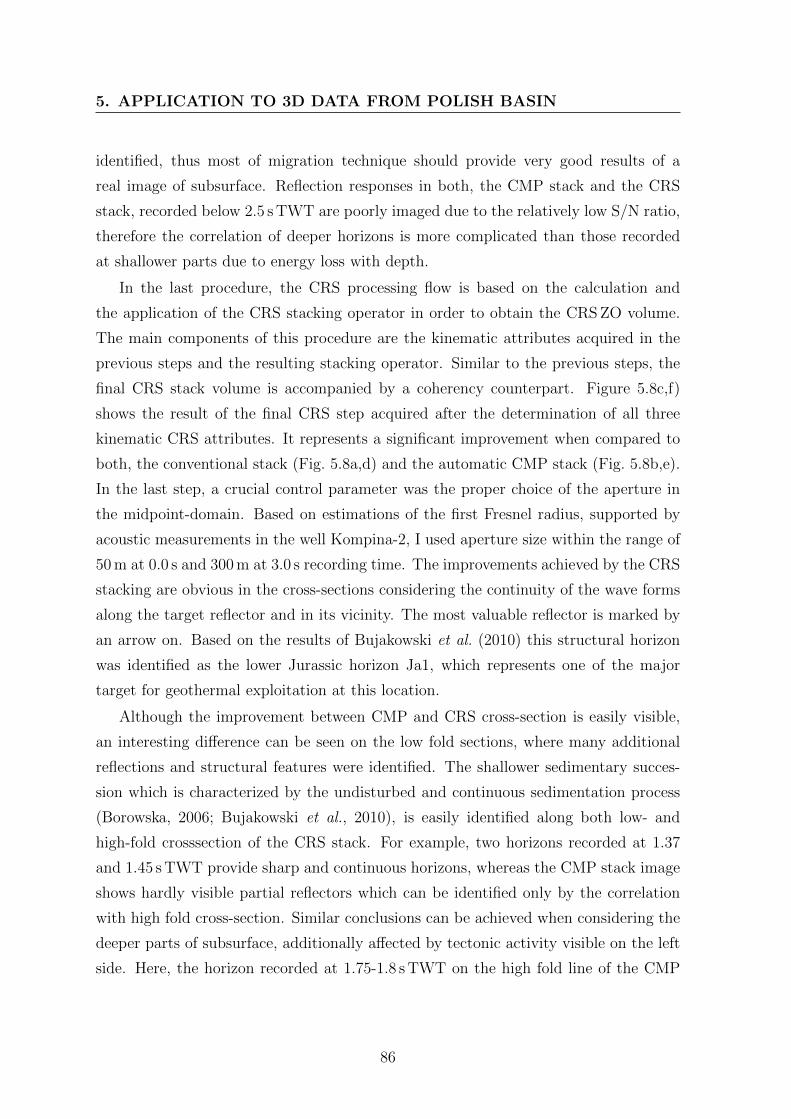
5. APPLICATION TO 3D DATA FROM POLISH BASIN
identified, thus most of migration technique should provide very good results of a
real image of subsurface. Reflection responses in both, the CMP stack and the CRS
stack, recorded below 2.5 s TWT are poorly imaged due to the relatively low S/N ratio,
therefore the correlation of deeper horizons is more complicated than those recorded
at shallower parts due to energy loss with depth.
In the last procedure, the CRS processing flow is based on the calculation and
the application of the CRS stacking operator in order to obtain the CRS ZO volume.
The main components of this procedure are the kinematic attributes acquired in the
previous steps and the resulting stacking operator. Similar to the previous steps, the
final CRS stack volume is accompanied by a coherency counterpart. Figure 5.8c,f)
shows the result of the final CRS step acquired after the determination of all three
kinematic CRS attributes. It represents a significant improvement when compared to
both, the conventional stack (Fig. 5.8a,d) and the automatic CMP stack (Fig. 5.8b,e).
In the last step, a crucial control parameter was the proper choice of the aperture in
the midpoint-domain. Based on estimations of the first Fresnel radius, supported by
acoustic measurements in the well Kompina-2, I used aperture size within the range of
50 m at 0.0 s and 300 m at 3.0 s recording time. The improvements achieved by the CRS
stacking are obvious in the cross-sections considering the continuity of the wave forms
along the target reflector and in its vicinity. The most valuable reflector is marked by
an arrow on. Based on the results of Bujakowski et al. (2010) this structural horizon
was identified as the lower Jurassic horizon Ja1, which represents one of the major
target for geothermal exploitation at this location.
Although the improvement between CMP and CRS cross-section is easily visible,
an interesting difference can be seen on the low fold sections, where many additional
reflections and structural features were identified. The shallower sedimentary succes-
sion which is characterized by the undisturbed and continuous sedimentation process
(Borowska, 2006; Bujakowski et al., 2010), is easily identified along both low- and
high-fold crosssection of the CRS stack. For example, two horizons recorded at 1.37
and 1.45 s TWT provide sharp and continuous horizons, whereas the CMP stack image
shows hardly visible partial reflectors which can be identified only by the correlation
with high fold cross-section. Similar conclusions can be achieved when considering the
deeper parts of subsurface, additionally affected by tectonic activity visible on the left
side. Here, the horizon recorded at 1.75-1.8 s TWT on the high fold line of the CMP
86

5.4 CRS Processing
stack is not visible on low fold section (Fig. 5.8a), whereas can be easily recognized on
their CRS counterpart, providing sharp and continuous reflection events.
The practical aspect from this experiment allows to assume that the application
of the CRS stack not only improve the imaging capabilities itself but when applied to
the low fold data it allows to image the reflection events that are partially or even not
visible when resolved by the CMP stack technique.
Figure 5.9: Results of the CRS stack processing obtained along Ja1 horizon: (a) CMP
hyperbolic search and radius of RNIP wave, (b) linear ZO search and the value of normal
ray RN , (c) ratio of RNIP /RN . Missing values are masked in gray.
Figure 5.10 of the corresponding coherency cross-section proves its usefulness help-
ing with the fault identification due to its higher values. In the coherency attribute the
amplitude of the signals along the structural or time horizon are observed in order to
find discontinuities within the amplitude field that are towards changes within struc-
tural characteristic of the formation (Klein et al., 2008). Coherency attribute belongs
to the group of a post-stack attributes that measures the signal continuity and are of-
ten used to delineate structural features like faults, channels, etc (Bahorich & Farmer,
1995; Marfurt et al., 1999).
87

5. APPLICATION TO 3D DATA FROM POLISH BASIN
Figure 5.10: Seismic cross section obtained from CRS stack (top) and corresponding
distribution of coherency attribute (bottom). The structural discontinuities observed
along Ja1 horizon are indicated by red ellipses.
Images presented on Figure 5.10 show two seismic cross sections obtained along
in-line 60 (a) and 90 (b), that were acquired with the use of standard CMP processing
sequence described on Fig. 5.6. The corresponding distribution of the coherency at-
88
5.5 Analysis of seismic signal attributes
tribute obtained from the CRS processed sections are presented at the bottom (c,d).
Areas marked by the red ellipses indicate the discontinuity of structural elements that
were already recognized as two faults (see Fig. 5.11). The section that goes along inline
60 crosses the main fault showing the broad zone between hanging and footwall. The
same results can be observed on the corresponding coherency section where Ja1 hori-
zon is marked by the highest coherency values. More interesting results are visible on
the cross section obtained along inline 90 where it goes through the main unit and the
smaller fault. Similar to the cross section of inline 60, the coherency image perfectly
match the location of Ja1 horizon.
The full spectrum of the CRS stack application is far more wider, but many aspects
of the CRS processing have been neglected due to the limited range of this thesis. As a
supplement to recent developments, describes in the section 3.3, it is worth to mention
others that are of particular importance. For instance due to the flat survey area and
a homogeneous 3D acquisition, the aspects of elevation variations and its influence on
time shifts and static correction that has been extensively described byHeilmann et al.
(2006); Zhang (2003) and Koglin (2005) were omitted. Another important problem of
nonuniform and arbitrary land acquisition geometries has been discussed by Boelsen
& Mann (2005) was also not implemented it this thesis. It is worth to mention that
as the results of these developments CRS method has been successfully adapted to
the ocean bottom seismic (OBS) and vertical seismic profiling (VSP) acquisition ge-
ometries. Another optimization aspect, consisting of a 2D CRS stack series performed
on restricted azimuth, described by Hocht (2002) however efficient in respect to the o
computational cost, was not applied d to heterogeneous distribution of azimuths. In
the next paragraph I will present the investigation on seismic signal attributes analysis
acquired from conventional and the CRS stacking method mapped across Ja1 horizon
within the 3D stacked data volume.
5.5 Analysis of seismic signal attributes
Seismic data volume usually contains particular information that can be extracted
by the analysis of seismic signal attributes, which allows to acquired an additional
characteristics of the subsurface. Additionally, seismic attributes are used to enhance
an image of structural features that helps to characterize reservoirs parameters or
provide information about media content accumulated within a sedimentary succession
89

5. APPLICATION TO 3D DATA FROM POLISH BASIN
(Chopra & Marfurt, 2007; Neidell & Taner, 1971; Taner et al., 1979). Attributes
are obtained from data cube over a time, depth or horizon within a specific time
window. Usually they describe signal characteristics or structural properties as well as
its statistics (Chopra & Marfurt, 2005; Taner, 2001).
Although the number of developed attributes still expand and many new were
evaluated since the introduction, there are only a few that have strong foundation and
relationship to the a physical properties of seismic signal. There are even many of
seismic attributes that can be seen as excessive or their application do not bring any
improvements, thus even make the interpreters even confused (Chen & Sidney, 1997;
Taner, 2001).
Generally, signal attributes are determined by the mathematical operation on am-
plitude, frequency or their spatial distribution, however, some specific information can
be provided by the use of multiple attribute apprach and/or its particular combination.
Seismic datasets may gain profits in the frame of structural interpretation, where sev-
eral attribute of seismic trace are extracted and evaluated. In this study, the attribute
analysis will focused on the application of the three attributes that can serve as a base
of signal characteristics classification.
In order to get the most benefits from the signal attribute analysis on Skierniewice
site, input dataset were prepared in the form of horizon picks. The selected Ja1 hori-
zon was picked manually within the stacked data volume. Special attention was given
the check the quality of picked horizon, where both in-line and cross-line grid orienta-
tion were considered. The distribution of two-way-time picked zero–offset reflections
obtained for horizon Ja1 is presented on Fig. 5.11.
The amplitude response of Ja1 horizon showed the presence of three distinct zones.
Its major border (marked by dashed line in Fig. 5.11) was identified as normal fault
of N330 azimuth that divides the structure on two parts. Southwestern part forms
the hangingwall, whereas the northeastern a larger block, shows an additional minor
fault of azimuth of N105. Proposed division remains in compliance with the fault
interpretation that was presented by Bujakowski et al. (2010).
Acquired picks of Ja1 horizon (Fig. 5.11) were used as the reference basis for the
attribute analysis. The selected attributes: root-mean-square (RMS) amplitude, in-
stantaneous frequency (Taner et al., 1979) were successively calculated within +/- 20 ms
time window centered on amplitude peak derived from Ja1 horizon (see Fig.5.12). The
selection of window length based on signal characteristics that is equal to one period
90
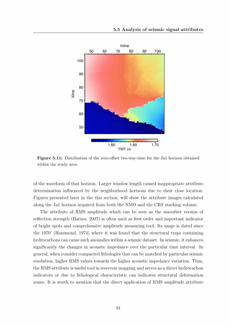
5.5 Analysis of seismic signal attributes
Figure 5.11: Distribution of the zero-offset two-way-time for the Ja1 horizon obtained
within the study area.
of the waveform of that horizon. Larger window length caused inappropriate attribute
determination influenced by the neighborhood horizons due to their close location.
Figures presented later in the this section, will show the attribute images calculated
along the Ja1 horizon acquired from both the NMO and the CRS stacking volume.
The attribute of RMS amplitude which can be seen as the smoother version of
reflection strength (Barnes, 2007) is often used as first order and important indicator
of bright spots and comprehensive amplitude measuring tool. Its usage is dated since
the 1970’ (Hammond, 1974) where it was found that the structural traps containing
hydrocarbons can cause such anomalies within a seismic dataset. In seismic, it enhances
significantly the changes in acoustic impedance over the particular time interval. In
general, when consider compacted lithologies that can be matched by particular seismic
resolution, higher RMS values towards the higher acoustic impedance variation. Thus,
the RMS attribute is useful tool in reservoir mapping and serves as a direct hydrocarbon
indicators or due to lithological characteristic can indicates structural deformation
zones. It is worth to mention that the direct application of RMS amplitude attribute
91
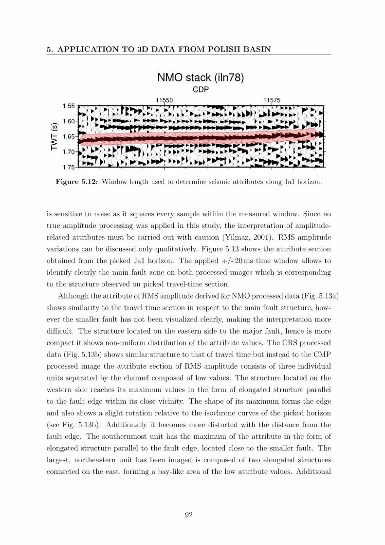
5. APPLICATION TO 3D DATA FROM POLISH BASIN
Figure 5.12: Window length used to determine seismic attributes along Ja1 horizon.
is sensitive to noise as it squares every sample within the measured window. Since no
true amplitude processing was applied in this study, the interpretation of amplitude-
related attributes must be carried out with caution (Yilmaz, 2001). RMS amplitude
variations can be discussed only qualitatively. Figure 5.13 shows the attribute section
obtained from the picked Ja1 horizon. The applied +/- 20ms time window allows to
identify clearly the main fault zone on both processed images which is corresponding
to the structure observed on picked travel-time section.
Although the attribute of RMS amplitude derived for NMO processed data (Fig. 5.13a)
shows similarity to the travel time section in respect to the main fault structure, how-
ever the smaller fault has not been visualized clearly, making the interpretation more
difficult. The structure located on the eastern side to the major fault, hence is more
compact it shows non-uniform distribution of the attribute values. The CRS processed
data (Fig. 5.13b) shows similar structure to that of travel time but instead to the CMP
processed image the attribute section of RMS amplitude consists of three individual
units separated by the channel composed of low values. The structure located on the
western side reaches its maximum values in the form of elongated structure parallel
to the fault edge within its close vicinity. The shape of its maximum forms the edge
and also shows a slight rotation relative to the isochrone curves of the picked horizon
(see Fig. 5.13b). Additionally it becomes more distorted with the distance from the
fault edge. The southernmost unit has the maximum of the attribute in the form of
elongated structure parallel to the fault edge, located close to the smaller fault. The
largest, northeastern unit has been imaged is composed of two elongated structures
connected on the east, forming a bay-like area of the low attribute values. Additional
92
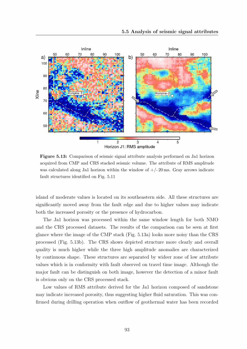
5.5 Analysis of seismic signal attributes
Figure 5.13: Comparison of seismic signal attribute analysis performed on Ja1 horizon
acquired from CMP and CRS stacked seismic volume. The attribute of RMS amplitude
was calculated along Ja1 horizon within the window of +/- 20ms. Gray arrows indicate
fault structures identified on Fig. 5.11
island of moderate values is located on its southeastern side. All these structures are
significantly moved away from the fault edge and due to higher values may indicate
both the increased porosity or the presence of hydrocarbon.
The Ja1 horizon was processed within the same window length for both NMO
and the CRS processed datasets. The results of the comparison can be seen at first
glance where the image of the CMP stack (Fig. 5.13a) looks more noisy than the CRS
processed (Fig. 5.13b). The CRS shows depicted structure more clearly and overall
quality is much higher while the three high amplitude anomalies are characterized
by continuous shape. These structures are separated by wideer zone of low attribute
values which is in conformity with fault observed on travel time image. Although the
major fault can be distinguish on both image, however the detection of a minor fault
is obvious only on the CRS processed stack.
Low values of RMS attribute derived for the Ja1 horizon composed of sandstone
may indicate increased porosity, thus suggesting higher fluid saturation. This was con-
firmed during drilling operation when outflow of geothermal water has been recorded
93
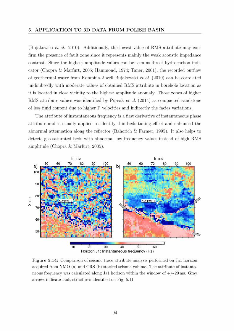
5. APPLICATION TO 3D DATA FROM POLISH BASIN
(Bujakowski et al., 2010). Additionally, the lowest value of RMS attribute may con-
firm the presence of fault zone since it represents mainly the weak acoustic impedance
contrast. Since the highest amplitude values can be seen as direct hydrocarbon indi-
cator (Chopra & Marfurt, 2005; Hammond, 1974; Taner, 2001), the recorded outflow
of geothermal water from Kompina-2 well Bujakowski et al. (2010) can be correlated
undoubtedly with moderate values of obtained RMS attribute in borehole location as
it is located in close vicinity to the highest amplitude anomaly. Those zones of higher
RMS attribute values was identified by Pussak et al. (2014) as compacted sandstone
of less fluid content due to higher P velocities and indirectly the facies variations.
The attribute of instantaneous frequency is a first derivative of instantaneous phase
attribute and is usually applied to identify thin-beds tuning effect and enhanced the
abnormal attenuation along the reflector (Bahorich & Farmer, 1995). It also helps to
detects gas saturated beds with abnormal low frequency values instead of high RMS
amplitude (Chopra & Marfurt, 2005).
Figure 5.14: Comparison of seismic trace attribute analysis performed on Ja1 horizon
acquired from NMO (a) and CRS (b) stacked seismic volume. The attribute of instanta-
neous frequency was calculated along Ja1 horizon within the window of +/- 20ms. Gray
arrows indicate fault structures identified on Fig. 5.11
94
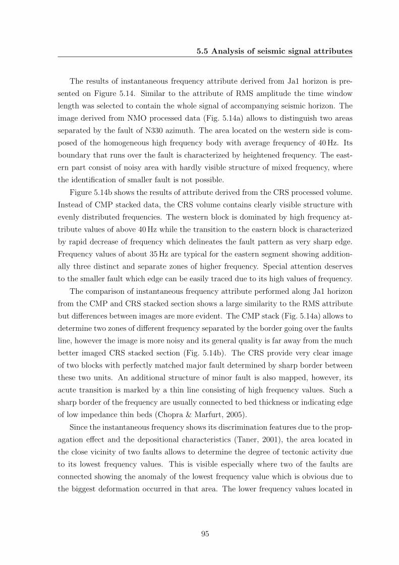
5.5 Analysis of seismic signal attributes
The results of instantaneous frequency attribute derived from Ja1 horizon is pre-
sented on Figure 5.14. Similar to the attribute of RMS amplitude the time window
length was selected to contain the whole signal of accompanying seismic horizon. The
image derived from NMO processed data (Fig. 5.14a) allows to distinguish two areas
separated by the fault of N330 azimuth. The area located on the western side is com-
posed of the homogeneous high frequency body with average frequency of 40 Hz. Its
boundary that runs over the fault is characterized by heightened frequency. The east-
ern part consist of noisy area with hardly visible structure of mixed frequency, where
the identification of smaller fault is not possible.
Figure 5.14b shows the results of attribute derived from the CRS processed volume.
Instead of CMP stacked data, the CRS volume contains clearly visible structure with
evenly distributed frequencies. The western block is dominated by high frequency at-
tribute values of above 40 Hz while the transition to the eastern block is characterized
by rapid decrease of frequency which delineates the fault pattern as very sharp edge.
Frequency values of about 35 Hz are typical for the eastern segment showing addition-
ally three distinct and separate zones of higher frequency. Special attention deserves
to the smaller fault which edge can be easily traced due to its high values of frequency.
The comparison of instantaneous frequency attribute performed along Ja1 horizon
from the CMP and CRS stacked section shows a large similarity to the RMS attribute
but differences between images are more evident. The CMP stack (Fig. 5.14a) allows to
determine two zones of different frequency separated by the border going over the faults
line, however the image is more noisy and its general quality is far away from the much
better imaged CRS stacked section (Fig. 5.14b). The CRS provide very clear image
of two blocks with perfectly matched major fault determined by sharp border between
these two units. An additional structure of minor fault is also mapped, however, its
acute transition is marked by a thin line consisting of high frequency values. Such a
sharp border of the frequency are usually connected to bed thickness or indicating edge
of low impedance thin beds (Chopra & Marfurt, 2005).
Since the instantaneous frequency shows its discrimination features due to the prop-
agation effect and the depositional characteristics (Taner, 2001), the area located in
the close vicinity of two faults allows to determine the degree of tectonic activity due
to its lowest frequency values. This is visible especially where two of the faults are
connected showing the anomaly of the lowest frequency value which is obvious due to
the biggest deformation occurred in that area. The lower frequency values located in
95

5. APPLICATION TO 3D DATA FROM POLISH BASIN
close vicinity of Kompina-2 well can be seen as bed thickness indicator where lower
frequencies may suggest a sand rich bedding, while on the other side, the lowest fre-
quency values recorded along faults plane can be seen as the fracture zone indicator
(Barnes, 2007, 1991; Taner, 2001).
96
6
Discussion and conclusions
In this thesis, a method for the improvement of seismic trace attribute quality has been
presented. The method is based on the application of the Common Reflection Surface
stack to prestack reflection data sets acquired from sedimentary basins. Instead of
conventional CMP stack, higher S/N ratio obtained from the CRS sections/volumes
allows to illuminate the structural elements with better accuracy. In consequence,
results of CRS imaging are used to enhance the seismic trace attribute calculation,
thus providing significant improvements in geothermal exploration campaign and help
in the determination of exploitation parameters at higher confidence level.
Imaging of seismic trace attributes acquired from CRS volume allows to indicate
potential zones for geothermal exploitation. The RMS amplitude and instantaneous
frequency attributes obtained from the CRS volume show higher quality when com-
pared to their CMP counterpart. Improved structural imaging performed in the close
vicinity of fault zones and its further lithological interpretation based on attribute
determination may significantly decrease drilling risk in further geothermal projects.
The method was tested on real data sets acquired from two sedimentary basins,
where different layouts of reflection seismic surveys were applied. The 2D seismic
reflection sections were obtained from the Alberta Basin within the Lithoprobe project,
whereas the 3D volume was acquired in the Polish basin within the I-GET project of
6th EU Framework Programme. The remaining part of the chapter shows the most
important improvements and conclusions within the CRS processing and seismic trace
attribute calculation.
97
6. DISCUSSION AND CONCLUSIONS
6.1 Improvements of stack images
2D seismic, Alberta basin
The Lithoprobe seismic reflection data (Eaton et al., 1995) presented within the
thesis consists of seven active seismic reflection lines of about 500 km total length ac-
quired within the Central Alberta Transects stage. The project was originally aimed
to provide the structural characteristics across the Western Canada Sedimentary Basin
(Hope et al., 1999) and deep crystalline basement. The acquisition parameters where
determined upon the strategy of deep basement imaging (see Table 4.1)) and allowed
also to highlight reflections from a sedimentary succession. In order to ensure the pen-
etration of very deep targets, the Vibroseis source was spaced at 100 m in asymmetric
split–spread layout over the large offsets up to 12 km length, while the seismic lines
crossed perpendicular the basement domains borders. Such a setup, highlighted the
very deep structures at expected resolution. The illumination of the shallower part
allowed to image the sedimentary succession only with moderate resolution, mostly
due to limited range of frequency content.
In the frame of the thesis, seismic data processing was performed within 2.0 s TWT
in order to provide structural images of the Alberta Basin with emphasis in develop-
ment of further geothermal exploration strategies. The investigated area can be char-
acterized by a regular subsidence process, undisturbed by far located tectonic units
and dominated by unique continuity of reflected horizons over regional scale. Gener-
ally, as presented in Section 4.5 (see Fig. 4.9–4.15), the processed data show lateral
homogeneity and continuous character within the sedimentary section, while holding
the consistency in vertical scale.
The top of the basement structure was depicted at 1.5-1.8 s TWT separating the
sedimentary succession from the low S/N image of the crustal zone, which is addition-
ally affected by multiple reflections. The undulating trend of the south-west dipping
monocline has shown a particular diversity in amplitude distribution across the cu-
mulative transect line. Its characteristic and correlation with respect to the location
of tectonic domains (see Fig. 4.1) will be discussed in the next section of attribute
analysis.
Figure 6.1a-c presents a selected example of stacked seismic line obtained with CMP
and CRS stack technique. The high quality image of CRS stack section has shown its
unique imaging capabilities with comparison to less quality reflections obtained from
98

6.1 Improvements of stack images
CMP counterpart. Independence from a given velocity model and rather small human
interaction, belong to the advantage of the CRS method.
Reflection events shown on Figure 6.1a can be easily distinguished on the basis of
exceptional continuity, visible only on the CRS stack section. Additional structural
feature of stratigraphic element, recorded on the right side at 550 ms TWT, could be
interpreted as apparent onlap simulated by further tectonic movements. It is worth to
note that an overwhelming number of minor stratigraphic interfaces, visible between
500 and 600 ms TWT show its continuity on the CRS image. Figure 6.1b can be seen as
an example of the unique feature of the CRS method, where redundancy of the seismic
traces is used to fill gaps in the shallower parts along stacked section. These gaps are
often visible for shallower parts of the CMP stack due to insufficient number of traces
with short offsets. Another improvement is shown in Figure 6.1c where noisy CMP
stack image can gain from the CRS technique. In this example the CRS stack shows
not only the overall improvements in signal characteristic and reflection continuity, but
also reveal the tectonic patterns that can be interpreted as a small listric fault (visible
on the right).
99

6. DISCUSSION AND CONCLUSIONS
Figure 6.1: Examples of CAT profiles showing improvements in the CRS stack over
CMP counterpart. Imaged reflections are more precisely and have better continuity,
moreover, even small events, recorded at are imaged.
100

6.1 Improvements of stack images
3D seismic, Polish basin
Seismic reflection data set, recorded in the central Poland that geologically belongs
to the Polish basin formation (see Fig. 5.1) were collected to perform the structural
analysis of the selected geothermal horizon that host within the Mesozoic sedimentary
formations. The acquisition geometry based on grid layout, with the well Kompina-2
located within its center. The log analysis from that borehole (see Fig. 5.3) indicates
the presence of geothermal waters within the Lower Jurassic aquifer. Seismic data
were acquired with the use of Vibroseis technology on the area characterized by a flat
topography. The layout consisted of six source lines oriented in the grid form where
three parallel lines spaced at 1 km were oriented perpendicular to the three others.
Six receiver lines followed the source lines orientation, whereas two supplemented lines
crossed the well Kompina-2. The signal from four Vibroseis trucks was generated at
252 locations and recorded by 1390 geophone groups that resulted in about 350 000
traces in total (see Sec. 5.2 for further details). Signal quality is high on all shots and
reflections from sedimentary succession were observed down to 1.5 s TWT. Although
the geometry layout of the survey allowed to obtain high coverage factor along source
lines the fold breaks down in between. Thus, the obtained seismic data in a sparse
acquisition were suited well (Trappe et al., 2005) to perform the CRS processing and
in order to enhance the S/N ratio.
The collected dataset, prepared in the form of preprocessed CDP gathers, were
used for both CMP and CRS stack methods. Within the CRS stack processing work
flow, eight kinematic wavefield attributes are obtained as well as the resulting CRS
staked ZO volume. Although the wavefield attributes contain the information that can
be used to perform the velocity inversion, a simultaneously eight-parameters search
procedure is the hard task even for nowadays computer centers. Therefore, in order to
conduct the search strategies within reasonable time frame, the complete evaluation
of the attributes is performed as the one-parameter search split into three steps. The
final step that is based on the constrained optimization provides the CRS staked ZO
volume. Figure 6.2 presents the results of the stacked CMP and CRS method.
Seismic processing using the CRS has shown its unique features to produce high
quality image of stacked seismic data volume. This method, which has a limited human
interaction and independence of external velocity model allows to obtain an image of
higher S/N ratio where reflection events are characterized by better continuity when
101
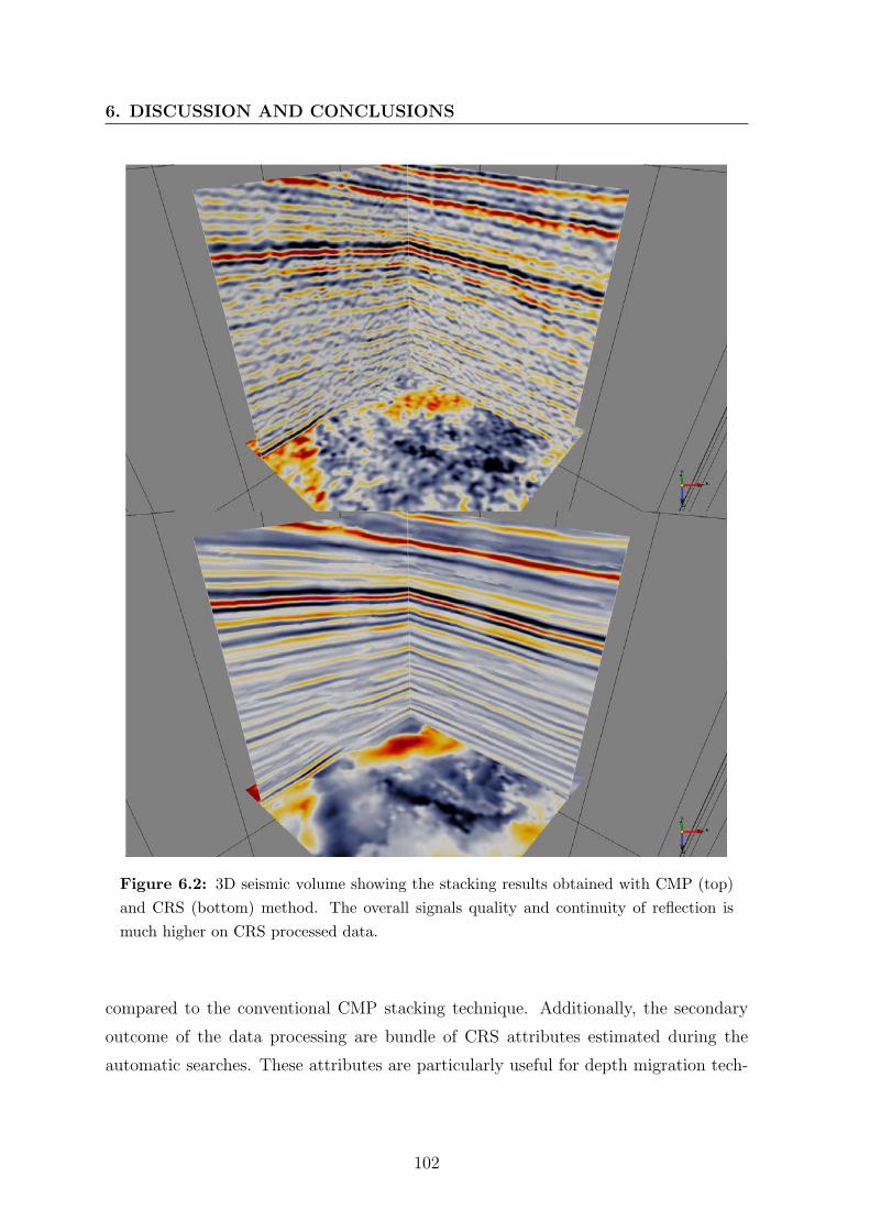
6. DISCUSSION AND CONCLUSIONS
Figure 6.2: 3D seismic volume showing the stacking results obtained with CMP (top)
and CRS (bottom) method. The overall signals quality and continuity of reflection is
much higher on CRS processed data.
compared to the conventional CMP stacking technique. Additionally, the secondary
outcome of the data processing are bundle of CRS attributes estimated during the
automatic searches. These attributes are particularly useful for depth migration tech-
102
6.1 Improvements of stack images
nique, where depth velocity model is acquired by the NIP-wave tomographic inversion
Duveneck (2004).
A high quality volume provided by the CRS stack method proved that the structural
setting of investigated geothermal site can be revised at higher confidence level when
compared to the conventional CMP technique. Acquired time-domain reflectors of
higher S/N ratio allows the horizon to be picked more easily and accurate. Figure 6.2
clearly demonstrates that the capabilities of low-fold data can be gained to the level
comparable with an image of higher fold data processed with conventional CMP method
Buness et al. (2014); Pussak et al. (2014). Additionally, the CRS method is particularly
suitable in the area located in the neighborhood of salt domes where conventional
velocity building methods can not achieve of the required reflections accuracy due to
limited coverage Baykulov et al. (2009).
The sedimentary succession within the investigated area was imaged down to 2.5 s TWT,
with the special focus on Ja1 horizon which corresponds to 2.7 km depth. The struc-
tural interpretation of CRS stacked seismic volume allowed to distinguish the Ja1
horizon more precisely, while the remaining reflectors at shallower depth also show
higher continuity compared to the conventional CMP stack. The time slice shown in
Figure 6.2 that pass through the horizon allowed the fault system to be imaged more
precisely within tested apertures. Moreover, more structural elements were recovered
in correspondence to rather scattered amplitude distribution within the CMP volume.
In consequence, manual picking performed in both in-line and cross-line direction can
be performed at higher confidence level.
In the thesis special attention was undertaken to highlight the reflection event of
the most favorable horizon from geothermal exploration perspective. It is worth to note
that improvements within the CRS volume strongly depend on selected apertures, thus
imaging of small scale structural discontinuities within the horizon may need special
parameters selection focused on investigated targets only. In the results of this tradeoff
solution other targets will require different apertures whose sizes do not meet criteria
of equality in relation to Fresnel zone selected for the main target. Nevertheless, the
CRS method provides advantageous results in geothermal projects of limited budget
when the target zone is known i.e from reprocessing of archive data (Buness et al.,
2014).
103
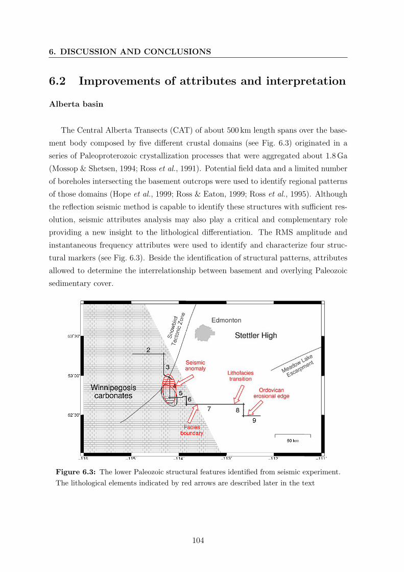
6. DISCUSSION AND CONCLUSIONS
6.2 Improvements of attributes and interpretation
Alberta basin
The Central Alberta Transects (CAT) of about 500 km length spans over the base-
ment body composed by five different crustal domains (see Fig. 6.3) originated in a
series of Paleoproterozoic crystallization processes that were aggregated about 1.8Ga
(Mossop & Shetsen, 1994; Ross et al., 1991). Potential field data and a limited number
of boreholes intersecting the basement outcrops were used to identify regional patterns
of those domains (Hope et al., 1999; Ross & Eaton, 1999; Ross et al., 1995). Although
the reflection seismic method is capable to identify these structures with sufficient res-
olution, seismic attributes analysis may also play a critical and complementary role
providing a new insight to the lithological differentiation. The RMS amplitude and
instantaneous frequency attributes were used to identify and characterize four struc-
tural markers (see Fig. 6.3). Beside the identification of structural patterns, attributes
allowed to determine the interrelationship between basement and overlying Paleozoic
sedimentary cover.
Figure 6.3: The lower Paleozoic structural features identified from seismic experiment.
The lithological elements indicated by red arrows are described later in the text
104
6.2 Improvements of attributes and interpretation
As mentioned in Section 4.6, the attribute was calculated for each trace over the
200 ms window length located above the basement horizon. Although the CAT profile
presented here consists of seven separate lines, however the individual intersection
between lines formed a smooth transition of the attribute values from neighboring
elements. The obtained data shows slightly scattering effect but still may disclose a
number of potentially significant features. Figure 6.4a shows composite section of the
RMS amplitude attribute calculated for both the CMP and the CRS stacked data.
In general, attribute values calculated along the CMP stacked lines do not differ
significantly from that obtained by the CRS processing. Their spatial characteristics
are similar in respect to the form like peak/trough location but the most visible differ-
ence concerns acquired values in particular segments along transects lines, thus making
the comparison more clear. Four major segments can be distinguished along the profile
that coincides with structural units identified on Figure 4.1. Borders between adjacent
segments are characterized by a sharp decline in the RMS amplitudes which is signif-
icantly more evident in the CRS-based results. Such an effect is clearly visible at the
end of line 3, close to the connection with line 4 and at the beginning of line 7. Further
drops in the RMS amplitude, although not as much extensive, were recorded at the
end of line 7 and in the middle of line 9.
The attribute values of RMS amplitude acquired along a composite section falls
between 0.3 and 1.5, while its average does not exceed 1.0. The highest observed
values were recorded in the form of maximum anomaly and traced along longer distance
between line 4 and 5 reaching a maximum of 1.5 close to the lines intersection. An
additional maximum anomaly was identified at the beginning of line 4 where the highest
value of 1.4 was obtained. That tendency of higher amplitude disappears slowly along
the rest of profile reaching the average value below 1.0 and containing a few local
minimal anomalies observed on line 7. The RMS amplitude values calculated for line 9
show an increase at the end of the profile suggesting the presence of an additional
geostructural element. The intensive variations of RMS values along line 3 to 5 probably
reflect the presence of unconsolidated low–grade volcanic and sedimentary rocks (Hope
et al., 1999) due to strong velocity anisotropy usually observed within slate type of
rock formation (Christensen & Mooney, 1995). The basement influence caused that
these RMS amplitude variations are approximately twice the average.
The attribute of instantaneous frequency calculated for the same composite profile
of NMO and the CRS stack is presented in Figure 6.4b. As can be seen, the profile is
105
6. DISCUSSION AND CONCLUSIONS
dominated by an average frequency of 30 Hz showing anomaly peaks ranging from 20 to
almost 40 Hz. Although considerable diversity in the frequency distribution make the
detailed observation hardly visible, especially the differentiation between NMO and the
CRS method, nevertheless it shows close correlation with the RMS amplitude distribu-
tion. There are two types of the frequency response that can correlate with even small
RMS amplitude anomalies. The wide zones of minimum anomaly identified on RMS
amplitude correlates with the minimum anomaly obtained for frequency attribute. This
effect is visible especially at the end of line 3, 7 and line 9, where significant anomalies
were observed. On the other side, there are high frequency anomalies recorded through
out the profile which are correlated with decreased RMS amplitude anomalies. Such an
effect can be observed on line 6 and 8 where high frequency anomalies are accompanied
by a decreased RMS values.
As mentioned, the data processed with NMO and the CRS show some conformity
based on location criteria along the CAT profiles, however their values differ substan-
tially. In order to make the differentiation within attribute subset and between CMP
and CRS stacked datasets more visible I used the crossplot method. The technique was
introduced by White (1991) to indicate similarity within a group of attributes. Ade-
quate selection of attributes may indicate the location of fluid bearing zones or similar
lithologies as they merge into common groups, thus providing possible exploration pa-
rameters to the interpretation. The tentative insight into the crossplotting technique
suggest that the trends between independently derived attributes should reveal addi-
tional structure which can be correlated with the unique features of particular horizons
(Chopra & Marfurt, 2009; Michelena et al., 2011). Such an indication was later used
in AVO analysis based on the aggregations of attributes which did not belong into a
specific cluster (Verm & Hilterman, 1995).
Figure 6.5 presents the crossplots image and the accompanying histograms obtained
for RMS amplitude and instantaneous frequency attribute, derived for a better inter-
pretation of anomaly identified on Figure 6.4. Histograms of both attributes obtained
from the CMP stacked data (see Fig. 6.5a-b) show the arrangement of presented data
in the form of normal distribution. A closer look, although not evident, shows slightly
tendency to split calculated values into two clusters. Within the CRS subset such a di-
vision is obvious, and what is more important, the location of anomalies within the two
attributes distribution match each others along the transect. These two well defined
clusters show that the CRS may offer the solution related to the issues of lithological
106

6.2 Improvements of attributes and interpretation
differentiation more than CMP stack. Additional extension of the crossplots method to
the three dimensional space or even use more recent methods i.e. SOM (Bauer et al.,
2012) may increase the readability of resulting images and improve the interpretation
substantially.
As the supplement to the composite profile, attribute analysis was extended by
additional crossplots of previously selected attributes acquired along three different
horizons. Figure 6.6 shows signal attributes of the Second White, Pika and Precam-
brian horizons which were calculated within 40 ms window length. Although the Pika
horizon does not reflect the interest in geothermal exploration, however is traceable
through almost all transect lines, thus can be used as a reference horizon, while the
others horizons may verify the heterogeneity of lithology at the intersection between
basement and sedimentary layers along the composite profile. Since both images clearly
differentiate three clusters, the attribute interpretation and their distribution can be
performed rather in terms of quality. As one can see, more compact structure of the
attribute distribution that comes from the CRS stack versus NMO counterpart may
suggest easier lithological differentiation not only between particular horizons but also
within one individual horizon. As illustrated on Figure 6.6, all clusters acquired from
CMP stack are shown to be diffuse and widely scattered in comparison to their CRS
counterpart. Moreover, the cloud of CRS obtained attribute allows to perform clus-
tering in a wider range, by the differentiation within a single cluster and correlation
of particular clusters with lithological features. Such an improved lithological response
can also be correlated with AVO response, that are used to detect fluid anomalies (Wa-
ters & Kemper, 2014) or combine with prestack attributes for fracture characterization
(Chen et al., 2014) or adapt for more lithology oriented SOM analysis (Bauer et al.,
2012).
107
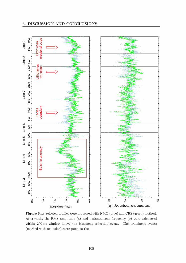
6. DISCUSSION AND CONCLUSIONS
Figure 6.4: Selected profiles were processed with NMO (blue) and CRS (green) method.
Afterwards, the RMS amplitude (a) and instantaneous frequency (b) were calculated
within 200ms window above the basement reflection event. The prominent events
(marked with red color) correspond to the.
108
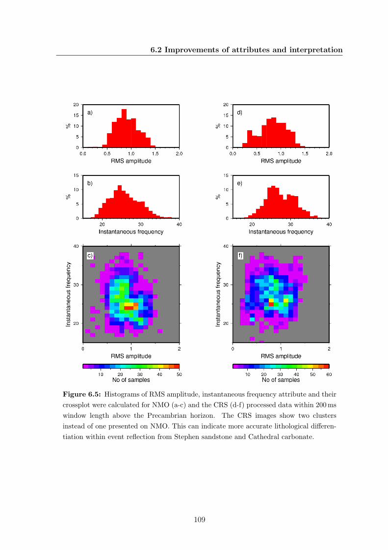
6.2 Improvements of attributes and interpretation
Figure 6.5: Histograms of RMS amplitude, instantaneous frequency attribute and their
crossplot were calculated for NMO (a-c) and the CRS (d-f) processed data within 200ms
window length above the Precambrian horizon. The CRS images show two clusters
instead of one presented on NMO. This can indicate more accurate lithological differen-
tiation within event reflection from Stephen sandstone and Cathedral carbonate.
109
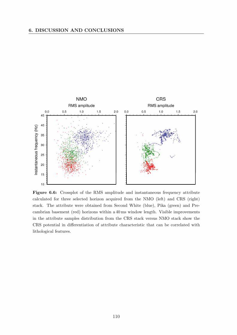
6. DISCUSSION AND CONCLUSIONS
Figure 6.6: Crossplot of the RMS amplitude and instantaneous frequency attribute
calculated for three selected horizon acquired from the NMO (left) and CRS (right)
stack. The attribute were obtained from Second White (blue), Pika (green) and Pre-
cambrian basement (red) horizons within a 40ms window length. Visible improvements
in the attribute samples distribution from the CRS stack versus NMO stack show the
CRS potential in differentiation of attribute characteristic that can be correlated with
lithological features.
110
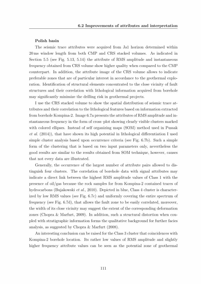
6.2 Improvements of attributes and interpretation
Polish basin
The seismic trace attributes were acquired from Ja1 horizon determined within
20 ms window length from both CMP and CRS stacked volumes. As indicated in
Section 5.5 (see Fig. 5.13, 5.14) the attribute of RMS amplitude and instantaneous
frequency obtained from CRS volume show higher quality when compared to the CMP
counterpart. In addition, the attribute image of the CRS volume allows to indicate
preferable zones that are of particular interest in accordance to the geothermal explo-
ration. Identification of structural elements concentrated to the close vicinity of fault
structures and their correlation with lithological information acquired from borehole
may significantly minimize the drilling risk in geothermal projects.
I use the CRS stacked volume to show the spatial distribution of seismic trace at-
tributes and their correlation to the lithological features based on information extracted
from borehole Kompina-2. Image 6.7a presents the attributes of RMS amplitude and in-
stantaneous frequency in the form of cross–plot showing clearly visible clusters marked
with colored ellipses. Instead of self organizing maps (SOM) method used in Pussak
et al. (2014)), that have shown its high potential in lithological differentiation I used
simple cluster analysis based upon occurrence criteria (see Fig. 6.7b). Such a simple
form of the clustering that is based on two input parameters only, nevertheless the
good results are similar to the results obtained from SOM technique, however, causes
that not every data are illustrated.
Generally, the occurrence of the largest number of attribute pairs allowed to dis-
tinguish four clusters. The correlation of borehole data with signal attributes may
indicate a direct link between the highest RMS amplitude values of Class 1 with the
presence of oil/gas because the rock samples for from Kompina-2 contained traces of
hydrocarbons (Bujakowski et al., 2010). Depicted in blue, Class 4 cluster is character-
ized by low RMS values (see Fig. 6.7c) and uniformly covering the entire spectrum of
frequency (see Fig. 6.7d), that allows the fault zone to be easily correlated, moreover,
the width of its close vicinity may suggest the extent of the corresponding deformation
zones (Chopra & Marfurt, 2009). In addition, such a structural distortion when cou-
pled with stratigraphic information forms the qualitative background for further facies
analysis, as suggested by Chopra & Marfurt (2008).
An interesting conclusion can be raised for the Class 3 cluster that coincidences with
Kompina-2 borehole location. Its rather low values of RMS amplitude and slightly
higher frequency attribute values can be seen as the potential zone of geothermal
111

6. DISCUSSION AND CONCLUSIONS
Figure 6.7: Simplified cluster analysis obtained from cross correlation of seismic at-
tributes determined along Ja1 horizon. Four classes were distinguished on a cross cor-
relation image (a) consisting of RMS and instantaneous frequency attributes calculated
from CRS stacked section. These classes were plotted back on geometry backgorund
(b) to perform a structural differentiation. Corresponding histograms of RMS amplitude
(b) and instantaneous frequency (d) show the distribution of classes among the relevant
variables of the attributes.
exploitation as the sandstone rocks of the Lower Jurassic found in Kompina-2 well
shows its favorable reservoir parameters. The higher flow rate recorded in the borehole
and its relationship to the seismic properties that were imaged by low value of frequency
attributes may suggest high saturation of surrounding rocks due to damping effect
at higher frequencies. Moreover, the higher saturation may suggest the presence of
sinkholes located NE from the borehole and visible in the form of rounded anomalies
The low RMS values and close location of Class 3 cluster in the vicinity of faults are
112
6.2 Improvements of attributes and interpretation
interpreted here as the effect of fracture porosity produced by tectonic activities (Lohr
et al., 2008) that affected the hanging wall east of the main fault line.
This fact makes the Class 3 cluster the most promising exploitation compartment
(depicted by red grid) for future drilling using the geothermal doublet technology.
Similar observations concerning geothermal exploitation and further productivity pa-
rameters determination within the same compartment were discussed by Cacace et al.
(2013) and Cherubini et al. (2013a). Although the assumed higher values of fracture
porosity in the surrounded rocks of the fault system hanging wall represents a promis-
ing geothermal reservoir model, nevertheless more advance modeling studies that can
determine the permeability of faults system itself are necessary to construct fully op-
erational hydrogeological model (Cherubini et al., 2013b) and verify its production
parameters (Blocher et al., 2009).
113
6. DISCUSSION AND CONCLUSIONS
6.3 Outlook
The presented thesis shown the improvement of seismic trace attributes with the CRS
stacking method. The CRS stack method implies the careful selection of stacking aper-
tures, both in midpoint and offset direction in order to provide accurate ZO approxi-
mation of the reflection response. Based on that improved ZO stacking section/volume
the seismic trace attribute analysis provides more detailed and valuable information
that can be transferred to the geological domain and used in reservoir rock model-
ing. Although the method has proved its usability in geothermal exploration, however,
further research and application of the CRS method coupled with the seismic trace
attribute analysis could be carried out.
The research extension could be addressed in the multivariate form, creating space
for a wider field of development. In the first step, the seismic section/volume, may be
improved by the use of different approaches in order to obtain final CRS counterpart.
In the original form, the CRS stack method (Mann et al., 1999; Muller, 2007)) is based
on single parameter search techniques. Although, it represents a pragmatic solution,
more advanced techniques appeared that allow to solve global non-linear minimization
problem and derive the CRS kinematic attributes with higher accuracy (Bonomi et al.,
2009; Garabito et al., 2012). Recent implementations of the simultaneous parameters
optimization for FPGA architecture may increase the speedup of calculation by a factor
of 200 (Marchetti et al., 2010) that allows to not only shorten the processing time but
also to test more scenarios what is especially important on 3D datasets.
Other acquisition layouts that meet the budget criteria of geothermal projects could
also be tested in order to ensure the appropriate balance between obtained data quality
and incurred expenses. The geometry of the 3D layout (Bujakowski et al., 2010) pre-
sented in this thesis was rather homogeneous thus testing other acquisition geometries
and its dependencies on fold (Buness et al., 2014) could also be a task for future de-
velopments. In addition to the modification of the CRS processing, the application of
other methods such as NIP-wave tomography (Duveneck, 2004) could supplement the
geothermal exploration campaign as the velocity estimation within the reservoir may
provide additional information for the hydrogeological modeling. Moreover, the appli-
cation of CRS diffraction imaging (Dell, 2012; Dell & Gajewski, 2011) could improve
significantly the structural image of the subsurface.
Another possible extension is the involvement of further seismic attributes. Nowa-
days, the attribute oriented processing includes more sophisticated solutions, where
114

6.3 Outlook
multiattribute and 3D attributes dominate (Farzadi, 2006). High imaging capabilities
of the CRS stack results can also be used in conjunction with texture attributes (Yenugu
et al., 2010), an also coherence and spectral decomposition may be applied in order
to better visualize lithological variations, thus simulate flow pathways for geothermal
media. An interesting solution of using clustering of seismic attributes was presented
by (Hustoft et al., 2007) to indicate relationships between lithology and fluid flow. Is
worth to mention high potential of the self organizing map (SOM) technique, used
for pattern recognition within geothermal environment based on continuous wavefield
records (Bauer et al., 2012; Kohler et al., 2010). This methodology can contains more
seismic attributes than those presented in this thesis.
Beside the conjunction of the CRS method with the signal attribute analysis, which
provided a sufficient platform for the structural and horizon interpretation, there are
other geophysical methods which can be with the seismic results in order to establish
an optimal geothermal exploration program. Some initial steps of such an application
were performed with electromagnetic methods (Bujakowski et al., 2010; Munoz et al.,
2010b), stress field analysis (Reiter et al., 2013) or geological modeling (Weides et al.,
2013) providing closer insight into geothermal environments.
115

6. DISCUSSION AND CONCLUSIONS
116

References
Al-Chalabi, M. (1973). Series approximation in velocity and traveltime computations. Geo-
physical Prospecting , 21, 783–795.
Albarello, D., Mantovani, E., Babbucci, D. & Tamburelli, C. (1995). Africa-
Eurasia kinematics: main constraints and uncertainties. Tectonophysics, 243, 25–36.
Arnason, K., Eysteinsson, H. & Hersir, G. (2010). Joint 1D inversion of TEM and
MT data and 3D inversion of MT data in the Hengill area, SW Iceland. Geothermics, 39,
13–34.
Arthaud, F. & Matte, P. (1977). Late Paleozoic strike-slip faulting in southern Europe
and northern Africa: Result of a right-lateral shear zone between the Appalachians and
the Urals. Geological Society of America Bulletin, 88, 1305–1320.
Bachu, S. (1993). Basement heat flow in the Western Canada Sedimentary Basin. Tectono-
physics, 222, 119–133.
Bachu, S. & Bennion, B. (2008). Effects of in-situ conditions on relative permeability
characteristics of CO2-brine systems. Environmental Geology , 54, 1707–1722.
Bahorich, M. & Farmer, S. (1995). 3-D seismic discontinuity for faults and stratigraphic
features; the coherence cube. The Leading Edge, 14, 1053–1058.
Bally, A.W., Gordy, P.L. & Stewart, G.A. (1966). Structure, seismic data, and oro-
genic evolution of southern Canadian Rocky Mountains. Bulletin of Canadian Petroleum
Geology , 14, 337–381.
Barbier, E. (1997). Nature and technology of geothermal energy: A review. Renewable and
Sustainable Energy Reviews, 1, 1–69.
Barbier, E. (2002). Geothermal energy technology and current status: An overview. Re-
newable and Sustainable Energy Reviews, 6, 3–65.
117
REFERENCES
Barnes, A. (2001). Seismic attributes in your facies. CSEG Recorder , 26, 41–47.
Barnes, A. (2007). Redundant and useless seismic attributes. Geophysics, 72, 33–38.
Barnes, A.E. (1991). Instantaneous frequency and amplitude at the envelope peak of a
constant-phase wavelet. Geophysics, 56, 1058–1060.
Barry, K.M., Cavers, D.A. & Kneale, C.W. (1975). Recommended standards for digital
tape formats. Geophysics, 40, 344–352.
Batini, F. & Nicolich, R. (1985). P and S reflection seismic profiling and well logging in
the Travale geothermal field. Geothermics, 14, 731–747.
Bauer, K., Schulze, A., Weber, M. & Moeck, I. (2006). Combining refraction seismic
tomography and analysis of wide-angle reflections in geothermal exploration. In AGU Fall
Meeting Abstracts.
Bauer, K., Moeck, I., Norden, B., Schulze, A., Weber, M. & Wirth, H. (2010).
Tomographic P wave velocity and vertical velocity gradient structure across the geothermal
site Groß Schonebeck (NE German Basin): Relationship to lithology, salt tectonics, and
thermal regime. Journal of Geophysical Research, 115, B08312.
Bauer, K., Munoz, G. & Moeck, I. (2012). Pattern recognition and lithological inter-
pretation of collocated seismic and magnetotelluric models using self-organizing maps.
Geophysical Journal International , 189, 984–998.
Bayer, U., Grad, M., Pharaoh, T., Thybo, H., Guterch, A., Banka, D.,
Lamarche, J., Lassen, A., Lewerenz, B., Scheck, M. & Marotta, A.M. (2002).
The southern margin of the East European Craton: new results from seismic sounding and
potential fields between the North Sea and Poland. Tectonophysics, 360, 301–314.
Baykulov, M. & Gajewski, D. (2009). Prestack seismic data enhancement with partial
common-reflection-surface (CRS) stack. Geophysics, 74, 49–58.
Baykulov, M., Brink, H.J., Gajewski, D. & Yoon, M.K. (2009). Revisiting the struc-
tural setting of the Glueckstadt Graben salt stock family, North German Basin. Tectono-
physics, 470, 162–172.
Berkovitch, A., Belfer, I. & Landa, E. (2008). Multifocusing as a method of improving
subsurface imaging. The Leading Edge, 27, 250–256.
Berryman, J., Berge, P. & Bonner, B. (2000). Transformation of seismic velocity data
to extract porosity and saturation values for rocks. Journal of the Acoustical Society of
America, 107, 3018–3027.
118

REFERENCES
Bertrand, E., Caldwell, T., Hill, G., Wallin, E., Bennie, S., Cozens, N.,
Onacha, S., Ryan, G., Walter, C., Zaino, A. & Wameyo, P. (2012). Magnetotel-
luric imaging of upper-crustal convection plumes beneath the Taupo Volcanic Zone, New
Zealand. Geophysical Research Letters, 39, L02304.
Blocher, G., Zimmermann, G. & Milsch, H. (2009). Impact of poroelastic response of
sandstones on geothermal power production. Pure and Applied Geophysics, 166, 1107–
1123.
Boelsen, T. & Mann, J. (2005). 2D CO CRS Stack for OBS and VSP data and arbitrary
top-surface topography. In 67th EAGE Conference and Exhibition, European Association
of Exploration Geophysicists.
Bojarski, L. & Sadurski, A. (2000). Deep connate groundwater of the Polish Lowlands.
Geological Review , 48, 587–595.
Bojarski, L., P lochniewski, Z. & Stachowiak, J. (1979). Mineral and thermal waters
of the Warsaw Marginal Basin. Geological Quarterly , 23, 435–446.
Bonomi, E., Cristini, A., Theis, D. & Marchetti, P. (2009). 3D CRS analysis: a
data-driven optimization for the simultaneous estimate of the eight parameters. In Pro-
ceedings of 79th Annual Meeting and International Exposition of the Society of Exploration
Geophysics, SEG.
Borowska, L. (2006). Report on the 2D seismic survey (reprocessing and reinterpretation)
at the Kompina Site, Skierniewice- Lowicz area. Tech. rep., Mineral and Energy Economy
Research Institute of the Polish Academy of Sciences, Krakow, Poland.
Brogi, A. (2004). Seismic reflection and borehole logs as tools for tectonic and stratigraphical
investigations: New geological data for the Tuscan Nappe exposed in the northeastern Mt.
Amiata area (Northern Apennines, Italy). Bollettino della Societa Geologica Italiana, 123,
189–199.
Brogi, A., Lazzarotto, A., Liotta, D. & Ranalli, G. (2003). Extensional shear zones
as imaged by reflection seismic lines: The Lardello geothermal field (central Italy). Tectono-
physics, 363, 127–139.
Bruhn, D., Manzella, A., Vuataz, F., Faulds, J., Moeck, I. & Erbas, K. (2010).
Exploration methods. In E. Huenges, ed., Geothermal Energy Systems: Exploration, De-
velopment, and Utilization, 37–112, Wiley-VCH Verlag GmbH & Co. KGaA, Weinheim.
Buchholtz, H. (1972). A note on signal distortion due to dynamic (NMO) corrections.
Geophysical Prospecting , 20, 395–402.
119

REFERENCES
Bujakowski, W. (2003). Termiczna charakterystyka gorotworu w rejonie wysadow solnych.
Wydawnictwo IGSMiE PAN, Krakow.
Bujakowski, W., Barbacki, A., Czerwinska, B., Pajak, L., Pussak, M., Stefaniuk,
M. & Trzesniowski, Z. (2010). Integrated seismic and magnetotelluric exploration of
the Skierniewice, Poland, geothermal test site. Geothermics, 39, 78–93.
Buness, H.A., von Hartmann, H., Rumpel, H.M., Krawczyk, C.M. & Schulz,
R. (2014). Fault imaging in sparsely sampled 3D seismic data using common-reflection-
surface processing and attribute analysis - a study in the Upper Rhine Graben. Geophysical
Prospecting , 62, 443–452.
Buntebarth, G. (1984). Geothermics: An introduction. Springer, Berlin.
Burliga, S. (1996). Implications for early basin dynamics of the Mid-Polish Trough from
deformational structures within salt deposits in central Poland. Geological Quarterly , 40,
185–202.
Cacace, M., Blocher, G., Watanabe, N., Mock, I., Borsing, N., Scheck-
Wenderoth, M., Kolditz, O. & Huenges, E. (2013). Modelling of fractured carbonate
reservoirs: outline of a novel technique via a case study from the Molasse Basin, southern
Bavaria, Germany. Environmental Earth Sciences, 70, 3585–3602.
Cagniard, L. (1953). Basic theory of the magnetotelluric method of geophysical prospecting.
Geophysics, 18, 605–645.
Cameron, A. & Smith, G. (1991). Coals of Canada: Distribution and compositional char-
acteristics. International Journal of Coal Geology , 19, 9–20.
Casini, M., Ciuffi, S., Fiordelisi, A., Mazzotti, A. & Stucchi, E. (2010). Results of
a 3D seismic survey at the Travale (Italy) test site. Geothermics, 39, 4–12.
Castle, R. (1994). A theory of normal moveout. Geophysics, 59, 983–999.
Chapman, D.S. & Rybach, L. (1985). Heat flow anomalies and their interpretation. Journal
of Geodynamics, 4, 3–37.
Charlety, J., Cuenot, N., Dorbath, C. & Dorbath, L. (2006). Tomographic study of
the seismic velocity at the Soultz-sous-Forets EGS/HDR site. Geothermics, 35, 532–543.
Chen, Q. & Sidney, S. (1997). Seismic attribute technology for reservoir forecasting and
monitoring. The Leading Edge, 16, 445–448.
120

REFERENCES
Chen, S., Huang, X. & Zhang, H. (2014). Fracture estimation using attenuation attributes
– a case study. In 76th EAGE Conference and Exhibition 2014 , European Association of
Exploration Geophysicists.
Chernyak, V. & Gritsenko, S. (1979). Interpretation of the effective common-depth-
point parameters for a three-dimensional system of homogeneous layers with curvilinear
boundaries. Geologiya i Geofizika, 20, 112–120.
Cherubini, Y., Cacace, M., Blocher, G. & Scheck-Wenderoth, M. (2013a). Impact
of single inclined faults on the fluid flow and heat transport: results from 3-D finite element
simulations. Environmental Earth Sciences, 70, 3603–3618.
Cherubini, Y., Cacace, M., Scheck-Wenderoth, M., Mock, I. & Lewerenz, B.
(2013b). Controls on the deep thermal field: implications from 3-D numerical simulations
for the geothermal research site Großschonebeck. Environmental Earth Sciences, 70, 3619–
3642.
Chopra, S. & Marfurt, K.J. (2005). Seismic attributes - A historical perspective. Geo-
physics, 70, 3–28.
Chopra, S. & Marfurt, K.J. (2007). Seismic attributes for prospect identification and
reservoir characterization. Society of Exploration Geophysicists, Tulsa, OK.
Chopra, S. & Marfurt, K.J. (2008). Emerging and future trends in seismic attributes.
The Leading Edge, 27, 298–318.
Chopra, S. & Marfurt, K.J. (2009). Detecting stratigraphic features via cross-plotting
of seismic discontinuity attributes and their volume visualization. The Leading Edge, 28,
1422–1426.
Chopra, S. & Marfurt, K.J. (2011). Interesting pursuits in seismic curvature attribute
analysis. CSEG Recorder , 36, 40–51.
Christensen, N.I. & Mooney, W.D. (1995). Seismic velocity structure and composition
of the continental crust: A global view. Journal of Geophysical Research: Solid Earth,
100, 9761–9788.
Cianciara, K. (1975). Opracowanie badan sejsmicznych z rejonu Skierniewice-Sochaczew.
Tech. rep., Geofizyka Krakow Sp. z o.o., Krakow, Poland.
Cianciara, K. & Piech, K. (1977). Opracowanie badan sejsmicznych z rejonu Brzeziny-
Lowicz-Skierniewice. Tech. rep., Geofizyka Krakow Sp. z o.o., Krakow, Poland.
121
REFERENCES
Corsi, R. (1986). Scaling and corrosion in geothermal equipment: problems and preventive
measures. Geothermics, 15, 839–856.
Criaud, A. & Fouillac, C. (1989). Sulfide scaling in low enthalpy geothermal environ-
ments: A survey. Geothermics, 18, 73–81.
Cuenot, N., Charlety, J., Dorbath, L. & Haessler, H. (2006). Faulting mechanisms
and stress regime at the european HDR site of Soultz-sous-Forets, France. Geothermics,
35, 561–575.
Cumming, W. & Bruhn, D. (2010). Preface. Geothermics, 39, 1–3, The European I-GET
Project: Integrated Geophysical Exploration Technologies for Deep Geothermal Reservoirs.
Dadlez, R. (2003). Mesozoic thickness pattern in the Mid-Polish Trough. Geological Quar-
terly , 47, 223–240.
Dadlez, R., Narkiewicz, M., Stephenson, R., Visser, M. & van Wees, J.D. (1995).
Tectonic evolution of the Mid-Polish Trough: modelling implications and significance for
central European geology. Tectonophysics, 252, 179–195.
Dadlez, R., Marek, S. & Pokorski, J. (1998). Palaeogeographical atlas of the epiconti-
nental Permian and Mesozoic in Poland . Panstwowy Instytut Geologiczny, Warszawa.
Danis, C., O’Neill, C., Lackie, M., Twigg, L. & Danis, A. (2011). Deep 3D structure
of the Sydney basin using gravity modelling. Australian Journal of Earth Sciences, 58,
517–542.
Davidson, J. & Elsner, W. (2005). Alberta’s ultimate potential for conventional natural
gas. Tech. rep., Alberta Energy and Utilities Board (EUB) and National Energy Board,
Alberta, Canada.
De Matteis, R., Vanorio, T., Zollo, A., Ciuffi, S., Fiordelisi, A. & Spinelli,
E. (2008). Three-dimensional tomography and rock properties of the Larderello-Travale
geothermal area, Italy. Physics of the Earth and Planetary Interiors, 168, 37–48.
Dell, S. (2012). Seismic processing and imaging with diffractions. Ph.D. thesis, University
of Hamburg.
Dell, S. & Gajewski, D. (2011). Common-reflection-surface-based workflow for diffraction
imaging. Geophysics, 76, 187–195.
Deregowski, S. (1986). What is DMO? First break , 4, 535–545.
122

REFERENCES
Dietrich, J. (1999). Seismic stratigraphy and structure of the Lower Paleozoic, Central
Alberta Lithoprobe Transect. Bulletin of Canadian Petroleum Geology , 47, 362–374.
Dummong, S., Meier, K., Hubscher, C. & Gajewski, D. (2007). Velocity model build-
ing: A comparison between prestack stereotomography and NIP-wave tomography. In SEG
Technical Program Expanded Abstracts 2007 , vol. 26, 3034–3038, SEG.
Duncan, P. & Eisner, L. (2010). Reservoir characterization using surface microseismic
monitoring. Geophysics, 75, 139–146.
Duveneck, E. (2004). 3D tomographic velocity model estimation with kinematic wavefield
attributes. Geophysical Prospecting , 52, 535–545.
Eaton, D.W., Milkereit, B., Ross, G.M., Kanasewich, F.R., Geis, W., Edwards,
D.J., Kelsch, L. & Varsek, J. (1995). Lithoprobe abasin-scale seismic profiling in
centreal Alberta: influence of basement on the sedimentary cover. Bulletin of Canadian
Petroleum Geology , 43, 65–77.
Eaton, D.W., Ross, G.M. & Hope, J. (1999). The rise and fall of a Cratonic Arch:
A regional seismic perspective on the Peace River Arch, Alberta. Bulletin of Canadian
Petroleum Geology , 47, 346–361.
Echols, J., Benoit, D., Ohren, M., Oppliger, G. & Van Gundy, T. (2011). Integra-
tion of a 3D-3C reflection seismic survey over a known geothermal resource: Soda Lake,
Churchill County, Nevada. Geothermal Resources Council Transactions, 35, 1633–1641.
Edwards, D. & Brown, R. (1999). Understanding the influence of Precambrian crystalline
basement on Upper Devonian carbonates in central Alberta from a geophysical perspective.
Bulletin of Canadian Petroleum Geology , 47, 412–438.
Eisenberg-Klein, G., Pruessmann, J., Gierse, G. & Trappe, H. (2008). Noise reduc-
tion in 2D and 3D seismic imaging by the CRS method. The Leading Edge, 27, 258–265.
Farzadi, P. (2006). Seismic facies analysis based on 3D multi-attribute volume classification,
Dariyan Formation, SE Persian Gulf. Journal of Petroleum Geology , 29, 159–173.
Foulger, G. (1982). Geothermal exploration and reservoir monitoring using earthquakes
and the passive seismic method. Geothermics, 11, 259–268.
Gallup, D. (1998). Aluminum silicate scale formation and inhibitor (2): Scale solubilities
and laboratory and field inhibition tests. Geothermics, 27, 485–501.
123
REFERENCES
Garabito, G., Stoffa, P.L., Lucena, L.S. & Cruz, J.C. (2012). Part I - CRS stack:
Global optimization of the 2D CRS-attributes. Journal of Applied Geophysics, 85, 92–101.
Garg, S., Pritchett, J., Wannamaker, P. & Combs, J. (2007). Characterization of
geothermal reservoirs with electrical surveys: Beowawe geothermal field. Geothermics, 36,
487–517.
Gasperikova, E., Newman, G., Feucht, D. & Arnason, K. (2011). 3D MT character-
ization of two geothermal fields in Iceland. Geothermal Resources Council Transactions,
35, 1667–1671.
Geiermann, J. & Schill, E. (2010). 2-D magnetotellurics at the geothermal site at Soultz-
sous-Forets: Resistivity distribution to about 3000 m depth. Comptes Rendus - Geoscience,
342, 587–599.
Gelchinsky, B. (1988). The Common Reflecting Element (CRE) method (non-uniform
asymmetric multifold system). Exploration Geophysics, 19, 71–75.
Gelchinsky, B., Berkovitch, A. & Keydar, S. (1999). Multifocusing homeomorphic
imaging: Part 1. Basic concepts and formulas. Journal of Applied Geophysics, 42, 229–242.
Gorecki, W., ed. (1995). Atlas of geothermal energy resources in the Polish Lowlands. 1.
Mesozoic formations. 2. Palaeozoic formations.. Geosynoptics Society GEOS, Krakow.
Gorecki, W., ed. (2006). Atlas of geothermal resources of Mesosoic formations in the Polish
Lowlands. AGH University of Science and Technology, Krakow.
Gorecki, W., Kozdra, T., Kuzniak, T., Mysko, A. & Strzetelski, W. (2003).
Geothermal-energy resources in the Polish Lowlands and the possibility of their industrial
utilization. Applied Energy , 74, 53–64.
Gosk, E. (1982). Geothermal resources assessment. In V. Cermak & R. Haenel, eds., Geother-
mics and geothermal energy , 257–263, Schweitzerbartsche Verlagsbuchhandlung, Stuttgart.
Grabowska, T. & Bojdys, G. (2001). The border of the East-European Craton in south-
eastern Poland based on gravity and magnetic data. Terra Nova, 13, 92–98.
Grabowska, T., Bojdys, G. & Dolnicki, J. (1998). Three-dimensional density model of
the Earth’s crust and the upper mantle for the area of Poland. Journal of Geodynamics,
25, 5–34.
Grad, M., Keller, G., Thybo, H. & Guterch, A. (2002). Lower lithospheric structure
beneath the Trans-European Suture Zone from POLONAISE’97 seismic profiles. Tectono-
physics, 360, 153–168.
124

REFERENCES
Guterch, A. & Grad, M. (2006). Lithospheric structure of the TESZ in Poland based on
modern seismic experiments. Geological Quarterly , 50, 23–32.
Guterch, A., Grad, M., Materzok, R. & Perchuc, E. (1986). Deep structure of the
Earth’s crust in the contact zone of the Palaeozoic and Precambrian Platforms in Poland
(Tornquist-Teisseyre zone). Tectonophysics, 128, 251–279.
Haites, T.B. (1960). Transcurrent faults in Western Canada. Alberta Society of Petroleum
Geologists Journal , 8, 33–77.
Hale, D. (1984). Dipmoveout by Fourier transform. Geophysics, 49, 741–757.
Hammond, A.L. (1974). Bright Spot: Better seismological indicators of gas and oil. Science,
185, 515–517.
Hardage, B. (2000). Vertical Seismic Profiling: Principles. Pergamon, New York, 3rd edn.
Haring, M.O., Schanz, U., Ladner, F. & Dyer, B.C. (2008). Characterisation of the
Basel 1 enhanced geothermal system. Geothermics, 37, 469–495.
Heilmann, Z., Mann, J. & Koglin, I. (2006). CRS-stack-based seismic imaging consid-
ering top-surface topography. Geophysical Prospecting , 54, 681–695.
Hein, F.J. & Nowlan, G.S. (1998). Regional sedimentology, conodont biostratigraphy
and correlation of Middle Cambrian-Lower Ordovician (?) strata of the ’Finnegan’ and
Deadwood formations, Alberta subsurface, Western Canada Sedimentary Basin. Bulletin
of Canadian Petroleum Geology , 46, 166–188.
Henrys, S. & Hochstein, M. (1990). Geophysical structure of the Broadlandsohaaki
geothermal field (New Zealand). Geothermics, 19, 129–150.
Hirowatari, K. (1996). Scale prevention method by brine acidification with biochemical
reactors. Geothermics, 25, 259–270.
Hocht, G. (2002). Traveltime approximations for 2D and 3D media and kinematic wavefield
attributes. Ph.D. thesis, University of Karlsruhe.
Hocht, G., de Bazelaire, E., Majer, P. & Hubral, P. (1999). Seismics and optics:
hyperbolae and curvatures. Journal of Applied Geophysics, 42, 261–281.
Hope, J., Eaton, D.W. & Ross, G.M. (1999). Lithoprobe seismic transect of the Alberta
Basin: Compliation and overview. Bulletin of Canadian petroleum geology , 47, 331–345.
125

REFERENCES
Houseman, G. & McKenzie, D.P. (1982). Numerical experiments on the onset of con-
vective instability in the Earth’s mantle. Geophysical Journal of the Royal Astronomical
Society , 68, 133–164.
Hubral, P. (1983). Computing true amplitude reflections in a laterally inhomogeneous
Earth. Geophysics, 48, 1051–1062.
Hubral, P. & Krey, T. (1980). Interval Velocities from Seismic Reflection Time Measure-
ments. Society of Exploration Geophysicists, Tulusa, OK.
Huenges, E. (2010). Geothermal Energy Systems: Exploration, Development, and Utiliza-
tion. Wiley-VCH Verlag GmbH & Co. KGaA, Weinheim.
Hustoft, S., Mienert, J., Bunz, S. & Nouze, H. (2007). High-resolution 3D-seismic
data indicate focussed fluid migration pathways above polygonal fault systems of the mid-
Norwegian margin. Marine Geology , 245, 89–106.
Jager, C. (2005). Minimum-aperture Kirchhoff migration with CRS stack attributes. Ph.D.
thesis, University of Karlsruhe, Berlin.
Jager, R., Mann, J., Hocht, G. & Hubral, P. (2001). Common-reflection-surface stack:
Image and attributes. Geophysics, 66, 97–109.
Jaupart, C. (1981). On the mechanisms of heat loss beneath continents and oceans. Ph.D.
thesis, Massachusetts Institute of Technology, Cambridge, MA.
Jaupart, C. & Parsons, B. (1985). Convective instabilities in a variable viscosity fluid
cooled from above. Physics of the Earth and Planetary Interiors, 39, 14–32.
Jones, F.W., Lam, H.L. & Majorowicz, J.A. (1985). Temperature distributions at the
Paleozoic and Precambrian surfaces and their implications for geothermal and energy re-
covery in Alberta. Canadian Journal of Earth Sciences, 22, 1774–1780.
Jousset, P., Haberland, C., Bauer, K. & Arnason, K. (2011). Hengill geothermal
volcanic complex (Iceland) characterized by integrated geophysical observations. Geother-
mics, 40, 1–24.
Karnkowski, P.H. (1999). Origin and evolution of the Polish Rotliegend Basin. Polish
Geological Institute Special Papers, 3, 1–93.
Kent, D.M. (1994). Paleogeographic evolution of the cratonic platform - Cambrian to Tri-
assic. In: Geological atlas of the Western Canada Sedimentary Basin G.D. Mossop and I.
Shetsen (comps.). Online; accessed 9-November-2012.
126

REFERENCES
Kepinska, B. (2003). Current geothermal activities and prospects in Poland – an overview.
Geothermics, 32, 397–407.
Kepinska, B. (2010). Geothermal energy country update report from Poland, 2005-2009. In
Proceedings of the World Geothermal Congress, Bali (Indonesia).
Klein, P., Richard, L. & James, H. (2008). 3D curvature attributes: a new approach for
seismic interpretation. First Break , 26, 105–111.
Koglin, I. (2005). Estimation of residual static time shifts by means of the CRS-based resid-
ual static correction approach. Ph.D. thesis, University of Karlsruhe, Berlin.
Kohler, A., Ohrnberger, M. & Scherbaum, F. (2010). Unsupervised pattern recog-
nition in continuous seismic wavefield records using Self-Organizing Maps. Geophysical
Journal International , 182, 1619–1630.
Krey, T. (1952). The significance of diffraction in the investigation of faults. Geophysics,
17, 843–858.
Krzywiec, P. (2004). Triassic evolution of the K lodawa salt structure: basement-controlled
salt tectonics within the Mid-Polish Trough (Central Poland). Geological Quarterly , 48,
123–134.
Kunz, B.F.J. (1960). Diffraction problems in fault interpretation. Geophysical Prospecting ,
8, 381–388.
Kutek, J. & G lazek, J. (1972). The Holy Cross area, Central Poland, in the Alpine cycle.
Acta Geologica Polonica, 4.
Lamarche, G. (1992). Seismic reflection survey in the geothermal field of the Rotorua
Caldera, New Zealand. Geothermics, 21, 109–119.
Landa, E., Shtivelman, V. & Gelchinsky, B. (1987). A method for detection of
diffracted waves on common-offset sections. Geophysical Prospecting , 35, 359–373.
Landa, E., Gurevich, B., Keydar, S. & Trachtman, P. (1999). Application of multi-
focusing method for subsurface imaging. Journal of Applied Geophysics, 42, 283–300.
Landa, E., Keydar, S. & Jan Moser, T. (2010). Multifocusing revisited-inhomogeneous
media and curved interfaces. Geophysical Prospecting , 58, 925–938.
Lees, J. (2004). Scattering from a fault interface in the Coso geothermal field. Journal of
Volcanology and Geothermal Research, 130, 61–75.
127

REFERENCES
Legarth, B. (2008). Drilling deep wells - Key challenges and cost implications. VDI
Berichte, 2026, 45–53.
Legaz, A., Revil, A., Roux, P., Vandemeulebrouck, J., Gouedard, P., Hurst,
T. & Boleve, A. (2009). Self-potential and passive seismic monitoring of hydrothermal
activity: A case study at Iodine Pool, Waimangu geothermal valley, New Zealand. Journal
of Volcanology and Geothermal Research, 179, 11–18.
Leszczynski, K. (2012). The internal geometry and lithofacies pattern of the Upper
Cretaceous-Danian sequence in the Polish Lowlands. Geological Quarterly , 56, 363–386.
Levin, S.A. (1989). Surface-consistent deconvolution. Geophysics, 54, 1123–1133.
Liberty, L. (1998). Seismic reflection imaging of a geothermal aquifer in an urban setting.
Geophysics, 63, 1285–1294.
Lohr, T., Krawczyk, C.M., Tanner, D.C., Samiee, R., Endres, H., Thierer, P.O.,
Oncken, O., Trappe, H., Bachmann, R. & Kukla, P.A. (2008). Prediction of subseis-
mic faults and fractures: Integration of three-dimensional seismic data, three-dimensional
retrodeformation, and well data on an example of deformation around an inverted fault.
AAPG Bulletin, 92, 473–485.
Luschen, E., Dussel, M., Thomas, R. & Schulz, R. (2011). 3D seismic survey for
geothermal exploration at Unterhaching, Munich, Germany. First Break , 29, 45–54.
Luschen, E., Wolfgramm, M., Fritzer, T., Dussel, M., Thomas, R. & Schulz,
R. (2014). 3D seismic survey explores geothermal targets for reservoir characterization at
Unterhaching, Munich, Germany. Geothermics, 50, 167–179.
Majer, E. (2003). 3-D seismic methods for geothermal reservoir exploration and assessment
– summary. Tech. Rep. LBNL-49881, Lawrence Berkeley National Laboratory, Berkeley,
CA.
Majorowicz, J., Cermak, V., Safanda, J., Krzywiec, P., Wroblewska, M.,
Guterch, A. & Grad, M. (2003). Heat flow models across the Trans-European Su-
ture Zone in the area of the POLONAISE97 seismic experiment. Physics and Chemistry
of the Earth, Parts A/B/C , 28, 375–391.
Majorowicz, J.A. (2004). Thermal lithosphere across the Trans-European suture zone in
Poland. Geological Quarterly , 48, 1–14.
Majorowicz, J.A. & Jessop, A.M. (1981). Regional heat flow patterns in the Western
Canada Sedimentary Basin. Tectonophysics, 74, 209–238.
128
REFERENCES
Majorowicz, J.A., Jones, F., Lam, H. & Jessop, A.M. (1985). Regional variations of
heat flow differences with depth in Alberta, Canada. Geophysical Journal of The Royal
Astronomical Society , 81, 479–487.
Mamczur, S. & Radecki, S. (1998). Z loze ropy naftowej BMB (Barnowko-Mostno-
Buszewo). Nafta-Gaz , 54, 105–109.
Mann, J. (2002). Extensions and Applications of the Common-Reflection-Surface Stack
Method . Ph.D. thesis, University of Karlsruhe.
Mann, J., Jager, R., Muller, T., Hocht, G. & Hubral, P. (1999). Common-reflection-
surface stack – a real data example. Journal of Applied Geophysics, 42, 301–318.
Mann, J., Duveneck, E., Hertweck, T. & Jager, C. (2003). A seismic reflection
imaging workflow based on the Common-Reflection-Surface stack. Journal of Seismic Ex-
ploration, 12, 283–295.
Marchetti, P., Oriato, D., Pell, O., Cristini, A. & Theis, D. (2010). Fast 3D
ZO CRS stack - An FPGA implementation for an optimization based on simultaneous
estimate of eight parameters. In 72nd European Association of Geoscientists and Engineers
Conference and Exhibition, 2915–2519.
Marek, S. (1988a). Paleothickness, lithofacies and paleotectonics of the epicontinental Lower
Cretaceous in Poland. Geological Quarterly , 32, 157–174.
Marek, S. (1988b). Paleothickness, lithofacies and paleotectonics of the epicontinental Per-
mian and Mesozoic in Poland. Geological Quarterly , 32, 1–14.
Marek, S. & Pajchlowa, M. (1997). The epicontinental Permian and Mesozoic in Poland .
Prace Panstwowego Instytutu Geologicznego, Panstwowy Instytut Geologiczny, Warszawa.
Marek, S. & Znosko, J. (1972). Tectonics of the Kujawy region. Geological Quarterly , 16,
1–18.
Marfurt, K.J., Sudhaker, V., Gersztenkorn, A., Crawford, K.D. & Nissen, S.E.
(1999). Coherency calculations in the presence of structural dip. Geophysics, 64, 104–111.
Matsushima, J., Okubo, Y., Rokugawa, S., Yokota, T., Tanaka, K., Tsuchiya,
T. & Narita, N. (2003). Seismic reflector imaging by prestack time migration in the
Kakkonda geothermal field, Japan. Geothermics, 32, 79–99.
May, B. & Straley, D. (1979). Higher-order moveout spectra. Geophysics, 44, 1193–1207.
129
REFERENCES
Mayne, W.H. (1962). Common reflection point horizontal data stacking techniques. Geo-
physics, 27, 927–938.
Mayr, S., Stanchits, S., Langenbruch, C., Dresen, G. & Shapiro, S. (2011). Acous-
tic emission induced by pore-pressure changes in sandstone samples. Geophysics, 76, 21–32.
Michelena, R.J., Godbey, K.S. & Rodrigues, P.E. (2011). Facies probabilities from
multidimensional crossplots of seismic attributes: Application to tight gas Mamm Creek
Field, Piceance Basin, Colorado. The Leading Edge, 30, 62–69.
Moeck, I., Hinz, N., Faulds, J., Bell, J., Kell-Hills, A. & Louie, J. (2010). 3D
geological mapping as a new method in geothermal exploration: A case study from central
Nevada. Geothermal Resources Council Transactions, 34, 742–746.
Moeck, I.S. (2014). Catalog of geothermal play types based on geologic controls. Renewable
and Sustainable Energy Reviews, 37, 867–882.
Monger, J.W.H. & Price, R.A. (1979). Geodynamic evolution of the Canadian Cordillera
– progress and problems. Canadian Journal of Earth Sciences, 16, 770–791.
Mossop, G. & Shetsen, I. (1994). Geological atlas of the Western Canada Sedimentary
Basin. Canadian Society of Petroleum Geologists and Alberta Research Council, online;
accessed 9-November-2012.
Muksin, U., Bauer, K. & Haberland, C. (2013). Seismic Vp and Vp/Vs structure
of the geothermal area around Tarutung (North Sumatra, Indonesia) derived from local
earthquake tomography. Journal of Volcanology and Geothermal Research, 260, 27–42.
Muller, N.A. (2007). Determination of interval velocities by inversion of kinematic 3D
wavefield attributes. Ph.D. thesis, University of Karlsruhe.
Muller, T. (1999). The Common Reflection Surface Stack Method – Seismic imaging with-
out explicit knowledge of the velocity model . Ph.D. thesis, University of Karlsruhe.
Munoz, G., Bauer, K., Moeck, I., Schulze, A. & Ritter, O. (2010a). Exploring
the Groß Schonebeck (Germany) geothermal site using a statistical joint interpretation of
magnetotelluric and seismic tomography models. Geothermics, 39, 35–45.
Munoz, G., Ritter, O. & Moeck, I. (2010b). A target-oriented magnetotelluric inver-
sion approach for characterizing the low enthalpy Groß Schonebeck geothermal reservoir.
Geophysical Journal International , 183, 1199–1215.
130
REFERENCES
Nakagome, O., Uchida, T. & Horikoshi, T. (1998). Seismic reflection and VSP in the
Kakkonda geothermal field, Japan: Fractured reservoir characterization. Geothermics, 27,
535–552.
Nawrocki, J., Wagner, R. & Grabowski, J. (2013). The permian/triassic boundary in
the Polish basin in the light of paleomagnetic data. Geological Quarterly , 37.
Neidell, N. & Taner, M. (1971). Semblance and other coherency measures for multichan-
nel data. Geophysics, 36, 482–497.
Newman, G., Gasperikova, E., Hoversten, G. & Wannamaker, P. (2008). Three-
dimensional magnetotelluric characterization of the Coso geothermal field. Geothermics,
37, 369–399.
Niitsuma, H., Fehler, M., Jones, R., Wilson, S., Albright, J., Green, A., Baria,
R., Hayashi, K., Kaieda, H., Tezuka, K., Jupe, A., Wallroth, T., Cornet, F.,
Asanuma, H., Moriya, H., Nagano, K., Phillips, W., Rutledge, J., House, L.,
Beauce, A., Alde, D. & Aster, R. (1999). Current status of seismic and borehole
measurements for HDR/HWR development. Geothermics, 28, 475–490.
Notfors, C. & Godfrey, R. (1987). Dip moveout in the frequency-wavenumber domain.
Geophysics, 52, 1718–1721.
Papiernik, B., Machowski, G., S lupczynski, K. & Semyrka, R. (2009). Geologiczny
model rejonu akumulacji ropno-gazowej Lubiatow-Miedzychod-Grotow (LMG). Geologia,
35, 175–182.
Pellerin, L., Johnston, J. & Hohmann, G. (1996). A numerical evaluation of electro-
magnetic methods in geothermal exploration. Geophysics, 61, 121–130.
Pichon, X.L., Bergerat, F. & Roulet, M.J. (1988). Plate kinematics and tectonics
leading to the Alpine belt formation: a new analysis. Special paper - Geological Society of
America, 218, 111–131.
Place, J., Diraison, M., Naville, C., Geraud, Y., Schaming, M. & Dezayes, C.
(2010). Decoupling of deformation in the Upper Rhine Graben sediments. Seismic reflec-
tion and diffraction on 3-component Vertical Seismic Profiling (Soultz-sous-Forets area).
Comptes Rendus - Geoscience, 342, 575–586.
Porter, J.W., Price, R.A. & McCrossan, R.G. (1982). The Western Canada Sedimen-
tary Basin. Philosophical Transactions of the Royal Society of London, 305, 169–182.
131

REFERENCES
Price, R.A. & Mountjoy, E.W. (1970). Geologic structure of the Canadian Rocky Moun-
tains between Bow and Athabasca Rivers - a progress report. In : Structure of the southern
Canadian Cordillera, J. O. Wheeler, ed. Geological Association of Canada Special Paper ,
6, 7–25.
Pussak, M., Bauer, K., Stiller, M. & Bujakowski, W. (2014). Improved 3D seismic
attribute mapping by CRS stacking instead of NMO stacking: Application to a geothermal
reservoir in the Polish Basin. Journal of Applied Geophysics, 103, 186–198.
Rabbel, W. & Luschen, E. (1996). Shear wave anisotropy of laminated lower crust at the
Urach geothermal anomaly. Tectonophysics, 264, 219–233.
Reiter, K., Heidbach, O. & Moeck, I. (2013). Stress field modelling in the Alberta
Basin, Canada. In International Workshop on Geomechanics and Energy: The Ground as
Energy Source and Storage, Lausanne, Switzerland.
Represas, P., Monteiro Santos, F., Ribeiro, J., Ribeiro, J., Almeida, E., Go-
nalves, R., Moreira, M. & Mendes-Victor, L. (2013). Interpretation of gravity
data to delineate structural features connected to low-temperature geothermal resources
at Northeastern Portugal. Journal of Applied Geophysics, 92, 30–38.
Resak, M., Narkiewicz, M. & Littke, R. (2008). New basin modelling results from the
Polish part of the Central European Basin system: implications for the late Cretaceous-
Early Paleogene structural inversion. International Journal of Earth Sciences, 97, 955–972.
Rial, J.A., Elkibbi, M. & Yang, M. (2005). Shear-wave splitting as a tool for the charac-
terization of geothermal fractured reservoirs: Lessons learned. Geothermics, 34, 365–385.
Ronen, J. & Claerbout, J.F. (1985). Surface-consistent residual statics estimation by
stack-power maximization. Geophysics, 50, 2759–2767.
Ross, G.M. & Eaton, D.W. (1999). Basement reactivation in the Alberta Basin: Obser-
vational constraints and mechanical rationale. Bulletin of Canadian petroleum geology , 47,
391–411.
Ross, G.M., Parrish, R.R., Villeneuve, M. & Bowring, S.A. (1991). Geophysics and
geochronology of the crystalline basement of the Alberta Basin, western Canada. Canadian
Journal of Earthh Sciences, 28, 512–552.
Ross, G.M., Milkereit, B., Eaton, D., White, D., Kanasewich, E.R. & Burianyk,
M.J.A. (1995). Paleoproterozoic collisional orogen beneath the western Canada sedimen-
tary basin imaged by Lithoprobe crustal seismic-reflection data. Geology , 23, 195–199.
132

REFERENCES
Sanyal, S. (2007). Ensuring resource adequacy for a commercial geothermal project.
Geothermal Resources Council Transactions, 31, 93–97.
Sausse, J., Dezayes, C., Dorbath, L., Genter, A. & Place, J. (2010). 3D model of
fracture zones at Soultz-sous-Forets based on geological data, image logs, induced micro-
seismicity and vertical seismic profiles. Comptes Rendus - Geoscience, 342, 531–545.
Schleicher, J., Tygel, M. & Hubral, P. (1993). Parabolic and hyperbolic paraxial
two-point traveltimes in 3D media. Geophysical Prospecting , 41, 495–513.
SEG (1995). Shell processing support format for land 3-D surveys. Geophysics, 60, 596–596.
Shah, P. (1973). Use of wavefront curvature to relate seismic data with subsurface parame-
ters. Geophysics, 38, 812–825.
Shapiro, S., Kruger, O., Dinske, C. & Langenbruch, C. (2011). Magnitudes of in-
duced earthquakes and geometric scales of fluid-stimulated rock volumes. Geophysics, 76,
55–63.
Sharpton, V.L., Grieve, R.A.F., Thomas, M.D. & Halpenny, J.F. (1987). Horizontal
gravity gradient: An aid to the definition of crustal structure in North America. Geophysical
Research Letters, 14, 808–811.
Shoffner, J., Li, Y., Hinz, N., Sabin, A., Lazaro, M. & Alm, S. (2010). Under-
standing fault characteristics and sediment depth for geothermal exploration using 3D
gravity inversion in Walker Valley, Nevada. Geothermal Resources Council Transactions,
34, 586–589.
Sigfusson, T. (2012). Geothermal energy. In A. Sayigh, ed., Comprehensive Renewable
Energy , Elsevier, Oxford.
Simmons, N., Forte, A. & Grand, S. (2006). Constraining mantle flow with seismic and
geodynamic data: A joint approach. Earth and Planetary Science Letters, 246, 109–124.
Simpson, F. & Bahr., K. (2005). Practical Magnetotellurics. Cambridge University Press,
Cambridge.
Slind, O., Andrews, G., Murray, D., Norford, B., Paterson, D., Salas, C. &
Tawadros, E. (1994). Middle Cambrian to Lower Ordovician strata of the Western
Canada Sedimentary Basin. In: Geological atlas of the Western Canada Sedimentary Basin
G.D. Mossop and I. Shetsen (comps.). Canadian Society of Petroleum Geologists and Al-
berta Research Council, online; accessed 9-November-2012.
133
REFERENCES
Sokolowski, J. (1993). Geothermal resources in Poland and possibility of their utilization
in environmental protection. Exploration Geology, Geosynoptics and Geothermal Energy ,
5-6, 67–80.
Soma, N. & Niitsuma, H. (1997). Identification of structures within the deep geothermal
reservoir of the Kakkonda field, Japan, by a reflection method using acoustic emission as
a wave source. Geothermics, 26, 43–64.
Spichak, V., Zakharova, O. & Rybin, A. (2011). Methodology of the indirect tempera-
ture estimation basing on magnetotelluric data: Northern Tien Shan case study. Journal
of Applied Geophysics, 73, 164–173.
Spinner, M. & Mann, J. (2005). True-amplitude CRS-based Kirchhoff time migration for
AVO analysis. In SEG Technical Program Expanded Abstracts 2005 .
Spinner, M.E.T. (2007). CRS-based minimum-aperture Kirchhoff migration in the time
domain. Ph.D. thesis, University of Karlsruhe.
Stephenson, R.A., Narkiewicz, M., Dadlez, R., van Wees, J.D. & Andriessen,
P. (2003). Tectonic subsidence modelling of the Polish Basin in the light of new data on
crustal structure and magnitude of inversion. Sedimentary Geology , 156, 59–70.
Stoakes, F. (1987). Evolution of the Upper Devonian of Western Canada. In G. Bloy &
M. Charest, eds., Principles and Concepts for Exploration and Exploitation of Reefs in the
Western Canada Basin, Short Course Notes, Canadian Society of Petroleum Geologists,
Calgary.
Stoakes, F.A. (1980). Nature and control of shale basin fill and its effect on reef growth
and termination; Upper Devonian Duvernay and Ireton formations of Alberta, Canada.
Bulletin of Canadian Petroleum Geology , 28, 345–410.
Stott, D. & Aitken, J. (1993). Sedimentary Cover of the Craton in Canada, vol. 5 of
Geology of North America. Geological Survey of Canada, Toronto.
Stringham, G. (2012). Energy Developments in Canada’s Oil Sands. In K.E. Percy, ed.,
Alberta Oil Sands, vol. 11, chap. 2, 19–34, Elsevier.
Sugama, T. & Gawlik, K. (2002). Anti-silica fouling coatings in geothermal environments.
Materials Letters, 57, 666–673.
Sugihara, M. & Ishido, T. (2008). Geothermal reservoir monitoring with a combination
of absolute and relative gravimetry. Geophysics, 73, 37–47.
134
REFERENCES
Szewczyk, J. & Gientka, D. (2009). Terrestrial heat flow density in Poland – a new
approach. Geological Quarterly , 53, 125–125.
Szuflicki, M., Malon, A. & Tynminski, M. (2013). Bilans zasobow z loz kopalin w
Polsce wg stanu na 31 XII 2012 r.. Panstwowy Instytut Geologiczny–Panstwowy Insty-
tut Badawczy, Warszawa, online; accessed 23-June-2013.
Tan, H., Yu, Q., Booker, J. & Wei, W. (2003). Three-dimensional rapid relaxation
inversion for the magnetotelluric method. Acta Geophysica Sinica, 46, 850–854.
Taner, M. (2001). Seismic attributes. CSEG Recorder , 26.
Taner, M. & Koehler, F. (1969). Velocity spectra - digital computer derivation applica-
tions of velocity functions. Geophysics, 34, 859–881.
Taner, M., Koehler, F. & Sheriff, R. (1979). Complex seismic trace analysis. Geo-
physics, 44, 1041–1063.
Tang, C., Rial, J. & Lees, J. (2008). Seismic imaging of the geothermal field at Krafla,
Iceland using shear-wave splitting. Journal of Volcanology and Geothermal Research, 176,
315–324.
Tikhonov, A. (1950). On determining electrical characteristics of the deep layers of the
Earth’s crust. Doklady , 73, 295–297.
Trappe, H., Coman, R., Gierse, G., Robinson, S., Owens, M. & Nielsen, E.M.
(2005). Combining CRS technology and sparse 3D seismic surveys - a new approach to
acquisition design. In 67th EAGE Conference & Exhibition.
Turcotte, D.L. & Schubert, G. (2002). Geodynamics. Cambridge University Press.
Unruh, J., Monastero, F. & Pullammanappallil, S. (2008). The nascent Coso meta-
morphic core complex, east-central California: Brittle upper plate structure revealed by
reflection seismic data. International Geology Review , 50, 245–269.
van Wees, J.D., Stephenson, R.A., Ziegler, P.A., Bayer, U., McCann, T.,
Dadlez, R., Gaupp, R., Narkiewicz, M., Bitzer, F. & Scheck, M. (2000). On
the origin of the Southern Permian Basin, Central Europe. Marine and Petroleum Geol-
ogy , 17, 43–59.
Vanorio, T., De Matteis, R., Zollo, A., Batini, F., Fiordelisi, A. & Ciulli,
B. (2004). The deep structure of the Larderello-Travale geothermal field from 3D mi-
croearthquake traveltime tomography. Geophysical Research Letters, 31, L07613.
135
REFERENCES
Verm, R. & Hilterman, F. (1995). Lithology, color-coded seismic sections; the calibration
of AVO crossplotting to rock properties. The Leading Edge, 14, 847–853.
Villeneuve, M., Ross, G.M., Theriault, R.J., Miles, M., Parrish, R.R. & Broome,
J. (1993). Tectonic subdivisions and U-Pb geochronology of the crystalline basement of
the Alberta Basin, Western Canada. Bulletin – Geological Survey of Canada, 447.
Volpi, G., Manzella, A. & Fiordelisi, A. (2003). Investigation of geothermal structures
by magnetotellurics (MT): An example from the Mt. Amiata area, Italy. Geothermics, 32,
131–145.
von Hartmann, H., Buness, H., Krawczyk, C. & Schulz, R. (2012). 3-D seismic
analysis of a carbonate platform in the Molasse Basin - reef distribution and internal
separation with seismic attributes. Tectonophysics, 572-573, 16–25.
Ward, P. (1972). Microearthquakes: Prospecting tool and possible hazard in the develop-
ment of geothermal resources. Geothermics, 1, 3–12.
Waters, K. & Kemper, M. (2014). Find the rocks and the fluids will follow – AVO as a
tool for lithology classification. Interpretation, 2, 77–91.
Watts, N. (1987). Carbonate sedimentology and depositional history of the Nisku Formation
(within the Western Canada Sedimentary Basin) in south central Alberta. In F. Krause
& O. Burrows, eds., Devonian lithofacies and reservoir styles in Alberta, 286, Canadian
Society of Petroleum Geologists, Toronto.
Weber, M., Zetsche, F., Ryberg, T., Schulze, A., Spangenberg, E. & Huenges, E.
(2005). Seismic detection limits of small, deep, man-made reflectors: A test at a geothermal
site in northern Germany. Bulletin of the Seismological Society of America, 95, 1567–1573.
Weides, S., Moeck, I., Majorowicz, J., Palombi, D. & Grobe, M. (2013). Geother-
mal exploration of Paleozoic formations in Central Alberta. Canadian Journal of Earth
Sciences, 50, 519–534.
White, R. (1991). Properties of instantaneous seismic attributes. The Leading Edge, 10,
26–32.
Winchester, J., Pharaoh, T. & Verniers, J. (2002). Palaeozoic amalgamation of Cen-
tral Europe. Special publication, Geological Society, London.
Wuestefeld, A., Al-Harrasi, O., Verdon, J., Wookey, J. & Kendall, J. (2010). A
strategy for automated analysis of passive microseismic data to image seismic anisotropy
and fracture characteristics. Geophysical Prospecting , 58, 755–773.
136
REFERENCES
Yahara, T. & Tokita, H. (2010). Sustainability of the Hatchobaru geothermal field, Japan.
Geothermics, 39, 382–390.
Yenugu, M., Marfurt, K. & Matson, S. (2010). Seismic texture analysis for reservoir
prediction and characterization. The Leading Edge, 29, 1116–1121.
Yilmaz, O. (2001). Seismic Data Analysis. Investigations in geophysics, Society Of Explo-
ration Geophysicists, Tulsa, OK.
Yilmaz, O. & Clearbout, J. (1980). Prestack partial migration. Geophysics, 45, 1753–
1779.
Yuen, D. & Fleitout, L. (1984). Stability of the oceanic lithosphere with variable viscosity:
an initial-value approach. Physics of the Earth and Planetary Interiors, 334, 173–185.
Zeng, H. (1991). Geologic significance of anomalous instantaneous frequency. Geophysics,
75, 23–30.
Zhang, B., Wang, T. & Marfurt, K.J. (2011). Revisiting NMO stretch and velocity
analysis. In SEG Technical Program Expanded Abstracts 2011 , chap. 795, 4040–4044.
Zhang, Q. & McMechan, G. (2011). Direct vector-field method to obtain angle-domain
common-image gathers from isotropic acoustic and elastic reverse time migration. Geo-
physics, 76, 135–149.
Zhang, Y. (2003). Common-Reflection-Surface Stack and the Handling of Top Surface To-
pography . Logos Verlag, Berlin.
Ziegler, P. (1990). Geological Atlas of Western and Central Europe. Shell International
Petroleum Maatschoppij B.V, Den Haag, 2nd edn.
137
Acknowledgements
I am grateful to Dr. Klaus Bauer for his patient supervision of this work
and for giving me a lot of freedom in planning of my research. His door
was always open for me when questions about my current working topics
occurred. He gave me the opportunity to produce this work and allowed
me to participate in many geophysical events and projects.
I am also grateful to Prof. Dr. Michael Weber for the co-supervision of
my thesis and also for giving me a possibility to extend my theoretical
background, although my project was more practically oriented.
I would also like to say thank you to Dr. Wieslaw Bujakowski from MEERI
PAS for introducing me the wonderful idea of geothermal energy and other
reneweables. I also enjoyed the times at MEERI PAS.
I am grateful to Manfred Stiller for deepen my knowledge of seismic data
processing and for proof reading of my texts. I am as well grateful to Dr.
Mikhail Baykulov, Dr. Sergius Dell for the CRS driven discussions and
good advices in the preliminary processing.
I am also grateful to Christian Feld for his companionship and for sharing an
office during my stay at the GFZ. I also like to say thank you to Christof
Lendl and Mathias Wanjek for solving most of my computer issues. My
thanks also goes to Anke Lerch, who always helped me with administration
issues and organized social activities.
I also like to thank Prof. Dr. Dirk Gajewski, Prof. Dr. Thomas Bohlen for
accepting my request for being part of the disputation council.
I gratefully acknowledge the Mineral and Energy Economy Research In-
stitute of the Polish Academy of Sciences (MEERI PAS) and Natural Re-
sources Canada (NRCan) for access to datasets which represent the basis for
the work I presented in this thesis. I gratefully acknowledge the Helmholtz-
Zentrum Potsdam - Deutsches GeoForschungsZentrum and the Helmholtz

Alberta Initiative (HAI) for funding of my position and the conference
attendance. I also acknowledge the Wave Inversion Technology (WIT) con-
sortium for the code provided by the consortium represents the basis for
the work presented in this thesis.
Last but not least, I would like to thank my family and especially my sons,
you were boys still smiling at me every time I was a doubt.

Declaration
I herewith declare that I have produced this paper without the prohibited
assistance of third parties and without making use of aids other than those
specified; notions taken over directly or indirectly from other sources have
been identified as such. This paper has not previously been presented in
identical or similar form to any other German or foreign examination board.
Potsdam, May 2014
Related Documents