HAL Id: tel-01246006 https://hal.inria.fr/tel-01246006v2 Submitted on 16 Mar 2016 HAL is a multi-disciplinary open access archive for the deposit and dissemination of sci- entific research documents, whether they are pub- lished or not. The documents may come from teaching and research institutions in France or abroad, or from public or private research centers. L’archive ouverte pluridisciplinaire HAL, est destinée au dépôt et à la diffusion de documents scientifiques de niveau recherche, publiés ou non, émanant des établissements d’enseignement et de recherche français ou étrangers, des laboratoires publics ou privés. Distributed under a Creative Commons Attribution - NonCommercial| 4.0 International License Segmentation and Skeleton Methods for Digital Shape Understanding Franck Hétroy-Wheeler To cite this version: Franck Hétroy-Wheeler. Segmentation and Skeleton Methods for Digital Shape Understanding. Graphics [cs.GR]. Université Grenoble Alpes, 2015. tel-01246006v2

Welcome message from author
This document is posted to help you gain knowledge. Please leave a comment to let me know what you think about it! Share it to your friends and learn new things together.
Transcript
HAL Id: tel-01246006https://hal.inria.fr/tel-01246006v2
Submitted on 16 Mar 2016
HAL is a multi-disciplinary open accessarchive for the deposit and dissemination of sci-entific research documents, whether they are pub-lished or not. The documents may come fromteaching and research institutions in France orabroad, or from public or private research centers.
L’archive ouverte pluridisciplinaire HAL, estdestinée au dépôt et à la diffusion de documentsscientifiques de niveau recherche, publiés ou non,émanant des établissements d’enseignement et derecherche français ou étrangers, des laboratoirespublics ou privés.
Distributed under a Creative Commons Attribution - NonCommercial| 4.0 InternationalLicense
Segmentation and Skeleton Methods for Digital ShapeUnderstanding
Franck Hétroy-Wheeler
To cite this version:Franck Hétroy-Wheeler. Segmentation and Skeleton Methods for Digital Shape Understanding.Graphics [cs.GR]. Université Grenoble Alpes, 2015. tel-01246006v2
HABILITATION À DIRIGER DES RECHERCHESSpécialité : Informatique
Présentée par
Franck Hétroy-Wheeler
Segmentation and Skeleton Methodsfor Digital Shape Understanding
soutenue publiquement le 20 novembre 2015,devant le jury composé de :
Marc DanielProfesseur, Université d’Aix-Marseille, RapporteurAdrian HiltonProfessor, University of Surrey, RapporteurMichela SpagnuoloResearch Director, Consiglio Nazionale delle Richerche Genova, RapporteurMarie-Paule CaniProfesseure, Université Grenoble Alpes, ExaminatriceRaphaëlle ChaineProfesseure, Université de Lyon, ExaminatriceBruno LévyDirecteur de Recherche, Inria Nancy Grand-Est, Examinateur

iii
ABSTRACT
Digitised geometric shape models are essentially represented as a collection of primi-tives without a general coherence. Shape understanding aims at retrieving global infor-mation about the shape geometry, topology or functionality, for subsequent uses suchas measurement, simulation or modification. In this context, this manuscript presentsmy main contributions to digital shape understanding, which are mostly based on shapedecomposition and skeleton computation. The first part explores the faithfulness of the3D mesh representation to the real world object, through topological and perceptualanalyses, and suggests a conversion to a regular volumetric model. The second partfocuses on shapes in motion and details tools to create, modify and analyse temporalmesh sequences. The third part explains through two concrete examples how digitalshape understanding can help experts in medicine and forestry. Finally, three openquestions for shape understanding of shapes in motion and scanned trees are discussedby way of perspectives.
RÉSUMÉ
Les modèles géométriques de formes numérisées sont pour l’essentiel représentéscomme une collection de primitives sans cohérence générale. La compréhension deformes a pour but de retrouver une information globale concernant la géométrie, topolo-gie ou fonction d’une forme, afin de pouvoir la mesurer, la modifier ou l’utiliser ensimulation. Dans ce contexte, ce manuscript présente mes principales contributions àla compréhension numérique de formes géométriques, qui sont principalement fondéessur la décomposition de formes et le calcul de squelette. La première partie explorela fidélité de la représentation par maillage 3D à l’objet du monde réel, à travers desanalyses topologiques et perceptuelles, et propose une conversion vers un modèle vo-lumique régulier. La deuxième partie se concentre sur les formes en mouvement et dé-taille des outils permettant de créer, modifier et analyser des séquences temporelles demaillages. La troisième partie explique à travers deux exemples concrets comment lacompréhension numérique de formes peut aider les experts dans des domaines commela médecine et la sylviculture. Enfin, trois questions ouvertes sur la compréhension deformes pour les formes en mouvement et les arbres scannés sont discutées en guise deperspectives.

iv

Acknowledgements
I would first like to thank the three reviewers of this manuscript, Marc Daniel, AdrianHilton and Michela Spagnuolo for their time and their very relevant comments. Thankstoo, to the three other committee members, Marie-Paule Cani, Raphaëlle Chaine andBruno Lévy, for their questions and encouragement.
I have learned a lot over the past years from several researchers, with whom Iworked: many thanks to my PhD thesis advisors Annick Montanvert and DominiqueAttali, to Marie-Paule Cani and Edmond Boyer who welcomed me in their teams andgave me the opportunity to conduct my research in almost perfect conditions, to mycolleagues from the EVASION and Morpheo teams Georges-Pierre Bonneau, FrançoisFaure, Jean-Sébastien Franco, Jean-Claude Léon, Olivier Palombi, Lionel Revéret andothers, to my collaborators, especially Eric Casella, Florent Dupont and Kai Wang. Ihave also learned from my students, especially my PhD students Sahar Hassan, Ro-main Arcila, Phuong Ho, Benjamin Aupetit, Georges Nader and Li Wang as well asDobrina Boltcheva and the interns I tutored. Each of them was different and helpedme question myself: thank you all.
I also wish to thank my colleagues and students from Grenoble INP - Ensimag,because teaching is the best way to learn something in depth, and teaching skills arealso useful for research.
Finally, I wish to acknowledge the support of my parents-in-law Frederick andFrancisca Wheeler who provided me with perfect conditions to write this manuscriptin a quiet environment in Stockport. Thanks to them also for their encouragement andfor their help in proof-reading the manuscript. Thanks also to my parents, my familyand in particular my dear Elisa and Emily for their help, patience, support and love.This habilitation is dedicated to them.
v

vi
Contents
1 Introduction 11.1 Research problem: digital shape understanding . . . . . . . . . . . . 1
1.1.1 Relation to digital geometry processing . . . . . . . . . . . . 21.2 Approach: segmentation and skeleton computation . . . . . . . . . . 21.3 Contributions . . . . . . . . . . . . . . . . . . . . . . . . . . . . . . 31.4 Influential encounters . . . . . . . . . . . . . . . . . . . . . . . . . . 5
1.4.1 Quick contextual elements . . . . . . . . . . . . . . . . . . . 51.4.2 Advised students . . . . . . . . . . . . . . . . . . . . . . . . 61.4.3 Main projects and collaborations . . . . . . . . . . . . . . . . 71.4.4 Remark . . . . . . . . . . . . . . . . . . . . . . . . . . . . . 8
2 Geometrical, topological and perceptual analysis of 3D meshes 92.1 Introduction . . . . . . . . . . . . . . . . . . . . . . . . . . . . . . . 9
2.1.1 3D meshes . . . . . . . . . . . . . . . . . . . . . . . . . . . 92.1.2 Objectives . . . . . . . . . . . . . . . . . . . . . . . . . . . . 10
2.2 Mesh repair with topology control . . . . . . . . . . . . . . . . . . . 112.2.1 Surface singularities . . . . . . . . . . . . . . . . . . . . . . 112.2.2 Discrete voxel membrane . . . . . . . . . . . . . . . . . . . . 122.2.3 Interactive topology modification . . . . . . . . . . . . . . . 12
2.3 Retrieving the homology of simplicial complexes . . . . . . . . . . . 132.3.1 Background on simplicial homology . . . . . . . . . . . . . . 142.3.2 Constructive homology . . . . . . . . . . . . . . . . . . . . . 152.3.3 Manifold-Connected decomposition . . . . . . . . . . . . . . 162.3.4 Mayer-Vietoris algorithm . . . . . . . . . . . . . . . . . . . . 16
2.4 Just-Noticeable Distortion profile for meshes . . . . . . . . . . . . . 172.4.1 Local perceptual properties . . . . . . . . . . . . . . . . . . . 192.4.2 Just Noticeable distortion profile . . . . . . . . . . . . . . . . 202.4.3 Perceptually optimal vertex coordinates quantization . . . . . 21
vii
viii CONTENTS
2.4.4 Perceptually optimal mesh simplification . . . . . . . . . . . 222.5 Regular volumetric discretisation . . . . . . . . . . . . . . . . . . . . 22
2.5.1 Regular Centroidal Voronoi Tessellations . . . . . . . . . . . 232.5.2 A hierarchical framework . . . . . . . . . . . . . . . . . . . 24
2.6 Perspectives . . . . . . . . . . . . . . . . . . . . . . . . . . . . . . . 252.6.1 Perceptual analysis of smooth shaded surfaces . . . . . . . . 252.6.2 Regularly tessellated volumes from point clouds . . . . . . . 25
3 Digital geometry processing for shapes in motion 273.1 Introduction . . . . . . . . . . . . . . . . . . . . . . . . . . . . . . . 27
3.1.1 Objectives . . . . . . . . . . . . . . . . . . . . . . . . . . . . 273.1.2 3D+t vs. 4D . . . . . . . . . . . . . . . . . . . . . . . . . . . 283.1.3 Temporal coherence . . . . . . . . . . . . . . . . . . . . . . 28
3.2 Harmonic skeleton for character animation . . . . . . . . . . . . . . . 303.2.1 A short survey on skeleton computation methods . . . . . . . 303.2.2 Reeb graph computation . . . . . . . . . . . . . . . . . . . . 323.2.3 Embedding into an animation skeleton . . . . . . . . . . . . . 333.2.4 Atlas generation . . . . . . . . . . . . . . . . . . . . . . . . 333.2.5 Skinning weights . . . . . . . . . . . . . . . . . . . . . . . . 34
3.3 A discrete Laplace operator for temporally coherent mesh sequences . 353.3.1 Definition of a 4D DEC Laplace operator . . . . . . . . . . . 353.3.2 Matrix representation . . . . . . . . . . . . . . . . . . . . . . 393.3.3 Behaviour for large and small time steps . . . . . . . . . . . . 403.3.4 Application to as-rigid-as-possible mesh sequence deformation 41
3.4 Mesh sequence decomposition into rigidly moving components . . . . 433.4.1 Shape-in-motion segmentation classification . . . . . . . . . 433.4.2 Mesh matching . . . . . . . . . . . . . . . . . . . . . . . . . 443.4.3 Motion-based spectral clustering . . . . . . . . . . . . . . . . 453.4.4 Shape in motion segmentation evaluation . . . . . . . . . . . 46
3.5 Perspectives . . . . . . . . . . . . . . . . . . . . . . . . . . . . . . . 473.5.1 Visual differences between shapes in motion . . . . . . . . . 473.5.2 3D+t Laplace operator spectral behaviour . . . . . . . . . . . 473.5.3 Modelling the factors of variability for human shape in motion 48
4 Understanding digital shapes from the life sciences 494.1 Introduction . . . . . . . . . . . . . . . . . . . . . . . . . . . . . . . 49
4.1.1 Context . . . . . . . . . . . . . . . . . . . . . . . . . . . . . 494.1.2 General approach: skeleton for segmentation and measurement 50
4.2 Cerebral aneurysm characterisation and quantification . . . . . . . . . 514.2.1 Centreline extraction . . . . . . . . . . . . . . . . . . . . . . 514.2.2 Aneurysm detection and quantification . . . . . . . . . . . . 524.2.3 Aneurysm localisation . . . . . . . . . . . . . . . . . . . . . 54
4.3 Tree seedling segmentation and measurement . . . . . . . . . . . . . 544.3.1 Graph computation . . . . . . . . . . . . . . . . . . . . . . . 56
CONTENTS ix
4.3.2 Spectral embedding . . . . . . . . . . . . . . . . . . . . . . . 574.3.3 Segmentation in spectral space . . . . . . . . . . . . . . . . . 57
4.4 Perspectives . . . . . . . . . . . . . . . . . . . . . . . . . . . . . . . 584.4.1 TLS point cloud noise detection and correction . . . . . . . . 584.4.2 Towards an accurate digital tree model . . . . . . . . . . . . . 59
5 Conclusion 615.1 Summary . . . . . . . . . . . . . . . . . . . . . . . . . . . . . . . . 615.2 General comments . . . . . . . . . . . . . . . . . . . . . . . . . . . 625.3 Open questions for shapes in motion and forest science . . . . . . . . 62
5.3.1 Appropriate shape representations . . . . . . . . . . . . . . . 635.3.2 Mathematical and computational tools . . . . . . . . . . . . . 635.3.3 Incorporating additional knowledge . . . . . . . . . . . . . . 64
A Selected papers 67A.1 Mesh repair with user-friendly topology control . . . . . . . . . . . . 69A.2 An iterative algorithm for homology computation on simplicial shapes 101A.3 Just Noticeable Distortion profile for flat-shaded 3D mesh surfaces . . 115A.4 A hierarchical approach for regular Centroidal Voronoi Tessellations . 141A.5 Harmonic skeleton for realistic character animation . . . . . . . . . . 159A.6 Simple flexible skinning based on manifold modeling . . . . . . . . . 171A.7 Segmentation of temporal mesh sequences into rigidly moving com-
ponents . . . . . . . . . . . . . . . . . . . . . . . . . . . . . . . . . 179A.8 Automatic localization and quantification of intracranial aneurysms . 193A.9 Segmentation of tree seedling point clouds into elementary units . . . 203
B List of publications 233B.1 Geometrical, topological and perceptual analysis of 3D meshes . . . . 233B.2 Digital geometry processing for shapes in motion . . . . . . . . . . . 234B.3 Understanding digital shapes from the life sciences . . . . . . . . . . 235
Bibliography 237
Index 251

x CONTENTS
CHAPTER 1
Introduction
1.1 RESEARCH PROBLEM: DIGITAL SHAPEUNDERSTANDING
Nowadays, shape digitisation is ubiquitous. Virtual geometric models allow for actionsthat are cumbersome or even impossible in the real world to be realised. For example,surgical training [FLA+05], forest inventory [OVSP13] or creation of special effectsfor the entertainment industry have been greatly simplified thanks to digitised models.Virtual shapes can be either modelled from scratch, thanks to the skills of the user andthe assistance of a computer, or digitised from real objects or scenes using sensors suchas cameras or scanners. In general, digitisation can easily create a more complex andfaithful representation of the real world than shape modelling.
Unfortunately, digitised shape models are essentially a collection of simple prim-itives (points, triangles, voxels, . . . ) with no general coherence. Global informationand semantics about the object (e.g. “this is an arm”, “this part is cylindrical”) and itsfunctionality are usually lost during the digitisation process. Only local informationis explicitly available: point coordinates, possibly normals or colours, neighbouringrelationships.
Nevertheless, high-level information can often be retrieved, by using powerfulmathematical tools to analyse the geometry of the shape together with some priorknowledge. This knowledge depends on the application and can be either injectedto the processing algorithms or interactively given by the user. The first solution issometimes preferable since the process is then automated. However, it is not alwayspossible since it requires the knowledge to be formalised. While it is always possibleto ask the user to provide the knowledge, it may be time consuming and the output
1
2 CHAPTER 1. INTRODUCTION
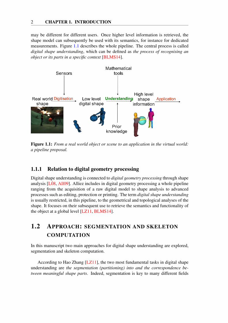
may be different for different users. Once higher level information is retrieved, theshape model can subsequently be used with its semantics, for instance for dedicatedmeasurements. Figure 1.1 describes the whole pipeline. The central process is calleddigital shape understanding, which can be defined as the process of recognising anobject or its parts in a specific context [BLMS14].
Figure 1.1: From a real world object or scene to an application in the virtual world:a pipeline proposal.
1.1.1 Relation to digital geometry processingDigital shape understanding is connected to digital geometry processing through shapeanalysis [L08, All09]. Alliez includes in digital geometry processing a whole pipelineranging from the acquisition of a raw digital model to shape analysis to advancedprocesses such as editing, protection or printing. The term digital shape understandingis usually restricted, in this pipeline, to the geometrical and topological analyses of theshape. It focuses on their subsequent use to retrieve the semantics and functionality ofthe object at a global level [LZ11, BLMS14].
1.2 APPROACH: SEGMENTATION AND SKELETONCOMPUTATION
In this manuscript two main approaches for digital shape understanding are explored,segmentation and skeleton computation.
According to Hao Zhang [LZ11], the two most fundamental tasks in digital shapeunderstanding are the segmentation (partitioning) into and the correspondence be-tween meaningful shape parts. Indeed, segmentation is key to many different fields
1.3. CONTRIBUTIONS 3
(think “divide and conquer”), and also makes sense for the analysis of a complexshape. The identification of its sub-parts and the understanding of their connectionsoften help to recognise the overall shape. The “meaning” of a shape element is ofcourse application-dependent, as this document will demonstrate. An overview of ex-isting segmentation methods can be found e.g. in [Sha08, TPT15].
Another popular technique for digital shape understanding is the reduction of theinput shape to a one-dimensional graph, often called a skeleton. While geometricaldetails are lost with such an approach, the skeleton usually keeps the main topologicalfeatures of the shape, thus enabling a rough general recognition. A short review ofstate of the art skeleton computation techniques for 3D meshes will be given in Sec-tion 3.2.1. It supplements the one in [Tag13].
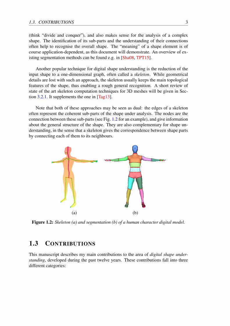
Note that both of these approaches may be seen as dual: the edges of a skeletonoften represent the coherent sub-parts of the shape under analysis. The nodes are theconnection between these sub-parts (see Fig. 1.2 for an example), and give informationabout the general structure of the shape. They are also complementary for shape un-derstanding, in the sense that a skeleton gives the correspondence between shape partsby connecting each of them to its neighbours.
(a) (b)
Figure 1.2: Skeleton (a) and segmentation (b) of a human character digital model.
1.3 CONTRIBUTIONS
This manuscript describes my main contributions to the area of digital shape under-standing, developed during the past twelve years. These contributions fall into threedifferent categories:
4 CHAPTER 1. INTRODUCTION
1. three-dimensional mesh analysis (Chapter 2), in which I question the faithfulnessof a discrete polygonal mesh to represent the real world object that has beendigitised;
2. moving shape understanding (Chapter 3), where I develop tools to retrieve gen-eral information on both the geometry and the motion of digitised dynamic mod-els;
3. digital shape understanding for life sciences (Chapter 4), where I explore twopractical applications of digital shape understanding for medical imaging anddendrometry (tree dimensions measurement).
In Chapter 2, I introduce topological and geometrical segmentation methods to helprecognise the general structure of an object represented by a 3D mesh. This is done indifferent stages:
• firstly, I present an interactive tool to convert an unorganised set of triangles intoa well-behaved (two-manifold) mesh. The user is proposed with a limited set ofpossible segmentations. Thus he or she provides knowledge about the correcttopology of the mesh;
• secondly, I develop an algorithm to compute the complete topological informa-tion of simplicial complexes. This allows for a decomposition of such objectsinto manifold-connected components. The knowledge used in the algorithmcomes from the mathematical theory of constructive homology [Ser94];
• thirdly, I investigate the discretisation into regular cells of the volumetric objectsurrounded by a given two-manifold mesh. Here again, knowledge about what aregular cell should be comes from a mathematical theory of quantisation [CS82].
In Chapter 3, I use both a skeleton and a segmentation process to decompose ashape in motion into meaningful sub-parts, in two different contexts. They are:
• 3D animation creation, for which I introduce a method to compute an accu-rate animation skeleton from a static meshed character as well as a method togenerate a variety of animations with this skeleton thanks to flexible skinningweights. Here, the knowledge is related to the bone anatomy of the character.This has been encoded into the skeleton computation algorithm for both humansand quadruped animals;
• motion analysis from videos, where I study the segmentation of a 3D movingshape, represented as a sequence of meshes without temporal coherence. Sincethe focus of this work is on human motion, the knowledge that the body is com-posed of rigidly moving parts is imposed.
In Chapter 4, I combine both skeleton and segmentation tools. A skeleton is firstcomputed to get a general picture of the object under study. It then drives a subsequentsegmentation of this object into the elements of interest. This is done for two differentapplications:
1.4. INFLUENTIAL ENCOUNTERS 5
• characterisation and quantification of cerebral aneurysms. Knowledge about thetopological structure of the cerebral tree is encoded into the algorithm;
• segmentation of a tree seedling point cloud into elementary elements (branches,petioles, leaves). Basic observations about the structure of a tree enable thealgorithm to split the point cloud into meaningful sub-sets. They can then berefined if the user decides. Doing so, he brings additional knowledge to theprocess.
Note that beside skeleton computation and segmentation methods, I have developedother approaches. In Chapter 2 I detail a perceptual study on vertex displacementvisibility on a mesh, and in Chapter 3 I present a generic tool to analyse shapes inmotion (a discrete Laplace operator).
1.4 INFLUENTIAL ENCOUNTERS
This manuscript is intended to give an overview of my research work as an assistantprofessor (”maître de conférences”) in computer science at Grenoble INP - Ensimag(part of the Université Grenoble Alpes, France) since 2004. Of course, I have notworked alone on the topic of digital shape understanding. Before entering into thedetails in the next chapters, allow me to pay tribute to my co-workers.
1.4.1 Quick contextual elementsI defended my PhD thesis (advised by Prof. Annick Montanvert and Dr. DominiqueAttali, in the GIPSA-Lab in Grenoble) in September 2003. In February 2004, I joinedthe computer graphics team of Prof. Pere Brunet at the Universitat Politècnica deCatalunya in Barcelona, Spain, thanks to a grant from the French Ministry of ForeignAffairs. The work described in Section 2.2 was started there. Within a few months, Iwas appointed to my current position at Grenoble INP - Ensimag in September of thesame year. As part of the university of Grenoble, I joined Prof. Marie-Paule Cani’steam EVASION at Inria and GRAVIR lab (later moved to the current Laboratoire JeanKuntzmann). While there, I was lucky enough to collaborate with a number of peoplewho are listed below, and to advise many students, including my first two PhD students.In 2011, EVASION came to an end and Marie-Paule decided to focus her new teamIMAGINE on the creation of digital content. As I was more interested in analysingand processing real world data, I accepted the offer of Prof. Edmond Boyer to joinhis new team Morpheo, which we created together with Dr. Lionel Revéret and soonjoined by Dr. Jean-Sébastien Franco. In Morpheo our work is at the intersection ofcomputer graphics and computer vision, since our overall goal is to model, recogniseand animate moving shapes from multiple camera systems. I am currently advisingtwo PhD students.
6 CHAPTER 1. INTRODUCTION
1.4.2 Advised students
PhD studentsCurrent PhD students:
• Georges Nader (started in 2013). Evaluation of the perceptual quality of 3D dy-namic meshes and applications. Co-advised by Prof. Florent Dupont (Universitéde Lyon) and Dr. Kai Wang (CNRS Grenoble). See Section 2.4;
• Li Wang (started in 2013). Centroidal Voronoi tessellations for shape recon-struction. Co-advised by Prof. Edmond Boyer (Inria Grenoble). See Section 2.5.
Past PhD students:
• Sahar Hassan (2007-2011). Integration of a priori anatomical knowledge intogeometrical models. Co-advised by Prof. Georges-Pierre Bonneau (UniversitéGrenoble Alpes). See Section 4.2;
• Romain Arcila (2008-2011). Mesh sequences: a classification and segmenta-tion methods. Co-advised by Prof. Florent Dupont (Université de Lyon). SeeSection 3.4.
I also advised 2 students who did not finished their PhD:
• Thi Phuong Ho (2011-2012, co-advised by Prof. Bruno Lévy from Inria Nancy),whose PhD was stopped after 16 months;
• Benjamin Aupetit (2011-2014, co-advised by Prof. Edmond Boyer from InriaGrenoble), who resigned after 3 years.
Master students• Romain Rombourg (Télécom Physique Strasbourg, 2015). Detection and cor-
rection of mixed point noise in laser scans. Co-advised by Dr. Eric Casella(Forest Research).
• Antoine Fond (Ecole Centrale Nantes, 2014). Recognition of actions using ashape sequence database. Co-advised by Dr. Jean-Sébastien Franco (UniversitéGrenoble Alpes).
• Li Wang (Grenoble INP - Ensimag, 2013). An optimal transport formulationof centroidal Voronoi tessellations. Co-advised by Prof. Edmond Boyer (InriaGrenoble).
• Benjamin Aupetit (Grenoble INP - Ensimag, 2011). A morphable model for birdskeleton meshes. Co-advised by Dr. Lionel Revéret (Inria Grenoble).

1.4. INFLUENTIAL ENCOUNTERS 7
• Sara Merino Aceituno (Université Grenoble Alpes, 2010). Homology compu-tation for unions of simplicial complexes: a constructive Mayer-Vietoris algo-rithm. Co-advised by Prof. Jean-Claude Léon and Dr. Dobrina Boltcheva (Uni-versité Grenoble Alpes). See Section 2.3.
• Sahar Hassan (Université Grenoble Alpes, 2007). Characterisation and quan-tification of aneurysms in volumetric models. Co-advised by Dr. François Faureand Dr. Olivier Palombi (Université Grenoble Alpes).
• Grégoire Aujay (Université Grenoble Alpes, 2006). From a geometrical skeletonto an animation skeleton. Co-advised by Dr. Francis Lazarus (CNRS Grenoble).See Section 3.2.
Postdoc• Dobrina Boltcheva (2009-2011). Computation of the homology of simplicial
complexes (2009-2010) and then virtual plant reconstruction mixing incompletegeometric data and prior knowledge (2010-2011). See Sections 2.3 and 4.3.
1.4.3 Main projects and collaborations• ASLAAF (2014-2015), PI. Funded by the Université Grenoble Alpes (AGIR
framework). Analysis of tree laser scans and applications for forestry. Collabo-ration with Forest Research (Dr. Eric Casella).
• PADME (2013-2016). Funded by the Rhône-Alpes Région (ARC6 framework).Evaluation of the perceptual quality of 3D dynamic meshes. Collaboration withUniversité de Lyon (Prof. Florent Dupont) and GIPSA-Lab Grenoble (Dr. KaiWang). See Section 2.4.
• MORPHO (2011-2015), PI. Funded by the National Research Agency (ANR).Human shape and motion analysis. Collaboration with Inria Nancy (Prof. BrunoLévy, Dr. Dobrina Boltcheva) and GIPSA-Lab Grenoble (Dr. Olivier Martin).See Section 2.5.
• IDEAL (2009-2011). Funded by the Université Grenoble Alpes (BQR frame-work). Idealised objects modelling. Collaboration with Università degli Studi diGenova (Prof. Leila de Floriani). See Section 2.3.
• PlantScan3D (2009-2011). Funded by the Agropolis Foundation and Inria (ARCframework). Reconstruction of geometrical models of plants and trees from laserscans. This was a large collaborative project between computer scientists and bi-ologists, within which I interacted mostly with CIRAD/Inria Montpellier (Prof.Christophe Godin, Dr. Frédéric Boudon) and Forest Research (Dr. Eric Casella).See Section 4.3.
8 CHAPTER 1. INTRODUCTION
• MADRAS (2008-2011). Funded by the ANR. Representation and segmentationof static and dynamic 3D models. Collaboration with Université de Lyon (Prof.Florent Dupont, Drs. Florence Denis, Guillaume Lavoué and Christian Wolf)and with Université de Lille (Prof. Mohamed Daoudi and Dr. Jean-PhilippeVandeborre). See Section 3.4.
• MEGA (2006-2007), PI. Funded by the Université Grenoble Alpes and Inria.Geometrical methods for the decomposition and deformation of 3D surfacesfor computer animation. Collaboration with GIPSA-Lab Grenoble (Dr. CédricGérot). See Section 3.2.
1.4.4 RemarkAs many researchers, I have worked on very different topics through various collabora-tions. To keep this document coherent, it is not an exhaustive summary of my researchto date. It leaves aside some of my contributions, including classification of non-manifold singularities (SMI 2009 paper [LDFH09]), a method to compute constrictioncurves on mesh surfaces (Eurographics 2005 short paper [H05]), some non-publishedwork on visually loss-less mesh sequence temporal compression (started with my sec-ond PhD student Romain Arcila, through a collaboration with Dr. Ron Rensink fromthe University of British Columbia), and the second half of Sahar Hassan’s PhD thesison ontology-guided mesh segmentation [HHP10].
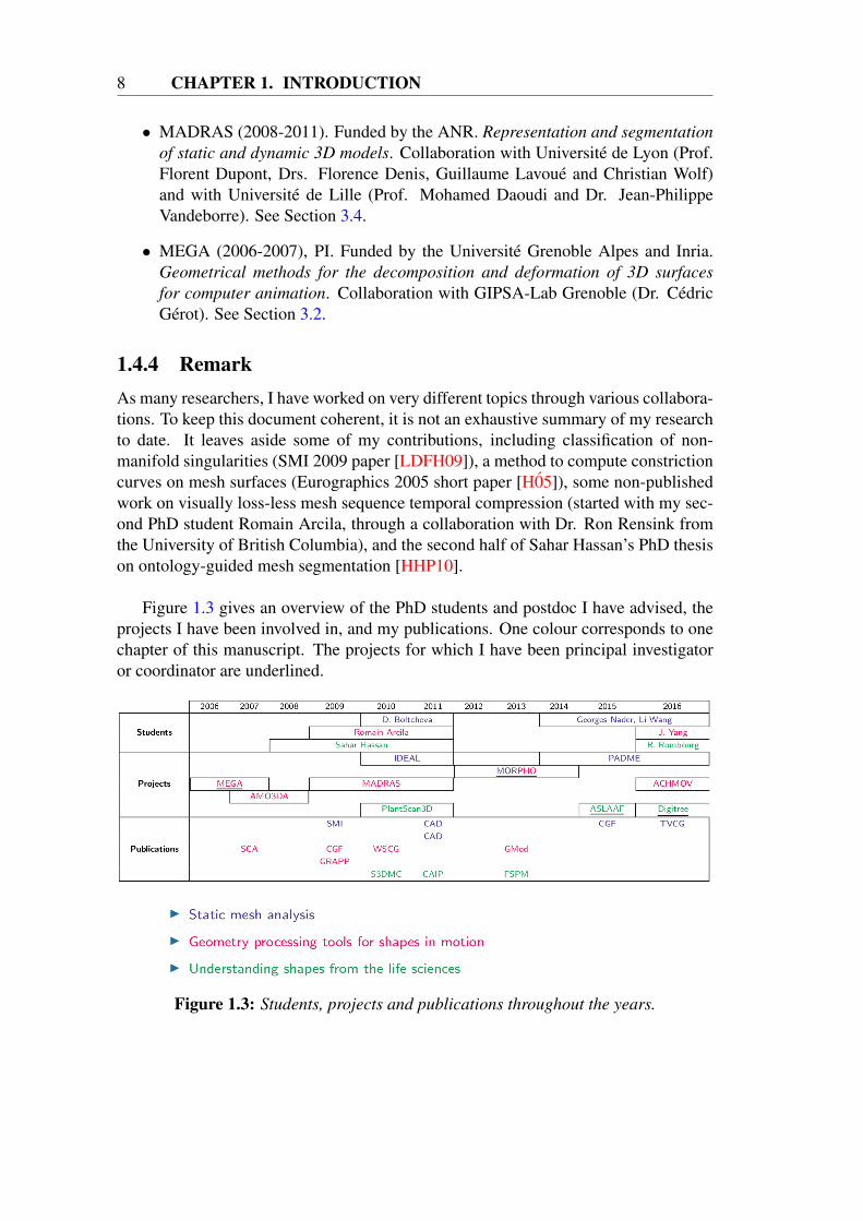
Figure 1.3 gives an overview of the PhD students and postdoc I have advised, theprojects I have been involved in, and my publications. One colour corresponds to onechapter of this manuscript. The projects for which I have been principal investigatoror coordinator are underlined.
Figure 1.3: Students, projects and publications throughout the years.
CHAPTER 2
Geometrical, topological and perceptual analysis of3D meshes
2.1 INTRODUCTION
2.1.1 3D meshesThis chapter focuses on static 3D meshes. A mesh is usually defined as a tripletM = (V,E, F ) where V is a set of vertices, i.e. 3D points, of M . E is a set ofedges, i.e. segments between neighbouring vertices, and F is a set of faces which de-fine a piece of the surface. Faces are usually polygonal and most often triangular sincea triangle is the simplest polygon that defines a surface. The 3D mesh is essentially alocal representation of the shape’s surface because only the neighbourhood of a givenpoint of a mesh is explicitly known.
Although other representations are also widely used, such as voxel sets in medicalimaging (see Section 4.2 for an example), it is meshes that are nowadays the mostcommonly used discrete 3D shape representation in many contexts. This results fromthe simplicity of creating a mesh from raw data, such as point clouds, even thoughmesh reconstruction methods may not easily generate a watertight model of the objectbecause of inconsistencies or occlusions in the data. This problem will be addressedin Section 2.2. Meshes are extremely useful since they allow for an easy rendering anddetection of collisions/intersections. Further to this, meshes provide a basis to definepiecewise linear functions which are crucial to subsequent pipeline processes such assolving partial differential equations using finite element methods.
9
10 CHAPTER 2. GEOMETRICAL, TOPOLOGICAL ANDPERCEPTUAL ANALYSIS OF 3D MESHES
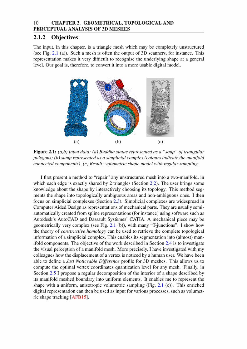
2.1.2 ObjectivesThe input, in this chapter, is a triangle mesh which may be completely unstructured(see Fig. 2.1 (a)). Such a mesh is often the output of 3D scanners, for instance. Thisrepresentation makes it very difficult to recognise the underlying shape at a generallevel. Our goal is, therefore, to convert it into a more usable digital model.
(a) (b) (c)
Figure 2.1: (a,b) Input data: (a) Buddha statue represented as a “soup” of triangularpolygons; (b) sump represented as a simplicial complex (colours indicate the manifoldconnected components). (c) Result: volumetric shape model with regular sampling.
I first present a method to “repair” any unstructured mesh into a two-manifold, inwhich each edge is exactly shared by 2 triangles (Section 2.2). The user brings someknowledge about the shape by interactively choosing its topology. This method seg-ments the shape into topologically ambiguous areas and non-ambiguous ones. I thenfocus on simplicial complexes (Section 2.3). Simplicial complexes are widespread inComputer Aided Design as representations of mechanical parts. They are usually semi-automatically created from spline representations (for instance) using software such asAutodesk’s AutoCAD and Dassault Systèmes’ CATIA. A mechanical piece may begeometrically very complex (see Fig. 2.1 (b)), with many “T-junctions”. I show howthe theory of constructive homology can be used to retrieve the complete topologicalinformation of a simplicial complex. This enables its segmentation into (almost) man-ifold components. The objective of the work described in Section 2.4 is to investigatethe visual perception of a manifold mesh. More precisely, I have investigated with mycolleagues how the displacement of a vertex is noticed by a human user. We have beenable to define a Just Noticeable Difference profile for 3D meshes. This allows us tocompute the optimal vertex coordinates quantization level for any mesh. Finally, inSection 2.5 I propose a regular decomposition of the interior of a shape described byits manifold meshed boundary into uniform elements. It enables me to represent theshape with a uniform, anisotropic volumetric sampling (Fig. 2.1 (c)). This enricheddigital representation can then be used as input for various processes, such as volumet-ric shape tracking [AFB15].
2.2. MESH REPAIR WITH TOPOLOGY CONTROL 11
2.2 MESH REPAIR WITH TOPOLOGY CONTROL
The digitisation process from a real object often creates inconsistent meshes. This isdue to the inherent limitations of the sensors, but also to the inner geometry of the ob-ject. For instance, occluded parts cannot be faithfully reconstructed by a laser scanner.Unfortunately, a consistent mesh is often necessary for further processing purposes.By “consistent”, it is often required that the neighbourhood of any point is homeomor-phic to a disk (or a half disk in case of a mesh representing a surface with boundary).For instance, T-junctions in which three faces are incident to an edge are to be avoided.Such a consistent mesh is called a two-manifold. Many methods have been introducedduring these last years to transform a given inconsistent mesh into a two-manifold one,see [ACK13] for a review. However, most of the time the user lacks control of theresult. In particular, the topology (number of handles and number of connected com-ponents of the mesh) may be ambiguous in the input data and the result may not be theone desired.
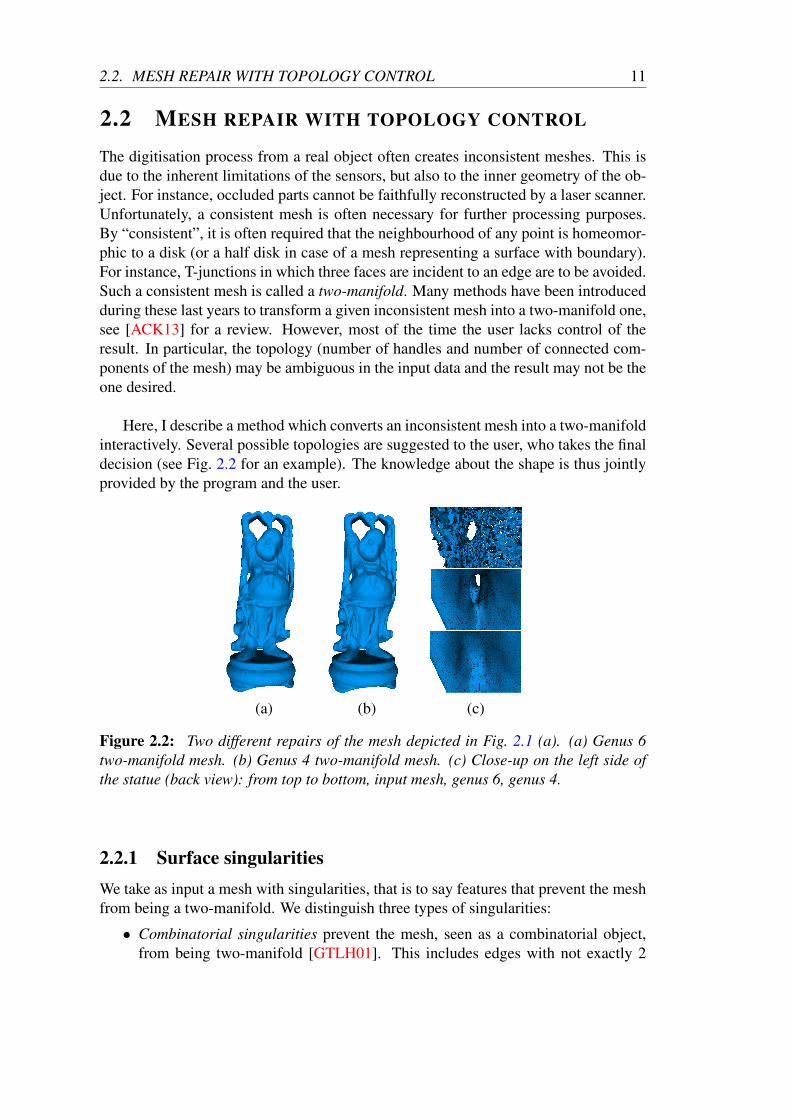
Here, I describe a method which converts an inconsistent mesh into a two-manifoldinteractively. Several possible topologies are suggested to the user, who takes the finaldecision (see Fig. 2.2 for an example). The knowledge about the shape is thus jointlyprovided by the program and the user.
(a) (b) (c)
Figure 2.2: Two different repairs of the mesh depicted in Fig. 2.1 (a). (a) Genus 6two-manifold mesh. (b) Genus 4 two-manifold mesh. (c) Close-up on the left side ofthe statue (back view): from top to bottom, input mesh, genus 6, genus 4.
2.2.1 Surface singularitiesWe take as input a mesh with singularities, that is to say features that prevent the meshfrom being a two-manifold. We distinguish three types of singularities:
• Combinatorial singularities prevent the mesh, seen as a combinatorial object,from being two-manifold [GTLH01]. This includes edges with not exactly 2
12 CHAPTER 2. GEOMETRICAL, TOPOLOGICAL ANDPERCEPTUAL ANALYSIS OF 3D MESHES
incident faces, isolated vertices, vertices whose link is neither a cycle or a chain,etc.
• Geometrical singularities prevent the mesh, embedded in R3, from being theboundary of a solid 3D object [RC99]. For instance, faces intersecting in theirinterior create a geometrical singularity.
• Topological singularities are unwanted handles or connected components whichprevent the surface from having the desired topology.
A mesh with singularities can be as general as a polygon “soup” (Fig. 2.1 (a)), that isto say a set of polygons, together with their incident vertices and edges, without anyexplicit combinatorial relation.
The mesh repair algorithm presented below is able to remove all geometrical, com-binatorial and topological singularities from an arbitrary polygonal mesh. This algo-rithm converts the mesh into a voxel set, called a discrete membrane, and iterativelyapplies morphological operators to detect areas which are likely to accept topologi-cally different reconstructions. The user then chooses the desired topology, before themodel is converted back to a two-manifold mesh.
2.2.2 Discrete voxel membraneA discrete membrane, described in [EBV05], is a set of vertex-connected voxels of thespace which divides the remaining voxels into the interior of a shape and its exterior.This means that there is no face-connected voxel path that goes from an interior voxelto an exterior one without intersecting the membrane. A discrete membrane has theadvantage of being a coarse approximation of the input triangles while already beingalmost a one-voxel-thick two-manifold.
A discrete membrane is initialised as the boundary of the voxelisation. It is thencontracted using sets of n× n voxels that form a square parallel to a coordinate planewith decreasing values of n. The voxels containing the input mesh triangles locallyterminate the shrinking; the process is stopped when there is nowhere on the membraneto be contracted.
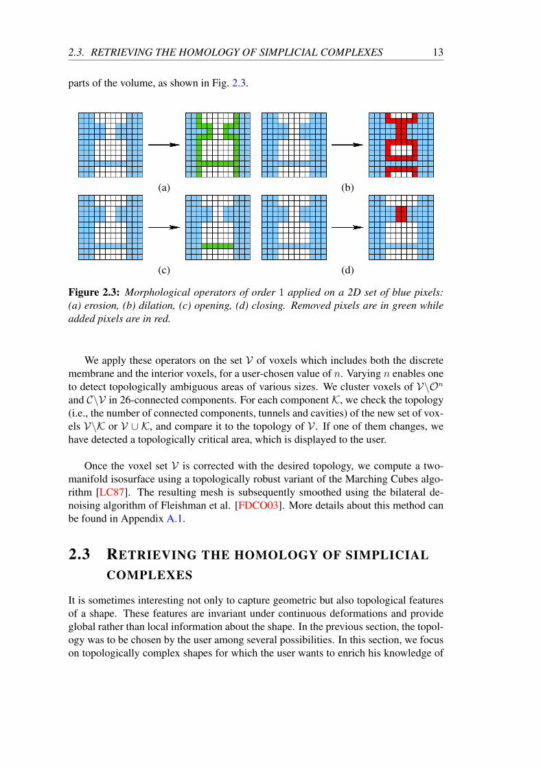
2.2.3 Interactive topology modificationIn order to track down areas of the object where topology may be wrong (that is tosay, irrelevant handles creating tunnels or connecting different components, or on thecontrary missing tunnels or bridges between several parts of a connected component),we use two morphological operators, opening On and closing Cn. An opening of or-der n is a sequence of n erosions followed by n dilations, while a closing of order nis a sequence of n dilations followed by n erosions. Openings can expand holes anddisconnect parts, while closings can close holes and connect previously disconnected
2.3. RETRIEVING THE HOMOLOGY OF SIMPLICIAL COMPLEXES 13
parts of the volume, as shown in Fig. 2.3.
(a) (b)
(c) (d)
Figure 2.3: Morphological operators of order 1 applied on a 2D set of blue pixels:(a) erosion, (b) dilation, (c) opening, (d) closing. Removed pixels are in green whileadded pixels are in red.
We apply these operators on the set V of voxels which includes both the discretemembrane and the interior voxels, for a user-chosen value of n. Varying n enables oneto detect topologically ambiguous areas of various sizes. We cluster voxels of V\Onand C\V in 26-connected components. For each component K, we check the topology(i.e., the number of connected components, tunnels and cavities) of the new set of vox-els V\K or V ∪ K, and compare it to the topology of V . If one of them changes, wehave detected a topologically critical area, which is displayed to the user.
Once the voxel set V is corrected with the desired topology, we compute a two-manifold isosurface using a topologically robust variant of the Marching Cubes algo-rithm [LC87]. The resulting mesh is subsequently smoothed using the bilateral de-noising algorithm of Fleishman et al. [FDCO03]. More details about this method canbe found in Appendix A.1.
2.3 RETRIEVING THE HOMOLOGY OF SIMPLICIALCOMPLEXES
It is sometimes interesting not only to capture geometric but also topological featuresof a shape. These features are invariant under continuous deformations and provideglobal rather than local information about the shape. In the previous section, the topol-ogy was to be chosen by the user among several possibilities. In this section, we focuson topologically complex shapes for which the user wants to enrich his knowledge of
14 CHAPTER 2. GEOMETRICAL, TOPOLOGICAL ANDPERCEPTUAL ANALYSIS OF 3D MESHES
the object. This is typically the case in Computer-Aided Design for industrial shapeswhich have been assembled from different pieces, see Fig. 2.1 (b) for an example.These shapes are usually represented as manifold-by-part meshes, with each piece be-ing a manifold mesh with boundary. Retrieving global information about the shape isnecessary to deduce how pieces are assembled. This is often visually impossible, thuscomputational tools are required.
In order to retrieve such complete topological information, we have suggested inthis work to rely on the constructive homology theory from Prof. Francis Sergeraert[Ser94], who explained the details of this theory to us in person. Homology is one ofthe most useful and algorithmically computable topological invariants. It characterisesa mesh (technically, a simplicial complex) through the notion of homological descrip-tors. Homological descriptors are defined in any dimension k and are related to thenon-trivial k-cycles in the complex which have intuitive geometrical interpretations upto dimension two. In dimension zero, they are related to the connected componentsof the complex, in dimension one, to the tunnels and the holes, and in dimension two,to the shells surrounding voids or cavities. Constructive homology focuses on homol-ogy computation. It provides a tool, the constructive Mayer-Vietoris sequence, whichoffers an elegant way of computing the homology of a simplicial complex from thehomology of its sub-complexes and of their intersections. This is precisely what isneeded for our purpose.
2.3.1 Background on simplicial homologyI will now lay down the ground work and background of simplicial homology.
A k-simplex σ = [v0, . . . , vk] is simply the convex hull of a set V of k + 1 affinelyindependent points in Rn (with n = 2 or 3 in our case). k is called the dimensionof the simplex. For example, a 0-simplex is a point, a 1-simplex is an edge connect-ing two points, a 2-simplex is a triangle, and a 3-simplex is a tetrahedron. For everynon-empty subset T ⊂ V , the simplex σ′ spanned by T is called a face of σ. A sim-plicial complex X is a collection of simplices such that all the faces of any simplexin X are also in X and the intersection of two simplices is either empty or a face ofboth. The dimension of the simplicial complex is defined as the largest dimension ofany simplex in X . A subset Y of a simplicial complex X is called a sub-complexof X if Y is itself a simplicial complex. Each k-simplex of a simplicial complex Xcan be oriented by assigning a linear ordering to its vertices. The boundary of anoriented k-simplex is defined as the alternate sum of its incident (k − 1)-simplices:
dk([v0, . . . , vk]) =k∑
i=0
(−1)i[v0, . . . , vi−1, vi+1, . . . , vk].
Homology is defined on simplicial complexes thanks to an algebraic object calleda chain complex. Let X be a simplicial complex and n be its dimension. A k-chainis defined for each dimension k ≤ n as ak =
∑i λiσ
ki , where λi ∈ Z are coefficients
2.3. RETRIEVING THE HOMOLOGY OF SIMPLICIAL COMPLEXES 15
assigned to each k-simplex σki of X . The kth chain group, denoted as Ck(X), isformed by the set of k-chains together with the addition operation, defined by addingthe coefficients simplex by simplex. The set of oriented k-simplices of X forms acanonical basis for this group. The chain complex, denoted as C∗ = (Ck, dk)k∈N, is thesequence of the chain groups Ck(X) connected by the boundary operator dk:
(C∗, d∗) : 00←− C0
d1←− C1d2←− . . .
dn−1←−−− Cn−1dn←− Cn
0←− 0.
The chain complex C∗(X) can be encoded as a set of pairs (Bk, Dk)0≤k≤n, whereBk is the canonical basis ofCk andDk is an integer matrix, called the incidence matrix,which expresses the boundary operator with respect to Bk−1 and Bk. Such a matrixis usually expressed in a special basis called the Smith basis, and is then named aSmith normal form (SNF) [Mun99]. Given a chain complex C∗(X), homology groupsare derived from two specific subgroups of the chain groups defined by the boundaryoperators:
Zk = Ker dk = c ∈ Ck(X)|dk(c) = 0and
Bk = Img dk+1 = c ∈ Ck(X)|∃a ∈ Ck+1 : c = dk+1(a).For each k ∈ [0, n], the kth homology group of X is defined as the quotient of thecycle group over the boundary group, i.e., Hk = Zk/Bk. Thus, the elements of thehomology group are equivalence classes of k-cycles which are not k-boundaries. Hk
can be written as a disjoint sum:
Hk = Z⊕ · · · ⊕ Z⊕ Z/λ1Z⊕ · · · ⊕ Z/λpZ. (2.1)
The number of occurrences of Z in the free part Z ⊕ · · · ⊕ Z is called the kth Bettinumber βk. It corresponds to the maximal number of independent k-cycles that donot bound the complex. For instance, β0 is the number of connected components, β1
is the number of tunnels (i.e., the genus if X is a surface) and β2 is the number ofcavities (voids) inside the object if X is volumetric. The values λ1, . . . , λp are strictlygreater than one and such that λi divides λi+1. They are called torsion coefficients.Intuitively, the torsion coefficients characterise the non-orientable aspect of X . Anorientable manifold has no torsion coefficient. The decomposition of Eq. 2.1 alsoshows that there exists a finite number of independent equivalent classes from whichwe can deduce all elements of Hk. Any set composed of one element of each of theseclasses is called a set of generators for Hk. The generators, Betti numbers and torsioncoefficients form the complete homology information of the simplicial complex X .
2.3.2 Constructive homologyConstructive homology has been developed in order to reformulate homology conceptsinto concepts with a computational nature, thus leading to effective implementable al-gorithms. It handles homology computations over chain groups of infinite dimension
16 CHAPTER 2. GEOMETRICAL, TOPOLOGICAL ANDPERCEPTUAL ANALYSIS OF 3D MESHES
[Ser94]. One fundamental concept is that of reduction which relates, through a mor-phism, a large chain complex C∗ to a small one C∗. C∗ is constructed so that it containsthe same homological information in the most compact way. The morphism can itselfbe represented as a chain complex, using a notion called the cone of a morphism. Fur-ther explanations can be found in Appendix A.2.
In our work we introduce a specific kind of reduction which we call the homologi-cal Smith reduction. Given a simplicial complexX of finite dimension n, this reductionrelates its chain complex, X∗, to a very small chain complex, EX∗, which containsonly the homological information of X∗. This information is computed through theSNF algorithm, which transforms each incidence matrix into its Smith normal form.
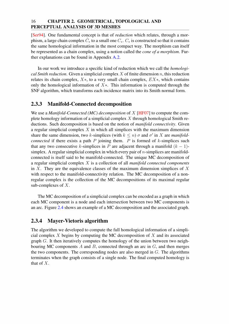
2.3.3 Manifold-Connected decompositionWe use a Manifold-Connected (MC) decomposition of X [HF07] to compute the com-plete homology information of a simplicial complex X through homological Smith re-ductions. Such decomposition is based on the notion of manifold connectivity. Givena regular simplicial complex X in which all simplices with the maximum dimensionshare the same dimension, two k-simplices (with k ≤ n) σ and σ′ in X are manifold-connected if there exists a path P joining them. P is formed of k-simplices suchthat any two consecutive k-simplices in P are adjacent through a manifold (k − 1)-simplex. A regular simplicial complex in which every pair of n-simplices are manifold-connected is itself said to be manifold-connected. The unique MC decomposition ofa regular simplicial complex X is a collection of all manifold connected componentsin X . They are the equivalence classes of the maximum dimension simplices of Xwith respect to the manifold-connectivity relation. The MC decomposition of a non-regular complex is the collection of the MC decompositions of its maximal regularsub-complexes of X .
The MC decomposition of a simplicial complex can be encoded as a graph in whicheach MC component is a node and each intersection between two MC components isan arc. Figure 2.4 shows an example of a MC decomposition and the associated graph.
2.3.4 Mayer-Vietoris algorithmThe algorithm we developed to compute the full homological information of a simpli-cial complex X begins by computing the MC decomposition of X and its associatedgraph G. It then iteratively computes the homology of the union between two neigh-bouring MC components A and B, connected through an arc in G, and then mergesthe two components. The corresponding nodes are also merged in G. The algorithmsterminates when the graph consists of a single node. The final computed homology isthat of X .
2.4. JUST-NOTICEABLE DISTORTION PROFILE FOR MESHES 17
(a) (b)
Figure 2.4: (a) MC decomposition of a simplicial complex. Each MC component isshown in a different colour. (b) The associated graph.
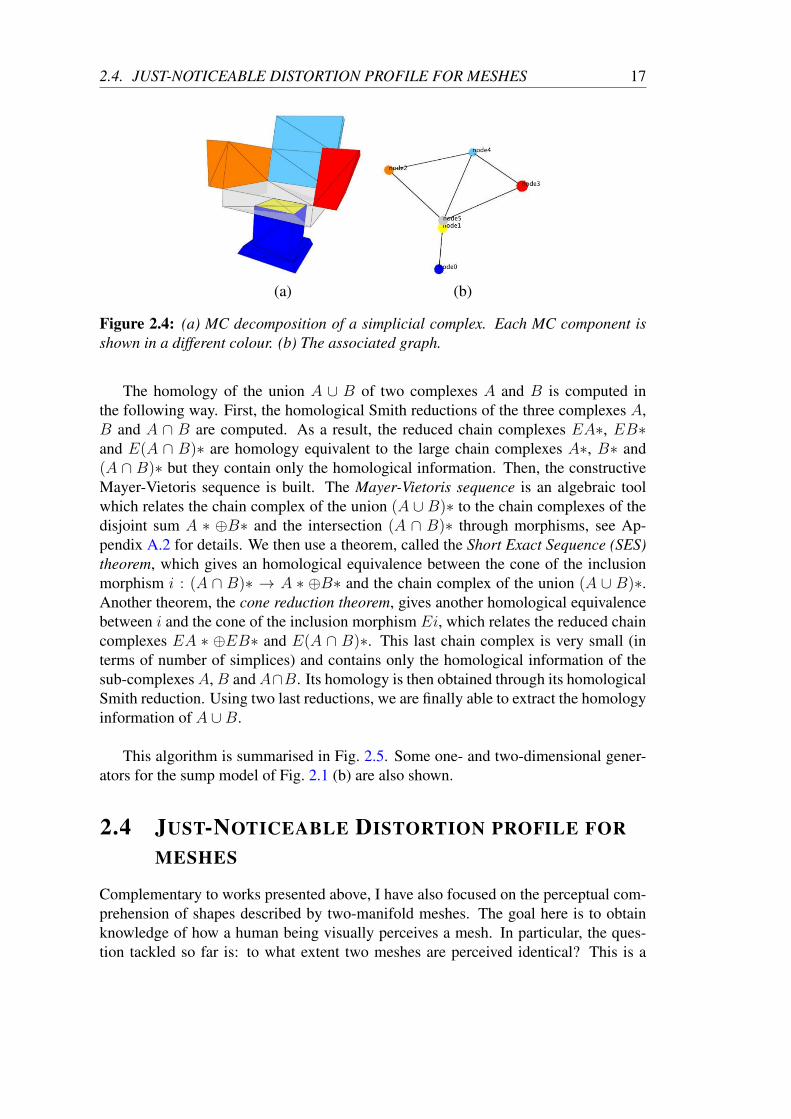
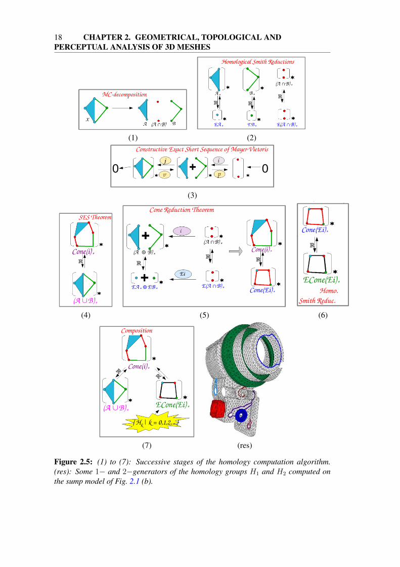
The homology of the union A ∪ B of two complexes A and B is computed inthe following way. First, the homological Smith reductions of the three complexes A,B and A ∩ B are computed. As a result, the reduced chain complexes EA∗, EB∗and E(A ∩ B)∗ are homology equivalent to the large chain complexes A∗, B∗ and(A ∩ B)∗ but they contain only the homological information. Then, the constructiveMayer-Vietoris sequence is built. The Mayer-Vietoris sequence is an algebraic toolwhich relates the chain complex of the union (A ∪ B)∗ to the chain complexes of thedisjoint sum A ∗ ⊕B∗ and the intersection (A ∩ B)∗ through morphisms, see Ap-pendix A.2 for details. We then use a theorem, called the Short Exact Sequence (SES)theorem, which gives an homological equivalence between the cone of the inclusionmorphism i : (A ∩ B)∗ → A ∗ ⊕B∗ and the chain complex of the union (A ∪ B)∗.Another theorem, the cone reduction theorem, gives another homological equivalencebetween i and the cone of the inclusion morphism Ei, which relates the reduced chaincomplexes EA ∗ ⊕EB∗ and E(A ∩ B)∗. This last chain complex is very small (interms of number of simplices) and contains only the homological information of thesub-complexesA,B andA∩B. Its homology is then obtained through its homologicalSmith reduction. Using two last reductions, we are finally able to extract the homologyinformation of A ∪B.
This algorithm is summarised in Fig. 2.5. Some one- and two-dimensional gener-ators for the sump model of Fig. 2.1 (b) are also shown.
2.4 JUST-NOTICEABLE DISTORTION PROFILE FORMESHES
Complementary to works presented above, I have also focused on the perceptual com-prehension of shapes described by two-manifold meshes. The goal here is to obtainknowledge of how a human being visually perceives a mesh. In particular, the ques-tion tackled so far is: to what extent two meshes are perceived identical? This is a
18 CHAPTER 2. GEOMETRICAL, TOPOLOGICAL ANDPERCEPTUAL ANALYSIS OF 3D MESHES
(1) (2)
(3)
(4) (5) (6)
(7) (res)
Figure 2.5: (1) to (7): Successive stages of the homology computation algorithm.(res): Some 1− and 2−generators of the homology groups H1 and H2 computed onthe sump model of Fig. 2.1 (b).
2.4. JUST-NOTICEABLE DISTORTION PROFILE FOR MESHES 19
key question in assessing the quality of mesh processing algorithms, for instance forsimplification, compression or watermarking purposes, which try to replace a givenmesh by another one with the least visible differences. In this section, I describe abottom-up approach to the perception of differences between meshes. The method re-lies on the known properties of the human visual system and is based on a series of userexperiments. These experiments define a Just-Noticeable Distortion (JND) profile fortwo-manifold meshes, which describes how much any vertex of a given mesh can bedisplaced without the change being noticed by the majority of users (see Fig. 2.8 (c)).Applications to the perceptually optimal quantization and simplification of meshes areshown.
This work forms part of the PhD thesis of Georges Nader.
2.4.1 Local perceptual propertiesIt is well known that for a human being the visibility of a visual pattern depends bothon its local contrast and its spatial frequency [Wan95]. Local contrast refers to thechange of light intensity over the light intensity of its surrounding. The spatial fre-quency is defined as the size of light patterns on the retina. It is expressed in unitsof cycles per degree (cpd). To quantify how these properties affect the visibility of avisual stimulus, two main concepts have been introduced in the literature. First, theconcept of contrast sensitivity function (CSF) describes the visibility threshold withrespect to spatial frequency. For any stimulus, CSF usually exhibits a peak at around2 to 5 cpd then drops off to a point where no detail can be resolved. The exact shapeof a CSF curve depends on the nature of the stimulus. The second concept, contrastmasking is the change in visibility of a stimulus (target) due to the presence of anotherstimulus (mask). The rate of change of the visibility threshold of the target with respectto the applied mask quantifies the effect of contrast masking. The curve possesses twoasymptotic regions. The first region is for mask contrast values below the mask visi-bility threshold and is constant indicating that there is no masking effect. The secondregion occurs for higher mask contrast values and has a positive slope of about 0.6 to1, depending on the stimulus [LF80].
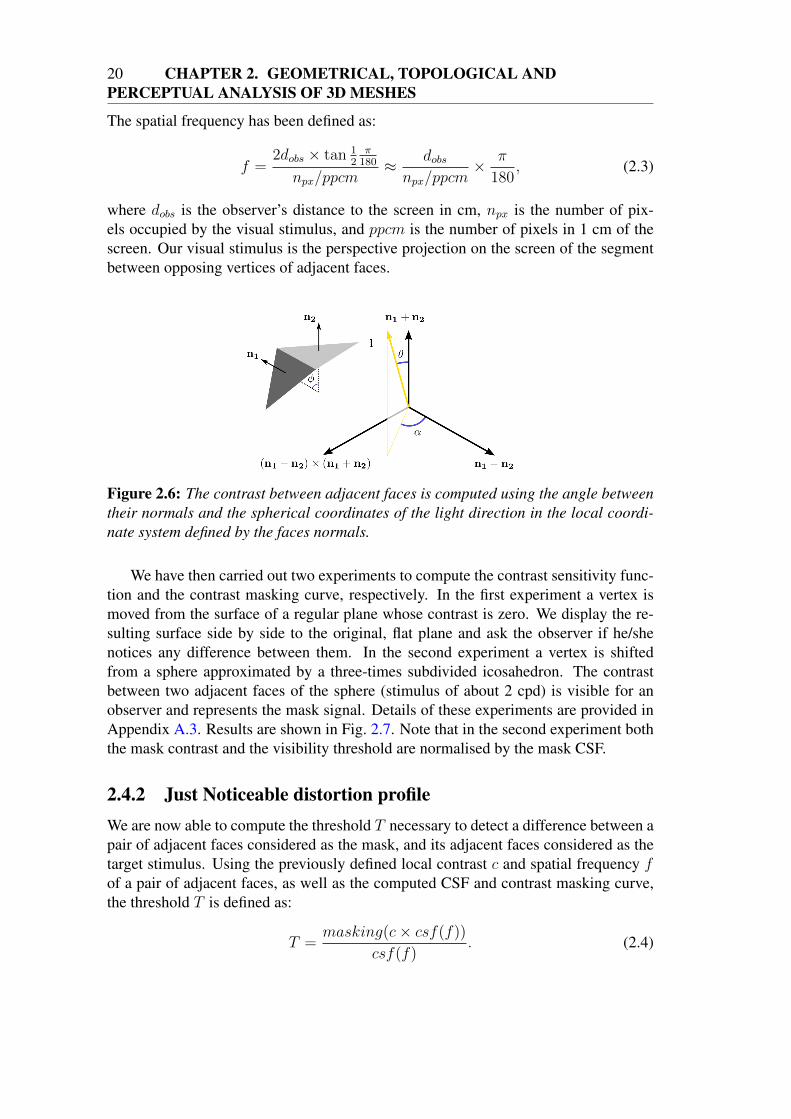
In the case of a 3D mesh, we have defined the contrast between two adjacent facesas:
c = ‖ cosα× tan θ × tanφ
2‖, (2.2)
where α and θ are the spherical coordinates of the light direction in the local coordinatesystem defined by ~n1− ~n2, ~n1 + ~n2 and their outer product (see Fig. 2.6). φ is the anglebetween the normals of the two faces. This formula takes into account both the sceneillumination and the surface geometry. A direction of light close to the normal direction(θ ≈ 0) will minimise the value of the contrast, as will a smooth surface (φ ≈ 0).
20 CHAPTER 2. GEOMETRICAL, TOPOLOGICAL ANDPERCEPTUAL ANALYSIS OF 3D MESHES
The spatial frequency has been defined as:
f =2dobs × tan 1
2π
180
npx/ppcm≈ dobsnpx/ppcm
× π
180, (2.3)
where dobs is the observer’s distance to the screen in cm, npx is the number of pix-els occupied by the visual stimulus, and ppcm is the number of pixels in 1 cm of thescreen. Our visual stimulus is the perspective projection on the screen of the segmentbetween opposing vertices of adjacent faces.
Figure 2.6: The contrast between adjacent faces is computed using the angle betweentheir normals and the spherical coordinates of the light direction in the local coordi-nate system defined by the faces normals.
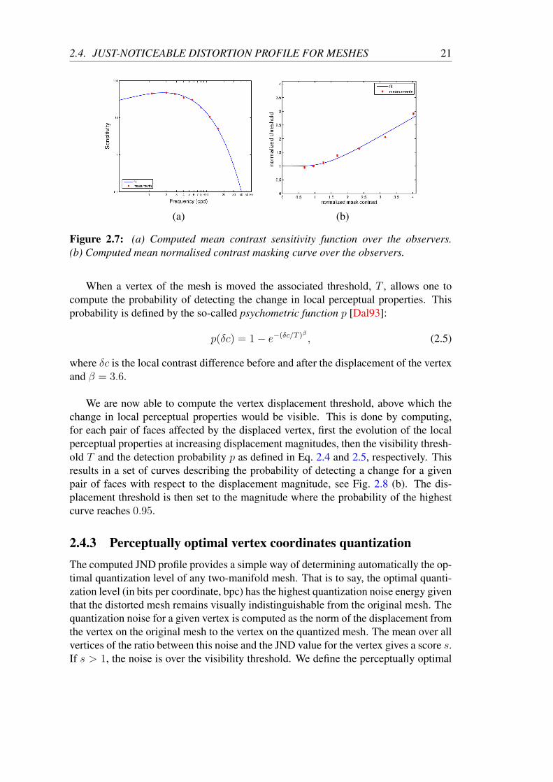
We have then carried out two experiments to compute the contrast sensitivity func-tion and the contrast masking curve, respectively. In the first experiment a vertex ismoved from the surface of a regular plane whose contrast is zero. We display the re-sulting surface side by side to the original, flat plane and ask the observer if he/shenotices any difference between them. In the second experiment a vertex is shiftedfrom a sphere approximated by a three-times subdivided icosahedron. The contrastbetween two adjacent faces of the sphere (stimulus of about 2 cpd) is visible for anobserver and represents the mask signal. Details of these experiments are provided inAppendix A.3. Results are shown in Fig. 2.7. Note that in the second experiment boththe mask contrast and the visibility threshold are normalised by the mask CSF.
2.4.2 Just Noticeable distortion profileWe are now able to compute the threshold T necessary to detect a difference between apair of adjacent faces considered as the mask, and its adjacent faces considered as thetarget stimulus. Using the previously defined local contrast c and spatial frequency fof a pair of adjacent faces, as well as the computed CSF and contrast masking curve,the threshold T is defined as:
T =masking(c× csf(f))
csf(f). (2.4)
2.4. JUST-NOTICEABLE DISTORTION PROFILE FOR MESHES 21
(a) (b)
Figure 2.7: (a) Computed mean contrast sensitivity function over the observers.(b) Computed mean normalised contrast masking curve over the observers.
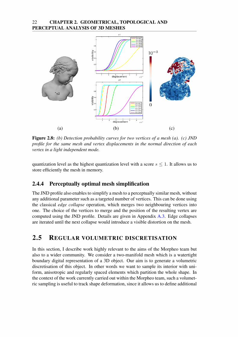
When a vertex of the mesh is moved the associated threshold, T , allows one tocompute the probability of detecting the change in local perceptual properties. Thisprobability is defined by the so-called psychometric function p [Dal93]:
p(δc) = 1− e−(δc/T )β , (2.5)
where δc is the local contrast difference before and after the displacement of the vertexand β = 3.6.
We are now able to compute the vertex displacement threshold, above which thechange in local perceptual properties would be visible. This is done by computing,for each pair of faces affected by the displaced vertex, first the evolution of the localperceptual properties at increasing displacement magnitudes, then the visibility thresh-old T and the detection probability p as defined in Eq. 2.4 and 2.5, respectively. Thisresults in a set of curves describing the probability of detecting a change for a givenpair of faces with respect to the displacement magnitude, see Fig. 2.8 (b). The dis-placement threshold is then set to the magnitude where the probability of the highestcurve reaches 0.95.
2.4.3 Perceptually optimal vertex coordinates quantizationThe computed JND profile provides a simple way of determining automatically the op-timal quantization level of any two-manifold mesh. That is to say, the optimal quanti-zation level (in bits per coordinate, bpc) has the highest quantization noise energy giventhat the distorted mesh remains visually indistinguishable from the original mesh. Thequantization noise for a given vertex is computed as the norm of the displacement fromthe vertex on the original mesh to the vertex on the quantized mesh. The mean over allvertices of the ratio between this noise and the JND value for the vertex gives a score s.If s > 1, the noise is over the visibility threshold. We define the perceptually optimal
22 CHAPTER 2. GEOMETRICAL, TOPOLOGICAL ANDPERCEPTUAL ANALYSIS OF 3D MESHES
(a) (b) (c)
Figure 2.8: (b) Detection probability curves for two vertices of a mesh (a). (c) JNDprofile for the same mesh and vertex displacements in the normal direction of eachvertex in a light independent mode.
quantization level as the highest quantization level with a score s ≤ 1. It allows us tostore efficiently the mesh in memory.
2.4.4 Perceptually optimal mesh simplificationThe JND profile also enables to simplify a mesh to a perceptually similar mesh, withoutany additional parameter such as a targeted number of vertices. This can be done usingthe classical edge collapse operation, which merges two neighbouring vertices intoone. The choice of the vertices to merge and the position of the resulting vertex arecomputed using the JND profile. Details are given in Appendix A.3. Edge collapsesare iterated until the next collapse would introduce a visible distortion on the mesh.
2.5 REGULAR VOLUMETRIC DISCRETISATION
In this section, I describe work highly relevant to the aims of the Morpheo team butalso to a wider community. We consider a two-manifold mesh which is a watertightboundary digital representation of a 3D object. Our aim is to generate a volumetricdiscretisation of this object. In other words we want to sample its interior with uni-form, anisotropic and regularly spaced elements which partition the whole shape. Inthe context of the work currently carried out within the Morpheo team, such a volumet-ric sampling is useful to track shape deformation, since it allows us to define additional
2.5. REGULAR VOLUMETRIC DISCRETISATION 23
volume constraints on the deformations [AFB15]. Other potential applications includeparticle-based physical simulation, finite-element modelling, etc.
This work forms part of the PhD thesis of Li Wang. It is described with moredetails in Appendix A.4.
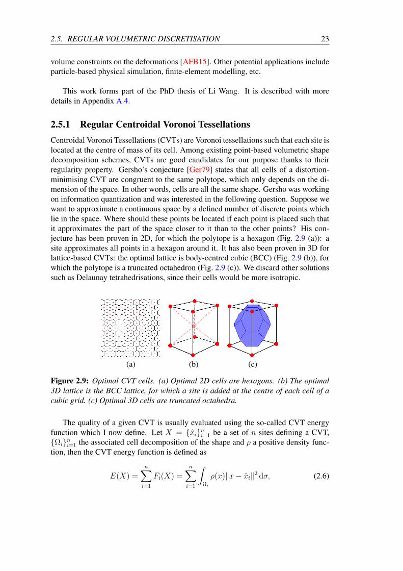
2.5.1 Regular Centroidal Voronoi TessellationsCentroidal Voronoi Tessellations (CVTs) are Voronoi tessellations such that each site islocated at the centre of mass of its cell. Among existing point-based volumetric shapedecomposition schemes, CVTs are good candidates for our purpose thanks to theirregularity property. Gersho’s conjecture [Ger79] states that all cells of a distortion-minimising CVT are congruent to the same polytope, which only depends on the di-mension of the space. In other words, cells are all the same shape. Gersho was workingon information quantization and was interested in the following question. Suppose wewant to approximate a continuous space by a defined number of discrete points whichlie in the space. Where should these points be located if each point is placed such thatit approximates the part of the space closer to it than to the other points? His con-jecture has been proven in 2D, for which the polytope is a hexagon (Fig. 2.9 (a)): asite approximates all points in a hexagon around it. It has also been proven in 3D forlattice-based CVTs: the optimal lattice is body-centred cubic (BCC) (Fig. 2.9 (b)), forwhich the polytope is a truncated octahedron (Fig. 2.9 (c)). We discard other solutionssuch as Delaunay tetrahedrisations, since their cells would be more isotropic.
(a) (b) (c)
Figure 2.9: Optimal CVT cells. (a) Optimal 2D cells are hexagons. (b) The optimal3D lattice is the BCC lattice, for which a site is added at the centre of each cell of acubic grid. (c) Optimal 3D cells are truncated octahedra.
The quality of a given CVT is usually evaluated using the so-called CVT energyfunction which I now define. Let X = xini=1 be a set of n sites defining a CVT,Ωini=1 the associated cell decomposition of the shape and ρ a positive density func-tion, then the CVT energy function is defined as
E(X) =n∑
i=1
Fi(X) =n∑
i=1
∫
Ωi
ρ(x)‖x− xi‖2 dσ, (2.6)
24 CHAPTER 2. GEOMETRICAL, TOPOLOGICAL ANDPERCEPTUAL ANALYSIS OF 3D MESHES
where dσ is the area differential.
An optimal CVT is obtained when a minimum of this functionE is reached. Unfor-tunately, this function depends on both the shape size and the number of sites, making itdifficult to compare across different shapes or discretisations. Inspired by early worksfrom Conway and Sloane [CS82], we rather suggest to evaluate CVTs using a criterionwe call a regularity criterion which is dimensionless and defined as:
G(X) =1
n
n∑
i=1
G(Ωi) =1
nm
n∑
i=1
∫Ωi‖x− xi‖2 dx
(∫Ωi
dx)(m+2)/m
, (2.7)
with m the dimension of the embedding space.
Both criteria are related since in the case of a uniform tessellation (uniform densityfunction), the optimal value Em of an infinite CVT with n sites and volume V for eachcell is:
Em = mnV (m+2)/mGm,
where Gm is the optimal m-dimensional cell quantizer, that is to say G2 = 536√
3=
0.0801875 . . . for a hexagon and G3 = 19
192 3√2= 0.0785433 . . . for a truncated octa-
hedron. However, our regularity criterion does not depend on the shape size or on thenumber n of sites. Therefore, it allows for a general evaluation of CVTs, for instance,to check if the sampling is dense enough to get a regular tessellation. Note that a CVTis usually stable since it is computed using an integral and not a derivative.
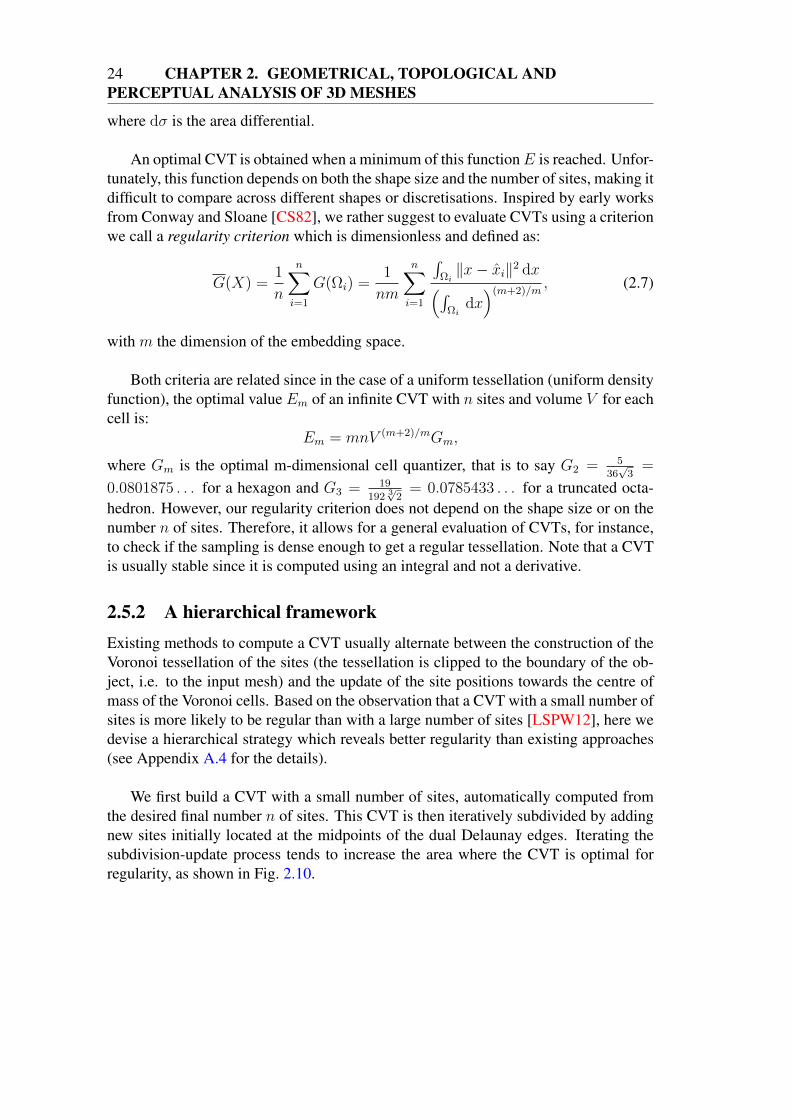
2.5.2 A hierarchical frameworkExisting methods to compute a CVT usually alternate between the construction of theVoronoi tessellation of the sites (the tessellation is clipped to the boundary of the ob-ject, i.e. to the input mesh) and the update of the site positions towards the centre ofmass of the Voronoi cells. Based on the observation that a CVT with a small number ofsites is more likely to be regular than with a large number of sites [LSPW12], here wedevise a hierarchical strategy which reveals better regularity than existing approaches(see Appendix A.4 for the details).
We first build a CVT with a small number of sites, automatically computed fromthe desired final number n of sites. This CVT is then iteratively subdivided by addingnew sites initially located at the midpoints of the dual Delaunay edges. Iterating thesubdivision-update process tends to increase the area where the CVT is optimal forregularity, as shown in Fig. 2.10.
2.6. PERSPECTIVES 25
(a) (b) (c) (d) (e)
Figure 2.10: Hierarchical CVT computation. From an initial CVT with 10 sites (left),successive subdivisions and updates lead to CVTs with 40, 160, 640 and n = 2560sites (from left to right). The cell regularity measure G2(Ωi) is colour-coded from blue(regular) to red (far from regular).
2.6 PERSPECTIVES
In this chapter I have presented a full pipeline to create regularly tessellated volumesfrom unstructured meshes of their boundaries. My efforts have first focused on thetopological and perceptual comprehension of these meshes, then on the discretisationof their interior into regular anisotropic cells. The short-term perspectives includeextensions of the last two works which I now discuss. They are tackled as part ofGeorges Nader and Kai Wang’s PhD theses.
2.6.1 Perceptual analysis of smooth shaded surfacesThe main limitation of the work presented in Section 2.4 is its restriction to flat shadedsurfaces. We rely on the visibility difference between adjacent faces to define 3D localperceptual properties. In the case of smooth shaded surfaces, the mask signal is morecomplicated than a simple local contrast between two adjacent faces. Thus, in orderto extend this work to smooth shaded surfaces, we need to take into account otheraspects of the human visual system, such as entropy masking [Wat97] or the free-energy principle [Fri10], which model how the visual system adapts to uncertainty. Astep further would be to define not only a JND profile but also a perceptual metric tocompare meshes. While the JND profile only says if meshes are perceived similar ornot, such a metric would provide a quantitative assessment of the perceptual differencebetween meshes.
2.6.2 Regularly tessellated volumes from point cloudsThe framework introduced in Section 2.5 has been applied to shapes defined by theirmeshed boundary surfaces. Computed Centroidal Voronoi Tessellations are clippedto the mesh (see Appendix A.4 for the details). Theoretically, nothing prevents thisframework from being applied to other shape representations. We are currently in-vestigating the case of implicit surfaces. This is of particular interest since it of-fers an alternative smoother way of defining a surface from a point cloud (see e.g.[CBC+01, OBA+03, KBH06]). It would also be interesting to investigate how this

26 CHAPTER 2. GEOMETRICAL, TOPOLOGICAL ANDPERCEPTUAL ANALYSIS OF 3D MESHES
work can be extended to anisotropic cells, which align to some geometric features. LpCVTs [LL10] are a good candidate for this. The behaviour of some Lp regularity cri-terion is still to be explored. Both the criterion and the hierarchical approach also needto be improved in order that the boundary cells of the CVT be more regular and adaptto the geometry of the surface, since the regularity properties are only proven onlyin an infinite, unbounded case so far. Optimisation of the boundary surface samplingtogether with the volume sampling is also still to be investigated. Finally, as stated inthe previous section, this uniform, anisotropic volumetric tessellation has been usedfor shape tracking [AFB15]. Another short-term plan is to combine such volumetricdecomposition of a moving shape with physical simulation methods, to generate newcomplex animations from a real motion.
CHAPTER 3
Digital geometry processing for shapes in motion
3.1 INTRODUCTION
3.1.1 ObjectivesOur world is dynamic and not static: moving shapes are clearly of interest in manyfields. There is a growing concern for the processing and recognition of 3D shapesin motion not only within the computer graphics and computer vision communitiesbut also in other fields, for instance, among the medical imaging community (see[SFR+12] for an example). Of course, the speed of motion differs according to theapplication of interest. Whereas human characters acting in a scene are obviouslymoving shapes, the growth of a tree or a tumour can also be thought of as a movingobject in biological or medical applications. However, despite much progress, there isstill a lot of work to do, and this is in particular why the Morpheo team devotes itselfto this topic.
Of particular interest in understanding a moving shape is the fact that its motion canhelp to identify the shape, since some redundancy can be expected between successiveposes of the shape during its motion. [LB12] for instance recovers the correct topologyof a model by studying the changes between successive poses during motion. Decom-posing a shape into rigidly moving components, as in [FB11] or as will be describedin Section 3.4, can also help to understand the functionality of the shape’s parts, par-ticularly if contextual knowledge is added to the process (e.g., if the shape is known tobe a human shape, it is easy to identify where are the arms, the legs and the torso). Itis also expected that, conversely, the shape can lead to a high-level comprehension ofthe motion, that is to say to deduce the activity performed by the model.
27
28 CHAPTER 3. DIGITAL GEOMETRY PROCESSING FOR SHAPESIN MOTION
In this chapter, I describe my first contributions to the field, which are mostly fo-cused on animated human or animal characters. In Section 3.2, I introduce a method tocreate realistic moving shapes from a static shape, with some control by the user. Thismethod first computes an accurate animation skeleton by using a topological tool calledthe Reeb graph and prior knowledge about the shape’s anatomy. Then it generates flex-ible skinning weights by decomposing the shape into overlapping parts. My methodallows the user to create rigid or elastic movement. This work began in response toa request by an infographist. In Section 3.3, I describe a universal mathematical toolI am developing to process moving shapes. This tool is a proper discretisation of theLaplace operator for such objects. As a practical example, I show how this operatorcan be applied to edit the shape and the motion of a given character. Finally, I explainin Section 3.4 a way to retrieve the rigidly moving parts of a shape that is representedas an evolving mesh without temporal coherence and I show how to validate segmen-tations of a moving shape into rigidly moving components. Before doing so, let meintroduce several general concepts.
3.1.2 3D+t vs. 4DAlthough we add one dimension with respect to the previous chapter, I claim that thestudy of 3D shapes in motion is somehow different to the study of objects embedded ina general four-dimensional Euclidean space. Although it is of interest to devise univer-sal tools (and I will introduce one in Section 3.3), the temporal dimension needs to beprocessed in a separate manner to the three geometrical dimensions. This is becausewe are interested in recognising the three-dimensional shape as well as its motion,and not the general four-dimensional behaviour of the moving shape. I elaborate onthis in Section 3.3. Therefore, our subjects of study are described as three-dimensionalmeshes (usually two-manifold, since they describe the boundary of a watertight object)evolving though time.
3.1.3 Temporal coherenceSince we focus on shapes described by their meshed surfaces, a moving shape is usu-ally defined as a temporal sequence of 3D meshes, sometimes called a dynamic mesh,a time-varying surface or a 3D video. Two types of mesh sequence can be considered,depending on whether or not temporal coherence is assumed, i.e. there is a one-to-one correspondence between vertices of successive meshes. In computer graphics, amoving shape is usually created by modelling a static shape and then animating it (seeSection 3.2). The temporal coherence is thus implicit, since the connectivity of themesh remains the same at each time frame. The main drawback of such a representa-tion is that the topology cannot change over time. On the contrary, in computer vision,a moving shape is usually defined as a sequence of static shapes captured at each timestep. A standard approach is to reconstruct a 3D mesh from the visual hull of the ob-ject’s silhouettes as seen from a set of cameras [SH07, FB09]. The lack of explicittemporal coherence is a major concern for any application, and many methods have
3.1. INTRODUCTION 29
been proposed to track a template (which may or may not be the reconstruction of thefirst frame of the videos) over the mesh sequence [KBH12, HBNI14, AFB15].
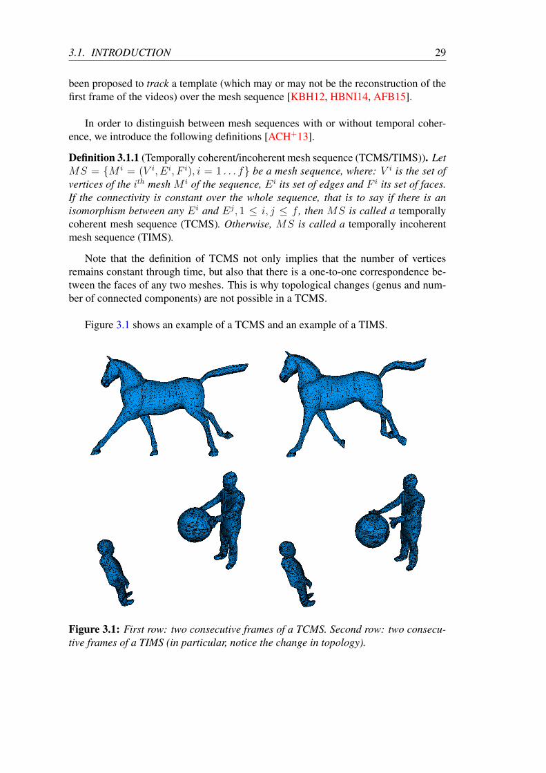
In order to distinguish between mesh sequences with or without temporal coher-ence, we introduce the following definitions [ACH+13].
Definition 3.1.1 (Temporally coherent/incoherent mesh sequence (TCMS/TIMS)). LetMS = M i = (V i, Ei, F i), i = 1 . . . f be a mesh sequence, where: V i is the set ofvertices of the ith mesh M i of the sequence, Ei its set of edges and F i its set of faces.If the connectivity is constant over the whole sequence, that is to say if there is anisomorphism between any Ei and Ej, 1 ≤ i, j ≤ f , then MS is called a temporallycoherent mesh sequence (TCMS). Otherwise, MS is called a temporally incoherentmesh sequence (TIMS).
Note that the definition of TCMS not only implies that the number of verticesremains constant through time, but also that there is a one-to-one correspondence be-tween the faces of any two meshes. This is why topological changes (genus and num-ber of connected components) are not possible in a TCMS.
Figure 3.1 shows an example of a TCMS and an example of a TIMS.
Figure 3.1: First row: two consecutive frames of a TCMS. Second row: two consecu-tive frames of a TIMS (in particular, notice the change in topology).
30 CHAPTER 3. DIGITAL GEOMETRY PROCESSING FOR SHAPESIN MOTION
3.2 HARMONIC SKELETON FOR CHARACTERANIMATION
In this section I describe my contribution to the creation of a TCMS, from a staticmesh only, using the standard skeletal animation framework. The TCMS is created byfirst generating an animation skeleton and then computing skinning weights. The priorknowledge used relates to the character’s anatomy, and is encoded in the algorithm.This work is the result of collaboration with an infographist, Christine Depraz. Sheidentified, from her point of view, the anatomical requirements of a skeleton that wouldgenerate a realistic animation.
3.2.1 A short survey on skeleton computation methodsSkeleton computation has been a popular topic in computer graphics and shape analysisfor a long time, following early work on medial axis computation in image process-ing [Blu67]. Skeletons are useful for shape analysis [BGSF08], matching [HSKK01],registration [ZST+10], retrieval [BMSF06, TVD09, BB13], or animation and defor-mation [LCF00], which is the application we focus on hereafter. We restrict ouroverview to curve skeletons, that is to say skeletons which can be represented as graphsembedded in R3. This excludes medial representations; see [SP08] for an in-depthdescription of these. Although skeleton computation methods exist on point clouds[TZCO09, HWCO+13] and voxel sets [CSM07], we restrict ourselves to the case ofmeshes, which are of interest for the later application. Many different methods existand they can be classified according to the criteria that they try to fulfil: centred-ness, homotopy equivalence to the shape, invariance under transformations, robustnessagainst geometric noise, . . . For ease of understanding, since a method can fulfilseveral criteria, I prefer to present them according to their methodological basis.
Segmentation-based methods
As stated in Chapter 1, segmentation and skeleton computation can be seen as dualproblems. Consequently, several people have suggested beginning by decomposing ashape into meaningful parts so as to deduce a skeleton. Many methods exist, including[KT03] which is based on a hierarchical decomposition and which gives rather star-shaped skeletons. Lien et al. [LKA06] use centroids and the principal axes of a shapeto build simultaneously a segmentation and a skeleton of the given shape. Dellas etal. [DMMT+07] have proposed a specific method to recover an animation skeletonfrom human scans. This method is based on the segmentation of the shape into seman-tically meaningful parts and uses prior knowledge about human anatomy. [JXC+13]have iterated a dual graph contraction and a mesh-face clustering process to generate askeleton.

3.2. HARMONIC SKELETON FOR CHARACTER ANIMATION 31
Force field and thinning-based methods
Following the method of [LcWcM+03], which uses a repulsive force field, severalauthors have suggested using a force field, which is not necessarily a distance field,to compute a skeleton inside a shape. For instance, [WML+06] combined a medialaxis approach with a decomposition and a potential field. These two methods aretime consuming, and the behaviour of the algorithm may be difficult to control. Thefirst popular method of this kind was by [ATC+08]. It shrinks the mesh in order toobtain the skeleton. Here, the general idea is to use a volume reduction force field. Ithas been implemented in [ATC+08] as a constrained mean curvature flow. While thisapproach is very robust to noise on the surface, there is once again no real guaranteeabout the reliability of the topology of the resulting skeleton. This approach has beenenhanced in [TAOZ12] to obtain a medially centred skeleton. [DS06] chose first tocompute an approximation of the medial axis of the surface and then to erode it toget a curve skeleton possessing certain desirable properties, notably centredness andinvariance under isometric deformation. [LCLJ10] have proposed a similar approachfor cell complexes.
Topology-based methods
The Reeb graph is a topological tool defined on a surface for a given function f . It willbe properly defined in Section 3.2.2. Once embedded in R3 and for a suitable function,it gives a useful topological skeleton of the shape. It has been used with several differ-ent functions for shape analysis [BGSF08]. The main difficulties in using a Reeb graphare the choices of the function and of the embedding. In our work (see Section 3.2.2),we choose to use a Laplacian function since it guarantees that the endpoints of thegraph will be located exactly where they are expected. The same idea has been usedindependently in a different context (skeletonisation of blood vessels) by Yang et al.[YZH+05]. The embedding of a node of the Reeb graph is often chosen to be the aver-age point on the surface of the corresponding function isoline. Additional features canbe used to enhance the geometrical quality of the skeleton [TS05, TVD06].
Example-based methods
Some authors [SY07, HXS09, HTRS10] have suggested constructing a skeleton of agiven shape based on previously created skeletons of the same shape under differentposes. The main drawbacks are the need to design manually these example skeletonsand the choice of the input poses, which may be critical.
Other approaches
The well known Level Set Diagram method of Lazarus and Verroust [LV99] is quitesimilar to a Reeb graph, except that the graph is not necessarily connected. The compu-tation is fast and generates expected centrelines on tubular shapes. Garro and Giachettihave also suggested computing centrelines on tubular shapes, by choosing a set of
32 CHAPTER 3. DIGITAL GEOMETRY PROCESSING FOR SHAPESIN MOTION
directions and perpendicular sweeping planes [GG13]. Baran and Popovic’s approach[BP07] is based on a sphere-packing strategy, which works well only for simple shapessince it is not easy to tune. Recently, Livesu et al. have proposed an original approachinspired by the visual hull computation [LGS12]. Their method is very fast and ro-bust, although it may fail if the surface is topologically (high genus) or geometricallydetailed.
Skeleton computation for animation
Animation skeletons are the standard control structure for animating 3D charactermodels [LCF00]. Defined as a hierarchy of local reference frames, each frame cor-responding to a joint, they consist of a simplified version of the true anatomical skele-ton, with only the main joints represented. Pairs (parent, child) of frames are calledthe “bones” of the skeleton. It is natural to try to compute automatically an animationskeleton from the shape, i.e. the skin, of the character only. However, the bone struc-ture of a human or animal character is not accurately related to its skin. For instance,the backbone does not lie in the middle of the torso but is, rather, close to the back.Hence, purely geometric methods fail to locate accurately the anatomical skeleton ofthe character to be animated, leading to non-realistic motion. Anatomical knowledgemust be added to the process in order to generate a more accurate skeleton. It caneither be learnt from a set of examples, or provided as a template. Both approacheshave been tackled by various methods: see the dedicated section I wrote for a surveyon quadruped animation for some examples [SRH+09].
3.2.2 Reeb graph computationThe first step of our approach is to build a Reeb graph over the input mesh M . Let fbe a real-valued function over M . The Reeb graph R of f [Ree46] (see Fig. 3.2) isdefined as the quotient space M/ ∼, where ∼ is the following equivalence relation onM :
x1 ∼ x2 ⇐⇒
f(x1) = f(x2)and x1 and x2 belong to the sameconnected component of f−1(f(x1)).
In other words, R is a graph whose nodes correspond to the critical points of f andwhose edges encode the connectivity between them. The leaves of the Reeb graphexactly match the local maxima and minima of f .
The choice of the function f is key in revealing geometric information about theshape. In this work we will find a smooth function, whose extrema will be anatomi-cally significant, by solving Laplace’s equation 4f = 0. The main property of suchan harmonic function is the absence of extrema except at boundary points. Thus, ifwe impose these boundary points, we control the leaves of our Reeb graph exactly.Moreover, it is well known that the Laplace equation with non-homogeneous Dirichlet

3.2. HARMONIC SKELETON FOR CHARACTER ANIMATION 33
f
Figure 3.2: From left to right: a surface, some level sets of f , the Reeb graph of f .
boundary conditions, that is to say with imposed values f(x) at boundary points x,admits a unique solution. Our pipeline thus includes the following operations:
1. the endpoints of the desired skeleton are chosen by the user or computed (how-ever, at least one of them, called the source node, must be manually chosen onthe head of the character);
2. the harmonic function f solving Laplace’s equation with non-homogeneous Dirich-let boundary conditions is computed;
3. the Reeb graph of f is computed.
In a post-processing step, the Reeb graph is subsequently filtered to retrieve thesymmetry of the character’s morphology (i.e., overall structure), the symmetry axis ofthe graph is detected from the source node, and the graph is refined by inserting regularnodes. Details can be found in Appendix A.5.
3.2.3 Embedding into an animation skeletonNote that so far we have used one fact that requires prior knowledge: the source nodeshould be chosen by the user on the head of the character. This allows us to retrievethe symmetry axis of the graph, if it exists. This symmetry axis is key if we are toembed the graph in R3. Firstly, it allows us to distinguish easily between a bipedand a quadruped character (except in the case of some amphibians and reptiles); seeFig. 3.3. Secondly, it allows us to divide the edges corresponding to the front and backlegs differently, mimicking the anatomical leg bones. This is done automatically usinganatomical references, as the embedding of the graph nodes.
20 animation skeletons generated for various quadrupeds using this approach arefreely available here: http://evasion.imag.fr/Membres/Franck.Hetroy/Projects/Skeleton/gallery.html.
3.2.4 Atlas generationNext, we propose a simple framework to compute flexible skinning weights that allowquasi-rigid to soft deformations by using the animation skeleton computed previously.
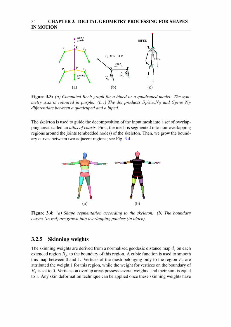
34 CHAPTER 3. DIGITAL GEOMETRY PROCESSING FOR SHAPESIN MOTION
(a) (b) (c)
Figure 3.3: (a) Computed Reeb graph for a biped or a quadruped model. The sym-metry axis is coloured in purple. (b,c) The dot products Spine.NS and Spine.NP
differentiate between a quadruped and a biped.
The skeleton is used to guide the decomposition of the input mesh into a set of overlap-ping areas called an atlas of charts. First, the mesh is segmented into non-overlappingregions around the joints (embedded nodes) of the skeleton. Then, we grow the bound-ary curves between two adjacent regions; see Fig. 3.4.
(a) (b)
Figure 3.4: (a) Shape segmentation according to the skeleton. (b) The boundarycurves (in red) are grown into overlapping patches (in black).
3.2.5 Skinning weightsThe skinning weights are derived from a normalised geodesic distance map dj on eachextended region Rj , to the boundary of this region. A cubic function is used to smooththis map between 0 and 1. Vertices of the mesh belonging only to the region Rj areattributed the weight 1 for this region, while the weight for vertices on the boundary ofRj is set to 0. Vertices on overlap areas possess several weights, and their sum is equalto 1. Any skin deformation technique can be applied once these skinning weights have
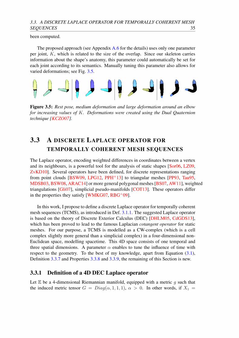
3.3. A DISCRETE LAPLACE OPERATOR FOR TEMPORALLY COHERENT MESHSEQUENCES 35
been computed.
The proposed approach (see Appendix A.6 for the details) uses only one parameterper joint, K, which is related to the size of the overlap. Since our skeleton carriesinformation about the shape’s anatomy, this parameter could automatically be set foreach joint according to its semantics. Manually tuning this parameter also allows forvaried deformations; see Fig. 3.5.
Figure 3.5: Rest pose, medium deformation and large deformation around an elbowfor increasing values of K. Deformations were created using the Dual Quaterniontechnique [KCZO07].
3.3 A DISCRETE LAPLACE OPERATOR FORTEMPORALLY COHERENT MESH SEQUENCES
The Laplace operator, encoding weighted differences in coordinates between a vertexand its neighbours, is a powerful tool for the analysis of static shapes [Sor06, LZ09,ZvKD10]. Several operators have been defined, for discrete representations rangingfrom point clouds [BSW09, LPG12, PPH+13] to triangular meshes [PP93, Tau95,MDSB03, BSW08, ARAC14] or more general polygonal meshes [BS07, AW11], weightedtriangulations [Gli07], simplicial pseudo-manifolds [COT13]. These operators differin the properties they satisfy [WMKG07, RBG+09].
In this work, I propose to define a discrete Laplace operator for temporally coherentmesh sequences (TCMS), as introduced in Def. 3.1.1. The suggested Laplace operatoris based on the theory of Discrete Exterior Calculus (DEC) [DHLM05, CdGDS13],which has been proved to lead to the famous Laplacian cotangent operator for staticmeshes. For our purpose, a TCMS is modelled as a CW-complex (which is a cellcomplex slightly more general than a simplicial complex) in a four-dimensional non-Euclidean space, modelling spacetime. This 4D space consists of one temporal andthree spatial dimensions. A parameter α enables to tune the influence of time withrespect to the geometry. To the best of my knowledge, apart from Equation (3.1),Definition 3.3.7 and Properties 3.3.8 and 3.3.9, the remaining of this Section is new.
3.3.1 Definition of a 4D DEC Laplace operatorLet E be a 4-dimensional Riemannian manifold, equipped with a metric g such thatthe induced metric tensor G = Diag(α, 1, 1, 1), α > 0. In other words, if X1 =
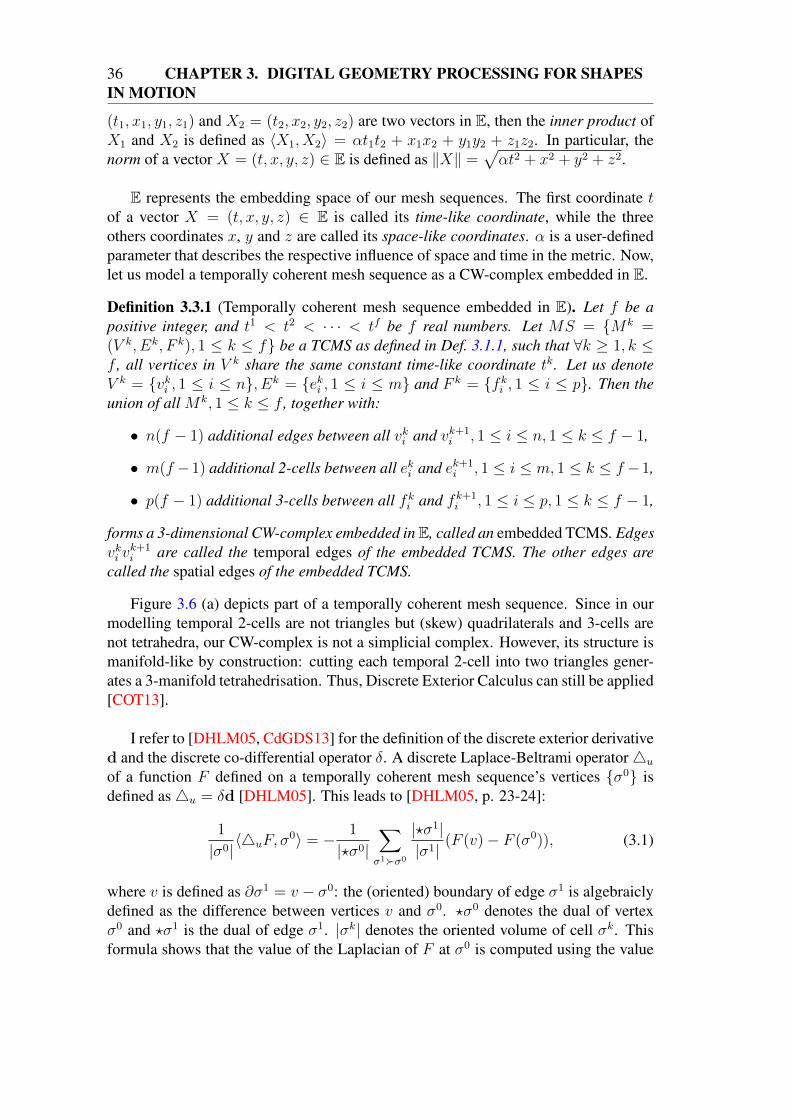
36 CHAPTER 3. DIGITAL GEOMETRY PROCESSING FOR SHAPESIN MOTION
(t1, x1, y1, z1) and X2 = (t2, x2, y2, z2) are two vectors in E, then the inner product ofX1 and X2 is defined as 〈X1, X2〉 = αt1t2 + x1x2 + y1y2 + z1z2. In particular, thenorm of a vector X = (t, x, y, z) ∈ E is defined as ‖X‖ =
√αt2 + x2 + y2 + z2.
E represents the embedding space of our mesh sequences. The first coordinate tof a vector X = (t, x, y, z) ∈ E is called its time-like coordinate, while the threeothers coordinates x, y and z are called its space-like coordinates. α is a user-definedparameter that describes the respective influence of space and time in the metric. Now,let us model a temporally coherent mesh sequence as a CW-complex embedded in E.
Definition 3.3.1 (Temporally coherent mesh sequence embedded in E). Let f be apositive integer, and t1 < t2 < · · · < tf be f real numbers. Let MS = Mk =(V k, Ek, F k), 1 ≤ k ≤ f be a TCMS as defined in Def. 3.1.1, such that ∀k ≥ 1, k ≤f , all vertices in V k share the same constant time-like coordinate tk. Let us denoteV k = vki , 1 ≤ i ≤ n, Ek = eki , 1 ≤ i ≤ m and F k = fki , 1 ≤ i ≤ p. Then theunion of all Mk, 1 ≤ k ≤ f , together with:
• n(f − 1) additional edges between all vki and vk+1i , 1 ≤ i ≤ n, 1 ≤ k ≤ f − 1,
• m(f −1) additional 2-cells between all eki and ek+1i , 1 ≤ i ≤ m, 1 ≤ k ≤ f −1,
• p(f − 1) additional 3-cells between all fki and fk+1i , 1 ≤ i ≤ p, 1 ≤ k ≤ f − 1,
forms a 3-dimensional CW-complex embedded in E, called an embedded TCMS. Edgesvki v
k+1i are called the temporal edges of the embedded TCMS. The other edges are
called the spatial edges of the embedded TCMS.
Figure 3.6 (a) depicts part of a temporally coherent mesh sequence. Since in ourmodelling temporal 2-cells are not triangles but (skew) quadrilaterals and 3-cells arenot tetrahedra, our CW-complex is not a simplicial complex. However, its structure ismanifold-like by construction: cutting each temporal 2-cell into two triangles gener-ates a 3-manifold tetrahedrisation. Thus, Discrete Exterior Calculus can still be applied[COT13].
I refer to [DHLM05, CdGDS13] for the definition of the discrete exterior derivatived and the discrete co-differential operator δ. A discrete Laplace-Beltrami operator4u
of a function F defined on a temporally coherent mesh sequence’s vertices σ0 isdefined as4u = δd [DHLM05]. This leads to [DHLM05, p. 23-24]:
1
|σ0| 〈4uF, σ0〉 = − 1
|?σ0|∑
σ1σ0
|?σ1||σ1| (F (v)− F (σ0)), (3.1)
where v is defined as ∂σ1 = v − σ0: the (oriented) boundary of edge σ1 is algebraiclydefined as the difference between vertices v and σ0. ?σ0 denotes the dual of vertexσ0 and ?σ1 is the dual of edge σ1. |σk| denotes the oriented volume of cell σk. Thisformula shows that the value of the Laplacian of F at σ0 is computed using the value
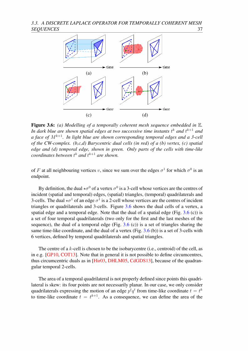
3.3. A DISCRETE LAPLACE OPERATOR FOR TEMPORALLY COHERENT MESHSEQUENCES 37
(a) (b)
(c) (d)
Figure 3.6: (a) Modelling of a temporally coherent mesh sequence embedded in E.In dark blue are shown spatial edges at two successive time instants tk and tk+1 anda face of Mk+1. In light blue are shown corresponding temporal edges and a 3-cellof the CW-complex. (b,c,d) Barycentric dual cells (in red) of a (b) vertex, (c) spatialedge and (d) temporal edge, shown in green. Only parts of the cells with time-likecoordinates between tk and tk+1 are shown.
of F at all neighbouring vertices v, since we sum over the edges σ1 for which σ0 is anendpoint.
By definition, the dual ?σ0 of a vertex σ0 is a 3-cell whose vertices are the centres ofincident (spatial and temporal) edges, (spatial) triangles, (temporal) quadrilaterals and3-cells. The dual ?σ1 of an edge σ1 is a 2-cell whose vertices are the centres of incidenttriangles or quadrilaterals and 3-cells. Figure 3.6 shows the dual cells of a vertex, aspatial edge and a temporal edge. Note that the dual of a spatial edge (Fig. 3.6 (c)) isa set of four temporal quadrilaterals (two only for the first and the last meshes of thesequence), the dual of a temporal edge (Fig. 3.6 (c)) is a set of triangles sharing thesame time-like coordinate, and the dual of a vertex (Fig. 3.6 (b)) is a set of 3-cells with6 vertices, defined by temporal quadrilaterals and spatial triangles.
The centre of a k-cell is chosen to be the isobarycentre (i.e., centroid) of the cell, asin e.g. [GP10, COT13]. Note that in general it is not possible to define circumcentres,thus circumcentric duals as in [Hir03, DHLM05, CdGDS13], because of the quadran-gular temporal 2-cells.
The area of a temporal quadrilateral is not properly defined since points this quadri-lateral is skew: its four points are not necessarily planar. In our case, we only considerquadrilaterals expressing the motion of an edge ptqt from time-like coordinate t = tk
to time-like coordinate t = tk+1. As a consequence, we can define the area of the
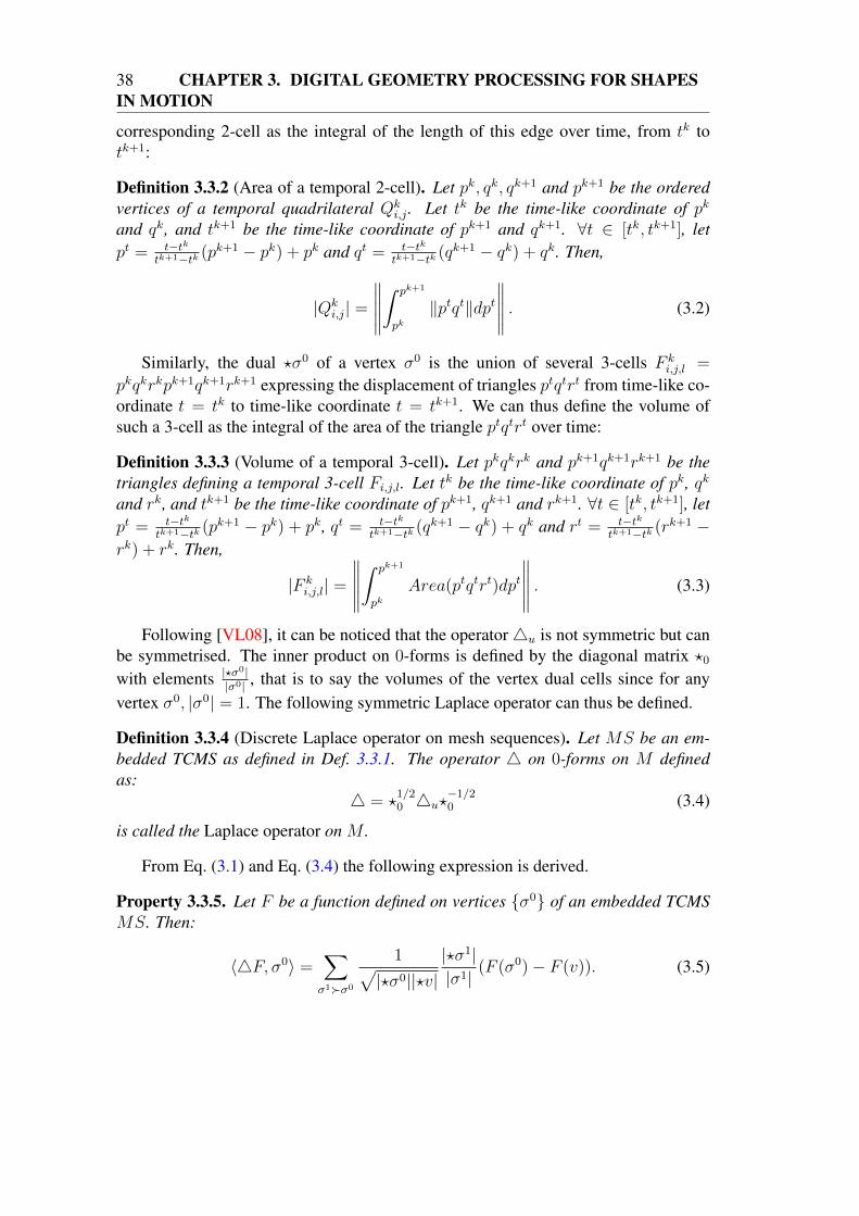
38 CHAPTER 3. DIGITAL GEOMETRY PROCESSING FOR SHAPESIN MOTION
corresponding 2-cell as the integral of the length of this edge over time, from tk totk+1:
Definition 3.3.2 (Area of a temporal 2-cell). Let pk, qk, qk+1 and pk+1 be the orderedvertices of a temporal quadrilateral Qk
i,j . Let tk be the time-like coordinate of pk
and qk, and tk+1 be the time-like coordinate of pk+1 and qk+1. ∀t ∈ [tk, tk+1], letpt = t−tk
tk+1−tk (pk+1 − pk) + pk and qt = t−tktk+1−tk (qk+1 − qk) + qk. Then,
|Qki,j| =
∥∥∥∥∥
∫ pk+1
pk‖ptqt‖dpt
∥∥∥∥∥ . (3.2)
Similarly, the dual ?σ0 of a vertex σ0 is the union of several 3-cells F ki,j,l =
pkqkrkpk+1qk+1rk+1 expressing the displacement of triangles ptqtrt from time-like co-ordinate t = tk to time-like coordinate t = tk+1. We can thus define the volume ofsuch a 3-cell as the integral of the area of the triangle ptqtrt over time:
Definition 3.3.3 (Volume of a temporal 3-cell). Let pkqkrk and pk+1qk+1rk+1 be thetriangles defining a temporal 3-cell Fi,j,l. Let tk be the time-like coordinate of pk, qk
and rk, and tk+1 be the time-like coordinate of pk+1, qk+1 and rk+1. ∀t ∈ [tk, tk+1], letpt = t−tk
tk+1−tk (pk+1 − pk) + pk, qt = t−tktk+1−tk (qk+1 − qk) + qk and rt = t−tk
tk+1−tk (rk+1 −rk) + rk. Then,
|F ki,j,l| =
∥∥∥∥∥
∫ pk+1
pkArea(ptqtrt)dpt
∥∥∥∥∥ . (3.3)
Following [VL08], it can be noticed that the operator4u is not symmetric but canbe symmetrised. The inner product on 0-forms is defined by the diagonal matrix ?0
with elements |?σ0|
|σ0| , that is to say the volumes of the vertex dual cells since for anyvertex σ0, |σ0| = 1. The following symmetric Laplace operator can thus be defined.
Definition 3.3.4 (Discrete Laplace operator on mesh sequences). Let MS be an em-bedded TCMS as defined in Def. 3.3.1. The operator 4 on 0-forms on M definedas:
4 = ?1/20 4u?
−1/20 (3.4)
is called the Laplace operator on M .
From Eq. (3.1) and Eq. (3.4) the following expression is derived.
Property 3.3.5. Let F be a function defined on vertices σ0 of an embedded TCMSMS. Then:
〈4F, σ0〉 =∑
σ1σ0
1√|?σ0||?v|
|?σ1||σ1| (F (σ0)− F (v)). (3.5)
3.3. A DISCRETE LAPLACE OPERATOR FOR TEMPORALLY COHERENT MESHSEQUENCES 39
3.3.2 Matrix representationThe Laplace operator defined in Def. 3.3.4 can be encoded as a nf ×nf matrix, wheren is the number of vertices in any mesh of the mesh sequence, and f is the number offrames. Although this matrix is big, it is also very sparse. Being a block tridiagonalmatrix, it can also be inverted easily, as I show now.
Property 3.3.6. LetM be a TCMS composed of f meshes, each having n vertices. Theoperator4 on 0-forms on M as defined in Eq. (3.5) is local, and can be encoded by asparse nf × nf symmetric block tridiagonal matrix L which can be written blockwiseas:
L =
L(1) D(1)
D(1) L(2) D(2)
. . . . . . . . .D(f−2) L(f−1) D(f−1)
D(f−1) L(f)
, (3.6)
where ∀k ≥ 1, k ≤ f − 1, the n× n matrices D(k) are diagonal, and ∀k ≥ 1, k ≤ f ,the n× n matrices L(k) being symmetric.
Proof. Operator 4 is obviously local since for any function F and any vertex σ0,〈4F, σ0〉 only depends on F values on σ0 and neighbouring vertices v. The matrixexpression derives from Eq. (3.5). Diagonal coefficients of matrices D(k) are given by:
D(k)i,i = − 1√
|?vki ||?vk+1i ||?vki vk+1
i ||vki vk+1
i | ,
where ?vki is the dual 3-cell of vertex vki and ?vki vk+1i is the dual 2-cell of temporal edge
vki vk+1i . The coefficients L(k)
i,j of matrices L(k) are equal to zero if there is no spatialedge in M between vertices vki and vkj . Otherwise,
L(k)i,j = − 1√
|?vki ||?vkj ||?vki vkj ||vki vkj |
.
Diagonal coefficients are given by:
L(k)i,i = −D(k)
i,i −∑
j 6=iL
(k)i,j .
Definition 3.3.7 ([Meu92, Sal06]). Let M be a TCMS composed of f meshes with nvertices each. Let L be its associated Laplacian matrix as defined in Prop. 3.3.6. LetΛ(k), 1 ≤ k ≤ f be n× n matrices defined recursively as:
• Λ(1) = L(1);
40 CHAPTER 3. DIGITAL GEOMETRY PROCESSING FOR SHAPESIN MOTION
• ∀k ≥ 2,Λ(k) = L(k) −D(k−1)Λ(k−1)−1D(k−1).
Let Σ(k), 1 ≤ k ≤ f be n× n matrices defined recursively as:
• Σ(f) = L(f);
• ∀k ≤ f − 1,Σ(k) = L(k) −D(k)Σ(k+1)−1D(k).
Property 3.3.8 ([Meu92]). Let Λ be the nf×nf block diagonal matrix Λ = diag(Λ(1), . . . ,Λ(f))and Σ be the nf × nf block diagonal matrix Σ = diag(Σ(1), . . . ,Σ(f)). Let Lo be theblock lower part of L:
Lo =
0D(1) 0
. . .. . .
. . .D(f−2) 0
D(f−1) 0
.
Then L can be decomposed as:
L = (Λ + Lo)Λ−1(Λ + Lto) = (Σ + Lto)Σ
−1(Σ + Lo). (3.7)
These two LDLT decompositions of L leads to a simple way to invert this matrix.
Property 3.3.9 ([Meu92]). Let Uk, 1 ≤ k ≤ f and Vk, 1 ≤ k ≤ f be twosequences of n× n matrices such as:
U1 = I, V1 = Σ(1)−1
,
where I is the n× n identity matrix and ∀k ≥ 2,
Uk = (−1)k−1D(k−1)−1
Λ(k−1) . . . D(1)−1
Λ(1), (3.8)
Vk = (−1)k−1Σ(1)−1
D(1)Σ(2)−1
. . . D(k−1)Σ(k)−1
. (3.9)
Then ∀j ≥ i, the (i, j) block of L−1 can be expressed as UiVj .
The inverse of L can thus be computed only by computing the inverse of f n × nmatrices, namely the inverse of the Σ(k) matrices. Note that in [Meu92] it is requestedthat L is proper, that is to say that sub-matrices D(k) are non-singular. This is our casesince these matrices are diagonal with non zero diagonal elements.
3.3.3 Behaviour for large and small time stepsI now investigate the behaviour of our Laplace operator when α tends to infinity or tozero. Remember from Section 3.3.1 that α is the parameter which scales the temporaldimension of the embedding space E with respect to the spatial dimensions. A largeα decreases the influence of the temporal neighbours vk−1
i and vk+1i of a given ver-
tex vki on this vertex with respect to its spatial neighbours sharing the same time-likecoordinates. Conversely, a small α increases their influence.
3.3. A DISCRETE LAPLACE OPERATOR FOR TEMPORALLY COHERENT MESHSEQUENCES 41
Property 3.3.10. When α tends to infinity, L tends to a block diagonal matrixDiag(L(1), . . . , L(f)),where each matrix L(k) is the spatial DEC Laplacian matrix with cotangent coordi-nates [DHLM05, CdGDS13].
Proof. If α 1, the difference between successive areas Ak−1i , Aki and Ak+1
i is negli-gible with respect to α. As a consequence, the volume of any vertex dual cell ?vki canbe approximated by
√α(tk+1 − tk)Aki , where Aki is the area of the spatial dual cell of
vki in the mesh Mk.For the same reason, the area of the dual cell ?vki v
kj is, for any spatial edge vki v
kj , equiv-
alent to√α(tk+1−tk) times the length |?svki vkj | of the spatial dual cell of vki v
kj in mesh
Mk. We thus have 1√|?vki ||?vkj |
|?vki vkj ||vki vkj |
∼ 1√Aki A
kj
|?svki vkj ||vki vkj |
. Thus, the n × n matrix L(k) is
equivalent to the spatial Laplacian matrix for mesh Mk.The length of any temporal edge vki v
k+1i of the mesh sequence is equivalent to
√α(tk+1−
tk), and the area of its dual is small with respect to α. Thus, any coefficient D(k)i,i of the
diagonal matrix D(k) is close to zero.
Property 3.3.11. Suppose the motion of each vertex is small with respect to the tessel-lation: ∀k,∀i,∀j such that vki v
kj ∈ Ek, ‖vki vk+1
i ‖ ‖vki vkj ‖. Then, when α tends tozero, the motion coefficients D(k)
i,i are dominating over the geometry coefficients L(k)i,j .
Proof. If ∀k,∀i,∀j such that vki vkj ∈ Ek, ‖vki vk+1
i ‖ ‖vki vkj ‖, then the differencebetween successive areas Ak−1
i , Aki and Ak+1i is negligible with respect to ‖vki vkj ‖.
As a consequence, the volume of any vertex dual cell ?vki can be approximated by‖vki vk+1
i ‖sAki , where Aki is the area of the spatial dual cell of vki in the mesh Mk.For the same reason, the area of the dual cell ?vki v
kj is, for any spatial edge vki v
kj , equiv-
alent to ‖vki vk+1i ‖s times the length |?svki vkj | of the spatial dual cell of vki v
kj in mesh
Mk. We thus have 1√|?vki ||?vkj |
|?vki vkj ||vki vkj |
∼ 1√Aki A
kj
|?svki vkj ||vki vkj |
. Thus, the n × n matrix L(k) is
equivalent to the spatial Laplacian matrix for mesh Mk.The area of the dual of any temporal edge vki v
k+1i of the mesh sequence is equivalent
to Aki . As a consequence, the coefficient D(k)i,i of the diagonal matrix D(k) is equivalent
to 1
‖vki vk+1i ‖2s
. Since the motion is small with respect to the tessellation, D(k)i,i L
(k)i,j for
any spatial edge vki vkj : the temporal coefficients are dominating.
These properties prove that, if α is large, our 4D Laplacian acts as a standard staticLaplacian on each frame, and if α is small and the motion is small with respect tothe geometric discretisation, our 4D Laplacian enables to recover the motion of eachvertex of the mesh independently.
3.3.4 Application to as-rigid-as-possible mesh sequence deforma-tion
I believe the suggested discrete Laplacian operator can be used for various mesh se-quence processing operations. In the near future, I plan to investigate several gener-
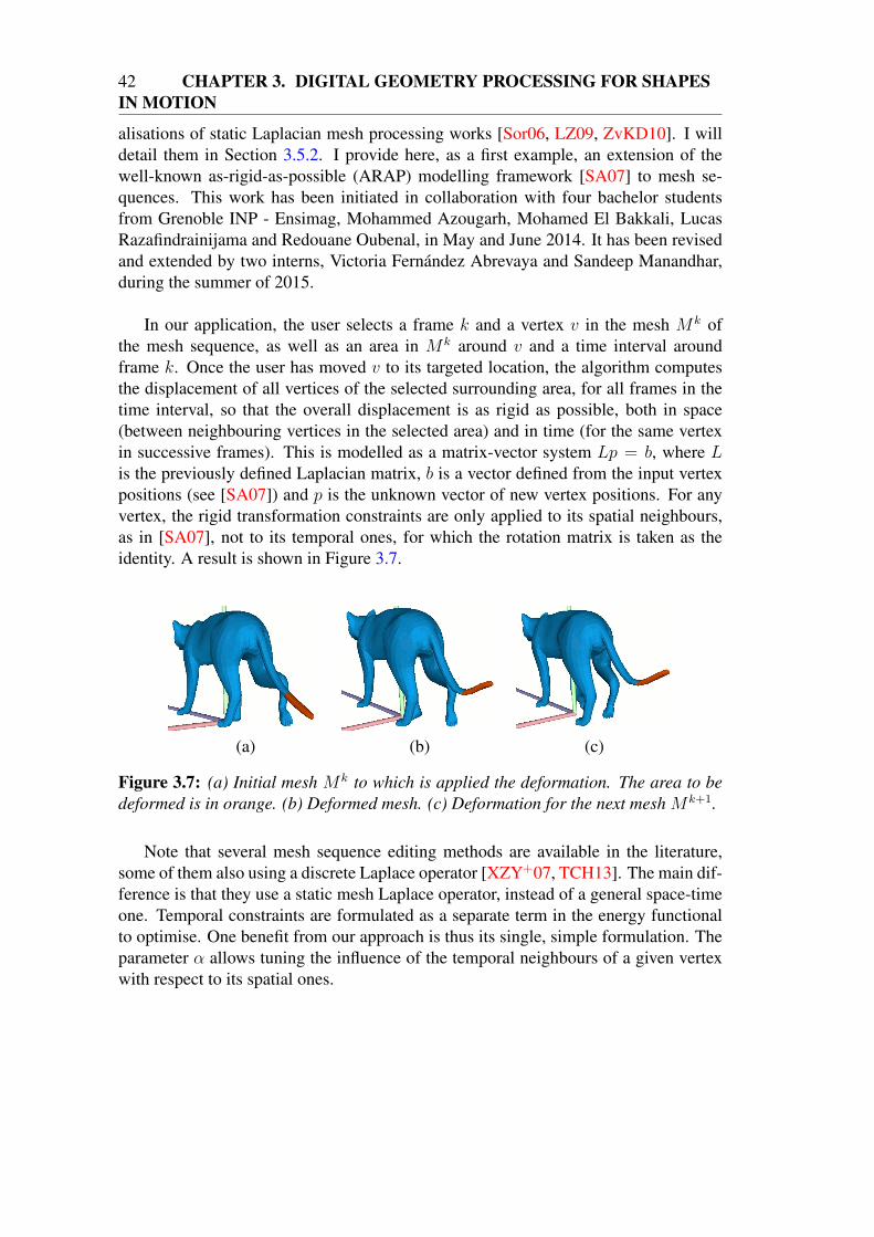
42 CHAPTER 3. DIGITAL GEOMETRY PROCESSING FOR SHAPESIN MOTION
alisations of static Laplacian mesh processing works [Sor06, LZ09, ZvKD10]. I willdetail them in Section 3.5.2. I provide here, as a first example, an extension of thewell-known as-rigid-as-possible (ARAP) modelling framework [SA07] to mesh se-quences. This work has been initiated in collaboration with four bachelor studentsfrom Grenoble INP - Ensimag, Mohammed Azougarh, Mohamed El Bakkali, LucasRazafindrainijama and Redouane Oubenal, in May and June 2014. It has been revisedand extended by two interns, Victoria Fernández Abrevaya and Sandeep Manandhar,during the summer of 2015.
In our application, the user selects a frame k and a vertex v in the mesh Mk ofthe mesh sequence, as well as an area in Mk around v and a time interval aroundframe k. Once the user has moved v to its targeted location, the algorithm computesthe displacement of all vertices of the selected surrounding area, for all frames in thetime interval, so that the overall displacement is as rigid as possible, both in space(between neighbouring vertices in the selected area) and in time (for the same vertexin successive frames). This is modelled as a matrix-vector system Lp = b, where Lis the previously defined Laplacian matrix, b is a vector defined from the input vertexpositions (see [SA07]) and p is the unknown vector of new vertex positions. For anyvertex, the rigid transformation constraints are only applied to its spatial neighbours,as in [SA07], not to its temporal ones, for which the rotation matrix is taken as theidentity. A result is shown in Figure 3.7.
(a) (b) (c)
Figure 3.7: (a) Initial mesh Mk to which is applied the deformation. The area to bedeformed is in orange. (b) Deformed mesh. (c) Deformation for the next mesh Mk+1.
Note that several mesh sequence editing methods are available in the literature,some of them also using a discrete Laplace operator [XZY+07, TCH13]. The main dif-ference is that they use a static mesh Laplace operator, instead of a general space-timeone. Temporal constraints are formulated as a separate term in the energy functionalto optimise. One benefit from our approach is thus its single, simple formulation. Theparameter α allows tuning the influence of the temporal neighbours of a given vertexwith respect to its spatial ones.

3.4. MESH SEQUENCE DECOMPOSITION INTO RIGIDLY MOVINGCOMPONENTS 43
3.4 MESH SEQUENCE DECOMPOSITION INTORIGIDLY MOVING COMPONENTS
In this section we focus on temporal incoherent mesh sequences (TIMS). Our goal isto segment the shape into parts that evolve approximately rigidly. By doing so, weshould be able to infer the articulated structure of a human or animal body: arms, legs,torso, . . . Possible applications include accurate motion measurement (for instance forvalidation or limb rehabilitation) and 3D action recognition. The only prior knowl-edge that we use is that the shape should be decomposable into almost rigidly movingcomponents. As a consequence, this work does not apply to shapes such as rodents[Rev14] or humans wearing loose clothing.
This work forms the main part of the PhD thesis of Romain Arcila [Arc11].
3.4.1 Shape-in-motion segmentation classificationBefore going into the details of the proposed algorithm for the segmentation of a TIMS,it is important to clarify what we mean by shape-in-motion segmentation, since severaldefinitions can be thought of:
Definition 3.4.1 (Temporal segmentation). LetMS = M i, i = 1 . . . f be a mesh se-quence. A temporal segmentation Σt ofMS is a set of sub-sequences Σt = MS1, . . . ,MSksuch that ∀j ∈ [1, k],MSj = M ij , . . . ,M ij+1−1 where i1 = 1 < i2 < · · · < ik+1 =f + 1.
Definition 3.4.2 (Coherent segmentation). Let MS = M i, i = 1 . . . f be a mesh se-quence. A coherent segmentation Σc ofMS is a set of segmentations Σi = M i
1, . . . ,Miki
of each mesh M i of MS, such that:
• the number k of sub-meshes is the same for all segmentations: ∀i, j ∈ [1, f ], ki =kj;
• there is a one-to-one correspondence between sub-meshes of any two meshes;
• the connectivity of the segmentations, that is to say the neighbourhood relation-ships between sub-meshes, is preserved over the sequence.
A coherent segmentation of a mesh sequence can be thought as a segmentation ofsome mesh of the sequence (for instance, the first one) which is mapped to the othermeshes.
Definition 3.4.3 (Variable segmentation). Let MS = M i, i = 1 . . . f be a mesh se-quence. A variable segmentation Σv ofMS is a set of segmentations Σi = M i
1, . . . ,Miki
of each mesh M i of MS which is not a coherent segmentation.
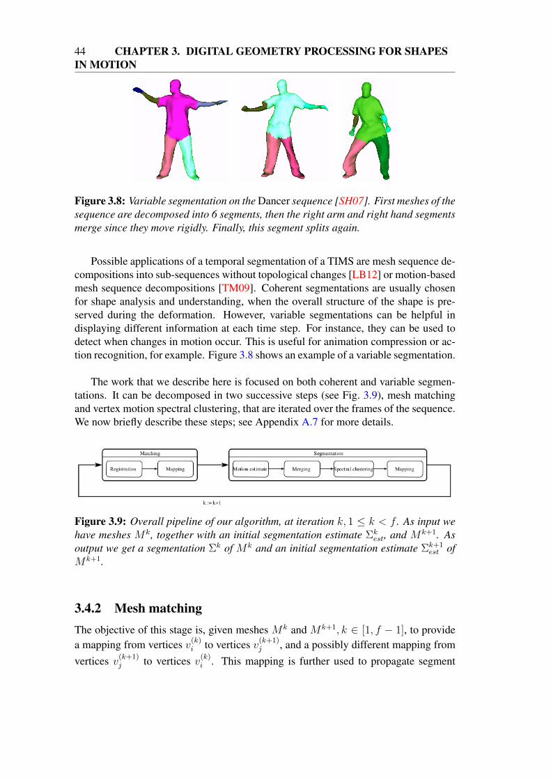
44 CHAPTER 3. DIGITAL GEOMETRY PROCESSING FOR SHAPESIN MOTION
Figure 3.8: Variable segmentation on the Dancer sequence [SH07]. First meshes of thesequence are decomposed into 6 segments, then the right arm and right hand segmentsmerge since they move rigidly. Finally, this segment splits again.
Possible applications of a temporal segmentation of a TIMS are mesh sequence de-compositions into sub-sequences without topological changes [LB12] or motion-basedmesh sequence decompositions [TM09]. Coherent segmentations are usually chosenfor shape analysis and understanding, when the overall structure of the shape is pre-served during the deformation. However, variable segmentations can be helpful indisplaying different information at each time step. For instance, they can be used todetect when changes in motion occur. This is useful for animation compression or ac-tion recognition, for example. Figure 3.8 shows an example of a variable segmentation.
The work that we describe here is focused on both coherent and variable segmen-tations. It can be decomposed in two successive steps (see Fig. 3.9), mesh matchingand vertex motion spectral clustering, that are iterated over the frames of the sequence.We now briefly describe these steps; see Appendix A.7 for more details.
Figure 3.9: Overall pipeline of our algorithm, at iteration k, 1 ≤ k < f . As input wehave meshes Mk, together with an initial segmentation estimate Σk
est, and Mk+1. Asoutput we get a segmentation Σk of Mk and an initial segmentation estimate Σk+1
est ofMk+1.
3.4.2 Mesh matchingThe objective of this stage is, given meshes Mk and Mk+1, k ∈ [1, f − 1], to providea mapping from vertices v(k)
i to vertices v(k+1)j , and a possibly different mapping from
vertices v(k+1)j to vertices v(k)
i . This mapping is further used to propagate segment
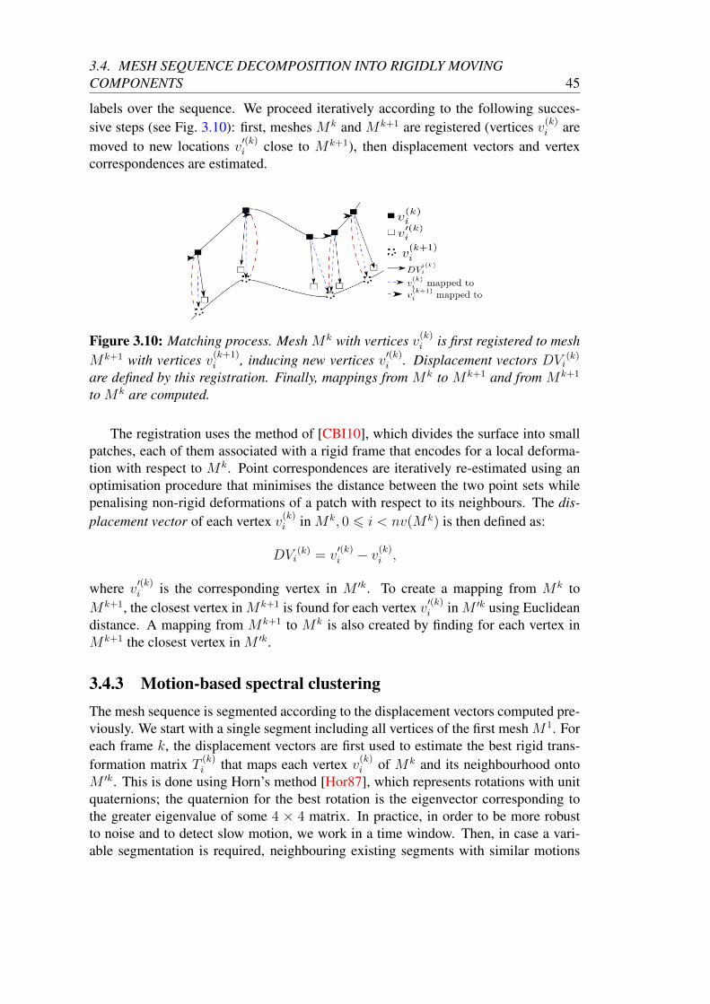
3.4. MESH SEQUENCE DECOMPOSITION INTO RIGIDLY MOVINGCOMPONENTS 45
labels over the sequence. We proceed iteratively according to the following succes-sive steps (see Fig. 3.10): first, meshes Mk and Mk+1 are registered (vertices v(k)
i aremoved to new locations v′(k)
i close to Mk+1), then displacement vectors and vertexcorrespondences are estimated.
Figure 3.10: Matching process. Mesh Mk with vertices v(k)i is first registered to mesh
Mk+1 with vertices v(k+1)i , inducing new vertices v′(k)
i . Displacement vectors DVi(k)
are defined by this registration. Finally, mappings from Mk to Mk+1 and from Mk+1
to Mk are computed.
The registration uses the method of [CBI10], which divides the surface into smallpatches, each of them associated with a rigid frame that encodes for a local deforma-tion with respect to Mk. Point correspondences are iteratively re-estimated using anoptimisation procedure that minimises the distance between the two point sets whilepenalising non-rigid deformations of a patch with respect to its neighbours. The dis-placement vector of each vertex v(k)
i in Mk, 0 6 i < nv(Mk) is then defined as:
DVi(k) = v
′(k)i − v(k)
i ,
where v′(k)i is the corresponding vertex in M ′k. To create a mapping from Mk to
Mk+1, the closest vertex in Mk+1 is found for each vertex v′(k)i in M ′k using Euclidean
distance. A mapping from Mk+1 to Mk is also created by finding for each vertex inMk+1 the closest vertex in M ′k.
3.4.3 Motion-based spectral clusteringThe mesh sequence is segmented according to the displacement vectors computed pre-viously. We start with a single segment including all vertices of the first mesh M1. Foreach frame k, the displacement vectors are first used to estimate the best rigid trans-formation matrix T (k)
i that maps each vertex v(k)i of Mk and its neighbourhood onto
M ′k. This is done using Horn’s method [Hor87], which represents rotations with unitquaternions; the quaternion for the best rotation is the eigenvector corresponding tothe greater eigenvalue of some 4 × 4 matrix. In practice, in order to be more robustto noise and to detect slow motion, we work in a time window. Then, in case a vari-able segmentation is required, neighbouring existing segments with similar motions
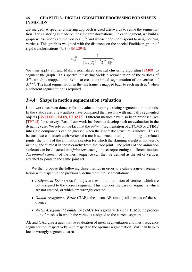
46 CHAPTER 3. DIGITAL GEOMETRY PROCESSING FOR SHAPESIN MOTION
are merged. A spectral clustering approach is used afterwards to refine the segmenta-tion. The clustering is made on the rigid transformations. On each segment, we build agraph whose nodes are the vertices v(k)
i and whose edges correspond to neighbouringvertices. This graph is weighted with the distances on the special Euclidean group ofrigid transformations SE(3) [MLS94]:
w(k)i,j =
1
‖log(T(k)i
−1T
(k)j )‖2
.
We then apply Shi and Malik’s normalised spectral clustering algorithm [SM00] tosegment the graph. This spectral clustering yields a segmentation of the vertices ofMk, which is mapped onto Mk+1 to create the initial segmentation of the vertices ofMk+1. The final segmentation in the last frame is mapped back to each meshMk whena coherent segmentation is required.
3.4.4 Shape in motion segmentation evaluationLittle work has been done so far to evaluate properly existing segmentation methods.In the static case, a few authors have compared their results with manually segmentedobjects [BVLD09, CGF09, LTBZ13]. Different metrics have also been proposed; see[TPT15] for a survey. Part of our work has been to develop such an evaluation in thedynamic case. We rely on the fact that the optimal segmentation of a TCMS or a TIMSinto rigid components can be guessed when the kinematic structure is known. This isbecause we can attach each vertex of a mesh sequence to one joint among its relatedjoints (the joints of the animation skeleton for which the skinning weight is non-zero),namely, the furthest in the hierarchy from the root joint. The joints of the animationskeleton can be clustered into joint sets, each joint set representing a different motion.An optimal segment of the mesh sequence can then be defined as the set of verticesattached to joints in the same joint set.
We then propose the following three metrics in order to evaluate a given segmen-tation with respect to the previously defined optimal segmentation:
• Assignment Error (AE): for a given mesh, the proportion of vertices which arenot assigned to the correct segment. This includes the case of segments whichare not created, or which are wrongly created;
• Global Assignment Error (GAE): the mean AE among all meshes of the se-quence;
• Vertex Assignment Confidence (VAC): for a given vertex of a TCMS, the propor-tion of meshes in which the vertex is assigned to the correct segment.
AE and GAE give a quantitative evaluation of mesh segmentation and mesh sequencesegmentation, respectively, with respect to the optimal segmentation. VAC can help tolocate wrongly segmented areas.
3.5. PERSPECTIVES 47
3.5 PERSPECTIVES
In this chapter I have presented some contributions to the analysis and segmentationof 3D mesh sequences. The overall common objective of all these methods is to con-tribute to a high-level understanding of shapes in motion, which includes the generalrecognition of the shape’s geometry as well as its motion. In the near term, I plan todevelop the three following points.
3.5.1 Visual differences between shapes in motionWork on extending the perceptive analysis of mesh distortion (Section 2.4) to meshsequences is planned as part of Georges Nader’s PhD thesis. A better comprehen-sion of visual differences between 3D shapes in motion has applications not only incompression and watermarking but also in classification and comparison of dynamicshapes. To the best of my knowledge, little work has been carried so far on this topic[KBAW11]. Defining a Just Noticeable Difference profile would be a first step. Find-ing a perceptually validated metric to compare shapes in motion is far more ambitious,and would probably need much more effort. I have spent some time investigating thissubject between 2011 and 2014, as part of a joint work with Romain Arcila (at theend of his PhD thesis) and Ron Rensink from the University of British Columbia inVancouver. We have devised an algorithm to segment temporally (see Definition 3.4.1above) and compress a TCMS. This algorithm takes as input a desired number of keyframes and automatically computes them. We have then investigated if the optimalnumber of key frames, defined as the minimum number for which there is no percep-tual difference between the original and the compress sequence, can be automaticallydetermined. This has been done by carrying perceptual experiments on three differentsequences. Although the results were inconclusive this method can be used to validatea proposed metric in the future.
3.5.2 3D+t Laplace operator spectral behaviourThere are numerous applications of the discrete 3D+t Laplace operator. It has al-ready been used recently, with other weight definitions, for motion editing and re-targeting [NCG13] (using Gaussian weights) and space-time filtering [YXF14] (usinga multi-scale combinatorial Laplacian). I plan to investigate the application of the 3D+tLaplace operator defined in Section 3.3 to various problems. Of particular interest arethe Laplacian eigenvectors, as they are known in 3D to be related to the geometryof the shape [L06, ZvKD10]. If the 3D+t Laplacian eigenvectors can also be inter-preted as vibration modes of either the shape or the motion, by tuning the parameterα, a huge number of applications for understanding shape in motion exist. They rangefrom shape or motion spectral clustering to shape or motion filtering, to the defini-tion of shape or motion descriptors, to classification with respect to shape or motion.This subject will be investigated in 2016 with the help of Stefanie Wuhrer from theMorpheo team and a Master student, Sandeep Manandhar. In the longer term, I wish

48 CHAPTER 3. DIGITAL GEOMETRY PROCESSING FOR SHAPESIN MOTION
to extent this 3D+t Laplace operator to TIMS and to check if a FEM-based defini-tion matches the DEC-based definition, as happens in the case of the 3D cotangentLaplacian [LZ09].
3.5.3 Modelling the factors of variability for human shape in mo-tion
The decomposition of a moving shape into rigidly moving components, as describedin Section 3.4, is limited to shapes for which the kinematic structure can be captured.This approach cannot address such situations as the motion of animals with large fatvolumes, such as rodents, or humans wearing loose clothing. The latter will be tackledwithin the ANR-funded project ACHMOV (“Accurate Human Modelling in Videos”),which has just started in October 2015. Together with Stefanie Wuhrer and a PhDstudent, Jinlong Yang, we plan to develop new statistical and geometric representationsfor modelling independently body shape, body motion and the motion of clothing.We will use 3D video acquisitions of humans wearing tight and loose clothes whileperforming the same movements.
CHAPTER 4
Understanding digital shapes from the life sciences
4.1 INTRODUCTION
4.1.1 ContextThe previous chapters examined static meshes and temporal sequences of meshes.Although very common, meshes are not the only possible representation of discreteshapes. Depending on the digitisation system, other shape models are widely usedfor various applications. For instance, medical imaging systems create 3D images asstacks of 2D images. Organs are thus first represented as voxel sets, which are some-times, but not always, subsequently converted to other shape representations. Anotherexample is the use of laser scanners in remote sensing. These devices generate a cloudof 3D points representing the scanned scene. The conversion of this point cloud into amesh is often not a trivial task because of non-uniform sampling, missing data due toocclusions, outliers or other types of noise caused by the acquisition process [BTS+14].As a consequence, it is sometimes simpler to work directly on the point cloud.
In this chapter I describe two shape-understanding methods that directly operateon acquired data, without converting it to a mesh. Both of these methods are focusedon particular applications and have been designed for and in cooperation with expertsin the relevant fields. These experts, being the end users of the methods, have broughtspecific requirements, as did the infographist Christine Depraz with whom I worked onthe animation skeleton method (Section 3.2). The first application, described in Sec-tion 4.2, was initiated by Dr. Olivier Palombi, a neurosurgeon (and also a researcher incomputer science and former colleague in the EVASION team). The goal was to locate,to characterise the shape and to quantify the volume of brain aneurysms automaticallyfrom voxel sets of the cerebral vascular tree. These voxel sets were segmented from 3DMRI or scan images (see Fig. 4.1 (a)). Such information is crucial in helping neurosur-
49
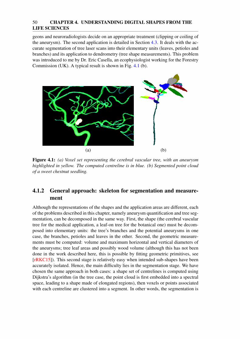
50 CHAPTER 4. UNDERSTANDING DIGITAL SHAPES FROM THELIFE SCIENCES
geons and neuroradiologists decide on an appropriate treatment (clipping or coiling ofthe aneurysm). The second application is detailed in Section 4.3. It deals with the ac-curate segmentation of tree laser scans into their elementary units (leaves, petioles andbranches) and its application to dendrometry (tree shape measurements). This problemwas introduced to me by Dr. Eric Casella, an ecophysiologist working for the ForestryCommission (UK). A typical result is shown in Fig. 4.1 (b).
(a) (b)
Figure 4.1: (a) Voxel set representing the cerebral vascular tree, with an aneurysmhighlighted in yellow. The computed centreline is in blue. (b) Segmented point cloudof a sweet chestnut seedling.
4.1.2 General approach: skeleton for segmentation and measure-ment
Although the representations of the shapes and the application areas are different, eachof the problems described in this chapter, namely aneurysm quantification and tree seg-mentation, can be decomposed in the same way. First, the shape (the cerebral vasculartree for the medical application, a leaf-on tree for the botanical one) must be decom-posed into elementary units: the tree’s branches and the potential aneurysms in onecase, the branches, petioles and leaves in the other. Second, the geometric measure-ments must be computed: volume and maximum horizontal and vertical diameters ofthe aneurysms; tree leaf areas and possibly wood volume (although this has not beendone in the work described here, this is possible by fitting geometric primitives, see[rRKC15]). This second stage is relatively easy when intended sub-shapes have beenaccurately isolated. Hence, the main difficulty lies in the segmentation stage. We havechosen the same approach in both cases: a shape set of centrelines is computed usingDijkstra’s algorithm (in the tree case, the point cloud is first embedded into a spectralspace, leading to a shape made of elongated regions), then voxels or points associatedwith each centreline are clustered into a segment. In other words, the segmentation is
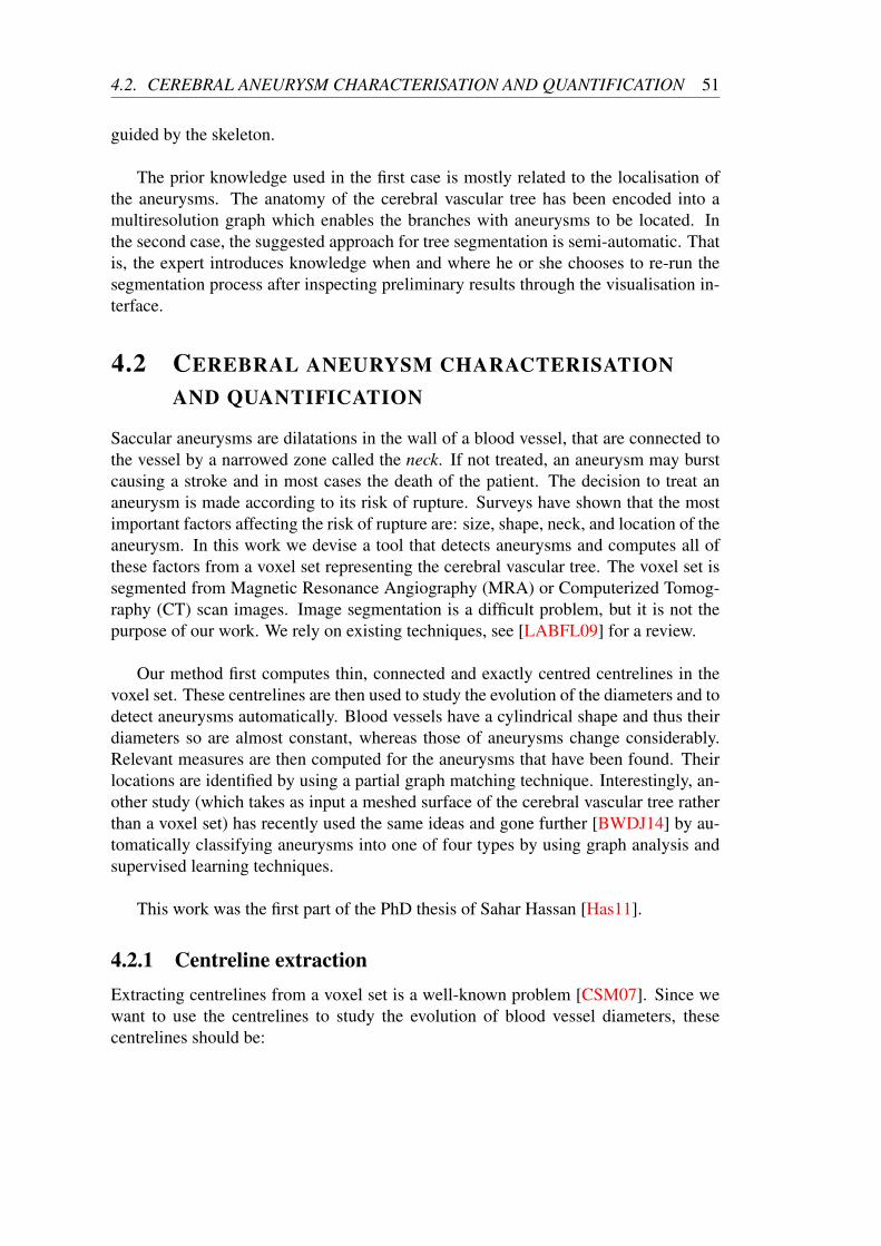
4.2. CEREBRAL ANEURYSM CHARACTERISATION AND QUANTIFICATION 51
guided by the skeleton.
The prior knowledge used in the first case is mostly related to the localisation ofthe aneurysms. The anatomy of the cerebral vascular tree has been encoded into amultiresolution graph which enables the branches with aneurysms to be located. Inthe second case, the suggested approach for tree segmentation is semi-automatic. Thatis, the expert introduces knowledge when and where he or she chooses to re-run thesegmentation process after inspecting preliminary results through the visualisation in-terface.
4.2 CEREBRAL ANEURYSM CHARACTERISATIONAND QUANTIFICATION
Saccular aneurysms are dilatations in the wall of a blood vessel, that are connected tothe vessel by a narrowed zone called the neck. If not treated, an aneurysm may burstcausing a stroke and in most cases the death of the patient. The decision to treat ananeurysm is made according to its risk of rupture. Surveys have shown that the mostimportant factors affecting the risk of rupture are: size, shape, neck, and location of theaneurysm. In this work we devise a tool that detects aneurysms and computes all ofthese factors from a voxel set representing the cerebral vascular tree. The voxel set issegmented from Magnetic Resonance Angiography (MRA) or Computerized Tomog-raphy (CT) scan images. Image segmentation is a difficult problem, but it is not thepurpose of our work. We rely on existing techniques, see [LABFL09] for a review.
Our method first computes thin, connected and exactly centred centrelines in thevoxel set. These centrelines are then used to study the evolution of the diameters and todetect aneurysms automatically. Blood vessels have a cylindrical shape and thus theirdiameters so are almost constant, whereas those of aneurysms change considerably.Relevant measures are then computed for the aneurysms that have been found. Theirlocations are identified by using a partial graph matching technique. Interestingly, an-other study (which takes as input a meshed surface of the cerebral vascular tree ratherthan a voxel set) has recently used the same ideas and gone further [BWDJ14] by au-tomatically classifying aneurysms into one of four types by using graph analysis andsupervised learning techniques.
This work was the first part of the PhD thesis of Sahar Hassan [Has11].
4.2.1 Centreline extractionExtracting centrelines from a voxel set is a well-known problem [CSM07]. Since wewant to use the centrelines to study the evolution of blood vessel diameters, thesecentrelines should be:

52 CHAPTER 4. UNDERSTANDING DIGITAL SHAPES FROM THELIFE SCIENCES
• connected: the centrelines we are looking for should be 26-connected;
• thin: a centreline is thin if each voxel of the centreline has only two of its neigh-bours in the centreline, except for the extremities which have one neighbour inthe centreline;
• centred: the centrelines should be centred within the vascular tree;
• such that the connections between branches are as orthogonal as possible.
To get such centrelines, our approach is to adapt Dijkstra’s algorithm [Dij59]. Fig-ure 4.2 (a) shows the flowchart of our centreline algorithm. A source voxel S is cho-sen at an extremity of the set by identifying the furthest voxel from a random voxel[LV99]. A modified Dijkstra’s algorithm finds the shortest path from S to the fur-thest voxel. This path is the first centreline B0. All the voxels belonging to B0 havethen their distance from the source voxel (DFS) put to 0, and the modified Dijkstra’salgorithm is re-run from S. This gives a new centreline B1, which connects the fur-thest voxel to B0. The process is iterated until the new centreline Bi is too short, and atmost 50 times, since a cerebral vascular tree usually has fewer than 50 visible branches.
Dijkstra’s algorithm is modified by using the following distance instead of the Eu-clidean distance:
d(v1, v2) =deucl(v1, v2)
1 +DFB(v1) +DFB(v2),
where deucl(v1, v2) is the Euclidean distance between the centres of voxels v1 and v2,and DFB(vi) is the Euclidean distance between the centre of voxel vi and the centreof the closest surface voxel, that is to say the closest voxel with at least one of its26-neighbours missing in the voxel set. Using d rather than deucl privileges the voxelsthat are far from the boundary of the voxel set, and so enforces the centredness of thecentreline. Setting the DFS of voxels of extracted centrelines to zero makes the newcentreline join orthogonally the set of previous centrelines and avoids cutting corners.Since the centrelines are connected and thin by construction, the four properties listedabove hold.
4.2.2 Aneurysm detection and quantificationOne key characteristic that differentiates a saccular aneurysm from a normal vessel isthat the normal vessel has an almost constant diameter, whereas the aneurysm, whichhas an irregular shape, has a diameter that changes considerably. In order to model theappearance of a vessel, we define a set of points (x, y) corresponding to the centre-line’s voxels v. x is the distance between the centre of the voxel and the centre of theorigin of the centreline. y represents the approximate diameter of the vessel at v, andis calculated using the real plane P passing through the centre of v and orthogonal tothe centreline, see Fig. 4.2 (b). P cuts the vessel or aneurysm surface on voxels vi, ata distance yi from v. y is simply defined as the average value of the yi. y is a reliable
4.2. CEREBRAL ANEURYSM CHARACTERISATION AND QUANTIFICATION 53
(a) (b) (c)
Figure 4.2: (a) Flowchart of the centreline extraction algorithm. (b) Diameter com-putation for a centreline. (c) Reference graph used for aneurysm localisation.
indicator of changes in diameter because of the centredness of centrelines and theirorthogonality. A least-square quadratic fit is then applied to the set of points (x, y)of a given centreline. Thresholding on the parameter associated with x2 enables us todetect aneurysms.
An aneurysm is defined as the set of voxels connected to the associated centrelinethrough the last iteration of the modified Dijkstra’s algorithm. However, this includesirrelevant voxels, which are geometrically located between the support vessel and theaneurysm neck, see Fig. 4.3 (a). These voxels are closer to the centreline of the supportvessel than its half-diameter and so they are removed, as shown in Fig. 4.3 (b). Theneck of the aneurysm is finally computed as the surface voxels of the aneurysm thathave at least one neighbour that is not in the aneurysm (Fig. 4.3 (c)).
Once an aneurysm and its neck are computed, several measurements are providedto the user:
• size of the aneurysm: the number of voxels in the aneurysm;
• shape: we compute the maximum vertical and horizontal diameters of the aneurysm(see Appendix A.8 for details);
• neck: the area of the neck (number of voxels) and its perimeter (number ofsurface voxels).
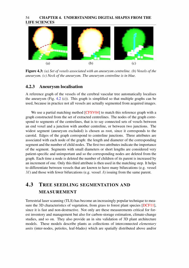
54 CHAPTER 4. UNDERSTANDING DIGITAL SHAPES FROM THELIFE SCIENCES
(a) (b) (c)
Figure 4.3: (a) Set of voxels associated with an aneurysm centreline. (b) Voxels of theaneurysm. (c) Neck of the aneurysm. The aneurysm centreline is in blue.
4.2.3 Aneurysm localisationA reference graph of the vessels of the cerebral vascular tree automatically localisesthe aneurysm (Fig. 4.2 (c)). This graph is simplified so that multiple graphs can beused, because in practice not all vessels are actually segmented from acquired images.
We use a partial matching method [CFSV04] to match this reference graph with agraph constructed from the set of extracted centrelines. The nodes of the graph corre-spond to segments of the centrelines, that is to say connected sets of voxels betweenan end voxel and a junction with another centreline, or between two junctions. Thewidest segment (aneurysm excluded) is chosen as root, since it corresponds to thecarotid. Edges of the graph correspond to centreline junctions. Three attributes areassociated with each node of the graph: the length and diameter of the correspondingsegment and the number of child nodes. The first two attributes indicate the importanceof the segment. Segments with small diameters or short lengths are considered verypatient-specific and unimportant and so the corresponding nodes are deleted from thegraph. Each time a node is deleted the number of children of its parent is increased byan increment of one. Only this third attribute is then used in the matching step. It helpsto differentiate between vessels that are known to have many bifurcations (e.g. vesselM ) and those with fewer bifurcations (e.g. vessel A) issuing from the same parent.
4.3 TREE SEEDLING SEGMENTATION ANDMEASUREMENT
Terrestrial laser scanning (TLS) has become an increasingly popular technique to mea-sure the 3D characteristics of vegetation, from grass to forest plant species [DCF11],since it is fast and non-destructive. Not only are these measurements critical for for-est inventory and management but also for carbon-storage estimation, climate-changestudies, and so on. They also provide an in situ validation of 3D plant architecturemodels. These models describe plants as collections of interconnected elementaryunits (inter-nodes, petioles, leaf-blades) which are spatially distributed above and/or
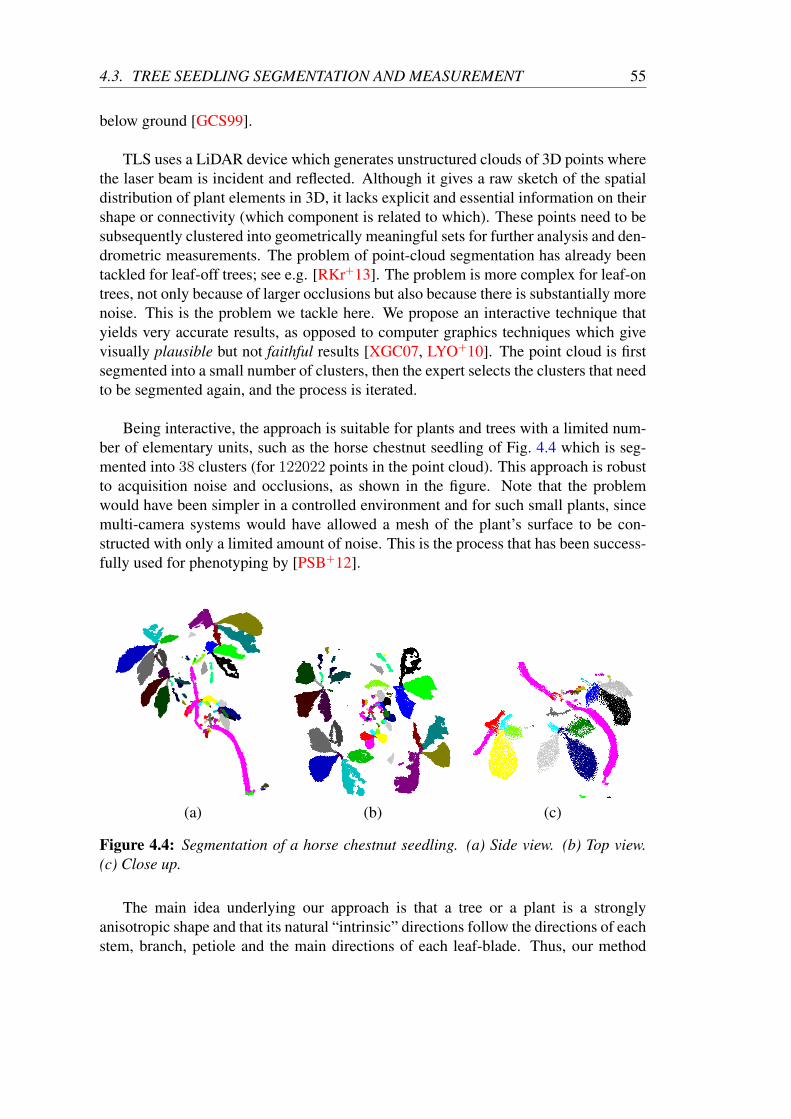
4.3. TREE SEEDLING SEGMENTATION AND MEASUREMENT 55
below ground [GCS99].
TLS uses a LiDAR device which generates unstructured clouds of 3D points wherethe laser beam is incident and reflected. Although it gives a raw sketch of the spatialdistribution of plant elements in 3D, it lacks explicit and essential information on theirshape or connectivity (which component is related to which). These points need to besubsequently clustered into geometrically meaningful sets for further analysis and den-drometric measurements. The problem of point-cloud segmentation has already beentackled for leaf-off trees; see e.g. [RKr+13]. The problem is more complex for leaf-ontrees, not only because of larger occlusions but also because there is substantially morenoise. This is the problem we tackle here. We propose an interactive technique thatyields very accurate results, as opposed to computer graphics techniques which givevisually plausible but not faithful results [XGC07, LYO+10]. The point cloud is firstsegmented into a small number of clusters, then the expert selects the clusters that needto be segmented again, and the process is iterated.
Being interactive, the approach is suitable for plants and trees with a limited num-ber of elementary units, such as the horse chestnut seedling of Fig. 4.4 which is seg-mented into 38 clusters (for 122022 points in the point cloud). This approach is robustto acquisition noise and occlusions, as shown in the figure. Note that the problemwould have been simpler in a controlled environment and for such small plants, sincemulti-camera systems would have allowed a mesh of the plant’s surface to be con-structed with only a limited amount of noise. This is the process that has been success-fully used for phenotyping by [PSB+12].
(a) (b) (c)
Figure 4.4: Segmentation of a horse chestnut seedling. (a) Side view. (b) Top view.(c) Close up.
The main idea underlying our approach is that a tree or a plant is a stronglyanisotropic shape and that its natural “intrinsic” directions follow the directions of eachstem, branch, petiole and the main directions of each leaf-blade. Thus, our method
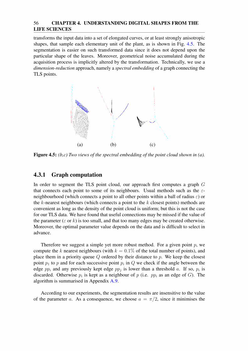
56 CHAPTER 4. UNDERSTANDING DIGITAL SHAPES FROM THELIFE SCIENCES
transforms the input data into a set of elongated curves, or at least strongly anisotropicshapes, that sample each elementary unit of the plant, as is shown in Fig. 4.5. Thesegmentation is easier on such transformed data since it does not depend upon theparticular shape of the leaves. Moreover, geometrical noise accumulated during theacquisition process is implicitly altered by the transformation. Technically, we use adimension-reduction approach, namely a spectral embedding of a graph connecting theTLS points.
(a) (b) (c)
Figure 4.5: (b,c) Two views of the spectral embedding of the point cloud shown in (a).
4.3.1 Graph computationIn order to segment the TLS point cloud, our approach first computes a graph Gthat connects each point to some of its neighbours. Usual methods such as the ε-neighbourhood (which connects a point to all other points within a ball of radius ε) orthe k-nearest neighbours (which connects a point to the k closest points) methods areconvenient as long as the density of the point cloud is uniform; but this is not the casefor our TLS data. We have found that useful connections may be missed if the value ofthe parameter (ε or k) is too small, and that too many edges may be created otherwise.Moreover, the optimal parameter value depends on the data and is difficult to select inadvance.
Therefore we suggest a simple yet more robust method. For a given point p, wecompute the k nearest neighbours (with k = 0.1% of the total number of points), andplace them in a priority queue Q ordered by their distance to p. We keep the closestpoint p1 to p and for each successive point pi in Q we check if the angle between theedge ppi and any previously kept edge ppj is lower than a threshold a. If so, pi isdiscarded. Otherwise pi is kept as a neighbour of p (i.e. ppi as an edge of G). Thealgorithm is summarised in Appendix A.9.
According to our experiments, the segmentation results are insensitive to the valueof the parameter a. As a consequence, we choose a = π/2, since it minimises the
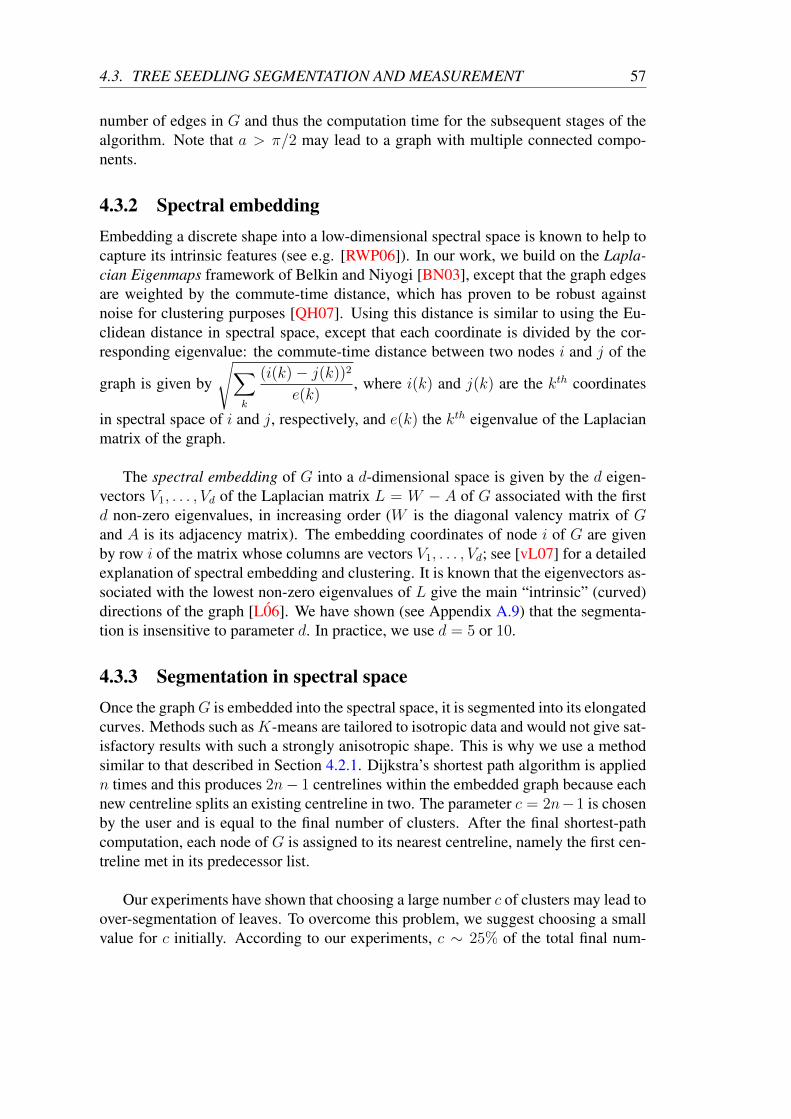
4.3. TREE SEEDLING SEGMENTATION AND MEASUREMENT 57
number of edges in G and thus the computation time for the subsequent stages of thealgorithm. Note that a > π/2 may lead to a graph with multiple connected compo-nents.
4.3.2 Spectral embeddingEmbedding a discrete shape into a low-dimensional spectral space is known to help tocapture its intrinsic features (see e.g. [RWP06]). In our work, we build on the Lapla-cian Eigenmaps framework of Belkin and Niyogi [BN03], except that the graph edgesare weighted by the commute-time distance, which has proven to be robust againstnoise for clustering purposes [QH07]. Using this distance is similar to using the Eu-clidean distance in spectral space, except that each coordinate is divided by the cor-responding eigenvalue: the commute-time distance between two nodes i and j of the
graph is given by
√∑
k
(i(k)− j(k))2
e(k), where i(k) and j(k) are the kth coordinates
in spectral space of i and j, respectively, and e(k) the kth eigenvalue of the Laplacianmatrix of the graph.
The spectral embedding of G into a d-dimensional space is given by the d eigen-vectors V1, . . . , Vd of the Laplacian matrix L = W − A of G associated with the firstd non-zero eigenvalues, in increasing order (W is the diagonal valency matrix of Gand A is its adjacency matrix). The embedding coordinates of node i of G are givenby row i of the matrix whose columns are vectors V1, . . . , Vd; see [vL07] for a detailedexplanation of spectral embedding and clustering. It is known that the eigenvectors as-sociated with the lowest non-zero eigenvalues of L give the main “intrinsic” (curved)directions of the graph [L06]. We have shown (see Appendix A.9) that the segmenta-tion is insensitive to parameter d. In practice, we use d = 5 or 10.
4.3.3 Segmentation in spectral spaceOnce the graphG is embedded into the spectral space, it is segmented into its elongatedcurves. Methods such asK-means are tailored to isotropic data and would not give sat-isfactory results with such a strongly anisotropic shape. This is why we use a methodsimilar to that described in Section 4.2.1. Dijkstra’s shortest path algorithm is appliedn times and this produces 2n− 1 centrelines within the embedded graph because eachnew centreline splits an existing centreline in two. The parameter c = 2n−1 is chosenby the user and is equal to the final number of clusters. After the final shortest-pathcomputation, each node of G is assigned to its nearest centreline, namely the first cen-treline met in its predecessor list.
Our experiments have shown that choosing a large number c of clusters may lead toover-segmentation of leaves. To overcome this problem, we suggest choosing a smallvalue for c initially. According to our experiments, c ∼ 25% of the total final num-
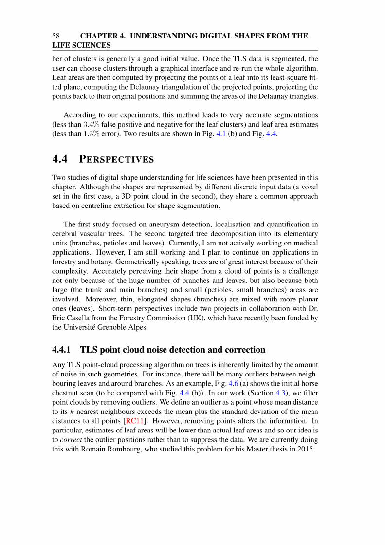
58 CHAPTER 4. UNDERSTANDING DIGITAL SHAPES FROM THELIFE SCIENCES
ber of clusters is generally a good initial value. Once the TLS data is segmented, theuser can choose clusters through a graphical interface and re-run the whole algorithm.Leaf areas are then computed by projecting the points of a leaf into its least-square fit-ted plane, computing the Delaunay triangulation of the projected points, projecting thepoints back to their original positions and summing the areas of the Delaunay triangles.
According to our experiments, this method leads to very accurate segmentations(less than 3.4% false positive and negative for the leaf clusters) and leaf area estimates(less than 1.3% error). Two results are shown in Fig. 4.1 (b) and Fig. 4.4.
4.4 PERSPECTIVES
Two studies of digital shape understanding for life sciences have been presented in thischapter. Although the shapes are represented by different discrete input data (a voxelset in the first case, a 3D point cloud in the second), they share a common approachbased on centreline extraction for shape segmentation.
The first study focused on aneurysm detection, localisation and quantification incerebral vascular trees. The second targeted tree decomposition into its elementaryunits (branches, petioles and leaves). Currently, I am not actively working on medicalapplications. However, I am still working and I plan to continue on applications inforestry and botany. Geometrically speaking, trees are of great interest because of theircomplexity. Accurately perceiving their shape from a cloud of points is a challengenot only because of the huge number of branches and leaves, but also because bothlarge (the trunk and main branches) and small (petioles, small branches) areas areinvolved. Moreover, thin, elongated shapes (branches) are mixed with more planarones (leaves). Short-term perspectives include two projects in collaboration with Dr.Eric Casella from the Forestry Commission (UK), which have recently been funded bythe Université Grenoble Alpes.
4.4.1 TLS point cloud noise detection and correctionAny TLS point-cloud processing algorithm on trees is inherently limited by the amountof noise in such geometries. For instance, there will be many outliers between neigh-bouring leaves and around branches. As an example, Fig. 4.6 (a) shows the initial horsechestnut scan (to be compared with Fig. 4.4 (b)). In our work (Section 4.3), we filterpoint clouds by removing outliers. We define an outlier as a point whose mean distanceto its k nearest neighbours exceeds the mean plus the standard deviation of the meandistances to all points [RC11]. However, removing points alters the information. Inparticular, estimates of leaf areas will be lower than actual leaf areas and so our idea isto correct the outlier positions rather than to suppress the data. We are currently doingthis with Romain Rombourg, who studied this problem for his Master thesis in 2015.
4.4. PERSPECTIVES 59
(a) (b)
Figure 4.6: (a) Raw scan of the horse chestnut (top view). (b) Modelling the acquisi-tion noise. In green is displayed the input scan as a function of distance to the LiDAR;in blue is our simulation, taking into account our mixed pixel mathematical model.
Several physical phenomena have been claimed to be responsible for outliers in theliterature [HK92], of which the so-called mixed pixel effect can explain the majority ofoutliers in our tree TLS point clouds (see Fig. 4.6 (b)). The effect occurs when a laserbeam partially hits the edge of one surface and partially anotherbehind it. We havedeveloped a mathematical model of this effect and methods to detect and correct foroutliers.
4.4.2 Towards an accurate digital tree modelNoise correction opens up new perspectives for our interactive segmentation approach(Section 4.3). Our ambition is to make it fully automated, in order to be able to seg-ment a full leaf-on tree accurately and not only seedlings or plants. This is not currentlypossible because of the amount of noise still present in the data, even after filtering.The boundary between elementary units (e.g. two spatially close leaves) is not alwaysobvious and the graph we create may contain several edges joining elementary unitsthat are not connected in the real tree.
I have recently been granted a PhD studentship by the Université Grenoble Alpesto investigate further the use of LiDAR data for digital tree modelling. The goal ofthis project is to develop a full pipeline from TLS point-cloud acquisition to single leafand branch geometric modelling and measurement, through to scan de-noising andautomated segmentation into elementary units. The student, Romain Rombourg, hasstarted his PhD thesis in October 2015.

60 CHAPTER 4. UNDERSTANDING DIGITAL SHAPES FROM THELIFE SCIENCES
CHAPTER 5
Conclusion
5.1 SUMMARY
In this manuscript I have reviewed my main contributions to digital shape understand-ing. I have developed several segmentation and skeleton-based methods to recogniseshapes from low-level digital representations, that have no overall coherence. My re-search has encompassed three different areas. First, I have focused on general purpose3D meshes. I have contributed to their topological and perceptual comprehension, aswell as to the transformation of a unorganised set of triangles into a manifold mesh, andthen to a regularly sampled volumetric model. Second, I have introduced methods thathelp to create, modify and analyse sequences of meshes as digital representations ofmoving shapes. Third, in the context of shape analysis and measurement for medicineand botany, I have worked on skeleton-based shape segmentation from two differentdigital representations, namely, voxel sets and point clouds.
In each of these studies, I have developed tools that are either interactive (or expe-riential) or automatic as the particular context and user need has required. Similarly,some of my work has had specific applications in mind while other work has aimed tobe more generally applicable. This is summarised in Table 5.1. The mesh sequencedecomposition algorithm is in the specific application category since it focuses on rigidmotion retrieval. A possible application is motion measurement for limb rehabilitationor sport gesture analysis. The harmonic skeleton tool is classified as interactive sincethe skinning weights are chosen by tuning a parameter (Section 3.2.5). As a futureresearch project, it could be automated by relating the skeleton to anatomy semantics.
61
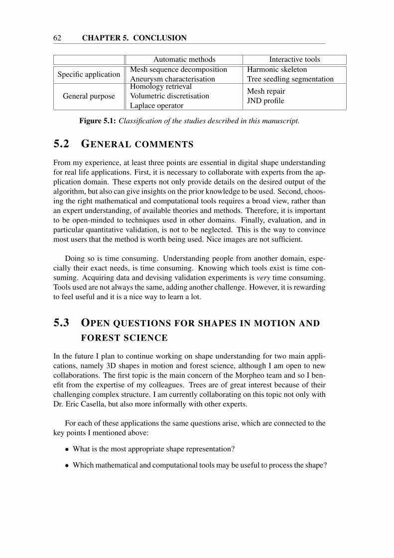
62 CHAPTER 5. CONCLUSION
Automatic methods Interactive tools
Specific applicationMesh sequence decompositionAneurysm characterisation
Harmonic skeletonTree seedling segmentation
General purposeHomology retrievalVolumetric discretisationLaplace operator
Mesh repairJND profile
Figure 5.1: Classification of the studies described in this manuscript.
5.2 GENERAL COMMENTS
From my experience, at least three points are essential in digital shape understandingfor real life applications. First, it is necessary to collaborate with experts from the ap-plication domain. These experts not only provide details on the desired output of thealgorithm, but also can give insights on the prior knowledge to be used. Second, choos-ing the right mathematical and computational tools requires a broad view, rather thanan expert understanding, of available theories and methods. Therefore, it is importantto be open-minded to techniques used in other domains. Finally, evaluation, and inparticular quantitative validation, is not to be neglected. This is the way to convincemost users that the method is worth being used. Nice images are not sufficient.
Doing so is time consuming. Understanding people from another domain, espe-cially their exact needs, is time consuming. Knowing which tools exist is time con-suming. Acquiring data and devising validation experiments is very time consuming.Tools used are not always the same, adding another challenge. However, it is rewardingto feel useful and it is a nice way to learn a lot.
5.3 OPEN QUESTIONS FOR SHAPES IN MOTION ANDFOREST SCIENCE
In the future I plan to continue working on shape understanding for two main appli-cations, namely 3D shapes in motion and forest science, although I am open to newcollaborations. The first topic is the main concern of the Morpheo team and so I ben-efit from the expertise of my colleagues. Trees are of great interest because of theirchallenging complex structure. I am currently collaborating on this topic not only withDr. Eric Casella, but also more informally with other experts.
For each of these applications the same questions arise, which are connected to thekey points I mentioned above:
• What is the most appropriate shape representation?
• Which mathematical and computational tools may be useful to process the shape?
5.3. OPEN QUESTIONS FOR SHAPES IN MOTION AND FOREST SCIENCE 63
• Which additional knowledge should be used, and how should it be integrated?
I will consider each of these questions in turn.
5.3.1 Appropriate shape representationsIn computer vision, 3D moving shapes are currently represented by temporally inco-herent mesh sequences (TIMS, see Definition 3.1.1). We have seen in Section 3.4 thatit is not easy to recognise the shape and its motion from such a representation. There-fore it may be relevant to try to find a more appropriate geometric representation. Wehave recently started focusing on regular volumetric discretisation, through the PhDproject of Li Wang (Section 2.5). A recent publication using our approach has shownthat there is interest in such volumetric discretisation for shape tracking [AFB15]. Thistopic will also be investigated within the context of the ANR ACHMOV project (seeSection 3.5.3), for clothed human body shapes. In the case of clothes, a volumetricmodel may not be appropriate since clothes are largely two-dimensional.
In forestry, the need for accurate measurements also requires appropriate shaperepresentations. A recent study has shown that cylinders are a simple yet efficient ge-ometric primitive to represent tree branches [rRKC15]. A similar study is planned forleaves in the context of the AGIR DigiTree project (see Section 4.4.2). However itmay not be possible to avoid having many parameters since the geometric variabilityof leaves is much greater than that of branches. To overcome this problem, a col-laboration with Florence Bertails-Descoubes from the BIPOP team of Inria Grenobleis envisaged. Florence’s project “From Geometry to Motion: inverse modelling ofcomplex mechanical structures”, recently granted by the ERC, aims at estimating me-chanical parameters from the geometric shape, for thin elastic rods, plates and shells.Tree leaves would be physically modelled as shells.
5.3.2 Mathematical and computational toolsThe question of appropriate mathematical and computational tools is closely relatedto the issue of representation. In the case of shapes in motion, I believe that the 3D+tLaplace operator, developed on TCMS (see Section 3.3), may be as useful for shapeand motion processing as discrete 3D Laplace operators are for static mesh processing[LZ09, ZvKD10]. The main benefit of such an operator lies in its ability to processboth shapes and motions, by simply varying a parameter. Its computational cost is itsmain drawback, since it requires a matrix whose size is the square of the total numberof vertices in the sequence, although this matrix is very sparse. Methods for sparsematrix manipulations need to be investigated further for this operator to be practicallyusable. A discrete Laplace operator on TIMS or volumetric space-time representationsmay be derived later, if such representations prove to be useful for the understandingof shapes in motion.
64 CHAPTER 5. CONCLUSION
In the case of tree laser scans, two main options can be envisaged. If the inputpoint cloud can be efficiently de-noised (see Section 4.4.1), it may be converted to atwo-manifold mesh. Then, standard mesh processing techniques may be used as wasrecently done for phenotyping [PSB+12]. However, I believe that, due to the partic-ular geometry of a tree, with many close yet non-intersecting branches and leaves, inmost cases there will be too many occlusions and topological ambiguities for a correctmesh reconstruction. Therefore instead, I plan to investigate point cloud processingtools. Since LiDAR have been used for a long time in many fields such as robotics,archaeology or building modelling, such tools are already well developed, see e.g.[RC11, NWH13].
In addition to these deterministic tools, statistical methods will be required to dealwith inherent uncertainty in the data. The development of statistical methods is plannedfor the PhD project that I will supervise with Stefanie Wuhrer on modelling clothedhumans in motion (see Section 3.5.3). In the case of scanned leaf-on trees, this is some-thing already quite popular in the literature: because of the large number of occlusionsbetween leaves, an exact reconstruction of each single leaf is impractical.
5.3.3 Incorporating additional knowledgePrior knowledge is crucial for the efficiency of shape understanding tools. As we haveseen in this manuscript, depending upon the application, an expert can provide knowl-edge about the shape. However, this is not the only possibility, and I think at least twodirections need to be explored.
First, this knowledge may be implicitly learnt from examples or from the environ-ment, as has been suggested recently by Hu et al. [HZvK+15]. This is an area of con-siderable interest nowadays, as is exemplified in the recent work on 3D shape recog-nition from depth sensors using deep learning techniques by Wu et al. [WSK+15].Another way to incorporate knowledge without formalising it is through a set of userexperiments, as we did with George Nader for 3D mesh visual perception (Section 2.4).One of the main questions in all these cases is to what extent does the example/userdatabase or the environment fully represents the set of possible situations.
Second, new sensors may be used to provide additional information about theshape. For shapes in motion, optical systems and depth cameras are widely used tocomplement video cameras. Within the Morpheo team, our acquisition platform Kino-vis benefits from a 20 Vicon motion capture system combined with 68 video cameras.Cameras can also be thought of as complementing laser scanners in the forestry case.Unfortunately, their resolution is currently too low to help with accurate measurement[CDMM13]. Handheld laser scanners are currently being investigated but again theiraccuracy remains insufficient at the moment [BBP+14]. Hyper-spectral imaging is apromising field, and several teams have recently started to investigate this technologyfor remote sensing; see e.g. [HSKC12]. The main challenges when various sensors are

5.3. OPEN QUESTIONS FOR SHAPES IN MOTION AND FOREST SCIENCE 65
combined are calibration and data fusion. The discrete representation of shapes mayalso need to be adapted.

66 CHAPTER 5. CONCLUSION

APPENDIX A
Selected papers
• Mesh repair with user-friendly topology control, F. Hétroy, S. Rey, C. Andújar,P. Brunet, À. Vinacua, Computer-Aided Design 43 (1), Elsevier, 2011.
• An iterative algorithm for homology computation on simplicial shapes, D. Boltcheva,D. Canino, S. Merino Aceituno, J.C. Léon, L. De Floriani, F. Hétroy, Computer-Aided Design 43 (11), Elsevier, 2011. Presented at the SIAM Conference onGeometric & Physical Modeling (GD/SPM) 2011.
• Just Noticeable Distortion profile for flat-shaded 3D mesh surfaces, G. Nader,K. Wang, F. Hétroy-Wheeler, F. Dupont, IEEE Transactions on Visualization andComputer Graphics, 2016.
• A hierarchical approach for regular centroidal Voronoi tessellations, L. Wang, F.Hétroy-Wheeler, E. Boyer, Computer Graphics Forum 35 (1), Wiley, 2016.
• Harmonic skeleton for realistic character animation, G. Aujay, F. Hétroy, F.Lazarus, C. Depraz, ACM-SIGGRAPH/Eurographics Symposium on ComputerAnimation, 2007.
• Simple flexible skinning based on manifold modeling, F. Hétroy, C. Gérot, L.Lu, B. Thibert, International Conference on Computer Graphics Theory and Ap-plications (GRAPP), 2009.
• Segmentation of temporal mesh sequences into rigidly moving components, R.Arcila, C. Cagniart, F. Hétroy, E. Boyer, F. Dupont, Graphical Models 75 (1),Elsevier, 2013.
67

68 APPENDIX A. SELECTED PAPERS
• Automatic localization and quantification of intracranial aneurysms, S. Hassan,F. Hétroy, F. Faure, O. Palombi, Lecture Notes in Computer Science 6854,Springer, 2011. Presented at the International Conference on Computer Anal-ysis of Images and Patterns (CAIP), 2011.
• Segmentation of tree seedling point clouds into elementary units, F. Hétroy-Wheeler, E. Casella, D. Boltcheva, International Journal of Remote Sensing,Taylor & Francis, 2016.
A.1. MESH REPAIR WITH USER-FRIENDLY TOPOLOGY CONTROL 69
∴
A.1 MESH REPAIR WITH USER-FRIENDLYTOPOLOGY CONTROL
Franck Hétroy, Stéphanie Rey, Carlos Andújar, Pere Brunet, Àlvar VinacuaComputer-Aided Design 43 (1), Elsevier, 2011.

70 APPENDIX A. SELECTED PAPERS
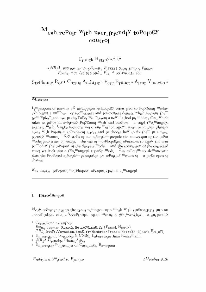
Mesh repair with user-friendly topology
control
Franck Hetroy a,∗,1,2
aINRIA, 655 avenue de l’Europe, F-38334 Saint Ismier, France
Phone: +33 476 615 504 – Fax: + 33 476 615 466
Stephanie Rey 1 Carlos Andujar 3 Pere Brunet 3 Alvar Vinacua 3
Abstract
Limitations of current 3D acquisition technology often lead to polygonal meshesexhibiting a number of geometrical and topological defects which prevent themfrom widespread use. In this paper we present a new method for model repair whichtakes as input an arbitrary polygonal mesh and outputs a valid two-manifoldtriangle mesh. Unlike previous work, our method allows users to quickly identifyareas with potential topological errors and to choose how to fix them in a user-friendly manner. Key steps of our algorithm include the conversion of the inputmodel into a set of voxels, the use of morphological operators to allow the userto modify the topology of the discrete model, and the conversion of the correctedvoxel set back into a two-manifold triangle mesh. Our experiments demonstratethat the proposed algorithm is suitable for repairing meshes of a large class ofshapes.
Key words: topology, morphology, opening, closing, 2-manifold
1 Introduction
Mesh repair refers to the transformation of a mesh with singularities into an“acceptable” one. “Acceptable” often means a two-manifold – a surface S
∗ Corresponding authorEmail address: [email protected] (Franck Hetroy).URL: http://evasion.imag.fr/Membres/Franck.Hetroy/ (Franck Hetroy).
1 Universite de Grenoble & CNRS, Laboratoire Jean Kuntzmann2 INRIA Grenoble Rhone-Alpes3 Universitat Politecnica de Catalunya, Barcelona
Preprint submitted to Elsevier 4 October 2010
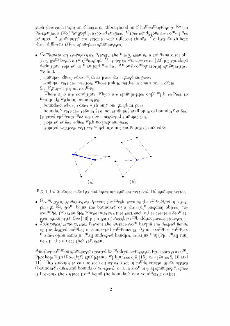
such that each point on S has a neighbourhood on S homeomorphic to R2 (in
particular, a two-manifold is a closed surface). Other conditions are sometimesrequired. A singularity can refer to very different things. We distinguish herethree different types of surface singularities.
• Combinatorial singularities prevent the mesh, seen as a combinatorial ob-ject, from being a two-manifold. We refer to Gueziec et al. [22] for standarddefinitions related to manifold meshes. Among combinatorial singularities,we find:· singular edges: edges with at least three incident faces;· singular vertices: vertices whose link is neither a chain nor a cycle.See Figure 1 for an example.There also are conditions which are singularities only with respect to
manifolds without boundaries:· boundary edges: edges with only one incident face;· boundary vertices: regular (i.e. not singular) endpoints of boundary edges.Isolated elements may also be considered singularities:· isolated edges: edges with no incident face;· isolated vertices: vertices which are not endpoints of any edge.
(a) (b)
Fig. 1. (a) Singular edge (its endpoints are singular vertices), (b) singular vertex.
• Geometrical singularities prevent the mesh, seen as the embedding of a sur-face in R
3, from being the boundary of a three-dimensional object. Forexample, two triangles whose interiors intersect each other create a geomet-rical singularity. See [40] for a list of possible embedding inconsistencies.
• Topological singularities prevent the surface from having the desired genusor the desired number of connected components. As an example, complexmeshes often contain small undesired handles, creating multiple small tun-nels in the object they represent.
Another common singularity created by modern acquisition processes is a com-plex hole with (possibly) tiny islands within (see e.g. [15], or Figures 9, 10 and11). This singularity can be seen either as a set of combinatorial singularities(boundary edges and boundary vertices), or as a geometrical singularity, sinceit prevents the surface from being the boundary of a volumetric object.
2
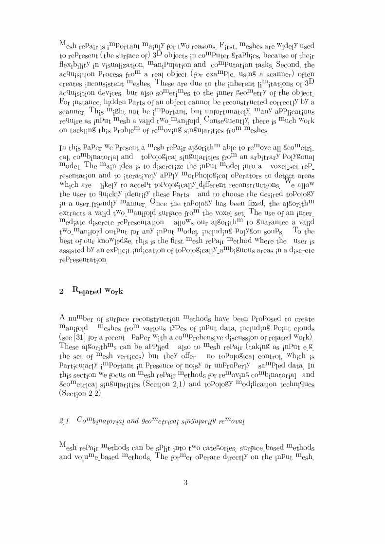
Mesh repair is important mainly for two reasons. First, meshes are widely usedto represent (the surface of) 3D objects in computer graphics, because of theirflexibility in visualization, manipulation and computation tasks. Second, theacquisition process from a real object (for example, using a scanner) oftencreates inconsistent meshes. These are due to the inherent limitations of 3Dacquisition devices, but also sometimes to the inner geometry of the object.For instance, hidden parts of an object cannot be reconstructed correctly by ascanner. This might not be important, but unfortunately, many applicationsrequire as input mesh a valid two-manifold. Consequently, there is much workon tackling this problem of removing singularities from meshes.
In this paper we present a mesh repair algorithm able to remove all geometri-cal, combinatorial and topological singularities from an arbitrary polygonalmodel. The main idea is to discretize the input model into a voxel-set rep-resentation and to iteratively apply morphological operators to detect areaswhich are likely to accept topologically-different reconstructions. We allowthe user to quickly identify these parts and to choose the desired topologyin a user-friendly manner. Once the topology has been fixed, the algorithmextracts a valid two-manifold surface from the voxel set. The use of an inter-mediate discrete representation allows our algorithm to guarantee a validtwo-manifold output for any input model, including polygon soups. To thebest of our knowledge, this is the first mesh repair method where the user isassisted by an explicit indication of topologically-ambiguous areas in a discreterepresentation.
2 Related work
A number of surface reconstruction methods have been proposed to createmanifold meshes from various types of input data, including point clouds(see [31] for a recent paper with a comprehensive discussion of related work).These algorithms can be applied also to mesh repair (taking as input e.g.the set of mesh vertices) but they offer no topological control, which isparticularly important in presence of noisy or unproperly sampled data. Inthis section we focus on mesh repair methods for removing combinatorial andgeometrical singularities (Section 2.1) and topology modification techniques(Section 2.2).
2.1 Combinatorial and geometrical singularity removal
Mesh repair methods can be split into two categories: surface-based methodsand volume-based methods. The former operate directly on the input mesh,
3
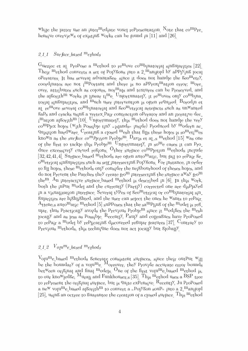
while the latter use an intermediate voxel representation. Note that compre-hensive overviews of existing works can be found in [11] and [26].
2.1.1 Surface-based methods
Gueziec et al. propose a method to remove combinatorial singularities [22].Their method converts a set of polygons into a 2-manifold by applying localoperators. It has several advantages: since it does not handle the geometry,coordinates are not important and there is no approximation error; more-over, attributes such as colours, normals and textures can be preserved, andthe algorithm works in linear time. Unfortunately, it removes only combina-torial singularities, and much user intervention is often required. Borodin etal. remove several combinatorial and geometrical artefacts such as unwantedgaps and cracks using a vertex-pair contraction operator and an iterative dec-imation algorithm [10]. Unfortunately, this method does not handle the verycomplex holes (with possible tiny “islands” inside) produced by modern ac-quisition hardware. Creating a closed mesh that fills these holes is sometimesknown as the surface completion problem. Davis et al.’s method [15] was oneof the first to tackle this problem. Unfortunately, in some cases it can pro-duce excessively curved regions. Other surface completion methods include[32,42,41,4]. Surface-based methods are often automatic, but fail to repair ge-ometrical singularities such as self-intersecting polygons. For instance, in orderto fill holes, these methods only consider the neigbourhood of theses holes, anddo not prevent the patches they create from intersecting the surface away fromthem. An interactive surface-based method is described in [6]. In this work,both the input model and the currently (partly) corrected one are displayedin a visualization interface. Several types of geometrical or combinatorial sin-gularities are highlighted, and the user can select the ones he wants to repair.Attene’s automatic method [5] supposes that the sampling of the model is reg-ular, thus practically avoids the previous problem since it modifies the meshlocally and as less as possible. Recently, Pauly and colleagues have proposedto repair a model by replicating discovered regular features [37]. Contrary toprevious methods, this technique does not act locally but globally.
2.1.2 Volume-based methods
Volume-based methods generate consistent surfaces, since their output willbe the boundary of a volume. Moreover, they provide accurate error boundsbetween original and final models. One of the first volume-based method is,to our knowledge, Murali and Funkhouser’s [35]. This method uses a BSP treeto represent the original surface, but is quite expensive. Recently, Ju proposeda new volume-based algorithm to convert a “polygon soup” into a 2-manifold[25], using an octree to guarantee the creation of a closed surface. This method
4
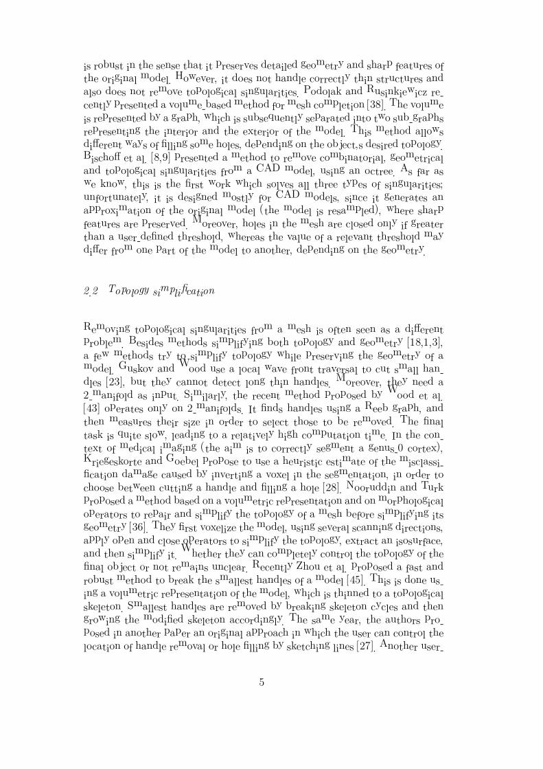
is robust in the sense that it preserves detailed geometry and sharp features ofthe original model. However, it does not handle correctly thin structures andalso does not remove topological singularities. Podolak and Rusinkiewicz re-cently presented a volume-based method for mesh completion [38]. The volumeis represented by a graph, which is subsequently separated into two sub-graphsrepresenting the interior and the exterior of the model. This method allowsdifferent ways of filling some holes, depending on the object’s desired topology.Bischoff et al. [8,9] presented a method to remove combinatorial, geometricaland topological singularities from a CAD model, using an octree. As far aswe know, this is the first work which solves all three types of singularities;unfortunately, it is designed mostly for CAD models, since it generates anapproximation of the original model (the model is resampled), where sharpfeatures are preserved. Moreover, holes in the mesh are closed only if greaterthan a user-defined threshold, whereas the value of a relevant threshold maydiffer from one part of the model to another, depending on the geometry.
2.2 Topology simplification
Removing topological singularities from a mesh is often seen as a differentproblem. Besides methods simplifying both topology and geometry [18,1,3],a few methods try to simplify topology while preserving the geometry of amodel. Guskov and Wood use a local wave front traversal to cut small han-dles [23], but they cannot detect long thin handles. Moreover, they need a2-manifold as input. Similarly, the recent method proposed by Wood et al.[43] operates only on 2-manifolds. It finds handles using a Reeb graph, andthen measures their size in order to select those to be removed. The finaltask is quite slow, leading to a relatively high computation time. In the con-text of medical imaging (the aim is to correctly segment a genus-0 cortex),Kriegeskorte and Goebel propose to use a heuristic estimate of the misclassi-fication damage caused by inverting a voxel in the segmentation, in order tochoose between cutting a handle and filling a hole [28]. Nooruddin and Turkproposed a method based on a volumetric representation and on morphologicaloperators to repair and simplify the topology of a mesh before simplifying itsgeometry [36]. They first voxelize the model, using several scanning directions,apply open and close operators to simplify the topology, extract an isosurface,and then simplify it. Whether they can completely control the topology of thefinal object or not remains unclear. Recently Zhou et al. proposed a fast androbust method to break the smallest handles of a model [45]. This is done us-ing a volumetric representation of the model, which is thinned to a topologicalskeleton. Smallest handles are removed by breaking skeleton cycles and thengrowing the modified skeleton accordingly. The same year, the authors pro-posed in another paper an original approach in which the user can control thelocation of handle removal or hole filling by sketching lines [27]. Another user-
5
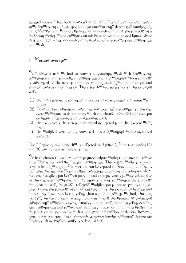
assisted program has been proposed in [4]. This method can not only repairsome geometrical singularities, but also automatically detect tiny handles. Fi-nally, Campen and Kobbelt propose an approach to modify the topology of apolygonal model, which combines an adaptive octree and nested binary spacepartitions [12]. Their approach can be used to remove geometrical singularitiesin a mesh.
3 Method overview
We propose a new method to convert a triangular mesh with geometrical,combinatorial and topological singularities into a 2-manifold whose topologyis supervised by the user. It combines volume-based 2-manifold creation andadapted topology modification. The algorithm proceeds through the followingsteps:
(1) the input surface is converted into a set of voxels, called a discrete mem-brane;
(2) morphological operators (openings and closings) are applied to the dis-crete membrane to detect areas which can change topology (hole creationor filling, shell connection or disconnection);
(3) the user selects the voxels to be added or deleted from the discrete mem-brane
(4) the modified voxel set is converted into a 2-manifold with guaranteedtopology.
The pipeline of our algorithm is depicted on Figure 2. Note that stages (2)and (3) can be iterated several times.
We have chosen to use a volumetric intermediate model to be sure to removeall combinatorial and geometrical singularities. The output model is guaran-teed to be a 2-manifold. Our method can be related to Nooruddin and Turk’s[36] since we also use morphological operators to control the topology. How-ever our classification between interior and exterior voxels is more robust dueto the discrete membrane, and we allow the user to monitor the topologymodification step. As in [27], topology modification is interactive: as the useroften knows the topology of the object (including the location of handles andholes), this provides a better repair than a fully automatic method. But, un-like [27], we have chosen to assist the user during the process, by indicatingtopologically ambiguous areas. Another interactive program to repair geomet-rical singularities and remove tiny handles is described in [4]. This program isperfectly suited for meshes with a relatively low number of defects; however,since it uses a surface-based approach, it cannot handle completely degeneratemeshes such as polygon soups (see Fig. 15 (a)).
6
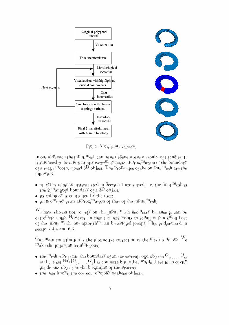
Fig. 2. Algorithm overview.
In our approach the input mesh can be as degenerate as a “soup” of triangles. Itis supposed to be a potentially extremely noisy approximation of the boundaryof a real, smooth, closed 3D object. The properties of the output mesh are thefollowing:
• all types of singularities listed in Section 1 are solved, i.e. the final mesh isthe 2-manifold boundary of a 3D object;
• its topology is controlled by the user;• its geometry is an approximation of that of the input mesh.
We have chosen not to rely on the input mesh geometry because it can beextremely noisy. However, in case the user wants to repair only a small partof the input mesh, our algorithm can be applied locally. This is discussed insections 4.4 and 6.3.
Our main contribution is the interactive correction of the mesh topology. Wemake the following assumptions:
• the mesh represents the boundary of one or several solid objects O1, . . . , Ok,and the set R
3\O1, . . . , Ok is connected; in other words there is no cavityinside any object at the beginning of the process;
• the user knows the correct topology of these objects;
7
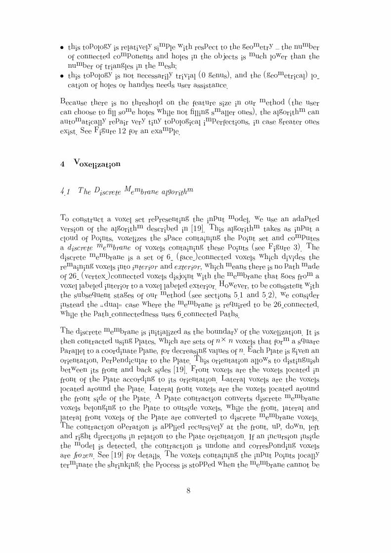
• this topology is relatively simple with respect to the geometry – the numberof connected components and holes in the objects is much lower than thenumber of triangles in the mesh;
• this topology is not necessarily trivial (0 genus), and the (geometrical) lo-cation of holes or handles needs user assistance.
Because there is no threshold on the feature size in our method (the usercan choose to fill some holes while not filling smaller ones), the algorithm canautomatically repair very tiny topological imperfections, in case greater onesexist. See Figure 12 for an example.
4 Voxelization
4.1 The Discrete Membrane algorithm
To construct a voxel set representing the input model, we use an adaptedversion of the algorithm described in [19]. This algorithm takes as input acloud of points, voxelizes the space containing the point set and computesa discrete membrane of voxels containing these points (see Figure 3). Thediscrete membrane is a set of 6- (face-)connected voxels which divides theremaining voxels into interior and exterior, which means there is no path madeof 26- (vertex-)connected voxels disjoint with the membrane that goes from avoxel labeled interior to a voxel labeled exterior. However, to be consistent withthe subsequent stages of our method (see sections 5.1 and 5.2), we considerinstead the “dual” case where the membrane is required to be 26-connected,while the path-connectedness uses 6-connected paths.
The discrete membrane is initialized as the boundary of the voxelization. It isthen contracted using plates, which are sets of n×n voxels that form a squareparallel to a coordinate plane, for decreasing values of n. Each plate is given anorientation, perpendicular to the plate. This orientation allows to distinguishbetween its front and back sides [19]. Front voxels are the voxels located infront of the plate according to its orientation. Lateral voxels are the voxelslocated around the plate. Lateral front voxels are the voxels located aroundthe front side of the plate. A plate contraction converts discrete membranevoxels belonging to the plate to outside voxels, while the front, lateral andlateral front voxels of the plate are converted to discrete membrane voxels.The contraction operation is applied recursively at the front, up, down, leftand right directions in relation to the plate orientation. If an incursion insidethe model is detected, the contraction is undone and corresponding voxelsare frozen. See [19] for details. The voxels containing the input points locallyterminate the shrinking; the process is stopped when the membrane cannot be
8
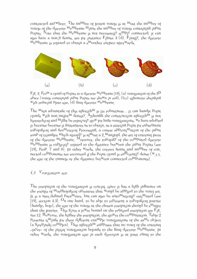
contracted anywhere. The number of frozen voxels is at most the number ofvoxels of the discrete membrane minus the number of voxels containing inputpoints. Note that the membrane is not necessarily simply connected; it canalso have a non-0 genus, see for instance Figure 3 (d). Finally, the discretemembrane is relaxed to obtain a smoother surface afterwards.
(a) (b) (c) (d)
Fig. 3. From a cloud of points to a discrete membrane [19]: (a) voxelization of the 3Dspace (voxels containing input points are shown in red), (b,c) silhouette shrinkingwith reducing plate size, (d) final discrete membrane.
The main advantage of this algorithm is its robustness – it can handle pointclouds with non-uniform density. Although the construction algorithm is nothierarchical and might be relatively slow for huge voxelizations, we have adoptedit because because it guarantees us to obtain, as a starting point for subsequenttopological and geometrical processing, a coarse approximation of the inputsoup of triangles which already is almost a 2-manifold: the set of external facesof the discrete membrane. Moreover, the topology of the computed discretemembrane is explicitly related to the distance between the input points (see[19], prop. 7 and 8). In other words, the correct genus and number of con-nected components are recovered if the point cloud is sufficiently dense (w.r.t.the size of the tunnels or the distance between connected components).
4.2 Voxelization size
The resolution of the voxelization is crucial, since it has a high influence onthe results of morphological operators that would be applied to the voxel set.It is a user-defined parameter, but can also be automatically estimated (see[19], section 4.3). On one hand, to be able to represent a topological feature(handle, hole), the size of the voxels at the chosen resolution should be smallerthan the feature. This gives a lower bound on the required resolution see Fig-ure 12. However, the higher the resolution, the slower the computation: Table 2presents timings for three different example voxelizations of the same object(a Sierpinski complex). This algorithm supposes that no voxel of the external“layer” of the initial voxelization belongs to the final discrete membrane. Inother words, the voxelization size in each direction is at least equal to the
9
discrete membrane size in the same direction + 2.
4.3 Extension to meshes
Since our input is not a cloud of points but a triangulated mesh, we havemodified the algorithm of [19]. We not only compute the voxels containing theinput points, but also the voxels intersecting the faces. This is done using asmall additional function, described below (Algorithm 1). Computation timedepends on the voxelization size but is bounded by the number of voxelsintersecting the triangle bounding boxes, thus the computation is usually donevery fast: about 2 minutes for a Buddha model (see Figure 15) with about 300Kfaces and a voxelization size of more than 2M voxels on a low-end computer(see Section 7.5 for details on timings).
Algorithm 1 Computation of the intersection between the input mesh andthe voxelization
function ComputeIntersection(V oxelization W,Mesh M)
for each triangle T of the mesh M do
Compute the bounding box BB of T ;for each voxel V of W that intersects BB do
if V intersects T then
Label V as red;end if
end for
end for
Return all voxels labeled as red;
end function
4.4 Local voxelization
To speed up the process, the user can choose to select only a part of themesh and to apply this voxelization stage locally. This does not change theinput mesh in distant areas from the selected polygons. For the subsequenttopology correction to be efficient, the selected zone must be significantlygreater than the size of the topological features to be repaired. Also, sincethe original discrete membrane algorithm aims at recovering a closed object,additional voxels must be added at the boundary of the computed voxelizationto fill unwanted tunnels and get a closed set of voxels (see Figure 14 for anexample). To do this, we add planes of voxels, lying on the boundary voxels.Areas of the final surface corresponding to these voxels will be removed later,once the topology has been modified.
10
4.5 Comparison with other voxelization techniques
As stated previously, we use an enhanced version of the algorithm presentedin [19] because it can handle difficult cases, including non-uniform polygonsoups. Some other techniques produce fast results but cannot be applied in allcases, such as [17] which requires as input a watertight mesh. We comparedour method with the binvox program [34], which is based on the algorithmproposed by Nooruddin and Turk [36] (discussed in Section 2.2), and with thealgorithm proposed by Haumont and Warzee [24]. On the noisy Buddha tri-angle soup (see Fig. 15 (a)), our method took 129s to create a 100×234×100voxelization, while binvox took 112s to create a 132 × 132 × 132 voxeliza-tion. Results are similar voxelizations with a similar number of voxels. In themeantime, the method by Haumont and Warzee only took 56s on the samelow-end computer to voxelize the input polygon soup with an octree of depth7. However, some voxels outside the model are wrongly included in the voxelset.
5 Interactive topology modification using morphological operators
Before converting the discrete membrane into a two-manifold mesh, it is impor-tant to let the user decide the final topology, including the number of surfaceshells and their genus (number of holes or, similarly, handles). To control thetopology of the output of our algorithm, we apply morphological operators ona volume. The volume is not the discrete membrane itself, but the discretemembrane plus the interior of the object it bounds, which is automaticallyknown from the discrete membrane construction. Since each voxel of the dis-crete membrane is 6-connected to at least one interior voxel, this voxel set is a3-manifold with boundary – the neighbourhood of each point is homeomorphicto either a sphere or a hemisphere.
5.1 Topology of discrete volumes: notations and definitions
Let V be the voxel set. Its numbers of vertices, edges, faces and voxels arerespectively noted k0(V), k1(V), k2(V) and k3(V). The Euler characteristic χof V is defined as χ = k0(V)− k1(V) + k2(V)− k3(V).
The topology of a 3-manifold can be characterized by three numbers, namedBetti numbers. jth Betti number βj is defined as the rank of the j
th homologygroup Hj (an introduction to homology groups, with accurate definitions ofBetti numbers, can be found in [16]). What is more interesting for our study is
11
that Betti numbers correspond to numbers of connected components (β0(V)),tunnels (β1(V)) and voids (or cavities) (β2(V)) of the volume V . Betti numbersare also related to χ, because V is a cell complex: χ = β0(V)− β1(V) + β2(V).
The topology of the final surface is linked to the topology of our voxel set,since this surface corresponds to its boundary. The number of connected com-ponents of the surface equals β0(V), and its genus (sum of the numbers ofholes of all connected components) equals β1(V), provided that we use consis-tent neighbourhood definitions. In the following, we use the 26-neighbourhoodrelationship for the volume V , and the 6-neighbourhood relationship for VC
the complementary set of V : two voxels sharing a vertex, but not an edge,are said to be neighbours if they both belong to V , but not if they belong toVC . This prevents topological inconsistencies. We use the 26- instead of the6-neighbourhood relationship for V to be consistent with the computation ofχ as k0(V)− k1(V) + k2(V)− k3(V).
Computing Betti numbers is not a trivial task [21]. The number of con-nected components β0(V) can be computed in various ways, for instance usingdisjoint-set data structures [14]. The number of cavities equals the number ofconnected components of VC minus one (representing the “exterior” of V), soit can also be computed. However β1(V) is not easily found. Lee et al. computeβ1(V) counting the number of non-separating cuts [30] (β1(V) is the maximalnumber of non-separating cuts not increasing β0(V)). Another algorithm todetect non-separating cuts has been proposed by Guskov and Wood [23]. Inour approach, we prefer to compute β1(V) locally, following the approach ofBischoff and Kobbelt [7]. This enables us to quickly detect topological changescaused by the application of morphological operators (see Section 5.3), evenif the two other Betti numbers still need to be computed globally. β1(V)is computed thanks to previous relations χ = β0(V) − β1(V) + β2(V) andχ = k0(V)− k1(V)+ k2(V)− k3(V). In order to efficiently compute χ (withoutkeeping track of faces, edges, etc.), we exploit the fact that χ is additive, as didfor instance [7] – given two sets A and B, χ(A∪B) = χ(A)+χ(B)−χ(A∩B).Since each vertex of V belongs to 8 voxels (remember that no voxel of Vbelongs to the external “layer” of the initial voxelization), χ is the sumof the local Euler characteristics around each vertex of the voxelization di-vided by 8. The local Euler characteristic around a vertex v is defined ask0(V , v) − k1(V , v) + k2(V , v) − k3(V , v), with k0(V , v), k1(V , v), k2(V , v) andk3(V , v) denoting respectively the number of vertices, edges, faces and voxelsthat both belong to V and are incident to v. It can be computed using alookup table, since only 256 2× 2 voxel configurations can occur (in fact, upto isomorphism, we only have 22 different configurations). Moreover, since χis additive, we do not need to compute the Euler characteristic around eachvertex at each step of our algorithm. Each time we add or remove voxels,we only need to update local Euler characteristics around corresponding ver-
12
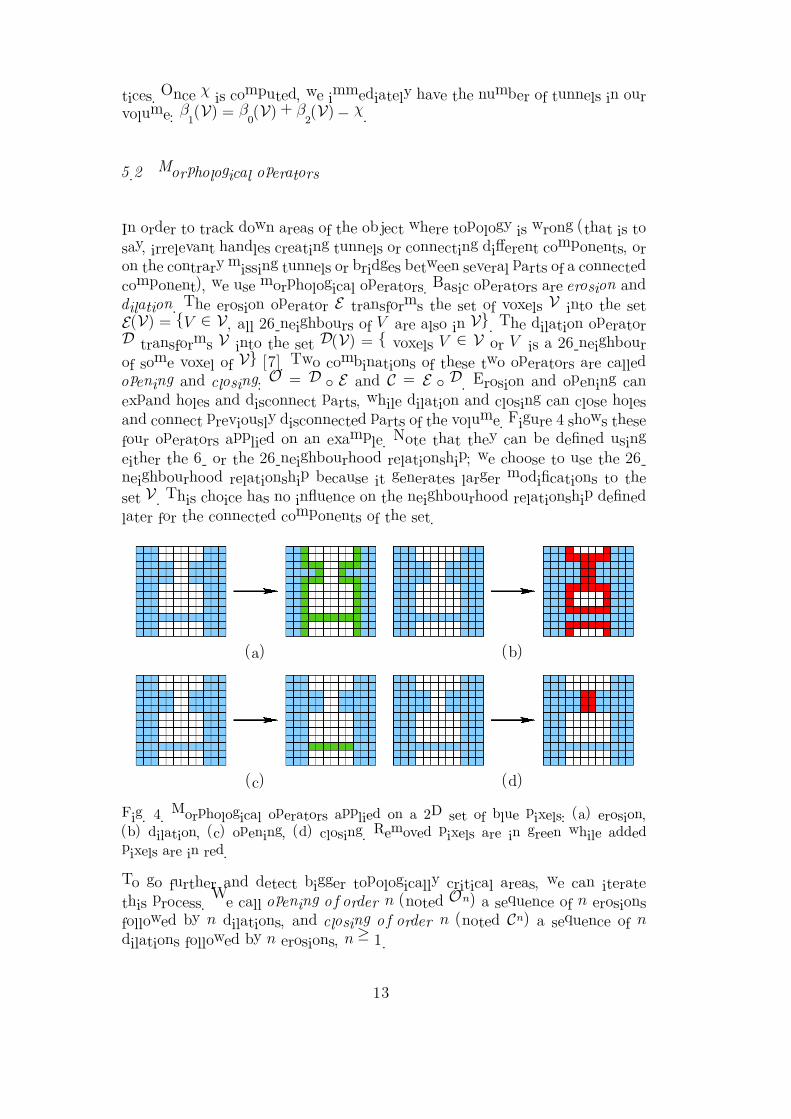
tices. Once χ is computed, we immediately have the number of tunnels in ourvolume: β1(V) = β0(V) + β2(V)− χ.
5.2 Morphological operators
In order to track down areas of the object where topology is wrong (that is tosay, irrelevant handles creating tunnels or connecting different components, oron the contrary missing tunnels or bridges between several parts of a connectedcomponent), we use morphological operators. Basic operators are erosion anddilation. The erosion operator E transforms the set of voxels V into the setE(V) = V ∈ V , all 26-neighbours of V are also in V. The dilation operatorD transforms V into the set D(V) = voxels V ∈ V or V is a 26-neighbourof some voxel of V [7]. Two combinations of these two operators are calledopening and closing: O = D E and C = E D. Erosion and opening canexpand holes and disconnect parts, while dilation and closing can close holesand connect previously disconnected parts of the volume. Figure 4 shows thesefour operators applied on an example. Note that they can be defined usingeither the 6- or the 26-neighbourhood relationship; we choose to use the 26-neighbourhood relationship because it generates larger modifications to theset V . This choice has no influence on the neighbourhood relationship definedlater for the connected components of the set.
(a) (b)
(c) (d)
Fig. 4. Morphological operators applied on a 2D set of blue pixels: (a) erosion,(b) dilation, (c) opening, (d) closing. Removed pixels are in green while addedpixels are in red.
To go further and detect bigger topologically critical areas, we can iteratethis process. We call opening of order n (noted On) a sequence of n erosionsfollowed by n dilations, and closing of order n (noted Cn) a sequence of ndilations followed by n erosions, n ≥ 1.
13
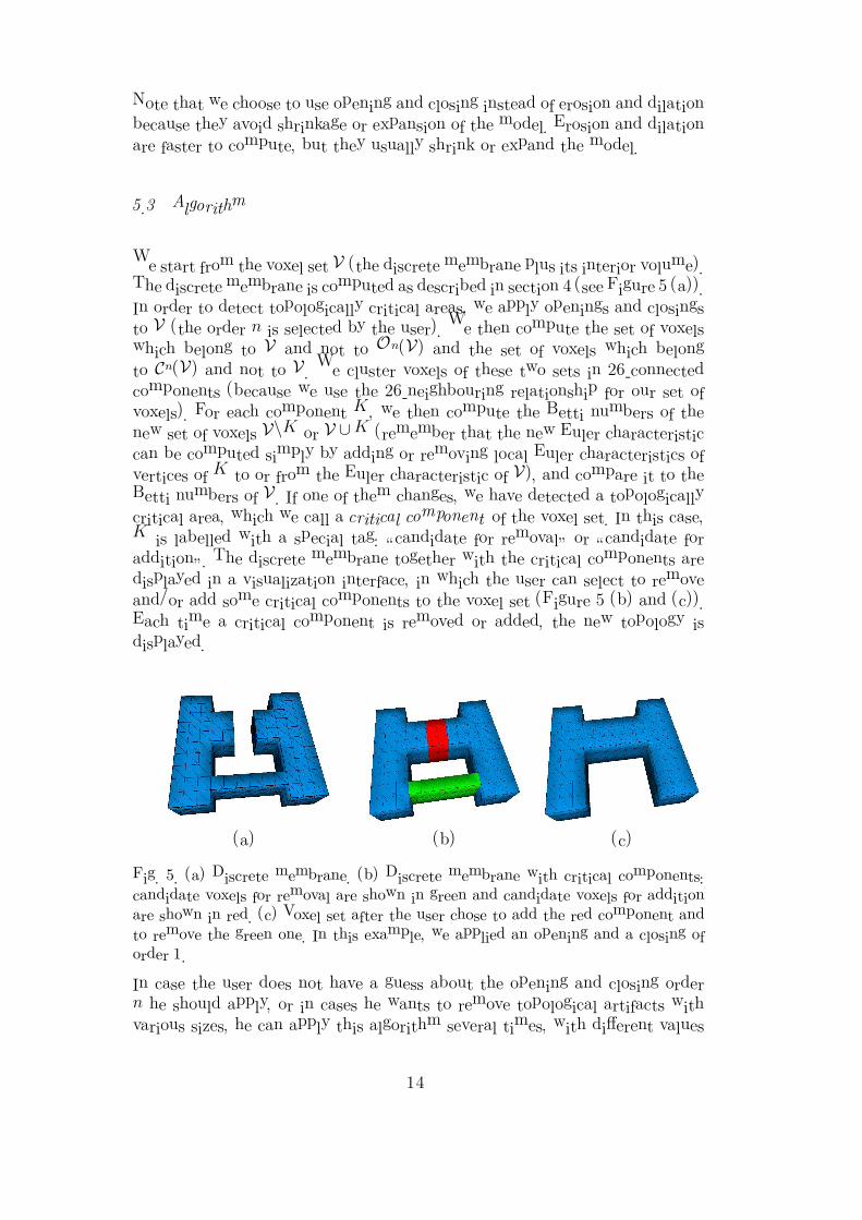
Note that we choose to use opening and closing instead of erosion and dilationbecause they avoid shrinkage or expansion of the model. Erosion and dilationare faster to compute, but they usually shrink or expand the model.
5.3 Algorithm
We start from the voxel set V (the discrete membrane plus its interior volume).The discrete membrane is computed as described in section 4 (see Figure 5 (a)).In order to detect topologically critical areas, we apply openings and closingsto V (the order n is selected by the user). We then compute the set of voxelswhich belong to V and not to On(V) and the set of voxels which belongto Cn(V) and not to V . We cluster voxels of these two sets in 26-connectedcomponents (because we use the 26-neighbouring relationship for our set ofvoxels). For each component K, we then compute the Betti numbers of thenew set of voxels V\K or V ∪K (remember that the new Euler characteristiccan be computed simply by adding or removing local Euler characteristics ofvertices of K to or from the Euler characteristic of V), and compare it to theBetti numbers of V . If one of them changes, we have detected a topologicallycritical area, which we call a critical component of the voxel set. In this case,K is labelled with a special tag: “candidate for removal” or “candidate foraddition”. The discrete membrane together with the critical components aredisplayed in a visualization interface, in which the user can select to removeand/or add some critical components to the voxel set (Figure 5 (b) and (c)).Each time a critical component is removed or added, the new topology isdisplayed.
(a) (b) (c)
Fig. 5. (a) Discrete membrane. (b) Discrete membrane with critical components:candidate voxels for removal are shown in green and candidate voxels for additionare shown in red. (c) Voxel set after the user chose to add the red component andto remove the green one. In this example, we applied an opening and a closing oforder 1.
In case the user does not have a guess about the opening and closing ordern he should apply, or in cases he wants to remove topological artifacts withvarious sizes, he can apply this algorithm several times, with different values
14
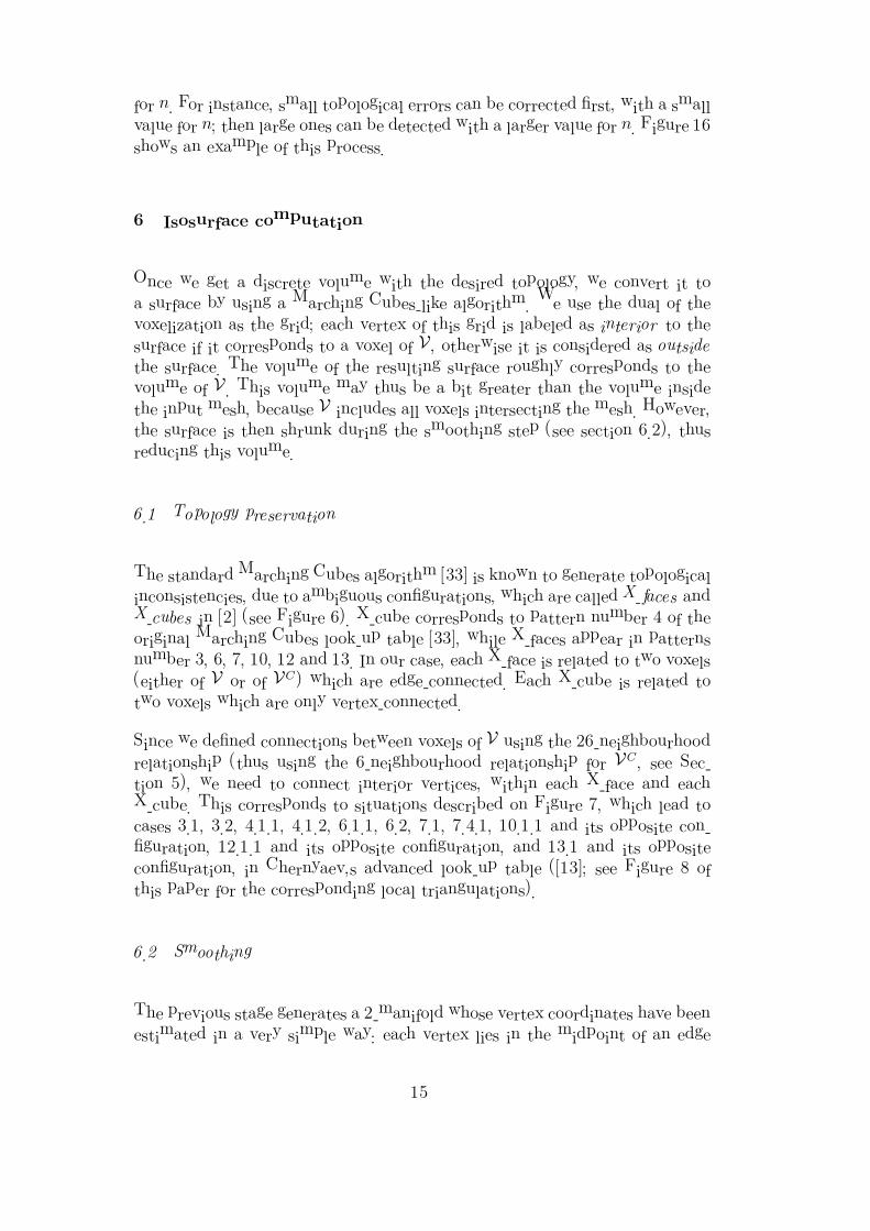
for n. For instance, small topological errors can be corrected first, with a smallvalue for n; then large ones can be detected with a larger value for n. Figure 16shows an example of this process.
6 Isosurface computation
Once we get a discrete volume with the desired topology, we convert it toa surface by using a Marching Cubes-like algorithm. We use the dual of thevoxelization as the grid; each vertex of this grid is labeled as interior to thesurface if it corresponds to a voxel of V , otherwise it is considered as outsidethe surface. The volume of the resulting surface roughly corresponds to thevolume of V . This volume may thus be a bit greater than the volume insidethe input mesh, because V includes all voxels intersecting the mesh. However,the surface is then shrunk during the smoothing step (see section 6.2), thusreducing this volume.
6.1 Topology preservation
The standard Marching Cubes algorithm [33] is known to generate topologicalinconsistencies, due to ambiguous configurations, which are called X-faces andX-cubes in [2] (see Figure 6). X-cube corresponds to pattern number 4 of theoriginal Marching Cubes look-up table [33], while X-faces appear in patternsnumber 3, 6, 7, 10, 12 and 13. In our case, each X-face is related to two voxels(either of V or of VC) which are edge-connected. Each X-cube is related totwo voxels which are only vertex-connected.
Since we defined connections between voxels of V using the 26-neighbourhoodrelationship (thus using the 6-neighbourhood relationship for VC , see Sec-tion 5), we need to connect interior vertices, within each X-face and eachX-cube. This corresponds to situations described on Figure 7, which lead tocases 3.1, 3.2, 4.1.1, 4.1.2, 6.1.1, 6.2, 7.1, 7.4.1, 10.1.1 and its opposite con-figuration, 12.1.1 and its opposite configuration, and 13.1 and its oppositeconfiguration, in Chernyaev’s advanced look-up table ([13]; see Figure 8 ofthis paper for the corresponding local triangulations).
6.2 Smoothing
The previous stage generates a 2-manifold whose vertex coordinates have beenestimated in a very simple way: each vertex lies in the midpoint of an edge
15
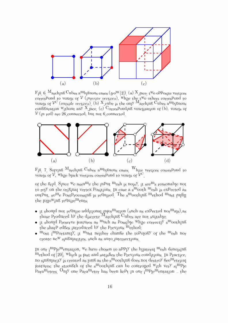
(a) (b) (c)
Fig. 6. Marching Cubes ambiguous cases (from [2]). (a) X-face: two opposite verticescorrespond to voxels of V (interior vertices), while the two others correspond tovoxels of VC (outside vertices). (b) X-cube is the only Marching Cubes ambiguousconfiguration without any X-face. (c) Corresponding voxelization of (b): voxels ofV (in red) are 26-connected, but not 6-connected.
(a) (b) (c) (d)
Fig. 7. Solving Marching Cubes ambiguous cases. White vertices correspond tovoxels of V, while black vertices correspond to voxels of VC .
of the grid. Since we assume the input mesh is noisy, it seems reasonable notto rely on the original vertex positions. In case a smooth mesh is expected asoutput, some postprocessing is required. The smoothing method must fulfillthe following requirements:
• it should not require additional information (such as expected normals),asthose produced by the discrete Marching Cubes are not suitable;
• it should preserve features as much as possible while correctly smoothingthe sharp edges introduced by the previous method;
• most importantly, it must neither change the topology of the mesh norcreate new singularities, such as auto-intersections.
In our implementation, we have chosen to apply the bilateral mesh denoisingmethod of [20], which is fast and satisfies the previous conditions. In practice,no singularity is created as long as the smoothing does not destroy geometricalfeatures; the strength of the smoothing can be controlled with very simpleparameters. Only one parameter has been kept in our implementation – the
16
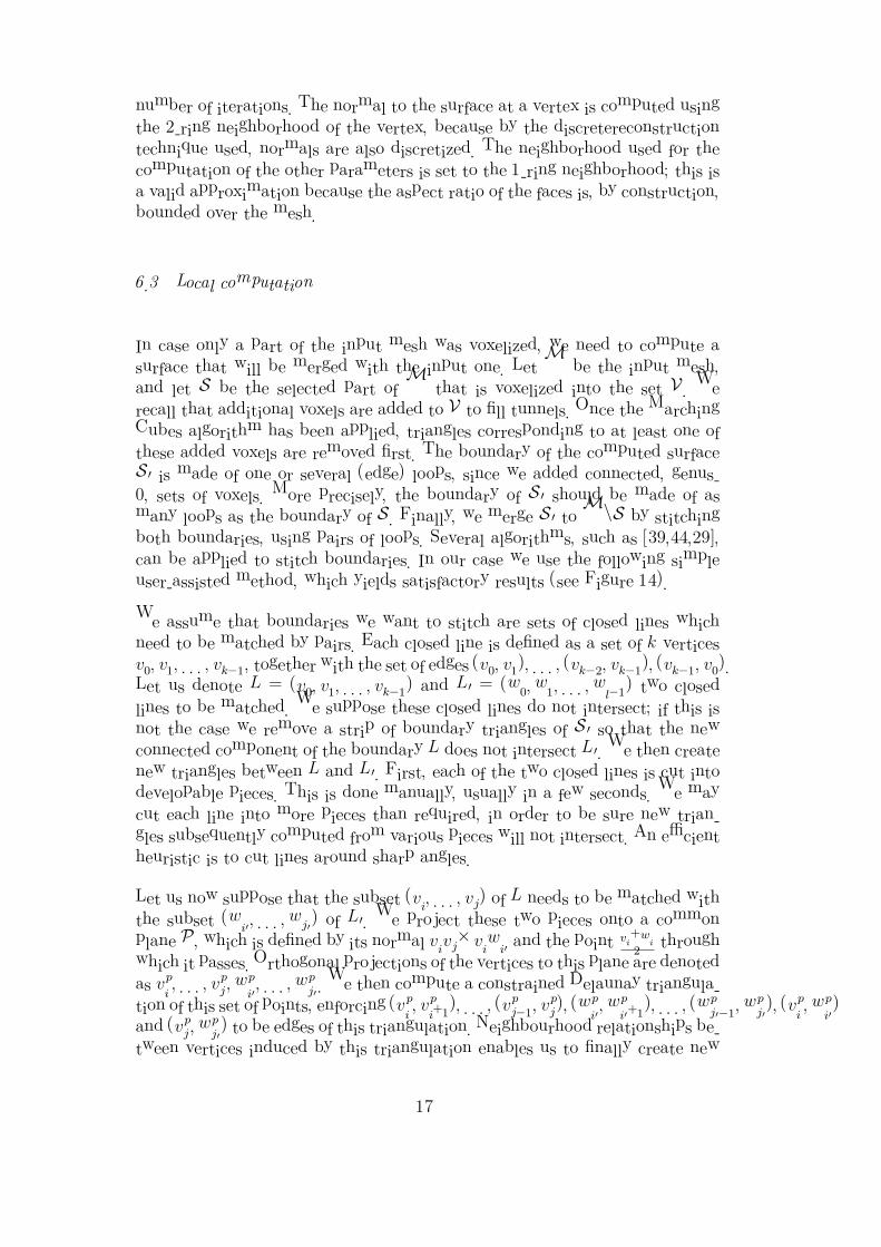
number of iterations. The normal to the surface at a vertex is computed usingthe 2-ring neighborhood of the vertex, because by the discretereconstructiontechnique used, normals are also discretized. The neighborhood used for thecomputation of the other parameters is set to the 1-ring neighborhood; this isa valid approximation because the aspect ratio of the faces is, by construction,bounded over the mesh.
6.3 Local computation
In case only a part of the input mesh was voxelized, we need to compute asurface that will be merged with the input one. Let M be the input mesh,and let S be the selected part of M that is voxelized into the set V . Werecall that additional voxels are added to V to fill tunnels. Once the MarchingCubes algorithm has been applied, triangles corresponding to at least one ofthese added voxels are removed first. The boundary of the computed surfaceS ′ is made of one or several (edge) loops, since we added connected, genus-0, sets of voxels. More precisely, the boundary of S ′ should be made of asmany loops as the boundary of S. Finally, we merge S ′ toM\S by stitchingboth boundaries, using pairs of loops. Several algorithms, such as [39,44,29],can be applied to stitch boundaries. In our case we use the following simpleuser-assisted method, which yields satisfactory results (see Figure 14).
We assume that boundaries we want to stitch are sets of closed lines whichneed to be matched by pairs. Each closed line is defined as a set of k verticesv0, v1, . . . , vk−1, together with the set of edges (v0, v1), . . . , (vk−2, vk−1), (vk−1, v0).Let us denote L = (v0, v1, . . . , vk−1) and L′ = (w0, w1, . . . , wl−1) two closedlines to be matched. We suppose these closed lines do not intersect; if this isnot the case we remove a strip of boundary triangles of S ′ so that the newconnected component of the boundary L does not intersect L′. We then createnew triangles between L and L′. First, each of the two closed lines is cut intodevelopable pieces. This is done manually, usually in a few seconds. We maycut each line into more pieces than required, in order to be sure new trian-gles subsequently computed from various pieces will not intersect. An efficientheuristic is to cut lines around sharp angles.
Let us now suppose that the subset (vi, . . . , vj) of L needs to be matched withthe subset (wi′ , . . . , wj′) of L′. We project these two pieces onto a commonplane P , which is defined by its normal vivj×viwi′ and the point
vi+wi
2through
which it passes. Orthogonal projections of the vertices to this plane are denotedas vp
i , . . . , vpj , w
pi′ , . . . , w
pj′ . We then compute a constrained Delaunay triangula-
tion of this set of points, enforcing (vpi , v
pi+1), . . . , (v
pj−1, v
pj ), (w
pi′ , w
pi′+1), . . . , (wp
j′−1, w
pj′), (v
pi , w
pi′)
and (vpj , w
pj′) to be edges of this triangulation. Neighbourhood relationships be-
tween vertices induced by this triangulation enables us to finally create new
17
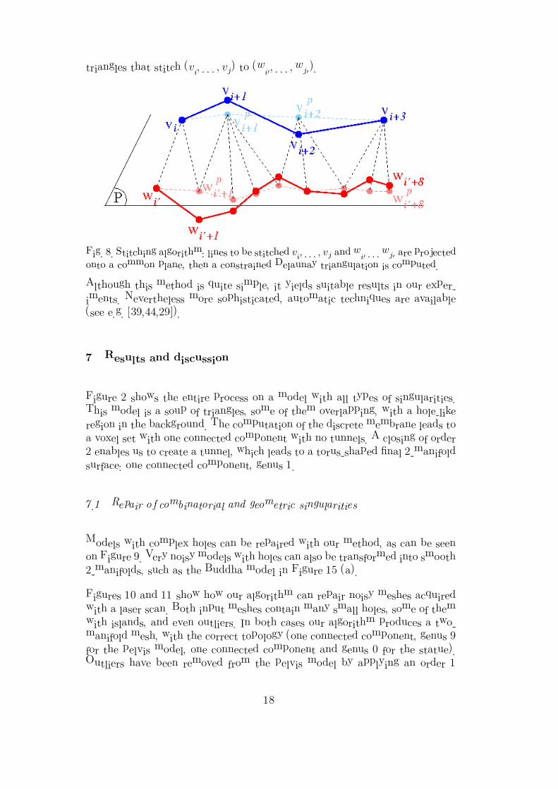
triangles that stitch (vi, . . . , vj) to (wi′ , . . . , wj′).
Fig. 8. Stitching algorithm: lines to be stitched vi, . . . , vj and wi′ . . . wj′ are projectedonto a common plane, then a constrained Delaunay triangulation is computed.
Although this method is quite simple, it yields suitable results in our exper-iments. Nevertheless more sophisticated, automatic techniques are available(see e.g. [39,44,29]).
7 Results and discussion
Figure 2 shows the entire process on a model with all types of singularities.This model is a soup of triangles, some of them overlapping, with a hole-likeregion in the background. The computation of the discrete membrane leads toa voxel set with one connected component with no tunnels. A closing of order2 enables us to create a tunnel, which leads to a torus-shaped final 2-manifoldsurface: one connected component, genus 1.
7.1 Repair of combinatorial and geometric singularities
Models with complex holes can be repaired with our method, as can be seenon Figure 9. Very noisy models with holes can also be transformed into smooth2-manifolds, such as the Buddha model in Figure 15 (a).
Figures 10 and 11 show how our algorithm can repair noisy meshes acquiredwith a laser scan. Both input meshes contain many small holes, some of themwith islands, and even outliers. In both cases our algorithm produces a two-manifold mesh, with the correct topology (one connected component, genus 9for the pelvis model, one connected component and genus 0 for the statue).Outliers have been removed from the pelvis model by applying an order 1
18
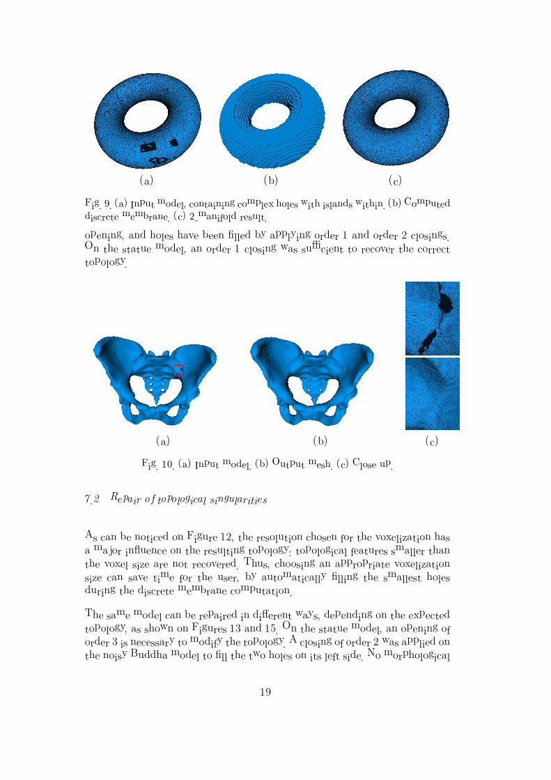
(a) (b) (c)
Fig. 9. (a) Input model, containing complex holes with islands within. (b) Computeddiscrete membrane. (c) 2-manifold result.
opening, and holes have been filled by applying order 1 and order 2 closings.On the statue model, an order 1 closing was sufficient to recover the correcttopology.
(a) (b) (c)
Fig. 10. (a) Input model. (b) Output mesh. (c) Close up.
7.2 Repair of topological singularities
As can be noticed on Figure 12, the resolution chosen for the voxelization hasa major influence on the resulting topology: topological features smaller thanthe voxel size are not recovered. Thus, choosing an appropriate voxelizationsize can save time for the user, by automatically filling the smallest holesduring the discrete membrane computation.
The same model can be repaired in different ways, depending on the expectedtopology, as shown on Figures 13 and 15. On the statue model, an opening oforder 3 is necessary to modify the topology. A closing of order 2 was applied onthe noisy Buddha model to fill the two holes on its left side. No morphological
19
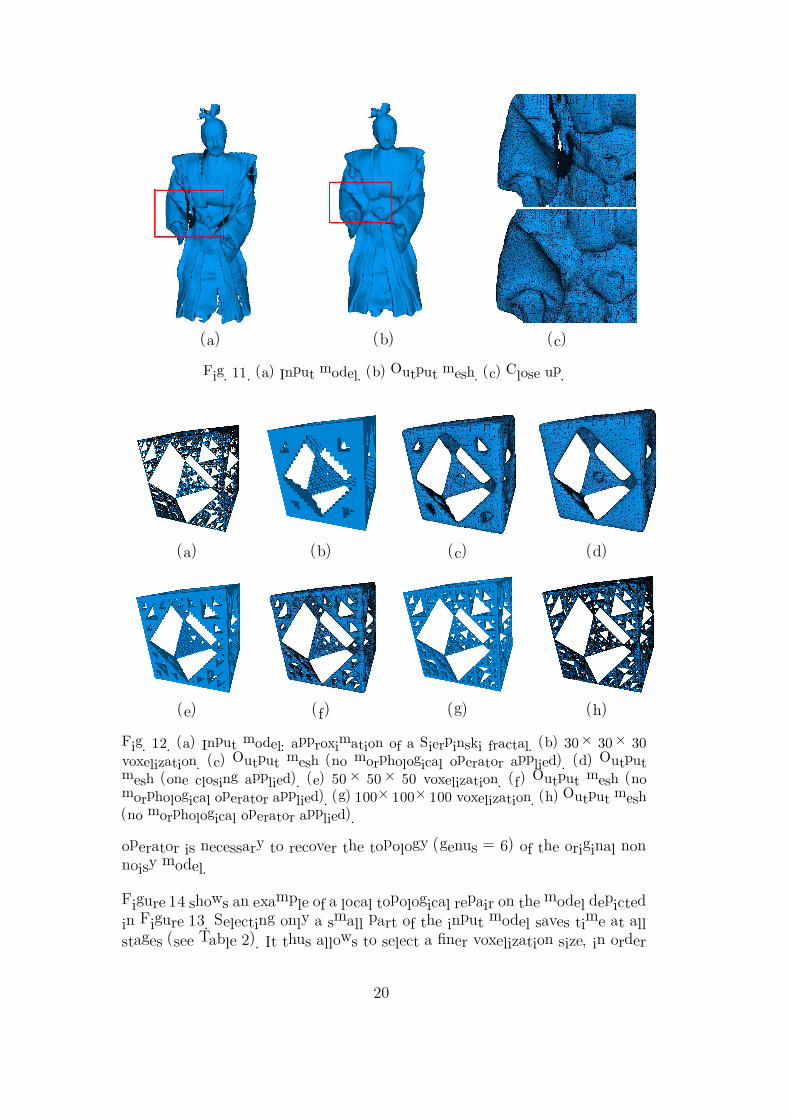
(a) (b) (c)
Fig. 11. (a) Input model. (b) Output mesh. (c) Close up.
(a) (b) (c) (d)
(e) (f) (g) (h)
Fig. 12. (a) Input model: approximation of a Sierpinski fractal. (b) 30 × 30 × 30voxelization. (c) Output mesh (no morphological operator applied). (d) Outputmesh (one closing applied). (e) 50 × 50 × 50 voxelization. (f) Output mesh (nomorphological operator applied). (g) 100×100×100 voxelization. (h) Output mesh(no morphological operator applied).
operator is necessary to recover the topology (genus = 6) of the original nonnoisy model.
Figure 14 shows an example of a local topological repair on the model depictedin Figure 13. Selecting only a small part of the input model saves time at allstages (see Table 2). It thus allows to select a finer voxelization size, in order
20
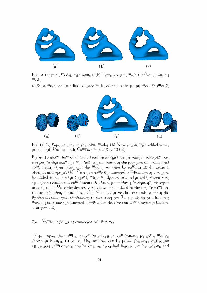
(a) (b) (c)
Fig. 13. (a) Input model, with genus 4. (b) Genus 3 output mesh. (c) Genus 1 outputmesh.
to get a more accurate final surface with respect to the initial mesh geometry.
(a) (b) (c) (d)
Fig. 14. (a) Selected zone on the input model. (b) Voxelization, with added voxelsin red. (c,d) Output mesh. Compare with Figure 13 (b).
Figure 16 shows how our method can be applied for interactive topology cor-rection. In this example, we merge all the bones of the foot into one connectedcomponent. After voxelizing the model, we start by computing the order 1opening and closing (b). We select some 6-connected components of voxels tobe added to the set (in yellow), while we discard others (in red). Green vox-els refer to connected components proposed for removal. Obviously, we selectnone of them. Once the desired voxels have been added to the set, we computethe order 2 opening and closing (c). Once again we choose to add some of theproposed connected components to the voxel set. This leads us to a final setmade of only one 6-connected component; thus we can now convert it back toa surface (d).
7.3 Number of critical connected components
Table 1 gives the number of computed critical components for some modelsshown in Figures 10 to 18. This number can be large, therefore inspectingall critical components one by one, as described before, can be tedious and
21
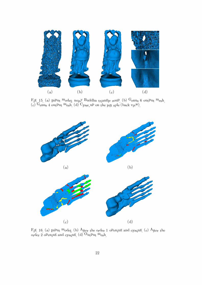
(a) (b) (c) (d)
Fig. 15. (a) Input model: noisy Buddha triangle soup. (b) Genus 6 output mesh.(c) Genus 4 output mesh. (d) Close-up on the left side (back view).
(a) (b)
(c) (d)
Fig. 16. (a) Input model. (b) After the order 1 opening and closing. (c) After theorder 2 opening and closing. (d) Output mesh.
22
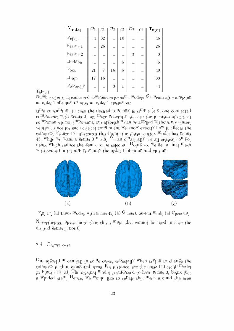
Model O1 C1 O2 C2 O3 C3Total
Pelvis 4 32 – 10 – – 46
Statue 1 – 26 – – – – 26
Statue 2 – – – – 3 – 3
Buddha – – – 5 – – 5
Foot 21 7 16 5 – – 49
Brain 17 16 – – – – 33
Paperclip – – 3 1 – – 4
Table 1Number of critical connected components for some models. O1 means after applyingan order 1 opening, C1 after an order 1 closing, etc.
time consuming. In case the desired topology is simple (e.g. one connectedcomponent with genus 0) or, more generally, in case the location of criticalcomponents is not important, our algorithm can be applied without user inter-vention, since for each critical component we know exactly how it affects thetopology. Figure 17 illustrates this point: the initial cortex model has genus45, while we want a genus 0 mesh. We automatically set all critical compo-nents which reduce the genus to be selected. Doing so, we get a final meshwith genus 0 after applying only the order 1 opening and closing.
(a) (b) (c)
Fig. 17. (a) Input model, with genus 45. (b) Genus 0 output mesh. (c) Close up.
Nevertheless, please note that this simple idea cannot be used in case thedesired genus is not 0.
7.4 Failure case
Our algorithm can fail in some cases, especially when trying to change thetopology in thin, elongated areas. For instance, see the noisy paperclip modelin Figure 18 (a). The original model is supposed to have genus 0, being justa winded stem. Hence, we would like to repair this mesh around the area
23
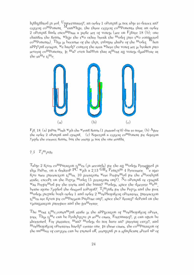
highlighted in red. Unfortunately, an order 1 opening is not able to detect anycritical component. Meanwhile, the three critical components that an order2 opening finds encompass a large set of voxels (see on Figure 18 (b); onechanges the genus, while the two other break the model into two connectedcomponents). This is because of the thin, tubular shape of the model. Whenapplying erosion, we hardly control the area where the voxel set is broken intoseveral components. It may even happen that almost all voxels disappear atthe same time.
(a) (b) (c)
Fig. 18. (a) Input mesh with the wrong genus (1 instead of 0) due to noise. (b) Afterthe order 2 opening and closing. (c) Selecting a critical component for deletionyields the correct genus, but the result is not the one sought.
7.5 Timings
Table 2 gives computation times (in seconds) for the all models presented inthis paper, on a desktop PC with a 2.13 GHz Pentium 4 processor. We alsogive user interaction times. 10 iterations were performed for the smoothingstage, except on the pelvis model (5 iterations only). No opening or closingwas performed for the torus and the bunny models, since the discrete mem-brane alone yielded the desired topology. Timings for the pelvis and the footmodels include both order 1 and order 2 morphological operators. Interactiontimes are given for comparison purpose only, since they greatly depend on thevisualization interface and the framerate.
The most time-consuming stage is the application of morphological opera-tors. This time can be prohibitive in some cases. Fortunately, it can often beshortened. For instance, many models do not have any internal cavity, andmorphological operators hardly create one. In these cases, the computation ofthe number of cavities can be turned off, resulting in a significant speed up of
24
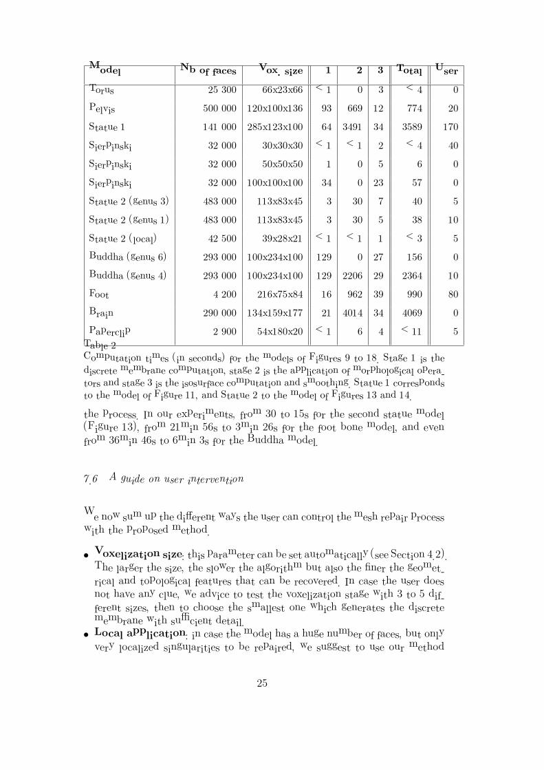
Model Nb of faces Vox. size 1 2 3 Total User
Torus 25 300 66x23x66 < 1 0 3 < 4 0
Pelvis 500 000 120x100x136 93 669 12 774 20
Statue 1 141 000 285x123x100 64 3491 34 3589 170
Sierpinski 32 000 30x30x30 < 1 < 1 2 < 4 40
Sierpinski 32 000 50x50x50 1 0 5 6 0
Sierpinski 32 000 100x100x100 34 0 23 57 0
Statue 2 (genus 3) 483 000 113x83x45 3 30 7 40 5
Statue 2 (genus 1) 483 000 113x83x45 3 30 5 38 10
Statue 2 (local) 42 500 39x28x21 < 1 < 1 1 < 3 5
Buddha (genus 6) 293 000 100x234x100 129 0 27 156 0
Buddha (genus 4) 293 000 100x234x100 129 2206 29 2364 10
Foot 4 200 216x75x84 16 962 39 990 80
Brain 290 000 134x159x177 21 4014 34 4069 0
Paperclip 2 900 54x180x20 < 1 6 4 < 11 5
Table 2Computation times (in seconds) for the models of Figures 9 to 18. Stage 1 is thediscrete membrane computation, stage 2 is the application of morphological opera-tors and stage 3 is the isosurface computation and smoothing. Statue 1 correspondsto the model of Figure 11, and Statue 2 to the model of Figures 13 and 14.
the process. In our experiments, from 30 to 15s for the second statue model(Figure 13), from 21min 56s to 3min 26s for the foot bone model, and evenfrom 36min 46s to 6min 3s for the Buddha model.
7.6 A guide on user intervention
We now sum up the different ways the user can control the mesh repair processwith the proposed method.
• Voxelization size: this parameter can be set automatically (see Section 4.2).The larger the size, the slower the algorithm but also the finer the geomet-rical and topological features that can be recovered. In case the user doesnot have any clue, we advice to test the voxelization stage with 3 to 5 dif-ferent sizes, then to choose the smallest one which generates the discretemembrane with sufficient detail.
• Local application: in case the model has a huge number of faces, but onlyvery localized singularities to be repaired, we suggest to use our method
25
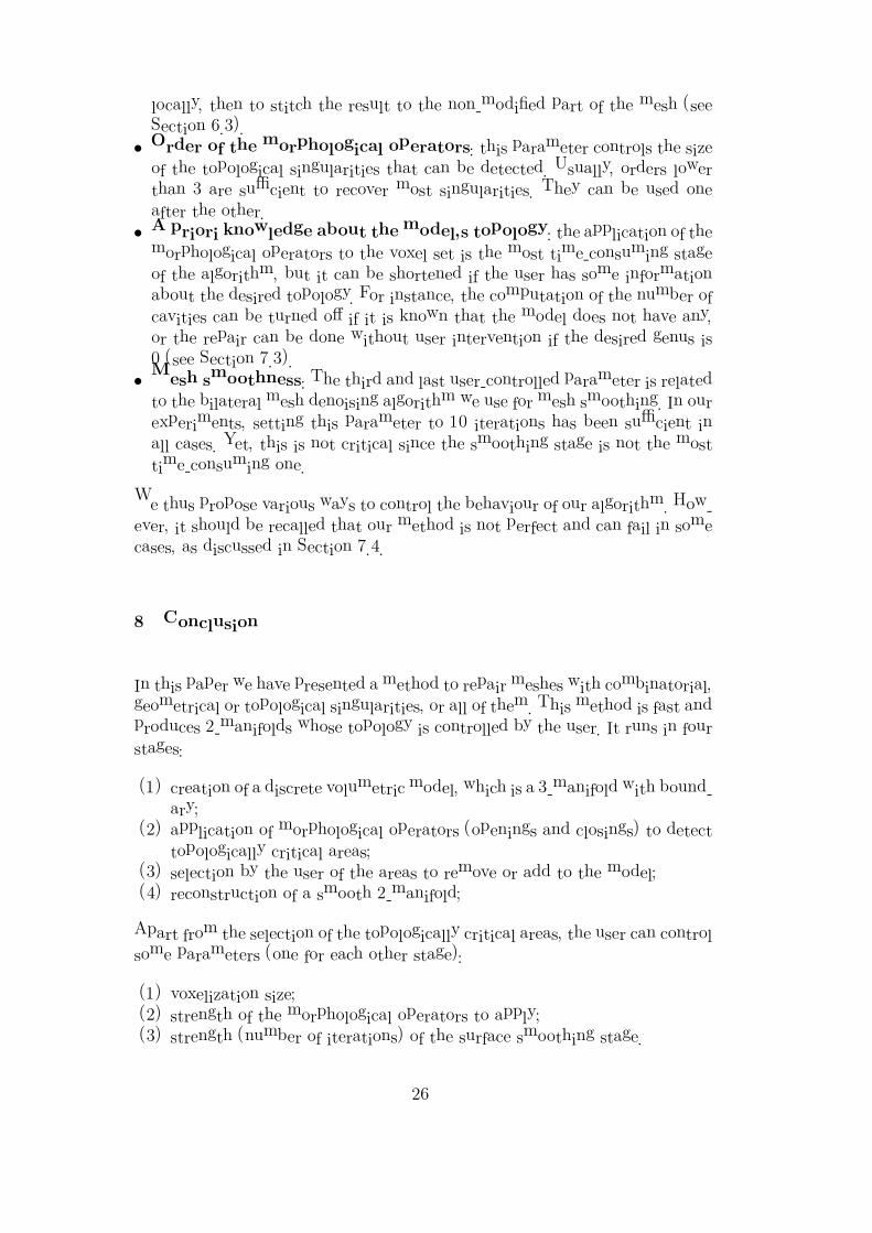
locally, then to stitch the result to the non-modified part of the mesh (seeSection 6.3).
• Order of the morphological operators: this parameter controls the sizeof the topological singularities that can be detected. Usually, orders lowerthan 3 are sufficient to recover most singularities. They can be used oneafter the other.
• A priori knowledge about the model’s topology: the application of themorphological operators to the voxel set is the most time-consuming stageof the algorithm, but it can be shortened if the user has some informationabout the desired topology. For instance, the computation of the number ofcavities can be turned off if it is known that the model does not have any,or the repair can be done without user intervention if the desired genus is0 (see Section 7.3).
• Mesh smoothness: The third and last user-controlled parameter is relatedto the bilateral mesh denoising algorithm we use for mesh smoothing. In ourexperiments, setting this parameter to 10 iterations has been sufficient inall cases. Yet, this is not critical since the smoothing stage is not the mosttime-consuming one.
We thus propose various ways to control the behaviour of our algorithm. How-ever, it should be recalled that our method is not perfect and can fail in somecases, as discussed in Section 7.4.
8 Conclusion
In this paper we have presented a method to repair meshes with combinatorial,geometrical or topological singularities, or all of them. This method is fast andproduces 2-manifolds whose topology is controlled by the user. It runs in fourstages:
(1) creation of a discrete volumetric model, which is a 3-manifold with bound-ary;
(2) application of morphological operators (openings and closings) to detecttopologically critical areas;
(3) selection by the user of the areas to remove or add to the model;(4) reconstruction of a smooth 2-manifold;
Apart from the selection of the topologically critical areas, the user can controlsome parameters (one for each other stage):
(1) voxelization size;(2) strength of the morphological operators to apply;(3) strength (number of iterations) of the surface smoothing stage.
26
Even if this method is better suited for smooth models because of the finalsmoothing stage, it has no requirement of the input model, which can be assimple as a triangle soup. A local application of this algorithm is possible, incase most parts of the input mesh do not need repair. It speeds up computa-tion, but needs the user to cleverly select the area to repair.
Possible enhancements of this work include:
• trying to use an octree for the first stage, to speed up the computation ofthe final voxel set, especially in case the whole input model is selected forrepair;
• investigating ways to better control the size and shape of computed topo-logically critical components;
• developing methods to automatically display these components from rele-vant viewpoints in the visualization interface;
• modifying the surface reconstruction stage in order to possibly fit somegeometrical features of the input model, if the user wants to (e.g. sharpedges). This could be done by using the exact intersection point betweenthe input model and each edge of the grid, instead of the midpoint of theedge. This can only be done when this intersection point is available andreliable; the key issue is to find when it is the case.
Acknowledgements
Part of this work was done while the first author was visiting the UniversitatPolitecnica de Catalunya in Barcelona with a Lavoisier grant from FrenchMinistry of Foreign Affairs. The Buddha model is courtesy of the Stanford3D Scanning Repository, the hip model is courtesy of Cyberware, and thepelvis, statue and brain models are courtesy of the AIM@SHAPE DigitalShape WorkBench. The authors would like to thank the anonymous reviewersfor their valuable comments, which helped greatly improve the paper, andNassim Jibai and Kartic Subr for proof-reading.
References
[1] Andujar C, Brunet P, Ayala D. Topology-reducing surface simplification usinga discrete solid representation. ACM Transactions on Graphics 2002; 21(2):88–105.
[2] Andujar C, Brunet P, Chica A, Navazo I, Rossignac J, Vinacua A. Optimizingthe topological and combinatorial complexity of isosurfaces. Computer-Aided
27
Design 2005; 37(8):847–857.
[3] Andujar C, Brunet P, Fairen M, Cebollada V. Error-Bounded Simplificationof Topologically-Complex Assemblies. Workshop on Multiresolution andGeometric Modelling 2003, p. 355–366.
[4] Attene M, Falcidieno B. ReMESH: an interactive environment to edit and repairtriangle meshes. Proceedings of the IEEE International Conference on ShapeModeling and Applications (SMI) 2006, p. 271-276.
[5] Attene M. A lightweight approach to repairing digitized polygon meshes. TheVisual Computer 2010; 26.
[6] Barequet G, Duncan C, Kumar S. RSVP: a geometric toolkit for controlledrepair of solid models. IEEE Transactions on Visualization and ComputerGraphics 1998; 4(2):162–177.
[7] Bischoff S, Kobbelt L. Isosurface reconstruction with topology control.Proceedings of Pacific Graphics 2002, p. 246–255.
[8] Bischoff S, Kobbelt L. Structure preserving CAD model repair. ComputerGraphics Forum (Eurographics Proceedings) 2005; 24(3):527–536.
[9] Bischoff S, Pavic D, Kobbelt L. Automatic restoration of polygon models. ACMTransactions on Graphics 2005; 24(4):1332–1352.
[10] Borodin P, Novotni M, Klein R. Progressive gap closing for mesh repairing.Advances in Modelling, Animation and Rendering, Springer-Verlag; 2002, p.201–213.
[11] Botsch M, Pauly M, Kobbelt L, Alliez P, Levy B, Bischoff S, Rossl C. Geometricmodeling based on polygonal meshes. SIGGRAPH 2007 Course Notes.
[12] Campen M, Kobbelt L. Exact and robust (self-)intersections for polygonalmeshes. Computer Graphics Forum (Eurographics Proceedings) 2010; 29(3).
[13] Chernyaev EV. Marching Cubes 33: construction of topologically correctisosurfaces. Technical Report CERN CN 95-17, CERN, 1995.
[14] Cormen T, Leiserson C, Rivest R, Stein C. Introduction to algorithms, 2ndedition. MIT Press, 2001.
[15] Davis J, Marschner SR, Garr M, Levoy M. Filling holes in complex surfacesusing volumetric diffusion. Proceedings of the Symposium on 3D DataProcessing, Visualization, and Transmission 2002; p. 428–438.
[16] Dey TK, Guha S. Computing homology groups of simplicial complexes in R3.
Journal of the ACM 1998; 45:266–287.
[17] Eisemann E, Decoret X. Single-pass GPU solid voxelization for real-timeapplications. Proceedings of Graphics Interface 2008; p. 73–80.
[18] El Sana J, Varshney A. Topology simplification for polygonal virtualenvironments. IEEE Transactions on Visualization and Computer Graphics1998;4(2):133–144.
28
[19] Esteve J, Brunet P, Vinacua A. Approximation of a cloud of points by shrinkinga discrete membrane. Computer Graphics Forum 2005; 24(4):791–807.
[20] Fleishman S, Drori I, Cohen-Or D. Bilateral mesh denoising. ACM Transactionson Graphics (SIGGRAPH Proceedings) 2003; 22(3):950–3.
[21] Friedman J. Computing Betti numbers via combinatorial Laplacians.Algorithmica 1998; 21(4):331–346.
[22] Gueziec A, Taubin G, Lazarus F, Horn W. Cutting and stitching: convertingsets of polygons to manifold surfaces. IEEE Transactions on Visualization andComputer Graphics 2001; 7(2):136–151.
[23] Guskov I, Wood Z. Topological noise removal. Proceedings of Graphics Interface2001; p. 19–26.
[24] Haumont D, Warzee N. Complete polygonal scene voxelization. Journal ofGraphics Tools 2002; 7(3):27–41.
[25] Ju T. Robust repair of polygonal models. ACM Transactions on Graphics(SIGGRAPH Proceedings) 2004; 23(3):888–895.
[26] Ju T. Fixing geometric errors on polygonal models: a survey. Journal ofComputer Science and Technology, 2009; 24(1):19–29.
[27] Ju T, Zhou QY, Hu SM. Editing the topology of 3D models by sketching. ACMTransactions on Graphics (SIGGRAPH Proceedings) 2007; 26(3):42.
[28] Kriegeskorte N, Goebel R. An efficient algorithm for topologically correctsegmentation of the cortical sheet in anatomical MR volumes. NeuroImage 2001;14:329–346.
[29] Lai HC, Lai JY. A partial mesh replacement technique for design modificationin rapid prototyping. Computers and Industrial Engineering 2009.
[30] Lee CN, Poston T, Rosenfeld A. Holes and genus of 2d and 3d digital images.Graphical Models and Image Processing 1993; 55(1):20–47.
[31] Li X, Han CY, Wee W. On surface reconstruction: a priority driven approach.Computer-Aided Design 2009;41(9):626–640.
[32] Liepa P. Filling holes in meshes. Proceedings of the Eurographics/ACMSIGGRAPH Symposium on Geometry Processing 2003; p. 200–5.
[33] Lorensen W, Cline H. Marching cubes: a high resolution 3D surface constructionalgorithm. Computer Graphics (SIGGRAPH Proceedings) 1987; 21(4):163–170.
[34] Min P. [binvox] 3D mesh voxelizer. http://www.cs.princeton.edu/∼min/
binvox/. Accessed Sept. 3rd, 2009.
[35] Murali T, Funkhouser T. Consistent solid and boundary representations fromarbitrary polygonal data. Proceedings of the Symposium on Interactive 3DGraphics 1997; p. 155–162.
29
[36] Nooruddin FS, Turk G. Simplification and repair of polygonal models usingvolumetric techniques. IEEE Transactions on Visualization and ComputerGraphics 2003; 9(2):191–205.
[37] Pauly M, Mitra NJ, Wallner J, Pottmann H, Guibas L. Discovering structuralregularity in 3D geometry. ACM Transactions on Graphics (SIGGRAPHProceedings) 2008; 27(3).
[38] Podolak J, Rusinkiewicz S. Atomic volumes for mesh completion. Proceedingsof the Eurographics/ACM SIGGRAPH Symposium on Geometry Processing2005; p. 33–42.
[39] Rocchini C, Cignoni P, Ganovelli F, Montani C, Pingi P, Scopigno R.The Marching Intersections algorithm for merging range images. The VisualComputer 2004; 20:149–164.
[40] Rossignac J, Cardoze D. Matchmaker: manifold B-Reps for non-manifold r-sets.Proceedings of the ACM Symposium on Solid Modeling and Applications 1999;p. 31–41.
[41] Sharf A, Alexa M, Cohen-Or D. Context-based surface completion. ACMTransactions on Graphics (SIGGRAPH Proceedings) 2004; 23(3):878–887.
[42] Verdera J, Caselles V, Bertalmıo M, Sapiro G. Inpainting surface holes.Proceedings of the IEEE International Conference on Image Processing 2003;p. 903–6.
[43] Wood Z, Hoppe H, Desbrun M, Schroder P. Removing excess topology fromisosurfaces. ACM Transactions on Graphics 2004; 23(2):190–208.
[44] Zaharescu A, Boyer E, Horaud R. TransforMesh: A topology-adaptive mesh-based approach to surface evolution. Proceedings of the Asian Conference onComputer Vision 2007; LNCS 4844:166–175.
[45] Zhou QY, Ju T, Hu SM. Topology repair of solid models using skeletons. IEEETransactions on Visualization and Computer Graphics 2007; 13(4):675–685.
30
A.2. AN ITERATIVE ALGORITHM FOR HOMOLOGY COMPUTATION ONSIMPLICIAL SHAPES 101
∴
A.2 AN ITERATIVE ALGORITHM FOR HOMOLOGYCOMPUTATION ON SIMPLICIAL SHAPES
Dobrina Boltcheva, David Canino, Sara Merino Aceituno, Jean-Claude Léon,Leila De Floriani, Franck Hétroy
Computer-Aided Design 43 (11), Elsevier, 2011. Presented at the SIAM Conferenceon Geometric & Physical Modeling (GD/SPM) 2011.

102 APPENDIX A. SELECTED PAPERS
An iterative algorithm for homology computation on simplicial shapes
Dobrina Boltchevaa,∗, David Caninob, Sara Merino Aceitunoa, Jean-Claude Leona, Leila De Florianib, Franck Hetroya
aGrenoble University, Laboratoire Jean Kuntzmann, INRIA, 655, av. de l’Europe, 38334, Montbonnot, FrancebUniversity of Genova, Department of Computer Science, Via Dodecaneso, 35, 16146, Genova, Italy
Abstract
We propose a new iterative algorithm for computing the homology of arbitrary shapes discretized through simplicialcomplexes, We demonstrate how the simplicial homology of a shape can be effectively expressed in terms of the homologyof its sub-components. The proposed algorithm retrieves the complete homological information of an input shapeincluding the Betti numbers, the torsion coefficients and the representative homology generators.
To the best of our knowledge, this is the first algorithm based on the constructive Mayer-Vietoris sequence, whichrelates the homology of a topological space to the homologies of its sub-spaces, i.e. the sub-components of the inputshape and their intersections. We demonstrate the validity of our approach through a specific shape decomposition,based only on topological properties, which minimizes the size of the intersections between the sub-components andincreases the efficiency of the algorithm.
Keywords: computational topology; simplicial complexes; shape decomposition; Z-homology; Mayer-Vietoris sequence;generators
1. Introduction
Recently, the problem of computing the topological fea-tures of a shape has drawn much attention because of itsapplications in several disciplines, including shape analy-sis and understanding, shape retrieval, and finite elementanalysis [15, 20, 38]. Unlike geometric features (such ascurvature) which are only invariant under rigid transfor-mations, topological features are invariant under contin-uous deformations. Thus, they provide global quantita-tive and qualitative information about a shape, such asthe number of its connected components, the number ofholes and tunnels. Topological features are the core de-scriptors to extend geometric modelers with non-manifoldshapes processing. For instance, the generation of sim-ulation models still lacks capabilities for processing non-manifold shapes, like idealized representations [36]. Homo-logical information on arbitrary shapes can strongly sup-port new modeling capabilities, because constructive mod-eling techniques are often used. Also, topological featuresare especially important in high dimensional data analysis,where pure geometric tools are usually not sufficient.
The most common way to discretize a shape is through asimplicial complex. Simplicial complexes are easy to con-struct and manipulate, and compact data structures have
∗Corresponding authorEmail addresses: [email protected] (Dobrina
Boltcheva), [email protected] (David Canino),[email protected] (Sara Merino Aceituno),[email protected] (Jean-Claude Leon),[email protected] (Leila De Floriani),[email protected] (Franck Hetroy)
been developed to encode them efficiently [7]. Simplicialhomology is one of the most useful and algorithmicallycomputable topological invariants. It characterizes a sim-plicial complex of dimension n through the notion of ho-mological descriptor. Homological descriptors are definedin any dimension k ≤ n and are related to the non-trivialk-cycles in the complex which have intuitive geometricalinterpretations up to dimension 2. In dimension 0, theyare related to the connected components of the complex,in dimension 1, to the tunnels and the holes, and in di-mension 2, to the shells surrounding voids or cavities.
Here, we propose a new algorithmic approach for ho-mology computation on arbitrary shapes represented byfinite simplicial complexes. Our framework is based onthe constructive homology theory discussed in [32, 34, 33].It provides a tool, the constructive Mayer-Vietoris se-quence, which offers an elegant way for computing thehomology of a simplicial complex from the homology ofits sub-complexes and of their intersections. This leads toa modular algorithm for homology computation, that wecall Mayer-Vietoris (MV) algorithm. Here, we show thatour algorithm is more efficient than the classical one basedon the reduction of the incidence matrices to a canonicalform, known as the Smith Normal Form (SNF) [1, 30].
We demonstrate the validity of our approach througha decomposition of an n-dimensional simplicial complex,called the Manifold-Connected (MC) decomposition andproposed in [26] for 2-dimensional simplicial complexes. Inour experiments, we demonstrate that the MC decompo-sition minimizes the size of the intersection between sub-complexes, and, thus, it is especially useful for the homol-
Preprint submitted to Elsevier July 29, 2011
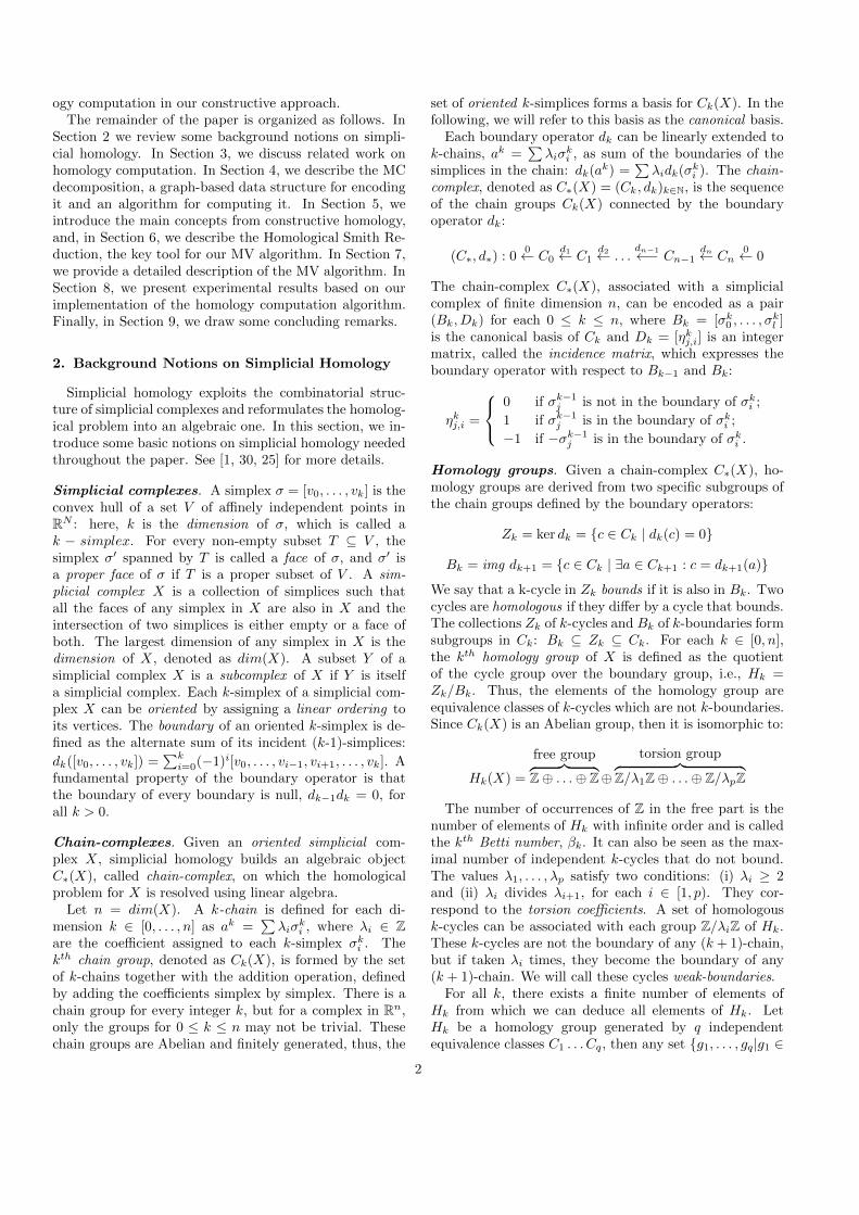
ogy computation in our constructive approach.The remainder of the paper is organized as follows. In
Section 2 we review some background notions on simpli-cial homology. In Section 3, we discuss related work onhomology computation. In Section 4, we describe the MCdecomposition, a graph-based data structure for encodingit and an algorithm for computing it. In Section 5, weintroduce the main concepts from constructive homology,and, in Section 6, we describe the Homological Smith Re-duction, the key tool for our MV algorithm. In Section 7,we provide a detailed description of the MV algorithm. InSection 8, we present experimental results based on ourimplementation of the homology computation algorithm.Finally, in Section 9, we draw some concluding remarks.
2. Background Notions on Simplicial Homology
Simplicial homology exploits the combinatorial struc-ture of simplicial complexes and reformulates the homolog-ical problem into an algebraic one. In this section, we in-troduce some basic notions on simplicial homology neededthroughout the paper. See [1, 30, 25] for more details.
Simplicial complexes. A simplex σ = [v0, . . . , vk] is theconvex hull of a set V of affinely independent points inRN : here, k is the dimension of σ, which is called ak − simplex. For every non-empty subset T ⊆ V , thesimplex σ′ spanned by T is called a face of σ, and σ′ isa proper face of σ if T is a proper subset of V . A sim-plicial complex X is a collection of simplices such thatall the faces of any simplex in X are also in X and theintersection of two simplices is either empty or a face ofboth. The largest dimension of any simplex in X is thedimension of X , denoted as dim(X). A subset Y of asimplicial complex X is a subcomplex of X if Y is itselfa simplicial complex. Each k-simplex of a simplicial com-plex X can be oriented by assigning a linear ordering toits vertices. The boundary of an oriented k-simplex is de-fined as the alternate sum of its incident (k-1)-simplices:
dk([v0, . . . , vk]) =∑k
i=0(−1)i[v0, . . . , vi−1, vi+1, . . . , vk]. Afundamental property of the boundary operator is thatthe boundary of every boundary is null, dk−1dk = 0, forall k > 0.
Chain-complexes. Given an oriented simplicial com-plex X , simplicial homology builds an algebraic objectC∗(X), called chain-complex, on which the homologicalproblem for X is resolved using linear algebra.
Let n = dim(X). A k-chain is defined for each di-mension k ∈ [0, . . . , n] as ak =
∑λiσ
ki , where λi ∈ Z
are the coefficient assigned to each k-simplex σki . The
kth chain group, denoted as Ck(X), is formed by the setof k-chains together with the addition operation, definedby adding the coefficients simplex by simplex. There is achain group for every integer k, but for a complex in Rn,only the groups for 0 ≤ k ≤ n may not be trivial. Thesechain groups are Abelian and finitely generated, thus, the
set of oriented k-simplices forms a basis for Ck(X). In thefollowing, we will refer to this basis as the canonical basis.
Each boundary operator dk can be linearly extended tok-chains, ak =
∑λiσ
ki , as sum of the boundaries of the
simplices in the chain: dk(ak) =∑
λidk(σki ). The chain-
complex, denoted as C∗(X) = (Ck, dk)k∈N, is the sequenceof the chain groups Ck(X) connected by the boundaryoperator dk:
(C∗, d∗) : 00← C0
d1← C1d2← . . .
dn−1←− Cn−1dn← Cn
0← 0
The chain-complex C∗(X), associated with a simplicialcomplex of finite dimension n, can be encoded as a pair(Bk, Dk) for each 0 ≤ k ≤ n, where Bk = [σk
0 , . . . , σkl ]
is the canonical basis of Ck and Dk = [ηkj,i] is an integer
matrix, called the incidence matrix, which expresses theboundary operator with respect to Bk−1 and Bk:
ηkj,i =
0 if σk−1j is not in the boundary of σk
i ;
1 if σk−1j is in the boundary of σk
i ;
−1 if −σk−1j is in the boundary of σk
i .
Homology groups. Given a chain-complex C∗(X), ho-mology groups are derived from two specific subgroups ofthe chain groups defined by the boundary operators:
Zk = ker dk = c ∈ Ck | dk(c) = 0
Bk = img dk+1 = c ∈ Ck | ∃a ∈ Ck+1 : c = dk+1(a)We say that a k-cycle in Zk bounds if it is also in Bk. Twocycles are homologous if they differ by a cycle that bounds.The collections Zk of k-cycles and Bk of k-boundaries formsubgroups in Ck: Bk ⊆ Zk ⊆ Ck. For each k ∈ [0, n],the kth homology group of X is defined as the quotientof the cycle group over the boundary group, i.e., Hk =Zk/Bk. Thus, the elements of the homology group areequivalence classes of k-cycles which are not k-boundaries.Since Ck(X) is an Abelian group, then it is isomorphic to:
Hk(X) =
free group︷ ︸︸ ︷Z⊕ . . .⊕ Z⊕
torsion group︷ ︸︸ ︷Z/λ1Z⊕ . . .⊕ Z/λpZ
The number of occurrences of Z in the free part is thenumber of elements of Hk with infinite order and is calledthe kth Betti number, βk. It can also be seen as the max-imal number of independent k-cycles that do not bound.The values λ1, . . . , λp satisfy two conditions: (i) λi ≥ 2and (ii) λi divides λi+1, for each i ∈ [1, p). They cor-respond to the torsion coefficients. A set of homologousk-cycles can be associated with each group Z/λiZ of Hk.These k-cycles are not the boundary of any (k + 1)-chain,but if taken λi times, they become the boundary of any(k + 1)-chain. We will call these cycles weak-boundaries.
For all k, there exists a finite number of elements ofHk from which we can deduce all elements of Hk. LetHk be a homology group generated by q independentequivalence classes C1 . . . Cq, then any set g1, . . . , gq|g1 ∈
2
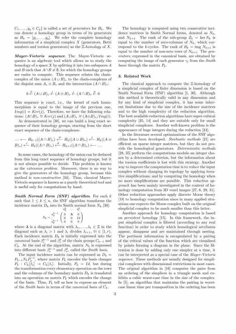
C1, . . . , gq ∈ Cq is called a set of generators for Hk. Wecan denote a homology group in terms of its generatorsas Hk = [g1, . . . , gq]. We refer the complete homologyinformation of a simplicial complex X (generators, Bettinumbers and torsion generators) as the Z-homology of X .
Mayer-Vietoris sequence. The Mayer-Vietoris se-quence is an algebraic tool which allows us to study thehomology of a space X by splitting it into two subspaces Aand B such that A∩B 6= ∅, for which the homology groupsare easier to compute. This sequence relates the chain-complex of the union (A ∪ B)∗ to the chain-complexes ofthe disjoint sum A∗ ⊕B∗ and the intersection (A ∩B)∗:
00← (A ∪B)∗
j← (A⊕B)∗i← (A ∩B)∗
0← 0
This sequence is exact, i.e., the kernel of each homo-morphism is equal to the image of the previous one,Img(i) = Ker(j). Therefore, we have the following rela-tions: (A∩B)∗ ∼= Ker(j) and (A∪B)∗ ∼= (A⊕B)∗/Img(i).
As demonstrated in [30], we can build a long exact se-quence of their homology groups, starting from the shortexact sequence of the chain-complexes:
. . . ←− Hk−1((A ∩ B)∗)∂←− Hk((A ∪ B)∗)
j←− Hk((A ⊕B)∗)
i←− Hk((A ∩B)∗)∂←− Hk+1((A ∩B)∗)←− . . .
In some cases, the homology of the union can be deducedfrom this long exact sequence of homology groups, but itis not always possible to decide. This problem is knownas the extension problem. Moreover, there is no way togive the generators of the homology group, because thismethod is non-constructive [34]. Thus, classical Mayer-Vietoris sequence is known as a purely theoretical tool andis useful only for computations by hand.
Smith Normal Form (SNF) algorithm. For each ksuch that 1 ≤ k ≤ n, the SNF algorithm transforms theincidence matrix Dk into its Smith normal form Nk [30]:
Nk =
0
@
sk0 . . . sk
l
sk−10 0 λ 0
: 0 0 Idsk−1p 0 0 0
1
A
where λ is a diagonal matrix with λr, . . . , λ1 ∈ Z in thediagonal such as λi > 1 and λi divides λi+1, ∀i ∈ [1, r).Each incidence matrix Dk is initially expressed into thecanonical basis βk−1
c and βkc of the chain groups Ck−1 and
Ck. At the end of the algorithm, matrix Nk is expressedinto different basis βk−1
s and βks , called the Smith basis.
The input incidence matrix can be expressed as Dk =Pk−1NkP−1
k , where matrix Pk encodes the basis changesPk : Ck[βs] → Ck[βc]. Initially, Pk = Id, but duringthe transformation every elementary operation on the rowsand the columns of the boundary matrix Dk is translatedinto an operation on matrix Pk which encodes the changeof the basis. Thus, Pk tell us how to express an elementof the Smith basis in terms of the canonical basis of Ck.
The homology is computed using two consecutive inci-dence matrices in Smith Normal forms, denoted as Nk,and Nk+1. The rank of the sub-group Zk = kerNk isequal to the number of zero-columns of Nk, which cor-respond to the k-cycles. The rank of Bk = img Nk+1 isequal to the number of non-zero rows of Nk+1. The gen-erators, expressed in the canonical basis, are obtained bycomputing the image of each generator γi from the Smithbasis through the matrix Pk.
3. Related Work
The classical approach to compute the Z-homology ofa simplicial complex of finite dimension is based on theSmith Normal Form (SNF) algorithm [1, 30]. Althoughthis method is theoretically valid in any dimension andfor any kind of simplicial complex, it has some inher-ent limitations due to the size of the incidence matricesand to the high complexity of the reduction algorithm.The best available reduction algorithms have super-cubicalcomplexity [35, 14] and they are suitable only for smallsimplicial complexes. Another well-known problem is theappearance of huge integers during the reduction [24].
In the literature several optimizations of the SNF algo-rithm have been developed. Stochastic methods [21] areefficient on sparse integer matrices, but they do not pro-vide the homological generators. Deterministic methods[28, 35] perform the computations modulo an integer cho-sen by a determined criterion, but the information aboutthe torsion coefficients is lost with this strategy. Anotherway to improve the computation time is to reduce the inputcomplex without changing its topology by applying itera-tive simplifications, and by computing the homology whenno more simplifications are possible. This reduction ap-proach has been mainly investigated in the context of ho-mology computation from 3D voxel images [27, 6, 29, 31].Other reduction approaches apply discrete Morse theory[18] to homology computation since in many applied situ-ations one expects the Morse complex built on the originalsimplicial complex to be much smaller than this latter.
Another approach for homology computation is basedon persistent homology [15]. In this framework, the in-put simplicial complex is filtered (according to any realfunction) in order to study which homological attributesappear, disappear and are maintained through nesting.The pertinent information is encapsulated by a pairingof the critical values of the function which are visualizedby points forming a diagram in the plane. Since the fil-tration is done by adding only one simplex at a time, itcan be interpreted as a special case of the Mayer-Vietorissequence. These methods are usually designed for simpli-cial complexes with dimensional restrictions in most cases.The original algorithm in [16] computes the pairs froman ordering of the simplices in a triangle mesh and ex-hibits a cubic worst-case time in the size of the complex.In [5], an algorithm that maintains the pairing in worst-case linear time per transposition in the ordering has been
3
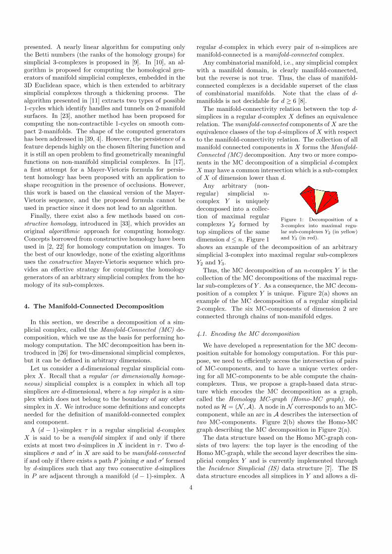
presented. A nearly linear algorithm for computing onlythe Betti numbers (the ranks of the homology groups) forsimplicial 3-complexes is proposed in [9]. In [10], an al-gorithm is proposed for computing the homological gen-erators of manifold simplicial complexes, embedded in the3D Euclidean space, which is then extended to arbitrarysimplicial complexes through a thickening process. Thealgorithm presented in [11] extracts two types of possible1-cycles which identify handles and tunnels on 2-manifoldsurfaces. In [23], another method has been proposed forcomputing the non-contractible 1-cycles on smooth com-pact 2-manifolds. The shape of the computed generatorshas been addressed in [39, 4]. However, the persistence of afeature depends highly on the chosen filtering function andit is still an open problem to find geometrically meaningfulfunctions on non-manifold simplicial complexes. In [17],a first attempt for a Mayer-Vietoris formula for persis-tent homology has been proposed with an application toshape recognition in the presence of occlusions. However,this work is based on the classical version of the Mayer-Vietoris sequence, and the proposed formula cannot beused in practice since it does not lead to an algorithm.
Finally, there exist also a few methods based on con-structive homology, introduced in [33], which provides anoriginal algorithmic approach for computing homology.Concepts borrowed from constructive homology have beenused in [2, 22] for homology computation on images. Tothe best of our knowledge, none of the existing algorithmsuses the constructive Mayer-Vietoris sequence which pro-vides an effective strategy for computing the homologygenerators of an arbitrary simplicial complex from the ho-mology of its sub-complexes.
4. The Manifold-Connected Decomposition
In this section, we describe a decomposition of a sim-plicial complex, called the Manifold-Connected (MC) de-composition, which we use as the basis for performing ho-mology computation. The MC decomposition has been in-troduced in [26] for two-dimensional simplicial complexes,but it can be defined in arbitrary dimensions.
Let us consider a d-dimensional regular simplicial com-plex X . Recall that a regular (or dimensionally homoge-neous) simplicial complex is a complex in which all topsimplices are d-dimensional, where a top simplex is a sim-plex which does not belong to the boundary of any othersimplex in X . We introduce some definitions and conceptsneeded for the definition of manifold-connected complexand component.
A (d − 1)-simplex τ in a regular simplicial d-complexX is said to be a manifold simplex if and only if thereexists at most two d-simplices in X incident in τ . Two d-simplices σ and σ′ in X are said to be manifold-connectedif and only if there exists a path P joining σ and σ′ formedby d-simplices such that any two consecutive d-simplicesin P are adjacent through a manifold (d − 1)-simplex. A
regular d-complex in which every pair of n-simplices aremanifold-connected is a manifold-connected complex.
Any combinatorial manifold, i.e., any simplicial complexwith a manifold domain, is clearly manifold-connected,but the reverse is not true. Thus, the class of manifold-connected complexes is a decidable superset of the classof combinatorial manifolds. Note that the class of d-manifolds is not decidable for d ≥ 6 [8].
The manifold-connectivity relation between the top d-simplices in a regular d-complex X defines an equivalencerelation. The manifold-connected components of X are theequivalence classes of the top d-simplices of X with respectto the manifold-connectivity relation. The collection of allmanifold connected components in X forms the Manifold-Connected (MC) decomposition. Any two or more compo-nents in the MC decomposition of a simplicial d-complexX may have a common intersection which is a sub-complexof X of dimension lower than d.
Figure 1: Decomposition of a3-complex into maximal regu-lar sub-complexes Y2 (in yellow)and Y3 (in red).
Any arbitrary (non-regular) simplicial n-complex Y is uniquelydecomposed into a collec-tion of maximal regularcomplexes Yd formed bytop simplices of the samedimension d ≤ n. Figure 1shows an example of the decomposition of an arbitrarysimplicial 3-complex into maximal regular sub-complexesY2 and Y3.
Thus, the MC decomposition of an n-complex Y is thecollection of the MC decompositions of the maximal regu-lar sub-complexes of Y . As a consequence, the MC decom-position of a complex Y is unique. Figure 2(a) shows anexample of the MC decomposition of a regular simplicial2-complex. The six MC-components of dimension 2 areconnected through chains of non-manifold edges.
4.1. Encoding the MC decomposition
We have developed a representation for the MC decom-position suitable for homology computation. For this pur-pose, we need to efficiently access the intersection of pairsof MC-components, and to have a unique vertex order-ing for all MC-components to be able compute the chain-complexes. Thus, we propose a graph-based data struc-ture which encodes the MC decomposition as a graph,called the Homology MC-graph (Homo-MC graph), de-noted asH = (N ,A). A node in N corresponds to an MC-component, while an arc in A describes the intersection oftwo MC-components. Figure 2(b) shows the Homo-MCgraph describing the MC decomposition in Figure 2(a).
The data structure based on the Homo MC-graph con-sists of two layers: the top layer is the encoding of theHomo MC-graph, while the second layer describes the sim-plicial complex Y and is currently implemented throughthe Incidence Simplicial (IS) data structure [7]. The ISdata structure encodes all simplices in Y and allows a di-
4
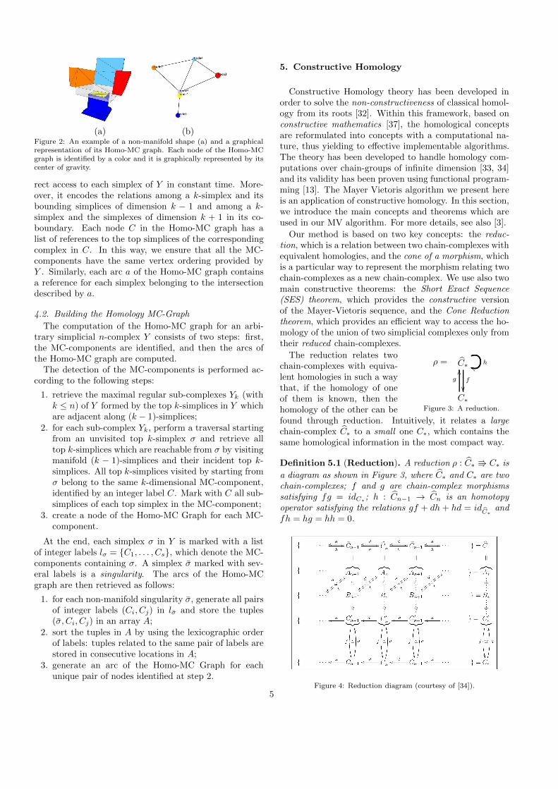
(a) (b)Figure 2: An example of a non-manifold shape (a) and a graphicalrepresentation of its Homo-MC graph. Each node of the Homo-MCgraph is identified by a color and it is graphically represented by itscenter of gravity.
rect access to each simplex of Y in constant time. More-over, it encodes the relations among a k-simplex and itsbounding simplices of dimension k − 1 and among a k-simplex and the simplexes of dimension k + 1 in its co-boundary. Each node C in the Homo-MC graph has alist of references to the top simplices of the correspondingcomplex in C. In this way, we ensure that all the MC-components have the same vertex ordering provided byY . Similarly, each arc a of the Homo-MC graph containsa reference for each simplex belonging to the intersectiondescribed by a.
4.2. Building the Homology MC-Graph
The computation of the Homo-MC graph for an arbi-trary simplicial n-complex Y consists of two steps: first,the MC-components are identified, and then the arcs ofthe Homo-MC graph are computed.
The detection of the MC-components is performed ac-cording to the following steps:
1. retrieve the maximal regular sub-complexes Yk (withk ≤ n) of Y formed by the top k-simplices in Y whichare adjacent along (k − 1)-simplices;
2. for each sub-complex Yk, perform a traversal startingfrom an unvisited top k-simplex σ and retrieve alltop k-simplices which are reachable from σ by visitingmanifold (k − 1)-simplices and their incident top k-simplices. All top k-simplices visited by starting fromσ belong to the same k-dimensional MC-component,identified by an integer label C. Mark with C all sub-simplices of each top simplex in the MC-component;
3. create a node of the Homo-MC Graph for each MC-component.
At the end, each simplex σ in Y is marked with a listof integer labels lσ = C1, . . . , Cs, which denote the MC-components containing σ. A simplex σ marked with sev-eral labels is a singularity. The arcs of the Homo-MCgraph are then retrieved as follows:
1. for each non-manifold singularity σ, generate all pairsof integer labels (Ci, Cj) in lσ and store the tuples(σ, Ci, Cj) in an array A;
2. sort the tuples in A by using the lexicographic orderof labels: tuples related to the same pair of labels arestored in consecutive locations in A;
3. generate an arc of the Homo-MC Graph for eachunique pair of nodes identified at step 2.
5. Constructive Homology
Constructive Homology theory has been developed inorder to solve the non-constructiveness of classical homol-ogy from its roots [32]. Within this framework, based onconstructive mathematics [37], the homological conceptsare reformulated into concepts with a computational na-ture, thus yielding to effective implementable algorithms.The theory has been developed to handle homology com-putations over chain-groups of infinite dimension [33, 34]and its validity has been proven using functional program-ming [13]. The Mayer Vietoris algorithm we present hereis an application of constructive homology. In this section,we introduce the main concepts and theorems which areused in our MV algorithm. For more details, see also [3].
Our method is based on two key concepts: the reduc-tion, which is a relation between two chain-complexes withequivalent homologies, and the cone of a morphism, whichis a particular way to represent the morphism relating twochain-complexes as a new chain-complex. We use also twomain constructive theorems: the Short Exact Sequence(SES) theorem, which provides the constructive versionof the Mayer-Vietoris sequence, and the Cone Reductiontheorem, which provides an efficient way to access the ho-mology of the union of two simplicial complexes only fromtheir reduced chain-complexes.
ρ = C∗
f
hhh
C∗
g
OO
Figure 3: A reduction.
The reduction relates twochain-complexes with equiva-lent homologies in such a waythat, if the homology of oneof them is known, then thehomology of the other can befound through reduction. Intuitively, it relates a largechain-complex C∗ to a small one C∗, which contains thesame homological information in the most compact way.
Definition 5.1 (Reduction). A reduction ρ : C∗ C∗ is
a diagram as shown in Figure 3, where C∗ and C∗ are twochain-complexes; f and g are chain-complex morphismssatisfying fg = idC∗; h : Cn−1 → Cn is an homotopyoperator satisfying the relations gf + dh + hd = id bC∗
andfh = hg = hh = 0.
Figure 4: Reduction diagram (courtesy of [34]).5
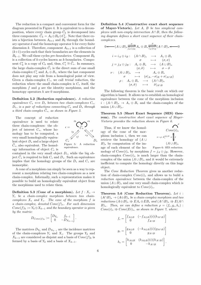
The reduction is a compact and convenient form for thediagram presented in Figure 4. It is equivalent to a decom-position, where every chain group Ck is decomposed intothree components: Ck = Ak⊕Bk⊕C′
k. Note that there ex-ists a bijection between Ak+1 and Bk through the bound-ary operator d and the homotopy operator h for every finitedimension k. Therefore, component Ak+1 is a collection of(k+1)-cycles such that their boundaries are the elements inBk−1. We call these cycles pre-boundaries. Component Bk
is a collection of k-cycles known as k-boundaries. Compo-nent C′
k is a copy of Ck and, thus, C′∗ ∼= C∗. In summary,
the large chain-complex C∗ is the direct sum of one smallchain-complex C′
∗ and A∗⊕B∗, where the last componentdoes not play any role from a homological point of view.Given a chain-complex C∗, we call trivial reduction, thereduction where the small chain-complex is C∗ itself, themorphism f and g are the identity morphisms, and thehomotopy operators h are 0 morphisms.
Definition 5.2 (Reduction equivalence). A reductionequivalence C∗ ⇐⇒ D∗ between two chain-complexes C∗,D∗, is a pair of reductions connecting C∗ and D∗ througha third chain-complex C∗, as shown in Figure 5.
ǫ = C∗
lf~~
rh
lh
rf
AAA
AAAA
A
C∗
lg>>
D∗
rg
``AAAAAAAA
Figure 5: A reductionequivalence.
The concept of reductionequivalence is used to relatethree chain-complexes: the ob-ject of interest C∗, whose ho-mology has to be computed, avery small homologically equiva-lent object D∗ and a large objectC∗, also equivalent. The homol-ogy information of object C∗ iscontained in the very small object D∗, while the big ob-ject C∗ is required to link C∗ and D∗. Such an equivalenceimplies that the homology groups of the D∗ and C∗ areisomorphic.
A cone of a morphism can simply be seen as a way to rep-resent a morphism relating two chain-complexes as a newchain-complex. Informally, such a representation makes itpossible to build an homologically equivalent object fromthe morphisms used to relate them.
Definition 5.3 (Cone of a morphism). Let f : X∗ →Y∗ be a chain-complex morphism between two chain-complexes X∗ and Y∗. The cone of the morphism f isa chain-complex, denoted Cone(f)∗. For each dimensionCone(f)k := Yk⊕Xk−1 and the boundary operator is givenby the matrix:
DCone(f)k:=
[DYk
fk−1
0 −DXk−1
].
The matrices DYkand DXk−1
are the incidence matricesof the chain-complexes Y∗ and X∗. The groups Yk andXk−1 are considered as disjoint and a basis of Cone(f)k isformed by a basis of Yk and a basis of Xk−1.
Definition 5.4 (Constructive exact short sequenceof Mayer-Vietoris). Let A, B be two simplicial com-plexes with non-empty intersection A∩B, then the follow-ing diagram defines a short exact sequence of their chain-complexes.
0 (A ∪B)∗ooν //
A∗ ⊕B∗jA⊖jB
ooρ //
(A ∩B)∗iA⊕iB
oo 0oo
i = iA ⊕ iB : (A ∩B)∗ −→ A∗ ⊕B∗σ 7−→ (σ, σ)
j = jA ⊖ jB : A∗ ⊕B∗ −→ (A ∪B)∗(σ, σ) 7−→ σ − σ
ν : (A ∪B)∗ −→ A∗ ⊕B∗σ 7−→ (σ|A,−σ|B + σ|A∩B)
ρ : A∗ ⊕B∗ −→ (A ∩B)∗(σ, σ) 7−→ σ|A∩B
The following theorem is the basic result on which ouralgorithm is based. It allows us to establish an homologicalequivalence between the cone of the morphism inclusioni : (A ∩ B)∗ → A∗ ⊕ B∗ and the chain-complex of theunion (A ∪B)∗.
Theorem 5.5 (Short Exact Sequence (SES) theo-rem). The constructive short exact sequence of Mayer-Vietoris provides the reduction shown in Figure 6.
Cone(i)∗
j
ρ
(A ∪B)∗
ν−ρ dA⊕B∗ ν
OO
Figure 6: SES reduction.
Thus, if we know the homol-ogy of the cone of the mor-phism inclusion i, then we canretrieve the homology of (A ∪B)∗ by computation of the im-age of each element of the ho-mology of Cone(i)∗ by morphism f = jA ⊖ jB. However,chain-complex Cone(i)∗ is much larger than the chain-complex of the union (A ∪B)∗ and it would be extremelyinefficient to compute the homology directly on this hugeobject.
The Cone Reduction Theorem gives us another reduc-tion of chain-complex Cone(i)∗ and allows us to build areduction equivalence between the chain-complex of theunion (A∪B)∗ and one very small chain-complex which ishomologically equivalent to Cone(i)∗.
Theorem 5.6 (Cone Reduction Theorem). Let i :(A∩B)∗ → (A⊕B)∗ be a chain-complex morphism and tworeductions (A⊕B)∗ EA∗⊕EB∗ and (A∩B)∗ E(A∩B)∗. Then, we can define a reduction ρ = (fc, gc, hc) :Cone(i)∗ Cone(Ei)∗, as shown in Figure 7, where:
fc =
[fA⊕B (−fA⊕B)(i)(hA∩B)
0 fA∩B
]
gc =
[gA⊕B (−hA⊕B)(i)(gA∩B)
0 gA∩B
]
hc =
[hA⊕B (hA⊕B)(i)(hA∩B)
0 −hA∩B
].
6
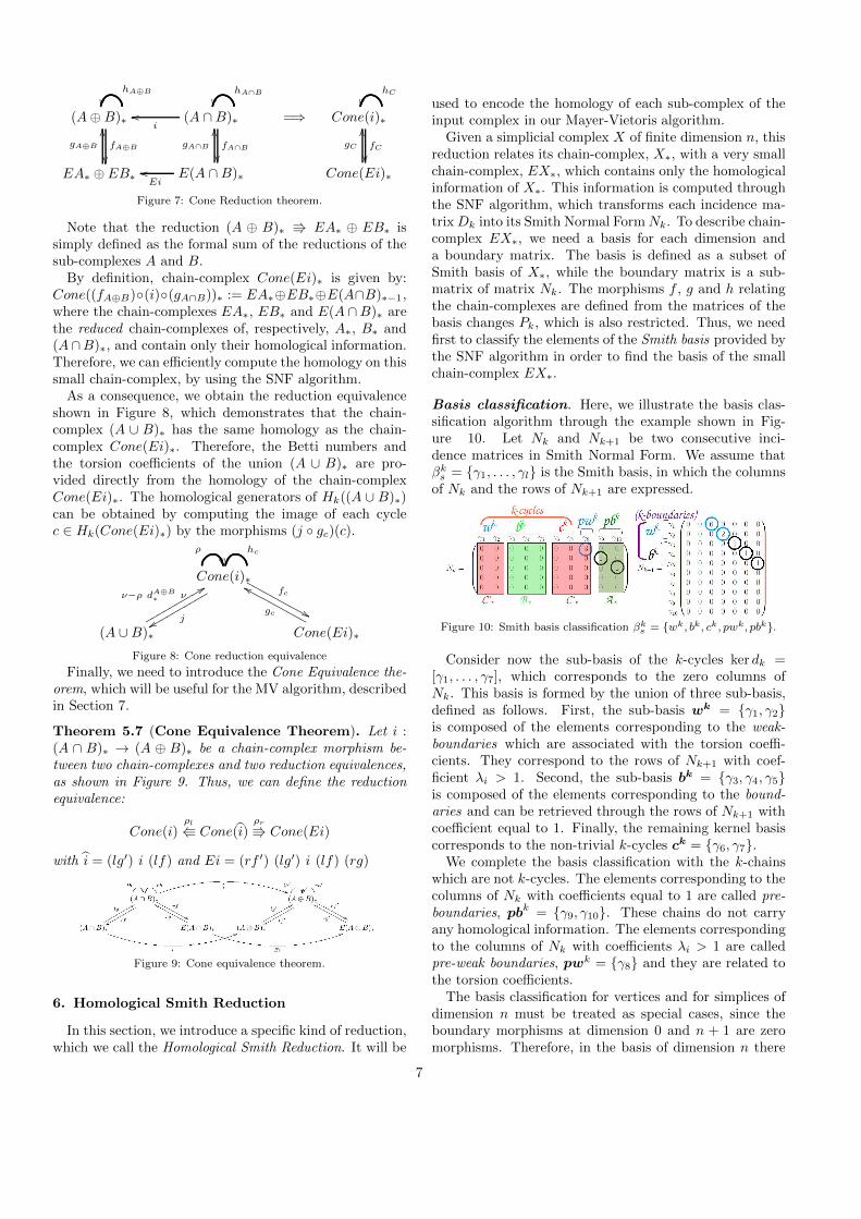
(A⊕B)∗
fA⊕B
hA⊕B
(A ∩B)∗
ioo
fA∩B
hA∩B
EA∗ ⊕ EB∗
gA⊕B
OO
E(A ∩B)∗Ei
oo
gA∩B
OO=⇒ Cone(i)∗
fC
hC
Cone(Ei)∗
gC
OO
Figure 7: Cone Reduction theorem.
Note that the reduction (A ⊕ B)∗ EA∗ ⊕ EB∗ issimply defined as the formal sum of the reductions of thesub-complexes A and B.
By definition, chain-complex Cone(Ei)∗ is given by:Cone((fA⊕B)(i)(gA∩B))∗ := EA∗⊕EB∗⊕E(A∩B)∗−1,where the chain-complexes EA∗, EB∗ and E(A ∩B)∗ arethe reduced chain-complexes of, respectively, A∗, B∗ and(A∩B)∗, and contain only their homological information.Therefore, we can efficiently compute the homology on thissmall chain-complex, by using the SNF algorithm.
As a consequence, we obtain the reduction equivalenceshown in Figure 8, which demonstrates that the chain-complex (A ∪ B)∗ has the same homology as the chain-complex Cone(Ei)∗. Therefore, the Betti numbers andthe torsion coefficients of the union (A ∪ B)∗ are pro-vided directly from the homology of the chain-complexCone(Ei)∗. The homological generators of Hk((A ∪ B)∗)can be obtained by computing the image of each cyclec ∈ Hk(Cone(Ei)∗) by the morphisms (j gc)(c).
Cone(i)∗
jxxrrrrrrrrrr fc
&&NNNNNNNNNN
hc
ρ
(A ∪B)∗
ν−ρ dA⊕B∗ ν
88rrrrrrrrrr
Cone(Ei)∗
gc
ffNNNNNNNNNN
Figure 8: Cone reduction equivalence
Finally, we need to introduce the Cone Equivalence the-orem, which will be useful for the MV algorithm, describedin Section 7.
Theorem 5.7 (Cone Equivalence Theorem). Let i :(A ∩ B)∗ → (A ⊕ B)∗ be a chain-complex morphism be-tween two chain-complexes and two reduction equivalences,as shown in Figure 9. Thus, we can define the reductionequivalence:
Cone(i)ρl
Cone(i)ρr
Cone(Ei)
with i = (lg′) i (lf) and Ei = (rf ′) (lg′) i (lf) (rg)
Figure 9: Cone equivalence theorem.
6. Homological Smith Reduction
In this section, we introduce a specific kind of reduction,which we call the Homological Smith Reduction. It will be
used to encode the homology of each sub-complex of theinput complex in our Mayer-Vietoris algorithm.
Given a simplicial complex X of finite dimension n, thisreduction relates its chain-complex, X∗, with a very smallchain-complex, EX∗, which contains only the homologicalinformation of X∗. This information is computed throughthe SNF algorithm, which transforms each incidence ma-trix Dk into its Smith Normal Form Nk. To describe chain-complex EX∗, we need a basis for each dimension anda boundary matrix. The basis is defined as a subset ofSmith basis of X∗, while the boundary matrix is a sub-matrix of matrix Nk. The morphisms f , g and h relatingthe chain-complexes are defined from the matrices of thebasis changes Pk, which is also restricted. Thus, we needfirst to classify the elements of the Smith basis provided bythe SNF algorithm in order to find the basis of the smallchain-complex EX∗.
Basis classification. Here, we illustrate the basis clas-sification algorithm through the example shown in Fig-ure 10. Let Nk and Nk+1 be two consecutive inci-dence matrices in Smith Normal Form. We assume thatβk
s = γ1, . . . , γl is the Smith basis, in which the columnsof Nk and the rows of Nk+1 are expressed.
Figure 10: Smith basis classification βks = wk, bk, ck, pwk, pbk.
Consider now the sub-basis of the k-cycles ker dk =[γ1, . . . , γ7], which corresponds to the zero columns ofNk. This basis is formed by the union of three sub-basis,defined as follows. First, the sub-basis wk = γ1, γ2is composed of the elements corresponding to the weak-boundaries which are associated with the torsion coeffi-cients. They correspond to the rows of Nk+1 with coef-ficient λi > 1. Second, the sub-basis bk = γ3, γ4, γ5is composed of the elements corresponding to the bound-aries and can be retrieved through the rows of Nk+1 withcoefficient equal to 1. Finally, the remaining kernel basiscorresponds to the non-trivial k-cycles ck = γ6, γ7.
We complete the basis classification with the k-chainswhich are not k-cycles. The elements corresponding to thecolumns of Nk with coefficients equal to 1 are called pre-boundaries, pbk = γ9, γ10. These chains do not carryany homological information. The elements correspondingto the columns of Nk with coefficients λi > 1 are calledpre-weak boundaries, pwk = γ8 and they are related tothe torsion coefficients.
The basis classification for vertices and for simplices ofdimension n must be treated as special cases, since theboundary morphisms at dimension 0 and n + 1 are zeromorphisms. Therefore, in the basis of dimension n there
7
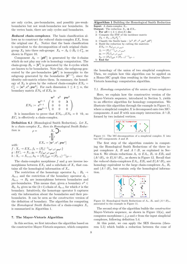
are only cycles, pre-boundaries, and possibly pre-weak-boundaries but not weak-boundaries nor boundaries. Inthe vertex basis, there are only cycles and boundaries.
Reduced chain-complexes. The basis classification al-lows us to construct the reduced chain-complex EX∗ fromthe original one X∗. Notice that the basis classificationis equivalent to the decomposition of each original chain-group Xk into three sub-groups: Xk = Ak ⊕ Bk ⊕ C′
k, asshown in Figure 10.
Component Ak = [pbk] is generated by the k-chainswhich do not play any role in homology computation. Thechain-group Bk = [bk] is generated by the k-cycles whichare known to be boundaries. Note that, the subgroup gen-erated by the pre-boundaries [pbk] is isomorphic to thesubgroup generated by the boundaries [bk−1], since theidentity sub-matrix relates them. In summary, the homol-ogy of Xk is given by the reduced chain-complex EXk =C′
k = [wk, ck,pwk]. For each dimension 1 ≤ k ≤ n, theboundary matrix ENk of EXk is:
ENk :=
wk ck pwk
wk−1 0 0 λck−1 0 0 0pwk−1 0 0 0
.
It is immediate to prove that ENk−1ENk = 0 ∀k, soEC∗ is effectively a chain-complex.
Definition 6.1 (Homological Smith Reduction). Let X∗be a chain-complex X∗, then its Homological Smith Reduc-tion is ρ = X∗
f
hii
EX∗ = [w∗, c∗,pw∗]
g
OO
with:f : X∗ → EX∗, fk = (Pk)−1|wk,ck,pwkg : EC∗ → X∗, gk = Pk|wk,ck,pwkh : X∗ → X∗+1, hk = (Pk)|pbk ∗ (Pk−1)
−1|bk−1
The chain-complex morphisms f and g are inverse iso-morphisms between EX∗ and a subchain of X∗ that con-tains all the homological information of X∗.
The restriction of the homotopy operator hk : Bk →Ak+1 and the restriction of the boundary operator dk :Ak+1 → Bk are isomorphisms between boundaries andpre-boundaries. This means that, given a boundary σk ∈Bk, hk gives us the (k+1)-chain of Ak+1 for which σ is theboundary. Intuitively, the homotopy operator h capturesonly the information about the boundaries and their pre-boundaries. It can be seen as the constructive version ofthe definition of boundary. The algorithm for computingthe Homological Smith Reduction of a chain-complex X∗is summarized in Algorithm 1.
7. The Mayer-Vietoris Algorithm
In this section, we first introduce the algorithm based onthe constructive Mayer-Vietoris sequence, which computes
Algorithm 1 Building the Homological Smith ReductionInput: A chain-complex X∗.Output: The reduction X∗ EX∗.1: For all 1 ≤ k ≤ dim(X) do:2: Compute the SNF of the incidence matrix
Dk = Pk−1NkP −1k .
3: Classify the Smith basis : [wk, bk, ck, pwk, pbk]4: Build the reduction by cutting the matrices:
EXk := Nk |wk,ck,pwk
fk := (Pk)−1|wk,ck,pwk
gk := (Pk)|wk,ck,pwk
hk := (Pk)|pbk ∗ (Pk−1)−1|bk−1
5: End for
the homology of the union of two simplicial complexes.Then, we explain how this algorithm can be applied ona Homo-MC graph thus resulting in the iterative Mayer-Vietoris homology computation algorithm.
7.1. Homology computation of the union of two complexes
Here, we explain how the constructive version of theMayer-Vietoris sequence, introduced in Section 5, yieldsto an effective algorithm for homology computation. Weillustrate this algorithm through the example in Figure 11,where a simplicial complex X is decomposed onto two MC-components A and B with non-empty intersection A ∩B,formed by two isolated vertices.
Figure 11: The MC-decomposition of a simplicial complex X intotwo MC-components A and B.
The first step of the algorithm consists in comput-ing the Homological Smith Reductions of the three in-put complexes A, B and A ∩ B, as explained in Sec-tion 6. We obtain reductions A∗ EA∗, B∗ EB∗ and(A∩B)∗ E(A∩B)∗, as shown in Figure 12. Recall thatthe reduced chain-complexes EA∗, EB∗ and E(A∩B)∗ arehomology equivalent to the large chain-complexes A∗, B∗and (A ∩ B)∗ but contain only the homological informa-tion.
Figure 12: Homological Smith Reductions of A∗, B∗ and (A ∩ B)∗,associated to the example in Figure 11.
The second step of the algorithm builds the constructiveMayer-Vietoris sequence, as shown in Figure 13(a), andcomputes morphisms i, j, ρ and ν from the input simplicialcomplexes, following definition 5.4.
At this point, we can apply the SES theorem (theo-rem 5.5) which builds a reduction between the cone of
8
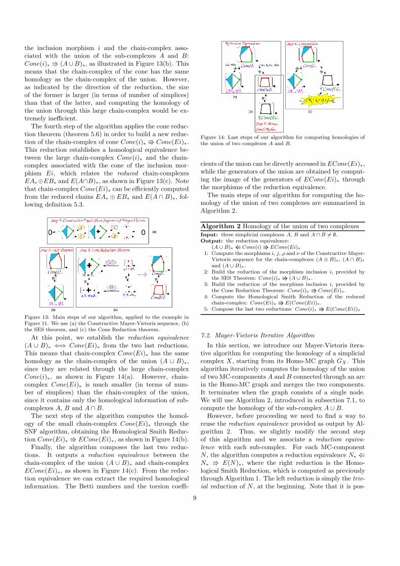
the inclusion morphism i and the chain-complex asso-ciated with the union of the sub-complexes A and B:Cone(i)∗ (A∪B)∗, as illustrated in Figure 13(b). Thismeans that the chain-complex of the cone has the samehomology as the chain-complex of the union. However,as indicated by the direction of the reduction, the sizeof the former is larger (in terms of number of simplices)than that of the latter, and computing the homology ofthe union through this large chain-complex would be ex-tremely inefficient.
The fourth step of the algorithm applies the cone reduc-tion theorem (theorem 5.6) in order to build a new reduc-tion of the chain-complex of cone Cone(i)∗ Cone(Ei)∗.This reduction establishes a homological equivalence be-tween the large chain-complex Cone(i)∗ and the chain-complex associated with the cone of the inclusion mor-phism Ei, which relates the reduced chain-complexesEA∗⊕EB∗ and E(A∩B)∗, as shown in Figure 13(c). Notethat chain-complex Cone(Ei)∗ can be efficiently computedfrom the reduced chains EA∗ ⊕ EB∗ and E(A ∩ B)∗, fol-lowing definition 5.3.
Figure 13: Main steps of our algorithm, applied to the example inFigure 11. We use (a) the Constructive Mayer-Vietoris sequence, (b)the SES theorem, and (c) the Cone Reduction theorem.
At this point, we establish the reduction equivalence(A ∪ B)∗ ⇐⇒ Cone(Ei)∗ from the two last reductions.This means that chain-complex Cone(Ei)∗ has the samehomology as the chain-complex of the union (A ∪ B)∗,since they are related through the large chain-complexCone(i)∗, as shown in Figure 14(a). However, chain-complex Cone(Ei)∗ is much smaller (in terms of num-ber of simplices) than the chain-complex of the union,since it contains only the homological information of sub-complexes A, B and A ∩B.
The next step of the algorithm computes the homol-ogy of the small chain-complex Cone(Ei)∗ through theSNF algorithm, obtaining the Homological Smith Reduc-tion Cone(Ei)∗ ECone(Ei)∗, as shown in Figure 14(b).
Finally, the algorithm composes the last two reduc-tions. It outputs a reduction equivalence between thechain-complex of the union (A ∪ B)∗ and chain-complexECone(Ei)∗, as shown in Figure 14(c). From the reduc-tion equivalence we can extract the required homologicalinformation. The Betti numbers and the torsion coeffi-
Figure 14: Last steps of our algorithm for computing homologies ofthe union of two complexes A and B.
cients of the union can be directly accessed in ECone(Ei)∗,while the generators of the union are obtained by comput-ing the image of the generators of ECone(Ei)∗ throughthe morphisms of the reduction equivalence.
The main steps of our algorithm for computing the ho-mology of the union of two complexes are summarized inAlgorithm 2.
Algorithm 2 Homology of the union of two complexesInput: three simplicial complexes A, B and A ∩ B 6= ∅.Output: the reduction equivalence:
(A ∪ B)∗ Cone(i) ECone(Ei)∗1: Compute the morphisms i, j, ρ and ν of the Constructive Mayer-
Vietoris sequence for the chain-complexes (A ⊕ B)∗, (A ∩ B)∗and (A ∪ B)∗.
2: Build the reduction of the morphism inclusion i, provided bythe SES Theorem: Cone(i)∗ (A ∪ B)∗.
3: Build the reduction of the morphism inclusion i, provided bythe Cone Reduction Theorem: Cone(i)∗ Cone(Ei)∗.
4: Compute the Homological Smith Reduction of the reducedchain-complex: Cone(Ei)∗ E(Cone(Ei))∗.
5: Compose the last two reductions: Cone(i)∗ E(Cone(Ei))∗
7.2. Mayer-Vietoris Iterative Algorithm
In this section, we introduce our Mayer-Vietoris itera-tive algorithm for computing the homology of a simplicialcomplex X , starting from its Homo-MC graph GX . Thisalgorithm iteratively computes the homology of the unionof two MC-components A and B connected through an arcin the Homo-MC graph and merges the two components.It terminates when the graph consists of a single node.We will use Algorithm 2, introduced in subsection 7.1, tocompute the homology of the sub-complex A ∪B.
However, before proceeding we need to find a way toreuse the reduction equivalence provided as output by Al-gorithm 2. Thus, we slightly modify the second stepof this algorithm and we associate a reduction equiva-lence with each sub-complex. For each MC-componentN , the algorithm computes a reduction equivalence N∗ N∗ E(N)∗, where the right reduction is the Homo-logical Smith Reduction, which is computed as previouslythrough Algorithm 1. The left reduction is simply the triv-ial reduction of N , at the beginning. Note that it is pos-
9
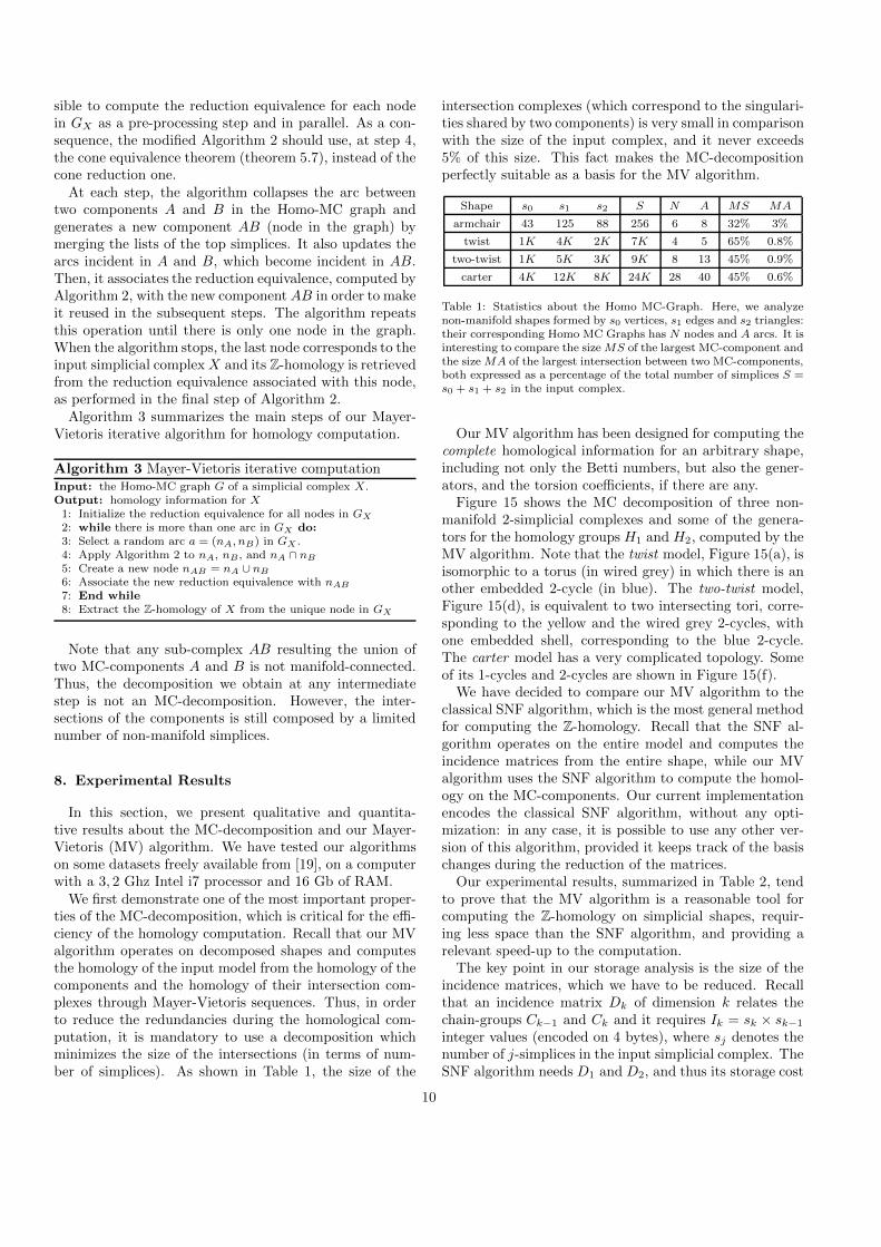
sible to compute the reduction equivalence for each nodein GX as a pre-processing step and in parallel. As a con-sequence, the modified Algorithm 2 should use, at step 4,the cone equivalence theorem (theorem 5.7), instead of thecone reduction one.
At each step, the algorithm collapses the arc betweentwo components A and B in the Homo-MC graph andgenerates a new component AB (node in the graph) bymerging the lists of the top simplices. It also updates thearcs incident in A and B, which become incident in AB.Then, it associates the reduction equivalence, computed byAlgorithm 2, with the new component AB in order to makeit reused in the subsequent steps. The algorithm repeatsthis operation until there is only one node in the graph.When the algorithm stops, the last node corresponds to theinput simplicial complex X and its Z-homology is retrievedfrom the reduction equivalence associated with this node,as performed in the final step of Algorithm 2.
Algorithm 3 summarizes the main steps of our Mayer-Vietoris iterative algorithm for homology computation.
Algorithm 3 Mayer-Vietoris iterative computationInput: the Homo-MC graph G of a simplicial complex X.Output: homology information for X1: Initialize the reduction equivalence for all nodes in GX
2: while there is more than one arc in GX do:3: Select a random arc a = (nA, nB) in GX .4: Apply Algorithm 2 to nA, nB, and nA ∩ nB
5: Create a new node nAB = nA ∪ nB
6: Associate the new reduction equivalence with nAB
7: End while8: Extract the Z-homology of X from the unique node in GX
Note that any sub-complex AB resulting the union oftwo MC-components A and B is not manifold-connected.Thus, the decomposition we obtain at any intermediatestep is not an MC-decomposition. However, the inter-sections of the components is still composed by a limitednumber of non-manifold simplices.
8. Experimental Results
In this section, we present qualitative and quantita-tive results about the MC-decomposition and our Mayer-Vietoris (MV) algorithm. We have tested our algorithmson some datasets freely available from [19], on a computerwith a 3, 2 Ghz Intel i7 processor and 16 Gb of RAM.
We first demonstrate one of the most important proper-ties of the MC-decomposition, which is critical for the effi-ciency of the homology computation. Recall that our MValgorithm operates on decomposed shapes and computesthe homology of the input model from the homology of thecomponents and the homology of their intersection com-plexes through Mayer-Vietoris sequences. Thus, in orderto reduce the redundancies during the homological com-putation, it is mandatory to use a decomposition whichminimizes the size of the intersections (in terms of num-ber of simplices). As shown in Table 1, the size of the
intersection complexes (which correspond to the singulari-ties shared by two components) is very small in comparisonwith the size of the input complex, and it never exceeds5% of this size. This fact makes the MC-decompositionperfectly suitable as a basis for the MV algorithm.
Shape s0 s1 s2 S N A MS MA
armchair 43 125 88 256 6 8 32% 3%
twist 1K 4K 2K 7K 4 5 65% 0.8%
two-twist 1K 5K 3K 9K 8 13 45% 0.9%
carter 4K 12K 8K 24K 28 40 45% 0.6%
Table 1: Statistics about the Homo MC-Graph. Here, we analyzenon-manifold shapes formed by s0 vertices, s1 edges and s2 triangles:their corresponding Homo MC Graphs has N nodes and A arcs. It isinteresting to compare the size MS of the largest MC-component andthe size MA of the largest intersection between two MC-components,both expressed as a percentage of the total number of simplices S =s0 + s1 + s2 in the input complex.
Our MV algorithm has been designed for computing thecomplete homological information for an arbitrary shape,including not only the Betti numbers, but also the gener-ators, and the torsion coefficients, if there are any.
Figure 15 shows the MC decomposition of three non-manifold 2-simplicial complexes and some of the genera-tors for the homology groups H1 and H2, computed by theMV algorithm. Note that the twist model, Figure 15(a), isisomorphic to a torus (in wired grey) in which there is another embedded 2-cycle (in blue). The two-twist model,Figure 15(d), is equivalent to two intersecting tori, corre-sponding to the yellow and the wired grey 2-cycles, withone embedded shell, corresponding to the blue 2-cycle.The carter model has a very complicated topology. Someof its 1-cycles and 2-cycles are shown in Figure 15(f).
We have decided to compare our MV algorithm to theclassical SNF algorithm, which is the most general methodfor computing the Z-homology. Recall that the SNF al-gorithm operates on the entire model and computes theincidence matrices from the entire shape, while our MValgorithm uses the SNF algorithm to compute the homol-ogy on the MC-components. Our current implementationencodes the classical SNF algorithm, without any opti-mization: in any case, it is possible to use any other ver-sion of this algorithm, provided it keeps track of the basischanges during the reduction of the matrices.
Our experimental results, summarized in Table 2, tendto prove that the MV algorithm is a reasonable tool forcomputing the Z-homology on simplicial shapes, requir-ing less space than the SNF algorithm, and providing arelevant speed-up to the computation.
The key point in our storage analysis is the size of theincidence matrices, which we have to be reduced. Recallthat an incidence matrix Dk of dimension k relates thechain-groups Ck−1 and Ck and it requires Ik = sk × sk−1
integer values (encoded on 4 bytes), where sj denotes thenumber of j-simplices in the input simplicial complex. TheSNF algorithm needs D1 and D2, and thus its storage cost
10
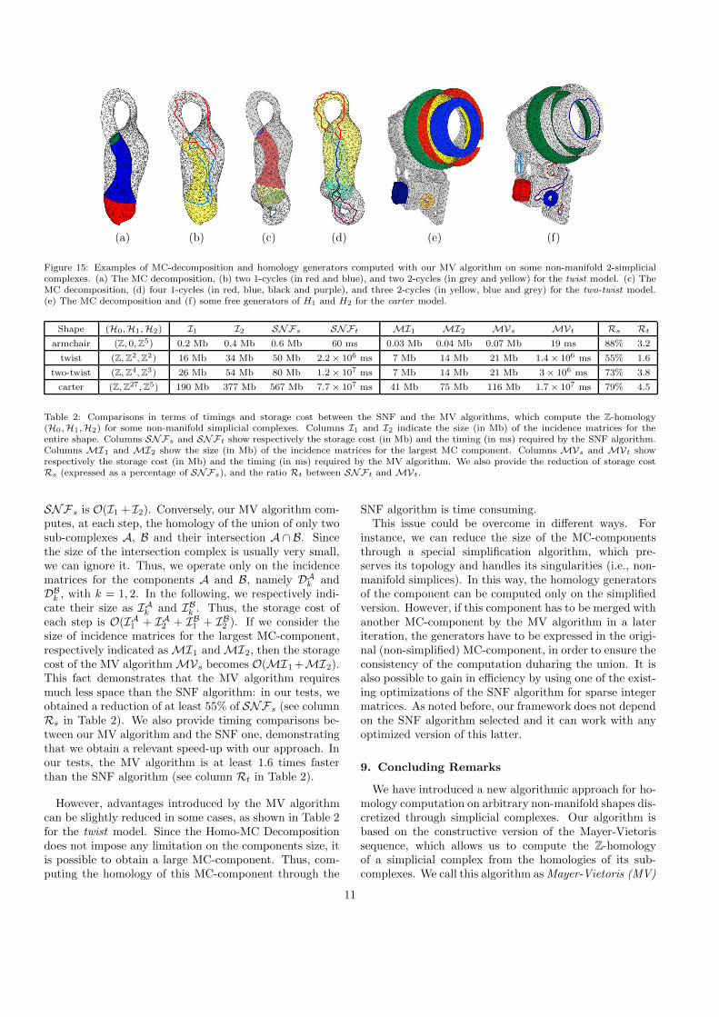
(a) (b) (c) (d) (e) (f)
Figure 15: Examples of MC-decomposition and homology generators computed with our MV algorithm on some non-manifold 2-simplicialcomplexes. (a) The MC decomposition, (b) two 1-cycles (in red and blue), and two 2-cycles (in grey and yellow) for the twist model. (c) TheMC decomposition, (d) four 1-cycles (in red, blue, black and purple), and three 2-cycles (in yellow, blue and grey) for the two-twist model.(e) The MC decomposition and (f) some free generators of H1 and H2 for the carter model.
Shape (H0, H1, H2) I1 I2 SNFs SNFt MI1 MI2 MVs MVt Rs Rt
armchair (Z, 0,Z5) 0.2 Mb 0.4 Mb 0.6 Mb 60 ms 0.03 Mb 0.04 Mb 0.07 Mb 19 ms 88% 3.2
twist (Z, Z2,Z2) 16 Mb 34 Mb 50 Mb 2.2 × 10⁶ ms 7 Mb 14 Mb 21 Mb 1.4 × 10⁶ ms 55% 1.6
two-twist (Z, Z4,Z3) 26 Mb 54 Mb 80 Mb 1.2 × 10⁷ ms 7 Mb 14 Mb 21 Mb 3 × 10⁶ ms 73% 3.8
carter (Z,Z27,Z5) 190 Mb 377 Mb 567 Mb 7.7 × 10⁷ ms 41 Mb 75 Mb 116 Mb 1.7 × 10⁷ ms 79% 4.5
Table 2: Comparisons in terms of timings and storage cost between the SNF and the MV algorithms, which compute the Z-homology(H0, H1, H2) for some non-manifold simplicial complexes. Columns I1 and I2 indicate the size (in Mb) of the incidence matrices for theentire shape. Columns SNFs and SNFt show respectively the storage cost (in Mb) and the timing (in ms) required by the SNF algorithm.Columns MI1 and MI2 show the size (in Mb) of the incidence matrices for the largest MC component. Columns MVs and MVt showrespectively the storage cost (in Mb) and the timing (in ms) required by the MV algorithm. We also provide the reduction of storage costRs (expressed as a percentage of SNFs), and the ratio Rt between SNFt and MVt.
SNFs is O(I1 + I2). Conversely, our MV algorithm com-putes, at each step, the homology of the union of only twosub-complexes A, B and their intersection A ∩ B. Sincethe size of the intersection complex is usually very small,we can ignore it. Thus, we operate only on the incidencematrices for the components A and B, namely DA
k andDB
k , with k = 1, 2. In the following, we respectively indi-cate their size as IA
k and IBk . Thus, the storage cost of
each step is O(IA1 + IA
2 + IB1 + IB
2 ). If we consider thesize of incidence matrices for the largest MC-component,respectively indicated asMI1 andMI2, then the storagecost of the MV algorithmMVs becomes O(MI1 +MI2).This fact demonstrates that the MV algorithm requiresmuch less space than the SNF algorithm: in our tests, weobtained a reduction of at least 55% of SNFs (see columnRs in Table 2). We also provide timing comparisons be-tween our MV algorithm and the SNF one, demonstratingthat we obtain a relevant speed-up with our approach. Inour tests, the MV algorithm is at least 1.6 times fasterthan the SNF algorithm (see column Rt in Table 2).
However, advantages introduced by the MV algorithmcan be slightly reduced in some cases, as shown in Table 2for the twist model. Since the Homo-MC Decompositiondoes not impose any limitation on the components size, itis possible to obtain a large MC-component. Thus, com-puting the homology of this MC-component through the
SNF algorithm is time consuming.This issue could be overcome in different ways. For
instance, we can reduce the size of the MC-componentsthrough a special simplification algorithm, which pre-serves its topology and handles its singularities (i.e., non-manifold simplices). In this way, the homology generatorsof the component can be computed only on the simplifiedversion. However, if this component has to be merged withanother MC-component by the MV algorithm in a lateriteration, the generators have to be expressed in the origi-nal (non-simplified) MC-component, in order to ensure theconsistency of the computation duharing the union. It isalso possible to gain in efficiency by using one of the exist-ing optimizations of the SNF algorithm for sparse integermatrices. As noted before, our framework does not dependon the SNF algorithm selected and it can work with anyoptimized version of this latter.
9. Concluding Remarks
We have introduced a new algorithmic approach for ho-mology computation on arbitrary non-manifold shapes dis-cretized through simplicial complexes. Our algorithm isbased on the constructive version of the Mayer-Vietorissequence, which allows us to compute the Z-homologyof a simplicial complex from the homologies of its sub-complexes. We call this algorithm as Mayer-Vietoris (MV)
11
algorithm. The starting point of the MV algorithm is theMC-decomposition of the shape, which minimizes the in-tersections between the manifold-connected components.Combined with this decomposition, the MV algorithm hasbeen proven to be more efficient (in terms of storage andtimings) than the classical SNF algorithm, which operateson the entire input model.
In the future, we are planning to improve our currentimplementation of the SNF algorithm, which will allow usto increase the efficiency of the homology computation oneach MC-component and, thus, process very large models.We are also planning to investigate how to combine ouralgorithm with a different approach for computing the ho-mology of the MC-components, since these latter can beviewed as almost manifold complexes, and thus efficientgeometric algorithms for homology computation on mani-fold shapes could be applied.
We are also planning to investigate different strategiesfor improving the geometric properties of the generatorsin order to provide the shortest set of loops that generatethe homology groups. One possible solution is to minimizetheir length, by associating a metric to the homology basis,as recently introduced in [12].
Acknowledgements. We thank Professor Francis Sergeraert for themany helpful discussions on Constructive Homology. We thank theanonymous reviewers for their helpful suggestions.
References
[1] Agoston, M.K., 1976. Algebraic topology: a first course. M.Dekker Publisher, New York, USA.
[2] Alayrangues, S., Damiand, G., Fuchs, L., Lienhardt, P., Peltier,S., 2009. Homology computation on cellular structures in imagecontext, in: CTIC, Austria. pp. 19–28.
[3] Boltcheva, D., Merino, S., Leon, J.C., Hetroy, F., 2010. Con-structive Mayer-Vietoris algorithm: computing the homology ofunions of simplicial complexes. Technical Report. INRIA-7471.
[4] Chen, C., Freedman, D., 2010. Measuring and computing natu-ral generators for homology groups. Computational Geometry:Theory & Applications 43, 169–181.
[5] Cohen-Steiner, D., Edelsbrunner, H., Morozov, D., 2006. Vinesand vineyards by updating persistence in linear time, in: Sym-posium on Computational geometry, SCG ’06, pp. 119–126.
[6] Damiand, G., Peltier, S., Fuchs, L., 2006. Computing homologyfor surfaces with generalized maps: Application to 3d images.,in: ISVC’06, Nevada, USA. pp. 235–244.
[7] De Floriani, L., Hui, A., Panozzo, D., Canino, D., 2010. Adimension-independent data structure for simplicial complexes,in: IMR, Chattanoga, TN, USA. pp. 403–420.
[8] De Floriani, L., Mesmoudi, M.M., Morando, F., Puppo, E.,2003. Decomposing non-manifold objects in arbitrary dimen-sions. Graph. Models 65, 2–22.
[9] Delfinado, C.J.A., Edelsbrunner, H., 1993. An incremental al-gorithm for betti numbers of simplicial complexes, in: SoCG’93,ACM, New York, NY, USA. pp. 232–239.
[10] Dey, T.K., Guha, S., 1996. Computing homology groups ofsimplicial complexes in R3, in: Proc. 28th ACM Symp. Comp.Theory (STOC 1996).
[11] Dey, T.K., Li, K., Sun, J., Cohen-Steiner, D., 2008. Computinggeometry-aware handle and tunnel loops in 3d models. ACMTransactions on Graphics 27, No. 45.
[12] Dey, T.K., Sun, J., Wang, Y., 2010. Approximating loops in ashortest homology basis from point data, in: Proc. 26th Annu.Sympos. Comput. Geom. (SOCG 2010), pp. 166–175.
[13] Dousson, X., Rubio, J., Sergeraert, F., Siret, Y., 2008.The kenzo program. http://www-fourier.ujf-grenoble.fr/
~sergerar/Kenzo/.[14] Dumas, J.G., Heckenbach, F., Saunders, B.D., Welker, V., 2003.
Computing simplicial homology based on efficient smith normalform algorithms. Alg., Geom., and Soft. Syst. , 177–207.
[15] Edelsbrunner, H., Harer, J., 2010. Computational topology, anintroduction. AMS, Providence, Rhode Island.
[16] Edelsbrunner, H., Letscher, D., Zomorodian, A., 2002. Topolog-ical persistence and simplification. Discrete & ComputationalGeometry 28, 511–533.
[17] Fabio, B., Landi, C., Medri, F., 2009. Recognition of occludedshapes using size functions, in: ICIAP’09, Springer-Verlag,Berlin, Heidelberg. pp. 642–651.
[18] Forman, R., 1998. Morse theory for cell complexes. Advancesin Mathematics 134, 90–145.
[19] Geometry and Graphics Group, 2009. Non-manifold MeshesRepository. http://indy.disi.unige.it/nmcollection/.
[20] Ghrist, R., Muhammad, A., 2005. Coverage and hole-detectionin sensor networks via homology, in: IPSN’05, IEEE Press, Pis-cataway, NJ, USA. p. No. 34.
[21] Giesbrecht, M., 1996. Probabilistic computation of the smithnormal form of a sparse integer matrix. Algorithmic NumberTheory. Lecture Notes in Computer Science 1122, 173–186.
[22] Gonzalez-Dıaz, R., Jimenez, M.J., Medrano, B., Real, P., 2009.Chain homotopies for object topological representations. Dis-crete Applied Mathematics 157, 490–499.
[23] Gotsman, C., Kaligosi, K., Mehlhorn, K., Michail, D., Pyrga,E., 2007. Cycle bases of graphs and sampled manifolds. Com-puter Aided Geometric Design 24, 464–480.
[24] Hafner, J.L., McCurley, K.S., 1991. Asymptotically fast trian-gularization of matrices over rings. SIAM Journal on Computing20, 1068–1083.
[25] Hatcher, A., 2002. Algebraic Topology. Cambr. Univ. Press.[26] Hui, A., De Floriani, L., 2007. A two-level topological decom-
position for non-manifold simplicial shapes, in: SPM, Beijing,China. pp. 355–260.
[27] Kaczynski, T., Mrozek, M., Slusarek, M., 1998. Homology com-putation by reduction of chain complexes. Computers & Math-ematics with Applications 35-4, 59–70.
[28] Kannan, R., A., B., 1979. Polinomial algorithms for computingthe smith and hermite normal forms of an integer matrix. SIAMJournal of Computing 8, 499–507.
[29] Mrozek, M., Pilarczyk, P., Zelazna, N., 2008. Homology algo-rithm based on acyclic subspace. Computers and Mathematicswith Applications 55, 2395–2412.
[30] Munkres, J., 1999. Algebraic Topology. Prentice Hall.[31] Peltier, S., Ion, A., Kropatsch, W.G., Damiand, G., Haxhimusa,
Y., 2009. Directly computing the generators of image homologyusing graph pyramids. Image & Vision Computing 27, 846–853.
[32] Sergeraert, F., 1994. The computability problem in algebraictopology. Advances in Mathematics 104, 139–155.
[33] Sergeraert, F., 1999. Constructive algebraic topology. SIGSAMBull. 33, 13–25.
[34] Sergeraert, F., Rubio, J., 2006. Constructive homological alge-bra and applications. http://www-fourier.ujf-grenoble.fr/
~sergerar/Papers/.[35] Storjohann, A., 1996. Near optimal algorithms for computing
smith normal forms of integer matrices, in: ISSAC’96, ACM,New York, NY, USA. pp. 267–274.
[36] Thakur, A., Banerjee, A.G., Gupta, S.K., 2009. A survey ofcad model simplification techniques for physics-based simula-tion applications. Comput. Aided Des. 41, 65–80.
[37] Troelstra, A.S., van Dalen, D., 1988. Constructivism in Mathe-matics, an Introduction. Studies in Logic and the Foundationsof Mathematics, North-Holland.
[38] Zhu, X., Sarkar, R., Gao, J., 2009. Topological data processingfor distributed sensor networks with morse-smale decomposi-tion, in: IEEE Infocom, pp. 2911–2915.
[39] Zomorodian, A., Carlsson, G., 2008. Localized homology. Com-putational Geometry: Theory & Applications 41, 126–148.
12
A.3. JUST NOTICEABLE DISTORTION PROFILE FOR FLAT-SHADED 3D MESHSURFACES 115
∴
A.3 JUST NOTICEABLE DISTORTION PROFILE FORFLAT-SHADED 3D MESH SURFACES
Georges Nader, Kai Wang, Franck Hétroy-Wheeler, Florent DupontIEEE Transactions on Visualization and Computer Graphics, 2016.

116 APPENDIX A. SELECTED PAPERS
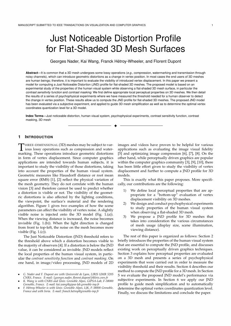
MANUSCRIPT SUBMITTED TO IEEE TRANSACTIONS ON VISUALIZATION AND COMPUTER GRAPHICS 1
Just Noticeable Distortion Profilefor Flat-Shaded 3D Mesh Surfaces
Georges Nader, Kai Wang, Franck Hetroy-Wheeler, and Florent Dupont
Abstract—It is common that a 3D mesh undergoes some lossy operations (e.g., compression, watermarking and transmission throughnoisy channels), which can introduce geometric distortions as a change in vertex position. In most cases the end users of 3D meshesare human beings; therefore, it is important to evaluate the visibility of introduced vertex displacement. In this paper we present amodel for computing a Just Noticeable Distortion (JND) profile for flat-shaded 3D meshes. The proposed model is based on anexperimental study of the properties of the human visual system while observing a flat-shaded 3D mesh surface, in particular thecontrast sensitivity function and contrast masking. We first define appropriate local perceptual properties on 3D meshes. We then detailthe results of a series of psychophysical experiments where we have measured the threshold needed for a human observer to detectthe change in vertex position. These results allow us to compute the JND profile for flat-shaded 3D meshes. The proposed JND modelhas been evaluated via a subjective experiment, and applied to guide 3D mesh simplification as well as to determine the optimal vertexcoordinates quantization level for a 3D model.
Index Terms—Just noticeable distortion, human visual system, psychophysical experiments, contrast sensitivity function, contrastmasking, 3D mesh
1 INTRODUCTION
THREE-DIMENSIONAL (3D) meshes may be subject to var-ious lossy operations such as compression and water-
marking. These operations introduce geometric distortionsin form of vertex displacement. Since computer graphicsapplications are intended towards human subjects, it isimportant to study the visibility of those distortions, takinginto account the properties of the human visual system.Geometric measures like Hausdorff distance or root meansquare error (RMS) [1], [2] reflect the physical variation ofthe mesh geometry. They do not correlate with the humanvision [3] and therefore cannot be used to predict whethera distortion is visible or not. The visibility of the geomet-ric distortions is also affected by the lighting conditions,the viewpoint, the surface’s material and the renderingalgorithm. Figure 1 gives two examples of how the sceneparameters can affect the visibility of vertex noise. A slightlyvisible noise is injected onto the 3D model (Fig. 1.(a)).When the viewing distance is increased, the noise becomesinvisible (Fig. 1.(b)). When the light direction is changedfrom front to top-left, the noise on the mesh becomes morevisible (Fig. 1.(c)).
The Just Noticeable Distortion (JND) threshold refers tothe threshold above which a distortion becomes visible tothe majority of observers [4]. If a distortion is below the JNDvalue, it can be considered as invisible. JND models reflectthe local properties of the human visual system, in partic-ular the contrast sensitivity function and contrast masking. Onone hand, in image/video processing, JND models of 2D
• G. Nader and F. Dupont are with Universite de Lyon, LIRIS UMR 5205CNRS, France. E-mail: georges.nader, [email protected]
• K. Wang is with CNRS and Univ. Grenoble Alpes, GIPSA-Lab, F-38000Grenoble, France. E-mail: [email protected]
• F. Hetroy-Wheeler is with Univ. Grenoble Alpes, LJK, F-38000 Grenoble,France and with Inria. E-mail: [email protected]
images and videos have proven to be helpful for variousapplications such as evaluating the image visual fidelity[5] and optimizing image compression [6], [7], [8]. On theother hand, while perceptually driven graphics are popularwithin the computer graphics community [3], [9], [10], therehas been little effort given to study the visibility of vertexdisplacement and further to compute a JND profile for 3Dmodels.
This is exactly what this paper proposes. More specifi-cally, our contributions are the following:
1) We define local perceptual properties that are ap-propriate for a ”bottom-up” evaluation of vertexdisplacement visibility on 3D meshes.
2) We design and conduct psychophysical experimentsto study properties of the human visual systemwhen observing a flat-shaded 3D mesh.
3) We propose a JND profile for 3D meshes thattakes into consideration the various circumstancesof mesh usage (display size, scene illumination,viewing distance).
The rest of this paper is organized as follows: Section 2briefly introduces the properties of the human visual systemthat are essential to compute the JND profile, and discussesexisting work on perceptually driven graphics techniques.Section 3 explains how perceptual properties are evaluatedon a 3D mesh and presents a series of psychophysicalexperiments that were carried out in order to measure thevisibility threshold and their results. Section 4 describes ourmethod to compute the JND profile for a 3D mesh. In Section5 we evaluate the proposed JND model’s performance viasubjective experiments. In Section 6 we apply our JNDprofile to guide mesh simplification and to automaticallydetermine the optimal vertex coordinates quantization level.Finally, we discuss the limitations and conclude the paper.
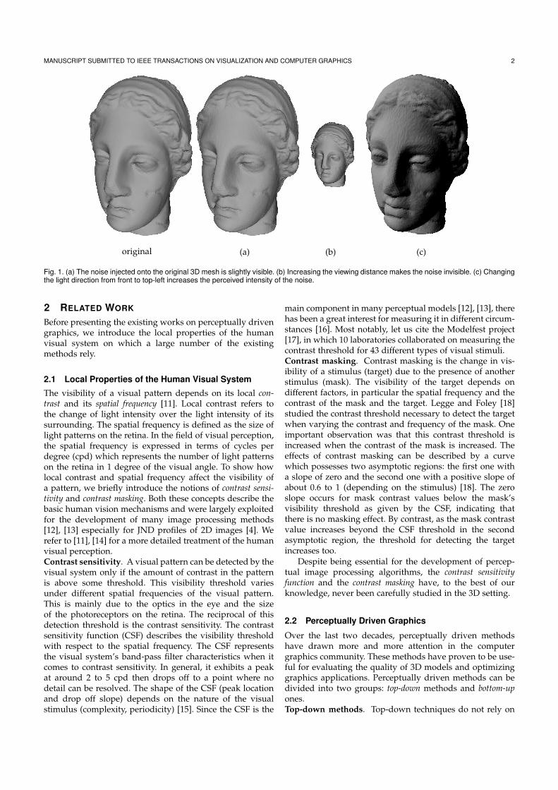
MANUSCRIPT SUBMITTED TO IEEE TRANSACTIONS ON VISUALIZATION AND COMPUTER GRAPHICS 2
original (b)(a) (c)
Fig. 1. (a) The noise injected onto the original 3D mesh is slightly visible. (b) Increasing the viewing distance makes the noise invisible. (c) Changingthe light direction from front to top-left increases the perceived intensity of the noise.
2 RELATED WORK
Before presenting the existing works on perceptually drivengraphics, we introduce the local properties of the humanvisual system on which a large number of the existingmethods rely.
2.1 Local Properties of the Human Visual System
The visibility of a visual pattern depends on its local con-trast and its spatial frequency [11]. Local contrast refers tothe change of light intensity over the light intensity of itssurrounding. The spatial frequency is defined as the size oflight patterns on the retina. In the field of visual perception,the spatial frequency is expressed in terms of cycles perdegree (cpd) which represents the number of light patternson the retina in 1 degree of the visual angle. To show howlocal contrast and spatial frequency affect the visibility ofa pattern, we briefly introduce the notions of contrast sensi-tivity and contrast masking. Both these concepts describe thebasic human vision mechanisms and were largely exploitedfor the development of many image processing methods[12], [13] especially for JND profiles of 2D images [4]. Werefer to [11], [14] for a more detailed treatment of the humanvisual perception.Contrast sensitivity. A visual pattern can be detected by thevisual system only if the amount of contrast in the patternis above some threshold. This visibility threshold variesunder different spatial frequencies of the visual pattern.This is mainly due to the optics in the eye and the sizeof the photoreceptors on the retina. The reciprocal of thisdetection threshold is the contrast sensitivity. The contrastsensitivity function (CSF) describes the visibility thresholdwith respect to the spatial frequency. The CSF representsthe visual system’s band-pass filter characteristics when itcomes to contrast sensitivity. In general, it exhibits a peakat around 2 to 5 cpd then drops off to a point where nodetail can be resolved. The shape of the CSF (peak locationand drop off slope) depends on the nature of the visualstimulus (complexity, periodicity) [15]. Since the CSF is the
main component in many perceptual models [12], [13], therehas been a great interest for measuring it in different circum-stances [16]. Most notably, let us cite the Modelfest project[17], in which 10 laboratories collaborated on measuring thecontrast threshold for 43 different types of visual stimuli.Contrast masking. Contrast masking is the change in vis-ibility of a stimulus (target) due to the presence of anotherstimulus (mask). The visibility of the target depends ondifferent factors, in particular the spatial frequency and thecontrast of the mask and the target. Legge and Foley [18]studied the contrast threshold necessary to detect the targetwhen varying the contrast and frequency of the mask. Oneimportant observation was that this contrast threshold isincreased when the contrast of the mask is increased. Theeffects of contrast masking can be described by a curvewhich possesses two asymptotic regions: the first one witha slope of zero and the second one with a positive slope ofabout 0.6 to 1 (depending on the stimulus) [18]. The zeroslope occurs for mask contrast values below the mask’svisibility threshold as given by the CSF, indicating thatthere is no masking effect. By contrast, as the mask contrastvalue increases beyond the CSF threshold in the secondasymptotic region, the threshold for detecting the targetincreases too.
Despite being essential for the development of percep-tual image processing algorithms, the contrast sensitivityfunction and the contrast masking have, to the best of ourknowledge, never been carefully studied in the 3D setting.
2.2 Perceptually Driven Graphics
Over the last two decades, perceptually driven methodshave drawn more and more attention in the computergraphics community. These methods have proven to be use-ful for evaluating the quality of 3D models and optimizinggraphics applications. Perceptually driven methods can bedivided into two groups: top-down methods and bottom-upones.Top-down methods. Top-down techniques do not rely on
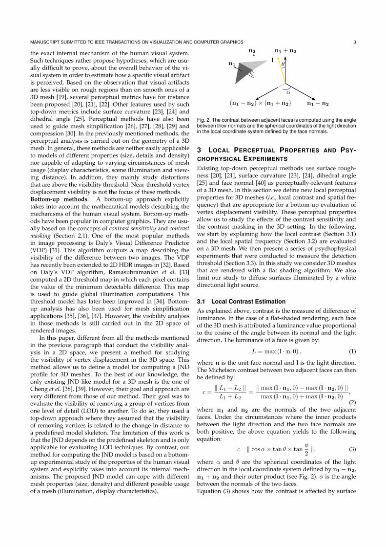
MANUSCRIPT SUBMITTED TO IEEE TRANSACTIONS ON VISUALIZATION AND COMPUTER GRAPHICS 3
the exact internal mechanism of the human visual system.Such techniques rather propose hypotheses, which are usu-ally difficult to prove, about the overall behavior of the vi-sual system in order to estimate how a specific visual artifactis perceived. Based on the observation that visual artifactsare less visible on rough regions than on smooth ones of a3D mesh [19], several perceptual metrics have for instancebeen proposed [20], [21], [22]. Other features used by suchtop-down metrics include surface curvature [23], [24] anddihedral angle [25]. Perceptual methods have also beenused to guide mesh simplification [26], [27], [28], [29] andcompression [30]. In the previously mentioned methods, theperceptual analysis is carried out on the geometry of a 3Dmesh. In general, these methods are neither easily applicableto models of different properties (size, details and density)nor capable of adapting to varying circumstances of meshusage (display characteristics, scene illumination and view-ing distance). In addition, they mainly study distortionsthat are above the visibility threshold. Near-threshold vertexdisplacement visibility is not the focus of these methods.Bottom-up methods. A bottom-up approach explicitlytakes into account the mathematical models describing themechanisms of the human visual system. Bottom-up meth-ods have been popular in computer graphics. They are usu-ally based on the concepts of contrast sensitivity and contrastmasking (Section 2.1). One of the most popular methodsin image processing is Daly’s Visual Difference Predictor(VDP) [31]. This algorithm outputs a map describing thevisibility of the difference between two images. The VDPhas recently been extended to 2D HDR images in [32]. Basedon Daly’s VDP algorithm, Ramasubramanian et al. [33]computed a 2D threshold map in which each pixel containsthe value of the minimum detectable difference. This mapis used to guide global illumination computations. Thisthreshold model has later been improved in [34]. Bottom-up analysis has also been used for mesh simplificationapplications [35], [36], [37]. However, the visibility analysisin those methods is still carried out in the 2D space ofrendered images.
In this paper, different from all the methods mentionedin the previous paragraph that conduct the visibility anal-ysis in a 2D space, we present a method for studyingthe visibility of vertex displacement in the 3D space. Thismethod allows us to define a model for computing a JNDprofile for 3D meshes. To the best of our knowledge, theonly existing JND-like model for a 3D mesh is the one ofCheng et al. [38], [39]. However, their goal and approach arevery different from those of our method. Their goal was toevaluate the visibility of removing a group of vertices fromone level of detail (LOD) to another. To do so, they used atop-down approach where they assumed that the visibilityof removing vertices is related to the change in distance toa predefined model skeleton. The limitation of this work isthat the JND depends on the predefined skeleton and is onlyapplicable for evaluating LOD techniques. By contrast, ourmethod for computing the JND model is based on a bottom-up experimental study of the properties of the human visualsystem and explicitly takes into account its internal mech-anisms. The proposed JND model can cope with differentmesh properties (size, density) and different possible usageof a mesh (illumination, display characteristics).
n1 + n2
(n1 − n2) × (n1 + n2)
α
n1 − n2
lθ
n2
φ
n1
Fig. 2. The contrast between adjacent faces is computed using the anglebetween their normals and the spherical coordinates of the light directionin the local coordinate system defined by the face normals.
3 LOCAL PERCEPTUAL PROPERTIES AND PSY-CHOPHYSICAL EXPERIMENTS
Existing top-down perceptual methods use surface rough-ness [20], [21], surface curvature [23], [24], dihedral angle[25] and face normal [40] as perceptually-relevant featuresof a 3D mesh. In this section we define new local perceptualproperties for 3D meshes (i.e., local contrast and spatial fre-quency) that are appropriate for a bottom-up evaluation ofvertex displacement visibility. These perceptual propertiesallow us to study the effects of the contrast sensitivity andthe contrast masking in the 3D setting. In the following,we start by explaining how the local contrast (Section 3.1)and the local spatial frequency (Section 3.2) are evaluatedon a 3D mesh. We then present a series of psychophysicalexperiments that were conducted to measure the detectionthreshold (Section 3.3). In this study we consider 3D meshesthat are rendered with a flat shading algorithm. We alsolimit our study to diffuse surfaces illuminated by a whitedirectional light source.
3.1 Local Contrast EstimationAs explained above, contrast is the measure of difference ofluminance. In the case of a flat-shaded rendering, each faceof the 3D mesh is attributed a luminance value proportionalto the cosine of the angle between its normal and the lightdirection. The luminance of a face is given by:
L = max (l · n, 0) , (1)
where n is the unit face normal and l is the light direction.The Michelson contrast between two adjacent faces can thenbe defined by:
c = L1 − L2
L1 + L2=
max (l · n1, 0) − max (l · n2, 0)
max (l · n1, 0) + max (l · n2, 0),
(2)where n1 and n2 are the normals of the two adjacentfaces. Under the circumstances where the inner productsbetween the light direction and the two face normals areboth positive, the above equation yields to the followingequation:
c = cosα × tan θ × tanφ
2, (3)
where α and θ are the spherical coordinates of the lightdirection in the local coordinate system defined by n1 −n2,n1 + n2 and their outer product (see Fig. 2). φ is the anglebetween the normals of the two faces.Equation (3) shows how the contrast is affected by surface
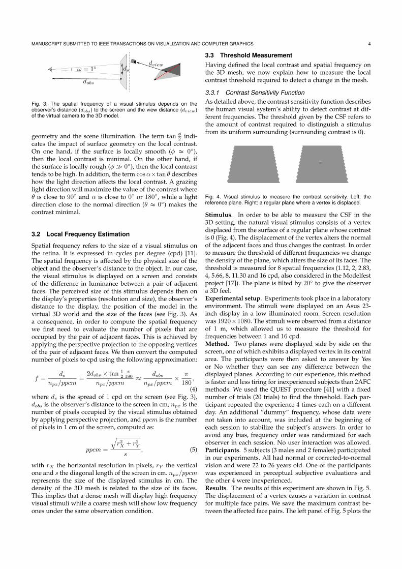
MANUSCRIPT SUBMITTED TO IEEE TRANSACTIONS ON VISUALIZATION AND COMPUTER GRAPHICS 4
ω = 1
dobs
dviewds
Fig. 3. The spatial frequency of a visual stimulus depends on theobserver’s distance (dobs) to the screen and the view distance (dview)of the virtual camera to the 3D model.
geometry and the scene illumination. The term tan φ2 indi-
cates the impact of surface geometry on the local contrast.On one hand, if the surface is locally smooth (φ ≈ 0),then the local contrast is minimal. On the other hand, ifthe surface is locally rough (φ ≫ 0), then the local contrasttends to be high. In addition, the term cosα×tan θ describeshow the light direction affects the local contrast. A grazinglight direction will maximize the value of the contrast whereθ is close to 90 and α is close to 0 or 180, while a lightdirection close to the normal direction (θ ≈ 0) makes thecontrast minimal.
3.2 Local Frequency Estimation
Spatial frequency refers to the size of a visual stimulus onthe retina. It is expressed in cycles per degree (cpd) [11].The spatial frequency is affected by the physical size of theobject and the observer’s distance to the object. In our case,the visual stimulus is displayed on a screen and consistsof the difference in luminance between a pair of adjacentfaces. The perceived size of this stimulus depends then onthe display’s properties (resolution and size), the observer’sdistance to the display, the position of the model in thevirtual 3D world and the size of the faces (see Fig. 3). Asa consequence, in order to compute the spatial frequencywe first need to evaluate the number of pixels that areoccupied by the pair of adjacent faces. This is achieved byapplying the perspective projection to the opposing verticesof the pair of adjacent faces. We then convert the computednumber of pixels to cpd using the following approximation:
f =ds
npx/ppcm=
2dobs × tan 12
π180
npx/ppcm≈
dobs
npx/ppcm× π
180,
(4)where ds is the spread of 1 cpd on the screen (see Fig. 3),dobs is the observer’s distance to the screen in cm, npx is thenumber of pixels occupied by the visual stimulus obtainedby applying perspective projection, and ppcm is the numberof pixels in 1 cm of the screen, computed as:
ppcm =
r2X + r2
Y
s, (5)
with rX the horizontal resolution in pixels, rY the verticalone and s the diagonal length of the screen in cm. npx/ppcmrepresents the size of the displayed stimulus in cm. Thedensity of the 3D mesh is related to the size of its faces.This implies that a dense mesh will display high frequencyvisual stimuli while a coarse mesh will show low frequencyones under the same observation condition.
3.3 Threshold MeasurementHaving defined the local contrast and spatial frequency onthe 3D mesh, we now explain how to measure the localcontrast threshold required to detect a change in the mesh.
3.3.1 Contrast Sensitivity FunctionAs detailed above, the contrast sensitivity function describesthe human visual system’s ability to detect contrast at dif-ferent frequencies. The threshold given by the CSF refers tothe amount of contrast required to distinguish a stimulusfrom its uniform surrounding (surrounding contrast is 0).
Fig. 4. Visual stimulus to measure the contrast sensitivity. Left: thereference plane. Right: a regular plane where a vertex is displaced.
Stimulus. In order to be able to measure the CSF in the3D setting, the natural visual stimulus consists of a vertexdisplaced from the surface of a regular plane whose contrastis 0 (Fig. 4). The displacement of the vertex alters the normalof the adjacent faces and thus changes the contrast. In orderto measure the threshold of different frequencies we changethe density of the plane, which alters the size of its faces. Thethreshold is measured for 8 spatial frequencies (1.12, 2, 2.83,4, 5.66, 8, 11.30 and 16 cpd, also considered in the Modelfestproject [17]). The plane is tilted by 20 to give the observera 3D feel.Experimental setup. Experiments took place in a laboratoryenvironment. The stimuli were displayed on an Asus 23-inch display in a low illuminated room. Screen resolutionwas 1920×1080. The stimuli were observed from a distanceof 1 m, which allowed us to measure the threshold forfrequencies between 1 and 16 cpd.Method. Two planes were displayed side by side on thescreen, one of which exhibits a displayed vertex in its centralarea. The participants were then asked to answer by Yesor No whether they can see any difference between thedisplayed planes. According to our experience, this methodis faster and less tiring for inexperienced subjects than 2AFCmethods. We used the QUEST procedure [41] with a fixednumber of trials (20 trials) to find the threshold. Each par-ticipant repeated the experience 4 times each on a differentday. An additional ”dummy” frequency, whose data werenot taken into account, was included at the beginning ofeach session to stabilize the subject’s answers. In order toavoid any bias, frequency order was randomized for eachobserver in each session. No user interaction was allowed.Participants. 5 subjects (3 males and 2 females) participatedin our experiments. All had normal or corrected-to-normalvision and were 22 to 26 years old. One of the participantswas experienced in perceptual subjective evaluations andthe other 4 were inexperienced.Results. The results of this experiment are shown in Fig. 5.The displacement of a vertex causes a variation in contrastfor multiple face pairs. We save the maximum contrast be-tween the affected face pairs. The left panel of Fig. 5 plots the

MANUSCRIPT SUBMITTED TO IEEE TRANSACTIONS ON VISUALIZATION AND COMPUTER GRAPHICS 5
1 2 3 4 5 6 7 8 910 20 30 40 50 600.1
1
10
100
1 2 3 4 5 6 7 8 910 20 301
10
100
Frequency (cpd)
Se
nsitiv
ity (
1/th
resh
old
)
participant 1
participant 2
participant 3
participant 4
participant 5
Frequency (cpd)
Se
nsitiv
ity (
1/th
resh
old
)
fit
measurements
Fig. 5. Left: plot of the mean sensitivity for each observer over each fre-quency. Right: plot of the subjects’ mean sensitivity over each frequencyfitted using Manos and Sakrison’s mathematical model.
mean sensitivity for each observer over each frequency. Theplot shows a high consistency between the participants: Allof them exhibit a peak in sensitivity at 2 cpd and the dropoff in sensitivity on either side of the peak is similar for allparticipants. The right panel of Fig. 5 shows the subjects’mean sensitivity over each frequency, fitted using Mannosand Sakrison’s mathematical model [42] that is defined by:
csf(f) =
1 − a +f
f0
e−fp
, (6)
with a = −15.13, f0 = 0.0096 and p = 0.64. The fitpredicts a peak in sensitivity at around 2 cpd that dropsrapidly at high frequencies. At low frequencies the drop insensitivity is much slower that the one measured with a2D contrast grating [15], [17]. This is due to the aperiodicnature of the visual stimulus [15]. Equation (6) shows therelation between the density of a mesh and the visibility of alocal contrast alteration. As the density increases from a verylow value, it would be slightly easier for the human visualsystem to notice the local contrast alteration on the mesh’ssurface until it reaches a certain limit (around 2 cpd) beyondwhich it would be harder to detect contrast alteration as thedensity increases.
3.3.2 Contrast MaskingContrast masking refers to the ability of the human visualsystem to discriminate between two visible visual stimuli(a target and a mask). Since the visibility of a visual stimu-lus depends on its spatial frequency, the contrast maskingthreshold is different at each frequency. However, if we nor-malize the threshold values by the mask’s CSF value, thenthe resulting threshold will be independent of the stimulus’sspatial frequency [31]. Therefore, measuring the maskingeffect can be done by only changing the contrast value of amask signal without the need to pay too much attention toits spatial frequency. Nevertheless, in our preliminary tests,we measured the normalized contrast masking effects for 3different frequencies and found that the results were indeedthe same (as stated in [31]), showing that measuring thecontrast masking effect can be done independently from thespatial frequency of the visual stimulus.Stimulus and method. In order to be able to measure
Fig. 6. Visual stimulus for measuring contrast masking. Left: a sphereapproximated by an icosahedron subdivided 3 times from which a vertexis displaced. Right: the reference sphere.
the threshold relative to the contrast masking effect, thevisual stimulus needs to exhibit a visible initial contrast (i.e.,above the CSF value). We then increase the initial contrastand measure the value needed to notice that change. Inother words, if c is the initial contrast (mask signal) andc′ is the increased value, we measure Δc = c′ − c (targetsignal) needed to discriminate between c and c′. Similarly tothe method used for measuring the CSF, two models weredisplayed on the screen and the participants were supposedto decide whether they saw the difference between the twoobjects or not. The stimulus consists of a vertex displacedfrom a sphere approximated by a subdivided icosahedron(Fig. 6). The icosahedron is subdivided 3 times, which makesthe contrast between two adjacent faces (stimulus of about 2cpd) visible for an observer. This initial contrast representsthe mask signal. Varying the light direction modifies thevalue of the initial contrast between two adjacent faces.We measured the threshold relative to 7 mask contraststhat were log-linearly spaced from 0.6 to 4 times the CSFthreshold.Experimental setup. The same experimental setup and thesame method than for the CSF measurement experimentpreviously described have been used. The same 5 subjectsalso participated in the contrast masking experiments.Results. The results of this experiment are shown in Fig. 7.The left panel plots for every participant the mean normal-ized threshold over the normalized contrast mask. For maskcontrasts below the visibility threshold (normalized contrastmask lower than 1), the measured normalized thresholdis close to 1. This indicates that the measured thresholdrefers to the one given by the CSF and that no masking hasoccurred. For mask contrasts above the visibility threshold,the measured normalized threshold is above the one givenby CSF and lies close to the asymptotic region with aslope near 0.7. The right panel of Fig. 7 shows the subjects’mean threshold over each mask contrast fitted using Daly’smathematical masking model [31] that is defined by:
masking(c) =
1 + (k1 × (k2 × c)s)b1/b
, (7)
with c the normalized threshold, and the fitted valuesk1 = 0.0078, k2 = 88.29, s = 1.00 and b = 4.207. Thefit exhibits the two asymptotic regions that characterize thecontrast masking effect with a transition between the tworegions at the CSF visibility threshold. To some extent, Eq.(7) shows how an increase in surface roughness can hidelocal geometric distortions on the mesh’s surface. A rough
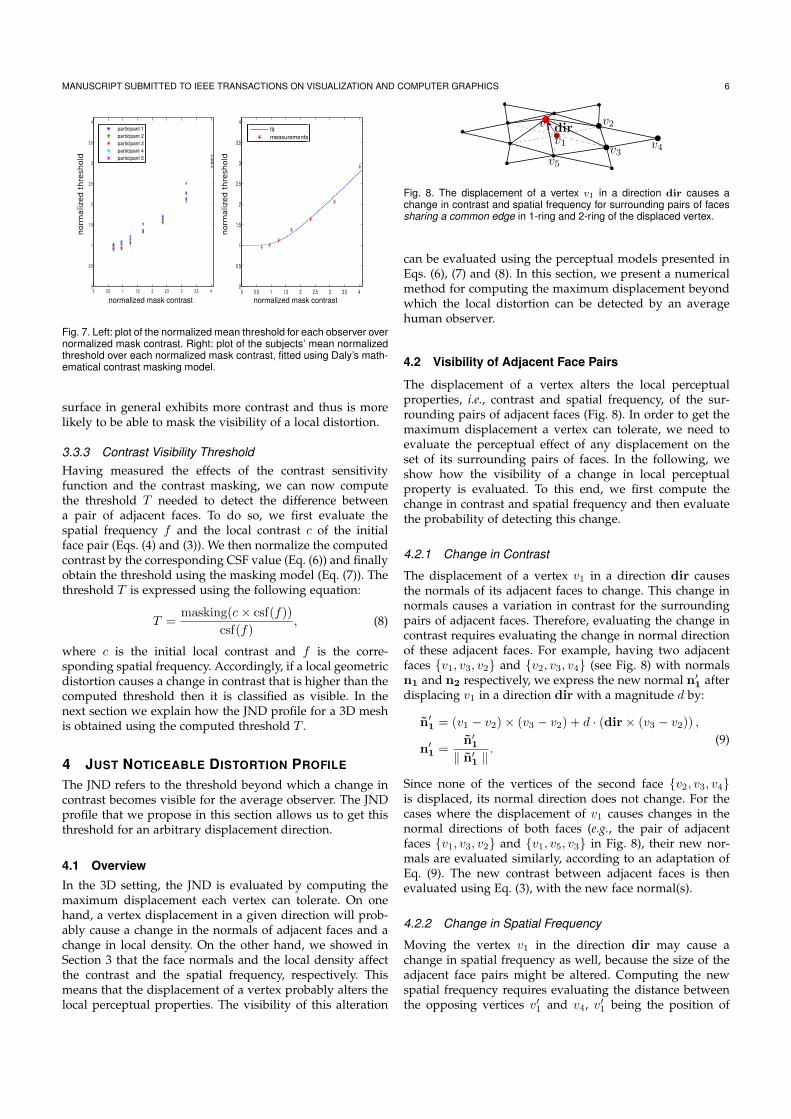
MANUSCRIPT SUBMITTED TO IEEE TRANSACTIONS ON VISUALIZATION AND COMPUTER GRAPHICS 6
0 0.5 1 1.5 2 2.5 3 3.5 40
0.5
1
1.5
2
2.5
3
3.5
4
normalized mask contrast
fit
measurements
0 0.5 1 1.5 2 2.5 3 3.5 40
0.5
1
1.5
2
2.5
3
3.5
4
normalized mask contrast
participant 1
participant 2
participant 3
participant 4
participant 5
norm
aliz
ed
thre
shold
norm
aliz
ed
thre
shold
Fig. 7. Left: plot of the normalized mean threshold for each observer overnormalized mask contrast. Right: plot of the subjects’ mean normalizedthreshold over each normalized mask contrast, fitted using Daly’s math-ematical contrast masking model.
surface in general exhibits more contrast and thus is morelikely to be able to mask the visibility of a local distortion.
3.3.3 Contrast Visibility ThresholdHaving measured the effects of the contrast sensitivityfunction and the contrast masking, we can now computethe threshold T needed to detect the difference betweena pair of adjacent faces. To do so, we first evaluate thespatial frequency f and the local contrast c of the initialface pair (Eqs. (4) and (3)). We then normalize the computedcontrast by the corresponding CSF value (Eq. (6)) and finallyobtain the threshold using the masking model (Eq. (7)). Thethreshold T is expressed using the following equation:
T =masking(c × csf(f))
csf(f), (8)
where c is the initial local contrast and f is the corre-sponding spatial frequency. Accordingly, if a local geometricdistortion causes a change in contrast that is higher than thecomputed threshold then it is classified as visible. In thenext section we explain how the JND profile for a 3D meshis obtained using the computed threshold T .
4 JUST NOTICEABLE DISTORTION PROFILE
The JND refers to the threshold beyond which a change incontrast becomes visible for the average observer. The JNDprofile that we propose in this section allows us to get thisthreshold for an arbitrary displacement direction.
4.1 Overview
In the 3D setting, the JND is evaluated by computing themaximum displacement each vertex can tolerate. On onehand, a vertex displacement in a given direction will prob-ably cause a change in the normals of adjacent faces and achange in local density. On the other hand, we showed inSection 3 that the face normals and the local density affectthe contrast and the spatial frequency, respectively. Thismeans that the displacement of a vertex probably alters thelocal perceptual properties. The visibility of this alteration
v′1v1
v3v4
v2dir
v5
Fig. 8. The displacement of a vertex v1 in a direction dir causes achange in contrast and spatial frequency for surrounding pairs of facessharing a common edge in 1-ring and 2-ring of the displaced vertex.
can be evaluated using the perceptual models presented inEqs. (6), (7) and (8). In this section, we present a numericalmethod for computing the maximum displacement beyondwhich the local distortion can be detected by an averagehuman observer.
4.2 Visibility of Adjacent Face Pairs
The displacement of a vertex alters the local perceptualproperties, i.e., contrast and spatial frequency, of the sur-rounding pairs of adjacent faces (Fig. 8). In order to get themaximum displacement a vertex can tolerate, we need toevaluate the perceptual effect of any displacement on theset of its surrounding pairs of faces. In the following, weshow how the visibility of a change in local perceptualproperty is evaluated. To this end, we first compute thechange in contrast and spatial frequency and then evaluatethe probability of detecting this change.
4.2.1 Change in Contrast
The displacement of a vertex v1 in a direction dir causesthe normals of its adjacent faces to change. This change innormals causes a variation in contrast for the surroundingpairs of adjacent faces. Therefore, evaluating the change incontrast requires evaluating the change in normal directionof these adjacent faces. For example, having two adjacentfaces v1, v3, v2 and v2, v3, v4 (see Fig. 8) with normalsn1 and n2 respectively, we express the new normal n′
1 afterdisplacing v1 in a direction dir with a magnitude d by:
n′
1 = (v1 − v2) × (v3 − v2) + d · (dir × (v3 − v2)) ,
n′
1 =n′
1
n′
1 .
(9)
Since none of the vertices of the second face v2, v3, v4is displaced, its normal direction does not change. For thecases where the displacement of v1 causes changes in thenormal directions of both faces (e.g., the pair of adjacentfaces v1, v3, v2 and v1, v5, v3 in Fig. 8), their new nor-mals are evaluated similarly, according to an adaptation ofEq. (9). The new contrast between adjacent faces is thenevaluated using Eq. (3), with the new face normal(s).
4.2.2 Change in Spatial Frequency
Moving the vertex v1 in the direction dir may cause achange in spatial frequency as well, because the size of theadjacent face pairs might be altered. Computing the newspatial frequency requires evaluating the distance betweenthe opposing vertices v′1 and v4, v′1 being the position of
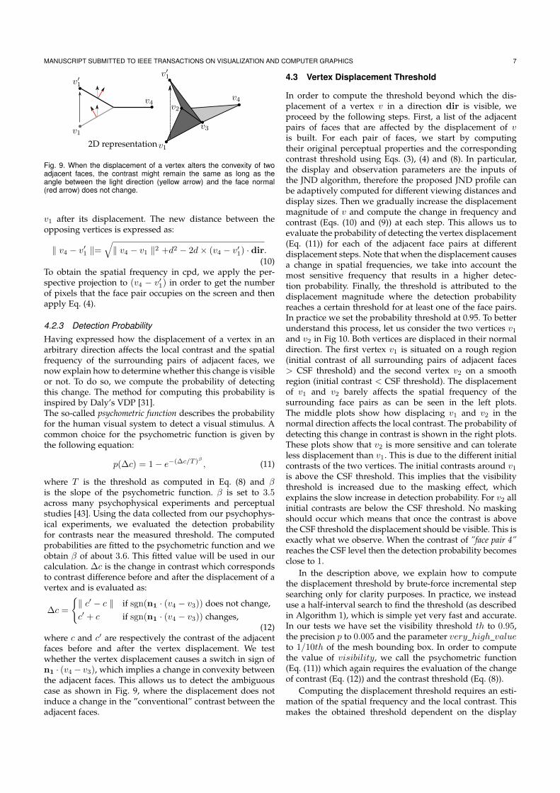
MANUSCRIPT SUBMITTED TO IEEE TRANSACTIONS ON VISUALIZATION AND COMPUTER GRAPHICS 7
2D representation
v4
v1
v4
v1
v′1v′1
v3
v2
Fig. 9. When the displacement of a vertex alters the convexity of twoadjacent faces, the contrast might remain the same as long as theangle between the light direction (yellow arrow) and the face normal(red arrow) does not change.
v1 after its displacement. The new distance between theopposing vertices is expressed as:
v4 − v′1 =
v4 − v1 2 +d2 − 2d × (v4 − v′1) · dir.(10)
To obtain the spatial frequency in cpd, we apply the per-spective projection to (v4 − v′1) in order to get the numberof pixels that the face pair occupies on the screen and thenapply Eq. (4).
4.2.3 Detection ProbabilityHaving expressed how the displacement of a vertex in anarbitrary direction affects the local contrast and the spatialfrequency of the surrounding pairs of adjacent faces, wenow explain how to determine whether this change is visibleor not. To do so, we compute the probability of detectingthis change. The method for computing this probability isinspired by Daly’s VDP [31].The so-called psychometric function describes the probabilityfor the human visual system to detect a visual stimulus. Acommon choice for the psychometric function is given bythe following equation:
p(Δc) = 1 − e−(Δc/T )β , (11)
where T is the threshold as computed in Eq. (8) and βis the slope of the psychometric function. β is set to 3.5across many psychophysical experiments and perceptualstudies [43]. Using the data collected from our psychophys-ical experiments, we evaluated the detection probabilityfor contrasts near the measured threshold. The computedprobabilities are fitted to the psychometric function and weobtain β of about 3.6. This fitted value will be used in ourcalculation. Δc is the change in contrast which correspondsto contrast difference before and after the displacement of avertex and is evaluated as:
Δc =
c′ − c if sgn(n1 · (v4 − v3)) does not change,c′ + c if sgn(n1 · (v4 − v3)) changes,
(12)where c and c′ are respectively the contrast of the adjacentfaces before and after the vertex displacement. We testwhether the vertex displacement causes a switch in sign ofn1 · (v4 − v3), which implies a change in convexity betweenthe adjacent faces. This allows us to detect the ambiguouscase as shown in Fig. 9, where the displacement does notinduce a change in the ”conventional” contrast between theadjacent faces.
4.3 Vertex Displacement Threshold
In order to compute the threshold beyond which the dis-placement of a vertex v in a direction dir is visible, weproceed by the following steps. First, a list of the adjacentpairs of faces that are affected by the displacement of vis built. For each pair of faces, we start by computingtheir original perceptual properties and the correspondingcontrast threshold using Eqs. (3), (4) and (8). In particular,the display and observation parameters are the inputs ofthe JND algorithm, therefore the proposed JND profile canbe adaptively computed for different viewing distances anddisplay sizes. Then we gradually increase the displacementmagnitude of v and compute the change in frequency andcontrast (Eqs. (10) and (9)) at each step. This allows us toevaluate the probability of detecting the vertex displacement(Eq. (11)) for each of the adjacent face pairs at differentdisplacement steps. Note that when the displacement causesa change in spatial frequencies, we take into account themost sensitive frequency that results in a higher detec-tion probability. Finally, the threshold is attributed to thedisplacement magnitude where the detection probabilityreaches a certain threshold for at least one of the face pairs.In practice we set the probability threshold at 0.95. To betterunderstand this process, let us consider the two vertices v1
and v2 in Fig 10. Both vertices are displaced in their normaldirection. The first vertex v1 is situated on a rough region(initial contrast of all surrounding pairs of adjacent faces> CSF threshold) and the second vertex v2 on a smoothregion (initial contrast < CSF threshold). The displacementof v1 and v2 barely affects the spatial frequency of thesurrounding face pairs as can be seen in the left plots.The middle plots show how displacing v1 and v2 in thenormal direction affects the local contrast. The probability ofdetecting this change in contrast is shown in the right plots.These plots show that v2 is more sensitive and can tolerateless displacement than v1. This is due to the different initialcontrasts of the two vertices. The initial contrasts around v1
is above the CSF threshold. This implies that the visibilitythreshold is increased due to the masking effect, whichexplains the slow increase in detection probability. For v2 allinitial contrasts are below the CSF threshold. No maskingshould occur which means that once the contrast is abovethe CSF threshold the displacement should be visible. This isexactly what we observe. When the contrast of ”face pair 4”reaches the CSF level then the detection probability becomesclose to 1.
In the description above, we explain how to computethe displacement threshold by brute-force incremental stepsearching only for clarity purposes. In practice, we insteaduse a half-interval search to find the threshold (as describedin Algorithm 1), which is simple yet very fast and accurate.In our tests we have set the visibility threshold th to 0.95,the precision p to 0.005 and the parameter very high valueto 1/10th of the mesh bounding box. In order to computethe value of visibility, we call the psychometric function(Eq. (11)) which again requires the evaluation of the changeof contrast (Eq. (12)) and the contrast threshold (Eq. (8)).
Computing the displacement threshold requires an esti-mation of the spatial frequency and the local contrast. Thismakes the obtained threshold dependent on the display
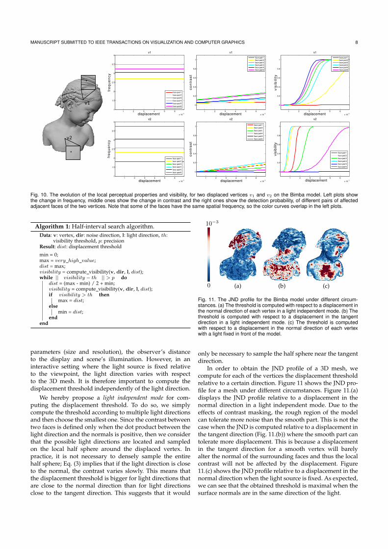
MANUSCRIPT SUBMITTED TO IEEE TRANSACTIONS ON VISUALIZATION AND COMPUTER GRAPHICS 8
1 2 3 4 5 6
x 10−3
1
1.5
2
2.5
3
3.5
4
v2
face pair1
face pair2
face pair3
face pair4
face pair5
face pair6
1 2 3 4 5 6
x 10−3
0
0.2
0.4
0.6
0.8
1
v2
vis
ibilit
y
face pair1
face pair2
face pair3
face pair4
face pair5
face pair6
1 2 3 4 5 6
x 10−3
0
0.2
0.4
0.6
0.8
1
v2
co
ntr
as
t
face pair1
face pair2
face pair3
face pair4
face pair5
face pair6
v1
v2
1 2 3 4 5 6
x 10−3
1
1.5
2
2.5
3
3.5
4
v1
fre
qu
en
cy
face pair1
face pair2
face pair3
face pair4
face pair5
face pair6
1 2 3 4 5 6
x 10−3
0
0.2
0.4
0.6
0.8
1
v1
displacement
vis
ibil
ity
face pair1
face pair2
face pair3
face pair4
face pair5
face pair6
displacement1 2 3 4 5 6
x 10−3
0
0.2
0.4
0.6
0.8
1
v1
co
ntr
as
t
face pair1
face pair2
face pair3
face pair4
face pair5
face pair6
displacement
displacement displacement displacement
fre
qu
en
cy
Fig. 10. The evolution of the local perceptual properties and visibility, for two displaced vertices v1 and v2 on the Bimba model. Left plots showthe change in frequency, middle ones show the change in contrast and the right ones show the detection probability, of different pairs of affectedadjacent faces of the two vertices. Note that some of the faces have the same spatial frequency, so the color curves overlap in the left plots.
Algorithm 1: Half-interval search algorithm.Data: v: vertex, dir: noise direction, l: light direction, th:
visibility threshold, p: precisionResult: dist: displacement threshold
min = 0;max = very high value;dist = max;visibility = compute visibility(v, dir, l, dist);while || visibility − th || > p do
dist = (max - min) / 2 + min;visibility = compute visibility(v, dir, l, dist);if visibility > th then
max = dist;else
min = dist;end
end
parameters (size and resolution), the observer’s distanceto the display and scene’s illumination. However, in aninteractive setting where the light source is fixed relativeto the viewpoint, the light direction varies with respectto the 3D mesh. It is therefore important to compute thedisplacement threshold independently of the light direction.
We hereby propose a light independent mode for com-puting the displacement threshold. To do so, we simplycompute the threshold according to multiple light directionsand then choose the smallest one. Since the contrast betweentwo faces is defined only when the dot product between thelight direction and the normals is positive, then we considerthat the possible light directions are located and sampledon the local half sphere around the displaced vertex. Inpractice, it is not necessary to densely sample the entirehalf sphere; Eq. (3) implies that if the light direction is closeto the normal, the contrast varies slowly. This means thatthe displacement threshold is bigger for light directions thatare close to the normal direction than for light directionsclose to the tangent direction. This suggests that it would
(a) (b) (c)0
10−3
Fig. 11. The JND profile for the Bimba model under different circum-stances. (a) The threshold is computed with respect to a displacement inthe normal direction of each vertex in a light independent mode. (b) Thethreshold is computed with respect to a displacement in the tangentdirection in a light independent mode. (c) The threshold is computedwith respect to a displacement in the normal direction of each vertexwith a light fixed in front of the model.
only be necessary to sample the half sphere near the tangentdirection.
In order to obtain the JND profile of a 3D mesh, wecompute for each of the vertices the displacement thresholdrelative to a certain direction. Figure 11 shows the JND pro-file for a mesh under different circumstances. Figure 11.(a)displays the JND profile relative to a displacement in thenormal direction in a light independent mode. Due to theeffects of contrast masking, the rough region of the modelcan tolerate more noise than the smooth part. This is not thecase when the JND is computed relative to a displacement inthe tangent direction (Fig. 11.(b)) where the smooth part cantolerate more displacement. This is because a displacementin the tangent direction for a smooth vertex will barelyalter the normal of the surrounding faces and thus the localcontrast will not be affected by the displacement. Figure11.(c) shows the JND profile relative to a displacement in thenormal direction when the light source is fixed. As expected,we can see that the obtained threshold is maximal when thesurface normals are in the same direction of the light.
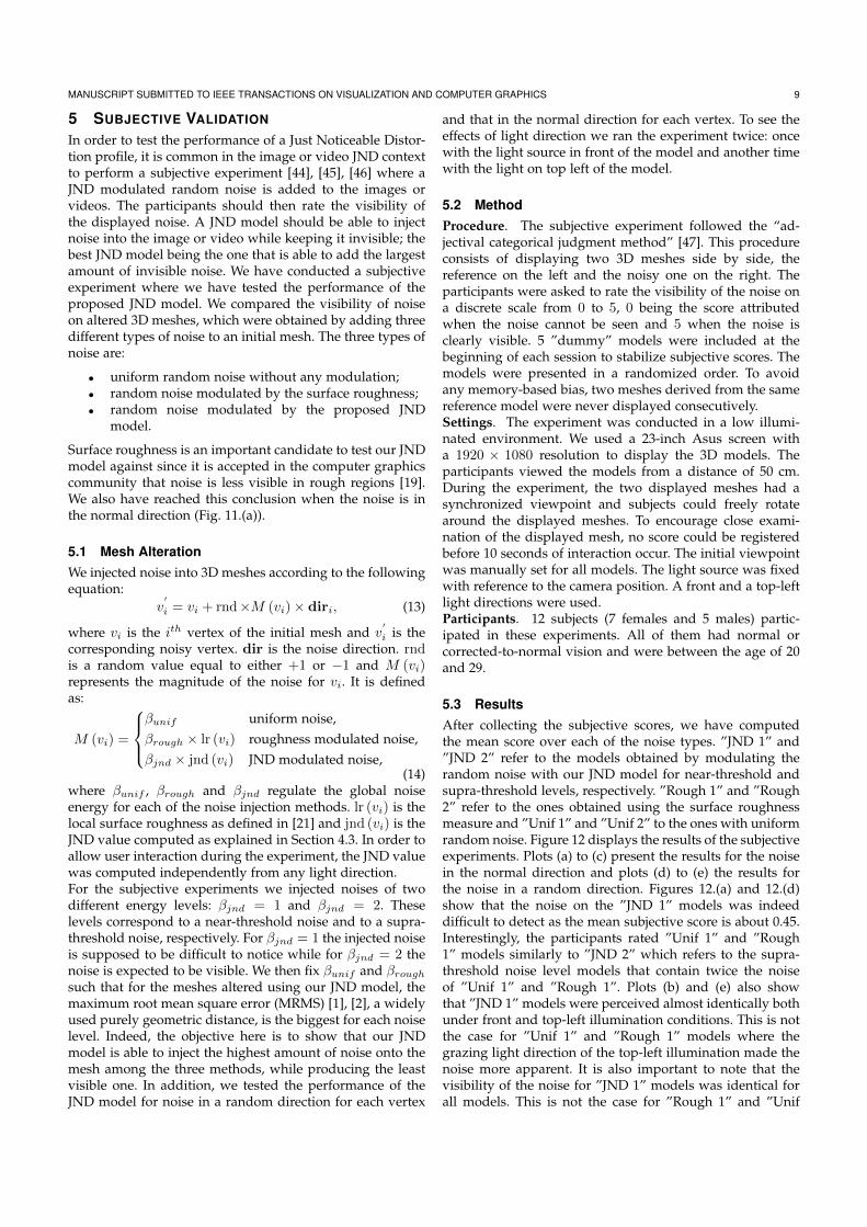
MANUSCRIPT SUBMITTED TO IEEE TRANSACTIONS ON VISUALIZATION AND COMPUTER GRAPHICS 9
5 SUBJECTIVE VALIDATION
In order to test the performance of a Just Noticeable Distor-tion profile, it is common in the image or video JND contextto perform a subjective experiment [44], [45], [46] where aJND modulated random noise is added to the images orvideos. The participants should then rate the visibility ofthe displayed noise. A JND model should be able to injectnoise into the image or video while keeping it invisible; thebest JND model being the one that is able to add the largestamount of invisible noise. We have conducted a subjectiveexperiment where we have tested the performance of theproposed JND model. We compared the visibility of noiseon altered 3D meshes, which were obtained by adding threedifferent types of noise to an initial mesh. The three types ofnoise are:
• uniform random noise without any modulation;• random noise modulated by the surface roughness;• random noise modulated by the proposed JND
model.
Surface roughness is an important candidate to test our JNDmodel against since it is accepted in the computer graphicscommunity that noise is less visible in rough regions [19].We also have reached this conclusion when the noise is inthe normal direction (Fig. 11.(a)).
5.1 Mesh AlterationWe injected noise into 3D meshes according to the followingequation:
v′
i = vi + rnd ×M (vi) × diri, (13)
where vi is the ith vertex of the initial mesh and v′
i is thecorresponding noisy vertex. dir is the noise direction. rndis a random value equal to either +1 or −1 and M (vi)represents the magnitude of the noise for vi. It is definedas:
M (vi) =
βunif uniform noise,βrough × lr (vi) roughness modulated noise,βjnd × jnd (vi) JND modulated noise,
(14)where βunif , βrough and βjnd regulate the global noiseenergy for each of the noise injection methods. lr (vi) is thelocal surface roughness as defined in [21] and jnd (vi) is theJND value computed as explained in Section 4.3. In order toallow user interaction during the experiment, the JND valuewas computed independently from any light direction.For the subjective experiments we injected noises of twodifferent energy levels: βjnd = 1 and βjnd = 2. Theselevels correspond to a near-threshold noise and to a supra-threshold noise, respectively. For βjnd = 1 the injected noiseis supposed to be difficult to notice while for βjnd = 2 thenoise is expected to be visible. We then fix βunif and βrough
such that for the meshes altered using our JND model, themaximum root mean square error (MRMS) [1], [2], a widelyused purely geometric distance, is the biggest for each noiselevel. Indeed, the objective here is to show that our JNDmodel is able to inject the highest amount of noise onto themesh among the three methods, while producing the leastvisible one. In addition, we tested the performance of theJND model for noise in a random direction for each vertex
and that in the normal direction for each vertex. To see theeffects of light direction we ran the experiment twice: oncewith the light source in front of the model and another timewith the light on top left of the model.
5.2 MethodProcedure. The subjective experiment followed the “ad-jectival categorical judgment method” [47]. This procedureconsists of displaying two 3D meshes side by side, thereference on the left and the noisy one on the right. Theparticipants were asked to rate the visibility of the noise ona discrete scale from 0 to 5, 0 being the score attributedwhen the noise cannot be seen and 5 when the noise isclearly visible. 5 ”dummy” models were included at thebeginning of each session to stabilize subjective scores. Themodels were presented in a randomized order. To avoidany memory-based bias, two meshes derived from the samereference model were never displayed consecutively.Settings. The experiment was conducted in a low illumi-nated environment. We used a 23-inch Asus screen witha 1920 × 1080 resolution to display the 3D models. Theparticipants viewed the models from a distance of 50 cm.During the experiment, the two displayed meshes had asynchronized viewpoint and subjects could freely rotatearound the displayed meshes. To encourage close exami-nation of the displayed mesh, no score could be registeredbefore 10 seconds of interaction occur. The initial viewpointwas manually set for all models. The light source was fixedwith reference to the camera position. A front and a top-leftlight directions were used.Participants. 12 subjects (7 females and 5 males) partic-ipated in these experiments. All of them had normal orcorrected-to-normal vision and were between the age of 20and 29.
5.3 ResultsAfter collecting the subjective scores, we have computedthe mean score over each of the noise types. ”JND 1” and”JND 2” refer to the models obtained by modulating therandom noise with our JND model for near-threshold andsupra-threshold levels, respectively. ”Rough 1” and ”Rough2” refer to the ones obtained using the surface roughnessmeasure and ”Unif 1” and ”Unif 2” to the ones with uniformrandom noise. Figure 12 displays the results of the subjectiveexperiments. Plots (a) to (c) present the results for the noisein the normal direction and plots (d) to (e) the results forthe noise in a random direction. Figures 12.(a) and 12.(d)show that the noise on the ”JND 1” models was indeeddifficult to detect as the mean subjective score is about 0.45.Interestingly, the participants rated ”Unif 1” and ”Rough1” models similarly to ”JND 2” which refers to the supra-threshold noise level models that contain twice the noiseof ”Unif 1” and ”Rough 1”. Plots (b) and (e) also showthat ”JND 1” models were perceived almost identically bothunder front and top-left illumination conditions. This is notthe case for ”Unif 1” and ”Rough 1” models where thegrazing light direction of the top-left illumination made thenoise more apparent. It is also important to note that thevisibility of the noise for ”JND 1” models was identical forall models. This is not the case for ”Rough 1” and ”Unif
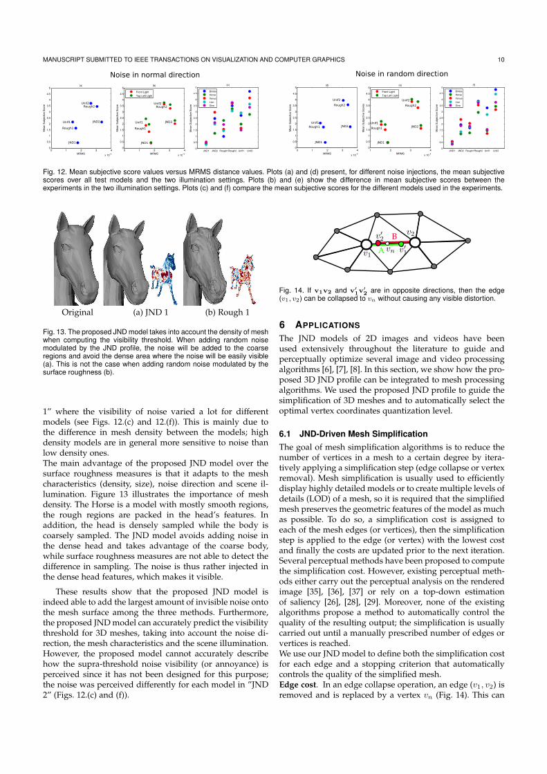
MANUSCRIPT SUBMITTED TO IEEE TRANSACTIONS ON VISUALIZATION AND COMPUTER GRAPHICS 10
Noise in normal direction Noise in random direction
0 1 2 3 4
x 10−4
0
0.5
1
1.5
2
2.5
3
3.5
4
4.5
5
MRMS
Mea
n Su
bjec
tive
Scor
e
(a)
0 1 2 3 4
x 10−4
0
0.5
1
1.5
2
2.5
3
3.5
4
4.5
5
MRMS
Mea
n Su
bjec
tive
Scor
e
(b)
Front LightTop Left Light
JND1 JND2 Rough1Rough2 Unif1 Unif20
0.5
1
1.5
2
2.5
3
3.5
4
4.5
5
Mea
n Su
bjec
tive
Scor
e
(c)
BimbaHorseVenusLionDino
JND1
Unif1
Unif2Rough2
Rough1
JND2
JND1
Unif1
Unif2Rough2
Rough1
JND2
0 1 2 3 4
x 10−4
0
0.5
1
1.5
2
2.5
3
3.5
4
4.5
5
MRMS
Mea
n Su
bjec
tive
Scor
e
(d)
1 2 3 4
x 10−4
0
0.5
1
1.5
2
2.5
3
3.5
4
4.5
5
MRMS
Mea
n Su
bjec
tive
Scor
es
(e)
Front LightTop Left Light
JND1 JND2 Rough1Rough2 Unif1 Unif20
0.5
1
1.5
2
2.5
3
3.5
4
4.5
5
Mea
n Su
bjec
tive
Scor
e
(f)
BimbaHorseVenusLionDino
JND1
Unif1
Unif2
Rough2
Rough1 JND2
JND1
Unif1
Unif2
Rough2
Rough1 JND2
Fig. 12. Mean subjective score values versus MRMS distance values. Plots (a) and (d) present, for different noise injections, the mean subjectivescores over all test models and the two illumination settings. Plots (b) and (e) show the difference in mean subjective scores between theexperiments in the two illumination settings. Plots (c) and (f) compare the mean subjective scores for the different models used in the experiments.
Original (a) JND 1 (b) Rough 1
Fig. 13. The proposed JND model takes into account the density of meshwhen computing the visibility threshold. When adding random noisemodulated by the JND profile, the noise will be added to the coarseregions and avoid the dense area where the noise will be easily visible(a). This is not the case when adding random noise modulated by thesurface roughness (b).
1” where the visibility of noise varied a lot for differentmodels (see Figs. 12.(c) and 12.(f)). This is mainly due tothe difference in mesh density between the models; highdensity models are in general more sensitive to noise thanlow density ones.The main advantage of the proposed JND model over thesurface roughness measures is that it adapts to the meshcharacteristics (density, size), noise direction and scene il-lumination. Figure 13 illustrates the importance of meshdensity. The Horse is a model with mostly smooth regions,the rough regions are packed in the head’s features. Inaddition, the head is densely sampled while the body iscoarsely sampled. The JND model avoids adding noise inthe dense head and takes advantage of the coarse body,while surface roughness measures are not able to detect thedifference in sampling. The noise is thus rather injected inthe dense head features, which makes it visible.
These results show that the proposed JND model isindeed able to add the largest amount of invisible noise ontothe mesh surface among the three methods. Furthermore,the proposed JND model can accurately predict the visibilitythreshold for 3D meshes, taking into account the noise di-rection, the mesh characteristics and the scene illumination.However, the proposed model cannot accurately describehow the supra-threshold noise visibility (or annoyance) isperceived since it has not been designed for this purpose;the noise was perceived differently for each model in ”JND2” (Figs. 12.(c) and (f)).
v1
v2
v′1
v′2
A
Bvn
Fig. 14. If v1v2 and v′
1v′
2 are in opposite directions, then the edge(v1, v2) can be collapsed to vn without causing any visible distortion.
6 APPLICATIONS
The JND models of 2D images and videos have beenused extensively throughout the literature to guide andperceptually optimize several image and video processingalgorithms [6], [7], [8]. In this section, we show how the pro-posed 3D JND profile can be integrated to mesh processingalgorithms. We used the proposed JND profile to guide thesimplification of 3D meshes and to automatically select theoptimal vertex coordinates quantization level.
6.1 JND-Driven Mesh SimplificationThe goal of mesh simplification algorithms is to reduce thenumber of vertices in a mesh to a certain degree by itera-tively applying a simplification step (edge collapse or vertexremoval). Mesh simplification is usually used to efficientlydisplay highly detailed models or to create multiple levels ofdetails (LOD) of a mesh, so it is required that the simplifiedmesh preserves the geometric features of the model as muchas possible. To do so, a simplification cost is assigned toeach of the mesh edges (or vertices), then the simplificationstep is applied to the edge (or vertex) with the lowest costand finally the costs are updated prior to the next iteration.Several perceptual methods have been proposed to computethe simplification cost. However, existing perceptual meth-ods either carry out the perceptual analysis on the renderedimage [35], [36], [37] or rely on a top-down estimationof saliency [26], [28], [29]. Moreover, none of the existingalgorithms propose a method to automatically control thequality of the resulting output; the simplification is usuallycarried out until a manually prescribed number of edges orvertices is reached.We use our JND model to define both the simplification costfor each edge and a stopping criterion that automaticallycontrols the quality of the simplified mesh.Edge cost. In an edge collapse operation, an edge (v1, v2) isremoved and is replaced by a vertex vn (Fig. 14). This can
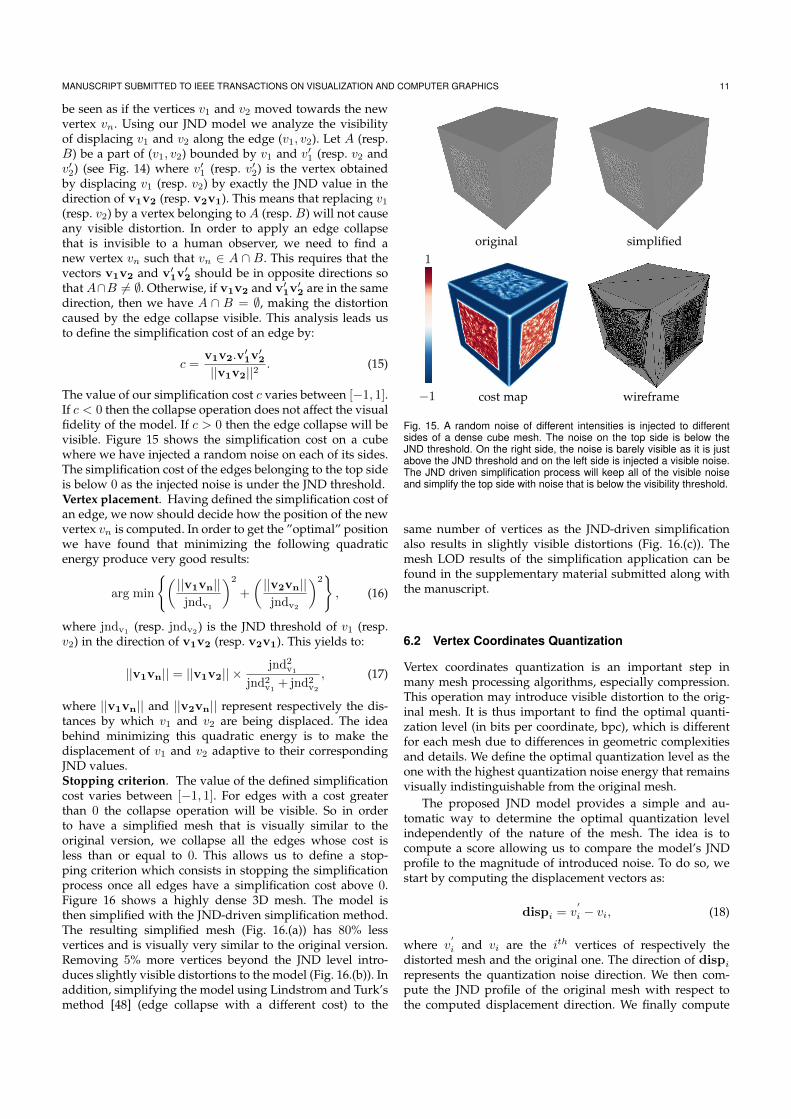
MANUSCRIPT SUBMITTED TO IEEE TRANSACTIONS ON VISUALIZATION AND COMPUTER GRAPHICS 11
be seen as if the vertices v1 and v2 moved towards the newvertex vn. Using our JND model we analyze the visibilityof displacing v1 and v2 along the edge (v1, v2). Let A (resp.B) be a part of (v1, v2) bounded by v1 and v′1 (resp. v2 andv′2) (see Fig. 14) where v′1 (resp. v′2) is the vertex obtainedby displacing v1 (resp. v2) by exactly the JND value in thedirection of v1v2 (resp. v2v1). This means that replacing v1
(resp. v2) by a vertex belonging to A (resp. B) will not causeany visible distortion. In order to apply an edge collapsethat is invisible to a human observer, we need to find anew vertex vn such that vn ∈ A ∩ B. This requires that thevectors v1v2 and v′
1v′
2 should be in opposite directions sothat A∩B = ∅. Otherwise, if v1v2 and v′
1v′
2 are in the samedirection, then we have A ∩ B = ∅, making the distortioncaused by the edge collapse visible. This analysis leads usto define the simplification cost of an edge by:
c =v1v2.v′
1v′
2
||v1v2||2 . (15)
The value of our simplification cost c varies between [−1, 1].If c < 0 then the collapse operation does not affect the visualfidelity of the model. If c > 0 then the edge collapse will bevisible. Figure 15 shows the simplification cost on a cubewhere we have injected a random noise on each of its sides.The simplification cost of the edges belonging to the top sideis below 0 as the injected noise is under the JND threshold.Vertex placement. Having defined the simplification cost ofan edge, we now should decide how the position of the newvertex vn is computed. In order to get the ”optimal” positionwe have found that minimizing the following quadraticenergy produce very good results:
arg min
||v1vn||jndv1
2
+
||v2vn||jndv2
2
, (16)
where jndv1(resp. jndv2
) is the JND threshold of v1 (resp.v2) in the direction of v1v2 (resp. v2v1). This yields to:
||v1vn|| = ||v1v2|| × jnd2v1
jnd2v1
+ jnd2v2
, (17)
where ||v1vn|| and ||v2vn|| represent respectively the dis-tances by which v1 and v2 are being displaced. The ideabehind minimizing this quadratic energy is to make thedisplacement of v1 and v2 adaptive to their correspondingJND values.Stopping criterion. The value of the defined simplificationcost varies between [−1, 1]. For edges with a cost greaterthan 0 the collapse operation will be visible. So in orderto have a simplified mesh that is visually similar to theoriginal version, we collapse all the edges whose cost isless than or equal to 0. This allows us to define a stop-ping criterion which consists in stopping the simplificationprocess once all edges have a simplification cost above 0.Figure 16 shows a highly dense 3D mesh. The model isthen simplified with the JND-driven simplification method.The resulting simplified mesh (Fig. 16.(a)) has 80% lessvertices and is visually very similar to the original version.Removing 5% more vertices beyond the JND level intro-duces slightly visible distortions to the model (Fig. 16.(b)). Inaddition, simplifying the model using Lindstrom and Turk’smethod [48] (edge collapse with a different cost) to the
original simplified
wireframecost map
1
−1
Fig. 15. A random noise of different intensities is injected to differentsides of a dense cube mesh. The noise on the top side is below theJND threshold. On the right side, the noise is barely visible as it is justabove the JND threshold and on the left side is injected a visible noise.The JND driven simplification process will keep all of the visible noiseand simplify the top side with noise that is below the visibility threshold.
same number of vertices as the JND-driven simplificationalso results in slightly visible distortions (Fig. 16.(c)). Themesh LOD results of the simplification application can befound in the supplementary material submitted along withthe manuscript.
6.2 Vertex Coordinates Quantization
Vertex coordinates quantization is an important step inmany mesh processing algorithms, especially compression.This operation may introduce visible distortion to the orig-inal mesh. It is thus important to find the optimal quanti-zation level (in bits per coordinate, bpc), which is differentfor each mesh due to differences in geometric complexitiesand details. We define the optimal quantization level as theone with the highest quantization noise energy that remainsvisually indistinguishable from the original mesh.
The proposed JND model provides a simple and au-tomatic way to determine the optimal quantization levelindependently of the nature of the mesh. The idea is tocompute a score allowing us to compare the model’s JNDprofile to the magnitude of introduced noise. To do so, westart by computing the displacement vectors as:
dispi = v′
i − vi, (18)
where v′
i and vi are the ith vertices of respectively thedistorted mesh and the original one. The direction of dispi
represents the quantization noise direction. We then com-pute the JND profile of the original mesh with respect tothe computed displacement direction. We finally compute
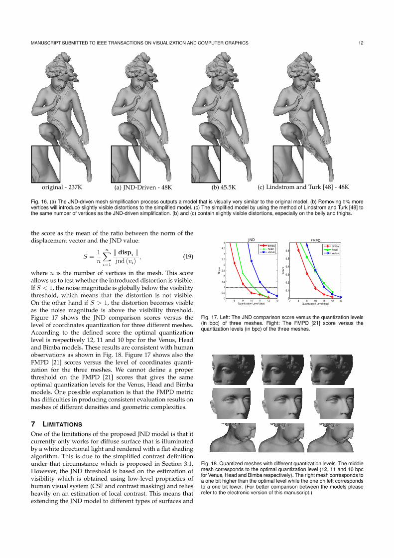
MANUSCRIPT SUBMITTED TO IEEE TRANSACTIONS ON VISUALIZATION AND COMPUTER GRAPHICS 12
(c) Lindstrom and Turk [48] - 48Koriginal - 237K (a) JND-Driven - 48K (b) 45.5K
Fig. 16. (a) The JND-driven mesh simplification process outputs a model that is visually very similar to the original model. (b) Removing 5% morevertices will introduce slightly visible distortions to the simplified model. (c) The simplified model by using the method of Lindstrom and Turk [48] tothe same number of vertices as the JND-driven simplification. (b) and (c) contain slightly visible distortions, especially on the belly and thighs.
the score as the mean of the ratio between the norm of thedisplacement vector and the JND value:
S =1
n
n
i=1
dispi
jnd (vi), (19)
where n is the number of vertices in the mesh. This scoreallows us to test whether the introduced distortion is visible.If S < 1, the noise magnitude is globally below the visibilitythreshold, which means that the distortion is not visible.On the other hand if S > 1, the distortion becomes visibleas the noise magnitude is above the visibility threshold.Figure 17 shows the JND comparison scores versus thelevel of coordinates quantization for three different meshes.According to the defined score the optimal quantizationlevel is respectively 12, 11 and 10 bpc for the Venus, Headand Bimba models. These results are consistent with humanobservations as shown in Fig. 18. Figure 17 shows also theFMPD [21] scores versus the level of coordinates quanti-zation for the three meshes. We cannot define a properthreshold on the FMPD [21] scores that gives the sameoptimal quantization levels for the Venus, Head and Bimbamodels. One possible explanation is that the FMPD metrichas difficulties in producing consistent evaluation results onmeshes of different densities and geometric complexities.
7 LIMITATIONS
One of the limitations of the proposed JND model is that itcurrently only works for diffuse surface that is illuminatedby a white directional light and rendered with a flat shadingalgorithm. This is due to the simplified contrast definitionunder that circumstance which is proposed in Section 3.1.However, the JND threshold is based on the estimation ofvisibility which is obtained using low-level proprieties ofhuman visual system (CSF and contrast masking) and reliesheavily on an estimation of local contrast. This means thatextending the JND model to different types of surfaces and
7 8 9 10 11 12 130
0.5
1
1.5
2
2.5
3
3.5
4
4.5
5
Quantization Level (bpc)
Scor
e
bimbaheadvenus
7 8 9 10 11 12 130
0.1
0.2
0.3
0.4
0.5
0.6
Sco
re
bimbaheadvenus
FMPDJND
Quantization Level (bpc)
Fig. 17. Left: The JND comparison score versus the quantization levels(in bpc) of three meshes. Right: The FMPD [21] score versus thequantization levels (in bpc) of the three meshes.
Fig. 18. Quantized meshes with different quantization levels. The middlemesh corresponds to the optimal quantization level (12, 11 and 10 bpcfor Venus, Head and Bimba respectively). The right mesh corresponds toa one bit higher than the optimal level while the one on left correspondsto a one bit lower. (For better comparison between the models pleaserefer to the electronic version of this manuscript.)
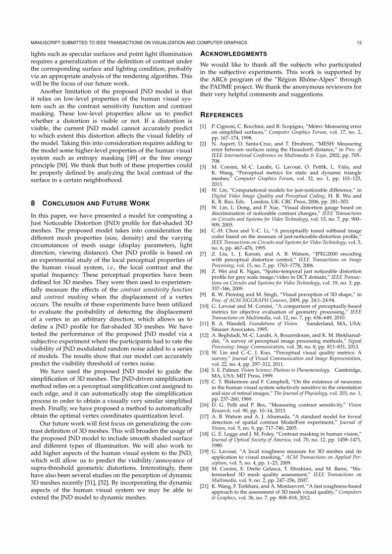
MANUSCRIPT SUBMITTED TO IEEE TRANSACTIONS ON VISUALIZATION AND COMPUTER GRAPHICS 13
lights such as specular surfaces and point light illuminationrequires a generalization of the definition of contrast underthe corresponding surface and lighting condition, probablyvia an appropriate analysis of the rendering algorithm. Thiswill be the focus of our future work.
Another limitation of the proposed JND model is thatit relies on low-level properties of the human visual sys-tem such as the contrast sensitivity function and contrastmasking. These low-level properties allow us to predictwhether a distortion is visible or not. If a distortion isvisible, the current JND model cannot accurately predictto which extent this distortion affects the visual fidelity ofthe model. Taking this into consideration requires adding tothe model some higher-level properties of the human visualsystem such as entropy masking [49] or the free energyprinciple [50]. We think that both of these properties couldbe properly defined by analyzing the local contrast of thesurface in a certain neighborhood.
8 CONCLUSION AND FUTURE WORK
In this paper, we have presented a model for computing aJust Noticeable Distortion (JND) profile for flat-shaded 3Dmeshes. The proposed model takes into consideration thedifferent mesh properties (size, density) and the varyingcircumstances of mesh usage (display parameters, lightdirection, viewing distance). Our JND profile is based onan experimental study of the local perceptual properties ofthe human visual system, i.e., the local contrast and thespatial frequency. These perceptual properties have beendefined for 3D meshes. They were then used to experimen-tally measure the effects of the contrast sensitivity functionand contrast masking when the displacement of a vertexoccurs. The results of these experiments have been utilizedto evaluate the probability of detecting the displacementof a vertex in an arbitrary direction, which allows us todefine a JND profile for flat-shaded 3D meshes. We havetested the performance of the proposed JND model via asubjective experiment where the participants had to rate thevisibility of JND modulated random noise added to a seriesof models. The results show that our model can accuratelypredict the visibility threshold of vertex noise.
We have used the proposed JND model to guide thesimplification of 3D meshes. The JND-driven simplificationmethod relies on a perceptual simplification cost assigned toeach edge, and it can automatically stop the simplificationprocess in order to obtain a visually very similar simplifiedmesh. Finally, we have proposed a method to automaticallyobtain the optimal vertex coordinates quantization level.
Our future work will first focus on generalizing the con-trast definition of 3D meshes. This will broaden the usage ofthe proposed JND model to include smooth shaded surfaceand different types of illumination. We will also work toadd higher aspects of the human visual system to the JND,which will allow us to predict the visibility/annoyance ofsupra-threshold geometric distortions. Interestingly, therehave also been several studies on the perception of dynamic3D meshes recently [51], [52]. By incorporating the dynamicaspects of the human visual system we may be able toextend the JND model to dynamic meshes.
ACKNOWLEDGMENTS
We would like to thank all the subjects who participatedin the subjective experiments. This work is supported bythe ARC6 program of the ”Region Rhone-Alpes” throughthe PADME project. We thank the anonymous reviewers fortheir very helpful comments and suggestions.
REFERENCES
[1] P. Cignoni, C. Rocchini, and R. Scopigno, “Metro: Measuring erroron simplified surfaces,” Computer Graphics Forum, vol. 17, no. 2,pp. 167–174, 1998.
[2] N. Aspert, D. Santa-Cruz, and T. Ebrahimi, “MESH: Measuringerror between surfaces using the Hausdorff distance,” in Proc. ofIEEE International Conference on Multimedia & Expo, 2002, pp. 705–708.
[3] M. Corsini, M.-C. Larabi, G. Lavoue, O. Petrık, L. Vasa, andK. Wang, “Perceptual metrics for static and dynamic trianglemeshes,” Computer Graphics Forum, vol. 32, no. 1, pp. 101–125,2013.
[4] W. Lin, “Computational models for just-noticeable difference,” inDigital Video Image Quality and Perceptual Coding, H. R. Wu andK. R. Rao, Eds. London, UK: CRC Press, 2006, pp. 281–303.
[5] W. Lin, L. Dong, and P. Xue, “Visual distortion gauge based ondiscrimination of noticeable contrast changes,” IEEE Transactionson Circuits and Systems for Video Technology, vol. 15, no. 7, pp. 900–909, 2005.
[6] C.-H. Chou and Y.-C. Li, “A perceptually tuned subband imagecoder based on the measure of just-noticeable-distortion profile,”IEEE Transactions on Circuits and Systems for Video Technology, vol. 5,no. 6, pp. 467–476, 1995.
[7] Z. Liu, L. J. Karam, and A. B. Watson, “JPEG2000 encodingwith perceptual distortion control,” IEEE Transactions on ImageProcessing, vol. 15, no. 7, pp. 1763–1778, 2006.
[8] Z. Wei and K. Ngan, “Spatio-temporal just noticeable distortionprofile for grey scale image/video in DCT domain,” IEEE Transac-tions on Circuits and Systems for Video Technology, vol. 19, no. 3, pp.337–346, 2009.
[9] R. W. Fleming and M. Singh, “Visual perception of 3D shape,” inProc. of ACM SIGGRAPH Courses, 2009, pp. 24:1–24:94.
[10] G. Lavoue and M. Corsini, “A comparison of perceptually-basedmetrics for objective evaluation of geometry processing,” IEEETransactions on Multimedia, vol. 12, no. 7, pp. 636–649, 2010.
[11] B. A. Wandell, Foundations of Vision. Sunderland, MA, USA:Sinauer Associates, 1995.
[12] A. Beghdadi, M.-C. Larabi, A. Bouzerdoum, and K. M. Iftekharud-din, “A survey of perceptual image processing methods,” SignalProcessing: Image Communication, vol. 28, no. 8, pp. 811–831, 2013.
[13] W. Lin and C.-C. J. Kuo, “Perceptual visual quality metrics: Asurvey,” Journal of Visual Communication and Image Representation,vol. 22, no. 4, pp. 297–312, 2011.
[14] S. E. Palmer, Vision Science: Photons to Phenomenology. Cambridge,MA, USA: MIT Press, 1999.
[15] C. T. Blakemore and F. Campbell, “On the existence of neuronesin the human visual system selectively sensitive to the orientationand size of retinal images,” The Journal of Physiology, vol. 203, no. 1,pp. 237–260, 1969.
[16] D. G. Pelli and P. Bex, “Measuring contrast sensitivity,” VisionResearch, vol. 90, pp. 10–14, 2013.
[17] A. B. Watson and A. J. Ahumada, “A standard model for fovealdetection of spatial contrast ModelFest experiment,” Journal ofVision, vol. 5, no. 9, pp. 717–740, 2005.
[18] G. E. Legge and J. M. Foley, “Contrast masking in human vision,”Journal of Optical Society of America, vol. 70, no. 12, pp. 1458–1471,1980.
[19] G. Lavoue, “A local roughness measure for 3D meshes and itsapplication to visual masking,” ACM Transactions on Applied Per-ception, vol. 5, no. 4, pp. 1–23, 2009.
[20] M. Corsini, E. Drelie Gelasca, T. Ebrahimi, and M. Barni, “Wa-termarked 3D mesh quality assessment,” IEEE Transactions onMultimedia, vol. 9, no. 2, pp. 247–256, 2007.
[21] K. Wang, F. Torkhani, and A. Montanvert, “A fast roughness-basedapproach to the assessment of 3D mesh visual quality,” Computers& Graphics, vol. 36, no. 7, pp. 808–818, 2012.
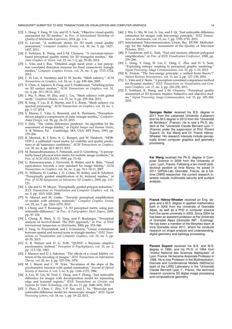
MANUSCRIPT SUBMITTED TO IEEE TRANSACTIONS ON VISUALIZATION AND COMPUTER GRAPHICS 14
[22] L. Dong, Y. Fang, W. Lin, and H. S. Seah, “Objective visual qualityassessment for 3D meshes,” in Proc. of International Workshop onQuality of Multimedia Experience, 2014, pp. 1–6.
[23] G. Lavoue, “A multiscale metric for 3D mesh visual qualityassessment,” Computer Graphics Forum, vol. 30, no. 5, pp. 1427–1437, 2011.
[24] F. Torkhani, K. Wang, and J.-M. Chassery, “A curvature-tensor-based perceptual quality metric for 3D triangular meshes,” Ma-chine Graphics & Vision, vol. 23, no. 1–2, pp. 59–82, 2014.
[25] L. Vasa and J. Rus, “Dihedral angle mesh error: a fast percep-tion correlated distortion measure for fixed connectivity trianglemeshes,” Computer Graphics Forum, vol. 31, no. 5, pp. 1715–1724,2012.
[26] C. H. Lee, A. Varshney, and D. W. Jacobs, “Mesh saliency,” ACMTransactions on Graphics, vol. 24, no. 3, pp. 659–666, 2005.
[27] X. Chen, A. Saparov, B. Pang, and T. Funkhouser, “Schelling pointson 3D surface meshes,” ACM Transactions on Graphics, vol. 31,no. 4, pp. 29:1–29:12, 2012.
[28] J. Wu, X. Shen, W. Zhu, and L. Liu, “Mesh saliency with globalrarity,” Graphical Models, vol. 75, no. 5, pp. 255–264, 2013.
[29] R. Song, Y. Liu, R. R. Martin, and P. L. Rosin, “Mesh saliency viaspectral processing,” ACM Transactions on Graphics, vol. 33, no. 1,pp. 1–17, 2014.
[30] S. Marras, L. Vasa, G. Brunnett, and K. Hormann, “Perception-driven adaptive compression of static triangle meshes,” Computer-Aided Design, vol. 58, pp. 24–33, 2015.
[31] S. Daly, “The visible differences predictor: An algorithm for theassessment of image fidelity,” in Digital Images and Human Vision,A. B. Watson, Ed. Cambridge, MA, USA: MIT Press, 1993, pp.179–206.
[32] R. Mantiuk, K. J. Kim, A. G. Rempel, and W. Heidrich, “HDR-VDP-2: a calibrated visual metric for visibility and quality predic-tions in all luminance conditions,” ACM Transactions on Graphics,vol. 30, no. 4, pp. 40:1–40:13, 2011.
[33] M. Ramasubramanian, S. Pattanaik, and D. Greenberg, “A percep-tually based physical error metric for realistic image synthesis,” inProc. of ACM SIGGRAPH, 1999, pp. 73–82.
[34] G. Ramanarayanan, J. Ferwerda, B. Walter, and K. Bala, “Visualequivalence: towards a new standard for image fidelity,” ACMTransactions on Graphics, vol. 26, no. 3, pp. 76:1–76:11, 2007.
[35] N. Williams, D. Luebke, J. D. Cohen, M. Kelley, and B. Schubert,“Perceptually guided simplification of lit, textured meshes,” inProc. of ACM Symposium on Interactive 3D Graphics, 2003, pp. 113–121.
[36] L. Qu and G. W. Meyer, “Perceptually guided polygon reduction,”IEEE Transactions on Visualization and Computer Graphics, vol. 14,no. 5, pp. 1015–1029, 2008.
[37] N. Menzel and M. Guthe, “Towards perceptual simplificationof models with arbitrary materials,” Computer Graphics Forum,vol. 29, no. 7, pp. 2261–2270, 2010.
[38] I. Cheng and P. Boulanger, “A 3D perceptual metric using just-noticeable-difference,” in Proc. of Eurographics Short Papers, 2005,pp. 97–100.
[39] I. Cheng, R. Shen, X. D. Yang, and P. Boulanger, “Perceptualanalysis of level-of-detail: The JND approach,” in Proc. of IEEEInternational Symposium on Multimedia, 2006, pp. 533–540.
[40] Y. Yang, N. Peyerimhoff, and I. Ivrissimtzis, “Linear correlationsbetween spatial and normal noise in triangle meshes,” IEEE Trans-actions on Visualization and Computer Graphics, vol. 19, no. 1, pp.45–55, 2013.
[41] A. B. Watson and D. G. Pelli, “QUEST: a Bayesian adaptivepsychometric method.” Perception & Psychophysics, vol. 33, no. 2,pp. 113–120, 1983.
[42] J. Mannos and D. J. Sakrison, “The effects of a visual fidelity cri-terion of the encoding of images,” IEEE Transactions on InformationTheory, vol. 20, no. 4, pp. 525–536, 1974.
[43] M. J. Mayer and C. W. Tyler, “Invariance of the slope of thepsychometric function with spatial summation,” Journal of OpticalSociety of America A, vol. 3, no. 8, pp. 1166–1172, 1986.
[44] A. Liu, W. Lin, M. Paul, C. Deng, and F. Zhang, “Just noticeabledifference for images with decomposition model for separatingedge and textured regions,” IEEE Transactions on Circuits andSystems for Video Technology, vol. 20, no. 11, pp. 1648–1652, 2010.
[45] Y. Zhao, Z. Chen, C. Zhu, Y.-P. Tan, and L. Yu, “Binocular just-noticeable-difference model for stereoscopic images,” IEEE SignalProcessing Letters, vol. 18, no. 1, pp. 19–22, 2011.
[46] J. Wu, G. Shi, W. Lin, A. Liu, and F. Qi, “Just noticeable differenceestimation for images with free-energy principle,” IEEE Transac-tions on Multimedia, vol. 15, no. 7, pp. 1705–1710, 2013.
[47] International Telecommunication Union, Rec. BT.500: Methodol-ogy for the Subjective Assessment of the Quality of TelevisionPictures, 2012.
[48] P. Lindstrom and G. Turk, “Fast and memory efficient polygonalsimplification,” in Proc. of IEEE Visualization Conference, 1998, pp.279–286.
[49] L. Dong, Y. Fang, W. Lin, C. Deng, C. Zhu, and H. S. Seah,“Exploiting entropy masking in perceptual graphic rendering,”Signal Processing: Image Communication, vol. 33, pp. 1–13, 2015.
[50] K. Friston, “The free-energy principle: a unified brain theory?”Nature Reviews Neuroscience, vol. 11, no. 2, pp. 127–138, 2010.
[51] L. Vasa and V. Skala, “A perception correlated comparison methodfor dynamic meshes,” IEEE Transactions on Visualization and Com-puter Graphics, vol. 17, no. 2, pp. 220–230, 2011.
[52] F. Torkhani, K. Wang, and J.-M. Chassery, “Perceptual qualityassessment of 3D dynamic meshes: Subjective and objective stud-ies,” Signal Processing: Image Communication, vol. 31, pp. 185–204,2015.
Georges Nader received his B.S. degree in2011 from the Lebanese University (Lebanon)and his M.S degree in 2013 from the “Universitede Bordeaux” (France). He is now a Ph.D. stu-dent at the “Universite Claude Bernard Lyon 1”(France) under the supervision of Prof. FlorentDupont, Dr. Kai Wang and Dr. Franck Hetroy-Wheeler. His research interests include percep-tually driven computer graphics and geometryprocessing.
Kai Wang received the Ph.D. degree in Com-puter Science in 2009 from the University ofLyon, Lyon, France. Following a ten-month post-doctoral position at Inria Nancy, he joined in2011 GIPSA-Lab, Grenoble, France, as a full-time CNRS researcher. His current research in-terests include multimedia security and surfaceanalysis.
Franck Hetroy-Wheeler received an Eng. de-gree and a M.S. degree in applied mathematicsboth in 2000 from the University of GrenobleAlpes, as well as a PhD in computer sciencefrom the same university in 2003. Since 2004 hehas been an assistant professor at the Universityof Grenoble Alpes (Grenoble INP - Ensimag).He has been a member of the Morpheo team atInria Grenoble since 2011, where he conductsresearch on shape analysis and understanding,digital geometry and topology processing.
Florent Dupont received his B.S. and M.S.degree in 1990, and his Ph.D. in 1994 from“Institut National des Sciences Appliquees” ofLyon, France. He became Associate Professor in1998. He is now Professor in the Multiresolution,Discrete and Combinatorial Models (M2DisCo)team of the LIRIS Laboratory in the “UniversiteClaude Bernard Lyon 1”, France. His technicalresearch concerns 3D digital image processingand computational geometry.
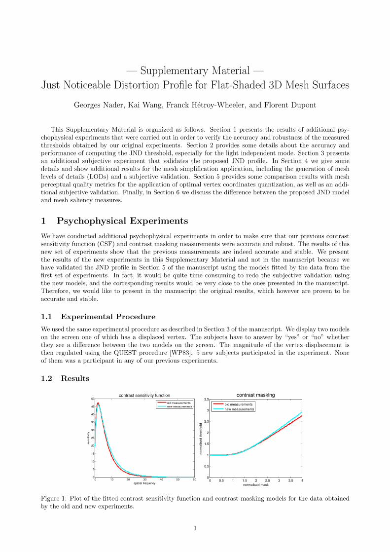
— Supplementary Material —
Just Noticeable Distortion Profile for Flat-Shaded 3D Mesh Surfaces
Georges Nader, Kai Wang, Franck Hetroy-Wheeler, and Florent Dupont
This Supplementary Material is organized as follows. Section 1 presents the results of additional psy-chophysical experiments that were carried out in order to verify the accuracy and robustness of the measuredthresholds obtained by our original experiments. Section 2 provides some details about the accuracy andperformance of computing the JND threshold, especially for the light independent mode. Section 3 presentsan additional subjective experiment that validates the proposed JND profile. In Section 4 we give somedetails and show additional results for the mesh simplification application, including the generation of meshlevels of details (LODs) and a subjective validation. Section 5 provides some comparison results with meshperceptual quality metrics for the application of optimal vertex coordinates quantization, as well as an addi-tional subjective validation. Finally, in Section 6 we discuss the difference between the proposed JND modeland mesh saliency measures.
1 Psychophysical Experiments
We have conducted additional psychophysical experiments in order to make sure that our previous contrastsensitivity function (CSF) and contrast masking measurements were accurate and robust. The results of thisnew set of experiments show that the previous measurements are indeed accurate and stable. We presentthe results of the new experiments in this Supplementary Material and not in the manuscript because wehave validated the JND profile in Section 5 of the manuscript using the models fitted by the data from thefirst set of experiments. In fact, it would be quite time consuming to redo the subjective validation usingthe new models, and the corresponding results would be very close to the ones presented in the manuscript.Therefore, we would like to present in the manuscript the original results, which however are proven to beaccurate and stable.
1.1 Experimental Procedure
We used the same experimental procedure as described in Section 3 of the manuscript. We display two modelson the screen one of which has a displaced vertex. The subjects have to answer by “yes” or “no” whetherthey see a difference between the two models on the screen. The magnitude of the vertex displacement isthen regulated using the QUEST procedure [WP83]. 5 new subjects participated in the experiment. Noneof them was a participant in any of our previous experiments.
1.2 Results
0 10 20 30 40 50 600
5
10
15
20
25
30
35
40
45
50contrast sensitivity function
spatial frequency
sensitiv
ity
old measurements
new measurements
0 0.5 1 1.5 2 2.5 3 3.5 40
0.5
1
1.5
2
2.5
3
3.5contrast masking
normalised mask
no
rma
lise
d t
hre
sh
old
old measurements
new measurements
Figure 1: Plot of the fitted contrast sensitivity function and contrast masking models for the data obtainedby the old and new experiments.
1
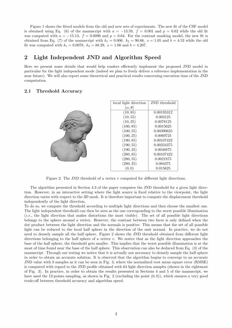
Figure 1 shows the fitted models from the old and new sets of experiments. The new fit of the CSF modelis obtained using Eq. (6) of the manuscript with a = −13.59, f = 0.001 and p = 0.62 while the old fitwas computed with a = −15.13, f = 0.0096 and p = 0.64. For the contrast masking model, the new fit isobtained from Eq. (7) of the manuscript with k1 = 0.006, k2 = 90.66, s = 1.05 and b = 4.53 while the oldfit was computed with k1 = 0.0078, k2 = 88.29, s = 1.00 and b = 4.207.
2 Light Independent JND and Algorithm Speed
Here we present some details that would help readers efficiently implement the proposed JND model inparticular for the light independent mode (indeed we plan to freely deliver a reference implementation in thenear future). We will also report some theoretical and practical results concerning execution time of the JNDcomputation.
2.1 Threshold Accuracy
v
local light direction JND threshold(α, θ)
(10, 85) 0.00195312(10, 55) 0.003125(10, 25) 0.0078125(100, 85) 0.0015625(100, 55) 0.00390625(100, 25) 0.0069725(190, 85) 0.00107422(190, 55) 0.00234375(190, 25) 0.0046875(280, 85) 0.00107422(280, 55) 0.0021875(280, 25) 0.004375
(0, 0) 0.015625
Figure 2: The JND threshold of a vertex v computed for different light directions.
The algorithm presented in Section 4.3 of the paper computes the JND threshold for a given light direc-tion. However, in an interactive setting where the light source is fixed relative to the viewpoint, the lightdirection varies with respect to the 3D mesh. It is therefore important to compute the displacement thresholdindependently of the light direction.To do so, we compute the threshold according to multiple light directions and then choose the smallest one.The light independent threshold can then be seen as the one corresponding to the worst possible illumination(i.e., the light direction that makes distortions the most visible). The set of all possible light directionsbelongs to the sphere around a vertex. However, the contrast between two faces is only defined when thedot product between the light direction and the normals is positive. This means that the set of all possiblelight can be reduced to the local half sphere in the direction of the unit normal. In practice, we do notneed to densely sample all the half sphere. Figure 2 shows the JND threshold obtained from different lightdirections belonging to the half sphere of a vertex v. We notice that as the light direction approaches thebase of the half sphere, the threshold gets smaller. This implies that the worst possible illumination is at themost of time found near the base of the half sphere. This observation can also be deduced from Eq. (3) of themanuscript. Through our testing we notice that it is actually not necessary to densely sample the half spherein order to obtain an accurate solution. It is observed that the algorithm begins to converge to an accurateJND value with 8 samples as it can be seen in Fig. 3, where the normalized root mean square error (RMSE)is computed with regard to the JND profile obtained with 64 light direction samples (shown in the rightmostof Fig. 3). In practice, in order to obtain the results presented in Sections 4 and 5 of the manuscript, wehave used the 12-points sampling, as shown in Fig. 2 (excluding the point (0, 0)), which ensures a very goodtrade-off between threshold accuracy and algorithm speed.
2
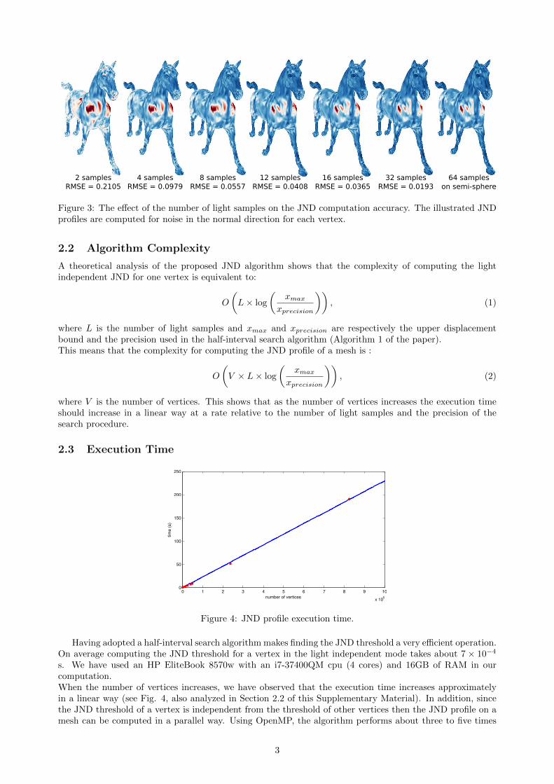
64 sampleson semi-sphere
16 samplesRMSE = 0.0365
8 samplesRMSE = 0.0557
4 samples RMSE = 0.0979
2 samples RMSE = 0.2105
12 samplesRMSE = 0.0408
32 samplesRMSE = 0.0193
Figure 3: The effect of the number of light samples on the JND computation accuracy. The illustrated JNDprofiles are computed for noise in the normal direction for each vertex.
2.2 Algorithm Complexity
A theoretical analysis of the proposed JND algorithm shows that the complexity of computing the lightindependent JND for one vertex is equivalent to:
O
L × log
xmax
xprecision
, (1)
where L is the number of light samples and xmax and xprecision are respectively the upper displacementbound and the precision used in the half-interval search algorithm (Algorithm 1 of the paper).This means that the complexity for computing the JND profile of a mesh is :
O
V × L × log
xmax
xprecision
, (2)
where V is the number of vertices. This shows that as the number of vertices increases the execution timeshould increase in a linear way at a rate relative to the number of light samples and the precision of thesearch procedure.
2.3 Execution Time
0 1 2 3 4 5 6 7 8 9 10
x 105
0
50
100
150
200
250
number of vertices
time
(s)
Figure 4: JND profile execution time.
Having adopted a half-interval search algorithm makes finding the JND threshold a very efficient operation.On average computing the JND threshold for a vertex in the light independent mode takes about 7 × 10⁻⁴
s. We have used an HP EliteBook 8570w with an i7-37400QM cpu (4 cores) and 16GB of RAM in ourcomputation.When the number of vertices increases, we have observed that the execution time increases approximatelyin a linear way (see Fig. 4, also analyzed in Section 2.2 of this Supplementary Material). In addition, sincethe JND threshold of a vertex is independent from the threshold of other vertices then the JND profile on amesh can be computed in a parallel way. Using OpenMP, the algorithm performs about three to five times
3

faster. For a model with 237K vertices, the JND profile took about 52 seconds to compute. Indeed, thevertex displacement threshold searching consumes the most part of the computation time. However, withthe simple but efficient half-interval search, this step can be accomplished in a very reasonable time and thusdoes not harm the efficiency of the whole algorithm.
3 JND Validation
We have conducted an additional subjective experiment in order to validate the proposed JND model. In themanuscript we have presented a subjective experiment where the participants rate the visibility of an injectednoise on scale of 0 to 5. It showed that the models with a JND modulated noise were rated the lowest onthe visibility scale but meanwhile could tolerate the biggest amount of distortions. However, in the followingnew experiment we gradually increase the intensity of the injected noise until the subject notices it.
3.1 Experimental Procedure
Similarly to the experiment presented in Section 5 of the manuscript, the noise is injected into the 3D meshesaccording to the following equation:
v′
i = vi + rnd ×M (vi) × diri, (3)
where vi is the ith vertex of the initial mesh and v′
i is the corresponding noisy vertex. dir is the noise direction.rnd is a random value equal to either +1 or −1 and M (vi) represents the magnitude of the noise for vi. Itis defined as:
M (vi) =
βunif uniform noise,
βrough × lr (vi) roughness modulated noise,
βjnd × jnd (vi) JND modulated noise,
(4)
where βunif , βrough and βjnd regulate the global noise intensity for each of the noise injection methods. lr (vi)is the local surface roughness as defined in [WTM12] and jnd (vi) is the JND value computed as explainedin Section 4 of the manuscript.
The idea behind this experiment is to find the minimum noise intensity (βunif , βrough and βjnd) startingfrom which the participants notice the noise in the model. To do so, we have adapted the same experimentalprocedure that we have used to measure the local contrast threshold in the studies of CSF and contrastmasking. Two models were displayed on the screen, one of which has noise injected. The subjects had toanswer by either “yes” or “no” whether they saw the noise on one of the model. The intensity of the noise(βunif , βrough and βjnd) is then adjusted using the QUEST procedure [WP83]. The subjects were allowedto interact with the displayed models by rotating the camera around them. 5 new subjects participated inthe experiment.
3.2 Results
Bimba Lion Dinosaur Venus Horse0
0.1
0.2
0.3
0.4
0.5
0.6
0.7
0.8
0.9
1
1.1
1.2
Bimba Lion Dinosaur Venus Horse0
0.5
1
1.5
2
2.5
3x 10⁻⁴
MR
MS
Uniform NoiseRoughness modulated noiseJND modulated noise
beta_jnd
(a) (b)
Figure 5: (a) Plot of the measured noise intensity relative to the JND modulated noise. (b) Plot of theMRMS induced by noise injection for three different types of noise at the same visibility level.
Figure 5 displays the results of this subjective experiment. Plot (a) shows the mean measured intensityrequired to make JND modulated noise visible on a 3D mesh. We see that the measured βjnd is close to 1 for
4
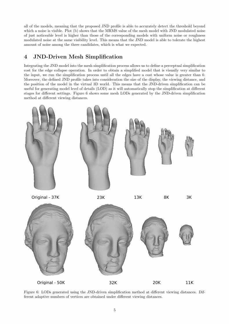
all of the models, meaning that the proposed JND profile is able to accurately detect the threshold beyondwhich a noise is visible. Plot (b) shows that the MRMS value of the mesh model with JND modulated noiseof just noticeable level is higher than those of the corresponding models with uniform noise or roughnessmodulated noise at the same visibility level. This means that the JND model is able to tolerate the highestamount of noise among the three candidates, which is what we expected.
4 JND-Driven Mesh Simplification
Integrating the JND model into the mesh simplification process allows us to define a perceptual simplificationcost for the edge collapse operation. In order to obtain a simplified model that is visually very similar tothe input, we run the simplification process until all the edges have a cost whose value is greater than 0.Moreover, the defined JND profile takes into consideration the size of the display, the viewing distance, andthe position of the model in the virtual 3D world. This means that the JND-driven simplification can beuseful for generating model level of details (LOD) as it will automatically stop the simplification at differentstages for different settings. Figure 6 shows some mesh LODs generated by the JND-driven simplificationmethod at different viewing distances.
Original - 37K 23K 13K 8K 3K
Original - 50K 32K 20K 11K
Figure 6: LODs generated using the JND-driven simplification method at different viewing distances. Dif-ferent adaptive numbers of vertices are obtained under different viewing distances.
5
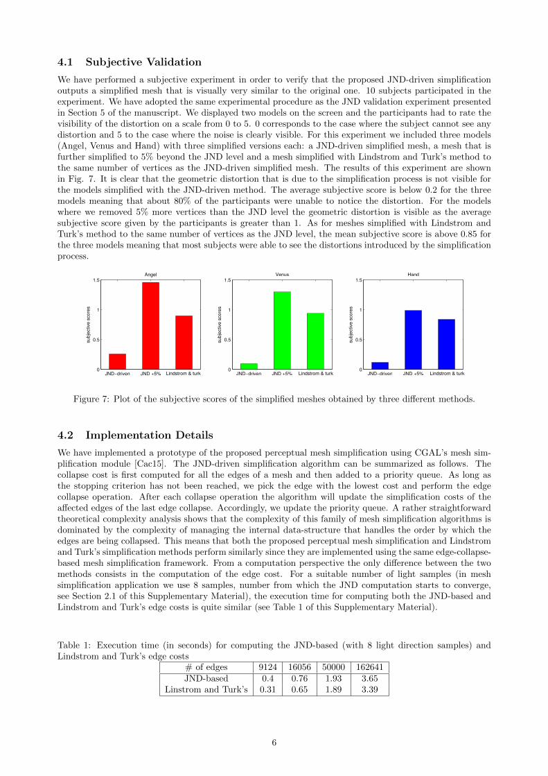
4.1 Subjective Validation
We have performed a subjective experiment in order to verify that the proposed JND-driven simplificationoutputs a simplified mesh that is visually very similar to the original one. 10 subjects participated in theexperiment. We have adopted the same experimental procedure as the JND validation experiment presentedin Section 5 of the manuscript. We displayed two models on the screen and the participants had to rate thevisibility of the distortion on a scale from 0 to 5. 0 corresponds to the case where the subject cannot see anydistortion and 5 to the case where the noise is clearly visible. For this experiment we included three models(Angel, Venus and Hand) with three simplified versions each: a JND-driven simplified mesh, a mesh that isfurther simplified to 5% beyond the JND level and a mesh simplified with Lindstrom and Turk’s method tothe same number of vertices as the JND-driven simplified mesh. The results of this experiment are shownin Fig. 7. It is clear that the geometric distortion that is due to the simplification process is not visible forthe models simplified with the JND-driven method. The average subjective score is below 0.2 for the threemodels meaning that about 80% of the participants were unable to notice the distortion. For the modelswhere we removed 5% more vertices than the JND level the geometric distortion is visible as the averagesubjective score given by the participants is greater than 1. As for meshes simplified with Lindstrom andTurk’s method to the same number of vertices as the JND level, the mean subjective score is above 0.85 forthe three models meaning that most subjects were able to see the distortions introduced by the simplificationprocess.
JND−driven JND +5%0
0.5
1
1.5Angel
subj
ectiv
e sc
ores
JND−driven JND +5%0
0.5
1
1.5Venus
subj
ectiv
e sc
ores
JND−driven JND +5%0
0.5
1
1.5Hand
subj
ectiv
e sc
ores
Lindstrom & turkLindstrom & turkLindstrom & turk
Figure 7: Plot of the subjective scores of the simplified meshes obtained by three different methods.
4.2 Implementation Details
We have implemented a prototype of the proposed perceptual mesh simplification using CGAL’s mesh sim-plification module [Cac15]. The JND-driven simplification algorithm can be summarized as follows. Thecollapse cost is first computed for all the edges of a mesh and then added to a priority queue. As long asthe stopping criterion has not been reached, we pick the edge with the lowest cost and perform the edgecollapse operation. After each collapse operation the algorithm will update the simplification costs of theaffected edges of the last edge collapse. Accordingly, we update the priority queue. A rather straightforwardtheoretical complexity analysis shows that the complexity of this family of mesh simplification algorithms isdominated by the complexity of managing the internal data-structure that handles the order by which theedges are being collapsed. This means that both the proposed perceptual mesh simplification and Lindstromand Turk’s simplification methods perform similarly since they are implemented using the same edge-collapse-based mesh simplification framework. From a computation perspective the only difference between the twomethods consists in the computation of the edge cost. For a suitable number of light samples (in meshsimplification application we use 8 samples, number from which the JND computation starts to converge,see Section 2.1 of this Supplementary Material), the execution time for computing both the JND-based andLindstrom and Turk’s edge costs is quite similar (see Table 1 of this Supplementary Material).
Table 1: Execution time (in seconds) for computing the JND-based (with 8 light direction samples) andLindstrom and Turk’s edge costs
# of edges 9124 16056 50000 162641JND-based 0.4 0.76 1.93 3.65
Linstrom and Turk’s 0.31 0.65 1.89 3.39
6
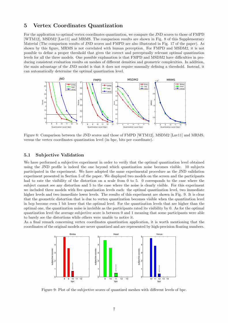
5 Vertex Coordinates Quantization
For the application to optimal vertex coordinates quantization, we compare the JND scores to those of FMPD[WTM12], MSDM2 [Lav11] and MRMS. The comparison results are shown in Fig. 8 of this SupplementaryMaterial (The comparison results of JND scores and FMPD are also illustrated in Fig. 17 of the paper). Asshown by this figure, MRMS is not correlated with human perception. For FMPD and MSDM2, it is notpossible to define a proper threshold that gives the correct and perceptually relevant optimal quantizationlevels for all the three models. One possible explanation is that FMPD and MSDM2 have difficulties in pro-ducing consistent evaluation results on meshes of different densities and geometric complexities. In addition,the main advantage of the JND model is that it does not require manually defining a threshold. Instead, itcan automatically determine the optimal quantization level.
7 8 9 10 11 12 130
0.5
1
1.5
2
2.5
3
3.5
4
4.5
5
Sco
re
bimbaheadvenus
7 8 9 10 11 12 130
0.1
0.2
0.3
0.4
0.5
0.6
0.7
Sco
re
bimbaheadvenus
JND FMPD
7 8 9 10 11 12 130
0.1
0.2
0.3
0.4
0.5
0.6
0.7
0.8
0.9
Sco
re
BimbaHeadVenus
MSDM2 MRMS
7 8 9 10 11 12 130
0.5
1
1.5
2
2.5
3
x 10−3
MR
MS
BimbaHeadVenus
Quantization Level (bpc) Quantization Level (bpc) Quantization Level (bpc) Quantization Level (bpc)
Figure 8: Comparison between the JND scores and those of FMPD [WTM12], MSDM2 [Lav11] and MRMS,versus the vertex coordinates quantization level (in bpc, bits per coordinate).
5.1 Subjective Validation
We have performed a subjective experiment in order to verify that the optimal quantization level obtainedusing the JND profile is indeed the one beyond which quantization noise becomes visible. 10 subjectsparticipated in the experiment. We have adopted the same experimental procedure as the JND validationexperiment presented in Section 5 of the paper. We displayed two models on the screen and the participantshad to rate the visibility of the distortion on a scale from 0 to 5. 0 corresponds to the case where thesubject cannot see any distortion and 5 to the case where the noise is clearly visible. For this experimentwe included three models with five quantization levels each: the optimal quantization level, two immediatehigher levels and two immediate lower levels. The results of this experiment are shown in Fig. 9. It is clearthat the geometric distortion that is due to vertex quantization becomes visible when the quantization levelin bcp become even 1 bit lower that the optimal level. For the quantization levels that are higher than theoptimal one, the quantization noise is invisible as the participants rated its visibility by 0. As for the optimalquantization level the average subjective score is between 0 and 1 meaning that some participants were ableto barely see the distortions while others were unable to notice it.As a final remark concerning vertex coordinates quantization application, it is worth mentioning that thecoordinates of the original models are never quantized and are represented by high-precision floating numbers.
8 9 10 11 120
1
2
3
4
5Bimba
bpc
subj
ectiv
e sc
ores
9 10 11 12 130
1
2
3
4
5Head
bpc
subj
ectiv
e sc
ores
10 11 12 13 140
1
2
3
4
5Venus
bpc
subj
ectiv
e sc
ores
opti
mal le
vel
opti
mal le
vel
opti
mal le
vel
Figure 9: Plot of the subjective scores of quantized meshes with different levels of bpc.
7
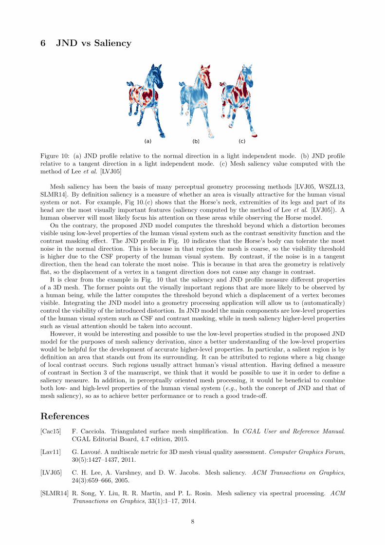
6 JND vs Saliency
(a) (c)(b)
Figure 10: (a) JND profile relative to the normal direction in a light independent mode. (b) JND profilerelative to a tangent direction in a light independent mode. (c) Mesh saliency value computed with themethod of Lee et al. [LVJ05]
Mesh saliency has been the basis of many perceptual geometry processing methods [LVJ05, WSZL13,SLMR14]. By definition saliency is a measure of whether an area is visually attractive for the human visualsystem or not. For example, Fig 10.(c) shows that the Horse’s neck, extremities of its legs and part of itshead are the most visually important features (saliency computed by the method of Lee et al. [LVJ05]). Ahuman observer will most likely focus his attention on these areas while observing the Horse model.
On the contrary, the proposed JND model computes the threshold beyond which a distortion becomesvisible using low-level properties of the human visual system such as the contrast sensitivity function and thecontrast masking effect. The JND profile in Fig. 10 indicates that the Horse’s body can tolerate the mostnoise in the normal direction. This is because in that region the mesh is coarse, so the visibility thresholdis higher due to the CSF property of the human visual system. By contrast, if the noise is in a tangentdirection, then the head can tolerate the most noise. This is because in that area the geometry is relativelyflat, so the displacement of a vertex in a tangent direction does not cause any change in contrast.
It is clear from the example in Fig. 10 that the saliency and JND profile measure different propertiesof a 3D mesh. The former points out the visually important regions that are more likely to be observed bya human being, while the latter computes the threshold beyond which a displacement of a vertex becomesvisible. Integrating the JND model into a geometry processing application will allow us to (automatically)control the visibility of the introduced distortion. In JND model the main components are low-level propertiesof the human visual system such as CSF and contrast masking, while in mesh saliency higher-level propertiessuch as visual attention should be taken into account.
However, it would be interesting and possible to use the low-level properties studied in the proposed JNDmodel for the purposes of mesh saliency derivation, since a better understanding of the low-level propertieswould be helpful for the development of accurate higher-level properties. In particular, a salient region is bydefinition an area that stands out from its surrounding. It can be attributed to regions where a big changeof local contrast occurs. Such regions usually attract human’s visual attention. Having defined a measureof contrast in Section 3 of the manuscript, we think that it would be possible to use it in order to define asaliency measure. In addition, in perceptually oriented mesh processing, it would be beneficial to combineboth low- and high-level properties of the human visual system (e.g., both the concept of JND and that ofmesh saliency), so as to achieve better performance or to reach a good trade-off.
References
[Cac15] F. Cacciola. Triangulated surface mesh simplification. In CGAL User and Reference Manual.CGAL Editorial Board, 4.7 edition, 2015.
[Lav11] G. Lavoue. A multiscale metric for 3D mesh visual quality assessment. Computer Graphics Forum,30(5):1427–1437, 2011.
[LVJ05] C. H. Lee, A. Varshney, and D. W. Jacobs. Mesh saliency. ACM Transactions on Graphics,24(3):659–666, 2005.
[SLMR14] R. Song, Y. Liu, R. R. Martin, and P. L. Rosin. Mesh saliency via spectral processing. ACMTransactions on Graphics, 33(1):1–17, 2014.
8

[WP83] A. B. Watson and D. G. Pelli. QUEST: a Bayesian adaptive psychometric method. Perception &Psychophysics, 33(2):113–120, 1983.
[WSZL13] J. Wu, X. Shen, W. Zhu, and L. Liu. Mesh saliency with global rarity. Graphical Models,75(5):255–264, 2013.
[WTM12] K. Wang, F. Torkhani, and A. Montanvert. A fast roughness-based approach to the assessmentof 3D mesh visual quality. Computers & Graphics, 36(7):808–818, 2012.
9

140 APPENDIX A. SELECTED PAPERS

A.4. A HIERARCHICAL APPROACH FOR REGULAR CENTROIDAL VORONOITESSELLATIONS 141
∴
A.4 A HIERARCHICAL APPROACH FOR REGULARCENTROIDAL VORONOI TESSELLATIONS
Li Wang, Franck Hétroy-Wheeler, Edmond BoyerComputer Graphics Forum 35 (1), Wiley, 2016.

142 APPENDIX A. SELECTED PAPERS
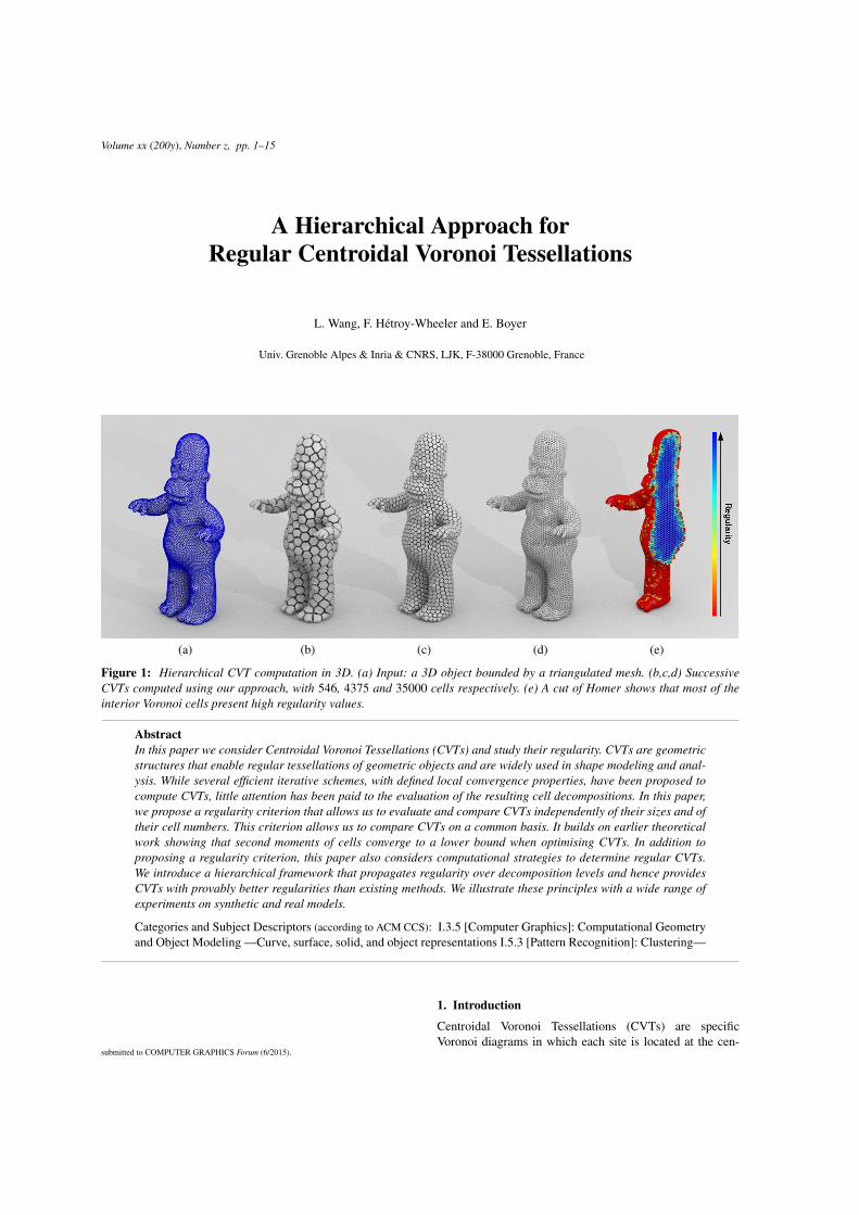
Volume xx (200y), Number z, pp. 1–15
A Hierarchical Approach forRegular Centroidal Voronoi Tessellations
L. Wang, F. Hétroy-Wheeler and E. Boyer
Univ. Grenoble Alpes & Inria & CNRS, LJK, F-38000 Grenoble, France
(a) (b) (c) (d) (e)
Figure 1: Hierarchical CVT computation in 3D. (a) Input: a 3D object bounded by a triangulated mesh. (b,c,d) SuccessiveCVTs computed using our approach, with 546, 4375 and 35000 cells respectively. (e) A cut of Homer shows that most of theinterior Voronoi cells present high regularity values.
AbstractIn this paper we consider Centroidal Voronoi Tessellations (CVTs) and study their regularity. CVTs are geometricstructures that enable regular tessellations of geometric objects and are widely used in shape modeling and anal-ysis. While several efficient iterative schemes, with defined local convergence properties, have been proposed tocompute CVTs, little attention has been paid to the evaluation of the resulting cell decompositions. In this paper,we propose a regularity criterion that allows us to evaluate and compare CVTs independently of their sizes and oftheir cell numbers. This criterion allows us to compare CVTs on a common basis. It builds on earlier theoreticalwork showing that second moments of cells converge to a lower bound when optimising CVTs. In addition toproposing a regularity criterion, this paper also considers computational strategies to determine regular CVTs.We introduce a hierarchical framework that propagates regularity over decomposition levels and hence providesCVTs with provably better regularities than existing methods. We illustrate these principles with a wide range ofexperiments on synthetic and real models.
Categories and Subject Descriptors (according to ACM CCS): I.3.5 [Computer Graphics]: Computational Geometryand Object Modeling —Curve, surface, solid, and object representations I.5.3 [Pattern Recognition]: Clustering—
1. Introduction
Centroidal Voronoi Tessellations (CVTs) are specificVoronoi diagrams in which each site is located at the cen-
submitted to COMPUTER GRAPHICS Forum (6/2015).
2 L. Wang & F. Hétroy-Wheeler & E. Boyer / A Hierarchical Approach for Regular CVTs
troid of the associated Voronoi cell. CVTs yield tessellationsof 2D or 3D domains that have strong regularity properties.Consequently, they are widely used to represent shapes andstructures in various scientific domains that include quan-tization, sensor networks, crystallography and shape mod-eling, among others (see e.g. [DFG99]). In this paper, weconsider CVTs for 2D and 3D regions that are bounded bypolygonal curves and 2-manifold meshes, respectively. In-spired by a recent work from Quinn et al. [QSL∗12], westudy CVT optimality with respect to the spatial regularityof the cells.
Over the last decades, even though many authors haveconsidered the construction of CVTs, little effort has beendevoted to the evaluation of their regularities. For manyapplications, such as climate modeling [JRG11] and shapetracking [AFB15], the regularity of the cell decompositionis crucial to ensure uniform local behaviour. Interestingly,for a few applications such as rendering and stippling, regu-larity should be avoided [BSD09]. Nonetheless, a measure isdesirable to assess the regularity of a CVT. This is true alsowhen comparing CVT decompositions of different shapes orof a single shape but with different decomposition levels. Tothe best of our knowledge, such a regularity measure has notyet been proposed for CVTs. In practice, they are usuallyevaluated using the CVT energy function (see Section 2.1),which integrates distances within cells. However, while thisenergy accounts for the compactness of the cells [LWL∗09],it is a metric that depends both on the number of cells andon the volume of the shape.
In this paper, we build on the theoretical work of Con-way and Sloane [CS82] and propose a regularity criterionbased on the normalized second order moments of the cells.We show that this regularity criterion is linked to the CVTenergy function but is dimensionless and therefore enablesglobal evaluations as well as comparisons. We also considercomputational strategies to build regular CVTs and we in-troduce a hierarchical approach that provides CVTs withmore regularity than state-of-the-art methods. Our strategy isbased on a subdivision scheme that preserves cell regularityand the (local) optimality of CVTs on unbounded domains.This scheme tends to propagate cell regularity through hier-archy levels when applied to bounded domains. We demon-strate the efficiency of this framework with an in-depth eval-uation that includes sensitivity analysis, comparisons withprevious work and analyses of the convergence speed andcomputation time.
The remainder of this paper is organized as follows. InSection 2, we review fundamental ideas and related work onCVTs. We introduce our CVT regularity criterion and detailour hierarchical framework in Sections 3 and 4, respectively.Section 5 evaluates the approach.
2. Background and Related Work
2.1. Centroidal Voronoi tessellation
Given a finite set of n points X = xini=1, called sites, in
a m-dimensional Euclidean space Em, the Voronoi cell orVoronoi region Ωi [Aur91, For92, OBSC00] of xi is definedas follows:
Ωi = x ∈ Em | x− xi ≤ x− x j, ∀ j = i.
The partition of Em into Voronoi cells is called a Voronoitessellation.
Some of the Voronoi cells are not closed. However, inmany applications, only the intersection of the Voronoi cellswith an input 2D or 3D object Ω are required. A clippedVoronoi tessellation [YWLL13] is the intersection betweenthe Voronoi tessellation and the object. A clipped Voronoicell is thus defined as:
Ωi = x ∈ Ω | x− xi ≤ x− x j, ∀ j = i.
A centroidal Voronoi tessellation [DFG99] is a specialtype of clipped Voronoi tessellation where the site of eachVoronoi cell is also its centre of mass. Let the clippedVoronoi cell Ωi be endowed with a density function ρ suchthat ρ(x) > 0 ∀x ∈ Ωi. The centre of mass xi, also called thecentroid, of Ωi is defined as follows:
xi =
Ωi
ρ(x)xdσ
Ωiρ(x)dσ
,
where dσ is the area differential.
CVTs are widely used to discretize 2D or 3D regions. Inthat respect, CVTs are optimal quantizers that minimise adistorsion or quantization error E : Enm → R defined as:
E(X) =n
∑i=1
Fi(X) =n
∑i=1
Ωi
ρ(x)x− xi2 dσ. (1)
CVTs correspond to local minima of the above functionE, also called CVT energy function [DFG99]. By defi-nition, an optimal CVT achieves the global minimum ofthis function. Yet finding an optimal CVT appears diffi-cult since the energy function is usually non linear and nonconvex [LWL∗09, LSPW12]. The function E measures thequantization error of a Voronoi tessellation and expresses, tosome extent, the compactness of the cells [LWL∗09]. How-ever, it does not quantify how regular a tessellation is sinceit depends on the dimensions of the original region as wellas the number of cells considered. As stated in the intro-duction, our objective in this paper is the ability to quantifya CVT decomposition independently of the shape, size andcell number.
It should be noticed that although Delaunay tetrahedriza-tions are dual to the Voronoi tessellations, optimizing tetra-hedral decompositions is a different problem without guar-anties over the dual Voronoi tesselations. As pointed out
submitted to COMPUTER GRAPHICS Forum (6/2015).
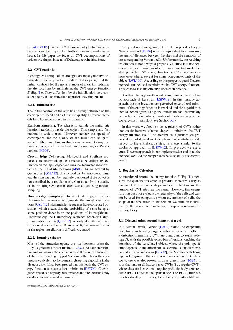
L. Wang & F. Hétroy-Wheeler & E. Boyer / A Hierarchical Approach for Regular CVTs 3
by [ACSYD05], duals of CVTs are actually Delaunay tetra-hedrizations that may contain badly shaped or irregular tetra-hedra. In this paper we focus on CVT decompositions ofvolumetric shapes instead of Delaunay tetrahedrizations.
2.2. CVT methods
Existing CVT computation strategies are mostly iterative op-timization that rely on two fundamental steps: (i) find theinitial locations for the given number of sites; (ii) optimizethe site locations by minimizing the CVT energy functionE (Eq. (1)). They differ then by the initialization they con-sider and by the optimization approach they implement.
2.2.1. Initialisation
The initial position of the sites has a strong influence on theconvergence speed and on the result quality. Different meth-ods have been considered in the literature.
Random Sampling. The idea is to sample the initial sitelocations randomly inside the object. This simple and fastmethod is widely used. However, neither the speed ofconvergence nor the quality of the result can be guar-anteed. Other sampling methods can be used to improvethese criteria, such as farthest point sampling or Ward’smethod [MS06].
Greedy Edge-Collapsing. Moriguchi and Sugihara pro-posed a method which applies a greedy edge-collapsing dec-imation on the input object and uses the decimated mesh ver-tices as the initial site locations [MS06]. As pointed out byQuinn et al. [QSL∗12], this method can be time-consuming,and the sites may not be regularly positioned if the object isnot described by a regular mesh. Consequently, the qualityof the resulting CVT can be even worse than using randomsampling.
Hammersley Sampling. Quinn et al. suggest to useHammersley sequences to generate the initial site loca-tions [QSL∗12]. Hammersley sequences have correlated po-sitions, which means that the probability of a site being atsome position depends on the positions of its neighbours.Unfortunately, the Hammersley sequence generation algo-rithm as described in [QSL∗12] can only place the sites in asquare in 2D or a cube in 3D. As a result, the number of sitesin the region tessellation is difficult to control.
2.2.2. Iterative scheme
Most of the strategies update the site locations using theLloyd’s gradient descent method [Llo82]. At each iteration,this method moves the current sites to the centroid locationsof the corresponding clipped Voronoi cells. This is the con-tinuous equivalent to the k-means clustering algorithm in thediscrete case. It has been proved that this leads the CVT en-ergy function to reach a local minimum [DFG99]. Conver-gence speed can anyway be slow since the site locations mayoscillate around a local minimum.
To speed up convergence, Du et al. proposed a Lloyd-Newton method [DE06] which is equivalent to minimizingthe sum of distances between the sites and the centroids ofthe corresponding Voronoi cells. Unfortunately, the resultingtessellation is not always a proper CVT since it is not nec-essarily a local minimum of E. In an influential work, Liuet al. prove that CVT energy function has C2 smoothness al-most everywhere, except for some non-convex parts of theobject [LWL∗09]. According to this property, quasi-Newtonmethods can be used to minimize the CVT energy function.This leads to fast and effective updates in practice.
Another strategy worth mentioning here is the stochas-tic approach of Lu et al. [LSPW12]. In this iterative ap-proach, the site locations are perturbed once a local mimi-mum of the energy function is reached and the algorithm isthen launched again. The global minimum can theoreticallybe reached after an infinite number of iterations. In practice,convergence is still slow (see Section 5.3).
In this work, we focus on the regularity of CVTs ratherthan on the iterative scheme adopted to minimize the CVTenergy function itself. The hierarchical algorithm we pro-pose does not depend on this scheme but contributes withrespect to the initialization step, in a way similar to thestochastic approach in [LSPW12]. In practice, we use aquasi-Newton approach in our implementation and in all themethods we used for comparisons because of its fast conver-gence.
3. Regularity Criterion
As mentioned before, the energy function E (Eq. (1)) mea-sures the quantization error. It provides therefore a way tocompare CVTs when the shape under consideration and thenumber of CVT sites are the same. However, this energyfunction does not evaluate the regularity of the cells and can-not be used for comparison when the number of cells, theshape or the size differ. In this section, we build on theoret-ical results on optimal quantizers to propose a measure forcell regularity.
3.1. Dimensionless second moment of a cell
In a seminal work, Gersho [Ger79] stated the conjecturethat, for a sufficiently large number of sites, all cells ofa distortion-minimising CVT are congruent to some poly-tope H, with the possible exception of regions touching theboundary of the tessellated object, where the polytope Honly depends on the dimension m. Gersho’s conjecture wasproved in two dimensions [New82], the Voronoi cells beingregular hexagons in that case. A weaker version of Gersho’sconjecture was also proved in three dimensions [BS83]. Itsays that among all lattice-based CVTs (i.e., regular CVTs,where sites are located on a regular grid), the body-centeredcubic (BCC) lattice is the optimal one. The BCC lattice hasits sites displayed on a regular cubic grid, with additional
submitted to COMPUTER GRAPHICS Forum (6/2015).
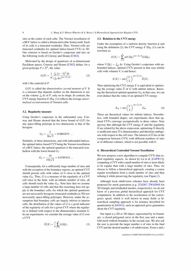
4 L. Wang & F. Hétroy-Wheeler & E. Boyer / A Hierarchical Approach for Regular CVTs
sites at the centre of each cube. The Voronoi tessellation ofa BCC lattice is called a bitruncated cubic honeycomb. Eachof its cells is a truncated octahedra. Thus, Voronoi cells aretruncated octahedra for optimal lattice-based CVTs in 3D.Our criterion is based on Gersho’s conjecture and also onthe following work of Conway and Sloane [CS82].
Motivated by the design of quantizers of m-dimensionalEuclidean spaces, Conway and Sloane [CS82] define, for agiven polytope P ∈ Em, the value:
G(P) =1m
P x− x2 dx
(
P dx)(m+2)/m, (2)
with x the centroid of P.
G(P) is called the dimensionless second moment of P. Itis a measure that depends neither on the dimension m noron the volume
P dx of P, only on its shape. In contrast, the
CVT energy function E (Eq. (1)) reflects the average unnor-malised second moment of Voronoi cells.
3.2. Regularity measure
Using Gersho’s conjecture in the unbounded case, Con-way and Sloane showed that the lower bound of G(P) forany space-filling polytope in two dimensions is that of thehexagon:
G2 =5
36√
3= 0.0801875 . . .
Similarly, in three dimensions, and with unbounded lattices,the optimal lattice-based CVT being the Voronoi tessellationof a BCC lattice, the optimal quantizer is the truncated octa-hedron with the lower-bound G3:
G3 =19
192 3√
2= 0.0785433 . . .
Consequently, for a sufficiently large number of sites andwith the exception of the boundary regions, an optimal CVTshould present cells with values of G close to the optimalvalue Gm. Thus, G is a measure of the regularity of a CVTcell since in the limit, with an infinite number of sites, allcells should reach the value Gm. Note here that we assumea large number of cells and that this reasoning does not ap-ply to the boundary cells, for which the optimal quantizersare not necessarily hexagons (truncated octahedra in 3D) nornecessarily space-filling polytopes. However, under the as-sumption that boundary cells are largely inferior to interiorcells, the distribution of the values of G is a good indicatorof the regularity of cells for a given CVT where the regular-ity is defined with respect to the dimensionless moment G.In our experiments, we consider the average value of G overa CVT:
G(X) =1n
n
∑i=1
G(Ωi). (3)
3.3. Relation to the CVT energy
Under the assumption of a uniform density function ρ andusing the definition (2), the CVT energy E (Eq. (1)) can berewritten as:
E(X) =n
∑i=1
mV (Ωi)(m+2)/mG(Ωi),
where V (Ωi) =
Ωidx. Using Gersho’s conjecture with un-
bounded lattices, optimal CVTs present in that case similarcells with volumes V/n and hence:
E(X) ∼ mn
Vn
(m+2)/m
G(X).
Thus optimizing the CVT energy E is equivalent to optimiz-ing the average value G of G with infinite lattices. Know-ing the theoretical optimal quantizer Gm in that case, we caneven deduce that the value of an optimal CVT energy:
Em = mn
Vn
(m+2)/m
Gm (4)
These are theoretical values for infinite lattices. Neverthe-less, with bounded shapes, our experiments show that op-timal CVTs converge asymptotically to these values. Noteanyway that although the CVT energy E and the regularityG are related by the above expression, optimizing G directlyis inefficient since G is dimensionless and therefore ambigu-ous with respect to the cell sizes. The interest of G lies in thecomparison between CVTs with different numbers of sitesor of different volumes, which is not possible with E.
4. Hierarchical Centroidal Voronoi Tessellation
We now propose a new algorithm to compute CVTs that ex-ploit regularity aspects. As shown by Lu et al. [LSPW12],computing a CVT with a small number of sites is more likelyto be regular than with a large number of sites. Thus, wechoose to follow a hierarchical approach, creating a coarseregular tessellation from a small number of sites and thenrefining it while preserving the regularity (see Figure 2).
Although local subdivision schemes have already beenproposed for mesh generation (e.g. [TAD07, TWAD09] for2D triangle and tetrahedral meshes, respectively), we do notknow of a previous global hierarchical approach for CVTcomputation. In addition to the acceleration of the conver-gence speed, which is well known in many fields (a hi-erarchical sampling approach is for instance described forquantization in [GG91]), such an approach gives guaranteesabout the CVT regularity.
Our input is a 2D or 3D object, represented by its bound-ary: a closed polygonal curve in the first case and a mani-fold mesh without boundary in the second case. We also askthe user to provide the target number n of sites in the finalCVT and the desired number s of subdivisions. From n and s
submitted to COMPUTER GRAPHICS Forum (6/2015).
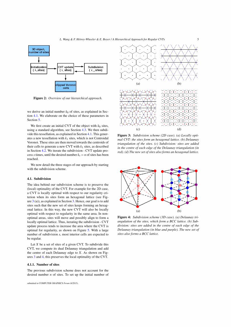
L. Wang & F. Hétroy-Wheeler & E. Boyer / A Hierarchical Approach for Regular CVTs 5
Figure 2: Overview of our hierarchical approach.
we derive an initial number k0 of sites, as explained in Sec-tion 4.1. We elaborate on the choice of these parameters inSection 5.
We first create an initial CVT of the object with k0 sites,using a standard algorithm, see Section 4.3. We then subdi-vide this tessellation, as explained in Section 4.1. This gener-ates a new tessellation with k1 sites, which is not CentroidalVoronoi. These sites are then moved towards the centroids oftheir cells to generate a new CVT with k1 sites, as describedin Section 4.2. We iterate the subdivision - CVT update pro-cess s times, until the desired number ks = n of sites has beenreached.
We now detail the three stages of our approach by startingwith the subdivision scheme.
4.1. Subdivision
The idea behind our subdivision scheme is to preserve the(local) optimality of the CVT. For example for the 2D case,a CVT is locally optimal with respect to our regularity cri-terion when its sites form an hexagonal lattice (see Fig-ure 3 (a)), as explained in Section 3. Hence, our goal is to addsites such that the new set of sites keeps forming an hexag-onal lattice. In this way, the new CVT will also be locallyoptimal with respect to regularity in the same area. In non-optimal areas, sites will move and possibly align to form alocally optimal lattice. Thus, iterating the subdivision - CVTupdate process tends to increase the area where the CVT isoptimal for regularity, as shown on Figure 5. With a largenumber of subdivision s, most interior cells are expected tobe regular.
Let X be a set of sites of a given CVT. To subdivide thisCVT, we compute its dual Delaunay triangulation and addthe centre of each Delaunay edge to X . As shown on Fig-ures 3 and 4, this preserves the local optimality of the CVT.
4.1.1. Number of sites
The previous subdivision scheme does not account for thedesired number n of sites. To set up the initial number of
(a) (b)
(c) (d)
Figure 3: Subdivision scheme (2D case). (a) Locally opti-mal CVT: the sites form an hexagonal lattice. (b) Delaunaytriangulation of the sites. (c) Subdivision: sites are addedin the centre of each edge of the Delaunay triangulation (inred). (d) The new set of sites also forms an hexagonal lattice.
(a) (b)
Figure 4: Subdivision scheme (3D case). (a) Delaunay tri-angulation of the sites, which form a BCC lattice. (b) Sub-division: sites are added in the centre of each edge of theDelaunay triangulation (in blue and purple). The new set ofsites also forms a BCC lattice.
submitted to COMPUTER GRAPHICS Forum (6/2015).
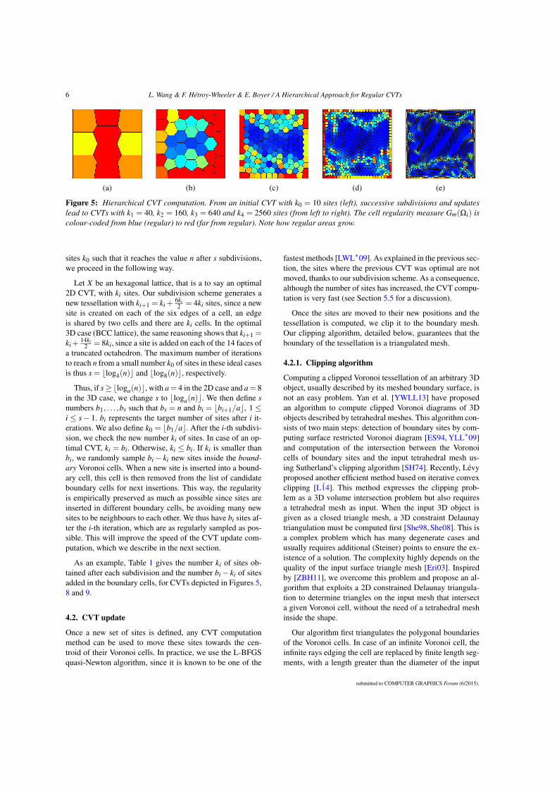
6 L. Wang & F. Hétroy-Wheeler & E. Boyer / A Hierarchical Approach for Regular CVTs
(a) (b) (c) (d) (e)
Figure 5: Hierarchical CVT computation. From an initial CVT with k0 = 10 sites (left), successive subdivisions and updateslead to CVTs with k1 = 40, k2 = 160, k3 = 640 and k4 = 2560 sites (from left to right). The cell regularity measure Gm(Ωi) iscolour-coded from blue (regular) to red (far from regular). Note how regular areas grow.
sites k0 such that it reaches the value n after s subdivisions,we proceed in the following way.
Let X be an hexagonal lattice, that is a to say an optimal2D CVT, with ki sites. Our subdivision scheme generates anew tessellation with ki+1 = ki +
6ki2 = 4ki sites, since a new
site is created on each of the six edges of a cell, an edgeis shared by two cells and there are ki cells. In the optimal3D case (BCC lattice), the same reasoning shows that ki+1 =ki +
14ki2 = 8ki, since a site is added on each of the 14 faces of
a truncated octahedron. The maximum number of iterationsto reach n from a small number k0 of sites in these ideal casesis thus s = log4(n) and log8(n), respectively.
Thus, if s≥loga(n), with a = 4 in the 2D case and a = 8in the 3D case, we change s to loga(n). We then define snumbers b1, . . . ,bs such that bs = n and bi = bi+1/a, 1 ≤i ≤ s− 1. bi represents the target number of sites after i it-erations. We also define k0 = b1/a. After the i-th subdivi-sion, we check the new number ki of sites. In case of an op-timal CVT, ki = bi. Otherwise, ki ≤ bi. If ki is smaller thanbi, we randomly sample bi − ki new sites inside the bound-ary Voronoi cells. When a new site is inserted into a bound-ary cell, this cell is then removed from the list of candidateboundary cells for next insertions. This way, the regularityis empirically preserved as much as possible since sites areinserted in different boundary cells, be avoiding many newsites to be neighbours to each other. We thus have bi sites af-ter the i-th iteration, which are as regularly sampled as pos-sible. This will improve the speed of the CVT update com-putation, which we describe in the next section.
As an example, Table 1 gives the number ki of sites ob-tained after each subdivision and the number bi − ki of sitesadded in the boundary cells, for CVTs depicted in Figures 5,8 and 9.
4.2. CVT update
Once a new set of sites is defined, any CVT computationmethod can be used to move these sites towards the cen-troid of their Voronoi cells. In practice, we use the L-BFGSquasi-Newton algorithm, since it is known to be one of the
fastest methods [LWL∗09]. As explained in the previous sec-tion, the sites where the previous CVT was optimal are notmoved, thanks to our subdivision scheme. As a consequence,although the number of sites has increased, the CVT compu-tation is very fast (see Section 5.5 for a discussion).
Once the sites are moved to their new positions and thetessellation is computed, we clip it to the boundary mesh.Our clipping algorithm, detailed below, guarantees that theboundary of the tessellation is a triangulated mesh.
4.2.1. Clipping algorithm
Computing a clipped Voronoi tessellation of an arbitrary 3Dobject, usually described by its meshed boundary surface, isnot an easy problem. Yan et al. [YWLL13] have proposedan algorithm to compute clipped Voronoi diagrams of 3Dobjects described by tetrahedral meshes. This algorithm con-sists of two main steps: detection of boundary sites by com-puting surface restricted Voronoi diagram [ES94, YLL∗09]and computation of the intersection between the Voronoicells of boundary sites and the input tetrahedral mesh us-ing Sutherland’s clipping algorithm [SH74]. Recently, Lévyproposed another efficient method based on iterative convexclipping [L14]. This method expresses the clipping prob-lem as a 3D volume intersection problem but also requiresa tetrahedral mesh as input. When the input 3D object isgiven as a closed triangle mesh, a 3D constraint Delaunaytriangulation must be computed first [She98, She08]. This isa complex problem which has many degenerate cases andusually requires additional (Steiner) points to ensure the ex-istence of a solution. The complexity highly depends on thequality of the input surface triangle mesh [Eri03]. Inspiredby [ZBH11], we overcome this problem and propose an al-gorithm that exploits a 2D constrained Delaunay triangula-tion to determine triangles on the input mesh that intersecta given Voronoi cell, without the need of a tetrahedral meshinside the shape.
Our algorithm first triangulates the polygonal boundariesof the Voronoi cells. In case of an infinite Voronoi cell, theinfinite rays edging the cell are replaced by finite length seg-ments, with a length greater than the diameter of the input
submitted to COMPUTER GRAPHICS Forum (6/2015).
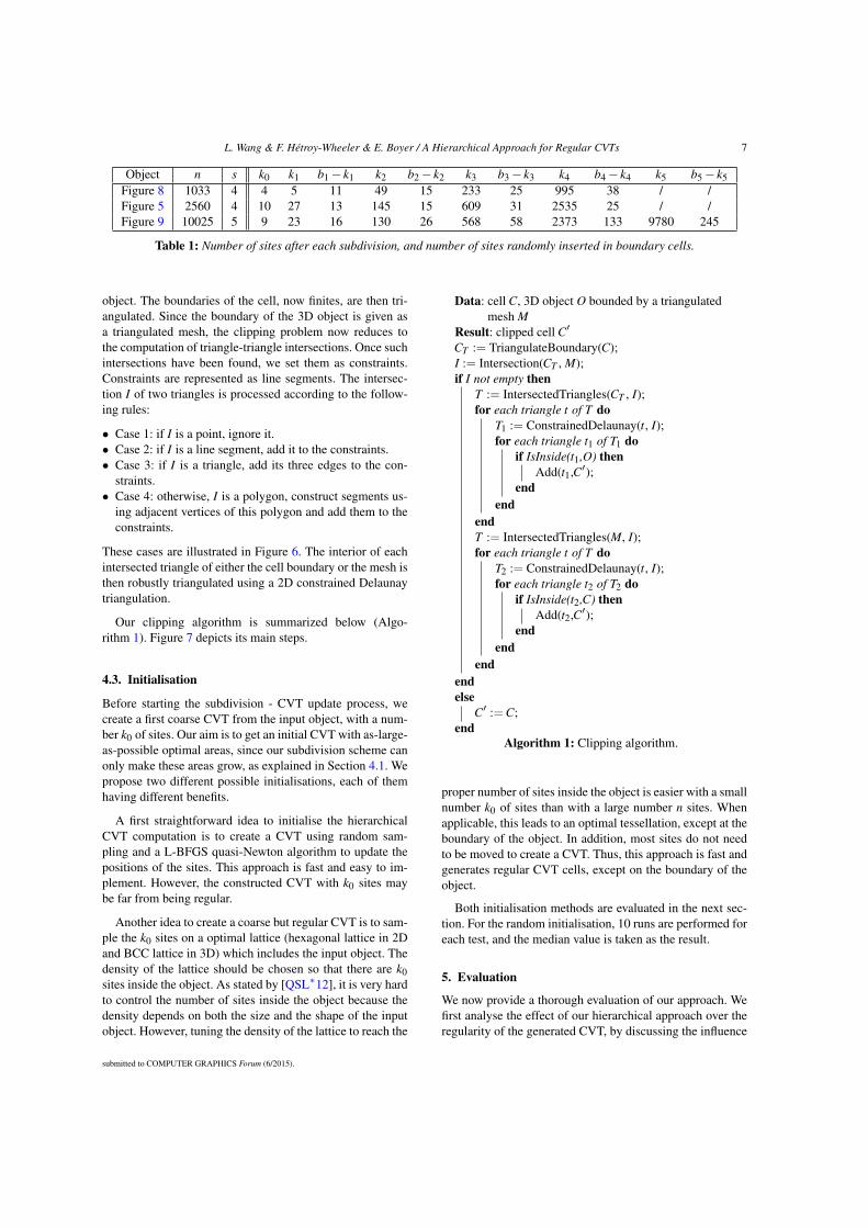
L. Wang & F. Hétroy-Wheeler & E. Boyer / A Hierarchical Approach for Regular CVTs 7
Object n s k0 k1 b1 − k1 k2 b2 − k2 k3 b3 − k3 k4 b4 − k4 k5 b5 − k5Figure 8 1033 4 4 5 11 49 15 233 25 995 38 / /Figure 5 2560 4 10 27 13 145 15 609 31 2535 25 / /Figure 9 10025 5 9 23 16 130 26 568 58 2373 133 9780 245
Table 1: Number of sites after each subdivision, and number of sites randomly inserted in boundary cells.
object. The boundaries of the cell, now finites, are then tri-angulated. Since the boundary of the 3D object is given asa triangulated mesh, the clipping problem now reduces tothe computation of triangle-triangle intersections. Once suchintersections have been found, we set them as constraints.Constraints are represented as line segments. The intersec-tion I of two triangles is processed according to the follow-ing rules:
• Case 1: if I is a point, ignore it.• Case 2: if I is a line segment, add it to the constraints.• Case 3: if I is a triangle, add its three edges to the con-
straints.• Case 4: otherwise, I is a polygon, construct segments us-
ing adjacent vertices of this polygon and add them to theconstraints.
These cases are illustrated in Figure 6. The interior of eachintersected triangle of either the cell boundary or the mesh isthen robustly triangulated using a 2D constrained Delaunaytriangulation.
Our clipping algorithm is summarized below (Algo-rithm 1). Figure 7 depicts its main steps.
4.3. Initialisation
Before starting the subdivision - CVT update process, wecreate a first coarse CVT from the input object, with a num-ber k0 of sites. Our aim is to get an initial CVT with as-large-as-possible optimal areas, since our subdivision scheme canonly make these areas grow, as explained in Section 4.1. Wepropose two different possible initialisations, each of themhaving different benefits.
A first straightforward idea to initialise the hierarchicalCVT computation is to create a CVT using random sam-pling and a L-BFGS quasi-Newton algorithm to update thepositions of the sites. This approach is fast and easy to im-plement. However, the constructed CVT with k0 sites maybe far from being regular.
Another idea to create a coarse but regular CVT is to sam-ple the k0 sites on a optimal lattice (hexagonal lattice in 2Dand BCC lattice in 3D) which includes the input object. Thedensity of the lattice should be chosen so that there are k0sites inside the object. As stated by [QSL∗12], it is very hardto control the number of sites inside the object because thedensity depends on both the size and the shape of the inputobject. However, tuning the density of the lattice to reach the
Data: cell C, 3D object O bounded by a triangulatedmesh M
Result: clipped cell C
CT := TriangulateBoundary(C);I := Intersection(CT , M);if I not empty then
T := IntersectedTriangles(CT , I);for each triangle t of T do
T1 := ConstrainedDelaunay(t, I);for each triangle t1 of T1 do
if IsInside(t1,O) thenAdd(t1,C);
endend
endT := IntersectedTriangles(M, I);for each triangle t of T do
T2 := ConstrainedDelaunay(t, I);for each triangle t2 of T2 do
if IsInside(t2,C) thenAdd(t2,C);
endend
endendelse
C := C;end
Algorithm 1: Clipping algorithm.
proper number of sites inside the object is easier with a smallnumber k0 of sites than with a large number n sites. Whenapplicable, this leads to an optimal tessellation, except at theboundary of the object. In addition, most sites do not needto be moved to create a CVT. Thus, this approach is fast andgenerates regular CVT cells, except on the boundary of theobject.
Both initialisation methods are evaluated in the next sec-tion. For the random initialisation, 10 runs are performed foreach test, and the median value is taken as the result.
5. Evaluation
We now provide a thorough evaluation of our approach. Wefirst analyse the effect of our hierarchical approach over theregularity of the generated CVT, by discussing the influence
submitted to COMPUTER GRAPHICS Forum (6/2015).
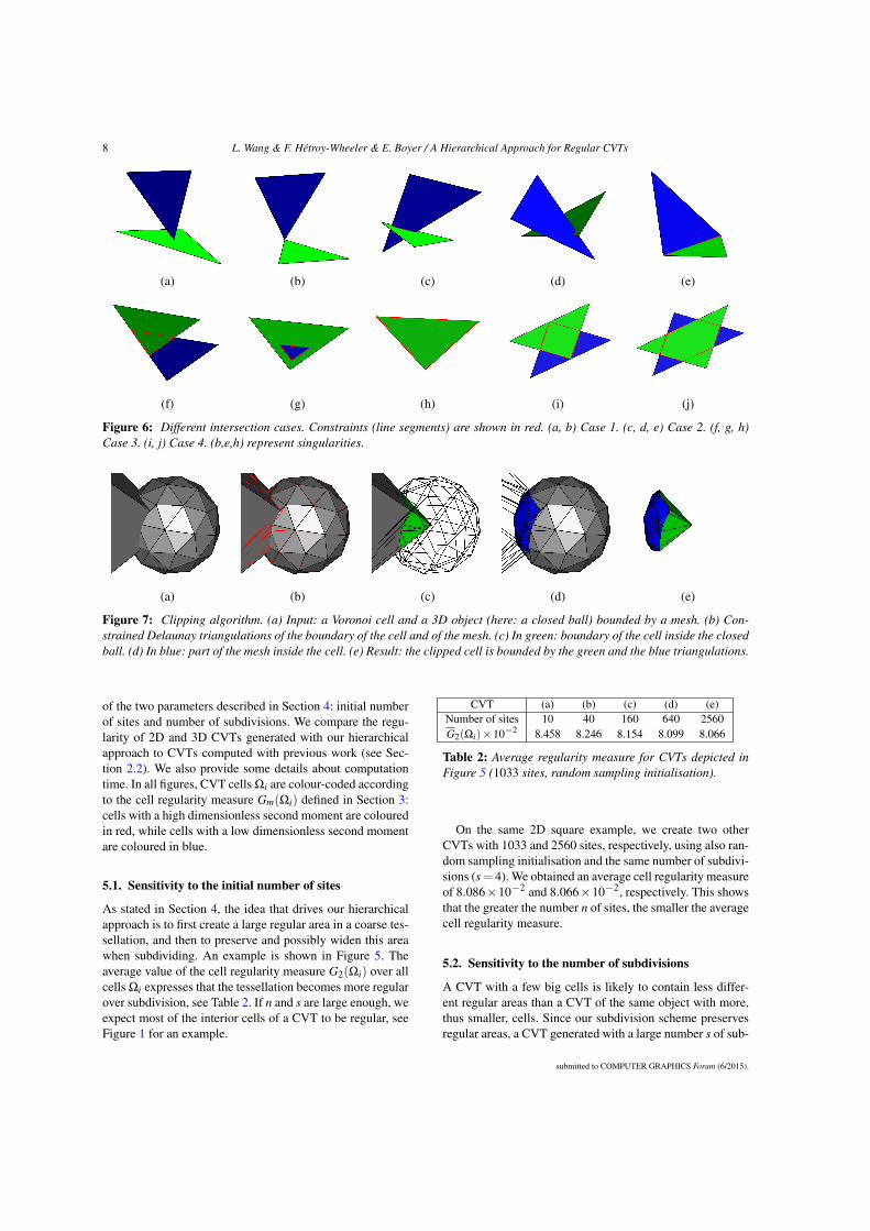
8 L. Wang & F. Hétroy-Wheeler & E. Boyer / A Hierarchical Approach for Regular CVTs
(a) (b) (c) (d) (e)
(f) (g) (h) (i) (j)
Figure 6: Different intersection cases. Constraints (line segments) are shown in red. (a, b) Case 1. (c, d, e) Case 2. (f, g, h)Case 3. (i, j) Case 4. (b,e,h) represent singularities.
(a) (b) (c) (d) (e)
Figure 7: Clipping algorithm. (a) Input: a Voronoi cell and a 3D object (here: a closed ball) bounded by a mesh. (b) Con-strained Delaunay triangulations of the boundary of the cell and of the mesh. (c) In green: boundary of the cell inside the closedball. (d) In blue: part of the mesh inside the cell. (e) Result: the clipped cell is bounded by the green and the blue triangulations.
of the two parameters described in Section 4: initial numberof sites and number of subdivisions. We compare the regu-larity of 2D and 3D CVTs generated with our hierarchicalapproach to CVTs computed with previous work (see Sec-tion 2.2). We also provide some details about computationtime. In all figures, CVT cells Ωi are colour-coded accordingto the cell regularity measure Gm(Ωi) defined in Section 3:cells with a high dimensionless second moment are colouredin red, while cells with a low dimensionless second momentare coloured in blue.
5.1. Sensitivity to the initial number of sites
As stated in Section 4, the idea that drives our hierarchicalapproach is to first create a large regular area in a coarse tes-sellation, and then to preserve and possibly widen this areawhen subdividing. An example is shown in Figure 5. Theaverage value of the cell regularity measure G2(Ωi) over allcells Ωi expresses that the tessellation becomes more regularover subdivision, see Table 2. If n and s are large enough, weexpect most of the interior cells of a CVT to be regular, seeFigure 1 for an example.
CVT (a) (b) (c) (d) (e)Number of sites 10 40 160 640 2560G2(Ωi)×10−2 8.458 8.246 8.154 8.099 8.066
Table 2: Average regularity measure for CVTs depicted inFigure 5 (1033 sites, random sampling initialisation).
On the same 2D square example, we create two otherCVTs with 1033 and 2560 sites, respectively, using also ran-dom sampling initialisation and the same number of subdivi-sions (s = 4). We obtained an average cell regularity measureof 8.086×10⁻² and 8.066×10⁻², respectively. This showsthat the greater the number n of sites, the smaller the averagecell regularity measure.
5.2. Sensitivity to the number of subdivisions
A CVT with a few big cells is likely to contain less differ-ent regular areas than a CVT of the same object with more,thus smaller, cells. Since our subdivision scheme preservesregular areas, a CVT generated with a large number s of sub-
submitted to COMPUTER GRAPHICS Forum (6/2015).

L. Wang & F. Hétroy-Wheeler & E. Boyer / A Hierarchical Approach for Regular CVTs 9
divisions is more regular than a CVT with the same numbern of sites but generated with a small s, as shown in Table 3.As a consequence, we suggest to set s as large as possible.
s 0 1 2 3 4G2(Ωi)×10−2 8.079 8.063 8.060 8.056 8.054
Table 3: Average regularity measure for CVTs of a squarewith 10000 sites generated using our hierarchical approach(random sampling initialisation) with different number ofsubdivisions.
In the case that an optimal lattice sampling is used as ini-tialisation, it is preferable to start from a small number ofsubdivisions, since we only have one large regular area what-ever the lattice size. Actually, s = 0 correspond to the opti-mal lattice sampling, as shown for instance in Figures 8 (f)and 9 (i). However, as stated before, the larger n, the moredifficult it is to build such a lattice with a prescribed numberof sites.
5.3. Comparison to previous work
We test our approach against previously mentioned meth-ods in a simple 2D square. To check which method givesthe most regular CVT, we first compute an hexagonal latticewith approximately 1000 sites. As stated above, it is difficultto accurately set the number n of sites. We were able to setn = 1033. We then compute CVTs with 1033 sites using thefollowing methods:
• random sampling and L-BFGS update;• Hammersley sampling [QSL∗12] and L-BFGS update;• global Monte-Carlo optimisation [LSPW12];• our hierarchical approach with random sampling initiali-
sation step (4 subdivisions, which is the maximum possi-ble);
• our hierarchical approach with a lattice sampling initiali-sation step (1 subdivision).
For the global Monte-Carlo optimisation, we have used theparameter values advised in [LSPW12]. In particular, 200updates have been performed.
Qualitative results are shown on Figure 8. The averagevalues of the cell regularity measure G2(Ωi) over all cellsΩi, as well as the CVT energy function values, are givenin Table 4. Remember that, as explained in Section 3, anoptimal cell has a dimensionless second moment value ofG2 = 5
36√
3= 0.08018 . . .
The hexagonal lattice is not optimal because of its bound-ary cells which are not hexagonal. Among other methods,the stochastic approach of [LSPW12] and our hierarchicalframework give similar results. The main difference in prac-tice between these two methods is the computation time: theglobal Monte-Carlo minimisation is about 100 times slowerthan our approach (207.08 seconds instead of 2.16).
We then test a geometrically more complex object: a five-branches star. We also increase the number of sites. As inthe previous case, we first start by computing an hexagonallattice with approximately 10000 sites. The lattice containsexactly n = 10025 sites. We discard the stochastic approachof [LSPW12] since it is too slow in this case. For the Ham-mersley sampling, we construct a bounding box of the ob-ject, and try different numbers of sites until we exactly ob-tain 10025 sites inside the object. It must be mentioned thatseveral attempts were necessary since the number of sitesinside the object does not necessarily increase when moresites are generated in the bounding box. For the hierarchicalapproach, we use 5 subdivisions after the random samplinginitialisation (the maximum possible) and only one after lat-tice sampling initialisation.
Results are shown on Figure 9 and in Table 5. These re-sults are in accordance with the results for the square. Ourhierarchical approach performs better than the previous ini-tialisation methods for both criteria. Moreover, lattice sam-pling initialisation gives better results than random samplinginitialisation by almost reaching the regularity of a clippedhexagonal lattice.
In Figure 10 and Table 6 we compare CVTs computed ona simple closed 3D ball using random sampling, Hammer-sley sampling, our hierarchical approach with random sam-pling initialisation and our hierarchical approach with latticesampling initialisation. It was not possible, in this case, toconstruct a BCC lattice with a prescribed and sufficientlylarge number of sites. Two different numbers n of sites weretested. We used the maximum number of subdivisions forthe hierarchical approach with random sampling initialisa-tion: two in the n = 1000 sites case and three in the n = 5000sites case.
Remember that in this 3D case, the optimal cell regularitymeasure value is G3 = 19
192 3√2= 0.0785433 . . . This example
shows that our hierarchical approach performs better thanother initialisation methods, in case the number n of sites ishigh enough. In case not, the number of boundary cells istoo high with respect to the number of interior cells for theGersho’s conjecture to apply in practice.
Other 3D CVTs with 50k, 80k and 100k sites, computedwith a standard random sampling initialisation + L-BFGSupdate, our hierarchical approach using a random samplinginitialisation and our hierarchical approach with a latticesampling initialisation, are shown in Figure 11. It was notpossible to create an Hammersley initialisation and a BCClattice with the correct number of sites inside the objects inthese cases.
5.4. Convergence speed
The main parameter in most CVT computation methods isthe number of iterations of the algorithm. A local minimumof the CVT energy function is asymptotically reached, but
submitted to COMPUTER GRAPHICS Forum (6/2015).
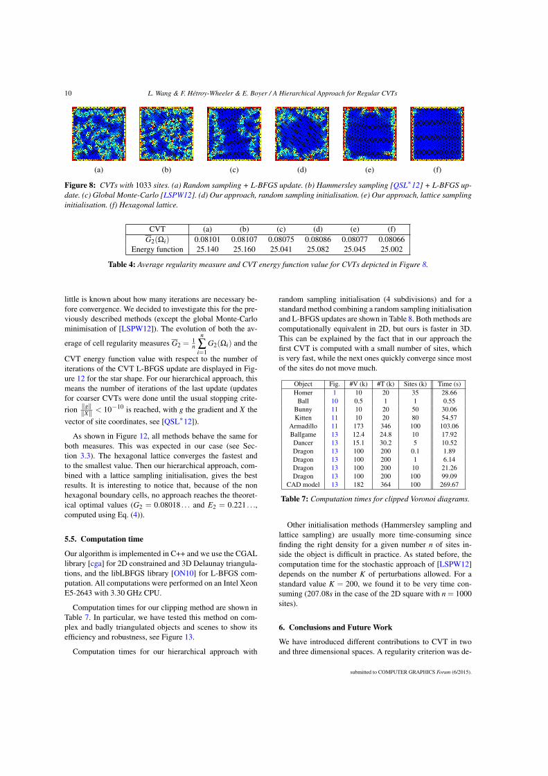
10 L. Wang & F. Hétroy-Wheeler & E. Boyer / A Hierarchical Approach for Regular CVTs
(a) (b) (c) (d) (e) (f)
Figure 8: CVTs with 1033 sites. (a) Random sampling + L-BFGS update. (b) Hammersley sampling [QSL∗12] + L-BFGS up-date. (c) Global Monte-Carlo [LSPW12]. (d) Our approach, random sampling initialisation. (e) Our approach, lattice samplinginitialisation. (f) Hexagonal lattice.
CVT (a) (b) (c) (d) (e) (f)G2(Ωi) 0.08101 0.08107 0.08075 0.08086 0.08077 0.08066
Energy function 25.140 25.160 25.041 25.082 25.045 25.002
Table 4: Average regularity measure and CVT energy function value for CVTs depicted in Figure 8.
little is known about how many iterations are necessary be-fore convergence. We decided to investigate this for the pre-viously described methods (except the global Monte-Carlominimisation of [LSPW12]). The evolution of both the av-
erage of cell regularity measures G2 = 1n
n
∑i=1
G2(Ωi) and the
CVT energy function value with respect to the number ofiterations of the CVT L-BFGS update are displayed in Fig-ure 12 for the star shape. For our hierarchical approach, thismeans the number of iterations of the last update (updatesfor coarser CVTs were done until the usual stopping crite-rion g
X < 10−10 is reached, with g the gradient and X thevector of site coordinates, see [QSL∗12]).
As shown in Figure 12, all methods behave the same forboth measures. This was expected in our case (see Sec-tion 3.3). The hexagonal lattice converges the fastest andto the smallest value. Then our hierarchical approach, com-bined with a lattice sampling initialisation, gives the bestresults. It is interesting to notice that, because of the nonhexagonal boundary cells, no approach reaches the theoret-ical optimal values (G2 = 0.08018 . . . and E2 = 0.221 . . .,computed using Eq. (4)).
5.5. Computation time
Our algorithm is implemented in C++ and we use the CGALlibrary [cga] for 2D constrained and 3D Delaunay triangula-tions, and the libLBFGS library [ON10] for L-BFGS com-putation. All computations were performed on an Intel XeonE5-2643 with 3.30 GHz CPU.
Computation times for our clipping method are shown inTable 7. In particular, we have tested this method on com-plex and badly triangulated objects and scenes to show itsefficiency and robustness, see Figure 13.
Computation times for our hierarchical approach with
random sampling initialisation (4 subdivisions) and for astandard method combining a random sampling initialisationand L-BFGS updates are shown in Table 8. Both methods arecomputationally equivalent in 2D, but ours is faster in 3D.This can be explained by the fact that in our approach thefirst CVT is computed with a small number of sites, whichis very fast, while the next ones quickly converge since mostof the sites do not move much.
Object Fig. #V (k) #T (k) Sites (k) Time (s)Homer 1 10 20 35 28.66
Ball 10 0.5 1 1 0.55Bunny 11 10 20 50 30.06Kitten 11 10 20 80 54.57
Armadillo 11 173 346 100 103.06Ballgame 13 12.4 24.8 10 17.92Dancer 13 15.1 30.2 5 10.52Dragon 13 100 200 0.1 1.89Dragon 13 100 200 1 6.14Dragon 13 100 200 10 21.26Dragon 13 100 200 100 99.09
CAD model 13 182 364 100 269.67
Table 7: Computation times for clipped Voronoi diagrams.
Other initialisation methods (Hammersley sampling andlattice sampling) are usually more time-consuming sincefinding the right density for a given number n of sites in-side the object is difficult in practice. As stated before, thecomputation time for the stochastic approach of [LSPW12]depends on the number K of perturbations allowed. For astandard value K = 200, we found it to be very time con-suming (207.08s in the case of the 2D square with n = 1000sites).
6. Conclusions and Future Work
We have introduced different contributions to CVT in twoand three dimensional spaces. A regularity criterion was de-
submitted to COMPUTER GRAPHICS Forum (6/2015).
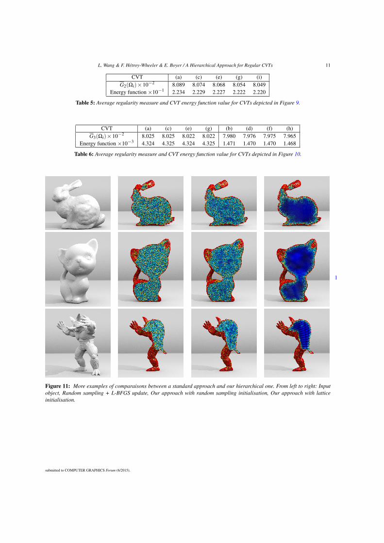
L. Wang & F. Hétroy-Wheeler & E. Boyer / A Hierarchical Approach for Regular CVTs 11
CVT (a) (c) (e) (g) (i)G2(Ωi)×10−2 8.089 8.074 8.068 8.054 8.049
Energy function ×10−1 2.234 2.229 2.227 2.222 2.220
Table 5: Average regularity measure and CVT energy function value for CVTs depicted in Figure 9.
CVT (a) (c) (e) (g) (b) (d) (f) (h)G3(Ωi)×10−2 8.025 8.025 8.022 8.022 7.980 7.976 7.975 7.965
Energy function ×10−3 4.324 4.325 4.324 4.325 1.471 1.470 1.470 1.468
Table 6: Average regularity measure and CVT energy function value for CVTs depicted in Figure 10.
1
Figure 11: More examples of comparaisons between a standard approach and our hierarchical one. From left to right: Inputobject, Random sampling + L-BFGS update, Our approach with random sampling initialisation, Our approach with latticeinitialisation.
submitted to COMPUTER GRAPHICS Forum (6/2015).
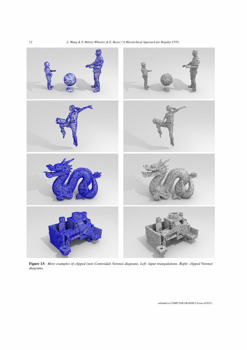
12 L. Wang & F. Hétroy-Wheeler & E. Boyer / A Hierarchical Approach for Regular CVTs
Figure 13: More examples of clipped (non Centroidal) Voronoi diagrams. Left: input triangulations. Right: clipped Voronoidiagrams.
submitted to COMPUTER GRAPHICS Forum (6/2015).
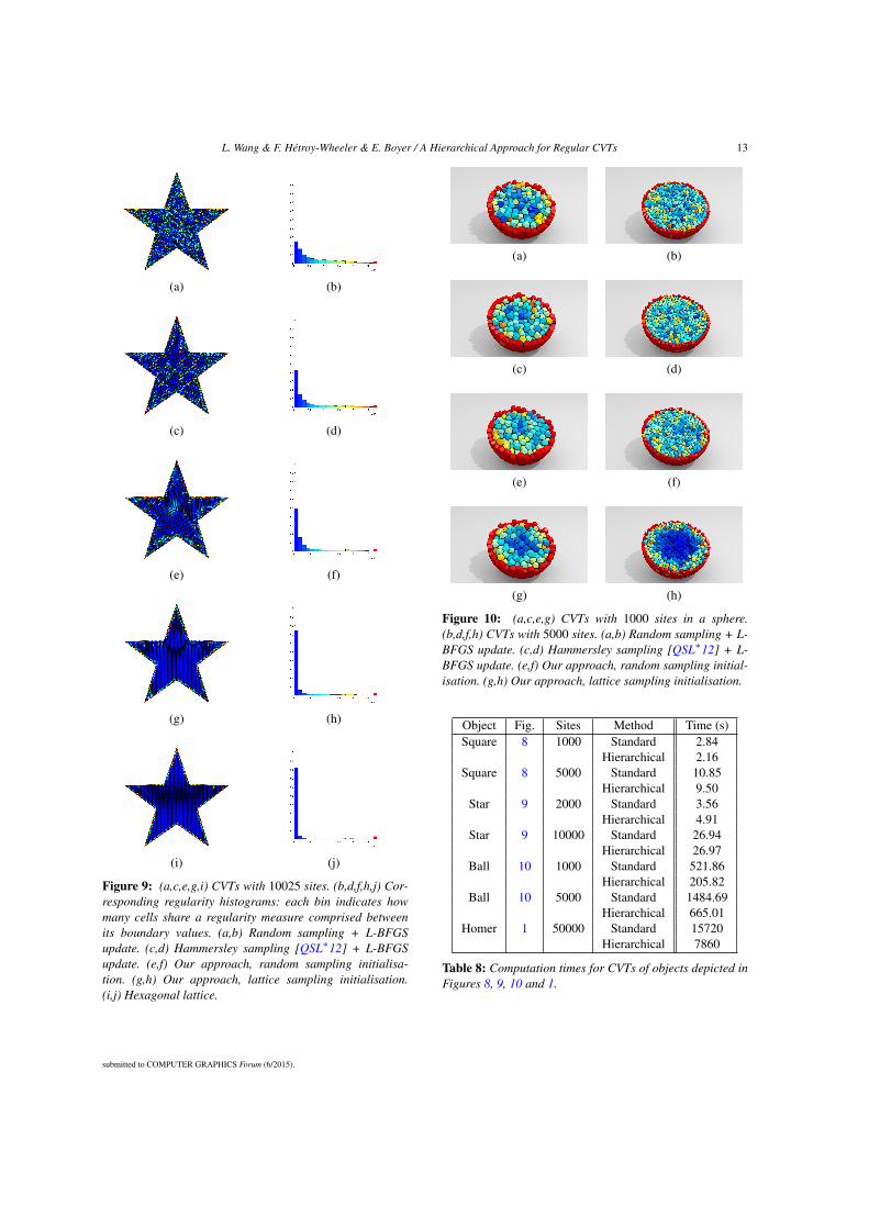
L. Wang & F. Hétroy-Wheeler & E. Boyer / A Hierarchical Approach for Regular CVTs 13
(a) (b)
(c) (d)
(e) (f)
(g) (h)
(i) (j)
Figure 9: (a,c,e,g,i) CVTs with 10025 sites. (b,d,f,h,j) Cor-responding regularity histograms: each bin indicates howmany cells share a regularity measure comprised betweenits boundary values. (a,b) Random sampling + L-BFGSupdate. (c,d) Hammersley sampling [QSL∗12] + L-BFGSupdate. (e,f) Our approach, random sampling initialisa-tion. (g,h) Our approach, lattice sampling initialisation.(i,j) Hexagonal lattice.
(a) (b)
(c) (d)
(e) (f)
(g) (h)
Figure 10: (a,c,e,g) CVTs with 1000 sites in a sphere.(b,d,f,h) CVTs with 5000 sites. (a,b) Random sampling + L-BFGS update. (c,d) Hammersley sampling [QSL∗12] + L-BFGS update. (e,f) Our approach, random sampling initial-isation. (g,h) Our approach, lattice sampling initialisation.
Object Fig. Sites Method Time (s)Square 8 1000 Standard 2.84
Hierarchical 2.16Square 8 5000 Standard 10.85
Hierarchical 9.50Star 9 2000 Standard 3.56
Hierarchical 4.91Star 9 10000 Standard 26.94
Hierarchical 26.97Ball 10 1000 Standard 521.86
Hierarchical 205.82Ball 10 5000 Standard 1484.69
Hierarchical 665.01Homer 1 50000 Standard 15720
Hierarchical 7860
Table 8: Computation times for CVTs of objects depicted inFigures 8, 9, 10 and 1.
submitted to COMPUTER GRAPHICS Forum (6/2015).
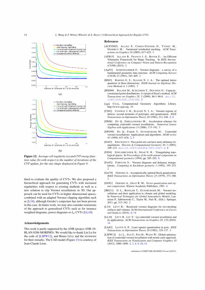
14 L. Wang & F. Hétroy-Wheeler & E. Boyer / A Hierarchical Approach for Regular CVTs
(a)
(b)
Figure 12: Average cell regularity (a) and CVT energy func-tion value (b) with respect to the number of iterations of theCVT update, for the star shape displayed in Figure 9.
fined to evaluate the quality of CVTs. We also proposed ahierarchical approach for generating CVTs with increasedregularities with respect to existing methods as well as anew solution to clip Voronoi tessellations in 3D. Our ap-proach can be used for CVTs in higher dimensional spaces,combined with an adapted Voronoi clipping algorithm suchas [L14], although Gersho’s conjecture has not been provenin this case. In future work, we may also consider extensionsof the approach to generalised CVTs such as for instanceweighted diagrams, power diagrams or Lp CVTs [LL10].
Acknowledgements
This work is partly supported by the ANR (project ANR-10-BLAN-0206 MORPHO). We would like to thank Lin Lu forthe code of [LSPW12], and Bruno Lévy and the reviewersfor their remarks. The CAD model (Figure 13) is courtesy ofJean-Claude Léon.
References[ACSYD05] ALLIEZ P., COHEN-STEINER D., YVINEC M.,
DESBRUN M.: Variational tetrahedral meshing. ACM Trans-actions on Graphics 24 (2005), 617–625. 3
[AFB15] ALLAIN B., FRANCO J.-S., BOYER E.: An EfficientVolumetric Framework for Shape Tracking. In IEEE Interna-tional Conference on Computer Vision and Pattern Recognition(CVPR) (2015). 2
[Aur91] AURENHAMMER F.: Voronoi diagrams - a survey of afundamental geometric data structure. ACM Computing Surveys(CSUR) 23 (1991), 345–405. 2
[BS83] BARNES E. S., SLOANE N. J. A.: The optimal latticequantizer in three dimensions. SIAM Journal on Algebraic Dis-crete Methods 4, 1 (1983). 3
[BSD09] BALZER M., SCHLÖMER T., DEUSSEN O.: Capacity-constrained point distributions: A variant of lloyd’s method. ACMTransactions on Graphics 28, 3 (2009), 86:1–86:8. doi:10.1145/1531326.1531392. 2
[cga] CGAL, Computational Geometry Algorithms Library.http://www.cgal.org. 10
[CS82] CONWAY J. H., SLOANE N. J. A.: Voronoi regions oflattices, second moments of polytopes, and quantization. IEEETransactions on Information Theory 28 (1982), 211–226. 2, 4
[DE06] DU Q., EMELIANENKO M.: Acceleration schemes forcomputing centroidal voronoi tessellations. Numerical LinearAlgebra with Applications 13 (2006), 173–192. 3
[DFG99] DU Q., FABER V., GUNZBURGER M.: Centroidalvoronoi tessellations: Applications and algorithms. SIAM review41 (1999), 637–676. 2, 3
[Eri03] ERICKSON J.: Nice point sets can have nasty delaunay tri-angulations. Discrete & Computational Geometry 30, 1 (2003),109–132. doi:10.1007/s00454-003-2927-4. 6
[ES94] EDELSBRUNNER H., SHAH N. R.: Triangulating topo-logical spaces. In Proceedings of the tenth annual symposium onComputational geometry (1994), pp. 285–292. 6
[For92] FORTUNE S.: Voronoi diagrams and delaunay triangu-lations. Computing in Euclidean geometry 1 (1992), 193–233.2
[Ger79] GERSHO A.: Asymptotically optimal block quantization.IEEE Transactions on Information Theory 25 (1979), 373–380.3
[GG91] GERSHO A., GRAY R. M.: Vector quantization and sig-nal compression. Kluwer Academic Publishers, 1991. 4
[JRG11] JU L., RINGLER T., GUNZBURGER M.: Voronoi tes-sellations and their application to climate and global modeling.In Numerical Techniques for Global Atmospheric Models, Lau-ritzen P., Jablonowski C., Taylor M., Nair R., (Eds.). Springer,2011, pp. 313–342. 2
[L14] LÉVY B.: Restricted voronoi diagrams for (re)-meshingsurfaces and volumes. In 8th International Conference on Curvesand Surfaces (2014). 6, 14
[LL10] LÉVY B., LIU Y.: Lp centroidal voronoi tessellation andits applications. ACM Transactions on Graphics 29, 119 (2010).14
[Llo82] LLOYD S. P.: Least squares quantization in pcm. IEEETransactions on Information Theory 28 (1982), 129–137. 3
[LSPW12] LU L., SUN F., PAN H., WANG W.: Global optimiza-tion of centroidal voronoi tessellation with monte carlo approach.IEEE Transactions on Visualization and Computer Graphics 18(2012), 1880–1890. 2, 3, 4, 9, 10, 14
submitted to COMPUTER GRAPHICS Forum (6/2015).
L. Wang & F. Hétroy-Wheeler & E. Boyer / A Hierarchical Approach for Regular CVTs 15
[LWL∗09] LIU Y., WANG W., LÉVY B., SUN F., YAN D.-M.,LIU L., YANG C.: On centroidal voronoi tessellation - energysmoothness and fast computation. ACM Transactions on Graph-ics 28, 101 (2009). 2, 3, 6
[MS06] MORIGUCHI M., SUGIHARA K.: A new initializationmethod for constructing centroidal voronoi tessellations on sur-face meshes. In 3rd International Symposium on Voronoi Dia-grams in Science and Engineering, 2006 (2006), pp. 159–165.3
[New82] NEWMAN D. J.: The hexagon theorem. IEEE Transac-tions on Information Theory 28 (1982), 137–139. 3
[OBSC00] OKABE A., BOOTS B., SUGIHARA K., CHI S. N.:Spatial Tessellations: Concepts and Applications of Voronoi Di-agrams. John Wiley, 2000. 2
[ON10] OKAZAKI N., NOCEDAL J.: libLBFGS: a li-brary of Limited-memory Broyden-Fletcher-Goldfarb-Shanno(L-BFGS), 2010. http://www.chokkan.org/software/liblbfgs/. 10
[QSL∗12] QUINN J., SUN F., LANGBEIN F. C., LAI Y.-K.,WANG W., MARTIN R. R.: Improved initialisation for cen-troidal voronoi tessellation and optimal delaunay triangulation.Computer-Aided Design 44 (2012), 1062–1071. 2, 3, 7, 9, 10, 13
[SH74] SUTHERLAND I. E., HODGMAN G. W.: Reentrant poly-gon clipping. Communications of the ACM 17 (1974), 32–42.6
[She98] SHEWCHUK J. R.: A condition guaranteeing the exis-tence of higher-dimensional constrained delaunay triangulations.In SCG ’98 Proceedings of the fourteenth annual symposium onComputational geometry (1998), pp. 76–85. 6
[She08] SHEWCHUK J. R.: General-dimensional constrained de-launay and constrained regular triangulations, i: Combinatorialproperties. Discrete & Computational Geometry 39 (2008), 580–637. 6
[TAD07] TOURNOIS J., ALLIEZ P., DEVILLERS O.: Inter-leaving delaunay refinement and optimization for 2d trianglemesh generation. In Proceedings of the 16th InternationalMeshing Roundtable (2007), pp. 83–101. doi:10.1007/978-3-540-75103-8_5. 4
[TWAD09] TOURNOIS J., WORMSER C., ALLIEZ P., DESBRUNM.: Interleaving delaunay refinement and optimization for prac-tical isotropic tetrahedron mesh generation. ACM Transactionson Graphics 28, 75 (2009). 4
[YLL∗09] YAN D.-M., LÉVY B., LIU Y., SUN F., WANG W.:Isotropic remeshing with fast and exact computation of restrictedvoronoi diagram. Computer Graphics Forum 28 (2009), 1445–1454. 6
[YWLL13] YAN D.-M., WANG W., LÉVY B., LIU Y.: Efficientcomputation of 3d clipped voronoi diagram for mesh generation.Computer-Aided Design 45 (2013), 843–852. 2, 6
[ZBH11] ZAHARESCU A., BOYER E., HORAUD R.: Topology-adaptive mesh deformation for surface evolution, morphing, andmulti-view reconstruction. IEEE Transactions on Pattern Analy-sis and Machine Intelligence 33 (2011), 823–837. 6
submitted to COMPUTER GRAPHICS Forum (6/2015).

158 APPENDIX A. SELECTED PAPERS

A.5. HARMONIC SKELETON FOR REALISTIC CHARACTER ANIMATION 159
∴
A.5 HARMONIC SKELETON FOR REALISTICCHARACTER ANIMATION
Grégoire Aujay, Franck Hétroy, Francis Lazarus, Christine DeprazACM-SIGGRAPH/Eurographics Symposium on Computer Animation, 2007.

160 APPENDIX A. SELECTED PAPERS
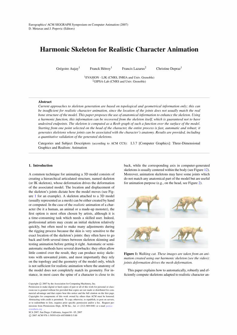
Eurographics/ ACM SIGGRAPH Symposium on Computer Animation (2007)D. Metaxas and J. Popovic (Editors)
Harmonic Skeleton for Realistic Character Animation
Grégoire Aujay1 Franck Hétroy1 Francis Lazarus2 Christine Depraz1
1EVASION - LJK (CNRS, INRIA and Univ. Grenoble)2GIPSA-Lab (CNRS and Univ. Grenoble)
AbstractCurrent approaches to skeleton generation are based on topological and geometrical information only; this canbe insufficient for realistic character animation, since the location of the joints does not usually match the realbone structure of the model. This paper proposes the use of anatomical information to enhance the skeleton. Usinga harmonic function, this information can be recovered from the skeleton itself, which is guaranteed not to haveundesired endpoints. The skeleton is computed as a Reeb graph of such a function over the surface of the model.Starting from one point selected on the head of the character, the entire process is fast, automatic and robust; itgenerates skeletons whose joints can be associated with the character’s anatomy. Results are provided, includinga quantitative validation of the generated skeletons.
Categories and Subject Descriptors (according to ACM CCS): I.3.7 [Computer Graphics]: Three-DimensionalGraphics and Realism: Animation
1. Introduction
A common technique for animating a 3D model consists ofcreating a hierarchical articulated structure, named skeleton(or IK skeleton), whose deformation drives the deformationof the associated model. The location and displacement ofthe skeleton’s joints dictate how the model moves (see Fig-ure 1 for an example). A skeleton attached to a 3D model(usually represented as a mesh) can be either created by handor computed. In the case of the realistic animation of a char-acter (be it a human, an animal or a made-up monster), thefirst option is most often chosen by artists, although it isa time-consuming task which needs a skilled user. Indeed,professional artists may create an initial skeleton relativelyquickly, but often need to make many adjustments duringthe rigging process because the skin is very sensitive to theexact location of the skeleton’s joints: they often have to goback and forth several times between skeleton skinning andtesting animation before getting it right. Automatic or semi-automatic methods have several drawbacks: they often allowlittle control over the result, they can produce noisy skele-tons with unwanted joints, and most importantly they relyon the topology and the geometry of the model only, whichis not sufficient for realistic animation where the anatomy ofthe model does not completely match its geometry. For in-stance, in most cases the spine of a character is close to its
back, while the corresponding axis in computer-generatedskeletons is usually centered within the body (see Figure 12).Moreover, animation skeletons may have some joints whichdo not match any anatomical part of the model but are usefulfor animation purpose (e.g., on the head, see Figure 2).
Figure 1: Walking cat. These images are taken from an ani-mation created using our harmonic skeleton (see the video):joints deformation drives the mesh deformation.
This paper explains how to automatically, robustly and ef-ficiently compute skeletons adapted to realistic character an-
Copyright c 2007 by the Association for Computing Machinery, Inc.Permission to make digital or hard copies of part or all of this work for personal or class-room use is granted without fee provided that copies are not made or distributed for com-mercial advantage and that copies bear this notice and the full citation on the first page.Copyrights for components of this work owned by others than ACM must be honored.Abstracting with credit is permitted. To copy otherwise, to republish, to post on servers,or to redistribute to lists, requires prior specific permission and/or a fee. Request per-missions from Permissions Dept, ACM Inc., fax +1 (212) 869-0481 or e-mail [email protected] .SCA 2007, San Diego, California, August 04 - 05, 2007c 2007 ACM 978-1-59593-624-4/07/0008 $ 5.00
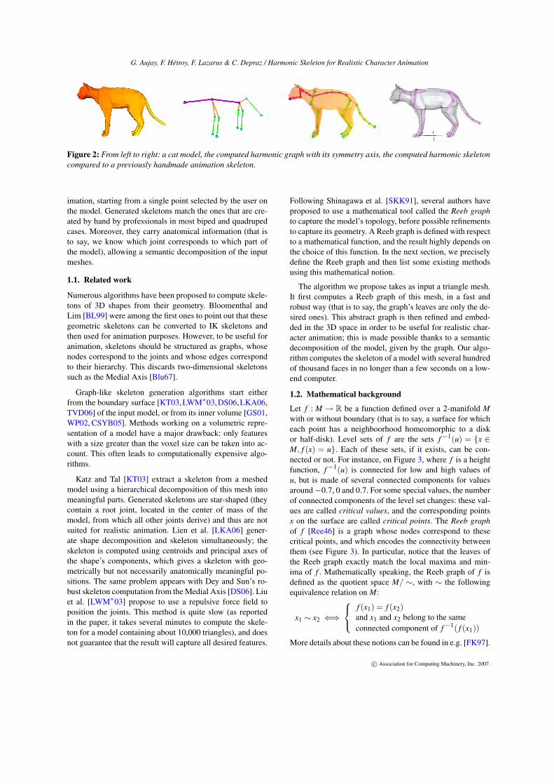
G. Aujay, F. Hétroy, F. Lazarus & C. Depraz / Harmonic Skeleton for Realistic Character Animation
Figure 2: From left to right: a cat model, the computed harmonic graph with its symmetry axis, the computed harmonic skeletoncompared to a previously handmade animation skeleton.
imation, starting from a single point selected by the user onthe model. Generated skeletons match the ones that are cre-ated by hand by professionals in most biped and quadrupedcases. Moreover, they carry anatomical information (that isto say, we know which joint corresponds to which part ofthe model), allowing a semantic decomposition of the inputmeshes.
1.1. Related work
Numerous algorithms have been proposed to compute skele-tons of 3D shapes from their geometry. Bloomenthal andLim [BL99] were among the first ones to point out that thesegeometric skeletons can be converted to IK skeletons andthen used for animation purposes. However, to be useful foranimation, skeletons should be structured as graphs, whosenodes correspond to the joints and whose edges correspondto their hierarchy. This discards two-dimensional skeletonssuch as the Medial Axis [Blu67].
Graph-like skeleton generation algorithms start eitherfrom the boundary surface [KT03,LWM∗03,DS06,LKA06,TVD06] of the input model, or from its inner volume [GS01,WP02, CSYB05]. Methods working on a volumetric repre-sentation of a model have a major drawback: only featureswith a size greater than the voxel size can be taken into ac-count. This often leads to computationally expensive algo-rithms.
Katz and Tal [KT03] extract a skeleton from a meshedmodel using a hierarchical decomposition of this mesh intomeaningful parts. Generated skeletons are star-shaped (theycontain a root joint, located in the center of mass of themodel, from which all other joints derive) and thus are notsuited for realistic animation. Lien et al. [LKA06] gener-ate shape decomposition and skeleton simultaneously; theskeleton is computed using centroids and principal axes ofthe shape’s components, which gives a skeleton with geo-metrically but not necessarily anatomically meaningful po-sitions. The same problem appears with Dey and Sun’s ro-bust skeleton computation from theMedial Axis [DS06]. Liuet al. [LWM∗03] propose to use a repulsive force field toposition the joints. This method is quite slow (as reportedin the paper, it takes several minutes to compute the skele-ton for a model containing about 10,000 triangles), and doesnot guarantee that the result will capture all desired features.
Following Shinagawa et al. [SKK91], several authors haveproposed to use a mathematical tool called the Reeb graphto capture the model’s topology, before possible refinementsto capture its geometry. A Reeb graph is defined with respectto a mathematical function, and the result highly depends onthe choice of this function. In the next section, we preciselydefine the Reeb graph and then list some existing methodsusing this mathematical notion.
The algorithm we propose takes as input a triangle mesh.It first computes a Reeb graph of this mesh, in a fast androbust way (that is to say, the graph’s leaves are only the de-sired ones). This abstract graph is then refined and embed-ded in the 3D space in order to be useful for realistic char-acter animation; this is made possible thanks to a semanticdecomposition of the model, given by the graph. Our algo-rithm computes the skeleton of a model with several hundredof thousand faces in no longer than a few seconds on a low-end computer.
1.2. Mathematical background
Let f : M → R be a function defined over a 2-manifold Mwith or without boundary (that is to say, a surface for whicheach point has a neighboorhood homeomorphic to a diskor half-disk). Level sets of f are the sets f−1(u) = x ∈M, f (x) = u. Each of these sets, if it exists, can be con-nected or not. For instance, on Figure 3, where f is a heightfunction, f−1(u) is connected for low and high values ofu, but is made of several connected components for valuesaround−0.7, 0 and 0.7. For some special values, the numberof connected components of the level set changes: these val-ues are called critical values, and the corresponding pointsx on the surface are called critical points. The Reeb graphof f [Ree46] is a graph whose nodes correspond to thesecritical points, and which encodes the connectivity betweenthem (see Figure 3). In particular, notice that the leaves ofthe Reeb graph exactly match the local maxima and min-ima of f . Mathematically speaking, the Reeb graph of f isdefined as the quotient space M/ ∼, with ∼ the followingequivalence relation onM:
x1 ∼ x2 ⇐⇒
f (x1) = f (x2)and x1 and x2 belong to the sameconnected component of f−1( f (x1))
More details about these notions can be found in e.g. [FK97].
c Association for Computing Machinery, Inc. 2007.
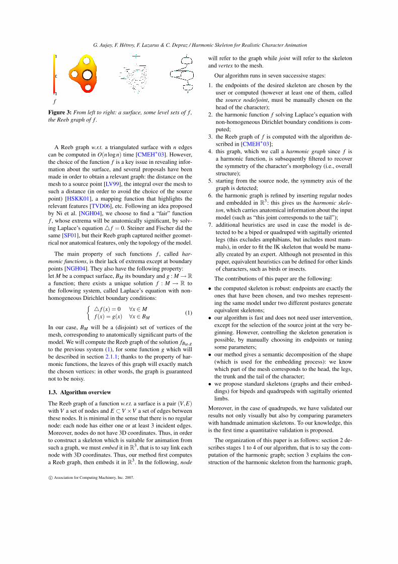
G. Aujay, F. Hétroy, F. Lazarus & C. Depraz / Harmonic Skeleton for Realistic Character Animation
f
Figure 3: From left to right: a surface, some level sets of f ,the Reeb graph of f .
A Reeb graph w.r.t. a triangulated surface with n edgescan be computed in O(n logn) time [CMEH∗03]. However,the choice of the function f is a key issue in revealing infor-mation about the surface, and several proposals have beenmade in order to obtain a relevant graph: the distance on themesh to a source point [LV99], the integral over the mesh tosuch a distance (in order to avoid the choice of the sourcepoint) [HSKK01], a mapping function that highlights therelevant features [TVD06], etc. Following an idea proposedby Ni et al. [NGH04], we choose to find a “fair” functionf , whose extrema will be anatomically significant, by solv-ing Laplace’s equation f = 0. Steiner and Fischer did thesame [SF01], but their Reeb graph captured neither geomet-rical nor anatomical features, only the topology of the model.
The main property of such functions f , called har-monic functions, is their lack of extrema except at boundarypoints [NGH04]. They also have the following property:letM be a compact surface, BM its boundary and g :M→ Ra function; there exists a unique solution f : M → R tothe following system, called Laplace’s equation with non-homogeneous Dirichlet boundary conditions:
f (x) = 0 ∀x ∈Mf (x) = g(x) ∀x ∈ BM
(1)
In our case, BM will be a (disjoint) set of vertices of themesh, corresponding to anatomically significant parts of themodel. We will compute the Reeb graph of the solution fBM ,gto the previous system (1), for some function g which willbe described in section 2.1.1; thanks to the property of har-monic functions, the leaves of this graph will exactly matchthe chosen vertices: in other words, the graph is guaranteednot to be noisy.
1.3. Algorithm overview
The Reeb graph of a function w.r.t. a surface is a pair (V,E)with V a set of nodes and E ⊂V ×V a set of edges betweenthese nodes. It is minimal in the sense that there is no regularnode: each node has either one or at least 3 incident edges.Moreover, nodes do not have 3D coordinates. Thus, in orderto construct a skeleton which is suitable for animation fromsuch a graph, we must embed it inR3, that is to say link eachnode with 3D coordinates. Thus, our method first computesa Reeb graph, then embeds it in R3. In the following, node
will refer to the graph while joint will refer to the skeletonand vertex to the mesh.
Our algorithm runs in seven successive stages:
1. the endpoints of the desired skeleton are chosen by theuser or computed (however at least one of them, calledthe source node/joint, must be manually chosen on thehead of the character);
2. the harmonic function f solving Laplace’s equation withnon-homogeneous Dirichlet boundary conditions is com-puted;
3. the Reeb graph of f is computed with the algorithm de-scribed in [CMEH∗03];
4. this graph, which we call a harmonic graph since f isa harmonic function, is subsequently filtered to recoverthe symmetry of the character’s morphology (i.e., overallstructure);
5. starting from the source node, the symmetry axis of thegraph is detected;
6. the harmonic graph is refined by inserting regular nodesand embedded in R3: this gives us the harmonic skele-ton, which carries anatomical information about the inputmodel (such as “this joint corresponds to the tail”);
7. additional heuristics are used in case the model is de-tected to be a biped or quadruped with sagittally orientedlegs (this excludes amphibians, but includes most mam-mals), in order to fit the IK skeleton that would be manu-ally created by an expert. Although not presented in thispaper, equivalent heuristics can be defined for other kindsof characters, such as birds or insects.
The contributions of this paper are the following:
• the computed skeleton is robust: endpoints are exactly theones that have been chosen, and two meshes represent-ing the same model under two different postures generateequivalent skeletons;
• our algorithm is fast and does not need user intervention,except for the selection of the source joint at the very be-ginning. However, controlling the skeleton generation ispossible, by manually choosing its endpoints or tuningsome parameters;
• our method gives a semantic decomposition of the shape(which is used for the embedding process): we knowwhich part of the mesh corresponds to the head, the legs,the trunk and the tail of the character;
• we propose standard skeletons (graphs and their embed-dings) for bipeds and quadrupeds with sagittally orientedlimbs.
Moreover, in the case of quadrupeds, we have validated ourresults not only visually but also by comparing parameterswith handmade animation skeletons. To our knowledge, thisis the first time a quantitative validation is proposed.
The organization of this paper is as follows: section 2 de-scribes stages 1 to 4 of our algorithm, that is to say the com-putation of the harmonic graph; section 3 explains the con-struction of the harmonic skeleton from the harmonic graph,
c Association for Computing Machinery, Inc. 2007.
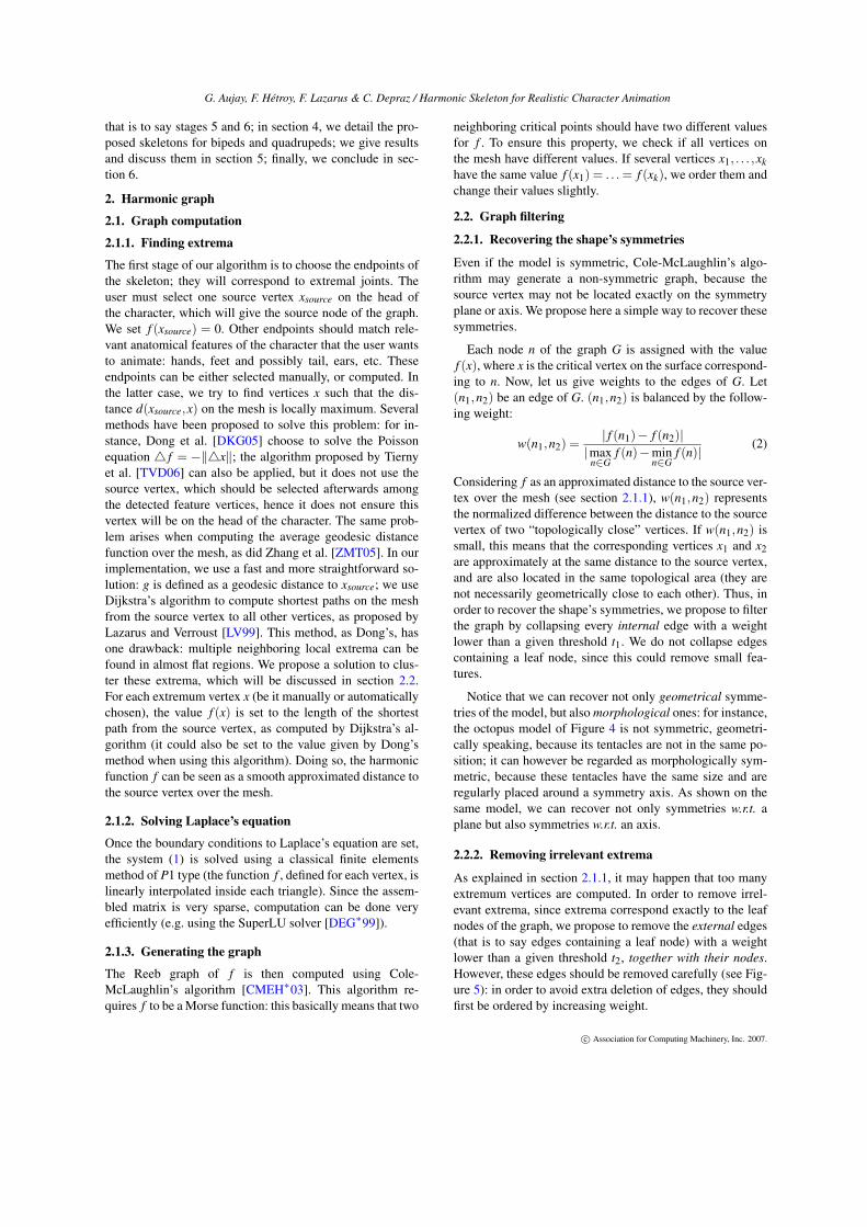
G. Aujay, F. Hétroy, F. Lazarus & C. Depraz / Harmonic Skeleton for Realistic Character Animation
that is to say stages 5 and 6; in section 4, we detail the pro-posed skeletons for bipeds and quadrupeds; we give resultsand discuss them in section 5; finally, we conclude in sec-tion 6.
2. Harmonic graph
2.1. Graph computation
2.1.1. Finding extrema
The first stage of our algorithm is to choose the endpoints ofthe skeleton; they will correspond to extremal joints. Theuser must select one source vertex xsource on the head ofthe character, which will give the source node of the graph.We set f (xsource) = 0. Other endpoints should match rele-vant anatomical features of the character that the user wantsto animate: hands, feet and possibly tail, ears, etc. Theseendpoints can be either selected manually, or computed. Inthe latter case, we try to find vertices x such that the dis-tance d(xsource,x) on the mesh is locally maximum. Severalmethods have been proposed to solve this problem: for in-stance, Dong et al. [DKG05] choose to solve the Poissonequation f = −x; the algorithm proposed by Tiernyet al. [TVD06] can also be applied, but it does not use thesource vertex, which should be selected afterwards amongthe detected feature vertices, hence it does not ensure thisvertex will be on the head of the character. The same prob-lem arises when computing the average geodesic distancefunction over the mesh, as did Zhang et al. [ZMT05]. In ourimplementation, we use a fast and more straightforward so-lution: g is defined as a geodesic distance to xsource; we useDijkstra’s algorithm to compute shortest paths on the meshfrom the source vertex to all other vertices, as proposed byLazarus and Verroust [LV99]. This method, as Dong’s, hasone drawback: multiple neighboring local extrema can befound in almost flat regions. We propose a solution to clus-ter these extrema, which will be discussed in section 2.2.For each extremum vertex x (be it manually or automaticallychosen), the value f (x) is set to the length of the shortestpath from the source vertex, as computed by Dijkstra’s al-gorithm (it could also be set to the value given by Dong’smethod when using this algorithm). Doing so, the harmonicfunction f can be seen as a smooth approximated distance tothe source vertex over the mesh.
2.1.2. Solving Laplace’s equation
Once the boundary conditions to Laplace’s equation are set,the system (1) is solved using a classical finite elementsmethod of P1 type (the function f , defined for each vertex, islinearly interpolated inside each triangle). Since the assem-bled matrix is very sparse, computation can be done veryefficiently (e.g. using the SuperLU solver [DEG∗99]).
2.1.3. Generating the graph
The Reeb graph of f is then computed using Cole-McLaughlin’s algorithm [CMEH∗03]. This algorithm re-quires f to be aMorse function: this basically means that two
neighboring critical points should have two different valuesfor f . To ensure this property, we check if all vertices onthe mesh have different values. If several vertices x1, . . . ,xkhave the same value f (x1) = . . . = f (xk), we order them andchange their values slightly.
2.2. Graph filtering
2.2.1. Recovering the shape’s symmetries
Even if the model is symmetric, Cole-McLaughlin’s algo-rithm may generate a non-symmetric graph, because thesource vertex may not be located exactly on the symmetryplane or axis. We propose here a simple way to recover thesesymmetries.
Each node n of the graph G is assigned with the valuef (x), where x is the critical vertex on the surface correspond-ing to n. Now, let us give weights to the edges of G. Let(n1,n2) be an edge of G. (n1,n2) is balanced by the follow-ing weight:
w(n1,n2) =| f (n1)− f (n2)|
|maxn∈G
f (n)−minn∈G
f (n)| (2)
Considering f as an approximated distance to the source ver-tex over the mesh (see section 2.1.1), w(n1,n2) representsthe normalized difference between the distance to the sourcevertex of two “topologically close” vertices. If w(n1,n2) issmall, this means that the corresponding vertices x1 and x2are approximately at the same distance to the source vertex,and are also located in the same topological area (they arenot necessarily geometrically close to each other). Thus, inorder to recover the shape’s symmetries, we propose to filterthe graph by collapsing every internal edge with a weightlower than a given threshold t1. We do not collapse edgescontaining a leaf node, since this could remove small fea-tures.
Notice that we can recover not only geometrical symme-tries of the model, but alsomorphological ones: for instance,the octopus model of Figure 4 is not symmetric, geometri-cally speaking, because its tentacles are not in the same po-sition; it can however be regarded as morphologically sym-metric, because these tentacles have the same size and areregularly placed around a symmetry axis. As shown on thesame model, we can recover not only symmetries w.r.t. aplane but also symmetries w.r.t. an axis.
2.2.2. Removing irrelevant extrema
As explained in section 2.1.1, it may happen that too manyextremum vertices are computed. In order to remove irrel-evant extrema, since extrema correspond exactly to the leafnodes of the graph, we propose to remove the external edges(that is to say edges containing a leaf node) with a weightlower than a given threshold t2, together with their nodes.However, these edges should be removed carefully (see Fig-ure 5): in order to avoid extra deletion of edges, they shouldfirst be ordered by increasing weight.
c Association for Computing Machinery, Inc. 2007.
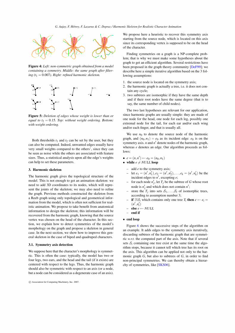
G. Aujay, F. Hétroy, F. Lazarus & C. Depraz / Harmonic Skeleton for Realistic Character Animation
Figure 4: Left: non-symmetric graph obtained from a modelcontaining a symmetry. Middle: the same graph after filter-ing (t1 = 0.007). Right: refined harmonic skeleton.
Figure 5: Deletion of edges whose weight is lower than orequal to t2 = 0.15. Top: without weight ordering. Bottom:with weight ordering.
Both thresholds t1 and t2 can be set by the user, but theycan also be computed. Indeed, unwanted edges usually havevery small weights compared to the others’, since they canbe seen as noise while the others are associated with featuresizes. Thus, a statistical analysis upon all the edge’s weightscan help to set these parameters.
3. Harmonic skeleton
The harmonic graph gives the topological structure of themodel. This is not enough to get an animation skeleton: weneed to add 3D coordinates to its nodes, which will repre-sent the joints of the skeleton; we may also need to refinethe graph. Previous methods constructed the skeleton froma Reeb graph using only topological and geometrical infor-mation from the model, which is often not sufficient for real-istic animation. We propose to take benefit from anatomicalinformation to design the skeleton; this information will berecovered from the harmonic graph, knowing that the sourcevertex was chosen on the head of the character. In this sec-tion, we explain how to detect symmetries of the model’smorphology on the graph and propose a skeleton in generalcase. In the next section, we show how to improve this gen-eral skeleton in the case of biped and quadruped characters.
3.1. Symmetry axis detection
We suppose here that the character’s morphology is symmet-ric. This is often the case: typically, the model has two orfour legs, two ears, and the head and the tail (if it exists) arecentered with respect to the legs. Thus, the harmonic graphshould also be symmetric with respect to an axis (or a node,but a node can be considered as a degenerate case of an axis).
We propose here a heuristic to recover this symmetry axisstarting from the source node, which is located on this axissince its corresponding vertex is supposed to be on the headof the character.
Finding symmetries on a graph is a NP-complete prob-lem; that is why we must make some hypotheses about thegraph to get an efficient algorithm. Several restrictions havebeen proposed in the graph theory community [DeF99]; wedescribe here a simple iterative algorithm based on the 3 fol-lowing assumptions:
1. the source node is located on the symmetry axis;2. the harmonic graph is actually a tree, i.e. it does not con-tain any cycle;
3. two subtrees are isomorphic if they have the same depthand if their root nodes have the same degree (that is tosay, the same number of child nodes).
The two last hypotheses are relevant for our application,since harmonic graphs are usually simple: they are made ofone node for the head, one node for each leg, possibly oneextremal node for the tail, for each ear and/or each wingand/or each finger, and that is usually all.
We use n0 to denote the source node of the harmonicgraph, and (n0,n1) = e0 as its incident edge: e0 is on thesymmetry axis. n and n denote nodes of the harmonic graph,whereas e denotes an edge. Our algorithm proceeds as fol-lows:
• e = (n,n)← e0 = (n0,n1)• while e = NULL loop
– add e to the symmetry axis;– let e1 = (n,n1),e2 = (n,n2), . . . ,ek = (n,nk) be theincident edges to n, excepting e;
– for each node nj, let Tj be the subtree of G whose rootnode is nj and which does not contain n
;– store the Tj into sets S1, . . . ,Sl of isomorphic trees,according to assumption number 3;
– if ∃!Si which contains only one tree Ti then e← ei =(n,ni)
– else e← NULL– end if
• end loop
Figure 6 shows the successive steps of the algorithm onan example. It adds edges to the symmetry axis iteratively,discarding subtrees of the harmonic graph that are symmet-ric w.r.t. the computed part of the axis. Note that if severalsets Si containing one tree exist at the same time the algo-rithm stops, because it cannot tell which tree has its root onthe axis. This algorithm can be applied not only to the har-monic graph G, but also to subtrees of G, in order to findnon-principal symmetries. We can thereby obtain a hierar-chy of symmetries, like [SKS06].
c Association for Computing Machinery, Inc. 2007.
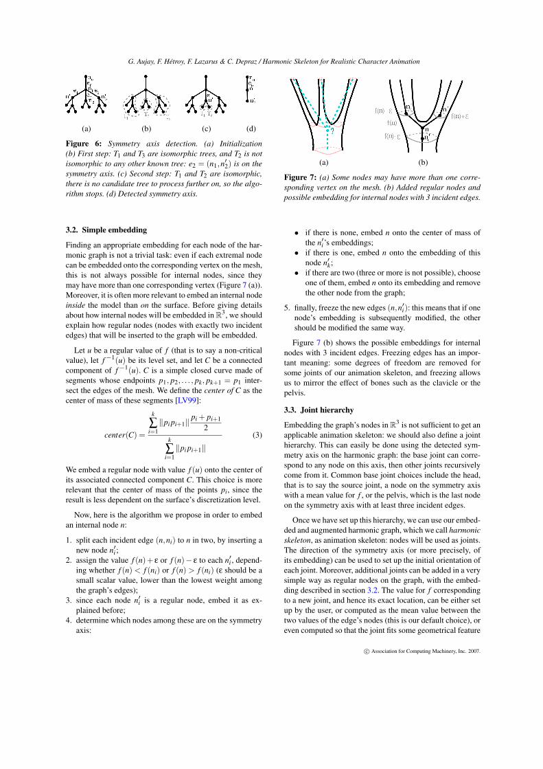
G. Aujay, F. Hétroy, F. Lazarus & C. Depraz / Harmonic Skeleton for Realistic Character Animation
(a) (b) (c) (d)
Figure 6: Symmetry axis detection. (a) Initialization(b) First step: T1 and T3 are isomorphic trees, and T2 is notisomorphic to any other known tree: e2 = (n1,n2) is on thesymmetry axis. (c) Second step: T1 and T2 are isomorphic,there is no candidate tree to process further on, so the algo-rithm stops. (d) Detected symmetry axis.
3.2. Simple embedding
Finding an appropriate embedding for each node of the har-monic graph is not a trivial task: even if each extremal nodecan be embedded onto the corresponding vertex on the mesh,this is not always possible for internal nodes, since theymay have more than one corresponding vertex (Figure 7 (a)).Moreover, it is often more relevant to embed an internal nodeinside the model than on the surface. Before giving detailsabout how internal nodes will be embedded inR3, we shouldexplain how regular nodes (nodes with exactly two incidentedges) that will be inserted to the graph will be embedded.
Let u be a regular value of f (that is to say a non-criticalvalue), let f−1(u) be its level set, and let C be a connectedcomponent of f−1(u). C is a simple closed curve made ofsegments whose endpoints p1, p2, . . . , pk, pk+1 = p1 inter-sect the edges of the mesh. We define the center of C as thecenter of mass of these segments [LV99]:
center(C) =
k
∑i=1pi pi+1
pi + pi+12
k
∑i=1pi pi+1
(3)
We embed a regular node with value f (u) onto the center ofits associated connected component C. This choice is morerelevant that the center of mass of the points pi, since theresult is less dependent on the surface’s discretization level.
Now, here is the algorithm we propose in order to embedan internal node n:
1. split each incident edge (n,ni) to n in two, by inserting anew node ni ;
2. assign the value f (n)+ ε or f (n)− ε to each ni , depend-ing whether f (n) < f (ni) or f (n) > f (ni) (ε should be asmall scalar value, lower than the lowest weight amongthe graph’s edges);
3. since each node ni is a regular node, embed it as ex-plained before;
4. determine which nodes among these are on the symmetryaxis:
(a) (b)
Figure 7: (a) Some nodes may have more than one corre-sponding vertex on the mesh. (b) Added regular nodes andpossible embedding for internal nodes with 3 incident edges.
• if there is none, embed n onto the center of mass ofthe ni’s embeddings;
• if there is one, embed n onto the embedding of thisnode nk;
• if there are two (three or more is not possible), chooseone of them, embed n onto its embedding and removethe other node from the graph;
5. finally, freeze the new edges (n,ni): this means that if onenode’s embedding is subsequently modified, the othershould be modified the same way.
Figure 7 (b) shows the possible embeddings for internalnodes with 3 incident edges. Freezing edges has an impor-tant meaning: some degrees of freedom are removed forsome joints of our animation skeleton, and freezing allowsus to mirror the effect of bones such as the clavicle or thepelvis.
3.3. Joint hierarchy
Embedding the graph’s nodes inR3 is not sufficient to get anapplicable animation skeleton: we should also define a jointhierarchy. This can easily be done using the detected sym-metry axis on the harmonic graph: the base joint can corre-spond to any node on this axis, then other joints recursivelycome from it. Common base joint choices include the head,that is to say the source joint, a node on the symmetry axiswith a mean value for f , or the pelvis, which is the last nodeon the symmetry axis with at least three incident edges.
Once we have set up this hierarchy, we can use our embed-ded and augmented harmonic graph, which we call harmonicskeleton, as animation skeleton: nodes will be used as joints.The direction of the symmetry axis (or more precisely, ofits embedding) can be used to set up the initial orientation ofeach joint. Moreover, additional joints can be added in a verysimple way as regular nodes on the graph, with the embed-ding described in section 3.2. The value for f correspondingto a new joint, and hence its exact location, can be either setup by the user, or computed as the mean value between thetwo values of the edge’s nodes (this is our default choice), oreven computed so that the joint fits some geometrical feature
c Association for Computing Machinery, Inc. 2007.
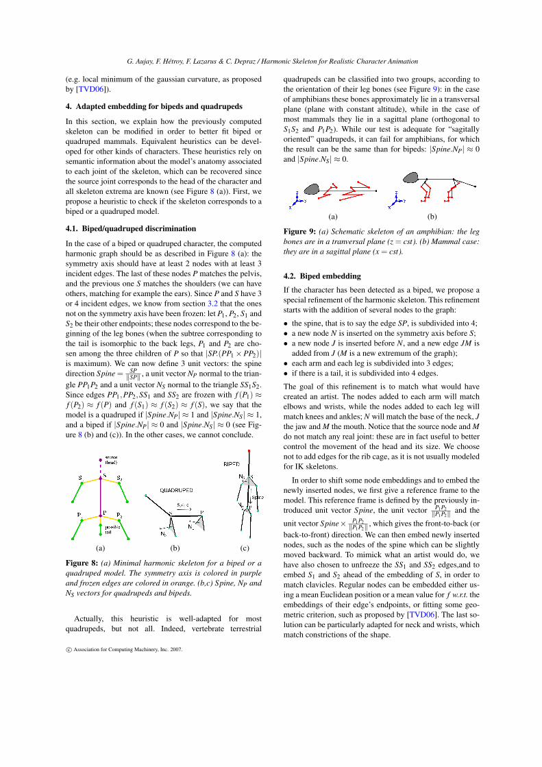
G. Aujay, F. Hétroy, F. Lazarus & C. Depraz / Harmonic Skeleton for Realistic Character Animation
(e.g. local minimum of the gaussian curvature, as proposedby [TVD06]).
4. Adapted embedding for bipeds and quadrupeds
In this section, we explain how the previously computedskeleton can be modified in order to better fit biped orquadruped mammals. Equivalent heuristics can be devel-oped for other kinds of characters. These heuristics rely onsemantic information about the model’s anatomy associatedto each joint of the skeleton, which can be recovered sincethe source joint corresponds to the head of the character andall skeleton extrema are known (see Figure 8 (a)). First, wepropose a heuristic to check if the skeleton corresponds to abiped or a quadruped model.
4.1. Biped/quadruped discrimination
In the case of a biped or quadruped character, the computedharmonic graph should be as described in Figure 8 (a): thesymmetry axis should have at least 2 nodes with at least 3incident edges. The last of these nodes P matches the pelvis,and the previous one S matches the shoulders (we can haveothers, matching for example the ears). Since P and S have 3or 4 incident edges, we know from section 3.2 that the onesnot on the symmetry axis have been frozen: let P1, P2, S1 andS2 be their other endpoints; these nodes correspond to the be-ginning of the leg bones (when the subtree corresponding tothe tail is isomorphic to the back legs, P1 and P2 are cho-sen among the three children of P so that |SP.(PP1×PP2)|is maximum). We can now define 3 unit vectors: the spinedirection Spine= SP
SP , a unit vector NP normal to the trian-gle PP1P2 and a unit vector NS normal to the triangle SS1S2.Since edges PP1,PP2,SS1 and SS2 are frozen with f (P1) ≈f (P2) ≈ f (P) and f (S1) ≈ f (S2) ≈ f (S), we say that themodel is a quadruped if |Spine.NP| ≈ 1 and |Spine.NS| ≈ 1,and a biped if |Spine.NP| ≈ 0 and |Spine.NS| ≈ 0 (see Fig-ure 8 (b) and (c)). In the other cases, we cannot conclude.
(a) (b) (c)
Figure 8: (a) Minimal harmonic skeleton for a biped or aquadruped model. The symmetry axis is colored in purpleand frozen edges are colored in orange. (b,c) Spine, NP andNS vectors for quadrupeds and bipeds.
Actually, this heuristic is well-adapted for mostquadrupeds, but not all. Indeed, vertebrate terrestrial
quadrupeds can be classified into two groups, according tothe orientation of their leg bones (see Figure 9): in the caseof amphibians these bones approximately lie in a transversalplane (plane with constant altitude), while in the case ofmost mammals they lie in a sagittal plane (orthogonal toS1S2 and P1P2). While our test is adequate for “sagitallyoriented” quadrupeds, it can fail for amphibians, for whichthe result can be the same than for bipeds: |Spine.NP| ≈ 0and |Spine.NS| ≈ 0.
(a) (b)
Figure 9: (a) Schematic skeleton of an amphibian: the legbones are in a tranversal plane (z = cst). (b) Mammal case:they are in a sagittal plane (x = cst).
4.2. Biped embedding
If the character has been detected as a biped, we propose aspecial refinement of the harmonic skeleton. This refinementstarts with the addition of several nodes to the graph:
• the spine, that is to say the edge SP, is subdivided into 4;• a new node N is inserted on the symmetry axis before S;• a new node J is inserted before N, and a new edge JM isadded from J (M is a new extremum of the graph);
• each arm and each leg is subdivided into 3 edges;• if there is a tail, it is subdivided into 4 edges.The goal of this refinement is to match what would havecreated an artist. The nodes added to each arm will matchelbows and wrists, while the nodes added to each leg willmatch knees and ankles; N will match the base of the neck, Jthe jaw andM the mouth. Notice that the source node andMdo not match any real joint: these are in fact useful to bettercontrol the movement of the head and its size. We choosenot to add edges for the rib cage, as it is not usually modeledfor IK skeletons.
In order to shift some node embeddings and to embed thenewly inserted nodes, we first give a reference frame to themodel. This reference frame is defined by the previously in-troduced unit vector Spine, the unit vector P1P2
P1P2 and the
unit vector Spine× P1P2P1P2 , which gives the front-to-back (or
back-to-front) direction. We can then embed newly insertednodes, such as the nodes of the spine which can be slightlymoved backward. To mimick what an artist would do, wehave also chosen to unfreeze the SS1 and SS2 edges,and toembed S1 and S2 ahead of the embedding of S, in order tomatch clavicles. Regular nodes can be embedded either us-ing a mean Euclidean position or a mean value for f w.r.t. theembeddings of their edge’s endpoints, or fitting some geo-metric criterion, such as proposed by [TVD06]. The last so-lution can be particularly adapted for neck and wrists, whichmatch constrictions of the shape.
c Association for Computing Machinery, Inc. 2007.
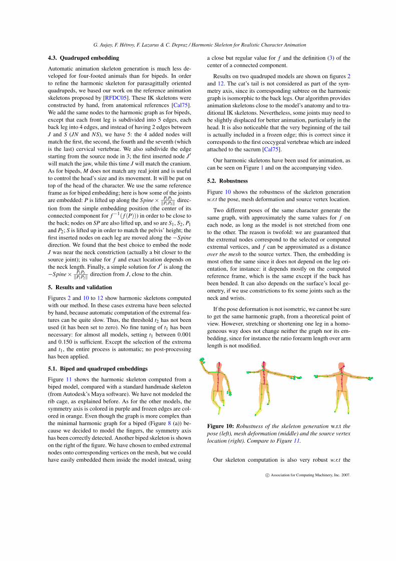
G. Aujay, F. Hétroy, F. Lazarus & C. Depraz / Harmonic Skeleton for Realistic Character Animation
4.3. Quadruped embedding
Automatic animation skeleton generation is much less de-veloped for four-footed animals than for bipeds. In orderto refine the harmonic skeleton for parasagittally orientedquadrupeds, we based our work on the reference animationskeletons proposed by [RFDC05]. These IK skeletons wereconstructed by hand, from anatomical references [Cal75].We add the same nodes to the harmonic graph as for bipeds,except that each front leg is subdivided into 5 edges, eachback leg into 4 edges, and instead of having 2 edges betweenJ and S (JN and NS), we have 5: the 4 added nodes willmatch the first, the second, the fourth and the seventh (whichis the last) cervical vertebrae. We also subdivide the edgestarting from the source node in 3; the first inserted node J
will match the jaw, while this time J will match the cranium.As for bipeds, M does not match any real joint and is usefulto control the head’s size and its movement. It will be put ontop of the head of the character. We use the same referenceframe as for biped embedding; here is how some of the jointsare embedded: P is lifted up along the Spine× P1P2
P1P2 direc-tion from the simple embedding position (the center of itsconnected component for f−1( f (P))) in order to be close tothe back; nodes on SP are also lifted up, and so are S1, S2, P1and P2; S is lifted up in order to match the pelvis’ height; thefirst inserted nodes on each leg are moved along the −Spinedirection. We found that the best choice to embed the nodeJ was near the neck constriction (actually a bit closer to thesource joint); its value for f and exact location depends onthe neck length. Finally, a simple solution for J is along the−Spine× P1P2
P1P2 direction from J, close to the chin.
5. Results and validation
Figures 2 and 10 to 12 show harmonic skeletons computedwith our method. In these cases extrema have been selectedby hand, because automatic computation of the extremal fea-tures can be quite slow. Thus, the threshold t2 has not beenused (it has been set to zero). No fine tuning of t1 has beennecessary: for almost all models, setting t1 between 0.001and 0.150 is sufficient. Except the selection of the extremaand t1, the entire process is automatic; no post-processinghas been applied.
5.1. Biped and quadruped embeddings
Figure 11 shows the harmonic skeleton computed from abiped model, compared with a standard handmade skeleton(from Autodesk’s Maya software). We have not modeled therib cage, as explained before. As for the other models, thesymmetry axis is colored in purple and frozen edges are col-ored in orange. Even though the graph is more complex thanthe minimal harmonic graph for a biped (Figure 8 (a)) be-cause we decided to model the fingers, the symmetry axishas been correctly detected. Another biped skeleton is shownon the right of the figure. We have chosen to embed extremalnodes onto corresponding vertices on the mesh, but we couldhave easily embedded them inside the model instead, using
a close but regular value for f and the definition (3) of thecenter of a connected component.
Results on two quadruped models are shown on figures 2and 12. The cat’s tail is not considered as part of the sym-metry axis, since its corresponding subtree on the harmonicgraph is isomorphic to the back legs. Our algorithm providesanimation skeletons close to the model’s anatomy and to tra-ditional IK skeletons. Nevertheless, some joints may need tobe slightly displaced for better animation, particularly in thehead. It is also noticeable that the very beginning of the tailis actually included in a frozen edge; this is correct since itcorresponds to the first coccygeal vertebrae which are indeedattached to the sacrum [Cal75].
Our harmonic skeletons have been used for animation, ascan be seen on Figure 1 and on the accompanying video.
5.2. Robustness
Figure 10 shows the robustness of the skeleton generationw.r.t the pose, mesh deformation and source vertex location.
Two different poses of the same character generate thesame graph, with approximately the same values for f oneach node, as long as the model is not stretched from oneto the other. The reason is twofold: we are guaranteed thatthe extremal nodes correspond to the selected or computedextremal vertices, and f can be approximated as a distanceover the mesh to the source vertex. Then, the embedding ismost often the same since it does not depend on the leg ori-entation, for instance: it depends mostly on the computedreference frame, which is the same except if the back hasbeen bended. It can also depends on the surface’s local ge-ometry, if we use constrictions to fix some joints such as theneck and wrists.
If the pose deformation is not isometric, we cannot be sureto get the same harmonic graph, from a theoretical point ofview. However, stretching or shortening one leg in a homo-geneous way does not change neither the graph nor its em-bedding, since for instance the ratio forearm length over armlength is not modified.
Figure 10: Robustness of the skeleton generation w.r.t thepose (left), mesh deformation (middle) and the source vertexlocation (right). Compare to Figure 11.
Our skeleton computation is also very robust w.r.t the
c Association for Computing Machinery, Inc. 2007.
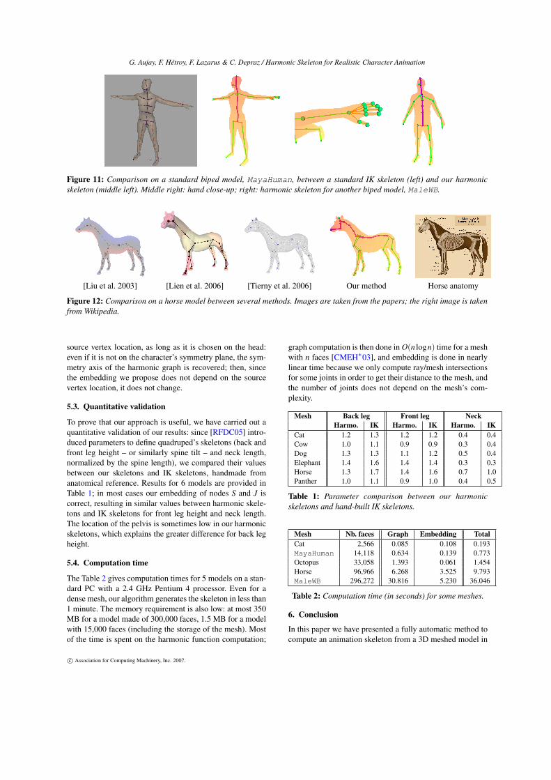
G. Aujay, F. Hétroy, F. Lazarus & C. Depraz / Harmonic Skeleton for Realistic Character Animation
Figure 11: Comparison on a standard biped model, MayaHuman, between a standard IK skeleton (left) and our harmonicskeleton (middle left). Middle right: hand close-up; right: harmonic skeleton for another biped model, MaleWB.
[Liu et al. 2003] [Lien et al. 2006] [Tierny et al. 2006] Our method Horse anatomy
Figure 12: Comparison on a horse model between several methods. Images are taken from the papers; the right image is takenfrom Wikipedia.
source vertex location, as long as it is chosen on the head:even if it is not on the character’s symmetry plane, the sym-metry axis of the harmonic graph is recovered; then, sincethe embedding we propose does not depend on the sourcevertex location, it does not change.
5.3. Quantitative validation
To prove that our approach is useful, we have carried out aquantitative validation of our results: since [RFDC05] intro-duced parameters to define quadruped’s skeletons (back andfront leg height – or similarly spine tilt – and neck length,normalized by the spine length), we compared their valuesbetween our skeletons and IK skeletons, handmade fromanatomical reference. Results for 6 models are provided inTable 1; in most cases our embedding of nodes S and J iscorrect, resulting in similar values between harmonic skele-tons and IK skeletons for front leg height and neck length.The location of the pelvis is sometimes low in our harmonicskeletons, which explains the greater difference for back legheight.
5.4. Computation time
The Table 2 gives computation times for 5 models on a stan-dard PC with a 2.4 GHz Pentium 4 processor. Even for adense mesh, our algorithm generates the skeleton in less than1 minute. The memory requirement is also low: at most 350MB for a model made of 300,000 faces, 1.5 MB for a modelwith 15,000 faces (including the storage of the mesh). Mostof the time is spent on the harmonic function computation;
graph computation is then done inO(n logn) time for a meshwith n faces [CMEH∗03], and embedding is done in nearlylinear time because we only compute ray/mesh intersectionsfor some joints in order to get their distance to the mesh, andthe number of joints does not depend on the mesh’s com-plexity.
Mesh Back leg Front leg NeckHarmo. IK Harmo. IK Harmo. IK
Cat 1.2 1.3 1.2 1.2 0.4 0.4Cow 1.0 1.1 0.9 0.9 0.3 0.4Dog 1.3 1.3 1.1 1.2 0.5 0.4Elephant 1.4 1.6 1.4 1.4 0.3 0.3Horse 1.3 1.7 1.4 1.6 0.7 1.0Panther 1.0 1.1 0.9 1.0 0.4 0.5
Table 1: Parameter comparison between our harmonicskeletons and hand-built IK skeletons.
Mesh Nb. faces Graph Embedding TotalCat 2,566 0.085 0.108 0.193MayaHuman 14,118 0.634 0.139 0.773Octopus 33,058 1.393 0.061 1.454Horse 96,966 6.268 3.525 9.793MaleWB 296,272 30.816 5.230 36.046
Table 2: Computation time (in seconds) for some meshes.
6. Conclusion
In this paper we have presented a fully automatic method tocompute an animation skeleton from a 3D meshed model in
c Association for Computing Machinery, Inc. 2007.
G. Aujay, F. Hétroy, F. Lazarus & C. Depraz / Harmonic Skeleton for Realistic Character Animation
a few seconds after the selection of an initial point. In thecase of most bipeds or quadrupeds, this skeleton fits the ani-mation skeleton that would be hand-built by an expert start-ing from anatomical boards, and is thus adapted for realisticanimation. The main idea is to construct the Reeb graph ofa harmonic function, which gives the overall morphologicalstructure of the model (especially its symmetry axis), then torefine and embed it using anatomical information. There aretwo main restrictions on the input mesh: it should be a trian-gulated 2-manifold (with or without boundary), and, in orderto recover the symmetry axis of the shape’s morphology, itshould not have handles (otherwise the Reeb graph containscycles). Although the method is fully automatic, the user cancontrol the skeleton generation by tuning a few optional pa-rameters. This tool has been designed both to help artists andto allow non-experts to quickly generate skeletons which canbe used for realistic character animation. Computed skele-tons can be edited and refined, for instance to add joints thatcorrespond to wings or to the trunk of an elephant.
Given this skeleton generation process, we see threepromising research directions. First, each vertex of the meshis related to the joints of the skeleton, since we have givenvalues for the harmonic function to the graph’s nodes, andhence the skeleton’s joints; these relations may be used toenhance skinning weights. Second, our semantic decompo-sition of the graph may also be used to define heuristics thatgive adapted skinning weights: weights may vary accordingto the meaning of neighboring joints. It may also help forautomatic mesh segmentation into anatomically meaningfulregions. Finally, even if not embedded to match the model’sanatomy, the harmonic graph may be useful for other appli-cations (e.g. shape matching), since its construction is robustand does not create unnecessary nodes.
Acknowledgments
The authors would like to thank Lionel Revéret for interest-ing discussions at the beginning of this work. The horse andMaleWB models are courtesy of Cyberware. The MayaHu-man model is courtesy of Autodesk.
References
[BL99] BLOOMENTHAL J., LIM C.: Skeletal methods of shapemanipulation. In Shape Modeling International (1999).
[Blu67] BLUM H.: A transformation for extracting new descrip-tors of shape. In Symposium on Models for the Perception ofSpeech and Visual Form (1967), pp. 362–380.
[Cal75] CALDERON W.: Animal Painting and Anatomy. Dover,1975.
[CMEH∗03] COLE-MCLAUGHLIN K., EDELSBRUNNER H.,HARER J., NATARAJAN V., PASCUCCI V.: Loops in reeb graphsof 2-manifolds. In Symposium on Computational Geometry(2003), pp. 344–350.
[CSYB05] CORNEA N., SILVER D., YUAN X., BALASUBRA-MANIAN R.: Computing hierarchical curve-skeletons of 3d ob-jects. The Visual Computer 21, 11 (2005), 945–955.
[DeF99] DEFRAYSSEIX H.: An heuristic for graph symmetry de-tection. In Symposium on Graph Drawing (1999), pp. 276–285.
[DEG∗99] DEMMEL J., EISENSTAT S., GILBERT J., LI X., LIUJ.: A supernodal approach to sparse partial pivoting. SIAM Jour-nal on Matrix Analysis and Applications 20, 3 (1999), 720–755.
[DKG05] DONG S., KIRCHNER S., GARLAND M.: Harmonicfunctions for quadrilateral remeshing of arbitrary manifolds.Computer Aided Geometric Design, Special issue on GeometryProcessing 22, 5 (2005), 392–423.
[DS06] DEY T., SUN J.: Defining and computing curve-skeletonswith medial geodesic function. In Symposium on Geometry Pro-cessing (2006), pp. 143–152.
[FK97] FOMENKO A., KUNII T.: Topological Modeling for Vi-sualization. Springer-Verlag, 1997.
[GS01] GAGVANI N., SILVER D.: Animating volumetric models.Graphical Models 63, 6 (2001), 443–458.
[HSKK01] HILAGA M., SHINAGAWA Y., KOMURA T., KUNIIT.: Topology matching for fully automatic similarity estimationof 3d shapes. In SIGGRAPH (2001), pp. 203–212.
[KT03] KATZ S., TAL A.: Hierarchical mesh decomposition us-ing fuzzy clustering and cuts. In SIGGRAPH (2003).
[LKA06] LIEN J., KEYSER J., , AMATO N.: Simultaneous shapedecomposition and skeletonization. In ACM Symposium on Solidand Physical Modeling (2006), pp. 219–228.
[LV99] LAZARUS F., VERROUST A.: Level set diagrams of poly-hedral objects. In ACM Symposium on Solid Modeling (1999).
[LWM∗03] LIU P., WU F., MA W., LIANG R., OUHYOUNG M.:Automatic animation skeleton construction using repulsive forcefield. In Pacific Graphics (2003), pp. 409–413.
[NGH04] NI X., GARLAND M., HART J.: Fair morse functionsfor extracting the topological structure of a surface mesh. In SIG-GRAPH (2004), pp. 613–622.
[Ree46] REEB G.: Sur les points singuliers d’une forme de pfaffcomplètement intégrable ou d’une fonction numérique. Comptes-Rendus de l’Académie des Sciences 222 (1946), 847–849.
[RFDC05] REVÉRET L., FAVREAU L., DEPRAZ C., CANI M.:Morphable model of quadruped skeletons for animating 3d ani-mals. In Symposium on Computer Animation (2005).
[SF01] STEINER D., FISCHER A.: Topology recognition of 3dclosed freeform objects based on topological graphs. In PacificGraphics (2001), pp. 82–88.
[SKK91] SHINAGAWA Y., KUNII T., KERGOSIEN Y.: Surfacecoding based on morse theory. IEEE Computer Graphics andApplications 11, 5 (1991), 66–78.
[SKS06] SIMARI P., KALOGERAKIS E., SINGH K.: Foldingmeshes: Hierarchical mesh segmentation based on planar sym-metry. In Symposium on Geometry Processing (2006).
[TVD06] TIERNY J., VANDEBORRE J., DAOUDI M.: 3d meshskeleton extraction using topological and geometrical analyses.In Pacific Graphics (2006), pp. 409–413.
[WP02] WADE L., PARENT R.: Automated generation of controlskeletons for use in animation. The Visual Computer 18 (2002).
[ZMT05] ZHANG E., MISCHAIKOW K., TURK G.: Feature-based surface parameterization and texture mapping. ACMTransactions on Graphics 24, 1 (2005), 1–27.
c Association for Computing Machinery, Inc. 2007.

A.6. SIMPLE FLEXIBLE SKINNING BASED ON MANIFOLD MODELING 171
∴
A.6 SIMPLE FLEXIBLE SKINNING BASED ONMANIFOLD MODELING
Franck Hétroy, Cédric Gérot, Lin Lu, Boris ThibertInternational Conference on Computer Graphics Theory and Applications (GRAPP),
2009.

172 APPENDIX A. SELECTED PAPERS
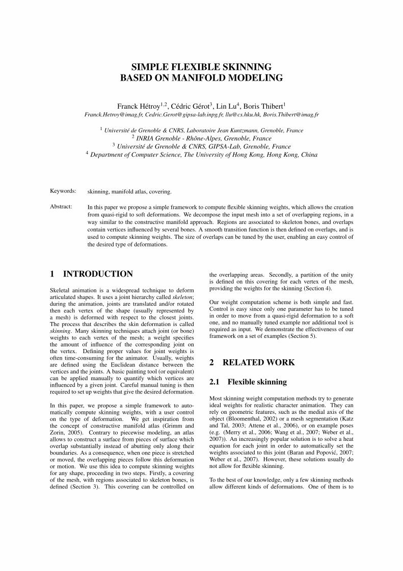
SIMPLE FLEXIBLE SKINNINGBASED ONMANIFOLD MODELING
Franck Hetroy1,2, Cedric Gerot3, Lin Lu4, Boris [email protected], [email protected], [email protected], [email protected]
1 Universite de Grenoble & CNRS, Laboratoire Jean Kuntzmann, Grenoble, France2 INRIA Grenoble - Rhone-Alpes, Grenoble, France
3 Universite de Grenoble & CNRS, GIPSA-Lab, Grenoble, France4 Department of Computer Science, The University of Hong Kong, Hong Kong, China
Keywords: skinning, manifold atlas, covering.
Abstract: In this paper we propose a simple framework to compute flexible skinning weights, which allows the creationfrom quasi-rigid to soft deformations. We decompose the input mesh into a set of overlapping regions, in away similar to the constructive manifold approach. Regions are associated to skeleton bones, and overlapscontain vertices influenced by several bones. A smooth transition function is then defined on overlaps, and isused to compute skinning weights. The size of overlaps can be tuned by the user, enabling an easy control ofthe desired type of deformations.
1 INTRODUCTION
Skeletal animation is a widespread technique to deformarticulated shapes. It uses a joint hierarchy called skeleton;during the animation, joints are translated and/or rotatedthen each vertex of the shape (usually represented bya mesh) is deformed with respect to the closest joints.The process that describes the skin deformation is calledskinning. Many skinning techniques attach joint (or bone)weights to each vertex of the mesh; a weight specifiesthe amount of influence of the corresponding joint onthe vertex. Defining proper values for joint weights isoften time-consuming for the animator. Usually, weightsare defined using the Euclidean distance between thevertices and the joints. A basic painting tool (or equivalent)can be applied manually to quantify which vertices areinfluenced by a given joint. Careful manual tuning is thenrequired to set up weights that give the desired deformation.
In this paper, we propose a simple framework to auto-matically compute skinning weights, with a user controlon the type of deformation. We get inspiration fromthe concept of constructive manifold atlas (Grimm andZorin, 2005). Contrary to piecewise modeling, an atlasallows to construct a surface from pieces of surface whichoverlap substantially instead of abutting only along theirboundaries. As a consequence, when one piece is stretchedor moved, the overlapping pieces follow this deformationor motion. We use this idea to compute skinning weightsfor any shape, proceeding in two steps. Firstly, a coveringof the mesh, with regions associated to skeleton bones, isdefined (Section 3). This covering can be controlled on
the overlapping areas. Secondly, a partition of the unityis defined on this covering for each vertex of the mesh,providing the weights for the skinning (Section 4).
Our weight computation scheme is both simple and fast.Control is easy since only one parameter has to be tunedin order to move from a quasi-rigid deformation to a softone, and no manually tuned example nor additional tool isrequired as input. We demonstrate the effectiveness of ourframework on a set of examples (Section 5).
2 RELATEDWORK
2.1 Flexible skinning
Most skinning weight computation methods try to generateideal weights for realistic character animation. They canrely on geometric features, such as the medial axis of theobject (Bloomenthal, 2002) or a mesh segmentation (Katzand Tal, 2003; Attene et al., 2006), or on example poses(e.g. (Merry et al., 2006; Wang et al., 2007; Weber et al.,2007)). An increasingly popular solution is to solve a heatequation for each joint in order to automatically set theweights associated to this joint (Baran and Popovic, 2007;Weber et al., 2007). However, these solutions usually donot allow for flexible skinning.
To the best of our knowledge, only a few skinning methodsallow different kinds of deformations. One of them is to
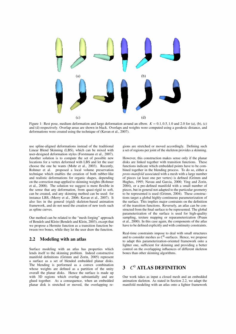
(a) (b)
(c) (d)
Figure 1: Rest pose, medium deformation and large deformation around an elbow. K = 0.1,0.5,1.0 and 2.0 for (a), (b), (c)and (d) respectively. Overlap areas are shown in black. Overlaps and weights were computed using a geodesic distance, anddeformations were created using the technique of (Kavan et al., 2007).
use spline-aligned deformations instead of the traditionalLinear Blend Skinning (LBS), which can be mixed withuser-designed deformation styles (Forstmann et al., 2007).Another solution is to compute the set of possible newlocations for a vertex deformed with LBS and let the userchoose the one he wants (Mohr et al., 2003). Recently,Rohmer et al. proposed a local volume preservationtechnique which enables the creation of both rubber-likeand realistic deformations for organic shapes, dependingon the correction map applied to skinning weights (Rohmeret al., 2008). The solution we suggest is more flexible inthe sense that any deformation, from quasi-rigid to soft,can be created, and any skinning method can be used: forinstance LBS, (Merry et al., 2006; Kavan et al., 2007). Italso lies in the general (rigid) skeleton-based animationframework, and do not need the creation of new tools suchas spline curves.
Our method can be related to the “mesh forging” approachof Bendels and Klein (Bendels and Klein, 2003), except thatwe propose a Hermite function as a transition function be-tween two bones, while they let the user draw the function.
2.2 Modeling with an atlas
Surface modeling with an atlas has properties whichlends itself to the skinning problem. Indeed constructivemanifold definitions (Grimm and Zorin, 2005) representa surface as a set of blended embedded planar disks.The blending is performed as a convex combinationwhose weights are defined as a partition of the unityoverall the planar disks. Hence the surface is made upwith 3D regions which overlap substantially and areglued together. As a consequence, when an embeddedplanar disk is stretched or moved, the overlapping re-
gions are stretched or moved accordingly. Defining sucha set of regions per joint of the skeleton provides a skinning.
However, this construction makes sense only if the planardisks are linked together with transition functions. Thesefunctions indicate which embedded points have to be com-bined together in the blending process. To do so, either aproto-manifold associated with a mesh with a large numberof pieces (at least one per vertex) is defined (Grimm andHughes, 1995; Navau and Garcia, 2000; Ying and Zorin,2004), or a pre-defined manifold with a small number ofpieces, but in general not adapted to the particular geometryto be represented is used (Grimm, 2004). These construc-tions target a global highly-continuous parameterization ofthe surface. This implies major contraints on the definitionof the transition functions. Reversely, an atlas can be con-structed from the final surface to be represented. The globalparameterization of the surface is used for high-qualitysampling, texture mapping or reparameterization (Praunet al., 2000). In this case again, the components of the atlashave to be defined explicitly and with continuity constraints.
Real-time constraints impose to deal with small structuresand to consider meshes as C0-surfaces. Hence, we proposeto adapt this parameterization-oriented framework onto alighter one, sufficient for skinning and providing a bettercontrol on the overlapping influences of different skeletonbones than other skinning algorithms.
3 C0 ATLAS DEFINITION
Our work takes as input a closed mesh and an embeddedanimation skeleton. As stated in Section 2.2, we adapt themanifold modeling with an atlas onto a lighter framework
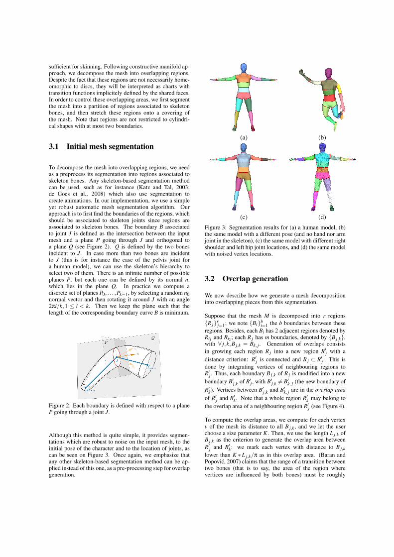
sufficient for skinning. Following constructive manifold ap-proach, we decompose the mesh into overlapping regions.Despite the fact that these regions are not necessarily home-omorphic to discs, they will be interpreted as charts withtransition functions implicitely defined by the shared faces.In order to control these overlapping areas, we first segmentthe mesh into a partition of regions associated to skeletonbones, and then stretch these regions onto a covering ofthe mesh. Note that regions are not restricted to cylindri-cal shapes with at most two boundaries.
3.1 Initial mesh segmentation
To decompose the mesh into overlapping regions, we needas a preprocess its segmentation into regions associated toskeleton bones. Any skeleton-based segmentation methodcan be used, such as for instance (Katz and Tal, 2003;de Goes et al., 2008) which also use segmentation tocreate animations. In our implementation, we use a simpleyet robust automatic mesh segmentation algorithm. Ourapproach is to first find the boundaries of the regions, whichshould be associated to skeleton joints since regions areassociated to skeleton bones. The boundary B associatedto joint J is defined as the intersection between the inputmesh and a plane P going through J and orthogonal toa plane Q (see Figure 2). Q is defined by the two bonesincident to J. In case more than two bones are incidentto J (this is for instance the case of the pelvis joint fora human model), we can use the skeleton’s hierarchy toselect two of them. There is an infinite number of possibleplanes P, but each one can be defined by its normal n,which lies in the plane Q. In practice we compute adiscrete set of planes P0, . . . ,Pk−1, by selecting a random n0normal vector and then rotating it around J with an angle2πi/k,1 ≤ i < k. Then we keep the plane such that thelength of the corresponding boundary curve B is minimum.
Figure 2: Each boundary is defined with respect to a planeP going through a joint J.
Although this method is quite simple, it provides segmen-tations which are robust to noise on the input mesh, to theinitial pose of the character and to the location of joints, ascan be seen on Figure 3. Once again, we emphasize thatany other skeleton-based segmentation method can be ap-plied instead of this one, as a pre-processing step for overlapgeneration.
(a) (b)
(c) (d)
Figure 3: Segmentation results for (a) a human model, (b)the same model with a different pose (and no hand nor armjoint in the skeleton), (c) the same model with different rightshoulder and left hip joint locations, and (d) the same modelwith noised vertex locations.
3.2 Overlap generation
We now describe how we generate a mesh decompositioninto overlapping pieces from this segmentation.
Suppose that the mesh M is decomposed into r regionsRjrj=1; we note Bibi=1 the b boundaries between theseregions. Besides, each Bi has 2 adjacent regions denoted byRi1 and Ri2 ; each Rj has m boundaries, denoted by Bj,k,with ∀ j,k,Bj,k = Bk, j. Generation of overlaps consistsin growing each region Rj into a new region Rj with adistance criterion: Rj is connected and Rj ⊂ Rj. This isdone by integrating vertices of neighbouring regions toRj. Thus, each boundary Bj,k of Rj is modified into a newboundary Bj,k of R
j, with Bj,k = Bk, j (the new boundary of
Rk). Vertices between Bj,k and Bk, j are in the overlap areaof Rj and Rk. Note that a whole region Rk may belong tothe overlap area of a neighbouring region Rj (see Figure 4).
To compute the overlap areas, we compute for each vertexv of the mesh its distance to all Bj,k, and we let the userchoose a size parameter K. Then, we use the length L j,k ofBj,k as the criterion to generate the overlap area betweenRj and Rk: we mark each vertex with distance to Bj,klower than K ∗ L j,k/π as in this overlap area. (Baran andPopovic, 2007) claims that the range of a transition betweentwo bones (that is to say, the area of the region wherevertices are influenced by both bones) must be roughly
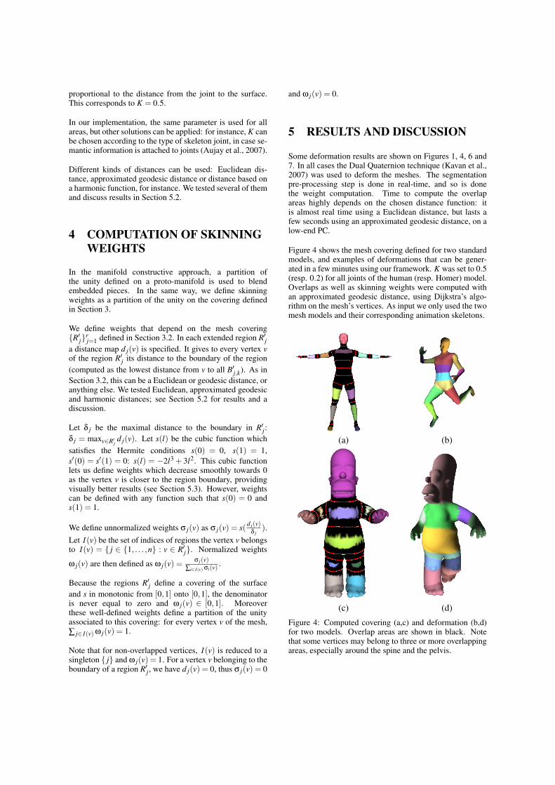
proportional to the distance from the joint to the surface.This corresponds to K = 0.5.
In our implementation, the same parameter is used for allareas, but other solutions can be applied: for instance, K canbe chosen according to the type of skeleton joint, in case se-mantic information is attached to joints (Aujay et al., 2007).
Different kinds of distances can be used: Euclidean dis-tance, approximated geodesic distance or distance based ona harmonic function, for instance. We tested several of themand discuss results in Section 5.2.
4 COMPUTATION OF SKINNINGWEIGHTS
In the manifold constructive approach, a partition ofthe unity defined on a proto-manifold is used to blendembedded pieces. In the same way, we define skinningweights as a partition of the unity on the covering definedin Section 3.
We define weights that depend on the mesh coveringRjrj=1 defined in Section 3.2. In each extended region Rja distance map d j(v) is specified. It gives to every vertex vof the region Rj its distance to the boundary of the region(computed as the lowest distance from v to all Bj,k). As inSection 3.2, this can be a Euclidean or geodesic distance, oranything else. We tested Euclidean, approximated geodesicand harmonic distances; see Section 5.2 for results and adiscussion.
Let δ j be the maximal distance to the boundary in Rj:δ j = maxv∈Rj d j(v). Let s(l) be the cubic function whichsatisfies the Hermite conditions s(0) = 0, s(1) = 1,s(0) = s(1) = 0: s(l) = −2l3 + 3l2. This cubic functionlets us define weights which decrease smoothly towards 0as the vertex v is closer to the region boundary, providingvisually better results (see Section 5.3). However, weightscan be defined with any function such that s(0) = 0 ands(1) = 1.
We define unnormalized weights σ j(v) as σ j(v) = s( d j(v)δ j
).Let I (v) be the set of indices of regions the vertex v belongsto I (v) = j ∈ 1, . . . ,n : v ∈ Rj. Normalized weights
ω j(v) are then defined as ω j(v) = σ j(v)∑i∈I (v) σi(v)
.
Because the regions Rj define a covering of the surfaceand s in monotonic from [0,1] onto [0,1], the denominatoris never equal to zero and ω j(v) ∈ [0,1]. Moreoverthese well-defined weights define a partition of the unityassociated to this covering: for every vertex v of the mesh,∑ j∈I (v) ω j(v) = 1.
Note that for non-overlapped vertices, I (v) is reduced to asingleton j and ω j(v) = 1. For a vertex v belonging to theboundary of a region Rj, we have d j(v) = 0, thus σ j(v) = 0
and ω j(v) = 0.
5 RESULTS AND DISCUSSION
Some deformation results are shown on Figures 1, 4, 6 and7. In all cases the Dual Quaternion technique (Kavan et al.,2007) was used to deform the meshes. The segmentationpre-processing step is done in real-time, and so is donethe weight computation. Time to compute the overlapareas highly depends on the chosen distance function: itis almost real time using a Euclidean distance, but lasts afew seconds using an approximated geodesic distance, on alow-end PC.
Figure 4 shows the mesh covering defined for two standardmodels, and examples of deformations that can be gener-ated in a few minutes using our framework. K was set to 0.5(resp. 0.2) for all joints of the human (resp. Homer) model.Overlaps as well as skinning weights were computed withan approximated geodesic distance, using Dijkstra’s algo-rithm on the mesh’s vertices. As input we only used the twomesh models and their corresponding animation skeletons.
(a) (b)
(c) (d)
Figure 4: Computed covering (a,c) and deformation (b,d)for two models. Overlap areas are shown in black. Notethat some vertices may belong to three or more overlappingareas, especially around the spine and the pelvis.
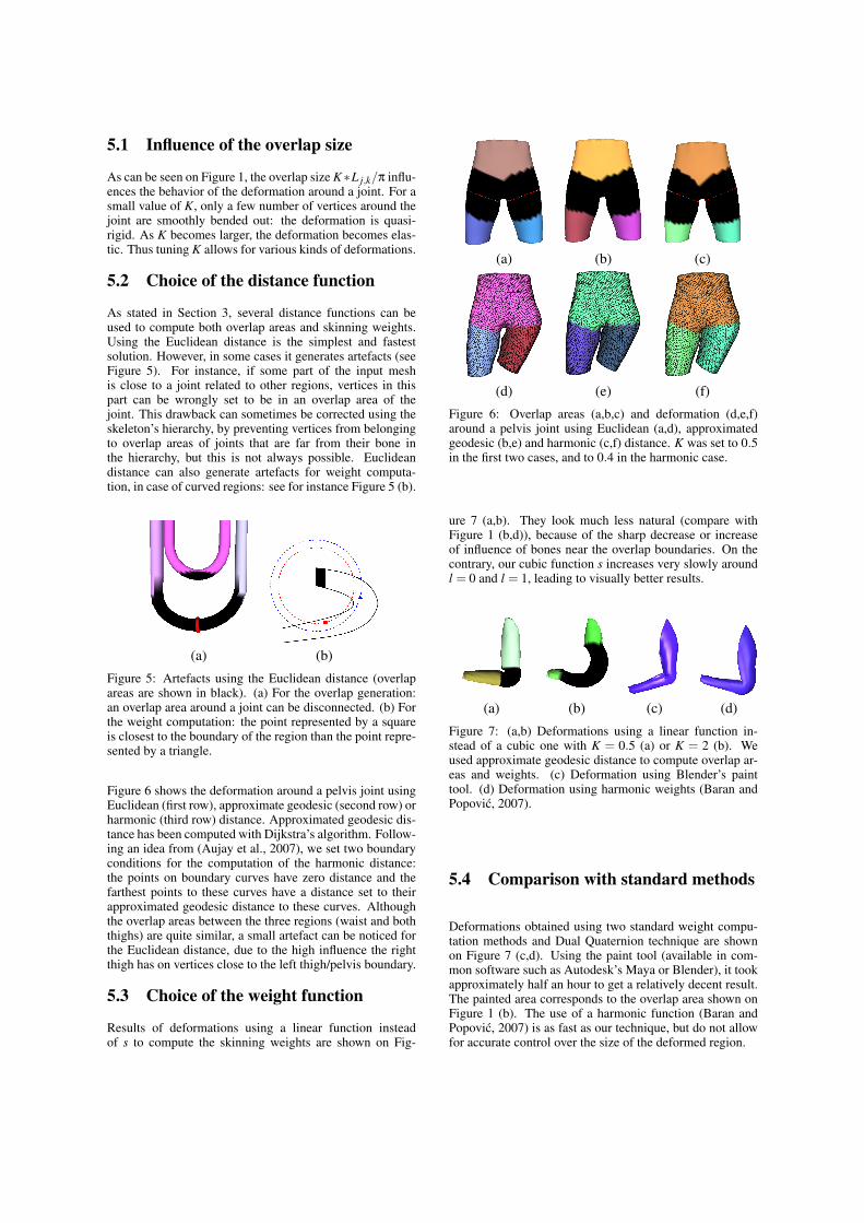
5.1 Influence of the overlap size
As can be seen on Figure 1, the overlap size K∗L j,k/π influ-ences the behavior of the deformation around a joint. For asmall value of K, only a few number of vertices around thejoint are smoothly bended out: the deformation is quasi-rigid. As K becomes larger, the deformation becomes elas-tic. Thus tuning K allows for various kinds of deformations.
5.2 Choice of the distance function
As stated in Section 3, several distance functions can beused to compute both overlap areas and skinning weights.Using the Euclidean distance is the simplest and fastestsolution. However, in some cases it generates artefacts (seeFigure 5). For instance, if some part of the input meshis close to a joint related to other regions, vertices in thispart can be wrongly set to be in an overlap area of thejoint. This drawback can sometimes be corrected using theskeleton’s hierarchy, by preventing vertices from belongingto overlap areas of joints that are far from their bone inthe hierarchy, but this is not always possible. Euclideandistance can also generate artefacts for weight computa-tion, in case of curved regions: see for instance Figure 5 (b).
(a) (b)
Figure 5: Artefacts using the Euclidean distance (overlapareas are shown in black). (a) For the overlap generation:an overlap area around a joint can be disconnected. (b) Forthe weight computation: the point represented by a squareis closest to the boundary of the region than the point repre-sented by a triangle.
Figure 6 shows the deformation around a pelvis joint usingEuclidean (first row), approximate geodesic (second row) orharmonic (third row) distance. Approximated geodesic dis-tance has been computed with Dijkstra’s algorithm. Follow-ing an idea from (Aujay et al., 2007), we set two boundaryconditions for the computation of the harmonic distance:the points on boundary curves have zero distance and thefarthest points to these curves have a distance set to theirapproximated geodesic distance to these curves. Althoughthe overlap areas between the three regions (waist and boththighs) are quite similar, a small artefact can be noticed forthe Euclidean distance, due to the high influence the rightthigh has on vertices close to the left thigh/pelvis boundary.
5.3 Choice of the weight function
Results of deformations using a linear function insteadof s to compute the skinning weights are shown on Fig-
(a) (b) (c)
(d) (e) (f)
Figure 6: Overlap areas (a,b,c) and deformation (d,e,f)around a pelvis joint using Euclidean (a,d), approximatedgeodesic (b,e) and harmonic (c,f) distance. K was set to 0.5in the first two cases, and to 0.4 in the harmonic case.
ure 7 (a,b). They look much less natural (compare withFigure 1 (b,d)), because of the sharp decrease or increaseof influence of bones near the overlap boundaries. On thecontrary, our cubic function s increases very slowly aroundl = 0 and l = 1, leading to visually better results.
(a) (b) (c) (d)
Figure 7: (a,b) Deformations using a linear function in-stead of a cubic one with K = 0.5 (a) or K = 2 (b). Weused approximate geodesic distance to compute overlap ar-eas and weights. (c) Deformation using Blender’s painttool. (d) Deformation using harmonic weights (Baran andPopovic, 2007).
5.4 Comparison with standard methods
Deformations obtained using two standard weight compu-tation methods and Dual Quaternion technique are shownon Figure 7 (c,d). Using the paint tool (available in com-mon software such as Autodesk’s Maya or Blender), it tookapproximately half an hour to get a relatively decent result.The painted area corresponds to the overlap area shown onFigure 1 (b). The use of a harmonic function (Baran andPopovic, 2007) is as fast as our technique, but do not allowfor accurate control over the size of the deformed region.
6 CONCLUSION
We have presented a simple way to compute flexibleskinning weights for skeleton-based animation, basedon the concept of manifold modeling. Starting from asegmentation of the input mesh into regions correspondingto skeleton bones, we generate overlaps by extendingeach region around joints. Size of these overlaps iscontrolled by a simple parameter, that can be user-chosenor automatically computed. Then, vertices belonging to anoverlap area are influenced by bones related to all regionsthat overlap. Skinning weights are defined using a simplesmooth function based on the distance to the overlapboundary.
Results show that this framework allows to create fromquasi-rigid to soft deformations, depending on the overlapsize. Using a geodesic distance instead of a Euclidean oneto create overlaps and compute skinning weights is moretime-consuming, but avoids some artefacts. We believe ourmethod can be especially useful for non-expert animators,since it is simple (only one parameter is to set) and fast touse.
Further work includes anatomic information into the over-lapping width definition. Such information can be derivedfrom semantic information associated with skeleton (Aujayet al., 2007). Besides, providing a skinning framework formultiresolution animated meshes, founded on our pseudo-parameterization on the initial mesh, would be a further de-velopment in the similarity with manifold parameterization.
ACKNOWLEDGEMENTS
This work was partially supported by the IMAG, ELESAand INRIA through the MEGA project and the ANRthrough the MADRAS project (ANR-07-MDCO-015). Partof this work was done while Lin Lu was visiting INRIAwith an INRIA Internship grant.
REFERENCES
Attene, M., Spagnuolo, M., and Falcidieno, B. (2006). Hi-erarchical mesh segmentation based on fitting primi-tives. The Visual Computer, 22(3):181–193.
Aujay, G., Hetroy, F., Lazarus, F., and Depraz, C. (2007).Harmonic skeleton for realistic character animation.In Symposium on Computer Animation, pages 151–160, San Diego, USA.
Baran, I. and Popovic, J. (2007). Automatic rigging and ani-mation of 3d characters. ACM Transactions on Graph-ics (SIGGRAPH proceedings), 26(3):72.
Bendels, G. and Klein, R. (2003). Mesh forging: Editingof 3d-meshes using implicitly defined occluders. InSymposium on Geometry Processing, pages 207–217,Aachen, Germany.
Bloomenthal, J. (2002). Medial-based vertex deformation.In Symposium on Computer Animation, pages 147–151, San Antonio, USA.
de Goes, F., Goldenstein, S., and Velho, L. (2008). A hierar-chical segmentation of articulated bodies. ComputerGraphics Forum (Symposium on Geometry Process-ing proceedings), 27(5):1349–1356.
Forstmann, S., Ohya, J., Krohn-Grimberghe, A., and Mc-Dougall, R. (2007). Deformation styles for spline-based skeletal animation. In Symposium on ComputerAnimation, pages 141–150, San Diego, USA.
Grimm, C. (2004). Parameterization using manifolds. In-ternational Journal of Shape Modeling, 10(1):51–80.
Grimm, C. and Hughes, J. (1995). Modeling surfaces ofarbitrary topology. In SIGGRAPH, pages 359–367,Los Angeles, USA.
Grimm, C. and Zorin, D. (2005). Surface modeling and pa-rameterization with manifolds. In SIGGRAPH CourseNotes, Los Angeles, USA.
Katz, S. and Tal, A. (2003). Hierarchical mesh de-composition using fuzzy clustering and cuts. ACMTransactions on Graphics (SIGGRAPH proceedings),22(3):954–961.
Kavan, L., Collins, S., Zara, J., and O’Sullivan, C. (2007).Skinning with dual quaternions. In Symposium on In-teractive 3D Graphics and Games, pages 39–46, Seat-tle, USA.
Merry, B., Marais, P., and Gain, J. (2006). Animationspace: a truly linear framework for character anima-tion. ACM Transactions on Graphics, 25(4):1400–1423.
Mohr, A., Tokheim, L., and Gleicher, M. (2003). Directmanipulation of interactive character skins. In Sym-posium on Interactive 3D Graphics and Games, pages27–30, Monterey, USA.
Navau, J. C. and Garcia, N. P. (2000). Modeling surfacesfrom meshes of arbitrary topology. Computer AidedGeometric Design, 17(1):643–671.
Praun, E., Finkelstein, A., and Hoppe, H. (2000). Lappedtextures. In SIGGRAPH, pages 465–470, New Or-leans, USA.
Rohmer, D., Hahmann, S., and Cani, M. (2008). Localvolume preservation for skinned characters. Com-puter Graphics Forum (Pacific Graphics proceed-ings), 27(7).
Wang, R., Pulli, K., and Popovic, J. (2007). Real-time enveloping with rotational regression. ACMTransactions on Graphics (SIGGRAPH proceedings),26(3):73.
Weber, O., Sorkine, O., Lipman, Y., and Gotsman, C.(2007). Context-aware skeletal shape deformation.Computer Graphics Forum (Eurographics proceed-ings), 26(3):265–274.
Ying, L. and Zorin, D. (2004). A simple manifold-based construction of surfaces of arbitrary smooth-ness. ACM Transactions on Graphics (SIGGRAPHproceedings), 23(3):271–275.
A.7. SEGMENTATION OF TEMPORAL MESH SEQUENCES INTO RIGIDLYMOVING COMPONENTS 179
∴
A.7 SEGMENTATION OF TEMPORAL MESHSEQUENCES INTO RIGIDLY MOVINGCOMPONENTS
Romain Arcila, Cédric Cagniart, Franck Hétroy, Edmond Boyer, Florent DupontGraphical Models 75 (1), Elsevier, 2013.

180 APPENDIX A. SELECTED PAPERS
Segmentation of temporal mesh sequences into rigidly moving components
Romain Arcilaa,b, Cedric Cagniartc,a, Franck Hetroya,∗, Edmond Boyera, Florent Dupontb
aLaboratoire Jean Kuntzmann, Inria & Grenoble University, FrancebLIRIS, CNRS & Universite de Lyon, France
cComputer Aided Medical Procedures & Augmented Reality (CAMPAR), Technische Universitat Munchen, Germany
Abstract
In this paper is considered the segmentation of meshes into rigid components given temporal sequences of deforming meshes. We
propose a fully automatic approach that identifies model parts that consistently move rigidly over time. This approach can handle
meshes independently reconstructed at each time instant. It allows therefore for sequences of meshes with varying connectivities as
well as varying topology. It incrementally adapts, merges and splits segments along a sequence based on the coherence of motion
information within each segment. In order to provide tools for the evaluation of the approach, we also introduce new criteria to
quantify a mesh segmentation. Results on both synthetic and real data as well as comparisons are provided in the paper.
Keywords: mesh sequence, segmentation, topology, mesh matching, rigid part
1. Introduction
Temporal sequences of deforming meshes, also called mesh
animations [1, 43], are widely used to represent 3D shapes
evolving through time. They can be created from a single static
mesh, which is deformed using standard animation techniques
such as skeletal subspace deformation [25] or cloth simulation
methods [15]. They can also be generated from multiple video
cameras [38, 43]. In this case, meshes are usually indepen-
dently estimated at each frame using 2D visual cues such as
silhouettes or photometric information.
These deforming mesh sequences can be edited [21, 8], com-
pressed [24], or used for deformation transfer [39, 23]. When
the shape represents an articulated body, such as a human or
animal character, identifying its rigid, or almost rigid, parts of-
fers useful understanding for most of these applications. To re-
cover the shape kinematic structure, an animation skeleton can
be extracted from the deforming mesh sequence [1]. Another
strategy is to segment the meshes into components that move
rigidly over the sequence [22, 19, 44, 29]. In both cases, mo-
tion information is required in order to cluster mesh elements
into regions with rigid motions. Most existing approaches as-
sume that surface registration is available for that purpose and
consider as the input a single mesh that deforms over time. In
contrast, we do not make any assumptions on the input mesh
sequences and we propose to match meshes and recover their
rigid parts simultaneously. Consequently, our method applies
to any kind of deforming mesh sequence including inconsistent
mesh sequences such as provided by multi-camera systems.
∗Corresponding author.
Email addresses: [email protected] (Franck Hetroy),
[email protected] (Edmond Boyer),
[email protected] (Florent Dupont)
1.1. Classification of mesh sequences
In order to distinguish between mesh sequences with or with-
out temporal coherence, i.e. with or without a one-to-one cor-
respondence between vertices of successive meshes, we first in-
troduce the following definitions.
Definition 1.1 (Temporally coherent mesh sequence (TCMS),
temporally incoherent mesh sequence (TIMS)). Let MS =
Mi = (Vi, Ei, Fi), i = 1 . . . f be a mesh sequence: Vi is the
set of vertices of the ith mesh Mi of the sequence, Ei its set of
edges and Fi its set of faces. If the connectivity is constant
over the whole sequence, that is to say if there is an isomor-
phism between any Ei and E j, 1 ≤ i, j ≤ f , then MS is called
a temporally coherent mesh sequence (TCMS). Otherwise, MS
is called a temporally incoherent mesh sequence (TIMS).
Note that the definition of TCMS not only implies that the
number of vertices remains constant through time, but also that
there is a one-to-one correspondence between faces of any two
meshes. As a consequence, topological changes (genus and
number of connected components) are not possible in a TCMS.
Figure 1 shows an example of a TCMS and an example of a
TIMS.
1.2. Classification of mesh sequence segmentations
In contrast to single mesh segmentation that consists in
grouping mesh vertices into spatial regions the segmentation of
a mesh sequence can have various interpretations with respect
to time and space. We propose here three different definitions.
Let us first recall a formal definition of a static mesh segmenta-
tion.
Definition 1.2 (Segmentation of a static mesh [33]). Let M =
(V, E, F) be a 3D surface mesh. A segmentation Σ of M is the
set of sub-meshes Σ = M1, . . . ,Mk induced by a partition of
either V or E or F into k disjoint sub-sets.
Preprint submitted to Graphical Models November 7, 2012
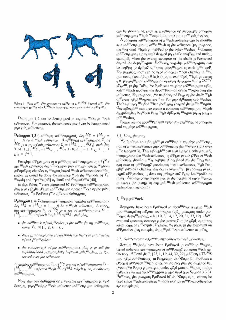
Figure 1: First row: two consecutive frames of a TCMS. Second row: two
consecutive frames of a TIMS (in particular, notice the change in topology).
Definition 1.2 can be generalized in various ways to mesh
sequences. For instance, the sequence itself can be partitionned
into sub-sequences:
Definition 1.3 (Temporal segmentation). Let MS = Mi, i =
1 . . . f be a mesh sequence. A temporal segmentation Σt of
MS is a set of sub-sequences Σt = MS 1, . . . ,MS k such that
∀ j ∈ [1, k],MS j = Mij , . . . ,Mij+1−1 with i1 = 1 < i2 < · · · <
ik+1 = f + 1.
Possible applications of a temporal segmentation of a TIMS
are mesh sequence decomposition into sub-sequences without
topological changes or motion-based mesh sequence decompo-
sition, as could be done for instance with the methods of Ya-
masaki and Aizawa [45] or Tung and Matsuyama [40].
In this paper, we are interested by geometric segmentations,
that is to say the spatial segmentation of each mesh of the input
sequence. We propose two different definitions.
Definition 1.4 (Coherent segmentation, variable segmentation).
Let MS = Mi, i = 1 . . . f be a mesh sequence. A coher-
ent segmentation Σc of MS is a set of segmentations Σi =
Mi1, . . . ,Mi
ki of each mesh Mi of MS , such that:
• the number k of sub-meshes is the same for all segmenta-
tions: ∀i, j ∈ [1, f ], ki = k j;
• there is a one-to-one correspondence between sub-meshes
of any two meshes;
• the connectivity of the segmentations, that is to say the
neighborhood relationships between sub-meshes, is pre-
served over the sequence.
A variable segmentation Σv of MS is a set of segmentations Σi =
Mi1, . . . ,Mi
ki of each mesh Mi of MS which is not a coherent
segmentation.
Note that our definition of a variable segmentation is very
general. Intermediate mesh sequence segmentation definitions
can be thought of, such as a sequence of successive coherent
segmentations which would differ only for a few sub-meshes.
A coherent segmentation of a mesh sequence can be thought
as a segmentation of some mesh of the sequence (for instance,
the first one) which is mapped to the other meshes. Coherent
segmentations are usually desired for shape analysis and under-
standing, when the overall structure of the shape is preserved
during the deformation. However, variable segmentations can
be helpful to display different information at each time step.
For instance, they can be used to detect when changes in mo-
tion occur (see Figure 9 (a,b,c) for an example), which is useful
e.g. for animation compression or event detection with a CCTV
system. In this paper, we propose a variable segmentation algo-
rithm which recovers the decomposition of the motion over the
sequence. For instance, two neighboring parts of the shape with
different rigid motions are first put into different sub-meshes.
They are later merged when they start sharing the same motion.
Our algorithm can also create a coherent segmentation, which
distinguishes between parts with different motion for at least a
few meshes.
Please see the accompanying video for examples of coherent
and variable segmentations.
1.3. Contributions
We propose an algorithm to compute a variable segmenta-
tion of a mesh sequence into components that move rigidly over
time (section 3). This algorithm can also create a coherent seg-
mentation of the mesh sequence. It applies to any types of mesh
sequences though it was originally designed for the most gen-
eral case of temporally incoherent mesh sequences, with pos-
sibly topology changes that occur over time. In contrast to ex-
isting approaches, it does not require any prior knowledge as
input. Another contribution lies in the design of error metrics
to assess the results of existing mesh sequence segmentation
techniques (section 5).
2. Related work
Solutions have been proposed to decompose a static mesh
into meaningful regions for motion (e.g., invariant under iso-
metric deformations), e.g. [10, 3, 14, 17, 20, 31, 37, 12]. How-
ever and since our concern is the recovery of the rigid, or almost
rigid, parts of a moving 3D shape, we focus in the following on
approaches that consider deforming mesh sequence as input.
2.1. Segmentation of temporally coherent mesh sequences
Several methods have been proposed to compute motion-
based coherent segmentation of temporally coherent mesh se-
quences. Among them, [23, 1, 19, 44, 32, 29] segment a TCMS
into rigid components. In particular, de Aguiar [1] proposes a
spectral approach which relies on the fact that the distance be-
tween two points is invariant under rigid transformation. In this
paper, a spectral decomposition is also used (see Section 3.3.3).
However, the invariant proposed by de Aguiar et al. cannot be
used since mesh sequences without explicit temporal coherence
are considered.
2
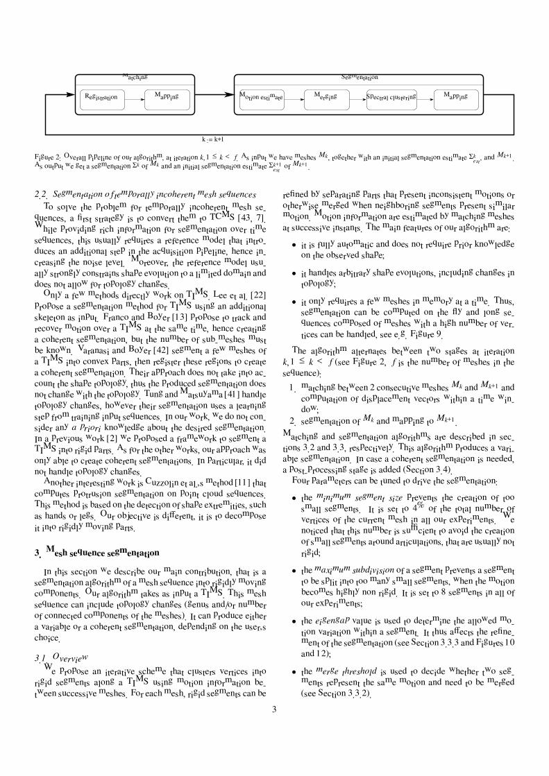
Matching
Mapping
k := k+1
Segmentation
MergingMotion estimate MappingRegistration Spectral clustering
Figure 2: Overall pipeline of our algorithm, at iteration k, 1 ≤ k < f . As input we have meshes Mk , together with an initial segmentation estimate Σkest , and Mk+1.
As output we get a segmentation Σk of Mk and an initial segmentation estimate Σk+1est of Mk+1.
2.2. Segmentation of temporally incoherent mesh sequences
To solve the problem for temporally incoherent mesh se-
quences, a first strategy is to convert them to TCMS [43, 7].
While providing rich information for segmentation over time
sequences, this usually requires a reference model that intro-
duces an additional step in the acquisition pipeline, hence in-
creasing the noise level. Moreover, the reference model usu-
ally strongly constrains shape evolution to a limited domain and
does not allow for topology changes.
Only a few methods directly work on TIMS. Lee et al. [22]
propose a segmentation method for TIMS using an additional
skeleton as input. Franco and Boyer [13] propose to track and
recover motion over a TIMS at the same time, hence creating
a coherent segmentation, but the number of sub-meshes must
be known. Varanasi and Boyer [42] segment a few meshes of
a TIMS into convex parts, then register these regions to create
a coherent segmentation. Their approach does not take into ac-
count the shape topology, thus the produced segmentation does
not change with the topology. Tung andMatsuyama [41] handle
topology changes, however their segmentation uses a learning
step from training input sequences. In our work, we do not con-
sider any a priori knowledge about the desired segmentation.
In a previous work [2] we proposed a framework to segment a
TIMS into rigid parts. As for the other works, our approach was
only able to create coherent segmentations. In particular, it did
not handle topology changes.
Another interesting work is Cuzzolin et al.’s method [11] that
computes protrusion segmentation on point cloud sequences.
This method is based on the detection of shape extremities, such
as hands or legs. Our objective is different, it is to decompose
it into rigidly moving parts.
3. Mesh sequence segmentation
In this section we describe our main contribution, that is a
segmentation algorithm of a mesh sequence into rigidly moving
components. Our algorithm takes as input a TIMS. This mesh
sequence can include topology changes (genus and/or number
of connected components of the meshes). It can produce either
a variable or a coherent segmentation, depending on the user’s
choice.
3.1. Overview
We propose an iterative scheme that clusters vertices into
rigid segments along a TIMS using motion information be-
tween successive meshes. For each mesh, rigid segments can be
refined by separating parts that present inconsistent motions or
otherwise merged when neighboring segments present similar
motion. Motion information are estimated by matching meshes
at successive instants. The main features of our algorithm are:
• it is fully automatic and does not require prior knowledge
on the observed shape;
• it handles arbitrary shape evolutions, including changes in
topology;
• it only requires a few meshes in memory at a time. Thus,
segmentation can be computed on the fly and long se-
quences composed of meshes with a high number of ver-
tices can be handled, see e.g. Figure 9.
The algorithm alternates between two stages at iteration
k, 1 ≤ k < f (see Figure 2, f is the number of meshes in the
sequence):
1. matching between 2 consecutive meshes Mk and Mk+1 and
computation of displacement vectors within a time win-
dow;
2. segmentation of Mk and mapping to Mk+1.
Matching and segmentation algorithms are described in sec-
tions 3.2 and 3.3, respectively. This algorithm produces a vari-
able segmentation. In case a coherent segmentation is needed,
a post-processing stage is added (Section 3.4).
Four parameters can be tuned to drive the segmentation:
• the minimum segment size prevents the creation of too
small segments. It is set to 4% of the total number of
vertices of the current mesh in all our experiments. We
noticed that this number is sufficient to avoid the creation
of small segments around articulations, that are usually not
rigid;
• the maximum subdivision of a segment prevents a segment
to be split into too many small segments, when the motion
becomes highly non rigid. It is set to 8 segments in all of
our experiments;
• the eigengap value is used to determine the allowed mo-
tion variation within a segment. It thus affects the refine-
ment of the segmentation (see Section 3.3.3 and Figures 10
and 12);
• the merge threshold is used to decide whether two seg-
ments represent the same motion and need to be merged
(see Section 3.3.2).
3
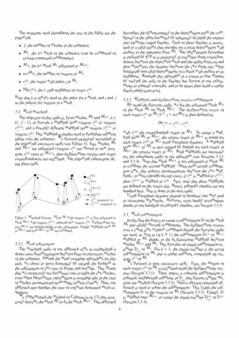
The notations used throughout the rest of the paper are the
following:
• f : the number of meshes in the sequence;
• Mk: the kth mesh of the sequence (can be composed of
several connected components);
• M′k: the kth mesh Mk registered to Mk+1;
• nv(Mk): the number of vertices in Mk;
• v(k)
i: the vertex with index i in Mk;
• Ng(v(k)
i): the 1-ring neighbors of vertex v
(k)
i.
Note that k is always used as the index for a mesh, and i and j
as the indices for vertices in a mesh.
3.2. Mesh matching
The objective of this stage is, given meshes Mk and Mk+1, k ∈
[1, f − 1], to provide a mapping from vertices v(k)
ito vertices
v(k+1)
j, and a possibly different mapping from vertices v
(k+1)
jto
vertices v(k)
i. This mapping is further used to propagate segment
labels over the sequence. We proceed iteratively according to
the following successive steps (see Figure 3): first, meshes Mk
and Mk+1 are registered (vertices v(k)
iare moved to new loca-
tions v′(k)
iclose to Mk+1), then displacement vectors and vertex
correspondences are estimated. The following subsections de-
tail these steps.
Figure 3: Matching process. Mesh Mk with vertices v(k)iis first registered to
mesh Mk+1 with vertices v(k+1)i
, inducing new vertices v′(k)i. Displacement vec-
tors DVi(k) are defined thanks to this registration. Finally, mappings from Mk
to Mk+1 and from Mk+1 to Mk are computed.
3.2.1. Mesh registration
The matching stage of our approach aims at establishing a
dense cross parametrization between pairs of successive meshes
of the sequence. Among the many available algorithms for this
task, we chose to favor generality by casting the problem as
the registration of two sets of points and normals. This means
that we exclusively use geometric cues to align the two meshes,
even when photometric information is available like in the case
of meshes reconstructed from multi-camera systems. Thus, our
approach also handles the case of software generated mesh se-
quences.
We implemented the method of Cagniart et al. [7] that itera-
tively deforms the mesh Mk to fit the mesh Mk+1. This approach
decouples the dimensionality of the deformation from the com-
plexity of the input geometry by arbitrarily dividing the surface
into elements called patches. Each of these patches is associ-
ated to a rigid frame that encodes for a local deformation with
respect to the reference pose Mk. The optimization procedure
is inspired by ICP as it iteratively re-estimates point correspon-
dences between the deformed mesh and the target point set and
then minimizes the distance between the two point sets while
penalizing non rigid deformations of a patch with respect to its
neighbors. Running this algorithm in a coarse-to-fine manner
by varying the radii of the patches has proven in our experi-
ments to robustly converge, and to be faster than using a single
patch-subdivision level.
3.2.2. Mappings and displacement vectors computation
By using the previous stage, we get the registered mesh M′k
of the mesh Mk on mesh Mk+1. The displacement vector of
each vertex v(k)
iin Mk, 0 i < nv(Mk) is then defined as:
DVi(k) = v
′(k)
i− v
(k)
i,
with v′(k)
ithe corresponding vertex in M′k. To create a map-
ping from Mk to Mk+1, the closest vertex in Mk+1 is found for
each vertex v′(k)
iin M′k using Euclidean distance. A mapping
from Mk+1 to Mk is also created by finding for each vertex in
Mk+1 the closest vertex in M′k. Both mappings are necessary
for the subsequent stage of our algorithm (see Sections 3.3.1
and 3.3.4). Note that mesh Mk+1 is not registered to mesh Mk
to compute the second mapping. Apart from saving computa-
tion time, this reduces inconsistencies between the two map-
pings: in most (though not all) cases, if v(k)
iis mapped to v
(k+1)
i,
then v(k+1)
iis mapped to v
(k)
i. Also, note that these mappings
are defined on the vertex sets. Hence, topology changes are not
handled here. This is done in the next stage.
Using Euclidean distance instead of geodesic one may lead
to occasional mismatchs. However, error hardly accumulates
thanks to our handling of topology changes, see Section 3.3.4.
3.3. Mesh segmentation
In this part the goal is to create a segmentation Σk of the mesh
Mk into rigidly moving components. The displacement vectors
over a small time window computed during the previous stage
are used, as well as (if k 1) the segmentation Σk−1 of Mk−1
mapped to Mk thanks to the bi-directional mapping between
meshes Mk−1 and Mk. This provides an initial segmentation es-
timate Σkest of Mk. For k = 1, the initial estimate is the trivial
segmentation of M1 into a single segment, containing all ver-
tices v(1)
iof M1.
We proceed in four successive steps. First, the motion of
each vertex v(k)
iof Mk is estimated using the displacements vec-
tors (Section 3.3.1). Then, unless a coherent segmentation is
required, neighboring segments in Σkest that present similar mo-
tions are merged (Section 3.3.2). Then a spectral clustering ap-
proach is used to refine the segmentation. This yields the seg-
mentation Σk of the vertices of Mk (Section 3.3.3). Finally, Σk
is mapped onto Mk+1, to create the initial estimate Σk+1est of Σk+1
(Section 3.3.4).
4
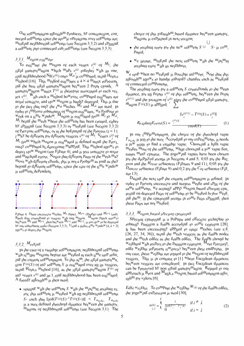
Our segmentation algorithm produces, by construction, con-
nected segments since the atomic operations over segments are:
merging neighboring segments (see Section 3.3.2) and splitting
a segment into connected sub-segments (see Section 3.3.3).
3.3.1. Motion estimate
To estimate the motion of each vertex v(k)
iof Mk, the
rigid transformation which maps v(k)
itogether with its one-
ring neighborhood Ng(v(k)
i) onto M′k is computed, using Horn’s
method [16]. This method estimates a 4 × 4 matrix represent-
ing the best rigid transformation between 2 point clouds. A
transformation matrix T(k)
iis therefore associated to each ver-
tex v(k)
i. With such a method however, computed estimates are
noise sensitive, and slow motion is hardly detected. This is due
to the fact that only the two meshes Mk and M′k are used. In
order to improve robustness of motion estimates, we propose to
work on a time window. Motion is estimated from Ml to M′k,
Ml being the mesh where the segment has been created, either
by splitting (see Section 3.3.3) or merging (see Section 3.3.2)
of previous segments, or at the beginning of the process (l = 1).
l may be different for different vertices v(k)
iof Mk. Vertex v
(l)
jof
Ml from which motion is estimated is defined using the previ-
ously computed bi-directional mapping. This method allows to
detect slow motion (see Figure 4), and is less sensitive to noise
and matching errors. Notice that different parts of the mesh may
move with different speeds, this is not a problem as long as they
belong to different segments, since the size of the time window
is segment-dependent.
Figure 4: Three successive meshes Mk (blue), Mk+1 (purple) and Mk+2 (red).
Black dots correspond to vertices with null motion. Motion (black arrows)
between Mk and Mk+1, then between Mk+1 and Mk+2, is too slow to be detected
by our subsequent stage (Section 3.3.3). Using a larger time window [k, k + 2]
allows to detect this motion.
3.3.2. Merging
In the case of a variable segmentation, neighboring segments
with similar motions before are merged at each time step refin-
ing the current segmentation. To this aim, the rigid transforma-
tion T (k)(S ) of any segment S is estimated over all its vertices,
using Horn’s method [16], as the rigid transformation T(k)
iof
any vertex v(k)
iand its 1-ring neighborhood has been estimated.
A greedy algorithm is then used:
• starting with the segment S with the minimal residual er-
ror, this segment is merged with all neighboring segments
S ′ such that log(T (k)(S )−1T (k)(S ′)) < Tmerge. Tmerge
is a user-defined threshold distance between the transfor-
mations of neighboring segments (see Section 3.1). The
choice of this logarithm-based distance between transfor-
mations is explained in next section;
• the residual error for the new segment S ∪
S ′ is com-
puted;
• we iterate, merging the next segment with the minimal
residual error with its neighbors.
We stop when no merging is possible anymore. Note that this
algorithm allows to handle topology changes such as merging
of connected components.
The residual error for a segment S corresponds to the mean
distance, for all points v(k)
iof this segment, between the point
v(k+1)
iand the location of v
(k)
iafter the computed rigid transfor-
mation T (k)(S ) is applied:
ResidualError(S ) =
v(k)
i∈S
v(k+1)
i− T (k)(S ) ∗ v
(k)
i
card(S )(1)
In our implementation, the choice of the threshold value
Tmerge is left to the user. According to our experiments, it needs
a few trials to find a suitable value. Choosing a high value
merges most of the segments, while choosing a low value gen-
erates many clusters. The following values have been chosen
for the displayed results in Sections 4 and 5: 0.03 for the Bal-
loon and the Horse sequences (Figures 9 and 11), 0.05 for the
Dancer sequence (Figure 9) and 0.2 for the Cat sequence (Fig-
ure 13).
During the next step the current segmentation is refined. In
order to prevent successive and useless merge and split of the
same segments, we actually apply motion-based spectral clus-
tering on detected pairs of segments to be merged before merg-
ing them. If the clustering results in some pairs splitting, then
these pairs are not merged.
3.3.3. Motion-based spectral clustering
Spectral clustering is a popular and effective technique to
robustly partition a graph according to some criterion [28].
It has been successfully applied to static meshes (see e.g.
[26, 27, 34, 36]), using the mesh vertices as the graph nodes
and the mesh edges as the graph edges. The graph should be
weighted with respect to the partition criterion. More precisely,
edge weights represent similarity between their endpoints. In
our case, these weights are related to the motion of neighboring
vertices. This is in contrast to [1] where Euclidean distances
between vertices are considered. In fact Euclidean distances
can be preserved by non rigud transformation. Related to our
approach is Brox and Malik’s motion-based segmentation algo-
rithm for videos [6].
Edge weights. To compute the weightsW (k) of the graph edges,
the following expression is used [30]:
w(k)
i, j=
1
log(T(k)
i
−1T(k)
j)2
if i j,
0 if i = j.(2)
5
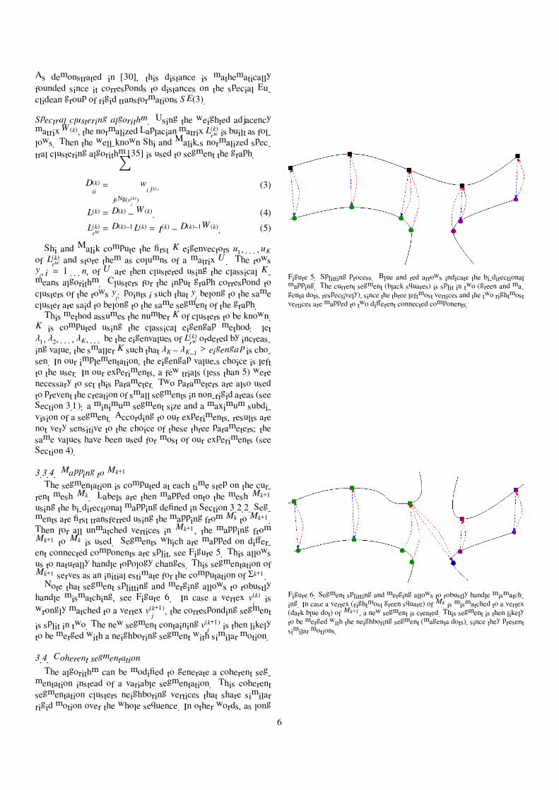
As demonstrated in [30], this distance is mathematically
founded since it corresponds to distances on the special Eu-
clidean group of rigid transformations S E(3).
Spectral clustering algorithm. Using the weighted adjacency
matrixW (k), the normalized Laplacian matrix L(k)rw is built as fol-
lows. Then the well-known Shi and Malik’s normalized spec-
tral clustering algorithm [35] is used to segment the graph.
D(k)
ii=
j∈Ng(v(k)
i)
wi j(k) . (3)
L(k) = D(k) −W (k). (4)
L(k)rw = D(k)−1L(k) = I(k) − D(k)−1W (k). (5)
Shi and Malik compute the first K eigenvectors u1, . . . , uKof L
(k)rw and store them as columns of a matrix U. The rows
yi, i = 1 . . . n, of U are then clustered using the classical K-
means algorithm. Clusters for the input graph correspond to
clusters of the rows yi: points i such that yi belong to the same
cluster are said to belong to the same segment of the graph.
This method assumes the number K of clusters to be known.
K is computed using the classical eigengap method: let
λ1, λ2, . . . , λK , . . . be the eigenvalues of L(k)rw ordered by increas-
ing value, the smaller K such that λK −λK−1 > eigengap is cho-
sen. In our implementation, the eigengap value’s choice is left
to the user. In our experiments, a few trials (less than 5) were
necessary to set this parameter. Two parameters are also used
to prevent the creation of small segments in non-rigid areas (see
Section 3.1): a minimum segment size and a maximum subdi-
vision of a segment. According to our experiments, results are
not very sensitive to the choice of these three parameters; the
same values have been used for most of our experiments (see
Section 4).
3.3.4. Mapping to Mk+1
The segmentation is computed at each time step on the cur-
rent mesh Mk. Labels are then mapped onto the mesh Mk+1
using the bi-directional mapping defined in Section 3.2.2. Seg-
ments are first transferred using the mapping from Mk to Mk+1.
Then for all unmatched vertices in Mk+1, the mapping from
Mk+1 to Mk is used. Segments which are mapped on differ-
ent connected components are split, see Figure 5. This allows
us to naturally handle topology changes. This segmentation of
Mk+1 serves as an initial estimate for the computation of Σk+1.
Note that segment splitting and merging allows to robustly
handle mismatching, see Figure 6. In case a vertex v(k)
iis
wrongly matched to a vertex v(k+1)
j, the corresponding segment
is split in two. The new segment containing v(k+1)
jis then likely
to be merged with a neighboring segment with similar motion.
3.4. Coherent segmentation
The algorithm can be modified to generate a coherent seg-
mentation instead of a variable segmentation. This coherent
segmentation clusters neighboring vertices that share similar
rigid motion over the whole sequence. In other words, as long
Figure 5: Splitting process. Blue and red arrows indicate the bi-directional
mapping. The current segment (black squares) is split in two (green and ma-
genta dots, respectively), since the three leftmost vertices and the two rightmost
vertices are mapped to two different connected components.
Figure 6: Segment splitting and merging allows to robustly handle mismatch-
ing. In case a vertex (rightmost green square) of Mk is mismatched to a vertex
(dark blue dot) of Mk+1, a new segment is created. This segment is then likely
to be merged with the neighboring segment (magenta dots), since they present
similar motions.
6
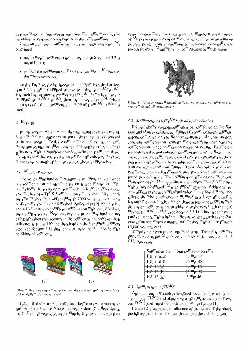
as their motion differs over at least one small time window, two
neighboring vertices do not belong to the same segment.
Creating a coherent segmentation is then straightforward. We
only need:
• not to merge segments (step described in Section 3.3.2 is
not applied);
• to map the segmentation Σ f of the last mesh Mf back to
the whole sequence.
To this purpose, the bi-directional mapping described in Sec-
tion 3.2.2 is simply applied in reverse order, from Mf to M1.
For each pair of successive meshes (Mk,Mk+1) we first use the
mapping from Mk+1 to Mk, then for all vertices of Mk which
are not assigned to a segment, the mapping from Mk to Mk+1 is
used.
4. Results
In this section we show and discuss visual results of our al-
gorithm. A quantitative evaluation of these results is discussed
in the next section. We first examine matching results, then seg-
mentation results on difficult cases (temporally incoherent mesh
sequences with topological changes, acquired from real data).
We also show that our results on temporally coherent mesh se-
quences are visually similar to state-of-the-art approaches.
4.1. Matching results
The vertex matching computation is an important step since
our segmentation algorithm relies on it (see Figure 2). Fig-
ure 7 shows the result of vertex matching between two succes-
sive meshes of a TIMS. Computation time is about 30 seconds
for two meshes with approximately 7000 vertices each. This
outperforms the matching method proposed in [2] which takes
about 13 minutes to complete computation with the same data,
for a similar result. Note that outliers in the matching are not
explicitly taken into account in the segmentation, however their
influence is limited by the threshold on the minimum segment
size (see Section 3.1) that tends to force them to merge with
neighboring segments.
(a) (b)
Figure 7: Result of vertex matching on real data captured from video cameras.
(a) Full display. (b) Partial display.
Figure 8 shows a matching result between two consecutive
frames of a sequence where the vertex density differs drasti-
cally. Even if vertex-to-vertex matching is less accurate than
vertex-to-face matching (that is to say, matching every vertex
of Mk to the closest point of Mk+1, which can lie on an edge or
inside a face), in our experiments it has proved to be sufficient
for our purpose. Meanwhile, its computation is much faster.
Figure 8: Result of vertex matching between two consecutive frames of a se-
quence with varying vertex density.
4.2. Segmentations of TIMS with topology changes
Figure 9 shows variable segmentations computed on two Bal-
loon andDancer sequences. Figure 10 shows coherent segmen-
tations computed on the Balloon sequence. By construction,
coherent segmentations contain more segments than variable
segmentations since no merging operation occurs. Parameters
for both variable and coherent segmentations of the Balloon se-
quence have the same values, except for the eigengap threshold
that is slightly lower in the variable segmentation case (0.40 vs.
0.48 for result shown on Figure 10 (a)). According to our ex-
periments, suitable parameter values for a given sequence are
found in a few trials. The computation time of one mesh seg-
mentation of the Dancer sequence is approximately 3 minutes
with a (not optimized) Matlab implementation. Additional re-
sults appear in the accompanying video. Our algorithm does not
require the whole sequence in memory at a given time step k,
but only previous meshes which share at least one segment with
the current segmentation, in addition to the next mesh (namely,
meshes from Ml toMk+1, see Section 3.3.1). Thus, it can handle
long sequences with a high number of vertices, such as the Bal-
loon sequence which contains 300 meshes with approximately
15,000 vertices each.
Timings are given in the following table. The algorithm was
implemented using Matlab on a laptop with a one-core 2.13
GHz processor.
Segmentation Total computation time
Fig. 9 (a–c) 43 min 14
Fig. 9 (d–g) 76 min 48
Fig. 12 (a) 29 min 07
Fig. 12 (b) 25 min 57
Fig. 13 (a) 3 min 46
4.3. Segmentation of TCMS
Although our approach is designed for general cases, it can
also handle TCMS and obtains visually similar results to previ-
ous TCMS-dedicated methods, as shown in Figure 11.
Figure 12 illustrates the influence of the eigengap threshold:
the higher the eigengap value, the coarser the segmentation.
7
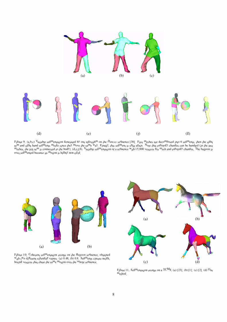
(a) (b) (c)
(d) (e) (f) (g)
Figure 9: (a,b,c) Variable segmentation generated by our algorithm on the Dancer sequence [38]. First meshes are decomposed into 6 segments, then the right
arm and right hand segments merge since they move the same way. Finally, this segment is split again. Note that topology changes can be handled (in the last
meshes, the left arm is connected to the body). (d,e,f,g): Variable segmentation of a sequence with 15,000 vertices per mesh and topology changes. The balloon is
over-segmented because its motion is highly non rigid.
(a) (b)
Figure 10: Coherent segmentation results on the Balloon sequence, obtained
with two different eigengap values: (a) 0.48, (b) 0.8. Segments cluster neigh-
boring vertices that share the same motion over the whole sequence.
(a) (b)
(c) (d)
Figure 11: Segmentation results on a TCMS. (a) [23]. (b) [1]. (c) [2]. (d) Our
method.
8
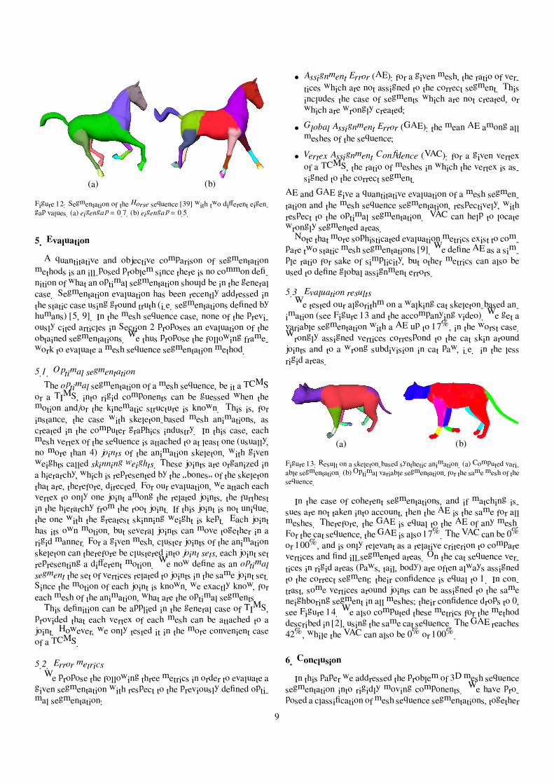
(a) (b)
Figure 12: Segmentation of the Horse sequence [39] with two different eigen-
gap values. (a) eigengap = 0.7. (b) eigengap = 0.5.
5. Evaluation
A quantitative and objective comparison of segmentation
methods is an ill-posed problem since there is no common defi-
nition of what an optimal segmentation should be in the general
case. Segmentation evaluation has been recently addressed in
the static case using ground truth (i.e. segmentations defined by
humans) [5, 9]. In the mesh sequence case, none of the previ-
ously cited articles in Section 2 proposes an evaluation of the
obtained segmentations. We thus propose the following frame-
work to evaluate a mesh sequence segmentation method.
5.1. Optimal segmentation
The optimal segmentation of a mesh sequence, be it a TCMS
or a TIMS, into rigid components can be guessed when the
motion and/or the kinematic structure is known. This is, for
instance, the case with skeleton-based mesh animations, as
created in the computer graphics industry. In this case, each
mesh vertex of the sequence is attached to at least one (usually,
no more than 4) joints of the animation skeleton, with given
weights called skinning weights. These joints are organized in
a hierarchy, which is represented by the “bones” of the skeleton
that are, therefore, directed. For our evaluation, we attach each
vertex to only one joint among the related joints, the furthest
in the hierarchy from the root joint. If this joint is not unique,
the one with the greatest skinning weight is kept. Each joint
has its own motion, but several joints can move together in a
rigid manner. For a given mesh, cluster joints of the animation
skeleton can therefore be clustered into joint sets, each joint set
representing a different motion. We now define as an optimal
segment the set of vertices related to joints in the same joint set.
Since the motion of each joint is known, we exactly know, for
each mesh of the animation, what are the optimal segments.
This definition can be applied in the general case of TIMS,
provided that each vertex of each mesh can be attached to a
joint. However, we only tested it in the more convenient case
of a TCMS.
5.2. Error metrics
We propose the following three metrics in order to evaluate a
given segmentation with respect to the previously defined opti-
mal segmentation:
• Assignment Error (AE): for a given mesh, the ratio of ver-
tices which are not assigned to the correct segment. This
includes the case of segments which are not created, or
which are wrongly created;
• Global Assignment Error (GAE): the mean AE among all
meshes of the sequence;
• Vertex Assignment Confidence (VAC): for a given vertex
of a TCMS, the ratio of meshes in which the vertex is as-
signed to the correct segment.
AE and GAE give a quantitative evaluation of a mesh segmen-
tation and the mesh sequence segmentation, respectively, with
respect to the optimal segmentation. VAC can help to locate
wrongly segmented areas.
Note that more sophisticated evaluation metrics exist to com-
pare two static mesh segmentations [9]. We define AE as a sim-
ple ratio for sake of simplicity, but other metrics can also be
used to define global assignment errors.
5.3. Evaluation results
We tested our algorithm on a walking cat skeleton-based an-
imation (see Figure 13 and the accompanying video). We get a
variable segmentation with a AE up to 17%, in the worst case.
Wrongly assigned vertices correspond to the cat skin around
joints and to a wrong subdivision in cat paw, i.e. in the less
rigid areas.
(a) (b)
Figure 13: Result on a skeleton-based synthetic animation. (a) Computed vari-
able segmentation. (b) Optimal variable segmentation, for the same mesh of the
sequence.
In the case of coherent segmentations, and if matching is-
sues are not taken into account, then the AE is the same for all
meshes. Therefore, the GAE is equal to the AE of any mesh.
For the cat sequence, the GAE is also 17%. The VAC can be 0%
or 100%, and is only relevant as a relative criterion to compare
vertices and find ill-segmented areas. On the cat sequence ver-
tices in rigid areas (paws, tail, body) are often always assigned
to the correct segment; their confidence is equal to 1. In con-
trast, some vertices around joints can be assigned to the same
neighboring segment in all meshes; their confidence drops to 0,
see Figure 14. We also computed these metrics for the method
described in [2], using the same cat sequence. The GAE reaches
42%, while the VAC can also be 0% or 100%.
6. Conclusion
In this paper we addressed the problem of 3D mesh sequence
segmentation into rigidly moving components. We have pro-
posed a classification of mesh sequence segmentations, together
9
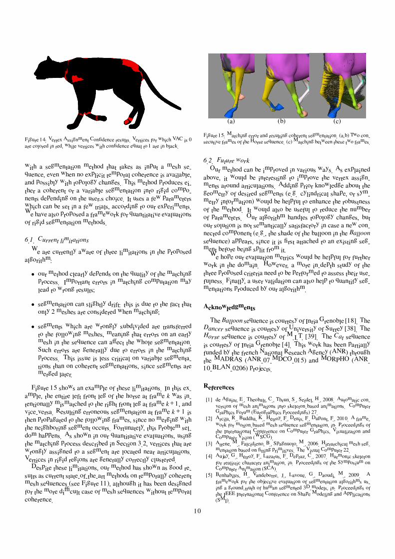
Figure 14: Vertex Assignment Confidence results. Vertices for which VAC is 0
are colored in red, while vertices with confidence equal to 1 are in black.
with a segmentation method that takes as input a mesh se-
quence, even when no explicit temporal coherence is available,
and possibly with topology changes. This method produces ei-
ther a coherent or a variable segmentation into rigid compo-
nents depending on the user’s choice. It uses a few parameters
which can be set in a few trials, according to our experiments.
We have also proposed a framework for quantitative evaluations
of rigid segmentation methods.
6.1. Current limitations
We are currently aware of three limitations in the proposed
algorithm:
• our method clearly depends on the quality of the matching
process. Important errors in matching computation may
lead to wrong results;
• segmentation can slightly drift: this is due to the fact that
only 2 meshes are considered when matching;
• segments which are wrongly subdivided are transferred
to the following meshes, meaning that errors on an early
mesh in the sequence can affect the whole segmentation.
Such errors are generally due to errors in the matching
process. This issue is less critical on variable segmenta-
tions than on coherent segmentations, since segments are
merged later.
Figure 15 shows an example of these limitations. In this ex-
ample, the entire left front leg of the horse at frame k was in-
tentionally mismatched to the right front leg at frame k+ 1, and
vice-versa. Resulting erroneous segmentation at frame k + 1 is
then propagated to the following frames, since no merging with
the neighboring segment occurs. Fortunately, this problem sel-
dom happens. As shown in our quantitative evaluations, using
the matching process described in Section 3.2, vertices that are
wrongly assigned to a segment are located near articulations.
Vertices in rigid regions are generally correctly clustered.
Despite these limitations, our method has shown as good re-
sults as current state-of-the-art methods on temporally coherent
mesh sequences (see Figure 11), although it has been designed
for the more difficult case of mesh sequences without temporal
coherence.
(a) (b) (c)
Figure 15: Matching error and resulting coherent segmentation. (a,b) Two con-
secutive frames of the Horse sequence. (c) Matching between these two frames.
6.2. Future work
Our method can be improved in various ways. As explained
above, it would be interesting to improve the vertex assign-
ments around articulations. Adding prior knowledge about the
geometry of desired segments (e.g. cylindrical shape, or sym-
metry information) would be helpful to enhance the robustness
of the method. It would also be useful to reduce the number
of parameters. Our algorithm handles topology changes, but
our solution is not semantically satisfactory in case a new con-
nected component (e.g., the shade of the balloon in the Balloon
sequence) appears, since it is first attached to an existing seg-
ment before being split from it.
We hope our evaluation metrics would be helpful for further
work in the domain. However, a more in-depth study of the
three proposed criteria need to be performed to assess their use-
fulness. Finally, a user validation can also help to quantify seg-
mentations produced by our algorithm.
Acknowledgments
The Balloon sequence is courtesy of Inria Grenoble [18]. The
Dancer sequence is courtesy of University of Surrey [38]. The
Horse sequence is courtesy of M.I.T. [39]. The Cat sequence
is courtesy of Inria Grenoble [4]. This work has been partially
funded by the french National Reseach Agency (ANR) through
the MADRAS (ANR-07-MDCO-015) and MORPHO (ANR-
10-BLAN-0206) projects.
References
[1] de Aguiar, E., Theobalt, C., Thrun, S., Seidel, H., 2008. Automatic con-
version of mesh animations into skeleton-based animations. Computer
Graphics Forum (Eurographics proceedings) 27.
[2] Arcila, R., Buddha, K., Hetroy, F., Denis, F., Dupont, F., 2010. A frame-
work for motion-based mesh sequence segmentation, in: Proceedings of
the International Conference on Computer Graphics, Visualization and
Computer Vision (WSCG).
[3] Attene, M., Falcidieno, B., Spagnuolo, M., 2006. Hierarchical mesh seg-
mentation based on fitting primitives. The Visual Computer 22.
[4] Aujay, G., Hetroy, F., Lazarus, F., Depraz, C., 2007. Harmonic skeleton
for realistic character animation, in: Proceedings of the Symposium on
Computer Animation (SCA).
[5] Benhabiles, H., Vandeborre, J., Lavoue, G., Daoudi, M., 2009. A
framework for the objective evaluation of segmentation algorithms us-
ing a ground-truth of human segmented 3D-models, in: Proceedings of
the IEEE International Conference on Shape Modeling and Applications
(SMI).
10
[6] Brox, T., Malik, J., 2010. Object segmentation by long term analysis of
point trajectories, in: Proceedings of the European Conference on Com-
puter Vision (ECCV).
[7] Cagniart, C., Boyer, E., Ilic, S., 2010. Iterative deformable surface track-
ing in multi-view setups, in: Proceedings of the International Symposium
on 3D Data Processing, Visualization and Transmission (3DPVT).
[8] Cashman, T., Hormann, K., 2012. A continuous, editable representation
for deforming mesh sequences with separate signals for time, pose and
shape. Computer Graphics Forum (Eurographics proceedings) 31.
[9] Chen, X., Golovinskiy, A., Funkhouser, T., 2009. A benchmark for 3d
mesh segmentation. ACM Transactions on Graphics (SIGGRAPH pro-
ceedings) 28.
[10] Cutzu, F., 2000. Computing 3d object parts from similarities among ob-
ject views, in: Proceedings of the IEEE Conference on Computer Vision
and Pattern Recognition (CVPR).
[11] Cuzzolin, F., Mateus, D., Knossow, D., Boyer, E., Horaud, R., 2008. Co-
herent laplacian 3-d protrusion segmentation, in: Proceedings of the IEEE
Conference on Computer Vision and Pattern Recognition (CVPR).
[12] Fang, Y., Sun, M., Kim, M., Ramani, K., 2011. Heat mapping: a robust
approach toward perceptually consistent mesh segmentation, in: Proceed-
ings of the IEEE Conference on Computer Vision and Pattern Recognition
(CVPR).
[13] Franco, J., Boyer, E., 2011. Learning temporally consistent rigidities,
in: Proceedings of the IEEE Conference on Computer Vision and Pattern
Recognition (CVPR).
[14] de Goes, F., Goldenstein, S., Velho, L., 2008. A hierarchical segmen-
tation of articulated bodies. Computer Graphics Forum (Symposium on
Geometry Processing proceedings) 27.
[15] Goldenthal, R., Harmon, D., Fattal, R., Bercovier, M., Grinspun, E., 2007.
Efficient simulation of inextensible cloth. ACM Transactions on Graphics
(SIGGRAPH proceedings) 26.
[16] Horn, B., 1987. Closed-form solution of absolute orientation using unit
quaternions. J. Opt. Soc. Am. A 4.
[17] Huang, Q., Wicke, M., Adams, B., Guibas, L., 2009. Shape decompo-
sition using modal analysis. Computer Graphics Forum (Eurographics
proceedings) 28.
[18] Inria, . Balloon sequence. http://4drepository.inrialpes.fr/.
[19] Kalafatlar, E., Yemez, Y., 2010. 3d articulated shape segmentation using
motion information, in: Proceedings of the International Conference on
Pattern Recognition (ICPR).
[20] Kalogerakis, E., Hertzmann, A., Singh, K., 2010. Learning 3d mesh seg-
mentation and labeling. ACM Transactions on Graphics (SIGGRAPH
proceedings) 29.
[21] Kircher, S., Garland, M., 2006. Editing arbitrarily deforming surface
animations. ACM Transactions on Graphics (SIGGRAPH proceedings)
25.
[22] Lee, N., T.Yamasaki, Aizawa, K., 2008. Hierarchical mesh decomposi-
tion and motion tracking for time-varying-meshes, in: Proceedings of the
IEEE International Conference on Multimedia and Expo (ICME).
[23] Lee, T.Y., Wang, Y.S., Chen, T.G., 2006. Segmenting a deforming mesh
into near-rigid components. The Visual Computer 22.
[24] Lengyel, J., 1999. Compression of time-dependent geometry, in: Pro-
ceedings of the Symposium on Interactive 3D graphics (I3D).
[25] Lewis, J., Cordner, M., Fong, N., 2000. Pose-space deformation: a uni-
fied approach to shape interpolation and skeleton-driven deformation, in:
Proceedings of SIGGRAPH.
[26] Liu, R., Zhang, H., 2004. Segmentation of 3d meshes through spectral
clustering, in: Proceedings of Pacific Graphics.
[27] Liu, R., Zhang, H., 2007. Mesh segmentation via spectral embedding and
contour analysis. Computer Graphics Forum (Eurographics proceedings)
26.
[28] von Luxburg, U., 2007. A tutorial on spectral clustering. Statistics and
Computing 17.
[29] Marras, S., Bronstein, M.M., Hormann, K., Scateni, R., Scopigno, R.,
2012. Motion-based mesh segmentation using augmented silhouettes.
Graphical Models .
[30] Murray, R., Sastry, S., Zexiang, L., 1994. A Mathematical Introduction
to Robotic Manipulation. CRC Press, Inc.
[31] Reuter, M., 2010. Hierarchical shape segmentation and registration via
topological features of laplace-beltrami eigenfunctions. International
Journal of Computer Vision 89.
[32] Rosman, G., Bronstein, M.M., Bronstein, A.M., Wolf, A., Kimmel, R.,
2011. Group-valued regularization framework for motion segmentation
of dynamic non-rigid shapes, in: Scale Space and Variational Methods in
Computer Vision.
[33] Shamir, A., 2008. A survey on mesh segmentation techniques. Computer
Graphics Forum 27.
[34] Sharma, A., von Lavante, E., Horaud, R., 2010. Learning shape segmen-
tation using constrained spectral clustering and probabilistic label trans-
fer, in: Proceedings of the European Conference on Computer Vision
(ECCV).
[35] Shi, J., Malik, J., 2000. Normalized cuts and image segmentation. IEEE
Transactions on Pattern Analysis and Machine Intelligence (PAMI) 22.
[36] Sidi, O., van Kaick, O., Kleiman, Y., Zhang, H., Cohen-Or, D., 2011. Un-
supervised co-segmentation of a set of shapes via descriptor-space spec-
tral clustering. ACM Transactions on Graphics (SIGGRAPH Asia pro-
ceedings) 30.
[37] Skraba, P., Ovsjanikov, M., Chazal, F., Guibas, L., 2010. Persistence-
based segmentation of deformable shapes, in: CVPR Workshop on Non-
Rigid Shape Analysis and Deformable Image Alignment.
[38] Starck, J., Hilton, A., 2007. Surface capture for performance-based ani-
mation. IEEE Computer Graphics and Applications .
[39] Sumner, R., Popovic, J., 2004. Deformation transfer for triangle meshes.
ACM Transactions on Graphics (SIGGRAPH proceedings) 23.
[40] Tung, T., Matsuyama, T., 2009. Topology dictionary with markov model
for 3d video content-based skimming and description, in: Proceedings
of the IEEE Conference on Computer Vision and Pattern Recognition
(CVPR).
[41] Tung, T., Matsuyama, T., 2010. 3d video performance segmentation, in:
Proceedings of the IEEE International Conference on Image Processing
(ICIP).
[42] Varanasi, K., Boyer, E., 2010. Temporally coherent segmentation of 3d
reconstructions, in: Proceedings of the International Symposium on 3D
Data Processing, Visualization and Transmission (3DPVT).
[43] Vlasic, D., Baran, I., Matusik, W., Popovic, J., 2008. Articulated mesh
animation from multi-view silhouettes. ACM Transactions on Graphics
(SIGGRAPH proceedings) 27.
[44] Wuhrer, S., Brunton, A., 2010. Segmenting animated objects into near-
rigid components. The Visual Computer .
[45] Yamasaki, T., Aizawa, K., 2007. Motion segmentation and retrieval for
3d video based on modified shape distribution. EURASIP Journal on
Applied Signal Processing .
11

192 APPENDIX A. SELECTED PAPERS

A.8. AUTOMATIC LOCALIZATION AND QUANTIFICATION OF INTRACRANIALANEURYSMS 193
∴
A.8 AUTOMATIC LOCALIZATION ANDQUANTIFICATION OF INTRACRANIALANEURYSMS
Sahar Hassan, Franck Hétroy, François Faure, Olivier PalombiLecture Notes in Computer Science 6854, Springer, 2011. Presented at the
International Conference on Computer Analysis of Images and Patterns (CAIP), 2011.

194 APPENDIX A. SELECTED PAPERS
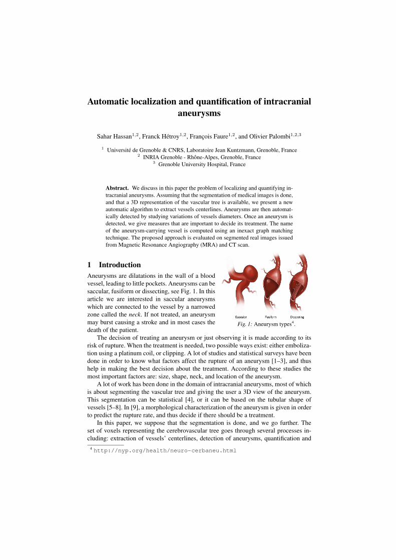
Automatic localization and quantification of intracranialaneurysms
Sahar Hassan1,2, Franck Hetroy1,2, Francois Faure1,2, and Olivier Palombi1,2,3
1 Universite de Grenoble & CNRS, Laboratoire Jean Kuntzmann, Grenoble, France2 INRIA Grenoble - Rhone-Alpes, Grenoble, France
3 Grenoble University Hospital, France
Abstract. We discuss in this paper the problem of localizing and quantifying in-tracranial aneurysms. Assuming that the segmentation of medical images is done,and that a 3D representation of the vascular tree is available, we present a newautomatic algorithm to extract vessels centerlines. Aneurysms are then automat-ically detected by studying variations of vessels diameters. Once an aneurysm isdetected, we give measures that are important to decide its treatment. The nameof the aneurysm-carrying vessel is computed using an inexact graph matchingtechnique. The proposed approach is evaluated on segmented real images issuedfrom Magnetic Resonance Angiography (MRA) and CT scan.
1 Introduction
Fig. 1: Aneurysm types4.
Aneurysms are dilatations in the wall of a bloodvessel, leading to little pockets. Aneurysms can besaccular, fusiform or dissecting, see Fig. 1. In thisarticle we are interested in saccular aneurysmswhich are connected to the vessel by a narrowedzone called the neck. If not treated, an aneurysmmay burst causing a stroke and in most cases thedeath of the patient.
The decision of treating an aneurysm or just observing it is made according to itsrisk of rupture. When the treatment is needed, two possible ways exist: either emboliza-tion using a platinum coil, or clipping. A lot of studies and statistical surveys have beendone in order to know what factors affect the rupture of an aneurysm [1–3], and thushelp in making the best decision about the treatment. According to these studies themost important factors are: size, shape, neck, and location of the aneurysm.
A lot of work has been done in the domain of intracranial aneurysms, most of whichis about segmenting the vascular tree and giving the user a 3D view of the aneurysm.This segmentation can be statistical [4], or it can be based on the tubular shape ofvessels [5–8]. In [9], a morphological characterization of the aneurysm is given in orderto predict the rupture rate, and thus decide if there should be a treatment.
In this paper, we suppose that the segmentation is done, and we go further. Theset of voxels representing the cerebrovascular tree goes through several processes in-cluding: extraction of vessels’ centerlines, detection of aneurysms, quantification and4 http://nyp.org/health/neuro-cerbaneu.html
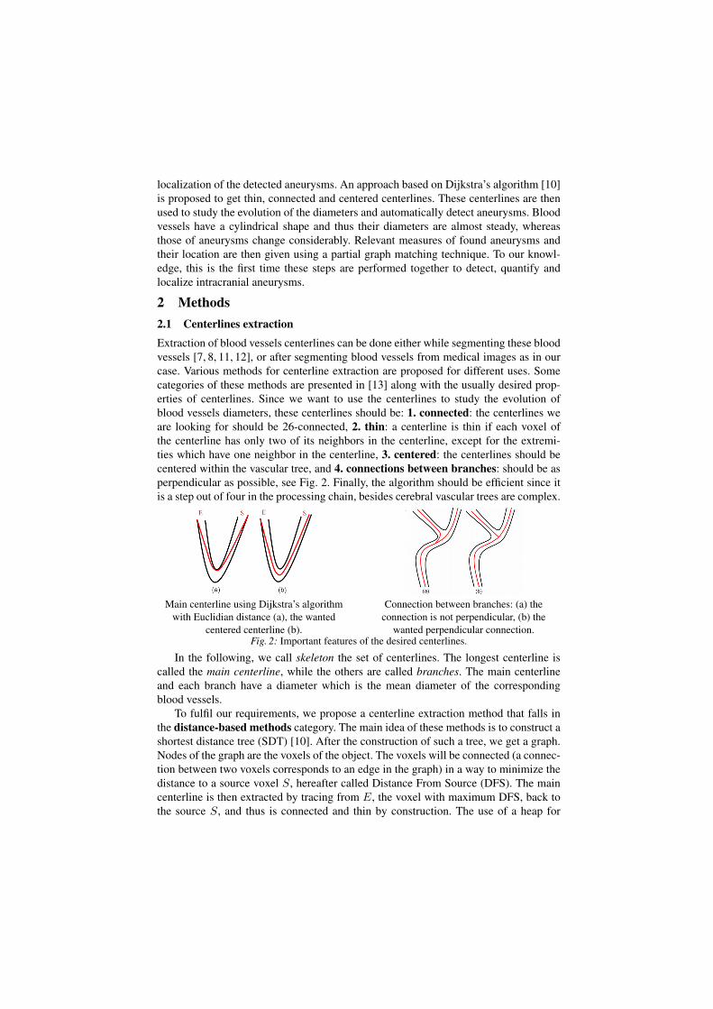
localization of the detected aneurysms. An approach based on Dijkstra’s algorithm [10]is proposed to get thin, connected and centered centerlines. These centerlines are thenused to study the evolution of the diameters and automatically detect aneurysms. Bloodvessels have a cylindrical shape and thus their diameters are almost steady, whereasthose of aneurysms change considerably. Relevant measures of found aneurysms andtheir location are then given using a partial graph matching technique. To our knowl-edge, this is the first time these steps are performed together to detect, quantify andlocalize intracranial aneurysms.
2 Methods2.1 Centerlines extraction
Extraction of blood vessels centerlines can be done either while segmenting these bloodvessels [7, 8, 11, 12], or after segmenting blood vessels from medical images as in ourcase. Various methods for centerline extraction are proposed for different uses. Somecategories of these methods are presented in [13] along with the usually desired prop-erties of centerlines. Since we want to use the centerlines to study the evolution ofblood vessels diameters, these centerlines should be: 1. connected: the centerlines weare looking for should be 26-connected, 2. thin: a centerline is thin if each voxel ofthe centerline has only two of its neighbors in the centerline, except for the extremi-ties which have one neighbor in the centerline, 3. centered: the centerlines should becentered within the vascular tree, and 4. connections between branches: should be asperpendicular as possible, see Fig. 2. Finally, the algorithm should be efficient since itis a step out of four in the processing chain, besides cerebral vascular trees are complex.
Main centerline using Dijkstra’s algorithmwith Euclidian distance (a), the wanted
centered centerline (b).
Connection between branches: (a) theconnection is not perpendicular, (b) thewanted perpendicular connection.
Fig. 2: Important features of the desired centerlines.
In the following, we call skeleton the set of centerlines. The longest centerline iscalled the main centerline, while the others are called branches. The main centerlineand each branch have a diameter which is the mean diameter of the correspondingblood vessels.
To fulfil our requirements, we propose a centerline extraction method that falls inthe distance-based methods category. The main idea of these methods is to construct ashortest distance tree (SDT) [10]. After the construction of such a tree, we get a graph.Nodes of the graph are the voxels of the object. The voxels will be connected (a connec-tion between two voxels corresponds to an edge in the graph) in a way to minimize thedistance to a source voxel S, hereafter called Distance From Source (DFS). The maincenterline is then extracted by tracing from E, the voxel with maximum DFS, back tothe source S, and thus is connected and thin by construction. The use of a heap for
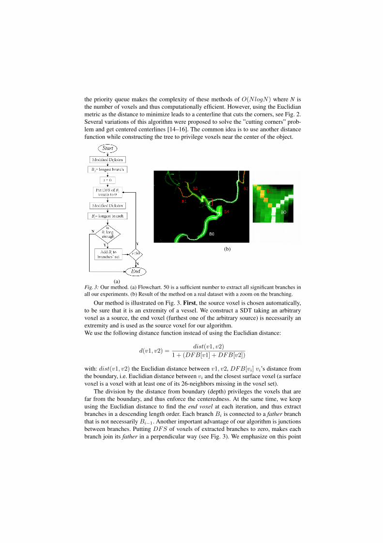
the priority queue makes the complexity of these methods of O(NlogN) where N isthe number of voxels and thus computationally efficient. However, using the Euclidianmetric as the distance to minimize leads to a centerline that cuts the corners, see Fig. 2.Several variations of this algorithm were proposed to solve the ”cutting corners” prob-lem and get centered centerlines [14–16]. The common idea is to use another distancefunction while constructing the tree to privilege voxels near the center of the object.
(a)
(b)
Fig. 3: Our method. (a) Flowchart. 50 is a sufficient number to extract all significant branches inall our experiments. (b) Result of the method on a real dataset with a zoom on the branching.
Our method is illustrated on Fig. 3. First, the source voxel is chosen automatically,to be sure that it is an extremity of a vessel. We construct a SDT taking an arbitraryvoxel as a source, the end voxel (furthest one of the arbitrary source) is necessarily anextremity and is used as the source voxel for our algorithm.We use the following distance function instead of using the Euclidian distance:
d(v1, v2) =dist(v1, v2)
1 + (DFB[v1] +DFB[v2])
with: dist(v1, v2) the Euclidian distance between v1, v2, DFB[vi] vi’s distance fromthe boundary, i.e. Euclidian distance between vi and the closest surface voxel (a surfacevoxel is a voxel with at least one of its 26-neighbors missing in the voxel set).
The division by the distance from boundary (depth) privileges the voxels that arefar from the boundary, and thus enforce the centeredness. At the same time, we keepusing the Euclidian distance to find the end voxel at each iteration, and thus extractbranches in a descending length order. Each branch Bi is connected to a father branchthat is not necessarily Bi−1. Another important advantage of our algorithm is junctionsbetween branches. Putting DFS of voxels of extracted branches to zero, makes eachbranch join its father in a perpendicular way (see Fig. 3). We emphasize on this point
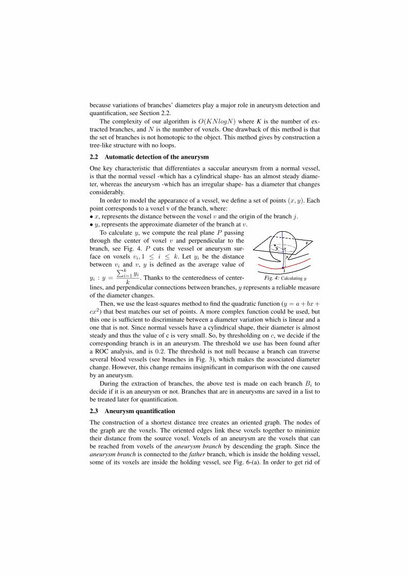
because variations of branches’ diameters play a major role in aneurysm detection andquantification, see Section 2.2.
The complexity of our algorithm is O(KNlogN) where K is the number of ex-tracted branches, and N is the number of voxels. One drawback of this method is thatthe set of branches is not homotopic to the object. This method gives by construction atree-like structure with no loops.
2.2 Automatic detection of the aneurysm
One key characteristic that differentiates a saccular aneurysm from a normal vessel,is that the normal vessel -which has a cylindrical shape- has an almost steady diame-ter, whereas the aneurysm -which has an irregular shape- has a diameter that changesconsiderably.
In order to model the appearance of a vessel, we define a set of points (x, y). Eachpoint corresponds to a voxel v of the branch, where:• x, represents the distance between the voxel v and the origin of the branch j.• y, represents the approximate diameter of the branch at v.
Fig. 4: Calculating y
To calculate y, we compute the real plane P passingthrough the center of voxel v and perpendicular to thebranch, see Fig. 4. P cuts the vessel or aneurysm sur-face on voxels vi, 1 ≤ i ≤ k. Let yi be the distancebetween vi and v, y is defined as the average value of
yi : y =
ki=1 yik
. Thanks to the centeredness of center-lines, and perpendicular connections between branches, y represents a reliable measureof the diameter changes.
Then, we use the least-squares method to find the quadratic function (y = a+ bx+cx2) that best matches our set of points. A more complex function could be used, butthis one is sufficient to discriminate between a diameter variation which is linear and aone that is not. Since normal vessels have a cylindrical shape, their diameter is almoststeady and thus the value of c is very small. So, by thresholding on c, we decide if thecorresponding branch is in an aneurysm. The threshold we use has been found aftera ROC analysis, and is 0.2. The threshold is not null because a branch can traverseseveral blood vessels (see branches in Fig. 3), which makes the associated diameterchange. However, this change remains insignificant in comparison with the one causedby an aneurysm.
During the extraction of branches, the above test is made on each branch Bi todecide if it is an aneurysm or not. Branches that are in aneurysms are saved in a list tobe treated later for quantification.
2.3 Aneurysm quantification
The construction of a shortest distance tree creates an oriented graph. The nodes ofthe graph are the voxels. The oriented edges link these voxels together to minimizetheir distance from the source voxel. Voxels of an aneurysm are the voxels that canbe reached from voxels of the aneurysm branch by descending the graph. Since theaneurysm branch is connected to the father branch, which is inside the holding vessel,some of its voxels are inside the holding vessel, see Fig. 6-(a). In order to get rid of
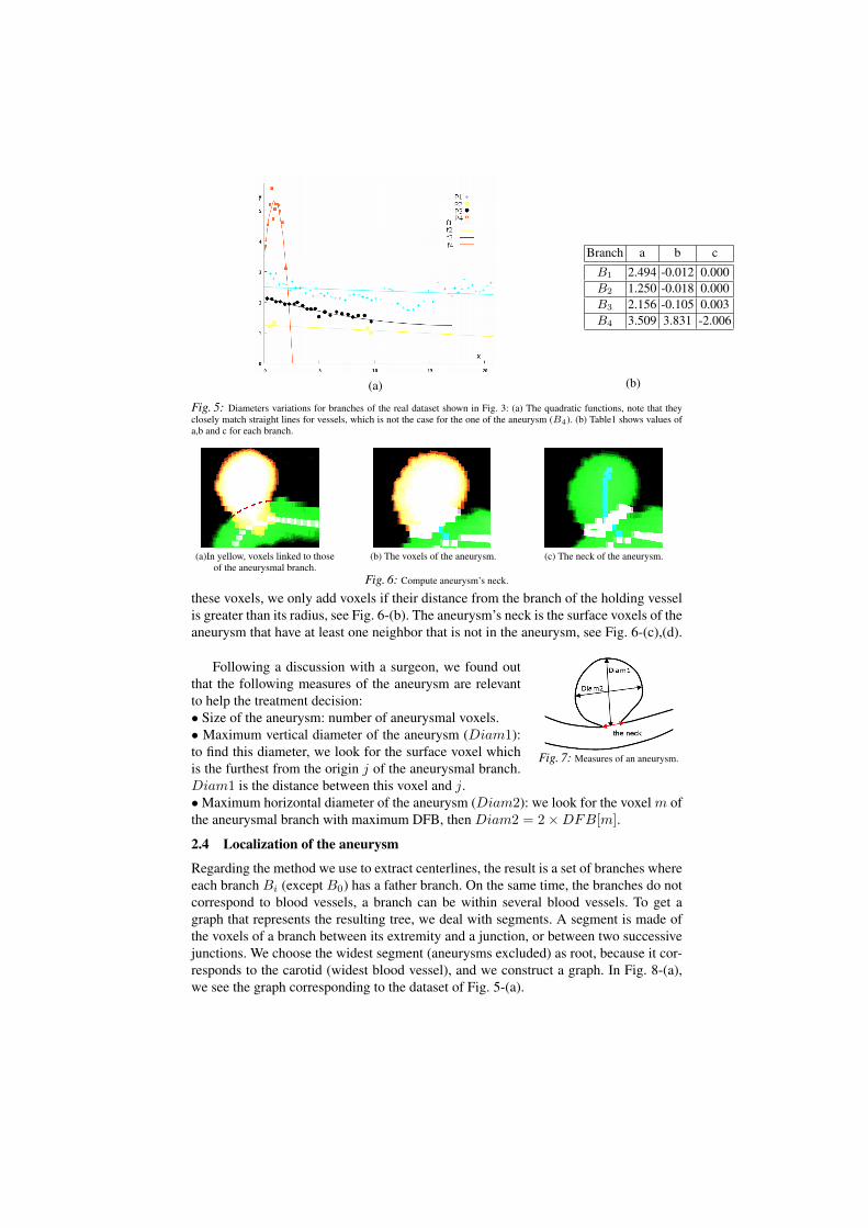
(a)
Branch a b c
B1 2.494 -0.012 0.000B2 1.250 -0.018 0.000B3 2.156 -0.105 0.003B4 3.509 3.831 -2.006
(b)
Fig. 5: Diameters variations for branches of the real dataset shown in Fig. 3: (a) The quadratic functions, note that theyclosely match straight lines for vessels, which is not the case for the one of the aneurysm (B4). (b) Table1 shows values ofa,b and c for each branch.
(a)In yellow, voxels linked to thoseof the aneurysmal branch.
(b) The voxels of the aneurysm. (c) The neck of the aneurysm.
Fig. 6: Compute aneurysm’s neck.these voxels, we only add voxels if their distance from the branch of the holding vesselis greater than its radius, see Fig. 6-(b). The aneurysm’s neck is the surface voxels of theaneurysm that have at least one neighbor that is not in the aneurysm, see Fig. 6-(c),(d).
Fig. 7: Measures of an aneurysm.
Following a discussion with a surgeon, we found outthat the following measures of the aneurysm are relevantto help the treatment decision:• Size of the aneurysm: number of aneurysmal voxels.• Maximum vertical diameter of the aneurysm (Diam1):to find this diameter, we look for the surface voxel whichis the furthest from the origin j of the aneurysmal branch.Diam1 is the distance between this voxel and j.•Maximum horizontal diameter of the aneurysm (Diam2): we look for the voxelm ofthe aneurysmal branch with maximum DFB, then Diam2 = 2×DFB[m].
2.4 Localization of the aneurysm
Regarding the method we use to extract centerlines, the result is a set of branches whereeach branch Bi (except B0) has a father branch. On the same time, the branches do notcorrespond to blood vessels, a branch can be within several blood vessels. To get agraph that represents the resulting tree, we deal with segments. A segment is made ofthe voxels of a branch between its extremity and a junction, or between two successivejunctions. We choose the widest segment (aneurysms excluded) as root, because it cor-responds to the carotid (widest blood vessel), and we construct a graph. In Fig. 8-(a),we see the graph corresponding to the dataset of Fig. 5-(a).
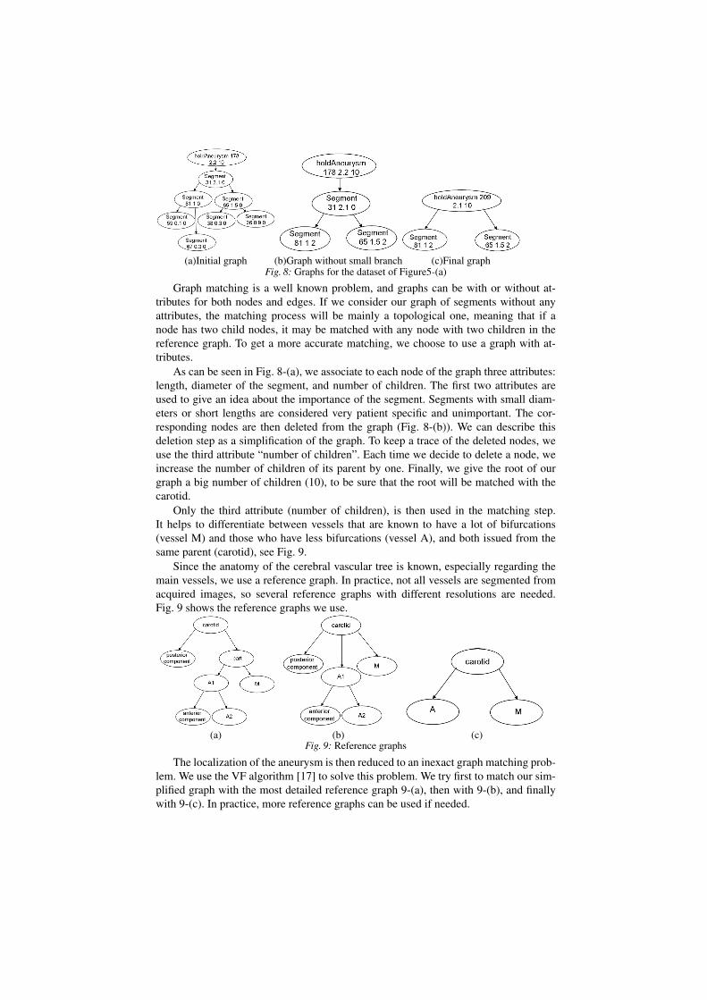
(a)Initial graph (b)Graph without small branch (c)Final graphFig. 8: Graphs for the dataset of Figure5-(a)
Graph matching is a well known problem, and graphs can be with or without at-tributes for both nodes and edges. If we consider our graph of segments without anyattributes, the matching process will be mainly a topological one, meaning that if anode has two child nodes, it may be matched with any node with two children in thereference graph. To get a more accurate matching, we choose to use a graph with at-tributes.
As can be seen in Fig. 8-(a), we associate to each node of the graph three attributes:length, diameter of the segment, and number of children. The first two attributes areused to give an idea about the importance of the segment. Segments with small diam-eters or short lengths are considered very patient specific and unimportant. The cor-responding nodes are then deleted from the graph (Fig. 8-(b)). We can describe thisdeletion step as a simplification of the graph. To keep a trace of the deleted nodes, weuse the third attribute “number of children”. Each time we decide to delete a node, weincrease the number of children of its parent by one. Finally, we give the root of ourgraph a big number of children (10), to be sure that the root will be matched with thecarotid.
Only the third attribute (number of children), is then used in the matching step.It helps to differentiate between vessels that are known to have a lot of bifurcations(vessel M) and those who have less bifurcations (vessel A), and both issued from thesame parent (carotid), see Fig. 9.
Since the anatomy of the cerebral vascular tree is known, especially regarding themain vessels, we use a reference graph. In practice, not all vessels are segmented fromacquired images, so several reference graphs with different resolutions are needed.Fig. 9 shows the reference graphs we use.
(a) (b) (c)Fig. 9: Reference graphs
The localization of the aneurysm is then reduced to an inexact graph matching prob-lem. We use the VF algorithm [17] to solve this problem. We try first to match our sim-plified graph with the most detailed reference graph 9-(a), then with 9-(b), and finallywith 9-(c). In practice, more reference graphs can be used if needed.
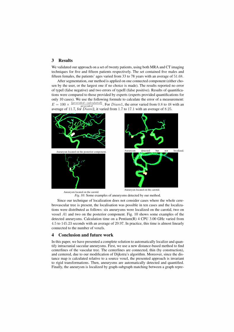
3 ResultsWe validated our approach on a set of twenty patients, using both MRA and CT imagingtechniques for five and fifteen patients respectively. The set contained five males andfifteen females, the patients’ ages varied from 33 to 78 years with an average of 51.68.
After segmentation, our method is applied on one connected component (either cho-sen by the user, or the largest one if no choice is made). The results reported no errorof typeI (false negative) and two errors of typeII (false positive). Results of quantifica-tions were compared to those provided by experts (experts provided quantifications foronly 10 cases). We use the following formule to calculate the error of a measurement:E = 100 × provided−calculated
provided . For Diam1, the error varied from 0.8 to 48 with anaverage of 11.7, for Diam2, it varied from 1.7 to 17.1 with an average of 8.25.
Aneurysm located on the posterior component.
Aneurysm located on the carotid.
Aneurysm detected but not localized.
Aneurysm located on the carotid.
Fig. 10: Some examples of aneurysms detected by our method.
Since our technique of localization does not consider cases where the whole cere-brovascular tree is present, the localisation was possible in ten cases and the localiza-tions were distributed as follows: six aneurysms were localized on the carotid, two onvessel A1 and two on the posterior component. Fig. 10 shows some examples of thedetected aneurysms. Calculation time on a Pentium(R) 4 CPU 3.00 GHz varied from4.5 to 145.23 seconds with an average of 29.97. In practice, this time is almost linearlyconnected to the number of voxels.
4 Conclusion and future workIn this paper, we have presented a complete solution to automatically localize and quan-tify intracranial saccular aneurysms. First, we use a new distance-based method to findcenterlines of the vascular tree. The centerlines are connected, thin (by construction),and centered, due to our modification of Dijkstra’s algorithm. Moreover, since the dis-tance map is calculated relative to a source voxel, the presented approach is invariantto rigid transformations. Then, aneurysms are automatically detected and quantified.Finally, the aneurysm is localized by graph-subgraph matching between a graph repre-
senting the centerlines and a reference graph.When applying our method to 3D medical images, it proved to be fast and robust sincethe quality of the results is independent of small segmentation artifacts.
References1. Ujiie, H., Tachibana, H., Hiramatsu, O., Hazel, A., Matsumoto, T., Ogasawara, Y., Naka-jima, H., Hori, T., Takakura, K., Kajiya, F.: Effectes of size and shape (aspect ratio) on theheomdynamics of saccular aneurysms: a possible index for surgical treatment of intracranialaneurysms. Neurosurgery 45 (1999) 119–130
2. Weir, B.: Unruptured intracranial aneurysms: a review. J Neurosurgery 96 (2002) 3–423. Ecker, R., Hopkins, L.: Natural history of unruptured intracranial aneurysms. NeurosurgFocus 17(5) (2004)
4. Wilson, D.L., Noble, J.A.: Segmentation of cerebral vessels and aneurysms from mr angiog-raphy data. In: IPMI ’97: Proceedings of the 15th International Conference on InformationProcessing in Medical Imaging, London, UK, Springer-Verlag (1997) 423–428
5. Aylward, S., Pizer, S., Eberly, D., Bullitt, E.: Intensity ridge and widths for tubular objectsegmentation and description. Mathematical Methods in Biomedical Image Analysis, IEEEWorkshop on 0 (1996) 0131
6. Frangi, A.F., Niessen, W.J., Vincken, K.L., Viergever, M.A.: Multiscale vessel enhancementfiltering. Medical Image Computing and Computer-Assisted Interventation, MICCAI 98(1998)
7. Wink, O., Niessen, W., Viergever, M.: Multiscale vessel tracking. Medical Image Analysis23(1) (January 2004) 130–133
8. Descoteaux, M., Collins, D.L., Siddiqi, K.: A geometric flow for segmenting vasculature inproton-density weighted mri. Medical Image Analysis 12(4) (2008) 497 – 513
9. Millan, R.D., Dempere-Marco, L., Pozo, J., Cebral, J., Frangi, A.: Morphological charac-terization of intracranial aneurysms using 3-d moment invariants. Medical Imaging, IEEETransactions on 26(9) (2007) 1270–1282
10. Dijkstra, E.W.: A note on two problems in connexion with graphs. Numerische Mathematik1 (1959) 269–271
11. Aylward, S.R., Bullitt, E.: Initialization, noise, singularities, and scale in height ridge traver-sal for tubular object centerline extraction. IEEE Transactions on Medical Imaging 21(2)(2002) 61–75
12. Deschamps, T., Cohen, L.: Fast extraction of minimal paths in 3D images and applicationsto virtual endoscopy. Medical Image Analysis 5(4) (2001)
13. Cornea, N., Silver, D., Min, P.: Curve-skeleton properties, applications, and algorithms.IEEE Transactions on Visualization and Computer Graphics 13(3) (2007) 530–548
14. Bitter, I., Sato, M., Bender, M., McDonnell, K.T., Kaufman, A., Wan, M.: CEASAR: asmooth, accurate and robust centerline extraction algorithm. In: VIS ’00: Proceedings ofthe conference on Visualization ’00, Los Alamitos, CA, USA, IEEE Computer Society Press(2000) 45–52
15. Bitter, I., Kaufman, A.E., Sato, M.: Penalized-distance volumetric skeleton algorithm. IEEETransactions on Visualization and Computer Graphics 7(3) (2001) 195–206
16. Wan, M., Liang, Z., Ke, Q., Hong, L., Bitter, I., Kaufman, A.E.: Automatic centerline ex-traction for virtual colonoscopy. IEEE Trans. Med. Imaging 21 (2002) 1450–1460
17. Cordella, L.P., Foggia, P., Sansone, C., Vento, M.: An improved algorithm for matching largegraphs. 3rd IAPRTC15 Workshop on Graph-based representations in Pattern Recognition(2001) 149–159
A.9. SEGMENTATION OF TREE SEEDLING POINT CLOUDS INTOELEMENTARY UNITS 203
∴
A.9 SEGMENTATION OF TREE SEEDLING POINTCLOUDS INTO ELEMENTARY UNITS
Franck Hétroy-Wheeler, Eric Casella, Dobrina BoltchevaInternational Journal of Remote Sensing, Taylor & Francis, 2016.

204 APPENDIX A. SELECTED PAPERS
March 16, 2016 International Journal of Remote Sensing plantscan
To appear in the International Journal of Remote SensingVol. 00, No. 00, Month 20XX, 1–27
Segmentation of tree seedling point clouds
into elementary units
Franck Hetroy-Wheelera∗, Eric Casellab∗ and Dobrina Boltchevac
aUniv. Grenoble Alpes & Inria, Laboratoire Jean Kuntzmann, 655 avenue de l’Europe,
F-38334 Saint Ismier cedex, FrancebCentre for Sustainable Forestry and Climate Change, Forest research, Farnham, Surrey,
GU10 4LH, United KingdomcUniv. Lorraine & Inria, LORIA, Nancy, France
(Received 00 Month 20XX; accepted 00 Month 20XX)
This paper describes a new semi-automatic method to cluster TLS data intomeaningful sets of points to extract plant components. The approach is designedfor small plants with distinguishable branches and leaves, such as tree seedlings.It first creates a graph by connecting each point to its most relevant neighbours,then embeds the graph into a spectral space, and finally segments the embeddinginto clusters of points. The process can then be iterated on each cluster separately.The main idea underlying the approach is that the spectral embedding of the graphaligns the points along the shape’s principal directions. A quantitative evaluation ofthe segmentation accuracy, as well as of leaf area estimates, is provided on a poplarseedling mock-up. It shows that the segmentation is robust with false positive andfalse negative rates around 1%. Qualitative results on four contrasting plant specieswith three different scan resolution levels each are also shown.
Keywords: terrestrial laser scanning; tLiDAR; 3D point cloud; segmentation;spectral clustering; tree seedling
1. Introduction
Functional-structural plant models describe a plant as a collection of intercon-nected elementary units (internode, petiole, leaf-blade, see Godin et al. (1999)).Their goal is to help biologists understand the relationships between the plantstructure and the biological and physical mechanisms underlying the plant growth(Godin and Sinoquet (2005)). These models require an in situ validation on realplants, that can be done by measuring the three-dimensional (3D) characteristicsof vegetation. Similarly the growing field of plant phenomics, which is concernedwith the discovery and analysis of complex plant traits (Furbank and Tester (2011);International Plant Phenotyping Network (2016)), requires the measurement ofindividual quantitative parameters such as leaf characteristics.
Destructive measurements have long been used but are time consuming andexpensive. As a consequence, various kinds of sensors are being investigated
∗Corresponding authors. Emails: [email protected]; [email protected]
1
March 16, 2016 International Journal of Remote Sensing plantscan
for non-destructive and non-invasive plant metrology. For example, the use ofdifferent imaging techniques has been proposed for plant phenotyping, see Li et al.(2014) for a review. The most popular imaging techniques are based on single-lenscameras (Quan et al. (2006); Paproki et al. (2012)), time-of-flight cameras (Cheneet al. (2012); Alenya et al. (2013); Chaivivatrakul et al. (2014); Xia et al. (2015))or multi-view stereo imaging systems (Golbach et al. (2015); Lou et al. (2015);Rose et al. (2015)). All these methods allow one to reconstruct and measure singleleaves, although some of them require manual interaction (Quan et al. (2006);Golbach et al. (2015); Rose et al. (2015)) or prior knowledge of the plant (Cheneet al. (2012); Chaivivatrakul et al. (2014)).
Terrestrial laser scanning (TLS), a remote sensing technique, has become anincreasingly popular technique to measure vegetation from grass to forest plantspecies, see e.g. Dassot et al. (2011); Lin (2015) for recent reviews. Comparedto imaging techniques, TLS provides direct accurate 3D measurements. It hasalso proved to be more robust to diverse environments, in particular to changinglighting conditions (Li et al. (2014); Lin (2015)). Thus, LiDAR seems moreadapted to greenhouse and field conditions (Tilly et al. (2012); Lin (2015)).
TLS generates unstructured sets of points where its laser beam is incident andreflected. Thus it gives a raw sketch of the spatial distribution of plant elements in3D, but it lacks explicit and essential information on their shape and connectivity.The points need to be clustered into geometrically meaningful sets for furtheranalysis and dendrometric measurements. For example, leaf-blade points need tobe separated from petiole and internode points to assess leaf areas.
In this paper, we segment TLS data of small plants or tree seedling scans intotheir elementary units: internodes, petioles and leaf-blades. Our method only con-siders the 3D positions of the points (no intensity value or normal estimate isrequired). As a consequence, it can be applied to sets of 3D points generated byother techniques than TLS such as time-of-flight cameras. We focus on accuratesegmentation so that individual elementary unit characteristics such as leaf areaare estimated as accurately as possible.
1.1. Related work
Segmentation of 3D data is critical for many applications in science. Researchhas considered the segmentation of point clouds into basic geometric primitives(planes, cylinders, spheres, etc.) for various purposes, such as building or citymodelling (see Haala and Kada (2010) for a survey), reverse engineering ofmechanical objects (e.g. Bey et al. (2011); Li et al. (2011)), or backgroundsubtraction, see Nguyen and Le (2013) for a recent overview. These approachesare designed for man-made objects which can be almost completely decomposedinto uniform geometric shapes. Yet since stems and leaves are not exactly cylin-drical and planar shapes, their efficiency to robustly segment plants is questionable.
The problem we are interested in, that is the segmentation of plants into theirelementary units, has been partially tackled in the literature. Recovering thebranching structure of a plant or a leaf-on tree is a specific issue that has beenaddressed in order to estimate various wood parameters by e.g., Bayer et al.(2013); Belton et al. (2013). Some authors additionally propose to reconstruct
2
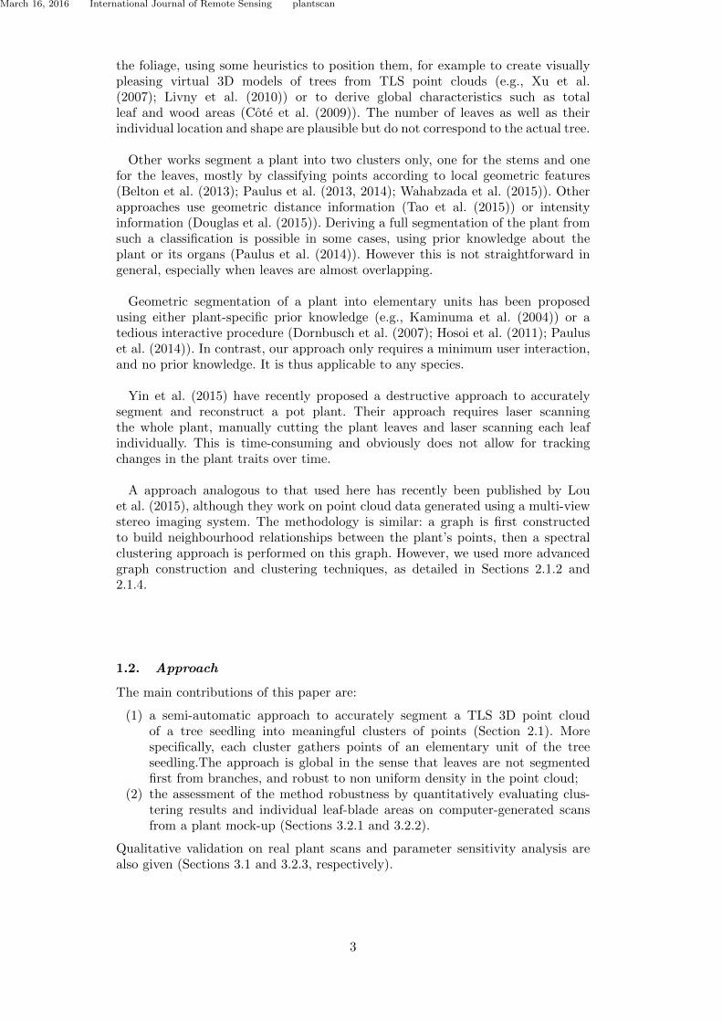
March 16, 2016 International Journal of Remote Sensing plantscan
the foliage, using some heuristics to position them, for example to create visuallypleasing virtual 3D models of trees from TLS point clouds (e.g., Xu et al.(2007); Livny et al. (2010)) or to derive global characteristics such as totalleaf and wood areas (Cote et al. (2009)). The number of leaves as well as theirindividual location and shape are plausible but do not correspond to the actual tree.
Other works segment a plant into two clusters only, one for the stems and onefor the leaves, mostly by classifying points according to local geometric features(Belton et al. (2013); Paulus et al. (2013, 2014); Wahabzada et al. (2015)). Otherapproaches use geometric distance information (Tao et al. (2015)) or intensityinformation (Douglas et al. (2015)). Deriving a full segmentation of the plant fromsuch a classification is possible in some cases, using prior knowledge about theplant or its organs (Paulus et al. (2014)). However this is not straightforward ingeneral, especially when leaves are almost overlapping.
Geometric segmentation of a plant into elementary units has been proposedusing either plant-specific prior knowledge (e.g., Kaminuma et al. (2004)) or atedious interactive procedure (Dornbusch et al. (2007); Hosoi et al. (2011); Pauluset al. (2014)). In contrast, our approach only requires a minimum user interaction,and no prior knowledge. It is thus applicable to any species.
Yin et al. (2015) have recently proposed a destructive approach to accuratelysegment and reconstruct a pot plant. Their approach requires laser scanningthe whole plant, manually cutting the plant leaves and laser scanning each leafindividually. This is time-consuming and obviously does not allow for trackingchanges in the plant traits over time.
A approach analogous to that used here has recently been published by Louet al. (2015), although they work on point cloud data generated using a multi-viewstereo imaging system. The methodology is similar: a graph is first constructedto build neighbourhood relationships between the plant’s points, then a spectralclustering approach is performed on this graph. However, we used more advancedgraph construction and clustering techniques, as detailed in Sections 2.1.2 and2.1.4.
1.2. Approach
The main contributions of this paper are:
(1) a semi-automatic approach to accurately segment a TLS 3D point cloudof a tree seedling into meaningful clusters of points (Section 2.1). Morespecifically, each cluster gathers points of an elementary unit of the treeseedling.The approach is global in the sense that leaves are not segmentedfirst from branches, and robust to non uniform density in the point cloud;
(2) the assessment of the method robustness by quantitatively evaluating clus-tering results and individual leaf-blade areas on computer-generated scansfrom a plant mock-up (Sections 3.2.1 and 3.2.2).
Qualitative validation on real plant scans and parameter sensitivity analysis arealso given (Sections 3.1 and 3.2.3, respectively).
3
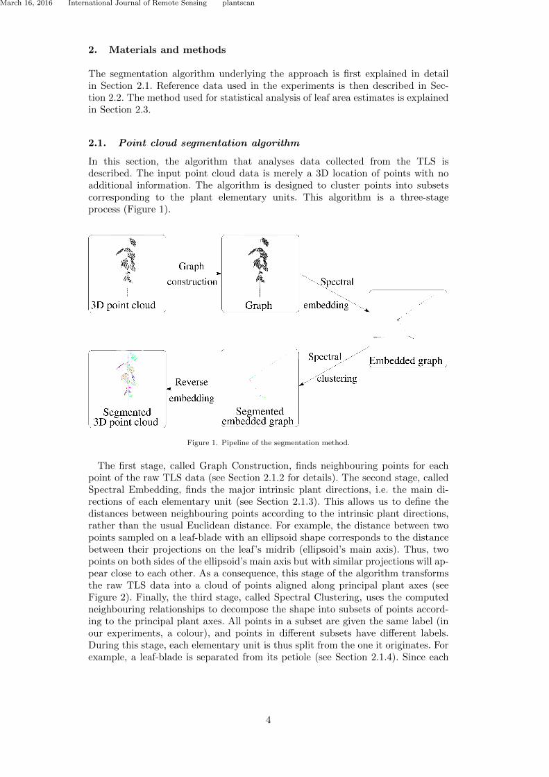
March 16, 2016 International Journal of Remote Sensing plantscan
2. Materials and methods
The segmentation algorithm underlying the approach is first explained in detailin Section 2.1. Reference data used in the experiments is then described in Sec-tion 2.2. The method used for statistical analysis of leaf area estimates is explainedin Section 2.3.
2.1. Point cloud segmentation algorithm
In this section, the algorithm that analyses data collected from the TLS isdescribed. The input point cloud data is merely a 3D location of points with noadditional information. The algorithm is designed to cluster points into subsetscorresponding to the plant elementary units. This algorithm is a three-stageprocess (Figure 1).
Figure 1. Pipeline of the segmentation method.
The first stage, called Graph Construction, finds neighbouring points for eachpoint of the raw TLS data (see Section 2.1.2 for details). The second stage, calledSpectral Embedding, finds the major intrinsic plant directions, i.e. the main di-rections of each elementary unit (see Section 2.1.3). This allows us to define thedistances between neighbouring points according to the intrinsic plant directions,rather than the usual Euclidean distance. For example, the distance between twopoints sampled on a leaf-blade with an ellipsoid shape corresponds to the distancebetween their projections on the leaf’s midrib (ellipsoid’s main axis). Thus, twopoints on both sides of the ellipsoid’s main axis but with similar projections will ap-pear close to each other. As a consequence, this stage of the algorithm transformsthe raw TLS data into a cloud of points aligned along principal plant axes (seeFigure 2). Finally, the third stage, called Spectral Clustering, uses the computedneighbouring relationships to decompose the shape into subsets of points accord-ing to the principal plant axes. All points in a subset are given the same label (inour experiments, a colour), and points in different subsets have different labels.During this stage, each elementary unit is thus split from the one it originates. Forexample, a leaf-blade is separated from its petiole (see Section 2.1.4). Since each
4
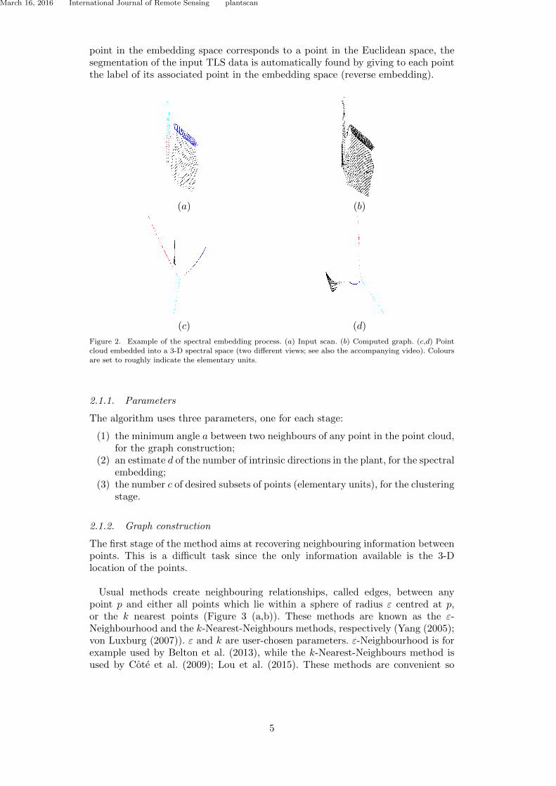
March 16, 2016 International Journal of Remote Sensing plantscan
point in the embedding space corresponds to a point in the Euclidean space, thesegmentation of the input TLS data is automatically found by giving to each pointthe label of its associated point in the embedding space (reverse embedding).
(a) (b)
(c) (d)
Figure 2. Example of the spectral embedding process. (a) Input scan. (b) Computed graph. (c,d) Point
cloud embedded into a 3-D spectral space (two different views; see also the accompanying video). Colours
are set to roughly indicate the elementary units.
2.1.1. Parameters
The algorithm uses three parameters, one for each stage:
(1) the minimum angle a between two neighbours of any point in the point cloud,for the graph construction;
(2) an estimate d of the number of intrinsic directions in the plant, for the spectralembedding;
(3) the number c of desired subsets of points (elementary units), for the clusteringstage.
2.1.2. Graph construction
The first stage of the method aims at recovering neighbouring information betweenpoints. This is a difficult task since the only information available is the 3-Dlocation of the points.
Usual methods create neighbouring relationships, called edges, between anypoint p and either all points which lie within a sphere of radius ε centred at p,or the k nearest points (Figure 3 (a,b)). These methods are known as the ε-Neighbourhood and the k-Nearest-Neighbours methods, respectively (Yang (2005);von Luxburg (2007)). ε and k are user-chosen parameters. ε-Neighbourhood is forexample used by Belton et al. (2013), while the k-Nearest-Neighbours method isused by Cote et al. (2009); Lou et al. (2015). These methods are convenient so
5
March 16, 2016 International Journal of Remote Sensing plantscan
long as the density of the point cloud is uniform, which is not the case for ourTLS data. For non-uniform samples, many redundant edges may be created orrelevant ones may be missed and the main problem is to find the right value for theparameters. This problem is shown on Figure 3 (a), where the ε-neighbourhoodof a blue point is depicted for two different values of ε (in green and in red andgreen, respectively). Similarly, the k-nearest-neighbours, for k = 2 (in green)and k = 5 (in red and green), are shown on Figure 3 (b). If ε or k is low, thecorresponding methods may miss relevant edges, such as the one between theblue point and the upper red point. If ε or k is high, they may create redun-dant edges such as the ones between the blue point and the left and right red points.
(a) (b) (c)
Figure 3. Examples of graph construction for the methods: (a) ε-neighbourhood of a point in blue, for
two different values of ε. (b) k-nearest-neighbours, for k = 2 and k = 5. (c) Proposed method, for a = 45.
Note that it is critical for the next stage of our approach, both in terms of mem-ory usage and computation time, to avoid redundant neighbouring relationshipssince during this stage we work with an adjacency matrix computed from theneighbouring graph. Therefore, the lower the number of neighbours for a givenpoint the sparser the matrix thus the faster the computation. This is why we havedeveloped a specific algorithm which is summarised in Algorithm 1 and Figure 3 (c).
This algorithm starts by selecting a number k of candidate neighbours for everypoint p ∈ P . In practice, we choose k = 0.1% of the total number of points. Then,in order to select the neighbours within the set of candidates, it uses one parameterwhich is the minimum angle a at p allowed between two edges with endpoint p(see Figure 3 (c)). If many candidates lie in the same direction, only one (theclosest) is selected as a neighbour of p. This prevents the creation of redundant,almost parallel, edges. On the contrary, this algorithm having found the closestpoint in a given direction will go on to look for other points farther away but ina distinctly different direction. Thus, this method captures all relevant edges andis robust to non-uniform density within the point cloud. Figure 3 (c) shows theresult of the method for a = 45. This method discards the two red points D sincethe corresponding edges are within a small angle of existing edges (in green) butit does capture point 3 which is a neighbour in a clearly different direction.
The graph construction runs this algorithm for every point p in the point cloud.The resulting neighbouring graph is thus the union of the selected edges E(p)for every p ∈ P . Note that we do not look for mutual nearest neighbours: if q iscomputed as a valid neighbour of p but p is not considered as a valid neighbourof q, we still connect these two points. Our experimental results have shownthat choosing the angle parameter a = 90 is a good compromise in practice(see Section 3.2.3). This allows us to search for neighbours in the 3 cardinaldirections around a point in 3D, which has been shown to be sufficient for building
6
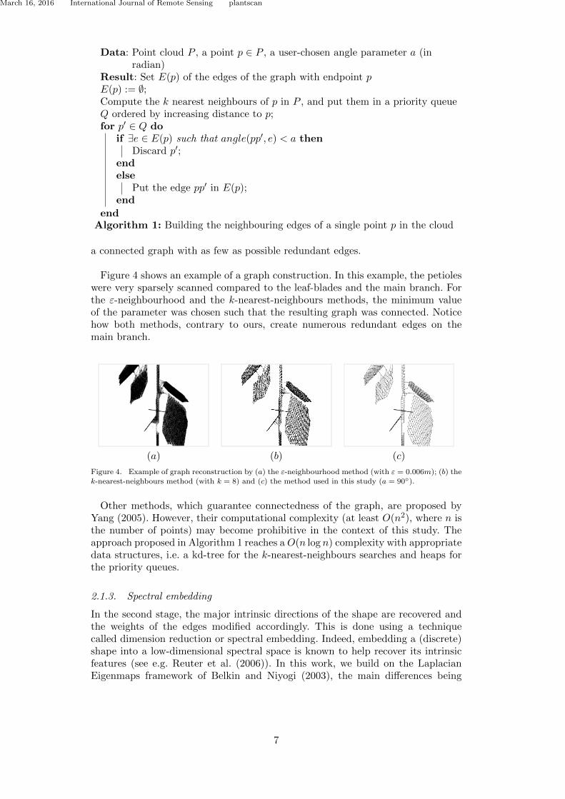
March 16, 2016 International Journal of Remote Sensing plantscan
Data: Point cloud P , a point p ∈ P , a user-chosen angle parameter a (inradian)
Result: Set E(p) of the edges of the graph with endpoint pE(p) := ∅;Compute the k nearest neighbours of p in P , and put them in a priority queueQ ordered by increasing distance to p;for p′ ∈ Q do
if ∃e ∈ E(p) such that angle(pp′, e) < a thenDiscard p′;
endelse
Put the edge pp′ in E(p);end
endAlgorithm 1: Building the neighbouring edges of a single point p in the cloud
a connected graph with as few as possible redundant edges.
Figure 4 shows an example of a graph construction. In this example, the petioleswere very sparsely scanned compared to the leaf-blades and the main branch. Forthe ε-neighbourhood and the k-nearest-neighbours methods, the minimum valueof the parameter was chosen such that the resulting graph was connected. Noticehow both methods, contrary to ours, create numerous redundant edges on themain branch.
(a) (b) (c)
Figure 4. Example of graph reconstruction by (a) the ε-neighbourhood method (with ε = 0.006m); (b) the
k-nearest-neighbours method (with k = 8) and (c) the method used in this study (a = 90).
Other methods, which guarantee connectedness of the graph, are proposed byYang (2005). However, their computational complexity (at least O(n2), where n isthe number of points) may become prohibitive in the context of this study. Theapproach proposed in Algorithm 1 reaches a O(n log n) complexity with appropriatedata structures, i.e. a kd-tree for the k-nearest-neighbours searches and heaps forthe priority queues.
2.1.3. Spectral embedding
In the second stage, the major intrinsic directions of the shape are recovered andthe weights of the edges modified accordingly. This is done using a techniquecalled dimension reduction or spectral embedding. Indeed, embedding a (discrete)shape into a low-dimensional spectral space is known to help recover its intrinsicfeatures (see e.g. Reuter et al. (2006)). In this work, we build on the LaplacianEigenmaps framework of Belkin and Niyogi (2003), the main differences being
7
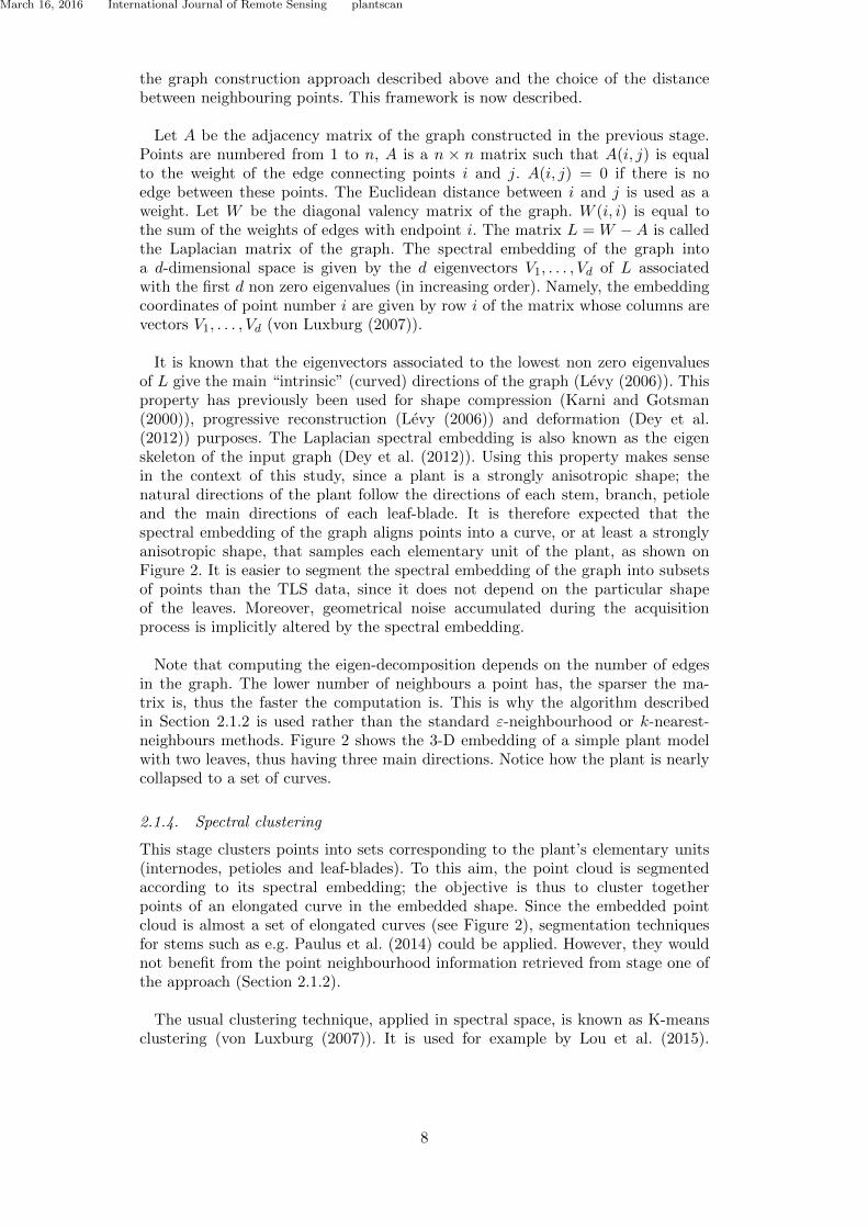
March 16, 2016 International Journal of Remote Sensing plantscan
the graph construction approach described above and the choice of the distancebetween neighbouring points. This framework is now described.
Let A be the adjacency matrix of the graph constructed in the previous stage.Points are numbered from 1 to n, A is a n × n matrix such that A(i, j) is equalto the weight of the edge connecting points i and j. A(i, j) = 0 if there is noedge between these points. The Euclidean distance between i and j is used as aweight. Let W be the diagonal valency matrix of the graph. W (i, i) is equal tothe sum of the weights of edges with endpoint i. The matrix L = W − A is calledthe Laplacian matrix of the graph. The spectral embedding of the graph intoa d-dimensional space is given by the d eigenvectors V1, . . . , Vd of L associatedwith the first d non zero eigenvalues (in increasing order). Namely, the embeddingcoordinates of point number i are given by row i of the matrix whose columns arevectors V1, . . . , Vd (von Luxburg (2007)).
It is known that the eigenvectors associated to the lowest non zero eigenvaluesof L give the main “intrinsic” (curved) directions of the graph (Levy (2006)). Thisproperty has previously been used for shape compression (Karni and Gotsman(2000)), progressive reconstruction (Levy (2006)) and deformation (Dey et al.(2012)) purposes. The Laplacian spectral embedding is also known as the eigenskeleton of the input graph (Dey et al. (2012)). Using this property makes sensein the context of this study, since a plant is a strongly anisotropic shape; thenatural directions of the plant follow the directions of each stem, branch, petioleand the main directions of each leaf-blade. It is therefore expected that thespectral embedding of the graph aligns points into a curve, or at least a stronglyanisotropic shape, that samples each elementary unit of the plant, as shown onFigure 2. It is easier to segment the spectral embedding of the graph into subsetsof points than the TLS data, since it does not depend on the particular shapeof the leaves. Moreover, geometrical noise accumulated during the acquisitionprocess is implicitly altered by the spectral embedding.
Note that computing the eigen-decomposition depends on the number of edgesin the graph. The lower number of neighbours a point has, the sparser the ma-trix is, thus the faster the computation is. This is why the algorithm describedin Section 2.1.2 is used rather than the standard ε-neighbourhood or k-nearest-neighbours methods. Figure 2 shows the 3-D embedding of a simple plant modelwith two leaves, thus having three main directions. Notice how the plant is nearlycollapsed to a set of curves.
2.1.4. Spectral clustering
This stage clusters points into sets corresponding to the plant’s elementary units(internodes, petioles and leaf-blades). To this aim, the point cloud is segmentedaccording to its spectral embedding; the objective is thus to cluster togetherpoints of an elongated curve in the embedded shape. Since the embedded pointcloud is almost a set of elongated curves (see Figure 2), segmentation techniquesfor stems such as e.g. Paulus et al. (2014) could be applied. However, they wouldnot benefit from the point neighbourhood information retrieved from stage one ofthe approach (Section 2.1.2).
The usual clustering technique, applied in spectral space, is known as K-meansclustering (von Luxburg (2007)). It is used for example by Lou et al. (2015).
8
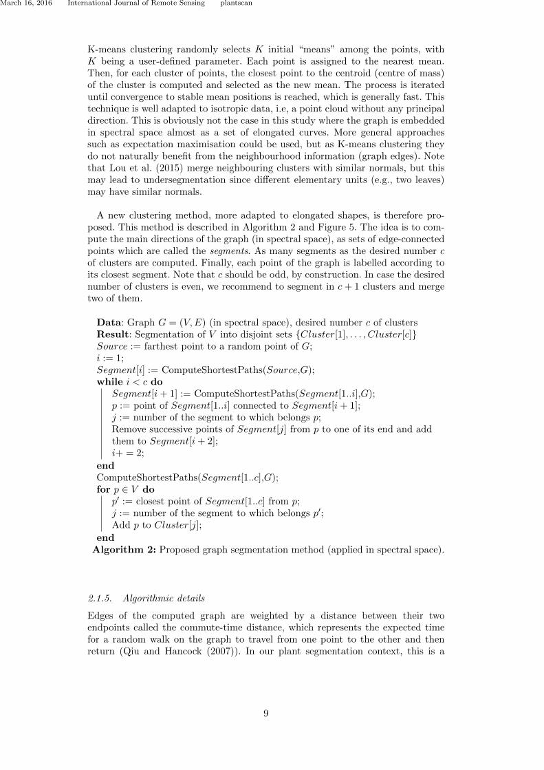
March 16, 2016 International Journal of Remote Sensing plantscan
K-means clustering randomly selects K initial “means” among the points, withK being a user-defined parameter. Each point is assigned to the nearest mean.Then, for each cluster of points, the closest point to the centroid (centre of mass)of the cluster is computed and selected as the new mean. The process is iterateduntil convergence to stable mean positions is reached, which is generally fast. Thistechnique is well adapted to isotropic data, i.e, a point cloud without any principaldirection. This is obviously not the case in this study where the graph is embeddedin spectral space almost as a set of elongated curves. More general approachessuch as expectation maximisation could be used, but as K-means clustering theydo not naturally benefit from the neighbourhood information (graph edges). Notethat Lou et al. (2015) merge neighbouring clusters with similar normals, but thismay lead to undersegmentation since different elementary units (e.g., two leaves)may have similar normals.
A new clustering method, more adapted to elongated shapes, is therefore pro-posed. This method is described in Algorithm 2 and Figure 5. The idea is to com-pute the main directions of the graph (in spectral space), as sets of edge-connectedpoints which are called the segments. As many segments as the desired number cof clusters are computed. Finally, each point of the graph is labelled according toits closest segment. Note that c should be odd, by construction. In case the desirednumber of clusters is even, we recommend to segment in c + 1 clusters and mergetwo of them.
Data: Graph G = (V,E) (in spectral space), desired number c of clustersResult: Segmentation of V into disjoint sets Cluster[1], . . . , Cluster[c]Source := farthest point to a random point of G;i := 1;Segment[i] := ComputeShortestPaths(Source,G);while i < c do
Segment[i + 1] := ComputeShortestPaths(Segment[1..i],G);p := point of Segment[1..i] connected to Segment[i + 1];j := number of the segment to which belongs p;Remove successive points of Segment[j] from p to one of its end and addthem to Segment[i + 2];i+ = 2;
endComputeShortestPaths(Segment[1..c],G);for p ∈ V do
p′ := closest point of Segment[1..c] from p;j := number of the segment to which belongs p′;Add p to Cluster[j];
endAlgorithm 2: Proposed graph segmentation method (applied in spectral space).
2.1.5. Algorithmic details
Edges of the computed graph are weighted by a distance between their twoendpoints called the commute-time distance, which represents the expected timefor a random walk on the graph to travel from one point to the other and thenreturn (Qiu and Hancock (2007)). In our plant segmentation context, this is a
9
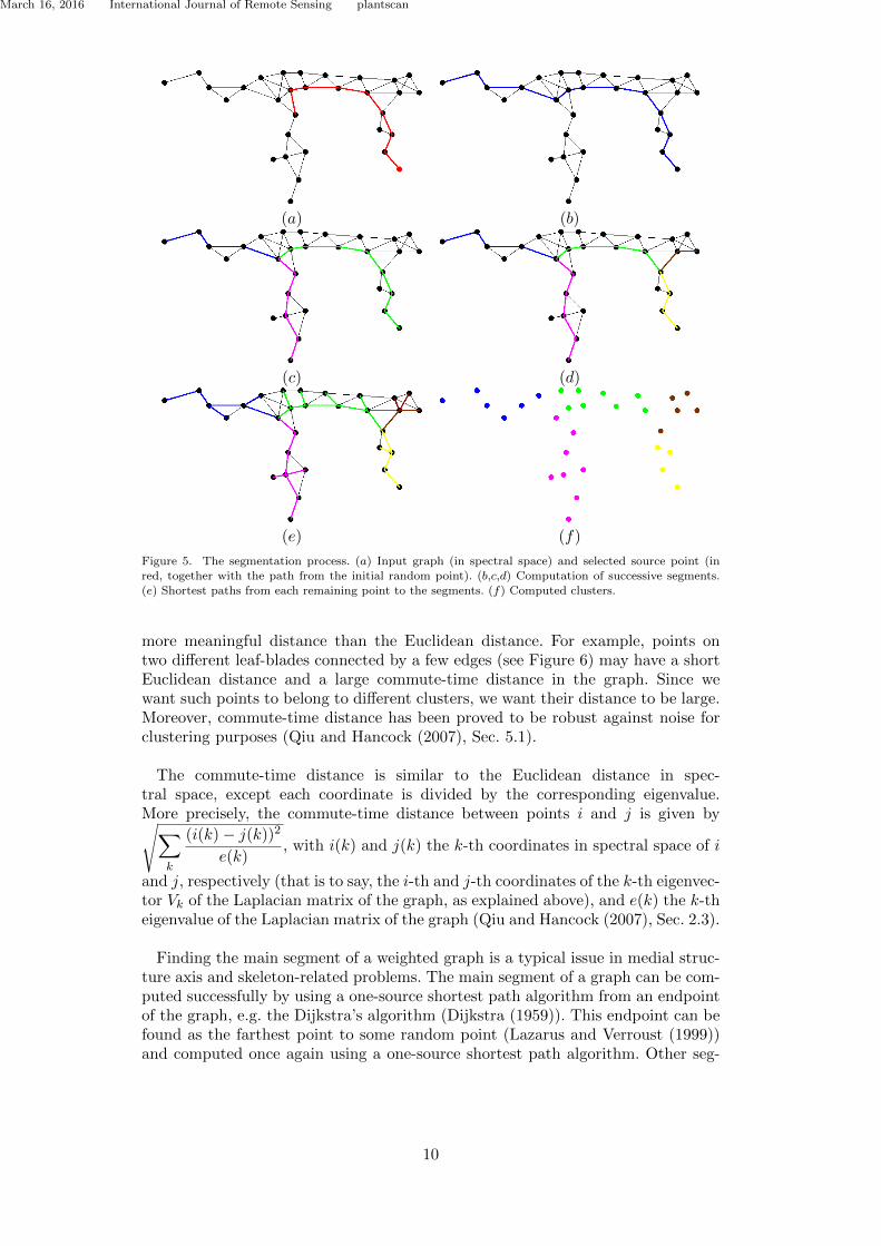
March 16, 2016 International Journal of Remote Sensing plantscan
(a) (b)
(c) (d)
(e) (f)
Figure 5. The segmentation process. (a) Input graph (in spectral space) and selected source point (in
red, together with the path from the initial random point). (b,c,d) Computation of successive segments.(e) Shortest paths from each remaining point to the segments. (f) Computed clusters.
more meaningful distance than the Euclidean distance. For example, points ontwo different leaf-blades connected by a few edges (see Figure 6) may have a shortEuclidean distance and a large commute-time distance in the graph. Since wewant such points to belong to different clusters, we want their distance to be large.Moreover, commute-time distance has been proved to be robust against noise forclustering purposes (Qiu and Hancock (2007), Sec. 5.1).
The commute-time distance is similar to the Euclidean distance in spec-tral space, except each coordinate is divided by the corresponding eigenvalue.More precisely, the commute-time distance between points i and j is given by√∑
k
(i(k)− j(k))2
e(k), with i(k) and j(k) the k-th coordinates in spectral space of i
and j, respectively (that is to say, the i-th and j-th coordinates of the k-th eigenvec-tor Vk of the Laplacian matrix of the graph, as explained above), and e(k) the k-theigenvalue of the Laplacian matrix of the graph (Qiu and Hancock (2007), Sec. 2.3).
Finding the main segment of a weighted graph is a typical issue in medial struc-ture axis and skeleton-related problems. The main segment of a graph can be com-puted successfully by using a one-source shortest path algorithm from an endpointof the graph, e.g. the Dijkstra’s algorithm (Dijkstra (1959)). This endpoint can befound as the farthest point to some random point (Lazarus and Verroust (1999))and computed once again using a one-source shortest path algorithm. Other seg-
10
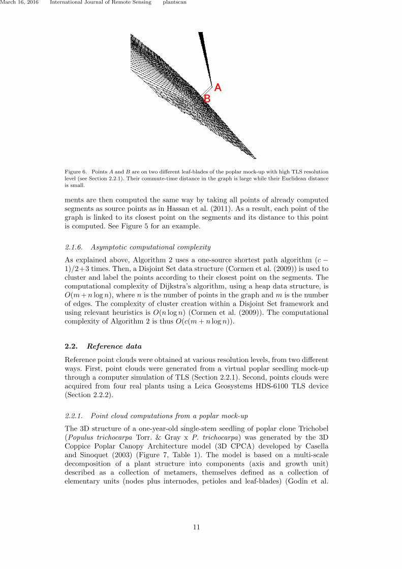
March 16, 2016 International Journal of Remote Sensing plantscan
Figure 6. Points A and B are on two different leaf-blades of the poplar mock-up with high TLS resolutionlevel (see Section 2.2.1). Their commute-time distance in the graph is large while their Euclidean distance
is small.
ments are then computed the same way by taking all points of already computedsegments as source points as in Hassan et al. (2011). As a result, each point of thegraph is linked to its closest point on the segments and its distance to this pointis computed. See Figure 5 for an example.
2.1.6. Asymptotic computational complexity
As explained above, Algorithm 2 uses a one-source shortest path algorithm (c −1)/2+3 times. Then, a Disjoint Set data structure (Cormen et al. (2009)) is used tocluster and label the points according to their closest point on the segments. Thecomputational complexity of Dijkstra’s algorithm, using a heap data structure, isO(m+n log n), where n is the number of points in the graph and m is the numberof edges. The complexity of cluster creation within a Disjoint Set framework andusing relevant heuristics is O(n log n) (Cormen et al. (2009)). The computationalcomplexity of Algorithm 2 is thus O(c(m + n log n)).
2.2. Reference data
Reference point clouds were obtained at various resolution levels, from two differentways. First, point clouds were generated from a virtual poplar seedling mock-upthrough a computer simulation of TLS (Section 2.2.1). Second, points clouds wereacquired from four real plants using a Leica Geosystems HDS-6100 TLS device(Section 2.2.2).
2.2.1. Point cloud computations from a poplar mock-up
The 3D structure of a one-year-old single-stem seedling of poplar clone Trichobel(Populus trichocarpa Torr. & Gray x P. trichocarpa) was generated by the 3DCoppice Poplar Canopy Architecture model (3D CPCA) developed by Casellaand Sinoquet (2003) (Figure 7, Table 1). The model is based on a multi-scaledecomposition of a plant structure into components (axis and growth unit)described as a collection of metamers, themselves defined as a collection ofelementary units (nodes plus internodes, petioles and leaf-blades) (Godin et al.
11
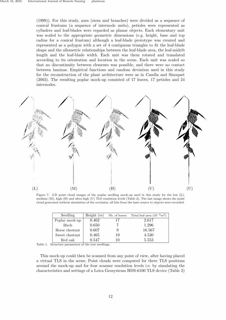
March 16, 2016 International Journal of Remote Sensing plantscan
(1999)). For this study, axes (stem and branches) were divided as a sequence ofconical frustums (a sequence of internode units), petioles were represented ascylinders and leaf-blades were regarded as planar objects. Each elementary unitwas scaled to the appropriate geometric dimensions (e.g. height, base and topradius for a conical frustum) although a leaf-blade prototype was created andrepresented as a polygon with a set of 4 contiguous triangles to fit the leaf-bladeshape and the allometric relationships between the leaf-blade area, the leaf-midriblength and the leaf-blade width. Each unit was them rotated and translatedaccording to its orientation and location in the scene. Each unit was scaled sothat no discontinuity between elements was possible, and there were no contactbetween laminae. Empirical functions and random deviation used in this studyfor the reconstruction of the plant architecture were as in Casella and Sinoquet(2003). The resulting poplar mock-up consisted of 17 leaves, 17 petioles and 24internodes.
(L) (M) (H) (U) (U)
Figure 7. 3-D point cloud images of the poplar seedling mock-up used in this study for the low (L),
medium (M), high (H) and ultra high (U) TLS resolution levels (Table 2). The last image shows the point
cloud generated without simulation of the occlusion: all hits from the laser source to objects were recorded.
Seedling Height (m) Nb. of leaves Total leaf area (10−2m2)
Poplar mock-up 0.462 17 2.617Birch 0.650 7 1.296
Horse chestnut 0.607 9 16.567Sweet chestnut 0.465 19 4.530
Red oak 0.547 10 5.553Table 1. Structure parameters of the tree seedlings.
This mock-up could then be scanned from any point of view, after having placeda virtual TLS in the scene. Point clouds were computed for three TLS positionsaround the mock-up and for four scanner resolution levels i.e. by simulating thecharacteristics and settings of a Leica Geosystems HDS-6100 TLS device (Table 2)
12
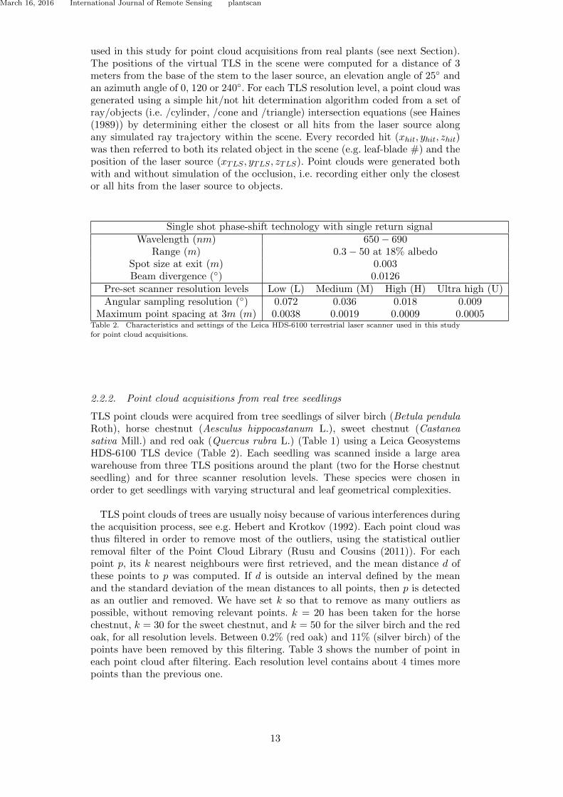
March 16, 2016 International Journal of Remote Sensing plantscan
used in this study for point cloud acquisitions from real plants (see next Section).The positions of the virtual TLS in the scene were computed for a distance of 3meters from the base of the stem to the laser source, an elevation angle of 25 andan azimuth angle of 0, 120 or 240. For each TLS resolution level, a point cloud wasgenerated using a simple hit/not hit determination algorithm coded from a set ofray/objects (i.e. /cylinder, /cone and /triangle) intersection equations (see Haines(1989)) by determining either the closest or all hits from the laser source alongany simulated ray trajectory within the scene. Every recorded hit (xhit, yhit, zhit)was then referred to both its related object in the scene (e.g. leaf-blade #) and theposition of the laser source (xTLS , yTLS , zTLS). Point clouds were generated bothwith and without simulation of the occlusion, i.e. recording either only the closestor all hits from the laser source to objects.
Single shot phase-shift technology with single return signalWavelength (nm) 650− 690
Range (m) 0.3− 50 at 18% albedoSpot size at exit (m) 0.003Beam divergence () 0.0126
Pre-set scanner resolution levels Low (L) Medium (M) High (H) Ultra high (U)Angular sampling resolution () 0.072 0.036 0.018 0.009
Maximum point spacing at 3m (m) 0.0038 0.0019 0.0009 0.0005Table 2. Characteristics and settings of the Leica HDS-6100 terrestrial laser scanner used in this studyfor point cloud acquisitions.
2.2.2. Point cloud acquisitions from real tree seedlings
TLS point clouds were acquired from tree seedlings of silver birch (Betula pendulaRoth), horse chestnut (Aesculus hippocastanum L.), sweet chestnut (Castaneasativa Mill.) and red oak (Quercus rubra L.) (Table 1) using a Leica GeosystemsHDS-6100 TLS device (Table 2). Each seedling was scanned inside a large areawarehouse from three TLS positions around the plant (two for the Horse chestnutseedling) and for three scanner resolution levels. These species were chosen inorder to get seedlings with varying structural and leaf geometrical complexities.
TLS point clouds of trees are usually noisy because of various interferences duringthe acquisition process, see e.g. Hebert and Krotkov (1992). Each point cloud wasthus filtered in order to remove most of the outliers, using the statistical outlierremoval filter of the Point Cloud Library (Rusu and Cousins (2011)). For eachpoint p, its k nearest neighbours were first retrieved, and the mean distance d ofthese points to p was computed. If d is outside an interval defined by the meanand the standard deviation of the mean distances to all points, then p is detectedas an outlier and removed. We have set k so that to remove as many outliers aspossible, without removing relevant points. k = 20 has been taken for the horsechestnut, k = 30 for the sweet chestnut, and k = 50 for the silver birch and the redoak, for all resolution levels. Between 0.2% (red oak) and 11% (silver birch) of thepoints have been removed by this filtering. Table 3 shows the number of point ineach point cloud after filtering. Each resolution level contains about 4 times morepoints than the previous one.
13
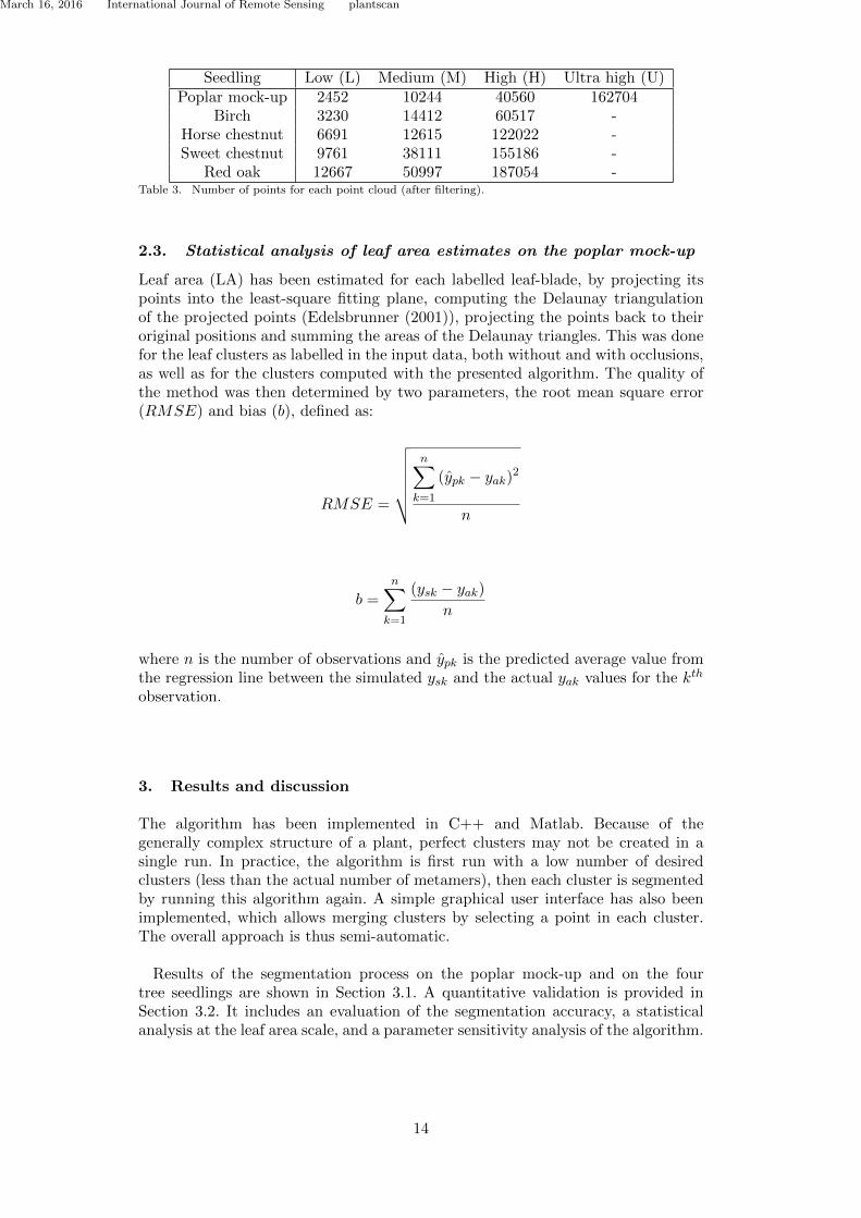
March 16, 2016 International Journal of Remote Sensing plantscan
Seedling Low (L) Medium (M) High (H) Ultra high (U)Poplar mock-up 2452 10244 40560 162704
Birch 3230 14412 60517 -Horse chestnut 6691 12615 122022 -Sweet chestnut 9761 38111 155186 -
Red oak 12667 50997 187054 -Table 3. Number of points for each point cloud (after filtering).
2.3. Statistical analysis of leaf area estimates on the poplar mock-up
Leaf area (LA) has been estimated for each labelled leaf-blade, by projecting itspoints into the least-square fitting plane, computing the Delaunay triangulationof the projected points (Edelsbrunner (2001)), projecting the points back to theiroriginal positions and summing the areas of the Delaunay triangles. This was donefor the leaf clusters as labelled in the input data, both without and with occlusions,as well as for the clusters computed with the presented algorithm. The quality ofthe method was then determined by two parameters, the root mean square error(RMSE) and bias (b), defined as:
RMSE =
√√√√√√
n∑
k=1
(ypk − yak)2
n
b =
n∑
k=1
(ysk − yak)
n
where n is the number of observations and ypk is the predicted average value fromthe regression line between the simulated ysk and the actual yak values for the kth
observation.
3. Results and discussion
The algorithm has been implemented in C++ and Matlab. Because of thegenerally complex structure of a plant, perfect clusters may not be created in asingle run. In practice, the algorithm is first run with a low number of desiredclusters (less than the actual number of metamers), then each cluster is segmentedby running this algorithm again. A simple graphical user interface has also beenimplemented, which allows merging clusters by selecting a point in each cluster.The overall approach is thus semi-automatic.
Results of the segmentation process on the poplar mock-up and on the fourtree seedlings are shown in Section 3.1. A quantitative validation is provided inSection 3.2. It includes an evaluation of the segmentation accuracy, a statisticalanalysis at the leaf area scale, and a parameter sensitivity analysis of the algorithm.
14
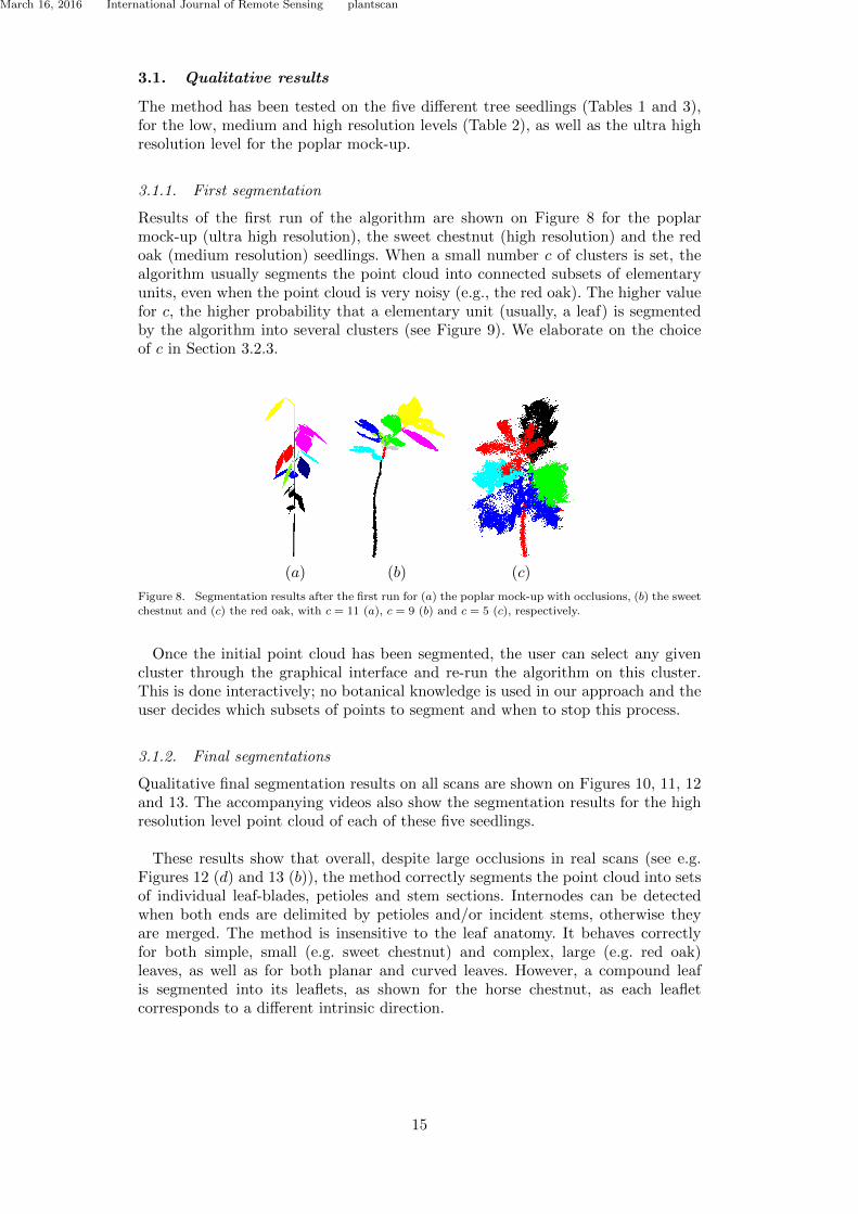
March 16, 2016 International Journal of Remote Sensing plantscan
3.1. Qualitative results
The method has been tested on the five different tree seedlings (Tables 1 and 3),for the low, medium and high resolution levels (Table 2), as well as the ultra highresolution level for the poplar mock-up.
3.1.1. First segmentation
Results of the first run of the algorithm are shown on Figure 8 for the poplarmock-up (ultra high resolution), the sweet chestnut (high resolution) and the redoak (medium resolution) seedlings. When a small number c of clusters is set, thealgorithm usually segments the point cloud into connected subsets of elementaryunits, even when the point cloud is very noisy (e.g., the red oak). The higher valuefor c, the higher probability that a elementary unit (usually, a leaf) is segmentedby the algorithm into several clusters (see Figure 9). We elaborate on the choiceof c in Section 3.2.3.
(a) (b) (c)
Figure 8. Segmentation results after the first run for (a) the poplar mock-up with occlusions, (b) the sweet
chestnut and (c) the red oak, with c = 11 (a), c = 9 (b) and c = 5 (c), respectively.
Once the initial point cloud has been segmented, the user can select any givencluster through the graphical interface and re-run the algorithm on this cluster.This is done interactively; no botanical knowledge is used in our approach and theuser decides which subsets of points to segment and when to stop this process.
3.1.2. Final segmentations
Qualitative final segmentation results on all scans are shown on Figures 10, 11, 12and 13. The accompanying videos also show the segmentation results for the highresolution level point cloud of each of these five seedlings.
These results show that overall, despite large occlusions in real scans (see e.g.Figures 12 (d) and 13 (b)), the method correctly segments the point cloud into setsof individual leaf-blades, petioles and stem sections. Internodes can be detectedwhen both ends are delimited by petioles and/or incident stems, otherwise theyare merged. The method is insensitive to the leaf anatomy. It behaves correctlyfor both simple, small (e.g. sweet chestnut) and complex, large (e.g. red oak)leaves, as well as for both planar and curved leaves. However, a compound leafis segmented into its leaflets, as shown for the horse chestnut, as each leafletcorresponds to a different intrinsic direction.
15
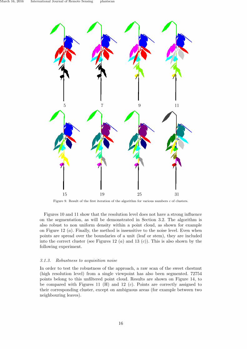
March 16, 2016 International Journal of Remote Sensing plantscan
5 7 9 11
15 19 25 31
Figure 9. Result of the first iteration of the algorithm for various numbers c of clusters.
Figures 10 and 11 show that the resolution level does not have a strong influenceon the segmentation, as will be demonstrated in Section 3.2. The algorithm isalso robust to non uniform density within a point cloud, as shown for exampleon Figure 12 (a). Finally, the method is insensitive to the noise level. Even whenpoints are spread over the boundaries of a unit (leaf or stem), they are includedinto the correct cluster (see Figures 12 (a) and 13 (c)). This is also shown by thefollowing experiment.
3.1.3. Robustness to acquisition noise
In order to test the robustness of the approach, a raw scan of the sweet chestnut(high resolution level) from a single viewpoint has also been segmented. 72754points belong to this unfiltered point cloud. Results are shown on Figure 14, tobe compared with Figures 11 (H) and 12 (c). Points are correctly assigned totheir corresponding cluster, except on ambiguous areas (for example between twoneighbouring leaves).
16
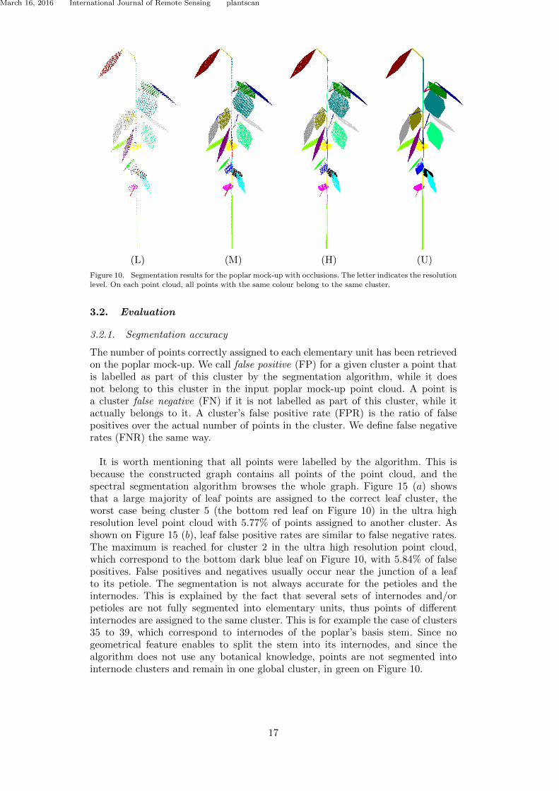
March 16, 2016 International Journal of Remote Sensing plantscan
(L) (M) (H) (U)
Figure 10. Segmentation results for the poplar mock-up with occlusions. The letter indicates the resolution
level. On each point cloud, all points with the same colour belong to the same cluster.
3.2. Evaluation
3.2.1. Segmentation accuracy
The number of points correctly assigned to each elementary unit has been retrievedon the poplar mock-up. We call false positive (FP) for a given cluster a point thatis labelled as part of this cluster by the segmentation algorithm, while it doesnot belong to this cluster in the input poplar mock-up point cloud. A point isa cluster false negative (FN) if it is not labelled as part of this cluster, while itactually belongs to it. A cluster’s false positive rate (FPR) is the ratio of falsepositives over the actual number of points in the cluster. We define false negativerates (FNR) the same way.
It is worth mentioning that all points were labelled by the algorithm. This isbecause the constructed graph contains all points of the point cloud, and thespectral segmentation algorithm browses the whole graph. Figure 15 (a) showsthat a large majority of leaf points are assigned to the correct leaf cluster, theworst case being cluster 5 (the bottom red leaf on Figure 10) in the ultra highresolution level point cloud with 5.77% of points assigned to another cluster. Asshown on Figure 15 (b), leaf false positive rates are similar to false negative rates.The maximum is reached for cluster 2 in the ultra high resolution point cloud,which correspond to the bottom dark blue leaf on Figure 10, with 5.84% of falsepositives. False positives and negatives usually occur near the junction of a leafto its petiole. The segmentation is not always accurate for the petioles and theinternodes. This is explained by the fact that several sets of internodes and/orpetioles are not fully segmented into elementary units, thus points of differentinternodes are assigned to the same cluster. This is for example the case of clusters35 to 39, which correspond to internodes of the poplar’s basis stem. Since nogeometrical feature enables to split the stem into its internodes, and since thealgorithm does not use any botanical knowledge, points are not segmented intointernode clusters and remain in one global cluster, in green on Figure 10.
17
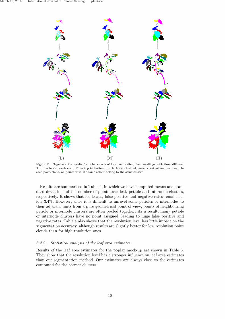
March 16, 2016 International Journal of Remote Sensing plantscan
(L) (M) (H)
Figure 11. Segmentation results for point clouds of four contrasting plant seedlings with three differentTLS resolution levels each. From top to bottom: birch, horse chestnut, sweet chestnut and red oak. On
each point cloud, all points with the same colour belong to the same cluster.
Results are summarised in Table 4, in which we have computed means and stan-dard deviations of the number of points over leaf, petiole and internode clusters,respectively. It shows that for leaves, false positive and negative rates remain be-low 3.4%. However, since it is difficult to unravel some petioles or internodes totheir adjacent units from a pure geometrical point of view, points of neighbouringpetiole or internode clusters are often pooled together. As a result, many petioleor internode clusters have no point assigned, leading to huge false positive andnegative rates. Table 4 also shows that the resolution level has little impact on thesegmentation accuracy, although results are slightly better for low resolution pointclouds than for high resolution ones.
3.2.2. Statistical analysis of the leaf area estimates
Results of the leaf area estimates for the poplar mock-up are shown in Table 5.They show that the resolution level has a stronger influence on leaf area estimatesthan our segmentation method. Our estimates are always close to the estimatescomputed for the correct clusters.
18
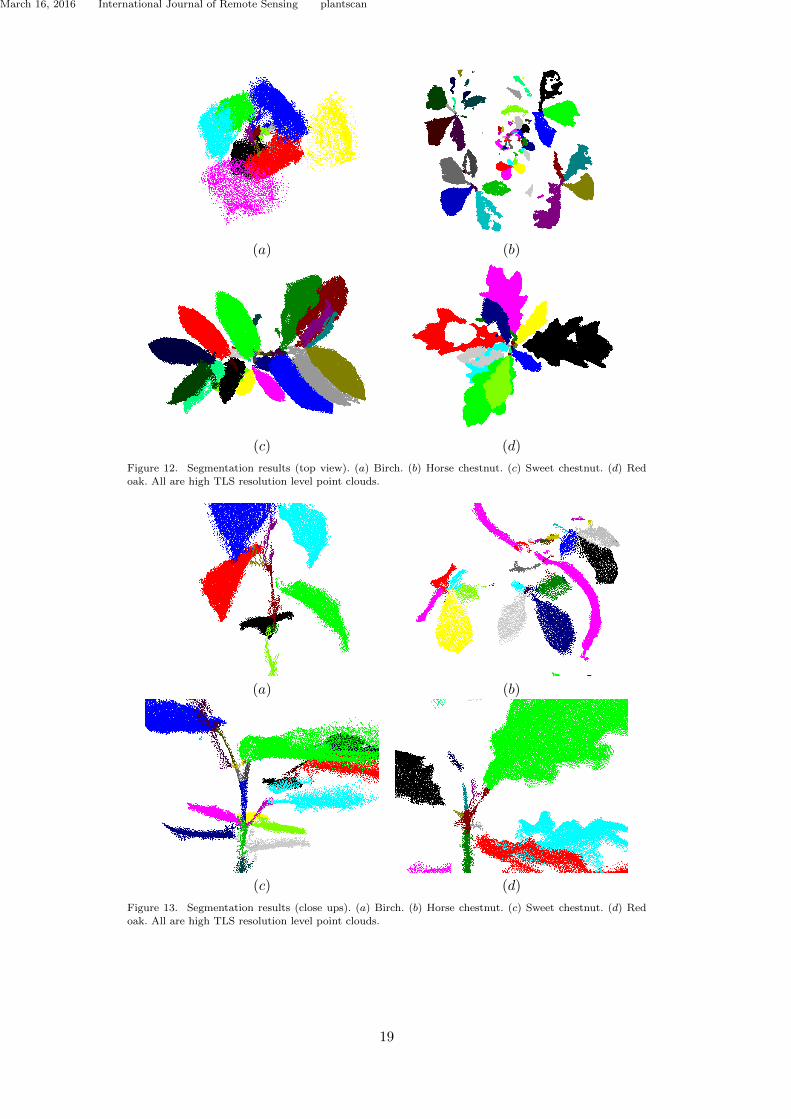
March 16, 2016 International Journal of Remote Sensing plantscan
(a) (b)
(c) (d)
Figure 12. Segmentation results (top view). (a) Birch. (b) Horse chestnut. (c) Sweet chestnut. (d) Red
oak. All are high TLS resolution level point clouds.
(a) (b)
(c) (d)
Figure 13. Segmentation results (close ups). (a) Birch. (b) Horse chestnut. (c) Sweet chestnut. (d) Red
oak. All are high TLS resolution level point clouds.
19
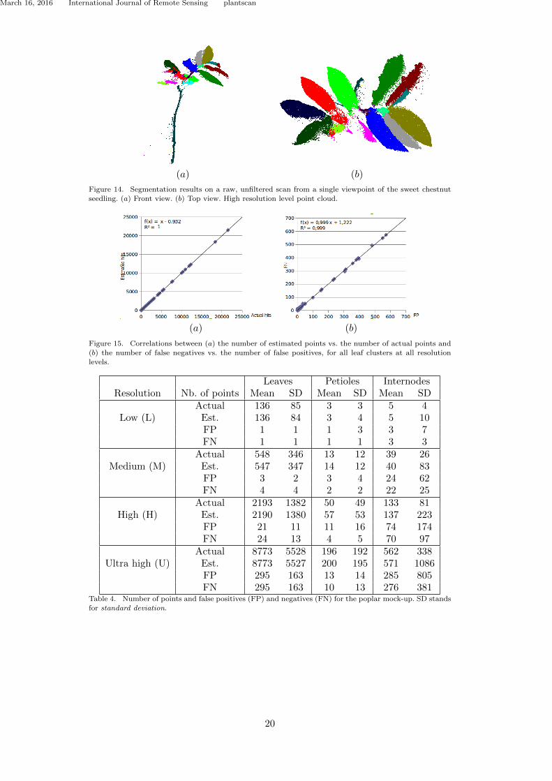
March 16, 2016 International Journal of Remote Sensing plantscan
(a) (b)
Figure 14. Segmentation results on a raw, unfiltered scan from a single viewpoint of the sweet chestnut
seedling. (a) Front view. (b) Top view. High resolution level point cloud.
(a) (b)
Figure 15. Correlations between (a) the number of estimated points vs. the number of actual points and
(b) the number of false negatives vs. the number of false positives, for all leaf clusters at all resolution
levels.
Leaves Petioles InternodesResolution Nb. of points Mean SD Mean SD Mean SD
Actual 136 85 3 3 5 4Low (L) Est. 136 84 3 4 5 10
FP 1 1 1 3 3 7FN 1 1 1 1 3 3
Actual 548 346 13 12 39 26Medium (M) Est. 547 347 14 12 40 83
FP 3 2 3 4 24 62FN 4 4 2 2 22 25
Actual 2193 1382 50 49 133 81High (H) Est. 2190 1380 57 53 137 223
FP 21 11 11 16 74 174FN 24 13 4 5 70 97
Actual 8773 5528 196 192 562 338Ultra high (U) Est. 8773 5527 200 195 571 1086
FP 295 163 13 14 285 805FN 295 163 10 13 276 381
Table 4. Number of points and false positives (FP) and negatives (FN) for the poplar mock-up. SD stands
for standard deviation.
20
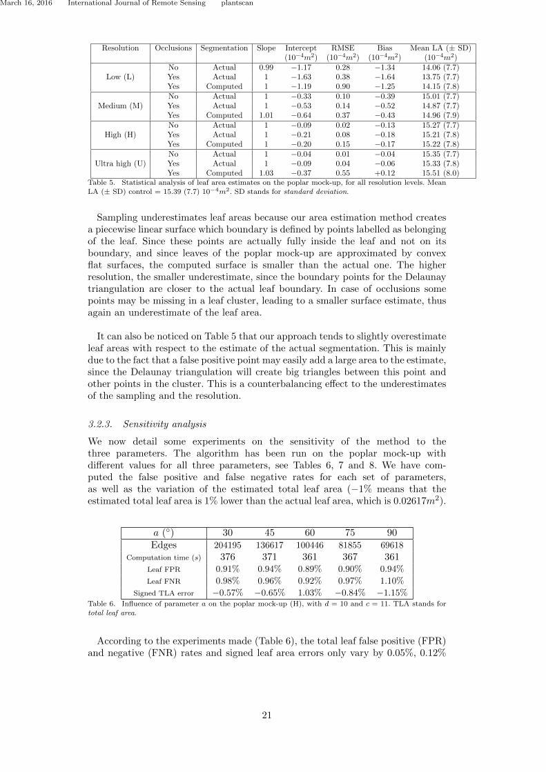
March 16, 2016 International Journal of Remote Sensing plantscan
Resolution Occlusions Segmentation Slope Intercept RMSE Bias Mean LA (± SD)(10−4m2) (10−4m2) (10−4m2) (10−4m2)
No Actual 0.99 −1.17 0.28 −1.34 14.06 (7.7)Low (L) Yes Actual 1 −1.63 0.38 −1.64 13.75 (7.7)
Yes Computed 1 −1.19 0.90 −1.25 14.15 (7.8)No Actual 1 −0.33 0.10 −0.39 15.01 (7.7)
Medium (M) Yes Actual 1 −0.53 0.14 −0.52 14.87 (7.7)Yes Computed 1.01 −0.64 0.37 −0.43 14.96 (7.9)No Actual 1 −0.09 0.02 −0.13 15.27 (7.7)
High (H) Yes Actual 1 −0.21 0.08 −0.18 15.21 (7.8)Yes Computed 1 −0.20 0.15 −0.17 15.22 (7.8)No Actual 1 −0.04 0.01 −0.04 15.35 (7.7)
Ultra high (U) Yes Actual 1 −0.09 0.04 −0.06 15.33 (7.8)Yes Computed 1.03 −0.37 0.55 +0.12 15.51 (8.0)
Table 5. Statistical analysis of leaf area estimates on the poplar mock-up, for all resolution levels. Mean
LA (± SD) control = 15.39 (7.7) 10−4m2. SD stands for standard deviation.
Sampling underestimates leaf areas because our area estimation method createsa piecewise linear surface which boundary is defined by points labelled as belongingof the leaf. Since these points are actually fully inside the leaf and not on itsboundary, and since leaves of the poplar mock-up are approximated by convexflat surfaces, the computed surface is smaller than the actual one. The higherresolution, the smaller underestimate, since the boundary points for the Delaunaytriangulation are closer to the actual leaf boundary. In case of occlusions somepoints may be missing in a leaf cluster, leading to a smaller surface estimate, thusagain an underestimate of the leaf area.
It can also be noticed on Table 5 that our approach tends to slightly overestimateleaf areas with respect to the estimate of the actual segmentation. This is mainlydue to the fact that a false positive point may easily add a large area to the estimate,since the Delaunay triangulation will create big triangles between this point andother points in the cluster. This is a counterbalancing effect to the underestimatesof the sampling and the resolution.
3.2.3. Sensitivity analysis
We now detail some experiments on the sensitivity of the method to thethree parameters. The algorithm has been run on the poplar mock-up withdifferent values for all three parameters, see Tables 6, 7 and 8. We have com-puted the false positive and false negative rates for each set of parameters,as well as the variation of the estimated total leaf area (−1% means that theestimated total leaf area is 1% lower than the actual leaf area, which is 0.02617m2).
a () 30 45 60 75 90Edges 204195 136617 100446 81855 69618
Computation time (s) 376 371 361 367 361Leaf FPR 0.91% 0.94% 0.89% 0.90% 0.94%
Leaf FNR 0.98% 0.96% 0.92% 0.97% 1.10%
Signed TLA error −0.57% −0.65% 1.03% −0.84% −1.15%Table 6. Influence of parameter a on the poplar mock-up (H), with d = 10 and c = 11. TLA stands for
total leaf area.
According to the experiments made (Table 6), the total leaf false positive (FPR)and negative (FNR) rates and signed leaf area errors only vary by 0.05%, 0.12%
21
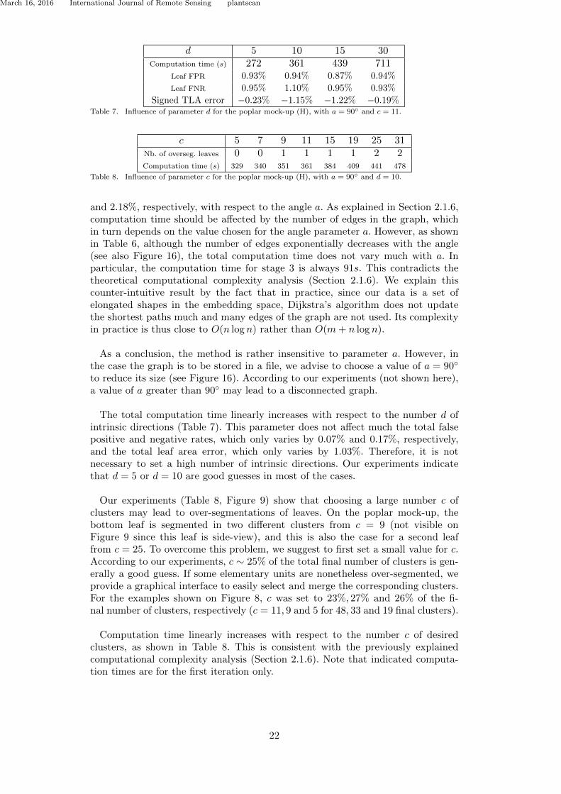
March 16, 2016 International Journal of Remote Sensing plantscan
d 5 10 15 30Computation time (s) 272 361 439 711
Leaf FPR 0.93% 0.94% 0.87% 0.94%
Leaf FNR 0.95% 1.10% 0.95% 0.93%
Signed TLA error −0.23% −1.15% −1.22% −0.19%Table 7. Influence of parameter d for the poplar mock-up (H), with a = 90 and c = 11.
c 5 7 9 11 15 19 25 31Nb. of overseg. leaves 0 0 1 1 1 1 2 2Computation time (s) 329 340 351 361 384 409 441 478
Table 8. Influence of parameter c for the poplar mock-up (H), with a = 90 and d = 10.
and 2.18%, respectively, with respect to the angle a. As explained in Section 2.1.6,computation time should be affected by the number of edges in the graph, whichin turn depends on the value chosen for the angle parameter a. However, as shownin Table 6, although the number of edges exponentially decreases with the angle(see also Figure 16), the total computation time does not vary much with a. Inparticular, the computation time for stage 3 is always 91s. This contradicts thetheoretical computational complexity analysis (Section 2.1.6). We explain thiscounter-intuitive result by the fact that in practice, since our data is a set ofelongated shapes in the embedding space, Dijkstra’s algorithm does not updatethe shortest paths much and many edges of the graph are not used. Its complexityin practice is thus close to O(n log n) rather than O(m + n log n).
As a conclusion, the method is rather insensitive to parameter a. However, inthe case the graph is to be stored in a file, we advise to choose a value of a = 90
to reduce its size (see Figure 16). According to our experiments (not shown here),a value of a greater than 90 may lead to a disconnected graph.
The total computation time linearly increases with respect to the number d ofintrinsic directions (Table 7). This parameter does not affect much the total falsepositive and negative rates, which only varies by 0.07% and 0.17%, respectively,and the total leaf area error, which only varies by 1.03%. Therefore, it is notnecessary to set a high number of intrinsic directions. Our experiments indicatethat d = 5 or d = 10 are good guesses in most of the cases.
Our experiments (Table 8, Figure 9) show that choosing a large number c ofclusters may lead to over-segmentations of leaves. On the poplar mock-up, thebottom leaf is segmented in two different clusters from c = 9 (not visible onFigure 9 since this leaf is side-view), and this is also the case for a second leaffrom c = 25. To overcome this problem, we suggest to first set a small value for c.According to our experiments, c ∼ 25% of the total final number of clusters is gen-erally a good guess. If some elementary units are nonetheless over-segmented, weprovide a graphical interface to easily select and merge the corresponding clusters.For the examples shown on Figure 8, c was set to 23%, 27% and 26% of the fi-nal number of clusters, respectively (c = 11, 9 and 5 for 48, 33 and 19 final clusters).
Computation time linearly increases with respect to the number c of desiredclusters, as shown in Table 8. This is consistent with the previously explainedcomputational complexity analysis (Section 2.1.6). Note that indicated computa-tion times are for the first iteration only.
22
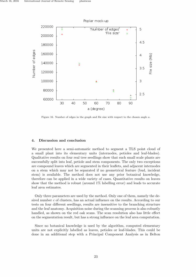
March 16, 2016 International Journal of Remote Sensing plantscan
Figure 16. Number of edges in the graph and file size with respect to the chosen angle a.
4. Discussion and conclusion
We presented here a semi-automatic method to segment a TLS point cloud ofa small plant into its elementary units (internodes, petioles and leaf-blades).Qualitative results on four real tree seedlings show that such small scale plants aresuccessfully split into leaf, petiole and stem components. The only two exceptionsare compound leaves which are segmented in their leaflets, and adjacent internodeson a stem which may not be separated if no geometrical feature (bud, incidentstem) is available. The method does not use any prior botanical knowledge,therefore can be applied in a wide variety of cases. Quantitative results on leavesshow that the method is robust (around 1% labelling error) and leads to accurateleaf area estimates.
Only three parameters are used by the method. Only one of them, namely the de-sired number c of clusters, has an actual influence on the results. According to ourtests on four different seedlings, results are insensitive to the branching structureand the leaf anatomy. Acquisition noise during the scanning process is also robustlyhandled, as shown on the red oak scans. The scan resolution also has little effecton the segmentation result, but has a strong influence on the leaf area computation.
Since no botanical knowledge is used by the algorithm, computed elementaryunits are not explicitly labelled as leaves, petioles or leaf-blades. This could bedone in an additional step with a Principal Component Analysis as in Belton
23

March 16, 2016 International Journal of Remote Sensing plantscan
et al. (2013) or feature based histograms as in Paulus et al. (2013).
The proposed method being semi-automatic, it is suited for small plants such astree seedlings but may be time consuming for more complex structures. In orderto enhance the quality of the segmentation with a large number c of clusters,thus to reduce the interaction time for large scale trees, two improvements areplanned in the future. First, we are currently working on the correction of theacquisition noise during the scanning process, in order to reduce the number ofpoints sparsely sampled between elementary units. Filtering the input scans in apre-processing step, which has been done in this paper, is not a perfect solutionsince it removes points and thus leads to underestimates of the leaf areas. Second,we plan to enhance the graph construction process (first step of the algorithm),in order to decrease the number of edges between two non adjacent elementaryunits from a botanical point of view (e.g., two leaves, as in Figure 6). Then, thealgorithm will be tested on more complex structures such as full-scale trees.
Acknowledgements
The authors would like to express their sincere gratitude to the Forestry Commis-sion, the University of Grenoble Alpes and Inria for funding this work, as well asto Remy Cumont for his participation in coding the segmentation algorithm andDr Elisa Hetroy-Wheeler for proof-reading the paper.
Author contributions: E.C. and F.H.W. designed the research; F.H.W. designedand coded the segmentation algorithm; E.C. performed the real data acquisitionand coded the hit-no hit algorithm for point cloud simulations; D.B. filtered thepoint clouds; F.H.W. and E.C. analysed the results and wrote the paper.
Funding
The Forestry Commission, the University of Grenoble Alpes (through an AGIRproject) and Inria (through the Action de Recherche Collaborative PlantScan3D).
References
Alenya, G., B. Dellen, S. Foix, and C. Torras (2013). Robotized plant probing: Leaf seg-mentation utilizing time-of-flight data. IEEE Robotics and Automation Magazine 20 (3),50–59.
Bayer, D., S. Seifert, and H. Pretzsch (2013). Structural crown properties of norway spruce(Picea abies [l.] karst.) and european beech (Fagus sylvatica [l.]) in mixed versus purestands revealed by terrestrial laser scanning. Trees 27, 1035–1047.
Belkin, M. and P. Niyogi (2003). Laplacian eigenmaps for dimensionality reduction anddata representation. Neural Computation 15, 1373–1396.
Belton, D., S. Moncrieff, and J. Chapman (2013). Processing tree point clouds usinggaussian mixture models. In Proceedings of the ISPRS Annals of the Photogrammetry,Remote Sensing and Spatial Information Sciences, pp. 43–48.
Bey, A., R. Chaine, R. Marc, G. Thibault, and S. Akkouche (2011). Reconstruction ofconsistent 3d cad models from point cloud data using a priori cad model. In Proceedingsof the ISPRS Workshop on Laser Scanning, pp. 289–294.
24
March 16, 2016 International Journal of Remote Sensing plantscan
Casella, E. and H. Sinoquet (2003). A method for describing the canopy architecture ofcoppice poplar with allometric relationships. Tree Physiology 23, 1153–1169.
Chaivivatrakul, S., L. Tang, M. N. Dailey, and A. D. Nakarmi (2014). Automatic morpho-logical trait characterization for corn plants via 3d holographic reconstruction. Comput-ers and Electronics in Agriculture 109, 10–123.
Chene, Y., D. Rousseau, P. Lucidarme, J. Bertheloot, V. Caffier, P. Morel, E. Belin, andF. Chapeau-Blondeau (2012). On the use of depth camera for 3d phenotyping of entireplants. Computers and Electronics in Agriculture 82, 122–127.
Cormen, T. H., C. E. Leiserson, R. L. Rivest, and C. Stein (2009). Introduction to algo-rithms. 3th ed. MIT Press.
Cote, J.-F., J.-L. Widlowski, R. A. Fournier, and M. M. Verstraete (2009). The structuraland radiative consistency of three-dimensional tree reconstructions from terrestrial lidar.Remote Sensing of Environment 113, 1067–1081.
Dassot, M., T. Constant, and M. Fournier (2011). The use of terrestrial lidar technology inforest science: application fields, benefits and challenges. Annals of Forest Science 68,959–974.
Dey, T. K., P. Ranjan, and Y. Wang (2012). Eigen deformation of 3d models. The VisualComputer 28, 585–595.
Dijkstra, E. (1959). A note on two problems in connexion with graphs. NumerischeMathematik 1, 269–271.
Dornbusch, T., P. Wernecke, and W. Diepenbrock (2007). A method to extract morpho-logical traits of plant organs from 3d point clouds as a database for an architecturalplant model. Ecological Modelling 200, 119–129.
Douglas, E. S., J. Martel, Z. Li, G. Howe, K. Hewawasam, R. A. Marshall, C. L. Schaaf,T. A. Cook, G. J. Newnham, A. Strahler, and S. Chakrabarti (2015). Finding leavesin the forest: the dual-wavelength echidna lidar. IEEE Geoscience and Remote SensingLetters 12 (4), 776–780.
Edelsbrunner, H. (2001). Geometry and topology for mesh generation. Cambridge Univer-sity Press.
Furbank, R. T. and M. Tester (2011). Phenomics – technologies to relieve the phenotypingbottleneck. Trends in Plant Science 16 (12), 635–644.
Godin, C., E. Costes, and H. Sinoquet (1999). A method for describing plant architecturewhich integrates topology and geometry. Annals of Botany 84, 343–357.
Godin, C. and H. Sinoquet (2005). Functionalstructural plant modelling. New phytolo-gist 166 (3), 705–708.
Golbach, F., G. Kootstra, S. Damjanovic, G. Otten, and R. van de Zedde (2015). Vali-dation of plant part measurements using a 3d reconstruction method suitable for high-throughput seedling phenotyping. Machine Vision and Applications, 1–18.
Haala, N. and M. Kada (2010). An update on automatic 3d building reconstruction. ISPRSJournal of Photogrammetry and Remote Sensing 65, 570–580.
Haines, E. (1989). Essential ray tracing algorithms. In A. Glassner (Ed.), An introductionto ray tracing, pp. 33–77. Academic Press.
Hassan, S., F. Hetroy, F. Faure, and O. Palombi (2011). Automatic localization andquantification of intracranial aneurysms. Computer Analysis of Images and Patterns.Lecture Notes in Computer Science 6854, 554–562.
Hebert, M. and E. Krotkov (1992). 3-d measurements from imaging laser radars: how goodare they? Image and Vision Computing 10 (3), 170–178.
Hosoi, F., K. Nakabayashi, and K. Omasa (2011). 3-d modeling of tomato canopies using ahigh-resolution portable scanning lidar for extracting structural information. Sensors 11,2166–2174.
International Plant Phenotyping Network (Accessed: 08-02-2016). http://www.plant-phenotyping.org/.
Kaminuma, E., N. Heida, Y. Tsumoto, N. Yamamoto, N. Goto, N. Okamoto, A. Konagaya,M. Matsui, and T. Toyoda (2004). Automatic quantification of morphological traits viathree-dimensional measurement of arabidopsis. The Plant Journal 38, 358–365.
Karni, Z. and C. Gotsman (2000). Spectral compression of mesh geometry. In Proceedings
25
March 16, 2016 International Journal of Remote Sensing plantscan
of the 27th annual conference on Computer graphics and interactive techniques (SIG-GRAPH), pp. 279–286.
Lazarus, F. and A. Verroust (1999). Level set diagrams of polyhedral objects. In Proceedingsof the 5th ACM Symposium on Solid Modeling and Applications (SMA), pp. 130–140.
Levy, B. (2006). Laplace-beltrami eigenfunctions: towards an algorithm that understandsgeometry. In Proceedings of the IEEE International Conference on Shape Modeling andApplications (SMI), pp. 13.
Li, L., Q. Zhang, and D. Huang (2014). A review of imaging techniques for plant pheno-typing. Sensors 14, 20078–20111.
Li, Y., X. Wu, Y. Chrysathou, A. Sharf, D. Cohen-Or, and N. Mitra (2011). Globfit:consistently fitting primitives by discovering global relations. ACM Transactions onGraphics 30 (4), 52.
Lin, Y. (2015). Lidar: An important tool for next-generation phenotyping technology ofhigh potential for plant phenomics? Computers and Electronics in Agriculture 119,61–73.
Livny, Y., F. Yan, M. Olson, B. Chen, H. Zhang, and J. El-Sana (2010). Automatic re-construction of tree skeletal structures from point clouds. ACM Transactions on Graph-ics 29, 151.
Lou, L., Y. Liu, M. Shen, J. Han, F. Corke, and J. H. Doonan (2015). Estimation of branchangle from 3d point cloud of plants. In Proceedings of the International Conference on3D Vision (3DV), pp. 554–561.
Nguyen, A. and B. Le (2013). 3d point cloud segmentation: a survey. In Proceedings of the6th IEEE Conference on Robotics, Automation and Mechatronics (RAM), pp. 225–230.
Paproki, A., X. Sirault, S. Berry, R. Furbank, and J. Fripp (2012). A novel mesh processingbased technique for 3d plant analysis. BMC Plant Biology 12 (1), 63.
Paulus, S., J. Dupuis, A.-K. Mahlein, and H. Kuhlmann (2013). Surface feature basedclassification of plant organs from 3d laserscanned point clouds for plant phenotyping.BMC Bioinformatics 14, 238.
Paulus, S., J. Dupuis, S. Riedel, and H. Kuhlmann (2014). Automated analysis of barley or-gans using 3d laser scanning: an approach for high throughput phenotyping. Sensors 14,12670–12686.
Paulus, S., H. Schumann, H. Kuhlmann, and J. Leon (2014). High-precision laser scan-ning system for capturing 3d plant architecture and analysing growth of cereal plants.Biosystems Engineering 121, 1–11.
Qiu, H. J. and E. R. Hancock (2007). Clustering and embedding using commute times.IEEE Transactions on Pattern Analysis and Machine Intelligence 29, 1873–1890.
Quan, L., P. Tan, G. Zeng, L. Yuan, J. Wang, and S. B. Kang (2006). Image-based plantmodeling. ACM Transactions on Graphics 25 (3), 599–604.
Reuter, M., F. E. Wolter, and N. Peinecke (2006). Laplace-beltrami spectra as ’shape-dna’of surfaces and solids. Computer-Aided Design 38, 342–366.
Rose, J. C., S. Paulus, and H. Kuhlmann (2015). Accuracy analysis of a multi-view stereoapproach for phenotyping of tomato plants at the organ level. Sensors 15, 9651–9665.
Rusu, R. B. and S. Cousins (2011). 3d is here: Point cloud library (pcl). In Proceedings ofthe IEEE International Conference on Robotics and Automation (ICRA).
Tao, S., Q. Guo, S. Xu, Y. Su, Y. Li, and F. Wu (2015). A geometric method for wood-leafseparation using terrestrial and simulated lidar data. Photogrammetric Engineering andRemote Sensing 81 (10), 767–776.
Tilly, N., D. Hoffmeister, H. Liang, Q. Cao, Y. Liu, V. Lenz-Wiedemann, Y. Miao, andG. Bareth (2012). Evaluation of terrestrial laser scanning for rice growth monitoring.International Archives of the Photogrammetry, Remote Sensing and Spatial InformationScience 39, B7.
von Luxburg, U. (2007). A tutorial on spectral clustering. Statistics and Computing 17,395–416.
Wahabzada, M., S. Paulus, K. Kersting, and A.-K. Mahlein (2015). Automated interpre-tation of 3d laserscanned point clouds for plant organ segmentation. BMC Bioinformat-ics 16, 248.
26

March 16, 2016 International Journal of Remote Sensing plantscan
Xia, C., L. Wang, B.-K. Chung, and J.-M. Lee (2015). In situ 3d segmentation of individualplant leaves using a rgb-d camera for agricultural automation. Sensors 15, 20463–20479.
Xu, H., N. Gossett, and B. Chen (2007). Knowledge and heuristic based modeling oflaser-scanned trees. ACM Transactions on Graphics 26 (4), 19.
Yang, L. (2005). Building connected neighborhood graphs for isometric data embedding.In Proceedings of the 11th ACM SIGKDD International Conference on Knowledge Dis-covery in Data Mining (KDD), pp. 722–728.
Yin, K., H. Huang, P. Long, A. Gaissinski, M. Gong, and A. Sharf (2015). Full 3d plantreconstruction via intrusive acquisition. Computer Graphics Forum.
27

232 APPENDIX A. SELECTED PAPERS
APPENDIX B
List of publications
B.1 GEOMETRICAL, TOPOLOGICAL ANDPERCEPTUAL ANALYSIS OF 3D MESHES
1. F. Hétroy, D. Attali. Topological quadrangulations of closed triangulated sur-faces using the Reeb graph. In A. Braquelaire, J.-O. Lachaud and A. Vialard,editors, Lecture Notes in Computer Science, Vol. 2301, pp. 57–68, Springer,2002. Proc. of Discrete Geometry for Computer Imagery (DGCI) 2002, Bor-deaux, France, April 2002.
2. F. Hétroy, D. Attali. Topological quadrangulations of closed triangulated sur-faces using the Reeb graph. Graphical Models, 65(1-3), pp. 131–148, Elsevier,2003. doi:10.1016/S1524-0703(03)00005-5.
3. F. Hétroy, D. Attali. Detection of constrictions on closed polyhedral surfaces.Eurographics-IEEE TCVG Visualization Symposium, pp. 67–74, Grenoble,France, May 2003.
4. F. Hétroy, D. Attali. From a closed piecewise geodesic to a constriction on aclosed polyhedral surface. Pacific Conference on Computer Graphics and Ap-plications (Pacific Graphics) 2003, pp. 394–398, Canmore, Alberta, Canada,October 2003.
5. F. Hétroy. Constriction computation using surface curvature. Eurographics(short paper), Aug. 29, 2005, Dublin, Ireland, pp. 1–4.
6. F. Hétroy, S. Rey, C. Andujar, P. Brunet, A. Vinacua. Mesh Repair with TopologyControl. Inria Research Report, RR-6535, 2008.
233
234 APPENDIX B. LIST OF PUBLICATIONS
7. J.-C. Léon, L. de Floriani, F. Hétroy. Classification of non-manifold singularitiesfrom transformations of 2-manifolds. IEEE International Conference on ShapeModeling and Applications (SMI), Jun., 2009, Beijing, China.
8. D. Boltcheva, S. Merino Aceituno, J.-C. Léon, F. Hétroy. Constructive Mayer-Vietoris Algorithm: Computing the Homology of Unions of Simplicial Com-plexes. Inria Research Report, RR-7471, 2010.
9. F. Hétroy, S. Rey, C. Andujar, P. Brunet, A. Vinacua. Mesh repair with user-friendly topology control. Computer Aided Design, 43(1), pp. 101–113, Else-vier, 2011. doi:10.1016/j.cad.2010.09.012.
10. D. Boltcheva, D. Canino, S. Merino Aceituno, J.-C. Léon, L. De Floriani, F.Hétroy. An iterative algorithm for homology computation on simplicial shapes.Computer-Aided Design, 43(11), pp. 1457–1467, Elsevier, 2011. doi:10.1016/j.cad.2011.08.015.
11. L. Wang, F. Hétroy-Wheeler, E. Boyer. A hierarchical approach for regularcentroidal Voronoi tessellations, Computer Graphics Forum, 35(1), pp. 152–165, Wiley-Blackwell, 2016. doi:10.1111/cgf.12716.
12. G. Nader, K. Wang, F. Hétroy-Wheeler, F. Dupont. Just Noticeable Distortionprofile for flat-shaded 3D mesh surfaces, IEEE Transactions on Visualizationand Computer Graphics, 2016. doi:10.1109/TVCG.2015.2507578.
B.2 DIGITAL GEOMETRY PROCESSING FOR SHAPESIN MOTION
1. G. Aujay, F. Hétroy, F. Lazarus. Construction automatique d’un squelette pourl’animation de personnages. 19èmes Journées de l’Association Française d’InformatiqueGraphique (AFIG), Nov. 22, 2006, Bordeaux, France.
2. G. Aujay, F. Hétroy, F. Lazarus, C. Depraz. Harmonic skeleton for realisticcharacter animation. ACM-SIGGRAPH/Eurographics Symposium on Com-puter Animation, Aug. 3, 2007, San Diego, United States.
3. L. Skrba, L. Revéret, F. Hétroy, M.P. Cani, C. O’Sullivan. Quadruped animation.Eurographics State-of-the-Art Report, Apr., 2008, Hersonissos, Creete, Greece,pp. 1–17.
4. L. Lu, F. Hétroy, C. Gérot, B. Thibert. Atlas-Based Character Skinning withAutomatic Mesh Decomposition. Inria Research Report, RR-6406, 2008.
5. L. Skrba, L. Revéret, F. Hétroy, M.P. Cani, C. O’Sullivan. Animating Quadrupeds:Methods and Applications. Computer Graphics Forum, 28(6), pp. 1541–1560,Blackwell Publishing, 2009. doi:10.1111/j.1467-8659.2008.01312.x.
B.3. UNDERSTANDING DIGITAL SHAPES FROM THE LIFE SCIENCES 235
6. F. Hétroy, C. Gérot, L. Lu, B. Thibert. Simple flexible skinning based on man-ifold modeling. International Conference on Computer Graphics Theory andApplications (GRAPP), Feb. 5, 2009, Lisbon, Portugal.
7. R. Arcila, F. Hétroy, F. Dupont. Etat de l’art des méthodes de segmentation deséquences de maillages et proposition d’une classification. COdage et REprésen-tation des Signaux Audiovisuels, CORESA’09, Mar., 2009, Toulouse, France.
8. J.-C. Léon, F. Hétroy. L. de Floriani. Propriétés topologiques pour la mod-élisation géométrique de domaines d’études comportant des singularités non-variétés. Congrès Français de Mécanique, Aug., 2009, Marseille, France.
9. R. Arcila, K. Buddha, F. Hétroy, F. Denis, F. Dupont. A Framework for motion-based mesh sequence segmentation. International Conference on Computer Graph-ics, Visualization and Computer Vision, WSCG, Feb., 2010, Plzen, Czech Re-public.
10. R. Arcila, C. Cagniart, F. Hétroy, E. Boyer, F. Dupont. Temporally coherentmesh sequence segmentations. Inria Research Report, RR-7856, 2012.
11. F. Hétroy. A discrete 3D+t Laplacian framework for mesh animation processing.Inria Research Report, RR-8003, 2012.
12. R. Arcila, C. Cagniart, F. Hétroy, E. Boyer, F. Dupont. Segmentation of tempo-ral mesh sequences into rigidly moving components, Graphical Models, 75(1),Elsevier, 2013. doi:10.1016/j.gmod.2012.10.004.
B.3 UNDERSTANDING DIGITAL SHAPES FROM THELIFE SCIENCES
1. S. Hassan, F. Hétroy, O. Palombi. Segmentation de maillage guidée par une on-tologie. 22èmes Journées de l’Association Française d’Informatique Graphique(AFIG), Nov. 24, 2009, Arles, France.
2. S. Hassan, F. Hétroy, O. Palombi. Ontology-guided mesh segmentation. FOCUSK3D Conference on Semantic 3D Media and Content, Feb. 11, 2010, SophiaAntipolis, France.
3. S. Hassan, F. Hétroy, F. Faure, O. Palombi. Automatic localization and quantifi-cation of intracranial aneurysms. Lecture Notes in Computer Science 6854, pp.554–562, Springer. Proceedings of the 14th International Conference on Com-puter Analysis of Images and Patterns, Aug. 2011, Seville, Spain. doi:10.1007/978-3-642-23672-3_67.

236 APPENDIX B. LIST OF PUBLICATIONS
4. D. Boltcheva, E. Casella, R. Cumont, F. Hétroy. A spectral clustering approachof vegetation components for describing plant topology and geometry from ter-restrial waveform LiDAR data. 7th International Conference on Functional-Structural Plant Models, 2013 (poster).
5. F. Hétroy-Wheeler, E. Casella, D. Boltcheva. Segmentation of tree seedling pointclouds into elementary units. International Journal of Remote Sensing, Taylor &Francis, 2016.

Bibliography
[ACH+13] Romain Arcila, Cédric Cagniart, Franck Hétroy, Edmond Boyer, andFlorent Dupont, Segmentation of temporal mesh sequences into rigidlymoving components, Graphical Models 75 (2013), no. 1, 10–22.
[ACK13] Marco Attene, Marcel Campen, and Leif Kobbelt, Polygon mesh re-pairing: An application perspective, ACM Computing Surveys 45(2013), no. 2, 15:1–15:33.
[AFB15] Benjamin Allain, Jean-Sébastien Franco, and Edmond Boyer, An effi-cient volumetric framework for shape tracking, IEEE Conference onComputer Vision and Pattern Recognition (CVPR), IEEE, 2015.
[All09] Pierre Alliez, Variational approaches for digital geometry processing,Habilitation à diriger des recherches, Université Nice Sophia Antipolis,2009.
[ARAC14] Mathieu Andreux, Emanuele Rodola, Mathieu Aubry, and DanielCremers, Anisotropic Laplace-Beltrami operators for shape analysis,Computer Vision-ECCV 2014 Workshops, Springer, 2014, pp. 299–312.
[Arc11] Romain Arcila, Mesh sequences: Classification and segmentation, Phdthesis, Université Claude Bernard - Lyon I, 2011.
[ATC+08] Oscar Kin-Chung Au, Chiew-Lan Tai, Hung-Kuo Chu, Daniel Cohen-Or, and Tong-Yee Lee, Skeleton extraction by mesh contraction, ACMTransactions on Graphics 27 (2008), no. 3, 44:1–44:10.
[AW11] Marc Alexa and Max Wardetzky, Discrete Laplacians on generalpolygonal meshes, ACM Transactions on Graphics 30 (2011), no. 4,102:1–102:10.
237
238 BIBLIOGRAPHY
[BB13] Vincent Barra and Silvia Biasotti, 3d shape retrieval using kernels onextended Reeb graphs, Pattern Recognition 46 (2013), no. 11, 2985–2999.
[BBP+14] Sébastien Bauwens, Harm Bartholomeus, Alexandre Piboule, KimCalders, and Philippe Lejeune, Forest inventory with terrestrial LiDAR:what about hand-held mobile LiDAR?, ForestSAT Conference, 2014.
[BGSF08] Silvia Biasotti, Daniela Giorgi, Michela Spagnuolo, and Bianca Fal-cidieno, Reeb graphs for shape analysis and applications, TheoreticalComputer Science 392 (2008), no. 1-3, 5–22.
[BLMS14] Silvia Biasotti, Hamid Laga, Michela Mortara, and Michela Spagn-uolo, Reasoning about shape in complex datasets: Geometry, structureand semantics, Eurographics Tutorials (Nicolas Holzschuch and KarolMyszkowski, eds.), The Eurographics Association, 2014.
[Blu67] Harry Blum, A transformation for extracting new descriptors of shape,Models for the Perception of Speech and Visual Form (Weiant Wathen-Dunn, ed.), MIT Press, Cambridge, 1967, pp. 362–380.
[BMSF06] Silvia Biasotti, Simone Marini, Michela Spagnuolo, and Bianca Falci-dieno, Sub-part correspondence by structural descriptors of 3d shapes,Computer-Aided Design 38 (2006), no. 9, 1002–1019.
[BN03] Mikhail Belkin and Partha Niyogi, Laplacian eigenmaps for dimen-sionality reduction and data representation, Neural Computation 15(2003), no. 6, 1373–1396.
[BP07] Ilya Baran and Jovan Popovic, Automatic rigging and animation of 3dcharacters, ACM Transactions on Graphics 26 (2007), no. 3, 72.
[BS07] Alexander I. Bobenko and Boris A. Springborn, A discrete Laplace-Beltrami operator for simplicial surfaces, Discrete and ComputationalGeometry 38 (2007), no. 4, 740–756.
[BSW08] Mikhail Belkin, Jian Sun, and Yusu Wang, Discrete Laplace operatoron meshed surfaces, Symposium on Computational Geometry (SoCG),ACM, 2008, pp. 278–287.
[BSW09] Mikhail Belkin, Jian Sun, and Yusu Wang, Constructing Laplace op-erator from point clouds in Rd, ACM-SIAM Symposium on DiscreteAlgorithms (SODA), 2009, pp. 1031–1040.
[BTS+14] Matthew Berger, Andrea Tagliasacchi, Lee Seversky, Pierre Alliez,Joshua Levine, Andrei Sharf, and Claudio Silva, State of the art in sur-face reconstruction from point clouds, Eurographics State of the ArtReport, 2014, pp. 161–185.
BIBLIOGRAPHY 239
[BVLD09] Halim Benhabiles, Jean-Phillipe Vandeborre, Guillaume Lavoué, andMohamed Daoudi, A framework for the objective evaluation of segmen-tation algorithms using a ground-truth of human segmented 3d-models,IEEE International Conference on Shape Modeling and Applications(SMI), IEEE, 2009.
[BWDJ14] Derek Burrows, Chad Washington, Ralph Dacey, and Tao Ju,Computer-assisted shape classification of middle cerebral arteryaneurysms for surgical planning, International Symposium on Biomed-ical Imaging (ISBI), IEEE, 2014, pp. 1311–1315.
[CBC+01] Jonathan C. Carr, Richard K. Beatson, Jon B. Cherrie, Tim J. Mitchell,Richard W. Fright, Bruce C. McCallum, and Tim R. Evans, Recon-struction and representation of 3d objects with radial basis functions,SIGGRAPH, ACM, 2001, pp. 67–76.
[CBI10] Cédric Cagniart, Edmond Boyer, and Slobodan Ilic, Iterative de-formable surface tracking in multi-view setups, International Sympo-sium on 3D Data Processing, Visualization and Transmission (3DPVT),2010.
[CdGDS13] Keenan Crane, Fernando de Goes, Mathieu Desbrun, and PeterSchröder, Digital geometry processing with discrete exterior calculus,SIGGRAPH Course Notes, ACM, 2013, pp. 7:1–7:126.
[CDMM13] Eric Casella, Mathias Disney, James Morison, and Helen McKay,tLiDAR methodologies can overcome limitations in estimating forestcanopy LAI from conventional hemispherical photograph analyses, In-ternational Conference on Functional-Structural Plant Models (FSPM),2013.
[CFSV04] Luigi P. Cordella, Pasquale Foggia, Carlo Sansone, and Mario Vento,A subgraph isomorphism algorithm for matching large graphs, IEEETransactions on Pattern Analysis and Machine Intelligence (PAMI) 26(2004), no. 10, 1367–1372.
[CGF09] Xiaobai Chen, Aleksey Golovinskiy, and Thomas Funkhouser, Abenchmark for 3d mesh segmentation, ACM Transactions on Graphics28 (2009), no. 3, 73.
[COT13] Gianluca Calcagni, Daniele Oriti, and Johannes Thürigen, Laplacianson discrete and quantum geometries, Classical and Quantum Gravity30 (2013), no. 12, 125006.
[CS82] John H. Conway and Neil J. A. Sloane, Voronoi regions of lattices,second moments of polytopes, and quantization, IEEE Transactions onInformation Theory 28 (1982), no. 2, 211–226.
240 BIBLIOGRAPHY
[CSM07] Nicu D. Cornea, Deborah Silver, and Patrick Min, Curve-skeleton prop-erties, applications, and algorithms, IEEE Transactions on Visualiza-tion and Computer Graphics 13 (2007), no. 3, 530–548.
[Dal93] Scott Daly, Digital images and human vision, MIT Press, 1993,pp. 179–206.
[DCF11] Mathieu Dassot, Thiéry Constant, and Meriem Fournier, The use of ter-restrial Lidar technology in forest science: Application fields, benefitsand challenges, Annals of Forest Science 68 (2011), no. 5, 959–974.
[DHLM05] Mathieu Desbrun, Anil N. Hirani, Melvin Leok, and Jerrold E. Mars-den, Discrete exterior calculus, arXiv:math/0508341 (2005).
[Dij59] Edsger W. Dijkstra, A note on two problems in connexion with graphs,Numerische Mathematik 1 (1959), 269–271.
[DMMT+07] Fabien Dellas, Laurent Moccozet, Nadia Magnenat-Thalmann, MichelaMortara, Giuseppe Patanè, Michela Spagnuolo, and Bianca Falcidieno,Knowledge-based extraction of control skeletons for animation, IEEEInternational Conference on Shape Modeling and Applications (SMI),IEEE, 2007, pp. 51–60.
[DS06] Tamal K. Dey and Jian Sun, Defining and computing curve-skeletonswith medial geodesic function, Eurographics Symposium on GeometryProcessing (SGP), The Eurographics Association, 2006, pp. 143–152.
[EBV05] Jordi Esteve, Pere Brunet, and Alvar Vinacua, Approximation of a vari-able density cloud of points by shrinking a discrete membrane, Com-puter Graphics Forum 24 (2005), no. 4, 791–807.
[FB09] Jean-Sébastien Franco and Edmond Boyer, Efficient polyhedral model-ing from silhouettes, IEEE Transactions on Pattern Analysis and Ma-chine Intelligence (PAMI) 31 (2009), no. 3, 414–427.
[FB11] Jean-Sébastien Franco and Edmond Boyer, Learning temporally con-sistent rigidities, IEEE Conference on Computer Vision and PatternRecognition (CVPR), IEEE, 2011, pp. 1241–1248.
[FDCO03] Shachar Fleishman, Iddo Drori, and Daniel Cohen-Or, Bilateral meshdenoising, ACM Transactions on Graphics 22 (2003), no. 3, 950–953.
[FLA+05] Laure France, Julien Lenoir, Alexis Angelidis, Philippe Meseure,Marie-Paule Cani, François Faure, and Christophe Chaillou, A layeredmodel of a virtual human intestine for surgery simulation, Medical Im-ages Analysis 9 (2005), no. 2, 123–132.
BIBLIOGRAPHY 241
[Fri10] Karl Friston, The free-energy principle: a unified brain theory?, NatureReviews Neuroscience 11 (2010), no. 2, 127–138.
[GCS99] Christophe Godin, Evelyne Costes, and Hervé Sinoquet, A method fordescribing plant architecture which integrates topology and geometry,Annals of Botany 84 (1999), no. 3, 343–357.
[Ger79] Allen Gersho, Asymptotically optimal block quantization, IEEE Trans-actions on Information Theory 25 (1979), 373–380.
[GG13] Valeria Garro and Andrea Giachetti, A tracking approach for the skele-tonization of tubular parts of 3d shapes, International Workshop onVision, Modeling and Visualization (VMV), The Eurographics Associ-ation, 2013, pp. 73–80.
[Gli07] David Glickenstein, A monotonicity property for weighted Delau-nay triangulations., Discrete and Computational Geometry 38 (2007),no. 4, 651–664.
[GP10] Leo Grady and Jonathan R. Polimeni, Discrete calculus: Applied anal-ysis on graphs for computational science, Springer, 2010.
[GTLH01] André Guéziec, Gabriel Taubin, Francis Lazarus, and William Horn,Cutting and stitching: Converting sets of polygons to manifold sur-faces, IEEE Transactions on Visualization and Computer Graphics 7(2001), no. 2, 136–151.
[H05] Franck Hétroy, Constriction computation using surface curvature, Eu-rographics (short paper) (J. Dingliana and F. Ganovelli, eds.), 2005,pp. 1–4.
[Has11] Sahar Hassan, Integration of anatomic a priori knowledge into geomet-ric models, Phd thesis, Université de Grenoble, 2011.
[HBNI14] Chun-Hao Huang, Edmond Boyer, Nassir Navab, and Slobodan Ilic,Human shape and pose tracking using keyframes, IEEE Conferenceon Computer Vision and Pattern Recognition (CVPR), IEEE, 2014,pp. 3446–3453.
[HF07] Annie Hui and Leila De Floriani, A two-level topological decompo-sition for non-manifold simplicial shapes, ACM Symposium on Solidand Physical Modeling (SPM), 2007, pp. 355–360.
[HHP10] Sahar Hassan, Franck Hétroy, and Olivier Palombi, Ontology-guidedmesh segmentation, FOCUS K3D Conference on Semantic 3D Mediaand Content, FOCUS K3D, 2010, p. 5.
[Hir03] Anil Hirani, Discrete exterior calculus, Phd thesis, Caltech, 2003.

242 BIBLIOGRAPHY
[HK92] Martial Hebert and Eric Krotkov, 3-d measurements from imaging laserradars: How good are they?, International Journal of Image and VisionComputing 10 (1992), no. 3, 170–178.
[Hor87] Berthold Horn, Closed-form solution of absolute orientation using unitquaternions, Journal of the Optical Society of America A 4 (1987),no. 4, 629–642.
[HSKC12] Teemu Hakala, Juha Suomalainen, Sanna Kaasalainen, and YuweiChen, Full waveform hyperspectral LiDAR for terrestrial laser scan-ning, Optics Express 20 (2012), no. 7, 7119–7127.
[HSKK01] Masaki Hilaga, Yoshihisa Shinagawa, Taku Kohmura, and Tosiyasu L.Kunii, Topology matching for fully automatic similarity estimation of3d shapes, SIGGRAPH, ACM, 2001, pp. 203–212.
[HTRS10] Nils Hasler, Thorsten Thormählen, Bodo Rosenhahn, and Hans-PeterSeidel, Learning skeletons for shape and pose, ACM SIGGRAPH Sym-posium on Interactive 3D Graphics and Games (I3D), ACM, 2010,pp. 23–30.
[HWCO+13] Hui Huang, Shihao Wu, Daniel Cohen-Or, Minglun Gong, Hao Zhang,Guiqing Li, and Baoquan Chen, L1-medial skeleton of point cloud,ACM Transactions on Graphics 32 (2013), 65:1–65:8.
[HXS09] Ying He, Xian Xiao, and Hock-Soon Seah, Harmonic 1-form basedskeleton extraction from examples, Graphical Models 71 (2009), no. 2,49–62.
[HZvK+15] Ruizhen Hu, Chenyang Zhu, Oliver van Kaick, Ligang Liu, ArielShamir, and Hao Zhang, Interaction context (ICON): Towards a geo-metric functionality descriptor, ACM Transactions on Graphics (2015).
[JXC+13] Wei Jiang, Kai Xu, Zhi-Quan Cheng, Ralph R. Martin, and Gang Dang,Curve skeleton extraction by coupled graph contraction and surfaceclustering, Graphical Models 75 (2013), no. 3, 137–148.
[KBAW11] Björn Krüger, Jan Baumann, Mohammad Abdallah, and Andreas We-ber, A study on perceptual similarity of human motions, Workshop onVirtual Reality Interaction and Physical Simulation (VRIPHYS) (JanBender, Kenny Erleben, and Eric Galin, eds.), The Eurographics Asso-ciation, 2011, pp. 65–72.
[KBH06] Michael Kazhdan, Mathtew Bolitho, and Hugues Hoppe, Poisson sur-face reconstruction, Eurographics Symposium on Geometry Process-ing (SGP), The Eurographics Association, 2006, pp. 61–70.
BIBLIOGRAPHY 243
[KBH12] Martin Klaudiny, Chris Budd, and Adrian Hilton, Towards optimalnon-rigid surface tracking, European Conference on Computer Vision(ECCV), 2012, pp. 743–756.
[KCZO07] Ladislav Kavan, Steven Collins, Jiri Zara, and Carol O’Sullivan, Skin-ning with dual quaternions, Symposium on Interactive 3D Graphicsand Games (I3D), 2007, pp. 39–46.
[KT03] Sagi Katz and Ayellet Tal, Hierarchical mesh decomposition usingfuzzy clustering and cuts, ACM Transactions on Graphics 22 (2003),no. 3, 954–961.
[L06] Bruno Lévy, Laplace-Beltrami eigenfunctions: Towards an algorithmthat “understands” geometry, IEEE International Conference on ShapeModeling and Applications (SMI), IEEE, 2006, p. 13.
[L08] , Géométrie numérique, Habilitation à diriger des recherches,Institut National Polytechnique de Lorraine - INPL, 2008.
[LABFL09] David Lesage, Elsa D. Angelini, Isabelle Bloch, and Gareth Funka-Lea,A review of 3d vessel lumen segmentation techniques: Models, featuresand extraction schemes, Medical Image Analysis 13 (2009), no. 6, 819–845.
[LB12] Antoine Letouzey and Edmond Boyer, Progressive shape models, IEEEConference on Computer Vision and Patern Recognition (CVPR),IEEE, 2012, pp. 190–197.
[LC87] William E. Lorensen and Harvey E. Cline, Marching Cubes: A highresolution 3d surface construction algorithm, SIGGRAPH 21 (1987),no. 4, 163–169.
[LCF00] J. P. Lewis, Matt Cordner, and Nickson Fong, Pose space deformation:A unified approach to shape interpolation and skeleton-driven defor-mation, SIGGRAPH, ACM, 2000, pp. 165–172.
[LCLJ10] Lu Liu, Erin W. Chambers, David Letscher, and Tao Ju, A simple androbust thinning algorithm on cell complexes, Computer Graphics Fo-rum 29 (2010), no. 7, 2253–2260.
[LcWcM+03] Pin-Chou Liu, Fu che Wu, Wan chun Ma, Rung huei Liang, and MingOuhyoung, Automatic animation skeleton construction using repulsiveforce field, Pacific Graphics, IEEE, 2003, pp. 409–413.
[LDFH09] Jean-Claude Léon, Leila De Floriani, and Franck Hétroy, Classifica-tion of non-manifold singularities from transformations of 2-manifolds,IEEE International Conference on Shape Modeling and Applications(SMI), IEEE, 2009, pp. 179–184.
244 BIBLIOGRAPHY
[LF80] Gordon E. Legge and John M. Foley, Contrast masking in human vi-sion, Journal of the Optical Society of America 70 (1980), no. 12,1458–1471.
[LGS12] Marco Livesu, Fabio Guggeri, and Riccardo Scateni, Reconstructingthe curve-skeletons of 3d shapes using the visual hull, IEEE Transac-tions on Visualization and Computer Graphics 18 (2012), no. 11, 1891–1901.
[LKA06] Jyh-Ming Lien, John Keyser, and Nancy M. Amato, Simultaneousshape decomposition and skeletonization, ACM Symposium on Solidand Physical Modeling (SPM), ACM, 2006, pp. 219–228.
[LL10] Bruno Lévy and Yang Liu, Lp centroidal Voronoi tessellation and itsapplications, ACM Transactions on Graphics 29 (2010), no. 4, 119:1–119:11.
[LPG12] Yang Liu, Balakrishnan Prabhakaran, and Xiaohu Guo, Point-basedmanifold harmonics, IEEE Transactions on Visualization and Com-puter Graphics 18 (2012), no. 10, 1693–1703.
[LSPW12] Lin Lu, Feng Sun, Hao Pan, and Wenping Wang, Global optimiza-tion of centroidal Voronoi tessellation with Monte Carlo approach,IEEE Transactions on Visualization and Computer Graphics 18 (2012),1880–1890.
[LTBZ13] Zhenbao Liu, Sicong Tang, Shuhui Bu, and Hao Zhang, New evalua-tion metrics for mesh segmentation, Computers & Graphics 37 (2013),no. 6, 553–564.
[LV99] Francis Lazarus and Anne Verroust, Level set diagrams of polyhedralobjects, ACM Symposium on Solid Modeling and Applications (SMA),ACM, 1999, pp. 130–140.
[LYO+10] Yotam Livny, Feilong Yan, Matt Olson, Baoquan Chen, Hao Zhang,and Jihad El-Sana, Automatic reconstruction of tree skeletal structuresfrom point clouds, ACM Transactions on Graphics 29 (2010), no. 6.
[LZ09] Bruno Lévy and Hao Zhang, Spectral mesh processing, SIGGRAPHAsia Course Notes, ACM, 2009.
[LZ11] , Elements of geometry processing, SIGGRAPH Asia CourseNotes, ACM, 2011, pp. 5:1–5:48.
[MDSB03] Mark Meyer, Mathieu Desbrun, Peter Schröder, and Alan H. Barr, Dis-crete differential geometry operators for triangulated 2-manifolds, Vi-sualization and mathematics III, Springer, 2003, pp. 35–57.
BIBLIOGRAPHY 245
[Meu92] G. Meurant, A review on the inverse of symmetric tridiagonal and blocktridiagonal matrices, SIAM Journal on Matrix Analysis and Applica-tions 13 (1992), no. 3.
[MLS94] Richard M. Murray, Zexiang Li, and S. Shankar Sastry, A mathematicalintroduction to robotic manipulation, CRC Press, 1994.
[Mun99] James R. Munkres, Algebraic topology, Prentice Hall, 1999.
[NCG13] Thibaut Le Naour, Nicolas Courty, and Sylvie Gibet, Spatiotemporalcoupling with the 3d+t motion laplacian, Computer Animation and Vir-tual Worlds 24 (2013), 419–428.
[NWH13] Andreas Nüchter, Thomas Wiemann, and Hamid Reza Houshiar,Large-scale 3d point cloud processing tutorial, International Confer-ence on Advanced Robotics, 2013.
[OBA+03] Yutaka Ohtake, Alexander Belyaev, Marc Alexa, Greg Turk, and Hans-Peter Seidel, Multi-level partition of unity implicits, ACM Transactionson Graphics 22 (2003), no. 3, 463–470.
[OVSP13] Ahlem Othmani, Lew-Fock-Chong Lew Yan Voon, Christophe Stolz,and Alexandre Piboule, Single tree species classification from terres-trial laser scanning data for forest inventory, Pattern Recognition Let-ters 34 (2013), 2144–2150.
[PP93] Ulrich Pinkall and Konrad Polthier, Computing discrete minimal sur-faces and their conjugates, Experimental Mathematics 2 (1993), no. 1,15–36.
[PPH+13] Fabiano Petronetto, Afonso Paiva, Elias S. Helou, D. E. Stewart, andLuis Gustavo Nonato, Mesh-free discrete Laplace-Beltrami operator,Computer Graphics Forum 32 (2013), no. 6, 214–226.
[PSB+12] Anthony Paproki, Xavier Sirault, Scott Berry, Robert Furbank, and Jur-gen Fripp, A novel mesh processing based technique for 3d plant anal-ysis, BMC Plant Biology 12 (2012), no. 1.
[QH07] Huaijun Qiu and Edwin R. Hancock, Clustering and embedding usingcommute times, IEEE Transactions on Pattern Analysis and MachineIntelligence (PAMI) 29 (2007), no. 11, 1873–1890.
[RBG+09] Martin Reuter, Silvia Biasotti, Daniela Giorgi, Giuseppe Patanè, andMichela Spagnuolo, Discrete Laplace-Beltrami operators for shapeanalysis and segmentation, Computers & Graphics 33 (2009), no. 3,381–390.
246 BIBLIOGRAPHY
[RC99] Jarek Rossignac and David E. Cardoze, Matchmaker: Manifold BRepsfor non-manifold r-sets, Symposium on Solid Modeling and Applica-tions (SMA), 1999, pp. 31–41.
[RC11] Radu Bogdan Rusu and Steve Cousins, 3d is here: Point Cloud Li-brary (PCL), IEEE International Conference on Robotics and Automa-tion (ICRA), 2011.
[Ree46] Georges Reeb, Sur les points singuliers d’une forme de Pfaff com-plètement intégrable ou d’une fonction numérique, Comptes-Rendusde l’Académie des Sciences 222 (1946), 847–849.
[Rev14] Lionel Reveret, Measurements and models for motion capture, Habil-itation à diriger des recherches, Institut Polytechnique de Grenoble -Grenoble INP, 2014.
[RKr+13] Pasi Raumonen, Mikko Kaasalainen, Markku Åkerblom, SannaKaasalainen, Harri Kaartinen, Mikko Vastaranta, Markus Holopainen,Mathias Disney, and Philip Lewis, Fast automatic precision tree mod-els from terrestrial laser scanner data, Remote Sensing 5 (2013), no. 2,491–520.
[rRKC15] Markku Åkerblom, Pasi Raumonen, Mikko Kaasalainen, and EricCasella, Analysis of geometric primitives in quantitative structure mod-els of tree stems, Remote Sensing 7 (2015), no. 4, 4581–4603.
[RWP06] Martin Reuter, Franz-Erich Wolter, and Niklas Peinecke, Laplace-Beltrami spectra as ’shape-DNA’ of surfaces and solids, Computer-Aided Design 38 (2006), no. 4, 342–366.
[SA07] Olga Sorkine and Marc Alexa, As-rigid-as-possible surface modeling,Eurographics Symposium on Geometry Processing (SGP), The Euro-graphics Association, 2007, pp. 109–116.
[Sal06] Davod Khojasteh Salkuyeh, Comments on “A note on a three-term re-currence for a triadiagonal matrix”, Applied Mathematics and Com-putation 176 (2006).
[Ser94] Francis Sergeraert, The computability problem in algebraic topology,Advances in Mathematics 104 (1994), 139–155.
[SFR+12] Joël Schaerer, Aurora Fassi, Marco Riboldi, Pietro Cerveri, Guido Ba-roni, and David Sarrut, Multi-dimensional respiratory motion trackingfrom markerless optical surface imaging based on deformable meshregistration, Physics in Medicine and Biology 57 (2012), no. 2, 357.
BIBLIOGRAPHY 247
[SH07] Jonathan Starck and Adrian Hilton, Surface capture for performance-based animation, IEEE Computer Graphics and Applications 27(2007), no. 3, 21–31.
[Sha08] Ariel Shamir, A survey on mesh segmentation techniques, ComputerGraphics Forum 27 (2008), no. 6, 1539–1556.
[SM00] Jianbo Shi and Jitandra Malik, Normalized cuts and image segmenta-tion, IEEE Transactions on Pattern Analysis and Machine Intelligence(PAMI) 22 (2000), no. 8.
[Sor06] Olga Sorkine, Differential representations for mesh processing, Com-puter Graphics Forum 25 (2006), no. 4, 789–807.
[SP08] Kaleem Siddiqi and Stephen Pizer, Medial representations: Mathemat-ics, algorithms and applications, 1st ed., Springer, 2008.
[SRH+09] Ljiljana Skrba, Lionel Reveret, Franck Hétroy, Marie-Paule Cani, andCarol O’Sullivan, Animating quadrupeds: Methods and applications,Computer Graphics Forum (2009), 1541–1560.
[SY07] Scott Schaefer and Can Yuksel, Example-based skeleton extraction,Eurographics Symposium on Geometry Processing (SGP), The Euro-graphics Association, 2007, pp. 153–162.
[Tag13] Andrea Tagliasacchi, Skeletal representations and applications, CoRRabs/1301.6809 (2013).
[TAOZ12] Andrea Tagliasacchi, Ibraheem Alhashim, Matt Olson, and Hao Zhang,Mean curvature skeletons, Computer Graphics Forum 31 (2012), no. 5,1735–1744.
[Tau95] Gabriel Taubin, A signal processing approach to fair surface design,SIGGRAPH, ACM, 1995, pp. 351–358.
[TCH13] Margara Tejera, Dan Casas, and Adrian Hilton, Animation control ofsurface motion capture, IEEE Transactions on Cybernetics 43 (2013),no. 6, 1532–1545.
[TM09] Tony Tung and Takashi Matsuyama, Topology dictionary with Markovmodel for 3d video content-based skimming and description, IEEEConference on Computer Vision and Pattern Recognition (CVPR),IEEE, 2009, pp. 469–476.
[TPT15] Panagiotis Theologou, Ioannis Pratikakis, and Theoharis Theoharis, Acomprehensive overview of methodologies and performance evaluationframeworks in 3d mesh segmentation, Computer Vision and Image Un-derstanding (2015).
248 BIBLIOGRAPHY
[TS05] Tony Tung and Francis Schmitt, The augmented multiresolution reebgraph approach for content-based retrieval of 3d shapes, InternationalJournal of Shape Modeling 11 (2005), no. 1, 91–120.
[TVD06] Julien Tierny, Jean-Philippe Vandeborre, and Mohamed Daoudi, 3dmesh skeleton extraction using topological and geometrical analyses,Pacific Graphics, 2006.
[TVD09] , Partial 3d shape retrieval by Reeb pattern unfolding, Com-puter Graphics Forum 28 (2009), no. 1, 41–55.
[TZCO09] Andrea Tagliasacchi, Hao Zhang, and Daniel Cohen-Or, Curve skeletonextraction from incomplete point cloud, ACM Transactions on Graphics28 (2009), no. 3, Article 71, 9 pages.
[vL07] Ulrike von Luxburg, A tutorial on spectral clustering, Statistics andComputing 17 (2007), no. 4, 395–416.
[VL08] Bruno Vallet and Bruno Lévy, Spectral geometry processing with man-ifold harmonics, Computer Graphics Forum 27 (2008), no. 2, 251–260.
[Wan95] Brian A. Wandell, Foundations of vision, Sinauer Associates, Inc.,1995.
[Wat97] Andrew B. Watson, Image quality and entropy masking, SPIE Confer-ence on Human Vision, Visual Processing, and Digital Display VIII,vol. SPIE 3016, 1997, pp. 2–12.
[WMKG07] Max Wardetzky, Saurabh Mathur, Felix Kälberer, and Eitan Grinspun,Discrete Laplace operators: No free lunch, Symposium on GeometryProcessing (SGP), The Eurographics Association, 2007, pp. 33–37.
[WML+06] Fu-Che Wu, Wan-Chun Ma, Rung-Huei Liang, Bing-Yu Chen, andMing Ouhyoung, Domain connected graph: The skeleton of a closed3d shape for animation, The Visual Computer 22 (2006), no. 2, 117–135.
[WSK+15] Zhirong Wu, Shuran Song, Aditya Khosla, Fisher Yu, Linguang Zhang,Xiaoou Tang, and Jianxiong Xiao, 3d ShapeNets: A deep representa-tion for volumetric shape modeling, IEEE Conference on ComputerVision and Patern Recognition (CVPR), 2015.
[XGC07] Hui Xu, Nathan Gossett, and Baoquan Chen, Knowledge and heuristic-based modeling of laser-scanned trees, ACM Transactions on Graphics26 (2007), no. 4.
[XZY+07] Weiwei Xu, Kun Zhou, Yizhou Yu, Qifeng Tan, Qunsheng Peng, andBaining Guo, Gradient domain editing of deforming mesh sequences,ACM Transactions on Graphics 26 (2007), no. 3.

BIBLIOGRAPHY 249
[YXF14] Long Yang, Chunxia Xiao, and Jun Fang, Multi-scale geometric detailenhancement for time-varying surfaces, Graphical Models 76 (2014),no. 5, 413–425.
[YZH+05] Yan Yang, Lei Zhu, Steven Haker, Allen Tannenbaum, and Don P. Gid-dens, Harmonic skeleton guided evaluation of stenoses in human coro-nary arteries, International Conference on Medical Image Computingand Computer-Assisted Intervention (MICCAI), 2005, pp. 490–497.
[ZST+10] Qian Zheng, Andrei Sharf, Andrea Tagliasacchi, Baoquan Chen, HaoZhang, Alla Sheffer, and Daniel Cohen-Or, Consensus skeleton for non-rigid space-time registration, Computer Graphics Forum 29 (2010),no. 2, 635–644.
[ZvKD10] Hao Zhang, Oliver van Kaick, and Ramsay Dyer, Spectral mesh pro-cessing, Computer Graphics Forum 29 (2010), no. 6, 1865–1894.

250 BIBLIOGRAPHY
Index
3D+t, 28
Aneurysm, 51Animation skeleton, 32, 33
Betti number, 15Boundary operator, 14
Centreline, 51Centroidal Voronoi tessellation, 23Chain, 14Chain complex, 15Closing, 12Coherent segmentation, 43Commute-time distance, 57Cone of a morphism, 16Constructive homology, 15Contrast masking, 19Contrast sensitivity function, 19CW-complex, 36
Digital geometry processing, 2Digital shape understanding, 2Dijkstra’s algorithm, 52Dimension reduction, 56Discrete exterior calculus, 36Discrete membrane, 12
Generator, 15
Homology, 15
Homology group, 15
Incidence matrix, 15
Laplace operator, 35, 38Laplacian Eigenmaps, 57Laplacian matrix, 39LiDAR, 55Local contrast, 19
Manifold, 11Manifold-Connected decomposition,
16Mesh, 9Mesh segmentation, 2Mesh sequence segmentation, 43Mesh singularity, 11Mixed pixel, 59Morphological operator, 12
Opening, 12
Reduction, 16Reeb graph, 31, 32Regularity, 24
Segmentation evaluation, 46Semantics, 1Simplex, 14Simplicial complex, 14Skeleton computation, 3, 30
251
252 BIBLIOGRAPHY
Smith normal form, 15Spatial frequency, 19Spectral embedding, 57
Temporal segmentation, 43Temporally coherent mesh sequence,
29, 36Temporally incoherent mesh sequence,
29
Terrestrial laser scanning, 54Topology, 12Torsion coefficient, 15Tree, 55
Variable segmentation, 43Visual perception, 17
Related Documents