South Asia Multidisciplinary Academic Journal Free-Standing Articles | 2018 Seeking the Indian Social Space A Multidimensional Portrait of the Stratifications of Indian Society Mathieu Ferry, Jules Naudet and Olivier Roueff Electronic version URL: http://journals.openedition.org/samaj/4462 DOI: 10.4000/samaj.4462 ISSN: 1960-6060 Publisher Association pour la recherche sur l'Asie du Sud (ARAS) Electronic reference Mathieu Ferry, Jules Naudet and Olivier Roueff, « Seeking the Indian Social Space », South Asia Multidisciplinary Academic Journal [Online], Free-Standing Articles, Online since 20 February 2018, connection on 19 April 2019. URL : http://journals.openedition.org/samaj/4462 ; DOI : 10.4000/ samaj.4462 This text was automatically generated on 19 April 2019. This work is licensed under a Creative Commons Attribution-NonCommercial-NoDerivatives 4.0 International License.

Welcome message from author
This document is posted to help you gain knowledge. Please leave a comment to let me know what you think about it! Share it to your friends and learn new things together.
Transcript

South Asia Multidisciplinary AcademicJournal Free-Standing Articles | 2018
Seeking the Indian Social SpaceA Multidimensional Portrait of the Stratifications of Indian Society
Mathieu Ferry, Jules Naudet and Olivier Roueff
Electronic versionURL: http://journals.openedition.org/samaj/4462DOI: 10.4000/samaj.4462ISSN: 1960-6060
PublisherAssociation pour la recherche sur l'Asie du Sud (ARAS)
Electronic referenceMathieu Ferry, Jules Naudet and Olivier Roueff, « Seeking the Indian Social Space », South AsiaMultidisciplinary Academic Journal [Online], Free-Standing Articles, Online since 20 February 2018,connection on 19 April 2019. URL : http://journals.openedition.org/samaj/4462 ; DOI : 10.4000/samaj.4462
This text was automatically generated on 19 April 2019.
This work is licensed under a Creative Commons Attribution-NonCommercial-NoDerivatives 4.0International License.

Seeking the Indian Social SpaceA Multidimensional Portrait of the Stratifications of Indian Society
Mathieu Ferry, Jules Naudet and Olivier Roueff
AUTHOR'S NOTE
The figures, tables and graphs in this article are best viewed in html (rather than in PDF).
The authors thank Himanshu for his help with NSSO data as well as Nicolas Robette and William
Meignan for their precious help at different stages of this research. This article also benefited from
presentations at OSC in Sciences Po, at LSQ-CREST in ENSAE and at the Congress of the Association
Française de Sociologie.
1 This article is meant as a contribution to a sociology apprehending Indian society as a
whole. It thus constitutes an attempt at countering the claim that the sociological unity of
the Indian society is a myth. Supporting Aseema Sinha’s call to change the scale of
analysis and to stop focusing solely on the regional variations (Sinha 2015), we indeed aim
at offering a synthetic map of the various forces structuring the Indian social space. Even
though one cannot ignore that the unequal division of available economic, symbolic,
cultural, political, and other resources is essentially carried out within the framework of
a nation state, social science researchers have not yet offered a panoptic view of the
Indian society as a relational space. This constitutes a serious gap in the sociological
literature on India.
2 This is all the more regrettable as the theoretical and graphical representation of the
social space of an entire nation state obviously constitutes an invaluable heuristic tool.
There is no doubt that, in spite of all its weaknesses, the central figure of Bourdieu’s
Distinction on which he maps the relationship between social stratification and taste has
enduringly transformed the way many sociologists read society (Coulangeon et Duval
2013: introduction). Offering a panoptic view of a society while simultaneously unveiling
the structuring principles of the relations between these groups constitutes an invaluable
resource for all the social scientists who attempt at “locating” or “contextualizing” their
research within a larger frame. One of Bourdieu’s main contributions indeed lies in the
Seeking the Indian Social Space
South Asia Multidisciplinary Academic Journal , Free-Standing Articles
1

relational perspective of his approach: to be located in a social space amounts at being
located in it in regards to other individuals or to other social groups. Therefore no aspect
of a society can be seriously studied without understanding its relationship with the
other components of this given society.
3 This article takes as its specific starting point the idea that the Indian society constitutes
a relational space, marked by the interdependency of various sub-spaces.1 We indeed
consider that the fragmentation of the Indian polity into several States is in itself a form
of integration that makes it possible to forge the coherence of the whole (Stepan, Linz
and Yadav 2010). Although the different States enjoy a certain autonomy, they are not
completely free of their neighbors and are hence caught up in extremely restrictive
relationships of interdependency. The form of the nation state thus forces the sociologist
to consider the Indian social space in its entirety, even if it is undoubtedly split into
subspaces that obey distinct rationales. Following this basic assumption, the aim of this
paper is to produce a sociologically coherent image of Indian society.2
4 Two points deserve to be underscored at this point. The first is that there is almost no
statistical representation of the stratifications of the Indian society based on a
multidimensional approach—that is to say one that simultaneously takes a large quantity
of social properties into account and goes beyond the caste/class debate, which we will
return to below. As in many countries, the national statistical scale in India is
monopolized by economists and development specialists, and thus focuses mainly on
questions of inequality in purchasing power or healthcare. So much so that the “macro”
nature of our analysis that aims to characterize a social structure consisting of 1.2 billion
people on the basis of 51 statistical indicators, could seem both too crude and too obvious.
Too crude for the advocates of qualitative methods, by far the dominant group within the
Indian social sciences, and too obvious for specialists of statistical studies from elsewhere,
who may consider our approach, at best, a first, elementary step before moving on to
more innovative interrogations. Now it is precisely this first, decisive step that is lacking
in the case of India and we intend to fill this gap by constructing it in the most substantial
manner possible: although based on pioneering works that we will return to below, the
statistical cartography of the Indian social space provided at the end of this article is
unprecedented.
5 Secondly, the debates on the transferability of concepts, nomenclatures and
methodologies developed by and for Western nation states in the rest of the world are
legion (Lardinois 2013). In this respect our approach is resolutely pragmatic. Convinced
that the devil does not lie in the statistical approach itself, but in the modalities of its
application, we will create our indicators as reflexively and explicitly as possible, on the
basis of available data, and we will use a geometric data analysis, which is relatively
inductive. While the choice of the variables before they are introduced into the
calculation is decisive, no hypothesis regarding their relative weight and their statistical
relationships is suggested a priori (for example on the importance of caste versus class) (Le
Roux and Rouanet 2004).3 In the end, the potential utility of the approach lies more in the
results than in its underlying principles: have we learnt something about Indian society?
Would other principles allow us to learn something more?
6 In order to achieve the objective of producing a synthetic representation of the Indian
social space, the analysis proposed in this paper is carried out in three stages. In a first
section, we explore four arguments in favor of the thesis of India’s unity. In a second
section, we attempt to discuss the methodological means employed to apprehend the
Seeking the Indian Social Space
South Asia Multidisciplinary Academic Journal , Free-Standing Articles
2

Indian social space. We specifically justify our choice to use factor analysis and to base
our analysis on the 2011-2012 data from the “consumption” section of the National
Sample Survey. Then in a third section we examine the data. To start with, we interpret
the factors that structure the dispersion of individuals or variables along the first two
axes of the factor analysis. Then on the basis of an Ascending hierarchical classification
(AHC), we attempt to produce a typology of consumption and position profiles around
which the people who make up the Indian social space are aggregated. This work leads us
to suggest a summary figure of the principles that organize the Indian social space and
the nine categories that comprise it. The most technical aspects of our methodology and
of our analysis are presented in two separate appendices (Appendix 1, Appendix 2).
Arguments in favor of a unified approach to the Indiansocial space
7 Before carrying out our relational analysis of the Indian social space, we would like to
briefly introduce the reasons that substantiate our choice of a unified approach to the
Indian society. Though there exist solid reasons in favor of the argument of the
irreducible fragmentation of the Indian society, it indeed seems to us that the opposite
thesis of a unified society has not been sufficiently investigated, except by Louis Dumont,
whose approach remains fundamentally idealistic. Choosing a more materialistic
approach, we more specifically base our study on four arguments that support a unified
approach to the Indian social space.
8 The first argument acknowledges the mobility that occurs at a pan-Indian scale. The
existence of extreme mobility trajectories is, in fact, sufficient reminder that although
the social space of a village in Bihar does not follow the same rationales as the social
space in Delhi, the educational success of some (Naudet 2012), or migration linked to daily
labor for others (Dupont 2013), creates indisputable links between these two spaces. In
addition, it is not by chance that the most encompassing and synthetic approaches to the
Indian social space are found among sociologists of social mobility. Their object of study
effectively forces them to conceptualize the social space as a whole. Following on from
the work by Bam Dev Sharda (1977), Edwin and Aloo Driver (1987) and many others,
Sanjay Kumar, Anthony Heath and Oliver Heath (2002) as well as Divya Vaid’s work
represents another crucial step forward (Vaid 2012; Vaid and Heath 2010). In order to
measure movement between social classes, these works are based on a schema of five
main classes that allow us to apprehend Indian society as a whole.
9 The second argument that pleads in favor of a unified approach to Indian society is the
erosion of the opposition between rural and urban Indian. Although the 2011 Census
shows that nearly three out of four Indians still live in a rural area, and that 58 percent of
the active population is still working in the agrarian sector, the frontier between these
two types of spaces is increasingly blurred. The concept of “subaltern urbanization”
(Denis, Mukhopadhyay and Zérah 2012) perfectly sums up this evolution of Indian society.
In India now, there are many spaces that are urbanized areas, despite the fact that they
were not originally planned urban centers and are not recognized by the Census of India
as urban territories. This phenomenon of new urbanization and the growing space
occupied by “small towns”, inhabited by an ever-increasing share of the population, are
reminders that the urban and the rural should not be considered as unique and distinct
Seeking the Indian Social Space
South Asia Multidisciplinary Academic Journal , Free-Standing Articles
3

but, on the contrary, should be looked at in combination. The official categories employed
by the Census of India are hence, in this respect, insufficient and it is reductive to
contrast two distinct social spaces solely on this basis.
10 However, the majority of sociologists continue today to approach urban and rural spaces
separately, sometimes going as far as creating a different class schema for each space. By
doing this they reinforce the idea that these spaces are different in “nature”, and
function according to unique and distinct rationales. It is hence urgent to forge
conceptual tools capable of explaining the changes taking place in Indian society. It is this
that Surinder Jodhka (2014) exhorts us to do when he recalls that numerous villages—still
counted as such by the Census of India—have evolved into small towns where the
inhabitants’ lifestyles and consumer practices are undergoing dramatic changes. Today
these spaces would include over half the inhabitants of the so-called “rural” zones.
11 To relativize the frontier between the rural and the urban in this manner, is in no way an
attempt to dissolve it completely: the social configurations of a small agricultural village,
a medium size town of several hundred thousand inhabitants and a megapolis, still
remain vastly different. What is called into question is the binary division, at the
empirical level, between the rural and the urban against a backdrop of continuity and
relative empirical diversity that runs from the little village to the vast megapolis. At the
theoretical level, what is challenged is the essentialization of this rupture, to the extent
that it would seem that each category requires a corresponding framework of analysis.
12 The third argument in favor of a unified approach to Indian society is the country’s
economic unity. Echoing (yet standing apart from) the debates on the cleavage between
urban and rural India, there is a trend of thought both in academic circles as well as in
the media that affirms the existence of two distinct “Indias”: that of the middle classes
who are integrated into the dynamics of globalization, and the marginalized India of the
poor masses. This trend of thought consists in stating, more or less theoretically, that two
social spaces coexist within a single society, and that they function according to
completely disjointed rationales. In terms of prenotions, this idea is most often embodied
—emblematically so—in the expression “the other half” or in the recurrent usage of the
title “A tale of two Indias” (just typing the name into a search engine clearly shows the high
number of articles with titles inspired by Dickens’ eponymous novel).
13 From an academic perspective, this conception of a social space irremediably
disassociated into two distinct subgroups appears in several avatars. The most frequent
opposition is between the formal and the informal economies, contrasting regular
financial transactions with a subterranean economy beyond the purview of the State
authorities (Chaudhuri, Schneider and Chattopadhyay 2006). Others recall the existence
in India of two distinct goods markets, as the Indian government buys wheat, rice and
sugar at prices lower than market price to distribute these products through “ration
shops” (Schiff 1994), which would contribute to destroying market unity.
14 Numerous economists also point to the existence of a two-tier economy, which, in
particular, leads to the emergence of a two-tier labor market. The question of workers’
legal statuses effectively constitutes a privileged argument when considering the
existence of “two Indias”. Barbara Harriss-White (2003) has thus drawn attention to the
importance of the divide between organized work (that is to say work controlled by the
regulations of the Indian labor code, which provides legal protection for workers) and
unorganized work (that is to say work undeclared under the Factories Act and not
regulated by any State law), with the latter involving between 40 to 85 percent of the
Seeking the Indian Social Space
South Asia Multidisciplinary Academic Journal , Free-Standing Articles
4

country’s active population, according to the estimates (Harriss-White 2004). The
demographer Vijay Joshi (2010) specifically points to the fact that the alarming
unemployment rate, despite high growth, may well reinforce the existence of a two-tier
economy, in which a first dynamic would benefit from liberalization and globalization,
but would only employ a minority of the population, while a second movement would
contribute to reinforcing an informal economy that would ensure the subsistence of the
poorest masses.
15 It is impossible not to acknowledge these types of huge gaps between living and working
conditions in Indian society—and the consumption analysis we present provides further
proof, if it were required. But nonetheless, is it justified to deduce that these gaps
determine incommensurable social worlds, in the true sense of the term, and that they
hence have heterogeneous structuring principles requiring different frames of analysis?
Our hypothesis posits that, on the contrary, these gaps develop out of common scales of
distribution of resources and statuses.
16 Lastly, a fourth element allows us to highlight the urgency of developing a unified
approach to Indian society. This is the growing obsession with the middle classes. While
these so-called “middle” classes were almost absent from Indian historiography (which
focused more on the peasantry and the dominated or subaltern classes) for a long time,
since the wave of accelerated liberalization that occurred from 1991 onwards, they have
been central to all the debates on the transformations affecting India. One can but
recognize that this recent interest is more the object of ideological speculation (Varma
1998) than empirical analyses, with a few exceptions among which we can mention the
works by E. Sridharan (2004), Leela Fernandes (2006) or Satish Deshpande (2006).
Attempts to define this group often remain limited, and the middle classes are very
commonly reduced to their urban location. They are also often assimilated to the upper
classes, with middle class often serving as a reference to the idea of the middle
bourgeoisie in English speaking countries (and upper class to the idea of the upper
bourgeoisie). As a result, the definitions generally emphasize their purchasing power,
suggesting by this that these social groups are primarily understood through the lens of
the marketing target they represent in a context of high economic growth (Jodhka and
Prakash 2016).
17 Numerous researchers have thus attempted to define the middle class on the basis of its
income or its levels of consumption, according to constantly shifting criteria.4 The
primacy of an approach based on purchasing power, however, contributes to maintaining
the confusion between the dominant classes and the middle classes, and neglects a more
sociological definition of social classes. Consumption is not only an economic activity to
be measured by specific monetary amounts: it also refers to “lifestyles” characterized by
different choices in the manner of spending a same sum of money.
18 It is also dangerous to assimilate groups endowed with strong decision-making power to
others that occupy intermediate positions and only have limited—and controlled—access
to mass consumption. Are senior executives with high purchasing power or long-armed
senior civil servants truly representative of a middle class? Given the decision-making
power they enjoy, should we not situate them instead within the dominant class (in
Bourdieu’s sense)? If the answer to this question is positive, then the Indian middle
classes are not what they were long thought to be.
19 One must also remember that certain senior civil servants may enjoy socially dominant
positions without necessarily possessing high purchasing power. As Mazzarella (2005)
Seeking the Indian Social Space
South Asia Multidisciplinary Academic Journal , Free-Standing Articles
5

recalls, the idea of middle class in India also refers to a bureaucracy that inherited the
legacy of the Nehruvian era that leaves them “short on money but long on institutional
perks”. It is hence important not to focus solely on consumption and it is imperative to
couple this with other social indicators (social class, place of residence, level of
qualification, profession, etc.).
20 In addition, there is a whole range of groups that Indian sociology has ignored for too
long, which lie between the country’s dominant classes and the most subaltern groups,
whose existence is worth mentioning. The definitions of the middle classes mentioned
above indeed tend to amalgamate people from very diverse social situations and with
highly contrasting lifestyles. What does an executive working for a multinational, who
has a degree from the East Coast of America, lives in a luxurious condominium in
Gurgaon, enjoys the comforts of domestic staff at home, dines regularly at five star hotels,
and travels abroad every now and then, have in common with an automobile showroom
salesman, who has a degree in commerce from a small university in Uttar Pradesh and
lives in a small room in an urban village that he shares with two colleagues? Certainly
very little. While the latter is closest to the masses that make up the Indian middle
classes, as they are defined in many of the works cited above, it nonetheless remains the
former who best corresponds to the stereotyped portrait of the middle classes that most
of the media draw upon. An encompassing approach to the Indian social space
undoubtedly constitutes the only means of arriving at a rigorous and clear definition of
the middle classes. And it is only such an approach that will allow us to consider the
connections between these fractions of classes, including the upper classes as well as the
most subaltern groups.
21 These four arguments in favor of a unified approach to Indian society thus lead us to
suggest a quantitative approach to the Indian social space. This offers an overall view of
the principles that structure the relationships between the social groups that compose it.
In our opinion, this requires a perspective that is both multidimensional and relational,
which a geometric data analysis can provide (Le Roux and Rouanet 2004). It effectively
allows one to study the distribution of consumer practices, both in comparison to each
other and in relation to the distribution of social properties, within one single statistical
calculation (and not studying one or two practices at a time, or one or two properties at a
time). Treating all the variables selected and their interactions simultaneously, moreover
allows the plurality of the principles that structure the distribution of practices to
emerge inductively: the social space obtained is multidimensional, organized according to
several factors, each one correlated to one or several variables that are to be interpreted.
Questions of method
22 The analysis presented here is based on the survey “Household Consumer Expenditure”
conducted by the National Sample Survey Office (NSSO) 2011-2012 (68th round), involving
101,662 households that are representative of the Indian population (1,210,193,000
inhabitants in 2011). This survey is conducted using questionnaires. The surveyors ask
questions regarding household consumption on no less than 273 different items of
consumption, and they collect both expenditure and quantities. The consumption
reference period is 7 or 30 days for daily consumer goods and 365 days for durable goods.
Whenever possible we focused on the thirty-day reference period, the method usually
preferred in Indian surveys (Deaton 2003).
Seeking the Indian Social Space
South Asia Multidisciplinary Academic Journal , Free-Standing Articles
6

23 The NSSO household consumer surveys show high divergences (of about 50 percent) from
the National Accounts Statistics of India (NAS), which corresponds to the national
accounting reports. These variances are due to the different means by which the surveys
are conducted, something we also find in other developing countries (Deaton 2001). Two
of these variances deserve to be mentioned here as they underscore the difficulty of
conducting statistical surveys on Indian society. To start with, surveyors have more
difficulty accessing the richest households, mainly because they tend to reside in isolated
private neighborhoods. Then, the collection method does not differentiate non-responses
from a lack of consumption (level 0). Now, non-responses are more likely to concern the
richest households, which can create distortions that are difficult to rectify.
24 Such datasets are generally mainly mobilized by economists in order to calculate poverty
thresholds on the basis of overall consumer levels (Deaton 2003; Rangarajan and Sharma
2014) or in order to measure global levels of inequality (Himanshu 2015). Contrarily to
such economic studies, our paper aims at revealing the disparities in the composition of
consumer baskets and this is why we thus favor an analysis of household budgets drawing
upon geometric data analysis.5 We are indeed as interested in styles of consumption as in
levels of consumption. We thus chose to develop an approach that is as inductive as
possible. Our analysis can more precisely be broken down into five steps that
progressively reveal the consumption structure of Indian households, which are
presented in detail in Appendix 1 (data and methods) and in Appendix 2 (“zooms”).
25 The first step consisted in selecting 37 detailed and aggregated6 budgetary items in order
to calculate budgetary coefficients for each household. This selection is based on
budgetary items that allow us to highlight disparities in consumption, while maintaining
the sociological coherence of the selected basket. The selected items end up representing
close to 86 percent of the average total budget of Indian households. Durable goods are
included in the analysis on the basis of possession (household appliances and means of
transport). In a second step, we selected 14 social position variables that allow us to grasp
different segmentations of Indian society, mainly the level of consumption, the living
environment (urban or rural, and geographic7), caste, religion and social class (see
Appendix 1 for a detailed presentation of the active and supplementary variables used in
this study).
26 In a third step, we produced a Principal Component Analysis (PCA) that permits a graphic
representation, on two-dimensional planes, of the correlations measured between the
budget variables (active variables), while seeking associations with social position
variables (supplementary variables). This offers a first representation of Indian social
space, of which the main factors (or “structuring principles”) are disparities of wealth
and geographical variations (see Appendix 1 for further details). 8 It is particularly
interesting to remark that the “States” variable is the most highly correlated, by far, on
the first plane. In other words the “State” variable “explains” a large share of the
correlations observed, as one can see by looking at the projection of State variables on
factorial plans 1 and 2 (Figure 1).
Seeking the Indian Social Space
South Asia Multidisciplinary Academic Journal , Free-Standing Articles
7

Figure 1 – Unstandardized Factor analysis (PCA) of the Indian social space. Plane 1-2
Note: The representation of planes 1-2 shows three coherent geographical groups. Axis 1is correlated with the standard of living (MPCE) whereas Axis 2 is correlated withownership of land.
Data: Consumer Expenditure Survey, National Sample Survey 68th Round (2011-2012)
27 The projection of the “State” variable on the first and second axes of the PCA indeed
reveals three coherent groups: the states of the north and the center (at the bottom of the
figure, and spread along the first axis), associated with the possession of large landed
property, the states of the south (at the top right of the figure) and the states of the
north-east (spread along a diagonal going from the top left of the figure towards the
bottom right). The weight of regional disparities is hence a determining factor in the
explanation of modes of consumption.
28 These three geographical clusters correspond to the well-documented divide between
regions on the basis of language (respectively Indo-European, Dravidian and Tibeto-
Burman), economics, culture and climate. But the identification of a geographical effect is
not really heuristic as such. The consumption of certain food goods may be linked to the
geographical location of the respondent, which is itself dependent on climatic conditions,
or linked to price variations between consumer goods, depending on the State. The
geographical variable may also conceal other effects that structure the social space, such
as standards of living, the caste system, or urbanization. In this latter hypothesis, the
geographical structure actually masks the social structure that we seek to reveal. In order
to avoid such an unfortunate bias, the fourth step of our analysis thus consists in
neutralizing the “State” variable in order to recalculate correlations “free” of this
geographical effect.9
29 To do this we use the Standardized factor analysis method (SFA) that neutralizes the
effect of a variable on the construction of the factor axes of a geometric analysis, in order
to study structural effects (Bry, Robette and Roueff 2015). In metaphorical words (see
Seeking the Indian Social Space
South Asia Multidisciplinary Academic Journal , Free-Standing Articles
8
Appendix 1 for a detailed presentation), this algorithm acts as if one had forced all
modalities of the “State” variable to be located at the crossing of the axes of our two-
planes figures (i.e., the coordinates “0,0”), just as if its effect were null. It then
reorganizes all other data (the points representing each individual as well as each
category of active and supplementary variables except “State”) depending on this
constraint. This manner of neutralizing one of the main indicator of heterogeneity in the
Indian social space (variations by State) directly illustrates the pragmatic nature of our
approach: it does not intend to demonstrate the unity of the Indian social space at the
national scale (not finding the variations we have neutralized can obviously not
constitute an empirical proof of unity!) but it’s rather focused on figuring out what kind
of knowledge can be produced by carrying out an inductive analysis based on the
hypothesis of unity. The analysis of the key polarizing factors of this Standardized PCA (to
which we will refer as “SFA”) is presented in this article.
30 In the same rationale, we also analyzed the structural effects revealed by “zooming” our
SFA on subsamples, in order to compare the pan-Indian social space with rural and urban
spaces, and richest, intermediate, and poorest households’ spaces. The main result is that
each of these spaces is very similar to the others—even if some minor variations are very
heuristic (see Appendix 2 for details and results). This methodological detour helped us
be confident in the statistical validity of the standardized factor space.
31 The last step of our analysis finally consisted in developing a synthetic description of the
fractions of the Indian social space by conducting an Ascending Hierarchical
Classification (AHC), based on the previous standardized factor step. This AHC allows us
to construct a rich typology of the Indian social space that distinguishes nine fractions of
classes with contrasting consumer profiles. Rather than corresponding to a mere scale of
economic capital, each of them corresponds to a combination of social properties (total
level of consumption, as well as the area they live in, caste, qualification and property
ownership). This allows us to construct a statistically substantiated representation of the
Indian social space. The discussion of this representation actually constitutes the core of
this article.
Structuring principles and fractions of the Indiansocial space
The weight of need: the structuring principles of the
Indian social space
32 Having statistically neutralized the effect of regional variations, our analysis consists in
drawing upon the SFA (see figure 2 below) in order to explore the key polarizing factors
in Indian society. The statistical method adopted allows us to reveal the massive weight of
the level of wealth and the specific effects of secondary principles such as caste or living
in a rural or an urban area. The overall outcome of the standardized factor analysis is
unambiguous. The distribution of consumption follows two correlated but distinct
rationales (figure 2, also see Appendix 1 for a detailed presentation of the contribution of
active and supplementary variables).
Seeking the Indian Social Space
South Asia Multidisciplinary Academic Journal , Free-Standing Articles
9

Figure 2 – Pan-Indian Standardized factor analysis. Plane 1-2
Note: In red, the consumption level; yellow crosses: the other position variables(specifically: level of education, professional category, religion, Scheduled Caste,demographic density, land ownership, area of residence); in blue: proportion of thebudget dedicated to each good; orange dots: the level of expenditure for each good.
Data: Consumer Expenditure Survey, National Sample Survey 68th Round(2011-2012)
33 On axis 1 (horizontal), most of the goods owned (orange dots) are located on the right and
most of the budgetary coefficients (blue dots) are located on the left. This axis thus sums
up an opposition between budgetary structures in which a large share is reserved for
subsistence goods (food, in particular, but also basic energy, basic clothing) and
budgetary structures in which a large share is dedicated to comfort goods (computer,
refrigerator, land line telephones, air conditioning and fan, expenditure on education,
leisure, transportation, etc.).
34 As for axis 2, it shows consumption structures related to rural lifestyles (at the bottom)
and consumption structures associated with urban lifestyles (at the top). Thus in
subsistence consumption, a rural variation (dung cake,10 non-subsidized sugar and
cereals) can be distinguished from an urban variation (other energy sources, subsidized
sugar and cereals11). Similarly, some comfort consumption categories are more urban
(commercial leisure activities, packaged drinks, served meals, fruits)—but few seem to be
specifically rural.
35 This interpretation is confirmed when we observe the variables of social position
projected onto the same space as supplementary variables.
36 Axis 1 (horizontal) is very clearly principally associated with social position variables: the
level of consumption, the professional category, the level of education and caste, with the
social scale “rising” from left to right. More precisely, on the right we find farmer
Seeking the Indian Social Space
South Asia Multidisciplinary Academic Journal , Free-Standing Articles
10

owners, higher and lower professionals, and on the left, subaltern agricultural and
industrial workers. Axis 2 (vertical) contrasts a more urban world of work (higher and
lower professionals) with a more rural working universe (farmers, subaltern agricultural
and industrial workers).
37 Finally, the diagonal along which the consumption variables, and moreover, the social
position variables are aligned, express the structuring power of the level of consumption
(Monthly Per Capita Expenditure or MPCE), associated with the level of education and
caste, and secondarily with the sector of residence—although the latter has a specific
weight, it is nonetheless clear that the rich are more commonly found in cities. It is also
to be noticed that the results obtained after zooming on subsamples distinguishing
respondents living in rural and urban environments, or the richest, intermediate and
poorest households, further show that these different sub-spaces are overall very similar
to each other and to the global space (see Appendix 2 for a detailed analysis of the minor
but nonetheless heuristic differences that appear on these subspaces).
38 The SFA shows different position variables—professional category, caste, level of
education—aligned with the level of consumption (see Figure 2). From this, one could
deduce that the latter is a sufficient indicator of the social position or, in other words,
that the social scale can be reduced to an opposition between rich and poor. Now, as
suggested above, this is not the case: the different position variables are certainly
correlated, but not strictly redundant. The case of caste is a good illustration of this.12
39 On the one hand, caste is strongly associated with the professional category. The
scheduled tribes (STs) and scheduled castes (SCs) are over-represented among the daily
agricultural workers and the unqualified or little qualified workers, while the upper
castes are very highly over-represented among the higher and lower professionals. The
OBCs are, for their part, represented in a relatively balanced manner over all the
professional categories, although they are under-represented among the higher
categories but over-represented among petty shopkeepers. On the other hand, a closer
look at what is happening at the “top” and the “bottom” of the social space shows that a
linear association between caste and class is not necessarily the rule (see Appendix 2 for
further details). A zoom on the sub-space of the poorest indeed show that the small
differences between the poor are more strongly based on caste than on education or the
professional category. Among the populations that possess no economic or cultural
capital, the caste one belongs to would hence make an enormous difference in terms of
creating a minimum distance from the weight of need, much more so than social class or
education.
40 This last remark encourages us to take into account the secondary differentiating factors
that “complicate” the massive effect of the level of consumption. Beyond an arbitrary
division into two (a two-tier India) or three (the classic upper, middle and lower classes),
is it possible to distinguish a typology of the Indian social space that simultaneously
reveals the dizzying length of the social scale, its twists dependent on the combination of
varying social power relationships (wealth, profession, education, caste) and the
multiplicity of its successive levels? The production of an ascending hierarchical
classification on the standardized PCA turns out to be particularly convincing in order to
further explore the multidimensionality of the Indian social space.
Seeking the Indian Social Space
South Asia Multidisciplinary Academic Journal , Free-Standing Articles
11

The nine categories of the Indian social space
41 As we’ve seen, the exploration of the structuring principles of the Indian social space
leads us to note an interaction between the massive weight of economic capital and the
secondary effects of other power relationships like the level of education, professional
category, caste and the rate of urbanization. To study this interaction further, we use an
Ascending Hierarchical Classification (AHC) carried out on the “standardized” space of
consumption. By segmenting the population on the basis of the relative commonality of
the same consumer practices, we expect to obtain groups that have sociologically
coherent social properties. The statistics of the semi-partial R squared show thresholds at 3,
7 and 9 clusters. The segmentation into 3 is rejected as one of the clusters groups
95 percent of the sample. The segmentation into 7 is more relevant, but has the drawback
of combining two diametrically opposed sociological profiles—the richest and the mass of
popular classes—within the most numerically important cluster (48.3 percent of the
sample). The classification combines them as they share a higher rate of non-responses.
In fact, the segmentation into 9 separates these two profiles into two distinct clusters.
42 The cluster analysis is based on the modalities of the consumption and position variables
that are over and under-represented within each cluster. We thus obtain the most typical
modalities of each cluster. It is all the more necessary to take the precautions usually
applicable to any classification, as the inevitable statistical “noise”—that is to say the
people in the sample whose qualities are badly captured by the segmentation—are
incorporated into the clusters here. Such classifications often produce a larger or smaller
cluster, which condenses the main residues that cannot be reduced to any factor of
classification. Here, this cluster, the 9th, turns out to be very small (0.69 percent of the
sample) and, moreover, it is relatively interpretable (we will return to this). In contrast,
each of the other clusters shows a sociologically coherent majority profile while also
remaining relatively heterogeneous: each cluster consists of a non-negligible proportion
of aberrant individuals from the viewpoint of the dominant profile they appear alongside.
Thus the segmentation we present should not be read as a strict representation of the
classes and fractions of classes that make up the Indian social space. It is a typology of
polarities that structure this space: the consumption and position profiles around which
cohesive circles of individuals aggregate are surrounded by wide, less homogenous
fringes with borders that overlap between profiles. It is this polarized rather than
segmented social space that Figure 4 (see below) attempts to represent in a synthetic
manner, the percentage size of each cluster being more an indication of the relative
importance of each profile rather than an accurate quantification of a social group.
43 The MPCE variable that contributes the most to the construction of the space clearly
organizes the nine clusters. Figure 3 also shows that the relative dispersion of each
cluster around the medians (bold lines separating the white rectangles from the second
and third quartiles) reduces linearly with the level of expenditure, with the exception of
cluster 5, which we will return to below. The size of the third quartiles (upper white
rectangles), the position of the averages (diamonds) and the position of the extreme
individuals in the fourth quartiles (stacking of bold dots at the apex of the graph) show
that this heterogeneity is mainly due to the relative presence of very high levels of
expenditure within each cluster.
Seeking the Indian Social Space
South Asia Multidisciplinary Academic Journal , Free-Standing Articles
12
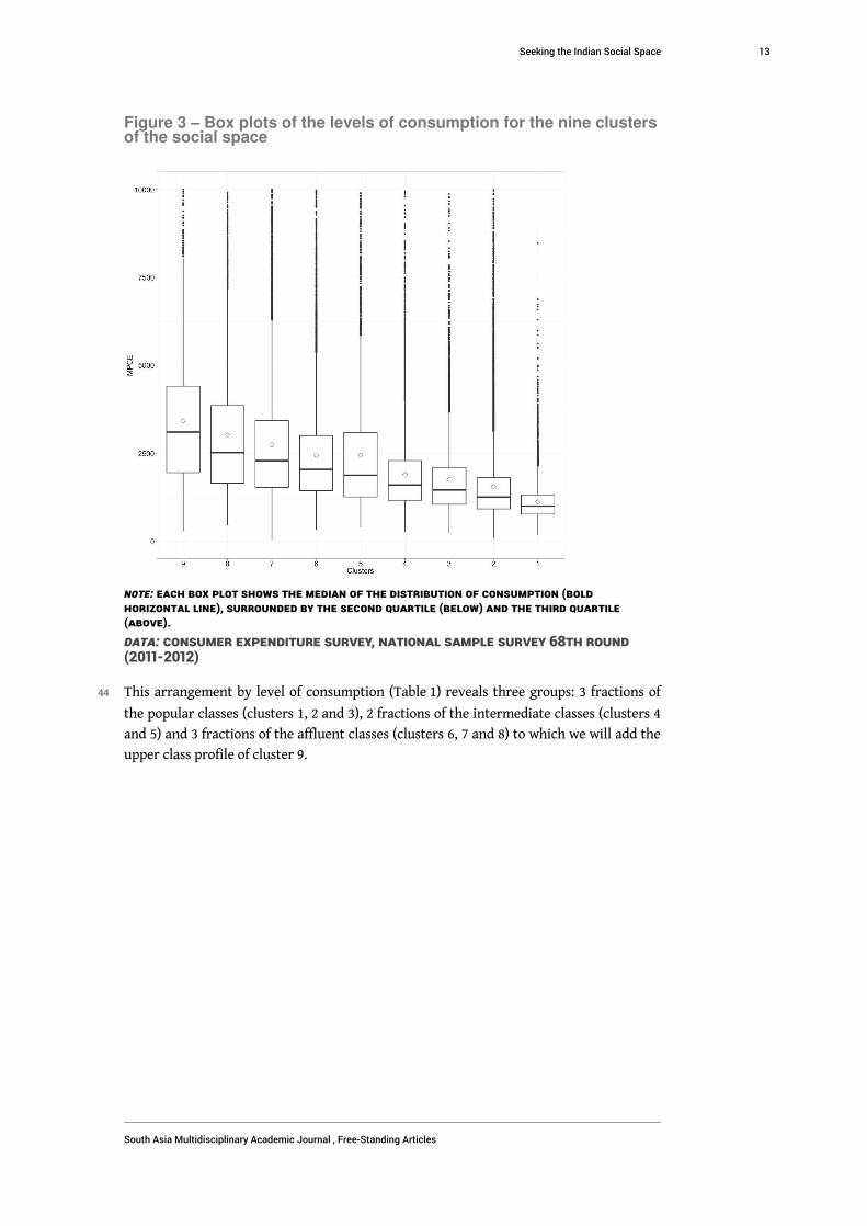
Figure 3 – Box plots of the levels of consumption for the nine clustersof the social space
Note: Each box plot shows the median of the distribution of consumption (boldhorizontal line), surrounded by the second quartile (below) and the third quartile(above).
Data: Consumer Expenditure Survey, National Sample Survey 68th Round(2011-2012)
44 This arrangement by level of consumption (Table 1) reveals three groups: 3 fractions of
the popular classes (clusters 1, 2 and 3), 2 fractions of the intermediate classes (clusters 4
and 5) and 3 fractions of the affluent classes (clusters 6, 7 and 8) to which we will add the
upper class profile of cluster 9.
Seeking the Indian Social Space
South Asia Multidisciplinary Academic Journal , Free-Standing Articles
13

Table 1 – Synthetic summary of the clusters in the Indian social space
Figure 4 – Synthetic diagram of the Indian social space
Legend: The clusters are positioned on the vertical scale of the level of consumption (MPCE)depending on their median, and on the horizontal rural/urban axis according to the share of urban andrural. Their width corresponds to the percentage of the sample represented by each of them (theheight is merely half the width). The vignettes show the name of the cluster and its number inbrackets, the under-represented modalities with a strikethrough, the over-represented social positionin italics, the distribution of reserved groups (castes)—scheduled tribes (ST), scheduled castes (SC), other backward classes (OBC), forward castes (FC).
Seeking the Indian Social Space
South Asia Multidisciplinary Academic Journal , Free-Standing Articles
14

The popular classes: 59 percent of the Indian population
45 Extreme deprivation. Cluster 1 gathers the most deprived households and represents no
less than 10 percent of the population. It is characterized by consumption structures
subject to the most compelling need, thus reduced to basic food, particularly subsidized
products, and does not even include access to cheap lentils (khesari) or the most common
energy source in rural zones (dung cake). The modal properties of the cluster agglomerate
the most vulnerable categories present in rural zones: agricultural workers or small
farmers, workers and unqualified employees, small informal businesses with a clear over-
representation of STs, SCs as well as religious minorities.
46 Popular classes. A comparison of cluster 1 with cluster 2 confirms the importance of micro-
resources among the poorest, which we had already noticed thanks to the PCA: caste
status and network and/or relative job stability enable the individual to escape at least
the most extreme deprivation. Indeed, cluster 2, the largest with 40 percent of the
population, embodies the most common profile in India, that of severe poverty (the
second lowest level of expenditure) in rural and suburban zones. The modal consumption
is marked by constraints, although it escapes the most extreme need: it is defined, in a
way, in opposition to rich and urban consumption (under-representation of expenditure
on leisure and education as well as jewelry) as well as to the most deprived level of
consumption (access to khesari, dung cake, food and basic footwear, under-representation
of subsidized food products). With 40 percent of the population, the spectrum of social
properties is relatively wide. It is nonetheless clearly located “below” the better endowed
groups in the social space and just “above” the most deprived: it is characterized by
illiterate and low-level qualifications, agricultural workers and small farmers, workers
and unqualified employees, as well as owners of land of all sizes (an agricultural holding
may be large but infertile) and owners of their homes. Members of all religions and castes
belong to this cluster, but forward Hindu castes are underrepresented whereas OBCs are
slightly overrepresented.
47 Stable popular classes. Cluster 3 is relatively poor but escapes the most compelling need.
With 9 percent of the population, it is concentrated around subsistence consumption,
including subsidized food, as well as small comfort expenditure—particularly everyday
intoxicants (tobacco, betel, etc.), spices, animal food products. In terms of social
properties, it is difficult to distinguish it clearly from cluster 2. But as Cluster 3 is
associated with average density areas, we interpret it as a fraction of the popular classes
who have achieved stability through access to small resources and jobs in areas of
subaltern urbanization.
48 As the positioning of the poverty threshold in Figure 4 shows, the three profiles described
above: extreme deprivation, severe ordinary poverty and stabilized positions in the
popular classes, in themselves justify the utility of a multidimensional approach. Focusing
only on the economic threshold of poverty and the debates on the methods used to
calculate it, obscures the amplitude of the social groups whose experience is reduced to
fulfilling basic needs, while micro-resources actually create significant differences among
this 59 percent of the Indian population. These micro-resources refer to caste status,
home production, job status, and access to infrastructure depending on the area of
residence.
Seeking the Indian Social Space
South Asia Multidisciplinary Academic Journal , Free-Standing Articles
15
The intermediate classes: 16 percent of the Indian population
49 Urban intermediate class. Cluster 4 represents 13 percent of the population and marks a
clearer distance from need—the modalities here represent the urban intermediate class
that is grouped around lower professionals. Small comfort consumption includes petrol
for motorized travel, purchase of fruits and packaged drinks, entertainment, toiletries,
pan (everyday intoxicants, more expensive than tobacco or betel), packaged food, which
is also to be seen in contrast to the served food of the richer urban inhabitants. In terms
of social properties, we note the absence of the ration card, the frequency of lower
professionals and average level qualifications, the stronger presence of forward castes
and the weaker presence of lower castes.
50 Upper caste intermediate class. Cluster 5 only represents 3 percent of the population. It
differs from the previous cluster mainly by the association between the frequency of
specifically Hindu upper castes, high-level qualifications, higher professionals and
ownership of large landed property. It is difficult to situate on the rural/urban axis, as
average densities are over-represented. Nonetheless, the modal consumption structure
shows an urban and cultivated lifestyle, suggesting a concern with distinction:
entertainment, leather shoes (a status symbol among professional male middle or higher
level executives), use of commercial services (tailor, hairdresser, household employees,
etc.), clothing, and reading. This association between an urban lifestyle, average densities
and ownership of property led us to position the cluster between the rural and the urban
in Figure 4.
The affluent classes: 25 percent of the Indian population
51 The cultural affluent class. Cluster 6 gathers 12 percent of the population around a
cultivated profile: urban, most often qualified, forward caste—and not necessarily the
richest nor the largest number of owners, but very often professionals or business people.
With their highly distinctive expenditure on reading, education and entertainment, this
profile adds motor fuel, leather shoes, and industrial milk products. Finally, this cluster
resembles the previous one by its lifestyle concerned with distinction, its qualification
level and the frequency of upper castes; it differs by a noticeable divergence in levels of
expenditure, which makes it a profile of the cultural bourgeoisie in the historical sense of
the term (urban and entrepreneur, shopkeeper or liberal profession, rather than
landowner).
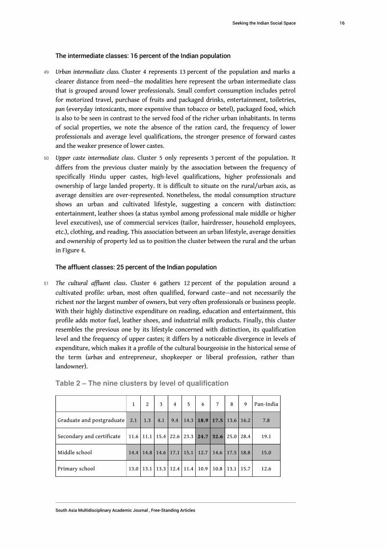
Table 2 – The nine clusters by level of qualification
1 2 3 4 5 6 7 8 9 Pan-India
Graduate and postgraduate 2.1 1.3 4.1 9.4 14.3 18.9 17.5 13.6 16.2 7.8
Secondary and certificate 11.6 11.1 15.4 22.6 23.3 24.7 32.6 25.0 28.4 19.1
Middle school 14.4 14.8 14.6 17.1 15.1 12.7 14.6 17.5 18.8 15.0
Primary school 13.0 13.1 13.3 12.4 11.4 10.9 10.8 13.1 15.7 12.6
Seeking the Indian Social Space
South Asia Multidisciplinary Academic Journal , Free-Standing Articles
16
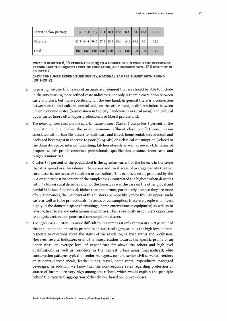
Literate below primary 13.6 15.4 13.5 11.4 10.4 12.4 8.4 7.6 11.6 12.3
Illiterate 45.3 44.4 39.0 27.1 25.5 20.4 16.1 23.2 9.3 33.2
Total 100 100 100 100 100 100 100 100 100 100
Note: In cluster 6, 19 percent belong to a household in which the referenceperson has the highest level of education, as compared with 17.5 percent incluster 7.
Data: Consumer Expenditure Survey, National Sample Survey 68th Round(2011-2012)
52 In passing, we also find traces of an analytical element that we should be able to include
in the survey using more refined caste indicators: not only is there a correlation between
caste and class, but more specifically, on the one hand, in general there is a connection
between caste and cultural capital and, on the other hand, a differentiation between
upper economic castes (businessmen in the city, landowners in rural areas) and cultural
upper castes (more often upper professionals or liberal professions).
53 The urban affluent class and the agrarian affluent class. Cluster 7 comprises 8 percent of the
population and embodies the urban economic affluent class: comfort consumption
associated with urban life (access to healthcare and travel, home rental, served meals and
packaged beverages) in contrast to poor (dung cake) or rich rural consumption (related to
the domestic space: interior furnishing, kitchen utensils as well as jewelry). In terms of
properties, this profile combines professionals, qualification, distance from caste and
religious minorities.
54 Cluster 8 (4 percent of the population) is the agrarian variant of the former, in the sense
that it is spread over less dense urban areas and rural areas of average density (neither
rural deserts, nor areas of subaltern urbanization). This echoes a result produced by the
SFA on the richest 20 percent of the sample: axis 2 contrasted the highest urban densities
with the highest rural densities and not the lowest, as was the case on the other global and
partial SFAs (see Appendix 2). Richer than the former, particularly because they are more
often landowners, the members of this clusters are more likely to be from an upper Hindu
caste as well as to be professionals. In terms of consumption, these are people who invest
highly in the domestic space (furnishings, home entertainment equipment) as well as in
jewelry, healthcare and entertainment activities. This is obviously in complete opposition
to budgets centered on poor rural consumption patterns.
55 The upper class. Cluster 9 is more difficult to interpret as it only represents 0.69 percent of
the population and one of its principles of statistical aggregation is the high level of non-
response to questions about the status of the residence, salaried status and profession.
However, several indicators orient the interpretation towards the specific profile of an
upper class: an average level of expenditure far above the others and high-level
qualifications as well as residence in the densest urban areas (megapolises); elite
consumption patterns typical of senior managers, owners, senior civil servants, rentiers
or students—served meals, leather shoes, travel, home rental expenditure, packaged
beverages. In addition, we know that the non-response rates regarding profession or
source of income are very high among the richest, which would explain the principle
behind the statistical aggregation of this cluster, based on non-responses.
Seeking the Indian Social Space
South Asia Multidisciplinary Academic Journal , Free-Standing Articles
17

56 It is important to note that, unlike traditional stratification studies that often focus solely
on the level of economic wealth, our multidimensional approach makes it possible to
observe a decisive distinction between cultural and economic fractions within both the
intermediate and upper classes. Table 2, which organizes the clusters by level of
qualification, shows that clusters 6 and 7 are the highest on the educational scale, while
their endowment in economic capital is relatively modest when compared to clusters 8
and 9.13
Conclusion
57 In that it attempts to develop a multidimensional approach, combining the level of wealth
with other social properties, our analysis of the Indian social space allowed us to reveal
the existence of a common scale of distribution of resources and statuses. This continuum
of social positions is structured by the relationship to material constraints and supports
the existence of a relatively unified Indian social space. Indeed, although it reveals a few
slight variations, a more precise analysis of the different subspaces provides confirmation
of the stability of this structure. Whether amongst the richest 20 percent, the poorest
30 percent or the intermediate 50 percent, people differentiate themselves from each
other primarily by being more or less subject to material constraints (see Appendix 2).
58 Our analysis also revealed the existence of nine different ideal types that each group
people with similar sociological profiles. This typology of polarities around which the
Indian social space is structured allows us to sketch a nuanced portrait of Indian society
that reveals the extreme diversity of lifestyles. In particular, the analysis brings to light
the massive nature of the three categories that constitute the popular classes. On their
own, they allow us to characterize the sociological profile of almost 60 percent of the
Indian population. These three categories reveal subtle variations amongst the poorest:
micro-resources that allow some to enjoy small comforts, like the purchase of tobacco or
the use of spices for cooking, while others stand out by the extreme deprivation they are
forced to endure.14 This study of the popular classes also enables us to relativize the
importance to be attributed to the notion of “poverty threshold”. The “poor popular
classes” are, in fact, crossed, almost at the center, by this arbitrary line, but it does not,
however, allow us to mark a clear break between lifestyles. The most sociologically
relevant boundaries seem to be located lower down (between “extreme deprivation” and
the “poor popular classes”) or higher up (between the “poor popular classes” and the
“stable popular classes”).
59 The two types that constitute the intermediate classes (that represent 16 percent of the
population) for their part, allow us to note a qualitative jump in terms of lifestyle. This
jump is particularly embodied by the abandonment of subsidized food products and a
wider variety of types of consumption. More qualified, more urban, more often of an
upper caste, their lifestyles can be clearly distinguished from those of the popular classes
by comfort consumption that seeks to affirm a comfortable status, marked for example by
wearing leather shoes, the use of motorized vehicles or the occasional consumption of
prepared meals (dhaba, street food, small restaurants, etc.).
60 The four types that constitute the affluent classes (25 percent of the population) reveal
the existence of more contrasted lifestyles as one escapes the tyranny of need. The
fractions within the upper classes, indeed, differ not only on the rural-urban scale, but
Seeking the Indian Social Space
South Asia Multidisciplinary Academic Journal , Free-Standing Articles
18

also on the basis of their economic capital, their cultural capital and their caste. It is
within these four most comfortable clusters that we find what economists or journalists
often call the “middle classes”. This observation hence leads to a certain wariness in the
usage of this term, too often based on an economic definition that takes the level of
consumption into account but pays little attention to variations in styles of consumption
and at the outset, lifestyle. Moreover, if the so-called “middle” classes are reduced to
those in fact located at the top of the society, there is a very high risk of confusion and of
mixing up categories. We thus prefer to speak of “intermediate” classes rather than
“middle classes”.
61 The idea of middle class, as it is commonly apprehended, does away with the relational
dimension necessarily contained in the term “middle” (“middle” classes only exist if so
called “upper” and “lower” classes exist) and it doubly distorts the vision of Indian
society. It leads not only to dissimulating the privileges enjoyed by the upper classes
(which are no longer dominant but only “middle”), it also encourages to amalgamate all
the groups that are not “middle” and are henceforth assimilated to the mass of those
excluded from globalized consumption. Now, our analysis clearly shows the diversity of
the popular and intermediate classes, which cannot be reduced to vast homogeneous
categories.
62 To sum up, our work hence encourages us to be wary of prenotions like those of “middle
class”, “two-tier India”, “urban-rural cleavage”, or ideas drawn from politico-
bureaucratic language like “poverty threshold”. While they produce the illusion of an
immediate understanding of the complexity of Indian society, these ideas turn out to be
dangerous simplifications and hamper a vision that is attentive to the various dimensions
at work in the production of classifications in India. We hence think that the
multidimensional approach to the Indian social space, initiated here, deserves to be
explored in further detail. In particular, it makes it possible to empirically investigate the
regional variations of the social structure that we have revealed: the methodology
adopted allows us to vary the focal point of the analysis, from the social space at the
national scale to its variants at the scale of each State. The comparative approach
between regions, which is the most common in the Indian social sciences, but nonetheless
has its weaknesses, which Aseema Sinha (2015) has underscored, could thus be revisited
and consolidated by adding a unified and multidimensional representation of the Indian
social space, something our analysis provides for the first time, along with synoptic
summaries in the form of tables and diagrams.
Appendix 1: Data and methods
63 This appendix details the methodological framework of this study, by presenting
thoroughly the data and the statistical method implemented here.
64 To start with, the consumption variables were selected from the overall basket and
transformed into budgetary coefficients (consumption level per head divided by the total
household consumption per head). We selected 37 detailed and aggregated (items that
group families of goods15) budgetary items. This selection is based on budgetary items
that allow us to highlight disparities in consumption, while maintaining the sociological
coherence of the selected basket, which ends up representing close to 86 percent of the
average total budget of Indian households (see column “Share in budget” in Table A1).
Hence the selected basket does not include certain extremely rare consumer goods, or
Seeking the Indian Social Space
South Asia Multidisciplinary Academic Journal , Free-Standing Articles
19

budgetary coefficients for durable goods, which are included in the analysis on the basis
of possession (household appliances and means of transport, see column “Distribution” in
Table A2).
Table A1 – Active variables used in the factorial analysis
Budget item
Share
in
budget
(%)
Axis 1 Axis 2
Contribution Coord.Cos2
SFA
Coord.
SFAContribution Coord.
Cos2
SFA
Coord.
SFA
Cereals 11.85 6.46 -0.47 0.00 0.03 4.86 -0.34 0.24 -0.49
Fuel and light
(no dung
cake)
8.97 6.35 -0.47 0.22 -0.47 0.92 0.15 0.04 -0.21
Milk and milk
products8.38 1.39 0.22 0.03 0.19 7.75 -0.42 0.01 -0.12
Clothing and
bedding7.03 1.83 -0.25 0.00 -0.06 0.68 -0.13 0.05 -0.21
Consumer
services (no
conveyance)
4.55 2.74 0.31 0.03 0.17 0.14 0.06 0.06 0.25
Vegetables
(no potato)3.92 10.03 -0.59 0.23 -0.48 1.25 0.17 0.08 -0.28
Egg. fish and
meat3.47 0.49 -0.13 0.03 -0.19 8.01 0.43 0.01 0.07
Pulses 3.40 7.97 -0.52 0.12 -0.35 0.05 -0.04 0.15 -0.39
Conveyance 2.99 0.40 0.12 0.01 -0.09 2.41 0.24 0.03 0.16
Education 2.82 6.91 0.49 0.15 0.39 0.38 -0.09 0.04 0.21
Toilet articles 2.53 1.47 -0.22 0.09 -0.30 2.39 0.24 0.00 -0.05
Spices 2.31 10.24 -0.59 0.34 -0.59 3.06 0.27 0.10 -0.31
Motor fuel 1.94 0.62 0.15 0.00 -0.02 0.94 0.15 0.03 0.17
Beverages 1.67 0.05 0.04 0.05 -0.22 4.05 0.31 0.04 0.19
Rent 1.56 3.51 0.35 0.02 0.14 1.02 0.15 0.08 0.28
Medical
(institutional)1.55 1.01 0.19 0.02 0.16 0.11 -0.05 0.00 0.06
Seeking the Indian Social Space
South Asia Multidisciplinary Academic Journal , Free-Standing Articles
20

Sugar 1.53 1.22 -0.20 0.00 0.05 14.16 -0.57 0.22 -0.47
served food 1.52 2.00 0.26 0.01 0.08 1.62 0.19 0.13 0.36
Fruits 1.41 1.43 0.22 0.00 -0.05 4.55 0.33 0.06 0.24
Packaged
processed
food
1.40 0.10 0.06 0.00 -0.03 0.68 0.13 0.03 0.18
Cooked meals
for assistance1.40 1.42 -0.22 0.00 -0.06 0.01 -0.02 0.02 -0.13
Potato 1.20 7.55 -0.51 0.05 -0.23 3.78 -0.30 0.09 -0.29
Entertainment
(cinema, club,
etc.)
1.17 2.36 0.28 0.00 0.04 4.12 0.31 0.10 0.32
Tobacco 1.14 0.90 -0.18 0.02 -0.15 0.01 0.01 0.01 -0.09
Cereals PDS 0.99 4.38 -0.39 0.26 -0.51 7.43 0.42 0.00 0.02
Dung cake 0.90 1.89 -0.25 0.00 0.03 10.67 -0.50 0.11 -0.33
Reading 0.77 3.65 0.35 0.12 0.35 0.85 -0.14 0.02 0.15
Intoxicants 0.73 0.07 -0.05 0.02 -0.13 1.61 0.19 0.01 0.08
Footwear (no
leather)0.69 2.98 -0.32 0.04 -0.20 0.46 -0.10 0.09 -0.29
Jewels 0.57 0.92 0.18 0.03 0.16 0.00 0.00 0.01 0.09
Leather shoes 0.50 2.61 0.30 0.05 0.22 0.37 -0.09 0.02 0.13
Pan 0.34 0.37 -0.11 0.02 -0.12 1.39 0.18 0.00 0.06
Crockery and
utensils0.23 0.19 -0.08 0.00 0.01 0.17 -0.06 0.00 -0.05
Sugar PDS 0.15 2.93 -0.32 0.24 -0.49 9.96 0.48 0.01 0.09
Goods for
recreation
(TV, DVD,
etc.)
0.12 0.34 0.11 0.00 0.04 0.09 0.05 0.01 0.09
Furniture 0.09 0.31 0.10 0.01 0.07 0.04 0.03 0.01 0.09
Khesari 0.04 0.89 -0.17 0.01 -0.07 0.00 -0.01 0.01 -0.08
Seeking the Indian Social Space
South Asia Multidisciplinary Academic Journal , Free-Standing Articles
21

Note: Budgetary items are used in the factor analysis as active variables. Theconsumption of cereals represents on average 12 percent of the total consumption. Thecontributions of the budgetary items for the first two factors of the PCA are presented,along with the coordinates of the SFA (“global” analyses).
Table A2 – Supplementary variables (1): Ownership of durable goodsand use of AYUSH treatments
ModalityDistribution
(%)
Axis 1 Axis 2
Coord.
PCA
Coord.
SFA
Coord.
PCA
Coord.
SFA
Possessed
items
Ayush Yes 30.14 0.12 0.08 -0.07 0.03
No 69.85 -0.05 -0.03 0.03 -0.01
Unknown 0.00 -0.77 -0.10 1.25 -0.36
Bicycle Yes 58.36 -0.18 0.04 -0.22 -0.02
No 41.64 0.26 -0.04 0.30 0.02
Scooter Yes 27.27 1.32 0.53 -0.10 0.26
No 72.73 -0.49 -0.24 0.04 -0.12
Car Yes 4.47 2.32 0.70 -0.07 0.41
No 95.53 -0.11 -0.05 0.00 -0.03
Clock Yes 87.00 0.20 0.07 0.04 0.05
No 13.00 -1.33 -0.57 -0.24 -0.36
Computer Yes 5.28 2.75 0.87 0.15 0.67
No 94.72 -0.15 -0.06 -0.01 -0.05
Mobile
handsetYes 85.22 0.28 0.12 -0.03 0.08
No 14.78 -1.62 -0.74 0.17 -0.45
Landline
phoneYes 5.53 2.05 0.60 0.33 0.35
No 94.47 -0.12 -0.05 -0.02 -0.03
Electric fan Yes 71.89 0.45 0.14 0.12 0.11
No 28.11 -1.16 -0.39 -0.30 -0.30
Refrigerator Yes 20.93 1.80 0.53 0.04 0.37
Seeking the Indian Social Space
South Asia Multidisciplinary Academic Journal , Free-Standing Articles
22

No 79.07 -0.48 -0.19 -0.01 -0.14
Note: The ownership of durable goods and the use of AYUSH treatments is included in theanalysis as supplementary variables. 30.14 percent of Indians live in households thatuse AYUSH treatments. The coordinates of the modalities (Yes/No) of the PCA and of theSFA are presented in the columns.
65 Secondly, we selected 14 social position variables that allow us to grasp different
segmentations of Indian society, mainly the level of consumption, the living environment
(urban or rural, and geographic16), caste, religion and social class. The latter was
constructed using the class schema developed by Vaid (2012), to date the only schema
that offers a synthetic representation of social classes in Indian society.
Table A3 – Supplementary variables (2): Social positions ofhouseholds
ModalityDistribution
(%)
Axis 1 Axis 2
Coord.
PCA
Coord.
SFA
Coord.
PCA
Coord.
SFA
Standard of
living
MPCE
P0-P5 5.00 -2.49 -1.15 -0.06 -0.63
P5-P10 5.00 -1.88 -0.63 -0.40 -0.65
P10-P20 10.00 -1.49 -0.56 -0.32 -0.55
P20-P30 10.00 -1.08 -0.40 -0.26 -0.48
P30-P40 10.00 -0.74 -0.32 -0.21 -0.38
P40-P50 10.00 -0.37 -0.24 -0.03 -0.30
P50-P60 10.00 0.00 -0.13 0.06 -0.18
P60-P70 10.00 0.41 -0.01 0.16 -0.05
P70-P80 10.00 0.94 0.15 0.18 0.13
P80-P90 10.00 1.63 0.36 0.28 0.36
P90-P95 5.00 2.36 0.55 0.35 0.66
P95-P100 5.00 3.41 0.94 0.38 0.97
Ration card
Ration card
holder84.11 -0.10 -0.07 0.04 -0.04
No ration card
hold15.88 0.50 0.29 -0.18 0.17
Seeking the Indian Social Space
South Asia Multidisciplinary Academic Journal , Free-Standing Articles
23

Ration card
unknown0.02 0.66 0.80 -1.43 -0.08
Land owned
No land owned 10.51 1.31 0.21 0.77 0.55
0-1 acre land
owned58.05 -0.19 -0.16 0.08 -0.04
1-5 acres land
owned23.45 -0.28 0.10 -0.30 -0.15
5-10 acres land
owned5.29 0.30 0.37 -0.66 -0.09
10-20 acres land
owned2.02 0.71 0.52 -0.73 -0.12
20+ acres land
owned0.67 1.17 0.68 -0.73 -0.01
Social
category
Social class
Farmers-owners
(large and
medium)
6.53 0.35 0.47 -0.78 -0.18
Farmers small
and tenants15.10 -0.42 0.10 -0.50 -0.31
Lower
agriculturists21.95 -1.08 -0.43 0.09 -0.38
Higher
professionals3.69 2.20 0.58 0.27 0.54
Lower
Professionals4.27 1.47 0.49 0.11 0.37
Business 6.77 0.96 0.18 0.16 0.18
Petty business 0.86 -0.33 -0.37 0.13 -0.04
Routine non
Manual7.25 0.80 0.14 0.21 0.19
Lower Routine-
non Manuel2.53 0.67 -0.03 0.31 0.20
Skilled workers 7.95 0.63 -0.05 0.37 0.08
Semi and
unskilled
workers
19.07 -0.44 -0.44 0.09 -0.19
Seeking the Indian Social Space
South Asia Multidisciplinary Academic Journal , Free-Standing Articles
24

Occupation
unknown4.03 0.73 0.11 0.26 0.28
Salary
Regular salary
earner20.95 1.23 0.27 0.32 0.34
No regular salary
earner79.04 -0.33 -0.11 -0.09 -0.13
Salary unknown 0.01 0.75 0.48 0.41 0.58
Education
illiterate 33.24 -0.81 -0.42 -0.15 -0.34
literate below
primary12.28 -0.48 -0.24 0.13 -0.23
Primary school 12.60 -0.18 -0.17 0.14 -0.09
Middle school 15.03 0.10 0.00 0.09 -0.04
Secondary and
certificate19.08 0.90 0.32 -0.02 0.24
Graduate and
postgraduate7.76 2.12 0.65 0.08 0.60
Edu unknown 0.01 -0.48 0.00 -0.64 0.57
Reserved
group
(caste)
STs 8.93 -1.13 -0.19 0.47 -0.11
SCs 19.03 -0.55 -0.33 0.01 -0.17
OBCs 44.06 0.00 0.01 -0.07 -0.07
Upper castes 27.97 0.74 0.25 -0.05 0.23
Caste unknown 0.01 -1.37 0.26 -0.01 0.59
Religion
Hinduism 81.49 -0.01 0.01 -0.02 -0.01
Islam 13.64 -0.20 -0.18 0.06 0.03
Christianity 2.23 0.75 0.13 1.21 0.04
Sikhism 1.61 1.07 0.12 -1.31 0.00
Jainism 0.25 2.39 0.69 -0.03 0.76
Buddhism 0.59 -0.15 -0.06 0.57 -0.10
Zoroastrianism 0.00 4.52 1.05 1.46 -1.10
Religion Others 0.19 -0.38 0.19 0.53 -0.15
Seeking the Indian Social Space
South Asia Multidisciplinary Academic Journal , Free-Standing Articles
25

Religion
unknown0.00 1.63 1.23 1.02 -0.11
Overlap
Hindu/
reserved
group
Hindu low caste 61.56 -0.33 -0.12 0.01 -0.12
Hindu Upper
castes19.92 0.96 0.33 -0.14 0.27
Non Hindu low
caste10.46 -0.04 -0.05 0.06 -0.04
Non-Hindu
middle & higher
castes
8.04 0.19 0.00 0.16 0.13
Cross Caste
unknown0.01 -1.35 0.27 0.01 0.61
Geographic
environment
State Jammu &
Kashmir0.89 0.28 1.11
Himachal
Pradesh0.59 0.26 0.49
Punjab 2.31 1.00 -1.17
Chandigarh 0.09 1.73 0.03
Uttaranchal 0.86 0.18 0.00
Haryana 2.25 1.15 -1.34
Delhi 1.14 1.63 0.19
Rajasthan 5.54 0.64 -0.86
Uttar Pradesh 16.54 -0.39 -1.17
Bihar 8.47 -0.73 -0.93
Sikkim 0.04 0.82 1.23
Arunachal
Pradesh0.09 -0.28 1.59
Nagaland 0.11 0.91 0.39
Manipur 0.21 0.54 0.11
Mizoram 0.09 -0.40 1.99
Tripura 0.32 -0.83 2.27
Seeking the Indian Social Space
South Asia Multidisciplinary Academic Journal , Free-Standing Articles
26

Meghalaya 0.24 0.66 1.81
Assam 2.54 -1.00 1.60
West Bengal 7.68 -0.47 0.17
Jharkhand 2.49 -0.74 -0.66
Orissa 3.35 -1.42 0.36
Chhattisgarh 2.18 -1.75 0.25
Madhya Pradesh 5.92 -0.68 -0.40
Gujarat 5.02 0.49 -0.06
Daman & Diu 0.01 0.82 0.92
D & N Haveli 0.03 -0.15 0.75
Maharashtra 9.50 0.52 0.33
Andhra Pradesh 7.22 0.59 0.92
Karnataka 5.11 0.62 0.81
Goa 0.11 2.05 1.49
Lakshadweep 0.00 0.49 3.25
Kerala 2.84 1.46 1.54
Tamil Nadu 6.10 0.46 2.15
Pondicherry 0.10 1.16 1.44
A & N Islands 0.03 -0.51 3.00
Sector
Rural 71.43 -0.49 -0.09 -0.16 -0.20
Urban 28.57 1.22 0.19 0.39 0.43
Density
(inhab /
km2)
Density rural
very low1.29 -0.54 -0.10 0.47 -0.22
Density rural low 12.59 -0.70 -0.14 0.07 -0.27
Density rural
medium21.03 -0.33 -0.11 0.22 -0.22
Density rural
medium high20.46 -0.51 -0.03 -0.41 -0.20
Seeking the Indian Social Space
South Asia Multidisciplinary Academic Journal , Free-Standing Articles
27

Density rural
high15.86 -0.53 -0.06 -0.57 -0.10
Density rural
very high0.19 1.56 0.18 0.39 -0.21
Density urban
very low0.33 1.07 0.33 0.24 0.21
Density urban
low3.02 0.79 0.21 0.27 0.38
Density urban
medium6.94 1.09 0.22 0.46 0.34
Density urban
medium high7.41 1.20 0.11 0.31 0.42
Density urban
high6.21 1.01 0.07 0.21 0.59
Density urban
very high4.67 2.02 0.34 0.73 0.66
Density urban
unknown0.00 1.14 0.13 0.45 -0.06
Density rural
unknown0.00 0.63 0.37 0.04 -0.20
Structure of
the household
Joint family
No joint fam 55.91 -0.06 -0.06 0.15 0.06
Joint family 44.09 0.07 0.11 -0.19 -0.10
Live-in
domestic
staff
No servant 99.50 -0.01 0.00 0.00 0.00
Servant 0.50 1.65 0.57 0.02 0.33
Status of
the
residence
No dwelling unit 0.06 -1.45 -0.39 0.24 -0.32
Hiring dwelling
unit9.61 1.89 0.40 0.78 0.74
Dwelling owner 88.58 -0.20 -0.05 -0.10 -0.10
Other kind of
dwelling unit1.75 -0.06 -0.14 0.66 0.19
Dwelling
unknown0.00 1.92 0.44 0.10 -0.16
Seeking the Indian Social Space
South Asia Multidisciplinary Academic Journal , Free-Standing Articles
28

Note: Social position indicators are included in the analysis as supplementary variablesin order to interpret the factorial plans. The share of each modality, along with thecoordinates in the PCA and the SFA are presented here. The coordinates of the differentstates in the SFA are not present since the state variable is used to “neutralize” thefactor plan.
66 The total level of consumption variable by individual MPCE (Monthly Per Capita
Expenditure) provides an approximate indicator of the households’ wealth, in the absence
of reliable data on the income (The NSSO surveys never record the households’ income).
Following the codification used in the survey reports, we obtain a breakdown of the
variable into 12 categories as the MPCE is split into 10 deciles and quintiles are
substituted for the extreme deciles.
67 Using Divya Vaid’s quantitative work cited above, a social class schema was constructed
on the basis of the main profession of the household. As only 22 percent of women
between the ages of 15 and 59 belong to the active population, the social class is primarily
a reflection of the male head of the household’s economic activity. Vaid’s schema was
produced by modifying Goldthorpe’s typology of “occupations” in British society, to
adapt it to Indian society, more specifically by associating rural and urban professions in
the same grid (Table A4). Farmers (over 40 percent of the active population) are thus
divided into three categories, according to their status as day laborers, sharecroppers or
landowners. The breakdown of class by sector of residence also shows that this grid of
analysis is well suited to India. Although certain categories are over-represented in urban
areas and others in rural areas, this schema clearly offers a synthetic view of social
classes in India (Table A5). The construction of this variable, based on the National
Classification of Occupations-2004 nomenclature (designed by the Directorate of General
Training of the Ministry of Skill Development and Entrepreneurship, based on the
ISCO-1988 nomenclature), nonetheless leaves the social class of 4 percent of the
population, located more amongst the richest and most urban fractions of the social
space, in abeyance. Whether it be due to the absence of a profession (rentiers) or the
refusal to declare their economic activity, we can conjecture about this fraction of the
social space that is impossible to grasp. The survey also records whether the profession is
a salaried one or not, which allows us to make a distinction between the self-employed,
day laborers and salaried employees.
Seeking the Indian Social Space
South Asia Multidisciplinary Academic Journal , Free-Standing Articles
29

Table A4 – Class schema used by Divya Vaid (Excerpt from Vaid 2005)
Table A5 – Social composition of the rural and urban Indianpopulation by class.
All India Rural Urban
Higher professionals 3.69 1.29 9.7
Lower professionals 4.27 2.81 7.94
Routine non-manual 7.25 4.63 13.81
Lower Routine non-manual 2.53 1.69 4.65
Business 6.77 4 13.67
Petty business 0.86 0.67 1.32
Skilled workers 7.95 5.06 15.18
Semi and unskilled workers 19.07 17.91 21.94
Farmers-owners (large and medium) 6.53 8.64 1.23
Farmers small and tenants 15.1 20.53 1.52
Lower agriculturists 21.95 29.46 3.17
Seeking the Indian Social Space
South Asia Multidisciplinary Academic Journal , Free-Standing Articles
30

Occupation unknown 4.03 3.3 5.88
Total 100 100 100
Note: 3.7 percent of the Indian population lives in a household where the mainprofessional activity belongs to the Higher Professionals social class.
68 The social structure of caste is reduced to a study of official categories: Scheduled caste
(SC), Scheduled Tribes (ST), Other Backward Classes (OBC). We further clustered all the
groups that do not benefit from reservations under the label “Forward castes” or “Upper
castes”. A knowledge of the religion of the households also allows us to specify the
congruence between caste and class, as Divya Vaid showed. She thus distinguishes the
Muslim minority (13.5 percent of the estimated population in our survey) from the rest of
the population, and establishes that this category is very close to the SCs and STs. This
justifies our creation of a variable combining Forward caste or low castes (combining ST,
SC and OBC) with the Hindu religion (81 percent of the estimated population) or religious
minority (the non-Hindus are Muslim, 13.5 percent, Christian, 2.3 percent, Sikh,
1.6 percent, Jain 0.25 percent or belong to other religious minorities).
Table A6 – Distribution of the population between Hindu and non-Hindu forward castes and Hindu and non-Hindu lower castes
Modalities Pan-India Rural Urban
Hindu Forward castes 20.0 15.9 29.8
Non Hindu forward castes 8.0 7.1 10.5
Hindu low caste 61.6 67.2 47.5
Non Hindu low caste 10.4 9.8 12.2
TOTAL 100 100 100
Note: 20 percent of the population belongs to the forward Hindu castes.
69 Lastly the household’s geographical location is taken into account through the State or
Union Territory of residence and the urban or rural living environment. But in order to
transcend the latter dichotomy, a variable showing population density by district was
introduced in an attempt to envisage more precise levels of urban development and rural
isolation. This variable was constructed from the 2011 Census data and follows a
classification of 6 density levels per district, distinguishing the urban and the rural. This
provides a variable with 12 modalities (Table A7). Indeed, it is quite surprising to note
that apart from the high and very high density modalities, the rural environment is over-
represented (in comparison to the total proportion of inhabitants in rural environments)
in all the density categories, including for the medium high and medium densities. This
result is yet another argument reinforcing the inadequacy of the categories rural and
urban, and the relevance of the introduction of our variable. The latter is nonetheless to
Seeking the Indian Social Space
South Asia Multidisciplinary Academic Journal , Free-Standing Articles
31

be considered cautiously as in itself it does not represent an indicator of urban
development.
Table A7 – Proportion of the population in each density category, byurban and rural Census categories
Rural Urban Total
Density very high 3.8 96.2 100
Density high 71.3 28.7 100
Density medium high 73.4 26.6 100
Density medium 75.2 24.8 100
Density low 80.7 19.3 100
Density very low 79.9 20.1 100
Density unknown 72.5 27.5 100
Total 71.4 28.6 100
Note: 3.8 percent of rural inhabitants live in a very high density zone.
Principal component analysis and standard factor
analysis
70 The next stage consisted of producing a Principal Component Analysis (PCA) that permits
a graphic representation on two-dimensional planes, of the correlations measured
between the budget variables (active variables17), while seeking associations with social
position variables (supplementary variables). The analysis is weighted using the survey
weight, which results from the weighting adjustment of random sampling design by the
NSSO. The use of the weighting coefficient multiplied by the number of people in the
household (a choice in line with other works that use this type of surveys for
consumption budgets) can be equated to studying the consumption of the average person
in each household. Here we only interpret the first plane made up of the two main
dimensions of the PCA (see Figure A1 for the cloud of individuals)—those that best resume
the inertia of the correlations between the active variables (or in other words, provide
the most information, see Table A8 for the variance explained by the different factors).
Table A8 – Eigenvalues and inertia of all factors of PCA
FactorProper
value
Variance
(%)
Cumulative
variance (%)
Modified rate
(%)
Cumulative modified
rate (%)
1 3.42 9.25 9.25 24.10 24.10
Seeking the Indian Social Space
South Asia Multidisciplinary Academic Journal , Free-Standing Articles
32

2 2.33 6.29 15.54 11.11 35.21
3 1.83 4.94 20.48 6.83 42.04
4 1.63 4.41 24.90 5.43 47.47
5 1.45 3.93 28.83 4.30 51.77
6 1.33 3.61 32.44 3.61 55.38
7 1.26 3.41 35.85 3.23 58.61
8 1.23 3.31 39.16 3.04 61.65
9 1.14 3.09 42.25 2.64 64.29
10 1.12 3.02 45.27 2.51 66.80
11 1.09 2.94 48.21 2.39 69.19
12 1.04 2.80 51.01 2.17 71.36
13 1.02 2.76 53.77 2.10 73.46
14 1.01 2.73 56.50 2.06 75.52
15 0.98 2.66 59.16 1.94 77.46
16 0.97 2.62 61.77 1.89 79.35
17 0.93 2.51 64.28 1.73 81.08
18 0.91 2.47 66.75 1.68 82.76
19 0.91 2.45 69.20 1.65 84.41
20 0.90 2.44 71.64 1.64 86.05
21 0.86 2.34 73.98 1.50 87.55
22 0.85 2.29 76.27 1.43 88.98
23 0.81 2.20 78.47 1.33 90.31
24 0.80 2.17 80.64 1.29 91.60
25 0.77 2.08 82.72 1.18 92.78
26 0.72 1.95 84.67 1.03 93.81
27 0.71 1.92 86.59 1.00 94.81
28 0.71 1.91 88.50 0.99 95.80
Seeking the Indian Social Space
South Asia Multidisciplinary Academic Journal , Free-Standing Articles
33

29 0.65 1.76 90.26 0.84 96.64
30 0.59 1.60 91.86 0.69 97.33
31 0.55 1.49 93.35 0.60 97.93
32 0.55 1.49 94.84 0.59 98.52
33 0.50 1.34 96.18 0.48 99.00
34 0.43 1.17 97.34 0.36 99.36
35 0.40 1.09 98.44 0.31 99.67
36 0.39 1.04 99.48 0.28 99.95
37 0.19 0.52 100.00 0.07 100.00
Note: The first two factors summarize 15.5 percent of the total variance, and35.21 percent when using the modified rate.
Figure A1 – Cloud of individuals of the unstandardized factor analysis of the Indian social space. Plane 1-2
71 The first results on the two selected axes immediately reveal the importance of the
geographic location of the households (although this tendency had already been taken
into consideration in our choice of variables). The “States” variable is the most highly
correlated, by far, not only on the second axis but also on the following axes, while on
axis 1 it is already in second position after the level of consumption. In other words,
Seeking the Indian Social Space
South Asia Multidisciplinary Academic Journal , Free-Standing Articles
34

although it is not the first, the State variable “explains” a large share of the correlations
observed.
72 This regional dimension of our results tends to mask other social disparities in the social
space (see the core article, part II, on this point). These potentially hidden associations
are unfortunately those we were initially trying to objectify when we started our project.
We hence run a Standardized Factor Analysis (SFA, see Bry, Robette and Roueff, 2015 for a
complete description) to neutralize geographical variations in the representation of the
social space. The SFA consists of integrating a reasoning of the type: “all other things
being equal” based on regression analyses, into the context of a factor analysis. A first
factor analysis is performed (in our case it corresponds to the PCA presented above) and
the coordinates of the people on each axis selected for the rest of the analysis are
extracted. Then a series of linear regressions is carried out (as many as there are axes
selected, in our case ten) using the people’s coordinates as dependent variables and the
variable(s) to be “neutralized” as (an) independent variable(s). The residues of each
regression are collected to obtain a table of coordinates of individuals on each selected
axis “free” of the effects of the “neutralized” variables (see table A1, A2 and A3). A
principal component analysis based on these new coordinates then makes it possible to
obtain a new factor space, on to which the active variables from the initial analysis are
projected as supplementary variables.
73 Applying SFA to the geometric plane also makes it impossible to use statistics that are
traditionally mobilized in order to assess the contribution of each factor to the dispersion
of individuals (variance of axes and contribution of individuals and categories to the
axes). The analysis hence focuses on the levels of correlation of the active variables to the
axes, which corresponds to the graphic coordinates of the variables. In addition, this
measurement is completed by the quality of the representation of the active variables on
the axes (cos2 measurements, see Table A1). In what concerns the supplementary
variables, we use the v-test, which measures the distance (expressed in standard
deviations of the normal distribution) between the modalities and the center of the axis.
The higher the value, the better the modality characterizes the axis. Above all, the
graphic interpretation is exploited (see Figure A2 and Figure A3). The active variables
close to the origin of both axes (below 0.01) are not essential to the construction of the
geometrical plane, and hence we do not project them on the figure. With regard to the
supplementary social position variables, we represent the modalities with test values that
are among the thirty highest on at least one of the axes. It should be noted that for the
social position variables (and only for these), the variables close to the origin of the axes
are not eliminated, as we consider these variables important for an attempt to
understand the “middle” of the social space. Lastly, the analysis is attentive to the “eta2”
indices which measure the structuring power of the supplementary variables on an axis
(this index calculates the relationship between the variance of the modalities of a variable
and the variance of an axis).
Seeking the Indian Social Space
South Asia Multidisciplinary Academic Journal , Free-Standing Articles
35

Figure A2 – Unstandardized factor analysis of the Indian social space. Plane 1-2
Note: In blue: consumption level, other dots: other position variables, crosses: the shareof the budget dedicated to each good; diamonds: expenditure level for each good owned.
74 If our SFA is based on ten factors, our analysis is nonetheless limited to its first two
factors. This is why, in order to attain more robust results, we finally decided to also run
an Ascending Hierarchical Classification (AHC) on the first ten factors of the SFA. As
presented in the core of the article (part III, section 2), this allows to push further the
multidimensional approach of the Indian social space by simultaneously integrating in
the analysis elements that could not be combined when interpreting the first two axes of
the SFA. It is to be noticed here that the results of the AHC conducted on the ten axes are
similar (although not identical) to the classification results obtained when limiting
ourselves to the first two or three factors of the SFA. This comforts our analysis: the first
two factors summarize adequately the variability of the household budget.
Seeking the Indian Social Space
South Asia Multidisciplinary Academic Journal , Free-Standing Articles
36

Figure A3 – Cloud of individuals of the standardized factor analysis of the Indian social space. Plane 1-2
Appendix 2: Zooms on the social space
75 The replication of our study on different sub-samples of the NSS “consumption” survey
reveals both a global stability of the results found at the all-India level as well as some
minor—but heuristic—variations. It also confirms the accuracy of a relational analysis
that takes into account all available social properties rather than monetary wealth only.
This appendix presents these results, based on the production of standardized factor
analyses (see Appendix 1) for two sets of subsamples: the urban and the rural households,
and the richest, intermediate, and poorest households.
Variations according to the rural/urban continuum:
more capital in cities
76 As mentioned in the article, the urban is commonly associated with the megapolis and
the rural with the small isolated, agricultural village. Common sense hence tends to
position them as two incommensurable universes. To explore further this rural/urban
divide, we created two subpopulations, one urban (Figure B1) and the other rural
(Figure B2), in order to produce two separate SFAs (or standardized PCAs).
Seeking the Indian Social Space
South Asia Multidisciplinary Academic Journal , Free-Standing Articles
37

Figure B1 – Standardized factor analysis, close-up of urban areas. Plane 1-2
Note: In red, the consumption level; yellow dots: the other position variables(specifically: level of education, professional category, religion, Scheduled Caste,demographic density, land ownership, area of residence); in blue: proportion of thebudget dedicated to each good; orange dots: the level of expenditure for each good.
Data: Consumer Expenditure Survey, National Sample Survey 68th Round(2011-2012)
Seeking the Indian Social Space
South Asia Multidisciplinary Academic Journal , Free-Standing Articles
38

Figure B2 – Standardized factor analysis, close-up of rural areas. Plane 1-2
Note: In red, the consumption level; yellow dots: the other position variables(specifically: level of education, professional category, religion, Scheduled Caste,demographic density, land ownership, area of residence); in blue: proportion of thebudget dedicated to each good; orange dots: the level of expenditure for each good.
Data: Consumer Expenditure Survey, National Sample Survey 68th Round(2011-2012)
77 To start with, the two spaces are overall very similar to each other and to the global
space. The first impression is that we are dealing with a copy of the global SFA. Indeed
one notices the same diagonal that contrasts the rich, educated and professionals, with
the poor, little educated and subaltern workers, and the possession of comfort goods with
the share of expenditure on subsistence goods. It is only by carefully observing the
contributions of the position variables to axes 1 and 2 that one can see some minor
differences (Table B1).
Table B1 – Rural and Urban SFA: correlations of supplementaryvariables to axes 1 and 2
Urban Rural
Axe 1 Axe 2 Axe 1 Axe 2
Eta² Rural/Urban - - - -
MPCE 32% 19% 30% 7%
Social position 16% 3% 10% 7%
Seeking the Indian Social Space
South Asia Multidisciplinary Academic Journal , Free-Standing Articles
39

Land owning 1% 7% 3% 5%
Education level 24% 2% 12% 4%
Caste 4% 0% 3% 3%
Joint family 0% 1% 0% 2%
Hindu or non-Hindu castes 4% 0% 3% 2%
Salaried worker 3% 1% 5% 1%
Ration card 2% 1% 0% 1%
Religion 2% 0% 0% 0%
Servant 0% 0% 0% 0%
Density 0% 2% 0% 0%
Residential status 1% 8% 3% 0%
Note: Eta2 measures the correlation between the axis and the categorical variables. MPCE “explains”32 percent of the variance of axis 1 in urban areas, 30 percent in rural areas.
Data: Consumer Expenditure Survey, National Sample Survey 68th Round(2011-2012)
78 In urban areas, the relationship to ownership of the residence and land is associated with
axis 2, connected to demographic density: there is an opposition between small
landowners and people who own their homes on the one side and non-landowners and
people who rent their homes on the other side. Counter intuitively, in comparison to
other countries, it is the fact of being an (small) owner that correlates with low levels of
consumption and education, and the fact of being a tenant of one’s residence that is
associated with high levels of expenditure and education. This does not signify that the
majority of poor people own their homes, but rather, it expresses differential
relationships to the contractualization of economic relationships. Often, a corner of a
property or a building is “made available” to the families of those employed by the owner
(or one of his allies), or these spaces are informally rented (without a lease, rent receipts,
etc.), or makeshift housing is tolerated in an area of a commune of uncertain ownership…
Thus, while most poor people’s status in terms of their residence would, in some way, be
“tenant” or “usufructuary”, these legal categories are, in fact, incorrect and do not make
sense to the people concerned (some, who built their accommodation themselves, may
even consider themselves the “owners” of it). Only the richest, less socially distanced
from their owner when they are tenants, declare themselves to be “tenants” (and they
more often draw up contracts). As for small landowners, they are located on the side of
low demographic densities on axis 2 and among the high levels of consumption on axis 1:
the richest owners of their homes, which also have land attached to them, live in
residential areas.
79 Inversely, in rural areas, the occupancy status of the home, and ownership of land are not
associated to the same axis. When we find tenants on the “rich” side, they are associated
Seeking the Indian Social Space
South Asia Multidisciplinary Academic Journal , Free-Standing Articles
40

with axis 1. On axis 2, small owners shift to the “poor” side and the modalities of large
owners appear on the “rich” side, associated with farmer owners. The second axis thus
contrasts households that have land capital with industrial or agricultural worker
households that possess no capital other than their labor power and, sometimes, a small
farm—in short the axis contrasts capitalists with their employees. The former are also
(weakly) associated with OBCs, which include a certain number of castes that are
dominant in rural areas, and the latter with SCs and STs, although they are little
differentiated on axis 1. Axis 1, for its part, contrasts levels of consumption and
education, such as those associated or not with a qualified salaried job (this is why lower
professionals are found on the side of the professionals).
80 Thus, in rural and urban areas, the contrasting principles are very similar with,
nonetheless, slight secondary differences. The social structure is globally the same but
tempered by the specificities of urban and rural spaces. This is confirmed by the
distribution of professional categories, levels of consumption and levels of education,
depending on whether the person lives in a rural or urban area (see tables B2, B3 and B4).
Unsurprisingly this distribution reproduces the polarization visible in the global SFA, but
additionally it appears to be strictly linear. The higher is the urban share, the higher the
level of expenditure, the level of education and the professional category (with the
expected exception of farmers who own large and average size farms).
Table B2 – Social position by sector of residence
Note: 25 percent of Higher Professionals live in rural areas.
Seeking the Indian Social Space
South Asia Multidisciplinary Academic Journal , Free-Standing Articles
41

Rural Urban Total
Higher professionals 25.0 75.0 100
Lower Professionals 46.9 53.1 100
Routine non Manual 45.6 54.4 100
Lower Routine-non Manuel 47.5 52.5 100
Business 42.3 57.7 100
Petty business 56.1 43.9 100
Skilled workers 45.4 54.6 100
Semi and unskilled workers 67.1 32.9 100
Farmers-owners (large and medium) 94.6 5.4 100
Farmers small and tenants 97.1 2.9 100
Lower agriculturists 95.9 4.1 100
Total 71.4 28.6 100
Data: Consumer Expenditure Survey, National Sample Survey 68th Round(2011-2012)
Table B3 – Level of consumption by sector of residence
Note: 94.1 percent of the population belonging to the 5 percent fractile of the lowestlevel of consumption live in rural areas.
Rural Urban Total
MPCE P0-P5 94.1 5.9 100
MPCE P5-P10 91.1 8.9 100
MPCE P10-P20 88.9 11.1 100
MPCE P20-P30 87.2 12.8 100
MPCE P30-P40 84;5 15.5 100
MPCE P40-P50 79.2 20.8 100
MPCE P50-P60 76.9 23.1 100
MPCE P60-P70 69.7 30.3 100
Seeking the Indian Social Space
South Asia Multidisciplinary Academic Journal , Free-Standing Articles
42

MCPE P70-P80 60.1 39.9 100
MPCE P80-P90 47.1 52.9 100
MPCE P90-P95 34.2 65.8 100
MPCE P95-P100 22.0 78.0 100
Total 71.4 2.6 100
Data: Consumer Expenditure Survey, National Sample Survey 68th Round(2011-2012)
Table B4 – Level of education by sector of residence
Note: 84.7 percent of the population that lives in a household in which the referenceperson is illiterate, lives in a rural area.
Rural Urban Total
Illiterate 84.7 15.3 100
Literate below primary 79.1 20.9 100
Primary school 75.1 24.9 100
Middle school 71.8 28.2 100
Secondary and certificate 56.6 43.4 100
Graduate and postgraduate 32.2 67.8 100
Total 71.4 28.6 100
Data: Consumer Expenditure Survey. National Sample Survey, 68th Round(2011-2012)
Variations according to the wealth (MPCE)
continuum: a scale with many levels
81 Zooming on various subsamples in terms of wealth produces similar results as zooming
on the rural and urban sub-spaces. Whether it is for the 20 percent richest households,
the 50 percent intermediate households, or the 30 percent poorest households, results are
very similar, displaying only minor but heuristic differences.
Is the “middle class” made up of the richest 20 percent?
82 The first lesson taught by zooming on the richest 20 percent subsample of our population
(Figure B3), is that the Hindu and non-Hindu forward castes are associated with higher
Seeking the Indian Social Space
South Asia Multidisciplinary Academic Journal , Free-Standing Articles
43

levels of capital. It also reveals that in this area of the Indian social space the Muslims and
SCs are not only less endowed with capital, but also more often urban. This is certainly
because, for these discriminated religious and caste minorities, the escape from dominant
castes’ power is more direct and enduring in rural areas, and the opportunities for social
ascension by enrichment are more likely to exist in cities.
83 The second lesson is that while the graph is very similar to the overall SFA, the second
axis is more obviously constructed around the urbanization rate. The main opposition it
reveals is between the highest urban densities on the one side and the highest rural
densities on the other side (with low urban densities and low rural densities closer to the
origin of the axes). This is something that we do not find in the other spaces where the
dispersion of densities on axis 2 is strictly linear. The lowest fractions of the affluent
social space, are clearly associated with rural areas but they are nevertheless more
urbanized than the rural fractions of the intermediate and popular social spaces. In other
words, affluent classes are better described as distributed among different level of
urbanization (from small cities to megapolis) rather than as split between rural and
urban areas. This is probably linked to the fact that it is very unlikely to be among the top
20 percent in terms of income and live in a rural, scarcely dense area.
84 The third lesson is that we clearly see that major differences contrast the upper class,
who are also highly qualified, and higher professionals, with the other well-to-do people,
who are sometimes little qualified such as semi and unskilled manual workers, or lower
agriculturalists. In other words, some comfort goods (computer, refrigerator, car, etc.)
are not accessible to the less rich of the richest 20 percent. The fact that the opposition
between comfort goods and basic goods also constitutes, for the richest 20 percent, the
main factor of polarization between styles of consumption, is an important indicator both
of the strength of the structure of this opposition across the whole Indian social space,
and of the considerable divergences that exist at the “apex” of this space.
85 It hence becomes difficult to identify the richest 20 percent with a homogeneous “middle
class”: it is not only extremely heterogeneous but also, for the most part, far removed
from the stereotype of the mobile urban executive who frequents luxury boutiques in
large shopping malls.
Seeking the Indian Social Space
South Asia Multidisciplinary Academic Journal , Free-Standing Articles
44

Figure B3 – SFA, close-up of the richest 20 percent (deciles 80 to 100). Plane 1-2
Note: In red, the consumption level; yellow dots: the other position variables(specifically: level of education, professional category, religion, Scheduled Caste,demographic density, land ownership, area of residence); in blue: proportion of thebudget dedicated to each good; orange dots: the level of expenditure for each good.
Data: Consumer Expenditure Survey, National Sample Survey 68th Round(2011-2012)
The “intermediate” 50 percent: the key resource of education
86 In line with previous results, the analysis of the social space of the intermediate levels of
consumption does not reveal significant differences with the results at the pan-Indian
level (Figure B4).
87 The most interesting difference appears when one focuses on levels of education. Among
the richest 20 percent there exists a division between the very highly qualified (graduates
and postgraduates) and the others (including the middle school level). The distinguishing
factor within a population that is overall qualified, is being highly qualified—or inversely,
not having any qualification, hence the significance of all the “low education” modalities
(illiterate, literate below primary and primary school, followed by middle school). In this
sub-space, only three modalities are significantly different from the global space: there is
a contrast between the illiterate on the one side and the (post)graduates, secondary and
certificate levels on the other side. Here, it is the mere fact of having prolonged one’s
education that is distinctive and that draws the most educated towards the “top” of this
intermediate zone.
88 At a wider level, this vast intermediate zone, made up of 50 percent of the population,
does not really show any sociological traits that would distinguish it from the other
spaces studies.
Seeking the Indian Social Space
South Asia Multidisciplinary Academic Journal , Free-Standing Articles
45
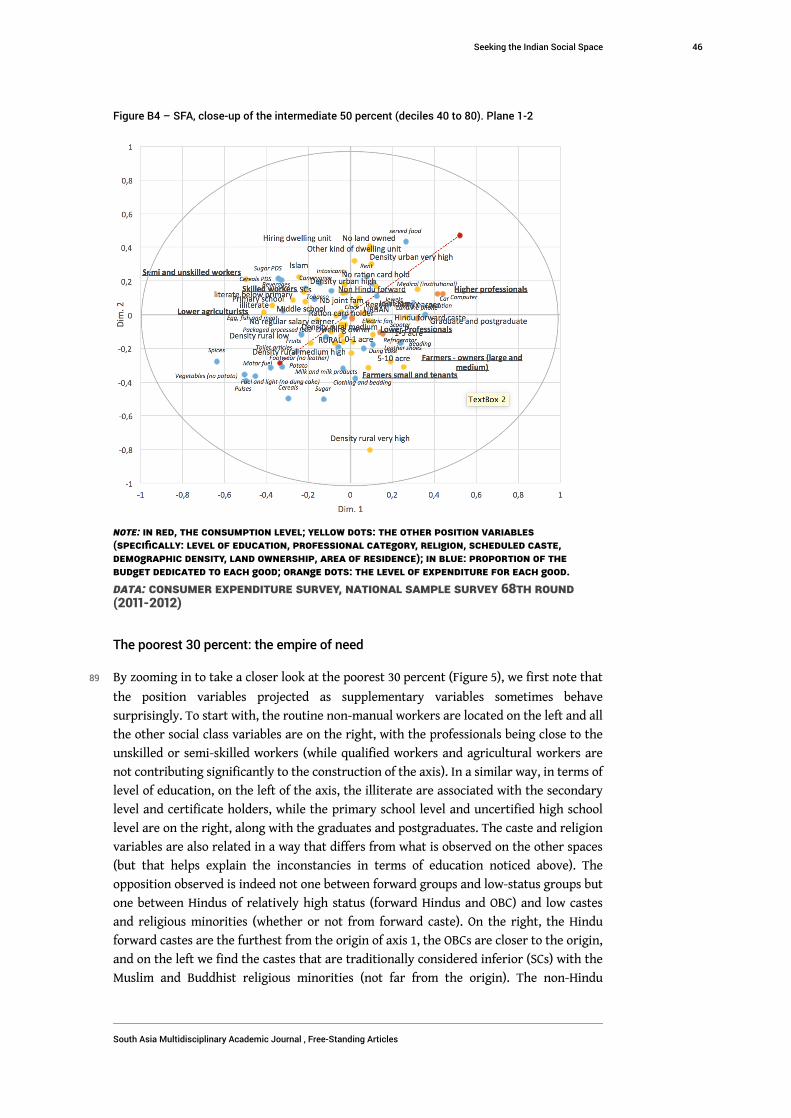
Figure B4 – SFA, close-up of the intermediate 50 percent (deciles 40 to 80). Plane 1-2
Note: In red, the consumption level; yellow dots: the other position variables(specifically: level of education, professional category, religion, Scheduled Caste,demographic density, land ownership, area of residence); in blue: proportion of thebudget dedicated to each good; orange dots: the level of expenditure for each good.
Data: Consumer Expenditure Survey, National Sample Survey 68th Round(2011-2012)
The poorest 30 percent: the empire of need
89 By zooming in to take a closer look at the poorest 30 percent (Figure 5), we first note that
the position variables projected as supplementary variables sometimes behave
surprisingly. To start with, the routine non-manual workers are located on the left and all
the other social class variables are on the right, with the professionals being close to the
unskilled or semi-skilled workers (while qualified workers and agricultural workers are
not contributing significantly to the construction of the axis). In a similar way, in terms of
level of education, on the left of the axis, the illiterate are associated with the secondary
level and certificate holders, while the primary school level and uncertified high school
level are on the right, along with the graduates and postgraduates. The caste and religion
variables are also related in a way that differs from what is observed on the other spaces
(but that helps explain the inconstancies in terms of education noticed above). The
opposition observed is indeed not one between forward groups and low-status groups but
one between Hindus of relatively high status (forward Hindus and OBC) and low castes
and religious minorities (whether or not from forward caste). On the right, the Hindu
forward castes are the furthest from the origin of axis 1, the OBCs are closer to the origin,
and on the left we find the castes that are traditionally considered inferior (SCs) with the
Muslim and Buddhist religious minorities (not far from the origin). The non-Hindu
Seeking the Indian Social Space
South Asia Multidisciplinary Academic Journal , Free-Standing Articles
46

forward castes and the STs are both significant and located on the origin of axis 1, slightly
to its left. It thus seems that among the poorest populations, the fact of belonging to a
Hindu forward caste or to an “other backward class” distinguishes the person from all the
other caste or religious minority attributes. In this sense one can interpret the apparent
inconsistencies of the professional category and of the level of education as an indication
that the small differences between the poor are more strongly based on caste than on
education (rare) or on the social class (as anyway most of them are workers and
agricultural workers). Among the populations that possess no economic or cultural
capital, the caste one belongs to would hence make an enormous difference in terms of
creating a minimum distance from the weight of need.
90 The subspace of the poorest reveals interesting other minor differences. If at first look
one can observe a contrast between comfort goods and basic goods on axis 1, as well as an
opposition between goods of a more urban character and goods that are more common in
rural areas on axis 2, this impression needs to be tempered. The zone of “rural” goods
only contains the variable “cereals” while some goods that are, in other sub-spaces,
located on the “rural” side are now located on the “urban” one. Pulses thus turn out to
become “urban”. In a similar fashion, “spices” are located on the “poor” side and sugar
on the “rich” side of axis 1, a reversed location compared to what is observed on the
other spaces and subspaces studied. What thus seems to be inconsistent cannot, in reality,
better express the effect of need: what is considered poor people’s goods for the
intermediate classes becomes rich people’s goods for the poorest. In other words, what
constitutes a basic good at a certain level (and thus weighs strongly on the budget of the
poorest) is considered a luxury lower down (and is thus traded-off from the consumption
basket of the poorest of the poorest).
91 The third point is that this sub-space reveals what constitute the cumulative
disadvantages that produce extreme deprivation. Indeed, the position variables,
projected as supplementary variables, are all aligned on axis 1—which thus represents
not only the level of wealth, but the volume of almost all economic, cultural, caste,
professional resources. Even ownership of land and the fact of working as a farmer-
owner, which are more dispersed on the rural/urban axis (2) in other spaces and
subspaces, are here mainly dispersed on axis 1. Furthermore, the only position variable
that makes a slightly significant contribution to axis 2 (4 percent of inertia) is the
possession of a ration card. This means that this axis mainly expresses the relationship to
state aid for the most disadvantaged, which we have already described as being more
accessible in urban areas: at this level of the social space, getting access to state aid is not
a sign of deprivation but rather a sign of integration. In summary, in the south of axis 2,
one finds the absence of ration card, Buddhism, very low urban density, and all of these
variables are associated with the “cereals” variable, that is the most vital and essential
food item. This is hence in the South of this subspace that are located the most dominated
amongst the dominated. Their portrait is one of Dalits converted to Buddhism, who are
excluded from accessing administrative resources (although these are intended for the
poorest), who eat the most basic food and who live in areas devoid of both urban micro-
opportunities as well as rural micro-resources (particularly home production).18
Seeking the Indian Social Space
South Asia Multidisciplinary Academic Journal , Free-Standing Articles
47

Figure B4 – SFA, close-up of the poorest 30 percent (deciles 0 to 30). Plane 1-2
Note: In red, the consumption level; yellow dots: the other position variables(specifically: level of education, professional category, religion, Scheduled Caste,demographic density, land ownership, area of residence); in blue: proportion of thebudget dedicated to each good; orange dots: the level of expenditure for each good.
Data: Consumer Expenditure Survey, National Sample Survey 68th Round(2011-2012)
92 In conclusion, these zooms confirm the relevance of taking into account the secondary
differentiating factors that “complicate” the massive effect of the level of consumption.
Beyond a division into two (a two-tier India) or three (the classic upper, middle and lower
classes), it is more heuristic to produce a typology of the Indian social space that at the
same times reveals the dizzying length of the social scale, its twists dependent on the
combination of varying social power relationships (wealth, profession, education, caste)
and the multiplicity of its successive levels. This typology is presented in the core article.
BIBLIOGRAPHY
Beinhocker, Eric D., Diana Farrell and Adil S. Zainulbhai. 2007. “Tracking the growth of
India's middle class” The McKinsey Quarterly 3: 50–61.
Bennett, Tony, Michael Emmison and John Frow. 1999. Accounting for Tastes: Australian Everyday
Cultures. Cambridge: Cambridge University Press
Seeking the Indian Social Space
South Asia Multidisciplinary Academic Journal , Free-Standing Articles
48

Bennett, Tony, Mike Savage, Elizabeth Silva, Alan Warde, Modesto Gayo-Cal and David Wright.
2009. Culture, class, distinction, Routledge, London & New York.
Borges Pereira, Virgilio. 2005. Classes e Culturas de Classe das Famílias Portuenses. Classes sociais
e “modalidades de estilização da vida” na cidade do Porto. Porto: Afrontamento/Instituto de
Sociologia da Faculdade de Letras da Universidade do Porto.
Brousse, Cécile. 2013. “Existe-t-il un espace social européen ?”. Paper presented at the Congress
of the Association Française de Sociologie. Nantes, September 2013
Bry, Xavier, Nicolas Robette and Olivier Roueff. 2015. “Adressing Structural Effects within a
Geometric Data Analysis”. Quality and Quantity 50(3): 1009-1020.
Chaudhuri, Kausik, Friedrich Schneider and Sumana Chattopadhyay. 2006. “The size and
development of the shadow economy: An empirical investigation from states of India”. Journal of
Development Economics. 80(2): 428-443.
Clémentin-Ojha, Catherine. 2014. “‘India, that is Bharat…’: One Country, Two Names”. South Asia
Multidisciplinary Academic Journal [Online], 10 | 2014, uploaded on 25 December 2014, URL: http://
samaj.revues.org/3717; DOI: 10.4000/samaj.3717, [accessed on 10 June 2016].
Cveticanin, Predrag and Mihaela Popescu. 2011. “The art of making classes in Serbia: Another
particular case of the possible”. Poetics 39: 444-468.
Dang, Hai-Han H. and Peter F. Lanjouw. 2015. “Poverty Dynamics in India between 2004 and 2012.
Insights From Longitudinal Analysis Using Synthetic Panel Data”. Policy Research Working Paper
7270. World Bank.
Deaton, Angus. 2001. “Counting the World’s Poor: Problems and Possible Solutions”. The World
Bank Observer Research Observer 16(2): 125‑147.
Deaton, Angus. 2003. “Adjusted Indian Poverty Estimates for 1999-2000”. Economic and Political
Weekly 38(4): 322‑326.
Denis, Eric, Partha Mukhopadhyay and Marie-Hélène Zérah. 2012. ”Subaltern urbanization in
India”. Economic and Political Weekly. 47(30): 52–62.
Desai, Sonalde. 2007. “Indian Middle Class”. in Oxford Companion to Economics in India, edited by K.
Basu. New Delhi: Oxford University Press.
Deshpande, Satish. 2006.”Mapping the ‘Middle’: issues in the analysis of the ‘Non Poor’ classes in
India”. Pp. 215-236 in Contested Transformations: Changing Economies and Identities in Contemporary
India, edited by M. John, P. K Jha and S. S. Jodhka. New Delhi: Tulika.
Driver, Edwin D. and Aloo E. Driver. 1987. Social class in urban
India: essays on cognitions and structures. Leiden: E.J. Brill.
Dumont, Louis.1964. La Civilisation indienne et nous. Paris: Armand Colin.
Dupont, Véronique. 2013. “Which Place for the Homeless in Delhi? Scrutiny of a Mobilization
Campaign in the 2010 Commonwealth Games Context”. South Asia Multidisciplinary Academic
Journal [Online] 8, Online since 17 December 2013, URL: http://samaj.revues.org/3662, [accessed
on 11 June 2015].
Fernandes, Leela. 2006. India’s New Middle Class. Democratic Politics in an Era of Economic Reform.
Minneapolis and London: University of Minnesota Press.
Harriss-White, Barbara. 2003. India Working. Essays on Society and Economy. Cambridge: Cambridge
University Press.
Seeking the Indian Social Space
South Asia Multidisciplinary Academic Journal , Free-Standing Articles
49

Harriss-White, Barbara. 2004. “India’s Informal Economy: Facing the 21st Century”. Pp. 265-292 in
India’s Emerging Economy, edited by K. Basu, New Delhi: Oxford University Press.
Himanshu. 2015. “Inequality in India”. Seminar 672, http://www.india-
seminar.com/2015/672/672_himanshu.htm.
Hugrée, Cédric, Etienne Penissat and Alexis Spire. 2017. “Les déterminants sociaux et nationaux
des inégalités culturelles en Europe”, Actes de la Recherche en Sciences Sociales, forthcoming.
Husson, François, Sébastien Lê and Jérôme Pagès. 2010. Analyse de données avec R. Rennes: PUR.
Jaffrelot, Christophe. 2003. India’s Silent Revolution. The Rise of the Lower Castes in North India. New
York: Columbia University Press, London: Hurst, New Delhi: Permanent Black.
Jodhka, Surinder S. 2014. “Changing Face of Rural India”, Economic and Political Weekly 49(14), 5
April 2014.
Jodhka, Surinder S. and Adarsh Kumar. 2017. “Non-farm Economy in Madhubani, Bihar: Social
Dynamics and Exclusionary Rural Transformations”, Economic and Political Weekly, 52 (25-26), 24
June 2017
Jodhka, Surinder S. and Aseem Prakash. 2016. The Indian Middle Class. Delhi: Oxford University
Press.
Joshi, Vijay. 2010. “Economic Resurgence, Lopsided Reform and Jobless Growth”. Pp. 73-106 in
Diversity and Change in Modern India, edited by A. F. Heath, R. Jeffrey, Oxford: Oxford University
Press.
Khilnani, Sunil. 2003. The Idea of India. Penguin UK: London.
Kumar, Sanjay, Anthony Heath and Oliver Heath. 2002. “Determinants of Social Mobility in
India”. Economic and Political Weekly XXXVII(29), 20 July 2002: 2983-2987.
Lardinois, Roland.2013. Scholars and Prophets. Sociology of India from France.19th-20th centuries.
New Delhi: Social Science Press.
Le Roux, Brigitte and Henri Rouanet. 2004. Geometric Data Analysis: From Correspondence Analysis to
Structured Data Analysis. Dordrecht: Kluwer Academic Publishers.
Le Roux, Brigitte and Henri Rouanet. 2005. Geometric data analysis: from correspondence analysis to
structured data analysis. New York: Springer
Le Roux, Brigitte and Henri Rouanet. 2010. Multiple correspondence analysis. Thousand Oaks: Sage.
Maitra, Sudeshna. 2008. “Who are the Indian Middle Class A Mixture Model of Class Membership
Based on Durables Ownership”. Working paper. York University (Toronto).
Mazzarella, William. 2005. “Middle Class”, in Keywords in South Asian Studies, edited R. Dwyer, an
online encyclopedia maintained by SOAS (https://www.soas.ac.uk/south-asia-institute/
keywords).
Meyer, Christian and Nancy Birdsall. 2012. “New Estimates of India’s Middle Class: A Technical
Note”. Washington D.C.: Center for Global Development.
Naudet, Jules and Claire-Lise Dubost. 2016. “The Indian exception: the densification of the
network of corporate interlocks and the specificities of the Indian business system (2000–2012)”.
Socio-Economic Review, first published online January 26, 2016 doi:10.1093/ser/mwv035
Naudet, Jules. 2012. Entrer dans l'élite: Parcours de réussite en France, aux Etats-Unis et en Inde. Paris:
Presses Universitaires de France.
Seeking the Indian Social Space
South Asia Multidisciplinary Academic Journal , Free-Standing Articles
50
Rangarajan, C. and S. Mahendra Dev. 2014. “Counting the poor: measurement and other issues”.
Working paper. Mumbai: Indira Gandhi Institute of Development Research.
Rosenlund, Lennart. 2000. “Cultural change in Norway: cultural and economic dimensions”.
International Journal of Contemporary Sociology. 37(2): 245-275
Schiff, Maurice. 1994. “The Impact of Two-Tier Producer and Consumer Food Pricing in India”.
World Bank Economic Review 8 (1): 103-125.
Sharda, Bam Dev. 1977. Status Attainment in Rural India. Delhi: Ajanta Publications.
Shukla, Rajesh and Roopa Purushothaman. 2008. “Market Information Survey”. New Delhi:
National Council for Applied Economics Research.
Sinha, Aseema. 2015. “Scaling Up: Beyond the Subnational Comparative Method for India”,
Studies in Indian Politics 3(1): 128-133.
Sridharan, Eswaran. 2004. “The Growth and Sectoral Composition of India’s Middle Class: Its
Impact on the Politics of Economic Liberalization”. India Review. 3(4): 405-428.
Stepan, Alfred, Juan J. Linz and Yogendra Yadav. 2010. “The Rise of ‘State-Nations’“, Journal of
Democracy 21(3): 50-68.
Thorat, Sukhdeo and Joel Lee. 2005. “Caste Discrimination and Food Security Programmes”,
Economic and Political Weekly 40(39): 4198-4201.
Vaid, Divya and Anthony Heath. 2010. “Unequal Opportunities: Class, Caste and Social Mobility”,
in Diversity and Change in Modern India: Economic, Social and Political Approaches, edited by A. Heath
and R. Jeffery. Oxford: Oxford University Press.
Vaid, Divya. 2012. “The Caste-Class association in India: an empirical analysis”. Asian Survey. 52
(2): 395-422.
Varma, Pavan K. 1998. The Great Indian Middle Class. New Delhi: Penguin.
NOTES
1. We indeed postulate the existence of a unified Indian space as a working hypothesis that
facilitates the study of the social structure of the Indian population. Though our article does not
pretend to solve the complex issue of knowing whether or not there actually exists a unified
social space, we nonetheless posit that analyzing data drawing upon such an assumption is
actually heuristic.
2. We are aware that doing so does not constitute a definite proof of the unity of the Indian social
space. This is not the aim of this paper.
3. On the application of these statistical techniques to different countries, see Bennett, Emmison
and Frow (1999); Rosenlund (2000); Borges Pereira (2005); Bennett, Savage, Silva, Warde, Gayo-Cal
and Wright (2009); Cveticanin and Popescu (2011).
4. For different definitions, all based on economic resources, see: Shukla and Purushothaman
(2008);Beinhocker, Farrell and Zainulbhai (2007); Meyer and Birdsall (2012); Maitra (2007).
5. We refer the reader to the following works for further details on these methods of analysis: Le
Roux and Rouanet (2010); Le Roux and Rouanet (2005); Husson, Lê and Pagès (2010).
6. Aggregated items are items that club together families of goods. This choice was particularly
driven by an attempt to reduce the consumption variability between geographical zones (for
example, vegetable oils were grouped together, to avoid a polarization between coconut oil and
South Indian states, and mustard oil and Eastern states).
Seeking the Indian Social Space
South Asia Multidisciplinary Academic Journal , Free-Standing Articles
51

7. We use States as a variable in our analysis (India is administratively a Federal State made up of
29 region States and 7 Union Territories, though there were only 28 States when the 2011-2012
NSS survey was conducted as Telangana had not been created yet).
8. Based on the decrease of eigenvalues we decide to interpret the first two axes. The
contribution of axis 1 to the total inertia of the factorial cloud is 9.25percent and the
contribution of axis 2 is 6.29percent (cumulative variance is 15.54percent). As suggested by
Benzécri (Le Roux and Rouanet, 2004: 200), the modified rates allow for a better appreciation of
the relative importance of the first axis. These are of 24.10percent for axis 1 and 11.11percent for
axis 2 (see Appendix 1 for more details).
9. Before taking this decision, three ACPs were run on the subpopulations of Bihar, Kerala, and
West Bengal in order to make sure that the main global structure was confirmed at the level of
these three very contrasted States. Though there were some minor variations, the general results
were very similar across the three States.
10. Dried “cow dung cakes” that are burnt as a source of energy for heating, or mainly for
cooking: they are cheap and widespread in rural areas, particularly among farmers (cattle
breeders).
11. “PDS”: public distribution system. Access to subsidized goods is easier and hence more
frequent among those entitled to them, in towns were public administrations are far more
present and close, both in terms of geographical distance and mediation through personal
networks (Thorat and Lee 2015).
12. Appendix 2 also provides further illustrations of the fact that these supplementary variables
are not linear and redundant.
13. The constraint of a two-dimensional drawing unfortunately makes it impossible to take this
information into account in Figure 4.
14. In their study of the non-farm economy in Madhubani, Surinder Jodhka and Adarsh Kumar
(2017) have also shown the importance played by micro-resources in stratification processes at
the bottom of society.
15. This was particularly driven by an attempt to reduce the consumption variability between
geographical zones (for example, vegetable oils were grouped together, to avoid a polarization
between coconut oil and South Indian states, and mustard oil and Eastern states).
16. The State variable is available here (we remind the reader that India is administratively a
Federal State made up of 29 region States and Union Territories).
17. It should be noted that the ownership of goods variables were selected as supplementary
variables so that they were not redundant with the budget variables.
18. A recent study of the dynamics of entering and exiting poverty clearly shows how much
“small” resources determine highly contrasting probabilities of upward or downward
reclassification (Dang and Lanjouw, 2015).
ABSTRACTS
This article takes as its specific starting point the idea that the Indian society constitutes a
relational space, marked by the interdependency of various sub-spaces. It more precisely aims at
producing a synthetic representation of the Indian social space. In order to do so, we draw upon
the 2011-2012 data from the “Household Consumer Expenditure” survey of the National Sample
Seeking the Indian Social Space
South Asia Multidisciplinary Academic Journal , Free-Standing Articles
52

Survey Office. The analysis leads us to produce a multidimensional typology of consumption and
position profiles around which the households who make up the Indian social space are
aggregated. Finally, we propose a summary figure of the principles that organize the Indian
social space and the nine categories that comprise it. In the conclusion of the article, we discuss
how this multidimensional approach to Indian society encourages to question prenotions like
those of “middle class”, “two-tier India”, “urban-rural cleavage”, or ideas drawn from politico-
bureaucratic language like “poverty threshold”.
INDEX
Keywords: relational space, social space, multidimensional social stratification, factor analysis,
social class, caste, urban-rural, poverty threshold
AUTHORS
MATHIEU FERRY
OSC & LSQ (GENES-CREST), Paris
JULES NAUDET
Centre for South Asian Studies (CEIAS), EHESS, Paris
OLIVIER ROUEFF
CRESPPA, Paris
Seeking the Indian Social Space
South Asia Multidisciplinary Academic Journal , Free-Standing Articles
53
Related Documents