Seeded Segmentation Methods for Medical Image Analysis

Linköping studies in science and technologyThesis No. 1434

S E G M E N T A T I O N M E T H O D S F O RM E D I C A L I M A G E A N A L Y S I S

Blood vessels, multi-scale filtering and level set methods

Gunnar Läthén

LIU-TEK-LIC-2010:5

Department of Science and TechnologyLinköping University, SE-601 74 Norrköping, Sweden

Norrköping, April 2010

Center for Medical Image Science and Visualization (CMIV)Linköping University/US, SE-581 85 Linköping, Sweden

Segmentation Methods for Medical Image AnalysisBlood vessels, multi-scale filtering and level set methods

Copyright © 2010 Gunnar Läthén (unless otherwise noted)

Department of Science and TechnologyCampus Norrköping, Linköping University

SE-601 74 Norrköping, Sweden

ISBN: 978-91-7393-410-7 ISSN: 0280-7971Printed in Sweden by LiU-Tryck, Linköping, 2010

abstract

Image segmentation is the problem of partitioning an image into meaningfulparts, often consisting of an object and background. As an important partof many imaging applications, e.g. face recognition, tracking of moving carsand people etc, it is of general interest to design robust and fast segmentationalgorithms. However, it is well accepted that there is no general method forsolving all segmentation problems. Instead, the algorithms have to be highlyadapted to the application in order to achieve good performance. In this thesis,we will study segmentation methods for blood vessels in medical images. Theneed for accurate segmentation tools in medical applications is driven by theincreased capacity of the imaging devices. Common modalities such as CTand MRI generate images which simply cannot be examined manually, due tohigh resolutions and a large number of image slices. Furthermore, it is verydifficult to visualize complex structures in three-dimensional image volumeswithout cutting away large portions of, perhaps important, data. Tools, such assegmentation, can aid the medical staff in browsing through such large imagesby highlighting objects of particular importance. In addition, segmentationin particular can output models of organs, tumors, and other structures forfurther analysis, quantification or simulation.

We have divided the segmentation of blood vessels into two parts. First, wemodel the vessels as a collection of lines and edges (linear structures) and usefiltering techniques to detect such structures in an image. Second, the outputfrom this filtering is used as input for segmentation tools. Our contributionsmainly lie in the design of a multi-scale filtering and integration scheme for de-tecting vessels of varying widths and the modification of optimization schemesfor finding better segmentations than traditional methods do. We validate ourideas on synthetical images mimicking typical blood vessel structures, andshow proof-of-concept results on real medical images.

i

acknowledgments

The writing of this thesis coincided with a lot of major events in my life: buyingthe first home, doing major renovations and last but not the least, expectingour second child. Actually, our son showed his sense of humor by arriving onthe day before my thesis deadline. Thank you, little Vide. Also, thank you Saraand Mira for constantly reminding me what is important in life and for keepingthe balance.

My PhD studies were initiated right after the completion of my MSc. Weigh-ing between industry and academia, I was pulled by my first supervisor KenMuseth to pursue the PhD. I thank him and Hamish Carr for a lot of inspirationand for introducing me to the never-ending problem of image segmentation.

For the last period, I’ve been working closely with my current supervisorand co-supervisor Reiner Lenz and Magnus Borga. Thank you for the numerousdiscussions and great ideas which have given many new insights.

Thank you also friends and colleagues in the Digital Media and MedicalInformatics groups for creating a friendly environment and appreciated cof-fee breaks during hectic periods. A special thanks to Ola Nilsson for lendingme the nice LATEX-style for the thesis. Finally, thanks to the members in the“Graphics Group” for sharing all the great software for level set methods andvarious algorithms.

Gunnar Läthén Norrköping, SwedenApril 2010

iii

list of publications

The following papers are included in this thesis:

I. Gunnar Johansson, Ken Museth, and Hamish Carr. Flexible and topo-logically localized segmentation. In Ken Museth, Torsten Möller, andAnders Ynnerman, editors, EUROVIS Symposium Proceedings, pages179–186, Aire-la-Ville, Switzerland, 2007. Eurographics, EurographicsAssociation

II. Gunnar Läthén, Jimmy Jonasson, and Magnus Borga. Phase based levelset segmentation of blood vessels. In Proceedings of 19th InternationalConference on Pattern Recognition, Tampa, FL, USA, December 2008.IAPR

III. Gunnar Läthén, Thord Andersson, Reiner Lenz, and Magnus Borga.Momentum based optimization methods for level set segmentation. In InProceedings of the Second International Conference on Scale SpaceMethodsand Variational Methods in Computer Vision (SSVM), volume 5567 ofLecture Notes in Computer Science, pages 124–136, Voss, Norway, June2009a. Springer

IV. Thord Andersson, Gunnar Läthén, Reiner Lenz, and Magnus Borga. Afast optimization method for level set segmentation. In Proceedings of the16:th Scandinavian Conference on Image Analysis (SCIA), volume 5575 ofLecture Notes in Computer Science, pages 400–409, Oslo, Norway, June2009. Springer

V. Gunnar Läthén, Jimmy Jonasson, and Magnus Borga. Blood vesselsegmentation using multi-scale quadrature filtering. Pattern RecognitionLetters, 2009b

v

contributions

Paper I

This paper presents a localization of the “active contours without edges” model[Chan and Vese, 2001] to better fit applications where you want to extractparticular objects in e.g. medical images. Furthermore, the paper presents auser guided approach to initialize the segmentation near objects of interest,based on topological analysis of the data. My main contribution to this paperwas identifying the problem with global behavior of the Chan-Vese model andsuggesting a method to localize the computations. Furthermore, I implementedthe prototype application for performing the experiments.

Paper II

Here, we present an approach to detect blood vessels using multi-scale filter-ing and use the filter response for level set segmentation. I was part in brainstorming the basic idea of the multi-scale filtering, taking active part in theimplementation of the filtering and implemented the level set methods toolbox.As the main author, I did most of the writing of the paper. This paper receiveda best scientific paper award at the ICPR conference 2008.

Paper III

This paper presents an alternative optimization method for level set segmenta-tion, which shows faster convergence and the tendency to overstep local optimasolutions. The basic idea was presented by my co-supervisor and I adjustedand formalized it to fit the level set framework. The formalization was basedupon an energy formulation of the level set propagation used in Paper II. Theimplementation was built on my level set toolbox and I did the writing of thepaper.

Paper IV

This is a variation of Paper III which uses a different optimization method.The implementation is based on the same level set toolbox, but I took on asecondary role in implementing the optimization and the writing of the paper.

Paper V

This is an extension to Paper II which evaluates some parameters of the modeland provides a more general presentation of the segmentation part of themethod. I implemented most parts of the experiments and produced the article.

vii

C O N T E N T S

Abstract

Acknowledgments

List of publications

Contributions

1 Introduction

Image segmentation, 1 ⋅ Medical image analysis, 2 ⋅ Aim and motivation, 2 ⋅Conventions and terminology, 2 ⋅Thesis outline, 3.

2 Linear structure detection

Background, 5 (Gradient operators, Laplace operators, Hessian operators, Spatialand frequency descriptions) ⋅Quadrature filters, 9 ⋅ Local phase, 11 ⋅ Structures indifferent orientations, 14 ⋅ Resolving edge ambiguities, 14 ⋅Multi-scale integration,15 ⋅ Edge localization, 15 ⋅ Results, 16.

3 Medical image segmentation

Thresholding and Region Growing, 19 ⋅ Variational Methods, 19 (Snakes, Levelset methods, Geodesic active contours, Active contours without edges, Active shapemodels, Direction of descent) ⋅ Combinatorial Methods, 22 (Optimality of solutions,Dynamic programming and optimal paths, Graph cuts).

4 Level-set based segmentation

Localized region-based segmentation, 25 ⋅ Phase-based level set segmentation, 26⋅ Optimization aspects of segmentation, 27 (Gradient descent with momentum,Resilient back-propagation) ⋅ Level-set based segmentation and optimization, 30 ⋅Results, 31.

5 Summary and conclusions

Linear structure detection, 35 ⋅ Level-set based segmentation, 35.

6 Future work

Filtering, 37 ⋅ Segmentation, 37.

7 Overview of papers

Bibliography

Paper I

Paper II

Paper III

Paper IV

Paper V

x

C H A P T E R 1

I N T R O D U C T I O N

The primary theme of this thesis is image segmentation applied on med-ical images. This chapter will begin by outlining the basic problem of

segmentation and motivate its importance in many applications. Modern med-ical imaging modalities generate larger and larger images which simply cannotbe examined manually. This drives the development of more efficient and ro-bust image analysis methods, tailored to the problems encountered in medicalimages. The aim and motivation of this thesis in Section 1.3 are directed towardsthe particular problem of segmenting blood vessels. However, the generality ofthe problem can lead to potential impacts also in other areas of image analysis.

1.1 image segmentation

Image segmentation is the problem of partitioning an image in a semanticallymeaningful way. This vague definition implies the generality of the problem

- segmentation can be found in any image-driven process, e.g. fingerprint/-text/face recognition, detection of anomalies in industrial pipelines, trackingof moving people/cars/airplanes, etc. For many applications, segmentationreduces to finding an object in an image. This involves partitioning the imageinto two class of regions - either object or background. Segmentation is tak-ing place naturally in the human visual system. We are experts on detectingpatterns, lines, edges and shapes, and making decisions based upon the visualinformation. At the same time, we are overwhelmed by the amount of imageinformation that can be captured by today’s technology. It is simply not feasiblein practice to manually process all the images (or it would be very expensive,and boring, to do so). Instead, we design algorithms which look for certainpatterns and objects of interest and put them to our attention. For example, arecent popular application is to search and match known faces in your photolibrary which makes it possible to automatically generate photo collections witha certain person. An important part of this application is to segment the imageinto “face” and “background”. This can be done in a number of ways, and it iswell accepted that no general purpose segmentation algorithm exists, or thatit ever will be invented. Thus, when designing a segmentation algorithm, theapplication is always of primary focus: Should we segment the image based onedges, lines, circles, faces, cats or dogs?

1.4 Conventions and terminology

1.2 medical image analysis

An interesting source of images is the medical field. Here, imaging modalitiessuch as CT (Computed Tomography), MRI (Magnetic Resonance Imaging),PET (Positron Emission Tomography) etc. generate a huge amount of imageinformation. Not only does the size and resolution of the images grow withimproved technology, also the number of dimensions increase. Previously,medical staff studied two-dimensional images produced by X-ray. Now, three-dimensional image volumes are common in everyday practice. Even four-dimensional data (three-dimensional images changing over time, i.e. movies)is often used. This increase in size and dimensionality provides major technicalchallenges as well as cognitive. How do we store and transmit all this data, andhow can we look at it and find relevant information? This is where automatic,or semi-automatic, algorithms are of interest. In the best of worlds, we wouldlike to have algorithms which can automatically detect diseases, lesions andtumors, and highlight their locations in the large pile of images. But anothercomplication arises, we also have to trust the results of the algorithms. This isespecially important in medical applications - we don’t want the algorithmsto signal false alarms, and we certainly don’t want them to miss fatal diseases.Therefore, developing algorithms for medical image analysis requires thoroughvalidation studies to make the results usable in practice. This adds anotherdimension to the research process which involves communication betweentwo different worlds - the patient-centered medical world, and the computer-centered technical world. The symbiosis between these worlds are rare to findand it requires significant efforts from both sides to join on a common goal.

1.3 aim and motivation

The aim of this thesis is to develop segmentation methods for medical imagingapplications. In particular, the main project involves the segmentation of bloodvessels in the liver. The segmentation generates a computer model of the vesseltree which can be used for simulating blood and heat flow during surgicalinterventions. The motivation for this work is to increase patient safety byproviding better and more precise data for medical decisions. As stated in theprevious section, this work involves much multi-disciplinary communication,so an overall goal of the work is to establish links and identify important andrelevant medical problems.

1.4 conventions and terminology

The examples throughout this thesis will use two-dimensional images since theillustration and visualization of the ideas are much simpler and provide betterunderstanding. Three-dimensional medical images are important, especiallywhen studying blood vessels, but most of the main ideas in this thesis generalize

2

introduction

to three dimensions without much effort. Such three-dimensional results arepresented in the papers, as proofs of concept. Thus, to keep the language simple,many terms used are natural for two dimensional images, i.e. curve and pixel.In most cases however, these terms can be exchanged with higher-dimensionalcounterparts such as surface and voxel.

1.5 thesis outline

This thesis contains two major parts. The first part in Chapter 2, describes thedetection of lines and edges (i.e. blood vessels) by using filtering techniques.The second part is introduced by Chapter 3 which presents common methodsand theories on image segmentation. Next, Chapter 4 will describe our con-tributions to the field of segmentation, and detail how the filtering results inChapter 2 are used for segmenting blood vessels. Conclusions and presentationof future work are given in Chapter 5 and Chapter 6. Finally, an overview ofthe contributed papers are presented in Chapter 7.

3

C H A P T E R 2

L I N E A R S T R U C T U R E D E T E C T I O N

The fo cus of this thesis is on the detection and segmentation of bloodvessels in medical images. There are numerous ways to model a blood

vessel, but we have chosen to think of a vessel as a collection of lines and edges.In a sufficiently small neighborhood, a vessel can even be described by straightlines and edges which simplifies the analysis greatly. In this chapter, we willdescribe the general problem of detecting linear structures, i.e. lines and edges,by means of filtering. The next section will present some well known techniquesfor line and edge detection using simple digital filters. Then, Section 2.2 willcontinue by describing quadrature filters, which form the basis of our algorithms.The remainder of the chapter will explain the output from the quadrature filtersand how it is used in a multi-scale setting to determine the location of bloodvessel edges.

2.1 background

One of the simplest ways to detect lines, edges and other structures in an imageis to design a mask, or filter which resembles this structure [Gonzales andWoods, 2002, Chap. 10.1]. When convolving an image with the mask, the pixelswith a neighborhood similar to the mask will give strong output. For example,the mask in Figure 2.1(a) would give a strong output for horizontal lines, whilethe remaining masks in Figure 2.1 would indicate lines at different orientations.If the convolved result is thresholded, the pixels which fit the given mask can beidentified. Note that all the masks in Figure 2.1 sum to zero. This is importantsince we do not want any output in constant areas of an image. In technicalterms, we say that the mask, or filter, should have a zero DC level.

It is possible to construct masks that perform well for simple type of struc-

-1 -1 -1

-1 -1 -1

2 2 2

(a) Horizontal

-1 -1 2

2 -1 -1

-1 2 -1

(b) +45○

-1 2 -1

-1 2 -1

-1 2 -1

(c) Vertical

2 -1 -1

-1 -1 2

-1 2 -1

(d) −45○

Figure 2.1: Masks for detecting one pixel thick lines at different orientations.

2.1 Background

Edge profile

First derivative

Second derivative

Figure 2.2: A model of an edge with first and second derivatives.

tures and rather idealistic type of images. If, for example, we want to detectlines of varying width in noisy images, more robust algorithms and generalmodels might be needed. Turning to the problem of detecting edges, a typicalmodel used is a ramp with a linear transition from dark to bright or vice versaas illustrated in Figure 2.2. On the right, we can see a profile of the edge and itsfirst and second derivatives. From this, it can be noted that the first derivativeis a candidate for edge detection, since it gives a non-zero output across theentire edge transition. In fact, the magnitude of the first derivative is probablythe most common feature used for edge detection. The second derivative canbe used to determine whether the edge is a transition from dark to bright orvice versa. But it can also be noted that the zero-crossing of the two peaks inthe second derivative can identify the center of the edge.

2.1.1 Gradient operators

Since we are studying images, the first derivative is represented by the gradient,defined by partial derivatives ∇I = (∂I/∂x , ∂I/∂y)T , for a two-dimensionalimage I. Now, edges can be identified by locating pixels with a high gradientmagnitude: ∣∇I∣ = √(∂I/∂x)2 + (∂I/∂y)2. The only thing missing is a discreteformulation of the partial derivatives. Two such common formulations aregiven in Figure 2.3 which shows the Prewitt and Sobel filter masks.

-1 0 1

-1 0 1

-1 0 1

(a) Prewitt ∂∂x

-1 -1 -1

1 1 1

0 0 0

(b) Prewitt ∂∂y

-1 0 1

-1 0 1

-2 0 2

(c) Sobel ∂∂x

-1 -2 -1

1 2 1

0 0 0

(d) Sobel ∂∂y

Figure 2.3: Common masks (filters) for gradient computation.

6

linear structure detection

0 -1 0

0 -1 0

-1 4 -1

-1 -1 -1

-1 -1 -1

-1 8 -1

Figure 2.4: Two different Laplace filters.

2.1.2 Laplace operators

Turning to the second derivative, a measure often used for images is given bythe Laplace operator:

∇2I = ∂2I∂x2 + ∂2I

∂y2 (2.1)

Two commonly used discrete filter masks are given in Figure 2.4. As previouslynoted, this filter can be used for identifying the type of edge transition, or tolocate an edge by its zero-crossing. However, due to the small size of this filter, itis very susceptible to noise in the image. A popular approach is to first smooth,or low-pass, the image using a Gaussian filter defined by:

Gσ = −e−(x2+y2)/2σ 2

(2.2)

Equivalent to applying the Gaussian followed by the Laplace filter, the Laplaceand Gaussian operators can be combined into the Laplacian of a Gaussian(LoG):

LoGσ = −(x2 + y2 − σ 2

σ 4 ) e−(x2+y2)/2σ 2

(2.3)

The continuous representation of this filter is shown in Figure 2.5(a) and onepossible discretization in Figure 2.5(b). The width of the filter and the size ofthe mask should be tweaked to suppress the noise in the image, while giving as“distinct” zero-crossings as possible. The idea of using the zero-crossings of theLaplacian as an edge indicator is however not easily implemented in practice(see e.g. Huertas and Medioni [1986]), so gradient based edge detection schemesare most widely used.

2.1.3 Hessian operators

A different second derivative-based measure is given by the Hessian matrix:

H = ⎛⎝∂2 I∂x2

∂2 I∂x∂y

∂2 I∂x∂y

∂2 I∂ y2

⎞⎠ (2.4)

The simplest possible filter masks for computing the partial derivatives on asampled image are shown in Figure 2.6. Much work on blood vessel enhance-ment and segmentation (see e.g. Sato et al. [1997] and Frangi et al. [1998])

7

2.1 Background

(a) Continuous filter

-1 -2 -1

0 -1 0

0 -1 0

-1 -2 -1

-2

0

0

0

0

-1

0

0

0

0

-116 -2

(b) Discrete implementation

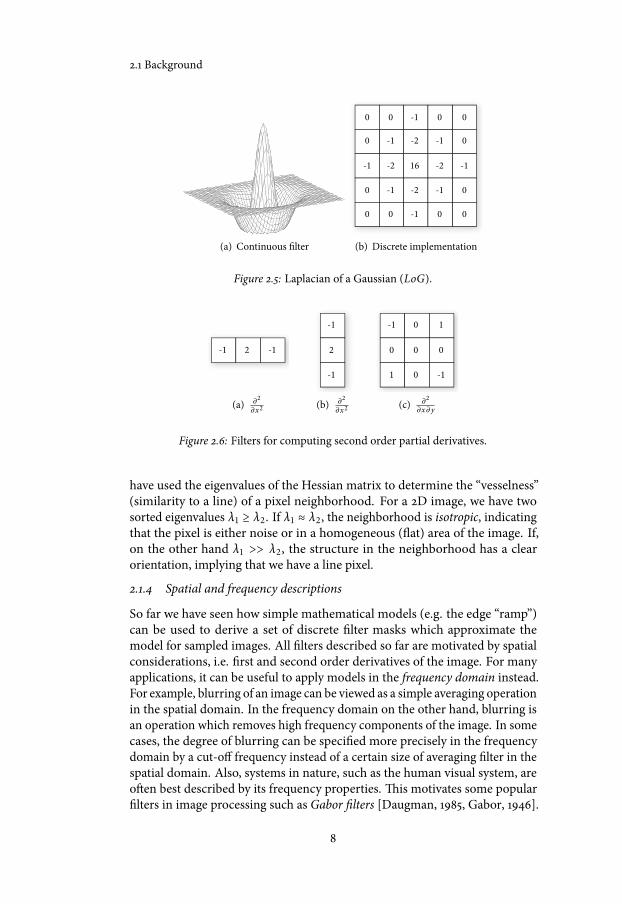
Figure 2.5: Laplacian of a Gaussian (LoG).

-1 2 -1

(a) ∂2

∂x2

-1

-1

2

(b) ∂2

∂x2

-1 0 1

1 0 -1

0 0 0

(c) ∂2

∂x∂y

Figure 2.6: Filters for computing second order partial derivatives.

have used the eigenvalues of the Hessian matrix to determine the “vesselness”(similarity to a line) of a pixel neighborhood. For a 2D image, we have twosorted eigenvalues λ1 ≥ λ2. If λ1 ≈ λ2, the neighborhood is isotropic, indicatingthat the pixel is either noise or in a homogeneous (flat) area of the image. If,on the other hand λ1 >> λ2, the structure in the neighborhood has a clearorientation, implying that we have a line pixel.

2.1.4 Spatial and frequency descriptions

So far we have seen how simple mathematical models (e.g. the edge “ramp”)can be used to derive a set of discrete filter masks which approximate themodel for sampled images. All filters described so far are motivated by spatialconsiderations, i.e. first and second order derivatives of the image. For manyapplications, it can be useful to apply models in the frequency domain instead.For example, blurring of an image can be viewed as a simple averaging operationin the spatial domain. In the frequency domain on the other hand, blurring isan operation which removes high frequency components of the image. In somecases, the degree of blurring can be specified more precisely in the frequencydomain by a cut-off frequency instead of a certain size of averaging filter in thespatial domain. Also, systems in nature, such as the human visual system, areoften best described by its frequency properties. This motivates some popularfilters in image processing such as Gabor filters [Daugman, 1985, Gabor, 1946].

8


(a) (b)

Figure 2.7: Illustrations of the directional function D(u). Figure (a) shows thisfunction in 2D with nk = (

√2/2,√

2/2)T . Figure (b) plots the direction as afunction of ϕ, i.e. the angle between u and nk .

2.2 quadrature filters

For our work, we use so called quadrature filters for line and edge detection.The schemes presented in the previous section rely on spatial derivatives todetermine the location of structures. A major drawback of this approach isthe dependence on image contrast. For example, edge detection using themagnitude of the gradient is highly dependent on quick transitions betweentwo regions of distinctly different intensities (i.e. sharp edges). For smooth orlow contrast edges, gradient-based approaches often fail. On the other hand,quadrature filters provide a contrast independent means of classifying edgesor lines by the local phase, which will be further described in Section 2.3. Butfirst we will introduce the general definition of quadrature filters and theirconstruction in the frequency domain.

Quadrature filters are complex filter pairs where the real and imaginaryparts are oriented line- and edge-filters respectively [Granlund and Knutsson,1995]. They can be defined in the Fourier domain as:

Fk(u) = 0, u ⋅ nk ≤ 0 (2.5)

where u is the frequency coordinate and nk is the filter direction. This spec-ification says that one half-plane of the Fourier domain is zero, i.e. that thefilter does not pick up frequencies on the “negative side” of the filter direction(i.e. the half-plane which has negative projection with nk). Traditionally thefilters are designed to be spherically separable into functions of radius (R) anddirection (D):

F(u) = R(ρ)D(u) (2.6)where ρ = ∣∣u∣∣ and u = u/∣∣u∣∣. To meet certain requirements (invariance andequivariance, see [Granlund and Knutsson, 1995] for a complete description) it

9

2.2 Quadrature filters

(a) Radial function in 1D (b) Radial function in 2D

Figure 2.8: Illustrations of the radial function R(ρ).

was shown in Knutsson [1982, 1985] that the directional function can be chosenas:

Dk(u) = ⎧⎪⎪⎨⎪⎪⎩(u ⋅ nk)2 if u ⋅ nk > 00 otherwise

(2.7)

See Figure 2.7(a) for a 2D plot of this function where nk = (√2/2,√

2/2)T . Itcan be noted that this function varies as cos2(ϕ) where ϕ is the angle betweenu and nk , see Figure 2.7(b) for a plot of this in 1D. Whereas the directionalfunction determines the angular restriction of the filter to discriminate betweendifferent orientation of structures, the radial function decides the radial shapeof the filter in the frequency domain. Thus, the radial function is designed todetect structures of particular frequency content, depending on a particularapplication. A useful class of radial functions is the lognormal functions:

R(ρ) = e− 4B2 log 2

log2 (ρ/ρi) (2.8)

where B is the bandwidth and ρi is the center frequency. See Figure 2.8 forplots of R(ρ) in 1D and 2D.

However, specifying appropriate radial and directional functions in thefrequency domain is not enough to solve the filter design problem. There arealso desired properties on the filter in the spatial domain. Especially importantis the local support, i.e. a good filter should typically be as small as possible.The requirements on the frequency and spatial designs are often in conflict, sothe optimal solution is a balance between the two. In [Knutsson et al., 1999] ageneral filter optimization framework is presented, which uses weighted idealfunctions in the spatial and frequency domains to find an optimal solution in aleast-square sense. Examples of filters generated using such a framework arepresented in Figure 2.9. Here we have chosen the center frequency ρi = π/4and bandwidth B = 2. The size of the spatial mask is 21 × 21. Unless otherwisenoted, these filters will be used for all 2D examples in this thesis.

10


(a) Frequency domain (b) Spatial domain (even) (c) Spatial domain (odd)

Figure 2.9: Optimized quadrature filter in 2D.

2.3 local phase

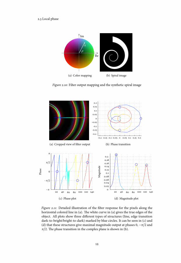
The output from a quadrature filter is complex valued, where the real andimaginary parts represent the output from the line and edge filter respectively.If the output is purely real, the image contains a line, while a purely imaginaryoutput indicates an edge. More generally, the relationship between the “line”-ness and “edge”-ness of a signal is encoded in the filter output as the argument ofthe complex value. Representing the filter output by q = Aeθ , the argument θ isreferred to as the local phase. The local phase has a number of properties makingit robust for detecting lines and edges. Firstly, the local phase is invariant tosignal energy, which means that it is not depending on image contrast. In otherwords, a “weak” line gives exactly the same local phase as a “strong”, or distinctsharp, line. Secondly, the phase varies smoothly and monotonically with theposition of edges and lines. The magnitude A of the output gives, on the otherhand, an indication of signal strength, or the contrast of the lines and edges.For illustrations we encode the complex filter output q using the color mappingof the complex plane shown in Figure 2.10(a).

To illustrate several examples, we use a synthetic image of a spiral displayedin Figure 2.10(b). This is a useful image since it contains lines of varyingthickness and orientation. We detail the concept of local phase in Figure 2.11.The cropped filter output from a filter oriented along n = (1, 0)T is shown inFigure 2.11(a). The plots in Figure 2.11(b-d) show the phase θ and magnitudeA along the horizontal line of pixels in Figure 2.11(a) where the color of thelines can be used to correlate the position of the filter between the plots. InFigure 2.11(d) we see that the first structure that the filter detects is a line at pixel22. The line is visualized by a green color in Figure 2.11(a) and characterizedby a phase of 0 in Figure 2.11(b,c). The next peak in the magnitude is due toan edge transition from dark (background) to bright (object) around pixel 91.This is represented by an orange color in Figure 2.11(a) and a phase of −π/2.Finally, the last structure is an edge transition from bright to dark around pixel124 which is indicated by a phase of π/2 and a purple color.

11

2.3 Local phase

Re

Im

θ

A

(a) Color mapping (b) Spiral image

Figure 2.10: Filter output mapping and the synthetic spiral image

(a) Cropped view of filter output (b) Phase transition

(c) Phase plot (d) Magnitude plot

Figure 2.11: Detailed illustration of the filter response for the pixels along thehorizontal colored line in (a). The white curve in (a) gives the true edges of theobject. All plots show three different types of structures (line, edge transitiondark-to-bright/bright-to-dark) marked by blue circles. It can be seen in (c) and(d) that these structures give maximal magnitude output at phases 0, −π/2 andπ/2. The phase transition in the complex plane is shown in (b).

12


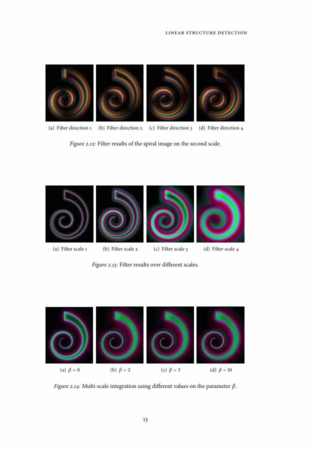
(a) Filter direction 1 (b) Filter direction 2 (c) Filter direction 3 (d) Filter direction 4

Figure 2.12: Filter results of the spiral image on the second scale.

(a) Filter scale 1 (b) Filter scale 2 (c) Filter scale 3 (d) Filter scale 4

Figure 2.13: Filter results over different scales.

(a) β = 0 (b) β = 2 (c) β = 5 (d) β = 10

Figure 2.14: Multi-scale integration using different values on the parameter β.

13

2.5 Resolving edge ambiguities

2.4 structures in different orientations

When a quadrature filter is designed, it is optimized to detect signal energyalong particular orientations. For most applications, it is important to detectstructures in all orientations, so a set of quadrature filters with different orien-tations is commonly used. To cover the space of all orientations, it has beenshown in [Knutsson, 1982, 1985] that at least 3 uniformly distributed orienta-tions are needed in 2D and 6 orientations in 3D. For the examples in this thesis,we use 4 directions in 2D given by:

n1 = (1, 0)T n2 = ( a, a)Tn3 = (0, 1)T n4 = (−a, a)T (2.9)

where a = 1/√2. In 3D, we use 6 filter directions:

n1 = c(a, 0, b)T n2 = c(−a, 0, b)Tn3 = c(b, a, 0)T n4 = c( b,−a, 0)Tn5 = c(0, b, a)T n6 = c( 0, b,−a)T

(2.10)

where a = 2, b = 1 +√5 and c = (10 + 2√

5)−1/2. Applying the 2D filter set tothe spiral image in Figure 2.10(b) yields the results in Figure 2.12, where thelocal phase is visualized using the color mapping in Figure 2.10(a).

2.5 resolving edge ambiguities

As was noted in the illustration of local phase in Figure 2.11, the filter distin-guishes between two types of edges: transitions from dark (background) tobright (object) around pixel 91, or vice versa around pixel 124. For our appli-cation, it is not important to make this distinction so we want to simplify thefilter output by reducing these two cases to only one edge event. This can alsobe motivated by the fact that two filters with opposing direction will result inedge ambiguities. Consider the last edge around pixel 124 in Figure 2.11. Thefilter with direction n1 = (1, 0)T views this edge as a transition from brightto dark and thus gives a local phase of π/2. However, a filter with directionn4 = (−1/√2, 1/√2)T will approach this edge from the other direction anddetects a transition from dark to bright with a local phase of −π/2. Directoperations, such as comparisons or summations, on the results of these twofilters is not possible due to this ambiguity.

Our solution to this problem is to simply take the absolute value of theimaginary part of the filter response. Then we view all edges as transitions frombright to dark with a local phase of π/2. The “rectification” of the filter outputmakes it possibly for direct operations between the results from different filterdirections. We use this to produce an orientation invariant output which is thesum of all filter directions. The result after rectification and summation of thefilter outputs in Figure 2.12 is shown in Figure 2.13(b).

14


2.6 multi-scale integration

We perform the filtering on multiple scales to handle vessels of varying width.Figure 2.13 shows the results on multi-scale filtering of the spiral image. We cannote that the finest scale in Figure 2.13(a) and Figure 2.13(a) detects the thinparts of the spiral as lines, whereas the thicker parts are detected as edges. Aswe traverse the scale hierarchy, also the thicker parts are detected as lines as canbe seen in Figure 2.13(d) and Figure 2.13(d). In practice, we compute the scalepyramid by subsampling the image and use the same set of filters on each scale.

The final step in the filter processing is to combine all the scales using amulti-scale integration. Our scheme is motivated by the fact that the filterresponses carry a certainty measure in the magnitude. We use this magnitudeas a weight to favor the scale with largest certainty. For example, if a filter givesstrong output indicating an edge at a given pixel on a certain scale, this pixelshould with large certainty be an edge pixel. We formalize the multi-scaleintegration by:

q = ∑Ni=1 ∣qi ∣βqi∑Ni=1 ∣qi ∣β (2.11)

where N is the number of scales, qi is the filter result for each scale and β ≥ 0is a weight parameter. Note that the extreme case β = 0 gives the average of allscales, while a very large value of β acts a maximum operation which basicallypicks out the scale with maximum output. Integrating the results in Figure 2.13using different values for β is shown in Figure 2.14. Visually, we can argue forchoosing β > 0 because β = 0 results in weaker line detection in the thickerpart of the spiral, while the edges are not as crisp. However, a too large valueof β gives “ringing” artifacts, also notable in the thicker parts. The choice ofβ was investigated further in Paper V, in which we concluded that a choice of0 < β < 5 generally performs well.

2.7 edge localization

The next step is to use the filter results to determine the location of lines andedges in particular. After the multi-scale integration, we have combined theoutput from quadrature filters with different orientations, applied on a scalepyramid of the image. So the final result is complex valued, where the relationbetween the real and imaginary parts (the local phase) describes the “line”-nessand “edge”-ness of the structure in each pixel. We can find lines where the realpart of the result is locally maximal (or where the phase θ = 0) and edges atimaginary maxima (at θ = π/2). Equivalently, it is possible to locate lines atthe zero-crossings of the imaginary part and edges at the zero-crossings of thereal part. For our work we use the later formulation, since the detection ofzero-crossings can be more robust algorithmically compared to the localizationof maxima. Since we are particularly interested in locating the edges of bloodvessels, we will mainly study the real part of the filter response and use it for the

15

2.8 Results

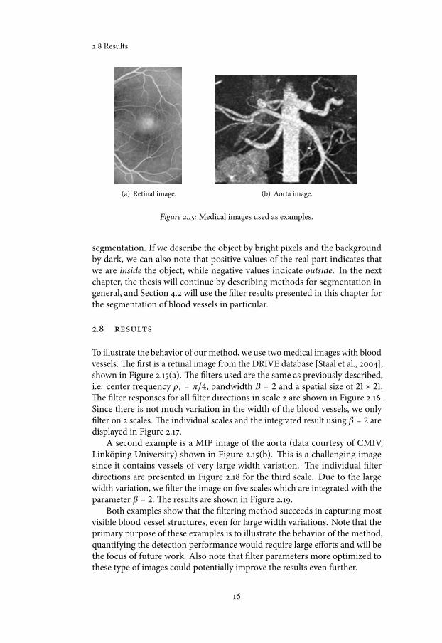
(a) Retinal image. (b) Aorta image.

Figure 2.15: Medical images used as examples.

segmentation. If we describe the object by bright pixels and the backgroundby dark, we can also note that positive values of the real part indicates thatwe are inside the object, while negative values indicate outside. In the nextchapter, the thesis will continue by describing methods for segmentation ingeneral, and Section 4.2 will use the filter results presented in this chapter forthe segmentation of blood vessels in particular.

2.8 results

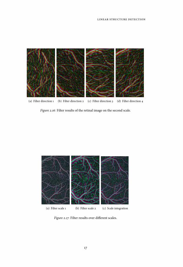
To illustrate the behavior of our method, we use two medical images with bloodvessels. The first is a retinal image from the DRIVE database [Staal et al., 2004],shown in Figure 2.15(a). The filters used are the same as previously described,i.e. center frequency ρi = π/4, bandwidth B = 2 and a spatial size of 21 × 21.The filter responses for all filter directions in scale 2 are shown in Figure 2.16.Since there is not much variation in the width of the blood vessels, we onlyfilter on 2 scales. The individual scales and the integrated result using β = 2 aredisplayed in Figure 2.17.

A second example is a MIP image of the aorta (data courtesy of CMIV,Linköping University) shown in Figure 2.15(b). This is a challenging imagesince it contains vessels of very large width variation. The individual filterdirections are presented in Figure 2.18 for the third scale. Due to the largewidth variation, we filter the image on five scales which are integrated with theparameter β = 2. The results are shown in Figure 2.19.

Both examples show that the filtering method succeeds in capturing mostvisible blood vessel structures, even for large width variations. Note that theprimary purpose of these examples is to illustrate the behavior of the method,quantifying the detection performance would require large efforts and will bethe focus of future work. Also note that filter parameters more optimized tothese type of images could potentially improve the results even further.

16


(a) Filter direction 1 (b) Filter direction 2 (c) Filter direction 3 (d) Filter direction 4

Figure 2.16: Filter results of the retinal image on the second scale.

(a) Filter scale 1 (b) Filter scale 2 (c) Scale integration


17

2.8 Results

(a) Filter direction 1 (b) Filter direction 2

(c) Filter direction 3 (d) Filter direction 4

Figure 2.18: Filter results of the aorta image on the third scale.

(a) Filter scale 1 (b) Filter scale 2 (c) Filter scale 3

(d) Filter scale 4 (e) Filter scale 5 (f) Scale integration


18

C H A P T E R 3

M E D I C A L I M A G E S E G M E N T A T I O N

This chapter will briefly introduce the most common categories of imagesegmentation methods used for medical image segmentation. We will start

by the most simple techniques typically referred to as thresholding and regiongrowing. Then, we introduce more recent techniques where a segmentation isfound by means of optimizing an energy functional. In this context we talkabout continuous variational and discrete combinatorial methods.

3.1 thresholding and region growing

Early, and simple, techniques for segmentation mainly used the assumptionthat relevant objects in an image can be identified based on intensity values.The most simple approach identifies objects using a single threshold value, suchthat pixels above and below the threshold are object pixels and backgroundpixels respectively. This works fine for high contrast objects with a sharp edge,but the method often fails as soon as the edges are smooth, of varying intensityand influenced by noise. This is most often the case for natural images, whichlimits the usefulness of this approach.

A slightly more sophisticated version of thresholding are region growingalgorithms. The basic idea is to start from a given seed point which is knownto be an object pixel. The neighborhood of the pixel is classified as backgroundor object depending on a threshold value. The (connected) object is segmentedby a recursive search through the pixels which are classified as object. A typicalproblem with this type of method is leakage, since it is hard to set a thresholdvalue which confines an actual object.

3.2 variational methods

Variational methods are based upon describing an energy functional where theoptimum defines a good segmentation. The functional is typically dependingon a curve, which defines the partitioning of the image, and a number of imagederived terms such as image intensity, image gradients, etc.

3.2.1 Snakes

The first work in this direction was the Snake in Kass et al. [1988] which usedan explicit type of curve representation. The energy is defined by:

E [C(s)] = −∫ ∣∇I(C(s))∣2 ds + ν1 ∫ ∣C′(s)∣2 ds + ν2 ∫ ∣C′′(s)∣2 ds (3.1)

3.2 Variational Methods

where C(s) is a parametric curve with parameter s, I is the image, and C′ andC′′ are the first and second derivatives of C with respect to its parameter s. Thefirst term is referred to as the external energy and the two last terms are theinternal energies of the snake. The external energy is derived from the image,and is used to drive the curve towards points with high gradient magnitude,i.e. strong edges. The first internal energy, weighted by ν1 ≥ 0, measures thelength of the snake, while the second, weighted by ν2 ≥ 0 measures the stiffness.Good segmentations are represented by curves which optimize the energy, i.e.where the first variation of E vanishes. The first variation can be viewed asa generalization of the first derivative from “ordinary” calculus. Recall thatstationary points (maxima, minima, saddles) of a function can be found bysearching for points where the first derivative is zero. The first variation inthe calculus of variations has exactly the same meaning, but for functionals (a“function of a function” such as Eq. (3.1)) instead of functions. Without goinginto details , this can be expressed by the Euler-Lagrange equation denotedby δE/δC = 0. This equation results in a partial differential equation (PDE)which, in most cases, is hard to solve directly. Instead an energy optimum isfound by evolving the curve in the steepest descent direction of the energy, suchthat ∂C/∂t = −δE/δC. This is the basic idea behind the popular variationalmethods used in image processing. Note however that any solution will be alocal optimum, so the result strongly depends on a proper initialization, or aproper starting curve.

The Snakes algorithm was the starting point for image segmentation usingvariational methods. However, it suffers from a number of drawbacks. Themain drawback is the explicit curve representation which does not easily al-low topological changes and requires complex reparameterization algorithms.Second, since the nodes of the curve are affected by local image features, i.e.there are no region based information, the solutions tend to be very sensitiveto a proper initialization. Also, from a mathematical point of view, the energyfunction is not intrinsic since it depends on the parameterization of the curve.This means that the energy will change if the parameterization changes, whichclearly is an undesirable property.

3.2.2 Level set methods

To address the first issue regarding curve parameterization, approaches usingthe implicit level set method by Osher and Sethian [1988] were simultaneouslyproposed by Caselles et al. [1993] and Malladi et al. [1993, 1994]. Using theseideas, a curve is represented implicitly as the zero level set of a time dependentfunction ϕ ∶ Ω → R, such that C = {x(t) ∈ Ω ∶ ϕ(x , t) = 0}. By differentiatingwith respect to time, we can couple the motion of the curve dx/dt with anevolution of the level set function ϕ using a PDE ∂ϕ/∂t = −dx/dt ⋅∇ϕ. A specialcase is when the motion is restricted to the normal direction of the curve, i.e.dx/dt = Fn, where n = ∇ϕ/ ∣∇ϕ∣. In this case, the scalar function F is usuallyreferred to as the speed function. This representation has the main advantageof allowing arbitrary topological changes, so the initial curve does not need to

20

medical image segmentation

have the same topology as the segmented object. Unlike the Snakes algorithm,which was motivated by energy minimization, the work by Caselles et al. andMalladi et al. was motivated by a geometric curve evolution approach. The basicidea was to generate a speed function which “pulled” the curve towards theboundaries of the target object while the curve was regularized with curvaturemotion. A typical speed function can be based on image gradients, such that itapproaches zero when the norm of the image gradient is large (i.e. there is adistinct edge).

The main advantage of this approach is the level set representation, whichallows arbitrary topological changes and robust and stable numerical schemesfor the curve propagation. However, the motivation is based on geometricalaspects of the image and the curve, so it is hard to validate the solutions andperform “deeper” mathematical analysis.

3.2.3 Geodesic active contours

The next major step in variational methods-based image segmentation wasthe Geodesic active contour proposed simultaneously by Caselles et al. [1997]and Kichenassamy et al. [1995]. In this work, it is shown that a special caseof the Snakes model can be interpreted as finding geodesics (locally shortestpaths) in a space with a metric derived by image content. This formalismprovides an analogue between segmentation using active contours and minimaldistance (geodesic) computations. Formally, the energy to be minimized hasthe following form:

EGAC[C(s)] = ∫ L(C)

0g(∣∇I(C(s))∣)ds (3.2)

where L(C) is the length of C, g(∣∇I∣) is a strictly decreasing inverse edgeindicator function, typically g(∣∇I∣) = 1/(1 + ∣∇I∣). We can note that choosingg = 1 gives the length of the curve C(s), so minimizing Eq. (3.2) gives a minimalcurve where the length of the curve is weighted by the function g(∣∇I∣).

Then, if the curve is represented as a level set, it is shown that the geodesiccomputations reduce to a form similar to the work in Caselles et al. [1993], Mal-ladi et al. [1993, 1994]. The geodesic active contour model provides a couplingbetween segmentation based on energy minimization and the level set frame-work. Thus, it is contained in a rigorous mathematical context of optimizationwhile the curve representation is flexible and robust, allowing both thoroughanalysis and practical implementation.

3.2.4 Active contours without edges

So far, the active contour models have primarily defined the objects by imagegradients. This is often problematic due to varying edge contrast and noise.The models will fail completely for objects with too blurred or weak edges,and there are risks of leakage if the edge is not well defined on the completeperimeter of the object. In contrast, the active contours without edges by Chanand Vese [2001] is based on regional measures and do not depend on any edge

21

3.3 Combinatorial Methods

definition. This approach incorporates region information and is a specialcase of the Mumford-Shah functional for segmentation [Mumford and Shah,1989]. Basically, it solves the minimal partition problem which aims to find apartitioning of the image which best separates the interior of the curve fromthe exterior. Formally, it is described as:

ECV [C(s)] =μ∫ L(C)

0ds +∬

ΩC(I(x , y) − c1)2 dxdy (3.3)

+∬Ω∖ΩC

(I(x , y) − c2)2 dxdy

where ΩC is the interior of the curve C, c1 and c2 are the average image intensi-ties in the interior and exterior of C respectively and μ ≥ 0 is a weight parameter.The first term is a regularization which minimizes the length and the secondlast terms provide the balancing between the interior and exterior. It can benoted that omitting the regularization by μ = 0 leeds to a solution equivalentto simple thresholding. This model assumes the image to be separable into tworegions (phases) which can be reasonably well approximated by constant valuesc1 and c2. This is a crude model which was later generalized to multi-phasepiecewise-smooth approximations in Vese and Chan [2002].

The main advantage of this model is the global dependence and the ten-dency to produce globally optimal solutions in practice. However, for manyapplications in medical image segmentation, the influence of the backgroundintensity can be problematic. This was investigated in Paper I and will be furtherdetailed in Section 4.1.

3.2.5 Active shape models

Many applications can include prior knowledge in the segmentation. For exam-ple, shape priors can be used to constrain the topology and general shape of theresult. A model for integration shape in medical applications was presented inRousson et al. [2004]. For a review on approaches to incorporate color, texture,motion and shape, see Cremers et al. [2007].

3.2.6 Direction of descent

As noted in Section 3.2.1, the derivation of level set flows by the Euler-Lagrangeequation leads to a gradient descent search for the energy optimum. The use ofa gradient implies a notion of inner product in the space of curves. Although afundamental property of the system, the effect of the choice of inner product hasnot been studied until recently in parallel work by Charpiat et al. [2005], Solemand Overgaard [2005], Sundaramoorthi et al. [2007], Yezzi and Mennucci[2005].

3.3 combinatorial methods

Whereas the previous section described approaches where the image domainis regarded as continuous and segmentation was posed as an optimization in

22

medical image segmentation

a continuous space, there are combinatorial methods formulated as a discreteoptimization problem on the pixels of the image. This section will introducethe main directions in this area for completeness, but since this is not the focusof this thesis, the presentation will be brief.

3.3.1 Optimality of solutions

In general, the variational methods previously presented use gradient descentsearch for optimization which can only be guaranteed to find stationary points.For most cases, it is not known whether the solution found is a local minima,maxima or a saddle point. Furthermore, the solution depends critically on theinitial condition (curve). The main benefit of the combinatorial methods isthat a global solution can be guaranteed. This has several advantages: First,the solution is not depending on a good initial condition, so the initial curvecan be placed arbitrarily in the image. Second, the quality of the solutionrelates directly to the energy functional and the parameters controlling thefunctional, rather than the initialization or other numerical implications of theimplementation. On the other hand, some applications might benefit fromthe possibility of inducing a local optima by a controlled initialization, such asextracting a particular branch of a blood vessel tree. But combinatorial methodscan in general be considered more robust due to the guaranteed global solution.

3.3.2 Dynamic programming and optimal paths

Like the Snakes algorithm in variational methods, the combinatorial methodsfor segmentation started with explicit representations of object boundaries.This was first presented by Amini et al. [1990] where dynamic programmingwas used to find a global optimum of the Snakes energy. Other researchers haveproposed similar techniques based on dynamic programming to find optimalpaths, see e.g. [Falcão et al., 1998, Geiger et al., 1995, Mortensen and Barrett,1998]. However, these approaches are limited to 2D images since the propertiesof 3D geometry require fundamentally different explicit representations.

3.3.3 Graph cuts

An important contribution for segmentation based on graph cuts was presentedby Boykov and Jolly [2001] (and extended in [Boykov and Funka-Lea, 2006]). Inthis work, pixels are classified as being either inside or outside the object, mak-ing this a combinatorial method using an implicit-type representation (albeitdiscrete). Thus, compared to the previously outlined path-based approaches,this method generalizes to higher dimensions more easily. The success of themethod relies on an efficient min-cut/max-flow algorithm which computes aglobally optimal cut [Boykov and Kolmogorov, 2004].

23

C H A P T E R 4

L E V E L - S E T B A S E D S E G M E N T A T I O N

Level set methods are popular for solving many types of segmentationproblems. The popularity is mainly due to the robust deformations and the

embedding in a well studied mathematical framework. The previous chapteroutlined the history of variational methods, which mostly are implementedusing the level set representation. This chapter will continue by describing thecontributions in this thesis to this field. Section 4.1 will start by presentinga localized version of the Chan-Vese model in Section 3.2.4 which can targetsingle objects in an image. Then, Section 4.2 will explain how the filter outputfrom Chapter 2 can be used for segmentation in a level set framework. Wenoted previously how the standard method for computing the segmentationsis by a gradient descent search. Inspired by ideas from the machine learningcommunity, Section 4.3 will give two alternative optimization strategies whichcan be adapted to the level set representation.

4.1 localized region-based segmentation

In Section 3.2.4 we reviewed the popular Chan-Vese model “active contourswithout edges”. The main benefit of this method is its ability to segment objectswith weak (low contrast) edges. In addition, the global dependence tends toproduce globally optimal solutions which do not depend as much on a goodinitialization as do traditional edge-based methods. However, some applicationssuffer from this global dependence. For example, a user might want to segmentonly a single object in a medical image. In this case, the result is also dependenton objects far from the region of interest, which is not natural for the user. Theglobal behavior also implies a background dependence which is not natural.Figure 4.1 illustrates this problem using a segmentation of the gray matterin the brain with the initializing curve in Figure 4.1(a). The background inthe bottom row of images is slightly brighter than the top row. Figure 4.1(b)shows the result using the traditional Chan-Vese model. We can note that thesegmentations differ purely due to the shift in background intensity. Also, thesegmentations are not related in a meaningful way to the initializing curve. Onecan use a narrow-band level set technique as in [Peng et al., 1999] to localizethe curve propagation, but this still leads to different results depending on thebackground as shown in Figure 4.1(c). By localizing also the computations, i.e.restricting the domain of the Chan-Vese model, we can get meaningful resultswhich are not background sensitive as in Figure 4.1(d) This problem, and a userinterface for initializing the segmentation, was presented in Paper I.

4.2 Phase-based level set segmentation

(a) (b) (c) (d)

Figure 4.1: Illustrates the global dependence of the Chan-Vese model in [Chanand Vese, 2001]. The initializing curve is shown in (a). The top and bottom rowsdiffer only in the background intensity which is slightly brighter in the bottomrow. Although the different background makes no semantical difference, theresults in (b) show that the original Chan-Vese model gives different segmentations.Only restricting the curve propagation by a narrow-band scheme in (c) does notremove the dependence on the background. We propose also a restriction ofthe computational domain of the problem which gives dependence only on therelevant objects in the image as in (d). (Reprint from Johansson et al. [2007])

4.2 phase-based level set segmentation

For segmenting linear structures, e.g. blood vessels, the output from the filteringapproach in Chapter 2 can be used as input for level set segmentation. The ideaof localizing edges by finding zero-crossings in the filter output was outlinedin Section 2.7. Recall that edges are located on the zero-crossings of the realpart, while positive and negative values indicate inside and outside of the bloodvessels respectively. This fact was used a geometric motivation for level setpropagation in Paper II. In fact, by directly using the real part of the filteroutput as a level set speed function and initializing the curve near a bloodvessel, the positive and negative forces will drive the curve towards the edgeswhere it will stop. A regularization term was added to increase the smoothnessof the curve, which gives:

∂ϕ∂t= −Re(q) ∣∇ϕ∣ + ακ ∣∇ϕ∣ (4.1)

where Re(q) is the real part of the filter output q, κ is the curvature and α ≥ 0 isa regularization weight parameter. A sequence of iterations on the spiral imagedescribed in Chapter 2 using α = 0.1 is shown in Figure 4.2. Here the curve isoverlaid the real part of the filter output, where positive and negative values are

26

level-set based segmentation

Figure 4.2: A sequence of segmentation iterations on the spiral image.

indicated by bright and dark colors respectively.In Paper V, it was shown that the geometrically derived speed function in

Eq. (4.1) comes from maximizing the energy:

E[C(s)] = ∬ΩC

f (x , y)dxdy − α∮Cds (4.2)

where f (x , y) = Re(q). This is the so calledweighted region functional [Kimmel,2003] which aims to maximize the function f (x , y) inside the region ΩC (insideof C) while at the same time minimizing the length of C. Basically, this willfind a curve which encloses all points with positive values on f while “small”regions (typically noise) will be removed due to the minimization of length.Thus, Eq. (4.2) can be interpreted as a noise suppressed thresholding on f > 0.This energy interpretation of Eq. (4.1) allows us to embed the phase-basedsegmentation ideas in a mathematical framework for constructing alternativeoptimization strategies. This will be further elaborated in the next section.

4.3 optimization aspects of segmentation

As was described in Section 3.2, image segmentation can be formulated as anoptimization problem, where the goal is to find a particular segmentation whichmaximizes/minimizes a given energy functional. Here we will present twooptimization strategies commonly used in the machine learning community,and show how these can be adapted to level-set based segmentation.

4.3.1 Gradient descent with momentum

The simplest numerical optimization method is gradient descent, where onlythe gradient of the cost function is used to guide the search towards an optimalsolution. However, common drawbacks of this scheme is the sensitivity tolocal optima and the poor rate of convergence for many practical problems.More sophisticated methods have been proposed which utilizes higher orderinformation to mainly improve the convergence rate, see [Nocedal and Wright,2006] for a complete reference.

However, to avoid the added complexity of these more sophisticated meth-

27

4.3 Optimization aspects of segmentation

(a) Sequence of iterations (b) Convergence rate

Figure 4.3: Gradient descent with momentum on a simple cost function.

ods, a simple and intuitive approach is to extend traditional gradient descent byadding momentum. This idea was initially proposed in the machine learningcommunity [Rumelhart et al., 1986], where the training of an artificial neuralnetwork is formulated as an optimization problem. The basic idea is to add afraction of the previous step to the current step, which adds a physical “inertia”to the motion in the search space. The practical benefits of this strategy are thatlocal optima can be overstepped while the search accelerates in favorable direc-tions, thereby increasing the rate of convergence. Formally, gradient descentcan be described by:

sk = −αk∇ fk (4.3)

where sk is the step in iteration k, αk is the step length and ∇ fk is the gradientof the cost function f . Gradient descent with momentum can be described by:

sk = −η(1 − ω)∇ fk + ωsk−1 (4.4)

where η > 0 is the so called learning rate and ω ∈ [0, 1] is the momentum, toadopt some terminology from the machine learning community. We can notethat ω = 0 gives the traditional gradient descent, while ω = 1 gives “infiniteinertia” sk = sk−1. A simple example illustrating traditional gradient descentand gradient descent with momentum on an elliptic cost function is shownin Figure 4.3. Here we see that traditional gradient descent with η = 0.04 andω = 0 gives slow convergence. Increasing the step length to η = 0.4 gives fasterconvergence but an oscillating motion in search space. Adding the momentumby ω = 0.1 stabilizes the motion and accelerates more quickly towards theoptimum. However, oscillation is still possible for a large momentum of ω = 0.4.

4.3.2 Resilient back-propagation

Both traditional gradient descent and gradient descent with momentum includethe problem of finding an appropriate step length αk or learning rate η. This isvery much depending on application and the shape of the cost function in a

28


(a) Sequence of iterations (b) Convergence rate

Figure 4.4: Rprop on a simple cost function.

neighborhood around the current solution. For simplicity, the step length iscommonly set to an ad-hoc constant value which “seems to work”, but whichcould result in either poor convergence or oscillatory motion. To addressthis issue, the resilient back-propagation algorithm (Rprop) was proposed inRiedmiller and Braun [1993]. This is another technique invented in the machinelearning community, which uses adaptive steps based on the behavior of thecost function. The basic idea is to look only at the sign of the gradient alongthe coordinate axes, according to:

sk = −Δk ∗ sign (∇ fk) (4.5)

where Δk is a vector of step sizes (one for each coordinate axis), sign(⋅) is thesign function and ∗ denotes element-wise multiplication. The step sizes areupdated such that the motion is accelerated if the sign of the gradient is thesame for consecutive iterations, while the motion is decelerated if the gradientchanges sign. Formally, this update rule is specified as:

Δik =⎧⎪⎪⎪⎪⎨⎪⎪⎪⎪⎩

min (Δik−1 ⋅ η+, Δmax) if ∇i fk ⋅∇i fk−1 > 0

max (Δik−1 ⋅ η−, Δmin) if ∇i fk ⋅∇i fk−1 < 0

Δik−1 else

(4.6)

where η+ and η− are acceleration and deceleration factors, Δmax and Δminare upper and lower limits on the step sizes and ∇i fk denotes the i:th partialderivative of the cost function. An illustration of Rprop on a simple cost functionis shown in Figure 4.4, together with conventional gradient descent. Here weuse the parameters η+ = 1.2, η− = 0.7, Δmax = 1, Δmin = 0.01 with initialconditions Δ0 = (0.1, 0.05)T . The gradient descent uses a constant step lengthof α = 0.04. This plot shows the typical “zig-zag” behavior of Rprop whileapproaching the optimum.

29

4.4 Level-set based segmentation and optimization

4.4 level-set based segmentation and optimization

We proceed with a discussion on how to utilize the alternative optimizationmethods presented in Section 4.3.1 and Section 4.3.2 in a level set framework. InSection 3.2 we presented the idea of deriving a level set flow by Euler-Lagrangeequations which optimizes an energy functional. It was noted that this levelset flow describes a gradient descent search in the solution space which, in thiscontext, is the space of all possible curves. The structure, and dimensional-ity, will depend on the parameterization of a curve. For example, an explicitrepresentation of a curve sampled using m number of nodes, embedded in ndimensions can be represented by one point in an n ×m-dimensional space.For the implicit level set representation, the level set function itself can be in-terpreted as a parameterization of the embedded curve. This will result in asolution space of N dimensions, where N is the number of samples of the levelset function.

Returning to the level set flow derived by Euler-Lagrange equations, whichresulted in a gradient descent motion in solution space. In light of the previousdiscussion, we can approximate the gradient by taking the finite differencebetween two subsequent time instances of the level set function (points insolution space):

∇ f (tn) ≈ ϕ(tn) − ϕ(tn−1)Δt

(4.7)

where ϕ(tn) is the level set function at time tn . This approximation is of firstorder, depending on the time step Δt. The gradient can be directly used tocompute a new step s(tn) using gradient descent with momentum in Eq. (4.4)or Rprop in Eq. (4.5) and evolve the level set function according to:

ϕ(tn) = ϕ(tn−1) + Δts(tn) (4.8)

Procedure UpdateLevelsetGiven the level set function ϕ(tn−1), compute the next (intermediate) time step22

ϕ(tn). This is performed by evolving ϕ according to a PDE using standardtechniques (e.g. Euler integration).Compute the approximate gradient by Eq. (4.7).44

Compute a step s(tn) according to Eq. (4.4) or Eq. (4.5). This step effectively66modifies the gradient direction by the momentum or Rprop schemes.Compute the next time step ϕ(tn) by Eq. (4.8). Note that this replaces the88intermediate level set function computed in Step 1.

To illustrate the behavior of the alternative optimization schemes, we usean “L”-shaped object consisting of two disconnected regions as shown in Fig-ure 4.5(a). We apply the filtering techniques presented in Chapter 2 which givesthe target function f (x , y) = Re(q), i.e. the real part of the filter response q.This is shown in Figure 4.5(b) where bright and dark colors indicate positive and

30


(a) Input image (b) Target function f (x , y)

Figure 4.5: Synthetic test image illustrating the presence of a local optima in thesolution space.

(a) time = 0 (b) time = 200 (c) time = 515

Figure 4.6: Iterations without momentum (conventional gradient descent).

negative values respectively. Applying traditional segmentation level set tech-niques using the initial curve in Figure 4.6(a) gives the result in Figure 4.6(c)which clearly is a local optimum (the global optimum would contain bothregions of the object). Applying the idea of momentum gives the sequence ofiterations in Figure 4.7 which succeeds in capturing both regions. The values ofthe energy functional (Eq. (4.2)) is shown in Figure 4.8 for traditional gradientdescent and gradient descent with momentum. We can see that gradient descentwith momentum oversteps a number of local maxima during the search whileshowing a more rapid increase in the energy.

4.5 results

To illustrate the alternative optimization schemes we use the previously intro-duced retinal image shown in Figure 4.9(a). The target function f (x , y) =Re(q) used for the segmentation is displayed in Figure 4.9(b). First, resultsusing conventional gradient descent is shown in Figure 4.10 when initializingmanually with the seeds in Figure 4.10(a). Comparing with the results forgradient descent with momentum in Figure 4.11, we see that the momentumapproach captures more of the visible vessels. The energy functions are shownin Figure 4.12 which indicate that gradient descent with momentum indeedfinds a stronger optimum.

31

4.5 Results

(a) time = 0 (b) time = 40 (c) time = 70

(d) time = 180 (e) time = 240 (f) time = 485

Figure 4.7: Iterations using momentum.

(a) Without momentum (b) With momentum

Figure 4.8: Plots of energy functionals for synthetic test image in Figure 4.5(a).

32


(a) Input image (b) Target f (x , y)

Figure 4.9: Retinal image.

(a) time = 0 (b) time = 20 (c) time = 40 (d) time = 100

(e) time = 200 (f) time = 400 (g) time = 600 (h) time = 1210

Figure 4.10: Iterations on the retinal image using conventional gradient descent.

33

4.5 Results

(a) time = 0 (b) time = 20 (c) time = 40 (d) time = 100

(e) time = 200 (f) time = 400 (g) time = 600 (h) time = 810

Figure 4.11: Iterations on the retinal image using gradient descent with momentum.

(a) Without momentum (b) With momentum

Figure 4.12: Plots of energy functionals for the retinal image.

34

C H A P T E R 5

S U M M A R Y A N D C O N C L U S I O N S

The primary fo cus of this thesis is on two different methods - linearstructure detection by multi-scale filtering, and the segmentation of these

structures using level set methods. We have proposed new schemes in bothfields, and have combined them by using the output of the filtering as input tothe segmentation. This chapter gives a summary of the work and restates themain conclusions of the results.

5.1 linear structure detection

The overall goal of the thesis is to segment blood vessels which can be usedfor later simulation and processing. We model the vessels as linear structures,i.e. as lines and edges. We detect the lines and edges of the vessels by usingquadrature filters, which are complex pairs of line and edge filters. The localphase (the argument of the complex filter output), can be used to classify the“line”-ness and “edge”-ness of a pixel neighborhood. Also, we can study thezero-crossings of the real part and the imaginary part to identify the positionsof edges and lines respectively.

A fundamental problem is that blood vessels typically vary significantly inwidth over an image. We approach this by applying the filtering scheme overmultiple scales and integrate the scales by weighting the scales based on themagnitude of the filter output. This is motivated by the fact the magnitudemeasures the certainty of the structure indication at a given pixel.

We illustrated the filtering results using two medical images of the retinaand aorta. Especially the aorta image, with vessel widths spanning five scales,shows the success in detecting both thin and thick blood vessels. By filtering forboth edges and lines, the results contains precise measures for both the edgesas well as the inside region of the vessels.

5.2 level-set based segmentation

The second part of this thesis described the contributions to the field of level-set based segmentation. First, the general problem of “globalness” with theChan-Vese model [Chan and Vese, 2001] was presented, and a solution forlocalizing the behavior was suggested. This can be practical for applicationswhere generally a local solution is needed.

Next, we presented the idea on how to use the zero-crossings of the quadra-ture filter results for segmenting linear structures, and blood vessels in particular.

5.2 Level-set based segmentation

This was motivated geometrically by the positive and negative values of thefilter result which acted as “forces”, pushing a curve towards the edges of vessels.The idea was natural for implementation using level set methods.

Later, we showed how the geometrically motivated level set speed functioncan be formulated as the solution of an energy optimization. This providedthe formalization of alternative optimization schemes, which can be used tooverstep local minima solutions and improve the rate of convergence. Apartfrom the varying width, another fundamental problem in the segmentation ofblood vessels is that the contrast changes over the image. This is mainly dueto technical constructions in the imaging modality and varying contrast agentconcentrations. In addition, plaques and stenoses can produce visible “gaps”along a vessel structure, making it hard to extract a completely connected vesseltree. These problems, naturally occurring in the imaging of blood vessels, leadto that typical level set segmentation techniques often produce local solutions,where disconnected parts of the vessel tree are missed. The goal of the alter-native optimization schemes is to overstep such “gaps” in the vessels, therebyconverging to a better solution or segmentation. Using the retinal image, theresults showed improvements over traditional methods. It is, however, futurework to study the validity of the solutions, i.e. that the vessels are segmentedcorrectly.

36

C H A P T E R 6

F U T U R E W O R K

Ideas for fu ture work can, like the rest of this thesis, be divided intofiltering and segmentation. In addition, an important part of the future work

is to design robust and fair methods for evaluating the actual segmentationresults. This is very important for the clinical application and usability of thesealgorithms.

6.1 filtering

A problem with traditional designs of quadrature filters is “ringing” effects inthe filter output, caused by a wrap-around of the local phase in the filter output(wrap-around from π to −π can be seen in Figure 2.11(c)). This can producefalse structure detection when identifying edges and lines by the zero-crossingsof the real and imaginary parts. In practice, this would result in repeated “rings”around the true structure. The effects of this is currently under investigation.

A problem with the current filter output is that linear structures also includeplanes in three dimensions. So currently, there is no distinction between ablood vessel or other sufficiently flat structures, such as the skull, in volumetricmedical images. This is why our results for such data only include proof-of-concept results. However, the output from quadrature filters can also be usedto construct a tensor representation of the local structure in a point. We plan touse this in future work to mask out plane-like objects which can be detected bythe tensor. The major challenge with this idea is using the tensor informationacross multiple scales.

6.2 segmentation

The major problem with the current level set approach for segmentation is thelong execution time, especially for volumetric images. Because of this, tweakingthe parameters, e.g. for regularization, can be cumbersome. This is typicalfor level set methods and can be improved somewhat with optimized imple-mentations. However, since the segmentation model is basically formulatedas a “soft threshold” on the zero-crossing of the filter output, applying the fulllevel set framework is likely overkill. Thus, future work includes investigatingalternative, probably simpler, methods for segmentation based on the filteroutput.

C H A P T E R 7

O V E R V I E W O F P A P E R S

paper i

The “active contours without edges” by Chan and Vese [2001] is a segmentationmodel with two major benefits: it can detect objects with very fuzzy edges andit tends to produce global solutions, independent of the initialization. However,for applications where a user wants to target a specific object in an image, theglobal behavior can also be the major weakness of the method. This paperidentifies this problem and suggests a modification by restricting the computa-tional dependence to a region-of-interest selected in a user interface based ontopological analysis of the data.

paper ii

This paper presents a method for segmenting blood vessels in medical images.It is based on two different components. First, we assume that blood vesselscan be described as lines and edges and use filter techniques for detecting suchstructures. To handle vessels of varying width, the filtering is applied in a scalepyramid and the scales are integrated. Then, the filter output is used as input toa standard level set model for segmentation.

paper iii

Level set models for segmentation can be derived by optimizing an energyfunctional depending on a curve and image terms. This derivation includes agradient descent search in the space of curves. It is well known that gradientdescent search suffers from sensitivity to local optima and poor convergencecompared to other, more sophisticated, optimization schemes. In this paperwe suggest the application of so called gradient descent with momentum forlevel-set based segmentation to relieve some of these drawbacks.

paper iv

The motivation for this paper is the same as for Paper III. In this paper, westudy the effect of using the resilient back-propagation (Rprop) optimizationscheme in the context of level set segmentation.

paper v

This is an extended journal version of Paper II which further investigates pa-rameters of the method (mainly the multi-scale integration) and describes anenergy formulation of the level set model for segmentation.

40

B I B L I O G R A P H Y

Amir Arsham Amini, Terry E. Weymouth, and Ramesh C. Jain. Using dynamicprogramming for solving variational problems in vision. Pattern Analysis andMachine Intelligence, IEEE Transactions on, 12(9):855 –867, Sep 1990.

Thord Andersson, Gunnar Läthén, Reiner Lenz, and Magnus Borga. A fast optimizationmethod for level set segmentation. In Proceedings of the 16:th Scandinavian Conferenceon Image Analysis (SCIA), volume 5575 of Lecture Notes in Computer Science, pages400–409, Oslo, Norway, June 2009. Springer.

Yuri Boykov and Gareth Funka-Lea. Graph cuts and efficient n-d image segmentation.Int. J. Comput. Vision, 70(2):109–131, 2006.

Yuri Boykov and Marie-Pierre Jolly. Interactive graph cuts for optimal boundaryamp; region segmentation of objects in n-d images. In Proceedings of Eighth IEEEInternational Conference on Computer Vision, 2001. ICCV 2001, volume 1, pages 105–112 vol.1, 2001.

Yuri Boykov and Vladimir Kolmogorov. An experimental comparison of min-cut/max-flow algorithms for energy minimization in vision. Pattern Analysis and MachineIntelligence, IEEE Transactions on, 26(9):1124 –1137, Sept. 2004.

Vincent Caselles, Francine Catté, Tomeu Coll, and Françoise Dibos. A geometricmodel for active contours in image processing. Numerische Mathematik, 66(1):1–31,December 1993.

Vincent Caselles, Ron Kimmel, and Guillermo Sapiro. Geodesic active contours. Inter-national Journal of Computer Vision, 22(1):61–79, February 1997.

Tony F. Chan and Luminita A. Vese. Active contours without edges. IEEE Transactionson Image Processing, 10(2):266–277, February 2001.

G. Charpiat, R. Keriven, J.-P. Pons, and O. Faugeras. Designing spatially coherentminimizing flows for variational problems based on active contours. ComputerVision, 2005. ICCV 2005. Tenth IEEE International Conference on, 2:1403–1408 Vol. 2,Oct. 2005.

Daniel Cremers, Mikael Rousson, and Rachid Deriche. A review of statistical approachesto level set segmentation: Integrating color, texture, motion and shape. Int. J. Comput.Vision, 72(2):195–215, 2007.

John G. Daugman. Uncertainty relation for resolution in space, spatial frequency, andorientation optimized by two-dimensional visual cortical filters. J. Opt. Soc. Am. A,2(7):1160–1169, 1985.

Alexandre X. Falcão, Jayaram K. Udupa, Supun Samarasekera, Shoba Sharma, Bruce El-liot Hirsch, and Roberto de A. Lotufo. User-steered image segmentation paradigms:Live wire and live lane. Graphical Models and Image Processing, 60(4):233–260, 1998.

Alejandro Frangi, Wiro Niessen, Koen Vincken, and Max Viergever. Multiscale vessel en-hancement filtering. Medical Image Computing and Computer-Assisted Interventation—MICCAI’98, pages 130–137, 1998.

Dennis Gabor. Theory of communication. J. Inst. Elec. Eng., 93(26):429–457, 1946.

Davi Geiger, Alok Gupta, Luiz A. Costa, and John Vlontzos. Dynamic programmingfor detecting, tracking, and matching deformable contours. Pattern Analysis andMachine Intelligence, IEEE Transactions on, 17(3):294 –302, Mar 1995.

Rafael C. Gonzales and Richard E. Woods. Digital Image Processing. Prentice Hall Inc.,Upper Saddle River, New Jersey, 2nd edition, 2002. ISBN 0-201-18075-8.

Gösta H. Granlund and Hans Knutsson. Signal Processing for Computer Vision. KluwerAcademic Publishers, Netherlands, 1995. ISBN 0-7923-9350-1.

Andres Huertas and Gerard Medioni. Detection of intensity changes with subpixelaccuracy using laplacian-gaussian masks. IEEE Trans. Pattern Anal. Mach. Intell., 8(5):651–664, 1986.

Gunnar Johansson, Ken Museth, and Hamish Carr. Flexible and topologically localizedsegmentation. In Ken Museth, Torsten Möller, and Anders Ynnerman, editors,EUROVIS Symposium Proceedings, pages 179–186, Aire-la-Ville, Switzerland, 2007.Eurographics, Eurographics Association.

Michael Kass, Andrew Witkin, and Demetri Terzopoulos. Snakes: Active contourmodels. International Journal of Computer Vision, 1(4):321–331, January 1988.

Satyanad Kichenassamy, Arun Kumar, Peter J. Olver, Allen R. Tannenbaum, and An-thony Joseph Yezzi. Gradient flows and geometric active contour models. ComputerVision, IEEE International Conference on, 0:810, 1995.

Ron Kimmel. Geometric Level Set Methods in Imaging, Vision and Graphics, chapterFast edge integration. Springer Verlag, 2003.

Hans Knutsson. Filtering and Reconstruction in Image Processing. PhD thesis, LinköpingUniversity, Sweden, 1982.

Hans Knutsson. Producing a continuous and distance preserving 5-D vector repre-sentation of 3-D orientation. In IEEE Computer Society Workshop on ComputerArchitecture for Pattern Analysis and Image Database Management - CAPAIDM, pages175–182, Miami Beach, Florida, November 1985. IEEE.

Hans Knutsson, Mats Andersson, and Johan Wiklund. Advanced filter design. In InProceedings of the Scandinavian Conference on Image analysis, Greenland, June 1999.SCIA.

Gunnar Läthén, Jimmy Jonasson, and Magnus Borga. Phase based level set segmentationof blood vessels. In Proceedings of 19th International Conference on Pattern Recognition,Tampa, FL, USA, December 2008. IAPR.

42

bibliography

Gunnar Läthén, Thord Andersson, Reiner Lenz, and Magnus Borga. Momentum basedoptimization methods for level set segmentation. In In Proceedings of the SecondInternational Conference on Scale SpaceMethods andVariationalMethods in ComputerVision (SSVM), volume 5567 of Lecture Notes in Computer Science, pages 124–136,Voss, Norway, June 2009a. Springer.

Gunnar Läthén, Jimmy Jonasson, and Magnus Borga. Blood vessel segmentation usingmulti-scale quadrature filtering. Pattern Recognition Letters, 2009b.

Ravi Malladi, James A. Sethian, and Baba C. Vemuri. Topology-independent shapemodeling scheme. In Baba C. Vemuri, editor, Society of Photo-Optical InstrumentationEngineers (SPIE) Conference Series, volume 2031 of Presented at the Society of Photo-Optical Instrumentation Engineers (SPIE) Conference, pages 246–258, June 1993.

Ravi Malladi, James A. Sethian, and Baba C. Vemuri. Evolutionary fronts for topology-independent shape modeling and recovery. Computer Vision —ECCV ’94, pages 1–13,1994.

Eric N. Mortensen and William A. Barrett. Interactive segmentation with intelligentscissors. Graphical Models and Image Processing, 60(5):349 – 384, 1998.

David Mumford and Jayant M. Shah. Optimal approximation by piecewise smoothfunctions and associated variational problems. Commun. Pure Applied Mathematics,42:577–685, 1989.

Jorge Nocedal and Stephen J. Wright. Numerical Optimization. Springer, 2nd edition,2006.

Stanley Osher and James A. Sethian. Fronts propagating with curvature-dependentspeed: Algorithms based on Hamilton-Jacobi formulations. Journal of ComputationalPhysics, 79:12–49, 1988.

Danping Peng, Barry Merriman, Stanley Osher, Hong-Kai Zhao, and Myungjoo Kang.A pde-based fast local level set method. Journal of Computational Physics, 155(2):410–438, 1999.

Martin Riedmiller and Heinrich Braun. A direct adaptive method for faster backpropa-gation learning: the rprop algorithm. In Neural Networks, 1993., IEEE InternationalConference on, pages 586–591 vol.1, 1993.

Mikael Rousson, Nikos Paragios, and Rachid Deriche. Implicit active shape models for3d segmentation in mr imaging. Medical Image Computing and Computer-AssistedIntervention –MICCAI 2004, pages 209–216, 2004.

David D. E. Rumelhart, Geoffrey E. Hinton, and Ronald J. Williams. Learning internalrepresentations by error propagation, pages 318–362. MIT Press, Cambridge, MA,USA, 1986.

Yoshinobu Sato, Shin Nakajima, Hideki Atsumi, Thomas Koller, Guido Gerig, ShigeyukiYoshida, and Ron Kikinis. 3d multi-scale line filter for segmentation and visualizationof curvilinear structures in medical images. In CVRMed-MRCAS ’97: Proceedings ofthe First Joint Conference on Computer Vision, Virtual Reality and Robotics inMedicineand Medial Robotics and Computer-Assisted Surgery, pages 213–222, London, UK,1997. Springer-Verlag.

43

Jan Erik Solem and Niels Chr. Overgaard. A geometric formulation of gradient descentfor variational problems with moving surfaces. Scale Space and PDE Methods inComputer Vision, pages 419–430, 2005.

J.J. Staal, M.D. Abramoff, M. Niemeijer, M.A. Viergever, and B. van Ginneken. Ridgebased vessel segmentation in color images of the retina. IEEE Transactions onMedicalImaging, 23(4):501–509, 2004.

Ganesh Sundaramoorthi, Anthony Yezzi, and Andrea Mennucci. Sobolev active con-tours. International Journal of Computer Vision, 73(3):345–366, 2007.

Luminita A. Vese and Tony F. Chan. A multiphase level set framework for imagesegmentation using the mumford and shah model. International Journal of ComputerVision, 50(3):271–293, 2002.

Anthony Yezzi and Andrea Mennucci. Conformal metrics and true "gradient flows" forcurves. iccv, 1:913–919, 2005.

44

Seeded Segmentation Methods for Medical Image Analysis

Documents