SEDIMENTATION BETWEEN PARALLEL PLATES By Yonas Kinfu Paulos B. E., Anna University A THESIS SUBMITTED IN PARTIAL FULFILLMENT OF THE REQUIREMENTS FOR THE DEGREE OF MASTERS OF APPLIED SCIENCE in THE FACULTY OF GRADUATE STUDIES CIVIL ENGINEERING We accept this thesis as conforming to the required standard THE UNIVERSITY OF BRITISH COLUMBIA April 1991 © Yonas Kinfu Paulos, 1991

Welcome message from author
This document is posted to help you gain knowledge. Please leave a comment to let me know what you think about it! Share it to your friends and learn new things together.
Transcript
S E D I M E N T A T I O N B E T W E E N P A R A L L E L P L A T E S
By
Yonas Kinfu Paulos
B. E., Anna University
A THESIS SUBMITTED IN PARTIAL FULFILLMENT OF
T H E REQUIREMENTS FOR T H E DEGREE OF
MASTERS OF APPLIED SCIENCE
in
T H E FACULTY OF GRADUATE STUDIES
CIVIL ENGINEERING
We accept this thesis as conforming
to the required standard
T H E UNIVERSITY OF BRITISH COLUMBIA
April 1991
© Yonas Kinfu Paulos, 1991
In presenting this thesis in partial fulfilment of the requirements for an advanced degree at the University of British Columbia, I agree that the Library shall make it freely available for reference and study. I further agree that permission for extensive copying of this thesis for scholarly purposes may be granted by the head of my department or by his or her representatives. It is understood that copying or publication of this thesis for financial gain shall not be allowed without my written permission.
Department of C\V J\L € N G \ C \ ) £ E K U V l G |
The University of British Columbia Vancouver, Canada
Date
DE-6 (2/88)
Abstract
Settling basins can be shortened by using a stack of horizontal parallel plates which
develop boundary layers in which sedimentation can occur. The purpose of this study is
to examine the design parameters for such a system and to apply this approach to a fish
rearing channel in which settling length is strictly limited.
Flow between parallel rough and smooth plates has been modelled together with
sediment concentration profile. Accurate description of boundary layer flow requires the
solution of Navier-Stokes equations, and due to the complexity of the equations to be
solved for turbulent flow some assumptions are made to relate the Reynolds stresses to
turbulent kinetic energy and turbulent energy dissipation rate. The simplified equations
are solved using a numerical method which uses the approach given by the TEACH
code. The flow parameters obtained from the turbulent flow model are used to obtain
the sediment concentration profile within the settling plates. Numerical solution of the
sedimentation process is obtained by adopting the general transport equation. The lower
plate is assumed to retain sediments reaching the bottom.
The design of a sedimentation tank for a fish rearing unit with high velocity of flow
has been investigated. The effectiveness of the sedimentation tank depends on the uni
formity of flow attained at the inlet, and experiments were conducted to obtain the most
suitable geometric system to achieve uniform flow distribution without affecting other
performances of the fish rearing unit. The main difficulties to overcome were the heavy
circulation present in the sedimentation tank and the clogging of the distributing sys
tem by suspended particles. Several distributing systems were investigated, the best is
discussed in detail.
u
It was concluded that a stack of horizontal parallel plates can be used in fish rearing
systems where space is limited for settling sediments. Flow distribution along the vertical
at the entrance to the plates determines the efficiency of the sediment settling process and
a suitable geometrical configuration can be constructed to distribute the high velocity
flow uniformly across the vertical. Numerical modelling of sediment removal ratio for
flow between smooth and rough parallel plates has been calculated. The results show
that almost the same pattern of sediment deposition occurs for both the smooth-smooth
and rough-smooth plate arrangements.
m
Table of Contents
Abstract ii
List of Tables vii
List of Figures viii
List of Symbols x
Acknowledgement xiv
1 I N T R O D U C T I O N 1
2 T H E O R E T I C A L B A C K G R O U N D 4
2.1 Fall Velocity 4
2.1.1 Factors affecting fall velocity 4
2.1.2 Theoretical equations 5
2.1.3 Empirical and Semi-empirical formulations 7
2.1.4 Experimental data for natural quartz grains 8
2.2 Sediment Transfer Coefficient 8
2.3 Flow and Sedimentation Models 13
2.3.1 Turbulent Flow Model 13
2.3.2 Sedimentation Model 1,7
3 PREVIOUS W O R K O N S E D I M E N T A T I O N M E T H O D S 23
3.1 High-rate Settlers 25
iv
3.1.1 Introduction 25
3.1.2 Different Types of High-rate Settlers 25
3.1.3 Discussion of Theoretical Study 28
3.2 Sedimentation Basins 28
3.2.1 Rectangular Sedimentation Basins 29
3.2.2 Vortex-type Sedimentation Basins 34
4 S E T T I N G T A N K F O R FISHERIES 37
4.1 Introduction 37
4.2 Components of the Sedimentation Unit 39
4.2.1 Inlet 39
4.2.2 Distributing System 41
4.2.3 The Settling Plate System 44
4.2.4 Control Weir Outlet 47
5 D E V E L O P M E N T OF T H E O R Y 49
6 N U M E R I C A L M O D E L L I N G OF F L O W A N D S E D I M E N T A T I O N 52
6.1 Physical Model and Boundary Conditions 52
6.2 Finite Difference Formulation 54
6.2.1 Control Volume Definition 54
6.2.2 Derivation of Finite Volume Equations 55
6.3 Solution Algorithm 58
6.4 Convergence Criteria ' 59
7 E X P E R I M E N T S 60
7.1 Objective of Experiments 60
7.2 Apparatus 61
v
7.3 Procedure 62
8 E X P E R I M E N T A L RESULTS 66
8.1 Computational result 69
9 CONCLUSIONS 78
Bibliography 82
Appendices ' 86
A Wall Function Treatment 86 A.l Smooth Wall 87
A.2 Rough Wall 88
B T E A C H Code Solution Procedure 89
vi
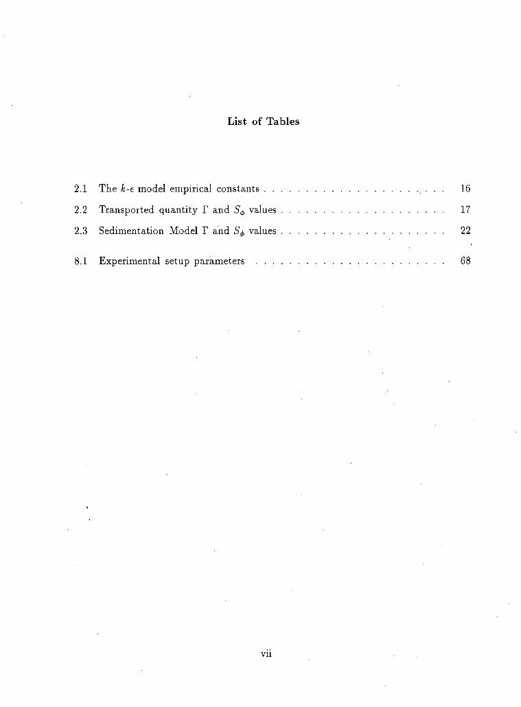
List of Tables
2.1 The k-e model empirical constants . . 16
2.2 Transported quantity T and values 17
2.3 Sedimentation Model T and values 22
8.1 Experimental setup parameters 68
vn
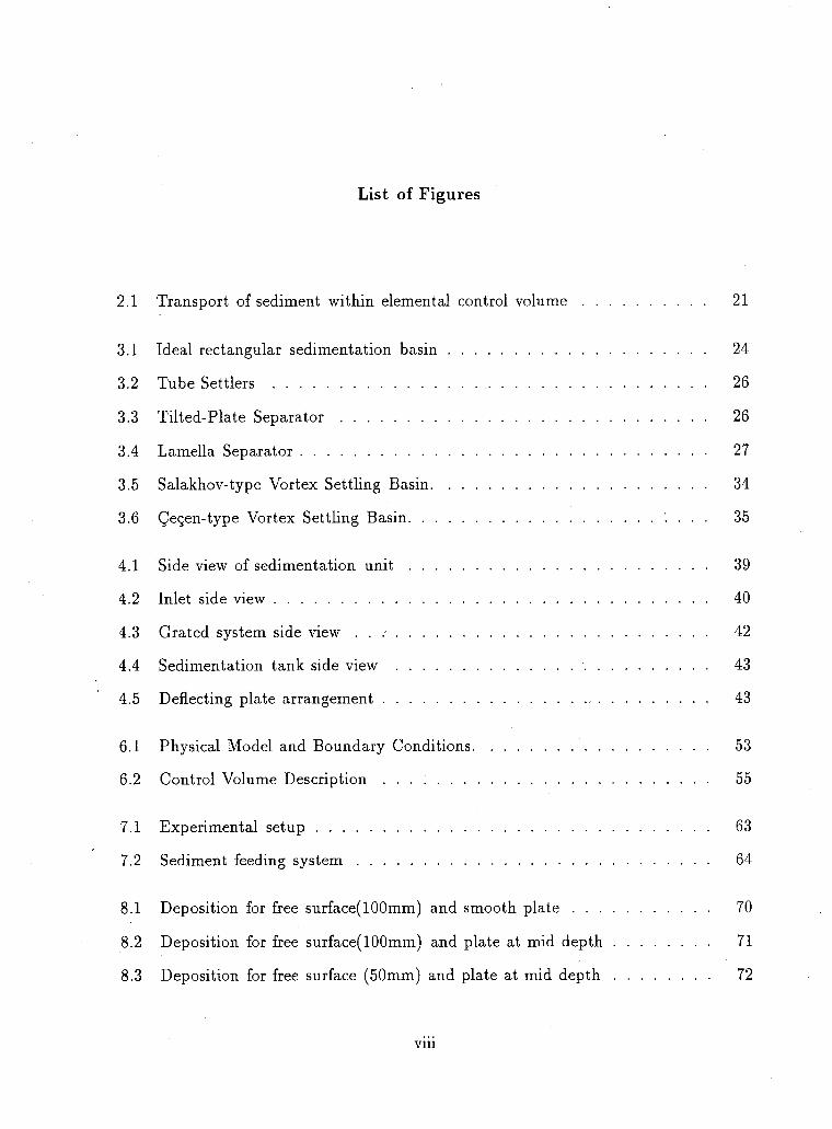
List of Figures
2.1 Transport of sediment within elemental control volume 21
3.1 Ideal rectangular sedimentation basin 24
3.2 Tube Settlers 26
3.3 Tilted-Plate Separator 26
3.4 Lamella Separator 27
3.5 Salakhov-type Vortex Settling Basin 34
3.6 Cecen-type Vortex Settling Basin '. . . . 35
4.1 Side view of sedimentation unit 39
4.2 Inlet side view 40
4.3 Grated system side view . . .- 42
4.4 Sedimentation tank side view 43
4.5 Deflecting plate arrangement 43
6.1 Physical Model and Boundary Conditions 53
6.2 Control Volume Description 55
7.1 Experimental setup 63
7.2 Sediment feeding system 64
8.1 Deposition for free surface( 100mm) and smooth plate 70
8.2 Deposition for free surface( 100mm) and plate at mid depth 71
8.3 Deposition for free surface (50mm) and plate at mid depth 72
viii
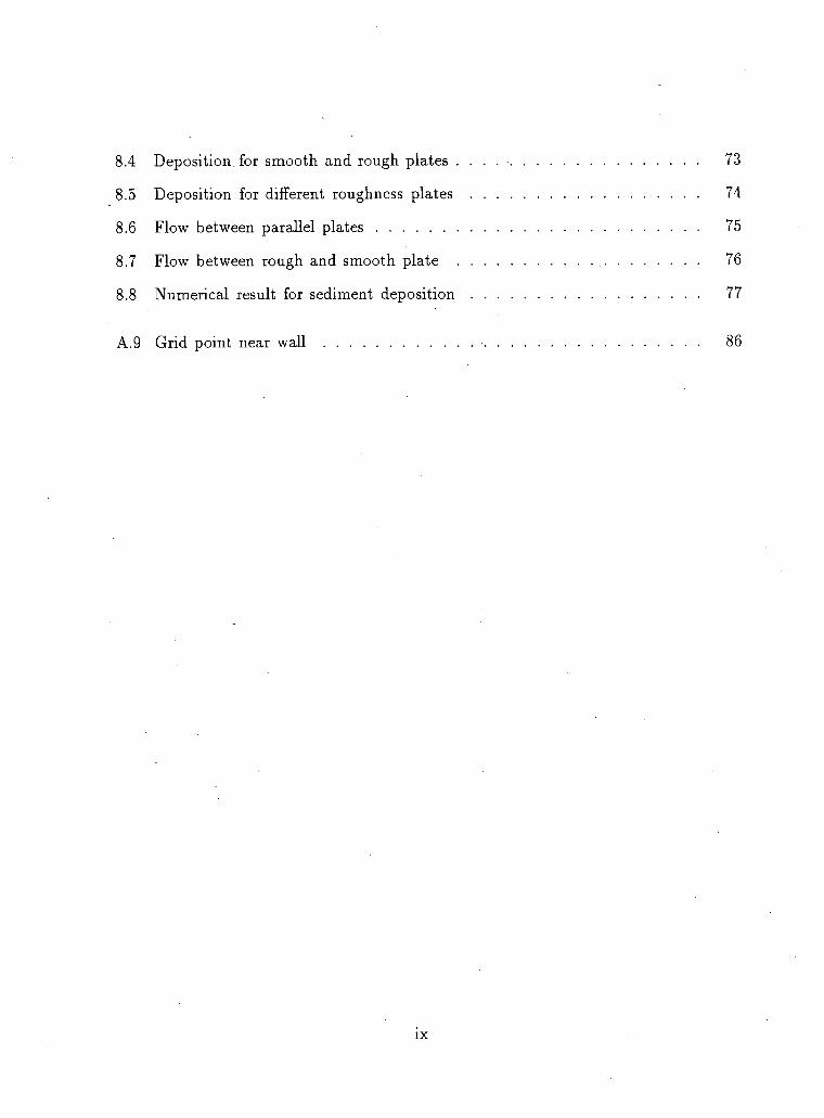
8.4 Deposition for smooth and rough plates . . . 73
8.5 Deposition for different roughness plates 74
8.6 Flow between parallel plates 75
8.7 Flow between rough and smooth plate 76
8.8 Numerical result for sediment deposition 77
A.9 Grid point near wall 86
I X
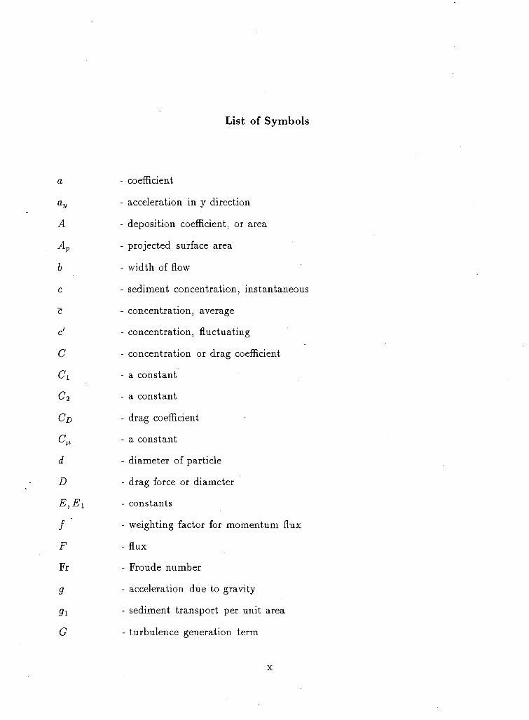
List of Symbols
a - coefficient
ay - acceleration in y direction
A - deposition coefficient, or area
Ap - projected surface area
b - width of flow
c - sediment concentration, instantaneous
c - concentration, average
c' - concentration, fluctuating
c - concentration or drag coefficient
- a constant
c2 - a constant
CD - drag coefficient
- a constant
d - diameter of particle
D - drag force or diameter
E, Ex - constants
f ' - weighting factor for momentum flux
F - flux
Fr - Froude number
9 - acceleration due to gravity
9i - sediment transport per unit area
G - turbulence generation term
X
H - depth of flow
- coordinate directions
k - kinetic energy per unit mass, turbulent
- roughness size
Kt - roughness size, non-dimensional
I - mixing length
L - length of basin
L, - length of basin for half sediment deposition
n, s, e, w - direction notation, for faces
N, S, E, W - direction notation, for nodes
P - pressure
Pe - Peclet number
Q - flow discharge
V - removal ratio of sediment
R(t> - residual
3? - Reynold's number
S - slope
t - time
Sp - source term
ss - specific gravity of particle
S<j> - a general source term
u - local horizontal velocity of flow
- average horizontal velocity
^max - maximum local horizontal velocity of flow
- shear velocity
X I

U+ - velocity, non-dimensional
V - local vertical velocity of flow
V - characteristic velocity
V, - mean settling velocity of suspension
VJ - fall velocity correction value
Vso - overflow rate
VOL - elemental volume
x - horizontal axis coordinate
y - vertical axis coordinate from bed
y+ - grid distance, non-dimensional
a - a coefficient
f3 - correlation coefficient or a coefficient
T - diffusion coefficient
8 - kronecker delta, boundary layer thickness
e - energy dissipation
em - transfer coefficient, momentum
e3 - transfer coefficient, sediment
- von Karman constant
A - time scale
\i - viscosity of fluid, laminar
u.eff - viscosity of fluid, effective
fit - viscosity of fluid, turbulent
v - kinematic viscosity of fluid, laminar
p - density of fluid
ps - density of particle
xn
std. dev. for sediment trajectory
shear stress
shear stress at wall
quantity to be transported
xm
Acknowledgement
I am deeply grateful to Dr. Michael C. Quick for his unfailing support , encouragement
and patience throughout the study. Without his advice and understanding this project
would not have been possible. I would like to thank also Mr. JefFery Quick for his
help in computational flow modelling and Mr. Kurt Neilsen for his constant help in the
laboratory work.
I am thankful to CIDA and Water Resources Commission (Ethiopia) for the finan
cial support provided. Discussions and cooperation with Mr. Jim Bomford of the B.C.
Department of the Environment, Fisheries Branch with regard to the work done on the
flow distributing system are gratefully acknowledged.
Finally I praise God for giving me the strength to finish this project and also for
making all things happen.
xiv
Chapter 1
I N T R O D U C T I O N
Water is a basic necessity for the existence of man, and as a resource it is found in
different quantities and qualities. The required quantity and quality for consumption
depends on the type of utilization, and it is the task of water engineering to provide the
required demand reasonably and economically.
Sediments in water for use with hydro-electric power plant cause turbine blade abra
sion to complete damage. In irrigation canals deposited sediments facilitate growth of
weed, which increases the flow resistance and hence reduces the carrying capacity of a
canal. One major problem is the removal of sediment from flowing water, especially
at canal intakes, at hydro electric installations and water intakes. A special situation
is removal and control of sediments for fish rearing systems and the present study was
initiated to examine a particular type of fish rearing system. However, the sediment
control techniques and the basic computational method and experiments can have wide
application to other types of sediment control.
Rivers are the major sources of water supply. But often they are loaded with fine and
coarse sediments. Different methods are used to reject and divert the sediments at intakes,
but still fine sediments find their way into canals. Sedimentation basins are employed
to remove fine sediments. Classical sedimentation basins facilitate sedimentation process
by providing low and uniform velocity with low level of turbulence.
The study presented in this paper was initiated from the need to design a suitable
sedimentation tank for a fish rearing system. The problem dealt with is different from the
1
Chapter 1. INTRODUCTION 2
classical type of sedimentation basins and the proposed sedimentation tank uses a stack
of horizontal parallel plates for efficient use of space. Also the fish rearing channel has
to be separated from the sedimentation tank so that sediments can be removed without
interfering with the young fish. In addition, it is desired to design the system so that the
water level can be kept constant. These constraints lead to complications in the design
of the inlet flow to the settling tank so that the flow entering the settling tank tends to
have a high velocity and a non-uniform distribution. This high velocity flow from the
rearing unit also creates a circulation which has to be overcome by designing a suitable
system. Therefore the task has been to have uniform distribution of flow in the settling
tank without circulation and to study ways of increasing the efficiency of settling within
the parallel plates.
For a turbulent flow there exists a velocity fluctuation in the vertical direction near
a horizontal solid boundary. Bagnold('66) based on photographs taken by Prandtl('55)
suggests that the upward and downward velocity fluctuations are unequal in magnitude,
that is,.the turbulence is unsymmetrical. Hence, this inequality in velocity fluctuation in
duces a net upward stress which is responsible for supporting solid particles in suspension.
If an unsymmetrical turbulence produced at the bed could create upward pressure, then
in line with the same thinking, an unsymmetrical turbulence created at a top boundary
of the flow surface would induce a downward pressure to push the sediments downwards.
This reduces the amount of sediment that can be suspended in a flow.
The above argument is to be investigated as a way of increasing the sediment re
moval efficiency of a sedimentation basin. Experimental and numerical investigations are
presented to study the effect on sedimentation of smooth and rough boundaries at top
surface of flow.
A necessary theoretical background for the study is given in Chapter 2. A review of
the different sedimentation methods that are used in different fields of application are
Chapter 1. INTRODUCTION 3
discussed in Chapter 3, with details given for high rate settlers. Based on the practical
problem posed, Chapter 4 discusses the design and modelling of sedimentation tank for
fisheries. Chapter 5 describes the development of theory for maximizing the sedimen
tation between parallel plates. The numerical modelling of flow and sedimentation for
different kinds of flow are given in Chapter 6. Experimental methods and procedure used
for the different types of flow selected are discussed in Chapter 7, and Chapter 8 describes
the experimental and numerical results with discussions. Finally Chapter 9 concludes
the whole study.
Chapter 2
T H E O R E T I C A L B A C K G R O U N D
2.1 Fall Velocity
In the study of sediment transport and sedimentation the fall velocity of a particle is an
important parameter describing the particle in relation to the fluid.
Depending on the concentration and type of particles encountered, four types of
settling can occur: discrete particle, flocculation, hindered and compression. The latter
three are commonly important for wastewater treatment. Discrete settling is the major
phenomenon which is of importance for this study and will be discussed in detail.
When particles fall in a fluid at rest, gravitational force causes particles to accelerate
until the retarding resistance force from the fluid equals the gravitational force. When
this equilibrium condition is reached, there is no acceleration, and hence a constant
velocity is attained which is called terminal velocity.
For fluids in motion, the fall velocity of a particle in water at rest is to be used for
the numerical computation to obtain the deposition pattern of particles under the effect
of turbulence.
2.1.1 Factors affecting fall velocity
The fall velocity of a particle depends on many factors such as Reynold's number of a
particle, shape, particle roughness, proximity of the boundary, concentration (including
the gradient), the velocity of flow (particle rotation) and turbulence. In most practical
4
Chapter 2. THEORETICAL BACKGROUND 5
problems all the above mentioned factors may act in group or simultaneously.
Analysis of fall velocities of particles of regular shapes such as circular cylinder, ellip
soids, discs and isometric particles have been studied by many investigators. For irregular
shapes Albertson studied the effects by defining shape factors. Hey wood represented the
shape effect by introducing volume coefficients. For practical use each method requires
a knowledge of particles proportion.
Camp('46) considers the effect of turbulence as delaying the settling of particles.
Paradoxically, Jobson et al.('70) report that the effective fall velocity in turbulent flow
is increased, specially of coarse particles. Their finding is based on experimental results;
by back calculating the fall velocity from governing suspended sediments mathematical
equation.
2.1.2 Theoretical equations
Newton in his classical law of sedimentation equated the drag resistance force as follows
D = CAppi (2.1)
where C is drag coefficient, D is drag force, AV is projected area of a particle, p is density
of fluid, and Vs fall velocity. Later on it was verified that C is not constant but a function
of Reynold's number, therefore it is substituted by CD-
D = C D A P P ^ (2.2)
The Reynold's number of a particle falling in fluid is computed using the effective
diameter as length scale, the fall velocity as velocity scale and using the viscosity of the
fluid. For very low Reynold's number Re< 0.1, the inertia forces may be neglected with
the respect to the viscous forces. Stoke(Graf('71)) obtained an analytical solution of
Navier-Stokes equations for drag resistance by ignoring inertia force (laminar case) for
Chapter 2. THEORETICAL BACKGROUND 6
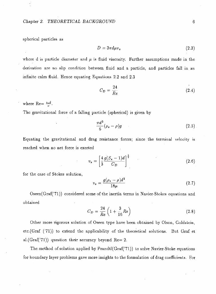
spherical particles as
D = Zirdpv, (2.3)
where d is particle diameter and p is fluid viscosity. Further assumptions made in the
derivation are no slip condition between fluid and a particle, and particles fall in an
infinite calm fluid. Hence equating Equations 2.2 and 2.3
24 CD = - (2.4)
where Re= u
The gravitational force of a falling particle (spherical) is given by
ird3
u (Ps-p)g (2.5)
Equating the gravitational and drag resistance forces; since the terminal velocity is
reached when no net force is exerted
*g(Sa-l)d 3 C D
for the case of Stokes solution, g(p, - p)d2
(2.6)
(2.7) 18p
0seen(Graf('71)) considered some of the inertia terms in Navier-Stokes equations and
obtained 24 / 3 \
°° = Te(1 + n R c ) <2-8>
Other more rigorous solution of Oseen type have been obtained by Olson, Goldstein,
etc.(Graf ('71)) to extend the applicability of the theoretical solutions. But Graf et
al.(Graf('71)) question their accuracy beyond Re= 2.
The method of solution applied by Prandtl(Graf('71)) to solve Navier-Stoke equations
for boundary layer problems gave more insights to the formulation of drag coefficients. For
Chapter 2. THEORETICAL BACKGROUND 7
higher Re, solutions for CD are given by many investigators. Proudman et al.(Graf('71))
suggested applying perturbation theory and matching of asymptotic solution to Navier-
Stokes equations. Jensen used relaxation techniques to solve the Navier-Stokes equations
for drag coefficient numerically at different Re. Fromm gave numerical solutions for
drag coefficients for flow with obstacles in channel flow for high Re by considering the
development of von Karman vortex street.
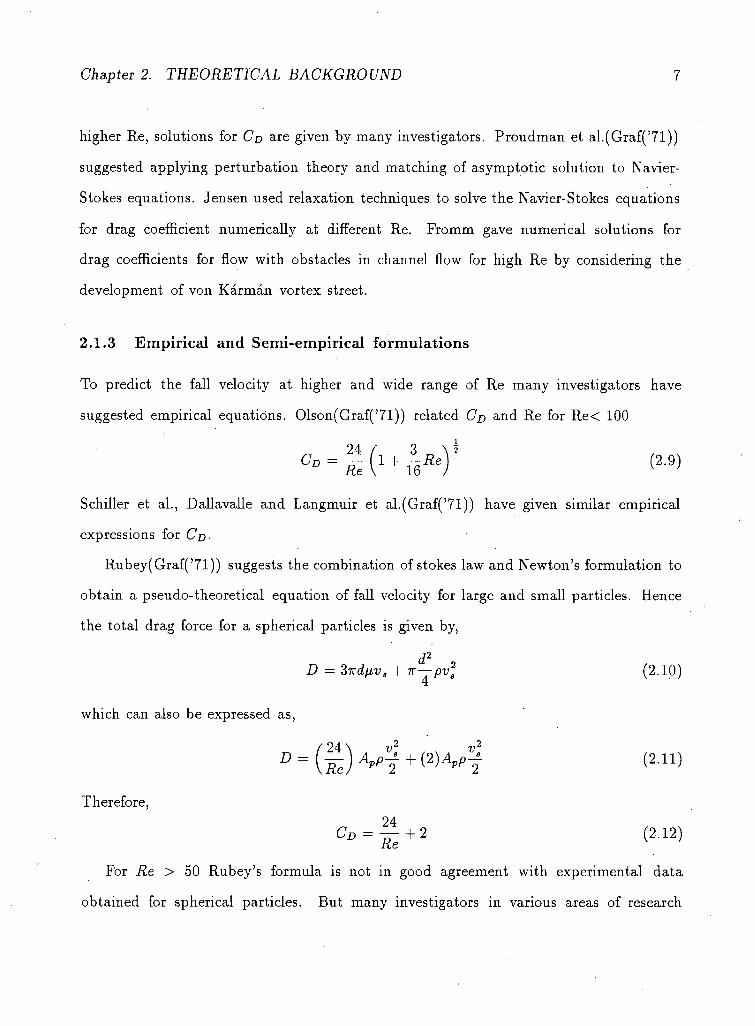
2.1.3 Empirical and Semi-empirical formulations
To predict the fall velocity at higher and wide range of Re many investigators have
suggested empirical equations. 01son(Graf('71)) related CD and Re for Re< 100
Schiller et al., Dallavalle and Langmuir et al.(Graf('71)) have given similar empirical
expressions for CD-
Rubey(Graf('71)) suggests the combination of stokes law and Newton's formulation to
obtain a pseudo-theoretical equation of fall velocity for large and small particles. Hence
the total drag force for a spherical particles is given by,
d2
D = Sivduv, + 7T—pv] (2.10)
which can also be expressed as,
/ 24 \ v2 v2
^ y ^ f ^ ( 2 - n )
Therefore,
C7D = | + 2 (2.12)
For Re > 50 Rubey's formula is not in good agreement with experimental data
obtained for spherical particles. But many investigators in various areas of research
Chapter 2. THEORETICAL BACKGROUND 8
have preferred the formula. Einstein used Rubey's formula in developing his sediment
transport equation in open channel flow.
2.1.4 Experimental data for natural quartz grains
The above discussed methods for obtaining fall velocity are less applicable for natural
grains. Most of the theoretical results are related to spherical or other regular shaped
particles. Moreover at higher Reynold's number the agreement with experimental result
is not good. Since most of the experiments were conducted in wind tunnel consideration
has to be made to relate them with the fall of a particle in water. Even the most popular
Rubey's formula doesn't give good result at very high Reynold's number.
Mamak has given a table listing the relationship between grain diameter and fall ve
locity. Even though Mamak(Graf('71)) hasn't specified the grain type and fluid property
his result is verified experimentally by Graf et al.(Graf('71)) for quartz grain in water
with temperature of 20°C. For computing the fall velocity of sand grains considered
in this study the plotting given by Vanoni('75), is used which gives the values for wide
range of temperatures. The fall velocity of a particle in water at rest is considered for
the numerical computation of sediment concentration.
2.2 Sediment Transfer Coefficient
The sediment transfer coefficient is approximately analogous to the momentum transfer
coefficient or kinematic eddy viscosity that is found in the theory of the diffusion of
momentum. Hinze('59) has indicated the approximate analogy between momentum and
mass transfer.
For channel flow the differential equation for sediment suspension in its simplest form

Chapter 2. THEORETICAL BACKGROUND 9
is given by,
e.^+V.C = Q (2.13) dy
where C is sediment concentration, es is sediment transfer coefficient, y is vertical distance
from the bottom. The complete derivation of the sediment suspension model is given in
the next section.
Rearranging Equation 2.13
dy
From accurate point measurement of concentration a graph of C against y may be
plotted to calculate e3 at any point on the curve. The value of es at a point is calculated by
estimating the slope of the tangent of the concentration curve where es is to be evaluated.
For free surface flow the sediment transfer coefficient is assumed to depend on the fall
velocity, depth of flow and shear velocity at the channel bed.
Therefore,
where Ux is shear velocity, H is depth of flow.
For wide channel neglecting the head loss difference between wall and bed , the shear
velocity may be calculated as follows,
U„ = {gHSf12 (2.16)
where S is slope of basin.
As given by von Karman and Vanoni('46) e3 is assumed to be proportional to the
momentum transfer coefficient em. The ratio between the two quantities is written as
= Sc, which is often referred as turbulent Schmidt number. Where \iejj is effective
viscosity of fluid which includes viscous and turbulent values.
r
Chapter 2. THEORETICAL BACKGROUND 10
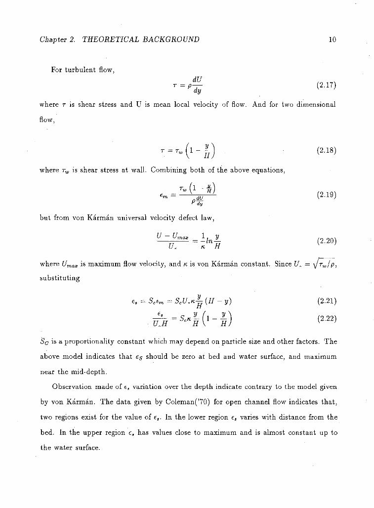
For turbulent flow,
where r is shear stress and U is mean local velocity of flow. And for two dimensional
flow,
t = T w { 1 ~ h ) ( 2 ' 1 8 )
where TW is shear stress at wall. Combining both of the above equations,
rw (l - £) = K
dJl
1 (2-19) P dy
but from von Karman universal velocity defect law,
U ~ ^ m a x = hn^ (2.20)
where Umax is maximum flow velocity, and K is von Karman constant. Since
substituting
e.=Scem=ScU.K^-(H-y) (2.21)
KM - *4 (' -1) <222)
Sc is a proportionality constant which may depend on particle size and other factors. The
above model indicates that e$ should be zero at bed and water surface, and maximum
near the mid-depth.
Observation made of e3 variation over the depth indicate contrary to the model given
by von Karman. The data given by Coleman('70) for open channel flow indicates that,
two regions exist for the value of es. In the lower region e, varies with distance from the
bed. In the upper region es has values close to maximum and is almost constant up to
the water surface.
Chapter 2. THEORETICAL BACKGROUND 11
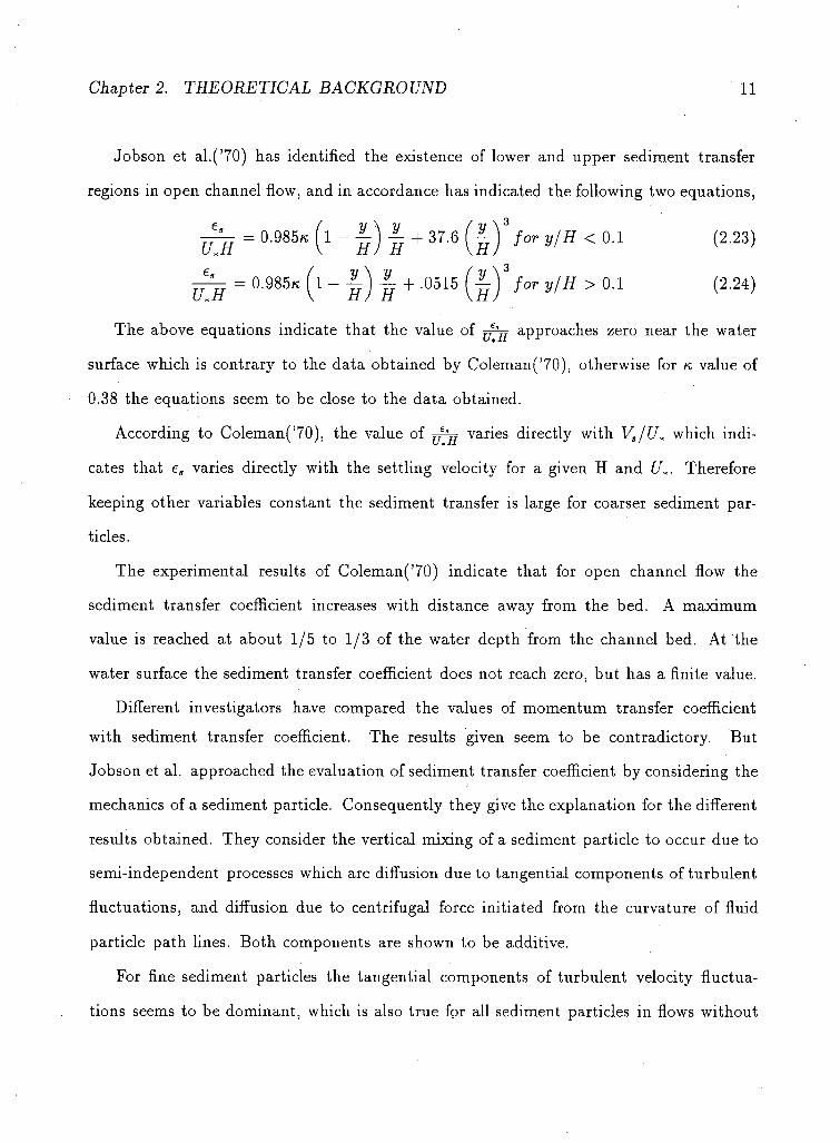
Jobson et al.('70) has identified the existence of lower and upper sediment transfer
regions in open channel flow, and in accordance has indicated the following two equations,
= 0.985K ( l - | ) | + 37.6 [^f for y/H < 0.1 (2.23)
^ = 0.985K ( l - f ) f + .0515 (I)''for y/H > 0.1 (2.24)
The above equations indicate that the value of approaches zero near the water
surface which is contrary to the data obtained by Coleman('70), otherwise for K value of
0.38 the equations seem to be close to the data obtained.
According to Coleman('70), the value of jf^j varies directly with Vs/Ux which indi
cates that es varies directly with the settling velocity for a given H and Ux. Therefore
keeping other variables constant the sediment transfer is large for coarser sediment par
ticles.
The experimental results of Coleman('70) indicate that for open channel flow the
sediment transfer coefficient increases with distance away from the bed. A maximum
value is reached at about 1/5 to 1/3 of the water depth from the channel bed. At the
water surface the sediment transfer coefficient does not reach zero, but has a finite value.
Different investigators have compared the values of momentum transfer coefficient
with sediment transfer coefficient. The results given seem to be contradictory. But
Jobson et al. approached the evaluation of sediment transfer coefficient by considering the
mechanics of a sediment particle. Consequently they give the explanation for the different
results obtained. They consider the vertical mixing of a sediment particle to occur due to
semi-independent processes which are diffusion due to tangential components of turbulent
fluctuations, and diffusion due to centrifugal force initiated from the curvature of fluid
particle path lines. Both components are shown to be additive.
For fine sediment particles the tangential components of turbulent velocity fluctua
tions seems to be dominant, which is also true for all sediment particles in flows without

Chapter 2. THEORETICAL BACKGROUND 12
strong vortex activity. This component is approximately proportional to the momentum
transfer coefficient and decreases with larger particle size. For coarse sediments with
strong vortex flow, diffusion due to the curvature of the fluid particle path lines seems
to be significant. The sediment transfer coefficient due to centrifugal acceleration is as
sumed to reach maximum in the zone of intense shear stress and increases with increasing
particle size in the fine to medium range. It is also closely related to the behavior of the
bed roughness specifically to those which give rise to flow separation.
The distribution of sediment transfer coefficient in closed channel flow is discussed by
Ismail('52). The derivation of the momentum transfer coefficient using the von Karman
universal velocity defect law gives zero value at the center. Von Karman has stated
that in the central part of a pipe the similarity assumption is correct. Brooks and
Berggren(Ismail('52)) have indicated that the momentum transfer coefficient at the center
has to be constant according to the results of Sherwood and Woertz(Ismail('52)) or an
error curve has to be assumed for em. Nikurade(Ismail('52)). gave definite values for em
at the center of pipes in his experimental results.
For numerical computation it is necessary to be able to calculate the sediment transfer
coefficient and the momentum transfer coefficient. The sediment transfer coefficient at
the center of a closed channel may be computed once the sediment concentration profile
is obtained. The experimental result indicate that for the middle third of the channel
the sediment transfer coefficient is almost constant. Due to the proportionality between
the two transfer coefficients, the results discussed for es could also represent the form of
em. Numerical computation results of flow in closed channel indicate a finite value of
momentum transfer coefficient at the center (described in Chapter 8). As shown for the
sediment transfer coefficient, em has almost constant value near the middle of a channel.
For numerical computation of a sediment concentration, it is therefore reasonable to
assume that the sediment transfer coefficient to be the same as the momentum transfer
Chapter 2. THEORETICAL BACKGROUND 13
coefficient. The same assumption was made by Camp('46), Sarikaya('77), and Bechteler
et al.('84). The evaluation of the momentum transfer coefficient is discussed in the
explanation of fluid flow computation model in the next section 2.3.
2.3 Flow and Sedimentation Models
2.3.1 Turbulent Flow Model
Background
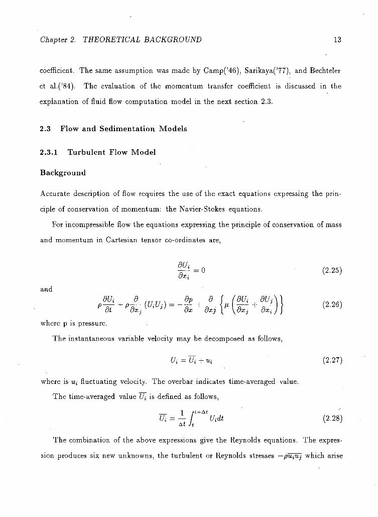
Accurate description of flow requires the use of the exact equations expressing the prin
ciple of conservation of momentum: the Navier-Stokes equations.
For incompressible flow the equations expressing the principle of conservation of mass
and momentum in Cartesian tensor co-ordinates are,
dxi
and
9 U i 0 (2.25)
dUi d , T r T T , dp d \ (dUi dUA] ,n n n .
dt dxj 1 dx dxj { \dxj dx
where p is pressure.
The instantaneous variable velocity may be decomposed as follows,
U^Ui+Ui (2.27)
where is U{ fluctuating velocity. The overbar indicates time-averaged value.
The time-averaged value U{ is defined as follows,
1 /-t + At Ui = — Uidt (2.28)
At Jt
The combination of the above expressions give the Reynolds equations. The expres
sion produces six new unknowns, the turbulent or Reynolds stresses — pU{Uj which arise
Chapter 2. THEORETICAL BACKGROUND 14
from the averaging of the non-linear convective terms. The Reynolds stresses represent
diffusion of momentum by turbulent motion. Since the unknowns are more than the
equations given, additional equations are required to have a closed solution to the prob
lem. These additional equations may be provided by making certain assumptions to
model the Reynolds stresses.
k-e Turbulence Model
The k-e model, Launder and Spaldling('74), which is to be used in this study requires
the solutions of two additional transport equations: one for the turbulent kinetic energy,
k, and the other for the turbulent kinetic energy dissipation rate, e. There seems to be
a good compromise between generality and cost of computation in using the model.
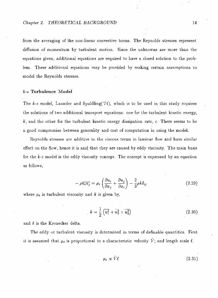
Reynolds stresses are additive to the viscous terms in laminar flow and have similar
effect on the flow, hence it is said that they are caused by eddy viscosity. The main basis
for the k-e model is the eddy viscosity concept. The concept is expressed by an equation
as follows,
- ^ = » l { — + ^ ) - r k S i l (2.29)
where /zt is turbulent viscosity and k is given by,
k = ^(^1+uj + uj) (2.30)
and 8 is the Kronecker delta.
The eddy or turbulent viscosity is determined in terms of definable quantities. First
it is assumed that fit is proportional to a characteristic velocity V; and length scale t.
Ht tx VI (2.31)
Chapter 2. THEORETICAL BACKGROUND 15
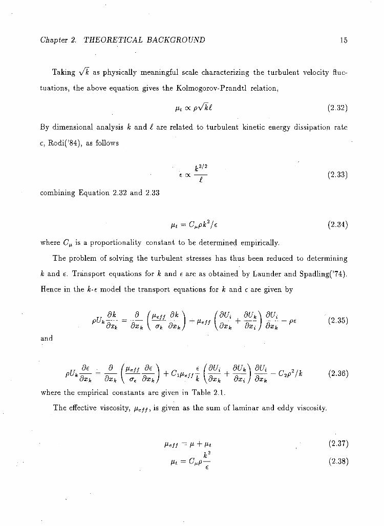
Taking y/k as physically meaningful scale characterizing the turbulent velocity fluc
tuations, the above equation gives the Kolmogorov-Prandtl relation,
fit oc py/kl (2.32)
By dimensional analysis k and t are related to turbulent kinetic energy dissipation rate
e, Rodi('84), as follows
£3/2
combining Equation 2.32 and 2.33
lit = C^pk2/e (2.34)
where C^ is a proportionality constant to be determined empirically.
The problem of solving the turbulent stresses has thus been reduced to determining
k and e. Transport equations for k and e are as obtained by Launder and Spadling('74).
Hence in the k-e model the transport equations for k and e are given by
kdxk dxk \ <rk dxkJ ^eff \dxk dxi J dxk
p €
and
ptffc—= — f — — - (— + —) — -C2p2/k (2 36) kdxk dxk \ <r€ dxkj 1 eff k \dxk dxi J dxk
2
where the empirical constants are given in Table 2.1.
The effective viscosity, peff, is given as the sum of laminar and eddy viscosity.
U.eff = p + pt
k2
Pt = C^p—
(2.37)
(2.38)
Chapter 2. THEORETICAL BACKGROUND 16
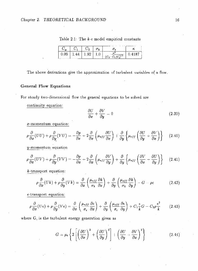
Table 2.1: The k-e model empirical constants
.Cl c2
0.09 1.44 1.92 1.0 0.4187 0.09 1.44 1.92 1.0 0.4187
The above derivations give the approximation of turbulent variables of a flow.
General Flow Equations
For steady two-dimensional flow the general equations to be solved are
continuity equation: dU dV n
& + ^ = ° <2 3 9 »
x-momentum equation:
d_ dy
dp dx
d_ dx
dU_ dx
d 'dU dV -dy I ̂ +
2/-momentum equation
^-transport equation:
dp dx
d dV " - + 2 ^ r e / / dy) ' dy +
d f (dV dU"
dx dy dx \ <rk dx) dy \ crk dy '
e-transport equation:
9 ,TT N d ,Tr . d (ueff de\ d (ueff de\ _ e ^ e2
where G, is the turbulent energy generation given as
G = fit<2 dU_ dx +
'dU d£ dV \dy dx
(2.40)
(2.41)
(2.42)
(2.43)
(2.44)

Chapter 2. THEORETICAL BACKGROUND 17
Table 2.2: Transported quantity T and values
Transported quantity 4> r S<fi Mass l 0 0 z-momentum u
ap i d ( au\ , a /,. av\ -ai + dx- [toff to) + a^ J
y-momentum V Peff _l 3 / „ au\ , a / „ a v \ + ai [fief fat) + a^ [^ffa^j
Tur. Kine. Energy k G-pe Tur. Kine. Energy Dissp. e tstL CiiG-C2pi
For convenience of numerical purposes the Equations 2.39 to 2.44 may be represented
by general transport equation
where (f> is quantity to be transported, T is general diffusivity coefficient and a general
source term. For each transported quantity; the particular values of T and are given
in Table 2.2.
The general transport expression given by Equation 2.45 will be used for the numerical
computation of each flow variables.
2.3.2 Sedimentation Model
Many theories have been forwarded to explain the process of sediment suspension in a
turbulent fluid. Some of the theories are: 1) suspension of sediment occurs when the
hydrodynamic lift force is greater than the submerged weight; 2) sediment is entrained
due to turbulent fluctuation at the bed; 3) the loss of contact of a particle with the
bed due to instability induced by irregularities on the bed; 4) due to the disruption of
particles on the bed by eddies. All of the theories require turbulence in the fluid to
produce suspension. The effect of turbulence in suspending sediment particles may be
Chapter 2. THEORETICAL BACKGROUND 18
derived in a similar way as the shear stress in a turbulent fluid.
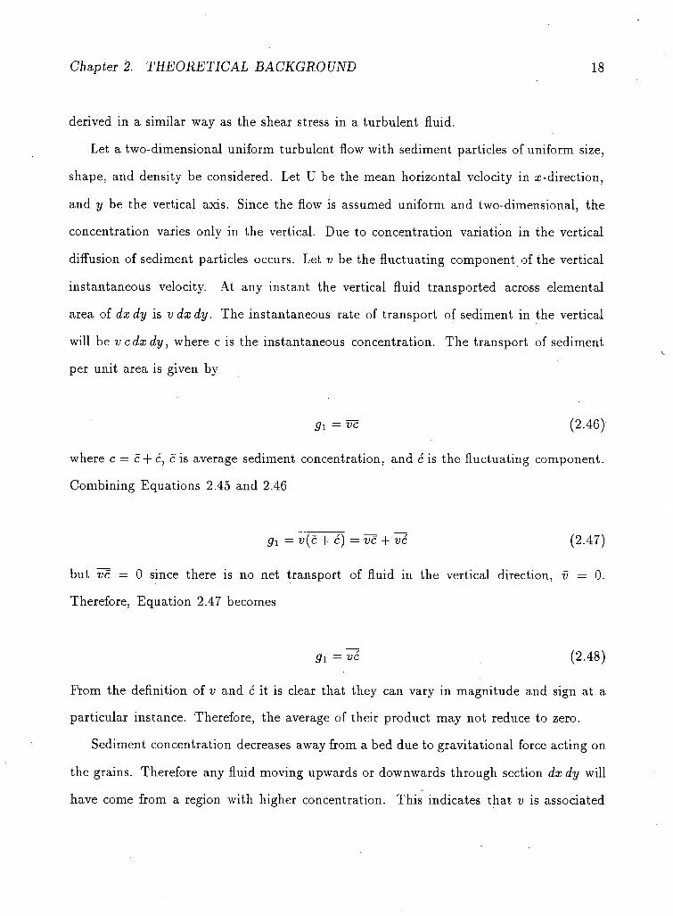
Let a two-dimensional uniform turbulent flow with sediment particles of uniform size,
shape, and density be considered. Let U be the mean horizontal velocity in s-direction,
and y be the vertical axis. Since the flow is assumed uniform and two-dimensional, the
concentration varies only in the vertical. Due to concentration variation in the vertical
diffusion of sediment particles occurs. Let v be the fluctuating component of the vertical
instantaneous velocity. At any instant the vertical fluid transported across elemental
area of dx dy is v dx dy. The instantaneous rate of transport of sediment in the vertical
will be vcdxdy, where c is the instantaneous concentration. The transport of sediment
per unit area is given by
gi=vc (2.46)
where c = c + c, c is average sediment concentration, and c is the fluctuating component.
Combining Equations 2.45 and 2.46
gx = v(c + c) = vc + vc (2-47)
but vc = 0 since there is no net transport of fluid in the vertical direction, v = 0.
Therefore, Equation 2.47 becomes
9 i = r i (2.48)
From the definition of v and c it is clear that they can vary in magnitude and sign at a
particular instance. Therefore, the average of their product may not reduce to zero.
Sediment concentration decreases away from a bed due to gravitational force acting on
the grains. Therefore any fluid moving upwards or downwards through section dx dy will
have come from a region with higher concentration. This indicates that v is associated
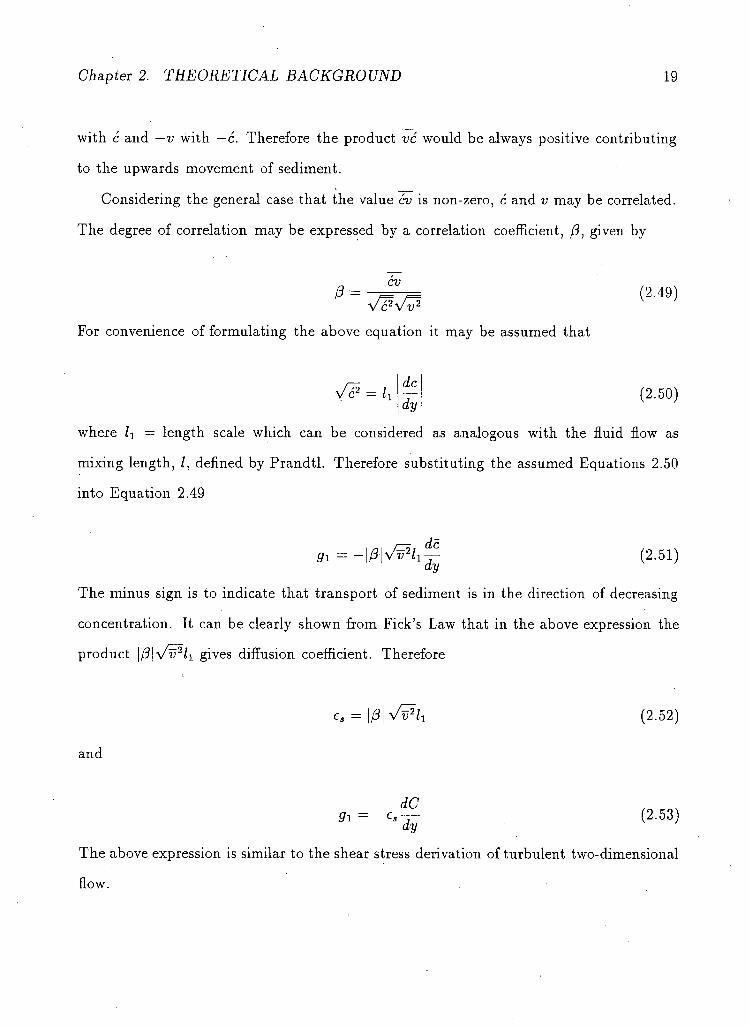
Chapter 2. THEORETICAL BACKGROUND 19
with c and —v with —6. Therefore the product vc would be always positive contributing
to the upwards movement of sediment.
Considering the general case that the value cv is non-zero, c and v may be correlated.
The degree of correlation may be expressed by a correlation coefficient, /3, given by
cv {3 = (2.49)
V c2Vv2
For convenience of formulating the above equation it may be assumed that
dc (2.50) c2 = h
dy
where li = length scale which can be considered as analogous with the fluid flow as
mixing length, /, defined by Prandtl. Therefore substituting the assumed Equations 2.50
into Equation 2.49
gx = (2.51) dy
The minus sign is to indicate that transport of sediment is in the direction of decreasing
concentration. It can be clearly shown from Fick's Law that in the above expression the
product \(3\\fv2lx gives diffusion coefficient. Therefore
es = |/3| s/tfh (2.52)
and
dC ». = - V 5 - (2-53)
The above expression is similar to the shear stress derivation of turbulent two-dimensional
flow.
Chapter 2. THEORETICAL BACKGROUND 20
In deriving Equation 2.53, it was assumed that the flow is steady, hence the average
concentration at any level will be constant and the net average sediment flow through
a horizontal is zero. Therefore, the upwards sediment diffusion due to turbulence is
balanced by downwards movement of sediment due to gravitation which is represented
by settling velocity. The settling rate per unit area due to gravity is given by CVS.
Equating the upward and downward transport of sediment for equilibrium condition
The above equation was first used by W. Schmidt(Vanoni('46)) in the study of suspension
of dust particles in the atmosphere, and by M.P. 0'Brien(Vanoni('46)) in the study of
suspended sediments in streams.
The flow in sedimentation basins may be treated as a stream flow with sediments.
But the above derivation assumes that the horizontal velocity and sediment concentra
tion along the flow direction is uniform. Therefore to study the sedimentation process
in a developing flow, with boundary layer development, a more general mathematical
expression is required.
Let an elemental volume with unit width and AX Ay area be considered. In time At,
the flow of sediment into the elemental volume less the flow sediment out of the elemental
volume equals the change of concentration in the volume. The net upward transport of
sediment is represented by eadC j dy. The sediment transfer coefficient in the x-direction is
taken to be equal with the sediment transfer coefficient in the y-direction, e3. Therefore,
transport of sediment in the horizontal direction is given by es8C/dx. In many cases
this term is omitted since the concentration gradient along the horizontal is very low.
The downward transport of sediment due to the weight of the grains is given by CVS.
The various terms involved with respect to the elemental volume are show in Figure 2.1.
(2.54)
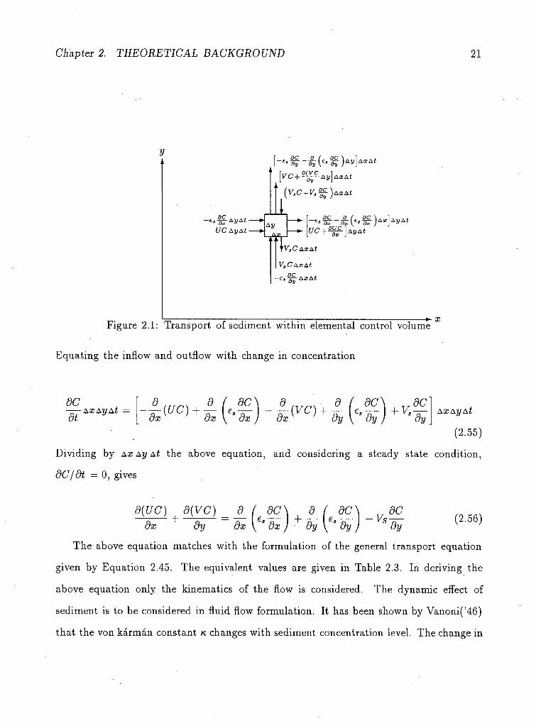
Chapter 2. THEORETICAL BACKGROUND 21
AyAt-UC Ay At -
-'•w-ki'-w)^}**" [VC + ̂ Ay]AxAt {y,c+va^)AxAt
Ay Ay Ay ac a dx dx , 3LTC " + 3x _ ( e ' ^ ) H A w A t
C Ax At VjCAXAt
Figure 2.1: Transport of sediment within elemental control volume
Equating the inflow and outflow with change in concentration
8C dt
AX AyAt — d _ ( u c ) + 9 _ ( dC_^ dx dx v dx
JL(VC) + — (e —\+V — dx dy \" dy) 3 dy
AX Ay At
(2.55)
Dividing by AX Ay At the above equation, and considering a steady state condition,
dC/dt = 0, gives
d{UC) d(VC) _d_(d(r dx dy dx \ " dx
+ 9_(edC\+v9C dy \ 3 dy j S dy
(2.56)
The above equation matches with the formulation of the general transport equation
given by Equation 2.45. The equivalent values are given in Table 2.3. In deriving the
above equation only the kinematics of the flow is considered. The dynamic effect of
sediment is to be considered in fluid flow formulation. It has been shown by Vanoni('46)
that the von karman constant n changes with sediment concentration level. The change in
Chapter 2. THEORETICAL BACKGROUND 22
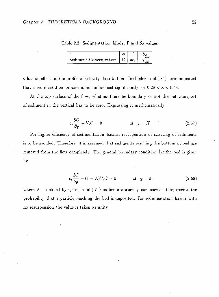
Table 2.3: Sedimentation Model T and Sj, values
r Scj, Sediment Concentration C V —
K has an effect on the profile of velocity distribution. Bechteler et al.('84) have indicated
that a sedimentation process is not influenced significantly for 0.28 < K < 0.44.
At the top surface of the flow, whether there be boundary or not the net transport
of sediment in the vertical has to be zero. Expressing it mathematically
e3^-+V3C = 0 dy
at y = H (2.57)
For higher efficiency of sedimentation basins, resuspension or scouring of sediments
is to be avoided. Therefore, it is assumed that sediments reaching the bottom or bed are
removed from the flow completely. The general boundary condition for the bed is given
by
dC es^+(l-A)VsC dy
0 at y = 0 (2.58)
where A is defined by Qecen et al.('71) as bed-absorbency coefficient. It represents the
probability that a particle reaching the bed is deposited. For sedimentation basins with
no resuspension the value is taken as unity.
Chapter 3
PREVIOUS WORK ON SEDIMENTATION METHODS
Many types of sedimentation basins are available for practical applications. The selection
depends on the type of suspension to be removed, size of suspended particles, flow volume,
relative cost and practical constraints or design features related with other structures.
In this chapter the basic features of many related sedimentation methods are dis
cussed with brief introduction of the ideal sedimentation theory.
Ideal Basin For design purposes, the classical theory of sedimentation was first given by Hazen('04).
He showed that the removal ratio of suspended matter depends on the surface area pro
vided and not upon the detention period or volume of basin and his argument is outlined
below. The ideal rectangular continuous flow basin for unhindered quiescent discrete
settling assumes the following
- horizontal, steady and uniform velocity of flow
- the concentration of each size particle is the same along the vertical at the inlet
- solid particle is removed from suspension once it reaches the bed
The removal ratio of suspended matter is one minus the ratio between outlet to inlet
concentration of sediment. The detention period is defined as time required for suspension
to reach bottom of basin.
23
Chapter 3. PREVIOUS WORK ON SEDIMENTATION METHODS 24
U
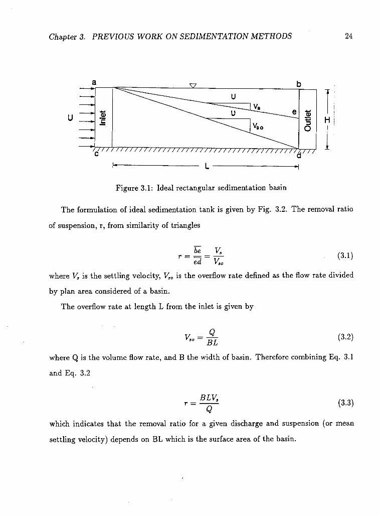
Figure 3.1: Ideal rectangular sedimentation basin
The formulation of ideal sedimentation tank is given by Fig. 3.2. The removal ratio
of suspension, r, from similarity of triangles
r = t = K (3.1) ed Vso
where Vs is the settling velocity, Vs0 is the overflow rate defined as the flow rate divided
by plan area considered of a basin.
The overflow rate at length L from the inlet is given by
v = - 9 -s o BL
(3.2)
where Q is the volume flow rate, and B the width of basin. Therefore combining Eq. 3.1
and Eq. 3.2
BLV, r =
Q (3.3)
which indicates that the removal ratio for a given discharge and suspension (or mean
settling velocity) depends on BL which is the surface area of the basin.
Chapter 3. PREVIOUS WORK ON SEDIMENTATION METHODS 25
The above analysis doesn't include the effects of turbulence, resuspension, inlet and
outlet conditions on sedimentation process. The theory is based on the idea of "overflow
rate"
3.1 High-rate Settlers
3.1.1 Introduction
It is clearly seen from the ideal basin theory that the surface area of a basin is important
design feature. For discrete settling without turbulence, the depth within wide range is
not important design parameter except for other practical constraints.
High-rate settlers employ a set of parallel plates or pipes arranged horizontally or
inclined with detention period not longer than 15 min. Within a limited plan area a
multiple settling area is provided. This reduces the cost of construction and the use of
land for building a basin. The increased surface area increases resistance, which lowers
the Reynold's number of the flow, and under these circumstances, turbulence is reduced
so that particle settling is increased. The high rate settlers are mainly used in water and
wastewater treatments.
3.1.2 Different Types of High-rate Settlers
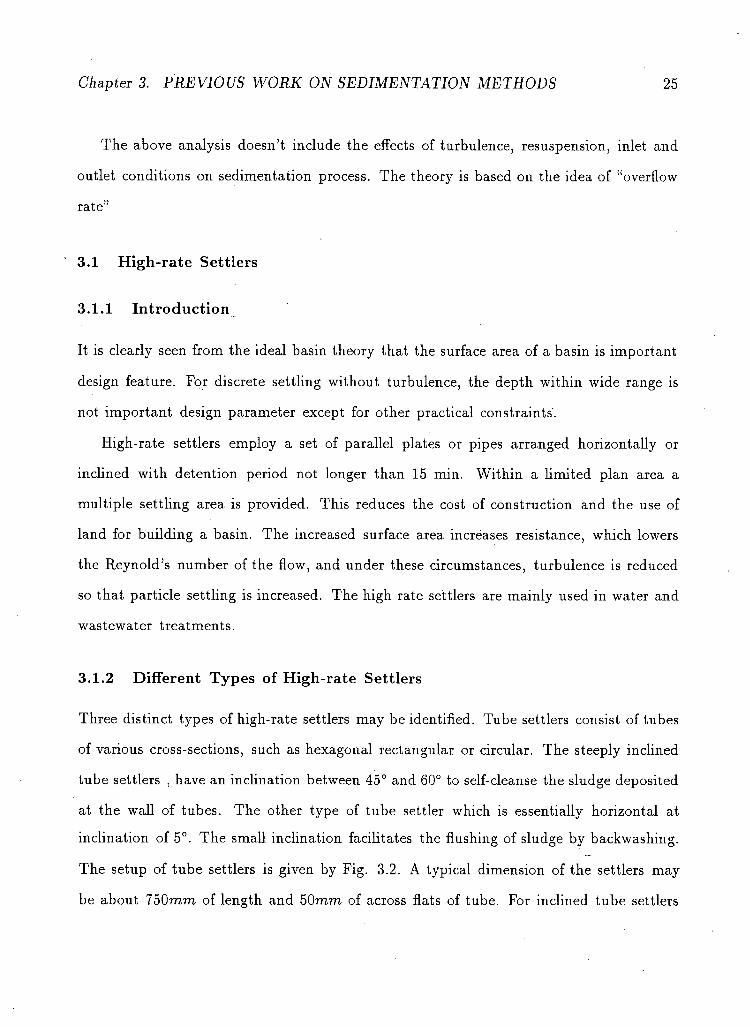
Three distinct types of high-rate settlers may be identified. Tube settlers consist of tubes
of various cross-sections, such as hexagonal rectangular or circular. The steeply inclined
tube settlers , have an inclination between 45° and 60° to self-cleanse the sludge deposited
at the wall of tubes. The other type of tube settler which is essentially horizontal at
inclination of 5°. The small inclination facilitates the flushing of sludge by backwashing.
The setup of tube settlers is given by Fig. 3.2. A typical dimension of the settlers may
be about 750mm of length and 50mm of across flats of tube. For inclined tube settlers
Chapter 3. PREVIOUS WORK ON SEDIMENTATION METHODS 26
a) Esaentialy Horizontal Tube Settler b) Inclined Tube Settler
Figure 3.2: Tube Settlers
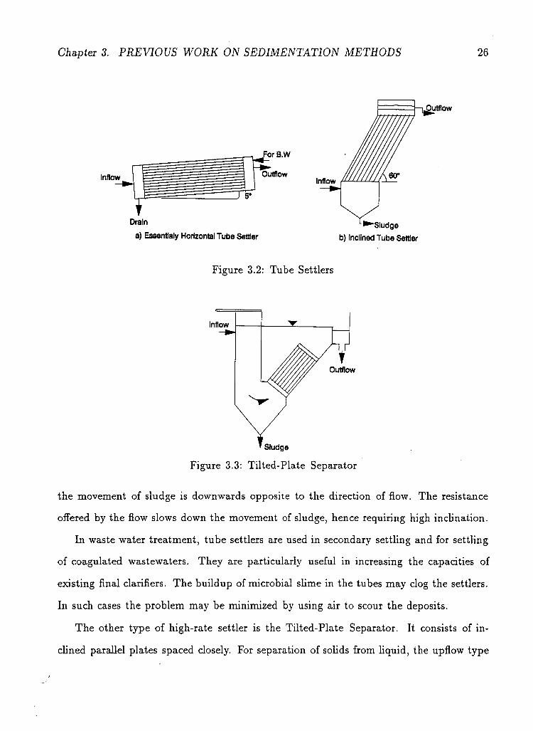
Figure 3.3: Tilted-Plate Separator
the movement of sludge is downwards opposite to the direction of flow. The resistance
offered by the flow slows down the movement of sludge, hence requiring high inclination.
In waste water treatment, tube settlers are used in secondary settling and for settling
of coagulated wastewaters. They are particularly useful in increasing the capacities of
existing final clarifiers. The buildup of microbial slime in the tubes may clog the settlers.
In such cases the problem may be minimized by using air to scour the deposits.
The other type of high-rate settler is the Tilted-Plate Separator. It consists of in
clined parallel plates spaced closely. For separation of solids from liquid, the upflow type
Chapter 3. PREVIOUS WORK ON SEDIMENTATION METHODS 27
Sludge
Outflow
Inflow
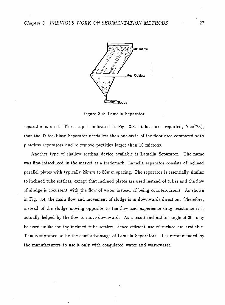
Figure 3.4: Lamella Separator
separator is used. The setup is indicated in Fig. 3.3. It has been reported, Yao('73),
that the Tilted-Plate Separator needs less than one-sixth of the floor area compared with
plateless separators and to remove particles larger than 10 microns.
Another type of shallow settling device available is Lamella Separator. The name
was first introduced in the market as a trademark. Lamella separator consists of inclined
parallel plates with typically 25mm to 50mm spacing. The separator is essentially similar
to inclined tube settlers, except that inclined plates are used instead of tubes and the flow
of sludge is cocurrent with the flow of water instead of being countercurrent. As shown
in Fig. 3.4, the main flow and movement of sludge is in downwards direction. Therefore,
instead of the sludge moving opposite to the flow and experience drag resistance it is
actually helped by the flow to move downwards. As a result inclination angle of 30° may
be used unlike for the inclined tube settlers, hence efficient use of surface are available.
This is supposed to be the chief advantage of Lamella Separators. It is recommended by
the manufacturers to use it only with coagulated water and wastewater.
Chapter 3. PREVIOUS WORK ON SEDIMENTATION METHODS 28
3.1.3 Discussion of Theoretical Study
The basic theoretical analysis of high-rate sedimentation has been given by Yao. The
analysis is given for sedimentation process in pipes, square conduits, shallow open tray,
uniform flow and flow between parallel plates. The theoretical derivations are discused
with experimental results obtained by Yao('73).
Yao made the assumptions that the flow is laminar and two-dimensional, particles
are discrete and inertia effect is negligible (no particle acceleration). The inlet and outlet
conditions are also idealized. The various parameters involved in the theoretical analysis
are, settler length, settler inclination, and lateral dimension of settler.
Combining the effect of fluid drag resistance and gravitational settling on a particle,
the equation of motion is formulated to obtain family of trajectories and to analyze the
effect of different parameters. Assuming a constant concentration along the vertical at
the inlet section, removal ratio of sediment is also determined. But, paradoxically, the
expression of sediment removal ratio for open tray flow and flow between parallel plates
at zero inclination indicate the same result as ideal rectangular sedimentation basin; even
though the velocity distribution along the vertical are different.
3.2 Sedimentation Basins
The design of sedimentation basins is based on the type of sediment suspended , the
smallest sediment size to be removed, and the degree of removal required. The maximum
velocity is limited to a critical value to prevent the pick-up of settled sediments.
There are many different types of sedimentation basins in use. Rectangular and
circular sedimentation basins are more popular. The use of vortex-type sedimentation
basins has been reported in wastewater and hydro-power plants.

Chapter 3. PREVIOUS WORK ON SEDIMENTATION METHODS 29
3.2.1 Rectangular Sedimentation Basins
Rectangular sedimentation basins are essentially rectangular box shaped, with the longer
dimension in the direction of flow. They may be constructed with or without top cover. A
sedimentation basin may be divided into three major regions; inlet, basin area and outlet.
Each part needs to be designed for maximum efficiency of sediment removal. From the
constructional point of view, rectangular sedimentation basins may be divided as classical
type and automatic type. In the classical type, the basin has different compartments, and
the operation and flushing of each compartment is done in turn. In the automatic type,
which is often known as Deflour sedimentation basin, the continuous flushing of sediment
trapped in a sand trap grate, located at the bottom, enables permanent operation of the
basin.
Inlet and Entrance Conditions
The inlet conditions of flow and sediment has an influence on the performance of sedi
mentation basins. The purpose of the inlet is to provide a proper condition for maximum
sediment deposition in the basin. Sarikaya's work suggest that a uniform flow velocity
with low turbulence level increases the basin efficiency. For this purpose various devices
such as weirs, deflecting plates, stilling devices and screens may be used. In waste water
treatment, possible floe break-up is to be avoided at the inlet.
The natural way of achieving uniform velocity is by having high inlet energy loss.
This idea was used by Camp(Larsen('77)) to estimate the associated uniformity of flow
as a function of inlet energy loss. Installing screen at the inlet to basin tend to reduce
the sediment transport capacity of a stream. This enhances the deposition of sediments.
Experimental work done by Bayazit('71) indicates that fine screens are effective in re
ducing turbulence, which means high deposition at upstream region. Coarse screens,
Chapter 3. PREVIOUS WORK ON SEDIMENTATION METHODS 30
conversely, tend to scour the bed. The experimental work also indicates that maximum
stable deposition with fine screens to occur by using vertical screen and another down
stream facing inclined screen together. Skimmer walls with little submergence are found
effective to reduce the turbulence level. Two parallel rows of alternately placed verti
cal bars are able to reduce the macro scale turbulence and small scale turbulence found
in small eddies. The use of a "honey comb" like obstruction in open-channel flow was
studied by Aydin(Cegen('77)) and his experiments show a reduction of turbulence level
about 30 — 40%. Discussion on the design of sedimentation basins with emphasis on
waste water treatment is given by Larsen et al.('77).
The sediment distribution along the vertical at the inlet has an effect on the amount
of sediment deposited in basin. It was shown by Hippola('73) that assuming a triangular
concentration distribution at inlet to basin reduces the length of sedimentation by 30 —
40%. The numerical work of Bechteler et al. shows that the removal ratio of sediment
is higher for triangular sediment distribution than for uniform sediment distribution at
the inlet.
The Basin Area
The deposition of sediments occur in the rectangular basin area. Basins with shallow
depths have low cost of construction and are easy to construct. But, the deposition occurs
mostly near the inlet section, within short distance, and may fill the basin in a short
period. Therefore, the depth is to be chosen between certain interval. A high-velocity
central current is also observed between dead spaces and vortices, instead of uniform
velocity distribution throughout the basin length. This phenomenon which is called
recirculation or hydraulic short circuit is to avoided for efficient removal of sediment.
The inlet and outlet conditions are important factors for the happening.
The analysis and design of rectangular sedimentation basins has been done by many
Chapter 3. PREVIOUS WORK ON SEDIMENTATION METHODS 31
investigators. The simple formulation is given by ideal rectangular sedimentation basin
which assumes idealized conditions. Camp('46) based on Dobbins('44) analytical work
has developed a design procedure which includes the effect of turbulence on sedimentation
process. But it is assumed that the flow is uniform and sediment transfer coefficient is
constant along a section. The analytical solution was given by solving the sedimentation
model (Eq. 2.56), neglecting the horizontal diffusion of sediment. It is discussed by
Masonyi('65) that the design procedure is conservative for design particle size below
0.1mm.
The numerical finite difference solution of the sedimentation model with velocity dis
tribution other than uniform was given by Sarikaya('77). The computation was made for
logarithmic and parabolic velocity distribution. Constant sediment concentration was as
sumed at the inlet. The sediment transfer coefficient distribution for the logarithmic and
parabolic velocity distribution was taken as parabolic and uniform respectively. Similar
solutions with inlet triangular sediment concentration, which is more realistic has been
given by Bechteler et al. The sedimentation process with point source was also analyzed.
The overall effect of turbulence in sedimentation may be taken as reducing the fall
velocity of a particle. The effective fall velocity may be assumed as Vs — Va\ Where Va' is
the value by which the quiescent fall velocity is to be reduced to account for turbulence
effect. Levin(Masonay('65)) has found that
K = aU0 [m/sec] (3.4)
where a is a coefficient. It is generally agreed by investigators that the coefficient may
be computed using a = ^=r where H is given in meter. The expression for V3' may be
rewritten as

Chapter 3. PREVIOUS WORK ON SEDIMENTATION METHODS 32
v: = 8-^= = 8 FT (3.5)
where 3 is a non-dimensional value equal to 0.413 and Fr is the Froude number of the
flow in the basin. Therefore the settling length required is
HUp HU„
Einstein(Strand'86) developed a method of predicting the deposition of fine particles
on a gravel bed. The same procedure have been used to design sedimentation basins.
The equations (for same sediment size) used are as follows
JJ T = 65.7— (3.7)
* 8
Lx = U0T (3.8)
r = i _ e-o.693^ ( 3 Q )
(3.10)
where T is time in seconds for sediment concentration to be half the initial value, L\ is
length of basin over which half the sediment allowed is deposited. The coefficient, 65.7 ,
was obtained from empirical flume studies. Combining the given three equations
, -0.01055̂ /o 1 1 \ r = 1 — e uoH (3.11)
Velikanov(Masonyi('65)) has suggested the use of probability theory for solution of
sedimentation process in turbulent flow. He studied the probability of settling of sediment
with definite fall velocity within a given length. The probability of deposition or removal
ratio (for uniform particle size) is given as
Chapter 3. PREVIOUS WORK ON SEDIMENTATION METHODS 33
r=WLrD{V/L)^LE~"DT <3-I2)
where
• A = 0 _. (3.13)
and (Ty is standard deviation of vertical deflections from the mean horizontal trajectory
of sediment. Based on the above analysis the settling length is given by
\2U2(y/H-0.2)2
1 = 7.51V? ' <3'14)
where 0.2 is essentially constant, and has the dimensions of y/Z.
Shamber et al. ('84) made a numerical analysis of flow in sedimentation basins by
using Galerkin finite element method to solve the general transport equations of motion.
The structure of turbulence was represented using eddy viscosity concept, the k-e model.
Realistic inlet and outlet conditions were incorporated in the solution. The velocity
field obtained may then be used further for modelling sedimentation process. Complete
simulation of flow and sedimentation process in primary clarifiers was made by Abdel-
Gawad et al.('85). The model developed was tested against the measurements obtained
in the rectangular clarifiers used in the city of Sarnia, Canada. The method employs the
Strip Integral Method (SIM) to solve the general transport equations. They discuss that
the SIM is advantageous over the finite element and finite difference model, because of
computer time and storage saving. The optimum design procedure considering possible
resuspension of deposits is given by Takamatsu et al.('74).
As an outlet device weir or sluice may be used to keep the water level in the sedi
mentation basin constant and to check water from outlet flushing canal returning back.
The use of high weir is to be avoided to eliminate undesirable vortex formation, which
directly reduces the basin efficiency.
Chapter 3. PREVIOUS WORK ON SEDIMENTATION METHODS 34
Inflow
II
Overflow Weir J
rd Outflow
Underflow
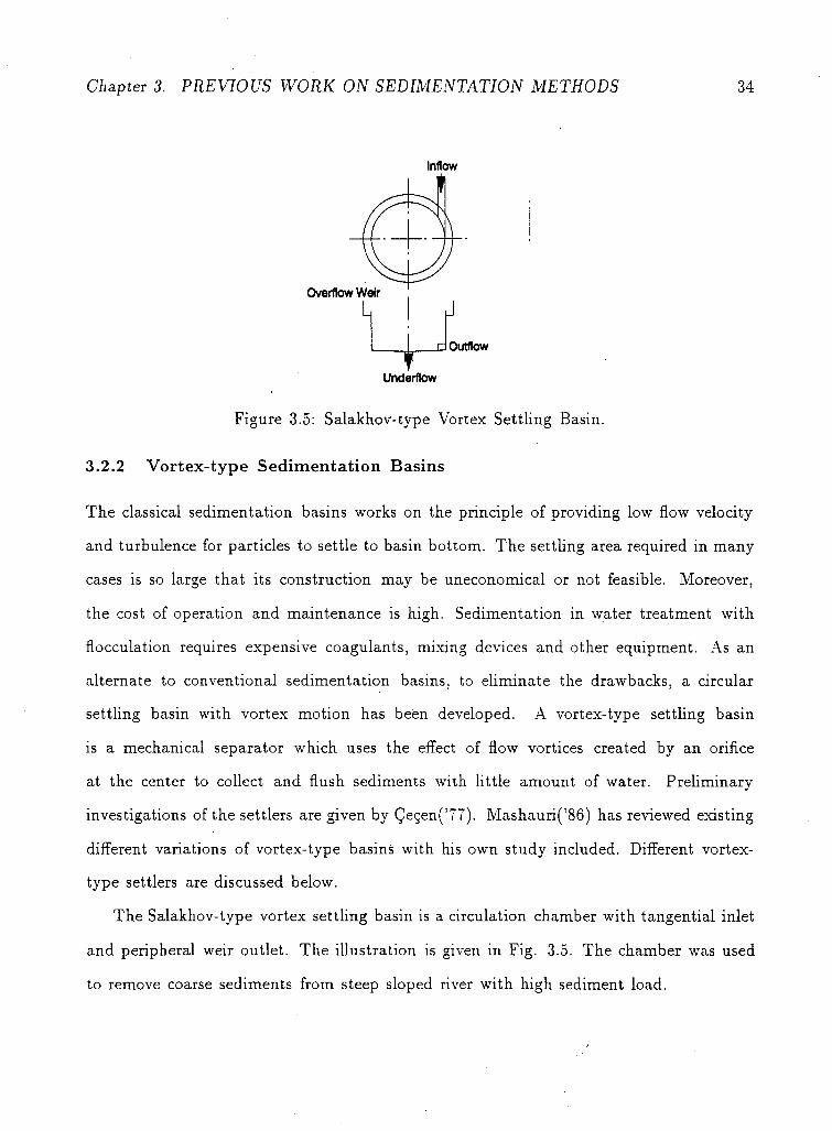
Figure 3.5: Salakhov-type Vortex Settling Basin.
3.2.2 Vortex-type Sedimentation Basins
The classical sedimentation basins works on the principle of providing low flow velocity
and turbulence for particles to settle to basin bottom. The settling area required in many
cases is so large that its construction may be uneconomical or not feasible. Moreover,
the cost of operation and maintenance is high. Sedimentation in water treatment with
flocculation requires expensive coagulants, mixing devices and other equipment. As an
alternate to conventional sedimentation basins, to eliminate the drawbacks, a circular
settling basin with vortex motion has been developed. A vortex-type settling basin
is a mechanical separator which uses the effect of flow vortices created by an orifice
at the center to collect and flush sediments with little amount of water. Preliminary
investigations of the settlers are given by Cecen('77). Mashauri('86) has reviewed existing
different variations of vortex-type basins with his own study included. Different vortex-
type settlers are discussed below.
The Salakhov-type vortex settling basin is a circulation chamber with tangential inlet
and peripheral weir outlet. The illustration is given in Fig. 3.5. The chamber was used
to remove coarse sediments from steep sloped river with high sediment load.
Chapter 3. PREVIOUS WORK ON SEDIMENTATION METHODS 35
• Outflow
Jj Inflow
underflow
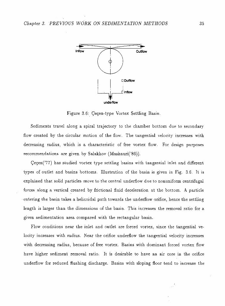
Figure 3.6: Cecen-type Vortex Settling Basin.
Sediments travel along a spiral trajectory to the chamber bottom due to secondary
flow created by the circular motion of the flow. The tangential velocity increases with
decreasing radius, which is a characteristic of free vortex flow. For design purposes
recommendations are given by Salakhov (Mashauri('86)).
Cegen('77) has studied vortex type settling basins with tangential inlet and different
types of outlet and basins bottoms. Illustration of the basin is given in Fig. 3.6. It is
explained that solid particles move to the central underflow due to nonuniform centrifugal
forces along a vertical created by frictional fluid deceleration at the bottom. A particle
entering the basin takes a helicoidal path towards the underflow orifice, hence the settling
length is larger than the dimensions of the basin. This increases the removal ratio for a
given sedimentation area compared with the rectangular basin.
Flow conditions near the inlet and outlet are forced vortex, since the tangential ve
locity increases with radius. Near the orifice underflow the tangential velocity increases
with decreasing radius, because of free vortex. Basins with dominant forced vortex flow
have higher sediment removal ratio. It is desirable to have an air core in the orifice
underflow for reduced flushing discharge. Basins with sloping floor tend to increase the
Chapter 3. PREVIOUS WORK ON SEDIMENTATION METHODS 36
orifice discharge due to increased water depth at the center. Basins with tangential outlet
produces a stronger vortex motion to separate sediments from the flow.
Other variations which use vortex flow as a basis for sediment separation are Sullivan-
type and Hydrocyclones (Mashauri('86)). Hydrocyclones are capable of separating solids
of size 2 to 200 am from liquids. The running cost is relatively high due to use of pumps to
create the necessary operating head. The Sullivan-type settling basin is commonly used
in water and wastewater treatments. Wilson('86) has coupled the free vortex energy
dissipation with sediment control, to remove abrasive sediments entering wastewater
treatment plant and sewer overflows. He reports that the area required to remove 30
micron sand is less than 5% compared with conventional settling basin.
Generally, vortex-type settling basins have economical advantage over the conven
tional sedimentation basins. It may be used as pre-settling basin in hydro-power plants
for separating coarse sediments to reduce the load entering the main sedimentation basin.
The dimensions and the flushing discharge are smaller. The operation is continuous with
minimum maintenance.

Chapter 4
S E T T I N G T A N K F O R FISHERIES
4.1 Introduction
This chapter discusses the experiments conducted to obtain a suitable geometrical con
figuration for uniform flow distribution in a high rate sedimentation tank used with fish
rearing units.
For effective performance of a high rate sedimentation tank the flow distribution
in the structure has to be uniform, because a uniform flow distribution minimizes the
flow velocity, thereby maximizing the opportunity for sediment to settle out of the flow.
Experiments were conducted to obtain the most suitable geometric system to achieve
uniform distribution. The main problem to overcome was the heavy circulation present
in the sedimentation tank, which gave quite high velocities around the outer part of the
settling basin, these velocities being considerably increased by the repeated recirculation
of the fluid.
In a fish rearing tanks it is necessary to circulate fresh water for effective growth
of fish. The wastewater from the tanks contains fine organic particles which need to
be removed before the water discharges to the stream system. One of the wastewater
treatment procedure to remove particles is sedimentation process. The problem in small
sized sedimentation tanks is recirculation. Recirculation occurs when some of the fluid
passes through the settling zone of a tank in less time than the detention period. It is
caused due to non-uniform velocity distribution and difference in length of streampaths.
37
Chapter 4. SETTING TANK FOR FISHERIES 38
Due to the high velocity of flow in some part of the tank sediment escapes with the
outflow. To avoid recirculation and for the maximum efficiency of sedimentation tank
the flow distribution has to be uniform.
The main particles present in a fish rearing effluent are fish manure and uneaten fish
feeds. The particles have the tendency to decompose with passage of time. Moreover
the physical property changes with time. The particles also have the tendency to stick
to rough surfaces and edges, and this makes it difficult to have small openings in the
sedimentation unit since such openings can be easily clogged.
The high rate sedimentation tank contains a number of horizontal parallel plates.
These horizontal plates are used to increase the surface area of the boundaries, which
dampens turbulence and encourages sedimentation in the developing boundary layers
on each plate. The opportunity for sedimentation is therefore greatly increased. The
uniform flow distribution is also necessary to have equal amount of flow within each
settling plate. The inlet and outlet conditions of the tank are arranged to fit in with the
operational requirements the whole system; settling and rearing tank.
Previous work has been done on high rate sedimentation tanks. One example is a
Lammela separator(Yao('73)). But the problem with the previously designed systems is
inability to clean or wash deposited particles on the settling plates. Moreover in some of
the systems pumping is required which in this case would disturb the settling of particles
and would induce turbulence affecting the overall efficiency of the system. Some of the
previous high sedimentation units rely on the self cleansing of the sediments by providing
sloping sedimentation surface, but this only works for non-cohesive sediments and is not
suitable for the sediment encountered in fish rearing which is highly cohesive and does
not have the ability to clean by itself.
Chapter 4. SETTING TANK FOR FISHERIES 39
0
J •
. - 7
0
J •
. - 7
0
J •
. - 7
0
J •
. - 7
0
J • 111//n n it i > 111) rrrminir
' / i h'i h'i i >',{,', h<>!/, l/> //, //, // rrrrrr/rrrrrn />un 111//n n it i > 111) rrrminir ' / i h'i h'i i >',{,', h<>!/, l/> //, //, //
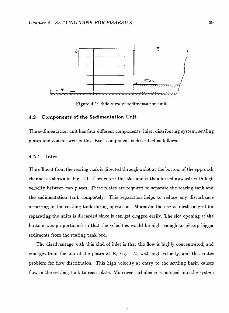
Figure 4.1: Side view of sedimentation unit
4.2 Components of the Sedimentation Unit
The sedimentation unit has four different components; inlet, distributing system, settling
plates and control weir outlet. Each component is described as follows.
4.2.1 Inlet
The effluent from the rearing tank is directed through a slot at the bottom of the approach
channel as shown in Fig. 4.1. Flow enters this slot and is then forced upwards with high
velocity between two plates. These plates are required to separate the rearing tank and
the sedimentation tank completely. This separation helps to reduce any disturbance
occurring in the settling tank during operation. Moreover the use of mesh or grid for
separating the units is discarded since it can get clogged easily. The slot opening at the
bottom was proportioned so that the velocities would be high enough to pickup bigger
sediments from the rearing tank bed.
The disadvantage with this kind of inlet is that the flow is highly concentrated; and
emerges from the top of the plates at B, Fig. 4.2, with high velocity, and this crates
problem for flow distribution. This high velocity at entry to the settling basin causes
flow in the settling tank to recirculate. Moreover turbulence is induced into the system
Chapter 4. SETTING TANK FOR FISHERIES 40
DIMENSION IN M WIDTH OF FLUME 51OM
0.12
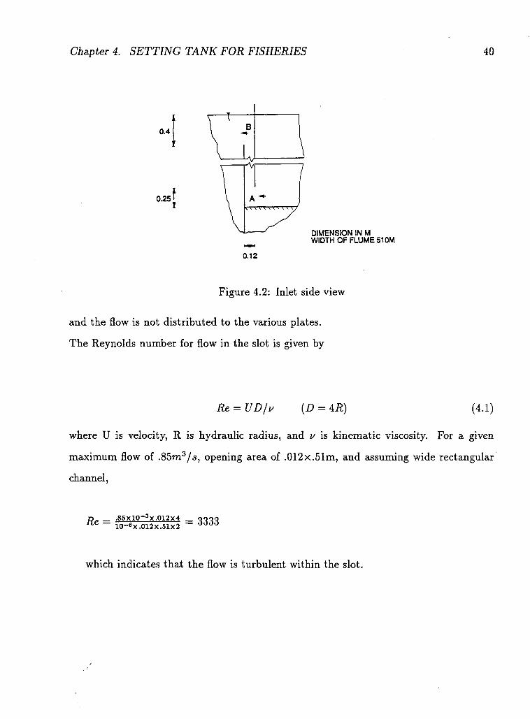
Figure 4.2: Inlet side view
and the flow is not distributed to the various plates.
The Reynolds number for flow in the slot is given by
Re = UD/v (D = AR) (4.1)
where U is velocity, R is hydraulic radius, and v is kinematic viscosity. For a given
maximum flow of .85m3/s, opening area of .012x.51m, and assuming wide rectangular
channel,
p „ _ .85XlO~3X.012x4 _ 9 9 9 9 N E — 10-«X.012X.51X2 - 0 0 0 0
which indicates that the flow is turbulent within the slot.
Chapter 4. SETTING TANK FOR FISHERIES 41
4.2.2 Distributing System
Different systems were tested during the experimentation to achieve uniform flow distri
bution within the settling tank. Two of the systems tested will be described here. In the
first one shown in Fig. 4.4 deflectors were placed at different levels, with the purpose of
deflecting the flow directly in line with and towards the plates. The second one Fig. 4.3
uses the principle of dissipating the incoming energy and directing the flow at an angle
towards the plates. Each type is discussed below.
Grated System
The circulation in the tank is by the incoming high velocity flow from the slot opening.
Since the outlet from the tank is near the water surface, there is a tendency for the flow
to concentrate within the top portion of the settling tank. In order to avoid the high
momentum flow coming out from the slot and hence the heavy circulation, an energy
dissipation mechanism has to be arranged. Moreover the flow has to be deflected at an
angle to the plates. In order to achieve the above mentioned processes three layers of a
grating formed from metal strips were used. The openings of the grate were staggered to
get the maximum energy dissipation.
Different trials were made using different spacings between the layers and different
percentage of opening for each layer. For the spacing a limit is reached that it is no
longer feasible to clean the metal strips.
Plate Deflectors
As discussed before without any arrangement at the slot outlet, the flow concentrates
within the top portion of the tank. To avoid this a baffle, was constructed to divert
the flow downwards, to the deflecting plates, as shown in Fig. 4.4. These deflecting
Chapter 4. SETTING TANK FOR FISHERIES 42
0.12
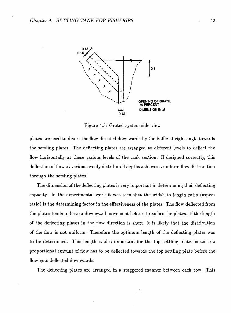
Figure 4.3: Grated system side view
plates are used to divert the flow directed downwards by the baffle at right angle towards
the settling plates. The deflecting plates are arranged at different levels to deflect the
flow horizontally at these various levels of the tank section. If designed correctly, this
deflection of flow at various evenly distributed depths achieves a uniform flow distribution
through the settling plates.
The dimension of the deflecting plates is very important in determining their deflecting
capacity. In the experimental work it was seen that the width to length ratio (aspect
ratio) is the determining factor in the effectiveness of the plates. The flow deflected from
the plates tends to have a downward movement before it reaches the plates. If the length
of the deflecting plates in the flow direction is short, it is likely that the distribution
of the flow is not uniform. Therefore the optimum length of the deflecting plates was
to be determined. This length is also important for the top settling plate, because a
proportional amount of flow has to be deflected towards the top settling plate before the
flow gets deflected downwards.
The deflecting plates are arranged in a staggered manner between each row. This
Chapter 4. SETTING TANK FOR FISHERIES 43
Baffle block A 0.5
0.7
0.2 0.7' /
Deflecting plate
0.5
0.2
I— B4> 0.2 0.5 0.17
0.9
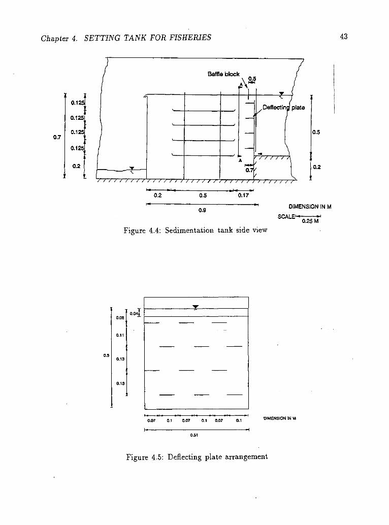
Figure 4.4: Sedimentation tank side view
DIMENSION IN M
SCALE 1 - -»< 0.25 M
0.08
o.s 0.13
0.13
0.07
u.
0.1 0.07 0.1 0.07 0.1
>J DIMENSION IN M
0.51
Figure 4.5: Deflecting plate arrangement
Chapter 4. SETTING TANK FOR FISHERIES 44
enables each row of deflecting plates to take a proportional amount of flow with respect
to the widths of the plates. The staggered arrangement as indicated in Fig. 4.5 gave a
better flow distribution. The plates apart from acting as deflecting devices; they created
resistance to the flow moving downwards deflected from the baffles. This enabled the
high velocity deflected flow to slow down and distribute itself horizontally.
The dimensions of the deflecting plates and the relative position and arrangement of
the deflecting baffle were determined after a lot of trial and error experimentation. The
top settling plate and at times the bottom settling plate were critical in determining the
dimensions.
4.2.3 The Settling Plate System
The design of the settling plates was based on the loading rate or on the removal of
sediment of specific settling velocity. For this case the loading rate was taken as 9.26 X
10 - 4ra 3/(ra 2 — sec)(807n3/(m2 — day)). The width of the plates is fixed by the width of the
rearing units. Moreover the length of the plates along the flow direction is dependent on
the space available for sedimentation tank. The main design objective is then determining
the number of plates required. The following are given values for design,
Design maximum flow= .85 x 10~6m3/.s
Design minimum flow = .425 x 10-6m3/.s
Width of tank. = 0.51 m
Length of plates = 0.5 m
Surface area required — flow rate
(4.2) loading rate
Chapter 4. SETTING TANK FOR FISHERIES 45
substituting the corresponding values,
Surface area required = 51 Xl0 3X 1440x60 60x80
= 0.918 m: 2
Number of settling plates required = .918 = 3.6 .51X.5
Therefore 4 settling plates to be used.
Spacing between each plate = 0.50/4 =0.125 m
When the flow rate is low as indicated by the minimum flow, the number of settling
plates required is less. Since at low flow all the provided plates are not necessary, the
uniform distribution of flow is not critical. Therefore high consideration was given for
high flow rate.
The settling plates were arranged horizontally and parallel to get the maximum pos
sible settling surface area within the provided space. The cleaning of the plates is to be
performed by rotating the whole plate system at right angle. Therefore an extra space
is required below the bottom plate to enable the whole system of plates to rotate. In
fact this extra space provides extra sedimentation area. Since the distribution of flow
in this area is not reliable, it is not considered in the design. This extra space has also
advantage of settling bigger particles which would easily fill up the other settling plates.
Moreover it compensates the reduction of efficiency of the plates due to any change of
flow phenomenon from the idealized case.
Chapter 4. SETTING TANK FOR FISHERIES 46
It is necessary to check whether the flow in the plates is laminar so that tranquil
settling is facilitated.
Assuming a laminar boundary layer development we have,
s _ 4.91 x a; \/Rex
substituting the corresponding values,
.125 4.91 X i 2 ' ix»,5xl0~
solving, x =.14m , hence the flow develops within the plate.
If a turbulent boundary layer is assumed,
Lr = ^ T <4-4> substituting the corresponding values and solving, x = .58m which is greater than the
plate length (0.5m).
But fully developed region was observed in the experiment. Hence the observation
suggests the development of laminar boundary layer.
Considering the Reynolds number of the fully developed region,
Re UD
— 51X1Q-3X1X4X. 125^1 60 x4x.125 x . 5 1 x 2 x 1 x 1 0 - °
= 833
which indicates that the flow is laminar since less than 2000.
Chapter 4. SETTING TANK FOR FISHERIES 47
It is obvious that due to the inlet conditions to the settling plates the flow is not
totally laminar at the beginning. But it changes to laminar flow as it proceeds further
down between the settling plates.
Particles deposited on the plates form a layer. Before washing deposits on the plates,
the water in the tank has to be drained. The deposited layer is of loose material which
can be disturbed easily. In the process of draining, the deposited material gets disturbed
and washed away. From wastewater treatment point of view the deposited material is to
be washed and collected separately for further treatment. The drained water from the
tank is not to be mixed with the deposited material. To restrict the washing away of
the deposited material while draining; the edges of the plates upstream and downstream
side are bent upwards. This helps to hold the deposited material from moving away.
Nevertheless the flow at the inlet to the plates gets disturbed due to the bend which is
not desirable. But from the operational point of view the setup is unavoidable.
The presence of the plates has an effect on the distribution pattern of the flow. Better
distribution of flow was observed without the presence of the plates . The relative position
of the plates in the tank unit has an effect on the flow pattern. This depends on how
far the edge (inlet) of the settling plates is located from the face of the baffle. It doesn't
seem that the gap between the downstream weir and outlet of the plates has an effect on
the flow distribution pattern.
4.2.4 Control Weir Outlet
The water level in the rearing tank has to be kept at a constant level. The control of
the water depth both in the rearing tank and the sedimentation unit is controlled by a
sharp crested weir. The head required over the sharp crested weir is very small compared
to the depth of flow. Any variation in the flow rate has minimum effect on the head
over the weir. With the installation of the crested weir the flow is concentrated at the
Chapter 4. SETTING TANK FOR FISHERIES 48
top section of the tank. Without flow distributors it contributes to the high circulating
tendency observed in the system. No special arrangement is made near the crested weir
for uniform flow distribution. The efficiency of the whole system is dependent on the
structure constructed near the baffle or the inlet to the settling tank.
Chapter 5
D E V E L O P M E N T OF T H E O R Y
Many investigators have attributed the process of suspension to the turbulent fluctuating
of fluid flow, Garde et al.('85). Bagnold('66) discusses that, near a solid boundary, the
turbulent shear flow causes an anisotropic turbulence which is responsible for supporting
sediments in suspension. In an anisotropic turbulence the upward and downward fluc
tuating turbulent velocity intensities are different in magnitudes so that there is a net
stress away from the boundary. Bagnold('66) illustrates this idea with flow visualization
photographs of flow near a solid boundary surface taken by Prandtl('52).
Bagnold considers a unit volume of fluid above a horizontal surface and evaluates
the net upward momentum flux with respect to upward velocity fluctuation. Within the
elemental volume the conservation of mass is satisfied. After maximizing the momentum
flux, he relates it to the rms of the vertical velocity fluctuation, which gives,
/ = 0.414/972 (5.1)
where / is momentum flux and v is vertical velocity fluctuation. The maximum value
Of vT 2
near the wall must be able to support the whole suspension up to the free sur
face, and from Laufer's ('51) experimental results the ratio yfiT1'max/[V'„ is approximately
equal to unity. Therefore expressing the net momentum fluctuation with respect to the
boundary shear stress, TW, which by definition equals pUl,
/ = 0.414rw (5.2)
49
Chapter 5. DEVELOPMENT OF THEORY 50
After further analysis he gives the sediment carrying capacity of a flow, in terms
of efficiency with respect to the total stream power. It is to be noted that Laufer's
experimental result is given for flow over a smooth boundary.
Bagnold compares his result with the work of Irmay ('80), which uses a totally different
approach, for the confirmation of his result. Irmay's analysis uses the simplified form
of the Navier-Stokes equation for turbulent steady two-dimensional fully developed flow.
For fully developed two-dimensional flow the variation of flow variables is in the vertical
direction only. Irmay derives the acceleration term of a fluid particle in the vertical
direction in terms of the pressure variation and hence to the vertical velocity fluctuation
after simplifying the Navier-Stokes equation as follows
I dp dv'2
a ^ - p d y = ^ y - <5'3>
Bagnold integrates the acceleration term to obtain the net upward momentum flux
in the fluid flow. Therefore
/ = p JO ~jy~dy = Pv'2y=H (since pv'2y=0 = 0) (5.4)
But Irmay has evaluated the ratio JJ- verses y/H, using Laufer's fully developed smooth
boundary experimental result. From the analysis it is shown that the value pv'2y=H is
given by 0.375^ (approx.). Substituting the result into Eq. 5.4,
/ = 0.375r™ (5.5)
from which Bagnold concludes that the above result is in good argument with his deriva
tion given by Eq. 5.2.
The main objective of this study- is to extend the whole idea discussed above to
sedimentation in closed conduits. It can be seen clearly from Eq. 5.4 that the supporting
Chapter 5. DEVELOPMENT OF THEORY 51
stress from the net momentum flux depends on the value of pv'2 in the limit considered.
At the lower solid boundary it is obvious that the value pv'2 — 0. If an upper boundary
is introduced, the same value pv'2 tends to be equal to zero, hence from Eq. 5.4 there
would not be net sediment supporting momentum flux.
Viewing the whole situation from another angle, if the lower smooth boundary is
responsible for the turbulence production and hence an upward momentum flux then a
solid upper boundary would be expected to exert a downward momentum flux to push
the sediments downwards. Which is to suggest that the net sediment transport with solid
upper boundary would be zero. Hence a sedimentation basin with top solid boundary
would be expected to have higher efficiency than the equivalent basin with free surface.
For rough solid boundary the rms of the vertical velocity fluctuation is found to be higher
than for smooth solid boundary, Hinze('59), Blinco et al.('72), McQuivey et al.('69), hence
higher momentum flux, hence higher momentum flux. Actually the non dimensional
turbulence intensity is more or less the same for both rough and smooth boundaries. But
for the same flow case the shear stress for the rough boundary is higher than that for
smooth; therefore the turbulence intensity is higher. From the above discussion, a rough
solid upper boundary is expected to generate more turbulence and hence higher downward
momentum flux than the smooth solid boundary at the bottom. The net downward push
on the sediments would be expected to facilitate the sedimentation process.
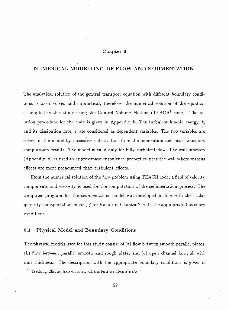
Chapter 6
N U M E R I C A L M O D E L L I N G OF F L O W A N D SEDIMENTATION
The analytical solution of the general transport equation with different boundary condi
tions is too involved and impractical, therefore, the numerical solution of the equation
is adopted in this study using the Control Volume Method (TEACH 1 code). The so
lution procedure for the code is given in Appendix B. The turbulent kinetic energy, fc,
and its dissipation rate, e, are considered as dependent variables. The two variables are
solved in the model by successive substitution from the momentum and mass transport
computation results. The model is valid only for fully turbulent flow. The wall function
(Appendix A) is used to approximate turbulence properties near the wall where viscous
effects are more pronounced than turbulent effects.
From the numerical solution of the flow problem using TEACH code, afield of velocity
components and viscosity is used for the computation of the sedimentation process. The
computer program for the sedimentation model was developed in line with the scalar
quantity transportation model, <f> for k and e in Chapter 2, with the appropriate boundary
conditions.
6.1 Physical Model and Boundary Conditions
The physical models used for this study consist of (a) flow between smooth parallel plates,
(b) flow between parallel smooth and rough plate, and (c) open channel flow, all with
unit thickness. The description with the appropriate boundary conditions is given in 1 Teaching Elliptic Axisymmetric Characteristics Heuristically
52
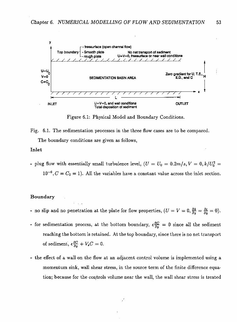
Chapter 6. NUMERICAL MODELLING OF FLOW AND SEDIMENTATION 53
u = u c
v=o c=c.
- - free8urface (open channal flow) Top boundary - - Smooth plate No net transport of sediment
L- rough plate U=V=0, freesurface or near wall conditions .y../..z.y../..y../..z.^../..y../..y.^../..y../..y.^.-y..y../..y.
SEDIMENTATION BASIN AREA Zero gradient for U, T.E., „
E.D., and C H
/ / / / / / / / / / / / / / / / / / / / / / / /
INLET U=V=0, and wall conditions Total deposition of sediment
OUTLET
Figure 6.1: Physical Model and Boundary Conditions.
Fig. 6.1. The sedimentation processes in the three flow cases are to be compared.
The boundary conditions are given as follows,
Inlet
plug flow with essentially small turbulence level, (U = U0 = 0.2m/s,V = Ojk/Ur2 =
10~6, C = Co = 1). All the variables have a constant value across the inlet section.
Boundary
- no slip and no penetration at the plate for flow properties, {U = V = 0, |^ = |^ = 0).
- for sedimentation process, at the bottom boundary, e g = 0 since all the sediment
reaching the bottom is retained. At the top boundary, since there is no net transport
of sediment, e g + V3C = 0.
- the effect of a wall on the flow at an adjacent control volume is implemented using a
momentum sink, wall shear stress, in the source term of the finite difference equa
tion; because for the controls volume near the wall, the wall shear stress is treated

Chapter 6. NUMERICAL MODELLING OF FLOW AND SEDIMENTATION 54
as external force in the horizontal momentum flux equation.
Outlet
- all variables have zero gradient, which assumes that fully developed or equilibrium
conditions exist. The computation domain is made long enough to justify this
assumption.
6.2 Finite Difference Formulation
6.2.1 Control Volume Definition
The conservation equations are solved numerically using the control volume integral
approach on a discrete grid. The grid network consists of orthogonally aligned nodes for
which the scalar properties (k,e,fieg, C) are computed. The boundaries for the scalar
control volumes are located midway between the nodes. The layout of the computational
grid is shown in Fig. 6.2. The point 'P' is a particular node point under consideration
and the neighbor nodes to the north, south, east and west are indicated by 'N', 'S',
'E', 'W respectively. The control volume faces are identified by the lower case letters
(n,s,e,w), and the solid lines indicate the boundaries.
The vector quantities, U and V, are defined at the boundaries of the scalar quantity
control volumes, between respective grid points. Their control volumes are indicated by
dashed lines. The velocity U, at a particular node is defined as being that entering the
left side, and the velocity V, as that entering from the bottom side of the control volume.
The velocity grids are staggered halfway to the east and south.
Chapter 6. NUMERICAL MODELLING OF FLOW AND SEDIMENTATION 55
Scalar quantity
U, valodty
V, velocity
Figure 6.2: Control Volume Description
6.2.2 Derivation of Finite Volume Equations
The derivation of the general finite difference equation is done by integrating the general
transport equation given by Eq. 2.45 over its corresponding control volume. Fluid
properties within each cell is assumed to be constant and linearly interpolated between
nodes to satisfy the continuity of total flux. Integrating Eq. 2.45
dCVOL) = J J S+dCVOL)
(6.1)
where VOL is volume of the cell considered.
Using the Gauss Divergence Theorem (to replace volume integrals by surface integrals),
the above equation may be written as
dy
+ f J W
dx = [SP<j>p + Su]VOL (6.2)
where Sp and Su are linearized source terms.

Chapter 6. NUMERICAL MODELLING OF FLOW AND SEDIMENTATION 56
Considering as an example the east face of control volume, the flux (convective and
diffusive terms) is given as
86 (6.3)
where Fe, is facial flux at the east side of control volume; the subscript indicates the
corresponding face. The hybrid differencing scheme is used to express the fluxes in terms
of modal 6 values, depending on the cell Peclet number, Pe, defined as
Pe = (PU)AX
(6.4)
For \Pe\ < 2 central deference is used and for \Pe\ > 2 an upwind differencing is used.
Therefore Eq. 6.3 may be rewritten as
Fe= pUAe[fe6E + (l- fe)6P] (6.5)
where Ae is area of eastern face of cell. The coefficient fe is given as follows
\(\-2Pe~1) for'|Pe|<2;
fe = { 0 for Pe > 2 ;
•1 for Pe < -2
where Pe is evaluated on the east side of the cell. In similar way, the fluxes Fw,Fn and
F3 are obtained.
Substitution of the flux and source expressions into the continuity expression (Eq.
6.2) yields
aP6P = aw4>w + a<s6s + &E4>E + a\v.<f>w + SpAP + SJJ (6.6)
where ap,aN,as,aE and aw are collected coefficients of (f)p,6N,6s,4>E and 6\y- For
eastern neighbor, the coefficient a# is expressed as
Chapter 6. NUMERICAL MODELLING OF FLOW AND SEDIMENTATION 57
aE = {PU)eAJe (6.7)
The coefficient for the considered node is given as
aP =J2an (6-8) n
where 'n' represents the face, and ,Y^n, is the summation over neighbours. It is to be
noted that for the velocity components the control volumes are displaced from the scalar
control volumes. The driving pressures for the velocities are located at each end of a
particular cell.
The momentum equations are solved by starting from a guessed pressure field. How
ever, these solutions may not satisfy continuity condition, so that a pressure correction
equation is therefore required. To meet the requirements of continuity, the calculated
flow velocities are adjusted by calculating the net accumulation of mass and then the
correction for local pressure. Integrating continuity equation over the main control vol
umes
\PUA\e - \PUA\W + \pVA\n - \PVA\S = 0 (6.9)
where 'A' denotes area. Expressing the velocities in terms of pressure
o{fP — fE)
where UE is velocity corresponding to guessed pressure field, P", and P' is the pressure
correction. Substituting for velocity in continuity equation, the finite difference equation
for pressure correction is
Chapter 6. NUMERICAL MODELLING OF FLOW AND SEDIMENTATION 58
(aP - SP)Pp = ]T anP'p + [PU'A)e - (PU~A)W + (pVA)n + {PV'A)S + Sv (6.11) 71
The U-momentum finite difference equation incorporating pressure correction is given
as
(aP - Sp)UP = Y > n r j n + SV + Ae(Pw - PP) (6.12) n
The algebraic equation given by Eq. 6.6, which links the nodal 6 value with the
surrounding <b's is established for all nodal points in the computation domain. Solution
is obtained by using 'Line by Line' method, which is described below
- equations are formulated as (ap — Sp)Sp = aw<f>w + asfis + S'u where S{j — aw^w +
aE4>E + SJJ, which is temporarily taken as known.
- solution along N-S line is obtained using Tri-Diagonal Matrix Algorithm (TDMA).
- solution along neighoring line is obtained using recently calculated 6 and Su values.
- the domain is swept repeatedly until the desired solution is obtained.
6.3 Solution Algorithm
To obtain complete solution of the flow and sedimentation process problem, the algebraic
equations are formulated for all dependent variables. The solution procedure adopted in
TEACH code is the SIMPLE2 algorithm. The sequence of operation is as follows
- pressure field is guessed.
- momentum equations are solved using guessed pressure values.
2 Semi-Implicit Method for Pressure Linked Equations
Chapter 6. NUMERICAL MODELLING OF FLOW AND SEDIMENTATION 59
- pressure is calculated based on pressure correction equation.
- velocities are calculated based on velocity correction formulae.
- conservation equations for other properties are solved (turbulence quantities). The
sediment concentration solution is obtained after flow field solution.
- the corrected pressure is treated as guessed pressure and the whole procedure is re
peated until desired convergence is obtained.
6.4 Convergence Criteria
The numerical solution of the established finite difference equations is obtained by iter
ation. All equations satisfy the necessary conditions that
\ap — Sp\ < |ajv| -f \as\ + \CLE\ + \aw\ provided Sp < 0 (6.13)
The momentum equations are non-linear by nature. This requires the under-relaxation
of the velocities. The under-relaxation factor is usually 0.5.
The degree of convergence is measured by checking how well the solution satisfies the
finite difference equations so that the residual error for each variable is given as
R<t> = [ap - Sp)4)P - a^n - Su (6-14) n
The absolute residual for the whole domain is obtained by summing, 52 1̂ 1- bi addition,
among the variable residuals, the highest value is checked not to exceed the maximum
error allowable.
Chapter 7
E X P E R I M E N T S
7.1 Objective of Experiments
The main objective of the experiments was to study the effect of a introducing top solid
boundary on the performance of sedimentation basins. It was to investigate experimen
tally the suggestion presented in the previous section that a top solid boundary is able to
exert a downward push on the solid particles and hence facilitate the settling of particles.
It was also required to check how far a rough top boundary is able to affect the efficiency
of sediment removal of a sedimentation basin. The effect of positioning a solid boundary
at half the depth from the bed of the basin was also investigated. The different set-ups
employed are discussed as follows.
Five different arrangements were necessary to conduct the study. The first experi
mental set-up was to study the deposition of sediment with free surface for the upper
boundary and this result will be used to compare with other experimental results. The
second experiment was conducted to study the effect of a smooth plate placed at half
the free surface flow depth. The third and fourth experiments are similar to the second
experiment except that two different types of roughness were used to study the effect
of a rough boundary on the deposition pattern of sediment in a sedimentation basin.
The fifth experiment is similar to the first experiment except that the depth of flow was
halved and was conducted to compare with the second experiment to check whether the
solid boundary helped to increase the efficiency of the basin.
60
Chapter 7. EXPERIMENTS 61
7.2 Apparatus
The experiments were conducted in a flume 0.51m wide, 1.0m deep, and 13.2m long,
without recirculating the flow. The flume has an adjustable slope. The bed level was
kept horizontal throughout the experiment. The flume bed was covered with strips of
aluminium plates (1mm thick) 0.1m wide in the flow direction. Details are given in
Fig. 7.1.
For the closed conduit experiment, an aluminium plate (3.4mm thick) was used as a
top cover. For the smooth top plate experiment, the plane aluminium plate was used.
For the rough top plate experiment, two roughness types were used. The first roughness
material selected was sand of 1.3mm mean size. The top aluminium cover was painted
and the roughness material spread uniformly. The second roughness material adopted
was a 5mm gravel. Instead of using paint directly on the aluminium plate, latex glue was
applied on a plywood and the gravel material spread uniformly. Then the plywood was
fixed to the top plate. The top boundary was made water-tight by fitting rubber along
the plate edge where it comes in contact with the flume wall. It was observed that no
leakage happened throughout the experiment.
The test section was set up at 8.1m from the inlet of the flume. This was made long
enough for the flow to be well developed. At the inlet wire mesh screens were where
arranged to dampen any disturbances and stabilize the flow.
The sediment was fed as a wet slurry into the flow using eight 4.8mm diameter plastic
pipes placed horizontaly, 50mm above the channel bed. The suitable pipe size for even
distribution of flow was selected by trial. The sediment water mixture was fed using a
peristaltic pump with the outlet plastic pipe 8.0 mm diameter distributing equal amount
of flow to the eight feed pipes. The detailed arrangement is shown in Fig. 7.2b. The
peristaltic pump used was Cole-Parmer made of type 7018 with total discharge capacity of
Chapter 7. EXPERIMENTS 62
50ml/sec. Sand of .11mm size was used as sediment particle throughout the experiment.
The sediment water mixture was pumped from a small tank 0.15x0.38 x0.25mm size.
The sediment was kept in suspension within the tank by using a small electric driven
stirrer. A constant amount of water supply was provided from an outside source, and
an overflow orifice provided a constant water level in the tank. The position from which
the sediment water mixture was pumped was kept fixed so that a constant sediment
concentration was supplied to the flow. The detail of the tank is given in Fig. 7.2a.
7.3 Procedure
A sill downstream of the flume provided a control section to keep the required depth of
flow of 0.1m. The velocity of flow was chosen to be O.lm/s to match with the practical
range of values used in the design of sedimentation basins and to keep a reasonable
settling length within the channel for the sediment size selected. Water to the flume was
supplied at a constant rate of 0.005m3/.sec from an external source. Water was allowed
to run in the flume for about five minutes for the flow to develop fully.
Before flow is allowed to the flume, 24 aluminium sheet metal strips (0.1mx 0.51m)
and one 0.2mx0.51m (near feeding area) were spread on the flume bed of the test section.
Sediment feed pipes were fixed securely at 0.05m (half the depth) above the flume bed
and then, for the top solid boundary experiments, the aluminium plate is placed in
position. Flow distribution in each feeding pipe is checked for even supply of sediment
across the channel width. Throughout the experiment, satisfactory feeding of sediments
was observed. Sediment and water mixture in the feeding tank is stirred well before the
experiment is started till sediment concentration equilibrium is reached.
For each different cases of set-up, the experiment is started by pumping the sediment-
water mixture once the main flow is fully developed. Each experiment was run for exactly
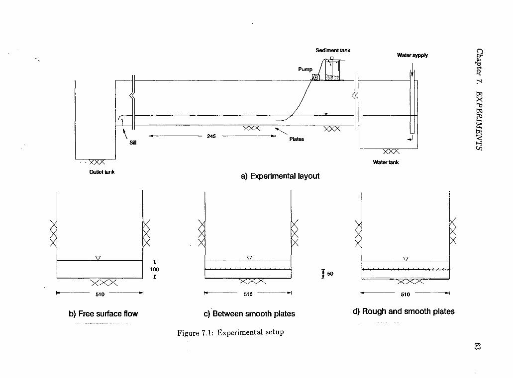
co

Chapter 7. EXPERIMENTS 64
Stirrer
To feeding pipes J
a) Sediment feed tank
Overflow
Water supply
From pump (Sediment tank)
4.8mm pipes
J 100 ±
b) Sediment feeding pipes
Figure 7.2: Sediment feeding system
Chapter 7. EXPERIMENTS 65
10 minutes. Thereafter the pumping was stopped and the water supply to the flume was
slowly reduced to avoid disturbance of settled material. After draining the whole flume,
the plates with the deposited sediments were left to dry by blowing hot air, very gently
from an electric fan. The sediment deposited on the plates was weighed using a balance
with a least count of O.Olgm.
Chapter 8
E X P E R I M E N T A L RESULTS
The purpose of the experiments was to determine whether the sediment settling rate could
be increased. Any increase would be indicated by changes in the deposition pattern in the
basin. However, it was difficult to control the sediment feed precisely, and since the inlet
sediment concentration was different, the total amount of sediment deposited was also
different. Therefore, to have a common ground to compare results, the settling length
and deposition pattern needed to be made non-dimensional. Consequently, results from
each experiment are compared using non-dimensional plots.
To make the sediment deposition non-dimensional, the amount of sediment deposited
on each plate is divided by the total amount of sediment settled in the channel. The
number of plates was made large enough to settle all the sediment fed in at the inlet.
The settling length or the position of the plate from the sediment feed point is made non-
dimensional by dividing by the depth of flow. Since the depth of flow is not the same
for all cases, a reference depth of H=100mm is used to obtain a non-dimensional length.
The plotting of the non-dimensional sediment deposition ratio and settling length gives
a picture of the sediment deposition distribution, and from these graphs, the deposition
pattern for the different experiments can be compared.
For sedimentation basins, the total cumulative amount of sediment removed at each
section from the inlet is also of major importance, and this characteristics is defined by
the removal ratio, which is the ratio of the amount of sediment deposited at a certain
section divided by the total amount of sediment deposited in the basin. At a section
66
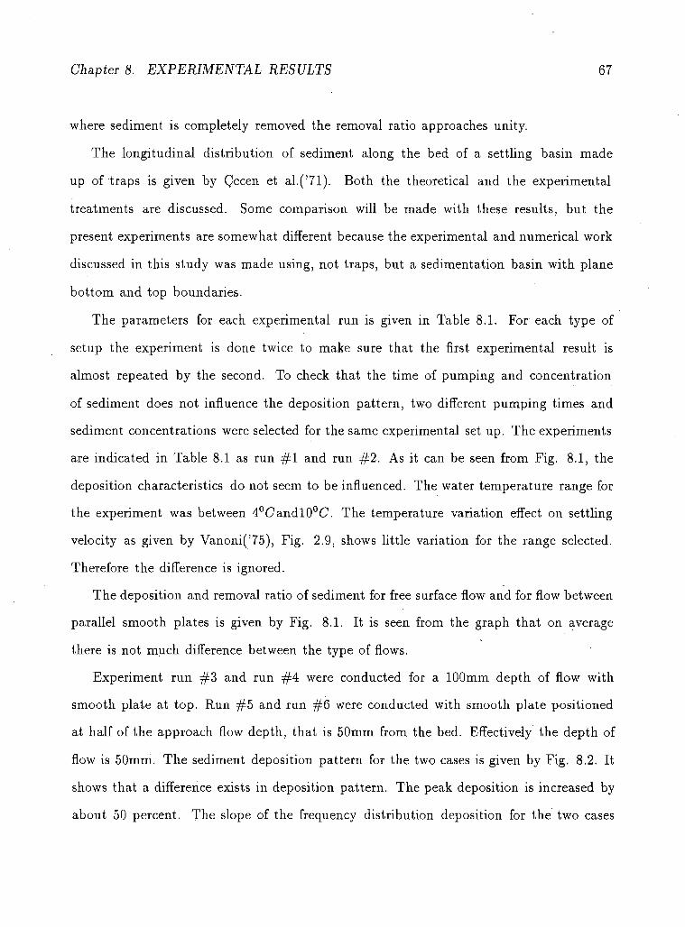
Chapter 8. EXPERIMENTAL RESULTS 67
where sediment is completely removed the removal ratio approaches unity.
The longitudinal distribution of sediment along the bed of a settling basin made
up of traps is given by Cecen et al.('71). Both the theoretical and the experimental
treatments are discussed. Some comparison will be made with these results, but the
present experiments are somewhat different because the experimental and numerical work
discussed in this study was made using, not traps, but a sedimentation basin with plane
bottom and top boundaries.
The parameters for each experimental run is given in Table 8.1. For each type of
setup the experiment is done twice to make sure that the first experimental result is
almost repeated by the second. To check that the time of pumping and concentration
of sediment does not influence the deposition pattern, two different pumping times and
sediment concentrations were selected for the same experimental set up. The experiments
are indicated in Table 8.1 as run #1 and run #2. As it can be seen from Fig. 8.1, the
deposition characteristics do not seem to be influenced. The water temperature range for
the experiment was between 4°CandlO°C The temperature variation effect on settling
velocity as given by Vanoni('75), Fig. 2.9, shows little variation for the range selected.
Therefore the difference is ignored.
The deposition and removal ratio of sediment for free surface flow and for flow between
parallel smooth plates is given by Fig. 8.1. It is seen from the graph that on average
there is not much difference between the type of flows.
Experiment run #3 and run #4 were conducted for a 100mm depth of flow with
smooth plate at top. Run #5 and run #6 were conducted with smooth plate positioned
at half of the approach flow depth, that is 50mm from the bed. Effectively the depth of
flow is 50mm. The sediment deposition pattern for the two cases is given by Fig. 8.2. It
shows that a difference exists in deposition pattern. The peak deposition is increased by
about 50 percent. The slope of the frequency distribution deposition for the two cases
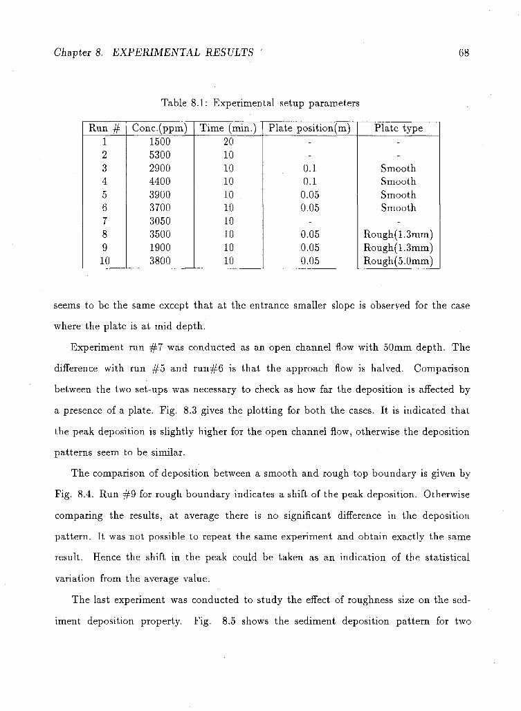
Chapter 8. EXPERIMENTAL RESULTS 68
Table 8.1: Experimental setup parameters
Run # Conc.(ppm) Time (min.) Plate position(m) Plate type 1 1500 20 - -
2 5300 10 - -3 2900 10 0.1 Smooth 4 4400 10 0.1 Smooth 5 3900 10 0.05 Smooth 6 3700 10 0.05 Smooth 7 3050 10 - -
8 3500 10 0.05 Rough( 1.3mm) 9 1900 10 0.05 Rough( 1.3mm) 10 3800 10 0.05 Rough(5.0mm)
seems to be the same except that at the entrance smaller slope is observed for the case
where the plate is at mid depth.
Experiment run #7 was conducted as an open channel flow with 50mm depth. The
difference with run ^5 and run#6 is that the approach flow is halved. Comparison
between the two set-ups was necessary to check as how far the deposition is affected by
a presence of a plate. Fig. 8.3 gives the plotting for both the cases. It is indicated that
the peak deposition is slightly higher for the open channel flow, otherwise the deposition
patterns seem to be similar.
The comparison of deposition between a smooth and rough top boundary is given by
Fig. 8.4. Run #9 for rough boundary indicates a shift of the peak deposition. Otherwise
comparing the results, at average there is no significant difference in the deposition
pattern. It was not possible to repeat the same experiment and obtain exactly the same
result. Hence the shift in the peak could be taken as an indication of the statistical
variation from the average value.
The last experiment was conducted to study the effect of roughness size on the sed
iment deposition property. Fig. 8.5 shows the sediment deposition pattern for two
Chapter 8. EXPERIMENTAL RESULTS 69
different types of roughness selected. Run #8 and run #9 were made for roughness size
of 1.3mm and run #10 was made for roughness size of 5mm. The figure indicates a
lower peak deposition for the more rough top boundary. But the removal ratio is not
significantly different for each types of roughness considered.
8.1 Computational result
To study the sediment deposition pattern using a numerical computation, it was necessary
to define the flow variables. The TEACH code as discussed in chapter 6 is used to obtain
computational results for velocity and momentum transfer coefficient profiles. The results
are given by Fig. 8.6 for flow between smooth parallel plates. The profiles for flow between
a rough and a smooth plate are given by Fig. 8.7. Considering the momentum transfer
coefficient profile for flow between smooth parallel plates, it can be seen that at the
central middle third of the flow its value almost constant and at maximum, as discussed
in the theoretical background. This confirms the discussion given by Ismail('52). As
it would be expected for the rough and smooth surface boundary the profiles are not
symmetrical. The velocity profile near the rough surface is steeper due to the high shear
stress generated by the roughness element. The momentum transfer coefficient is also
higher for the same reason.
The numerical computational result for sediment deposition pattern is given by Fig.
8.8. As it is shown in the figure, no significant difference in deposition pattern is indicated
between the smooth-smooth and rough-smooth flow. This is in accordance with the
experimental observation.

Chapter 8. EXPERIMENTAL RESULTS
0.14
0.12 H
o.io CO T3 cr 0.08
0.06
S 0.04 CL CO
Q 0.02 H
0.00
o o o o o R U N #1
° ° ° ° ° R U N #2
* * * * * R U N #3
x_x_x_x_x RUfxJ #4
8 10 12 14 16 18 20 22 x / H
a) Depos i t ion f requency d is t r ibut ion .
24 26
1.1 i.o H 0.9
.O 0.8 O 0.7
_ 0.6 O > 0.5 -\ O E ° - 4 i CD 0.3
0.2 -0.1 -0.0
0 1 I i
18 20 22 24 26
b; Remova l ratio of sed iment . Figure 8.1: Deposition for free surface( 100mm) and smooth plate
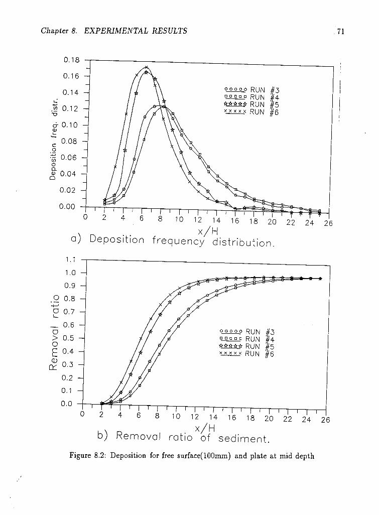
Chapter 8. EXPERIMENTAL RESULTS
0.18
1.1
1 I I I I I I I I
0 2 4 6 8 10 12 14 16 18 20 ' 22 ' 24 ' 26 n X / H
Deposi t ion f r equency d is t r ibut ion
RUN #3 • • • • • RUN #4 •k±±k£ RUN #5 x x x x x RUN #6
1 I 1 I 1 I ' I l I I | I | I | i | i 8 10 12 14 16 18 20 22 24 26
x / H b) Remova l rat io of sed iment .
Figure 8.2: Deposition for free surface( 100mm) and plate at mid depth
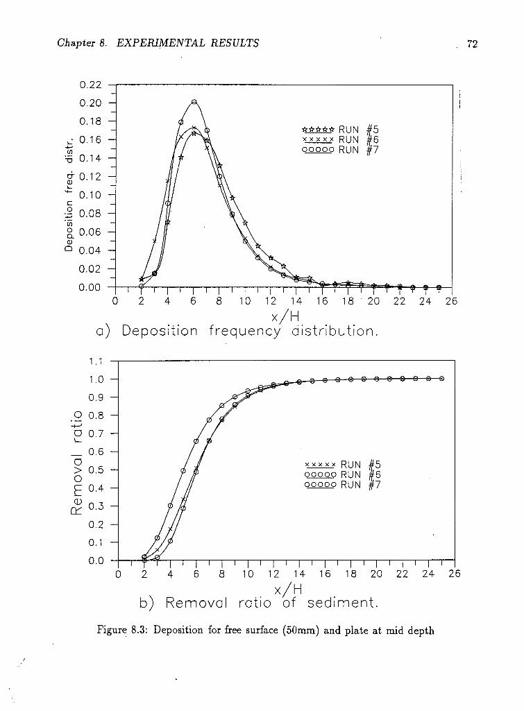
Chapter 8. EXPERIMENTAL RESULTS
0.22
x / H a) Depos i t ion f requency d is t r ibut ion .
1.1
0 2 4 6 8 10 12 14 16 18 20 22 24 26 x / H
b) Remova l ratio of sed iment . Figure 8.3: Deposition for free surface (50mm) and plate at mid depth
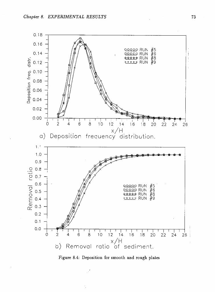
Chapter 8. EXPERIMENTAL RESULTS
0.18
x / H a) Depos i t ion f requency d i s t r ibut ion .
1.1
Figure 8.4: Deposition for smooth and rough plates
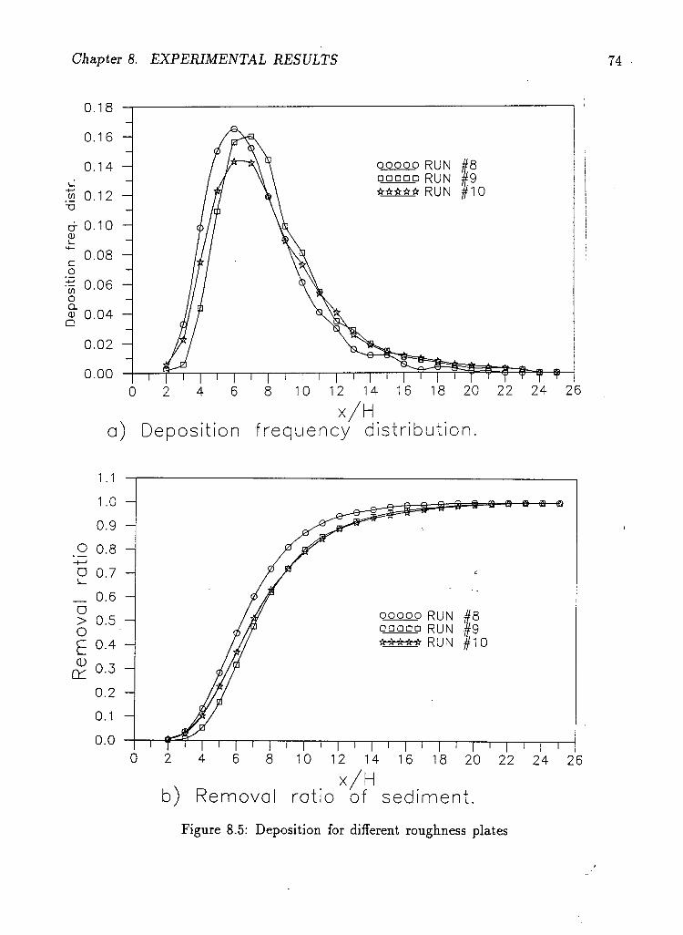
Chapter 8. EXPERIMENTAL RESULTS
0.18
0 2 4 6 8 10 12 14 16 18 20 22 24 26 x / H
a) D e p o s i t i o n f r e q u e n c y d i s t r i b u t i o n .
1.1
Figure 8.5: Deposition for different roughness plates
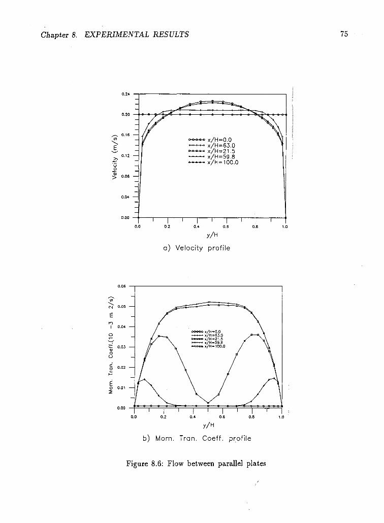
Chapter 8. EXPERIMENTAL RESULTS 75
0.2+
0.20
0.12 —
U
o g 0.08 — |
x/H=0.0 x/H=63.0 x/H=21.5 x/H=59.8 x / H = 100.0
' i 1 i ' r 0.2 0.* 0.6
y / H
a) Velocity profile
0.06
in
y / H
b) Mom. Tran. Coeff. profile
Figure 8.6: Flow between parallel plates

Chapter 8. EXPERIMENTAL RESULTS 76
. y / H
a) Velocity profile
0.2 0.4 0.6 0.
y / H
b) Mom. Tran. Coeff. profile
Figure 8.7: Flow between rough and smooth plate
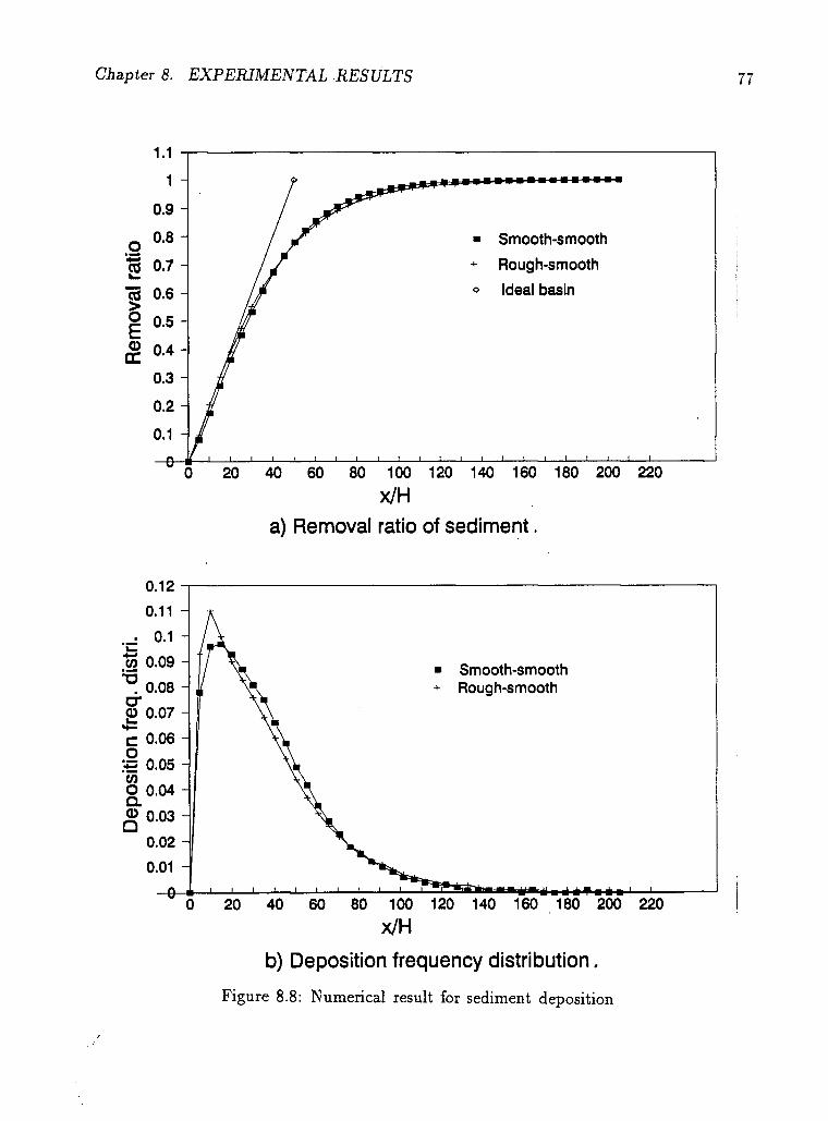
Chapter 8. EXPERIMENTAL RESULTS 77
x / H a) Removal ratio of sediment.
0.12
x / H
b) Deposition frequency distribution. Figure 8.8: Numerical result for sediment deposition
Chapter 9
C O N C L U S I O N S
The total investigation consists of two sets of experiments and a theoretical numerical
calculation of sedimentation. One set of experiments studied a settling tank for a fish
rearing system and took into account all the constraints imposed by the rest of the
system. A further set of experiments examined a more idealized arrangement of just one
component of the total system. This arrangement was also analyzed theoretically.
The first set of experiments was carried out to investigate the effectiveness of using
a stack of horizontal plates to increase sediment removal from a flow. This first set
of experiments investigated a complete settling system for a fish rearing system and is
reported in Chapter 4. These experiments confirmed that it is possible to use a stack of
horizontal parallel plates to make maximum use of a limited space available in a settling
tank. The efficiency of the settling tank was highly dependent on the flow distribution
among the settling plates and it was found that circulation of flow within the tank has
to be avoided since it has a big influence on the performance. The sediment deposition
pattern between the settling plates contributes to the overall efficiency of the settling
tank. Practical considerations at the entrance to the settling basin gave a concentrated
high speed turbulent flow which disrupted the sedimentation process. To achieve a more
uniform distribution of flow between each set of plates and to prevent a general circulation
of flow within the settling chamber, it was necessary to design a set of deflecting plates
at tank inlet. These deflecting plates were arranged at different levels at the inlet to
deflect the incoming high velocity vertical flow horizontally at various levels of the tank
78
Chapter 9. CONCLUSIONS 79
at the inlet section. The dimensions and positions of the deflecting plates for maximum
efficiency were determined experimentally. The resulting geometrical design is given by
Fig. 4.4 and Fig. 4.5 in Chapter 4.
In a second set of experiments an idealized simple system was studied to find a way
of improving the settling efficiency of a sedimentation basin. Bagnold('66) explains that
sediments are kept in suspension due to anisotropic turbulence in the vertical direction
produced near a bed surface. If the argument put forward by Bagnold('66) and supported
by work of Irmay('80) suggests that the shear near a bottom boundary induces an upward
supporting stress which supports sediment in suspension, then it was argued that a
plate at the upper boundary would cause a downward turbulent stress, which should
increase deposition of sediment. This argument was investigated by designing suitable
experimental set-up as indicated in Chapter 7. The three different cases considered in the
experiments are a) open channel flow, b) flow with upper smooth boundary and c) flow
with upper rough boundary. The sediment was injected at the same position in each case
and the deposition pattern observed. This was necessary to investigate a) the effect of
upper boundary on sedimentation, b) the effect of positioning a horizontal plate in a flow
on the settling of sediment and c) the effect of rough upper boundary on sedimentation.
Clearly, introducing extra plates, in a multiplate sedimentation, will increase sedi
mentation because it is equivalent to having a much larger settling basin. One set of
experiments, Fig. 8.2, showed an increase in sedimentation when a plate was placed
at mid-level of the flow. The reason for this increase are still not clear, because there
are several factors to be considered. For example, in the tests reported in Fig. 8.2, the
approach flow turbulence and velocity distribution were similar, but the introduction of
a plate at half depth will tend to reduce the scale of the approach flow turbulence. Also
a boundary layer will develop on the upper plates and the turbulence in this boundary
layer will influence more of the cross-section as the boundary layer thickens.

Chapter 9. CONCLUSIONS 80
In a second experiment, Fig. 8.1, free surface flow of a given depth was compared
with flow with a top plate, but of the same water depth. This test showed no significant
change in sedimentation rate. This result may be explained because the upper boundary
layer takes time to develop and therefore the flow with the plate is probably very similar
to the free surface case. Therefore there is still an interesting difference between the
results of these two experiments, Fig. 8.1 and Fig. 8.2, one which indicates a significant
improvement in settling rate and one which does not. This clearly needs further work.
The further series of tests used a rough upper plate to test whether this would increase
settling rate, but no benefit was found. This was also indicated by the numerical result
obtained. The reason for no increase in settling could be that at the inlet section the
shear stress produced due to flow transition from free surface to solid boundary is so high
that it exceeds the effect of providing roughness.
The comparison between a flow with a plate positioned at mid depth and that of free
surface flow with half approach depth of the previous shows that the latter has slightly
higher peak deposition. The approach depth of flow for each case is different and hence
the ambient turbulence level at the inlet. This may be one of the reasons for the difference
observed in the deposition pattern. Flow depth of a free surface flow seems to have an
effect on the sediment deposition pattern. This can be explained by the difference of
turbulence level generated in different flow depths due to different Reynolds numbers.
This flow between parallel plates is fairly similar to closed conduit flow. For high
flows, sediment transport exists in closed conduits. This indicates the existence of net
upward turbulent stress produced between the upper and lower boundary. From pub
lished measurements (for example Graf('71) and Ismail('52)) it can be seen from the
velocity profile that the shear stress at the top and bottom walls is not the same. Since
the bottom boundary experiences a higher shear stress than the upper boundary a net
upward momentum flux is created to keep sediments in suspension.
Bibliography
Abdel-Gawad, S. M. , and McCorquodale, J. A., "Numerical Simulation of Rectangular Settling Tanks," Journal of Hydraulic Research, Vol. 23, No. 2, 1985, pp. 85-100.
Bagnold, R. A., "An Approach to the Sediment Transport Problem from General Physics," U.S. Geological Survey Professional Paper, 422-1, 1966.
Bayazit, M. , "Turbulent Transfer Characteristics of Settling Phenomenon," Proceedings of the 14th Congress of the IAHR, Vol. 1, 1971.
Bechteler, W., and Schrimpf, W., "Improved Numerical Model for Sedimentation," Journal of Hydraulic Engineering, Vol. 110, No. HY3, March, 1984, pp. 234-246.
Blinco, P. H., and Partheniades, E. , "Turbulence Characteristics in Free Surface Flows over Rough and Smooth Boundaries," Journal of Hydraulic Research, 9, 43, 1972, 43-69.
Camp, T. R., "Sedimentation and the Design of Settling Tanks," Transactions, ASCE, Paper No. 2285, Vol. I l l , 1946, pp.895-958.
Cecen, K., "Hydraulic Criteria of Settling Basins for Water Treatment, Hydropower and Irrigation," Proceedings of the 17th Congress of the IAHR, Vol. 4, 1977.
C/ecen, K., and Siimer, M. , "Longitudinal Distribution of Matters Settling to the Bed in Settling Basins," Proceedings of the 14th Congress of the IAHR, Vol. 1, 1971.
Coleman, N. L., "Flume Studies of the Sediment Transfer Coefficient," Water Resources Research, Vol. 6, No. 3, June, 1970, pp. 801-809.
Dobbins, W. E. , "Effect of Turbulence on Sedimentation," Transactions, ASCE, Vol. 109, Paper No. 2218, 1944, pp. 629-656.
Garde, R. J., and Ranga Raju, K. G.,Mechanics of Sediment Transportation and Alluvial Stream Problems, 2nd ed., Wiley Eastern Limited, 1985.
Graf, W. H., Hydraulics of Sediment Transport, 1st ed., McGraw-Hill Book Co., Inc., New York, 1971.
81
Bibliography 82
Gosman, A. D., and Ideriah, F.J.K., "TEACH T: A General Computer Program for Two Dimensional, Turbulent, Recirculating Flows," Report, Department of Mechanical Engineering, Imperial College, London, U.K., 1976.
Hama, F. R., "Boundary-Layer Characteristics for Smooth and Rough Surfaces," Transactions of the Society of Naval Architecture and Marine Engineers, Vol. 62, 1954, pp. 333-358.
Hazen, A., "On Sedimentations," Transactions, ASCE, Vol. 53, Paper No. 980, Dec, 1904, pp. 45-88.
Hinze, J. O., Turbulence, McGraw-Hill Book Co., Inc., New York, 1959.
Hippola, U. T. B., "Influence of Suspended Sediment Distribution on Settling Basin Design," International Symposium on River Mechanics, IAHR, Bangkok, Thailand, Jan., 1973 pp. 277-288
Irmay, S., "Accelerations and Mean Trajectories in Turbulent Channel Flow," Transactions, ASCE, Dec, 1980.
Ismail, H. M., "Turbulent Transfer Mechanism and Suspended Sediment in Closed Channels," Transactions, ASCE, Vol. 117, 1952, pp.409.
Jobson, H. E. , and Sayre, W. W., "Vertical Transfer in Open Channel Flow," Journal of the Hydraulics Division, ASCE, Vol. 96, No. HY3, Mar., 1970, pp. 703-724.
Jobson, H. E. , and Sayre, W. W., "Predicting Concentration Profiles in Open Channels," Journal of the Hydraulics Division, ASCE, Vol. 96, No. HY10, Oct., 1970, pp. 1983-1996.
Kolmogorov, A. N., "Equations of Turbulent Motion in an Incompressible Fluid," Izv. Akad. Wauk. SSSR, Sexia fizicheska, VI, 1-2, 56-58, 1968.
Larsen, P., Rissler, S., "On the Hydraulics of Settling Basin Inlets," Proceedings of the 17th Congress of the IAHR, Vol. 4, 1977, pp. 309-316.
Laufer, J., "The Structure of Turbulence in Fully Developed Pipe Flow," Report 1174, National Advisory Committee for Aeronautics, 1954.
Laufer, J., "Investigation of Turbulent Flow in a Two-Dimensional Channel," Report 1053, National Advisory Committee for Aeronautics, 1951.
Launder, B. E. , and Spalding, D. B., "The Numerical Computation of Turbulent Flows," Computer Methods in Applied Mechanics and Engineering, Vol. 3, North-Holland Publishing Co., 1974, pp. 269-289.
Bibliography 83
[27] Mashauri, D. A., Modelling of a Vortex Settling Basin for Primary Clarification of Water, Tempere University of Technology, Pub. 42, Tempere, 1986.
[28] Masonyi, E. , Water Power Development, Vol. 2, 2nd ed., Academia Kiado, Budapest, Hungary, 1965.
[29] McQuivey, R. S., Richardson, E. V., "Some Turbulence Measurement in Open Channel Flow," Journal of the Hydraulics Division, Vol. 95, No. HY1, Jan., 1969, pp. 209-223.
[30] Patankar, S. V., Numerical Heat Transfer and Fluid Flow, Hemisphere Publishing Corporation, New York, 1980.
[31] Perry, A. E. , "Rough Walls Boundary Layers," Journal of Fluid Mechanics, 37, 1969, pp. 383-413.
[32] Perry, A. E. , Schofield W. H., Joubert, P. N., "Rough Wall Turbulent Boundary Layers," Journal of Fluid Mechanics, Vol. 37, Part 2, 1969, pp. 383-503.
[33] Prandtl, L., "Uber ein neues Formel-System fur die ausgenbildate Turbulenz," Nacr. Ahad. Wiss. Gottingin, Math.-Phys., K.L. , 6, 1945.
[34] Prandtl, L., Essentials of Fluid Dynamics, London, Blakie and Son, 1952.
[35] Richardson E. V., and McQuivey, R. S., "Measurement of Turbulence in Water," Journal of the Hydraulics Division, Vol. 94, No. HY 2, Mar., 1968, pp. 411-429.
[36] Rodi, W. "Turbulent Models and their Applications to Hydraulics, A State of the Art Review," IAHR, Delft, The Netherlands, 1984.
[37] Sarikaya, H. Z., "Numerical Model for Discrete Settling," Journal of the Hydraulics Division, ASCE, Vol. 103, No. HY8, Aug., 1977, pp. 865-876.
[38] Schamber, D. R., and Larock, B. E. , "Numerical Analysis of Flow in Sedimentation Basins," Journal of the Hydraulic Division, ASCE, Vol. 107, No. HY5, May, 1981, pp. 575-591.
[39] Schlicting, H., Theory of Boundary Layers,6th ed., McGraw-Hill Book Co. Inc. New York, 1968.
[40] Shaubauer, G. B., "Turbulent Process as Observed in Boundary Layer and Pipe," Journal of Applied Physics, Vol. 25, No. 2, 1954, pp. 188.
[41] Strand, R. I., "Sedimentation at Canal In-Line Structures," Water Forum '86, 1986, pp. 885-889.
Bibliography 84
[42] Takamatsu, T., Naito, M. , Shiba, S., and Ueda, Y., "Effects of Deposit Resuspention on Settling Basin," Journal of Environmental Engineering Division, ASCE, Vol. 100, No. EE4, Aug., 1974, 883-903.
[43] Townsend, A.A., The structure of Turbulent Shear Flow, Cambridge University Press, 1956.
[44] Vanoni, V. A., "Transportation of Suspended Sediments by Water," Transactions, ASCE, Vol. I l l , No.2267, 1946, pp. 67-133.
[45] Vanoni, V. A., Ed., Sedimentation Engineering, ASCE, Manuals and Reports on Engineering Practice, No. 54, 1975.
[46] Wilson, G. E. , "Coupling Free Vortex Energy Dissipation with Sediment Control," Water Forum '86, 1986, pp. 421-426.
[47] Yao, K. M., "Design of High-Rate Settlers," Journal of Environmental Engineering Division, ASCE, Vol. 99, No. EE5, Oct., 1973, pp. 621-637.
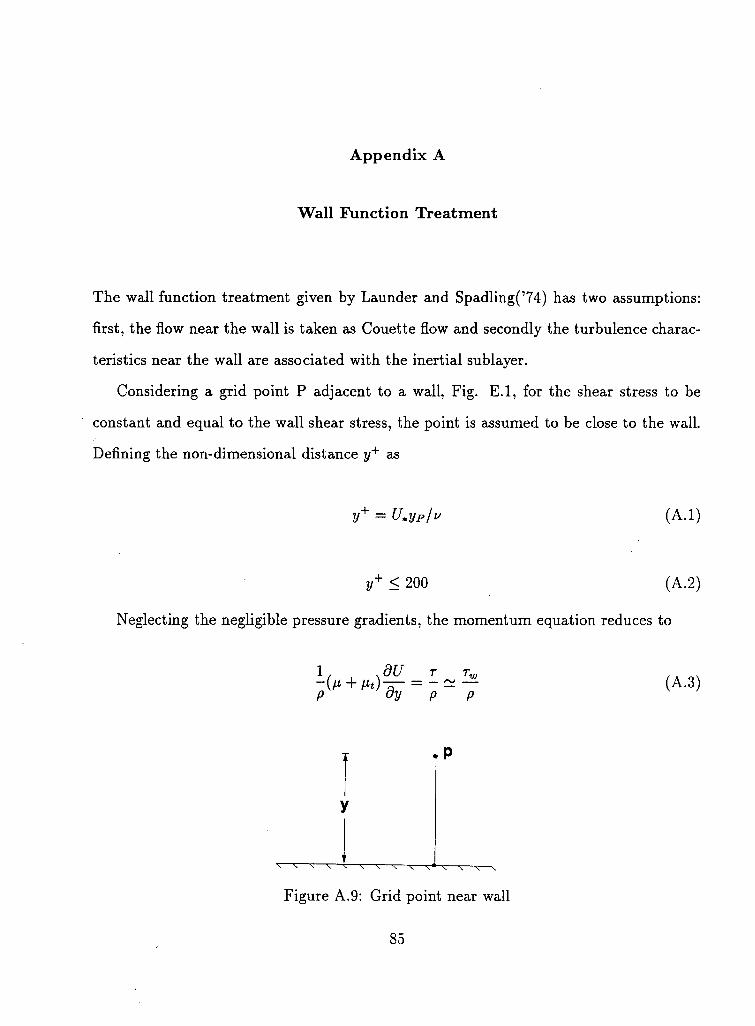
Appendix A
Wall Function Treatment
The wall function treatment given by Launder and Spadling('74) has two assumptions:
first, the flow near the wall is taken as Couette flow and secondly the turbulence charac
teristics near the wall are associated with the inertial sublayer.
Considering a grid point P adjacent to a wall, Fig. E . l , for the shear stress to be
constant and equal to the wall shear stress, the point is assumed to be close to the wall.
Defining the non-dimensional distance y+ as
Neglecting the negligible pressure gradients, the momentum equation reduces to
y+ -- UmyP/v (A.l)
y+ < 200 (A.2)
(A.3)
y
Figure A.9: Grid point near wall
85

Appendix A. Wall Function Treatment 86
Non-dimensionalizing the velocity as
U* = | (A.4)
Eq. A.3 reduces to
The near wall region may be divided into viscous sublayer where molecular viscosity is
dominant, and inertial sublayer where the turbulent viscosity term is dominant as given
below
^ < 1 y+ < 11.63 (A.6)
— > 1 y+> 11-63 (A.7)
Integrating Eq. A.5 for y+ < 11.63, viscous sublayer region,
U+ = y+ (A.8)
A . l Smooth Wall
For fully turbulent flow where y+ > 11.63, from the mixing length concept, Hinze('59):
fj,t = KpU*y (A.9)
Substituting the above into Eq. A.5 and integrating
U+ = -ln(Ey+) (A.10)
Appendix A. Wall Function Treatment 87
which is the logarithmic law of the wall, where E=9, is a constant of integration.
A.2 Rough Wall
A wall is said to be hydraulically rough or smooth depending on the size of roughness
and flow characteristics. The non-dimensional roughness may be defined as
where ks is the equivalent sand roughness. For fc+ > 50 a wall is considered to be
hydraulically rough, Townsend('56). Therefore Eq. A.10 is written as
where the constant, E\ = 30 for rough sand surfaces.
The TEACH code assumes a hydraulically smooth surface boundary. The above
formulation was incorporated in the code to handle rough wall surfaces.
For rough surfaces the point of origin for the velocity distribution (Eq. A.12) is
between the edge and base of the roughness element. According to the study and com
parisons made by Perry et al.('69) and Blinco et al.('72), the origin is taken to be 0.25ka
from the edge to the base of the roughness considered. Accordingly the TEACH code
was also modified.
(A.ll)
(A.12)
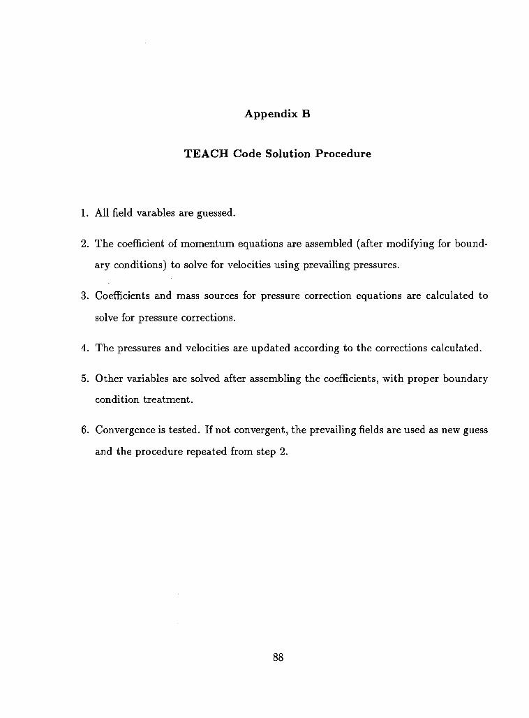
Appendix B
T E A C H Code Solution Procedure
1. All field varables are guessed.
2. The coefficient of momentum equations are assembled (after modifying for bound
ary conditions) to solve for velocities using prevailing pressures.
3. Coefficients and mass sources for pressure correction equations are calculated to
solve for pressure corrections.
4. The pressures and velocities are updated according to the corrections calculated.
5. Other variables are solved after assembling the coefficients, with proper boundary
condition treatment.
6. Convergence is tested. If not convergent, the prevailing fields are used as new guess
and the procedure repeated from step 2.
88
Related Documents