Sediment and wood storage and dynamics in small ...lancasts/SedWoodDynStor_fin.pdf · Modeling Sediment and Wood Storage and Dynamics in Small Mountainous Watersheds ... valley network

Modeling Sediment and Wood Storage and Dynamics in Small Mountainous Watersheds

Stephen T. Lancaster and Shannon K. Hayes

Department of Geosciences, Oregon State University, Corvallis, Oregon

Gordon E. Grant

USDA Forest Service, Pacific Northwest Research Station, Corvallis, Oregon

We examine controls on supply and transport of sediment and wood in a small(approximately two square kilometers) basin in the Oregon Coast Range, typicalof streams at the interface between episodic sediment and wood delivery by massmovements and frequent fluvial sediment transport. We hypothesize that wooddeposited by mass movements forms dams that lead to persistent sediment storageand inhibit coherent propagation of sediment pulses. Field data show that muchsediment is stored behind such dams and in terraces after the dams breach. We de-veloped a drainage basin-scale model driven by stochastic storm and fire se-quences that combines empirical, stochastic and physical models of forest growth,tree fall, wood decay, soil production and diffusion, landslide initiation, debrisflow runout, and fluvial sediment transport. In a 3000-year simulation of the studyarea, woody debris flow deposits form dams on the main channel and lead to stepsin the channel profile and terraces on the valley floor that persist in place even af-ter nearly all deposited wood has decayed. Simulated sediment output from thenetwork is relatively steady and shows little evidence of episodic input. Our re-sults suggest that abundant wood plays a key role in moderating sediment fluxfrom small basins following debris flow events. Debris flow events coincidentwith a lack of abundant wood, such as might occur following forest harvest, couldlead to more episodic sediment flux to downstream, fish-bearing reaches.

1. INTRODUCTION

The decline of salmonid species in the Pacific Northwesthas prompted increased attention to the temporal and spatialdynamics of aquatic habitat. In particular, various aspectsof salmonid life history are influenced by the abundance,location, quality, and spatial distribution of gravel and

wood, which create key fluvial environments used forspawning and rearing [Reeves et al., 1998]. Although it iswidely viewed that hillslope and channel processes influ-encing erosion, input, transport, or deposition of sedimentand wood are inextricably linked to the quality and quantityof aquatic habitat, the degree of coupling in time and spacebetween hillslopes and channels remains a fundamentalproblem. Specifically, it has proven difficult to show whenaccelerated mass wasting will occur, how sediment andwood introduced into steep, low-order channels will berouted downstream, and what the long-term consequencesof these processes might be for channel and valley floor

Geomorphic Processes and Riverine HabitatWater Science and Application Volume 4, pages 85-102Copyright 2001 by the American Geophysical Union

85

86 SEDIMENT AND WOOD STORAGE AND DYNAMICS

morphology, sediment flux, or the quality or quantity ofaquatic habitat.

This study addresses sediment and wood dynamics insmall (~2 km2) drainage basins because this part of thelandscape represents the interface between mass move-ments originating on the hillslopes and fluvial transportprocesses. Woody debris has a potentially strong effect onsediment dynamics and storage in these basins because ofthe large wood constituent in debris flows and the tendencyfor wood to form large wood dams [Kochel et al., 1987;Abbe and Montgomery, 1996; Montgomery et al., 1996;Hogan et al., 1998; Massong and Montgomery, 2000]. Ourgoal is to better understand how both episodic and chronicinputs of sediment and wood interact with each other andwith drainage network structure to produce changing vol-umes of stored sediment and wood in channels and on val-ley floors. To that end, we have developed a drainage basin-scale model that encapsulates much of our understanding ofthe relevant controls on sediment and wood dynamics.

We begin with a review of current approaches to model-ing sediment and wood dynamics and distribution in for-ested mountain streams and then describe our modelingapproach. We use the model to simulate sediment and woodinfluxes to the valley network over millennial timescales,corresponding locations and amounts of sediment and woodstorage in the valleys, and sediment outflux from the basin.A comparison of model and field results reveals useful in-sights into locations, controls, and temporal dynamics ofwood and sediment storage and dynamics in upland basinsand consequences for interpreting responses of watershedsto disturbance.

1.1. Current Perspectives and Modeling Criteria for Understanding Sediment and Wood Dynamics

Benda and Dunne [1997a, b] used a model to explore theinteraction between episodic sediment supply and the chan-nel network in relatively large (~100 km2) drainage basins.In their modeling they assumed that sediment moves in co-herent waves, as documented by Madej and Ozaki [1996].Because of the episodic delivery of sediment from debrisflows, the assumption of wave-like translation resulted inthe prediction that headwater basins, such as that consid-ered in the present study, are sediment “starved” most ofthe time.

In contrast, other studies have identified different first-or-der controls on sediment storage and transport in streams. Afunction of drainage area and channel slope, a proxy forstream power or sediment transport capacity, discriminatedmany bedrock and alluvial stream reaches, but only in theabsence of wood dams [Montgomery et al., 1996]. Sedi-

ment supply, lithology, and woody debris have significanteffects on the ability to discriminate bedrock from alluvialreaches with a stream power model [Massong and Mont-gomery, 2000]. Some of the factors affecting sediment sup-ply are highly variable in time, such as volumes ofsediment-trapping woody debris and recent landslides[Hogan et al., 1998]. These studies suggest that, while localsediment volumes may vary over time, they do not neces-sarily migrate downstream as coherent wave forms but of-ten disperse in place [Lisle et al., 1997, 2000].

Existing models to date have only considered sedimentstored or transported within the channel proper, and havegenerally not explicitly included dynamic interactions be-tween wood and sediment. In our experience, in-channelsediment and wood are relatively small fractions of totalvalley storage, and models to explain long-term evolutionof drainage basins should predict storage and dynamics inthe valley as well as the channel. More generally, modelspredicting sediment and wood storage and dynamics instream and valley networks should account for all processesdriving input and output from those networks.

1.2. Study Site: Oregon Coast Range

Field and modeling work were both sited in a 2.1-km2

tributary to Hoffman Creek in the Oregon Coast Range(Figure 1). We selected the site according to the followingcriteria: (a) homogeneous lithology; (b) absence of mid-slope or valley-bottom roads; (c) access to study area; (d)access to land-use records; (e) significant number of recentdebris flows; and (f) basin small enough to study and modeland large enough to exhibit network-scale effects. The ba-sin is underlain by massive, gently dipping, Eocene Tyeesandstone. The topography is steep—valley sideslopes aretypically 40o—and highly dissected with elevations rangingfrom 10 to 265 m above sea level. Soils are relatively shal-low, highly porous, and have low bulk densities (about 1kg/m3) [Reneau and Dietrich, 1991] (Table 1). The climateis maritime with warm, dry summers and mild, wet wintersand mean annual precipitation of approximately 1800 mm[Oregon Climate Service].

The area is forested with primary species Douglas-fir(Pseudotsuga menziesii) and secondary species westernhemlock (Tsuga heterophylla) and western red cedar (Thujaplicata) on the hillslopes and red alder (Alnus rubra) in ri-parian areas, though these so-called riparian areas often ex-tend upslope through the smallest hollows to the ridges,especially in immature stands. Nearly half of the basin hasbeen harvested as recently as ca. 1965, and there is field ev-idence of earlier, undocumented harvest in other parts ofthe basin. This forest, typical of the Oregon Coast Range,

LANCASTER ET AL. 87

results in surficial biomass that is less than but of the sameorder of magnitude as the mass of the soil layer, especiallyin mature stands, and, therefore, wood is a significant partof the mass moved by landslides and debris flows.

2. MODELING METHODS, ASSUMPTIONS, AND INITIALIZATION

Most of the sediment and much of the wood in streamsand valleys originates on the hillslopes. A model encom-passing sediment inputs to the valley network must accountfor sediment production from the parent material, i.e., con-version of bedrock to soil, and delivery of that sediment tothe valley via diffusion and mass movements, i.e., land-slides and debris flows. Likewise, a model encompassingwood inputs to the valley network must account for biom-ass growth and delivery to the valley via tree fall and massmovements. Since forest dynamics play a vital role in thetiming and location of mass movements, that interactionshould be included as well. Some of these processes, suchas biomass growth, can be modeled relatively simply (Fig-ure 2). Others, such as debris flows, are more complicatedand require more sophisticated modeling.

Our new model is an extension of the Channel-HillslopeIntegrated Landscape Development (CHILD) model [Lan-caster, 1998; Tucker et al., 2001a, b]. As such, the presentmodel operates on a triangulated irregular network (TIN)and shares the CHILD model’s drainage area calculation al-gorithm and stochastic precipitation and runoff generationmodels.

2.1. Landscape and Storm Characteristics

The model uses gridded digital elevation model (DEM)data with 10-meter discretization to interpolate the eleva-tions of the nodes in the TIN. Node locations are random toeliminate grid bias and form a TIN with the same averagediscretization as the original DEM. Additional points areadded at large drainage areas to eliminate “jaggy” channelstypical of interpolated TIN’s. Finally, channel-adjacentnodes that would fall within channels are removed [Lan-caster, 1998]. Nodes in the landscape are classified accord-ing to three types: (1) hillslope nodes containing vegetationand soil; (2) channel nodes with wood and sediment depos-its and vegetation; and (3) valley nodes with wood and sed-iment deposits and vegetation (Figure 3). Elevations ofhillslope nodes are static because relative elevations on hill-slopes do not change much over millennial time scales andany model-driven changes would only decrease the accu-racy of topographically driven transport processes [Dietrichet al., 1995]. Channel and valley node elevations evolveover time in response to aggradation and evacuation of sed-iment and wood because fluvial processes are sensitive tothese fluctuations, but bedrock elevations are held static forchannel and valley nodes.

We attempt a compromise between the model’s descrip-tiveness and the area modeled by lumping hillslope areasinto aggregates. Calculations on each hillslope node (e.g.,~100 m2) result in a fine-scale map of landscape character-

Figure 2. Conceptual figure illustrating the climatic, geomorphic,and vegetative processes simulated in the model.

Figure 1. Location map of the Oregon Coast Range showing theHoffman Creek watershed (outlined with dotted line) and studybasin (outlined with solid line).


istics, e.g., soil depth, vegetation age, and landslide suscep-tibility. Channel source and channel-adjacent areas formthe lumped aggregates (Figure 3b). Nodes are classified andgrouped according to the topographic component of land-slide susceptibility [Montgomery and Dietrich, 1994] such

that each aggregate contains several “bins” of nodes withsimilar susceptibility. During storms each bin, rather thaneach hillslope node, is considered against a failure criterionusing bin-average values of soil depth and root strength.This method saves processing time and mimics the way that

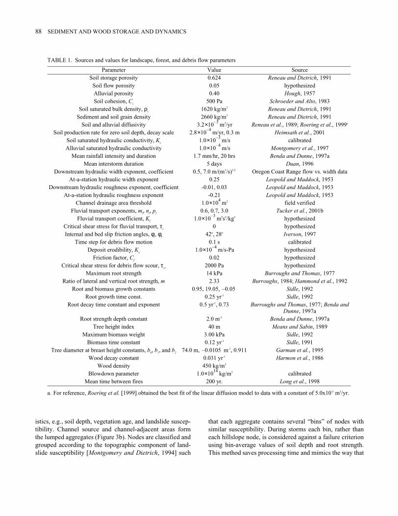
TABLE 1. Sources and values for landscape, forest, and debris flow parameters

Parameter Value SourceSoil storage porosity 0.624 Reneau and Dietrich, 1991

Soil flow porosity 0.05 hypothesizedAlluvial porosity 0.40 Hough, 1957Soil cohesion, Cs 500 Pa Schroeder and Alto, 1983

Soil saturated bulk density, ρs 1620 kg/m3 Reneau and Dietrich, 1991Sediment and soil grain density 2660 kg/m3 Reneau and Dietrich, 1991

Soil and alluvial diffusivity m2/yr Reneau et al., 1989; Roering et al., 1999a

a. For reference, Roering et al. [1999] obtained the best fit of the linear diffusion model to data with a constant of 5.0x10-3 m2/yr.

Soil production rate for zero soil depth, decay scale m/yr, 0.3 m Heimsath et al., 2001Soil saturated hydraulic conductivity, Ks m/s calibratedAlluvial saturated hydraulic conductivity m/s Montgomery et al., 1997

Mean rainfall intensity and duration 1.7 mm/hr, 20 hrs Benda and Dunne, 1997aMean interstorm duration 5 days Duan, 1996

Downstream hydraulic width exponent, coefficient 0.5, 7.0 m/(m3/s)1/2 Oregon Coast Range flow vs. width dataAt-a-station hydraulic width exponent 0.25 Leopold and Maddock, 1953

Downstream hydraulic roughness exponent, coefficient -0.01, 0.03 Leopold and Maddock, 1953At-a-station hydraulic roughness exponent -0.21 Leopold and Maddock, 1953

Channel drainage area threshold m2 field verifiedFluvial transport exponents, mf, nf, pf 0.6, 0.7, 3.0 Tucker et al., 2001b

Fluvial transport coefficient, Kf m5s5/kg3 hypothesizedCritical shear stress for fluvial transport, τc 0 hypothesizedInternal and bed slip friction angles, φi, φb 42o, 28o Iverson, 1997

Time step for debris flow motion 0.1 s calibratedDeposit erodibility, Ke m/s-Pa hypothesized

Friction factor, Cf 0.02 hypothesizedCritical shear stress for debris flow scour, τcr 2000 Pa hypothesized

Maximum root strength 14 kPa Burroughs and Thomas, 1977Ratio of lateral and vertical root strength, m 2.33 Burroughs, 1984; Hammond et al., 1992

Root and biomass growth constants 0.95, 19.05, Sidle, 1992Root growth time const. 0.25 yr-1 Sidle, 1992

Root decay time constant and exponent 0.5 yr-1, 0.73 Burroughs and Thomas, 1977; Benda and Dunne, 1997a

Root strength depth constant 2.0 m-1 Benda and Dunne, 1997aTree height index 40 m Means and Sabin, 1989

Maximum biomass weight 3.00 kPa Sidle, 1992Biomass time constant 0.12 yr-1 Sidle, 1991

Tree diameter at breast height constants, b0, b1, and b2 74.0 m, m-1, 0.911 Garman et al., 1995Wood decay constant 0.031 yr-1 Harmon et al., 1986

Wood density 450 kg/m3

Blowdown parameter kg/m3 calibratedMean time between fires 200 yr. Long et al., 1998

3.23–×10

2.84–×10

1.03–×10

1.04–×10

1.04×10

1.03–×10

1.04–×10

0.05–

0.0105–

1.014×10

LANCASTER ET AL. 89

whole hollows evacuate during a failure but tends to aver-age out local heterogeneities in soil depth and root strength.The hillslope nodes making up the aggregates are updatedupon evacuation of soil and wood during landslides.

The model is fed a stochastic time series of storms basedon the work of Eagleson [1978], as in Benda and Dunne[1997a], Duan et al. [1998], Tucker and Bras [2000], andTucker et al. [2001b]. The parameters of the stochasticmodel were derived from storm data for the Oregon CoastRange [Benda and Dunne, 1997a] or elsewhere in westernOregon [Duan et al., 1998] (Table 1). In response to eachstorm event, landslides may initiate and resulting debrisflows propagate downstream until they deposit on channeland valley nodes. The storms also drive tree fall. The modelrecords both the runout path and the deposited depths ofwood and sediment at each point along the stream. The his-tory of previous events bears directly on later ones: slidinghollows are evacuated of soil, runout paths are scoured ofwood and sediment or have wood and sediment deposited,and subsequent debris flows and fluvial transport encounterprevious deposits, which may change channel and valleygradients and act as barriers.

The sediment deposited in the valley network by debrisflows must originate as hillslope soil, defined here as mate-rial lacking the structure of underlying bedrock. Soil depthson hillslopes are governed by soil production and diffusion,where the soil production rate at a point decreases exponen-tially with the soil depth [Heimsath et al., 1997, 2001]. Dif-fusion [Reneau et al., 1989; Roering et al., 1999] and soilproduction [Heimsath et al., 2001] parameter values havebeen measured in the Oregon Coast Range (Table 1).Though hillslope elevations do not change, soil depthsevolve over time. Soil production is only active on the hill-slopes, but diffusion acts on all landscape nodes and, thus,may transport material among hillslope, valley and channelnodes. Diffusion of material from a node is contingent onsupply—bedrock does not diffuse. The maximum timesteps for soil production and diffusion are the storm and in-ter-storm durations but may be dynamically shortened ifnecessary for numerical stability [Tucker et al., 2001b].

Channel nodes are those with a drainage area exceeding athreshold of 104 m2, determined from analysis of slope-areaplots [Tarboton et al., 1991; Ijjasz-Vasquez and Bras,1995] and trial and error. Channel source area values fromfield measurements [Montgomery and Dietrich, 1988,1992] produce a channel network with “feathered” extremi-ties on relatively coarse DEMs such as ours. Through fieldreconnaissance we found that this threshold may excludesome small channels but effectively marks the transitionfrom bowl-shaped hollows to V-shaped valleys. Drainagearea is determined by routing each node’s area downstream

Figure 3. (a) Schematic diagram of nodes, mesh, and flowrouting. Nodes are connected by edges of Delaunay triangularmesh and have associated Voronoi areas, i.e., area closer than toany other node. Flow follows steepest edge to neighboring node(arrows). Hillslope nodes have vegetation and soil overlyingbedrock; channel and valley nodes have vegetation and alluviumoverlying bedrock; and channel nodes contain a channel segment.(b) Part of irregular mesh showing aggregates of hillslope nodes(shaded gray) and channels (thick gray line). Nodes neither withinan aggregate nor connected to a channel segment are valley nodes.


in the direction of steepest descent. As debris flows depositsediment and wood and those deposits are re-worked bysubsequent debris flows and fluvial processes, the locationof the channel may change. When that happens, hillslopeand valley nodes may become channel nodes, and aban-doned channel nodes become valley nodes.

Sediment deposited in the channel network is transportedaccording to a power law of excess shear stress, whereshear stress is represented as a power law of unit dischargeand slope derived from continuity and the Manning equa-tion:

(1)

where Qs is potential sediment discharge, i.e., contingenton supply; Kf, mf, nf, and pf are constants; b is hydraulicwidth; Q is water discharge; n is Manning’s hydraulicroughness; S is hydraulic slope; ρ is water density; g isgravitational acceleration; and τc is critical shear stress[Tucker et al., 2001b] (Table 1). Discharge is generated bysaturation overland flow, such that alluvial depth in thechannel affects discharge, and hydraulic width and rough-ness are calculated from empirical power laws of discharge,both downstream and at-a-station [Tucker et al., 2001b](Table 1). Equation (1) represents total load, i.e., both sus-pended and bed load, for values of pf in the range of 2.5-3[Engelund and Hansen, 1972; Vanoni, 1975; Govers,1992]. This transport law has not been calibrated forstreams in the Oregon Coast Range. Rather, it is simple andgeneric. The most salient feature of equation (1) for thepresent study is the dependence on local hydraulic slope,which changes during the simulation as a result of sedimentand wood aggradation and scour. Our observations indicatethat the streams in the study area are not competent to re-move wood from debris flow deposits, and these observa-tions are consistent with findings of Lienkaemper andSwanson [1987]. Therefore, we assume that wood cannotbe transported by fluvial processes, so until they decay,wood deposits act as barriers to sediment transport by de-creasing upstream hydraulic slope.

2.2. Landslide Susceptibility

Landslide initiation is stochastic, where the probability ofa landslide, i.e., sites that fail and become debris flows, ex-ists when rainfall exceeds a duration-dependent intensity.Our formulation of this critical precipitation is based onMontgomery and Dietrich [1994] and Dietrich et al. [1995]and lies somewhere between the two in complexity, similar

to Montgomery et al. [2000]. We assume uniform saturatedhydraulic conductivity within the soil layer and zero con-ductivity beneath that layer. The critical precipitation, Pcr, isgiven by

(2)

where Ks is saturated soil hydraulic conductivity; h is verti-cal soil thickness; b is flow width; θ is slope angle; ρs is soilsaturated bulk density; ρw is water density; Aeff is effectivearea contributing to flow and is dependent on storm dura-tion; φi is internal friction angle; Cr is cohesive rootstrength; and Cs is soil cohesion (Table 1). We derived asimple expression for the effective area contributing toflow, Aeff, by solving the Darcy equation for an effectiveupslope length contributing to subsurface flow during astorm of known duration, td, and squaring that length to getAeff:

(3)

where A is topographically defined contributing area; andneff is the effective porosity for subsurface flow, which fieldexperiments have shown is much smaller than the actualporosity (i.e., the actual travel time is much smaller thanthat calculated from the actual porosity [Iverson et al.,1997; Montgomery et al., 1997]), most likely because theexperiments are actually measuring the arrival of a peak indischarge rather than of the water itself. Using Aeff accountsfor greater saturation during longer storms but does notaccount for transient pore pressure increases from short,intense rainfall periods during longer storms. These tran-sient increases may be responsible for many natural failures[Montgomery et al., 1997; Iverson, 2000]. We made failurestochastic to account for some of the great uncertaintyaround predicting actual failure at a site. Greater landslidesusceptibility corresponds to lower critical precipitation,Pcr, and the probability for stochastic failure during a givenstorm of intensity, P, is given by

(4)

Note that saturated hydraulic conductivity, Ks, may varyover orders of magnitude between sites and even within rel-

Qs Kfb ρg Qnb

------- mf

Snf τc–pf

≤

Pcr

Kshb θ θρssincos

Aeffρw------------------------------------------ 1 1

φitan------------ θtan

Cr Cs+

hρsg θ2cos

--------------------------–

–=

Aeff mintdKs θsin

neff

--------------------- 2

A[ , ]=

Prob failure( ) 1Pcr

P-------– P Pcr≥,=

0 P Pcr<,=

LANCASTER ET AL. 91

atively small regions in the field, and critical precipitationis directly proportional to this highly variable and uncertainparameter [Duan, 1996]. If this parameter is too small (ortoo large), failures will occur too often (or too seldom). Be-cause the amount of sediment delivered to the channel net-work by debris flows is ultimately limited by the soilproduction rate, Ks will mainly affect soil depths by allow-ing, or not, realistic amounts of soil to accumulate beforefailing. We calibrated, albeit roughly, saturated hydraulicconductivity by running several simulations on a small partof the study area while varying Ks’s order of magnitudewithin the range of reported values [Montgomery et al.,1997] and selecting the value that produced reasonable av-erage soil depths on the hillslopes (~0.5 m) [Montgomery etal., 1997; Heimsath et al., 2001] (Table 1).

2.3. Debris Flow Runout

When landslides occur the sediment and wood from hill-slope nodes in the failing bin(s) are delivered to the nearestchannel where they continue to move as debris flows. Todescribe debris flow runout, we use a physically-based de-bris flow model, summarized here, that is simplified to runwithin the network scale model. Iverson [1997] and Iversonet al. [2000] developed a model describing debris flowrunout with mixture theory and depth-averaged conserva-tion of mass and momentum in two dimensions. We neglectsmaller terms and convective accelerations in the momen-tum balance and treat debris flow motion as a one-dimen-sional point process, where that point moves with the frontof the flow [R. Iverson, U.S. Geological Survey, personalcommunication, 1999]. Conservation of momentum in theflow direction is then given by:

(5)where h is slope-normal debris flow depth; v is slope-paral-lel debris flow velocity; pb is pore pressure at the bed; ρm isdebris flow mixture density; s is the slope-parallel direc-tion; φb is bed friction angle (Table 1); and the factor,

, indicates the direction opposite that of the debrisflow velocity. The terms on the left-hand side representchanges in flow velocity and depth, respectively. The firstgroup of terms on the right-hand side resists motion and istherefore multiplied by friction slope. The terms withinparentheses represent normal forces on the flow: normalgravitational force, basal pore pressure, and centripetalacceleration due to changes in slope angle, respectively. Toget the basal pore pressure in equation (5), hydrostatic pres-sure is multiplied by 1.8, consistent with the experimental

observations of Iverson et al. [2000]. The last term on theright-hand side represents the slope-parallel component ofthe gravitational force.

Debris flow velocity conforms to changes in flow direc-tion, i.e., , where α is the angle betweenthe new and old downstream directions. This angle, α, iscalculated over a spacing of several nodes (>30 m) both up-and downstream. Debris flow length is held constant. Depthmust conform to changes in flow width, i.e.,

. Width can cover as many as threenodes and is determined by the flow depth and local chan-nel or topographic geometry. When width and, therefore,depth change, velocity changes as if no forces were actingon the flow, i.e., equation (5) is solved for the change in ve-locity with the right-hand side set to zero.

Iverson [1997] and Iverson et al. [2000] assumed con-stant debris volume with time. But, we need to model theeffects on runout of increases in debris flow volume duringrunout—May [1998] found that on the order of half of de-bris flow deposit volumes that she measured in the OregonCoast Range were from entrainment during runout. Tomodel depth changes through scour, we employ a shear-ex-cess law similar to equation (1) with pf equal to 1, as scourhas often been considered to be proportional to shear stress(e.g., Howard and Kerby [1983]):

(6)

where Ke is deposit erodibility; Cf is a friction factor; τcr iscritical shear stress (Table 1); t is time; and the rate of scouris constrained to be positive or zero. We assume that bed-rock is not erodible. Although the physics of scour bydebris flows are poorly understood and equation (6) and itsparameters are essentially a hypothesis for that physics,momentum conservation and bedrock’s non-erodibilityenforce rigorous physical bounds on scour.

Debris flows are processed sequentially with a separatetime step (Table 1) and travel from node to node in the di-rection of steepest descent. Initial width depends on meshdiscretization and is approximately 9 m in the simulationpresented here, and length is defined by the number ofnodes contributing to the initiating landslide. Debris flowsare divided into two parts, head and tail, and equations (5)and (6) and the other rules are applied at the head. Headlength is total length divided by the number of nodes con-tributing to the landslide. Scoured and incorporated mate-rial is added to the head, and when it stops the front of thetail becomes the new head with the old head’s prior veloc-ity. This scheme accounts for two observations. First,scoured material and accumulated debris usually remain at

ht∂

∂v vt∂

∂h+ vsgn hg θcospb

ρm------– hv2

s∂∂θ+

φbtan– hg θsin+=

vsgn–

vnew vold αcos=

hnew hold bold bnew⁄( )=

t∂∂h

e

Ke ρmCfv2 τcr–( )=


the front. Second, tails often bypass the more debris-ladenheads when the latter stop. Our scheme retains a feasiblesimplicity while allowing process dynamics to determinethe final deposit geometry.

Unlike any other debris flow runout model that we areaware of, ours incorporates all three major constituents ob-served in the field: sediment, water, and wood. Debrisflows must incorporate all surface wood in their paths orstop. As with sediment, we use equation (6) to model scourof wood from deposits. We neglect any other effects ofwood, such as the resistance by standing trees to uprootingor breakage and any extra resistance due to the shape andstrength of the wood pieces, because a previous series ofmodel experiments determined that the simulated runoutlength distribution was closest to an observed distributionwithout these other effects.

2.4. Forest Growth, Root Strength, Blowdown, and Wood Decay

As indicated above, the presence of wood in channels af-fects fluvial sediment transport; the strength of tree roots af-fects landslide susceptibility; and the presence of wood onhillslopes and in valleys affects debris flow momentum.Therefore, we must account for these effects by modeling:(a) growth and decay of tree roots; (b) growth and decay ofwood biomass; (c) stochastic movement of wood, e.g., fromriparian areas to channels, by treefall; and (d) stochasticevents resulting in forest death, i.e., fires.

The evolution of several variables describing the forest isgoverned by a set of empirical equations, the parameters ofwhich vary according to species. We have chosen parame-ter values that are representative of Douglas-fir (Pseudot-suga menziesii) because it is the dominant species in thefield area. Root strength, Cr, evolves according to exponen-tial decay of root strength after stand death and sigmoid-in-creasing strength, as in Sidle [1992] and Duan [1996], andpartitioning of root strength between vertical and lateralcomponents, with the vertical component decreasing expo-nentially with soil depth. Some parameter values used inroot strength calculation were derived specifically for theOregon Coast Range, while others are generic (Table 1).The lateral and vertical components of root strength aresummed to get the total root cohesion, Cr, which is added tosoil cohesion in equation (2). In our model, root strengthcan decay from an arbitrary value rather than being con-strained to decay from the maximum value. Also, we use adifferential form so that root strength at the next time stepevolves from the present value. Upon stand death, the con-stants representing “initial” lateral and vertical rootstrength, and , respectively, are reset from the total

root strength at the time of death, , according to a parti-tioning coefficient, m:

, . (7)

This root strength model neglects scale effects. In reality,larger failure perimeters should have larger lateral rootstrength [Montgomery et al., 2000], but, in practice, themodel does not calculate failure perimeter.

Wood volume grows as the stand ages according to thesigmoid function of Sidle [1992]. Again, our model em-ploys a differential form during evolution so that biomass atthe next time step evolves from the present value. Parame-ter values for this relationship are generic (Table 1). Maxi-mum tree height is determined by Richards’s [1959]equation on a 5-parameter base as used by Duan [1996] andevolves with time according to a differential form of thatequation. The tree height index used in the maximum treeheight relationship was derived for Douglas-fir in the Ore-gon Coast Range [Means and Sabin, 1989] (Table 1).

Tree diameter at breast height (Dbh, height = 1.37m) iscalculated by inverting an empirical relationship describingheight as a function of Dbh [Garman et al., 1995] to solvefor it as a function of maximum tree height, Hw:

, (8)

,

where b0, b1, and b2 are empirical coefficients determinedfor Douglas-fir in the Oregon Coast Range [Garman et al.,1995], and Hb is breast height, 1.37 m. In order that theargument of the logarithm does not become negative, treeheight may not exceed b0.

Trees fall via a stochastic blowdown model. The numberof trees falling at a given landscape node during each stormis exponentially distributed, and the mean, or expected,number of blowdowns, µN, is given by the ratio of the dragforce from wind to the resisting strength of roots:

(9)

where P is the storm precipitation rate; Cr is the rootstrength; ρa is the density of air; Cd is the drag coefficient;VR is the ratio of storm wind velocity to precipitation rate;BT is the ratio of tree crown width (i.e., the cross-sectionalCV0

CL0

Cr0

CV0

Cr0

1 m+-------------= CL0

mCV0=

Dbh1b1

----- 1Hw Hb–

b0

--------------------

1b2

-----

–ln= Hb Hw< b0≤

0= Hw Hb≤

µNP2

Cr------

ρaCdVR2

2BT-------------------

=

LANCASTER ET AL. 93

area presented to the wind divided by tree height) to height.Shelter or exposure effects are neglected. The term inparentheses is lumped into a single “blowdown” parameterfor model input (Table 1). The order of magnitude of thisparameter is calibrated to provide slightly decreasing livebiomass over time for old-growth stands, as has beenobserved in the Oregon Coast Range [T. Spies, U.S. ForestService, pers. comm., 2000]. As in Van Sickle and Gregory[1990] and Robison and Beschta [1990], fall direction foreach blowdown is chosen at random. Wood is distributedover the nodes on which the tree falls as if it were a perfectcone with the maximum tree height and Dbh calculated fromequation (8), and biomass is conserved, i.e., a tree cannotfall from a node unless it has enough live biomass. In thisway, wood is contributed to the channel from riparian zonesand, depending on the tree height, may come from severalnodes’ distance. Fallen and deposited wood decay overtime according to a single exponential [Harmon et al.,1986] with a rate derived for Douglas-fir in western Oregon(Table 1).

Fires occur at exponentially distributed intervals and killthe entire forest, whereupon all trees fall. In nature, fireshave variable size and intensity, and many trees are leftstanding, but, for simplicity, we assume we may neglectthese variations. Neglecting size variation is justified by thefinding that nearly all fires are larger than the basins wemodel (i.e., < 5 km2) [Wimberly et al., 2000; M. Wimberly,U.S. Forest Service, pers. comm., 2000]. As stand-killingfires typically burn only a small fraction of existing biom-ass [Huff, 1984; Harmon et al., 1986; Spies et al., 1988], weassume that fires consume no wood.

2.5. Model initial conditions from digital elevation models and surveyed channel profiles

The initial topography for the model simulations wasgenerated from a 10-meter digital elevation model (DEM)and characteristics of the longitudinal channel profile. TheDEM was generated from 7.5 minute topographic maps.For the purposes of modeling locations of sediment storage,the DEM-based valley topography is inappropriate becauseit results in a longitudinal channel profile with large stepsand intervening “flats” as long as several hundred meterssuch that sediment accumulates on the flats. The problem isexacerbated by the fact that the model considers this initialprofile to be bedrock and, therefore, not erodible. To rem-edy this problem we used characteristics of the longitudinalchannel profile surveyed in the field to make a smooth ini-tial bedrock profile.

It is often observed that stream gradient, or slope, andcontributing area are related as,

(10)

where θ is the concavity index; and K is the steepness index[Flint, 1974]. This relationship has been used in many stud-ies to characterize streams [e.g., Hack, 1957; Tarboton etal., 1991; Willgoose, 1994; Moglen and Bras, 1995; Tuckerand Bras, 1998]. By finding contributing areas with theDEM and matching the longitudinal profiles from the DEMand field survey, we found the contributing area at everypoint along the surveyed profile. We then used the surveyedprofile and the DEM contributing areas to derive K and θ(Table 2). We used the method of Snyder et al. [2000], inwhich the slopes are calculated between 10-meter elevationintervals from the surveyed profile. To extrapolate a bed-rock surface from the outlet up every branch of the networkwith equation (10), we “tuned” the steepness and concavityindexes to transition smoothly with the DEM elevationsalong the main channel (Table 2). This method resulted insteps along some tributary channels, but these steps areunlikely to affect the results for the main channel.

In order to avoid an entrenched bedrock profile only onenode wide, we repeatedly determined drainage directionsaccording to a probabilistic criterion such that the probabil-ity of flowing to any downslope neighbor is proportional tothe relative magnitude of the slope in that neighbor’s direc-tion (whereas at all other times in the simulation flow direc-tion is deterministic and follows steepest descent). Thebedrock elevation was calculated for every channel nodeeach time flow directions were re-determined, but node ele-vations were not changed until the end, when elevations atall nodes that had been channels, i.e., channel and valleynodes, were changed. This method resulted in some ele-vated bedrock “terraces” with thick soil adjacent to thechannel, especially in the lower reaches of the main channel(Plate 1a). The profile-smoothing procedure successfullyeliminated the main channel steps and flats that were arti-facts of the DEM.

Finally, we developed a procedure to provide both heter-ogeneous soil depths in landslide-prone hollows and realis-tic soil depths on ridges and side-slopes. An initial soillayer evolved by diffusion and soil production over 6000years (as in, e.g., Dietrich et al., [1995]). The storm modelran in isolation for 100 years to find the maximum intensityand duration during that time. Assuming a 6-year-old for-est, when root strength is at a minimum, we determinedfailure areas given a storm with that intensity and duration,and the soil was removed from these areas. At this point,most of the landslide-prone hollows were emptied of soil,but soil remained on the ridges and planar slopes. In orderto refill the hollows to different depths to mimic different

S KA θ–=


Plate 1. Shaded relief maps colored according to soil or sediment depth of (a) initial condition for model simulation, (b)after 200 years (18 years after the first fire), and (c) after 3000 years (the end of the simulation). The color scale iscompressed to show variations in soil depth and to highlight all deposits greater than 3 meters in depth.

LANCASTER ET AL. 95

times since failure, evolution of the soil layer then pro-ceeded for different random times between 0 and 2000years in each aggregate. The forest at each failure site wasregrown for the lesser of 300 years or the randomly chosentime of soil evolution to provide an old forest on all nodesexcept those that had recently failed. Finally, the landscapeevolved for 10 more years while it was submitted to sto-chastic storm input, and during this time failed soil was re-moved from the system. This procedure produced aheterogeneous, realistic initial soil layer (Plate 1a) and pre-vented a massive initial influx of debris flows to the valleynetwork.

3. PREDICTING SEDIMENT AND WOOD FLUXES

3.1. Simulation and Field Methods

Beginning with the initial condition described in the pre-vious section, we simulated a period of 3000 yrs. in thestudy basin (Plate 1). In order to adequately represent thespatial distribution of sediment and wood inputs to the val-ley network, the model must adequately represent observedrunout lengths.

In order to locate all recent debris flows in the study ba-sin, we attempted to walk the entire channel network de-fined by a 104 m2-contributing area threshold. We identified35 debris flow deposits, and were able to measure therunout length from source area to deposit for 28 of them.Horizontal runout length was then measured between fail-ure source and deposit terminus on a DEM using a GIS. Wegrouped all measured debris flows into approximate ageclasses based on aerial photographs (1945-1997) and theage of trees growing on the deposits. We also measured to-tal deposit and wood constituent volumes and down woodvolumes in several of the smaller channels [Harmon et al.,1986]. Although we tried to capture the full failure historyof the study basin, evidence of many smaller events iserased over time as new failures occur, and therefore theolder part of our record is skewed towards large events.

3.2. Simulation Results and Comparison to Field Data

We test how reasonable the modeled sediment and wood

fluxes are by comparing simulation results to field data. Wecheck modeled debris flow runout length, size, sedimentand wood input rates, and longer term denudation rates. Ourmain concern is correctly simulating the spatial distributionof sediment input to the channel network from debris flows.

The cumulative distribution function (CDF) of simulateddebris flows mimics the CDF of the 28 debris flow runoutlengths measured in the study basin (Figure 4). The spatialdistribution of debris flow inputs to the valley network istherefore reasonably accurate.

Simulated debris flow sizes are also similar to measuredfailure volumes. The average debris flow volume for thesimulation is 165 m3, well within the range of reported val-ues (Table 3). Our own field measurements of wood in de-bris flow deposits also indicate that wood volumespredicted by the model are reasonable.

The simulated failure rate per unit area is similar to themeasured rate in the study area. From 35 debris flows in thestudy area within the last 50 years, we calculate a failurerate of 0.33 km-2 yr-1. Since the mean fire recurrence intervalfor this area is approximately 200 yrs [Long et al., 1998], orone basin-wide disturbance in 200 years, and nearly half thebasin was clearcut in 50 years, approximately equivalent toone basin-wide disturbance in 100 years, the measured de-bris flow rate may exceed the long-term “natural” rate by afactor of about 2 such that the “correct” rate is closer to0.17 km-2 yr-1. During the 3000-year simulation, 1182 debrisflows occurred, for a failure rate of 0.191 km-2 yr-1, which issimilar to the estimated natural rate for the study area. Thisvalue is low compared to short-term landslide frequenciesreported in the literature (Table 3), but higher than the long-term failure rate, based on measured lowering rates, of0.01–0.03 km-2 yr-1 calculated by Montgomery et al. [2000].

Other comparisons suggest that the rate and timing oflandslides may not be realistic. Extended periods of severalhundred years pass in the simulation without a landslideevent, and the time series of simulated debris flow eventsshows that, except before the first fire, all debris flows oc-cur shortly after fires (Figure 5a). Schmidt et al. [2001]found that landslides in older forests occurred in significantgaps between trees. The model’s binning procedure aver-ages out such heterogeneities in root strength and makesfailures in older forests unlikely. Soil storage increases dur-

TABLE 2. Parameters of slope-area relationship, both derived from data and “tuned”

Range of contributing area, A (m2), used for

derivation

Range of contributing area, A (m2), to which

tuned profile was applied

Derived concavity index, θ

Tuned concavity index, θ

Derived steepness index, K

Tuned steepness index, K

0.407 0.41 14.8 13.5

1.41 1.41

105 A 106<≤ 8.54×10 A 106<≤

A 106≥ A 106≥ 1.637×10 1.6

7×10


ing the simulation (Figure 5b), and the simulated denuda-tion rate from landslides, 0.0158 mm yr-1, is low relative tothe bedrock lowering rate determined from colluvial trans-port of 0.061 ± 0.025 mm yr-1 [Reneau and Dietrich, 1991]and from soil production of 0.1 mm yr-1 [Heimsath et al.,2001]. The coarseness of the DEM-derived topographyshould lower effective diffusion rates below those observedin the field, and errors in hillslope gradient will affect land-slide susceptibility. Both of these factors could lower thedenudation rate from landslides. Neither of these possibleshortcomings affect the spatial distribution of sediment in-put by debris flows.

In contrast to the event-based sediment input dominatedby debris flow deposition (Figure 5b), simulated sedimentoutput from the basin is relatively smooth because it is con-trolled primarily by fluvial transport (Figure 5c). Occa-sional debris flows reaching the outlet lead to small steps inthe cumulative output coincident with debris flow occur-

Figure 4. Simulated and observed cumulative distributionfunctions of debris flow runout length, i.e., sample probability ofrunout length less than or equal to some length, L.

Figure 5. (a) Precipitation intensity vs. simulated time, indicating fires and landslide events. Part of the precipitationseries (0.5 years) is shown with a dilated time axis to illustrate variations in storm duration and intensity and interstormperiods. (b) Normalized storage masses vs. simulated time: sediment and wood in deposits normalized by valley area(sum of channel and valley node areas); soil normalized by hillslope area (sum of hillslope node areas); live wood andfallen (dead) wood (excluding wood in deposits) normalized by basin area (sum of all hillslope, valley and channel nodeareas). (c) Mass of cumulative sediment output normalized by basin area vs. simulated time.

LANCASTER ET AL. 97

rences, and impoundment of sediment by woody debriscauses a relative flattening of sediment output in periodsfollowing these occurrences and lasts for approximately100 years. This period of flattened sediment output is coin-cident with the period over which wood deposits decay(Figure 5b). The sediment output during the simulation isequivalent to a denudation rate of 7.6 x 10-3 mm yr-1, indi-cating that roughly half of the denudation by debris flows isstored in the valley network at the end of the simulation.

4. PREDICTING LOCATIONS AND AMOUNTS OF SEDIMENT AND WOOD STORAGE

4.1. Simulation and Field Methods

To quantify simulated sediment and wood storage, wecalculated the cross-sectional area of simulated deposits ateach point along the main channel. The down-valley direc-tion was determined by fitting a line to the channel nodeand the next three downstream nodes. From the channelnode, sediment and wood depths were read, or “measured”,at 0.1-meter intervals along line segments perpendicular tothe down-valley direction to the right and left as long as themeasurement points were still within the valley, i.e., be-longed to a channel or valley node, and were within a maxi-mum of 20 meters from the channel node. This latter

criterion was based on the maximum valley widths mea-sured in the study area and was necessary to keep the simu-lated valley transects from extending up tributary valleys.These “surveys” provide snapshots of simulated valley stor-age at each model output time, every 20 years. We also cal-culated average storage along the main channel by puttingeach of the instantaneous measurements into 50-meter binsand calculating the average for each bin.

We determined sediment and wood storage in the field bya similar method. We surveyed the longitudinal profile ofthe main channel of the study basin with a hand level andstadia rod. This survey was relatively detailed, with usually<5 channel widths between survey points. At longer inter-vals, ~10 channel widths, we surveyed valley transects. Us-ing the valley transects and the assumption of 40o valleyside slopes, we calculated the cross-sectional area of sedi-ment stored above the elevation of the channel. This infor-mation combined with the channel survey allowed us tocalculate the sediment stored in the valley above the eleva-tion of the channel (Figure 6). Where the channel bed isbedrock, sediment stored above the channel is equal to thesediment stored in the valley. Where valley floor depositsformed distinct wedges, i.e., relatively flat surfaces fol-lowed by downward steps, we estimated the cross-sectionalarea of valley floor storage with a line connecting the be-ginning of the flat surface to the bottom of the step. Includ-

TABLE 3. Summary of the present study and landslide and debris flow studies in areas geologically similar to the Hoffman Creeksite in the Oregon Coast Range

Average landslide volume (m3)

Landslide frequency (km-2 yr-1)

Number Period of record (yr) Reference

610 N/A 73 single storm May, 1998

450 N/A 36 N/A Benda and Cundy, 1990

54 0.533 39 15 Swanson et al., 1977a

a. field-based survey in mature forest

110 1.03 317 10 Swanson et al., 1977b

b. air photo-based survey in recent clear-cut

250 8.0 35 10 Montgomery et al., 2000

5.8 25 10 Montgomery et al., 2000c

c. non-road-related slides only

20 N/A 92 single storm Robison et al., 1999d

d. landslide initiation site only, Mapleton, Oregon, site only

115 N/A 76 single storm Robison et al., 1999e

e. landslide and non-channelized debris flow, Mapleton, Oregon, site only

0.33 35 50 field data, present study

165 0.191 1182 3000 simulation, present study


ing these wedges yielded a second, larger estimate of valleystorage (Figure 6).

4.2. Simulation Results and Comparison with Field Data

Comparing simulation and field results following a simi-lar disturbance, fire in the case of the simulation and partialclearcutting in the case of the field area, indicates that themodel accurately predicts many of the observed sedimentand wood accumulation features both in terms of spatialdistribution and magnitude (Figures 7, 8a).

Cross-sectional areas of valley floor sediment and woodstorage show that local storage maxima are often associatedwith steps in the longitudinal channel profile (Figure 7).Some storage maxima, however, are not associated withchannel steps, e.g., the storage maximum near the bedrockpoints in the middle of the profile. This fact indicates, andour observations confirm, that much of the storage on thevalley floor is in fans and terraces that are incised by thechannel.

As sediment and wood influx in our model are dominatedby debris flows, the pattern of debris flow deposition domi-nates the pattern of storage early in the simulation (Plate1b) and many of the storage peaks are dominated by wood(Figure 8a). These storage peaks are associated with largesteps in the longitudinal channel profile, many of which ac-tually form dams (Figures 8a, 9a).

Over 100 years of simulated time, wood deposits decay,and sediment deposits are reworked by fluvial transport(Figures 5b, 8b, 9b). The same peaks are evident at thesame locations, and the dams have become steps (Figures8b, 9b). For example, the location of maximum storage isthe same, approximately 600 m downstream, at 200 and300 years, and at 300 years the channel step associated withthis maximum is still pronounced. Dams at 200 years lead

to fluvial deposition upstream such that stored sedimentvolume at some places actually increases between 200 and300 years. For example, the magnitude of the storage peakat 1200 m downstream decreases slightly between 200 and300 years, but the wood component decays while the sedi-ment component increases (Figure 8). This increase mustbe due to fluvial deposition because no debris flows oc-curred in the interval (Figure 5a).

None of the storage peaks move between 200 and 300years, and persistent peaks in storage are also evident in theaverage storage profile (Figure 10). The valley cross-sec-tions in the neighborhood of the location of maximum stor-age show that at 300 years the channel has incised thedeposit and formed a high terrace that accounts for most ofthe storage in the cross-section (Figure 9). If this cross-sec-tion is typical of others, then most of the storage in the val-ley at 300 years is in terraces, resulting in persistentstationary storage peaks. The actual amount of storage interraces is influenced by bank erosion or channel avulsiondue to local wood input, which will tend to increase terraceerosion. Conversely, lower decay rates for buried wood anddecay-resistant species would tend to increase the longevityof dammed deposits. These effects are not represented inthe current model.

Toward the end of the simulation, storage is dominatedby an area of fluvial deposition in the middle of the lowerhalf of the profile (Figure 10) because the fluvial model cre-ated a graded profile to smooth out the difference in con-cavity between the upper and lower parts of the initialbedrock profile (Table 2). Note that, because the elevationat the basin outlet is fixed, the reach near the outlet cannotaggrade.

Figure 6. Schematic diagram of the sediment volume estimationmethod. Storage is calculated for sediment and wood both abovethe channel bed and including some sediment and wood below thechannel bed in distinct wedges detectable from the longitudinalchannel profile.

Figure 7. Surveyed Hoffman Creek channel profile with bedrockpoints highlighted and cross-sectional areas of sediment stored insurveyed valley transects vs. distance from divide. Two storageestimates are shown: sediment stored above the channel bed,representing a minimum estimate; and a more realistic estimateincluding sediment “wedges”.

LANCASTER ET AL. 99

5. DISCUSSION

In small mountain drainage basins where debris flows arecommon, such as the study area, large deposits composedof both debris flow and fluvial deposits are the rule ratherthan the exception, as overlapping parts of the valley net-work receive debris flows and fluvial deposition from di-verse sources. The simulation reproduces this phenomenon.

The model predicts that relatively large quantities of sed-iment and wood are stored high in the network, in small,headwater streams and their valleys. The amounts of stor-age predicted by the model are comparable to the volumesobserved in the field. This prediction was contingent on re-producing the correct spatial distribution of debris flow in-puts to the network, i.e., mimicking the observeddistribution of debris flow runout lengths. These large stor-

age volumes predicted by the model are composed of bothdebris flow and fluvial deposits, similar to what we observein the field.

The model correctly predicts the existence of nodalpoints of sediment and wood accumulation, and, in theshort term, the relative magnitudes of these storage peaksare close to those of the data (Figures 7, 8a). In the simula-tion these nodal points of larger storage fluctuate volumetri-cally but remain stationary and persist over time such thateven the average storage has distinct maxima and minimaalong the profile (Figure 10). Storage nodal points are sta-tionary because deposition leads to more deposition. Evenas wood dams decay, impounded sediment is not releasedall at once. These wood dams lead to depositional zones be-cause deposition behind dams reduces stream gradient and,thus, transport capacity in these zones.

These depositional zones negate the possibility of coher-ent, wave-like sediment movement. Rather, sediment tendsto accumulate at and move between these “sticky spots” inthe network that correspond to locations of frequent debrisflow deposition, e.g., at changes in valley width and flowdirection, both of which often occur at tributary junctions.These deposits can grow over time as they trap sediment

Figure 8. Simulated main channel profile and cross-sectionalareas of sediment and wood deposit storage at every point alongthe main channel vs. distance downstream at two times, (a) 200years (18 years after the first fire) and (b) 300 years (118 yearsafter the first fire and before the second fire).

Figure 9. Simulated valley cross sections of the maximumsediment and wood deposit storage at (a) 200 years and (b) 300years. At the earlier time (a), wood and sediment fill the valleyfloor and form a dam at the location of maximum storage. Later(b), almost all wood has decayed, but a sediment wedge remains.The channel is incised into the sediment such that most of thesediment at the location of maximum storage is in a terrace next tothe channel. Note that the channel takes a different route throughthis part of the valley between the two times shown.


transported from upstream, and shrink as the valley-span-ning wood jams that help dam sediment decay.

Small mountain drainage basins, then, add capacitance tothe system. The pulsed sediment input to the system doesnot cause pulsed output, as we might expect if sediment de-posits translated as waves, as posited by Benda and Dunne[1997b]. Rather, these small basins absorb the sporadic andabrupt inputs of sediment from debris flows and output arelatively smooth fluvial sediment transport signal, as pos-ited by Massong and Montgomery [2000]. Managementpractices that remove wood from the system would likelyremove much of this capacitance and dramatically alter thesediment output of small basins to larger, fish-bearingstreams.

Complex interactions among sediment, wood, climate,and disturbance regime necessitate use of a complex model,albeit with simple parts, to explore sediment and wood de-livery to the channel network, storage patterns, and subse-quent transport. We do not presume to test the model as apredictive tool. Rather, the model represents a kind of hy-pothesis of what processes and phenomena control sedi-ment and wood dynamics and storage in small mountainousdrainage basins. Simulation results presented here illumi-nate some aspects of interactions among these controlswhile raising new questions, some of which may be ad-dressed by future field studies. For example, our resultsshow a strong interaction between wood and sediment, andwe have pointed out that burial of wood may slow its decay.By dating buried wood deposits we hope to quantify this ef-fect.

6. CONCLUSIONS

The simulation indicates, and our field observations con-firm, that wood and sediment dynamics are strongly linked.The coupling between sediment and wood implies a strongcoupling between forests and channels. Through this cou-pling, forest conditions “drive” channel conditions, and for-ests, sediment dynamics, and channels are inextricablylinked. Forest management practices that change forestconditions will inevitably change channel conditions andmust therefore be carefully tailored to mitigate adverse im-pacts on riverine habitat.

Acknowledgements. This research was funded by the CoastalLandscape Analysis and Modeling Study (CLAMS), USDA For-est Service, Pacific Northwest Research Station. John Green,Simon Mudd, and Christine May assisted us in the field. RichardIverson offered helpful advice concerning the debris flow runoutmodel. Arjun Heimsath graciously shared his findings on soil pro-duction rates in the Oregon Coast Range. Michael Wimberlyoffered advice for modeling forest fires. Discussions with LeeBenda, Mauro Casadei, William Dietrich, Daniel Miller, DavidMontgomery, and Jonathan Stock yielded useful insight. GregoryTucker, Nicole Gasparini, and Rafael Bras are continuing collabo-rators with the CHILD model and its offspring. Thorough reviewsby William Dietrich, Faith Fitzpatrick, David Montgomery, andGregory Tucker greatly improved the paper.

REFERENCES

Abbe, T.B., and D.R. Montgomery, Large woody debris jams,channel hydraulics and habitat formation in large rivers, Reg.Rivers: Res. Mgmt., 12, 201-221, 1996.

Benda, L.E., and T.W. Cundy, Predicting deposition of debrisflows in mountain channels, Can. Geotech. J., 27(4), 409-417,1990.

Benda, L., and T. Dunne, Stochastic forcing of sediment supply tochannel networks from landsliding and debris flow, WaterResour. Res., 33(12), 2849-2863, 1997a.

Benda, L., and T. Dunne, Stochastic forcing of sediment routingand storage in channel networks, Water Resour. Res., 33(12),2865-2880, 1997b.

Burroughs, E.R., Landslide hazard rating for portions of the Ore-gon Coast Range, in Proceeding of Symposium on Effects ofForest Land Use on Erosion and Slope Stability, pp. 265-274,East-West Cent., Univ. of Hawaii, Honolulu, 1984.

Burroughs, E.R., and B.R. Thomas, Declining root strength inDouglas fir after felling as a factor in slope stability, Res. Pap.INT Intermt. For. Range Exp. Stn. INT-190, 27 pp., 1977.

Dietrich, W.E., R. Reiss, M.-L. Hsu, and D.R. Montgomery, Aprocess-based model for colluvial soil depth and shallow lands-liding using digital elevation data, Hydrol. Proc., 9, 383-400,1995.

Duan, J., A Coupled Hydrologic-Geomorphic Model for Evaluat-ing Effects of Vegetation Change on Watersheds, Ph.D. Thesis,

Figure 10. Cross-sectional areas of sediment and wood depositstorage averaged over 50-meter channel segments and samplesevery 20 years for the 3000 year simulation, and contributing areaat 3000 years vs. distance downstream. Step-increases incontributing area occur at tributary junctions.

LANCASTER ET AL. 101

133 pp., Oregon State Univ., Corvallis, 1996. Duan, J., J. Selker, and G.E. Grant, Evaluation of probability den-

sity functions in precipitation models for the pacific northwest,J. Am. Wat. Resour. Assoc., 34(3), 617-627, 1998.

Eagleson, P.S., Climate, soil, and vegetation, 2, the distribution ofannual precipitation derived from observed storm sequences,Water Resour. Res., 14(5), 713-721, 1978.

Engelund, F., and E. Hansen, A Monograph on Sediment Trans-port in Alluvial Streams, Teknisk Forlag, Copenhagen, 1972.

Flint, J.J., Stream gradient as a function of order, magnitude, anddischarge, Water Resour. Res., 10, 969-973, 1974.

Garman, S.L., S.A. Acker, J.L. Ohmann, and T.A. Spies, Asymp-totic height-diameter equations for twenty-four tree species inwestern Oregon, Forest Research Laboratory, Oregon StateUniversity, Corvallis, Research Contribution 10, 22 pp., 1995.

Govers, G., Evaluation of transporting capacity formulae for over-land flow, in Overland Flow, ed. By A.J. Parsons and A.D.Abrahams, 243-273, Chapman & Hall, New York, 1992.

Hack, J.T., Studies of longitudinal stream profiles in Virginia andMaryland, U.S. Geol. Surv. Prof. Pap., 294-B, 1957.

Hammond, C., D. Hall, S. Miller, and P. Swetik, Level 1 stabilityanalysis (LISA), documentation of version 2.0, U.S. For. Ser.Gen. Tech. Rep. INT-285, 190 pp., 1992.

Harmon, M.E., J.F. Franklin, F.J. Swanson, P. Sollins, S.V. Gre-gory, J.D. Lattin, N.H. Anderson, S.P. Cline, N.G. Aumen, J.Sedell, G.W. Lienkaemper, K. Cromack, Jr., and K.W. Cum-mins, Ecology of coarse woody debris in temperate ecosystems,Adv. Ecol. Res., 15, 133- 302, 1986.

Heimsath, A.M., W.E. Dietrich, K. Nishiizumi, and R.C. Finkel,The soil production function and landscape equilibrium,Nature, 388, 358-361, 1997.

Heimsath, A.M., W.E. Dietrich, K. Nishiizumi, and R.C. Finkel,Stochastic processes of soil production and transport: erosionrates, topographic variation, and cosmogenic nuclides in theOregon Coast Range, Earth Surf. Processes Landforms, inpress, 2001.

Hogan, D.L., S.A. Bird, and M.A. Hassan, Spatial and temporalevolution of small coastal gravel- bed streams: Influence of for-est management on channel morphology and fish habitats, inGravel-Bed Rivers in the Environment, ed. by P.C., Klingeman,R.L. Beschta, P.D. Komar, and J.B. Bradley, pp. 365-392,Water Resources Publications, Highlands Ranch, CO, 1998.

Hough, B.K., Basic Soils Engineering, 513 pp., Ronald Press,New York, 1957.

Howard, A.D., and Kerby, G., Channel changes in badlands, Geol.Soc. Amer. Bull., 94, 739-752, 1983.

Huff, M.H., Post-Fire Succession in the Olympic Mountains,Washington: Forest Vegetation, Fuels, and Avifauna, Ph.D. dis-sertation, Univ. Washington, Seattle, 1984.

Ijjasz-Vasquez, E.J., and R.L. Bras, Scaling regimes of local slopeversus contributing area in digital elevation models, Geomor-phology, 12(4), 299-311, 1995.

Iverson, R.M., The physics of debris flows, Rev. Geophys., 35(3),245-296, 1997.

Iverson, R.M., Landslide triggering by rain infiltration, Water

Resour. Res., 36(7), 1897-1910, 2000.Iverson, R.M., M.E. Reid, and R.G. LaHusen, Debris-flow mobili-

zation from landslides, Annu. Rev. Earth Planet. Sci., 25, 85-138, 1997.

Iverson, R.M., R.P. Denlinger, R.G. LaHusen, and M. Logan,Two-phase debris flow across 3-D terrain: model predictionsand experimental tests, Proceedings, Second International Con-ference on Debris-flow Hazards Mitigation, Taiwan, 2000.

Kochel, R.C., D.F. Ritter, and J. Miller, Role of tree dams in theconstruction of pseudo-terraces and variable geomorphicresponses to floods in Little River valley, Virginia, Geology, 15,718-721, 1987.

Lancaster, S.T., A Nonlinear River Meandering Model and itsIncorporation in a Landscape Evolution Model, Ph.D. Thesis,277 pp., Massachusetts Institute of Technology, Cambridge,1998.

Leopold, L.B., and T. Maddock, Jr., The hydraulic geometry ofstream channels and some physiographic implications, U.S.Geol. Surv. Prof. Pap. 252, 57 pp., 1953.

Lienkaemper, G.W., and F.J. Swanson, Dynamics of large woodydebris in streams in old-growth Douglas-fir forests, Can. J. For.Res., 17, 150-156, 1987.

Lisle, T.E., J.M. Nelson, J. Pitlick, M.A. Madej, and B.L. Barkett,Variability of bed mobility in natural, gravel-bed channels andadjustments to sediment load at local and reach scales, WaterResour. Res., 36(12), 3743-3755, 2000.

Lisle, T.E., J.E. Pizzuto, H. Ikeda, F. Iseya, and Y. Kodama, Evo-lution of a sediment wave in an experimental channel, WaterResour. Res., 33(8), 1971-1981, 1997.

Long, C.J., C. Whitlock, P.J. Bartlein, and S.H. Millspaugh, A9000-year fire history from the Oregon Coast Range, based on ahigh-resolution charcoal study, Can. J. For. Res., 28, 774-787,1998.

Madej, M.A, and V. Ozaki, Channel response to sediment wavepropagation and movement, Redwood Creek, California, USA,Earth Surf. Processes Landform, 21(10), 911-927, 1996.

Massong, T.M., and D.R. Montgomery, Influence of sedimentsupply, lithology, and wood debris on the distribution of bed-rock and alluvial channels, Geol. Soc. Amer. Bull., 112(5), 591-599, 2000.

May, C.L., Debris Flow Characteristics Associated with ForestPractices in the Central Oregon Coast Range, M.S. Thesis, 121pp., Oregon State Univ., Corvallis, 1998.

Means J.E., and T.E. Sabin, Height growth and site index curvesfor Douglas-fir in the Siuslaw National Forest, Oregon, WesternJournal of Applied Forestry, 4(4), 136-142, 1989.

Moglen, G., and R.L. Bras, The effect of spatial heterogeneities ongeomorphic expression in a model of basin evolution, WaterResour. Res., 31(10), 2613-2623, 1995.

Montgomery, D.R., and W.E. Dietrich, Where do channels begin?,Nature, 336, 232-234, 1988.

Montgomery, D.R., and W.E. Dietrich, Channel initiation and theproblem of landscape scale, Science, 255, 826-830, 1992.

Montgomery, D.R., and W.E. Dietrich, A physically based modelfor the topographic control on shallow landsliding, Water


Resour. Res., 30(4), 1153-1171, 1994. Montgomery, D.R., T.B. Abbe, J.M. Buffington, N.P. Peterson,

K.M. Schmidt, and J.D. Stock, Distribution of bedrock and allu-vial channel in forested mountain drainage basins, Nature, 318,587-589, 1996.

Montgomery, D.R., W.E. Dietrich, R. Torres, S.P. Anderson, J.T.Heffner, and K. Loague, Hydrologic response of a steepunchanneled valley to natural and applied rainfall, WaterResour. Res., 33, 91-109, 1997.

Montgomery, D.R., K.M. Schmidt, H.M. Greenberg, and W.E.Dietrich, Forest clearing and regional landsliding, Geology,28(4), 311-314, 2000.

Reeves, G.H., P.A. Bisson, and J.M. Dambacher, Fish communi-ties, in River Ecology and Management: Lessons from thePacific Coastal Ecoregion, ed. by R.J. Naiman and R.E. Bilby,pp. 200-234, Springer-Verlag, New York, 1998.

Reneau, S.L., W.E. Dietrich, M. Rubin, D.J. Donahue, and A.J.T.Jull, Analysis of hillslope erosion rates using dated colluvialdeposits, J. Geol., 97, 47-63, 1989.

Reneau, S.L., and W.E. Dietrich, Erosion rates in the southernOregon Coast Range: Evidence for an equilibrium between hill-slope erosion and sediment yield, Earth Surf. Processes Land-forms, 16, 307-322, 1991.

Richards, F.J., A flexible growth function for empirical use, J.Exp. Biol., 10, 290-300, 1959.

Robison, E.G., and R.L. Beschta, Identifying trees in riparianareas that can provide coarse woody debris to streams, For. Sci.,36(3), 790-801, 1990.

Robison, E.G., K. Mills, J. Paul, L. Dent, and A. Skaugset, Stormimpacts and landslides of 1996: final report, For. Pract. Tech.Rep. No. 4, 145 pp., Oregon Department of Forestry, 1999.

Roering, J.J., J.W. Kirchner, and W.E. Dietrich, Evidence for non-linear, diffusive sediment transport on hillslopes and implica-tions for landscape morphology, Water Resour. Res., 35(3),853-870, 1999.

Schmidt, K.M., J.J. Roering, J.D. Stock, W.E. Dietrich, and D.R.Montgomery, The variability of root cohesion as an influenceon shallow landslide susceptibility in the Oregon Coast Range,Can. Geotech. J., in press, 2001.

Schroeder, W.L., and J.V. Alto, Soil properties for slope stabilityanalysis: Oregon and Washington Coastal Mountains, For. Sci.,29, 823-833, 1983.

Sidle, R.C., A conceptual model of changes in root cohesion inresponse to vegetation management, J. Environ. Qual., 20, 43-52, 1991.

Sidle, R.C., A theoretical model of the effects of timber harvestingon slope stability, Water Resour. Res., 28(7), 1897-1910, 1992.

Snyder, N.P., K.X Whipple, G.E. Tucker, and D.J. Merritts, Land-scape response to tectonic forcing: Digital elevation modelanalysis of stream profiles in the Mendocino triple junctionregion, northern California. Geol. Soc. Amer. Bull., 112(8),1250-1263, 2000.

Spies, T.A., J.F. Franklin, and T.B. Thomas, Coarse woody debrisin Douglas-fir forests of western Oregon and Washington, Ecol-ogy, 69(6), 1689-1702, 1988.

Swanson, F.J., M.M. Swanson, and C. Woods, Inventory of masserosion in the Mapleton Ranger District Siuslaw National For-est, a cooperative study of the Siuslaw National Forest and thePNW Forest and Range Experiment Station, 1977.

Tarboton, D.G., R.L. Bras, and I. Rodriguez-Iturbe, On the extrac-tion of channel networks from digital elevation data, Hydrol.Processes, 5, 81-100, 1991.

Tucker, G.E., and R.L. Bras, Hillslope processes, drainage den-sity, and landscape morphology, Water Resour. Res., 34, 2751-2764, 1998.

Tucker, G.E., and R.L. Bras, A Stochastic Approach to Modelingthe Role of Rainfall Variability in Drainage Basin Evolution,Water Resour. Res., 36(7), 1953-1964, 2000.

Tucker, G.E., S.T. Lancaster, N.M. Gasparini, R.L. Bras, and S.M.Rybarczyk, An object-oriented framework for hydrologic andgeomorphic modeling using triangulated irregular networks,Comp. Geosci., in press, 2001a.

Tucker, G.E., S.T. Lancaster, N.M. Gasparini, and R.L. Bras, Thechannel-hillslope integrated landscape development (CHILD)model, Landscape Erosion and Landscape Evolution Modeling,GSA special volume, ed. by R.S. Harmon and W.W. Doe, III, inpress, 2001b.

Van Sickle, J., and S.V. Gregory, Modeling inputs of large woodydebris to streams from falling trees, Can. J. For. Res., 20(10),1593-1601, 1990.

Vanoni, V.A., Sedimentation Engineering, A.S.C.E., New York,1975.

Willgoose, G., A statistic for testing the elevation characteristicsof landscape simulation models, J. Geophys. Res., 99(B7),13,987-13,996, 1994.

Wimberly, M.C., T.A. Spies, C.J. Long, and C. Whitlock, Simu-lating historical variability in the amount of old forests in theOregon Coast Range, Conservation Biology, 14(1), 167-180,2000.

Stephen T. Lancaster, Shannon K. Hayes and Gordon E. Grant,Forestry Sciences Laboratory, 3200 SW Jefferson Way, Corvallis,OR 97331

Sediment and wood storage and dynamics in small ...lancasts/SedWoodDynStor_fin.pdf · Modeling Sediment and Wood Storage and Dynamics in Small Mountainous Watersheds ... valley network

Documents