SECURITY EVALUATION - ipa.go.jp rep... · 2.1 Keystream Generation 4 2.2 Initialization ... is not an LFSR with a primitive connection polynomial ... represented as a matrix.

SECURITY EVALUATION OF

MUGI

JOVAN GOLIĆ

JULY 31, 2002

Contents 1. Introduction 3 2. Description of MUGI 4 2.1 Keystream Generation 4 2.2 Initialization 6

3. Analysis of Buffer 6 3.1 Linear Recurrences 7 3.2 Generating Functions 7 3.3 Solution 8 3.4 Properties 10 4. Elimination of Buffer 11 5. Linear Cryptanalysis 12 5.1 Linear Approximations for 12 F5.2 LFSM Approximations for MUGI 13 5.2.1 Basic Equation 14 5.2.2 Initial State Reconstruction 16 5.2.3 Linear Statistical Weakness 18 5.3 LFSM Approximations for Simplified MUGI 19

6. On Low-Diffusion Statistical Distinguishers 21 7. On Using Overdefined Equations for S-boxes 23 8. Summary of Weaknesses and Strengths 24 9. References 25

2

1. Introduction MUGI is a specific keystream generator for stream cipher applications proposed in [SpM]. Due to its design rationale, it is mainly suitable for software implementations. Efficient hardware implementations are also possible, but are more complex than the usual designs based on linear feedback shift registers (LFSRs), nonlinear combining functions, and irregular clocking. It is interesting to note that in mathematical terms, the structure of MUGI is essentially one of a combiner with memory, which is a well-known type of keystream generators (see [G96a]). Specific features are the following:

• the nonlinear combining function has a large internal memory size and is based on a round function of the block cipher AES [AES]

• the driving linear finite-state machine (LFSM) providing input to the combining function is not an LFSR with a primitive connection polynomial

• the LFSM receives feeback from a part of the internal memory of the combining function

• the output at a given time is a binary word taken from the internal memory of the combining function.

A security analysis of MUGI is presented in [EvM]. The main claims from [EvM] are essentially that MUGI is not vulnerable to common attacks on block ciphers and also to some attacks on stream ciphers. However, some general methods for analyzing stream ciphers based on combiners with memory, most notably the so-called linear cryptanalysis of stream ciphers [G92, G94, G96a, G96b], are not addressed in [EvM] at all. Since MUGI can essentially be regarded as a combiner with memory, such methods are in principle also applicable to MUGI. Also, the underlying LFSM of MUGI, the so-called buffer, is not analyzed in [EvM]. Linear cryptanalysis of stream ciphers is essentially different from linear cryptanalysis of block ciphers because of the underlying iterative structure in which the initial state is unknown. It essentially consists in finding linear relations among the unknown internal variables, possibly conditioned on the known output sequence, which hold with probabilities different from one half. It has two main objectives:

• to reconstruct the secret key, in particular, the initial state of the keystream generator • to derive a linear statistical distinguisher which can distinguish the output sequence from

a purely random sequence. Surprisingly, the recently introduced, so-called cryptanalysis of stream ciphers with linear masking [CHJ02] is not original and is just a special case of the linear cryptanalysis of stream ciphers mentioned above. However, [CHJ02] also contains a conceptually new, so-called low-diffision statistical distinguisher for certain types of stream ciphers. A new method od cryptanalyzing block ciphers, potentially applicable to AES, is recently proposed in [CP02]. It is essentially based on the multiply-and-linearize method applied to an overdefined system of relatively sparse quadratic binary equations that can be associated with S-boxes of AES. Since the same S-boxes are used in MUGI, this new method also deserves some attention. This report is organized as follows. Section 2 contains a brief description of MUGI. Analysis of the LFSM of MUGI is presented in Section 3, a related transformation of the underlying system of nonlinear recurrences is given in Section 4, and the linear cryptanalysis of MUGI is developed in Section 5. Section 6 is devoted to low-diffusion statistical distinguishers and

3

Section 7 to using overdefined systems of sparse equations associated with S-boxes. Finally, Section 8 contains a summary of weaknesses and strengths of MUGI. 2. Description of MUGI A concise description of MUGI is specified here in as much detail as needed for the analysis. More details can be found in [SpM]. 2.1 Keystream Generation The keystream generator is a finite-state machine (FSM) whose internal state has two components:

• a linearly updated component, called buffer, b , where each b is a 64-bit word; the size of this component is bits

1510 bbb L= i102

• a nonlinearly updated component, called state, a , where each a is a 64-bit word; the size of this component is 192 bits.

210 aaa= i

The next-state or update function is invertible and has two components, ),( λρϕ = , where ρ updates and a λ updates b , that is,

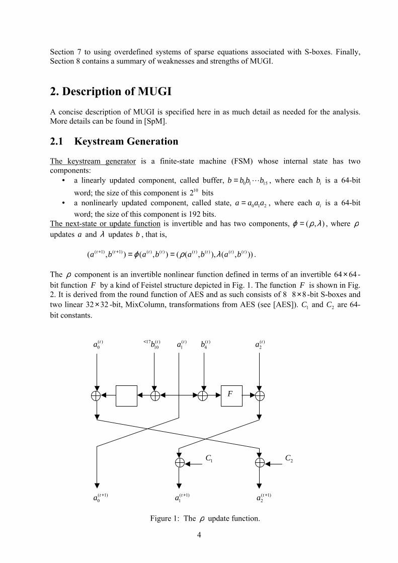
)),(),,((),(),( )()()()()()()1()1( tttttttt babababa λρϕ ==++ . The ρ component is an invertible nonlinear function defined in terms of an invertible 64 -bit function by a kind of Feistel structure depicted in Fig. 1. The function is shown in Fig. 2. It is derived from the round function of AES and as such consists of 8 8 -bit S-boxes and two linear 32 -bit, MixColumn, transformations from AES (see [AES]). C and C are 64-bit constants.

64×

2

F

×

F8×

132

)(

0ta )(

1017 tb< )(

1ta )(

4tb )(

2ta

F 1C 2C )1(

0+ta )1(

1+ta )1(

2+ta

F

Figure 1: The ρ update function.

4

S S S S S S S

MixColumn MixColumn

S

Figure 2: The function. F The corresponding equations for ρ are given below: )(

1)1(

0tt aa =+

1)(

4)(

1)(

2)1(

1 )( CbaFaa tttt ⊕⊕⊕=+

. (1) 2)(

1017)(

1)(

0)1(

2 )( CbaFaa tttt ⊕⊕⊕= <+

The λ component is an invertible linear function defined by the following equations: 10,4,0,)(

1)1( ≠= −

+ ibb ti

ti

)(0

)(15

)1(0

ttt abb ⊕=+

)(7

)(3

)1(4

ttt bbb ⊕=+

. )(13

32)(9

)1(10

ttt bbb <+ ⊕= (For a 64-bit word x , and denote the rotations of xi< xi> x by bits to the left and right, respectively.)

i

The 64-bit output of the keystream generator at time is defined as . t )(

2ta

The described structure is essentially a specific combiner with memory, which is a well-known type of keystream generators (see [G96a]), in which:

• the nonlinear combining function has a large internal memory size and is based on a round function of block ciphers

• the driving LFSM providing input to the combining function is not necessarily an LFSR with a primitive connection polynomial; in fact, it will be shown that the design of LFSM for MUGI is not good

• the LFSM may be non-autonomous, that is, may have an input taken from a part of the internal memory of the combining function

• the output at a given time is not a single bit, but a binary word taken from the internal memory of the combining function.

5

2.2 Initialization The initial internal state ( of the keystream generator is produced from the 128-bit secret key K and the 128-bit initialization vector IV in the following three stages, by using the keystream generator itself. In the first two stages only the

), )0()0( ba

10KK= 10IVIV=ρ function is

used. Firstly, the state is defined in terms of a K and a 64-bit constant C by: 0

00 Ka = 11 Ka = . 01

70

72 CKKa ⊕⊕= ><

The buffer is then defined by iterating )(Kb ρ as follows: . 150,))0,(()( 0

115 ≤≤= +

− iaKb ii ρ

Secondly, the last produced state a and are linearly combined together into

by: )0,()( 16 aK ρ= IV

),( IVKa 000 )(),( IVKaIVKa ⊕=

111 )(),( IVKaIVKa ⊕= . 01

70

722 )(),( CIVIVKaIVKa ⊕⊕⊕= ><

The ρ function is again iterated 16 times to produce . )0),,((16 IVKaρ Thirdly, the keystream generator is initialized by and and then iterated 15 times (both

)0),,((16 IVKaρ )(Kbρ and λ ) without producing output. The keystream generation starts from the

16th iteration on. Thus, effectively, the initial contents of both a and b , at the time when the first output is produced, depend on both K and . However, it is important to note that the content of b at the beginning of the third stage depends on

IVK only.

3. Analysis of Buffer In this section, the buffer is analyzed as a non-autonomous LFSM with one input sequence, namely, . The input sequence and all the internal sequences in the buffer are 64-bit sequences. Our objective is to derive expressions for the internal sequences in the buffer in terms of the input sequence and the initial state of the buffer, .

( )∞== 0)(

00 ttaa

0a )15(15

)1(1

)0(0

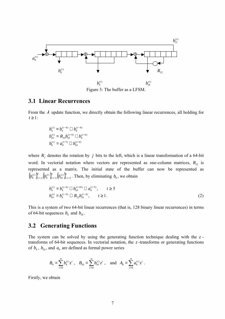
)0( bbbb L= In view of the λ update function, the 16 internal sequences in the buffer can be divided in three groups, in each group the sequences being phase shifts of each other (see Fig. 3).

6

)(

15tb

)(

0ta

)(

0tb 32R

)(

4tb )(

10tb

Figure 3: The buffer as a LFSM. 3.1 Linear Recurrences From the λ update function, we directly obtain the following linear recurrences, all holding for

: 1≥t )4(

0)4(

4)(

4−− ⊕= ttt bbb

)6(4

)4(1032

)(10

−− ⊕= ttt bbRb )6(

10)1(

0)(

0−− ⊕= ttt bab

where denotes the rotation by jR j bits to the left, which is a linear transformation of a 64-bit word. In vectorial notation where vectors are represented as one-column matrices, R is represented as a matrix. The initial state of the buffer can now be represented as

. Then, by eliminating , we obtain

32

( ) ( ) ( )0 5)(

100

5)0)(

0 −=−== tt

tt

tt bb (

43− b 0b 5,)5(

0)10(

10)4(

4)(

4 ≥⊕⊕= −−− tabbb tttt

. (2) 1,)4(1032

)6(4

)(10 ≥⊕= −− tbRbb ttt

This is a system of two 64-bit linear recurrences (that is, 128 binary linear recurrences) in terms of 64-bit sequences b and b . 4 10

3.2 Generating Functions The system can be solved by using the generating function technique dealing with the z -transforms of 64-bit sequences. In vectorial notation, the z -transforms or generating functions of , b , and are defined as formal power series 4b 10 0a

, , and . ∑∞

=

=0

)(44

t

tt zbB ∑∞

=

=0

)(1010

t

tt zbB ∑∞

=

=0

)(00

t

tt zaA

Firstly, we obtain

7

∑∑∑∑∞

=

−−∞

=

−−∞

=

−−∞

=

⊕⊕=5

5)5(0

5

5

10)10(10

10

5

4)4(4

4

5

)(4

t

tt

t

tt

t

tt

t

tt zazzbzzbzzb

. ∑∑∑∞

=

−−∞

=

−−∞

=

⊕=1

4)4(1032

4

1

6)6(4

6

1

)(10

t

tt

t

tt

t

tt zbRzzbzzb

Then, we get

t

t

t

t

ttt

t

t

t

t

ttt

t

t

t

t

tt

zbzbbbzbAz

zbzbbbzAz

zbbzzbAzBzBz

∑∑

∑∑

∑∑

=

−

=

−−

=

−

=

−−

=

−

=

⊕⊕⊕⊕⊕=

⊕⊕⊕⊕⊕=

⊕⊕⊕=⊕⊕

9

5

)10(10

3

1

)4(0

)4(4

)0(0

4)0(40

5

9

5

)10(10

4

1

)4(0

)4(4

)0(4

40

5

9

5

)10(10

)0(4

44

0

)(40

510

104

4

)(

)()1(

)1(

∑∑=

−

=

− ⊕⊕=⊕⊕3

1

)4(1032

)0(10

5

1

)6(44

61032

4 )(t

tt

t

tt zbRbzbBzBRzI

where I denotes the 64 identity matrix. In a simplified notation, we thus have 64× 10

510

104

4 )1( ∆⊕=⊕⊕ AzBzBz (3) 21032

44

6 )( ∆=⊕⊕ BRzIBz where

t

t

t

t

ttt zbzbbbzb ∑∑=

−

=

−− ⊕⊕⊕⊕=∆9

5

)10(10

3

1

)4(0

)4(4

)0(0

4)0(41 )(

∑∑=

−

=

− ⊕⊕=∆3

1

)4(1032

)0(10

5

1

)6(42

t

tt

t

tt zbRbzb

are 64-dimensional vectors ( matrices) whose elements are polynomials in z defined by the initial state of the buffer and whose degrees are at most 9 and 5, respectively. Essentially, this is a system of 128 linear equations with coefficients being polynomials in z and with unknowns being 128 generating functions of 64 binary sequences in b and 64 binary sequences in b .

164×

4

10

3.3 Solution The system has a unique solution which can be found in the following way. First, by elimination we obtain ( ) 2

10132

4032

454

1632

832

4 )()()( ∆⊕∆⊕⊕⊕=⊕⊕⊕⊕ zRzIARzIzBIzRzRIzI . ( ) 2

41

60

1110

1632

832

4 )1()( ∆⊕⊕∆⊕=⊕⊕⊕⊕ zzAzBIzRzRIzI Let (4) IzRzRIzIzF 16

328

324 )()( ⊕⊕⊕⊕=

8

denote the 64 matrix whose coefficients are polynomials in z of degree at most 16. The system can then be written as

64×

2

10132

4032

454 )()()( ∆⊕∆⊕⊕⊕= zRzIARzIzBzF

24

16

011

10 )1()( ∆⊕⊕∆⊕= zzAzBzF . When regarded over a field of rational functions in z , is invertible as is seen from the following equation:

)(zF

( )

IzzIzIzIIzI

IzRzRIzI

IzRzRIzIzFzFzF

16232168

32232

16232

8

21632

832

42

)1()(

)(

)()()()(

⊕⊕=⊕⊕⊕⊕=

⊕⊕⊕⊕=

⊕⊕⊕⊕==

because of . Thus we get that IR =232 )(

)(1 zFzf

is the inverse of , where )(zF

1623216 )1(1)( zzzzzf ⊕⊕=⊕⊕= .

Accordingly, we obtain the solution for the generating functions and in the form of 4B 10B

( )210

1324

03245

4 )()()()(

1 ∆⊕∆⊕⊕⊕= zRzIARzIzzFzf

B

( )24

16

011

10 )1()()(

1 ∆⊕⊕∆⊕= zzAzzFzf

B .

Unfortunately, it turns out that the polynomial has a very small exponent (period), equal to 48, because of

)(zf

16

48

11)(

zzzf

⊕⊕= .

So, the solution can also be put into the form of

( )210

1324

03245

48

16

4 )()()(11 ∆⊕∆⊕⊕⊕

⊕⊕= zRzIARzIzzF

zzB

( )24

16

011

48

16

10 )1()(11 ∆⊕⊕∆⊕

⊕⊕= zzAzzF

zzB .

Equivalently, we have

116

480165

48

105

4

)1(1

1)()1(1

1)(

1)()(

1

∆′⊕⊕

⊕⊕⊕

=

∆′⊕=

zz

AzGzzz

zfAzGz

zfB

(5)

9

216

4801611

48

2011

10

)1(1

1)()1(1

1)(

1)()(

1

∆′⊕⊕

⊕⊕⊕

=

∆′⊕=

zz

AzFzzz

zfAzFz

zfB

(6)

where (7) 32

20443232

4 )1())(()( RzIzzzzRzIzFzG ⊕⊕⊕⊕⊕=⊕= denotes the matrix whose coefficients are polynomials in of degree at most 20, and 6464× z 2

1011 )()( ∆⊕∆=∆′ zFzzG

( )24

16

2 )1()( ∆⊕⊕∆=∆′ zzzF are 64-dimensional vectors ( matrices) whose elements are polynomials in z defined by the initial state of the buffer and whose degrees are at most 31.

164×

3.4 Properties Consequently, both b and b have two components, one being a linear transform of the input sequence and the other being a linear transform of the initial conditions contained in and

. For both b and , the other, intrinsic component consists of 64 binary linear recurring subsequences produced by the LFSR with the feedback polynomial , or equivalently, by the cycling LFSR with the feedback polynomial 1 . Therefore, the period of each of these binary subsequences is equal to 48 or divides 48.

4

b

10

0a 1∆

2∆ 4 10

)(zf48z⊕

• This period is unacceptably small for cryptographic applications, especially in view of

the fact that these subsequences depend only on the secret key and not on the initialization vector.

• In common designs of keystream generators, the linear component, with the feedback from the nonlinear component disconnected, normally ensures a large period of the corresponding internal state sequence which itself very likely provides a lower bound on the period of the keystream sequence. This criterion is not satisfied here.

• Another weakness is that the degree of is only 32, and with an appropriate design it could have been as large as 16 , which is the size of the internal state of the buffer.

)(zf102=64×

• The polynomial also defines a sequential linear transform of the buffer sequence that is equal to a sequential linear transform of the input sequence coming from the nonlinear component. Its low degree and small period facilitate the initial state reconstruction and finding statistical distinguishers for the keystream sequence (see Sections 4-6).

)(zf

Yet another interesting property to analyze is the dependence of the intrinsic binary linear recurring subsequences upon the initial conditions. A careful analysis reveals (details are omitted) that for both b and b each such subsequence depends on only 32 bits of the initial state of the buffer. More precisely, for both b and b and for any 1 , the

4 10

4 10 64≤≤ j j -th binary

10

subsequence depends on the j -th and the ( -th binary subsequences of b , that is, on

. (Here the subscript 64 denotes the residue mod 64.) 64)32+j

64≤≤ j

)0(

( ) ( 15

0)0(

)32(,15

0)0(

, 64 =+= ijiiji bb

32R

10bj ( j

4b 10

0

)1

)2C⊕

)1(1 aa =−

25(0

)17(0

−− ⊕ tt a

32)31(0

32

)43(0

<−

−

⊕t

t

a

a

48≥

)30(1

(2

)47(1

−

−

⊕⊕

⊕t

tt

a

aa

)16(1

49)

)49(1

1(−<

−−

⊕

⊕t

t

a

a

1(1

t +

( (1a t

32

)9

<⊕

⊕

)15

<

−

⊕

(1

) ⊕ta

32(1

)1

−

+

t

t

(4

)(1 ba tt ⊕

17)(1 ba t ⊕ <

1−F

(0

)48(4

)(4

−

⊕

=⊕ tt abb

(0

)48(10

)(10

− =⊕ tt abb

1a 2

)10(1

)6(1

1)48(1

)(1 (

−−

−−

⊕⊕

⊕⊕tt

tt

aa

aFaa

(1

17)12(1

17

1)48(1

)(1 (

<−<

−−

⊕

⊕⊕tt

tt

aa

Faa

(1

32 −ta

)36−

)(2ta

)

• This means that mixing between different binary subsequences in the buffer, provided by the linear transform , is not good.

In addition, for both b and and for any 1 , the 4 j -th binary subsequence depends on the -th and the -th binary subsequences of the input 64-bit sequence a . 64)32+ 4. Elimination of Buffer The obtained expressions (5) and (6) for the generating functions of the 64-bit buffer sequences

and b can be transformed into the time domain and then appropriately substituted in the recurrences (1) for the update function ρ . In this way, we can derive the recurrences involving only the state sequences a and , where the output sequence a is assumed to be known, in the known-plaintext scenario. Namely, from (1) we first eliminate a and use the fact that F is invertible to get for

1 2a 2

0

0≥t (8) ( )(

2)1) CaaF t ⊕⊕= −

(9) )1(2

)11)(10 aF tt ⊕= +−−

where is the inverse of F and formally . Now by converting (5) and (6) into the time domain we get the following linear recurrences holding for t :

)0(0

48≥

)41(0

)25(0

32

)37(0

)33(0

)29(0

))13(0

(0

)5

−−<

−−−−−− ⊕⊕⊕⊕⊕tt

tttttt

aa

aaaaaa (10)

)35(0

)19(0

32)15(0

32

)31(0

(0

)11

−<−−<

−−

⊕⊕

⊕⊕⊕ttt

ttt

aaa

aa . (11)

Finally, by combining (8) with (10) and (9) with (11), we get the following recurrences involving and a only, which hold for t :

)42)26(1

32)38(1

)34(1

)26(1

)18)14(1

1)481

1(2

)1(1 )()

<−<−−−−−

−−+

⊕⊕⊕⊕⊕

=⊕⊕⊕ttttt

tt

aaaaa

CFCa (12)

(1

49)32(1

49)20(1

4944(1

17)17)162

)47(22

(2

)1(1 ))

<−<−<−<<−

−−

⊕⊕⊕⊕⊕

=⊕⊕⊕⊕tttt

tt

aaaaa

CaFCaa. (13)

The recurrences are nonlinear because of nonlinear F . As the first 16 outputs ( are not known, it is interesting to consider (12) and (13) only for t .

1− )150=t

64≥

11

One can also obtain different recurrences by using the polynomial of degree 32 instead of the polynomial 1 They will hold for t , but each will involve three times which makes them less useful.

)(zf.48z⊕ 32≥ 1−F

In principle, there are two general ways of using (12) and (13).

• One is to try to eliminate a from these two recurrences, possibly with certain approximation probabilities, thus yielding a recurrence in a holding with a certain probability which will represent a statistical distinguisher between the keystream sequence and a purely random sequence (i.e., a sequence of mutually independent uniformly distributed random variables).

1

2

• The other is to assume that a is known, in the known-plaintext scenario, and try to solve the corresponding nonlinear equations (or their approximations) for a for particular , e.g., for t . This might open the door for a further attack targeting the secret key.

2)(

1t

t 15=

Both ways are essentially addressed in the following sections. 5. Linear Cryptanalysis Linear cryptanalysis of stream ciphers is essentially different from linear cryptanalysis of block ciphers because of the underlying iterative structure in which the initial state is unknown, whereas the output sequence is assumed to be known in the known-plaintext scenario. A general way of conducting the linear cryptanalysis of stream ciphers is to linearize the next-state and output functions, with certain approximation probabilities, and to analyze the LFSM resulting from these linear approximations (see [G92, G94, G96a, G96b]). The obtained LFSM is in fact a LFSM approximation of the keystream generator, which itself is a nonlinear FSM. It can be analyzed with respect to the following two general objectives [G94]:

• to reconstruct the secret key, in particular, the initial state of the keystream generator • to derive a linear statistical distinguisher which can distinguish the keystream sequence

from a purely random sequence. Linearizing the next-state function of MUGI reduces to linearizing the nonlinear function F or its inverse . More precisely, we will linearize equations (8) and (9), where the sequences b and b are determined by (5) and (6). In turn, linearizing reduces to linearizing the S-boxes of AES. The effectiveness of the linear cryptanalysis depends on the way this linearization is performed and on the underlying approximation probabilities.

1−F 4

101−F

5.1 Linear Approximations for F Our objective in this section is to derive linear approximations to F or . In particular, especially effective are the linear approximations involving only one active S-box, as the underlying approximation probability is then most different from one half.

1−F

First note that the 64 -bit can be divided into two separate 32 -bit functions G , where G is a composition of S-boxes and the linear MixColumn transformation. An S-box is a composition of the multiplicative inversion in GF(256), with 0 mapped to 0, and an invertible affine transformation. Linearizing G then consists of linearizing the S-boxes and of linearly

64× F 32×

12

transforming the obtained linear approximations by the MixColumn transformation. If we want only one S-box to be active, then we have to find a linear approximation to any linear combination of 8 input bits for any chosen S-box and then to express the found linear combination of 8 output bits of this S-box in terms of 32 output bits of G by using the linear MixColumn transformation. Effectively, we thus linearize the inverse function G . 1−

β

8/

, βα

1−

What remains to be examined is how to find linear approximations for individual S-boxes. The correlation between a linear input function α and a linear output function of an S-box can be measured by the correlation coefficient

)Pr()Pr(),( βαβαβα ≠−==c . It is well known that the maximal correlation coefficient magnitude is 1 . We examined the linear approximations by computer simulations, that is, we computed the correlation coefficients for every ( )0,0(), ≠βα . Table 1 displays the number of β correlated to any given α with a given correlation coefficient magnitude. The same table is valid for the inverse S-box.

{ }cc =),(| βαβ 16 36 24 34 40 36 48 16 { }cc =),(| βαβ 5 c 8/64 7/64 6/64 5/64 4/64 3/64 2/64 1/64 0 c±

5 16 36 24 34 40 36 48 16 8/64 7/64 6/64 5/64 4/64 3/64 2/64 1/64 0

Table 1: Distribution of correlation coefficient magnitudes for an S-box.

We also considered linear approximations for the whole G by taking into account the MixColumn transformation. For each

1−

α involving only the 8 input bits to any individual S-box, we thus determined all the corresponding β , involving the corresponding 32 output bits of the MixColumn transformation. An interesting conclusion is that each pair ( ) such that

=|),(| βαc 8/64 or 7/64 involves at least 10 input and output bits. In addition, it is interesting to note that for each α involving the 16 input bits to any pair of S-boxes, each pair ( ), βα such that |),(| βαc is close to being maximal, ( , involves at least 5 input and output bits. However, observe that the correlation coefficient reduced because of two S-boxes being active.

2)64/8

5.2 LFSM Approximations for MUGI We will use equations (8) and (9) in which, for convenience, t is substituted for t . A basic way of linearization is to find linear approximations to 64 component Boolean functions of . In this case linearization is performed by substituting a 64 -bit vectorial linear function for

in (8) and (9). A more general way is to find linear approximations to some 64 linearly independent linear combinations of 64 component Boolean functions of F . In this case linearization is performed by applying an invertible matrix L to the left-hand sides of (8) and (9) and by substituting a matrix for on the right-hand sides of (8) and (9). Namely, we thus get for t

1−1−F

64×

1

1−F

2L 1−F1≥

)(

112)1(

22)(

12)1(

41)1(

11ttttt eCLaLaLbLaL ⊕⊕⊕=⊕ −−−

(14) )(

222)(

22)2(

12)1(

1017

1)1(

11ttttt eCLaLaLbLaL ⊕⊕⊕=⊕ −−<−

(15)

13

where and are the 64-bit approximation-error sequences whose binary component subsequences are expressed as nonbalanced Boolean functions of the corresponding inputs to

. The more nonbalanced these functions, the better the underlying linear approximations to . However, we will see that the effectiveness of the linear cryptanalysis does not depend

only on that. The linear approximation L to and the corresponding correlation coefficients are obtained by using the linear approximations to S-boxes as explained in Section 5.1.

1e 2e

1−F1

−FL 1

21

1−FL

5.2.1 Basic Equation Equations (14) and (15) in fact define an LFSM with input sequences e and e . The LFSM can be solved for and by using the generating function method already applied in Section 3. Let

1 2

1a 2a

∑∞

=

=0

)(11

t

tt zaA , , , and ∑∞

=

=0

)(22

t

tt zaA ∑∞

=

=1

)(11

t

tt zeE ∑∞

=

=1

)(22

t

tt zeE

denote the generating functions of , , , and e , respectively. Then we get 1a 2a 1e 2

∑∑∑∑∑∞

=

∞

=

−−∞

=

∞

=

−−∞

=

−− ⊕⊕

⊕⊕=⊕1

)(112

1

1)1(22

1

)(12

1

1)1(41

1

1)1(11 1 t

tt

t

ttt

t

t

t

tt

t

tt zeCLz

zzazLzaLzbzLzazL

∑∑∑∑∑∞

=

∞

=

∞

=

−−∞

=

−−∞

=

−− ⊕⊕

⊕⊕=⊕1

)(222

1

)(22

1

2)2(12

2

1

1)1(10171

1

1)1(11 1 t

tt

t

tt

t

tt

t

tt

t

tt zeCLz

zzaLzaLzzbRzLzazL

and accordingly

)0(1212122124111 1

aLCLz

zEAzLALBzLAzL ⊕⊕

⊕⊕⊕=⊕

)0(22

)0(022222212

21017111 1

aLazLCLz

zEALALzBRzLAzL ⊕⊕⊕

⊕⊕⊕=⊕

in view of . By rearranging the terms we obtain )0(

0)1(

1 aa =−

)0(

121214122121 1)( aLCL

zzEBzLAzLALzL ⊕

⊕⊕⊕=⊕⊕

)0(22

)( aLLz ⊕0(022221017122121 1

) azLCLz

zEBRzLALAzL ⊕⊕

⊕⊕=⊕⊕

where and are determined in terms of by (5) and (6), respectively, and 4B 10B 0A

)0(010 azAA ⊕= .

For simplicity, let C and denote the generating functions of the constant sequences, of period equal to 1, corresponding to the constants C and , respectively. Altogether, we finally obtain

′1

′2C

1 2C

14

( )))(()()()(

)())((

1)0(

12)0(

016

11122

117

21

′⊕⊕⊕′∆⊕⊕

=⊕⊕

CaLzfazGLzzLEzfALzzf

AzGLzLzLzf (16)

( )

))(())()(()()(

)())((

2)0(

22)0(

0217111

2171222

117112

21

′⊕⊕⊕⊕′∆⊕⊕

=⊕⊕

CaLzfaLzfzFRLzzRzLEzfALzf

AzFRLzzLLzfz . (17)

Here and are not known. However, E and are generating functions of nonbalanced sequences and as such in fact make (16) and (17) a system of binary linear recurrences each holding with a probability different from one half. Therefore, it is desirable that has as few terms as possible. This is why it is better to use its polynomial multiple 1 with only two terms. Consequently, (16) and (17) can be written in a different form where is replaced by

and all the other terms are multiplied by 1 , because 1 . We thus get

1E

48

2E 1 2E

⊕

)(zf48

)z1)((z ⊕

z⊕(f

48 f=1 z⊕ 16z )16zz⊕

′⊕⊕″∆⊕⊕⊕⊕= 148

1148

2248

11 )1()1()1()( CzEzALzzAzF (18)

′⊕⊕″∆⊕⊕⊕⊕= 248

2248

2248

12 )1()1()1()( CzEzALzAzF (19) where we introduced the following abbreviated notation:

( ))())(()1(

)()1())(1()(

17

2116

1167

2148

1

zGLzLzLzfz

zGLzzLzLzzF

⊕⊕⊕=

⊕⊕⊕⊕=

( )

( ))())(()1(

)()1())(1()(

17112

2116

1711612

2148

2

zFRLzzLLzfzz

zFRLzzzLLzzzF

⊕⊕⊕=

⊕⊕⊕⊕=

)0(

1248)0(

016

1116

1 )1())()(1( aLzazGLzzLz ⊕⊕⊕′∆⊕=″∆

( ) )0(22

48)0(02

48171

16112171

162 )1()1()()1()1( aLzaLzzFRLzzzRLzz ⊕⊕⊕⊕⊕⊕′∆⊕=″∆ .

The matrices F and depend on the performed linearization and and it is very likely

that at least one of them is invertible, because of L being invertible. Note that

)(1 z )(2 zF

1″∆ and 1

″∆ are 64-dimensional vectors whose elements are polynomials in defined by the initial state of the whole keystream generator ( and a ) and whose degrees are at most 48.

2

z)0(b )0(

2)0(

1)0(

0 aa The objective is to eliminate unknown A from (18) and (19). If F is invertible, then we have , where F is the adjunct matrix of F , and accordingly obtain

1

1(z)(1 z

*11

11 )()(det)( zFzFzF ⋅=− *) )(1 z

′⊕⊕″∆⊕⊕⊕⊕

=

′⊕⊕″∆⊕⊕⊕⊕

248

2248

2248

1

148

1148

2248*

12

)1()1()1()(det

)1()1()1()()(

CzEzALzzF

CzEzALzzzFzF.

15

By rearranging the terms we finally get the basic equation:

( )( ) ″∆⊕″∆⊕⊕⊕

=

′⊕′⊕⊕⊕⊕

211*

12211*

1248

211*

1248

221*

1248

)(det)()()(det)()()1(

)(det)()()1()(det)()()1(

zFzFzFEzFEzFzFz

CzFCzFzFzALIzFzFzzFz

. (20)

If, as above, t is taken as the initial time, then the first 16 elements of the output sequence,

, are unknown, but the initial state of the buffer, b , represented by and ∆ , depends on the secret key only. Alternatively, if t is taken as the initial time, then the output sequence, represented by , is known, but the initial state of the buffer (i.e., b ) depends on the initialization vector as well. The choice can influence the analysis whose objective is to reconstruct the secret key from the known output sequence for a number of initialization vectors.

0=( )15

0)(

2 =tta )0(

1∆ 2

16=2A )16(

5.2.2 Initial State Reconstruction Let us put the basic equation (20) into the following form:

( )

′⊕′⊕⊕

⊕⊕=⊕

″∆⊕″∆

211*

12221*

12

211*

1248211

*12

)(det)()()(det)()(

)(det)()(1

)(det)()(

CzFCzFzFALIzFzFzzF

EzFEzFzFz

zFzFzF

(21)

and let us take t as the initial time. Then 16= ″∆ and 1″∆2 are in fact determined by the initial

conditions and where is known. The effective number of binary unknowns is thus 18 .

)

⋅

16(b )16(2

)16(1

)16(0 aaa

115264 =

)16(2a

It is important to note that if we are able to reconstruct the state b and a at time

, then we can reconstruct the initial state b and simply by reversing the equations for the next-state function of MUGI even if the output sequence is unknown (as is the case in this situation). More precisely, the next-state function can be reversed in the following way:

)16(

)0(2

)0(1 a

)16(2

)16(1

)16(0 aa

16=t )0( )0(0 aa

15,9,3,)1(

1)( ≠= +

+ ibb ti

ti

)1(0

)(1

+= tt aa 2

)(10

17)(1

)1(2

)(0 )( CbaFaa tttt ⊕⊕⊕= <+

1)(

4)(

1)1(

1)(

2 )( CbaFaa tttt ⊕⊕⊕= +

)(7

)1(4

)(3

ttt bbb ⊕= +

)(13

32)1(10

)(9

ttt bbb <+ ⊕=)(

0)1(

0)(

15ttt abb ⊕= + .

16

Also, the 128-bit secret key can be directly obtained from b by reversing the update equations for

)0(1

)0(0 b

ρ . Accordingly, reconstructing the secret key is not more difficult than reconstructing b and, altogether, than reconstructing the internal state b and

. In fact, this should be regarded as a weakness of the initialization algorithm.

)0(1

)0(0 b )16(

)16(1

)16(0 aa

In the time domain, the left-hand side of (21) is a 64-bit sequence, x , denoted as X in the generating function domain, which depends on the initial conditions, and the last two terms on the right-hand side of (21) are linear transforms of the known sequence a and of the constant

sequences corresponding to C and C , respectively. The first term on the right-hand side of (21) is the noise term depending on the performed linear approximations. Consequently, (21) means that the linear recurring sequence

2

′1

′2

x depending on the initial conditions which is ultimately periodic with period of only 48 is termwise correlated to a sequential linear transform

of and of the constant sequences corresponding to C and C . More precisely, this is the case for each of the 64 constituent binary subsequences. The effectiveness of the correlation equation (21) is determined by how much the probabilities for the 64 underlying binary noise subsequences deviate from one half, and the corresponding correlation coefficients can be positive or negative.

2a ′1

′2

Accordingly, the periodic part of the 64-bit linear recurring sequence x , that is, the corresponding 48 64-bit words can in principle be reconstructed by a sort of a fast correlation attack. These 48 64-bit words in fact define a system of 48 binary equations among the unknown 17 initial state bits, b and , which can thus be obtained by solving the system. This is because does not affect the periodic part of the sequence , due to

64⋅64⋅ )16( )16(

0a)16(

1a x

⊕⊕⊕

⊕′∆⊕

= )0(12

*1248

)0(01

611

*12

16

)()(1

)()()()1(aLzFzF

z

azGLzzLzFzFzX

)()(det1

)()1()1()(det)0(

22)0(

02148

)0(0171

16122171

161

aLazLzFz

azFRLzzRLzzzF⊕⊕

⊕

⊕⊕′∆⊕

where the periodic part depends only on a , and not on a . To get the whole initial state, the 64-bit part a has to be guessed and this can be achieved in steps.

)0(0

)0(1

)16(1

642 What facilitates the attack is that the period of the sequence x is only 48, so that the required low-weight parity checks are easily obtained by considering the sequence at times being the integer multiples of 48. More precisely, to reconstruct a bit of a binary constituent subsequence of x , we need O bits of the corresponding binary output subsequence and the complexity is O . The reconstructed bit value is simply obtained by the majority count. Here c denotes the (positive or negative) correlation coefficient of the corresponding binary noise subsequence where

)48( 2−c)2−c(

p21−=p is the probability that the noise bit is equal to 1. In order to

estimate we will use a well-known fact that the correlation coefficient of a binary sum of mutually independent binary random variables is equal to the product of their individual correlation coefficients.

c

17

So, the feasibility of the attack depends on the correlation coefficients c for the underlying 64 binary noise subsequences. Recall that the generating function of the 64-bit noise sequence is given by the linear transform

211*

12 )(det)()( EzFEzFzFE ⊕= . (22) The correlation coefficients of the binary noise subsequences of e and depend on the linearization of the S-boxes and their magnitudes are equal to 2 or are close to this value (see Section 5.1). The underlying probabilistic assumption is that the noise subsequences are mutually independent sequences of mutually independent and uniformly distributed binary random variables. The correlation coefficient magnitude of the i -th constituent binary subsequence of the resulting noise sequence e , defined by (22), is then given as | where m (depending on i ) denotes the total number of binary terms from e and present in this subsequence or, equivalently, the total number of nonzero binary coefficients of the (involved) polynomials in the i -th row of the matrix F and in the polynomial

. In turn, this depends on the linearization of F , that is, on the properties of the S-boxes and the linear MixColumn transformation.

1

*)

2e

1

3−

) Fz

mc 32| −=

2e

12 (( z1)z(det 1F −

In theory, the attack would be effective only if the total complexity is faster than the exhaustive search over the initial states, that is, if 18 , that is, if m . Note that the exhaustive search requires 18 64-bit output values to be produced. To be on the conservative side, it is here assumed that one round of MUGI (i.e., producing one 64-bit output value) has the same complexity as one elementary operation in the described attack. It seems that such linearizations of F are likely to exist, but the problem may be to find them. In practice, since the secret key of MUGI has only 128 bits, the attack would be effective if 18 , that is, if m . Such linearizations of are very unlikely to exist. This may be related to the diffusion properties of the linear MixColumn transformation and is an interesting topic for further investigations.

64186 218264 ⋅⋅≤⋅⋅ m

1−F

191≤

64 ⋅⋅

1−

1286 2182 ⋅≤m

20≤

5.2.3 Linear Statistical Weakness The basic equation (20) can also be put into the form

″∆⊕″∆⊕

′⊕′⊕

⊕⊕=

211*

12211*

1248

482

)(det)()()(det)()()1(

)1()(

zFzFzFCzFCzFzFz

EzAzL

(23)

where the matrix

( )IzFzFzzFzzL )(det)()()1()( 1*

1248 ⊕⊕=

defines a sequential linear transform of the output sequence a . This equation specifies a linear statistical distinguisher between the output sequence and a purely random sequence. Namely, all the terms on the right-hand side of (23) except the noise term are polynomials in and as such vanish in the time domain after a sufficiently large t depending on the degrees of polynomials in and det . So, (23) means that a linear transform of the output sequence is termwise correlated to the all-zero 64-bit sequence where the approximation/correlation noise is

2

z

*12 )()( zFzF )(1 zF

18

defined by ( . Equivalently, the 64 constituent binary subsequences, obtained as linear transforms of the output sequence, are bitwise correlated to the all-zero binary sequence, where the corresponding correlation coefficients can be approximated as squares of the correlation coefficients of the corresponding binary noise subsequences of e . If c is such a correlation coefficient, then the output sequence length required for detecting the weakness in the corresponding binary subsequence is O . The output sequence length required to detect the weakness by using all the 64 subsequences is then O .

Ez )1 48⊕

12 64 ⋅≤m

)48(1

)(1 ⊕ −aa tt

48(1

)(1 ⊕ −aa tt

) 121 =⊕ AL

) 121 ⊕ AzLL

1()(1 zF ⊕=1()(2 zzF =

2

1−

)1

2C

)′

(f

)( 4−c

64⋅

11≤

10b

1)(

2 ⊕ Ca t

)1(2 ⊕+a t

)( 1 ⊕Ezf

)( 2 ⊕Ezf

1( z⊕=1()2 z=

64/)( 4−c

96≤

( )47(1

1 ⊕−− aF t

( )49(1

1 −− aF t

)((1 ⊕′ Lzf

(217 ⊕′∆ zfR

)(( 21 LzLz ⊕)(() 1Lzf ⊕

)48

47−t

) ⊕(02a

The correlation coefficient of the i -th constituent binary noise subsequence is now approximately given as c with the same notation as in Section 5.2.2. Accordingly, in theory, the statistical distinguisher would be effective if the total required output sequence length (proportional to the complexity) is smaller than the expected period for the size of the internal state, that is, if 2 , i.e., if m . It seems that such linearizations of F may exist. In practice, since the secret key of MUGI has only 128 bits, the attack would be effective if 2 , that is, if m . Such linearizations of F are extremely unlikely to exist.

m62 2−=

12 64 ⋅≤m

128

182 1−

2

5.3 LFSM Approximations for Simplified MUGI We will now conduct linear cryptanalysis of a simplified MUGI in which the feedback from the nonlinear component (i.e., the 64-bit sequence a ) to the linear component (i.e., the buffer) is disconnected. The resulting keystream generator then becomes weaker and our objective is to examine its resistance to linear cryptanalysis. It is reasonable to regard the obtained complexity results for the simplified MUGI as lower bounds to the complexity of attacks on the full version of MUGI.

0

In this case, the buffer sequences b and depend only on the initial state of the buffer and are thus determined by (5) and (6) where the first terms corresponding to the input sequence a are removed. They are both periodic with a very small period of 48. It is of separate interest to notice that the nonlinear recurrences (12) and (13) obtained by eliminating and b then have a simple form of

4

0

4b 10

0)( (

2)1(

11 =⊕⊕⊕⊕ −+− CaaF tt

.0))( )(22

)1(1

1) =⊕⊕⊕⊕⊕ −− aCaF t The linearization method from Section 5.2 is then essentially the same as linearizing F in these expressions. More precisely, in the generating function domain, (16) and (17) become

1−

)()(( 10(

12122 ∆⊕ CazLALzzfzLzf

))())()(( 2)0(

22)0

122′⊕⊕⊕= CaLzLzzLALzfzzf .

Equivalently, (18) and (19) remain to be true, but with simplified expressions:

))))( 1621

48 fLzLz ⊕ ))( 2

161

48 zLzzLLz ⊕⊕⊕

19

)0(12

4811

161 )1()1( aLzLzz ⊕⊕′∆⊕=″∆

)0(22

48)0(02

482171

162 )1()1()1( aLzaLzzRLzz ⊕⊕⊕⊕′∆⊕=″∆ .

Because of L being invertible, both matrices F and are invertible. For example, the inverse matrix of is given as

1 )(1 z )(2 zF)(1 zF

1

1*

21

12

11

481

1 )()det()1(

1)( −−−

− ⊕⊕⊕

= LLLzILLzIz

zF .

Note that is by definition the characteristic polynomial of the matrix . So, by eliminating unknown from (18) and (19) we get the same basic equation (2), but with simplified expressions for the involved component terms. The conclusions from Sections 5.2.2 and 5.2.3 remain to be true, but in this case the number, m , of binary terms in the equivalent noise sequence is expected to be smaller, as the coefficients of the matrices F and are then polynomials with a smaller number of terms.

)det( 21

1 LLzI −⊕ 21

1 LL−

2F

1A

)(1 z )(z

It is interesting to analyze a special case when the matrices L and commute, that is, when

. The basic equation (20) then takes a simplified form, which, in fact, can be directly obtained by eliminating A from (18) and (19). Namely, it then follows that the matrices

and commute so that we have

1 2L

1221 LLLL =

21 LzL ⊕1

21 zLL ⊕

′⊕⊕″∆⊕⊕⊕⊕⊕

=

′⊕⊕″∆⊕⊕⊕⊕⊕

248

2248

2248

21

148

1148

2248

21

)1()1()1()(

)1()1()1()(

CzEzALzLzL

CzEzALzzzLLz

which by rearranging the terms becomes

( )( ) ″∆⊕⊕″∆⊕⊕⊕⊕⊕⊕

=

′⊕⊕′⊕⊕⊕⊕⊕⊕⊕

22112122112148

22112148

222121248

)()()()()1(

)()()1()()()1(

LzLzLLzELzLEzLLzz

CLzLCzLLzzALLzLzLLzz. (24)

The generating function of the 64-bit correlation noise sequence is then given as

221121 )()( ELzLEzLLzE ⊕⊕⊕= so that the number, m , of terms in each row of E is explicitly determined by the number of binary terms in each row of L and the number of terms in each row of L . The number of terms in a row of is the number of binary terms in the corresponding linear combination of output bits of and the number of terms in a row of is the number of binary terms in the corresponding linear combination of input bits of F . What is relevant is the sum of the two numbers. The results obtained by computer simulations, reported in Section 5.1, show that this sum can be as small as 10. The total number of terms in the corresponding row of

1 2

1L1−F 2L

1−

E is then 20. The resulting correlation coefficient magnitude is then | . If linearizations with two 602| −=c

20

active S-boxes are considered, then the total number of terms can reduce to 10, but the overall correlation coefficient magnitude remains the same. It follows that the initial state reconstruction attack from Section 5.2.2 is then effective in theory and on the borderline to be effective in practice, whereas the linear statistical weakness from Section 5.2.3 is detectable in theory, but not in practice. 6. On Low-Diffusion Statistical Distinguishers The concept of low-diffusion statistical distinguishers for certain types of stream ciphers is introduced in [CHJ02]. Here we present a more general and more precise treatment of the subject. Consider a general type of keystream generator with the binary internal state vector

consisting of two components one of which, b , is updated linearly. More precisely, let the component next-state functions and the output function have the following form, respectively:

),( )()( tt ba )(t

) (25) ( )()()1( ttt baa µρ ⊕=+

(26) )()()1( tb

ta

t bab λλ ⊕=+

(27) )()()( tb

ta

t baz ηη ⊕= where ,,,, aba ηλλµ and bη are all linear functions, and ρ is a nonlinear function. In general, the linearly updated component can be solved to yield (28) )()1( t

aat

b ab λΛ=Λ +

where Λ and Λ are sequential linear transforms and Λ is binary, that is, in the generating function domain it is represented by the matrix where is a binary polynomial and

b a b

I)zp( ,1)0(),( =pzpI is the identity matrix of appropriate dimension. In this regard, see (10) and

(11) for MUGI. As such, Λ is invertible and commutes with any sequential linear transform (i.e., for every sequential linear transform

b

bΛbLΛ L= L ). If ρ is invertible, then this can be used to eliminate the linear component from the update equations, namely, )1()1(1)( −+− Λ=Λ⊕Λ t

aat

bt

b aaa λµρ (see Section 4 for MUGI). This is a nonlinear recurrence for the internal state component a , but as a is generally not obserbavle, it does not yield a statistical distinguisher. What is observable in the known-plaintext scenario is the output value z . However, (27) generally does not allow to be expressed in terms of , unless

)(t

)(t

)(t

)(ta )(tz aη is invertible. Suppose now that aη is invertible. In this case, we first get )(1)(1)( t

bat

at bza ηηη −− ⊕=

and then in view of (28)

21

. )(1)(1)1( taaa

tbaaa

tb zbb −−+ Λ=Λ⊕Λ ηληηλ

This again can be solved to yield

)(1)1( taaaa

tb zb −+ Λ′Λ=′Λ ηλ (29)

and then (30) )1(11)(1)( −−−− Λ′Λ⊕′Λ=′Λ t

aaaabat

abt

b zza ηληηη

where Λ and Λ are sequential linear transforms and Λ is binary (its dimension is adjusted to the dimension of the sequence it is applied to). Note that (29) and (30) are linear recurrences, but cannot be solved to directly yield the sequences a and because of unknown initial conditions. If that was possible, then (25) would directly define a very effective statistical distinguisher. However, in principle (29), (30), and (25) represent a basis for finding statistical distinguishers.

′b

′a

′b

b

For example, for the so-called low-diffusion statistical distinguisher [CHJ02] we just have to

note that we can compute the same sequential linear transform, namely Λ , of both the 64-bit input and output sequences to

′b

ρ in (25). More precisely, we have )(11)1(1)1( t

aaaabat

abt

b zza −−+−+ Λ′Λ⊕′Λ=′Λ ηληηη

)1(11)(1)1()( )()( −−−−+ Λ′Λ⊕′Λ⊕Λ′Λ=⊕′Λ taaaaba

tabaaa

ttb zzba ηληηηλµµ

which means that we can compute, in terms of the known output sequence z , the paired sequence

, where u and . (31)

′Λ′Λ )()( , t

bt

b uu ρ )1()()( +⊕= ttt ba µ )1()( += tt auρ

As Λ is binary, when computed for a given value of t , each pair is in fact a bitwise sum of the current and some previous inputs and outputs to

′b

ρ , that is, ( ))()()()()()( 11 , mm tttttttttt uuuuuu −−−− ⊕⊕⊕⊕⊕⊕ ρρρ LL . (32) A set of sufficiently many such pairs can in principle be statistically distinguished from a purely random sequence. The complexity predominantly depends on the number of nonzero terms in

, but also on the bit-size of the input/output to ′Λb ρ . To this end, it may be desirable to reduce this bit-size by considering linear functions of the input and output to ρ . Namely, instead of

we can consider ( where . In a special case of 4 terms only ( ), an approximation to the probability distribution of the pairs is given in [CHJ02] for a probabilistic model in which the function

), )(tuρ( )(tu ), )()( tin

tin ulul ρ′ )()( t

int

out ulu ρρ ′=l3=m

ρ is assumed to be random. In general, the larger the number of terms, the larger the complexity of the statistical distinguisher.

22

In the case when there is no feedback to the linearly updated component, we have 0=aλ and

, so that the linear transform Λ may in principle have a smaller number of terms than in the case with feedback.

bb Λ=′Λ ′b

The main point of the described low-diffusion statistical distinguisher is that a can be expressed in terms of , i.e., that

)(t

)(tz aη is invertible. In the case of MUGI, this assumption is not satisfied and, in fact, a large portion of the 192-bit a remains to be unknown, that is, the 64-bit . Accordingly, this statistical distinguisher is not applicable to MUGI. What one can obtain by eliminating the linearly updated component are the nonlinear recurrences (12) and (13) in the unknown 64-bit sequence . However, it has to be noted that the number of terms in

for MUGI is only 2, because of a bad design of the buffer.

)(t

)(1

ta

1a

bΛ 7. On Using Overdefined Equations for S-boxes The nonlinear part of an S-box in AES realizes the multiplicative inversion in GF(256) and maps zero to zero. As such it can be described by the equation for . On the basis of this, it is pointed out in [CP02] that one can associate with an S-box 39 linearly independent and relatively sparse quadratic binary equations in 8 input and 8 output binary variables. They hold with probability 1, so they are not approximations. Among them, there are 23 bi-affine equations which do not include products of input or output variables solely.

1=xy 0≠x

For AES, one can thus write down a large system of quadratic binary equations obtained by associating 39 or 23 equations with each S-box and by taking into account the key-scheduling algorithm too. The system can be treated by the multiply-and-linearize method to obtain a large overdefined system of linear equations in new variables. The method essentially consists in multiplying the equations by (appropriate) products of binary variables and by replacing the obtained products by new binary variables. The complexity of the method is determined by the number of variables in the resulting system of linear equations. It is shown in [CP02] that AES with 128-bit key is not vulnerable to this method. It is also shown that AES with 256-bit key is on the borderline to be vulnerable, but the complexity estimate is based on the questionable assumption that the resulting linear equations are linearly independent. Since MUGI is a keystream generator, the system of nonlinear equations is produced in a different way from that of a block cipher like AES. For example, one can consider the system in 18 64-bit initial state variables obtained by assuming that 19 consecutive 64-bit outputs are known. More precisely, the initial state variables are b and , whereas a and ( are assumed to be known. The 128-bit secret key can then easily be obtained from the reconstructed initial state as explained in Section 5.2.2. The

)0( )0(1

)0(0 aa )0(

2 )181

)(2 =tta

ρ update function of MUGI is not the same as the round function of AES, but the two are similar. To get the system, one then has to iterate ρ 18 times, which is much bigger then 10, which is the number of rounds in AES with 128-bit key. The complexity of the multiply-and-linearize method would then very likely be lower than 2 but much higher than 6418⋅ 1282 . Another way of getting the system would be to write down directly the system in 128 binary secret key variables from the first two or three known 64-bit outputs. One then has to take into account the initialization algorithm which altogether takes 48 iterations of ρ in order to

23

produce the first 64-bit output. Again, in light of [CP02], the complexity of the multiply-and-linearize method would very likely be (much) higher than 2 . 128

One can of course ask the question if the method from [CP02] can be improved. For example, is it possible to derive sequential variants of the multiply-and-linearize method that would employ some sort of chaining the variables, which may reduce the total number of variables and hence the complexity? This does not appear to be likely mainly because of an interesting property of the quadratic equations associated with an S-box that each of them includes at least one mutual product of an input and an output variable. Because of this, it is difficult to perform chaining (composition) of these equations in iterative structures like in AES or MUGI. 8. Summary of Weaknesses and Strengths Our main finding is that the linearly updated component of MUGI, the so-called buffer, is not designed properly. We proved that if the feedback from the nonlinearly updated component is disconnected, then the binary subsequences of the buffer are linear recurring sequences with the linear complexity of only 32 and with the period of only 48. This is what can be called the intrinsic response of the buffer. Accordingly, the buffer does not provide a large lower bound on the period of output sequences of MUGI which is normally the case with many designs of keystream generators. Furthermore, as each such subsequence depends on only 32 bits of the initial state of the buffer, the mixing between the 16 bits of the initial state of the buffer is not good.

64⋅

As a consequence of this small period, it is shown that the buffer sequence can easily be eliminated from the update equations for the nonlinearly updated component of MUGI, the so-called state, thus yielding the nonlinear recurrences involving only the output sequence and a part of the state sequence. It is then pointed out that this may facilitate the cryptanalysis of MUGI such as the linear cryptanalysis as well as finding the statistical distinguishers for MUGI. However, the period of MUGI is not expected to be small, primarily because of a large bit-size of the internal state and because of the 1-1 next-state function, but not because of a good design of the linearly updated component. A theoretical analysis of the period is thus very likely to be intractable. The linear cryptanalysis of MUGI performed by linearizing the next-state function and by solving the resulting linear finite-state machine shows that MUGI may in theory be vulnerable to the initial state reconstruction attack faster than the exhaustive search over the 1152-bit initial states (the whole internal state has 1216 bits, but 64 bits are taken to the output). This is again a consequence of the bad design of the buffer, but the attack is very unlikely to be faster than the exhaustive search over the 128-bit secret key. This is due to good linear correlation properties of the S-boxes and good diffusion properties of the linear MixColumn transformation, both from AES. Moreover, it is also argued that the linear statistical distinguishers may exist in theory, but not in practice, as their complexity is expected to be much higher than the exhaustive search over the 128-bit secret key. It is also shown that the simplified version of MUGI obtained by removing the feedback to the buffer is more vulnerable to the linear cryptanalysis. So, this feedback is also one of the strengths of MUGI. It is pointed out that the 128-bit secret key can easily be recovered from the reconstructed internal state of MUGI at any time. This is a weakness of the initialization algorithm, which is

24

itself relatively complex, but does not have the property that it should be infeasible to recover the secret key from the initial state. An in-depth general analysis of low-diffusion statistical distinguishers is conducted and it is argued that they are not applicable to MUGI, primarily because of the fact that only a part of the whole state vector is taken to the output, so that a large portion of it remains to be unknown. In addition, it is also argued that MUGI is very unlikely to be vulnerable to the multiply-and-linearize attack based on overdefined systems of quadratic binary equations associated with S-boxes of AES. This is related to the large bit-size of the internal state and a relatively complicated initialization algorithm. 9. References [CHJ02] D. Coppersmith, S. Halevi, and C. Jutla, “Cryptanalysis of stream ciphers with linear masking,” Cryptology ePrint Archive, IACR, 2002/020. [CP02] N. Courtois and J. Pieprzyk, “Cryptanalysis of block ciphers with overdefined systems of equations,” Cryptology ePrint Archive, IACR, 2002/044. [AES] J. Daemen and V. Rijmen, “AES Proposal: Rijndael,” 1999, available at http://www.nist.gov/aes/. [G92] J. Golić, “Correlation via linear sequential circuit approximation of combiners with memory,” Advances in Cryptology – EUROCRYPT ’92, Lecture Notes in Computer Science, vol. 658, pp. 124-137, 1993. [G94] J. Golić, “Linear cryptanalysis of stream ciphers,” Fast Software Encryption – FSE ’94, Lecture Notes in Computer Science, vol. 1008, pp. 154-169, 1995. [G96a] J. Golić, “Correlation properties of a general combiner with memory,” Journal of Cryptology, vol. 9, pp. 111-126, 1996. [G96b] J. Golić, “Linear models for keystream generators,” IEEE Transactions on Computers, vol. 45, pp. 41-49, 1996. [SpM] D. Watanabe, S. Furuya, H. Yoshida, and K. Takaragi, MUGI Pseudorandom number generator, Specification, Ver. 1.2, 2001, available at http://www.sdl.hitachi.co.jp/crypto/ mugi/index-e.html.

[EvM] D. Watanabe, S. Furuya, H. Yoshida, and K. Takaragi, MUGI Pseudorandom number generator, Self-evaluation report, Ver. 1.1, 2001, available at http://www.sdl.hitachi.co.jp/ crypto/mugi/index-e.html.

25