Securing Transient Stability Using Time-Domain Simulations Within an Optimal Power Flow

IEEE TRANSACTIONS ON POWER SYSTEMS, VOL. 25, NO. 1, FEBRUARY 2010 243

Securing Transient Stability Using Time-DomainSimulations Within an Optimal Power Flow

Rafael Zárate-Miñano, Student Member, IEEE, Thierry Van Cutsem, Fellow, IEEE,Federico Milano, Senior Member, IEEE, and Antonio J. Conejo, Fellow, IEEE

Abstract—This paper provides a methodology to restoretransient stability. It relies on a well-behaved optimal powerflow model with embedded transient stability constraints. Theproposed methodology can be used for both dispatching andredispatching. In addition to power flow constraints and limits,the resulting optimal power flow model includes discrete timeequations describing the time evolution of all machines in thesystem. Transient stability constraints are formulated by reducingthe initial multi-machine model to a one-machine infinite-busequivalent. This equivalent allows imposing angle bounds thatensure transient stability. The proposed optimal power flow modelis tested and analyzed using an illustrative nine-bus system, thewell-known New England 39-bus system, a ten-machine system,and a real-world 1228-bus system with 292 synchronous machines.

Index Terms—Dispatching, optimal power flow, redispatching,single-machine equivalent, transient stability.

NOTATION

T HE main notation used throughout the paper is statedbelow for quick reference. Other symbols are defined as

needed throughout the paper.

A. Functions

Cost function.

Current magnitude from bus to bus as afunction of state variables.Active power flow from bus to bus as afunction of state variables.Reactive power flow from bus to bus as afunction of state variables.

B. Variables

Emf magnitude of generator .

Electrical power of generator .

Manuscript received September 17, 2008; revised April 12, 2009. First pub-lished October 16, 2009; current version published January 20, 2010. The workof R. Zárate-Miñano, F. Milano, and A. J. Conejo was supported in part by theGovernment of Castilla-La Mancha under Project PCI08-0102 and in part bythe Ministry of Education and Science of Spain under CICYT Project DPI2006-08001. Paper no. TPWRS-00722-2008.

R. Zárate-Miñano, F. Milano, and A. J. Conejo are with the University ofCastilla-La Mancha, Ciudad Real, Spain (e-mails: [email protected]; [email protected]; [email protected]).

T. Van Cutsem is with the Fund for Scientific Research (FNRS), Universityof Liège, Liège, Belgium (e-mail: [email protected]).

Digital Object Identifier 10.1109/TPWRS.2009.2030369

Active power production of generator .

Total active power production in bus .

Reactive power production of generator .

Total reactive power production in bus .

Voltage magnitude at bus .

Rotor angle of the one-machine infinite-bus(OMIB) equivalent.

Rotor angle of generator .

Voltage angle at bus .

Rotor speed of the OMIB equivalent.

Rotor speed of generator .

C. Constants

Constant cost coefficient of generator .

Lineal cost coefficient of generator .

Quadratic cost coefficient of generator .

Maximum current magnitude through line .

Total active power consumed in bus .

Capacity of generator .

Minimum power output of generator .

Total reactive power consumed in bus .

Maximum reactive power limit of generator .

Minimum reactive power limit of generator .

Maximum voltage magnitude at bus .

Minimum voltage magnitude at bus .

Rotor angle limit of the OMIB equivalent.

D. Parameters

Element of the reduced susceptance matrix.

Element of the reduced conductance matrix.

Total inertia coefficient of the critical machinegroup.

Inertia coefficient of generator .

Total inertia coefficient of the noncritical machinegroup.

0885-8950/$26.00 © 2009 IEEE

Authorized licensed use limited to: Thierry Van Cutsem. Downloaded on February 15,2010 at 11:35:18 EST from IEEE Xplore. Restrictions apply.

244 IEEE TRANSACTIONS ON POWER SYSTEMS, VOL. 25, NO. 1, FEBRUARY 2010

Reduced admittance matrix.

Equivalent load admittance in bus .

Transient reactance of generator .

Integration time step.

Return angle of the OMIB equivalent.

Instability limit angle of the OMIB equivalent.

Frequency rating.

E. Sets

Set of online generators.

Set of critical machines.

Set of online generators located at bus .

Set of noncritical machines.

Set of buses.

Set of time steps.

Set of buses connected to bus .

I. INTRODUCTION

A. Motivation

The optimal power flow (OPF) is an appropriate and well-established tool to identify the control actions (e.g., generatingunit dispatching or redispatching actions) needed to ensure anappropriate security level prior to real-time operation.

The use of a security constrained OPF is increasingly needednowadays in stressed electric energy systems, which operateunder market rules. Thus, there exists a significant need to de-velop OPF models that incorporate a diverse type of securityconstraints to guarantee an appropriate security level.

On the other hand, to study the transient stability under amajor disturbance requires generally cumbersome time-domainsimulations. Also, to incorporate transient stability constraintswithin an OPF model poses the challenge of marrying time-sim-ulation and optimization. We propose an efficacious procedureto achieve this marriage.

B. Literature Review

The transient stability constrained OPF (TSC-OPF) is anonlinear semi-infinite optimization problem that includesalgebraic constraints and differential equations. For this reason,standard mathematical programming techniques cannot bedirectly applied and a variety of ad hoc algorithms has beenproposed. A critical review of several approaches proposed forsolving the TSC-OPF problem can be found in [1].

Two main aspects differentiate the TSC-OPF models thathave been proposed in the literature, namely, 1) how the tran-sient stability constraints are embedded in the OPF problem;and 2) how the transient stability assessment is approached. Abrief literature review of these two aspects follows.

1) Inclusion of Transient Stability Constraints in the OPF: In[2]–[4], the authors convert the original TSC-OPF into an opti-mization problem via a constraint transcription based on func-tional transformation techniques. This approach seems to be apromising method to solve large systems. In [5] and [6], the au-thors convert the power system transient stability model into analgebraic set of equations for each time step of the time-domainsimulation. This set of algebraic equations is introduced in theOPF as transient stability constraints. The size of the resultingproblem is typically large. Also, in [7], this model is extendedto consider multiple contingencies. The number of constraints issignificantly reduced by using the reduced admittance matrix in[7] and [8]. In [9], [10], and [11], the transient stability assess-ment is solved and the results are used to determine a bound onthe active power generation of a group of “critical machines”within the OPF problem. The main advantages of this approachare the compatibility with any dynamic model of the system anda low computational burden, while the main drawback is that ob-taining an optimal solution cannot be guaranteed.

2) Transient Stability Assessment: The transient stabilityassessment can be done through time-domain simulation [2],[6]–[8], [10], [12]; transient energy function (TEF) and poten-tial energy boundary surface (PEBS) [5], [13], [14], [15]; orhybrid methods [9], [16]–[19]. The time-domain simulationallows taking into account the full system dynamic model andconsists in checking that inter-machine rotor angle deviationslie within a specific range of values. Unfortunately, this range issystem, if not operating point, dependent and, in general, is noteasy to establish. The methods based on the transient energyfunction are able to highly reduce computational times. How-ever, the main limitation on the applicability of these methodslies in the construction of a suitable Lyapounov function andin the definition of the stability domain. Hybrid methods allowcombining the advantages of time-domain simulation and tran-sient energy function methods and avoiding some drawbacks.This paper uses the hybrid method proposed in [9].

C. Model Features

We strive to simplify the constraints related to the time-do-main simulation while retaining the essential features charac-terizing this time simulation, which allows ruling out transientsinstabilities. To do this, we reduce the original multi-machinemodel to a two-machine model using the concept of SIngle Ma-chine Equivalent (SIME), well documented in [20]. This two-machine model is further reduced to a one-machine infinite-bus(OMIB) equivalent, following well-established procedures [17],[20]. A bound calculated through appropriate time-domain sim-ulations is imposed on the angle of the single equivalent ma-chine to ensure transient stability.

The considered TSC-OPF includes, among others, thepre-fault power flow equations, technical bounds on genera-tors, buses and lines, discrete-time swing equations for all themachines of the system (reproducing the actual time-domainsimulation), as well as the transient stability bound on the angleof the single equivalent machine. The objective function to beminimized is the cost incurred as a result of dispatching orredispatching available generating units.


ZÁRATE-MIÑANO et al.: SECURING TRANSIENT STABILITY USING TIME-DOMAIN SIMULATIONS 245

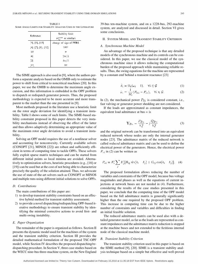
TABLE ISOME ANGLE LIMITS FOR STABILITY ANALYSIS USED IN THE LITERATURE

The SIME approach is also used in [9], where the authors per-form a separate analysis based on the OMIB only to estimate thepower to shift from critical to noncritical machines [20]. In thispaper, we use the OMIB to determine the maximum angle ex-cursion, and this information is embedded in the OPF problemto dispatch or redispatch generator powers. Thus, the proposedmethodology is expected to be more accurate and more trans-parent to the market than the one presented in [9].

Most methods proposed in the literature use a heuristic limiton the rotor angle deviation for identifying a transient insta-bility. Table I shows some of such limits. The SIME-based sta-bility constraint proposed in this paper detects the very insta-bility mechanisms instead of observing the effect of the latterand thus allows adaptively determining an appropriate value ofthe maximum rotor angle deviation to avoid a transient insta-bility.

Solving an OPF model requires the use of a nonlinear solverand accounting for nonconvexity. Currently available solvers(CONOPT [21], MINOS [22]) are robust and sufficiently effi-cient in terms of computing time to tackle OPFs. These solversfully exploit sparse matrix techniques and can be started fromdifferent initial points so local minima are avoided. Alterna-tively to optimization solvers, heuristic procedures (e.g., [18] or[19]) can be used but at the cost of not being able to characterizeprecisely the quality of the solution attained. Thus, we advocatethe use of state-of-the-art solvers such as CONOPT or MINOSand multiple runs using different initial solutions to solve OPFs.

D. Contributions

The main contributions of this paper are:1) to develop transient stability constraints based on an effec-

tive hybrid method for transient stability assessment;2) to provide a novel dispatching/redispatching OPF-based it-

erative methodology to ensure transient stability by iden-tifying the minimal corrective actions to avoid first- andmulti-swing instability.

E. Paper Organization

The remainder of the paper is organized as follows. Section IIpresents the dynamic model used for the machines of the systemand the transient stability criterion. Section III provides thedetailed mathematical formulation of the proposed TSC-OPFmodel, while Section IV describes the proposed dispatching/re-dispatching procedure. In Section V, three case studies based onthe WECC nine-bus three-machine system, on the New England

39-bus ten-machine system, and on a 1228-bus, 292-machinesystem, are analyzed and discussed in detail. Section VI givessome conclusions.

II. SYSTEM MODEL AND TRANSIENT STABILITY CRITERION

A. Synchronous Machine Model

An advantage of the proposed technique is that any detailedmodels of the synchronous machine and its controls can be con-sidered. In this paper, we use the classical model of the syn-chronous machine since it allows reducing the computationalburden of the proposed approach while maintaining reliable re-sults. Thus, the swing equations for the machine are representedby a constant emf behind a transient reactance [23]

(1)

(2)

In (2), the mechanical power is considered constant, i.e.,fast valving or generator power shedding are not considered.

If the loads are approximated as constant impedances, theequivalent load admittance at bus is

(3)

and the original network can be transformed into an equivalentreduced network whose nodes are only the internal generatornodes [23]. The admittance matrix of the reduced network iscalled reduced admittance matrix and can be used to define theelectrical power of the generators. Hence, the electrical power

in (2) can be written as

(4)

The proposed formulation allows reducing the number ofvariables and constraints of the OPF model, because bus voltagemagnitudes and phases as well as the equations of current in-jections at network buses are not needed in (4). Furthermore,considering the results of the case studies presented in thispaper, we conclude that the computing time of the OPF modelbased on the full admittance matrix is generally significantlyhigher than the one required by the proposed OPF problem.This increase in computing time can be due to the highernumber of constraints and variables and difficulties in findingan initial feasible solution.

The reduced admittance matrix can be used also with a de-tailed generator model, as far as the loads are represented as con-stant impedances and the admittance matrix reduction is stoppedat the machine buses and not extended to the fictitious internalnode of the classical machine model.

B. Transient Stability Criterion

The transient stability criterion used in this paper is based onthe SIME method [9], [20]. SIME is a transient stability anal-ysis technique based on a simple but effective and well-proved



technique. For each step of the time-domain simulation, SIMEdivides the multi-machine system into two groups, 1) the groupof machines that are likely to lose synchronism (critical ma-chines) and 2) all other machines (noncritical machines). Themaximum difference between two adjacent rotor angles, say

, indicates the frontier between the two machine groups,as follows. All generators whose rotor angles are greater thanare part of the critical machine group, while all generators whoserotor angles are lower than are part of the noncritical machinegroup. These two groups are replaced by an OMIB equivalentsystem, whose transient stability is determined by means of theequal-area criterion (EAC). Finally, SIME establishes a set ofstability conditions based on the equivalent OMIB parametersand on the EAC. A detailed description of the SIME method isgiven in [20], whereas a brief summary can be found in [24]. Inthe sequel, the SIME method is illustrated through some exam-ples.

If the simulation is unstable, SIME provides informationabout which are the critical machines, the time and therotor unstable angle for which the instability conditions arereached. Similarly, if a simulation is first-swing stable, SIMEprovides the time and the rotor return angle for which theOMIB equivalent meets the first-swing stability conditions. Weuse SIME criteria to define transient stability limits in the OPFproblem, as described in Section IV.

III. TSC-OPF MODEL DESCRIPTION

A. Objective Function

If the TSC-OPF is used as a dispatching tool, the objectivefunction represents the operating cost of power pro-duction:

(5)

where is the active power generation of generator andand are its cost coefficients.

If the TSC-OPF is used as a redispatching tool, the objectivefunction represents the cost of power adjustments as

(6)

where and are the power adjustments of gen-erator and and are the prices offered by the gen-erator to decrease and increase its power dispatch for securitypurposes, respectively. In this case, the active generation powers

are defined by

(7)

where represents the base case active generation power ofgenerator . The power adjustments need the following addi-tional constraints:

(8)

Note that (6) establishes that any change from the base caseimplies a payment to the agents involved [25].

B. Power Flow Equations

The power flow equations are defined by the active and reac-tive power balances at all buses:

(9)

(10)

where the powers on the left-hand side of each equation aredefined as

(11)

(12)

C. Technical Limits

The power production is limited by the capacity of the gen-erators

(13)

(14)

The bus voltages magnitudes must be within the operating limits

(15)

The current flow through all series elements of the network mustbe below thermal limits:

(16)

D. Initial Values of Machine Rotor Angles and emf Magnitudes

The initial values of generator rotor angles and emfare obtained from the system pre-fault steady-state conditionsas follows:

(17)



(18)

Furthermore, since the pre-fault is a steady-state condition, onehas

(19)

E. Discrete Swing Equations

The swing equations (1) and (2) are discretized using thetrapezoidal rule. Hence, generator rotor angles and speeds fora generic time step are defined by the following equa-tions:

(20)

(21)

where

(22)

Note that the reduced admittance matrix depends on the networktopology. Hence, in (22), the values of and are differentfor the during-fault and post-fault states, and consequently de-pend on time.

F. Transient Stability Limit

For each time step, the equivalent OMIB rotor angle must bebelow the instability limit provided by SIME:

(23)

where is as small as possible to reduce computing timebut larger than the instability time as defined by the SIMEmethod. The inequality (23) is the main constraint that forcesredispatching and is always binding. The dual variableassociated with (23) indicates the sensibility of the objectivefunction with respect to :

(24)

and is thus a measure of the impact of the stability constraintson the total dispatching or redispatching cost. The equivalentOMIB rotor angle is computed as

(25)

where

(26)

It is worth observing that (23) is a stability constraint compat-ible with most solution methods that have been proposed in theliterature. Thus, (23) can be used in conjunction with reduced orfull admittance matrix, detailed or simplified generator model,etc. The TSC-OPF formulation that is used in this paper is justone possible way of implementing (23).

G. Other Constraints

The proposed OPF problem is completed with the followingadditional constraints:

(27)

(28)

Equation (27) is included to reduce the feasibility region, thusgenerally speeding up the convergence of the OPF problem.

H. Problem Formulation

The formulation of the OPF problem is summarized as fol-lows:

subject to1) power flow (9)–(10);2) technical limits (13)–(16);3) initial values of machine rotor angles and emf magnitudes

(17)–(19);4) discrete swing equations (20)–(21);5) transient stability limit (23);6) other constraints (27)–(28).The above formulation can be easily extended to the multi-

contingency case by including constraints (20)–(21) and (23)for each considered contingency.

IV. PROCEDURE TO ENSURE TRANSIENT STABILITY

Converting the whole time-domain simulation of the systemtransient stability model into a set of algebraic equations resultsin a very large number of equations to be included in an OPF.Solving such nonlinear OPF problem may require prohibitivecomputing times and prohibitive memory size, and may lead toconvergence issues. To reduce the number of constraints, we usethe reduced admittance matrix and constrain the OMIB equiv-alent trajectory only during the first swing of the system. Thelatter allows including the discretized transient stability equa-tions (20)–(21) and (23) only for a few seconds after the faultoccurrence.

The proposed procedure is as follows.1) Base case solution. The base case solution can be obtained

from an OPF problem that consists of minimizing (5) sub-jected to power flow (9)–(10), technical limits (13)–(16),



and constraints (27)–(28). If the procedure is used as a re-dispatching tool, the base case corresponds to a dispatchingsolution obtained by any suitable technique.

2) Contingency analysis. The contingency analysis consistsin identifying, from a set of credible contingencies, theones that lead the system to instability. This identificationis carried out by means of a time-domain simulation com-plemented by SIME using a technique similar to the onein [24]. For first-swing unstable contingencies, SIME pro-vides the sets of critical and noncritical machines and theinstability limit for the OMIB equivalent. Equations(23) and (25) incorporate this information.

3) Solve the TSC-OPF problem. The OPF problem describedin Section III-H is solved and the new generating powersand bus voltages are computed.

4) Check the new solution. A time-domain simulation that in-cludes SIME is solved for the new operating point obtainedat step 3. This simulation is necessary to check the transientstability of the new operating point. Three different casescan be encountered.

a) The system is stable and the procedure stops.b) The system is first-swing unstable. This is due to the

fact that the reduced admittance used in the op-timization problem has been calculated for the initialsolution that exhibits different voltage values than thesolution obtained at step 3 [see (3)]. Thus, the reducedadmittance matrix is updated and the transient sta-bility limit is fixed to the new value of . Theprocedure continues at step 3.

c) The system is multi-swing unstable. In this case, theOMIB equivalent has a return angle in the firstswing. However, after some cycles, the system losessynchronism. The return angle value is used to de-fine the new transient stability limit . In order toavoid multi-swing phenomena, is set to ,i.e., is fixed to a value smaller than . The valueof the decrement is defined based on a heuristiccriterion. Finally, the reduced admittance matrixis updated. The procedure continues at step 3.

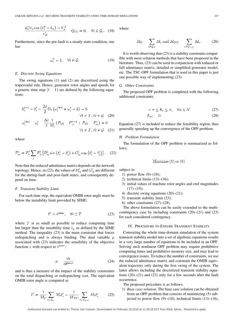
The flowchart depicted in Fig. 1 illustrates the proposed proce-dure.

Note that in the first iteration, the TSC-OPF problem is initial-ized with the base case solution while in the following iterations,the TSC-OPF problem is initialized with the solution of the pre-vious iteration. Since the OPF problem is nonconvex, the solu-tion for each iteration can be double-checked by starting fromseveral different initial guesses. Starting points are obtained byrandomly perturbing (using a normal distribution within a 20%range) the base-case solution or the solution of the previous OPFsolved. In our simulations, we did not observe convexity prob-lems, mainly due to the fact that the initial guess is close to theoptimum.

We consider that one single harmful contingency is foundat step 2. However, as discussed in Subsection III-H, mul-tiple contingencies can be readily taken into account byincluding (20)–(21) and (23) for each contingency in theTSC-OPF problem. In what follows, we are concerned onlywith single-contingency scenarios.

Fig. 1. Flow chart of the proposed procedure.

There could be situations where the power shifts determinedby the proposed procedure could modify the instability mode,i.e., change the set of critical/noncritical machines. This requiresto include (23) and (25) for both the previous and the new insta-bility mode.

V. CASE STUDIES

In this section, we present the result of a variety of casestudies based on the WECC nine-bus, three-machine system;the New England 39-bus, ten -machine system; and a 1228-bus,292-machine system. While the nine-bus and 39-bus systemsare presented for the sake of comparison with existing literature[10], [19], the 1228-bus system is used for testing the proposedtransient stability criterion in a real-world large-scale system.All simulations were carried out using Matlab 7.6 [26] andGAMS 22.7 [27]. For solving time-domain simulations, weused PSAT [28] that has been modified to include an embeddedSIME algorithm. Finally, the proposed TSC-OPF problem hasbeen solved using CONOPT [21].

The whole simulation time is 5 s for time-domain simula-tions, whereas the discretized dynamic equations are includedfor the first 2 s in the TSC-OPF problem. Setting s issufficient to reveal first swing transient instabilities. However,performing time-domain simulation over 5 s guarantees that thesystem does not undergoes multi-swing instability.



Fig. 2. One-line diagram of the WECC three-machine, nine-bus system.

A. WECC Nine-Bus, Three-Machine System

Fig. 2 shows the WECC three-machine, nine-bus system. Thefull dynamic data of this system can be found in [29], while gen-erator cost data and limits are defined in [10] and [19]. In orderto compare results with [10] and [19], we use the proposed tech-nique as a dispatching TSC-OPF; thus, (5) is used as objectivefunction.

In this case study, we consider the following two cases.Case A: A three-phase-to-ground fault occurs at bus 7 andis cleared after 0.35 s by tripping line 7-5. This case corre-sponds to Case A of [10] and [19].Case B: A three-phase-to-ground fault occurs at bus 9 andis cleared after 0.30 s by tripping line 9-6. This case corre-sponds to Case B of [10] and [19].

The base case solution is first-swing unstable for the contin-gencies of both cases, and . In case of multi-swing insta-bility, we use degree for computing the new value of

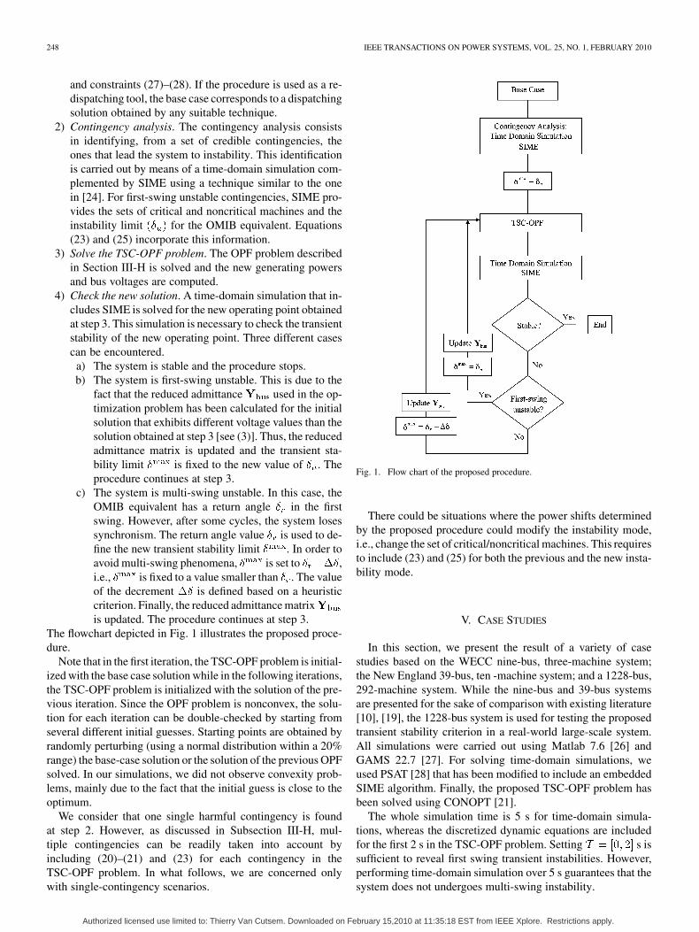
. The time step used in these case studies is s.1) Case A: The equivalent OMIB for the base case solution is

unstable since the rotor angle increases beyond the admissibleangle degrees after s. Fig. 3 showsthe unstable behavior of the base case OMIB equivalent and ofrotor angle trajectories after the occurrence of the contingencyand the subsequent fault clearing. After carrying out the stepsof the procedure described in Section IV, the system becomesstable. The procedure requires three iterations to converge, asfollows.

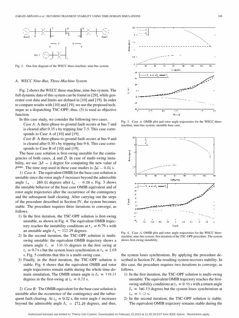
1) In the first iteration, the TSC-OPF solution is first-swingunstable, as shown in Fig. 4. The equivalent OMIB trajec-tory reaches the instability conditions at s withan unstable angle degrees.

2) In the second iteration, the TSC-OPF solution is multi-swing unstable: the equivalent OMIB trajectory shows areturn angle degrees in the first swing at

s but the system loses synchronism ats. Fig. 5 confirms that this is a multi-swing case.

3) Finally, in the third iteration, the TSC-OPF solution isstable. Fig. 6 shows that the equivalent OMIB and rotorangle trajectories remain stable during the whole time-do-main simulation. The OMIB return angle isdegrees in the first-swing at s.

2) Case B: The OMIB equivalent for the base case solution isunstable after the occurrence of the contingency and the subse-quent fault clearing. At s, the rotor angle increasesbeyond the admissible angle degrees, and thus,

Fig. 3. Case �. OMIB plot and rotor angle trajectories for the WECC three-machine, nine-bus system: unstable base case.

Fig. 4. Case �. OMIB plot and rotor angle trajectories for the WECC three-machine, nine-bus system: first iteration of the TSC-OPF procedure. The systemshows first-swing instability.

the system loses synchronism. By applying the procedure de-scribed in Section IV, the resulting system recovers stability. Inthis case, the procedure requires two iterations to converge, asfollows.

1) In the first iteration, the TSC-OPF solution is multi-swingunstable. The equivalent OMIB trajectory reaches the first-swing stability conditions at s with a return angle

degrees but the system loses synchronism ats.

2) In the second iteration, the TSC-OPF solution is stable.The equivalent OMIB trajectory remains stable during the



Fig. 5. Case�. OMIB plot and rotor angle trajectories for the WECC three-ma-chine, nine-bus system: second iteration of the TSC-OPF procedure. The systemshows multi-swing instability.

Fig. 6. Case �. OMIB plot and rotor angle trajectories for the WECC three-machine, nine-bus system: third and final iteration of the TSC-OPF procedure.The system is stable.

whole time-domain simulation with a return angledegrees in the first swing at s.

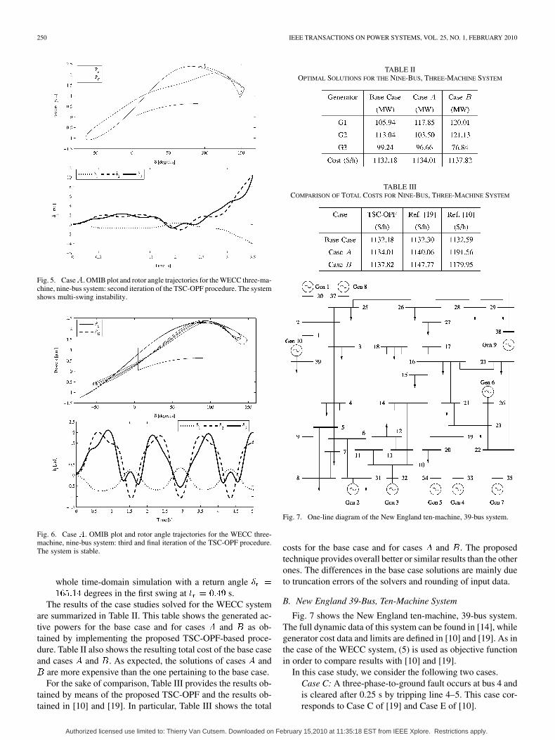
The results of the case studies solved for the WECC systemare summarized in Table II. This table shows the generated ac-tive powers for the base case and for cases and as ob-tained by implementing the proposed TSC-OPF-based proce-dure. Table II also shows the resulting total cost of the base caseand cases and . As expected, the solutions of cases and

are more expensive than the one pertaining to the base case.For the sake of comparison, Table III provides the results ob-

tained by means of the proposed TSC-OPF and the results ob-tained in [10] and [19]. In particular, Table III shows the total

TABLE IIOPTIMAL SOLUTIONS FOR THE NINE-BUS, THREE-MACHINE SYSTEM

TABLE IIICOMPARISON OF TOTAL COSTS FOR NINE-BUS, THREE-MACHINE SYSTEM

Fig. 7. One-line diagram of the New England ten-machine, 39-bus system.

costs for the base case and for cases and . The proposedtechnique provides overall better or similar results than the otherones. The differences in the base case solutions are mainly dueto truncation errors of the solvers and rounding of input data.

B. New England 39-Bus, Ten-Machine System

Fig. 7 shows the New England ten-machine, 39-bus system.The full dynamic data of this system can be found in [14], whilegenerator cost data and limits are defined in [10] and [19]. As inthe case of the WECC system, (5) is used as objective functionin order to compare results with [10] and [19].

In this case study, we consider the following two cases.Case C: A three-phase-to-ground fault occurs at bus 4 andis cleared after 0.25 s by tripping line 4–5. This case cor-responds to Case C of [19] and Case E of [10].



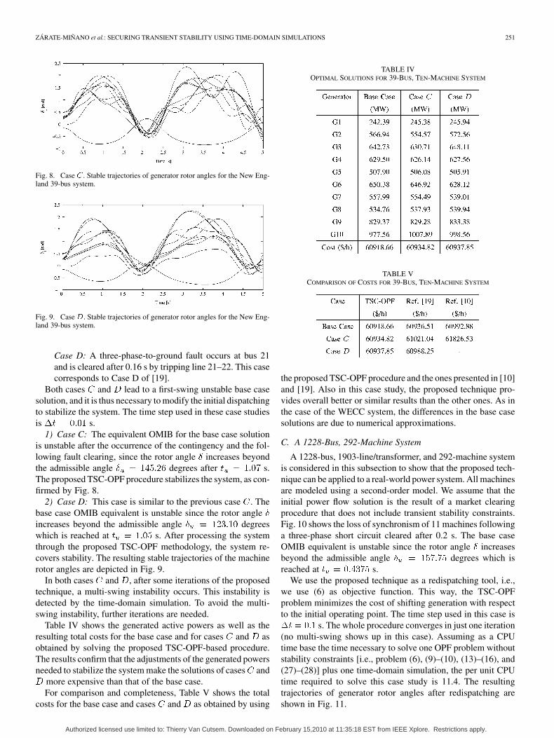
Fig. 8. Case � . Stable trajectories of generator rotor angles for the New Eng-land 39-bus system.

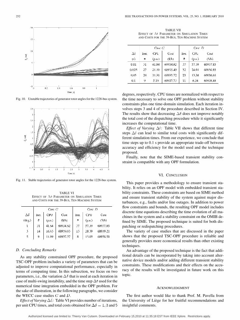
Fig. 9. Case�. Stable trajectories of generator rotor angles for the New Eng-land 39-bus system.

Case D: A three-phase-to-ground fault occurs at bus 21and is cleared after 0.16 s by tripping line 21–22. This casecorresponds to Case D of [19].

Both cases and lead to a first-swing unstable base casesolution, and it is thus necessary to modify the initial dispatchingto stabilize the system. The time step used in these case studiesis s.

1) Case C: The equivalent OMIB for the base case solutionis unstable after the occurrence of the contingency and the fol-lowing fault clearing, since the rotor angle increases beyondthe admissible angle degrees after s.The proposed TSC-OPF procedure stabilizes the system, as con-firmed by Fig. 8.

2) Case D: This case is similar to the previous case . Thebase case OMIB equivalent is unstable since the rotor angleincreases beyond the admissible angle degreeswhich is reached at s. After processing the systemthrough the proposed TSC-OPF methodology, the system re-covers stability. The resulting stable trajectories of the machinerotor angles are depicted in Fig. 9.

In both cases and , after some iterations of the proposedtechnique, a multi-swing instability occurs. This instability isdetected by the time-domain simulation. To avoid the multi-swing instability, further iterations are needed.

Table IV shows the generated active powers as well as theresulting total costs for the base case and for cases and asobtained by solving the proposed TSC-OPF-based procedure.The results confirm that the adjustments of the generated powersneeded to stabilize the system make the solutions of cases and

more expensive than that of the base case.For comparison and completeness, Table V shows the total

costs for the base case and cases and as obtained by using

TABLE IVOPTIMAL SOLUTIONS FOR 39-BUS, TEN-MACHINE SYSTEM

TABLE VCOMPARISON OF COSTS FOR 39-BUS, TEN-MACHINE SYSTEM

the proposed TSC-OPF procedure and the ones presented in [10]and [19]. Also in this case study, the proposed technique pro-vides overall better or similar results than the other ones. As inthe case of the WECC system, the differences in the base casesolutions are due to numerical approximations.

C. A 1228-Bus, 292-Machine System

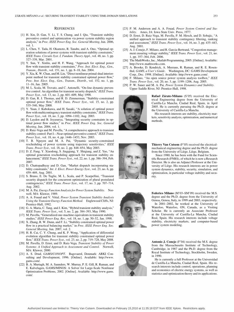
A 1228-bus, 1903-line/transformer, and 292-machine systemis considered in this subsection to show that the proposed tech-nique can be applied to a real-world power system. All machinesare modeled using a second-order model. We assume that theinitial power flow solution is the result of a market clearingprocedure that does not include transient stability constraints.Fig. 10 shows the loss of synchronism of 11 machines followinga three-phase short circuit cleared after 0.2 s. The base caseOMIB equivalent is unstable since the rotor angle increasesbeyond the admissible angle degrees which isreached at s.

We use the proposed technique as a redispatching tool, i.e.,we use (6) as objective function. This way, the TSC-OPFproblem minimizes the cost of shifting generation with respectto the initial operating point. The time step used in this case is

s. The whole procedure converges in just one iteration(no multi-swing shows up in this case). Assuming as a CPUtime base the time necessary to solve one OPF problem withoutstability constraints [i.e., problem (6), (9)–(10), (13)–(16), and(27)–(28)] plus one time-domain simulation, the per unit CPUtime required to solve this case study is 11.4. The resultingtrajectories of generator rotor angles after redispatching areshown in Fig. 11.



Fig. 10. Unstable trajectories of generator rotor angles for the 1228-bus system.

Fig. 11. Stable trajectories of generator rotor angles for the 1228-bus system.

TABLE VIEFFECT OF �� PARAMETER ON SIMULATION TIMES

AND COSTS FOR THE 39-BUS, TEN-MACHINE SYSTEM

D. Concluding Remarks

As any stability constrained OPF procedure, the proposedTSC-OPF problem includes a variety of parameters that can beadjusted to improve computational performance, especially interms of computing time. In this subsection, we focus on twoparameters, i.e., the variation that is used at each iteration incase of multi-swing instability, and the time step used for thenumerical time integration embedded in the OPF problem. Forthe sake of illustration, in the following paragraphs, we considerthe WECC case studies and .

Effect of Varying : Table VI provides number of iterations,per unit CPU times, and total costs obtained for and

TABLE VIIEFFECT OF �� PARAMETER ON SIMULATION TIMES

AND COSTS FOR THE 39-BUS, TEN-MACHINE SYSTEM

degrees, respectively. CPU times are normalized with respect tothe time necessary to solve one OPF problem without stabilityconstraints plus one time-domain simulation. Each iteration in-volves steps 3 and 4 of the procedure described in Section IV.The results show that decreasing does not improve notablythe total cost of the dispatching procedure while it significantlyincreases the computational time.

Effect of Varying : Table VII shows that different timesteps can lead to similar total costs with significantly dif-ferent simulation times. From our experience, we conclude thattime steps up to 0.1 s provide an appropriate trade-off betweenaccuracy and efficiency for the model used and the techniqueproposed.

Finally, note that the SIME-based transient stability con-straint is compatible with any OPF formulation.

VI. CONCLUSION

This paper provides a methodology to ensure transient sta-bility. It relies on an OPF model with embedded transient sta-bility constraints. These constraints are based on SIME methodand ensure transient stability of the system against major dis-turbances, e.g., faults and/or line outages. In addition to powerflow constraints and bounds, the resulting OPF model includesdiscrete time equations describing the time evolution of all ma-chines in the system and a stability constraint on the OMIB de-fined by SIME. The proposed technique is suited for both dis-patching or redispatching procedures.

The variety of case studies that are discussed in the papershows that the proposed TSC-OPF procedure is reliable andgenerally provides more economical results than other existingtechniques.

An advantage of the proposed technique is the fact that addi-tional details can be incorporated by taking into account alter-native device models and/or adding different transient stabilityconstraints. These modifications and their effects on the accu-racy of the results will be investigated in future work on thistopic.

ACKNOWLEDGMENT

The first author would like to thank Prof. M. Pavella fromthe University of Liège for her fruitful recommendations andinsightful comments.



REFERENCES

[1] H. Xin, D. Gan, Y. Li, T. S. Chung, and J. Qiu, “Transient stabilitypreventive control and optimization via power system stability regionanalysis,” in Proc. IEEE Power Eng. Soc. General Meeting, Jun. 2006,vol. 1.

[2] L. Chen, Y. Tada, H. Okamoto, R. Tanabe, and A. Ono, “Optimal op-eration solutions of power systems with transient stability constraints,”IEEE Trans. Circuits Syst. I, Fundam. Theory Appl., vol. 48, no. 3, pp.327–339, Mar. 2001.

[3] Y. Sun, Y. Xinlin, and H. F. Wang, “Approach for optimal powerflow with transient stability constraints,” Proc. Inst. Elect. Eng., Gen.,Transm., Distrib., vol. 151, no. 1, pp. 8–18, Jan. 2004.

[4] Y. Xia, K. W. Chan, and M. Liu, “Direct nonlinear primal-dual interior-point method for transient stability constrained optimal power flow,”Proc. Inst. Elect. Eng., Gen., Transm., Distrib., vol. 152, no. 1, pp.11–16, Jan. 2005.

[5] M. L. Scala, M. Trovato, and C. Antonelli, “On-line dynamic preven-tive control: An algorithm for transient security dispatch,” IEEE Trans.Power Syst., vol. 13, no. 2, pp. 601–609, May 1998.

[6] D. Gan, R. J. Thomas, and R. D. Zimmerman, “Stability-constrainedoptimal power flow,” IEEE Trans. Power Syst., vol. 15, no. 2, pp.535–540, May 2000.

[7] Y. Yuan, J. Kubokawa, and H. Sasaki, “A solution of optimal powerflow with multicontingency transient stability constraints,” IEEE Trans.Power Syst., vol. 18, no. 3, pp. 1094–1102, Aug. 2003.

[8] D. Layden and B. Jeyasurya, “Integrating security constraints in op-timal power flow studies,” in Proc. IEEE Power Eng. Soc. GeneralMeeting, Jun. 2004, vol. 1.

[9] D. Ruiz-Vega and M. Pavella, “A comprehensive approach to transientstability control: Part I—Near optimal preventive control,” IEEE Trans.Power Syst., vol. 18, no. 4, pp. 1446–1453, Nov. 2003.

[10] T. B. Nguyen and M. A. Pai, “Dynamic security-constrainedrescheduling of power systems using trajectory sensitivities,” IEEETrans. Power Syst., vol. 18, no. 2, pp. 848–854, May 2003.

[11] D. Z. Fang, Y. Xiaodong, S. Jingqiang, Y. Shiqiang, and Z. Yao, “Anoptimal generation rescheduling approach for transient stability en-hancement,” IEEE Trans. Power Syst., vol. 22, no. 1, pp. 386–394, Feb.2007.

[12] D. Chattopadhyay and D. Gan, “Market dispatch incorporating sta-bility constraints,” Int. J. Elect. Power Energy Syst., vol. 23, no. 6, pp.459–469, Aug. 2001.

[13] S. Bruno, E. De Tuglie, M. L. Scala, and P. Scarpellini, “Transientsecurity dispatch for the concurrent optimization of plural postulatedcontingencies,” IEEE Trans. Power Syst., vol. 17, no. 3, pp. 707–714,Aug. 2002.

[14] M. A. Pai, Energy Function Analysis for Power System Stability. Nor-well, MA: Kluwer, 1989.

[15] A. A. Fouad and V. Vittal, Power System Transient Stability AnalysisUsing the Transient Energy Function Method. Englewood Cliffs, NJ:Prentice-Hall, 1992.

[16] G. A. Maria, C. Tang, and J. Kim, “Hybrid transient stability analysis,”IEEE Trans. Power Syst., vol. 5, no. 2, pp. 384–393, May 1990.

[17] M. Pavella, “Generalized one-machine equivalents in transient stabilitystudies,” IEEE Power Eng. Rev., vol. 18, no. 1, pp. 50–52, Jan. 1998.

[18] X. Zhang, R. W. Dunn, and F. Li, “Stability constrained optimal powerflow in a practical balancing market,” in Proc. IEEE Power Eng. Soc.General Meeting, Jun. 2007, vol. 2.

[19] H. R. Cai, C. Y. Chung, and K. P. Wong, “Application of differentialevolution algorithm for transient stability constrained optimal powerflow,” IEEE Trans. Power Syst., vol. 23, no. 2, pp. 719–728, May 2008.

[20] M. Pavella, D. Ernst, and D. Ruiz-Vega, Transient Stability of PowerSystems: A Unified Approach to Assessment and Control. Norwell,MA: Kluwer, 2000.

[21] A. S. Drud, GAMS/CONOPT. Bagsvaerd, Denmark: ARKI Con-sulting and Development, 1996. [Online]. Available: http://www.gams.com/.

[22] B. A. Murtagh, M. A. Saunders, W. Murray, P. E. Gill, R. Raman, andE. Kalvelagen, GAMS/MINOS: A Solver for Large-Scale NonlinearOptimization Problems, 2002. [Online]. Available: http://www.gams.com/.

[23] P. M. Anderson and A. A. Fouad, Power System Control and Sta-bility. Ames, IA: Iowa State Univ. Press, 1977.

[24] D. Ernst, D. Ruiz-Vega, M. Pavella, P. M. Hirsch, and D. Sobajic, “Aunified approach to transient stability contingency filtering, rankingand assessment,” IEEE Trans. Power Syst., vol. 16, no. 3, pp. 435–443,Aug. 2001.

[25] A. J. Conejo, F. Milano, and R. Garcia-Bertrand, “Congestion manage-ment ensuring voltage stability,” IEEE Trans. Power Syst., vol. 21, no.1, pp. 357–364, Feb. 2006.

[26] The MathWorks, Inc., Matlab Programming, 2005. [Online]. Available:http://www.mathworks.com.

[27] A. Brooke, D. Kendrick, A. Meeraus, R. Raman, and R. E. Rosen-thal, GAMS, a User’s Guide. Washington, DC: GAMS DevelopmentCorp., Dec. 1998. [Online]. Available: http://www.gams.com/.

[28] F. Milano, “An open source power system analysis toolbox,” IEEETrans. Power Syst., vol. 20, no. 3, pp. 1199–1206, Aug. 2005.

[29] P. W. Sauer and M. A. Pai, Power System Dynamics and Stability.Upper Saddle River, NJ: Prentice-Hall, 1998.

Rafael Zárate-Miñano (S’05) received the Elec-trical Engineering degree from the University ofCastilla-La Mancha, Ciudad Real, Spain, in April2005. He is currently pursuing the Ph.D. degree atthe University of Castilla-La Mancha.

His research interests are stability, electricity mar-kets, sensitivity analysis, optimization, and numericalmethods.

Thierry Van Cutsem (F’05) received the electrical-mechanical engineering degree and the Ph.D. degreefrom the University of Liège, Liège, Belgium.

Since 1980, he has been with the Fund for Scien-tific Research (FNRS), of which he is now a ResearchDirector. He is also an Adjunct Professor at the Uni-versity of Liège. His research interests are in powersystem dynamics, stability, security, simulation, andoptimization, in particular voltage stability and secu-rity.

Federico Milano (M’03–SM’09) received the M.S.degree and the Ph.D. degree from the University ofGenoa, Genoa, Italy, in 1999 and 2003, respectively.

In 2001–2002, he worked at the University ofWaterloo, Waterloo, ON, Canada, as a VisitingScholar. He is currently an Associate Professorat the University of Castilla-La Mancha, CiudadReal, Spain. His research interests include voltagestability, electricity markets, and computer-basedpower system modeling.

Antonio J. Conejo (F’04) received the M.S. degreefrom the Massachusetts Institute of Technology,Cambridge, in 1987 and the Ph.D. degree from theRoyal Institute of Technology, Stockholm, Sweden,in 1990.

He is currently a full Professor at the Universidadde Castilla-La Mancha, Ciudad Real, Spain. His re-search interests include control, operations, planningand economics of electric energy systems, as well asstatistics and optimization theory and its applications.


Securing Transient Stability Using Time-Domain Simulations Within an Optimal Power Flow

Documents