SECURE QUANTUM ENCRYPTION By Michael St-Jules November 2016 A Thesis submitted to the School of Graduate Studies and Research in partial fulfillment of the requirements for the degree of Master of Science in Mathematics 1 c Michael St-Jules, Ottawa, Canada, 2016 1 The M.Sc. Program is a joint program with Carleton University, administered by the Ottawa- Carleton Institute of Mathematics and Statistics

Welcome message from author
This document is posted to help you gain knowledge. Please leave a comment to let me know what you think about it! Share it to your friends and learn new things together.
Transcript
SECURE QUANTUM ENCRYPTION
By
Michael St-Jules
November 2016
A Thesis
submitted to the School of Graduate Studies and Research
in partial fulfillment of the requirements
for the degree of
Master of Science in Mathematics1
c© Michael St-Jules, Ottawa, Canada, 2016
1The M.Sc. Program is a joint program with Carleton University, administered by the Ottawa-Carleton Institute of Mathematics and Statistics

Abstract
To the field of cryptography, quantum mechanics is a game changer. The exploitation
of quantum mechanical properties through the manipulation of quantum information,
the information encoded in the state of quantum systems, would allow many proto-
cols in use today to be broken as well as lead to the expansion of cryptography to
new protocols. In this thesis, quantum encryption, i.e. encryption schemes for quan-
tum data, is defined, along with several definitions of security, broadly divisible into
semantic security and ciphertext indistinguishability, which are proven equivalent, in
analogy to the foundational result by Goldwasser and Micali. Private- and public-key
quantum encryption schemes are also constructed from quantum-secure cryptographic
primitives, and their security is proven. Most of the results are in the joint paper
Computational Security of Quantum Encryption, to appear in the 9th International
Conference on Information Theoretic Security (ICITS2016).
ii

Acknowledgements
I would like to thank my supervisor, Anne, for her support, guidance, patience and
understanding, and the last two particularly when I was distracted by coursework,
taking away from our research and my work on this thesis.
I’d also like to thank her and my other coauthors, Gorjan Alagic, Bill Fefferman,
Tommaso Gagliardoni and Christian Schaffner, for their work on our joint paper and
the stimulating discussions that accompanied it.
iii
Contents
Abstract ii
Acknowledgements iii
Contents iv
List of Figures vii
List of Acronyms viii
List of Notation ix
1 Introduction 1
1.1 Overview . . . . . . . . . . . . . . . . . . . . . . . . . . . . . . . . . . 1
1.2 Summary of Contributions and Techniques . . . . . . . . . . . . . . . 2
1.2.1 Semantic Security vs. Indistinguishability . . . . . . . . . . . 3
1.2.2 Quantum Encryption Schemes . . . . . . . . . . . . . . . . . . 5
1.2.3 Author’s Contributions . . . . . . . . . . . . . . . . . . . . . . 6
1.3 Related Work . . . . . . . . . . . . . . . . . . . . . . . . . . . . . . . 6
1.4 Structure of This Thesis . . . . . . . . . . . . . . . . . . . . . . . . . 7
2 Background 9
2.1 Cryptography Before the Digital Computer . . . . . . . . . . . . . . . 9
2.2 Cryptography in the Digital World . . . . . . . . . . . . . . . . . . . 10
2.3 The Quantum Era . . . . . . . . . . . . . . . . . . . . . . . . . . . . 12
iv
2.4 Quantum Information Theory . . . . . . . . . . . . . . . . . . . . . . 14
2.5 The Dawn of Quantum Computing . . . . . . . . . . . . . . . . . . . 15
2.6 Quantum Algorithms and Quantum Complexity Theory . . . . . . . 17
2.7 Quantum Teleportation . . . . . . . . . . . . . . . . . . . . . . . . . . 18
2.8 Cryptography in a Quantum World . . . . . . . . . . . . . . . . . . . 19
3 Preliminaries 21
3.1 Binary Strings, Functions on Them, and the One-time Pad . . . . . . 22
3.2 Linear Algebra . . . . . . . . . . . . . . . . . . . . . . . . . . . . . . 23
3.3 Quantum States . . . . . . . . . . . . . . . . . . . . . . . . . . . . . . 30
3.4 Admissible Maps . . . . . . . . . . . . . . . . . . . . . . . . . . . . . 32
3.5 Quantum Circuits . . . . . . . . . . . . . . . . . . . . . . . . . . . . . 40
3.6 Efficient Classical and Quantum Computations . . . . . . . . . . . . 42
3.6.1 Oracles . . . . . . . . . . . . . . . . . . . . . . . . . . . . . . . 44
3.7 Negligible Functions . . . . . . . . . . . . . . . . . . . . . . . . . . . 45
3.8 Distinguishing Between States and Channels . . . . . . . . . . . . . . 46
3.8.1 The Quantum One-time Pad . . . . . . . . . . . . . . . . . . . 51
3.8.2 Computational Indistinguishability . . . . . . . . . . . . . . . 53
3.9 Modern Cryptography . . . . . . . . . . . . . . . . . . . . . . . . . . 54
4 Computational Security of Quantum Encryption 59
4.1 Quantum Encryption and Indistinguishability . . . . . . . . . . . . . 59
4.1.1 Quantum Encryption Schemes . . . . . . . . . . . . . . . . . . 59
4.1.2 Indistinguishability of Encryptions . . . . . . . . . . . . . . . 62
4.2 Quantum Semantic Security . . . . . . . . . . . . . . . . . . . . . . . 63
4.2.1 Difficulties in the Quantum Setting . . . . . . . . . . . . . . . 64
4.2.2 Definition of Semantic Security . . . . . . . . . . . . . . . . . 66
4.2.3 Semantic Security Is Equivalent to Indistinguishability . . . . 67
4.3 Quantum Encryption Schemes . . . . . . . . . . . . . . . . . . . . . . 69
4.3.1 Quantum Symmetric-Key Encryption from One-Way Functions 69
4.3.2 Quantum Public-Key Encryption from Trapdoor Permutations 73
4.4 Alternative Definitions of Quantum Security . . . . . . . . . . . . . . 79
v

4.4.1 SEM2 . . . . . . . . . . . . . . . . . . . . . . . . . . . . . . . 80
4.4.2 SEM3 . . . . . . . . . . . . . . . . . . . . . . . . . . . . . . . 81
4.4.3 IND’ . . . . . . . . . . . . . . . . . . . . . . . . . . . . . . . . 82
5 Proofs for Cryptographic Primitives 86
5.1 qOWFs to qPRFs . . . . . . . . . . . . . . . . . . . . . . . . . . . . . 86
5.2 The Goldreich-Levin Theorem . . . . . . . . . . . . . . . . . . . . . . 87
5.3 qTOWPs with Hard-cores to qPRGs . . . . . . . . . . . . . . . . . . 96
6 More (on) Security Definitions 101
6.1 IND with a Pair of Challenge Messages . . . . . . . . . . . . . . . . . 101
6.2 Multiple Message Security . . . . . . . . . . . . . . . . . . . . . . . . 103
6.3 Further Motivation for SEM and Alternatives . . . . . . . . . . . . . 107
6.3.1 Absolute Values in Semantic Security . . . . . . . . . . . . . . 107
6.3.2 The Swap Test as a Distinguisher for SEM . . . . . . . . . . . 107
6.3.3 Simulator Oracle Access . . . . . . . . . . . . . . . . . . . . . 108
6.3.4 Semantic Security with a Channel as the Target . . . . . . . . 110
6.3.5 Alternative Message Distributions . . . . . . . . . . . . . . . . 113
7 Conclusion 116
7.1 Extensions and Future Work . . . . . . . . . . . . . . . . . . . . . . . 116
Bibliography 118
vi
List of Figures
1 Circuit for quantum teleportation. . . . . . . . . . . . . . . . . . . . . 41
2 IND posits that a QPT (M,D) cannot distinguish between these two
scenarios. . . . . . . . . . . . . . . . . . . . . . . . . . . . . . . . . . 64
3 SEM: for all adversaries A there exists a simulator S such that these
two scenarios are indistinguishable. . . . . . . . . . . . . . . . . . . . 67
4 Relationship between security definitions. . . . . . . . . . . . . . . . 80
5 Circuit for the swap test . . . . . . . . . . . . . . . . . . . . . . . . . 108
vii
List of Acronyms
CCA1 Non-adaptive chosen ciphertext attack, e.g. in
Definition 4.1.3
CPA Chosen plaintext attack, e.g. in Definition 4.1.3
IND Indistinguishability, Definition 4.1.3
PPT Probabilistic polynomial-time algorithm, Definition 3.6.1
PT Polynomial-time algorithm, Definition 3.6.1
QOTP Quantum one-time pad, Definition 3.8.7
qOWF Quantum-secure one-way function, Definition 4.3.1
qPKE Quantum public-key encryption scheme, Definition 4.1.2
qPRG Quantum-secure pseudorandom generator,
Definition 4.3.9
qPRF Quantum-secure pseudorandom function,
Definition 4.3.2
QPT Quantum polynomial-time algorithm, Definition 3.6.3
qSKE Quantum symmetric-key encryption scheme,
Definition 4.1.1
qTOWP Quantum-secure trapdoor one-way permutation,
Definition 4.3.5
SEM Semantic security, Definition 4.2.1
viii
List of Notation
x $←−X x is distributed uniformly randomly in X, Section 3.1
0n, 1n The strings consisting of n 1’s and 0’s, respectively, Section 3.1
H A Hilbert space, Definition 3.2.2
† The adjoint operator, Definition 3.2.4
|ψ〉 , 〈ψ| Bra-ket notation, Notation 3.2.11
⊗ The tensor product, Definition 3.2.12
Tr The trace operator, Definition 3.2.14
ρ, σ Density operators or matrices, Definition 3.3.2
HA, ρAB,TrA(ρAB),1A Subscript notation, Notation 3.4.11
negl A negligible function, Definition 3.7.1
ix
Chapter 1
Introduction
1.1 Overview
Cryptography is the study and practice of secure communication in the presence of
malicious entities, and one of its pillars is the secure encryption of messages, trans-
forming them into information unintelligible except to the intended receiver, who may
read them only after decryption. Quantum mechanics leads to new possibilities in
cryptography. Three important properties of quantum mechanics separating it from
classical physics are quantum superposition, which allows a quantum system to be in
two or more states simultaneously; quantum entanglement, the existence of quantum
systems whose behaviour cannot be adequately through classical (probabilistic) corre-
lations between their subsystems; and the impossibility of copying arbitrary quantum
states, a consequence of the no-cloning theorem (see Theorem 3.4.1). The exploitation
of such properties through the manipulation of quantum information, the informa-
tion encoded in the state of quantum systems and whose basic building block is the
qubit, would allow many protocols in use today to be broken — by the application
of Shor’s algorithm for integer factorization [Sho94] implemented on a quantum com-
puter — as well as lead to the expansion of cryptography to new protocols. These
new tasks, falling under the heading of quantum cryptography, include, perhaps most
prominently, the information-theoretically secure distribution of keys in the presence
of eavesdroppers, by quantum key distribution [BB84].
1
CHAPTER 1. INTRODUCTION 2
This thesis seeks to add to them. Quantum encryption, i.e. encryption schemes
for quantum data, is defined. Quantum homomorphic encryption, in particular, as
described in [BJ15], would allow one to delegate computations on quantum infor-
mation to a more powerful quantum computer, and if secure, this more powerful
quantum computer would learn nothing from the states sent. Of course, then, what
does it mean for a quantum encryption scheme to be secure? This is one of the major
questions this thesis answers. Several security definitions are given, broadly divisible
into the intuitive–and intuitively strong–definitions of semantic security and the more
easily verifiable definitions of ciphertext indistinguishability, all of which are proven
equivalent in the same settings, in analogy to the foundational result by Goldwasser
and Micali in [GM84]. Private- and public-key quantum encryption schemes are also
constructed from quantum-secure cryptographic primitives (one-way functions and
trapdoor one-way permutations), and their security is proven. Most of the results
are in the joint paper Computational Security of Quantum Encryption [ABF+16], to
appear in the 9th International Conference on Information Theoretic Security (IC-
ITS2016), that makes up a chapter of this thesis.
Section 1.2, Section 1.3, Section 3.1, and the conclusion Chapter 7 are also taken
directly from the paper. It is noted again at the beginning of each when this is done.
Some modifications have been made to some of them, and these are also noted.
1.2 Summary of Contributions and Techniques
This section (except for Subsection 1.2.3) is taken from the joint paper [ABF+16].
In this work, we establish quantum versions of several fundamental classical (i.e.
“non-quantum”) results in the setting of computational security. Following Broadbent
and Jeffery [BJ15], we consider private-key and public-key encryption schemes for
quantum data. In these schemes, the key is a classical bitstring1, but both the
plaintext and the ciphertext are quantum states. Key generation, encryption, and
decryption are implemented by polynomial-time quantum algorithms. Such schemes
1While quantum keys might be of interest, they are not necessary for constructing secureschemes [BJ15].

CHAPTER 1. INTRODUCTION 3
admit an appropriate definition of indistinguishability security, following the classical
approach [BJ15]: the quantum adversary is given access to an encryption oracle, and
must output a challenge plaintext; given either the corresponding ciphertext or the
encryption of |0〉〈0| (each with probability 1/2), the adversary must decide which was
the case.
Our main contributions are the following. First, we give several natural formu-
lations of semantic security for quantum encryption schemes, and show that all of
them are equivalent to indistinguishability. This cements the intuition that posses-
sion of the ciphertext should not help the adversary in computing anything about the
plaintext. Second, we give two constructions of encryption schemes with semantic
security: a private-key scheme, and a public-key scheme. The private-key scheme
satisfies a stronger notion of security: indistinguishability against chosen ciphertext
attacks (IND-CCA1). A more detailed summary of these contributions follows.
1.2.1 Semantic Security vs. Indistinguishability
Semantic security formalizes the notion of security of an encryption scheme under
computational assumptions. Originally introduced by Goldwasser and Micali [GM84],
this definition posits a game: an adversary is given the encryption of a message m
and some side information σ, and is challenged to output the value of an objective
function f evaluated at m. An encryption scheme is deemed secure if every adver-
sary can be closely approximated by a simulator who is given only σ; crucially, the
simulator must work for every possible choice f of objective function. This models
the intuitive notion that having access to a ciphertext gives the adversary essentially
no advantage in computing functions related to the plaintext.
While semantic security corresponds to a notion of security that is intuitively
strong, it is cumbersome to use in terms of security proofs. In order to address
this problem, Goldwasser and Micali [GM84] showed the equivalence of semantic
security with another cryptographic notion, called indistinguishability. The intuitive
description of indistinguishability is also in terms of a game, this time with a single
adversary. The adversary prepares a pair of plaintextsm0 andm1 and submits them to
CHAPTER 1. INTRODUCTION 4
a challenger, who chooses a uniformly random bit b and returns the encryption of mb.
The adversary then performs a computation and outputs a bit v; the adversary wins
the game if v = b and loses otherwise. An encryption scheme is deemed secure if no
adversary wins the game with probability significantly larger than 1/2. This definition
models the intuitive notion that the ciphertexts are indistinguishable: whatever the
adversary does with one ciphertext, the outcome is essentially the same if run on the
other ciphertext.
In Section 4.2, we define semantic security for the encryption of quantum data—
thus establishing a parallel with the notions and results of encryptions as laid out
by Goldwasser and Micali. When attempting to transfer the definition of semantic
security to the quantum world, the main question one encounters is to determine the
quantum equivalents of σ and f(m) as described above (because of the no-cloning
theorem [WZ82], we cannot postulate a polynomial-time experiment that simulta-
neously involves some quantum plaintext and a function of the plaintext—see Sub-
sections 4.2.1 and 6.3.4 for further discussions related to this issue). We propose a
number of alternative definitions in order to deal with this situation (Definition 4.2.1,
Definition 4.4.2, and Definition 4.4.5.) Perhaps the most surprising is our definition
of SEM (Definition 4.2.1), which does away completely with the need to explicitly
define an analogues of the function f , instead relying on a message generator that
outputs three registers, consisting of the “plaintext”, “side information” and “target
output” (there is no further structure imposed on the contents of these registers).
Intuitively, we think of the adversary’s goal being to output the value contained in
the “target output” register. Formally, however, Definition 4.2.1 shows that the role
of the “target output” register is actually to help the distinguisher: semantic security
corresponding to the situation where no distinguisher has a non-negligible advantage
in telling apart the real scenario (involving the adversary) and the ideal scenario (in-
volving the simulator), even given access to the “target output” system. Our main
result in this direction (see Section 4.2.3) is the equivalence between semantic security
and indistinguishability for quantum encryption schemes:
Theorem 1.2.1. A quantum encryption scheme is semantically secure if and only if
it has indistinguishable encryptions.
CHAPTER 1. INTRODUCTION 5
What is more, because our definitions and proofs hold when restricted to the
classical case (and in fact can be shown as generalizations of the standard classical
definitions), our contribution sheds new light on semantic security: to the best of our
knowledge, this is the first time that semantic security has been defined without the
need to explicitly refer to the function f .
1.2.2 Quantum Encryption Schemes
In Section 4.3, we give two constructions of quantum encryption schemes that achieve
semantic security (and thus also indistinguishability, by Theorem 1.2.1.) Our con-
structions make use of two basic primitives. The first is a quantum-secure one-way
function (qOWF). This is a family of deterministic functions which are efficiently
computable in classical polynomial time, but which are impossible to invert even in
quantum polynomial time. It is believed that such functions can be constructed from
certain algebraic problems [MRV07, KK07]. The existence of qOWFs implies the ex-
istence of quantum-secure pseudorandom functions (qPRFs) [Zha12]. We show that
a qPRF can, in turn, be used to securely encrypt quantum data with classical private
keys. More precisely, we have the following:
Theorem 1.2.2. If quantum-secure one-way functions exist, then so do IND-CCA1-
secure private-key quantum encryption schemes.
The second basic primitive we consider is a quantum-secure one-way permutation
with trapdoors (qTOWP). In analogy with the classical case, a qTOWP is a qOWF
with an additional property: each function in the family is a permutation whose
efficient inversion is possible if one possesses a secret string (the trapdoor). While
our results appear to be the first to consider applications to quantum data, the no-
tion of quantum security for trapdoor permutations is of obvious relevance in the
security of classical cryptosystems against quantum attacks. Some promising candi-
date qTOWPs from lattice problems are known [PW08, GPV08]. We show that such
functions can be used to give secure public-key encryption schemes for quantum data,
again using only classical keys.
CHAPTER 1. INTRODUCTION 6
Theorem 1.2.3. If quantum-secure trapdoor one-way permutations exist, then so do
semantically secure public-key quantum encryption schemes.
We remark that Theorem 1.2.2 and Theorem 1.2.3 are analogues of standard
results in the classical literature [Gol04].
1.2.3 Author’s Contributions
The main contributions of the author of this thesis to the joint paper Computa-
tional Security of Quantum Encryption [ABF+16], which makes up Chapter 4 of
this thesis, are the definitions for semantic security SEM (Definition 4.2.1), SEM2
(Definition 4.4.2), SEM3 (Definition 4.4.5), their equivalence (Theorem 1.2.1, Theo-
rem 4.2.2 and Theorem 4.2.3) with IND (Definition 4.1.3) and IND’ (Definition 4.4.7).
This includes the definitions and results in Sections 4.2 and 4.4, but not the proof
of Theorem 4.2.3 as it appears in Section 4.2, nor the definitions for IND and IND’
in Section 4.4. Further contributions in this thesis include, in Chapter 5, full proofs
for results for cryptographic primitives used (and sketched or omitted) in the paper,
closely following the treatment in [Gol04]. These are the quantum version of the
Goldreich-Levin theorem (Theorem 5.2.1), and a stronger proof of security for the
construction of a qPRG from a qTOWP (Theorem 5.3.1). Finally, in Section 6.3,
more alternative definitions for semantic security are given and semantic security is
further motivated. In Subsection 6.3.4, in particular, obstacles to defining semantic
security with a channel or noncomputable classical function for F are discussed in
detail.
1.3 Related Work
This section is from the joint paper [ABF+16].
Prior work has considered the computational security of quantum methods to
encrypt classical data [OTU00, Kos07, XY12]. Information-theoretic security for
the encryption of quantum states has been considered in the context of the one-time
pad [AMTdW00, BR03, HLSW04, Leu02], as well as entropic security [Des09, DD10].
CHAPTER 1. INTRODUCTION 7
Computational indistinguishability notions for encryption in a quantum world were
proposed in two independent and concurrent works [BJ15, GHS15]. While [BJ15]
considers the encryption of quantum data (and proposes the first constructions based
on hybrid classical-quantum encryption), [GHS15] considers the security of classical
schemes which can be accessed in a quantum way by the adversary.
The results of [GHS15] are part of a line of research of “quantum-secure classical
cryptography”, which investigates the security of classical schemes against quantum
adversaries, with the goal of finding “quantum-safe” schemes. In this scenario, [BZ13]
considers quantum indistinguishability under chosen plaintext and chosen ciphertext
attacks. This definition was improved in [GHS15] to allow for a quantum challenge
phase. The latter paper also initiates the study of quantum semantic security of
classical schemes and gives the first classical construction of a quantumly secure
encryption scheme from a family of quantum-secure pseudorandom permutations.
Another quantum indistinguishability notion in the same spirit has been suggested
(but not further analyzed) in [Vel13, Def. 5.3].
Several previous works have considered how classical security proofs change in
the setting of quantum attacks (see, e.g., [Unr10, FKS+13, Son14].) Our results
can be viewed as part of this line of work; one distinguishing feature is that we
are able to extend classical security proofs to the setting of quantum functional-
ity secure against quantum adversaries. This setting has seen increasing interest in
the past decade, with progress being made on several topics: multi-party quantum
computation [BOCG+06], secure function evaluation [DNS10, DNS12], one-time pro-
grams [BGS13], and delegated quantum computation [BFK09, Bro15].
1.4 Structure of This Thesis
The remainder of this thesis is structured as follows:
Chapter 2 gives some background on developments in modern cryptography, quan-
tum information theory generally and quantum cryptography specifically. Section 2.8
is taken from the joint paper [ABF+16].
CHAPTER 1. INTRODUCTION 8
Preliminaries are given in Chapter 3, including background in linear algebra, quan-
tum information and quantum computing, as well as the notation used in quantum
information. The last section, Section 3.9 contains the definitions and results from
modern cryptography whose quantum counterparts are given in this thesis. Sec-
tion 3.1, Section 3.6 and Subsection 3.8.1 are taken from the joint paper [ABF+16].
Chapter 4 is taken from the joint paper [ABF+16]. In Section 4.1, private-key and
public-key encryption for quantum states and the security of such schemes, as cipher-
tex indistinguishability (IND, IND-CPA and IND-CCA1), are defined. Section 4.2
defines semantic security (SEM) for quantum encryption schemes, and proves its
equivalence with indistinguishability. Section 4.3 gives two constructions for quantum
encryption schemes and proves their security from the existence of quantum-secure
one-way functions and quantum-secure trapdoor one-way permutations. Section 4.4
defines semantic security in two more ways (SEM2, SEM3) and indistinguishability
in another that is common in cryptography (IND’), and all of the security definitions
given so far are proven equivalent.
Some omitted or sketched results for cryptographic primitives used in the con-
structions are proven in detail in Chapter 5.
In Chapter 6, further variations on security definitions are given and discussed,
including indistinguishability between encryptions of pairs of generated messages,
rather than a single message and a fixed trivial message in Section 6.1, extensions to
multiple messages in Section 6.2, the omission of the absolute values in the semantic
security definitions in Subsection 6.3.1, semantic security with the swap test as the
distinguisher in Subsection 6.3.2, security in which the simulator never has oracle
access under CPA or CCA1 in Subsection 6.3.3, semantic security with a channel as
the target in Subsection 6.3.4, and security for more general message distributions in
Subsection 6.3.5.
Finally, the concluding chapter, Chapter 7, also mostly taken from the joint paper
[ABF+16], discusses extensions, including non-uniform adversaries, the open problems
of the equivalence of IND and an appropriate definition of semantic security with a
channel for F , and defining CCA2 security.

Chapter 2
Background
This chapter discusses some of the most important theoretical results in cryptography
and quantum information leading up to the development of quantum cryptography.
This starts with the development of modern cryptography, including provably secure
encryption before computers in Section 2.1, followed by security and public-key cryp-
tography against computationally-bounded adversaries in Section 2.2. Next, early
important theoretical results in quantum mechanics and quantum information are
outlined in Sections 2.3 and 2.4, respectively. Then, the initial motivation and devel-
opment of quantum computers are summarized in Section 2.5, and the design of some
important quantum algorithms and results about their computational power follow in
Section 2.5. An important quantum protocol, quantum teleportation, is described in
Section 2.7. Finally, quantum cryptography is discussed and motivated in Section 2.8.
2.1 Cryptography Before the Digital Computer
Historically, every cipher used to encrypt messages was eventually broken [KL07], and
there wasn’t even any notion of what it meant for a cipher to be unbreakable, that
is, until Claude Shannon’s 1949 paper Communication Theory of Secrecy Systems
[Sha49]. In this paper, he introduced the definition of perfect secrecy : perfect secrecy
holds if the probability that the message is x, given that its encryption is c, is equal to
the probability that the message is x, for all possible x, c, i.e. knowing the encryption
9
CHAPTER 2. BACKGROUND 10
of a message does not change the likelihood that it is a particular message. The
one-time pad (or Vernam’s cipher) is one such cipher having this property, and any
other must be very similar in that the key space must be as large as the message
space, effectively meaning that the keys must be as long as the messages themselves,
a very impractical requirement. “One-time” refers to the fact that using the same
key to encrypt multiple messages is not safe, making the cipher inefficient, too.
2.2 Cryptography in the Digital World
However, with the advent of the digital computer, the idea of computational security,
in which the power of attackers is bounded, replaced perfect secrecy, and secure com-
munication over an insecure channel without a previously shared secret (i.e. a private
key) became possible. “We stand today on the brink of a revolution in cryptography.”
Thus began the 1976 paper New Directions in Cryptography by Whitfield Diffie and
Martin Hellman [DH76], in which they described the Diffie-Hellman key exchange
(or Diffie-Hellman-Merkle key exchange, for Ralph Merkle’s precursory and initially
rejected work as an undergraduate [Mer78, Mer10]) and introduced the notion of a
public-key cryptosystem, both allowing such secure communication. They also de-
scribed digital signatures, which would allow an individual sending a message to sign
it in such a way that anyone can verify its authenticity. These three ideas marked the
birth of public-key cryptography, and public-key encryption schemes were soon pub-
lished, the first being RSA (for Ronald L. Rivest, Adi Shamir and Leonard Adleman,
the authors), based on the difficulty of prime factoring, in 1978 [RSA78]. It later be-
came known that the concept of public-key encryption, RSA and Diffie-Hellman key
exchange were discovered earlier and independently at the British intelligence agency
GCHQ in 1970 by James Henry Ellis [Ell70], in 1973 by Clifford Cocks [Coc73] and
in 1974 by Malcolm J. Williamson [Wil76], respectively; their research was classified
until 1997.
Yet it wasn’t until 1982 that the notion of security of a cryptosystem was actually
made rigorous in the computational setting, by Shafi Goldwasser and Silvio Micali
[GM82]. In their 1984 paper [GM84], they furthered their defininition to semantic
CHAPTER 2. BACKGROUND 11
security : an encryption scheme is semantically secure if access to the encryption
of a message does not allow an attacker to compute partial information about the
message that he or she could not compute without the ciphertext. While intuitive, this
“partial information” was actually modelled as a function from the message space,
and semantic security then means quantifying over all such functions—even non-
computable ones—and all message distributions (generated in polynomial time), a
daunting task. However, in the same paper, Goldwasser and Micali reduced verifying
semantic security to checking if what they called polynomial security (now usually
called ciphertext indistinguishability) holds, which is defined to be the case when,
given the ciphertext of one from a pair of two chosen equal-length messages, no
polynomially bounded adversary can tell to which message it corresponds.
Not only did they define security intuitively and rigorously, they provided a practi-
cal means to prove an encryption scheme secure. It was for this paper—and their other
work on digital signatures, random functions, interactive proofs and zero-knowledge
protocols—that they received the Turing award, the “Nobel prize of computing”, in
2012; Goldwasser and Micali “laid the foundations of modern theoretical cryptography,
taking it from a field of heuristics and hopes to a mathematical science” [ACM13].
Since Goldwasser and Micali, there have been numerous variations in the defi-
nitions of security, reflecting variations in the definitions of the adversaries; these
include security for multiple messages, and security under chosen plaintext attacks
(CPA) and two different kinds of chosen ciphertext attacks (non-adaptive or a pri-
ori, CCA1 [NY90], and adaptive or a posteriori, CCA2 [RS92]). Furthermore, in
1993, Goldreich contributed a uniform-complexity treatment of security, replacing
the (non-uniform) families of circuits with Turing machines, and also renamed poly-
nomial security indistinguishability of encryptions or ciphertext indistinguishability
[Gol93].
Cryptographic primitives have also been important in the construction of secure
encryption schemes, in particular starting from one-way functions in the private-key
setting [HILL99, GGM86, Gol04] and trapdoor one-way permutations in the public-
key setting [GL89, Gol04].
CHAPTER 2. BACKGROUND 12
A candidate trapdoor one-way permutation that is secure against classical ad-
versaries and still widely used to this day is the RSA function, on which the RSA
cryptosystem is based and whose security depends on the difficulty of factoring. How-
ever, the RSA function, and the RSA scheme, by extension, are not secure against
quantum adversaries, due to Shor’s algorithm for integer factorization [Sho94].
Some of these definitions and results that are most relevant to this thesis are given
in Section 3.9.
2.3 The Quantum Era
Quantum mechanics, to this day still extremely accurate in its predictions, has refuted
much of our classical intuition about the universe. Several important experiments
mark its development, but this section will focus on outlining some of the most
important theoretical results.
In 1923, in his research for his PhD thesis [dB24], Louis de Broglie hypothesized
that matter behaves like waves, having wavelengths (the de Broglie wavelength), so
that, for example, the interference patterns in the double-slit experiment could even
be observed with electrons instead of light. His so-called matter waves fall under
the more general concept of wave-particle duality, the property of physical objects
situationally exhibiting both wave and particle properties.
Werner Heisenberg, Max Born, and Pascual Jordan developed the first complete
formulation of quantum mechanics as matrix mechanics in 1925 [Hei25, BJ26, BHJ26],
which was followed by Erwin Schrodinger’s wave mechanics and his proof of equiva-
lence in 1926. In wave mechanics, one of the fundamental postulates is the evolution of
quantum systems according to Schrodinger’s equation, a partial differential equation
involving the system’s Hamiltonian, which describes its energy states.
In 1927, Heisenberg introduced his uncertainty principle [Hei27], which predicts
that the more precisely a particle’s momentum is measured, the less precisely can its
position be, and vice-versa, as an inequality bounding the product of their standard
deviations from below (by the reduced Planck’s constant, divided by 2). If quantum

CHAPTER 2. BACKGROUND 13
mechanics were complete as a theory, this principle suggested that particles do not
even have simultaneously well-defined positions and momenta.
That same year, John von Neumann [vN27] and Lev Landau [SS82] independently
introduced the density matrix ; von Neumann, for quantum statistical mechanics and
a theory of measurement; and, Landau, to describe subsystems of composite systems.
Then, in 1930 and 1932, Dirac [Dir30] and von Neumann [vN55], respectively, laid
the mathematical foundations of quantum mechanics, including the Dirac–von Neu-
mann axioms, describing the evolution of quantum systems in the language of Hilbert
spaces and operators on them, preceded by von Neumann’s 1927 paper with David
Hilbert and Lothar Wolfgang Nordheim [HvN28]. In von Neumann’s 1932 text, he
also introduced what later become known as the von Neumann entropy, the starting
point of Quantum Shannon theory. Of course, before this, Hilbert had initiated the
study of infinite-dimensional Hilbert spaces [Hil06] (concrete ones for integral equa-
tions, von Neumann gave their abstract definition) and their corresponding spectral
theory, remarking later “I developed my theory of infinitely many variables from purely
mathematical interests, and even called it ’spectral analysis’ without any presentiment
that it would later find application to the actual spectrum of physics.” [Ste73]
Several new predictions from the theory followed, and notably that made by the
EPR paradox [EPR35] in 1935 by Albert Einstein, Boris Podolsky and Nathan Rosen.
They described a thought experiment in which a pair of particles could interact in
such a way that the measuring the position of one completely determines the position
of the other, and similarly for the momenta. Then, one particle’s position could be
measured, and the other’s momentum, each to arbitrary precision, and from each of
these, the other two quantities could be inferred, contrary to the uncertainty principle.
If the uncertainty principle must hold, then somehow a measurement of one particle
“affects” the other, to break these correlations, and this can occur instantaneously
and independently of the distance between the two, and hence faster than the speed
of light. EPR rejected this, with Einstein calling it “spooky action at a distance”,
and concluded that quantum mechanics was incomplete, so that hidden variables (for
the positions and momenta of particles, among others) were necessary for a complete

CHAPTER 2. BACKGROUND 14
description of physical reality. However, in 1964, John Stewart Bell derived Bell’s in-
equality [Bel64], which put the predictions made by any local hidden variable theory
(in particular, for particle spin) and those of quantum mechanics in conflict, con-
cluding with Bell’s theorem, ruling out such local hidden variables. The phenomenon
described in EPR is what Schrodinger named entanglement, calling it not “one but
rather the characteristic trait of quantum mechanics, the one that enforces its en-
tire departure from classical lines of thought.”[Sch35] Since Bell’s inequality and the
derivation of other so-called Bell inequalities, there have been several tests of them,
and recently, a loophole-free test [HBD+15].
2.4 Quantum Information Theory
Scientists took further interest in the information encoded in quantum systems and
more abstract mathematical characterizations of open quantum systems and their
evolution.
In 1955 and in 1940, William Forrest Stinespring [Sti55] and Mark Naimark [Nai40]
published their dilation theorems, respectively. Stinespring’s dilation theorem (stated
in Theorem 3.4.12, although different from the original result) allows one to represent
every quantum channel, which characterize the evolution of open quantum systems
without measurement, as a unitary operator, which captures the deterministic evolu-
tion of closed quantum systems, on a larger Hilbert space, while Naimark’s dilation
theorem allows one to represent every positive operator-valued measure (POVM), the
most general type of measurement, as a projection-valued measure (PVM) or spectral
measure, on a larger Hilbert space.
Further important initial developments in quantum information theory were made
in the 1970s and 1980s. In 1970, Stephen Wiesner invented conjugate coding and
unforgeable quantum money, but the results were unpublished until 1983 [Wie83],
despite inspiring some of the first developments in quantum cryptography (see Sec-
tion 2.8). In 1973, Alexander Holevo proved a theorem, now named in his sake
[Hol73], which implies that from n qubits, only n classical bits of information can be

CHAPTER 2. BACKGROUND 15
retrieved, despite requiring, in general, 2n complex numbers to represent n qubits. Ro-
man Stanis law Ingarden in his 1976 paper Quantum Information Theory showed that
Shannon’s information theory could not be generalized directly to quantum systems,
but laid forth generalizations despite this obstacle [Ing76]. Then, William Woot-
ters and Wojciech Zurek [WZ82], and independently Dennis Dieks [Die82] proved
the no-cloning theorem in 1982, a no-go theorem for the impossibility to copy ar-
bitrary quantum states. The no-cloning theorem is stated in the preliminaries as
Theorem 3.4.1.
2.5 The Dawn of Quantum Computing
The idea of quantum computing, however, was not introduced until the early 1980s.
Foreshadowing it, in 1975, R. P. Poplavskii showed that simulating quantum sys-
tems on classical computers is computationally infeasible: “The quantum-mechanical
computation of one molecule of methane requires 1042 grid points. Assuming that at
each point we have to perform only 10 elementary operations, and that the compu-
tation is performed at the extremely low temperature T = 3 × 10⁻³K, we would still
have to use all the energy produced on Earth during the last century.” (as quoted by
Manin) [Pop75]. Then, in 1980, Yuri Manin [Man80] proposed the idea of a quantum
computer, suggesting that quantum computers could be used to more efficiently sim-
ulate quantum systems, with Richard Feynmann independently suggesting the same
with a universal quantum simulator [Fey82]. In 1980, Paul Benioff proposed quan-
tum mechanical Hamiltonian models of Turing machines [Ben80, Ben82], followed in
1993 by David Albert’s quantum mechanical automaton, a true quantum computer
[Alb83], and then in 1985, David Deutsch developed the more general quantum Tur-
ing machines, introducing a physical Church-Turing principle stating: “Every finitely
realizable physical system can be perfectly simulated by a universal model comput-
ing machine operating by finite means”, and introducing universal quantum Turing
machines, quantum Turing machines that can simulate any other with at most a poly-
nomial increase in running time [Deu85]. In 1989, Deutsch also proposed the quantum
circuit model, then quantum computational networks, as well as the definition of a

CHAPTER 2. BACKGROUND 16
universal gate set, a set of unitaries from which the constructable quantum circuits
can approximate all n-qubit unitaries, for any n [Deu89]. In this paper, he also de-
fined what’s now known as the Deutsch gate, a 3-qubit quantum gate, and proved
that it is universal. In 1993, quantum Turing machines were further developed by
Ethan Bernstein and Umesh Vazirani [BV93], and the two models of quantum com-
puters, quantum Turing machines and quantum circuits, were then shown equivalent
by Andrew Yao [Yao93]. Further universal gate sets were subsequently identified,
and in 1995 Robert Solovay [DN06] and in 1997 Alexei Kitaev [Kit97] independently
proved the Solovay-Kitaev theorem, which states that any universal gate set can be
used to approximate any unitary with only O(logc(1/ε)) gates, where ε is the desired
accuracy. Kitaev’s proof was the design of an efficient algorithm to build such a cir-
cuit. In particular, this implies that quantum algorithms implemented with any gate
set will have the same running time, up to polynomial increases or decreases. Finally,
returning to the initial motivation for quantum computing, Seth Lloyd proved in 1996
that universal quantum computers, in the quantum circuit model, can simulate any
local quantum system [Llo96].
The first quantum error-correcting codes were designed by Shor [Sho95] and An-
drew Steane [Ste96] in 1995, and fault-tolerant quantum computation was also iniati-
ated Shor [Sho96]. Together, these would protect quantum data from accumulating
errors in storage and during computations, respectively.
The density matrix formalism for quantum circuits, which is common in quantum
computing and used in this thesis, allowing more general quantum channels and even
measurements in the middle of computations, was developed and proven equivalent to
the unitary gate model in 1998 by Dorit Aharonov, Kitaev and Noam Nisan [AKN98].

CHAPTER 2. BACKGROUND 17
2.6 Quantum Algorithms and Quantum Complex-
ity Theory
Around this time, too, the study of quantum complexity theory was initiated. In 1992,
David Deutsch and Richard Jozsa conceived an exact polynomial-time quantum ora-
cle algorithm (the Deutsch-Jozsa algorithm [DJ92]) to solve a problem that cannot be
solved in polynomial-time on a deterministic classical computer, i.e. that there exists
an oracle (or sequence of oracles, more specifically) f relative to which EQPf * Pf ,
where EQPf is the set of all decision problems solvable by exact polynomial-time
quantum algorithms with oracle access to f , and Pf is the set of decision problems
solvable by deterministic polynomial-time Turing machines with oracle access to f .
Bernstein and Vazirani built upon the work of Deutsch and Jozsa in their 1993 pa-
per [BV93] to prove the existence of an oracle f relative to which EQPf * BPPf ,
where BPPf is the set of decision problems solvable with bounded error by proba-
bilistic polynomial time Turing machines with oracle access to f , so that not even
probabilistic classical computers with oracle access to f can solve the problem effi-
ciently. They also remarked that deterministic polynomial-space algorithms, which
solve the decision problems in PSPACE, could simulate polynomial-time quantum
algorithms and hence concluded that BQP ⊆ PSPACE, where BQP is the set of
decision problems solvable with bounded error and in polynomial time by quantum
algorithms. Continuing along these lines, in 1994, Daniel Simon devised an oracle
problem (Simon’s problem) infeasible to probabilistic polynomial-time Turing ma-
chines and a polynomial-time quantum algorithm (Simon’s algorithm) to solve it,
proving the existence of an oracle A relative to which BPPA $ BQPA [Sim94].
Inspired by Simon’s work, Peter Shor, in 1994, developed polynomial-time quan-
tum algorithms for integer factorization (now known as Shor’s algorithm [Sho94]) and
the discrete logarithm, problems for which no known efficient classical algorithms ex-
ist, suggesting (but not proving) BPP $ BQP. These two algorithms could be
used to break many of the cryptographic protocols still used widely today, and the
results were some of the first strong evidence that quantum computers were superior
to classical computers (along with quantum simulation, as described in the previous
CHAPTER 2. BACKGROUND 18
section, Section 2.5, and quantum key distribution, in the the last section of this
chapter, Section 2.8). As a response, much more interest in the field developed, as
well as in post-quantum cryptography, i.e. cryptography with classical computers
that is secure against quantum computers.
Another important algorithm developed in this period is Grover’s search algorithm
[Gro96], an oracle algorithm, by Lov Grover in 1996, able to find a marked entry in a
database of N entries in O(√N) time, a quadratic improvement over the classically
optimal O(N). Around the same time, the algorithm’s asymptotic optimality was
proven by Charles H. Bennett, Ethan Bernstein, Gilles Brassard and Umesh Vazirani
[BBBV97], as a consequence of their more general result that “relative to an oracle
chosen uniformly at random, with probability 1, the class NP (of decision problems
whose yes instances can be verified with polynomial-length proofs in polynomial-time
by deterministic Turing machines) cannot be solved on a quantum Turing machine in
time o(√N)”. While not conclusive, this suggest that NP * BQP, i.e. there exist
problems in NP that quantum computers still cannot solve efficiently. In fact, they
also proved a similar oracle result for NP ∩ co-NP instead of simply NP.
2.7 Quantum Teleportation
In 1993, quantum teleportation was invented by Charles H. Bennett, Gilles Brassard,
Claude Crepeau, Richard Jozsa, Asher Peres, and William Wootters [BBC+93]. This
protocol would allow one party to transfer an arbitrary quantum state to another,
given only an entangled state shared between the two and using local operations and
the communication of classical bits from the party sending the state to the receiver.
The current record distance for quantum teleportation is 143 km, between the two
Canary Islands of La Palma and Tenerife [MHS+12]. Quantum teleportation is used
to illustrate quantum circuit notation, which is used minimally in this thesis, as
Figure 1.
CHAPTER 2. BACKGROUND 19
2.8 Cryptography in a Quantum World
The following section is from the joint paper [ABF+16].
Cryptography is one of the areas that is most seriously impacted by the poten-
tial of quantum information processing. As described in Section 2.6, the security
of most cryptographic primitives in use today relies on the hardness of computa-
tional problems that are easily broken by adversaries having access to a quantum
computer [Sho94].
While the impact of quantum computers on cryptanalysis is tremendous, quantum
mechanics itself predicts physical phenomena that can be exploited in order to achieve
new levels of security. These advantages were already mentioned in the late 1970’s in
pioneering work of Wiesner [Wie83] (as described in Section 2.4), and have led to the
very successful theory of quantum key distribution (QKD) [BB84], which has already
seen real-world applications [ABB+14]. QKD achieves information-theoretically se-
cure key expansion, and has the advantage of relatively simple hardware requirements
(notwithstanding a long history of successful attacks to QKD at the implementation
level [ABB+14]).
The cryptographic possibilities of quantum information go well beyond QKD.
Indeed, quantum copy-protection [Aar09], quantum money [Wie83, AC12, MS10] and
revocable time-release encryption [Unr14] are just some examples where properties
unique to quantum data enable new cryptographic constructions. Thanks in part to
these tremendous cryptographic opportunities, we envisage an increasing need for an
information infrastructure that enables quantum information. Such an infrastructure
will be required to support:
• Quantum functionality: honest parties can store, exchange, and compute on
quantum data;
• Quantum security: quantum functionality is protected against quantum ad-
versaries.
The current state-of-the-art is lacking even the most basic cryptographic concepts
in the context of quantum functionality and quantum adversaries. In particular, the
CHAPTER 2. BACKGROUND 20
study of encryption of quantum data (which is arguably one of the most fundamental
building blocks) has so far been almost exclusively limited to the quantum one-time
pad [AMTdW00] and other aspects of the information-theoretic setting [Des09, DD10]
(one notable exception being [BJ15]). The achievability of other basic primitives such
as public-key encryption has not been thoroughly investigated for the case of fully
quantum cryptography. This thesis and the joint paper [ABF+16] on which it is based
take some of the first steps in this direction.
Chapter 3
Preliminaries
Most of the following preliminaries can be found in the standard quantum information
and quantum computing textbooks [NC00] and [KLM07]. The chapter is structured
as follows:
Basic notation for classical concepts is given in Section 3.1. Concepts in linear
algebra important in quantum information are given in Section 3.2. Quantum states
are defined in Section 3.3. Admissible maps on quantum states, i.e. the operations
that can be applied to them, are defined and some results about them are presented
in Section 3.4. Quantum circuits are defined in Section 3.5. Efficient classical and
quantum computation are defined in Section 3.6. Negligible functions, informally,
functions that decrease to 0 faster than any inverse polynomial, are defined and some
of their basic properties are given in Section 3.7. Ensembles of quantum states and
results on the probability of distinguishing them are given in Section 3.8, with the
quantum one-time pad and computational indistinguishability defined in Subsections
3.8.1 and 3.8.2, respectively. Finally, definitions and results in modern cryptography
in the classical setting whose quantum analogues this thesis uses or defines are given
in Section 3.9.
21
CHAPTER 3. PRELIMINARIES 22
3.1 Binary Strings, Functions on Them, and the
One-time Pad
This section is taken from the joint paper [ABF+16].
Let N be the set of positive integers. For n ∈ N, we set [n] = 1, · · · , n. Define
0, 1∗ := ∪n0, 1n. An element x ∈ 0, 1∗ is called a bitstring or binary string,
and |x| denotes its length, i.e., its number of bits. We reserve the notation 0n (resp.,
1n) to denote the n-bit string with all zeroes (resp., all ones).
For a finite set X, the notation x $←−X indicates that x is selected uniformly at
random from X, i.e. each x has probability 1|X| of being selected. For a probability
distribution S, the notation x← S indicates that x is sampled according to S. Given
finite sets X and Y , the set of all functions from Y to X is denoted XY (or sometimes
X → Y ).We will usually consider functions f acting on binary strings, that is, of the form
f : 0, 1n → 0, 1m, for some positive integers n and m. We will also consider
function families f : 0, 1∗ → 0, 1∗ defined on bitstrings of arbitrary size. One can
construct such a family simply by choosing one function with input size n, for each n.
We will sometimes abuse notation by stating that f : 0, 1n → 0, 1m defines
a function family; in that case, it is implicit that n is a parameter that indexes the
input size and m is some function of n (usually a polynomial) that indexes the output
size. Given a bitstring y and a function family f , the preimage of f under y is defined
by f−1(y) := x ∈ 0, 1∗ : f(x) = y.Given two bitstrings x and y of equal length, we denote their bitwise XOR, or
equivalently, their bitwise sum modulo 2, by x⊕ y. Recall that the classical one-time
pad encrypts a plaintext x ∈ 0, 1n by XORing it with a uniformly random string
(the key) r $←−0, 1n. Decryption is performed by repeating the operation, i.e., by
XORing the key with the ciphertext. Since the uniform distribution on 0, 1n is
invariant under XOR by x, the ciphertext is uniformly random to parties having no
knowledge about r [Sha49]. A significant drawback of the one-time pad is the key
length. In order to reduce the key length, one may generate r pseudorandomly; this
CHAPTER 3. PRELIMINARIES 23
key-length reduction requires making computational assumptions about the adver-
sary.
3.2 Linear Algebra
We are concerned with finite-dimensional vectors spaces only in this thesis. It is
assumed that the reader is familiar with the basics of linear algebra (vectors spaces,
bases and orthonormal bases, linear transformations and matrices, eigenvalues and
eigenvectors, etc.).
Definition 3.2.1 (Normed vector space). A normed vector space is a tuple (V, ‖ · ‖),where V is a vector space over the field F = C or R, and ‖ · ‖ : V → R≥0 is a norm,
i.e. it satisfies, for all x, y ∈ V and α ∈ F:
1. ‖αx‖ = |α|‖x‖ ,
2. ‖x+ y‖ ≤ ‖x‖+ ‖y‖ , and
3. ‖x‖ = 0 ⇐⇒ x = 0 .
Definition 3.2.2 (Inner product space). A complex inner product space is a tuple
(V, 〈·, ·〉), where V is a complex vector space and 〈·, ·〉 : V × V → C is an inner
product, i.e., it satisfies for all x, y, z ∈ V and α ∈ C:
1. 〈y, x〉 = 〈x, y〉 (conjugate symmetry),
2. 〈x, αy〉 = α〈x, y〉〈x, y + z〉 = 〈x, y〉 + 〈x, z〉 (linearity in the second argument, the physics con-
vention), and
3. 〈x, x〉 ≥ 0, and
〈x, x〉 = 0 ⇐⇒ x = 0 (positive definiteness).
A norm ‖ · ‖ : V → R can be defined from the inner product by, for x ∈ V ,
‖x‖ =√〈x, x〉. This corresponds to the Euclidean norm, usually denoted by ‖ · ‖2,
but in this thesis, it will just be denoted by ‖ · ‖.

CHAPTER 3. PRELIMINARIES 24
An inner product space which is a complete metric space with respect to the
metric given by the above norm is called a Hilbert space. Finite-dimensional inner
product spaces are Hilbert spaces. In this thesis, we are only concerned with finite
dimensional complex vectors spaces, concretely Cn, for n ∈ N.
Definition 3.2.3 (Identity). Let V be a vector space. The identity (on V ) is the
linear transformation 1V : V → V defined by 1V (x) = x, for all x ∈ V
The set of linear transformations U → V is denoted by L(U, V ), and the set of
linear transformations (or linear operators) V → V by L(V ). These are also vector
spaces.
Definition 3.2.4 (Adjoint). Let A : U → V be a linear transformation from
(U, 〈·, ·〉U) to (V, 〈·, ·〉V ), finite-dimensional (complex) Hilbert spaces. The adjoint
of T is a linear transformation A† : V → U satisfying 〈v,Au〉V = 〈A†v, u〉U for all
u ∈ U, v ∈ V .
Note that adjoints always exist for bounded/continuous linear operators between
Hilbert spaces and is unique (hence the notation). For us, the matrix of the ad-
joint of a linear transformation is the conjugate transpose of the matrix of the linear
transformation, i.e. [A†]kj = [A]jk.
Proposition 3.2.5 (Adjoint properties). For A,C : U → V,B : V → W,α ∈ C,
1. (A†)† = A ,
2. (BA)† = A†B† , and
3. (αA+ C)† = αA† + C† .
Definition 3.2.6 (Normal operator). A linear operator A : H → H is normal if
A†A = AA†.
Definition 3.2.7 (Self-adjoint operator). A linear operator A : H → H is self-adjoint
(or Hermitian) if A† = A.
An operator is self-adjoint if and only if it is normal and its spectrum is real.

CHAPTER 3. PRELIMINARIES 25
Definition 3.2.8 (Positive semidefinite operator). A linear operator A : H → H is
positive semidefinite if it is self-adjoint and 〈x,Ax〉 ≥ 0 for all x ∈ H. This is often
denoted by A ≥ 0.
An operator is positive semidefinite if and only if it is normal and has only non-
negative eigenvalues. A : H → H is also positive semidefinite if and only if A = C†C,
for some operator C : H → H. Furthermore, there is a unique positive semidefinite
operator C satisfying this equality, and it is denoted by√A.
Definition 3.2.9 (Orthogonal projection). A linear operator P : H → H is an
orthogonal projection if P 2 = P † = P .
An operator is an orthogonal projection if and only if it is normal and its spectrum
is a subset of 0, 1. Orthogonal projections are therefore positive semidefinite.
Definition 3.2.10 (Unitary operator). A linear operator U : H → H is unitary if
U †U = UU † = 1H, so that U−1 = U †.
An operator is unitary if and only if it is normal and its spectrum is a subset of
the complex unit circle.
Notation 3.2.11 (Dirac Bra-ket Notation). Hilbert spaces are denoted by H, and
every vector x ∈ H corresponds uniquely to a linear functional Lx : H → C, defined
by
Lx(y) = 〈x, y〉 . (1)
By the Riesz representation theorem, this correspondence is a bijection between ele-
ments ofH and linear functionals onH, and it is also anti-linear, i.e. Lx+αy = Lx + αLy.
WhenH = Cn, linear transformations are given by matrix multiplication, and Lx = x†,
i.e. the transpose of x, where x is interpreted as an n by 1 matrix. We denote vectors
in H by kets, |ψ〉, |ϕ〉 (or with subscripts or superscripts on ψ or ϕ within these kets),
and the corresponding linear functionals as bras, 〈ψ|, 〈ϕ| (or with subscripts or super-
scripts on ψ or ϕ within these kets), so that whenH = Cn, (|ψ〉+ α|ϕ〉)† = 〈ψ|+ α〈ϕ|,and 〈ψ|ϕ〉 := 〈ψ||ϕ〉 is the inner product of |ψ〉 (on the left) and |ϕ〉 (on the right).
For convenience, |i1〉 ⊗ |i2〉 ⊗ · · · ⊗ |in〉 is written |i1i2 . . . in〉, for ij = 0, 1,+,−, and
CHAPTER 3. PRELIMINARIES 26
|ψ1〉 ⊗ |ψ2〉 ⊗ · · · ⊗ |ψn〉 is written |ψ1〉 |ψ2〉 . . . |ψn〉, for any other ψi. Often, |0n〉 will
simply be written |0〉; this should be understood from the context, in which the state
is composed of multiple qubits.
Definition 3.2.12 (Tensor product). Let U and V be vector spaces. Then, the
tensor product space U ⊗ V is the quotient of the set of all finite linear combinations
of formal symbols u ⊗ v, u ∈ U, v ∈ V by equivalence relation ∼ generated by the
following, for u, u′ ∈ U, v, v′ ∈ V, α ∈ C:
1. (u+ u′)⊗ v ∼ u⊗ v + u′ ⊗ v, and u⊗ (v + v′) ∼ u⊗ v + u⊗ v′, and
2. αu⊗ v ∼ u⊗ αv ∼ α(u⊗ v).
By convention, U ⊗ C and C⊗ U are defined simply to be U .
U ⊗ V is, in fact, a vector space.
Note that U ⊗ C,C⊗ U and U are all isomorphic, by u⊗ α↔ α⊗ u↔ αu.
The definition can be extended straightforwardly to arbitrarily many vector spaces,
or one can note that (U⊗V )⊗W and U⊗(V ⊗W ) are isomorphic as vector spaces and
define finite tensor products recursively (noting that the tensor product is associative
and symmetric, up to isomorphism).
Note that if BU and BV are bases for U and V , respectively, then
BU ⊗BV := u⊗ v|u ∈ U, v ∈ V (2)
is a basis for U ⊗ V . Hence dim(U ⊗ V ) = dim(U) dim(V ).
Furthermore, if U and V are inner product spaces, then
〈u⊗ v, u′ ⊗ v′〉U⊗V := 〈u, u′〉U〈v, v′〉V (3)
extends linearly to a well-defined inner product on U ⊗ V , and the if BU and BV are
orthonormal bases for U and V , respectively, then BU ⊗BV is an orthonormal basis
for U ⊗ V .
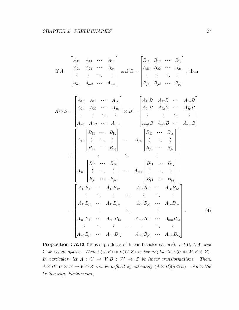
Concretely, the tensor product of two complex matrices A and B (of any dimen-
sion, including vectors as columns and rows) is the matrix A⊗B that can be computed
in block-matrix form as follows:
CHAPTER 3. PRELIMINARIES 27
If A =
A11 A12 · · · A1n
A21 A22 · · · A2n
......
. . ....
Am1 Am2 · · · Amn
and B =
B11 B12 · · · B1q
B21 B22 · · · B2q
......
. . ....
Bp1 Bp2 · · · Bpq
, then
A⊗B =
A11 A12 · · · A1n
A21 A22 · · · A2n
......
. . ....
Am1 Am2 · · · Amn
⊗B =
A11B A12B · · · A1nB
A21B A22B · · · A2nB...
.... . .
...
Am1B Am2B · · · AmnB
=
A11
B11 · · · B1q
.... . .
...
Bp1 · · · Bpq
· · · A1n
B11 · · · B1q
.... . .
...
Bp1 · · · Bpq
...
. . ....
Am1
B11 · · · B1q
.... . .
...
Bp1 · · · Bpq
· · · Amn
B11 · · · B1q
.... . .
...
Bp1 · · · Bpq
=
A11B11 · · · A11B1q
.... . .
...
A11Bp1 · · · A11Bpq
· · ·A1nB11 · · · A1nB1q
.... . .
...
A1nBp1 · · · A1nBpq
.... . .
...
Am1B11 · · · Am1B1q
.... . .
...
Am1Bp1 · · · Am1Bpq
· · ·AmnB11 · · · AmnB1q
.... . .
...
AmnBp1 · · · AmnBpq
. (4)
Proposition 3.2.13 (Tensor products of linear transformations). Let U, V,W and
Z be vector spaces. Then L(U, V ) ⊗ L(W,Z) is isomorphic to L(U ⊗ W,V ⊗ Z).
In particular, let A : U → V,B : W → Z be linear transformations. Then,
A⊗B : U ⊗W → V ⊗ Z can be defined by extending (A⊗B)(u⊗ w) = Au⊗Bwby linearity. Furthermore,
CHAPTER 3. PRELIMINARIES 28
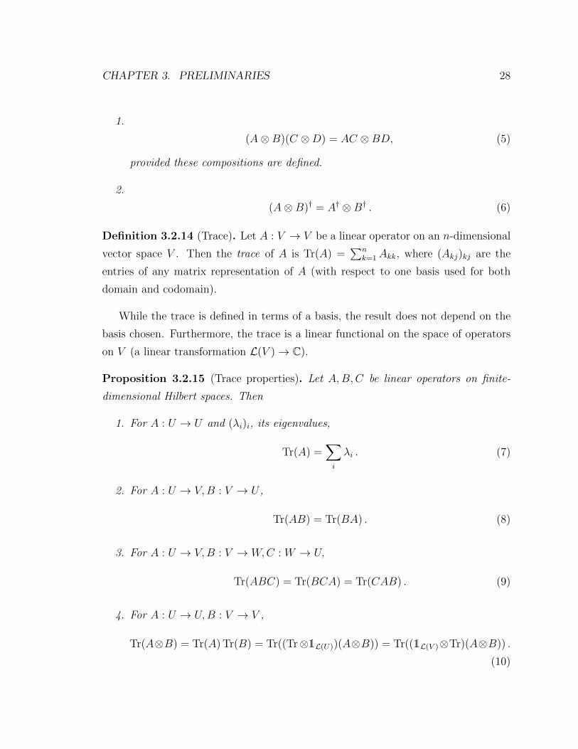
1.
(A⊗B)(C ⊗D) = AC ⊗BD, (5)
provided these compositions are defined.
2.
(A⊗B)† = A† ⊗B† . (6)
Definition 3.2.14 (Trace). Let A : V → V be a linear operator on an n-dimensional
vector space V . Then the trace of A is Tr(A) =∑n
k=1Akk, where (Akj)kj are the
entries of any matrix representation of A (with respect to one basis used for both
domain and codomain).
While the trace is defined in terms of a basis, the result does not depend on the
basis chosen. Furthermore, the trace is a linear functional on the space of operators
on V (a linear transformation L(V )→ C).
Proposition 3.2.15 (Trace properties). Let A,B,C be linear operators on finite-
dimensional Hilbert spaces. Then
1. For A : U → U and (λi)i, its eigenvalues,
Tr(A) =∑i
λi . (7)
2. For A : U → V,B : V → U ,
Tr(AB) = Tr(BA) . (8)
3. For A : U → V,B : V → W,C : W → U,
Tr(ABC) = Tr(BCA) = Tr(CAB) . (9)
4. For A : U → U,B : V → V ,
Tr(A⊗B) = Tr(A) Tr(B) = Tr((Tr⊗1L(U))(A⊗B)) = Tr((1L(V )⊗Tr)(A⊗B)) .
(10)

CHAPTER 3. PRELIMINARIES 29
5. For C : U ⊗ V → U ⊗ V ,
Tr(C) = Tr((Tr⊗1L(U))(C)) = Tr((1L(V ) ⊗ Tr)(C)) . (11)
6. For A : U → V,
‖A‖1 := Tr(√A†A) =
∑k
|Akk| (12)
defines a norm.
7. For A,B : U → V,
Tr(A†B) =∑kj
AkjBkj (13)
for any matrix representations (Akj)kj of A and (Bkj)kj of B with respect to a
common basis. This defines an inner product on L(U, V ).
The norm ‖·‖1 above is called the trace norm, and the corresponding metric when
multiplied by 12
is called the trace distance and is equal to the maximum probability
of distinguishing the two quantum states (see Proposition 3.8.5), as represented by
density operators (as defined in the next section).
Finally, normal operators on Hilbert spaces are diagonalizable by unitary oper-
ators. The result is one of the most important in linear algebra (and functional
analysis).
Theorem 3.2.16 (Spectral theorem). Let A be a normal operator on an n-dimensional
Hilbert space H, where n <∞. Then, the following hold:
1. There exists an othonormal basis for H of eigenvectors of H
2.
A =n∑i=1
λi |φi〉 〈φi| , (14)
where |φi〉 is the i-th eigenvector from 1, with corresponding eigenvalue λi, and
|φi〉 〈φi| is the orthogonal projection onto the subspace spanned by |φi〉.
CHAPTER 3. PRELIMINARIES 30
3.3 Quantum States
We are now ready to describe quantum states, as both vectors (pure states) in a
Hilbert space or density operators acting on them.
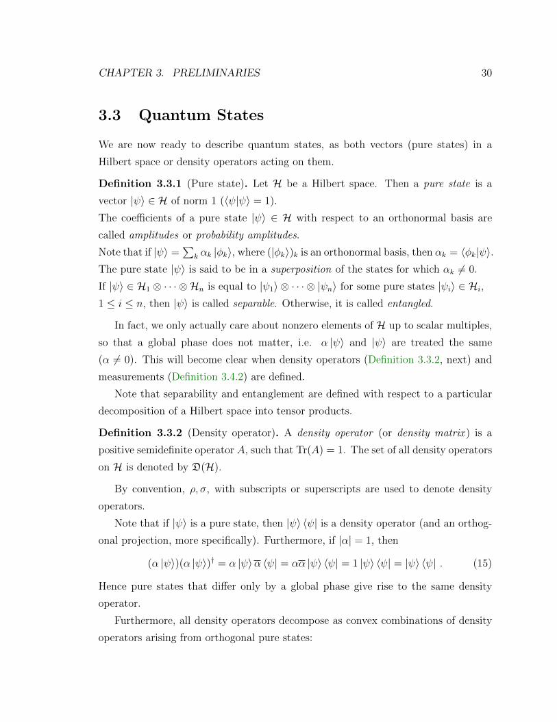
Definition 3.3.1 (Pure state). Let H be a Hilbert space. Then a pure state is a
vector |ψ〉 ∈ H of norm 1 (〈ψ|ψ〉 = 1).
The coefficients of a pure state |ψ〉 ∈ H with respect to an orthonormal basis are
called amplitudes or probability amplitudes.
Note that if |ψ〉 =∑
k αk |φk〉, where (|φk〉)k is an orthonormal basis, then αk = 〈φk|ψ〉.The pure state |ψ〉 is said to be in a superposition of the states for which αk 6= 0.
If |ψ〉 ∈ H1 ⊗ · · · ⊗ Hn is equal to |ψ1〉 ⊗ · · · ⊗ |ψn〉 for some pure states |ψi〉 ∈ Hi,
1 ≤ i ≤ n, then |ψ〉 is called separable. Otherwise, it is called entangled.
In fact, we only actually care about nonzero elements of H up to scalar multiples,
so that a global phase does not matter, i.e. α |ψ〉 and |ψ〉 are treated the same
(α 6= 0). This will become clear when density operators (Definition 3.3.2, next) and
measurements (Definition 3.4.2) are defined.
Note that separability and entanglement are defined with respect to a particular
decomposition of a Hilbert space into tensor products.
Definition 3.3.2 (Density operator). A density operator (or density matrix ) is a
positive semidefinite operator A, such that Tr(A) = 1. The set of all density operators
on H is denoted by D(H).
By convention, ρ, σ, with subscripts or superscripts are used to denote density
operators.
Note that if |ψ〉 is a pure state, then |ψ〉 〈ψ| is a density operator (and an orthog-
onal projection, more specifically). Furthermore, if |α| = 1, then
(α |ψ〉)(α |ψ〉)† = α |ψ〉α 〈ψ| = αα |ψ〉 〈ψ| = 1 |ψ〉 〈ψ| = |ψ〉 〈ψ| . (15)
Hence pure states that differ only by a global phase give rise to the same density
operator.
Furthermore, all density operators decompose as convex combinations of density
operators arising from orthogonal pure states:
CHAPTER 3. PRELIMINARIES 31
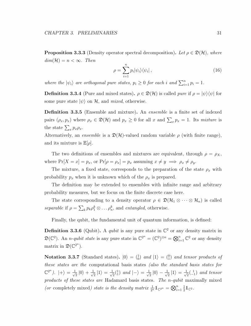
Proposition 3.3.3 (Density operator spectral decomposition). Let ρ ∈ D(H), where
dim(H) = n <∞. Then
ρ =n∑i=1
pi|ψi〉〈ψi| , (16)
where the |ψi〉 are orthogonal pure states, pi ≥ 0 for each i and∑n
i=1 pi = 1.
Definition 3.3.4 (Pure and mixed states). ρ ∈ D(H) is called pure if ρ = |ψ〉〈ψ| for
some pure state |ψ〉 on H, and mixed, otherwise.
Definition 3.3.5 (Ensemble and mixture). An ensemble is a finite set of indexed
pairs (ρx, px) where ρx ∈ D(H) and px ≥ 0 for all x and∑
x px = 1. Its mixture is
the state∑
x pxρx.
Alternatively, an ensemble is a D(H)-valued random variable ρ (with finite range),
and its mixture is E[ρ].
The two definitions of ensembles and mixtures are equivalent, through ρ = ρX ,
where Pr[X = x] = px, or Pr[ρ = ρx] = px assuming x 6= y =⇒ ρx 6= ρy.
The mixture, a fixed state, corresponds to the preparation of the state ρx with
probability px when it is unknown which of the ρx is prepared.
The definition may be extended to ensembles with infinite range and arbitrary
probability measures, but we focus on the finite discrete case here.
The state corresponding to a density operator ρ ∈ D(H1 ⊗ · · · ⊗ Hn) is called
separable if ρ =∑
k pkρk1 ⊗ . . . ρkn, and entangled, otherwise.
Finally, the qubit, the fundamental unit of quantum information, is defined:
Definition 3.3.6 (Qubit). A qubit is any pure state in C2 or any density matrix in
D(C2). An n-qubit state is any pure state in C2n = (C2)⊗n =⊗n
i=1 C2 or any density
matrix in D(C2n).
Notation 3.3.7 (Standard states). |0〉 = (10) and |1〉 = (01) and tensor products of
these states are the computational basis states (also the standard basis states for
C2n). |+〉 = 1√2|0〉 + 1√
2|1〉 = 1√
2(11) and |−〉 = 1√
2|0〉 − 1√
2|1〉 = 1√
2( 1−1) and tensor
products of these states are Hadamard basis states. The n-qubit maximally mixed
(or completely mixed) state is the density matrix 12n1C2n =
⊗ni=1
121C2.
CHAPTER 3. PRELIMINARIES 32
Note that 1d1H =
∑di=1
1d|ψi〉 〈ψi|, where (|ψi〉)di=1 is any orthonormal basis forH =
Cd, i.e. the maximally mixed state is the mixture of the states in any orthonormal
basis with equal probability each.
3.4 Admissible Maps
This section describes admissible maps, but before they are defined in their generality,
several elementary examples are introduced, from which are admissible maps can be
constructed by tensor products and compositions.
An important restriction on the physically realizable operations on quantum sys-
tems is the no-cloning theorem, ruling out the admissibility of an operation:
Theorem 3.4.1 (No-cloning theorem). [WZ82, Die82, KLM07] There is no unitary
U : H⊗H → H⊗H and pure state |φ〉 ∈ H such that for all pure states |ψ〉 ∈ H
U(|ψ〉 |φ〉) = eiα(ψ) |ψ〉 |ψ〉 (17)
for some α(ψ) ∈ R.
At the end of interactions with quantum data, when the information stored therin
is to be accessed and classical information, readable to humans, extracted, a mea-
surement must be performed:
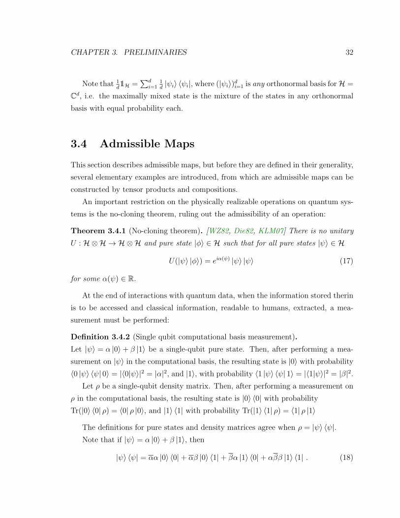
Definition 3.4.2 (Single qubit computational basis measurement).
Let |ψ〉 = α |0〉+ β |1〉 be a single-qubit pure state. Then, after performing a mea-
surement on |ψ〉 in the computational basis, the resulting state is |0〉 with probability
〈0 |ψ〉 〈ψ| 0〉 = |〈0|ψ〉|2 = |α|2, and |1〉, with probability 〈1 |ψ〉 〈ψ| 1〉 = |〈1|ψ〉|2 = |β|2.Let ρ be a single-qubit density matrix. Then, after performing a measurement on
ρ in the computational basis, the resulting state is |0〉 〈0| with probability
Tr(|0〉 〈0| ρ) = 〈0| ρ |0〉, and |1〉 〈1| with probability Tr(|1〉 〈1| ρ) = 〈1| ρ |1〉
The definitions for pure states and density matrices agree when ρ = |ψ〉 〈ψ|.Note that if |ψ〉 = α |0〉+ β |1〉, then
|ψ〉 〈ψ| = αα |0〉 〈0|+ αβ |0〉 〈1|+ βα |1〉 〈0|+ αββ |1〉 〈1| . (18)

CHAPTER 3. PRELIMINARIES 33
On the other hand, the mixture of the states after measuring is αα |0〉 〈0|+ ββ |1〉 〈1|,with no mixed terms. Furthermore, the state after measurement is not this mixture, it
is either |0〉 〈0| or |1〉 〈1|: measurement is not a deterministic function D(H)→ D(H).
Definition 3.4.3 (Partial measurement in the computational basis). Let |ψ〉 be an
n-qubit pure state. Suppose the i-th qubit is measured in the computational basis,
1 ≤ i ≤ n. Letting b = 0 or 1, and P = P1 ⊗ P2 ⊗ . . . Pn, where Pk = |b〉 〈b| if k = i,
and Pk = 1C2 , otherwise, then after performing the measurement, the resulting state
is 1‖P |ψ〉‖P |ψ〉, with probability ‖P |ψ〉 ‖2.If the state was instead given by the n-qubit density matrix ρ, the resulting state
after measurement is 1Tr(Pρ)
PρP , with probability Tr(Pρ).
For single qubits, this reduces to the previous definition.
Again, the pure state and density matrix definitions agree, noting that each P is
an orthogonal projection.
A partial measurement on n-qubits can be represented as a function from the
pure states in C2n to the random variable pure states in C2n , or from D(C2n)-valued
random variables, and as such, can be composed with other functions, including other
partial measurements.
Partial measurements in the computational basis commute, i.e. the order in which
such successive measurements are applied does not matter.
Note that∑
P P = 1.
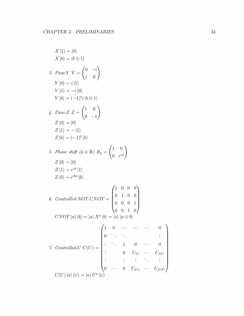
Notation 3.4.4 (Standard unitaries). The following are standard unitary operators:
1. Hadamard H =1√2
(1 1
1 −1
)H |0〉 = 1√
2|0〉+ 1√
2|1〉 = |+〉
H |1〉 = 1√2|0〉 − 1√
2|1〉 = |−〉
H |b〉 = 1√2|0〉+ (−1)b 1√
2|1〉
2. Pauli-X (or NOT gate) X =
(0 1
1 0
)X |0〉 = |1〉
CHAPTER 3. PRELIMINARIES 34
X |1〉 = |0〉X |b〉 = |b⊕ 1〉
3. Paui-Y Y =
(0 −ii 0
)Y |0〉 = i |1〉Y |1〉 = −i |0〉Y |b〉 = (−1)bi |b⊕ 1〉
4. Paui-Z Z =
(1 0
0 −1
)Z |0〉 = |0〉Z |1〉 = − |1〉Z |b〉 = (−1)b |b〉
5. Phase shift (φ ∈ R) Rφ =
(1 0
0 eiφ
)Z |0〉 = |0〉Z |1〉 = eiφ |1〉Z |b〉 = eibφ |b〉
6. Controlled-NOT CNOT =
1 0 0 0
0 1 0 0
0 0 0 1
0 0 1 0
CNOT |a〉 |b〉 = |a〉Xa |b〉 = |a〉 |a⊕ b〉
7. Controlled-U C(U) =
1 0 · · · · · · · · · 0
0. . . . . .
......
. . . 1 0 · · · 0... 0 U11 · · · U12n
......
.... . .
...
0 · · · 0 U2n1 · · · U2n2n
C(U) |a〉 |ψ〉 = |a〉Ua |ψ〉
CHAPTER 3. PRELIMINARIES 35
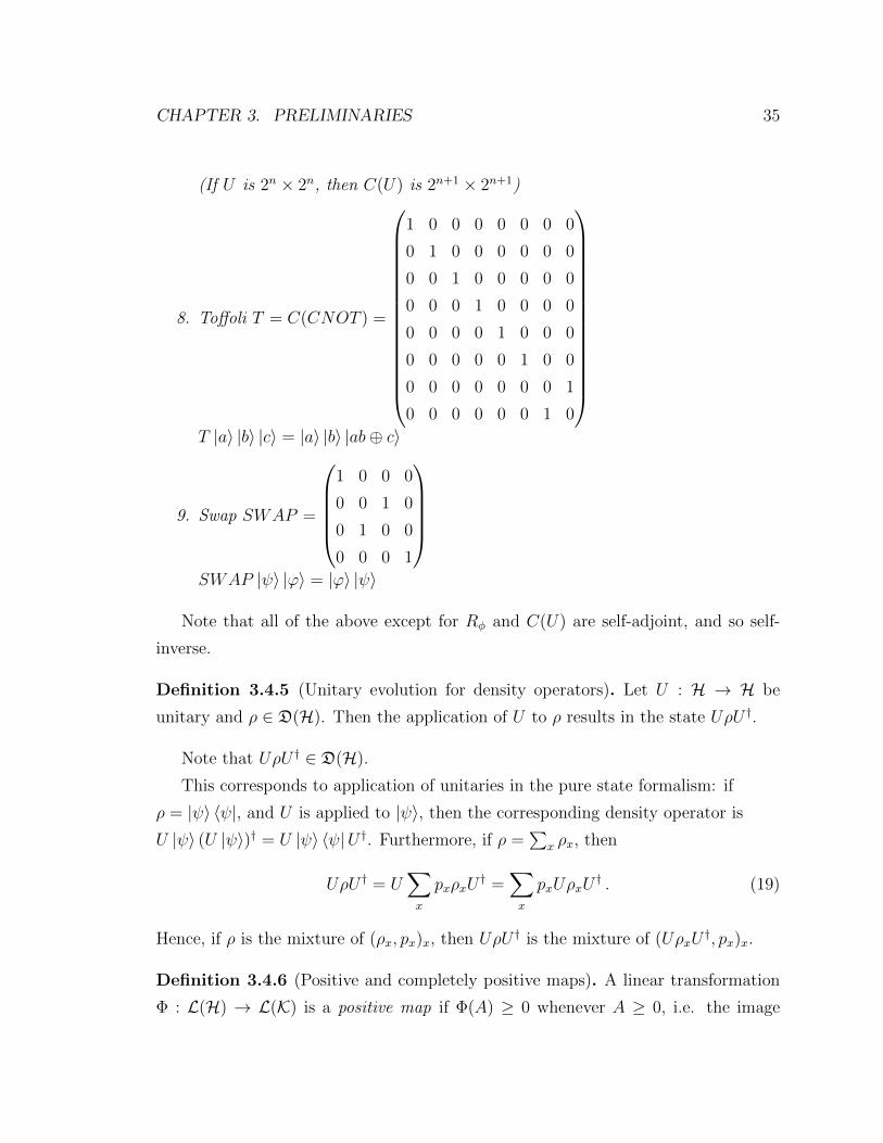
(If U is 2n × 2n, then C(U) is 2n+1 × 2n+1)
8. Toffoli T = C(CNOT ) =
1 0 0 0 0 0 0 0
0 1 0 0 0 0 0 0
0 0 1 0 0 0 0 0
0 0 0 1 0 0 0 0
0 0 0 0 1 0 0 0
0 0 0 0 0 1 0 0
0 0 0 0 0 0 0 1
0 0 0 0 0 0 1 0
T |a〉 |b〉 |c〉 = |a〉 |b〉 |ab⊕ c〉
9. Swap SWAP =
1 0 0 0
0 0 1 0
0 1 0 0
0 0 0 1
SWAP |ψ〉 |ϕ〉 = |ϕ〉 |ψ〉
Note that all of the above except for Rφ and C(U) are self-adjoint, and so self-
inverse.
Definition 3.4.5 (Unitary evolution for density operators). Let U : H → H be
unitary and ρ ∈ D(H). Then the application of U to ρ results in the state UρU †.
Note that UρU † ∈ D(H).
This corresponds to application of unitaries in the pure state formalism: if
ρ = |ψ〉 〈ψ|, and U is applied to |ψ〉, then the corresponding density operator is
U |ψ〉 (U |ψ〉)† = U |ψ〉 〈ψ|U †. Furthermore, if ρ =∑
x ρx, then
UρU † = U∑x
pxρxU† =
∑x
pxUρxU† . (19)
Hence, if ρ is the mixture of (ρx, px)x, then UρU † is the mixture of (UρxU†, px)x.
Definition 3.4.6 (Positive and completely positive maps). A linear transformation
Φ : L(H) → L(K) is a positive map if Φ(A) ≥ 0 whenever A ≥ 0, i.e. the image

CHAPTER 3. PRELIMINARIES 36
of a positive semidefinite operator is positive semidefinite. Φ is completely positive if
Φ⊗ 1L(Ck) is positive for all k ≥ 1.
Note that Φ⊗1L(C) is just Φ under a canonical isomorphism, since L(C) ' C and
1C = 1, multiplication by 1.
Definition 3.4.7 (Induced operator 1-norm). For a linear transformation Φ : X →Y , where X and Y are normed vector spaces, with norms ‖·‖X and ‖·‖Y , respectively,
its operator norm is defined by
‖Φ‖ := supx∈X,x 6=0
‖Φ(x)‖Y‖x‖X
= sup0<‖x‖X≤1
‖Φ(x)‖Y = sup‖x‖X=1
‖Φ(x)‖Y (20)
Positive maps are bounded in this norm (i.e. the operator norm is finite).
Furthermore, completely positive maps are completely bounded :
Definition 3.4.8 (Completely bounded). A linear transformation Φ : X → Y be-
tween normed vector spaces (X, ‖ · ‖X) and (Y, ‖ · ‖Y ) is completely bounded if
supk‖Φ⊗ 1L(Ck)‖ <∞ . (21)
Note that the norms on X ⊗ L(Ck) and Y ⊗ L(Ck) must first be chosen.
The completely bounded maps X → Y form a normed vector space, with the
diamond norm, which is defined in the obvious way:
Definition 3.4.9 (Diamond norm). The diamond norm (or norm of complete bound-
edness or cb-norm) of a completely bounded map Φ : X → Y is defined by
‖Φ‖ := supk‖Φ⊗ 1L(Ck)‖ . (22)
The diamond norm is used because it gives the maximum probability of distin-
guishing between two quantum channels (see Proposition 3.8.5 and Definition 3.8.6
in Section 3.8), which we now define:
Definition 3.4.10 (Quantum channel). A quantum channel is a completely positive
trace-preserving (CPTP) linear transformation L(H) → L(K), i.e. it is completely
positive and Tr(Φ(A)) = Tr(A) for all A ∈ L(H).
CHAPTER 3. PRELIMINARIES 37
If one restricts the domain of a quantum channel L(H) → L(K) to D(H), its
range will be in D(K). Hence, quantum channels send quantum states to quantum
states.
Notation 3.4.11 (Subscript notation). Given a Hilbert space H = HA ⊗HB where
HA and HB are also Hilbert spaces (subsystems or registers of H), the subscripts
A,B will often be used on states and quantum channels (and admissible maps, defined
shortly) to specify to which subsystem a channel applies. For example, if |ψ〉 ∈ H, then
|ψ〉AB or |ψ〉 〈ψ|AB may be written, and if ρ ∈ D(H), then ρAB may be written. Then,
for quantum channels F and G with domains D(HA) and D(HB), (FA⊗GB)ρAB may
be written. Furthermore, TrA := Tr⊗1HB, ρB := TrA(ρAB) (called a reduced density
operator) and 1B := 1HB. This notation will be used when the roles of A and B are
switched or when more subsystems and subscripts are used.
Examples of quantum channels include:
• U(·)U †, where U is unitary, as above,
• Tr ,
• C→ L(K) defined by α 7→ αρ, where ρ ∈ D(K) is fixed, and
• tensor products and (well-defined) compositions of the above.
In fact, all quantum channels can be obtained this way, and in a particular fac-
torized form:
Theorem 3.4.12 (Stinespring’s dilation theorem). [Sti55] Φ : L(H) → L(K) is a
quantum channel if and only if
Φ(A) = TrF (V (A⊗ |φ〉 〈φ|)V †) , (23)
for some unitary V : H ⊗ HE → K ⊗ HF , for some pure state |φ〉 ∈ HE, for all
A ∈ L(H).
CHAPTER 3. PRELIMINARIES 38
Furthermore, for every pair of representations, one can be embedded isometrically
into the other, so that minimal representations (those for which dimHE and dimHF
are minimized) are unique up unitaries.
Like the no-cloning theorem for unitaries (3.4.1), there is also a no-cloning theorem
for quantum channels:
Theorem 3.4.13 (No-cloning theorem (for quantum channels)). [WZ82, Die82,
KLM07] There is no quantum channel Φ : L(H) → L(H ⊗ H), where dimH ≥ 2,
such that for all ρ ∈ D(H),
Φ(ρ) = ρ⊗ ρ . (24)
Note that the above actually holds even for classical channels acting on density
matrices representing classical (probabilistic) states, by considering, for example, the
states |0〉 〈0| and |1〉 〈1|, and 12|0〉 〈0|+ 1
2|0〉 〈0| and using the linearity of the channel.
Next, we consider more general measurements.
Definition 3.4.14 (POVM and PVM measurements). A (finite) positive operator-
valued measure (POVM ) is a (finite) set (Ak)k of positive semidefinite operators
Ak : H → H, Ak such that∑
k Ak = 1H (so Ak ≤ 1H for all k).
A (finite) projection-valued measure (PVM ) is a POVM such that each operator Ak,
usually denoted instead by Pk, is an orthogonal projection.
A von Neumann measurement is a PVM such that Pk = |ψk〉 〈ψk|, where the |ψk〉form an orthonormal basis for H.
Given a pure state |ψ〉 ∈ H, measuring |ψ〉 with respect to the POVM (Ak)k results in
the state 1√〈ψ|Ak|ψ〉
Bk |ψ〉 with probability 〈ψ|Ak |ψ〉, where Bk satisfies B†kBk = Ak.
Given ρ ∈ D(H), measuring ρ with respect to the POVM (Ak)k results in the state1
Tr(Akρ)BkρB
†k with probability Tr(Akρ).
In the case of PVMs, Bk = Pk suffices, and in the case of von Neumann mea-
surements, the state becomes |ψk〉 〈ψk|. PVM measurements are also called projective
measurements.
These further generalize measurements in the computational basis. Note also that
the tensor product of a POVM (PVM) with the identity on any other space is again

CHAPTER 3. PRELIMINARIES 39
a POVM (PVM), and in the case of von Neumann measurements, this corresponds
to partial measurements.
For general POVMs, Bk :=√Ak’s can be computed by diagonalizing Ak = SDS†
where S is unitary (by the spectral theorem) and D is diagonal, and then setting
Bk = SD′S†, where D′ is obtained from D by taking the square root of each (diagonal)
entry. These entries are nonnegative, since Ak is positive semidefinite. Bk as defined
is positive semidefinite and
B†kBk = BkBk = (SD′S†)(SD′S†) = SD′D′S† = SDS† = Ak . (25)
By the spectral theorem, to any self-adjoint operator is associated a von Neumann
measurement, but, unless all eigenvalues have multiplicity 1, this measurement is not
unique.
Again, a POVM can be represented as a function from D(H) to D(H)-valued
random variables, and as such, can be composed with other functions, including
quantum channels and other POVMs.
By Naimark’s dilation theorem [Nai40], every POVM can be represented as a PVM
on a larger Hilbert space in the same way every quantum channel can be represented
as a unitary on a larger Hilbert space (by Stinespring’s dilation theorem). In general,
all POVMs can be implemented through unitaries, ancillae, the trace and partial
measurements in the computational basis (see [NC00, 2.2.8]).
Definition 3.4.15 (Admissible map). An admissible map is the (well-defined) com-
position of a finite sequence of quantum channels and POVMs.
We consider only admissible maps whose domain and codomain are qubits, i.e.
D(C2n)→ D(C2m).
Due to measurements, an admissible map’s output on a fixed input is, in general,
a random variable.
When admissible maps are composed only of by unitaries, α 7→ α |ψ〉 and POVMs,
it suffices to deal entirely with pure states. This is the pure state formalism. In this
thesis, the more general density matrix formalism is used.

CHAPTER 3. PRELIMINARIES 40
3.5 Quantum Circuits
Quantum circuits are admissible maps constructed from fixed set of admissible maps,
called a gate set.
Definition 3.5.1 (Gate set). A gate set is a set of admissible maps.
Definition 3.5.2 (Standard gate set). The standard gate set consists of the standard
unitaries (except SWAP and general C(U)), Tr : C2 → C, ancilla qubits C → C2
defined by α 7→ α |0〉 〈0| and single-qubit partial measurements in the computational
basis.
Measurement gate will be used to refer only to single-qubit partial measurements
in the computational basis.
Definition 3.5.3 (Quantum circuit). A quantum circuit is a directed acyclic graph
in which
• each edge is called a wire, representing a single qubit;
• each vertex which has no wires into it is labelled as one or multiple input or
ancilla qubits;
• each vertex which has no wires out of it is labelled as one or multiple output
qubits, or by one or multiple trace gates;
• every other vertex is labelled by a gate from a gate set representing an admissible
map L(C2n) → L(C2m), with n wires in and m wires out (if n = 0, there are
no wires in, and if m = 0, there are no wires out), and measurement gates,
specifically, have exactly the wires being measured in and out; and
• at the vertex, the wires into it are ordered (1 to n), and the wires out of it are
ordered (1 to m).
Single-qubit measurement gates correspond to partial measurements, and for other
gates with wires into them, the admissible map applied is actually the tensor product

CHAPTER 3. PRELIMINARIES 41
of the admissible map the gate represents with the identity on the subsystem corre-
sponding to the wires to which the gate does not apply and that are parallel to (that
have not ended in trace gates before) the gate. Wires crossing correspond to the
application of the SWAP gate (so the explicit use of the SWAP gate is unnecessary).
In circuit diagrams, the wires into a gate are ordered from top to bottom. Figure 1 is
an example of a quantum circuit; it implements the quantum teleportation of a single
qubit.
|ψ〉 • H •
A X •
B X Z |ψ〉|Φ〉+
Figure 1: Circuit for quantum teleportation.
In Figure 1,
• single lines represent qubits while double lines represent classical bits;
• |Φ〉+ = 1√2|00〉+ 1√
2|11〉, a Bell state, which is maximally entangled;
• the lines extending down from dots represent controlled operations; and
• the meter gates represent measurements in the computational basis.
For more complex circuits than that pictured in Figure 1, to condense pictorial
representations, multiple wires may be drawn as a single wire, labelling it instead by
the subsystem the wires represent, e.g. A and B, where the state is over HA ⊗HB,
where HA = C2n and HB = C2m . Multiple ancilla qubit gates may be combined, and
similarly, multiple trace gates may be combined. Whole circuits, used as subcircuits,
may be treated as gates.
CHAPTER 3. PRELIMINARIES 42
Definition 3.5.4 (Universal gate set). A gate set is called universal if every unitary
operator can be approximated arbitrarily (in any norm) by quantum circuits using
gates from the gate set.
The standard gate set is one such universal gate set. In fact, just the Toffoli and
the Hadamard (or any other gate which does not preserve the computational basis,
up to global phases) together form a universal gate set, noting that complex numbers
can be simulated with more qubits.
Definition 3.5.5 (Purification of a quantum circuit). Let A be a quantum circuit
composed only of ancilla qubit, trace and unitary gates (no measurement or more
general admissible maps). Then the purification of A is the circuit obtained by
replacing in A the ancilla gates with input and the trace gates with output.
The purification of a circuit implements a unitary operator.
3.6 Efficient Classical and Quantum Computations
This section is based on the section of the same name from the joint paper [ABF+16],
athough it largely rewritten for consistency with the rest of the preliminaries.
Turing machines are left formally undefined. It suffices to think of them as algo-
rithms or computer programs.
Note that classical Boolean circuits are analogous to quantum circuits; they are
instead (usually) composed of the standard AND, OR and NOT gates.
We will refer to several different notions of efficient algorithms. The most basic
of these is a deterministic polynomial-time algorithm (or PT).
Definition 3.6.1 (Polynomial-time algorithm (PT)). A polynomial-time algorithm
(or PT ) is a deterministic polynomial-time Turing machine A that on input n in
unary, prints a description of a classical Boolean circuit An that itself receives n bits.
For a binary string x, A(x) := A|x|(x) (overloading the notation).
A function family f : 0, 1n → 0, 1m is PT-computable if there exists a PT A such
that A(x) = f(x) for all x; it is implicit that m is a function of n which is bounded
by some polynomial, e.g., the same one that bounds the running time of A.

CHAPTER 3. PRELIMINARIES 43
Definition 3.6.2 (Probabilistic polynomial-time algorithm (PPT)). A probabilistic
polynomial-time algorithm (or PPT ) is a deterministic polynomial-time Turing ma-
chine A that on input n in unary, prints a description of a classical Boolean circuit
An that itself receives n bits of input, as well as an additional p(n) random bits. For
a PPT A, n-bit input x and p(n)-bit coin string r, A(x; r) := An(x; r). A(x) refers
to the random variable A(x; r) where r $←−0, 1p(n) and the corresponding probability
distribution.
Note that uniformity enforces that the function p is bounded by some polynomial.
Definition 3.6.3 (Quantum polynomial-time algorithm (QPT)). A quantum
polynomial-time algorithm (or QPT ) is a deterministic polynomial-time Turing ma-
chine A that on input n in unary, prints a description of a quantum circuit An,
composed of gates from a fixed finite (and usually universal) gate set, that itself re-
ceives n qubits. When ρ is an n-qubit state, A(ρ) denotes the corresponding output
state or the random variable over the possible output states. For n-bit strings x,
A(x) := A(|x〉〈x|). The expression A(x) = y for classical y is taken to evaluate to
true if the output register of the circuit contains the state |y〉〈y| exactly.
A commonly-used alternative is to specify that the elements of the gate set are
unitary. In terms of computational power, the models are the same [AKN98], however
using admissible operations (versus unitary ones only) allows us to formalize a wider
range of oracle-enabled QPT machines (see Subsection 3.6.1). In general, a QPT Adefines a family of admissible maps from input registers to output registers.Unless
explicitly stated, any statements about the probability of an event involving a QPT
are taken over the measurements of the QPT, in addition to any indicated random
variables. For instance, the expression Prx∈R0,1n [A(x) = y] means the probability
that, given a uniformly random input string x, the output register of the nth circuit of
the QPT A executed on |x〉〈x|, after all gates and measurements have been applied,
is in the state |y〉〈y|.At times, we will define QPTs with many input and output quantum registers.
In these cases, some straightforward bookkeeping (e.g., via an additional classical
CHAPTER 3. PRELIMINARIES 44
register) may be required; for the sake of clarity, we will simply assume that this has
been handled.
Throughout this work, we are concerned only with polynomial-time uniform com-
putation. That is to say, the circuit families that describe any PT, PPT, or QPT
will always be both of polynomial length and generatable by some fixed (classical)
deterministic polynomial-time Turing machine. In particular, we consider uniform ad-
versaries only—although all of our results carry over appropriately to the non-uniform
setting as well.
3.6.1 Oracles
Definition 3.6.4 (Oracles). For a function family f on binary strings (whose output
lengths depend only the input lengths, and one function fn for each n), Af denotes
an oracle PT, PPT or QPT whose gates come from a finite fixed set as well as gates
evaluating fn for the circuit An. In the case of QPTs, f may only be applied to
classical strings.
Also for QPTs, any family of admissible maps C is further allowed, denoted by, e.g.AC.The algorithms are said to have oracle access to f or C.Furthermore, the oracles may be indexed by strings rather than simply n to be used
in An. In this case, the particular gate An uses from the family will depend on an
external event, e.g. the generation of a key k, and the index will also be used to
denote the algorithm, so Afk or ACk will be written in this example.
The second definition for QPTs generalizes the first with a classical oracle, if it is
assumed that the queries are measured before the oracle is applied (this is sometimes
referred to as “standard-security” [Zha12]). We emphasize that we do not require
that the oracle is made reversible, nor do we allow the QPT to input superpositions.
While it might seem that disallowing superposition inputs is an artificial and unre-
alistic restriction, in our case it actually strengthens results. For instance, we will
show that secure quantum encryption can be achieved using pseudorandom functions
which are secure only against quantum adversaries possessing just classical oracle
access. One can of course also ask for more powerful functions (which are secure

CHAPTER 3. PRELIMINARIES 45
against superposition access, or “quantum-secure” [Zha12]) but this turns out to be
unnecessary in our case.
In any case, each use of an oracle gate counts towards the circuit length, and hence
also towards the total computation time of the algorithm. In particular, no PT, PPT
or QPT algorithm may make more than a polynomial number of oracle calls.
3.7 Negligible Functions
It is the norm in cryptography to allow small probabilities of “failure” that converge
quickly to 0 in a security parameter 1n, so that this probability can easily be made
arbitrarily small. This is captured by negligible functions. For references, see [Gol06,
KL07].
Definition 3.7.1 (Negligible Function). A function f : N→ R is called negligible if
for every positive polynomial p, there exists an N ∈ N such that for all n > N (or
for sufficiently large n),
f(n) <1
p(n). (26)
Note that we allow f to take on negative values in this definition, although it will
only be used for non-negative functions in this thesis.
Some examples of negligible functions are: 0,1
2n,−1,−2n,
1
(1.0000001)(log(n))2,
and 2n, if n<10100
2−n, otherwise .
We will often write negl(·) to denote a negligible function.
The following results are immediate from the definition:
Proposition 3.7.2 (Equivalent Definitions of Negligible Function).
1. f is negligible if and only if f(n) is O(n−c) for all c ≥ 0.
2. If f is positive for all sufficiently large n, then it is negligible if and only if1
f(n)
grows faster than any polynomial (i.e.1
f(n)is Ω(nc) for all c > 0).
CHAPTER 3. PRELIMINARIES 46
3. f is not negligible if and only if there exists a polynomial p such that f(n) ≥ 1
p(n)for infinitely many n.
Proposition 3.7.3 (Properties of Negligible Functions).
1. f negligible and non-negative (for all sufficiently large n)⇒ limn→∞ f(n) = 0.
2. f negligible ⇒ lim supn f(n) ≤ 0.
3. f(n) ≤ g(n) for all (sufficiently large) n, and g negligible ⇒ f negligible. In
particular, f = ming, h is negligible, for any h : N→ R.
4. f and g negligible ⇒ maxf, g and f + g negligible.
5. f negligible and g non-negative (for all sufficiently large n) and polynomially
bounded (e.g. constant) ⇒ g × f negligible.
Furthermore, since the product of a polynomially bounded function and a negli-
gible function is again negligible, any event that occurs with negligible probability,
even if repeated in polynomially many independent trials, will remain negligible:
Proposition 3.7.4. Let t be a positive and polynomially bounded integer-valued func-
tion, Xni , 1 ≤ i ≤ t(n) be independent events such that Pr[Xn
i ] = negl(n). Then
Pr[⋃t(n)i=1 X
ni ] is negligible.
Proof.
Pr[
t(n)⋃i=1
Xni ] ≤
t(n)∑i=1
Pr[Xni ] = t(n) negl(n) , (27)
which is, again, negligible.
3.8 Distinguishing Between States and Channels
In this section, we consider quantum circuits whose measurements are all in the
computational basis, and the probability that they can distinguish between distinct
quantum states.
CHAPTER 3. PRELIMINARIES 47
First, a useful result that allows quantum circuits with measurements to be rep-
resented as they were initially developed, as unitaries with all measurement occuring
at the end, is the principle of deferred measurement :
Proposition 3.8.1 (Principle of deferred measurement [NC00]). Every quantum cir-
cuit with measurement gates is equivalent to a quantum circuit in which all of the
measurement gates appear at the end of the circuit (possibly followed by trace gates).
Furthermore, every quantum algorithm is equivalent to a quantum algorithm in which
the measurements are at the end of each circuit.
Using this principle, quantum circuits whose wires all end in measurements gates,
correspond to POVMs:
Proposition 3.8.2 (Measurement circuits as POVMs). Consider a quantum cir-
cuit A with input from H, all of whose output is classical (so, without loss of gen-
erality, all wires end in either trace or measurement gates). Then there exists a
POVM (Ax)x∈0,1m over H, where m is the number of output wires, such that for all
ρ ∈ D(H), and all x ∈ 0, 1m,
Pr[A(ρ) = x] = Tr[Axρ] . (28)
Proof. By the principle of deferred measurement, without loss of generality, all mea-
surement gates appear at the end of the circuit, whether followed by trace gates or
not. Since all wires end in either measurement gates or trace gates, any measurement
gates that are followed by trace gates can be omitted. To see why, consider the state
|ψ〉 =∑
x,y αxy |x〉 |y〉, which is the state of the system before any measurement or
trace gates are applied, where the x subsystem is to be measured and kept, and the
y subsystem is to be traced out, and either (1) measured or (2) not measured before
the trace is applied.
In (1), after measuring the entire state, but before applying the trace, the state
becomes |x〉 |y〉 with probability |αxy|2, and then after applying the trace, it becomes
|x〉. The probability that |x〉 is obtained is the sum over the y’s of the probability of
measuring |x〉 |y〉, i.e.∑
y |αxy|2.

CHAPTER 3. PRELIMINARIES 48
In (2), after measuring only the x subsystem, the state becomes∑
y αxy |x〉 |y〉(normalized) with probability
∑y |αxy|2. Applying the trace to the y subsystem, the
state becomes just |x〉, and again, the probability that |x〉 is obtained is∑
y |αxy|2.Or, we could apply the partial trace first, obtaining the mixed state
∑x,y |αxy|2 |x〉 〈x|,
and |x〉 is again obtained by measurement with probability∑
y |αxy|2.Similarly, measurements of subsystems of the y subsystem are also equivalent.
Now, consider a purification A of A.
Let Bx = (〈x| ⊗ 1)A(1⊗ |0〉), where |0〉 is the ancillary qubits in A.
Then, let
Ax = B†xBx
= (1⊗ 〈0|)A†(|x〉 ⊗ 1)(〈x| ⊗ 1)A(1⊗ |0〉)
= (1⊗ 〈0|)A†(|x〉 〈x| ⊗ 1)A(1⊗ |0〉), (29)
so that Ax is positive semidefinite for each x, and

CHAPTER 3. PRELIMINARIES 49
∑x
Ax =∑x
(1⊗ 〈0|)A†(|x〉 〈x| ⊗ 1)A(1⊗ |0〉)
= (1⊗ 〈0|)A†∑x
(|x〉 〈x| ⊗ 1)A(1⊗ |0〉)
= (1⊗ 〈0|)A†(∑x
|x〉 〈x| ⊗ 1)A(1⊗ |0〉)
= (1⊗ 〈0|)A†(1⊗ 1)A(1⊗ |0〉)
= (1⊗ 〈0|)A†1A(1⊗ |0〉)
= (1⊗ 〈0|)A†A(1⊗ |0〉)
= (1⊗ 〈0|)1(1⊗ |0〉)
= (1⊗ 〈0|)(1⊗ |0〉)
= 1⊗ 〈0|0〉
= 1⊗ 1
= 1
(30)
Hence (Ax)x is a POVM. Finally,
Pr[A(ρ) = x] = 〈x| (1⊗ Tr)(A(ρ⊗ |0〉 〈0|)A†) |x〉 (trace before measurement)
= Tr(〈x| (1⊗ Tr)(A(ρ⊗ |0〉 〈0|)A†) |x〉)
= Tr((1⊗ Tr)(A(ρ⊗ |0〉 〈0|)A†) |x〉 〈x|)
= Tr(A(ρ⊗ |0〉 〈0|)A†) |x〉 〈x|)
= Tr(A† |x〉 〈x|A(ρ⊗ |0〉 〈0|)
= Tr(A† |x〉 〈x|A(1⊗ |0〉)ρ(1⊗ 〈0|))
= Tr((1⊗ 〈0|)A† |x〉 〈x|A(1⊗ |0〉)ρ)
= Tr[Axρ] (31)
CHAPTER 3. PRELIMINARIES 50
As POVMs, measurement statistics from quantum circuits depend only on the
mixture of an ensemble of quantum states, not the states individually:
Proposition 3.8.3. Let (ρx, px)x be an ensemble and ρ =∑
x pxρx be its mixture.
Let X be a random variable defined by Pr[X = x] = px. Then, for any quantum
circuit A with classical output, written as a POVM (Ai)i with A1 corresponding to an
output of 1,
Pr[ A(ρX) = 1 ] = Tr[A1ρ] = Pr[ A(ρ) = 1 ] , (32)
where the first probability is taken over X, and both probabilities are also taken
over any internal randomness in D.
Proof.
Pr[ A(ρX) = 1 ] =∑x
Pr[ A(ρX) = 1| X = x ]Pr[X = x]
=∑x
Tr[A1ρx]px
= Tr[A1
∑x
pxρx] by linearity of Tr and A1
= Tr[A1ρ] (33)
Although in this thesis we are only concerned with ensembles over finite index sets
of x with probabilities px, the above can be extended to arbitrary (ρ, PX) where PX
is a measure defined on a sigma algebra on X and ρ : X → D(H) is PX-integrable,
replacing the convex combinations with integrals.
Corollary 3.8.4. Ensembles with identical mixtures are indistinguishable.
Proof.∣∣Pr[ A(ρX) = 1 ]−Pr[ A(σY ) = 1 ]∣∣= ∣∣Tr[A1ρ]−Tr[A1σ]
∣∣= ∣∣Tr[A1(ρ−σ)]∣∣= 0 . (34)
CHAPTER 3. PRELIMINARIES 51
It is worth noting that the maximum difference in probability of distinguishing
between any pair of states (and hence pairs of ensembles, by linearity) is half of the
distance between them, in the 1-norm (see [NC00, Chapter 9]):
Proposition 3.8.5. Let ρ, σ ∈ D(H), then
max0≤A≤1H
Tr[A(ρ− σ)] = 12‖ρ− σ‖1 . (35)
The maximization can equivalently be taken over orthogonal projections only. The
maximum is achieved by some orthogonal projection P in either case.
Since quantum circuits built from a universal gate set and computational basis
measurements can approximate any unitary, they can approximate optimal measure-
ments. However, the size of the circuit may grow exponentially in the number of
qubits in the states.
Related to this is the diamond norm (Definition 3.4.9), which we extend here
to a metric between admissible maps. Following this proposition, it measures the
maximum probability of distinguishing between a pair of them (multiplied by 2).
Definition 3.8.6 (Diamond metric). The diamond metric, D(·, ·), is defined by, for
admissible maps Φ1,Φ2 : D(HM)→ D(HN), by
D(Φ1,Φ2) := supHE ,ρME∈D(HM⊗HE)
E[‖(Φ1 ⊗ 1E)ρME − (Φ2 ⊗ 1E)ρME‖1] , (36)
where the expected value is taken over the internal randomness of Φ1 and Φ2 (and is
equivalent to taking the 1-norm of the difference of mixtures of their outputs).
Note that the supremum is taken over density operators only.
3.8.1 The Quantum One-time Pad
This subsection is from the joint paper [ABF+16].
It is easy to check that applying a uniformly random Pauli operator to any single-
qubit density operator results in the maximally mixed state:
1
4(ρ+XρX + Y ρY + ZρZ) =
11
2, for all ρ ∈ D(H1) . (37)

CHAPTER 3. PRELIMINARIES 52
Since the Pauli operators are self-adjoint, we may implement the above map by
choosing two bits s and t uniformly at random and then applying
ρ 7→ XsZtρZtXs .
To observers with no knowledge of s and t, the resulting state is information-theoretically
indistinguishable from 11/2. Of course, if we know s and t, we can invert the above
map and recover ρ completely.
The above map can be straightforwardly extended to the n-qubit case in order to
obtain an elementary quantum encryption scheme called the quantum one-time pad.
We first set Xj = 1⊗j−1⊗X⊗1⊗n−j and likewise for Yj and Zj. We define the n-qubit
Pauli group Pn to be the subgroup of SU(C2n) generated by Xj, Yj, Zj : j = 1, . . . , n.Note that Hermiticity is inherited from the single-qubit case, i.e. P † = P for every
P ∈ Pn.
Definition 3.8.7. [Quantum one-time pad] For r ∈ 0, 12n, we define the quantum
one-time pad (QOTP) on n qubits with classical key r to be the map:
Pr :=n∏j=1
Xr2j−1
j Zr2jj ∈ Pn .
The effect of Pr on any quantum state ρ ∈ D(C2n) is simply
1
22n
∑r∈0,12n
PrρPr =1n
2n. (38)
As before, the map ρ 7→ PrρPr (for uniformly random key r) is an information-
theoretically secure symmetric-key encryption scheme for quantum states.
Just as in the classical case [Sha49], any reduction in key length is not possible
without compromising information-theoretic security [AMTdW00, BR03]. Of course,
in practice the key length of the one-time pad (quantumly or classically) is highly
impractical. This is a crucial reason to consider—as we do in this work—encryption
schemes which are secure only against computationally bounded adversaries.

CHAPTER 3. PRELIMINARIES 53
3.8.2 Computational Indistinguishability
An important notion in modern cryptography is that of computational indistinguisha-
bility. Ciphertext indistinguishability (see Definition 3.9.4 and Definition 4.1.3), defin-
ing the security of encryption, is a special case. Computational indistinguishability
applies to sequential ensembles:
Definition 3.8.8 (Sequential ensemble). A sequential ensemble is a sequence of en-
sembles of quantum states, (ρn)∞n=1 (where ρn is taken to be a random variable).
Often, such a sequential ensemble will simply be referred to as an ensemble, and
denoted by (ρn)n or simply ρn.
Definition 3.8.9 (Computational indistinguishability). Two sequential ensembles
(ρn)n and (σn)n are computationally indistinguishable if for every QPT D,
|Pr[D(ρn) = 1]− Pr[D(σn) = 1]| ≤ negl(n) , (39)
where the probabilities are taken over the randomness inherent in ρn and σn as
ensembles as well as any internal randomness in D.
Typically, the number of registers (size or length) in the ensembles making up a
sequential ensemble is polynomially bounded in n, and we assume that their sizes are
also at least linear in n, since otherwise we include 1n as input to D. This ensures
that D’s running time is polynomial in n, not the sizes of the states. Usually, also,
the ensembles will be generated by a QPTs.
By Proposition 3.8.3, it suffices to consider the mixtures of the ensembles instead
of the ensembles themselves.
Note also that computational indistinguishability forms an equivalence relation,
i.e. each ensemble is computationally indistinguishable from itself (reflexivity), com-
putational indistinguishability is symmetric, and it is transitive (by the triangle in-
equality and since the sum of two negligible functions is negligible). Furthermore,
the resulting ensembles from the application of a QPT to a pair of computationally
indistinguishable ensembles are again computationally indistinguishable, since the
composition of the QPT and any QPT distinguisher is a QPT distinguisher acting
on the original pair.
CHAPTER 3. PRELIMINARIES 54
3.9 Modern Cryptography
The modern cryptography definitions and results whose quantum analogues are con-
tained in this thesis are given in this section. See [Gol04] for a reference, although
the definition of semantic security has been simplified here.
First, we define encryption schemes, both in the private- and public-key settings.
These definitions can be relaxed in various ways.
Definition 3.9.1. A symmetric-key encryption scheme or private-key encryption
scheme or SKE is a triple of PPTs (KeyGen,Enc,Dec) such that Dec(k, (Enc(k,m)) =
m for all keys k ∈ suppKeyGen(1n) and messages m ∈ 0, 1∗. We write Enck =
Enc(k, ·) and Deck = Dec(k, ·). c = Enck(m) is called a ciphertext (corresponding to
m)
Definition 3.9.2. A public-key encryption scheme or PKE is a triple of PPTs
(KeyGen,Enc,Dec) such that Dec(sk, (Enc(pk,m)) = m for all (pk, sk) ∈ suppKeyGen(1n)
and m ∈ 0, 1∗. We write Encpk = Enc(pk, ·) and Decsk = Dec(sk, ·). pk is called the
public key and sk, the secret key (or private key).
The security of an encryption scheme is captured by the equivalent definitions of
semantic security and ciphertext indistinguishability. It may also be defined under
chosen plaintext attack (CPA), non-adaptive chosen ciphertext attack (CPA1) or
adaptive chosen ciphertext attack (CPA2)
Definition 3.9.3 (Semantic Security). A public-key encryption scheme (KeyGen,Enc,Dec)
is semantically secure if for any PPT adversary A, there exists a PPT simulator Ssuch that for any PPT M and PT f 1,
Pr[A(Encpk(m), σ) = fpk(m)
]− Pr
[S(σ) = fpk(m)
]≤ negl(n) , (40)
where (m,σ)←M(pk),2 and the probabilities are taken over (pk, sk)← KeyGen(1n)
and the internal randomness of Enc, A and S.
1Originally, f was any family of functions, not just PT [GM84].2Originally, there was no σ [GM84].

CHAPTER 3. PRELIMINARIES 55
• SEM-CPA: In addition to the above,M,A and S have oracle access to Encpk.
• SEM-CCA1: In addition to SEM-CPA, M has oracle access to Decsk.
• SEM-CCA2: In addition to SEM-CCA1, A and S have oracle access to Decsk
but cannot apply it to the challenge ciphertext Encpk(m).
In [Gol04], A and S are also given access to hpk(m), for some efficiently computable
h, representing partial side information, and security must hold for all such h, but
this can simply be captured with σ.
Definition 3.9.4 (Ciphertext Indistinguishability). A public-key encryption scheme
(KeyGen,Enc,Dec) has indistinguishable encryptions if for every PPT adversary
A = (M,D) we have:∣∣Pr[D(Encpk(m), σ) = 1
]− Pr
[D(Encpk(0
|m|), σ) = 1]∣∣ ≤ negl(n) , (41)
where (m,σ)←M(pk),2 and the probabilities are taken over (pk, sk)← KeyGen(1n)
and the internal randomness of Enc, M, and D.
• IND-CPA: In addition to the above, M and D have oracle access to Encpk.
• IND-CCA1: In addition to IND-CPA, M has oracle access to Decsk.
• IND-CCA2: In addition to IND-CCA1, D has oracle access to Decsk but
cannot apply it to the challenge ciphertext Encpk(m).
Note that a secure public-key encryption scheme must be CPA-secure, as oracle
calls can be implemented directly with access to Enc and pk. Security in the private-
key setting is defined similarly, but with M receiving the security parameter 1n
instead of pk.
Goldwasser and Micali famously proved in [GM84] that indistinguishability im-
plied semantic security (the converse, which is relatively easy to show, was left out):
Theorem 3.9.5. An encryption scheme is semantically secure if and only if it has
indistinguishable encryptions.

CHAPTER 3. PRELIMINARIES 56
Their equivalence holds for corresponding scenarios only, i.e. in the private- or
public-key setting, and under regular attacks, CPA, CCA1 or CCA2. The security
definitions can also be extended to the encryption of multiple messages with the
same key, so that multiple-message SEM and IND are equivalent to one another.
Furthermore, IND-CPA implies multiple message IND-CPA.
Secure encryption schemes are often constructed using cryptographic primitives,
in particular, one-way functions, trapdoor one-way permutations, pseudorandom gen-
erators and pseudorandom functions.
First, a one-way function is an efficiently computable function that is difficult for
PPTs to invert on random inputs.
Definition 3.9.6. A PT-computable function f : 0, 1∗ → 0, 1∗ is a one-way
function (OWF) if for every PPT A,
Prx
$←−0,1n[A(f(x), 1n) ∈ f−1(f(x))] ≤ negl(n) . (42)
A trapdoor one-way permutation is an (efficiently) indexed family of one-way
permutations (injective one-way functions that preserve the lengths of their inputs)
that are easy to invert given a string, called the trapdoor.
Definition 3.9.7. A trapdoor one-way permutation (TOWP) is a PT-computable
collection
f = fi : Di → Dii∈I
of permutations on sets Di ⊆ 0, 1l(i), i ∈ I, for some (infinite) set I of strings, and
a PT-computable function l : N→ N, together with a triple of PPTs (G,S, I) which
1. (generate (index, trapdoor) pair) supp G(1n) ⊆ (I ∩ 0, 1n)× 0, 1n;
2. (sample from domain) for all i ∈ I, supp S(i) = Di;
3. (invert using trapdoor) for all (i, t) ∈ supp G(1n) and all x ∈ Di, I(fi(x), t) = x,
such that for every PPT A,
Pr(i,t)←G(1n),x←S(i)
[A(fi(x), i) = x] ≤ negl(n) . (43)

CHAPTER 3. PRELIMINARIES 57
A hard-core of a one-way function f is a predicate whose value on a random x is
infeasible to guess with probability non-negligibly better than 12, even given access to
f(x):
Definition 3.9.8. A PT-computable b : 0, 1∗ → 0, 1 is a hard-core of a OWF f
if for every PPT A,
Prx
$←−0,1n[A(f(x), 1n) = b(x)] ≤ 1
2+ negl(n) . (44)
The definition of hard-core may also be modified in the case of trapdoor one-way
functions or permutations in the obvious way, by indexing f and b by i, generating
x← S(i), where (i, t)← G(1n), and giving A access to i in place of 1n.
Definition 3.9.9. A hard-core of a TOWP (f,G,S, I) is a PT-computable collection
b = bi : Di → 0, 1i∈I such that for every PPT A,
Pr(i,t)←G(1n),x←S(i)
[A(fi(x), i) = bi(x)] ≤ 1
2+ negl(n) . (45)
Theorem 3.9.10 (Goldreich-Levin Theorem). [Gol06] If OWFs (or TOWPs) exist,
then OWFs (or TOWPs, respectively) with hard-cores exist.
Next is the pseudorandom generator, which expands a uniformly random seed to
an output that is computationally indistinguishable from a longer uniformly random
string, hence “pseudorandom”.
Definition 3.9.11. A PT-computable function G : 0, 1∗ → 0, 1∗ is a pseudo-
random generator (PRG) if |G(s)| = p(|s|) for all s ∈ 0, 1∗ and for every PPT
D, ∣∣∣∣∣ Prs
$←−0,1n[D(G(s)) = 1] − Pr
y$←−0,1p(n)
[D(y) = 1]
∣∣∣∣∣ ≤ negl(n) . (46)
Note that p must necessarily itself be PT-computable, and hence polynomially
bounded.
Pseudorandom generators can be constructed from one-way functions [HILL99] or
more easily from trapdoor one-way permutations with hard-cores [Gol06].
CHAPTER 3. PRELIMINARIES 58
A pseudorandom function is an efficiently computable family of functions which
are indistinguishable from perfectly random functions, even when allowed to query
an oracle for the given function polynomially many times.
Definition 3.9.12. A PT-computable function family
f = f (n) : 0, 1n × 0, 1p(n) → 0, 1`(n)n∈N ,
with p, ` : N→ N PT-computable, is a pseudorandom function (PRF) if for every
PPT D equipped with an oracle,∣∣∣∣∣ Prk
$←−0,1n[Dfk(1n) = 1] − Pr
g$←−0,1p(n)→0,1`(n)
[Dg(1n) = 1]
∣∣∣∣∣ ≤ negl(n) , (47)
where fk := f (n)(k, ·) : 0, 1p(n) → 0, 1`(n) for k ∈ 0, 1n.
Pseudorandom functions can be constructed from pseudorandom generators [GGM86].
Hence, combining the two results,
Theorem 3.9.13. If one-way functions exist, then pseudorandom functions exist.
Finally, pseudorandom functions and trapdoor one-way permutations with hard-
cores can be used to construct secure private-key and public-key encryption schemes,
respectively. Hence,
Theorem 3.9.14. If one-way functions exist, then so do IND-CCA1-secure private-
key encryption schemes.
Theorem 3.9.15. If trapdoor one-way permutations exist, then so do semantically
secure public-key quantum encryption schemes.
Chapter 4
Computational Security of
Quantum Encryption
This chapter is taken from the joint paper [ABF+16].
4.1 Quantum Encryption and Indistinguishability
In this section, we give general definitions of encryption schemes for quantum data
(Section 4.1.1) and a corresponding notion of indistinguishability, including IND-CPA
and IND-CCA1 (Section 4.1.2.)
The definitions of quantum encryption schemes Definitions 4.1.1 and 4.1.2 in Sub-
section 4.1.1, have been modified slightly from the original paper [ABF+16] for this
thesis.
4.1.1 Quantum Encryption Schemes
We start by defining symmetric-key encryption for quantum data. In the following
we assume that the secret key is a classical bitstring, while the plaintext and the
ciphertext can be arbitrary quantum states.
We refer to K as the key space and we assume that K := 0, 1∗. The key-
generation algorithm, KeyGen, accepts a description of the security parameter n in
59
CHAPTER 4. COMP. SECURITY OF QUANTUM ENCRYPTION 60
unary (i.e. 1n) and outputs a classical key of length n. We let HM,n and HC,n
denote the message (or plaintext) and ciphertext spaces for the security parameter
1n, respectively. We remark that these are potentially infinite families of spaces, i.e.
HM,n = H(i)M,ni and HC,n = H(i)
C,ni, and we thus define D(HM,n) =⋃iD(H(i)
M,n)
and D(HC,n) =⋃iD(H(i)
C,n)
Encryption, Enc, accepts a classical key and a plaintext, and outputs a ciphertext;
decryption, Dec, accepts a classical key and a ciphertext, and outputs a plaintext. We
assume that the encryption and decryption algorithms output a fixed state denoting
failure on input states not from the correct plaintext or ciphertext spaces, respectively.
The correctness guarantee is that plaintexts are preserved under encryption followed
by decryption under the same key.
Definition 4.1.1. A quantum symmetric-key encryption scheme or quantum private-
key encryption scheme or qSKE is a triple of QPTs:
1. (key generation) KeyGen : 1n 7→ k ∈ K
2. (encryption with k ∈ suppKeyGen(1n))
Enck := Enc(k, ·) : D(HM,n)→ D(HC,n)
3. (decryption with k ∈ suppKeyGen(1n))
Deck := Dec(k, ·) : D(HC,n)→ D(HM,n)
such that for all k ∈ suppKeyGen(1n),
Deck Enck = 1M,n (48)
In order to further simplify notation, the subscript n will be dropped from the
spaces, i.e. we write HM instead of HM,n, 1M instead of 1M,n, and CM instead of
CM,n. Later, we will define additional Hilbert spaces (or families of Hilbert spaces)
HE and HF in order to model auxiliary information used by some adversary, and
again these implicitly depend on the input the adversaries receive.
CHAPTER 4. COMP. SECURITY OF QUANTUM ENCRYPTION 61
Next, we define a notion of public-key encryption for quantum data. In addition
to the usual spaces from the symmetric-key setting above, we now also have a pub-
lic key of polynomially bounded length. We define the related public-key space as
Kpub ⊆ 0, 1∗ and reuse K for the corresponding private-key space, whose length is
also polynomially bounded, noting that in this case, neither need be the entirety of
0, 1∗. Furthermore, rather than depending simply on n, the message (or plaintext)
and ciphertext spaces may in general depend upon the public key pk, i.e. we write
HM,pk and HC,pk. Again, we will later drop the pk subscripts, but the definition is
presented below with it for clarity.
Definition 4.1.2. A quantum public-key encryption scheme or qPKE is a triple of
QPTs:
1. (key-pair generation) KeyGen : 1n 7→ (pk, sk) ∈ Kpub ×K
2. (encryption with public key pk ∈ Kpub, (pk, sk) ∈ suppKeyGen(1n))
Encpk := Enc(pk, ·) : D(HM,pk)→ D(HC,pk)
3. (decryption with private key sk ∈ K, (pk, sk) ∈ suppKeyGen(1n))
Decsk := Dec(sk, ·) : D(HC,pk)→ D(HM,pk)
such that for all (pk, sk) ∈ suppKeyGen(1n),
Decsk Encpk = 1M,pk (49)
Remarks Some variations on the above two definitions are also possible. For in-
stance, one could restrict the messages spaces to particular subsets of the density
operators on Hilbert spaces. In the paper [ABF+16], a uniform diamond metric (Def-
inition 3.8.6) relaxation is used in both definitions for (48) and (49), and only exact
decryption was noted as an alternative. That is, we would only require
D(Decsk Encpk,1M) ≤ negl(n), (50)
CHAPTER 4. COMP. SECURITY OF QUANTUM ENCRYPTION 62
uniformly in the key-pairs (pk, sk) ∈ suppKeyGen(1n). This allows errors in encryp-
tion and decryption with negligible probability for each pair of keys. One can weaken
the condition further to
E[‖(Deck Enck ⊗ 1E)(ρME)− ρME‖1] ≤ negl(n) , (51)
for all HE and ρME ∈ HM ⊗HE, where the expected value is taken over
(pk, sk)← KeyGen(1n) and the internal randomness of Encpk and Decsk. This even
allows a negligible probability of choosing keys for which large errors are consistently
obtained. An even weaker constraint could be a computational one, along the lines
of computational indistinguishability.
4.1.2 Indistinguishability of Encryptions
Following the classical definition, the security notion of quantum indistinguishability
under chosen plaintext attacks has been considered previously for the case of quantum
encryption schemes in [BJ15] and for classical encryption schemes in [GHS15]. Here,
we extend the definition of [BJ15] to the CCA1 (chosen ciphertext attack) setting.
The security definitions are formulated with the public-key (or asymmetric-key) set-
ting in mind, and we clarify when meaningful differences in the symmetric-key setting
arise.
Our definition models a situation in which an honest user encrypts messages of
the adversary’s choice; the adversary then attempts to match the ciphertexts to the
plaintexts. In our formulation, an IND adversary A = (M,D) consists of two QPTs:
the message generator,M, and the distinguisher, D. The message generator takes as
input the security parameter and a public key, and outputs a challenge state consisting
of a plaintext and some auxiliary information. The auxiliary information models, for
instance, the fact that the output state might be entangled with some internal state
of the adversary itself. Then the distinguisher receives this auxiliary information,
and a state which might be either the encryption of the original challenge state or the
encryption of the zero state. The distinguisher’s goal is to decide which of the two is
the case.
CHAPTER 4. COMP. SECURITY OF QUANTUM ENCRYPTION 63
Security in this model requires that the adversary does not succeed with proba-
bility significantly better than guessing. We also define two standard variants: in-
distinguishability under chosen plaintext attack (IND-CPA) and indistinguishability
under chosen ciphertext attack (IND-CCA1). We leave the definition of CCA2 (adap-
tive chosen ciphertext attack) security as an interesting open problem. As before, all
circuits are indexed by the security parameter.
Definition 4.1.3 (IND). A qPKE scheme (KeyGen,Enc,Dec) has indistinguishable
encryptions (or is IND secure) if for every QPT adversary A = (M,D) we have:∣∣Pr[D(Encpk ⊗ 1E)ρME = 1
]−Pr
[D(Encpk ⊗ 1E)(|0〉 〈0|M ⊗ ρE) = 1
]∣∣ ≤ negl(n) ,(52)
where ρME ←M(pk), ρE = TrM(ρME), and the probabilities are taken over
(pk, sk)← KeyGen(1n) and the internal randomness of Enc, M, and D.
• IND-CPA: In addition to the above, M and D have oracle access to Encpk.
• IND-CCA1: In addition to IND-CPA, M has oracle access to Decsk.
Here we use |0〉 〈0|M to denote |0m〉 〈0m|, where m is the number of qubits in the
M register.
The definition is illustrated in Figure 2. The symmetric-key scenario is the same,
except pk = sk, and M receives only a blank input. We remark that in the public-
key setting, IND implies IND-CPA: an adversary with knowledge of pk can easily
simulate the Encpk oracle. Note that, under CPA, the IND definition is known to be
equivalent to IND in the multiple-message scenario [BJ15]. Section 6.2 contains the
details.
4.2 Quantum Semantic Security
This section is devoted to defining quantum semantic security (Section 4.2.2), and
showing its equivalence with quantum indistinguishability (Section 4.2.3).
Following the classical definition, the security notion of quantum semantic security
under chosen plaintext attacks has been given previously in [GHS15] for the case

CHAPTER 4. COMP. SECURITY OF QUANTUM ENCRYPTION 64
pk MEncpk
DM
E
pk M|0〉 Encpk
DM
E
Figure 2: IND posits that a QPT (M,D) cannot distinguish between these two
scenarios.
of a special class of quantum states arising when considering quantum access to
classical encryption schemes. Here, we give a more general definition for arbitrary
quantum plaintexts. As we outlined the classical situation with semantic security in
Section 1.2.1, we start with a discussion of some difficulties in transitioning to the
quantum setting. A similar discussion can be found in [GHS15] and we explain below
where and why we make different choices.
4.2.1 Difficulties in the Quantum Setting
When attempting to transfer the definition of semantic security to the quantum world,
the main question one encounters is to determine the quantum equivalents of σ and
f(m) (as it is relatively clear that the plaintext m would have as quantum equivalent
a quantum state ρM , in a message register, M).
For the case of the side-information, σ, one might attempt to postulate that this
side information is available via the output of a quantum map Φh, evaluated on ρM .
There are, however, two obvious problems with this approach: firstly, it is unclear
how to simultaneously generate both ρM and Φh(ρM) (the main obstacle stemming
from the quantum no-cloning theorem [WZ82], according to which it is not possible
to perfectly copy an unknown quantum state)1. Secondly, it is well-established that
1[GHS15] solves the issue by essentially requiring that the quantum circuits generating messagesuse no measurement gates, but instead output random states by taking random classical strings asinput. Hence, multiple plaintext states can be generated by using the same string.
CHAPTER 4. COMP. SECURITY OF QUANTUM ENCRYPTION 65
the most general type of quantum side-information includes entanglement (contrary
to the scenario studied in [GHS15]). We therefore conclude that side information
should be modelled simply as an extra register (called E) such that ρME are in an
arbitrary quantum state (as generated by some process—for a formal description, see
Definition 4.2.1).
For the case of the target function f , one might also postulate a quantum map Φf ,
the goal then (for both the adversary and simulator), being to output Φf (ρM). How-
ever, given that quantum states and maps form a continuum, one must exercise care
in quantifying when a simulator has successfully simulated the adversary. We pro-
pose three possible tests for quantifying “success” in the semantic security game, each
leading to its own definition. Since we show that all three definitions are equivalent,
we conclude that it is a matter of taste (or context) which definition to label as the
definition of quantum semantic security. We focus in this section on the first one,
which we called SEM, because we find it the most natural. We give formal definitions
and proofs of equivalence for all three definitions in Appendix 4.4. Here is an overview
of the three different notions:
• SEM. In Definition 4.2.1, a state ρMEF is generated; intuitively, the contents of
register F can be seen as a “target” output that the adversary tries to achieve
(however, this is not quite the case as we point out shortly). We then postulate a
quantum polynomial time distinguisher who is given the F register and charged
with distinguishing the output of the adversary from the output of the simulator,
with security being associated with the inability of the distinguisher in telling
the two situations apart. We thus see that the role of register F is actually to
assist the distinguisher: semantic security corresponds to the situation where
the distinguisher essentially cannot tell the real from ideal apart, even with
access to the F system.
• SEM2. In Definition 4.4.2, we specify instead that the state ρMEF be a
classical-quantum state. That is, ρME is quantum, but the register F contains
a classical pure state, and hence ρMEF = ρME⊗ρF , with ρF corresponding to a
binary string. The requirement for security is that the simulator should provide
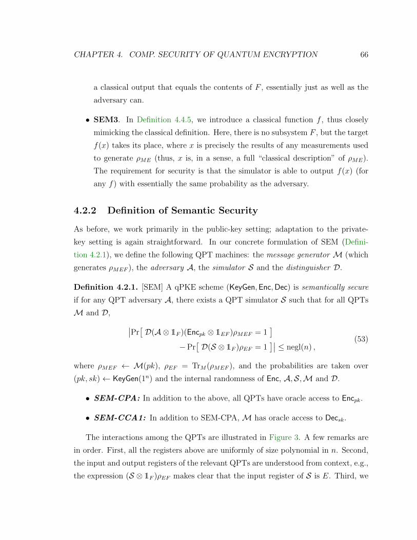
CHAPTER 4. COMP. SECURITY OF QUANTUM ENCRYPTION 66
a classical output that equals the contents of F , essentially just as well as the
adversary can.
• SEM3. In Definition 4.4.5, we introduce a classical function f , thus closely
mimicking the classical definition. Here, there is no subsystem F , but the target
f(x) takes its place, where x is precisely the results of any measurements used
to generate ρME (thus, x is, in a sense, a full “classical description” of ρME).
The requirement for security is that the simulator is able to output f(x) (for
any f) with essentially the same probability as the adversary.
4.2.2 Definition of Semantic Security
As before, we work primarily in the public-key setting; adaptation to the private-
key setting is again straightforward. In our concrete formulation of SEM (Defini-
tion 4.2.1), we define the following QPT machines: the message generator M (which
generates ρMEF ), the adversary A, the simulator S and the distinguisher D.
Definition 4.2.1. [SEM] A qPKE scheme (KeyGen,Enc,Dec) is semantically secure
if for any QPT adversary A, there exists a QPT simulator S such that for all QPTs
M and D, ∣∣Pr[D(A⊗ 1F )(Encpk ⊗ 1EF )ρMEF = 1
]−Pr
[D(S ⊗ 1F )ρEF = 1
]∣∣ ≤ negl(n) ,(53)
where ρMEF ← M(pk), ρEF = TrM(ρMEF ), and the probabilities are taken over
(pk, sk)← KeyGen(1n) and the internal randomness of Enc, A,S,M and D.
• SEM-CPA: In addition to the above, all QPTs have oracle access to Encpk.
• SEM-CCA1: In addition to SEM-CPA, M has oracle access to Decsk.
The interactions among the QPTs are illustrated in Figure 3. A few remarks are
in order. First, all the registers above are uniformly of size polynomial in n. Second,
the input and output registers of the relevant QPTs are understood from context, e.g.,
the expression (S ⊗ 1F )ρEF makes clear that the input register of S is E. Third, we
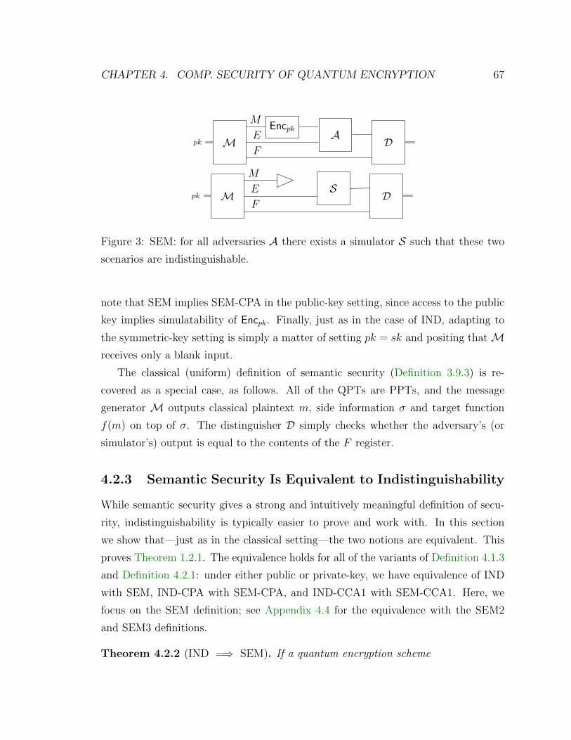
CHAPTER 4. COMP. SECURITY OF QUANTUM ENCRYPTION 67
pk MEncpk
AD
M
E
F
pk MS
D
M
E
F
Figure 3: SEM: for all adversaries A there exists a simulator S such that these two
scenarios are indistinguishable.
note that SEM implies SEM-CPA in the public-key setting, since access to the public
key implies simulatability of Encpk. Finally, just as in the case of IND, adapting to
the symmetric-key setting is simply a matter of setting pk = sk and positing thatMreceives only a blank input.
The classical (uniform) definition of semantic security (Definition 3.9.3) is re-
covered as a special case, as follows. All of the QPTs are PPTs, and the message
generator M outputs classical plaintext m, side information σ and target function
f(m) on top of σ. The distinguisher D simply checks whether the adversary’s (or
simulator’s) output is equal to the contents of the F register.
4.2.3 Semantic Security Is Equivalent to Indistinguishability
While semantic security gives a strong and intuitively meaningful definition of secu-
rity, indistinguishability is typically easier to prove and work with. In this section
we show that—just as in the classical setting—the two notions are equivalent. This
proves Theorem 1.2.1. The equivalence holds for all of the variants of Definition 4.1.3
and Definition 4.2.1: under either public or private-key, we have equivalence of IND
with SEM, IND-CPA with SEM-CPA, and IND-CCA1 with SEM-CCA1. Here, we
focus on the SEM definition; see Appendix 4.4 for the equivalence with the SEM2
and SEM3 definitions.
Theorem 4.2.2 (IND =⇒ SEM). If a quantum encryption scheme
CHAPTER 4. COMP. SECURITY OF QUANTUM ENCRYPTION 68
(KeyGen,Enc,Dec) has indistinguishable encryptions (IND), then it is semantically
secure (SEM).
Proof. Suppose that an encryption scheme (KeyGen,Enc,Dec) has indistinguishable
encryptions. Let A be QPT SEM attacker against semantic security as in Defini-
tion 4.2.1. We define the QPT SEM simulator S as follows: S does not receive
Encpk(ρM), but instead runs A on input (Encpk⊗1E)(|0〉 〈0|⊗ ρE) and outputs what-
ever A outputs. Let M be a QPT SEM message generator that outputs ρMEF .
Assume for a contradiction the existence of a QPT SEM distinguisher D which
successfully distinguishes the output of A from the output of S (with the help of regis-
ter F ), then the combination of A and D successfully distinguishes (Encpk⊗IEF )ρMEF
from (Encpk ⊗ IEF )(|0〉 〈0| ⊗ ρEF ), hence contradicting the indistinguishability.
In the private-key setting without CPA oracle access, S runs KeyGen(1n) to gen-
erate his own secret key k′, and then encrypts |0n〉 〈0n| using k′ instead of k. The
challenges (Enck ⊗1E)(|0〉 〈0| ⊗ ρE) and (Enck′ ⊗1E)(|0〉 〈0| ⊗ ρE) will be distributed
identically since k and k′ are and ρE doesn’t depend on the key. Hence, the success
probability of the SEM simulator S does not change.
In case of CPA and CCA1 oracles, both for the public- and private-key setting,
the simulator S forwards A’s oracle queries to his own oracle(s), and S obtains A’s
input state by a call to his encryption oracle on state |0〉 〈0|, joined with his auxiliary
information ρE.
Note that we defined semantic security with quantifiers as ∀A∃S∀M∀D, but the
above proof actually yields ∃S∀A∀M∀D, where S is an oracle algorithm with oracle
access to A, i.e. S’s strategy is essentially the same no matter the adversary A.
Theorem 4.2.3 (SEM =⇒ IND). If a quantum encryption scheme
(KeyGen,Enc,Dec) is semantically secure (SEM), then it has indistinguishable encryp-
tions (IND).
Proof. Let (M,D) be an IND adversary such that D distinguishes (Encpk ⊗ 1E)ρME
from (Encpk ⊗ 1E)(|0〉 〈0| ⊗ ρE) with advantage ε(n) if ρME ← M. Let us consider
the SEM message generatorM′ which runs ρME ←M and outputs (with probability

CHAPTER 4. COMP. SECURITY OF QUANTUM ENCRYPTION 69
12
each) either the state ρME ⊗ |1〉 〈1|F or the state |0〉 〈0|M ⊗ ρE ⊗ |0〉 〈0|F . Next
we consider the SEM attacker A which runs D and outputs the classical bit that
D outputs. We also consider the SEM attacker A ⊕ 1, which outputs the opposite
bit. As SEM distinguisher, let us consider the procedure which compares A’s output
bit to a measurement (in the computational basis) of the qubit in register F . Any
SEM simulator S that does not have access to the encrypted M -register has to guess
the state of the random bit in F and will be correct with probability 1/2. Then
ε(n) is twice the maximum of the advantages that A and A⊕ 1 have in successfully
predicting F over 1/2, the probability of success of any simulator. By SEM, both of
these advantages are negligible, and hence so is ε(n).
4.3 Quantum Encryption Schemes
We now turn to the question of existence for encryption schemes for quantum data.
We present two schemes based on the existence of classical functions which are difficult
to invert for quantum computers. The first scheme (Section 4.3.1) is symmetric-key
and IND-CCA1-secure; the second scheme (Section 4.3.2) is public-key and IND-CPA-
secure, and hence, by Theorem 4.2.3, also semantically secure. The cryptographic
primitives in this section are quantum-secure versions of those in Section 3.9.
4.3.1 Quantum Symmetric-Key Encryption from One-Way
Functions
In this section, we prove Theorem 1.2.2: If quantum-secure one-way functions exist,
then so do IND-CCA1-secure private-key quantum encryption schemes.
The proof proceeds in two steps. First, we define quantum-secure one-way func-
tions (qOWFs) and quantum-secure pseudorandom functions (qPRFs); we can ar-
gue as in the classical world that qPRFs exist if qOWFs do (Theorem 4.3.3.) Sec-
ond, we show that any qPRF can be used to construct an explicit IND-CCA1-secure
symmetric-key scheme for quantum data.
We begin with the formal definitions of qOWFs and qPRFs, and a statement of
CHAPTER 4. COMP. SECURITY OF QUANTUM ENCRYPTION 70
the result connecting the two.
First, a quantum-secure one-way function is an efficiently computable function
that is difficult for QPTs to invert on random inputs.
Definition 4.3.1. A PT-computable function f : 0, 1∗ → 0, 1∗ is a quantum-
secure one-way function (qOWF) if for every QPT A,
Prx
$←−0,1n[A(f(x), 1n) ∈ f−1(f(x))] ≤ negl(n) . (54)
Next, a quantum-secure pseudorandom function is an efficiently computable family
of functions which are indistinguishable to QPTs from perfectly random functions,
even when allowed to query an oracle for the given function polynomially many times.
Definition 4.3.2. A PT-computable function family
f = f (n) : 0, 1n × 0, 1p(n) → 0, 1`(n)n∈N ,
with p, ` : N→ N PT-computable, is a quantum-secure pseudorandom function (qPRF)
if for every QPT D equipped with a classical oracle,∣∣∣∣∣ Prk
$←−0,1n[Dfk(1n) = 1] − Pr
g$←−0,1p(n)→0,1`(n)
[Dg(1n) = 1]
∣∣∣∣∣ ≤ negl(n) , (55)
where fk := f (n)(k, ·) : 0, 1p(n) → 0, 1`(n) for k ∈ 0, 1n.
We remark that, to some readers, the restriction to classical oracles might seem
artificial. While one can certainly consider functions with the stronger guarantee of
resistance to quantum adversaries with quantum oracle access, stronger functions are
not necessary to establish our results. We thus opt for the weaker primitive. In either
case, the following holds.
Theorem 4.3.3. If qOWFs exist, then qPRFs exist.
Since our definitions are in terms of classical oracles, the classical proof that
shows that qOWFs imply qPRFs carries through [HILL99, GGM86]. We remark
that Zhandry [Zha12] extended this result to the case of functions secure against
CHAPTER 4. COMP. SECURITY OF QUANTUM ENCRYPTION 71
quantum superposition queries, what he calls “quantum-secure PRFs.” It should be
noted that the proof of the Theorem 4.3.3 actually implies the existence of a qPRF
for any PT-computable choice of the parameters p and ` in Definition 4.3.2.
We are now ready to proceed with the second part of the proof of Theorem 1.2.2,
namely the construction of an encryption scheme from a given qPRF. Essentially,
this scheme encrypts a quantum state ρ by first selecting a random string r, then
inputting r into a qPRF; the output fk(r) is then used as an encryption key for the
quantum one-time pad, Pfk(r) (see Subsection 3.8.1).
Scheme 1. If f = f (n) : 0, 1n × 0, 12n → 0, 12nn∈N is a qPRF, then let
qPRF-SKE be the following triple of QPT algorithms:
1. (key generation) KeyGen(1n): output k $←−0, 1n;
2. (encryption) Enck(ρ), for ρ ∈ D(C2n), an n-qubit state: choose r $←−0, 12n and
output |r〉 〈r| ⊗ Pfk(r)ρPfk(r),
3. (decryption) Deck(σ), for σ ∈ D(C23n), a 3n-qubit state: measure the first 2n
qubits in the computational basis to obtain r′ ∈ 0, 12n; apply Pfk(r′) to the
remaining n qubits and output the result.
For simplicity, we chose D(C2n) for the plaintext space, and D(C23n) for the
ciphertext space; we can easily adapt the above to other polynomially related cases
by selecting a qPRF with different parameters. The correctness of Scheme 1 is easily
verified:
Deck(Enck(ρ)) = Deck(|r〉 〈r| ⊗ Pfk(r)ρPfk(r)
)= Pfk(r)Pfk(r)ρPfk(r)Pfk(r) = ρ , (56)
where the second equality follows from the definition of the decryption function and
the last step is due to the fact that the Pauli operators are self-inverse. Next, we
show that the scheme is secure against non-adaptive chosen ciphertext attacks. The
classical version of this result is standard, and we use essentially the same proof; see,
e.g., Proposition 5.4.18 in Goldreich’s textbook [Gol04].
Lemma 4.3.4. If f is a qPRF, then Scheme 1 is an IND-CCA1-secure symmetric-key
quantum encryption scheme as defined in Definition 4.1.3.
CHAPTER 4. COMP. SECURITY OF QUANTUM ENCRYPTION 72
Proof. First, we analyse the security of the scheme in an idealized scenario where
f is a truly random function. We claim that in this case, A correctly guesses the
challenge with probability at most 1/2 + negl(n)(see Definition 4.4.7). In fact, this
bound holds for a stronger adversary A′, who has access to a classical oracle for f
prior to the challenge, and access to polynomially many pairs (ri, f(ri)) for random
ri, 1 ≤ i ≤ q, after the challenge. This adversary is stronger than A since it can
simulate A by implementing Encf and Decf oracles using its f oracles. Since the
input r into f in the challenge ciphertext is uniformly random, the probability that
any of the polynomially many oracle calls of A′ uses the same r is negligible. In the
case that no oracle calls use r, the mixtures of the inputs to A′ (including the pairs
(ri, f(ri))) are the same for the original challenge and the zero challenge. This fact
can be verified by first averaging over the values of f(r): since f is uniformly random,
f(r) is also uniformly random as well as independent of the other values of f (and
hence ρME). In both cases, applying the quantum one-time pad results in the state:
|r〉 〈r| ⊗ 1
2n1⊗ ρE ⊗ |r1〉 〈r1| ⊗ |f(r1)〉 〈f(r1)| ⊗ · · · ⊗ |rq〉 〈rq| ⊗ |f(rq)〉 〈f(rq)| , (57)
and indistinguishability follows.
Next, we consider the case that f is a pseudorandom function. We show that a
successful IND-CCA1 adversary A (i.e., one that distinguishes challenges with better
than negligible probability) can be used to construct a successful f -adversary A0 (i.e.,
one that distinguishes f from random with non-negligible probability.) The adversary
A0 is a QPT with classical oracle access to a function ϕ : 0, 12n → 0, 12n, and
aims to output 0 if ϕ is perfectly random and 1 if ϕ = fk for some k. Define the
simulated oracles
Encϕ : ρ 7→(r, Pϕ(r)ρPϕ(r)
)for r $←−0, 12n, and
Decϕ : |r′〉 〈r′| ⊗ ρ 7→ Pϕ(r′)ρPϕ(r′) ,
where, as before, we assume that Decϕ measures the first register before decrypting
the second. Note that if ϕ = fk then these are exactly the encryption and decryption
oracles (with key k) of the qPRF-SKE scheme.
The QPT Aϕ0 proceeds as follows. First, it simulates A, and replies to its queries
to the encryption oracle with Encϕ and its queries to the decryption oracle with

CHAPTER 4. COMP. SECURITY OF QUANTUM ENCRYPTION 73
Decϕ. When it transmits the challenge, Aϕ0 replies with either the encryption of the
challenge, or the encryption of |0n〉 〈0n|, each with probability 1/2. If A responds
correctly, Aϕ0 outputs 1; otherwise it outputs 0. If ϕ = fk then we have exactly
simulated the IND-CCA1 game with adversary A; in that case, since A is IND-CCA1-
breaking, Aϕ0 outputs 1 with probability at least 1/2 + 1/t(n) for some polynomial t,
for infinitely many n.
We conclude that∣∣∣∣∣ Prk
$←−0,1n[Afk0 (1n) = 1] − Pr
ϕ$←−0,12n→0,12n
[Aϕ0 (1n) = 1]
∣∣∣∣∣ ≥ 1
t(n)− negl(n) , (58)
for infinitely many n, i.e., f is not a qPRF.
The proof of Theorem 1.2.2 thus follows from Theorem 4.3.3 and Lemma 4.3.4.
4.3.2 Quantum Public-Key Encryption from Trapdoor Per-
mutations
For the construction of public-key schemes, we will need qOWFs with an additional
property: the existence of trapdoors which enable efficient inversion. Following the
classical approach of Diffie and Hellman [DH76], we set down the notion of a quantum-
secure trapdoor one-way permutation (or qTOWP), and then show how to use any
qTOWP to construct IND-CPA secure public-key encryption schemes for quantum
data. This will establish Theorem 1.2.3: If quantum-secure trapdoor one-way permu-
tations exist, then so do semantically secure public-key quantum encryption schemes.
Some of the proofs that are omitted or only sketched here are done in detail in Chap-
ter 5.
We begin with a definition of qTOWPs. We require a slight (but standard) varia-
tion of Definition 4.3.1, namely the notion of a quantum-secure one-way permutation
(or qOWP). A qOWP is a qOWF whose input domains are sets Di; moreover, the
function restricted to any such domain must be a permutation. When we augment
such a qOWP with trapdoors, with which it can be efficiently inverted, we arrive at
the following definition.
CHAPTER 4. COMP. SECURITY OF QUANTUM ENCRYPTION 74
Definition 4.3.5. A quantum-secure trapdoor one-way permutation (qTOWP) is a
PT-computable collection
f = fi : Di → Dii∈I
of permutations on sets Di ⊆ 0, 1l(i), i ∈ I, for some (infinite) set I of strings, and
a PT-computable function l : N→ N, together with a triple of PPTs (G,S, I) which
1. (generate (index, trapdoor) pair) supp G(1n) ⊆ (I ∩ 0, 1n)× 0, 1n;
2. (sample from domain) for all i ∈ I, supp S(i) = Di;
3. (invert using trapdoor) for all (i, t) ∈ supp G(1n) and all x ∈ Di, I(fi(x), t) = x,
such that for every QPT A,
Pr(i,t)←G(1n),x←S(i)
[A(fi(x), i) = x] ≤ negl(n) . (59)
For simplicity, we will assume that l(i) = |i| = n.
Before we can describe the public-key scheme and prove its security, we need two
additional (well-known) primitives which can be constructed from any qOWP, with
or without trapdoors. The first is a quantum-secure “hard-core” predicate, which is a
“yes” or “no” question about the uniformly random input x that is difficult to answer
if one only knows f(x).
Definition 4.3.6. A PT-computable b : 0, 1∗ → 0, 1 is a (quantum-secure) hard-
core of a qOWP f if for every QPT A,
Prx
$←−0,1n[A(f(x), 1n) = b(x)] ≤ 1
2+ negl(n) . (60)
The definition of hard-core may also be modified in the case of quantum-secure
trapdoor one-way functions or permutations in the obvious way, by indexing f and b
by i, generating x← S(i), where (i, t)← G(1n), and giving A access to i in place of
1n.
Definition 4.3.7. A hard-core of a qTOWP (f,G,S, I) is a PT-computable collection
b = bi : Di → 0, 1i∈I such that for every QPT A,
Pr(i,t)←G(1n),x←S(i)
[A(fi(x), i) = bi(x)] ≤ 1
2+ negl(n) . (61)
CHAPTER 4. COMP. SECURITY OF QUANTUM ENCRYPTION 75
A Goldreich-Levin theorem for our setting implies the following2:
Theorem 4.3.8. ([AC02], quantum analogue of [GL89]) If qOWPs (or qTOWPs)
exist, then qOWPs (or qTOWPs, respectively) with hard-cores exist.
The other primitive we need is a quantum-secure pseudorandom generator, which ex-
pands a uniformly random seed to an output that is computationally indistinguishable
from a longer uniformly random string, hence “pseudorandom”. The classical proof
that one-way permutations with hard-cores imply pseudorandom generators carries
over with little modification (see Lemma 4.3.10).
Definition 4.3.9. A PT-computable function G : 0, 1∗ → 0, 1∗ is a quantum-
secure pseudorandom generator (qPRG) if |G(s)| = p(|s|) for all s ∈ 0, 1∗ and for
every QPT D,∣∣∣∣∣ Prs
$←−0,1n[D(G(s)) = 1] − Pr
y$←−0,1p(n)
[D(y) = 1]
∣∣∣∣∣ ≤ negl(n) . (62)
We write m := p(n). Note that p must necessarily itself be PT-computable, and
hence polynomially bounded.
Lemma 4.3.10. If f is a qOWP with hard-core predicate b, and p : N→ N is PT-
computable, then G : s 7→ b(fp(|s|)−1(s))b(fp(|s|)−2(s)) . . . b(s) is a qPRG.
Sketch. 3 The proof proceeds almost identically as in the classical case (see, e.g.,
[Gol04].) Let D be a quantum adversary that distinguishes G(Un) from uniform.
Note that, as stated in Definition 4.3.9, D gets only classical bitstring outputs from
the pseudorandom generator. In the classical proof, one constructs an adversary Awhich uses D as a black-box subroutine, and breaks the hard-core of f . We use the
exact same A now; in particular, we only need to invoke D on classical inputs and
read out its (post-measurement) classical outputs (0 or 1). Of course, by virtue of
needing to invoke D, A itself will now be a QPT.
In slightly greater detail, we use a standard hybrid argument to give a “predictor”
algorithm A that, for some index i ≤ m = p(n), can predict the i+ 1st bit of G(Un),
2It is proven in detail as Theorem 5.2.1 in Section 5.2.3A more general result is proven in detail as Theorem 5.3.1 in Section 5.3.
CHAPTER 4. COMP. SECURITY OF QUANTUM ENCRYPTION 76
given as input the first i bits of the output of G. A succeeds with non-negligible advan-
tage over random, i.e., the probability over s that A(b(fm−1(s)) . . . b(fm−i(s))) out-
puts b(fm−(i+1)(s)) is at least 1/2 + 1/q(n) where q is some positive polynomial. Cru-
cially, since f implements a permutation over 0, 1n, we have that b(f i−1(Un)) . . . b(Un)
is distributed identically to b(fm−1(Un)) . . . b(fm−i(Un)). Therefore, given uniform
x, and y = f(x), we can use the output of the predictor, A(b(f i−1(y)) . . . b(y)) =
A(b(f i(x)) . . . b(f(x))) to predict b(x) with non-negligible advantage, in violation of
the security guarantee of the hard-core predicate.
We can now describe a public-key scheme for encrypting quantum data.
Scheme 2. If f is a qTOWP, and assume for simplicity that l(i) = |i| = n, and let
b and G : 0, 1∗ → 0, 1∗ be the corresponding hard-core and qPRG, respectively
with p(n) = 2n as in Lemma 4.3.10 4. Let qTOWP-PKE be the following triple of
algorithms:
1. ((public, private) key-pair generation) KeyGen(1n):
• output G(1n) = (i, t) ∈ 0, 1n × 0, 1n;
2. (encryption with public key) Enci(ρ), for ρ ∈ D(C2n), an n-qubit state:
• apply S(i) to select d ∈ Di, and compute r := G(d) = b(f 2n−1(d)) . . . b(d);
• output |f 2ni (d)〉 〈f 2n
i (d)| ⊗ PrρPr;
3. (decryption with private key) Dect(σ), for σ ∈ D(C22n), a 2n-qubit state:
• measure the first n qubits in the computational basis to obtain s ∈ 0, 1n
• for j = 1, . . . , 2n, apply b (It)j to s, where It := I(·, t); concatenate the
resulting bits to get u = b(f−1i (s))b(f−2i (s)) . . . b(f−2ni (s)) ∈ 0, 12n;
• apply Pu to the remaining n qubits of σ and output the result.
The correctness of the scheme is straightforward; fix a key-pair (i, t), a randomly
4As with the qPRF in the private-key scheme, we can use G = Gn,m : 0, 1n → 0, 12mn,mto encrypt and decrypt messages of different lengths with the same keys, and this will remain secure,noting that messages must be polynomially bounded in length, so that m will be bounded above bythe same polynomial
CHAPTER 4. COMP. SECURITY OF QUANTUM ENCRYPTION 77
sampled d ∈ Di, and the corresponding r. Then
Dect(Enci(ρ)) = Dect(|f 2ni (d)〉 〈f 2n
i (d)| ⊗ PrρPr)
= PuPrρPrPu = ρ , (63)
where the last step follows from the fact that u = r for valid ciphertexts: in this case,
s = f 2ni (d), so
u = b(f−1i (s)) . . . b(f−2ni (s))
= b(f−1i (f 2ni (d))) . . . b(f−2ni (f 2n
i (d)))
= b(f 2n−1(d)) . . . b(d)
= G(d)
= r . (64)
It remains to show that this scheme is secure against chosen plaintext attacks.
We begin by proving indistinguishability of ciphertexts for the quantum one-time
pad which uses randomness supplied by a qPRG. We first set the following nota-
tion. Recall from Subsection 3.8.1 that a string r of 2n bits determines a Pauli
group element Pr ∈ U(2n). Given an n-qubit register A, an arbitrary register B, and
ρ ∈ D(HA ⊗HB), define Pr;A(ρ) := (Pr ⊗ 1B)ρ(Pr ⊗ 1B).
Lemma 4.3.11. If G : 0, 1∗ → 0, 1∗ is a qPRG, then for any efficiently preparable
states ρAB ∈ D(HA ⊗HB) and σA ∈ D(HA), and any QPT D∣∣∣∣∣ Prs
$←−0,1n[D(PG(s);A(ρAB)) = 1
]− Pr
s$←−0,1n
[D(PG(s);A(σA ⊗ ρB)) = 1
]∣∣∣∣∣ ≤ negl(n) .
(65)
Proof. The two key observations are (i.) distinguishability as in Equation (65) is
impossible if we replace G(s) with uniform randomness, and (ii.) with only classical
input/output access to G, we can simulate D(PG(s);A(·)). Putting these two facts
together, it follows that violating (65) implies that outputs of G can be distinguished
from uniformly random.
Formally, let us assume that there is an adversary D that violates our hypothesis,
i.e., that distinguishes some pair of inputs (PG(s);A(ρAB), PG(s);A(σA⊗ρB)) with prob-
ability at least 1/q(n) for some positive polynomial q. Then we’ll show an algorithm

CHAPTER 4. COMP. SECURITY OF QUANTUM ENCRYPTION 78
D′, that breaks the pseudorandom generator G. On input y ∈ 0, 1m, algorithm D′
does the following:
• with probability 1/2, run D on input Py;A(ρAB);
• with probability 1/2, run D on input Py;A(σA ⊗ ρB).
Now if D is able to correctly determine which of the cases we gave it, D′ decides that
y must have been distributed pseudorandomly and outputs 1, else it decides that y
is uniformly distributed and outputs 0.
Notice that if y = G(s), by definition D′ outputs 1 when D correctly distin-
guishes the two inputs, which occurs with probability at least 1/2 + 1/q(n) by the
assumption on D. On the other hand, suppose y $←−0, 1m; then after mixing over
y, the register A is mapped to the maximally mixed state, i.e. 12m
∑y Py;A(ρAB) =
12m
∑y Py;A(σA ⊗ ρB) = 1A ⊗ ρB. In that case, D is correct with probability at most
1/2 (indeed, this is true for any QPT.) We conclude that D′ distinguishes the case
y = G(s) from the case y $←−0, 1m with non-negligible probability; this contradicts
the assumption that G is a qPRG.
Finally, to prove that the construction in Scheme 2 is IND-CPA-secure, and thus
establish Theorem 1.2.3, it remains to extend the above proof to a slightly more
general scenario. Recall that Enci(ρ) = |f 2ni (d)〉〈f 2n
i (d)| ⊗ PrρPr where r = G(d).
Lemma 4.3.11 already shows that essentially no QPT adversary can distinguish
(Pr ⊗ 1E)ρME(Pr ⊗ 1E) from (Pr ⊗ 1E)(|0〉 〈0| ⊗ ρE)(Pr ⊗ 1E), for any efficiently pre-
parable bipartite state ρME over the message space and the environment. It remains
to show that this indistinguishability still holds if the adversary is also provided the
classical advice i and f 2ni (d). We can prove this extended indistinguishability by ex-
tending the hybrid argument in the proof of Lemma 4.3.10 in a standard way. To
sketch the argument, first recall that the “predictor” algorithm succeeds at predicting
the j + 1st bit of G(Un) given as input the first j bits of the output of G. Now we
also allow the predictor to read the bits of i and f 2ni (d). Success implies breaking
the hard-core of f (which is used to define the qPRG G and ensure its security). We
CHAPTER 4. COMP. SECURITY OF QUANTUM ENCRYPTION 79
conclude that the strings
i f 2ni (d) G(s) and i f 2n
i (d) r′
are computationally indistinguishable for uniformly random s, r′, and (i, t)← G(1n).5
Hence the states
|i〉 〈i| ⊗ |f 2ni (d)〉〈f 2n
i (d)| ⊗ PG(s);M(ρME) and |i〉 〈i| ⊗ |f 2ni (d)〉〈f 2n
i (d)| ⊗ Pr′;M(ρME)
must also be computationally indistinguishable, since they are obtained by the ap-
plication of a quantum algorithm to the previous pairs of strings, respectively, where
ρME ←M(i) (i is copied, and M is applied to one of the copies; then the quantum
one-time pad is applied to the result with G(s) or r′, respectively). The right-hand
side is indistinguishable from the same state with |0〉 〈0|M ⊗ ρE in place of ρME, by
observing that their mixtures over r′ are identical, so we also have the computational
indistinguishability of
|i〉 〈i| ⊗ |f 2ni (d)〉〈f 2n
i (d)| ⊗ Pr′;M(ρME) and
|i〉 〈i| ⊗ |f 2ni (d)〉〈f 2n
i (d)| ⊗ Pr′;M(|0〉 〈0|M ⊗ ρE) .
By the transitivity of computational indistinguishability, we conclude that
|i〉 〈i| ⊗ |f 2ni (d)〉〈f 2n
i (d)| ⊗ PG(s);M(ρME) and
|i〉 〈i| ⊗ |f 2ni (d)〉〈f 2n
i (d)| ⊗ PG(s);M(|0〉 〈0|M ⊗ ρE)
are indistinguishable, which completes the proof of Theorem 1.2.3.
4.4 Alternative Definitions of Quantum Security
Here, we present further definitions of quantum semantic security and indistinguisha-
bility, and prove their equivalence. The full chain of equivalences is given in Figure 4.
SEM3 (Definition 4.4.5) helps to illustrate that quantum semantic security as de-
fined in this thesis is a proper quantum analogue of classical semantic security, while
5This is proven in detail as Theorem 5.3.1 in Section 5.3.

CHAPTER 4. COMP. SECURITY OF QUANTUM ENCRYPTION 80
IND′
IND
SEM
SEM2
SEM3
Prop.4.4.8
Thm. 4.2.2
Prop. 4.4.3
Prop. 4.4.6
Thm. 4.4.9
Figure 4: Relationship between security definitions.
SEM2 (Definition 4.4.2) serves primarily as an intermediate between SEM (Defini-
tion 4.2.1) and SEM3. IND’ (Definition 4.4.7) is the quantum version of a common
reformulation of IND (Definition 4.1.3), which is essentially used in the proof of The-
orem 4.2.3 SEM =⇒ IND.
4.4.1 SEM2
Definition 4.4.1 (Message-classical function generator). A message-classical func-
tion generator M is a QPT message generator (as in SEM (Definition 4.2.1)) such
that for each pk ∈ Kpub and ρMEF in the range ofM(pk), there is some binary string
y such that |y〉 ∈ HF and ρMEF = ρME ⊗ |y〉 〈y|.
That is, the F system is classical, unentangled from and uncorrelated with the
rest of ρ.
In particular, ρF = |y〉 〈y|.
Definition 4.4.2 (SEM2). A qPKE scheme (KeyGen,Enc,Dec) is SEM2-secure if for
any QPT adversary A, there exists a QPT simulator S such that for all message-
classical function generators M,∣∣Pr[A(Encpk ⊗ 1E)ρME = y
]− Pr
[SρE = y
]∣∣ ≤ negl(n) , (66)

CHAPTER 4. COMP. SECURITY OF QUANTUM ENCRYPTION 81
where the outputs of A and S are measured in the computational basis before
equality is checked, ρME ⊗ |y〉 〈y|F ← M(pk), and the probabilities are taken over
(pk, sk)← KeyGen(1n) and the internal randomness of Enc, A,S,M and D.
• SEM2-CPA: In addition to the above, all QPTs have oracle access to Encpk.
• SEM2-CCA1: In addition to SEM2-CPA, M has oracle access to Decsk.
Proposition 4.4.3. If a quantum encryption scheme is semantically secure, then it
is SEM2 secure.
Proof. A message-classical function generator is also a message. In SEM, have the
distinguisher D implement an equality test (simulate any efficient classical circuit
implementing it; if the input lengths aren’t the same, output 0 immediately).
4.4.2 SEM3
Definition 4.4.4 (Message Generator-Function Pair). A message generator-function
pair is a tuple (M, f), such that M is a QPT message generator (as in IND (Def-
inition 4.1.3)) and f = (fn)n is a QPT algorithm, such that fpk := fn(pk) is the
description of a boolean circuit, for pk ∈ Kpub, with the number of input bits to
fpk equal to the number of measurement gates in the quantum circuit Mn. In the
symmetric-key scenario, fn has no input.
Definition 4.4.5 (SEM3). A qPKE scheme (KeyGen,Enc,Dec) is SEM3-secure if for
any QPT adversary A, there exists a QPT simulator S such that for all message
generator-function pairs (M, f),∣∣Pr[A(Encpk ⊗ 1E)ρME = fpk(x)
]− Pr
[SρE = fpk(x)
]∣∣ ≤ negl(n) , (67)
where the outputs of A and S are measured in the computational basis before equality
is checked, ρME ←M(pk), x is the string of measurement results generating ρME, and
the probabilities are taken over (pk, sk) ← KeyGen(1n) and the internal randomness
of Enc, A,M and S.
• SEM3-CPA: In addition to the above, all QPTs have oracle access to Encpk.

CHAPTER 4. COMP. SECURITY OF QUANTUM ENCRYPTION 82
• SEM3-CCA1: In addition to SEM3-CPA, M has oracle access to Decsk.
We note that fpk is a function of the random input and measurement results,
which completely determine the state. Hence, if fpk is the identity for all pk, and it
can be computed given a ciphertext, this means we can compute measurement results
necessary to prepare the state. Simulating the message generator but selecting for
the correct measurement results would allow the preparation of the same state again,
although this is not in general efficient.
Proposition 4.4.6 (SEM2 =⇒ SEM3). If a quantum encryption scheme is SEM2
secure, then it is SEM3 secure.
Proof. A message generator-function pair (M, f) can be turned into a message-
classical function generator M by copying the measurement results x1, x2, . . . , xm
after each measurement gate, and applying fpk to x1x2 . . . xm and letting the result
be the F system.
4.4.3 IND’
Definition 4.4.7 (IND’). A qPKE scheme (KeyGen,Enc,Dec) is IND’ secure if for
every QPT adversary A = (M,D) we have:
Pr[D(Encpk ⊗ 1E)ρ
(b)ME = b
]≤ 1
2+ negl(n) , (68)
where ρME ← M(pk), for b a uniformly random bit, ρ(1)ME = ρME and ρ
(0)ME =
|0〉 〈0|M ⊗ ρE, and the probabilities are taken over (pk, sk) ← KeyGen(1n), b and
the internal randomness of Enc, M, and D.
• IND’-CPA: In addition to the above, M and D have oracle access to Encpk.
• IND’-CCA1: In addition to IND’-CPA, M has oracle access to Decsk.
Proposition 4.4.8 (IND’ ⇐⇒ IND). A quantum encryption scheme is IND’ secure
if and only if it is IND secure.
CHAPTER 4. COMP. SECURITY OF QUANTUM ENCRYPTION 83
Proof. We drop the register subscripts where possible.
Pr[D(Encpk ⊗ 1E)ρ(b) = b]
= Pr[D(Encpk ⊗ 1E)ρ(b) = b | b = 1] Pr[b = 1]
+ Pr[D(Encpk ⊗ 1E)ρ(b) = b | b = 0] Pr[b = 0]
= 12(Pr[D(Encpk ⊗ 1E)ρ = 1] + Pr[D(Encpk |0〉 〈0| ⊗ ρE) = 0])
≤ 12(Pr[D(Encpk ⊗ 1E)ρ = 1] + 1− Pr[D(Encpk |0〉 〈0| ⊗ ρE) = 1])
= 12
+ 12(Pr[D(Encpk ⊗ 1E)ρ = 1]− Pr[D(Encpk |0〉 〈0| ⊗ ρE) = 1]) . (69)
Note that we only get ≤ since D may output some binary string other than 0 or 1.
So:
Pr[D(Encpk ⊗ 1E)ρ(b) = b]− 12
≤ 12|Pr[D((Encpk ⊗ 1E)ρ = 1]− Pr[D(Encpk |0〉 〈0| ⊗ ρE) = 1]| . (70)
Thus, IND =⇒ IND’.
Now consider replacing D with the distinguisher which starts the same as D, but
if D would have output something other than 0 or 1, it simply outputs 0. Then the
quantity |Pr[D(Encpk⊗1E)ρ = 1]−Pr[D(Encpk |0〉 〈0|⊗ρE) = 1]| is the same for this
new distinguisher, so without loss of generality, D only outputs 0 or 1.
Then the first ≤ becomes an = , i.e.
Pr[D(Encpk ⊗ 1E)ρ(b) = b]− 12
= 12(Pr[D(Encpk ⊗ 1E)ρ = 1]− Pr[D(Encpk |0〉 〈0| ⊗ ρE) = 1]) (71)
and, similarly,
Pr[D(Encpk ⊗ 1E)ρ(b) = b⊕ 1]
= Pr[D(Encpk ⊗ 1E)ρ(b) = b⊕ 1 | b = 1] Pr[b = 1]
+ Pr[D(Encpk ⊗ 1E)ρ(b) = b⊕ 1 | b = 0] Pr[b = 0]
= 12(Pr[D(Encpk ⊗ 1E)ρ = 0] + Pr[D(Encpk |0〉 〈0| ⊗ ρE) = 1])
= 12(1− Pr[D(Encpk ⊗ 1E)ρ = 1] + Pr[D(Encpk |0〉 〈0| ⊗ ρE) = 1])
= 12
+ 12(Pr[D(Encpk |0〉 〈0| ⊗ ρE) = 1]− Pr[D(Encpk ⊗ 1E)ρ = 1]) , (72)
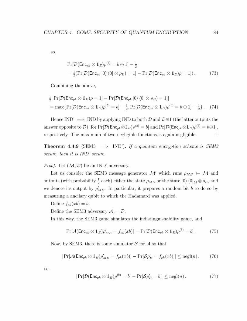
CHAPTER 4. COMP. SECURITY OF QUANTUM ENCRYPTION 84
so,
Pr[D(Encpk ⊗ 1E)ρ(b) = b⊕ 1]− 12
= 12(Pr[D(Encpk |0〉 〈0| ⊗ ρE) = 1]− Pr[D(Encpk ⊗ 1E)ρ = 1]) . (73)
Combining the above,
12|Pr[D(Encpk ⊗ 1E)ρ = 1]− Pr[D(Encpk |0〉 〈0| ⊗ ρE) = 1]|
= maxPr[D(Encpk ⊗ 1E)ρ(b) = b]− 12,Pr[D(Encpk ⊗ 1E)ρ(b) = b⊕ 1]− 1
2 . (74)
Hence IND’ =⇒ IND by applying IND to bothD andD⊕1 (the latter outputs the
answer opposite to D), for Pr[D(Encpk⊗1E)ρ(b) = b] and Pr[D(Encpk⊗1E)ρ(b) = b⊕1],
respectively. The maximum of two negligible functions is again negligible.
Theorem 4.4.9 (SEM3 =⇒ IND’). If a quantum encryption scheme is SEM3
secure, then it is IND’ secure.
Proof. Let (M,D) be an IND’ adversary.
Let us consider the SEM3 message generator M′ which runs ρME ← M and
outputs (with probability 12
each) either the state ρME or the state |0〉 〈0|M ⊗ρE, and
we denote its output by ρ′ME. In particular, it prepares a random bit b to do so by
measuring a ancilary qubit to which the Hadamard was applied.
Define fpk(xb) = b.
Define the SEM3 adversary A := D.
In this way, the SEM3 game simulates the indistinguishability game, and
Pr[A(Encpk ⊗ 1E)ρ′ME = fpk(xb)] = Pr[D(Encpk ⊗ 1E)ρ(b) = b] . (75)
Now, by SEM3, there is some simulator S for A so that
|Pr[A(Encpk ⊗ 1E)ρ′ME = fpk(xb)]− Pr[Sρ′E = fpk(xb)]| ≤ negl(n) , (76)
i.e.
|Pr[D(Encpk ⊗ 1E)ρ(b) = b]− Pr[Sρ′E = b]| ≤ negl(n) . (77)

CHAPTER 4. COMP. SECURITY OF QUANTUM ENCRYPTION 85
Note that S’s input ρ′E is independent of b. Hence
Pr[Sρ′E = b] ≤ 12. (78)
Finally, by summing the last two inequalities and dropping the absolute values,
Pr[D(Encpk ⊗ 1E)ρ(b) = b] ≤ 12
+ negl(n) . (79)

Chapter 5
Proofs for Cryptographic
Primitives
Results that were sketched or omitted in Section 4.3 are reviewed here. Classical
results, whose extensions to our setting may be used to prove Theorem 4.3.3, are
mentioned in Section 5.1. This theorem was used for the construction of the private-
key quantum encryption scheme in Section 4.3.1.
The remaining results in this chapter are used in the construction of the public-
key quantum encryption scheme in Section 4.3.2, based on their classical counterparts
as found in [Gol06]. They are the quantum analogues of the Goldreich-Levin theo-
rem for trapdoor one-way permutations (Theorem 4.3.8 in Section 4.3.2, and Theo-
rem 5.2.1 here in Section 5.2) and an extended proof of security for the construction
of quantum-secure pseudorandom generators from quantum-secure trapdoor one-way
permutations with hard-cores (Lemma 4.3.10 in Section 4.3.2, and Theorem 5.3.1
here in Section 5.3).
5.1 qOWFs to qPRFs
For the construction of the private-key quantum encryption scheme in Section 4.3.1,
the following result is used:
Theorem 5.1.1 (qOWF to qPRF). If quantum-secure one way functions exist, then
86
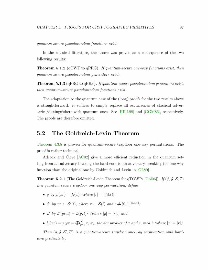
CHAPTER 5. PROOFS FOR CRYPTOGRAPHIC PRIMITIVES 87
quantum-secure pseudorandom functions exist.
In the classical literature, the above was proven as a consequence of the two
following results:
Theorem 5.1.2 (qOWF to qPRG). If quantum-secure one-way functions exist, then
quantum-secure pseudorandom generators exist.
Theorem 5.1.3 (qPRG to qPRF). If quantum-secure pseudorandom generators exist,
then quantum-secure pseudorandom functions exist.
The adaptation to the quantum case of the (long) proofs for the two results above
is straightforward: it suffices to simply replace all occurrences of classical adver-
saries/distinguishers with quantum ones. See [HILL99] and [GGM86], respectively.
The proofs are therefore omitted.
5.2 The Goldreich-Levin Theorem
Theorem 4.3.8 is proven for quantum-secure trapdoor one-way permutations. The
proof is rather technical.
Adcock and Cleve [AC02] give a more efficient reduction in the quantum set-
ting from an adversary beaking the hard-core to an adversary breaking the one-way
function than the original one by Goldreich and Levin in [GL89].
Theorem 5.2.1 (The Goldreich-Levin Theorem for qTOWPs [Gol06]). If (f,G,S, I)
is a quantum-secure trapdoor one-way permutation, define
• g by gi(xr) = fi(x)r where |r| = |fi(x)|;
• S ′ by xr ← S ′(i), where x← S(i) and r $←−0, 1|fi(x)|;
• I ′ by I ′(yr, t) = I(y, t)r (where |y| = |r|); and
• bi(xr) = xr =⊕|x|
j=1 xj ·rj, the dot product of x and r, mod 2 (where |x| = |r|).
Then (g,G,S ′, I ′) is a quantum-secure trapdoor one-way permutation with hard-
core predicate bi.

CHAPTER 5. PROOFS FOR CRYPTOGRAPHIC PRIMITIVES 88
Note that bi does not depend on i.
Proof. We follow the proof of Theorem 2.5.2 in [Gol06]. First, note that (g,G,S ′, I ′)is a trapdoor one-way permutation, since
I ′(gi(xr), t) = I ′(fi(x)r, t) = I(fi(x), t)r = xr. It is quantum-secure, since an algo-
rithm capable of guessing xr from (gi(xr), i) = (fi(x)r, i) with non-negligible prob-
ability can be used as a subroutine in an algorithm to guess x from (fi(x), i), by
simply generating a random string r of length |fi(x)| and applying the first algorithm
to (fi(x)r, i).
For one-way functions, an algorithm guessing y ∈ g−1(g(x)) can be used similarly.
Now, we prove by way of contradiction that bi is a hard-core. Suppose that is
isn’t, i.e. there exists a quantum algorithm A and a positive polynomial p such
that ε(n) := Pr[A(gi(xr), i) = bi(xr)] − 12>
1
p(n)for infinitely many n, where
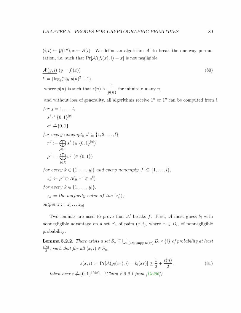
CHAPTER 5. PROOFS FOR CRYPTOGRAPHIC PRIMITIVES 89
(i, t)← G(1n), x← S(i). We define an algorithm A′ to break the one-way permu-
tation, i.e. such that Pr[A′(fi(x), i) = x] is not negligible:
A′(y, i) (y = fi(x)) (80)
l := dlog2(2|y|p(n)2 + 1)e
where p(n) is such that ε(n) >1
p(n)for infinitely many n,
and without loss of generality, all algorithms receive 1n or 1n can be computed from i
for j = 1, . . . , l,
sj $←−0, 1|y|
σj $←−0, 1
for every nonempty J ⊆ 1, 2, . . . , l
rJ :=⊕j∈K
sj (∈ 0, 1|y|)
ρJ :=⊕j∈K
σj (∈ 0, 1)
for every k ∈ 1, . . . , |y| and every nonempty J ⊆ 1, . . . , l,
zJk ← ρJ ⊕ A(y, rJ ⊕ ek)
for every k ∈ 1, . . . , |y|,
zk := the majority value of the (zJk )J
output z := z1 . . . z|y|
Two lemmas are used to prove that A′ breaks f . First, A must guess bi with
nonnegligible advantage on a set Sn of pairs (x, i), where x ∈ Di, of nonnegligible
probability:
Lemma 5.2.2. There exists a set Sn ⊆⋃i:(i,t)∈supp G(1n)Di×i of probability at least
ε(n)2
, such that for all (x, i) ∈ Sn,
s(x, i) := Pr[A(gi(xr), i) = bi(xr)] ≥1
2+ε(n)
2, (81)
taken over r $←−0, 1|fi(x)|. (Claim 2.5.2.1 from [Gol06])

CHAPTER 5. PROOFS FOR CRYPTOGRAPHIC PRIMITIVES 90
Proof. Let Sn be the set of all such (x, i), i.e Sn = (x, i)|s(x, i) ≥ 12
+ ε(n)2, and let
a = 12
+ ε(n)2
. Note that E(s(x, i)) = 12
+ ε(n). If Pr[(x, i) ∈ Sn] < ε(n)2
, then
1
2+ ε(n) = E[s(x, i)]
=∑x
s(x, i)p(x, i)
where p(x, i) is the joint probability of x and i
=∑
(x,i):s(x,i)<a
s(x, i)p(x, i) +∑
(x,i):s(x,i)≥a
s(x, i)p(x, i)
≤∑
(x,i):s(x,i)<a
ap(x, i) +∑
(x,i):s(x,i)≥a
1p(x, i) since s ≤ 1
= aPr[s(x, i) < a] + Pr[s(x, i) ≥ a]
= a(1− Pr[s(x, i) ≥ a]) + Pr[s(x, i) ≥ a]
= (1− a) Pr[s(x, i) ≥ a] + a
=(1
2− ε(n)
2
)Pr[s(x, i) ≥ a] +
1
2+ε(n)
2
⇐⇒ ε(n)
2≤(
1
2− ε(n)
2
)Pr[s(x, i) ≥ a]
=⇒ Pr[s(x, i) ≥ a] ≥
ε(n)
21
2− ε(n)
2
=ε(n)
1− ε(n)> ε(n) , if 0 < ε(n) < 1, (82)
and if this last implication doesn’t hold, either ε(n) = 0 or ε(n) = 1, and we just let
Sn =⋃i:(i,t)∈supp G(1n)Di × i. This completes the proof of the lemma.
Now we prove a lemma regarding the behaviour of A for (x, i) ∈ Sn:
Lemma 5.2.3. For all (x, i) ∈ Sn and for all 1 ≤ k ≤ |fi(x)|,
Pr[|J |bi(x, rJ)⊕A(fi(x), rJ ⊕ ek) = xk| > 12(2l − 1)] > 1− 1
2|fi(x)|, (83)
for infinitely many n, where xk is the kth character of the string x, ek := 0k−110|fi(x)|−k
is the string of the length |fi(x)| with 1 in its kth position and 0 in all others, and
rJ and l are defined and distributed as above in the definition of A′. (Claim 2.5.2.2
from [Gol06])

CHAPTER 5. PROOFS FOR CRYPTOGRAPHIC PRIMITIVES 91
Proof. For each nonempty J ⊆ 1, . . . , l, let
ξJ =
1, if bi(x, rJ)⊕A(fi(x), rJ ⊕ ek) = xk
0, otherwise,(84)
and let m = 2l − 1, the number of nonempty subsets of 1, . . . , l.Note that this condition for ξJ = 1 is equivalent toA(fi(x), rJ⊕ek) = bi(x, r
J⊕ek),since
bi(x, rJ)⊕ bi(x, rJ ⊕ ek) = bi(x, e
k) = xk . (85)
Then, since the rJ and hence the rJ ⊕ ek are uniformly distributed in 0, 1|fi(x)|,
Pr[ξJ = 1] = Pr[A(fi(x), rJ ⊕ ek) = bi(x, rJ ⊕ ek)] = s(x, i) ≥ 1
2+
1
2p(n), (86)
for infinitely many n.
Furthermore,
|J |bi(x, rJ)⊕A(fi(x), rJ ⊕ ek) = xk| =∑J
ξJ . (87)
Recall Chebyshev’s inequality :
Lemma 5.2.4 (Chebyshev’s inequality). For X a random variable with finite mean
µ and variance σ2, and c > 0,
Pr[|X − µ| ≥ c] ≤ σ2
c2. (88)
We would like to apply it to X =∑
J ξJ with c = m
2p(n), and to do so, we need
the variance of∑
J ξJ . Note that the ξJ are all identically distributed, since the rJ
are. Then, if the ξJ are pairwise independent, it follows that Var[∑
J ξJ ] = mVar[ξ],
where ξ is any of the ξJ and m = 2l − 1, the number of J ’s. To prove that the ξJ
are pairwise independent, it suffices to show that the rJ are, since the ξJ differ only
through their dependence on the corresponding rJ (i.e. ξJ = F (rJ , wJ), where F is a
deterministic function and wJ is a random variable for the independent random coin
tosses in the use of A for each J). Let J 6= J ′ be two nonempty subsets of 1, . . . , l.
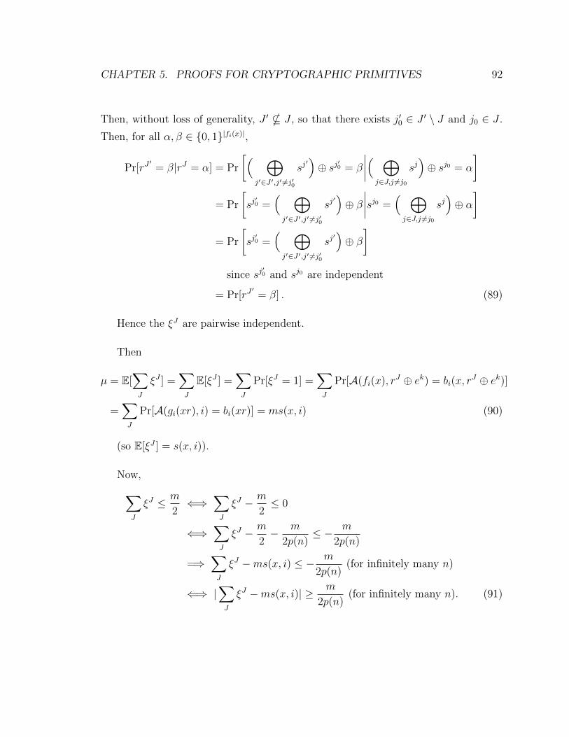
CHAPTER 5. PROOFS FOR CRYPTOGRAPHIC PRIMITIVES 92
Then, without loss of generality, J ′ * J , so that there exists j′0 ∈ J ′ \ J and j0 ∈ J .
Then, for all α, β ∈ 0, 1|fi(x)|,
Pr[rJ′= β|rJ = α] = Pr
[( ⊕j′∈J ′,j′ 6=j′0
sj′)⊕ sj′0 = β
∣∣∣∣( ⊕j∈J,j 6=j0
sj)⊕ sj0 = α
]
= Pr
[sj′0 =
( ⊕j′∈J ′,j′ 6=j′0
sj′)⊕ β
∣∣∣∣sj0 =( ⊕j∈J,j 6=j0
sj)⊕ α
]
= Pr
[sj′0 =
( ⊕j′∈J ′,j′ 6=j′0
sj′)⊕ β
]since sj
′0 and sj0 are independent
= Pr[rJ′= β] . (89)
Hence the ξJ are pairwise independent.
Then
µ = E[∑J
ξJ ] =∑J
E[ξJ ] =∑J
Pr[ξJ = 1] =∑J
Pr[A(fi(x), rJ ⊕ ek) = bi(x, rJ ⊕ ek)]
=∑J
Pr[A(gi(xr), i) = bi(xr)] = ms(x, i) (90)
(so E[ξJ ] = s(x, i)).
Now,∑J
ξJ ≤ m
2⇐⇒
∑J
ξJ − m
2≤ 0
⇐⇒∑J
ξJ − m
2− m
2p(n)≤ − m
2p(n)
=⇒∑J
ξJ −ms(x, i) ≤ − m
2p(n)(for infinitely many n)
⇐⇒ |∑J
ξJ −ms(x, i)| ≥ m
2p(n)(for infinitely many n). (91)
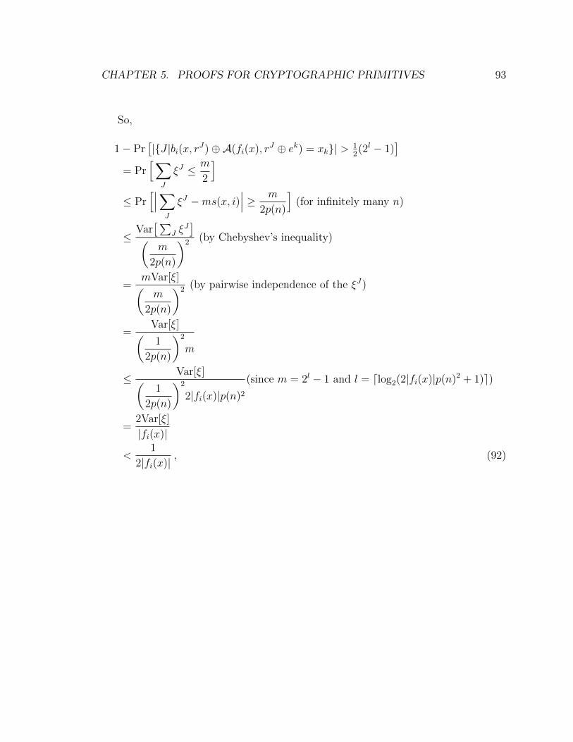
CHAPTER 5. PROOFS FOR CRYPTOGRAPHIC PRIMITIVES 93
So,
1− Pr[|J |bi(x, rJ)⊕A(fi(x), rJ ⊕ ek) = xk| > 1
2(2l − 1)
]= Pr
[∑J
ξJ ≤ m
2
]≤ Pr
[∣∣∣∑J
ξJ −ms(x, i)∣∣∣ ≥ m
2p(n)
](for infinitely many n)
≤Var[∑
J ξJ](
m
2p(n)
)2 (by Chebyshev’s inequality)
=mVar[ξ](m
2p(n)
)2 (by pairwise independence of the ξJ)
=Var[ξ](1
2p(n)
)2
m
≤ Var[ξ](1
2p(n)
)2
2|fi(x)|p(n)2(since m = 2l − 1 and l = dlog2(2|fi(x)|p(n)2 + 1)e)
=2Var[ξ]
|fi(x)|
<1
2|fi(x)|, (92)
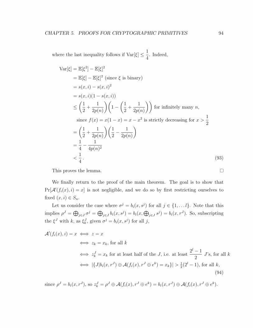
CHAPTER 5. PROOFS FOR CRYPTOGRAPHIC PRIMITIVES 94
where the last inequality follows if Var[ξ] ≤ 1
4. Indeed,
Var[ξ] = E[ξ2]− E[ξ]2
= E[ξ]− E[ξ]2 (since ξ is binary)
= s(x, i)− s(x, i)2
= s(x, i)(1− s(x, i))
≤(
1
2+
1
2p(n)
)(1−
(1
2+
1
2p(n)
))for infinitely many n,
since f(x) = x(1− x) = x− x2 is strictly decreasing for x >1
2
=
(1
2+
1
2p(n)
)(1
2− 1
2p(n)
)=
1
4− 1
4p(n)2
<1
4. (93)
This proves the lemma.
We finally return to the proof of the main theorem. The goal is to show that
Pr[A′(fi(x), i) = x] is not negligible, and we do so by first restricting ourselves to
fixed (x, i) ∈ Sn.
Let us consider the case where σj = bi(x, sj) for all j ∈ 1, . . . l. Note that this
implies ρJ =⊕
j∈J σj =
⊕j∈J bi(x, s
j) = bi(x,⊕
j∈J sj) = bi(x, r
J). So, subscripting
the ξJ with k, as ξJk , given σj = bi(x, sj) for all j,
A′(fi(x), i) = x ⇐⇒ z = x
⇐⇒ zk = xk, for all k
⇐⇒ zJk = xk for at least half of the J , i.e. at least2l − 1
2J ’s, for all k
⇐⇒ |J |bi(x, rJ)⊕A(fi(x), rJ ⊕ ek) = xk| > 12(2l − 1), for all k,
(94)
since ρJ = bi(x, rJ), so zJk = ρJ ⊕A(fi(x), rJ ⊕ ek) = bi(x, r
J)⊕A(fi(x), rJ ⊕ ek).

CHAPTER 5. PROOFS FOR CRYPTOGRAPHIC PRIMITIVES 95
Hence, for fixed (x, i) ∈ Sn, letting Ek denote the event
|J |bi(x, rJ)⊕ A(fi(x), rJ ⊕ ek) = xk| > 12(2l − 1), (95)
Pr[A′(fi(x), i) = x|σj = bi(x, sj) ∀j]
= Pr[|J |bi(x, rJ)⊕A(fi(x), rJ ⊕ ek) = xk| > 12(2l − 1) ∀k|σj = bi(x, s
j) ∀j]
= Pr[⋂k
Ek|σj = bi(x, sj) ∀j]
= 1− Pr[⋃k
Eck|σj = bi(x, s
j) ∀j]
≥ 1−∑k
Pr[Eck|σj = bi(x, s
j) ∀j]
= 1−∑k
(1− Pr[Ek|σj = bi(x, sj) ∀j])
> 1−∑k
1
2|fi(x)|by Lemma 5.2.3.
= 1− 1
2=
1
2. (96)
Finally,
Pr[A′(fi(x), i) = x]
≥ Pr[A′(fi(x), i) = x|(x, i) ∈ Sn, σj = bi(x, sj) ∀j] Pr[(x, i) ∈ Sn, σj = bi(x, s
j) ∀j]
= Pr[A′(fi(x), i) = x|(x, i) ∈ Sn, σj = bi(x, sj) ∀j] Pr[(x, i) ∈ Sn]Pr[σj = bi(x, s
j) ∀j]
>1
2ε(n)
1
2l
≥ 1
2ε(n)
1
2|fi(x)|p(n)2 + 1
≥ 1
2p(n)(2|fi(x)|p(n)2 + 1), for infinitely many n,
(97)
which, since |fi(x)| must also be polynomially bounded, is not negligible, contrary
to f being one-way, completing the proof of the theorem.
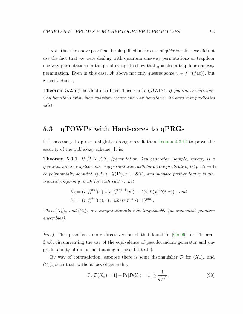
CHAPTER 5. PROOFS FOR CRYPTOGRAPHIC PRIMITIVES 96
Note that the above proof can be simplified in the case of qOWFs, since we did not
use the fact that we were dealing with quantum one-way permutations or trapdoor
one-way permutations in the proof except to show that g is also a trapdoor one-way
permutation. Even in this case, A′ above not only guesses some y ∈ f−1(f(x)), but
x itself. Hence,
Theorem 5.2.5 (The Goldreich-Levin Theorem for qOWFs). If quantum-secure one-
way functions exist, then quantum-secure one-way functions with hard-core predicates
exist.
5.3 qTOWPs with Hard-cores to qPRGs
It is necessary to prove a slightly stronger result than Lemma 4.3.10 to prove the
security of the public-key scheme. It is:
Theorem 5.3.1. If (f,G,S, I) (permutation, key generator, sample, invert) is a
quantum-secure trapdoor one-way permutation with hard-core predicate b, let p : N→ Nbe polynomially bounded, (i, t)← G(1n), x← S(i), and suppose further that x is dis-
tributed uniformly in Di for each such i. Let
Xn = (i, fp(n)i (x), b(i, f
p(n)−1i (x)) . . . b(i, fi(x))b(i, x)) , and
Yn = (i, fp(n)i (x), r) , where r $←−0, 1p(n).
Then (Xn)n and (Yn)n are computationally indistinguishable (as sequential quantum
ensembles).
Proof. This proof is a more direct version of that found in [Gol06] for Theorem
3.4.6, circumventing the use of the equivalence of pseudorandom generator and un-
predictability of its output (passing all next-bit-tests).
By way of contradiction, suppose there is some distinguisher D for (Xn)n and
(Yn)n such that, without loss of generality,
Pr[D(Xn) = 1]− Pr[D(Yn) = 1] ≥ 1
q(n), (98)
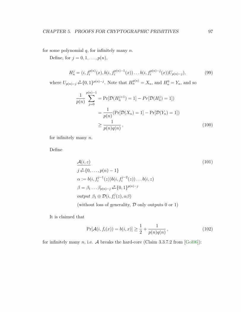
CHAPTER 5. PROOFS FOR CRYPTOGRAPHIC PRIMITIVES 97
for some polynomial q, for infinitely many n.
Define, for j = 0, 1, . . . , p(n),
Hjn = (i, f
p(n)i (x), b(i, f
p(n)−1i (x)) . . . b(i, f
p(n)−ji (x))Up(n)−j), (99)
where Up(n)−j$←−0, 1p(n)−j. Note that H
p(n)n = Xn, and H0
n = Yn, and so
1
p(n)
p(n)−1∑j=0
= Pr[D(Hj+1n ) = 1]− Pr[D(Hj
n) = 1])
=1
p(n)(Pr[D(Xn) = 1]− Pr[D(Yn) = 1])
≥ 1
p(n)q(n), (100)
for infinitely many n.
Define
A(i, z) (101)
j $←−0, . . . , p(n)− 1
α := b(i, f j−1i (z))b(i, f j−2i (z)) . . . b(i, z)
β = β1 . . . βp(n)−j$←−0, 1p(n)−j
output β1 ⊕D(i, f ji (z), αβ)
(without loss of generality, D only outputs 0 or 1)
It is claimed that
Pr[A(i, fi(x)) = b(i, x)] ≥ 1
2+
1
p(n)q(n), (102)
for infinitely many n, i.e. A breaks the hard-core (Claim 3.3.7.2 from [Gol06]):
CHAPTER 5. PROOFS FOR CRYPTOGRAPHIC PRIMITIVES 98
Conditioning on j and β1,
Pr[A(i, fi(x)) = b(i, x)]
= Pr(j)
p(n)−1∑j=0
(Pr[D(i, f ji (f(x)), αβ) = 1 and β1 = b(i, x)]
+ Pr[D(i, f ji (f(x)), αβ) = 0 and β1 ⊕ 1 = b(i, x)])
=1
p(n)
p(n)−1∑j=0
(Pr[D(i, f j+1i (x), b(i, f ji (x))b(i, f j−1i (x)) . . . b(i, f(x))β) = 1 and β1 = b(i, x)]
+ Pr[D(i, f j+1i (x), b(i, f ji (x))b(i, f j−1i (x)) . . . b(i, f(x))β) = 0 and β1 ⊕ 1 = b(i, x)])
=1
2p(n)
p(n)−1∑j=0
(Pr[D(i, f j+1i (x), b(i, f ji (x))b(i, f j−1i (x)) . . . b(i, f(x))b(i, x)β2 . . . βp(n)−j) = 1]
+ Pr[D(i, f j+1i (x), b(i, f ji (x))b(i, f j−1i (x)) . . . b(i, f(x))(b(i, x)⊕ 1)β2 . . . βp(n)−j) = 0]) ,
(103)
since Pr[β1 ⊕ 1 = b(i, x)] = Pr[β1 = b(i, x)] = 12.
Now, note that
(i, f j+1i (x), b(i, f ji (x))b(i, f j−1i (x)) . . . b(i, f(x))b(i, x)β2 . . . βp(n)−j) , and
Hj+1n = (i, f
p(n)i (x), b(i, f
p(n)−1i (x))b(i, f
p(n)−j−1i (x)) . . . b(i, f(x))b(i, x)β2 . . . βp(n)−j)
are identically distributed, since x being distributed uniformly implies that fp(n)−j−1i (x)
is as well, as the image of x under the permutation fp(n)−j−1i .
Define H ′jn to be Hjn but with the jth bit in the third component flipped (the last
bit before Up(n)−j). By the same reasoning,
(i, f j+1i (x), b(i, f ji (x))b(i, f j−1i (x)) . . . b(i, f(x))(b(i, x)⊕ 1)β2 . . . βp(n)−j) , and
H ′j+1n = (i, f
p(n)i (x), b(i, f
p(n)−1i (x))b(i, f
p(n)−j−1i (x)) . . . b(i, f(x))(b(i, x)⊕1)β2 . . . βp(n)−j)
are identically distributed.

CHAPTER 5. PROOFS FOR CRYPTOGRAPHIC PRIMITIVES 99
Hence,
Pr[A(i, fi(x)) = b(i, x)] =1
2p(n)
p(n)−1∑j=0
(Pr[D(Hj+1n ) = 1] + Pr[D(H ′j+1
n ) = 0])
=1
2p(n)
p(n)−1∑j=0
(Pr[D(Hj+1n ) = 1] + 1− Pr[D(H ′j+1
n ) = 1])
=1
2+
1
2p(n)
p(n)−1∑j=0
(Pr[D(Hj+1n ) = 1]− Pr[D(H ′j+1
n ) = 1]) .
(104)
Now, since Hjn = Hj+1
n and Hjn = H ′j+1
n each with probability1
2because Hj
n’s
j + 1st bit is uniformly random,
Pr[D(Hjn) = 1] =
1
2(Pr[D(Hj+1
n ) = 1] + Pr[D(H ′j+1n ) = 1]). (105)
Hence
Pr[D(H ′j+1n ) = 1]) = 2 Pr[D(Hj
n) = 1]− Pr[D(Hj+1n ) = 1] (106)
and
Pr[D(Hj+1n ) = 1])− Pr[D(H ′j+1
n ) = 1]) = 2(Pr[D(Hjn) = 1]− Pr[D(Hj+1
n ). (107)
Finally,
Pr[A(i, fi(x)) = b(i, x)] =1
2+
1
2p(n)
p(n)−1∑j=0
2(Pr[D(Hjn) = 1]− Pr[D(Hj+1
n )
=1
2+
1
p(n)
p(n)−1∑j=0
(Pr[D(Hjn) = 1]− Pr[D(Hj+1
n )
≥ 1
2+
1
p(n)q(n), (108)
for infinitely many n. Hence b is not a hard-core for f , a contradiction.

CHAPTER 5. PROOFS FOR CRYPTOGRAPHIC PRIMITIVES 100
Theorem 5.3.2. If f is a quantum one-way permutation with hard-core predicate b,
then G(x) := b(i, fp(n)−1i (x)) . . . b(i, fi(x))b(i, x) defines a quantum-secure pseudoran-
dom generator.
Proof. Same as the above, omitting the i’s and fp(n)i (x).
Chapter 6
More (on) Security Definitions
In this chapter, further security definitions are discussed. In Section 6.1, indistin-
guishability is defined so that the adversary generates a pair of messages, and it is
proven equivalent to IND (Definition 4.1.3). In Section 6.2, security for the encryp-
tion of multiple messages encrypted with the same key is defined, and it is shown that
security under CPA or CCA1 implies security for multiple messages under CPA or
CCA1, respectively. The last section of this chapter contains discussion on the abso-
lute values in the semantic security definitions in Subsection 6.3.1, semantic security
with the SWAP test as the distinguisher in Subsection 6.3.2, security in which the
simulator never has oracle access under CPA or CCA1 in Subsection 6.3.3, semantic
security with a channel as the target in Subsection 6.3.4, and security for more general
message distributions in Subsection 6.3.5.
6.1 IND with a Pair of Challenge Messages
Rather than fixing one of the messages to be the trivial message, |0〉 〈0| as in IND
and IND’ (Definitions 4.1.3 and 4.4.7, the adversary can generate a pair of messages.
Definition 6.1.1 (INDp). [BJ15] A qPKE scheme (KeyGen,Enc,Dec) is INDp secure
101
CHAPTER 6. MORE (ON) SECURITY DEFINITIONS 102
if for every QPT adversary A = (M,D) we have:∣∣Pr[D(Encpk ⊗ 1E)ρM0E = 1
]−Pr
[D(Encpk ⊗ 1E)ρM1E = 1
]∣∣ ≤ negl(n) ,(109)
where ρM0M1E ←M(pk), and the probabilities are taken over (pk, sk)← KeyGen(1n)
and the internal randomness of Enc, M, and D.
• INDp-CPA: In addition to the above, M and D have oracle access to Encpk.
• INDp-CCA1: In addition to INDp-CPA, M has oracle access to Decsk.
INDp’ can also be defined by modifying IND’ in the same way. These are all
proven equivalent by IND’ ⇐⇒ IND ⇐⇒ INDp ⇐⇒ INDp’, where the first is
already proven, the third can be proven the same way as the first, and the second is
proven as follows:
Proposition 6.1.2 (INDp ⇐⇒ IND). [BJ15] A quantum encryption scheme
(KeyGen,Enc,Dec) is INDp secure if and only if it is IND secure.
Proof. INDp secure =⇒ IND secure: IND is essentially a special case of INDp.
From any IND adversary A = (M,D), define an INDp adversary A′ = (M′,D′)such that D′ = D, and M′ on input pk, outputs ρM0M1E = |0〉 〈0|M0
⊗ ρME, where
ρME ←M(pk), and M1 = M .
IND secure =⇒ INDp secure: this is essentially the transitivity of indistinguish-
able ensembles. From any INDp adversary A = (M,D), define two IND message
generators M0 = TrM1M and M1 = TrM0M. Then,∣∣Pr[D(Encpk ⊗ 1E)ρM0E = 1
]− Pr
[D(Encpk ⊗ 1E)ρM1E = 1
]∣∣≤∣∣Pr[D(Encpk ⊗ 1E)ρM0E = 1
]− Pr
[D(Encpk ⊗ 1E)(|0〉 〈0|M ⊗ ρE) = 1
]∣∣+∣∣Pr[D(Encpk ⊗ 1E)(|0〉 〈0|M ⊗ ρE) = 1
]−∣∣Pr[D(Encpk ⊗ 1E)ρM0E = 1
]∣∣ .(110)
By the triangle inequality, where ρM0M1E ←M(pk), and the probabilities are taken
over (pk, sk)← KeyGen(1n) and the internal randomness of Enc,M, and D. By IND

CHAPTER 6. MORE (ON) SECURITY DEFINITIONS 103
applied to the adversary (M0,D), the quantity on the second line is negligible, and,
applied to the adversary (M1,D), the quantity on the third line is also negligible.
Hence, their sum is negligible, and so must be the quantity on the first line.
6.2 Multiple Message Security
Security in the multiple message setting, where the output of the message generator
is to be divided into multiple message registers, M1, . . . ,M t (where t may depend on
n) and E (and F ) can be defined as follows:
Definition 6.2.1 (IND-mult). [BJ15] A qPKE scheme (KeyGen,Enc,Dec) is IND-
mult secure if for every QPT adversary A = (M,D) we have:∣∣Pr[D(Encpk,M1 ⊗ · · · ⊗ Encpk,Mt ⊗ 1E)ρM1...MtE = 1
]−Pr
[D(Encpk,M1 ⊗ · · · ⊗ Encpk,Mt ⊗ 1E)(|0〉 〈0|M1...Mt ⊗ ρE) = 1
]∣∣ ≤ negl(n) ,
(111)
where ρM1...MtE ←M(pk), ρE = TrM1...Mt(ρM1...MtE), and the probabilities are taken
over (pk, sk)← KeyGen(1n) and the internal randomness of Enc, M, and D.
• IND-mult-CPA: In addition to the above, M and D have oracle access to
Encpk.
• IND-mult-CCA1: In addition to IND-mult-CPA, M has oracle access to
Decsk.
Note that t must be polynomially bounded (and computable), since M is poly-
nomial time.
Definition 6.2.2 (INDp-mult). [BJ15] A qPKE scheme (KeyGen,Enc,Dec) is INDp-
mult secure if for every QPT adversary A = (M,D) we have:∣∣Pr[D(Encpk,M1
0⊗ · · · ⊗ Encpk,Mt
0⊗ 1E)ρM1
0 ...Mt0E
= 1]
−Pr[D(Encpk,M1
1⊗ · · · ⊗ Encpk,Mt
1⊗ 1E)ρM1
1 ...Mt1E
= 1]∣∣ ≤ negl(n) ,
(112)
where ρM10 ...M
t0M
11 ...M
t1E←M(pk), and the probabilities are taken over
(pk, sk)← KeyGen(1n) and the internal randomness of Enc, M, and D.
CHAPTER 6. MORE (ON) SECURITY DEFINITIONS 104
• INDp-mult-CPA: In addition to the above, M and D have oracle access to
Encpk.
• INDp-mult-CCA1: In addition to INDp-mult-CPA, M has oracle access to
Decsk.
IND’-mult and INDp’-mult can also be defined similarly. IND-mult, INDp-mult,
IND’-mult and INDp’-mult are all equivalent, with proofs as in the single message
(or pair of messages) settings.
Definition 6.2.3. [SEM-mult] A qPKE scheme (KeyGen,Enc,Dec) is semantically
secure if for any QPT adversary A, there exists a QPT simulator S such that for all
QPTs M and D,∣∣Pr[D(A⊗ 1F )(Encpk,M1 ⊗ · · · ⊗ Encpk,Mt ⊗ 1EF )ρM1...MtEF = 1
]−Pr
[D(S ⊗ 1F )ρEF = 1
]∣∣ ≤ negl(n) ,
(113)
where ρM1...MtEF ← M(pk), ρEF = TrM1...Mt(ρM1...MtEF ), and the probabilities are
taken over (pk, sk) ← KeyGen(1n) and the internal randomness of Enc, A,S,Mand D.
• SEM-mult-CPA: In addition to the above, all QPTs have oracle access to
Encpk.
• SEM-mult-CCA1: In addition to IND-mult-CPA, M has oracle access to
Decsk.
As in the single message setting, indistinguishability and semantic security are
equivalent under the same form of attack.
Furthermore, under CPA, multiple message security and single message secu-
rity are equivalent. This allows the construction of CPA-secure quantum encryption
schemes that can encrypt messages of arbitrary (polynomial) length from CPA-secure
quantum encryption schemes that can only encrypt messages of a fixed length, by
breaking up the intended message and encrypting it in blocks (and padding if nec-
essary). That is, CPA-secure quantum encryption schemes (as we’ve defined them,
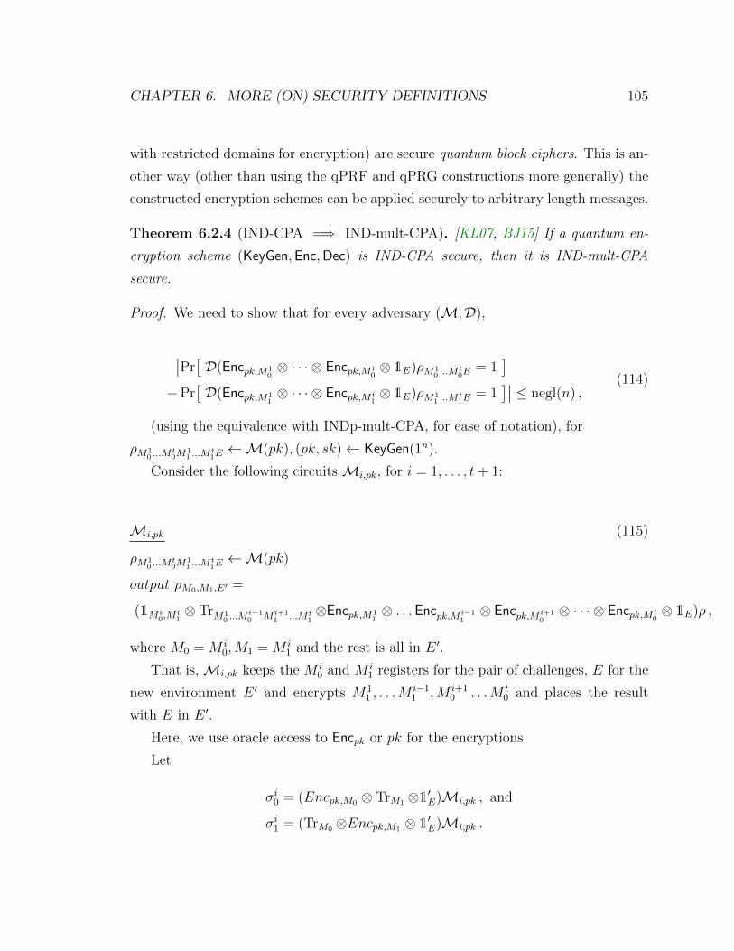
CHAPTER 6. MORE (ON) SECURITY DEFINITIONS 105
with restricted domains for encryption) are secure quantum block ciphers. This is an-
other way (other than using the qPRF and qPRG constructions more generally) the
constructed encryption schemes can be applied securely to arbitrary length messages.
Theorem 6.2.4 (IND-CPA =⇒ IND-mult-CPA). [KL07, BJ15] If a quantum en-
cryption scheme (KeyGen,Enc,Dec) is IND-CPA secure, then it is IND-mult-CPA
secure.
Proof. We need to show that for every adversary (M,D),
∣∣Pr[D(Encpk,M1
0⊗ · · · ⊗ Encpk,Mt
0⊗ 1E)ρM1
0 ...Mt0E
= 1]
−Pr[D(Encpk,M1
1⊗ · · · ⊗ Encpk,Mt
1⊗ 1E)ρM1
1 ...Mt1E
= 1]∣∣ ≤ negl(n) ,
(114)
(using the equivalence with INDp-mult-CPA, for ease of notation), for
ρM10 ...M
t0M
11 ...M
t1E←M(pk), (pk, sk)← KeyGen(1n).
Consider the following circuits Mi,pk, for i = 1, . . . , t+ 1:
Mi,pk (115)
ρM10 ...M
t0M
11 ...M
t1E←M(pk)
output ρM0,M1,E′ =
(1M i0,M
i1⊗ TrM1
0 ...Mi−10 M i+1
1 ...Mt1⊗Encpk,M1
1⊗ . . .Encpk,M i−1
1⊗ Encpk,M i+1
0⊗ · · · ⊗ Encpk,Mt
0⊗ 1E)ρ ,
where M0 = M i0,M1 = M i
1 and the rest is all in E ′.
That is,Mi,pk keeps the M i0 and M i
1 registers for the pair of challenges, E for the
new environment E ′ and encrypts M11 , . . .M
i−11 ,M i+1
0 . . .M t0 and places the result
with E in E ′.
Here, we use oracle access to Encpk or pk for the encryptions.
Let
σi0 = (Encpk,M0 ⊗ TrM1 ⊗1′E)Mi,pk , and
σi1 = (TrM0 ⊗Encpk,M1 ⊗ 1′E)Mi,pk .

CHAPTER 6. MORE (ON) SECURITY DEFINITIONS 106
Then σ10 is distributed identically with (Encpk,M1
0⊗ · · · ⊗ Encpk,Mt
0⊗ 1E)ρM1
0 ...Mt0E
,
and σt1, with (Encpk,M11⊗· · ·⊗Encpk,Mt
1⊗1E)ρM1
1 ...Mt1E
, where ρM10 ...M
t0M
11 ...M
t1E←M(pk).
Furthermore, σi+10 and σi1 are distirbuted identically (they both have the encrypted
registers of M11 , . . . ,M
i1,M
i+10 , . . . ,M t
0).
Hence, we need to show
|Pr[D(σ10) = 1]− Pr[D(σt1) = 1]| ≤ negl(n) . (116)
Define the new message generator M′ by
M′(pk) (117)
i $←−1, . . . , t
output ρ′ ←Mi,pk
Now, using the fact that σi+10 and σi1 are distributed identically,∣∣Pr
[D(Encpk ⊗ 1E′)ρ
′M0E′ = 1
]− Pr
[D(Encpk ⊗ 1E′)ρ
′M1E′ = 1
]∣∣=∣∣∣ t∑i=1
Pr[D(Encpk ⊗ 1E′)ρ
′M0E′ = 1 | i
]Pr[i]
−t∑i=1
Pr[D(Encpk ⊗ 1E′)ρ
′M1E′ = 1 | i
]Pr[i]
∣∣∣=1t
∣∣∣ t∑i=1
(Pr[D(σi0) = 1]− Pr[D(σi1) = 1])∣∣∣
=1t
∣∣∣ t∑i=1
(Pr[D(σi0) = 1]− Pr[D(σi+10 ) = 1])
∣∣∣, where σt+10 := σt1
=1t
∣∣∣ t∑i=1
Pr[D(σi0) = 1]−t+1∑i=2
Pr[D(σi0) = 1]∣∣∣
=1t|Pr[D(σ1
0) = 1]− Pr[D(σt+10 ) = 1]|
=1t|Pr[D(σ1
0) = 1]− Pr[D(σt1) = 1]| .
(118)
Then, by INDp-CPA, applied to (M′,D) the above quantity is negligible, and
since |Pr[D(σ10) = 1] − Pr[D(σt1) = 1]| is the product of this negligible function and
t, polynomially bounded in n, it is also negligible.
CHAPTER 6. MORE (ON) SECURITY DEFINITIONS 107
6.3 Further Motivation for SEM and Alternatives
This sections discusses further variations on semantic security and indistinguishability.
6.3.1 Absolute Values in Semantic Security
Note that SEM, SEM2 and SEM3 (Definitions 4.2.1, 4.4.2 and 4.4.5) were defined
with the expression in absolute values. This was not necessary, and previous defini-
tions did not include the absolute values [Gol04, GM84]. Without absolute values,
semantic security means that for each adversary, there exists a simulator that does
just as well or better. With absolute values, semantic security means that for each
adversary, there exists a simulator that does just as well and just as poorly. Clearly
semantic security with absolute values implies semantic security without, but these
definitions are, in fact, equivalent. The proofs for Theorem 4.2.3 SEM =⇒ IND and
Theorem 4.4.9 SEM3 =⇒ IND’ carry through when the absolute values are dropped,
so that, combined with Proposition 4.4.8 IND’ ⇐⇒ IND and Theorem 4.2.2 IND
=⇒ SEM, semantic security without absolute values implies semantic security with
absolute values.
6.3.2 The Swap Test as a Distinguisher for SEM
The swap test [GC01] can be used as the distinguisher D in SEM. The swap test
proceeds by applying controlled-SWAP s (CSWAP or Fredkin gates) to the corre-
sponding qubits of ρ and σ, controlled on the state H |0〉 = |+〉 = 12|0〉 + 1
2|1〉,
applying the Hadamard again to the control qubit, measuring the control qubit and
outputting the (negation of) the result.
The probability of acceptance of the swap test applied to a product state ρ ⊗ σ(where ρ and σ have the same number of qubits) is
1 + Tr(σρ)
2. (119)
Then, taking D in SEM to be the SWAP-test and considering only message gen-
erators whose outputs are product states of the form ρME⊗ρF and adversaries whose
CHAPTER 6. MORE (ON) SECURITY DEFINITIONS 108
|0〉 H • H
ρSWAP
σ
Figure 5: Circuit for the swap test
output has the same number of qubits as F , the expression in SEM becomes
|Tr[ρF (A(Encpk ⊗ 1E)ρME − SρE)]| ≤ negl(n) . (120)
It’s easy to see that defining semantic security in this restricted way implies SEM2
(Definition 4.4.2), since for a message-classical function generator (Definition 4.4.1)
outputting ρMEF = ρME ⊗ |y〉 〈y|F ,
|Tr[ρF (A(Encpk ⊗ 1E)ρME − SρE]| = | 〈y| (A(Encpk ⊗ 1E)(ρME − SρE) |y〉 |
= |Pr[A(Encpk ⊗ 1E)(ρME) = y]− Pr[S(ρE) = y]| ,(121)
where the probabilities are taken after measuring in the computational basis.
6.3.3 Simulator Oracle Access
Semantic security could be defined, not by ∀A∃S∀M∀D, but by ∀A∃A′∀M∃M′∀Dwith some restrictions on M′, i.e.:
Definition 6.3.1. A qPKE scheme (KeyGen,Enc,Dec) is SEM’ if for any QPT
A, there exists a QPT A′ such that for every QPT M, there exists a QPT M′
such that ∀n, ρMEF and ρ′MEF are identically distributed, where ρMEF ←M(pk),
(pk, sk)← KeyGen(1n) and ρ′MEE′F = ρ′MEF ⊗ |x〉 〈x|E′ ←M′(1n), and for every QPT
D, ∣∣Pr[D(A⊗ 1F )(Encpk ⊗ 1EF )ρMEF = 1
]−Pr
[D(A′ ⊗ 1F )(ρ′EF ⊗ |x〉 〈x|E′) = 1
]∣∣ ≤ negl(n) ,(122)
CHAPTER 6. MORE (ON) SECURITY DEFINITIONS 109
where ρMEF ←M(pk), ρ′MEF ⊗ |x〉 〈x|E′ ←M′(1n), and the probabilities are taken
over (pk, sk)← KeyGen(1n) and the internal randomness of Enc,A,A′,M,M′ and D.
• SEM’-CPA: In addition to the above, A and M have oracle access to Encpk.
• SEM’-CCA1: In addition to SEM’-CPA, M has oracle access to Decsk.
This definition is closer to that in [Gol04]. A and M are as before in SEM
(Definition 4.2.1), but A′ and S ′ do not receive public keys in the public-key setting
or oracle access under CPA or CCA1. Furthermore, M′ also outputs a binary string
x into an extra register E ′, on top of ρ′MEF , to be passed along to A′, which receives
this x on top of ρE. Of course, one could allow more general states in E ′, even for
E ′ to be entangled with the rest, as long as the “challenges” are the same, i.e. ρMEF
and ρ′MEF are identically distributed, where ρMEF ←M(pk), (pk, sk)← KeyGen(1n)
and ρ′MEF ← TrE′M′(1n). However, just a classical binary string is sufficient for (an
easy proof that) IND =⇒ SEM, so the definition is seemingly stronger by further
restricting M′, whose existence is required for SEM’ to hold.
To prove IND =⇒ SEM’, as in [Gol04], A′ is defined as before in the proof of
Theorem 4.2.3, but also takes extra classical input to use as keys in the encryption and
decryption algorithms as subroutines in place of oracle queries. M′ is defined from
M by generating its own (pk, sk) ← KeyGen(1n), using M on the pk it generated,
replacing any oracle queries with the use of the encryption and decryption algorithms
as subroutines with these keys, and then forwarding the keys as x in E ′ along to A′.In the private-key scenario under regular attack (neither CPA nor CCA1), there’s no
need to pass along a key at all, as A′ simply generates its own, as did S previously.
SEM2 and SEM3 can also be modified accordingly, and the rest of the cycle of
implications from SEM’ =⇒ SEM2’ =⇒ SEM3’ =⇒ IND’ =⇒ IND can again
be completed as before.
Such a definition may appear stronger, since a simulator that knows nothing
about the keys and without any oracle access always suffices. It is, however, much
clunkier. Furthermore, once it’s fully parsed and understood, it seems less intuitive
if one interprets M as the behaviour of some honest party sending messages, since
the adversary and simulator should be working on the same message generator, not

CHAPTER 6. MORE (ON) SECURITY DEFINITIONS 110
different ones that output identically distributed messages when the probabilities are
taken over the keys (and the internal randomness ofM andM′). That being said, the
interpretation of the behaviour of M as honest when it is given oracle access to the
encryption or decryption algorithms is itself somewhat tenuous, although perhaps
justified by the possibility that the message sender can be deceived into using the
oracles or into sending particular messages after interacting with a malicious party
with access to the oracles.
6.3.4 Semantic Security with a Channel as the Target
As mentioned already in Subsection 4.2.1, one of first obvious definitions of semantic
security for the encryption of quantum states is to replace, in the classical definition,
the function of the plaintext that adversaries attempt to predict with quantum circuits
or general quantum channels (which may not be efficiently implemented) and consider
how well the adversaries approximate them.
In more detail, in the classical setting, semantic security is defined with some
function f of the plaintext to be predicted by the adversary A and simulator S. A
natural quantum version of this could mean replacing f by a quantum channel Φ,
and rather than looking for the difference between the probability that the output
of A and the output of Φ are strictly identical, and the probability that the output
of S and the output of Φ are strictly identical, one can pass the outputs through a
QPT distinguisher D (i.e. measurements) and check for equality of the outcomes.
Furthermore, in the original definition of semantic security given by Goldwasser and
Micali in [GM84], f was any sequence of functions, indexed by the keyed encryption
algorithm (equivalently, the public key), i.e. it need not be computable.
A candidate definition for semantic security could be the following:
Definition 6.3.2. A qPKE scheme (KeyGen,Enc,Dec) is SEMF if for any QPT
adversary A, there exists a QPT simulator S such that for all quantum channels Φ,
for all QPTs M and D, there exists a negligible function negl such that
|Pr[DA(Encpk ⊗ 1E)ρME = DΦpkρM ]− Pr[DSρE = DΦpkρM ]| ≤ negl(n) , (123)
for all n, (pk, sk)← KeyGen(1n), ρME ←M(pk).

CHAPTER 6. MORE (ON) SECURITY DEFINITIONS 111
With the usual additions for CPA and CCA1.
The channel Φ above can be restricted to be QPT (or one could allow more general
quantum operations, although this misses the point of semantic security).
However, such a definition may be asking too much, since the “game” that the
semantic security definition captures does not appear to be generally realistic, as it
would require two copies of the message to exist: one for encryption and one to which
the quantum circuit or channel is applied: the event DA(Encpk⊗1E)ρME = DΦpkρM
contains the M subsystem of ρME twice, so attempting to generate events distributed
this way in an IND game may not be feasible in polynomial time. In the original
proof by Goldwasser and Micali in [GM84], despite defining a different IND message
generator based on the original SEM one, the algorithm they defined required multiple
encryptions of the same message. Of course, cloning arbitrary quantum states is
known to be impossible (by the no-cloning theorem, Theorem 3.4.13, but we need
only prepare states ρ ⊗ ρ, such that ρ is distributed identically to the output of M(or some other suitable message generator).
One might instead hope that setting D′ := DA and M′ :=M for a distinguisher
would work, but a proof along these lines has not been found. One obstacle is that,
since the output of D is not fixed on each of the trivial 0 and message generator
challenges, a priori, D′ = 1 may occur with the same probability on the two challenges,
despite the non-negligible difference in the probabilities that the outputs of D′ and
DΦpk are the same. To illustrate the problem with a simple example, consider two
uniformly random bits, x, and y. Then, |Pr[x = x] − Pr[y = x]| = 1 − 12
= 12, but
Pr[x = 1] = Pr[y = 1] = 12.
Furthermore, in SEM3 (Definition 4.4.5, as in [GM84] or [Des09, DD10]), one could
allow f to be arbitrary (with polynomially bounded output), not just QPT. However,
again the proof in [GM84] does not carry through due to no-cloning, and the proof
in [Des09, DD10] has its own problems. The latter uses Goldreich-Levin predicates
to go from breaking semantic security with arbitrary f to breaking semantic security
with a predicate, and from an adversary A to the distinguisher D := r A, the
dot product of r and A for some appropriate r. However, r is not chosen uniformly,
CHAPTER 6. MORE (ON) SECURITY DEFINITIONS 112
and it’s not clear that it can be, nor can r simply be chosen randomly and the same
message generator be used, since the same obstacle as in the previous paragraph is
encountered. It’s also not clear that their proof will carry over into the non-uniform
computational setting. The idea is to generate messages that satisfy r f = 1 only
or r f = 0 only, with r fixed, for each pair of keys (so the message generators
would become non-uniform, too). Since r f is, in general, an arbitrary function in
0, 1m → 0, 1, the 2m values of r f cannot all be hardcoded into the circuit or
used as advice, and the function’s circuit complexity may grow faster in n than any
polynomial, so no polynomial size subcircuit to implement it may exist.
Returning to the problem of preparing multiple copies of a message, applying the
deferred measurement principle toM and purifying the result will give, on input pk,
a pure state∑
x αx |ψx〉 |x〉, so that measuring the x system and tracing out part of
the resulting state gives ρ distributed as the output of M.
Two approaches would be
1. Prepare∑
x αx |ψx〉 |x〉 |ψx〉 |x〉, and then measure and apply traces as appropri-
ate to obtain two identical messages.
2. Generate one message, recording the measurement result x0, and then “amplify
the amplitude” of the x0 term in∑
x αx |ψx〉 |x〉 to obtain (or approximate)
|ψx0〉 |x0〉. Then measure and apply traces as appropriate to obtain a second
copy of the first message.
It is not clear how to achieve 1. The no-cloning theorem prevents us from passing
from arbitrary∑
x αx |ψx〉 |x〉 to∑
x αx |ψx〉 |x〉 |ψx〉 |x〉 with a single deterministic
channel, but∑
x αx |ψx〉 |x〉 is fixed for each n or key or pair of keys.
To expand on the second approach, amplitude amplification [BHMT02, KLM07]
is a generalization of Grover’s search algorithm, which would use the purification of
the message generator as a black box. However, it appears not to be efficient enough,
since the algorithm uses Θ( 1√p) applications of the purified circuit and its inverse in
the worst case for p the probability that a particular message is generated: with even
a just linear number of measurement gates (fixing the input to the quantum circuit), p
may be exponentially small, so the running time may be exponential. This is also for
CHAPTER 6. MORE (ON) SECURITY DEFINITIONS 113
p known, but they design a quantum search algorithm that works in Θ( 1√p) expected
applications for p unknown. Θ( 1√p) is optimal (as a generalization of Grover’s), but
the problem it solves is posed with the preparation circuit and the characteristic
function for solutions given as black boxes, which is not the case here: a description
of the circuit and the measurements are both given.
One possible solution to avoid the whole issue is to not permit measurement gates
at all, or at least limit the number in the message generator to be O(log n) to be able
to use quantum search or just repeatedly generate messages until the measurement
matches the first one, but in doing so, the definitions become contrived and may no
longer even be equivalent to the ones used in this thesis. When it is possible to
prepare the messages multiple times and Φ is QPT, SEM as defined in 4.2.1 captures
this.
The possible equivalence of IND and SEMF is left as an open problem.
6.3.5 Alternative Message Distributions
However, if SEMF is defined as above in Definition 6.3.2, but where ρ is distributed
arbitrarily (not necessarily generated, but indexed by the security parameter n as a
sequential ensemble (ρn)n, or possibly the public key pk), and the same is done for
IND, it is easy to show IND =⇒ SEM:
Proof. By contrapositive, suppose not SEM. Then there exists an A such that for all
S, there exists ρME,Φ and D and a polynomial p such that the above difference in
probabilities is > 1/p(n) for infinitely many n.
Define a simulator S by SρE := A(Encpk(|0〉 〈0|)⊗ρE) and consider corresponding
Φ,D and p that together violate SEM. In the private-key without oracle access to
Encpk, generate a new key, and use it instead.
Simulating the above SEM game by an IND game is enough to show
IND =⇒ SEM. Given ρME distributed arbitrarily, define quantum states distributed
as ρ′ME′ = ρME ⊗ Φ(ρM). Here, there are two copies of ρ, but they haven’t been
obtained from a single one through a quantum channel, so no-cloning is not violated.
CHAPTER 6. MORE (ON) SECURITY DEFINITIONS 114
Define the IND distinguisher, D′ by D′(σCEF ) = 1 if D(A⊗ I)σCE = DσF , and 0
otherwise.
Doing this, we’ve simulated the SEM game by an IND game in which D′ distin-
guishes encryptions of ρ′ME′ from encryptions of |0〉 〈0|⊗ρ′E′ , since the SEM expression
becomes
|Pr[D′(Encpk ⊗ 1E)(ρ′ME′) = 1]− Pr[D′(Encpk(|0〉 〈0|)⊗ ρ′E′) = 1]| > 1p(n)
, (124)
for infinitely many n.
The above proof can also be adapted to unbounded depth message generators
(with at most polynomially many measurement gates, uniform or non-uniform, but
still requiring the size of the state to be polynomially bounded in n): ρ could be gen-
erated and while doing so, the measurement results that lead to it could be recorded,
putting them in E ′. Then the message generator is reused until, with high enough
probability (so that 1− Pr is negligible), a second copy of a state resulting from the
same measurement results (and thus identical to the first) is obtained. In the non-
uniform setting, if Φ is allowed to be arbitrarily chosen (but polynomially bounded
in output size), then Φ could be approximated in order to generate ρ′ME′ as above.
The uniform setting with Φ arbitrary would be a closer analogue of the original for-
mulation of semantic security in [GM84], and a similarly more complex proof would
likely be necessary.
However, in having messages distributed this way (either through unbounded
depth generators or arbitrary distributions), the following cannot be allowed, as in
the classical setting, or else such a definition of security will never be satisfied:
1. the length of the messages (|M |+ |E|) grows at least exponentially, or
2. the messages depend on (i.e. are indexed by) pk or the encryption or decryption
oracle.
The same arguments as in the classical case work, see the exercises 3 and 28.2,
respectively, in [Gol04, Chapter 5].
CHAPTER 6. MORE (ON) SECURITY DEFINITIONS 115
Arbitrary message distributions (with the above restrictions) could allow continu-
ous message distributions (as in [XY12]) or even more general ones. Of course, CCA1
security would have to be defined differently, for example, by having another algo-
rithm taking pk (or 1n) as input, with access to the encryption and decryption oracles
and whose output is given to the adversary and simulator, along with the challenge
to the adversary, independently of the message in the challenge.
Chapter 7
Conclusion
This chapter is from the joint paper [ABF+16]: one item in Section 7.1 from the paper
has been removed for this thesis, and the second one listed here has been added.
We have defined semantic security for the encryption of quantum data and shown
its equivalence with indistinguishability. We have given general constructions of
CCA1-secure private-key quantum encryption schemes and a secure public-key quan-
tum encryption schemes from quantum-secure one-way functions and quantum-secure
trapdoor one-way permutations.
7.1 Extensions and Future Work
We now briefly discuss some possible extensions of the above results. In most cases,
these extensions are a matter of modifying our definitions and proofs in a fairly
straightforward way. We leave the other cases as interesting open problems.
1. Our definitions of IND-CPA, IND-CCA1 and SEM assume that all of the rele-
vant messages are generated in polynomial time. In other words, our results as-
sume “uniform” adversaries. As is standard classically (see Chapter 5 of Goldre-
ich’s text [Gol04]), these definitions can be adjusted to the case of “non-uniform”
(but still polynomial-time) adversaries, whose messages need not be generated
efficiently. While the proof is of course somewhat different, the equivalence
116
CHAPTER 7. CONCLUSION 117
of IND and SEM still hold in this case. The encryption schemes (IND-CCA1
private-key and IND-CPA public-key) presented above carry over as well, ex-
cept that we now require primitives (qPRFs and qTOWPs, respectively) which
are secure against non-uniform adversaries.
2. The possible equivalence of IND and a suitable semantic security definition
with the contents F as the output of a channel applied to ρM (as in Defini-
tion 6.3.2 SEMF) is left as an open problem. Various obstacles were raised in
Subsection 6.3.4.
3. Another outstanding open problem is to define and construct schemes for CCA2
(adaptive chosen ciphertext attack) security in the case of the encryption of
quantum states. Classically, CCA2 security is defined as CCA1, with the further
property that the adversary is allowed to query the decryption oracle even after
the challenge query, provided he does not query about the challenge ciphertext
itself (otherwise the challenger aborts the game.) The obvious way to define
this in the quantum world is to require that every decryption query performed
by the adversary after the challenge query is ‘very different’ from the challenge
query itself (e.g., it is orthogonal to the challenge ciphertext.) But the problem
here is that this condition might be impossible for the challenger to check: for
example, the adversary might embed in a decryption query a component non-
orthogonal to the challenge query, but with such a small amplitude that the
challenger cannot detect it with high probability. Even if it is unclear whether
this issue could raise problems in any actual reduction, it would be anyway a
striking asymmetry to the classical case, because there would be no way for the
challenger to check that the adversary actually fulfilled the required condition.
Hence, giving a satisfactory definition for CCA2 security in the quantum world
remains an interesting open problem.
Bibliography
[Aar09] Scott Aaronson. Quantum copy-protection and quantum money. In
Computational Complexity, 2009. CCC’09. 24th Annual IEEE Confer-
ence on, pages 229–242. IEEE, 2009.
[ABB+14] Romain Alleaume, Cyril Branciard, Jan Bouda, Thierry Debuiss-
chert, Mehrdad Dianati, Nicolas Gisin, Mark Godfrey, Philippe Grang-
ier, Thomas Langer, Norbert Lutkenhaus, Christian Monyk, Philippe
Painchault, Momtchil Peev, Andreas Poppe, Thomas Pornin, John Rar-
ity, Renato Renner, Gregoire Ribordy, Michel Riguidel, Louis Salvail,
Andrew Shields, Harald Weinfurter, and Anton Zeilinger. Using quan-
tum key distribution for cryptographic purposes: A survey. Theoretical
Computer Science, 560:62–81, 2014.
[ABF+16] Gorjan Alagic, Anne Broadbent, Bill Fefferman, Tommaso Gagliar-
doni, Christian Schaffner, and Michael St. Jules. Computational se-
curity of quantum encryption, 2016. To appear in the 9th Inter-
national Conference on Information Theoretic Security (ICITS2016).
http://arxiv.org/abs/1602.01441.
[AC02] Mark Adcock and Richard Cleve. A quantum Goldreich-Levin theorem
with cryptographic applications. In Helmut Alt and Afonso Ferreira,
editors, STACS 2002, volume 2285 of Lecture Notes in Computer Sci-
ence, pages 323–334. Springer Berlin Heidelberg, 2002.
118

BIBLIOGRAPHY 119
[AC12] Scott Aaronson and Paul Christiano. Quantum money from hidden
subspaces. In Proceedings of the forty-fourth annual ACM symposium
on Theory of computing, pages 41–60. ACM, 2012.
[ACM13] Association for Computing Machinery ACM. Listen to interviews
with 2012 ACM Turing Award recipients Shafi Goldwasser and
Silvio Micali, 2013. http://www.acm.org/news/featured/awards/
turing-award-2012.
[AKN98] Dorit Aharonov, Alexei Kitaev, and Noam Nisan. Quantum circuits
with mixed states. In Proceedings of the Thirtieth Annual ACM Sym-
posium on Theory of Computing, STOC ’98, pages 20–30, New York,
NY, USA, 1998. ACM.
[Alb83] David Z. Albert. On quantum-mechanical automata. Physics Letters
A, 98(5):249 – 252, 1983.
[AMTdW00] Andris Ambainis, Michele Mosca, Alain Tapp, and Ronald de Wolf.
Private quantum channels. In Foundations of Computer Science, 2000.
Proceedings. 41st Annual Symposium on, pages 547–553, 2000.
[BB84] Charles H. Bennett and Gilles Brassard. Quantum cryptography: Pub-
lic key distribution and coin tossing. In Proceedings of the International
Conference on Computers, Systems, and Signal Processing, pages 175–
179, 1984.
[BBBV97] Charles H. Bennett, Ethan Bernstein, Gilles Brassard, and Umesh Vazi-
rani. Strengths and weaknesses of quantum computing. SIAM J. Com-
put., 26(5):1510–1523, October 1997.
[BBC+93] Charles H. Bennett, Gilles Brassard, Claude Crepeau, Richard Jozsa,
Asher Peres, and William K. Wootters. Teleporting an unknown quan-
tum state via dual classical and einstein-podolsky-rosen channels. Phys.
Rev. Lett., 70:1895–1899, Mar 1993.

BIBLIOGRAPHY 120
[Bel64] John Stewart Bell. On the Einstein-Podolsky-Rosen paradox. Physics,
1(3):195–200, 1964.
[Ben80] Paul Benioff. The computer as a physical system: A microscopic quan-
tum mechanical Hamiltonian model of computers as represented by Tur-
ing machines. Journal of Statistical Physics, 22(5):563–591, 1980.
[Ben82] Paul Benioff. Quantum mechanical Hamiltonian models of Turing ma-
chines. Journal of Statistical Physics, 29(3):515–546, 1982.
[BFK09] Anne Broadbent, Joseph Fitzsimons, and Elham Kashefi. Universal
blind quantum computation. In Foundations of Computer Science,
2009. FOCS’09. 50th Annual IEEE Symposium on, pages 517–526.
IEEE, 2009.
[BGS13] Anne Broadbent, Gus Gutoski, and Douglas Stebila. Quantum one-time
programs. In Advances in Cryptology–CRYPTO 2013, pages 344–360.
Springer, 2013.
[BHJ26] Max Born, Werner Heisenberg, and Pascual Jordan. Zur quanten-
mechanik. ii. Zeitschrift fur Physik, 35(8):557–615, 1926.
[BHMT02] Gilles Brassard, Peter Høyer, Michele Mosca, and Alain Tapp. Quan-
tum amplitude amplification and estimation. In Quantum Computation
and Quantum Information: A Millennium Volume, volume 305 of AMS
Contemporary Mathematics Series, pages 53–74. American Mathemat-
ical Society, 2002. Earlier version in arxiv:quant-ph/0005055.
[BJ26] Max Born and Pascual Jordan. Zur quantenmechanik. Zeitschrift fur
Physik, 34(1):858–888, 1926.
[BJ15] Anne Broadbent and Stacey Jeffery. Quantum homomorphic encryp-
tion for circuits of low T -gate complexity. In Advances in Cryptology–
CRYPTO 2013, pages 609–629. Springer, 2015.
BIBLIOGRAPHY 121
[BOCG+06] Michael Ben-Or, Claude Crepeau, Daniel Gottesman, Avinatan Has-
sidim, and Adam Smith. Secure multiparty quantum computation with
(only) a strict honest majority. In Foundations of Computer Science,
2006. FOCS’06. 47th Annual IEEE Symposium on, pages 249–260.
IEEE, 2006.
[BR03] P. Oscar Boykin and Vwani Roychowdhury. Optimal encryption of
quantum bits. Physical Review A, 67(4):042317, 2003.
[Bro15] Anne Broadbent. Delegating private quantum computations. Canadian
Journal of Physics, pages 941–946, Jun 2015.
[BV93] Ethan Bernstein and Umesh Vazirani. Quantum complexity theory. In
Proceedings of the Twenty-fifth Annual ACM Symposium on Theory of
Computing, STOC ’93, pages 11–20, New York, NY, USA, 1993. ACM.
[BZ13] Dan Boneh and Mark Zhandry. Secure Signatures and Chosen Cipher-
text Security in a Quantum Computing World. In Ran Canetti and
Juan A. Garay, editors, Crypto 2013, volume 8043 of LNCS, pages
361–379. Springer, 2013.
[Coc73] Clifford C. Cocks. A note on non-secret encryption. CESG, 1973.
[dB24] Louis de Broglie. Recherches sur la theorie des Quanta. Theses, Migra-
tion - universite en cours d’affectation, November 1924.
[DD10] Simon Pierre Desrosiers and Frederic Dupuis. Quantum entropic se-
curity and approximate quantum encryption. IEEE Transactions on
Information Theory, 56(7):3455–3464, 2010.
[Des09] Simon Pierre Desrosiers. Entropic security in quantum cryptography.
Quantum Information Processing, 8(4):331–345, August 2009.

BIBLIOGRAPHY 122
[Deu85] David Deutsch. Quantum theory, the Church-Turing principle and the
universal quantum computer. Proceedings of the Royal Society of Lon-
don A: Mathematical, Physical and Engineering Sciences, 400(1818):97–
117, 1985.
[Deu89] David Deutsch. Quantum computational networks. Proceedings of the
Royal Society of London A: Mathematical, Physical and Engineering
Sciences, 425(1868):73–90, 1989.
[DH76] Whitfield Diffie and Martin E. Hellman. New directions in cryptogra-
phy. IEEE transactions on Information Theory, 22(6):644–654, 1976.
[Die82] Dennis Dieks. Communication by EPR devices. Physics Letters A,
92(6):271 – 272, 1982.
[Dir30] Paul. A. M. Dirac. The Principles of Quantum Mechanics. Interna-
tional series of monographs on physics (Oxford, England). Oxford, the
Clarendon Press, 1930.
[DJ92] David Deutsch and Richard Jozsa. Rapid solution of problems by quan-
tum computation. Proceedings of the Royal Society of London A: Math-
ematical, Physical and Engineering Sciences, 439(1907):553–558, 1992.
[DN06] Christopher M. Dawson and Michael A. Nielsen. The Solovay-Kitaev
algorithm. Quantum Info. Comput., 6(1):81–95, January 2006.
[DNS10] Frederic Dupuis, Jesper Buus Nielsen, and Louis Salvail. Secure two-
party quantum evaluation of unitaries against specious adversaries. In
Advances in Cryptology–CRYPTO 2010, pages 685–706. Springer, 2010.
[DNS12] Frederic Dupuis, Jesper Buus Nielsen, and Louis Salvail. Actively se-
cure two-party evaluation of any quantum operation. In Advances in
Cryptology–CRYPTO 2012, pages 794–811. Springer, 2012.
[Ell70] James Henry Ellis. The possibility of secure non-secret digital encryp-
tion. CESG, 1970.

BIBLIOGRAPHY 123
[EPR35] Albert Einstein, Boris Podolsky, and Nathan Rosen. Can quantum-
mechanical description of physical reality be considered complete?
Phys. Rev., 47:777–780, May 1935.
[Fey82] Richard P. Feynman. Simulating physics with computers. International
Journal of Theoretical Physics, 21(6):467–488, 1982.
[FKS+13] Serge Fehr, Jonathan Katz, Fang Song, Hong-Sheng Zhou, and Vas-
silis Zikas. Feasibility and completeness of cryptographic tasks in the
quantum world. In Theory of Cryptography, pages 281–296. Springer,
2013.
[GC01] Daniel Gottesman and Isaac Chuang. Quantum digital signatures, 2001.
https://arxiv.org/abs/quant-ph/0105032.
[GGM86] Oded Goldreich, Shafi Goldwasser, and Silvio Micali. How to construct
random functions. Journal of the ACM, 33(4):792–807, 1986.
[GHS15] Tommaso Gagliardoni, Andreas Hulsing, and Christian Schaffner. Se-
mantic security and indistinguishability in the quantum world, 2015.
To appear in CRYPTO2016. http://arxiv.org/abs/1504.05255.
[GL89] Oded Goldreich and Leonid A. Levin. A hard-core predicate for all
one-way functions. In Proceedings of the Twenty-first Annual ACM
Symposium on Theory of Computing, STOC ’89, pages 25–32, New
York, NY, USA, 1989. ACM.
[GM82] Shafi Goldwasser and Silvio Micali. Probabilistic encryption & how to
play mental poker keeping secret all partial information. In Proceedings
of the Fourteenth Annual ACM Symposium on Theory of Computing,
STOC ’82, pages 365–377, New York, NY, USA, 1982. ACM.
[GM84] Shafi Goldwasser and Silvio Micali. Probabilistic encryption. Journal
of Computer and System Sciences, 28(2):270 – 299, 1984.
BIBLIOGRAPHY 124
[Gol93] Oded Goldreich. A uniform-complexity treatment of encryption and
zero-knowledge. Journal of Cryptology, 6(1):21–53, 1993.
[Gol04] Oded Goldreich. Foundations of Cryptography: Volume 2, Basic Appli-
cations. Cambridge University Press, Cambridge, UK, 2004.
[Gol06] Oded Goldreich. Foundations of Cryptography: Volume 1, Basic Tools.
Cambridge University Press, New York, NY, USA, 2006.
[GPV08] Craig Gentry, Chris Peikert, and Vinod Vaikuntanathan. Trapdoors for
hard lattices and new cryptographic constructions. In Proceedings of
the Fortieth Annual ACM Symposium on Theory of Computing, STOC
’08, pages 197–206, New York, NY, USA, 2008. ACM.
[Gro96] Lov K. Grover. A fast quantum mechanical algorithm for database
search. In Proceedings of the Twenty-Eighth Annual Symposium on the
Theory of Computing, pages 212–219, New York, 1996. ACM Press.
[HBD+15] B. Hensen, H. Bernien, A. E. Dreau, A. Reiserer, N. Kalb, M. S.
Blok, J. Ruitenberg, R. F. L. Vermeulen, R. N. Schouten, C. Abellan,
W. Amaya, V. Pruneri, M. W. Mitchell, M. Markham, D. J. Twitchen,
D. Elkouss, S. Wehner, T. H. Taminiau, and R. Hanson. Loophole-free
Bell inequality violation using electron spins separated by 1.3 kilome-
tres. Nature, 526(7575):682–686, October 2015.
[Hei25] Werner Heisenberg. Uber quantentheoretische umdeutung kinematis-
cher und mechanischer beziehungen. Zeitschrift fur Physik, 33(1):879–
893, 1925.
[Hei27] Werner Heisenberg. Uber den anschaulichen inhalt der quantentheo-
retischen kinematik und mechanik. Zeitschrift fur Physik, 43(3):172–
198, 1927.
[Hil06] David Hilbert. Grundzuge einer allgemeinen theorie der linearen in-
tegralgleichungen. vierte mitteilung. Nachrichten von der Gesellschaft
BIBLIOGRAPHY 125
der Wissenschaften zu Gottingen, Mathematisch-Physikalische Klasse,
1906:157–228, 1906.
[HILL99] Johan Hastad, Russell Impagliazzo, Leonid A. Levin, and Michael Luby.
A pseudorandom generator from any one-way function. SIAM J. Com-
put., 28:1364–1396, March 1999.
[HLSW04] Patrick Hayden, Debbie Leung, Peter W Shor, and Andreas Winter.
Randomizing quantum states: Constructions and applications. Com-
munications in Mathematical Physics, 250(2):371–391, 2004.
[Hol73] Alexander S. Holevo. Bounds for the quantity of information transmit-
ted by a quantum communication channel. Problems of Information
Transmission, 9(3):177–183, 1973.
[HvN28] David Hilbert, John von Neumann, and Lothar Wolfgang Nordheim.
Uber die grundlagen der quantenmechanik. Mathematische Annalen,
98(1):1–30, 1928.
[Ing76] Roman S. Ingarden. Quantum information theory. Reports on Mathe-
matical Physics, 10(1):43 – 72, 1976.
[Kit97] Alexei Yu Kitaev. Quantum computations: algorithms and error cor-
rection. Uspekhi Mat. Nauk, 52:53 – 112, 1997.
[KK07] Elham Kashefi and Iordanis Kerenidis. Statistical zero knowledge and
quantum one-way functions. Theoretical Computer Science, 378(1):101
– 116, 2007.
[KL07] Jonathan Katz and Yehuda Lindell. Introduction to Modern Cryptogra-
phy. Chapman & Hall/CRC Cryptography and Network Security Series,
2007.
[KLM07] Phillip Kaye, Raymond Laflamme, and Michele Mosca. An Introduction
to Quantum Computing. Oxford University Press, 2007.

BIBLIOGRAPHY 126
[Kos07] Takeshi Koshiba. Security notions for quantum public-key cryptogra-
phy. IEICE TRANSACTIONS on Fundamentals of Electronics, Com-
munications and Computer Sciences, J90-A(5):367–375, Feb 2007.
[Leu02] Debbie W. Leung. Quantum Vernam cipher. Quantum Information
and Computation, 2(1):14–34, 2002.
[Llo96] Seth Lloyd. Universal quantum simulators. Science, 273(5278):1073–
1078, 1996.
[Man80] Yuri Ivanovitch Manin. Vychislimoe i nevychislimoe (Computable and
Uncomputable). ”Sov. radio,” Moskva, 1980.
[Mer78] Ralph C. Merkle. Secure communications over insecure channels. Com-
mun. ACM, 21(4):294–299, April 1978.
[Mer10] Ralph C. Merkle. Publishing a new idea, 2010. http://merkle.com/
1974/.
[MHS+12] X.-S. Ma, T. Herbst, T. Scheidl, D. Wang, S. Kropatschek, W. Naylor,
B. Wittmann, A. Mech, J. Kofler, E. Anisimova, V. Makarov, T. Jen-
newein, R. Ursin, and A. Zeilinger. Quantum teleportation over 143
kilometres using active feed-forward. Nature, 489:269–273, September
2012.
[MRV07] Cristopher Moore, Alexander Russell, and Umesh Vazirani. A classical
one-way function to confound quantum adversaries. eprint arXiv:quant-
ph/0701115, January 2007.
[MS10] Michele Mosca and Douglas Stebila. Quantum coins. Error-Correcting
Codes, Finite Geometries and Cryptography, 523:35–47, 2010.
[Nai40] Mark A. Naimark. Spectral functions of a symmetric operator. Izvestiya
Rossiiskoi Akademii Nauk. Seriya Matematicheskaya, 4:309 – 318, 1940.
BIBLIOGRAPHY 127
[NC00] Michael A. Nielsen and Isaac L. Chuang. Quantum Computation and
Quantum Information. Cambridge University Press, 2000.
[NY90] Moni Naor and Moti Yung. Public-key cryptosystems provably secure
against chosen ciphertext attacks. In Proceedings of the Twenty-second
Annual ACM Symposium on Theory of Computing, STOC ’90, pages
427–437, New York, NY, USA, 1990. ACM.
[OTU00] Tatsuaki Okamoto, Keisuke Tanaka, and Shigenori Uchiyama. Quan-
tum public-key cryptosystems. In Mihir Bellare, editor, Advances in
Cryptology CRYPTO 2000, volume 1880 of Lecture Notes in Computer
Science, pages 147–165. Springer Berlin Heidelberg, 2000.
[Pop75] R. P. Poplavskii. Thermodynamic models of information processes.
Physics-Uspekhi, 18(3):222–241, 1975.
[PW08] Chris Peikert and Brent Waters. Lossy trapdoor functions and their
applications. In Proceedings of the Fortieth Annual ACM Symposium
on Theory of Computing, STOC ’08, pages 187–196, New York, NY,
USA, 2008. ACM.
[RS92] Charles Rackoff and Daniel R. Simon. Non-interactive zero-knowledge
proof of knowledge and chosen ciphertext attack. In Joan Feigenbaum,
editor, Advances in Cryptology — CRYPTO ’91: Proceedings, pages
433–444, Berlin, Heidelberg, 1992. Springer Berlin Heidelberg.
[RSA78] Ronald L. Rivest, Adi Shamir, and Leonard Adleman. A method for
obtaining digital signatures and public-key cryptosystems. Commun.
ACM, 21(2):120–126, February 1978.
[Sch35] Erwin Schrodinger. Discussion of probability relations between sepa-
rated systems. Mathematical Proceedings of the Cambridge Philosophi-
cal Society, 31:555–563, 10 1935.

BIBLIOGRAPHY 128
[Sha49] Claude E. Shannon. Communication theory of secrecy systems. Bell
System Technical Journal, 28(4):656–715, Oct 1949.
[Sho94] Peter W. Shor. Algorithms for quantum computation: Discrete loga-
rithms and factoring. In FOCS 1994, pages 124–134. IEEE Computer
Society Press, 1994.
[Sho95] Peter W. Shor. Scheme for reducing decoherence in quantum computer
memory. Phys. Rev. A, 52:R2493–R2496, Oct 1995.
[Sho96] Peter W. Shor. Fault-tolerant quantum computation. In Proceedings
of the 37th Annual Symposium on Foundations of Computer Science,
FOCS ’96, pages 56–, Washington, DC, USA, 1996. IEEE Computer
Society.
[Sim94] Daniel R. Simon. On the power of quantum computation. In Founda-
tions of Computer Science, 1994 Proceedings., 35th Annual Symposium
on, pages 116–123, Nov 1994.
[Son14] Fang Song. A note on quantum security for post-quantum cryptography.
In Post-Quantum Cryptography, pages 246–265. Springer, 2014.
[SS82] Michael Schluter and Lu Jeu Sham. Density functional theory. Phys.
Today, 35(2):36, 1982.
[Ste73] Lynn A. Steen. Highlights in the history of spectral theory. The Amer-
ican Mathematical Monthly, 80(4):359–381, 1973.
[Ste96] Andrew M. Steane. Error correcting codes in quantum theory. Phys.
Rev. Lett., 77:793–797, Jul 1996.
[Sti55] William Forrest Stinespring. Positive functions on C*-algebras. Pro-
ceedings of the AMS, 6:211 – 216, 1955.
[Unr10] Dominique Unruh. Universally composable quantum multi-party com-
putation. In Advances in Cryptology–EUROCRYPT 2010, pages 486–
505. Springer, 2010.

BIBLIOGRAPHY 129
[Unr14] Dominique Unruh. Revocable quantum timed-release encryption. In
Advances in Cryptology–EUROCRYPT 2014, pages 129–146. Springer,
2014.
[Vel13] Maria Velema. Classical encryption and authentication under quantum
attacks. Master’s thesis, Master of Logic, University of Amsterdam,
2013. http://arxiv.org/abs/1307.3753.
[vN27] John von Neumann. Wahrscheinlichkeitstheoretischer aufbau der quan-
tenmechanik. Nachrichten von der Gesellschaft der Wissenschaften zu
Gottingen, Mathematisch-Physikalische Klasse, 1927:245–272, 1927.
[vN55] John von Neumann. Mathematical Foundations of Quantum Mechanics.
Princeton Landmarks in Mathematics and Physics. Princeton Univer-
sity Press, Princeton, NJ, USA, 1955. Translated from the German
edition by Robert T. Beyer. Original first edition published in German
in 1932.
[Wie83] Stephen Wiesner. Conjugate coding. ACM Sigact News, 15(1):78–88,
1983.
[Wil76] Malcolm J. Williamson. Thoughts on cheaper non-secret encryption.
CESG, 1976.
[WZ82] William K. Wootters and Wojciech H. Zurek. A single quantum cannot
be cloned. Nature, 299(5886):802–803, Oct 1982.
[XY12] Chong Xiang and Li Yang. Indistinguishability and semantic security
for quantum encryption scheme. Proc. SPIE, 8554:85540G–85540G–8,
2012.
[Yao93] Andrew Chi-Chih Yao. Quantum circuit complexity. In Foundations
of Computer Science, 1993. Proceedings., 34th Annual Symposium on,
pages 352–361, Nov 1993.
BIBLIOGRAPHY 130
[Zha12] Mark Zhandry. How to construct quantum random functions. In FOCS
2012, pages 679–687. IEEE, 2012.
Related Documents