SECURE CONNECTIVITY THROUGH KEY PREDISTRIBUTION UNDER JAMMING ATTACKS IN AD HOC AND SENSOR NETWORKS by Korporn Panyim BEng in Computer Engineering, Chulalongkorn University, 2000 M.S. in Telecommunications, University of Pittsburgh, 2003 Submitted to the Graduate Faculty of the School of Information Sciences in partial fulfillment of the requirements for the degree of Doctor of Philosophy University of Pittsburgh 2010

Welcome message from author
This document is posted to help you gain knowledge. Please leave a comment to let me know what you think about it! Share it to your friends and learn new things together.
Transcript
SECURE CONNECTIVITY THROUGH KEY
PREDISTRIBUTION UNDER JAMMING
ATTACKS IN AD HOC AND SENSOR NETWORKS
by
Korporn Panyim
BEng in Computer Engineering, Chulalongkorn University, 2000
M.S. in Telecommunications, University of Pittsburgh, 2003
Submitted to the Graduate Faculty of
the School of Information Sciences in partial fulfillment
of the requirements for the degree of
Doctor of Philosophy
University of Pittsburgh
2010
UNIVERSITY OF PITTSBURGH
SCHOOL OF INFORMATION SCIENCES
This dissertation was presented
by
Korporn Panyim
It was defended on
September 2 2010
and approved by
Prashant Krishnamurthy, PhD, Associate Professor, SIS, University of Pittsburgh
David Tipper, PhD, Associate Professor, SIS, University of Pittsburgh
Richard Thompson, PhD, Professor, SIS, University of Pittsburgh
James B.D. Joshi, PhD, Associate Professor, SIS, University of Pittsburgh
Yi Qian, PhD, Assistant Professor, CEEN, University of Nebraska - Lincoln
Dissertation Director: Prashant Krishnamurthy, PhD, Associate Professor, SIS, University
of Pittsburgh
ii
SECURE CONNECTIVITY THROUGH KEY PREDISTRIBUTION UNDER
JAMMING ATTACKS IN AD HOC AND SENSOR NETWORKS
Korporn Panyim, PhD
University of Pittsburgh, 2010
Wireless ad hoc and sensor networks have received attention from research communities over
the last several years. The ability to operate without a fixed infrastructure is suitable for
a wide range of applications which in many cases require protection from security attacks.
One of the first steps to provide security is to distribute cryptographic keys among nodes
for bootstrapping security. The unique characteristics of ad hoc networks create a challenge
in distributing keys among limited resource devices.
In this dissertation we study the impact on secure connectivity achieved through key
pre-distribution, of jamming attacks which form one of the easiest but efficient means for
disruption of network connectivity. In response to jamming, networks can undertake different
coping strategies (e.g., using power adaptation, spatial retreats, and directional antennas).
Such coping techniques have impact in terms of the changing the initial secure connectivity
created by secure links through key predistribution. The objective is to explore how whether
predistribution techniques are robust enough for ad hoc/sensor networks that employ various
techniques to cope with jamming attacks by taking into account challenges that arise with
key predistribution when strategies for coping with jamming attacks are employed.
In the first part of this dissertation we propose a hybrid key predistribution scheme that
supports ad hoc/sensor networks that use mobility to cope with jamming attacks. In the
presence of jamming attacks, this hybrid scheme provides high key connectivity while reduc-
ing the number of isolated nodes (after coping with jamming using spatial retreats). The
hybrid scheme is a combination of random key predistribution and deployment-based key
iii

predistribution schemes that have complementary useful features for secure connectivity. In
the second part we study performance of these key predistribution schemes under other jam-
ming coping techniques namely power adaptation and directional antennas. We show that
the combination of the hybrid key predistribution and coping techniques can help networks
in maintaining secure connectivity even under jamming attacks.
iv
TABLE OF CONTENTS
1.0 INTRODUCTION . . . . . . . . . . . . . . . . . . . . . . . . . . . . . . . . . 1
1.1 Motivation . . . . . . . . . . . . . . . . . . . . . . . . . . . . . . . . . . . . 4
1.2 Problem Statement . . . . . . . . . . . . . . . . . . . . . . . . . . . . . . . . 5
1.3 Organization of the Dissertation . . . . . . . . . . . . . . . . . . . . . . . . 6
1.4 Contributions . . . . . . . . . . . . . . . . . . . . . . . . . . . . . . . . . . . 8
2.0 BACKGROUND . . . . . . . . . . . . . . . . . . . . . . . . . . . . . . . . . . 10
2.1 Key Predistribution Techniques for Sensor Networks . . . . . . . . . . . . . 10
2.1.1 Random Key Predistribution Scheme (EG Scheme) . . . . . . . . . . 13
2.1.2 Key Predistribution with Deployment Knowledge (EGD Scheme) . . . 17
2.1.3 Classification and Characteristics of Key Predistribution Schemes . . . 20
2.1.3.1 Key Material and Link Key Establishment . . . . . . . . . . . 20
2.1.3.2 Key Pool and Deployment Method . . . . . . . . . . . . . . . 24
2.2 Jamming Attack and Countermeasures . . . . . . . . . . . . . . . . . . . . . 25
2.2.1 Jamming Attack Classification . . . . . . . . . . . . . . . . . . . . . . 25
2.2.2 Jamming Detection . . . . . . . . . . . . . . . . . . . . . . . . . . . . 27
2.2.3 Response to Jamming Attacks . . . . . . . . . . . . . . . . . . . . . . 28
2.2.3.1 Power and Rate Adaptation . . . . . . . . . . . . . . . . . . . 29
2.2.3.2 Adjusting Frequency and Channel . . . . . . . . . . . . . . . . 29
2.2.3.3 Spatial Retreat . . . . . . . . . . . . . . . . . . . . . . . . . . 30
2.2.3.4 Using Directional Antennas . . . . . . . . . . . . . . . . . . . 30
3.0 THE HYBRID KEY PREDISTRIBUTION FOR NETWORKS EM-
PLOYING SPATIAL RETREAT TECHNIQUES . . . . . . . . . . . . . 31
v

3.1 Issues with Key Predistribution Under Jamming Attacks . . . . . . . . . . . 31
3.2 Impact of Jamming Attacks on Secure Communications in Sensor Networks 32
3.2.1 Jamming Attack Model . . . . . . . . . . . . . . . . . . . . . . . . . . 32
3.2.2 Strategy for Spatial Retreat: The Random Spatial Retreat . . . . . . 33
3.3 Demonstration of the Impact of Jamming on the Secure Connectivity after
Spatial Retreat . . . . . . . . . . . . . . . . . . . . . . . . . . . . . . . . . . 34
3.4 The Hybrid Key Predistribution Scheme . . . . . . . . . . . . . . . . . . . . 37
3.4.1 Deployment Model . . . . . . . . . . . . . . . . . . . . . . . . . . . . 37
3.4.2 Setting up Keypool . . . . . . . . . . . . . . . . . . . . . . . . . . . . 38
3.4.3 The Hybrid Threshold . . . . . . . . . . . . . . . . . . . . . . . . . . . 38
3.4.4 Key Distribution Process . . . . . . . . . . . . . . . . . . . . . . . . . 40
3.4.5 Analyzing Secure Connectivity . . . . . . . . . . . . . . . . . . . . . . 40
3.5 Performance Evaluation . . . . . . . . . . . . . . . . . . . . . . . . . . . . . 43
3.5.1 Simulation Setup . . . . . . . . . . . . . . . . . . . . . . . . . . . . . 43
3.5.2 Model Validation . . . . . . . . . . . . . . . . . . . . . . . . . . . . . 44
3.5.3 Performance with a Single Jammer . . . . . . . . . . . . . . . . . . . . 45
3.5.4 Performance with Multiple Jammers . . . . . . . . . . . . . . . . . . . 47
3.5.5 Impact of Grid Size . . . . . . . . . . . . . . . . . . . . . . . . . . . . 50
3.5.6 Impact of Node Density . . . . . . . . . . . . . . . . . . . . . . . . . . 50
3.5.7 Length of Secure Path . . . . . . . . . . . . . . . . . . . . . . . . . . . 52
3.5.8 Number of Isolated Nodes . . . . . . . . . . . . . . . . . . . . . . . . . 55
3.5.9 Summary . . . . . . . . . . . . . . . . . . . . . . . . . . . . . . . . . . 57
3.6 Hybrid Key Predistribution Scheme with Partial Random Spatial Retreats . 58
3.6.1 Limitations of the Random Spatial Retreat . . . . . . . . . . . . . . . 58
3.6.2 Partial Random Spatial Retreat . . . . . . . . . . . . . . . . . . . . . 58
3.7 Results on Partial Random Spatial Retreat . . . . . . . . . . . . . . . . . . 59
3.7.1 Results on Travel Distances . . . . . . . . . . . . . . . . . . . . . . . . 60
3.7.2 Results with Multiple Jammers . . . . . . . . . . . . . . . . . . . . . . 61
3.7.3 Results with Single Jammer . . . . . . . . . . . . . . . . . . . . . . . 62
3.7.4 Network Topology after Spatial Retreats . . . . . . . . . . . . . . . . 62
vi

3.7.5 Summary . . . . . . . . . . . . . . . . . . . . . . . . . . . . . . . . . . 66
4.0 EXPLORING KEY PREDISTRIBUTION UNDER VARIOUS JAM-
MING COPING TECHNIQUES . . . . . . . . . . . . . . . . . . . . . . . . 70
4.1 The Unit Disk Model and its Limitations . . . . . . . . . . . . . . . . . . . 70
4.2 Wireless Link Model for Exploring the Impact of Jammers . . . . . . . . . . 72
4.2.1 Model Overview . . . . . . . . . . . . . . . . . . . . . . . . . . . . . . 73
4.2.2 Assumptions and Model Parameters . . . . . . . . . . . . . . . . . . . 74
4.3 Secure Connectivity with the Power Adaption Technique to Cope with Jam-
ming Attacks . . . . . . . . . . . . . . . . . . . . . . . . . . . . . . . . . . . 77
4.3.1 Impact of Increasing Transmission Power on Secure Connectivity . . . 78
4.3.2 Power Adaptation Strategy . . . . . . . . . . . . . . . . . . . . . . . . 79
4.3.3 Performance Metrics . . . . . . . . . . . . . . . . . . . . . . . . . . . . 80
4.3.4 Results and Discussion . . . . . . . . . . . . . . . . . . . . . . . . . . 81
4.3.4.1 Simulation Setup . . . . . . . . . . . . . . . . . . . . . . . . . 81
4.3.4.2 Impact on Secure Links with Power Adaptation Strategy . . . 83
4.3.4.3 Global Connectivity of Secure Links . . . . . . . . . . . . . . . 87
4.3.4.4 Impact of Node Density . . . . . . . . . . . . . . . . . . . . . 88
4.3.4.5 Summary . . . . . . . . . . . . . . . . . . . . . . . . . . . . . 91
4.4 Secure Connectivity with Directional Antennas to Cope with Jamming Attacks 93
4.4.1 Introduction . . . . . . . . . . . . . . . . . . . . . . . . . . . . . . . . 93
4.4.2 Directional Antenna Model and Assumptions . . . . . . . . . . . . . . 95
4.4.2.1 Directional Antenna Model . . . . . . . . . . . . . . . . . . . 95
4.4.2.2 Antenna Gain . . . . . . . . . . . . . . . . . . . . . . . . . . . 95
4.4.2.3 Link Model with Directional Antenna . . . . . . . . . . . . . . 97
4.4.3 Impact of Jamming on the Secure Connectivity after Directional Trans-
missions . . . . . . . . . . . . . . . . . . . . . . . . . . . . . . . . . . 98
4.4.4 Performance metrics . . . . . . . . . . . . . . . . . . . . . . . . . . . . 100
4.4.5 Results and Discussion . . . . . . . . . . . . . . . . . . . . . . . . . . 101
4.4.5.1 Simulation Setup . . . . . . . . . . . . . . . . . . . . . . . . . 102
4.4.5.2 Results with Random Jammers . . . . . . . . . . . . . . . . . 103
vii

4.4.5.3 Global Connectivity of Secure Links with Directional Trans-
missions . . . . . . . . . . . . . . . . . . . . . . . . . . . . . . 104
4.4.5.4 Impact of Node Density . . . . . . . . . . . . . . . . . . . . . 106
4.4.5.5 Combining Directional Transmissions and Power Adjustment . 107
4.4.5.6 Summary . . . . . . . . . . . . . . . . . . . . . . . . . . . . . 109
5.0 CONCLUSIONS AND FUTURE WORK . . . . . . . . . . . . . . . . . . 110
5.1 Conclusions . . . . . . . . . . . . . . . . . . . . . . . . . . . . . . . . . . . . 110
5.2 Future Work . . . . . . . . . . . . . . . . . . . . . . . . . . . . . . . . . . . 115
BIBLIOGRAPHY . . . . . . . . . . . . . . . . . . . . . . . . . . . . . . . . . . . . 118
viii
LIST OF TABLES
1 Antenna pattern with different gain and beamwidth . . . . . . . . . . . . . . 97
2 Transmission ranges with different antenna patterns . . . . . . . . . . . . . . 98
ix

LIST OF FIGURES
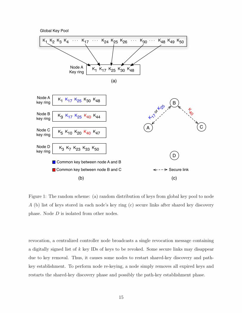
1 The random scheme: (a) random distribution of keys from global key pool to
node A (b) list of keys stored in each node’s key ring (c) secure links after
shared key discovery phase. Node D is isolated from other nodes. . . . . . . . 15
2 Blom’s scheme . . . . . . . . . . . . . . . . . . . . . . . . . . . . . . . . . . . 22
3 (a) Local connectivity of EG and EGD schemes and (b) number of moved
nodes that are isolated in EG and EGD schemes with different jamming radii 36
4 Compare simulation results and analysis of local connectivity of the hybrid
scheme . . . . . . . . . . . . . . . . . . . . . . . . . . . . . . . . . . . . . . . 44
5 (a) Local connectivity and (b) number of moved nodes that are isolated for
EG, EGD, and HB schemes with different sizes of jamming areas . . . . . . . 46
6 (a) Local connectivity and (b) number of moved nodes that are isolated for
EG, EGD, and HB schemes with multiple jammers. Each jammer has radius
= 40 meters. . . . . . . . . . . . . . . . . . . . . . . . . . . . . . . . . . . . . 48
7 (a) Local connectivity and (b) number of moved nodes that are isolated for
EG, EGD, and HB schemes with multiple jammers. Each jammer has radius
= 80 meters. . . . . . . . . . . . . . . . . . . . . . . . . . . . . . . . . . . . . 49
8 (a) Local connectivity and (b) number of moved node that are isolated for EG,
EGD, and HB schemes with different size of jamming areas for 4×4 grid size 51
9 (a) Local connectivity and (b) number of moved node that are isolated for EG,
EGD, and HB schemes with multiple jammers for 4×4 grid size . . . . . . . . 52
x

10 (a) Local connectivity and (b) number of moved node that are isolated for
EG, EGD, and HB schemes with different size of node density when number
of jammers is 50. The jamming radius of each jammer is 40 meters . . . . . . 53
11 Measuring the length of the secure path using ph(L) with EG, EGD, and HB
schemes (a) before jamming attacks occur, and after attack by 40 jammers
with radius (b) = 40 meters and (c) = 80 meters. . . . . . . . . . . . . . . . . 55
12 Number of isolated nodes of EG, EGD, and HB scheme before and after launch-
ing jamming attacks with different size of jamming areas. . . . . . . . . . . . 57
13 Average travel distance of jammed nodes after different spatial retreat strategies. 61
14 (a) Local connectivity and (b) number of moved nodes that are isolated after
partial random spatial retreats (maxDist = 80 meters) for EG, EGD, and HB
schemes with multiple jammers. . . . . . . . . . . . . . . . . . . . . . . . . . 63
15 a) Local connectivity and (b) number of moved nodes that are isolated after
partial random spatial retreats (maxDist = 200 meters) for EG, EGD, and
HB schemes with multiple jammers. . . . . . . . . . . . . . . . . . . . . . . . 64
16 (a) Local connectivity and (b) number of moved nodes that are isolated for
EG, EGD, and HB schemes with different sizes of jamming areas. . . . . . . . 65
17 Network topology after moved with random spatial retreats. . . . . . . . . . . 66
18 Network topology after moved with border-move strategy. . . . . . . . . . . . 67
19 Network topology after moved with partial random spatial retreats (maxDist
= 80 meters). . . . . . . . . . . . . . . . . . . . . . . . . . . . . . . . . . . . 68
20 Network topology after moved with partial random spatial retreats (maxDist =200
meters). . . . . . . . . . . . . . . . . . . . . . . . . . . . . . . . . . . . . . . . 69
21 The unit disk model. (a) An example of a link between two nodes and (b) a
communication link when a jammer impacts node B. . . . . . . . . . . . . . . 72
22 SNR when a jammer is at different distances from the receiver . . . . . . . . 77
23 Transmission of a regular node with different transmission power levels. If
group deployment is used, a node may reach more neighbors from different
deployment groups with higher transmission power. . . . . . . . . . . . . . . 80
xi

24 (a) Total number of links and (b) total number of secure links before and after
jamming, and after nodes transmit at different transmission power levels to
cope with jamming . . . . . . . . . . . . . . . . . . . . . . . . . . . . . . . . 85
25 Fraction of secure links before and after jamming, and after nodes transmit at
different transmission power levels to cope with jamming . . . . . . . . . . . 86
26 Percentage of impacted nodes that have at least one secure link with their
neighbors before and after jamming, and after nodes transmit at different
transmission power levels to cope with jamming . . . . . . . . . . . . . . . . 87
27 (a) Global connectivity of secure links and (b) average number of hops from
nodes to the sink before and after jamming, and after nodes transmit at dif-
ferent transmission power levels to cope with jamming . . . . . . . . . . . . . 89
28 Percentage of impacted nodes that have at least one secure link with their
neighbors before and after jamming, and after nodes transmit at different
transmission power levels to cope with jamming of a 1,500 nodes network . . 90
29 (a) Global connectivity of secure links and (b) average number of hops from
nodes to the sink before and after jamming, and after nodes transmit at differ-
ent transmission power levels to cope with jamming of networks with different
number of nodes . . . . . . . . . . . . . . . . . . . . . . . . . . . . . . . . . . 92
30 Directional antenna model . . . . . . . . . . . . . . . . . . . . . . . . . . . . 96
31 Transmission range with directional antenna and omni-directional antenna . . 101
32 Fraction of secure links before and after nodes perform directional beamforming
to cope with jamming . . . . . . . . . . . . . . . . . . . . . . . . . . . . . . . 103
33 (a) Global connectivity (b) average number of hops to sink node for EG, EGD
and HB schemes under jamming with different antenna’s patterns . . . . . . 105
34 (a) Global connectivity (b) average number of hops to sink node for EG, EGD,
and HB schemes under jamming with 1,500 and 2,500 nodes networks . . . . 107
35 (a) Global connectivity (b) average number of hops to sink for EG, EGD, and
HB schemes with -10 dBm transmission power . . . . . . . . . . . . . . . . . 108
xii
1.0 INTRODUCTION
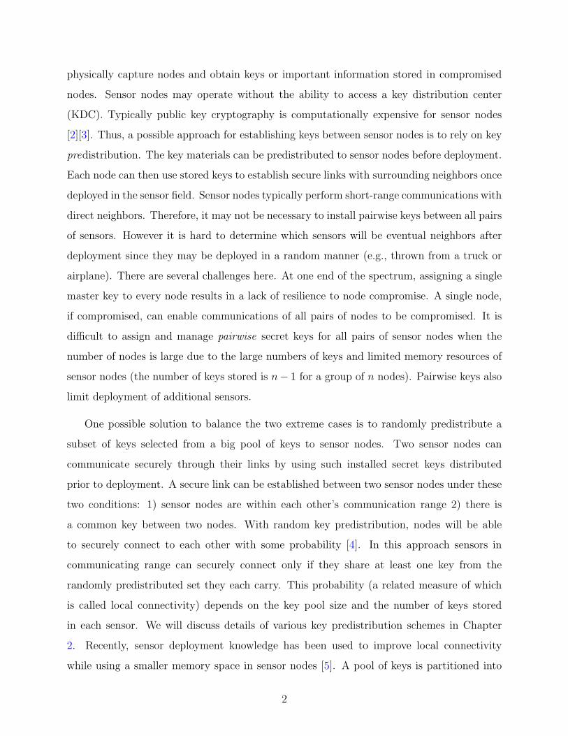
Wireless ad hoc networks have gained attention from research communities as they offer
alternative ways to deliver information and extend availability of the existing communica-
tion infrastructure. An ad hoc network can operate without continual help from a fixed
infrastructure. Each node acts as a router to relay packets on behalf of other nodes to the
destination. A sensor network is a specialized example of ad hoc networks that consists of
a large number of small sensor devices that connect and communicate in ad hoc fashion to
achieve some specific missions. Sensor nodes usually have limited computation and commu-
nication power for simple calculation on raw sensing data and short-range radio transmission
capabilities for communication. Sensors are usually densely deployed on a large scale. A
group of sensor devices can quickly self-organized together to form an ad hoc network after
deployment. These features make a sensor network an attractive option to a wide range of
wireless applications including environmental sensing, object detection, health monitoring,
goods tracking, disaster recovery, and military services. In many of these applications, secu-
rity services are needed to preserve confidentiality and authentication of the data exchanged
by sensors to prevent them from being eavesdropped upon or modified during their trip to
the intended receiver [1]. One of the first steps for providing security services is to establish
shared secret keys between sensor nodes. Each node can use such keys to enable secure
communications between neighbors using cryptographic techniques.
The unique characteristics of wireless sensor networks introduce challenges in providing
keys for bootstrapping security services. A sensor node usually has a limited size of memory,
which allows node to store only a small number of cryptographic keys, but the number of
sensor nodes involved in an application can potentially be very large (1,000 to 10,000 nodes).
Sensor nodes are usually deployed in an unattended area, which makes it easy for attackers to
1
physically capture nodes and obtain keys or important information stored in compromised
nodes. Sensor nodes may operate without the ability to access a key distribution center
(KDC). Typically public key cryptography is computationally expensive for sensor nodes
[2][3]. Thus, a possible approach for establishing keys between sensor nodes is to rely on key
predistribution. The key materials can be predistributed to sensor nodes before deployment.
Each node can then use stored keys to establish secure links with surrounding neighbors once
deployed in the sensor field. Sensor nodes typically perform short-range communications with
direct neighbors. Therefore, it may not be necessary to install pairwise keys between all pairs
of sensors. However it is hard to determine which sensors will be eventual neighbors after
deployment since they may be deployed in a random manner (e.g., thrown from a truck or
airplane). There are several challenges here. At one end of the spectrum, assigning a single
master key to every node results in a lack of resilience to node compromise. A single node,
if compromised, can enable communications of all pairs of nodes to be compromised. It is
difficult to assign and manage pairwise secret keys for all pairs of sensor nodes when the
number of nodes is large due to the large numbers of keys and limited memory resources of
sensor nodes (the number of keys stored is n− 1 for a group of n nodes). Pairwise keys also
limit deployment of additional sensors.
One possible solution to balance the two extreme cases is to randomly predistribute a
subset of keys selected from a big pool of keys to sensor nodes. Two sensor nodes can
communicate securely through their links by using such installed secret keys distributed
prior to deployment. A secure link can be established between two sensor nodes under these
two conditions: 1) sensor nodes are within each other’s communication range 2) there is
a common key between two nodes. With random key predistribution, nodes will be able
to securely connect to each other with some probability [4]. In this approach sensors in
communicating range can securely connect only if they share at least one key from the
randomly predistributed set they each carry. This probability (a related measure of which
is called local connectivity) depends on the key pool size and the number of keys stored
in each sensor. We will discuss details of various key predistribution schemes in Chapter
2. Recently, sensor deployment knowledge has been used to improve local connectivity
while using a smaller memory space in sensor nodes [5]. A pool of keys is partitioned into
2
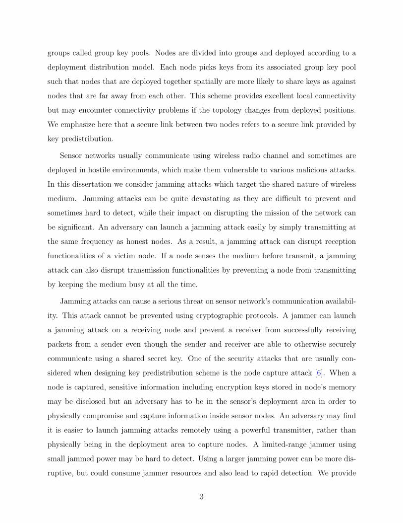
groups called group key pools. Nodes are divided into groups and deployed according to a
deployment distribution model. Each node picks keys from its associated group key pool
such that nodes that are deployed together spatially are more likely to share keys as against
nodes that are far away from each other. This scheme provides excellent local connectivity
but may encounter connectivity problems if the topology changes from deployed positions.
We emphasize here that a secure link between two nodes refers to a secure link provided by
key predistribution.
Sensor networks usually communicate using wireless radio channel and sometimes are
deployed in hostile environments, which make them vulnerable to various malicious attacks.
In this dissertation we consider jamming attacks which target the shared nature of wireless
medium. Jamming attacks can be quite devastating as they are difficult to prevent and
sometimes hard to detect, while their impact on disrupting the mission of the network can
be significant. An adversary can launch a jamming attack easily by simply transmitting at
the same frequency as honest nodes. As a result, a jamming attack can disrupt reception
functionalities of a victim node. If a node senses the medium before transmit, a jamming
attack can also disrupt transmission functionalities by preventing a node from transmitting
by keeping the medium busy at all the time.
Jamming attacks can cause a serious threat on sensor network’s communication availabil-
ity. This attack cannot be prevented using cryptographic protocols. A jammer can launch
a jamming attack on a receiving node and prevent a receiver from successfully receiving
packets from a sender even though the sender and receiver are able to otherwise securely
communicate using a shared secret key. One of the security attacks that are usually con-
sidered when designing key predistribution scheme is the node capture attack [6]. When a
node is captured, sensitive information including encryption keys stored in node’s memory
may be disclosed but an adversary has to be in the sensor’s deployment area in order to
physically compromise and capture information inside sensor nodes. An adversary may find
it is easier to launch jamming attacks remotely using a powerful transmitter, rather than
physically being in the deployment area to capture nodes. A limited-range jammer using
small jammed power may be hard to detect. Using a larger jamming power can be more dis-
ruptive, but could consume jammer resources and also lead to rapid detection. We provide
3

more discussion on jamming attacks in Chapter 2.
1.1 MOTIVATION
Jammers can impact connectivity of sensor nodes even though the network is protected
through shared secret keys (predistributed before deployment). The nodes that are impacted
by jammers may not be able to communicate with neighbors even though they share keys.
This forces nodes to act in response to the jamming attack. Techniques to overcome jam-
ming attacks include moving away from jammed area (spatial retreat) or jammed frequency
(frequency hopping), increasing the transmission power (power adjustment), and using direc-
tional antennas. However, these coping techniques can cause changes in secure connectivity
among nodes. If the coping technique results in a node not having secure connectivity, this
is similar to the impact of jamming itself - in that a node cannot communicate any longer (if
secure connectivity is a prerequisite for communication). Different coping techniques result
in differences in how secure connectivity changes. With spatial retreat, a jammed node may
move away from the jammed area to new locations surrounded by new neighbors. Node
that increases their transmission power to overcome the jamming signal also achieve longer
transmission range and may reach more neighbors that are usually unreachable with the
regular transmission power. Using directional antennas also result in longer transmission
ranges but only in the antenna beam’s direction.
Different key distribution techniques also respond differently to changes in network con-
nectivity due to the jamming coping process. Spatial retreats may cause a large number of
sensor nodes to be isolated from the rest of the network after they move out of the jammed
area. This is because moved nodes may not be able to find shared secret keys with new neigh-
bors at new locations. With high transmission power (and directional beamforming), a node
may not be able to securely connect with new neighbors (reachable with higher transmission
power) because they do not share keys. Thus, there may be a need for a key predistribution
scheme that is robust under jamming scenarios, especially even after the network applies
techniques to combat the jamming attack. To the best of our knowledge there is no work
4

that has looked at the effects of jamming attacks over connectivity of secure links (in the
key predistribution context), and how this problem can be solved.
1.2 PROBLEM STATEMENT
In this dissertation we investigate impact of jamming attacks on secure connectivity of sensor
nodes. A secure link refers to a link between two neighbor nodes that is secured through
shared secret keys predistributed before deployment. The dissertation is led by the following
research questions:
• What are the impacts of jamming attacks over connectivity with secure links after the
network performs various techniques to cope with jamming?
• If such impact is significant, is it possible to design a more robust key predistribution
scheme that works well even when jamming coping techniques are employed by the net-
work?
The goal is to evaluate the impact of jamming coping techniques on secure connectivity
and design a key predistribution scheme (where necessary) that is robust to changes in secure
connectivity when nodes adopt different techniques to cope with jamming. The jamming
coping techniques that we study in this dissertation are:
1. Spatial retreats where nodes move away from jammed areas.
2. Power adjustment where nodes increase transmission power to compete with jamming
signal.
3. Using directional antennas where nodes use directional transmissions to compete with
jamming signal.
We present our results with various scenarios in Chapters 3 and 4. To be specific, we first
study the impact on secure connectivity when a sensor network performs spatial retreats to
cope with jamming. In this case, it becomes necessary to design a new key predistribution
scheme that solves the problem of poor secure connectivity. Then we study the impacts
5
on secure links when nodes adopt other coping techniques (increasing transmission power
and using directional antennas). In these cases, both our proposed scheme and one of the
existing schemes perform well. However we identify the impact of the coping schemes on
secure connectivity under jamming attacks with various key predistribution schemes.
The models for the wireless link and jamming are important and need to be considered
when studying the impact of jamming. In this dissertation we investigate two wireless link
models namely the unit disk model and the SNR-based model. The unit disk model offers
a simple model to analyze impact of jamming attacks but it is overly simplistic (closer to a
worst-case condition) and does not provide a depiction of the complex relationships between
power level and geometry of the deployment of source node and jammers. We later use
an SNR-based model that captures insight information factors that determine existence of
wireless links under jamming attacks.
1.3 ORGANIZATION OF THE DISSERTATION
Chapter 2 of this dissertation will present the background material. We start this section with
a brief introduction about ad hoc and sensor networks, some definitions, applications, and
the unique characteristics that introduce challenges in distributing cryptographic keys among
nodes in the network. We present the existing key predistribution techniques for sensor
networks. We focus on two important techniques: the random key predistribution and the
deployment knowledge based key predistribution scheme. We also describe variations of key
predistribution schemes. The jamming attack is discussed next. We present classifications of
jamming attacks, jamming strategies, and detection of jamming attacks. Then we describe
jamming countermeasure techniques namely power and rate adaptation, frequency hopping,
spatial retreats and using directional antennas.
In Chapter 3 we present the hybrid (HB) key predistribution scheme. The hybrid scheme
is originally proposed as a key predistribution technique that supports sensor networks that
employ spatial retreat strategies to escape from jamming attacks. The HB scheme combines
the beneficial properties of the random (EG) and the deployment knowledge based (EGD)
6

key predistribution schemes. We present the impact of jamming attacks on secure links
(initially provided by key predistribution). First, we present the case where the random
spatial retreat strategy is employed. We describe the jamming attack model used in this
chapter. The unit disk model is used for wireless link between nodes and jammer’s signal.
A demonstration of the impact of jamming attacks on secure links provided by the EG
and the EGD schemes is presented. The local connectivity and number of moved nodes
that are isolated are used as the performance metrics. We identify tradeoffs between local
connectivity level and number of moved nodes that are isolated after spatial retreats with
the EG and the EGD schemes. The idea of the hybrid scheme is to balance this tradeoff by
maintaining high level of local connectivity and low number of isolated nodes after spatial
retreats. The hybrid key predistribution scheme is explained with details and examples. We
describe the deployment model and explain how we set up key pools for the hybrid scheme.
We present the hybrid threshold (τ), which is the parameter that designs connectivity level
and amount of isolated nodes in this scheme. Several issues related to the protocol is analyzed
and discussed. We present simulation-based results evaluating the hybrid scheme with single
jammer and multiple jammers with various jammer’s radii and number of jammers. We
compared the hybrid scheme with the EG and the EGD scheme. We also present several
results related to the hybrid scheme (impact of grid size and node density, results on length of
secure paths and number of isolated nodes before/after jammed). The random movement in
both distance and direction in the random spatial retreat strategy may cause jammed nodes
to move a significant larger distance than they should. Nodes may consume large amount
of energy due to moving if nodes move a larger distance than is necessary. We present
an improved strategy called partial random spatial retreat, and its performance evaluation
results.
In Chapter 4, we employ a more realistic wireless link model for evaluating impact of
jamming attacks on secure links provided by key predistribution. We address limitations
of the unit disk model used in Chapter 3. The unit disk model does not capture the fact
that successful reception is primarily determined by the ratio of signal strength from sender
and jammer at the receiver, and the ratio depends on multiple factors. The SNR-based link
model is presented. The model considers factors that impact the link condition between nodes
7
including sender and jammer’s transmission power, distance between jammer and receiver,
and distance between sender and receiver. We present assumptions and model parameters
used to study impact of jamming attack on secure links. We show that a sensor node that is
located in the jammer’s range may be able to communicate with neighbors. We describe the
impact of jamming attacks on secure connectivity when the network increases transmission
power to compete with the jamming signal. The power adaption strategy is explained. The
fraction of secure links after jammed and the global connectivity of secure links are used as
the performance metrics. We evaluate various key predistribution schemes under jamming
attack when the network employs power adaptation to cope with jamming by simulations.
We present the results when jammers are randomly deployed in the network. Results on
secure connectivity when nodes transmit with different power levels are presented. We also
present the impact of node density on secure connectivity after jamming attack.
We present the impact on secure connectivity under jamming attacks when a network
uses directional antennas in response to jamming. We briefly discuss the model of directional
transmissions employed and the assumptions that we used in this study. The impacts on
secure network topology before and after directional transmission is discussed. The beam-
forming strategy used in this study is presented. We explain the performance metrics that
we used to evaluate the performance of key predistribution schemes with directional anten-
nas. We present our simulation-based results evaluating various key predistribution schemes
under directional transmissions. We describe the simulation setup and relevant parameters.
The results with random jammers are presented. We present the results on global connectiv-
ity of secure links, impact of different node densities, and results when sensor nodes combine
directional transmissions and power adjustment to cope with jamming attacks.
Chapter 5 will conclude this dissertation and discuss issues that we would like to pursue
and continue in our future research.
1.4 CONTRIBUTIONS
The main contributions of this dissertation are summarized as follows:
8

• We have proposed and evaluated the hybrid key predistribution scheme for ad hoc/sensor
networks. The hybrid scheme is proposed as a key predistribution scheme that supports
a network that employs spatial retreat techniques to cope with jamming attacks. This
scheme combines the beneficial properties of random and deployment knowledge based
key predistribution schemes. In the presence of node retreats under jamming attacks,
the scheme provides high local connectivity while reducing the number of isolated nodes
due to movement of nodes.
• We have proposed the partial random spatial retreat technique to balance a sensor node’s
travel distance and distribution over the sensor field.
• We have evaluated various key predistribution schemes under scenarios where the net-
works use power adjustment and directional antennas to cope with jamming attacks.
9
2.0 BACKGROUND
2.1 KEY PREDISTRIBUTION TECHNIQUES FOR SENSOR NETWORKS
A sensor network is a collection of small devices that usually connect and communicate in
ad hoc manner to achieve some mission objectives. Sensor network applications have been
constantly diversifying to include environmental sensing, object detection, structural health
monitoring, patient health monitoring, and goods tracking [7]. In many of these scenarios it
is important to preserve confidentiality and authentication of the data exchanged by sensors
to prevent them from being eavesdropped upon or modified during their trip to the intended
receiver [1]. For these purposes, it is essential for sensor nodes to share secret keys and use
this information to establish secure communications between neighbors.
The unique characteristics of wireless sensor networks introduce challenges in providing
keys for bootstrapping security services. A sensor is a low-cost device that has a limited
size of memory, and battery life. Smart Dust sensors have only 8Kb of program and 512
bytes for data memory, and processors with 32 8-bit general registers that run at 4 MHz
and 3.0V (the ATMEL 90LS8535 processor). Berkeley Mica Motes feature an 8-bit 4 MHz
Atmel ATmega 128L Processor with 128K bytes program store, and 4K bytes SRAM. This
leaves only 4K bytes for security and applications. The number of sensor nodes involved
in a given application can potentially be very large (1,000 to 10,000 nodes). Sensor nodes
communicate via a short-range radio interface. The communication pattern is usually node-
to-node to avoid long distance transmissions between nodes and remote base stations which
can consume large amount of sensor’s energy. Since sensor nodes are usually deployed in
an unattended area, it is easy for attacks that can physically capture nodes and reveal keys
stored in compromised nodes. Moreover, sensor nodes may operate without the ability to
10
access a fixed infrastructure; therefore a key distribution server may not be available all the
time.
Typically public key schemes are computationally expensive for sensors because of their
complex mathematical algorithms. A 512-bit RSA signature generation can take 2-6 seconds
on a RIM Pager and on a Palm Pilot [8]. The energy consumption on Motorola MC68328
Dragonball of a 1024-bit RSA is 42 mJ for encryption and 840 mJ for digital signature while
a 1024-bit AES encryption takes only 0.104 mJ for encryption and digital signature [9]. The
large amount of time required to perform public key encryption makes the devices vulner-
able to some denial-of-service (DOS) attacks and introduces delays in public key certificate
validation through certificate chains.
A possible approach for providing security services in wireless sensor networks is to
rely on symmetric key predistribution. These keys can be installed in sensor nodes prior to
deployment. Each node uses stored key information to establish secure links with surrounding
neighbors once deployed in the sensor field. Since sensors typically communicate locally with
direct neighbors, it may not be necessary to install pairwise keys between all pairs of sensors.
However it is hard to determine which sensors will be eventual neighbors after deployment.
There are two extreme solutions to predistribute keys to sensor nodes, namely the single key
scheme and the fully pairwise key scheme.
Single Key or Network-wide Key Scheme: The simplest way to establish shared
keys is to pre-install a single secret key in every node. Nodes can securely communicate by
using this mission key to encrypt messages or use it for message authentication. The advan-
tages of using a single network-wide key is the simplicity of key distribution. No additional
step is required for distributing a shared key. This method requires minimal memory storage
as only one key is stored in the memory. The main drawback of this technique is it lacks of
resilience against node capture. Only one compromised node can impact the entire network.
One solution to this problem is to use the mission key to establish link keys for each pair
of nodes. Then the established link key is used for further communications. However, this
solution is still vulnerable during link key establishment phase. Key revocation is not easy
since the entire network uses the same key.
Fully Pairwise Scheme: Another extreme solution is to use fully pairwise keys. Every
11

pair of nodes shares a unique key. For a network of n nodes, each node stores n-1 keys.
The total number of keys used by every node is n(n−1)2
. The advantage of this fully pairwise
scheme is that it has very good resilience against node capture. One compromised node only
reveals n-1 link keys (from the total of n(n−1)2
keys). It will not reveal information about
other on going communications in other parts of the network. Selective revocation of keys
is also possible (since a key is uniquely used at every link) by just broadcasting a set of
revoked keys. The disadvantage of this scheme is unnecessary storage requirement at each
node, since each node needs to store n - 1 keys. The amount of storage requirement increases
linearly with the size of the network. For an 128 bit key, a network with 10,000 nodes will
require about 1 megabits of storage on each node only for pre-key material which may be
too large for some devices. Thus the fully pairwise scheme has poor scalability.
The two naive solutions introduce a tradeoff between security level and storage require-
ment. The single mission key scheme has very low resiliency but offers a very good storage
requirement. The fully pairwise scheme has very good resiliency against node capture, but
requires a large amount of storage especially in a network with a large number of nodes.
This implies that the key predistribution technique should provide strong security levels
while offering efficient storage requirement.
The connectivity of probabilistic key distribution scheme can be modeled using random
graph theory [10]. A random graph G(n, c) is a graph of n nodes and the probability that a
link (or an edge) exists between any two nodes (or vertices) is c. When c = 1, the graph is
fully connected (there exists an edge between all pairs of vertices). When c = 0, there is no
edge between nodes at all. Eschenauer and Gligor [4] showed the expected node degree d in
terms of the size of the network n as:
d = (n− 1
n)(ln(n)− ln(−ln(c))) (2.1)
For c = 0.99999 (which means that the network will almost certainly be connected) and
n = 10, 000 nodes, d can be calculated by Equation 2.1 as 20.7.
Let n′ be expected number of nodes within a node’s communication range. For the value
of d required for a network to be connected, we can calculate the required probability of key
sharing between two nodes (p) as:
12

p =d
n′(2.2)
An operator can adjust the key distribution parameters (i.e., size of key pool and size
of keys stored at each node) that satisfy the value of required p. If n′ = 40, an operator
needs to find a combination of key pool and key ring size that yields the connectivity of
20.7/40 ≈ 0.5.
2.1.1 Random Key Predistribution Scheme (EG Scheme)
The random key predistribution scheme (also called“basic” scheme) was proposed by Es-
chenauer and Gligor to overcome communication and security constraints in wireless sensor
networks (we will also refer to this scheme by the name EG scheme throughout this disser-
tation). The basic idea is to randomly distribute a subset of keys from a large key pool to
each sensor. Two neighbor nodes will be able to find a common key with some probability.
The EG scheme consists of three phases: key distribution phase, shared-key discovery phase,
and path-key establishment phase. Note that most of the key predistribution techniques
proposed in literature also follow this procedure.
Step 1: Key Distribution Phase: In the key distribution phase, an off-line key
distribution center generates a key pool (global key pool S of size |S| keys) consisting of
large number of keys (e.g., 217 − 220 keys). Each key is associated with a key identification
(key-ID). Each node randomly picks k keys from this global key pool and stores them in its
memory. The set of keys drawn from the key pool with associated key-IDs is called a key
ring.
Step 2: Shared Key Discovery Phase: In the shared-key discovery phase, each node
exchanges, with its neighbors, information used to establish a shared key. The goal of this
phase is to find a common key between two neighboring nodes (neighboring here implies
nodes that are in transmission range of one another). The common key(s) can be used to
establish a secure link between two nodes by encrypting all messages with their shared key
(or performing local key establishment using these keys). A secure link exists between two
13

nodes if they share a key and are within each other’s radio range. The simplest way to do
this is to have each node broadcast, in clear text, its list of key IDs in the key ring. To add
security to exchanged information, a challenge-response protocol can be used to hide key
sharing patterns among nodes from an adversary [4]. For every key on a key ring, each node
could broadcast a list of k challenges. Each challenge has key ki, i = 1, . . . , k as an encryption
key. A correct response from a recipient would indicate that a common key exists between
the broadcasting node and the recipient. A pair of nodes sharing the same key can establish
secure communications using their common key as a link key (such a path is referred to as
a direct path). After the shared key discovery phase, a graph of secure links is formed that
consists of all links between neighbor nodes who share at least one key.
Step 3: Path Key Establishment Phase: Since keys in a node’s key ring are ran-
domly drawn from the key pool, it is possible that a pair of nodes (that are within each
other’s communication range) may not have any common key. The path-key establishment
phase allows a pair of nodes that do not have common key to establish a secure path through
two or more links. For example, node A and B that do not share a key may establish a
secure link through another node C if C shares a common key with both A and B. In other
words, node A and B securely communicate using an indirect path through node C.
Next we show an example of the EG scheme in Figure 1. Suppose we need to distribute
keys to 4 sensor nodes (A,B,C and D), each has memory size of 5 keys. We assume a
global key pool of size 50 keys. First, a key distribution server generates a global key pool
that contains 50 keys (k1, k1, k3, . . . , k49, k50). Before deployment, the key distribution center
randomly distributes 5 keys from a global key pool to each node (Figure 1a). Figure 1b
shows the list of keys stored at each node. Let us assume that every node will be in each
other’s radio range after deployment. In Figure 1c, after exchanging a list of keys stored in
each node, node A and node B can establish a secure link using a common key k17 or k25.
Node B and node C also find a secure link through key k40. Node A and node C cannot
establish a direct secure link since they share no key. However, they can establish a secure
link through node B since it has common keys with both node A and node C. Node D
shares no key with any neighbor, thus it is isolated from the group.
The basic scheme supports key revocation and re-keying with simple procedures. For key
14
K1 K2 K3 K4 . . . K24 K25 K26 . . . K48 K49 K50 K17 K30 . . . . . .
K1 K17 K25 K30 K48
K9 K17 K25 K40 K44
K5 K10 K20 K40 K47
K3 K7 K23 K33 K50
A
B
C
D
K1 K17 K25 K30 K48Node A Key ring
Node A key ring
Node B key ring
Node C key ring
Node D key ring
Common key between node A and B
Common key between node B and C
Global Key Pool
K 17 or
K 25 K40
Secure link
(a)
(b) (c)
Figure 1: The random scheme: (a) random distribution of keys from global key pool to node
A (b) list of keys stored in each node’s key ring (c) secure links after shared key discovery
phase. Node D is isolated from other nodes.
revocation, a centralized controller node broadcasts a single revocation message containing
a digitally signed list of k key IDs of keys to be revoked. Some secure links may disappear
due to key removal. Thus, it causes some nodes to restart shared-key discovery and path-
key establishment. To perform node re-keying, a node simply removes all expired keys and
restarts the shared-key discovery phase and possibly the path-key establishment phase.
15
Connectivity of the EG Scheme: The graph of sensor nodes is connected (securely) if
each sensor node has enough neighbors even though k is small compared to |S|. Typically, k
is on the order of a hundred while |S| is on the order of several tens or hundreds of thousands.
From [4], the probability that any two sensor nodes share a key given |S| and k is:
1− ((|S| − k)!)2
(|S| − 2k)!|S|! (2.3)
The above equation considers the number of possible sets of size k chosen from a set of size
|S| that have no overlap to compute the probability that two nodes do not share a key and
subtracts this from 1 to determine the probability that two nodes do share at least one key.
We will refer to the fact that two nodes within transmission range share at least one key as
constituting secure connectivity or local connectivity which is defined in Section 3.3 in this
dissertation.
The random key pre-distribution scheme has better resilience to node capture compared
to a single mission key and better storage requirement compared to fully pair-wise key
schemes. For only one compromised node, in a single mission key scheme, all links would be
compromised. In a pair-wise key scheme, since each link key is unique, only n-1 links would
be revealed. However, in the EG scheme, for a key ring of size k � n, an attacker would
have a probability of k|S| to successfully attack any communication link [11]. Note that it
is possible that the same key is shared by more than a pair of nodes, since the key ring is
drawn randomly from the same key pool. When an adversary compromises a node, all key
information of the compromised node would be revealed and also some shared keys of other
pairs of nodes somewhere in the network.
To achieve a high resiliency to node capture in the EG scheme, it is desirable to use a
large keypool (high value of |S|). If an adversary can compromise one node, it will reveal key
information only k out of |S| keys. However, since a memory size k is usually fixed, using
higher value of |S| results in a low connectivity (probability that two nodes share a key)
which may cause nodes to be isolated from their neighbors (since they cannot find common
keys to establish secure links with neighbors). Next, we present a solution to improve secure
connectivity over the EG scheme.
16

2.1.2 Key Predistribution with Deployment Knowledge (EGD Scheme)
The use of deployment knowledge is proposed as an improvement to the EG scheme. The
deployment knowledge based key predistribution scheme, proposed by Du, et al [5], is based
on the idea that the way that sensor nodes are deployed can be use to improve secure
connectivity (we shall call it the EGD scheme throughout this paper). The scheme has been
shown to improve the network connectivity over the EG scheme for the same number of keys
installed in each node’s memory.
Since sensor applications involve deploying a large number of sensors into a large, unat-
tended target field, one practical way to deploy sensor nodes is to divide sensors into small
deployment groups or clusters. Each group may be dropped sequentially from a truck or
an airplane as the vehicle moves forward. Sensor nodes that are from the same deployment
group will have a higher chance to reside close to each other. The sensors that are in different
but adjacent groups still have some chance of being close, while sensors from non-adjacent
groups will have a slim chance to be close after being deployed to the field. Knowing which
pair of nodes is “likely” to comprise of neighbors is valuable in assigning keys from the key
pool.
The clustered deployment of sensor nodes is modeled in [12] by using probability den-
sity functions. In the EG scheme, nodes are deployed uniformly in the entire sensor field –
therefore there is no information on clustering or where a node is more likely to be deployed.
Every pair of nodes has the same chance to be neighbors. The EGD scheme uses a two
dimensional Gaussian distribution to model node deployment in clusters where a mean (µ)
is the targeted deployment point of each group. The actual location of nodes after deploy-
ment lie around the target deployment point of their associated group. Given the target
deployment point of the group Gi,j is at the point µ = (xi, yj), the pdf of sensor node k that
is in group Gi,j follows:
f (x, y|k ∈ Gi,j) =1
2πσ2e−
»(x−xi)
2+(y−yj)
2–
2σ2 (2.4)
The operator can arrange the distance between deployment points (which implies to the size
of each deployment group) and the value of σ in the pdf to make sure that distribution of
17
nodes will cover all areas in the target field. If the value of σ is too small compared to the
distance between two deployment points, sensors may cluster more around their deployment
points and cause nodes from neighboring groups a smaller chance to be close.
Next, multiple key pools are used in the EGD scheme as opposed to a single global key
pool in the EG scheme. Each deployment group has its associated group key pool of size
|Sc| which is generated from the larger key pool of size |S|. A sensor node will pick keys
from the group key pool associated with the group that the node belongs to. Keys from
the global key pool are assigned to group key pools in a way that the group key pools that
are deployed nearby have a certain number of common keys. Overlapping factors denoted
by a and b determine the fraction of common keys between two adjacent group key pools.
Assuming that clusters of sensors are arranged in a grid, of the |Sc| keys in a given group
key pool, a|Sc| keys are shared between its horizontal and vertical neighboring clusters. The
number of keys shared with its diagonal neighbors is b|Sc|. If two clusters are not neighbors,
the group key pools do not share any keys. Given a global key pool of size |S|, the number
of deployment groups, and overlapping factors, one can calculate |Sc| by using a method
described in [12].
The key distribution process follows the three steps process as in the EG scheme. For a
memory size of k, a node randomly picks k keys from its associated group key pool of size
|Sc|. Shared key discovery and path-key establishment phase can be performed the same
way as the EG scheme.
The probability of finding at least one common key between two nodes ni and nj that
belong to deployment groups Gi and Gj respectively can be determined as follows. Let δ(i, j)
denote the number of common keys between the deployment groups Gi and Gj and the
overlapping factors between vertical-horizontal and diagonal groups be a and b respectively.
The value of δ(i, j) changes as follows:
• When i = j, δ(i, j) = |Sc|
• When Gi and Gj are horizontal or vertical group neighbors, δ(i, j) = a|Sc|
• When Gi and Gj are diagonal group neighbors, δ(i, j) = b|Sc|
• When Gi and Gj are not neighbors, δ(i, j) = 0
18
The probability that two nodes share at least one key is:
1−∑min(k,δ(i,j))
m=0
(δ(i,j)m
)(|Sc|−δ(i,j)k−m
)(|Sc|−mk
)(|Sc|k
)2 (2.5)
The computation of the above probability again considers the chance that two sets of k keys
(now drawn differently as described) have no overlap (and subtracts this probability from
1). To calculate Pr[two nodes do not share any key], the idea is as follows: First, a sensor
node with a key ring of size k selects m keys from the intersecting key pool of size δ(i, j)
and k −m keys from its non-intersecting group key pool. A second node, in order to avoid
selecting any key from the k keys that were already selected by the first node, can pick its
own k keys only from |Sc| −m keys from its group key pool where m is the number of keys
already picked by the first node from the intersecting key pool.
Instead of sharing keys, it is possible to share key spaces (e.g., using Blom’s approach
[13][14], that increases the resiliency of the network to multiple node compromise). While
the proposed hybrid scheme can be changed to include this, we only consider sharing of keys
in this dissertation.
Both equations (2.3) and (2.5) ignore the fact that two sensor nodes may not be in
transmission range. The local connectivity, the probability that two sensor nodes can securely
communicate, is actually conditional on the fact that they are within range of one another.
Given A is the event that two nodes are within each other’s communication range and B
is the event that two nodes share at least one common key, the local connectivity can be
calculated as follows:
Local Connectivity = Pr (B|A) =Pr (B and A)
Pr (A)(2.6)
The EG scheme uses uniform node distribution. A node can be deployed at any position
inside the deployment area with the same probability. Every pair of nodes will have the
same chance of being neighbor, thus we can only consider only event B when calculating
local connectivity of EG scheme. For a group deployment (EGD) scheme, each pair of
nodes will have different probability of being in each other’s communication range depends
on deployment group and deployment model of each node. The probability Pr(A) for two
nodes i and j can be computed by calculating probability that node i will reside in node j’s
19

communication range (a circle where radius R is the node’s transmission range)[5], where
the location of j is modeled by the deployment model described in Equation 2.4. Each
deployment group has a different target deployment point (µ in Equation 2.4). Nodes from
the same group will have higher Pr(A) since they use the same deployment model with the
same µ. The probability Pr(A) for nodes from different groups depends on the distance
between two groups target deployment point and standard deviation of the deployment
model (σ in Equation 2.4). Given the same value of σ, the longer the distance between
target deployment points of two nodes is, the less is the probability that they will be in
each other’s communication range. Nodes from non-adjacent groups will have a small value
of Pr(A) since their target deployment point will be further away. For example, given a
deployment area of 100m× 100m where the target deployment is at the middle of the area,
assuming σ = 50m, the deployment points of two adjacent groups will be 100m = 2σ apart.
Two non-adjacent deployment points will be at least 200m = 4σ apart.
2.1.3 Classification and Characteristics of Key Predistribution Schemes
We summarize the characteristics of key distribution schemes proposed in literature. All
key predistribution schemes follow the 3-steps procedure described in Section 2.1.1. The
difference is in the type of key material stored in each node and how to establish a link key
between two nodes from the stored key material. Another characteristic is how sensor nodes
are deployed in a target field and how key pools are prepared. These variations offer different
tradeoffs in terms of connectivity, memory requirement, computation and communication
complexity, and resilience again node capture.
2.1.3.1 Key Material and Link Key Establishment In the EG scheme [4], each node
stores cryptographic keys randomly drawn from the same key pool. A secure link between
two nodes exists if they have at least one common key. However, key materials and how to
establish a link key can be done in different ways.
• q-composite scheme: proposed in [3], as an extension of the EG scheme. Here a secure
link between two nodes exists if they share at least q keys. The secure link key K is
20
generated as the hash of all shared keys, K = hash(k1‖k2‖ . . . ‖kq). The scheme improves
resilience to node capture. The probability that a link is compromised decreases from k|S|
to(kq
)/(|S|q
). However, the probability of key sharing is decreased as it requires q shared
keys instead of one. When q = 1, the scheme is equivalent to the EG scheme. The key
connectivity is 1− (p(0) + p(1) + · · ·+ p(q− 1)), where p(i) = probability that two nodes
have exactly i keys in common.
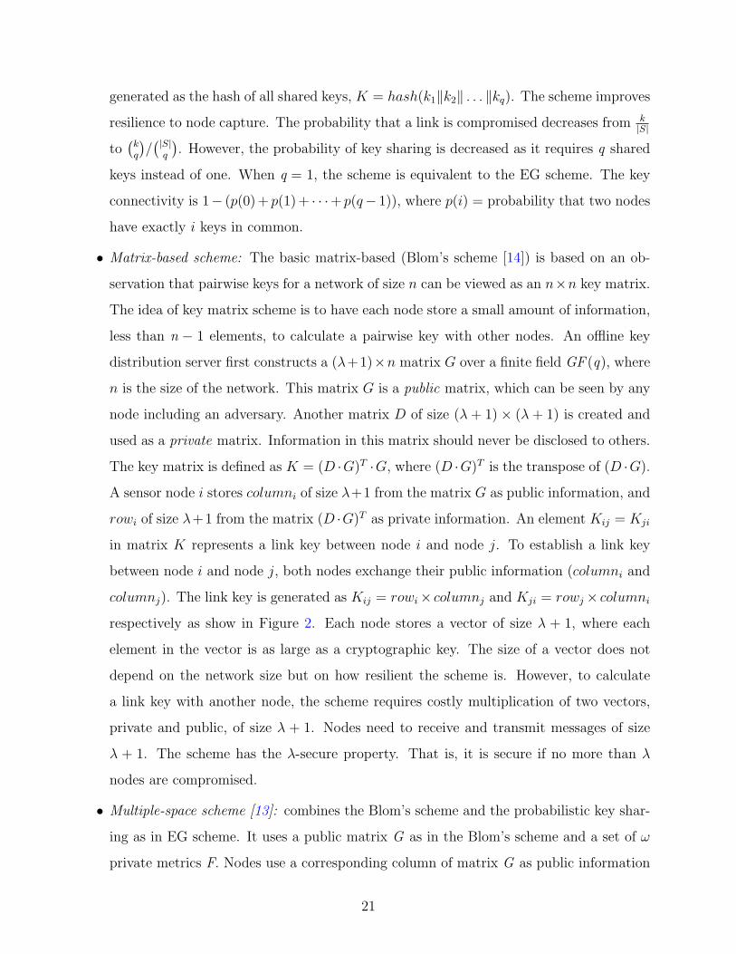
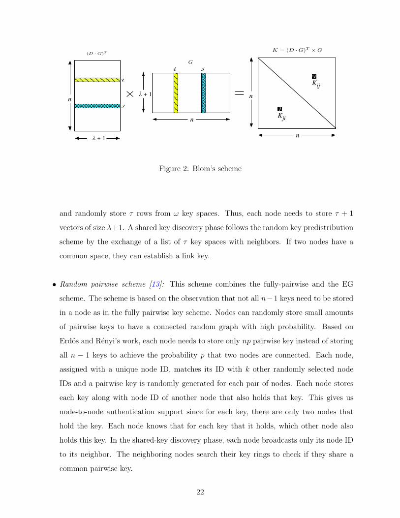
• Matrix-based scheme: The basic matrix-based (Blom’s scheme [14]) is based on an ob-
servation that pairwise keys for a network of size n can be viewed as an n×n key matrix.
The idea of key matrix scheme is to have each node store a small amount of information,
less than n − 1 elements, to calculate a pairwise key with other nodes. An offline key
distribution server first constructs a (λ+1)×n matrix G over a finite field GF (q), where
n is the size of the network. This matrix G is a public matrix, which can be seen by any
node including an adversary. Another matrix D of size (λ+ 1)× (λ+ 1) is created and
used as a private matrix. Information in this matrix should never be disclosed to others.
The key matrix is defined as K = (D ·G)T ·G, where (D ·G)T is the transpose of (D ·G).
A sensor node i stores columni of size λ+1 from the matrix G as public information, and
rowi of size λ+1 from the matrix (D ·G)T as private information. An element Kij = Kji
in matrix K represents a link key between node i and node j. To establish a link key
between node i and node j, both nodes exchange their public information (columni and
columnj). The link key is generated as Kij = rowi× columnj and Kji = rowj× columnirespectively as show in Figure 2. Each node stores a vector of size λ + 1, where each
element in the vector is as large as a cryptographic key. The size of a vector does not
depend on the network size but on how resilient the scheme is. However, to calculate
a link key with another node, the scheme requires costly multiplication of two vectors,
private and public, of size λ + 1. Nodes need to receive and transmit messages of size
λ + 1. The scheme has the λ-secure property. That is, it is secure if no more than λ
nodes are compromised.
• Multiple-space scheme [13]: combines the Blom’s scheme and the probabilistic key shar-
ing as in EG scheme. It uses a public matrix G as in the Blom’s scheme and a set of ω
private metrics F. Nodes use a corresponding column of matrix G as public information
21
nnλ + 1
i
j
(D · G)T
i j
G
K = (D · G)T !G
! =
n
Kij
Kji
λ + 1 n
Figure 2: Blom’s scheme
and randomly store τ rows from ω key spaces. Thus, each node needs to store τ + 1
vectors of size λ+1. A shared key discovery phase follows the random key predistribution
scheme by the exchange of a list of τ key spaces with neighbors. If two nodes have a
common space, they can establish a link key.
• Random pairwise scheme [13]: This scheme combines the fully-pairwise and the EG
scheme. The scheme is based on the observation that not all n−1 keys need to be stored
in a node as in the fully pairwise key scheme. Nodes can randomly store small amounts
of pairwise keys to have a connected random graph with high probability. Based on
Erdos and Renyi’s work, each node needs to store only np pairwise key instead of storing
all n − 1 keys to achieve the probability p that two nodes are connected. Each node,
assigned with a unique node ID, matches its ID with k other randomly selected node
IDs and a pairwise key is randomly generated for each pair of nodes. Each node stores
each key along with node ID of another node that also holds that key. This gives us
node-to-node authentication support since for each key, there are only two nodes that
hold the key. Each node knows that for each key that it holds, which other node also
holds this key. In the shared-key discovery phase, each node broadcasts only its node ID
to its neighbor. The neighboring nodes search their key rings to check if they share a
common pairwise key.
22
• Pseudo random scheme [15]: The idea of this scheme is to trade computation with
communication. It reduces the cost of transmission at the expense of more computation.
The computation-communication trade-off is one of the core ideas behind low energy ad
hoc sensor networks [16]. It uses a deterministic algorithm along with required unique
node ID to assign k keys selected from a key pool of size P to each node. The key server
uses a pseudo-random number generator with node ID as input to generate k key-IDs
which will be assigned to that node. Thus, each key in the key pool has a probability of kP
to be assigned to each node. To find common keys, the pseudo-random function and node
ID allows nodes to determine which keys are held by other nodes by exchanging node
IDs instead of the whole list of key IDs. Thus it trades computation for communication
efficiency. To be more general, a node can not only determine the keys that its neighbors
have, it also can determine common keys between any pair of nodes if it knows the node
IDs of that pair. This knowledge is valuable – node A, which has no common key with
B, can find an indirect path to B by searching for a node that shares a key with B and
also with itself.
• Polynomial-based scheme: The basic polynomial-based key predistribution scheme is pro-
posed by Blundo et al. [17]. The key distribution server randomly generates a bivariate
k degree symmetric polynomial f(x, y) = f(y, x) over finite field GF(q), q > ny. Any
pair of nodes i and j can compute the link key f(i, j). Node i evaluates f(i, y) at point
j, and node j can compute f(j, i) = f(i, j) by evaluating f(j, y) at point i. Later Liu
et al. [18] proposed the polynomial pool-based scheme which combines basic polynomial
scheme and random scheme (EG scheme). The key distribution server generates a set F
of bivariate k-degree polynomials over the finite field GF(q). If two nodes have a shared
polynomial which is randomly picked from a set F , they can generate a link key using
the method as in Blundo’s scheme.
• Combinatorial design scheme: This scheme belongs to the class of deterministic schemes
where the probability of key sharing between any pair of nodes is 1. The symmetric
Balanced Incomplete Block Design (symmetric BIBD) with parameters (v, r, λ) is an
arrangement of v objects into v blocks such that each block contains exactly r distinct
objects. Each object occurs in exactly r different blocks, and every pair of distinct objects
23

occurs together in exactly λ blocks [19]. This idea has been mapped into key distribution
problems [20][21]. With design parameters (m2+m+1,m+1, 1), the scheme can support
m2 + m + 1 nodes, and the key pool size is also m2 + m + 1. In the key distribution
phase, each node stores a key chain of size m + 1 consisting of a set of keys and key
identifiers. Note that the size of the key pool is exactly the same as the number of nodes
that the network can support. After deployment, every pair of nodes has exactly one key
in common and every key appears in exactly m + 1 key chains. Thus, the probability
of key sharing between any pair of nodes is 1. The scheme has the advantage that it
guarantees key connection between any pair of nodes. The main drawback of this scheme
is that the same keys are shared between many nodes leading to weaker resilience to node
compromise [22]. The probability that any link is compromised, when a node is captured,
is ≈ 1/m [11]. Also, the size of the key chain depends on the parameter m. The number
of keys required to be stored in a node becomes large in networks with large numbers of
nodes. Thus, this scheme does not scale well. Another problem is that the parameter m
has to be of prime power. Thus not all network sizes can use this scheme directly.
2.1.3.2 Key Pool and Deployment Method A key pool consists of a large number
of key materials prepared to distribute to sensor nodes before deployment. There are two
types of key pools in the literature: a single key pool and multiple key pools. The way
sensor nodes are deployed to the target field can be used to improve the key predistribution
method. The EG scheme uses a uniform deployment where each node can be deployed at
anywhere in the sensor field with the same probability. Group deployment has the benefit
that sensors that are in the same group will have more chance to be located close to each
other. The group deployment usually features multiple key pools. Each group will have an
associated key pool. A node will pick keys from a key pool associated to the group that
it belongs to. The EGD scheme [12] uses multiple key pools and group deployment which
results in a better connectivity compared to the EG scheme, given the same size of sensor
field. In [23], Liu et al. proposed a group-based key predistribution scheme which requires
nodes to be deployed in groups. Nodes in the same group can establish pair-wise keys by
in-group key predistribution (e.g., random scheme, polynomial based). Nodes that are in
24

different groups can establish a pair-wise key through the cross-group key predistribution
process. Some nodes in a group will be selected as belonging to cross-groups and they bridge
the connection between different groups.
2.2 JAMMING ATTACK AND COUNTERMEASURES
Wireless ad hoc networks are vulnerable to many security attacks. Some of these attacks
cannot be prevented using cryptographic protocols. Jamming attacks are considered one
of the most devastating attacks as they are difficult to prevent and sometimes hard to
detect. Communications among ad hoc devices usually rely on a shared medium that makes
it easy for attackers to launch attacks on communication availability. Jamming attacks
can be deployed easily by transmitting on the same frequencies as honest nodes, which
results in disruption of transmission (of nodes that use sensing of the medium) or reception
functionalities.
2.2.1 Jamming Attack Classification
There are different types of jamming attacks that an attacker can launch against a target
wireless ad hoc network. All of the attacks have the same goal – to block ongoing commu-
nications by disrupting a node’s ability to transmit or receive packets. The goal of efficient
jamming attacks is to cause maximum damage by using less resources (e.g., jamming power,
number of jammers), and to be hard to detect. Jammers with high transmission power can
cause large damage to the networks but can be easily detected by its strong signal. A more
efficient jamming can be accomplished by deploying number of low-cost small transmission
power jamming devices over the area of jamming interest to the adversary. Transmission
power of jammers can be equal to or even smaller than transmission power of a regular node.
Xu et al. [24] have classified jammers into the following types:
1. Constant jammers: This jammer will constantly emit a radio signal. The constant
jamming signal can be implemented by using a waveform generator that sends a radio
25
signal or using a wireless device to send out a series of random bits without following
the MAC protocol.
2. Deceptive jammers: They also try to disrupt the channel continuously as the constant
jammer. Instead of sending a random radio signal or bits, this jammer constantly injects
fake packets into the network without following the medium access protocol which can
keep other nodes to remain in the receiving state.
3. Random jammers: This can be considered as energy an efficient attack for jammers that
have limited power supply. A random jammer randomly chooses a period of time to
sleep and a random period of time to jam. When the jammer is in the jam state, it can
perform either constant or deceptive jamming.
4. Reactive jammers: The previous types of jammers are considered as active jammers
which attack regardless the communication state of victim nodes. In reactive jamming,
jammers will remain silent and will only jam when they sense valid traffic being exchanged
in the network. This jammer is harder to detect compared to active jammers.
Jammers may be static or mobile. Mobile jammers are able to move along the network
to find locations in the network that result the maximum damage. This can be the location
close to nodes that are transmitting high volume of traffic. Jammers may move or arrange
themselves to cause a network partition which results in disconnection between nodes in
different partitions. Law et al. [25] derive a collection of energy efficient jamming attacks
by observing MAC behavior in sensor networks. The approaches aim at jamming data
packets by specifically looking at the probability distribution of the interarrival times between
packets.
Jamming strategy can be considered as an optimization problem. The objective is gen-
erally to cause maximal damage in terms of number of victim nodes or communication links
while minimizing jamming resources such as power consumption or probability of being de-
tected by nodes in the network. Li et al. derive optimal solutions for both an attacker and
a defender [26]. Attackers control the probability of jamming and transmission range while
trying to cause maximal damage while an optimal detection test that is based on percentage
of incurred collisions can be used by defenders.
26
Tague et al. propose flow-jamming attacks which use multiple jammers to jam packets
in order to reduce traffic flow [27]. They assume that the jammer can selectively jam specific
traffic (packet) that runs through any flow. The flow-jamming problem is formulated using
a linear programming framework. The authors also present performance metrics to evaluate
the effect of flow-jamming attacks on traffic flows and the jammer’s resources. In [28], the
authors consider the case where a jammer has no information about the topology of the
target network. The problem is posed as finding the optimal number of jammers required
to jam all nodes in a network using geometry and graph theory. The jammed area was
considered as a circle and the solution was to find the optimal number of circles required to
cover all nodes in the network.
2.2.2 Jamming Detection
Detecting jamming attacks is a challenge since it includes discrimination between the at-
tack and normal network failures (e.g., poor connectivity, congestion, device failure, and
interference from other node’s transmission). Jamming detection can be done at the MAC
or PHY layer. The work in [29] considers improving jamming gain, targeted jamming at
specific nodes, links, or flows and reduced probability of detection. Xu et al. [30] propose
techniques to detect jamming at the MAC layer by monitoring the channel sensing time
before the medium becomes idle and at the PHY layer by observing the interference level
in the channel. At the MAC layer, nodes monitor the time taken to obtain access to the
medium. If this carrier sensing time is above a threshold, a node will assume that it is being
jammed. Otherwise, the delay in medium access is considered to be legitimate (e.g., due to
congestion). The sensing threshold is derived (a) using the probability density of the time
that a node needs to wait before starting transmission and (b) empirically using the distri-
bution of normal MAC delay time observed by simulations. At the PHY layer, the authors
run experiments with Berkeley motes to observe the signal strength at a sensor node when
there is no interference, with concurrent transmission from other nodes, and with a jamming
signal. The results show differences when there is jamming at the jammed node. But no
observations of signal strength by neighbors of the jammed node are reported. The author
27

suggests that signal discrimination can differentiate between normal and jammed scenarios
but did not specify certain signal levels that separate normal and jammed conditions. Basic
statistics such as differences in received signal strength (RSS) during normal transmission
and various types of jamming attacks, carrier sensing time, and packet send and delivery
ratios (PSR/PDR) are used to detect the existence of jamming attacks in [31]. Individual
statistics (e.g., only PDR) may not be sufficient to differentiate jamming attacks from nor-
mal network failures (e.g., due to low link quality, interference from neighbors). The authors
propose using combinations of basic statistics as a consistency check.
To detect jamming, a work in [32] proposes using a utility threshold for the communi-
cation channel. The factors that impact the utility metric include channel busy time, bad
framing and checksum, low SNR, and collisions. A node recognizes jamming attacks once the
utility drops below a certain threshold. How the utility threshold can be calculated and what
should be the appropriate threshold to determine occurrence of jamming is not discussed.
In simulations, jamming is detected by monitoring the number of consecutive unsuccessful
attempts to capture the channel. A jammed node then broadcasts a JAMMED message to
inform its neighbors that it is being attacked. The authors assume that nodes can bypass
MAC protocol to sent out the JAMMED message. The authors also propose an algorithm
to identify the border of the jammed area through interactions between jammed nodes and
non-jammed neighboring nodes. Amin et al. [33] propose a detection scheme that can detect
constant and deceptive jamming and selective forwarding attacks in sensor networks.
In summary, most work on jamming detection assumes that a node that is being jammed
can detect whether it is being jammed and other nodes are not responsible for detecting the
jammed condition of neighbors. We do not consider the detection problem in this disserta-
tion.
2.2.3 Response to Jamming Attacks
Once jamming is detected, an important task is to eliminate impact of jamming and keep
maintaining ongoing communications. We summarize techniques proposed in literature to
cope with jamming attacks. The goal of a jamming countermeasure technique is to overcome
28
the effects of the jammer with as little resource expense and performance penalty as possible.
2.2.3.1 Power and Rate Adaptation A jammer can prevent a transmission from a
sender from reaching a victim node by increasing the interference level at the node’s receiver.
This results in decreasing signal to noise (SNR) level and therefore higher bit error rate
(BER) from desired levels. The straightforward way to ensure acceptable level of SNR at
receiver is to increase the transmit power at the sending node [34][35]. A jammed node may
want to increase its transmit power to send an SOS message to inform other nodes that it
is being jammed. Using a higher power will make sure that the signal will reach some nodes
that are outside the jammed region (or some nodes nearby which are also being jammed).
What also needs to be considered is that using high power to reach jammed node may cause
more interference to other legitimate nodes. Using high transmit power consumes a more
node’s energy which may results in shorter battery-life. Transmitting a packet with high data
rate reflects the use of a less robust error correction code which may increase susceptibility
to jamming. A jammer may jam just a few bits which may cause the whole packet to be
corrupted. Using a lower data rate allow a stronger error correction code which may increase
the probability to reach the destination [36] [37]. However, a stronger error correction code
results in a lower information rate which may reduce the performance of the network.
2.2.3.2 Adjusting Frequency and Channel Jammed nodes can avoid impact of jam-
ming attacks by moving to unjammed frequency channels. The changing of frequencies can
be done on demand when the network detects the presence of jamming [24]. Nodes agree
on a list of channels they will move to (this can be done by using a pseudo-random num-
ber generator). However, if the hopping pattern is too simple, a jammer can decipher the
sequence and then launch an attack according to the disclosed list. In [38], researchers use
random key predistribution to hide the channel frequency from jamming attack. Cagalj et
al. used frequency hopping to create a wormhole link that is robust to jamming in order to
communicate between jammed and unjammed areas [39]. The wormhole can be implemented
in a slower way by hopping on a per packet basis. In a large network, the channel switching
may create significant latency for all nodes to receive an announcement of the new channel.
29
2.2.3.3 Spatial Retreat One of the solutions to cope with jamming attacks is to escape
from the jammed region. This technique is suitable for mobile devices. The goal is to move a
jammed node to a safe region outside the jammed area and so it can stay connected with the
rest of the network. The network should also maintain its even distribution after evacuation
to the extent possible. The evacuation technique proposed by [40] is to move the jammed
nodes in a random direction out of the jammed area. Upon moving, each node continuously
runs its jamming detection algorithm until it reaches the border of the jammed region. After
the node is outside the jammed area, it tries to connect to the sensor nodes nearby (finding
new neighbor nodes). If there is no node within its radio range, the node will move along
the jammed perimeter until it connects to other nodes. A mobility technique can be applied
to a mobile base station to evacuate in response of jamming attacks (that are targeted at
the base station) and maintain its accessibility to static sensor nodes [41].
2.2.3.4 Using Directional Antennas The use of directional antennas can help the
transmitted signal to reach its destination by focusing the energy towards the intended
direction[42]. Previous works showed that a directional antenna can be deployed in ad hoc
and mesh networks [43][44]. By employing directional antennas randomly along with omni-
directional antennas, the probability of finding a path between any two nodes in ad hoc
networks can be improved [45][46]. In a manner similar to increasing transmission power,
directional beamforming can increase the received signal strength at a destination node and
increase the transmission range. The difference is that directional beamforming is focusing
into a particular direction. Therefore, directional transmissions can create more links to
nodes that are further away (but are in the beamforming direction). However, a node may
also lose some links to nearby nodes that are not within the main beam or strong side beam.
30

3.0 THE HYBRID KEY PREDISTRIBUTION FOR NETWORKS
EMPLOYING SPATIAL RETREAT TECHNIQUES
This chapter will present and discuss the hybrid key predistribution scheme. The key distri-
bution technique will support mobile sensor networks that employ spatial retreat techniques
to cope with jamming attacks.
3.1 ISSUES WITH KEY PREDISTRIBUTION UNDER JAMMING
ATTACKS
The previous chapter showed that one possible solution to provide cryptographic keys to
sensor nodes is to randomly predistribute a subset of keys from a big pool of keys to sensor
nodes and have nodes securely connect to each other with some probability [4] [47]. In this
approach sensors in communicating range can securely connect only if they share at least
one key from the randomly pre-distributed set they each carry. This probability (a related
measure of which is called local connectivity) depends on the key pool size and the number of
keys stored in each sensor. Recently, sensor deployment knowledge has been used to improve
local connectivity while using a smaller memory space [5] by partitioning the pool of keys
such that nodes that are deployed together spatially are more likely to share keys as against
nodes that are far away from each other. This scheme provides excellent local connectivity
but may encounter connectivity problems if nodes are forced to be move away from their
deployed positions.
Jamming attacks form efficient means for disruption of the connectivity of sensors and
thus the operation of a sensor network. One solution for mobile sensor nodes to overcome
31

the impact of jamming is to perform spatial retreats [40][24] by moving nodes away from
jammed regions. With spatial retreats and deployment based key predistribution a large
number of sensor nodes can be isolated from the rest of the network after they move out
of the jammed area. This is because moved nodes may not be able to find shared secret
keys with new neighbors at new locations. The random key predistribution scheme [4] is
not affected by movement of nodes, but it has a lower local connectivity than the one that
employs deployment knowledge given the same number of keys stored in sensor nodes.
In this chapter, we propose a hybrid key predistribution scheme that supports local con-
nectivity even under mobility and is evaluated when spatial retreat strategies are used to
cope with jamming attacks. This scheme combines the beneficial properties of random and
deployment knowledge based key predistribution schemes. In the presence of node retreats
under jamming attacks, the scheme provides high local connectivity (similar to the deploy-
ment knowledge based schemes) while reducing the number of isolated nodes (like the random
scheme) due to movement of nodes. We evaluate the performance of our scheme by anal-
ysis and a variety of simulations testing various jamming possibilities and spatial retreat
strategies.
3.2 IMPACT OF JAMMING ATTACKS ON SECURE
COMMUNICATIONS IN SENSOR NETWORKS
In this section, we demonstrate the impact of jamming attacks on the probability of secure
links in sensor networks. We first describe the jamming attack model and the spatial retreat
strategy that we will use in this chapter. Then we will describe the performance metrics and
discuss the impact of jamming attacks on secure connectivity after spatial retreat.
3.2.1 Jamming Attack Model
Here we describe the model of the jamming attacks that will be used in this paper.
• The jammer performs constant or deceptive jamming.
32

• Jammers are static once deployed. The location of the jammed region will remain con-
stant.
• The jammed region is assumed to be a disk centered at the jammer’s location – the size
of jammed region is measured in terms of the transmission range of the jamming device.
Any node that lies in jammed area is assumed to be completely incommunicado (We
relax this assumption in later chapter).
• The jammer interferes with part of the deployment area. As a result, there will be some
nodes that are jammed and some nodes that are not jammed.
We will analyze the performance of the key predistribution schemes under this jamming
model.
3.2.2 Strategy for Spatial Retreat: The Random Spatial Retreat
The first step when a sensor network is under jamming attacks is to detect the presence of the
attack. We assume that sensor nodes use various statistical methods to detect the presence of
jamming [31]. Once jamming is detected, nodes can identify jammed and non-jammed areas
and map them [32]. As mentioned previously, one possible solution to overcome jamming
is to escape from the jammed area (spatial retreat) [30]. The main goal of the evacuation
process is to move jammed nodes out of the jammed region. The solution proposed by [40]
is to move the jammed nodes in a random direction out of jammed area. Upon moving, each
node continuously runs its jamming detection algorithm until it reaches the border of the
jammed region. After the node is outside the jammed area, it tries to connect to the sensor
nodes nearby (finding new neighbor nodes). If there is no node within its radio range, the
node will move along the jammed perimeter until it connects to other nodes.
We use a simpler strategy namely random spatial retreats for node evacuation. If a node is
deployed within a jammed area, the node will move out from the jammed region by randomly
selecting its new location within the sensor field (it random picks a new x and y coordinate).
This can be accomplished by the node moving a random distance in a random direction.
Once the node moves to new location, it will check if its new location is also jammed. If so,
it will randomly pick another location. After that, node will try to connect with sensor node
33
nearby. In our simulations, we repeat the move till the node moves out of the jammed area.
It is possible to improve the approach by increasing the distance moved from the current
location in subsequent tries or to use the original approach in [40]. However, the strategy we
have used here is sufficient for our purpose, which is to demonstrate and evaluate the impact
in terms of secure local connectivity as described next. We use the original approach from
[40] in Section 3.6.
3.3 DEMONSTRATION OF THE IMPACT OF JAMMING ON THE
SECURE CONNECTIVITY AFTER SPATIAL RETREAT
In this section, we demonstrate the impact of jamming attacks on the probability of secure
links in sensor networks. We use local connectivity (defined as the fraction of neighbors with
whom at least one key is shared) and number of moved nodes that are isolated (nodes that
share no keys with any neighboring nodes after spatial retreat) as our performance metrics.
Two sensor nodes can communicate securely through their links by using shared secret
keys distributed prior to deployment. A secure link can be established between two sensor
nodes under these two conditions: 1) sensor nodes are within each others’ communication
range 2) there is a common key between two nodes. After a node moves to its new location
due to jamming, it tries to find whether it has a common key with its new neighbors. A
neighbor node that has at least one shared key will be able to establish a secure link with
the moved node. The probability of having at least one common key with the new neighbor
node depends on the type of key predistribution that was employed. If the sensor nodes
select keys from a single key pool as in the EG scheme, each node will have (on average) the
same chance as in Equation (2.3) to have a common key with its neighbor because the keys
stored in the node’s memory are selected regardless of the location of the nodes.
However, when the key predistribution scheme employs multiple key pools with deploy-
ment knowledge, each node will select its keys according to its associated key pool which
depends on the deployment group that the node belongs to. Two nodes that picked their
keys from the same key pool (they are from the same deployment group) will have greater
34

probability of finding a common key than two nodes that chose their keys from different key
pools (they are from different deployment groups). If the jammed node moves far enough
to enter a completely different deployment area, the chance of finding some common keys to
establish secure links with the new set of neighbors will be small.
To see what impact jamming has on the local connectivity and the number of moved
nodes that are isolated, we ran simulations that used a global key pool |S| of size 100,000
keys, group key pools |Sc| of size 1,760 keys, number of keys installed in a node’s memory
k = 100 keys, overlap factors a = 0.15 and b = 0.1 in a 10,000 nodes network in a 1,000m
× 1,000m sensor field. The clusters of sensors in the deployment based multiple key pool
approach are arranged as a 10× 10 grid, where each grid cell is of size 100m × 100m. The
transmission range of a sensor is 40 meters. The numbers and scenario used here are very
similar to the ones in [5][4]. The jammer is placed at the center of the entire sensor field.
Figure 3a shows the local connectivity after the nodes evacuate from the jammed region.
We show the results of local connectivity for the whole network for different sizes of the
jamming region. When the size of jamming radius is 0, it is equivalent to a network with
no jamming. We compare the random scheme (EG) with the deployment knowledge scheme
(EGD). Under jamming, we calculate the average connectivity of the whole network after
all jammed nodes move away from jamming area. It is clear that the local connectivity
with the EGD scheme decreases while connectivity for EG scheme remain at the same level.
Note however that the EG scheme already has poor connectivity (in this case, only 10% of
neighbors share a key which implies that a high node density is mandatory for a securely
connected network).
When a jammed node moves out of the location where it first deployed, it will see a new
set of one-hop neighbors at its final destination. With the EGD scheme, a node may travel
beyond its initial deployment group to non-adjacent deployment groups. Nodes will have
a slim chance of finding common keys with new neighbors since the selected keys are from
non-overlapping group key pools. Thus, these nodes may be isolated from the network as
they cannot connect to other sensors securely. By isolated we mean the node that is isolated
because of jamming evacuation. Such a node cannot connect because it does not have any
shared key with its new neighbors even though it is within each other’s communication
35
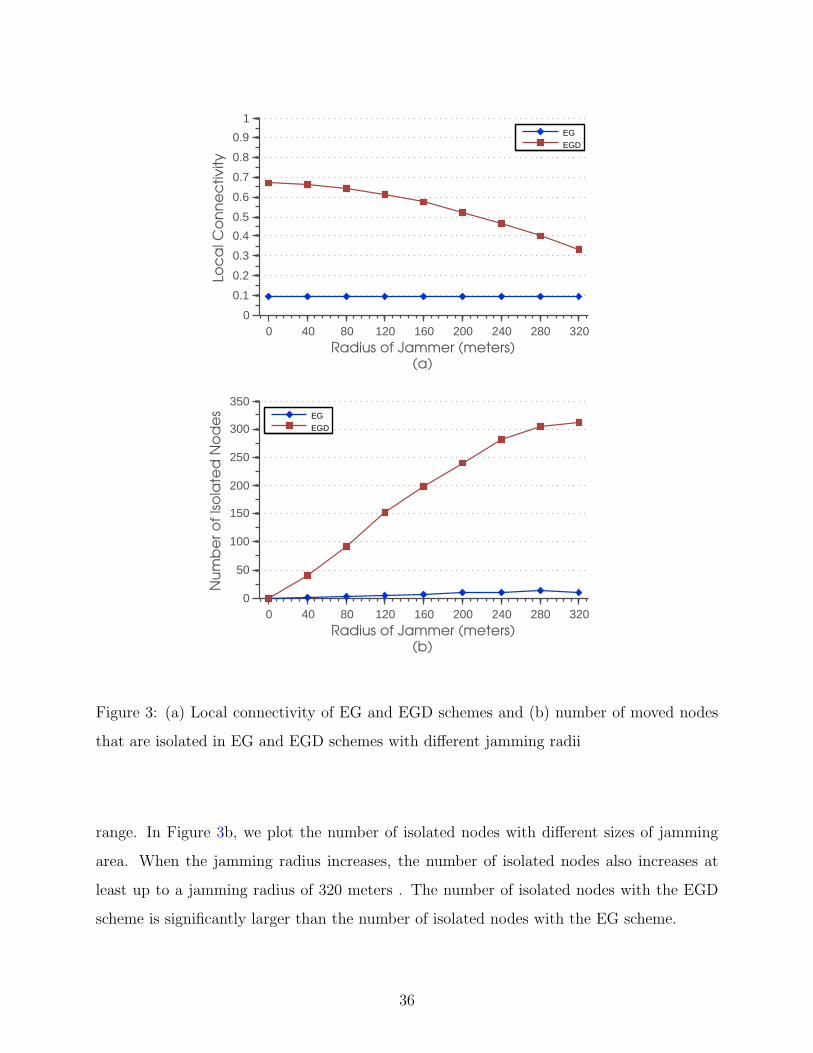
0 40 80 120 160 200 240 280 3200
0.1
0.2
0.3
0.4
0.5
0.6
0.7
0.8
0.9
1
Radius of Jammer (meters)(a)
Loc
al C
on
ne
ctiv
ity
EG
EGD
0 40 80 120 160 200 240 280 3200
50
100
150
200
250
300
350
Radius of Jammer (meters)(b)
Nu
mb
er
of
Iso
late
d N
od
es
EG
EGD
Figure 3: (a) Local connectivity of EG and EGD schemes and (b) number of moved nodes
that are isolated in EG and EGD schemes with different jamming radii
range. In Figure 3b, we plot the number of isolated nodes with different sizes of jamming
area. When the jamming radius increases, the number of isolated nodes also increases at
least up to a jamming radius of 320 meters . The number of isolated nodes with the EGD
scheme is significantly larger than the number of isolated nodes with the EG scheme.
36

3.4 THE HYBRID KEY PREDISTRIBUTION SCHEME
This section presents the design framework of the hybrid key predistribution scheme (HB
scheme). The terms hybrid key predistribution scheme and HB scheme will be used inter-
changeably throughout this dissertation. The idea of the hybrid scheme is based on the
observation in Section 3.3. It makes use of the beneficial features of both the EG and EGD
schemes. The goal of our scheme is as follows: When there is no jamming, the HB scheme
should show better local connectivity compared to the random (EG) scheme (and close to
the connectivity level of the EGD scheme). Under jamming attacks, the hybrid scheme
should have an acceptable level of local connectivity even when the nodes have moved away
from their original locations and few nodes should be isolated. All of this must be achieved
without increasing the number of installed keys in a sensor node.
3.4.1 Deployment Model
Here we explain the deployment model used in the hybrid scheme. We adopt the group-
based deployment model proposed in [5]. A group of N sensor nodes is divided into small
groups of equal size. We call each group a deployment group Gi,j, where i = 1, 2, 3, . . . , t
and j = 1, 2, 3, . . . , n. The total number of deployment group is |Gi,j| = t × n. Each group
will have an associated target point. A sensor node that belongs to a group Gi,j is deployed
according to a target deployment point (xi, yj). We arrange the locations of each deployment
point as a square grid of size t× n as in [5]. Note that deployment points can be differently
arranged depending on the method of deployment and application objective.
We use a two-dimensional Gaussian distribution (Normal distribution) as in [5] for mod-
eling deployment where the target deployment point is the mean of the distribution. Once
deployed, the actual location of a sensor node will be around the associated target deploy-
ment point of the group. The standard deviation of the distribution determines how much
nodes will spread out from the deployment point. Here we use the standard deviation (σ) =
50 meters, which is similar to the number used in [5].
37

3.4.2 Setting up Keypool
This section describes two types of key pools that will be used in the hybrid scheme, namely
global key pool and group key pools. The global key pool (S) consists of a large number of
cryptographic keys. The size of the key pool can be very large as it does not impact the
small storage of the sensor node. We use a global key pool |S| of size = 100, 000 keys. The
global key pool stores keys with indices k1, k2, . . . , k|S|. All sensor nodes will pick keys from
this key pool. The group key pool (Si,j) consists of subsets of keys selected from a global key
pool. A deployment group Gi,j will associate itself with the group key pool Si,j. The total
number of group key pools is t×n, which is equal to the number of deployment groups. The
number of keys in each group key pool is |Sc|.We divide keys from the global key pool to each group key pools Si,j. The goal is that
each group key pool will have exactly |Sc| keys and will share a certain number of keys
with adjacent group key pools (vertically, horizontally, and diagonally). These common keys
between adjacent groups will serve as a potential bridge for nodes from different deployment
groups that are neighbors to have a shared key. The number of shared keys between two
groups that are neighbors is indicated by an overlapping factor, which indicates the percent-
age of keys in a group key pool that will be shared with a group neighbor. The number
of keys shared between two horizontal or vertical group neighbors will be a · |Sc|, and two
diagonal group neighbors will share b · |Sc| keys. It is possible to create group key pools from
the first global key pool, but we keep the two key pools separate to simplify the analysis
presented next. For the hybrid scheme, we create a second global key pool (S2) that also
contains |S| keys. Each group key pool will be created by selecting keys from this global key
pool. Simulations (not shown here) show little difference between the two approaches since
the group key pool is typically smaller than the global key pool (by two orders of magnitude
– |Sc| � |S| – for the 10×10 grid).
3.4.3 The Hybrid Threshold
The main idea of the hybrid scheme is to select the right numbers of keys from the global and
group key pools that balance connectivity and robustness to jamming attacks. We define a
38

hybrid threshold (τ) to control key selection for each node. This threshold τ indicates the
fraction of keys that a node will select from the global key pool S and its associated group
key pool Si,j (which is created from the second global key pool S2). The value of τ ranges
from 0 to 1 (τ = 0, . . . , 1). Given that a sensor node can store k cryptographic keys in its
memory, it will select τ · k keys from the global key pool S. For the remaining space of
(1− τ) · k keys, the node will select keys from its associated group key pool.
Example: For instance, given a memory size of k = 100 keys, when τ is set to 0.25, a
node will select 0.25×100 = 25 keys from the first global key pool and (1−0.25)×100 = 75
keys from its group key pool. We look at how the value of τ reflects the behavior of the
hybrid scheme. We look at values of τ at two extreme points, 0 and 1.
• When τ = 0, a node will select no key from the global key pool. This means each node
will only pick keys from its group key pool. With τ = 0, the hybrid scheme is equivalent
to the EGD scheme.
• When τ = 1, a node will select all keys from the global key pool. As a result, the hybrid
scheme with τ = 1 is converted to the random scheme (EG scheme). Each node will
select keys from the same (global) key pool. No keys are selected based on the groups
deployment.
We show in the previous section that selection of keys only from group key pools, although
this has high connectivity, can cause high numbers of isolated nodes after nodes move away
from a jammed area. Using keys only from a global key pool causes low numbers of isolated
nodes but it has significantly low connectivity compared to using multiple key pools with
same number of stored keys. The goal of our scheme is to gain the benefit from both key
predistribution methods by selecting an appropriate value of τ that balances the level of key
connectivity and robustness to node isolation caused by jamming attacks. We will show by
simulations that the hybrid scheme with an appropriate value of τ can keep a high level of
local connectivity and maintain a low number of isolated nodes after nodes perform spatial
retreats in order to cope with jamming attacks.
39

3.4.4 Key Distribution Process
Like other existing key pre-distribution schemes proposed in the literature, the hybrid scheme
comprises of 3 phases: a key distribution phase, a shared key discovery phase, and a path-key
establishment phase.
Step 1: Key Distribution Phase: This phase is done off-line before nodes are deployed
to the target field. The key distribution server generates a global key pool and group key
pools for each deployment groups. Each sensor node randomly selects keys from the global
key pool and the group key pool associated with its deployment group. The number of keys
selected from each key pool is indicated by the hybrid threshold τ . Each sensor loads the
selected keys into its memory and then will be deployed to the sensor field according to the
group deployment approach.
Step 2: Shared Key Discovery Phase: In this phase, the main task of each node is
to find if it has any common key with neighbors that are within its radio range. After nodes
are deployed to the target field, each node broadcasts a message that contains the indices of
the keys in its possession. Each node may broadcast these messages in clear text since the
key-ID by itself does not reveal the actual keys. Each node compares the list of keys in each
incoming message with its own stored keys. If a common key exists between a pair of nodes,
both nodes can establish a secure link using a shared key as the link key.
Step 3: Path-Key Establishment Phase: Since the distribution of keys to each
node is done randomly, it is possible that some nodes may not be able to find any common
key with a subset of neighbors. In this case, as long as the key sharing graph of the entire
sensor network is connected, it is possible that a given node can establish secure links with
neighbors through their shared-key neighbors. Simulation results show that, two nodes that
do not share key can establish a secure link within 3 hops with high probability. Note that
step 2 and 3 are similar to EG and EGD schemes.
3.4.5 Analyzing Secure Connectivity
We calculate the probability that two nodes share at least one key (the probability Pr(B)
discussed in Section 2.1.2). This probability is computed by 1 minus the probability that
40

two nodes do not share any key. For the hybrid scheme, it is simply 1 minus the probability
that two nodes do not share a key from the first global key pool nor do they share a key
from the group key pools.
As mentioned in Section 3.4.2, we create 2 global key pools S and S2 for simplicity of
analysis. Both key pools contain |S| keys. Group key pools are created by selecting keys
from the S2 pool. The global key pool contains |S| keys and each group key pool contains
|Sc| keys. Two nodes ni and nj that belong to deployment groups Gi and Gj respectively
pick totally k keys which are kτ keys from the first global key pool S and k(1− τ) keys from
its group key pool Si and Sj.
To calculate Pr[two nodes share at least one key], first we need to calculate Pr[two nodes
ni and nj share no key]. The first node ni has to pick k(1− τ) keys from it group key pool.
As mentioned in Section 2.1.2, two groups Gi and Gj will have δ(i, j) shared key between
their group key pools. The value δ(i, j) depends on whether Gi and Gj are the same group,
from adjacent groups or non-adjacent groups. Keys that ni picks from its group key pool
may be keys that are shared or not shared with nj’s group key pool. Let m be the number
of keys the first node picks from the shared part of the key pools (totally δ(i, j) keys). The
number of possible keys that the first node picks is
(δ(i, j)
m
)(3.1)
, where m can range from 0 to min(δ(i, j), k(1−τ)). Then the first node picks the remaining
k(1− τ)−m keys which are keys in Si that are not shared with Sj. The number of possible
cases is ( |Sc| − δ(i, j)k(1− τ)−m
)(3.2)
. At this point, the first node ni has already picked k(1 − τ) keys from its group key pool.
Now it has to pick τk more keys from global key pool S. The number of possible cases that
node ni can pick is (|S|τk
)(3.3)
We then consider the number of possible cases of keys that the second node nj can choose.
Again node nj has to pick k(1− τ) keys from its group key pool and τk keys from the global
41

key pool. Since ni has already picked m keys from nj’s group key pool, node nj has only
|Sc| −m remaining keys to pick (such that ni and nj will not pick any same key). Thus, the
possible number of cases is (|Sc| −mk(1− τ)
)(3.4)
In the case of keys from the global key pool, since ni has already picked τk keys from this
pool, the number of possible sets of keys that nj can choose from the global key pool is
(|S| − τkτk
)(3.5)
Since key pools S and S2 are independent, given τ , the probability that two nodes share no
key, the fraction of cases where two nodes do not pick the same key over all possible cases,
can be written by combining Equations 3.1 to 3.5 as:
∑min(k(1−τ),δ(i,j))m=0
(δ(i,j)m
)(|Sc|−δ(i,j)k(1−τ)−m
)(|S|τk
)(|Sc|−mk(1−τ)
)(|S|−τkτk
)( |Sc|k(1−τ)
)2(|S|τk
)2 (3.6)
The probability that two nodes share at least one key can be computed by subtracting
Equation 3.6 from 1 as:
1−{
((|S| − kτ)!)2
(|S| − 2kτ)!|S|!
}×
∑min(k(1−τ),δ(i,j))
m=0
(δ(i,j)m
)(|Sc|−δ(i,j)k(1−τ)−m
)(|Sc|−mk(1−τ)
)( |Sc|k(1−τ)
)2 (3.7)
Note that this probability is for the situation when there is no jamming. Under jamming
and spatial retreat, the equation will change in terms of the value of δ(i, j) which could be
0 in the worst case where nodes are from non-adjacent groups or |Sc| in the best case where
nodes are from the same group.
42

3.5 PERFORMANCE EVALUATION
In this section, we evaluate the performance of the hybrid key predistribution scheme through
simulations. The metrics considered are local connectivity and the the number of moved
nodes that are isolated after detecting jamming and performing spatial retreat. We compare
our results to the random scheme (EG scheme) [4] and the deployment knowledge based
scheme (EGD scheme) [5]. Simulation parameters set up and the jammer model are the
same as described in Section 3.3 unless otherwise stated. Each simulation is run 10 times
with different seeds of the random number generator, and the results represent the average
value of the 10 runs with 90% confidence interval. We consider a range of values for the hybrid
threshold τ , namely τ = 0, 0.25, 0.50, 0.75, 1, to assess the performance. We reiterate that
when τ is 0, the scheme converts to the EGD scheme (node selects all keys from the group
key pool) and when τ is 1, the scheme converts to the EG scheme with group deployment
(sensor nodes are deployed as groups but every node selects keys from the same global key
pool). Under jamming, nodes perform spatial retreat to escape from the jamming signal as
previously described in Section 3.2.2. We show the results from two types of jammers. The
first case is where a single jammer presents in the network. For the second case, we put
multiple jammers in the network, each with random locations.
3.5.1 Simulation Setup
We describe the parameters setting used in our simulations. We deploy 10,000 sensor nodes
into a square area (sensor field) of size 1, 000m × 1, 000m. For the hybrid scheme and the
EGD scheme, we assume sensor deployment groups are arranged in a 10 × 10 grid. Thus,
the total number of sensor clusters is 100 groups, where each deployment group is of size
100m × 100m. A sensor node’s location follows the two dimensional Gaussian distribution
where the mean of the distribution is the group deployment point and the standard deviation
(σ) is 50 meters. We use overlapping factor a = 0.15 and b = 0.10. The size of the global key
pool is 100,000 keys. With a 10×10 grid deployment, each group key pool will contain 1,760
keys. The transmission range of a sensor is 40 meters. We assume each node has memory
43
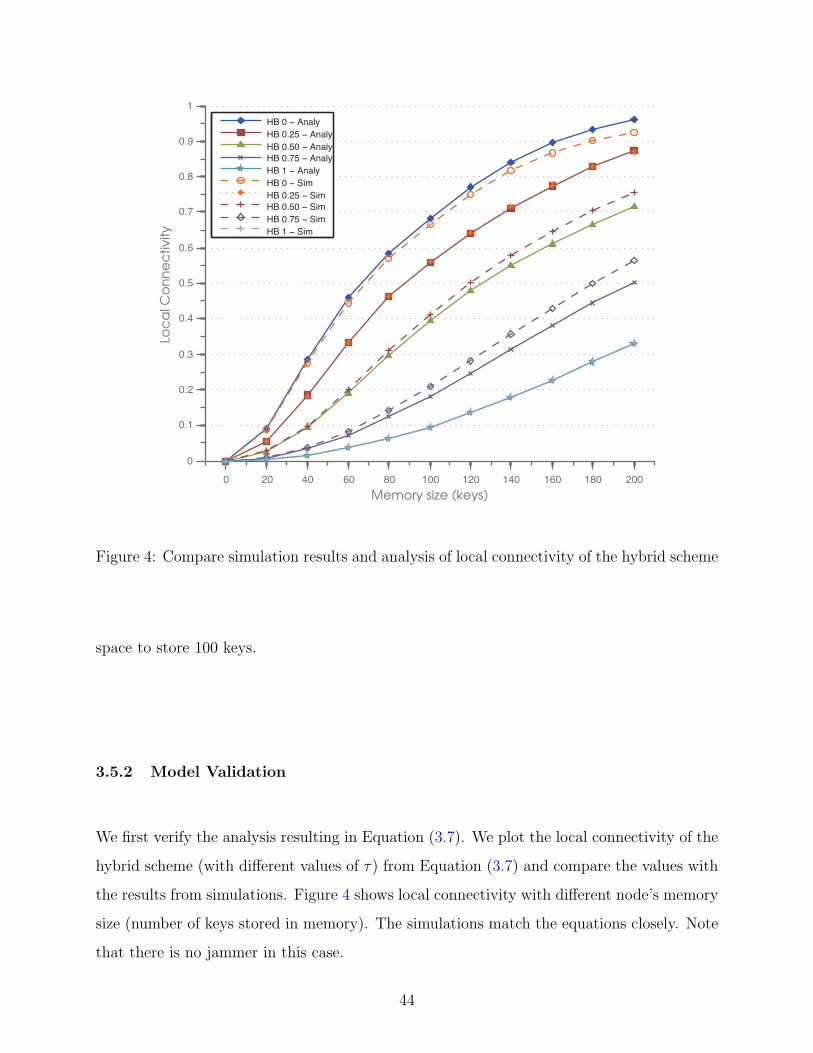
0 20 40 60 80 100 120 140 160 180 200
0
0.1
0.2
0.3
0.4
0.5
0.6
0.7
0.8
0.9
1
Memory size (keys)
Loc
al C
on
ne
ctiv
ity
HB 0 − AnalyHB 0.25 − AnalyHB 0.50 − AnalyHB 0.75 − AnalyHB 1 − AnalyHB 0 − SimHB 0.25 − SimHB 0.50 − SimHB 0.75 − SimHB 1 − Sim
Figure 4: Compare simulation results and analysis of local connectivity of the hybrid scheme
space to store 100 keys.
3.5.2 Model Validation
We first verify the analysis resulting in Equation (3.7). We plot the local connectivity of the
hybrid scheme (with different values of τ) from Equation (3.7) and compare the values with
the results from simulations. Figure 4 shows local connectivity with different node’s memory
size (number of keys stored in memory). The simulations match the equations closely. Note
that there is no jammer in this case.
44
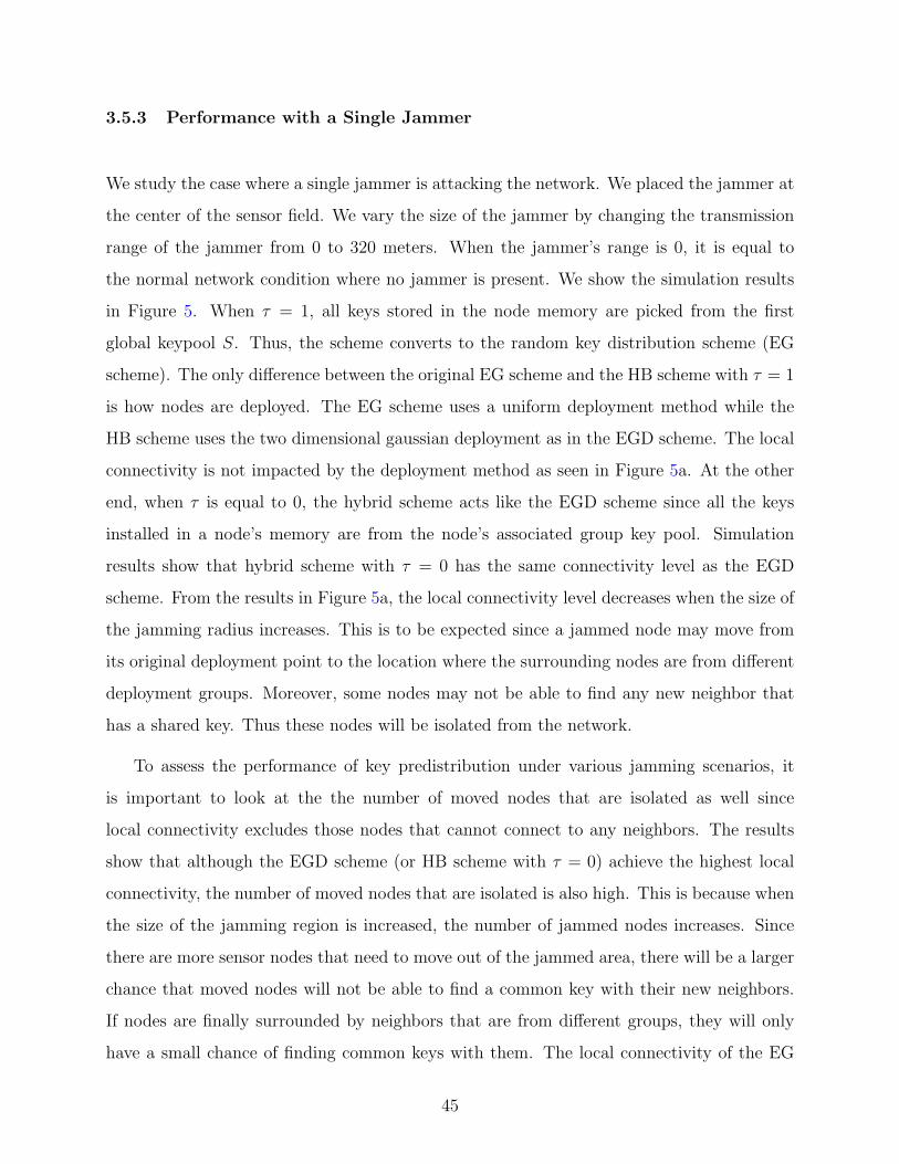
3.5.3 Performance with a Single Jammer
We study the case where a single jammer is attacking the network. We placed the jammer at
the center of the sensor field. We vary the size of the jammer by changing the transmission
range of the jammer from 0 to 320 meters. When the jammer’s range is 0, it is equal to
the normal network condition where no jammer is present. We show the simulation results
in Figure 5. When τ = 1, all keys stored in the node memory are picked from the first
global keypool S. Thus, the scheme converts to the random key distribution scheme (EG
scheme). The only difference between the original EG scheme and the HB scheme with τ = 1
is how nodes are deployed. The EG scheme uses a uniform deployment method while the
HB scheme uses the two dimensional gaussian deployment as in the EGD scheme. The local
connectivity is not impacted by the deployment method as seen in Figure 5a. At the other
end, when τ is equal to 0, the hybrid scheme acts like the EGD scheme since all the keys
installed in a node’s memory are from the node’s associated group key pool. Simulation
results show that hybrid scheme with τ = 0 has the same connectivity level as the EGD
scheme. From the results in Figure 5a, the local connectivity level decreases when the size of
the jamming radius increases. This is to be expected since a jammed node may move from
its original deployment point to the location where the surrounding nodes are from different
deployment groups. Moreover, some nodes may not be able to find any new neighbor that
has a shared key. Thus these nodes will be isolated from the network.
To assess the performance of key predistribution under various jamming scenarios, it
is important to look at the the number of moved nodes that are isolated as well since
local connectivity excludes those nodes that cannot connect to any neighbors. The results
show that although the EGD scheme (or HB scheme with τ = 0) achieve the highest local
connectivity, the number of moved nodes that are isolated is also high. This is because when
the size of the jamming region is increased, the number of jammed nodes increases. Since
there are more sensor nodes that need to move out of the jammed area, there will be a larger
chance that moved nodes will not be able to find a common key with their new neighbors.
If nodes are finally surrounded by neighbors that are from different groups, they will only
have a small chance of finding common keys with them. The local connectivity of the EG
45
0 40 80 120 160 200 240 280 3200
0.1
0.2
0.3
0.4
0.5
0.6
0.7
0.8
0.9
1
Radius of Jammer (meters)
(a)
Loc
al C
on
ne
ctiv
ity
0 40 80 120 160 200 240 280 3200
50
100
150
200
250
300
350
Radius of Jammer (meters)
(b)
Nu
mb
er
of
Iso
late
d N
od
es
EGEGDHB, τ = 0HB, τ = 0.25HB, τ = 0.50HB, τ = 0.75HB, τ = 1
EGEGDHB, τ = 0HB, τ = 0.25HB, τ = 0.50HB, τ = 0.75HB, τ = 1
Figure 5: (a) Local connectivity and (b) number of moved nodes that are isolated for EG,
EGD, and HB schemes with different sizes of jamming areas
scheme and hybrid scheme with τ = 1 remain constant as the jammer’s radius increases.
Nevertheless, the number of isolated nodes after spatial retreat is also low. This is because
all pairs of nodes have on average the same probability of having a common key, since every
node picks key from the same key pool. Although local connectivity is not impacted by
46
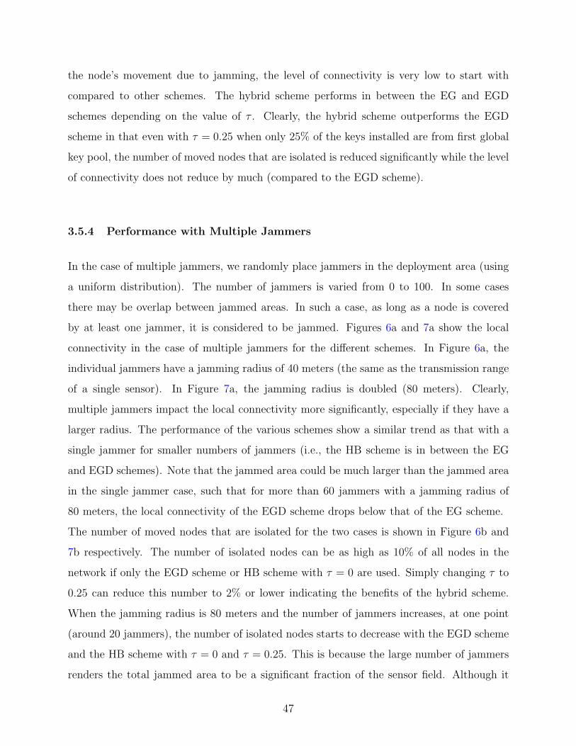
the node’s movement due to jamming, the level of connectivity is very low to start with
compared to other schemes. The hybrid scheme performs in between the EG and EGD
schemes depending on the value of τ . Clearly, the hybrid scheme outperforms the EGD
scheme in that even with τ = 0.25 when only 25% of the keys installed are from first global
key pool, the number of moved nodes that are isolated is reduced significantly while the level
of connectivity does not reduce by much (compared to the EGD scheme).
3.5.4 Performance with Multiple Jammers
In the case of multiple jammers, we randomly place jammers in the deployment area (using
a uniform distribution). The number of jammers is varied from 0 to 100. In some cases
there may be overlap between jammed areas. In such a case, as long as a node is covered
by at least one jammer, it is considered to be jammed. Figures 6a and 7a show the local
connectivity in the case of multiple jammers for the different schemes. In Figure 6a, the
individual jammers have a jamming radius of 40 meters (the same as the transmission range
of a single sensor). In Figure 7a, the jamming radius is doubled (80 meters). Clearly,
multiple jammers impact the local connectivity more significantly, especially if they have a
larger radius. The performance of the various schemes show a similar trend as that with a
single jammer for smaller numbers of jammers (i.e., the HB scheme is in between the EG
and EGD schemes). Note that the jammed area could be much larger than the jammed area
in the single jammer case, such that for more than 60 jammers with a jamming radius of
80 meters, the local connectivity of the EGD scheme drops below that of the EG scheme.
The number of moved nodes that are isolated for the two cases is shown in Figure 6b and
7b respectively. The number of isolated nodes can be as high as 10% of all nodes in the
network if only the EGD scheme or HB scheme with τ = 0 are used. Simply changing τ to
0.25 can reduce this number to 2% or lower indicating the benefits of the hybrid scheme.
When the jamming radius is 80 meters and the number of jammers increases, at one point
(around 20 jammers), the number of isolated nodes starts to decrease with the EGD scheme
and the HB scheme with τ = 0 and τ = 0.25. This is because the large number of jammers
renders the total jammed area to be a significant fraction of the sensor field. Although it
47
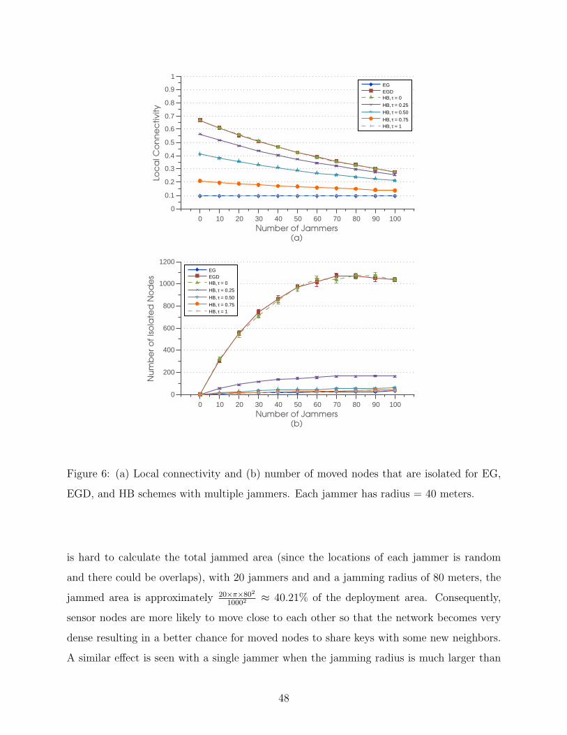
0 10 20 30 40 50 60 70 80 90 1000
0.1
0.2
0.3
0.4
0.5
0.6
0.7
0.8
0.9
1
Number of Jammers(a)
Loc
al C
on
ne
ctivity
EGEGDHB, τ = 0
HB, τ = 0.25
HB, τ = 0.50
HB, τ = 0.75HB, τ = 1
0 10 20 30 40 50 60 70 80 90 1000
200
400
600
800
1000
1200
Number of Jammers(b)
Nu
mb
er
of
Iso
late
d N
od
es
EGEGDHB, τ = 0
HB, τ = 0.25
HB, τ = 0.50
HB, τ = 0.75HB, τ = 1
Figure 6: (a) Local connectivity and (b) number of moved nodes that are isolated for EG,
EGD, and HB schemes with multiple jammers. Each jammer has radius = 40 meters.
is hard to calculate the total jammed area (since the locations of each jammer is random
and there could be overlaps), with 20 jammers and and a jamming radius of 80 meters, the
jammed area is approximately 20×π×802
10002 ≈ 40.21% of the deployment area. Consequently,
sensor nodes are more likely to move close to each other so that the network becomes very
dense resulting in a better chance for moved nodes to share keys with some new neighbors.
A similar effect is seen with a single jammer when the jamming radius is much larger than
48
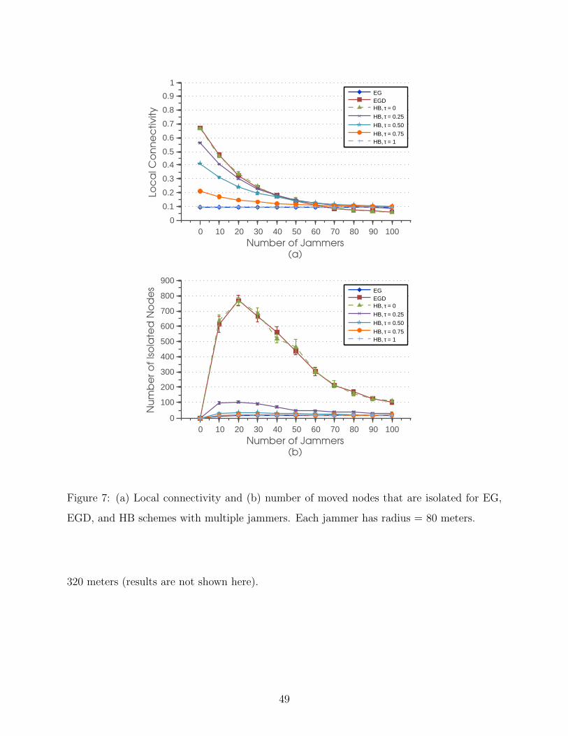
0 10 20 30 40 50 60 70 80 90 1000
0.1
0.2
0.3
0.4
0.5
0.6
0.7
0.8
0.9
1
Number of Jammers(a)
Loc
al C
on
ne
ctiv
ity
EGEGDHB, τ = 0
HB, τ = 0.25
HB, τ = 0.50
HB, τ = 0.75HB, τ = 1
0 10 20 30 40 50 60 70 80 90 1000
100
200
300
400
500
600
700
800
900
Number of Jammers(b)
Nu
mb
er
of
Iso
late
d N
od
es
EGEGDHB, τ = 0
HB, τ = 0.25
HB, τ = 0.50
HB, τ = 0.75HB, τ = 1
Figure 7: (a) Local connectivity and (b) number of moved nodes that are isolated for EG,
EGD, and HB schemes with multiple jammers. Each jammer has radius = 80 meters.
320 meters (results are not shown here).
49

3.5.5 Impact of Grid Size
In the previous results, a 10 × 10 grid of sensor clusters (deployment groups) was used in
the EGD and hybrid schemes. This means there are 100 group key pools, and each cluster
of sensors is deployed in a 100m×100m grid with a deployment at the center of each grid.
With a transmission range of 40 meters, sensors in same cluster (deployment group) will
have a good chance of being in each other’s transmission range. The work in [5] does not
look at the sensitivity of the key predistribution scheme to changes in the size of the grid.
With the same size of deployment area (1,000m×1,000m), we run simulations using a 4× 4
grid – there are 16 clusters of sensors and a grid is 250m×250m in size. The group key pool
size increases to |Sc| = 9, 433 keys while it is 1,760 keys in the 10×10 grid. There are 10,000
sensors deployed in the field as before. We show the average of 10 simulation runs. Figures
8 and 9 show the local connectivity and the number of moved nodes that are isolated for
single and multiple jammers respectively for various schemes. The drop in local connectivity
of the EGD scheme or HB schemes compared to the 10 × 10 grid is not significant, and is
in fact stable with increase in jamming radius. Moreover, the the number of moved nodes
that are isolated is much smaller. This can be expected since a greater number of sensors
derive keys from the same key pool (about six times more sensors than before). There is
more chance that a moved node will still be surrounded by neighbors that are from the same
group. It is thus better to deploy fewer clusters of grids to provide resilience to jamming.
3.5.6 Impact of Node Density
The node density will influence the connectivity and the ability to create a securely connected
graph in the network. This is an issue that has not received much attention in the literature
on key predistribution. We ran simulations to obtain some understanding of the impact
of node density. The averages for 10 simulation runs are shown here. Figure 10 shows
the results of the local connectivity and the number of moved nodes that are isolated as
the number of deployed sensors changes in the 10 × 10 grid. We picked 50 jammers for
illustration and compare the EG, EGD, and HB (τ = 0.25, 0.5, and 0.75) schemes. We omit
the results for τ = 0 and 1 since the results are very similar to the EGD and EG schemes,
50
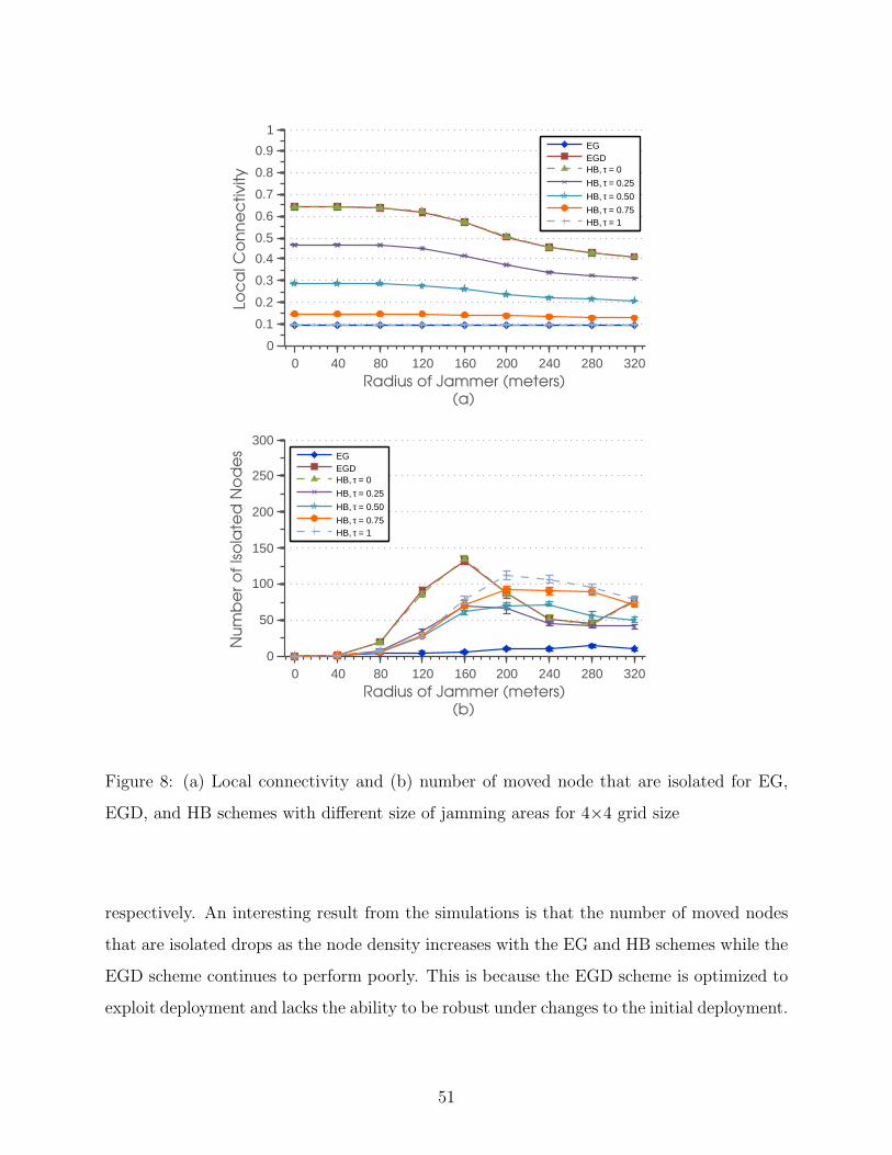
0 40 80 120 160 200 240 280 3200
0.1
0.2
0.3
0.4
0.5
0.6
0.7
0.8
0.9
1
Radius of Jammer (meters)(a)
Loc
al C
on
ne
ctiv
ity
EGEGDHB, τ = 0
HB, τ = 0.25
HB, τ = 0.50
HB, τ = 0.75HB, τ = 1
0 40 80 120 160 200 240 280 3200
50
100
150
200
250
300
Radius of Jammer (meters)(b)
Nu
mb
er
of
Iso
late
d N
od
es
EGEGDHB, τ = 0
HB, τ = 0.25
HB, τ = 0.50
HB, τ = 0.75HB, τ = 1
Figure 8: (a) Local connectivity and (b) number of moved node that are isolated for EG,
EGD, and HB schemes with different size of jamming areas for 4×4 grid size
respectively. An interesting result from the simulations is that the number of moved nodes
that are isolated drops as the node density increases with the EG and HB schemes while the
EGD scheme continues to perform poorly. This is because the EGD scheme is optimized to
exploit deployment and lacks the ability to be robust under changes to the initial deployment.
51
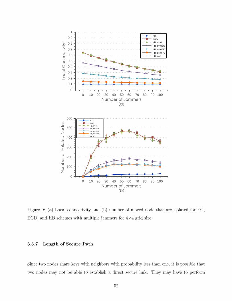
0 10 20 30 40 50 60 70 80 90 1000
0.1
0.2
0.3
0.4
0.5
0.6
0.7
0.8
0.9
1
Number of Jammers(a)
Loc
al C
on
ne
ctiv
ity
EGEGDHB, τ = 0
HB, τ = 0.25
HB, τ = 0.50
HB, τ = 0.75HB, τ = 1
0 10 20 30 40 50 60 70 80 90 1000
100
200
300
400
500
600
Number of Jammers(b)
Nu
mb
er
of
Iso
late
d N
od
es
EG
EGD
HB, τ = 0
HB, τ = 0.25
HB, τ = 0.50HB, τ = 0.75
HB, τ = 1
Figure 9: (a) Local connectivity and (b) number of moved node that are isolated for EG,
EGD, and HB schemes with multiple jammers for 4×4 grid size
3.5.7 Length of Secure Path
Since two nodes share keys with neighbors with probability less than one, it is possible that
two nodes may not be able to establish a direct secure link. They may have to perform
52
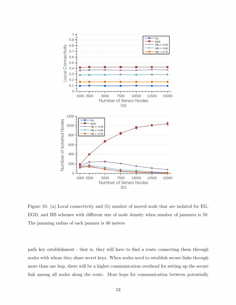
1000 2500 5000 7500 10000 12500 150000
0.1
0.2
0.3
0.4
0.5
0.6
0.7
0.8
0.9
1
Number of Sensor Nodes(a)
Loc
al C
on
ne
ctiv
ity
EGEGDHB, τ = 0.25
HB, τ = 0.50
HB, τ = 0.75
1000 2500 5000 7500 10000 12500 150000
200
400
600
800
1000
1200
Number of Sensor Nodes(b)
Nu
mb
er
of
Iso
late
d N
od
es
EGEGDHB, τ = 0.25
HB, τ = 0.50
HB, τ = 0.75
Figure 10: (a) Local connectivity and (b) number of moved node that are isolated for EG,
EGD, and HB schemes with different size of node density when number of jammers is 50.
The jamming radius of each jammer is 40 meters
path key establishment - that is, they will have to find a route connecting them through
nodes with whom they share secret keys. When nodes need to establish secure links through
more than one hop, there will be a higher communication overhead for setting up the secure
link among all nodes along the route. More hops for communication between potentially
53
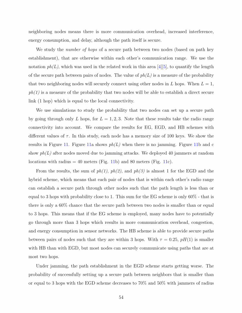
neighboring nodes means there is more communication overhead, increased interference,
energy consumption, and delay, although the path itself is secure.
We study the number of hops of a secure path between two nodes (based on path key
establishment), that are otherwise within each other’s communication range. We use the
notation ph(L), which was used in the related work in this area [4][5], to quantify the length
of the secure path between pairs of nodes. The value of ph(L) is a measure of the probability
that two neighboring nodes will securely connect using other nodes in L hops. When L = 1,
ph(1) is a measure of the probability that two nodes will be able to establish a direct secure
link (1 hop) which is equal to the local connectivity.
We use simulations to study the probability that two nodes can set up a secure path
by going through only L hops, for L = 1, 2, 3. Note that these results take the radio range
connectivity into account. We compare the results for EG, EGD, and HB schemes with
different values of τ . In this study, each node has a memory size of 100 keys. We show the
results in Figure 11. Figure 11a shows ph(L) when there is no jamming. Figure 11b and c
show ph(L) after nodes moved due to jamming attacks. We deployed 40 jammers at random
locations with radius = 40 meters (Fig. 11b) and 80 meters (Fig. 11c).
From the results, the sum of ph(1), ph(2), and ph(3) is almost 1 for the EGD and the
hybrid scheme, which means that each pair of nodes that is within each other’s radio range
can establish a secure path through other nodes such that the path length is less than or
equal to 3 hops with probability close to 1. This sum for the EG scheme is only 60% - that is
there is only a 60% chance that the secure path between two nodes is smaller than or equal
to 3 hops. This means that if the EG scheme is employed, many nodes have to potentially
go through more than 3 hops which results in more communication overhead, congestion,
and energy consumption in sensor networks. The HB scheme is able to provide secure paths
between pairs of nodes such that they are within 3 hops. With τ = 0.25, pH(1) is smaller
with HB than with EGD, but most nodes can securely communicate using paths that are at
most two hops.
Under jamming, the path establishment in the EGD scheme starts getting worse. The
probability of successfully setting up a secure path between neighbors that is smaller than
or equal to 3 hops with the EGD scheme decreases to 70% and 50% with jammers of radius
54
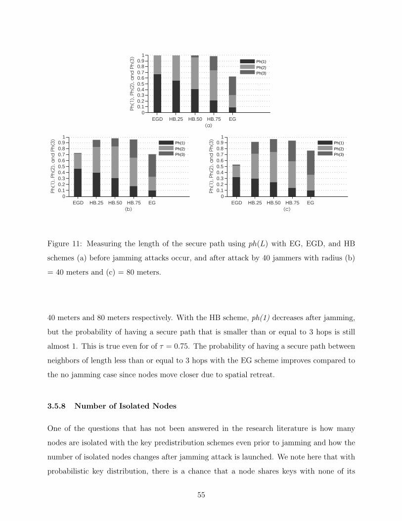
EGD HB.25 HB.50 HB.75 EG0
0.10.20.30.40.50.60.70.80.9
1
(a)
Ph
(1),
Ph
(2),
an
d P
h(3
)
Ph(1)
Ph(2)Ph(3)
EGD HB.25 HB.50 HB.75 EG0
0.10.20.30.40.50.60.70.80.9
1
(b)
Ph
(1),
Ph
(2),
an
d P
h(3
)
Ph(1)
Ph(2)Ph(3)
EGD HB.25 HB.50 HB.75 EG0
0.10.20.30.40.50.60.70.80.9
1
(c)P
h(1
), P
h(2
), a
nd
Ph
(3)
Ph(1)
Ph(2)Ph(3)
Figure 11: Measuring the length of the secure path using ph(L) with EG, EGD, and HB
schemes (a) before jamming attacks occur, and after attack by 40 jammers with radius (b)
= 40 meters and (c) = 80 meters.
40 meters and 80 meters respectively. With the HB scheme, ph(1) decreases after jamming,
but the probability of having a secure path that is smaller than or equal to 3 hops is still
almost 1. This is true even for of τ = 0.75. The probability of having a secure path between
neighbors of length less than or equal to 3 hops with the EG scheme improves compared to
the no jamming case since nodes move closer due to spatial retreat.
3.5.8 Number of Isolated Nodes
One of the questions that has not been answered in the research literature is how many
nodes are isolated with the key predistribution schemes even prior to jamming and how the
number of isolated nodes changes after jamming attack is launched. We note here that with
probabilistic key distribution, there is a chance that a node shares keys with none of its
55

immediate neighbors, thereby isolating it. Clearly, the probability of sharing keys is higher
in the EGD scheme while it is poorer in the EG scheme, however, another interesting issue is
how robust the key predistribution schemes are under the topology changes due to jamming.
Under normal conditions, where jamming is not present, a node may be isolated from
the rest of the network if after deployment it does not have any shared key with any of its
surrounding neighbors (within radio transmission range). Under jamming attacks, we study
scenarios where sensor nodes perform spatial retreat to move away from jammed regions.
Movement of nodes and the type of key predistribution used could cause the number of
isolated nodes to either increase or decrease as explained next. A node could become an
isolated node after it moves out of the jammed area. A node may move to a location where
its new neighbors do not share any key at all with it. The chance for being isolated is higher
when nodes use the group key pool based scheme (i.e., the EGD scheme) since a node may
move to area where neighbor nodes have selected keys from an entirely different group key
pool. A node may have some chance to find a neighbor with a shared key if it moves to one of
its adjacent group’s territory (because the group key pools used in adjacent areas have some
overlapping keys). If a node moves to an area where neighbors are all from non-adjacent
groups, it will not be able to find any shared key as their key pools have no overlapping
keys. On the other hand, a previously isolated node could now be able to find a shared key
with a new neighbor that moves into its radio range due to node movement. Alternatively,
a jammed node that was previously isolated may move to a location that is in range of some
neighbors with shared keys.
We ran simulations to see how many isolated nodes are present totally in the sensor
field before and after jamming with different key predistribution schemes. The number of
isolated nodes present here includes all nodes that are isolated even before jamming or due
to spatial retreat from jamming. Figure 12 shows the average number of isolated nodes with
10 simulation runs. We present the total number of isolated nodes before jamming and after
nodes are jammed by single jammer with different jamming ranges. We compare the results
for the EGD, EG, and HB scheme with different τs.
As expected, the EGD scheme is the best under no jamming. Almost every node shares a
key with some other sensor node. The EG scheme results in about 1% of nodes being isolated
56
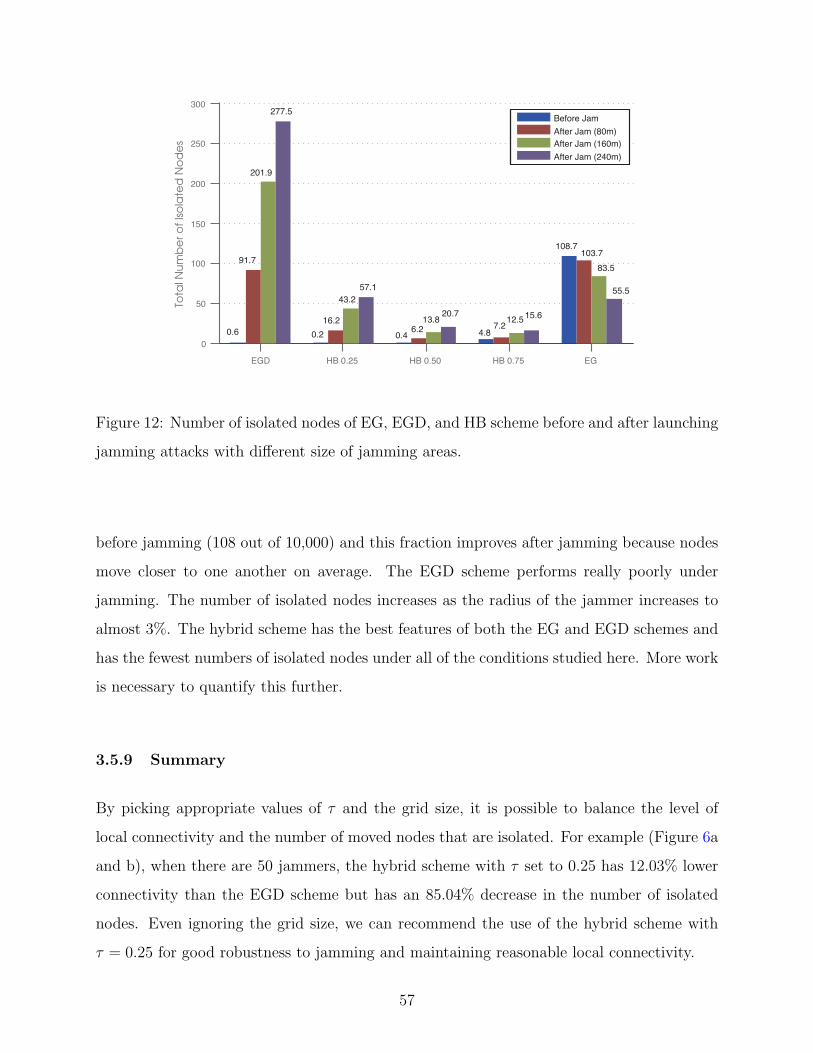
EGD HB 0.25 HB 0.50 HB 0.75 EG
0
50
100
150
200
250
300
Tota
l Nu
mb
er o
f Is
ola
ted
No
de
s
Before Jam
After Jam (80m)After Jam (160m)
After Jam (240m)
277.5
0.6
91.7
201.9
0.46.2
13.820.7
0.2
16.2
43.257.1
4.87.2
12.5 15.6
55.5
83.5
103.7108.7
Figure 12: Number of isolated nodes of EG, EGD, and HB scheme before and after launching
jamming attacks with different size of jamming areas.
before jamming (108 out of 10,000) and this fraction improves after jamming because nodes
move closer to one another on average. The EGD scheme performs really poorly under
jamming. The number of isolated nodes increases as the radius of the jammer increases to
almost 3%. The hybrid scheme has the best features of both the EG and EGD schemes and
has the fewest numbers of isolated nodes under all of the conditions studied here. More work
is necessary to quantify this further.
3.5.9 Summary
By picking appropriate values of τ and the grid size, it is possible to balance the level of
local connectivity and the number of moved nodes that are isolated. For example (Figure 6a
and b), when there are 50 jammers, the hybrid scheme with τ set to 0.25 has 12.03% lower
connectivity than the EGD scheme but has an 85.04% decrease in the number of isolated
nodes. Even ignoring the grid size, we can recommend the use of the hybrid scheme with
τ = 0.25 for good robustness to jamming and maintaining reasonable local connectivity.
57

3.6 HYBRID KEY PREDISTRIBUTION SCHEME WITH PARTIAL
RANDOM SPATIAL RETREATS
In this section, we consider the partial random spatial retreats as the jamming evacuation
strategy to support establishing secure links after a jammed node moves out of the jammed
region. We present the evacuation process of the partial random spatial retreats and present
simulation results with various key predistribution schemes and different jamming scenarios.
3.6.1 Limitations of the Random Spatial Retreat
Here we discuss the limitations of the random spatial retreats technique used in previous
sections. Nodes’ movement with a random distance and direction can maintain even distri-
bution of sensor nodes. However, this may cause some nodes to move a significantly larger
distance than they should thus resulting in reduced sensing capability or coverage in areas
closer to the jammed region. Nodes may consume a large amount of energy due to moving
if nodes move a larger distance than is necessary.
One possible approach is to move jammed nodes in a random direction until nodes leave
the jammed area (move across the border of jammed area) [24]. This can reduce the distance
that the jammed node has to move but may cause a large number of nodes to cluster along
the border of the jammed region and would result in highly uneven distribution of nodes.
(We present the resulting network topology of different moving strategies in Section 3.7.4).
We propose the partial random spatial retreats to support establishing of secure links
after node’s evacuation due to jamming. Our goals are 1) reduce a node’s travel distance due
to jamming (compared to random spatial retreats), 2) maintain even distribution of nodes
in the deployment area, and 3) maintain high local connectivity and low number of isolated
nodes. We present the process of partial random retreats in the next section.
3.6.2 Partial Random Spatial Retreat
In this section we explain the random spatial retreats strategy. The objective is to reduce
a jammed node’s travel distance due to spatial retreats. A jammed node still moves in a
58
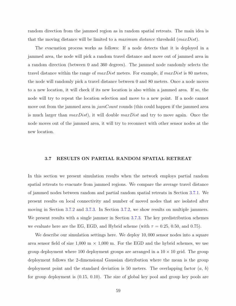
random direction from the jammed region as in random spatial retreats. The main idea is
that the moving distance will be limited to a maximum distance threshold (maxDist).
The evacuation process works as follows: If a node detects that it is deployed in a
jammed area, the node will pick a random travel distance and move out of jammed area in
a random direction (between 0 and 360 degrees). The jammed node randomly selects the
travel distance within the range of maxDist meters. For example, if maxDist is 80 meters,
the node will randomly pick a travel distance between 0 and 80 meters. Once a node moves
to a new location, it will check if its new location is also within a jammed area. If so, the
node will try to repeat the location selection and move to a new point. If a node cannot
move out from the jammed area in jamCount rounds (this could happen if the jammed area
is much larger than maxDist), it will double maxDist and try to move again. Once the
node moves out of the jammed area, it will try to reconnect with other sensor nodes at the
new location.
3.7 RESULTS ON PARTIAL RANDOM SPATIAL RETREAT
In this section we present simulation results when the network employs partial random
spatial retreats to evacuate from jammed regions. We compare the average travel distance
of jammed nodes between random and partial random spatial retreats in Section 3.7.1. We
present results on local connectivity and number of moved nodes that are isolated after
moving in Section 3.7.2 and 3.7.3. In Section 3.7.2, we show results on multiple jammers.
We present results with a single jammer in Section 3.7.3. The key predistribution schemes
we evaluate here are the EG, EGD, and Hybrid scheme (with τ = 0.25, 0.50, and 0.75).
We describe our simulation settings here. We deploy 10, 000 sensor nodes into a square
area sensor field of size 1,000 m × 1,000 m. For the EGD and the hybrid schemes, we use
group deployment where 100 deployment groups are arranged in a 10× 10 grid. The group
deployment follows the 2-dimensional Gaussian distribution where the mean is the group
deployment point and the standard deviation is 50 meters. The overlapping factor (a, b)
for group deployment is (0.15, 0.10). The size of global key pool and group key pools are
59
100,000 and 1,760 keys respectively. Each sensor node has a 40 meters transmission range.
Each node can store a maximum of 100 keys.
3.7.1 Results on Travel Distances
To see how partial random spatial retreats reduces the movement of jammed nodes, we
compare the average travel distance of moved nodes between a network that employs random
spatial retreat and one that employs partial random spatial retreats. We randomly deploy
multiple jammers (uniformly deployed over the sensor field) and measure the travel distance
of each jammed node after moving out of the jammed area. Each jammer has a jamming
radius of 40 meters which is the same as the transmission range of a single sensor. We vary
the number of jammers from 20 to 100.
We define the travel distance of each node as the physical (Euclidean) distance between
a node’s initial location after deployment and the final location after it moves out of the
jammed region.We calculate the average travel distance in meters of random spatial retreats
and one the employs partial random spatial retreats where the maxDist is 80 and 200 meters.
We present the results in Figure 13. The result shows that the average travel distance of
partial random movement is less than average distance of random spatial retreats. The
random spatial retreats where a node can move to anywhere in sensor field of 1,000 × 1,000
m2 has its average around 500 meters. The distance slightly increases as the number of
jammers increases. The average travel distance of the partial random strategy is around 50
meters with maxDist = 80 meters and around 100 meters with maxDist = 200 meters.
The maxDist limit offers a tradeoff between travel distance and node distribution. With
maxDist = 200 meters, nodes will move (on average) a further distance than with partial
movement with maxDist = 80 meters, but nodes will spread out more with maxDist = 200
meters. We present sample node topologies after movement with different values of maxDist
in Section 3.7.4.
60
20 40 60 80 1000
100
200
300
400
500
600
700
800
Number of Jammers
Tra
ve
l D
ista
nc
e (
me
ters
)
RandomPartial Rand. (80m)Partial Rand. (200m)
Figure 13: Average travel distance of jammed nodes after different spatial retreat strategies.
3.7.2 Results with Multiple Jammers
In this section we present the simulation results in the case of multiple jammers. We ran-
domly place jammers in the deployment area. We vary the number of jammers from 0 (equal
to no jamming) to 100. The individuals jammers have a jamming radius of 40 meters. This
is the same simulation scenario as in Section 3.5.4.
Figures 14a and 15a present local connectivity in the case of multiple jammers for EG,
EGD, and HB schemes. The maximum distance (maxDist) thresholds are 80 meters in
Figure 14a and 200 meters in Figure 15a. The results show that using partial random spatial
retreats offers better robustness to multiple jammers than using the maximum distance for
movements. The local connectivity only decreases to a small degree when maxDist = 80
meters. With maxDist = 200 meters, local connectivity of EGD scheme decreases to 0.6
with 100 jammers while it decreases to 0.4 with random spatial retreats (Figure 6a).
We present the number of moved nodes that are isolated for the two maxDist values
in Figure 14b and 15b. The HB scheme with τ = 0.25 results in the smallest number of
isolated nodes for both maxDist values. The number of isolated nodes for the EGD scheme
61

improves over the case with random spatial retreats. The 200meters maxDist results in
higher isolated nodes but the number is much lower compared to random spatial retreats in
Figure 6b. This shows that it is better for jammed nodes to move together (stay in close
range) out of jammed area.
3.7.3 Results with Single Jammer
We also show simulation results for the case of a single jammer. We use the same jamming
scenario as in Section 3.5.3. We place a jammer at the center of the sensor field. We vary
the jammer’s radius from 0 to 240 meters. We present the simulation results in Figure 16.
In this case the value of maxDist is 200 meters. The local connectivity of all schemes show
a similar trend as that with multiple jammers (i.e., local connectivity slightly decreases as
the jammer radius increases). Almost every jammed node is able to reconnect securely with
new neighbors after moving (number of isolated nodes is less than 5 for all schemes). The
number of moved nodes that are isolated for EGD scheme is higher for a jammer radius
of 240 meters but the number of isolated nodes is only between 15 and 20. With partial
random retreats, the hybrid scheme is also able to maintain high local connectivity and a
low number of isolated nodes (i.e., HB with τ = 0.25).
3.7.4 Network Topology after Spatial Retreats
In this section we present sample network topologies after evacuation from jammers with
different spatial retreats strategies. We compare the three spatial retreat strategies: the
random spatial retreats where a jammed node moves out of the jammed area in random
distance and direction, border-move spatial retreats where a jammed node moves (in ran-
dom direction) only until it is out of jammed area, and the partial random spatial retreats
presented in Section 3.6.2. The initial topology before evacuation is the 10 × 10 groups
deployment used in EGD and HB schemes. We present the results with 20 and 80 jammers
randomly placed in the sensor field. Each jammer has a jamming radius of 40 meters.
We first present a sample network topology after nodes move using random spatial re-
treats in Figure 17. The topology shows that jammed nodes are evenly distributed over
62
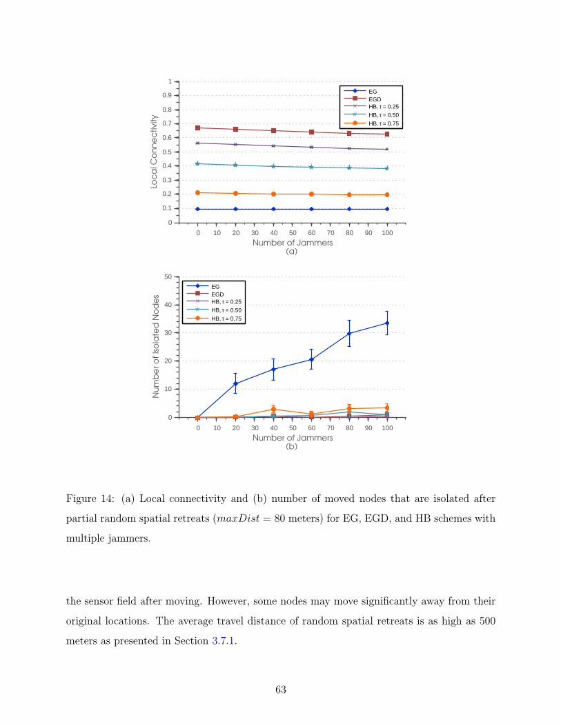
0 10 20 30 40 50 60 70 80 90 100
0
0.1
0.2
0.3
0.4
0.5
0.6
0.7
0.8
0.9
1
Number of Jammers(a)
Loc
al C
on
ne
ctivity
EGEGDHB, τ = 0.25
HB, τ = 0.50
HB, τ = 0.75
0 10 20 30 40 50 60 70 80 90 100
0
10
20
30
40
50
Number of Jammers(b)
Nu
mb
er
of
Iso
late
d N
od
es
EGEGDHB, τ = 0.25
HB, τ = 0.50
HB, τ = 0.75
Figure 14: (a) Local connectivity and (b) number of moved nodes that are isolated after
partial random spatial retreats (maxDist = 80 meters) for EG, EGD, and HB schemes with
multiple jammers.
the sensor field after moving. However, some nodes may move significantly away from their
original locations. The average travel distance of random spatial retreats is as high as 500
meters as presented in Section 3.7.1.
63
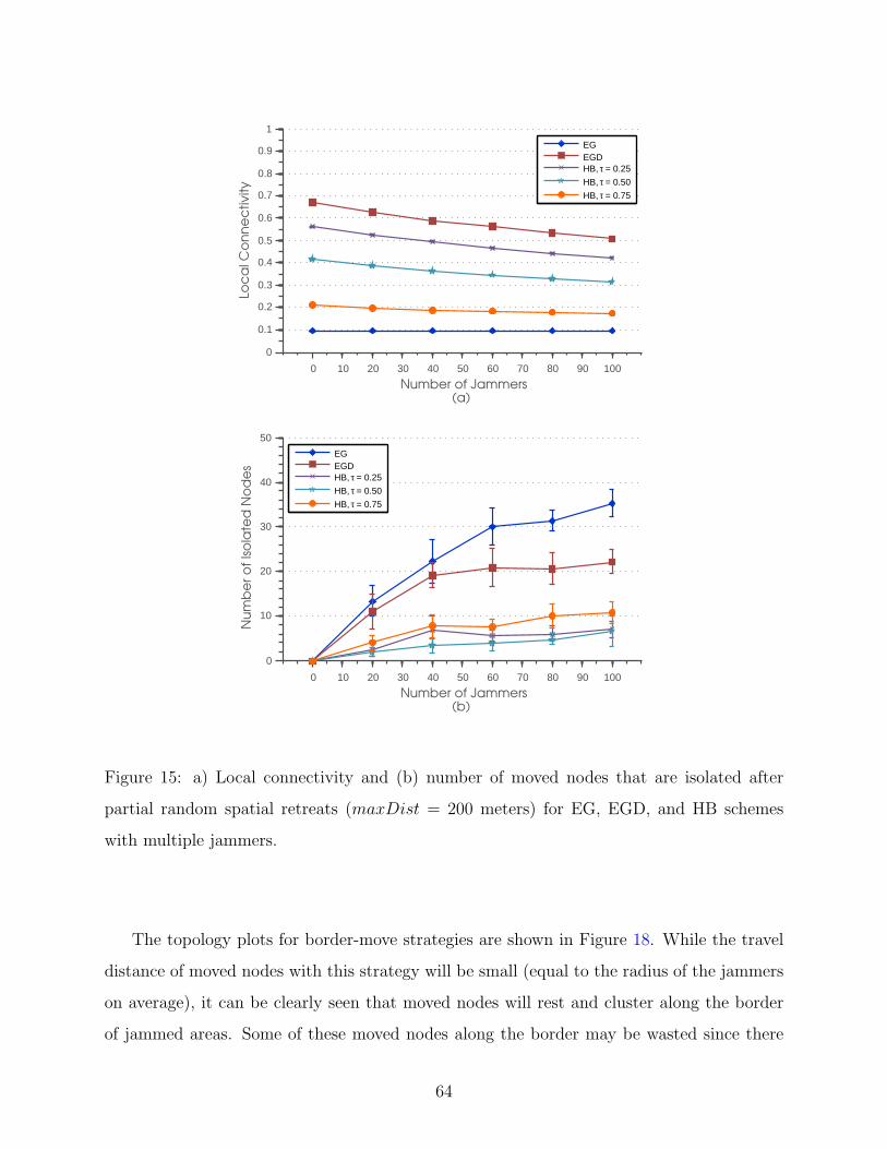
0 10 20 30 40 50 60 70 80 90 100
0
0.1
0.2
0.3
0.4
0.5
0.6
0.7
0.8
0.9
1
Number of Jammers(a)
Loc
al C
on
ne
ctivity
EGEGDHB, τ = 0.25
HB, τ = 0.50
HB, τ = 0.75
0 10 20 30 40 50 60 70 80 90 100
0
10
20
30
40
50
Number of Jammers(b)
Nu
mb
er
of
Iso
late
d N
od
es
EGEGDHB, τ = 0.25
HB, τ = 0.50
HB, τ = 0.75
Figure 15: a) Local connectivity and (b) number of moved nodes that are isolated after
partial random spatial retreats (maxDist = 200 meters) for EG, EGD, and HB schemes
with multiple jammers.
The topology plots for border-move strategies are shown in Figure 18. While the travel
distance of moved nodes with this strategy will be small (equal to the radius of the jammers
on average), it can be clearly seen that moved nodes will rest and cluster along the border
of jammed areas. Some of these moved nodes along the border may be wasted since there
64
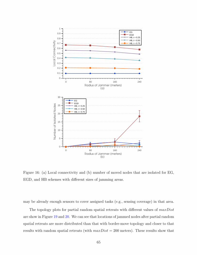
0 80 160 240
0
0.1
0.2
0.3
0.4
0.5
0.6
0.7
0.8
0.9
1
Radius of Jammer (meters)(a)
Loc
al C
on
ne
ctivity
EGEGDHB, τ = 0.25
HB, τ = 0.50
HB, τ = 0.75
0 80 160 240
0
5
10
15
20
25
30
Radius of Jammer (meters)(b)
Nu
mb
er
of
Iso
late
d N
od
es
EGEGDHB, τ = 0.25
HB, τ = 0.50
HB, τ = 0.75
Figure 16: (a) Local connectivity and (b) number of moved nodes that are isolated for EG,
EGD, and HB schemes with different sizes of jamming areas.
may be already enough sensors to cover assigned tasks (e.g., sensing coverage) in that area.
The topology plots for partial random spatial retreats with different values of maxDist
are show in Figure 19 and 20. We can see that locations of jammed nodes after partial random
spatial retreats are more distributed than that with border-move topology and closer to that
results with random spatial retreats (with maxDist = 200 meters). These results show that
65
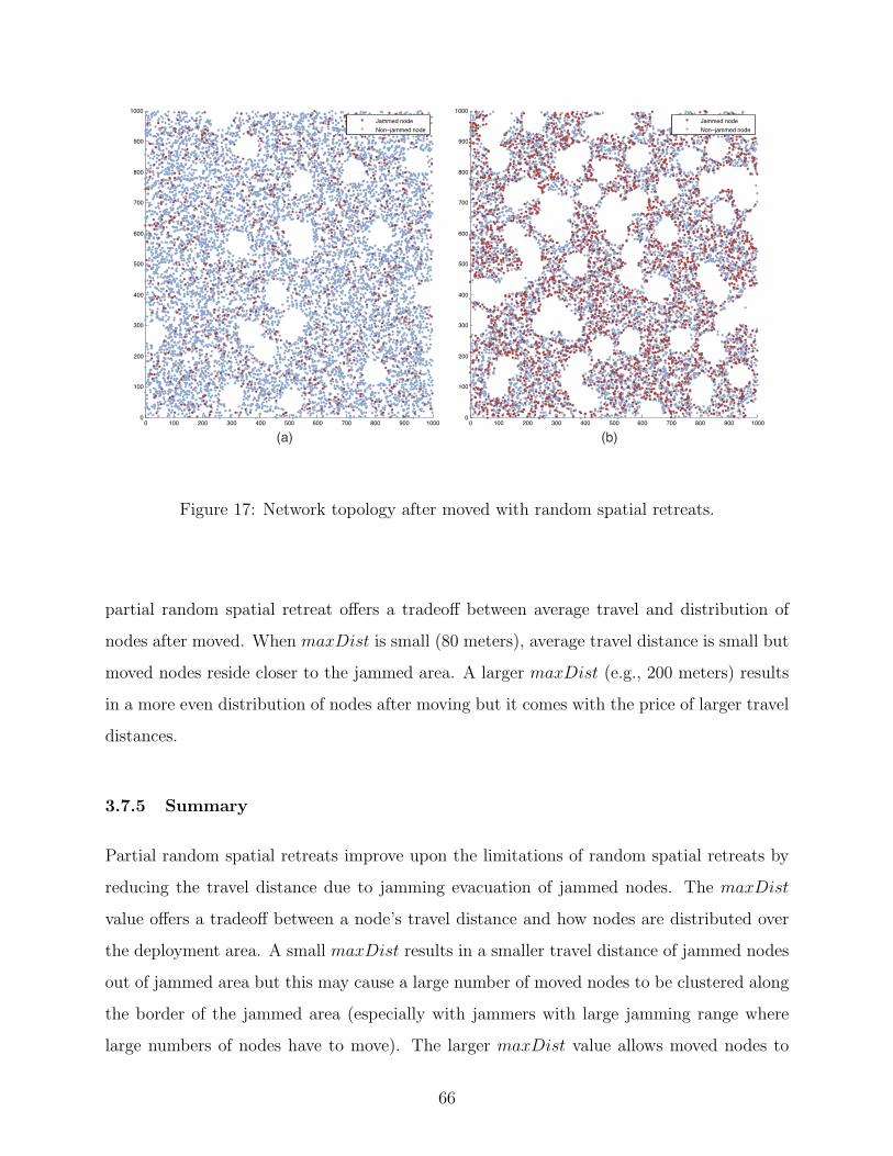
0 100 200 300 400 500 600 700 800 900 10000
100
200
300
400
500
600
700
800
900
1000
Jammed nodeNon−jammed node
0 100 200 300 400 500 600 700 800 900 10000
100
200
300
400
500
600
700
800
900
1000
Jammed nodeNon−jammed node
(a) (b)
Figure 17: Network topology after moved with random spatial retreats.
partial random spatial retreat offers a tradeoff between average travel and distribution of
nodes after moved. When maxDist is small (80 meters), average travel distance is small but
moved nodes reside closer to the jammed area. A larger maxDist (e.g., 200 meters) results
in a more even distribution of nodes after moving but it comes with the price of larger travel
distances.
3.7.5 Summary
Partial random spatial retreats improve upon the limitations of random spatial retreats by
reducing the travel distance due to jamming evacuation of jammed nodes. The maxDist
value offers a tradeoff between a node’s travel distance and how nodes are distributed over
the deployment area. A small maxDist results in a smaller travel distance of jammed nodes
out of jammed area but this may cause a large number of moved nodes to be clustered along
the border of the jammed area (especially with jammers with large jamming range where
large numbers of nodes have to move). The larger maxDist value allows moved nodes to
66
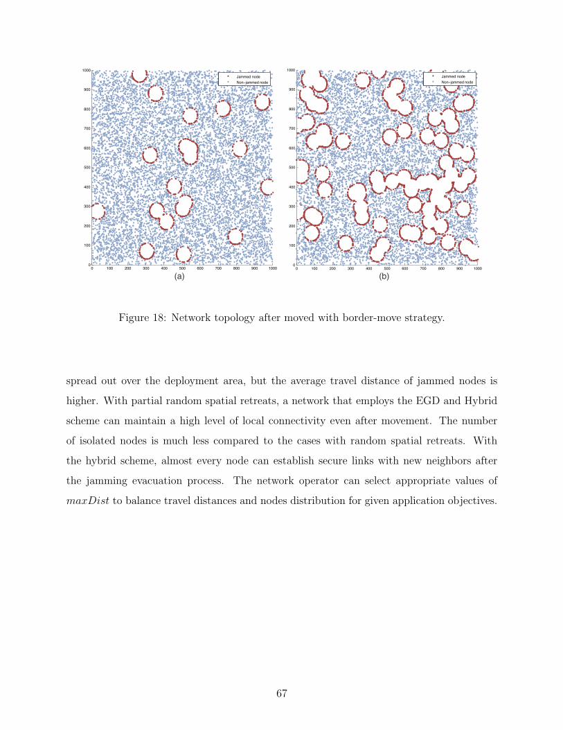
(a) (b)0 100 200 300 400 500 600 700 800 900 1000
0
100
200
300
400
500
600
700
800
900
1000
Jammed nodeNon−jammed node
0 100 200 300 400 500 600 700 800 900 10000
100
200
300
400
500
600
700
800
900
1000
Jammed nodeNon−jammed node
Figure 18: Network topology after moved with border-move strategy.
spread out over the deployment area, but the average travel distance of jammed nodes is
higher. With partial random spatial retreats, a network that employs the EGD and Hybrid
scheme can maintain a high level of local connectivity even after movement. The number
of isolated nodes is much less compared to the cases with random spatial retreats. With
the hybrid scheme, almost every node can establish secure links with new neighbors after
the jamming evacuation process. The network operator can select appropriate values of
maxDist to balance travel distances and nodes distribution for given application objectives.
67
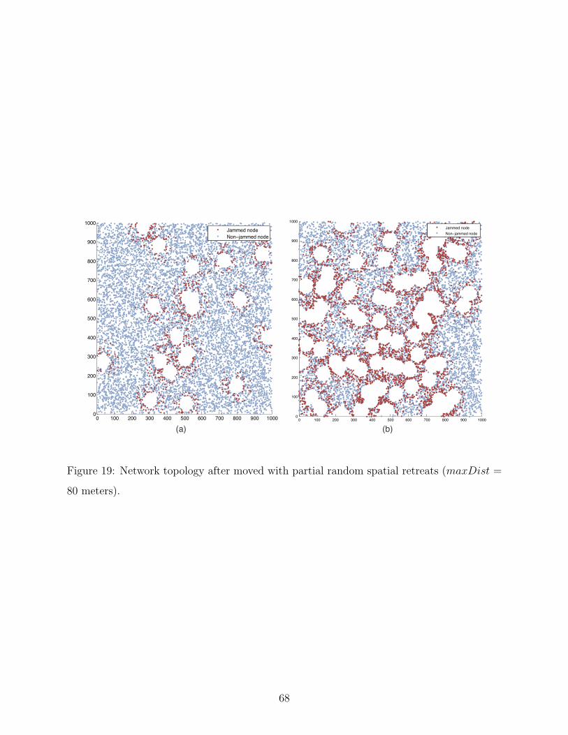
(a) (b)0 100 200 300 400 500 600 700 800 900 1000
0
100
200
300
400
500
600
700
800
900
1000
Jammed nodeNon−jammed node
0 100 200 300 400 500 600 700 800 900 10000
100
200
300
400
500
600
700
800
900
1000
Jammed nodeNon−jammed node
Figure 19: Network topology after moved with partial random spatial retreats (maxDist =
80 meters).
68
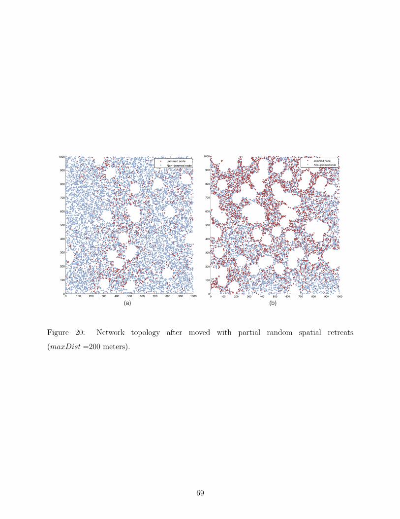
(a) (b)0 100 200 300 400 500 600 700 800 900 1000
0
100
200
300
400
500
600
700
800
900
1000
Jammed nodeNon−jammed node
0 100 200 300 400 500 600 700 800 900 10000
100
200
300
400
500
600
700
800
900
1000
Jammed nodeNon−jammed node
Figure 20: Network topology after moved with partial random spatial retreats
(maxDist =200 meters).
69

4.0 EXPLORING KEY PREDISTRIBUTION UNDER VARIOUS
JAMMING COPING TECHNIQUES
In this chapter, we study other techniques to cope with jamming attacks, namely using higher
transmit power and using directional antennas. In the first part of the chapter we discuss
the limitations of the unit disk jamming model widely employed in the research literature
on sensor and ad hoc networks ([28], [42], and [41]). While this model can provide some
insights for consideration of the impact of transmit power, a better model is needed. We
describe an SNR-based link model that is more suitable to this study. Next, we show the
results on secure connectivity under jamming when networks use higher transmission power
and directional antennas.
4.1 THE UNIT DISK MODEL AND ITS LIMITATIONS
In the previous chapter we assume a unit disk model for transmission range of sensor nodes
and that of jammers. The unit disk model assumes the transmission/reception range of a
node as a circular region centered at the node’s location. The radius of the disk equals the
node’s transmission range. With this model, a link between two nodes exists if a receiver’s
location is within the sender’s transmission circle. A link is symmetric if two nodes are in
each other’s transmission range.
The impact of the jamming signal is also modeled as a circular area where the jamming
range is the radius of the circle. A node is assumed to be jammed if its location is within
the jammed region. Under the unit disk model, we assume that a node in the jamming disk
is completely incommunicado. An example in Figure 21a shows a symmetric link between
70

two nodes with the unit disk model. Nodes A and B are within communication range of
one another; therefore there exists a wireless link from node A to node B and vice versa.
A communication link under a jamming attack with the unit disk model is shown in Figure
21b. Here node B’s location is in the jamming area. With the unit disk model, node B is
considered jammed and cannot communicate with its neighbors. Thus, a link between node
A and B is jammed. Node B will not be able to transmit/receive packets to/from node A.
The circular interpretation of node transmission and jamming signal has an advantage
that it offers a simple model to analyze impact of jamming attacks and for considering optimal
jamming strategies [28][42]. The assumption under the unit disk model about the inability to
transmit when a node is within the jamming range makes sense for sensor nodes that perform
carrier sensing where a jammed signal makes the channel appear busy at all times. However,
in reality, the disk interpretation of communication range is overly simplistic and does not
provide a depiction of the complex relationships between power level and geometry of the
deployment of the sending node and jammers. The unit disk jamming model does not capture
the fact that the success reception is primarily determined by the difference between signal
strength from sender and combined power from jammers at receiving node. In other words,
the unit disk jamming model is like the worst case scenario where all communication abilities
are disabled if a node is located within the jamming range. Under this model, jamming coping
techniques such as increasing transmission power or using directional antennas cannot help
nodes overcome the impact of jamming. This leaves spatial retreats as an only solution to
cope with jamming with the unit disk model.
We would like to explore the possibility that a sensor node will be able to communicate
even though it is located within the jamming range. Thus, a more realistic model is needed
to study this problem. The new model should be able to capture factors that impact link
conditions such as the transmit power of source node and jammer(s), distance between sender
and receiver as well as distance between jammer and receiver. This dissertation is not going
to propose a new MAC protocol or suggest appropriate MAC parameters under jamming
attacks. The problem of designing a MAC protocol that is robust against jamming has been
considered in literatures [48][49].
71
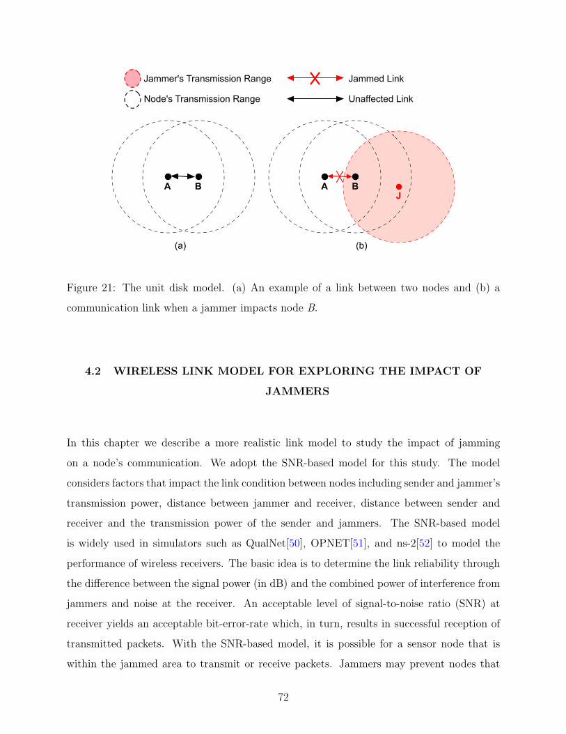
(a) (b)
A BJ
A B
Jammed Link
Unaffected Link
Jammer's Transmission Range
Node's Transmission Range
Figure 21: The unit disk model. (a) An example of a link between two nodes and (b) a
communication link when a jammer impacts node B.
4.2 WIRELESS LINK MODEL FOR EXPLORING THE IMPACT OF
JAMMERS
In this chapter we describe a more realistic link model to study the impact of jamming
on a node’s communication. We adopt the SNR-based model for this study. The model
considers factors that impact the link condition between nodes including sender and jammer’s
transmission power, distance between jammer and receiver, distance between sender and
receiver and the transmission power of the sender and jammers. The SNR-based model
is widely used in simulators such as QualNet[50], OPNET[51], and ns-2[52] to model the
performance of wireless receivers. The basic idea is to determine the link reliability through
the difference between the signal power (in dB) and the combined power of interference from
jammers and noise at the receiver. An acceptable level of signal-to-noise ratio (SNR) at
receiver yields an acceptable bit-error-rate which, in turn, results in successful reception of
transmitted packets. With the SNR-based model, it is possible for a sensor node that is
within the jammed area to transmit or receive packets. Jammers may prevent nodes that
72
perform carrier sensing from transmitting by keeping the channel busy at all times. However,
nodes may choose to by pass MAC and transmit packets such as alarm messages to inform
neighbors the existence of jammers. Nodes may transmit with higher transmission power so
that the message will reach jammed neighbors and propagate to the rest of the network. The
SNR-based model may allow a node that is in jammed area to receive packets from neighbor
nodes if the SNR at the receiver exceeds an acceptable level for successful reception. Next,
we describe the SNR-based link model and our assumptions on transmission and jamming
range.
4.2.1 Model Overview
We define how to decide whether or not there is a wireless link from a sender S to a receiver
R. A receiver R will be able to receive and correctly decode a signal from a sender S if the
signal-to-interference and noise ratio (which we simply call SNR) is higher than a required
level (SNRrequired). Thus, a communication link from S to R exists if
SNR ≥ SNRrequired (4.1)
The SNR is determined by the ratio of the received signal level from the sender PRS over the
total noise (which is the received signal from jammer PRJ and background noise Pnoise).
SNR =PRS
PRJ + Pnoise(4.2)
In the case of multiple jammers, PRJ is the total received signal from all jammers in the area.
To calculate the received power at receiver, we use a log-distance path loss model where the
loss occurs as a function of distance and a path loss exponent (α). Let the distance between
a sender i and a receiver j be Di,j. The path loss (PLi,j) from i to j is computed as:
PLi,j = (Di,j)α (4.3)
We assume that sensor nodes and jammers use omnidirectional antennas. We ignore the
antenna gain at both the sender and receiver’s antenna in our calculations (we assume the
gain is 1). We can calculate the received power from sender S at receiver R as:
PRS = PTS (DS,R)−α (4.4)
73

where PTS is transmission power of node S and DS,R is the distance between node S and
node R (in meters). The received power of the jamming signal at receiver PRJ is computed
as:
PRJ = PTJ (DJ,R)−α (4.5)
where PTJ is the jamming transmit power level and DJ,R is the distance between the jammer
and receiver R.
From Equation 4.2 to 4.5, we can see that the SNR is mainly determined by relationships
between transmission power of sender and jammer, and their distances from the receiver.
If the sender and jammer use the same power level, the SNR mainly depends on DS,R and
DJ,R. The limitations of this model is that we ignore an impact of signal variation caused
by small-scale fading and shadowing.
4.2.2 Assumptions and Model Parameters
We describe the assumptions in the link model that we used to study the impact of jammers.
Our main assumptions are as follows:
• We set the transmission range of a regular node to 40 meters
• We define that jamming range is as twice that of a node’s transmission range
The reasons for these assumptions are provided as follows: We control the transmission range
of a sensor node to be 40 meters. This is the same transmission range we used in previous
chapter. In order to do this, we need to compute the path-loss exponent that matches with
our assumption on a node’s transmission range. A sensor node has the default transmission
power = −20 dBm. The default receiver sensitivity is −80 dBm. Using the log-distance
path loss equations, we can compute the path-loss exponent (α) as 3.74.
We define the jamming range to be twice that of a node’s transmission range if both of
them transmit using the same power level. Nodes that are within the jamming range may
be impacted by the jamming signal. Note that this also depends on DS,R and DJ,R. Our
assumption follows the interference model presented in literature [53]. In the interference
model, two nodes can communicate successfully if no other nodes, located within the inter-
ference range of the receiver node, is transmitting at the same time. Usually the interference
74

range IR is greater than the transmission range TR (IR = ηTR with η > 1). A typical value
for IEEE 802.11 networks is η = 2 [54], which means the interference range is twice the trans-
mission range of a node (given that regular node and interference source are transmitting at
the same power level). For example, if two nodes are 40 meters apart, a jammer can disrupt
a communication between two nodes if it is within 80 meters from the receiving node. This
link will not be disrupted if a jammer is more than 80 meters away from the receiving node.
If the distance between node S and node R is closer than 40 meters, a jammer has to be
closer than 80 meters in order to impact the receiving node.
To satisfy the second assumption, we computed the required SNR level, which is the
SNR level where distance between jammer and received node is twice the distance between
the sending and receiving nodes.
DJ,R = 2×DS,R (4.6)
Using equation 4.6, we can calculate the required SNR from equations 4.2 to 4.5. We assume
that the noise from jammers is much larger than the background noise. Thus the background
noise can be neglected.
SNRrequired = path loss(DJ,R)− path loss(DS,R) (4.7)
= 10α · log10(DJ,R)− 10α · log10(DS,R) (4.8)
= 10α · log10(2×DS,R)− 10α · log10(DS,R) (4.9)
= 11.2742 dB (4.10)
Figure 22 shows different SNR values with combinations of distance between a jammer and
receiving node (DJ,R). The plot also shows changes in SNR values with different distances
between sender and receiver (DS,R) and a comparison of the SNR level and the required SNR
level from our calculations. The plot in Figure 22 follows our assumption. The SNR level
is above the required level for successful reception when DJ,R ≥ 2 ×DS,R (indicated that a
75
node is not jammed). The SNR level falls below SNRrequired when DJ,R < DS,R (indicates
that a node is jammed). In the plot, any point above the required SNR line indicates the
cases where the SNR is above a required value, thus it is not impacted by a jamming signal.
We illustrate the plot in Figure 22 by an example. Let a sender S and a jammer J
transmit with the same power level and let node S and a receiver R be 40 meters apart
(DS,R = 40 m). With our assumptions, this is the maximum transmission range.
• If node J is 90 meters from node R, then the link is not jammed since DJ,R > 2×DS,R.
The SNR exceeds the required value. This is the point A in Figure 22.
• If node J is 80 meters from node R, then the link is not jammed since DJ,R = 2×DS,R.
The SNR equals the required value. This is the point B in Figure 22.
• If node J is 70 meters from node R, then the link is jammed since DJ,R < 2×DS,R. The
SNR level is below the required value. This is the point C in Figure 22.
To overcome the impact of the jammer J , node S and R may choose to move closer.
If distance between two nodes decreases to 30 meters, the link will not be jammed since
the SNR is increased to above the required value (as shown in the point D in Figure 22).
Alternatively, node S can increase its transmission power in order to improve the SNR at the
receiver for successful reception. We will use this model to explore the impact of jamming
on secure connectivity through key predistribution and the impact of using different coping
techniques to overcome jamming attacks.
Issues on Impacted Node: With the unit disk model it is easy to determine which node
is jammed and which node is not. The unit disk model in Chapter 3 uses the simplified
assumption that if a node is located within one of the jammer’s jammed circle, it will
completely lose its communication functionalities. A jammed node A will not be able to
transmit to and receive from all of its neighbors regardless of DJ,R and DS,R.
With the SNR-based link model, it is not easy to completely distinguish between jammed
and non-jammed nodes simply by looking at DJ,R as in the disk model. Thus, we define
a node that is located within the maximum jamming range of a jammer as an impacted
node. We define the maximum jamming range as the jamming range at the maximum node
transmission range. In this case, the maximum transmission range is 40 meters; therefore the
76
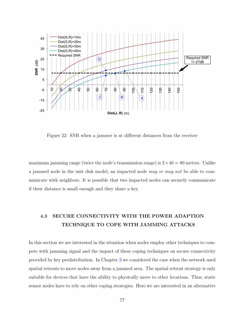
-25
-15
-5
5
15
25
35
45
10
20
30
40
50
60
70
80
90
100
110
120
130
140
150
SN
R
Dist(J, R)
Dist(S,R)=10m Dist(S,R)=20m Dist(S,R)=30m Dist(S,R)=40m Required SNR
(m)
(dB)
Required SNR11.27dB
B AC
D
Figure 22: SNR when a jammer is at different distances from the receiver
maximum jamming range (twice the node’s transmission range) is 2×40 = 80 meters. Unlike
a jammed node in the unit disk model, an impacted node may or may not be able to com-
municate with neighbors. It is possible that two impacted nodes can securely communicate
if their distance is small enough and they share a key.
4.3 SECURE CONNECTIVITY WITH THE POWER ADAPTION
TECHNIQUE TO COPE WITH JAMMING ATTACKS
In this section we are interested in the situation when nodes employ other techniques to com-
pete with jamming signal and the impact of these coping techniques on secure connectivity
provided by key predistribution. In Chapter 3 we considered the case when the network used
spatial retreats to move nodes away from a jammed area. The spatial retreat strategy is only
suitable for devices that have the ability to physically move to other locations. Thus, static
sensor nodes have to rely on other coping strategies. Here we are interested in an alternative
77
solutions to fight with jamming – rather than moving away from jammers, nodes attempt to
compete with the jamming signal. Upon detecting the presence of a jamming attack, nodes
respond to jammers by increasing their transmission power levels. The goal is to overcome
the jamming signal and improve the signal to noise ratio at the receiver for successful packet
receptions.
We use the SNR-based link model that determines the link condition by using the SNR
level at the receiver to study the overall secure connectivity of the network under jamming
attacks and after nodes increased their transmission power. We are interested in following
questions: Will increasing transmission power help the network to overcome the impact of
jamming? The second question that we are interested is: What will happen to secure con-
nectivity provided by key predistribution when nodes transmit with higher power levels and
the performance of the hybrid key predistribution scheme with higher node’s transmission
power levels.
We begin by discussing the impact of using higher transmission power on secure links
initially provided by key predistribution. We explain our strategies to adjust a node’s trans-
mission power. Then we describe the performance metrics used to evaluate secure connec-
tivity before and after jamming. We perform computer-based simulations to evaluate secure
connectivity provided by various key distribution schemes after jamming and after nodes
increase their transmission power to cope with jamming.
4.3.1 Impact of Increasing Transmission Power on Secure Connectivity
To answer the first question:“Will increasing transmission power help the network to over-
come the impact of jamming?”, we examine the SNR calculation in our model. We can
clearly see that if we increase transmission power PTS (while other factors remain the same),
the SNR level can be improved and a node may reach the required SNR level for correct
packet reception. Transmitting with high power may consume a node’s energy which results
in a shorter battery life, but nodes may choose to do so in order to deliver critical information
to the sink node or their cluster heads.
The next question we are interested in what will happen to secure links (created through
78

key predistribution) when jammers have launched the attacks and after nodes tune up trans-
mission power to compete with the jamming signal. Higher transmission power improves the
SNR level at receiver of original neighbors (share-key neighbor nodes that connected before
jamming), thus it helps node to regain secure links that lost due to jammers. Additionally,
higher transmission power also increases the transmission range of nodes. This longer link
can help nodes reach new nodes that were unreachable with the original transmission power
level. An illustration of a node’s reachability with different levels of transmission powers is
show in Figure 23. The issue we like to explore here is will a node be able to establish secure
links with these new neighbors (reachable at higher transmission power). In other words,
from a set of new neighbors, what will be the number of neighbors that a node shares keys
with. We would like to know which key predistribution scheme can create the most number
of secure links with new and old neighbors. We perform a set of simulations to answer these
questions and present our results in next section. One benefit of longer secure links is that
it helps nodes reach the sink in fewer numbers of hops (reduce computation cost due to
encryption at each hop).
4.3.2 Power Adaptation Strategy
We use simple a strategy for power adaption: upon detecting the presence of a jamming
attack, every node will adjust its transmission power to higher levels. This strategy is
enough to demonstrate impact of using higher power on secure links. One benefit of having
all nodes adjust their transmission powers is that this can reduce the creation of asymmetric
links. However, it is still possible that asymmetric links are created with higher transmit
powers with nodes that are very close to a jammer’s location. Alternatively, we can have
only the impacted node that loses some links due to jamming increase its power in order to
regain connection with its original neighbors, but determining an optimal strategy for power
adaption is out of scope of this dissertation.
79
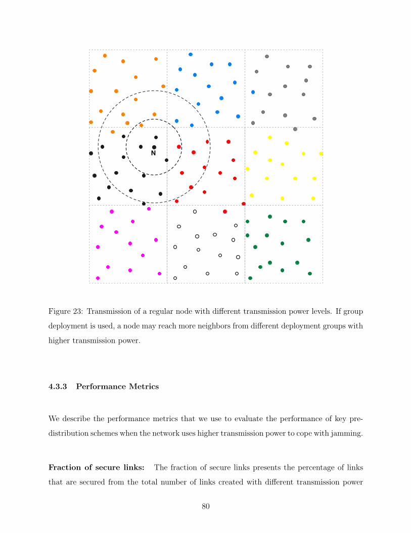
N
Figure 23: Transmission of a regular node with different transmission power levels. If group
deployment is used, a node may reach more neighbors from different deployment groups with
higher transmission power.
4.3.3 Performance Metrics
We describe the performance metrics that we use to evaluate the performance of key pre-
distribution schemes when the network uses higher transmission power to cope with jamming.
Fraction of secure links: The fraction of secure links presents the percentage of links
that are secured from the total number of links created with different transmission power
80

levels. The fraction of secure links is defined as:
Fraction of Secure Links =total number of secure links
total number of links× 100. (4.11)
A link from node A to node B exists if the signal from node A can be received at node B
with adequate SNR level. If node A and node B have a common key, then the link from
node A to node B is a secure link. The link between node A and node B is symmetric
(bidirectional) if there exists a link from node A to node B, and vice versa.
Global connectivity of secure links: We use the global connectivity of secure links
to measure multi hop connectivity between sensor nodes. The global connectivity of secure
links is defined as the number of nodes that are able to find a multi hop path between the
node and a sink node. It is important to look at number of hops for each multi hop paths.
We also measure the average number of hops from each node (that is able to find a path) to
the sink node. The number of hops is measured only nodes that are able to create at least
one multi hop secure path to the sink.
4.3.4 Results and Discussion
4.3.4.1 Simulation Setup We evaluate performance of previous key predistribution
schemes under jamming attacks and after nodes increase transmission power to cope with
jamming. We deployed 2,500 nodes in a 500 m × 500 m sensor field. The wireless link
between two nodes follows the SNR-based link model described in the previous sections.
The default transmission power of a sensor node is -20 dBm. The default receiver sensitivity
is -80 dBm. With this setting, the default transmission range of a sensor node is 40 meters.
The EG, EGD, and hybrid key predistribution schemes are evaluated with a group of sensor
nodes that perform power adaptation strategy to cope with jamming.
In this study we perform simulations with smaller number of sensor nodes on a smaller
sensor field. The benefit is the faster simulation runs. In Chapter 3 we deployed 10,000
sensor nodes. A sensor field of size 1,000 m × 1,000 m is divided into equal sized groups
arranged in a grid of size 10 × 10. Thus, there is on average 100 nodes per a deployment
81
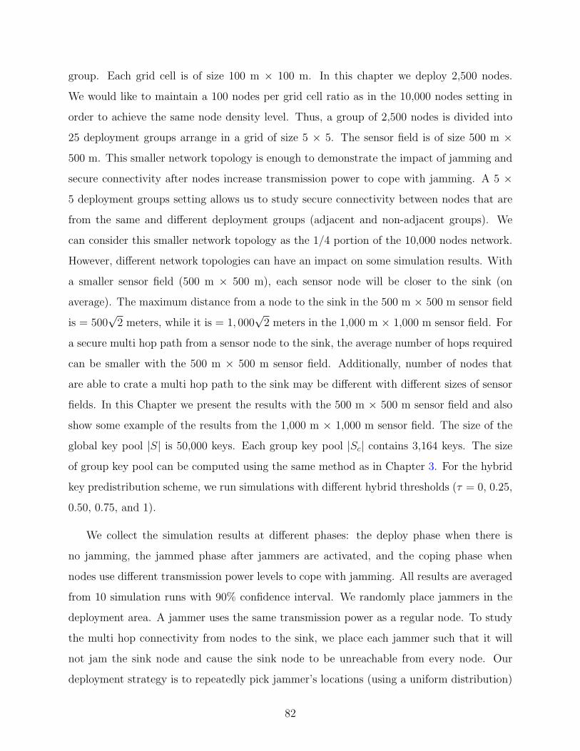
group. Each grid cell is of size 100 m × 100 m. In this chapter we deploy 2,500 nodes.
We would like to maintain a 100 nodes per grid cell ratio as in the 10,000 nodes setting in
order to achieve the same node density level. Thus, a group of 2,500 nodes is divided into
25 deployment groups arrange in a grid of size 5 × 5. The sensor field is of size 500 m ×500 m. This smaller network topology is enough to demonstrate the impact of jamming and
secure connectivity after nodes increase transmission power to cope with jamming. A 5 ×5 deployment groups setting allows us to study secure connectivity between nodes that are
from the same and different deployment groups (adjacent and non-adjacent groups). We
can consider this smaller network topology as the 1/4 portion of the 10,000 nodes network.
However, different network topologies can have an impact on some simulation results. With
a smaller sensor field (500 m × 500 m), each sensor node will be closer to the sink (on
average). The maximum distance from a node to the sink in the 500 m × 500 m sensor field
is = 500√
2 meters, while it is = 1, 000√
2 meters in the 1,000 m × 1,000 m sensor field. For
a secure multi hop path from a sensor node to the sink, the average number of hops required
can be smaller with the 500 m × 500 m sensor field. Additionally, number of nodes that
are able to crate a multi hop path to the sink may be different with different sizes of sensor
fields. In this Chapter we present the results with the 500 m × 500 m sensor field and also
show some example of the results from the 1,000 m × 1,000 m sensor field. The size of the
global key pool |S| is 50,000 keys. Each group key pool |Sc| contains 3,164 keys. The size
of group key pool can be computed using the same method as in Chapter 3. For the hybrid
key predistribution scheme, we run simulations with different hybrid thresholds (τ = 0, 0.25,
0.50, 0.75, and 1).
We collect the simulation results at different phases: the deploy phase when there is
no jamming, the jammed phase after jammers are activated, and the coping phase when
nodes use different transmission power levels to cope with jamming. All results are averaged
from 10 simulation runs with 90% confidence interval. We randomly place jammers in the
deployment area. A jammer uses the same transmission power as a regular node. To study
the multi hop connectivity from nodes to the sink, we place each jammer such that it will
not jam the sink node and cause the sink node to be unreachable from every node. Our
deployment strategy is to repeatedly pick jammer’s locations (using a uniform distribution)
82

until all jammers are not placed near sink node.
4.3.4.2 Impact on Secure Links with Power Adaptation Strategy In this section
we look at the impact on secure links when nodes increase their transmission power to
overcome the impact of jamming. First, we look at number of links in the network before
and after jamming. A link from node A to node B exists if the received signal (from node
A) at node B’s receiver has the SNR level exceed a required level. To study the impact of
jammers on secure links we randomly deploy 20 jammers to the sensor field. We measure
the total number of links for the network when nodes transmit at different power level. The
result is shown in Figure 24a. The first data point (deploy phase) indicates the case when
there is no jamming (Node transmits at the default transmission power level). The second
data point presents the jammed phase where jammers are active. The rest shows the cases
where nodes respond to jamming with different transmission power levels. The total number
of links after jammers are active is reduced more than 50%. This shows that jammers can
disable around half of the communication links. The total number of links increase when
nodes increase the transmission power. With -10 dBm transmission power, the total number
of links already exceeds the total number of links at deploy phase. The increase in number
of links is because of two reasons: 1) the higher transmission power overcomes transmission
power from jammers and improves the SNR level at receiver to an adequate level, and 2)
the higher transmission power results in the higher transmission range which allows nodes
to reach more neighbors (usually unreachable by the default transmission power level). At
0 dBm transmission power, the total number of links is 5 times more than the total number
of links at the deploy phase.
Next, we look at number of secure links before and after jamming. We reiterate that
a secure link from node A to node B exists if there exists a link from node A to node
B and both nodes have a common key. The results is show in Figure 24b. The trend
is the same as the result in the total number of links. Number of secure links decreases
after jammers are active and increases when nodes transmit with higher transmission power
level. Different key predistribution schemes result in different total number of secure links.
The EGD key predistribution scheme has the highest number of secure links while the EG
83

key predistribution results in the lowest number of secure links. This is because the EGD
scheme has a higher probability of key sharing with close neighbor nodes especially if they
are from the same deployment group. The higher transmission power helps nodes reach more
neighbors in the same deployment group. The EG scheme has the lowest increase in secure
links since the probability of key sharing is the same (whether nods are close neighbors or
far from each others). The number of secure links with the hybrid scheme is in between the
EG and the EGD scheme depended on the value of hybrid threshold. With τ = 0.25, the
number of secure links is close to that with the EGD scheme. It is important to study the
relationship between the total number of links and the total number of secure links. We
study this by looking at the fraction of secure links (defined in previous section). The result
is presented in Figure 25. We can see that changes in fraction of secure links act differently
and this depends on the key predistribution scheme. The fraction of secure links with the
EG scheme remains the same with different transmission power levels. The fraction of secure
links for the EGD scheme decreases as the transmission power increases. This is the same
for the hybrid scheme with τ = 0.25, and 0.50. The decrease in fraction of secure links in the
EGD scheme is because nodes are unable to find shared keys to establish secure links with
new neighbors (reachable with higher transmission power level). These new neighbors may
come from the non-adjacent deployment groups (which usually have no share key). This is
the same for the hybrid scheme (with τ = 0.25, and 0.50) as more than half of keys stored in
node’s memory is picked from the group key pool (associated with node’s deployment group).
The EG scheme has a stable fraction of secure links since every node picks keys from the same
key pool (the global key pool). However, this fraction is low compared to other schemes.
Note that the fraction of secure links is close to the local connectivity. The fraction of secure
links is the fraction of the total number of secure links over the total number of links while
the local connectivity presents average fraction of neighbors with whom at least one key is
shared.
To study whether nodes are able to securely communicate with neighbors even they
are within jamming range, we measure the percentage of impacted nodes that are able to
establish at least one secure link with their neighbors. The impacted node is defined as a node
that is located within at least one jammer’s range (The jamming range is twice of the node’s
84
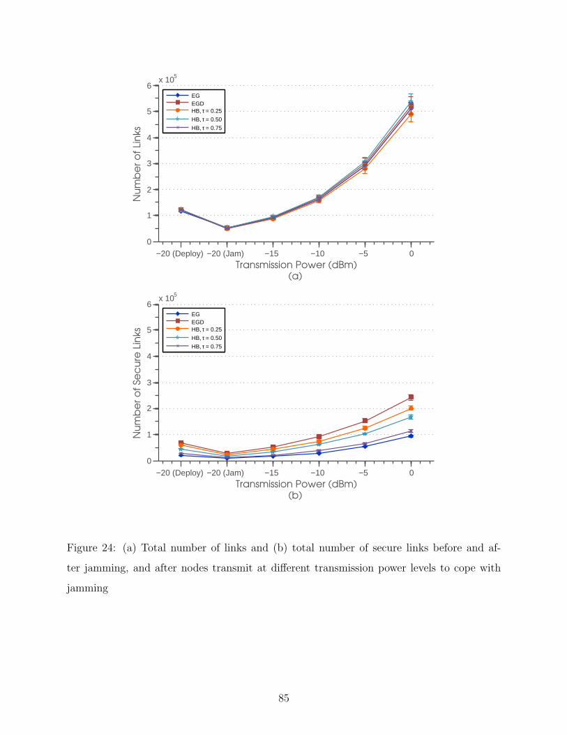
−20 (Deploy) −20 (Jam) −15 −10 −5 00
1
2
3
4
5
6x 10⁵
Transmission Power (dBm)
(a)
Nu
mb
er
of
Lin
ks
EGEGDHB, τ = 0.25
HB, τ = 0.50
HB, τ = 0.75
−20 (Deploy) −20 (Jam) −15 −10 −5 00
1
2
3
4
5
6x 10⁵
Transmission Power (dBm)
(b)
Nu
mb
er
of
Se
cu
re L
inks
EGEGDHB, τ = 0.25
HB, τ = 0.50
HB, τ = 0.75
Figure 24: (a) Total number of links and (b) total number of secure links before and af-
ter jamming, and after nodes transmit at different transmission power levels to cope with
jamming
85
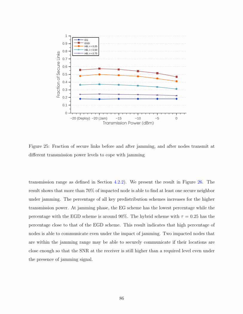
−20 (Deploy) −20 (Jam) −15 −10 −5 0
0
0.1
0.2
0.3
0.4
0.5
0.6
0.7
0.8
0.9
1
Transmission Power (dBm)
Fra
ctio
n o
f Se
cu
re L
inks
EGEGDHB, τ = 0.25
HB, τ = 0.50
HB, τ = 0.75
Figure 25: Fraction of secure links before and after jamming, and after nodes transmit at
different transmission power levels to cope with jamming
transmission range as defined in Section 4.2.2). We present the result in Figure 26. The
result shows that more than 70% of impacted node is able to find at least one secure neighbor
under jamming. The percentage of all key predistribution schemes increases for the higher
transmission power. At jamming phase, the EG scheme has the lowest percentage while the
percentage with the EGD scheme is around 90%. The hybrid scheme with τ = 0.25 has the
percentage close to that of the EGD scheme. This result indicates that high percentage of
nodes is able to communicate even under the impact of jamming. Two impacted nodes that
are within the jamming range may be able to securely communicate if their locations are
close enough so that the SNR at the receiver is still higher than a required level even under
the presence of jamming signal.
86
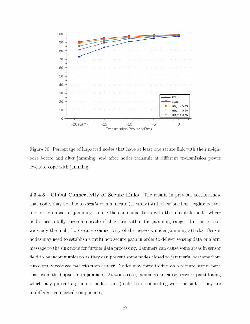
−20 (Jam) −15 −10 −5 0
0
10
20
30
40
50
60
70
80
90
100
Transmission Power (dBm)
EG
EGD
HB, τ = 0.25HB, τ = 0.50
HB, τ = 0.75
Figure 26: Percentage of impacted nodes that have at least one secure link with their neigh-
bors before and after jamming, and after nodes transmit at different transmission power
levels to cope with jamming
4.3.4.3 Global Connectivity of Secure Links The results in previous section show
that nodes may be able to locally communicate (securely) with their one hop neighbors even
under the impact of jamming, unlike the communications with the unit disk model where
nodes are totally incommunicado if they are within the jamming range. In this section
we study the multi hop secure connectivity of the network under jamming attacks. Sensor
nodes may need to establish a multi hop secure path in order to deliver sensing data or alarm
message to the sink node for further data processing. Jammers can cause some areas in sensor
field to be incommunicado as they can prevent some nodes closed to jammer’s locations from
successfully received packets from sender. Nodes may force to find an alternate secure path
that avoid the impact from jammers. At worse case, jammers can cause network partitioning
which may prevent a group of nodes from (multi hop) connecting with the sink if they are
in different connected components.
87
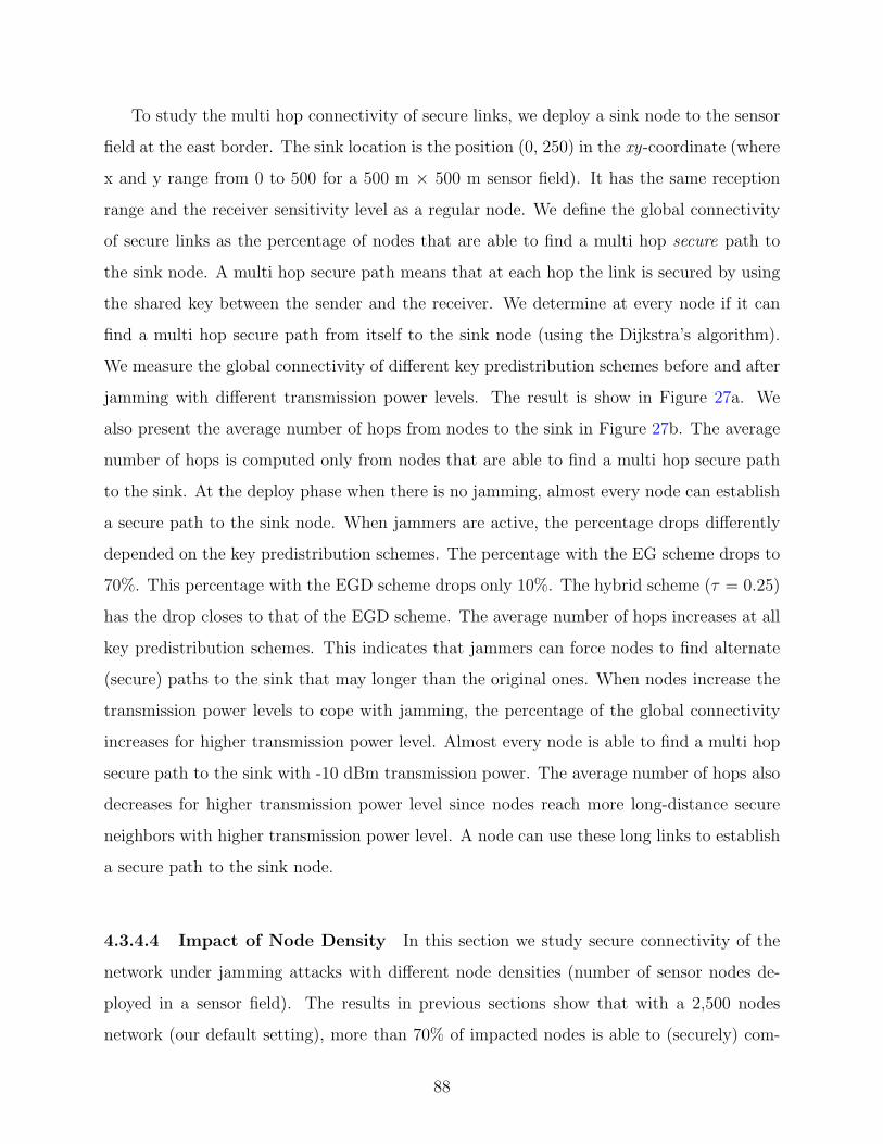
To study the multi hop connectivity of secure links, we deploy a sink node to the sensor
field at the east border. The sink location is the position (0, 250) in the xy-coordinate (where
x and y range from 0 to 500 for a 500 m × 500 m sensor field). It has the same reception
range and the receiver sensitivity level as a regular node. We define the global connectivity
of secure links as the percentage of nodes that are able to find a multi hop secure path to
the sink node. A multi hop secure path means that at each hop the link is secured by using
the shared key between the sender and the receiver. We determine at every node if it can
find a multi hop secure path from itself to the sink node (using the Dijkstra’s algorithm).
We measure the global connectivity of different key predistribution schemes before and after
jamming with different transmission power levels. The result is show in Figure 27a. We
also present the average number of hops from nodes to the sink in Figure 27b. The average
number of hops is computed only from nodes that are able to find a multi hop secure path
to the sink. At the deploy phase when there is no jamming, almost every node can establish
a secure path to the sink node. When jammers are active, the percentage drops differently
depended on the key predistribution schemes. The percentage with the EG scheme drops to
70%. This percentage with the EGD scheme drops only 10%. The hybrid scheme (τ = 0.25)
has the drop closes to that of the EGD scheme. The average number of hops increases at all
key predistribution schemes. This indicates that jammers can force nodes to find alternate
(secure) paths to the sink that may longer than the original ones. When nodes increase the
transmission power levels to cope with jamming, the percentage of the global connectivity
increases for higher transmission power level. Almost every node is able to find a multi hop
secure path to the sink with -10 dBm transmission power. The average number of hops also
decreases for higher transmission power level since nodes reach more long-distance secure
neighbors with higher transmission power level. A node can use these long links to establish
a secure path to the sink node.
4.3.4.4 Impact of Node Density In this section we study secure connectivity of the
network under jamming attacks with different node densities (number of sensor nodes de-
ployed in a sensor field). The results in previous sections show that with a 2,500 nodes
network (our default setting), more than 70% of impacted nodes is able to (securely) com-
88
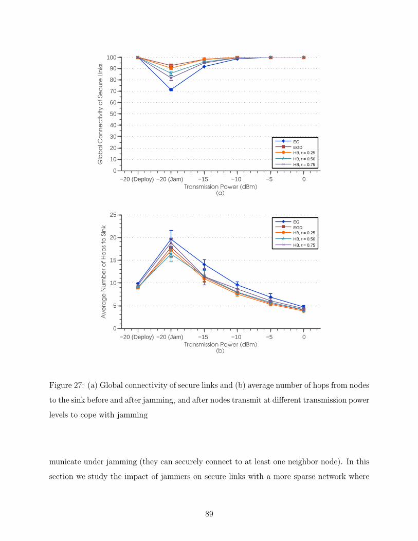
−20 (Deploy) −20 (Jam) −15 −10 −5 00
10
20
30
40
50
60
70
80
90
100
Transmission Power (dBm)(a)
Glo
ba
l Co
nn
ec
tivity o
f Se
cu
re L
inks
EGEGDHB, τ = 0.25
HB, τ = 0.50HB, τ = 0.75
−20 (Deploy) −20 (Jam) −15 −10 −5 00
5
10
15
20
25
Transmission Power (dBm)(b)
Ave
rag
e N
um
be
r o
f H
op
s to
Sin
k
EGEGDHB, τ = 0.25
HB, τ = 0.50
HB, τ = 0.75
Figure 27: (a) Global connectivity of secure links and (b) average number of hops from nodes
to the sink before and after jamming, and after nodes transmit at different transmission power
levels to cope with jamming
municate under jamming (they can securely connect to at least one neighbor node). In this
section we study the impact of jammers on secure links with a more sparse network where
89
−20 (Jam) −15 −10 −5 0
0
10
20
30
40
50
60
70
80
90
100
Transmission Power (dBm)
EG
EGD
HB, τ = 0.25HB, τ = 0.50
HB, τ = 0.75
Figure 28: Percentage of impacted nodes that have at least one secure link with their neigh-
bors before and after jamming, and after nodes transmit at different transmission power
levels to cope with jamming of a 1,500 nodes network
number of nodes is smaller than the number used in previous sections. We ran simulations
with a 1,500 nodes network. Other parameters are the same. First, we measure number
of impacted that can securely connect to neighbors under jamming. We show the result in
Figure 28. When jammers are active, the percentage with all key predistribution schemes
drops more than the case with a 2,500 nodes network (Figure 26). With the EG scheme, the
percentage with a 1,500 nodes network drops to around 60% while it is around 70% with a
2,500 nodes network. This shows that a more sparse network is more impacted by jammers
since the number of neighbors (and number of neighbors that share key) is on average smaller
than a dense network. The percentage with all key predistribution schemes increases as the
transmission power level increases.
Next, we study the global connectivity of secure links with a 1,500 nodes network. We
compare results from different node densities with the EG, the EGD, and the hybrid (τ =
90

0.25) key predistribution schemes (Figure 29a). At the jammed phase, the global connectivity
drops more with a 1,500 nodes network for all key predistribution schemes. With the EG
scheme, the drop in the global connectivity is more than 50%. The drops with the EG
and the hybrid schemes is around 10% which indicates that the EGD and the hybrid are
more robust to the changes in the node density. The percentage with all key predistribution
schemes increases as the transmission power level increases. The average number of hops to
the sink with different node densities is show in Figure 29b. We can see that the average
number of hops with a 1,500 nodes network for all key predistribution schemes is higher than
that of the 2,500 nodes network. With a sparse network, a node may have to travel in a
longer hop count in order to reach the sink since number of surrounded secure neighbors is
smaller than that of the dense network. It is interesting to see that at the jammed phase,
an average number of hops with the EG scheme (for a 1,500 nodes network) is the lowest
around 15 hops (and become the highest when nodes increase the transmission power level).
This is because this average number of hops is calculated from only small number of nodes.
We can see from the Figure 29a that there is only 20% (around 300 nodes) of nodes that
are able to find a multi hop path to the sink with the EG scheme at the jammed phase.
Some of these nodes are the nodes that locate near the sink. Therefore, nodes can find multi
hop paths to the sink with small number of hops. The average number of hops increases
when nodes use higher transmission power leve. This is because the average is computed
from more number of nodes (around 1,225 nodes). Another reason is jammers can cause
a network to be partitioned. A large portion of nodes that is not in the same connected
component as the sink node will not be able to find a multi hop secure path to the sink.
4.3.4.5 Summary Increasing transmission power level helps nodes to overcome impacts
of jamming. The total number of secure links at all key predistribution schemes increases for
higher transmission power levels. The fraction of secure links (with the EGD and the hybrid
key predistribution schemes) decreases for the higher transmission power levels indicates that
using transmission power that is too high does not help nodes create more secure links since
long-distance neighbors may come from the non-adjacent deployment groups (which usually
have no share key). With the EG scheme, the fraction of secure links is stable for higher
91
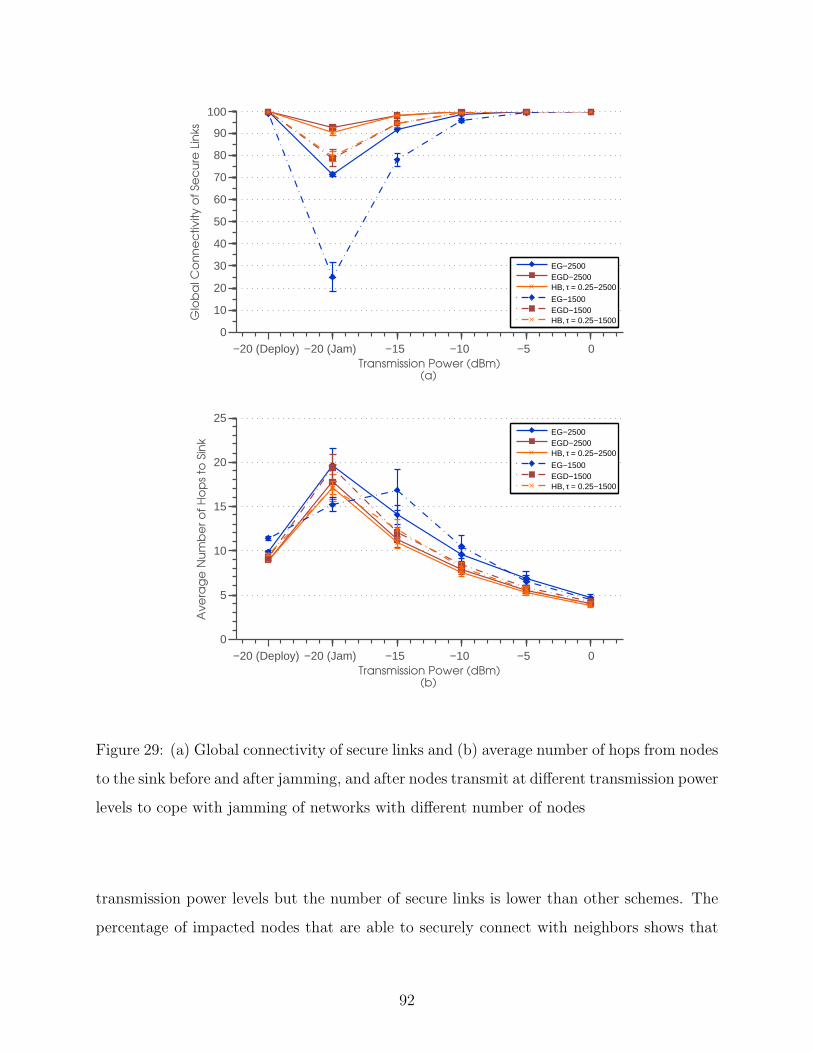
−20 (Deploy) −20 (Jam) −15 −10 −5 00
10
20
30
40
50
60
70
80
90
100
Transmission Power (dBm)(a)
Glo
ba
l Co
nn
ec
tivity o
f Se
cu
re L
inks
EG−2500EGD−2500HB, τ = 0.25−2500
EG−1500EGD−1500HB, τ = 0.25−1500
−20 (Deploy) −20 (Jam) −15 −10 −5 00
5
10
15
20
25
Transmission Power (dBm)(b)
Ave
rag
e N
um
be
r o
f H
op
s to
Sin
k
EG−2500EGD−2500HB, τ = 0.25−2500
EG−1500EGD−1500HB, τ = 0.25−1500
Figure 29: (a) Global connectivity of secure links and (b) average number of hops from nodes
to the sink before and after jamming, and after nodes transmit at different transmission power
levels to cope with jamming of networks with different number of nodes
transmission power levels but the number of secure links is lower than other schemes. The
percentage of impacted nodes that are able to securely connect with neighbors shows that
92
it is possible for nodes to communicate (locally with one hop neighbors) under jamming.
The global connectivity shows that, with all key predistribution schemes, more than 70% of
nodes is able to find a multi hop secure path to the sink node. This percentage increases for
higher transmission power levels. Jammers can force nodes to travel at longer hops to the
sink but increasing transmission power allows nodes to select long-distance secure neighbors
to reach the sink by fewer number of hops. The EGD scheme has the best performance
with the power adaptation strategy. The performance of the hybrid scheme with τ = 0.25
is very close to that with the EGD scheme. Thus, it is desirable to use low value of τ for a
network that increases transmission power to cope with jamming. Different node densities
also impacts secure connectivity of sensor nodes (under jamming and after nodes increase
transmission power). The higher node density results in more robustness to jamming attacks.
4.4 SECURE CONNECTIVITY WITH DIRECTIONAL ANTENNAS TO
COPE WITH JAMMING ATTACKS
4.4.1 Introduction
In this chapter we explore techniques that employ beamforming antennas to alleviate the
impact of jamming attacks. We study the impact of directional transmission on secure con-
nectivity provided by key predistribution. An interesting phenomena here is that switching
from omni-directional to directional transmission mode not only helps nodes overcome the
impact of jamming but also causes changes in the network topology of secure links before
and after jamming. We evaluate the performance of different key predistribution schemes
before and after jamming.
Wireless communication relies on antennas at each end of the links. The antennas couple
energy from one end through the air and allow another end to capture the transmitting
electromagnetic power. An omnidirectional antenna ideally radiates energy equally in all
directions. A directional antenna offers more control over radiation as it allows energy to
radiate only in preferred directions.
93
There has been a growing interest in using directional antennas to improve connectivity
and reduce interference among wireless ad hoc and sensor devices. As operating frequencies
move to higher bands, the size of the antenna becomes smaller, which makes it possible to
equip them in small wireless ad hoc devices. With higher operating frequency band, the size
of directional antennas can be made small enough to equip in handheld devices or sensors
since the size of the antenna is related to the wavelength. Many such antennas are now
practical. For example, Antenova products [55] provide 5 and 16-sectored antennas of small
dimensions (5cm × 15cm).
A directional antenna offers a number of advantages over the omnidirectional antenna.
The work in [56] shows that beamforming antennas can improve throughput and reduce
end-to-end delay among ad hoc nodes. Directional transmissions can reduce the network in-
terference since they do not beam in unnecessary directions. Routing protocols incorporated
with directional antennas can improve the routing performance over routing with omnidi-
rectional antennas [57]. Beamforming transmissions offer directional gain, which results in
higher signal quality (better SNR at receiver) toward the intended direction. Providing
directional stronger signals make directional antenna a potential solution for coping with
jamming. Noubir [42] shows that using sectored antennas can maintain connectivity among
nodes in the presence of jammers.
For a network that forms secure links initially through key predistribution, switching
from omnidirectional transmission mode to directional transmission mode can cause changes
in the network topology before and after jamming. With the signal concentrated in one
direction, a node may lose connections with some initial neighbors (reachable by omnidi-
rectional transmission) that are not located in the beam’s direction. However, a node can
reach more neighbors (usually unreachable by omnidirectional transmission) located in the
direction of beamforming. Different key predistribution schemes may have different levels
of robustness against change in network topology. In what follows, we are interested in ex-
ploring the performance of different key predistribution schemes before and after a network
switches to directional transmission mode in response to jamming. Our main objectives in
this study are: 1) Study secure connectivity of network before and after nodes perform direc-
tional transmissions to cope with jamming attacks and 2) Evaluate performance of various
94

key predistribution schemes with directional beamforming.
We first describe the antenna model that we used in this study. We give a discussion on
secure network topology before and after directional transmission. We explain the perfor-
mance metrics that we used to evaluate the performance of key predistribution schemes with
directional antennas. We present simulation results and end the chapter with conclusions.
4.4.2 Directional Antenna Model and Assumptions
In this section, we present general concepts related to beamforming antennas. We describe
the directional antenna model that we used in this study and explain our assumptions related
to the wireless link model using directional transmissions.
4.4.2.1 Directional Antenna Model We present a directional antenna radiation pat-
tern in Figure 31. The antenna pattern indicates the area that transmission achieves a
directional gain. The pattern is defined by the antenna’s beam direction φb and beamwidth
θw. An antenna’s beam direction φb (0 ≤ φb < 2π) is defined as the angle measured counter-
clockwise from the x-axis to the antenna boresight. The antenna’s beamwidth generally
refers to the angle subtended by the two directions on either side of the direction of peak
gain that are 3 dB down in gain [56]. The antenna beamwidth is usually described as the
angle centered at the beam direction [φb − θw2, φb + θw
2]. Note that the pattern of antenna’s
main lobe is ideal as the actual pattern does not have a constant gain along the beamwidth
[46]. This ideal pattern is used to keep simulations tractable and for the purpose of obtaining
insights, this is reasonable. This model has also been used elsewhere ([56], [57], and [42]).
4.4.2.2 Antenna Gain The gain of the antenna is used to quantify the antenna’s direc-
tionality. The gain of the antenna is defined as the power density in a particular direction
~d = (θ, φ) over the power density in all directions [58]
G(~d) = ηU(~d)
Uave(4.12)
where U(~d) is the power density (having units of W/(rad)2)) in the direction ~d and Uave is the
power density over all directions. Note that this is the relative power in one direction over
95

beam direction
θw
φb
Figure 30: Directional antenna model
an omnidirectional antenna. We can say that a higher directional antenna results in higher
gain. The parameter η is the efficiency of the antenna. In this dissertation we consider a
lossless antenna where η = 1. The gain is usually measured in unitless decibels (dBi), where
GdBi = 10 · log10(Gabs). An omnidirectional has gain = 0 dBi.
We describe how we compute the antenna gain for our link model. We use a constant
gain pattern where an antenna in direction φb has a constant value in all directions over the
beam of width θw
G(θ) =
const for φb − θw2≤ θ < φb + θw
2
0 otherwise
(4.13)
All receivers located within the main lobe of a transmitter will receive the same gain value.
Gain and beamwidth are related. The more directional an antenna is the smaller is the
beamwidth, which yields a higher gain. To compute antenna gain for a given beamwidth,
we adopt the method from [56] for directional gain approximation. We assume that the
side lobe of an antenna is very small compared to the main lobe and is neglected. Thus, a
96

Table 1: Antenna pattern with different gain and beamwidth
Beamwidth θw Gain G
(deg) (dBi)
120 1.2
90 6
60 10.8
30 17.5
directional link is only considered at the antenna’s main lobe. An example of our antenna
pattern is shown in Figure 31.
First we describe the method to derive the approximate maximum beamwidth θmax for a
given gain G. Let P be the transmit power, S be the surface area of sphere of radius r, and
A be the surface area on a sphere for a beamwidth θw. The area A can be approximated as
a circle of radius r tan( θmax2
). From the definition of gain in Equation 4.12, we can write
G =P/A
P/S=
4πr2
π · (r2 · tan2(θmax/2))(4.14)
From the above Equation, we can solve G for a given θmax. Using this equation, we can
generate different antenna patterns with different beamwidth and gain as show in Table 1.
4.4.2.3 Link Model with Directional Antenna In this section we define how we de-
cide if there is a wireless link between a pair of nodes when a sending node uses a directional
antenna. We define that a sender transmits with power PTS . The directional gain of trans-
mitter’s antenna in the direction toward the receiver is G. We assume the gain of receiver’s
antenna is 0 dB (omnidirectional). The received power PRS from transmitter S at receiver
R can be computed by
PRS = PTS ·G · (DS,R)−α (4.15)
97

Table 2: Transmission ranges with different antenna patterns
Beamwidth θw Gain G Transmission Range
(deg) (dBi) (meters)
360 0 40
120 1.2 43
90 6 57.84
60 10.8 77.70
30 17.5 117.31
where DS,R is the distance between two nodes and α is the path loss exponent. The SNR is
defined as in Equation 4.2. If the SNR is larger than or equal to a required SNR threshold,
the transmitted signal is received properly. The higher the gain, the more improvement in
received signal strength at the receiver. The higher gain also means higher transmission
range in the direction of the main lobe. For example, with a transmission power of -20
dBm, the transmission range for omnidirectional antennas (beamwidth = 360 degrees) is 40
meters. With the same power level, the transmission range for beamwidth = 60 degrees is
around 77 meters. Table 2 shows the transmission ranges with different antenna patterns.
Note that a higher transmission range through directional antennas comes with the price of
losing connections with neighbors that are outside the transmitter’s main lobe.
4.4.3 Impact of Jamming on the Secure Connectivity after Directional Trans-
missions
We are interested in the following questions: Do directional transmissions help nodes by
improving secure connectivity under jamming?. If so, what is the impact compared to
initial secure connectivity provided by key predistribution after nodes switch to directional
98
transmissions to cope with jamming?
Transmitting in directional mode allows a node to focus its transmission power along the
intended direction. The directional gain improves the received signal strength at receivers
located in the direction that an antenna is beaming to. Thus, it is possible that directional
transmissions will allow a sender’s signal to beat the jamming signal and be received correctly
at the receiver. However, to adjust the beam direction into the correct direction, that is in
the direction of a jammed node, required knowledge about location of neighbors through
additional signaling for directional neighbor discovery and significant signal processing for
direction estimation of incoming signals [46], may be necessary.
Here we consider a simpler way of beamforming strategy. Each node randomly adjusts
its beam direction in order to cope with jamming. Upon detecting the presence of jamming,
every node will randomly pick a beam direction φb from a uniform random distribution on
[0, 2π], completely independent of other nodes. With random beamforming strategy, our
question is now “Does random beamforming help nodes improve secure connectivity under
jamming?”. Since we are considering a secure sensor network, this approach is sufficient to
evaluate the answers to the previous questions. The advantage of directional beamforming
over omnidirectional transmission is it enables nodes to transmit to focus their energy into an
intended direction which results in a higher transmission distance. It also improves received
signal level at a receiver. Thus, it improves the SNR at the receiver which may allow packets
from a sender to be properly received at the receiver even under the presence of jammers.
However, a node will lose links to neighbors that are outside its main lobe. It is important
to transmit with a suitable value of beamwidth. If the beamwidth is too large, a node may
not have enough directional gain to overcome the impact of jamming. On the other hand, a
node may lose its connections with neighbors if the beamwidth is too small.
The next question that we are interested in is what is the impact on secure links when
nodes switch from omnidirectional to directional transmissions to cope with jamming. Di-
rectional transmissions allow a transmitter’s signal to propagate over a longer distance in its
beam direction. As a result, a node may reach neighbors that are further away but reside
within transmitter’s the beam direction (usually unreachable with omnidirectional transmis-
sion). The question we are interested is, now will a node be able to establish secure links
99

with these new neighbors? Different key distribution schemes may act differently in estab-
lishing secure links with new neighbors. If the EGD scheme is employed, a node may have
low chance to establish secure links with new neighbors since long-distance neighbors may
come from different deployment groups (their keys are selected from different key pools).
If the EG scheme is used, a node may have the same chance to securely connect with new
neighbors but the connectivity is low compared to other schemes. The hybrid scheme may
be able to maintain secure connectivity even with long-distance neighbors that are from
different deployment groups. An illustration of a node’s transmission with omnidirectional
and directional antenna is shown in Figure 31.
4.4.4 Performance metrics
We describe the main performance metrics that we use to evaluate key distribution schemes
with directional antennas to cope with jamming.
Fraction of secure links: We present the percentage of secure links to evaluate the establish-
ment of secure links when nodes transmit in directional mode. The fraction of secure links
is defined by
fraction of secure link =total number of secure links
total number of wireless links(4.16)
A wireless link from node S to node R exists if SNR at R exceeds the required ratio (ac-
cording to the SNR-based model described in Sections 4.2.1 and 4.4.2.3). A secure link from
node S to R exists if there exists a wireless link from S to R and both nodes have at least
one common key.
Global connectivity of secure links: To study the global connectivity of secure links, we would
like to see if nodes will be able to establish a secure multi hop path between a sink node
under jamming scenarios. We define the global connectivity of secure links as the percentage
of nodes that are able to find a path to a sink node located in the sensor field. Additional to
the percentage of nodes that establish multi hop paths, we also compute the average number
of hops from each node to the sink. We consider only those nodes that are able to establish
100
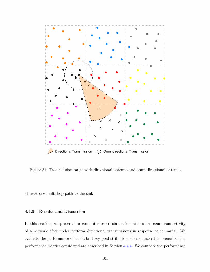
N
Directional Transmission Omni-directional Transmission
Figure 31: Transmission range with directional antenna and omni-directional antenna
at least one multi hop path to the sink.
4.4.5 Results and Discussion
In this section, we present our computer based simulation results on secure connectivity
of a network after nodes perform directional transmissions in response to jamming. We
evaluate the performance of the hybrid key predistribution scheme under this scenario. The
performance metrics considered are described in Section 4.4.4. We compare the performance
101

of the hybrid key predistribution scheme (described in Section 3.4) with the random (EG)
scheme and the deployment knowledge (EGD) scheme. For the hybrid scheme, we run
simulations with different hybrid thresholds (τ = 0.25, 0.50, 0.75) to assess the performance.
To cope with jamming, all nodes will switch their antennas from omnidirectional mode to
directional mode. Each node will randomly choose the direction that its beamform is pointed
to. We run simulations with different antenna’s beamwidths which result in different antenna
gains. We collect results at different phases: before jammers are activated (deploy phase),
after jammers are activated (jammed phase), and after nodes start directional transmissions
(coping phase). For coping phase, we collect results with different values of beamwidths
(120, 90, 60, and 30 degrees). We also evaluate the impact of changing node density and the
number of deployment groups (changing grid size).
4.4.5.1 Simulation Setup We describe the parameters setting used in our simulations.
All results are averaged with 90% confidence intervals from 10 simulation runs with different
seeds. We deploy 2,500 sensor nodes into a square area sensor field of size 500× 500m2. The
default transmission power of a regular node is -20 dBm. The receiver sensitivity is -80 dBm.
This results in a default transmission range of 40 meters. We assume that a sensor node is
equipped with an antenna system that can switch between omnidirectional and directional
transmissions once a jamming attack is detected. The antenna’s directional gain and pattern
is described in Table 2. The wireless link between nodes is determined by the SNR-based
link model as described in Section 4.4.2.3.
The global key pool |S| contains 50,000 keys and each group key pool |Sc| contains
3,164 keys. For the EGD and the hybrid scheme, sensor deployment groups are arranged
in a 5 × 5 grid. The total number of sensor deployment groups is 25 groups, where each
deployment group is of size 100×100m2. The group deployment follows the two dimensional
Gaussian distribution where the mean is the group deployment point and σ is 50 meters.
The overlapping factor (a, b) is (0.15, 0.10). Each node has a memory space to store only
100 cryptographic keys.
In this study we deploy 20 jammers randomly in the area. Jammers transmit only in
omnidirectional mode with default transmission power = -20 dBm. We place each jammer
102
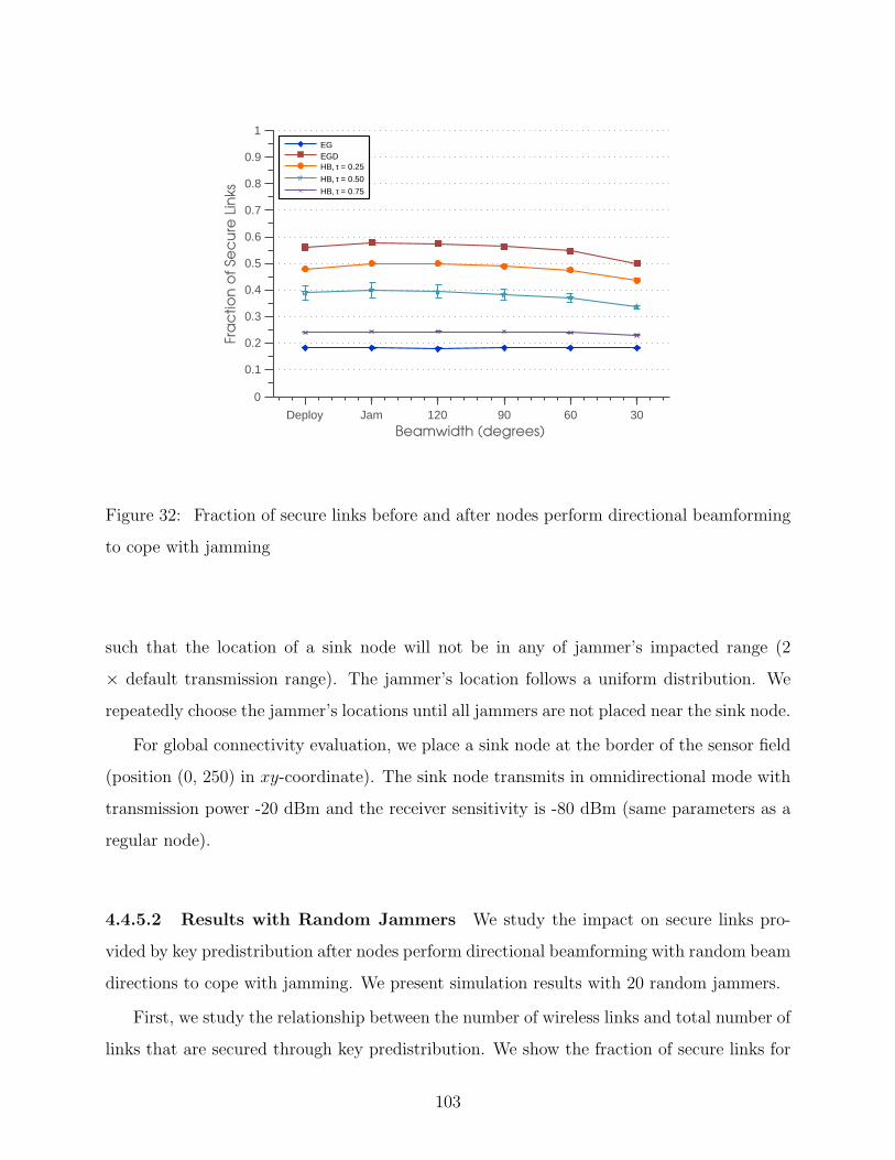
Deploy Jam 120 90 60 30
0
0.1
0.2
0.3
0.4
0.5
0.6
0.7
0.8
0.9
1
Beamwidth (degrees)
Fra
ctio
n o
f Se
cu
re L
inks
EGEGDHB, τ = 0.25
HB, τ = 0.50
HB, τ = 0.75
Figure 32: Fraction of secure links before and after nodes perform directional beamforming
to cope with jamming
such that the location of a sink node will not be in any of jammer’s impacted range (2
× default transmission range). The jammer’s location follows a uniform distribution. We
repeatedly choose the jammer’s locations until all jammers are not placed near the sink node.
For global connectivity evaluation, we place a sink node at the border of the sensor field
(position (0, 250) in xy-coordinate). The sink node transmits in omnidirectional mode with
transmission power -20 dBm and the receiver sensitivity is -80 dBm (same parameters as a
regular node).
4.4.5.2 Results with Random Jammers We study the impact on secure links pro-
vided by key predistribution after nodes perform directional beamforming with random beam
directions to cope with jamming. We present simulation results with 20 random jammers.
First, we study the relationship between the number of wireless links and total number of
links that are secured through key predistribution. We show the fraction of secure links for
103
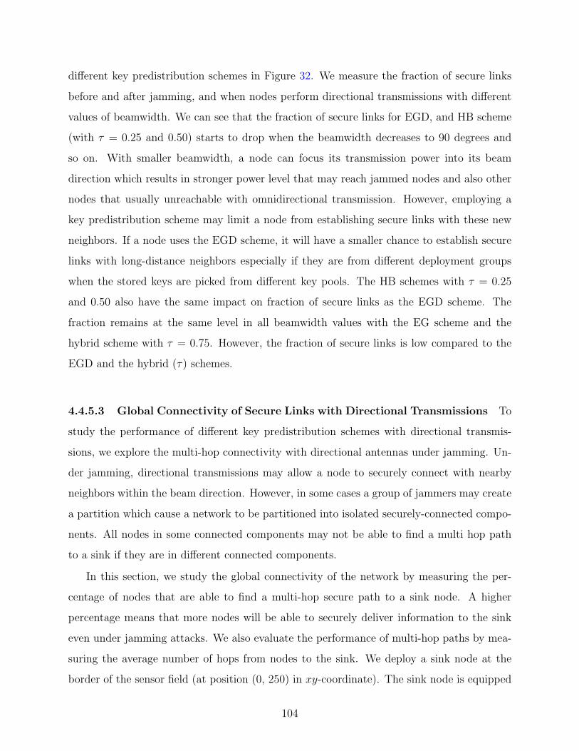
different key predistribution schemes in Figure 32. We measure the fraction of secure links
before and after jamming, and when nodes perform directional transmissions with different
values of beamwidth. We can see that the fraction of secure links for EGD, and HB scheme
(with τ = 0.25 and 0.50) starts to drop when the beamwidth decreases to 90 degrees and
so on. With smaller beamwidth, a node can focus its transmission power into its beam
direction which results in stronger power level that may reach jammed nodes and also other
nodes that usually unreachable with omnidirectional transmission. However, employing a
key predistribution scheme may limit a node from establishing secure links with these new
neighbors. If a node uses the EGD scheme, it will have a smaller chance to establish secure
links with long-distance neighbors especially if they are from different deployment groups
when the stored keys are picked from different key pools. The HB schemes with τ = 0.25
and 0.50 also have the same impact on fraction of secure links as the EGD scheme. The
fraction remains at the same level in all beamwidth values with the EG scheme and the
hybrid scheme with τ = 0.75. However, the fraction of secure links is low compared to the
EGD and the hybrid (τ) schemes.
4.4.5.3 Global Connectivity of Secure Links with Directional Transmissions To
study the performance of different key predistribution schemes with directional transmis-
sions, we explore the multi-hop connectivity with directional antennas under jamming. Un-
der jamming, directional transmissions may allow a node to securely connect with nearby
neighbors within the beam direction. However, in some cases a group of jammers may create
a partition which cause a network to be partitioned into isolated securely-connected compo-
nents. All nodes in some connected components may not be able to find a multi hop path
to a sink if they are in different connected components.
In this section, we study the global connectivity of the network by measuring the per-
centage of nodes that are able to find a multi-hop secure path to a sink node. A higher
percentage means that more nodes will be able to securely deliver information to the sink
even under jamming attacks. We also evaluate the performance of multi-hop paths by mea-
suring the average number of hops from nodes to the sink. We deploy a sink node at the
border of the sensor field (at position (0, 250) in xy-coordinate). The sink node is equipped
104
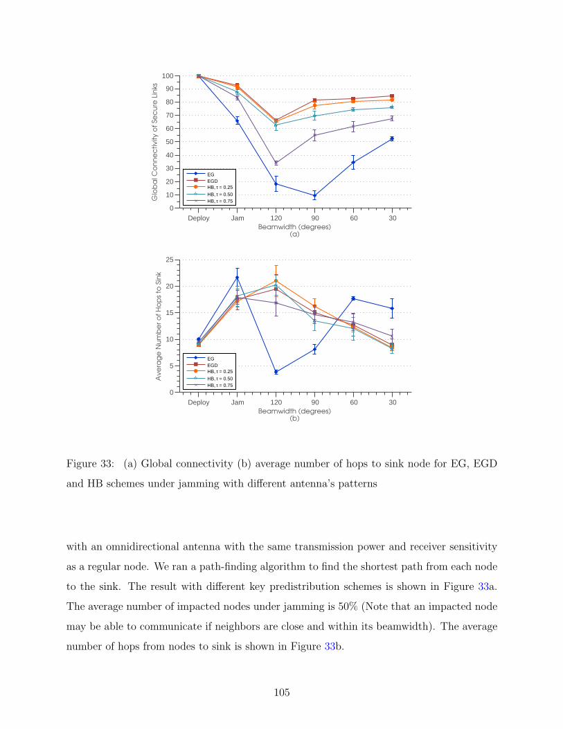
Deploy Jam 120 90 60 300
10
20
30
40
50
60
70
80
90
100
Beamwidth (degrees)(a)
Glo
ba
l Co
nn
ec
tiv
ity o
f Se
cu
re L
inks
EGEGDHB, τ = 0.25
HB, τ = 0.50HB, τ = 0.75
Deploy Jam 120 90 60 300
5
10
15
20
25
Beamwidth (degrees)(b)
Av
era
ge
Nu
mb
er
of
Ho
ps
to S
ink
EGEGDHB, τ = 0.25
HB, τ = 0.50HB, τ = 0.75
Figure 33: (a) Global connectivity (b) average number of hops to sink node for EG, EGD
and HB schemes under jamming with different antenna’s patterns
with an omnidirectional antenna with the same transmission power and receiver sensitivity
as a regular node. We ran a path-finding algorithm to find the shortest path from each node
to the sink. The result with different key predistribution schemes is shown in Figure 33a.
The average number of impacted nodes under jamming is 50% (Note that an impacted node
may be able to communicate if neighbors are close and within its beamwidth). The average
number of hops from nodes to sink is shown in Figure 33b.
105

In the jammed phase where jammers are activated, the percentage of global connectivity
drops with all key distribution schemes. The global connectivity also drops when nodes
switch to directional mode with 120 degrees bandwidth. The global connectivity drops
more than 70% in the EG scheme with beamwidth = 120 and 90 degrees. The percentage
increases with narrower beamwidth in all schemes. It is important to choose the right
value of antenna’s beamwidth in order to achieve high global connectivity under jamming.
At beamwidth = 120 degrees, the global connectivity is worse than the connectivity with
omnidirectional antennas since the directional gain is only 1.2 dBi which may not be enough
to overcome jammer’s signal. With 120 degrees, node also loses connections with close range
neighbor that are not within the beamwidth. The connectivity increases with narrower
beamwidth. With 30◦ beamwidth, the connectivity is only 5% less than using omnidirectional
antennas. More than 80% of nodes can establish a secure path to the sink node. It is
important to look at the average number of hops from each nodes to the sink. We can see
that nodes with 30◦ beamwidth use on average less number of hops to reach sink node than
nodes with omnidirectional antennas. One benefit of using directional antennas to cope with
jamming is that it will create long secure links which allow nodes to reach the sink node
faster. Note that the average number of hops with the EG scheme with 120◦ and 90◦ is
dropped because the average is computed from only 20% of nodes that are able to find a
path to the sink, which means these are nodes in locations close to the sink.
4.4.5.4 Impact of Node Density The node density may have an impact on the connec-
tivity and the ability to create secure links. We ran simulations with a 1,500 nodes network
to obtain some understanding on impact of node density with beamforming antennas. We
present the global connectivity of a 1,500 nodes network of the EG, EGD and HB scheme
with τ = 0.25 in Figure 34a and show the average number of hops in Figure 34b. We com-
pared this with the result from a 2,500 nodes network. The results show the same trend as
in a 2,500 nodes networks. The global connectivity drops more at all schemes for the 1,500
nodes network. The average number of hops is smaller than the 2,500 nodes but the average
is computed from a smaller group of nodes (that are able to find a path to the sink). Thus,
the network with higher density has a higher chance to create secure links with directional
106
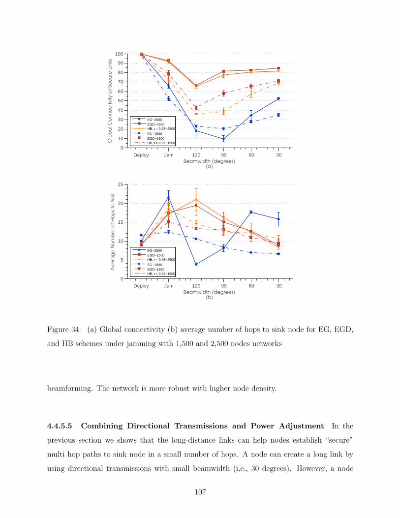
Deploy Jam 120 90 60 300
10
20
30
40
50
60
70
80
90
100
Beamwidth (degrees)(a)
Glo
ba
l Co
nn
ec
tiv
ity o
f Se
cu
re L
inks
EG−2500EGD−2500HB, τ = 0.25−2500
EG−1500EGD−1500HB, τ = 0.25−1500
Deploy Jam 120 90 60 300
5
10
15
20
25
Beamwidth (degrees)(b)
Av
era
ge
Nu
mb
er
of
Ho
ps
to S
ink
EG−2500EGD−2500HB, τ = 0.25−2500
EG−1500EGD−1500HB, τ = 0.25−1500
Figure 34: (a) Global connectivity (b) average number of hops to sink node for EG, EGD,
and HB schemes under jamming with 1,500 and 2,500 nodes networks
beamforming. The network is more robust with higher node density.
4.4.5.5 Combining Directional Transmissions and Power Adjustment In the
previous section we shows that the long-distance links can help nodes establish “secure”
multi hop paths to sink node in a small number of hops. A node can create a long link by
using directional transmissions with small beamwidth (i.e., 30 degrees). However, a node
107
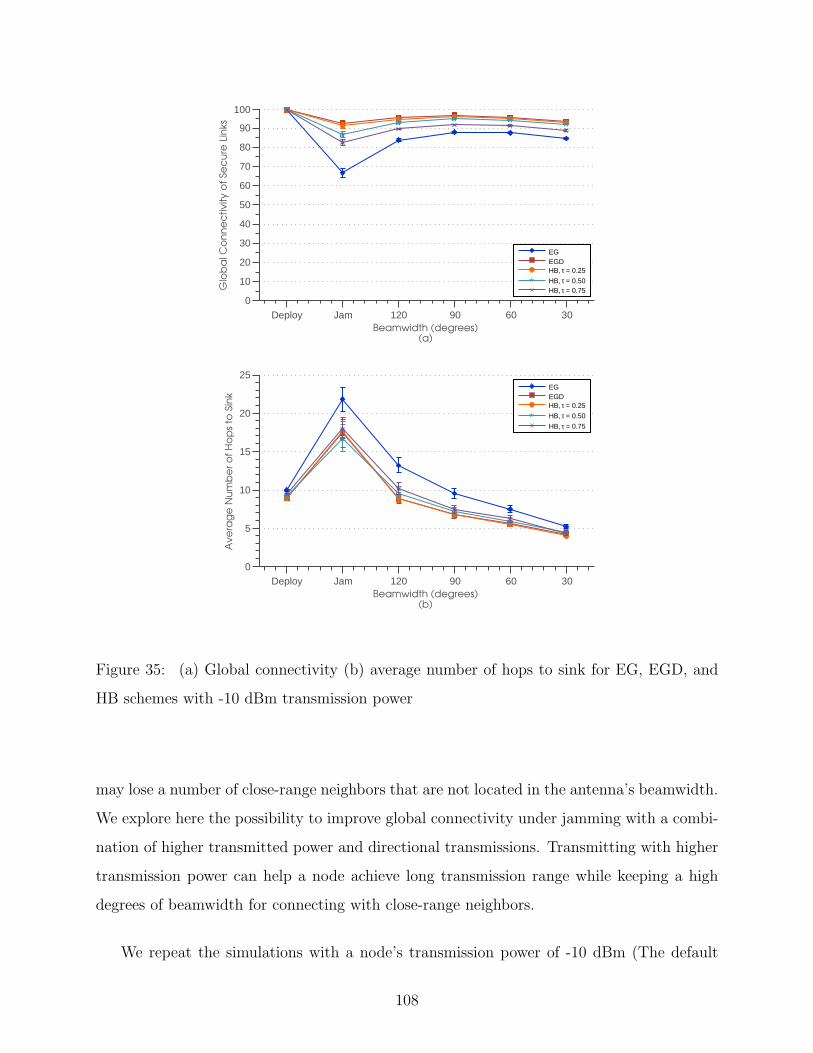
Deploy Jam 120 90 60 300
10
20
30
40
50
60
70
80
90
100
Beamwidth (degrees)(a)
Glo
ba
l Co
nn
ec
tiv
ity o
f Se
cu
re L
inks
EGEGDHB, τ = 0.25
HB, τ = 0.50HB, τ = 0.75
Deploy Jam 120 90 60 300
5
10
15
20
25
Beamwidth (degrees)(b)
Av
era
ge
Nu
mb
er
of
Ho
ps
to S
ink
EGEGDHB, τ = 0.25
HB, τ = 0.50
HB, τ = 0.75
Figure 35: (a) Global connectivity (b) average number of hops to sink for EG, EGD, and
HB schemes with -10 dBm transmission power
may lose a number of close-range neighbors that are not located in the antenna’s beamwidth.
We explore here the possibility to improve global connectivity under jamming with a combi-
nation of higher transmitted power and directional transmissions. Transmitting with higher
transmission power can help a node achieve long transmission range while keeping a high
degrees of beamwidth for connecting with close-range neighbors.
We repeat the simulations with a node’s transmission power of -10 dBm (The default
108

transmission power is -20 dBm). The results on global connectivity under jamming is shown
in Figure 35a. The average number of hops from nodes to the sink is shown in Figure 35b.
The global connectivity with high power/directional transmission improves over omnidirec-
tional transmission with all values of beamwidth. The average number of hops from nodes
to sink with high power/directional transmission is also smaller than the omnidirectional
transmission with all beamwidths. The EGD scheme and the HB scheme with τ = 0.25 has
the highest connectivity under jamming and smallest number of hops to the sink.
4.4.5.6 Summary By picking appropriate antenna’s patterns (beamwidth), directional
beamforming may improve network’s global connectivity (and number of hops to the sink)
under jamming attacks. Using a smaller value of beamwidth can improve connectivity and
average number of hops through long-distance links. This also means an improved received
power for better reception which help nodes communicate even within jammer’s range. How-
ever, a node may lose connections to nearby neighbors if the beamwidth is too narrow. Using
a combination of directional transmission and higher power can help a node transmit with
large beamwidth while achieving longer transmission range. The EGD scheme has the best
performance with this strategy but the performance of the hybrid scheme with τ = 0.25 is
also very close to that with the EGD scheme.
109

5.0 CONCLUSIONS AND FUTURE WORK
5.1 CONCLUSIONS
Wireless ad hoc and sensor networks offer alternative ways to communicate which suits many
applications. Nodes communicate through the wireless medium and this makes it possible
for adversaries to launch malicious attacks. Some applications contain critical information
that needs to be protected from attackers. One of the first step for providing security is to
provide shared secrets keys to establish secure communications between nodes. Due to the
unique characteristics of ad hoc and sensor networks such as potentially large numbers of
nodes with resource constraints, one possible solution is to predistribute secret keys prior to
deployment. One of the serious attacks on wireless communications is the jamming attack
since it is easy to launch and cannot be protected by cryptographic protocols. If existing key
predistribution schemes are used as-is, secure connectivity may be severely impacted when
the network undertakes various strategies to overcome the impact of jamming. Consequently,
designing a robust key predistribution scheme for networks that are under jamming attacks
is an important issue.
We present the background material related to key predistribution techniques for ad hoc
and sensor networks and jamming attacks in Chapter 2 of this dissertation. Definitions and
characteristics of ad hoc and sensor networks that make securing these networks become
a challenging problem is discussed. Key predistribution techniques for ad hoc and sensor
networks are presented with a focus on two important techniques: the random key pre-
distribution (EG) scheme and the deployment knowledge based key predistribution (EGD)
scheme. These two ends of key predistribution solutions present tradeoffs in secure conectiv-
ity and storage requirement. The step-by-step key predistribution process, key pools set up,
110
node deployment, and connectivity calculations are presented in detail. A classification for
key predistribution schemes is presented based on key materials used to establish link keys,
methods for calculating link keys, types of key pools and node’s deployment methods. The
details of jamming attacks are described with definitions, classifications, jamming strategies,
and detection methods. Techniques to eliminate the impact of jamming attacks and to keep
maintaining ongoing communications are presented. The jamming coping techniques dis-
cussed include power and rate adaption, adjusting frequencies and channels, spatial retreats,
and using directional antennas. Based on the literature review, there is no work that has
looked at the effects of jamming attacks over connectivity with secure links (provided by key
predistribution), and how this problem can be addressed. In this dissertation we study the
impact of jamming attacks on connectivity of secure links when the network performs spatial
retreats, power adaptation, or directional transmissions to cope with jamming attacks.
In Chapter 3 of this dissertation, we study the impact of jamming attacks on secure
connectivity when nodes perform the spatial retreat strategy to cope with jamming. We
present the hybrid key predistribution scheme (HB scheme), a key predistribution technique
for sensor networks that employs spatial retreat techniques to cope with jamming attacks.
The HB scheme combines the beneficial properties of existing key predistribution schemes:
the random key predistribution scheme (EG) and the deployment knowledge key predistri-
bution scheme (EGD). The basic idea is to balance the tradeoffs between local connectivity
and number of isolated nodes due to movement of nodes. In the presence of node retreats un-
der jamming attacks, the scheme provides high local connectivity (similar to the deployment
knowledge based – EGD – scheme) while reducing the number of isolated nodes (like the ran-
dom scheme). The hybrid scheme achieves this property without extra memory requirement
for storing secret keys (compared to existing schemes).
Under jamming attacks, one solution to cope with jamming for mobile sensor nodes
is to perform spatial retreats by moving nodes away from the jammed region. Depending
on the key predistribution techniques employed, secure connectivity can be impacted after
nodes perform spatial retreats. With the deployment based key predistribution a large
number of sensor nodes can be isolated from the rest of the network after they move out
of the jammed area. This is because moved nodes may not be able to find shared secret
111

keys with new neighbors at new locations. The random key predistribution scheme is not
affected by movement of nodes, but it has a lower a priori connectivity than the one that
employs deployment knowledge given the same number of keys stored in sensor nodes. In this
chapter the transmission range of a regular node and a jammer follows the unit disk model.
Transmission region of a node and a jammer is assumed to be a disk where transmission range
is the radius of the circle. Any node that lies in jammer’s transmission range is assumed to
be completely incommunicado. The first spatial retreat strategy considered in this chapter
is the simple strategy (the random spatial retreats) where nodes move out from jammed area
in random distance and direction. The simulation results confirm our analysis on tradeoffs
between local connectivity level and number of isolated nodes for the EG and the EGD
schemes.
The hybrid (HB) key predistribution scheme is described in detail and with analysis and
examples in Chapter 3. The idea of the hybrid scheme is that each node randomly picks
keys from both a global key pool and a group key pool derived from another global key pool.
The hybrid threshold τ plays an important role in the HB scheme. Its value determine the
number of keys that a node selects from the global key pool and from the group key pool.
The value of τ ranges from 0 to 1. For example, when τ is set to 0.25, a node that stores 100
keys selects 75 keys from its group key pool and 25 keys from the global key pool. The lower
the τ value, the closer the HB scheme is to the EGD scheme. On the other hand, the higher
the τ value, the closer the HB scheme is to the EG scheme. Keys picked from the global key
pool allow a node a higher chance to connect with new neighbors after moving but results
in a lower local connectivity level. A network operator can use results in this dissertation to
decide an appropriate value of τ that gives a satisfactory level of connectivity and number
of isolated nodes under jamming attacks.
The hybrid scheme is evaluated through simulations for different jamming scenarios (sin-
gle jammer and multiple jammers), number of deployment groups, and different node den-
sities. The results are compared with the random (EG) scheme and the deployment knowl-
edge based (EGD) schemes. The metrics considered are local connectivity and the number
of moved nodes that are isolated after detecting jamming and performing spatial retreats.
Under all evaluated scenarios, the hybrid scheme shows high local connectivity level (close to
112
the EGD scheme) while the number of isolated nodes is low especially when the τ threshold
is set to 0.25. We test the hybrid scheme while changing the number of deployment groups.
The hybrid scheme also performs well under different node densities. The number of hops
to establish a secure path between two neighbor nodes that do not have a shared key is also
studied. The simulation results show that, with the hybrid scheme, the probability of having
a secure path that is smaller than or equal to 3 hops is more than 0.9 (both before and after
jamming). The number of isolated nodes that are present totally in the sensor field before
and after jamming is also studied. Number of isolated nodes before and after jamming with
the hybrid scheme does not change much (compared to the EGD scheme). This can imply
that the hybrid scheme is robust against change in network topology due to spatial retreats.
To reduce unnecessary travel distance for jammed nodes in the random spatial retreat strat-
egy, the partial random spatial retreat strategy is presented and is evaluated with the hybrid
scheme. The idea is to move a jammed node in random direction but the travel distance
will be limited by a maxDist threshold. The goal is to reduce a node’s travel distance and
achieve even distribution of nodes in the sensor field after moved. The hybrid scheme with
the partial random spatial retreat strategy is evaluated by simulations with random jammers
and different values of maxDist threshold.
Chapter 4 of this dissertation addresses the impact on secure links when nodes perform
other techniques to cope with jamming. The first coping technique we study is power adap-
tation where nodes increase their transmission power level to cope with jamming. Then we
study the impact on secure links when nodes perform directional transmissions to cope with
jamming. We evaluate the performance of the hybrid key predistribution scheme with a
sensor network that performs these techniques to cope with jamming. In this chapter the
limitation of the unit disk model used in Chapter 3 is first discussed. The unit disk jamming
model assumes that if a node is located within a jamming transmission range, it is assumed
to be jammed and cannot communicate with its neighbors. This model assumption does not
capture the fact that the success reception of a packet is primarily determined by the dif-
ference between signal strength from sender and combined power from jammers at receiving
node. We adopt the SNR-based model – a more realistic link model to explore the possibility
that a node can communicate under jamming. The basic idea is to determine the link reli-
113

ability through the difference between the received signal power (in dB) and the combined
power of interference from jammers and noise at the receiver (the SNR ratio). The factors
that impact the link condition between nodes including sender and jammer’s transmission
power, distance between jammer and receiver, and distance between sender and receiver.
Thus, it is possible for a node to communicate (receive a packet) even though a node is
located within a jamming range. For example, the distance between nodes are close enough,
or the transmission power is high enough to overcome the jammer’s transmission power. The
SNR-based model is presented with details and assumptions. This link and jamming model
is used to study the impact of jamming attacks in this chapter.
We study the impact of jamming attacks on secure connectivity (provided by different
key predistribution schemes) when the network increases transmission power to cope with
jamming. We use a simple power adaption strategy where every node in the network in-
creases its transmission power upon detection of a jamming attack. A group of 20 jammers is
randomly deployed in the sensor field. The simulation results show that increasing transmis-
sion power level helps nodes to overcome impacts of jamming. The total number of secure
links with all key predistribution schemes increases for higher transmission power levels. The
increase in number of secure links is different depending on the key predistribution scheme.
The EGD scheme has the highest number of secure links. The result with the hybrid scheme
(τ = 0.25) is close to that of the EGD scheme. The fraction of secure links (with the EGD
and the hybrid key predistribution schemes) decreases for the higher transmission power
levels indicating that using transmission power that is too high does not help nodes create
more secure links since long-distance neighbors may come from non-adjacent deployment
groups (which usually have no shared keys). With the EG scheme, the fraction of secure
links is stable for higher transmission power levels but the number of secure links is lower
than other schemes to start with. By looking at the percentage of impacted nodes that are
able to securely connect with neighbors, we see that it is possible for nodes to communi-
cate (locally with one hop neighbors) under jamming. The global connectivity shows that,
with all key predistribution schemes, more than 70% of nodes are able to find a multihop
secure path to the sink node. This percentage increases for higher transmission power levels.
Jammers can force nodes to travel a larger number of hops to the sink but increasing the
114

transmission power allows nodes to select long-distance secure neighbors to reach the sink
with fewer numbers of hops. The EGD scheme has the best performance with the power
adaptation strategy. The performance of the hybrid scheme with τ = 0.25 is very close to
that with the EGD scheme. Thus, it is desirable to use a low value of τ for a network that
increases its transmission power to cope with jamming. Different node densities also impact
secure connectivity of sensor nodes (under jamming and after nodes increase transmission
power). A higher node density results in more robustness to jamming attacks.
We study the impact of jamming attacks on secure connectivity (provided by different key
predistribution schemes) when the network uses directional antennas to cope with jamming.
In this scenario, nodes perform random transmissions with random directions and different
beamwidths to cope with jamming. The simulation results show that by selecting appropri-
ate antennas patterns (beamwidth), directional beamformings can improve networks global
connectivity (and number of hops to the sink) under jamming attacks. Using a smaller value
of beamwidth can improve connectivity and reduce the average number of hops through long-
distance links. This also means an improved received power for better reception which helps
nodes communicate even within a jammers range. However, nodes may lose connections to
nearby neighbors if the beamwidth is too narrow. Using a combination of directional trans-
mission and higher power can help a node transmit with larger beamwidths while achieving
longer transmission ranges. The EGD scheme has the best performance with this strategy
but the performance of the hybrid scheme with τ = 0.25 is also very close to that with the
EGD scheme.
5.2 FUTURE WORK
This dissertation addresses problems related to the impact on secure links created by key
predistribution when a network employs various techniques to cope with jamming attacks.
There are several issues in this topic that are potential topics for future research. We
would like to expand our study on the global connectivity of secure links when the network
performs different spatial retreat strategies to cope with jamming. In this dissertation it is
115

shown that an appropriate value of the hybrid threshold (τ) can maintain reasonable level
of local connectivity and robustness to jamming attacks. We would like to study perhaps
a better way (e.g, to pick value of τ for each node or group of nodes). A node that is in
the deployment group that is closer to the border of the sensor field may use a different
value of τ compared to a sensor node that is in the group deployed at the center of the
sensor field. Information of areas that are more susceptible to jamming could be useful for
network operators in predistributing keys to sensor nodes. In Section 3.4.5, we show our
analysis on secure connectivity (local connectivity) of the hybrid scheme. Our analysis is for
the situation when there is no jamming. Under jamming and spatial retreat, the equation
will change in terms of the value of δ(i, j) which could be 0 in the worst case where nodes
are from non-adjacent groups or |Sc| in the best case where nodes are from the same group.
We would like to expand our analysis on local connectivity of the hybrid key predistribution
scheme to include an analysis on local connectivity after jamming and after nodes perform
different strategies to cope with jamming.
Simple strategies to cope with jamming have been used to study the impact of increasing
transmission power and using directional antennas. Employing smart coping strategies and
studying the impact of such strategies on secure connectivity under jamming is a topic
for future research. With the power adaptation strategy, not every node needs to increase
the transmission power. Only a node that loses its secure neighbors due to jamming may
choose to increase its transmission power to reconnect with its neighbors in order to reduce
total power consumption for the whole network. A sensor node equipped with a directional
antenna may choose to adjust its beam direction towards a jammed neighbor (whom it
shares key with) or the sink node. However, location information of neighbors is needed
to determine the beam direction. Also, a node may switch to directional antennas only
when it appears to be isolated (it cannot reach anyone with an omnidirectional antenna)
instead of switching to a directional antenna when it realizes that it is under jamming. It is
shown in this dissertation that combining different jamming coping techniques can improve
secure connectivity under jamming. We would like to explore this issue further. Nodes may
combine the spatial retreats with the power adaption strategy or directional antennas. A
jammed node may choose to move closer to its neighbor so that nodes do not have to increase
116

their transmission powers to overcome the signal from the jammer. In this dissertation we
focus on secure links created if two nodes share a common key. As discussed in Chapter 2,
two neighbor nodes that do not share key can establish a secure link through two or more
links from other neighbors with whom they share a key with in order to improve the number
of secure links in the network. Thus, it is interesting to study the path key establishment
process under jamming attacks. The impact of various jamming coping techniques on the
path key establishment process is an issue that we would like to explore in the future.
We consider only the static jammers in this dissertation. It will be interesting to study
the impact on secure links from mobile jammers. We would like to test our key predistri-
bution schemes with jammers with different mobility models. It is also important to study
this problem from the jammer’s point of view. A smart jamming strategy that focused on
prevent nodes from establishing secure links is also a challenging problem (i.e., how would a
jammer chose a strategy to optimally jam to disable secure connectivity). Finally, an actual
implementation of the hybrid key predistribution scheme will be useful for an experimental
testing on the impact of jamming attacks on secure connectivity of the network.
117
BIBLIOGRAPHY
[1] Y. Wang, G. Attebury, and B. Ramamurthy, “A survey of security issues in wirelesssensor networks,” IEEE Commun. Surv. Tutorials, vol. 8, no. 2, pp. 2–23, 2006.
[2] A. Perrig, R. Szewczyk, V. Wen, D. Culler, and J. D. Tygar, “Spins: Security protocolsfor sensor networks,” in Wireless Networks, vol. 8, 2001, pp. 189–199.
[3] H. Chan, A. Perrig, and D. Song, “Random key predistribution schemes for sensornetworks,” in Proceeding of IEEE Symposium on Security and Privacy, 2003, pp. 197–213.
[4] L. Eschenauer and V. D. Gligor, “A key-management scheme for distributed sensornetworks,” in Proceedings of the 9th ACM conference on Computer and communicationssecurity (CCS’02). New York, NY, USA: ACM, 2002, pp. 41–47.
[5] W. Du, J. Deng, Y. S. Han, and P. K. Varshney, “A key predistribution scheme for sen-sor networks using deployment knowledge,” IEEE Trans. Dependable Secure Comput.,vol. 3, no. 1, pp. 62–77, 2006.
[6] R. Di Pietro, L. V. Mancini, and A. Mei, “Efficient and resilient key discovery basedon pseudo-random key pre-deployment,” in IEEE International Parallel and DistributedProcessing Symposium (IPDPS’04), 2004.
[7] I. Akyildiz, W. Su, Y. Sankarasubramaniam, and E. Cayirci, “A survey on sensor net-works,” IEEE Commun. Mag., vol. 40, no. 8, pp. 102–114, August 2002.
[8] M. Brown, D. Cheung, D. Hankerson, J. Hernandez, M. Kirkup, and A. Menezes, “PGPin constrained wireless devices,” in Proceedings of the 9th conference on USENIX Secu-rity Symposium-Volume 9. USENIX Association, 2000, p. 19.
[9] D. W. Carman, P. S. Kruus, and B. J. Matt, “Constraints and approaches for distributedsensor network security,” NAI Labs, Tech. Rep., September 2000.
[10] J. Spencer, “The strange logic of random graphs,” in Algorithms and Combinatorics 22.Springer-Verlag, 2000.
[11] S. A. Camtepe and B. Yener, “Key distribution mechanisms for wireless sensor networks:a survey,” Rensselaer Polytechnic Institute, Tech. Rep., Mar 2005.
118
[12] W. Du, J. Deng, Y. S. Han, S. Chen, and P. K. Varshney, “A key management schemefor wireless sensor networks using deployment knowledge,” in IEEE INFOCOM, vol. 1,2004, p. 597.
[13] W. Du, J. Deng, Y. Han, and P. Varshney, “A pairwise key pre-distribution scheme forwireless sensor networks,” in Proceedings of the 10th ACM conference on Computer andcommunications security (CCS’03). New York, NY, USA: ACM, 2003, pp. 42–51.
[14] R. Blom, “An optimal class of symmetric key generation systems,” in Proceedings ofthe EUROCRYPT 84 Workshop on Advances in Cryptology. New York, NY, USA:Springer-Verlag New York, Inc., 1985, pp. 335–338.
[15] S. Zhu, S. Xu, S. Setia, and S. Jajodia, “Establishing pairwise keys for secure communi-cation in ad hoc networks: A probabilistic approach,” in Proceedings of the 11th IEEEInternational Conference on Network Protocols (ICNP’03), 2003.
[16] S. Meguerdichian, F. Koushanfar, M. Potkonjak, and M. B. Srivastava, “Coverage prob-lems in wireless ad-hoc sensor networks,” in IEEE INFOCOM, 2001.
[17] C. Blundo, A. D. Santis, A. Herzberg, S. Kutten, U. Vaccaro, and M. Yung,“Perfectly-secure key distribution for dynamic conferences,” in Advances in cryptology(CRYPTO’92), 1992.
[18] D. Liu and P. Ning, “Establishing pairwise keys in distributed sensor networks,” inProceedings of the 10th ACM conference on Computer and communications security.ACM, 2003, pp. 52–61.
[19] J. Lee and D. R. Stinson. (2004) Deterministic key predistribution schemes fordistributed sensor networks. [Online]. Available: http://www.cacr.math.uwaterloo.ca/∼dstinson/publist.html
[20] S. A. Camtepe and B. Yener, “Combinatorial design of key distribution mechanisms forwireless sensor networks,” in 9th European Symposium on Research in Computer Securit(ESORICS’04), 2004.
[21] J. Lee and D. R. Stinson. (2004) A combinatorial approach to key predistribution fordistributed sensor networks. [Online]. Available: http://www.cacr.math.uwaterloo.ca/∼dstinson/publist.html
[22] H. Chan, V. D. Gligor, A. Perrig, and G. Muralidharan, “On the distribution andrevocation of cryptographic keys in sensor networks,” IEEE Transactions on Dependableand Secure Computing, vol. 2, no. 3, pp. 233–247, July–September 2005.
[23] D. Liu, P. Ning, and W. Du, “Group-based key predistribution for wireless sensor net-works,” ACM Transactions on Sensor Network, 2008.
[24] W. Xu, K. Ma, W. Trappe, and Y. Zhang, “Jamming sensor networks: Attack anddefense strategies,” IEEE Network, vol. 20, no. 3, pp. 41–47, May/June 2006.
119
[25] Y. W. Law, L. van Hoesel, J. Doumen, P. Hartel, and P. Havinga, “Energy-efficientlink-layer jamming attacks against wireless sensor network mac protocols,” in 3rd ACMWorkshop on Security of Ad Hoc and Sensor Networks (SASN’05), 2005.
[26] M. Li, I. Koutsopoulos, and R. Poovendran, “Optimal jamming attacks and networkdefense policies in wireless sensor networks,” in IEEE INFOCOM, 2007.
[27] P. Tague, D. Slater, G. Noubir, and R. Poovendran, “Linear programming models forjamming attacks on network traffic flows,” in ICST WiOpt, April 2008.
[28] C. W. Commander, P. M. Pardalos, V. Ryabchenko, O. Shylo, S. Uryasev, andG. Zrazhevsky, “Jamming communication networks under complete uncertainty,” Opti-mization Letters, pp. 53–70, 2007.
[29] T. X. Brown, J. E. James, and A. Sethi, “Jamming and sensing of encrypted wirelessad hoc networks,” in Proceedings of the 7th ACM international symposium on Mobilead hoc networking and computing (MobiHoc’06). New York, NY, USA: ACM, 2006.
[30] W. Xu, T. Wood, W. Trappe, and Y. Zhang, “Channel surfing and spatial retreats:defenses against wireless denial of service,” in Proceedings of the 3rd ACM workshop onWireless security (WiSe’04). New York, NY, USA: ACM, 2004, pp. 80–89.
[31] W. Xu, W. Trappe, Y. Zhang, and T. Wood, “The feasibility of launching and detectingjamming attacks in wireless networks,” in Proceedings of the 6th ACM internationalsymposium on Mobile ad hoc networking and computing (MobiHoc’05). New York,NY, USA: ACM, 2005, pp. 46–57.
[32] A. D. Wood, J. A. Stankovic, and S. H. Son, “Jam: a jammed-area mapping servicefor sensor networks,” in Proceedings of the 24th IEEE Real-Time Systems Symposium(RTSS’03), 2003, pp. 286–297.
[33] S. O. Amin, M. S. Siddiqui, and C. S. Hong, “Detecting jamming attacks in ubiquitoussensor networks,” in Proc. IEEE SAS, 2008.
[34] W. Xu, “On adjusting power to defend wireless networks from jamming,” in 4th AnnualInternational Conference on Mobile and Ubiquitous Systems (MobiQuitous’07), August2007, pp. 1–6.
[35] V. P. Mhatre, K. Papagiannaki, and F. Baccelli, “Interference mitigation through powercontrol in high density 802.11 wlans,” in IEEE INFOCOM, 2007.
[36] K. Pelechrinis, I. Broustis, and S. V. Krishnamurthy, “Ares: An anti-jamming reinforce-ment system for 802.11 networks,” in Proceedings of the 5th international conference onEmerging networking experiments and technologies. ACM, 2009, pp. 181–192.
[37] G. Lin and G. Noubir, “On link layer denial of service in data wireless lans,” WirelessCommunications and Mobile Computing, vol. 5, no. 3, pp. 273–284, 2005.
120
[38] P. Tague, M. Li, and R. Poovendran, “Probabilistic mitigation of control channel jam-ming via random key distribuiton,” in Proc. 18th Ann. IEEE Int’l Symp. Personal,Indoor, and Mobile Radio Comm.(PIMRC’07), 2007.
[39] M. Cagalj, S. Capkun, and J.-P. Hubaux, “Wormhole-based antijamming techniquesin sensor networks,” IEEE Transaction on Mobile Computing, vol. 6, no. 1, pp. 1–15,January 2007.
[40] K. Ma, Y. Zhang, and W. Trappe, “Mobile network management and robust spatial re-treats via network dynamics,” in International Conference on Mobile Adhoc and SensorSystems Conference (MASS’05). New York, NY, USA: IEEE, November 2005.
[41] S. Khattab, D. Mosse, and R. Melhem, “Honeybees: Combining replication and evasionfor mitigating base-station jamming in sensor networks,” in In Proc. WPDRTS, 2006.
[42] G. Noubir, “On connectivity in ad hoc network under jamming using directional anten-nas and mobility,” in International Conference on Wired /Wireless Internet Communi-cations (WWIC’04). Springer-Verlag, 2004, pp. 186–200.
[43] R. R. Choudhury and N. H. Vaidya, “On designing mac protocols for wireless networksusing directional antennas,” IEEE Trans. on Mobile Computing, 2005.
[44] G. Jakllari, W. Luo, and S. V. Krishnamurthy, “An integrated neighbor discovery andmac protocol for ad hoc networks using directional antennas,” IEEE Trans. on WirelessCommunications, 2007.
[45] S. Shankar and D. Kundur, “Towards improved connectivity with hybrid uni/omni-directional antennas in wireless sensor networks,” in IEEE INFOCOM, 2008.
[46] C. Bettstetter, C. Hartmann, and C. Moser, “How does randomized beamforming im-prove the connectivity of ad hoc networks?” in in Proc. IEEE International Conferenceon Communications (ICC’05), 2005.
[47] J. Jeong and Z. J. Haas, “Predeployed secure key distribution mechanisms in sensornetoworks: Current state-of-the-art and a new approach using time information,” IEEEWireless Communications, August 2008.
[48] B. Awerbuch, A. Richa, and C. Scheideler, “A jamming-resistant mac protocol for single-hop wireless networks,” in Proceedings of the twenty-seventh ACM symposium on Prin-ciples of distributed computing. ACM, 2008, pp. 45–54.
[49] S. Ye, Y. Wang, and Y. Tseng, “A jamming-based mac protocol to improve the per-formance of wireless multihop ad-hoc networks,” Wireless Communications and MobileComputing, vol. 4, no. 1, pp. 75–84, 2004.
[50] “Qualnet network simulator.” [Online]. Available: http://www.scalable-networks.com
[51] “Opnet simulator.” [Online]. Available: http://www.opnet.com
121
[52] “The network simulator ns-2.” [Online]. Available: http://www.isi.edu/nsnam/ns/
[53] P. Gupta and P. R. Kumar, “The capacity of wireless networks,” IEEE Trans. Info.Theory, vol. 64, no. 2, pp. 388–404, 2000.
[54] G. Brar, D. M. Blough, and P. Santi, “Computationally efficient scheduling with thephysical interference model for throughput improvement in wireless mesh networks,”in Proceedings of the 12th annual international conference on Mobile computing andnetworking. ACM, 2006.
[55] “Antenova solutions.” [Online]. Available: http://www.antenova.com/
[56] R. Ramanathan, “On the performance of ad hoc networks with beamforming antennas,”in Proceedings of the 2nd ACM international symposium on Mobile ad hoc networkingand computing (MobiHoc’01), 95-105, Ed. New York, NY, USA: ACM, 2001.
[57] R. Choudhury and N. Vaidya, “Impact of directional antennas on ad hoc routing,”PersonalWireless Communications, pp. 590–600, 2003.
[58] J. Liberti and T. Rappaport, Smart antennas for wireless communications: IS-95 andthird generation CDMA applications. Prentice Hall PTR Upper Saddle River, NJ,USA, 1999.
122
Related Documents


![Enabling Secure Always-On Connectivity [Name] Microsoft Corporation.](https://static.cupdf.com/doc/110x72/56649f4e5503460f94c6ffc2/enabling-secure-always-on-connectivity-name-microsoft-corporation.jpg)
