Secular variation signals in magnetic field gradient tensor ...

Geophys. J. Int. (2022) 229, 2096–2114 https://doi.org/10.1093/gji/ggac004Advance Access publication 2022 January 07GJI Geomagnetism, Rock Magnetism and Palaeomagnetism

Secular variation signals in magnetic field gradient tensor elementsderived from satellite-based geomagnetic virtual observatories

Magnus D. Hammer, Christopher C. Finlay and Nils OlsenDivision of Geomagnetism and Geospace, Technical University of Denmark - DTU Space, 2800 Kongens Lyngby, Denmark. E-mail: [email protected]

Accepted 2022 January 5. Received 2022 January 4; in original form 2021 June 1

S U M M A R YWe present local time-series of the magnetic field gradient tensor elements at satellite altitudederived using a Geomagnetic Virtual Observatory (GVO) approach. Gradient element time-series are computed in 4-monthly bins on an approximately equal-area distributed worldwidenetwork. This enables global investigations of spatio-temporal variations in the gradient tensorelements. Series are derived from data collected by the Swarm and CHAMP satellite missions,using vector field measurements and their along-track and east–west differences, when avail-able. We find evidence for a regional secular variation impulse (jerk) event in 2017 in the firsttime derivative of the gradient tensor elements. This event is located at low latitudes in thePacific region. It has a similar profile and amplitude regardless of the adopted data selectioncriteria and is well fit by an internal potential field. Spherical harmonic models of the internalmagnetic field built from the GVO gradient series show lower scatter in near-zonal harmonicscompared with models built using standard GVO vector field series. The GVO gradient ele-ment series are an effective means of compressing the spatio-temporal information gatheredby low-Earth orbit satellites on geomagnetic field variations, which may prove useful for coreflow inversions and in geodynamo data assimilation studies.

Key words: Magnetic field variations through time; Rapid time variations; Satellite magnet-ics.

1 I N T RO D U C T I O N

The main part of the geomagnetic field is generated in the Earth’s fluid outer core by a process known as the geodynamo. Knowledge ofhow this core field varies with space and time provides information on the fluid flow dynamics in the liquid metal outer core. Although thetemporal behaviour of the geomagnetic field is well characterized in time-series from ground observatories, a global spatio-temporal study ishampered by the uneven distribution of these observatories. Even though low-Earth-orbit (LEO) satellites do provide good global coverageon timescales of weeks and longer, the direct study of the first time derivative of the core field, the secular variation (SV), from satellitemeasurements is not straightforward. This is because LEO satellites are not geostationary (i.e. do not have the same orbital period as theEarth’s rotation, such that their position does not stay fixed as seen from ground), which leads to an ambiguity, since it is not possible toestablish whether an observed field variation is caused by a temporal or spatial change of the field (Olsen & Stolle 2012). Spherical harmonic(SH) field models derived from satellite measurements provide an established way of studying the SV field and its time derivative, the secularacceleration (SA), globally. However, such harmonic functions have global support, which means that an estimate of the SV at a specificposition may be affected by noise from remote locations.

These issues lead Mandea & Olsen (2006) to introduce the concept of Geomagnetic Virtual Observatories (GVOs) in space, in whichsatellite magnetic measurements from within a selected region, collected during one month time windows, were used to derive a localmonthly mean vector field at the satellite mean altitude. The resulting GVO time-series resemble monthly mean series computed using groundobservatory magnetic measurements, by providing the magnetic vector field elements at fixed locations. However, since they are based onsatellite data, regular sampling in both space and time is possible. Thus, the GVO method provides a tool for compressing satellite magneticfield measurements into a data set that contains time-series distributed on a global grid, and which may also be supplied with error estimates(Hammer et al. 2021a). Olsen & Mandea (2007) used CHAMP measurements to derive GVO vector component time-series, and carried outa global investigation of SV that identified a regional geomagnetic jerk event in 2003.

In the original GVO approach of Mandea & Olsen (2006), processing of the satellite measurements followed that of simple monthlyfield means at ground observatories, taking measurements from all local times and with all levels of geomagnetic activity, and relied on the

2096

C© The Author(s) 2022. Published by Oxford University Press on behalf of The Royal Astronomical Society. This is an Open Accessarticle distributed under the terms of the Creative Commons Attribution License (http://creativecommons.org/licenses/by/4.0/), whichpermits unrestricted reuse, distribution, and reproduction in any medium, provided the original work is properly cited.

Dow

nloaded from https://academ

ic.oup.com/gji/article/229/3/2096/6500194 by guest on 11 July 2022

mailto:[email protected]

http://creativecommons.org/licenses/by/4.0/

SV in magnetic gradient tensor elements 2097

assumption that short period external fields would have zero mean over the course of one month. However, later studies revealed that externalfields, especially those due to the magnetospheric ring current and ionospheric current systems, cause contamination of the retrieved internalGVO field signal (Olsen & Mandea 2007; Beggan et al. 2009; Domingos et al. 2019). In addition, insufficient local time sampling fromwithin one month of polar orbiting satellites resulted in a bias due to the local time dependence of ionospheric and magnetosphere–ionospherecoupling currents (Shore 2013). Recently, the GVO processing algorithm has been further developed in an effort to reduce contaminationfrom magnetospheric and ionospheric sources, and the local time sampling bias, with the aim of better isolating the field signal generated bythe Earth’s outer core (Hammer et al. 2021a). These new GVO vector field series have been used to study global patterns of field changes(Hammer et al. 2021a,c), for inferring fluid flows close to the core surface (Kloss & Finlay 2019; Rogers et al. 2019) and for data assimilationstudies (Barrois et al. 2018; Huder et al. 2020).

In parallel to the development of these GVO-based techniques there has also been recent progress in the theory of space-based magneticgradiometry, inspired by advances in satellite gravimetry. Initial studies have demonstrated that knowledge of the second-order 3 × 3 magneticgradient tensor may be beneficial when seeking to retrieve small scale features of the field (both the lithospheric field and the time-dependentcore field). This is possible because gradient elements effectively give more weight to shorter wavelengths, while at the same time some noisesources (e.g. unmodelled magnetospheric fields) are predominantly of long wavelength, which can result in a higher signal-to-noise ratio forshort wavelengths compared to using the vector field components (Kotsiaros & Olsen 2012, 2014). Information on these shorter spatial lengthscales is crucial for core dynamic studies, yet their robust determination is a major obstacle in core field modelling. This issue has motivatedus to derive time-series of field gradient elements using the GVO method, and to investigate whether such series allow, via for example SHanalysis, an improved retrieval of field changes. Gradient GVO series have the potential to also be used directly in core flow inversions anddata assimilation studies of the geodynamo.

Assuming a potential field due to internal sources and no in situ electrical currents, the field becomes a solenoidal irrotational vectorfield and the gradient tensor has the special property of being symmetric with a trace of zero. The assumption of a symmetric gradient tensorreduces the number of independent gradient tensor elements from nine to six, while a trace of zero further reduces this number to five.Each element of the magnetic gradient tensor may be considered as a directional filter providing specific information on the magnetic fieldstructures. Thereby, certain gradient tensor elements better constrain specific SHs (Olsen & Kotsiaros 2011). According to the studies ofKotsiaros & Olsen (2012) and Kotsiaros & Olsen (2014), knowledge of the radial gradient of the radial field, written as [∇B]rr, is particularlysuitable for resolving the higher degree parts and zonal harmonics. The east–west gradient of the azimuthal field, [∇B]φφ , and radial field[∇B]rφ , are especially sensitive to sectorial harmonics, while the north–south gradient of the radial, [∇B]rθ , and meridional, [∇B]θθ , fields areespecially useful for determining near-zonal harmonics. The east–west gradient of the meridional field, [∇B]θφ does not provide significantadditional information. In addition, knowledge of how certain external fields may influence certain gradient tensor elements is important toconsider, for instance the magnetospheric ring current is expected to affect zonal terms constrained by the [∇B]rr element but not the [∇B]rφ

element (Kotsiaros & Olsen 2014). Although it is not yet possible to directly measure the full magnetic gradient tensor in space (Nogueira et al.2015), it is nonetheless possible to compute the tensor elements from a magnetic potential determined using satellite magnetic measurements.

In this paper, our aim is to estimate local time-series of the magnetic field gradient tensor elements using the GVO method. Our primarymotivation for deriving such gradient field series, is to improve the recovery of the small length-scales of the SV, compared with the traditionaluse of vector field data. In particular, the gradient elements are expected to enable a higher signal-to-noise ratio as compared to vector elements(Kotsiaros & Olsen 2014). This is because they are more sensitive to the small length scales of the field, and less affected by large scaleexternal fields. We use satellite magnetic measurements to derive the GVO gradient series, and follow Hammer et al. (2021a) in implementingdark and quiet time data selection criteria and use 4-month time windows to minimize problems related to local time sampling.

In Section 2 we provide a detailed description of the satellite magnetic measurements and selection criteria used, and in Section 3 wedescribe the GVO method and the computation of both GVO vector and GVO gradient element time-series. In Section 4.1 we present resultsof the GVO series for each of the SV gradient elements, and visually inspect these. In order to investigate the possible benefits of using GVOgradient data, we compare SH field models derived epoch by epoch from the GVO vector data and GVO gradient tensor data in Section 4.2.We study the detailed behaviour of the gradient tensor elements going from 2015 to 2018 with a focus on the Pacific region. Finally, Section 5provides discussions and conclusions.

2 DATA

To derive the GVO time-series we select vector magnetic field measurements from the CHAMP and Swarm satellite missions. We usedCHAMP L3 magnetic data between July 2000 and September 2010 and Swarm Level 1b MAG-L, version 0505/0506, from all three Swarmsatellites Alpha, Bravo and Charlie between January 2014 and April 2020, and subsample at 15 s intervals (i.e. taking measurements every15 s), in the vector field magnetometer (VFM) frame. Next, the magnetic data in the VFM frame are rotated into an Earth-Centred Earth-Fixed(ECEF) local Cartesian North-East-Centre (NEC) coordinate frame (for details see Olsen et al. (2006)) by using the Euler rotation anglesfrom the CHAOS-7.2 model (Finlay et al. 2020). Measurements from known problematic days (e.g. where satellite manoeuvres took place)were removed and gross data outliers for which the vector field components deviated more than 500 nT from CHAOS-7.2 field model[http://www.spacecenter.dk/f iles/magnetic-models/CHAOS-7/], see also Finlay et al. (2020), values were rejected. The measurements werethen selected using dark quiet time criteria defined here as: (i) the sun is at least 10◦ below horizon, (ii) geomagnetic activity index Kp < 3◦

Dow



http://www.spacecenter.dk/files/magnetic-models/CHAOS-7/

2098 M.D. Hammer, C.C. Finlay and N. Olsen

and (iii) ring current index |dRC/dt| < 3 nT hr−1 (Olsen et al. 2014), merging electric field (averaged over 2 hr) at magnetopause Em ≤ 0.8mV m−1 (Olsen et al. 2014), and placing constraints on the interplanetary magnetic field (IMF, averaged over two-hours) requiring Bz > 0 nTand |By| < 10 nT (Ritter et al. 2004). Using the definition in Olsen et al. (2014), the merging electric field was derived using 1-min values ofthe solar wind, solar clock angle and IMF extracted from the OMNI database, [http://omniweb.gsfc.nasa.gov], see also King & Papitashvili(2005).

Previous studies have demonstrated the benefits of using along-track differences of the satellite magnetic field measurements forretrieving higher spatial resolution of the core and also the lithospheric fields, as such differences filter out correlated noise caused byexternal sources (Kotsiaros et al. 2015; Olsen et al. 2015; Kotsiaros 2016; Finlay 2019). However, from data differences alone it is notpossible to obtain robust information on the longer wavelength part of the field. Therefore, we also use the complementary data means in asimilar manner as in previous studies of the core signal (Sabaka et al. 2013; Hammer 2018). From the satellite magnetic field measurements,Bk(r), where k is the vector component of a given coordinate system, we use measurement means, �dk, and differences, �dk as data.The differences, �dk = (�dAT

k , �dEWk ), and the means, �dk = (�dAT

k , �dEWk ), are taken along-track (AT) for each satellite and east–west

(EW) between the Swarm Alpha (SWA) and Charlie (SWC) satellites. Here along-track differences are calculated from the 15 s differences�dAT

k = [Bk(r, t) − Bk(r + δr, t + 15 s)] while the means are given by �d ATk = [Bk(r, t) + Bk(r + δr, t + 15 s)]/2. The EW differences

were calculated as �dEWk = [BSWA

k (r1, t1) − BSWCk (r2, t2)], and the means as �dEW

k = [BSWAk (r1, t1) + BSWC

k (r2, t2)]/2. Considering a givenorbit of Swarm Alpha, the corresponding Swarm Charlie measurement were chosen to be that closest in colatitude provided that |�t| = |t1 −t2| < 50 s (Olsen et al. 2015).

3 T H E O RY A N D M E T H O D

The purpose of this paper is to derive time-series of the magnetic field gradient tensor elements using the GVO method. In Section 3.1,we begin by recalling the GVO method and how this is used to derive time-series of the magnetic field vector elements. Following this, inSection 3.2, we describe our new extension of the GVO method and how this can be used to derive time-series of the magnetic field gradienttensor elements.

3.1 Geomagnetic virtual observatory method

The GVO method allows for epoch estimates of the magnetic vector field components at a given target point (referred to as a GVO targetlocation) to be derived using available satellite measurements enclosed within a cylinder of radius 700 km during the course of four months.A radius of 700 km enables enough data for computing reliable and independent GVO estimates every four months (Hammer 2018). Fromthese measurements, provided in an ECEF coordinate frame given by the spherical polar components, Bobs = (Br , Bθ , Bφ), magnetic fieldresiduals are calculated as (Hammer et al. 2021a)

δB = Bobs − BMF − Blit − Bmag − Biono, (1)

where model fields subtracted are: the main field (MF), BMF, for SH degrees n ∈ [1, 13] determined using the CHAOS-7.2 model [http://www.spacecenter.dk/f iles/magnetic-models/CHAOS-7/], see also Finlay et al. (2020); the static lithospheric field, Blit, for SH degrees n ∈[14, 185] determined using the LCS-1 model (Olsen et al. 2017); the large-scale magnetospheric and associated Earth induced fields, Bmag, asgiven by the CHAOS-7.2 model parametrized in time by the RC index (Finlay et al. 2020); and the ionospheric and associated Earth inducedfields, Biono, as determined using the CIY4 model parametrized by 90-day averages of solar flux F10.7 (Sabaka et al. 2018).

Note here that we remove values of the time-dependent main field and then at a later stage, add back main field values at the GVOtarget position and target epoch (Mandea & Olsen 2006; Hammer et al. 2021a). However, the precise choice of main field used in both stepsis not crucial (Hammer 2018; Hammer et al. 2021c). Note that in removing estimates of the time-dependent main field in eq. (1) estimatesof the SV field (up to degree 13) are also effectively removed for each data point during the 4-month time windows, which aids a robustestimation. Adding back a main field estimate at the GVO epoch time then synchronizes the data from the considered four month windowto this common epoch. This way of correcting the individual data includes spatial gradients of the main field model used, so the resultinglocal potential does no longer contain the tensor information from the main field model which has been removed. It is thus necessary toreinstate the tensor information from the main field model when computing the magnetic field gradient tensor in Section 3.2. Note that despiteimplementing a dark quiet time data selection scheme and also having removed estimates of magnetospheric and ionospheric fields togetherwith their associated Earth-induced fields, contamination from non-core electrical currents may persist in the residual GVO field eq. (1). Suchcontamination could be related to ionospheric currents such as the polar electrojets and F-region currents.

Next, for each data point, both the position of the data point and the corresponding residual magnetic vector, eq. (1), are transformedfrom the spherical system to a right-handed local topocentric Cartesian system (x, y, z) having its origin at the GVO target location, as detailedin (Hammer 2018, p. 64). At this specific GVO location (and only at this location), x points towards geographic south, y points towards eastand z points radially upwards (Hammer et al. 2021a).

At the GVO target point, the unit vectors of the local Cartesian frame coincide with the spherical polar unit vectors, that is (ez, ex, ey) =(er, eθ , eφ). Assuming that the magnetic field measurements are made in a source free region, the residual field, δB, is a Laplacian potential

Dow



http://omniweb.gsfc.nasa.gov



2000 2001 2002 2003 2004 2005 2006 2007 2008 2009 2010 2011 2012 2013 2014 2015 2016 2017 2018 2019 2020 2021Time [year]

0

50

100

150

200

250

300

No.

of a

vaila

ble

GV

Os

(max

=30

0)

GVO CHAMPGVO Swarm

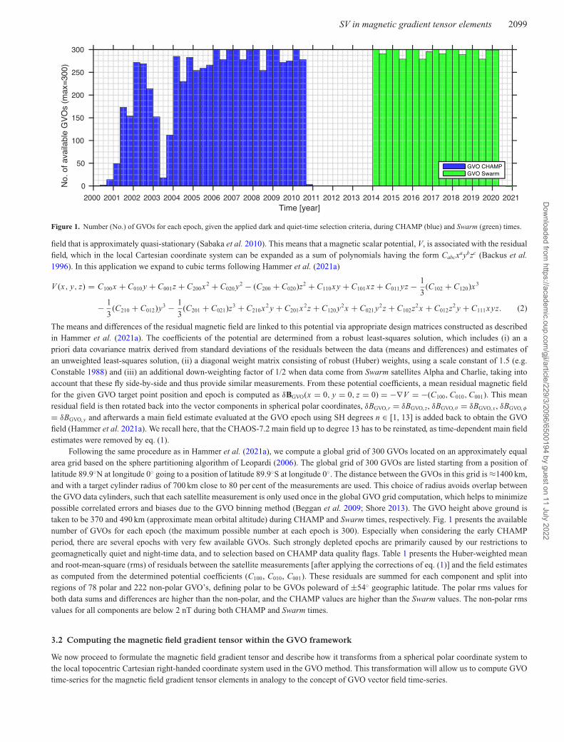
Figure 1. Number (No.) of GVOs for each epoch, given the applied dark and quiet-time selection criteria, during CHAMP (blue) and Swarm (green) times.

field that is approximately quasi-stationary (Sabaka et al. 2010). This means that a magnetic scalar potential, V, is associated with the residualfield, which in the local Cartesian coordinate system can be expanded as a sum of polynomials having the form Cabcxaybzc (Backus et al.1996). In this application we expand to cubic terms following Hammer et al. (2021a)

V (x, y, z) = C100x + C010 y + C001z + C200x2 + C020 y2 − (C200 + C020)z2 + C110xy + C101xz + C011 yz − 1

3(C102 + C120)x3

− 1

3(C210 + C012)y3 − 1

3(C201 + C021)z3 + C210x2 y + C201x2z + C120 y2x + C021 y2z + C102z2x + C012z2 y + C111xyz. (2)

The means and differences of the residual magnetic field are linked to this potential via appropriate design matrices constructed as describedin Hammer et al. (2021a). The coefficients of the potential are determined from a robust least-squares solution, which includes (i) an apriori data covariance matrix derived from standard deviations of the residuals between the data (means and differences) and estimates ofan unweighted least-squares solution, (ii) a diagonal weight matrix consisting of robust (Huber) weights, using a scale constant of 1.5 (e.g.Constable 1988) and (iii) an additional down-weighting factor of 1/2 when data come from Swarm satellites Alpha and Charlie, taking intoaccount that these fly side-by-side and thus provide similar measurements. From these potential coefficients, a mean residual magnetic fieldfor the given GVO target point position and epoch is computed as δBGVO(x = 0, y = 0, z = 0) = −∇V = −(C100, C010, C001). This meanresidual field is then rotated back into the vector components in spherical polar coordinates, δBGVO, r = δBGVO, z, δBGVO, θ = δBGVO, x, δBGVO, φ

= δBGVO, y and afterwards a main field estimate evaluated at the GVO epoch using SH degrees n ∈ [1, 13] is added back to obtain the GVOfield (Hammer et al. 2021a). We recall here, that the CHAOS-7.2 main field up to degree 13 has to be reinstated, as time-dependent main fieldestimates were removed by eq. (1).

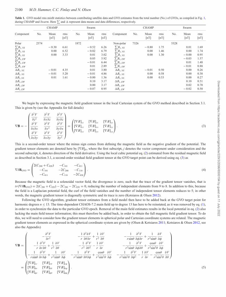
Following the same procedure as in Hammer et al. (2021a), we compute a global grid of 300 GVOs located on an approximately equalarea grid based on the sphere partitioning algorithm of Leopardi (2006). The global grid of 300 GVOs are listed starting from a position oflatitude 89.9◦N at longitude 0◦ going to a position of latitude 89.9◦S at longitude 0◦. The distance between the GVOs in this grid is ≈1400 km,and with a target cylinder radius of 700 km close to 80 per cent of the measurements are used. This choice of radius avoids overlap betweenthe GVO data cylinders, such that each satellite measurement is only used once in the global GVO grid computation, which helps to minimizepossible correlated errors and biases due to the GVO binning method (Beggan et al. 2009; Shore 2013). The GVO height above ground istaken to be 370 and 490 km (approximate mean orbital altitude) during CHAMP and Swarm times, respectively. Fig. 1 presents the availablenumber of GVOs for each epoch (the maximum possible number at each epoch is 300). Especially when considering the early CHAMPperiod, there are several epochs with very few available GVOs. Such strongly depleted epochs are primarily caused by our restrictions togeomagnetically quiet and night-time data, and to selection based on CHAMP data quality flags. Table 1 presents the Huber-weighted meanand root-mean-square (rms) of residuals between the satellite measurements [after applying the corrections of eq. (1)] and the field estimatesas computed from the determined potential coefficients (C100, C010, C001). These residuals are summed for each component and split intoregions of 78 polar and 222 non-polar GVO’s, defining polar to be GVOs poleward of ±54◦ geographic latitude. The polar rms values forboth data sums and differences are higher than the non-polar, and the CHAMP values are higher than the Swarm values. The non-polar rmsvalues for all components are below 2 nT during both CHAMP and Swarm times.

3.2 Computing the magnetic field gradient tensor within the GVO framework

We now proceed to formulate the magnetic field gradient tensor and describe how it transforms from a spherical polar coordinate system tothe local topocentric Cartesian right-handed coordinate system used in the GVO method. This transformation will allow us to compute GVOtime-series for the magnetic field gradient tensor elements in analogy to the concept of GVO vector field time-series.

Dow




Table 1. GVO model rms misfit statistics between contributing satellite data and GVO estimates from the total number (No.) of GVOs, as compiled in Fig. 1,during CHAMP and Swarm. Here

∑and � represent data means and data differences, respectively.

CHAMP Swarm CHAMP Swarm

Component No. Mean rms No. Mean rms Component No. Mean rms No. Mean rms[nT] [nT] [nT] [nT] [nT] [nT] [nT] [nT]

Polar 2574 1872 Non-polar 7326 5328∑Bx, NS − 0.30 6.61 − 0.52 6.26

∑Bx, NS − 0.80 1.75 0.01 1.69∑

By, NS 0.00 6.52 − 0.02 6.79∑

By, NS 0.00 1.46 0.00 1.74∑Bz, NS 0.00 3.33 0.01 3.02

∑Bz, NS 0.00 1.30 − 0.00 0.95∑

Bx, EW 0.05 5.92∑

Bx, EW − 0.03 1.57∑By, EW − 0.01 6.44

∑By, EW 0.01 1.48∑

Bz, EW 0.01 2.89∑

Bz, EW − 0.01 0.88�Bx, NS − 0.01 4.35 0.01 3.80 �Bx, NS − 0.01 0.50 0.00 0.26�By, NS − 0.01 5.20 − 0.01 4.86 �By, NS 0.00 0.58 0.00 0.38�Bz, NS 0.01 1.61 − 0.00 1.36 �Bz, NS 0.00 0.53 0.00 0.27�Bx, EW 0.10 3.17 �Bx, EW 0.10 0.51�By, EW 0.00 3.17 �By, EW 0.02 0.70�Bz, EW − 0.07 0.95 �Bz, EW − 0.02 0.50

We begin by expressing the magnetic field gradient tensor in the local Cartesian system of the GVO method described in Section 3.1.This is given by (see the Appendix for full details)

∇B = −

⎛⎜⎜⎜⎜⎜⎜⎜⎝

∂2V

∂z2

∂2V

∂x∂z

∂2V

∂y∂z∂2V

∂z∂x

∂2V

∂x2

∂2V

∂y∂x∂2V

∂z∂y

∂2V

∂x∂y

∂2V

∂y2

⎞⎟⎟⎟⎟⎟⎟⎟⎠

=

⎛⎜⎝[∇ B]zz [∇ B]zx [∇ B]zy

[∇ B]xz [∇ B]xx [∇ B]xy

[∇ B]yz [∇ B]yx [∇ B]yy

⎞⎟⎠ . (3)

This is a second-order tensor where the minus sign comes from defining the magnetic field as the negative gradient of the potential. Thegradient tensor elements are denoted here by [∇B]jk, where the first subscript, j denotes the vector component under consideration and thesecond subscript, k, denotes direction of the field derivative. Using the local cubic potential eq. (2) estimated from the residual magnetic fieldas described in Section 3.1, a second-order residual field gradient tensor at the GVO target point can be derived using eq. (3) as

∇δBGVO =

⎛⎜⎝2(C200 + C020) −C101 −C011

−C101 −2C200 −C110

−C011 −C110 −2C020

⎞⎟⎠ . (4)

Because the magnetic field is a solenoidal vector field, the divergence is zero, such that the trace of the gradient tensor vanishes, that istr (∇δBGVO) = 2(C200 + C020) − 2C200 − 2C020 = 0, reducing the number of independent elements from 9 to 8. In addition to this, becausethe field is a Laplacian potential field, the curl of the field vanishes and the number of independent tensor elements reduces to 5; in otherwords, the magnetic gradient tensor is diagonally symmetric and its trace is zero (Kotsiaros & Olsen 2012).

Following the GVO algorithm, gradient tensor estimates from a field model then have to be added back at the GVO target point forharmonic degrees n ≤ 13. The time-dependent CHAOS-7.2 main field up to degree 13 has here to be reinstated, as it was removed by eq. (1),in order to synchronize the data to the particular GVO epoch. Removal of the main field estimates results in the local potential in eq. (2) alsolacking the main field tensor information; this must therefore be added back, in order to obtain the full magnetic field gradient tensor. To dothis, we will need to consider how the gradient tensor elements in spherical polar and Cartesian coordinate systems are related. The magneticgradient tensor elements as expressed in the spherical coordinate system are given by (Olsen & Kotsiaros 2011; Kotsiaros & Olsen 2012, seealso the Appendix)

∇B =

⎛⎜⎜⎜⎜⎜⎜⎜⎝

−∂2V

∂r 2−1

r

∂2∂V

∂θ∂r+ 1

r 2

∂V

∂θ− 1

rsinθ

∂2V

∂φ∂r+ 1

r 2sinθ

∂V

∂φ

−1

r

∂2V

∂r∂θ+ 1

r 2

∂V

∂θ− 1

r 2

∂2V

∂θ 2− 1

r

∂V

∂r− 1

r 2sinθ

∂2V

∂φ∂θ+ cosθ

r 2sin2θ

∂V

∂φ

− 1

rsinθ

∂2V

∂r∂φ+ 1

r 2sinθ

∂V

∂φ− 1

r 2sinθ

∂2V

∂θ∂φ+ cosθ

r 2sin2θ

∂V

∂φ− 1

r 2sin2θ

∂2V

∂φ2− 1

r

∂V

∂r− cosθ

r 2sin2θ

∂V

∂θ

⎞⎟⎟⎟⎟⎟⎟⎟⎠

=

⎛⎜⎝[∇ B]rr [∇ B]rθ [∇ B]rφ

[∇ B]θr [∇ B]θθ [∇ B]θφ

[∇ B]φr [∇ B]φθ [∇ B]φφ

⎞⎟⎠ . (5)

Dow




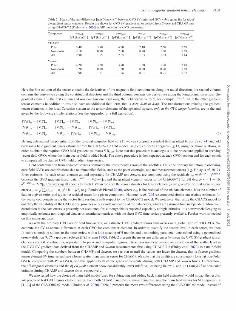
Table 2. Mean of the rms differences [in pT (km yr)–1] between GVO SV series and GCV cubic spline fits for six ofthe gradient tensor elements. Results are shown for GVO SV gradient series derived from Swarm and CHAMP datausing CHAOS-7.2 (Finlay et al. 2020) as MF model in the GVO processing.

Component rms[rr] rms[θθ] rms[φφ] rms[rθ] rms[rφ] rms[θφ]

[pT (km yr)–1] [pT (km yr)–1] [pT (km yr)–1] [pT (km yr)–1] [pT (km yr)–1] [pT (km yr)–1]

CHAMPPolar 5.40 3.90 4.20 2.10 2.60 2.60Non-polar 2.10 0.70 2.00 0.70 1.60 0.60All 2.98 1.55 2.55 1.03 1.83 1.14

SwarmPolar 4.20 3.20 3.90 1.60 1.70 2.10Non-polar 1.20 0.30 1.20 0.30 0.70 0.60All 1.98 1.01 1.86 0.61 0.95 0.97

Here the first column of the tensor contains the derivatives of the magnetic field components along the radial direction, the second columncontains the derivatives along the colatitudinal direction and the third column contains the derivatives along the longitudinal direction. Thegradient element in the first column and row contains one term only, the field derivative term, for example ∂2/∂r2, while the other gradienttensor elements in addition to this also have an additional field term, that is ∂/∂r, ∂/∂θ or ∂/∂φ. The transformations relating the gradienttensor elements in the local Cartesian system to the tensor elements of the spherical system, only at the GVO target location, are in the endgiven by the following simple relations (see the Appendix for a full derivation).

[∇ B]zz = [∇ B]rr [∇ B]zx = [∇ B]rθ [∇ B]zy = [∇ B]rφ

[∇ B]xz = [∇ B]θr [∇ B]xx = [∇ B]θθ [∇ B]xy = [∇ B]θφ

[∇ B]yz = [∇ B]φr [∇ B]yx = [∇ B]φθ [∇ B]yy = [∇ B]φφ . (6)

Having determined the potential from the residual magnetic field eq. (1), we can compute a residual field gradient tensor by eq. (4) and addback main field gradient tensor estimates from the CHAOS-7.2 field model using eq. (5) for SH degrees n ≤ 13, using the above relations, inorder to obtain the required GVO field gradient estimates ∇BGVO. Note that this procedure is analogous to the procedure applied in derivingvector field GVOs where the main vector field is added back. The above procedure is then repeated at each GVO location and for each epochto compute all the desired GVO field gradient time-series.

Field contamination from non-core sources dominates the instrumental errors of the satellites. Thus, the primary limitation in obtainingcore field GVOs are contributions due to unmodelled fields, such as the polar electrojet, and not measurement errors (e.g. Finlay et al. 2017).Error estimates for each tensor element jk, and separately for CHAMP and Swarm, are computed using the residuals ejk = dGVO − dCHAOS

between the GVO gradient tensor data, dGVO = [∇BGVO]jk, and the gradient element values of the CHAOS-7.2 for SH degree n = 1 − 16,dCHAOS = [∇B]jk. Considering all epochs for each GVO in the grid, the error estimates for tensor element jk are given by the total mean square

error σ jk =√∑

i (e jk,i − μ jk)2/M + μ2jk (e.g. Bendat & Piersol 2010), where ejk,i is the residual of the ith data element, M is the number of

data in a given series and μjk is the residual mean for a given component. Hammer et al. (2021a) computed similar uncertainty estimates forthe vector components using the vector field residuals with respect to the CHAOS-7.2 model. We note here, that using the CHAOS model toquantify the variability of the GVO series, provides only a crude indication of the data errors, which are assumed time independent. Moreover,correlation in the data errors is presently not accounted for, although this is expected especially at high latitudes. It is however challenging toempirically estimate non-diagonal data error covariance matrices with the short GVO time-series presently available. Further work is neededon this important topic.

As with the ordinary GVO vector field time-series, we estimate GVO gradient tensor time-series on a global grid of 300 GVOs. Wecompute the SV as annual differences at each GVO for each tensor element. In order to quantify the scatter level in each series, we thenfit cubic smoothing splines to the time-series, with a knot spacing of 4 months and a smoothing parameter determined using a generalizedcross-validation (GCV) approach (Green & Silverman 1993). Table 2 presents the mean rms differences between the GVO SV gradient tensorelements and GCV spline fits, separated into polar and non-polar regions. These rms numbers provide an indication of the scatter level inthe GVO SV gradient data derived from the CHAMP and Swarm measurements first using CHAOS-7.2 (Finlay et al. 2020) as a main fieldmodel. Comparing the numbers between CHAMP and Swarm, we see that overall the values are lower for Swarm, that is Swarm gradienttensor element SV time-series have a lower scatter than similar series for CHAMP. We note that the misfits are considerably lower at non-PolarGVOs, compared with Polar GVOs, and this applies to all of the gradient elements, during both CHAMP and Swarm times. Furthermore,the off-diagonal elements and the d[∇B]θθ /dt element show considerably lower misfit values being below 2 and 1 pT (km yr)–1 at non-Polarlatitudes during CHAMP and Swarm times, respectively.

We also tested how the choice of main field model (used for subtracting and adding back main field estimates) would impact the results.We produced test GVO tensor element series from both CHAMP and Swarm measurements using the main field values for SH degrees n ∈[1, 13] of the COV-OBS.x2 model (Huder et al. 2020). Table 3 presents the mean rms differences using the COV-OBS.x2 model instead of

Dow




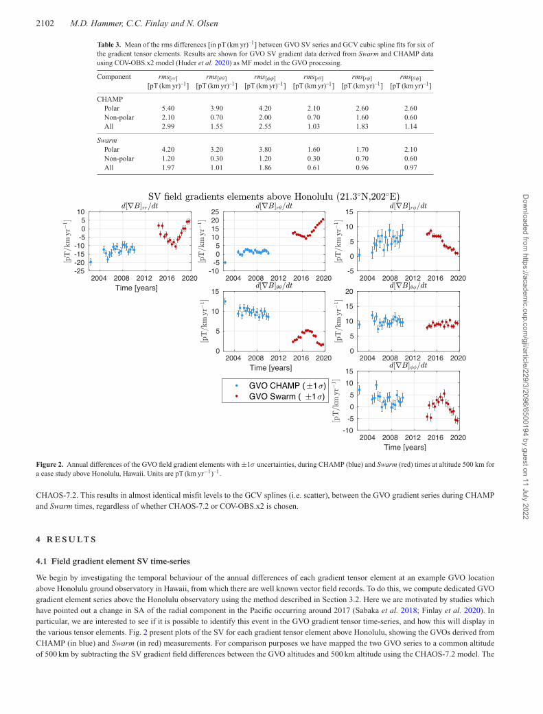
Table 3. Mean of the rms differences [in pT (km yr)–1] between GVO SV series and GCV cubic spline fits for six ofthe gradient tensor elements. Results are shown for GVO SV gradient data derived from Swarm and CHAMP datausing COV-OBS.x2 model (Huder et al. 2020) as MF model in the GVO processing.

Component rms[rr] rms[θθ] rms[φφ] rms[rθ] rms[rφ] rms[θφ]

[pT (km yr)–1] [pT (km yr)–1] [pT (km yr)–1] [pT (km yr)–1] [pT (km yr)–1] [pT (km yr)–1]

CHAMPPolar 5.40 3.90 4.20 2.10 2.60 2.60Non-polar 2.10 0.70 2.00 0.70 1.60 0.60All 2.99 1.55 2.55 1.03 1.83 1.14

SwarmPolar 4.20 3.20 3.80 1.60 1.70 2.10Non-polar 1.20 0.30 1.20 0.30 0.70 0.60All 1.97 1.01 1.86 0.61 0.96 0.97

Figure 2. Annual differences of the GVO field gradient elements with ±1σ uncertainties, during CHAMP (blue) and Swarm (red) times at altitude 500 km fora case study above Honolulu, Hawaii. Units are pT (km yr−1)–1.

CHAOS-7.2. This results in almost identical misfit levels to the GCV splines (i.e. scatter), between the GVO gradient series during CHAMPand Swarm times, regardless of whether CHAOS-7.2 or COV-OBS.x2 is chosen.

4 R E S U LT S

4.1 Field gradient element SV time-series

We begin by investigating the temporal behaviour of the annual differences of each gradient tensor element at an example GVO locationabove Honolulu ground observatory in Hawaii, from which there are well known vector field records. To do this, we compute dedicated GVOgradient element series above the Honolulu observatory using the method described in Section 3.2. Here we are motivated by studies whichhave pointed out a change in SA of the radial component in the Pacific occurring around 2017 (Sabaka et al. 2018; Finlay et al. 2020). Inparticular, we are interested to see if it is possible to identify this event in the GVO gradient tensor time-series, and how this will display inthe various tensor elements. Fig. 2 present plots of the SV for each gradient tensor element above Honolulu, showing the GVOs derived fromCHAMP (in blue) and Swarm (in red) measurements. For comparison purposes we have mapped the two GVO series to a common altitudeof 500 km by subtracting the SV gradient field differences between the GVO altitudes and 500 km altitude using the CHAOS-7.2 model. The

Dow




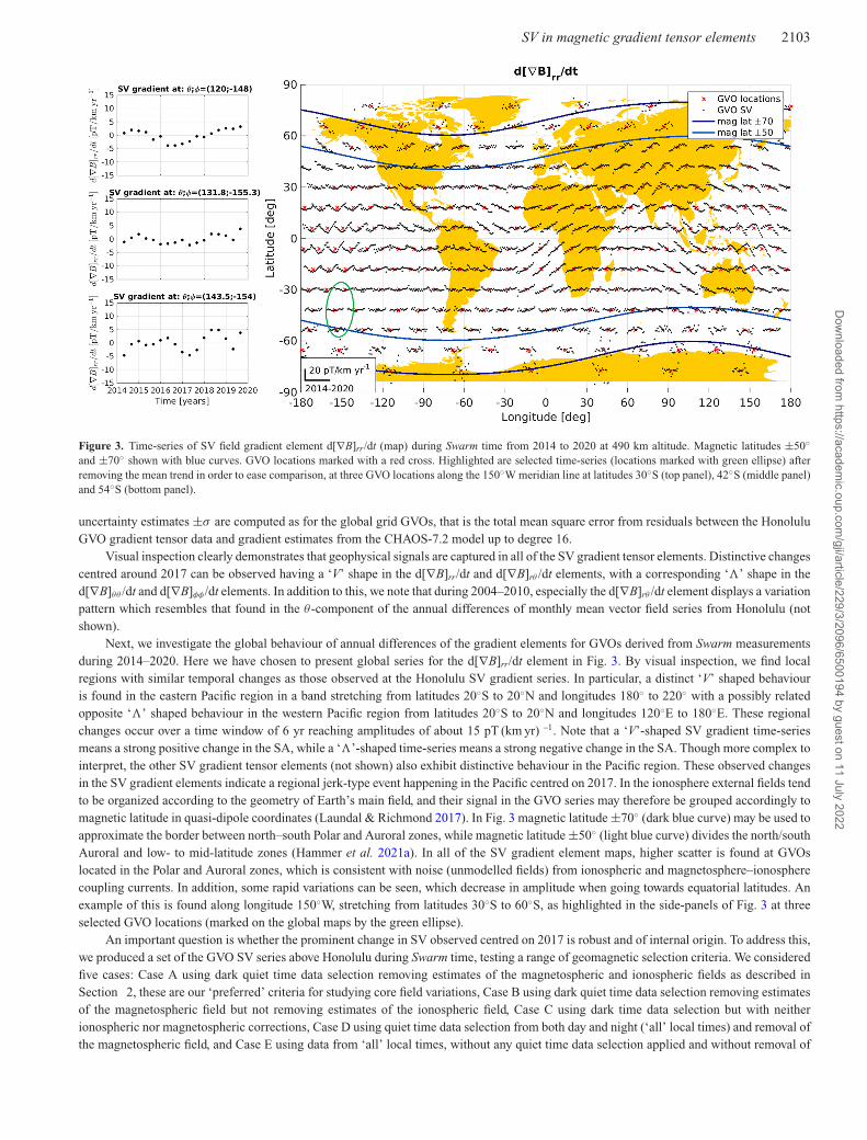
Figure 3. Time-series of SV field gradient element d[∇B]rr/dt (map) during Swarm time from 2014 to 2020 at 490 km altitude. Magnetic latitudes ±50◦and ±70◦ shown with blue curves. GVO locations marked with a red cross. Highlighted are selected time-series (locations marked with green ellipse) afterremoving the mean trend in order to ease comparison, at three GVO locations along the 150◦W meridian line at latitudes 30◦S (top panel), 42◦S (middle panel)and 54◦S (bottom panel).

uncertainty estimates ±σ are computed as for the global grid GVOs, that is the total mean square error from residuals between the HonoluluGVO gradient tensor data and gradient estimates from the CHAOS-7.2 model up to degree 16.

Visual inspection clearly demonstrates that geophysical signals are captured in all of the SV gradient tensor elements. Distinctive changescentred around 2017 can be observed having a ‘V’ shape in the d[∇B]rr/dt and d[∇B]rθ /dt elements, with a corresponding ‘’ shape in thed[∇B]θθ /dt and d[∇B]φφ /dt elements. In addition to this, we note that during 2004–2010, especially the d[∇B]rθ /dt element displays a variationpattern which resembles that found in the θ -component of the annual differences of monthly mean vector field series from Honolulu (notshown).

Next, we investigate the global behaviour of annual differences of the gradient elements for GVOs derived from Swarm measurementsduring 2014–2020. Here we have chosen to present global series for the d[∇B]rr/dt element in Fig. 3. By visual inspection, we find localregions with similar temporal changes as those observed at the Honolulu SV gradient series. In particular, a distinct ‘V’ shaped behaviouris found in the eastern Pacific region in a band stretching from latitudes 20◦S to 20◦N and longitudes 180◦ to 220◦ with a possibly relatedopposite ‘’ shaped behaviour in the western Pacific region from latitudes 20◦S to 20◦N and longitudes 120◦E to 180◦E. These regionalchanges occur over a time window of 6 yr reaching amplitudes of about 15 pT (km yr) –1. Note that a ‘V’-shaped SV gradient time-seriesmeans a strong positive change in the SA, while a ‘’-shaped time-series means a strong negative change in the SA. Though more complex tointerpret, the other SV gradient tensor elements (not shown) also exhibit distinctive behaviour in the Pacific region. These observed changesin the SV gradient elements indicate a regional jerk-type event happening in the Pacific centred on 2017. In the ionosphere external fields tendto be organized according to the geometry of Earth’s main field, and their signal in the GVO series may therefore be grouped accordingly tomagnetic latitude in quasi-dipole coordinates (Laundal & Richmond 2017). In Fig. 3 magnetic latitude ±70◦ (dark blue curve) may be used toapproximate the border between north–south Polar and Auroral zones, while magnetic latitude ±50◦ (light blue curve) divides the north/southAuroral and low- to mid-latitude zones (Hammer et al. 2021a). In all of the SV gradient element maps, higher scatter is found at GVOslocated in the Polar and Auroral zones, which is consistent with noise (unmodelled fields) from ionospheric and magnetosphere–ionospherecoupling currents. In addition, some rapid variations can be seen, which decrease in amplitude when going towards equatorial latitudes. Anexample of this is found along longitude 150◦W, stretching from latitudes 30◦S to 60◦S, as highlighted in the side-panels of Fig. 3 at threeselected GVO locations (marked on the global maps by the green ellipse).

An important question is whether the prominent change in SV observed centred on 2017 is robust and of internal origin. To address this,we produced a set of the GVO SV series above Honolulu during Swarm time, testing a range of geomagnetic selection criteria. We consideredfive cases: Case A using dark quiet time data selection removing estimates of the magnetospheric and ionospheric fields as described inSection 2, these are our ‘preferred’ criteria for studying core field variations, Case B using dark quiet time data selection removing estimatesof the magnetospheric field but not removing estimates of the ionospheric field, Case C using dark time data selection but with neitherionospheric nor magnetospheric corrections, Case D using quiet time data selection from both day and night (‘all’ local times) and removal ofthe magnetospheric field, and Case E using data from ‘all’ local times, without any quiet time data selection applied and without removal of

Dow




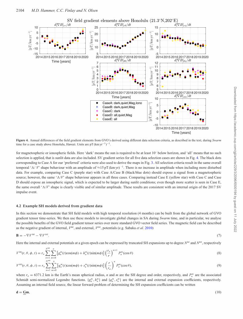
Figure 4. Annual differences of the field gradient elements from GVO’s derived using different data selection criteria, as described in the text, during Swarmtime for a case study above Honolulu, Hawaii. Units are pT (km yr−1)−1.

for magnetospheric or ionospheric fields. Here ‘dark’ means the sun is required to be at least 10◦ below horizon, and ‘all’ means that no suchselection is applied, that is sunlit data are also included. SV gradient series for all five data selection cases are shown in Fig. 4. The black dotscorresponding to Case A for our ‘preferred’ criteria were also used to derive the maps in Fig. 3. All selection criteria result in the same overalltemporal ‘/ V’ shape behaviour with an amplitude of ≈15 pT (km yr) –1. There is no increase in amplitude when including more disturbeddata. For example, comparing Case C (purple star) with Case A/Case B (black/blue dots) should expose a signal from a magnetosphericsource; however, the same ‘/V’ shape behaviour appears in all three cases. Comparing instead Case E (yellow star) with Case C and CaseD should expose an ionospheric signal, which is expected to be larger during sunlit conditions; even though more scatter is seen in Case E,the same overall ‘/V’ shape is clearly visible and of similar amplitude. These results are consistent with an internal origin of the 2017 SVimpulse event.

4.2 Example SH models derived from gradient data

In this section we demonstrate that SH field models with high temporal resolution (4 months) can be built from the global network of GVOgradient tensor time-series. We then use these models to investigate global changes in SA during Swarm time, and in particular, we analysethe possible benefits of the GVO field gradient tensor series over more standard GVO vector field series. The magnetic field can be describedas the negative gradient of internal, Vint, and external, Vext, potentials (e.g. Sabaka et al. 2010)

B = −∇V int − ∇V ext. (7)

Here the internal and external potentials at a given epoch can be expressed by truncated SH expansions up to degree Nint and Next, respectively

V int(r, θ, φ, t) = ra

N int∑n=1

n∑m=0

[gm

n (t)cos(mφ) + hmn (t)sin(mφ)

] (ra

r

)n+1Pm

n (cos θ ) (8)

V ext(r, θ, φ, t) = ra

N ext∑n=1

n∑m=0

[qm

n (t)cos(mφ) + smn (t)sin(mφ)

] (r

ra

)n

Pmn (cos θ ), (9)

where ra = 6371.2 km is the Earth’s mean spherical radius, n and m are the SH degree and order, respectively, and Pmn are the associated

Schmidt semi-normalized Legendre functions. {gmn , hm

n } and {qmn , sm

n } are the internal and external expansion coefficients, respectively.Assuming an internal field source, the linear forward problem of determining the SH expansion coefficients can be written

d = Gm, (10)

Dow




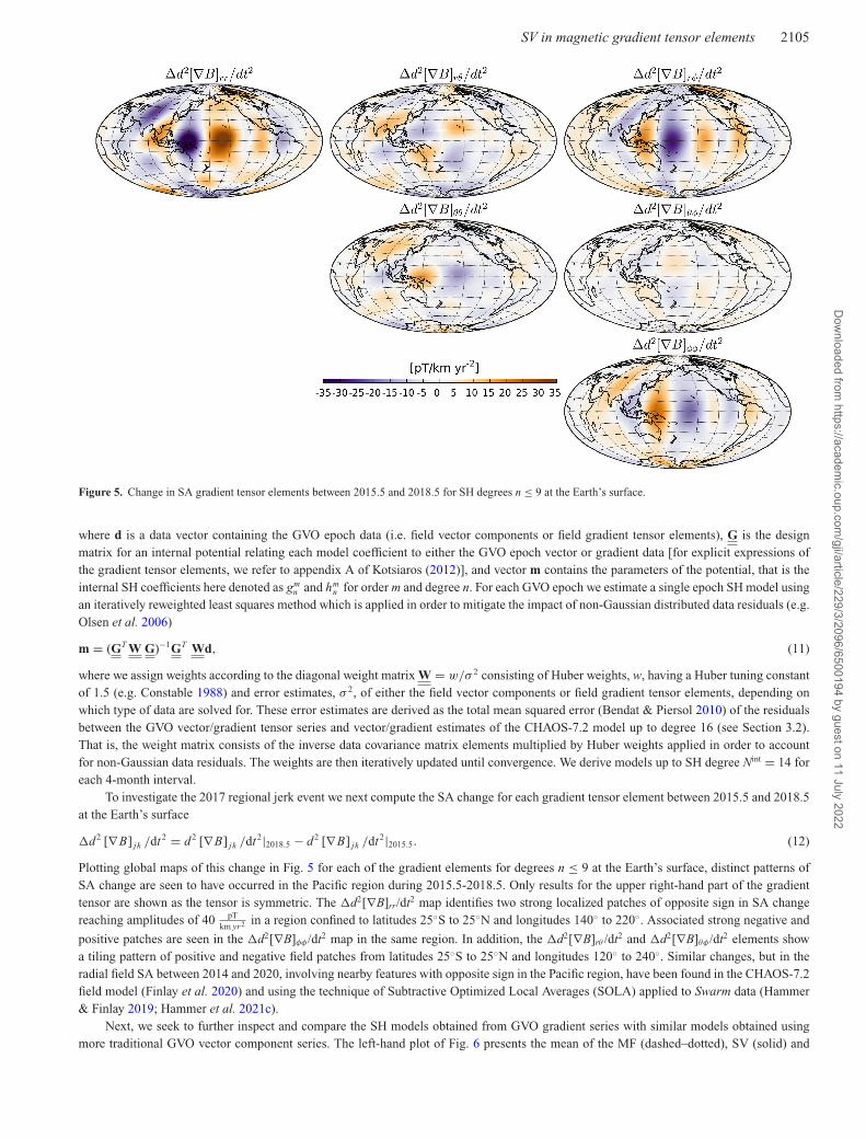
Figure 5. Change in SA gradient tensor elements between 2015.5 and 2018.5 for SH degrees n ≤ 9 at the Earth’s surface.

where d is a data vector containing the GVO epoch data (i.e. field vector components or field gradient tensor elements), G is the designmatrix for an internal potential relating each model coefficient to either the GVO epoch vector or gradient data [for explicit expressions ofthe gradient tensor elements, we refer to appendix A of Kotsiaros (2012)], and vector m contains the parameters of the potential, that is theinternal SH coefficients here denoted as gm

n and hmn for order m and degree n. For each GVO epoch we estimate a single epoch SH model using

an iteratively reweighted least squares method which is applied in order to mitigate the impact of non-Gaussian distributed data residuals (e.g.Olsen et al. 2006)

m = (GT W G)−1GT Wd, (11)

where we assign weights according to the diagonal weight matrix W = w/σ 2 consisting of Huber weights, w, having a Huber tuning constantof 1.5 (e.g. Constable 1988) and error estimates, σ 2, of either the field vector components or field gradient tensor elements, depending onwhich type of data are solved for. These error estimates are derived as the total mean squared error (Bendat & Piersol 2010) of the residualsbetween the GVO vector/gradient tensor series and vector/gradient estimates of the CHAOS-7.2 model up to degree 16 (see Section 3.2).That is, the weight matrix consists of the inverse data covariance matrix elements multiplied by Huber weights applied in order to accountfor non-Gaussian data residuals. The weights are then iteratively updated until convergence. We derive models up to SH degree Nint = 14 foreach 4-month interval.

To investigate the 2017 regional jerk event we next compute the SA change for each gradient tensor element between 2015.5 and 2018.5at the Earth’s surface

�d2 [∇ B] jk /dt2 = d2 [∇ B] jk /dt2|2018.5 − d2 [∇ B] jk /dt2|2015.5. (12)

Plotting global maps of this change in Fig. 5 for each of the gradient elements for degrees n ≤ 9 at the Earth’s surface, distinct patterns ofSA change are seen to have occurred in the Pacific region during 2015.5-2018.5. Only results for the upper right-hand part of the gradienttensor are shown as the tensor is symmetric. The �d2[∇B]rr/dt2 map identifies two strong localized patches of opposite sign in SA changereaching amplitudes of 40 pT

km yr2 in a region confined to latitudes 25◦S to 25◦N and longitudes 140◦ to 220◦. Associated strong negative and

positive patches are seen in the �d2[∇B]φφ /dt2 map in the same region. In addition, the �d2[∇B]rθ /dt2 and �d2[∇B]θφ /dt2 elements showa tiling pattern of positive and negative field patches from latitudes 25◦S to 25◦N and longitudes 120◦ to 240◦. Similar changes, but in theradial field SA between 2014 and 2020, involving nearby features with opposite sign in the Pacific region, have been found in the CHAOS-7.2field model (Finlay et al. 2020) and using the technique of Subtractive Optimized Local Averages (SOLA) applied to Swarm data (Hammer& Finlay 2019; Hammer et al. 2021c).

Next, we seek to further inspect and compare the SH models obtained from GVO gradient series with similar models obtained usingmore traditional GVO vector component series. The left-hand plot of Fig. 6 presents the mean of the MF (dashed–dotted), SV (solid) and

Dow




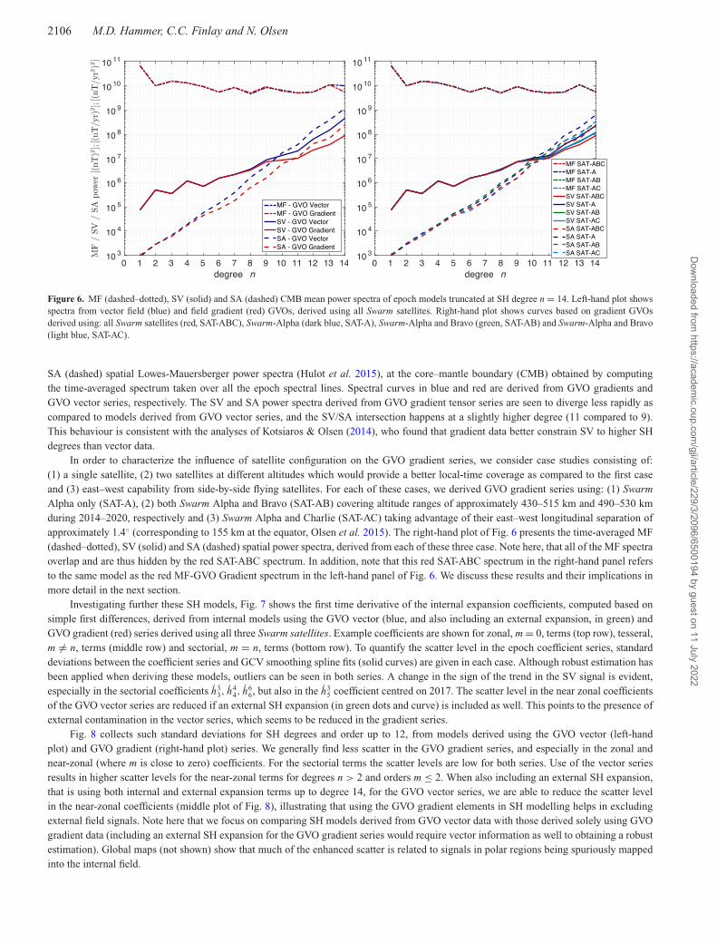
Figure 6. MF (dashed–dotted), SV (solid) and SA (dashed) CMB mean power spectra of epoch models truncated at SH degree n = 14. Left-hand plot showsspectra from vector field (blue) and field gradient (red) GVOs, derived using all Swarm satellites. Right-hand plot shows curves based on gradient GVOsderived using: all Swarm satellites (red, SAT-ABC), Swarm-Alpha (dark blue, SAT-A), Swarm-Alpha and Bravo (green, SAT-AB) and Swarm-Alpha and Bravo(light blue, SAT-AC).

SA (dashed) spatial Lowes-Mauersberger power spectra (Hulot et al. 2015), at the core–mantle boundary (CMB) obtained by computingthe time-averaged spectrum taken over all the epoch spectral lines. Spectral curves in blue and red are derived from GVO gradients andGVO vector series, respectively. The SV and SA power spectra derived from GVO gradient tensor series are seen to diverge less rapidly ascompared to models derived from GVO vector series, and the SV/SA intersection happens at a slightly higher degree (11 compared to 9).This behaviour is consistent with the analyses of Kotsiaros & Olsen (2014), who found that gradient data better constrain SV to higher SHdegrees than vector data.

In order to characterize the influence of satellite configuration on the GVO gradient series, we consider case studies consisting of:(1) a single satellite, (2) two satellites at different altitudes which would provide a better local-time coverage as compared to the first caseand (3) east–west capability from side-by-side flying satellites. For each of these cases, we derived GVO gradient series using: (1) SwarmAlpha only (SAT-A), (2) both Swarm Alpha and Bravo (SAT-AB) covering altitude ranges of approximately 430–515 km and 490–530 kmduring 2014–2020, respectively and (3) Swarm Alpha and Charlie (SAT-AC) taking advantage of their east–west longitudinal separation ofapproximately 1.4◦ (corresponding to 155 km at the equator, Olsen et al. 2015). The right-hand plot of Fig. 6 presents the time-averaged MF(dashed–dotted), SV (solid) and SA (dashed) spatial power spectra, derived from each of these three case. Note here, that all of the MF spectraoverlap and are thus hidden by the red SAT-ABC spectrum. In addition, note that this red SAT-ABC spectrum in the right-hand panel refersto the same model as the red MF-GVO Gradient spectrum in the left-hand panel of Fig. 6. We discuss these results and their implications inmore detail in the next section.

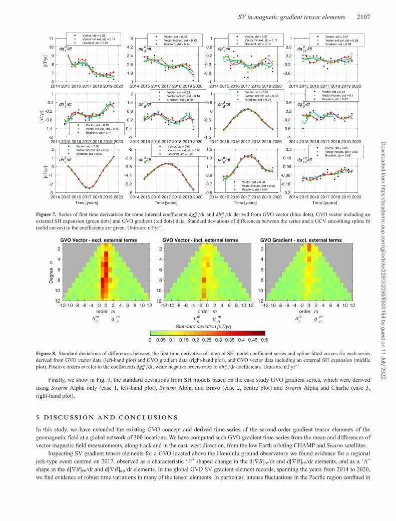
Investigating further these SH models, Fig. 7 shows the first time derivative of the internal expansion coefficients, computed based onsimple first differences, derived from internal models using the GVO vector (blue, and also including an external expansion, in green) andGVO gradient (red) series derived using all three Swarm satellites. Example coefficients are shown for zonal, m = 0, terms (top row), tesseral,m �= n, terms (middle row) and sectorial, m = n, terms (bottom row). To quantify the scatter level in the epoch coefficient series, standarddeviations between the coefficient series and GCV smoothing spline fits (solid curves) are given in each case. Although robust estimation hasbeen applied when deriving these models, outliers can be seen in both series. A change in the sign of the trend in the SV signal is evident,especially in the sectorial coefficients h3

3, h44, h6

6, but also in the h35 coefficient centred on 2017. The scatter level in the near zonal coefficients

of the GVO vector series are reduced if an external SH expansion (in green dots and curve) is included as well. This points to the presence ofexternal contamination in the vector series, which seems to be reduced in the gradient series.

Fig. 8 collects such standard deviations for SH degrees and order up to 12, from models derived using the GVO vector (left-handplot) and GVO gradient (right-hand plot) series. We generally find less scatter in the GVO gradient series, and especially in the zonal andnear-zonal (where m is close to zero) coefficients. For the sectorial terms the scatter levels are low for both series. Use of the vector seriesresults in higher scatter levels for the near-zonal terms for degrees n > 2 and orders m ≤ 2. When also including an external SH expansion,that is using both internal and external expansion terms up to degree 14, for the GVO vector series, we are able to reduce the scatter levelin the near-zonal coefficients (middle plot of Fig. 8), illustrating that using the GVO gradient elements in SH modelling helps in excludingexternal field signals. Note here that we focus on comparing SH models derived from GVO vector data with those derived solely using GVOgradient data (including an external SH expansion for the GVO gradient series would require vector information as well to obtaining a robustestimation). Global maps (not shown) show that much of the enhanced scatter is related to signals in polar regions being spuriously mappedinto the internal field.

Dow




Figure 7. Series of first time derivatives for some internal coefficients dgmn /dt and dhm

n /dt derived from GVO vector (blue dots), GVO vector including anexternal SH expansion (green dots) and GVO gradient (red dots) data. Standard deviations of differences between the series and a GCV smoothing spline fit(solid curves) to the coefficients are given. Units are nT yr–1.

Figure 8. Standard deviations of differences between the first time derivative of internal SH model coefficient series and spline-fitted curves for each seriesderived from GVO vector data (left-hand plot) and GVO gradient data (right-hand plot), and GVO vector data including an external SH expansion (middleplot). Positive orders m refer to the coefficients dgm

n /dt , while negative orders refer to dhmn /dt coefficients. Units are nT yr–1.

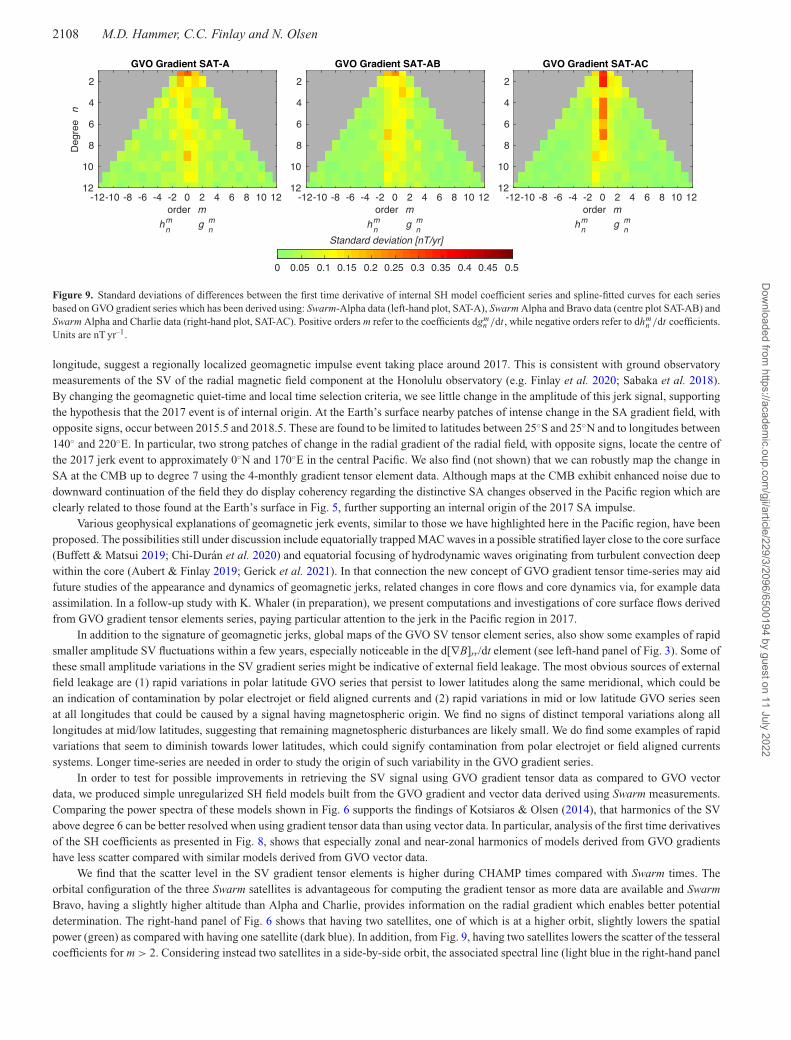
Finally, we show in Fig. 9, the standard deviations from SH models based on the case study GVO gradient series, which were derivedusing Swarm Alpha only (case 1, left-hand plot), Swarm Alpha and Bravo (case 2, centre plot) and Swarm Alpha and Charlie (case 3,right-hand plot).

5 D I S C U S S I O N A N D C O N C LU S I O N S

In this study, we have extended the existing GVO concept and derived time-series of the second-order gradient tensor elements of thegeomagnetic field at a global network of 300 locations. We have computed such GVO gradient time-series from the mean and differences ofvector magnetic field measurements, along track and in the east–west direction, from the low Earth orbiting CHAMP and Swarm satellites.

Inspecting SV gradient tensor elements for a GVO located above the Honolulu ground observatory we found evidence for a regionaljerk-type event centred on 2017, observed as a characteristic ‘V ’ shaped change in the d[∇B]rr/dt and d[∇B]rθ /dt elements, and as a ‘’shape in the d[∇B]θθ /dt and d[∇B]φφ /dt elements. In the global GVO SV gradient element records, spanning the years from 2014 to 2020,we find evidence of robust time variations in many of the tensor elements. In particular, intense fluctuations in the Pacific region confined in

Dow




Figure 9. Standard deviations of differences between the first time derivative of internal SH model coefficient series and spline-fitted curves for each seriesbased on GVO gradient series which has been derived using: Swarm-Alpha data (left-hand plot, SAT-A), Swarm Alpha and Bravo data (centre plot SAT-AB) andSwarm Alpha and Charlie data (right-hand plot, SAT-AC). Positive orders m refer to the coefficients dgm

n /dt , while negative orders refer to dhmn /dt coefficients.

Units are nT yr–1.

longitude, suggest a regionally localized geomagnetic impulse event taking place around 2017. This is consistent with ground observatorymeasurements of the SV of the radial magnetic field component at the Honolulu observatory (e.g. Finlay et al. 2020; Sabaka et al. 2018).By changing the geomagnetic quiet-time and local time selection criteria, we see little change in the amplitude of this jerk signal, supportingthe hypothesis that the 2017 event is of internal origin. At the Earth’s surface nearby patches of intense change in the SA gradient field, withopposite signs, occur between 2015.5 and 2018.5. These are found to be limited to latitudes between 25◦S and 25◦N and to longitudes between140◦ and 220◦E. In particular, two strong patches of change in the radial gradient of the radial field, with opposite signs, locate the centre ofthe 2017 jerk event to approximately 0◦N and 170◦E in the central Pacific. We also find (not shown) that we can robustly map the change inSA at the CMB up to degree 7 using the 4-monthly gradient tensor element data. Although maps at the CMB exhibit enhanced noise due todownward continuation of the field they do display coherency regarding the distinctive SA changes observed in the Pacific region which areclearly related to those found at the Earth’s surface in Fig. 5, further supporting an internal origin of the 2017 SA impulse.

Various geophysical explanations of geomagnetic jerk events, similar to those we have highlighted here in the Pacific region, have beenproposed. The possibilities still under discussion include equatorially trapped MAC waves in a possible stratified layer close to the core surface(Buffett & Matsui 2019; Chi-Duran et al. 2020) and equatorial focusing of hydrodynamic waves originating from turbulent convection deepwithin the core (Aubert & Finlay 2019; Gerick et al. 2021). In that connection the new concept of GVO gradient tensor time-series may aidfuture studies of the appearance and dynamics of geomagnetic jerks, related changes in core flows and core dynamics via, for example dataassimilation. In a follow-up study with K. Whaler (in preparation), we present computations and investigations of core surface flows derivedfrom GVO gradient tensor elements series, paying particular attention to the jerk in the Pacific region in 2017.

In addition to the signature of geomagnetic jerks, global maps of the GVO SV tensor element series, also show some examples of rapidsmaller amplitude SV fluctuations within a few years, especially noticeable in the d[∇B]rr/dt element (see left-hand panel of Fig. 3). Some ofthese small amplitude variations in the SV gradient series might be indicative of external field leakage. The most obvious sources of externalfield leakage are (1) rapid variations in polar latitude GVO series that persist to lower latitudes along the same meridional, which could bean indication of contamination by polar electrojet or field aligned currents and (2) rapid variations in mid or low latitude GVO series seenat all longitudes that could be caused by a signal having magnetospheric origin. We find no signs of distinct temporal variations along alllongitudes at mid/low latitudes, suggesting that remaining magnetospheric disturbances are likely small. We do find some examples of rapidvariations that seem to diminish towards lower latitudes, which could signify contamination from polar electrojet or field aligned currentssystems. Longer time-series are needed in order to study the origin of such variability in the GVO gradient series.

In order to test for possible improvements in retrieving the SV signal using GVO gradient tensor data as compared to GVO vectordata, we produced simple unregularized SH field models built from the GVO gradient and vector data derived using Swarm measurements.Comparing the power spectra of these models shown in Fig. 6 supports the findings of Kotsiaros & Olsen (2014), that harmonics of the SVabove degree 6 can be better resolved when using gradient tensor data than using vector data. In particular, analysis of the first time derivativesof the SH coefficients as presented in Fig. 8, shows that especially zonal and near-zonal harmonics of models derived from GVO gradientshave less scatter compared with similar models derived from GVO vector data.

We find that the scatter level in the SV gradient tensor elements is higher during CHAMP times compared with Swarm times. Theorbital configuration of the three Swarm satellites is advantageous for computing the gradient tensor as more data are available and SwarmBravo, having a slightly higher altitude than Alpha and Charlie, provides information on the radial gradient which enables better potentialdetermination. The right-hand panel of Fig. 6 shows that having two satellites, one of which is at a higher orbit, slightly lowers the spatialpower (green) as compared with having one satellite (dark blue). In addition, from Fig. 9, having two satellites lowers the scatter of the tesseralcoefficients for m > 2. Considering instead two satellites in a side-by-side orbit, the associated spectral line (light blue in the right-hand panel

Dow




of Fig. 6) is only marginally lower, but differences are most obvious from Fig. 9, where the scatter level of the tesseral coefficients is smaller fororders m > 2. The zonal terms for n < 7 are found in this case to have higher scatter, but this is expected as east–west information alone doesnot allow determination of zonal terms (Kotsiaros & Olsen 2012). Comparing the three case studies with the original case of using all threeSwarm satellites, the associated spatial power (red in the right-hand panel of Fig. 6) is lower, while the scatter level across all SH coefficientsas shown in Fig. 8 is the lowest, except for lowest zonal terms which seems to be related to including the east–west gradient information asshown in the right-hand plot of Fig. 9. In order to mitigate such behaviour of the low degree zonal terms, in future studies it might be worthexploring a Selective Infinite-Variance Weighting approach (Kotsiaros & Olsen 2014; Sabaka et al. 2013), wherein weights are applied todata subsets that are more sensitive to certain parameter subsets. By this approach, the east–west data could in the future be given less weightwith regard to parts of the GVO potential that provide information of the zonal terms. The larger misfits during CHAMP times, may alsoresult from a closer proximity of the lower flying CHAMP satellite to ionospheric current systems. From our tests we therefore conclude thatthe Swarm satellite trio is advantageous for deriving GVO gradient series. Having satellites at different altitudes better fills the 3-D space ofthe GVO data cylinder, improving the recovery of the gradient quantities, for example improving the determination of the tesseral harmonics.Using all three satellites enhances the recovery of all harmonic coefficients and is clearly superior to having a single satellite.

AVA I L A B I L I T Y O F DATA S E T S A N D M AT E R I A L

The GVO gradient tensor data underlying this article and their associated uncertainty estimates are available from https://doi.org/10.11583/DTU.14695590.v2, at (Hammer et al. 2021b). The data sets used in this paper are available at the following repositories: Swarm data areavailable from https://earth.esa.int/web/guest/swarm/data-access (data provided by the European Space Agency); CHAMP data are availablefrom https://isdc.gfz-potsdam.de/champ-isdc; The RC-index is available from http://www.spacecenter.dk/f iles/magnetic-models/RC/; TheCHAOS-7.2 model and its updates are available at http://www.spacecenter.dk/f iles/magnetic-models/CHAOS-7/; the Kp-index is availablefrom ftp://ftp.gfz-potsdam.de/pub/home/obs/kp-ap/ provided by the GFZ German Research Centre for Geosciences; the OMNI data wereobtained from the GSFC/SPDF OMNIWeb interface at https://omniweb.gsfc.nasa.gov/ow.html, (King & Papitashvili (2005).

A C K N OW L E D G M E N T S

We wish to thank Gauthier Hulot and an anonymous reviewer for constructive comments that helped us improve the manuscript. We thankthe GFZ German Research Centre for Geoscience for providing access to the CHAMP MAG-L3 data and the European Space Agency(ESA) for providing access to the Swarm L1b data. The high resolution 1-min OMNI data were provided by the Space Physics Data Facility(SPDF), NASA Goddard Space Flight Centre. We thank the staff of the geomagnetic observatories and the INTERMAGNET for providinghigh-quality observatory data. MDH and CCF were supported by the European Research Council (ERC) under the European Union’s Horizon2020 research and innovation programme (grant agreement No. 772561). In addition, this study was partly funded by ESA through the SwarmDISC activities, contract no. 4000109587.

C O N F L I C T O F I N T E R E S T

The authors declare that they have no competing interests.

R E F E R E N C E SAubert, J. & Finlay, C.C., 2019. Geomagnetic jerks and rapid hydromagnetic

waves focusing at Earth’s core surface, Nat. Geosci., 12(5), 393–398.Backus, G., Parker, R. & Constable, C., 1996. Foundations of Geomag-

netism, Cambridge Univ. Press.Barrois, O., Hammer, M.D., Finlay, C.C., Martin, Y. & Gillet, N., 2018.

Assimilation of ground and satellite magnetic measurements: inferenceof core surface magnetic and velocity field changes, Geophys. J. Int., 215,695–712.

Beggan, C.D., Whaler, K.A. & Macmillan, S., 2009. Biased residuals ofcore flow models from satellite-derived virtual observatories, Geophys. J.Int., 177(2), 463–475.

Bendat, J. & Piersol, A., 2010. Random Data, Analysis and MeasurementProcedures, Wiley.

Buffett, B. & Matsui, H., 2019. Equatorially trapped waves in Earth’s core,Geophys. J. Int., 218(2), 1210–1225.

Casotto, S. & Fantino, E., 2009. Gravitational gradients by tensor analysiswith application to spherical coordinates, J. Geod., 83(7), 621–634.

Chi-Duran, R., Avery, M.S., Knezek, N. & Buffett, B.A., 2020. Decom-position of geomagnetic secular acceleration into traveling waves using

complex empirical orthogonal functions, Geophys. Res. Lett., 47(17),e2020GL087940, doi:10.1029/2020GL087940.

Constable, C.G., 1988. Parameter estimation in non-Gaussian noise,Geophys. J. Int., 94(1), 131–142.

Domingos, J., Pais, M.A., Jault, D. & Mandea, M., 2019. Temporal resolu-tion of internal magnetic field modes from satellite data, Earth, PlanetsSpace, 71(1), 1–17.

Finlay, C.C., 2019. Models of the main geomagnetic field based on multi-satellite magnetic data techniques and latest results from the SwarmMission, in Ionospheric Multi-Spacecraft Analysis Tools, ISSI Scien-tific Report Series, Vol 17, pp. 255–284, eds Dunlop, M. & Luhr, H.,Springer, Cham.

Finlay, C.C., Kloss, C., Olsen, N., Hammer, M.D., Tøffner-Clausen, L.,Grayver, A. & Kuvshinov, A., 2020. The CHAOS-7 geomagnetic fieldmodel and observed changes in the South Atlantic Anomaly, Earth, Plan-ets Space, 72(1), 1–31.

Finlay, C.C., Lesur, V., Thebault, E., Vervelidou, F., Morschhauser, A. &Shore, R., 2017. Challenges handling magnetospheric and ionosphericsignals in internal geomagnetic field modelling, Space Sci. Rev., 206(1–4), 157–189.

Dow



https://doi.org/10.11583/DTU.14695590.v2

https://data.dtu.dk/

https://earth.esa.int/web/guest/swarm/data-access

https://isdc.gfz-potsdam.de/champ-isdc

http://www.spacecenter.dk/files/magnetic-models/RC/


https://www.gfz-potsdam.de/en/kp-index/

ftp://ftp.nerc-murchison.ac.uk/geomag/Swarm/AUX_OBS/hour/

https ://omniw eb.gsfc.nasa.gov/ow.html

http://dx.doi.org/10.1038/s41561-019-0355-1

http://dx.doi.org/10.1093/gji/ggy297

http://dx.doi.org/10.1111/j.1365-246X.2009.04111.x

http://dx.doi.org/10.1093/gji/ggz233

http://dx.doi.org/10.1007/s00190-008-0276-z

http://dx.doi.org/10.1029/2020GL087940

http://dx.doi.org/10.1111/j.1365-246X.1988.tb03433.x

http://dx.doi.org/10.1186/s40623-018-0983-5

http://dx.doi.org/10.1186/s40623-020-01252-9

http://dx.doi.org/10.1007/s11214-016-0285-9


Gerick, F., Jault, D. & Noir, J., 2021. Fast quasi-geostrophic magneto-coriolismodes in the Earth’s core, Geophys. Res. Lett., 48(4), e2020GL090803,doi:10.1029/2020GL090803.

Green, P.J. & Silverman, B.W., 1993. Nonparametric Regression and Gen-eralized Linear Models: A Roughness Penalty Approach, Chapman andHall.

Hammer, M.D., 2018. Local estimation of the Earth’s core magnetic field,PhD thesis, Technical University of Denmark.

Hammer, M.D., Cox, G., Brown, W., Beggan, C.D. & Finlay, C.C., 2021a.Geomagnetic virtual observatories: monitoring geomagnetic secular vari-ation with the Swarm satellites, Earth, Planets Space, 73(1), 1–22.

Hammer, M.D. & Finlay, C.C., 2019. Local averages of the core–mantleboundary magnetic field from satellite observations, Geophys. J. Int.,216(3), 1901–1918.

Hammer, M.D., Finlay, C.C. & Olsen, N., 2021b. Secular variation signalsin magnetic field gradient tensor elements derived from satellite-basedgeomagnetic virtual observatories., Technical University of Denmark.Dataset. doi:10.11583/DTU.14695590.

Hammer, M.D., Finlay, C.C. & Olsen, N., 2021c. Applications of CryoSat-2 satellite magnetic data in studies of the Earth’s core field variations,Earth, Planets Space, 73(1), 1–22.

Huder, L., Gillet, N., Finlay, C.C., Hammer, M.D. & Tchoungui, H., 2020.COV-OBS.x2: 180 years of geomagnetic field evolution from ground-based and satellite observations, Earth, Planets Space, 72(1), 1–18.

Hulot, G., Sabaka, T.J., Olsen, N. & Fournier, A., 2015. The present field, inTreatise on Geophysics, Chapter 5.02, Vol. 5, ed. Kono, M., Elsevier Ltd.

King, J.H. & Papitashvili, N.E., 2005. Solar wind spatial scales in and com-parisons of hourly Wind and ACE plasma and magnetic field data, J.Geophys. Res., 110, No. A2, A02209.

Kloss, C. & Finlay, C.C., 2019. Time-dependent low latitude core flow andgeomagnetic field acceleration pulses, Geophys. J. Int., 217, 140–168.

Koop, R., 1993. Global gravity field modelling using satellite gravity gra-diometry, Netherlands Geodetic Comission, Publications on Geodesy,New Series, Number 38, Delft, The Netherlands.

Kotsiaros, S., 2012. Determination of Earth’s magnetic field from satelliteconstellation magnetic field observations, PhD thesis, DTU Space.

Kotsiaros, S., 2016. Toward more complete magnetic gradiometry with theSwarm mission, Earth, Planets Space, 68(1), 1–13.

Kotsiaros, S., Finlay, C. & Olsen, N., 2015. Use of along-track magneticfield differences in lithospheric field modelling, Geophys. J. Int., 200(2),878–887.

Kotsiaros, S. & Olsen, N., 2012. The geomagnetic field gradient tensor,GEM-Int. J. Geomath., 3(2), 297–314.

Kotsiaros, S. & Olsen, N., 2014. End-to-end simulation study of a full mag-netic gradiometry mission, Geophys. J. Int., 196(1), 100–110.

Laundal, K.M. & Richmond, A.D., 2017. Magnetic coordinate systems,Space Sci. Rev., 206(1–4), 27–59.

Leopardi, P., 2006. A partition of the unit sphere into regions of equal areaand small diameter, Electr. Trans. Numer. Anal., 25(12), 309–327.

Mandea, M. & Olsen, N., 2006. A new approach to directly determinethe secular variation from magnetic satellite observations, Geophys. Res.Lett., 33(15), doi:10.1029/2006GL026616.

Nogueira, T., Scharnagl, J., Kotsiaros, S. & Schilling, K., 2015. NetSat-4GA four nano-satellite formation for global geomagnetic gradiometry, inProceedings of 10th IAA Symposium on Small Satellites for Earth Obser-vation, Berlin, Germany, 20 Apr 2015–24 Sep 2015.

Olsen, N. et al., 2015. The Swarm Initial Field Model for the 2014 geomag-netic field, Geophys. Res. Lett., 42(4), 1092–1098.

Olsen, N. & Kotsiaros, S., 2011. Magnetic satellite missions and data, inGeomagnetic Observations and Models, pp. 27–44, Springer.

Olsen, N., Luhr, H., Finlay, C.C., Sabaka, T.J., Michaelis, I., Rauberg, J.& Tøffner-Clausen, L., 2014. The CHAOS-4 geomagnetic field model,Geophys. J. Int., 197(2), 815–827.

Olsen, N., Luhr, H., Sabaka, T.J., Mandea, M., Rother, M., Tøffner-Clausen,L. & Choi, S., 2006. CHAOS—a model of the Earth’s magnetic field de-rived from CHAMP, Ørsted, and SAC-C magnetic satellite data, Geophys.J. Int., 166(1), 67–75.

Olsen, N. & Mandea, M., 2007. Investigation of a secular variation impulseusing satellite data: the 2003 geomagnetic jerk, Earth planet. Sci. Lett.,255(1), 94–105.

Olsen, N., Ravat, D., Finlay, C.C. & Kother, L.K., 2017. LCS-1: a high-resolution global model of the lithospheric magnetic field derived fromCHAMP and Swarm satellite observations, Geophys. J. Int., 211(3), 1461–1477.

Olsen, N. & Stolle, C., 2012. Satellite geomagnetism, Annu. Rev. Earthplanet. Sci., 40, 441–465.

Reed, G., 1973. Application of kinematical geodesy for determining theshorts wavelength component of the gravity field by satellite gradiome-try, PhD thesis, The Ohio State University, Dept. of Geod Science, Rep.No. 201, Columbus, Ohio.

Riley, K.F., Hobson, M. & Bence, S., 2004. Mathematical Methods forPhysics and Engineering, Cambridge Univ. Press.

Ritter, P., Luhr, H., Maus, S. & Viljanen, A., 2004. High-latitude ionosphericcurrents during very quiet times: their characteristics and predictability,Ann. Geophys., 22, 2001–2014.

Rogers, H.F., Beggan, C.D. & Whaler, K.A., 2019. Investigation of regionalvariation in core flow models using spherical Slepian functions, Earth,Planets Space, 71(1), 19.

Sabaka, T.J., Hulot, G. & Olsen, N., 2010. Mathematical properties rele-vant to geomagnetic field modeling, in Handbook of Geomathematics,pp. 503–538, Springer.

Sabaka, T.J., Tøffner-Clausen, L. & Olsen, N., 2013. Use of the comprehen-sive inversion method for Swarm satellite data analysis, Earth, PlanetsSpace, 65(11), 1201–1222.

Sabaka, T.J., Tøffner-Clausen, L., Olsen, N. & Finlay, C.C., 2018. Acomprehensive model of the Earth’s magnetic field determined from4 years of Swarm satellite observations, Earth, Planets Space, 70(1),1–26.

Shore, R.M., 2013. An improved description of Earth’s external magneticfields and their source regions using satellite data, PhD thesis, The Uni-versity of Edinburgh.

Tscherning, C., 1976. Computation of the second-order derivatives ofthe normal potential based on the representation by a Legendre series,Manuscr. Geod., 1, 71–92.

A P P E N D I X : T H E M A G N E T I C F I E L D G R A D I E N T T E N S O R A N D G E N E R A LC O O R D I NAT E T R A N S F O R M AT I O N S

Here we provide details on the magnetic gradient tensor and how its elements transform between different coordinate systems. In particular,we are interested in the transformation between the local topocentric Cartesian coordinate system described in Section 3.1 and the sphericalpolar coordinate system. Formulations from gravimetry of the gravitational gradient tensor (also referred to as the Marussi tensor) can befound in Reed (1973), Koop (1993), Casotto & Fantino (2009) and Tscherning (1976). Here we follow the notation of Casotto & Fantino(2009), which is inspired by common usage in general relativity. The reader should however take care concerning the differences betweenthe magnetic and gravity cases, and in particular, of the coordinate systems adopted, that is their orientation and whether they are left- orright-handed systems.

Referring to a point P (which would denote a given GVO target point), the usual geocentric system is given by the Cartesian coordinatesas x p = (x, y, z) and by the spherical polar coordinates as (r, θ , φ), where θ is the colatitude. The geocentric system can be described by the

Dow



http://dx.doi.org/10.1029/2020GL090803

http://dx.doi.org/10.1186/s40623-020-01323-x


http://dx.doi.org/10.1186/s40623-020-01323-x

http://dx.doi.org/10.1186/s40623-020-01194-2

http://dx.doi.org/10.1029/2004JA010649


http://dx.doi.org/10.1186/s40623-016-0498-x

http://dx.doi.org/10.1093/gji/ggu431

http://dx.doi.org/10.1007/s13137-012-0041-6

http://dx.doi.org/10.1093/gji/ggt339

http://dx.doi.org/10.1007/s11214-016-0275-y

http://dx.doi.org/10.1029/2006GL026616

http://dx.doi.org/10.1002/2014GL062659

http://dx.doi.org/10.1093/gji/ggu033

http://dx.doi.org/10.1111/j.1365-246X.2006.02959.x

http://dx.doi.org/10.1016/j.epsl.2006.12.008

http://dx.doi.org/10.1093/gji/ggx381

http://dx.doi.org/10.1146/annurev-earth-042711-105540

http://dx.doi.org/10.5194/angeo-22-2001-2004

http://dx.doi.org/10.1186/s40623-019-0997-7

http://dx.doi.org/10.5047/eps.2013.09.007

http://dx.doi.org/10.1186/s40623-018-0896-3


Cartesian unit vectors (i1, i2, i3) denoting the basis ip. At P a local Cartesian coordinate system (z, x, y) is defined by the basis ep where p= 1, 2, 3, which is same one as used in GVO method (see Section 3.1). This covariant right-handed orthogonal basis is determined by thecomponents of the partial derivatives of the position vector r as: e1 = ∂r/∂r pointing radially outwards, e2 = ∂r/∂θ pointing to the southand e3 = ∂r/∂φ pointing to the east, that is similar to the spherical polar basis vector at the target point P. The normalized basis vectors forthe local system are given as e1 = e1, e2 = (1/r )e2, e3 = 1/(rsin θ )e1, such that the position vector can be written as r = ze1 + x e2 + ye3.Note that while the basis vectors ip are constant in magnitude and direction, the basis vectors ep have constant magnitude but their directionsvary (the same goes for the spherical basis vectors). Thus when computing the spatial derivatives of a vector, the basis vectors also need to bedifferentiated as they depend on position. The position vector from origin O to the point P can be written in geocentric Cartesian coordinatesas (Riley et al. 2004)

r = x i1 + y i2 + z i3 = x pi p, (A1)

where the summation convention has been used. The Cartesian coordinates are related to the spherical coordinates via (Riley et al. 2004,p. 363)

r =

⎡⎢⎣x

yz

⎤⎥⎦ = r

⎡⎢⎣sinθcosφ

sinθsinφ

cosθ

⎤⎥⎦. (A2)

The magnetic scalar potential, V, can be considered as a tensor of zero-order (or rank). The gradient operator in the generalized coordinatesup, where p = 1, 2, 3, having the covariant basis ep = ∂r/∂u p and contravariant basis ep can be defined as (Riley et al. 2004; Casotto &Fantino 2009)

∇ = ep ∂

∂u p. (A3)

Applying the gradient operator to the potential generates a new tensor of one order higher, which is the first-order tensor (vector) describingthe magnetic field

∇V = V,pep, (A4)

where we use the comma notation V, p = ∂V/∂up to denote partial differentiation. The components that arise by applying an operator such aseq. (A3) which is represented in the covariant basis, are here referred to as the ‘natural’ components. In contrast, describing the gradient interms of the normalized basis vectors, the ‘physical’ components of the first order gradient can be expressed as

V ∗,p = 1

h p

∂V

∂u p= 1

h pV,p. (A5)

That is, we use the ‘∗’ notation to denote the physical components represented in the normalized basis, and distinguish it from the naturalcomponents. The metric scale factor hp is determined by the elements of the metric tensor gpq = ep · eq (which completely characterize anycurvilinear coordinate system) as h p = √

gpp . Note that the metric tensor also facilitates the conversion between covariant and contravariantbases (Riley et al. 2004; Casotto & Fantino 2009).

Applying the gradient operator to eq. (A3), produces the second-order gradient operator

∇∇ = eq ∂

∂uq

(ep ∂

∂u p

)

= epeq

(∂2

∂u p∂uq− s

pq

∂

∂us

), (A6)

where spq denotes the Christoffel’s symbols of the second kind (an array of numbers describing the derivatives of the covariant basis vector

along that same basis), which can be expressed in terms of the metric tensor as (Riley et al. 2004, p. 814)

spq = 1

2gst

(∂gqt

∂u p+ ∂gpt

∂uq− ∂gpq

∂ut

). (A7)

Applying the operator eq. (A6) to the magnetic potential V generates the second-order magnetic gradient tensor elements which can be writtenusing the Christoffel’s symbols

V;pq =(

∂2V

∂u p∂uq− s

pq

∂V

∂us

). (A8)

Here the semicolon notation is used to denote covariant differentiation. In addition, indices which occurs after a semicolon, means differenti-ation. In physical components eq. (A8) is written as

V ∗;pq = 1

h phqV;pq . (A9)

Dow




Recall here, that the ‘∗’ denotes the physical components. An essential aspect of the first- and second-order tensors is how their physicalelements V ∗

,p′ or V ∗;p′q ′ in one coordinate system u p′

transforms to a new coordinate system up (Casotto & Fantino 2009; Riley et al. 2004,p. 811)

V ∗,p = h p′

h p

∂u p′

∂u pV ∗

,p′ (A10)

V ∗;pq = h p′

h p

hq ′

hq

∂u p′

∂u p

∂u p′

∂uqV;p′q ′ , (A11)

where the partial derivatives ∂u p′/∂u p are expressed by the Jacobian matrix. The Jacobian matrix times the metric scale factor term, can be

regarded as a rotation matrix such that we may rewrite eqs (A10) and (A11)

V ∗,p = V ∗

,p′ R (A12)

V ∗;pq = RV ∗

;p′q ′ RT , (A13)

having the transformation matrix determined as

R = ∂u p′

∂u pD, (A14)

where D = diag(h p′/h p) = diag(h1′/h1, h2′/h2, h3′/h3) is a diagonal 3 × 3 matrix of the scale factor ratios between the two coordinatesystems using the physical components. Thus eqs (A10) and (A11) [equivalently eqs (A12) and (A13)] allow us to transform the tensors inone coordinate system, for instance the global (x, y, z), to another, for instance (r, θ , φ). Note here, that for the equivalence of eqs (A12)and (A13) in the natural components, the transformation matrix is defined by eq. (A14) but without the matrix D, that is without the metriccorrection. Let us now consider the two transformations:

(i) Transformation from the global Cartesian (x, y, z) to the spherical system (r, θ , φ).(ii) Transformation from the spherical system (r, θ , φ) to the local system (z, x, y).

First, we specify the inner products of the basis vectors, the covariant metric tensors for the Cartesian system, which is valid for both theglobal and local Cartesian coordinate systems having basis vectors (i1, i2, i3) and (e1, e2, e3), respectively

gpq =

⎡⎢⎣1 0 0

0 1 00 0 1

⎤⎥⎦ . (A15)

and the spherical system, having the un-normalized basis vectors ep , that is (er , eθ , eφ)

gpq =

⎡⎢⎣1 0 0

0 r 2 00 0 r 2sin2θ

⎤⎥⎦ . (A16)

Note, that the un-normalized vectors (er , eθ , eφ) are the same as the vectors of the basis e1, e2 and e3 mentioned in the introduction of thisappendix. Thus the metric scale factors of the Cartesian system become

hx = 1, hy = 1, hz = 1, (A17)

and for the spherical system

hr = 1, hθ = r, hφ = rsinθ. (A18)

Dow




The Christoffel’s symbols for the spherical coordinate system determined by eq. (A7) yields 27 values of which 9 are non-zero

1pq =

⎡⎢⎣0 0 0

0 −r 00 0 −rsin2θ

⎤⎥⎦

2pq =

⎡⎢⎢⎢⎢⎣

01

r0

1

r0 0

0 0 −cosθsinθ

⎤⎥⎥⎥⎥⎦

3pq =

⎡⎢⎢⎢⎢⎢⎢⎣

0 01

r

0 0cosθ

sinθ

1

r

cosθ

sinθ0

⎤⎥⎥⎥⎥⎥⎥⎦

. (A19)

Note that for both the global and local Cartesian systems, the Christoffel’s symbols are zero as the metric tensor is the identity matrix. Incase (a) the Jacobian matrix between the spherical coordinates up = (r, θ , φ) and the Cartesian coordinates u p′ = x p = (x, y, z) is derivedconsidering the position vector in eq. (A2)

(∂u p′

∂u p

)= ∂(x, y, z)

∂(r, θ, φ)=

⎛⎜⎜⎜⎜⎜⎜⎝

∂ x

∂r

∂ x

∂θ

∂ x

∂φ

∂ y

∂r

∂ y

∂θ

∂ y

∂φ

∂ z

∂r

∂ z

∂θ

∂ z

∂φ

⎞⎟⎟⎟⎟⎟⎟⎠

=

⎛⎜⎝sinθcosφ rcosθcosφ −rsinθsinφ

sinθsinφ rcosθsinφ rsinθcosφcosθ −rsinθ 0

⎞⎟⎠. (A20)

In case (b) the Jacobian matrix between the local Cartesian coordinates up = (z, x, y) and the spherical coordinates u p′ = (r, θ, φ) is found byconsidering the position vector in the local Cartesian basis

r = ze1 + x e2 + ye3 = z∂r

∂r+ x

r

∂r

∂θ+ y

rsin θ

∂r

∂φ. (A21)

From this, we can compute the Jacobian matrix

(∂u p′

∂u p

)= ∂(r, θ, φ)

∂(z, x, y)=

⎛⎜⎜⎜⎜⎜⎜⎝

∂r

∂z

∂r

∂x

∂r

∂y∂θ

∂z

∂θ

∂x

∂θ

∂y∂φ

∂z

∂φ

∂x

∂φ

∂y

⎞⎟⎟⎟⎟⎟⎟⎠

=

⎛⎜⎜⎜⎝

1 0 0

01

r0

0 01

rsin θ

⎞⎟⎟⎟⎠. (A22)

The first-order tensor (i.e. the magnetic field vector) in the spherical polar coordinates is given by eq. (A5) using the metric scale factorseq. (A18)

∇V = V,r er + 1

rV,θ eθ + 1

rsinθV,φ eφ. (A23)

The physical components of first-order magnetic tensor elements in the local Cartesian system, can be derived from eqs (A12) and (A14),using the Jacobian matrix eq. (A22). Here the transformation matrix R becomes the identity matrix because the Jacobian matrix, (∂u p′

/∂u p =∂(r, θ, φ)/∂(z, x, y)), is the inverse of the D matrix. Therefore the physical elements in the local Cartesian system are identical to those in thespherical polar coordinates given by the relations

V ∗;z = V ∗

,r , V ∗;x = V ∗

,θ , V ∗;y = V ∗

,φ . (A24)

In addition, from eqs (A5) and (A18), and using the fact that eq. (A17) also holds for the local Cartesian system having (hz = hx = hy = 1),we obtain the relations

V,z = V,r , V,x = 1

rV,θ , V,y = 1

rsin θV,φ . (A25)

Dow




The second-order tensor in the spherical polar coordinates is given by eq. (A8) using the Christoffel’s symbols from eq. (A19) and metricscale factors eq. (A18)

∇∇V = V,rr erer +(

1

rV,θr − 1

r 2V,θ

)ereθ +

(1

rsinθV,φr − 1

r 2sinθV,φ

)ereφ +

(1

rV,rθ − 1

r 2V,θ

)eθ er +

(1

r 2V,θθ+1

rV,r

)eθ eθ

+(

1

r 2sinθV,φθ − cosθ

r 2sin2θV,φ

)eθ eφ +

(1

rsinθV,rφ − 1

r 2sinθV,φ

)eφ er +

(1

r 2sinθV,θφ − cosθ

r 2sin2θV,φ

)eφ eθ + · · ·

+(

1

r 2sin2θV,φφ + 1

rV,r + cosθ

r 2sinθV,θ

)eφ eφ. (A26)

At the position P (being the GVO target point), we can relate the physical components of eq. (A26) to the local Cartesian system by using eq.(A13) having the transformation matrix equal to the identity matrix, that is R = I. This leads to the following relations

V ∗;zz = V ∗

;rr V ∗;zx = V ∗

;rθ V ∗;zy = V ∗

;rφ (A27)

V ∗;xz = V ∗

;θr V ∗;xx = V ∗

;θθ V ∗;xy = V ∗

;θφ (A28)

V ∗;yz = V ∗

;φr V ∗;yx = V ∗

;φθ V ∗;yy = V ∗

;φφ. (A29)

Since the natural and physical component are identical in the local Cartesian system (in fact in any Cartesian system), we have the relations

V,zz = V ∗;rr V,zx = V ∗

;rθ V,zy = V ∗;rφ (A30)

V,xz = V ∗;θr V,xx = V ∗

;θθ V,xy = V ∗;θφ (A31)

V,yz = V ∗;φr V,yx = V ∗

;φθ V,yy = V ∗;φφ. (A32)

By using eqs (A30)–(A32) together with eq. (A26), we can infer the relations between the gradient tensor elements in the local Cartesiansystem and the gradient tensor described in the spherical system. We can do this by recognizing, that the components in front of the elementaryunit tensor (e.g. er er ) of eq. (A26), are the physical components of the ∇∇V tensor, so that:

V,zz = V,rr

V,xz = 1

rV,θr − 1

r 2V,θ

V,yz = 1

rsinθV,φr − 1

r 2sin2θV,φ

V,zx = 1

rV,rθ − 1

r 2V,θ

V,xx = 1

r 2V,θθ + 1

rV,r

V,yx = 1

r 2sin2θV,φθ − cosθ

r 2sin2θV,φ

V,zy = 1

rsinθV,rφ − 1

r 2sinθV,φ

V,xy = 1

r 2sinθV,θφ − cosθ

r 2sin2θV,φ

V,yy = 1

r 2sin2θV,φφ + 1

rV,r + cosθ

r 2sinθV,θ . (A33)

In order to express the gradient tensor in Cartesian coordinates, we note that the metric tensor becomes the identity matrix meaning thatthe metric scale factors hp becomes unity, and all of the Christoffel’s symbols becomes zero such that the gradient tensor is given by eq. (A8)

∇B = −

⎛⎜⎜⎜⎜⎜⎜⎜⎝

∂2V

∂z2

∂2V

∂x∂z

∂2V

∂y∂z∂2V

∂z∂x

∂2V

∂x2

∂2V

∂y∂x∂2V

∂z∂y

∂2V

∂x∂y

∂2V

∂y2

⎞⎟⎟⎟⎟⎟⎟⎟⎠

= −

⎛⎜⎝V,zz V,zx V,zy

V,xz V,xx V,xy

V,yz V,yx V,yy

⎞⎟⎠ =

⎛⎜⎝[∇ B]zz [∇ B]zx [∇ B]zy

[∇ B]xz [∇ B]xx [∇ B]xy

[∇ B]yz [∇ B]yx [∇ B]yy

⎞⎟⎠ , (A34)

where the minus sign comes from defining the field as the negative gradient of the potential. We recall that the semicolon notation denotestensor elements following Casotto & Fantino (2009), and not the second order spatial derivatives. However, in the case of the gradient tensorin Cartesian coordinates, these two are equivalent, cf. eq. (A34).

Dow



Secular variation signals in magnetic field gradient tensor ...

Documents