Section 6. Laplace

Section 6. Laplace Transformations

Process Control: Loop Tuning and Analysis

Slide 1

Laplace Transformations

So why do we need to know anything about Laplace Transforms?W ll fi tl it’ t ti lWell, firstly, it’s not essential. I’d estimate that more than 99.9% of the population have never heard of them – never mind use them. But what about in control engineering?But what about in control engineering? Well, that’s a different matter. Pick up virtually any book on the subject and you’re like to be faced with at least one transfer block making use of Laplace Transformswith at least one transfer block making use of Laplace Transforms. Why? Well, the fact is that they make life easy for us.

Slide 2

Transfer Functions

As we’ve seen, we make use of block diagrams to represent the composition and interconnection of a system. p y

When used together with Transfer Functions we can represent the cause-and-effect relationships throughout the system.

A Transfer Function is defined simply as the relationship between the

Rf

p y pinput and output signal of a device.

–Ri

Rf

Vi

Vo

ii

fo V

RR

V −=

+o i

Slide 3

Transfer Functions

In block diagram representation the gain of the amplifier is G and the g p g poutput Vo (ignoring the inversion) is:

Vi VoG io VGV ⋅=

Slide 4

Transfer Functions

Supposing we had two amplifiers in series having gains G1 and G2 respectivelyG2 respectively.

Vi VoG1 VoG2

What would be the total gain of the system?

io VGGV ⋅⋅= 21

Very simple!Why?There is no time dependency

Slide 5

There is no time dependency

Transfer Functions

In the integrator circuit the output is time dependent.

–Ri

Cf

Vi ∫ +−= AdtVV i1

+Vo

∫ +⋅

AdtVCR

V ifi

o

We no longer have a straightforward relationship between the input and the output

The output (Vo) is now described in a linear Ordinary Differential Equation (ODE).

The most important point to recognize is that the output is now d d t ti d it i id t b d i d ti i th

Slide 6

dependent on time and it is said to be dynamic and operating in the time domain.

Transfer Functions

The consequence of this is that we can no longer manipulate the block in the same manner as we had done so previously.block in the same manner as we had done so previously.

–Ri

Cf

Vi ∫ + AdtVV 1

+

Vi

Vo∫ +

⋅−= AdtV

CRV i

fio

We cannot, for example, perform the simple multiplication of two integrating blocks as we had done previously.

Slide 7

Laplace Transforms

The Laplace Transform is a powerful tool used to solve a wide variety of problems by transforming the difficult differential equations into simple algebraic problems wheredifferential equations into simple algebraic problems where solutions can be easily obtained. Applying Laplace Transforms is analogous to using logarithms to simplify certain types of mathematical operationsto simplify certain types of mathematical operations.By taking logarithms, numbers are transformed into powers of 10 (or e – natural logarithms) to allow multiplication and division to be replaced by addition and subtractiondivision to be replaced by addition and subtraction respectively.Similarly, the application of Laplace Transforms to the analysis of systems which can be described by linear ODEs enable usof systems, which can be described by linear ODEs, enable us to solve ODEs using algebra instead of calculus.

Slide 8

Laplace Transforms

They also provide a straightforward method for handling the mathematical time shift associated with dead time equations. Thus, complicated analysis can be performed in a straightforward manner.Once the result from a transformation has been obtained we

fcan then apply the Inverse Laplace Transform to retrieve solutions to the original problems.

Slide 9

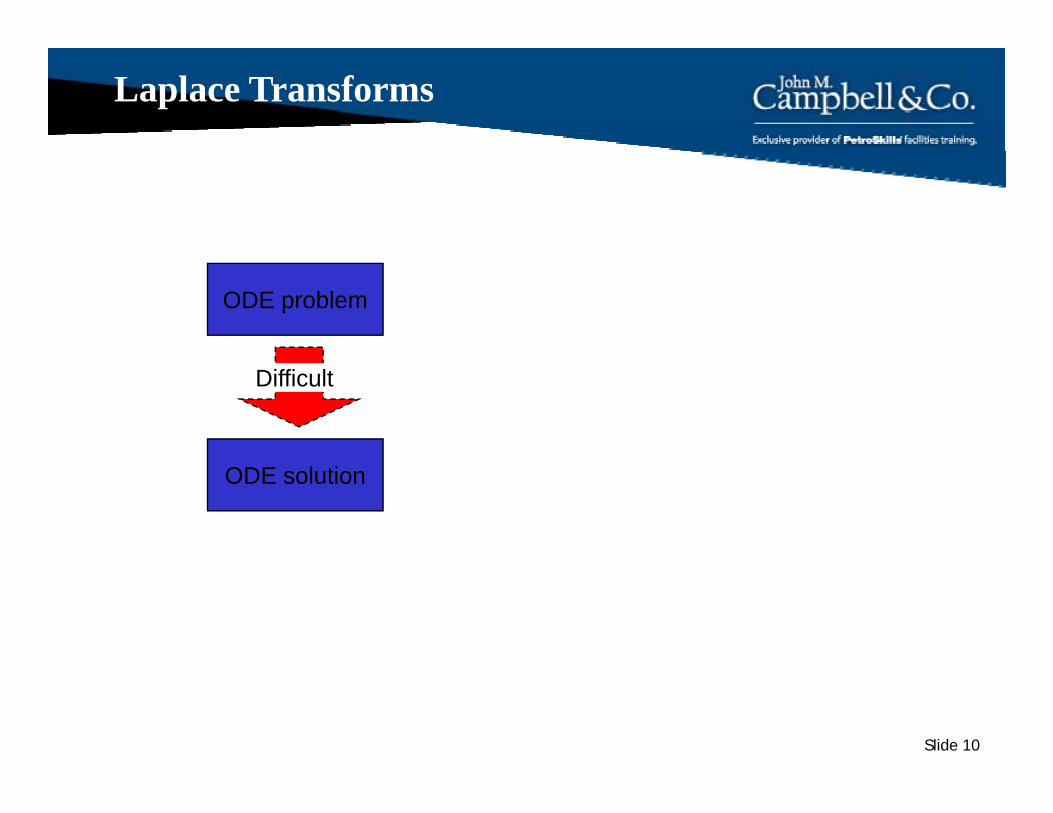
Laplace Transforms

ODE problem

Difficult

ODE solution

Slide 10

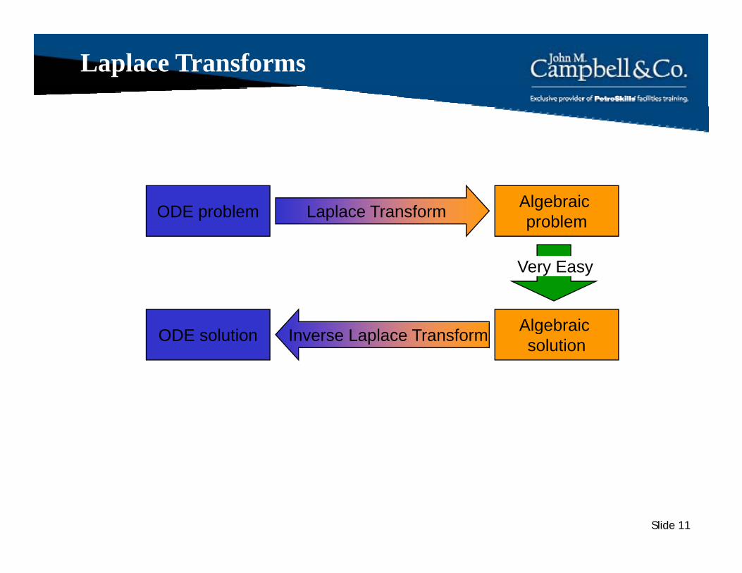
Laplace Transforms

ODE problem Laplace Transform Algebraic problem

Algebraic

Very Easy

Inverse Laplace TransformODE solution Algebraic solution

Slide 11

Laplace Transforms

The definition of a Laplace Transform is:

where: ∫∞

− ≡≡O

st sFdtetftf )()()]([L

l i bl ( jb) i d d b h

= the symbol for the Laplace Transformation in the brackets; .L )]([ tf

s = complex variable (s = a +jb) introduced by the transformation.

Ho hum you thought that this was supposed to make thingsHo-hum….you thought that this was supposed to make things simple?

Slide 12

Laplace Transforms

Probably the easiest way to look at this ‘s’ operator is that it represents the derivative relative to time:

dtds =dt

Slide 13

Laplace Transforms

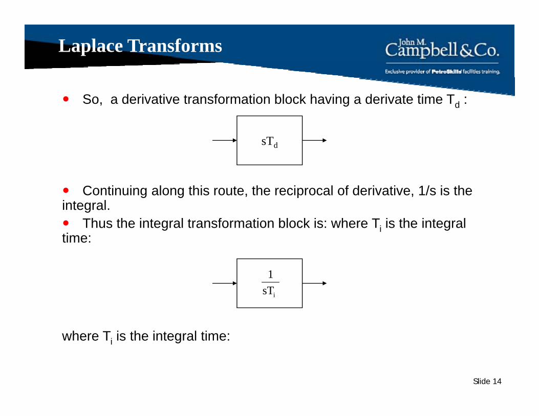
So, a derivative transformation block having a derivate time Td :

sTd

Continuing along this route, the reciprocal of derivative, 1/s is the integral.

Thus the integral transformation block is: where Ti is the integral titime:

T1

where Ti is the integral time:

isT

Slide 14

where Ti is the integral time:

Transformation blocks

G =1 sT11

+

Gain block First order lag

sTd

Derivative block

( ) ( )21 sT1sT11

+⋅+

Second order lag

T1

g

T1sT+isT

Integral block

sT1+

Lead block

Slide 15

Laplace Transforms

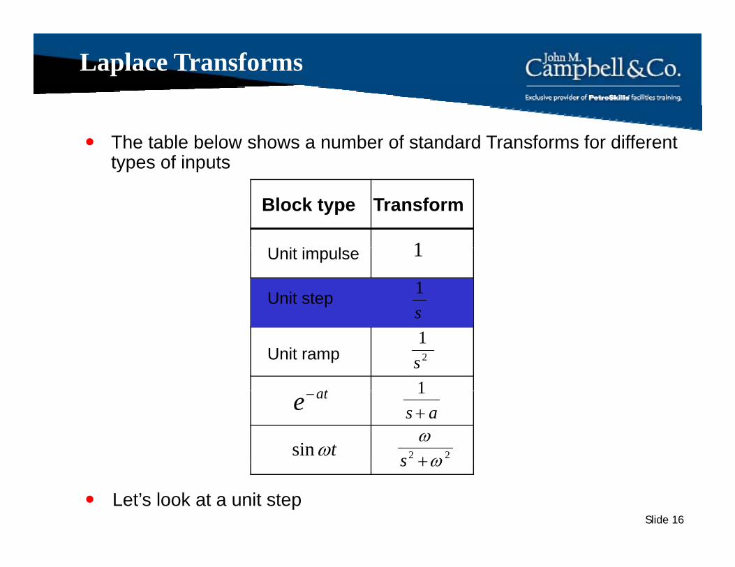
The table below shows a number of standard Transforms for different types of inputs

U it i l 1

Block type Transform

Unit impulse

Unit steps1

1

Unit ramp

1

2

1s

tas +

1

22 ωω+s

ate−

tωsin

Slide 16

ω+s

Let’s look at a unit step

Laplace Transforms

If we applied a unit step to a Gain Block what would we expect out? So, a unit step in….

G =1s1

Step input

s1

Step outputStep input Step output

….results in a unit step out

Slide 17

Laplace Transforms

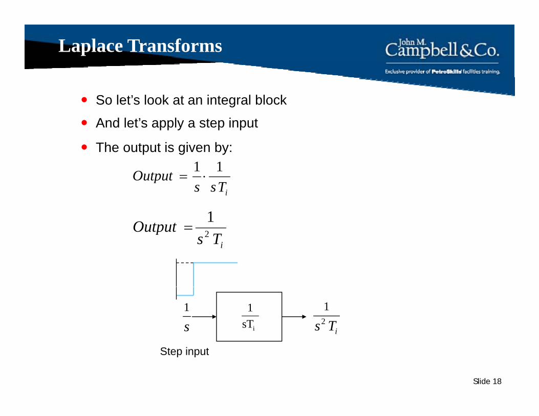
So let’s look at an integral block

And let’s apply a step input

Output 11⋅=

pp y p p

The output is given by:

iTssp

TOutput 2

1=

iTsp 2

s1

iTs2

1

isT1

Slide 18

Step input

Laplace Transforms

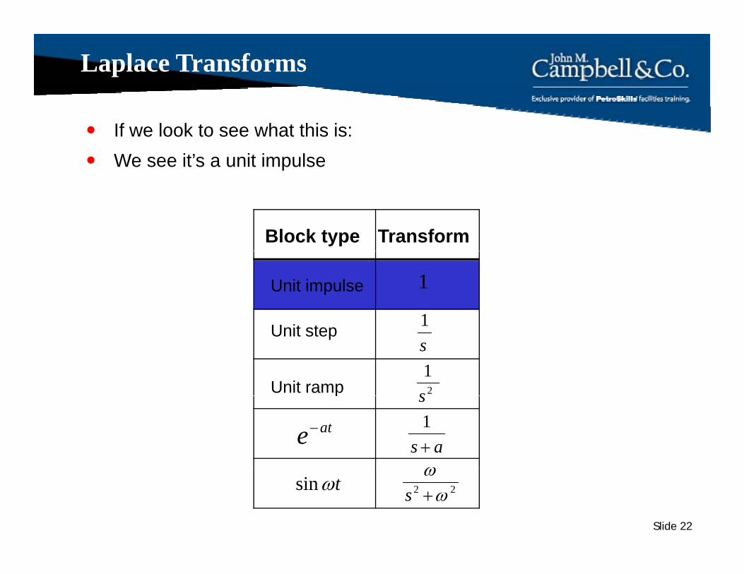
If we look to see what this is:We see it’s a unit ramp

Block type Transform

Unit impulse

Unit step 1

1

p

Unit ramp 2

1s

s

as +1

ω

ate−

tωsin

Slide 19

22 ω+stωsin

Laplace Transforms

So, for a step input …

we get a ramp output (with time T )….we get a ramp output (with time TI)

Which is what we would expect from an integral block

1 11

Step input

s iTs2isT

Ramp output

Slide 20

Laplace Transforms

Let’s apply a step input

We can apply the same rationale to a Derivative block

sTOutput ⋅=1

Let s apply a step input

The output is given by:

dsTs

Output ⋅=

dTOutput ⋅= 1

s1

sTd 1.Td

Slide 21

Step input

Laplace Transforms

If we look to see what this is:We see it’s a unit impulse

Block type Transform

Unit impulse

1

1

Unit step

Unit ramp 2

1s

s1

p

as +1s

ω

ate−

Slide 22

22 ωω+stωsin

Laplace Transforms

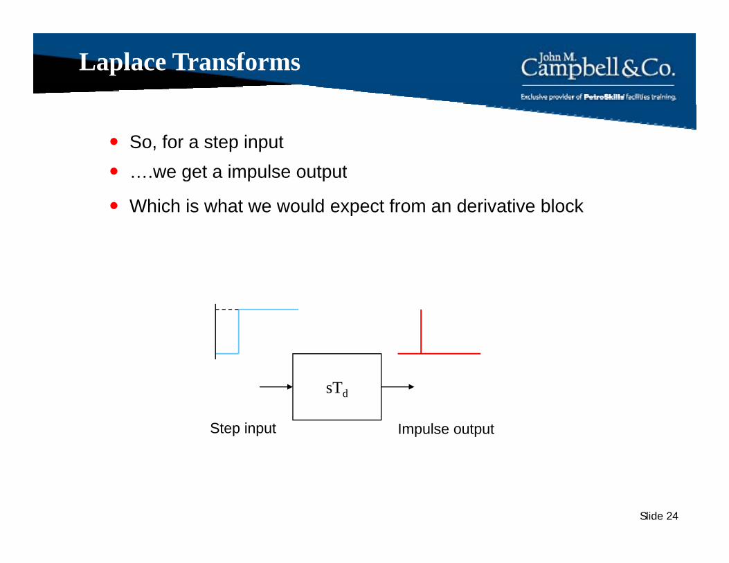
So, for a step input we get a impulse output….we get a impulse output

Which is what we would expect from an derivative block

sTsTd

Step input Impulse output

Slide 23

Laplace Transforms

So, for a step input we get a impulse output….we get a impulse output

Which is what we would expect from an derivative block

sTsTd

Step input Impulse output

Slide 24

First order lag

The general form of a First Order Lag:

τ+ s1K

τ+ s1K

Slide 25Response time

τ

Deadtime

The general form of deadtime:

θθse− θse−

Slide 26

θDeadtime

FOLPDT

When combined the form is:

τ+

θ

s1eK s-

τ+

θ

s1eK s-

Slide 27

θDeadtime Response time

τ