Chapter 3 218 Section 3.7 Rational Functions In the previous sections, we have built polynomials based on the positive whole number power functions. In this section, we explore functions based on power functions with negative integer powers, called rational functions. Example 1 You plan to drive 100 miles. Find a formula for the time the trip will take as a function of the speed you drive. You may recall that multiplying speed by time will give you distance. If we let t represent the drive time in hours, and v represent the velocity (speed or rate) at which we drive, then distance = vt . Since our distance is fixed at 100 miles, 100 = vt . Solving this relationship for the time gives us the function we desired: 1 100 100 ) ( − = = v v v t While this type of relationship can be written using the negative exponent, it is more common to see it written as a fraction. This particular example is one of an inversely proportional relationship – where one quantity is a constant divided by the other quantity, like 5 y x = . Notice that this is a transformation of the reciprocal toolkit function, 1 () f x x = Several natural phenomena, such as gravitational force and volume of sound, behave in a manner inversely proportional to the square of another quantity. For example, the volume, V, of a sound heard at a distance d from the source would be related by 2 d k V = for some constant value k. These functions are transformations of the reciprocal squared toolkit function 2 1 () f x x = . We have seen the graphs of the basic reciprocal function and the squared reciprocal function from our study of toolkit functions. These graphs have several important features.

Welcome message from author
This document is posted to help you gain knowledge. Please leave a comment to let me know what you think about it! Share it to your friends and learn new things together.
Transcript

Chapter 3 218
Section 3.7 Rational Functions
In the previous sections, we have built polynomials based on the positive whole number
power functions. In this section, we explore functions based on power functions with
negative integer powers, called rational functions.
Example 1
You plan to drive 100 miles. Find a formula for the time the trip will take as a function
of the speed you drive.
You may recall that multiplying speed by time will give you distance. If we let t
represent the drive time in hours, and v represent the velocity (speed or rate) at which
we drive, then distance=vt . Since our distance is fixed at 100 miles, 100=vt .
Solving this relationship for the time gives us the function we desired:
1100100
)( −== vv
vt
While this type of relationship can be written using the negative exponent, it is more
common to see it written as a fraction.
This particular example is one of an inversely proportional relationship – where one
quantity is a constant divided by the other quantity, like 5
yx
= .
Notice that this is a transformation of the reciprocal toolkit function, 1
( )f xx
=
Several natural phenomena, such as gravitational force and volume of sound, behave in a
manner inversely proportional to the square of another quantity. For example, the
volume, V, of a sound heard at a distance d from the source would be related by 2d
kV =
for some constant value k.
These functions are transformations of the reciprocal squared toolkit function 2
1( )f x
x= .
We have seen the graphs of the basic reciprocal function and the squared reciprocal
function from our study of toolkit functions. These graphs have several important
features.
3.7 Rational Functions 219
1( )f x
x=
2
1( )f x
x=
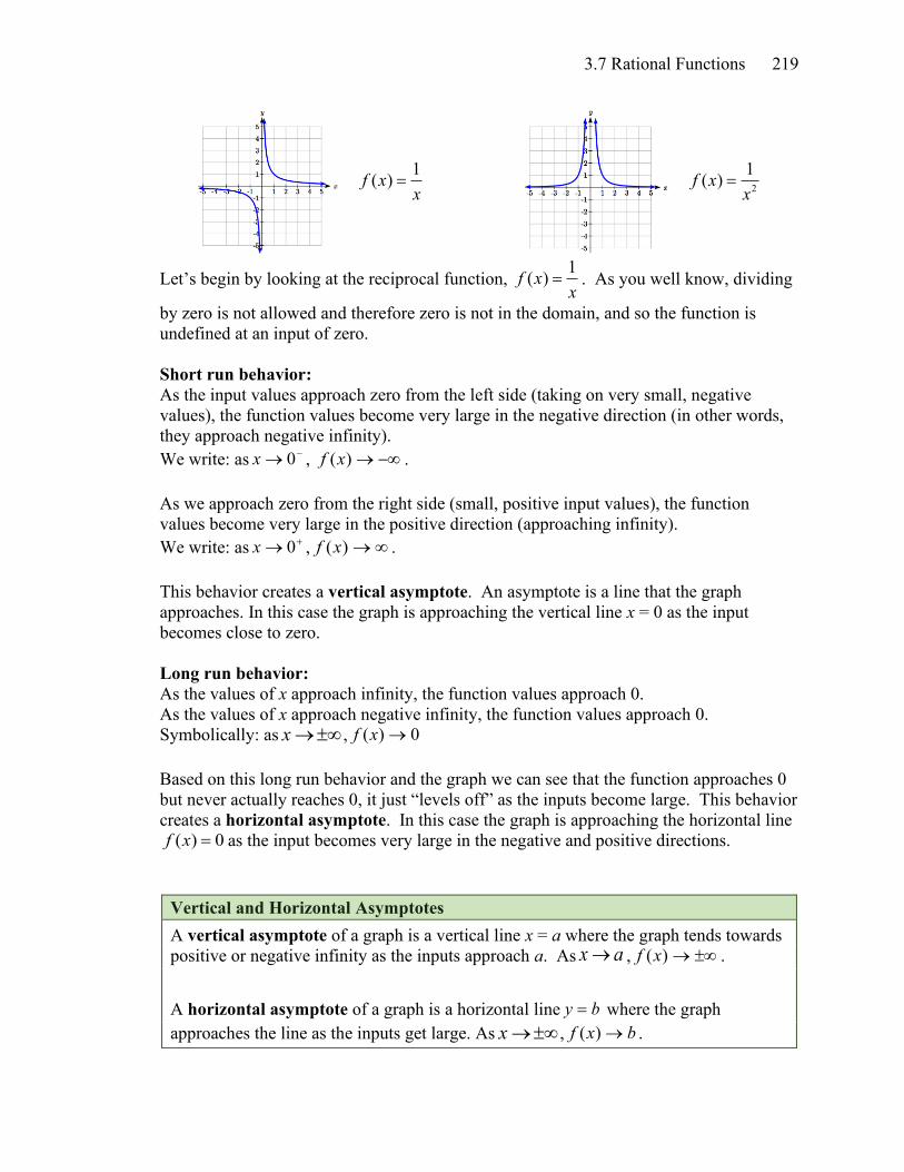
Let’s begin by looking at the reciprocal function, 1
( )f xx
= . As you well know, dividing
by zero is not allowed and therefore zero is not in the domain, and so the function is
undefined at an input of zero.
Short run behavior:
As the input values approach zero from the left side (taking on very small, negative
values), the function values become very large in the negative direction (in other words,
they approach negative infinity).
We write: as−→ 0x , −→)(xf .
As we approach zero from the right side (small, positive input values), the function
values become very large in the positive direction (approaching infinity).
We write: as+→ 0x , →)(xf .
This behavior creates a vertical asymptote. An asymptote is a line that the graph
approaches. In this case the graph is approaching the vertical line x = 0 as the input
becomes close to zero.
Long run behavior:
As the values of x approach infinity, the function values approach 0.
As the values of x approach negative infinity, the function values approach 0.
Symbolically: as →x , 0)( →xf
Based on this long run behavior and the graph we can see that the function approaches 0
but never actually reaches 0, it just “levels off” as the inputs become large. This behavior
creates a horizontal asymptote. In this case the graph is approaching the horizontal line ( ) 0f x = as the input becomes very large in the negative and positive directions.
Vertical and Horizontal Asymptotes
A vertical asymptote of a graph is a vertical line x = a where the graph tends towards
positive or negative infinity as the inputs approach a. As ax → , →)(xf .
A horizontal asymptote of a graph is a horizontal line y b= where the graph
approaches the line as the inputs get large. As →x , bxf →)( .
Chapter 3 220
Try it Now:
1. Use symbolic notation to describe the long run behavior and
short run behavior for the reciprocal squared function.
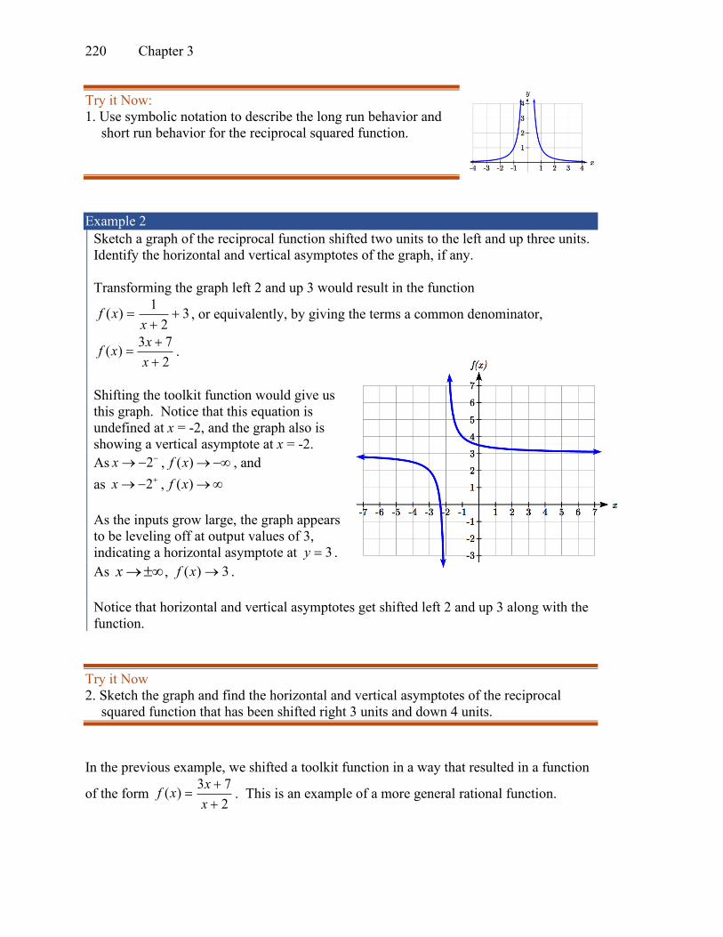
Example 2
Sketch a graph of the reciprocal function shifted two units to the left and up three units.
Identify the horizontal and vertical asymptotes of the graph, if any.
Transforming the graph left 2 and up 3 would result in the function
32
1)( +
+=
xxf , or equivalently, by giving the terms a common denominator,
2
73)(
+
+=
x
xxf .
Shifting the toolkit function would give us
this graph. Notice that this equation is
undefined at x = -2, and the graph also is
showing a vertical asymptote at x = -2.
As 2x −→− , ( )f x →− , and
as 2x +→− , ( )f x →
As the inputs grow large, the graph appears
to be leveling off at output values of 3,
indicating a horizontal asymptote at 3y = .
As →x , 3)( →xf .
Notice that horizontal and vertical asymptotes get shifted left 2 and up 3 along with the
function.
Try it Now
2. Sketch the graph and find the horizontal and vertical asymptotes of the reciprocal
squared function that has been shifted right 3 units and down 4 units.
In the previous example, we shifted a toolkit function in a way that resulted in a function
of the form 2
73)(
+
+=
x
xxf . This is an example of a more general rational function.
3.7 Rational Functions 221
Rational Function
A rational function is a function that can be written as the ratio of two polynomials,
P(x) and Q(x). 2
0 1 2
2
0 1 2
( )( )
( )
p
p
q
q
a a x a x a xP xf x
Q x b b x b x b x
+ + + += =
+ + + +
Example 3
A large mixing tank currently contains 100 gallons of water, into which 5 pounds of
sugar have been mixed. A tap will open pouring 10 gallons per minute of water into the
tank at the same time sugar is poured into the tank at a rate of 1 pound per minute. Find
the concentration (pounds per gallon) of sugar in the tank after t minutes.
Notice that the amount of water in the tank is changing linearly, as is the amount of
sugar in the tank. We can write an equation independently for each: twater 10100 +=
tsugar 15 +=
The concentration, C, will be the ratio of pounds of sugar to gallons of water
t
ttC
10100
5)(
+
+=
Finding Asymptotes and Intercepts
Given a rational function, as part of investigating the short run behavior we are interested
in finding any vertical and horizontal asymptotes, as well as finding any vertical or
horizontal intercepts, as we have done in the past.
To find vertical asymptotes, we notice that the vertical asymptotes in our examples occur
when the denominator of the function is undefined. With one exception, a vertical
asymptote will occur whenever the denominator is undefined.
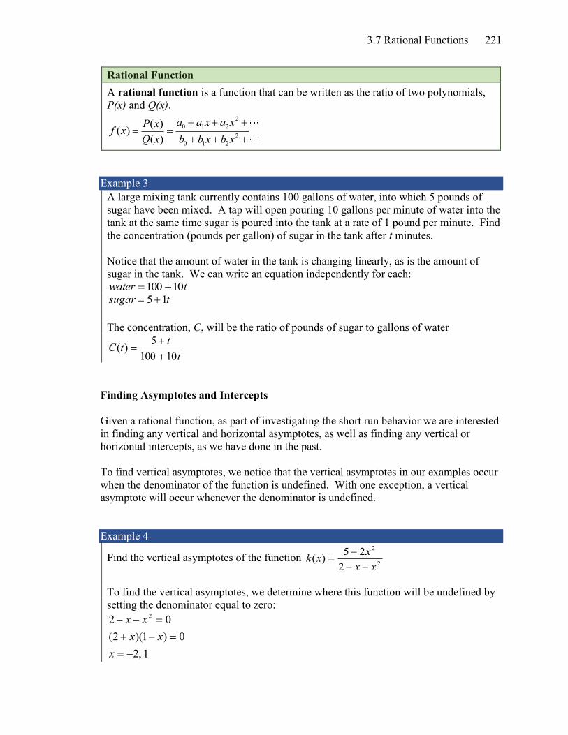
Example 4
Find the vertical asymptotes of the function 2
2
2
25)(
xx
xxk
−−
+=
To find the vertical asymptotes, we determine where this function will be undefined by
setting the denominator equal to zero:
1,2
0)1)(2(
02 2
−=
=−+
=−−
x
xx
xx
Chapter 3 222
This indicates two vertical asymptotes, which a look
at a graph confirms.
The exception to this rule can occur when both the
numerator and denominator of a rational function are zero at the same input.
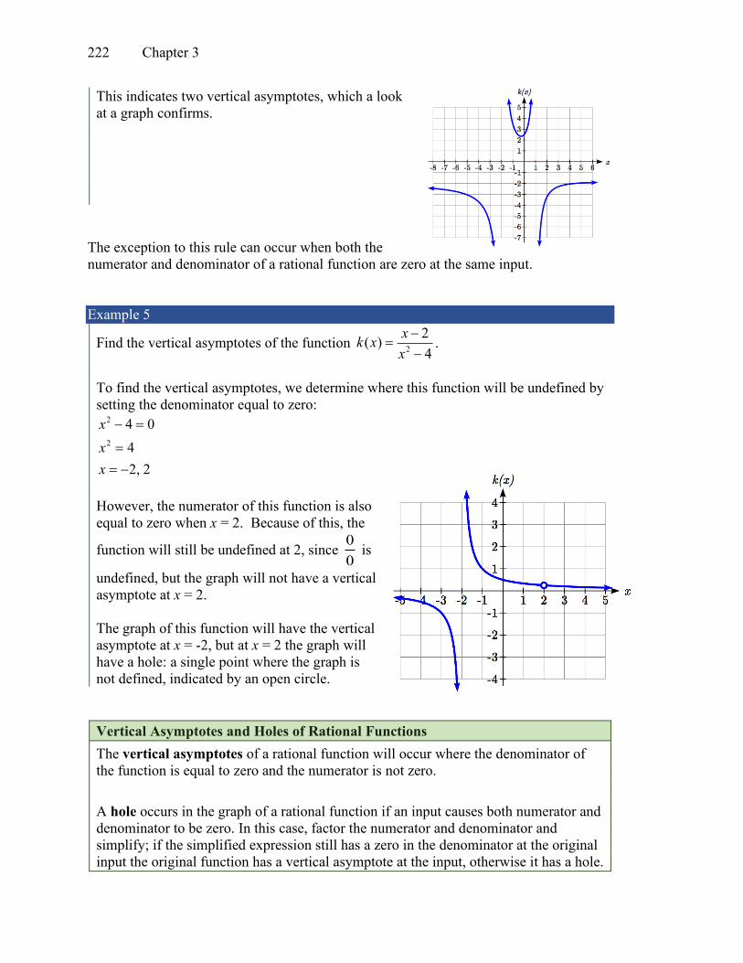
Example 5
Find the vertical asymptotes of the function 2
2( )
4
xk x
x
−=
−.
To find the vertical asymptotes, we determine where this function will be undefined by
setting the denominator equal to zero: 2
2
4 0
4
2, 2
x
x
x
− =
=
= −
However, the numerator of this function is also
equal to zero when x = 2. Because of this, the
function will still be undefined at 2, since 0
0 is
undefined, but the graph will not have a vertical
asymptote at x = 2.
The graph of this function will have the vertical
asymptote at x = -2, but at x = 2 the graph will
have a hole: a single point where the graph is
not defined, indicated by an open circle.
Vertical Asymptotes and Holes of Rational Functions
The vertical asymptotes of a rational function will occur where the denominator of
the function is equal to zero and the numerator is not zero.
A hole occurs in the graph of a rational function if an input causes both numerator and
denominator to be zero. In this case, factor the numerator and denominator and
simplify; if the simplified expression still has a zero in the denominator at the original
input the original function has a vertical asymptote at the input, otherwise it has a hole.
3.7 Rational Functions 223
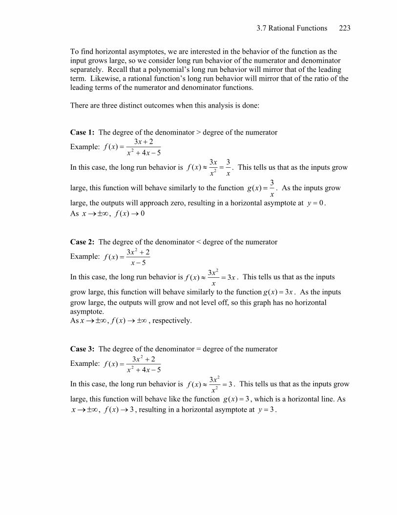
To find horizontal asymptotes, we are interested in the behavior of the function as the
input grows large, so we consider long run behavior of the numerator and denominator
separately. Recall that a polynomial’s long run behavior will mirror that of the leading
term. Likewise, a rational function’s long run behavior will mirror that of the ratio of the
leading terms of the numerator and denominator functions.
There are three distinct outcomes when this analysis is done:
Case 1: The degree of the denominator > degree of the numerator
Example: 54
23)(
2 −+
+=
xx
xxf
In this case, the long run behavior is 2
3 3( )
xf x
x x = . This tells us that as the inputs grow
large, this function will behave similarly to the function 3
( )g xx
= . As the inputs grow
large, the outputs will approach zero, resulting in a horizontal asymptote at 0y = .
As →x , 0)( →xf
Case 2: The degree of the denominator < degree of the numerator
Example: 5
23)(
2
−
+=
x
xxf
In this case, the long run behavior is23
( ) 3x
f x xx
= . This tells us that as the inputs
grow large, this function will behave similarly to the function ( ) 3g x x= . As the inputs
grow large, the outputs will grow and not level off, so this graph has no horizontal
asymptote.
As →x , →)(xf , respectively.
Case 3: The degree of the denominator = degree of the numerator
Example: 54
23)(
2
2
−+
+=
xx
xxf
In this case, the long run behavior is 2
2
3( ) 3
xf x
x = . This tells us that as the inputs grow
large, this function will behave like the function ( ) 3g x = , which is a horizontal line. As
→x , 3)( →xf , resulting in a horizontal asymptote at 3y = .

Chapter 3 224
Horizontal Asymptote of Rational Functions
The horizontal asymptote of a rational function can be determined by looking at the
degrees of the numerator and denominator.
Degree of denominator > degree of numerator: Horizontal asymptote at 0y =
Degree of denominator < degree of numerator: No horizontal asymptote
Degree of denominator = degree of numerator: Horizontal asymptote at ratio of
leading coefficients.
Example 6
In the sugar concentration problem from earlier, we created the equation
t
ttC
10100
5)(
+
+= .
Find the horizontal asymptote and interpret it in context of the scenario.
Both the numerator and denominator are linear (degree 1), so since the degrees are
equal, there will be a horizontal asymptote at the ratio of the leading coefficients. In the
numerator, the leading term is t, with coefficient 1. In the denominator, the leading
term is 10t, with coefficient 10. The horizontal asymptote will be at the ratio of these
values: As t → , 1
( )10
C t → . This function will have a horizontal asymptote at
1
10y = .
This tells us that as the input gets large, the output values will approach 1/10. In
context, this means that as more time goes by, the concentration of sugar in the tank will
approach one tenth of a pound of sugar per gallon of water or 1/10 pounds per gallon.
Example 7
Find the horizontal and vertical asymptotes of the function
)5)(2)(1(
)3)(2()(
−+−
+−=
xxx
xxxf
First, note this function has no inputs that make both the numerator and denominator
zero, so there are no potential holes. The function will have vertical asymptotes when
the denominator is zero, causing the function to be undefined. The denominator will be
zero at x = 1, -2, and 5, indicating vertical asymptotes at these values.
The numerator has degree 2, while the denominator has degree 3. Since the degree of
the denominator is greater than that of the numerator, the denominator will grow faster
than the numerator, causing the outputs to tend towards zero as the inputs get large, and
so as →x , 0)( →xf . This function will have a horizontal asymptote at 0y = .
3.7 Rational Functions 225
Try it Now
3. Find the vertical and horizontal asymptotes of the function )3)(2(
)12)(12()(
+−
+−=
xx
xxxf
Intercepts
As with all functions, a rational function will have a vertical intercept when the input is
zero, if the function is defined at zero. It is possible for a rational function to not have a
vertical intercept if the function is undefined at zero.
Likewise, a rational function will have horizontal intercepts at the inputs that cause the
output to be zero (unless that input corresponds to a hole). It is possible there are no
horizontal intercepts. Since a fraction is only equal to zero when the numerator is zero,
horizontal intercepts will occur when the numerator of the rational function is equal to
zero.
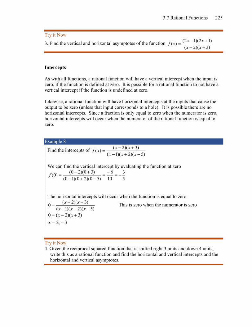
Example 8
Find the intercepts of )5)(2)(1(
)3)(2()(
−+−
+−=
xxx
xxxf
We can find the vertical intercept by evaluating the function at zero
5
3
10
6
)50)(20)(10(
)30)(20()0( −=
−=
−+−
+−=f
The horizontal intercepts will occur when the function is equal to zero:
)5)(2)(1(
)3)(2(0
−+−
+−=
xxx
xx This is zero when the numerator is zero
3,2
)3)(2(0
−=
+−=
x
xx
Try it Now
4. Given the reciprocal squared function that is shifted right 3 units and down 4 units,
write this as a rational function and find the horizontal and vertical intercepts and the
horizontal and vertical asymptotes.

Chapter 3 226
Graphical Behavior at Intercepts and Vertical Asymptotes
As with polynomials, factors of the numerator may have integer powers greater than one.
Happily, the effect on the shape of the graph at those intercepts is the same as we saw
with polynomials: if the factor giving the intercept is not squared, the graph passes
through the axis; if the factor is squared, the graph will bounce off the axis at that
intercept. The behavior at vertical asymptotes also depends on the power on the factor.
Graphical Behavior of Rational Functions at Vertical Asymptotes
If a rational function contains a factor of the form phx )( − in the denominator, the
behavior near the asymptote h is determined by the power on the factor.
p = 1 p = 1 p = 2 p = 2
When the factor is not squared, on one side of the asymptote the graph heads towards
positive infinity and on the other side the graph heads towards negative infinity.
When the factor is squared, the graph either heads toward positive infinity on both
sides of the vertical asymptote, or heads toward negative infinity on both sides.
For example, the graph of
)2()3(
)3()1()(
2
2
−+
−+=
xx
xxxf is shown here.
At the horizontal intercept x = -1
corresponding to the 2)1( +x factor of the
numerator, the graph bounces at the
intercept, consistent with the quadratic
nature of the factor.
At the horizontal intercept x = 3 corresponding to the )3( −x factor of the numerator, the
graph passes through the axis as we’d expect from a linear factor.
At the vertical asymptote x = -3 corresponding to the 2)3( +x factor of the denominator,
the graph heads towards positive infinity on both sides of the asymptote, consistent with
the behavior of the 2
1
x toolkit.
3.7 Rational Functions 227
At the vertical asymptote x = 2 corresponding to the )2( −x factor of the denominator,
the graph heads towards positive infinity on the left side of the asymptote and towards
negative infinity on the right side, consistent with the behavior of the x
1 toolkit.
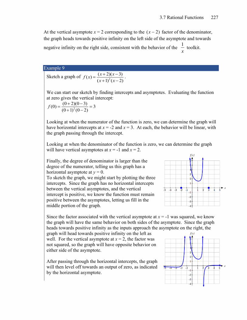
Example 9
Sketch a graph of 2
( 2)( 3)( )
( 1) ( 2)
x xf x
x x
+ −=
+ −.
We can start our sketch by finding intercepts and asymptotes. Evaluating the function
at zero gives the vertical intercept:
2
(0 2)(0 3)(0) 3
(0 1) (0 2)f
+ −= =
+ −
Looking at when the numerator of the function is zero, we can determine the graph will
have horizontal intercepts at x = -2 and x = 3. At each, the behavior will be linear, with
the graph passing through the intercept.
Looking at when the denominator of the function is zero, we can determine the graph
will have vertical asymptotes at x = -1 and x = 2.
Finally, the degree of denominator is larger than the
degree of the numerator, telling us this graph has a
horizontal asymptote at y = 0.
To sketch the graph, we might start by plotting the three
intercepts. Since the graph has no horizontal intercepts
between the vertical asymptotes, and the vertical
intercept is positive, we know the function must remain
positive between the asymptotes, letting us fill in the
middle portion of the graph.
Since the factor associated with the vertical asymptote at x = -1 was squared, we know
the graph will have the same behavior on both sides of the asymptote. Since the graph
heads towards positive infinity as the inputs approach the asymptote on the right, the
graph will head towards positive infinity on the left as
well. For the vertical asymptote at x = 2, the factor was
not squared, so the graph will have opposite behavior on
either side of the asymptote.
After passing through the horizontal intercepts, the graph
will then level off towards an output of zero, as indicated
by the horizontal asymptote.
Chapter 3 228
Try it Now
5. Given the function )3()1(2
)2()2()(
2
2
−−
−+=
xx
xxxf , use the characteristics of polynomials and
rational functions to describe its behavior and sketch the function.
Since a rational function written in factored form will have a horizontal intercept where
each factor of the numerator is equal to zero, we can form a numerator that will pass
through a set of horizontal intercepts by introducing a corresponding set of factors.
Likewise, since the function will have a vertical asymptote where each factor of the
denominator is equal to zero, we can form a denominator that will produce the vertical
asymptotes by introducing a corresponding set of factors.
Writing Rational Functions from Intercepts and Asymptotes
If a rational function has horizontal intercepts at nxxxx ,,, 21 = , and vertical
asymptotes at mvvvx ,,, 21 = then the function can be written in the form
n
n
q
m
p
n
pp
vxvxvx
xxxxxxaxf
)()()(
)()()()(
21
21
21
21
−−−
−−−=
where the powers pi or qi on each factor can be determined by the behavior of the
graph at the corresponding intercept or asymptote, and the stretch factor a can be
determined given a value of the function other than the horizontal intercept, or by the
horizontal asymptote if it is nonzero.
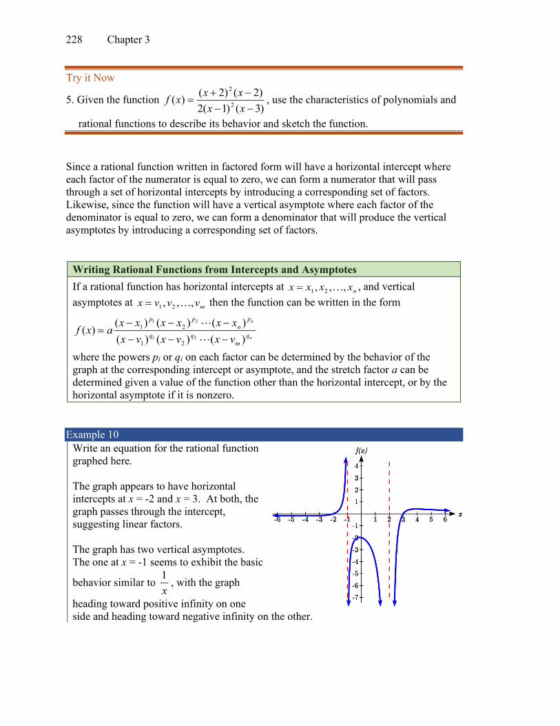
Example 10
Write an equation for the rational function
graphed here.
The graph appears to have horizontal
intercepts at x = -2 and x = 3. At both, the
graph passes through the intercept,
suggesting linear factors.
The graph has two vertical asymptotes.
The one at x = -1 seems to exhibit the basic
behavior similar to x
1, with the graph
heading toward positive infinity on one
side and heading toward negative infinity on the other.

3.7 Rational Functions 229
The asymptote at x = 2 is exhibiting a behavior similar to 2
1
x, with the graph heading
toward negative infinity on both sides of the asymptote.
Utilizing this information indicates an function of the form
2)2)(1(
)3)(2()(
−+
−+=
xx
xxaxf
To find the stretch factor, we can use another clear point on the graph, such as the
vertical intercept (0,-2):
3
4
6
8
4
62
)20)(10(
)30)(20(2
2
=−
−=
−=−
−+
−+=−
a
a
a
This gives us a final function of 2)2)(1(3
)3)(2(4)(
−+
−+=
xx
xxxf
Oblique Asymptotes
Earlier we saw graphs of rational functions that had no horizontal asymptote, which
occurs when the degree of the numerator is larger than the degree of the denominator.
We can, however, describe in more detail the long-run behavior of a rational function.
Example 11
Describe the long-run behavior of 5
23)(
2
−
+=
x
xxf
Earlier we explored this function when discussing horizontal asymptotes. We found the
long-run behavior is23
( ) 3x
f x xx
= , meaning that →x , →)(xf ,
respectively, and there is no horizontal asymptote.
If we were to do polynomial long division, we could get a better understanding of the
behavior as →x .

Chapter 3 230
( )
( )
2
2
3 15
5 3 0 2
3 15
15 2
15 75
77
x
x x x
x x
x
x
+
− + +
− −
+
− −
This means 5
23)(
2
−
+=
x
xxf can be rewritten as
77( ) 3 15
5f x x
x= + +
−.
As →x , the term 77
5x − will become very
small and approach zero, becoming insignificant.
The remaining 3 15x+ then describes the long-run
behavior of the function: as →x ,
( ) 3 15f x x→ + .
We call this equation 3 15y x= + the oblique
asymptote of the function.
In the graph, you can see how the function is
approaching the line on the far left and far right.
Oblique Asymptotes
To explore the long-run behavior of a rational function,
1) Perform polynomial long division (or synthetic division)
2) The quotient will describe the asymptotic behavior of the function
When this result is a line, we call it an oblique asymptote, or slant asymptote.
Example 12
Find the oblique asymptote of 2 2 1
( )1
x xf x
x
− + +=
+
Performing polynomial long division:

3.7 Rational Functions 231
( )
( )
2
2
3
1 2 1
3 1
3 3
2
x
x x x
x x
x
x
− +
+ − + +
− − −
+
− +
−
This allows us to rewrite the function as
2( ) 3
1f x x
x= − + −
+.
The quotient, 3y x= − + , is the oblique asymptote
of f(x). Just like functions we saw earlier
approached their horizontal asymptote in the long
run, this function will approach this oblique
asymptote in the long run.
Try it Now
6. Find the oblique asymptote of
21 7 2( )
2
x xf x
x
+ −=
−
While we primarily concern ourselves with oblique asymptotes, this same approach can
describe other asymptotic behavior.
Example 13
Describe the long-run shape of 3 2 4 2
( )1
x x xf x
x
− − + +=
+
We could rewrite this using long division as
2 2( ) 4
1f x x
x= − + +
+.
Just looking at the quotient gives us the
asymptote, 2 4y x= − + .
This suggests that in the long run, the function
will behave like a downwards opening parabola.
The function will also have a vertical asymptote
at 1x = − .
Chapter 3 232
Important Topics of this Section
Inversely proportional; Reciprocal toolkit function
Inversely proportional to the square; Reciprocal squared toolkit function
Horizontal Asymptotes
Vertical Asymptotes
Rational Functions
Finding intercepts, asymptotes, and holes.
Given equation sketch the graph
Identifying a function from its graph
Oblique Asymptotes
Try it Now Answers
1. Long run behavior, as →x , 0)( →xf
Short run behavior, as 0→x , →)(xf (there are no horizontal or vertical intercepts)
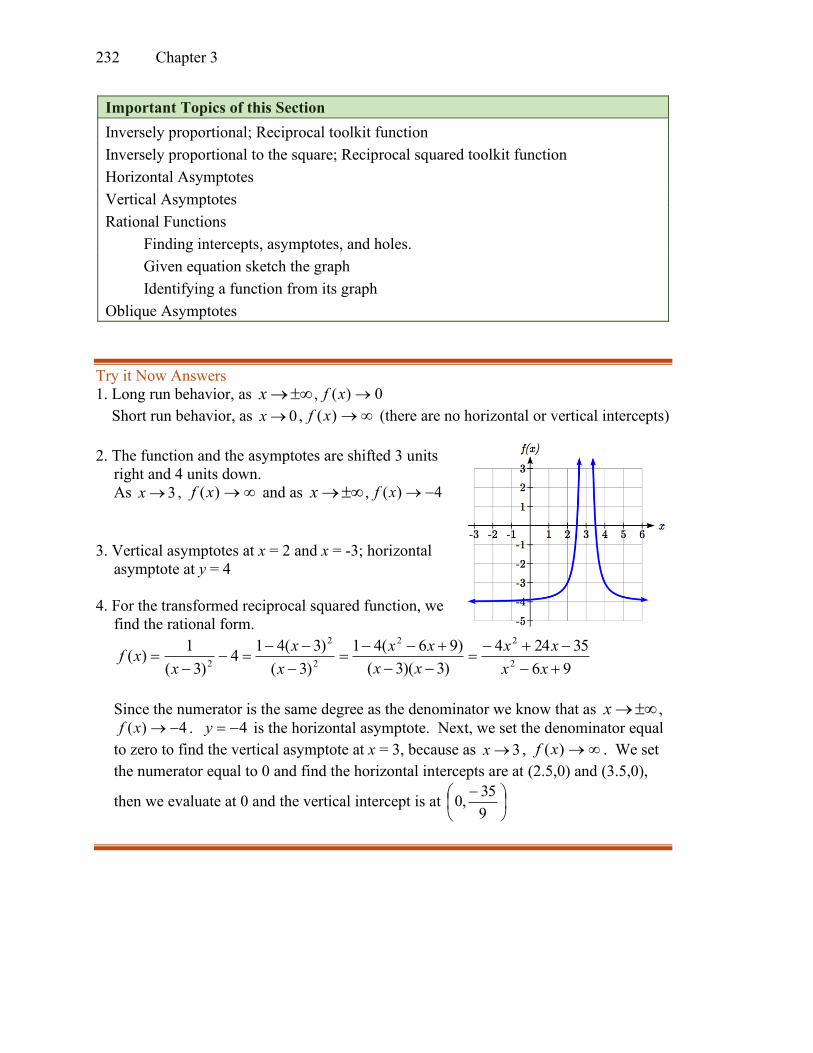
2. The function and the asymptotes are shifted 3 units
right and 4 units down.
As 3→x , →)(xf and as →x , 4)( −→xf
3. Vertical asymptotes at x = 2 and x = -3; horizontal
asymptote at y = 4
4. For the transformed reciprocal squared function, we
find the rational form.
96
35244
)3)(3(
)96(41
)3(
)3(414
)3(
1)(
2
22
2
2
2 +−
−+−=
−−
+−−=
−
−−=−
−=
xx
xx
xx
xx
x
x
xxf
Since the numerator is the same degree as the denominator we know that as →x ,
4)( −→xf . 4y = − is the horizontal asymptote. Next, we set the denominator equal
to zero to find the vertical asymptote at x = 3, because as 3→x , →)(xf . We set
the numerator equal to 0 and find the horizontal intercepts are at (2.5,0) and (3.5,0),
then we evaluate at 0 and the vertical intercept is at
−
9
35,0
3.7 Rational Functions 233
Try it Now Answers, Continued
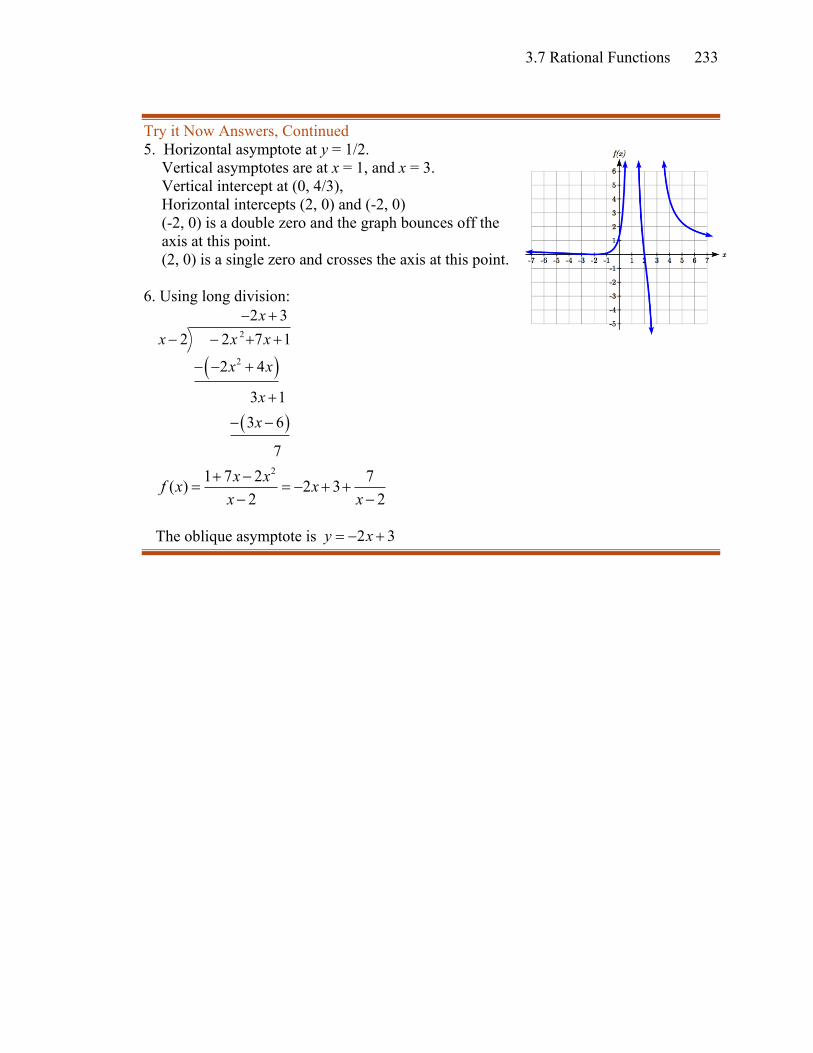
5. Horizontal asymptote at y = 1/2.
Vertical asymptotes are at x = 1, and x = 3.
Vertical intercept at (0, 4/3),
Horizontal intercepts (2, 0) and (-2, 0)
(-2, 0) is a double zero and the graph bounces off the
axis at this point.
(2, 0) is a single zero and crosses the axis at this point.
6. Using long division:
( )
( )
2
2
2 3
2 2 7 1
2 4
3 1
3 6
7
x
x x x
x x
x
x
− +
− − + +
− − +
+
− −
21 7 2 7( ) 2 3
2 2
x xf x x
x x
+ −= = − + +
− −
The oblique asymptote is 2 3y x= − +

Chapter 3 234
Section 3.7 Exercises
Match each equation form with one of the graphs.
1. ( )x A
f xx B
−=
− 2. ( )
( )2
x Ag x
x B
−=
− 3. ( )
( )2
x Ah x
x B
−=
− 4. ( )
( )
( )
2
2
x Ak x
x B
−=
−
A B C D
For each function, find the horizontal intercepts, the vertical intercept, the vertical
asymptotes, and the horizontal asymptote. Use that information to sketch a graph.
5. ( )2 3
4
xp x
x
−=
+ 6. ( )
5
3 1
xq x
x
−=
−
7. ( )( )
2
4
2s x
x=
− 8. ( )
( )2
5
1r x
x=
+
9. ( )2
2
3 14 5
3 8 16
x xf x
x x
− −=
+ − 10. ( )
2
2
2 7 15
3 14 15
x xg x
x x
+ −=
− +
11. ( )2
2
2 3
1
x xa x
x
+ −=
− 12. ( )
2
2
6
4
x xb x
x
− −=
−
13. ( )22 1
4
x xh x
x
+ −=
− 14. ( )
22 3 20
5
x xk x
x
− −=
−
15. ( )2
3 2
3 4 4
4
x xn x
x x
+ −=
− 16. ( ) 2
5
2 7 3
xm x
x x
−=
+ +
17. ( )( )( )( )
( )2
1 3 5
2 ( 4)
x x xw x
x x
− + −=
+ − 18. ( )
( ) ( )
( )( )( )
22 5
3 1 4
x xz x
x x x
+ −=
− + +
Write an equation for a rational function with the given characteristics.

3.7 Rational Functions 235
19. Vertical asymptotes at 5x = and 5x = −
x intercepts at (2, 0) and ( 1, 0)− y intercept at ( )0, 4
20. Vertical asymptotes at 4x = − and 1x = −
x intercepts at ( )1, 0 and ( )5, 0 y intercept at (0, 7)
21. Vertical asymptotes at 4x = − and 5x = −
x intercepts at ( )4, 0 and ( )6, 0− Horizontal asymptote at 7y =
22. Vertical asymptotes at 3x = − and 6x =
x intercepts at ( )2, 0− and ( )1, 0 Horizontal asymptote at 2y = −
23. Vertical asymptote at 1x = −
Double zero at 2x = y intercept at (0, 2)
24. Vertical asymptote at 3x =
Double zero at 1x = y intercept at (0, 4)
Write an equation for the function graphed.
25. 26.
27. 28.
Write an equation for the function graphed.

Chapter 3 236
29. 30.
31. 32.
33. 34.
35. 36.

3.7 Rational Functions 237
Write an equation for the function graphed.
37. 38.
Find the oblique asymptote of each function.
39. 23 4
( )2
x xf x
x
+=
+ 40.
22 3 8( )
1
x xg x
x
+ −=
−
41. 2 3
( )2 6
x xh x
x
− −=
− 42.
25 2( )
2 1
x xk x
x
+ −=
+
43. 3 2
2
2 6 7( )
3
x x xm x
x
− + − +=
+ 44.
3 2
2
2( )
1
x x xn x
x x
+ +=
+ +
45. A scientist has a beaker containing 20 mL of a solution containing 20% acid. To
dilute this, she adds pure water.
a. Write an equation for the concentration in the beaker after adding n mL of
water.
b. Find the concentration if 10 mL of water has been added.
c. How many mL of water must be added to obtain a 4% solution?
d. What is the behavior as n → , and what is the physical significance of this?
46. A scientist has a beaker containing 30 mL of a solution containing 3 grams of
potassium hydroxide. To this, she mixes a solution containing 8 milligrams per mL
of potassium hydroxide.
a. Write an equation for the concentration in the tank after adding n mL of the
second solution.
b. Find the concentration if 10 mL of the second solution has been added.
c. How many mL of water must be added to obtain a 50 mg/mL solution?
d. What is the behavior as n → , and what is the physical significance of this?
47. Oscar is hunting magnetic fields with his gauss meter, a device for measuring the
strength and polarity of magnetic fields. The reading on the meter will increase as

Chapter 3 238
Oscar gets closer to a magnet. Oscar is in a long hallway at the end of which is a
room containing an extremely strong magnet. When he is far down the hallway from
the room, the meter reads a level of 0.2. He then walks down the hallway and enters
the room. When he has gone 6 feet into the room, the meter reads 2.3. Eight feet into
the room, the meter reads 4.4. [UW]
a. Give a rational model of form ( )ax b
m xcx d
+=
+ relating the meter reading ( )m x
to how many feet x Oscar has gone into the room.
b. How far must he go for the meter to reach 10? 100?
c. Considering your function from part (a) and the results of part (b), how far
into the room do you think the magnet is?
48. The more you study for a certain exam, the better your performance on it. If you
study for 10 hours, your score will be 65%. If you study for 20 hours, your score will
be 95%. You can get as close as you want to a perfect score just by studying long
enough. Assume your percentage score, ( )p n , is a function of the number of hours, n,
that you study in the form ( )an b
p ncn d
+=
+. If you want a score of 80%, how long do
you need to study? [UW]
49. A street light is 10 feet north of a
straight bike path that runs east-
west. Olav is bicycling down the
path at a rate of 15 miles per
hour. At noon, Olav is 33 feet
west of the point on the bike path
closest to the street light. (See the
picture). The relationship between the intensity C of light (in candlepower) and the
distance d (in feet) from the light source is given by 2
kC
d= , where k is a constant
depending on the light source. [UW]
a. From 20 feet away, the street light has an intensity of 1 candle. What is k?
b. Find a function which gives the intensity of the light shining on Olav as a
function of time, in seconds.
c. When will the light on Olav have maximum intensity?
d. When will the intensity of the light be 2 candles?
Related Documents
![Rational, unirational and stably rational varietiespirutka/survey.pdf · could be rational (resp. stably rational, resp. retract rational) [30, p.282]. Unirational nonrational varieties.](https://static.cupdf.com/doc/110x72/5f8fad2d18211140cf6c6b61/rational-unirational-and-stably-rational-varieties-pirutka-could-be-rational.jpg)