Section 2 – Roots of Equations

2 - 1

Section 2 – Roots of Equations In this section, we will look at finding the roots of functions. The basic root-finding problem involves many concepts and techniques that will be useful in more advanced topics. Algebraic and Transcendental Functions A function of the form )(xfy is algebraic if it can be expressed in the form:

0... 012

21

1 fyfyfyfyf nn

nn

nn

where if is an ith-order polynomial in x. Polynomials are a simple class of algebraic functions that are represented by

nnn xaxaxaxaaxf ...)( 3

32

210 Where n is the order of the polynomial and the ai are constants. For example,

6326

22

75)(5.737.21)(

xxxxfxxxf

A transcendental function is one that is not algebraic. These types of functions include trigonometric, logarithmic, exponential or other functions. Examples include

)5.03sin()(1ln)(

2.02

xexfxxf

x There are two distinct areas when it comes to finding the root of functions:

1. Determination of the real roots of algebraic and transcendental functions, and usually only a single root, given its approximate location

2. Determination of all of the real and complex roots of polynomials 2.1 Graphical Methods Graphical methods are straightforward – simply graph the function f(x) and see where it crosses the x-axis. This method will immediately yield a rough approximation of the value of the root, which can be refined through finer and more detailed graphs. It is not necessarily precise, but it is very useful in order to determine a starting point for more sophisticated methods.

2 - 2

2.2 Closed Methods The following methods work on “closed” or bounded domains, defined by upper and lower values that bracket the root of interest. 2.2.1 Bisection Method If f(x) is real and continuous in the interval from xl to xu, and f(ul) and f(xu) have opposite signs, then there must be at least one real root between xl and xu. The bisection method (or binary chopping, interval halving or Bolzano’s Method) divides the interval between the upper and lower bound in half to find the next approximate root xr,

2ul

rxxx

which replaces the bound of the interval, either xl or xu, whose function value has the same sign as f(xr). The method proceeds until the termination criterion is met

newr

oldr

newra x

xx Pseudocode – Bisection method

FUNCTION Bisection(xl, xu, xr, ea, imax) DIM iter, es, fxl, fxu, fxr, xrold iter=0 fxl=f(xl) fxu=f(xu)

xrold=xl+(xu-xl)/3 DO

iter = iter+1 xr = (xu + xl)/2 ‘ Bisection method

fxr = f(xr) IF xr = 0 then es = ABS(xr - xrold)

ELSE

xr

f(x)

xl xu

2 - 3

es = ABS((xr - xrold)/xr) END IF ‘ if fxr and fxu have different signs, replace lower bound IF fxr*fxu < 0 THEN

xl = xr fxl = fxr

ELSE // replace upper bound xu = xr fxu = fxr

END IF xrold = xr

UNTIL iter ≥ imax OR es ≤ ea Bisection = xr END Bisection

Examples:

1. Find all of the real roots of a. f(x) = sin(10x) + cos(3x) ; 0 ≤ x ≤ 5 b. f(x) = -0.6x2 + 2.4x + 5.5 c. f(x) = x10 – 1 ; 0 ≤ x ≤ 1.3 d. f(x) = 4x3 – 6x2 + 7x -2.3 e. f(x) = -26 + 85x – 91x2 + 44x3 - 8x4 + x5

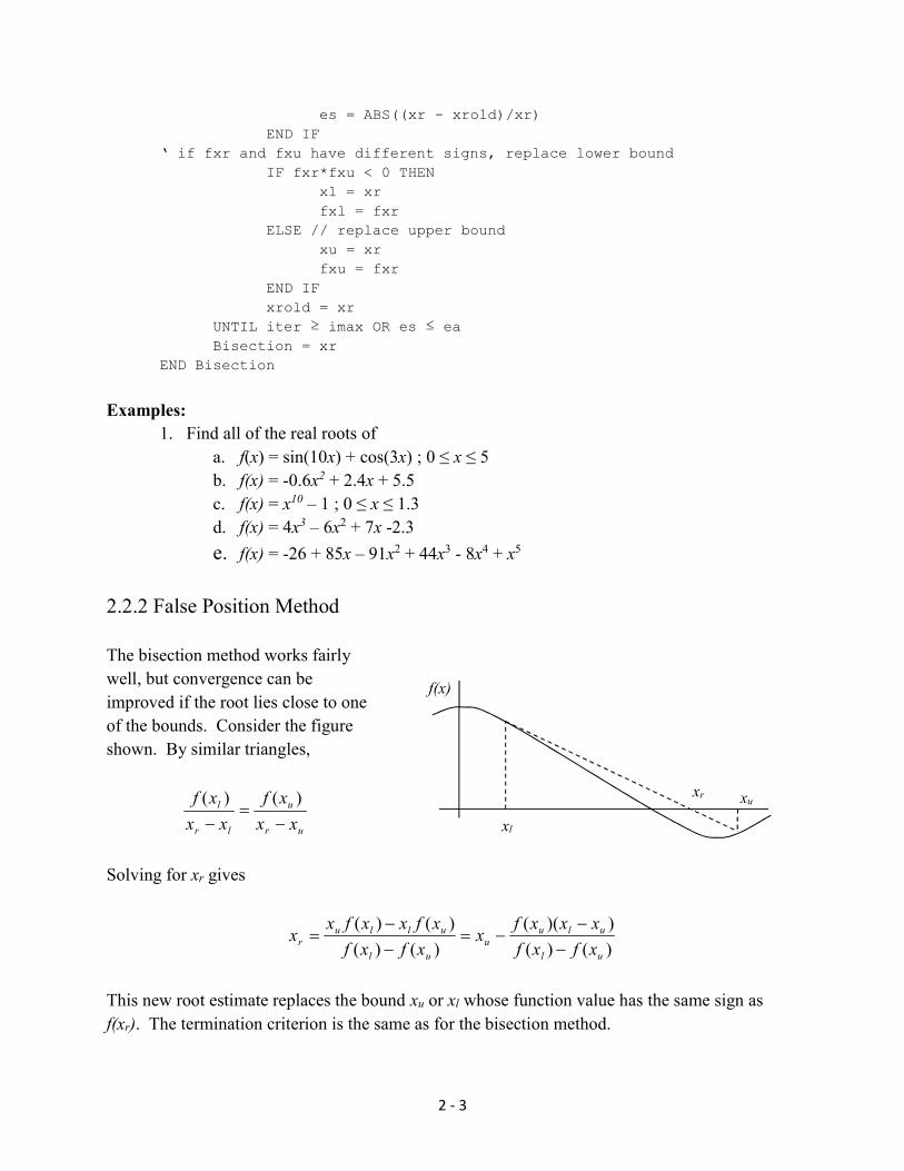
2.2.2 False Position Method The bisection method works fairly well, but convergence can be improved if the root lies close to one of the bounds. Consider the figure shown. By similar triangles,

uru

lrl

xxxf

xxxf

)()(

Solving for xr gives

)()())((

)()()()(

ululu

uul

ullur xfxf

xxxfxxfxfxfxxfxx

This new root estimate replaces the bound xu or xl whose function value has the same sign as f(xr). The termination criterion is the same as for the bisection method.

xu xl

xr

f(x)

2 - 4

The false position method is generally more efficient than bracketing, but not always (consider, for example, the function f(x) = x10-1 between x = 0 and x = 1.3). The false position method can tend to be one-sided, leading to slow convergence. If this appears to be a problem, try the modified false position method. In this technique, if one bound is fixed for two successive iterations, bisect the interval once and proceed with the false position method. 2.3 Open Methods The bracketing and false position methods are “closed” methods, that is, they “close” an interval and converge on the root from both ends of that interval. Open methods require only one (sometimes two) starting values that do not bracket the root, making them self-starting and more efficient. However, they can diverge and even move away from the root that is sought. 2.3.1 Simple Fixed-Point Iteration Some functions can be manipulated to be of the form x = g(x), either algebraically or by adding x to both sides of f(x)=0. If this is the case, one can converge on a root by iterating

)(1 ii xgx

with termination criterion

11

iii

a xxx

While this method is easy to implement, it has several drawbacks. Convergence can be slow; at best it is linear. Also, the method can diverge, with convergence determined by the sign of the first derivative of g(x): if 1)( xg then the method converges, if 1)( xg then fixed-point iteration diverges. Pseudocode – Fixed Point Iteration

FUNCTION FixedPoint(x0, es, imax, iter, ea)

xr = x0 iter = 0 DO

iter = iter + 1 xr = g(xrold) ‘ fixed point iteration IF iter>1 then

IF xr = 0 then es = ABS(xr - xrold)

2 - 5

ELSE es = ABS((xr - xrold)/xr)

END IF END IF xrold=xr

END DO FixedPoint = xr

END FixedPoint 2.3.2 Newton-Raphson Method Newton-Raphson is the most widely used method of the root-finding formulas. The tangent to the curve at the point xi, f(xi) is used to determine the next estimate for the root. The slope of the curve at the point xi can be written as

1

)()(

iii

i xxxfxf

so that

)()(

1ii

ii xfxfxx

with termination criterion

11

iii

a xxx

Newton-Raphson is quadratically convergent, that is, Ei+1≈Ei2. The method is very fast and very efficient. Care must be taken, however, since

N-R can diverge if the tangent to the curve takes it away from the root N-R can converge slowly if multiple roots exist. Two methods exist to deal with multiple

roots:

)()(

1ii

ii xfxfmxx

xi xr

f(x)

2 - 6

where m is the multiplicity of the root, or

)()()()()(

21iii

iiii xfxfxf

xfxfxx

It must be noted that Newton-Raphson method needs an analytical function to work since

the derivatives must be explicitly determined. 2.3.3 Secant Method This method is similar to Newton-Raphson, substituting a backward finite-difference approximation for the derivative:

iiii

i xxxfxfxf

1

1 )()()( So that

)()())((

11

1iiiii

ii xfxfxxxfxx

The secant method requires two points to start, xi-1 and xi. It also may diverge, similar to the Newton-Raphson method. 2.3.4 Modified Secant Method Instead of using a finite difference approximation of the derivative in Newton-Raphson, estimate the derivative using a small perturbation of the independent variable:

iiii

i xxfxxfxf

)()()(

)()()(

1iii

iiii xfxxf

xfxxx

2 - 7

2.3.5 Multiple Roots Multiple roots, for example f(x)=(x-a)(x-a)(x-b) cause difficulties when searching for roots. Bracketing methods do not work with multiple roots (why?). In addition, f’(x)=0 at the root, causing problems for the Newton-Raphson and the Secant methods. 2.3.6 Multivariate Methods Given a set of equations f(x) = 0

( , … ) = ( ) = 0 ( , … ) = ( ) = 0

⋯ ( , … ) = ( ) = 0

The first-order Taylor expansion can be written as

( + ) = ( ) + ( ) where the Jacobian of f(x) is

( ) = ( ) =⋯

⋮ ⋮⋯

Solving for δx, the multivariate Newton-Raphson can be expressed as = − ( ) ( ) Example:

( ) =3 − cos( ) − 3

2 = 04 − 625 + 2 − 1 = 0

20 + + 9 = 0

( ) =

3 sin ( ) sin ( )8 −1250 2

− − 20

If the analytical derivatives are not available, it is possible to approximate the Jacobian from two consecutive iterations (multivariate Secant method)

2 - 8

= ( , ⋯ , ) =

( ), ⋯ , ( ), ⋯ ( ) − ( ), ⋯ , ( ), ⋯ ( )( ) − ( )

2.4 Roots of Polynomials Finding all of the roots of a polynomial is a common problem in numerical analysis. Before delving into the methods, let’s first examine efficient ways to evaluate and manipulate polynomials. Evaluation of Polynomials Consider the following polynomial:

012

23

33 )( axaxaxaxf Evaluating the function as it is written involves 6 multiplications and three additions. However, if it is written

01233 ))(()( axaxaxaxf it can be evaluated with only three multiplications and three additions. In pseudocode, given a vector of coefficients a(j),

DO FOR j=n to 0 STEP -1 df = df * x + p p = p * x + a(j)

END DO Note that in the pseudocode above, the derivative of the polynomial, df, is evaluated at the same time as the function. Polynomial Deflation Recall that polynomials can be divided in a manner similar to basic arithmetic, sometimes referred to as synthetic division:

2 - 9

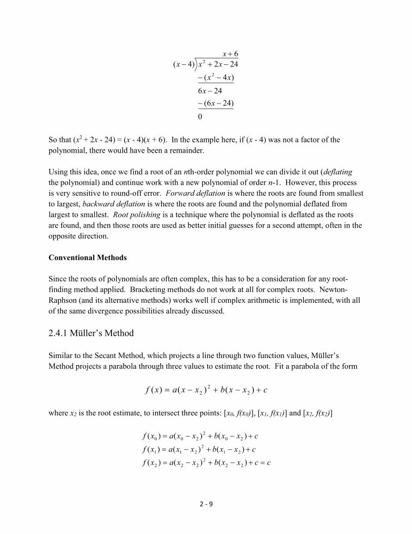
6

0)246(

246)4(242)4(

22

x

xx

xxxxx

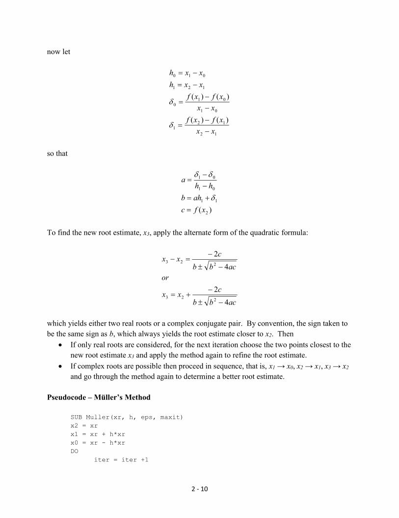
So that (x2 + 2x - 24) = (x - 4)(x + 6). In the example here, if (x - 4) was not a factor of the polynomial, there would have been a remainder. Using this idea, once we find a root of an nth-order polynomial we can divide it out (deflating the polynomial) and continue work with a new polynomial of order n-1. However, this process is very sensitive to round-off error. Forward deflation is where the roots are found from smallest to largest, backward deflation is where the roots are found and the polynomial deflated from largest to smallest. Root polishing is a technique where the polynomial is deflated as the roots are found, and then those roots are used as better initial guesses for a second attempt, often in the opposite direction. Conventional Methods Since the roots of polynomials are often complex, this has to be a consideration for any root-finding method applied. Bracketing methods do not work at all for complex roots. Newton-Raphson (and its alternative methods) works well if complex arithmetic is implemented, with all of the same divergence possibilities already discussed. 2.4.1 Müller’s Method Similar to the Secant Method, which projects a line through two function values, Müller’s Method projects a parabola through three values to estimate the root. Fit a parabola of the form

cxxbxxaxf )()()( 22

2 where x2 is the root estimate, to intersect three points: [x0, f(x0)], [x1, f(x1)] and [x2, f(x2)]

ccxxbxxaxfcxxbxxaxfcxxbxxaxf

)()()()()()()()()(

222

22221

2211

202

200

2 - 10

now let

1212

1

0101

0

121010

)()(

)()(

xxxfxf

xxxfxf

xxhxxh

so that

)( 211

0101

xfcahb

hha

To find the new root estimate, x3, apply the alternate form of the quadratic formula:

acbbcxx

oracbb

cxx

42

42

223

223

which yields either two real roots or a complex conjugate pair. By convention, the sign taken to be the same sign as b, which always yields the root estimate closer to x2. Then

If only real roots are considered, for the next iteration choose the two points closest to the new root estimate x3 and apply the method again to refine the root estimate.

If complex roots are possible then proceed in sequence, that is, x1 → x0, x2 → x1, x3 → x2 and go through the method again to determine a better root estimate.

Pseudocode – Müller’s Method

SUB Muller(xr, h, eps, maxit) x2 = xr x1 = xr + h*xr x0 = xr - h*xr DO iter = iter +1

2 - 11

h0 = x1 - x0 h1 = x2 - x1 d0 = (f(x1) - f(x0)) / h0 d1 = (f(x2) - f(x1)) / h1 a = (d1 - d0) / (h1 + h0) b = a*h1 + d1 c = f(x2) rad = SQRT(b*b - 4*a*c) IF |b+rad| > |b-rad| THEN den = b + rad ELSE den = b - rad END IF dxr = -2*c / den xr = x2 + dxr PRINT iter, xr IF (|dxr| < eps*xr OR iter > maxit) EXIT x0 = x1 x1 = x2 x2 = xr END DO END Muller

2.4.2 Bairstow’s Method If we have a general polynomial

nnn xaxaxaaxf ...)( 2

210 that is divided by a factor (x-t), it yields a polynomial that is one order lower

122101 ...)( n

nn xbxbxbbxf where

tbabab

iiinn

1

and i = n-1 to 0. If t is a root of the original polynomial, then b0 = 0. Bairstow’s Method divides the polynomial by a quadratic factor, (x2 – rx – s) to yield

224322 ...)( n

nn xbxbxbbxf

2 - 12

with remainder

01 )( brxbR and

2111

iiiinnn

nn

sbrbabrbab

ab

where i = n-2 to 0. The idea behind Bairstow’s Method is to drive the remainder to zero. To do this, both b1 and b0 must be zero. Expand both in first-order Taylor series:

ssbrr

bbssrrbss

brrbbssrrb

0000

1111

),(),(

so that

000

111

bssbrr

bbss

brrb

Now let

2111

iiiinnn

nn

scrcbcrcbc

bc

where rbc /01 , rbsbc //2 10 , sbc /13 , etc., so that

021132

bscrcbscrc

2 - 13

Solve these two equations for Δr and Δs, then use them to improve the initial guesses of r and s. At each step, the approximate errors are

ss

rr

sa

ra

,

,

When both of these error estimates fall below a specified value, then the root can be identified as

242 srrx

and the deflated polynomial with coefficients bi remains. Three possibilities exist:

1. The polynomial is third-order or higher. In this case, apply the method again to find the root(s).

2. The remaining polynomial is quadratic – solve for the two remaining roots with the quadratic formula.

3. The polynomial is linear. In this case, the last root is x = -s/r Pseudocode – Bairstow’s Method

SUB Bairstow(a, nn, es, rr, ss, maxit, re, im, ier) DIMENSION b(nn), c(nn) r= rr s = ss n = nn ier = 0 ea1 = 1 ea2 = 1 DO

IF n<3 OR iter>= maxit EXIT iter = 0 DO

iter = iter +1 b(n) = a(n) b(n-1) = a(n-1) + r*b(n) c(n) = b(n) c(n-1) = b(n-1) + r*c(n) DO i = n-2, 0, -1

b(i) = a(i) + r*b(i+1) + s*b(i+2) c(i) = b(i) + r*c(i+1) + s*c(i+2)

2 - 14

END DO det = c(2)*c(2) - c(3)*c(1) IF det <> 0 THEN

dr = (-b(1)*c(2) + b(0)*c(3))/det ds = (-b(0)*c(2) + b(1)*c(1))/det r = r + dr s = s + ds IF r<>0 THEN ea1 = ABS(dr/r)*100 IF s<>0 THEN ea2 = ABS(ds/s)*100

ELSE r = r + 1 s = s + 1 iter = 0

END IF IF ea1 <= es AND ea2 <=es OR iter >= maxit EXIT

END DO CALL QuadRoot(r, s, r1, i1, r2, i2) re(n) = r1 im(n) = i1 re(n-1) = r2 im(n-1) = i2 n = n-2 DO i = 0, n

a(i) = b(i+2) END DO

END DO IF iter < maxit THEN

IF n = 2 THEN r = -a(1)/a(2) s = -a(0)/a(2) CALL Quadroot(r, s, r1, i1, r2, i2) re(n) = r1 im(n) = i1 re(n-1) = r2 im(n-1) = i2

ELSE re(n) = -a(0)/a(1) im(n) = 0

END IF ELSE

ier = 1 END IF End Bairstow SUB Quadroot(r, s, r1, i1, r2, i2) disc = r*r + 4*s IF disc > 0 THEN r1 = (r + SQRT(disc))/2 r2 = (r - SQRT(disc))/2

2 - 15

i1 = 0 i2 = 0 ELSE r1 = r/2 r2 = r1 i1 = SQRT(ABS(disc))/2 i2 = -i1 END IF END Quadroot