HAWKES LEARNING SYSTEMS Students Matter. Success Counts. Copyright © 2013 by Hawkes Learning Systems/Quant Systems, Section 12.3 Regression Analysis

Section 12.3
Jan 01, 2016
Section 12.3. Regression Analysis. Objectives. Construct a prediction interval for an individual value of y. Construct confidence intervals for the slope and the y -intercept of a regression line. Regression Analysis. Residual - PowerPoint PPT Presentation
Welcome message from author
This document is posted to help you gain knowledge. Please leave a comment to let me know what you think about it! Share it to your friends and learn new things together.
Transcript
HAWKES LEARNING SYSTEMS
Students Matter. Success Counts.
Copyright © 2013 by Hawkes Learning
Systems/Quant Systems, Inc.
All rights reserved.
Section 12.3
Regression Analysis
HAWKES LEARNING SYSTEMS
Students Matter. Success Counts.
Copyright © 2013 by Hawkes Learning
Systems/Quant Systems, Inc.
All rights reserved.
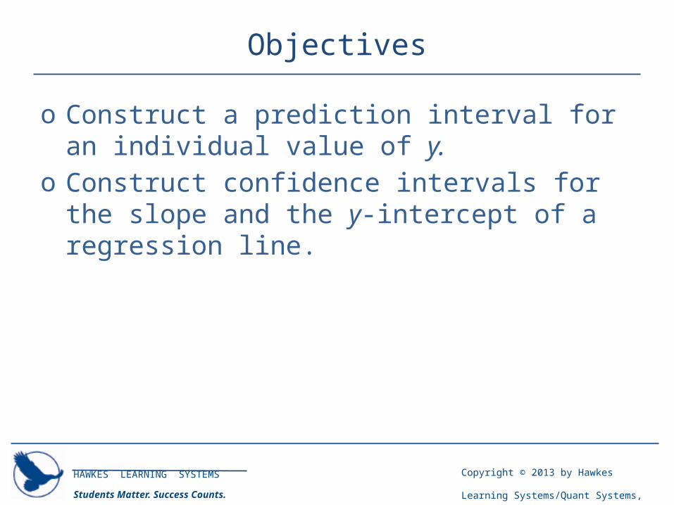
Objectives
o Construct a prediction interval for an individual value of y.
o Construct confidence intervals for the slope and the y-intercept of a regression line.

HAWKES LEARNING SYSTEMS
Students Matter. Success Counts.
Copyright © 2013 by Hawkes Learning
Systems/Quant Systems, Inc.
All rights reserved.
Regression Analysis
Residual A residual is the difference between the actual value of y from the original data and the predicted value of ŷ found using the regression line, given by
Residual = y − ŷwhere y is the observed value of the response variable and ŷ is the predicted value of y using the least-squares regression model.
HAWKES LEARNING SYSTEMS
Students Matter. Success Counts.
Copyright © 2013 by Hawkes Learning
Systems/Quant Systems, Inc.
All rights reserved.
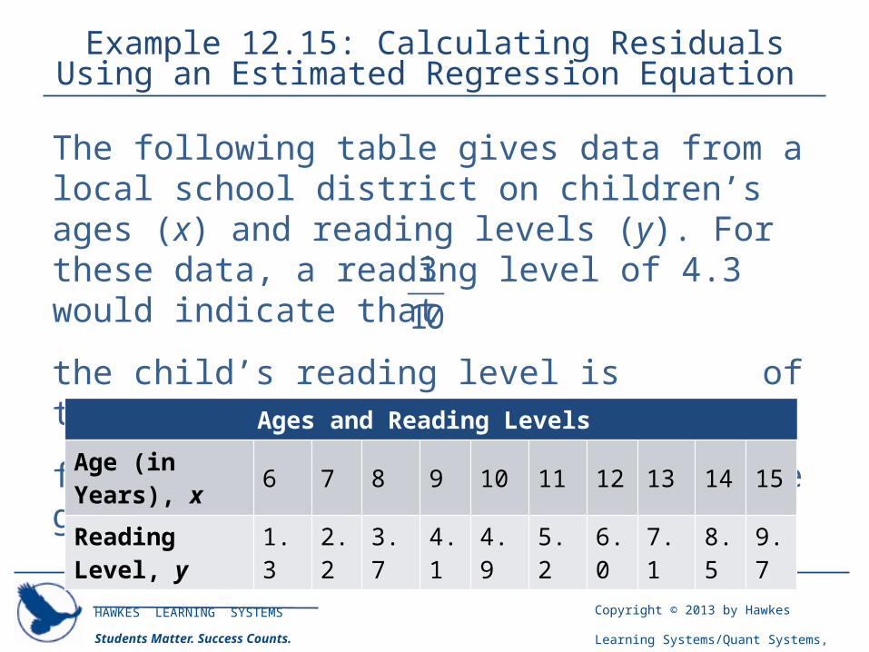
Example 12.15: Calculating Residuals Using an Estimated Regression Equation
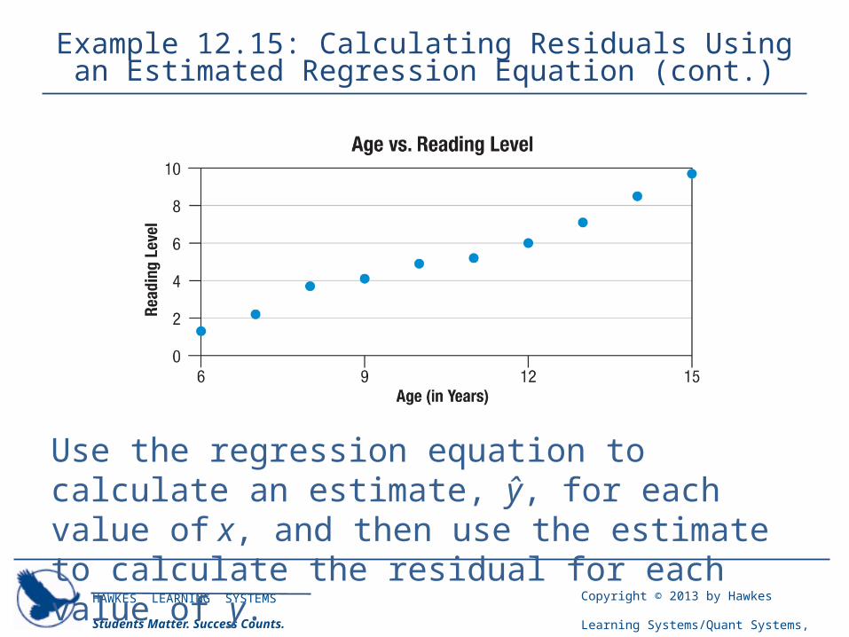
The following table gives data from a local school district on children’s ages (x) and reading levels (y). For these data, a reading level of 4.3 would indicate that
the child’s reading level is of the year through the
fourth grade. The children’s ages are given in years.
310
Ages and Reading Levels Age (in Years), x 6 7 8 9 10 11 12 13 14 15Reading Level, y 1.3 2.2 3.7 4.1 4.9 5.2 6.0 7.1 8.5 9.7
HAWKES LEARNING SYSTEMS
Students Matter. Success Counts.
Copyright © 2013 by Hawkes Learning
Systems/Quant Systems, Inc.
All rights reserved.
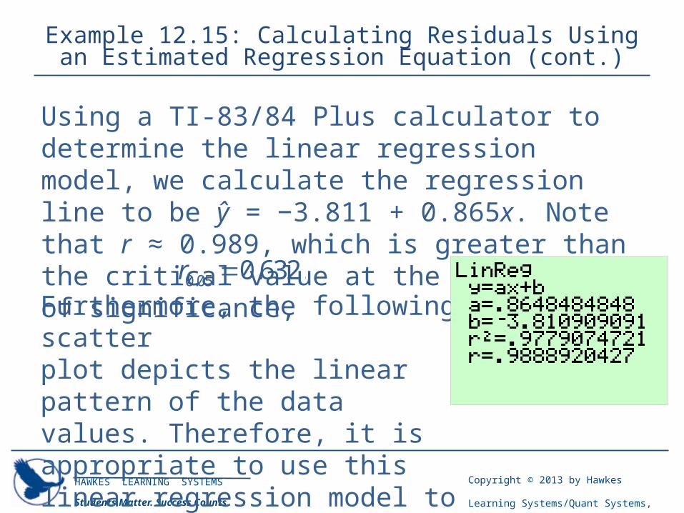
Example 12.15: Calculating Residuals Using an Estimated Regression Equation (cont.)
Using a TI-83/84 Plus calculator to determine the linear regression model, we calculate the regression line to be ŷ = −3.811 + 0.865x. Note that r ≈ 0.989, which is greater than the critical value at the 0.05 level of significance,
0.05 0.632.r Furthermore, the following scatter plot depicts the linear pattern of the data values. Therefore, it is appropriate to use this linear regression model to make predictions.
HAWKES LEARNING SYSTEMS
Students Matter. Success Counts.
Copyright © 2013 by Hawkes Learning
Systems/Quant Systems, Inc.
All rights reserved.
Example 12.15: Calculating Residuals Using an Estimated Regression Equation (cont.)
Use the regression equation to calculate an estimate, ŷ, for each value of x, and then use the estimate to calculate the residual for each value of y.
HAWKES LEARNING SYSTEMS
Students Matter. Success Counts.
Copyright © 2013 by Hawkes Learning
Systems/Quant Systems, Inc.
All rights reserved.
Example 12.15: Calculating Residuals Using an Estimated Regression Equation (cont.)
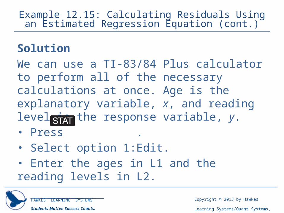
SolutionWe can use a TI-83/84 Plus calculator to perform all of the necessary calculations at once. Age is the explanatory variable, x, and reading level is the response variable, y. • Press .• Select option 1:Edit. • Enter the ages in L1 and the reading levels in L2.

HAWKES LEARNING SYSTEMS
Students Matter. Success Counts.
Copyright © 2013 by Hawkes Learning
Systems/Quant Systems, Inc.
All rights reserved.
Example 12.15: Calculating Residuals Using an Estimated Regression Equation (cont.)
• Use the arrow keys to highlight L3 and enter the formula -3.811+0.865*L1. This will calculate the predicted y-value for each x-value. • Highlight L4 and enter the formula L2ÞL3. This formula will calculate each of the residuals. The results will be as follows.
HAWKES LEARNING SYSTEMS
Students Matter. Success Counts.
Copyright © 2013 by Hawkes Learning
Systems/Quant Systems, Inc.
All rights reserved.
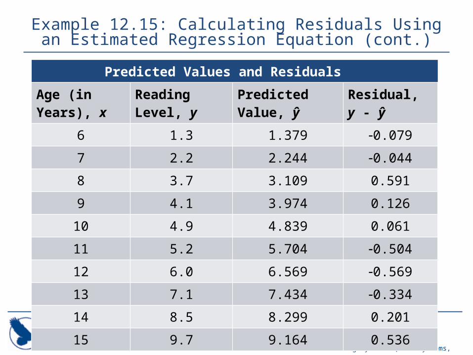
Example 12.15: Calculating Residuals Using an Estimated Regression Equation (cont.)
Predicted Values and Residuals Age (in Years), x Reading Level, y Predicted Value, ŷ Residual, y - ŷ
6 1.3 1.379 -0.0797 2.2 2.244 -0.0448 3.7 3.109 0.5919 4.1 3.974 0.126
10 4.9 4.839 0.06111 5.2 5.704 -0.50412 6.0 6.569 -0.56913 7.1 7.434 -0.33414 8.5 8.299 0.20115 9.7 9.164 0.536
HAWKES LEARNING SYSTEMS
Students Matter. Success Counts.
Copyright © 2013 by Hawkes Learning
Systems/Quant Systems, Inc.
All rights reserved.
Regression Analysis
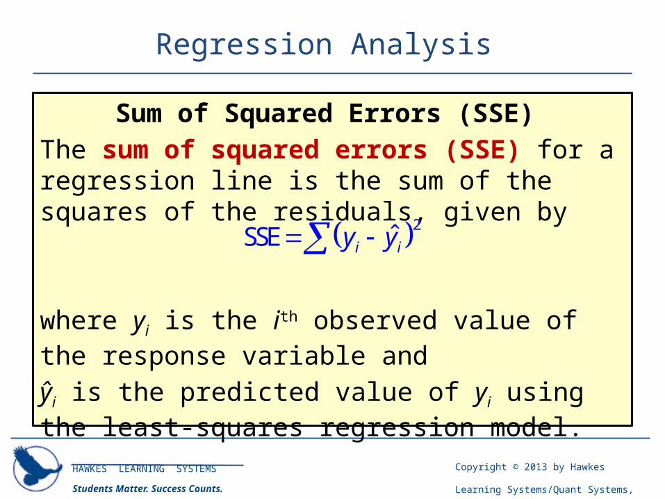
Sum of Squared Errors (SSE) The sum of squared errors (SSE) for a regression line is the sum of the squares of the residuals, given by
where yi is the ith observed value of the response variable and ŷi is the predicted value of yi using the least-squares regression model.
2ˆSSE i iy y -
HAWKES LEARNING SYSTEMS
Students Matter. Success Counts.
Copyright © 2013 by Hawkes Learning
Systems/Quant Systems, Inc.
All rights reserved.
Example 12.16: Calculating the Sum of Squared Errors
Calculate the sum of squared errors, SSE, for the data on children’s ages and reading levels from the previous example. SolutionUsing the values we calculated in the previous example, we begin by squaring each error as shown in the following table.
HAWKES LEARNING SYSTEMS
Students Matter. Success Counts.
Copyright © 2013 by Hawkes Learning
Systems/Quant Systems, Inc.
All rights reserved.
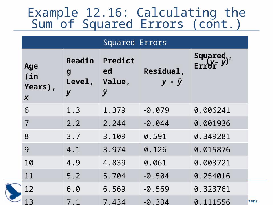
Example 12.16: Calculating the Sum of Squared Errors (cont.)
Squared Errors Age (in Years), x
Reading Level, y
Predicted Value, ŷ
Residual, y - ŷ
Squared Error
6 1.3 1.379 -0.079 0.0062417 2.2 2.244 -0.044 0.0019368 3.7 3.109 0.591 0.3492819 4.1 3.974 0.126 0.01587610 4.9 4.839 0.061 0.00372111 5.2 5.704 -0.504 0.25401612 6.0 6.569 -0.569 0.32376113 7.1 7.434 -0.334 0.111556
2ˆy y-
HAWKES LEARNING SYSTEMS
Students Matter. Success Counts.
Copyright © 2013 by Hawkes Learning
Systems/Quant Systems, Inc.
All rights reserved.
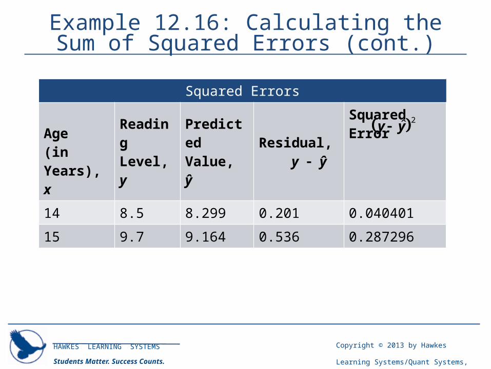
Example 12.16: Calculating the Sum of Squared Errors (cont.)
Squared Errors Age (in Years), x
Reading Level, y
Predicted Value, ŷ
Residual, y - ŷ
Squared Error
14 8.5 8.299 0.201 0.04040115 9.7 9.164 0.536 0.287296
2ˆy y-
HAWKES LEARNING SYSTEMS
Students Matter. Success Counts.
Copyright © 2013 by Hawkes Learning
Systems/Quant Systems, Inc.
All rights reserved.
Example 12.16: Calculating the Sum of Squared Errors (cont.)
The last column lists the squares of the residual values. The sum of the squared errors is the sum of the values in this last column. Thus, SSE ≈ 1.394.
HAWKES LEARNING SYSTEMS
Students Matter. Success Counts.
Copyright © 2013 by Hawkes Learning
Systems/Quant Systems, Inc.
All rights reserved.
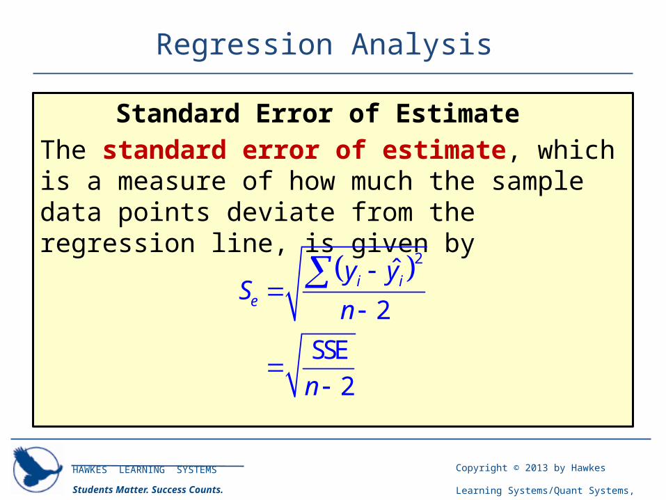
Regression Analysis
Standard Error of Estimate The standard error of estimate, which is a measure of how much the sample data points deviate from the regression line, is given by
2ˆ
2
SSE2
i ie
y yS
n
n
-
-
-
HAWKES LEARNING SYSTEMS
Students Matter. Success Counts.
Copyright © 2013 by Hawkes Learning
Systems/Quant Systems, Inc.
All rights reserved.
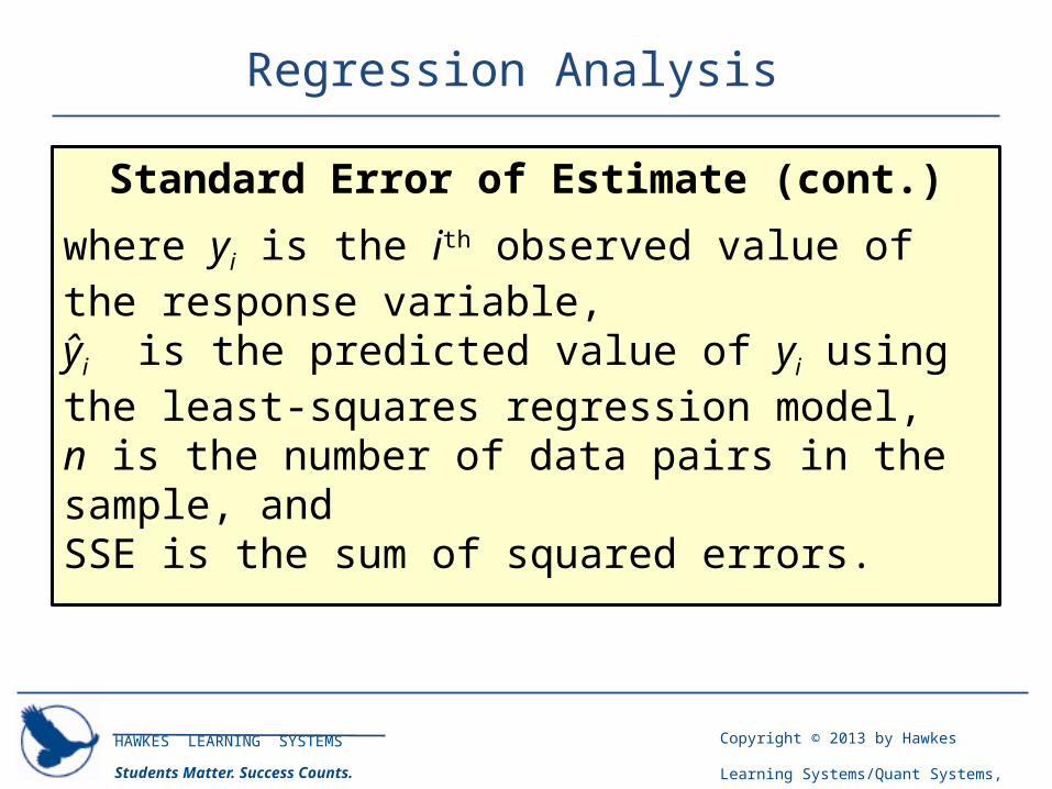
Regression Analysis
Standard Error of Estimate (cont.)
where yi is the ith observed value of the response variable, ŷi is the predicted value of yi using the least-squares regression model, n is the number of data pairs in the sample, and SSE is the sum of squared errors.
HAWKES LEARNING SYSTEMS
Students Matter. Success Counts.
Copyright © 2013 by Hawkes Learning
Systems/Quant Systems, Inc.
All rights reserved.
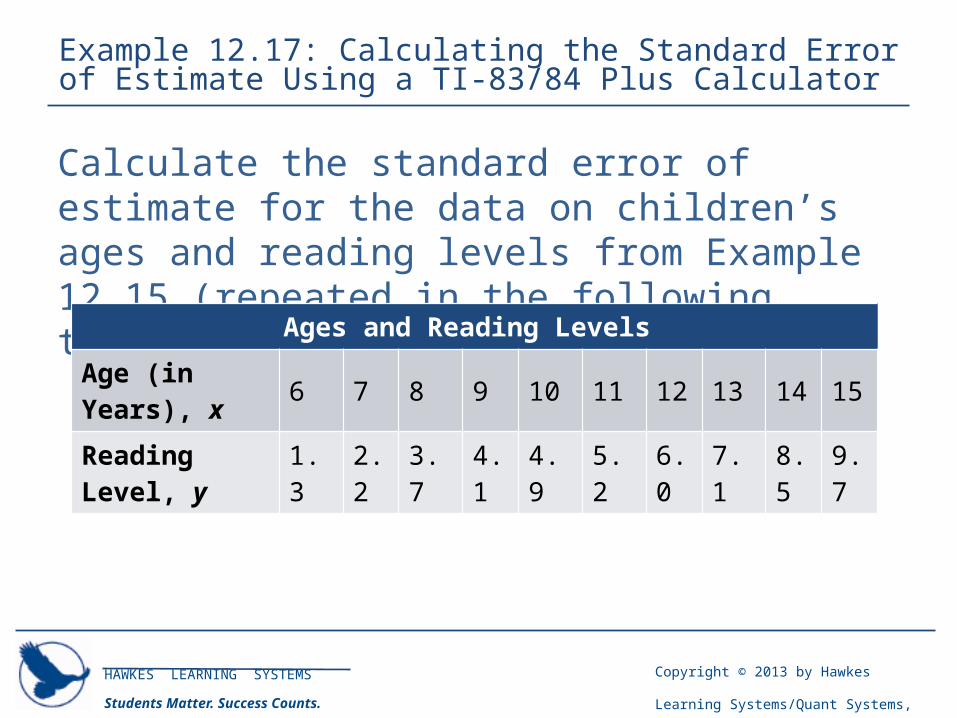
Example 12.17: Calculating the Standard Error of Estimate Using a TI-83/84 Plus Calculator
Calculate the standard error of estimate for the data on children’s ages and reading levels from Example 12.15 (repeated in the following table).
Ages and Reading Levels Age (in Years), x 6 7 8 9 10 11 12 13 14 15Reading Level, y 1.3 2.2 3.7 4.1 4.9 5.2 6.0 7.1 8.5 9.7
HAWKES LEARNING SYSTEMS
Students Matter. Success Counts.
Copyright © 2013 by Hawkes Learning
Systems/Quant Systems, Inc.
All rights reserved.
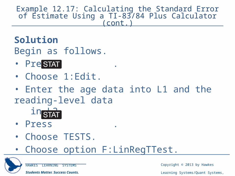
Example 12.17: Calculating the Standard Error of Estimate Using a TI-83/84 Plus Calculator (cont.)
SolutionBegin as follows. • Press . • Choose 1:Edit. • Enter the age data into L1 and the reading-level data in L2. • Press . • Choose TESTS. • Choose option F:LinRegTTest.
HAWKES LEARNING SYSTEMS
Students Matter. Success Counts.
Copyright © 2013 by Hawkes Learning
Systems/Quant Systems, Inc.
All rights reserved.
Example 12.17: Calculating the Standard Error of Estimate Using a TI-83/84 Plus Calculator (cont.)
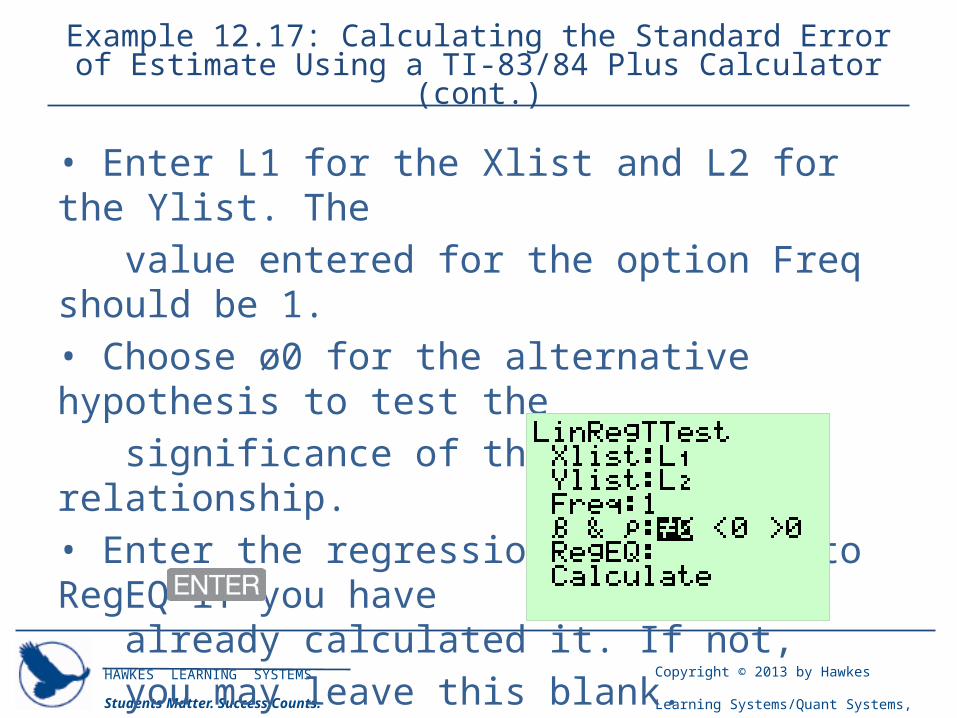
• Enter L1 for the Xlist and L2 for the Ylist. The value entered for the option Freq should be 1. • Choose ø0 for the alternative hypothesis to test the significance of the linear relationship. • Enter the regression equation into RegEQ if you have
already calculated it. If not, you may leave this blank. • Choose Calculate. • Press .
HAWKES LEARNING SYSTEMS
Students Matter. Success Counts.
Copyright © 2013 by Hawkes Learning
Systems/Quant Systems, Inc.
All rights reserved.
Example 12.17: Calculating the Standard Error of Estimate Using a TI-83/84 Plus Calculator (cont.)
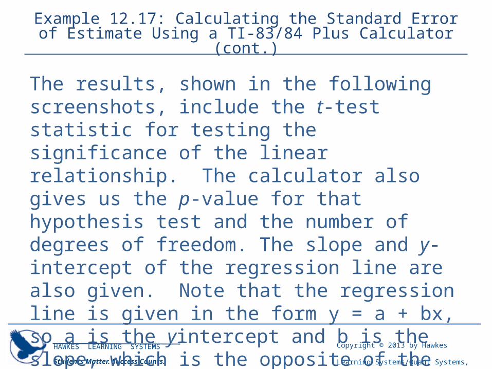
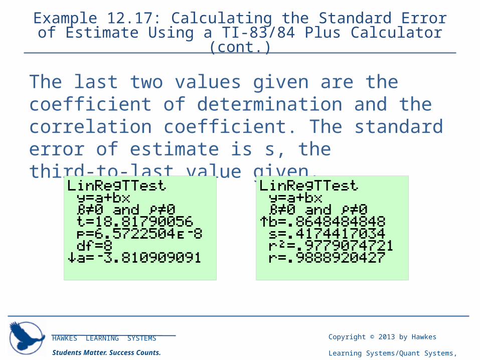
The results, shown in the following screenshots, include the t-test statistic for testing the significance of the linear relationship. The calculator also gives us the p value for that hypothesis test and the number of ‑degrees of freedom. The slope and y-intercept of the regression line are also given. Note that the regression line is given in the form y = a + bx, so a is the y intercept and b is the slope, which is the opposite of the results that we get when we use the LinReg(ax+b) function.
HAWKES LEARNING SYSTEMS
Students Matter. Success Counts.
Copyright © 2013 by Hawkes Learning
Systems/Quant Systems, Inc.
All rights reserved.
Example 12.17: Calculating the Standard Error of Estimate Using a TI-83/84 Plus Calculator (cont.)
The last two values given are the coefficient of determination and the correlation coefficient. The standard error of estimate is s, the third to last value ‑ ‑given.
HAWKES LEARNING SYSTEMS
Students Matter. Success Counts.
Copyright © 2013 by Hawkes Learning
Systems/Quant Systems, Inc.
All rights reserved.
Example 12.17: Calculating the Standard Error of Estimate Using a TI-83/84 Plus Calculator (cont.)
Thus, the standard error of estimate for the data on ages and reading levels is Se ≈ 0.417. Since this value is close to 0, we can conclude that the data points do not deviate very much from the regression line.
HAWKES LEARNING SYSTEMS
Students Matter. Success Counts.
Copyright © 2013 by Hawkes Learning
Systems/Quant Systems, Inc.
All rights reserved.
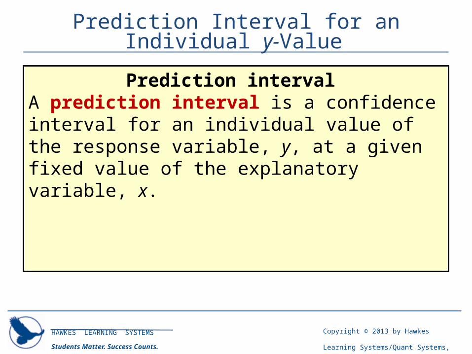
Prediction Interval for an Individual y-Value
Prediction interval A prediction interval is a confidence interval for an individual value of the response variable, y, at a given fixed value of the explanatory variable, x.
HAWKES LEARNING SYSTEMS
Students Matter. Success Counts.
Copyright © 2013 by Hawkes Learning
Systems/Quant Systems, Inc.
All rights reserved.
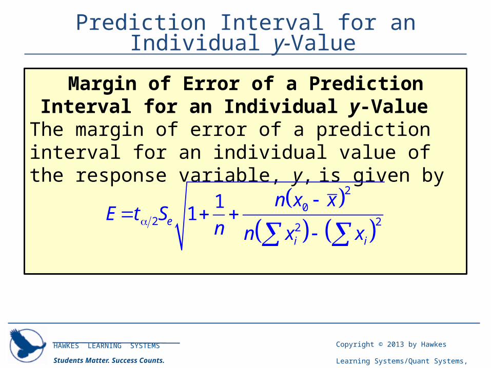
Prediction Interval for an Individual y-Value
Margin of Error of a Prediction Interval for an Individual y-Value
The margin of error of a prediction interval for an individual value of the response variable, y, is given by
2
02 22
11e
i i
n x xE t S
n n x x
-
-
HAWKES LEARNING SYSTEMS
Students Matter. Success Counts.
Copyright © 2013 by Hawkes Learning
Systems/Quant Systems, Inc.
All rights reserved.
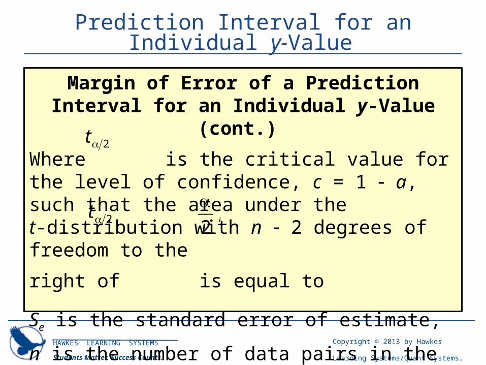
Prediction Interval for an Individual y-Value
Margin of Error of a Prediction Interval for an Individual y-Value (cont.)
Where is the critical value for the level of confidence, c = 1 - a, such that the area under the t distribution with ‑ n - 2 degrees of freedom to the
right of is equal to
Se is the standard error of estimate,
n is the number of data pairs in the sample,
2t
2t ,2
HAWKES LEARNING SYSTEMS
Students Matter. Success Counts.
Copyright © 2013 by Hawkes Learning
Systems/Quant Systems, Inc.
All rights reserved.
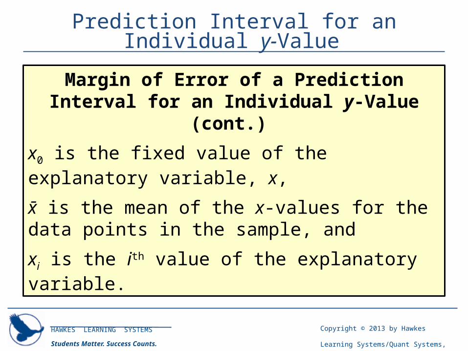
Prediction Interval for an Individual y-Value
Margin of Error of a Prediction Interval for an Individual y-Value (cont.)
x0 is the fixed value of the explanatory variable, x,
x̄� is the mean of the x-values for the data points in the sample, and
xi is the ith value of the explanatory variable.
HAWKES LEARNING SYSTEMS
Students Matter. Success Counts.
Copyright © 2013 by Hawkes Learning
Systems/Quant Systems, Inc.
All rights reserved.
Prediction Interval for an Individual y-Value
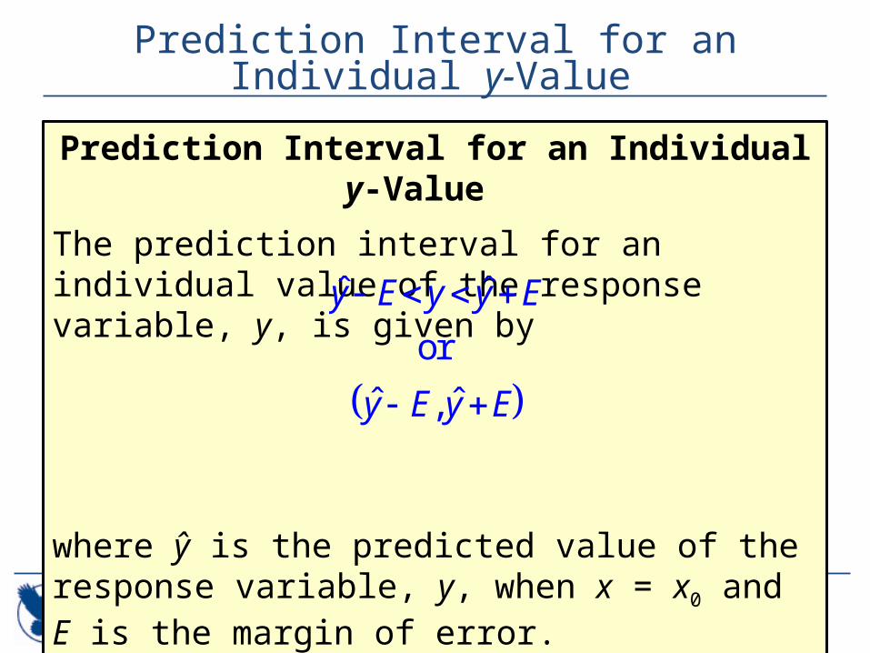
Prediction Interval for an Individual y-Value
The prediction interval for an individual value of the response variable, y, is given by
where ŷ is the predicted value of the response variable, y, when x = x0 and E is the margin of error.
ˆ ˆ
orˆ ˆ,
y E y y E
y E y E
-
-
HAWKES LEARNING SYSTEMS
Students Matter. Success Counts.
Copyright © 2013 by Hawkes Learning
Systems/Quant Systems, Inc.
All rights reserved.
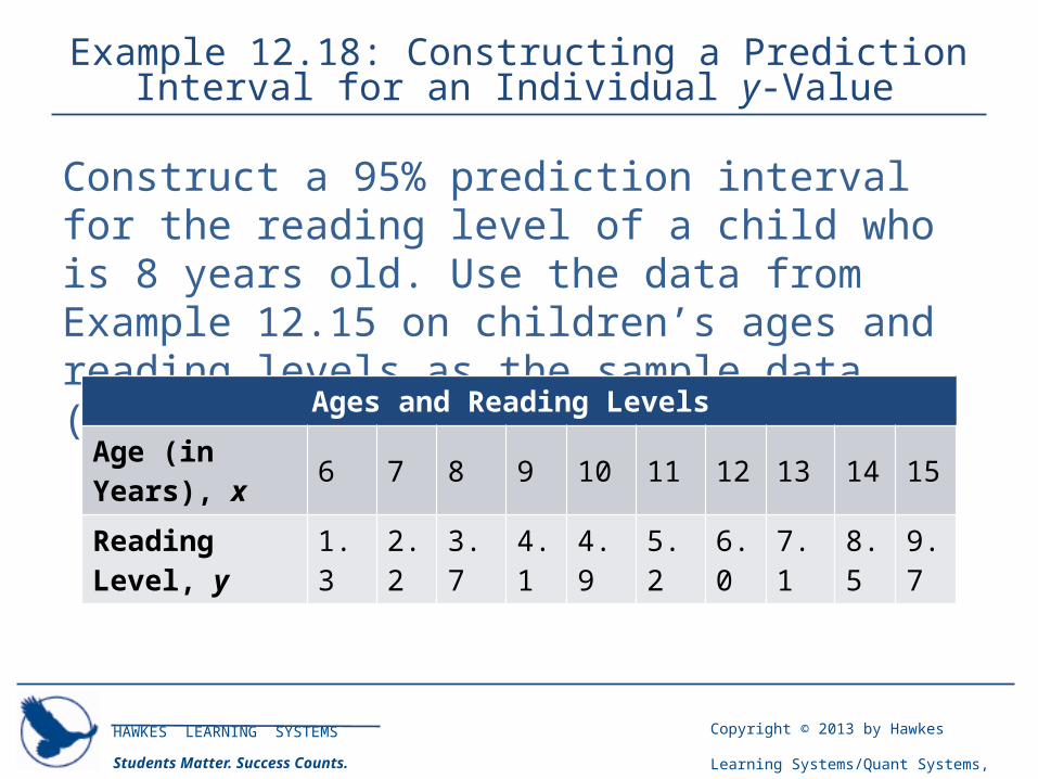
Example 12.18: Constructing a Prediction Interval for an Individual y-Value
Construct a 95% prediction interval for the reading level of a child who is 8 years old. Use the data from Example 12.15 on children’s ages and reading levels as the sample data (repeated in the following table).
Ages and Reading Levels Age (in Years), x 6 7 8 9 10 11 12 13 14 15Reading Level, y 1.3 2.2 3.7 4.1 4.9 5.2 6.0 7.1 8.5 9.7
HAWKES LEARNING SYSTEMS
Students Matter. Success Counts.
Copyright © 2013 by Hawkes Learning
Systems/Quant Systems, Inc.
All rights reserved.
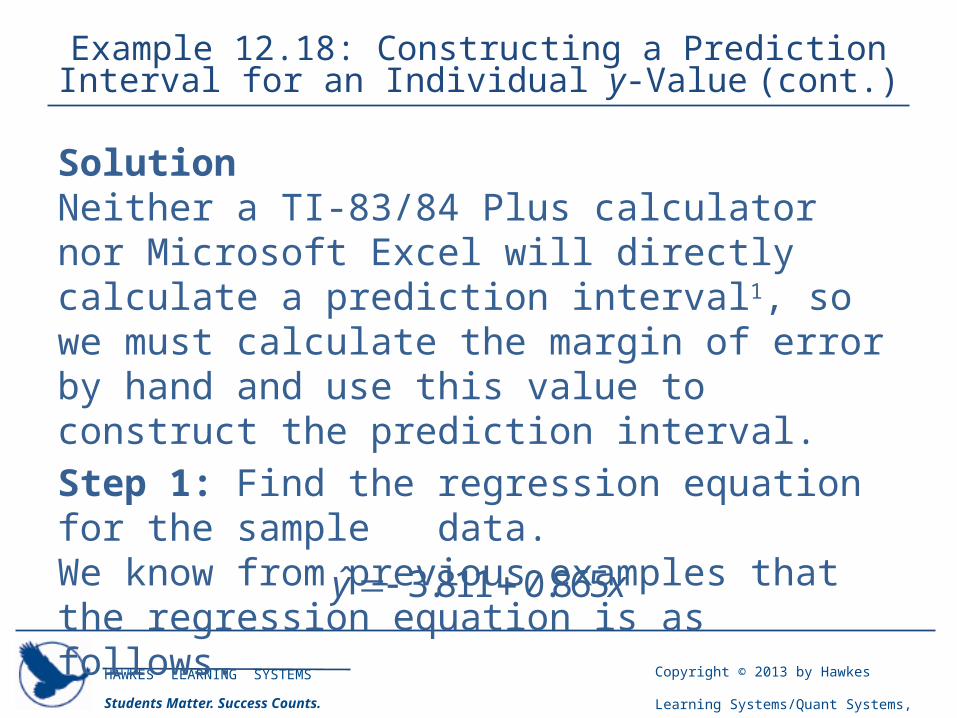
Example 12.18: Constructing a Prediction Interval for an Individual y-Value (cont.)
SolutionNeither a TI-83/84 Plus calculator nor Microsoft Excel will directly calculate a prediction interval1, so we must calculate the margin of error by hand and use this value to construct the prediction interval.Step 1: Find the regression equation for the sample data. We know from previous examples that the regression equation is as follows.
ˆ 3.811 0.865y x-
HAWKES LEARNING SYSTEMS
Students Matter. Success Counts.
Copyright © 2013 by Hawkes Learning
Systems/Quant Systems, Inc.
All rights reserved.
Example 12.18: Constructing a Prediction Interval for an Individual y-Value (cont.)
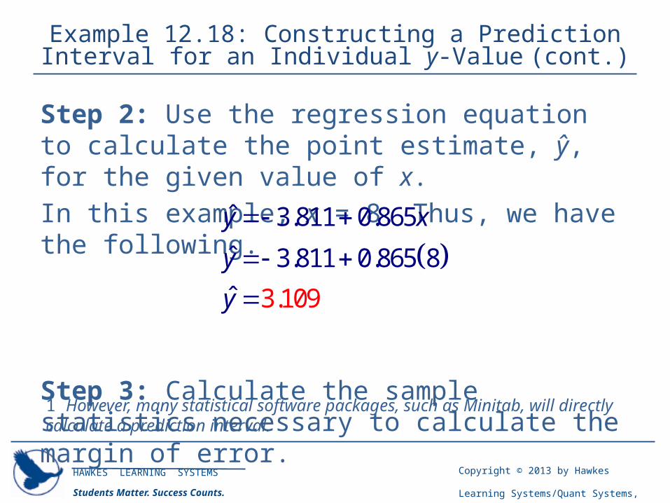
Step 2: Use the regression equation to calculate the point estimate, ŷ, for the given value of x. In this example, x = 8. Thus, we have the following.
Step 3: Calculate the sample statistics necessary to calculate the margin of error.
ˆ 3.811 0.865ˆ 3.811 0.865 8
3.109ˆ
y x
y
y
-
-
1 However, many statistical software packages, such as Minitab, will directly calculate a prediction interval.
HAWKES LEARNING SYSTEMS
Students Matter. Success Counts.
Copyright © 2013 by Hawkes Learning
Systems/Quant Systems, Inc.
All rights reserved.
Example 12.18: Constructing a Prediction Interval for an Individual y-Value (cont.)
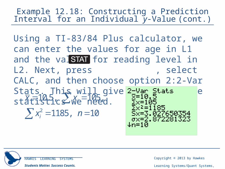
Using a TI-83/84 Plus calculator, we can enter the values for age in L1 and the values for reading level in L2. Next, press , select CALC, and then choose option 2:2-Var Stats. This will give us many of the statistics we need.
2
10.5, 105,
1185, 10i
i
x x
x n
HAWKES LEARNING SYSTEMS
Students Matter. Success Counts.
Copyright © 2013 by Hawkes Learning
Systems/Quant Systems, Inc.
All rights reserved.
Example 12.18: Constructing a Prediction Interval for an Individual y-Value (cont.)
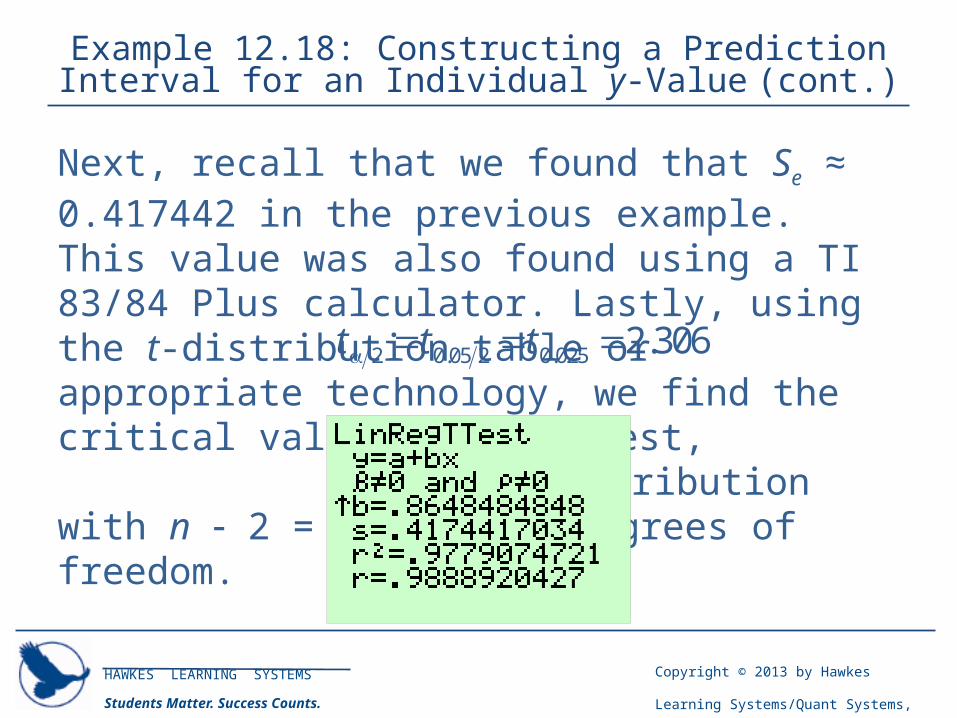
Next, recall that we found that Se ≈ 0.417442 in the previous example. This value was also found using a TI 83/84 Plus calculator. Lastly, using the t-distribution table or appropriate technology, we find the critical value for this test, for the t distribution with n - 2 = 10 - 2 = 8 degrees of freedom.
2 0.05 2 0.025 2.306tt t
HAWKES LEARNING SYSTEMS
Students Matter. Success Counts.
Copyright © 2013 by Hawkes Learning
Systems/Quant Systems, Inc.
All rights reserved.
Example 12.18: Constructing a Prediction Interval for an Individual y-Value (cont.)
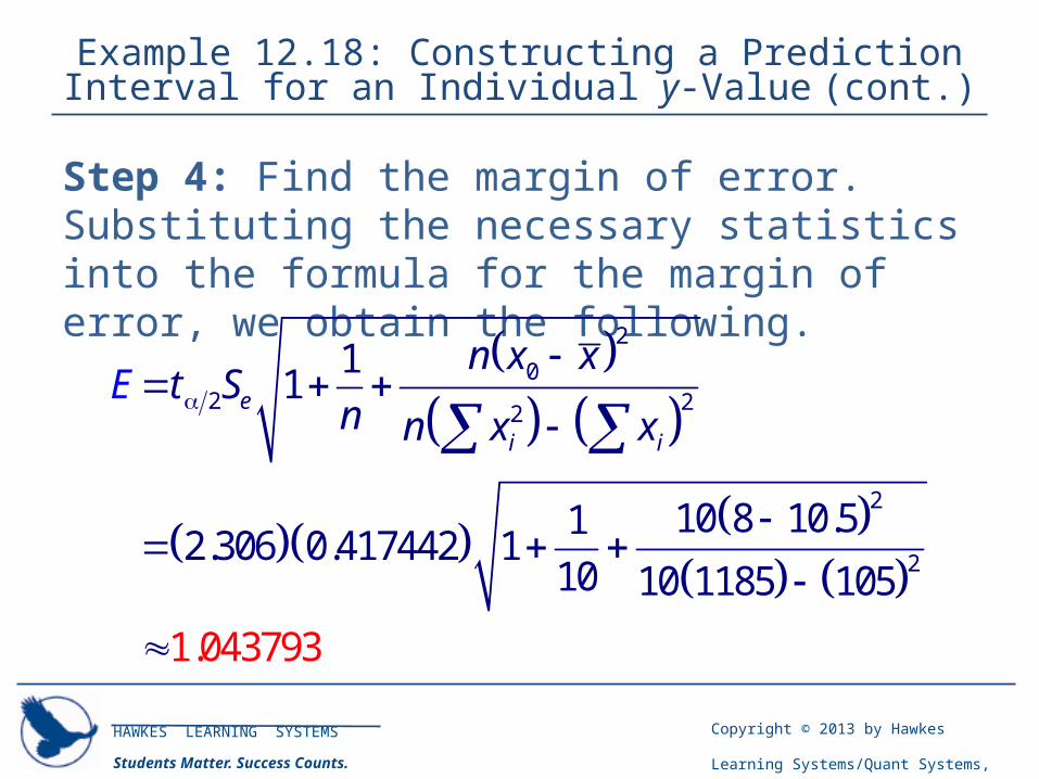
Step 4: Find the margin of error. Substituting the necessary statistics into the formula for the margin of error, we obtain the following.
2
02 22
2
2
11
10 8 10.512.306 0.417442 1
10
1.043793
10 1185 105
e
i i
n x xt S
n nE
x x
-
-
-
-
HAWKES LEARNING SYSTEMS
Students Matter. Success Counts.
Copyright © 2013 by Hawkes Learning
Systems/Quant Systems, Inc.
All rights reserved.
Example 12.18: Constructing a Prediction Interval for an Individual y-Value (cont.)
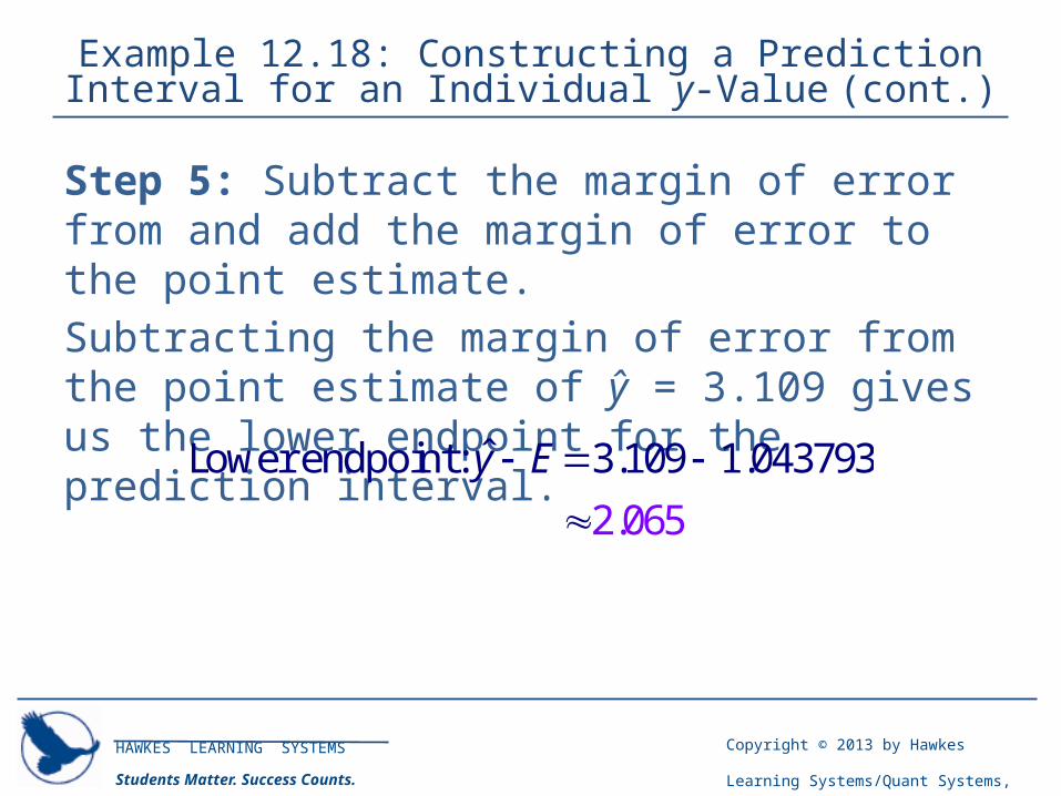
Step 5: Subtract the margin of error from and add the margin of error to the point estimate. Subtracting the margin of error from the point estimate of ŷ = 3.109 gives us the lower endpoint for the prediction interval.
2.0
ˆLower endpoint: 3.109 1.04365
793y E- -

HAWKES LEARNING SYSTEMS
Students Matter. Success Counts.
Copyright © 2013 by Hawkes Learning
Systems/Quant Systems, Inc.
All rights reserved.
Example 12.18: Constructing a Prediction Interval for an Individual y-Value (cont.)
By adding the margin of error to the point estimate, we obtain the upper endpoint for the prediction interval as follows.
4.1
ˆUpper endpoint: 3.109 1.04353
793y E

HAWKES LEARNING SYSTEMS
Students Matter. Success Counts.
Copyright © 2013 by Hawkes Learning
Systems/Quant Systems, Inc.
All rights reserved.
Example 12.18: Constructing a Prediction Interval for an Individual y-Value (cont.)
Thus the 95% confidence interval for the individual y value ranges from 2.065 to 4.153. The confidence interval can be written mathematically using either inequality symbols or interval notation, as shown below.
or
2.
2.
065
0
4.
65
15
, 5
3
4.1 3
y
HAWKES LEARNING SYSTEMS
Students Matter. Success Counts.
Copyright © 2013 by Hawkes Learning
Systems/Quant Systems, Inc.
All rights reserved.
Example 12.18: Constructing a Prediction Interval for an Individual y-Value (cont.)
Thus, for an 8-year-old child, we can be 95% confident that he or she would have a reading level between 2.065 and 4.153, or be reading between the second and fourth grade levels.
HAWKES LEARNING SYSTEMS
Students Matter. Success Counts.
Copyright © 2013 by Hawkes Learning
Systems/Quant Systems, Inc.
All rights reserved.
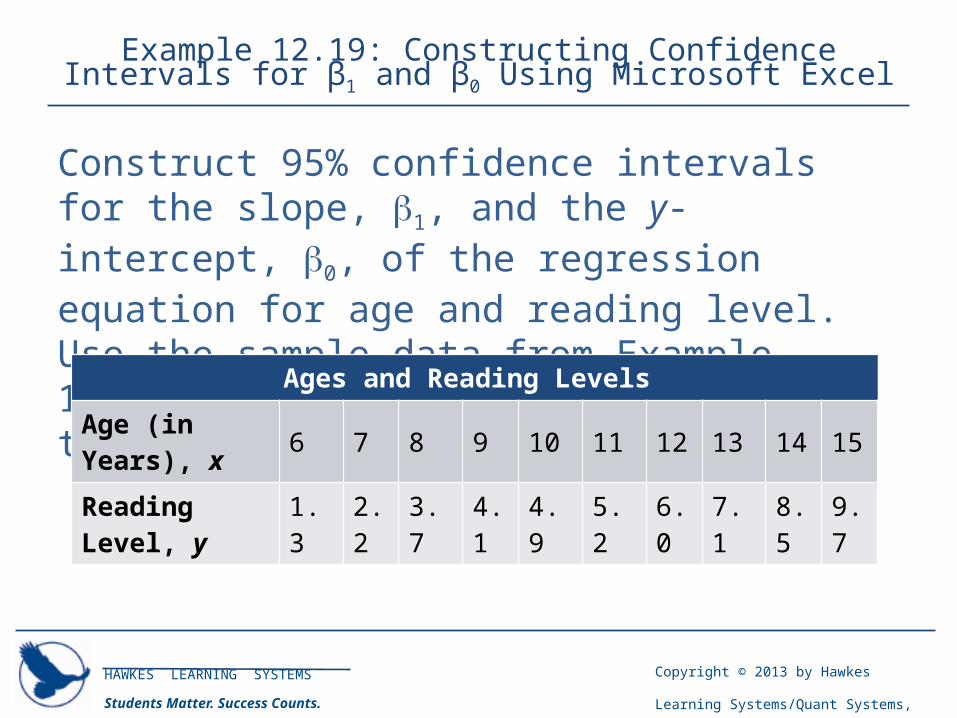
Example 12.19: Constructing Confidence Intervals for β1 and β0 Using Microsoft Excel
Construct 95% confidence intervals for the slope, b1, and the y-intercept, b0, of the regression equation for age and reading level. Use the sample data from Example 12.15 (repeated in the following table).
Ages and Reading Levels Age (in Years), x 6 7 8 9 10 11 12 13 14 15Reading Level, y 1.3 2.2 3.7 4.1 4.9 5.2 6.0 7.1 8.5 9.7
HAWKES LEARNING SYSTEMS
Students Matter. Success Counts.
Copyright © 2013 by Hawkes Learning
Systems/Quant Systems, Inc.
All rights reserved.
Example 12.19: Constructing Confidence Intervals for β1 and β0 Using Microsoft Excel (cont.)
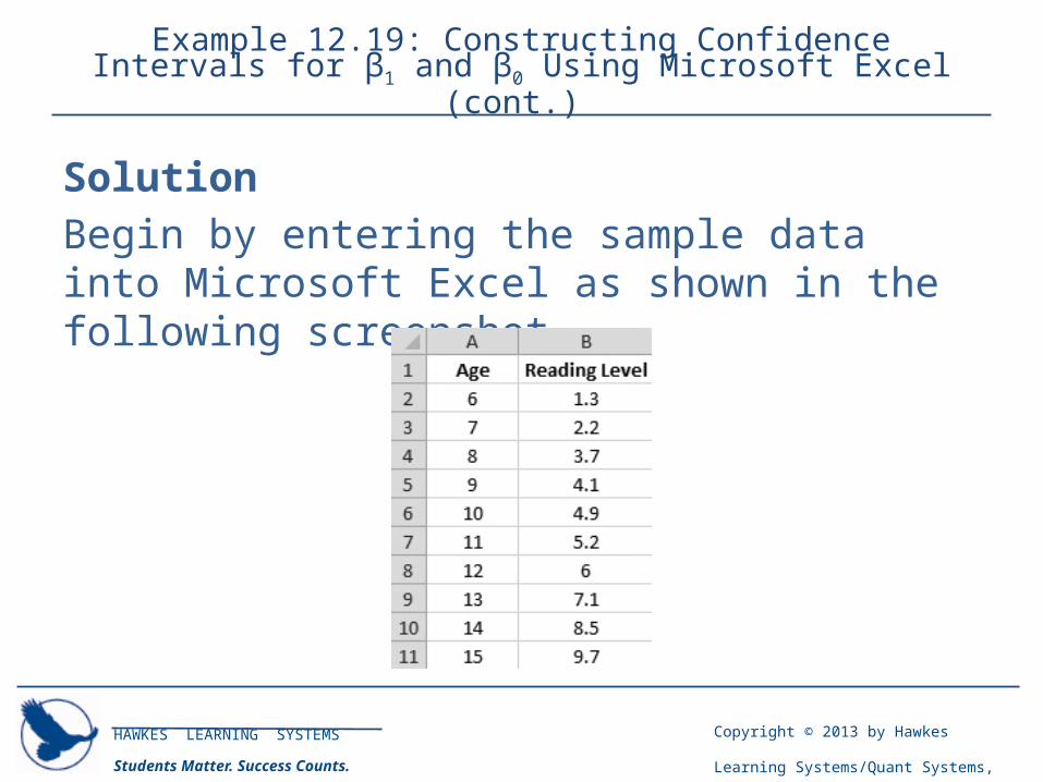
SolutionBegin by entering the sample data into Microsoft Excel as shown in the following screenshot
HAWKES LEARNING SYSTEMS
Students Matter. Success Counts.
Copyright © 2013 by Hawkes Learning
Systems/Quant Systems, Inc.
All rights reserved.
Example 12.19: Constructing Confidence Intervals for β1 and β0 Using Microsoft Excel (cont.)
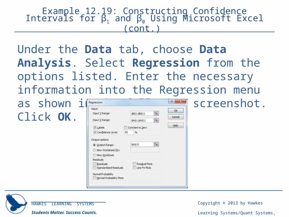
Under the Data tab, choose Data Analysis. Select Regression from the options listed. Enter the necessary information into the Regression menu as shown in the following screenshot. Click OK.
HAWKES LEARNING SYSTEMS
Students Matter. Success Counts.
Copyright © 2013 by Hawkes Learning
Systems/Quant Systems, Inc.
All rights reserved.
Example 12.19: Constructing Confidence Intervals for β1 and β0 Using Microsoft Excel (cont.)
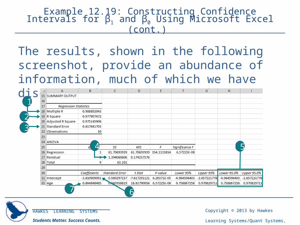
The results, shown in the following screenshot, provide an abundance of information, much of which we have discussed throughout this chapter.
1
23
4 5
7 6

HAWKES LEARNING SYSTEMS
Students Matter. Success Counts.
Copyright © 2013 by Hawkes Learning
Systems/Quant Systems, Inc.
All rights reserved.
Example 12.19: Constructing Confidence Intervals for β1 and β0 Using Microsoft Excel (cont.)
Multiple R is the absolute value of the correlation coefficient, |r|. R Square is the coefficient of determination, r2. Standard Error is the standard error of estimate,
Se.
The ANOVA table will be discussed in the next section, since it is more meaningful when discussing more than one explanatory variable. However, it does contain a few of the important values we discussed so far in this section.
1
2
3

HAWKES LEARNING SYSTEMS
Students Matter. Success Counts.
Copyright © 2013 by Hawkes Learning
Systems/Quant Systems, Inc.
All rights reserved.
Example 12.19: Constructing Confidence Intervals for β1 and β0 Using Microsoft Excel (cont.)
The intersection of the Residual row and the SS column is the sum of squared errors, SSE. 5 The Lower 95.0% and Upper 95.0% columns
give the lower and upper endpoints of the 95% confidence intervals for the y-intercept and slope.
The Coefficients column gives the values for the coefficients, that is, the y-intercept and slope, of the regression line.
4
5
6 7
HAWKES LEARNING SYSTEMS
Students Matter. Success Counts.
Copyright © 2013 by Hawkes Learning
Systems/Quant Systems, Inc.
All rights reserved.
Example 12.19: Constructing Confidence Intervals for β1 and β0 Using Microsoft Excel (cont.)
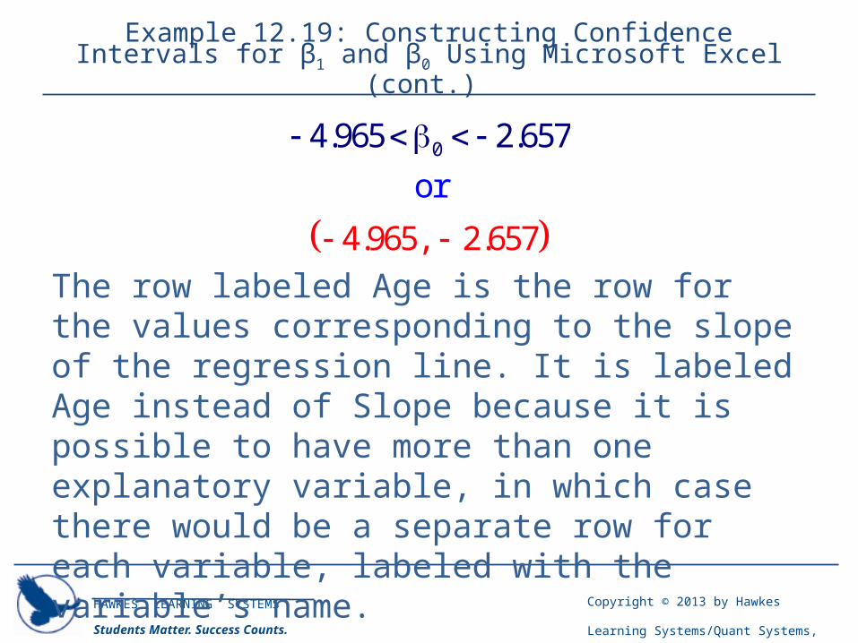
The lower and upper endpoints of the 95% confidence intervals for the y-intercept and slope are the values we are interested in for this example.The row labeled Intercept is the row for the values corresponding to the y-intercept. Notice that the first value in this row is b0 ≈ −3.811. The last two values in this row are the lower and upper endpoints for a 95% confidence interval for the y-intercept of the regression line, b0. Thus, the 95% confidence interval for b0 can be written as follows.
HAWKES LEARNING SYSTEMS
Students Matter. Success Counts.
Copyright © 2013 by Hawkes Learning
Systems/Quant Systems, Inc.
All rights reserved.
Example 12.19: Constructing Confidence Intervals for β1 and β0 Using Microsoft Excel (cont.)
The row labeled Age is the row for the values corresponding to the slope of the regression line. It is labeled Age instead of Slope because it is possible to have more than one explanatory variable, in which case there would be a separate row for each variable, labeled with the variable’s name.
0
or4.965 2.657
4.965, 2.657- -
- b -
HAWKES LEARNING SYSTEMS
Students Matter. Success Counts.
Copyright © 2013 by Hawkes Learning
Systems/Quant Systems, Inc.
All rights reserved.
Example 12.19: Constructing Confidence Intervals for β1 and β0 Using Microsoft Excel (cont.)
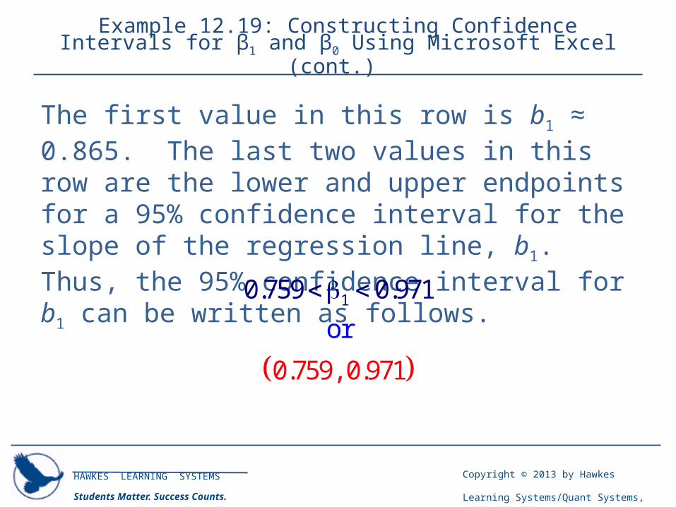
The first value in this row is b1 ≈ 0.865. The last two values in this row are the lower and upper endpoints for a 95% confidence interval for the slope of the regression line, b1. Thus, the 95% confidence interval for b1 can be written as follows.
1
or0.7
0.7
59 0
59
.971
, 0.971
b
Related Documents