Second problem (PH-353) Monte Carlo in Quantum Mechanicspyweb.swan.ac.uk/~pybl/PH353/mc.pdf · Outline Second problem (PH-353) Monte Carlo in Quantum Mechanics Biagio Lucini February

Outline

Second problem (PH-353)

Monte Carlo in Quantum Mechanics

Biagio Lucini

February 2008

Biagio Lucini Monte Carlo Methods

Outline

Pseudorandom number generators

1 Integrals and random events

2 Random numbers

3 Random number generators

4 A simple generator


Outline

Monte Carlo integration

5 Comparison with grid methods

6 Example: computation of π


Outline

Monte Carlo in Statistical

7 Example: gaussian distribution

8 Markov chains

9 Algorithms


Outline

Monte Carlo in Quantum Mechanics

10 Path Integrals and Monte Carlo

11 Discretised and continuum physics


Outline

Analysis of Monte Carlo data

12 Analysis of uncorrelated data

13 Analysis of correlated data

14 Extrapolation


Outline

Assignment

15 Monte Carlo in practice

16 The Gaussian system

17 The harmonic oscillator

18 The anharmonic oscillator

19 References


Integrals and random eventsRandom numbers

Random number generatorsA simple generator

Part I

Pseudorandom number generators




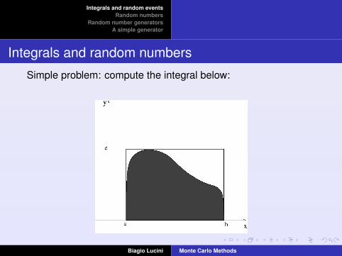
Integrals and random numbers

Simple problem: compute the integral below:




Random numbers

Physical approach: construction of a cosmic ray detector

area ∝ number of events per second

We need to know the number of events per unit area⇒ thedetector has known area

Numerical computation⇒ code for the generation of randomnumbersDeterministic algorithm for the generation of random numbers




Random numbers





Contradiction?




Random numbers





Contradiction?No: PSEUDOrandom numbers




Random number generators

Algorithm that generates a flat distribution P(x) in the interval[0,1] ∫ b

aP(x)dx = b − a, 0 ≤ a ≤ b < 1

P is then homogeneous in the interval [A,B[

P(x) = A + (B − A)× P(x)

Other probability distributions can be obtained from thehomogeneous distribution

e.g. Box-Muller transformation⇒ gaussian distributionBiagio Lucini Monte Carlo Methods



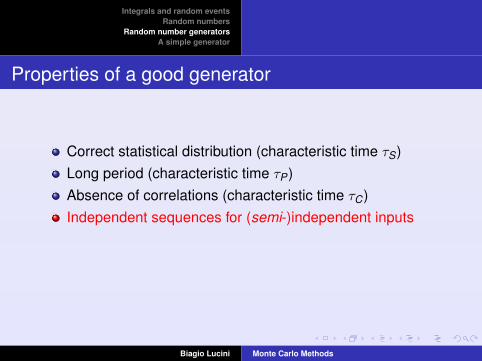
Properties of a good generator

Correct statistical distribution (characteristic time τS)Long period (characteristic time τP)Absence of correlations (characteristic time τC)Independent sequences for (semi-)independent inputs





















How good a generator is depends on how long we need to useit for: τ � min(τS, τP , τC)




Linear Congruential Method

xi = [(a× xi−1 + b) mod (c)] xi ,a, b, c ∈ Nr = xi/c

How good the generator is depends on the choice of theparameters. In particular, the period is related to c




Very bad generator

a = 121, b = 0, c = 6133Biagio Lucini Monte Carlo Methods



Good generator

a = 135121, b = 0, c = 61331237Biagio Lucini Monte Carlo Methods

Comparison with grid methodsExample: computation of π

Part II

Integration by Monte Carlo methods



Monte Carlo vs. Grid methods

Grid Methods

Systematic error ∝ O(1/Ns/d )

for instance, for the Simpson method s = 4

Monte Carlo methods

Systematic error ∝ O(1/√

N)

Monte Carlo methods become convenient for a large number ofintegration variables



Computation of π

−1

−1 1

1

π/4 = Events inside the circle / Total number of eventsBiagio Lucini Monte Carlo Methods


Algorithm for the computation of π

generate pairs of random numbers in [-1;1[compute how many pairs fall inside the circletake the ratio of those over the total number of generatedevents

A more efficient method

I =

∫D

F (x)dx =1V

∫D

F (x)Vdx = V

∫D F (x)dx∫

D dx' V

N

∑f (xi)



Convergence of the estimate


Example: gaussian distributionMarkov chains

Algorithms

Part III

Monte Carlo in Statistical Mechanics



Algorithms

A simple example

H = x2

The partition function

Z =

∫dx e−βH , β = 1/T

is exactly computable

P(x) = e−βH/Z probability distribution

〈U〉 =1Z

∫dx H(x) e−βH =

12β

internal energy



Algorithms

Dynamics

Ergodic hypothesis: average over a statistical ensemble 'average in time

Problem: give dynamics to the system

Fundamental property: at equilibrium, the configurations mustfollow Boltzmann distribution



Algorithms

Markov chains

Sequence of configurations Cnm in which Ct

m depends only fromCt−1

n according to a probability distribution Pnm (upper index:time; lower index: number of the configuration)

Irreducible if from any Cj we can reach Cl l > j , i.e. if a time kexists such that Pk

jl =∑

i1...in Pji1Pi1i2 ...Pin l 6= 0 for any j , l

Aperiodic if Pkii 6= 1 for any i , k

State Ci positive if it occurs on average for a finite time



Algorithms

Equilibrium distribution

{Ci} irreducible and aperiodic Markov chain with only positivestates

the equilibrium distribution exists and is unique(⇒ independence from the initial state)

limN→∞

PNij = Pj

the equilibrium distribution is stationary

Pj =∑

i

P1ij Pi

if the variance of the recurring time is finite∑i

PiO(Ci) = 〈O〉 = limN→∞

1N

N∑j=1

O(Cj)



Algorithms




limN→∞

PNij = Pj


Pj =∑

i

P1ij Pi



1N

N∑j=1

O(Cj)



Algorithms




limN→∞

PNij = Pj


Pj =∑

i

P1ij Pi



1N

N∑j=1

O(Cj)



Algorithms

Detailed balance

Monte Carlo dynamics: any Markovian dynamics

Problem: given a Hamiltonian, write a Markovian dynamics

Necessary condition unknown

Sufficient condition: detailed balance

e−βH(Ci )Pij = e−βH(Cj )Pji

Still freedom on the choice of Pij



Algorithms

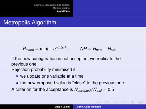
Metropolis Algorithm

Pmetro = min(1,e−β∆H) , ∆H = Hnew − Hold

If the new configuration is not accepted, we replicate theprevious oneRejection probability minimised if

we update one variable at a timethe new proposed value is “close” to the previous one

A criterion for the acceptance is Naccepted/Ntrial = 0.5



Algorithms

Heath Bath Algorithm

Phb ∝ e−βHnew

The HB probability does not depend on the previous value ofthe variable we want to update

Compared to Metropolisadvantage: better exploration of the configuration spacedisadvantage: requires random number with the sameprobability distribution as the system



Algorithms

Monte Carlo example

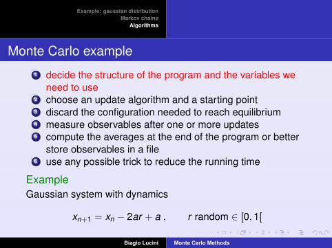
1 decide the structure of the program and the variables weneed to use

2 choose an update algorithm and a starting point3 discard the configuration needed to reach equilibrium4 measure observables after one or more updates5 compute the averages at the end of the program or better

store observables in a file6 use any possible trick to reduce the running time

ExampleGaussian system with dynamics

xn+1 = xn − 2ar + a , r random ∈ [0,1[


Path Integrals and Monte CarloDiscretised and continuum physics

Part IV

Monte Carlo methods in Quantum Mechanics



Path Integrals in Quantum Mechanics

An alternative way to formulate Quantum Mechanics (due toFeynman) is the path integral

For a system with mass m subject to a potential V (x) inaddition to the Hamiltonian H = (1/2m)p2 + V (x) we define theLagrangian L = (1/2)mx2 − V (x)

The probability amplitude of having xt0 at time t0 and xf at timetf is

〈xf (t)|e−iHt |x0(0)〉 =

∫(Dx) eiS, S =

∫ tf

t0d tL

and (Dx) is a formal expression that means “integration over allpossible paths connecting x0 and xf



Wick rotation

The weighting with the action of the paths involves a complexintegral that is not suitable for numerical computations

We perform the Wick rotation t → it and define the Euclideanversion of L and S

LE =12

mx2 + V (x) , SE =

∫ tf

t0d tLE

〈xf (t)|e−iHt |x0(0)〉 can be obtained by continuing analytically∫(Dx) e−SE ,

Analogy with a statistical mechanical system with HamiltonianSE



Path integral and ground state

for Z , integrate over all possible initial and final x , with thecondition xf = x0one can prove that with this choice

limtf→∞

Z = e−E0tf |c0|2

Expectation values of observables over the ground stateare given by

〈O1(t1) . . . On(tn)〉 = Z−1∫

O1(t1) . . . On(tn) (Dx) e−SE ,

Note the analogy with ensemble averages in StatisticalMechanics

This formulation is particularly suited for extracting informationabout the ground states and the first exited (see later)



Discretisation

Dx is a formal symbol, which needs to be definedone possibility is to divide the temporal extension tf in Nsteps of interval a such that Na = tf (temporal lattice)the original theory is recovered in the limit a→ 0⇒ needto choose a small a (compared to the time scale of thesystem)with this choice Dx =

∏i dx(t = ia), i.e. a finite but large

number of integrals has to be performed⇒ Monte Carlointegration is a good choice



Continuum limit

for finite a the solution is distorted by discretisation effects(see later for an example with the harmonic oscillator)this effect disappears in the smooth limit a→ 0⇒ need towork with small aremember that tf has to be largea good choice takes into account these two requirements


Analysis of uncorrelated dataAnalysis of correlated data

Extrapolation

Part V

Analysis of Monte Carlo data



Extrapolation

Probability

Probability distribution P(x)

f = 〈f (x)〉 =

∫f (x)P(x)dx

Let us define

x = 〈x〉 averageσ2 = 〈(x − x)2〉 = 〈x2〉 − x2 variance

σ is called standard deviation



Extrapolation

Gaussian Distribution

P(x) =1

σ√

2πe−

(x−x)2

2σ2

95% of the measurements are within 2σ from the average

Central limit theorem: for N →∞ the averages of themeasurements are distributed according to a Gaussiandistribution with average the real value and variance σ2/N



Extrapolation

Bias

We have a bias when the average of the estimates does notcoincide with the true value

bias ∝ O(1/N)

This is irrelevant in the limit of infinite measurements

It is important to remove the bias when we average non-linearfunctions of the measured value.



Extrapolation

Average and Error

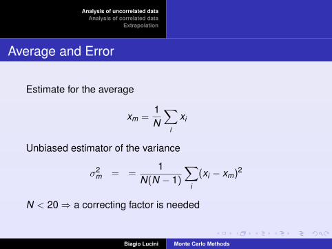
Estimate for the average

xm =1N

∑i

xi

Unbiased estimator of the variance

σ2m = =

1N(N − 1)

∑i

(xi − xm)2

N < 20⇒ a correcting factor is needed



Extrapolation

Thermalisation

The starting point is arbitrary

Equilibrium distribution obtained after a time τeq

Strategy: discard nτeq sweeps at the beginning

For a run with N measurementsweight of initial sweeps ∝ n/Nstatistical error ∝ 1/

√N

↪→ we do not need an exact estimate of τeq



Extrapolation

Thermalisation

Gaussian system



Extrapolation

Common sense rulesτeq � N: we can be cautious and discard more sweepsthan strictly neededτeq < N: we need to estimate τeq carefully



Extrapolation

Correlations

Hypothesis for the Gaussian analysis: uncorrelated dataThe independence among the data means that only thestatistical weight of the configurations determines the history ofthe system

However Monte Carlo dynamics limits the possibilities ofmoving in configuration space

ExampleDinamics xn+1 = xn − 2ar + aProblem: remove correlations



Extrapolation

Correlation time

For a given observable and given dynamicsExponential correlation time

C(τ) = 〈O(t)O(t + τ)〉 ∝ e−τ/τexp

Integrated correlation time

τint = 1 + 2N−1∑τ=1

C(τ)

For the error σ2 = σ2naiveτint

Moreover 2τexp ' τint



Extrapolation

Results for the Gaussian system

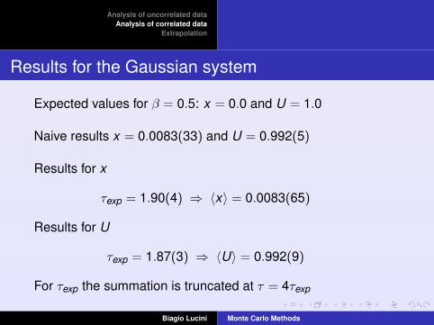
Expected values for β = 0.5: x = 0.0 and U = 1.0

Naive results x = 0.0083(33) and U = 0.992(5)

Results for x

τexp = 1.90(4) ⇒ 〈x〉 = 0.0083(65)

Results for U

τexp = 1.87(3) ⇒ 〈U〉 = 0.992(9)

For τexp the summation is truncated at τ = 4τexp



Extrapolation

Binning

Binning: averages over groups of M consecutive data

M (often taken as 2k ) is the amplitude of the binning interval

M � τ ⇒ the partial averages are independent⇒ we canapply simple Gaussian analysis to them

M has to be chosen in such a way that we have at least 20partial averages

We still have to deal with the bias



Extrapolation

Jack-Knife method

It’s a method for eliminating the biasJack-Knife sample y1, . . . , yN starting with partial averages(binned data) y1, . . . , yN

yk =1

N − 1

∑j 6=k

xj

Elimination of the bias

f = 1N∑

f (yk ) average

σ2f = N−1

N∑

(f (yk )− f )2 variance



Extrapolation

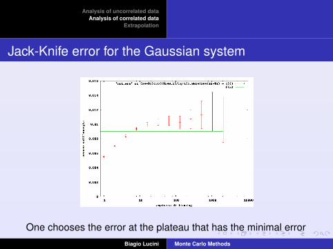
Jack-Knife error for the Gaussian system

One chooses the error at the plateau that has the minimal errorBiagio Lucini Monte Carlo Methods


Extrapolation

Fit

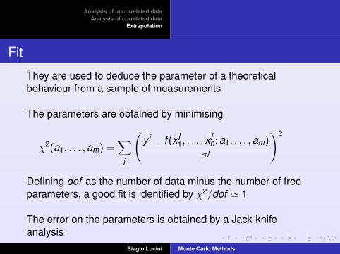
They are used to deduce the parameter of a theoreticalbehaviour from a sample of measurements

The parameters are obtained by minimising

χ2(a1, . . . ,am) =∑

j

(y j − f (x j

1, . . . , xjn; a1, . . . ,am)

σj

)2

Defining dof as the number of data minus the number of freeparameters, a good fit is identified by χ2/dof ' 1

The error on the parameters is obtained by a Jack-knifeanalysis



Extrapolation

Example: Monte Carlo error for π

We expect |π − π(N)| = a/N1/2 ⇒ we want to determine a

Result a = 1.23± 0.29 with χ2/dof = 0.14 (GNUPLOT)



Extrapolation

Single Histogram Reweighting

We have the following identity

〈O〉β′ =

∫dEO(E)ρ(E)e−(β′−β)Ee−βE∫

dEρ(E)e−(β′−β)Ee−βE =〈Oe−∆βE〉β〈e−∆βE〉β

In principle by simulating only at one β we can obtain results forany βIn practice a Monte Carlo will never generate configurationswith very low probability⇒ we have information only for thoseβs for which 〈U〉rew is less than 2σ apart from 〈U〉orig

More sophisticated method: Multi Histogram



Extrapolation

Reweighting for the Gaussian model

Starting point: β = 0.9Biagio Lucini Monte Carlo Methods

Monte Carlo in practiceThe Gaussian system

The harmonic oscillatorThe anharmonic oscillator

References

Monte Carlo praxis

Identify the fundamental variables and the observablesWrite an update algorithm for the fundamental variablesWrite a measurement routine for the observables (store thevalues in a file for off-line analysis)Run the Monte Carlo with sensible parameters(thermalisation time, total number of measurements,number of sweeps between two measurements)Perform off-line the error analysis using binning andJack-KnifeIf requested do some reweighting




References

Exercise 1: the Gaussian System

For the Gaussian system described in these noteswrite a Metropolis update algorithmwrite a routine that measures x2

run the Monte Carlo at β = 0.1,1,10 measuring x2

for each β reweight the results for x2 at the other βs andcomment the agreement/disagreement with the expectedresults




References

Metropolis for the Gaussian System - I

Familiarise with the V.B. Random number generator andmake sure you can extract random numbers between 0and 1start with x0 = 1 and define a variable αwrite an algorithm that computes

y = xn − 2ar + a

with r random number and a = 0.1 to start withcompute

P = e−β(y2−x2)




References

Metropolis for the Gaussian System - I

If P > 1 xn+1 = yif P < 1 generate a random number r1 in [0;1[

1 if r1 < P xn+1 = y2 if r1 > P xn+1 = xn

generate a new y and repeat the processrecord xn+1 in a file The process that generate xn+1 fromxn (whether they are equal or not) is called “sweep”After N sweeps we generate the sequence x1, . . . , xN




References

Thermalisation

To reach the statistical equilibrium the system needs a givennumber of sweeps NTThe thermal equilibrium is defined by the average of theobservable not changing within errors when changing thenumber of the sweepsIn practice, we do the following

1 discard N1 sweeps at the beginning2 divide the remaining ones in two samples with the same

number of measurements3 compute the average of the observables in the two

samples and compare4 if there is agreement we are at equilibrium, otherwise we

discard more sweepsBiagio Lucini Monte Carlo Methods



References

Acceptance

The parameter a should be tuned in such a way that the systemdoes not get stuck at some xn (likely if a is big), nor movesslowly (if a is small)

This can be quantified by introducing the concept ofacceptance: if xn+1 6= xn our attempt at changing the variablehas succeeded, otherwise it has failed.

The acceptance is defined as the ratio between the number ofsuccess over the number of sweeps; a rule of thumb is having itbetween 0.5 and 0.8, and we use this to choose a

Warning: the acceptance should not take into accountthermalisation




References

Measurements

To measure an observable (e.g. x2) we record the set of the xNon a file and we take the simple averages

The statistical analysis should use the binning plus Jack-knifemethod, as described earlier, and should allow to identify τexp

To estimate the observable at another value of β we usereweighting:

〈x2〉β′ =〈x2e∆βx2〉β〈e∆βx2〉β

, ∆β = β − β′




References

Exercise II - The harmonic oscillator

The system described by the discretised action

SE =N∑

i=1

(12

m(xi+1 − xi)2 +

12µ2x2

i

)with µ the elastic constant and m the mass (all variables andparameters are adimensional, i.e. pure numbers, in thisproblem)




References

Step 1: Monte Carlo Simulations

Generalise the Metropolis algorithm for the Gaussiansystem to the harmonic oscillatorHow do you choose tf and the lattice spacing? (justify)Run the code for m = 1.0 and µ = 1.0 for 10000 iterations(each iteration is tf in length) and record x at the end ofeach iteration




References

Step 2: ground state energy

The virial theorem allows to write the energy of the ground stateas

E0 = µ2〈x2〉

Based on the Monte Carlo ensemble generated at Step 1,compute E0Discuss carefully the errors




References

Step 3: reweighting

From the simulation performed, reweight the ground stateenergy to the points obtained by

fixing m = 1.0 and taking µ2 = 0.1 and µ2 = 10fixing µ2 = 1.0 and taking m = 0.1 and m = 10taking m = 0.2 and µ2 = 0.5

Comment on the reliability of the results




References

Step 4: ground state wave function

For m = 1, sort the measured ensemble of the x from thesmallest to the largestDivide the interval in 100 bins of equal length and count howmany data are in each binAssign this number to a function f (x), where x is the centralvalue of the bin, and take

√f (x) as the error on f (x)

Fit f (x) with the formula

f (x) =(ωπ

)1/2e−ωx2

,

and compare ω with the expected value

ω = µ

√1 +

µ2

4




References

Step 5: first excited state energy

Define the quantity

∆E(τ) = log〈x(0)x(τ + 1)〉〈x(0)x(τ)〉

Measure ∆E(τ) for τ = 1,2, . . . ,10Show that at large τ ∆E reaches a plateauFit this plateau with the function f (τ) = c, determining inthis way the value of c

The energy of the first excited state can be obtained as

E1 = E0 + c




References

Exercise III - The anharmonic oscillator

Consider the harmonic oscillator with the additional termλ∑

i x4i ; now

E0 = µ2〈x2〉+ 3λ〈x4〉 ,

while all other formulas stay the sameAfter generalising the Monte Carlo to this case, computethe energy of the ground state and of the first excited statefor m = 1.0, M = 1.0 and λ = 0.2, 1.0,5.0For the λ = 1.0, evaluate the probability distribution for x inthe ground state (i.e. the square of the wave function) witha binning procedure similar to that described for theharmonic oscillator




References

References

1 For random numbers, Monte Carlo in Statistical Mechanicsand the Gaussian System seeB.A. Berg, Introduction to Markov Chain Monte CarloSimulations and their statistical analysis,arXiv:cond-mat/0410490

2 For an introduction to Path Integral methods and MonteCarlo in Quantum Mechanics seeM. Creutz, A. Freedman, A Statistical Approach toQuantum Mechanics, Annals Phys. 132, 427 (1981)


Second problem (PH-353) Monte Carlo in Quantum Mechanicspyweb.swan.ac.uk/~pybl/PH353/mc.pdf · Outline Second problem (PH-353) Monte Carlo in Quantum Mechanics Biagio Lucini February

Documents