arXiv:1310.1197v3 [cs.IT] 6 Oct 2015 1 Second-Order Asymptotics for the Gaussian MAC with Degraded Message Sets Jonathan Scarlett, Member, IEEE and Vincent Y. F. Tan, Senior Member, IEEE Abstract This paper studies the second-order asymptotics of the Gaussian multiple-access channel with degraded message sets. For a fixed average error probability ε ∈ (0, 1) and an arbitrary point on the boundary of the capacity region, we characterize the speed of convergence of rate pairs that converge to that boundary point for codes that have asymptotic error probability no larger than ε. As a stepping stone to this local notion of second-order asymptotics, we study a global notion, and establish relationships between the two. We provide a numerical example to illustrate how the angle of approach to a boundary point affects the second-order coding rate. This is the first conclusive characterization of the second-order asymptotics of a network information theory problem in which the capacity region is not a polygon. Index Terms Gaussian multiple-access channel, Degraded message sets, Superposition coding, Strong converse, Finite block- lengths, Second-order coding rates, Dispersion. I. I NTRODUCTION In this paper, we revisit the Gaussian multiple-access channel (MAC) with degraded message sets. This is a communication model in which two independent messages are to be sent from two sources to a common destination; see Fig. 1. One encoder, the cognitive or informed encoder, has access to both messages, while the uninformed encoder only has access to its own message. Both transmitted signals are power limited, and their sum is corrupted by additive white Gaussian noise (AWGN). The capacity region C , i.e. the set of all pairs of achievable rates, is well-known (e.g. see [1, Ex. 5.18(b)]), and is given by the set of rate pairs (R 1 ,R 2 ) satisfying R 1 ≤ C ( (1 − ρ 2 )S 1 ) (1) R 1 + R 2 ≤ C ( S 1 + S 2 +2ρ S 1 S 2 ) (2) for some ρ ∈ [0, 1], where S 1 and S 2 are the admissible transmit powers, and C(x) := 1 2 log(1 + x) is the Gaussian capacity function. The capacity region C does not depend on whether the average or maximal error probability formalism is employed, and no time-sharing is required. The region C for S 1 = S 2 =1 is illustrated in Fig. 2; observe that C is formed from a union of trapezoids, each parametrized by ρ. The vertical line segment corresponds to ρ =0, while the curved part corresponds to ρ ∈ (0, 1]. The direct part of the coding theorem for C is proved using superposition coding [2]. While the capacity region is well-known, there is substantial motivation to understand the second-order asymp- totics for this problem. For any given point (R ∗ 1 ,R ∗ 2 ) on the boundary of the capacity region, we study the rate of convergence to that point for an ε-reliable code. More precisely, we characterize the set of all (L 1 ,L 2 ) pairs, known as second-order coding rates [3]–[6], for which there exist sequences of codes whose asymptotic error probability does not exceed ε, and whose code sizes M 1,n and M 2,n behave as log M j,n ≥ nR ∗ j + √ nL j + o (√ n ) ,j =1, 2. (3) J. Scarlett was with the Department of Engineering, University of Cambridge, Cambridge CB2 1PZ, U.K. He is now with the Laboratory for Information and Inference Systems, ´ Ecole Polytechnique F´ ed´ erale de Lausanne, CH-1015, Switzerland (email: [email protected]). V. Y. F. Tan was with the Institute for Infocomm Research (I 2 R), Agency for Science, Technology and Research (A*STAR). He is now with the Department of Electrical and Computer Engineering and the Department of Mathematics, National University of Singapore. (email: [email protected]). This paper was presented in part at the 2014 IEEE International Symposium on Information Theory in Honolulu, HI.

Welcome message from author
This document is posted to help you gain knowledge. Please leave a comment to let me know what you think about it! Share it to your friends and learn new things together.
Transcript
arX
iv:1
310.
1197
v3 [
cs.IT
] 6
Oct
201
51
Second-Order Asymptotics for the GaussianMAC with Degraded Message Sets
Jonathan Scarlett,Member, IEEE and Vincent Y. F. Tan,Senior Member, IEEE
Abstract
This paper studies the second-order asymptotics of the Gaussian multiple-access channel with degraded messagesets. For a fixed average error probabilityε ∈ (0, 1) and an arbitrary point on the boundary of the capacity region,we characterize the speed of convergence of rate pairs that converge to that boundary point for codes that haveasymptotic error probability no larger thanε. As a stepping stone to this local notion of second-order asymptotics,we study a global notion, and establish relationships between the two. We provide a numerical example to illustratehow the angle of approach to a boundary point affects the second-order coding rate. This is the first conclusivecharacterization of the second-order asymptotics of a network information theory problem in which the capacityregion is not a polygon.
Index Terms
Gaussian multiple-access channel, Degraded message sets,Superposition coding, Strong converse, Finite block-lengths, Second-order coding rates, Dispersion.
I. INTRODUCTION
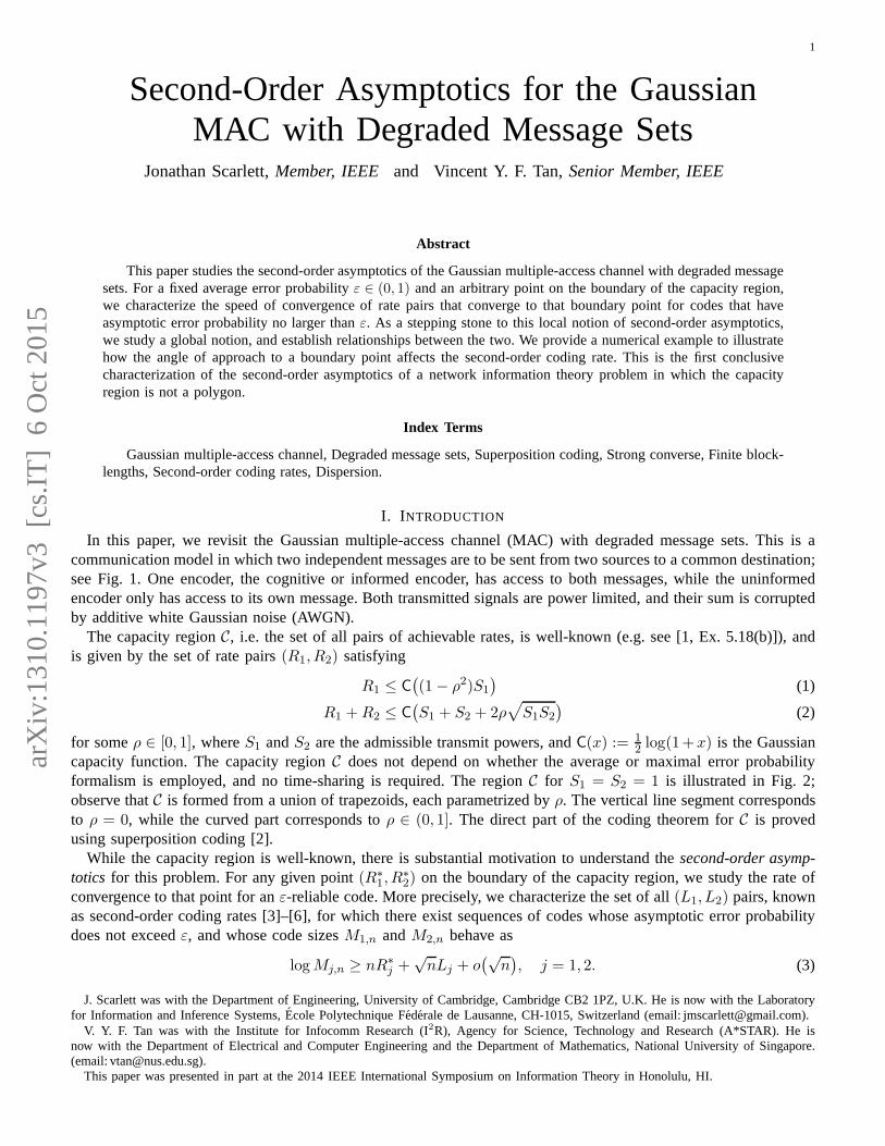
In this paper, we revisit the Gaussian multiple-access channel (MAC) with degraded message sets. This is acommunication model in which two independent messages are to be sent from two sources to a common destination;see Fig. 1. One encoder, the cognitive or informed encoder, has access to both messages, while the uninformedencoder only has access to its own message. Both transmittedsignals are power limited, and their sum is corruptedby additive white Gaussian noise (AWGN).
The capacity regionC, i.e. the set of all pairs of achievable rates, is well-known(e.g. see [1, Ex. 5.18(b)]), andis given by the set of rate pairs(R1, R2) satisfying
R1 ≤ C(
(1− ρ2)S1)
(1)
R1 +R2 ≤ C(
S1 + S2 + 2ρ√
S1S2)
(2)
for someρ ∈ [0, 1], whereS1 andS2 are the admissible transmit powers, andC(x) := 12 log(1+x) is the Gaussian
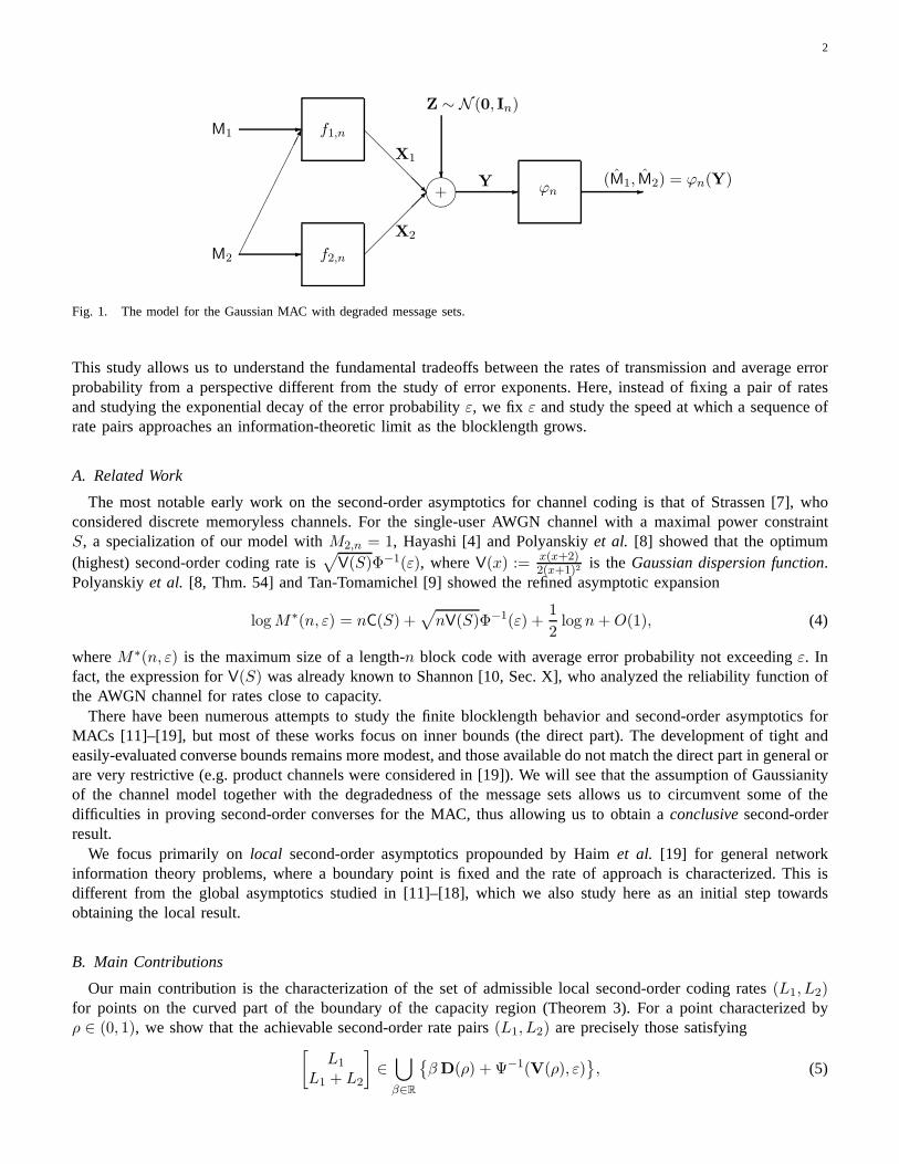
capacity function. The capacity regionC does not depend on whether the average or maximal error probabilityformalism is employed, and no time-sharing is required. Theregion C for S1 = S2 = 1 is illustrated in Fig. 2;observe thatC is formed from a union of trapezoids, each parametrized byρ. The vertical line segment correspondsto ρ = 0, while the curved part corresponds toρ ∈ (0, 1]. The direct part of the coding theorem forC is provedusing superposition coding [2].
While the capacity region is well-known, there is substantial motivation to understand thesecond-order asymp-totics for this problem. For any given point(R∗
1, R∗2) on the boundary of the capacity region, we study the rate of
convergence to that point for anε-reliable code. More precisely, we characterize the set of all (L1, L2) pairs, knownas second-order coding rates [3]–[6], for which there existsequences of codes whose asymptotic error probabilitydoes not exceedε, and whose code sizesM1,n andM2,n behave as
logMj,n ≥ nR∗j +√nLj + o
(√n)
, j = 1, 2. (3)
J. Scarlett was with the Department of Engineering, University of Cambridge, Cambridge CB2 1PZ, U.K. He is now with the Laboratoryfor Information and Inference Systems,Ecole Polytechnique Federale de Lausanne, CH-1015, Switzerland (email: [email protected]).
V. Y. F. Tan was with the Institute for Infocomm Research (I2R), Agency for Science, Technology and Research (A*STAR). He isnow with the Department of Electrical and Computer Engineering and the Department of Mathematics, National Universityof Singapore.(email: [email protected]).
This paper was presented in part at the 2014 IEEE International Symposium on Information Theory in Honolulu, HI.
2
+
M2
M1
X1
X2
f1,n
f2,n
Z ∼ N (0, In)
Y ϕn(M1, M2) = ϕn(Y)
Fig. 1. The model for the Gaussian MAC with degraded message sets.
This study allows us to understand the fundamental tradeoffs between the rates of transmission and average errorprobability from a perspective different from the study of error exponents. Here, instead of fixing a pair of ratesand studying the exponential decay of the error probabilityε, we fix ε and study the speed at which a sequence ofrate pairs approaches an information-theoretic limit as the blocklength grows.
A. Related Work
The most notable early work on the second-order asymptoticsfor channel coding is that of Strassen [7], whoconsidered discrete memoryless channels. For the single-user AWGN channel with a maximal power constraintS, a specialization of our model withM2,n = 1, Hayashi [4] and Polyanskiyet al. [8] showed that the optimum(highest) second-order coding rate is
√
V(S)Φ−1(ε), whereV(x) := x(x+2)2(x+1)2 is the Gaussian dispersion function.
Polyanskiyet al. [8, Thm. 54] and Tan-Tomamichel [9] showed the refined asymptotic expansion
logM∗(n, ε) = nC(S) +√
nV(S)Φ−1(ε) +1
2log n+O(1), (4)
whereM∗(n, ε) is the maximum size of a length-n block code with average error probability not exceedingε. Infact, the expression forV(S) was already known to Shannon [10, Sec. X], who analyzed the reliability function ofthe AWGN channel for rates close to capacity.
There have been numerous attempts to study the finite blocklength behavior and second-order asymptotics forMACs [11]–[19], but most of these works focus on inner bounds(the direct part). The development of tight andeasily-evaluated converse bounds remains more modest, andthose available do not match the direct part in general orare very restrictive (e.g. product channels were considered in [19]). We will see that the assumption of Gaussianityof the channel model together with the degradedness of the message sets allows us to circumvent some of thedifficulties in proving second-order converses for the MAC,thus allowing us to obtain aconclusivesecond-orderresult.
We focus primarily onlocal second-order asymptotics propounded by Haimet al. [19] for general networkinformation theory problems, where a boundary point is fixedand the rate of approach is characterized. This isdifferent from the global asymptotics studied in [11]–[18], which we also study here as an initial step towardsobtaining the local result.
B. Main Contributions
Our main contribution is the characterization of the set of admissible local second-order coding rates(L1, L2)for points on the curved part of the boundary of the capacity region (Theorem 3). For a point characterized byρ ∈ (0, 1), we show that the achievable second-order rate pairs(L1, L2) are precisely those satisfying
[
L1
L1 + L2
]
∈⋃
β∈R
βD(ρ) + Ψ−1(V(ρ), ε)
, (5)
3
where the entries ofD(ρ) are the derivatives of the capacities in (1)–(2),V(ρ) is thedispersion matrix[11], [12],andΨ−1 is the2-dimensional generalization of the inverse of the cumulative distribution function of a Gaussian. (Allquantities are defined precisely in the sequel.) Thus, the contribution from the Gaussian approximationΨ−1(V(ρ), ε)is insufficient for characterizing the second-order asymptotics of multi-terminal channel coding problems in general;in this case, the vectorD(ρ) is also required. This is in stark contrast to single-user problems (e.g. [3], [4], [6]–[8])and the (two-encoder) Slepian-Wolf problem [5], [11] wherethe Gaussian approximation in terms of a dispersionquantity is sufficient for the second-order asymptotics. Our main result, which comprises the statement in (5),provides the first complete characterization of the local second-order asymptotics of a multi-user information theoryproblem in which the boundary of the capacity region (or optimal rate region for source coding problems) is curved.
Some intuition can be gained as to why the extra derivative term is needed by considering the possible anglesof approach to a fixed boundary point(R∗
1, R∗2) ∈ C. Using asingle multivariate Gaussian input distribution with
correlationρ for all blocklengths is suboptimal in the second-order sense, as we can only achieve the angles ofapproach within the trapezoid parametrized byρ (see Fig. 2 and its caption). Our strategy is to consider sequences ofinput distributions that vary with the blocklength, i.e. they are parametrized by a sequenceρnn∈N that convergesto ρ with speedΘ
(
1√n
)
. By a Taylor expansion of the first-order capacity vectorI(ρ) (the vector of capacities in(1)–(2)),
I(ρn) ≈ I(ρ) + (ρn − ρ)D(ρ), (6)
we see that this sequence results in the derivative/slope term D(ρ) observed in (5). Thus, the slope term correspondsto the deviation ofρn from ρ, while the dispersion term involvingV(ρ) results from, by now, standard central limit(fixed error) analysis of Shannon-theoretic coding problems [20].
We briefly comment onρn converging toρ at different speeds. Ifρn − ρ = o( 1√n), then the contribution of
the remainder term in (6) is dominated by the dispersion term, and hence this is, up to second order, equivalentto consideringρn = ρ. In contrast, forρn − ρ = ω( 1√
n), this remainder term dominates the dispersion term.
Nevertheless, this case does not feature in the local result, due to the way we define the second-order coding rateregion in (3)—the backoff terms with coefficientsL1 andL2 scale as
√n. In particular, we show in the converse
proof that if ρn − ρ = ω( 1√n), then no finite(L1, L2) pairs satisfy the conditions in this definition.
An auxiliary contribution is a global second-order result [11], [19] (Theorem 2), which we use as an importantstepping stoneto obtain our local second-order result. We show that for anysequenceρn ∈ [0, 1], all rate pairs(R1,n, R2,n) satisfying
[
R1,n
R1,n +R2,n
]
∈ I(ρn) +Ψ−1(V(ρn), ε)√
n+ o
(
1√n
)
1 (7)
are achievable at blocklengthn and with average error probability no larger thanε + o(1). Our proof techniqueyields a third-order term that remainso( 1√
n) no matter howρn varies withn. This property does not typically hold
in previous results on multi-user fixed error asymptotics, but it turns out to be crucial in deriving the local resultand the additional slope term (cf. (6)), at least using our proof techniques.
In summary, we submit that both the global and local results on their own provide complementary and usefulinsights into fundamental limits of the communication system, but in this paper our main goal is the latter.
II. PROBLEM SETTING AND DEFINITIONS
In this section, we state the channel model, various definitions and some known results.Notation: Given integersl ≤ m, we use the discrete interval [1] notations[l : m] := l, . . . ,m and [m] := [1 :
m]. All log’s and exp’s are with respect to the natural basee. The ℓp-norm of the vectorized version of matrix
A is denoted by‖A‖p :=(∑
i,j |ai,j|p)1/p
. For two vectors of the same lengtha,b ∈ Rd, the notationa ≤ b
means thataj ≤ bj for all j ∈ [d]. The notationN (u;µ,Λ) denotes the multivariate Gaussian probability densityfunction (pdf) with meanµ and covarianceΛ. The argumentu will often be omitted. We use standard asymptoticnotations:fn ∈ O(gn) if and only if (iff) lim supn→∞
∣
∣fn/gn∣
∣ < ∞; fn ∈ Ω(gn) iff gn ∈ O(fn); fn ∈ Θ(gn) ifffn ∈ O(gn) ∩Ω(gn); fn ∈ o(gn) iff lim supn→∞
∣
∣fn/gn∣
∣ = 0; andfn ∈ ω(gn) iff lim infn→∞∣
∣fn/gn∣
∣ =∞.
4
0 0.05 0.1 0.15 0.2 0.25 0.3 0.35 0.40
0.1
0.2
0.3
0.4
0.5
0.6
0.7
0.8
R1 (nats/use)
R2
(nats
/use
)
The Capacity Region
CR Boundaryρ = 0ρ = 1/3ρ = 2/3
v
v′
Fig. 2. Capacity region of the Gaussian MAC with degraded message sets in the case thatS1 = S2 = 1. Observe thatρ ∈ [0, 1] parametrizespoints on the boundary. The vertical line segment corresponds to ρ = 0, while the curved part corresponds toρ ∈ (0, 1]. Eachρ ∈ (0, 1]corresponds to a trapezoid of rate pairs that are achievableby a unique input distributionN (0,Σ(ρ)). This coding strategy is insufficientto allow for all possible angles of approach to the fixed pointparametrized byρ, as there are non-empty regions withinC that not in thetrapezoid parametrized byρ. In the figure above withρ = 2
3, one can approach the corner point in the direction indicated by the vectorv
using the fixed input distributionN (0,Σ( 23)), but the same is not true of the direction indicated byv
′, since the approach is from outsidethe trapezoid.
A. Channel Model
The signal model is given by
Y = X1 +X2 + Z, (8)
whereX1 andX2 represent the inputs to the channel,Z ∼ N (0, 1) is additive Gaussian noise with mean zero andunit variance, andY is the output of the channel. Thus, the channel from(X1,X2) to Y can be written as
W (y|x1, x2) =1√2π
exp
(
−1
2(y − x1 − x2)2
)
. (9)
The channel is usedn times in a memoryless manner without feedback. The channel inputs (i.e., the transmittedcodewords)x1 = (x11, . . . , x1n) andx2 = (x21, . . . , x2n) are required to satisfy the maximal power constraints
‖x1‖22 ≤ nS1, and ‖x2‖22 ≤ nS2, (10)
whereS1 andS2 are arbitrary positive numbers. We do not incorporate multiplicative gainsg1 andg2 to X1 andX2 in the channel model in (8); this is without loss of generality, since in the presence of these gains we mayequivalently redefine (10) withS′
j := Sj/g2j for j = 1, 2.
B. Definitions
Definition 1 (Code). An (n,M1,n,M2,n, S1, S2, εn)-codefor the Gaussian MAC with degraded message sets consistsof two encodersf1,n, f2,n and a decoderϕn of the formf1,n : [M1,n] × [M2,n] → R
n, f2,n : [M2,n] → Rn and
5
ϕn : Rn → [M1,n]× [M2,n] satisfying
‖f1,n(m1,m2)‖22 ≤ nS1 ∀ (m1,m2) ∈ [M1,n]× [M2,n], (11)
‖f2,n(m2)‖22 ≤ nS2 ∀m2 ∈ [M2,n], (12)
Pr(
(M1,M2) 6= (M1, M2))
≤ εn, (13)
where the messagesM1 and M2 are uniformly distributed on[M1,n] and [M2,n] respectively, and(M1, M2) :=ϕn(Y
n) is the decoded message pair.
Since S1 and S2 are fixed positive numbers, we suppress the dependence of thesubsequent definitions, re-sults and parameters on these constants. We will often make reference to(n, ε)-codes; this is the family of(n,M1,n,M2,n, S1, S2, ε)-codes where the sizesM1,n,M2,n are left unspecified.
Definition 2 ((n, ε)-Achievability). A pair of non-negative numbers(R1, R2) is (n, ε)-achievableif there exists an(n,M1,n,M2,n, S1, S2, εn)-code such that
1
nlogMj,n ≥ Rj, j = 1, 2, and εn ≤ ε. (14)
The (n, ε)-capacity regionC(n, ε) ⊂ R2+ is defined to be the set of all(n, ε)-achievable rate pairs(R1, R2).
Definition 2 is a non-asymptotic one that is used primarily for the global second-order results. We now introduceasymptotic-type definitions that involve the existence ofsequencesof codes.
Definition 3 (First-Order Coding Rates). A pair of non-negative numbers(R1, R2) is ε-achievableif there exists asequence of(n,M1,n,M2,n, S1, S2, εn)-codes such that
lim infn→∞
1
nlogMj,n ≥ Rj , j = 1, 2, and lim sup
n→∞εn ≤ ε. (15)
The ε-capacity regionC(ε) ⊂ R2+ is defined to be the closure of the set of allε-achievable rate pairs(R1, R2).
Thecapacity regionC is defined as
C :=⋂
ε>0
C(ε) = limε→0C(ε), (16)
where the limit exists because of the monotonicity ofC(ε).
Next, we state the most important definitions concerning local second-order coding rates in the spirit of Nomura-Han [5] and Tan-Kosut [11]. We will spend the majority of the paper developing tools to characterize these rates.Here (R∗
1, R∗2) is a pair of rates on the boundary ofC(ε).
Definition 4 (Second-Order Coding Rates). A pair of numbers(L1, L2) is (ε,R∗1, R
∗2)-second-order achievableif
there exists a sequence of(n,M1,n,M2,n, S1, S2, εn)-codes such that
lim infn→∞
1√n(logMj,n − nR∗
j) ≥ Lj, j = 1, 2, and lim supn→∞
εn ≤ ε. (17)
The (ε,R∗1, R
∗2)-optimal second-order coding rate regionL(ε;R∗
1, R∗2) ⊂ R
2 is defined to be the closure of the setof all (ε,R∗
1, R∗2)-second-order achievable rate pairs(L1, L2).
Stated differently, if(L1, L2) is (ε,R∗1, R
∗2)-second-order achievable, then there are codes whose errorprobabilities
are asymptotically no larger thanε, and whose sizes(M1,n,M2,n) satisfy the asymptotic relation in (3). Even thoughwe refer toL1 andL2 as “rates”, they may be negative [3]–[6]. A negative value corresponds to a backoff fromthe first-order term, whereas a positive value corresponds to an addition to the first-order term.
6
C. Existing First-Order Results
To put things in context, we review some existing results concerning theε-capacity region. To state the resultcompactly, we define themutual information (or capacity) vectoras
I(ρ) =
[
I1(ρ)I12(ρ)
]
:=
[
C(
S1(1− ρ2))
C(
S1 + S2 + 2ρ√S1S2
)
]
(18)
whereρ ∈ [−1, 1]. For a pair of rates(R1, R2), let the rate vectorbe
R :=
[
R1
R1 +R2
]
. (19)
A statement of the following result is provided in [1, Ex. 5.18(b)]. A weak converse was proved for the moregeneral Gaussian MAC a with common message in [21].
Proposition 1 (Capacity Region). The capacity region of the Gaussian MAC with degraded message sets is givenby
C =⋃
0≤ρ≤1
(R1, R2) ∈ R2+ : R ≤ I(ρ)
. (20)
The union on the right is a subset ofC(ε) for every ε ∈ (0, 1). However, only the weak converse is impliedby (20). The strong converse has not been demonstrated previously. Thus, a by-product of the derivation of thesecond-order asymptotics in this paper is the strong converse, allowing us to assert that for allε ∈ (0, 1),
C = C(ε). (21)
The direct part of Proposition 1 can be proved using superposition coding [2], treatingX2 as the cloud centerandX1 as the satellite codeword. The input distribution to achieve a point on the boundary characterized by someρ ∈ [0, 1] is a 2-dimensional Gaussian with mean zero and covariance matrix
Σ(ρ) :=
[
S1 ρ√S1S2
ρ√S1S2 S2
]
. (22)
Thus, the parameterρ represents the correlation between the two users’ codewords.
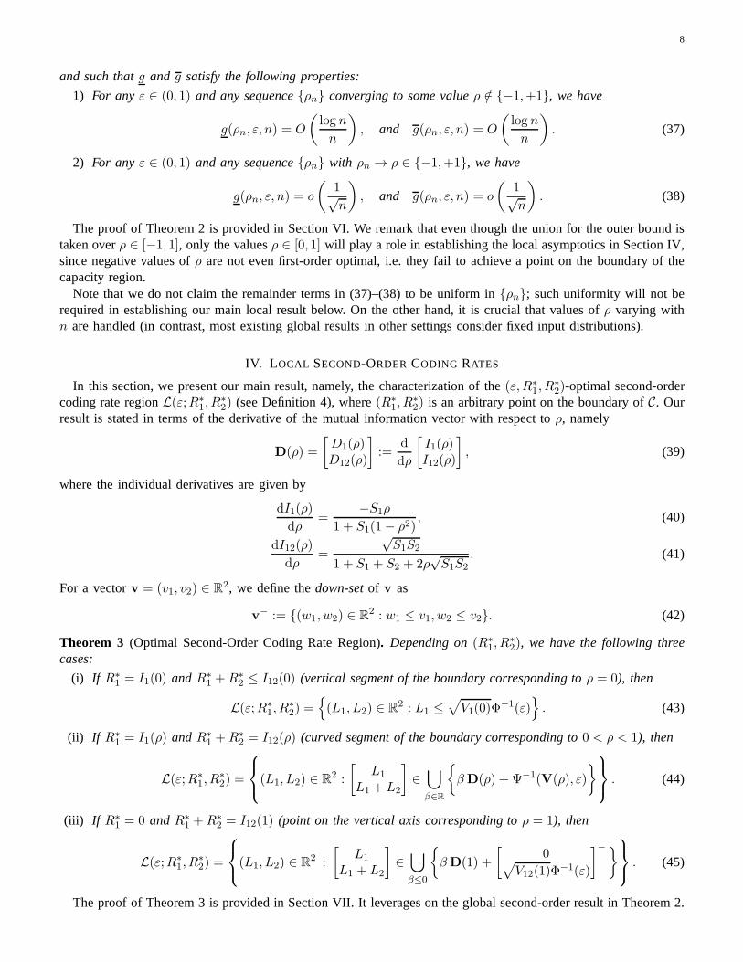
III. G LOBAL SECOND-ORDER RESULTS
In this section, we present inner and outer bounds onC(n, ε). We begin with some definitions. LetV(x, y) :=x(y+2)
2(x+1)(y+1) be theGaussian cross-dispersion functionand letV(x) := V(x, x) be theGaussian dispersion func-tion [4], [8], [10] for a single-user AWGN channel with signal-to-noise ratiox. For fixed0 ≤ ρ ≤ 1, define theinformation-dispersion matrix
V(ρ) :=
[
V1(ρ) V1,12(ρ)V1,12(ρ) V12(ρ)
]
, (23)
where the elements of the matrix are
V1(ρ) := V(
S1(1− ρ2))
, (24)
V1,12(ρ) := V(
S1(1− ρ2), S1 + S2 + 2ρ√
S1S2)
, (25)
V12(ρ) := V(
S1 + S2 + 2ρ√
S1S2)
. (26)
Let (X1,X2) ∼ PX1,X2= N (0;Σ(ρ)), and defineQY |X2
andQY to be Gaussian distributions induced byPX1,X2
and the channelW , namely
QY |X2(y|x2) := N
(
y;x2(1 + ρ√
S1/S2), 1 + S1(1− ρ2))
, (27)
QY (y) := N(
y; 0, 1 + S1 + S2 + 2ρ√
S1S2)
. (28)
7
−0.2 −0.15 −0.1 −0.05 0 0.05−0.2
−0.15
−0.1
−0.05
0
0.05
z1
z 2
ρ = 0.5
ε = 0.01ε = 0.80
−0.2 −0.15 −0.1 −0.05 0 0.05−0.2
−0.15
−0.1
−0.05
0
0.05
z1
z 2
ρ = 0.995
ε = 0.01ε = 0.80
Ψ−1(V(ρ),0.80)√n
Ψ−1(V(ρ),0.80)√n
Ψ−1(V(ρ),0.01)√n
Ψ−1(V(ρ),0.01)√n
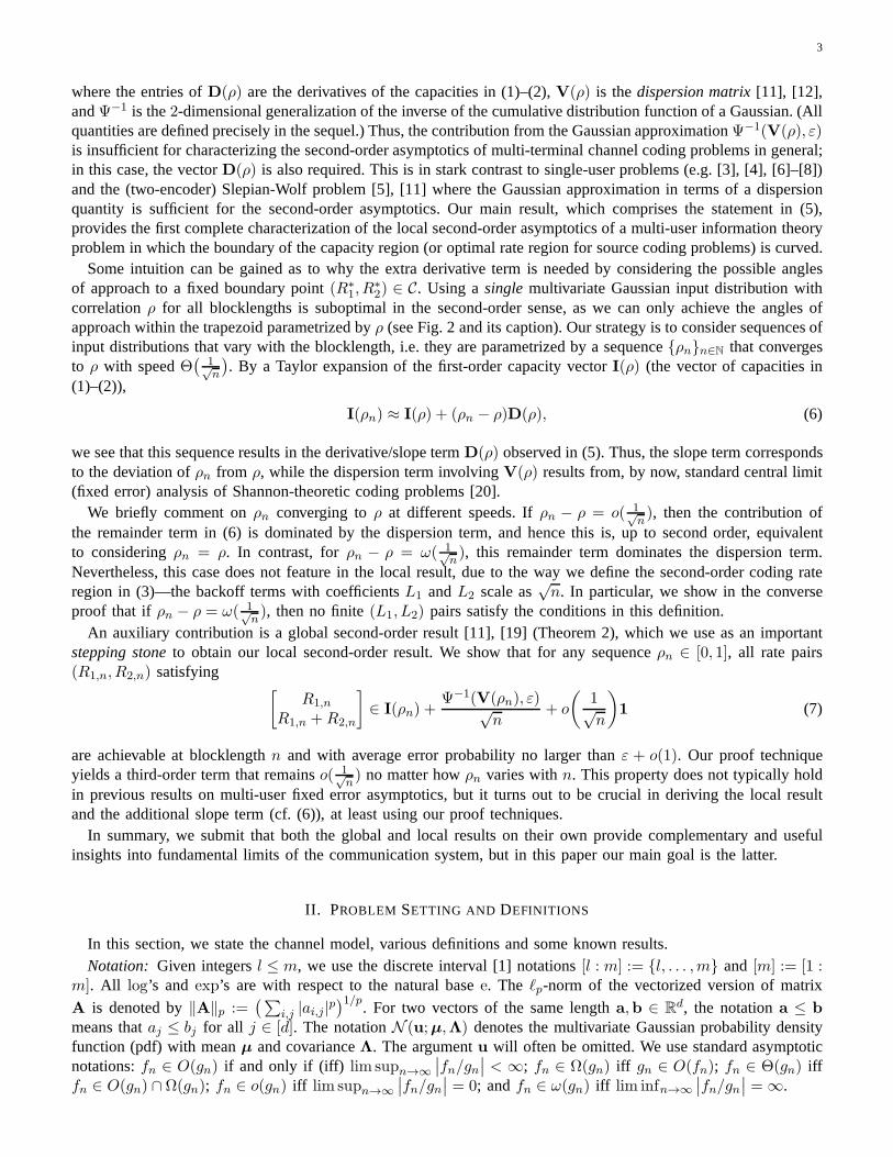
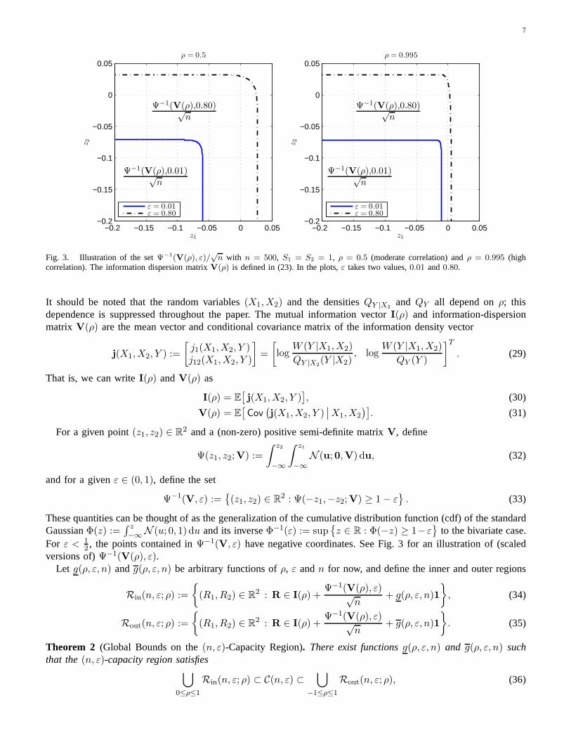
Fig. 3. Illustration of the setΨ−1(V(ρ), ε)/√n with n = 500, S1 = S2 = 1, ρ = 0.5 (moderate correlation) andρ = 0.995 (high
correlation). The information dispersion matrixV(ρ) is defined in (23). In the plots,ε takes two values,0.01 and0.80.
It should be noted that the random variables(X1,X2) and the densitiesQY |X2andQY all depend onρ; this
dependence is suppressed throughout the paper. The mutual information vectorI(ρ) and information-dispersionmatrix V(ρ) are the mean vector and conditional covariance matrix of theinformation density vector
j(X1,X2, Y ) :=
[
j1(X1,X2, Y )j12(X1,X2, Y )
]
=
[
logW (Y |X1,X2)
QY |X2(Y |X2)
, logW (Y |X1,X2)
QY (Y )
]T
. (29)
That is, we can writeI(ρ) andV(ρ) as
I(ρ) = E[
j(X1,X2, Y )]
, (30)
V(ρ) = E[
Cov(
j(X1,X2, Y )∣
∣X1,X2
)]
. (31)
For a given point(z1, z2) ∈ R2 and a (non-zero) positive semi-definite matrixV, define
Ψ(z1, z2;V) :=
∫ z2
−∞
∫ z1
−∞N (u;0,V) du, (32)
and for a givenε ∈ (0, 1), define the set
Ψ−1(V, ε) :=
(z1, z2) ∈ R2 : Ψ(−z1,−z2;V) ≥ 1− ε
. (33)
These quantities can be thought of as the generalization of the cumulative distribution function (cdf) of the standardGaussianΦ(z) :=
∫ z−∞N (u; 0, 1) du and its inverseΦ−1(ε) := sup
z ∈ R : Φ(−z) ≥ 1−ε
to the bivariate case.For ε < 1
2 , the points contained inΨ−1(V, ε) have negative coordinates. See Fig. 3 for an illustration of(scaledversions of)Ψ−1(V(ρ), ε).
Let g(ρ, ε, n) andg(ρ, ε, n) be arbitrary functions ofρ, ε andn for now, and define the inner and outer regions
Rin(n, ε; ρ) :=
(R1, R2) ∈ R2 : R ∈ I(ρ) +
Ψ−1(V(ρ), ε)√n
+ g(ρ, ε, n)1
, (34)
Rout(n, ε; ρ) :=
(R1, R2) ∈ R2 : R ∈ I(ρ) +
Ψ−1(V(ρ), ε)√n
+ g(ρ, ε, n)1
. (35)
Theorem 2 (Global Bounds on the(n, ε)-Capacity Region). There exist functionsg(ρ, ε, n) and g(ρ, ε, n) suchthat the(n, ε)-capacity region satisfies
⋃
0≤ρ≤1
Rin(n, ε; ρ) ⊂ C(n, ε) ⊂⋃
−1≤ρ≤1
Rout(n, ε; ρ), (36)
8
and such thatg and g satisfy the following properties:
1) For any ε ∈ (0, 1) and any sequenceρn converging to some valueρ /∈ −1,+1, we have
g(ρn, ε, n) = O
(
log n
n
)
, and g(ρn, ε, n) = O
(
log n
n
)
. (37)
2) For any ε ∈ (0, 1) and any sequenceρn with ρn → ρ ∈ −1,+1, we have
g(ρn, ε, n) = o
(
1√n
)
, and g(ρn, ε, n) = o
(
1√n
)
. (38)
The proof of Theorem 2 is provided in Section VI. We remark that even though the union for the outer bound istaken overρ ∈ [−1, 1], only the valuesρ ∈ [0, 1] will play a role in establishing the local asymptotics in Section IV,since negative values ofρ are not even first-order optimal, i.e. they fail to achieve a point on the boundary of thecapacity region.
Note that we do not claim the remainder terms in (37)–(38) to be uniform inρn; such uniformity will not berequired in establishing our main local result below. On theother hand, it is crucial that values ofρ varying withn are handled (in contrast, most existing global results in other settings consider fixed input distributions).
IV. L OCAL SECOND-ORDER CODING RATES
In this section, we present our main result, namely, the characterization of the(ε,R∗1, R
∗2)-optimal second-order
coding rate regionL(ε;R∗1, R
∗2) (see Definition 4), where(R∗
1, R∗2) is an arbitrary point on the boundary ofC. Our
result is stated in terms of the derivative of the mutual information vector with respect toρ, namely
D(ρ) =
[
D1(ρ)D12(ρ)
]
:=d
dρ
[
I1(ρ)I12(ρ)
]
, (39)
where the individual derivatives are given by
dI1(ρ)
dρ=
−S1ρ1 + S1(1− ρ2)
, (40)
dI12(ρ)
dρ=
√S1S2
1 + S1 + S2 + 2ρ√S1S2
. (41)
For a vectorv = (v1, v2) ∈ R2, we define thedown-setof v as
v− := (w1, w2) ∈ R2 : w1 ≤ v1, w2 ≤ v2. (42)
Theorem 3 (Optimal Second-Order Coding Rate Region). Depending on(R∗1, R
∗2), we have the following three
cases:
(i) If R∗1 = I1(0) andR∗
1 +R∗2 ≤ I12(0) (vertical segment of the boundary corresponding toρ = 0), then
L(ε;R∗1, R
∗2) =
(L1, L2) ∈ R2 : L1 ≤
√
V1(0)Φ−1(ε)
. (43)
(ii) If R∗1 = I1(ρ) andR∗
1 +R∗2 = I12(ρ) (curved segment of the boundary corresponding to0 < ρ < 1), then
L(ε;R∗1, R
∗2) =
(L1, L2) ∈ R2 :
[
L1
L1 + L2
]
∈⋃
β∈R
βD(ρ) + Ψ−1(V(ρ), ε)
. (44)
(iii) If R∗1 = 0 andR∗
1 +R∗2 = I12(1) (point on the vertical axis corresponding toρ = 1), then
L(ε;R∗1, R
∗2) =
(L1, L2) ∈ R2 :
[
L1
L1 + L2
]
∈⋃
β≤0
βD(1) +
[
0√
V12(1)Φ−1(ε)
]−
. (45)
The proof of Theorem 3 is provided in Section VII. It leverages on the global second-order result in Theorem 2.
9
−2 −1.5 −1 −0.5 0 0.5−1.5
−1
−0.5
0
0.5
1
1.5
L1 (nats/√use)
L2(nats/√use)
Second-Order Region
GΨ
−1 (V(ρ), ε)L(ε;R∗
1, R∗
2)L2 = L1 tan θ
∗
ρ,ε
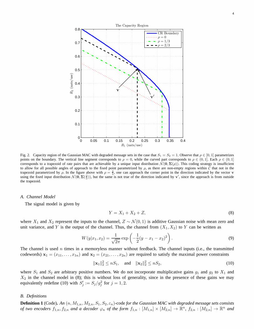
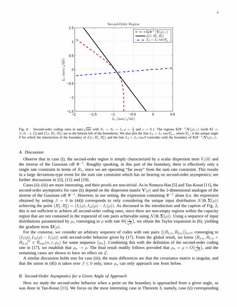
Fig. 4. Second-order coding rates in nats/√
use withS1 = S2 = 1, ρ = 1
2and ε = 0.1. The regionsGΨ−1(V(ρ), ε) (with G :=
[1, 0;−1, 1]) andL(ε;R∗
1 , R∗
2) are to the bottom left of the boundaries. We also plot the lineL2 = L1 tan θ∗
ρ,ε, whereθ∗ρ,ε is the unique angleθ for which the intersection of the boundary ofL(ε;R∗
1, R∗
2) and the lineL2 = L1 tan θ coincides with the boundary ofGΨ−1(V(ρ), ε).
A. Discussion
Observe that in case (i), the second-order region is simply characterized by a scalar dispersion termV1(0) andthe inverse of the Gaussian cdfΦ−1. Roughly speaking, in this part of the boundary, there is effectively only asingle rate constraint in terms ofR1, since we are operating “far away” from the sum rate constraint. This resultsin a large deviations-type event for the sum rate constraintwhich has no bearing on second-order asymptotics; seefurther discussions in [5], [11] and [19].
Cases (ii)–(iii) are more interesting, and their proofs arenon-trivial. As in Nomura-Han [5] and Tan-Kosut [11], thesecond-order asymptotics for case (ii) depend on the dispersion matrixV(ρ) and the2-dimensional analogue of theinverse of the Gaussian cdfΨ−1. However, in our setting, the expression containingΨ−1 alone (i.e. the expressionobtained by settingβ = 0 in (44)) corresponds to only considering the unique input distribution N (0,Σ(ρ))achieving the point(R∗
1, R∗2) = (I1(ρ), I12(ρ)− I1(ρ)). As discussed in the introduction and the caption of Fig. 2,
this is not sufficient to achieve all second-order coding rates, since there are non-empty regions within the capacityregion that are not contained in the trapezoid of rate pairs achievable usingN (0,Σ(ρ)). Using a sequence of inputdistributions parametrized byρn converging toρ with rateΘ
(
1√n
)
, we obtain the Taylor expansion in (6), yieldingthe gradient termD(ρ).
For the converse, we consider an arbitrary sequence of codeswith rate pairs(R1,n, R2,n)n∈N converging to(I1(ρ), I12(ρ) − I1(ρ)) with second-order behavior given by (17). From the global result, we know[R1,n, R1,n +R2,n]
T ∈ Rout(n, ε; ρn) for some sequenceρn. Combining this with the definition of the second-order codingrate in (17), we establish thatρn → ρ. The final result readily follows provided thatρn = ρ + O
(
1√n
)
, and theremaining cases are shown to have no effect onL.
A similar discussion holds true for case (iii); the main differences are that the covariance matrix is singular, andthat the union in (45) is taken overβ ≤ 0 only, sinceρn can only approach one from below.
B. Second-Order Asymptotics for a Given Angle of Approach
Here we study the second-order behavior when a point on the boundary is approached from a given angle, aswas done in Tan-Kosut [11]. We focus on the most interesting case in Theorem 3, namely, case (ii) corresponding
10
0.3 0.4 0.5 0.6 0.7 0.8 0.90
2
4
6
8
10
12
14
16
18
20
Normalized Angle of Approach θ/(2π)
√
L2 1+L2 2(nats/√use)
Norm of [L1, L2] vs θ
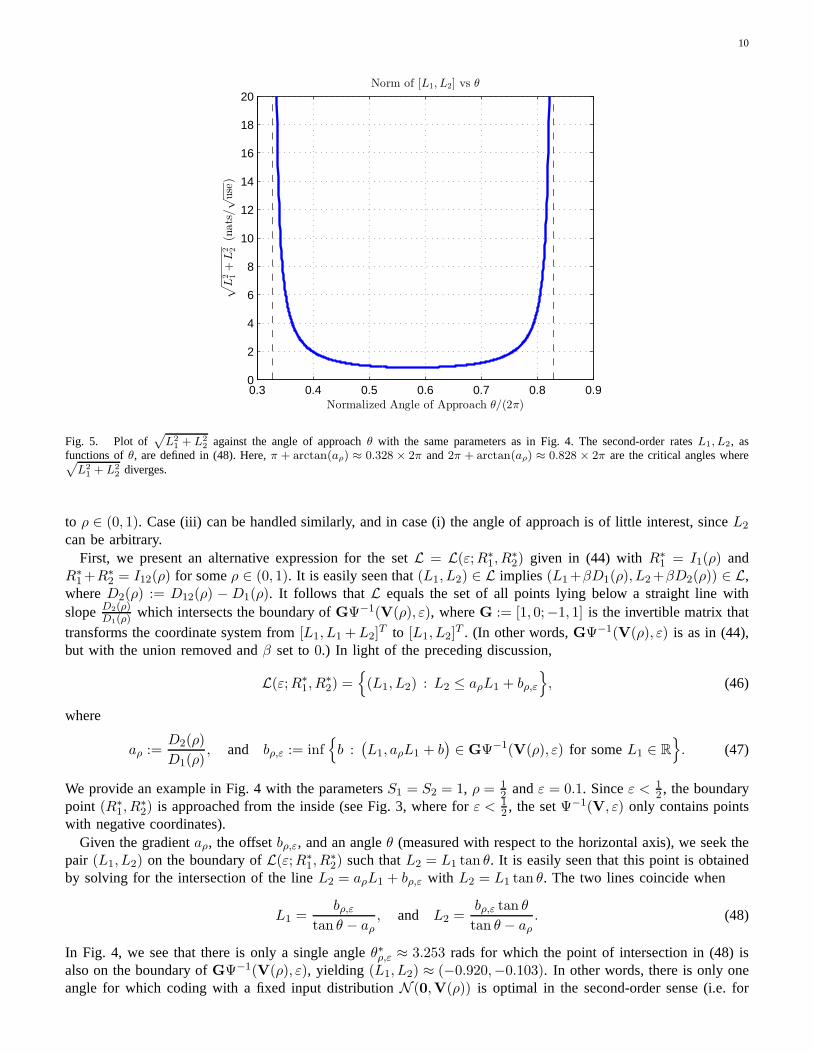
Fig. 5. Plot of√
L2
1+ L2
2against the angle of approachθ with the same parameters as in Fig. 4. The second-order ratesL1, L2, as
functions ofθ, are defined in (48). Here,π + arctan(aρ) ≈ 0.328 × 2π and2π + arctan(aρ) ≈ 0.828 × 2π are the critical angles where√
L2
1+ L2
2diverges.
to ρ ∈ (0, 1). Case (iii) can be handled similarly, and in case (i) the angle of approach is of little interest, sinceL2
can be arbitrary.First, we present an alternative expression for the setL = L(ε;R∗
1, R∗2) given in (44) withR∗
1 = I1(ρ) andR∗
1+R∗2 = I12(ρ) for someρ ∈ (0, 1). It is easily seen that(L1, L2) ∈ L implies (L1+βD1(ρ), L2+βD2(ρ)) ∈ L,
whereD2(ρ) := D12(ρ) − D1(ρ). It follows thatL equals the set of all points lying below a straight line withslopeD2(ρ)
D1(ρ)which intersects the boundary ofGΨ−1(V(ρ), ε), whereG := [1, 0;−1, 1] is the invertible matrix that
transforms the coordinate system from[L1, L1 +L2]T to [L1, L2]
T . (In other words,GΨ−1(V(ρ), ε) is as in (44),but with the union removed andβ set to0.) In light of the preceding discussion,
L(ε;R∗1, R
∗2) =
(L1, L2) : L2 ≤ aρL1 + bρ,ε
, (46)
where
aρ :=D2(ρ)
D1(ρ), and bρ,ε := inf
b :(
L1, aρL1 + b)
∈ GΨ−1(V(ρ), ε) for someL1 ∈ R
. (47)
We provide an example in Fig. 4 with the parametersS1 = S2 = 1, ρ = 12 andε = 0.1. Sinceε < 1
2 , the boundarypoint (R∗
1, R∗2) is approached from the inside (see Fig. 3, where forε < 1
2 , the setΨ−1(V, ε) only contains pointswith negative coordinates).
Given the gradientaρ, the offsetbρ,ε, and an angleθ (measured with respect to the horizontal axis), we seek thepair (L1, L2) on the boundary ofL(ε;R∗
1, R∗2) such thatL2 = L1 tan θ. It is easily seen that this point is obtained
by solving for the intersection of the lineL2 = aρL1 + bρ,ε with L2 = L1 tan θ. The two lines coincide when
L1 =bρ,ε
tan θ − aρ, and L2 =
bρ,ε tan θ
tan θ − aρ. (48)
In Fig. 4, we see that there is only a single angleθ∗ρ,ε ≈ 3.253 rads for which the point of intersection in (48) isalso on the boundary ofGΨ−1(V(ρ), ε), yielding (L1, L2) ≈ (−0.920,−0.103). In other words, there is only oneangle for which coding with a fixed input distributionN (0,V(ρ)) is optimal in the second-order sense (i.e. for
11
which the added termβD(ρ) in (44) is of no additional help andβ = 0 is optimal). For all the other angles, weshould choose a non-zero coefficientβ, which corresponds to choosing an input distribution that varies withn.
Finally, in Fig. 5, we plot the norm of the vector of second-order rates[L1, L2]T in (48) againstθ, the angle of
approach. Forε < 12 , the point[L1, L2]
T may be interpreted as that corresponding to the “smallest backoff” fromthe first-order optimal rates.1 Thus,
√
L21 + L2
2 is a measure of the total backoff. Forε > 12 , [L1, L2]
T correspondsto the “largest addition” to the first-order rates. It is noted that the norm tends to infinity when the angle tends toπ + arctan(aρ) (from above) or2π + arctan(aρ) (from below). This corresponds to an approach almost parallelto the gradient at the point on the boundary parametrized byρ. A similar phenomenon was observed for theSlepian-Wolf problem [11].
V. CONCLUDING REMARKS
We have identified the optimal second-order coding rate region of the Gaussian MAC with degraded messagesets. There are two reasons as to why the analysis here is moretractable vis-a-vis finite blocklength or second-orderanalysis for the the discrete memoryless MAC (DM-MAC) studied extensively in [11]–[13], [17]–[19]. Gaussianityallows us to identify the boundary of the capacity region andassociate each point on the boundary with an inputdistribution parametrized byρ. For the DM-MAC, one needs to take the convex closure of the union over inputdistributionsPX1,X2
to define the capacity region [1, Sec. 4.5], and hence the boundary points are more difficultto characterize. In addition, one needs to ensure in a converse proof (possibly related to thewringing techniqueof Ahlswede [22]) that the codewords pairs are almost orthogonal. By leveraging on the assumption of degradedmessage sets, we circumvent this requirement.
For future investigations, we note that the Gaussian broadcast channel [1, Sec. 5.5] is a problem which issimilar to the Gaussian MAC with degraded message sets (e.g.both require superposition coding, and each pointon the boundary is achieved by a unique input distribution).As such, we expect that some of the second-orderanalysis techniques contained herein may be applicable to the Gaussian broadcast channel. The authors have recentlyadapted the techniques herein for the discrete memoryless MAC with degraded message sets [23], again obtaininga conclusive characterization of the second-order rate region.
VI. PROOF OFTHEOREM 2: GLOBAL SECOND-ORDER RESULT
A. Converse Part
We first prove the outer bound in (36). The analysis is split into seven steps.1) A Reduction from Maximal to Equal Power Constraints:Let Ceq(n, ε) be the(n, ε)-capacity region in the case
that (11) and (12) are equality constraints, i.e.,‖f1,n(m1,m2)‖22 = nS1 and‖f2,n(m2)‖22 = nS2 for all (m1,m2).We claim that
Ceq(n, ε) ⊂ C(n, ε) ⊂ Ceq(n+ 1, ε). (49)
The lower bound is obvious, because the equal power constraint is more stringent than the maximal power constraint.The upper bound follows by noting that the decoder for the length-(n+1) code can ignore the last symbol, whichcan be chosen to equalize the powers.
It follows from (49) that for the purpose of second-order asymptotics,Ceq(n, ε) andC(n, ε) are equivalent. Thisargument was also used in [8, Lem. 39] and [10, Sec. XIII]. Henceforth, we assume that all codewords(x1,x2)have normalized powersexactlyequal to(S1, S2).
2) A Reduction from Average to Maximal Error Probability:Let Cmax(n, ε) be the(n, ε)-capacity region in thecase that, along with the replacements in the previous step,(13) is replaced by
maxm1∈[M1,n],m2∈[M2,n]
Pr(
(M1,M2) 6= (M1, M2)∣
∣ (M1,M2) = (m1,m2))
≤ εn. (50)
That is, the average error probability is replaced by the maximal error probability. Here we show thatC(n, ε) andCmax(n, ε) are equivalent for the purposes of second-order asymptotics, thus allowing us to focus on the maximalerror probability for the converse proof.
1There may be some imprecision in the use of the word “backoff”here as for angles in the second (resp. fourth) quadrant,L2 (resp.L1)is positive. On the other hand, one could generally refer to “backoff” as moving in some inward direction relative to the capacity regionboundary, even if it is in a direction where one of the second-order rates increases. The same goes for the term “addition”.
12
By combining ideas from Csiszar-Korner [24, Lem. 16.2] and Polyanskiy [25, Sec 3.4.4], we will start with theaverage-error code, and use an expurgation argument to obtain a maximal-error code having the same asymptoticrates and error probability. Letεn(m1,m2) be the error probability given that the message pair(m1,m2) is encoded,and let
εn(m2) :=1
M1,n
M1,n∑
m1=1
εn(m1,m2) (51)
be the error probability for messagem2, averaged overM1.Consider a sequence of codes with message setsM1,n andM2,n, having an error probability not exceeding
εn. Let M2,n contain the fraction 1√n
of the messagesm2 ∈ M2,n with the highest values ofεn(m2) (here andsubsequently, we ignore rounding issues, since these do notaffect the argument). It follows that
εn(m2) ≤εn
1− 1√n
(52)
since otherwise the codewords not appearing inM2,n would contribute more thanεn to the average error probabilityof the original code, causing a contradiction.
Before proceeding, we observe the simple fact that for eachm2, we can arbitrarily re-arrange the codewordsx1(m1,m2)M1,n
m1=1 (e.g. interchanging the codewords corresponding to two differentm1 values) without changingthe average or maximal error probability. In contrast, for the standard MAC,x1 can only depend onm1, meaningthat such a re-arrangement cannot be doneseparatelyfor each value ofm2. Thus, the assumption of degradedmessage sets is crucial in the following arguments. This should be unsurprising, since the capacity regions for theaverage and maximal error differ in general for the standardMAC [26].
For eachm2 ∈ M2,n, let M1,n(m2) contain the fraction 1√n
of the messagesm1 with the highest values ofεn(m1,m2). By relabeling the codewords in accordance with the previous paragraph if necessary, we can assumethatM1,n := M1,n(m2) is the same for eachm2. Repeating the argument following (51), we conclude that
εn(m1,m2) ≤εn(m2)
1− 1√n
≤ εn(
1− 1√n
)2 = εn +O
(
1√n
)
(53)
for all m1 ∈ M1,n andm2 ∈ M2,n. Moreover, we have by construction that
1
nlog∣
∣Mj,n
∣
∣ =1
nlog∣
∣Mj,n
∣
∣− log n
2n(54)
for j = 1, 2. By absorbing the remainder terms in (53) and (54) into the third-order termg(ρ, ε, n) in (35), we seethat it suffices to prove the converse result for the maximal error probability.
3) Correlation Type Classes:DefineI0 := 0 andIk := (k−1n , kn ], k ∈ [n], and letI−k := −Ik for k ∈ [n].
We see that the familyIk : k ∈ [−n : n] forms a partition of[−1, 1]. Consider thecorrelation type classes(orsimply type classes)
Tn(k) :=
(x1,x2) :〈x1,x2〉‖x1‖2‖x2‖2
∈ Ik
(55)
wherek ∈ [−n : n], and 〈x1,x2〉 :=∑n
i=1 x1ix2i is the standard inner product inRn. The total number of typeclasses is2n + 1, which is polynomial inn analogously to the case of discrete alphabets [24, Ch. 2].
Here we perform a further reduction (along with those in the first two steps) to codes for which all codewordpairs have the same type. Let the codebookC := (x1(m1,m2),x2(m2)) : m1 ∈ M1,n,m2 ∈ M2,n be given; inaccordance with the previous two steps, we assume that it hascodewords meeting the power constraints with equality,andmaximalerror probability not exceedingεn. For eachm2 ∈ M2,n, we can find a setM1,n(m2) ⊂M1,n (re-using the notation of the previous step) such that all pairs of codewords(x1(m1,m2),x2(m2)), m1 ∈ M1,n(m2)have the same type, say indexed byk(m2) ∈ [−n : n], and such that
1
nlog∣
∣M1,n(m2)∣
∣ ≥ 1
nlog∣
∣M1,n(m2)∣
∣− log(2n + 1)
n, ∀m2 ∈ M2,n. (56)
We may assume that all the setsM1,n(m2),m2 ∈ M2,n have the same cardinality; otherwise, we can remove extracodeword pairs from some setsM1,n(m2) and (56) will still be satisfied. Similarly to the previous step, we may
13
assume (by relabeling if necessary) thatM1,n := M1,n(m2) is the same for eachm2. We now have a subcodebookC1 := (x1(m1,m2),x2(m2)) : m1 ∈ M1,n,m2 ∈ M2,n, where for eachm2, all the codeword pairs have thesame type and (56) is satisfied. Across them2’s, there may be different types indexed byk(m2) ∈ [−n : n], butthere exists a dominant type indexed byk∗ ∈ k(m2) : m2 ∈ M2,n and a setM2,n ⊂M2,n such that
1
nlog∣
∣M2,n
∣
∣ ≥ 1
nlog∣
∣M2,n
∣
∣− log(2n+ 1)
n. (57)
As such, we have shown that there exists a subcodebookC12 := (x1(m1,m2),x2(m2)) : m1 ∈ M1,n,m2 ∈ M2,nof constant type indexed byk∗ whose sum rate satisfies
1
nlog∣
∣M1,n × M2,n
∣
∣ ≥ 1
nlog∣
∣M1,n ×M2,n
∣
∣− 2 log(2n + 1)
n. (58)
The reduced code clearly has a maximal error probability no larger than that ofC. Combining this observationwith (57) and (58), we see that the converse part of Theorem 2 for fixed-type codes implies the same for generalcodes, since the additionalO
( lognn ) factors in (57) and (58) can be absorbed into the third-orderterm g(ρ, ε, n).
Thus, in the remainder of the proof, we limit our attention tofixed-type codes. For eachn, the type is indexed byk ∈ [−n : n], and we defineρ := k
n ∈ [−1, 1]. In some cases, we will be interested insequencesof such values,in which case we will make the dependence onn explicit by writing ρn.
4) A Verdu-Han-type Converse Bound:We now state a non-asymptotic converse bound based on analogousbounds in Han’s work on the information spectrum approach for the general MAC [27, Lem. 4] and in Boucheron-Salamatian’s work on the information spectrum approach forthe general broadcast channel with degraded messagesets [28, Lem. 2]. The bound only requires that theaverageerror probability is no larger thanεn, which isguaranteed by the fact that the maximal error probability isno larger thanεn. That is, the reduction to the maximalerror probability in Section VI-A2 was performed for the sole purpose of making the reduction to fixed types inSection VI-A3 possible.
Proposition 4. Fix a blocklengthn ≥ 1, auxiliary output distributionsQY|X2and QY, and a constantγ > 0.
For any (n,M1,M2, S1, S2, ε)-code with codewords of fixed empirical powersS1 and S2 falling into a singlecorrelation type classTn(k), there exist random vectors(X1,X2) with joint distribution PX1,X2
supported on(x1,x2) ∈ Tn(k) : ‖xj‖22 = nSj, j = 1, 2 such that
ε ≥ Pr(A ∪ B)− 2e−nγ , (59)
where
A :=
1
nlog
W n(Y|X1,X2)
QY|X2(Y|X2)
≤ 1
nlogM1 − γ
(60)
B :=
1
nlog
W n(Y|X1,X2)
QY(Y)≤ 1
nlog(
M1M2
)
− γ
, (61)
with Y | X1 = x1,X2 = x2 ∼W n(·|x1,x2).
Proof: The proof is nearly identical to those appearing in [27]–[29], so we omit the details. The starting pointis the basic identity
ε ≥ Pr(A ∪ B)− Pr(A ∩ no error)− Pr(B ∩ no error). (62)
We can upper bound the second probability bye−nγ by explicitly writing it in terms of the distributions of thecodewords and the channel, and using (60) to upper boundW n by QY|X2
M1e−nγ . Handling the third term in (62)
similarly yields a seconde−nγ term, thus resulting in (59).There are several differences in Proposition 4 compared to [27, Lem. 4]. First, in our work, there are constraints
on the codewords, and the support of the input distributionPX1,X2is specified to reflect this. Second, there are two
(instead of three) events in the probability in (59) becausethe informed encoderf1,n has access to both messages.Third, we can choose arbitrary output distributionsQY|X2
andQY. This generalization is analogous to the non-asymptotic converse bound by Hayashi and Nagaoka for classical-quantum channels [29, Lem. 4]. The freedom tochoose the output distribution is crucial in both our problem and [29].
14
5) Evaluation of the Verdu-Han Bound forρ ∈ (−1, 1): Recall from Sections VI-A1 and VI-A3 that thecodewords satisfy exact power constraints and belong to a single type classTn(k). In this subsection, we considerthe case thatρ := k
n ∈ (−1, 1), and we derive bounds that will be useful for sequencesρn bounded away from−1and1. In Section VI-A6, we present alternative bounds to handle the case thatρn → ±1.
We setγ := logn2n in (59), yielding2e−nγ = 2√
n. Moreover, we choose the output distributionsQY|X2
andQY
to be then-fold products ofQY |X2andQY , defined in (27)–(28) respectively, withρ in place ofρ.
We now characterize the statistics of the first and second moments of∑n
i=1 j(x1i, x2i, Yi) in (29) for fixedsequences(x1,x2) ∈ Tn(k). From Appendix A, these moments can be expressed as affine functions of the empiricalpowers 1
n‖x1‖22, 1n‖x2‖22 and the empirical correlation coefficient〈x1,x2〉
‖x1‖2‖x2‖2
. The former two quantities are fixed
due to the reduction in Section VI-A1, and the latter is within 1n of ρ by the assumption that(x1,x2) ∈ Tn(k).
Moreover, a direct substitution into (A.6) and (A.12) reveals that the mean vector and covariance matrix coincidewith I(ρ) andV(ρ) when 〈x1,x2〉
‖x1‖2‖x2‖2
is preciselyequal toρ. Combining the preceding observations, we obtain∥
∥
∥
∥
∥
E
[
1
n
n∑
i=1
j(x1i, x2i, Yi)
]
− I(ρ)
∥
∥
∥
∥
∥
∞≤ ξ1n
(63)
∥
∥
∥
∥
∥
Cov
[
1√n
n∑
i=1
j(x1i, x2i, Yi)
]
−V(ρ)
∥
∥
∥
∥
∥
∞≤ ξ2n
(64)
for Y ∼ W n(·|x1,x2), whereξ1 > 0 and ξ2 > 0 are constants. Moreover, we can take these constants to beindependent ofρ, since the corresponding coefficients in (A.6) and (A.12) are uniformly bounded.
Let Rj,n := 1n logMj,n for j = 1, 2, and letRn := [R1,n, R1,n +R2,n]
T . We have
Pr(A ∪ B) = 1− Pr(Ac ∩ Bc) = 1− EX1,X2
[
Pr(Ac ∩ Bc|X1,X2)]
(65)
and in particular, using the definition ofj(x1, x2, y) in (29) and the fact thatQY|X2andQY are product distributions,
Pr(Ac ∩ Bc|x1,x2) = Pr
(
1
n
n∑
i=1
j(x1i, x2i, Yi) > Rn − γ1)
(66)
≤ Pr
(
1
n
n∑
i=1
(
j(x1i, x2i, Yi)− E[j(x1i, x2i, Yi)])
> Rn − I(ρ)− γ1− ξ1n1
)
, (67)
where (67) follows from (63).We are now in a position to apply the multivariate Berry-Esseen theorem [30], [31] (see Appendix B). The first
two moments are bounded according to (63)–(64), and in Appendix A we show that, upon replacing the given(x1,x2) pair by a different pair yielding the same statistics of
∑ni=1 j(x1i, x2i, Yi) if necessary (cf. Lemma 9), the
required third moment is uniformly bounded (cf. Lemma 10). It follows that
Pr(Ac ∩ Bc|x1,x2)
≤ Ψ
(
√n(
I1(ρ)+γ+ξ1n−R1,n
)
,√n(
I12(ρ)+γ+ξ1n−(R1,n+R2,n)
)
;Cov
[
1√n
n∑
i=1
j(x1i, x2i, Yi)
])
+ψ(ρ)√n,
(68)
whereψ(ρ) represents the remainder term. By Taylor expanding the continuously differentiable function(z1, z2,V) 7→Ψ(z1, z2;V), and using the approximation in (64) and the fact thatdet(V(ρ)) > 0 for ρ ∈ (−1, 1), we obtain
Pr(Ac ∩ Bc|x1,x2) ≤ Ψ(√n(
I1(ρ)−R1,n
)
,√n(
I12(ρ)− (R1,n +R2,n))
;V(ρ))
+η(ρ) log n√
n(69)
for some suitable remainder termη(ρ). It should be noted thatψ(ρ), η(ρ)→∞ as ρ→ ±1, sinceV(ρ) becomessingular asρ→ ±1. Despite this non-uniformity, we conclude from (59), (65) and (69) that any(n, ε)-code withcodewords inTn(k) must have rates that satisfy
[
R1,n
R1,n +R2,n
]
∈ I(ρ) +Ψ−1
(
V(ρ), ε+ 2√n+ η(ρ) logn√
n
)
√n
. (70)
15
The following “continuity” lemma forε 7→ Ψ−1(V, ε) is proved in Appendix C.
Lemma 5. Fix 0 < ε < 1 and a positive sequenceλn = o(1). Let V be a non-zero positive semi-definite matrix.There exists a functionh(V, ε) such that
Ψ−1(
V, ε+ λn) ⊂ Ψ−1(
V, ε) + h(V, ε)λn 1, (71)
and such thath(V(ρ), ε) is finite for eachρ 6= ±1, while being possibly divergent only asρ→ ±1.
We conclude from Lemma 5 that
Ψ−1(
V(ρ), ε+2√n+η(ρ) log n√
n
)
⊂ Ψ−1(
V(ρ), ε)
+h(ρ, ε) log n√
n1 (72)
whereh(ρ, ε) := h(V(ρ), ε) diverges only asρ→ ±1. Uniting (70) and (72), we deduce that[
R1,n
R1,n +R2,n
]
∈ I(ρ) +Ψ−1
(
V(ρ), ε)
√n
+h(ρ, ε) log n
n1. (73)
6) Evaluation of the Verdu-Han Bound withρn → ±1: Here we consider a sequence of codes of a single typeindexed bykn such thatρn := kn
n → 1. The caseρn → −1 is handled similarly, and the details are thus omitted.Our aim is to show that
[
R1,n
R1,n +R2,n
]
∈ I(ρn) +Ψ−1
(
V(ρn), ε)
√n
+ o
(
1√n
)
1. (74)
The following lemma states that asρn → 1, the setΨ−1(V(ρn), ε)
in (74) can be approximated byΨ−1(V(1), ε)
,which is a simpler rectangular set. The proof of the lemma is provided in Appendix D.
Lemma 6. Fix 0 < ε < 1 and a sequenceρn such thatρn → 1. There exist positive sequencesan, bn =Θ((1− ρn)1/4) and cn = Θ((1− ρn)1/2) satisfying
[
0√
V12(1)Φ−1(ε+ an)
]−− bn1 ⊂ Ψ−1(V(ρn), ε) ⊂
[
0√
V12(1)Φ−1(ε)
]−+ cn1. (75)
From the inner bound in Lemma 6, in order to show (74) it suffices to show[
R1,n
R1,n +R2,n
]
≤ I(ρn) +
√
V12(1)
n
[
0Φ−1(ε)
]
+ o
(
1√n
)
1, (76)
where we absorbed the sequencesan, bn into theo(
1√n
)
term.We return to the step in (67), which when combined with the Verdu-Han-type bound in Proposition 4 (with
γ := logn2n ) yields for some(x1,x2) ∈ Tn(k) that
εn ≥ 1− Pr
(
1
n
n∑
i=1
(
j(x1i, x2i, Yi)− E[j(x1i, x2i, Yi)])
> Rn − I(ρn)− γ1−ξ1n1
)
− 2√n
(77)
≥ max
Pr
(
1
n
n∑
i=1
(
j1(x1i, x2i, Yi)− E[j1(x1i, x2i, Yi)])
≤ R1,n − I1(ρn)− γ −ξ1n
)
,
Pr
(
1
n
n∑
i=1
(
j12(x1i, x2i, Yi)− E[j12(x1i, x2i, Yi)])
≤ R1,n +R2,n − I12(ρn)− γ −ξ1n
)
− 2√n. (78)
From (64) and the assumption thatρn → 1, the variance of∑n
i=1 j12(x1i, x2i, Yi) equalsn(V12(1)+o(1)). SinceV12(1) > 0, we can treat the second term in the maximum in (78) in an identical fashion to the single-user setting[7], [8] to obtain the second of the element-wise inequalities in (76). It remains to prove the first, i.e. to show thatno Θ
(
1√n
)
addition toR1,n is possible forε ∈ (0, 1).SinceV1(1) = 1 andV1(·) is continuous inρ, we haveV1(ρn) → 0. Combining this observation with (64), we
conclude that the variance of∑n
i=1 j1(x1i, x2i, Yi) is o(n), and we thus have from Chebyshev’s inequality that
Pr
(
1
n
n∑
i=1
(
j1(x1i, x2i, Yi)− E[j1(x1i, x2i, Yi)])
≤ c√n
)
→ 1 (79)
for all c > 0. Substituting (79) into (78) and takingc→ 0 yieldsR1,n ≤ I1(ρn) + o(
1√n
)
, as desired.
16
7) Completion of the Proof:Combining (73) and (74), we conclude that for any sequence ofcodes with errorprobability not exceedingε ∈ (0, 1), we have for some sequenceρn ∈ [−1, 1] that
[
R1,n
R1,n +R2,n
]
∈ I(ρn) +Ψ−1
(
V(ρn), ε)
√n
+ g(ρn, ε, n)1, (80)
whereg(ρ, ε, n) satisfies the conditions in the theorem statement. Specifically, the first condition follows from (73)(with g(ρ, ε, n) := h(ρ, ε) log nn ), and the second from (74) (withg(ρ, ε, n) = o
(
1√n
)
). This concludes the proof ofthe global converse.
B. Direct Part
We now prove the inner bound in (36). At a high level, we will adopt the strategy of drawing random codewordson appropriate spheres, similarly to Polyanskiyet al. [8, Thm. 54] and Tan-Tomamichel [9].
1) Random-Coding Ensemble:Let ρ ∈ [0, 1] be a fixed correlation parameter. The ensemble will be definedinsuch a way that, with probability one, each codeword pair falls into the set
Dn(ρ) :=
(
x1,x2
)
: ‖x1‖22 = nS1, ‖x2‖22 = nS2, 〈x1,x2〉 = nρ√
S1S2
. (81)
This means that the power constraints in (10) are satisfied with equality, and the empirical correlation between eachcodeword pair is exactlyρ. We use superposition coding, in which the codewords are generated according to
(
X2(m2), X1(m1,m2)M1,n
m1=1
)
M2,n
m2=1
∼M2,n∏
m2=1
(
PX2(x2(m2))
M1,n∏
m1=1
PX1|X2(x1(m1,m2)|x2(m2))
)
(82)
for codeword distributionsPX2andPX1|X2
. We choose the codeword distributions to be
PX2(x2) ∝ δ
‖x2‖22 = nS2
, and (83)
PX1|X2(x1|x2) ∝ δ
‖x1‖22 = nS1, 〈x1,x2〉 = nρ√
S1S2
, (84)
whereδ· is the Diracδ-function, andPX(x) ∝ δx ∈ A means thatPX(x) = δx∈Ac , with the normalization
constantc > 0 chosen such that∫
A PX(x) dx = 1. In other words, eachX2(m2),m2 ∈ [M2,n] is drawn uniformlyfrom an (n − 1)-sphere (i.e. an(n − 1)-dimensional manifold inRn) with radius
√nS2 and for eachm2, each
x1(m1,m2),m1 ∈ [M1,n] is drawn uniformly from the set of allx1 satisfying the power and correlation coefficientconstraints with equality. We will see that this set is in fact an (n − 2)-sphere of radius
√
nS1(1− ρ2), and isthus non-empty for allρ ∈ [0, 1]. These distributions clearly ensure that the codeword pairs belong toDn(ρ) withprobability one.
2) A Feinstein-type Achievability Bound:We now state a non-asymptotic achievability based on an analogousbound for the MAC [27, Lem. 3]. This bound can be considered asa dual of Proposition 4. Define
PX1|X2W n(y|x2) :=
∫
Rn
PX1|X2(x1|x2)W
n(y|x1,x2) dx1, (85)
PX1,X2W n(y) :=
∫
Rn
∫
Rn
PX1,X2(x1,x2)W
n(y|x1,x2) dx1 dx2 (86)
to be output distributions induced by a joint distributionPX1,X2and the channelW n. Moreover, letdP1
dP2
denotethe Radom-Nikodym derivative between two probability distributionsP1 andP2.
Proposition 7. Fix a blocklengthn ≥ 1, a joint distributionPX1,X2such that‖X1‖22 ≤ nS1 and ‖X2‖22 ≤ nS2
almost surely, auxiliary output distributionsQY|X2andQY, a constantγ > 0, and two setsA1 ⊆ X n2 × Yn and
A12 ⊆ Yn. Then there exists an(n,M1,M2, S1, S2, ε)-code for which
ε ≤ Pr(F ∪ G) + Λ1e−nγ +Λ12e
−nγ + Pr(
(X2,Y) /∈ A1
)
+ Pr(
Y /∈ A12
)
, (87)
where
Λ1 := sup(x2,y)∈A1
dPX1|X2W n( · |x2)
dQY|X2( · |x2)
(y), Λ12 := supy∈A12
dPX1,X2W n
dQY
(y), (88)
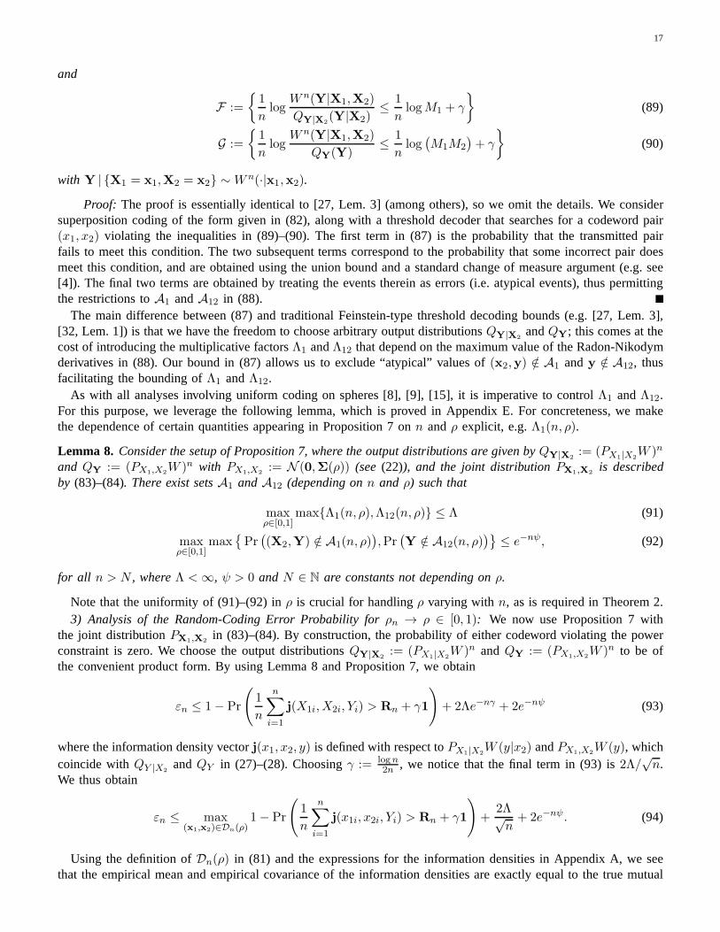
17
and
F :=
1
nlog
W n(Y|X1,X2)
QY|X2(Y|X2)
≤ 1
nlogM1 + γ
(89)
G :=
1
nlog
W n(Y|X1,X2)
QY(Y)≤ 1
nlog(
M1M2
)
+ γ
(90)
with Y | X1 = x1,X2 = x2 ∼W n(·|x1,x2).
Proof: The proof is essentially identical to [27, Lem. 3] (among others), so we omit the details. We considersuperposition coding of the form given in (82), along with a threshold decoder that searches for a codeword pair(x1, x2) violating the inequalities in (89)–(90). The first term in (87) is the probability that the transmitted pairfails to meet this condition. The two subsequent terms correspond to the probability that some incorrect pair doesmeet this condition, and are obtained using the union bound and a standard change of measure argument (e.g. see[4]). The final two terms are obtained by treating the events therein as errors (i.e. atypical events), thus permittingthe restrictions toA1 andA12 in (88).
The main difference between (87) and traditional Feinstein-type threshold decoding bounds (e.g. [27, Lem. 3],[32, Lem. 1]) is that we have the freedom to choose arbitrary output distributionsQY|X2
andQY; this comes at thecost of introducing the multiplicative factorsΛ1 andΛ12 that depend on the maximum value of the Radon-Nikodymderivatives in (88). Our bound in (87) allows us to exclude “atypical” values of(x2,y) /∈ A1 andy /∈ A12, thusfacilitating the bounding ofΛ1 andΛ12.
As with all analyses involving uniform coding on spheres [8], [9], [15], it is imperative to controlΛ1 andΛ12.For this purpose, we leverage the following lemma, which is proved in Appendix E. For concreteness, we makethe dependence of certain quantities appearing in Proposition 7 onn andρ explicit, e.g.Λ1(n, ρ).
Lemma 8. Consider the setup of Proposition 7, where the output distributions are given byQY|X2:= (PX1|X2
W )n
and QY := (PX1,X2W )n with PX1,X2
:= N (0,Σ(ρ)) (see(22)), and the joint distributionPX1,X2is described
by (83)–(84). There exist setsA1 andA12 (depending onn and ρ) such that
maxρ∈[0,1]
maxΛ1(n, ρ),Λ12(n, ρ) ≤ Λ (91)
maxρ∈[0,1]
max
Pr(
(X2,Y) /∈ A1(n, ρ))
,Pr(
Y /∈ A12(n, ρ))
≤ e−nψ, (92)
for all n > N , whereΛ <∞, ψ > 0 andN ∈ N are constants not depending onρ.
Note that the uniformity of (91)–(92) inρ is crucial for handlingρ varying withn, as is required in Theorem 2.3) Analysis of the Random-Coding Error Probability forρn → ρ ∈ [0, 1): We now use Proposition 7 with
the joint distributionPX1,X2in (83)–(84). By construction, the probability of either codeword violating the power
constraint is zero. We choose the output distributionsQY|X2:= (PX1|X2
W )n andQY := (PX1,X2W )n to be of
the convenient product form. By using Lemma 8 and Proposition 7, we obtain
εn ≤ 1− Pr
(
1
n
n∑
i=1
j(X1i,X2i, Yi) > Rn + γ1
)
+ 2Λe−nγ + 2e−nψ (93)
where the information density vectorj(x1, x2, y) is defined with respect toPX1|X2W (y|x2) andPX1,X2
W (y), whichcoincide withQY |X2
andQY in (27)–(28). Choosingγ := logn2n , we notice that the final term in (93) is2Λ/
√n.
We thus obtain
εn ≤ max(x1,x2)∈Dn(ρ)
1− Pr
(
1
n
n∑
i=1
j(x1i, x2i, Yi) > Rn + γ1
)
+2Λ√n+ 2e−nψ. (94)
Using the definition ofDn(ρ) in (81) and the expressions for the information densities inAppendix A, we seethat the empirical mean and empirical covariance of the information densities are exactly equal to the true mutual
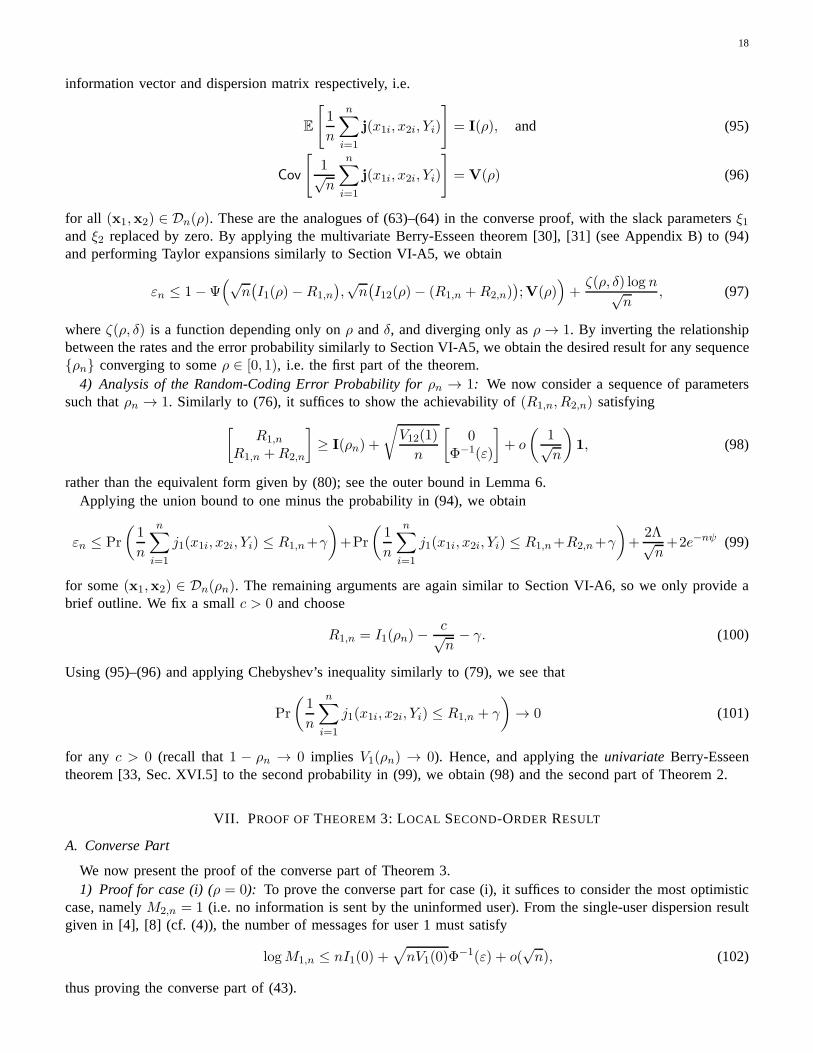
18
information vector and dispersion matrix respectively, i.e.
E
[
1
n
n∑
i=1
j(x1i, x2i, Yi)
]
= I(ρ), and (95)
Cov
[
1√n
n∑
i=1
j(x1i, x2i, Yi)
]
= V(ρ) (96)
for all (x1,x2) ∈ Dn(ρ). These are the analogues of (63)–(64) in the converse proof,with the slack parametersξ1and ξ2 replaced by zero. By applying the multivariate Berry-Esseen theorem [30], [31] (see Appendix B) to (94)and performing Taylor expansions similarly to Section VI-A5, we obtain
εn ≤ 1−Ψ(√
n(
I1(ρ)−R1,n
)
,√n(
I12(ρ)− (R1,n +R2,n))
;V(ρ))
+ζ(ρ, δ) log n√
n, (97)
whereζ(ρ, δ) is a function depending only onρ andδ, and diverging only asρ→ 1. By inverting the relationshipbetween the rates and the error probability similarly to Section VI-A5, we obtain the desired result for any sequenceρn converging to someρ ∈ [0, 1), i.e. the first part of the theorem.
4) Analysis of the Random-Coding Error Probability forρn → 1: We now consider a sequence of parameterssuch thatρn → 1. Similarly to (76), it suffices to show the achievability of(R1,n, R2,n) satisfying
[
R1,n
R1,n +R2,n
]
≥ I(ρn) +
√
V12(1)
n
[
0Φ−1(ε)
]
+ o
(
1√n
)
1, (98)
rather than the equivalent form given by (80); see the outer bound in Lemma 6.Applying the union bound to one minus the probability in (94), we obtain
εn ≤ Pr
(
1
n
n∑
i=1
j1(x1i, x2i, Yi) ≤ R1,n+γ
)
+Pr
(
1
n
n∑
i=1
j1(x1i, x2i, Yi) ≤ R1,n+R2,n+γ
)
+2Λ√n+2e−nψ (99)
for some(x1,x2) ∈ Dn(ρn). The remaining arguments are again similar to Section VI-A6, so we only provide abrief outline. We fix a smallc > 0 and choose
R1,n = I1(ρn)−c√n− γ. (100)
Using (95)–(96) and applying Chebyshev’s inequality similarly to (79), we see that
Pr
(
1
n
n∑
i=1
j1(x1i, x2i, Yi) ≤ R1,n + γ
)
→ 0 (101)
for any c > 0 (recall that1 − ρn → 0 implies V1(ρn) → 0). Hence, and applying theunivariate Berry-Esseentheorem [33, Sec. XVI.5] to the second probability in (99), we obtain (98) and the second part of Theorem 2.
VII. PROOF OFTHEOREM 3: LOCAL SECOND-ORDER RESULT
A. Converse Part
We now present the proof of the converse part of Theorem 3.1) Proof for case (i) (ρ = 0): To prove the converse part for case (i), it suffices to consider the most optimistic
case, namelyM2,n = 1 (i.e. no information is sent by the uninformed user). From the single-user dispersion resultgiven in [4], [8] (cf. (4)), the number of messages for user 1 must satisfy
logM1,n ≤ nI1(0) +√
nV1(0)Φ−1(ε) + o(
√n), (102)
thus proving the converse part of (43).
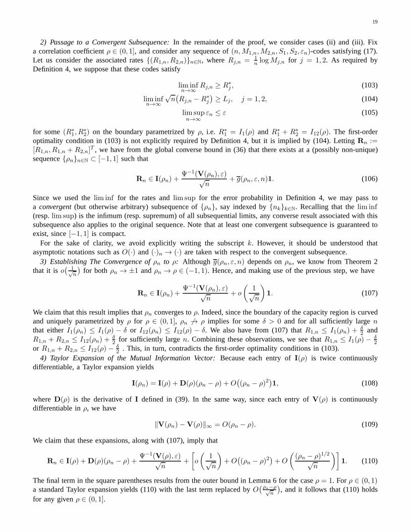
19
2) Passage to a Convergent Subsequence:In the remainder of the proof, we consider cases (ii) and (iii). Fixa correlation coefficientρ ∈ (0, 1], and consider any sequence of(n,M1,n,M2,n, S1, S2, εn)-codes satisfying (17).Let us consider the associated rates(R1,n, R2,n)n∈N, whereRj,n = 1
n logMj,n for j = 1, 2. As required byDefinition 4, we suppose that these codes satisfy
lim infn→∞
Rj,n ≥ R∗j , (103)
lim infn→∞
√n(
Rj,n −R∗j
)
≥ Lj, j = 1, 2, (104)
lim supn→∞
εn ≤ ε (105)
for some(R∗1, R
∗2) on the boundary parametrized byρ, i.e. R∗
1 = I1(ρ) andR∗1 + R∗
2 = I12(ρ). The first-orderoptimality condition in (103) is not explicitly required byDefinition 4, but it is implied by (104). LettingRn :=[R1,n, R1,n +R2,n]
T , we have from the global converse bound in (36) that there exists at a (possibly non-unique)sequenceρnn∈N ⊂ [−1, 1] such that
Rn ∈ I(ρn) +Ψ−1(V(ρn), ε)√
n+ g(ρn, ε, n)1. (106)
Since we used thelim inf for the rates andlim sup for the error probability in Definition 4, we may pass toa convergent(but otherwise arbitrary) subsequence ofρn, say indexed bynkk∈N. Recalling that thelim inf(resp.lim sup) is the infimum (resp. supremum) of all subsequential limits, any converse result associated with thissubsequence also applies to the original sequence. Note that at least one convergent subsequence is guaranteed toexist, since[−1, 1] is compact.
For the sake of clarity, we avoid explicitly writing the subscript k. However, it should be understood thatasymptotic notations such asO(·) and (·)n → (·) are taken with respect to the convergent subsequence.
3) Establishing The Convergence ofρn to ρ: Although g(ρn, ε, n) depends onρn, we know from Theorem 2that it is o
(
1√n
)
for both ρn → ±1 andρn → ρ ∈ (−1, 1). Hence, and making use of the previous step, we have
Rn ∈ I(ρn) +Ψ−1(V(ρn), ε)√
n+ o
(
1√n
)
1. (107)
We claim that this result implies thatρn converges toρ. Indeed, since the boundary of the capacity region is curvedand uniquely parametrized byρ for ρ ∈ (0, 1], ρn 6→ ρ implies for someδ > 0 and for all sufficiently largenthat eitherI1(ρn) ≤ I1(ρ) − δ or I12(ρn) ≤ I12(ρ) − δ. We also have from (107) thatR1,n ≤ I1(ρn) +
δ2 and
R1,n + R2,n ≤ I12(ρn) +δ2 for sufficiently largen. Combining these observations, we see thatR1,n ≤ I1(ρ) − δ
2or R1,n +R2,n ≤ I12(ρ)− δ
2 . This, in turn, contradicts the first-order optimality conditions in (103).4) Taylor Expansion of the Mutual Information Vector:Because each entry ofI(ρ) is twice continuously
differentiable, a Taylor expansion yields
I(ρn) = I(ρ) +D(ρ)(ρn − ρ) +O(
(ρn − ρ)2)
1, (108)
whereD(ρ) is the derivative ofI defined in (39). In the same way, since each entry ofV(ρ) is continuouslydifferentiable inρ, we have
‖V(ρn)−V(ρ)‖∞ = O(ρn − ρ). (109)
We claim that these expansions, along with (107), imply that
Rn ∈ I(ρ) +D(ρ)(ρn − ρ) +Ψ−1(V(ρ), ε)√
n+
[
o
(
1√n
)
+O(
(ρn − ρ)2)
+O
(
(ρn − ρ)1/2√n
)]
1. (110)
The final term in the square parentheses results from the outer bound in Lemma 6 for the caseρ = 1. Forρ ∈ (0, 1)a standard Taylor expansion yields (110) with the last term replaced byO
(ρn−ρ√n
)
, and it follows that (110) holdsfor any givenρ ∈ (0, 1].

20
5) Completion of the Proof for Case (ii) (ρ ∈ (0, 1)): Suppose for the time being thatρn − ρ = O( 1√n), and
henceτn :=√n(ρn − ρ) is a bounded sequence. By the Bolzano-Weierstrass theorem [34, Thm. 3.6(b)],τn
contains a convergent subsequence, say indexed byn′k; let the limit of this subsequence beβ ∈ R. For theblocklengths indexed byn′k, we know from (110) that
√
n′k(
Rn′
k− I(ρ)
)
∈ βD(ρ) + Ψ−1(V(ρ), ε) + o(1)1, (111)
where theo(1) term combines theo(
1√n
)
term in (110) and the deviation(τn′
k− β)max−D1(ρ),D12(ρ). From
the second-order optimality condition in (104), we know that everyconvergent subsequence ofRj,nn∈N has asubsequential limit that satisfieslimk→∞
√nk(
Rj,nk−R∗
j ) ≥ Lj for j = 1, 2. In other words, for allγ > 0, thereexist an integerK1 such that
√
n′k(
R1,n′
k− I1(ρ)
)
≥ L1 − γ (112)√
n′k(
R1,n′
k+R1,n′
k− I12(ρ)
)
≥ L1 + L2 − 2γ (113)
for all k ≥ K1. Thus, we may lower bound the components in the vector on the left of (111) byL1 − γ andL1 + L2 − 2γ. There also exists an integerK2 such that theo(1) terms are upper bounded byγ for all k ≥ K2.We conclude that any pair of(ε,R∗
1, R∗2)-second-order achievable rate pairs(L1, L2) must satisfy
[
L1 − 2γL1 + L2 − 3γ
]
∈⋃
β∈R
βD(ρ) + Ψ−1(V(ρ), ε)
. (114)
Finally, sinceγ > 0 is arbitrary, we can takeγ ↓ 0, thus yielding the right-hand side of (44).To complete the proof, we must handle the case thatρn − ρ is notO
(
1√n
)
. By passing to another subsequence
if necessary, we may assume thatρn − ρ = ω(
1√n
)
. Roughly speaking, in (110), the term1√nΨ−1(V(ρ), ε) is
dominated byD(ρ)(ρn − ρ), and hence the second-order term scales asω( 1√n) instead of the desiredΘ( 1√
n). To
be more precise, because
Ψ−1(V(ρ), ε) ⊂[√
V1(ρ)Φ−1(ε)
√
V12(ρ)Φ−1(ε)
]−, (115)
the bound in (110) implies thatRn must satisfy
Rn ∈ I(ρ) +D(ρ)(ρn − ρ) +1√n
[√
V1(ρ)Φ−1(ε)
√
V12(ρ)Φ−1(ε)
]−+ o(ρn − ρ)1. (116)
Therefore, we have
Rn ≤ I(ρ) +D(ρ)(ρn − ρ) + o(ρn − ρ)1. (117)
Since the first entry ofD(ρ) is negative and the second entry is positive, (117) implies that at least one of the twolim inf values in (104) is equal to−∞. That is, there are either no values ofL1 or no values ofL2 such that thedesired second-order rate conditions are satisfied. We conclude that this case plays no role in the characterizationof L.
6) Completion of the Proof for Case (iii) (ρ = 1): The caseρ = 1 is handled in essentially the same way asρ ∈ (0, 1), so we only state the differences. Sinceβ represents the difference betweenρn andρ, and sinceρn ≤ 1,we should only consider the case thatβ ≤ 0. Furthermore, forρ = 1 the setΨ−1(V(ρ), ε) can be written in asimpler form; see Lemma 6. Using this form, we readily obtain(45).
B. Direct Part
We obtain the local result from the global result using a similar (yet simpler) argument to the converse part inSection VII-A. For fixedρ ∈ [0, 1] andβ ∈ R, let
ρn := ρ+β√n, (118)
21
where we requireβ ≥ 0 (resp.β ≤ 0) whenρ = 0 (resp.ρ = 1). By Theorem 2 (global bound) and the definitionof Rin(n, ε; ρ) in (34), rate pairs(R1,n, R2,n) satisfying
Rn ∈ I(ρn) +Ψ−1(V(ρn), ε)√
n+ o
(
1√n
)
1 (119)
are(n, ε)-achievable. Substituting (118) into (119) and performingTaylor expansions in an identical fashion to theconverse part (cf. the argument from (108) to (110)), we obtain
Rn ∈ I(ρ) +βD(ρ)√
n+
Ψ−1(V(ρ), ε)√n
+ o
(
1√n
)
1. (120)
We immediately obtain the desired result for case (ii) whereρ ∈ [0, 1). We also obtain the desired result for case(iii) where ρ = 1 using the alternative form ofΨ−1(V(1), ε) (see Lemma 6), similarly to the converse proof.
For case (i), we substituteρ = 0 into (40) and (41) to obtainD(ρ) = [0 D12(ρ)]T with D12(ρ) > 0. Sinceβ
can be arbitrarily large, it follows from (120) thatL2 can take any real value. Furthermore, the setΨ−1(V(0), ε)contains vectors with a first entry arbitrarily close to
√
V1(0)Φ−1(ε) (provided that the other entry is sufficiently
negative), and we thus obtain (43).
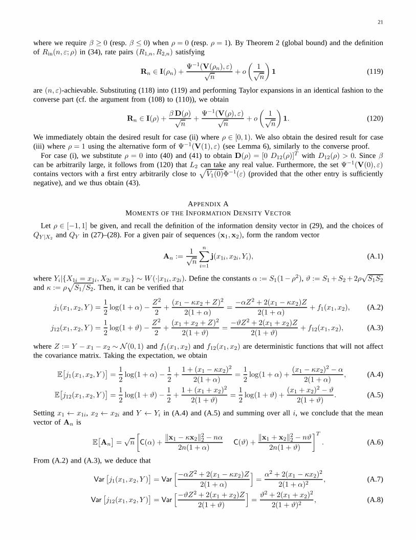
APPENDIX AMOMENTS OF THEINFORMATION DENSITY VECTOR
Let ρ ∈ [−1, 1] be given, and recall the definition of the information density vector in (29), and the choices ofQY |X2
andQY in (27)–(28). For a given pair of sequences(x1,x2), form the random vector
An :=1√n
n∑
i=1
j(x1i, x2i, Yi), (A.1)
whereYi|X1i = x1i,X2i = x2i ∼W (·|x1i, x2i). Define the constantsα := S1(1− ρ2), ϑ := S1+S2+2ρ√S1S2
andκ := ρ√
S1/S2. Then, it can be verified that
j1(x1, x2, Y ) =1
2log(1 + α)− Z2
2+
(x1 − κx2 + Z)2
2(1 + α)=−αZ2 + 2(x1 − κx2)Z
2(1 + α)+ f1(x1, x2), (A.2)
j12(x1, x2, Y ) =1
2log(1 + ϑ)− Z2
2+
(x1 + x2 + Z)2
2(1 + ϑ)=−ϑZ2 + 2(x1 + x2)Z
2(1 + ϑ)+ f12(x1, x2), (A.3)
whereZ := Y − x1 − x2 ∼ N (0, 1) andf1(x1, x2) andf12(x1, x2) are deterministic functions that will not affectthe covariance matrix. Taking the expectation, we obtain
E[
j1(x1, x2, Y )]
=1
2log(1 + α)− 1
2+
1 + (x1 − κx2)22(1 + α)
=1
2log(1 + α) +
(x1 − κx2)2 − α2(1 + α)
, (A.4)
E[
j12(x1, x2, Y )]
=1
2log(1 + ϑ)− 1
2+
1 + (x1 + x2)2
2(1 + ϑ)=
1
2log(1 + ϑ) +
(x1 + x2)2 − ϑ
2(1 + ϑ). (A.5)
Settingx1 ← x1i, x2 ← x2i andY ← Yi in (A.4) and (A.5) and summing over alli, we conclude that the meanvector ofAn is
E[
An
]
=√n
[
C(α) +‖x1 − κx2‖22 − nα
2n(1 + α)C(ϑ) +
‖x1 + x2‖22 − nϑ2n(1 + ϑ)
]T
. (A.6)
From (A.2) and (A.3), we deduce that
Var[
j1(x1, x2, Y )]
= Var
[−αZ2 + 2(x1 − κx2)Z2(1 + α)
]
=α2 + 2(x1 − κx2)2
2(1 + α)2, (A.7)
Var[
j12(x1, x2, Y )]
= Var
[−ϑZ2 + 2(x1 + x2)Z
2(1 + ϑ)
]
=ϑ2 + 2(x1 + x2)
2
2(1 + ϑ)2, (A.8)
22
where we have usedVar[Z2] = 2 andCov[Z2, Z] = EZ3 − (EZ)(EZ2) = 0. The covariance is
Cov[
j1(x1, x2, Y ), j12(x1, x2, Y )]
= Cov
[−αZ2 + 2(x1 − κx2)Z2(1 + α)
,−ϑZ2 + 2(x1 + x2)Z
2(1 + ϑ)
]
(A.9)
=1
4(1 + α)(1 + ϑ)
E[
(−αZ2 + 2(x1 − κx2)Z)(−ϑZ2 + 2(x1 + x2)Z)]
− E[
− αZ2 + 2(x1 − κx2)Z]
E[
− ϑZ2 + 2(x1 + x2)Z]
(A.10)
=3αϑ + 4(x1 − κx2)(x1 + x2)− αϑ
4(1 + α)(1 + ϑ)=αϑ + 2(x21 + (1− κ)x1x2 − κx22)
2(1 + α)(1 + ϑ). (A.11)
Settingx1 ← x1i, x2 ← x2i and Y ← Yi in (A.7), (A.8) and (A.11) and summing over alli, we conclude thatcovariance matrix ofAn is
Cov[
An
]
=
nα2 + 2‖x1 − κx2‖222n(1 + α)2
nαϑ+2(‖x1‖22+(1−κ)〈x1,x2〉−κ‖x2‖22)2n(1 + α)(1 + ϑ)
nαϑ+2(‖x1‖22+(1−κ)〈x1,x2〉−κ‖x2‖22)2n(1 + α)(1 + ϑ)
nϑ2 + 2‖x1 + x2‖222n(1 + ϑ)2
.
(A.12)
In the remainder of the section, we analyze the third absolute moments associated withAn appearing in themultivariate Berry-Esseen theorem [30], [31] (see Appendix B). The following lemma will be used to replace anygiven (x1,x2) pair by an “equivalent” pair (in the sense that the statistics of An are unchanged) for which thecorresponding third moments have the desired behavior. This is analogous to Polyanskiyet al. [8], where for theAWGN channel, one can use a spherical symmetry argument to replace any given sequencex such that‖x‖22 = nSwith a fixed sequence(
√S, · · · ,
√S). In fact, this symmetry argument has been used by many other authors
including Shannon [10].
Lemma 9. The joint distribution ofAn depends on(x1,x2) only through the powers‖x1‖22, ‖x2‖22 and the innerproduct〈x1,x2〉.
Proof: This follows by substituting (A.2)–(A.3) into (A.1) and using the symmetry of the additive noisesequenceZ = (Z1, . . . , Zn). For example, from (A.2), the first entry ofAn can be written as
1√n
(
n
2log(1 + α)− 1
2‖Z‖22 +
1
2(1 + α)‖x1 − κx2 + Z‖22
)
, (A.13)
and the desired result follows by writing
‖x1 − κx2 + Z‖2 = ‖x1‖2 + κ2‖x2‖2 + ‖Z‖2 − 2κ〈x1,x2〉+ 2〈x1 − κx2,Z〉. (A.14)
SinceZ is i.i.d. Gaussian (and in particular, circularly symmetric), the distribution of the final term depends on(x1,x2) only through‖x1 − κx2‖, which in turn depends only on‖x1‖22, ‖x2‖22 and 〈x1,x2〉.
We now provide lemmas showing that, upon replacing a given pair (x1,x2) with an equivalent pair usingLemma 9 if necessary, the corresponding third moments have the desired behavior. It will prove useful to workwith the empirical correlation coefficient
ρemp(x1,x2) :=〈x1,x2〉‖x1‖2‖x2‖2
. (A.15)
It is easily seen that Lemma 9 remains true when the inner product 〈x1,x2〉 is replaced by this normalized quantity.
Lemma 10. For any fixedρ ∈ [−1, 1], S1 > 0 and S2 > 0, there exists a sequence of pairs(x1,x2) (indexed byincreasing lengthsn) such that‖x1‖22 = nS1, ‖x2‖22 = nS2, ρemp(x1,x2) = ρ, and
Tn :=
n∑
i=1
E
[
∥
∥
∥
1√n
(
j(x1i, x2i, Yi)− E[j(x1i, x2i, Yi)])
∥
∥
∥
3
2
]
= O
(
1√n
)
, (A.16)
where theO(
1√n
)
term is uniform inρ ∈ [−1, 1].
23
Proof: Using the fact that‖v‖2 ≤ ‖v‖1 and(|a| + |b|)3 ≤ 4|a|3 + 4|b|3, we obtain
Tn ≤n∑
i=1
E
[
∥
∥
∥
1√n
(
j(x1i, x2i, Yi)− E[j(x1i, x2i, Yi)])
∥
∥
∥
3
1
]
(A.17)
≤ 4
n∑
i=1
E
[
∣
∣
∣
1√n
(
j1(x1i, x2i, Yi)− E[j1(x1i, x2i, Yi)])
∣
∣
∣
3]
+ 4
n∑
i=1
E
[
∣
∣
∣
1√n
(
j12(x1i, x2i, Yi)− E[j12(x1i, x2i, Yi)])
∣
∣
∣
3]
. (A.18)
We now specify(x1,x2) whose powers and correlation match those given in the lemma statement. Assuming forthe time being that|ρ| ≤ n−1
n , we choose
x1 =(
√
S1, · · · ,√
S1)
(A.19)
x2 =(√
S2(1 + η),√
S2, · · · ,√
S2,−√
S2(1− η),−√
S2, · · · ,−√
S2)
, (A.20)
whereη ∈ (−1, 1), andx2 containsk ≥ 1 negative entries andn − k ≥ 1 positive entries. It is easily seen that‖x1‖22 = nS1 and‖x2‖22 = nS2, as desired. Furthermore, we can choosek andη to obtain the desired correlationsince
〈x1,x2〉 =(
n− 2(k − 1) +√
1 + η −√
1− η)
√
S1S2, (A.21)
and since the range of the functionf(η) :=√1 + η −√1− η for η ∈ (−1, 1) is given by(−
√2,√2).
Using (A.2)–(A.3), it can easily be verified that the third absolute moment of each entry ofj(x1, x2, Y ) (i.e.E∣
∣j1(x1, x2, Y )−E[j1(x1, x2, Y )]∣
∣
3andE
∣
∣j12(x1, x2, Y )−E[j12(x1, x2, Y )]∣
∣
3) is bounded above by some constant
for any (x1, x2) = (√S1,±
√cS2) (c ∈ (0, 2)). We thus obtain (A.16) using (A.18). The proof is concludedby
noting that a similar argument applies for the caseρ ∈ (n−1n , 1] by replacing (A.20) by
x2 =(√
S2(1 + η),√
S2(1− η),√
S2, · · · ,√
S2)
, (A.22)
and similarly (with negative entries) whenρ ∈ [−1, n−1n ).
APPENDIX BA M ULTIVARIATE BERRY-ESSEENTHEOREM
In this section, we state a version of the multivariate Berry-Esseen theorem [30], [31] that is suited for our needsin this paper. The following is a restatement of Corollary 38in [35].
Theorem 11. Let U1, . . . ,Un be independent, zero-mean random vectors inRd. Let Zn := 1√
n(U1 + · · ·+Un),
AssumeV := Cov(Zn) is positive definite with minimum eigenvalueλmin(V) > 0. Let t := 1n
∑ni=1 E
[
‖Ui‖32]
andlet Z be a zero-mean Gaussian random vector with covarianceV. Then, for alln ∈ N,
supC∈Cd
∣
∣Pr(Zn ∈ C )− Pr(Z ∈ C )∣
∣ ≤ kd t
λmin(V)3/2√n, (B.1)
whereCd is the family of all convex, Borel measurable subsets ofRd, and kd is a function only of the dimension
d (e.g.,k2 = 265).
APPENDIX CPROOF OFLEMMA 5
Fix (z1, z2) ∈ Ψ−1(
V, ε+λn) and defineZ = (Z1, Z2) ∼ N (0,V). SinceΨ−1(
V, ε) is monotonic in the sensethatΨ−1
(
V, ε) ⊂ Ψ−1(
V, ε′) for ε ≤ ε′, it suffices to verify that(z1, z2) belongs to the set on the right-hand sideof (71) for those(z1, z2) on the boundary ofΨ−1
(
V, ε+ λn). That is (cf. (33)),
Pr(
Z1 ≤ −z1, Z2 ≤ −z2)
= 1− (ε+ λn). (C.1)
24
Defineνn := inf
ν > 0 : (−z1 − ν,−z2 − ν) ∈ Ψ−1(V, ε)
. We need to show thatνn = o(1) is bounded aboveby some linear function ofλn. By using (C.1) and the definition ofνn, we see that
λn = Pr(
Z1 ∈ [−z1 − νn,−z1] ∪ Z2 ∈ [−z2 − νn,−z2])
(C.2)
≥ maxj=1,2
Φ
(
−zj√
Vjj
)
− Φ
(
−zj − νn√
Vjj
)
. (C.3)
The assumption thatV is a non-zero positive-semidefinite matrix ensures that at least one ofVjj, j = 1, 2 isnon-zero. We have the lower bound
Φ
( −z√V
)
− Φ
(−z − νn√V
)
≥ νn√V
min N (z; 0, V ),N (z + νn; 0, V ) . (C.4)
Hence, for alln large enough, each of the terms in· in (C.3) is bounded below byνnf(zj, Vjj) for j = 1, 2 wheref(z, V ) := 1
2√VN (z; 0, V ) satisfieslimz→±∞ f(z, V ) = 0. Hence,νn ≤ λnminj=1,2f(zj , Vjj)−1. For every
fixed ε ∈ (0, 1), every(z1, z2) ∈ Ψ−1(
V, ε+λn) satisfiesmin|z1|, |z2| <∞, and henceminj=1,2f(zj, Vjj)−1is finite. This concludes the proof.
APPENDIX DPROOF OFLEMMA 6
Recall thatρn → 1. We start by proving the inner bound onΨ−1(V(ρn), ε). Let (w1, w2) be an arbitrary elementof the left-hand-side of (75), i.e.w1 ≤ −bn andw2 ≤
√
V12(1)Φ−1(ε + an) − bn. Define the random variables
(Z1,n, Z2,n) ∼ N (0,V(ρn)) and the sequencebn := (1− ρn)1/4. Consider
Pr(
Z1,n ≤ −w1, Z2,n ≤ −w2
)
≥ Pr(
Z1,n ≤ bn, Z2,n ≤ −(√
V12(1)Φ−1(ε+ an)− bn
)
)
(D.1)
≥ Pr(
Z2,n ≤ −(√
V12(1)Φ−1(ε+ an)− bn
)
)
− Pr(
Z1,n > bn
)
(D.2)
= Φ
(
−(√
V12(1)Φ−1(ε+ an)− bn
)
√
V12(ρn)
)
− Φ
(
−bn√
V1(ρn)
)
. (D.3)
From the choice ofbn and the fact that√
V1(ρn) = Θ(√1− ρn) (sinceV1(ρ) = Θ(1− ρ) asρ→ 1 by continuous
differentiability), the argument of the second term scalesas−(1− ρn)−1/4, which tends to−∞. Hence, the secondterm vanishes. We may thus choose a vanishing sequencean so that the expression in (D.3) equals1 − ε. Sucha choice satisfiesan = Θ(bn) = Θ((1 − ρn)1/4), in accordance with the lemma statement. From the definitionin(33), we have proved that(w1, w2) ∈ Ψ−1(V(ρn), ε) for this choice of(an, bn).
For the outer bound onΨ−1(V(ρn), ε), let (u1, u2) be an arbitrary element ofΨ−1(V(ρn), ε). By definition,
Pr(Z1,n ≤ −u1, Z2,n ≤ −u2) ≥ 1− ε, (D.4)
where(Z1,n, Z2,n) ∼ N (0,V(ρn)) as above. Thus,
1− ε ≤ Pr(Z2,n ≤ −u2) = Φ
(
−u2√
V12(ρn)
)
. (D.5)
This leads tou2 ≤
√
V12(ρn)Φ−1(ε) =
√
V12(1)Φ−1(ε) + c′n (D.6)
for somec′n = Θ(1 − ρn), sinceρ 7→√
V12(ρ) is continuously differentiable and its derivative does notvanish atρ = 1. Similarly, we have
u1 ≤√
V1(ρn)Φ−1(ε) = c′′n (D.7)
for somec′′n = Θ(√1− ρn), sinceV1(1) = 0 and
√
V1(ρn) = Θ(√1− ρn). Letting cn := max|c′n|, |c′′n| =
Θ(√1− ρn), we deduce that(u1, u2) belongs to the rightmost set in (75). This completes the proof.
25
APPENDIX EPROOF OFLEMMA 8
Throughout the proof, we use the fact that for jointly Gaussian (X1,X2) with powers(S1, S2) and correlationρ (i.e. the covariance matrix given in (22)), we have
X1|X2 = x2 ∼ N(
ρ
√
S1S2x2, S1(1− ρ2)
)
. (E.1)
Several aspects of the proof are similar to Polyanskiyet al. [8, Lem. 61] for the single-user setting, so we focusprimarily on the parts that are different.
A. Upper boundingΛ1
A straightforward symmetry argument reveals that
dPX1|X2W n( · |x2)
dQY|X2( · |x2)
(y) (E.2)
is the same for allx2 having a fixed magnitude. Since‖X2‖22 = nS2 almost surely by construction, we focus onthe convenient sequencex2 = (
√nS2, 0, . . . , 0). The constraint〈x1,x2〉 = nρ
√S1S2 in (84) implies that the first
entry ofx1 equalsρ√nS1 with probability one. Moreover, since‖X1‖22 = nS1 almost surely, the remaining(n−1)
symbols must have a total power ofnS1(1 − ρ2). Since (84) is the uniform distribution on the set satisfying thegiven conditions, we conclude that the final(n−1) entries ofX1 are uniform on the sphere of radius
√
nS1(1− ρ2)centered at zero.
We wish to bound the Radon-Nikodym (RN) derivative ofY := X1+x2+Z with respect toY′ := X′1+x2+Z,
whereX1 has the conditional distribution in (84), andX′1 is i.i.d. onPX1|X2
W givenx2 (recall the choice ofQY|X2
in the lemma statement). For notational convenience, we work with the vectorsY := Y− x2 andY′ := Y′ − x2,we let y denote a generic sequence equalingy−x2, and we writeY = (Y1, Y
n2 ) to split the first entry ofY from
the other(n − 1) entries (and similarly forY′, y andZ). SinceY and Y′ are shifted versions ofY andY′, itsuffices to bound the RN derivative associated the former sequences. Observing thatY1 is independent ofY n
2 andsimilarly for Y′, we have
dPY
dPY′
(y) =dPY1
dPY ′
1
(y1)dPY n
2
dPY ′n2
(yn2 ). (E.3)
By (E.1) and the fact that the first entry ofx2 equals√nS2, the first RN derivative on the right-hand side equals
the ratio of the densitiesN(
ρ√nS1, 1
)
andN (ρ√nS1, 1 + S1(1− ρ2)). Since the means coincide and the former
has a smaller variance, this derivative is upper bounded by its value at the mean, which equals
1√2π1√
2π(1+S1(1−ρ2))=√
1 + S1(1− ρ2), (E.4)
and is thus uniformly bounded inρ ∈ [0, 1].We now handle the second term in (E.3), which is between the uniform distribution on the sphere of radius√nS and the(n− 1)-fold memoryless extension ofN (0, 1 + S), whereS := S1(1− ρ2). This is the same as the
setting of [8, Lem. 61] other than two differences: (i) The block length isn− 1 instead ofn, so the radius√nS is
slightly larger than that which might be expected in analogywith [8], namely√
(n− 1)S. (ii) We must allow forall S ∈ [0, S1] (to accommodate for allρ ∈ [0, 1]), rather than considering only a fixedpositivevalue. Fortunately,the proof of [8, Lem. 61] turns out to automatically handle both of these issues. Rather than repeating the proofhere, we simply outline the differences.
We first note that, as in [8], we can restrict attention to sequencesyn2 such that
(n− 1)(1 + S − δ) ≤ ‖yn2 ‖22 ≤ (n− 1)(1 + S + δ) (E.5)
for someδ ∈ (0, 1), since the Chernoff bound implies that the probability of all remaining sequences vanishesexponentially fast, explaining the exponentially decaying term in (92). Note that the condition in (E.5) corresponds
26
to the choice ofA1 in the lemma statement; in the more general case wherex2 may differ from(√nS2, 0, . . . , 0),
yn2 should be replaced by the projection ofy onto the(n − 1)-dimensional subspace orthogonal tox2.Next, we observe that the second term in term in (E.3) dependson yn2 only through its squared magnitude
r := ‖yn2 ‖22. Thus, using [8, Eqs. (212)–(213)] to obtain explicit formulas for the densities of‖Y n2 ‖22 and‖Y ′n
2 ‖22,we obtain the following analog of [8, Eq. (426)]:
dPY n2
dPY ′n2
(yn2 ) = (1+S)n′
2 exp(
−n′S2− r S
2(S + 1)
)
(
(n′+1)Sr)− 1
2(n′
2−1)
2n′
2 Γ(n′
2
)
In′/2−1
(√
(n′ + 1)Sr)
, (E.6)
whereIk(z) is the modified Bessel function of the first kind,Γ(·) is the Gamma function, and we have writtenn′ := n − 1 for the sake of ease of comparison with [8, Lem. 61]. The desired result is now obtained as in [8,Lem. 61] by upper bounding the Gamma function and Bessel function using [8, Eq. (428)] and [8, Eq. (430)] (theformer of which should be combined withsinh−1(z) = log(z +
√1 + z2)) and applying algebraic manipulations.
To gain some intuition as to why arbitrarily small values ofS are permitted (which is the main difference in ouranalysis compared to [8]), one may consider the caseS = 0, corresponding toρ = 1. This case is trivial, since ityields Y n
2 = Zn2 and Y ′n2 = Zn2 with probability one, thus yielding an RN derivative of one.
B. Upper boundingΛ12
Observe that, by construction in (83)–(84), we have‖X1+X2‖22 = nS1+n2ρ√S1S2+nS2 with probability one.
Thus, by symmetry,X1+X2 is uniform on the sphere of radius√
n(S1 + S2 + 2ρ√S1S2), and the RN derivative
we seek isidentical to that characterized in the proof of [8, Lem. 61]. Thus, the desired result follows by choosingA12 in the same way as [8, Eq. (416)]:
A12 =
y : n(1 + S1 + S2 + 2ρ√
S1S2 − δ) ≤ ‖y‖22 ≤ n(1 + S1 + S2 + 2ρ√
S1S2 + δ)
(E.7)
for someδ ∈ (0, 1).
ACKNOWLEDGMENT
We are grateful to Ebrahim MolavianJazi for pointing us to a minor error in an earlier version of the paper.This first author has been funded in part by the European Research Council under ERC grant agreement 259663,
by the European Union’s 7th Framework Programme under grantagreement 303633, and by the Spanish Ministryof Economy and Competitiveness under grant TEC2012-38800-C03-03. The second author has been supported byA*STAR and NUS grants R-263-000-A98-750/133.
REFERENCES
[1] A. El Gamal and Y.-H. Kim,Network Information Theory. Cambridge, U.K.: Cambridge University Press, 2012.[2] T. Cover, “Broadcast channels,”IEEE Trans. on Inf. Th., vol. 18, no. 1, pp. 2–14, 1972.[3] M. Hayashi, “Second-order asymptotics in fixed-length source coding and intrinsic randomness,”IEEE Trans. on Inf. Th., vol. 54,
pp. 4619–37, Oct 2008.[4] M. Hayashi, “Information spectrum approach to second-order coding rate in channel coding,”IEEE Trans. on Inf. Th., vol. 55, pp. 4947–
66, Nov 2009.[5] R. Nomura and T. S. Han, “Second-order Slepian-Wolf coding theorems for non-mixed and mixed sources,”IEEE Trans. on Inf. Th.,
vol. 60, pp. 5553–5572, Sep 2014.[6] R. Nomura and T. S. Han, “Second-order resolvability, intrinsic randomness, and fixed-length source coding for mixed sources:
Information spectrum approach,”IEEE Trans. on Inf. Th., vol. 59, pp. 1–16, Jan 2013.[7] V. Strassen, “Asymptotische Abschatzungen in Shannons Informationstheorie,” inTrans. Third Prague Conf. Inf. Theory, (Prague),
pp. 689–723, 1962.[8] Y. Polyanskiy, H. V. Poor, and S. Verdu, “Channel codingin the finite blocklength regime,”IEEE Trans. on Inf. Th., vol. 56, pp. 2307–
2359, May 2010.[9] V. Y. F. Tan and M. Tomamichel, “The third-order term in the normal approximation for the AWGN channel,”IEEE Trans. on Inf.
Th., vol. 61, pp. 2430–2438, May 2015.[10] C. E. Shannon, “Probability of error for optimal codes in a Gaussian channel,”Bell Systems Technical Journal, vol. 38, pp. 611–656,
1959.[11] V. Y. F. Tan and O. Kosut, “On the dispersions of three network information theory problems,”IEEE Trans. on Inf. Th., vol. 60, no. 2,
pp. 881–903, 2014.[12] Y.-W. Huang and P. Moulin, “Finite blocklength coding for multiple access channels,” inInt. Symp. Inf. Th., (Boston, MA), 2012.
27
[13] E. MolavianJazi and J. N. Laneman, “Simpler achievablerate regions for multiaccess with finite blocklength,” inInt. Symp. Inf. Th.,(Boston, MA), 2012.
[14] E. MolavianJazi and J. N. Laneman, “A random coding approach to Gaussian multiple access channels with finite blocklength,” inAllerton Conference, (Monticello, IL), 2012.
[15] E. MolavianJazi and J. N. Laneman, “A finite-blocklength perspective on Gaussian multi-access channels,”arXiv:1309.2343[cs.IT], Sep 2013.
[16] S. Verdu, “Non-asymptotic achievability bounds in multiuser information theory,” inAllerton Conference, (Monticello, IL), 2012.[17] P. Moulin, “A new metaconverse and outer region for finite-blocklength MACs,” inInfo. Th. and Applications (ITA) Workshop, (San
Diego, CA), 2013.[18] J. Scarlett, A. Martinez, and A. Guillen i Fabregas, “Second-order rate region of constant-composition codes for the multiple-access
channel,”IEEE Trans. on Inf. Th., vol. 61, no. 1, pp. 157–172, 2015.[19] E. Haim, Y. Kochman, and U. Erez, “A note on the dispersion of network problems,” inConvention of Electrical and Electronics
Engineers in Israel (IEEEI), 2012.[20] V. Y. F. Tan, “Asymptotic estimates in information theory with non-vanishing error probabilities,”Foundations and Trends in
Communications and Information Theory, vol. 11, no. 1-2, pp. 1–183, 2014.[21] S. I. Bross, A. Lapidoth, and M. Wigger, “Dirty-paper coding for the Gaussian multiaccess channel with conferencing,” IEEE Trans.
on Inf. Th., vol. 58, no. 9, pp. 5640–5668, 2012.[22] R. Ahlswede, “An elementary proof of the strong converse theorem for the multiple access channel,”J. of Combinatorics, Information
& System Sciences, pp. 216–230, 1982.[23] J. Scarlett and V. Y. F. Tan, “Second-order asymptoticsfor the discrete memoryless MAC with degraded message sets,” in Intl. Symp.
Info. Th., (Hong Kong), June 2015.[24] I. Csiszar and J. Korner,Information Theory: Coding Theorems for Discrete Memoryless Systems. Cambridge University Press, 2011.[25] Y. Polyanskiy,Channel coding: Non-asymptotic fundamental limits. PhD thesis, Princeton University, 2010.[26] G. Dueck, “Maximal error capacity regions are smaller than average error capacity regions for multi-user channels,” Probl. Control
Inf. Theory, vol. 7, pp. 11–19, 1978.[27] T. S. Han, “An information-spectrum approach to capacity theorems for the general multiple-access channel,”IEEE Trans. on Inf. Th.,
vol. 44, pp. 2773–2795, Jul 1998.[28] S. Boucheron and M. R. Salamatian, “About priority encoding transmission,”IEEE Trans. on Inf. Th., vol. 46, no. 2, pp. 699–705,
2000.[29] M. Hayashi and H. Nagaoka, “General formulas for capacity of classical-quantum channels,”IEEE Trans. on Inf. Th., vol. 49, pp. 1753–
1768, Jul 2003.[30] F. Gotze, “On the rate of convergence in the multivariate CLT,” The Annals of Probability, vol. 19, no. 2, pp. 721–739, 1991.[31] R. Bhattacharya and S. Holmes, “An exposition of Gotze’s estimation of the rate of convergence in the multivariatecentral limit
theorem,” tech. rep., Stanford University, 2010.arxiv:1003.4254 [math.ST].[32] J. N. Laneman, “On the distribution of mutual information,” in Information Theory and Applications Workshop, 2006.[33] W. Feller,An Introduction to Probability Theory and Its Applications. John Wiley and Sons, 2nd ed., 1971.[34] W. Rudin,Principles of Mathematical Analysis. McGraw-Hill, 1976.[35] S. Watanabe, S. Kuzuoka, and V. Y. F. Tan, “Non-asymptotic and second-order achievability bounds for coding with side-information,”
IEEE Trans. on Inf. Th., vol. 61, pp. 1574–1605, Apr 2015.
Jonathan Scarlett (S’14-M’15) was born in Melbourne, Australia, in 1988. In 2010, he received the B.Eng. degree in electrical engineeringand the B.Sci. degree in computer science from the University of Melbourne, Australia. In 2011, he was a research assistant at the Departmentof Electrical & Electronic Engineering, University of Melbourne. From October 2011 to August 2014, he was a Ph.D. student in the SignalProcessing and Communications Group at the University of Cambridge, United Kingdom. He is now a post-doctoral researcher with theLaboratory for Information and Inference Systems at theEcole Polytechnique Federale de Lausanne, Switzerland.His research interestsare in the areas of information theory, signal processing, and high-dimensional statistics. He received the Poynton Cambridge AustraliaInternational Scholarship, and the ‘EPFL Fellows’ postdoctoral fellowship co-funded by Marie Curie.
Vincent Y. F. Tan (S’07-M’11-SM’15) is an Assistant Professor in the Department of Electrical and Computer Engineering (ECE) andthe Department of Mathematics at the National University ofSingapore (NUS). He received the B.A. and M.Eng. degrees in Electrical andInformation Sciences from Cambridge University in 2005 andthe Ph.D. degree in Electrical Engineering and Computer Science (EECS)from the Massachusetts Institute of Technology in 2011. He was a postdoctoral researcher in the Department of ECE at the University ofWisconsin-Madison and a research scientist at the Institute for Infocomm (I2R) Research, A*STAR, Singapore. His research interests includeinformation theory, machine learning and signal processing.
Dr. Tan received the MIT EECS Jin-Au Kong outstanding doctoral thesis prize in 2011 and the NUS Young Investigator Award in 2014.He is currently an Editor of the IEEE Transactions on Communications.
Related Documents