SECOND LAW ANALYSIS OF SOLID OXIDE FUEL CELLS A THESIS SUBMITTED TO THE GRADUATE SCHOOL OF NATURAL AND APPLIED SCIENCES OF THE MIDDLE EAST TECHNICAL UNIVERSITY BY BAŞAR BULUT IN PARTIAL FULFILLMENT OF THE REQUIREMENTS FOR THE DEGREE OF MASTER OF SCIENCE IN THE DEPARTMENT OF MECHANICAL ENGINEERING SEPTEMBER 2003

Welcome message from author
This document is posted to help you gain knowledge. Please leave a comment to let me know what you think about it! Share it to your friends and learn new things together.
Transcript
SECOND LAW ANALYSIS OF SOLID OXIDE FUEL CELLS
A THESIS SUBMITTED TO
THE GRADUATE SCHOOL OF NATURAL AND APPLIED SCIENCES
OF
THE MIDDLE EAST TECHNICAL UNIVERSITY
BY
BAŞAR BULUT
IN PARTIAL FULFILLMENT OF THE REQUIREMENTS FOR THE
DEGREE OF
MASTER OF SCIENCE
IN
THE DEPARTMENT OF MECHANICAL ENGINEERING
SEPTEMBER 2003
iii
ABSTRACT
SECOND LAW ANALYSIS OF SOLID OXIDE FUEL CELLS
Bulut, Başar
M.S., Department of Mechanical Engineering
Supervisor : Assoc. Prof. Dr. Cemil Yamalı
Co-Supervisor : Prof. Dr. Hafit Yüncü
September 2003, 111 pages
In this thesis, fuel cell systems are analysed thermodynamically and electrochemically.
Thermodynamic relations are applied in order to determine the change of first law and
second law efficiencies of the cells, and using the electrochemical relations, the
irreversibilities occuring inside the cell are investigated.
Following this general analysis, two simple solid oxide fuel cell systems are examined.
The first system consists of a solid oxide unit cell with external reformer. The second
law efficiency calculations for the unit cell are carried out at 1273 K and 1073 K, 1 atm
and 5 atm, and by assuming different conversion ratios for methane, hydrogen, and
oxygen in order to investigate the effects of temperature, pressure and conversion ratios
on the second law efficiency. The irreversibilities inside the cell are also calculated and

iv
graphed in order to examine their effects on the actual cell voltage and power density of
the cell.
Following the analysis of a solid oxide unit cell, a simple fuel cell system is modeled.
Exergy balance is applied at every node and component of the system. First law and
second law efficiencies, and exergy loss of the system are calculated.
Keywords: Exergy, Solid oxide fuel cell, Second law efficiency

v
ÖZ
KATI OKSİT YAKIT HÜCRELERİNİN İKİNCİ KANUN ANALİZİ
Bulut, Başar
Yüksek Lisans, Makina Mühendisliği Bölümü
Tez Yöneticisi : Doç. Dr. Cemil Yamalı
Ortak Tez Yöneticisi : Prof. Dr. Hafit Yüncü
Eylül 2003, 111 sayfa
Bu tez çalışmasında, yakıt hücresi sistemleri termodinamiksel ve elektrokimyasal olarak
analiz edilmiştir. Hücrelerin birinci ve ikinci kanun verimlerinin değişiminin
incelenmesi için genel termodinamik bağıntılar kullanılmış, elektrokimyasal bağıntılar
kullanaran hücre içinde meydana gelen tersinmezlikler incelenmiştir.
Bu genel analizin ardından, iki basit katı oksit yakıt hücresi sistemi incelenmiştir. Birinci
sistem dış düzenleyicili bir katı oksit hücresinden oluşmaktadır. İkinci kanun verim
hesaplamaları, sıcaklık, basınç ve değişme oranlarının ikinci kanun verimine etkilerini
inceleyebilmek amacıyla 1273 K ve 1073 K, 1 atm ve 5 atm, ve de metan, hidrojen ve
oksijen için değişik değişme oranları varsayılarak tamamlanmıştır. Hücre içerisindeki

vi
tersinmezlikler de hesaplanmış ve fiili hücre voltajına ve hücrenin güç yoğunluğuna olan
etkilerini inceleyebilmek için grafikleri çizilmiştir.
Katı oksit hücre analizini, basit bir katı oksit sisteminin modellenmesi takip etmiştir.
Ekserji denklemi, sistem içindeki her parça ve düğüm noktasına uygulanmıştır. Birinci
ve ikinci kanun verimleri ve sistemin ekserji kayıpları hesaplanmıştır.
Anahtar Kelimeler: Ekserji, Katı oksit yakıt hücresi, İkinci kanun verimi

vii
To My Parents

viii
ACKNOWLEDGMENTS
I would like to thank to my supervisor Assoc. Prof. Dr. Cemil Yamalı for his guidance
and insight throughout the research. I express sincere appretiation to my co-supervisor
Prof. Dr. Hafit Yüncü for his guidance, suggestions and comments.
I express sincere thanks to my family for their support and faith in me, and for their
understanding in every step of my education.

ix
TABLE OF CONTENTS
ABSTRACT ........................................................................................................... iii
ÖZ ........................................................................................................................... v
ACKNOWLEDGMENTS....................................................................................... viii
TABLE OF CONTENTS ........................................................................................ ix
LIST OF TABLES .................................................................................................. xiii
LIST OF FIGURES................................................................................................. xvi
LIST OF SYMBOLS .............................................................................................. xix
CHAPTER
1. INTRODUCTION................................................................................. 1
1.1 Definition of a Fuel Cell............................................................. 1
1.2 Fuel Cell Plant Description ........................................................ 4
1.3 Fuel Cell Stacking ...................................................................... 4
1.4 Characteristics of Fuel Cells ...................................................... 6
1.4.1 Efficiency ...................................................................... 6
1.4.2 Flexibility in Power Plant Design ................................. 7
1.4.3 Manufacturing and Maintenance................................... 7
1.4.4 Noise.............................................................................. 7
x
1.4.5 Heat................................................................................ 8
1.4.6 Low Emissions .............................................................. 8
1.5 Types of Fuel Cells and Their Fields of Applications................. 9
2. THERMODYNAMICS OF FUEL CELLS .......................................... 11
2.1 Some Fundamental Relations..................................................... 11
2.1.1 TdS Equations and Maxwell Relations ......................... 11
2.1.2 Partial Molal Properties................................................. 16
2.1.3 Chemical Potential......................................................... 18
2.2 Thermodynamics of Chemical Reactions................................... 19
2.2.1 Free Energy Change of Chemical Reactions................. 19
2.2.2 Standard Free Energy Change of a Chemical Reaction. 19
2.2.3 Relation Between Free Energy Change in a Cell Reaction and Cell Potential .......................................................... 20
2.3 Nernst Equation.......................................................................... 22
2.4 Exergy Concept .......................................................................... 24
2.4.1 Exergy Balance.............................................................. 24
2.4.2 Chemical Exergy ........................................................... 26
2.4.3 Physical Exergy............................................................. 27
2.5 Efficiency of Fuel Cells.............................................................. 27
2.5.1 Thermodynamic ( First and Second Law ) Efficiencies 27
2.5.2 Electrochemical Efficiencies......................................... 33
3. KINETIC EFFECTS ............................................................................. 34
3.1 Introduction ................................................................................ 34
3.2 Fuel Cell Irreversibilities............................................................ 37
xi
3.2.1 Activation Polarization.................................................. 38
3.2.2 Ohmic Polarization........................................................ 42
3.2.3 Concentration Polarization ............................................ 42
3.3 Mass Transport Effects............................................................... 46
3.3.1 Knudsen Diffusion......................................................... 46
3.3.2 Molecular Diffusion ...................................................... 48
3.3.3 Transition Region Diffusion.......................................... 48
4. MODELING AND CALCULATION .................................................. 54
4.1 Fuel Cell Type Selection ............................................................ 54
4.2 Environment and Air Composition ............................................ 55
4.3 Chemical Reactions and Components of SOFC System ........... 55
4.4 Simulation Models...................................................................... 58
4.4.1 Simulation Model 1: SOFC Unit Analysis.................... 58
4.4.2 Simulation Model 2: SOFC System Analysis ............... 59
4.5 Electrochemical Model............................................................... 60
4.6 Heat Exchanger Model............................................................... 63
4.7 Calculation Procedure................................................................. 65
4.7.1 General Assumptions..................................................... 66
4.7.2 Calculation Steps for Simulation Model 1..................... 67
4.7.3 Calculation Steps for Simulation Model 2 .................... 69
5. RESULTS AND DISCUSSION............................................................ 72
5.1 Results of Simulation Model 1................................................... 72
5.1.1 Electrochemical Model Analysis................................... 72
5.1.2 Thermodynamic Analysis.............................................. 83

xii
5.2 Results of Simulation Model 2................................................... 98
5.2.1 The Heat Required by The Reformer and Vaporizer .... 98
5.2.2 Heat Exchanger Design .................................................101
5.2.3 Thermodynamic Analysis..............................................102
6. CONCLUSION......................................................................................108
REFERENCES........................................................................................................110

LIST OF TABLES
TABLE
1.1 Classification of fuel cells ................................................................... 9
1.2 Application fields of fuel cells............................................................. 10
4.1 Properties of SOFC materials ............................................................... 55
5.1 Mixture compositions for ideal case ( i.e. 14=CHη , 1
2=Hη ,
12=Oη ) ……………………………………………………………… 84
5.2 Mixture compositions for 9.04=CHη , 9.0
2=Hη , 9.0
2=Oη ……….. 84
5.3 Mixture compositions for 9.04=CHη , 9.0
2=Hη , 8.0
2=Oη ……….. 84
5.4 Mixture compositions for 9.04=CHη , 9.0
2=Hη , 7.0
2=Oη ……….. 85
5.5 Mixture compositions for 9.04=CHη , 8.0
2=Hη , 8.0
2=Oη ……… 85
5.6 Mixture compositions for 9.04=CHη , 8.0
2=Hη , 7.0
2=Oη ……….. 85
5.7 Mixture compositions for 9.04=CHη , 7.0
2=Hη , 7.0
2=Oη ………... 86
5.8 Calculated second law efficiencies as functions of conversion ratios ( T = 1273 K, P = 1 atm, I = 8000 A / m² ) ……………………. 87
5.9 Calculated second law efficiencies as functions of conversion
ratios ( T = 1073 K, P = 1 atm, I = 8000 A / m² )…………………….87
xiii
xiv
5.10 Calculated second law efficiencies as functions of conversion
ratios ( T = 1273 K, P = 1 atm, I = 6000 A / m² ) …………………. 88
5.11 Calculated second law efficiencies as functions of conversion ratios ( T = 1073 K, P = 1 atm, I = 6000 A / m² ) …………………. 88
5.12 Calculated second law efficiencies as functions of conversion ratios ( T = 1273 K, P = 1 atm, I = 4000 A / m² ) …………………. 89
5.13 Calculated second law efficiencies as functions of conversion ratios ( T = 1273 K, P = 1 atm, I = 4000 A / m² ) …………………. 89
5.14 Calculated second law efficiencies as functions of conversion ratios ( T = 1273 K, P = 1 atm, I = 2000 A / m² ) …………………. 90
5.15 Calculated second law efficiencies as functions of conversion ratios ( T = 1073 K, P = 1 atm, I = 2000 A / m² ) …………………. 90
5.16 Calculated second law efficiencies as functions of conversion ratios ( T = 1273 K, P = 5 atm, I = 8000 A / m² ) …………………. 91
5.17 Calculated second law efficiencies as functions of conversion ratios ( T = 1073 K, P = 5 atm, I = 8000 A / m² ) …………………. 91
5.18 Calculated second law efficiencies as functions of conversion ratios ( T = 1273 K, P = 5 atm, I = 6000 A / m² ) …………………. 92
5.19 Calculated second law efficiencies as functions of conversion ratios ( T = 1073 K, P = 5 atm, I = 6000 A / m² ) …………………. 92
5.20 Calculated second law efficiencies as functions of conversion ratios ( T = 1273 K, P = 5 atm, I = 4000 A / m² ) …………………. 93
5.21 Calculated second law efficiencies as functions of conversion ratios ( T = 1073 K, P = 5 atm, I = 4000 A / m² ) …………………. 93
5.22 Calculated second law efficiencies as functions of conversion ratios ( T = 1273 K, P = 5 atm, I = 2000 A / m² ) …………………. 94
5.23 Calculated second law efficiencies as functions of conversion ratios ( T = 1073 K, P = 5 atm, I = 2000 A / m² ) …………………. 94
5.24 Heat exchanger design conditions and results ……………………...102
5.25 Calculated molar chemical compositions of gas streams at each node……………………………………………………………103
xv
5.26 Net work output of the SOFC operating at Ta = 1000 K, Tc = 900 K, I = 1000 A/m² …………………………………..……104
5.27 The first and second law efficiencies of model 2 …………………...104
5.28 The comparison of input, output, and loss of energy and exergy in the system. Energy and exergy values are normalized relative to the lower heating value and chemical exergy of the fuel, respectively ……………………………………………………106

xvi
LIST OF FIGURES
FIGURES
1.1 Schematic of an individual fuel cell................................................. ..... 2
1.2 Direct energy conversion with fuel cells in comparison to
to indirect energy conversion ............................................................... 3
1.3 Fuel cell power plant processes .......................................................... 5
1.4 Stacking of individual fuel cells ......................................................... 6
2.1 An open thermodynamic system with single inlet and outlet ............. 24
2.2 Simple H2/O2 fuel cell system, T = 25°C ............................................ 28
2.3 Schematic of the system used to calculate the second law efficiency of the simple fuel cell ………………………………….... 30
2.4 Comparison between fuel cell first law and second law efficiency changes with temperature and Carnot efficiency change with temperature……………………………………………… 32
3.1 Voltage change with current density for a simple fuel cell operating at about 40°C, and at standard pressure ................................ 35
3.2 Voltage change with current density for a solid oxide fuel cell operating at about 800°C ................................................................ 36
3.3 The film thickness theory .................................................................... 43
3.4 Types of diffusion through the pores: ( a ) Knudsen diffusion, ( b ) molecular diffusion, ( c ) transition diffusion................................ 47

xvii
4.1 Schematic of simulation model 1 ........................................................ 58
4.2 Schematic of simulation model 2 ........................................................ 59
5.1 Activation polarization change with current density ( T = 1273 K )…………………………………………………………. 73
5.2 Ohmic polarization change with current density ( T = 1273 K ) …… 73
5.3 Concentration polarization change with current density ( T = 1273 K )…………………………………………………………. 74
5.4 Change in the cell voltage and the power density with current density ( T = 1273 K )………………………………………… 74
5.5 Calculated polarization effects with current density ( T = 1273 K )…………………………………………………………. 75
5.6 Calculated power density, cell voltage and polarizations with current density ( 1273 K )…..…………………………………… 76
5.7 Activation polarization change with current density ( T = 1073 K ) ………………………………………………………. 77
5.8 Ohmic polarization change with current density ( T = 1073 K ) ..….... 78
5.9 Concentration polarization change with current density ( T = 1073 K )…………………………………………………………. 78
5.10 Change in the cell voltage and the power density with current density ( T = 1073 K )……………………………………… 79
5.11 Calculated polarization effects with current density ( T = 1073 K )………………………………………………………. 80
5.12 Calculated power density, cell voltage and polarizations with current density ( 1073 K )……………………………………… 81
5.13 Second law efficiency with current density at P = 1 atm, and P = 5 atm, conversion ratios are 100% and 90% respectively, T = 1273 K …………………………………………………………. 95
5.14 Second law efficiency with current density at P = 1 atm, and P = 5 atm, conversion ratios are 100% and 90% respectively, T = 1073 K …………………………………………………………. 96
xviii
5.15 Second law efficiency with current density at T = 1273 K, and T = 1073 K, conversion ratios are 100% and 90% respectively, P = 1 atm……………………………………………………………. 96
5.16 Second law efficiency with current density at T = 1273 K, and T = 1073 K, conversion ratios are 100% and 90% respectively, P = 5 atm……………………………………………………………. 97
5.17 Heat requirement of the components of the SOFC system with methane reforming rate ( Tr,i = 1100 K )…………………………… 99
5.18 Heat release of the combustion processes in the afterburner With respect to the mole number of the fuel that is burnt………….. 99
5.19 Comparison of heat release by methane and hydrogen with reformer efficiency …………………………………………………100
5.20 Change in fuel utilization rate with reformer efficiency …………...101
5.21 System 2 operating at 1 atm, 90% reformer efficiency, 75% fuel utilization rate, fuel inlet temperature is 1000 K, air inlet temperature is 900 ………………………………………………......105

xix
LIST OF SYMBOLS
a Activity C Concentration ( mole / m³ ) D Diffusion coefficient ( m² / s ) e Energy of molecular interaction ( ergs ) E Cell voltage F Faraday constant ( = 96487 kJ / V.kmole electrons ) G Gibbs free energy ( jJ ) i Current density ( A / m² ) io Exchange current density ( A / m² ) I Current density ( A / m² ) IL Limiting current density ( A / m² ) İ Irreversibility ( kJ / s ) J Mass flux ( kg / s ) K Equilibrium constant n Number of moles ne Electrons transferred per reaction M Molecular mass p Partial pressure ( atm ) P Pressure ( atm ) Q Heat ( kJ ) R Universal gas constant ( = 8.3145 kJ / kmole K ) Re Area specific resistance ( Ω / m² ) T Temperature ( K ) w Thickness ( µm ) W Work ( kJ ) We Electrical work ( kJ ) X Mole fraction
xx
Greek Letters α Transfer coefficient δ Thickness of the diffusion layer ( m ) ε Porosity η Polarization ( V ) ηI First law efficiency ηII Second law efficiency µ Chemical potential ( kJ / mole ) ρ Resistivity ( Ω cm ) ξ Tortuosity σ Collision diameter ( Ả ) ΩD Collision integral nased on the Lennard-Jones potential Subscripts a Anode A A specie B B specie c Cathode k Knudsen diffusion P Products R Reactants rev Reversible (eff) Effective Superscripts I Inlet condition
1
CHAPTER 1
INTRODUCTION
1.1 Definition of a Fuel Cell
A fuel cell is an electrochemical device which can continuously convert the free energy
of the reactants ( i.e. the fuel and the oxidant ), which are stored outside the cell itself,
directly to electrical energy. The basic physical structure or building block of a fuel cell
consists of an electrolyte layer in contact with two porous electrodes; the anode or the
fuel electrode, where the fuel that feeds the cell is oxidised, and the cathode or the
oxygen ( or air ) electrode, where the reduction of molecular oxygen occurs, on either
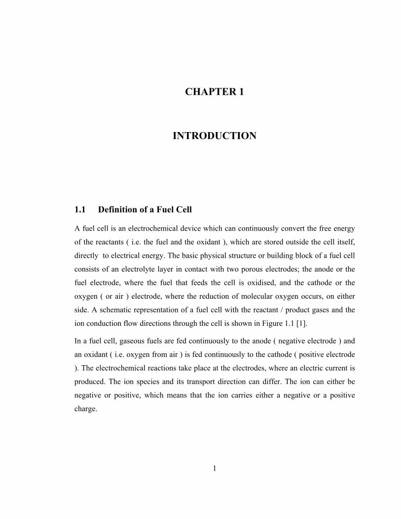
side. A schematic representation of a fuel cell with the reactant / product gases and the
ion conduction flow directions through the cell is shown in Figure 1.1 [1].
In a fuel cell, gaseous fuels are fed continuously to the anode ( negative electrode ) and
an oxidant ( i.e. oxygen from air ) is fed continuously to the cathode ( positive electrode
). The electrochemical reactions take place at the electrodes, where an electric current is
produced. The ion species and its transport direction can differ. The ion can either be
negative or positive, which means that the ion carries either a negative or a positive
charge.
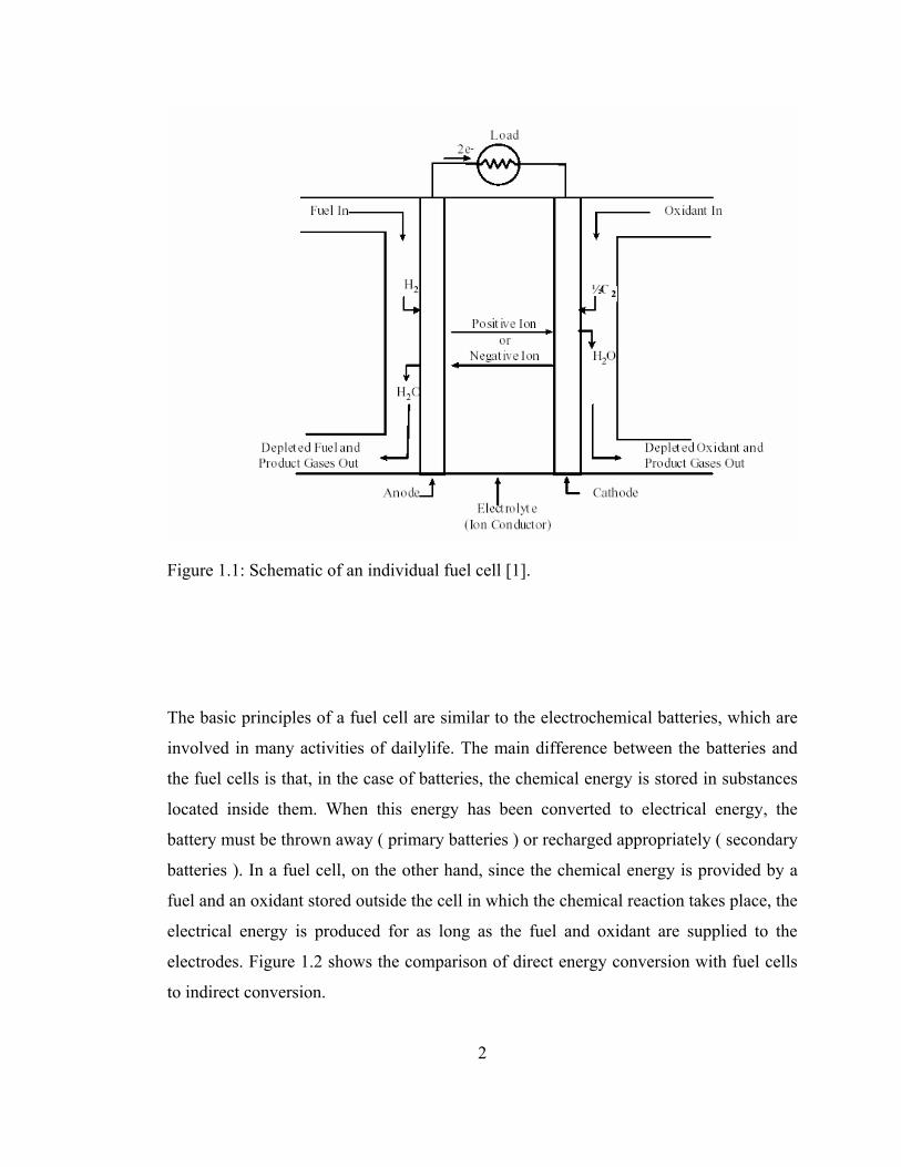
Figure 1.1: Schematic of an individual fuel cell [1].
The basic principles of a fuel cell are similar to the electrochemical batteries, which are
involved in many activities of dailylife. The main difference between the batteries and
the fuel cells is that, in the case of batteries, the chemical energy is stored in substances
located inside them. When this energy has been converted to electrical energy, the
battery must be thrown away ( primary batteries ) or recharged appropriately ( secondary
batteries ). In a fuel cell, on the other hand, since the chemical energy is provided by a
fuel and an oxidant stored outside the cell in which the chemical reaction takes place, the
electrical energy is produced for as long as the fuel and oxidant are supplied to the
electrodes. Figure 1.2 shows the comparison of direct energy conversion with fuel cells
to indirect conversion.
2
Chemical energy of the fuel(s)
Electrical energy conversion
Thermal and/or mechanical energy conversion
Figure 1.2: Direct energy conversion with fuel cells in comparison to indirect energy conversion.
Gaseous hydrogen has become the fuel of choice for most applications, because of
its high reactivity when suitable catalysts are used, its ability to be produced from
hydrocarbons and its high energy density when stored cryogenically for closed
environment applications. Similarly, the most common oxidant is gaseous oxygen,
which is readily and economically available from air, and easily stored in a closed
environment.
The electrolyte not only transports dissolved reactants to the electrode, but also
conducts ionic charge between the electrodes and thereby completes the cell electric
circuit. It also provides a pysical barrier to prevent the mixing of the fuel and oxidant gas
streams.
The porous electrodes in the fuel cells provide a surface site where gas/liquid
ionization or de-ionization reaction can take place. In order to increase the rates of
3reactions, the electrode material should be catalytic as well as conductive, porous rather
4
.2 Fuel Cell Plant Description
he fuel and oxygen from the air are combined
.3 Fuel Cell Stacking
r to produce the required voltage level. The
lar plate between
conditions, and an excellent electronic conductor. [2]
than solid. The catalytic function of electrodes is more important in lower temperature
fuel cells and less so in high temperature fuel cells, because ionization reaction rates are
directly proportional with temperature ( i.e. increase with temperature ). The porous
electrodes also provide a physical barrier that separates the bulk gas phase and the
electrolyte.
1
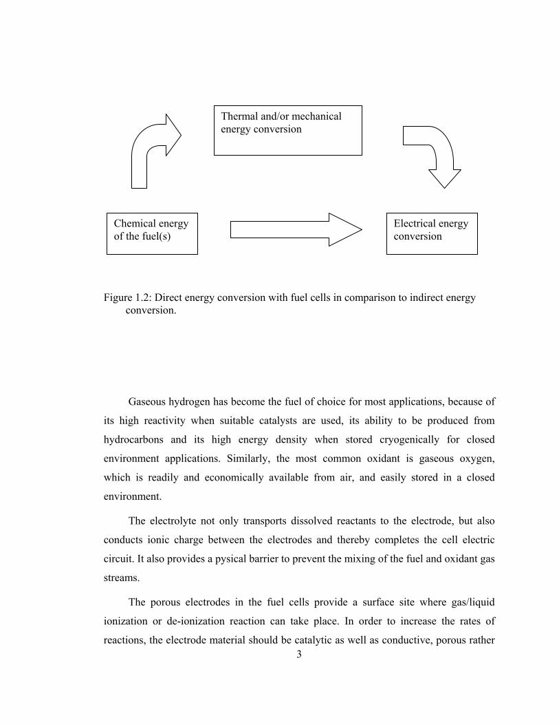
In the fuel cell, hydrogen produced from t
to produce dc power, water, and heat. In cases where CO and CH4 are reacted in the cell
to produce H2, CO2 is also a product. These reactions must be carried out at a suitable
temperature and pressure for fuel cell operation. A system must be built around the fuel
cells to supply air and clean fuel, convert the power to a more usable form
( i.e. AC power ), and remove the depleted reactants and heat that are produced by the
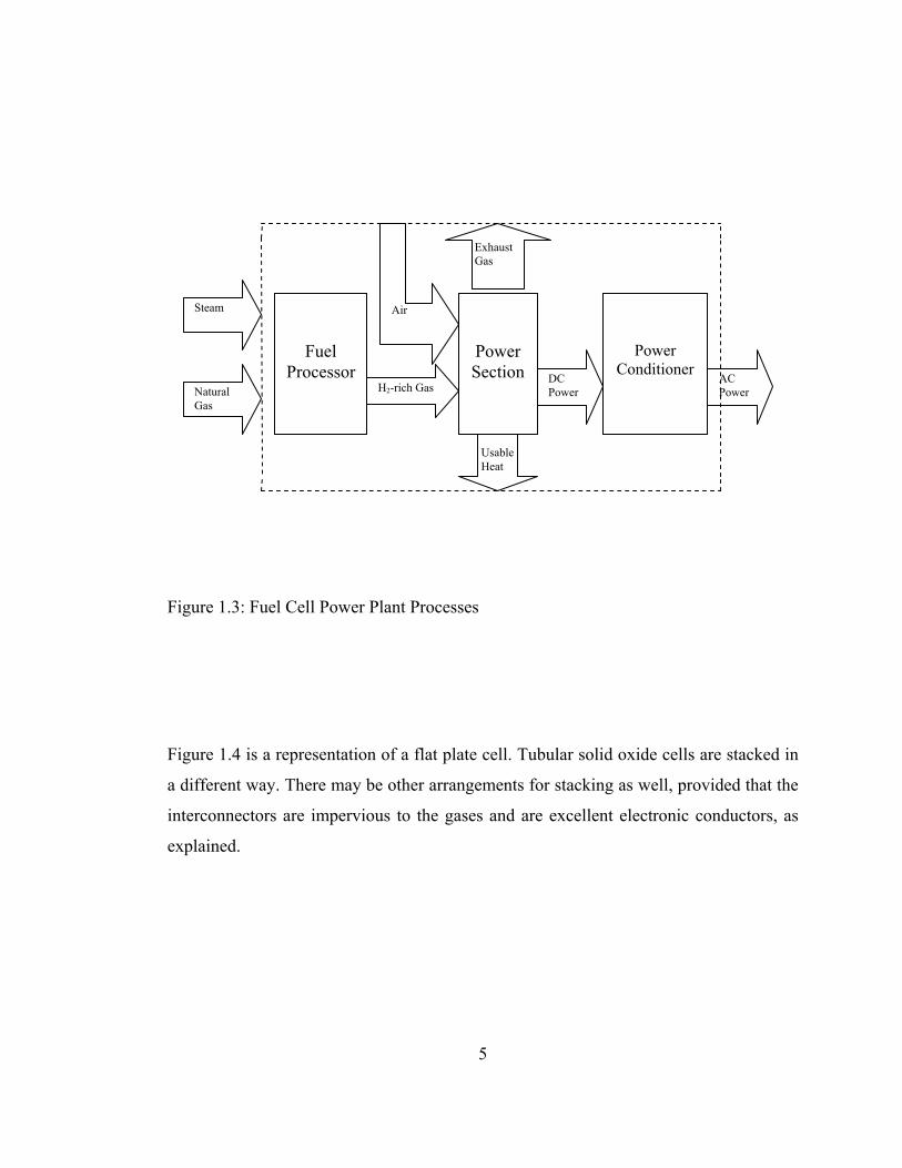
reactions in the cells. Figure 1.3 shows a simple rendition of a fuel cell power plant.
Beginning with fuel processing, a conventional fuel ( natural gas, other gaseous
hydrocarbons, methanol, coal, etc. ) is cleaned, then converted into a gas containing
hydrogen. Energy conversion occurs when dc electricity is generated by means of
individual fuel cells combined in stacks or bundles. A varying number of cells or stacks
can be matched to a particular power application. Finally, power conditioning converts
the electric power from DC into regulated DC or AC for consumer use [1].
1
Individual fuel cells are combined in orde
schematic of stacking of individual fuel cells is given in Figure 1.4. [2]
Anode – electrolyte – cathode sections are connected in series by a bipo
the cathode of the cell and the anode of the other cell. The bipolar plate must be
impervious to the fuel and oxidant gases, chemically stable under reducing and oxidizing
Fuel Processor
Power Section
Power Conditioner
Natural Gas
H Gas
5
igure 1.4 is a representation of a flat plate cell. Tubular solid oxide cells are stacked in
different way. There may be other arrangements for stacking as well, provided that the
Figure 1.3: Fuel Cell Power Plant Processes
F
a
interconnectors are impervious to the gases and are excellent electronic conductors, as
explained.
2-richDC Power
AC Power
ir
Exhaust Gas
A
Usable Heat
Steam
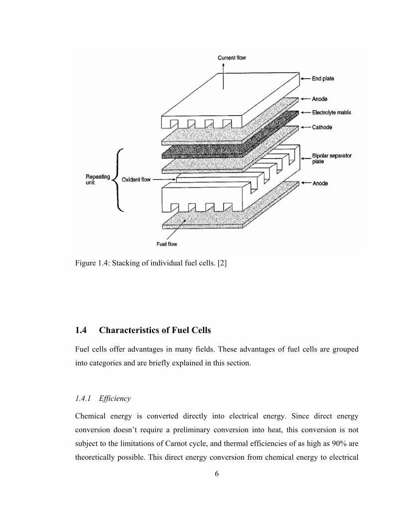
Figure 1.4: Stacking of individual fuel cells. [2]
.4 Characteristics of Fuel Cells
These advantages of fuel cells are grouped
.4.1 Efficiency
ical energy is converted directly into electrical energy. Since direct energy
1
Fuel cells offer advantages in many fields.
into categories and are briefly explained in this section.
1
Chem
conversion doesn’t require a preliminary conversion into heat, this conversion is not
subject to the limitations of Carnot cycle, and thermal efficiencies of as high as 90% are
theoretically possible. This direct energy conversion from chemical energy to electrical
6
7
.4.2 Flexibility in Power Plant Design
e o low voltage level of an individual cell, it is
.4.3 Manufacturing and Maintenance
a low as engines. The whole system of the fuel
.4.4 Noise
l s no moving parts. It runs quietly, does not vibrate, does not generate
energy does not require any mechanical conversion, such as boiler-to-turbine and
turbine-to-generator systems. The efficiency of a cell is not dependent upon the size of
the cell. A small cell operates with an efficiency equivalent to a larger one, consequently
can be just as efficient as large ones. This is very important in the case of the small local
power generating systems needed for combined heat and power systems.
1
In ord r to obtain a desired voltage, due t
necessary to connect a number of cells in series. The current delivered by an individual
cell is proportional to the geometrical area of the electrode. The electrode may be
increased in size, or alternatively, several cells may be connected in parallel to increase
the current. These cell groups may also be connected in series or parallel to yield high
currents at high voltages. The cells need not be localized in one place, thus providing
flexibility in weight distribution and space utilization. This characteristics is most
convenient from a design viewpoint.
1
The m nufacturing cost of fuel cells is as
cells can be manufactured by mass production methods. There are no moving parts in a
cell, hence sealing problems are minimum and no bearing problems exist. Because of
these, fuel cells require little or no maintenance. Corrosion, on the other hand, is a
serious problem, especially for high temperature cells.
1
A fue cell ha
gaseous pollutants [2]. This characteristics is very important in military and
communication applications.
8
.4.5 Heat
e inefficiencies in a fuel cell may manifest themselves as heat. With proper
.4.6 Low Emissions
y main fuel cell reaction, when hydrogen is the fuel, is water,
ffer can be listed as
el flexibility
ty
pability
General negative features of fuel cells and fuel cell plants can be listed as follows :
iliar technology to the power industry
1
The el ctrical
design of a cell, efficiency can be maximized and heat can be minimized [3].
1
The b -product of the
instead of carbon dioxide, nitrogen oxides, sulfur oxides, and particulate matter inherent
to fossil fuel combustion, which means a fuel cell can be essentially a “zero emission”
device. This is fuel cells’ main advantage when used in vehicles, as there is a
requirement to reduce vehicle emissions, and even eliminate them within cities.
However, it should be noted that, at present, emissions of CO2 are nearly always
involved in the production of the hydrogen needed as the fuel [4].
Some other characteristics that fuel cells and fuel cell plants o
follows :
• Fu
• Cleanliness
• Size flexibili
• Cogeneration ca
• Site flexibility
• Cost
• Unfam
9
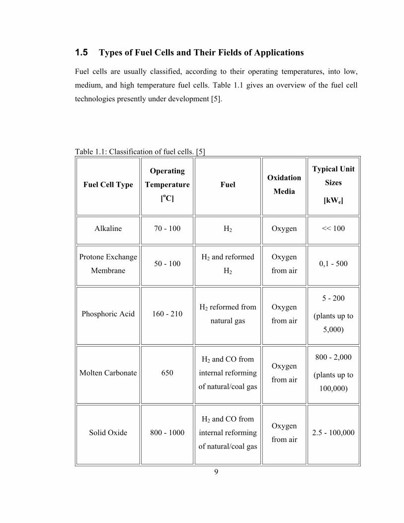
1.5 Types of Fuel Cells and Their Fields of Applications
Fuel cells are usually classified, according to their operating temperatures, into low,
medium, and high temperature fuel cells. Table 1.1 gives an overview of the fuel cell
technologies presently under development [5].
Table 1.1: Classification of fuel cells. [5]
Fuel Cell Type
Operating
Temperature
[oC]
Fuel Oxidation
Media
Typical Unit
Sizes
[kWe]
Alkaline 70 - 100 H2 Oxygen << 100
Protone Exchange
Membrane 50 - 100
H2 and reformed
H2
Oxygen
from air 0,1 - 500
Phosphoric Acid 160 - 210 H2 reformed from
natural gas
Oxygen
from air
5 - 200
(plants up to
5,000)
Molten Carbonate 650
H2 and CO from
internal reforming
of natural/coal gas
Oxygen
from air
800 - 2,000
(plants up to
100,000)
Solid Oxide 800 - 1000
H2 and CO from
internal reforming
of natural/coal gas
Oxygen
from air 2.5 - 100,000
10
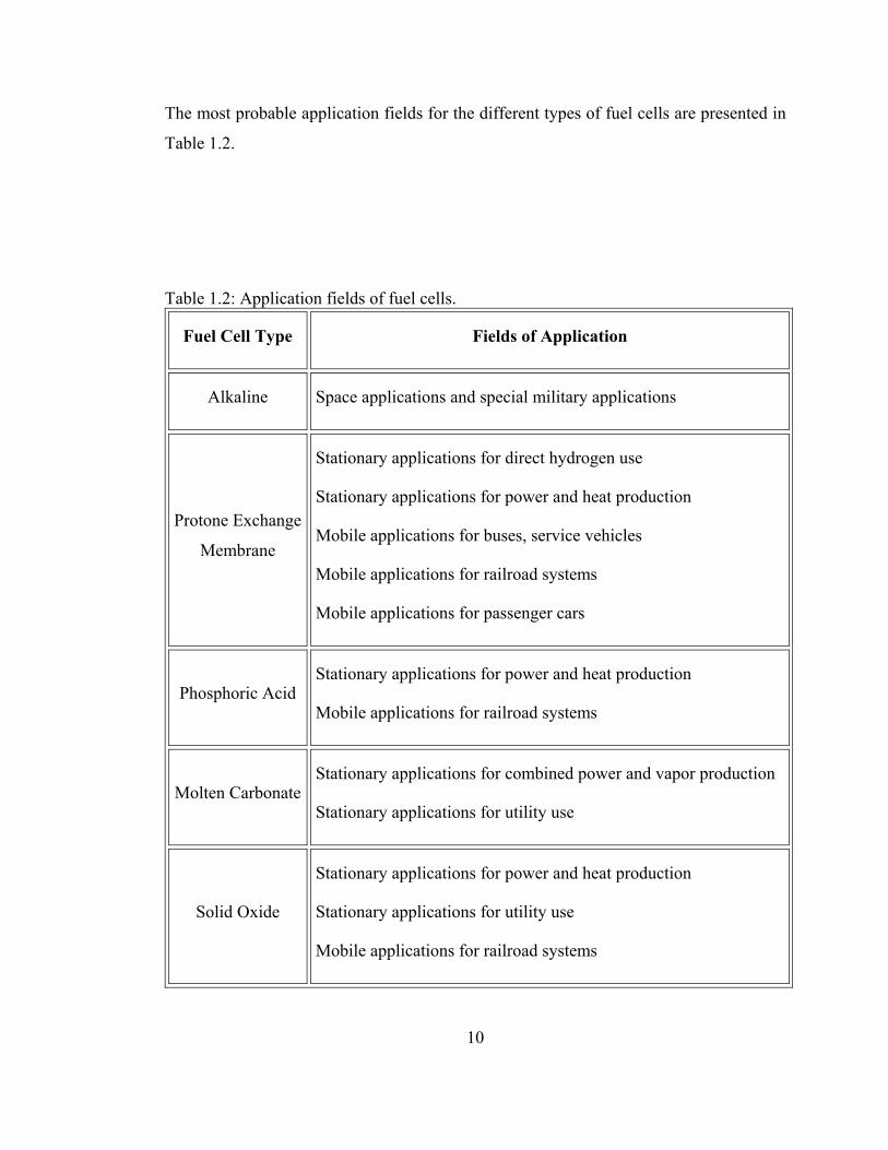
The most probable application fields for the different types of fuel cells are presented in
Table 1.2.
Table 1.2: Application fields of fuel cells.
Fuel Cell Type Fields of Application
Alkaline Space applications and special military applications
Protone Exchange
Membrane
Stationary applications for direct hydrogen use
Stationary applications for power and heat production
Mobile applications for buses, service vehicles
Mobile applications for railroad systems
Mobile applications for passenger cars
Phosphoric Acid Stationary applications for power and heat production
Mobile applications for railroad systems
Molten Carbonate Stationary applications for combined power and vapor production
Stationary applications for utility use
Solid Oxide
Stationary applications for power and heat production
Stationary applications for utility use
Mobile applications for railroad systems
CHAPTER 2
THERMODYNAMICS OF FUEL CELLS
2.1 Some Fundamental Relations
2.1.1 TdS Equations and Maxwell Relations
Consider a simple compressible system undergoing an internally reversible process. An
energy balance for this simple compressible system, in the absence of overall system
motion and gravity effect, can be written in differential form as follows;
..int..int revrev WdUQ δδ += ( 2.1 )
The only mode of energy transfer by work that can occur as a simple compressible
system undergoes quasiequilibrium processes is associated with volume change and is
given by ∫ [6]. Therefore, the work is given by pdV
pdVW rev =..intδ ( 2.2 )
The equation for entropy change on a differential basis is given by
..int revTQdS δ
= ( 2.3 )
11
By rearrangement,
TdSQ rev =..intδ ( 2.4 )
Substituting Eqs.2.2 and 2.4 into Eq.2.1 and rearranging the terms gives the first TdS
equation;
pdVTdSdU −= ( 2.5 )
Enthalpy is, by definition,
pVUH += ( 2.6 )
On a differential basis,
VdppdVdUpVddUdH ++=+= )( ( 2.7 )
Rearranging the terms results,
VdpdHpdVdU −=+ ( 2.8 )
Substituting Eq.2.8 into Eq.2.5 and rearranging the terms gives the second TdS equation;
VdpTdSdH += ( 2.9 )
The TdS equations on a unit mass basis can be written as
pdvTdsdu −= (2.10)
vdpTdsdh += (2.11)
or on a per mole basis as
vpdsTdud −= (2.12)
pvdsTdhd += (2.13)
From these two fundamental relations, two additional equations may be formed by
defining two other properties of matter.
The Helmholtz function ψ is defined by the equation
Tsu −=Ψ (2.14)
12
Forming the differential dψ results,
sdTTdsduTsddud −−=−=Ψ )( (2.15)
Substituting Eq.2.10 into Eq.2.15 gives
sdTpdVd −−=Ψ (2.16)
The Gibbs function is defined by the equation
Tshg −= (2.17)
Forming the differential dg results,
sdTTdsdhTsddhdg −−=−= )( (2.18)
Substituting Eq. 2.1 into Eq. 2.8 gives
sdTvdpdg −= (2.19)
From the comparison of Eq.2.16 and Eq.2.19, one can conclude that Gibbs function
carries out reactions at constant pressure and temperature, while Helmholtz function
does at constant volume and temperature. Since it is more practical to carry out reactions
at constant pressure and temperature, Gibbs function is more useful and is preferred in
calculations.
As a result, the summary of these four important relationships among properties of
simple compressible systems are collected and presented below:
pdvTdsdu −= (2.10)
vdpTdsdh += (2.11)
sdTpdVd −−=Ψ (2.16)
sdTvdpdg −= (2.19)
These equations are referred to as TdS ( or Gibbsian ) equations. Note that the variables
on the right-hand sides of these equations include only T, s, p, and v.
13
Consider three thermodynamic variables represented by x, y, and z. Their functional
relationship may be expressed in the form x = x ( y, z ). The total differential of the
dependent variable x is given by the equation
dzzxdy
yxdx
yz
⎟⎠⎞
⎜⎝⎛∂∂
+⎟⎟⎠
⎞⎜⎜⎝
⎛∂∂
= (2.20a)
If in Eq.2.20a we denote the coefficient of dy by M and the coefficient of dz by N,
Eq.2.20a becomes
NdzMdydx += (2.20b)
Partial differentiation of M and N with resprect to z and y, respectively, leads to
zyx
zM
y ∂∂∂
=⎟⎠⎞
∂∂ 2
(2.21a)
and
yzx
yN
z ∂∂∂
=⎟⎟⎠
⎞∂∂ 2
(2.21b)
If these partial derivatives exist, it is known from the calculus that the order of
differentiation is immaterial, so that
zy yN
zM
⎟⎟⎠
⎞∂∂
=⎟⎠⎞
∂∂ (2.21c)
When Eq.2.21c is satisfied for any function x, then dx is an exact differential. Eq.2.21c
is known as the test for exactness. [7]
Since only properties are involved, each TdS equation is an exact differential exhibiting
the general form of Eq.2.20a. Underlying these exact differentials are functions of the
form u ( s, v ), h ( s, p ), ψ ( v, T ), and g ( T, p ), respectively.
The differential of the function u ( s, v ) is
dvvuds
sudu
sv⎟⎠⎞
⎜⎝⎛∂∂
+⎟⎠⎞
⎜⎝⎛∂∂
= (2.22)
14
Comparing Eq.2.22 to Eq.2.10 results,
vsuT ⎟⎠⎞
⎜⎝⎛∂∂
= (2.23a)
svup ⎟⎠⎞
⎜⎝⎛∂∂
=− (2.23b)
The differential of the function h ( s, p ) is
dpphds
shdh
sp⎟⎟⎠
⎞⎜⎜⎝
⎛∂∂
+⎟⎠⎞
⎜⎝⎛∂∂
= (2.24)
Comparing Eq.2.24 to Eq.2.11 results,
pshT ⎟⎠⎞
⎜⎝⎛∂∂
= (2.25a)
sphv ⎟⎟⎠
⎞⎜⎜⎝
⎛∂∂
= (2.25b)
The differential of the function ψ ( v, T ) is
dTT
dvv
dvT⎟⎠⎞
⎜⎝⎛∂Ψ
+⎟⎠⎞
⎜⎝⎛∂Ψ∂
=Ψα (2.26)
Comparing Eq.2.26 to Eq.2.16 results,
Tvp ⎟
⎠⎞
⎜⎝⎛∂Ψ∂
=− (2.27a)
vTs ⎟
⎠⎞
⎜⎝⎛∂Ψ∂
=− (2.27b)
The differential of the function g ( T, p ) is
dTTgdp
pgdg
pT
⎟⎠⎞
⎜⎝⎛∂∂
+⎟⎟⎠
⎞⎜⎜⎝
⎛∂∂
= (2.28)
15
Comparing Eq.2.28 to Eq.2.19 results,
Tpgv ⎟⎟⎠
⎞⎜⎜⎝
⎛∂∂
= (2.29a)
pTgs ⎟⎠⎞
⎜⎝⎛∂∂
=− (2.29b)
Since each of the four differentials is exact and similar to Eq.2.20a, referring to
Eq.2.21c, the following relations can be written:
vs sp
vT
⎟⎠⎞
⎜⎝⎛∂∂
−=⎟⎠⎞
⎜⎝⎛∂∂
(2.30)
ps sv
pT
⎟⎠⎞
⎜⎝⎛∂∂
=⎟⎟⎠
⎞⎜⎜⎝
⎛∂∂
(2.31)
Tv vs
Tp
⎟⎠⎞
⎜⎝⎛∂∂
=⎟⎠⎞
⎜⎝⎛∂∂
(2.32)
Tp ps
Tv
⎟⎟⎠
⎞⎜⎜⎝
⎛∂∂
−=⎟⎠⎞
⎜⎝⎛∂∂
(2.33)
This set of equations is referred to as the Maxwell relations.
2.1.2 Partial Molal Properties
In general, the change in any extensive thermodynamic property X of a multicomponent
system can be expressed as a function of two independent intensive properties and size
of the system. Selecting temperature and pressure as the independent properties and the
number of moles n as the measure of size, this change in any extensive thermodynamic
property X can be expressed as follows:
inpTi inTnp
dnnXdp
pXdT
TXdX
j,,,,∑ ⎟⎟
⎠
⎞⎜⎜⎝
⎛∂∂
+⎟⎟⎠
⎞⎜⎜⎝
⎛∂∂
+⎟⎠⎞
⎜⎝⎛∂∂
= (2.34)
16
where the subscript nj denotes that all n’s except ni are held fixed during differentiation.
The last term on the right-hand side of the Eq.2.34 is defined as the partial molal
property iX of the ith component in a mixture. Therefore, the partial molal property
iX is, by definition
jnpTii n
XX,,
⎟⎟⎠
⎞∂∂
= (2.35)
The extensive thermodynamic property X, can be expressed in terms of the partial molal
property iX as
∑=j
ii XnX1
(2.36)
Eq.2.36 can be referred in order to evaluate the change in volume on mixing of pure
components which are at the same temperature and pressure. Selecting V as the
extensive property X in Eq.2.36 the total volume of the pure components before mixing
is
∑=
=j
iiicomp vnV
1,0. (2.37)
where iv ,0 is the molar specific volume of pure component i. The volume of the mixture,
using Eq.2.36, is
∑=
=j
iiimix vnV
1. (2.38)
where iv is the partial molal volume of component i in the mixture. Hence, the volume
change on mixing is given by
∑∑==
−=−=∆j
iii
j
iiicompmixmixing vnvnVVV
1,0
1.. (2.39a)
or
17
( )∑=
−=∆j
iiiimixing vvnV
1,0 (2.39b)
Selecting U, H, and S as the extensive properties, the similar results can be obtained as
follows:
( )∑=
−=∆j
iiiimixing uunU
1,0 (2.40a)
( )∑=
−=∆j
iiiimixing hhnH
1,0 (2.40b)
( )∑=
−=∆j
iiiimixing ssnS
1,0 (2.40c)
In Eqs.2.40a – c, iu ,0 , ih ,0 , and is ,0 denote molar internal energy, enthalpy, and entropy
of pure component i; iu , ih , and is denote respective partial molal properties.
2.1.3 Chemical Potential
Of the partial molal properties, the partial molal Gibbs function is particularly useful in
describing the behaviour of mixtures and solutions. This quantity plays a central role in
the criteria of both chemical and phase equilibrium. Because of its importance in study
of multicomponent systems, the partial molal Gibbs function of component i is given a
special name and symbol. It is called the chemical potential of component i and
symbolized by µi. [6]
jnpTiii n
GG,,
⎟⎟⎠
⎞∂∂
==µ (2.41)
Gibbs function can be expressed in terms of chemical potential as
∑=j
iinG1
µ (2.42)
18
The differential of G ( T, p, n1, n2, ... , nj ) can be formed as
∑ ⎟⎟⎠
⎞⎜⎜⎝
⎛∂∂
+⎟⎠⎞
⎜⎝⎛∂∂
+⎟⎟⎠
⎞⎜⎜⎝
⎛∂∂
=i
inpTinpnT
dnnGdT
TGdp
pGdG
j,,,,
(2.43)
Substituting Eqs.2.29a – b into Eq.2.43 yields,
∑=
+−=j
iii dnSdTVdpdG
1µ (2.44)
2.2 Thermodynamics of Chemical Reactions
2.2.1 Free Energy Change of Chemical Reactions
Consider the chemical reaction below;
dDcCbBaA +→+ (2.45)
The change in Gibbs function of reaction, or Gibbs free energy of the reaction, under
constant temperature and pressure, is given by the equation
BADC badcG µµµµ −−+=∆ (2.46)
where µ is the chemical potential of the species.
The maximum net work obtainable from a chemical reaction can be calculated by the
free energy change of the chemical reaction. Referring to Eq.2.17, the free energy
change of a chemical reaction is given by,
STHG ∆−∆=∆ (2.47)
2.2.2 Standard Free Energy Change of a Chemical Reaction
The chemical potential of any substance may be expressed by an equation of the form
aRTo ln+= µµ (2.48)
19
where a is the activity of the substance and µ has the value µ° when a is unity. The
standard free energy change ∆G° of the reaction 2.43 is given by
oooo BADCo badcG µµµµ −−+=∆ (2.49)
where µC° indicates the standard chemical potential of product C, and so on. Substituting
Eqs.2.48 and 2.49 into Eq.2.46 yields
bB
aA
dD
cCo
aaaa
RTGG ln+∆=∆ (2.50)
Hence, the standard free energy change of a chemical reaction is
bB
aA
dD
cCo
aaaaRTGG ln−∆=∆ (2.51)
Assuming a process at constant temperature and pressure at equilibrium, since the free
energy change for this process is zero, Eq.2.51 becomes
KRTaaaa
RTG beqB
aeqA
deqD
ceqCo lnln
,,
,, −=−=∆ (2.52)
where the suffixes eq in the activity terms indicate the values of the activities at
equilibrium, and K is the equilibrium constant for the reaction.
The importance of the knowledge of ∆G° is that it allows ∆G to be calculated for any
composition of a reaction mixture. Knowledge of ∆G indicates whether a reaction will
occur or not. If ∆G is positive, a reaction cannot occur for the assumed composition of
reactants and products. If ∆G is negative, a reaction can occur. [8]
2.2.3 Relation Between Free Energy Change in a Cell Reaction and Cell Potential
The enthalpy change of any reaction, assuming constant temperature and pressure, can
be showed as follows :
VPWQVPEH ∆+−=∆+∆=∆ (2.53)
20
If the reaction is carried out in a heat engine, then the only work done by the system
would be the expansion work,
VPW ∆= (2.54)
Hence Eq.2.51 becomes;
QH =∆ (2.55)
If the same reaction, which is under consideration is carried out electrochemically, the
only work done by the system will not be the expansion work of the gases produced, but
will also be the electrical work due to the charges being transported around the circuit
between the electrodes. The maximum electrical work that can be done by the overall
reaction carried out in a cell, where Vrev,c and Vrev,a are the reversible potentials at the
cathode and anode respectively, is given by
( )arevcreve VVneW ,,max, −= (2.56)
In the cell, n electrons are involved and the cell is assumed to be reversible
( i.e., overpotential losses are assumed to be zero ). Multiplying Eq.2.56 by the
Avogadro number, N, in order to have molar quantities gives;
reve VnFW ∆=max, (2.57)
where F is the Faraday number, and revV∆ is the difference between reversible electrode
potentials.
The only work forms assumed are the expansion work and electrical work.
VPWW e ∆+= max, (2.58)
In addition to these, assuming the process is reversible
STQ ∆= (2.59)
Substituting Eqs.2.57 – 2.59 into Eq.2.53, the enthalpy change will be
revVnFSTH ∆−∆=∆ (2.60)
21
Eq.2.60 can be rearranged as follows,
revVnFSTH ∆−=∆−∆ (2.61)
where
STHG ∆−∆=∆ (2.47)
and
revVE ∆= (2.62)
Substituting Eqs.2.47 and 2.62 into Eq.2.61 gives
nFEG −=∆ (2.63)
E, which is defined as the difference in potentials between the electrodes is called as the
electromotive force of the cell ( i.e, the reversible potential of the cell, Erev ). If both the
reactants and the products are in their standard states, Eq.2.63 can be written as,
oo nFEG −=∆ (2.64)
where E° is the standard electromotive force, or – as most commonly referred to – is the
standard reversible potential of the cell.
2.3 Nernst Equation
Let us consider the following reaction,
mMlLkK →+ (2.65)
where k moles of K react with l moles of L to produce m moles of M. Each of the
reactants and the products have an associated activity; aK , and aL being the activity of
the reactants, aM being the activity of the product. For ideal gases, activity term can be
written as
(2.66) 0p
pa =
22
p is the partial pressure of the gas, and p0 is the pressure of the cell. Eq.2.50 can be
rearranged for the the reaction given in Eq.2.65, as follows.
⎟⎟⎠
⎞⎜⎜⎝
⎛+∆=∆ l
LkK
mMo
aaaRTGG ln (2.67)
In the Eq.2.67, G∆ and oG∆ show the change in molar Gibbs free energy of formation,
and the change in standard molar Gibbs free energy of formation.
From Eq.2.63, the following relation can be written,
nFGE ∆
−= (2.68)
Substituting Eq.2.68 into Eq.2.67 gives the effect on voltage as follows,
⎟⎟⎠
⎞⎜⎜⎝
⎛−
∆−= l
LkK
mM
o
aaa
nFRT
nFGE ln (2.69)
Substituting Eq. 2.64 into Eq 2.69 yields,
⎟⎟⎠
⎞⎜⎜⎝
⎛−= l
LkK
mMo
o aaa
nFRTEE ln (2.70a)
where E° is the standard electromotive force, and Eo is defined to indicate the reversible
electric voltage. Eq.2.70a can be rewritten by substituting Eq.2.52 and Eq.2.66, as
follows.
⎟⎟⎟⎟⎟
⎠
⎞
⎜⎜⎜⎜⎜
⎝
⎛
⎟⎟⎠
⎞⎜⎜⎝
⎛⎟⎟⎠
⎞⎜⎜⎝
⎛
⎟⎟⎠
⎞⎜⎜⎝
⎛
−= l
o
L
k
o
K
m
o
M
o
pp
pp
pp
nFRTK
nFRTE lnln (2.70b)
Eq. 2.70a and 2.70b give the electromotive force in terms of product or/and reactant
activity, and is called Nernst equation. The electromotive force calculated using this
equation is known as the Nernst voltage, and is the reversible cell voltage that would
exist at a given temperature and pressure.
23

2.4 Exergy Concept
2.4.1 Exergy Balance
Exergy is defined as the maximum amount of work obtainable a substance can yield
when it is brought reversibly to equilibrium with the environment [9]. The exergy
analysis of a system is based on the second law of thermodynamics and the concept of
entropy production. In order to describe the exergy concept, a fuel cell can be modeled
as a control volume of a thermodynamic system with a single inlet and outlet, as shown
in Figure 2.1.
To
24
Figure 2.1 : An open thermodynamic system with single inlet and outlet.
inlet outlet
oQ& W&
Environment jQ&
kiTP iooo
,,1,, ,
K=
µ lj ,,1K= Tj
The goal in power producing systems is to maximize net work and efficiency. A power
plant operates according to the first and second laws of thermodynamics [10]. To
calculate the maximum work that can be produced, let us consider the system in Figure
2.1. The streams in and out of the system consist of n species with molar flow
rates , where i = 1… k. The heat transfer interactions … and properties at
the inlet and outlet are assumed to be fixed. [11] The first law for the system in Figure
2.1 can be written as;
outiini nn ,, , && 1Q& lQ&
( ) ( )∑∑∑===
−−−+−+=k
ioutioutiit
k
iiniiniit
l
jj nhhnhhWQQ
dtdE
1,,0,
1,,0,
10 &&&&& (2.71)
The second law for the same system can be written as;
( ) ( ) gen
k
ioutioutii
k
iiniinii
l
j j
j SnssnssTQ
TQ
dtdS &&&
&&+−−−+⎟
⎟⎠
⎞⎜⎜⎝
⎛+⎟⎟
⎠
⎞⎜⎜⎝
⎛= ∑∑∑
=== 1,,0
1,,0
10
0 (2.72)
In the equations above, ht,i is the total specific enthalpy and is
iit gzVhh ⎟
⎠⎞
⎜⎝⎛ ++= 2
, 21 (2.73)
½V2 is the kinetic energy, gz is the potential energy of the mass flow, and these kinetic
and potential energies may be neglected so that ht,i = hi. E is the total energy of the
system, and S is the entropy of the system. In order to make time derivatives zero,
system is assumed to be steady state, steady flow. By eliminating between Eqs.2.71
and 2.72, the exergy balance can be obtained. Therefore, the exergy balance is given by
the following equation.
0Q&
( )[ ]
( )[ ] gen
k
ioutiioutii
k
iiniiinii
l
jj
j
STnsThW
nsThQTT
&&&
&&
01
,,00
1,,00
1
01
+⋅−−+=
⋅−−+⎟⎟⎠
⎞⎜⎜⎝
⎛−
∑
∑∑
=
==
µ
µ
(2.74)
25
W& is the actual work of the system. It can be noted that entropy generation reduces the
available work, as is expected. The exergy balance for an open system in Eq.2.74 shows
that the exergies in heat flows ( the first term on the left hand side of the equation ) and
mass flows ( the second term on the left hand side of the equation ) supplied to the
system are equal to the work produced ( the first term on the right hand side of the
equation ), exergy in the outlet mass flow ( the second term on the right hand side of the
equation ), and exergy destroyed through irreversible processes ( the third term on the
right hand side of the equation ) [11]. For the steady state, steady flow system, energy
input is equal to the energy output. Due to irreversible processes, outlet exergy is always
less than the inlet exergy. Exergy destruction is a result of chemical and physical
processes that take place in the system.
Irreversibility, for a system can be described as the difference between the reversible
work ( maximum work that can be obtained ) and the actual work. Hence, from the
definition
genactrev STWWI &&&&0=−= (2.75)
The exergy balance ( Eq.2.74 ) can be used to calculate the irreversibility.
Exergy analysis requires that the environment is defined. For a general case,
environment can be assumed to be at standard temperature and pressure conditions
( i.e., T = 298 K, P = 1 atm ), but this assumption is not always the case. Environment
definition can differ from system to system.
2.4.2 Chemical Exergy
Chemical exergy is equal to the maximum amount of work obtainable when the
substance under consideration is brought from the environmental state to the dead state
by processes involving heat transfer and exchange of substances only with the
environment. [9]
Chemical exergy of a mixture is given by the following equation.
26
∑∑ +=i
iioi
oiimix xxRTxEx ln~ε (2.76)
oiε
~ is the standard chemical exergy of substance i. [9] The exergy of the mixture is
always less than the sum of the exergies of its components at the temperature and
pressure of the mixture, since the second term on the right hand side is always negative.
2.4.3 Physical Exergy
Physical exergy is equal to the maximum amount of work obtainable when the stream of
substance is brought from its initial state to the environmental state defined by Po and To
by physical processes involving only thermal interaction with the environment. [9]
Defining the environment state at Po, To, assuming the kinetic and potential energies are
negligible, the physical exergy of a substance at state P1, T1 is calculated by the
following equation.
( ) ( ooooph sThsThEx −−−= 111, ) (2.77)
2.5 Efficiency of Fuel Cells
2.5.1 Thermodynamic ( First and Second Law ) Efficiencies
In order to define the efficiency of fuel cells, let us consider a simple H2/O2 fuel cell,
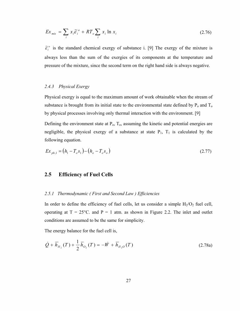
operating at T = 25°C. and P = 1 atm. as shown in Figure 2.2. The inlet and outlet
conditions are assumed to be the same for simplicity.
The energy balance for the fuel cell is,
)()(21)(
222ThWThThQ OHOH +−=++ && (2.78a)
27
28
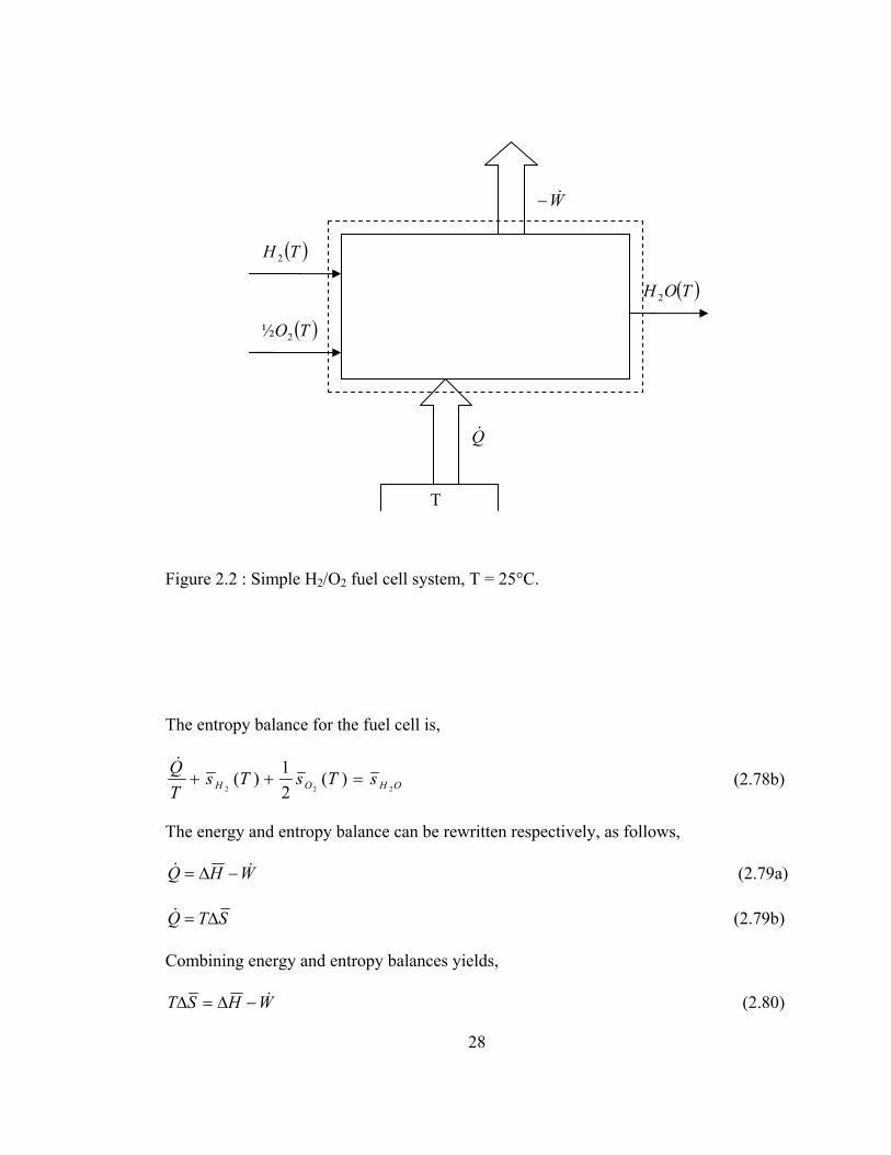
Figure 2.2 : Simple H2/O2 fuel cell system, T = 25°C.
The entropy balance for the fuel cell is,
OHOH sTsTsTQ
222)(
21)( =++
& (2.78b)
The energy and entropy balance can be rewritten respectively, as follows,
WHQ && −∆= (2.79a)
STQ ∆=& (2.79b)
Combining energy and entropy balances yields,
WHST &−∆=∆ (2.80)
( )TH 2
( )TO2½
( )TOH 2
W&−
Q&
T
Hence, work output of the system is,
STHW ∆−∆=& (2.81)
The first law efficiency is defined as the ratio of the work output of the system to energy
input to the system. The work output of the system is equal to the free energy change
( i.e., Gibbs function ). The energy input to the system, is the chemical energy of the
fuel. Therefore the energy input is,
HQ ∆=& (2.82)
Hence, the first law efficiency is given by,
HST
HSTH
QW
I ∆∆
−=∆
∆−∆== 1
&
&η (2.83)
The second law efficiency is defined as the ratio of the work output of the system to the
maximum work output ( i.e., reversible work ) of the system. To determine the second
law efficiency, let us assume that the fuel cell is adiabatic, and no work interactions
occur inside the cell. Hence, the energy input to the system is unchanged at the outlet of
the fuel cell. If we can consume all of this energy and change it to work, then we can
determine the reversible work output of the system. A model for this study is shown in
Figure 2.3.
The reversible heat exchanger, added to the exit of the fuel cell, operates between the
fuel cell outlet temperature and the environment temperature To ( which usually
is 25°C ). The heat consumed is sent to a reversible heat engine, operating between the
heat exchanger and the environment. The work obtained by the heat engine is the
reversible work output of the system.
The subscripts “R” and “P” are used in order to indicate the reactants, and the products
respectively.
29
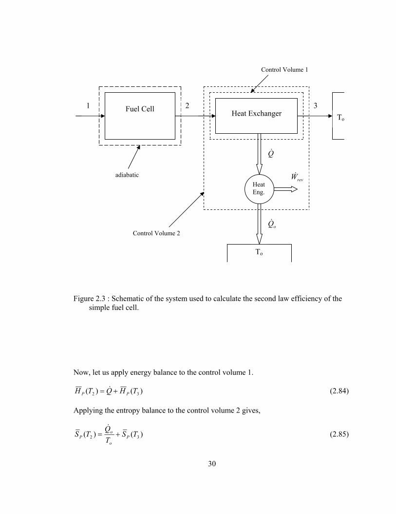
30
Figure 2.3 : Schematic of the system used to calculate the second law efficiency of the simple fuel cell.
Now, let us apply energy balance to the control volume 1.
)()( 32 THQTH PP += & (2.84)
Applying the entropy balance to the control volume 2 gives,
)()( 32 TSTQ
TS Po
oP +=
& (2.85)
Fuel Cell
Heat Exchanger
Heat Eng.
1 2 3
To
To
Q&
oQ&
revW&
Control Volume 1
adiabatic
Control Volume 2
The energy balance for the heat engine can be written as,
orev QWQ &&& += (2.86)
Therefore, substituting Eqs.2.84 and 2.85 into Eq.2.86, the reversible work output can be
obtained.
( ) ( ))()()()( 3232 TSTSTTHTHW PPoPPrev −−−=& (2.87a)
STHW orev ∆−∆=& (2.87b)
The work output of the system was found by Eq.2.81 as
STHW ∆−∆=& (2.81)
Therefore, the second law efficiency for the fuel cell can be written as follows.
STHSTH
WW
orevII ∆−∆
∆−∆==
&
&η (2.88)
One of the advantages of the fuel cells is their high efficiency, as mentioned before.
Using Eq.2.83 and 2.88, the change of first and second law efficiencies with temperature
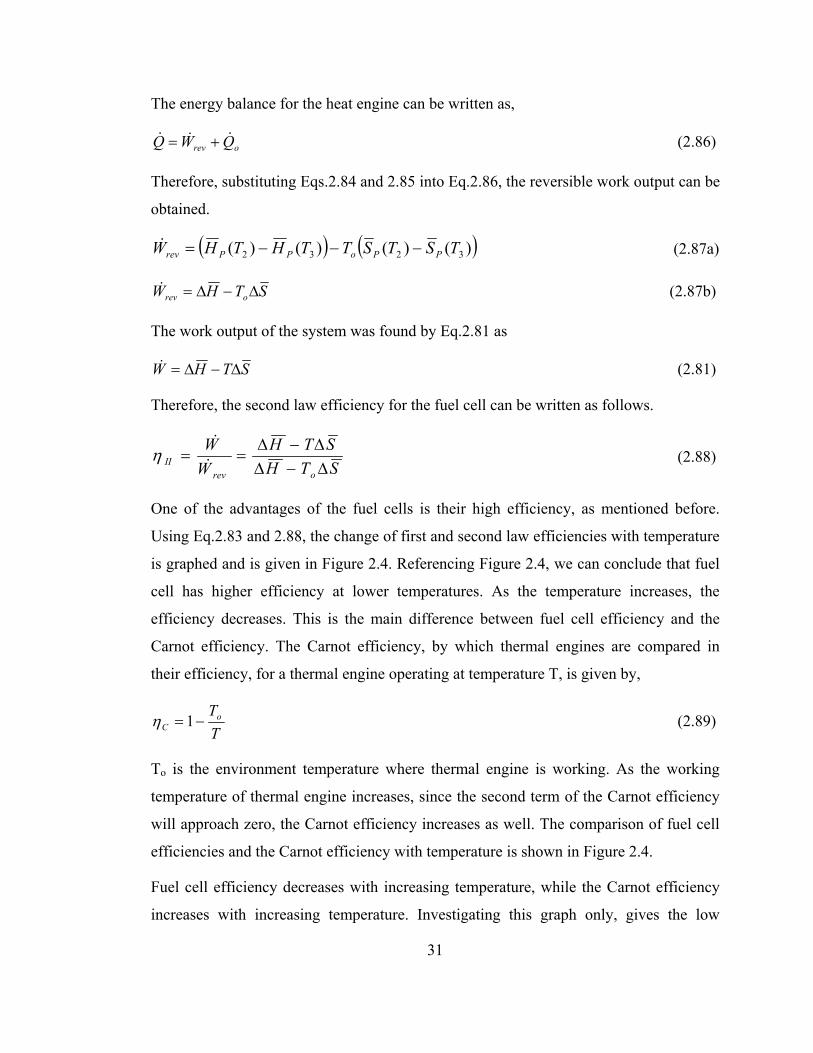
is graphed and is given in Figure 2.4. Referencing Figure 2.4, we can conclude that fuel
cell has higher efficiency at lower temperatures. As the temperature increases, the
efficiency decreases. This is the main difference between fuel cell efficiency and the
Carnot efficiency. The Carnot efficiency, by which thermal engines are compared in
their efficiency, for a thermal engine operating at temperature T, is given by,
TTo
C −= 1η (2.89)
To is the environment temperature where thermal engine is working. As the working
temperature of thermal engine increases, since the second term of the Carnot efficiency
will approach zero, the Carnot efficiency increases as well. The comparison of fuel cell
efficiencies and the Carnot efficiency with temperature is shown in Figure 2.4.
Fuel cell efficiency decreases with increasing temperature, while the Carnot efficiency
increases with increasing temperature. Investigating this graph only, gives the low
31
temperature fuel cells have high efficiencies than the high temperature ones. But,
although the graph suggests that lower temperature fuel cells are better, the voltage
losses are usually less at high temperatures.* So, in general, fuel cell voltages are usually
higher at high temperatures. On the other hand, the waste heat from the high temperature
fuel cells is more useful than the waste heat from the low temperature fuel cells.
Therefore, only this graph itself cannot be referenced to make a decision on fuel cells
working at different conditions.
0,0
0,2
0,4
0,6
0,8
1,0
0 200 400 600 800 1000 1200
Temperature [ °C ]
Effic
ienc
y ( %
)
Carnot Ef f .
F.C.Ist Law Ef f ic iency
F.C. IInd Law Ef f iciency
Figure 2.4: Comparison between fuel cell first law and second law efficiency changes with temperature and Carnot efficiency change with temperature.
32* Voltage losses and causes of voltage drops are discussed in Chapter 3.
2.5.2 Electrochemical Efficiencies
The efficiency term for fuel cells, given by the Eq. 2.81, can be written in terms of the
reversible electrode potentials, using Eq. 2.63, the ideal efficiency is given as follows,
HnFV rev
i ∆−
=η (2.90)
Vrev is the reversible potential of the cell, which is the ideal case. When the fuel cell is
under load, the actual potential of the cell, Vact, will fall below the reversible potential,
due to the irreversibilities. Hence, the actual efficiency will be,
HnFV act
ac ∆−
=η (2.91)
These irreversibilities are unwanted effects in the cell, since they decrease the reversible
potential. As a result, the reversible work of the system will decrease. This difference
between the reversible work and the actual work is the heat rejected from the system.,
and is larger than the reversible heat transfer T∆S.
The ratio of the actual potential of the cell to the reversible potential of the cell is
defined as the voltage efficiency, ηv. Hence,
rev
actv V
V=η (2.92)
When the fuel reacts electrochemically in the cell, some fuels may react directly to give
heat release in the cell or may react to products other than those required, hence do not
take place in the electrochemical reaction. Considering the total number of moles of
fuels, being reacted electrochemically, the faradaic efficiency, ηF can be expressed as
follows.
fF NnF
i&
=η (2.93)
fN& is the total number of moles of fuel reacted electrochemically per second. ηF is the
fraction of reaction which is occurring electrochemically to give current.
33
34
CHAPTER 3
KINETIC EFFECTS
3.1 Introduction
In order for a chemical reaction to be considered as a source of energy in a fuel cell,
there are two criteria that must be satisfied. First, at least one of the reactants must be
ionizable at the operating conditions. The formation of ions results in the establishment
of an oxidation – reduction potential which, when traversed by the ions, ultimately
provides the energy that will be used at the terminals. Second, while the ionizable
reaction system is the source of energetic electron flow that does work in the external
circuit, a high flow rate is required for practical purposes. [3] As a result, rapid rates for
the electron supplying and consuming reactions are a second criterion.
This second criterion is the subject of chemical kinetics and is dynamic in nature. On the
other hand, the first criterion is associated with a static or equilibrium system and is
often the object of thermodynamics inquiry. The equal rates of the forward and
backward electrode reactions that occur at static conditions establish the equilibrium.
Therefore, this equilibrium may be considered dynamic and it may be helpful to
consider it a problem in kinetics.
The open circuit voltage of a fuel cell is given by the following formula,
nFGE ∆
−= (2.66)
This is the theoretical value of the open circuit voltage, which is also referred to as the
reversible open circuit voltage.
Whenever a load is applied to a cell in which the electrodes are reversible, it causes its
electrodes to shift its potential, i.e. polarize in opposite direction. As a result of this
polarization, the cathodes become less cathodic and the anodes become less anodic,
resulting a decrease in the available cell voltage. Therefore, the operating voltage is less
than the reversible voltage and this is because of the losses or irreversibilities.
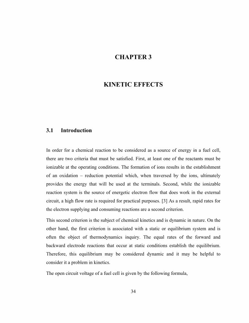
Figure 3.1 shows the performance of a simple fuel cell operating at about 40°C, at
normal air pressure [4].
0
0,2
0,4
0,6
0,8
1
1,2
1,4
0 200 400 600 800 1000
Current Density ( mA/cm² )
Cel
l Vol
tage
( Vo
lts )
Reversible Cell Voltage ( no loss )
Actual Cell Voltage
Figure 3.1: Voltage change with current density for a simple fuel cell operating at about 40°C, and at standard pressure. [4]
35
By examining Figure 3.1, some key points may be listed as follows:
• The open circuit voltage is less the theoretical open circuit voltage.
• There is a rapid initial fall in voltage.
• After this rapid fall, voltage loss is less slowly, and more linearly.
• At some higher current density, voltage falls rapidly.
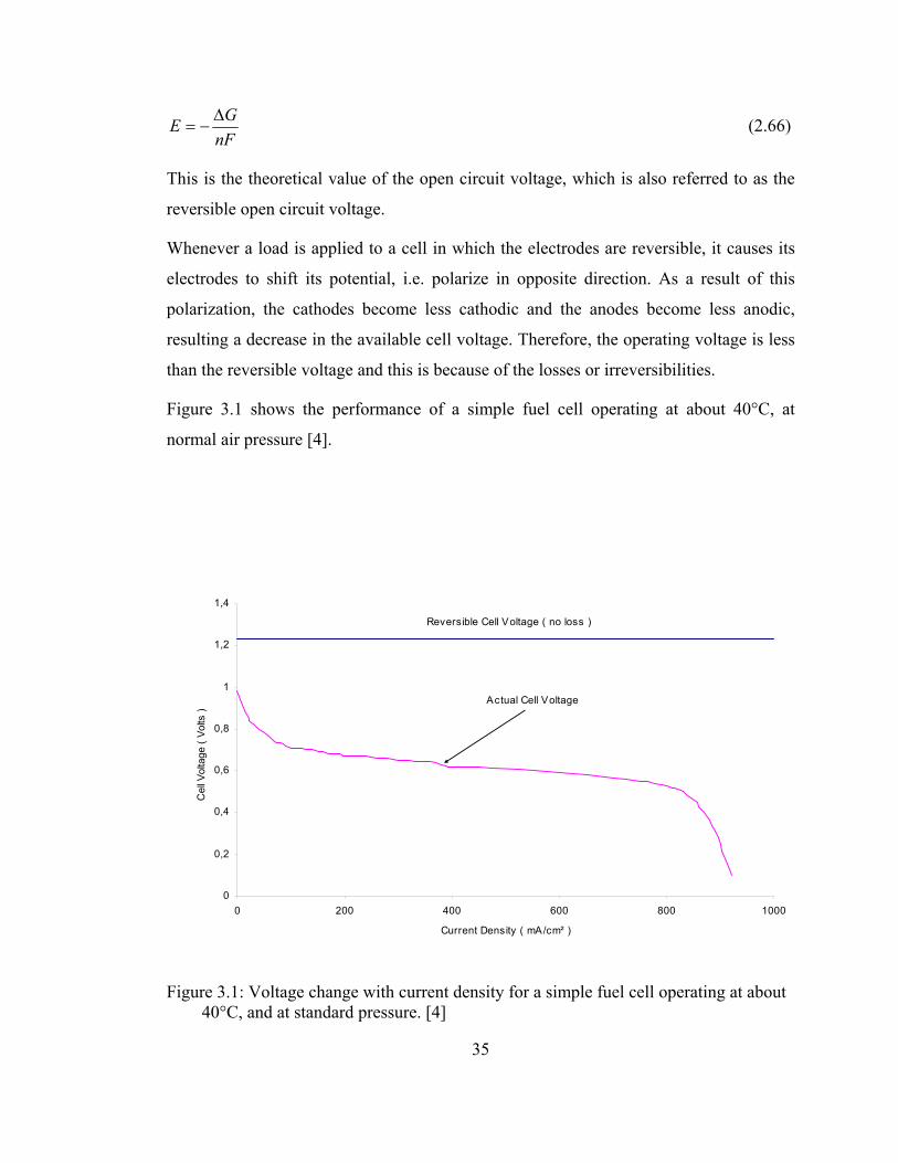
Another graph showing the voltage change with current density for a fuel cell, which is a
solid oxide fuel cell this time, is shown in Figure 3.2, in order to show the effect of high
temperature on circuit voltage change. From this graph, the following key points may be
listed:
0
0,2
0,4
0,6
0,8
1
1,2
0 200 400 600 800 1000
Current Density ( m A/cm ² )
Cur
rent
Vol
tage
( Vo
lts )
Reversible Cell Voltage ( no loss )
Actual Cell Voltage
Figure 3.2: Voltage change with current density for a solid oxide fuel cell operating at about 800°C.
36

• The open circuit voltage is equal to the theoretical open circuit voltage, or there is
only a very little difference
• Initial fall of voltage is very small, the graph is much more linear
• At some higher current density, voltage falls rapidly.
Comparison between Figures 3.1 and 3.2, it can be shown that the high temperature fuel
cells have lower reversible cell voltage, while they can have high operating voltages
since the voltage drop is smaller.
Examining Figures 3.1 and 3.2, the difference between the reversible cell voltage and
the actual voltage can be noticed. This difference, which grows as the current density is
increased is called the voltage drop. Voltage drop is the result of the irreversibilities in
the cell. These irreversibilities are the main subject of this chapter. The effects which
cause the actual voltage fall below the reversible voltage will be considered.
3.2 Fuel Cell Irreversibilities
If the cell is reversible, there will not be any voltage drop and the electric voltage will be
determined from the Nernst equation. The electric voltage, due to the irreversibilities
occuring in the cell decreases from its ideal value ( i.e., reversible value ). This relation
can be shown as follows.
η−= oEE (3.1)
η is the sum of the irreversibilities in the cell.
The causes of voltage drop in the fuel cell can be the results of three major
irreversibilities. These irreversibilities are explained in details in this section.
37
3.2.1 Activation Polarization
When the forward and backward reactions occur at equal rates and the currents
associated with these reactions are equal and are in opposite direction, electrode
processes are said to be in a state of reversible equilibrium, in which no net reaction
takes place. This state of reversible equilibrium is satisfied unless a current flows in an
external circuit connecting the two electrodes of the cell. Due to this reversible state, for
a current to flow, a net reaction must occur at each electrode and the forward and
backward reaction rates at each electrode cannot be equal.
In many chemical reactions the reacting species have to overcome an energy barrier in
order to react. This energy barrier is called the “activation energy” and results in
activation polarization.
Consider the elementary electrode reaction below;
PneR ↔+ (3.2)
where R shows the reactants and P shows the products, both of which include the
molecules and ions as well. For this reaction, the forward ( or the cathodic ) and the
backward ( or the anodic ) reaction rates can be written as follows:
Rff aAkV ⋅⋅= (3.3a)
Pbb aAkV ⋅⋅= (3.3b)
where A is the actual electrode surface area, kf and kb are the forwanrd anc backward
reaction rate constants per unit area, respectively, and aR and aP are the activities of the
reactants and products, respectively.
The relation between the electron flow ( or current ) and the reaction rate is given as,
nFVi = (3.4)
where F is the Faraday’s constant. The net current in the forward direction ( i.e. cathodic
current ) will then be the resultant of the forward and backward currents,
( ) bfbfc iiVVnFi −=−= (3.5a)
38
and the net current in the backward direction ( i.e. anodic current ) will be,
( ) fbfba iiVVnFi −=−= (3.5b)
Substituting Eqs.3.3a and 3.3b into Eq.3.5a, the net cathodic current becomes
( ) ( )[ ]PbRfc akaknFAi ⋅−⋅= (3.6)
Figures 3.1 and 3.2 show that the electrode potential decreases as the net current
increases. From this given fact, it is obvious that either the reactant and product
activities are not constant, or that potential and rate constants are interdependent.
Assuming that the activities of the reactants and the products can be held constant, the
relation of change in potential to current must depend on its relation to the reaction rate
constant. Since the reaction rates are functions of the activation energy, activation
energy may then be affected by potential.
The relation between reaction rate and activation energy is exponential and it is given as
follows:
⎟⎟⎠
⎞⎜⎜⎝
⎛ +°∆−⎟⎠⎞
⎜⎝⎛=
RTnFEG
ah
kTAV fRf
αexp (3.7)
where ∆Gf° is the standard free energy of activation for the forward reaction, k is
Boltzmann constant, h is Planck’s constant, and α is a proportionality factor which is
usually referred to as the transfer coefficient. Eq.3.7 can be rewritten in terms of reaction
rate constants for both forward and backward reactions as follows:
⎟⎟⎠
⎞⎜⎜⎝
⎛ +°∆−=
RTnFEG
hkTk f
f
αexp (3.8a)
( )⎟⎠⎞
⎜⎝⎛ −−°∆−
=RT
nFEGh
kTk bb
α1exp (3.8b)
where ∆Gb° is the standard free energy of activation for the backward reaction, and may
also be written as,
°∆+°∆=°∆ fb GGG (3.9)
39
From Eqs.3.6 and 3.8a and b, the rate of the forward reaction, expressed as current
density ic may be written as
( )⎪⎭
⎪⎬⎫
⎪⎩
⎪⎨⎧
⎟⎟⎠
⎞⎜⎜⎝
⎛ −−°∆−°∆−−⎟⎟⎠
⎞⎜⎜⎝
⎛ +°∆−=
RTnFEGG
aRT
nFEGa
hkTnFAi f
Pf
Rc
αα 1expexp (3.10)
Substituting Eq.3.7 into Eq. 3.10 gives
( )⎭⎬⎫
⎩⎨⎧
⎟⎠⎞
⎜⎝⎛ −−
−⎟⎠⎞
⎜⎝⎛=
RTnFEV
RTnFEVnFi rfc
αα 1expexp (3.11)
Referring from Eq.3.1, polarization, or overpotential, can be written as,
0EE −=η (3.12)
where E0 is the reversible potential. Modifying Eq.3.11 in terms of polarization and the
reversible potential yields,
( ) ( )⎟⎠⎞
⎜⎝⎛ −−
⎟⎠
⎞⎜⎝
⎛ −−−⎟
⎠⎞
⎜⎝⎛⎟
⎠
⎞⎜⎝
⎛=RT
nFRT
nFEnFV
RTnF
RTnFE
nFVi bfcηααηαα 1exp
1expexpexp 00 (3.13)
At open circuit or reversible potential, the net cathodic and anodic currents are zero, i.e.,
Eq.3.13 equals zero. The cathodic current if and anodic current ib are equal. This current,
which flows with equal intensity anodically and cathodically, at Eo is specifically
identified as the exchange current, io [3]. Therefore, the net cathodic current can be
written as
( )⎥⎦⎤
⎢⎣⎡ −−
−=RT
nFRTnFii oc
ηαηα 1expexp (3.14a)
The transfer coefficient is considered to be the fraction of the change in polarization that
leads to a change in the reaction rate constant, and its value is usually 0.5 for the fuel
cell applications [12]. Therefore, Eq.3.14a may be written as,
⎥⎦⎤
⎢⎣⎡ −
−=RTnF
RTnFii oc 2
exp2
exp ηη (3.14b)
40
From calculus the following relation can be written.
( ) ( ) ( )bbb sinh2expexp
=−− (3.15)
where b is any variable. Using this general knowledge, Eq.3.14b can be rearranged in
terms of sinh function as follows,
⎟⎠⎞
⎜⎝⎛=
RTnFii oc 2
sinh2 η (3.16)
In the discussion up to this point, we assumed that the reaction occurs in a single step.
But, in reality, this is not the case all the time, the reaction may go through several
intermediate steps, each with an associated energy barrier. The step with the highest
energy barrier within these intermediate steps is usually assumed to be the rate
determining step. Hence the other steps will be in an equilibrium state. The rate
determining step, however, may involve fewer electrons than the overall reaction. For
this reason, for the Eqs.3.4 – 3.16, the number of electrons term “n” must be replaced
with the number of electrons transferred in the rate determining step “ne” and ne must be
lower than or equal to n [13].
The cathodic current and the anodic current are the same in magnitude but are opposite
in sign. This is because of the direction of flowing electrons through the electric current.
Therefore, rearranging Eq.3.16, the cathodic and anodic activation polarization can be
determined as follows,
⎟⎟⎠
⎞⎜⎜⎝
⎛= −
coecAct i
iFn
RT
,
1, 2
sinh2η (3.17a)
⎟⎟⎠
⎞⎜⎜⎝
⎛= −
aoeaAct i
iFn
RT
,
1, 2
sinh2η (3.17b)
where ηAct,c and ηAct,a are the cathodic activation polarization and the anodic activation
polarization respectively, and io,c and io,a are the cathodic exchange current density and
anodic exchange current density respectively.
41
3.2.2 Ohmic Polarization
Resistance to the flow of ions through the electrolyte and resistance to the flow of
electrons between electrodes via electric circuit cause ohmic losses in the fuel cell.
These resistances obey Ohm’s law. Therefore, ohmic polarization can be expressed by
the equation,
eOhm Ri ⋅=η (3.18)
Re is the resistance of each material used in the fuel cell components and can be
calculated by the equation,
ρ⋅= wRe (3.19)
where w is the thickness and ρ is the electrical resistivity of each component.
3.2.3 Concentration Polarization
Certain changes in the concentration of the potential determining species ( i.e., ions )
will occur after current begins to flow in an electrochemical cell. This concentration
produces an electromotive force, which reduces the reversible electrical voltage of the
cell.
The concentration polarization is the reduction in potential due to a concentration
change of the electrolyte during a reaction in the vicinity of an electrode. Assuming that
the supply of the potential determining species to the electrode is by diffusion only,
Fick’s law of diffusion can be used to give the rate of diffusion. If the concentration of
species at the electrode is Ce and the bulk concentration is Co, then the rate of diffusion
can be written as [13],
( )nFICCDJ eo =−=
δ (3.20)
J is the mass flux ( i.e. mass transfer rate ), D is the diffusion coefficient, and δ is the
thickness of the diffusion layer. The diffusion layer is represented in Figure 3.3.
42
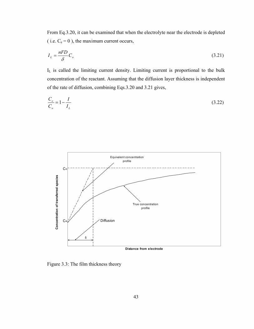
From Eq.3.20, it can be examined that when the electrolyte near the electrode is depleted
( i.e. Ce = 0 ), the maximum current occurs,
oL CnFDIδ
= (3.21)
IL is called the limiting current density. Limiting current is proportional to the bulk
concentration of the reactant. Assuming that the diffusion layer thickness is independent
of the rate of diffusion, combining Eqs.3.20 and 3.21 gives,
Lo
e
II
CC
−=1 (3.22)
Distance from electrode
Con
cent
ratio
n of
tran
sfer
red
spec
ies
True concentration profile
Equivalent concentration profile
Diffusion
δ
Ce
Co
Figure 3.3: The film thickness theory
43
Assuming that migration of the potential determining ion is negligible and that the ions
in the bulk fluid and near the electrode have the same activity coefficients, the
concentration polarization can be written as, [14]
⎟⎟⎠
⎞⎜⎜⎝
⎛=
o
eConc C
CnFRT lnη (3.23)
Concentration polarization can be written in terms of the limiting current density as
follows,
⎟⎟⎠
⎞⎜⎜⎝
⎛ −=
L
LConc I
IInFRT lnη (3.24)
Eq.3.24 refers to the electrode process where species is being removed from the
electrolyte. Concentration polarization at the opposite electrode where species is
generated and concentration builds up can be written as,
⎟⎟⎠
⎞⎜⎜⎝
⎛ +=
L
LConc I
IInFRT lnη (3.25)
From Eqs.3.24 and 3.25, it can be noticed that to calculate the concentration
polarization, the limiting current density must be calculated. In order to eliminate this
difficulty, another calculation method for the concentration polarization analysis may be
developed from the same point of view. Since the reactants and products are in gaseous
states, and a change in the partial pressure of the potential determining gaseous species
at the reaction zone occurs in respect to its partial pressure in the bulk of the gaseous
phase, gas side concentration polarization arises.
The relation of the limiting current density to the concentration is given in Eq.3.22 as,
Lo
e
II
CC
−=1 (3.22)
A similar relation may be estimated between the limiting current and the change in the
pressure of the fuel gas as follows.
44
We postulate a limiting current density, IL, at which the fuel is used up at a rate equal to
its maximum supply speed. The current density cannot rise above this value, because the
fuel gas cannot be supplied at a greater rate. At this current density the pressure will
have just reached zero [4].
If P1 is the pressure when the current density is zero, and assuming a linear drop of
pressure to zero, when the limiting current density is reached, then the pressure ratio of
P2, at any current density to P1 can be expressed as,
⎟⎟⎠
⎞⎜⎜⎝
⎛−=
LII
PP 1
1
2 (3.26)
Substituting Eq.3.26 into Eq.3.24, the following relation is obtained.
⎟⎟⎠
⎞⎜⎜⎝
⎛=
1
2lnPP
nFRT
Concη (3.27)
Eq.3.26 is named as the gas side concentration polarization.
The gases have to diffuse through the gas filled pores of the electrode in order to reach
the reaction sites. Whenever this happens, it is possible for the concentration
polarization to be significant, since when the current is being drawn, the gas partial
pressure at the reaction sites will be less than that in the bulk of the gas stream. Hence,
decrease of gas concentration in the gas filled pores of the electrode may give rise to
severe polarization and lead to limiting current. [15]
To determine the concentration polarization, the mass transport effects in the fuel cell is
to be investigated. The concentration polarizations at anode and cathode are obtained in
the next section.
45
3.3 Mass Transport Effects
Diffusion through the porous material is described by molecular diffusion, Knudsen
diffusion, or transition region diffusion ( the case both molecular and Knudsen diffusion
occurs ). Since the pores of porous solids are usually very small, the diffusion of gases
depends on the diameter of the pores. Because of this reason, different diffusion types
may occur. To determine which mechanisms of diffusion occur, a mean free path is
defined firstly. The mean free path is the average distance a molecule passes through
until it collides with another molecule. Mean free path is given as follows [16].
MgRT
P cπµλ
22.3
= (3.28)
In the equation, λ is the mean free path, µ is the viscosity, gc is the gravitational
acceleration, and M is the molecular weight.
After the calculation of the mean free path, from the comparison between the mean free
path and the average pore diameter, the diffusion type can be determined. Each diffusion
type is shown in Figure 3.4a – c [16].
In the Figures 3.4a - c, NA indicates the flux of the molecules A, pA,I and pA,o are the
total pressure at the inlet and exit of the pore. The total pressure on either side in these
cases is the same, but the partial pressures of the molecules may be different.
3.3.1 Knudsen Diffusion
As shown in Figure 3.4a, if the mean free path is very large compared to the average
pore diameter, the molecule collides with the pore walls frequently. This type of
diffusion is called Knudsen diffusion. The Knudsen diffusion coefficient is given as
follows, [16]
46
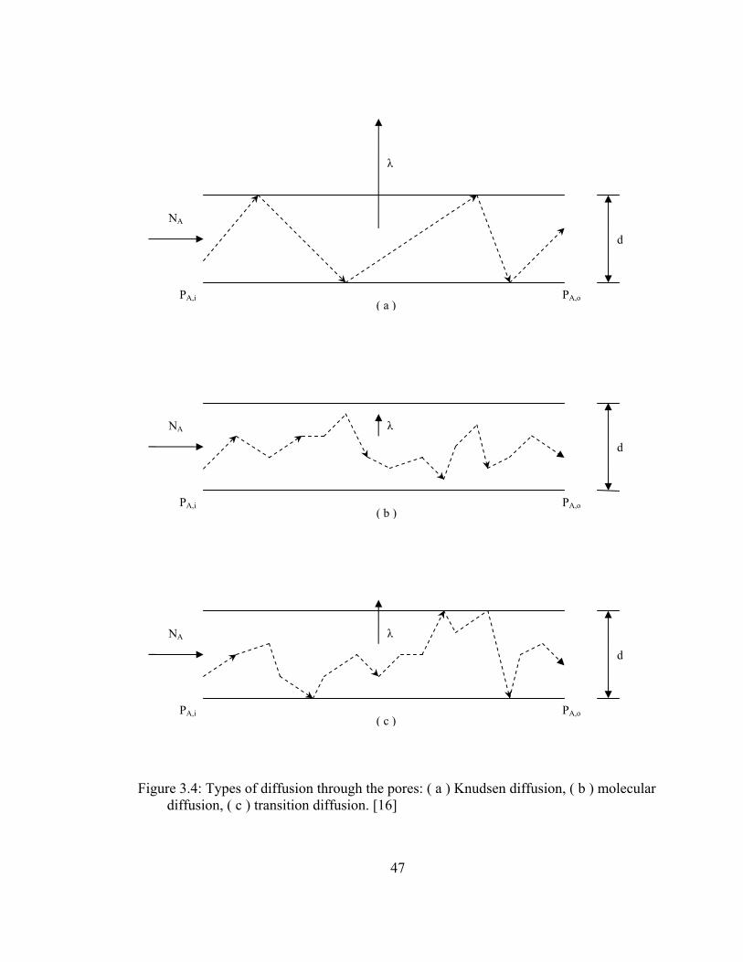
λ
NA
d
PA,i PA,o( a )
λ
47
Figure 3.4: Types of diffusion through the pores: ( a ) Knudsen diffusion, ( b ) molecular diffusion, ( c ) transition diffusion. [16]
d
( b )
λ
NA
PA,i PA,o
NA
d
PA,i PA,o( c )
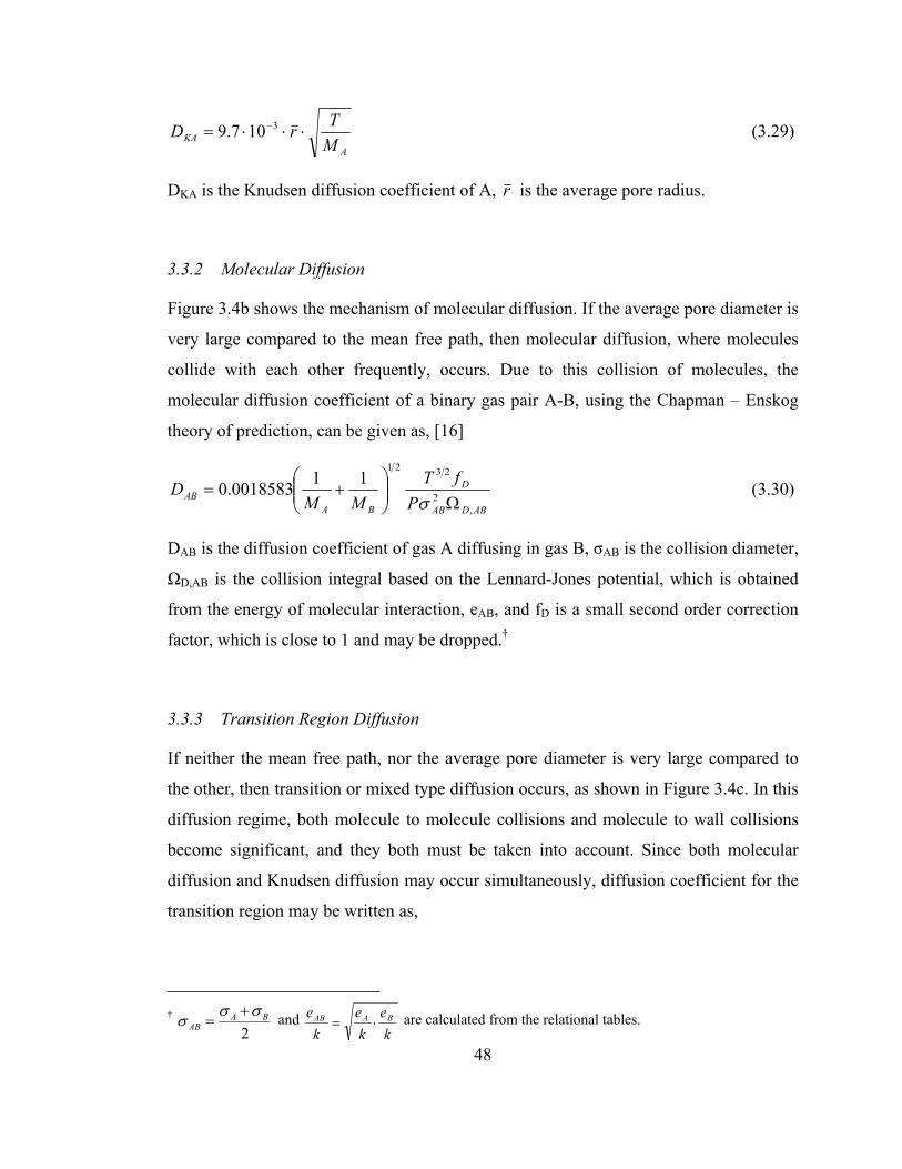
AKA M
TrD ⋅⋅⋅= −3107.9 (3.29)
DKA is the Knudsen diffusion coefficient of A, r is the average pore radius.
3.3.2 Molecular Diffusion
Figure 3.4b shows the mechanism of molecular diffusion. If the average pore diameter is
very large compared to the mean free path, then molecular diffusion, where molecules
collide with each other frequently, occurs. Due to this collision of molecules, the
molecular diffusion coefficient of a binary gas pair A-B, using the Chapman – Enskog
theory of prediction, can be given as, [16]
ABDAB
D
BAAB P
fTMM
D,
2
2321110018583.0
Ω⎟⎟⎠
⎞⎜⎜⎝
⎛+=
σ (3.30)
DAB is the diffusion coefficient of gas A diffusing in gas B, σAB is the collision diameter,
ΩD,AB is the collision integral based on the Lennard-Jones potential, which is obtained
from the energy of molecular interaction, eAB, and fD is a small second order correction
factor, which is close to 1 and may be dropped.†
3.3.3 Transition Region Diffusion
If neither the mean free path, nor the average pore diameter is very large compared to
the other, then transition or mixed type diffusion occurs, as shown in Figure 3.4c. In this
diffusion regime, both molecule to molecule collisions and molecule to wall collisions
become significant, and they both must be taken into account. Since both molecular
diffusion and Knudsen diffusion may occur simultaneously, diffusion coefficient for the
transition region may be written as,
48
† 2
BAAB
σσσ += and
ke
ke
ke BAAB ⋅= are calculated from the relational tables.
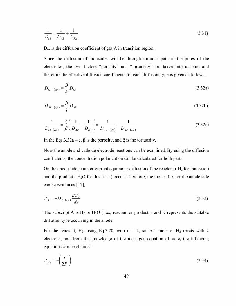
KAABtA DDD111
+= (3.31)
DtA is the diffusion coefficient of gas A in transition region.
Since the diffusion of molecules will be through tortuous path in the pores of the
electrodes, the two factors “porosity” and “tortuosity” are taken into account and
therefore the effective diffusion coefficients for each diffusion type is given as follows,
( ) KAeffKA DDξβ
= (3.32a)
( ) ABeffAB DDξβ
= (3.32b)
( ) ( ) ( )effKAeffABKAABefftA DDDDD11111
+=⎟⎟⎠
⎞⎜⎜⎝
⎛+=
βξ (3.32c)
In the Eqs.3.32a – c, β is the porosity, and ξ is the tortuosity.
Now the anode and cathode electrode reactions can be examined. By using the diffusion
coefficients, the concentration polarization can be calculated for both parts.
On the anode side, counter-current equimolar diffusion of the reactant ( H2 for this case )
and the product ( H2O for this case ) occur. Therefore, the molar flux for the anode side
can be written as [17],
( ) dxdCDJ A
effAA −= (3.33)
The subscript A is H2 or H2O ( i.e., reactant or product ), and D represents the suitable
diffusion type occurring in the anode.
For the reactant, H2, using Eq.3.20, with n = 2, since 1 mole of H2 reacts with 2
electrons, and from the knowledge of the ideal gas equation of state, the following
equations can be obtained.
⎟⎠⎞
⎜⎝⎛−=
FiJ H 22
(3.34)
49
⎟⎟⎠
⎞⎜⎜⎝
⎛=
RTdp
dC HH
2
2 (3.35)
Substituting Eqs.3.34 and 3.35 into Eq.3.33 and solving for the pressure, for the
hydrogen the pressure change can be written as,
( )dx
FDRTidp
effHH
2
2 2= (3.36)
Integrating this equation gives,
( )a
effHH
IH l
FDRTipp
2
22 2=− (3.37)
The superscript “I” is used to denote initial values of the pressure of the hydrogen, la is
the thickness of the anode.
For the product, H2O, using the same equations as for the hydrogen, the following
reaction is obtained.
( )a
effOH
IOHOH l
FDRTipp
2
22 2=− (3.38)
Rearranging the Eqs.3.37 and 3.38, partial pressures of hydrogen and water vapor in
terms of current density are obtained as follows,
( )i
FDRTlpp
effH
aIHH
2
22 2−= (3.39)
( )i
FDRTlpp
effOH
aIOHOH
2
22 2+= (3.40)
At the cathode side, on the other hand, there are two gases, and diffusion is
nonequimolar. The molar flux for this case can be written as,
( ) JXdx
dCDJ AA
effAA +⎟⎠⎞
⎜⎝⎛−= (3.41)
50
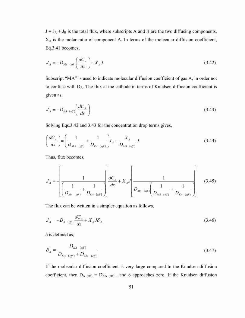
J = JA + JB is the total flux, where subscripts A and B are the two diffusing components,
XA is the molar ratio of component A. In terms of the molecular diffusion coefficient,
Eq.3.41 becomes,
( ) JXdx
dCDJ AA
effMAA +⎟⎠⎞
⎜⎝⎛−= (3.42)
Subscript “MA” is used to indicate molecular diffusion coefficient of gas A, in order not
to confuse with DA. The flux at the cathode in terms of Knudsen diffusion coefficient is
given as,
( ) ⎟⎠⎞
⎜⎝⎛−=
dxdCDJ A
effKAA (3.43)
Solving Eqs.3.42 and 3.43 for the concentration drop terms gives,
( ) ( ) ( )J
DX
JDDdx
dC
effMA
AA
effKAeffAM
A −⎟⎟⎠
⎞⎜⎜⎝
⎛+=⎟
⎠⎞
⎜⎝⎛ 11 (3.44)
Thus, flux becomes,
( ) ( ) ⎥⎥⎥⎥⎥
⎦
⎤
⎢⎢⎢⎢⎢
⎣
⎡
⎟⎟⎠
⎞⎜⎜⎝
⎛+
+
⎥⎥⎥⎥⎥
⎦
⎤
⎢⎢⎢⎢⎢
⎣
⎡
⎟⎟⎠
⎞⎜⎜⎝
⎛+
−=
)()()(
11
1
11
1
effKAeffMAeffMA
AA
effKAeffMA
A
DDD
JXdx
dC
DD
J (3.45)
The flux can be written in a simpler equation as follows,
( ) AAA
effAA JXdx
dCDJ δ+−= (3.46)
δ is defined as,
( )
( ) )(effMAeffKA
effKAA DD
D+
=δ (3.47)
If the molecular diffusion coefficient is very large compared to the Knudsen diffusion
coefficient, then DA (eff) = DKA (eff) , and δ approaches zero. If the Knudsen diffusion
51
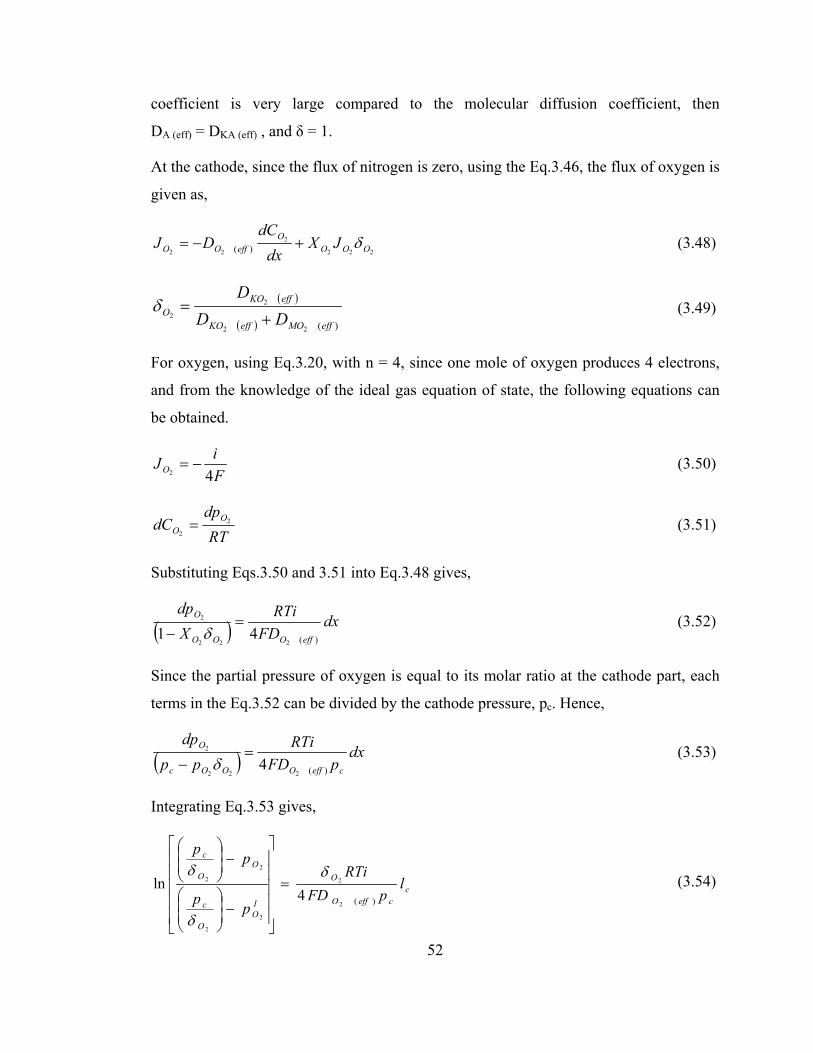
coefficient is very large compared to the molecular diffusion coefficient, then
DA (eff) = DKA (eff) , and δ = 1.
At the cathode, since the flux of nitrogen is zero, using the Eq.3.46, the flux of oxygen is
given as,
222
2
22 )( OOOO
effOO JXdx
dCDJ δ+−= (3.48)
( )
( ) )(22
2
2effMOeffKO
effKOO DD
D+
=δ (3.49)
For oxygen, using Eq.3.20, with n = 4, since one mole of oxygen produces 4 electrons,
and from the knowledge of the ideal gas equation of state, the following equations can
be obtained.
FiJO 42
−= (3.50)
RTdp
dC OO
2
2= (3.51)
Substituting Eqs.3.50 and 3.51 into Eq.3.48 gives,
( ) dxFD
RTiXdp
effOOO
O
)(222
2
41=
− δ (3.52)
Since the partial pressure of oxygen is equal to its molar ratio at the cathode part, each
terms in the Eq.3.52 can be divided by the cathode pressure, pc. Hence,
( ) dxpFD
RTipp
dp
ceffOOOc
O
)(222
2
4=
− δ (3.53)
Integrating Eq.3.53 gives,
(3.54) cceffO
O
IO
O
c
OO
c
lpFD
RTi
pp
pp
)(2
2
2
2
2
2
4ln
δ
δ
δ=
⎥⎥⎥⎥⎥
⎦
⎤
⎢⎢⎢⎢⎢
⎣
⎡
−⎟⎟⎠
⎞⎜⎜⎝
⎛
−⎟⎟⎠
⎞⎜⎜⎝
⎛
52
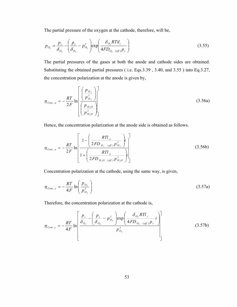
The partial pressure of the oxygen at the cathode, therefore, will be,
⎟⎟⎠
⎞⎜⎜⎝
⎛⎟⎟⎠
⎞⎜⎜⎝
⎛−−=
ceffO
cOIO
O
c
O
cO pFD
RTilp
ppp
)(2
2
2
22
2 4exp
δδδ
(3.55)
The partial pressures of the gases at both the anode and cathode sides are obtained.
Substituting the obtained partial pressures ( i.e. Eqs.3.39 , 3.40, and 3.55 ) into Eq.3.27,
the concentration polarization at the anode is given by,
⎥⎥⎥⎥⎥
⎦
⎤
⎢⎢⎢⎢⎢
⎣
⎡
⎟⎟⎠
⎞⎜⎜⎝
⎛
⎟⎟⎠
⎞⎜⎜⎝
⎛
−=
IOH
OH
IH
H
aConc
pp
pp
FRT
2
2
2
2
ln2,η (3.56a)
Hence, the concentration polarization at the anode side is obtained as follows.
⎥⎥⎥⎥⎥
⎦
⎤
⎢⎢⎢⎢⎢
⎣
⎡
⎟⎟⎠
⎞⎜⎜⎝
⎛+
⎟⎟⎠
⎞⎜⎜⎝
⎛−
−=
ipFD
RTl
ipFD
RTl
FRT
IOHeffOH
a
IHeffH
a
aConc
22
22
)(
)(,
21
21
ln2
η (3.56b)
Concentration polarization at the cathode, using the same way, is given,
⎟⎟⎠
⎞⎜⎜⎝
⎛−= I
O
OcConc p
pF
RT
2
2ln4,η (3.57a)
Therefore, the concentration polarization at the cathode is,
⎥⎥⎥⎥⎥
⎦
⎤
⎢⎢⎢⎢⎢
⎣
⎡⎟⎟⎠
⎞⎜⎜⎝
⎛⎟⎟⎠
⎞⎜⎜⎝
⎛−−
−= IO
ceffO
cOIO
O
c
O
c
cConc p
ipFD
RTlppp
FRT
2
2
2
2
22 )(,
4exp
ln4
δδδ
η (3.57b)
53

54
CHAPTER 4
MODELING AND CALCULATION
4.1 Fuel Cell Type Selection
As a first step, the type of fuel cell that will be studied on throughout the study must be
selected. Solid oxide fuel cell with external reformer is selected for the calculations.
Solid oxide type fuel cell has the following advantages:
• SOFC unit sizes can be as small as 2.5 kW, and as large as 100 kW.
• Its ability to be used for power production applications.
• SOFC is simple in concept than the other types of fuel cell systems, since it is a
completely solid state device that uses an oxide ion conducting ceramic
electrolyte, whereas the other types require solid and gas phases.
• The solid state character of the SOFC components means that there is no
restiriction on the cell configuration, in principle. SOFC can be designed as
tubular or as flat plate.
The material data of the SOFC type selected referencing from [18], and is given in Table
4.1.
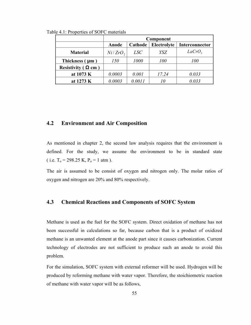
Table 4.1: Properties of SOFC materials Component
Anode Cathode Electrolyte InterconnectorMaterial LSC YSZ
Thickness ( µm ) 150 1000 100 100 Resistivity ( Ω cm )
at 1073 K 0.0003 0.001 17.24 0.033 at 1273 K 0.0003 0.0011 10 0.033
3LaCrO2/ ZrONi
4.2 Environment and Air Composition
As mentioned in chapter 2, the second law analysis requires that the environment is
defined. For the study, we assume the environment to be in standard state
( i.e. To = 298.25 K, Po = 1 atm ).
The air is assumed to be consist of oxygen and nitrogen only. The molar ratios of
oxygen and nitrogen are 20% and 80% respectively.
4.3 Chemical Reactions and Components of SOFC System
Methane is used as the fuel for the SOFC system. Direct oxidation of methane has not
been successful in calculations so far, because carbon that is a product of oxidized
methane is an unwanted element at the anode part since it causes carbonization. Current
technology of electrodes are not sufficient to produce such an anode to avoid this
problem.
For the simulation, SOFC system with external reformer will be used. Hydrogen will be
produced by reforming methane with water vapor. Therefore, the stoichiometric reaction
of methane with water vapor will be as follows,
55
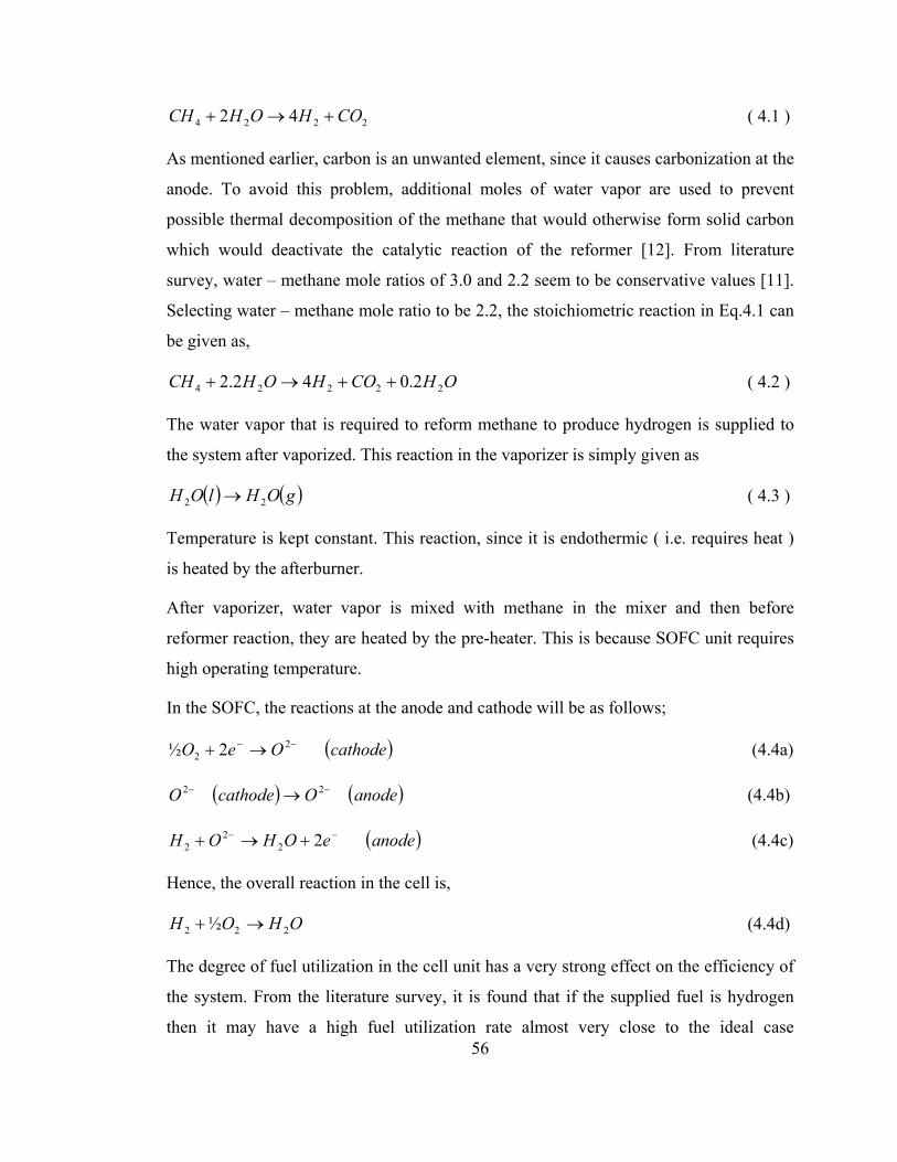
2224 42 COHOHCH +→+ ( 4.1 )
As mentioned earlier, carbon is an unwanted element, since it causes carbonization at the
anode. To avoid this problem, additional moles of water vapor are used to prevent
possible thermal decomposition of the methane that would otherwise form solid carbon
which would deactivate the catalytic reaction of the reformer [12]. From literature
survey, water – methane mole ratios of 3.0 and 2.2 seem to be conservative values [11].
Selecting water – methane mole ratio to be 2.2, the stoichiometric reaction in Eq.4.1 can
be given as,
OHCOHOHCH 22224 2.042.2 ++→+ ( 4.2 )
The water vapor that is required to reform methane to produce hydrogen is supplied to
the system after vaporized. This reaction in the vaporizer is simply given as
( ) ( )gOHlOH 22 → ( 4.3 )
Temperature is kept constant. This reaction, since it is endothermic ( i.e. requires heat )
is heated by the afterburner.
After vaporizer, water vapor is mixed with methane in the mixer and then before
reformer reaction, they are heated by the pre-heater. This is because SOFC unit requires
high operating temperature.
In the SOFC, the reactions at the anode and cathode will be as follows;
(cathodeOeO −− →+ 22 2½ )
)
(4.4a)
( ) (anodeOcathodeO −− → 22 (4.4b)
( )anodeeOHOH −− +→+ 222
2 (4.4c)
Hence, the overall reaction in the cell is,
OHOH 222 ½ →+ (4.4d)
56
The degree of fuel utilization in the cell unit has a very strong effect on the efficiency of
the system. From the literature survey, it is found that if the supplied fuel is hydrogen
then it may have a high fuel utilization rate almost very close to the ideal case
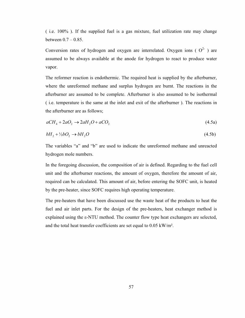
( i.e. 100% ). If the supplied fuel is a gas mixture, fuel utilization rate may change
between 0.7 – 0.85.
Conversion rates of hydrogen and oxygen are interrelated. Oxygen ions ( O2- ) are
assumed to be always available at the anode for hydrogen to react to produce water
vapor.
The reformer reaction is endothermic. The required heat is supplied by the afterburner,
where the unreformed methane and surplus hydrogen are burnt. The reactions in the
afterburner are assumed to be complete. Afterburner is also assumed to be isothermal
( i.e. temperature is the same at the inlet and exit of the afterburner ). The reactions in
the afterburner are as follows;
2224 22 aCOOaHaOaCH +→+ (4.5a)
ObHbObH 222 ½ →+ (4.5b)
The variables “a” and “b” are used to indicate the unreformed methane and unreacted
hydrogen mole numbers.
In the foregoing discussion, the composition of air is defined. Regarding to the fuel cell
unit and the afterburner reactions, the amount of oxygen, therefore the amount of air,
required can be calculated. This amount of air, before entering the SOFC unit, is heated
by the pre-heater, since SOFC requires high operating temperature.
The pre-heaters that have been discussed use the waste heat of the products to heat the
fuel and air inlet parts. For the design of the pre-heaters, heat exchanger method is
explained using the ε-NTU method. The counter flow type heat exchangers are selected,
and the total heat transfer coefficients are set equal to 0.05 kW/m².
57
4.4 Simulation Models
4.4.1 Simulation Model 1: SOFC Unit Analysis
The first model is used to investigate the fuel cell and reformer reactions, and their
effects on the SOFC second law efficiency. Besides, the effects of polarizations on fuel
cell voltage and power density are also examined. Each polarization type effects and
their change with current density are examined and are presented in graphs. This model
is limited to the calculation of a unit cell, operating at constant temperature and pressure
only. Operating the fuel cell unit with different temperature and pressure values, its
second law efficiency change and polarization changes are examined. The schematic of
this model is given in Figure 4.1.
58
Figure 4.1: Schematic of simulation model 1.
SOFC Stack Reformer
3
4 1
2
4.4.2 Simulation Model 2: SOFC System Analysis
The second model is more complex than the first one. The components: afterburner, two
preheaters, mixer and a vaporizer, are added in addition to the basic system requirements
described for the first model. The model of the system is given in Figure 4.2.
59
Figure 4.2: Schematic of simulation model 2.
SOFC
Reactor
Vaporizer
Preheater 2
Mixer
Preheater 1
Reformer
Afterburner
11
2 7
Wact Air Inlet
Qlost
10
1 4 5
6
3 9
8Q1
Q2
Qo
Environment, To
Water
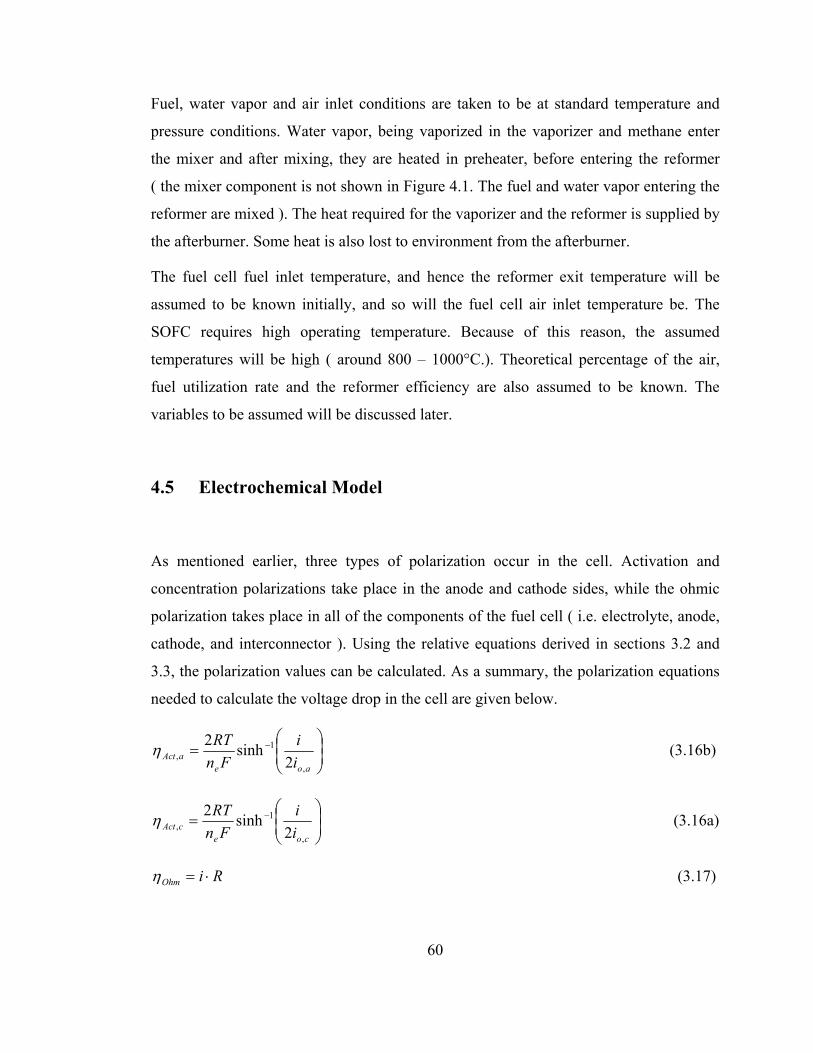
Fuel, water vapor and air inlet conditions are taken to be at standard temperature and
pressure conditions. Water vapor, being vaporized in the vaporizer and methane enter
the mixer and after mixing, they are heated in preheater, before entering the reformer
( the mixer component is not shown in Figure 4.1. The fuel and water vapor entering the
reformer are mixed ). The heat required for the vaporizer and the reformer is supplied by
the afterburner. Some heat is also lost to environment from the afterburner.
The fuel cell fuel inlet temperature, and hence the reformer exit temperature will be
assumed to be known initially, and so will the fuel cell air inlet temperature be. The
SOFC requires high operating temperature. Because of this reason, the assumed
temperatures will be high ( around 800 – 1000°C.). Theoretical percentage of the air,
fuel utilization rate and the reformer efficiency are also assumed to be known. The
variables to be assumed will be discussed later.
4.5 Electrochemical Model
As mentioned earlier, three types of polarization occur in the cell. Activation and
concentration polarizations take place in the anode and cathode sides, while the ohmic
polarization takes place in all of the components of the fuel cell ( i.e. electrolyte, anode,
cathode, and interconnector ). Using the relative equations derived in sections 3.2 and
3.3, the polarization values can be calculated. As a summary, the polarization equations
needed to calculate the voltage drop in the cell are given below.
⎟⎟⎠
⎞⎜⎜⎝
⎛= −
aoeaAct i
iFn
RT
,
1, 2
sinh2η (3.16b)
⎟⎟⎠
⎞⎜⎜⎝
⎛= −
coecAct i
iFn
RT
,
1, 2
sinh2η (3.16a)
RiOhm ⋅=η (3.17)
60
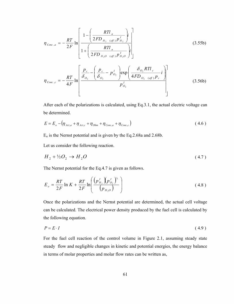
⎥⎥⎥⎥⎥
⎦
⎤
⎢⎢⎢⎢⎢
⎣
⎡
⎟⎟⎠
⎞⎜⎜⎝
⎛+
⎟⎟⎠
⎞⎜⎜⎝
⎛−
−=
ipFD
RTl
ipFD
RTl
FRT
IOHeffOH
a
IHeffH
a
aConc
22
22
)(
)(,
21
21
ln2
η (3.55b)
⎥⎥⎥⎥⎥
⎦
⎤
⎢⎢⎢⎢⎢
⎣
⎡⎟⎟⎠
⎞⎜⎜⎝
⎛⎟⎟⎠
⎞⎜⎜⎝
⎛−−
−= IO
ceffO
cOIO
O
c
O
c
cConc p
ipFD
RTlppp
FRT
2
2
2
2
22 )(,
4exp
ln4
δδδ
η (3.56b)
After each of the polarizations is calculated, using Eq.3.1, the actual electric voltage can
be determined.
( )cConcaConcOhmcActaActoEE ,,,, ηηηηη ++++−= ( 4.6 )
Eo is the Nernst potential and is given by the Eq.2.68a and 2.68b.
Let us consider the following reaction.
OHOH 222 ½ →+ ( 4.7 )
The Nernst potential for the Eq.4.7 is given as follows.
( )( )( ) ⎟
⎟
⎠
⎞
⎜⎜
⎝
⎛+=
OH
IO
IH
o ppp
FRTK
FRTE
2
22
½
ln2
ln2
( 4.8 )
Once the polarizations and the Nernst potential are determined, the actual cell voltage
can be calculated. The electrical power density produced by the fuel cell is calculated by
the following equation.
IEP ⋅= ( 4.9 )
For the fuel cell reaction of the control volume in Figure 2.1, assuming steady state
steady flow and negligible changes in kinetic and potential energies, the energy balance
in terms of molar properties and molar flow rates can be written as,
61
( ) ( )∑ ∑−=−i i
RiiPii hnhnWQ &&&& (4.10)
For the same reaction, the entropy balance can be written as,
( ) ( )∑ ∑ −−=i i
genRiiPii SsnsnTQ &&&&
(4.11)
Combining Eqs.4.10 and 4.11, the exergy balance can be obtained.
( ) ( ) geni
Riiiii
Piiii STsnThnsnThnW &&&&&& +−−−=− ∑∑
(4.12)
The work done by the cell is the electrical work. Hence, from Eq.2.61, Eq.4.12 can be
rearranged as follows.
( ) ( ) geni i
RiiPii STgngnnFE &&& −+−= ∑ ∑ (4.13)
Substituting Eqs.2.64 and 2.65 into Eq.4.13 gives,
geni Ro
Ii
iPi o
ii
o STpp
RTnpp
RTnGnFE &&& −⎟⎟⎠
⎞⎜⎜⎝
⎛+⎟⎟
⎠
⎞⎜⎜⎝
⎛−∆−= ∑∑ lnln (4.14)
Substituting Eq.2.62 into Eq.4.14, and solving for the cell voltage yields,
( )( )( )( ) nF
ST
pp
ppnFRTK
nFRTE gen
IO
IH
oOH&
−⎟⎟
⎠
⎞
⎜⎜
⎝
⎛−= ½
½
22
2lnln (4.15)
The first term on the right hand side of the Eq.4.15 shows the effect of temperature on
the cell voltage, the second term shows the effect of the pressures on the cell voltage.
The third term shows the irreversibility drop ( i.e. polarization ) in the cell voltage.
The heat lost to the environment from the fuel cell can be calculated from,
( )genSSTQ && −∆= (4.16)
62
The terms ∆S and are defined as follows. genS&
( ) ( ) ⎟⎟
⎠
⎞
⎜⎜
⎝
⎛−−−=∆ ½
22
2
222ln½
OH
OHoO
oH
oOH pp
pRSSSS (4.17)
( cConcaConcOhmcActaActgen TnFS ,,,, ηηηηη ++++=& ) (4.18)
4.6 Heat Exchanger Model
To model the preheaters of the SOFC system ( i.e. simulation model 1 ), effectiveness-
NTU method ( ε-NTU ) is used. The counter flow type heat exchangers are selected as
the preheaters. The heat transfer coefficients are set equal to 0.05 kW/m²K. The areas of
the heat exchangers must be determined before the calculation steps, in order to use the
effectiveness-NTU method. Because of this reason, the preheaters are first sized
according to the assumed operating conditions. After sizing, the performance analysis
can be carried out.
The outlet temperatures of the preheaters depend on the inlet conditions. To define the
effectiveness of the heat exchanger, the maximum possible heat transfer rate, qmax must
be determined. This maximum possible heat transfer rate depends on the minimum heat
capacity rate. [19] To determine the minimum heat capacity rate, the heat capacity rates
of the cold and hot gas streams are calculated from the following equations.
∑= cpcc cmC ,& (4.19a)
∑= hphh cmC ,& (4.19b)
The subscripts “c” and “h” indicate cold and hot gas streams respectively. Comparing
the heat capacity rates of the cold and hot gas streams, one with the lower value is
determined as the minimum heat capacity rate, while the other is determined as the
maximum heat capacity rate. Following this, the heat capacity rates ratio is given as,
63
max
min
CCCr = (4.20)
Hence, the maximum possible heat transfer rate can be calculated by,
( )icih TTCq ,,minmax −= (4.21)
Th,i is the inlet temperature of the hot gas stream, and Tc,i is the inlet temperature of the
cold gas stream.
The number of transfer units ( NTU ) is a dimensionless parameter that is used for heat
exchanger analysis and is defined as,
minCUANTU = (4.22)
U is the heat transfer coefficient; A is the area of the heat exchanger.
The effectiveness of the counter flow type heat exchangers can be calculated from the
following equation.
( )[ ]([ )]rr
r
CNTUCCNTU−−−
−−−=
1exp11exp1
ε (4.23)
The effectiveness, ε, is defined as the ratio of the actual heat transfer rate to the
maximum possible heat transfer rate. Therefore, with known effectiveness and
maximum possible heat transfer rate, the actual heat transfer rate can be calculated.
maxqq ⋅= ε (4.24)
The energy balance for the cold and hot gas streams can be written as follows.
( )icocc TTCq ,, −= (4.25a)
( )ohihh TTCq ,, −= (4.25b)
Tc,o and Th,o represents the outlet temperature of the cold gas stream and the outlet
temperature of the hot gas stream respectively. As a result, the cold and hot gas streams’
outlet temperatures can be found by rearranging Eqs.4.25a – b, as follows.
64
cicoc C
qTT += ,, (4.26a)
hihoh C
qTT −= ,, (4.26b)
The hot gas stream inlet temperature is also the SOFC outlet temperature. Because of
this, the hot gas inlet temperatures of both of the preheaters are affected by the SOFC
outlet temperature. For this reason, the calculation steps for the heat exchanger model
are repeated until the outlet temperatures of the gas streams from the preheaters
converge.
4.7 Calculation Procedure
In the calculations, two different models are simulated as mentioned. The reason for this
is first of all to investigate the effects on the fuel cell unit and the changes of effects with
different conditions. After this study, using a simple model, a general thermodynamic
analysis for every component of the fuel cell system is made.
The model 1 is simulated in order to examine
• The effect of reformer efficiency and fuel utilization rate on the fuel cell second
law efficiency,
• The effect of pressure on the fuel cell second law efficiency,
• The comparison of the results obtained with different temperatures,
• The polarization effects on fuel cell voltage,
• The effect of temperature on fuel cell voltage and power density.
On the other hand, the more complex system, model 2, is simulated in order to make a
full thermodynamic analysis on each component of a simple SOFC system. The first
model deals with the SOFC unit with external reformer only. But the second model
examines the use of the waste heat at the exit of the SOFC unit to heat the reformer and
65
66
vaporizer for the reactions to take place, and to heat the fuel and air inlet nodes to the
required temperatures. For these purposes afterburner and two preheaters are added to
the system. The preheaters are designed using the heat exchanger model.
4.7.1 General Assumptions
Before the calculation steps, the general assumptions and conditions for the simulation
models are listed as follows;
• Steady flow throughout the nodes,
• Kinetic and potential energy changes are neglected,
• Frictional effects are assumed to be negligible,
• Fuel supplying rate is 1 kg/s,
• Operating temperature is constant throughout the fuel cell unit ( i.e. fuel cell unit
inlet, exit and reformer inlet temperatures are all the same ) ( for model 1 only ),
• Afterburner is assumed to be isothermal, i.e. the inlet and outlet temperatures are
the same ( for model 2 only ),
• The reactions in the afterburner are assumed to be complete ( for model 2 only),
• The environment is at standard temperature and pressure conditions, i.e. 298 K,
and 1 atm.
The calculations are carried out under the given assumptions. Since simulation model 1
will investigate the effects of the reformer efficiency, fuel utilization rate, the operating
pressure on the fuel cell efficiency and the effects of polarizations on fuel cell voltage
and power density with changing current density, there is no need to make additional
assumptions for these variables for model 1. Hence, the general assumptions are applied
to the simulation model 1 directly. For simulation model 2, the following variables will
be assumed to be known initially, and the values will be given for these variables.
• The operating pressure of the fuel cell system,
• Percentage of theoretical air,
• Reformer efficiency,
• Fuel utilization rate,
• Fuel cell fuel inlet and air inlet temperatures.
4.7.2 Calculation Steps for Simulation Model 1
Before thermodynamic analysis of the fuel cell unit, using the electrochemical model,
the voltage drops in fuel cell unit due to polarizations, their effect on fuel cell voltage
and power density are calculated.
The model is first assumed to be at T = 1273 K , and then at T = 1073 K. The
electrochemical model to calculate the polarizations is used for both temperature values.
By this way, the effect of temperature on fuel cell power density, voltage and
polarizations can be considered. The anode and cathode exchange current densities are
taken as Io,a = 70000 A / m² , Io,c = 24000 A / m² for T = 1273 K, and Io,a = 5000 A / m²,
Io,c = 2000 A / m² for T = 1073 K [12].
After the calculation of the polarization effects using the electrochemical model,
thermodynamic analysis of the fuel cell unit is made.
Exergy efficiency is defined as the ratio of the work output to the maximum work output
of the system. Hence, it can be written as follows,
max
max
WWW lost
II−
=η (4.27)
The maximum work available for the system is given by the Eq.2.45. Writing Eq.2.45 in
terms of molar properties,
STHGW o∆−∆=∆=max (4.28)
The work losses are due to incomplete reactions in the reformer and fuel cell unit, and
polarizations occurring in the fuel cell unit. Since hydrogen is reformed from methane
67
gas, the moles of hydrogen depend on reformed methane, and so do the moles of
oxygen. The reactions occurring in reformer and at the anode and cathode of the fuel cell
are written assuming methane is completely reformed and the fuel cell reactions are
ideal.
( )reformerOHCOHOHCH 22224 2.042.2 ++→+ (4.29a)
( )anodeeOHOH −− +→+ 8444 22
2 (4.29b)
( )cathodeOeO −− →+ 22 482 (4.29c)
The overall reaction of the system is the sum of reactions 4.17a – c.
2224 22 COOHOCH +→+ (4.30)
The maximum work of the system is calculated using complete conversion ratios
( i.e. 14=CHη , 1
2=Hη , and 1
2=Oη ).§ In reality, maximum values of the conversion
ratios will not be unity, but smaller. These differences cause incomplete reactions and
hence work loss.
The reformer reaction, since it is an irreversible combustion process, is a complete loss
of work. Hence work loss can be calculated using the Gibbs function.
STHGW refloss ∆−∆=∆=, (2.45)
The work loss for the incomplete reactions can be calculated the same way, since the
conversion ratio decreases the available work output of the reaction.
STHGW incloss ∆−∆=∆=., (2.45)
In the electrolyte cracks may occur. This means that the cell is short circuited, some fuel
reacts irreversible with oxygen and this produces hot spots. [20] An assumption of 1 %
of the hydrogen react in this way, the work loss due to cracks is given by the following
equation.
68
§ 224
,, OHCH ηηη are the conversion ratios of CH4, H2, and O2, respectively. This value indicates how much of CH4 is reformed and how much of H2, and O2 is reacted in the reaction. Since maximum work is the reversible work, the ideal conversion ratios are assumed, which is not the case realistically.
reactionHreactionHcrackloss STHGW −− ∆−∆=∆⋅=22
)(01.001.0, (4.31)
The polarizations occurring in the fuel cell causes work loss. From the electrochemical
model, the polarizations are calculated with current density. Hence, operating fuel cell
with an assumed current density, the work loss due to polarizations can be calculated.
The work loss caused by polarizations is,
69
)( OhmConcActirrloss FnW ηηη ++⋅⋅=, (4.32)
The number of electrons, n, is 8 in ideal case. But, that depends on the conversion ratios
of methane, hydrogen, and oxygen, and is calculated according to the given conversion
ratios.
As seen from Figure 4.1, there are four nodes in model 1. At each node of the system,
there is a mixture of gases, and since partial pressures apply, the composition of the
mixtures is to be figured out. For this reason, before analyzing the system
thermodynamically, the mixture compositions at each node of the system regarding to
the conversion ratios of each reaction are determined. With the mixture components
known at each node, the related properties of the gases can be calculated.
After thermodynamic analysis is accomplished, the heat release in the fuel cell will also
be examined.
4.7.3 Calculation Steps for Simulation Model 2
The complete reforming of methane in the reformer and complete reaction of hydrogen
in the fuel cell stack are not realistic.
Reforming of methane is an endothermic reaction and requires heat input to the system
for the reaction to take place. The vaporizing of liquid water to water vapor is also an
endothermic reaction and requires heat input. Because of these heat requirements of the
reformer and vaporizer reactions, there must be some fuel left at the exit of the fuel cell.
The afterburner is added to the exit of the fuel cell stack in order to burn the remaining
fuel and release heat required for the reformer and vaporizer reactions.
70
Before calculations, the heat requirements of the components are investigated.
Regarding to these results, the conversion ratios for the reformer and the fuel cell unit
reactions are determined.
Before stepping into calculations, using the heat exchanger model, the heat areas of the
two preheaters are calculated. The system is modeled stoichiometrically, that is the air
supplied to the system is 100% theoretical ( i.e. there is no extent of air ).
With the calculations explained above, the reformer efficiency due to the conversion
ratio of methane, the fuel utilization rate due to the conversion ratio of hydrogen are
determined, and the heat transfer area needed in the two preheaters are calculated.
Modeling the inlet conditions at standard temperature and pressure ( i.e. T = 298 K,
P = 1 atm ), under the general assumptions and the assumed and calculated values for the
reformer efficiency, fuel utilization rate and heat transfer area, the simulation model 2
can be analyzed. The calculation steps for this model are numbered and listed in order as
follows:
1. Since the methane and hydrogen conversion ratios are determined, and there is a
complete combustion in the afterburner, the required air amount by the SOFC
stack and the afterburner to sustain the system operation is calculated.
2. The molar chemical compositions of the flow streams at each node of the system
are determined.
3. Using the known molar chemical compositions of the flow streams at each node
and the fuel supplying rate, the mass flow rates at each node are determined.
4. The temperature values of the fuel and air inlet must be assumed. With known
fuel and air inlet temperatures, the electrochemical model can be used in order to
determine the electrical work output, the exit temperature, and the heat rejection
of the SOFC stack. The first law and second law efficiencies of the SOFC stack
are also calculated.
5. Heat exchanger model is used to determine the exit temperatures of the heat
exchangers. The reformer inlet temperature is calculated at this step. The cold
gas stream outlet temperature of the preheater 2, which is also the assumed air
71
inlet temperature of the SOFC, is compared with the calculated result. Since the
exit temperatures of the preheaters depend on the exit temperature of the SOFC
stack, the iteration is continued until the outlet temperature of the preheater 2
converges.
6. Since temperatures and molar chemical compositions at each node are known,
applying the energy and exergy balance at each component, the enthalpy and
exergy at each node are calculated.
The exergy balance for a component is derived in Eq.2.74 and is used to calculate the
exergy destruction in the component. The exergy of a mixture at a node, where the
temperature and molar chemical compositions are known, is calculated by using
Eqs.2.76 and 2.77.

72
CHAPTER 5
RESULTS AND DISCUSSION
5.1 Results of Simulation Model 1
5.1.1 Electrochemical Model Analysis
The first electrochemical results for the simulation model 1 are calculated at T = 1273 K.
The changes in activation, ohmic, and concentration polarizations with current density
are given in Figures 5.1, 5.2, and 5.3, respectively. The change in cell voltage and power
density due to the polarizations is given in Figure 5.4. The change in all kinds of
polarizations with current density is grouped and shown in a single graph in Figure 5.5.
The calculated power density, cell voltage, and polarizations versus current density is
given in Figure 5.6.
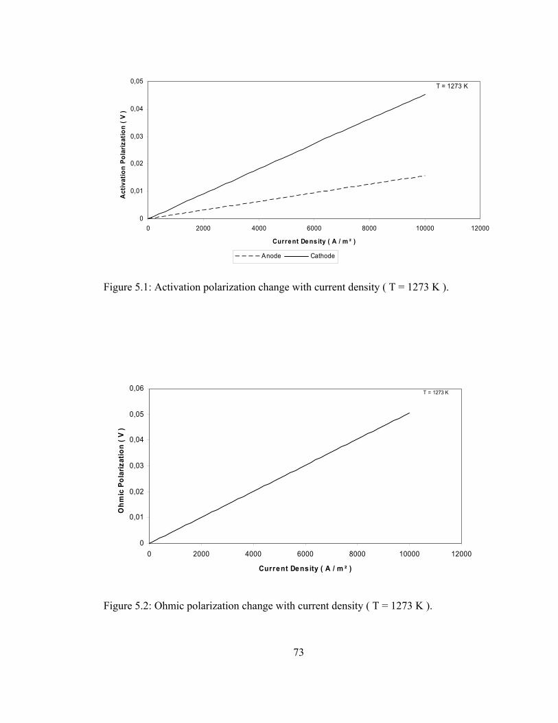
0
0,01
0,02
0,03
0,04
0,05
0 2000 4000 6000 8000 10000 12000
Current Dens ity ( A / m ² )
Act
ivat
ion
Pola
rizat
ion
( V )
Anode Cathode
T = 1273 K
Figure 5.1: Activation polarization change with current density ( T = 1273 K ).
0
0,01
0,02
0,03
0,04
0,05
0,06
0 2000 4000 6000 8000 10000 12000
Current Density ( A / m ² )
Ohm
ic P
olar
izat
ion
( V )
T = 1273 K
Figure 5.2: Ohmic polarization change with current density ( T = 1273 K ).
73
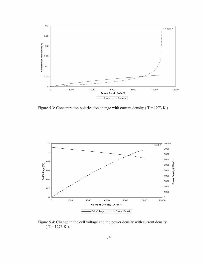
0
0,05
0,1
0,15
0,2
0,25
0,3
0 2000 4000 6000 8000 10000 12000Current Density ( A / m² )
Con
cent
ratio
n Po
lariz
atio
n ( V
)
Anode Cathode
T = 1273 K
Figure 5.3: Concentration polarization change with current density ( T = 1273 K ).
0
0,2
0,4
0,6
0,8
1
1,2
0 2000 4000 6000 8000 10000 12000
Current Density ( A / m ² )
Cel
l Vol
tage
( V
)
0
1000
2000
3000
4000
5000
6000
7000
8000
9000
10000
Pow
er D
ensi
ty (
W /
m² )
Cell Voltage Pow er Density
T = 1273 K
Figure 5.4: Change in the cell voltage and the power density with current density ( T = 1273 K ).
74
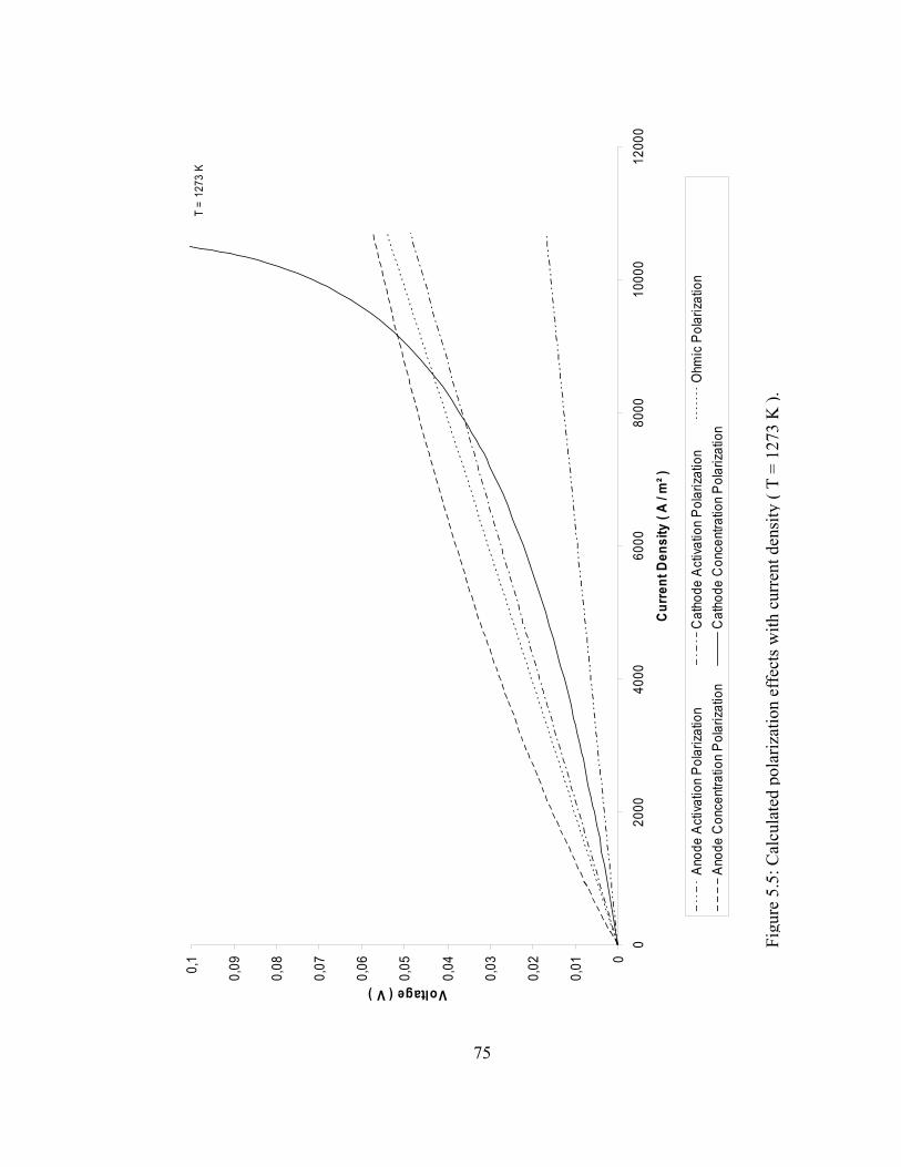
0
0,01
0,02
0,03
0,04
0,05
0,06
0,07
0,08
0,090,
1
020
0040
0060
0080
0010
000
1200
0
Cur
rent
Den
sity
( A
/ m² )
Voltage ( V )
Anod
e Ac
tivat
ion
Pola
rizat
ion
Cat
hode
Act
ivatio
n Po
lariz
atio
nO
hmic
Pol
ariza
tion
Anod
e C
once
ntra
tion
Pola
rizat
ion
Cat
hode
Con
cent
ratio
n Po
lariz
atio
n
T =
1273
K
Figu
re 5
.5: C
alcu
late
d po
lariz
atio
n ef
fect
s with
cur
rent
den
sity
( T
= 12
73 K
).
75
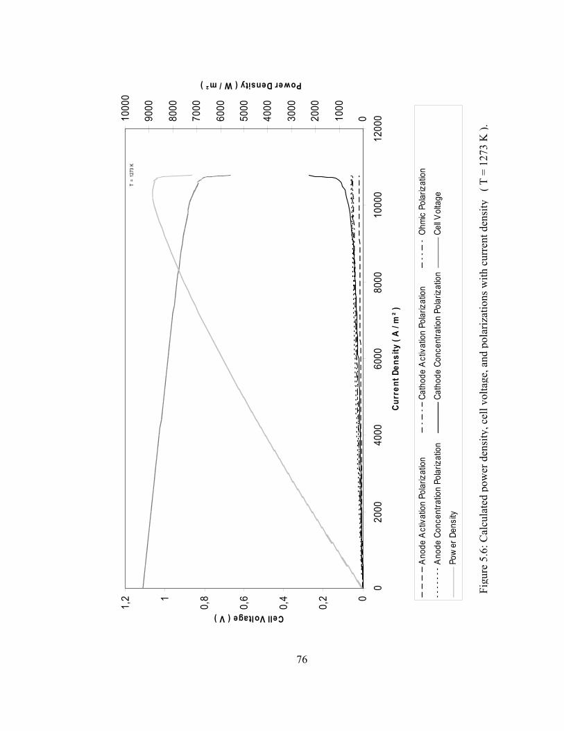
0
0,2
0,4
0,6
0,81
1,2
020
0040
0060
0080
0010
000
1200
0Cu
rren
t Den
sity
( A
/ m² )
Cell Voltage ( V )
01000
2000
3000
4000
5000
6000
7000
8000
9000
1000
0
Power Density ( W / m² )
Ano
de A
ctiv
atio
n Po
lariz
atio
nCa
thod
e A
ctiv
atio
n Po
lariz
atio
nO
hmic
Pol
ariz
atio
n
Ano
de C
once
ntra
tion
Pola
rizat
ion
Cath
ode
Conc
entra
tion
Pola
rizat
ion
Cell V
olta
ge
Pow
er D
ensi
ty
T =
1273
K
Figu
re 5
.6: C
alcu
late
d po
wer
den
sity
, cel
l vol
tage
, and
pol
ariz
atio
ns w
ith c
urre
nt d
ensi
ty
( T =
127
3 K
).
76
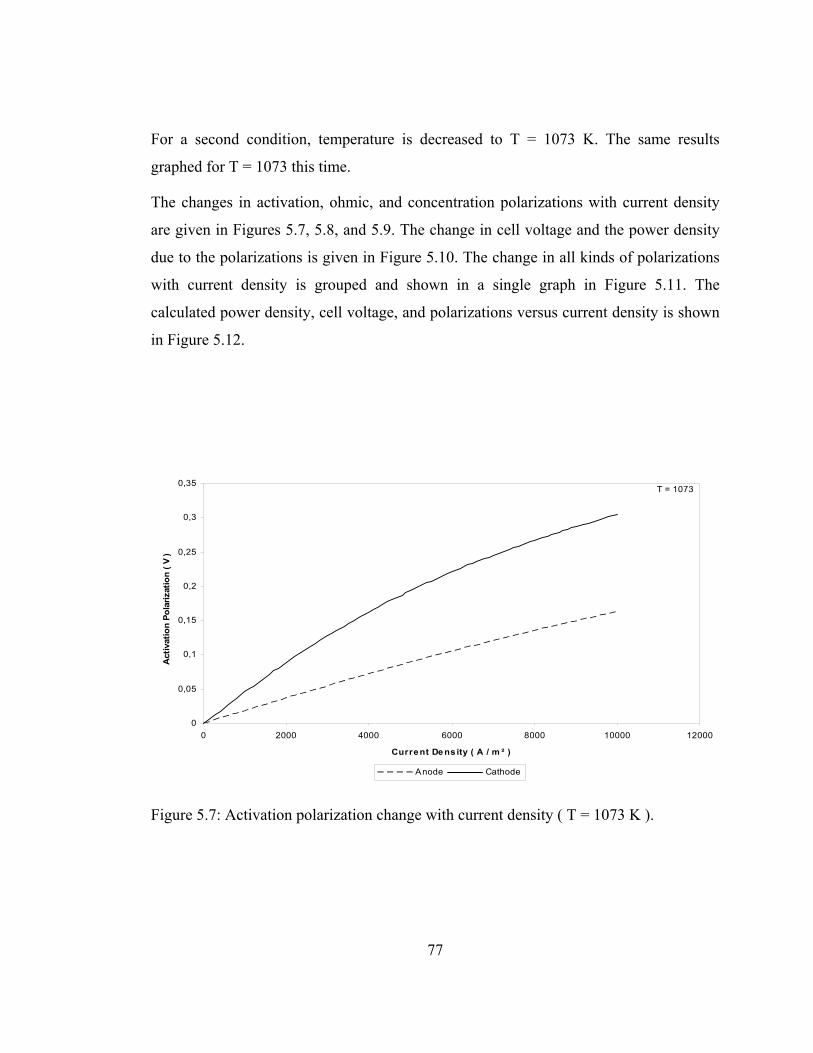
For a second condition, temperature is decreased to T = 1073 K. The same results
graphed for T = 1073 this time.
The changes in activation, ohmic, and concentration polarizations with current density
are given in Figures 5.7, 5.8, and 5.9. The change in cell voltage and the power density
due to the polarizations is given in Figure 5.10. The change in all kinds of polarizations
with current density is grouped and shown in a single graph in Figure 5.11. The
calculated power density, cell voltage, and polarizations versus current density is shown
in Figure 5.12.
0
0,05
0,1
0,15
0,2
0,25
0,3
0,35
0 2000 4000 6000 8000 10000 12000
Current Dens ity ( A / m ² )
Act
ivat
ion
Pola
rizat
ion
( V )
Anode Cathode
T = 1073
Figure 5.7: Activation polarization change with current density ( T = 1073 K ).
77
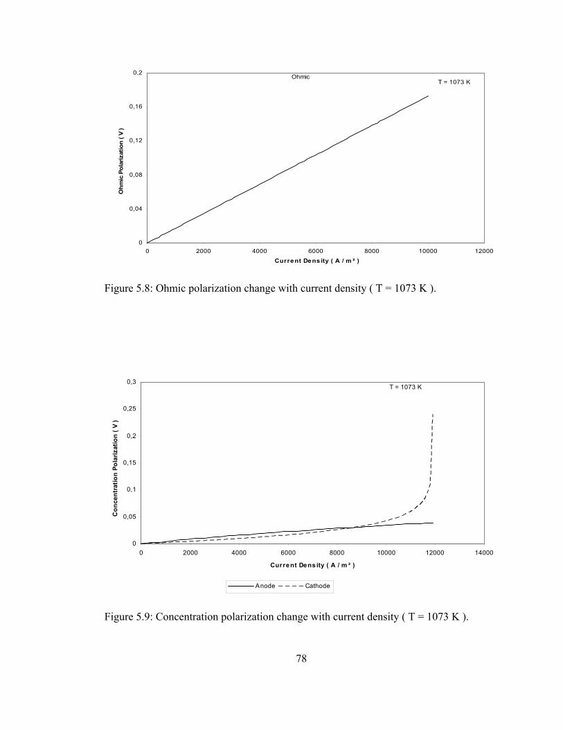
Ohmic
0
0,04
0,08
0,12
0,16
0,2
0 2000 4000 6000 8000 10000 12000Current Dens ity ( A / m ² )
Ohm
ic P
olar
izat
ion
( V )
T = 1073 K
Figure 5.8: Ohmic polarization change with current density ( T = 1073 K ).
0
0,05
0,1
0,15
0,2
0,25
0,3
0 2000 4000 6000 8000 10000 12000 14000
Current Dens ity ( A / m ² )
Con
cent
ratio
n Po
lariz
atio
n ( V
)
Anode Cathode
T = 1073 K
Figure 5.9: Concentration polarization change with current density ( T = 1073 K ).
78
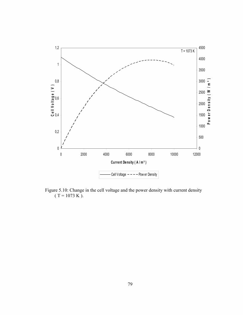
0
0,2
0,4
0,6
0,8
1
1,2
0 2000 4000 6000 8000 10000 12000
Current Dens ity ( A / m ² )
Cel
l Vol
tage
( V
)
0
500
1000
1500
2000
2500
3000
3500
4000
4500
Pow
er D
ensi
ty (
W /
m² )
Cell Voltage Pow er Density
T = 1073 K
Figure 5.10: Change in the cell voltage and the power density with current density ( T = 1073 K ).
79
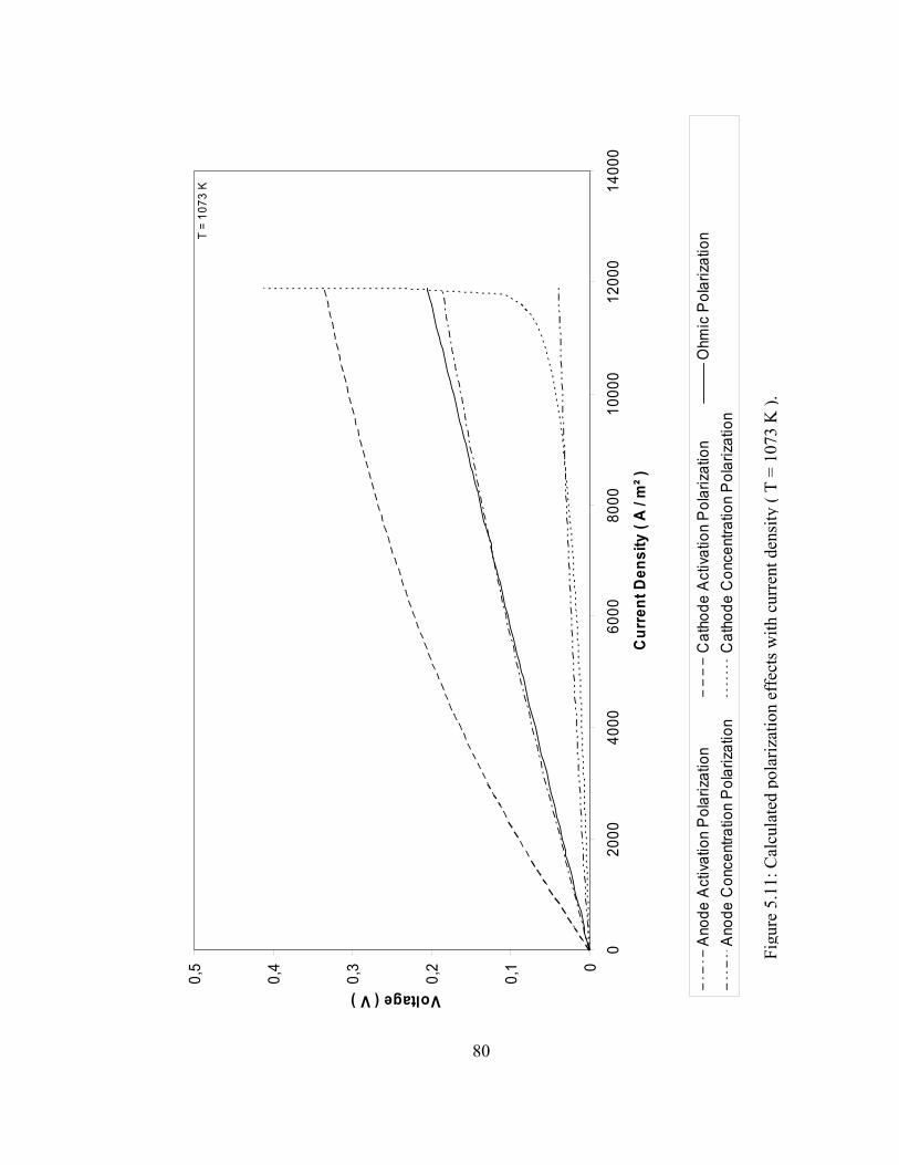
0
0,1
0,2
0,3
0,4
0,5
020
0040
0060
0080
0010
000
1200
014
000
Cur
rent
Den
sity
( A
/ m² )
Voltage ( V )
Ano
de A
ctiv
atio
n P
olar
izat
ion
Cat
hode
Act
ivat
ion
Pol
ariz
atio
nO
hmic
Pol
ariz
atio
nA
node
Con
cent
ratio
n P
olar
izat
ion
Cat
hode
Con
cent
ratio
n P
olar
izat
ion
T =
1073
K
Figu
re 5
.11:
Cal
cula
ted
pola
rizat
ion
effe
cts w
ith c
urre
nt d
ensi
ty (
T =
1073
K ).
80
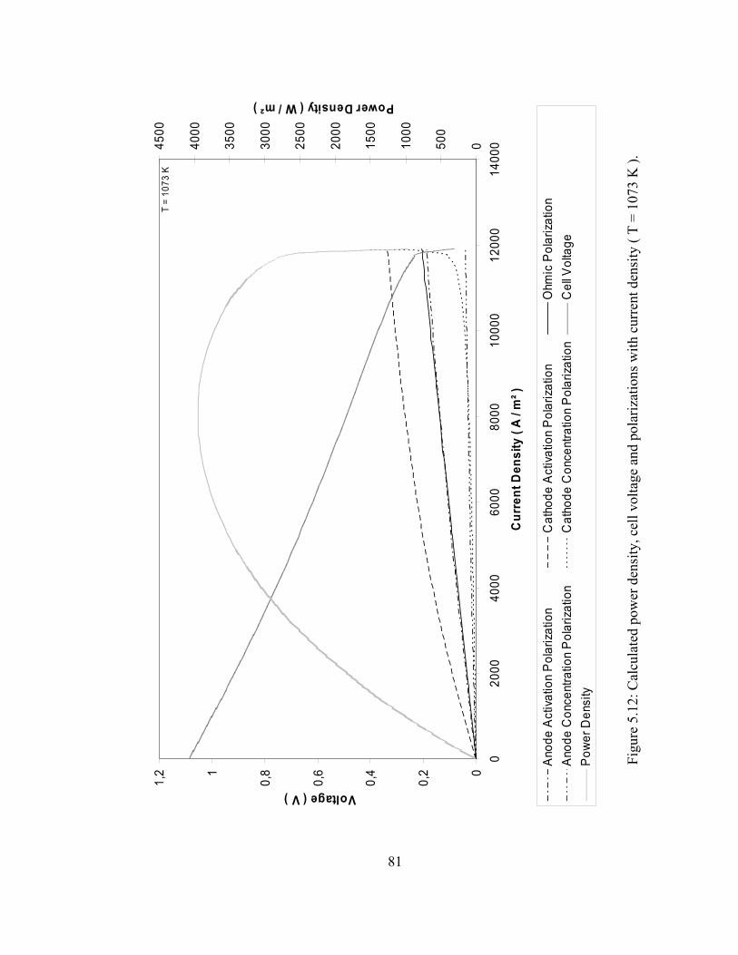
0
0,2
0,4
0,6
0,81
1,2
020
0040
0060
0080
0010
000
1200
014
000
Cur
rent
Den
sity
( A
/ m² )
Voltage ( V )
0500
1000
1500
2000
2500
3000
3500
4000
4500
Power Density ( W / m² )
Ano
de A
ctiv
atio
n P
olar
izat
ion
Cat
hode
Act
ivat
ion
Pol
ariz
atio
nO
hmic
Pol
ariz
atio
nA
node
Con
cent
ratio
n P
olar
izat
ion
Cat
hode
Con
cent
ratio
n P
olar
izat
ion
Cel
l Vol
tage
Pow
er D
ensi
ty
T =
1073
K
Figu
re 5
.12:
Cal
cula
ted
pow
er d
ensi
ty, c
ell v
olta
ge a
nd p
olar
izat
ions
with
cur
rent
den
sity
( T
= 10
73 K
).
81

82
The cathode activation polarization is obviously higher than the anode activation
polarization. This is because of the cathode’s lower exchange current density. Both the
cathode and anode activation polarizations increase almost linearly at T = 1273 K.
Ohmic polarization changes linearly with increasing current, since it is related to the
material thickness. Electrolyte section has the main effect on ohmic polarization due to
its material’s high resistivity. The effect of ohmic polarization can be changed by
changing the thickness of materials or by using another material instead.
Anode concentration polarization is higher than the cathode concentration polarization at
low current densities. But after a critical region, cathode concentration polarization
increases exponentially and goes to infinity as can be seen from the graphs. Regarding to
Figures 5.3 and 5.9, for the cell working at T = 1273 K, IL = 10788 A / m², and for the
one working at T = 1073 K, IL = 11900 A / m² are the limiting current densities.
Figures 5.4 and 5.10 give the change of the cell voltage and the power densities with
current density. The lower the temperature, the more the cell voltage drops, and the less
the power density is. This result is just as expected. In chapter 3, it was explained that
the efficiency of fuel cells decreases with increasing temperature, but on the other hand,
as it can be observed from the results, as the temperature increases, the drop in cell
voltage decreases, and power density increases.
Figures 5.5 and 5.11 show the polarization effects in a single graph for both
temperatures. The results show that at lower temperatures, the cathode activation
polarization becomes significant and has the most effect on voltage drop. The ohmic and
anode activation polarizations behave similarly at lower temperatures. The anode
concentration polarization, on the other hand, becomes significant at high temperature
values, while cathode concentration polarization has very little effect at low
temperatures and low current densities. At high temperature, cathode concentration
polarization increases exponentially. Anode and cathode activation polarizations depend
on temperature much more than the other types of polarizations. The increase in
83
activation polarization with decreasing temperature is the highest in all types of
polarizations.
Figures 5.6 and 5.12 give a better understanding of the effect of temperature on the fuel
cell voltage and the power density. For the cell operating at T = 1273 K, at I ≈ 10400 A /
m², the power density reaches its peak point P ≈ 8889 W / m². For the cell operating at T
= 1073 K, at I ≈ 8000 A / m², the power density reaches its peak point P ≈ 3955 W / m².
At I = 6000 A / m², for the cell working at T = 1273, cell voltage is, E = 0.989 V, while
for the cell working at T = 1073 K, cell voltage is, E = 0.621 V. There is a significant
difference between the two cell voltages.
As a conclusion, as the fuel cell operating temperature increases, the polarizations
decrease and this results higher cell voltages and high power densities
5.1.2 Thermodynamic Analysis
The system is assumed to be at following conditions:
• T = 1273 K., P = 1 atm.
• The air consists of 20 % O2 and 80 % N2 in molar ratios.
In order to calculate the entropies at each node of the system, the partial pressures of the
molecules must be determined. For this reason, mixture compositions at each node of the
system for ideal case ( i.e. conversion ratios are unity ) is given in Table 5.1. Mixture
compositions for different conversion ratios at each node of the system are given in
Tables 5.2 – 7.

Table 5.1: Mixture compositions for ideal case ( i.e. 14=CHη , 1
2=Hη , 1
2=Oη ).
Mole Numbers Mole Ratios Nodes Nodes 1 2 3 4 1 2 3 4
CH4 1 0 0 0 0,3125 0 0 0
H2O 2,2 0,2 0 4,2 0,6875 0,03846 0 0,31818
H2 0 4 0 0 0 0,76923 0 0
O2 0 0 2 0 0 0 0,2 0
CO2 0 1 0 1 0 0,19231 0 0,07576
N2 0 0 8 8 0 0 0,8 0,60606
Table 5.2: Mixture compositions for 9.04=CHη , 9.0
2=Hη , 9.0
2=Oη .
Mole Numbers Mole Ratios Nodes Nodes 1 2 3 4 1 2 3 4
CH4 1 0,1 0 0,1 0,3125 0,02 0 0,00747
H2O 2,2 0,4 0 3,64 0,6875 0,08 0 0,27205
H2 0 3,6 0 0,36 0 0,72 0 0,02691
O2 0 0 2 0,38 0 0 0,2 0,02840
CO2 0 0,9 0 0,9 0 0,18 0 0,06727
N2 0 0 8 8 0 0 0,8 0,59791
Table 5.3: Mixture compositions for 9.04=CHη , 9.0
2=Hη , 8.0
2=Oη .
Mole Numbers Mole Ratios Nodes Nodes 1 2 3 4 1 2 3 4
CH4 1 0,1 0 0,1 0,3125 0,02 0 0,00746
H2O 2,2 0,4 0 3,6 0,6875 0,08 0 0,26866
H2 0 3,6 0 0,4 0 0,72 0 0,02985
84
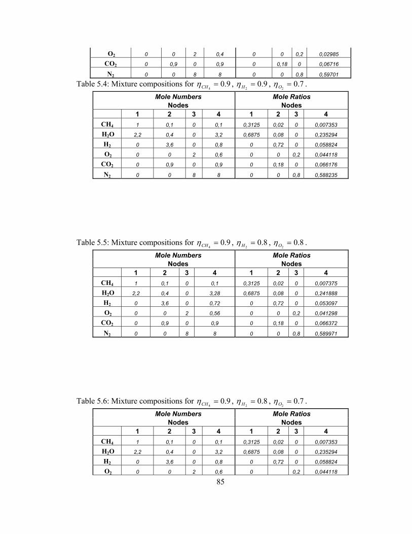
O2 0 0 2 0,4 0 0 0,2 0,02985
CO2 0 0,9 0 0,9 0 0,18 0 0,06716
N2 0 0 8 8 0 0 0,8 0,59701
Table 5.4: Mixture compositions for , , . 9.04=CHη 9.0
2=Hη 7.0
2=Oη
Mole Numbers Mole Ratios Nodes Nodes 1 2 3 4 1 2 3 4
CH4 1 0,1 0 0,1 0,3125 0,02 0 0,007353
H2O 2,2 0,4 0 3,2 0,6875 0,08 0 0,235294
H2 0 3,6 0 0,8 0 0,72 0 0,058824
O2 0 0 2 0,6 0 0 0,2 0,044118
CO2 0 0,9 0 0,9 0 0,18 0 0,066176
N2 0 0 8 8 0 0 0,8 0,588235
Table 5.5: Mixture compositions for 9.04=CHη , 8.0
2=Hη , 8.0
2=Oη .
Mole Numbers Mole Ratios Nodes Nodes 1 2 3 4 1 2 3 4
CH4 1 0,1 0 0,1 0,3125 0,02 0 0,007375
H2O 2,2 0,4 0 3,28 0,6875 0,08 0 0,241888
H2 0 3,6 0 0,72 0 0,72 0 0,053097
O2 0 0 2 0,56 0 0 0,2 0,041298
CO2 0 0,9 0 0,9 0 0,18 0 0,066372
N2 0 0 8 8 0 0 0,8 0,589971
Table 5.6: Mixture compositions for 9.04=CHη , 8.0
2=Hη , 7.0
2=Oη .
Mole Numbers Mole Ratios Nodes Nodes 1 2 3 4 1 2 3 4
CH4 1 0,1 0 0,1 0,3125 0,02 0 0,007353
H2O 2,2 0,4 0 3,2 0,6875 0,08 0 0,235294
H2 0 3,6 0 0,8 0 0,72 0 0,058824
O2 0 0 2 0,6 0 0,2 0,044118
85
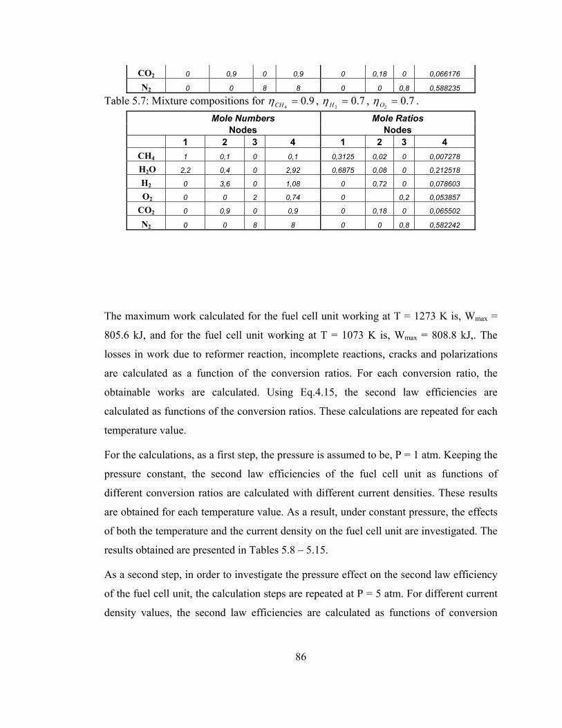
CO2 0 0,9 0 0,9 0 0,18 0 0,066176
N2 0 0 8 8 0 0 0,8 0,588235
Table 5.7: Mixture compositions for , , . 9.04=CHη 7.0
2=Hη 7.0
2=Oη
Mole Numbers Mole Ratios Nodes Nodes 1 2 3 4 1 2 3 4
CH4 1 0,1 0 0,1 0,3125 0,02 0 0,007278
H2O 2,2 0,4 0 2,92 0,6875 0,08 0 0,212518
H2 0 3,6 0 1,08 0 0,72 0 0,078603
O2 0 0 2 0,74 0 0,2 0,053857
CO2 0 0,9 0 0,9 0 0,18 0 0,065502
N2 0 0 8 8 0 0 0,8 0,582242
The maximum work calculated for the fuel cell unit working at T = 1273 K is, Wmax =
805.6 kJ, and for the fuel cell unit working at T = 1073 K is, Wmax = 808.8 kJ,. The
losses in work due to reformer reaction, incomplete reactions, cracks and polarizations
are calculated as a function of the conversion ratios. For each conversion ratio, the
obtainable works are calculated. Using Eq.4.15, the second law efficiencies are
calculated as functions of the conversion ratios. These calculations are repeated for each
temperature value.
For the calculations, as a first step, the pressure is assumed to be, P = 1 atm. Keeping the
pressure constant, the second law efficiencies of the fuel cell unit as functions of
different conversion ratios are calculated with different current densities. These results
are obtained for each temperature value. As a result, under constant pressure, the effects
of both the temperature and the current density on the fuel cell unit are investigated. The
results obtained are presented in Tables 5.8 – 5.15.
As a second step, in order to investigate the pressure effect on the second law efficiency
of the fuel cell unit, the calculation steps are repeated at P = 5 atm. For different current
density values, the second law efficiencies are calculated as functions of conversion
86
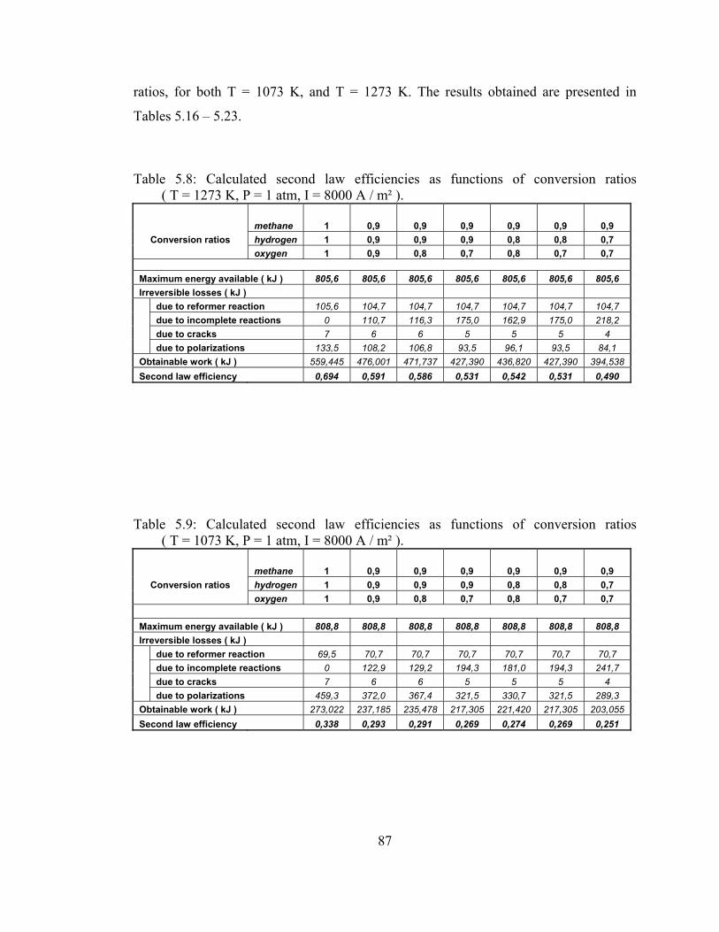
87
ratios, for both T = 1073 K, and T = 1273 K. The results obtained are presented in
Tables 5.16 – 5.23.
Table 5.8: Calculated second law efficiencies as functions of conversion ratios ( T = 1273 K, P = 1 atm, I = 8000 A / m² ).
methane 1 0,9 0,9 0,9 0,9 0,9 0,9
Conversion ratios hydrogen 1 0,9 0,9 0,9 0,8 0,8 0,7 oxygen 1 0,9 0,8 0,7 0,8 0,7 0,7 Maximum energy available ( kJ ) 805,6 805,6 805,6 805,6 805,6 805,6 805,6 Irreversible losses ( kJ ) due to reformer reaction 105,6 104,7 104,7 104,7 104,7 104,7 104,7 due to incomplete reactions 0 110,7 116,3 175,0 162,9 175,0 218,2 due to cracks 7 6 6 5 5 5 4 due to polarizations 133,5 108,2 106,8 93,5 96,1 93,5 84,1 Obtainable work ( kJ ) 559,445 476,001 471,737 427,390 436,820 427,390 394,538 Second law efficiency 0,694 0,591 0,586 0,531 0,542 0,531 0,490
Table 5.9: Calculated second law efficiencies as functions of conversion ratios ( T = 1073 K, P = 1 atm, I = 8000 A / m² ).
methane 1 0,9 0,9 0,9 0,9 0,9 0,9
Conversion ratios hydrogen 1 0,9 0,9 0,9 0,8 0,8 0,7 oxygen 1 0,9 0,8 0,7 0,8 0,7 0,7 Maximum energy available ( kJ ) 808,8 808,8 808,8 808,8 808,8 808,8 808,8 Irreversible losses ( kJ ) due to reformer reaction 69,5 70,7 70,7 70,7 70,7 70,7 70,7 due to incomplete reactions 0 122,9 129,2 194,3 181,0 194,3 241,7 due to cracks 7 6 6 5 5 5 4 due to polarizations 459,3 372,0 367,4 321,5 330,7 321,5 289,3 Obtainable work ( kJ ) 273,022 237,185 235,478 217,305 221,420 217,305 203,055 Second law efficiency 0,338 0,293 0,291 0,269 0,274 0,269 0,251
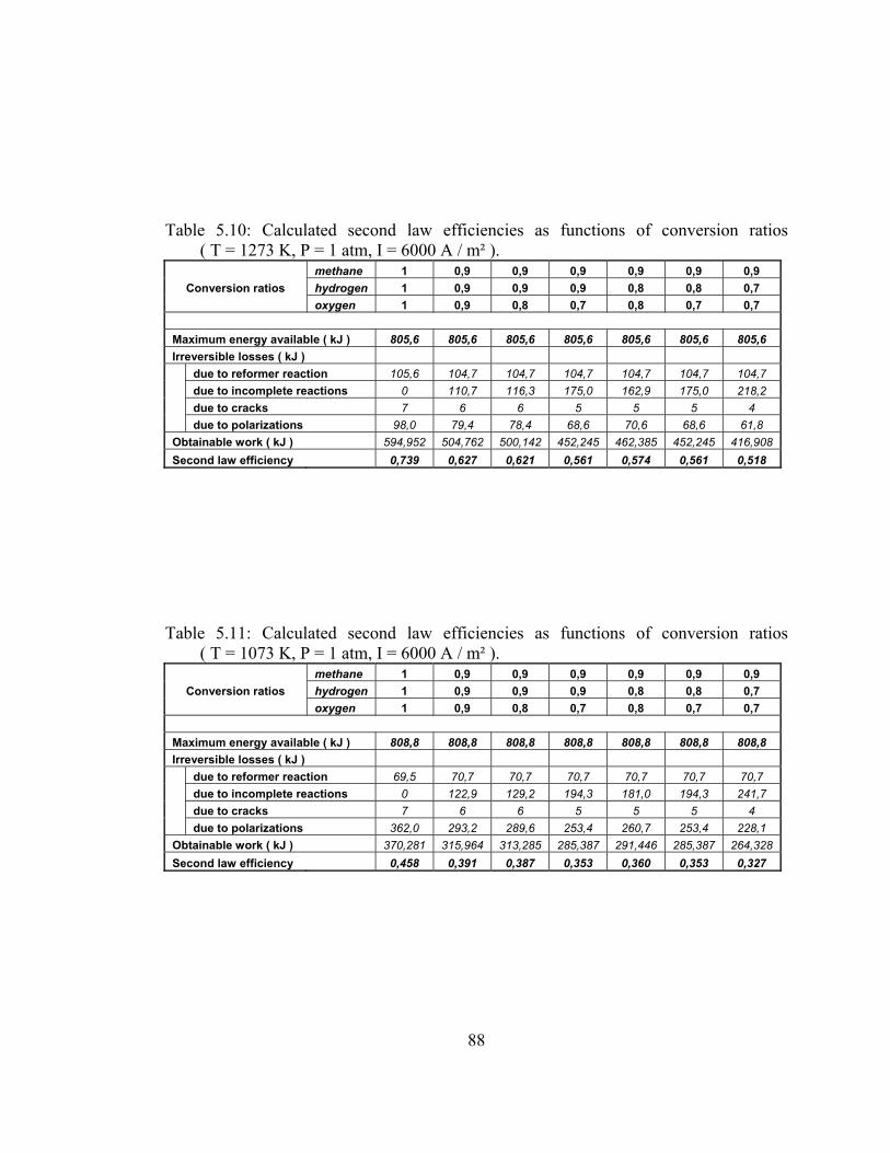
88
Table 5.10: Calculated second law efficiencies as functions of conversion ratios ( T = 1273 K, P = 1 atm, I = 6000 A / m² ).
methane 1 0,9 0,9 0,9 0,9 0,9 0,9 Conversion ratios hydrogen 1 0,9 0,9 0,9 0,8 0,8 0,7
oxygen 1 0,9 0,8 0,7 0,8 0,7 0,7 Maximum energy available ( kJ ) 805,6 805,6 805,6 805,6 805,6 805,6 805,6 Irreversible losses ( kJ ) due to reformer reaction 105,6 104,7 104,7 104,7 104,7 104,7 104,7 due to incomplete reactions 0 110,7 116,3 175,0 162,9 175,0 218,2 due to cracks 7 6 6 5 5 5 4 due to polarizations 98,0 79,4 78,4 68,6 70,6 68,6 61,8 Obtainable work ( kJ ) 594,952 504,762 500,142 452,245 462,385 452,245 416,908 Second law efficiency 0,739 0,627 0,621 0,561 0,574 0,561 0,518
Table 5.11: Calculated second law efficiencies as functions of conversion ratios ( T = 1073 K, P = 1 atm, I = 6000 A / m² ).
methane 1 0,9 0,9 0,9 0,9 0,9 0,9 Conversion ratios hydrogen 1 0,9 0,9 0,9 0,8 0,8 0,7
oxygen 1 0,9 0,8 0,7 0,8 0,7 0,7 Maximum energy available ( kJ ) 808,8 808,8 808,8 808,8 808,8 808,8 808,8 Irreversible losses ( kJ ) due to reformer reaction 69,5 70,7 70,7 70,7 70,7 70,7 70,7 due to incomplete reactions 0 122,9 129,2 194,3 181,0 194,3 241,7 due to cracks 7 6 6 5 5 5 4 due to polarizations 362,0 293,2 289,6 253,4 260,7 253,4 228,1 Obtainable work ( kJ ) 370,281 315,964 313,285 285,387 291,446 285,387 264,328 Second law efficiency 0,458 0,391 0,387 0,353 0,360 0,353 0,327

89
Table 5.12: Calculated second law efficiencies as functions of conversion ratios ( T = 1273 K, P = 1 atm, I = 4000 A / m² ).
methane 1 0,9 0,9 0,9 0,9 0,9 0,9 Conversion ratios hydrogen 1 0,9 0,9 0,9 0,8 0,8 0,7
oxygen 1 0,9 0,8 0,7 0,8 0,7 0,7 Maximum energy available ( kJ ) 805,6 805,6 805,6 805,6 805,6 805,6 805,6 Irreversible losses ( kJ ) due to reformer reaction 105,6 104,7 104,7 104,7 104,7 104,7 104,7 due to incomplete reactions 0 110,7 116,3 175,0 162,9 175,0 218,2 due to cracks 7 6 6 5 5 5 4 due to polarizations 65,6 53,1 52,5 45,9 47,2 45,9 41,3 Obtainable work ( kJ ) 627,372 531,022 526,078 474,939 485,727 474,939 437,332 Second law efficiency 0,779 0,659 0,653 0,590 0,603 0,590 0,543
Table 5.13: Calculated second law efficiencies as functions of conversion ratios ( T = 1073 K, P = 1 atm, I = 4000 A / m² ).
methane 1 0,9 0,9 0,9 0,9 0,9 0,9 Conversion ratios hydrogen 1 0,9 0,9 0,9 0,8 0,8 0,7
oxygen 1 0,9 0,8 0,7 0,8 0,7 0,7 Maximum energy available ( kJ ) 808,8 808,8 808,8 808,8 808,8 808,8 808,8 Irreversible losses ( kJ ) due to reformer reaction 69,5 70,7 70,7 70,7 70,7 70,7 70,7 due to incomplete reactions 0 122,9 129,2 194,3 181,0 194,3 241,7 due to cracks 7 6 6 5 5 5 4 due to polarizations 254,7 206,3 203,8 178,3 183,4 178,3 160,5 Obtainable work ( kJ ) 477,574 402,872 399,119 360,492 368,698 360,492 331,923 Second law efficiency 0,590 0,498 0,493 0,446 0,456 0,446 0,410
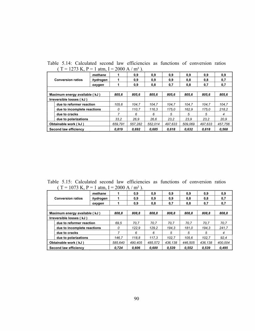
90
Table 5.14: Calculated second law efficiencies as functions of conversion ratios ( T = 1273 K, P = 1 atm, I = 2000 A / m² ).
methane 1 0,9 0,9 0,9 0,9 0,9 0,9 Conversion ratios hydrogen 1 0,9 0,9 0,9 0,8 0,8 0,7
oxygen 1 0,9 0,8 0,7 0,8 0,7 0,7 Maximum energy available ( kJ ) 805,6 805,6 805,6 805,6 805,6 805,6 805,6 Irreversible losses ( kJ ) due to reformer reaction 105,6 104,7 104,7 104,7 104,7 104,7 104,7 due to incomplete reactions 0 110,7 116,3 175,0 162,9 175,0 218,2 due to cracks 7 6 6 5 5 5 4 due to polarizations 33,2 26,9 26,6 23,2 23,9 23,2 20,9 Obtainable work ( kJ ) 659,791 557,282 552,014 497,633 509,069 497,633 457,756 Second law efficiency 0,819 0,692 0,685 0,618 0,632 0,618 0,568
Table 5.15: Calculated second law efficiencies as functions of conversion ratios ( T = 1073 K, P = 1 atm, I = 2000 A / m² ).
methane 1 0,9 0,9 0,9 0,9 0,9 0,9 Conversion ratios hydrogen 1 0,9 0,9 0,9 0,8 0,8 0,7
oxygen 1 0,9 0,8 0,7 0,8 0,7 0,7 Maximum energy available ( kJ ) 808,8 808,8 808,8 808,8 808,8 808,8 808,8 Irreversible losses ( kJ ) due to reformer reaction 69,5 70,7 70,7 70,7 70,7 70,7 70,7 due to incomplete reactions 0 122,9 129,2 194,3 181,0 194,3 241,7 due to cracks 7 6 6 5 5 5 4 due to polarizations 146,7 118,8 117,3 102,7 105,6 102,7 92,4 Obtainable work ( kJ ) 585,640 490,405 485,572 436,138 446,505 436,138 400,004 Second law efficiency 0,724 0,606 0,600 0,539 0,552 0,539 0,495
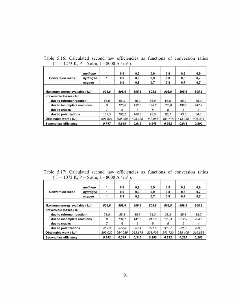
91
Table 5.16: Calculated second law efficiencies as functions of conversion ratios ( T = 1273 K, P = 5 atm, I = 8000 A / m² ).
methane 1 0,9 0,9 0,9 0,9 0,9 0,9
Conversion ratios hydrogen 1 0,9 0,9 0,9 0,8 0,8 0,7 oxygen 1 0,9 0,8 0,7 0,8 0,7 0,7 Maximum energy available ( kJ ) 805,6 805,6 805,6 805,6 805,6 805,6 805,6 Irreversible losses ( kJ ) due to reformer reaction 63,6 66,9 66,9 66,9 66,9 66,9 66,9 due to incomplete reactions 0 125,6 132,0 198,6 185,0 198,6 247,4 due to cracks 7 6 6 5 5 5 4 due to polarizations 133,5 108,2 106,8 93,5 96,1 93,5 84,1 Obtainable work ( kJ ) 591,627 500,099 495,135 443,988 454,718 443,988 406,336 Second law efficiency 0,747 0,619 0,613 0,548 0,562 0,548 0,500
Table 5.17: Calculated second law efficiencies as functions of conversion ratios ( T = 1073 K, P = 5 atm, I = 8000 A / m² ).
methane 1 0,9 0,9 0,9 0,9 0,9 0,9
Conversion ratios hydrogen 1 0,9 0,9 0,9 0,8 0,8 0,7 oxygen 1 0,9 0,8 0,7 0,8 0,7 0,7 Maximum energy available ( kJ ) 808,8 808,8 808,8 808,8 808,8 808,8 808,8 Irreversible losses ( kJ ) due to reformer reaction 33,5 38,3 38,3 38,3 38,3 38,3 38,3 due to incomplete reactions 0 134,7 141,6 212,9 198,3 212,9 264,6 due to cracks 7 6 6 5 5 5 4 due to polarizations 459,3 372,0 367,4 321,5 330,7 321,5 289,3 Obtainable work ( kJ ) 309,022 264,985 262,678 238,405 243,720 238,405 219,855 Second law efficiency 0,382 0,319 0,316 0,286 0,292 0,286 0,263
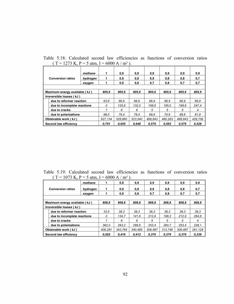
92
Table 5.18: Calculated second law efficiencies as functions of conversion ratios ( T = 1273 K, P = 5 atm, I = 6000 A / m² ).
methane 1 0,9 0,9 0,9 0,9 0,9 0,9
Conversion ratios hydrogen 1 0,9 0,9 0,9 0,8 0,8 0,7 oxygen 1 0,9 0,8 0,7 0,8 0,7 0,7 Maximum energy available ( kJ ) 805,6 805,6 805,6 805,6 805,6 805,6 805,6 Irreversible losses ( kJ ) due to reformer reaction 63,6 66,9 66,9 66,9 66,9 66,9 66,9 due to incomplete reactions 0 125,6 132,0 198,6 185,0 198,6 247,4 due to cracks 7 6 6 5 5 5 4 due to polarizations 98,0 79,4 78,4 68,6 70,6 68,6 61,8 Obtainable work ( kJ ) 627,134 528,860 523,540 468,843 480,283 468,843 428,706 Second law efficiency 0,791 0,655 0,648 0,579 0,593 0,579 0,528
Table 5.19: Calculated second law efficiencies as functions of conversion ratios ( T = 1073 K, P = 5 atm, I = 6000 A / m² ).
methane 1 0,9 0,9 0,9 0,9 0,9 0,9
Conversion ratios hydrogen 1 0,9 0,9 0,9 0,8 0,8 0,7 oxygen 1 0,9 0,8 0,7 0,8 0,7 0,7 Maximum energy available ( kJ ) 808,8 808,8 808,8 808,8 808,8 808,8 808,8 Irreversible losses ( kJ ) due to reformer reaction 33,5 38,3 38,3 38,3 38,3 38,3 38,3 due to incomplete reactions 0 134,7 141,6 212,9 198,3 212,9 264,6 due to cracks 7 6 6 5 5 5 4 due to polarizations 362,0 293,2 289,6 253,4 260,7 253,4 228,1 Obtainable work ( kJ ) 406,281 343,764 340,485 306,487 313,746 306,487 281,128 Second law efficiency 0,502 0,416 0,412 0,370 0,379 0,370 0,339

93
Table 5.20: Calculated second law efficiencies as functions of conversion ratios ( T = 1273 K, P = 5 atm, I = 4000 A / m² ).
methane 1 0,9 0,9 0,9 0,9 0,9 0,9 Conversion ratios hydrogen 1 0,9 0,9 0,9 0,8 0,8 0,7
oxygen 1 0,9 0,8 0,7 0,8 0,7 0,7 Maximum energy available ( kJ ) 805,6 805,6 805,6 805,6 805,6 805,6 805,6 Irreversible losses ( kJ ) due to reformer reaction 63,6 66,9 66,9 66,9 66,9 66,9 66,9 due to incomplete reactions 0 125,6 132,0 198,6 185,0 198,6 247,4 due to cracks 7 6 6 5 5 5 4 due to polarizations 65,6 53,1 52,5 45,9 47,2 45,9 41,3 Obtainable work ( kJ ) 659,554 555,120 549,476 491,537 503,625 491,537 449,130 Second law efficiency 0,831 0,688 0,680 0,607 0,622 0,607 0,554
Table 5.21: Calculated second law efficiencies as functions of conversion ratios ( T = 1073 K, P = 5 atm, I = 4000 A / m² ).
methane 1 0,9 0,9 0,9 0,9 0,9 0,9 Conversion ratios hydrogen 1 0,9 0,9 0,9 0,8 0,8 0,7
oxygen 1 0,9 0,8 0,7 0,8 0,7 0,7 Maximum energy available ( kJ ) 808,8 808,8 808,8 808,8 808,8 808,8 808,8 Irreversible losses ( kJ ) due to reformer reaction 33,5 38,3 38,3 38,3 38,3 38,3 38,3 due to incomplete reactions 0 134,7 141,6 212,9 198,3 212,9 264,6 due to cracks 7 6 6 5 5 5 4 due to polarizations 254,7 206,3 203,8 178,3 183,4 178,3 160,5 Obtainable work ( kJ ) 513,574 430,672 426,319 381,592 390,998 381,592 348,723 Second law efficiency 0,635 0,524 0,518 0,463 0,475 0,463 0,422
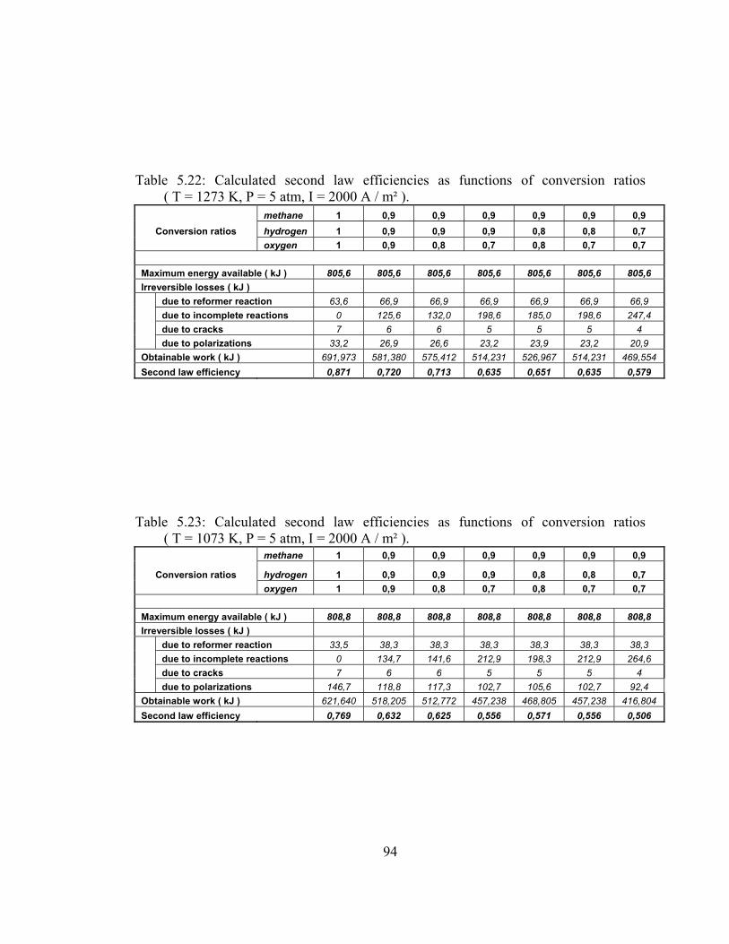
94
Table 5.22: Calculated second law efficiencies as functions of conversion ratios ( T = 1273 K, P = 5 atm, I = 2000 A / m² ).
methane 1 0,9 0,9 0,9 0,9 0,9 0,9 Conversion ratios hydrogen 1 0,9 0,9 0,9 0,8 0,8 0,7
oxygen 1 0,9 0,8 0,7 0,8 0,7 0,7 Maximum energy available ( kJ ) 805,6 805,6 805,6 805,6 805,6 805,6 805,6 Irreversible losses ( kJ ) due to reformer reaction 63,6 66,9 66,9 66,9 66,9 66,9 66,9 due to incomplete reactions 0 125,6 132,0 198,6 185,0 198,6 247,4 due to cracks 7 6 6 5 5 5 4 due to polarizations 33,2 26,9 26,6 23,2 23,9 23,2 20,9 Obtainable work ( kJ ) 691,973 581,380 575,412 514,231 526,967 514,231 469,554 Second law efficiency 0,871 0,720 0,713 0,635 0,651 0,635 0,579
Table 5.23: Calculated second law efficiencies as functions of conversion ratios ( T = 1073 K, P = 5 atm, I = 2000 A / m² ).
methane 1 0,9 0,9 0,9 0,9 0,9 0,9
Conversion ratios hydrogen 1 0,9 0,9 0,9 0,8 0,8 0,7 oxygen 1 0,9 0,8 0,7 0,8 0,7 0,7 Maximum energy available ( kJ ) 808,8 808,8 808,8 808,8 808,8 808,8 808,8 Irreversible losses ( kJ ) due to reformer reaction 33,5 38,3 38,3 38,3 38,3 38,3 38,3 due to incomplete reactions 0 134,7 141,6 212,9 198,3 212,9 264,6 due to cracks 7 6 6 5 5 5 4 due to polarizations 146,7 118,8 117,3 102,7 105,6 102,7 92,4 Obtainable work ( kJ ) 621,640 518,205 512,772 457,238 468,805 457,238 416,804 Second law efficiency 0,769 0,632 0,625 0,556 0,571 0,556 0,506
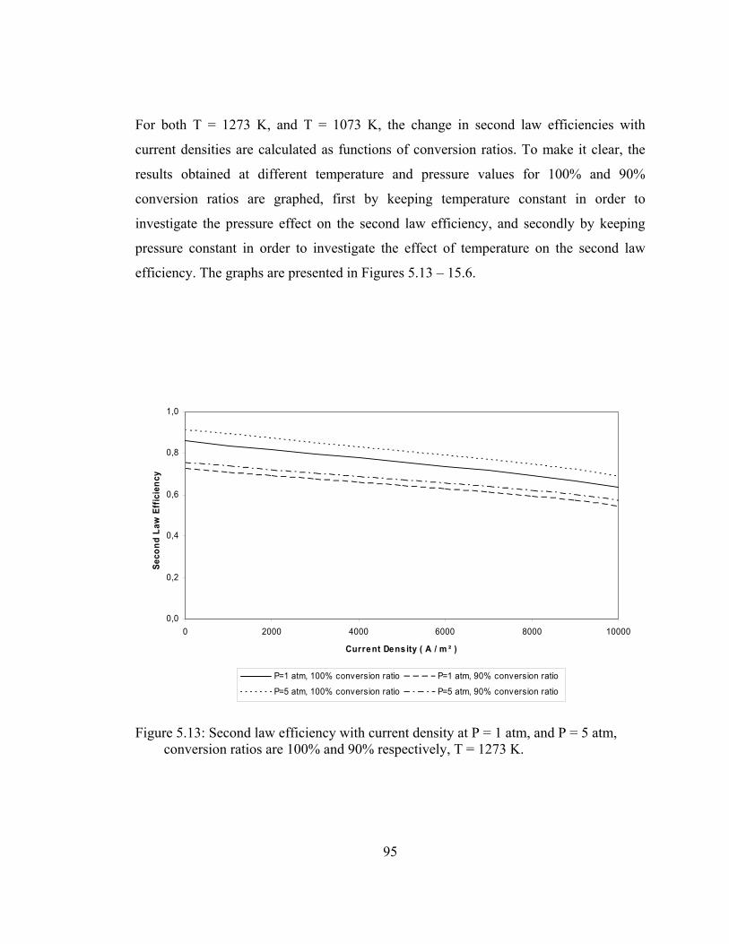
For both T = 1273 K, and T = 1073 K, the change in second law efficiencies with
current densities are calculated as functions of conversion ratios. To make it clear, the
results obtained at different temperature and pressure values for 100% and 90%
conversion ratios are graphed, first by keeping temperature constant in order to
investigate the pressure effect on the second law efficiency, and secondly by keeping
pressure constant in order to investigate the effect of temperature on the second law
efficiency. The graphs are presented in Figures 5.13 – 15.6.
0,0
0,2
0,4
0,6
0,8
1,0
0 2000 4000 6000 8000 10000
Current Density ( A / m ² )
Seco
nd L
aw E
ffic
ienc
y
P=1 atm, 100% conversion ratio P=1 atm, 90% conversion ratio
P=5 atm, 100% conversion ratio P=5 atm, 90% conversion ratio
Figure 5.13: Second law efficiency with current density at P = 1 atm, and P = 5 atm, conversion ratios are 100% and 90% respectively, T = 1273 K.
95
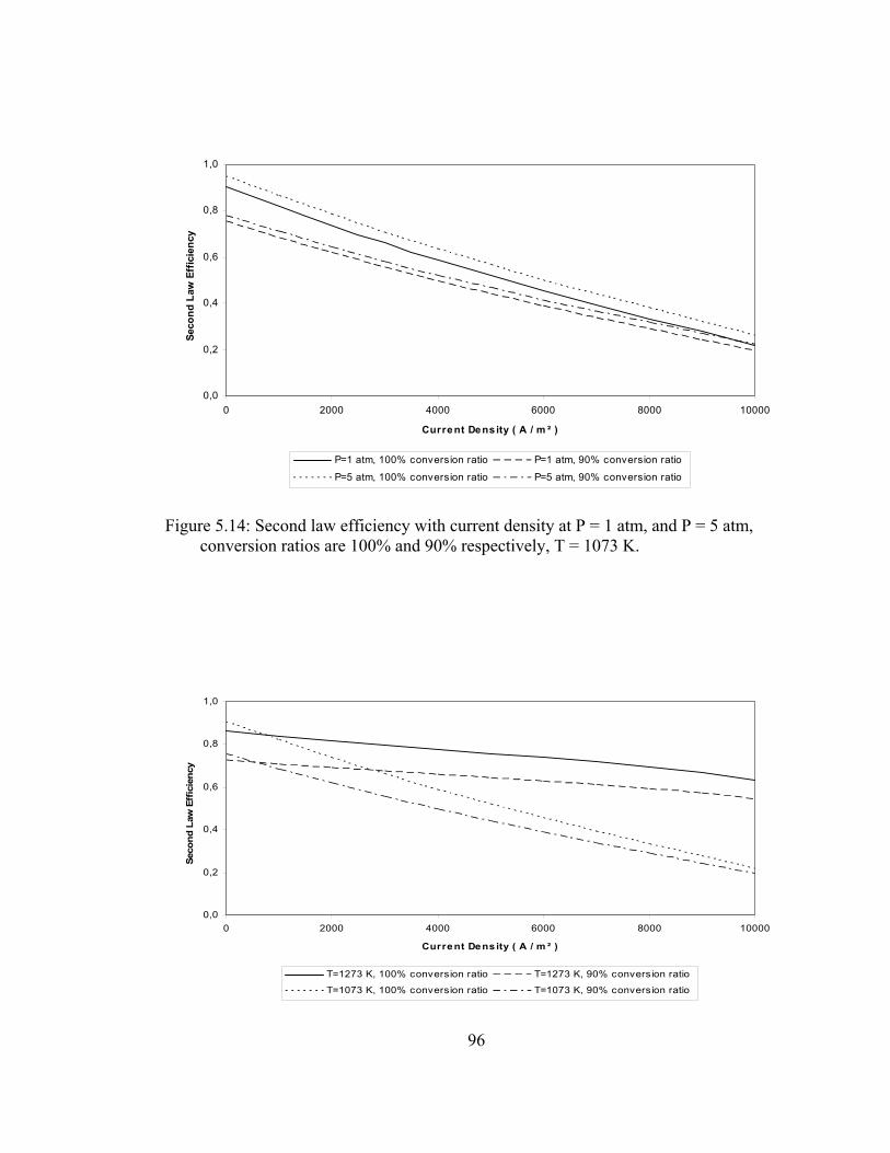
0,0
0,2
0,4
0,6
0,8
1,0
0 2000 4000 6000 8000 10000
Current Density ( A / m ² )
Seco
nd L
aw E
ffic
ienc
y
P=1 atm, 100% conversion ratio P=1 atm, 90% conversion ratio
P=5 atm, 100% conversion ratio P=5 atm, 90% conversion ratio
Figure 5.14: Second law efficiency with current density at P = 1 atm, and P = 5 atm, conversion ratios are 100% and 90% respectively, T = 1073 K.
0,0
0,2
0,4
0,6
0,8
1,0
0 2000 4000 6000 8000 10000
Current Density ( A / m ² )
Seco
nd L
aw E
ffic
ienc
y
T=1273 K, 100% conversion ratio T=1273 K, 90% conversion ratio
T=1073 K, 100% conversion ratio T=1073 K, 90% conversion ratio
96
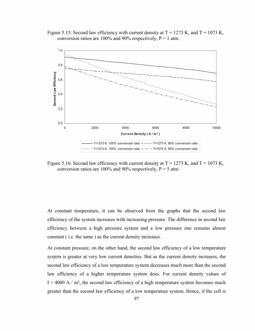
Figure 5.15: Second law efficiency with current density at T = 1273 K, and T = 1073 K, conversion ratios are 100% and 90% respectively, P = 1 atm.
0,0
0,2
0,4
0,6
0,8
1,0
0 2000 4000 6000 8000 10000
Current Density ( A / m ² )
Seco
nd L
aw E
ffic
ienc
y
T=1273 K, 100% conversion ratio T=1273 K, 90% conversion ratio
T=1073 K, 100% conversion ratio T=1073 K, 90% conversion ratio
Figure 5.16: Second law efficiency with current density at T = 1273 K, and T = 1073 K, conversion ratios are 100% and 90% respectively, P = 5 atm.
At constant temperature, it can be observed from the graphs that the second law
efficiency of the system increases with increasing pressure. The difference in second law
efficiency between a high pressure system and a low pressure one remains almost
constant ( i.e. the same ) as the current density increases.
At constant pressure, on the other hand, the second law efficiency of a low temperature
system is greater at very low current densities. But as the current density increases, the
second law efficiency of a low temperature system decreases much more than the second
law efficiency of a higher temperature system does. For current density values of
I > 4000 A / m², the second law efficiency of a high temperature system becomes much
greater than the second law efficiency of a low temperature system. Hence, if the cell is 97
98
operated at low current densities, the low temperature gives a better second law
efficiency, while for the cell operated at high current densities, the high temperature
gives a better second law efficiency.
As a conclusion, it can be stated that, for a system operating at a constant current density
value, keeping the temperature constant, the second law efficiency increases as the
pressure is increased, and keeping the pressure constant, the second law efficiency
increases as the temperature is increased, unless it is operated at very low current
density.
5.2 Results of Simulation Model 2
5.2.1 The Heat Required by The Reformer and Vaporizer
In order to determine how much fuel must be left to be burnt in the afterburner, the heat
requirement of the reformer and vaporizer must be determined, as a first step. The heat
requirement of the reformer and vaporizer reactions with percentage of methane
reforming ( or the reformer efficiency ) is presented in Figure 5.17. The fuel left at the
exit of the fuel cell stack is burnt in the afterburner, and the heat released by the
combustion process is used in reformer and vaporizer reactions. The remaining heat is
lost to the environment. The heat release by the combustion of the fuel in the afterburner
is given in Figure 5.18. The temperatures are assumed to be Tr,i = 1100 K for the
reformer reaction and T = 1200 K for the afterburner reaction, while T=298 K is the
exact temperature value for the vaporizer reaction. Tr,i is used to indicate the reformer
inlet temperature. These temperatures will differ with the calculated temperatures of the
reformer inlet and afterburner temperatures, but they are assumed so, in order to make
conservative assumptions for the reformer efficiency and the fuel utilization rate.
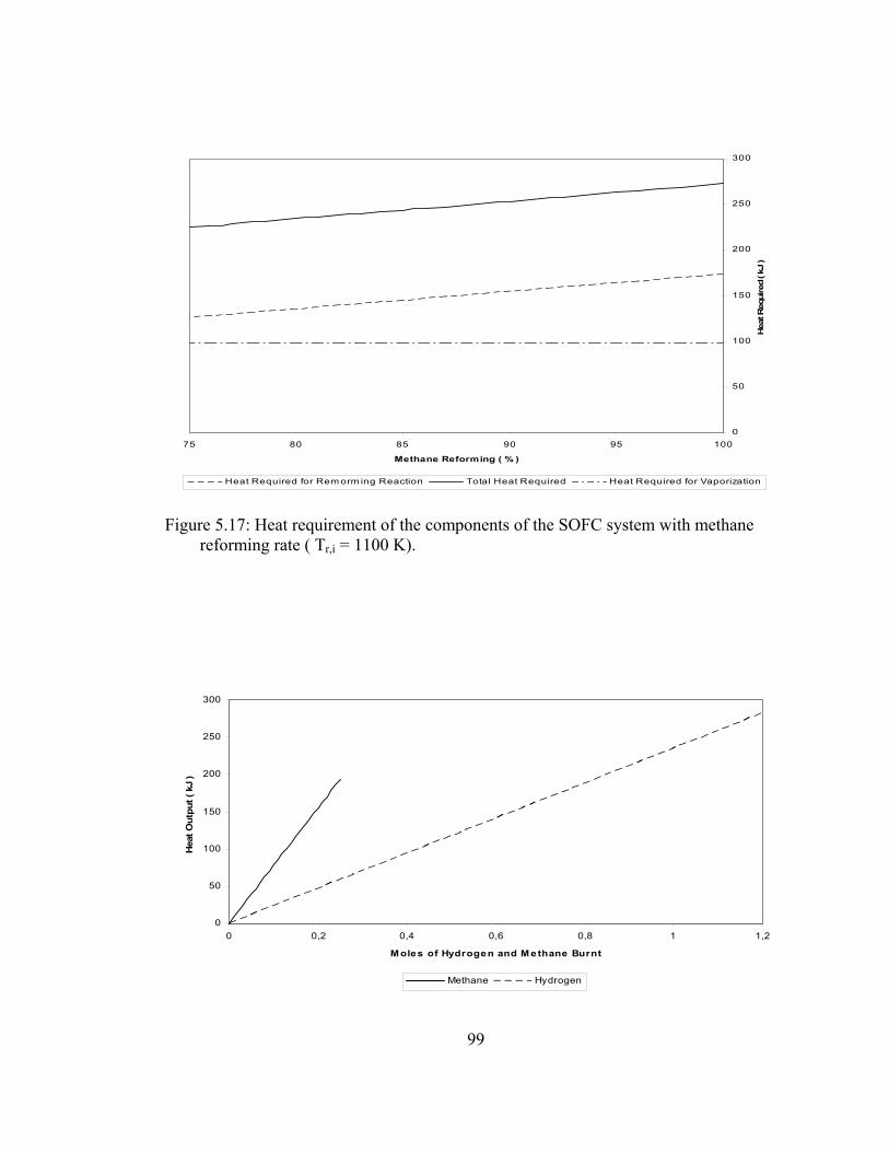
0
50
100
150
200
250
300
75 80 85 90 95 100
Methane Reforming ( % )
Hea
t Req
uire
d ( k
J )
Heat Required for Rem orm ing Reaction Total Heat Required Heat Required for Vaporization
Figure 5.17: Heat requirement of the components of the SOFC system with methane reforming rate ( Tr,i = 1100 K).
0
50
100
150
200
250
300
0 0,2 0,4 0,6 0,8 1 1,2
M oles of Hydrogen and M ethane Burnt
Hea
t Out
put (
kJ
)
Methane Hydrogen
99
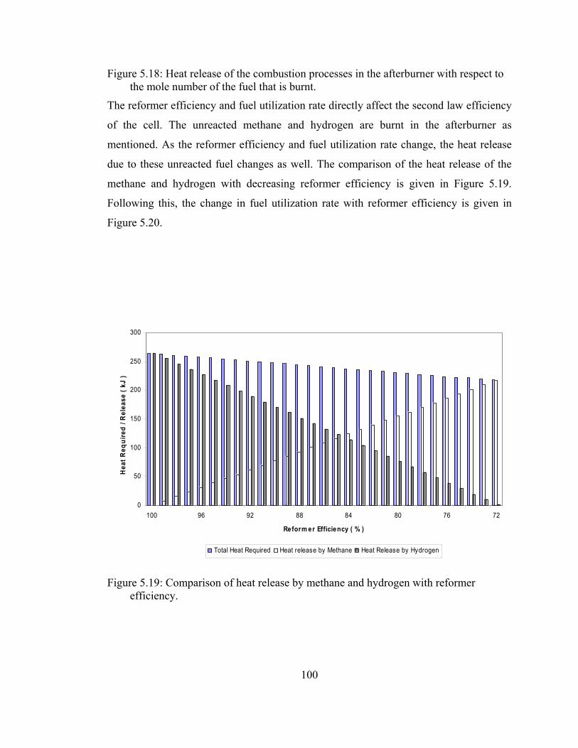
Figure 5.18: Heat release of the combustion processes in the afterburner with respect to the mole number of the fuel that is burnt.
The reformer efficiency and fuel utilization rate directly affect the second law efficiency
of the cell. The unreacted methane and hydrogen are burnt in the afterburner as
mentioned. As the reformer efficiency and fuel utilization rate change, the heat release
due to these unreacted fuel changes as well. The comparison of the heat release of the
methane and hydrogen with decreasing reformer efficiency is given in Figure 5.19.
Following this, the change in fuel utilization rate with reformer efficiency is given in
Figure 5.20.
0
50
100
150
200
250
300
100 96 92 88 84 80 76 72
Reform er Efficiency ( % )
Hea
t Req
uire
d / R
elea
se (
kJ )
Total Heat Required Heat release by Methane Heat Release by Hydrogen
Figure 5.19: Comparison of heat release by methane and hydrogen with reformer efficiency.
100
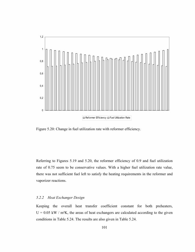
0
0,2
0,4
0,6
0,8
1
1,2
Reformer Ef f iciency Fuel Utilization Rate
Figure 5.20: Change in fuel utilization rate with reformer efficiency.
Referring to Figures 5.19 and 5.20, the reformer efficiency of 0.9 and fuel utilization
rate of 0.75 seem to be conservative values. With a higher fuel utilization rate value,
there was not sufficient fuel left to satisfy the heating requirements in the reformer and
vaporizer reactions.
5.2.2 Heat Exchanger Design
Keeping the overall heat transfer coefficient constant for both preheaters,
U = 0.05 kW / m²K, the areas of heat exchangers are calculated according to the given
conditions in Table 5.24. The results are also given in Table 5.24.
101
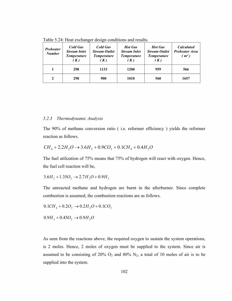
Table 5.24: Heat exchanger design conditions and results.
Preheater Number
Cold Gas Stream Inlet Temperature
( K )
Cold Gas Stream Outlet Temperature
( K )
Hot Gas Stream Inlet Temperature
( K )
Hot Gas Stream Outlet Temperature
( K )
Calculated Preheater Area
( m² )
1 298 1133 1200 959 566
2 298 900 1010 560 1657
5.2.3 Thermodynamic Analysis
The 90% of methane conversion ratio ( i.e. reformer efficiency ) yields the reformer
reaction as follows.
OHCHCOHOHCH 242224 4.01.09.06.32.2 +++→+
The fuel utilization of 75% means that 75% of hydrogen will react with oxygen. Hence,
the fuel cell reaction will be,
2222 9.07.235.16.3 HOHOH +→+
The unreacted methane and hydrogen are burnt in the afterburner. Since complete
combustion is assumed, the combustion reactions are as follows.
2224 1.02.02.01.0 COOHOCH +→+
OHOH 222 9.045.09.0 →+
As seen from the reactions above, the required oxygen to sustain the system operations,
is 2 moles. Hence, 2 moles of oxygen must be supplied to the system. Since air is
assumed to be consisting of 20% O2 and 80% N2, a total of 10 moles of air is to be
supplied into the system.
102
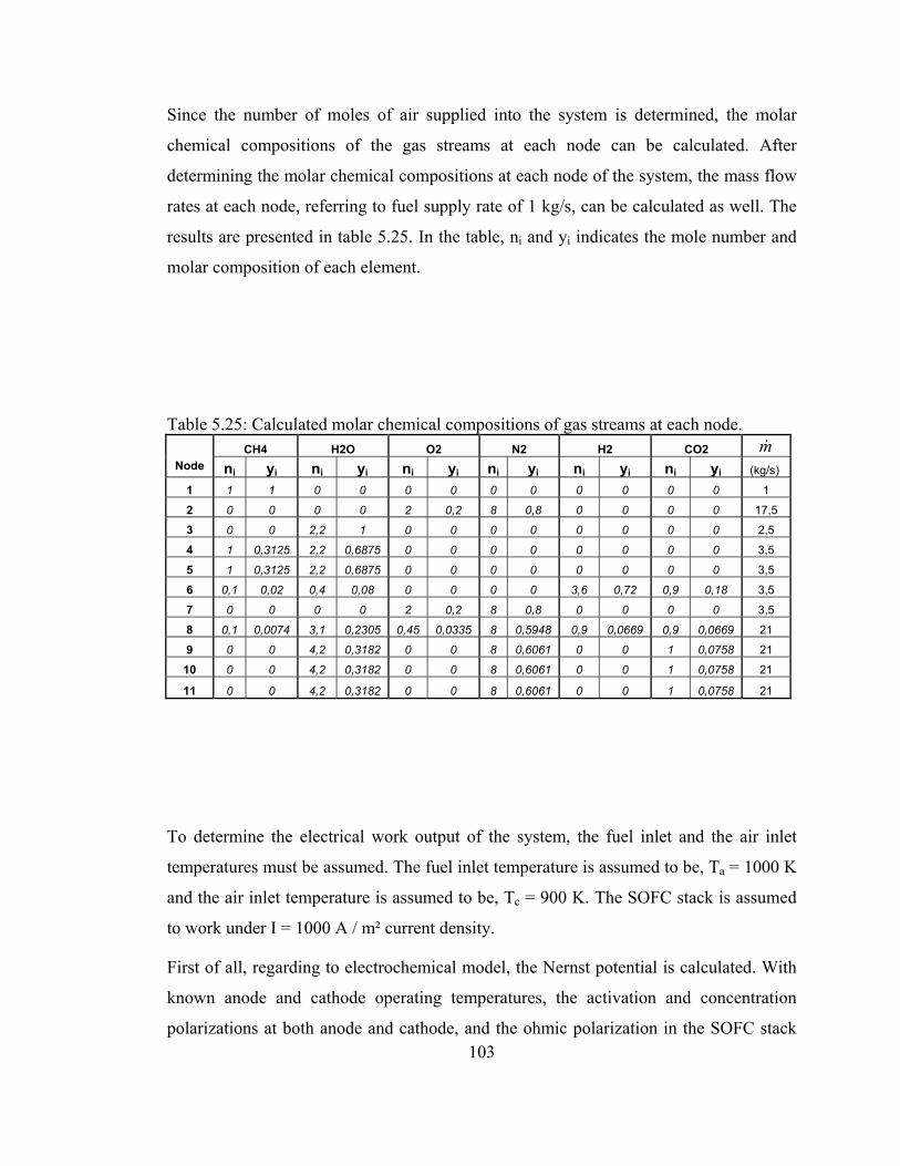
Since the number of moles of air supplied into the system is determined, the molar
chemical compositions of the gas streams at each node can be calculated. After
determining the molar chemical compositions at each node of the system, the mass flow
rates at each node, referring to fuel supply rate of 1 kg/s, can be calculated as well. The
results are presented in table 5.25. In the table, ni and yi indicates the mole number and
molar composition of each element.
Table 5.25: Calculated molar chemical compositions of gas streams at each node. CH4 H2O O2 N2 H2 CO2 m&
Node ni yi ni yi ni yi ni yi ni yi ni yi (kg/s)
1 1 1 0 0 0 0 0 0 0 0 0 0 1
2 0 0 0 0 2 0,2 8 0,8 0 0 0 0 17,5
3 0 0 2,2 1 0 0 0 0 0 0 0 0 2,5
4 1 0,3125 2,2 0,6875 0 0 0 0 0 0 0 0 3,5
5 1 0,3125 2,2 0,6875 0 0 0 0 0 0 0 0 3,5
6 0,1 0,02 0,4 0,08 0 0 0 0 3,6 0,72 0,9 0,18 3,5
7 0 0 0 0 2 0,2 8 0,8 0 0 0 0 3,5
8 0,1 0,0074 3,1 0,2305 0,45 0,0335 8 0,5948 0,9 0,0669 0,9 0,0669 21
9 0 0 4,2 0,3182 0 0 8 0,6061 0 0 1 0,0758 21
10 0 0 4,2 0,3182 0 0 8 0,6061 0 0 1 0,0758 21
11 0 0 4,2 0,3182 0 0 8 0,6061 0 0 1 0,0758 21
To determine the electrical work output of the system, the fuel inlet and the air inlet
temperatures must be assumed. The fuel inlet temperature is assumed to be, Ta = 1000 K
and the air inlet temperature is assumed to be, Tc = 900 K. The SOFC stack is assumed
to work under I = 1000 A / m² current density.
First of all, regarding to electrochemical model, the Nernst potential is calculated. With
known anode and cathode operating temperatures, the activation and concentration
polarizations at both anode and cathode, and the ohmic polarization in the SOFC stack 103
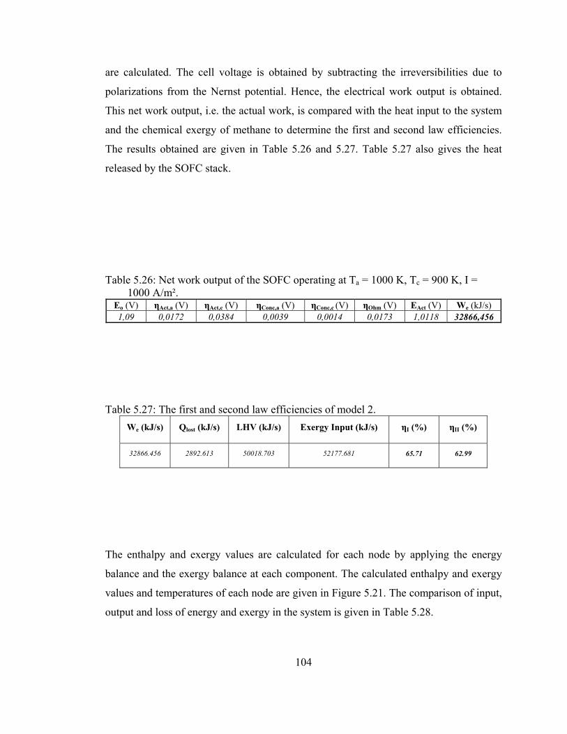
104
are calculated. The cell voltage is obtained by subtracting the irreversibilities due to
polarizations from the Nernst potential. Hence, the electrical work output is obtained.
This net work output, i.e. the actual work, is compared with the heat input to the system
and the chemical exergy of methane to determine the first and second law efficiencies.
The results obtained are given in Table 5.26 and 5.27. Table 5.27 also gives the heat
released by the SOFC stack.
Table 5.26: Net work output of the SOFC operating at Ta = 1000 K, Tc = 900 K, I =
1000 A/m². Eo (V) ηAct,a (V) ηAct,c (V) ηConc,a (V) ηConc,c (V) ηOhm (V) EAct (V) We (kJ/s) 1,09 0,0172 0,0384 0,0039 0,0014 0,0173 1,0118 32866,456
Table 5.27: The first and second law efficiencies of model 2. We (kJ/s) Qlost (kJ/s) LHV (kJ/s) Exergy Input (kJ/s) ηI (%) ηII (%)
32866.456 2892.613 50018.703 52177.681 65.71 62.99
The enthalpy and exergy values are calculated for each node by applying the energy
balance and the exergy balance at each component. The calculated enthalpy and exergy
values and temperatures of each node are given in Figure 5.21. The comparison of input,
output and loss of energy and exergy in the system is given in Table 5.28.
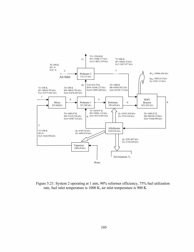
105
Figure 5.21: System 2 operating at 1 atm, 90% reformer efficiency, 75% fuel utilization rate, fuel inlet temperature is 1000 K, air inlet temperature is 900 K.
SOFC
Reactor 1831.025 kJ/s
Vaporizer 2868.29 kJ/s
Preheater 2714.113 kJ/s
Mixer
325.602kJ/s
Preheater 1 357.389 kJ/s
Reformer 993.629 kJ/s
Afterburner3529.976 kJ/s
T11=556.06 K H11=5680.777 kJ/s T7=900 K 11 Ex11=4851.519 kJ/s H7=10665.35 kJ/s
Ex7=5427.977 kJ/s T2=298 K H2= 0 Ex2= 0 2 7
Wact=32866.456 kJ/s Air Inlet Qlost=2892.613 kJ/s
Ex=2101.113 kJ/s
T10=919.79 K T6=1000 K 10 H10=16346.127 kJ/s H6=65443.051 kJ/s T4=298 K T1=298 K Ex10=10993.609 kJ/s Ex6=63238.711 kJ/s H4=50018.703 kJ/s H1=50018.703 kJ/s
Ex4=53476.663 kJ/s Ex1=52177.681 kJ/s
1 4 5
6 8
3
9
T5=1034.97 K H5=55091.112 kJ/s T9=1089.07 K T8=1089.07 K Q1=10351.939 kJ/s Ex5=56712.981 kJ/s H9=21418.536 kJ/s H8=409349.332kJ/s Ex=7519.359 kJ/s
Ex9=14587.316 kJ/s Ex8=31868.094 kJ/s
Q2=6185.36 kJ/s T3=298 K H3=0 Ex=4492.874 kJ/s Ex3=1624.584 kJ/s
Qo=2393.497 kJ/s Ex=1738.569 kJ/s
Environment, To
Water
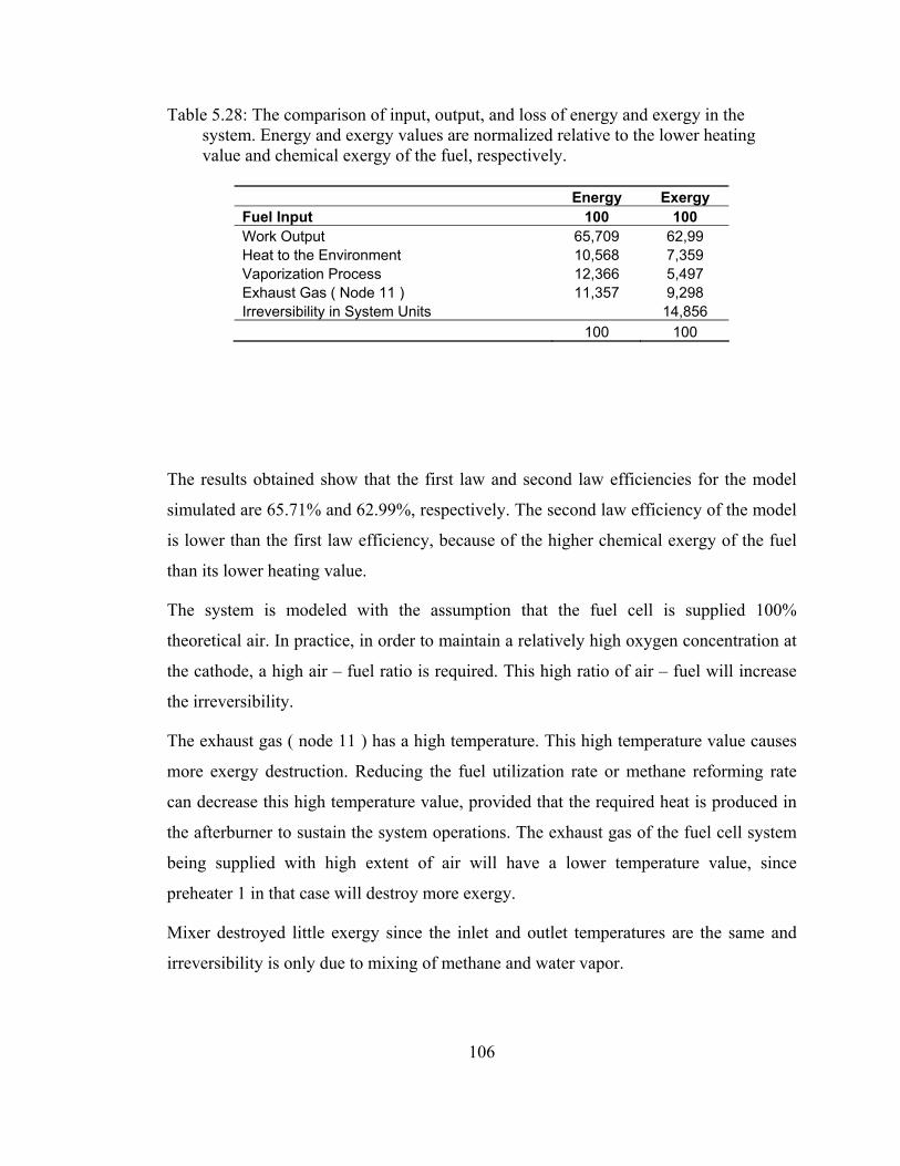
106
Table 5.28: The comparison of input, output, and loss of energy and exergy in the system. Energy and exergy values are normalized relative to the lower heating value and chemical exergy of the fuel, respectively.
Energy Exergy
Fuel Input 100 100 Work Output 65,709 62,99 Heat to the Environment 10,568 7,359 Vaporization Process 12,366 5,497 Exhaust Gas ( Node 11 ) 11,357 9,298 Irreversibility in System Units 14,856
100 100
The results obtained show that the first law and second law efficiencies for the model
simulated are 65.71% and 62.99%, respectively. The second law efficiency of the model
is lower than the first law efficiency, because of the higher chemical exergy of the fuel
than its lower heating value.
The system is modeled with the assumption that the fuel cell is supplied 100%
theoretical air. In practice, in order to maintain a relatively high oxygen concentration at
the cathode, a high air – fuel ratio is required. This high ratio of air – fuel will increase
the irreversibility.
The exhaust gas ( node 11 ) has a high temperature. This high temperature value causes
more exergy destruction. Reducing the fuel utilization rate or methane reforming rate
can decrease this high temperature value, provided that the required heat is produced in
the afterburner to sustain the system operations. The exhaust gas of the fuel cell system
being supplied with high extent of air will have a lower temperature value, since
preheater 1 in that case will destroy more exergy.
Mixer destroyed little exergy since the inlet and outlet temperatures are the same and
irreversibility is only due to mixing of methane and water vapor.

107
The most irreversible process is the combustion in the afterburner. The system with a
high fuel cell exit temperature value would have less irreversibility in the afterburner.
The irreversibility in the SOFC stack would be decreased with a low fuel cell exit
temperature value.
Vaporization process requires heat input. This irreversibility can be eliminated by
developing a recycling fuel cell system which can be used to eliminate the need for the
vaporizer.
Methane reforming causes more exergy destruction within the system. Reducing the
combustion of fuel while reforming as much methane as possible ( hence producing as
much fuel as possible ) would increase the second law efficiency.

108
CHAPTER 6
CONCLUSION
The results obtained for the simulation models show that solid oxide fuel cells have high
second law efficiencies. As discussed before, this high efficiency values are one of the
benefits of fuel cell systems. Solid oxide fuel cell’s high operating temperature caused
less voltage drop, and therefore the irreversibilities occuring inside the fuel cell were
less.
Different configurations for the system might be studied, such as assuming different
methane – water vapor ratio, supplying some extent air, or trying different reformer
efficiency and fuel utilization rate values. Results obtained from these configurations
can be compared with the results obtained in this study to give a more general discussion
to the subject.
High operating temperature of the solid oxide fuel cell system gives the advantage to be
combined with a gas turbine system for higher efficiencies. Studies on this combined
system show that high efficiency values can be obtained this way.
The exhaust gas stream of the solid oxide fuel cell system has high exergy value. This
exhaust gas may be used for local area heating.

109
The vaporizer and afterburner components of the system destroyed more exergy when
compared with the other components of the system. Hence, different alternatives should
be tried in order to increase the second law efficiency of the system.
One of the alternatives can be the elimination of vaporizer. Since water vapor is
produced at the exit of the fuel cell stack, addition of a splitter at the outlet of the fuel
cell stack might be used to recycle the required water vapor to the reformer. The
required water vapor can be recycled from the splitter to the reformer. This arrangement
would eliminate the need for the vaporizer while increasing the system’s second law
efficiency.
Another alternative should consider the heating requirement of the reformer. Since this
heat requirement is supplied by combustion of methane and hydgoren, the fuel
utilization rate and the reformer efficiency are lower. Instead of using hydrogen, some of
the methane entering the system might directly be used to heat the reformer, hence the
reformer efficiency would be higher and system would be modeled in order to reform as
much methane as possible. This way, more methane would be reformed and more fuel
would be produced. Combustion of the fuel should therefore be reduced as much as
possible. Such a model with higher reformer efficiency and fuel utilization rate would
have high second law efficiency.
These alternatives can increase the second law efficiency, and hence offers much better
results. The future works should consider these alternative configurations.
110
REFERENCES
1. “Fuel Cell Handbook ( Fifth Edition )”, EG&G Services Parsons, Inc. Science Applications International Corporation, 2000.
2. Robert H. Perry, Don W. Green, James O. Maloney, “Perry’s Chemical Engineers’ Handbook ( Seventh Edition )”, McGraw-Hill, 1999.
3. J.R. Will Mitchell, “Fuel Cells”, Academic Press, 1963.
4. James Larminie, Andrew Dicks, “Fuel Cell Systems Explained”, John Wiley & Sons, 2000.
5. Reinhold Wurster, “PEM Fuel Cells in Stationary and Mobile Applications: infrastructural requirements, environmental benefits, efficiency advantages and economical implications”, Ludwig-Bölkow-Systemtechnik GmbH, 1997.
6. Michael J. Moran, Howard N. Shapiro, “Fundamentals of Engineering Thermodynamics ( Third Edition )”, John Wiley & Sons, 1998.
7. Jr. Kenneth Wark, “Advanced Thermodynamics For Engineers”, Mc-Graw-Hill, 1995.
8. J.O’M. Bockris, S. Srinivasan, “Fuel Cells: Their Electrochemistry”, McGraw-Hill, 1969.
9. T.J.Kotas, “The Exergy Method of Thermal Plant Analysis”, Butterworths, 1985.
111
10. Adrian Bejan, “Advanced Engineering Thermodynamics”, John Wiley & Sons, 1988.
11. Kai W. Bedringǻs, Ivar S. Ertesvǻg, Stǻle Byggstøyl, Bjørn F. Magnussen, “Exergy Analysis of Solid Oxide Fuel cell ( SOFC ) Systems”, Energy, 4, 1997, 403 – 412.
12. S.H. Chan, C.F. Low, O.L. Ding, “Energy and Exergy Analysis of Simple Solid-Oxide Fuel-Cell Power Systems”, Journal of Power Sources, 103, 2002, 188 – 200.
13. Keith R. Williams, “An Introduction to Fuel Cells”, Elsevier Pub. Co., 1966.
14. Stanley W. Angrist, “Direct Energy Conversion ( Third Edition )”, Allyn and Bacon, Boston, 1976.
15. S.H. Chan, K.A. Khor, Z.T. Xia, “A Complete Polarization Model of a Solid Oxide Fuel Cell and Its Sensitivity to the Change of Cell Component Thickness”, Journal of Power Sources, 93, 2001, 130 – 140.
16. Christie J. Geankoplis, “Mass Transport Phenomena”, Holt, Rinehart and Winston, Inc., 1972.
17. Carl Berger, “Handbook of Fuel Cell Technology”, Prentice-Hall, 1968.
18. Karl Kordesch, Günter Simader, “Fuel Cells and Their Applications”, VCH, 1996.
19. Frank P. Incropera, David P. De Witt, “Fundamentals of Heat and Mass Transfer ( Third Edition )”, John Wiley & Sons, 1990.
20. Signe Kjelstrup Ratkje, Steffen Møller-Holst, “Exergy Efficiency and Local Heat Production in Solid Oxide Fuel Cells”, Electrochimiza Acta, 38, 2/3, 1993, 447 – 453.
Related Documents