NASA Conference Publication 3352 Second Computational Aeroacoustics (CAA) Workshop on Benchmark Problems Edited by C.K.W. Tam and J.C. Hardin Proceedings of a workshop sponsored by the National Aeronautics and Space Administration, Washington, D.C. and the Florida State University, Tallahassee, Florida and held in Tallahassee, Florida November 4-5, 1996 June 1997 /

Welcome message from author
This document is posted to help you gain knowledge. Please leave a comment to let me know what you think about it! Share it to your friends and learn new things together.
Transcript
NASA Conference Publication 3352
Second Computational Aeroacoustics (CAA)Workshop on Benchmark Problems
Edited by
C.K.W. Tam and J.C. Hardin
Proceedings of a workshop sponsored by theNational Aeronautics and Space Administration,
Washington, D.C. and the Florida State University,Tallahassee, Florida
and held in
Tallahassee, FloridaNovember 4-5, 1996
June 1997/
=i
iii i
i
.Y
NASA Conference Publication 3352
Second Computational Aeroacoustics (CAA)Workshop on Benchmark Problems
Edited by
C.K. W. Tam
Florida State University ,, Tallahassee, Florida
J. C. Hardin
Langley Research Center • Hampton, Virginia
Proceedings of a workshop sponsored by the
National Aeronautics and Space Administration,
Washington, D. C. and the Florida State University,Tallahassee, Florida
and held in
Tallahassee, Florida
November 4-5, 1996
National Aeronautics and Space Administration
Langley Research Center • Hampton, Virginia 23681-0001
June 1997
Cover photo
(Contour plot of acoustic pressure field produced by source scattering from cylinder)
E
B
L
EE
!
Printed copies available from the following:
NASA Center for AeroSpace Information
800 Elkridge Landing Road
Linthicum Heights, MD 21090-2934
(301) 621-0390
National Technical Information Service (NTIS)
5285 Port Royal Road
Springfield, VA 22161-2171
(703) 487-4650
ii
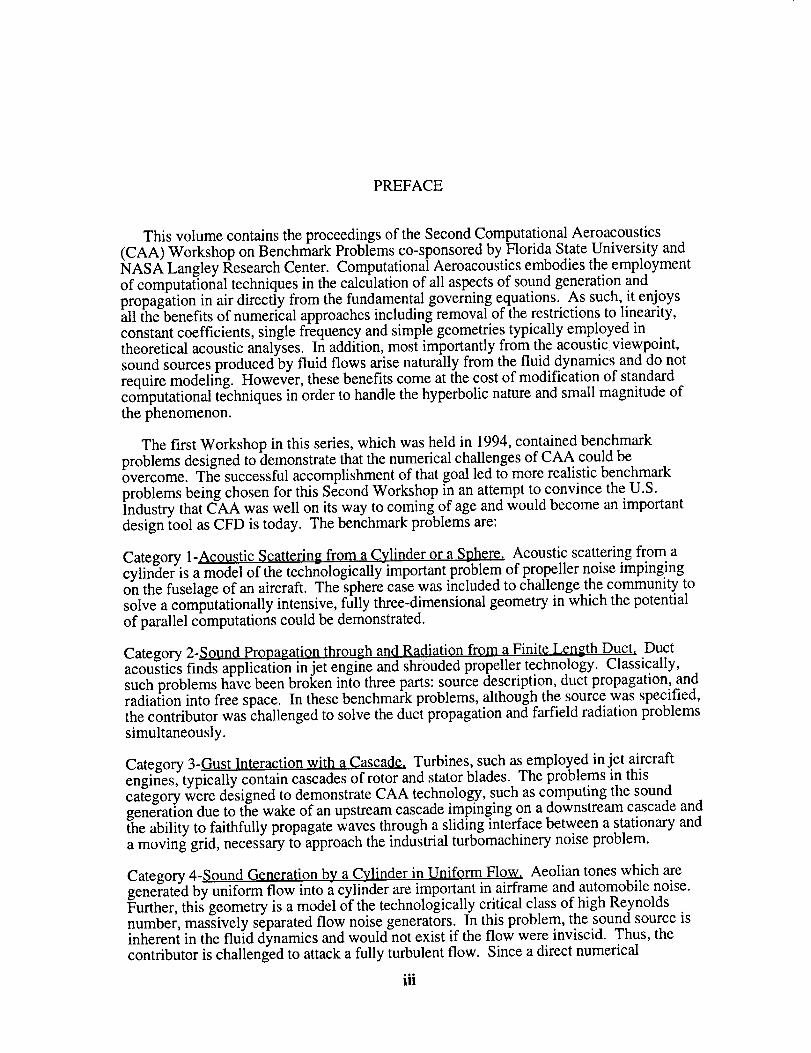
PREFACE
Thisvolumecontainstheproceedingsof theSecondComputationalAeroacoustics(CAA) WorkshoponBenchmarkProblemsco-sponsoredbyFloridaStateUniversityandNASA LangleyResearchCenter.ComputationalAeroacousticsembodiestheemploymentof computationaltechniquesin thecalculationof all aspectsof soundgenerationandpropagationin air directlyfrom thefundamentalgoverningequations.As such,it enjoysall thebenefitsof numericalapproachesincludingremovalof therestrictionsto linearity,constantcoefficients,singlefrequencyandsimplegeometriestypicallyemployedintheoreticalacousticanalyses.In addition,mostimportantlyfrom theacousticviewpoint,soundsourcesproducedby fluid flowsarisenaturallyfrom thefluid dynamicsanddonotrequiremodeling. However,thesebenefitscomeat thecostof modificationof standardcomputationaltechniquesin orderto handlethehyperbolicnatureandsmallmagnitudeofthephenomenon.
Thefirst Workshopin thisseries,whichwasheldin 1994,containedbenchmarkproblemsdesignedto demonstratethatthenumericalchallengesof CAA couldbeovercome.Thesuccessfulaccomplishmentof thatgoalledto morerealisticbenchmarkproblemsbeingchosenfor this SecondWorkshopin anattemptto convincetheU.S.IndustrythatCAA waswell on its wayto comingof ageandwouldbecomeanimportantdesigntool asCFDistoday. Thebenchmarkproblemsare:
Category1-AcousticScattering frgrn a Cylinder or a Sphere. Acoustic scattering from acylinder is a model of the technologically important problem of propeller noise impingingon the fuselage of an aircraft. The sphere case was included to challenge the community to
solve a computationally intensive, fully three-dimensional geometry in which the potentialof parallel computations could be demonstrated.
Category 2-Sound Propagation through and Radiation from a Finite Length Duct. Ductacoustics finds application in jet engine and shrouded propeller technology. Classically,such problems have been broken into three parts: source description, duct propagation, andradiation into free space. In these benchmark problems, although the source was specified,the contributor was challenged to solve the duct propagation and farfield radiation problemssimultaneously.
Category 3-Gust Interaction with a Cascade. Turbines, such as employed in jet aircraftengines, typically contain cascades of rotor and stator blades. The problems in thiscategory were designed to demonstrate CAA technology, such as computing the soundgeneration due to the wake of an upstream cascade impinging on a downstream cascade andthe ability to faithfully propagate waves through a sliding interface between a stationary anda moving grid, necessary to approach the industrial turbomachinery noise problem.
Category 4-Sound Generation by a Cylinder in Uniform Flow. Aeolian tones which aregenerated by uniform flow into a cylinder are important in airframe and automobile noise.Further, this geometry is a model of the technologically critical class of high Reynoldsnumber, massively separated flow noise generators. In this problem, the sound source isinherent in the fluid dynamics and would not exist if the flow were inviscid. Thus, thecontributor is challenged to attack a fully turbulent flow. Since a direct numerical
IIo
Iil
simulation cannot be carried out at the Reynolds number requested with present
computational capabilities, of particular interest is the success of the turbulent modelingemployed and the dimensionality of the solution attempted.
Exact solutions for all but the Category 4 problem are available for comparison and arecontained in this volume.
Christopher K.W. Tam, Florida State UniversityJay C. Hardin, NASA Langley Research Center
i
=im
_iE
iv
ORGANIZING COMMITTEE
This workshop was organized by a Scientific Committee which consisted of:
Thomas Barber, United Technologies Research CenterLeo Dadone, Boeing Helicopters
Sanford Davis, NASA Ames Research Center
Phillip Gliebe, GE Aircraft EnginesYueping Guo, McDonnell Douglas Aircraft Company
Jay C. Hardin, NASA Langley Research CenterRay Hixon, ICOMP, NASA Lewis Research Center
Fang Hu, Old Donfinion UniversityDennis Huff, NASA Lewis Research Center
Sanjiva Lele, Stanford UniversityPhillip Morris, Pennsylvania State University
N.N. Reddy, Lockheed Martin Aeronautical SystemsLakshmi Sankar, Georgia Institute of Technology
Rahul Sen, Boeing Commercial Airplane CompanySteve Shih, ICOMP, NASA Lewis Research Center
Gary Strumolo, Ford Motor CompanyChristopher Tam, Florida State University
James L. Thomas, NASA Langley Research Center
V
m
tl
m|z
mE
m_
m_
k_
CONTENTS
Preface ............................................................................................................................... iii
Organizing Committee ..................................................................................................... v _ ,.7, z
Benchmark Problems ....................................................................................................... 1 -,_1 7
Analytical Solutions of the Category 1, Benchmark Problems I and 2 ....................... 9 /Konstantin A. Kurbatskii
Scattering of Sound by a Sphere: Category 1: Problems 3 and 4 ............................... 15 - 2----Phillip L Morris
-3Radiation of Sound from a Point Source in a Short Duet ........................................... 19
M. K. Myers
Exact Solutions for Sound Radiation from a Circular Duet ....................................... 27 -
Y. C. Cho and K. Uno Ingard
Exact Solution to Category 3 Problems-Turbomachinery Noise ................................ 41 - *3Kenneth C. Hall
Application of the Discontinuous Galerkin Method to Acoustic Scatter Problems.. 45 "gH. L. Atkins
Computation of Acoustic Scattering by a Low-Dispersion Scheme ........................... 57" "7
Oktay Baysal and Dinesh K. Kaushik
Solution of Acoustic Scattering Problems by a Staggered-Grid Spectral DomainDecomposition Method ................................................................................................... 69 "
Peter J. Bismuti and David A. Kopriva
Application of Dispersion-Relation-Preserving Scheme to the Computation ofAcoustic Scattering in Benchmark Problems ............................................................... 79 - [
R. F. Chen and M. Zhuang
Development of Compact Wave Solvers and Applications ......................................... 85 _j6
K.-Y. Fung
Computations of Acoustic Scattering off a Circular Cylinder ................................... 93 "_//
M. Ehtesham Hayder, Gorden Erlebacher, and M. Yousuff Hussaini
Application of an Optimized MacCormack-type Scheme to Acoustic ScatteringProblems ........................................................................................................................ 101 -/2----
Ray Hixon, S.-H. Shih, and Reda R. Mankbadi
Computational Aeroacoustics for Prediction of Acoustic Scattering ....................... 111-7/2Morris Y. Hsi and Fred P6ri6
vii
Application of PML Absorbing Boundary Conditions to the BenchmarkProblems of Computational Aeroacoustics ................................................................. 119
Fang Q. Hu and Joe L. Manthey
Acoustic Calculations with Second- and Fourth-Order Upwind LeapfrogSchemes .......................................................................................................................... 153
Cheolwan Kim and Phillip Roe
Least-Squares Spectral Element Solutions to the CAA Workshop BenchmarkProblems ........................................................................................................................ 165 --/_'
Wen H. Lin and Daniel C. Chan
Adequate Boundary Conditions for Unsteady Aeroacoustic Problems ................... 179 -/7
Yu. B. Radvogin and N. A. Zaitsev
Numerical Boundary Conditions for Computational Aeroacoustics Benchmark _/de/Problems ........................................................................................................................ 191
Christopher K. W. Tam, Konstantin A. Kurbatskii, and Jun Fang
Testing a Linear Propagation Module on Some Acoustic Scattering Problems ..... 221 -'G. S. Djambazov, C.-H. Lai, and K. A. Pericleous
Solution of Aeroacoustic Problems by a Nonlinear, Hybrid Method ....................... 231 -'--_Yusuf 0zy_3riik and Lyle N. Long
Three'Dimensional Calculations of Acoustic Scattering by a Sphere: A ParallelImplementation ............................................................................................................. 241 _-)-,/
Chingwei M. Shieh and Phillip J. Morris
On Computations of Duct Acoustics with Near Cut-Off Frequency ........................ 247 _
Thomas Z. Dong and Louis A. Povinelli
A Computational Aeroacoustics Approach to Duct Acoustics ................................. 259 -- 2-Douglas M. Nark
A Variational Finite Element Method for Computational Aeroacoustic
Calculations of Turbomachinery Noise ....................................................................... 269 _-_2.yKenneth C. Hall
A Parallel Simulation of Gust/Cascade Interaction Noise ........................................ 279 -..2 5"-
David A. Lockard and Phillip J. Morris
Computation of Sound Generated by Flow over a Circular Cylinder: An
Acoustic Analogy Approach ......................................................................................... 289 _,_ _=
Kenneth S. Brentner, J'ared S. Cox, Christopher L. Rumsey, and Bassam A. Younis
Computation of Noise Due to the Flow over a Circular Cylinder ............................ 297 --_ 7
Sanjay Kumarasamy, Richard A. Korpus, and Jewel B. Barlow
A Viscous/Acoustic Splitting Technique for Aeolian Tone Prediction ..................... 305 ---_ 8"
D. Stuart Pope
|
i
i
i
,°°
VlU
Large-Eddy Simulation of a High Reynolds Number Flow around a CylinderIncluding Aeroacoustic Predictions ............................................................................. 319 -_Evangelos T. Spyropoulos and Bayard S. Holmes
A Comparative Study of Low Dispersion Finite Volume Schemes for CAABenchmark Problems ................................................................................................... 329 - _ C_
D. V. Nance, L. N. Sankar, and K. Viswanathan
Overview of Computed Results ................................................................................... 349 "-3/
Christopher K. W. Tam
Solution Comparisons: Category 1: Problems 1 and 2 .............................................. 351
Konstantin A. Kurbatskii and Christopher K. W. Tam /Solution Comparisons. Category 1: Problems 3 and 4. Category 2: Problem 1 ..... 359
Phillip J. Morris /J
Solution Comparisons: Category 2: Problem 2 .......................................................... 3631Konstantin A. Kurbatskii and Christopher K. W. Tam \Solution Comparisons: Category 3 .............................................................................. 367 _J/7"-Kenneth C. Hall
Solution Comparisons: Category 4 .............................................................................. 373Jay C. Hardin
Industry Panel Presentations and Discussions ........................................................... 377,N.N. Reddy
ix
i
i
m_
--7
Benchmark Problems
Category 1 -- Acoustic Scattering
Problem 1
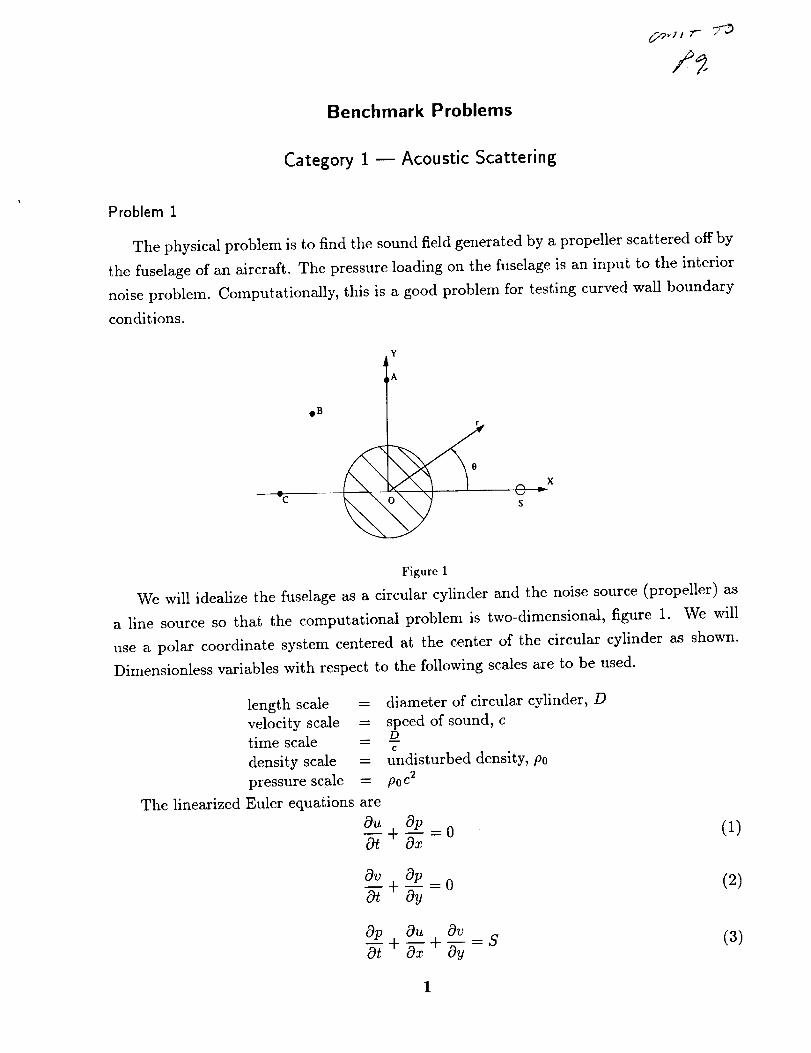
The physical problem is to find the sound field generated by a propeller scattered off by
the fuselage of an aircraft. The pressure loading on the fuselage is an input to the interior
noise problem. Computationally, this is a good problem for testing curved wall boundary
conditions.
Figure 1
We will idealize the fuselage as a circular cylinder and the noise source (propeller) as
a line source so that the computational problem is two-dimensional, figure 1. We will
use a polar coordinate system centered at the center of the circular cylinder as shown.
Dimensionless variables with respect to the following scales are to be used.
length scale
velocity scaletime scale
density scale
pressure scale
= diameter of circular cylinder, D
= speed of sound, c= DO_
c
= undisturbed density, p0
-- PO C2
The linearized Euler equations are
(1)
(2)
cgp Ou Ov
a-7+N+N =s (3)
1
where
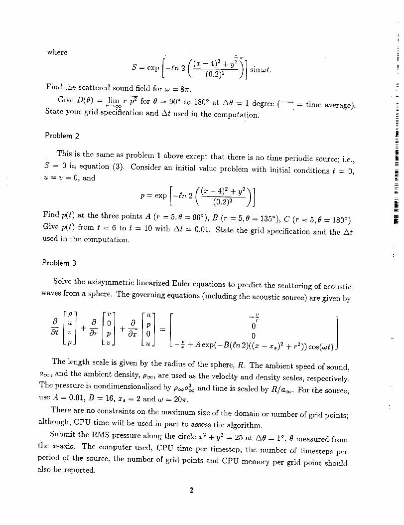
(0.2)2 sinwt.
Find the scattered sound field for _v = 8rr.
GiveD(0) = lira rp2 for0 = 90 ° to 180 ° at A0 = 1 degree (--=
State your grid specification and At used in the Computation.
time average).
Problem 2
This is the same as problem 1 above except that there is no time periodic source; i.e.,
S = 0 in equation (3). Consider an initial value problem with initial conditions t = 0,
u = v = 0, and
Find p(t) at the three points A (r = 5,0 = 90°), B (r = 5,0 = 135°), C (r = 5,0 = 180°).
Give p(t) from t = 6 to t = 10 with At = 0.01. State the grid specification and the At
used in the computation.
Problem 3
Solve the axisymmetric linearized Euler equations to predict the scattering of acoustic
waves from a sphere. The governing equations (including the acoustic source) are given by
[i][i]I0 0 0+N =
p
V
r
0
0
--_ + Aexp(-B(gn2)((x - x,) 2 + r2))cos(wt)
The length scale is given by the radius of the sphere, R. The ambient speed of sound,
ao,, and the ambient density, po_, are used as the velocity and density scales, respectively.
The pressure is nondimensionalized by 2p_ao_ and time is scaled by R/a_. For the source,
use A = 0.01, B = 16, xs = 2 and w = 20rr.
There are no constraints on the maximum size of the domain or number of grid points;
although, CPU time will be used in part to assess the algorithm.
Submit the RMS pressure along the circle x 2 + y2 = 25 at A0 = 1 °, 0 measured from
the x-axis. The computer used, CPU time per timestep, the number of timesteps per
period of the source, the number of grid points and CPU memory per grid point should
also be reported.
_'2
=
|
J|=
m
m
2
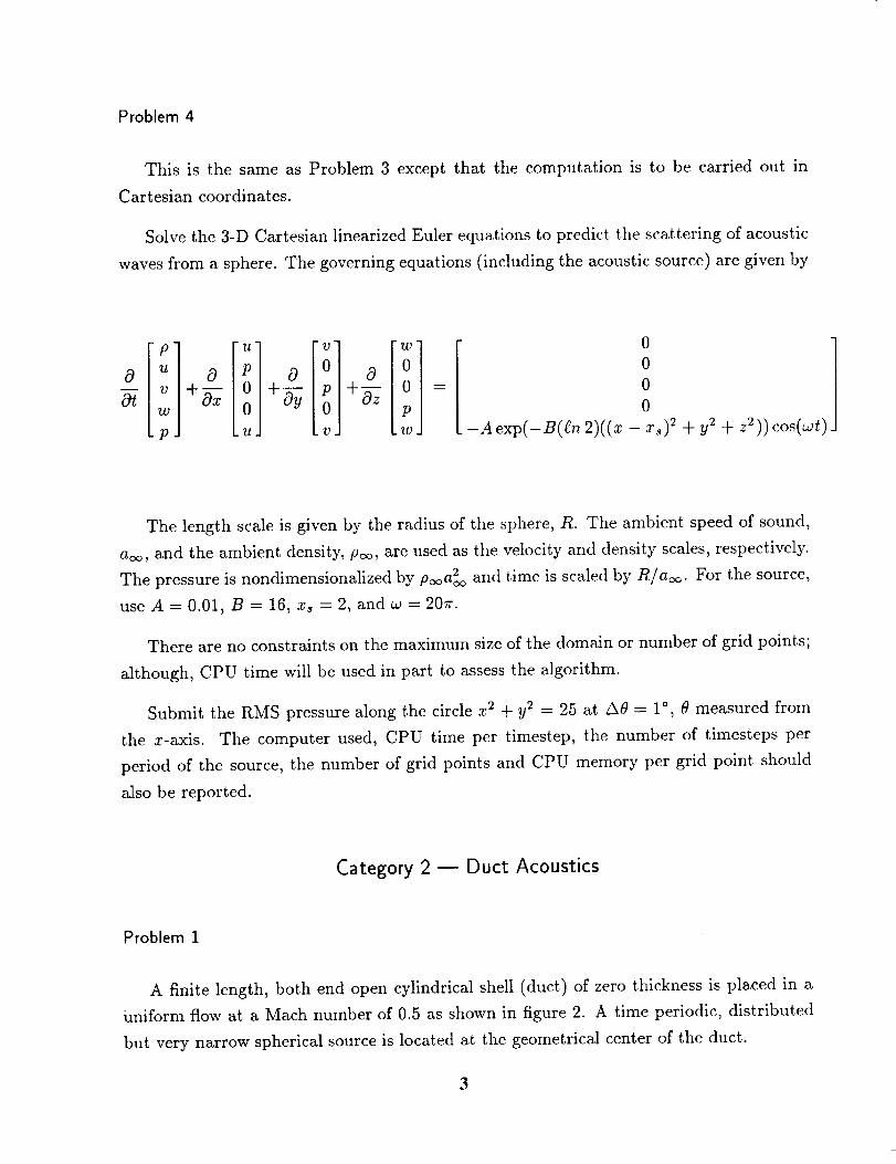
Problem 4
This is the same as Problem 3 except that the computation is to be carried out in
Cartesian coordinates.
Solve the 3-D Cartesian linearized Euler equations to predict the scattering of acoustic
waves from a sphere. The governing equations (including the acoustic source) are given by
_0Ot [i]+2_ +_0
Ox Oy
pJ
;] 0 ]0
0
0
-Aexp(-B(en2)((x - xs) 2 + y2 + z2))cos(wt)
The length scale is given by the radius of the sphere, R. The ambient speed of sound,
ac_, and the ambient density, poo, are used as the velocity and density scales, respectively.
The pressure is nondimensionalized by 2p_aoo and time is scaled by R/ao_. For the source,
use A = 0.01, B = 16, xs = 2, and w = 207r.
There are no constraints on the maximum size of the domain or number of grid points;
although, CPU time will be used in part to assess the algorithm.
Submit the RMS pressure along the circle x 2 + y2 = 25 at A0 = 1°, 0 measured from
the x-axis. The computer used, CPU time per timestep, the number of timesteps per
period of the source, the number of grid points and CPU memory per grid point should
also be reported.
Category 2 -- Duct Acoustics
Problem 1
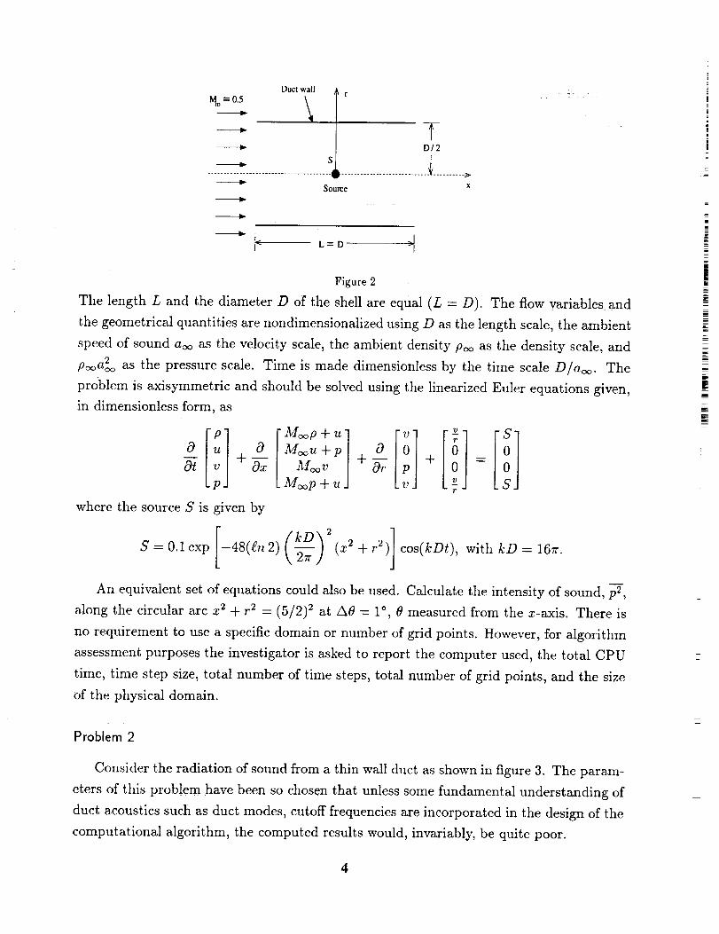
A finite length, both end open cylindrical shell (duct) of zero thickness is placed in a
Uniform flow at a Mach number of 0.5 as shown in figure 2. A time periodic, distributed
but very narrow spherical source is located at the geometrical center of the duct.
Duct wallr
M=0.5___ \
--_" D/2
1S
Source x
Figure 2
The length L and the diameter D of the shell are equal (L = D). The flow variables and
the geometrical quantities are nondimensionalized using D as the length scale, the ambient
speed of sound a_ as the velocity scale, the ambient density p_ as the density scale, and2
p_a_ as the pressure scale. Time is made dimensionless by the time scale D/a_. The
problem is axisymmetric and should be solved using the linearized Euler equations given,
in dimensionless form, as
0 0
0-7P
where the source S' is given by
" Moop + u
M_u + p
Mc_ v
M_p + u
?)
0+
P
?)
S=0.1exp -48(gn2) _ (x 2+r 2) cos(kDt), withkD=167r.
An equivalent set of equations could also be used. Calculate the intensity of sound, _-,
along the circular arc x 2 + r 2 = (5/2) _ at A0 = 1 °, 0 measured from the x-axis. There is
no requirement to use a specific domain or number of grid points. However, for algorithm
assessment purposes the investigator is asked to report the computer used, the total CPU
time, time step size, total number of time steps, total number of grid points, and the size
of the physical domain.
Problem 2
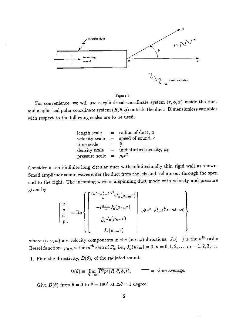
Consider the radiation of sound from a thin wall duct as shown in figure 3. The param-
eters of this problem have been so chosen that unless some fundamental understanding of
duct acoustics such as duct modes, cutoff frequencies are incorporated in the design of the
computational algorithm, the computed results would, invariably, be quite poor.
ii
mi
|m=
i
i
t
mE
, / circilar duct
I incomingsound
R
o x
_sound radiation
Figure 3
For convenience, we will use a cylindrical coordinate system (r, ¢, x) inside the duct
and a spherical polar coordinate system (R, O, ¢) outside the duct. Dimensionless variables
with respect to the following scales are to be used.
length scale = radius of duct, a
velocity scale = speed of sound, ctime scale = _-
C
density scale = undisturbed density, p0
pressure scale = p0c 2
Consider a semi-infinite long circular duct with infinitesimally thin rigid wall as shown.
Small amplitude sound waves enter the duct from the left and radiate out through the open
end to the right. The incoming wave is a spinning duct mode with velocity and pressure
given by
i -'- Re
P
2 2 t/2(+ -t%m) Jn(pnmr)
oJ
-i 2: s'(...,,-)
"--J.(u..:')hg r
ei[(w2-#_,_) _x+n¢-wt]
L J.(U..:)
where (u, v, w) axe velocity components in the (x, r, ¢) directions. ,In( ) is the n th order
Besselfunction. #nm is the mth zero of J_; i.e., ,,(#nrn)=0, n=0,1,2,., m 1,2,3, ....
1. Find the directivity, D(0), of the radiated sound.
D(8) = lim R2p2(R,O,¢,t),R'---* oo
--= time average.
Give D(O) from 0 = 0 to 0 = 180 ° at A0 = 1 degree.
5
2. Find the pressure envelope inside the duct along the four radial lines r = 0, 0.34, 0.55,
0.79. The pressure envelope, P(x), is given by
P(x)= max p(r,¢,x,t).over time
Give P(x) from x = -6 to x = 0 at Ax = 0.1.
For both parts of the problem, consider only n = 0, m = 2 and the two cases
(a) co = 7.2
(b) = 10.3Note: #o2 = 7.0156. You are to solve the linearized Euler equations.
Category 3 m Turbomachinery Noise
The purpose of these problems is to study the computational requirements for modeling
the aeroacoustic response of typical rotor-stator interactions that generates tonal noise in
turbomachinery. You may solve either the full Euler or Ilne_(zedEuier equations. Be sure
to specify the grid size, the total CPU time required, the CPU t:[me per period, and the
type of computer used for each problem.
and. L
. :=
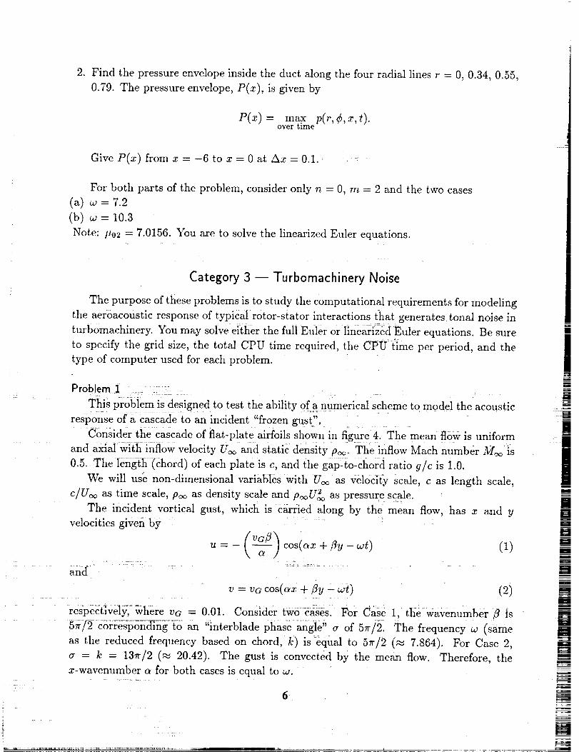
This problem........ is designed to test the ability of a numerical scheme to model the acoustic
response ofacascade to an incident "frozen gust_,',_
ConslaeT_h_-c_scaae of flat-plate airfoils Shown in figure41 The mean flow is uniform
and axial wi{h inflow velocity Uoo and s{atiC density po_. The inflow Mach number M_:{S
0.5. The length (chord) of each plate is c, and {he gap-ico-chord ratio g/c is i.0.
: We will use non-dimensional variables with U_ as velodty scale, c as length scale,
c/U_ as time scale, poo as density scale and pooU_ as pressure scale.
The incident:vortical gust, which is carried along by the mean flow; has z and y
velocities givefi by ......
v = cos( x + av (2)
respectiveiy;::where vG = 0.01. Consider two cases. For CaSe 1, the Wavenumber/3 is
g_r[2 Correspond{ng:{o an "interblade phase angle!' a of 5rr/2. The frequency w (same
as the reduced frequency based on chord, k)_is equal to 5rr/2 (_ 7'864). For Case 2,
a = k = 13_r/2 (_ 20.42). The gust is convected by the mean flow. Therefore, the
x-wavenumber _ for both cases is equal to co.:
: : : : :: : Z72 L ::
7;
Z !
!m
mNi
Ii
l
I
m
U
IN
Computational __
Domain _X .
GUST
Ua_
Periodic Boundaty..__ _ Vgrid ---- U
I
0 1 2 x
Reference Plate
with length e
Figure 4
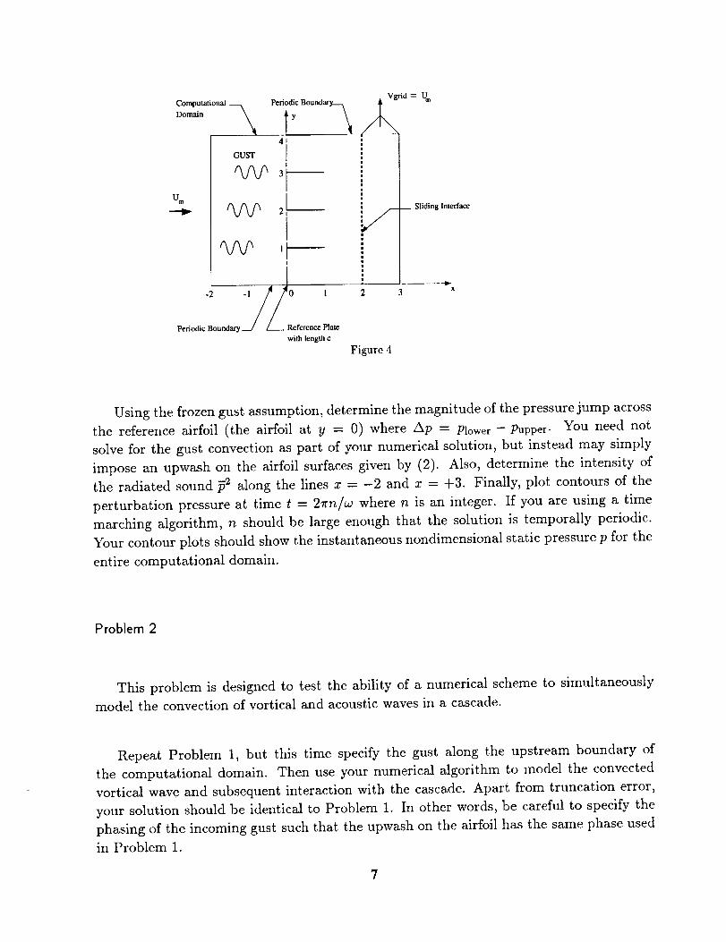
Using the frozen gust assumption, determine the magnitude of the pressure jump across
the reference airfoil (the airfoil at y = 0) where Ap = Plower- Pupper. You need not
solve for the gust convection as part of your numerical solution, but instead may simply
impose an upwash on the airfoil surfaces given by (2). Also, determine the intensity of
the radiated sound _2 along the lines z = -2 and z = +3. Finally, plot contours of the
perturbation pressure at time t = 2rrr_/w where n is an integer. If you are using a time
marching algorithm, n should be large enough that the solution is temporally periodic.
Your contour plots should show the instantaneous nondimensional static pressure p for the
entire computational domain.
Problem 2
This problem is designed to test the ability of a numerical scheme to simultaneously
model the convection of vortical and acoustic waves in a cascade.
Repeat Problem 1, but this time specify the gust along the upstream boundary of
the computational domain. Then use your numerical algorithm to model the convected
vortical wave and subsequent interaction with the cascade. Apart from truncation error,
your solution should be identical to Problem 1. In other words, be careful to specify the
phasing of the incoming gust such that the upwash on the airfoil has the same phase used
in Problem 1.
7
Problem 3L77:
This problem is designed to test the ability of a numerical scheme to model the p_0p-
agation of acoustic and vortical waves across a sliding-interface typical of those used in
rotor stator interaction problems.
Repeat Problem 2, but translate the portion of the grid aft of the line x = 2 in the
positive ?]-direction with speed 1. If possible, arrange the sliding grid motion so that at
times corresponding to the start of each period (t = 27rn/w) the sliding grid is in the
original nonsiiding position. This will aid in the plotting and evaluation of solutions.
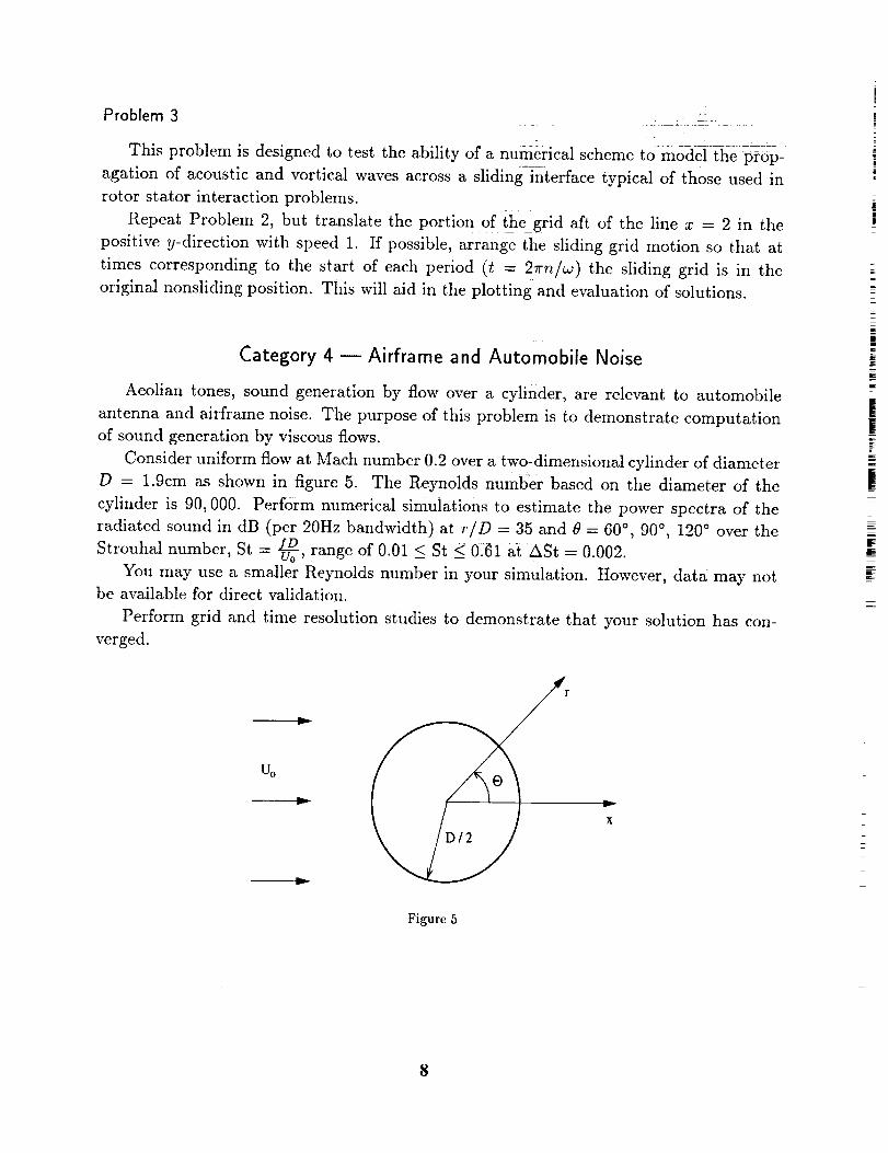
Category 4 m Airframe and Automobile Noise
Aeolian tones, sound generation by flow over a cylinder, are relevant to automobile
antenna and airfl'ame noise. The purpose of this problem is to demonstrate computation
of sound generation by viscous flows.
Consider uniform flow at Math number 0.2 over a two-dimensional cylinder of diameter
D = 1.9cln as shown in figure 5. The Reynolds number based on the diameter of the
cylinder is 90,000. Perform numerical simulations to estimate the power spectra of the
radiated sound in dB (per 20Hz bandwidth) at r/D = 35 and 0 = 60 °, 90 °, 120 ° over the
Strouhal number, St = u/_-0D, range of 0.01 < St __ 0'61 a{ ASt = 0.002,
You may use a smaller Reynolds number in your simulation. However, data may notbe available for direct validation.
Perform grid and time resolution studies to demonstrate that your solution has con-
verged.
|R
i
i
F
le
E
Co
v
Figure 5
x
8
ANALYTICAL SOLUTIONS OF THE CATEGORY 1,
BENCHMARK PROBLEMS i AND 2
Konstantin A. Kurbatskii
Department of Mathematics
Florida State University
5t - 4,/_
Tallahassee, FL 32306-3027
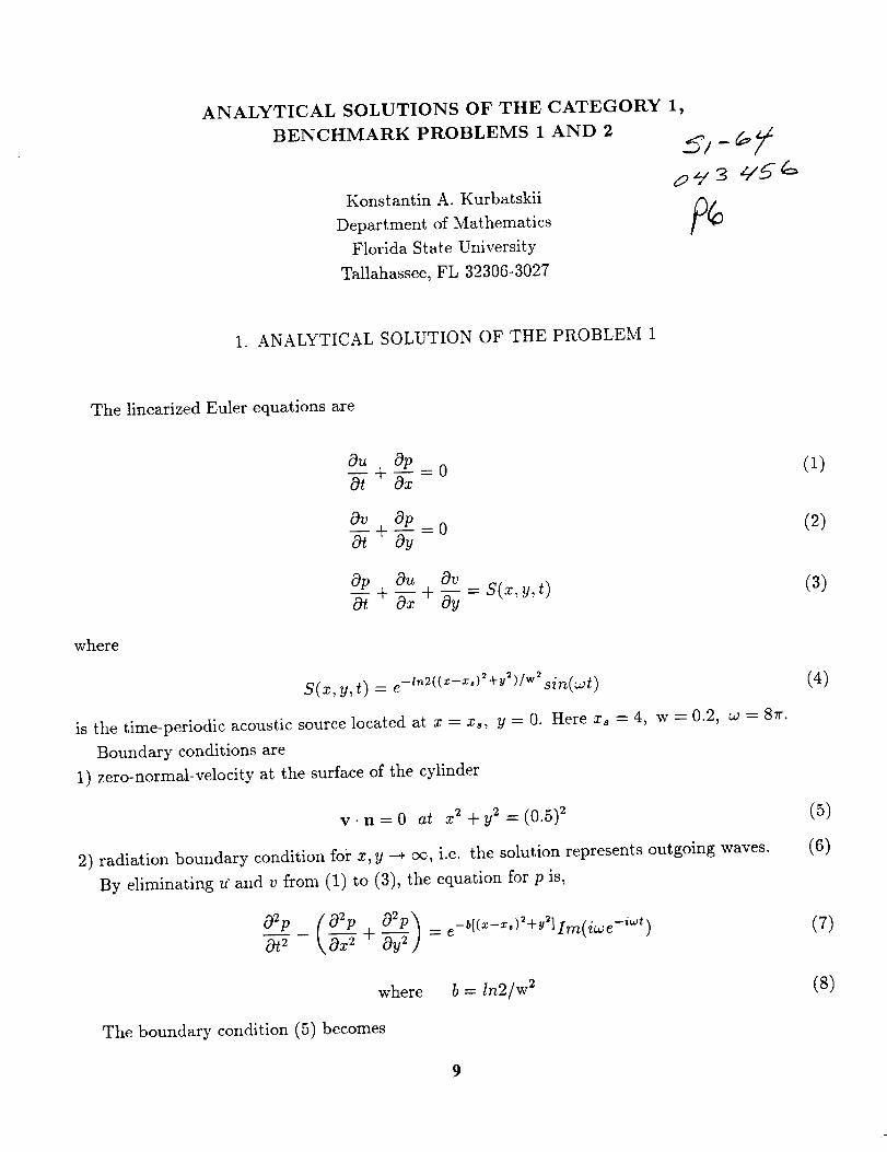
1. ANALYTICAL SOLUTION OF THE PROBLEM 1
The linearized Euler equations are
Ou Op = 00-7+ 0-7
Op Ou Ov-_ + _x + o_ = s(x,_,_)
where
S(x, y, t) = e-l"2((_-_')2 +u_)/W_sin(a_t)
is the time-periodic acoustic source located at x = xs, y = 0. Here xs = 4, w = 0.2, w = 87r.
Boundary conditions are
1) zero-normal-velocity at the surface of the cylinder
v . n = O at x 2 4- y2 - (0.5)_
2) radiation boundary condition for x, y --+ oc, i.e. the solution represents outgoing waves.
By eliminating u" and v from (1) to (3), the equation for p is,
O2p (O2p O2p_ e-b[(x-z,)2+y2]im(iaJe-i_t )o_ \-g_+ N_ ) =
where b = In2/w 2
The boundary condition (5) becomes
(1)
(2)
(3)
(4)
(5)
(6)
(7)
(s)
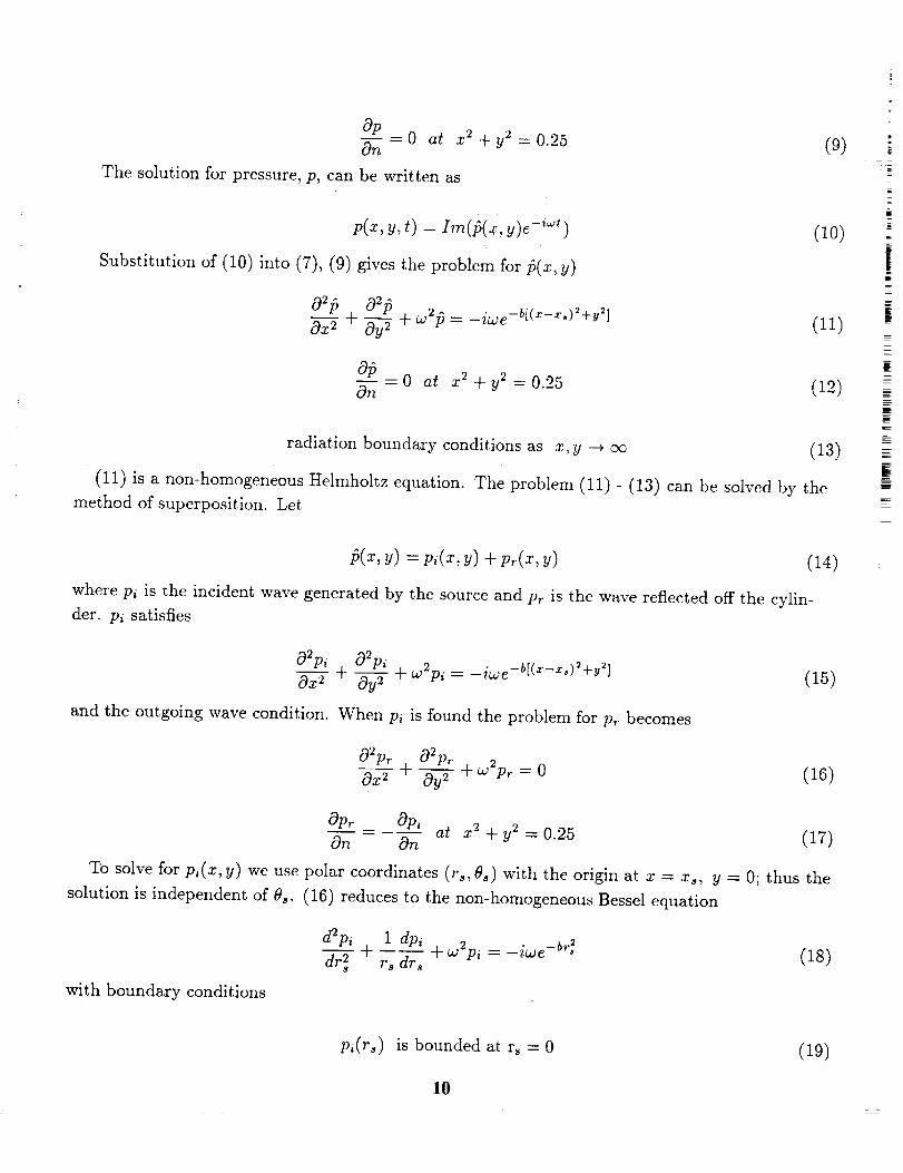
__OP=0 at z_+y2=0.25 (9) _;
The solution for pressure, p, can be written as
p(x,y,t) = !m(_(x,g)e -i_') (10)
|Substitution of (10) into (7), (9) gives the problem for _(x,y)
02D 02P -ia;e -b[(x-=')_+y_] (11)Ox----7 + _ + _2i_ =
015 _ g2On -0 at x _+ =0.25 (12)
radiation boundary conditions as x, y --4 oc (13)
(11) is a non-homogeneous I-Ielmholtz equation. The problem (11) - (13) can be solved by the
method of superposition. Let
_(_,y) = pi(x,_) + p_(x,y) (14)
where pi is the incident wave generated by the source and p_ is the wave reflected off the cylin-
der. pi satisfies
-4- w2pi --" -iwe -b[(_-_')_ +y_]
and the outgoing wave condition. When pi is found the problem for p_ becomes
(15)
02pr 02pr
Ox---7- + _ + W2p_ = 0 (16)
Op____Z__= Opi at x 2 + g2 = 0.25 (17)On On
To solve for p,(z, y) we use polar coordinates (r=, 0_) with the origin at x = z=, y = 0; thus the
solution is independent of 0_. (16) reduces to the non-homogeneous Bessel equation
d2Pi d- 1 dpi -4-wZpi --iwe -br_ (18)dr] r s dr=
with boundary conditions
pi(r=) is bounded at r= = 0 (19)
10
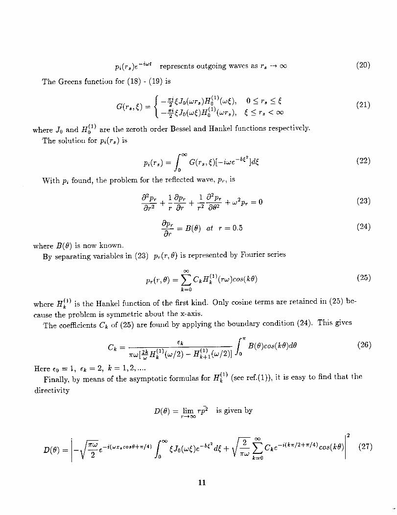
pi(rs)e -i_t represents outgoing waves as rs --, cc
The Greens function for (18)- (19) is
(20)
G(rs,() = ___(j0(w()H_l)(wr_), ( _< % < oc
where J0 and H_ 1) are the zeroth order BesseI and Hankel functions respectively.
The solution for pi(rs) is
(21)
_0 °(3pi(r_) = G(r_,_)[-iwe-b_2]d_
With pi found, the problem for the reflected wave, pr, is
(22)
02pr 1 Opt 1 02p_Or------_ + -_ + + _o2p_ = 0r Or r 2 002
(23)
Pr
Or -B(O) at r=0.5
where B(O) is now known.
By separating variables in (23) pr(r, 0) is represented by Fourier series
(24)
pr(r,O) = E CkH_l)(ra_)c°s(kO) (25)
k=0
(1)where H k is the Hankel function of the first kind. Only cosine terms are retained in (25) be-
cause the problem is symmetric about the x-axis.
The coefficients Ck of (25) are found by applying the boundary condition (24). This gives
gTek B(O)co (kO)dO (26)
Ck "- 71.co[2kH(1) (1) (W 2L-L- k (W/2)-- Hk+l, / )]
Heree0 =I, ek=2, k= 1,2, ....
Finally, by means of the asymptotic formulas for H_ 1) (see ref.(1)), it is easy to find that the
directivity
D(O) = llm rp 2 is given byr --), oo
D(O) = r(Jo(w_)e -b_ d( + Cke-i(_'_/2+'_/4) cos(kO)
k=O
(27)
II
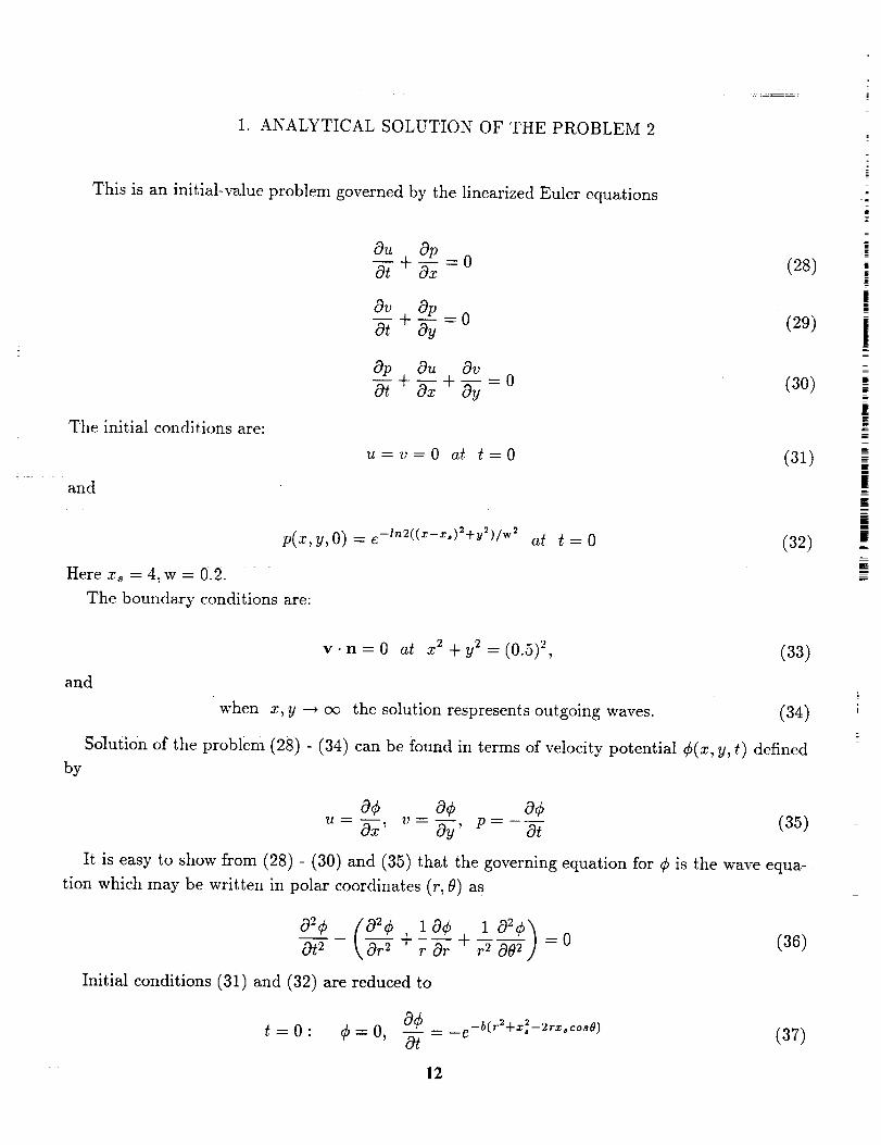
I. ANALYTICAL SOLUTION OF THE PROBLEM 2
This is an initial-value problem governedby the linearized Euler equations
The initial conditions are:
and
p(x, y, 0) = e -u'2((,-*'):+y2)/w2
Here xs = 4, w = 0.2.
The boundary conditions are:
=
i
IiE
Ou Op-_ + N = 0 (28)
Ov OpN + _yy = 0 (29)
Op Ou OvN + _ + N = 0 (30)
u=v=0 at t 0 (31)
lE
l
at t = 0 (32) _*E
and
v.n=O at x 2+y2=(0.5) 2, (33)
when x, y ---+ oc the solution respresents outgoing waves. (34)
Solution of the problem (28) - (34) can be found in terms of velocity potential ¢(x, y, t) defined
by
0¢ 0¢ 0¢= N' "= 0_' p - ot (35)
It is easy to show from (28) - (30) and (35) that the governing equation for ¢ is the wave equa-
tion which may be written in polar coordinates (r, O) as
102¢ f82¢ 10¢ __02¢_Ot 2 \ Or 2 + r -_r + r 2 002 ,] = 0 (36)
Initial conditions (31) and (32) are reduced to
t=O:¢=0, Ot - e (37)
12
where b = In2/w 2.
Boundary condition (33) becomes
0¢ o at r 0.5 (3S)Or
The problem (36) - (38) can be solved by the method of superposition. Let
¢(r,/9,t) = ¢_(r,/9,t)+ Cr(_,/9,t) (39)
where ¢i is the incident wave generated by the initial pressure pulse, and Cr is the wave reflected
off the cylinder. ¢i(r,/9, t) satisfies
02¢i (0 2¢i 1 0¢iOr2 _,0_ + --_, ] = 0 (4O)
with the initial conditions
0¢i _ _b_ (41)t=O: ¢i=0, Ot e
where (%,/gs) are the polar coordinates with the origin at x = xs, y = O.
The initial value problem of (40) and (41) can be solved by means of the order-zero Hankel
transform. The solution is (see ref.(2))
lf0_¢i(_s,t) = -2-_
or in terms of (r,/9) coordinates
e--b_2/(4b) Zo(o.)rs ).si12(o3t )do.)
fo :x)¢i(r,O,t) = Ai(r,O,w)sin(wt)dw (42)
where Ai(r, 0,w) = 1 _b_2/(4b) r£bo _0(wv/_2+ x_ - 2_x_co_0) (43)
The problem for ¢_ is
02¢_ (02¢r 1 0¢r 1 02¢_)Ot 2 _,0r 2 +-_+ =0 (44)r Or r 2 002
0¢_ 0¢i0---_-= - 0--_- at r = 0.5 (45)
In view of (42) we will represent the solution for ¢_ by Fourier sine transform it t,
f0 _¢_(r,/9, t) = A_(r,O,w)sin(wt)dw (46)
13
Substitution of (46)into (44), (45) gives=
02At 1 OAr 10ZA,.
Or 2 + + +ofiA = 0 (47) :r Or r 2 002 ._I
_rr |= B(6,o_) at r =0.5 (48)
]where B(0,0J)= OA.___i (49) iOr It=0.5
(47) can be solved by separation of variables giving,
O0
A4r, e,_) = _ Ck(_)lC_l)(r_)co_(ke) (50)k=0
The coefficients Ck of (50) are found by applying the boundary condition (48). It is straight-
forward to find,
_ B(e,_)cos(ke)de (51)Ck = 7rw[ZkH(1) ' ,,,,--d k (w/z)- g_l(w/2)]
Finaiiy, substitution of (50), (51) into (46) and on combining (42), (46), the velocity potential
is found,
where
j00 _¢(r,e,t) = A(r,e,_)_i.(_t)d_ (52)
!
[]
im
g-bw=/(4b){2/) OO [ 71"_3[_-H_I)(O2/2)_kH(kl)(Fc'O)g°'S(ICe)--A(_,e,_) = Jo(_/_ _+ _ - 2_z._o.e) + F_.n_
.. k+l (w/2)]D "(1)k=0
r + (53)]0 v/0.25 + x] - x,cos_ JThe pressure field may be calculated by
f0 _
p(_,e,t) = _o¢ = _ A(_,e,_)_¢o.(_t)d_Ot
(54)
REFERENCES
1. Abramowitz, M.; and Stegun, I.A.: Handbook of Mathematical Functions.
2. Tam, C.K.W.; and Webb, J.C.: Dispersion-Relation-Preserving Finite Difference Schemes for
Computational Acoustics. J. Comput. Phys., vol. 107, Aug. 1993, pp. 262-281.
14
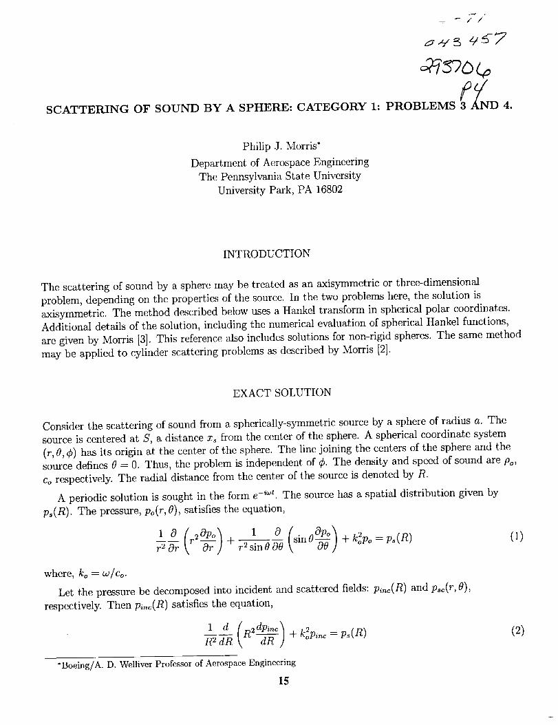
SCATTERING OF SOUND BY A SPHERE: CATEGORY 1: PROBLEMS 3_NDo
Philip J. Morris*
Department of Aerospace Engineering
The Pennsylvania State University
University Park, PA 16802
INTRODUCTION
The scattering of sound by a sphere may be treated as an axisymmetric or three-dimensional
problem, depending on the properties of the source. In the two problems here, the solution is
axisymmetric. The method described below uses a Hankel transform in spherical polar coordinates.
Additional details of the solution, including the numerical evaluation of spherical Hankel functions,
are given by Morris [3]. This reference also includes solutions for non-rigid spheres. The same method
may be applied to cylinder scattering problems as described by Morris [2].
EXACT SOLUTION
Consider the scattering of sound from a spherically-symmetric source by a sphere of radius a. The
source is centered at S, a distance x_ from the center of the sphere. A spherical coordinate system
(r, 9, ¢) has its origin at the center of the sphere. The line joining the centers of the sphere and the
source defines 9 = 0. Thus, the problem is independent of ¢. The density and speed of sound are Po,
co respectively. The radial distance from the center of the source is denoted by R.
A periodic solution is sought in the form e -_t. The source has a spatial distribution given by
p,(R). The pressure, po(r, 0), satisfies the equation,
r20r r2or) +r2sinO00 sinO +koPo--p_(R ) (1)
where, ko = w/co.
Let the pressure be decomposed into incident and scattered fields: pi_c(R) and p,c(r, 9),
respectively. Then p_nc(R) satisfies the equation,
1 d R2 + kop_nc -- p_ (R)R 2 dR
*Boeing/A. D. Welliver Professor of Aerospace Engineering
(2)
15
and the scatteredfield satisfiesthe homogeneousform of Eq. (I). -::_ ,
The solution for the incident field is obtained here through the useof a Hankel transform, given by
oc
G(s)= -2 R2 jo(sR)g(R)dR (3) _'T"
0
g(R)--/s2j°(sR)G(s)dSo (4) i
where jn(z) is the spherical Bessel function of the first kind and order n. The properties of spherical
Bessel functions are given by Abramowitz and Stegun [1]. i
Now, integration by parts and the use of general expressions for the derivatives of spherical Bessel ||
functions [1], gives i
_ n _3o(ns) N_ n _ dR = -s2a(s) (5) .
So, the Hankel transform of Eq. (2) leads to i
p_n_(R) = - jo(sR)P_(s) z0 (s 2 _ k2o) ds (6) _--
where,
P_(s) = -rr2/R2jo(sR)p,(R)d R0
Now, with R = Cr 2 + x_ - 2rx_ cos 0, Abramowitz and Stegun [1] give an addition theorem forspherical Bessel functions,
z
(7)
sin(sR)jo(_n) - _n
oo
-- -- _(2n + 1) j,,(sr) jn(sx,) P,(cos0)n=0
(8)
where P, (cos 0) is the Legendre polynomial of order n. Thus, from Eqs. (6) and (8),
c_
p_,_(R) = - y_' (2n + 1) Pn(cos 0) I_(r)n=0
where,
f s_j.(_) j.(_) P_(_)(s 2 _ k2 ) es
The general solution for the scattered field may be written in separable form as
oo
p_(r,O) = _ A_h_)(kor) P,(eos 0)n_O
16
(9)
(_o)
(11)
whereh O) (z) is the spherical Hankel function of the first kind and order n.
At the boundary of the sphere we require that the normal derivative of the pressure be zero. So
that,
A,, = (2n, + 1) I'_(a)ko (1), (12)hn (koa)
where,
j (82_ ko ds0
j_(z) denotes the derivative of j_(z) with respect to z and is given by
j'n(z) = jn-l(Z) - (n + 1) jn(z)/z
with fo(Z) = -jl (z). Identical forms of expression may be used for the spherical Hankel function
derivatives.
Now, consider a spherically-symmetric, spatially-distributed Gaussian source given by
ps(R) = aexp(-bR 2)
(13)
(14)
(15)
Then, from Eq. (7),
Ps(s) = a exp(_s2/4b ) (16)2bv/_
In this case, neither the incident field nor the unknown integrals I_ (a) and I'_ (a) may be evaluated
analytically. However, they may be obtained numerically. The numerical procedure used involves the
use of an integration contour in the complex s plane to include the effect of the pole at s = ko. It is
described by Morris [2] and is not repeated here.
In the present problem, where the source is introduced into the linearized energy equation,
a = -ikoA (17)
b = B
and
A=0.01, B=16, xs=2
Different frequencies are considered in the model problems.
(18)
REFERENCES
[1] M. Abramowitz and I. A. Stegun. Handbook of Mathematical Functions. Dover, 1965.
[2] P. J. Morris. The scattering of sound from a spatially-distributed axisymmetric cylindrical source
by a circular cylinder. Journal of the Acoustical Society of America, 97(5):2651-2656, 1995.
[3] P. J. Morris. Scattering of sound from a spatially-distributed, spherically-symmetric source by a
sphere. Journal of the Acoustical Society of America, 98(6):3536-3539, 1995.
17
!
?
!
|IE
r,Im
i
RADIATION OF SOUND FROM A POINT SOURCE
IN A SHORT DUCT
M. K. Myers
The George Washington University
Joint Institute for Advancement of Flight Sciences
Hampton, VA
-:1/
7?z
INTRODUCTION
It is the purpose of this paper to provide, in relatively brief form, a summary of a boundary
integral approach that has been developed for calculating the sound field radiated from short ducts in
uniform axial motion. The method was devised primarily to study sound generated by rotating sources
in the duct, as is of current practical interest in connection with ducted-fan aircraft engines. Detailed
background on the fan source application of the technique can be found in refs. 1 and 2. The author has
not previously discussed the simpler monopole source case of interest in these proceedings. However,
readers desiring a more detailed treatment than will be included here should have little difficulty in
extracting it from those references after making the relatively minor modifications necessary to adapt the
analyses to the monopole case.
It should be noted that other authors have also considered radiation from short ducts. In
particular, readers may find the finite-element approach of Eversman [3] of interest as well as the
alternate boundary integral method treatments of Martinez [4] and of Dunn, Tweed, and Farassat [5].
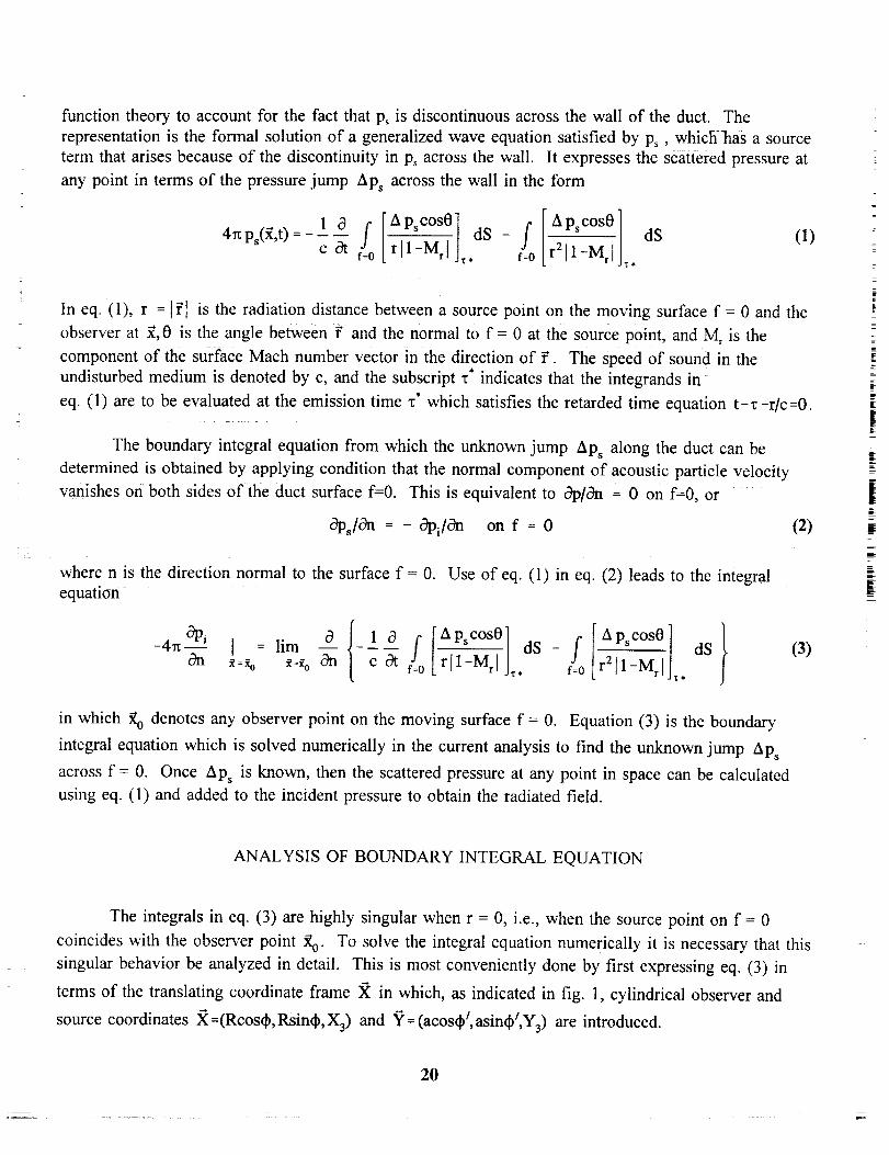
BOUNDARY INTEGRAL EQUATION
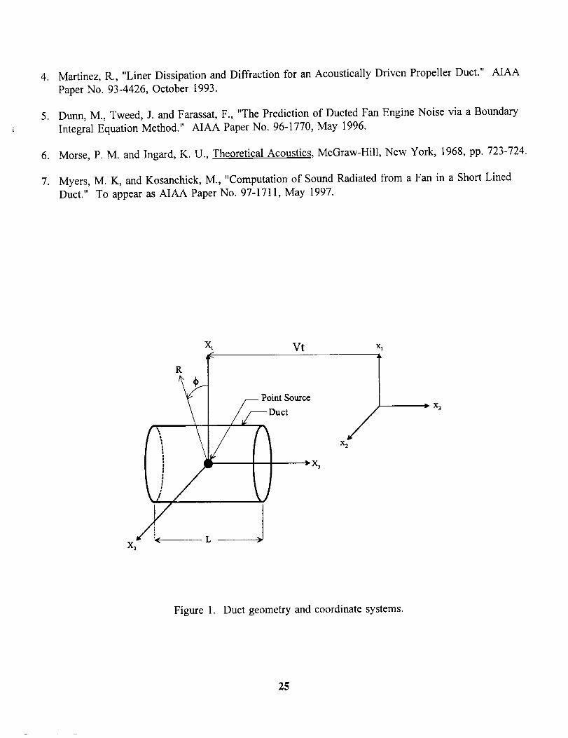
The problem to be considered is illustrated in fig. 1. An infinitesimally thin, rigid circular
cylinder of radius a and length L moves at subsonic speed V in the negative x 3 direction relative to a
frame of reference 2 fixed in fluid at rest. The duct encloses a monopole source located at its center,
which is taken as the origin of a co-moving system X. The monopole emits sound harmonically at
circular frequency m in the moving frame X. The objective is to determine the acoustic field radiated
into infinite space through the ends of the moving duct.
The field is assumed to be described by the linearized equations of ideal isentropic compressible
fluid motion. The problem is expressed in a scattering formulation in which the acoustic pressure is
written as p = p_ + Ps, where the incident pressure p_ is the free-space field radiated by the monopole
source in the absence of the duct. The scattered pressure ps(z_,t) is then sought as an outgoing solution
to the homogeneous wave equation subject to appropriate boundary conditions on the inner and outer
surfaces of the duct.
As shown elsewhere [1, 2], an integral representation of p_ is obtained by utilizing generalized
19
function theory to accountfor the fact that Psis discontinuousacrossthewall of the duct. Therepresentationis the formal solutionof a generalizedwave equationsatisfiedby Ps, which hasa sourceterm that arisesbecauseof the discontinuityin Psacrossthe wall. It expressesthe scatteredpressureatanypoint in termsof the pressurejump Aps acrossthe wall in the form
4r_ps(:_,t)- l a [ A pscos0] [ A p cos0 ]c & f[0[r]l---_] ],,dS - f=of r2il---_rlJr, dS (1)
In eq. (1), r = ]gl is the radiation distance between a source point on the moving surface f = 0 and the
observer at _, 0 is the angle between f and the normal to f = 0 at the source point, and Mr is the
component of the surface Mach number vector in the direction of f. The speed of sound in the
undisturbed medium is denoted by c, and the subscript "_" indicates that the integrands in
eq. (1) are to be evaluated at the emission time z" which satisfies the retarded time equation t-v-r/c=0.
The boundary integral equation from which the unknown jump Aps along the duct can be
determined is obtained by applying condition that the normal component of acoustic particle velocity
vanishes on both sides of the duct surface f=0. This is equivalent to 0p]0n = 0 on f=0, or
aps/an = - @i[C_l on f = 0 (2)
where n is the direction normal to the surface f = 0. Use of eq. (1) in eq. (2) leads to the integralequation
-4_xOPi l = lima la
On cOt I r- c°s°l tf .r211_M [j, ' dSf=0
(3)
in which _ denotes any observer point on the moving surface f = 0. Equation (3) is the boundary
integral equation which is solved numerically in the current analysis to find the unknown jump Ap_
across f = 0. Once Ap_ is known, then the scattered pressure at any point in space can be calculated
using eq. (1) and added to the incident pressure to obtain the radiated field.
z
iiw:
i
E-
E
ANALYSIS OF BOUNDARY INTEGRAL EQUATION
The integrals in eq. (3) are highly singular when r = 0, i.e., when the source point on f = 0
coincides with the observer point :_o- To solve the integral equation numerically it is necessary that this
singular behavior be analyzed in detail. This is most conveniently done by first expressing eq. (3) in
terms of the translating coordinate frame _ in which, as indicated in fig. 1, cylindrical observer and
source coordinates _ =(Rcos_, Rsin_, X3) and Y: (aeos4}, asintD/,Y3) are introduced.
2O
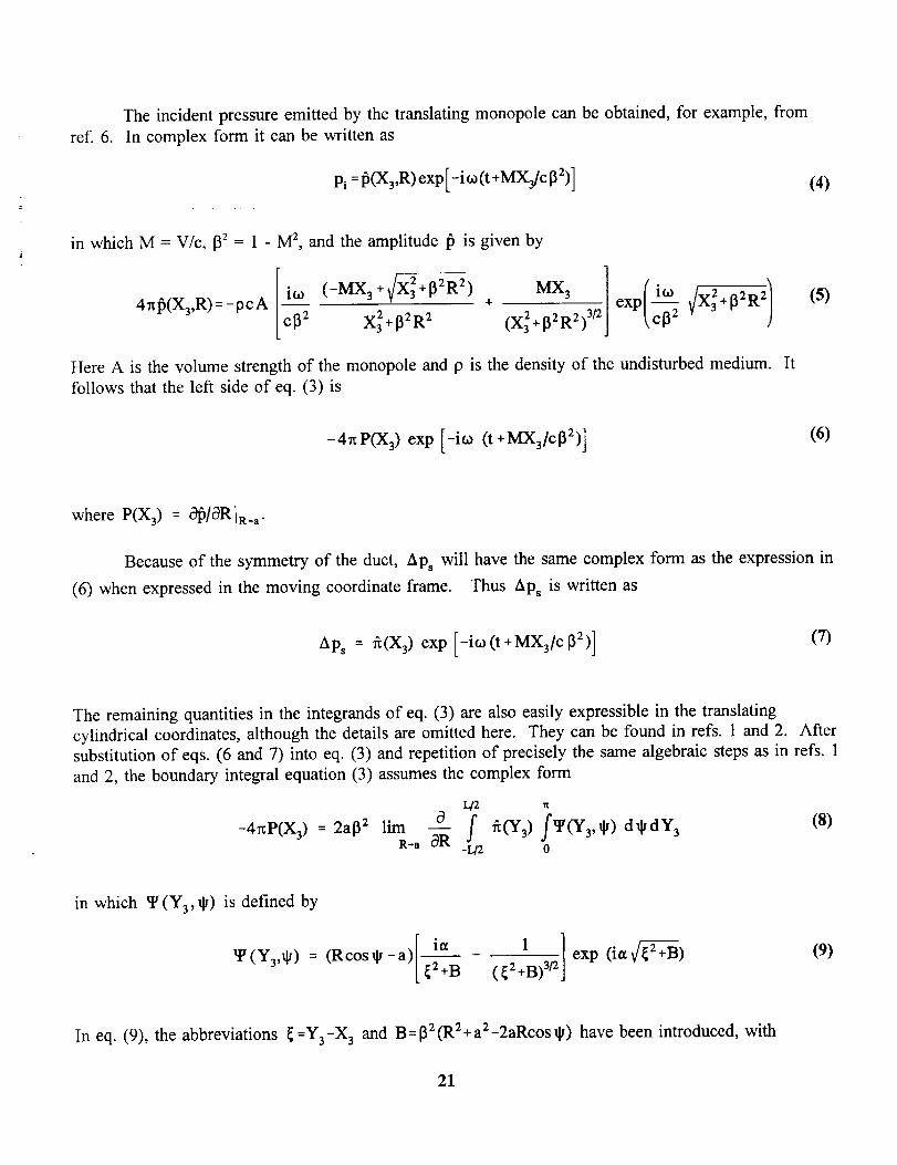
ref. 6.Theincidentpressureemittedby the translatingmonopolecanbeobtained,for example,fromIn complexform it canbewritten as
Pi=15(X3,R)exp[-i(° (t+MX3]cl32)]
exp( in which M = V/c, 132= 1 - M 2, and the amplitude _ is given by
[,iw (-MXa+IX_+[ _2R2) + MX34nlb(X3,R) = - pc A
cl32 X_+132R 2 (X32 + 132R2) 3/2
Here A is the volume strength of the monopole and p is the density of the undisturbed medium.
follows that the left side of eq. (3) is
(4)
(5)
It
-4rrP(X3) exp [-it,) (t +MX3/c132)](6)
where P(X3) = O_IOR[R=a.
Because of the symmetry of the duct, bps will have the same complex form as the expression in
(6) when expressed in the moving coordinate frame. Thus bps is written as
Ap_ : _(X3) exp [-i60(t +MX3/cl32)](7)
The remaining quantities in the integrands of eq. (3) are also easily expressible in the translating
cylindrical coordinates, although the details are omitted here. They can be found in refs. 1 and 2. After
substitution of eqs. (6 and 7) into eq. (3) and repetition of precisely the same algebraic steps as in refs. 1
and 2, the boundary integral equation (3) assumes the complex form
-4riP(X3) = 2ap 2
L/2 1_
lira d f _(Y3) fvcY ,,) d_dY 3 (8)R-a OR -I_ o
in which u? (Y3, _) is defined by
_ (Y3,_) = (Rcos_ -a)[-- ia _ 1 ]_2+B (_2+B) 3/2 exp (itz _2_--B) (9)
In eq. (9), the abbreviations ¢ =Y3-X3 and B=[32(R2+ a2-2aRcos _) have been introduced, with
21
_:C-_ and _=,.o/ct32.=:
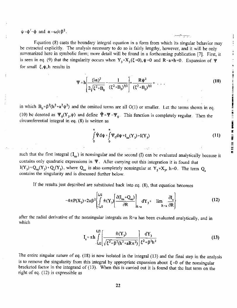
Equation (8) casts the boundary integral equation in a form from which its singular behavior may
be extracted explicitly. The analysis necessary to do so is fairly lengthy, however, and it will be only
summarized here in symbolic form; more detail will be found in a forthcoming publication [7]. First, it
is seen in eq. (9) that the singularity occurs when Y3=X3(_=0),_=0 and R-a-h=0. Expansion of
for small _,_,h results in
1 i_- R*2
(_Z+Bo)3/zj (_2 +B0)3/2
+• , ,
(lO)
in which Bo=[32(h2+a2_ 2) and the omitted terms are all O(1) or smaller. Let the terms shown in eq.
(10) be denoted as _o(Y3,#) and define q=_-_0- This function is completely regular. Then the
circumferential integral in eq. (8) is written as
f@d* +fVod* =I._(V_)+I(Y_)0 o
(11)
such that the first integral (Ins) is nonsingular and the second (I) can be evaluated analytically because it
contains only quadratic expressions in _. After carrying out this integration it is found that
I(Y3) = Q,_(Y3) ÷ Qs(Y3), where Q,_ is also completely nonsingular at Y3 =X3, h=O. The term Qs
contains the singularity and is discussed further below.
If the results just described are substituted back into eq. (8), that equation becomes
I?-4r_P(X3) :2a[32 _(Y3)
l-L/2 -ff_ jR= dY3 + lima._ aRj
(12)
after the radial derivative of the nonsingular integrals on R=a has been evaluated analytically, and inwhich
-u2[ ¢_2 +[32Cn2+aR_2) J_2+[32h2(13)
=
[l
The entire singular nature of eq. (18) is now isolated in the integral (13) and the final step in the analysis
is to remove the singularity from this integral by appropriate expansion about _ =0 of the nonsingularbracketed factor in the integrand of (13). When this is carried out it is found that the last term on the
right of eq. (12) is expressible as
22
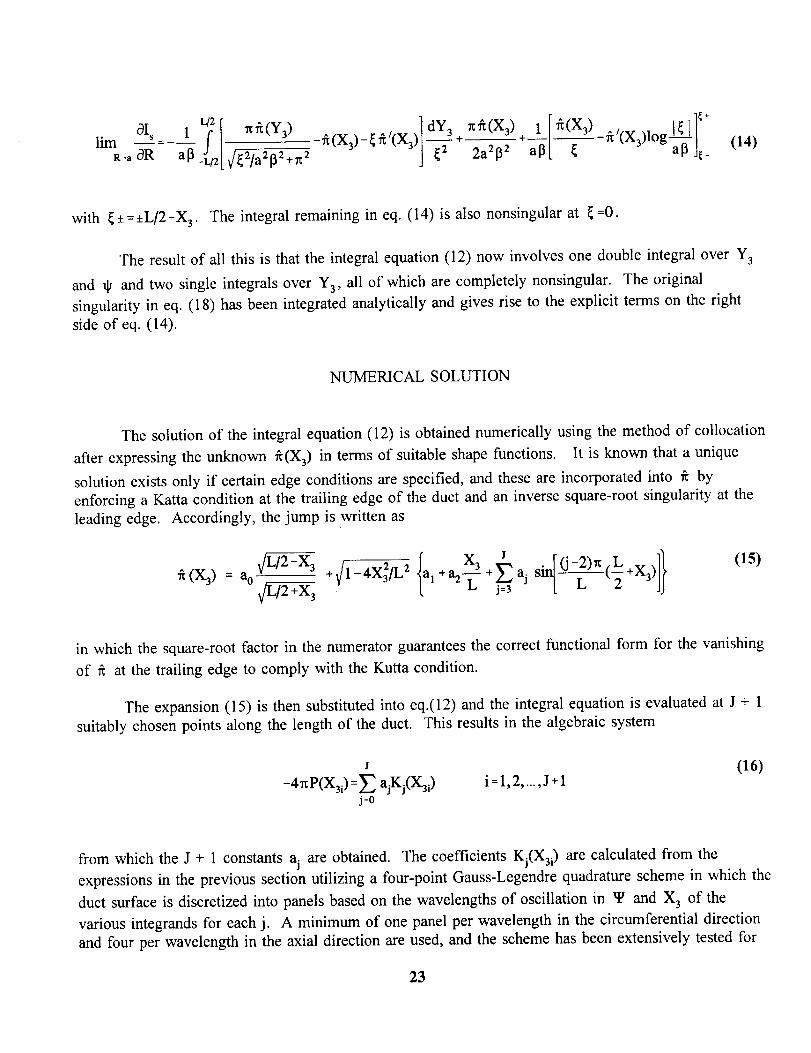
-_I ] dY3 "K '_ (X3) + 1
(Y3)1 -g- _ (X 3) - _ _ _(X3)lim .... ÷ -- --
R-a OR a13 X/_2/a2132+n2 _2 2a2132 a13
(X3) - _ Z(X3)l°g (14)
with _,=±L/2-X 3. The integral remaining in eq. (14) is also nonsingular at _=0.
The result of all this is that the integral equation (12) now involves one double integral over Y3
and @ and two single integrals over Y3, all of which are completely nonsingular. The original
singularity in eq. (18) has been integrated analytically and gives rise to the explicit terms on the right
side of eq. (14).
NUMERICAL SOLUTION
The solution of the integral equation (12) is obtained numerically using the method of collocation
after expressing the unknown _(X3) in terms of suitable shape functions. It is known that a unique
solution exists only if certain edge conditions are specified, and these are incorporated into _ by
enforcing a Katta condition at the trailing edge of the duct and an inverse square-root singularity at the
leading edge. Accordingly, the jump is written as
_(X,) =a0 _ +_/1-4X2/L 2 ,+a2--_2+_a j [ L 2j=3
(15)
in which the square-root factor in the numerator guarantees the correct functional form for the vanishing
of _ at the trailing edge to comply with the Kutta condition.
The expansion (15) is then substituted into eq.(12) and the integral equation is evaluated at J + 1
suitably chosen points along the length of the duct. This results in the algebraic system
J
-47zP(X3i) :E ajKj(X3i)j:o
i=l,2,...,J+l(16)
from which the J + 1 constants aj are obtained. The coefficients Kj(X3i ) are calculated from the
expressions in the previous section utilizing a four-point Gauss-Legendre quadrature scheme in which the
duct surface is discretized into panels based on the wavelengths of oscillation in • and X 3 of the
various integrands for each j. A minimum of one panel per wavelength in the circumferential direction
and four per wavelength in the axial direction are used, and the scheme has been extensively tested for
23
accuracy. The numberof shapefunctionsJ is chosensufficiently large to captureat Ieast 2-3 t_mes the
number of oscillations in _ expected along the duct; this number can be inferred from the incident field
given in eq. (6).
RESULTS
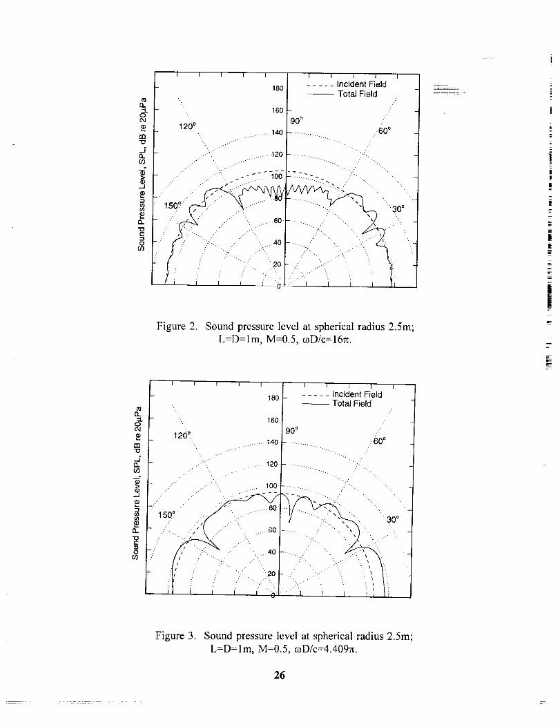
Numerical predictions from the theory outlined in thispaper are illustrated in figs. 2 and 3.
Figure 2 corresponds to the case of primary interest in the current proceedings: the forward Mach
number is 0.5, the duct (D) diameter and length are both I m, and the dimensionless clrcular frequency
is tzD/c=16r_. On the figure is shown the sound pressure level in dB re lO-51.tPa radiated from a
monopole for which pc tAI= IN. The polar plot gives the SPL of the incident field alone and that of the
total field in the presence of the duct on a spherical radius 2.5m from the origin of _. The angles 0 °
and 180 ° correspond to the exit and inlet ends of the duct, respectively. As would be expected at this
relatively high frequency, the duct causes very little scattering in the axial directions. There is, however,
a lateral shielding effect that cuts the SPL about 20dB around the 90 ° direction as is seen in all
problems of this type [1, 2, 7].
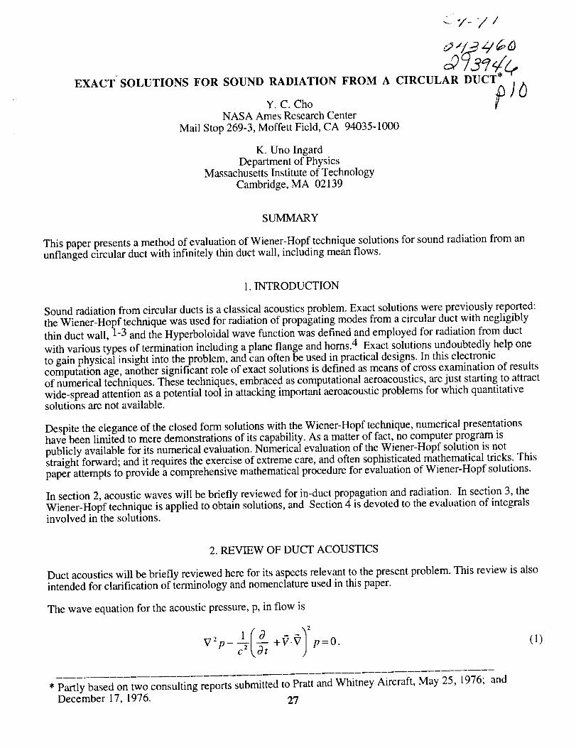
Figure 3 illustrates the directivity found for the same case except with the frequency reduced to
wD/c=4.409n (corresponding to 750 Hz). While the axial scattering is somewhat stronger in this case,
the duct obviously affords minimal lateral shielding at the lower frequency.
i
ACKNOWLEDGMENTS
This research was supported by NASA Langley Research Center under Cooperative Agreement
NCCI-14. Essential assistance with computer code development was provided by Mr. Melvin
Kosanchick III, Ms. Barbara Lakota and Mr. Jason Buhler.
REFERENCES
.
.
.
Myers, M. K. and Lan, J. H., "Sound Radiation from Ducted Rotating Sources in Uniform Motion."
AIAA Paper No. 93-4429, October 1993.
Myers, M. K., "Boundary Integral Formulations for Ducted Fan Radiation Calculations."
Proceedings of First Joint CEAS/AIAA Aerocoustics Conference, Munich, Germany, Vol. I, June
1995, pp. 565-573.
Eversman, W., "Ducted Fan Acoustic Radiation Including the Effects of Nonuniform Mean Flow and
Acoustic Treatment." AIAA Paper No. 93-4424, October 1993.
24
,
,
.
7.
Martinez, R., "Liner Dissipation and Diffraction for an Acoustically Driven Propeller Duct." AIAA
Paper No. 93-4426, October 1993.
Dunn, M., Tweed, J. and Farassat, F., "The Prediction of Ducted Fan Engine Noise via a Boundary
Integral Equation Method." AIAA Paper No. 96-1770, May 1996.
Morse, P. M. and Ingard, K. U., Theoretical Acoustics, McGraw-Hill, New York, 1968, pp. 723-724.
Myers, M. K, and Kosanchick, M., "Computation of Sound Radiated from a Fan in a Short Lined
Duct." To appear as AIAA Paper No. 97-1711, May 1997.
r_
R
\
/
/
x Vt,(
L
_J
J
• X 3w
Figure 1. Duct geometry and coordinate systems.
25
13.
O
o,I
nn
13.
(/3
_9
Q.
IE-.iO
O3
=I.o
m
"o
J13.
r.f)
-J
{/)
O,.
"Ot-
O
O9
I I I I I I I I I I I I
iI ..... IncidentField180 ..... TotalField
"-.., 160 [-90 o ."120° _ " o
140........... 60•. .....,-."
• ....""-.. ..-
...-"-_" .....120..............
• :_ .---"_-_6o:-_:_.--. :::
Is0q , 3o°,'".............,o.............,
i .j,
l i i i , ....a. ...._ _ i .., li
Figure 2. Sound pressure level at spherical radius 2.5m;L=D=Im, M=0.5, coD/c--16n.
I I
1200.
I i I
180
160
.................. 140
.......... 120
I I I I
..... IncidentFieldTotalField
_0°.60 °
-',, .. ..
._ .,.......,.._.Y .-."::_. ..100
7"'" .""" .-_̧ _' 80_150" _j,'/ .:-," " t' ':,-.: ",'-----,x.. 30 °
- '. ,_'_,"'/-- .....60...... ' " ",
. t ." ""...,' ._'." " "" "" "" "'" ' _ '
I
ilJ
i
Jr
F
Figure 3. Sound pressure level at spherical radius 2.5m;
L=D=lm, M=0.5, o)D/c=4.409_.
26
EXACT-SOLUTIONS FOR SOUND RADIATION FROM A
Y. C. ChoNASA Ames Research Center
Mail Stop 269-3, Moffett Field, CA 94035-1000
K. Uno IngardDepartment of Physics
Massachusetts Institute of TechnologyCambridge, MA 02139
.7-
CIRCULAR DUCT
SUMMARY
This paper presents a method of evaluation of Wiener-Hopf technique solutions for sound radiation from anunflanged circular duct with infinitely thin duct wall, including mean flows.
1. INTRODUCTION
Sound radiation from circular ducts is a classical acoustics problem. Exact solutions were previously reported:the Wiener-Hopf technique was used for radiation of propagating modes from a circular duct with negligibly
thin duct wall, 1-3 and the Hyperboloidal wave function was defined and employed for radiation from duct
with various types of termination including a plane flange and horns. 4 Exact solutions undoubtedly help oneto gain physical insight into the problem, and can often be used in practical designs. In this electroniccomputation age, another significant role of exact solutions is defined as means of cross examination of results
of numerical techniques. These techniques, embraced as computational aeroacoustics, are just starting to attractwide-spread attention as a potential tool in attacking important aeroacoustic problems for which quantitativesolutions are not available.
Despite the elegance of the closed form solutions with the Wiener-Hopf technique, numerical presentationshave been limited to mere demonstrations of its capability. As a matter of fact, no computer program ispublicly available for its numerical evaluation. Numerical evaluation of the Wiener-Hopf solution is notstraight forward; and it requires the exercise of extreme care, and often sophisticated mathematical tricks. Thispaper attempts to provide a comprehensive mathematical procedure for evaluation of Wiener-Hopf solutions.
In section 2, acoustic waves will be briefly reviewed for in-duct propagation and radiation. In section 3, theWiener-Hopf technique is applied to obtain solutions, and Section 4 is devoted to the evaluation of integralsinvolved in the solutions.
2. REVIEW OF DUCT ACOUSTICS
Duct acoustics will be briefly reviewed here for its aspects relevant to the present problem. This review is alsointended for clarification of terminology and nomenclature used in this paper.
The wave equation for the acoustic pressure, p, in flow is
1 O o. (1)V P-? - Z P=
* Partly based on two consulting reports submitted to Pratt and Whitney Aircraft, May 25, 1976; and
December 17, 1976. 27
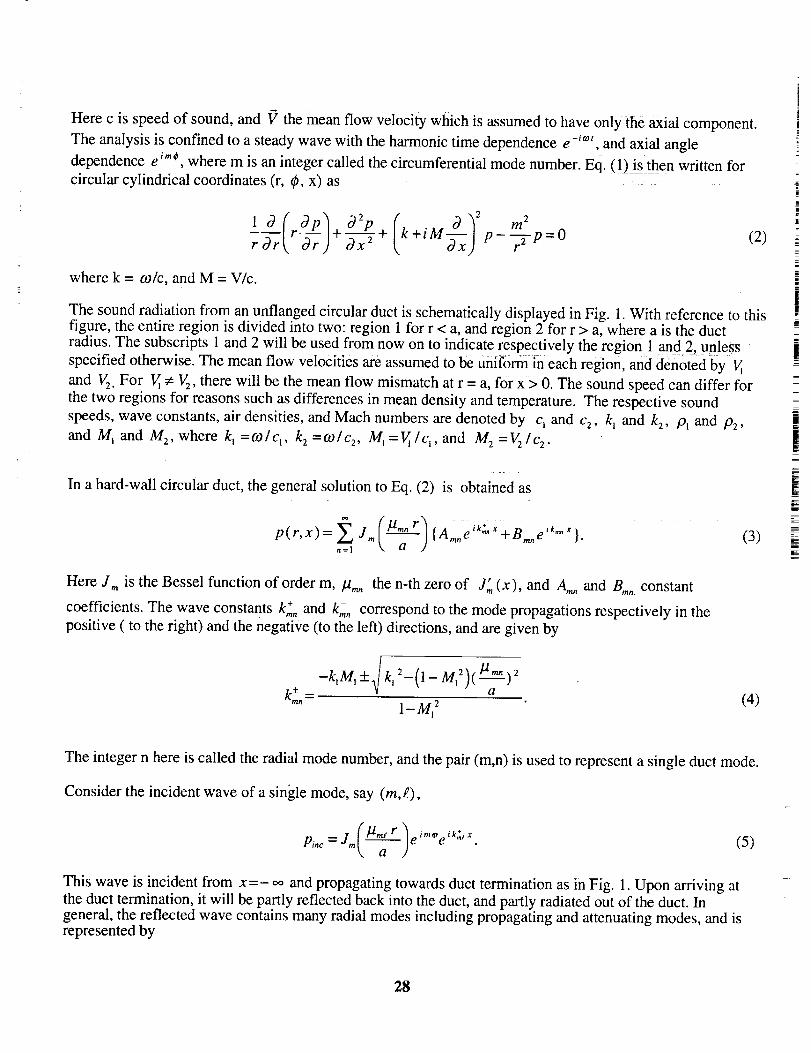
Herec is speedof sound,and 1) themeanflow velocitywhichis assumedto haveonlytheaxialcomponent.Theanalysisis confinedto a steadywavewith theharmonictimedependencee -_o,,, and axial angle
dependence e '" _, where m is an integer called the circumferential mode number. Eq. (1)_is then written for
circular cylindrical coordinates (r, _b, x) as
-(r grt, G-r)+ax -7-p=° (2)
where k = co/c, and M = V/c.
The sound radiation from an unflanged circular duct is schematically displayed in Fig. 1. With reference to this
figure, the entire region is divided into two: region 1 for r < a, and region 2 for r > a, where a is the ductradius. The subscripts 1 and 2 will be used from now on to indicate respectively the region 1 and 2, unless
specified otherwise. The mean flow velocities are assumed to be uniform in each region, and denoted by Vj
and Vz. For V_4: V2, there will be the mean flow mismatch at r = a, for x > 0. The sound speed can differ for
the two regions for reasons such as differences in mean density and temperature. The respective sound
speeds, wave constants, air densities, and Mach numbers are denoted by q and c2, k_ and k2, Pl and P2,
and M I and M 2, where k t = co / q, k 2 = co / c2, ,,141= Vt / q, and M 2 -- V2 / q.
In a hard-wall circular duct, the general solution to Eq. (2) is obtained as
p(r,x)= Jr. {A,..e_L'X +B,..e_'_} •n=l
(3)
Here J., is the Bessel function of order m, /1,.. the n-th zero of J" (x), and A,.. and B,... constant
coefficients. The wave constants k_. and k,7,. correspond to the mode propagations respectively in the
positive ( to the right) and the negative (to the left) directions, and are given by
-klM j q-_ kl 2-(1 - M 2)( l'lmn ) 2
÷ a (4)kmn "_- 2l-m,
M
J
The integer n here is called the radial mode number, and the pair (m,n) is used to represent a single duct mode.
Consider the incident wave of a single mode, say (m,g),
Pinc--Jml--I e e .kay
(5)
This wave is incident from x =- _ and propagating towards duct termination as in Fig. 1. Upon arriving at
the duct termination, it will be partly reflected back into the duct, and partly radiated out of the duct. Ingeneral, the reflected wave contains many radial modes including propagating and attenuating modes, and is
represented by
28
n=l
(6)
Here R,.m is the conversion coefficient for the (m,g)mode incident and the (m,n) mode reflected. The
reflection problem is completely solved by determining this coefficient for all values of n. The Wiener-Hopftechnique yields radiation solutions in terms of the far field, which is represented by
__im(p .l" [0_ 1 eiA(k2,M2,R)Prad -- e, Jm__ J" k2---_
(7)
Here R is the radial distance from the center of the duct termination, and 0 the polar angle measured from the
x-axis (duct axis) as shown in Fig. 1. (R, 0, ¢) are spherical coordinates. The complex factor free(O) is called
the amplitude gain function, which provides the far field directivity of radiation. The phase A(k 2, M 2, R) of the
far field depends on M 2 as well as on k 2 and R. The radiation problem is completely solved by determining
fm_(O) and A(k2,M2,R).
This analysis with a single mode incident can be extended to accommodate incident waves composed of many
modes in a straight-forward manner.
3. WIENER-HOPF FORMULATION
The Wiener-Hopf technique involves extensive mathematical manipulation in the Fourier transform space. The
Fourier transform of p(r, x) is given by
1
• (r,a) = .vt_- _2 p(r,x)eiaXdx, (8)
and p(r, x) is restored by the inverse transform
1
p(r,x) = _ _2 _(r'a)e-i_Xd°t " (9)
In the process of the Wiener-Hopf formulation, various parameters and functions are defined and derived asfollows:
± +kj for i=1, 2,yi(oO=__(ot-q;)'(O_-q;), qj -l_Mi
I,_Oqa)w, (a)=
),_a l" (?'_a), I.. being I- Besselfunctionofoder m,
G(a)=Km(y2a)
i aY2a K,.(Y2 ), K,. being K - Besselfunction ofoder m,
(10)
(11)
(12)
29
+ 1- j (13)
a 2 )2 2K(of)=_[p,c, (ki+ocM, W_(o_)-P2c_(k2+aM2) W2(00]. (14)TM?',L
In deriving K(o0, we have used the condition of the continuity of the acoustic pressure and acoustic
displacement at the mean flow mismatch at r = a, for x >0. K(a) is factorized into two, one is analytic in the
upper half plane (+) and the other in the lower half plane (') as K(a)= K÷ (o_). K (o0. These factors will be
included in the final solutions with arguments representing physical quantities. For the present problem, thefactorization is obtained not in closed forms but in integral representations a s follows:
1____, LogeK(a) do_ 'Log<K+ (y+)= 2rci C+ or-y+ (15)
-1 £ Log_K(a) da.Log J( (y_)= 2zri C o_-y_
(16)
Here the integral path is from - _ to + _ near the real axis, and the argument y+ (y_) is located above
(below) the respective integral path, as illustrated in Fig. 2:
Forgoing details of the formulation, 5 the final results are presented here. The conversion coefficient for thereflection is obtained as
m
__ 2, (m m + 1-<,+Re'" aTM_-M, 2 J,,,(tA,,,,,) \ ]lmn) Lt. 1-Mr) 1--_ ]]
(ki-MI k7")2 - K_(-k,,u,)K+(-k,,,)]+ _ -1k + - (k I + (1-Ml2)k,7,,, ) "[(.,<-k,.°) M,
The symmetry between the radial mode numbers g and n is salient, implying that the result satisfies the
reciprocity principle, 6 which can be used to infer the conversion coefficients of a nonpropagating mode.
For the radiation, the phase is obtained as
A (k 2, M 2, R) = k2 M 2 x1_ff_22 (R ff----777 )'41-M?
and the amplitude gain function is
(17)
(18)
30
f_,(O) =(-i) ' J=(vm,)p24 (1-v2 cosO')2
_ TM(1-M22) '/2
• sin0. m' k2asinO'
.{K÷(_rl(O)).[k+ e _r/(0)].t( k_1+ M z /, +,I/<1}77(o) .K --km, " k2,+ (19)
where
7"/(0) = kz(c°s0'- M2 )1- M_
(20)
Here the modified coordinates R' and 0' are defined as
I X2R'= r24 1-Mff 'tan0'= t_- Mff tan0 .
(2I)
f
H2_(x) is the Hankel function of the first kind, and H2 _) (x) is its derivative with respect to x.
Comments are made on the expression of f,.,,(O) for two limiting cases• First, as can be shown readily, when
0 becomes zero, the quantity in the first square bracket will be infinite except for the case of m = 0. In other
words, the radiated field is zero for 0 = 0 except for the radiation of axi-symmetric modes. Second, as will be
seen later, when its argument approaches - k+.,., K+ in the second square bracket varies as [ k+..e- r/(0)]-'. It
follows that the radiated field will be zero for the angle satisfying
J _
r/(0)=k_+, or cos0'= M 2+ (1-M 2_'_" for n,e. (22)2jk2 ,
However, for the angle corresponding to the incident propagation constant k2,., the radiated field is non-zero,
because the term adjacent to K÷ becomes zero in this limit. In fact, the radiated field reaches the maximum in
this limit. These findings are all familiar for cases of no mean flows. We will also see later that if its argument
approaches - k_/(1 + M_), K+ varies in such a way as to compensate the term involving the square root in thesame square bracket to maintain the amplitude gain finite.
A remark should be made on the constant TM. As M_ and M 2 both become zero, this constant becomes zero,
but the expressions for the conversion coefficients and the radiation directivity remains correct, and finitewhen evaluated as a limit.
4. NUMERICAL EVALUATION
The integrals in Eqs. (15) and (16) cannot be carried out analytically, and thus, we will employ a semi-numerical method. To this end, all the variables are made dimensionless by multiplying or dividing with theduct radius a. For notation simplification, the sub- or superscript m will often be dropped.
31
K(a) satisfies all the conditions required for its factorization by the integration. Nevertheless, the integrand
possesses singular points in the vicinity of the integral paths. These singular points arise as branch points,
simple poles, and zeroes of K(a). It should be emphasized that there are no other singularities near the
integral paths. The branch points are located at o_= q_. We adopt a rule for determining phase around these
branch points, as illustrated in Fig. 3. For example, consider (cz-q_). Its phase is 180 degrees for its real
part less than zero, and changes clockwise to zero as the real part bec0mes positive. On the other hand, the
phase of (_z-q() is -180 degrees for the real part less than zero, and changes counterclockwise to zero as the
real part becomes positive. This rule should be strictly observed for the integrations.
The simple poles of K(a) occur at zeroes of 1" (7'_ a), Which is included through W_ (a) as in Eqs. (11) and
(14). Theses zeroes correspond to the wave constants of duct modes, and one can show that the simple poles
of K(a) are located at a=v, _ -- -k_,. Note that v + ( =-- k_,) is above the respective integral path, and v;
( -- k_+,) below the respective integral path as shown in Fig. 2. K(a) can also possess zeroes near the+ + +
integral path if q( > qz. The zeroes are located between o_=qz and a=qj, and above the integral path. The
number of zeroes equals that of simple poles between a = q_ and a = q_, or can be less by one. The zeroes are
denoted by z,, for n = 1, 2 .... n o, n o being the number of zeroes. These zeroes are ordered such that z_ is the
smallest, and z,o the largest.
The imaginary parts of all the singular points are related to 9,_ (k). As the latter tends to zero, all the singularpoints approach the real axis, and the integral paths are then indented as shown in Fig. 2b.
Consider the integral
I =I_ L°ge K(a) dol (23)f
a-y
This integral is divided, for convenience, as
I=R_+R+ +B_+B+ +S+S.+Z+Y+N. (24)
R's are the contribution from the integration over larger arguments as
where Z >[q;[
Loge K(a)R_ = 1_- da,
o_- y
Loge K(a)t?,+= l do_ ,
,IZ÷ Ot- y
(25)
(26)
B's are the contribution from the integration over small intervals containing the branch points:
f_ Log e K(cx)B = da, with b_-< q_-< b_-,; _z-y
(27)
i
32
,i Log e K(ot) da, with b_+< q_+< b]. (28)B+= ; _-Y
S's are the contribution from the integration over small intervals containing the simple poles:
n c
S± = _ S,_ , n Cbeing the largest propagating radial mode number, (29)n=l
S-_= If 2 L°ge K(a) da, with s,_ < v_- < s_-2, (30)o:-y
÷
S+ = ,.2 Log, K(a) do_, with s,i < v, < s,z.2, O_-y
Z's are the contribution from the integration over small intervals containing the zeroes of K(a):
no
Z = _ Z., (32)n=l
Z. = r..[2 Log_ K(ct) d_, with z.i < z. < z.z •"%1 o_-y
Y is the contribution from the interval containing the pole at a = y:
i>;2 LogeK(a) do_ ' with y_ < Y < Y2,Y_ = ', Ot-y
(33)
where the plus (negative) sign indicates that the pole is above (below) the integral path. This integral needs to
be evaluated only if K(a) is free of singularity and zeroes within the integral limit. Otherwise, it should
belong to one of B, S, and Z because there are no other singular points than those involved in B, S, or Z.
large _, as
Finally N is the integral over the whole remaining intervals. There is no singularity at all in these intervals, andthus the integration can be carried out numerically.
K(o0 approaches unity as l al becomes large, that is,
AiK(_) _= 1 + -- + -- (35)
O_ a 2 '
where the expansion coefficients A_ and A z can be readily obtained. With this substitution to Eqs. (25) and(26), one obtains
[+d l(l+dlLogJZ+-yl] (36)R_=A, ,f-_+ T-y\ YJ \ Z± ; '
33
Lim K(o_) = 1., and thus, K(o_) can be expanded for a
(34)
where
d - A2 AI
A x 2
Error limits and the expansion coefficients are used to determine the integral limits Z±.
(37)
The integral near the branch points can be replaced by
where
B±=IL°g_Q_(a)daa-y-211 Log_(a-q_)da,a_y
Q±(a)=x(a)._.
(38)
(39)
Q4 (o0 are free of singularity and zeroes within the respective chosen integral limits.
The simple poles of K(a) are separated as follows:
where
s-+ Loge L_(a) Loge (a - v_. )t" P=Ia-y _ oe-y
L±(a)=K(a). (a- v_).
(40)
(41)
L± (a) are free of singularity and zeroes within the respective integral limits.
The zeroes of K(a) are similarly separated as
where
Z. = I L°geU(°_) d_ + I L°ge(a-Z") doe,o_- y o_- y
(42)
K(o0U(a) - (43)
U(a) is free of singularity and zeroes within the respective integral limit.
Now consider the integral
H(y) =If L°ge G(a) da,o_- y
(44)
Here G(a) is free of singularity and zeroes within the integral limit, and thus represents Q_(a) in Eq. (38),
L+(a) in Eq. (40), U(o0 in Eq. (42), or K(o0 in Eq. (34) if K(a) is free of singularity in that region. Thisintegral can be written as
b da
H(y) =i_ Loge[G(oOIG(y)]ot_y da + LogeG(y) I£ ot-y (45)
i
z
II
|E
34
As a approachesy, onereadilyobtains
Log e [G(ot) / G(y)] _- G'(y) (46)
a-y G(y)
Thus, the first integral in Eq. (45) does not involve any singularity, and can be easily evaluated whether y iswithin the integral limit, or not. The integral contained in the second term yields
,'.| dot _ Loge[b-Y±[,('') for y±<a, or y.>b,_a ot- y± \a-y± )
fork y±-a )
(47)
where (_+) signs are used to indicate that the simple pole is above (+) or below (-) the integral path, which isindented around the pole like u for (+), and n for (-).
Consider the integrals
fh Log e (ot - __)£2- dot,d, ot- y_
(48)
H Log_ (ot-__)_ =J_ dot,
ot - y+
(49)
Loge (ot-_+ )eb
_+ =l dot,- .,_ ot-y_
(50)
eb Log_ (ot-_+)YS_ =jo dot.
ot - y+(5i)
Here, the singular point at ot = _ is within the integral limit, that is, a < 4_+< b. The subscript on _ and y is
used to indicate that the pole is above (+) or below (-) the integral path. The indented integral paths are shownin Fig. 4. The second integral in each of Eqs. (38), (40), and (42) is identified with one of the integrals in
Eqs. (48) - (51). These integrals are evaluated as follows:
For y < a,
=4_ircLoge(._+-y+ I /z"2 1 r.\ a-y± )--_'+2 "[(L°g_(b-y±))2+(L°ge(_±-y±))2]
1 a-y._ JI (52)
fory >b,
35
= + l- la_y ± 3 _
1 y±-b \ y±-a+ L°ge(Y±-_±)'L°ge(Y±-b)-j_=lT[(y±-_+_ )J+(Y-+--_±)J];(53)
for a<y <b,
f2_ = + irc Loge(Y_-a) + Dr[-Loge(y_-_±) T- Loge(y -_+_) ]
- l[(Loge(b-¢e))2+(Loge(y-a))2 ] + Loge(b-_+_). Loge(b- y_)
,_ J J
2 f"-lj2LLb-¢±) Ly_-a)]'(54)
n+-+= +igLoge(y+-a)+ iTr[ Loge(y+-_±) T- Loge(y+-_±)]
-l[(Log,(b-_±))2+(Log_(y+-a))2]+ Log_(b -_±). Log_(b- y+)
rc2 S, 1 Y+_-_± + Y+-_+ 2 j2 b-_+_--- y÷-a (55)
All the integrals involving singular points are analytically evaluated according to Eqs. (47), (52) - (55). Forlarge arguments extending to the infinite, the integral is evaluated according to Eq. (36). The rest involvesfinite integrals with well-behaved integrands, and thus can be numerically evaluated without any difficulty.
A remark will be made on the results in Eqs. (54) and (55), particularly on the second term on the right. This
term vanishes if y and _ are on the same side (above or below) with respect to the integral path. However, if y
and_ are separated by the integral path, the second term equals +2mLog,(y± - _), and diverges as y
approaches _. Of the K-factors contained in the results in Eqs. (17) and (19), only 1(.(-71(0)) can have y
and _ separated by the integral path. Its argument is above the integral path according to Eq. (15). As 0varies, the argument can approach a singular point located below the integral path. For this case, the second
term above is given by 2zciLog_(-rl(O)-__), where __ is v_- or q_-. Inspecting Eqs. (15), (23), (24), (38),
and (55), one obtains, for -7/(0) close to ql-,
1
K÷ (-rl(O)) o_ 4_rl(O)_q? . (56)
Similarly, from Eqs. (15), (23), (24), (40), and (55), one obtains, for -r/(0) close to v,-,
(57)
36
It follows thenthat, as7/(0)approachesk_,, f,,e(O) given in Eq. (19) tends to be zero for nag, and will
reach the maximum for n=g. Also one can see that f,,_(O) will remain finite asr/(0) approaches to
k_/(1 + M_) as discussed earlier.
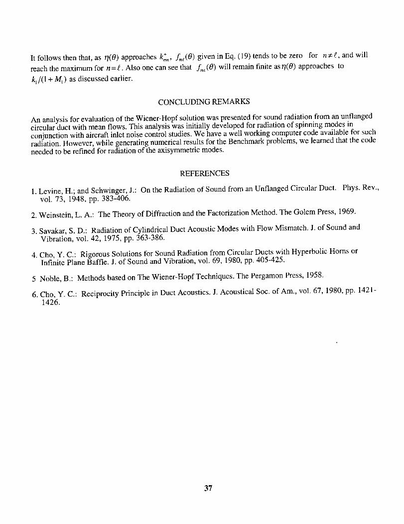
CONCLUDING REMARKS
An analysis for evaluation of the Wiener-Hopf solution was presented for sound radiation from an unflangedcircular duct with mean flows. This analysis was initially developed for radiation of spinning modes inconjunction with aircraft inlet noise control studies. We have a well working computer code available for suchradiation. However, while generating numerical results for the Benchmark problems, we learned that the codeneeded to be refined for radiation of the axisymmetric modes.
REFERENCES
1. Levine, H.; and Schwinger, J.: On the Radiation of Sound from an Unflanged Circular Duct. Phys. Rev.,vol. 73, 1948, pp. 383-406.
2. Weinstein, L. A.: The Theory of Diffraction and the Factorization Method. The Golem Press, 1969.
3. Savakar, S. D.: Radiation of Cylindrical Duct Acoustic Modes with Flow Mismatch. J. of Sound andVibration, vol. 42, 1975, pp. 363-386.
4. Cho, Y. C.: Rigorous Solutions for Sound Radiation from Circular Ducts with Hyperbolic Horns orInfinite Plane Baffle. J. of Sound and Vibration, vol. 69, 1980, pp. 405-425.
5 Noble, B.: Methods based on The Wiener-Hopf Techniques. The Pergamon Press, 1958.
6. Cho, Y. C.: Reciprocity Principle in Duct Acoustics. J. Acoustical Soc. of Am., vol. 67, 1980, pp. 1421-1426.
37
Dinc
V2
x=O
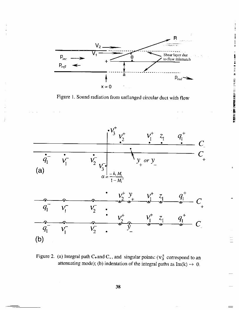
Figure 1. Sound radiation from unflanged circular duct with flow
(a)_b
• • • •
- k, M,
\y+or y_
C
C+
(b)
v; v; . y_
v_+ z_ q_+ C+
v_÷ z_ q_+•,_,------ C
z
Figure 2. (a) Integral path C+and C., and singular points: (v_ correspond to an
attenuating mode); (b) indentation of the integral paths as Im(k) _ O.
38
Ira(a)
J. :::--::::::::_'.-.::,
a=ql O.
Branch Cuts
. .........<bJRe(a)
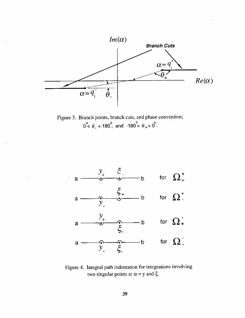
Figure 3. Branch points, branch cuts, and phase convention;0 0 0 0
0<0_<180, and -180<0+<0.
a b for .Q, +
a ,_ ,_, b for _ +_
Y.
a b for _"_ +
a '_ _ b for .0,_
Y. __
Figure 4. Integral path indentation for integrations involving
two singular points at ot = y and _.
39
s'5-y/
EXACT SOLUTION TO CATEGORY 3 PROBLEMS- TURBOMACHINERY NOISE
Kenneth C. Hall _ _'_5"._
Duke University z/Department of Mechanical Engineering and Materials Science
Durham, NC 27708-0300
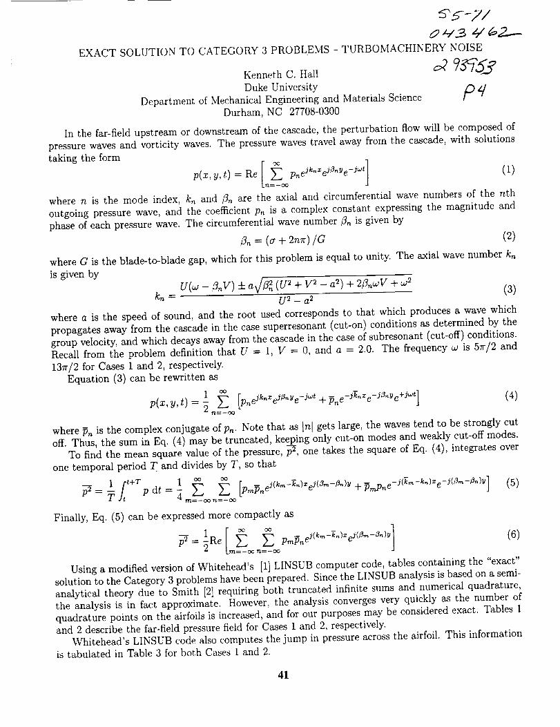
In the far-field upstream or downstream of the cascade, the perturbation flow will be composed of
pressure waves and vorticity waves. The pressure waves travel away from the cascade, with solutionstaking the form
p(x, y, t) = Re p,,eJk'xeJ_'Ue-J_t (1)
where n is the mode index, kn and /3n are the axial and circumferential wave numbers of the nth
outgoing pressure wave, and the coefficient p, is a complex constant expressing the magnitude and
phase of each pressure wave. The circumferential wave number ¢?,_is given by
_. = (_ + 2,_) /a (2)
where G is the blade-to-blade gap, which for this problem is equal to unity. The axial wave number k,is given by
u(_- _,,v)+ a_'N (u_+ v_-a_) + 2A_V +Jk_ = Us - a2 (3)
where a is the speed of sound, and the root used corresponds to that which produces a wave which
propagates away from the cascade in the case superresonant (cut-on) conditions as determined by the
group velocity, and which decays away from the cascade in the case of subresonant (cut-off) conditions.
Recall from the problem definition that U = 1, V = 0, and a = 2.0. The frequency w is 5_r/2 and137r/2 for Cases 1 and 2, respectively.
Equation (3) can be rewritten as
1
p(x,y,t) = "_ E [pnejk'xejz'ye-j_°t + Pn e-jg'xe-j_'ye+j_t] (4)
where p,, is the complex conjugate of pn. Note that as ln[ gets large, the waves tend to be strongly cut
off. Thus, the sum in Eq. (4) may be truncated, keeping only cut-on modes and weakly cut-off modes.
To find the mean square value of the pressure, )-_, one takes the square of Eq. (4), integrates over
one temporal period T and divides by T, so that
1 ft+T 1 _-_ = -T "Jr p at = -_ _ _ [pm_d(k"-k")Xe j(_-_)_ + _mp, e-J(k'-k_)_e-;(_"-_")Y] (5)
Finally, Eq. (5) can be expressed more compactly as
_ae _ (6)
Using a modified version of Whitehead's [1] LINSUB computer code, tables containing the "exact"
solution to the Category 3 problems have been prepared. Since the LINSUB analysis is based on a semi-
analytical theory due to Smith [2] requiring both truncated infinite sums and numerical quadrature,
the analysis is in fact approximate. However, the analysis converges very quickly as the number of
quadrature points on the airfoils is increased, and for our purposes may be considered exact. Tables 1
and 2 describe the far-field pressure field for Cases 1 and 2, respectively.
Whitehead's LINSUB code also computes the jump in pressure across the airfoil. This informationis tabulated in Table 3 for both Cases 1 and 2.
41
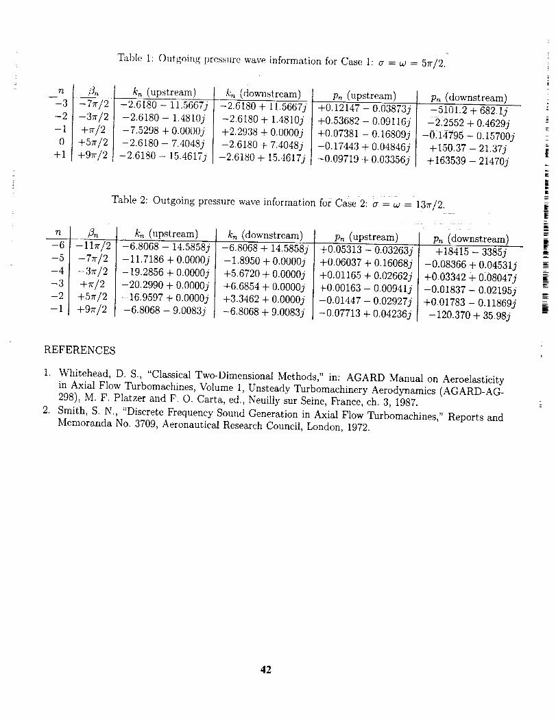
Table [: Outgoingpressurewaveinformation for Case1: o" = co = 57r/2,
n
-3
-2
-1
0
+l
-77r/2-37r/2+7r/2
+57r/2+9n-/2
kn (upstream)
-2.6180 - 11.5667j
-2.6180 - 1.4810j
-7.5298 + 0.0000j
-2.6180 - 7.4048j
-2,6180 - 15.4617j
k,., (downstream)
-2.6180 + 11.5667j
-2.6180 + 1.4810j
+2.2938 + 0.0000j
-2.6180 + 7.4048j
-2.6180 + 15.4617j
p_ (upstream)
+0.12147 - 0.03873j
+0.53682 - 0.09116j
+0.07381 - 0.16809j
-0.17443 + 0.04846j
-0.09719 + 0.03356j
p_ (downstream)
-5101.2 + 682.1j
2_12552 + 0.4629j
-0;14795 - 0.15700j
+150:37 - 21.37j
+163539 - 2i470j
72
-6
-5
-4
-3
-2
-1
Table 2: Outgoing pressure wave information for Case 2: a =_ = 137r/2.
-llrr/2
-7 /2-3rc/2
+7r/2+57r/2+97r/2
k,_ (upstream)
-6.8068 - 14.5858j
-11.7186 + 0.0000j
-19.2856 + 0.0000j
-20.2990 + 0.0000j
-16.9597 + 0.0000j
-6.8068 - 9.0083j
k_ (downstream)
-6.8068 + 14.5858j
-1.8950 + 0.0000j
+5.6720 + 0.0000j
+6.6854 + 0.0000j
+3.3462 + 0.0000j
-6.8068 + 9.0083j
p, (upstream)
+0.05313 - 0.03263j
+0.06037 + 0.16068j
+0.01165 + 0.02662j
+0.00163 - 0.00941j
-0.01447 - 0.029273'
-0.07713 + 0.04236j
Pn (downstream)
+18415 - 3385j
-0.08366 + 0.04531j
+0.03342 + 0.08047j
-0.01837 - 0.02195j
+0.01783 - 0.11869j
-120.370 + 35.98j
REFERENCES
1. Whitehead, D. S., "Classical Two-Dimensional Methods," in: AGARD Manual on Aeroelasticityin Axial Flow Turbomachines, Volume 1, Unsteady Turbomachinery Aerodynamics (AGARD-AG-
298), M. F. Platzer and F. O. Carta, ed., Neuilly sur Seine, France, ch. 3, 1987.
2. Smith, S. N., "Discrete Frequency Sound Generation in Axial Flow Turbomachines," Reports and
Memoranda No. 3709, Aeronautical Research Council, London, 1972.
=
i
E
i
l
1
42
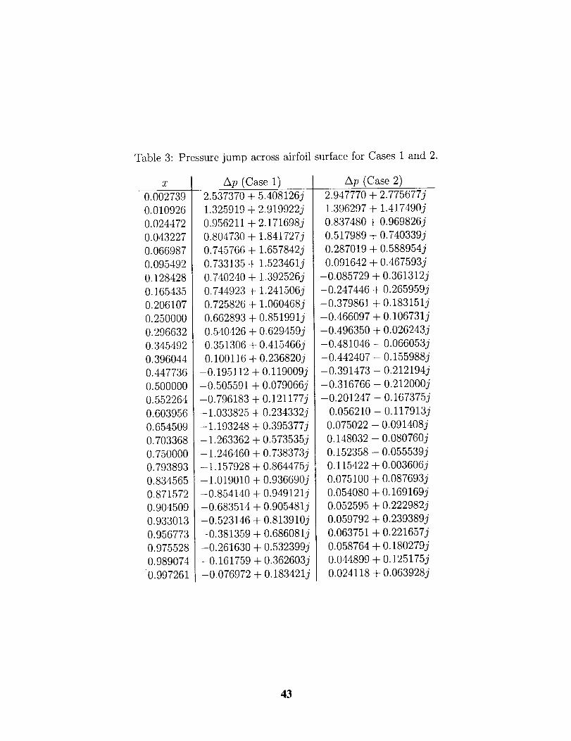
Table 3: Pressurejump acrossairfoil surfacefor Cases1 and 2.
X
0.002739
0.01O926
0.024472
0.043227
0.066987
0.095492
0.128428
0.165435
0.206107
0.250000
0.296632
0.345492
O.396O44
0.447736
0.500000
0.552264
0.603956
0.654509
0.703368
0.750000
0.793893
0.834565
0.871572
0.904509
0.933013
0.956773
0.975528
0.989074
0.997261
Ap (Case 1)
2.537370 + 5.408126j
1.325919 + 2.919922j
0.956211 + 2.171698j
0.804730 + 1.841727j
0.745766 + 1.657842j
0.733135 + 1.523461j
0.740240 + 1.392526j
0.744923 + 1.241506j
0.725826 + 1.060468j
0.662893 + 0.851991j
0.540426 + 0.629459j
0.351306 + 0.415466j
0.100116 + 0.236820j
-0.195112 + 0.119009j
-0.505591 + 0.079066j
-0.796183 + 0.121177j
-1.033825 + 0.234332j
-1.193248 + 0.395377j
-1.263362 + 0.573535j
-1.246460 + 0.738373j
-1.157928 + 0.864475j
-1.019010 + 0.936690j
-0.854140 + 0.949121j
-0.683514 + 0.905481j
-0.523146 + 0.813910j
-0.381359 + 0.686081j
-0.261630 + 0.5323993"
-0.161759 + 0.362603j
-0.076972 + 0.183421j
Ap (Case 2)
2.947770
1.396297
0.837480
0.517989
0.287019
0.091642
-0.085729 +
-0.247446 +
-0.379861 +
-0.466097 +
-0.496350 +
-0.481046 -
-0.442407 -
-0.391473 -
-0.316766 -
-0.201247 -
-O.O5621O -
0.075022
0.148032
0.152358
0.115422
0.075100
0.054080
0.052595
0.059792
0.063751
0.058764
0.044899
0.024118
+ 2.7756773
+ 1.4174903
+ 0.9698263
+ O.74O3393
+ 0.5889543
+ 0.4675933
0.3613123
0.2659593
0.1831513
0.1067313
0.0262433
0.O660533
0.1559883
0.2121943
0.2120003
O. 1673753
0.117913j
- 0.0914083
- 0.0807603
- O.O555393
+ 0.0O36O63
+0.0876933
+ O.1691693
+ 0.2229823
+ 0.2393893
+ 0.2216573
+ 0.1802793
+ 0.1251753
+ 0.0639283
43
z
Application of the Discontinuous Galerkin
method to Acoustic Scatter Problems
H. L. Atkins
NASA LaRC
Hampton, VA
Introduction
The discontinuous Galerkin method is a highly compact formulation that obtains the high accu-
racy required by computational aeroacoustics (CAA) on unstructured grids. The use of unstructured
grids on these demanding problems has many advantages. Although the computer run times of CAA
simulations may take tens of hours, the time required to obtain a structured grid around a complex
configuration is often measured in weeks or months. The mesh smoothness constraints imposed
by conventional high-order finite-difference methods further complicates the mesh generation pro-
cess. Furthermore, the impact of poor mesh quality on the accuracy obtained by these high-order
methods is not well known.
Unstructured meshes, on the other hand, can be generated in a nearly automated manner in
a relatively short time. Unstructured grids often have fewer cells because the cell distribution is
more easily controlled. In the case of structured grids, regions of unnecessarily small cells often
exist. These small cells can be a waste of computer memory and time; furthermore, in the ease
of an explicit time-accurate method the small cells may result in an unnecessarily small time step.
The use of an unstructured grid allows such cases to be avoided, and the savings usually makes
up for the increased cost per cell that is common with most unstructured methods. The use of an
unstructured approach also facilitates grid-adaption and refinement techniques, which can further
reduce the cost of a simulation.
Although most finite-element methods can be applied to unstructured grids, the property of
the discontinuous Galerkin method that distinguishes it from its finite-element counterparts is its
compactness. In a typical finite-element method with an order that is greater than 1, the mass
matrix is global but sparse; however, the mass matrix becomes more dense as the order of the
method is increased because the basis functions, or shape functions, must be globally C O functions.
The discontinuous GMerkin formulation relaxes this constraint; as a result, the mass matrix becomes
local to its generating element. This property makes the approach ideally suited to advection- and
propagation-dominated flows for which an explicit time-marching strategy is appropriate.
This article describes the application of the quadrature-free form 1 of the discontinuous Galerkin
method to two problems from Category I of the Second Computational Aeroacoustics Workshop on
Benchmark Problems. The quadrature-free form imposes several additional constraints and permits
an implementation that is more computationally efficient than is otherwise possible. The first part
of this article describes the method and boundary conditions relevant to this work; however, details
of the implementation can be found in reference 1. The next section describes two test problems,
both of which involve the scattering of an acoustic wave off a cylinder. The last section describes
the numerical test performed to evaluate mesh-resolution requirements and boundary-condition
effectiveness.
4S
Disconthmous Galerkin Method ==
The discontinuous Galerkin method can be applied to systems of first-order equa_ns in the
divergence formOU--+ v. P(u)= s(u) (1)Ot ::: ::
where U = {Uo, U,,...}, ,6 = (j_,._,...}, and S = {s0, s,,...}, defined on Some domafn _ with a
boundary 0fL
domain f_ =The domain is partitioned into a set of nonoverlapping elements f_i that cover the
U _2i. Within each element, the following set of equations is solved:vi
Ot_ _f bk-_didf_-f Vbk.a-[lfi(_/})Jidfl+ / bka_-llJn. Jifs=O (2)a, ai Oh,
for k = 0, 1,..., N where {bk, k = 0, 1,...,N} is a set of basis functions,
O(.,v,Z) :=U _ Vii = __,vi,jbj, Ji- and Ji = tail
,=0
Equation set (2) is obtained byprojecting equation (1) ontoeach: member of the basis set and then
integrating by parts to obtain the weak conservation form. In the present work, the basis set is
composed of the polynomials that are defined local to the element and are of degree < n. In two
dimensions, for example, the basis set is {1, _, r/, {e, gr/, r/=,...,_,g_-_r/,..., {r/_-_, 71_}, where (_, r/)
are the local coordinates. The solution U is approximated as an expansion in terms of the basis
functions; thus, both V and ,F(V) are discontinuous at the boundary between adjacent elements
(hence, the name discontinuous Galerkin). The discontinuity in V between adjacent elements is
treated with an approximate Riemann flux, which is denoted by baR; Ji is the Jacobian of the
transformation from the global coordinates (x,y,z) to the local element coordinates ({,r/,_) ofelement i.
In the usual implementation of the discontinuous Galerkin method 2, 3, 4 the integrals are eval-
uated with quadrature formulas. This approach is problematic for even moderately high-order
implementations in multidimensions and has limited most efforts to n = 2 or 3. The difficulties are
due in part to two considerations; first the integral formulas used in the evaluation of (2) must be
exact for polynomials of degree 2n (even higher when /_ is nonlinear). Second, multidimensional
Gaussian quadrature formulas do not always exist. Near-optimal quadrature formulas that have
desirable properties such as symmetry are uncommon, and usually the number of quadrature points
exceeds N + 1 (the number of terms in the expansion) by a wide margin. The Common practice of
forming tensor products of one-dimensional Gaussian quadrature formulas is straightforward but
also results in considerably more than N + 1 quadrature points.
In the quadrature-free form, the integral evaluations are reduced to a summation over the coeffi-
cients of the solution expansion, which is an operation of order N + 1. To implement this approach,
the flux F must also be written as an expansion in terms of the basis functions:
N
j=0
(a similar expansion is made for the approximate Riemann flux _n). This Step is tr_i-ally ac-
complished for linear equations, and several approaches for nonlinear equations are discussed in
|
46
reference1. In addition, the allowedelementshapesare limited to those for which the coordinatetransformation from a fixed computational element(suchasa unit squareor anequilateral trianglein two dimensions)to the physicalelementis linear; thus,ai is a constantwithin the element. Withtheseassumptions,the integrals can be evaluated exactly and efficiently, and equation (2) can bewritten in matrix form as
TI e
JiM OV--_ - .& . JiJf'd_ + Z Bk (ffiJ_ldiRh) " ffi,k -_- 0 (3)Ot
k=l
where n_ is the number of sides around element i, gi,k is the outward unit normal on side k,
Vi [Ui,O,1'i, 1, "l, Gi [9-_,o,g-'i,1, .], and 6 n __n -.Ri,k [gi,k,O, .]. The matrix M and_--- . . _ . . z gi,k,1, " " mass
the vector matrix _& are given by
M : [,na-,z], ink,, : f bk-lbl-1 df_, and X : [ga-,l], fla-,, : f b,_,Vbk_, d_f_ f_
for 1 _< k, l _< N + i. The matrices are the same for all elements of a given type (e.g. the same for
all triangles, the same for all squares, etc.) and can be precomputed and stored at a considerable
savings.
Derivation of the boundary integral terms is complicated by the fact that the solutions on either
side of the element boundary are represented in terms of different coordinate systems. This problem
is circumvented by expressing the solution on both sides of the element boundary in terms of a
common edge-based coordinate system (a simple coordinate transformation). After some additional
algebraic simplification, an edge matrix Bk is obtained that is the same for similar sides of similar
element types. A detailed derivation of the matrices M, .&, and Bk is given in reference 1. Because
equation (3) is of the same form for all elements, the element index i is dropped for clarity.
The first two terms of equation (3) depend only on the solution within the element, and com-
munication between adjacent elements occurs only through the Riemann flux _n. The Riemann
flux provides this communication in a biased manner by evaluating the flux with data from the
"upwind" side of the element boundary. In the case of a system of equations, the upwind side may
be different for each characteristic wave component; thus, the flux/_R will usually be a function of
the solution on both sides of the element boundary. Cockburn and Shu 5 have demonstrated that
this upwind bias is essential to the stability of the discontinuous Galerkln method.
In this work, the discontinuous Galerkin method is applied to the two-dimensional linear Euler
equations given by
U -[p- P, p, u, v] T and F- _TIU + [0, l/, iP, )p]X (4)
where aTI = [M,.,Mv], 17" -- [u, vl, and i and 3 are the Cartesian unit vectors [1,01 and [0,1],
respectively. The dependent variables p, p, u, and v are the normMized perturbation values of
density, pressure, and the x- and 9-components of the velocity, respectively; Mx and M v are the
normalized x- and 9-components of the mean flow velocity. The density, pressure, and velocities
are normalized with respect to the mean flow density po, the sound speed of the mean flow c, and
poc, respectively. The length scale lr is problem dependent, and the time scale is given by l,./c. The
source term ,_qis also problem dependent and is described in a later section.
47
Equation (3) is advancedin time with a three-stageRunge-Kutta method developedby ShuandOsher6. Analysis of the stability of this approach,alongwith many numerical validation tests, canbe found in reference1.
Boundary Conditions
An important feature of the discontinuous Galerkin method is that the Riemann flux is the
only mechanism by which an element communicates with it surroundings, rega-rdiess of whether
the element boundary is on the interior of the domain or coincides with the domain boundary.
A notable consequence is that the usual interior algorithm is valid at elements that are adjacent
to the boundary. In contrast, the interior point operator of most high-order finite-dlfference and
finite-volume methods cannot be applied at points near the boundary without some modifications.
These modifications usually result in reduced accuracy, and careful attention is required to preventthe introduction of numerical instabilities 7 The discontinuous Galerkin method eliminates these
problems and, thereby, eliminates a major source of error that is common to most high-order finite-difference and finite-volume methods.
A detailed description of the implementation of boundary conditions for the discontinuous
Galerkin method is in preparation 8. The implementation of the two types of boundary conditions
required for the benchmark problems (i.e. hard wall and nonreflecting freestream) are described
here. These boundary conditions can be implemented either by supplying the exterior side of the
Riemann flux with a complete solution or by reformulating the flux such that it requires only the
interior solution and the known boundary data. The later approach is usually more accurate and
is used in the present work.
The flux on the element boundary is given by
!
V(U)b -- f(U) . + [0, Vn, Px, p ]r
where Air_,= A). g, I/_ = lP. g, P_ = Pi. g, Py = Pj. g, and g = J-'ldd_ is the boundary-normal
vector for an arbitrary, edge. At a hard-wall boundary, the flow through the boundary Vn is zero.
Also, hard-wall boundary conditions can only be applied at boundaries where M_ = 0. After these
constraints have been imposed, the flux at a hard wall becomes
F(U)w . [0, 0, Px, r: Py]interior
The pressure contribution to the flux can be attributed to both inbound and outbound acoustic
waves. The evaluation of both components by using the interior pressure value corresponds to
specifying that the wave entering the domain is the reflection of the wave leaving the domain whichis the desired behavior at a hard wall.
Many CAA problems are defined on an infinite or semi-infinite domain; however, limited com-
putational resources require that the numerical simulation be performed on the smallest domain
possible. Thus, certain boundaries of the computational domain must behave as if no boundary
existed at all. The development of effective nonreflective boundary conditions for treating these
boundaries is a critical and ongoing area of study within CAA. The approach used here is a simple
variation of standard characteristic boundary conditions that works well in many cases.
In the standard characteristic boundary condition, the flux through the boundary is written in
terms of tile set of characteristic variables Q as F(U)b = [A]Q(U), where
Q(U) = [p - P, oev - flu, au + flv + P, o_u + flv - p]r,
48
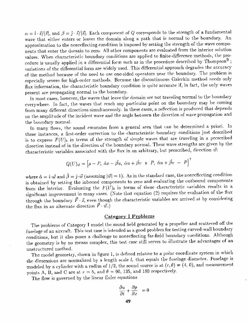
c_ = i. $/Igl, and fl = j-_/l_l. Each component of Q corresponds to the strength of a fundamental
wave that either enters or leaves the domain along a path that is normal to the boundary. An
approximation to the nonreflecting condition is imposed by setting the strength of the wave compo-
nents that enter the domain to zero. All other components are evaluated from the interior solution
values. When characteristic boundary conditions are applied to finite-difference methods, the pro-
cedure is usually applied in a differential form such as in the procedure described by Thompson 9 ;
variations of the differential form are widely used. This differential approach degrades the accuracy
of the method because of the need to use one-sided operators near the boundary. The problem is
especially severe for high-order methods. Because the discontinuous Galerkin method needs only
flux information, the characteristic boundary condition is quite accurate if, in fact, the only waves
present are propagating normal to the boundary.
In most cases, however, the waves that leave the domain are not traveling normal to the boundary
everywhere. In fact, the waves that reach any particular point on the boundary may be coming
from many different directions simultaneously. In these cases, a reflection is produced that depends
on the amplitude of the incident wave and the angle between the direction of wave propagation and
the boundary normal.
In many flows, the sound emanates from a general area that can be determined a priori. In
these instances, a first-order correction to the characteristic boundary conditions just described
is to express F(U)b in terms of the strength of simple waves that are traveling in a prescribed
direction instead of in the direction of the boundary normal. These wave strengths are given by the
characteristic variables associated with the flux in an arbitrary, but prescribed, direction u_:
Q(U)_=[p-P, Sv-fiu, &u+_v + P, &u+fiv - p]T
where _ = i.t_ and ¢) = j.t_ (assuming lull = 1). As in the standard case, the nonreflecting condition
is obtained by setting the inbound components to zero and evaluating the outbound components
from the interior. Evaluating the F(U)b in terms of these characteristic variables results in a
significant improvement in many cases. (Note that equation (2) requires the evaluation of the flux
through the boundary 1_. _, even though the characteristic variables are arrived at by considering
the flux in an alternate direction ft. v_.)
Category I Problems
The problems of Category I model the sound field generated by a propeller and scattered off the
fuselage of an aircraft. This test case is intended as a good problem for testing curved-wall boundary
conditions, but it also poses a challenge to nonreflecting far-field boundary conditions. Although
the geometry is by no means complex, this test case still serves to illustrate the advantages of an
unstructured method.
The model geometry, shown in figure 1, is defined relative to a polar coordinate system in which
the dimensions are normalized by a length scale l_ that equals the fuselage diameter. Fuselage is
modeled by a cylinder with a radius of 1/2, the sound source is at (r, 0) = (4, 0), and measurement
points A, B, and C are at r = 5, and 0 = 90, 135, and 180 respectively.
The flow is governed by the linear Euler equations
Ou OpO-t + Ox - 0
49
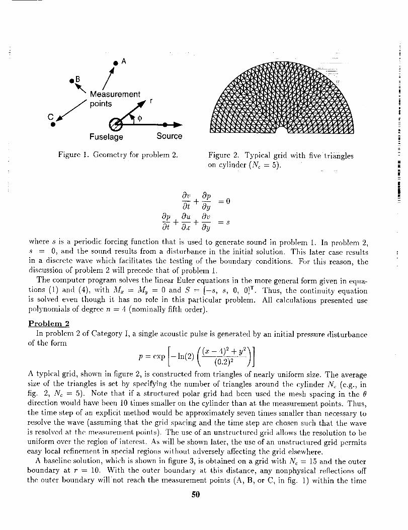
oA
Measurement
c/pOints ._,r
Fuselage Source
Figure 1. Geometry for problem 2.
=
Figure 2. Typical grid with five triangles
on cylinder (No = 5).
Ov Op
0--[+ oy - oOp Ou Ov
O--[+ -5-x + Oy - s
where s is a periodic forcing function that is used to generate sound in problem 1. In problem 2,
s = 0, and the sound results from a disturbance in the initial solution. This later case results
in a discrete wave which facilitates the testing of the boundary conditions. For this reason, the
discussion of problem 2 will precede that of problem 1.
The computer program solves the linear Euler equations in the more general form given in equa-
tions (1) and (4), with Mx = M v = 0 and S' = [-s, s, 0, 0] T. Thus, the continuity equation
is solved even though it has no role in this particular problem. All calculations presented use
polynomials of degree n = 4 (nominally fifth order).
Problem 2
In problem 2 of Category I, a single acoustic pulse is generated by an initial pressure disturbanceof the form
p=exp
A typical grid, shown in figure 2, is constructed from triangles of nearly uniform size. The average
size of the triangles is set by specifying the number of triangles around the cylinder Arc (e.g., in
fig. 2, Nc = 5). Note that if a structured polar grid had been used the mesh spacing in the 0
direction would have been 10 times smaller on the cylinder than at the measurement points. Thus,
the time step of an explicit method would be approximately seven times smaller than necessary to
resolve the wave (assuming that the grid spacing and the time step are chosen such that the wave
is resolved at the measurement points). The use of an unstructured grid allows the resolution to be
uniform over the region of interest. As will be shown later, the use of an unstructured grid permits
easy local refinement in special regions without adversely affecting the grid elsewhere.
A baseline solution, which is shown in figure 3, is obtained on a grid with Nc = 15 and the outer
boundary at r = 10. With the outer boundary at this distance, any nonphysical reflections off
the outer boundary will not reach the measurement points (A, B, or C, in fig. 1) within the time
5O
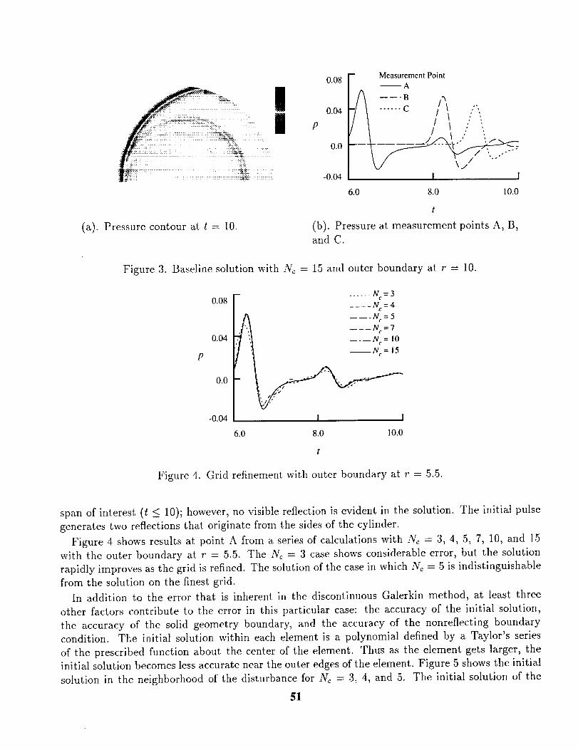
(a). Pressurecontour at t = 10.
P
0.0
-0.04
Measurement Point--A
....... /\ :'./ t :' ",
/ I : ',,
\ j// -.
I I
6.0 8.0 10.0
t
(b). Pressure at measurement points A, B,
and C.
Figure 3. Baseline solution with N_ = 15 and outer boundary at r = 10.
P
0.08
0.04
0.0
-0.04
. ..... Nc=3
.... Nc=4
_N=5-Nc=7
-N c= 10
I _u=15
I I
6.0 8.0 I0.0
Figure 4. Grid refinement with outer boundary at r = 5.5.
span of interest (t _< 10); however, no visible reflection is evident in the solution. The initial pulse
generates two reflections that originate from the sides of the cylinder.
Figure 4 shows results at point A from a series of calculations with .X_ = 3, 4, 5, 7, 10, and 15
with the outer boundary at r = 5.5. The N_ = 3 case shows considerable error, but the solution
rapidly improves as the grid is refined. The solution of the case in which Arc = 5 is indistinguishable
from the solution on the finest grid.
In addition to the error that is inherent in the discontinuous Galerkin method, at least three
other factors contribute to the error in this particular case: the accuracy of the initial solution,
the accuracy of the solid geometry boundary, and the accuracy of the nonreflecting boundary
condition. Tke initial solution within each element is a polynomial defined by a Taylor's series
of the prescribed function about the center of the element. Thus as the element gets larger, the
initial solution becomes less accurate near the outer edges of the element. Figure 5 shows the initial
solution in the neighborhood of the disturbance for Arc = 3, 4, and 5. The initial solution of the
51
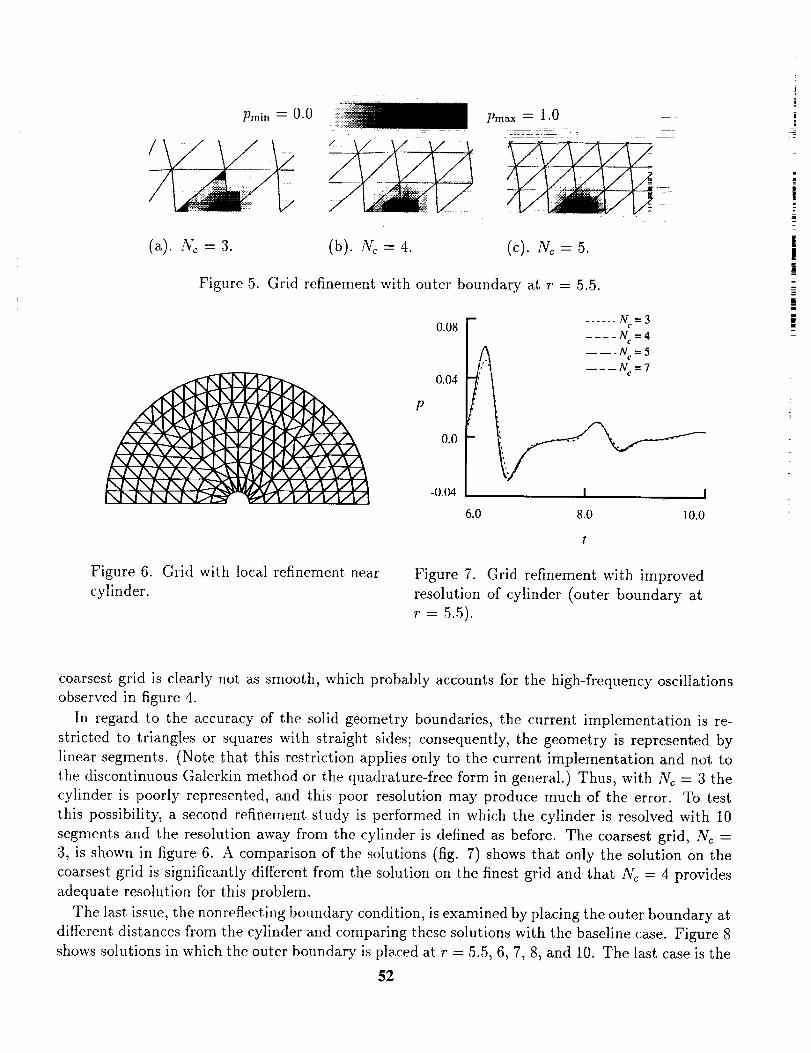
Pmin = 0.0 Pmax = 1.0 -_
(a). l\_ = 3. (b). x =4. (c). = 5.
Figure 5. Grid refinement with outer boundary at r = 5.5.
4
0.08
0.04
p
0.0
-0.04
...... N=3
.... Nc =4
l,,_ -----N=5
' ti\S -----Ne = 7
I I
6.0 8.0 10.0
Figure 6. Grid with local refinement near
cylinder.Figure 7. Grid refinement with improved
resolution of cylinder (outer boundary at
r = 5.5).
i!
i
i|
||
|!
=
coarsest grid is clearly not as smooth, which probably accounts for the high-frequency oscillations
observed in figure 4.
In regard to the accuracy of the solid geometry boundaries, the current implementation is re-
stricted to triangles or squares with straight sides; consequently, the geometry is represented by
linear segments. (Note that this restriction applies only to the current implementation and not to
the discontinuous Galerkin method or the quadrature-free form in general.) Thus, with Arc = 3 the
cylinder is poorly represented, and this poor resolution may produce much of the error. To test
this possibility, a second refinement study is performed in which the cylinder is resolved with 10
segments and the resolution away from the cylinder is defined as before. The coarsest grid, Arc =
3, is shown in figure 6. A comparison of the solutions (fig. 7) shows that only the solution on the
coarsest grid is significantly different from the solution on the finest grid and that Arc = 4 provides
adequate resolution for this problem.
The last issue, the nonreflecting boundary condition, is examined by placing the outer boundary at
different distances from the cylinder and comparing these solutions with the baseline case. Figure 8
shows solutions in which the outer boundary is placed at r = 5.5, 6, 7, 8, and 10. The last case is the
52
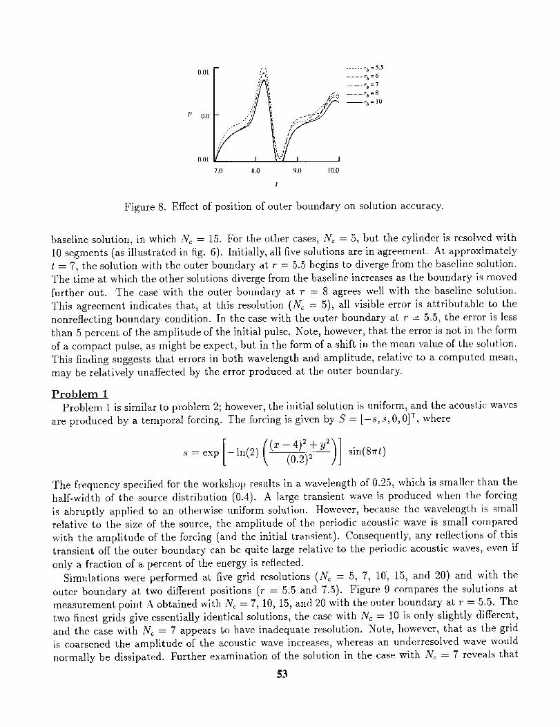
i0.01 : "
.:y I
o.o - _;"
-0.01 _ t
7.0 8,0
......%=5.5
.... r_=6
-----rb=7
,_.._ -----rb=8
./_ --rb= 10
orf--.-._,Ct, Y,
9.0 10.0
Figure 8. Effect of position of outer boundary on solution accuracy.
baseline solution, in which Nc = 15. For the other cases, Nc = 5, but the cylinder is resolved with
10 segments (as illustrated in fig. 6). Initially, all five solutions are in agreement. At approximately
t = 7, the solution with the outer boundary at r = 5.5 begins to diverge from the baseline solution.
The time at which the other solutions diverge from the baseline increases as the boundary is moved
further out. The case with the outer boundary at r = 8 agrees well with the baseline solution.
This agreement indicates that, at this resolution (No = 5), all visible error is attributable to the
nonreflecting boundary condition. In the case with the outer boundary at r = 5.5, the error is less
than 5 percent of the amplitude of the initial pulse. Note, however, that the error is not in the form
of a compact pulse, as might be expect, but in the form of a shift in the mean value of the solution.
This finding suggests that errors in both wavelength and amplitude, relative to a computed mean,
may be relatively unaffected by the error produced at the outer boundary.
Problem 1
Problem 1 is similar to problem 2; however, the initial solution is uniform, and the acoustic waves
are produced by a temporal forcing. The forcing is given by S = [-s, s, 0, 0] v, where
s:ex,[ ,n,2) +'2)](0'2) 2 sin(87rt)
The frequency specified for the workshop results in a wavelength of 0.25, which is smaller than the
half-width of the source distribution (0.4). A large transient wave is produced when the forcing
is abruptly applied to an otherwise uniform solution. However, because the wavelength is small
relative to the size of the source, the amplitude of the periodic acoustic wave is small compared
with the amplitude of the forcing (and the initial transient). Consequently, any reflections of this
transient off the outer boundary can be quite large relative to the periodic acoustic waves, even if
only a fraction of a percent of the energy is reflected.
Simulations were performed at five grid resolutions (No = 5, 7, 10, 15, and 20) and with the
outer boundary at two different positions (r = 5.5 and 7.5). Figure 9 compares the solutions at
measurement point A obtained with N_ = 7, 10, 15, and 20 with the outer boundary at 7"= 5.5. The
two finest grids give essentially identical solutions, the case with Nc = 10 is only slightly different,
and the case with Arc = 7 appears to have inadequate resolution. Note, however, that as the grid
is coarsened the amplitude of the acoustic wave increases, whereas an underresolved wave would
normally be dissipated. Further examination of the solution in the case with Arc = 7 reveals that
53
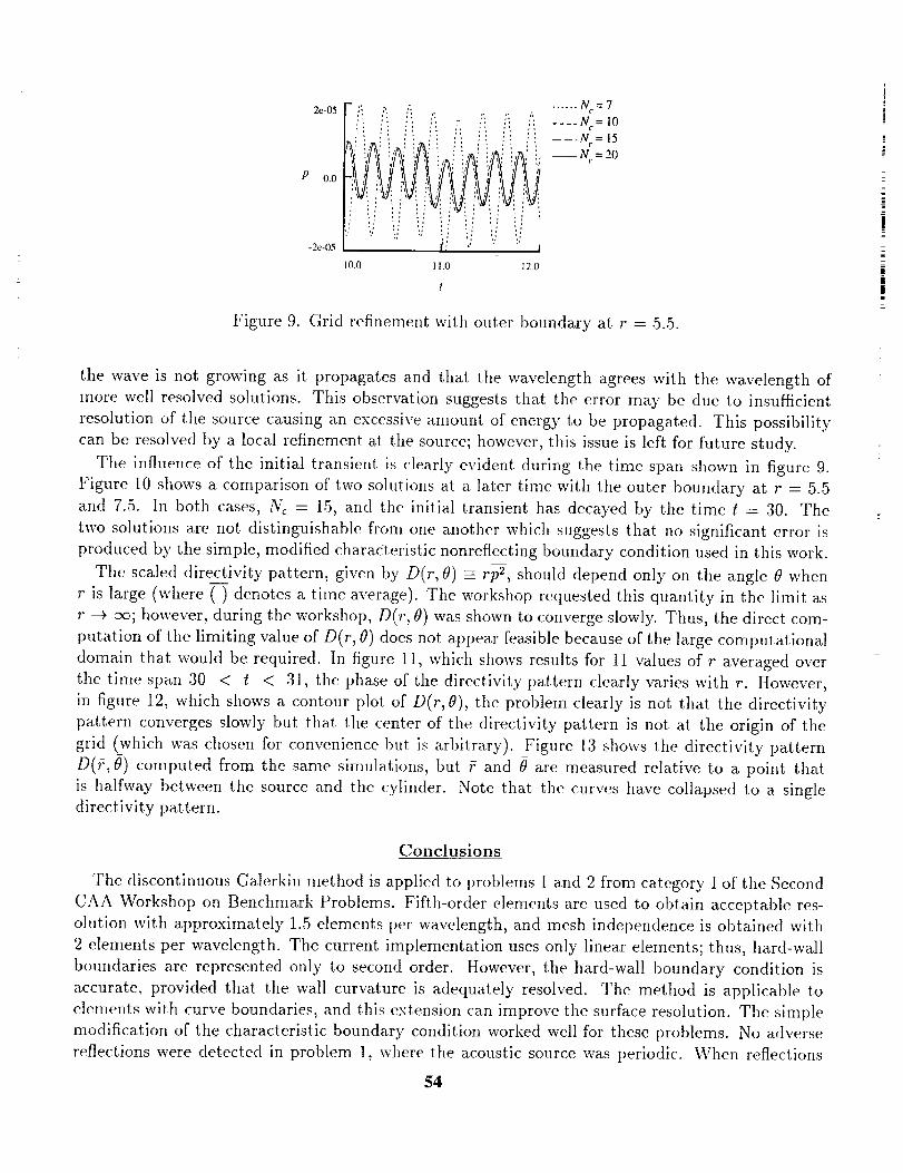
2e-05
P 0.0
-2e-05
/i!iJi ......
lo.o ,_,o _zo
Figure 9. Grid refinement with outer boundary at 7"= 5.5.
the wave is not growing as it propagates and that the wavelength agrees with the wavelength of
more well resolved solutions. This observation suggests that the error may be due to insufficient
resolution of the source causing an excessive amount of energy to be propagated. This possibility
can be resolved by a local refinement at the source; however, this issue is left for future study.
The influence of the initial transient is clearly evident during the time span shown in figure 9.
Figure 10 shows a comparison of two solutions at a later time with the outer boundary at r = 5.5
and 7.5. In both cases, N_ = 1.5, and the initial transient has decayed by the time t = 30. The
two solutions are not distinguishable fl'om one another which suggests that no significant error is
produced by the simple, modified characteristic nonreflecting boundary condition used in this work.
The scaled directivity pattern, given by D(r, O) = rp-g, should depend only on the angle 0 when
r is large (where ( ) denotes a time average). The workshop requested this quantity in the limit as
r -+ :x_; however, during the workshop, D(r, 0) was shown to converge slowly. Thus, the direct com-
putation of the limiting value of D(r, 0) does not appear feasible because of the large computational
domain that would be required. In figure 11, which shows results for 11 values of r averaged over
the time span 30 < t < 31, the phase of the directivity pattern clearly varies with r. However,
in figure 12, which shows a contour plot of D(r,O), the problem clearly is not that the directivity
pattern converges slowly but that the center of the directivity pattern is not at the origin of the
grid (which was chosen for convenience but is arbitrary). Figure la shows the directivity pattern
D(/;, 0) computed from the same simulations, but _ and 0 are measured relative to a point that
is halfway between the source and the cylinder. Note that the curves have collapsed to a singledirectivity pattern.
Conclusions
The discontinuous Galerkin method is applied to problems i and 2 from category I of the Second
CAA Workshop on Benchmark Problems. Fifth-order elements are used to obtain acceptable res-
olution with approximately 1.5 elements per wavelength, and mesh independence is obtained with
2 elements per wavelength. The current implementation uses only linear elements; thus, hard-wall
boundaries are represented only to second order. However, the hard-wall boundary condition is
accurate, provided that the wall curvature is adequately resolved. The method is applicable to
elements with curve boundaries, and this extension can improve the surface resolution. The simple
modification of the characteristic boundary condition worked well for these problems. No adverse
reflections were detected in problem 1, where the acoustic source was periodic. When reflections
54
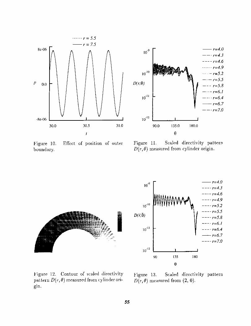
...... r=5.5
--r=7.5
8e-06_ A /_ l
P 0.0 -
-8e-06
30.0 30.5 31.0
t
Figure 10. Effect of position of outer
boundary.
!0 "9
10 -1o
D(r,O)
10 "11
10 -12 I
90.0 135.0
0
-- r=4.0
----- r=4.3
.... r=4.6
...... r=4.9
---- r=5.2
----- r=5.5
---- r=5.8
.... r=6.1
.... r=6.4
-- r=6. 7
----- r= 7.0
180.0
Figure 11. Scaled directivity pattern
D(r, 0) measured from cylinder origin.
Figure 12. Contour of scaled directivity
pattern D(r, 0) measured from cylinder ori-
gin.
lO "9
10 -11
10 -12
-- r=4.0
.... r=4.3
.... r=4.6
.... r=4.9
.... r=5.2
.... r=5.5
.... r=5.8
.... r=6. !
.... r=6.4
r=6.7
.... r=7.0
90
I I
135 180
0
Figure 13. Scaled directivity pattern
D(r,O) measured from (2, 0).
55
were detected, the error was in the form of a shift in the average of the solution rather than a
discrete pulse. The acoustic directivity pattern can be estimated directly from a simulation on a
small domain, provided that the correct center of the pattern is identified.
References
1. H. L. Atkins and Chi-Wang Shu, "Quadrature-Free Implementation of the Discontinuous
Galerkin Method for Hyperbolic Equations," AIAA-paper 96-1683, 1996.
. B. Cockburn, S. Hou, and C.-W. Shu, "The Runge-Kutta local projection discontinuous
Galerkin finite element method for conservation laws IV: The multidimensional case," Mathe-
matics of Computation, v54 (1990), pp. 545-581.
. F. Bassi and S. Rebay, "Accurate 2D Euler Computations by Means of a High-Order Discontin-
uous Finite Element Method," Proceedings of the 14th international Conference on Numerical
Methods in Fluid Dynamics, Bangalor, india, July ll-15, 1994.
. R. B. Lowrie, P. L. Roe, and B. van Leer, "A Space-Time Discontinuous Galerkin Method for
Time-Accurate Numerical Solution of Hyperbolic Conservation Laws," Presented at the 12th
AIAA computational Fluid Dynamics Conference, San Diego, CA, June 19-22, 1995.
. B. Cockburn and C.-W. Shu, "TVB Runge-Kutta local projection discontinuous Galerkin finite
element method for conservation laws II: General framework," Mathematics of Computation,
v52 (1989), pp. 411-435.
6. C.-W. Shu and S. Osher, "Efficient implementation of essentially non-oscillatory shock-
capturing schemes," Journal of Computational Physics, v77 (1988), pp. 361-383.
. B. Gustafson, H.-O. Kreiss, and A. Sundstr5m, "Stability theory of difference approximations
for mixed initial-boundary value problems, II," Mathematics of Computation, v26 (1972), pp.649-686.
. H. L. Atkins, "Continued Development of Discontinuous Galerkin Method for Aeroacoustic
Applications " To be presented at the 3rd AIAA/CEAS Aeroacoustic Conference, Atlanta,
CA, May 12-14, 1997.
9. Kevin W. Thompson, "Time dependent Boundary Conditions for Hyperbolic Systems," Journal
of Computational Physics, v68 (1987), pp. 1-24.
!!m
!
||
i
!=
56
COMPUTATION OF ACOUSTIC SCATTERING BY ASCHEME
<=7LOW-DISPERSION i+
Oktay Baysal and Dinesh K. Kaushik
Department of Aerospace EngineeringOld Dominion University, Norfolk, Virginia 23529-0247
Physical problem and background
The objective is the evaluation of a proposed computational aeroacoustics (CAA) method in simulating anacoustic scattering problem. An example may be the sound field generated by a propeller scattered off bythe fuselage of an aircraft. The pressure loading on the fuselage would be an input to the interior noiseproblem. To idealize the problem, the fuselage is assumed to be a circular cylinder and the noisegeneration by the propeller is represented by a line source.
A typical CFD algorithm may not be adequate for this aeroacoustics problem: amplitudes are an order
of magnitude 0 smaller yet frequencies are 0 larger than the flow variations generating the sound. For
instance, an 0 (2) CFD method was previously used for a nonlinear wave propagation problem inunsteady, nonuniform mean flow (Baysal et al., 1994). It was observed that a direct simulation of acousticwaves using a higher-order CFD would become prohibitively expensive, due to the required excessivenumber of grid points per wavelength (PPM). Also, CAA would need minimal dispersion and dissipation,
which would preclude a typical 0 (2) CFD method from a long-term wave propagation simulation.Furthermore, a consistent, stable, convergent, high-order scheme is not necessarily dispersion-relation
preserving, i.e. no guarantee for a quality numerical solution. Therefore, a baseline 0 (4) dispersion-relation-preserving (DRP) method (Tam and Webb, 1993) was investigated (Vanel and Baysal, 1997) for avariety of wave propagation problems, such as, single-, simultaneous-, and successive-acoustic-pulses.Then, a number of algorithmic extensions were performed (Kaushik and Baysal, 1996), when thefollowing were studied: viscous effects by solving the linearized Navier-Stokes equations, low-storageand low-CPU time integration by an optimized Runge-Kutta scheme, generalized curvilinear coordinates
for curved boundaries, higher-order accuracy by comparing 0 (4) DRP vs. va (6) DRP, and choice ofboundary conditions and differencing stencils. The scheme is now being investigated for nonlinear wavepropagation in nonuniform flow (Baysal et al., 1997).
Mathematical approach
The linearized, two-dimensional, compressible, Euler equations were considered in generalized curvilinearcoordinates
0/(1) o/£18__7.= -R(I) ) + S , where R(O) = _ +--,90
The primitive variables, 0, and the transformed fluxes, /_ and _, are,
(2) 0=_[p u v p]', D={[_=E+_yF], F=-}[rl, E+rlyF]
57
and the physical fluxes and the source vector are,
l"°"+p/(3) E= 1 Mov 1, F= 0 S=
LMop+Uj
0I:tThe perturbed values of density (p), pressure (p), and velocity (u, v) are denoted without a subscript, butthose of the mean flow are demarcated using the subscript 0. These variables were normalized using thecylinder diameter (D) for length, speed of sound (ao) for velocity, D/ao for time, Po for density, andpo(aofi for pressure.
Dispersion relation of a proposed numerical scheme should match closely that of eq. (1) for large
range of resolution; i.e. _ and N be close approximations to a and 09. Assuming -flAx was a periodic
(2r0 function of aAx with, Fourier-Laplace transforms rendered,
-i M ei.aj_ -- i(e -i'°_at - 1)= _ aj and co - N(4) a Ax j--Z'-L
At E bj e i'j°Jat
Finite difference coefficients were obtained from Taylor series expansions as one-parameter family, andthe remaining coefficient from an error minimization, where the integration limit e depended on theshortest wavelength to be simulated: _
__7r/2_ _4. SAx_(5) min fl=min_ iI' Ax--fla t where l,_Axl-_e and e-[ 1.1J for [. 7Ax J"
/.
The time integration of eq. (i) was performed in two different ways. In the first approach, a four-point finite difference, which in a standard sense could be up to third-order accurate, was derived from the
Taylor series as a one-parameter family. The remaining coefficient (bJ) was determined, as in the spatialcoefficients, by minimizing the discrepancy between the effective and the exact dispersion relations. After
discretizing all the terms in eqs. (1)-(3), the resulting O(At2,Ax N+M-2) DRP scheme was as follows:
M ^n M ^n
A.÷_ ". s ._j " E aj E.j,,. -_,, E aj F_,,.+j(6) "e,m = U_.,, + At 5".bj Re.,, where Re.,,, = _-_j=O j=-N j--.-N
In eq. (6), g and m are the spatial indices and n indicates the time level. For N=M, difference is central,for N=0, it is fully forward, and for M=0, it is fully backward. All the interior cells were computed usingcentral differences with N=M=3. However, since these high-order stencils require multiple layers ofboundary cells, all combinations between a central and a fully-one-sided difference need also be derived.Only then, it would be possible to always utilize the information from the nearest possible points for betteraccuracy. In the present computations a fourth-order scheme was used, requiring 7-point stencil: N takesvalues from 6 to 0, M takes values from 0 to 6, and N+M=6.
The numerically stable maximum time step At was calculated from the Courant-Friedrichs-Lewyrelation. For example, for the fourth-order scheme in Cartesian coordinates, the stable CFL number wasfound to be 0.4. However, after analyzing the numerical damping of the time integration scheme, the CFLvalue was set to the more stringent value of 0.19. Since, however, time integration with DRP wouldrequire the storage of four time levels, a lower storage alternative, the low-dissipation and low-dispersion
58
five-stage Runge-Kutta scheme (Hu et al., 1996) was adapted and implemented. The resulting scheme hadthe spatial integration identical to eq. (6), but the time integration was replaced by the following:
(7) 0_o) = (j., (j_i) =0_o) -fli At R(i-t) , (j.+t : (fie), i = 1,2 .... p
The indices n, p and i indicate the time level, and the order and the stage of the Runge-Kutta method,respectively. As for the coefficients,/31=0 and the other coefficients/3i were determined from
i
(8) ci= I-l flp_k+2 , i=2 .... ,pk=2
The coefficients c i were computed by considering the amplification factor of the Runge-Kutta scheme, thenminimizing the dispersion-relation error. The time steps were determined from the stability as well as theaccuracy limits. In the present study, a five-stage Runge-Kutta (p =5) was used, which required twolevels of storage and it was at least second-order accurate. When it was used with the present 7-pointspatial stencil to solve the scalar linear wave equation, the CFL limit from the stability was found to be3.05, but it was only 1.16 from the accuracy limit. Since, however, this still was larger than the CFL limit
of the DRP time integration, this method was also more efficient in processing time.
Usually low-order schemes are used in resolving the highly nonlinear flow or acoustic phenomena.Even with second-order schemes, it is common to have limiters or artificial damping mechanisms, eitherimplicit in the scheme or explicitly added. Since simulating low-amplitude acoustic waves for a long timeand for many wavelengths of travel is the objective in CAA, devising such artificial damping mechanismsrequires extreme care. For example, constant damping over all wave numbers need to be avoided. Tam etal. (1993) suggested terms, which have small damping over the long wave range but significant damping inthe short wave range. The present central-difference scheme includes similar terms with a user specifiedartificial Reynolds number, to overcome the expected spurious oscillations:
M
(9) D_,, n _ I _c [ 1 _n 1 ^nn _ _eD j=-NJ" _ g+j,m +-_02Ug,m+j], where Re o -- P°a°Dlaa
The boundaries should be transparent to the acoustic disturbances reaching them to avoid anydegradation of the numerical solution. From the asymptotic solutions of the finite difference form of theEuler equations, a set of radiation boundary conditions, were derived and implemented. Therefore,following Tam and Webb (1993) and from the asymptotic solutions of the finite difference form of eq. (1),a set of radiation boundary conditions were derived,
(10) --+A_--:_-.+__-z---+CU = 0, whereo_t o¢
(ll) A=vX_x+Y_rr ' B=vXOx+yrlYr ' C_'_r and r=l_ x2+y2, V=XMo+_ 1-(MOy)2r
For an inviscid solid wall (w) or a symmetry plane, the impermeability condition dictates that the normalcontravariant velocity be zero at all times:
(12) ¢_= rlxU+ rlyv = 0 .
When this equation was constructed from the q- and {-momentum equations, after multiplying them by theappropriate metrics and adding, the wall value of pressure at the ghost point (subscript -1) was obtained,
59
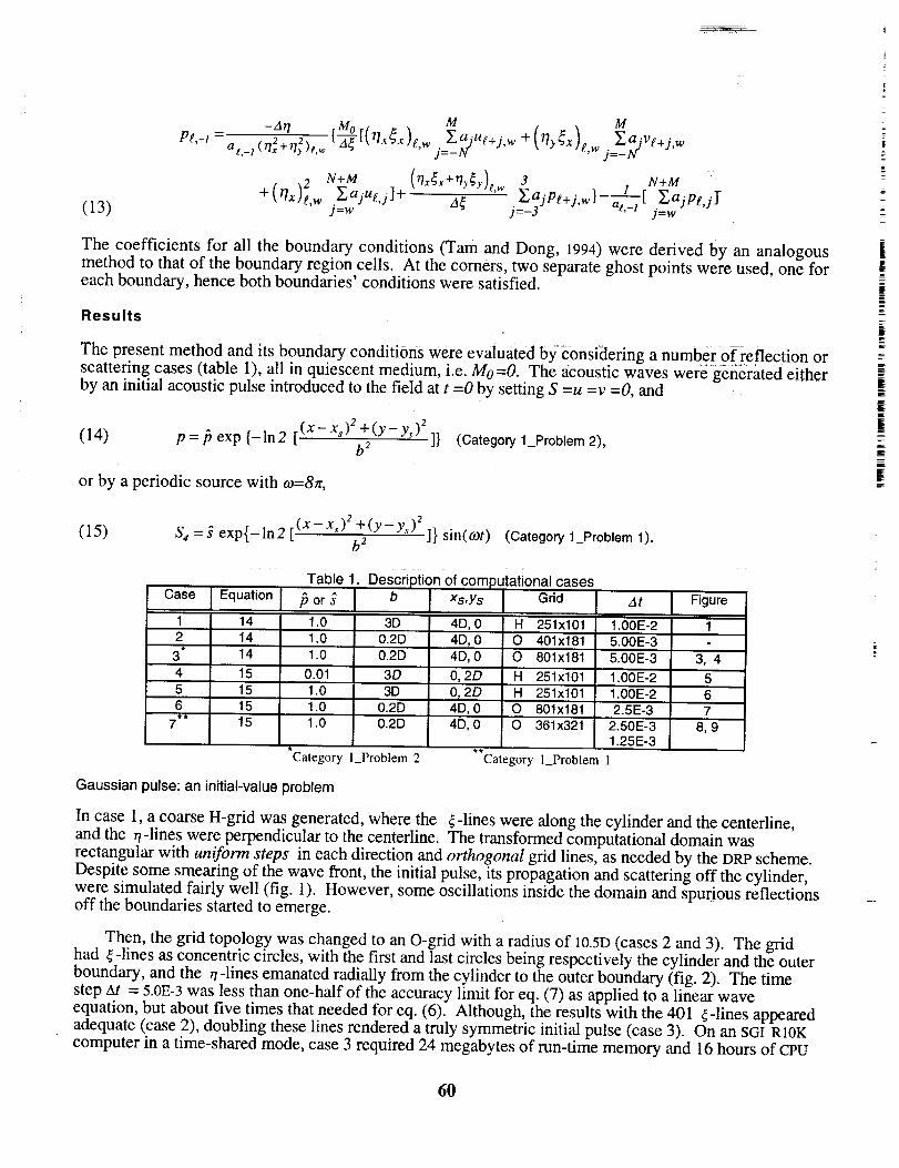
(13)
Pg,-I =2 2 { [(rlx_x)gw aqjrt(+j,w +(Tly_x)g,w jSagl"vg+j,wat_l(rlx+71y)e, w , .=_
N+M (Ox_x+Oy_y)g w 3 . N+M
+(rlx)_,w ._.,ajue,j]_ A_ ' Y.ajpe+j,w}-a@,[ _.ajpg jJJ=W j=-3 t,-I j=w "
The coefficients for all the boundary conditions (Tam and Dong, 1994)were derived by an analogousmethod to that of the boundary region cells. At the corners, two separate ghost points were used, one foreach boundary, hence both boundaries' conditions were satisfied.
Results
The present method and its boundary conditions were evaluated by:consiaering a number of reflection or
scattering cases (table 1), all in quiescent medium, i.e. Mo =0. The acoustic waves were generated eitherby an initial acoustic pulse introduced to the field at t =0 by setting S =u =v =0, and
(14) p=/3 exp {-In2 [ (x-xs)2+(y-y')2b2 ]} (Category 1_Problem 2),
or by a periodic source with w=8zr,
(15)--Xs)2 +(y--ys) 2
$4 = g exp{- In 2 [ (x b 2 ]} sin(cot) (Category 1_Problem 1).
Case EquationTable ii Description of computational cases
/3 or _ b xs,y s Grid ,_t Figure
1 14 1.00E-2 12 14 5.00E-3
3* 14 5.00E-3 3, 44 15 1.00E-2 55 15 1.00E-2 6
1.0 3D1.0 0.2D1.0 0.2D
0.01 3D1.0 3D1.0 0.2D1.0 0.2D
Category I_Problem 2
4D, 0 H 251x1014D, 0 O 401x1814D, 0 O 801x181
0,2D H 251x10t0,2D H 251x1014D, 0 O 801x1814D, 0 "O 361x321
Category l_Problem 1
6
7
2.5E-3 72.50E-31.25E-3
1515 8, 9
Gaussian pulse: an initial-value problem
In case 1, a coarse H-grid was generated, where the _-lines were along the cylinder and the centerline,and the 77-1ines were perpendicular to the centedine. The transformed computational domain wasrectangular with uniform steps in each direction and orthogonal grid lines, as needed by the DRP scheme.Despite some smearing of the wave front, the initial pulse, its propagation and scattering off the cylinder,were simulated fairly well (fig. 1). However, some oscillations inside the domain and spurious reflectionsoff the boundaries started to emerge.
Then, the grid topology was changed to an O-grid with a radius of 10.5D (cases 2 and 3). The gridhad _-lines as concentric circles, with the first and last circles being respectively the cylinder and the outerboundary, and the 71-lines emanated radially from the cylinder to the outer boundary (fig. 2). The timestep At = 5.0E-3 was less than one-half of the accuracy limit for eq. (7) as applied to a linear waveequation, but about five times that needed for eq. (6). Although, the results with the 401 _-lines appearedadequate (case 2), doubling these lines rendered a truly symmetric initial pulse (case 3). On an SGI R10Kcomputer in a time-shared mode, case 3 required 24 megabytes of run-time memory and 16 hours of CPU
6O
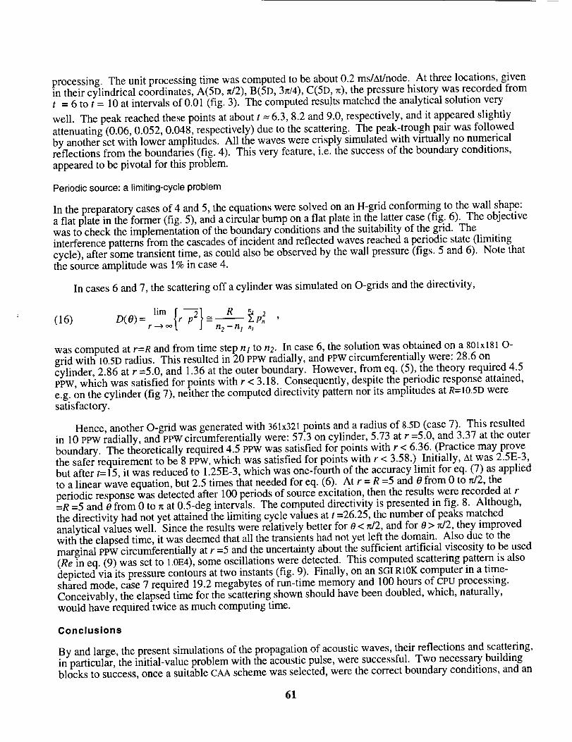
processing.Theunit processingtimewascomputedto beabout0.2ms/At/node.At threelocations,givenin their cylindrical coordinates,A(5D,n/2), B(5D, 3n/4), C(5D, n), the pressure history was recorded fromt = 6 to t = 10 at intervals of 0.01 (fig. 3). The computed results matched the analytical solution very
well. The peak reached these points at about t ---6.3, 8.2 and 9.0, respectively, and it appeared slightly
attenuating (0.06, 0.052, 0.048, respectively) due to the scattering. The peak-trough pair was followedby another set with lower amplitudes. All the waves were crisply simulated with virtually no numericalreflections from the boundaries (fig. 4). This very feature, i.e. the success of the boundary conditions,appeared to be pivotal for this problem.
Pedodic source: a limiting-cycle problem
In the preparatory cases of 4 and 5, the equations were solved on an H-grid conforming to the wall shape:a flat plate in the former (fig. 5), and a circular bump on a flat plate in the latter case (fig. 6). The objectivewas to check the implementation of the boundary conditions and the suitability of the grid. Theinterference patterns from the cascades of incident and reflected waves reached a periodic state (limitingcycle), after some transient time, as could also be observed by the wall pressure (figs. 5 and 6). Note thatthe source amplitude was 1% in case 4.
In cases 6 and 7, the scattering off a cylinder was simulated on O-grids and the directivity,
lira [r--_ R " 2(16) D( O) = r __ _ t.,.. j= _, p,
n 2 -- n I nl
was computed at r=R and from time step n I to n2. In case 6, the solution was obtained on a 801x181 O-gridwith 10.5D radius. This resulted in 20 PPW radially, and PPW circumferentially were: 28.6 oncylinder, 2.86 at r =5.0, and 1.36 at the outer boundary. However, from eq. (5), the theory required 4.5PPW, which was satisfied for points with r < 3.18. Consequently, despite the periodic response attained,e.g. on the cylinder (fig 7), neither the computed directivity pattern nor its amplitudes at R=10.5D weresatisfactory.
Hence, another O-grid was generated with 361x321 points and a radius of 8.5D (case 7). This resultedin 10 PPW radially, and PPW circumferentially were: 57.3 on cylinder, 5.73 at r =5.0, and 3.37 at the outerboundary. The theoretically required 4.5 PPW was satisfied for points with r < 6.36. (Practice may provethe safer requirement to be 8 PPW, which was satisfied for points with r < 3.58.) Initially, At was 2.5E-3,but after t=-15, it was reduced to 1.25E-3, which was one-fourth of the accuracy limit for eq. (7) as appliedto a linear wave equation, but 2.5 times that needed for eq. (6). At r = R =5 and 0 from 0 to rd2, theperiodic response was detected after 100 periods of source excitation, then the results were recorded at r=R =5 and 0 from 0 to n at 0.5-deg intervals. The computed directivity is presented in fig. 8. Although,the directivity had not yet attained the limiting cycle values at t =26.25, the number of peaks matchedanalytical values well. Since the results were relatively better for 0 < rd2, and for 0 > rd2, they improvedwith the elapsed time, it was deemed that all the transients had not yet left the domain. Also due to themarginal PPW circumferentially at r =5 and the uncertainty about the sufficient artificial viscosity to be used(Re in eq. (9) was set to 1.0E4), some oscillations were detected. This computed scattering pattern is alsodepicted via its pressure contours at two instants (fig. 9). Finally, on an SGI R10K computer in a time-shared mode, case 7 required 19.2 megabytes of run-time memory and 100 hours of CPU processing.Conceivably, the elapsed time for the scattering shown should have been doubled, which, naturally,would have required twice as much computing time.
Conclusions
By and large, the present simulations of the propagation of acoustic waves, their reflections and scattering,in particular, the initial-value problem with the acoustic pulse, were successful. Two necessary buildingblocks to success, once a suitable CAA scheme was selected, were the correct boundary conditions, and an
61
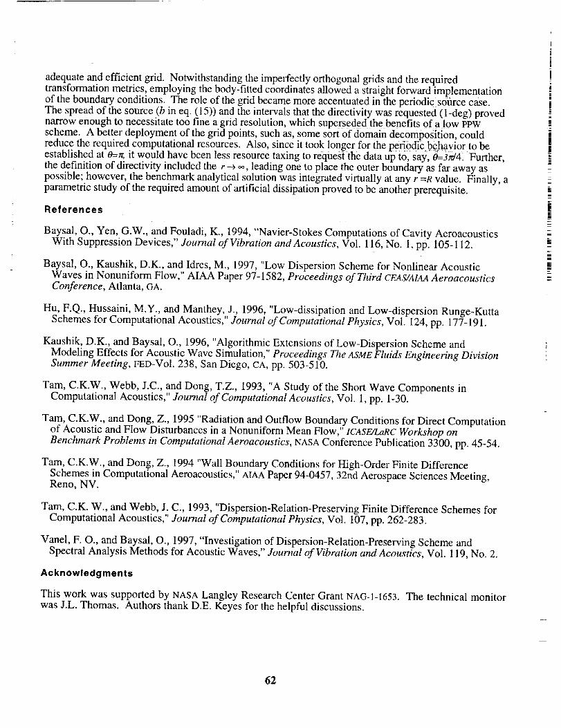
adequateandefficientgrid. Notwithstandingtheimperfectlyorthogonalgridsandtherequiredtransformationmetrics,employingthebody-fittedcoordinatesallowedastraightforwardimplementationof theboundaryconditions.Theroleof thegrid becamemoreaccentuatedin theperiodicsourcecase.The spreadof thesource(b in eq.(15))andtheintervalsthatthedirectivity wasrequested(1-deg)provednarrowenoughto necessitatetoo fineagrid resolution,whichsupersededthebenefitsof a low PPWscheme.A betterdeploymentof thegrid points,suchas,somesortof domaindecomposition,couldreducetherequiredcomputationalresources.Also,sinceit took longerfor theperi0dicbehaviorto beestablishedat 0=-_ it would have been less resource taxing to request the data up to, Say, _3_41 Further,the definition of directivity included the r --_ oo, leading one to place the outer boundary as far away as
possible; however, the benchmark analytical solution was integrated virtually at any r =R value. Finally, aparametric study of the required amount of artificial dissipation proved to be another prerequisite.
References
Baysal, O., Yen, G.W., and Fouladi, K., 1994, "Navier-Stokes Computations of Cavity AeroacousticsWith Suppression Devices," Journal of Vibration and Acoustics, Vol. 116, No. 1, pp. 105-112.
Baysal, O., Kaushik, D.K., and Idres, M., 1997, "Low Dispersion Scheme for Nonlinear AcousticWaves in Nonuniform Flow," AIAA Paper 97-1582, Proceedings of Third CEAS/AIAA AeroacousticsConference, Atlanta, GA.
Hu, F.Q., Hussaini, M.Y., and Manthey, J., 1996, "Low-dissipation and Low-dispersion Runge-KuttaSchemes for Computational Acoustics," Journal of Computational Physics, Vol. 124, pp. 177-191.
Kaushik, D.K., and Baysal, O., 1996, "Algorithmic Extensions of Low-Dispersion Scheme andModeling Effects for Acoustic Wave Simulation," Proceedings The ASME Fluids Engineering DivisionSummer Meeting, FED-Vol. 238, San Diego, CA, pp. 503-510.
Tam, C.K.W., Webb, J.C., and Dong, T.Z., 1993, "A Study of the Short Wave Components inComputational Acoustics," Journal of Computational Acoustics, Vol. 1, pp. 1-30.
Tam, C.K.W., and Dong, Z., 1995 "Radiation and Outflow Boundary Conditions for Direct Computationof Acoustic and Flow Disturbances in a Nonuniform Mean Flow," ICASE/LaRC Workshop on
Benchmark Problems in Computational Aeroacoustics, NASA Conference Publication 3300, pp. 45-54.
Tam, C.K.W., and Dong, Z., 1994 "Wall Boundary Conditions for High-Order Finite Difference
Schemes in Computational Aeroacoustics," AIAA Paper 94-0457, 32nd Aerospace Sciences Meeting,Reno, NV.
Tam, C.K.W., and Webb, J. C., 1993, "Dispersion-Relation-Preserving Finite Difference Schemes forComputational Acoustics," Journal of Computational Physics, Vol. 107, pp. 262-283.
Vanel, F. O., and Baysal, O., 1997, "Investigation of Dispersion-Relation-Preserving Scheme andSpectral Analysis Methods for Acoustic Waves," Journal of Vibration and Acoustics, Vol. 119, No. 2.
Acknowledgments
This work was supported by NASA Langley Research Center Grant NAG-I-1653. The technical monitor
was J.L. Thomas. Authors thank D.E. Keyes for the helpful discussions.
i
i
ii
|
|
__1|¢i
J
z
|i
E
mi
m
62
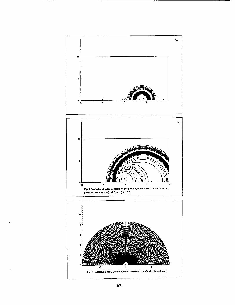
(a)
!
lo
51-
o'-1o
I , • •-5
(b)
10
0-10
l
-5 0 5 10
Rg. 1 Scattering of pulse-generated waves off a cylinder (case1): instantaneous
pressure contours at (a) t=2.0, and Co) t=7.0.
,°i8
6
4
2
0-5 0 5
Rg. 2 Representative O-gdd conforming to the surface of a circular cylinder.
63
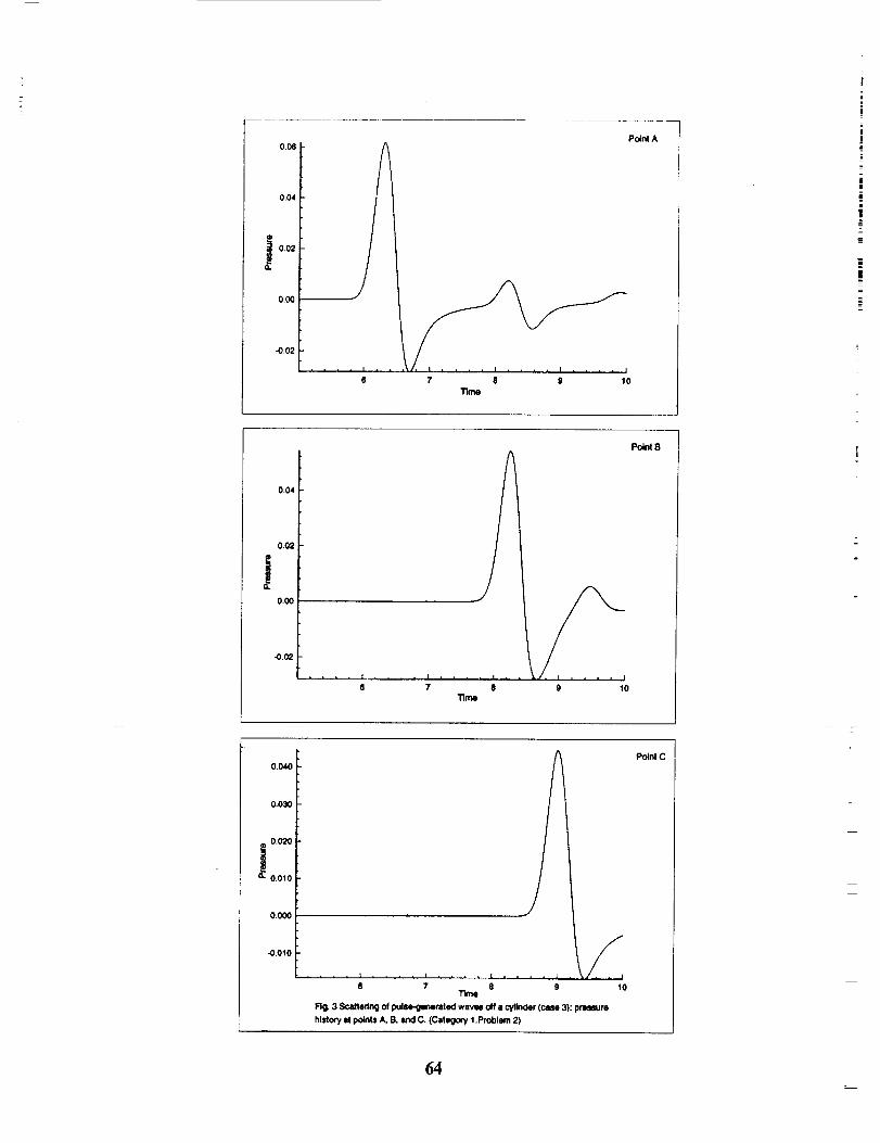
006
0.04
i 0.02
0.00.
002!
6 7 8 g 10Time
P_ntA
0.04
0.02
J0.00
002
0.040
0.030 i
0.000 !
-0.010 F
.... i _ i , i i .... ! ,7 8
Time9 I0
/.... z .... i . . , , l , , , , L , _/_ . K
e 7 8 9 10Time
Rg 3 Sc_ledng of pulse-generated wavee off a cylinder (case 3): pressure
hlstor_ al points A, B and C (Category I Problem 2)
Point B
P_ntC
64
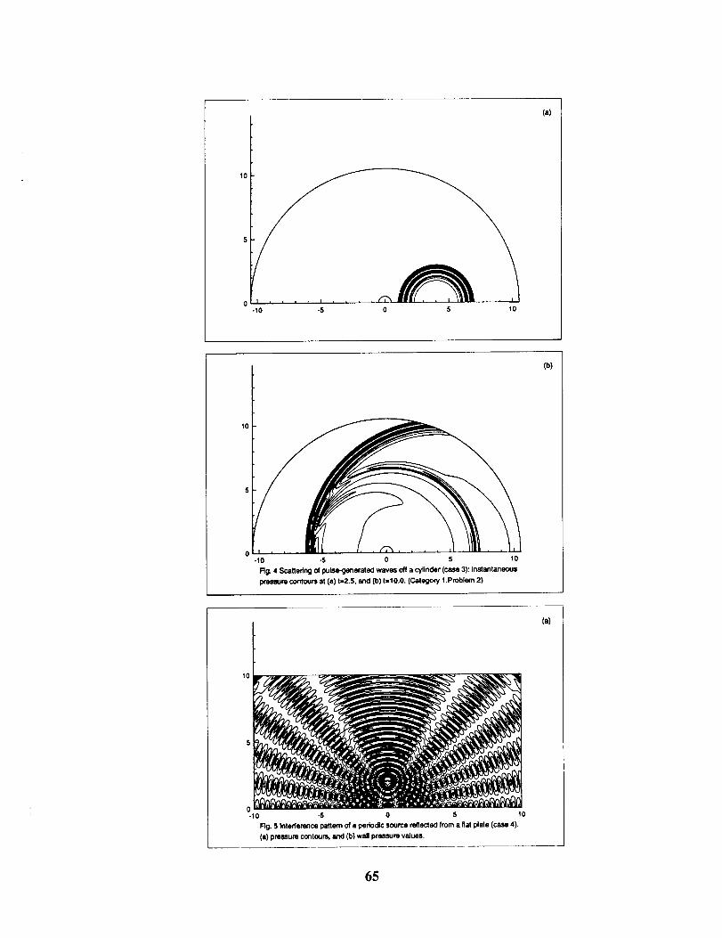
(a)
i , , ,0 ] ' ' ' f
-10 -5 0 5 10
(b)
10
it
-10 -5 0 5 10
Rg. 4 Scattering of puise-genoratod waves off a cyJinder (case 3): instantaneous
pressure contours at (a) t-2.5, and (b) t-10.0. (Category 1 .problem 2)
(a)
10
$
0-I0 -5 0 5 10
Rg. 5 Intederence pattern of a periodic source reflected from a fiat plate (case 4).
(a) pressure contours, snd (b) wall pressure values.
65
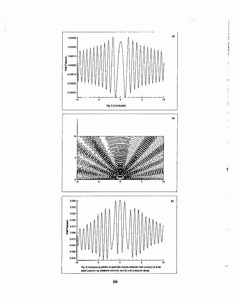
0.00030
0.00020
0.00010
0.00000
-O.OOO1O
-0.00020
-O.OOO3O
, , , , I , , • I , , , I .... I
-I0 -5 0 5 10
rig. s (Cor_uded)
_0
0-10 -5 0 5 tO
(b)
(a)
0.050
O.04O
0.030
0.020
i 0.010
0.000
`0.010
-0.O2O
-0.030
-0.04O i-
-10 -5 0 5 10
Fig. 8 Interference patlem of aperlod4c source reflected from a bump on a fiat
plate (case 5). (a) pressure cordoum, and (b) wall pre_qure values.
(b)
66
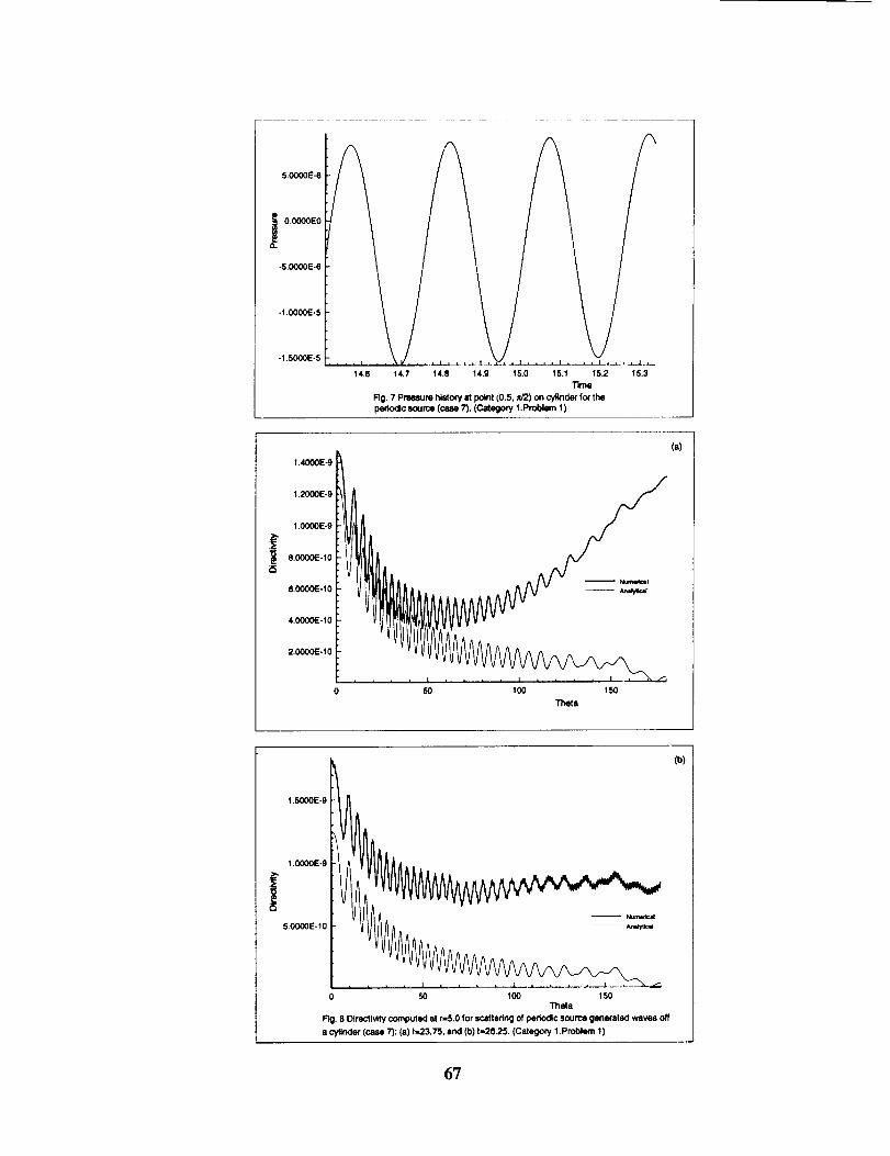
5,0000E-6
O.O000EO0.
-5.O000E-e
-1,0000E-5
-1,5000E-5
/
14,8 14,7 14.8 14.9 15.0 15.1 15.2 15.3
Time
Fig. 7 PrNsure hlato_y at point (0.5, x/2) on cyllnc_" for theperiodic source (case 7). (Category 1.Problem 1)
_5
(a)1.,IO00E-9
1.2000E-9
1.0000E-9
8.0000E-10
Nume=lcal8.0000E-10
4.0000E-10
2.0000E-10
0 50 100 150
Theta
i
1.5000E-9
1.0000E-9
5.00OOE- 10
0 50 100 150Thata
Fig. 8 Dlrectlvlty computed at r=5.0 for scatledng of pedodlc source gene{atecl waves off
ii cylinder (case 7): (a) t,,23.75, and (b) t=26.25. {Category 1.Problem 1)
(b)
6?
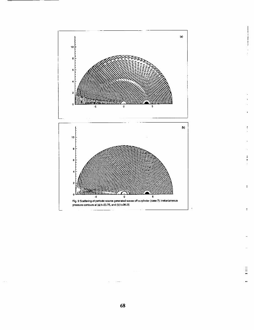
loiFP
-5 0 5
10-
8
642-5 0 5
Fig. 9 Scattering of pedodic source generated waves off a cylinder (case 7): inslanJansous
pressure contours at {a) I=23.75, and (b) t=26.25
(a)
{b)
68
o 13
soLvT ON Acoustic S ,ERIN PROBLEMSASTAGGER -GRIDSPECTR DOmAiN EOO POSI ON
!
Peter J. Bismuti and David A. Kopriva
Department of Mathematics and Supercomputer Computations Research Institute
Florida State University, Tallahassee, Florida 32306
ABSTRACT
We use a Staggered-Grid Chebyshev spectral multidomain method to solve two of the workshop
benchmark problems. The spatial approximation has the ability to compute wave-propagation
problems with exponential accuracy in general geometries. The method has been modified by the use
of a stretching transformation to extend the range of accurately represented Fourier modes and to
increase the allowable time step. We find that the Category 1, Problem 1 solution requested is
accurate to 2.6% at r = 15 using five points per wavelength. In the second problem, we find that the
over the times and angles requested, the maximum error is less than 10 -6.
INTRODUCTION
The efficient and accurate approximation of time dependent compressible flow problems requires
high order methods both in space and in time [9], [11]. Second order finite difference methods,
typically designed for steady-state computational fluid dynamics problems, are strongly dissipative
and dispersive unless the number of grid points per wavelength computed is on the order of 20 to 40
[9]. Computing with so many points per wavelength is impractical in problems where waves must be
propagated many hundreds of wavelengths. With high order methods, the required number of points
per wavelength can be reduced significantly, making accurate multidimensional solutions more
practical.
Spectral methods [1] are natural choices for the solution of flow problems where high spatial
accuracy is required. They are exponentially convergent for smooth problems. Phase and dissipation
errors decay exponentially fast [5]. Special boundary stencils are not required, since spatial
derivatives are defined right up to the boundaries.
The advantages of spectral methods are balanced in many peoples' minds by the methods' cost
and inflexibility. The cost per grid point is higher than a fixed stencil finite difference method because
the cost of computing the spatial derivatives is high, and explicit time marching procedures typically
used for wave-propagation problems require a more restrictive time step. Inflexibility is a result of the
global polynomial nature of the approximation.
As a means for reducing the high cost and inflexibility of spectral methods, spectral
multidomain methods were introduced in the mid 1980's [10], [4]. The basic premise is that high cost
69
and inflexibility canbe reducedby subdividing the computational domain into multiple subdomainson which a spectral approximation is applied. As a result, the method canbe usedon more complexgeometries.The useof lower order approximating polynomials in eachSubdomainmeansthat matrixmultiplication can be both efficient and accurate,and the time step restrictions neednot be assevere.
Recently,a staggered-gridspectral approximation method wasdeveloped:that givesspectralaccuracyand geometric flexibility [7], [6]. In this method, the solution and the fluxes areapproximated on different grids. Unstructured subdomaindecompositionscan be used,andconnectivity betweensubdomainsis simplified becausesubdomaincorner points are not usedaspartof the approximation. The useof Chebyshevpolynomial approximationsgivesexponentialconvergenceand simplicity at boundaries.The isoparametricrepresentationof boundariesmeansthatthey are approximated to the sameaccuracyasthe solution.
In this paper, weuse the staggered-gridmultidomain method of [7] to compute solutions to theCategory 1 benchmarkProblems 1 and 2. To increasethe rangeof accuratelyapproximatedwavelengths,and to increasethe time step requiredby the Chebyshevapproximation, weuse thetransformation presentedby Kozloff and Tal-Ezer [8]. To treat radiation boundary conditions,wereplacethe equationsin outer subdomainswith the Perfectly-Matched-Layerequationsof Hu [3].
!
=
i=
=
i
|!
|___--
THE STAGGERED-GRID SPECTRAL MULTIDOMAIN METHOD
The staggered-grid method [7], [6] solves the Euler equations in conservative form,
Qt + F_ + G_ = S (1)
where Q is the vector of solution unknowns, S is the source vector, and F(Q) and G(Q) are the flux
vectors. In this paper, we solve the linearized Euler equations where
[Pl [0]Q= v F= 0 G= p (2)
p U V
In the multidomain approximation, we subdivide a computational domain, f_, into quadrilateral
subdomains, gtk, k = 1,2,..., K. Under the mapping _k _ [0, 1] x [0, 1], the Euler equations (1)become
where
Q,=JQ, s=Js
F'= yyF- xyG, G = -yxF + xxG
J(X, Y) = xxyy - xyyx
(3)
The staggered-grid approximation computes the solution and source values, 1_ and o6 , and the
fluxes fi" and G on separate grids. These grids aretensor products of the Lobatto grid, Xj, and the
70
Gaussgrid, Xj+I/2 , mapped onto [0,1]
Xj=½(1-cos(_)) j=O, 1,...,N
/2j+l \\Xj+il2=½(1-cos(_m 7r)) j=0,1,...,N-1
On the Lobatto and Gauss grids, we define two Lagrange interpolating polynomials
(!-x;)ej(_)= ,:oII\x_ - x,i¢j
and
(_ %,.i:0 \ Xj+_/2 - Xi+l/_ JiCj
We see that g.j(x) E PN(X), and hj+l/2(_) c PN-t, where PN iS the space of polynomials of degree
less than or equal to N.
The mapping of each subdomain onto the unit square is done by a static isoparametric
transformation. By making the mapping isoparametric, the boundaries are approximated to the same
accuracy as is the solution. Let the vector function g(s), 0 _< s <_ 1 define a parametric curve. The
polynomial of degree N that interpolates g at the Lobatto points is
N
d=O
Four such polynomial curves, Fra(S), ra = 1, 2, 3, 4, counted counter-clockwise, bound each subdomain.
As in [7], we map each subdomain onto the unit square by the linear blending formula
x_(x,Y) = (1 - Y)rl(x) + YF3(x) + (1 - x)r4(Y) + xr2(Y)
-x,(1 - x)(1 - Y)- x2X(1 - Y) - x3xY
where the xj's represent the locations of the corners of the subdomain, counted counter-clockwise.
The solution unknowns are approximated at (J(i+l/2,_+t/2), i,j = 0, 1, ..., N- 1 , which we
will call the Gauss/Gauss points. The interpolant through these unknowns is a polynomial in
PN-t,N-1 = PN-t ® PN-_,
N-1 N-10i+l/2,j+l/2O.(x,v) = E E h,+_/2(x)h_+,/2(v) (4)
i=0 j=0 Ji+l/2,j+t/_
The horizontal fluxes are approximated at the Lobatto/Gauss points (X_, _+t/2), i, j = 0, i,..., N,
computed from the polynomial 4
= - d(x,,71
Finally, the vertical fluxes are approximated at tile Gauss/Lobatto points
(ffi+_/2,Yj), i,j = 0, 1, ..., N - 1 and are computed as
Gi+t/2,j = N - .
It remains now to show how the fluxes are computed at subdomain interfaces and at physical
boundaries. The coupling of the subdomains is made by defining interface conditions that compute
the interface fluxes. Though the interface points between two neighboring subdomains coincide, the
two solutions at the interface need not, since they are computed independently from the interpolant
through the Gauss/Gauss points in each subdomain. A unique flux is computed, however, by
choosing from the solutions on the forward and backward side of the interface according to the
normal characteristics at the interface point. In non-linear problems, this is done using a Roe solver
(see [7]). For the linear system (1), we do a linear decomposition of the normal coefficient matrix into
forward and backward going waves
A
o o0 0 N_ =A++A -
N_NyO
where A + = ½ (A + ]At), and A- = ½ (A - IAI). Then the normal flux is computed as
FN = A+Q + + A-Q- = F} + FN, where Q=_ refers to the forward and backward solutions along the
normal direction. One of the eigenvalues of A is identically zero, and we put that case into A +. The
flux P or G, depending on which side is being considered, is then computed directly from the normal
flux at the interface.
Wall boundary conditions are imposed as simply as they are in a finite volume formulation,
through the evaluation of the wall flux. At walls, the reflection condition is imposed by choosing the
exterior solution value, Q+ to have the same pressure, but opposite normal velocity to Q- when
computing the boundary flux.
Radiation boundary conditions are implemented by a buffer-zone technique. Buffer-zone
methods are natural for use with multidomain spectral methods, since all that is required is to change
the equations in the outer subdomains to ones that will not reflect waves into the interior. It is not as
convenient, however, to impose radiation boundary conditions through the solution of a one-way wave
equation, since boundary solutions are not part of the approximation.
We will report results using the Perfectly Matched Layer (PML) method of Hu [3]. In thismethod, the solution vector, O, is split into two vectors, Q = QI + Q2, where the components satisfy
the equations
o-7-+ =
+ dy = _orO Ot
72
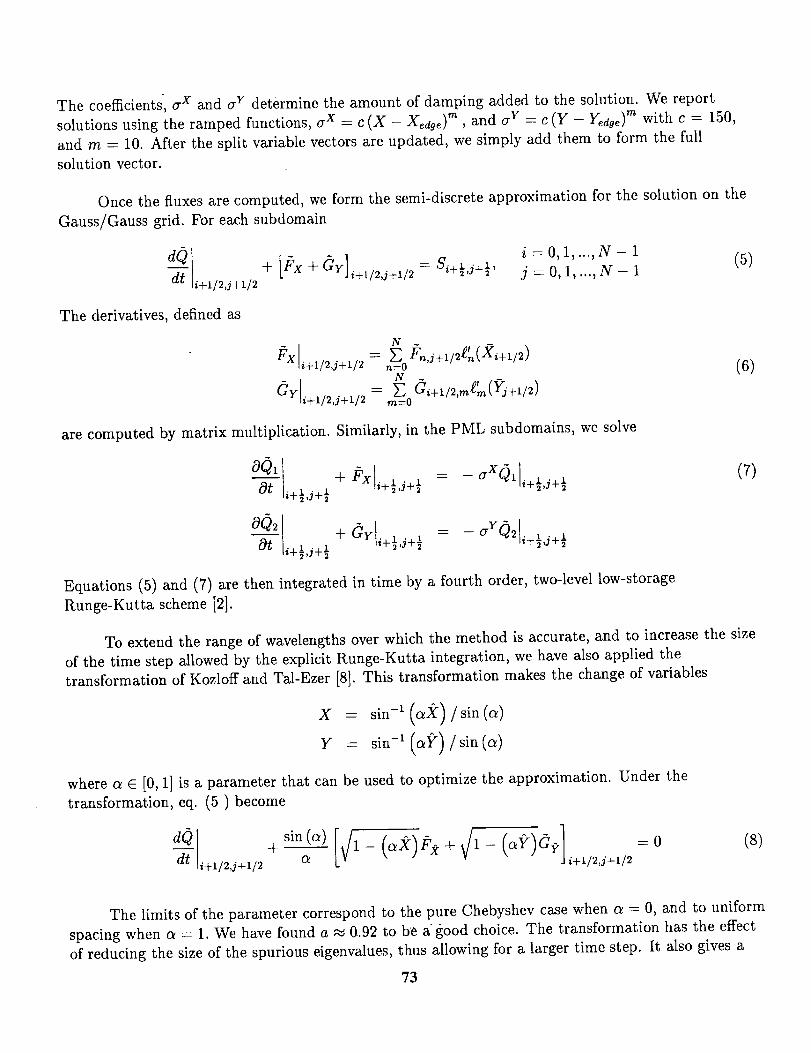
The coefficients,a x and aY determine the amount of damping added to the solution. We report
solutions using the ramped functions, a x = c (X - Xedge) m , and a w = c (Y - Y_dge) 'n with c = 150,
and m = 10. After the split variable vectors are updated, we simply add them to form the fullsolution vector.
Once the fluxes are computed, we form the semi-discrete approximation for the solution on the
Gauss/Gauss grid. For each subdomain
dt i+1/2,j+_/2
The derivatives, defined as
i =O, 1,...,N-1
S_+_,j+½, j = 0, 1, ..., W - 1 (5)
N
-_ Fn,j+i/2_n(Xi+l/2)gx i+1/2,j+l/2 _ ~ t -n=O
O.,+,m+,/ = _ O,+_/2,me'(D+,/,)in-----0
are computed by matrix multiplication. Similarly, in the PML subdomains, we solve
°011 + g,-),+½,j+½= -o-"01 _+.,,_÷½0/ _+½,j+½
o02[ + dr ,+½,_+½= - o-Y02,+_,s+½Ot _+½,J+½
Equations (5) and (7) are then integrated in time by a fourth order, two-level low-storage
Runge-Kutta scheme [2].
(6)
(7)
To extend the range of wavelengths over which the method is accurate, and to increase the size
of the time step allowed by the explicit Runge-Kutta integration, we have also applied the
transformation of Kozloff and Tal-Ezer [8]. This transformation makes the change of variables
x =Y = sin -t (aI_')/sin(a)
where a c [0, 1] is a parameter that can be used to optimize the approximation. Under the
transformation, eq. (5) become
s,.(o>[,/ (o,. 1 o+_ 1- 1- )_ : (8)a J i+t/2,j+l/z
The limits of the parameter correspond to the pure Chebyshev case when a = 0, and to uniform
spacing when a = 1. We have found a _ 0.92 to be a good choice. The transformation has the effect
of reducing the size of the spurious eigenvalues, thus allowing for a larger time step. It also gives a
73
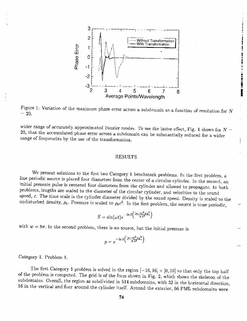
LU(D03
t'-
fl.
3
2
1
0
-1
-2
-32
.... I .... I .... I '" ' ' I .... I ....
, 1........._, :..,: l_With Transformation
",,t
.....i d'
__L_ , , , t , j_M__ ..... I .... L
3 4 5 6 7 8
Average Points/Wavelength
!i|
Figure 1: Variation of the maximum phase error across a subdomain as a flmction of resolution for N= 20.
wider range of accurately approximated Fourier modes. To see the latter effect, Fig. 1 shows for N =
20, that the accumulated phase error across a subdomain can be substantially reduced for a wider
range of frequencies by the use of the transformation.
RESULTS
We present solutions to the first two Category 1 benchmark problems. In the first problem, a
line periodic source is placed four diameters from the center of a circular cylinder. In the second, an
initial pressure pulse is centered four diameters from the cylinder and allowed to propagate. In both
problems, lengths are scaled to the diameter of the circular cylinder, and velocities to the sound
speed, c. The time scale is the cylinder diameter divided by the sound speed. Density is scaled to the
undisturbed density, P0. Pressure is scaled to poc 2. In the first problem, the source is time periodic,
_--4 2+ 2• . .S = sln(cot)e _ o., /
with w = 87r. In the second problem, there is no source, but the initial pressure is
Category t. Problem l.
The first Category 1 problem is solved in the region [-16, 16] x [0, 16] so that only the top half
of the problem is computed. The grid is of tile form shown in Fig. 2, which shows the skeleton of the
subdomains. Overall, the region as subdivided in 514 subdomains, with 32 in the horizontal direction,
16 in the vertical and four around the cylinder itself. Around the exterior, 66 PML subdomains were
74
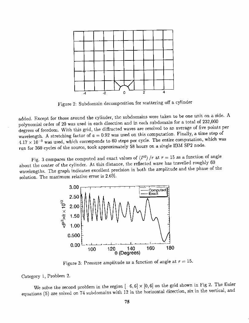
-4 -2 0 2 4
Figure 2: Subdomain decomposition for scattering off a cylinder
added. Except for those around the cylinder, the subdomains were taken to be one unit on a side. A
polynomial order of 20 was used in each direction and in each subdomain for a total of 232,000
degrees of freedom. With this grid, the diffracted waves are resolved to an average of five points per
wavelength. A stretching factor of a = 0.92 was used on this computation. Finally, a time step of
4.17 × 10 -3 was used, which corresponds to 60 steps per cycle. The entire computation, which was
run for 360 cycles of the source, took approximately 58 hours on a single IBM SP2 node.
Fig. 3 compares the computed and exact values of (P2)/r at r = 15 as a function of angle
about the center of the cylinder. At this distance, the reflected wave has travelled roughly 60
wavelengths. The graph indicates excellent precision in both the amplitude and the phase of the
solution. The maximum relative error is 2.6%.
3.00 , , , ,
i-- Computed2.50 Exact !0
2.00
-_ 1.50¢q
13.
v 1.00 _-
O.500
0.00 ...... ' ' ' '100 120 140 160 180
e (Degrees)
Figure 3: Pressure amplitude as a function of angle at r = 15.
Category 1, Problem 2.
We solve the second problem in the region [-6, 6] × [0, 6] on the grid shown in Fig 2. The Euler
equations (5) are solved on 74 subdomains with 12 in the horizontal direction, six in the vertical, and
75
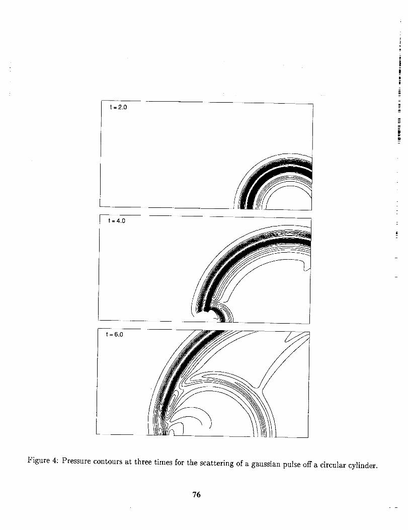
t=2.0
t=4.0
t =6.0
=_=
i1!
i
=
=
|
Figure 4: Pressure contours at three times for the scattering of a gaussian pulse off a circular cylinder.
76
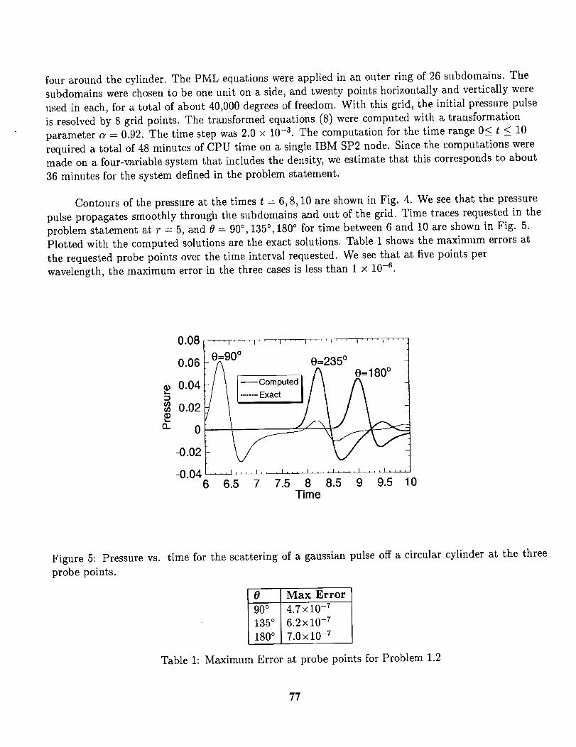
four around the cylinder. The PML equations were applied in an outer ring of 26 subdomains. The
subdomains were chosen to be one unit on a side, and twenty points horizontally and vertically were
used in each, for a total of about 40,000 degrees of freedom. With this grid, the initial pressure pulse
is resolved by 8 grid points. The transformed equations (8) were computed with a transformation
parameter a = 0.92. The time step was 2.0 × 10 -3. The computation for the time range 0< t < 10
required a total of 48 minutes of CPU time on a single IBM SP2 node. Since the computations were
made on a four-variable system that includes the density, we estimate that this corresponds to about
36 minutes for the system defined in the problem statement.
Contours of the pressure at the times t = 6, 8, 10 are shown in Fig. 4. We see that the pressure
pulse propagates smoothly through the subdomains and out of the grid. Time traces requested in the
problem statement at r = 5, and t? = 90 °, 135 °, 180 ° for time between 6 and 10 are shown in Fig. 5.
Plotted with the computed solutions are the exact solutions. Table 1 shows the maximum errors at
the requested probe points over the time interval requested. We see that at five points per
wavelength, the maximum error in the three cases is less than 1 × 10 -6.
{D{D
0..
0.08
0.06
0.04
0.02
0
-0.02
-0.046
0=90 ° 0=235 °
..... Exact /_1_
6.5 7 7.5 8 8.5 9 9.5 10Time
Figure 5: Pressure vs. time for the scattering of a gaussian pulse off a circular cylinder at the three
probe points.
8 Max Error
90 ° 4.7×10 -T
135 ° 6.2×10 -T
1800 7.0×10 -T
Table 1: Maximum Error at probe points for Problem 1.2
77
i
CONCLUSIONSi
E
We have used a Chebyshev spectral multidomain method to solve two 0(tt_eworkshop |
benchmark problems. The method, described in detail in [7], has been modified_by i_e use of a
stretching transformation to extend the range of accurately represented Fourier modes and to increase
the allowable time step. In the first problem, we use an average of five points per wavelength. We find
that the Category 1, Problem 1 solution requested is accurate to 2.6% at r = 15. In the second
problem, with eight points across the width of the initial pulse, we find that the over the times and at
the angles requested, the maximum error is less than 10 -6.
References=
[1] C. Canuto, M. Hussaini, A. Quarteroni, and T. Zang. Spectral Methods in Fluid Dynamics.
Springer-Verlag, New York, 1987.
[2] M. Carpenter and C. Kennedy. Fourth-order 2n-storage runge-kutta schemes. SIAM J. Sci.
Comp.
[3] F. Q. Hu. On absorbing boundary conditions for linearized euler equations by a perfectly
matched layer. J. Comp. Phys., 129:201-219, 1996.
[4] D. A. Kopriva. A spectral multidomain method for the solution of hyperbolic systems. Appl.
Num. Math., 2:221-241, 1986.
[5] D. A. Kopriva. Spectral solution of acoustic wave-propagation problems. 1990. AIAA-Paper
90-3916.
[6] D. A. Kopriva. A conservative staggered-grid chebyshev multidomain method for compressible
flows, ii. a semi-structured method. J. Comp. Phys., 128:475-488, 1996.
[7] D. A. Kopriva and J. H. Kolias. A conservative staggered-grid chebyshev multidomain method
for compressible flows. J. Comp. Phys., 125:244-261, 1996.
[8] D. Kozloff and H. Tal-Ezer. A modified chebyshev pseudospectral method with o(n-1) time
restriction. J. Comp. Phys., 104:457-469, 1993.
[9] H.-O. Kreiss and J. Oliger. Methods for the Approximate Solution of Time-Dependent Problems.
World Meteorological Organization, Geneva, 1973. GARP Rept. No.10.
[10] A. Patera. A spectral element method for fluid dynamics. J. Comp. Phys., 54:468-488, 1984.
[11] C. Tam. Computational aeroacoustics: Issues and methods. AIAA J., 33:1785, 1995.
78
7!
Application of Dispersion-Relation-Preserving Scheme to the
Computation of Acoustic Scattering in Benchmark Problems
R. F. Chen and M. Zhuang
Department of Mechanical Engineering
Michigan State University
East Lansing, MI 48824
SUMMARY
The results for the first two CAA benchmark problems of the category 1 are presented here.
These two problems are designed for testing curved wall boundary conditions. The governing
equations for the problems are the linearized Euler equations. For the better treatment of
the curved boundary, coordinate transform is used to map the Cartesian coordinate system
to polar coordinate system. The governing equations are discretized using the Dispersion-
Relation-Preserving (DRP) scheme of Tam and Webb. The DRP schemes with artificial
viscosity terms are evaluated as to their suitability for equations in curvilinear coordinate
system.
INTRODUCTION
The computation of aeroacoustic problems requires numerical schemes of high accuracy,
low dispersion and almost non-dissipation. 1'2 Recently developed 7-point stencil Dispersion-
Relation-Preserving (DRP) scheme of Tam and Webb 3 was designed so that the dispersion
relation of the finite difference scheme is formally the same as that of original partial dif-
ferential equations. The DRP method has been shown to be quite successful on calculating
linear waves in many acoustic computations 3'4'5.
In this work the DRP method is used to solve the acoustic scattering problems in the presence
of a curved wall boundary. The physical problem is to find the sound field generated by a
propeller scattered off by the fuselage of an aircraft. The fuselage in our computations is
idealized as a circular cylinder, and the noise source is given at a specified location. Since
the problems are axisymmetric, the computations are conducted only for the upper half of
the flow field. Computational domain is chosen as a semi-circular region (see Fig. 1) which is
79
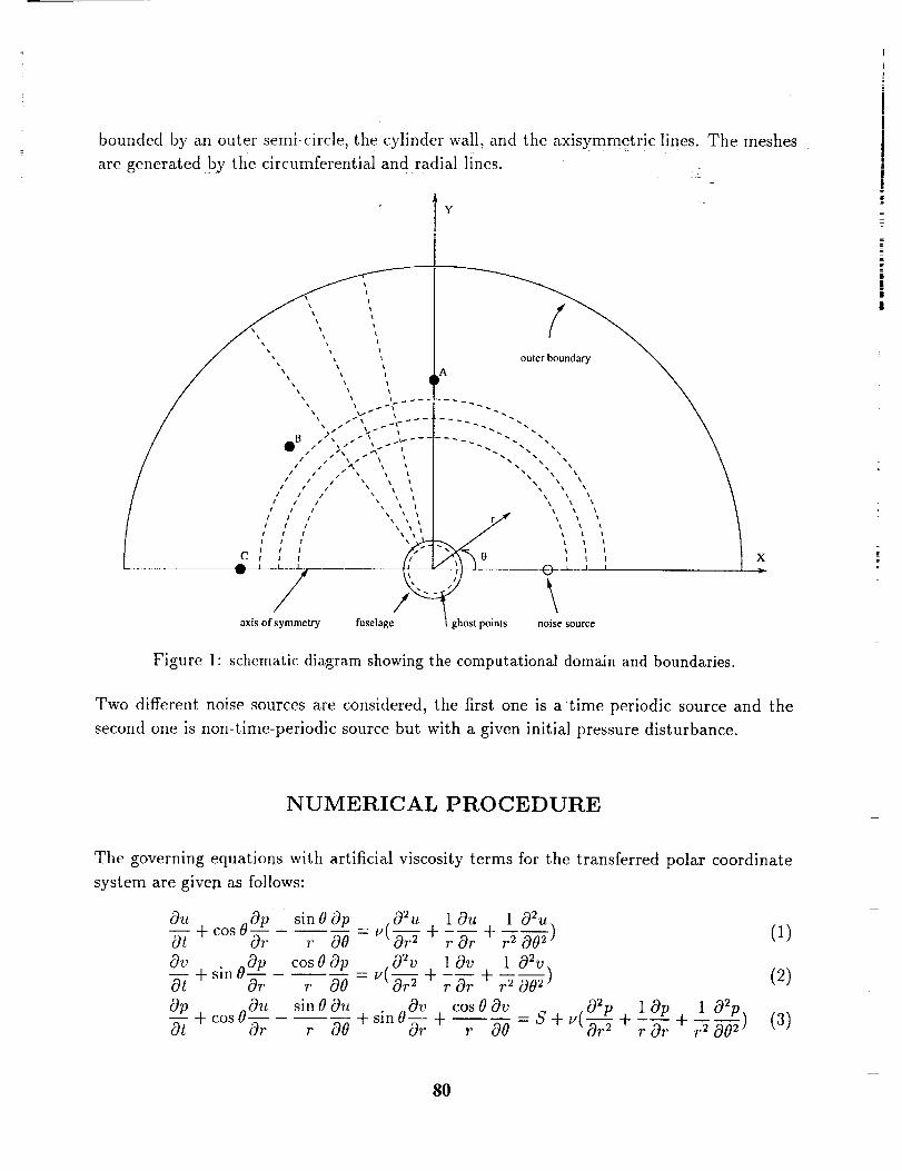
boundedby an outer semi-circle,the cylinder wall, and the axisymmetric lines. The meshesare generatedby the circumferential and radial lines.
Y
axis of'sylmetry fuselage _ noise source
Figure 1: schematic diagram showing the computational domain and boundaries.
X
Two different noise sources are considered, the first one is atime periodic source and the
second one is non-time-periodic source but with a given initial pressure disturbance.
NUMERICAL PROCEDURE
The governing equations with artificial viscosity terms for the transferred polar coordinate
system are given as follows:
Ou Op sinO Op .02u l Ou 1 02u0--7 +c°s0_ r O0-U(-_r 2+-rOt +-_002) (1)
Ov cos 00p 02v 10v 10=vOt + sin00Pr -u( + +----) (2)-- o0Op oOu sin 00u oOV cos 00v .02p 10p 1 02p0--/+c°s Or r 00 +sin Or + -r -_ = S + u(_r2 + -r-_r + r2 OO2) (3)
8O
where damping factor v = eAr × A9 with the damping coefficient c. Here the artificial
viscosity is added to damp out spurious oscillation.
The DRP spatial difference scheme is applied for both the first order derivatives, O/Or and
0/00, and the second order derivatives 02�Or 2 and 02/002. The derivatives are discretized by
seven-point damping stencil of Tam and his colleagues for interior points. Near the boundary
standard five-point and three-point central difference schemes are used for the second order
derivatives. So the values of time derivatives at grid points are then obtained from the
equations and DRP time marching scheme can thus be used to get values of variable at next
time level.
BOUNDARY AND INITIAL CONDITIONS
Boundary and initial conditions for the acoustic simulations are given below:
Solid Wall: The pressure derivative condition at the cylinder surface _ = 0 is derived from
the governing equations using the no-slip condition, IP. 77 = 0, at the cylinder wall. One row
of ghost points for p is placed inside the circle to enforce this condition. Ghost points are
shown in figure 1. One-side DRP schemes are used for descretizing velocities u and v near
the boundary.
Axis of Symmetry: The symmetric boundary conditions, u(x, y) = u(x,-y), v(x, y) =
-v(x,-y) and p(x,y) = p(x,-y), are used near the x-axis.
Outer Boundary: Radiation conditions 2 are used near the outer boundary.
solving the linearized Euler equations, the following equations are solved:
Instead of
001[ ]=o. (4)p
Initial Condition: For both problems, the initial velocity is zero, u = v = 0, because of no
fluid flow at the beginning. For the problem 1, there is a periodic disturbance source located
at (4, 0) described by the expression below:
exp[_ ln2(( z _4)2 + y2S0.22 )] sin wt.
81
For the problem 2, a pressuredisturbancelocated at (4, 0),
p=exp[-ln2( (z-4)20.22+ y 2)],
is initially released.
RESULTS AND DISCUSSION
Two sets of grid are used for the problem 1. One is 400 x 360 with Ar = 0.02 and A0 = 0.50
and the other one is 200 x 180 with Ar = 0.04 and A0 = 1°. In both cases the outer
boundary is chosen as 8 times the diameter of the cylinder. Time step is determined by the
formula0.19At
t=
1.75_/1 + (Ar/AO) 2"
The damping coefficient e is chosen as 1/60 after several trials. The result of directivity as
a function of the angle 0 is shown in Fig. 2. The directivity here is defined by
D(O) = lim rp _,T "4" C_
where r is chosen as 7.5 and time average of pressure square is obtained over two time periods
of t from 39.5 to 40, in which the pressure p is ahnost periodic. Different patterns shown in
the Fig. 2 indicate that the finer grid 400 should be used in order to predict the directivity
correctly. In the computation of problem 2, The grid 200 x 180 with Ar = 0.0375 and
A0 = 1° are used. The outer boundary is chosen as 7.5 times the diameter of the cylinder
with the time step At = 0.001 and the damping c oefficient c = 1/20. The Fig. 3 shows the
pressure as a function of time for three different points A, B and C shown in figure 1. The
profiles of the first wave and its reflection wave can be clearly seen in the Fig. 3.
We should mention that the simulations of both problems can also be proceeded without
any artificial viscosity, but spurious short waves is observed with the reflection waves.
CONCLUSIONS
The aeroacoustic computations with curved boundary are presented here. One way to han-
dle this class of problems is to map a non-rectangle domain into a rectangular domain. The
82
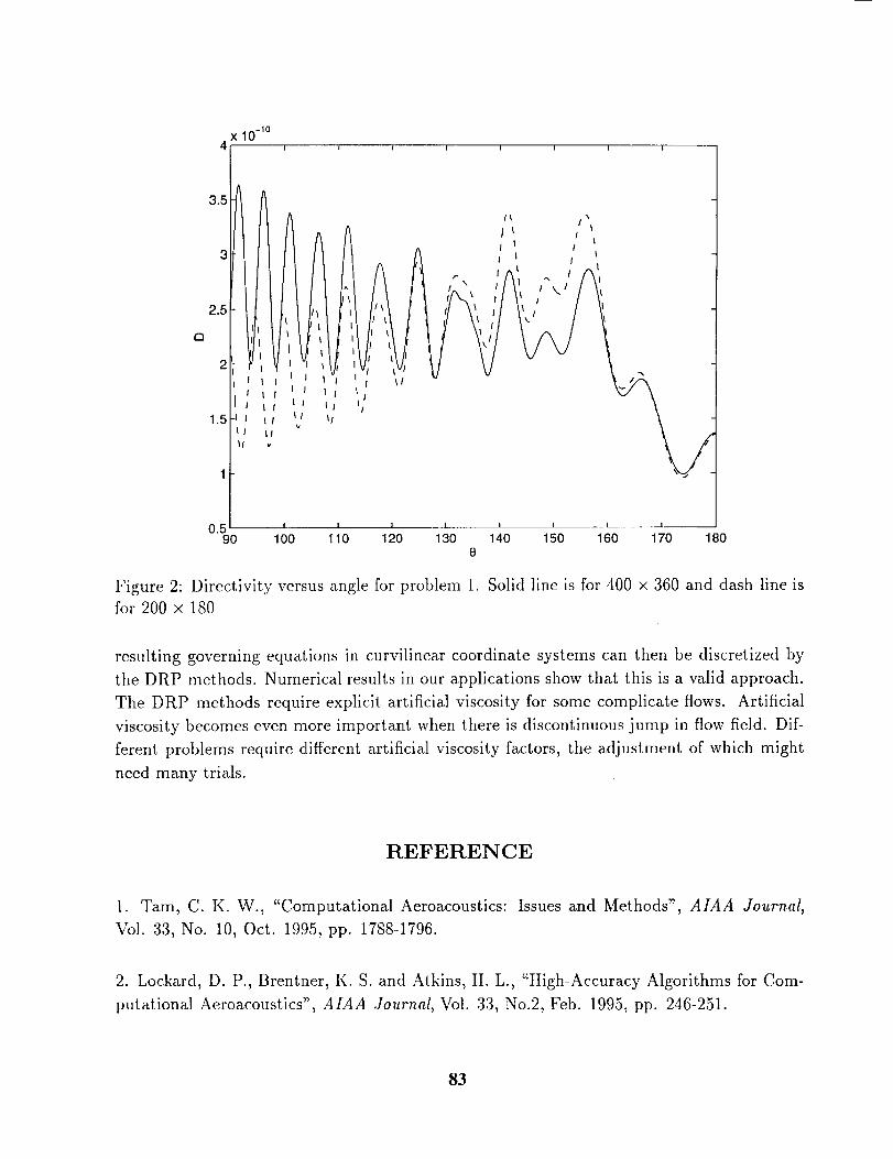
x 10-l°4, , , , , ....
i3.5
1_ /"
IA _ I /,_t
2.5 q I_1 _ / \/
I
O
2_ ?, _/ I 7 _JlI;,,, ',t , ,"
0.5 ' I l ] l i , , _ __._---_90 100 110 120 130 140 150 160 170 180
8
Figure 2: Directivity versus angle for problem 1. Solid line is for 400 x 360 and dash line is
for 200 x 180
resulting governing equations in curvilinear coordinate systems can then be discretized by
the DRP methods. Numerical results in our applications show that this is a valid approach.
The DRP methods require explicit artificial viscosity for some complicate flows. Artificial
viscosity becomes even more important when there is discontinuous jump in flow field. Dif-
ferent problems require different artificial viscosity factors, the adjustment of which might
need many trials.
REFERENCE
1. Tam, C. K. W., "Computational Aeroacoustics: Issues and Methods", AIAA Journal,
Vol. 33, No. 10, Oct. 1995, pp. 1788-1796.
2. Lockard, D. P., Brentner, K. S. and Atkins, H. L., "High-Accuracy Algorithms for Com-
putational Aeroacoustics", AIAA Journal, Vol. 33, No.2, Feb. 1995, pp. 246-251.
83
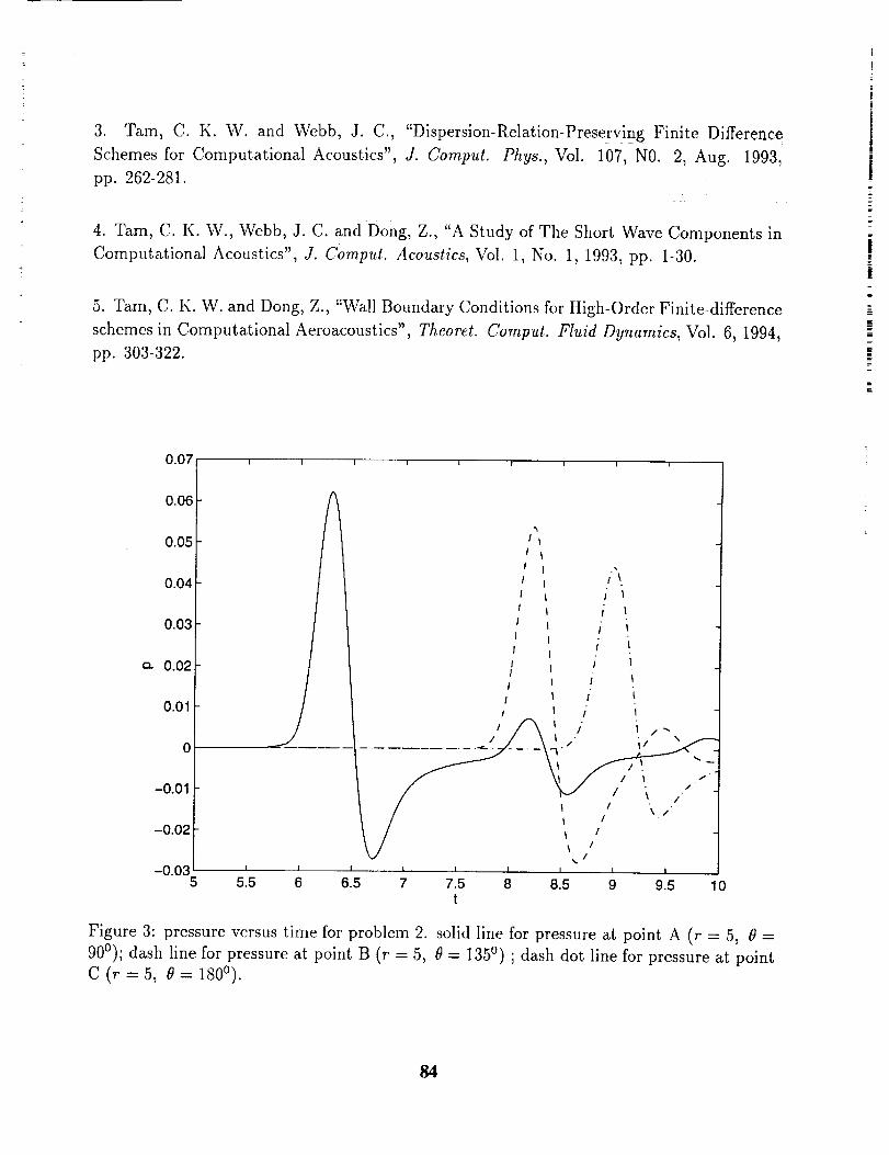
3. Tam, C. K. W. and Webb, J. C., "Dispersion-Relation-PreservingFinite DifferenceSchemesfor Computational Acoustics", J. Cornput. Phys., Vol. 107, NO. 2, Aug. 1993,
pp. 262-281.
4. Tam, C. K. W., Webb, J. C. and Dong, Z., "A Study of The Short Wave Components in
Computational Acoustics", J. Comput. Acoustics, Vol. 1, No. 1, 1993, pp. 1-30.
5. Tam, C. K. W. and Dong, Z., "Wall Boundary Conditions for High-Order Finite-difference
schemes in Computational Aeroacoustics", Theoret. Comput. Fluid Dynamics, Vol. 6, 1994,
pp. 303-322.
0.07
0.06
0.05
0.04
0.03
o,. 0.02
0.01
0
-0.01
-0.02
I I I I 1 ! I i i
-0.03 _ I I5 5.5 6 6.5
! TM
I
II /"_.
f i i
tI i I
i i Ir i i
1
/ i,-
I : ,.-.
J _ /11
I I I I I I
7 7.5 8 8.5 9 9.5 10t
Figure 3: pressure versus time for problem 2. solid line for pressure at point A (r = 5, 0 =
900); dash line for pressure at point B (r = 5, 0 = 135 °) ; dash dot line for pressure at pointC (r = 5, O = 180°).
84
/ 7"DEVELOPMENT OF COMPACT WAVE SOLVERS AND APPLICATIONS
K.-Y. FungThe Hong Kong Polytechnic University
(Voice: 832-2766-6644; Fax: 852-2364-7183; email: [email protected])
ABSTRACT
This paper reports the progress in the development of solvers based on a compact schemefor the computation of waves scattered and diffracted by an arbitrary surface. The formulation thatallows the reduction of multidimensional wave problems involving curved surfaces into a set of
one-dimensional problems involving line segments will be revisited and the schemes for labelingand enforcing time-domain physical or impedance boundary conditions on an arbitrary surface willbe briefly introduced. Applications of these algorithms and benchmarking comparisons withavailable exact solutions for scattering and diffraction of harmonic and compact wave sources bygeneric and realistic geometries are presented, and results for Problem 2 of Category 1 arereported.
INTRODUCTION
The major difficulties for time-domain approaches to wave computation are representation ofcurved surfaces and enforcement of boundary conditions on these surfaces. Current methods can
be classified into four types: I) the use of simple unstructured elements to fill the space restrictedby the surface, 2) the mapping of the bounding surface to a coordinate plane, 3) the labeling ofboundary points and application of special stencils for them, and 4) the employment of domaininhomogeneities for their desirable reflective or absorptive properties. The use of structured andunstructured surface-conforming grids has been quite successful for steady flow computations.This success is largely due to effective suppression of all physical and spurious waves byartificially added damping during convergence. The technique of adding artificial viscosity forenhanced algorithmic stability can be detrimental for wave computation. Surface-conforming gridsmay be inappropriate for their often hard-to-control excessive stretching and skewness and theresultant equations after the transformation are so entangled with the coefficients of transformationthat only exlblicit and stability-stringent boundary conditions are practical, compromising theaccuracy and effectiveness of the interior scheme. On the other hand, if Cartesian coordinates are
used, the management of the points on a curved surface may become too complex for manyschemes, particularly implicit ones to operate efficiently. The employment of domaininhomogeneities avoids the management of boundary points for rectangular grids but compromisesthe accuracy of the surface definition to within a grid cell and correspondingly a reduction ofnumerical accuracy.
Reference [ll describes the development of a new class of efficient and accurate numericalschemes for computation of waves. It demonstrates that wave propagation in a multi-dimensionalmedium involving solid boundaries can be efficiently and accurately predicted using an implicitscheme on a suitable, finite, not asymptotically large domain without having to apply specificoutgoing conditions at the domain boundaries. The advances described in this paper are: 1)development of an essentially fourth-order, unconditionally stable, implicit scheme having a simplethree-point, two-level data structure suitable for various nonuniform grids, 2) introduction of animplicit, stable, characteristically exact, easily implementable end scheme for the exit Of wave at
any end point of a numerical domain, and 3) demonstration of the feasibility of solving multi-
85
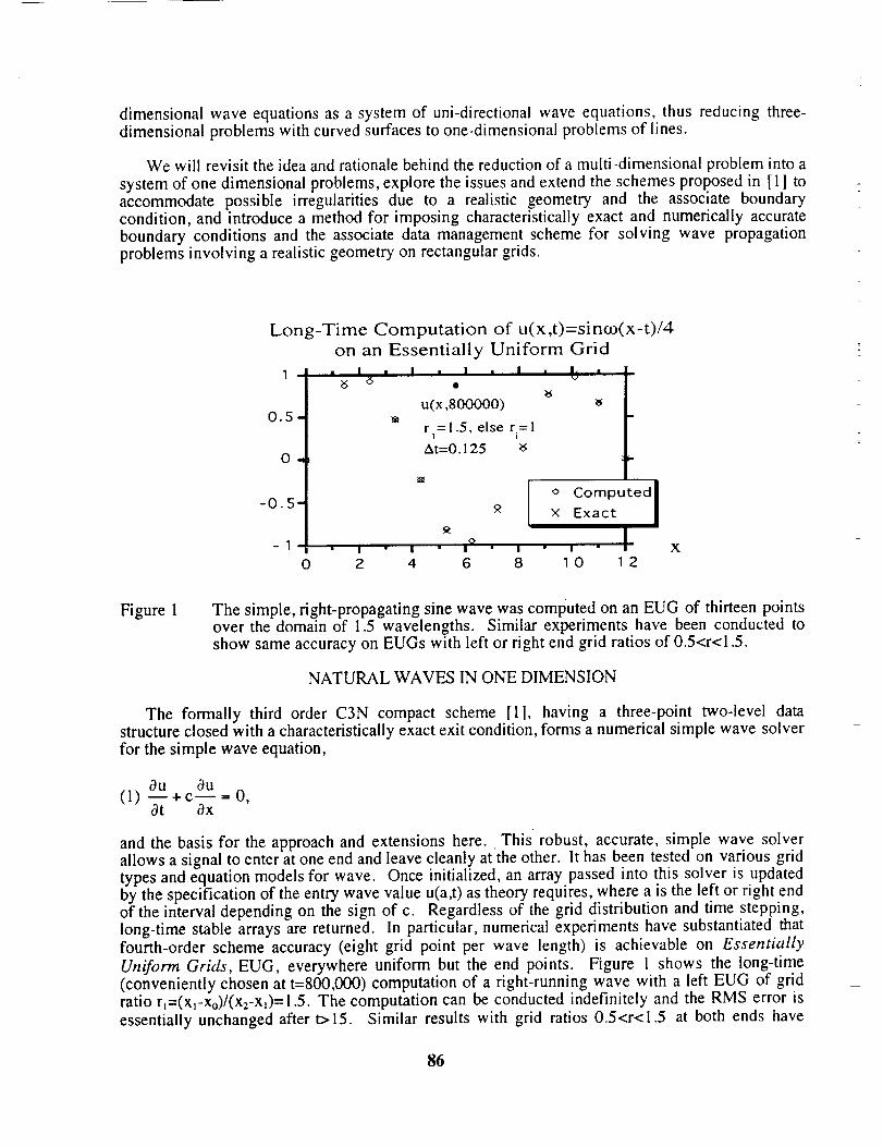
dimensionalwave equationsasa systemof uni-directionalwave equations,thus reducingthree-dimensionalproblemswith curvedsurfacesto one-dimensionalproblemsof lines.
We will revisit theideaandrationalebehindthereductionof a multi-dimensional problem into a
system of one dimensional problems, explore the issues and extend the schemes proposed in [ 1 ! toaccommodate possible irregularities due to a realistic geometry and the assoctate boundarycondition, and introduce a method for imposing characteristically exact and numerically accurate
boundary conditions and the associate data management scheme for solving wave propagationproblems involving a realistic geometry on rectangular grids.
Long-Time Computation of u(x,t)=sinco(x-t)/4
on an Essentially Uniform Grid
1 I •
0.5
O
-0.5
0
I • !
_5 _5• I . i
u(x,800000)
r =1.5, else r=lI i
At=O. 125 ;6
• IL i
;6
m
I,=
I o Computed Ix Exact I
_, ,'I " I " I " I " I " X
2 4 6 8 10 12
Figure 1 The simple, right-propagating sine wave was computed on an EUG of thirteen pointsover the domain of 1.5 wavelengths. Similar experiments have been conducted to
show same accuracy on EUGs with left or right end grid ratios of 0.5<r<1.5.
NATURAL WAVES IN ONE DIMENSION
The formally third order C3N compact scheme [1], having a three-point two-level datastructure closed with a characteristically exact exit condition, forms a numerical simple wave solver
for the simple wave equation,
0u 0u(1) --+c-- = 0,
0t 0x
and the basis for the approach and extensions here. This robust, accurate, simple wave solverallows a signal to enter at one end and leave cleanly atthe other. It has been tested on various gridtypes and equation models for wave. Once initialized, an array passed into this solver is updatedby the specification of the entry wave value u(a,t) as theory requires, where a is the left or right endof the interval depending on the sign of c. Regardless of the grid distribution and time stepping,long-time stable arrays are returned. In particular, numerical experiments have substantiated thatfourth-order scheme accuracy (eight grid point per wave length) is achievable on Essentially
Uniform Grids, EUG, everywhere uniform but the end points. Figure 1 shows the long-time(conveniently chosen at t=800,000) computation of a right-running wave with a left EUG of gridratio r,=(x_-Xo)/(x2-x,)= 1.5. The computation can be conducted indefinitely and the RMS error is
essentially unchanged after t>15. Similar results with grid ratios 0.5<r<1.5 at both ends have
86
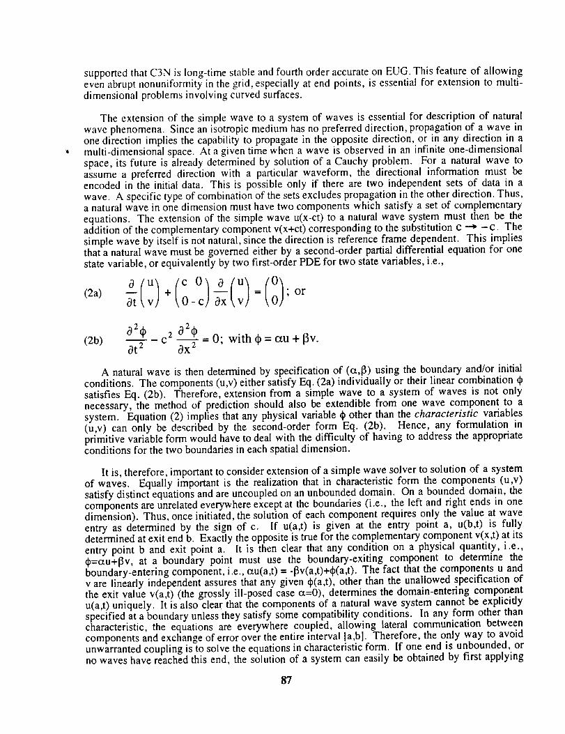
supportedthat C3N is long-time stable and fourth order accurate on EUG. This feature of allowingeven abrupt nonuniformity in the grid, especially at end points, is essential for extension to multi-dimensional problems involving curved surfaces.
The extension of the simple wave to a system of waves is essential for description of natural
wave phenomena. Since an isotropic medium has no preferred direction, propagation of a wave inone direction implies the capability to propagate in the opposite direction, or in any direction in amulti-dimensional space. At a given time when a wave is observed in an infinite one-dimensional
space, its future is already determined by solution of a Cauchy problem. For a natural wave toassume a preferred direction with a particular waveform, the directional information must beencoded in the initial data. This is possible only if there are two independent sets of data in a
wave. A specific type of combination of the sets excludes propagation in the other direction. Thus,a natural wave in one dimension must have two components which satisfy a set of complementary
equations. The extension of the simple wave u(x-ct) to a natural wave system must then be theaddition of the complementary component v(x+ct) corresponding to the substitution c _ - c. Thesimple wave by itself is not natural, since the direction is reference frame dependent. This impliesthat a natural wave must be governed either by a second-order partial differential equation for one
state variable, or equivalently by two first-order PDE for two state variables, i.e.,
c(2a) --(;)Ot +(0 '
(2b) 02_ C 2 02(_ = 0; with qb= c_u + [Sv.0t 2 0X 2
A natural wave is then determined by specification of (ct,t3) using the boundary and/or initial
conditions. The components (u,v) either satisfy Eq. (2a) individually or their linear combination d_satisfies Eq. (2b). Therefore, extension from a simple wave to a system of waves is not onlynecessary, the method of prediction should also be extendible from one wave component to asystem. Equation (2) implies that any physical variable _bother than the characteristic variables(u,v) can only be described by the second-order form Eq. (2b). Hence, any formulation inprimitive variable form would have to deal with the difficulty of having to address the appropriateconditions for the two boundaries in each spatial dimension.
It is, therefore, important to consider extension of a simple wave solver to solution of a systemof waves. Equally important is the realization that in characteristic form the components (u,v)satisfy distinct equations and are uncoupled on an unbounded domain. On a bounded domain, thecomponents are unrelated everywhere except at the boundaries (i.e., the left and right ends in onedimension). Thus, once initiated, the solution of each component requires only the value at wave
entry as determined by the sign of c. If u(a,t) is given at the entry point a, u(b,t) is fullydetermined at exit end b. Exactly the opposite is true for the complementary component v(x,t) at its
entry point b and exit point a. It is then clear that any condition on a physical quantity, i.e.,¢=ctu+13v, at a boundary point must use the boundary-exiting component to determine theboundary-entering component, i.e., c_u(a,t) = -[3v(a,t)+d_(a,t). The fact that the components u andv are linearly independent assures that any given _(a,t), other than the unallowed specification ofthe exit value v(a,t) (the grossly ill-posed case ct=O), determines the domain-entering componentu(a,t) uniquely. It is also clear that the components of a natural wave system cannot be explicitlyspecified at a boundary unless they satisfy some compatibility conditions. In any form other thancharacteristic, the equations are everywhere coupled, allowing lateral communication betweencomponents and exchange of error over the entire interval ia,bl. Therefore, the only way to avoidunwarranted coupling is to solve the equations in characteristic form. If one end is unbounded, orno waves have reached this end, the solution of a system can easily be obtained by first applying
87
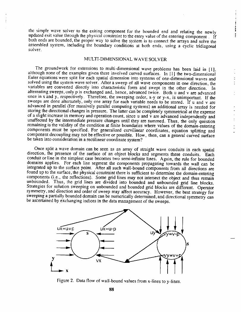
the simple wave solver to the exiting componentfor the boundedend and relating the newlyupdatedexit valuethroughthephysicalconstrainttotheentryvalueof theenteringcomponent. Ifbothendsarebounded,the properway to solvethe systemis to connectthe arraysand solvetheassembledsystem, including the boundaryconditions at both ends, using a cyclic tridiagonalsolver.
MULTI-DIMENSIONAL WAVE SOLVER
The groundwork for extensionsto multi-dimensionalwave problemshas been laid in [I],althoughnoneof the examplesgiventhere involvedcurvedsurfaces. In [11the two-dimensionalEulerequationsweresplit for eachspatialdimensioninto systemsof one-dimensionalwavesandsolvedusingthesystemwavesolver. After a sweep of all wave components in one direction, thevariables are converted directly into characteristic form and swept in the other direction. Inalternating sweeps, only p is exchanged and, hence, advanced twice. Both u and v are advanced
once in x and y, respectively. Therefore, the sweeping order, x-y or y-x, is unimportant. If thesweeps are done alternately, only one array for each variable needs to be stored. If u and v are
advanced in parallel (for massively parallel computing systems) an additional array is needed for
storing the directional changes in pressure. The latter can be completely symmetrical at the expenseof a slight increase in memory and operation count, since u and v are advanced independently andunaffected by the intermediate pressure changes until they are summed. Thus, the only questionremaining is the validity of the condition at finite boundaries where values of the domain-enteringcomponents must be specified. For generalized curvilinear coordinates, equation splitting andcomponent decoupling may not be effective or possible. How, then, can a general curved surfacebe taken into consideration in a rectilinear coordinate system?
Once split a wave domain can be seen as an array of straight wave conduits in each spatialdirection, the presence of the surface of an object blocks and segments these conduits. Eachconduit or line in the simplest case becomes two semi-infinite lines. Again, the rule for boundeddomains applies. For each line segment the components propagating towards the wall can beintegrated up to the surface point. After all such wall-bound components from all directions are
found up to the surface, the physical constraint there is sufficient to determine the domain-enteringcomponents (i.e., the reflections). Some grid lines may not intersect the object and thus remainunbounded. Thus, the grid lines are divided into bounded and unbounded grid line blocks.Strategies for solution sweeping on unbounded and bounded grid blocks are different. Operatorsymmetry, and direction and order of sweep may affect accuracy. However, the best strategy forsweeping a partially bounded domain can be numerically determined, and directional symmetry canbe ascertained by exchanging indices in the data management of the sweeps.
Figure 2. Data flow of wall-bound values from x-lines to y-lines.
88
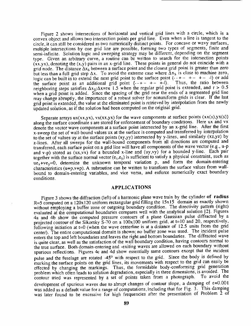
Figure 2 shows intersectionsof horizontaland verticalgrid lines with a circle, which is aconvexobjectandallowstwo intersectionpointsper grid line. Evenwhena line is tangentto thecircle,it canstill beconsideredastwo numericallydistinctpoints. For concaveor wavy surfaces,multipleintersectionsby one grid line arepossible,forming two types of segments,finite andsemi-infinite. Solution logic andsweepingstrategymaybedifferent, dependingon the segmenttype. Given an arbitrarycurve, a routinecanbe written to searchfor the intersectionpoints(xx,yx), denotingthe(x,y) pairsin anx-grid line. Thesepointsin generaldo not coincidewith agrid node. ThedistanceAxs between a surface point and the closest grid point is greater than zerobut less than a full grid step Ax. To avoid the extreme case where Axs is close to machine zero,logic can be built in to extend the next grid point to the surface point {- - + - +- +- -I}. or addthe surface point as an additional grid point {--+- +- +-I}. Thus, the ratio betweenneighboring steps satisfies Axs/Ax=r< 1.5 when the regular grid point is extended, and r > 0.5when a grid point is added. Since the spacing of the grid near the ends of a segmented grid linemay change abruptly, the importance of a robust solver for nonuniform grids is clear. If the lastgrid point is extended, the value at the eliminated point is retrieved by interpolation from the newly
updated solution, as if the solution had been computed on the original grid.
Separate arrays ux(xx,yx), vx(xx,yx) for the wave components at surface points (xx(s),yx(s))along the surface coordinate s are stored for enforcement of boundary conditions. Here ux and vxdenote the vector wave components at a surface point intersected by an x-grid line. After the firstx-sweep the set of wall-bound values ux at the surface is computed and transferred by interpolationto the set of values uy at the surface points (xy,yy) intersected by y-lines, and similarly (xz,yz) byz-lines. After all sweeps for the wall-bound components from all directions are computed andtransferred, each surface point on a grid line will have all components of the wave vector (e.g., u-pand v-p) stored as (ux,vx) for a bounded x-line and (uy,vy) for a bounded y-line. Each pairtogether with the surface normal vector (ex,ey) is sufficient to satisfy a physical constraint, such as
Uex+Vey=0, determine the unknown temporal variation p, and form the domain-enteringcharacteristics (u+p,v+p). A subroutine can be written to transform the surface values from wall-bound to domain-entering variables, and vice versa, and enforce numerically exact boundaryconditions.
APPLICATIONS
Figure 3 shows the diffraction (left) of a harmonic plane wave train by the cylinder of radiusR=5 computed on a 120x120 uniform rectangular grid filling the 15x15 domain as exactly shownwithout employing a buffer zone or outgoing boundary condition. The directivity pattern (right)evaluated at the computational boundaries compares well with the analytical solution 12]. Figures4a and 4b show the computed pressure contours of a plane Gaussian pulse diffracted by aprojected contour of the Sikorsky S-70 on a 100xl00 uniform grid, at t=10 and 20, respectively,following initiation at t=0 (when the wave centerline is at a distance of 12.5 units from the gridcenter). The entire computational domain is shown; no buffer zone was used. The incident pulseenters the top and left boundaries and leaves the right and bottom boundaries. The diffracted waveis quite clear, as well as the satisfaction of the wall boundary condition, having contours normal tothe true surface. Both domain-entering and -exiting waves are allowed on each boundary without
spurious reflections. Figures 4c and 4d show essentially same contours except that the incident
pulse and the fuselage are rotated -45 ° with respect to the grid. Since the body is defined bymarking the surface points on the grid lines, its movements with respect to the grid can easily beeffected by changing the markings. Thus, the formidable body-conforming grid generationproblem which often leads to solution degradation, especially in three dimensions, is avoided. Thecontour used was represented by a set of points taken from a photograph. To avoid the
development of spurious waves due to abrupt changes of contour slope, a damping of E=0.001
was added as a default value for a range of computations, including that for Fig. 3. This dampingwas later found to be excessive for high frequencies after the presentation of Problem 2 of
89
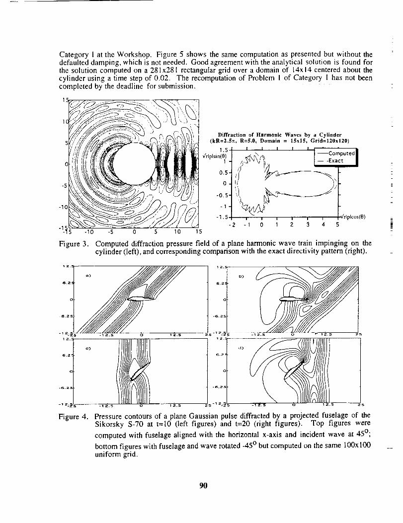
Category1at theWorkshop. Figure5 shows thesamecomputationaspresentedbut without thedefaulteddamping,which is notneeded.Goodagreementwith theanalyticalsolution is found forthesolutioncomputedon a 281x28l rectangulargrid overa domainof 14x14centeredaboutthecylinderusing a time stepof 0.02. The recomputationof Problem1of Category[ hasnot beencompletedby thedeadlinefor submission.
Diffraction of Harmonic Waves by a Cylinder(kR=2.5:_, R=5.0, Domain = 15x15, Grid=120xl20)
1.5 1 1 1 1 I • ' ' •
v'rl plsin(O) --'_ I --Computed •
, I--'x= I0 I/ \
-o.s \_ _'_'-_---_-----.----'_
-I - _/_I- I . ! , I , , , , qrlplcos(O)
2 -1 0 I Z 3 4 5
Figure 3. Computed diffraction pressure field of a plane harmonic wave train impinging on thecylinder (left), and corresponding comparison with the exact directivity pattern (right).
15.ZS
o
-6.2!
-1 ;'.;
12.;
-6.2S
Pressure contours of a plane Gaussian pulse diffracted by a projected fuselage of theSikorsky S-70 at t=10 (left figures) and t=20 (right figures). Top figures were
computed with fuselage aligned with the horizontal x-axis and incident wave at 450;
bottom figures with fuselage and wave rotated -45 ° but computed on the same 100x 100
uniform grid.
90
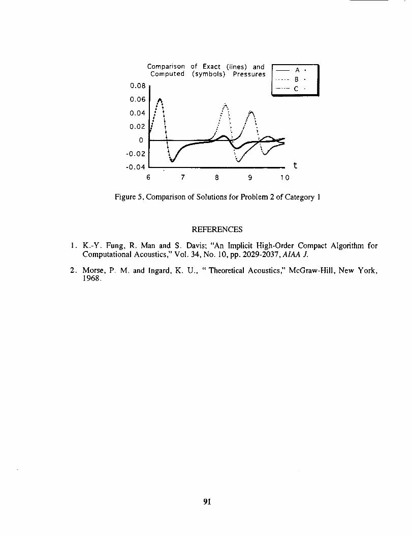
0.08
0.06
0.04
0.02
0
-0.02
-0.04
Comparison of Exact (lines) and I A
Computed (symbols) Pressures I ..... BC
t
6 7 8 9 10
Figure 5, Comparison of Solutions for Problem 2 of Category 1
REFERENCES
1. K.-Y. Fung, R. Man and S. Davis; "An Implicit High-Order Compact Algorithm for
Computational Acoustics," Vol. 34, No. 10, pp. 2029-2037, AIAA J.
2. Morse, P. M. and Ingard, K. U., " Theoretical Acoustics," McGraw-Hill, New York,1968.
91
5//-7/
04/2
Computations of acoustic scattering off a circular cylinder __
M. Ehtesham Hayder
Institute for Computer Applications in Science and Engineering
MS 403, NASA Langley Research Center, Hampton, VA 23681-0001
Gordon Erlebacher and M. Yousuff Hussaini
Program in Computational Science & Engineering
Florida State University, Tallahassee, FL 32306-3075
Abstract
We compute tile sound field scattered off a circular cylinder as given in category I.
The linearized Euler equations are solved using a multi-block algorithm. A Low-Dissipation
and Low-Dispersion Runge-Kutta Scheme is adopted for the time integration, while spatial
derivatives are discretized with a combination of spectral and 6th order compact schemes.
In this study, spectral discretization is performed in the radial direction in domains adjacent
to the cylinder. Away from the cylinder and in the azimuthal direction we use compact
differencing. Explicit filtering of the solution field is avoided. We exploit the symmetry of
the problem and only compute the solution in the upper half plane. Symmetry boundary
conditions are built into the derivative operators. Absorbing layers near the computational
boundary at large radii minimize numerical reflections. The absorbing-layer equations are
based on the Perfectly Matched Layer (PML) formulation of Hu (1996).
Problem Formulation
Problems in category 1 model the sound field generated by a propeller and scattered by
the fuselage of an aircraft. The model consists of a line noise source (propeller) and a circular
cylinder (fuselage). The governing equations are the linear Euler equations:
Ou Op
Ov Op
0-7+N =°
Op Ou Ov= s(x,y,t).o-i+ + ov
where S(x, y, t) is an acoustic source term.
The above equations are transformed to polar coordinates through x = r cos 0, Y = r sin 0
which leads to the transformed Euler equations
OU Op
0-7
93
OV 10p--+---=00t 7- 00
Op 1 c)(rU) 1 0Vo-7+ + -sr Or r O0
where U and V are velocity components in the radial and azimuthal directi0ns respectively.
Boundary conditions on tile cylinder demand a zero normal velocity. " _:_-
We consider problem 1 for which
S(x,y,t) = exp [-ln2 ((x-4)2 + Y2)](0.2)2 sin(8rct)
and problem 2 for which S(x, y, t) = 0. Initial conditions in problem 2 are given by u = v = 0an d
|
||
|
Numerical Method
The governing equations are solved with a recently developed multi-block algorithm. In
each domain, and in each coordinate direction, derivatives are either spectral or 6th order
compact. Oil domains which abut a solid boundary, spectral discretization is chosen normal
to the boundary to improve the dissipation characteristics of the derivative operator. Away
from wall, and in the azimuthal direction, a compact discretization is prefered for reasons of
computational efficiency. If N is the number of points along a coordinate direction, the cost
of a derivative computation is O(N) for compact schemes, and O(N 2) for spectral methods.
Spectral domains are often limited to a maximum of 15 points in each direction, leading to a
high number of domains. Higher densities of grid points on spectral discretizations are also
detrimental to explicit time stepping algorithms.
Compact difference schemes in general lack adequate numerical damping and filtering is
often required to eliminate high frequency errors in the computational domain. However,
we prefer to avoid explicit filtering of the solution. There is no general prescription on how
the filtering should be applied or how often. These decisions are often left to the intuition
of the numerical analyst. Time integration is implemented with a Low-Dissipation and
Low-Dispersion Runge-Kutta Scheme [Hu et al., 1996].
The problem is symmetric about 0 = 0; we only compute the solution for 0 _< 0 _< rr. To
this end, the compact operator stencil is modified at the symmetry plane to maintain 6th
order accuracy. In the radial direction, we use then standard 5= - 6 - 52 scheme [Carpenteret al., 1993].
We use a non-staggered uniform mesh in the coordinate directions used by the com-
pact derivative stencils, and a Gauss-Lobatto grid in the directions used by the spectral
differentiation. Along the domain edges, continuity of the fluxes is imposed normal to the
domain interfaces. As a consequence, only two domains are taken into account at all bound-
ary points, including corners (by continuity). Continuity of normal fluxes is imposed at
94
the boundary interface (in computational space),which leadsto discontinuousvaluesof theprimitive variables. Except for the grid and the discretization, the schemepartially followsthat of Kopriva (1996).
To minimize numerical reflections in the far field direction, we implement an absorb-ing layer techniquein the radial direction. The absorbing-layerequationsare obtained byoperator-splitting the governingequationsin the two coordinatedirections and by introduc-ing absorption coefficientsin eachsplit equation. Sinceweusethe symmetry condition in theazimuthal direction, our model problem has only one absorbing layer (see Figure 1). This
layer is located at large r. The equations inside the absorbing layer are
OU Om--+ - _rUOt Or
OV 10p2
0--[ + ....r O0 aoV
0pl 1 0(rU)
O---_ + r Or -- --O'rpl
Op2 10V
0---[+ r O0 - _rop2
where p = pl + p2, o'0 = 0, o'_ = cr0z 2 where z increases linearly from 0 at the inte-
rior/absorbing layer interface to 1 at the exterior computational boundary. In general one
may also have a layer which is parallel to the radial direction, i.e., at a constant azimuthal
location. In those layers, o'0 is positive and _r_ is zero. Further details on the formulation of
absorbing layers and their effectiveness and limitations are given by Hu, 1996 and Hayder et
al., 1997. Note that the source term in the pressure equation decays rapidly from its center
(i.e., x=4 and y=0, or r= 4, 0=0). It is set to zero inside the absorbing layer.
Results and discussion
The computational domain is shown in Figure 1. We use two computational blocks and
an absorbing layer. For the oscillatory source in problem 1, we obtain a flow field with
interference patterns. A snapshot of pressure is shown in Figure 2. This computations was
done with 671 points in the radial direction (46 points in block-1 and 625 points in block-2)
and 361 points in the azimuthal direction. For simplicity, we used a polar grid with the origin
at the center of the cylinder. The edge of the buffer domain is at r --- 12.5. Unfortunately,
the grid spacing at the cylinder boundary is extremely tight in the azimuthal direction which
forces the time step to be very small. On the other hand, although the resolution is very fine
near the cylinder, it becomes coarse at large radii. Poor azimuthal resolution in the far field
for our choice of grid is a weakness of the present study. This shortcoming may be overcome
by increasing the number of points in the azimuthal direction at large radii (possibly through
the use of multiple blocks). The absorbing layer is very effective and the oscillations vanish
smoothly inside this layer. At r = 12 and with 361 azimuthal points, there are 487r waves
around the outer boundary, which is 2.4 points per wavelength. The wavefront is almost
95
parallel to the radial direction, so the waves are more resolved than is indicated. Nonetheless,
there is a lack of resolution at large 7"in the azimuthal direction as seen from Figure 3, which
shows the computed and analytical D(O) at r = 11.44; the analytical solution was obtained
flom Hu (1997). In addition to results with 361 azimuthal points (ny), we also show results
with 181 aziml_tl_al points. Lack of suNcient resolution in the azimuthal direction probably
is a major cause for the disagreements between the analytical and computed solutions.
Temporal variations of pressure at point A in the problem 2 is shown in figures 4 and
5. Results for 671x361 and 671x181 grid resolutions are visually indistinguishable, and are
also indistinguishable from the exact solution. This indicates sufficient azimuthal resolution
at r = 5. However, when the number of radial points is halved, noticeable discrepancies in
the solution are visible.
References
Carpenter, M.H., Gottlieb, D. & Abarbanel, S., "The Stability of Numerical Boundary
Treatments for Compact High-Order Finite-Difference Schemes." J. Comp. Phys. 108, No.
2, 1993.
Hu, F. Q., Hussaini, M. Y. and Manthey, J. L., "Low-Dissipation and Low-Dispersion Runge-
I(_ltta Schemes for Computational Acoustics" J. Cornp. Phgs., 124, 177-191, 1996.
IIu, V. Q., _'011 Absorbing Boundary Conditions for Linearized Euler Equations by a Perfectly
Matched Layer", J. Comp. Phys., 129,201-219. 1996.
Hayder, M. E., Hu, F. Q. and Hussaini, M. Y., "Towards Perfectly Absorbing Boundary
Conditions for Euler Equations", AIAA paper 97-9075, 13th AIAA CFD Conference, 1997.
Hu, F. Q., Private Communications, 1997.
Kopriva, D. A., "A Conservative Staggered-Grid Chebyshev Multidomain Method for Com-
pressible Flows. II: A Semi-Structured Method," NASA CR-198292, ICASE Report No.
96-15, 1996, 27 p.
96
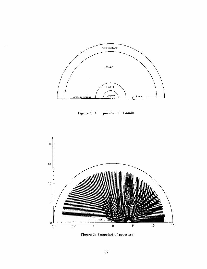
Syn_,netrycondition _ c)S .... [ I
Figure 1: Computational domain
2O
15
10 "" "" _ _
0-15 -10 -5 0 5 10 15
Figure 2: Snapshot of pressure
97
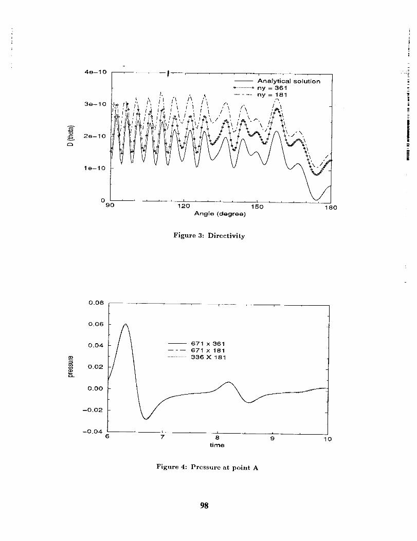
4e--10
3e--10
2e--10
le--10
f I '-r'r, i'_ /
i
O90
Analytical solution........... ny = 361
t, _ ----- ny = 181; Iq, /\,, /"_
i _ i _ i ' ,"X _'_ !'_, , t _ I ' ,' , I# ;
;,_ _ l ,,,I ; _, ,, _ I \ _ ,_ _,
_ i'_'l l",,_ll I \.,1\ / \ ::
v _ V _ V v
120 150 80
Angle (degree)
1
||
!
Figure 3: Directivity
¢-_
0.08
0.06
0.04
0.02
0.00
--0.02
--0.04 I I I
6 7 8 9
time
Figure 4: Pressure at point A
98
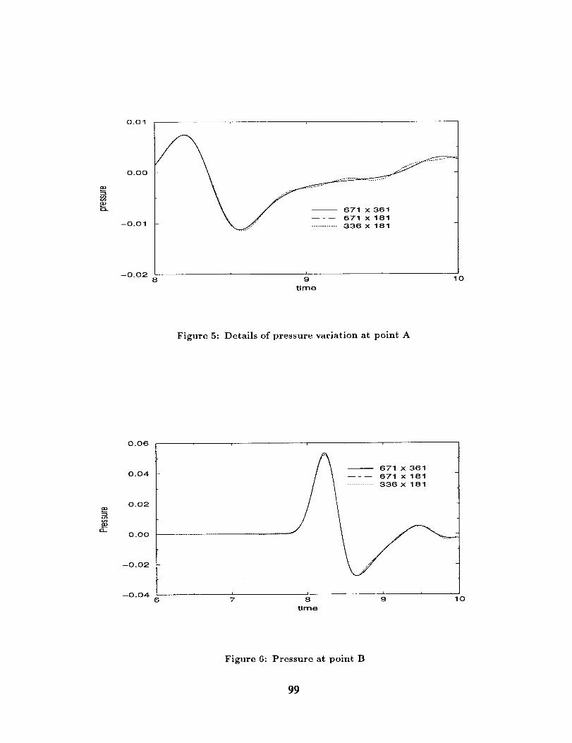
(3)
O_
0.01
0.00
--0.01
--0.02
671 x 361----- 671 X 181
............ 336 x 181
8
time
Figure 5: Details of pressure variation at point A
0.06
0.04
0.02
0.00
--0.02
--0.04 L
6 7
//_ 671 x 361--- 671xlal
I r •
8 9 1 0
time
Figure 6: Pressure at point B
99
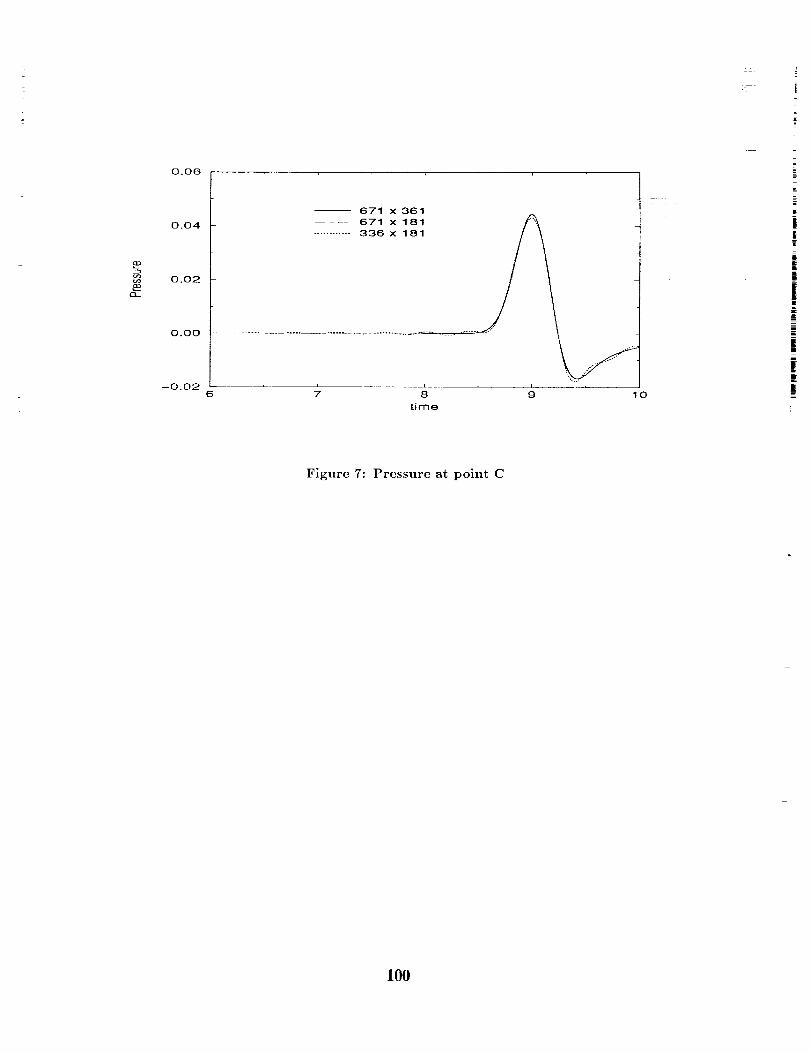
[3L-
0.06
0.04
0.02
0.00
--0.02 ......6
671 X 361----- 671 x 181............ 336 x 181
i , i i
• 8 9 10
time
L
!i|
i
E
If
Figure 7: Pressure at point C
100
APPLICATION OF AN OPTIMIZED MACCORMACK-TYPE SCHEME TOACOUSTIC SCATTERING PROBLEMS
Ray Hixon and S.-H. ShihInstitute for Computational Mechanics in Propulsion
NASA Lewis Research CenterCleveland, OH 44135
Reda R. Mankbadi
Mechanical Power Engineering Dept.Cairo University
Cairo, Egypt
o L/3 7
203%&
fr
Abstract
In this work, a new optimized MacCormack-type scheme, which is 4th orderaccurate in time and space, is applied to Problems 1 and 2 of Category 1. The performanceof this new scheme is compared to that of the 2-4 MacCormack scheme, and results forProblems 1 and 2 of Category 1 are presented and compared to the exact solutions.
Introduction
In the past, the 2-4 MacCormack scheme of Gottlieb and Turkel 1 has been used for
aeroacoustics computations. It is a scheme that is robust and easily implemented, withreasonable accuracy. Past experience has shown that the 2-4 scheme requires 25 points perwavelength for accurate wave propagation.
Recently, a new family of MacCormack-type schemes have been developed 2, using
the Dispersion Relation Preserving methodology, of Tam and Webb 3 for guidance. Theseschemes have been tested on 1-D wave propagation, showing a significant improvement
over the existing 2-4 and 2-6 schemes 4. As an initial test of this new scheme, Problems 1
and 2 of Category 1 were chosen.
These problems require accurate propagation of high-frequency low-amplitudewaves for a considerable distance, with curved-wall boundary conditions adding to the
difficulties. The performance of the new scheme as well as the results obtained will beshown and discussed.
Governing Eauations
In this work, the Iinearized Euler equations are solved in non-conservative form
101

overahalf-plane.Theequationsusedare:
vo' + 0 +
p' v_'t f
r , +J;o[voJo iv,,
=S
For Problem l, S is a simple harmonic source, given by:
0
0
exp(-In(2) (x _(&__._2)24)2+ y2"sin(87rt)
In Problem 2, S is an initial disturbance at time t = 0, given by:
Sl[=o =,
o
o
exp(-In(2) (x _(.__._._)24)2+ y2
=E:Z2E: :=
-- 17
(2)
(3)
= i
:: .7
. e
: -=
m_
_=
_|
Numerical Formulation
The scheme used is a new variant of the 2-4 MacCormack-type scheme I, which is
optimized in both space and time for improved wave propagation and accuracy 2. Tam andWebb's Dispersion Relation Preserving scheme 3 is used to specify the spatial derivatives,
and Hu, et. al.'s Low Dissipation and Dispersion Runge-Kutta scheme 4 is used for thetime marching. The scheme can be written as follows:
_)(1} = dk
d(2)=_ik (" 1/2 1+k.a53323. tF(6/')
112 ,StF -_2)
d)(41 = Ok +( 1 )AtF(d(3)/
k,.240823) t /
0 latF(dc'q.240823) _ /
102
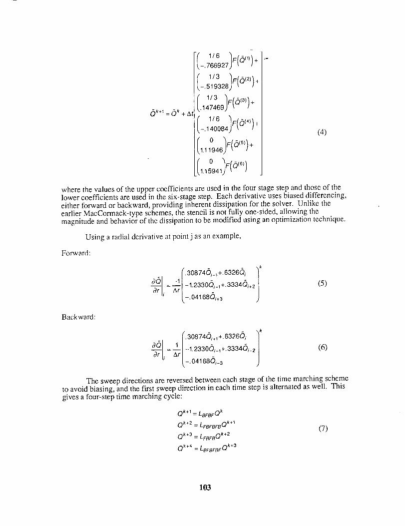
6k+1 = (_k + At
-.766927) _ /
•147469
-. ] 40084
01.15941) _ J
(4)
where the values of the upper coefficients are used in the four stage step and those of thelower coefficients are used in the six-stage step. Each derivative uses biased differencing,either forward or backward, providing inherent dissipation for the solver. Unlike theearlier MacCormack-type schemes, the stencil is not fully one-sided, allowing the
magnitude and behavior of the dissipation to be modified using an optimization technique.
Using a radial derivative at point j as an example,
Forward:
Od) (.30874_)i_,+.6326_i ]k_rr i = -1 |_1.2330d_i+, +.3334C)i+2Ar __. 04168Qi+a
(5)
Backward:
1.30874_i+1+. 6326d)i )k
OQ I = 1|-l.2330Qi_,+.3334di_2|-_-i z_r__.04168di_3
(6)
The sweep directions are reversed between each stage of the time marching schemeto avoid biasing, and the first sweep direction in each time step is alternated as well. This
gives a four-step time marching cycle:
Qk+l= LBFBFQk
ok+2 = LFBFBFBQk+I
Qk+3 = LFBFBQk+2
Qk+4 = LBFBFBFQk+3
(7)
103
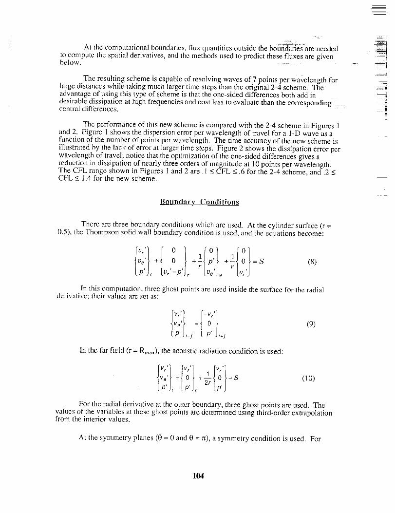
At the computational boundaries, flux quantities outside the boundaries are needed
to compute the spatial derivatives, and the methods used to predict these fluxes are givenbelow .......
The resulting scheme is capable of resolving waves of 7 points per wavelength forlarge distances while taking much larger time steps than the original 2-4 scheme. Theadvantage of using this type of scheme is that the one-sided differences both add in
desirable dissipation at high frequencies and cost less to evaluate than the correspondingcentral differences.
The performance of this new scheme is compared with the 2-4 scheme in Figures 1and 2. Figure 1 shows the dispersion error per wavelength of travel for a 1-D wave as afunction of the number of points per wavelength. The time accuracy of the new scheme is
illustrated by the lack of error at larger time steps. Figure 2 shows the dissipation error perwavelength of travel; notice that the optimization of the one-sided differences gives areduction in dissipation of nearly three orders of magnitude at 10 points per wavelength.The CFL range shown in Figures i and 2 are. 1 < CFL < .6 for the 2-4 scheme, and .2 <CFL < 1.4 for the new scheme.
...... =
2 -=--_
4j
=-
=
Boundary Conditions
There are three boundary conditions which are used. At the cylinder surface (r =0.5), the Thompson solid wall boundary condition is used, and the equations become:
, F
t v. -p Jr LVo Jo '
In this computation, three ghost points are used inside the surface for the radialderivative; their values are set as:
[P'JI-j _ P'-I+j
(9)
In the far field (r = Rmax), the acoustic radiation condition is used:
I1_ I0l;2 +v;,+ v.[P'Jr 2r[p,J
=s (10)
For the radial derivative at the outer boundary, three ghost points are used. Thevalues of the variables at these ghost points are determined using third-order extrapolationfrom the interior values.
At the symmetry planes (0 = 0 and 0 = n), a symmetry condition is used. For
104
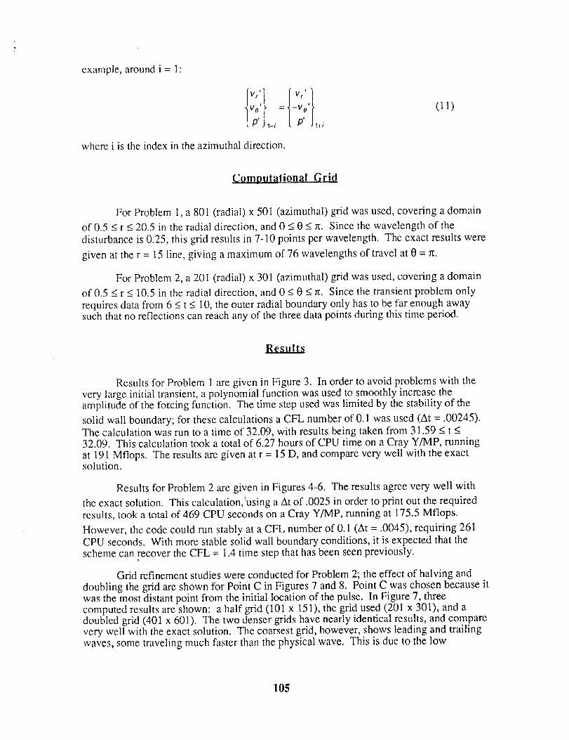
example,aroundi = 1"
where i is the index in the azimuthal direction.
(11)
Com0utational Grid
For Problem 1, a 801 (radial) x 501 (azimuthal) grid was used, coveting a domain
of 0.5 < r < 20.5 in the radial direction, and 0 < 0 < r_. Since the wavelength of the
disturbance is 0.25, this grid results in 7-10 points per wavelength. The exact results were
given at the r = 15 line, giving a maximum of 76 wavelengths of travel at 0 = _.
For Problem 2, a 201 (radial) x 301 (azimuthal) grid was used, coveting a domain
of 0.5 < r < 10.5 in the radial direction, and 0 < 0 < _. Since the transient problem only
requires data from 6 < t < 10, the outer radial boundary only has to be far enough awaysuch that no reflections can reach any of the three data points during this time period.
Results
Results for Problem 1 are given in Figure 3. In order to avoid problems with the
very large initial transient, a polynomial function was used to smoothly increase theamplitude of the fo_:cing function. The time step used was limited by the stability of the
solid wall boundary; for these calculations a CFL number of 0.1 was used (At = .00245).The calculation was run to a time of 32.09, with results being taken from 31.59 _<t <32.09. This calculation took a total of 6.27 hours of CPU time on a Cray Y/MP, running
at 191 Mflops. The results are given at r = 15 D, and compare very well with the exactsolution.
Results for Problem 2 are given in Figures 4-6. The results agree very well with
the exact solution. This calculation, :using a At of .0025 in order to print out the required
results, took a total of 469 CPU seconds on a Cray Y/MP, running at 175.5 Mflops.
However, the code could run stably at a CFL number of 0.1 (At = .0045), requiring 261
CPU seconds. With more stable solid wall boundary conditions, it is expected that thescheme can recover the CFL = 1.4 time step that has been seen previously.
Grid refinement studies were conducted for Problem 2; the effect of halving and
doubling the grid are shown for Point C in Figures 7 and 8. Point C was chosen because itwas the most distant point from the initial location of the pulse. In Figure 7, threecomputed results are shown: a half grid (101 x 151), the grid used (201 x 301), and adoubled grid (401 x 601). The two denser grids have nearly identical results, and comparevery well with the exact solution. The coarsest grid, however, shows leading and trailing
waves, some traveling much faster than the physical wave. This is due to the low
105
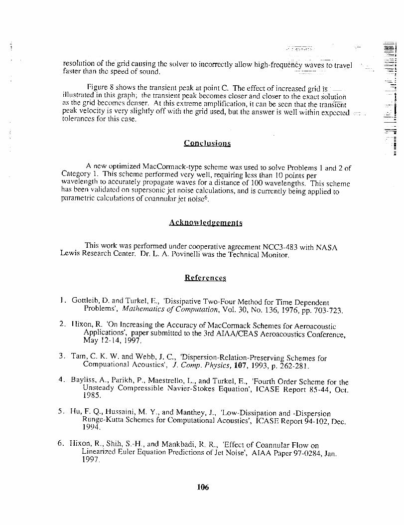
resolution of the grid causing the solver to incorrectly allow high-frequency waves to travel
faster than the speed of sound. --_--_
Figure 8 shows the transient peak at point C. The effect of increased grid'rsillustrated in this graph; the transient peak becomes closer and closer to the exact solutionas the grid becomes denser. At this extreme amplification, it can be seen that the transTienx =peak velocity is very slightly off with the grid used, but the answer is well within expected _::tolerances for this case.
Conclusions
.... i_=
• _=
_= _
8
I7.
A new optimized MacCormack-type scheme was used to solve Problems 1 and 2 ofCategory 1. This scheme performed very well, requiring less than 10 points perwavelength to accurately propagate waves for a distance of 100 wavelengths. This schemehas been validated on supersonic jet noise calculations, and is currently being applied to
parainetric calculations of coannular jet noise 6.
Acknowled gements
This work was performed under cooperative agreement NCC3-483 with NASALewis Research Center. Dr. L. A. Povinelli was the Technical Monitor.
Ref¢rence,_
.
.
.
.
°
.
Gottleib, D. and Turkel, E., 'Dissipative Two-Four Method for Time DependentProblems', Mathematics of Computation, Vol. 30, No. 136, 1976, pp. 703-723.
Hixon, R. 'On Increasing the Accuracy of MacCormack Schemes for AeroacousticApplications', paper submitted to the 3rd AIAA/CEAS Aeroacoustics Conference,May 12-14, 1997.
Tam, C. K. W. and Webb, J. C., 'Dispersion-Relation-Preserving Schemes forCompuational Acoustics', J. Comp. Physics, 10'7, 1993, p. 262-281.
Bayliss, A., Parikh, P., Maestrello, L., and Turkel, E., 'Fourth Order Scheme for theUnsteady Compressible Navier-Stokes Equation', ICASE Report 85-44, Oct.1985.
Hu, F. Q., Hussaini, M. Y., and Manthey, J., 'Low-Dissipation and -DispersionRunge-Kutta Schemes for Computational Acoustics', ICASE Report 94-102, Dec.1994.
Hixon, R., Shih, S.-H., and Mankbadi, R. R., 'Effect of Coannular Flow onLinearized Euler Equation Predictions of Jet Noise', AIAA Paper 97-0284, Jan.1997.
106
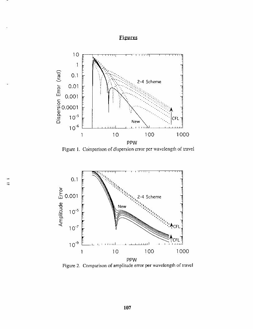
10
1
"O0.1
'-- 0.01Ok--
w 0.001t-O
o.ooo 1{#
O_ 0. 5
cl
10 _
Figure 1.
-- i 1 i i i i i I i i i i i i i i I i i I i iii1:
_r ,",,'.'. "-.:::-. 2-4 Scheme !
r
z i t I IJA_---L- I j,_jj_j_h_l___ i I" ]11
1 0 1 O0 1 000
PPW
Coinparison of dispersion error per wavelength of travel
0.1
k,..
0k--k- 0.001
"O
0-5•,-' 1O..E
< 1 0 r
1 0 -9
Figure 2.
_1_. i I I Ill I I I I I t Iit I I ; t I! !!:.,
[r "," !1 D
- "I_|1 -
"';_,,, 2-4 Scheme 7
" New ',_.,, :-
I I •
! CFL !
1 10 1 O0 1 000
PPWComparison of amplitude error per wavelength of travel
107
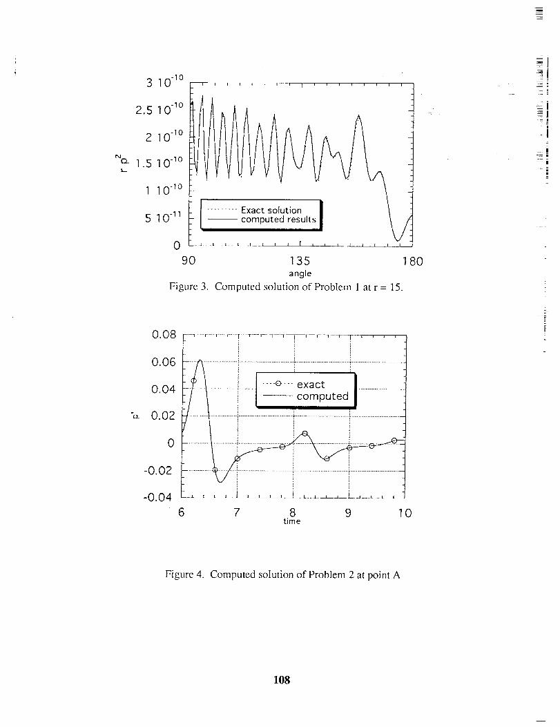
0.08 q'- I ' "'I ..... T--F --[ I I ....
0.06
0.04
-o_ 0.02
0
-0.02
-0.04 _, __.i____,,,, h__ ........ J , , , ,
6 7 8 9time
........................."A _..............................i..............................._............................-_................._.........I....o---exactI.........................
. I--c°mputed !
10
: =
|
= i
LE
Figure 4. Computed solution of Problem 2 at point A
108

"o_
0.06
0.04
0.02
r i i I I I t i I I i I l I I I
....................F............................
o .-o_o-.--&................. !............
6 7 8 9 10time
Figure 5. Computed solution of Problem 2 at point B
-0.02
-0.04
0.05
0.04
0.03
0.02"oi
0.01
0
-0.01
-0.02
i I I i I i I I i I I i I i i I I
6 7 8 9time
IO
Figure 6. Computed solution of Problem 2 at point C
109
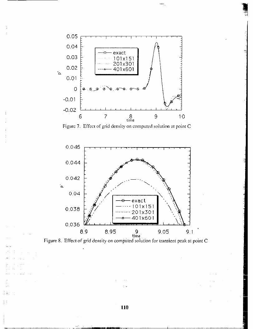
!
"o_
0.05
0.04
0.03
0.02
0.01
0
-0.01
-0.02
......... 201 x301 ]
--_--- 401 x601 J
6 7 8 9 10time
Figure 7. Effect of grid density on computed solution at point C
0 046 ........' ' _ ' ' I _ ' _ ' I ' ' ' ' I " ' "'" '
0.044
., 0.0380.0420.04, , , "
0.036t
8.9 8.95 9 9.05 9.1{line
Figure 8. Effect of grid density on computed solution for transient peak at point C
110
III
- • t ....... I
COMPUTATIONAL AEROACOUSTICS FOR
PREDICTION OF ACOUSTIC SCATTERING
Morris Y. Hsi
Ford Motor Company
Dearborn, Michigan
e-mail: [email protected]
Fred P6ri6
Mecalog
Paris, France
e-mail: fperie @ mecalog.fr
o 4,7/
ff
ABSTRACT
Two problems are investigated : Category 1 - Acoustic Scattering, Problems 1 and 2. RADIOSS CFD,
an industrial software package is the solver used. The computations were performed on a HP9000 Model
735 workstation. No slip conditions are imposed on the surface of the cylinder body and non reflecting
boundary conditions are utilized at the artificial boundary of the computational domain. Numerical results
were reported in the specified format for comparison and assessment.
NUMERICAL MODEL
RADIOSS CFD finite element code includes several formulations that can solve a wide variety of
problems ranging from transient fluid flow to fully coupled fluid structure interaction. These formulations
include Lagrangian, Eulerian as well as Arbitrary Lagrangian Eulerian (ALE) [1] representations of the
compressible Navier-Stokes equations. To solve the proposed linearized Euler equations, an explicit time
integration and a Lagrangian Finite Element representation were chosen, because the associated algorithm
involves theoretically no numerical dissipation and minimizes dispersion effects [2]. In practice, some
numerical dissipation is artificially introduced to avoid zero energy modes (shear modes).
Outer domain boundaries are treated using the silent boundary of Bayliss and Turkell [3]
Op/Ot = p c (OVn �Or - vn div Iv - vn n]) + c (p_-p)/2l c
where v is velocity vector, n normal vector at boundary, vn normal velocity, p_ pressure at infinity,
Ic characteristic length for low frequency filtering. Here p_= 0 and lc = _ •
111
Forbothproblems(1& 2 of Category1),noslipconditionsareappliedat thesurfaceof thecircularcylinder,andnodesonx-axis areconstrainediny to takeadvantageof thesymmetryof theproblem.Themeshusedfor bothproblemsisunstructuredandcontainsroughly112000elements,whosesizesrangefrom h=0.01to 0.04,withmostof thembeingcloseto 0.025(correspondingtoanaverageof tenelementsperwavelengthinProblem1).As usualinexplicitmethods,timestepisgovernedby Courant'sstabilitycondition•
At < Min (h/c)
At=O.O1 is used in all the calculations presented here.
The above assumptions (formulation, mesh size, boundary conditions) were first evaluated for a
monodimensional acoustic problem described below.
PRELIMINARY TEST
A rectangle (Fig. 1) is loaded with white noise propagating horizontally. The length of the model is
L=2.5 whereas the height is H=0.25 ; the total number of elements of the mesh is roughly 1000, with
mesh size comparable to that in Problems 1 and 2. The purpose of this test is to evaluate the transfer
function resulting from the numerical algorithm and the spatial discretization of waves propagating over
100 elements.
Inlet and outlet velocity signals can be decomposed using Fourier's transform,
vi(t) = Y_covi(03) eJ(C°t-cpi)
Vo(t ) = Zoo f o(_) eJ(cot-Cpo)
and the transfer function error can then be displayed in terms of dissipation error ed and dispersion error
(phase velocity error) e_p [4]"
ed(o_) = 20 Log(_o/fi)
e_p(co) = (Cpo-(Pi )/kL -1
Results are presented in Figures 2 and 3. Spectra are averaged as usual when dealing with white noise.
The cut-off frequency of the model is close to frequency f=6 ; there is less than ldB attenuation and 3%
dispersion error for f=4. This shows that the mesh size chosen for the two problems presented hereafter
should be good enough. For these problems, waves will indeed propagate over roughly 200 elements and
2dB attenuation and 6% dispersion error can a priori be expected.
mm
112
PROBLEM 1.1
The transient simulation was run until convergence was obtained at time 30. Isocontours of pressure
(Fig.4) show an image of the waves propagating through the mesh. No major reflection can be observed at
the outer boundary of the domain. The size of computational domain and the behavior of the silent
boundary seem good enough for this problem. The visible interference patterns are however altered by
region of lower intensities, whose origin is unclear. There are strong indications though, that this problem
stems from the discretization of the source region. Contours of pressure near the source (Fig.5) clearly
show that the wave shape is influenced by the square nature of the mesh. A much finer mesh of this
region should improve the solution. Figure 6 compares the computed results with the reference data
provided by the Workshop Committee. It is noted that the reported results are at r=5, boundary of the
computational domain. This boundary is obviously too close to allow the numerical results there to
approximate the solution at infinity. An extrapolation could have been made using a Boundary Element
Method, which would be in conflict with the underlying purposes of this benchmark. Differences can be
observed between the computed and the reference results at r=5, in particular around 0= 120 ° ; this is
probably due to the source modelization problem mentioned above. Orders of magnitude are anyhow
relevant.
More work will be undertaken to improve the model of the source region and to evaluate the influence
of the size of computational domain and of the amount of numerically added dissipation.
PROBLEM 1.2
Figure 7 shows the comparison between computed results at three locations (0=90 °, 135 ° and 180 °)
and the reference data provided by the Workshop Committee. A reasonably good correlation can be
observed. Presence of higher frequencies and early arrival of first peaks can be noted. This appears
consistent with the positive error in terms of phase velocity, that was noticed in the preliminary test
(Fig.3). This defect is inherent to the central difference nature of space and time derivatives used in this
simulation.
CONCLUSION
This work shows a promising application of time domain simulations to acoustics. Main limitations lie
in the dispersive and to some extent diffusive character of the method at high frequencies. Investigations
should be undertaken on how to improve accuracy, specially for Problem 1 in Category 1, including
sensitivity to computational domain, mesh size and source modelization, as well as methods for
extrapolating results to region away from the mesh boundaries.
113
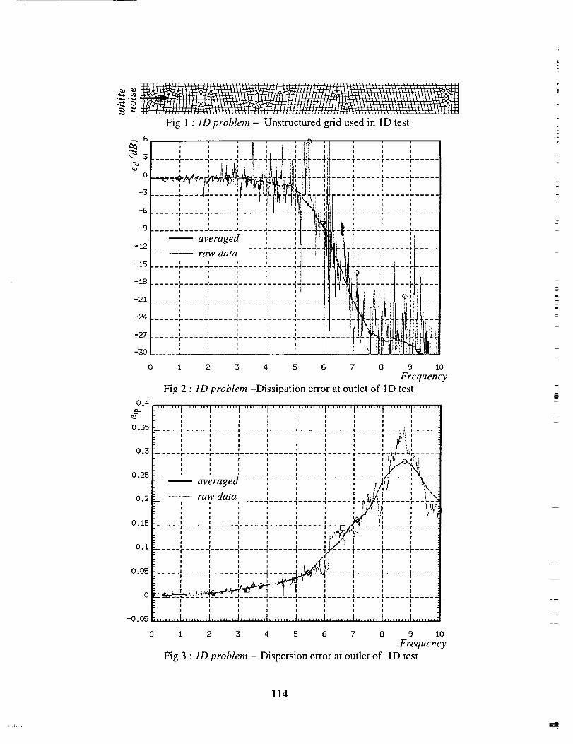
Fig. 1 • 1D problem - Unstructured grid used in ID test
0
-3
-6
-9
-12
-15
-18
-21
-24
-27
-30
0
0.49.-
0.35
0.3
0.25
0.2
0.15
O.i
0.05
0
-0.05
0
1 2 3 4 5 6 7 8 9 10
FrequencyFig 2 • 1D problem -Dissipation error at outlet of ID test
I II II II 1
I I
t I I I
IIII
1II
III
I Ir tI I
I I
1 '"1...... T.....I .....1 ', '!1 ! 1
__J ..... J ..... J ..... .dl..... 1 ..... L .....I I I I I I II I I I I II I I I I I
1 2 3 4 5 6 7 13 9 10
Frequency
Fig 3 • 1D problem - Dispersion error at outlet of ID test
114
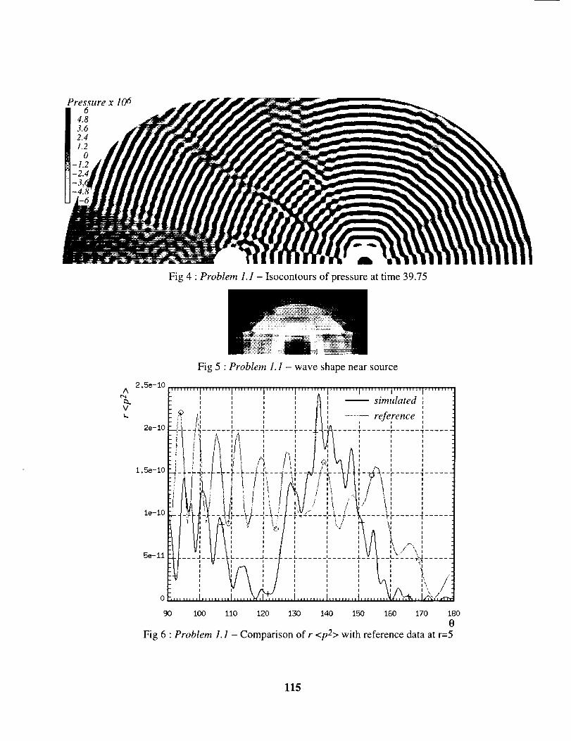
Pressure x 1066
4.83.6
2.4
1.2
Fig 4 • Problem 1.1 - Isocontours of pressure at time 39.75
A¢"-1
Vk..
2.5e-10
2e-lO
Fig 5 • Problem 1. I - wave shape near source
1.5e-10
le-I0
5e-ll
0
90 100 110 120 130 140 150 180 170 180
8Fig 6 • Problem l. 1 - Comparison of r <p2> with reference data at r=5
115
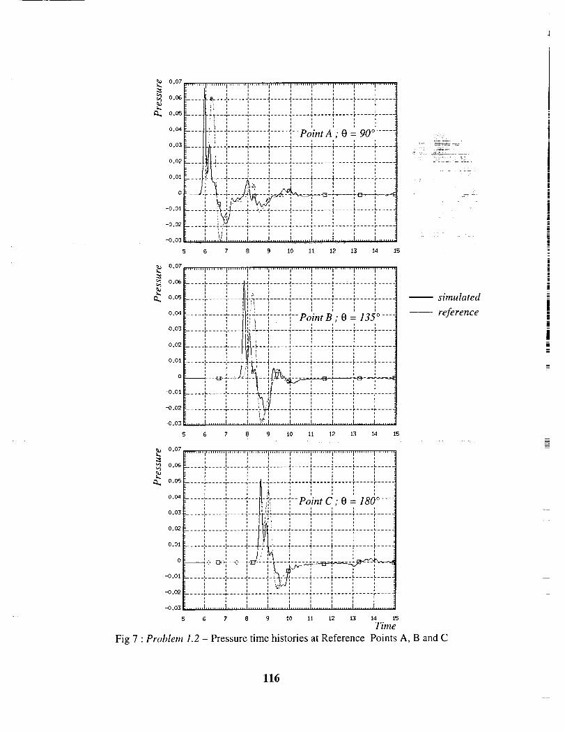
0.07
0.06
0.05
0.04
0.03
0.02
0.01
0
-0.01
.-"................ i ......... I ......... i......... I......... I......... i......... i......... I........
...... I ; I: v i J i i
-" .... i'_ i __ J .... J ..... J ..... J ..... i ..... L ..... L .....
; I_ I n ! n I l t i: _ I n ! i i l I 1
= _ i v (
= _ I i J i i J ,
"....._J........................,, Point A ; 0 = 90 ° ......= ; I J __
= _ q i I i ; i i ___ • I J _ i i i i ,--- ........ i..... 7 ..... '1 ..... "1 ........... T ..... r r • i_ , i t i i t _ q
r_. ............. -i ..... -i ..... -4 ..... .1 ..... _ ..... _- ..... _. .....
- ..... I....._-....J.....H.....J,.....+.....F.....F......
.......: i i • , I i i i..... ; : .
: ,:;:) r-- V'_yZ ..... i
___ ........ )- .... Jm-- J--/-- J ..... J ..... J ..... I ..... &...... L .....
_o.° !-0.O3 ........ I ...... ',;,1 ......... 1 ......... 1 ......... I ......... I ......... I ......... I ......... I .........
5 6 7 8 9 10 Ii 12 13 14 15
0 07
: i _ l l i i , i i= i _ I T I i _ i i
0.06 : .... c .... J .... 4J ..... J ..... J ..... a ..... i ..... _ ..... _ ....
: I ; 1 I I s i i i: I i v _ I m v _ i I
0.05 .------, .... _---- _---_ ..... _..... , ..... , ..... r ..... , .... simulated
: , , .- , • , , , , _{p0
•o4 ....;:............. 1_"_'_............,' "; Pomt B," 0 = 135 ° ___] r... rence003 , , li, ' , , , , , , 4
• _ .... r ..... , .... rn_-'7 ..... '1 ..... _ ..... r ..... r ..... r .... l
; i t / t _11l_ _ i i i i i t ]: i i i t I-1 , ; , _ , , , , , ,
0.02 ................ _. _1.._. ].. ..................................... -_
o.o,-.... :_..... ;.... ..... ..... j ..... !..... f..... ....i i i ", i i i ! i
i i i i, , 1 | ,Y _ ', t 1 :
i _ i | iI t i i i +-O.Oi ..... _ ..... , ..... J_.____ .... _ ..... a ..... s ..... t ..... L .....
i i i T /i i i i I i
-0 02 ' ' ' ' ' ' ' '
! ; I l i i
-0.03 ........ ' 'h,,,,,,,,' ......... I ...... -,,,t ......... I ......... I......... t ......... I ......... I ........
5 6 7 8 9 I0 11 12 13 14 15
0.07
........ i......... I ......... I ......... i ......... I......... i......... i ......... I ......... I........ ':
i i I i
0.06 ..... ,_ ..... ,,........... J,..... J,..... _,..... _, ..... L,..... ,L.....
, , I : , : , ,o.o_ , l l I
..... _ ..... I..... 7 ..... "I..... 7 ..... _ ..... r ..... r ..... r .....
I ' ' ', ....
o.o4 ' ' !r...._ "..... L ..... i..... J ......
: , PointC, 0 = 180.....' ' i,i , ,
0.03 .......... ,,...... ,.... _ .... _ ..... _ ..... r ..... r ..... r .....
, , , F_
0.02 ' ' J _ _ ' ' ' ' '
, : : i i :0 "01 ..... r ..... , ..... 4 .... .... J ..... 41} ..... + ..... _ ..... F .....
I ; ; q_ i ; i I Ii i l i i i I ___
0 _.C-- E).:>_ ,-Z_ --_-_---_ ..... _ .... +_z_--_w"_-_
.... .....i.....i * i i i I 1 I
--0.01 I I ! I , I ! ,..... U ..... I..... J ..... J-L .-J ..... 4 ..... 1 ..... £ ..... k .....
' _ _ ' b.'vJ ' i i , i
-0.02 ' ' ' ' ' '
• I t I I t I: i i i i i l
-0.03 i ........ 1 ......... t ......... I ......... I ......... 1 ......... I ......... I ......... I ......... I ........
Time
Fig 7 " Problem 1.2 - Pressure time histories at Reference Points A, B and C
116
REFERENCES
[1] J.Donea,"ArbitraryLagrangian-Eulerian Finite Element Methods", Computational Methods in
Mechanics. Vol. 1, No 10 (1983)
[2] T. Belytschko, "Overview ofsemidiscretization", Computational Methods in Mechanics Vol. l, No l
(1983)
[3] A. Bayliss and E. Turkell, "Outflow Boundary Conditions for Fluid Dynamics", SIAM J. SCI.
STAT. COMPUT. Vol. 3, No 2 (1982)
[4] H.L. Schreyer, "Dispersion of Semidiscretized and Fully Discret&ed Systems", Computational
Methods in Mechanics Vol. 1, No 6 (1983)
117
•sy" _'J
ApplicationAbsorb,n..oun ary on itionsto the Benchmark Problems of Computational Aeroacoustics /
Fang Q. Hu and Joe L. Manthey
Department of Mathematics and Statistics, Old Dominion University
Norfolk, VA 23529
ABSTRACT
Accurate numerical non-reflecting boundary condition is important in all the proposed bench-
mark problems of the Second Workshop. Recently, a new absorbing boundary condition has been
developed using Perfectly Matched Layer (PML) equations for the Euler equations. In this ap-
proach, a region with a width of a few grid points is introduced adjacent to the non-reflecting
boundaries. In the added region, Perfectly Matched Layer equations are constructed and applied
so that the out-going waves are absorbed inside the layer with little reflection to the interior do-
main. It will be demonstrated in the present paper that the proposed absorbing boundary condition
is quite general and versatile, applicable to radiation boundaries as well as inflow and outflow
boundaries. It is also easy to implement. The emphasis of the paper will be on the application
of the PML absorbing boundary condition to problems in Categories 1, 2, and 3. In Category
1, solutions of problems 1 and 2 are presented. Both problems are solved using a multi-domain
polar grid system. Perfectly Matched Layer equations for a circular boundary are constructed and
their effectiveness assessed. In Category 2, solutions of problem 2 are presented. Here, in addition
to the radiation boundary conditions at the far field in the axisymmetric coordinate system, the
inflow boundary condition at duct inlet is also dealt with using the proposed Perfectly Match Layer
equations. At the inlet, a PML domain is introduced in which the incident duct mode is simulated
while the waves reflected from the open end of the duct are absorbed at the same time. In Category
3, solutions of all three problems are presented. Again, the PML absorbing boundary condition is
used at the inflow boundary so that the incoming vorticity wave is simulated while the outgoing
acoustic waves are absorbed with very little numerical reflection. All the problems are solved
using central difference schemes for spatial discretizations and the optimized Low-Dissipation and
Low-Dispersion Runge-Kutta scheme for the time integration. Issues of numerical accuracy and
efficiency are also addressed.
1. INTRODUCTION
Recently, a new absorbing boundary condition has been developed using Perfectly Matched
Layer (PML) equations for the Euler equations 1'2'3. In this approach, a region with a width of a few
grid points is introduced adjacent to the non-reflecting boundaries. In the added region, Perfectly
119
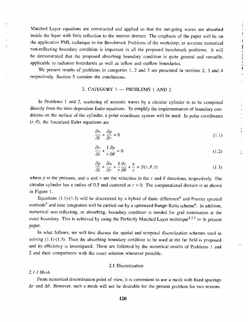
MatchedLayer equationsare constructedand appliedso that the out-goingwavesare absorbedinside thelayer with little reflectionto the interiordomain.Theemphasisof thepaperwill beontheapplicationPML techniqueto theBenchmarkProblemsof theworkshop,asaccuratenumericalnon-reflectingboundarycondition is importantin all the proposedbenchmarkproblems. It will
be demonstratedthat the proposedabsorbingboundarycondition is quite generaland versatile,applicableto radiationboundariesas well as inflow andoutflow boundaries.
We presentresultsof problemsin categoriesI, 2 and3 arepresentedin sections2, 3 and 4respectively.Section5 containsthe conclusions.
2. CATEGORY1 -- PROBLEMS1 AND 2
In Problemsl and 2, scatteringof acousticwavesby a circularcylinder is to be computeddirectly from thetime-dependentEulerequations.Tosimplify the implementationof boundarycon-ditions on thesurfaceof thecylinder,a polarcoordinatesystemwill beused.In polarcoordinates(r, 0), the linearized Euler equations are
Ou Op
0--_-+ _r. =0 (1.1)
Ov 10p0---t-+ - 0 (1.2)r 00
Op Ou 10v u
0---t-+ _ + -tO-0 + -r = S'(r, 0, t) (1.3)
where p is the pressure, and u and v are the velocities in the r and 0 directions, respectively. The
circular cylinder has a radius of 0.5 and centered at r = 0. The computational domain is as shown
in Figure 1.
Equations (1.1)-(1.3) will be discretized by a hybrid of finite difference 4 and Fourier spectral
methods 5 and time integration will be carried out by a optimized Runge-Kutta scheme 6. In addition,
numerical non-reflecting, or absorbing, boundary condition is needed for grid termination at the
outer boundary. This is achieved by using the Perfectly Matched Layer technique ],2,3 in th present
paper.
In what follows, we will first discuss the spatial and temporal discretization schemes used in
solving (1.1)-(i.3). Then the absorbing boundary condition to be used at the far field is proposed
and its efficiency is investigated. These are followed by the numerical results of Problems 1 and
2 and their comparisons with the exact solution whenever possible.
2. l Discretization
2.1.1 Mesh
From numerical discretization point of view, it is convenient to use a mesh with fixed spacings
Ar and A0. However, such a mesh will not be desirable for the present problem for two reasons.
120
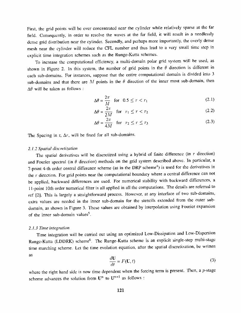
First, the grid pointswill beoverconcentratednearthe cylinderwhile relativelysparseat thefarfield. Consequently,in orderto resolvethe wavesat the far field, it will result in a needlesslydensegrid distributionnearthecylinder.Secondly,andperhapsmoreimportantly,theoverlydensemeshnearthe cylinderwill reducethe CFL numberand thus leadto a very small time stepinexplicit time integrationschemessuchas the Runge-Kuttaschemes.
To increase the computational efficiency, a multi-domain polar grid system will be used, as
shown in Figure 2. In this system, the number of grid points in the 0 direction is different in
each sub-domains. For instances, suppose that the entire computational domain is divided into 3
sub-domains and that there are M points in the 0 direction of the inner most sub-domain, then
`50 will be taken as follows :
,50 = 2_______for 0.5 < r < rl (2.1)M27r
A0 = -- for rl <_ r < r2 (2.2)2M27r
,50 = -- for 7 2 '_ r ___ r3 (2.3)4M
The Spacing in r, ,st, will be fixed for all sub-domains.
2.1.2 Spatial discretization
The spatial derivatives will be discretized using a hybrid of finite difference (in r direction)
and Fourier spectral (in 0 direction) methods on the grid system described above. In particular, a
7-point 4-th order central difference scheme (as in the DRP scheme 4) is used for the derivatives in
the 7"direction. For grid points near the computational boundary where a central difference can not
be applied, backward differences are used. For numerical stability with backward differences, a
11-point 10th order numerical filter is all applied in all the computations. The details are referred to
ref [2]. This is largely a straightforward process. However, at any interface of two sub-domains,
extra values are needed in the inner sub-domain for the stencils extended from the outer sub-
domain, as shown in Figure 3. These values are obtained by interpolation using Fourier expansion
of the inner sub-domain values 5.
2.1.3 Time integration
Time integration will be carried out using an optimized Low-Dissipation and Low-Dispersion
Runge-Kutta (LDDRK) scheme 6. The Runge-Kutta scheme is an explicit single-step multi-stage
time marching scheme. Let the time evolution equation, after the spatial discretization, be written
as
dU= F(U, t) (3)
dt
where the right hand side is now time dependent when the forcing term is present. Then, a p-stage
scheme advances the solution from U n to U "+1 as follows :
121
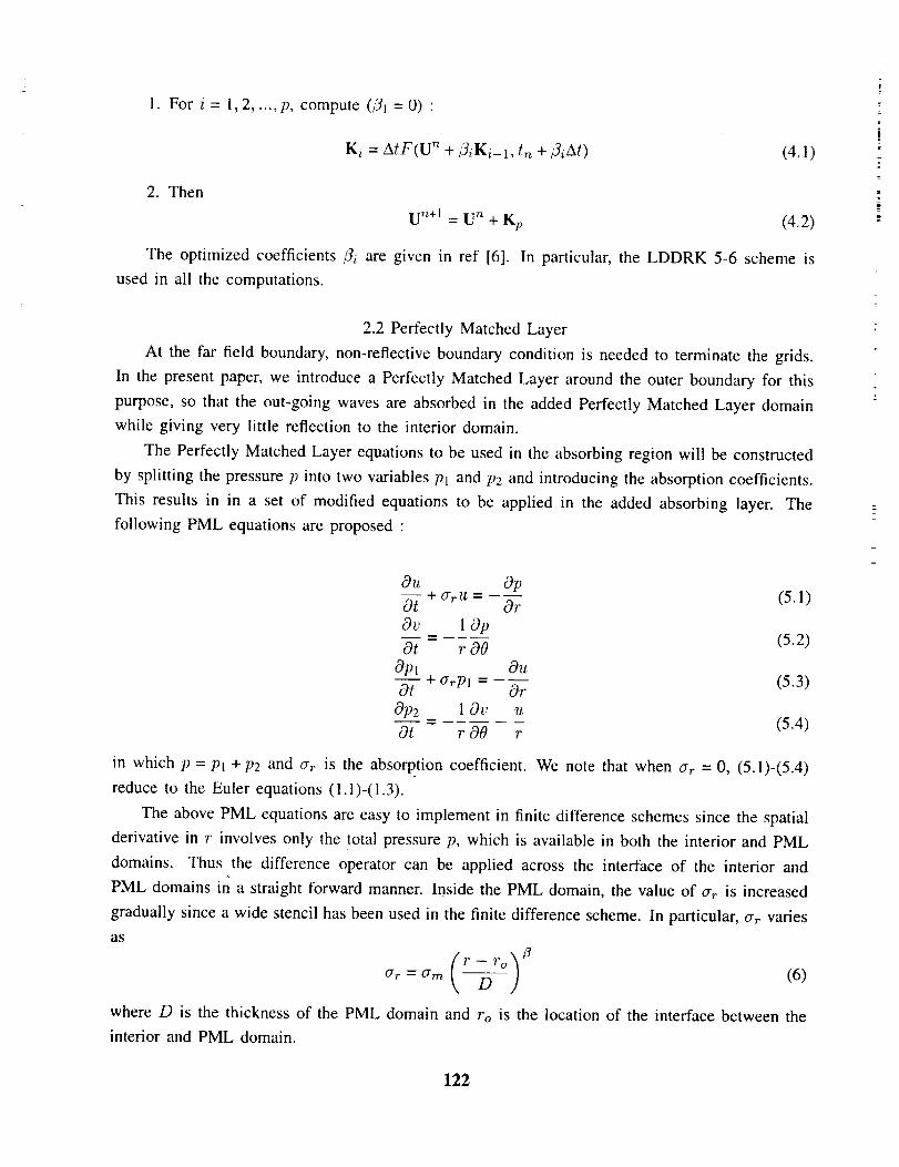
1. For i = 1,2, ...,p, compute (_31 = 0) •
Ki = AtF(U n +/3iKi-l, tn +/3iAt)
2. Then
U n+l = U n + Kp
The optimized coefficients ,3i are given in ref [6].
used in all the computations.
(4.1)
(4.2)
In pa_icular, the LDDRK 5-6 scheme is
2.2 Perfectly Matched Layer
At the far field boundary, non-reflective boundary condition is needed to terminate the grids.
In the present paper, we introduce a Perfectly Matched Layer around the outer boundary for this
purpose, so that the out-going waves are absorbed in the added Perfectly Matched Layer domain
while giving very little reflection to the interior domain.
The Perfectly Matched Layer equations to be used in the absorbing region will be constructed
by splitting the pressure p into two variables Pl and P2 and introducing the absorption coefficients.
This results in in a set of modified equations to be applied in the added absorbing layer. The
following PML equations are proposed :
Ou OpO-t+ u = - 0--7 (5.l)0_' I Op
0-t- = r O0 (5.2)
Opt Ou
0--7-+ a,.pt - Or (5.3)
Op2 10"t' u- (5.4)
Ot r O0 r
in which p = Pt +P2 and or,- is the absorption coefficient. We note that when Or = 0, (5.1)-(5.4)
reduce to the Euler equations (1.1)-(1.3).
The above PML equations are easy to implement in finite difference schemes since the spatial
derivative in r involves only the total pressure p, which is available in both the interior and PML
domains. Thus the difference operator can be applied across the interface of the interior and
PML domains in a straight forward manner. Inside the PML domain, the value of o-,- is increased
gradually since a wide stencil has been used in the finite difference scheme. In particular, o-,- varies
as
T F o
a_ = crm (6)
where D is the thickness of the PML domain and ro is the location of the interface between the
interior and PML domain.
122
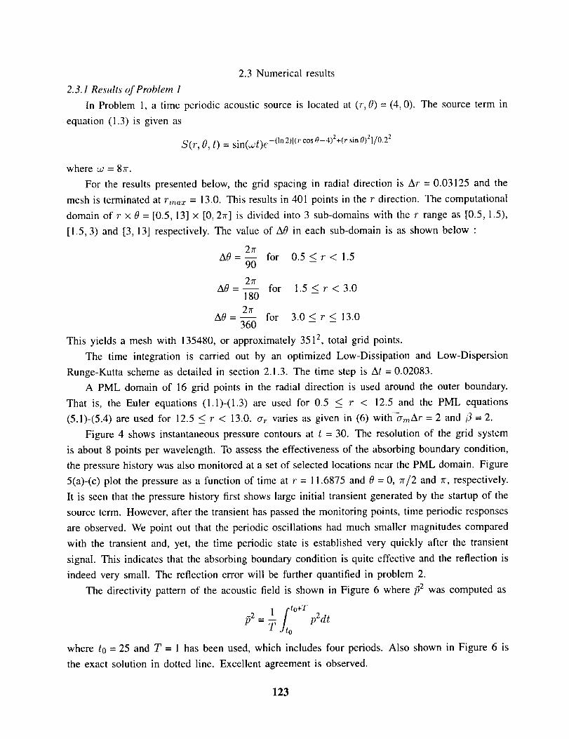
2.3 Numerical results
2.3.1 Results of Problem 1
In Problem 1, a time periodic acoustic source is located at (r, 0) = (4, 0). The source term in
equation (1.3) is given as
S(r, 0, t) = sin(_t)e -0n 2)[(r cos 0-4)2+(r sin 0)2]/0.2 2
where :v = 87r.
For the results presented below, the grid spacing in radial direction is Ar = 0.03125 and the
mesh is terminated at rma:_ = 13.0. This results in 401 points in the r direction. The computational
domain of r x 0 = [0.5, 13] x [0, 27r] is divided into 3 sub-domains with the r range as [0.5, 1.5),
[1.5, 3) and [3, 13] respectively. The value of A0 in each sub-domain is as shown below •
27rA0=-- for 0.5<r< 1.5
90
27rA0=-- for 1.5 <r <3.0
180
27rA0- for 3.0<r < 13.0
360 - -
This yields a mesh with 135480, or approximately 3512, total grid points.
The time integration is carried out by an optimized Low-Dissipation and Low-Dispersion
Runge-Kutta scheme as detailed in section 2.1.3. The time step is At = 0.02083.
A PML domain of 16 grid points in the radial direction is used around the outer boundary.
That is, the Euler equations (1.1)-(1.3) are used for 0.5 _< r < 12.5 and the PML equations
(5.1)-(5.4) are used for 12.5 < 'r < 13.0. ar varies as given in (6) with_mAr = 2 and fl = 2.
Figure 4 shows instantaneous pressure contours at t = 30. The resolution of the grid system
is about 8 points per wavelength. To assess the effectiveness of the absorbing boundary condition,
the pressure history was also monitored at a set of selected locations near the PML domain. Figure
5(a)-(c) plot the pressure as a function of time at r = 11.6875 and 0 = 0, 7r/2 and 7r, respectively.
It is seen that the pressure history first shows large initial transient generated by the startup of the
source term. However, after the transient has passed the monitoring points, time periodic responses
are observed. We point out that the periodic oscillations had much smaller magnitudes compared
with the transient and, yet, the time periodic state is established very quickly after the transient
signal. This indicates that the absorbing boundary condition is quite effective and the reflection is
indeed very small. The reflection error will be further quantified in problem 2.
The directivity pattern of the acoustic field is shown in Figure 6 where/72 was computed as
fi2 1 [to+r= pZdtT Jr o
where to = 25 and T = I has been used, which includesfour periods.Also shown in Figure 6 is
the exact solutionin dotted line.Excellentagreement isobserved.
123
2.3.2 Results of Problem 2
In problem 2, the source term in (1.3) is not present, i.e. S(r, 0, t) = 0, and the acoustic field
is initialized with a pressure pulse given as
p = e -(ln2)[(rc°sO-4)2+(rsinO)2]/0,22, It = u = 0
For the results presented below, Ar = 0.05 and the mesh is truncated at rma_ = 8.5. Thus the
number of grid points in the r direction is 161. Again, the computational domain is divided into
three sub-domains and the values of A0 are
A0=--27r for 0.5<r< 1.564
27rA0=-- for 1.5<r<3.0
128
27rA0=-- for 3.0<r<8.5
256
This yields a mesh with 33536, or approximately 1832, total grid points. Time step is At = 0.03125.
Figure 7 shows the instantaneous pressure contours at select times. The out-going waves are
absorbed in the PML domain giving no visible reflection to the interior domain. A PML domain
of l0 points in the radial direction is used for this problem. Thus the domain where the PML
equations are applied is for 8 < r _< 8.5. Pressure responses at three chosen locations are shown
in Figure 8.
To further quantify the numerical reflection error at the artificial boundary, the current solution
is compared with a reference solution. The reference solution is computed using a larger com-
putational domain so that its solution is not affected by the grid truncation. The differences of
the computed solutions using PML domains and the reference solution are plotted in Figure 9.
We observe that, first, the reflection errors are small when PML domains of 10 or more points
are used. Second, the reflection errors, however, does not show order-of-magnitude improvements
as the thickness of PML domain increases. This is a different behavior as compared to that of
Cartesian PML equations 1,2,3.
3. CATEGORY 2 -- PROBLEM 2
In this problem, CAA technique is applied to compute sound radiation from a circular duct
(Figure 10). The progressive duct wave mode is specified at the duct inlet and the radiated sound
field is to be calculated. In particular, sound directivity pattern and pressure envelope inside the duct
are to be determined. For the given problem, the duct mode has been chosen to be axisymmetric.
In cylindrical coordinates (m, r, 0), the Linearized Euler Equations for the axisymmetric dis-
turbances are
Ou Op
O----t+ _m = 0 (7.1)
124
Ov Op
0--t-+ Or = 0 (7.2)
Op Ou 0;, v0--t-+ _x + _ + -r = 0 (7.3)
where p is the pressure, u and v are the velocities in the x and r directions respectively.
As in the previous section, the spatial derivatives will be discretized by the 7-point 4th-order
central difference scheme and the time integration will be carried out by the LDDRK 5-6 scheme.
These are the same as those used for the First Workshop Problems, ref [7], including the solid
wall and centerline treatments. The emphasis of this section will be on the implementation of the
non-reflective boundaries in the current problem.
There are two types of non-reflective boundaries encountered in the present problem, as shown
in Figure 10. One is the far field non-reflecting boundary condition for the termination of grids.
The numerical boundary condition should be such that the out-going waves are not reflected. The
second type is the inflow boundary condition at the duct inlet. At the inlet of the duct, we wish
to feed-in the progressive duct mode and at the same time absorb the waves reflected from the
open end of the duct. In the present paper, both types of non-reflective boundary conditions are
implemented using the Perfectly Matched Layer technique. The details are given below.
3.1 PML absorbing boundary condition
To absorb the out-going waves, we introduce a PML domain around the outer boundary of
the computational domain, similar to that used in the previous section only that the form of PML
equations will be different. For the linearized Euler equations (7.1)-(7.3) in cylindrical coordinates,
we proposed the following PML equations :
Op-- + (rxU - (8.1)Ot Ox
Ov Op-- + o'_-v = --- (8.2)Ot Or
Opl Ou-- + crxpl - (8.3)Ot Ox
Op2 Ov v-- + O'rP2 - (8.4)Ot Or r
where p = Pl +P2 and the absorption coefficients crx and err have been introduced for absorbing the
waves that enter the PML domain, The above form follows the PML equations for the Cartesian
coordinates given in refs [1, 2]. Here we need only to split the pressure since no mean flow is
present. We note that, the Euler equations (7.1)-(7.3) can be recovered from the PML equations
(8.1)-(8.4) with crx = err = 0 by adding the split equations. Consequently, the interior domain
where the Euler equations are applied is regarded as absorption coefficients being zero.
The absorption coefficients ax and or,. are matched in a special way, namely, a_: will remain
the same across a horizontal interface and o'r will remain the same across a vertical interface, as
125
shownin Figure 11anddescribedin detail in ref [1, 2]. Within the PML domain,crx or or,. are
increased gradually as discussed in the previous section.
3.2 Infow Boundary Condition
At the inlet of the duct, we wish to feed-in the progressive duct modes and at the same time
absorb the waves reflected from the open end of the duct, as shown in Figure 12. For this purpose,
a PML domain is also introduced at the inlet. In this region, referred to as the inflow-PML domain,
we treat the solution as a summation of the incoming and out-going waves and apply the PML
equations (8.1)-(8.4) to the out-going part. That is, we express and store the variables as
= Vin + Y l (9)
Pin pt
in which Uin , vin, and Pin are the "incoming wave", traveling to the right, and u t, v I, and pt are
the "out-going" wave, reflected from the open end and traveling to the left. Since the incoming
wave satisfies the linearized Euler equation, it follows that the out-going reflected wave will also
satisfy (7.1)-(7.3). To absorb the "out-going" part in the inflow-PML domain, we apply the PML
equations (8.1)-(8.4) to the reflected waves. This results in following equations for u t, v t and pt :
OU t Op OPin
O---t_+ O'xUI - Ox Ox (10.1)
Or� Op OPin
0--{ + a_vt - 0'I" Or (10.2)
Op', Ou OuOt- + crxp_l - Ox Ox (10.3)
Op_2 t O'O OVin 1) Yin
Ot + arP2 - Or Or + (10.4)f r
where pt = p] +p_ and u, v, p are those given in (9). Since the inflow-PML domain involves only
a vertical interface between the interior and PML domains, it results in a,. = 0 in (10.1)-(10.4).
The right hand sides of (10.1)-(10.4) have been written in such a way that they can be readily
evaluated in finite difference schemes. In particular, we note that, first, since the incoming wave
is known, there should be no difficulty in computing their spatial derivatives. Second, the other
spatial spatial derivative terms inyolve only the total u, v and p which are available in the interior
domain as well as the inflow-PML domain by using (9).
3.3 Numerical Results
For the results given below, the computational domain is x x r = [-9, 9] x [0,9] in the
cylindrical coordinate system. The duct centerline is at r = 0 and the radius of the duct is unity.
The open end of the duct is located at x = 0. For both the low and high frequency cases, we have
used a uniform grid with &c = Ar = 0.05. This results in a 361 x 181 grid system. The time step
that ensures both accuracy and stability is At = 0.0545 in the LDDRK 5-6 scheme.
126
To absorbthe out-goingwavesat thefar field, PML domainswith a width of 10 grid points
are used around the outer boundaries of the computational domain. In addition, an inflow-PML
domain is employed at the duct inlet with the same width as in the far field.
Figure 13 shows the instantaneous pressure contours at t = 87.2 and w = 7.2 (low frequency
case). It is seen that the waves decay rapidly in the PML domain. As in the previous section, the
pressure as a function of time is monitored at a set of chosen points. Figure 14 shows the pressure
histories at two points near the interior-PML interfaces (x, r) = (8, 0), (0, 8), and two points inside
the duct (x, r) = (-2, 0), (-4.5, 0). We observe that, while the pressure responses at the far field
quickly become time periodic after the initial transients have passed, it takes a longer time for the
pressure inside the duct to reach the periodic state. This is believed to be due to the reflection
of the transient at the open end of the duct which has to be absorbed by the inflow-PML domain
before a periodic state can be established.
Numerical reflection error has also been assessed by comparing the computed solution using
PML absorbing boundary condition to a reference solution using a larger computational domain.
The maximum difference of the two solutions around the outer boundaries is plotted in Figure 15
for n = 10 and 20 where n is the width of the PML domain used. It is seen that satisfactory results
are obtainable with a width of 10 points and the reflection error is further reduced significantly
by increase the width of the PML domain.
Figure 16 shows the directivity pattern of the radiated sound field. The envelopes of the
pressure distribution inside the duct are given in Figure 17. Results for the high frequency case,
_o = 10.3, are shown in Figures 18-21.
4. CATEGORY 3
In this category, CAA technique is applied to a turbomachinery problem in which the sound
field generated by a gust passing through a cascade of flat plates is to be computed directly from
the time-dependent Euler equations :
0-_+ Ox+_x =0 (11.1)
&, MaY OpO-t + Ox + _ = 0 (! 1.2)
Op _xx Ou Ovo +M (11.3)
where M is the Mach number of the mean flow. In the above, the velocities have been non-
dimensionalized by the speed of sound ao and pressure by poa2o where Po is the density scale.
The problem configuration is as shown in Figure 22. In non-dimensional scales, the chord length
and the gap-to-chord ratio are both unity. In addition, periodicity is assumed for the top and
bottom boundaries. A uniform mean flow is present which has a Mach number of 0.5. The
127
incident vortical gust is given as
ui,_ - cos(c_x + fly - wt) (12.1)Og
vin = Vg cos(a'x + _3y - wt) (12.2)
Pi,_ = 0 (i2.3)
where 1,_ = 0.005.
In all three problems posed in this category, the sound field scattered by the plates as well as
the loadings on the plates are to be determined. In Problem 1, the solutions are to be calculated
by using a frozen gust assumption. In problem 2, the convected gust is to be simulated together
with the scattered sound field. In prob|em 3, a sliding interface is introduced and the grids down
stream of the interface are moving vertically with a given speed _. Problems in this category
include several important and challenging issues in developing CAA techniques, such as the inflow
and out flow conditions, solid boundaries and moving zones. In the present paper, the inflow and
outflow conditions are implemented by the PML technique. The details of the boundary conditions
as well as the sliding zone treatments are described below.
4.1 Outflow condition
At the downstream outflow boundary, the out-going waves consist of the acoustic waves scat-
tered from the plates and the vorticity waves convected by the mean flow. To absorbed these waves
with as little reflection as possible, a PML domain is used at the outflow boundary. For the linear
Euler equations (11.1)-(11.3) with a uniform mean flow in the x direction, the following equations
are applied in the added PML domain :
Ou Ou Op-- + ax u = -M (13.1)Ot Ox Ox
Ovl Op- (13.2)
Ot Oy
0v___22+ crz v2 = -M cjp (13.3)Ot Ox
Opl O,v Ou-M --_" + -- (13.4)
O---t-+ ax p, = Ox Ox
Op2 Ov__ = _w (13.5)Ot Oy
where v and p have been split into vt, '/;2 and Pl, P2, i.e., v = vl + v2 and p = Pl + P2. Note
that, since now the top and bottom boundaries are periodic, only one absorption coefficient, crx,
is needed. In addition, the u velocity may not be split. For the Cartesian coordinates, it has been
shown that the PML domain so constructed is reflectionless for all the linear waves supported by
the Euler equations and the waves that enter the PML domain decay exponentially. The details
are referred to ref. [1, 2].
128
4.2 Inflow condition
At the inflow, two types of waves co-exist, namely, the downstream propagating vorticity waves
(the gust) and the upstream propagating acoustic waves (scattered from the plates). A successful
inflow condition should simulate the downstream connection of the vorticity waves and at the same
time be non-reflective for the upstream acoustic waves. As in the previous section (category 2),
the inflow condition is implemented by introducing a PML domain at the inflow boundary. In
the inflow-PML domain, the variables u, v and p are expressed and stored as a summation of the
"incoming" vorticity wave and "out-going" acoustic waves as those given in (9). The incoming
wave _tin, vin and Pin is as given in (12.1)-(12.3). The PML equations (13.1)-(13.5) are then
applied to the "out-going" waves u t, v _ and p'. Thus, in the inflow-PML domain, we solve
Out u I - Af Ozt OR Ou in Opi________n ( 14.1 )O-Y,+ _r_ = O:r Ox + AI _ + Ox
0_, I Op OPin- -- + -- (14.2)
Ot Oy Oy
Ot- + o'x v_ = -M + M (14.3)
Op_ _ Ou Oui,, (14.4)
Op'z Ov OVin- + (14.5)
Ot Oy Oy
Again, the right hand sides have been written in a way that the spatial derivatives can be readily
evaluated in finite difference schemes. The implementation of above is similar to that in section
3.2.
4.3 Sliding Zone Treatments
In problem 3, a sliding interface is added to the computational domain and the grids down-
stream of the sliding interface is moving vertically with a speed _,_, Figure 23. That is, after each
time step, the grids in the sliding zone advance vertically by l,sAt. Due to this movement, the
grids in the two zones are not necessary aligned in the horizontal direction. This will obviously
give rise to difficulties in finite difference schemes when the stencils extend across the interface.
Extra grid points are created as shown in Figure 24. In the present paper, values of variables on
these points are obtained by interpolation using Fourier expansions in the vertical direction. For
instance, let the values of pressure p on the regular grids be denoted as pOAx, kay). Then the
values of p on a point (jA.r, y), not on a regular grid point, will be computed as
p(jA:r, y) =
X/2-
n=-N/2
129
where /3),_ is the Fourier transform of p(jAx, kAy) in the y direction and N is the number of
grid points (N = L/Ay). The Fourier expansions are implemented efficiently using FFT. It is
well known that Fourier interpolation is highly accurate, better than any polynomial interpolations.
Indeed, we found that, using Fourier interpolation, the results with sliding zone (Problem 3) are
virtually identical to those without a sliding interface (Problem 2).
4.4 Numerical Results
Since solutions of all three problems in this category are similar, we will concentrate on nu-
merical results of Problem 2 in particular and present the results of Problems 1 and 3 as references.
4.4.1 Effectiveness of the inflow-PML boundary condition
We first demonstrate the validity and effectiveness of the inflow-PML boundary condition
described in section 4.2 by a numerical example plane wave simulation. In this example, a plane
vorticity wave, convecting with the mean flow, will be simulated. The computational domain is
the same as that of problem 2 except that now no plate is present. The flow field is initialized as
follows •
At t=0 •
Vg; _L- cos(crx + fly - _,t)H(x + 1)
O:
v = k 9 cos(c_x + t3y - _,t)H(x + 1)
p=O
where H(x) is a step function which has a value of zero for x > 0 and unity for x < 0.
Figure 25 shows instantaneous pressure contours at the initial state t = 0 and subsequent
moments at t = 4.8 and 14.4. The inflow-PML domain described in 4.2 is applied at the inflow
boundary. It is seen that a plane vorticity wave is established. Figure 26 shows the v-velocity
and pressure as functions of time at a point (x, y) = (-2, 0). Notice that while the velocity is
periodic, the pressure is not exactly zero as a plane vorticity wave should behave. This is due to
our initial flow field being not exact along the cut-off line x = -l which generates small pressure
waves. Although these pressure waves are eventually absorbed by the PML domains at both the
inflow and out-flow boundaries, the decay of the pressure is slow due to periodicity of the top and
bottom boundaries. However, the magnitude of these pressure waves is small as shown in Figure
25.
Simulation of a plane acoustic wave has also been performed with similar results.
4.4.2 Low frequency gust
For the low frequency case, oJ = 57r/4, _ = /3 = 57r/2. The computational domain is
[-3.5, 4.5] x [0, 4]. A uniform grid with Ax = Ay = 0.05 is used and time step used is At = 0.044.
The PML domains contain 20 points in the x-direction. Thus the interior domain in which the
Euler equations are applied is [-2.5, 3.5] x [0,4]. Figure 27 shows the instantaneous pressure
130
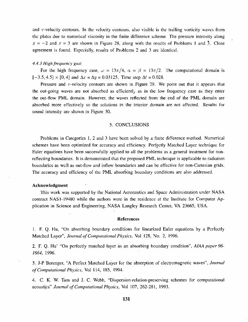
and u-velocity contours. In the velocity contours, also visible is the trailing vorticity waves from
the plates due to numerical viscosity in the finite difference scheme. The pressure intensity along
.r = -2 and :r = 3 are shown in Figure 28, along with the results of Problems I and _. Close
agreement is found. Especially, results of Problems 2 and 3 are identical.
4.4.3 High frequency gust
For the high frequency case, _ = 137r/4, c_ = _ = I37r/2. The computational domain is
[-3.5,4.5] x [0,4] and At'= Ay = 0.03125. Time step At =0.028.
Pressure and e-velocity contours are shown in Figure 29. We point out that it appears that
the out-going waves are not absorbed as efficientl_, as in the low frequency case as they enter
the out-flow PML domain. However, the waves reflected from the end of the PML domain are
absorbed more effectively so the solutions in the interior domain are not affected. Results for
sound intensity are shown in Figure 30.
5. CONCLUSIONS
Problems in Categories l, 2 and 3 have been solved by a finite difference method. Numerical
schemes have been optimized for accuracy and efficiency. Perfectly Matched Layer technique for
Euler equations have been successfully applied to all the problems as a general treatment for non-
reflecting boundaries. It is demonstrated that the proposed PML technique is applicable to radiation
boundaries as well as out-flow and inflow boundaries and can be effective for non-Cartesian grids.
The accuracy and efficiency of the PML absorl_ing boundary conditions are also addressed.
Acknowledgment
This work was supported by the National Aeronautics and Space Administration under NASA
contract NASl-19480 while the authors were in the residence at the Institute for Computer Ap-
plication in Science and Engineering, NASA Langley Research Center, VA 23665, USA.
References
1. E Q. Hu, "On absorbing boundary conditions for linearized Euler equations by a Perfectly
Matched Layer", Journal of Computational Physics, Vol 128, No. 2, 1996.
2. F. Q. Hu' "On perfectly matched layer as an absorbing boundary condition", AIAA paper 96-
1664, 1996.
3. J-P Berenger, "A Perfect Matched Layer for the absorption of electromagnetic waves", Journal
of ComputationaI Physics, Vol 114, 185, 1994.
4. C. K. W. Tam and J. C. Webb, "Dispersion-relation-preserving schemes for computational
acoustics" Journal of Computational Physics, Vol 107, 262-281, 1993.
131
5. C. Canuto,M. Y.Hussainin,A. QuarteroniandT. A. Zang,SpectralMethods in Fluid Dynamics,
Springer-Verlag, 1988.
6. F. Q. Hu, M. Y. Hussaini, J. L. Manthey, "Low-dissipation and low-dispersion Runge-Kutta
schemes for computational acoustics", Journal of Computational Physics, Vol 124, !77-191, 1996.
7. E Q. Hu, M. Y. Hussaini, J. L. Manthey, " Application of low-dissipation and low-dispersion
Runge-Kutta schemes to Benchmark Problems in Computational Aeroacoustics", ICASE/LaRC
Workshop on Benchmark Problems in Computational Aeroacoustics, Hardin et al Eds, NASA CP
3300, 1995.
132
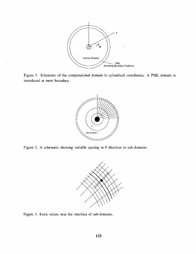
r
mtel
BPouMLary Condition
Figure 1. Schematic of the computational domain in cylindrical coordinates.
introduced at outer boundary.
A PML domain is
Figure 2. A schematic showing variable spacing in 0 direction in sub-domains.
/
Figure 3. Extra values near the interface of sub-domains.
133
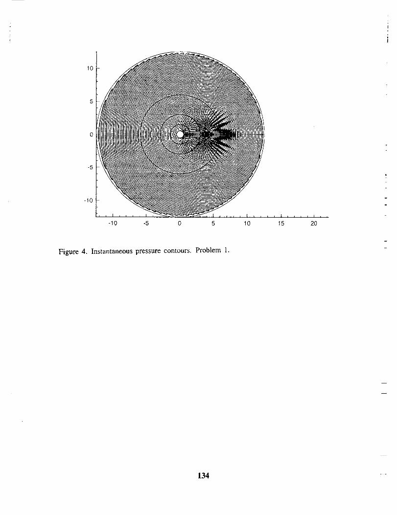
10
-5
-10
-10 -5 0 5 10 15 20
E
Figure 4. Instantaneous pressure contours. Problem 1.
m
134
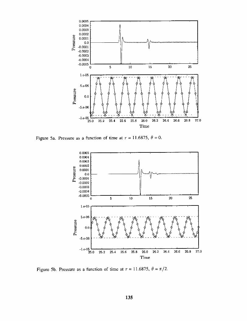
0°00050.0004
0.00030.0002
0.0001
m 0.0-0.0001
-0.0002
-0.0003
-0.0004
-0.00050 5 10 15 20 25
l.e-05, ...... , ....... ___ ,__:_ , ___ , ___,_ _,
+m
-5.e-06
-l.e-0525.0 25.2 25.4 25.6 25.8 26.0 26.2 26.4 26.6 26.8 27.0
Time
Figure 5a. Pressure as a function of time at r = 11.6875, 0 = 0.
0.0005
0.0004
0.0003
0.0002
0.0001o.o
-0.0001-0.0002
-0.0003
-0.0004
-0.0005
1 .e-05
m m
0 5 10 15 20 25
5.e-06
o-5.e-06
-l.e-05 ' ' ' ' ' ' ' ' - ' ' ' ' ' ' '25.0 25.2 25.4 25.6 25.8 26.0 26.2 26.4 26.6 26.8 27.0
Time
Figure 5b. Pressure as a function of time at r = 11.6875, 0 = 7r/2.
135
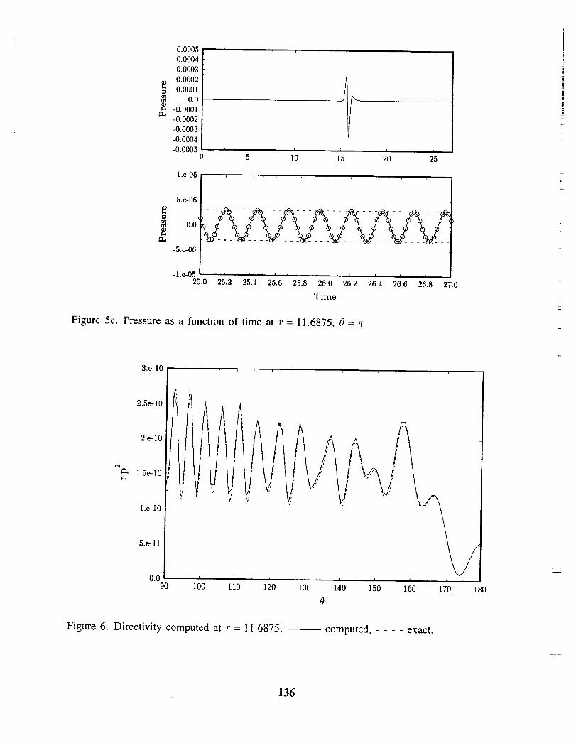
0.0005
0.0004
0.0003
0.0002
0.00010.0
_._ -0.0001-0.0002
-0.0003
-0.0004
-0.0005
k--i , I , I , l I
0 5 10 15 20 25
r_
I.e-05
I5.e-06
0.0'
-5.e-06
-l.e-05 ' ' ' ', ' .... _ ' ' , _ , ' ,25.0 25.2 25.4 25.6 25.8 26.0 26.2 26.4 26.6 26.8 27.0
Time
Figure 5c. Pressure as a function of time at r = 11.6875, 0 = 7r
3.e-10
2.5e-i0
2.e-lO
1.e-lO
5.e-ll
0.090 i00 ii0 120 130 140 150 160 170 180
0
Figure 6. Directivity computed at r = 11.6875. computed, - - - - exact.
136
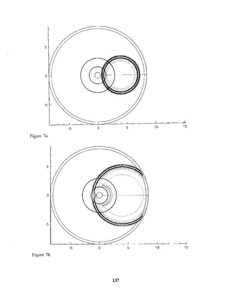
-5
5
0
ii
-5 0 5
Figure 7a.
I 1 i i i
10 15
0
-5
i
i
Figure 7b.
-5 0 5 10 15
137
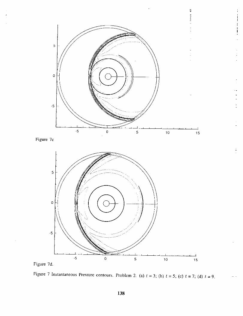
-5
Figure 7c
-5
-5 0 5
...............................iiiii.......
/J
10 15
Figure 7d.
-5 0 5 10 15
Figure 7 Instantaneous Pressure contours. Problem 2. (a) t = 3; (b) t = 5; (c) t = 7; (d) t = 9.
138
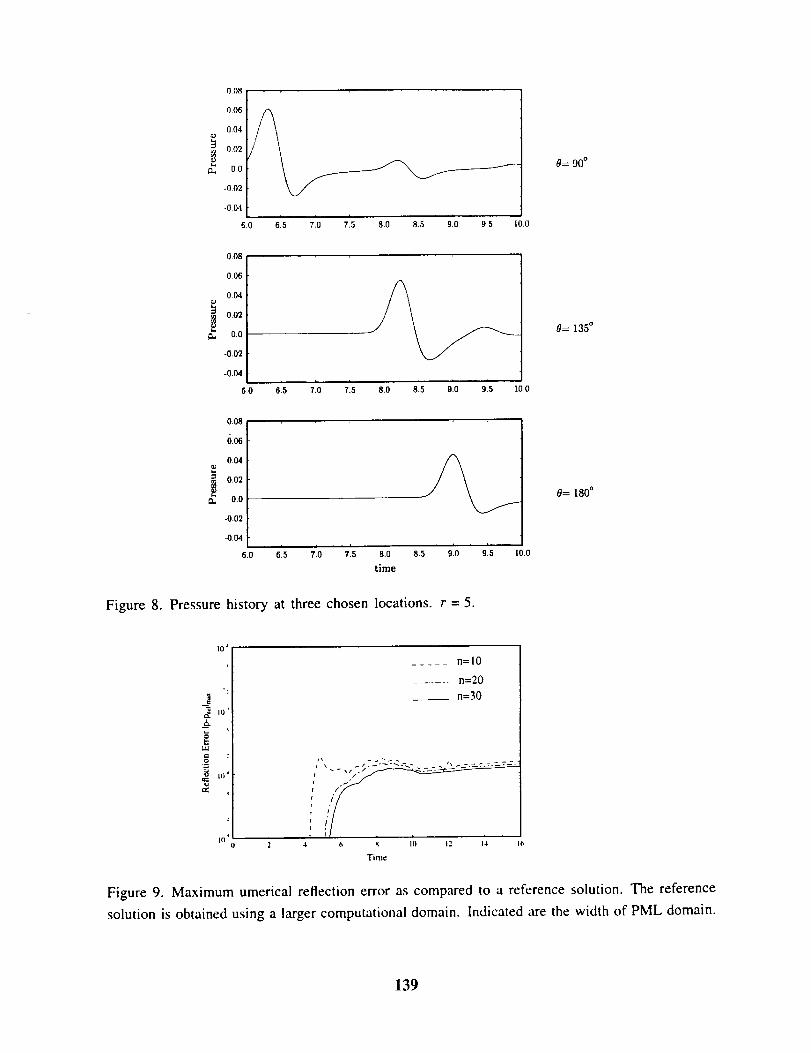
008
006
0,04
i 0.02
O,., 0.0
.002
-0,04
,. , ,60 6 5 7.0 7.5 8.0 8.5 9.0 9.5 I0.0
0,08
0,06
0,04
0.02
0.0
-0.02
-0.04
6.0
i6.5 7.0 7.5 8.0 8.5 9.0 9.5 10.0
13,
0.08
0.o6
0.04
0.02
0.0
-0.02
-0.04
6.0 6 5 7.0 7.5 8.0 8.5 9.0 9 10.0
time
Figure 8. Pressure history at three chosen locations, r = 5.
o= 90°
8= 135°
0= 180°
10"
=_"_ I0'
8
10
I(}(I
..... n=10
....... n=20
n=30
I_ _,,/. .
f /"
i i
2 4 6 8 10 12 14 16
Time
Figure 9. Maximum umerical reflection error as compared to a reference solution. The reference
solution is obtained using a larger computational domain. Indicated are the width of PML domain.
139
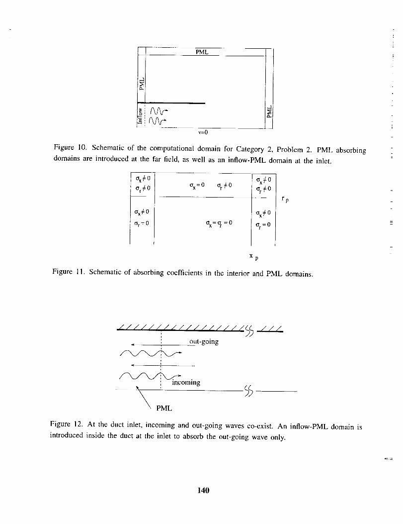
Figure 10. Schematic of
domains are introduced at
_[ PML
I
I
v=O
__
r
e_
the computational domain for Category 2, Problem 2. PML absorbing
the far field, as well as an inflow-PML domain at the inlet.
q)'r_:O
(rx4 0
C;r= 0
_=o %¢o
_x=or =o
%¢oar¢O
ax¢O
Or=O
rp
Xp
Figure 1 I. Schematic of absorbing coefficients in the interior and PML domains.
///////M/////////_,i
', out-going
|
i
,, incoming
PML
///
Figure 12. At the duct inlet, incoming and out-going waves co-exist. An inflow-PML domain is
introduced inside the duct at the inlet to absorb the out-going wave only.
140
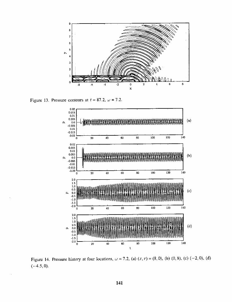
i /
-8 -6 -4 -2 0 2 4 6 8
X
Figure 13. Pressure contours at t = 87.2, _ = 7.2.
0,02
0,015
0.01
0.0050.0
-0.005
-0.01-0.015
-0.020
I i i , 1 , b i i
20 40 60 80 100 120 140
(a)
0,02
0.0150.01
0.005
0,0-0.005
-0.01
-0.015-0.02 , / I , I , , I I , I
20 40 60 80 100 120 140
(b)
2.0 , ,
1.5
0 20 40 60 80 100 1 0 140
(c)
2,0
1.5 __t1/t i
1.0
0.50.0
-0.5
-1.0
-1.5-2.0
0 20
I I I I
40 60 80 100 120 140
(d)
Figure 14. Pressure history at four locations, w = 7.2, (a) (x, r) = (8, 0), (b) (0, 8), (c) (-2, 0), (d)
(-4.5, o).
141
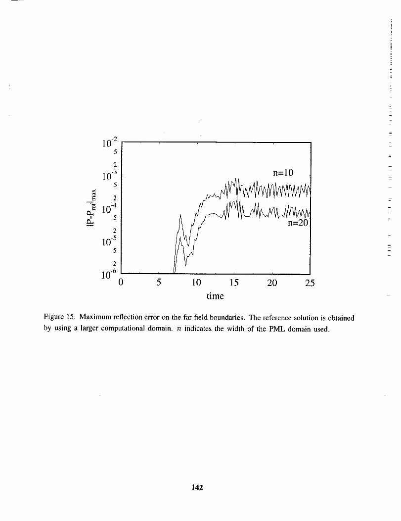
10-25
210-3
5
E 210-4
5
210 -5
5
n=10
5
2-6
10 ' ' ' ' ' '0 10 15 20
time
25
Figure 15. Maximum reflection error on the far field boundaries. The reference solution is obtained
by using a larger computational domain, n indicates the width of the PML domain used.
142
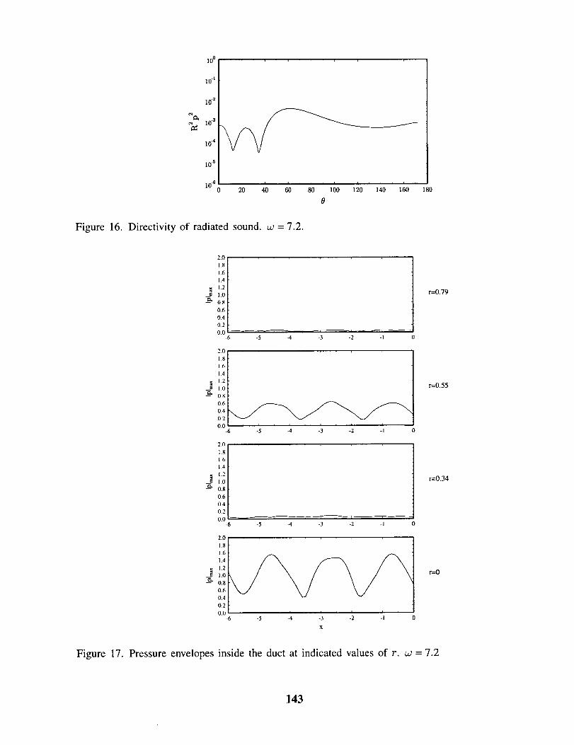
100
i0 -I
10 -z
i0"3
10 .4
lO-s
i0-_ i i , i , i i , i , i
20 40 60 80 I(30 120 140 160
0
180
Figure 16. Directivity of radiated sound, w = 7.2.
2.0
1.8
1.6
t.4
1.2
1.0
0.8
0.6
0.4
02
O0
2,0
1.8 I1.6
1.4
1.2
1.0
0.8
0.6
0.4
0.2
0,0-6 -5 -4 -3 -2 -1
2.0
1.8
1.6
1.4
1.2
1.0
0.8
0.6
0.4
0.2
0.0-6 -5 -4 -3 -2 -i
2.0
1.8
1.6
1.4
1.2
1.0
0.8
0.6
0.4
02-
0.0-6
i J o ...... i
-5 -4 -3 -2 -I
r=0.79
r=0.55
r=0.34
r---O
Figure 17. Pressure envelopes inside the duct at indicated values of r. co = 7.2
143
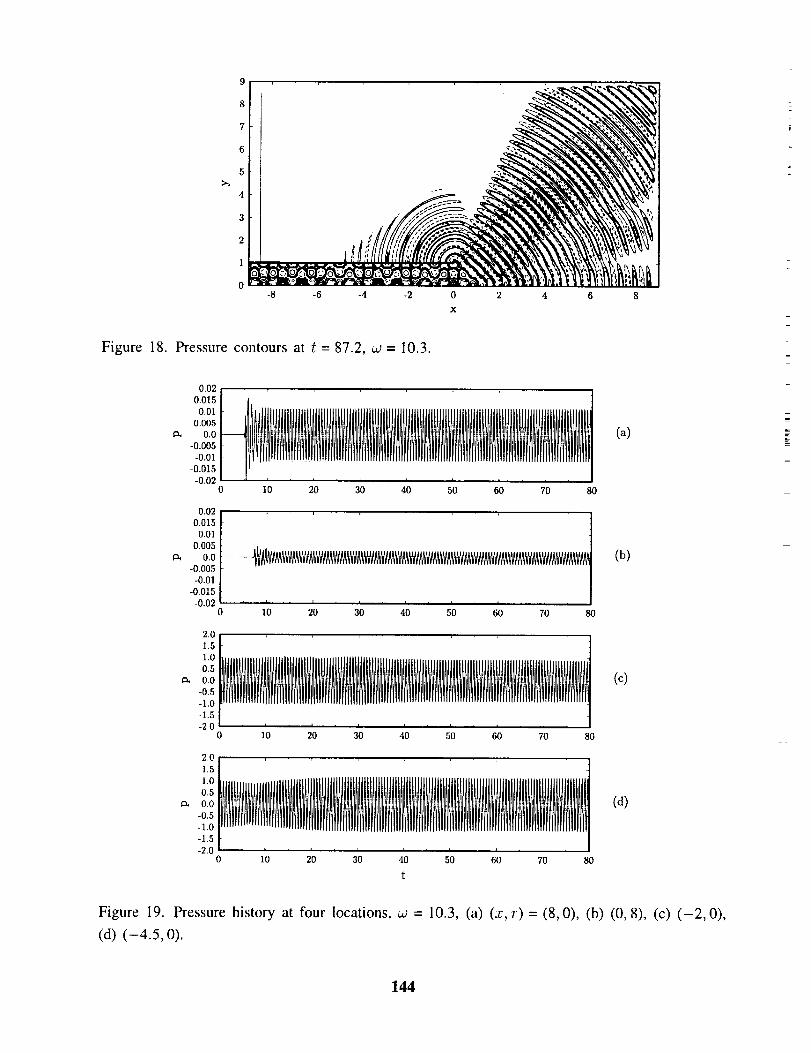
-8 -6 -4 -2 0 2 4 6 8
X
Figure 18. Pressure contours at t = 87.2, co = 10.3.
ca,
0.02
0.015
0.010.005
0.0-0.005
-0.01
-0.015
-0,02
I , I , i I , I I , , , I
0 I 0 20 30 40 50 60 70 80
0.02 I ' ' .... '
0.015 [0.01 |
-0.005 |
-0.01
-OoO i ..........0 I0 20 30 40 50 60 70 80
2.0
1.5
1.0
0.5
0.0-0,5
-I.0
-1.5-2.0 • I i I , l I i i , i ,
10 20 30 40 50 60 70 80
2.0
1.5
1.0
0.5
0.0-0.5
-1.0
-1.5
-2.0 , I i I i I i , l i I ,
0 10 20 30 40 50 60 70 80
t
Ca)
(b)
(c)
(d)
Figure 19. Pressure history at four locations, w = 10.3, (a) (x, r) = (8, 0), (b) (0, 8), (c) (-2, 0),
(d) (-4.5, 0).
144
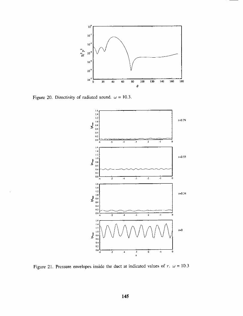
100
i0 "]
i0 "_
e_ i0 "s
10 -4
10 -5
10-6 'o .... 'o'2 40 60 8
0
/
i , I . , L .100 120 140 160 180
Figure 20. Directivity of radiated sound, w = 10.3.
e,
1.6
1.4
1.2
l.O
0.8
0.6
04
0.2
0.0-6
1.6
1.4
1,2
I0
0.8
0.6
0.4
0.2
0,0-6
1.6
t.4
1,2
1,0
0.8
0.6
0.4
0.2i i
0'0-6 -5 -4 -3
i i * ---5 -4 -3 -2 -I
-4 -3 -2 -1 0
-2 -I 0
i- -2 -|
x
1,6
14
1,2
I0
0.8
0.6
0.4
0.2
i i0"0-6 -5 -4
r---0.79
r--0.55
r=0.34
r=O
Figure 21. Pressure envelopes inside the duct at indicated values of r. _ = 10.3
145
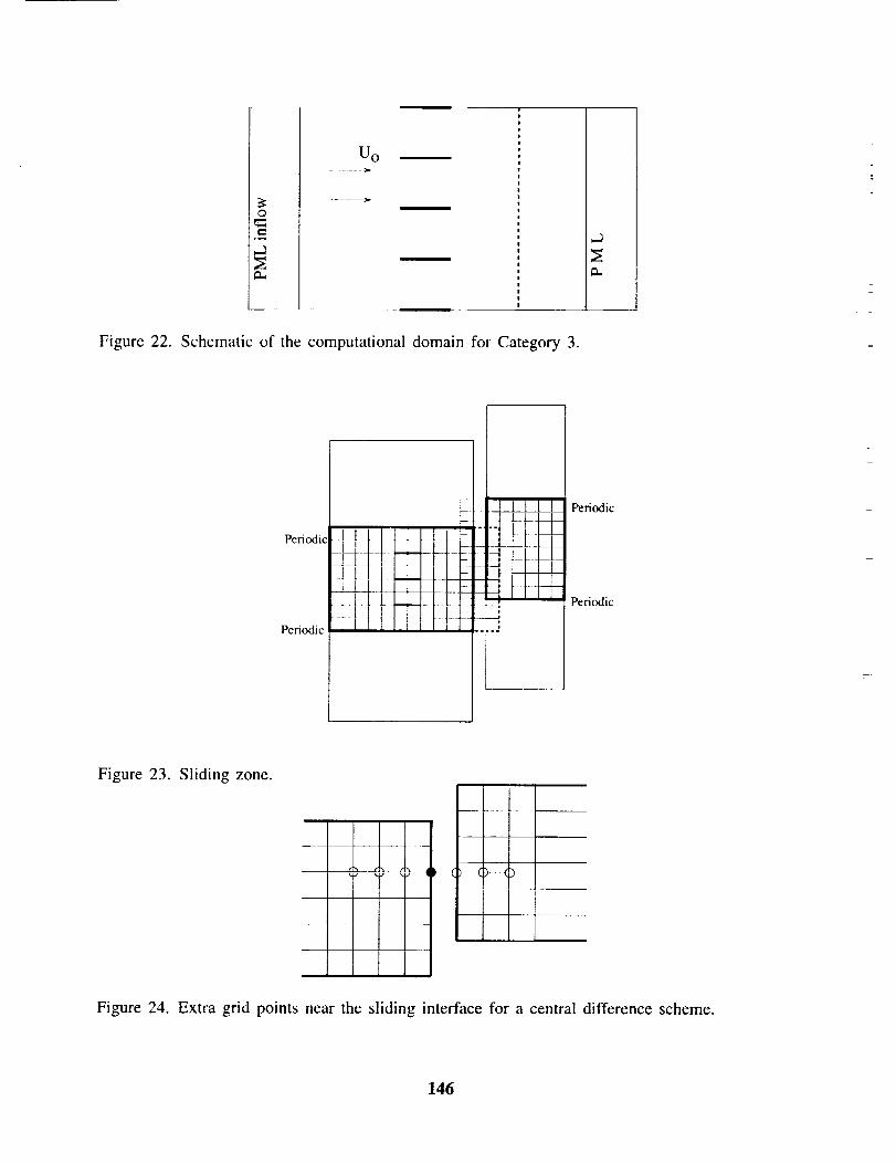
U o
o
Figure 22. Schematic of the computational domain for Category 3.
Periodic
Periodic
s_
_L! r
_TT-
Periodic
Periodic
Figure 23. Sliding zone.
_---()---()---_)
Figure 24. Extra grid points near the sliding interface for a central difference scheme.
146
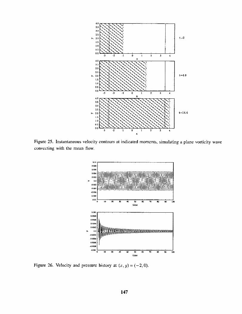
::,..,
4.0
3,0
2.5
2.0
0.0-3 -2 -I
4.0 _-._-,_
3.0 _, _.
2.0 _-'_ _ •
_. -% •
0.5 ,,_. ,,.0.0 _
-3
0 1
x
i t
2 3 4
t
t
2 3 4
t=O
-2 -I 0 I
x
3.540 --_..x_"_'_
.
2.5,. _
_, 2.o-:-:- t=14.4
0.0
-3 -2 -I 0 I 2 3 4
x
t=4.8
Figure 25. Instantaneous velocity contours at indicated moments, simulating a plane vorticity wave
convecting with the mean flow.
0008
0._
0.004
O0O2
0.0
-0.C02
-0004
-0005
-0008
4],01
0001
0.0008
000_
00004
O.t_02
_, 0.0
-0 0002
-0 0004
-000_
-0 000a
-0.001
I0 20 30 4G 50 60 70 80 90 I00
time
llttli tt ,,lttt
i ,I'0 20 30 40 SO _ TO 80 90 100
time
Figure 26. Velocity and pressure history at (:r, y)= (-2, 0).
147
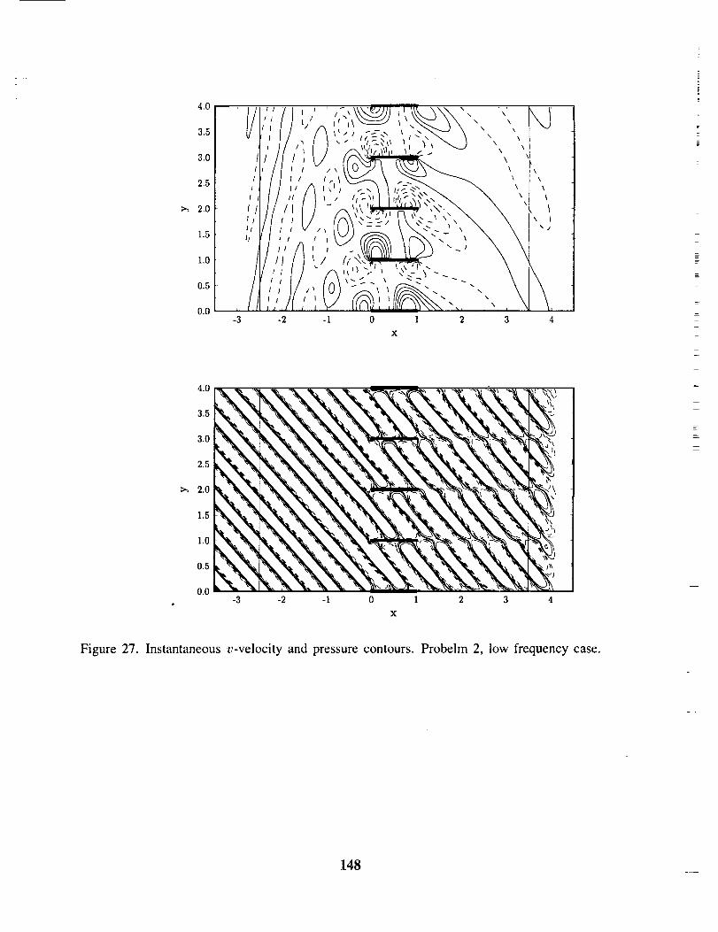
=
=
4.0 l/ _J /l i I ...... \'
3.5 " I/ ' ' [/ ' /_ "£'.-, ,,,., ,'-._ \ '. ,
2.5 ,_ // ,, A,<',-;-'_ t,;m _,, #/ ,, / I, , ,,:-,,11,;,,.7-
_,o t i I I II I J -/2k','!'._ " ".,,,\ \)l III i I v,_ lt)/_ \ ...".'--'">-\
Ai ,, M, , - \tflr",,'k'_kl1z.o III I I i l _ I 6""t_
/7 ,, l/ " ,,'-x,,'>'-;', ',",/r _ I t/ /,.,\_-c. _ "
I/]lj t[ _ 't/ ((,..'_ll0,0 , I /i t i ,! I I I "1"/ Ill lo' _ z
-3 -2 -i 0 I 2 3
\
\
\ i\ )
\\,4
x
=
Figure 27. Instantaneous v-velocity and pressure contours. Probelm 2, low frequency case.
148
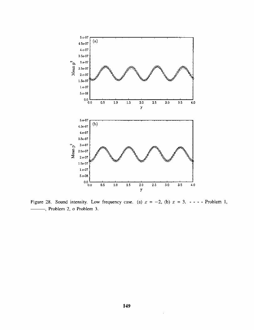
5.e-07
4.5e-07
4.e-07
3.5e-07
¢_¢x, 3.e-07
_ 2.5e-07
2.e-07
1.5e-07 ¢
1.e-07
5.e-08
0.00.0
(a)
o:_ 11o '115 2:0 2:5 3:0 '3:5 ',oY
5.e-07 i
4.5e-07 ]
4.e-07 [
%::_,
2.5e-07
2.e-07
1.5e-07
1.e-07
5.e-08
0.00.0
(b)
I , I I , I _ , I , I ,
0.5 1.0 1.5 2.0 2.5 3.0 3.5
Y
4.0
Figure 28. Sound intensity. Low frequency case. (a) x = -2, (b) x = 3. - - - - Problem 1,
--, Problem 2, o Problem 3.
149
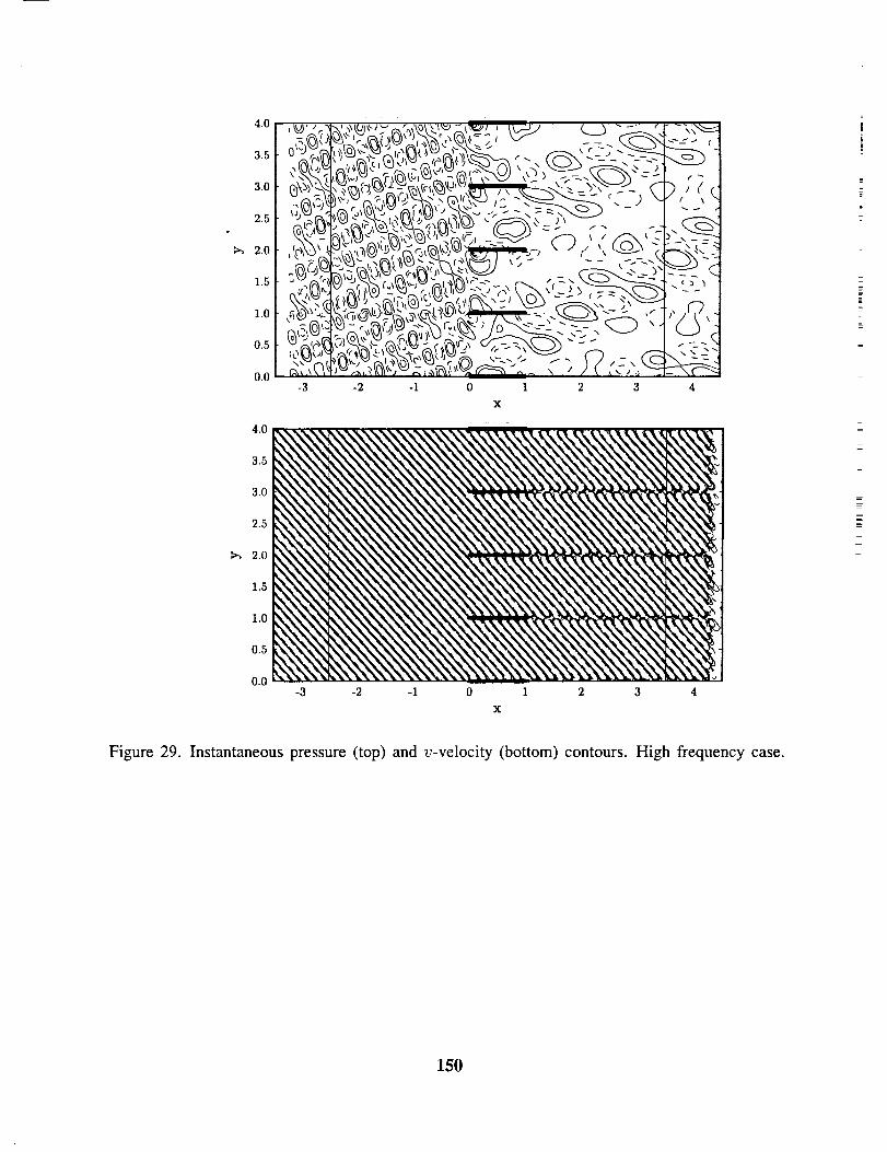
4
,_..
4
=
T
Figure 29. Instantaneous pressure (top) and v-velocity (bottom) contours. High frequency case.
150
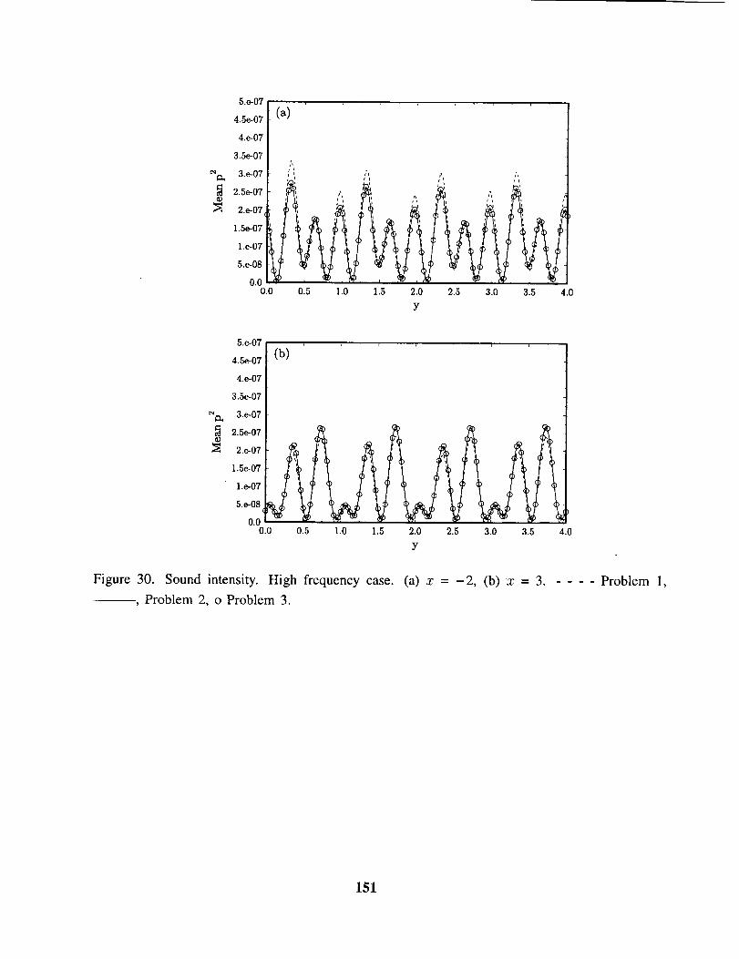
5.e-07 |
4.5e-07 I
4.e-07 [
_ 2.5e-07
N 2.e-07,
1.5e-07
l,e-07
5.e-08
0.00.0
(a)
't
0.5 1.0 1.5 2.0 2.5 3.0 3.5 4.0
Y
5.e-07
4.5e-07
4.e-07
3.5e-07
_ 3.e-07
2.5e-07
2.e-07
1.5e-07
l.e-07
5.e-08
0.00.0
(b)
0.5 1.0 1.5 2.0 2.5
Y
Figure 30. Sound intensity. High frequency case. (a) x = -2, (b) x = 3. - - - - Problem 1,
, Problem 2, o Problem 3.
151
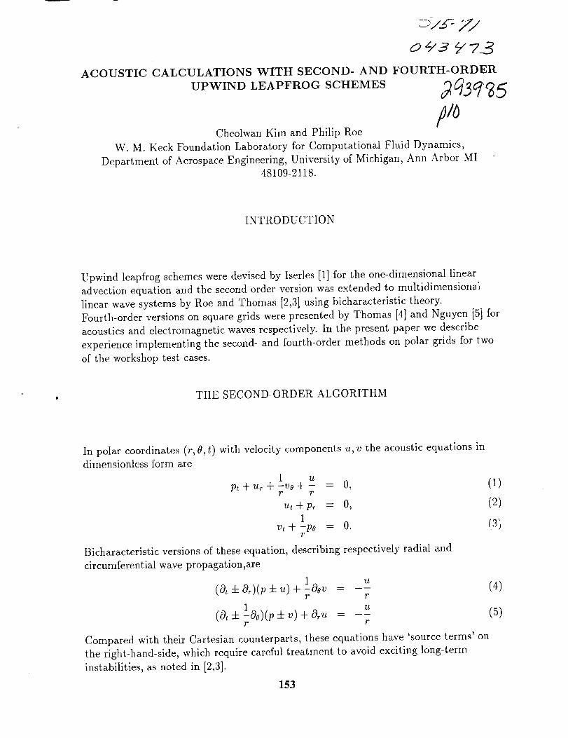
oz/3 Vz3
ACOUSTIC CALCULATIONS WITH SECOND- AND FOURTH-ORDER
UPWIND LEAPFROG SCHEMES __5
Cheolwan Kim and Philip Roe
W. M. Keck Foundation Laboratory for Computational Fluid Dynamics,
Department of Aerospace Engineering, University of Michigan, Ann Arbor MI48109-2118.
INTRODUCTION
Upwind leapfrog schemes were devised by Iserles [1] for the one-dimensional linear
advection equation and the second-order version was extended to multidimensional
linear wave systems by Roe and Thomas [2,3] using bicharacteristic theory.
Fourth-order versions on square grids were presented by Thomas [4] and Nguyen [5] for
acoustics and electromagnetic waves respectively. In the present paper we describe
experience implementing the second- and fourth-order methods on polar grids for two
of the workshop test cases.
THE SECOND-ORDER ALGORITHM
In polar coordinates (r, 0, t) with velocity components u, v the acoustic equations in
dimensionless form are
1 uPt + Ur Jr- -vo -t- -- = 0, (1)
r r
u,+p_ = 0, (2)1
v_+-po = 0. (3)r
Bicharacteristic versions of these equation, describing respectively radial and
circumferential wave propagation,are
(O,+O,)(p±u)+ a-00v = -_- (4)r r
(o,4-LOo)(p4-v)+ o,_, - u (5)I" 7"
Compared with their Cartesian counterparts, these equations have 'source terms' on
the right-hand-side, which require careful treatment to avoid exciting long-term
instabilities, as noted in [2,3].
153
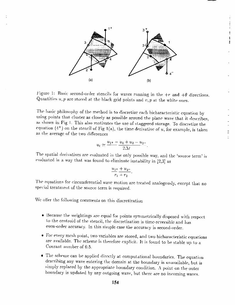
1 + 3 +
4
(a) (b)
Figure 1" Basic second-order stencils for waves running in the +r and +0 directions.
Quantities u, p are stored at the black grid points and v, p at the white ones.
Tile basic philosophy of the method is to discretize each bicharacteristic equation by
using points that cluster as closely as possible around the plane wave that it describes,
as shown in Fig 1. This also motivates the use of staggered storage. To discretize the
equation (4 +) on the stencil of Fig l(a), the time derivative of u, for example, is taken
as the average of the two differences
_I+ -- _gl -[-U2 -- 7A2-
2At
The spatial derivatives are evaluated in the only possible way, and the 'source term' is
evaluated in a way that was found to eliminate instability in [2,3] as
ill+ Bt- t/2-
T1 @ T2
The equations for circumferential wave motion are treated analogously, except that no
special treatment of the source term is required.
We offer tile following comments on this discretization
• Because the weightings are equal for points symmetrically disposed with respect
to the centroid of the stencil, the discretization is time-reversible and has
even-order accuracy. In this simple case the accuracy is second-order.
• For every mesh point, two variables are stored, and two bicharacteristic equations
are available. The scheme is therefore explicit. It is found to be stable up to a
Courant number of 0.5.
• The scheme can be applied directly at computational boundaries. The equation
describing any wave entering the domain at the boundary is unavailable, but is
simply replaced by the appropriate boundary condition. A point on the outer
boundary is updated by any outgoing wave, but there are no incoming waves.
154
• Becausethe discretization connectsthree time levels thereexist, as with allleapfrogschemes,spurious (non-physical) solutions.
• Becausethe pressureis stored twice, there is a possibleerror mode in which thepressuresstored at the black and white meshpoints becomeuncoupled.
• It is an easyconsequenceof the governingequationsthat the vorticity shouldnotchangewith time. However,this is not enforcedby the discretization, so anotherspuriousmode may appearthat is linked to vorticity.
The first three of thesepropertiesare desirable;the last three constitute potential
problems.
Like any other leapfrog method, we need a special starting procedure for the first time
step. This is important, because errors generated at that moment can be inherited by
all later times. At present, however, we use a very crude starting procedure. We p,Lt
u 1 = u °, and then advance to u 2 with one half of the regular timestep. It is easy to
show that this effectively advances u ° to u 2 with the regular timestep according to a
first-order upwind scheme.
THE FOURTH-ORDER ALGORITHM
Construction of this is straightforward in principle. Each of the quantities appearing in
the second-order scheme can be replaced by its Taylor expansion (with respect to the
centroid of the stencil) to give the equivalent equation of the scheme. The higher
derivatives that appear can be regarded as error terms and are mixtures of space and
time derivatives. The time derivatives are due to expansions like
h2 __ k2u,+ - _1 + u_ - u_- = 0,_, + -gO_,u + O_u_ + --ffO,,u + O(h _ k4).2At
from which the terms involving time can be eliminated, in the spirit of Lax-Wendroff
methods, by using the governing equations to convert time derivatives to space
derivatives..The outcome is an estimate of the truncation error entirely in terms of
space derivatives. Evaluating these merely to second order is enough to eliminate the
errors, because they come already multiplied by second-order factors. If the error
terms are kept in a form that preserves the symmetry with respect to the centroid of
the stencil, it is guaranteed that no third-order terms will be introduced. The resulting
scheme will be fourth-order, time-reversible, and fully discrete. All of the above
algebraic manipulations can be carried out using symbolic manipulation, and the
neccessary FORTRAN expressions can be generated in the same way.
155
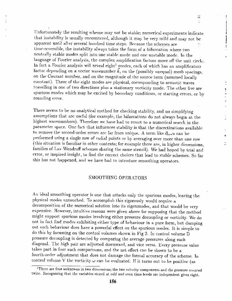
Unfortunately the resulting schememay not be stable;numerical experimentsindicatethat instability is usually encountered,although it may bevery mild and may not b}apparentuntil after severalhundred time steps. Becausethe schemesaretime-reversible,the instability alwaystakesthe form of a bifurcation wheretwoneutrally stable modessplit into onestable modeand one unstablemode. In thelanguageof Fourier analysis,the complexamplification factors moveoff the unit circle.In fact a Fourier analysiswill revealeight1modes,eachof which has an amplificatloafactor dependingon a vector wavenumberk, on the (possibly unequal) mesh spacings,
on the Courant number, and on the magnitude of the source term (assumed locally
constant). Three of the eight modes are physical, corresponding to acoustic waves
travelling in one of two directions plus a stationary vorticity mode. The other five are
spurious modes which may be excited by boundary conditions, or starting errors, or by
rounding error.
There seems to be no analytical method for checking stability, and no simplifying
assumptions that are useful (for example, the bifurcations do not always begin at the
highest wavenumbers). Therefore we have had to resort to a numerical search in the
parameter space. One fact that influences stability is that the discretizations available
to remove the second-order errors are far from unique. A term like &rrU can be
performed using a single row of radial points or by averaging over more than one row
(this situation is familiar in other contexts; for example there are, in higher dimensions,
families of Lax-Wendroff schemes sharing the same stencil). We had hoped by trial and
error, or inspired insight, to find the correct choices that lead to stable schemes. So far
this has not happened, and we have had to introduce smoothing operators.
1
SMOOTHING OPERATORS
An ideal smoothing operator is one that attacks only the spurious modes, leaving the
physical modes untouched. To accomplish this rigorously would require a
decomposition of the numerical solution into its eigenmodes, and that would be very
expensive. However, intuitive reasons were given above for supposing that the method
might support spurious modes involving either pressure decoupling or vorticity. We do
not in fact find modes exhibiting either type of behaviour in a pure form, but damping
out such behaviour does have a powerful effect on the spurious modes. It is simple to
do this by focussing on the control volumes shown in Fig 2. In control volume D
pressure decoupling is detected by comparing the average pressures along each
diagonal. The high pair are adjusted dowrtward, and vice versa. Every pressure value
takes part in four such comparisons, and the net effect can be shown to be a
fourth-order adjustment that does not damage the formal accuracy of the scheme. In
control volume V the vorticity co can be evaluated. If it turns out to be positive (as
iThere are four unknowns in two dimensions; the two velocity components and the pressure eoun_,ed
twice. Recognizing that the variables stored at odd and even time levels are independent gives eight.
156
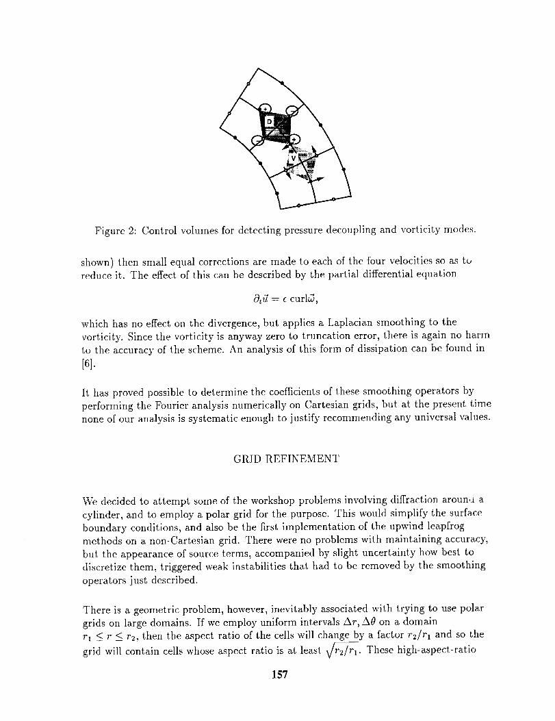
Figure 2: Control volumesfor detecting pressuredecouplingand vorticity modes.
shown) then small equal correctionsare madeto eachof the four velocitiesso astoreduceit. The effectof this canbe describedby the partial differential equation
0try = e curlaS,
which has no effect on the divergence, but applies a Laplacian smoothing to the
vorticity. Since the vorticity is anyway zero to truncation error, there is again no harm
to the accuracy of the scheme. An analysis of this form of dissipation can be found in
[6].
It has proved possible to determine the coefficients of these smoothing operators by
performing the Fourier analysis numerically on Cartesian grids, but at the present time
none of our analysis is systematic enough to justify recommending any universal values.
GRID REFINEMENT
We decided to attempt some of the workshop problems involving diffraction around a
cylinder, and to employ a polar grid for the purpose. This would simplify the surface
boundary conditions, and also be the first implementation of the upwind leapfrog
methods on a non-Cartesian grid. There were no problems with maintaining accuracy,
but the appearance of source terms, accompanied by slight uncertainty how best to
discretize them, triggered weak instabilities that had to be removed by the smoothing
operators just described,
There is a geometric problem, however, inevitably associated with trying to use polar
grids on large domains. If we employ uniform intervals At, A0 on a domain
rl _< r _< r2, then the aspect ratio of the cells will change by a factor r2/rl and so the
grid will contain cells whose aspect ratio is at least _-2/rl. These high-aspect-ratio
157
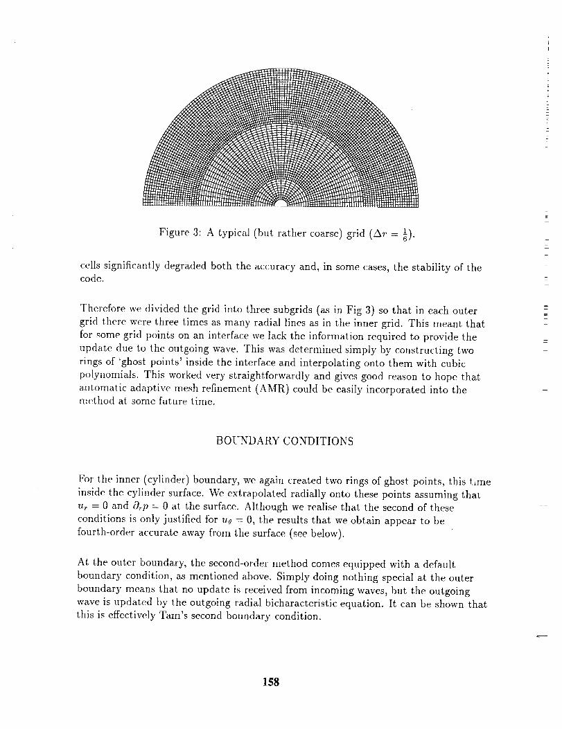
Figure 3: A typical (but rather coarse) grid (At = _).
cells significantly degraded both the accuracy and, in some cases, the stability of thecode.
Therefore we divided the grid into three subgrids (as in Fig 3) so that in each outer
grid there ,,,,'ere three times as many radial lines as in the inner grid. This meant that
for some grid points on an interface we lack the information required to provide the
update due to the outgoing wave. This was determined simply by constructing two
rings of 'ghost points' inside the interface and interpolating onto them with cubic
polynomials. This worked very straightforwardly and gives good reason to hope that
automatic adaptive mesh refnement (AMR) could be easily incorporated into themethod at some future time.
BOUNDARY CONDITIONS
For the inner (cylinder) boundary, we again created two rings of ghost points, this time
inside the cylinder surface. We extrapolated radially onto these points assuming thaL
u_ = 0 and &p = 0 at the surface. Although we realise that the second of these
conditions is only justified for uo = 0, the results that we obtain appear to be
fourth-order accurate away from the surface (see below).
At the outer boundary, the second-order method comes equipped with a default
boundary condition, as mentioned above. Simply doing nothing special at the outer
boundary means that no update is received from incoming waves, but the outgoing
wave is updated by the outgoing radial bicharacteristic equation. It can be shown that
this is effectively Tam's second boundary condition.
158

3.5 x 10¹⁰
3
2.5
2
1.5
1
0.5
0
9O
i
100
:\• l i, %
! • =
I :,, , ,. ,
= I I t I !
110 120 130 140 150 160 170 180
Figure 4: The mean square pressure rip2[ at r = 15.0 for problem 1. The dashed line is
the exact solution and the solid line is the numerical prediction on a grid with 10 points
per wavelength (Ar = _0)"
RESULTS
CATEGORY 1, PROBLEM 1. We obtained results for this problem using grids
defined radially by 8 and 10 grid points per wavelength. Using 8 points did not se_m
to be enough and we present only our results with 10 points. This translates to
Ar = 426. The frequency is w = 87r and the solution is given in Figure 4 for r = 15.0.
The computational domain was 0.5 < r < 16.0. The directivity pattern seems to be
very well predicted, but the amplitude is less satisfactory. Partly we attribute this to
the effect of the small damping terms we had to introduce to cure instability due to the
source terms arising from the non-Cartesian grid. It is possible that dealing with this
more systematically would improve the agreement. We estimate that a calculation with
12 points per wavelength would be much better, but with our code still undergoing
modification as the deadline approaches, we have not yet been able to perform such a
calculation. There is moreover the possibility that we have some interference due to
spurious reflections from the computational boundary. In the future we hope to
implement some of the ideas described at this meeting by Radvogln and by Goodrich.
CATEGORY 1, PROBLEM 2. This problem is distinctly easier and we are able to
make a fairly thorough comparison of results from different schemes on different grids.
Figure 5 shows a snapshot of the pressure at t = 6.0, according to the fourth-order
scheme with Ar = 1 The main purpose of including this is to show that no wave20"
reflections are visible from the grid refinement lines at r = 2.0 and r = 6.0. Next w_: •
give time histories of the pressure at the points A,B,C. First we show results from the
second-order scheme for grid sizes Ar - 1 1 1 The heavy dashed line is the 'exact'24 _ 32 _ 40"
solution, and it can be seen that not even on the finest grid is there really close
159
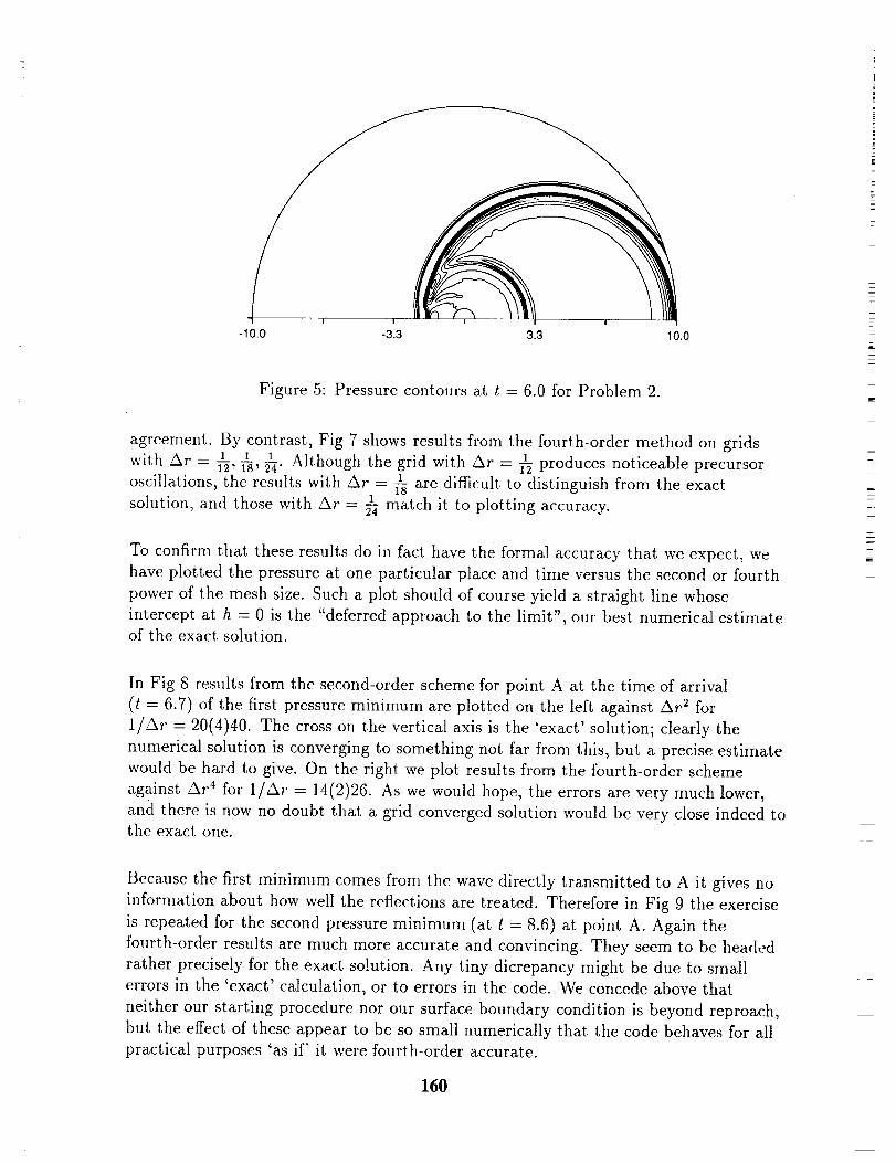
!
-10.0 -3.3 3.3 10.0
Figure 5: Pressure contours at t = 6.0 for Problem 2.
agreement. By contrast, Fig 7 shows results from the fourth-order method on grids
with Ar = 12,1lS,1 24"1Although the grid with Ar = _ produces noticeable precursor
oscillations, the results with Ar = _ are difficult to distinguish from the exact
solution, and those with Ar = _ match it to plotting accuracy.
To confirm that these results do in fact have the formal accuracy that we expect, we
have plotted the pressure at one particular place and time versus the second or fourth
power of the mesh size. Such a plot should of course yield a straight line whose
intercept at h = 0 is the "deferred approach to the limit", our best numerical estimateof the exact solution.
In Fig 8 results from the second-order scheme for point A at the time of arrival
(t = 6.7) of the first pressure minimum are plotted on the left against Ar 2 for
1/Ar = 20(4)40. The cross on the vertical axis is the 'exact' solution; clearly the
numerical solution is converging to something not far from this, but a precise estimate
would be hard to give. On the right we plot results from the fourth-order scheme
against Ar 4 for 1�At = 14(2)26. As we would hope, the errors are very much lower,
and there is now no doubt that a grid-converged solution would be very close indeed tothe exact one.
Because the first minimum comes from the wave directly transmitted to A it gives no
information about how well the reflections are treated. Therefore in Fig 9 the exercise
is repeated for the second pressure minimum (at t = 8.6) at point A. Again the
fourth-order results are much more accurate and convincing. They seem to be headed
rather precisely for the exact solution. Any tiny dicrepancy might be due to small
errors in the 'exact' calculation, or to errors in the code. We concede above that
neither our starting procedure nor our surface boundary condition is beyond reproach,
but the effect of these appear to be so small numerically that the code behaves for all
practical purposes 'as if' it were fourth-order accurate.
160
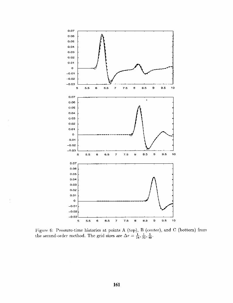
0.07
0.06
0.05
0.04
0.03
0.02
0.01
0
-0.01
-0.02
--0.03
5 5.5 6 6.5 7 7.5 8 8.5 9 9.5 10
0.07
0.06
0.05
0.04
0.03
0.02
0.01
0
--0.01
--0.02
-0.03 i i i i i
5 5.5 6 6.5 7 7.5
i__
8 8.5 9 9.5 10
0.07
0.06
0.05
0.04
0.03
0.02
0.01
0
-0.01
-0.02
-0.03
5
B
i i i
5.5 6 6.5 7 7.5 8 8.5 9 9.5 10
Figure 6: Pressure-time histories at points A (top), B (center), and C (bottom) from1 1 1
the second-order method. The grid sizes are An -- 24,32, 40"
161
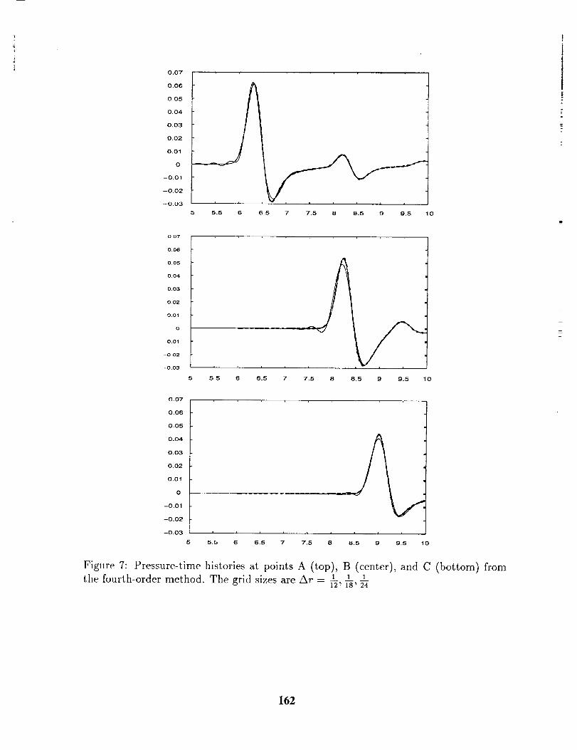
0.07
0.06
0.05
0.04
0,03
0.02
0.01
0
-0.01
--0.02
--0,03
5 5.5 6 6.5 7 7.5 6 8.5 9 9.5 10
0.07
0.06
0.05
0.04
0.03
0.02
0.01
0
--0,01
-0 02
-0.03
5 5.5 6 6.5 7 7.5 8 8.5 9 9.5 10
0.07
0.06
0.05
0.04
0.03
0.02
0.01
0
-0.01
-0.02
--0.03 ,L i
5.5 6 6.5 7 7.5 8
I ! I
8.5 9 9.5 10
Figure 7: Pressure-time histories at points A (top), B (center), and C (bottom) from
the fourth-order method. The grid sizes are Ar - 1 1 112 _ 18' 24
162
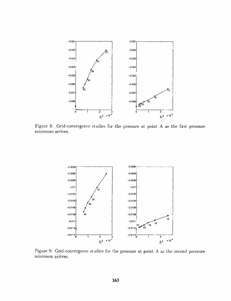
-0.021 -0.021
-0.022
-0.023
-0.024
-0.025
-0.026
-0.027
-0028
-0.022
-0.02:
-0.02,
-0.025
-0.026
-0.027
-0.028
i i1 2 0 1 2
h2 xlo -_ h 4 xlo -5
Figure 8: Grid-convergence studies for the pressure at point A as the first pressure
minimum arrives.
-0.0094
-0.0096
-0.0098
-0.01
-0.0102
-0.0104
-0.0106
-0.0108
-0.011
-0,01 _2,
-0.011 ,_0
-0,0094
-0.0096
-0.0091
-0.0
-0.0102
-0.0104
-0.0106
-0.0108
.-0.011
-0.0112
-0.011401 2 1 2
h2 x 10-3 h4 X I0 -5
Figure 9: Grid-convergence studies for the pressure at point A as the second pressureminimum arrives.
163
CONCLUSIONS
_Te have presented a progress report giving the outcome of applying to two of the
Workshop problems a fourth-order version of the upwind leapfrog method. The
exercise has proved very useful in developing the method and we are grateful to the
organisers for providing test cases that were originally just beyond our reach, together
with independent solutions against which to measure our progress.
We feel encouraged by the outcome, especially by our results for Problem 2 where a
careful analysis of the error is possible. We find that the fourth-order method is a very
substantial improvement beyond the second-order version and amply repays the
additional costs. Tile ability to implement the scheme on non-Cartesian grids with
local refinement is a new and valuable feature to which we have been impelled by our
efforts to solve the workshop problems. However, we have much to do to make the
scheme more systematic, and we hope eventually to eliminate the need for smoothing
operators with arbitrary coefficients. Current work aims to develop the schemes not
only for acoustic and electromagnetic problems, but for linear elastodynamics also. We
hope to achieve a general methodology, first for long-range linear wave propagation,
and eventually for weakly non-linear waves also.
g
|
=
REFERENCES
1. A. ISERLES, Generalised leapfrog schemes, IMA Journal of Numerical Analysis, 6,
1986.
2. P. L. ROE, Linear bicharacteristic schemes without dissipation, ICASE Report
94-65, 1994, SIAM J. Scientific Computing, to appear, 1997.
3. J. Po THOMAS, P. L. ROE, Development of non-dissipative numerical schemes for
computational aeroacoustics, AIAA paper 93-3382, 1993.
4. J. P. THOMAS, Ph.D. Thesis, Department of Aerospace Engineering, University of
Michigan. 1996.
5. B. T. NGUYEN, Ph.D. Thesis, Department of Aerospace Engineering, University of
Michigan. 1996.
6. H. R. STRAUSS, An artificial viscosity for 2D hydrodynamics, J. Comput. Phys.
28, 1978.
164
LEAST-SQUARES SPECTRAL ELEMENT SOLUTIONSTHE CAA WORKSHOP BENCHMARK PROBLEMS
Wen H. Lin and Daniel C. Chan
Rocketdyne Division, Boeing North American, Inc.Canoga Park, CA 91309-7922
ABSTRACT
TO
o4'3 e--/-7 z/-
This paper presents computed results for some of the CAA benchmark problems via the acousticsolver developed at Rocketdyne CFD Technology Center under the corporate agreement between BoeingNorth American, Inc. and NASA for the Aerospace Industry Technology Program. The calculations areconsidered as benchmark testing of the functionality, accuracy, and performance of the solver. Results ofthese computations demonstrate that the solver is capable of solving the propagation of aeroacousticsignals. Testing of sound generation and on more realistic problems is now pursued for the industrialapplications of this solver.
Numerical calculations were performed for the second problem of Category 1 of the current workshopproblems for an acoustic pulse scattered from a rigid circular cylinder, and for two of the first CAAworkshop problems, i. e., the first problem of Category 1 for the propagation of a linear wave and thefirst problem of Category 4 for an acoustic pulse reflected from a rigid wall in a uniform flow of Mach0.5. The aim for including the last two problems in this workshop is to test the effectiveness of someboundary conditions set up in the solver. Numerical results of the last two benchmark problems havebeen compared with their corresponding exact solutions and the comparisons are excellent. Thisdemonstrates the high fidelity of the solver in handling wave propagation problems. This feature lends themethod quite attractive In developing a computational acoustic solver for calculating theaero/hydrodynamic noise in a violent flow environment.
INTRODUCTION
Accurate determination of sound generation, propagation, and attenuation in a moving medium is vitalfor noise reduction and control, especially for the design of quiet devices and vehicles. Currently, asophisticated tool to accurately predict the noise generation and propagation is still lacking even though theaerodynamic noise theory has been extensively studied since Sir James Lighthill's famous paper on soundgenerated aerodynamically appeared in 1952 [1]. The major difficulty in computational aeroacoustics iscaused by inaccurate calculations of the amplitude and phase of an acoustic signal. Because of its relativelysmall magnitude compared with its carrier - the flow field - an acoustic signature is not easily computedwithout distortion and degradation. Nowadays it is relatively easy to compute a steady flow field at mostspeeds with reasonable accuracy but it is still quite difficult to accurately compute an acoustic signatureassociated with a violent flow field. The basic reason for this difficulty is caused by the dispersion anddissipation effects introduced by most numerical methods for stability control in performing numericalcomputations. To circumvent the deficiency of current numerical methods for computational aeroacoustics,we have proposed a spectrally accurate method to compute the reference flow field and the generation andpropagation of sound in an unsteady flow.
165
The methodis basedona least-squaresspectralelementmethod.This methodsolvesthe linearizedacousticfield equationsby firstly expandingthe acousticvariablesin terms of somebasis (or trial)functionsandunknowncoefficients.Then,themethodminimizestheintegralof thesquaresof theresidualover the domainof influence.The resultantequationsarea set of linear algebraicequationsfor theunknowncoefficients.Thesealgebraicequationsincorporatethe systemderivativesof the acousticfieldequationsin integralforms.Thespatialderivativesarediscretizedby theuseof Legendrepolynomials,andthetime derivativeis performedby a three-leveltime steppingmethod.Theresultantmatrix equationissolvedby aJacobipreconditionedconjugategradientmethod.
Alongwith thefield equationsis asetof boundaryconditions,includingthenonreflectingandradiationconditions,to besatisfiedfor agivenproblem.Theseboundaryconditionswereexplicitly implementedintheacousticsolver.For instance,the normalvelocity componentis setequalto zero for anacousticallyrigid wall. Testingof the solver hasbeenbegunon the secondproblemof Category 1 for the currentworkshopbenchmarkandthefirst problemsof Categories1and4 for thefist CAA workshopbenchmark.Resultsof the last two computationscomparevery well with theanalyticresults.Thesecalculationswereconsideredasbenchmarktestingon thefunctionality,accuracy,andperformanceof thesolver.
MATHEMATICAL FORMULATION
Consideraninhomogeneous,partialdifferentialequationof theform
[L] {u} = {fl, (1)
where L is the first-order partial differential operator, {u} the column vector of unknown variables, and{f} the column vector of forcing functions. The aim of working with the first-order derivatives is to
ensure C O continuity in field variables at element interfaces. Next, we divide the domain of influence, D,
into S elements and assume an approximate solution to Eq. (1) for a typical element can be written as
N
{ue} = _1 {aj} _je,j=
(2)
where _je are linearly independent basis (or trial) functions, aj the expansion Coefficients for the unknown -variables, and N the total number of basis functions (or degrees of freedom) in an element. It should benoted that the same basis functions are used for all unknown variables. This feature is a characteristic of
the proposed method and it simplifies the mathematical formulation and numerical implementation. Ingeneral, the basis functions are arbitrary and need not satisfy the differential equation or the boundaryconditions. However, they must be differentiable once in the domain D and at the boundaries. The basis
functions used in the current study are Legendre polynomials of the independent variables.
Substituting Eq. (2) into Eq. (I), forming the residual, and applying the method of least squares with
respect to the expansion coefficients, one leads to
166
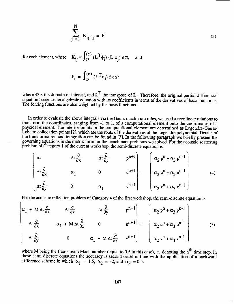
N
j_l Kijaj = Fi (3)
for each element, where Kij = S (e) (LTq)i) (L _j) dD, and
F i = S(e) (LT¢i) f dD
where D is the domain of interest, and L T the transpose of L. Therefore, the original partial differentialequation becomes an algebraic equation with its coefficients in terms of the derivatives of basis functions.
The forcing functions are also weighted by the basis functions.
In order to evaluate the above integrals via the Gauss quadrature rules, we used a rectilinear relations totransform the coordinates, ranging from -1 to 1, of a computational element onto the coordinates of a
physical element. The interior points in the computational element are determined as Legendre-Gauss-Lobatto collocation points [2], which are the roots of the derivatives of the Legendre polynomial. Details ofthe transformation and integration can be found in [3]. In the following paragraph we briefly present thegoverning equations in the matrix form for the benchmark problems we solved. For the acoustic scatteringproblem of Category 1 of the current workshop, the semi-discrete equation is
_ pn+l"a 1 At _-_ At _-_
un+lAt _-_ a 1 0
vn+lAt _ 0 _x1
a2 pn + a3 pn-1
_x2 un + o_3 un- 1
a2 v n + a3 v n- 1
(4)
For the acoustic reflection problem of Category 4 of the first workshop, the semi-discrete equation is
0_1 3 3 __ pn+l"+ M At _ At _-_ At
_ un+lAt_-_ a 1 + MAt_--_ 0
_ vn+lAt_-_ 0 ¢x1 + MAt_--_
a2 pn + a3 pn-1
a2 u n + a3 u n- 1
o_2 v n + cz3 v n- 1
(5)
where M being the free-stream Mach number (equal to 0.5 in this case), n denoting the n th time step. In
these semi-discrete equations the accuracy is second order in time with the application of a backward
difference scheme in which a 1 = 1.5, o_2 = -2, and ot3 = 0.5.
167
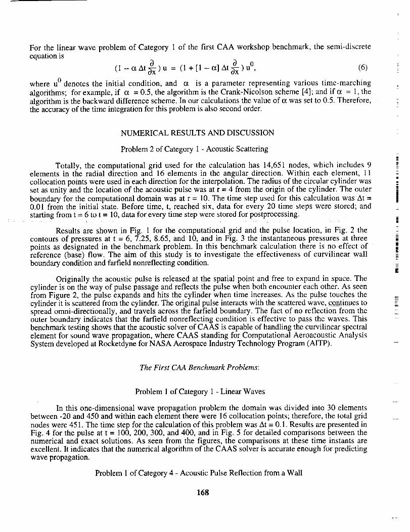
For the linear wave problem of Category1 of the first CAA workshopbenchmark,the semi-discreteequationis
(1-ctAt_)u = (l+[1-o_]At_-_)u 0, (6)
where u° denotesthe initial condition, and o_ is a parameterrepresentingvarious time-marchingalgorithms; for example,if ct = 0.5,the algorithmis theCrank-Nicolsonscheme[4]; andif ct = 1,thealgorithmis thebackwarddifferencescheme.In ourcalculationsthevalueof ct was set to 0.5. Therefore,the accuracy of the time integration for this problem is also second order.
NUMERICAL RESULTS AND DISCUSSION
Problem 2 of Category 1 - Acoustic Scattering
Totally, the computational grid used for the calculation has 14,651 nodes, which includes 9elements in the radial direction and 16 elements in the angular direction. Within each element, 11
collocation points were used in each direction for the interpolation. The radius of the circular cylinder wasset as unity and the location of the acoustic pulse was at r = 4 from the origin of the cylinder. The outer
boundary for the computational domain was at r = 10. The time step used for this calculation was At =0.01 from the initial state. Before time, t, reachedsix, data for every 20 time steps were stored; and
starting from t = 6 to t = 10, data for every time step were stored for postprocessing.
Results are shown in Fig. 1 for the computational grid and the pulse location, in Fig. 2 thecontours of pressures at t = 6, 7.25, 8.65, and 10, and in Fig. 3 the instantaneous pressures at threepoints as designated in the benchmark problem. In this benchmark calculation there is no effect ofreference (base) flow. The aim of this study is to investigate the effectiveness of curvilinear wall
boundary condition and farfield nonreflecting condition.
Originally the acoustic pulse is released at the spatial point and free to expand in space. Thecylinder is on the way of pulse passage and reflects the pulse when both encounter each other. As seenfrom Figure 2, the pulse expands and hits the cylinder when time increases. As the pulse touches thecylinder it is scattered from the cylinder. The original pulse interacts with the scattered wave, continues tospread omni-directionally, and travels across the farfield boundary. The fact of no reflection from theouter boundary indicates that the farfield nonreflecting condition is effective to pass the waves. Thisbenchmark testing shoxCs that the acoustic solver of CAAS is capable of handling the curvilinear spectralelement for sound wave propagation, where CAAS standing for Computational Aeroacoustic AnalysisSystem developed at Rocketdyne for NASA Aerospace Industry Technology Program (AITP).
The First CAA Benchmark Problems:
Problem 1 of Category 1 -Linear Waves
In this one-dimensional wave propagation problem the domain was divided into 30 elementsbetween -20 and 450 and within each element there were 16 collocation points; therefore, the total grid
nodes were 451. The time step for the calculation of this problem was At = 0.1. Results are presented inFig. 4 for the pulse at t = 100, 200, 300, and 400, and in Fig. 5 for detailed comparisons between thenumerical and exact solutions. As seen from the figures, the comparisons at these time instants areexcellent. It indicates that the numerical algorithm of the CAAS solver is accurate enough for predicting
wave propagation.
Problem 1 of Category 4 - Acoustic Pulse Reflection from a Wall
168
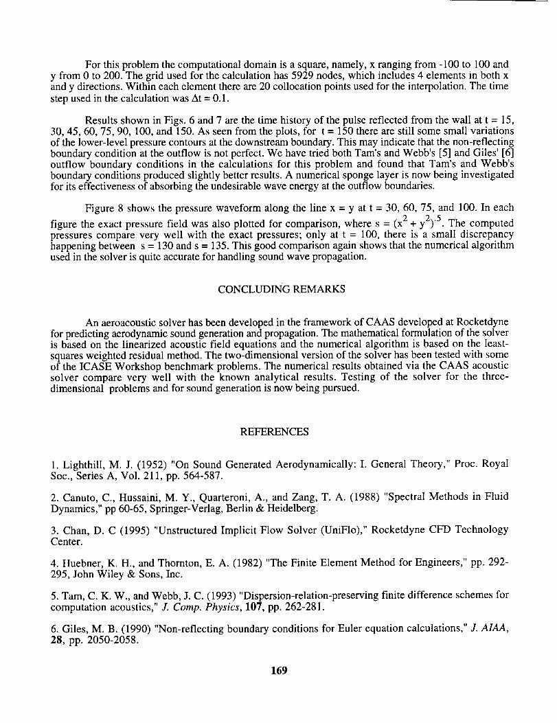
For thisproblemthecomputationaldomainis asquare,namely,x rangingfrom -100to 100andy from 0 to 200.The grid usedfor thecalculationhas5929nodes,which includes4 elementsin bothxandy directions.Within eachelementthereare20collocationpointsusedfor the interpolation.Thetimestepusedin thecalculationwasAt = 0.1.
Results shown in Figs. 6 and 7 are the time history of the pulse reflected from the wall at t = 15,30, 45, 60, 75, 90, 100, and 150. As seen from the plots, for t = 150 there are still some small variationsof the lower-level pressure contours at the downstream boundary. This may indicate that the non-reflectingboundary condition at the outflow is not perfect. We have tried both Tam's and Webb's [5] and Giles' [6]outflow boundary conditions in the calculations for this problem and found that Tam's and Webb'sboundary conditions produced slightly better results. A numerical sponge layer is now being investigatedfor its effectiveness of absorbing the undesirable wave energy at the outflow boundaries.
Figure 8 shows the pressure waveform along the line x = y at t = 30, 60, 75, and 100. In each
figure the exact pressure field was also plotted for comparison, where s = (x 2 + y2).5. The computed
pressures compare very well with the exact pressures; only at t = 100, there is a small discrepancyhappening between s = 130 and s = 135. This good comparison again shows that the numerical algorithmused in the solver is quite accurate for handling sound wave propagation.
CONCLUDING REMARKS
An aeroacoustic solver has been developed in the framework of CAAS developed at Rocketdyne
for predicting aerodynamic sound generation and propagation. The mathematical formulation of the solveris based on the linearized acoustic field equations and the numerical algorithm is based on the least-
squares weighted residual method. The two-dimensional version of the solver has been tested with someof the ICASE Workshop benchmark problems. The numerical results obtained via the CAAS acousticsolver compare very well with the known analytical results. Testing of the solver for the three-dimensional problems and for sound generation is now being pursued.
REFERENCES
1. Lighthill, M. J. (1952) "On Sound Generated Aerodynamically: I. General Theory," Proc. Royal
Soc., Series A, Vol. 211, pp. 564-587.
2. Canuto, C., Hussaini, M. Y., Quarteroni, A., and Zang, T. A. (1988) "Spectral Methods in Fluid
Dynamics," pp 60-65, Springer-Verlag, Berlin & Heidelberg.
3. Chan, D. C (1995) "Unstructured Implicit Flow Solver (UniFlo)," Rocketdyne CFD TechnologyCenter.
4. Huebner, K. H., and Thornton, E. A. (1982) "The Finite Element Method for Engineers," pp. 292-
295, John Wiley & Sons, Inc.
5. Tam, C. K. W., and Webb, J. C. (1993) "Dispersion-relation-preserving finite difference schemes forcomputation acoustics," J. Comp. Physics, 107, pp. 262-281.
6. Giles, M. B. (1990) "Non-reflecting boundary conditions for Euler equation calculations," J. AIAA,28, pp. 2050-2058.
169
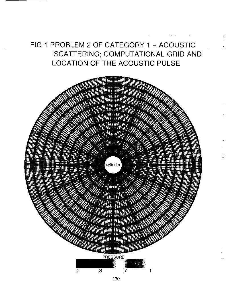
FIG.1 PROBLEM 2 OF CATEGORY 1 - ACOUSTIC
SCATTERING; COMPUTATIONAL GRID AND
LOCATION OF THE ACOUSTIC PULSE
cylinder
PREI ;URE
0 .3 .7 1
170
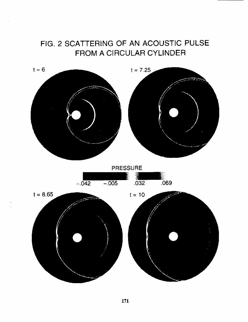
FIG. 2
t=6
SCATTERING OF AN ACOUSTIC PULSE
FROM A CIRCULAR CYLINDER
t = 7.25
t = 8.65
PRESSURE
-.042 -.005 .032
t=10
.069
171
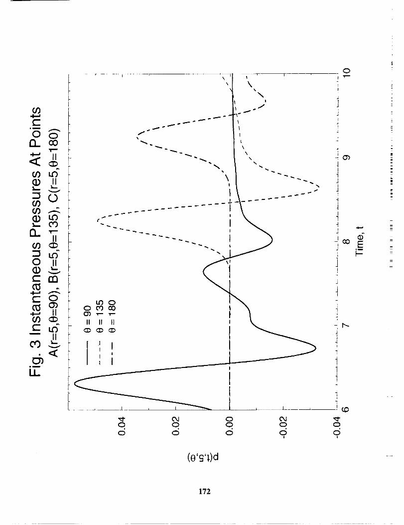
0 0 0 0
0 0 0 0!
0
-4
4
JI
J
J
-4
i
-_Ob4I
1I
J
i
J
-t
4I
I.,4J
Jm1
4
lI
i
4I
114
"I,
00
!
E0E
(e'£'],)d
172
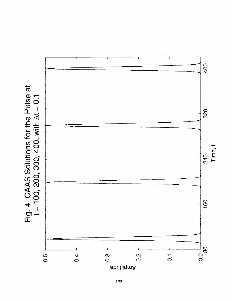
(D ,r-.__d
13_
0.m
"5
II_.,...,
.i
LL
l t I I "_
J
J L I L J
d d d d d
epn_,!ldwV
0
o
0OJ03
04
0r.D
0O0
0d
173
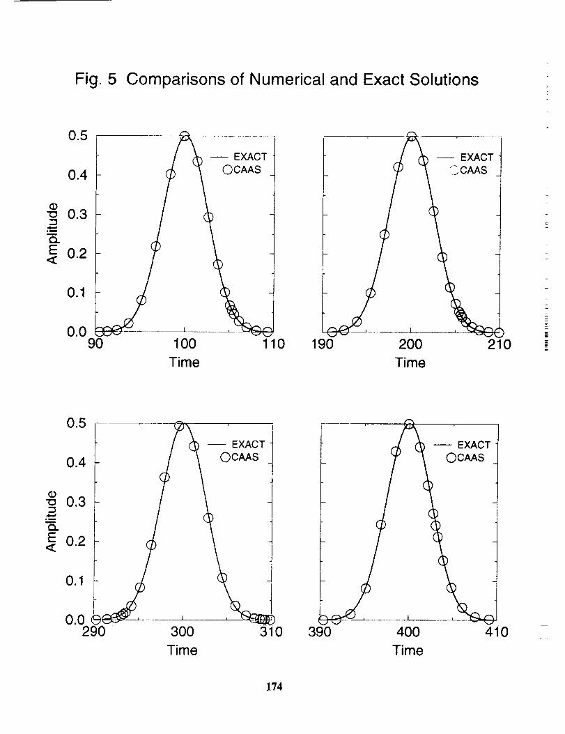
Fig. 5 Comparisons of Numerical and Exact Solutions
"Z3
c_E<
0.5
0.4
0.1
_EXACT
QCAAS
0,0
90 100 110 190 200
Time Time
210
Q"13
iii
{3.E<
0.5
0.4
0.1 "
0.0290 300
Time
EXACT t
OCAAS tJ
3i0 390
EXACT
OCAAS
l
40O
Time
410
174
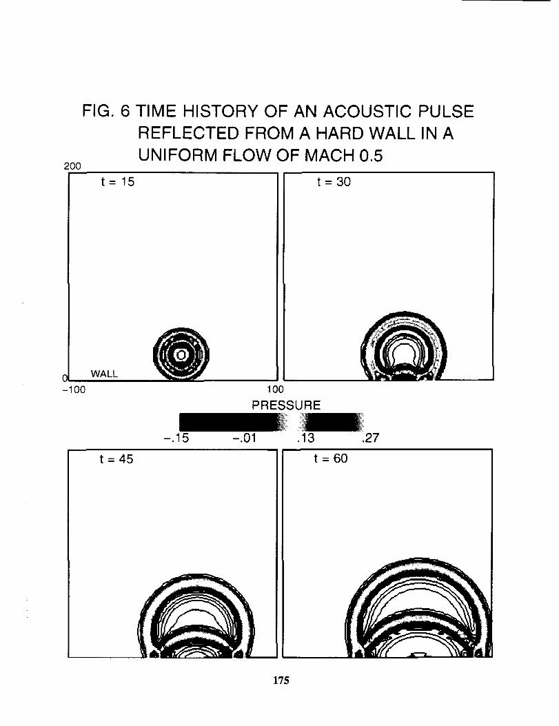
200
0
-" O0
FIG. 6 TIME
t=15
WALL
HISTORY OF AN ACOUSTIC PULSE
REFLECTED FROM A HARD WALL IN A
UNIFORM FLOW OF MACH 0.5
t= 30
100
PRESSURE
-.15 -.01 .13 .27
t= 45 t = 60
175
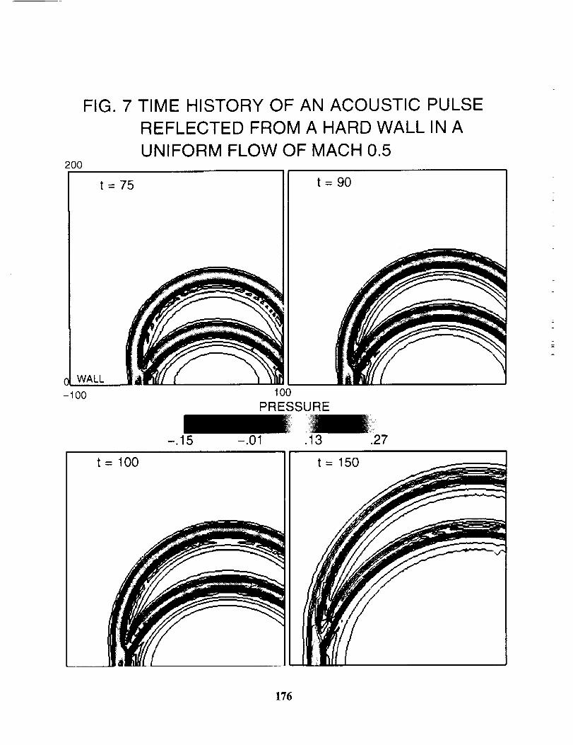
FIG. 7 TIME HISTORY OF AN ACOUSTIC PULSE
REFLECTED FROM A HARD WALL IN A
UNIFORM FLOW OF MACH 0.5200
t = 75
WALL
-100
t= 90
100
PRESSURE
t = 100
-.15 -.01 .13 .27
t = 150
176
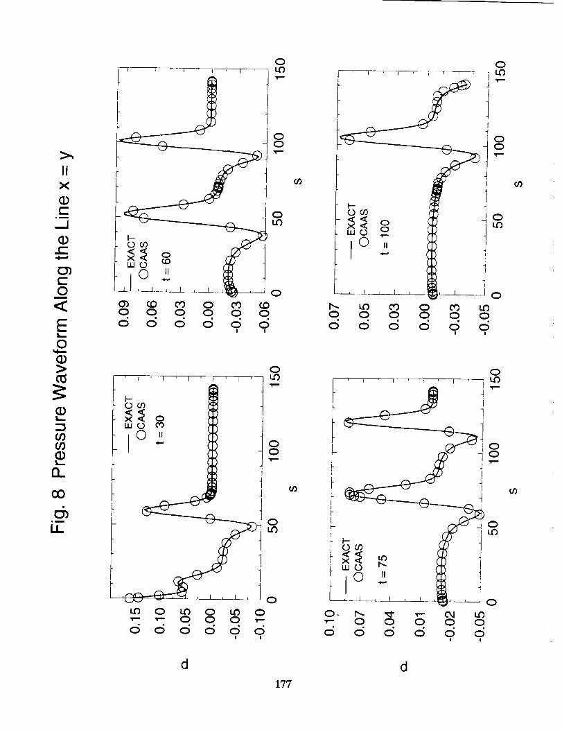
IIX
0
00
d d
177

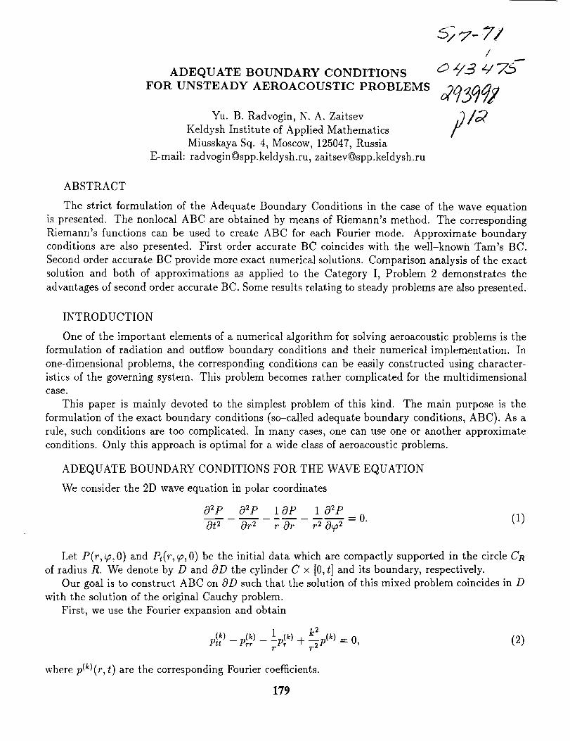
ADEQUATE BOUNDARY CONDITIONS
FOR UNSTEADY AEROACOUSTIC PROBLEMS
Yu. B. Radvogin, N. A. Zaitsev
Keldysh Institute of Applied Mathematics
Miusskaya Sq. 4, Moscow, 125047, Russia
E-maih radvogin_spp.keldysh.ru, [email protected]
7//
!
2¢50q/
ABSTRACT
The strict formulation of the Adequate Boundary Conditions in the case of the wave equation
is presented. The nonlocal ABC are obtained by means of Riemann's method. The corresponding
Riemann's functions can be used to create ABC for each Fourier mode. Approximate boundary
conditions are also presented. First order accurate BC coincides with the well-known Tam's BC.
Second order accurate BC provide more exact numerical solutions. Comparison analysis of the exact
solution and both of approximations as applied to the Category I, Problem 2 demonstrates the
advantages of second order accurate BC. Some results relating to steady problems are also presented.
INTRODUCTION
One of the important elements of a numerical algorithm for solving aeroacoustic problems is the
formulation of radiation and outflow boundary conditions and their numerical implementation. In
one-dimensional problems, the corresponding conditions can be easily constructed using character-
istics of the governing system. This problem becomes rather complicated for the multidimensional
case.
This paper is mainly devoted to the simplest problem of this kind. The main purpose is the
formulation of the exact boundary conditions (so-called adequate boundary conditions, ABC). As a
rule, such conditions are too complicated. In many cases, one can use one or another approximate
conditions. Only this approach is optimal for a wide class of aeroacoustic problems.
ADEQUATE BOUNDARY CONDITIONS FOR THE WAVE EQUATION
We consider the 2D wave equation in polar coordinates
02P 02P 10P 1 c92P
Ot 2 Or 2 r Or r 2 c9_o2-0. (1)
Let P(r, q_, 0) and Pt(r, qp, 0) be the initial data which are compactly supported in the circle Cn
of radius R. We denote by D and OD the cylinder C × [0, t] and its boundary, respectively.
Our goal is to construct ABC on OD such that the solution of this mixed problem coincides in D
with the solution of the original Cauchy problem.
First, we use the Fourier expansion and obtain
pl_) ,jk) 1,,(k) k:-- Urr -- rt, _ + _-Tp (k) 0, (2)
where p(k)(r, t) are the corresponding Fourier coefficients.
179
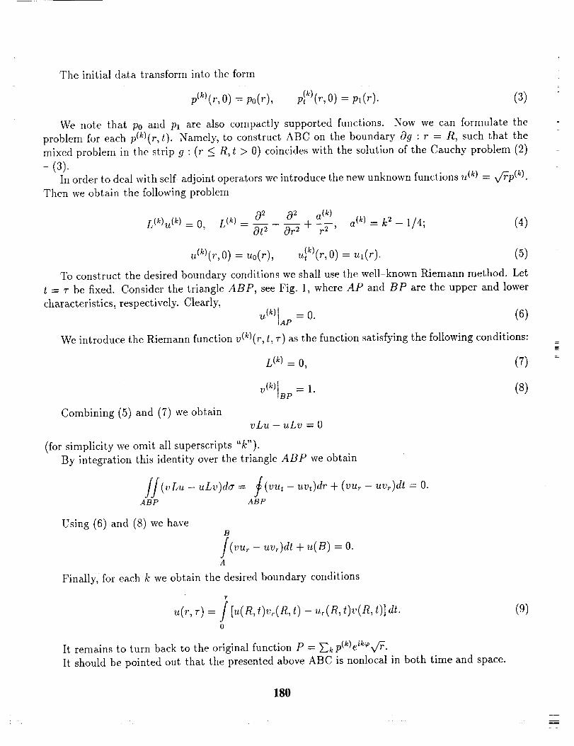
The initial data transform into the form
p(k)(r, 0) = p0(r), plk)(r,O) = pl(r). (3)
We note that p0 and pl are also compactly supported functions. Now we can formulate the
problem for each p(k)(r, t). Namely, to construct ABC on the boundary 09 : r = R, such that the
mixed problem in the strip g : (r _< R, t > 0) coincides with the solution of the Cauchy problem (2)
-(3).In order to deal with self-adjoint operators we introduce the new unknown functions u (k) = v/Tp (k).
Then we obtain the following problem
02 02 a (k)L(k)u (k) = O, L (k) _ + -- a (k) = k _ - 1/4; (4)
Ot 2 Or 2 r 2 ,
0) = Ikl(r,0) = (5)
To construct the desired boundary conditions we shall use the well-known Riemann method. Let
t = r be fixed. Consider the triangle ABP, see Fig. 1, where AP and BP are the upper and lower
characteristics, respectively. Clearly,
u(k)la p = 0. (6)
We introduce the Riemann function v(k)(r, t, r) as the function satisfying the following conditions:
L (k) =0, (7)
Combining (5) and (7) we obtain
v(k)lB P = 1. (8)
vLu -uLv = 0
(for simplicity we omit all superscripts "k").
By integration this identity over the triangle ABP we obtain
ff (vLu - uLv)do" = J(vut- uvt)dr + (vu_ - uv_)dt = O.ABP ABP
Using (6) and (8) we haveB
j(vu_ - uv_)dt + u(B) = O.A
Finally, for each k we obtain the desired boundary conditions
7"
u(r, r) = f [u(R,t)v_(R,t) - u_(R,t)v(R,t)]dt.0
(9)
It remains to turn back to the original function P = _2k P(k)eik_°X/_.
It should be pointed out that the presented above ABC is nonlocal in both time and space.
180
}Ve note that each v (k) is determined not uniquely. To find v (k) we have to define v(k)(R, t), for
example. Thus, we can choose Riemann's fimctions in a convenient way, which is important for
applications.
We also note that despite the non-uniqueness all AB conditions lead to the same solution of mixed
problem.
Some of Riemann's functions are connected with Legendre functions. For example, let v(r, t, r) =
v((), where _ = (R + r- t)/r. Then
d 2v dv k2({2 _ 1)_3 - + 2_--_- + - 1/4 = 0. (10)
Therefore v(_) = Pk-1]2(_).
Boundary condition (9) can be rewritten in the following way. Since us is also a compact supported
function, it follows that we can rewrite (9) replacing u by u_:
_,(R, _-)= f(_,_r -
T
_,.v)gt -_[_,v.- ..V]o - f (_,v. - ,,.v,)gt.0
In other words,
T
.,(n, T) + _,.(n,T) = .(n, ,-)v.(n, T) - f (_,v.- u.v,)dt.0
(11)
Further we shall consider Riemann's functions satisfying the condition
v(R, t) : 1. (12)
In this case v,(R, r) = 0 and vt - 0. Therefore ABC (11) takes the form
T
ut + ttr = -- / uv,tdt.0
(13)
We shall call V(r, t) the base function if
LV=O and V=I fort=r-R.
It is obvious that V(r, t) gives the correspondent Riemann's function v(r, t, r) = V(r, r - t).
Some properties of V(r, t) were investigated numerically and analytically. In particularly, it was
found that limt--,oo V_t(R,t) = 0 and limt__+_ V_(R,t) = -(k- 1/2) in the case V(R,t) = 1. Only
these V(r, t) will be considered below.
APPROXIMATE BOUNDARY CONDITIONS
The exact ABC (13) is too complicated for practical use. In many cases one can apply approximate
boundary conditions. In order to construct such conditions we consider the approximations of v,t in
(13).
181
(i) As the first approximation we put V = 1.
boundary condition in the form
Ut + Ur = O,
However, u (k) = p(k)v_. Thus, we have
Then v = 1 and v_ - 0.
r =R.
As a result we obtain
(14)
p(k)plk)+ p_k)+ 2---R--0.
We recall that p(k) are the Fourier coefficients.
original function p(r, t, _):P
Pt+P_+ 9"_=O.
Note that condition (15) coincides with the well-known Tam's condition [1].
(ii) The second approximation can also be easy obtained:
Clearly, this condition remains the same for the
(15)
a
v(,,t) = 1- - n)(t + n-
This leads to
and
From (13) we obtain
a R)(T t + R r)v ( r, t ) = 1 - -_-ff (r - - -
a ,(k)-- k2-1/4vrt = _-R-7, i.e. vrt 2R 2
ulk)(R,T)WU_k)(n,w) k2--1/4 "_ - 2R 2 f u(k)(R,t)dt.0
(16)
Turning back to p(k)(r, t) we obtain
p}k) + p_k) + 2__p(k) _ _ k2-1/4 ]2R 2 p(k)(R, t)dt.0
Finally, we havet
P 1/Pt + P_ + 2R - 2R 2 (P_ + P/4)dr, r = R. (17)0
(Here we interchanged t and T for convenience.)
Further we use approximate boundary conditions only. Thus, we shall denote by ABC an approx-
imate BC.
One can show that the truncation error 5 = O(T 2) for ABC (17) unlike 5 = O(T) for ABC (15).
In accordance with these estimates, boundary conditions (15) or (17) will be denoted 1ABC and
2ABC, respectively.
182
FORMULATION OF THE PROBLEM AND THE NUMERICAL ALGORITHM
We consider the linearized Euler system for M_ = 0 in the form
Ou OP
0--[+ Or o,Ov 1 OP
4- - 0,Ot r Oc2
OP Ou 1 l"
o---f+ + [=0.
(18)
where P is the pressure, u and v are the polar components of velocity.
The initial data equal zero outside the circle Cn of radius R. Since this system can be reduced
to the wave equation with respect to p, it follows that the foregoing construction does apply. Using
ABC we replace the Cauchy problem in the whole plane by the mixed problem in Cn.
Thus we have the boundary condition on OCn in the form
P
Pt + Pr + 2--R = F(P), (19)
where
p(P)- 0
which corresponds to the first order approximation (1ABC), see (15), or
t1
F(P) = -_ f (P_ao + P/4)dr0
which corresponds to the second order approximation (2ABC), see (17).
We note that, as a rule, additional boundary conditions can lead to an ill-posed problem.
The numerical algorithm we apply is a modification of our method [2]. The original second order
accurate differertce scheme belongs to the TVD-type class and uses the minimal stencil. In order to
create a third order accurate scheme we apply the well-known Runge's rule.
We write the initial scheme in the form
U2+1 = RhU .
The first step of the desired scheme is a reconstruction of U n at the intermediate points (m +
1/2, k + 1/2). It can be done using the cubic interpolation. As a result we obtain "the fine" grid.
Then according to Runge's rule we have
Uh(t n + r) = 3[4Uh(tn + r) - Uh/2(t n + r)].
SinceUh(t n + T) = RhU_ Uh/2(U + r)= 2 n, Rh/2U[/2 we obtain the resulting scheme in the form
1= Rh/_U;;/_). (20)U_+I 5(4RhU__ 2 ,,
183
To calculate(P, u, v) at the boundary one can use a difference approximation of two characteristic
relations
Ot + Or + -r u+ =0,
Ov 10P
57 + = o,
and ABC (19).
NUMERICAL RESULTS
In this section, results for the Category I, Problem 2 are presented. To estimate the validity of
the method including approximate BC we present three sets of numerical data.
The computational domain is the ring GR: r0 < r < R; r0 = 0.5. The grid size in the _ direction
is constant. As for size in the r direction, we use a nonuniform grid. Namely,
1 Rr = roe _(°-'°), c_ - In--.
R - ro To
This method allows to deal with practically square cells over the whole domain, which leads to
the improvement of the numerical results.
Each variant is defined by three constants: R, Acp and Ap and the type of BC.
The first variant: R = 5 (this is the minimal size of the computational region because of given
coordinates of the points A, B, C); A_o = 7r/600, Ap = 1/440; 1ABC.
The second variant differs from the first one by ABC only. Here we use 2ABC.
Finally, for the third variant we apply the same A_ and Ap but R = 10.40284; 2ABC. Since in
this case the boundary OGlo does not affect the solution in Gs up to t = 10, it follows that we can
consider this solution "exact".
Comparing all these solutions one can estimate the role of the type of ABC.
The time histories of P at A, B, C are plotted in Figs 2 - 4, respectively. It is seen that 2ABC-
results look at A and B better then 1ABC-results.
The superiority of 2ABC over 1ABC is considerably more visible in Figs 5 - 8. Here we show
spatial distributions of pressure on some semi-infinite lines: Fig. 5: _, = 0 °, t = 2; Fig. 6: _o = 45 °,
t = 4; Fig. 7: _= 90 ° ,t =7; Fig. 8: _= 135 ° ,t = 10. In all these Figures "exact" solutions are
plotted up to r = 10. This gives an indication of the structure of the solution.
As for the accuracy of the difference method we examined it using calculations with fine grid
A@ = A_/2, A_ = Ap/2. It was found that the third-order accuracy is achieved and results for
both grids are prac£ically the same. Thus, we can omit quotes and call the third variant the exact
solution.
CONCLUSION
The presented method of constructing ABC can be generalized to the case Mo, -¢ 0 as well as to
a wide class of hyperbolic systems. One can use the exact ABC if the problem admits the Fourier
expansion. Otherwise we are forced to use the approximate ABC like it was shown above.
We also note that this approach can be applied to the steady-state problems. The case of the
wave equation outside G is presented in the Appendix.
184
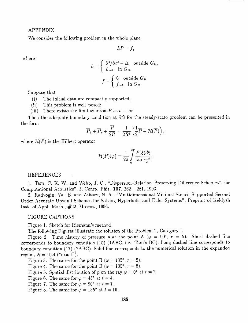
APPENDfX
We considerthe following problem in the wholeplane
LP -- f,
where
Suppose that
L
02�Or - A outside Gn,Lint in Gn.
0 outside GRf = fi_t in GR.
(i) The initial data are compactly supported;
(ii) This problem is well-posed;
(iii) There exists the limit solution P as t --* oc.
Then the adequate boundary condition at OG for the steady-state problem can be presented in
the form
_ _ P 1 'IT+7./(T)\_,_ )Pt + Pr + 2R - 2R 2
where 7Y(P) is the Hilbert operator
1 2['P(5)d__(P)(_) = _ J tan gz__"
o 2
REFERENCES
i. Tam, C. K. W. and Webb, J. C., "Dispersion-Relation-Preserving Difference Schemes", for
Computational Acoustics", J. Comp. Phis. 107, 262 - 281, 1993.
2. Radvogin, Yu. B. and Zaitsev, N. A., "Multidimensional Minimal Stencil Supported Second
Order Accurate Upwind Schemes for Solving Hyperbolic and Euler Systems", Preprint of Keldysh
Inst. of Appl. Math., #22, Moscow, 1996.
FIGURE CAPTIONS
Figure 1. Sketch for Riemann's method
The following Figures illustrate the solution of the Problem 2, Category I.
Figure 2. Time history of pressure p at the point A (c2 = 90 ° , r = 5). Short dashed line
corresponds to boundary condition (15) (1ABC, i.e. 'ram's BC). Long dashed line corresponds to
boundary condition (17) (2ABC). Solid line corresponds to the numerical solution in the expanded
region, R = 10.4 ("exact").
Figure 3. The same for the point B (_o = 135 °, r = 5).
Figure 4. The same for the point B (_o = 135 °, r = 5).
Figure 5. Spatial distribution of p on the ray p = 0 ° at t = 2.
Figure 6. The same for _ = 45 ° at t = 4.
Figure 7. The same for V' = 90° at t = 7.
Figure 8. The same for c2 = 135 ° at t = 10.
185
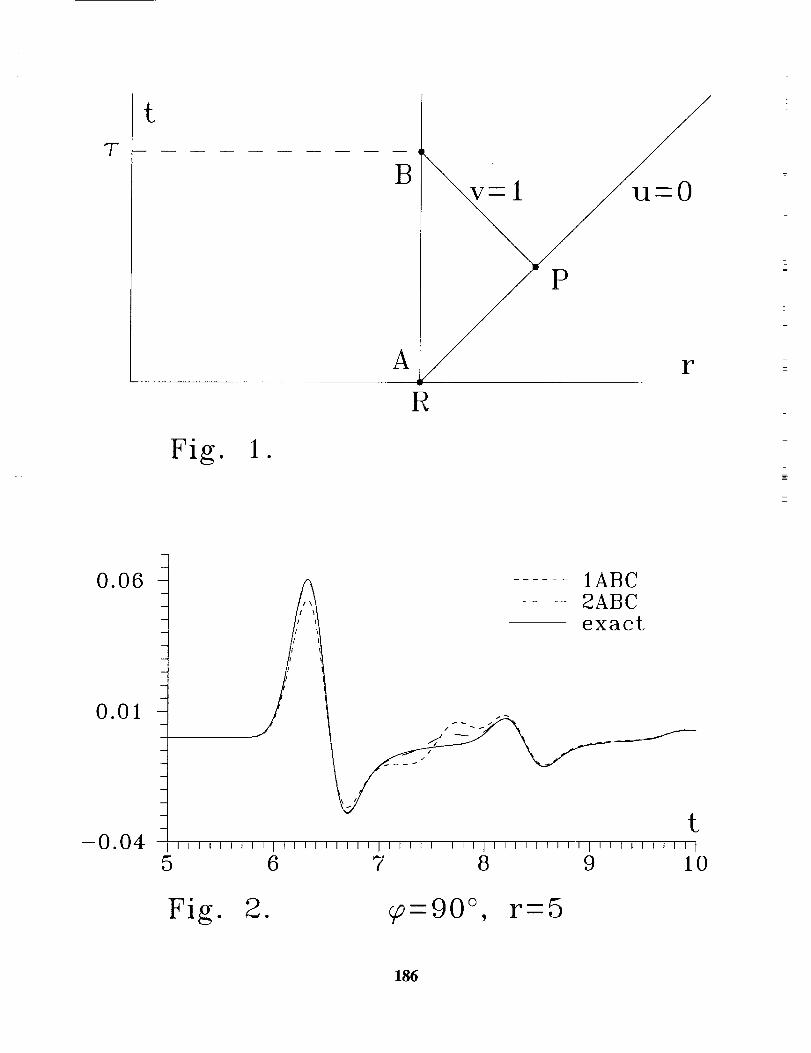
7"
t
B
A
R
-i u-O
P
F
Fig. 1.
0.06
0.01 -
-0.04
5
A ...... 1ABC/"1 -- 2ABC
l/ '1 j._-- exact
ti I I I I I t t I I I I I I I I I I I J I I r I I I I I ] I I I I I I I I I I I 1 I I 1 I t I I 1
6 7 8 9 10
Fig. 2. _-90 °, r-5
186
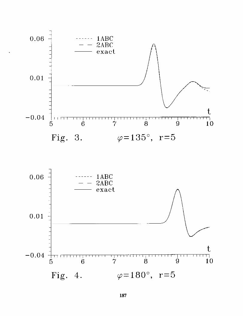
0.06
0.01
-0.04
m
w
m
m
m
m
5
1ABC2ABCexact
tI I I I I I I I I I I I I I I I I I I [ t I I t t t I I t ] I I t t t I I I I I I I I I I I I I I I
6 7 8 9 10
Fig. 3. _-135 °, r-5
0.06
0.01
-0.045
...... 1ABC2ABCexact
t[1 I t I I I I I I I I I i I I i t I I I I I I I I I t [ t I t t I t I I I I I I I I I I I I I I
6 7 13 9 10
Fig. 4. _-180 °, r-5
187
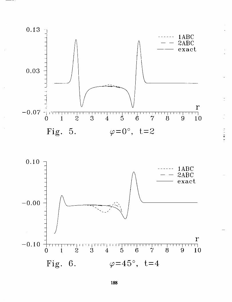
0.13 -
0.03 -
1ABC2ABCexact
\
r
Fig. 5. _-0 °, L-2
0.10 -
-0.00 -
-0.10 -0
1ABC2ABCexact
r
1 2 3 4 5 6 7 8 9 10
Fig. 6. _-45 °, L=4
188
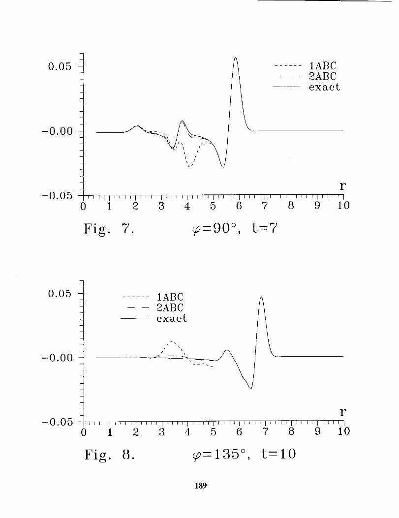
i
0.05 -
-0.00 -\
1ABC2ABCexact
FilillO_EIIIIIlillllllt,,IzllJlllllllililllllllllll
1 2 3 4 5 6 7 8 9 10
Fig. 7. _-90 °, t=7
i
0.05 -
-0.00 -
-0.050
1ABC2ABCexact
/ \
// -- \\
Fig. 8. _-135 °, t-lO
189
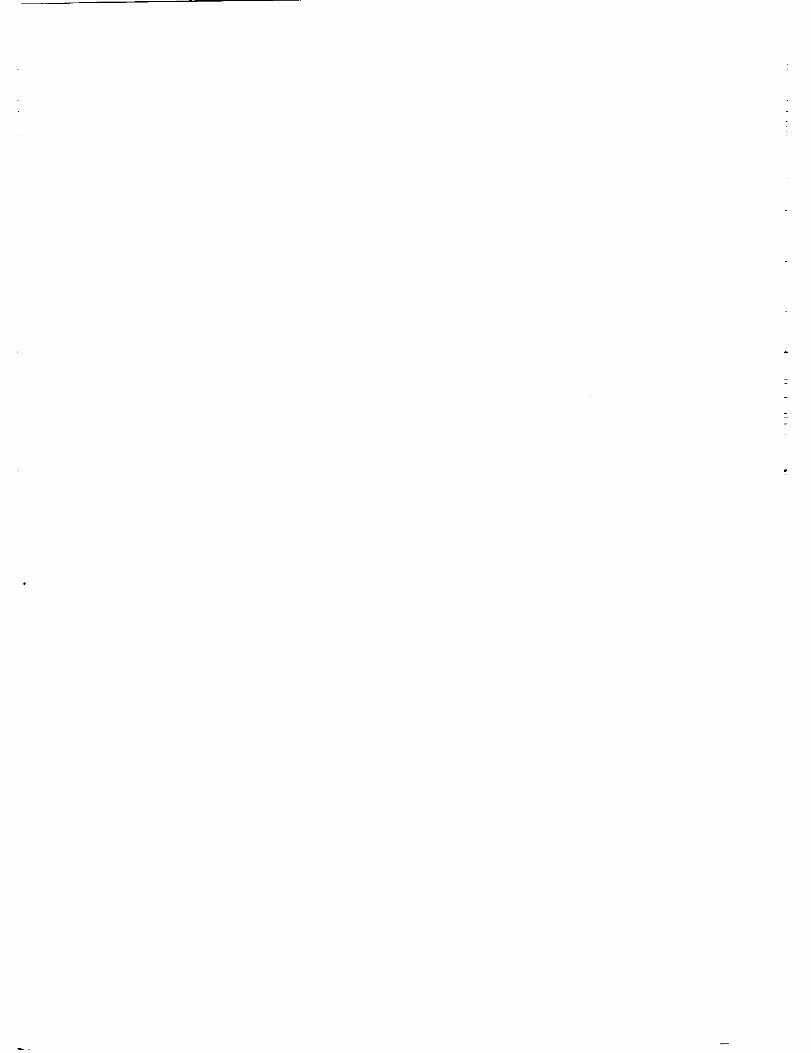
NUMERICAL BOUNDARY CONDITIONS FOR
COMPUTATIONAL AEROACOUSTICS BENCHMARK PROBLEMS
Chritsopher K.W. Tam, Konstantin A. Kurbatskii, and Jun Fang
Department of Mathematics
Florida State University
Tallahassee, FL 32306-3027
SUMMARY
¢ooo
/)io
Category 1, Problems 1 and 2, Category 2, Problem 2, and Category 3, Problem 2 are solved
computationally using the Dispersion-Relation-Preserving (DRP) scheme. All these problems are
governed by the linearized Euler equations. The resolution requirements of the DRP scheme for
maintaining low numerical dispersion and dissipation as well as accurate wave speeds in solving the
linearized Euler equations are now well understood. As long as 8 or more mesh points per wave-
length is employed in the numerical computation, high quality results are assured. For the first
three categories of benchmark problems, therefore, the real challenge is to develop high quality nu-
merical boundary conditions. For Category 1, Problems 1 and 2, it is the curved wall boundary
conditions. For Category 2, Problem 2, it is the internal radiation boundary conditions inside the
duct. For Category 3, Problem 2, they are the inflow and outflow boundary conditions upstream
and downstream of the blade row. These are the foci of the present investigation. Special non-
homogeneous radiation boundary conditions that generate the incoming disturbances and at the
same time allow the outgoing reflected or scattered acoustic disturbances to leave the computation
domain without significant reflection are developed. Numerical results based on these boundary
conditions are provided.
1. INTRODUCTION
The governing equations of the Category 1, 2 and 3 benchmark problems are the linearized Eu-
ler equations. Recent works have shown that the linearized Euler equations can be solved accu-
rately by the 7-point stencil time marching Dispersion-Relation-Preserving (DRP) scheme (Tam
and Webb, ref. 1) using 8 or more grid points per wavelength. At such a spatial resolution, the nu-
merical dispersion and dissipation of the scheme is minimal. Also, the scheme would support waves
with wave speeds almost the same as those of the original linearized Euler equations. Thus, from a
purely computational point of view, all these problems are the same except for their boundary con-
191
ditions. The formulation and implementation of the appropriate numerical boundary conditions for
the solutions of these problems are the primary focus of the present paper.
For spatial discretization, the 7-point stencil DRP scheme uses central difference approxima-
tion with optimized coefficients. For instance, the first derivative _ at the _th node of a grid with
spacing Ax is approximated by,
Of _ 1 E ajft+j (1)- 3
where the coefficients aj (see Tam and Shen, ref. 2) are:
ao =0
al = -a-1 = 0.770882380518
a2 = -a-2 = -0.166705904415
as = -a-3 = 0.020843142770.
For time marching, the DRP scheme uses a four levels marching algorithm. Let At be the time
step. We will use superscript n to indicate the time level. To advance the solution f(t) to the next
time level the DRP scheme uses the formula,
where the coefficients bj are:
f(n+l) = f(n) + At bj -_j=o
(2)
b0 = 2.302558088838
b, = -2.491007599848
b2 = 1.574340933182
b3 = -0.385891422172.
In (2) the functions (d/_(n-2 are provided by the governing equation.dt ]
The DRP scheme, just as all the other high-order finite difference schemes, supports short wave-
length spurious numerical waves. These spurious waves are often generated at computation bound-
aries (both internal and external), at interfaces and by nonlinearities. They are pollutants of the
numerical solution. When excessive amount of spurious waves is produced, it leads not only to the
degradation of the quality of the numerical solution but also, in many instances, to numerical in-
stability. To obtain a high quality numerical solution, it is, therefore, necessary to eliminate the
192
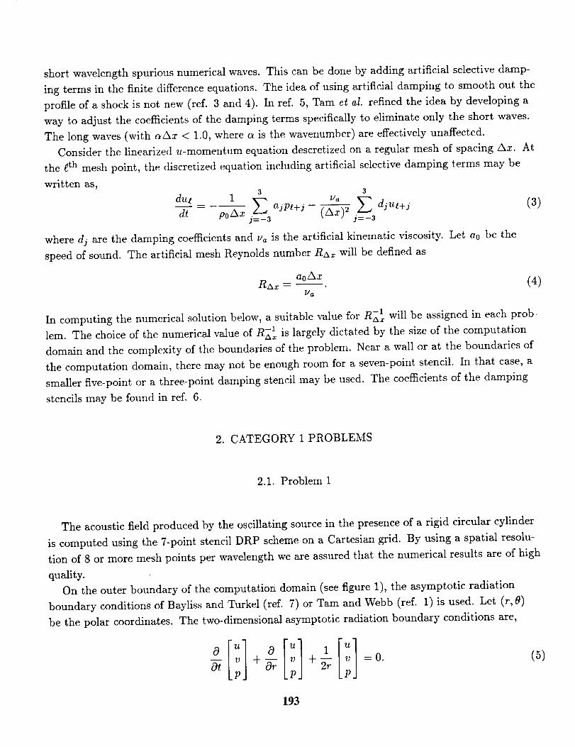
short wavelength spurious numerical waves. This can be done by adding artificial selective damp-
ing terms in the finite difference equations. The idea of using artificial damping to smooth out the
profile of a shock is not new (ref. 3 and 4). In ref. 5, Tam et aI. refined the idea by developing a
way to adjust the coemcients of the damping terms specifically to eliminate only the short waves.
The long waves (with aAx < 1.0, where a is the wavenumber) are effectively unaffected.
Consider the linearized u-momentum equation descretized on a regular mesh of spacing _Sx. At
the t th mesh point, the discretized equation including artificial selective damping terms may be
written as,
dut 1 3 3__ l]a
p0 x ( x)2 (3)j=-3 j=-3
where dj are the damping coefficients and us is the artificial kinematic viscosity. Let a0 be the
speed of sound. The artificial mesh Reynolds number Rax will be defined as
a0/_x
Raz -- (4)b' a
In computing the numerical solution below, a suitable value for R_,l, will be assigned in each prob-
lem. The choice of the numerical value of R_l, is largely dictated by the size of the computation
domain and the complexity of the boundaries of the problem. Near a wall or at the boundaries of
the computation domain, there may not be enough room for a seven-point stencil. In that case, a
smaller five-point or a three-point damping stencil may be used. The coefficients of the damping
stencils may be found in ref. 6.
2. CATEGORY 1 PROBLEMS
2.1. Problem 1
The acoustic field produced by the oscillating source in the presence of a rigid circular cylinder
is computed using the 7-point stencil DRP scheme on a Cartesian grid. By using a spatial resolu-
tion of 8 or more mesh points per wavelength we are assured that the numerical results are of high
quality.
On the outer boundary of the computation domain (see figure 1), the asymptotic radiation
boundary conditions of Bayliss and Turkel (ref. 7) or Tam and Webb (ref. 1) is used. Let (r, 0)
be the polar coordinates. The two-dimensional asymptotic radiation boundary conditions are,
0
Ot ] [1'° v+P P
i] =0.(5)
193
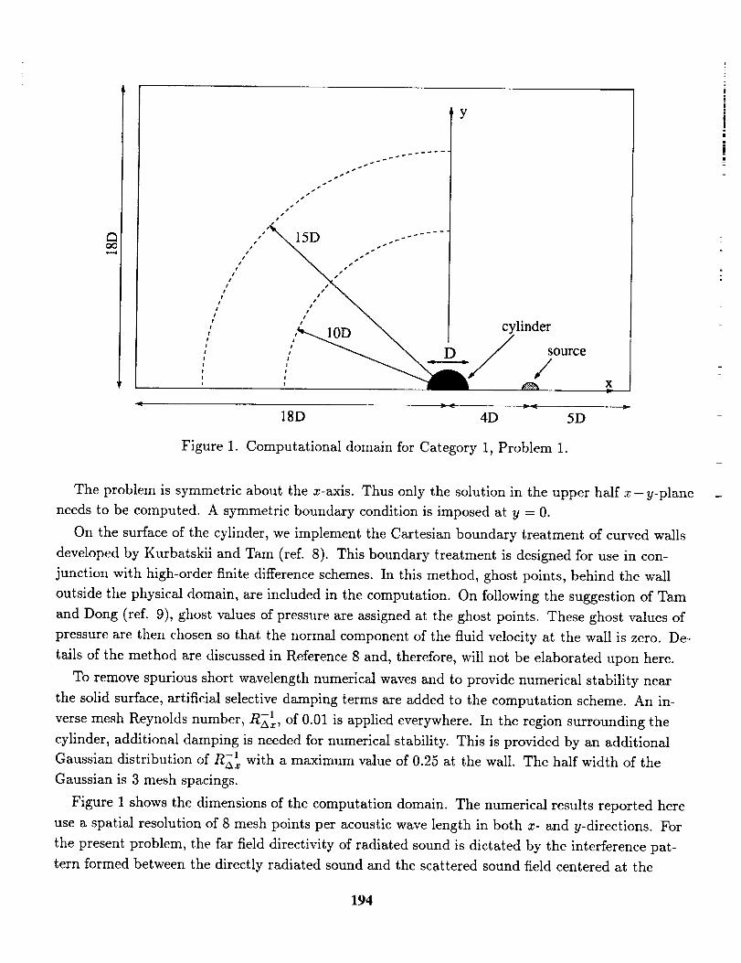
Y
!s
J
J
X
18D 4D 5D
Figure 1. Computational domain for Category 1, Problem 1.
The problem is symmetric about the x-axis. Thus only the solution in the upper half x-y-plane
needs to be computed. A symmetric boundary condition is imposed at y = 0.
On the surface of the cylinder, we implement the Cartesian boundary treatment of curved walls
developed by Kurbatskii and Tam (ref. 8). This boundary treatment is designed for use in con-
junction with high-order finite difference schemes. In this method, ghost points, behind the wall
outside the physical domain, are included in the computation. On following the suggestion of Tam
and Dong (ref. 9), ghost values of pressure are assigned at the ghost points. These ghost values of
pressure are then chosen so that the normal component of the fluid velocity at the wall is zero. De-
tails of the method are discussed in Reference 8 and, therefore, will not be elaborated upon here.
To remove spurious short wavelength numerical waves and to provide numerical stability near
the solid surface, artificial selective damping terms are added to the computation scheme. An in--1
verse mesh Reynolds number, Rcxx, of 0.01 is applied everywhere. In the region surrounding the
cylinder, additional damping is needed for numerical stability. This is provided by an additional
Gaussian distribution of R_ with a maximum value of 0.25 at the wall. The half width of the
Gaussian is 3 mesh spacings.
Figure 1 shows the dimensions of the computation domain. The numerical results reported here
use a spatial resolution of 8 mesh points per acoustic wave length in both x- and y-directions. For
the present problem, the far field directivity of radiated sound is dictated by the interference pat-
tern formed between the directly radiated sound and the scattered sound field centered at the
194
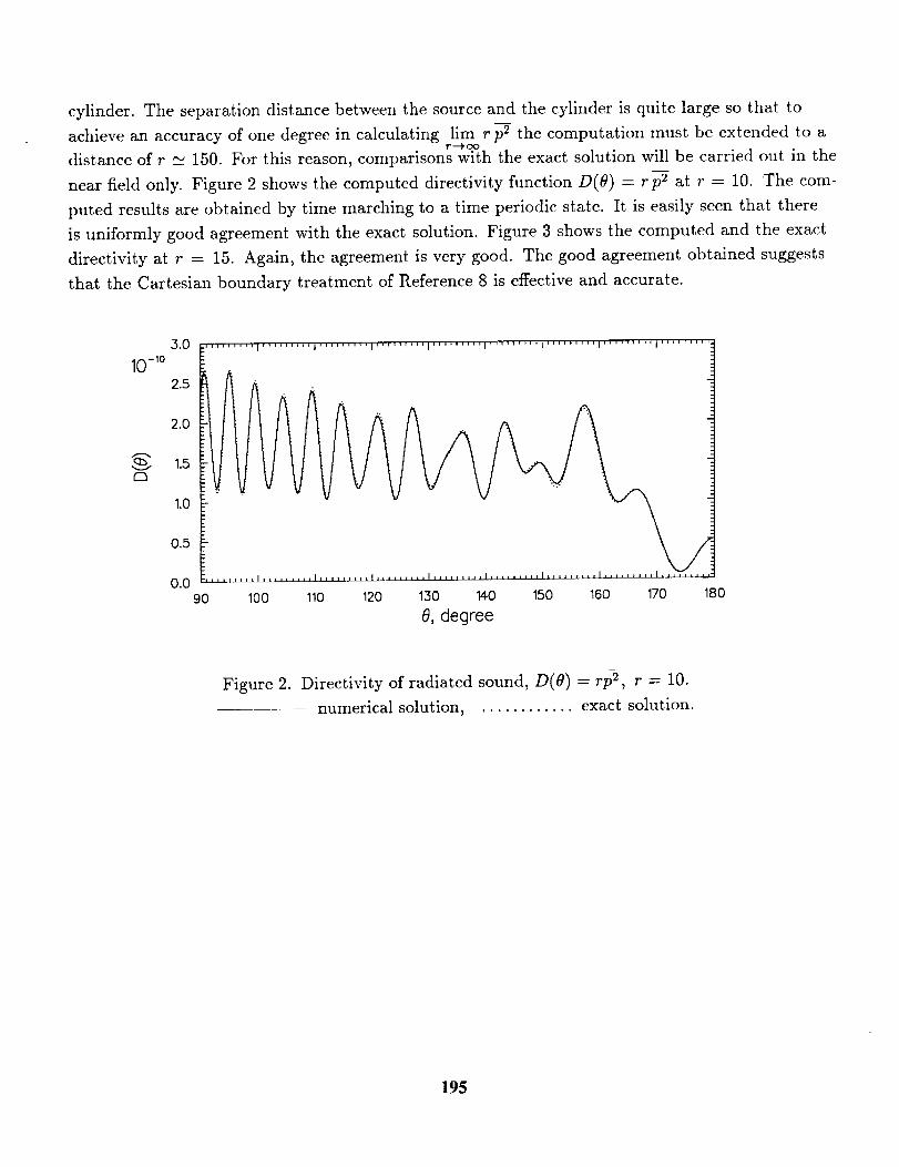
cylinder. The separation distancebetweenthe sourceand the cylinder is quite large so that toachievean accuracy of one degreein calculating lim r p2 the computation must be extended to a7---,oodistance of r __ 150. For this reason, comparisons with the exact solution will be carried out in the
near field only. Figure 2 shows the computed directivity function D(O) = r p2 at r = 10. The com-
puted results are obtained by time marching to a time periodic state. It is easily seen that there
is uniformly good agreement with the exact solution. Figure 3 shows the computed and the exact
directivity at r = 15. Again, the agreement is very good. The good agreement obtained suggests
that the Cartesian boundary treatment of Reference 8 is effective and accurate.
_.0 .......... t ......... t ......... I ......... t ......... I ......... t ......... I ......... I .........
10-1°_ 2.02.51.5
1.0
0.5
0.09o
i ..... ,_,1_,,, I I _ I jl I _LLLUJJJJJJ=U--L
II,lJ Zlll,,,,I ill ,ll II|l|lH _Jl,|,ll, J,,l|_lL_ U
100 110 120 130 140 150 160 170 180
8, degree
Figure 2. Directivity of radiated sound, D(O) = rp 2, r = 10.
numerical solution, ............ exact solution.
195
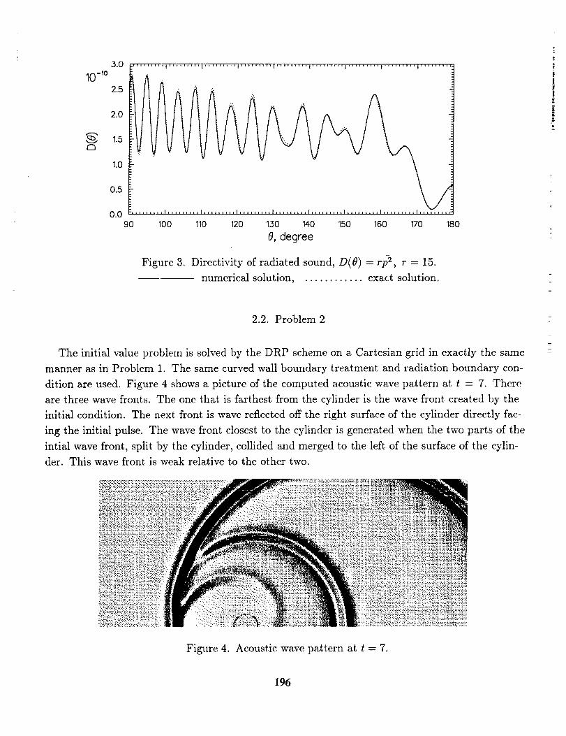
10 -10
rm
3.0
2.5
2.0
1.5
1.0
0.5
0.0
.......... ! ......... t ......... I ......... I ......... t ......... 1 ......... t ......... I ........ "
90 180
/100 1t0 120 130 140 150 160 170
8, degree
Figure 3. Directivity of radiated sound, D(O) = rp 2, r = 15.
numerical solution, ............ exact solution.
2.2. Problem 2
The initial value problem is solved by the DRP scheme on a Cartesian grid in exactly the same
manner as in Problem 1. The same curved wall boundary treatment and radiation boundary con-
dition are used. Figure 4 shows a picture of the computed acoustic wave pattern at t = 7. There
are three wave fronts. The one that is farthest from the cylinder is the wave front created by the
initial condition. The next front is wave reflected off the right surface of the cylinder directly fac-
ing the initial pulse. The wave front closest to the cylinder is generated when the two parts of the
intial wave front, split by the cylinder, collided and merged to the left of the surface of the cylin-
der. This wave front is weak relative to the other two.
::::::::::::::::::::::::::::::::::::::::::::::::::::::::::::::::::::::::::::: : ..atjll__, _:_':_'_'"_::::;::!:;:-: _:;_!-_;ii_i!i;i!i;_!$!;_1_ l_i,_$_'_,mmm_mw_-,q_L
.:;_:L ::::::::::::::::::::::: ::::::::::::::::::::::::::::::::: :'-:.'b:.'::_ . __-_ ..:.::::": "-":i "_:.::":- _._?._F_;_::_._._.:._;?._?:._._._:._;_:_:_!_?_:;_::_5:_:-.:!_,_,_ " _,_
....... -:,...::: ..::: ..:.:............. _.:-:............ , ....... _, ...... '..:'.-.:,.,_ .........v-,': ,..,.. _ ........ _.:-._ _._................................. .-., : .:_-,, _ ...................... , ......
==================================================== " " _ib'=:: _ " .,:':':: ":":2.:.:.'.:_... :._:.:e'.:*.'.'.*.'.'_:....*.'.: :...:-:; :..'.:.:_:':':';'+;-:,':':,;:.:x .;.:.a_U_=:f:::::;;:::::,...::.,:.f,y,,.
r._::.,:,:_._., ":'.';".;V::..:,':.:',:.::'::.:.:'-:':":'::" .' ' " ":_ *._._ .... , _::: :"_';:"> _:" _::':"::'::."': "":":' ,:" !,.': ...................... _ ........................
==================================================================" '",,.:_ _'_. _ , :: • ' • "/-"X; ; :-.+::, ":':'.'¢" "1":"-:_ .c:_._..:_.:r:_)_...:.:_+'::_._:+_.x'....::::..:::;_`:-_:_:£_:!:.-".2:_-".:.:::::::::_x_.._
i!i:;;$_i_iiii:i:!_!,_i;-::i:_i2)?ii!i:!:!.:.::J_W ._:._:::::(?;:.ii)i ;i:_.:i::!ii_!_:ii_ii_?i:_);!!:i_!_.)2i:...;_!i_i_}!ii_i_ii_i_;;1?_!_i_g_i._i!!!!}:_:::.:::-;:::_:;':;::::_': :_.'::'..'::: _ ' ' "...... "::'_: S':;."_ ::I " :.':::.. ::' .:.:'.:::::i._$'.si_;_?4 :_ ;: :.:'::;; "::'.::;.:;;:..:.::?:;;':"::.::;:':':::_::::'. _5:;:'_.:, :
Figure 4. Acoustic wave pattern at t = 7.
196
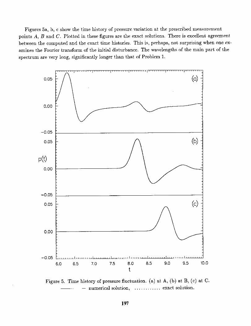
Figures 5a, b, c show the time history of pressure variation at the prescribed measurement
points A, B and C. Plotted in these figures are the exact solutions. There is excellent agreement
between the computed and the exact time histories. This is, perhaps, not surprising when one ex-
amines the Fourier transform of the initial disturbance. The wavelengths of the main part of the
spectrum are very long, significantly longer than that of Problem 1.
0.05
0.00
-0.05
0.05
-0.05
0.05
0.00
-0.05
(c)
......... I ......... I ....... ,,I ..... ,,,,I,,,,,,,,,I,,,,,,,,,t,,,,,,,,,I ....... ,_
6.0 6.5 7.0 7.5 8.0 8.5 9.0 9.5 10.0
t
Figure 5. Time history of pressure fluctuation. (a) at A, (b) at B, (c) at C.
numerical solution, ............ exact solution.
197
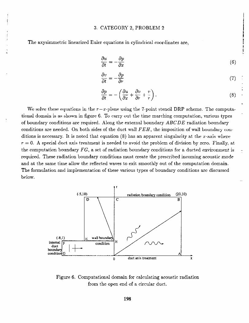
3. CATEGORY 2, PROBLEM 2
The axysimmetric linearized Euler equations in cylindrical coordinates are,
0u 0p- (6)
Ot Ox
Ov Op- (7)
Ot Or
(o ovv)-g=- _+_+ (8)
We solve these equations in the r-x-plane using the 7-point stencil DRP scheme. The computa-
tional domain is as shown in figure 6. To carry out the time marching computation, various types
of boundary conditions are required. Along the external boundary ABCDE radiation boundary
conditions are needed. On both sides of the duct wall FEH, the imposition of wall boundary con-
ditions is necessary. It is noted that equation (8) has an apparent singularity at the x-axis where
r = 0. A special duct axis treatment is needed to avoid the problem of division by zero. Finally, at
the computation boundary FG, a set of radiation boundary conditions for a dueted environment is
required. These radiation boundary conditions must create the prescribed incoming acoustic mode
and at the same time allow the reflected waves to exit smoothly out of the computation domain.
The formulation and implementation of these various types of boundary conditions are discussed
below.
Tr
(-5,10) [ radiation boundary condition (20,10)
D C B
/(-8,1) E wal /_
internal IF . . ]H ' / /"k../'kJ'k_duct[
conditionLG A
0 duct axis treatment
Figure 6. Computational domain for calculating acoustic radiation
from the open end of a circular duct.
198
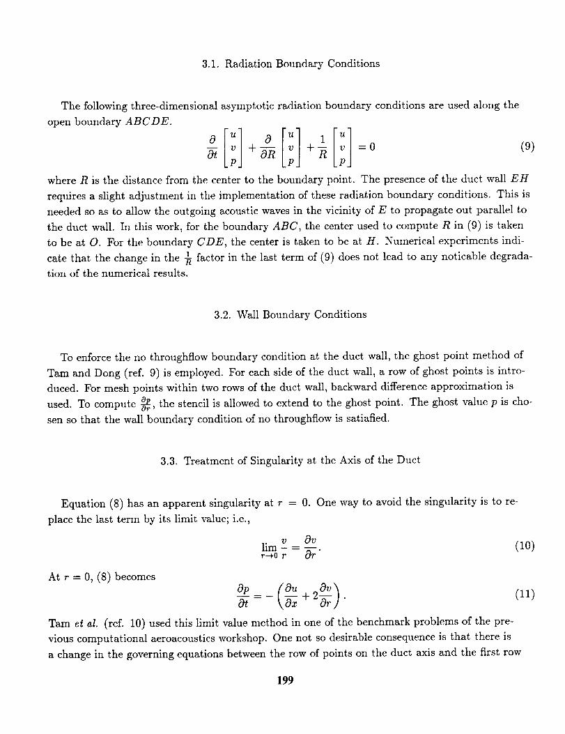
3.1. Radiation Boundary Conditions
The following three-dimensional asymptotic radiation boundary conditions are used along the
open boundary ABCDE.
+2 =0 (9)
where R is the distance from the center to the boundary point. The presence of the duct wall EH
requires a slight adjustment in the implementation of these radiation boundary conditions. This is
needed so as to allow the outgoing acoustic waves in the vicinity of E to propagate out parallel to
the duct wall. In this work, for the boundary ABC, the center used to compute R in (9) is taken
to be at O. For the boundary CDE, the center is taken to be at H. Numerical experiments indi-
cate that the change in the -_ factor in the last term of (9) does not lead to any noticable degrada-
tion of the numerical results.
3.2. Wall Boundary Conditions
To enforce the no throughflow boundary condition at the duct wall, the ghost point method of
Tam and Dong (ref. 9) is employed. For each side of the duct wall, a row of ghost points is intro-
duced. For mesh points within two rows of the duct wall, backward difference approximation is
used. To compute -_, the stencil is allowed to extend to the ghost point. The ghost value p is cho-
sen so that the wall boundary condition of no throughflow is satiafied.
3.3. Treatment of Singularity at the Axis of the Duct
Equation (8) has an apparent singularity at r = 0. One way to avoid the singularity is to re-
place the last term by its limit value; i.e.,
lim v = __Or (10)r--+0 r Or"
At r = 0, (8) becomes
Or- Ox + Or/"
Tam et al. (ref. 10) used this limit value method in one of the benchmark problems of the pre-
vious computational aeroacoustics workshop. One not so desirable consequence is that there is
a change in the governing equations between the row of points on the duct axis and the first row
(11)
199
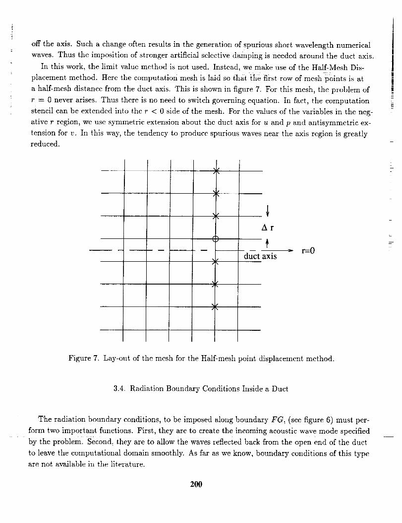
off the axis. Such a change often results in the generation of spurious short wavelength numerical
waves. Thus the imposition of stronger artificial selective damping is needed around the duct axis.
In this work, the limit value method is not used. Instead, we make use of the Half-Mesh Dis-
placement method. Here the computation mesh is laid so that the first row of mesh points is at
a half-mesh distance from the duct axis. This is shown in figure 7. For this mesh, the problem of
r = 0 never arises. Thus there is no need to switch governing equation. In fact, the computation
stencil can be extended into the r < 0 side of the mesh. For the values of the variables in the neg-
ative r region, we use symmetric extension about the duct axis for u and p and antisymmetric ex-
tension for v. In this way, the tendency to produce spurious waves near the axis region is greatly
reduced.
% •
)(
()
)(
Ar
duct axis-_ r=-O
Figure 7. Lay-out of the mesh for the Half-mesh point displacement method.
3.4. Radiation Boundary Conditions Inside a Duet
The radiation boundary conditions, to be imposed along boundary FG, (see figure 6) must per-
form two important functions. First, they are to create the incoming acoustic wave mode specified
by the problem' Second, they are to allow the waves reflected back from the open end of the duct
to leave the computational domain smoothly. As far as we know, boundary conditions of this type
are not available in the literature.
200
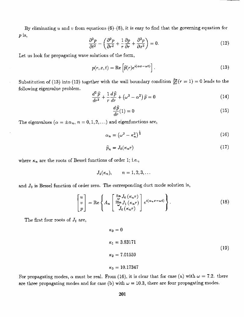
By eliminating u and v from equations (6)-(8), it is easy to find that the governing equation for
p is,
a2p (a _p 1ap a_p'_k._r2 +r_rr+_-fix2] =0. (12)Ot2
Let us look for propagating wave solutions of the form,
p(r,x,t) = Re [_r)ei(ax-_t)] . (13)
Substitution of (13) into (12) together with the wall boundary condition a°-_(r = 1) = 0 leads to the
following eigenvalue problem.d2_ I d_dr--T + r-_r + (w2 - a2) if= 0 (14)
-_- (1) =0 (15)
The eigenvalues (a = ±an, n = 0, 1,2,...) and eigenfunctions are,
(16)
_. = Jo(_.r) (17)
where ,q, are the roots of Bessel functions of order 1; i.e.,
Jl(,_n), n = 1,2,3,...
and J0 is Bessel function of order zero. The corresponding duct mode solution is,
= Re {A_
O_nj (/_nr)w 0
___j , (_n')YO(_._)
The first four roots of 3"] are,
_0--0
(18)
_1 = 3.83171
n2 = 7.01559
(19)
,_3 = 10.17347
For propagating modes, a must be real. From (16), it is clear that for case (a) with w = 7.2. there
are three propagating modes and for case (b) with w = 10.3, there are four propagating modes.
201
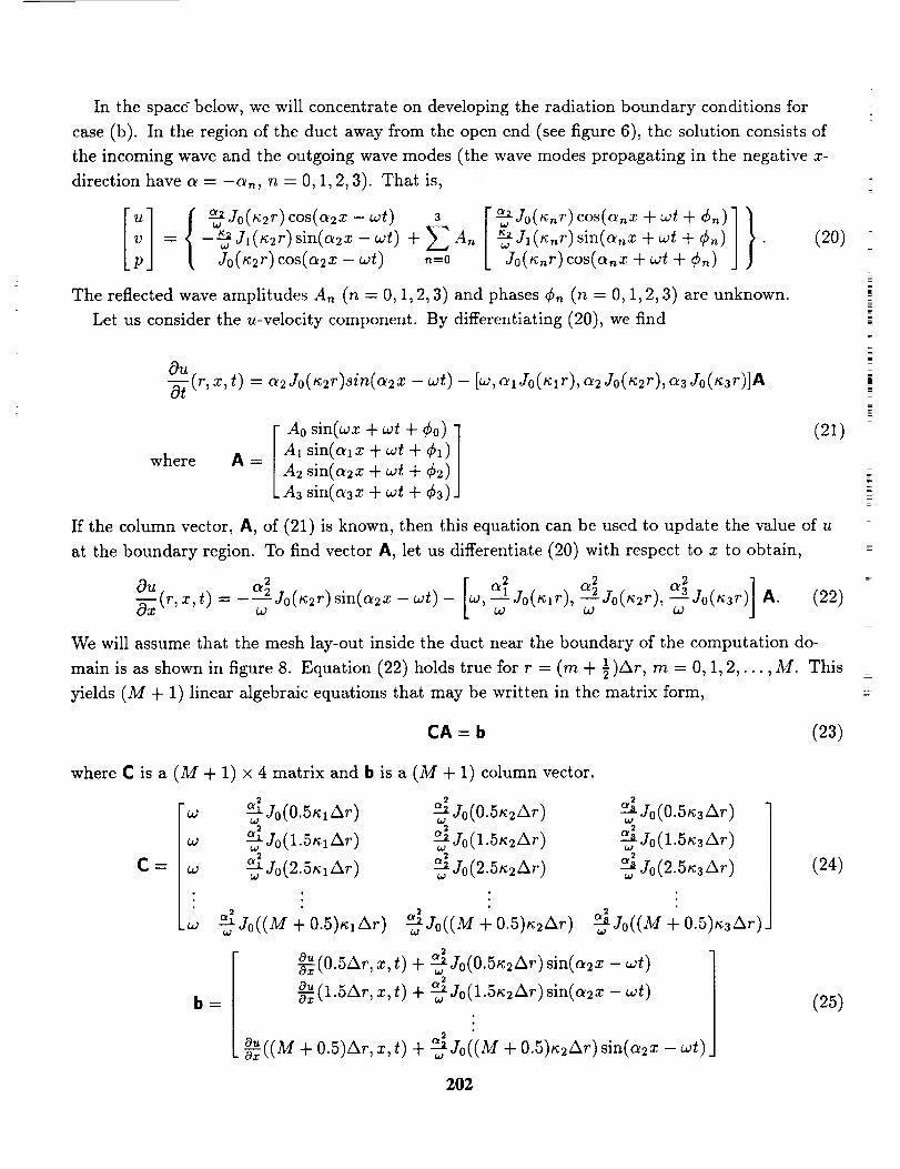
In the space" below, we will concentrate on developing the radiation boundary conditions for
case (b). In the region of the duct away from the open end (see figure 6), the solution consists of
the incoming wave and the outgoing wave modes (the wave modes propagating in the negative x-
direction have a = -a,, n = 0, 1, 2, 3). That is,
= -_Sl(_,.)sin(_2x -_t) + _ A.J0(_2r)cos(_x -cot) .=0
_J0(_.d ¢os(_.x +cot + ¢.)_J
Ja(_nr)sin(anx + cot + On)
J0(_.r) cos(_._ + cot+ ¢.) o
The reflected wave amplitudes An (n - 0, 1, 2, 3) and phases Cn (n = 0, 1, 2, 3) are unknown.
Let us consider the u-velocity component. By differentiating (20), we find
(20)
_(_,_,t) = _Jo(_)_i_(_z -_t) - [_,_lJ0(_), _2J0(_2_),_ J0(_)]A
A0 sin(cox + cot + ¢0)
where A = Aa sin(aax +wt + ¢1)A2 sin(a2x + wt + ¢2)
A3 sin(a3x + cot + ¢3)
If the column vector, A, of (21) is known, then this equation can be used to update the value of u
at the boundary region. To find vector A, let us differentiate (20) with respect to x to obtain,
__x(r,x,t)=_____jo(x2r)sin(_2x_cot)_Oua_ [ a2 _2 o_ ]co,_z0(_lr),_J0(_2_),_J0(_) A. (22)
We will assume that the mesh lay-out inside the duct near the boundary of the computation do-
main is as shown in figure 8. Equation (22) holds true for r = (m + 1)At, m = 0, 1,2,... ,M. This
yields (M + 1) linear algebraic equations that may be written in the matrix form,
(21)
CA=b (23)
where C is a (M + 1) × 4 matrix and b is a (M + 1) column vector.
C __
-co elZ0(0.5_Ar) zlJ0(0.5_AdOJ _1
co dZ0(1.D_lA_) ZlJ0(1.5_A_)02 _9
co _ J0(2.5xlAr) _Y0(2.5_2Ar)
.w -_Jo((M,,,,, +0.5)n_Ar) --_a_Jo((M +0.5)_2Ar)
b __.
_ J0(0.5_3Ar){aJ
4 J0(i.5_3A_)laJ
-_ J0(2.5x3 Ar)lag
_i 0.5)_3A_),o Jo((M +
o,,ta _Ar t) + 2__Jo(O.5tc2Ar)sin(a2x wt)_kv.v ,X, w
°"(i.5Ar, z,0 + dJo(1.5x2Ar)sin(_2x-wt)
Ou_((M + 0.5)A_,_,t) + d_So((M + 0.5)_zXd sin(_2_-cot)
(24)
(25)
202
z
=
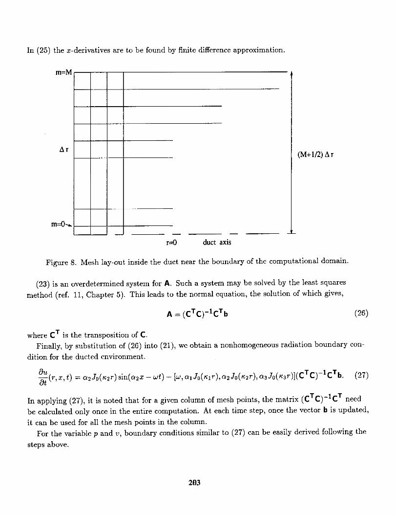
In (25) the z-derivatives are to be found by finite difference approximation.
m=M
Ar
m---0_,
m
r=O duct axis
(M+ 1/2) A r
Figure 8. Mesh lay-out inside the duct near the boundary of the computational domain.
(23) is an overdetermined system for A. Such a system may be solved by the least squares
method (ref. 11, Chapter 5). This leads to the normal equation, the solution of which gives,
A = (cTc)-IcTb (26)
where C T is the transposition of C.
Finally, by substitution of (26) into (21), we obtain a nonhomogeneous radiation boundary con-
dition for the ducted environment.
-_-(r,x0U ,t) = a2J0(R2r) sin((x2x - cot) - [w,_lJo(nlr),(_2Jo(tc2r),_3Jo(R3r)](cTc)-lcTb. (27)
In applying (27), it is noted that for a given column of mesh points, the matrix (cTc)-Ic T need
be calculated only once in the entire computation. At each time step, once the vector b is updated,
it can be used for all the mesh points in the column.
For the variable p and v, boundary conditions similar to (27) can be easily derived following the
steps above.
203
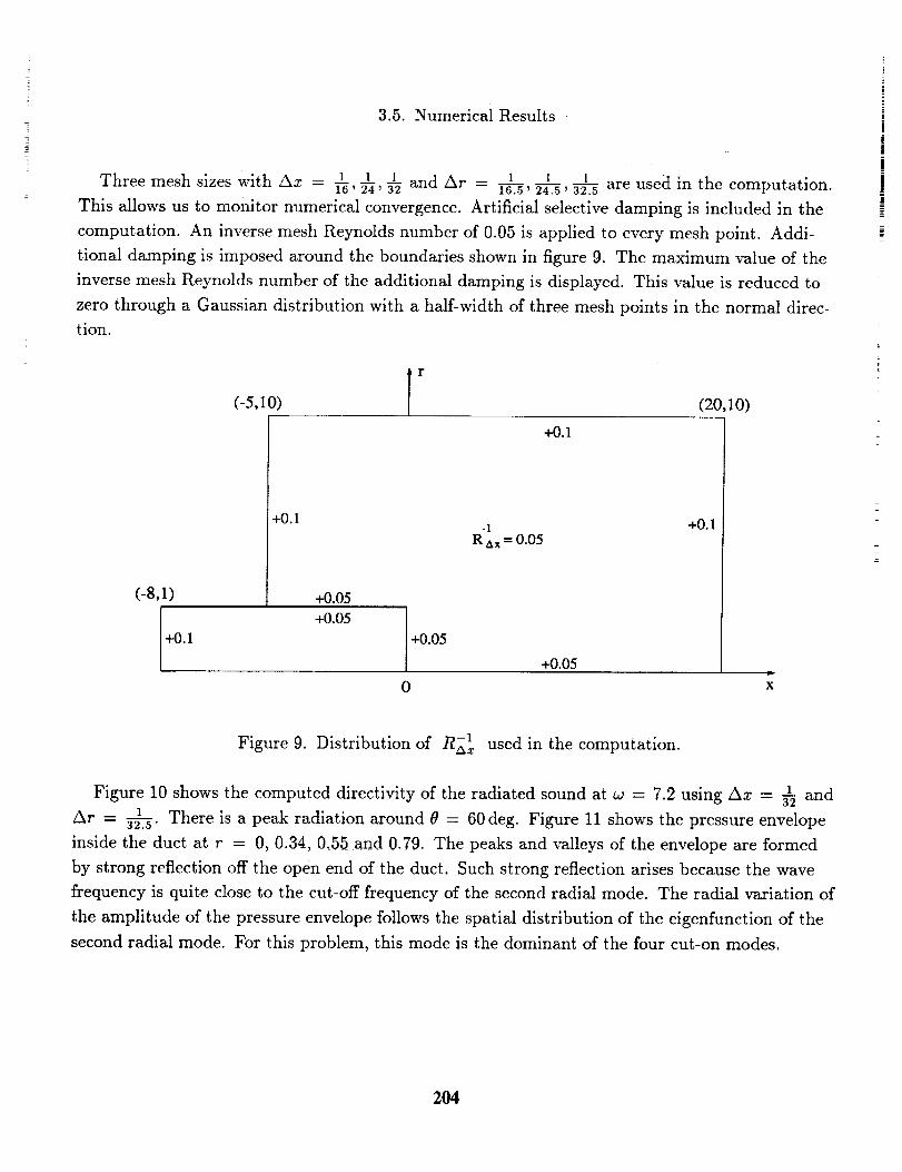
3.5. Numerical Results
1 I 11 1 1 and Ar = 16.s, 24.s, 32.5 are used in the computation.Three mesh sizes with Ax - a6,24, 32
This allows us to monitor numerical convergence. Artificial selective damping is included in the
computation. An inverse mesh Reynolds number of 0.05 is applied to every mesh point. Addi-
tional damping is imposed around the boundaries shown in figure 9. The maximum value of the
inverse mesh Reynolds number of the additional damping is displayed. This value is reduced to
zero through a Gaussian distribution with a half-width of three mesh points in the normal direc-
tion.
r(-5,10) (20,10)
(-8,1)
+0.1
+0.05
+O.1
+0.05
+O.1
+0.05
+0.1
+0.05D
0 x
Figure 9. Distribution of RT,_ used in the computation.
Figure 10 shows the computed directivity of the radiated sound at w = 7.2 using Ax -- _ and
Ar = _ There is a peak radiation around 8 = 60deg. Figure 11 shows the pressure envelope32.5 "
inside the duct at r = 0, 0.34, 0.55 and 0.79. The peaks and valleys of the envelope are formed
by strong reflection off the open end of the duct. Such strong reflection arises because the wave
frequency is quite close to the cut-off frequency of the second radial mode. The radial variation of
the amplitude of the pressure envelope follows the spatial distribution of the eigenfunction of the
second radial mode. For this problem, this mode is the dominant of the four cut-on modes.
204
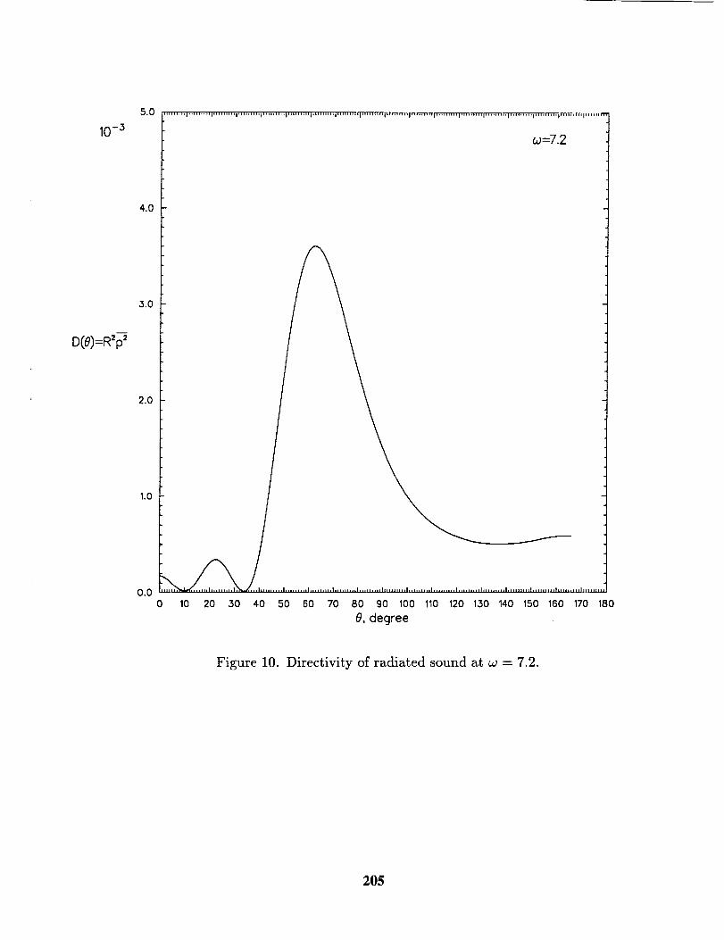
I0 -3
D(8)=R'_
5.0
4.0
3.0
2.0
'''ii''' '1'''''0' H I'''''' '01 I' l llllill I '0' '' ''IIII l l'lllll I I II i llllll'l II i I_ _iiii, I lll ii_l rFi n liin _ m_ FTTTnl_TTTm_TTT_T,,, i,,,,,,,,,l,,,,,,,,,p,'"* 'llll''l''_
ca---7.2
1.0
0.00 10 20 30 40 50 60 70 80 90 100 110 120 130 140 150 160 170 180
e, degree
Figure 10. Directivity of radiated sound at co = 7.2.
2O5
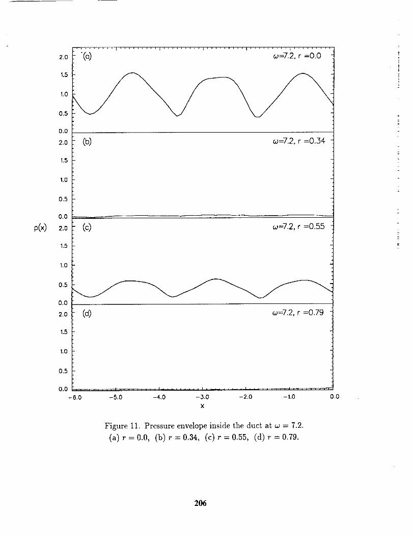
p(x)
2.0
1.5
1.0
0.5
0.0
2.0
1.5
1,0
0.5
0.0
2.0
1.5
t,0
0.5
0.0
2.0
1.5
1.0
0.5
0.0
-6.0
"(a) w=7.2, r =0.0
(b) w=7.2, r =0...34
(c) w=7.2, r =0.55
(d) w=7.2, r =0.79
-5.0 --4.0 -,.3.0 --2.0 -1.0 0.0
X
[
|
Figure 11. Pressure envelope inside the duct at w = 7.2.
(a) r=0.0, (b) r=0.34, (c) r=0.55, (d) r=0.79.
206
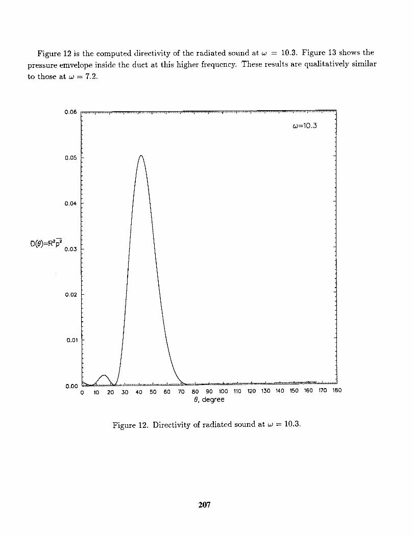
Figure 12 is the computed directivity of the radiated sound at w = 10.3. Figure 13 shows the
pressure emvelope inside the duct at this higher frequency. These results are qualitatively similar
to those at _o = 7.2.
D(@=R_
0.06
0.05
0.04
0.03
0.02
0.01
0.00
' "' '"' 'I' "''" "I" '""' 'I' '" "" 'I" '" '" 'I' '"'" "I'" '" '"I'"'"' "I'" '" "'I"" '"' 'I' "*'" "I" ,,**.H I''" '"' 'I"'"'" 'I'"" "' 'I'"'" '"I" '" '"' I'"'" '"
w=lO.3
A
0 10 20 30 40 50 60 70 80 90 100 110 120 130 140 150 160 170 180
8, degree
Figure 12. Directivity of radiated sound at w = 10.3.
207
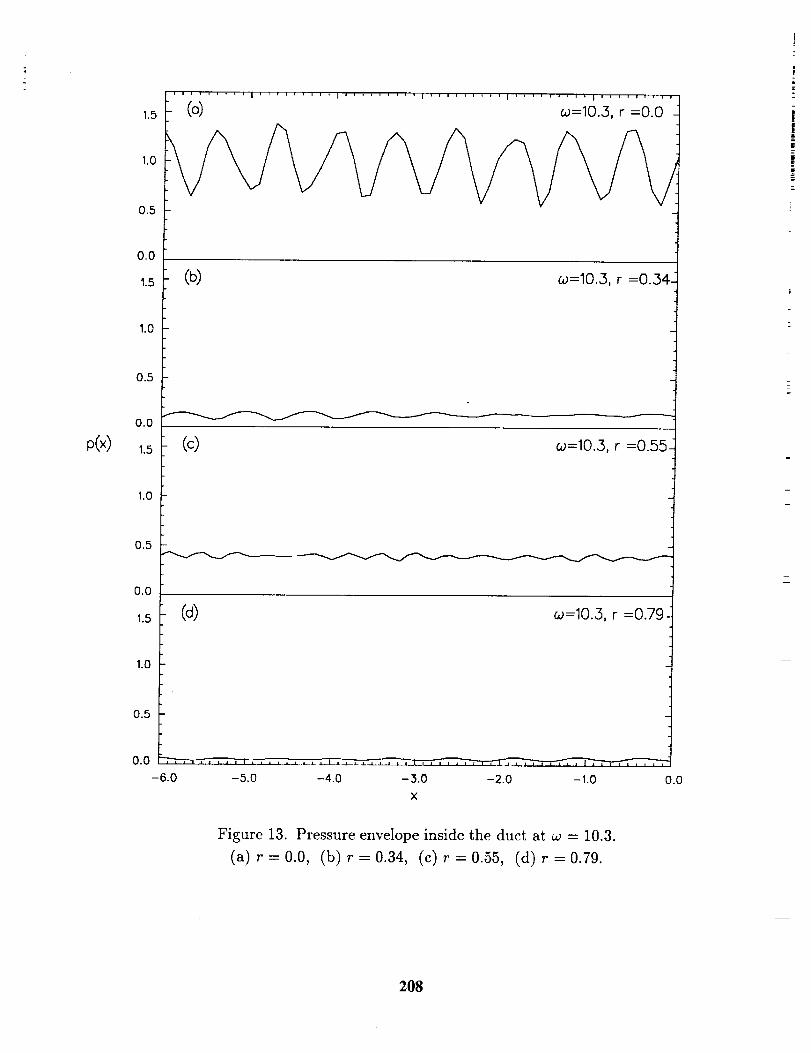
p(x)
1.5
1.0
0.5
0.0
1.5
1.0
0.5
0.0
1.5
1.0
0.5
0.0
1.5
1.0
(o) w=10.3, r =0.0 "
0.5
0.0
-6.0
(b) w=10.,3, r =0..34:
(c) w=10.3, r =0.55-
(d) co=10.3, r =0.79
11, ,,1tl i,,,,,lllll_
-5.0 -4.0
ii11,,, .,.,,1111 J.llllll,t|, I,..,,
-3.0 -2.0 -1.0 0.0
x
Figure 13. Pressure envelope inside the duct at w = 10.3.
(a) r=0.0, (b) r=0.34, (c) r=0.55, (d) r=0.79.
208
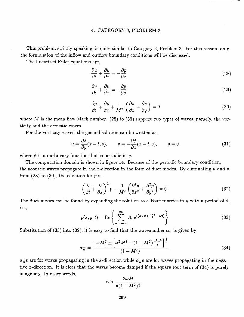
4. CATEGORY 3, PROBLEM 2
This problem, strictly speaking, is quite similar to Category 2, Problem 2. For this reason, only
the formulation of the inflow and outflow boundary conditions will be discussed.
The linearized Euler equations are,
Ou Ou Op--_ + Ox Ox (28)
Ov Ov OpO--t+ Ox - Oy (29)
Op Op 1 (Ou O_yy)0---/+ _xx + _-2- _xx + =0 (30)
where M is the mean flow Mach number. (28) to (30) support two types of waves, namely, the vor-
ticity and the acoustic waves.
For the vorticity waves, the general solution can be written as,
0¢(x_t,y), v= 0¢(x_t,y), p=0 (31)
where ¢ is an arbitrary function that is periodic in y.
The computation domain is shown in figure 14. Because of the periodic boundary condition,
the acoustic waves propagate in the x-direction in the form of duct modes. By eliminating u and v
from (28) to (30), the equation for p is,
(o__+_o) 2 M21 (02p 02p_p \_x2 + 0-_-y2] =0. (32)
The duct modes can be found by expanding the solution as a Fourier series in y with a period of 4;
i,e,,
- i_o, -'"--_-._0 (33)p(x, y, t) = Re Ane" "-" =
Substitution of (33) into (32), it is easy to find that the wavenumber a,, is given by
1
± (34)an = (1 - M 2)
a+s are for waves propagating in the x-direction while o_s are for waves propagating in the nega-
tive x-direction. It is clear that the waves become damped if the square root term of (34) is purely
imaginary. In other words,2w M
n>_(1 - M2)½ "
209
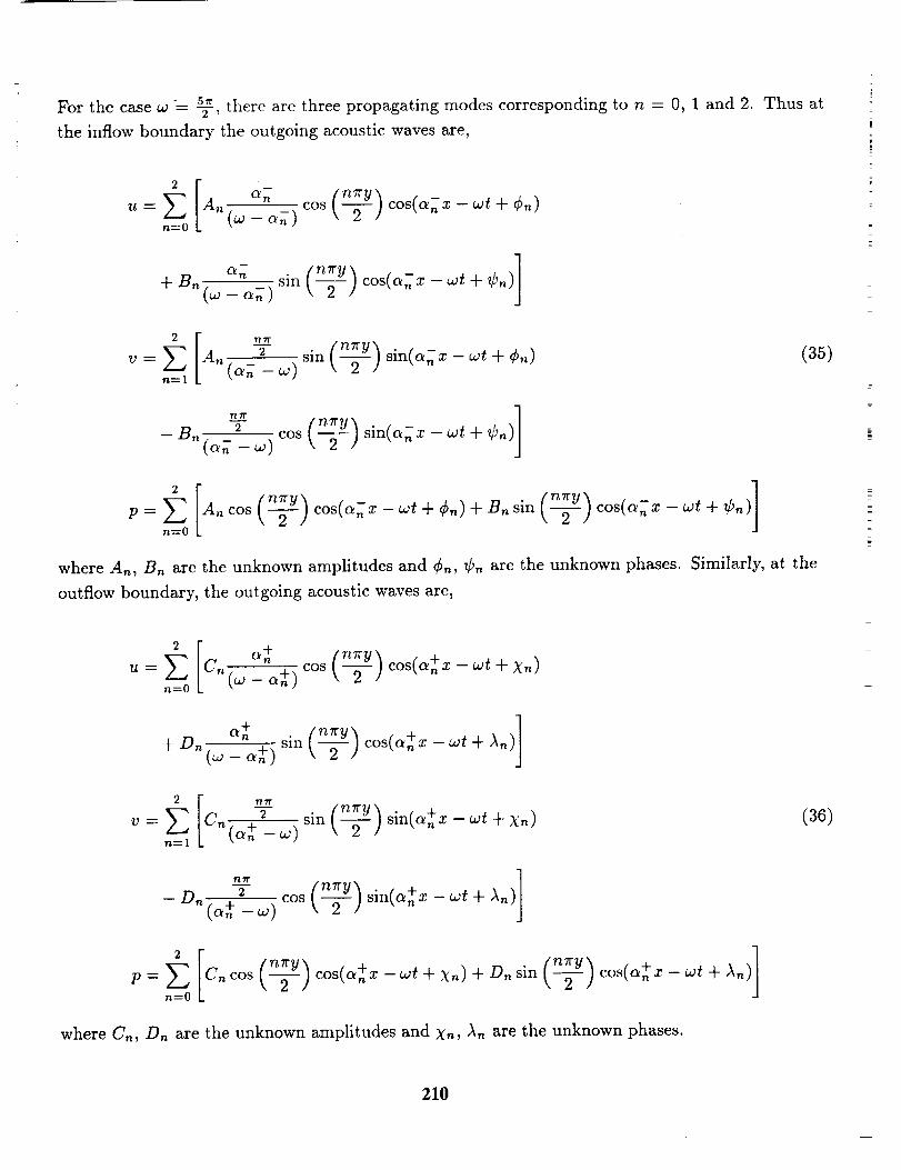
For the case w " _s_, there are three propagating modes corresponding to n = 0, 1 and 2. Thus at
the inflow boundary the outgoing acoustic waves are,
_[ o_ (_)u= An (w--_;) cos cos(c_;x - oat + Cn)rt=0
+ B.(oa _ _.)
v = E An 2 sin sin((__ x - oat + Cn) (35)n----1 (O_n -oa)
n_
2
- B,, (a_ _ oa)COS
Iv) ]P=E A_cos cos( a-_ x - wt + ¢. ) + Bn sin cos( a'(_ x - oat + ¢_ )n=O
where An, Bn are the unknown amplitudes and ¢,_, ¢. are the unknown phases. Similarly, at the
outflow boundary, the outgoing acoustic waves are,
_:E c°(__o_)_o_n:O
v = E Cn(. oa) sin sin(a+x-wt +Xn)n=l
COS
(v) (v) ]P: E Cncos cos(a+x -oat + X.) + Dnsin cos(a+x-oat + _.)n----0
where C., Dn are the unknown amplitudes and X-, An are the unknown phases.
(36)
210
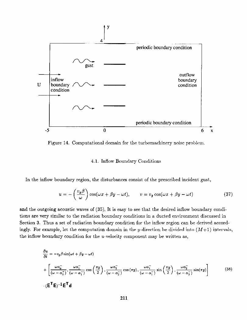
U
gust
periodic boundary condition
= outflow
inflow boundaryboundary _ conditioncondition
periodic boundary condition
-5 0 6 x
Figure 14. Computational domain for the turbomachinery noise problem.
4.1• Inflow Boundary Conditions
In the inflow boundary region, the disturbances consist of the prescribed incident gust,
u = - (_-fl-) cos(wx + fly-wt), v = vgcos(wx + fly-wt) (37)
and the outgoing acoustic waves of (35), It is easy to see that the desired inflow boundary condi-
tions are very similar to the radiation boundary conditions in a ducted environment discussed in
Section 3. Thus a set of radiation boundary condition for the inflow region can be derived accord-
ingly. For example, let the computation domain in the y-direction be divided into (M+I) intervals,
the inflow boundary condition for the u-velocity component may be written as,
(9//
-_ = -vgflsin(wt + fly - wt)
, cos , -- cos (_ry), sin sin(Try) (38)+ L(_ - %) (_ - _;) (_ - ,_;) (_ -_T) ' (_ - ,_;)
• (ETE)-I ETd
211
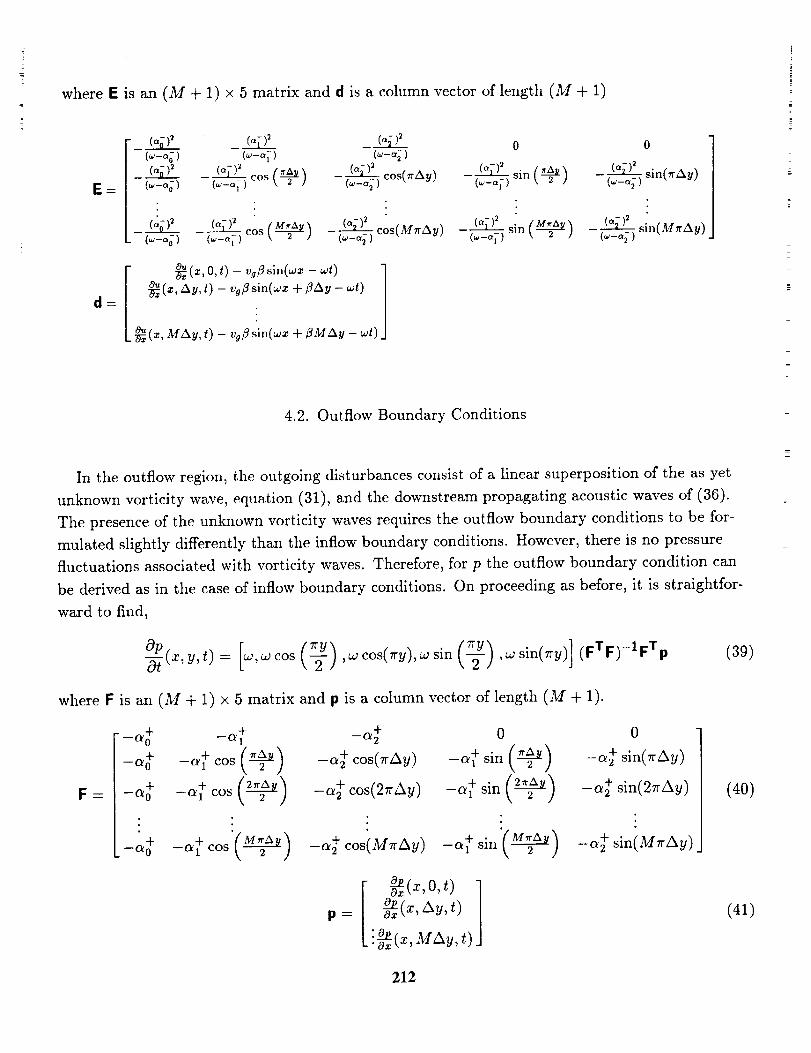
where E is an (M + 1) x 5 matrix and d is a column vector of length (M + 1)
E
d
____11_ ___!sZ_ (o-_Z_(u-ok) (_,-a?) (_-a;)
("_-%) (,___,;_)cos (,o-_)
__? _oL (____?) _ , ....('-°o) (,____ } cos - ('_-_'_) costivJ lrza y)
_(z, O,t) - vg3 sin(a_z - a_t)
_(z, Ay, t) -- va3:in(wz + flAy -- wt)
(z, MAy, t) - vg¢_sin(wz + 3MAy - wt)
0 0
(°-)_- sin (_) -(--_ sin(trAy)
_ (.__-_ sin ( M_----_-2_ )('_-G)
-(--_- sin(MrrAy)(,_-_,_)
4.2. Outflow Boundary Conditions
In the outflow region, the outgoing disturbances consist of a linear superposition of the as yet
unknown vorticity wave, equation (31), and the downstream propagating acoustic waves of (36).
The presence of the unknown vorticity waves requires the outflow boundary conditions to be for-
mulated slightly differently than the inflow boundary conditions. However, there is no pressure
fluctuations associated with vorticity waves. Therefore, for p the outflow boundary condition can
be derived as in the case of inflow boundary conditions. On proceeding as before, it is straightfor-
ward to find,
Ot(39)
where F is an (M + 1) x 5 matrix and p is a column vector of length (M + 1).
F
-04 -04 -,_t o o--a + -o_ + cos (_-_2_ ) -a + cos(trAy) -a+ sin (_2-_-) --a+ sin(trAy)
-c_ + --a + cos (2_-_2_) -a+cos(2rrAy) -a+ sin (2_2-_) -a+sin(27rAy)
_o0 )
(40)
p
_(x,O,_)
!°o-_.(x,MAy, t)
(41)
212
Also, in the course of deriving (39), the following relationship is established.
e =
Co sin(a+x - wt + Xo)
C1 sin(a+x - wt + _1 )
C2sin(a+x wt + X2)
D1 sin(a+x - a_t + A1)D2 sin(a+x - wt + A2)
e = (FTF)-IF-Ip
(42)
(43)
Now in the outflow region, the velocity component u of the outgoing disturbances is represented
by,
0¢(x-t,_)u(x, _,_)=
[ a°+ a+ (2) a+ cos(Try), a+ sin (-_) a+ sin(try)]+ +cos , ,
Cocos(,_o+x - _ + xo)c1 cos(_+x - _t + xl)c2 cos(a+x - ,or+ x2)Di cos(a+x - wt + A1)
02 cos(a+x - wt + A2)
(44)
__o) to (44) and rewrite as,To eliminate the unknown function ¢, we apply (o + 0_
Ou Ou [a+,a+ (_2_y) , a+ cos(try), ol+ sin (__) , a+ sin(Try)]-b7(x'_'_) - o_(_'_'t) + cos e. (45)
The outflow boundary condition can be obtained by replacing e in (45) by (43). Hence
Ou Ou
ot (x,y,t)= -_(x,u,O
+ [a+,a + cos (2) 'a+ c°s(zrY)'a+ sin (2) 'a+ sinOry)]
(FTF)-IFTp.
(46)
213
The v-velocity component in the outflow region is given by
a¢ (xv- Kz -t,_)
C1 sin(a+x -oat + x1)l
C2 sin(a+x -oat + X2)|
D1 sin(a+x -oat + A,)| '
Dz sin(_+.-oat + X_).J
__o) to (47) it is found,Upon eliminating ¢ by applying (o + 0x
(47)
y,t) -- Ox (x,y,t) + -_ sin , _-sin0ry), _ cos , _- cos(Try)
c1 cos(_tx -oat + x,)lc=cos(o # -oat+x=)/01cos( ,+xoat+ l)/"Dzcos(_+x oat+ _z)J
To determine the last column vector of (48), we may start by differentiating p of (36) with respect
to y. This yields,
c1 cos(_+x -oat + xl)]
(z,y,t) = _sin ,-Tr sin0ry), _cos ,Tr cos(_'y) D1 cos( a+ x - oat + A1)| "
D2 cos(a+x - oat + Az) J
The unknown column vector can now be evaluated as an overdetermined system by enforcing (49)
at y = mAy, rn = 0, 1,2,... ,M. Once this vector is found in terms of a column vector of _, it is
inserted into (48) to provide the desired outflow boundary condition for v.
(48)
(49)
4.3. Numerical Results
We carried out numerical computation for the case oa = -_ using two size meshes with Ax =
± and _. The distribution of inverse mesh Reynolds number associated with the ar-Ay = 20
tificial selective damping is shown in figure 15. A R_,lx = 0.05 is used for general background
damping. Extra damping is added near the flat plate. A Gaussian distribution of inverse mesh
214
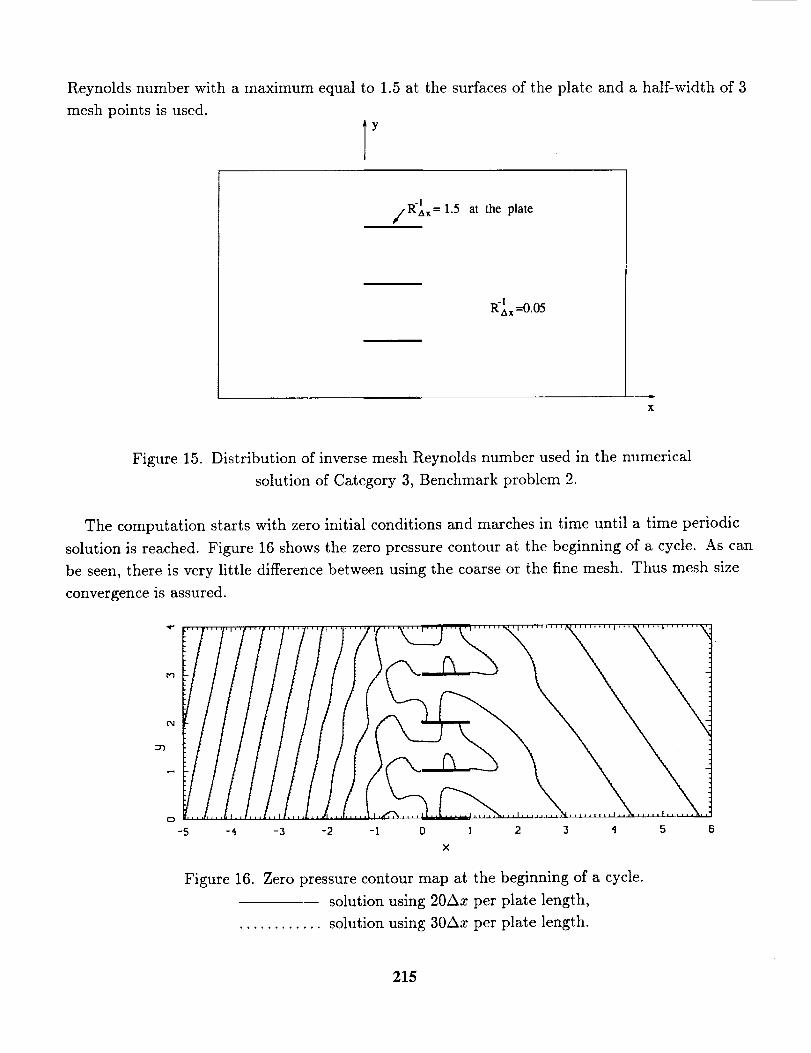
Reynolds number with a maximum equal to 1.5 at the surfaces of the plate and a half-width of 3
mesh points is used.
-1
//Rax= 1.5 at the plate
R'_x ----0.05
x
Figure 15. Distribution of inverse mesh Reynolds number used in the numerical
solution of Category 3, Benchmark problem 2.
The computation starts with zero initial conditions and marches in time until a time periodic
solution is reached. Figure 16 shows the zero pressure contour at the beginning of a cycle. As can
be seen, there is very little difference between using the coarse or the fine mesh. Thus mesh size
convergence is assured.
i'M
:J3
CD
-5 -4 -3 -2
[,,_, .....1 l ........ ,,'iX,.,,,.........N ......... ,,.k...... , .......-1 0 1 2 3 4 5 6
X
Figure 16. Zero pressure contour map at the beginning of a cycle.
solution using 20Ax per plate length,
............ solution using 30Ax per plate length.
215
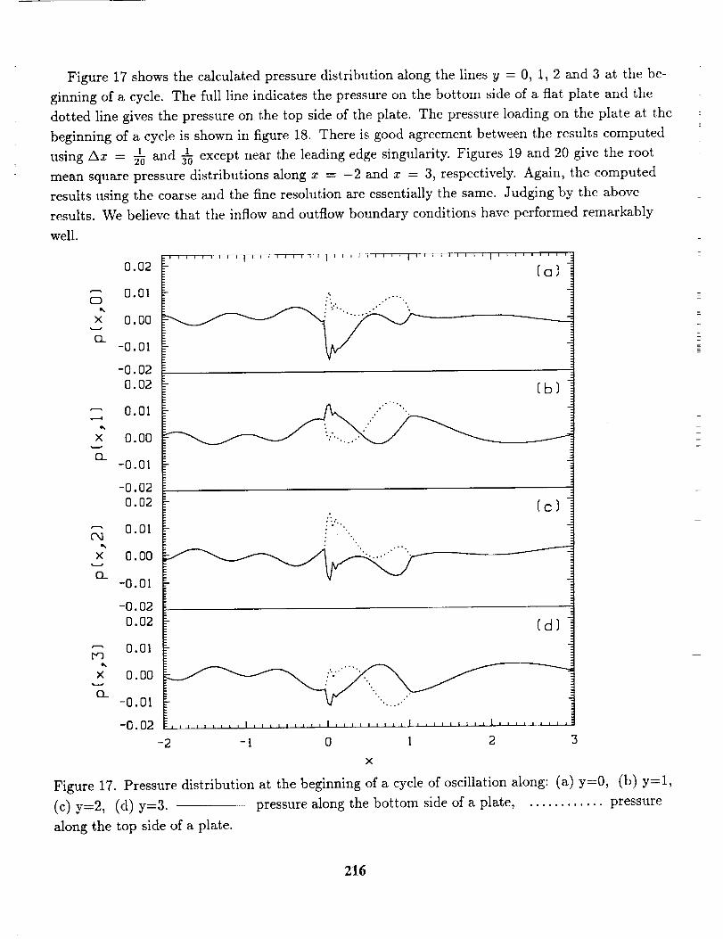
Figure 17 shows the calculated pressure distribution along the lines y = 0, 1, 2 and 3 at the be-
ginning of a cycle. The full line indicates the pressure on the bottom side of a flat plate and the
dotted line gives the pressure on the top side of the plate. The pressure loading on the plate at the
beginning of a cycle is shown in figure 18. There is good agreement between the results computed
using Ax = ! and _ except near the leading edge singularity. Figures 19 and 20 give the root2o
mean square pressure distributions along x = -2 and x = 3, respectively. Again, the computed
results using the coarse and the fine resolution are essentially the same. Judging by the above
results. We believe that the inflow and outflow boundary conditions have performed remarkably
well.
0.02
'-" 0.01C3
i%
x 0.00
cl-0.01
-0.02
0.02
0.01,r----I
t%
x 0.00
CI_-0.01
Ca]
-0.02
0.02
o,a O.Ol
x 0.00
O_-0.01
-0.02
0.02
"-" 0.01
x 0.00
n-0.01
-0.02
:-',.
[c]
X
Figure 17. Pressure distribution at the beginning of a cycle of oscillation along: (a) y=0,
(c) y=2, (d) y:3.
along the top side of a plate.
(b) y=l,
pressure along the bottom side of a plate, ............ pressure
216
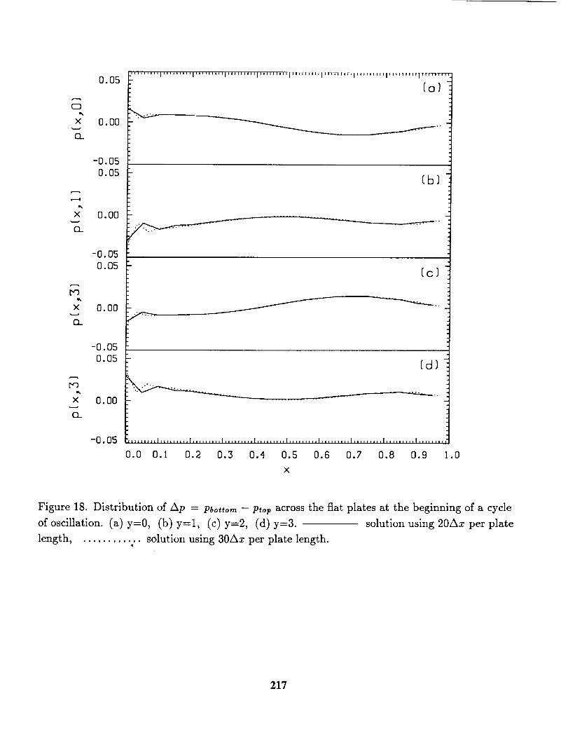
C3
X
t'_
w
(2_
['O
O..
V'3
X
EL
0.05
0.00
0.00
0.00
-0.05
0.05
0.00
-0.05
......... I ..... '"'1"''"'"1''"' .... I .... ''''':l'''''_ll;";Tln_]Tn]Tn]]]]Tr_ll_;lrtrT_T_--_.b-
[a]
f.o
[b]
-.o .°
[c]
[d]
,,,, .... I ......... I,, ....... I ..... ,,,,I,,,,,,,,,1,,,, ..... I ......... I ......... I ......... I ........
0.0 0.1 0.2 0.3 0.4 0.5 0.6 0.7 0.8 0.9 1.0
X
Figure 18. Distribution of Ap : Pbottom -- Prop across the flat plates at the beginning of a cycle
of oscillation. (a) y=0, (b) y=l, (c) y:2, (d) y=3. solution using 20Ax per plate
length, .......... .. solution using 30Ax per plate length.
217
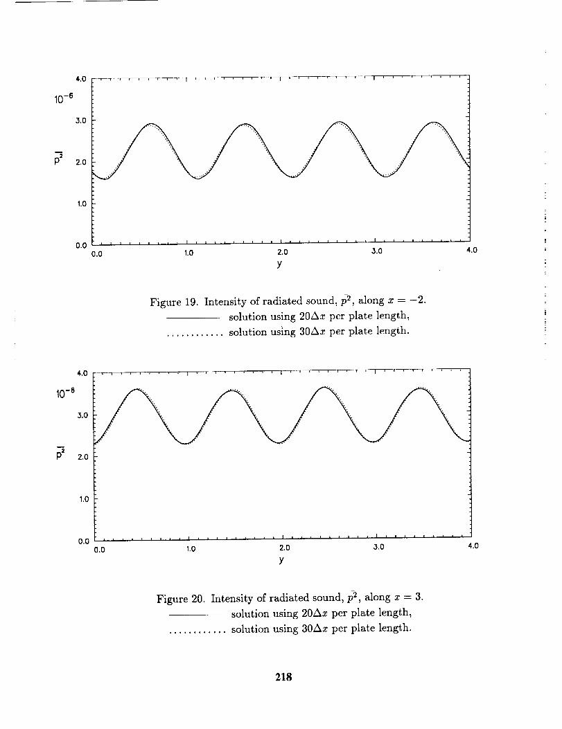
4.0
10-6
3.0
1.0
0.0 , l , J , = , [ i I [ i ! , . i , = | I . ] , , = , , • , I , , , , , = i L |
0.0 1.0 2.0 3.0
Y
4.0
Figure 19. Intensity of radiated sound, p_, along x = -2.
solution using 20Ax per plate length,
............ solution using 30Ax per plate length.
4.0 _==,,,..,I,,'T,, I -_* ''' I'''''''''
1.0
0.0 l..i..=.llf,=,J_.
0.0 1.0
|=,,,=,==,l,,]=:Jl==
2.0 3.0
Y
4.0
Figure 20. Intensity of radiated sound, p2, along x = 3.
solution using 20Ax per plate length,
............ solution using 30Ax per plate length.
218
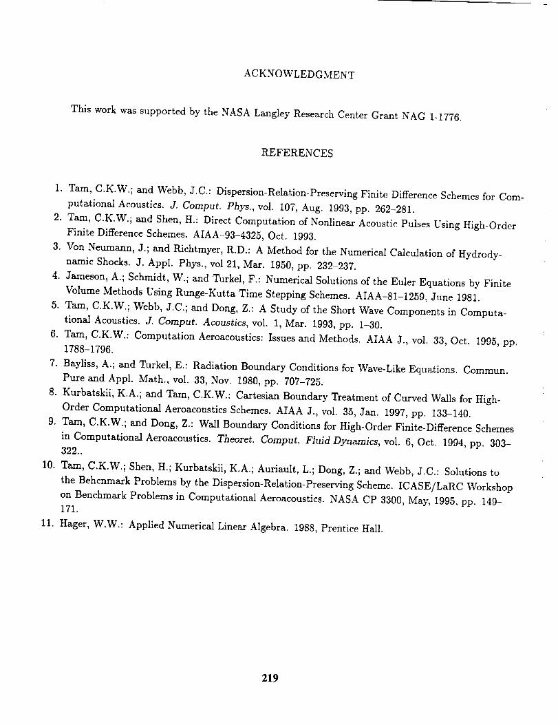
ACKNOWLEDGMENT
This work was supported by the NASA Langley Research Center Grant NAG 1-1776.
REFERENCES
1. Tam, C.K.W.; and Webb, J.C.: Dispersion-Relation-Preserving Finite Difference Schemes for Com-
putational Acoustics. J. Comput. Phys., vol. 107, Aug. 1993, pp. 262-281.
2. Tam, C.K.W.; and Shen, H.: Direct Computation of Nonlinear Acoustic Pulses Using High-Order
Finite Difference Schemes. AIAA-93-4325, Oct. 1993.
3. Von Neumann, J.; and Richtmyer, R.D.: A Method for the Numerical Calculation of Hydrody-
namic Shocks. J. Appl. Phys., vol 21, Max. 1950, pp. 232-237.
4. Jameson, A.; Schmidt, W.; and Turkel, F.: Numerical Solutions of the Euler Equations by Finite
Volume Methods Using Runge-Kutta Time Stepping Schemes. AIAA-81-1259, June 1981.
5. Tam, C.K.W.; Webb, J.C.; and Dong, Z.: A Study of the Short Wave Components in Computa-
tional Acoustics. J. Comput. Acoustics, vol. 1, Max. 1993, pp. 1-30.
6. Tam, C.K.W.: Computation Aeroacoustics: Issues and Methods. AIAA J., vol. 33, Oct. 1995, pp.
1788-1796.
7. Bayliss, A.; and Turkel, E.: Radiation Boundary Conditions for Wave-Like Equations. Commun.
Pure and Appl. Math., vol. 33, Nov. 1980, pp. 707-725.
8. Kurbatskii, K.A.; and Tam, C.K.W.: Cartesian Boundary Treatment of Curved Walls for High-
Order Computational Aeroacoustics Schemes. AIAA J., vol. 35, Jan. 1997, pp. 133-140.
9. Tam, C.K.W.; and Dong, Z.: Wall Boundary Conditions for High-Order Finite-Difference Schemes
in Computational Aeroacoustics. Theoret. Comput. Fluid Dynamics, vol. 6, Oct. 1994, pp. 303-
322..
10. Tam, C.K.W.; Shen, H.; Kurbatskii, K.A.; Auriault, L.; Dong, Z.; and Webb, J.C.: Solutions to
the Behcnmaxk Problems by the Dispersion-Relation-Preserving Scheme. ICASE/LaRC Workshop
on Benchmark Problems in Computational Aeroacoustics. NASA CP 3300, May, 1995, pp. 149-
171.
11. Hager, W.W.: Applied Numerical Linear Algebra. 1988, Prentice Hall.
219
7'/
L/3 <-i,77
TESTING A LINEAR PROPAGATION MODULE ON SOME
ACOUSTIC SCATTERING PROBLEMS
(',..S. Djambazov, C.-ll. Lai, l{...\. Pericl_'ous
School of Computing and Mathematical Sciences, University of Creenwich
Wellington Street. Woolwich, London SEI8 6PF, U[x
ABSTRACT
Finite volume discretization of the Linearized Euler
Equations on a fully staggered computational gridresults in an efficient semi-implicit numerical schemewhich can be used in the 'near field' of aerodynamicnoise problems.
INTRODUCTION
Since sound is a form of fluid motion, when solving aeroacoustic
problems it is desirable to use existing Computational Fluid Dynamics
(CFD) codes as much as possible. They can simulate any flow field but, due
to numerical diffusion, they tend to smear the noise signal close to its
source. That is why they have to be combined with some other method to
produce accurate acoustic results. Traditionally the Acoustic Analogy [1]
has been used as a complementary technique [2, :3]. The alternative
Computational Aeroacoustics (CAA) approach provides additional
flexibility and simplicity when handling complex and/or moving geometries.
To reduce the computational cost Domain Decomposition methods are
used to define the 'near field' containing the noise generation region with
nonlinear acoustic effects and the 'far field' of linear sound propagation
[4, 2]. Special high accuracy CAA methods [.5] or I(irchhoff's surface
integral method [6] can be used in the far field.
In the near field commercial CFD codes cannot do the aeroacoustic
simulation alone because of the highly diffusive nature of the CFD
algorithms. This 'near field' has to be large enough to contain all the
nonlinearities of the sound field, and no CFD code can carry the acoustic
signal that fat'. This problem has been addressed at the University of
221
Greenwich [7] by creating an acoustic software module which can be
combined with a CFD code to solve aerodynamic noise problems. The code
can also be used on its own in smaller domains of linear propagation or it
can be combined with some structural acoustics software for internal noise
problems.
The code has been applied to the first two problems in "'Category 1 -
Acoustic Scattering" of the Second CAA Workshop on Benchmark
Problems. The method and results are described below.
METHOD
With the popular approach of splitting the flow variables into mean-flow
and perturbation parts [8, 9] the Linearized Euler Equations are obtained
to describe the sound field. If the mean flow is uniform, or if there is no
mean flow at all, the relative form of these equations can be used, and in
two dimensions they can be written as:
or)O--i + c\ax+ =q
Ou Op
0-7 + c-07z u=pocv Ov Op
a--/ + cN=L' O : poCV_
(1)
Op c_ Po-- = =7--, 7_i_ = 1.4 (2)Op po
Pert'urbation velocity components along the axes a: and g are denoted vx
and v_ respectively, c is the speed of sound, p0 is the density of undisturbed
air, p0 is the atmospheric pressure, and p is the pressure perturbation. The
right-hand sides q, .f,., fy are considered known functions of z, g and time t.
When discretizing the three unknown fimctions p,u and v, a fully
staggered (along both space and time) grid has been chosen. This is done
because it allows (as shown below) a fully explicit, stable, second-order
accurate scheme to be formulated. Its accuracy can then be extended to
third order by allowing the scheme to become implicit while retaining a
strong diagonal dominancy that guarantees fast convergence.
222
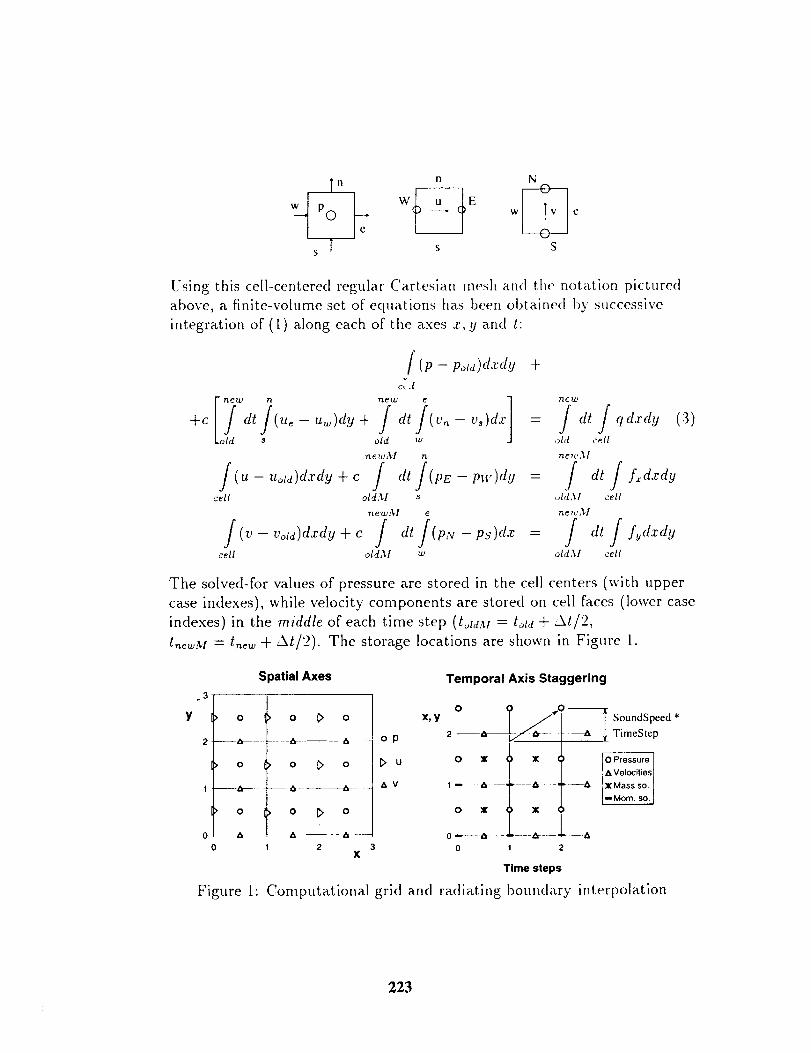
w E
W C w
s S
[.;sing this ceil-centered regular ('artesian mesh and the notation pictured
above, a finite-volume set of equations has been obtained t)5' successive
integration of (!.) along each of the axes .r, !./and t:
-'{-C
f (p - pold)d.rdg
Ct ,I
[i7, J,dt ue -u_)dg + t v,_ - vs z
old us
newM n
+
cell oldAI s
newAl e
/ (V - Vold)dzdg + c / dt /(pN - ps)d,v =cell old3,l w
7l e R2
J <"i (a)old cell
newAI
old3,l cell
newM
old3,I cell
The solved-for values of pressure are stored in the cell centers (with upper
case indexes), while velocity components are stored on cell faces (lower case
indexes) in the middle of each time step (toldM = told + At�2,
t,_e,,M = tnew + At�2). The storage locations are shown in Figure 1.
Y
.,3
Spatial Axes
> o I> o I> o
--gt--- --Ift- ..... #',< -
> o I> o I> o
> o I> o l> o
0 -- _ _----_ ......
0 l 2X
Temporal Axis Staggering
op
[> u
& V
x,y0
2--_
0 X
0 X
0
X
X
m _ m,
_A-----_SoundSpee d *TimeStep
0 Pressure IA Velocities
--A X Mass so.
Morn. so.
Time steps
Figure 1" Computational grid and radiating boundary interpolation
223
The integrals in (3) are first e,,'al,tatcd throltgh tnean values providing an
easy-to-prograln, second-order accurate, fully explicit numerical
scheme:
p = P_.l+l-- _rA"e -- ",+,) -- o'_,(v. -- v+) + qAt
u = Uol+- a+(pE - pw) + f.At (4)
v = eot,+- ,:r_(p,: - Ps) + f,jAt
cat catO',r -- O'g --
=_k.r' :S g
This scheme is accurate enough within about 5 wavelengths, accumulating
not more than S % error, and it can be used on its own in small domains,
e. g. with internal noise problems.
A second-order approximation of all the functions in all the integrals in
(3) can be employed to extend the accuracy of the method. Instead of
[(Xo, h) = hf(xo) now we have
hx0+_-
Z(xo,h) = / fCx)dx =
hxo-
= h[Af(xo - h) + (1 - 2A)f(xo) + Af(xo + h)],
1A=--
24
applied to all integrals. In 2D this means
ff(.r,g)dxdg= [A_-'_f,.,b+(1-4A)f,:_u]AxAgnbcell
with 'nb' used to denote all four neighboring cells.
(.5)
(6)
This semi-implicit scheme proved to be accurate enough to take the
sound generated out of the 'neat" field'. The resulting linear system is solved
iteratively at each time step starting with a very good initial gness
computed using the explicit scheme (4). Only one level of neighboring cells
are involved, and not second or further neighbors. The boundary cells are
processed with the explicit scheme only. With the discretization of those
integrals corttaining time as one of the argttments, "future' and "past'
224
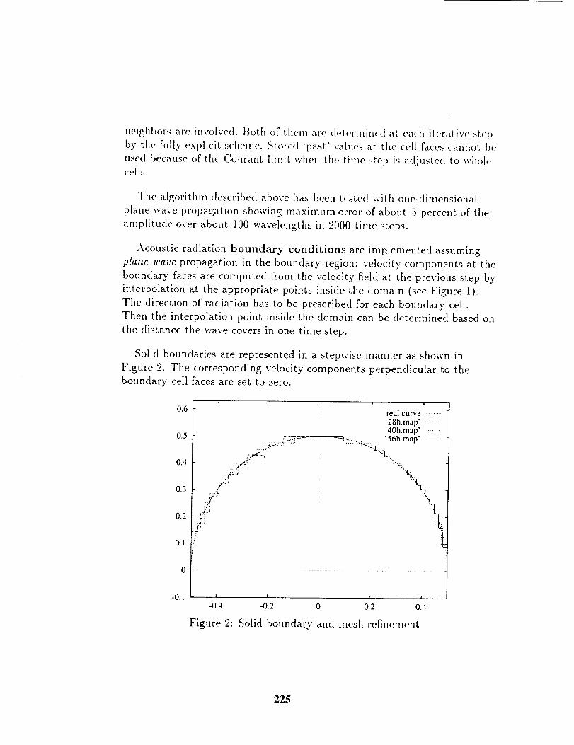
neighbors are involved. Both of them are (h'ternfined at each iterative step
by the fillly explicit scheme. Stored "past' values at the cell faces cannot be
used because of the Courant limit when the time step is adjusted to whole
cells.
Thc algorithm described above has been tested with one-dimensional
plane wave propagation showing maximum error of about 5 percent o[" the
amplitude over about i00 wavelengths in 2000 time steps.
Acoustic radiation boundary conditions are implemented assuming
plane u,ave propagation in the boundary region: velocity components at the
boundary faces are computed from the velocity field at the previous step by
interpolation at the appropriate points inside the domain (see Figure 1).
The direction of radiation has to be prescribed for each boundary cell.
Then the interpolation point inside the domain can be determined based on
the distance the wave covers in one time step.
Solid boundaries are represented in a stepwise manner as shown in
Figure :2. The corresponding velocity components perpendicular to the
boundary cell faces are set to zero.
0.6
0.5
0.4
0.3
0.2
0.1
0
-0.1
i i t t
real curve ......
'28h.map' - ....
"40h.map' -.....
ij_2-7..... _' 56h. map'.. : ...::-_-":, ........... .......>i _
_f-! : .... .p_
jl -
/!#.
i'.i
! 1 1 I 1
-0.4 -0.2 0 0.2 0.4
Figure "2: SoLid boundary and mesh refinement
225
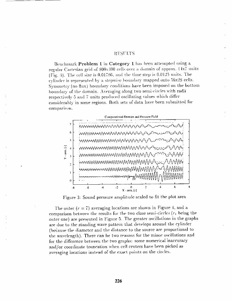
1_I'],51:UI'S
Benchmark Problem 1 in Category 1 has been attetnpted ttsing a
reglllar ('artesian grid of 800x 100 (:ell.s over a dornain of apl)rox, l.lx7 units
(Fig. 3). The cell .size is 0.01786. an(I the time step is 0.0125 units. The
cvliu<ler is represented by a st(,pwise bo!tu(lary mapped onto 56x2S cells.
Symmetry (no flux) t)omldary conditions have been imposed on the bottom
boundary of the domain. Averaging along two semi-circles with radii
respectively 5 and 7 units produced oscillating values which differ
considerably in some regions. Both sets of data have been submitted for
comparison.
Computational Domain and Pressure Fieldi i i i I i I
' i ........ iZ 4 ............ i
2
1
0I..r_ I I ,,. t 1 I 1
-8 -6 -4 -2 0 2 4 6
X -axis.[-I
Figure 3: Sound pressure amplitude scaled to fit the plot area
The outer (r = 7) averaging locations are shown in Figure 4, and a
comparison between the results for the two close semi-circles (rt being the
outer one) are pres.ented in Figure 5. The greater oscillations in the graphs
are due to the standing wave pattern that develops around the cylinder
(be_:ause the diameter and the distance to the source are proportional to
the wavelength). There can be two reasons for the minor oscillations and
for the difference between the two graphs: some numerical inaccuracy
and/or coordinate truncation when cell centers have been picked as
averaging locations instead of the exact points on the circles.
226
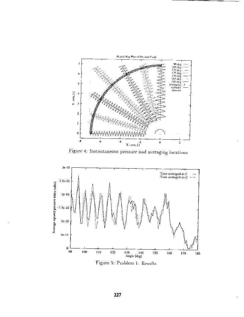
Radial-Ray Ph}t of Pressure Fieldi i i i
tN) deg --
7 "¢" 105 deg .....
.,:"_.___;' 120 deg --
6 .,.? a-; _ 165 deg .....
" dt:,fTl_li n
1_,I)dog --
5 averagmg ocylinder --
E 4
3
2
I
oI I 1 t I
-8 -6 -4 -2 0 2
X - axis. ['1
Figure 4: Instantaneous pressure and averaging locations
3e- 10
2.5e-10
._ 2e-10
• 1.5e- 10e-,
_ le-IO
e
<5e-ll
090
I
I00
i i
Time averaged at rl --Time averaged at r2 .....
¢
I I , i I I 1
110 120 130 140 150 160 170 180
Angle [degJ
Figure 5: Prob[em [: Results
227
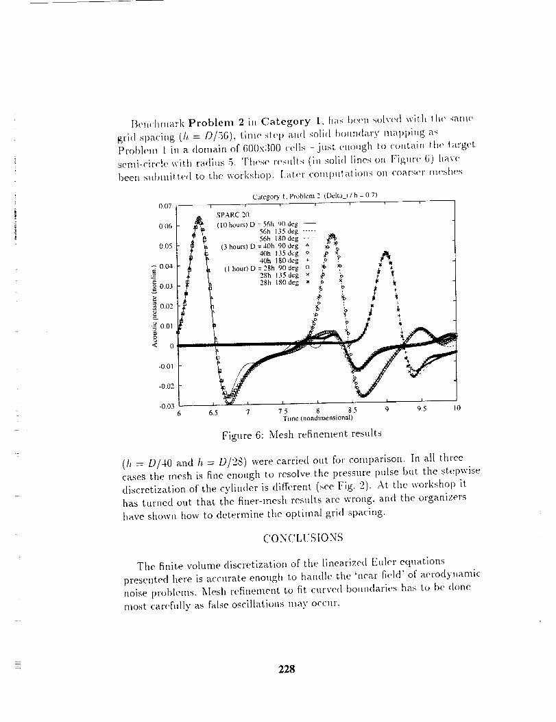
B('ll('llulark Problem 2 i,i Category 1, has l)(,en solvc<l witli the sam(,
grid spacing (h = DiS(J), tinie six' I) ali([ solid t)oundarv Inal)l)ing as
Drot)l('iil [ ill a donlairi of O00x;lO0 cells - just enough to contain lh(, target
senli-circle witti ra(liils 5. These results (in solid lines on Pigiir(" O) [lave
been sitl)iilitted to tile workshop. Later coilllJlllatiotls on coarser ill('shes
0.07
0.06
0.05
--: 0.04.
0.03
_, 0,02.u
,_ 0.01
< 0
-0,01
-0.02
-0.03
Category I. Problem 2 (Delta_t / h = 0.7)i i i i -- i i i
SPARC 20:
(10 hours) D = 56h 90 deg --56h 135 deg .....56h 180 deg ..... _.
(3 hours) D = 40h 90 deg adOh 135 deg '::' ,i_.40h 180deg + , ',
I hour) D = 28b 90deg D • _
28h 135 dog × } _28h 180deg _ _. , 1f
i
6 6.5 7 7.5 8 8.5 9 9.5 IO
Time (nondimensional)
Figure 6: Mesh refinement resttlts
(h = D/40 and h = D/28) were carried out for comparison. In all three
case_ the mesh is fine enough to resolve the pressure pulse but the stepwise
discretization of the cylinder is different (see Fig. 2). At the workshop it
has turned out that the finer-mesh results are wrong, and the organizers
have shown how to determine the oi)timal grid spacing.
' N'CO: CLUSIONS
The finite volume discretization of the linearized Euler equations
presented here is accurate enough to handle the 'near field' of aerodynamic
noise problems. Mesh refinement to fit curved boundaries has to be done
most carefully as false oscillations mar occm'.
228
Future work involves the inclttsiotl o[ tt.. convecthm and no./m(ar
terms [rom the Navior-Stokes [')ittat ions to pro+lttce a co.le capable of
simulatil G the getleration of aerodynamic noise.
References
[IJ
[.,]
[3]
[4]
[.q
[r]
[sl
Lighthill, NI.J., 1952, "On sound generated aerodynamically. Part I:
General theory", Proc. t_o!j. Soc. A, Vol. 21 i. pp. 564-557.
Sankar, S. and IIussaini, M.Y., 1993, %\ hybrM direct numerical
simulation of sound radiated from isotropic ttn'bulenc,:", ASME FED
Vol. 147, pp. $3-89.
Zhang, X., Rona, A., Lilley, G.M., "Far-field noise radiation from an
unsteady supersonic cavity flow", C'EAS/.-tL4A Paper 9.5-040.
Shih, S.H., Hixon, D.R. and Mankbadi, R.R., 1995, "A zonal approach
for prediction of jet noise", CEAS/AL4A Paper 95-144.
_. • _ " . .Tam, K. W. and .J.C. Vv'ebb, 1993, Dtsp_rslon-relatmn-preservmg
finite difference schemes for computational aeroacoustics"..]. Comp.
Phys., \_I. 107, pp. 262-281.
Lyrintzis, A.S., 1993, "The use of Kirchhoff's method in computational
aeroacoustics", ASME FED Vol. 147, pp. 53-6[.
Djambazov, C,.S., Lai, C.-H., Pericleous, K.A., 1996, "Development of a
domain decomposition method for computational aeroacoustics", Proc.
of the 9-th Conf. on Domain Decomposition, Bergen, Norway, June
1996, Editor P.Bjorstad, M.Espedal and D.Keves.
Viswanathatl, K. and Sankar, L.N., 199.5, "'Ntttnerical simulation of
airfoil noise", ASME FED. Vol. 219, pp. 6,5 70.
[lardin, .1., Invited Lecture given at the AS.lIE Forum on
Computational Aeroacou._tic.s and Hgdroacou.stic.s, June 1993.
229
E
SOLUTION OF AEROACOUSTIC PROBLEMS BY A NONLINEAI_,
HYBRID METHOD*
Yusuf OzySriik t and Lyle N. Long _
Department of Aerospace Engineering
The Pennsylvania State University
University Park, PA 16802
ABSTRACT
Category 1, problem 3 (scattering of sound by a sphere) and category 2, problem 1 (spherical
source in a cylindrical duct subject to uniform flow) are solved in generalized coordinates using
the nonlinear Euler equations together with nonreflecting boundary conditions. A temporally
and spatially fourth-order accurate finite-difference, Runge-Kutta time-marching technique is
employed for the near-field calculations and a Kirchhoff method is employed for the prediction of
far-field sound. Computations are all performed on parallel processors using the data-parallel
paradigm.
INTRODUCTION
Past several years have withnessed a significant activity [1] to develop computational tools for
aeroacoustic applications. This has been so because of the increasing availability of powerful
computers to the computational sciences community as well as the continuous need for further
understanding of the physics of flow associated noise and its accurate prediction for quiet engineering
designs. This activity ranged from the development of high level algorithms [2, 3] to high level
applications [4, 5, 6]. Recently, the present authors have developed a nonlinear, fourth-order accurate
(both in space and time), hybrid, parallel code [4, 7, 8] for the prediction of ducted fan noise. This
code solves the full Euler equations in the near field and uses a Kirchhoff method for the prediction of
far-field sound. This code has been shown to be able to make accurate predictions. It is the purpose
of this paper to describe the application of this code to the solutions of the benchmark problems of
the Second Computational Aeroacoustics (CAA) Workshop. Particularly, problem 3 of category 1,
and problem 1 of category 2 are solved. It is shown here that even relatively simple problems, such as
these, could be computationally intense and demanding if the far-field sound is of interest. Therefore,
far-field extrapolation techniques, such as the Kirchhoff method, must be used for feasible solutions.
*Work sponsored by NASA grant NAG-l-1367tpostdoctoral Scholar
tAssociate Professor
231
NONLINEAR, HYBRID CODE
The hybrid ducted fan noiseradiation code [7,4] solvestile 3-D Euler equationson a 3-Dbody-fitted coordinate systemand passesthe near-fieldacousticpressureto a Kirchhoff method basedon the formulation of Farassatand Myers [9] to predict the far-field sound. The governingequationsaresolvedin a relatively small domain using nonreflectingboundary conditions basedon the works ofBayliss and Turkel [10] and Tam and Webb [2]. For realistic engineinlet geometriesan orthogonalmeshsystemis created through a sequenceof conformalmappings [11]and the governingequationsare formulated in cylindrical coordinates to effectively treat the grid singularity at the centerline.
Fourth-order accurate, cell-centered finite differencing and four-stage, noncompact R-K time
integration are performed to advance the solution. Adaptive artificial dissipation [12] is used to
suppress high-fl-equency spurious waves. The Euler solver and the Kirchhoff method are coupled such
that as soon as the Euler solution becomes available, the Kirchhoff surface integrations are performed
in a forward-time-binning manner to predict the far-field noise. All calculations are carried out on
parallel computers using the data parallel paradigm. Ref. [7] describes the fourth-order flow solver
with emphasis on the hybrid code's parallel aspects. Ref. [4] discusses the acoustic source model and
the Kirchhoff coupling issues for engine inlet noise predictions. The hybrid code utilizes a spatially
fourth-order accurate multigrid procedure for efficient calculations of the mean flow and this
procedure is described in Ref. [8].
The boundary conditions routines of this code have been modified to accommodate the present
workshop problems. Also, the Kirchhoff routine of this code has been improved for time-periodic
problems. In such cases, after the trensients are gone, the near-field Euler solution is obtained only
for one time period and this solution is replicated in the Kirchhoff routine for longer time periods so
that the forward-time-binning procedure [4] can be completed for a converged far-field solution. This
approach results in significant CPU time savings.
RESULTS AND DISCUSSION
Solution of Category 1, Problem 3
This problem requires the solution of the acoustic field driven by a spherical (Gaussian) source
plus its scattered field from a sphere. The source and sphere centers are separated from each other by
a distance of one sphere diameter. Since this problem is axisymmetric, it is solved on a polar mesh in
a constant 0 plane (i.e. x - r plane, (x, r, 0) denote cylindrical coordinates) with an (x, r)-to-((, rl)
coordinate transformation. This mesh is constructed such that there exist 384 grid points along the
half-sphere wall (_) and 256 grid points in the normal direction to the sphere wall (7/). The physical
size of the computational domain is taken to be about 6 sphere radii so that a direct Euler solution
on a 5-radius circular are on the mesh could be obtained and compared with the Kirchhoff solution.
The Kirchhoff surface is chosen to be at about 3 radii, where the source strength is diminished. This
mesh has approximately 18 grid points per wavelength in both curvilinear coordinate directions in the
vicinity of the Kirchhoff surface so that the acoustic waves are well resolved on the Kirehhoff surface.
Figure 1 shows a snapshot of the acoustic pressure contours in the domain for a nondimensional
232
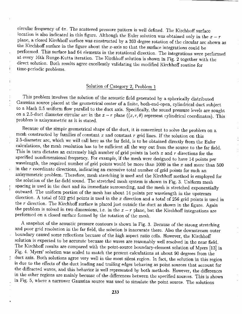
circular frequency of 4rr. The scattered pressure pattern is well defined. The Kirchhoff surface
location is also indicated in this figure. Although the Euler solution was obtained only in the x - r
plane, a closed Kirchhoff surface was constructed by a 360 degree rotation of the circular arc shown as
the Kirchhoff surface in the figure about the x-axis so that the surface integrations could be
performed. This surface had 64 elements in the rotational direction. The integrations were performed
at every 16th Runge-Kutta iteration. The Kirchhoff solution is shown in Fig. 2 together with the
direct solution. Both results agree excellently validating the modified Kirchhoff routine for
time-periodic problems.
Solution of Category 2, Problem 1
This problem involves the solution of the acoustic field generated by a spherically distributed
Gaussian source placed at the geometrical center of a finite, both-end-open, cylindrical duct subject
to a Mach 0.5 uniform flow parallel to the duct axis. Specifically, the sound pressure levels are sought
on a 2.5-duct diameter circular arc in the x - r plane ((x, r, 0) represent cylindrical coordinates). This
problem is axisymmetric as it is stated.
Because of the simple geometrical shape of the duct, it is convenient to solve the problem on a
mesh constructed by families of constant x and constant r grid lines. If the solution on this
2.5-diameter arc, which we will call here as the far field, is to be obtained directly from the Euler
calculations, the mesh resolution has to be sufficient all the way out from the source to the far field.
This in turn dictates an extremely high number of grid points in both x and r directions for the
specified nondimensional frequency. For example, if the mesh were designed to have 14 points per
wavelength, the required number of grid points would be more than 1000 in the x and more than 500
in the r coordinate directions, indicating an excessive total number of grid points for such an
axisymmetric problem. Therefore, mesh stretching is used and the Kirchhoff method is employed for
the solution of the far-field sound. The stretched mesh system is shown in Fig. 3. Uniform mesh
spacing is used in the duct and its immediate surrounding, and the mesh is stretched exponentially
outward. The uniform portion of the mesh has about 14 points per wavelength in the upstream
direction. A total of 512 grid points is used in the x direction and a total of 256 grid points is used in
the r direction. The Kirchhoff surface is placed just outside the duct as shown in the figure. Again
the problem is solved in two dimensions, i.e. in the x - r plane, but the Kirchhoff integrations are
performed on a closed surface formed by the rotation of the mesh.
A snapshot of the acoustic pressure contours is shown in Fig. 3. Because of the strong stretching
and poor grid resolution in the far field, the solution is inaccurate there. Also the downstream outer
boundary caused some reflections becuase of the high aspect ratio cells. However, the Kirchhoff
solution is expected to be accurate becuase the waves are reasonably well resolved in the near field.
The Kirchhoff results are compared with the point-source boundary-element solution of Myers [13] in
Fig. 4. Myers' solution was scaled to match the present calculations at about 90 degrees from the
duct axis. Both solutions agree very well in the most silent region. In fact, the solution in this region
is due to the effects of the duct leading and trailing edges behaving as point sources that account for
the diffracted waves, and this behavior is well represented by both methods. However, the differences
in the other regions are mainly becuase of the differences between the specified sources. This is shown
in Fig. 5, where a narrower Gaussian source was used to simulate the point source. The solutions
233
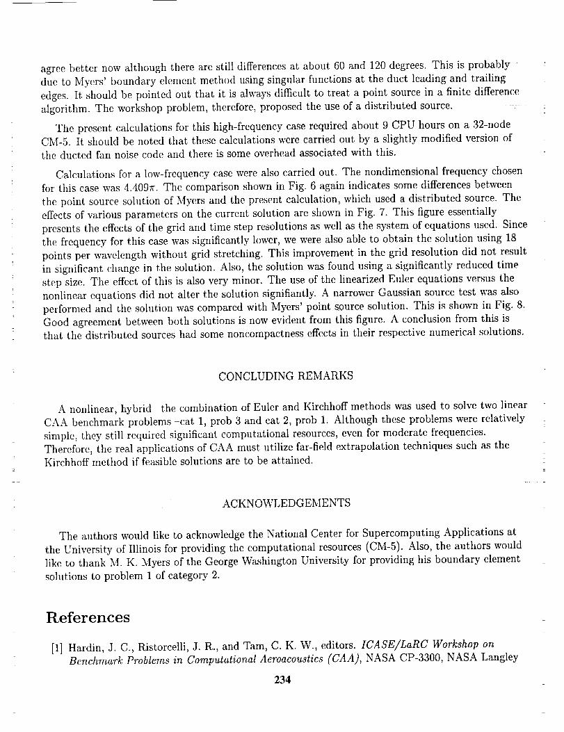
agree better now although there are still differences at about 60 and 120 degrees. This is probably
due to Myers' boundary element method using singular functions at the duct leading and trailing
edges. It should be pointed out that it is always difficult to treat a point source in a finite difference
algorithm. The workshop problem, therefore, proposed the use of a distributed source.
The present calculations for this high-frequency case required about 9 CPU hours on a 32-node
CM-5. It should be noted that these calculations were carried out by a slightly modified version of
the ducted fan noise code and there is some overhead associated with this.
Calculations for a low-frequency case were also carried out. The nondimensional frequency chosen
for this case was 4.4097_. The comparison shown in Fig. 6 again indicates some differences between
the point source solution of Myers and tile present calculation, which used a distributed source. The
effects of various parameters on the current solution are shown in Fig. 7. This figure essentially
presents the effects of the grid and time step resolutions as well as the system of equations used. Since
the frequency for this case was significantly lower, we were also able to obtain the solution using 18
points per wavelength without grid stretching. This improvement in the grid resolution did not result
in significant change in the solution. Also, the solution was found using a significantly reduced time
step size. The effect of this is also very minor. The use of the linearized Euler equations versus the
nonlinear equations did not alter the solution signifiantly. A narrower Gaussian source test was also
performed and the solution was compared with Myers' point source solution. This is shown in Fig. 8.
Good agreement between both solutions is now evident from this figure. A conclusion from this is
that the distributed sources had some noncompactness effects in their respective numerical solutions.
CONCLUDING REMARKS
z
A nonlinear, hybrid the combination of Euler and Kirchhoff methods was used to solve two linear
CAA benchmark problems -cat 1, prob 3 and cat 2, prob 1. Although these problems were relatively
simple, they still required significant computational resources, even for moderate frequencies.
Therefore, the real applications of CAA must utilize far-field extrapolation techniques such as the
Kirchhoff method if feasible solutions are to be attained.
. z
ACKNOWLEDGEMENTS
The authors would like to acknowledge the National Center for Supercomputing Applications at
the University of Illinois for providing the computational resources (CM-5). Also, the authors would
like to thank M. K. Myers of the George Washington University for providing his boundary element
solutions to problem 1 of category 2.
References
[1] Hardin, J. C., Ristorcelli, J. R., and Tam, C. K. W., editors. ICASE/LaRC Workshop on
Benchmark Problems in Computational Aeroacoustics (CAA), NASA CP-3300, NASA Langley
234
[2]
[3]
[4]
[5]
Research Center, Hampton, VA, May 1995.
Tam, C. K. W., and \Vebb, J. C. Dispersion-relation-preserving finite difference schemes for
computational acoustics. Journal of Computational Physics, 107, pp. 262-281, 1993.
Hu, F. Q., Hussaini, M. Y., and Manthey, J. Low-dissipation and low-dispersion Runge-Kutta
schemes for computational acoustics. Journal of Computational Physics, 124(1), pp. 177-191,1996.
OzySriik, Y., and Long, L. N. Computation of sound radiating from engine inlets. AIAA
Journal, 34(5), pp. 894-901, May 1996.
Chyczewski, T. S., and Long, L. N. Numerical prediction of the noise produced by a perfectly
expanded rectangular jet. AIAA paper 96-1730, 2nd AIAA/CEAS Aeroacoustics Conference,State College, PA, May 1996.
[6] Bangalore, A., Morris, P. J., and Long, L. N. A parallel three-dimensional computational
aeroacoustics method using non-linear disturbance equations. AIAA Paper 96-1728, 2nd
AIAA/CEAS Aeroacoustics Conference, State College, PA, May 1996.
[7] OzySriik, Y., and Long, L. N. A new efficient algorithm for computational aeroacoustics on
parallel processors. Journal of Computational Physics, 125(1), pp. 135-149, April 1996.
[8] OzySriik, Y., and Long, L. N. Multigrid acceleration of a high-resolution computational
aeroacoustics scheme. AIAA Journal, 35(3), March 1997.
[9]
[10]
[11]
[12]
[13]
Farassat, F., and Myers, M. K. Extension of Kirchhoff's formula for radiation from moving
surfaces. Journal of Sound and Vibration, 123, pp. 451-460, 1988.
Bayliss, A., and Turkel, E. Far field boundary conditions for compressible flow. Journal ofComputational Physics, 48, pp. 182-199, 1982.
C)zySriik, Y. Sound Radiation From Ducted Fans Using Computational Aeroacoustics On Parallel
Computers. PtI.D. thesis, The Pennsylvania State University, December 1995.
Swanson, R. C., and Turkel, E. Artificial dissipation and central difference schemes for the Euler
and Navier-Stokes equations. AIAA Paper 87-1107, 1987.
Myers, M. K. Boundary integral formulations for ducted fan radiation calculations. CEAS/AIAAPaper 95 076, 1995.
235
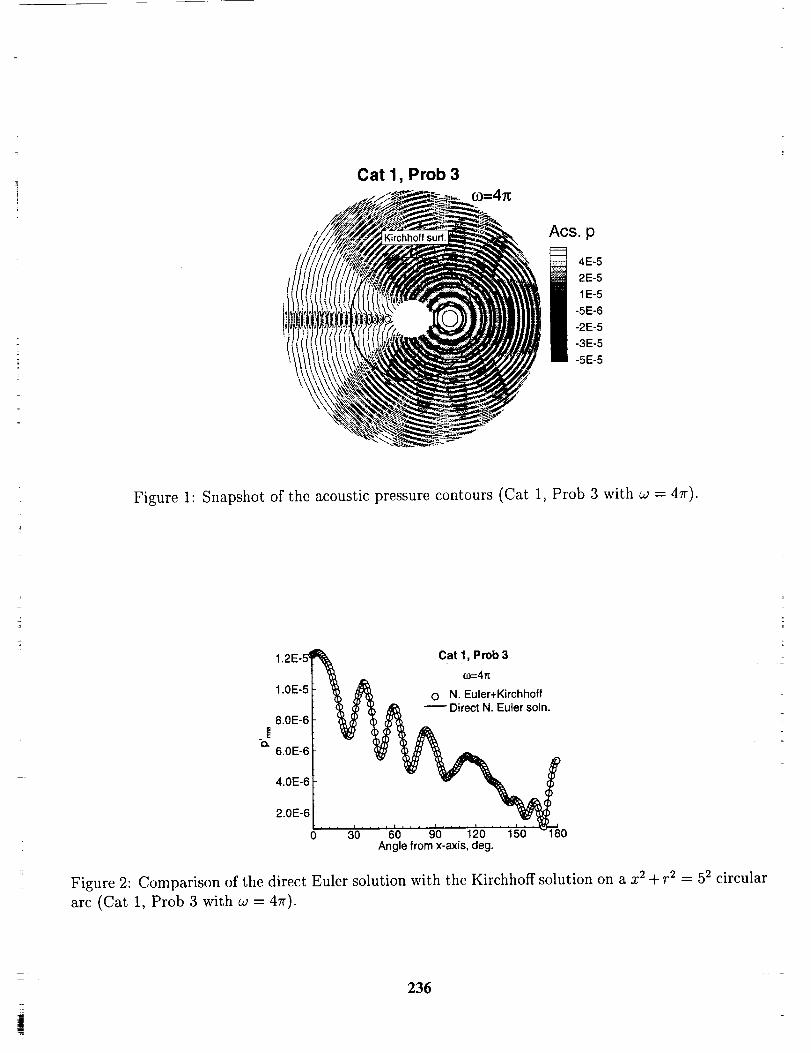
Figure 1: Snapshot of the acoustic pressure contours (Cat 1, Prob 3 with w = 47r).
.[¢k
1.2E.5 _
1.0E-5
8,0E-6
6.0E-6
4.0E-6
2.0E-6
0
Cat 1, Prob 3
co=4=
O N. Euler+Kirchhoff
_ Direct N. Euler soln.
0Angle from x-_is, deg.
Figure 2: Comparison of the direct Euler solution with the Kirchhoff solution on a x 2 + r2 = 52 circular
arc (Cat 1, Prob 3 with w = 47r).
236
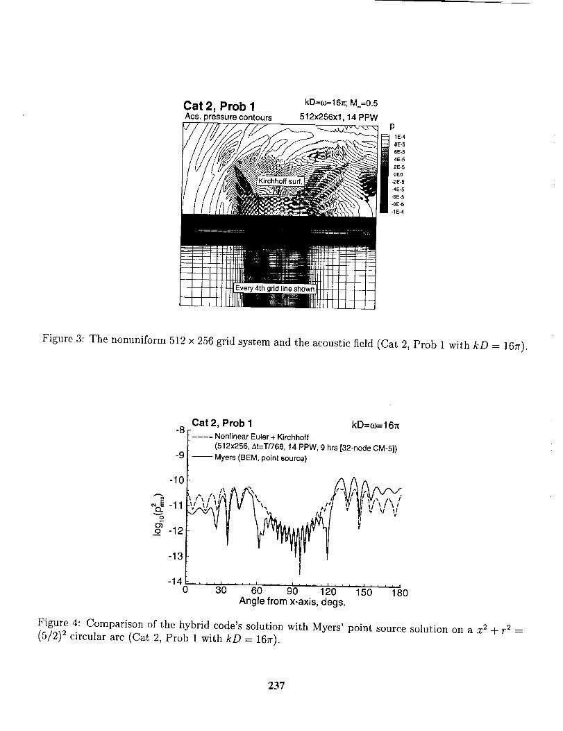
Cat 2, Prob 1Acs. pressurecontours
kD=e_=16_;M=0.5
512x256x1, 14 PPWP
1 E-4
8E-5
6E-5
4E-5
2E-5
OEO
-2E-5
-4E-5
-6E-5
-8E-5
-1E-4
Figure 3: The nonuniform 512 × 256 grid system and the acoustic field (Cat 2, Prob 1 with kD = 167r).
-11v
o
o_o -12
Cat 2, Prob I kD=co=16_-8 [ .... NonlinearEuler+ Kirchhoff
[ (512x2.56,&t=T/768,14 PPW,9 hrs [32-nodeCM-5])
-9 [-- Myers(BEM,pointsource)!
, ,,, f,/2,¢_ _', , •
_13____ '
-14 ......... , ............ ,, _, , ,, _0 30 150 18060 90 120
Angle from x-axis, degs.
Figure 4: Comparison of the hybrid code's solution with Myers' point source solution on a x 2 + r 2 =
(5/2) 2 circular arc (Cat 2, Prob 1 with kD = 167r).
237
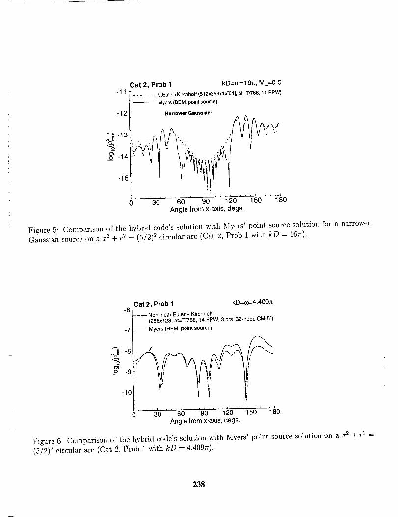
-11
-12
-13
--%
oT.9o -14
-15
Cat 2, Prob I kD=e)=16_; M=0.5
....... L.Euler+Kirchhoff (512x256xlx[64], At=T/768, 14 PPW)
Myers (BEM, point source)
-Narrower Gausslan-
, f
i i i i r i i ' ' I .... 1_ I , , , 1 .... t .... 1
0 30 60 90 120 150 180Angle from x-axis, degs.
Figure 5: Comparison of the hybrid code's solution with Myers' point source solution for a narrower
Gaussian source on a x 2 + r 2 = (5/2) 2 circular arc (Cat 2. Prob 1 with kD = 167r).
Cat 2, Prob I kD=¢_--4.409_
-6 [____ Nonlinear Euler + Kirchhoff
t (256xl 28, At=T/768, 14 PPW, 3 hrs [32-node CM-5])
-7 I_ Myers (BEM, point source)
1 l/
-,° V!
_ -8v
o -9
o .... 3'0.... 6'o.... 9'o'' ' 1_6' ' 1_5 " 18oAngle from x-axis, degs.
Figure 6: Comparison of the hybrid code's solution with Myers' point source solution on a x 2 + r 2 =
(5/2) 2 circular arc (Cat 2, Prob 1 with kD = 4.4097r).
238
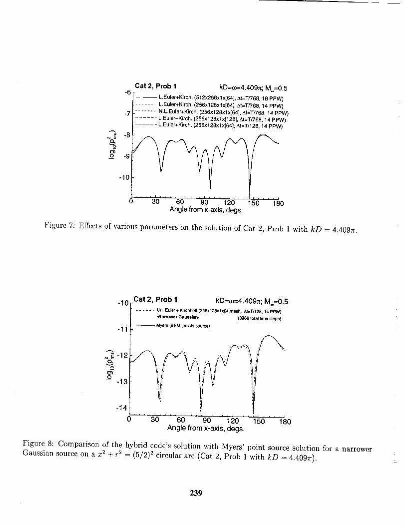
O3O
-6
-7
-8
-9
-10
0
Cat 2, Prob I kD=m=4.409_; M=0.5
-- L.Euler+Kirch. (512x256xl x[64], At=T/768, 18 PPW)
....... L.Euler+Kirch. (256x128xlx[64], At=T/768, 14 PPW)
............. N.L.Euler+Kirch. (256x128xlx[64], At=T/768, 14 PPW)
...... L.Euler+Kirch. (256xl 28xl x[128], At=T/768, 14 PPW)
............. L.Euler+Kirch. (256x128xlx[64], At=T/128, 14 PPW)
1 .... I
50 180, , . . I i , i i .L. i i , i ! .... I , , .
30 60 90 120Angle from x-axis, degs.
Figure 7: Effects of various parameters on the solution of Cat 2, Prob 1 with kD = 4.4097r.
-10
-11
v
_DO-- -13
-14
0
Cat 2, Prob 1 kD=o)=4.409_; M=0.5...... Lin. Euler + Kirchhoff (256x128xlx64 mesh, ht=T/128, 14 PPW)
-Narrower Gausslan- (3968 total time steps)
-- Myers (BEM, points source)
iI
. J/ /I
i I i i i i l , , , I. I • , I i I r i ,
30 60 90 120
Angle from x-axis, degs.
. I .... I
50 180
Figure 8: Comparison of the hybrid code's solution with Myers' point source solution for a narrower
Gaussian source on a x 2 + r 2 = (5/2) 2 circular arc (Cat 2, Prob 1 with kD = 4.4097r).
239
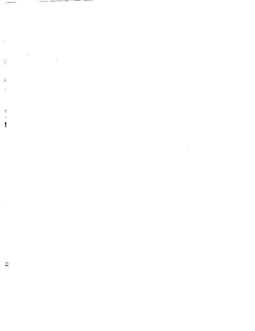
m
7THREE-DIMENSIONAL CALCULATIONS OF ACOUSTIC SCATTERING BY A
SPHERE: A PARALLEL IMPLEMENTATION
Chingwei M. Shieh* and Philip J. Morris t
Department of Aerospace Engineering
The Pennsylvania State University
University Park, PA 16802
ABSTRACT
In this paper, the problem of acoustic scattering by a sphere is considered. The calculations
are carried out with the use of a high-order, high-bandwidth numerical scheme and explicit time
integration. Asymptotic non-reflecting radiation boundary conditions are applied at the outer
boundaries of the computational domain, and the Impedance Mismatch Method (IMM)
developed by Chung and Morris 1 is implemented in order to treat solid wall boundaries. Since a
three-dimensional simulation of moderate source frequency is desired, parallel computation is
exploited in order to decrease the computation time required. This study further demonstrates
that in order for realistic CAA calculations to be performed, the computational power of parallel
computers has to be harnessed.
INTRODUCTION
The scattering of sound from a spatially distributed, spherically symmetric source by a sphere is
an excellent test case for numerical simulations in CAA. While the phenomenon is well understood,
three-dimensional calculations of such problem with a moderate to high frequency source are still a
daunting task because of the number of grid points per wavelength needed in order to resolve the
acoustic waves. In this paper, such simulations are performed with the utilization of parallel
computation. Numerical results are compared with the analytical solutions derived by Morris 2, and
excellent agreement has been found.
NUMERICAL ALGORITHM
In the section, the governing equations that describe the acoustic scattering problem are given.
The solution algorithm, with the implementation of non-reflecting boundary conditions and the IMM
for the solid wall boundaries, are mentioned only briefly. The parallel numerical algorithm is also
discussed briefly, and data from a scalability study are presented to demonstrate the improvement in
performance using parallel computations.
*Graduate research assistant
tBoeing Professor of Aerospace Engineering
241
Governing Equations
The problem of acoustic scattering is governed by the linearized Euler equations. In a
three-dimensional Cartesian co-ordinate system, the equations can be written as
0 I [ 0ul]1p0vl][ 0wl][0]p' ' Ap0 pou' 0 pov' 0 P°oW = 0
u' p'lpo o +-5-;v I 0 P'/Po 0 0
w' 0 0 P' / Po 0
(1)
where it is assumed that there is no mean flow. In the above equations, all quantities are
non-dimensionalized by the radius of the sphere, R, the ambient speed of sound, a_o, and the ambient
density, Poo, as the length, velocity, and density scales, respectively. The characteristic scales for the
pressure and time are pooa_ and R/am, and the source term, Ap, is given by
-A exp _ - B(log 2)[(x- x_) 2 + y2 + z21_ cos(wt) (2)ApL J
where A - 0.01, B = 16, xs = 2, and w = 2u. p0 is the non-dimensional mean density equal to unity
exterior to the body.
Solution Algorithm
In the present study, a high-order, high-bandwidth numerical scheme is implemented for the
spatial discretization of the governing equations. This scheme, the Dispersion-Relation-Preserving
(DRP) method developed by Tam and Webb 3, is an optimized third-order finite difference operator
with the use of a seven-point stencil. A standard fourth-order Runge-Kutta time integration
algorithm has been applied for explicit time stepping. It has been shown in various CFD studies that
central difference operators are inherently unstable. Therefore, in order to circumvent this problem, a
filter is added explicitly. A sixth derivative is used as a smoother, as proposed by Lockard and
Morris4; however, since a uniform computational grid is used, and it is expected that the problem
does not possess any nonlinear effects, the artificial dissipation model has been further simplified so
that only a constant coefficient filter is applied. This decreases the computational time significantly
without sacrificing the integrity of the data.
Asymptotic non-reflecting radiation boundary conditions, first developed by Tam and Webb z in
two dimensions and later extended to three-dimensional cases by Chung and Morris l, are applied at
the outer boundaries of the computational domain. The Impedance Mismatch Method (IMM) is
introduced to treat the solid wall boundaries. This is achieved by simply setting a different value of p0
inside the sphere. Further details are given by Chung and Morris 1.
Parallel Implementation and Performance
The parallel implementation employed in the present study follows the same strategy outlined by
Lockard and Morris 4. The code is written in Fortran 90 with the Message Passing Interface (MPI) on :;
242 _
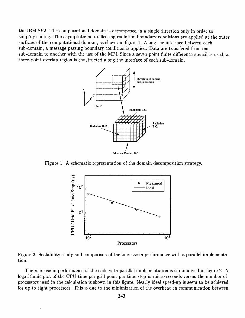
the IBM SP2. The computational domain is decomposedin a singledirection only in order tosimplify coding. The asymptotic non-reflectingradiation boundary conditions areapplied at the outersurfacesof the computational domain, asshownin figure 1. Along the interfacebetweeneachsub-domain,a messagepassingboundary condition is applied. Data are transfered from onesub-domainto another with the useof the MPI. Sincea sevenpoint finite differencestencil is used,athree-point overlap region is constructedalong the interface of eachsub-domain.
r ....
II
..................... t_=:
Z ............................... "1
I." Direction of domain
..'1 .,. decomposition
Radiation B.C.
_ Radiation
Radiation B.C. B.C.
!Message Passing B.C.
Figure 1: A schematic representation of the domain decomposition strategy.
=L
102Ci3
1
[] Measured
Ideal
10° 101
Processors
Figure 2: Scalability study and comparison of the increase in performance with a parallel implementa-
tion.
The increase in performance of the code with parallel implementation is summarized in figure 2. A
logarithmic plot of the CPU time per grid point per time step in micro-seconds versus the number of
processors used in the calculation is shown in this figure. Nearly ideal speed-up is seem to be achieved
for up to eight processors. This is due to the minimization of the overhead in communication between
243
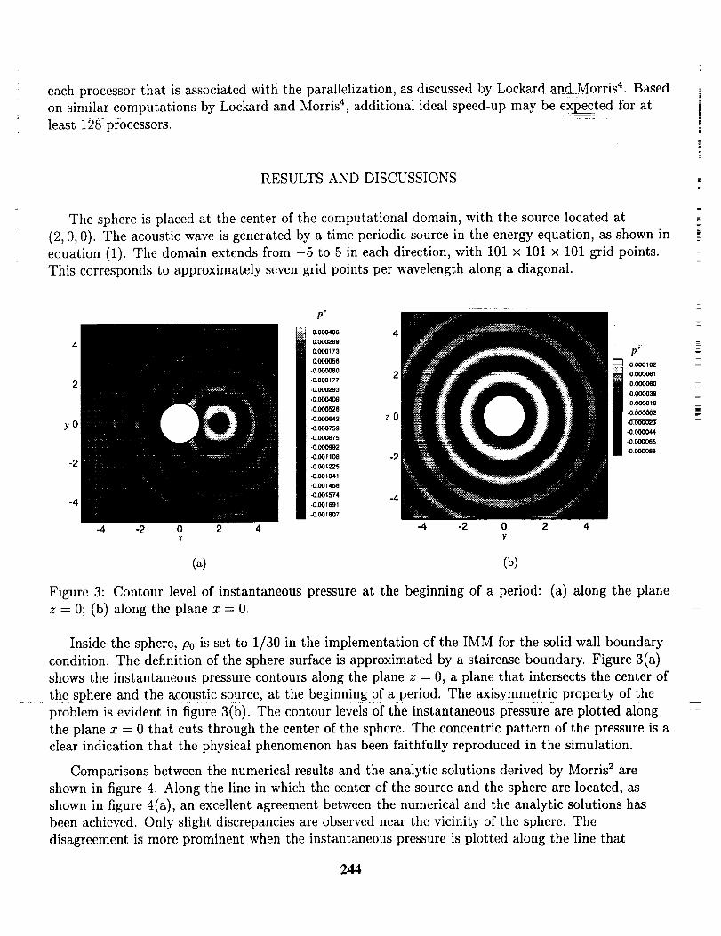
each processor that is associated with the paralMization, as discussed by Lockard and Morris 4. Based
on similar computations by Lockard and Morris 4, additional ideal speed-up may be eXl;)ected for at
least 128 processors.
RESULTS AND DISCUSSIONS
The sphere is placed at the center of the computational domain, with the source located at
(2, 0, 0). The acoustic wave is generated by a time periodic source in the energy equation, as shown in
equation (1). The domain extends from -5 to 5 in each direction, with 101 x 101 x 101 grid points.
This corresponds to approximately seven grid points per wavelength along a diagonal.
4
y0
-2
-4
p'
o.o0o4o6 40.0002R9
0.000173
0.000056
-0.000060 2-0.O00177
-0.000293
-0.000409
-0.000526
.0.ooo_2 z 0-0.000759
-0.000875
KI.000992
-o.oo,me -2-0.00,_5
-0.001341
-0.001458
-0.001574 -4-0.001691
-0.001807
-4 -2 0 2 4 -4 -2 0 2 4X Y
p_
i 0.000 log
0.000061
0.000039
0.000019-0.000002
..0.0o00_
41.000044
41.000065
-0.000086
(a) (b)
Figure 3: Contour level of instantaneous pressure at the beginning of a period: (a) along the plane
z = 0; (b) along the plane x = 0.
Inside the sphere, P0 is set to 1/30 in the implementation of the IMM for the solid wall boundary
condition. The definition of the sphere surface is approximated by a staircase boundary. Figure 3(a)
shows the instantaneous pressure contours along the plane z = 0, a plane that intersects the center of
the sphere and the a_coustic source, at the beginning of a period. The axisymmetric property of the
problem is evident in figure 3(b). The contour levels of the instantaneous pressure are plotted along
the plane x = 0 that cuts through the center of the sphere. The concentric pattern of the pressure is a
clear indication that the physical phenomenon has been faithfully reproduced in the simulation.
Comparisons between the numerical results and the analytic solutions derived by Morris _ are
shown in figure 4. Along the line in which the center of the source and the sphere are located, as
shown in figure 4(a), an excellent agreement between the numerical and the analytic solutions has
been achieved. Only slight discrepancies are observed near the vicinity of the sphere. The
disagreement is more prominent when the instantaneous pressure is plotted along the line that
244
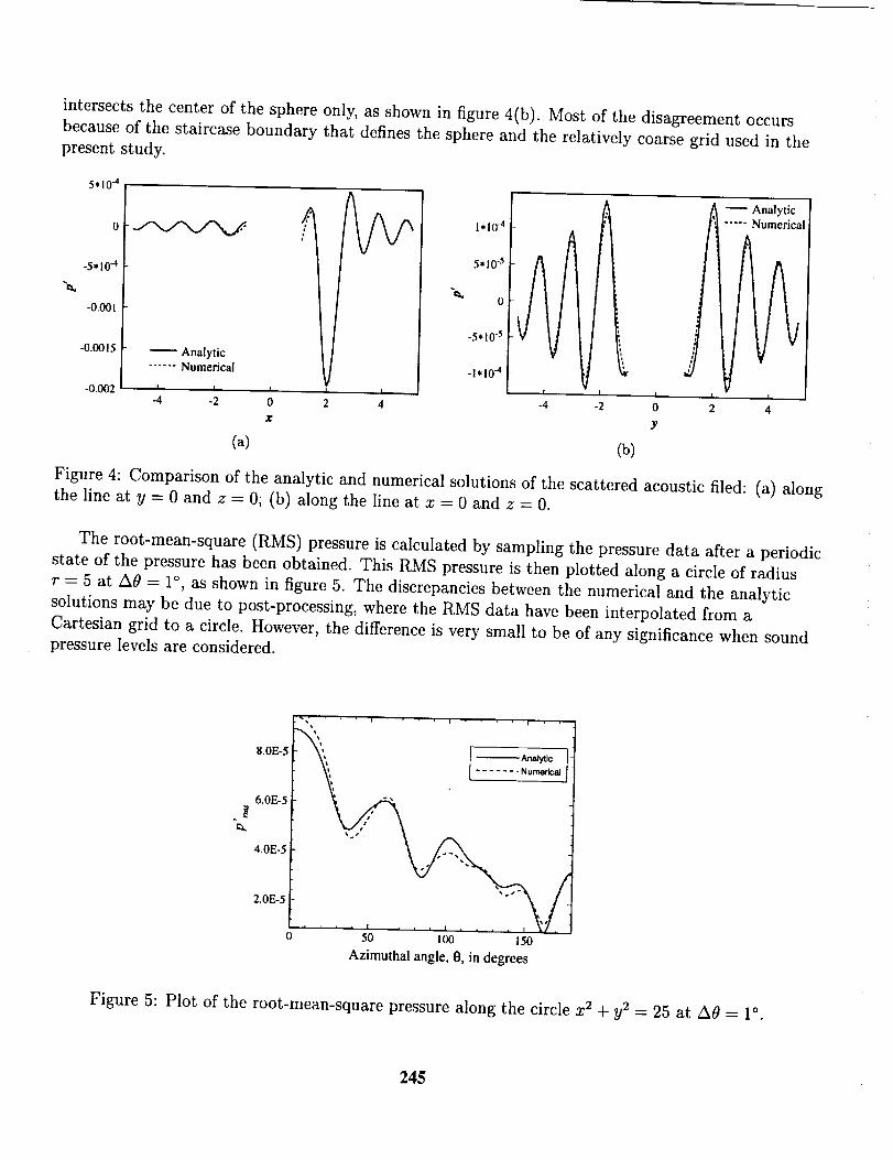
intersects the center of the sphere only, as shown in figure 4(b). Most of the disagreement occurs
because of the staircase boundary that defines the sphere and the relatively coarse grid used in the
present study.
5.10.4
-0.00 l
-0.0015
:.:,:,: ¢ 1,10.4
5,10-s
0
-5,1ffs
-I,I0_
jAnalytic _¢
...... Numerical
-0.002 i J i i _ f J i i-4 -2 0 2 4 -4 -2 0 2
x Y
(a) (b)
Analytic
..... Numerical
A
.t
I
4
Figure 4: Comparison of the analytic and numerical solutions of the scattered acoustic filed: (a) along
the line at y = 0 and z --- 0; (b) along the line at x = 0 and z = 0.
The root-mean-square (RMS) pressure is calculated by sampling the pressure data after a periodic
state of the pressure has been obtained. This RMS pressure is then plotted along a circle of radius
r -- 5 at A0 = 1°, as shown in figure 5. The discrepancies between the numerical and the analytic
solutions may be due to post-processing, where the RMS data have been interpolated from a
Cartesian grid to a circle. However, the difference is very small to be of any significance when sound
pressure levels are considered.
8.0E-5
6.0E-5
4.0E-5
2.0E-5
_' '' ' ' I I i ' '
_, •
_ s
50 100 150
Azimuthal angle, 0, in degrees
Figure 5: Plot of the root-mean-square pressure along the circle x 2 + y2 = 25 at A0 = 1°.
245
CONCLUSIONS
In this paper, a three-dimensionalcalculation of acousticscattering by a spherehas beenperformed with a parallel implementation. It hasbeendemonstratedthat parallel computing canbeexploited for CAA calculations in order to achievebetter computation time. The treatment of solidwall boundarieswith the useof the IMM hasbeenimplementedin the presentcomputation. Thismethod hasmany advantagesover traditional solid wall boundary conditions, suchassimplicity incoding, increasein speedof computation, and the ability to treat curved boundariesin Cartesian
grids. Good agreement between the numerical and the analytic solutions has been observed.
REFERENCES
[1] Chung, C., and Morris, P. J. Acoustic scattering from two- and three-dimensional bodies.
CEAS/AIAA Paper 95-008. Submitted to Journal of Computational Acoustics.
[2] Morris, P. J. Scattering of sound from a spatially distributed, spherically symmetric source by a
sphere. Journal of Acoustical Society of America, 98, pp. 3536-3539, 1995.
[3] Tam, C. K. W., and Webb, J. C. Dispersion-relation-preserving finite difference schemes for
computational aeroacoustics. Journal of Computational Physics, 107, pp. 262-281, 1993.
[4] Lockard, D., and Morris, P. J. A parallel implementation of a computational aeroacoustic
algorithm for airfoil noise. AIAA Paper 96-1754, 1996. To appear in Journal of ComputationalAcoustics.
246
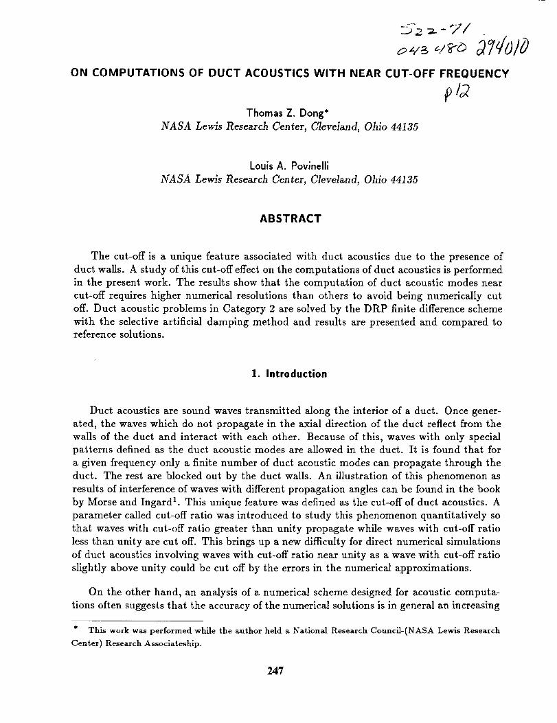
ON COMPUTATIONS OF DUCT ACOUSTICS WITH NEAR CUT-OFF FREQUENCY
Thomas Z. Dong*
NASA LeMs Research Center, Cleveland, Ohio 44135
Louis A. Povinelli
NASA Lewis Research Center, Cleveland, Ohio 44135
ABSTRACT
The cut-off is a unique feature associated with duct acoustics due to the presence of
duct walls. A study of this cut-off effect on the computations of duct acoustics is performed
in the present work. The results show that the computation of duct acoustic modes near
cut-off requires higher numerical resolutions than others to avoid being numerically cut
off. Duct acoustic problems in Category 2 are solved by the DRP finite difference scheme
with the selective artificial damping method and results are presented and compared toreference solutions.
1. Introduction
Duct acoustics are sound waves transmitted along the interior of a duct. Once gener-
ated, the waves which do not propagate in the axial direction of the duct reflect from the
walls of the duct and interact with each other. Because of this, waves with only special
patterns defined as the duct acoustic modes are allowed in the duct. It is found that for
a given frequency only a finite number of duct acoustic modes can propagate through the
duct. The rest are blocked out by the duct walls. An illustration of this phenomenon as
results of interference of waves with different propagation angles can be found in the book
by Morse and Ingard 1. This unique feature was defined as the cut-off of duct acoustics. A
parameter called cut-off ratio was introduced to study this phenomenon quantitatively so
that waves with cut-off ratio greater than unity propagate while waves with cut-off ratio
less than unity are cut off. This brings up a new difficulty for direct numerical simulations
of duct acoustics involving waves with cut-off ratio near unity as a wave with cut-off ratio
slightly above unity could be cut off by the errors in the numerical approximations.
On the other hand, an analysis of a numerical scheme designed for acoustic computa-
tions often suggests that the accuracy of the numerical solutions is in general an increasing
* This work was performed while the author held a National Research Council-(NASA Lewis Research
Center) Research Associateship.
247
function of the number of mesh points per wave length. This implies that more accurate
solutions will be produced for waves containing more mesh points than those containing
less. So if a scheme can produce an accurate solution for a wave with say eight points
per wave length, one would expect better or least equally accurate solutions for waves
containing more mesh points. For computations of duct acoustics, this is not necessarily
the case. In the present work, it will be shown that poor numerical solutions could be
produced for duct acoustic waves near cut-off, although the waves are well in the accurate
solution range. Higher resolutions are required for these duct acoustic waves in order to
produce the expected accuracy.
In the next section, we start with a brief review of linear duct acoustics including the
definitions of cut-off ratio, group velocity. In Section 3, a duct acoustic inflow boundary
condition is derived. The numerical simulations and a discussion of the results are given
in Section 4.
2. Linear Duct Acoustics
Consider a uniform subsonic mean flow with Mach number M0 in an infinitely long
circular duct with radius R. The linear duct acoustics is governed by the linearized Euler's
equations which can be further simplified to give the convective wave equation for acoustic
pressure p
0 0 2p(_+M0 ) -V_p= 0 (1)
and the boundary condition at r = R
0p -0 (2)Or
The flow variables are non-dimensionalized by a0, p0 and poa_ where a0 and p0 are the
speed of sound and density of the mean flow.
A single eigen-solution or duct acoustic solution to the above system can be written as
pm,_(r,O,z,O = P,,_,_d_(t.t,,._r)e i(:_''_°-_t) (3)
where m is the circumferential mode number and n is the radial mode number. The
eigenvalue #,_,_ is the nth zero of the derivative of the ruth order Bessel function din,
namely
J'(#m,_n) =0 (4)
The variable k is the axial wave number and w is the angular frequency. They are related
by the dispersion relation of equation (1)
D(k,w) (w Mok)2 k _ 2.... #m,_ = 0 (5)
248
It can be easily seen that duct acoustic waves are dispersive. The group velocity of the
duct acoustics can be obtained from the above equation as
d02 k
V_(02, k)- dk - Mo + (6)oJ-Mok
The axial wave number can be solved as
1-- - M_),_ ]k+ (l_Mo_)[_Mow± V/022_(1 _ 2 (7)
where k+ represents waves propagating downstream and k_ represents waves travelingupstream. For
022>1
2 --
k+ are real. Waves propagate both upstream and downstream without attenuation. For
02 2<1
2 2(:-
k_: are a pair of conjugate complex numbers. Waves in both directions are attenuated ex-
ponentiaUy with distance. This means no waves with these wave numbers can be observed
away from the source region in both upstream and downstream directions. These waves
axe defined as being cut off while the waves propagating without attenuation are referred
as to being cut on. A special parameter "cut-off ratio" is therefore introduced as
_'n'b 'rb =
O2
ttm,_V/1 - Moa
Waves with cut-off ratio greater than unity are cut on and waves with cut-off ratio less than
unity are cut off. For waves with cut-off ratio less than or equal to unity, the group velocities
are equal to zero. This means that the waves which are cut-off are not propagating and
waves with cut-off ratio only slightly greater than unity will propagate very slowly.
3. Duct Acoustics Inflow Boundary Condition
In numerical simulations of duct acoustics radiation, where the duct acoustic waves are
generated inside the duct and propagate through the duct and radiate to the ambient from
the duct open end, the duct must have a finite length. The boundary condition imposed
at the inflow boundary or the inner boundary of the duct, for problem 2 of Category 2,
serves two purposes. First, it simulates a noise source to generate duct acoustic waves
propagating towards the open end. Second, it must allow the acoustic waves reflected
249
from the open end to travel out of the computational domain. The acoustic solution therecan be written as a sum of the incident and reflected waves,namely ....
p = p,. + p.o (8)
Assuming a single angular frequency w, the reflected wave must be in the form
The axial wave number km,_ can be computed from the dispersion relation
]i_ m Tb
O3_ 1 [-Mo + 11-(I- Mo2)(_) 2 ]l-Mo 2
(10)
For reflected waves the plus sign in the above equation should be taken.
Differentiating equation (9) with respect to x and t yields
Op Oplr_ (11)Oz Oz
mTb
and Op Opin-- -- zWpreOt Ot
Since only the cut-on modes of the reflected waves are considered,
(V/1 - Mg)gm,_/w < 1. A Taylor series approximation leads to
(12)
we must have
il (1 M{)(_-_) _ 1+0((1 M2 (#m'_)2.... 0) --d- )
Therefore, by combining equations (11)-(13), we obtain the boundary equation for p
(13)
0I) +(1 + Op Op_,_O-7 Mo)_- Ot + (1 + Mo)_-_ '_ (14)
Similarly, boundary equations for other variables with the same form can be obtained.
4. Numerical Simulations of Duct Acoustics
In this section, the duct acoustics problems in Category 2 were solved by the DRP
scheme with the selective artificial damping method in reference 2-3. Schematic diagrams
of the computational domains for both problem 1 and 2 are shown in Figure 1-2. The duct
wall thickness was set to be Ar instead of zero to eliminate the ambiguity in numerical
approximation of x derivatives at points near the tips. The the length scale L is set to be
250
the duct diameter D for problem 1 and the radius R for problem 2. The time scale is L/ao.
The damping coefficient # was set to be 0.05. To remove the singularities at the tips of the
duct wall due to the inviscid approximation, larger damping coefficients were used at the
tips (#t = 1.0) and along the wall (/_,o = 0.1). A Gaussian function with half width equal
to three mesh points was used to make a smooth transition of the damping. The time
step was set to be At = 0.05Az. The amplitude of the source was multiplied by a time
dependent factor 1 - e -('_'_t/_°°°a*)2 to make a smooth transient. The governing equations
are the Euler's equations. A numerical treatment of sofid wall boundary condition with the
minimum number of ghost points for high order schemes, developed by Tam and Dong 4,
was applied to the solid surfaces of the duct walls. The computations are done on IBM
RS/6000-590 workstations.
For problem 1, a harmonic source function with a narrow Gaussian spatial distribution
located at the center of the duct was added to the continuity and energy equations as
specified by the problem. The acoustic radiation boundary condition was used at the
inflow and top boundaries and the outflow boundary condition was used at the outflow
boundary. These boundary conditions can be found in reference S by Tam and Webb. Two
cases with angular frequency w = 4.409507rr and 16rc were computed. The mesh size for
the lower frequency case was Az = Ar = D/51. The shortest acoustic wave contains about
12Az. The mesh size for the higher frequency case was set to be Az = Ar = D/159. The
shortest wave in this case is about 10Aa:. The computational domain contains 272x136
and 801x401 mesh points for the lower and higher frequency cases respectively. The
solutions took a long time to reach a good periodic state. This could be partially due
to the fact that the modes near cut-off took long time to travel out of the duct. The
w = 4.409507_" case took 12 CPU hours and the w = 16re case took about 200 CPU hours.
The sound pressure levels (p,-ef = 2 x 10-SPa) for both cases are measured along a circular
arc z 2 + r 2 = (5D/2) 2 and plotted in Figure 3-4. The computed results in general agree
with the reference solutions which are computed by boundary element method with a point
source and rescaled with the computed solutions at a point. Because of the mean flow,
acoustic waves take longer time to travel upstream. More loss in sound pressure level due
to the numerical dissipation is expected in the upstream region (0 near 180 °) than in the
downstream region (0 near 0°).
The results from problem 2 are more interesting. The Mach number of the mean flow
is zero. The same acoustic radiation boundary condition was used at the boundaries of the
ambient region as shown in Figure 2. A single incoming duct acoustic mode was specified
at the inflow boundary of the duct as follows
P
= ere {Jm(#m,r)
")2)'+' Jm(gm.r)
_--Jm(tzmnr)r_
S..(,m.r)
x e i[(w'-_*_')tl'=+rn°-u'tl(15)
The mode numbers are m = 0 and n = 2. Cases with w = 7.2 and w = 10.3 are considered.
The mesh size was Ax = Ar = R/15.5. So the wave with the lower frequency has about
251
J
13.5 Az per wave length in the free space and the one with high frequency has about 9.5
Az. Waves in both cases are in the well resolved long wave range for the chosen scheme
and mesh size according to the analysis in reference s .
The computed results are compared with the reference solutions with mesh size Az =
Ar = R/32 which is smaller than half of the mesh size used in the present work. The
reference solution was computed by Tam. Figures 5-6 show the pressure envelope, which
is defined as the maximum amplitude of pressure, inside the duct along four radial lines
r = 0, 0.34, 0.55, 0.79. For the second radial mode (n=2), these are the locations of peak
and trough. It can be seen that the computed solutions agree in general with the reference
solutions except that the computed solutions have less interactions between the incident
and reflected waves. This could be due to the fact that the lip of the duct wall in the
present work is Ar instead of zero which is used by the reference solution. The directivity
D(O) (0 is the polar angle measured from the center of the duct exit plane as shown in
Figure 2) of the radiated sound, which is defined by
D(O) = n2p2(n,o,¢,t)
where the bar denotes the time average, is measured along the outer boundary of the
computational domain and plotted in Figure 7-8.
It is observed from Figure 7-8 that solutions of both cases predict the locations of the
lobes and nodes very well. The solutions of the present computations predict higher level of
sound in the forward direction than the reference solution. Again this could be caused by
a finite thickness of the duct wall. The solution with the high frequency in general matches
the reference solution very well as expected. The solution with the lower frequency loses
more than 30% of sound in the direction of the peak comparing to the reference solution
which is in contradiction with the analysis as both solutions have enough grid resolutions.
If this is caused by the numerical damping, the lower frequency solution should still perform
better than the higher one.
With a close look at the parameters, it is observed that the radial eigenvalue/_02 is
equal to 7.0156. This makes the lower frequency w = 7.2 very close to the cut-off frequency
wc = 7.0156 with M0 = 0. The group velocity computed from equation (6) is equal to
about 0.2 while the group velocity for the higher frequency solution is about 0.7. This
means that the amount of time for the lower frequency solution to propagate through the
duct is 3.5 ti_es the amount needed for the higher frequency solutions. Therefore, much
more numerical dissipation is experienced by the lower frequency solution.
In addition to the numerical dissipation, it is well known that on a discrete grid a
single wave spreads its spectrum to the adjacent frequencies. This spreading is usually not
a major concern as the propagation properties like dispersion, dissipation and wave speeds
are continuous functions of wave numbers. But for duct acoustics, if part of the energy of
the solution is spread to the adjacent modes which are cut off, a loss of sound level could
happen, in this particular case, any energy leaked to the next higher radial mode (n=3)
will be cut off by the duct wall.
252
ii
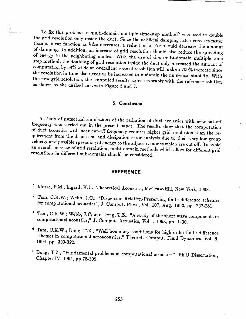
To fix "this problem, a multi-domain multiple time-step method s was used to double
the grid resolution only inside the duct. Since the artificial damping rate decreases faster
than a linear function as kAz decreases, a reduction of Az should decrease the amount
of damping. In addition, an increase of grid resolution should also reduce the spreading
of energy to the neighboring modes. With the use of this multi-domain multiple time
step method, the doubling of grid resolution inside the duct only increased the amount of
computation by 58% while an overall increase of resolution will make a 700% increase since
the resolution in time also needs to be increased to maintain the numerical stability. With
the new grid resolution, the computed results agree favorably with the reference solution
as shown by the dashed curves in Figure 5 and 7.
5. Conclusion
A study of numerical simulations of the radiation of duct acoustics with near cut-off
frequency was carried out in the present paper. The results show that the computation
of duct acoustics with near cut-off frequency requires higher grid resolution than the re-
quirement from the dispersion and dissipation error analysis due to their very low group
velocity and possible spreading of energy to the adjacent modes which are cut off. To avoid
an overall increase of grid resolution, multi-domain methods which allow for different grid
resolutions in different sub-domains should be considered.
REFERENCE
Morse, P.M.; Ingard, K.U., Theoretical Acoustics, McGraw-Hill, New York, 1968.
Tam, C.K.W.; Webb, J.C.: "Dispersion-Relation-Preserving finite difference schemes
for computational acoustics", J. Comput. Phys., Vol. 107, Aug. 1993, pp. 262-281.
Tam, C.K.W.; Webb, J.C; and Dong, T.Z.: "A study of the short wave components in
computational acoustics," J. Comput. Acoustics, Vol 1, 1993, pp. 1-30.
Tam, C.K.W.; Dong, T.Z., "Wall boundary conditions for high-order finite difference
schemes in computational aeroacoustics," Theoret. Comput. Fluid Dynamics, Vol. 6,
1994, pp. 303-322.
Dong, T.Z., "Fundamental problems in computational acoustics", Ph.D Dissertation,
Chapter IV, 1994, pp.78-105.
253
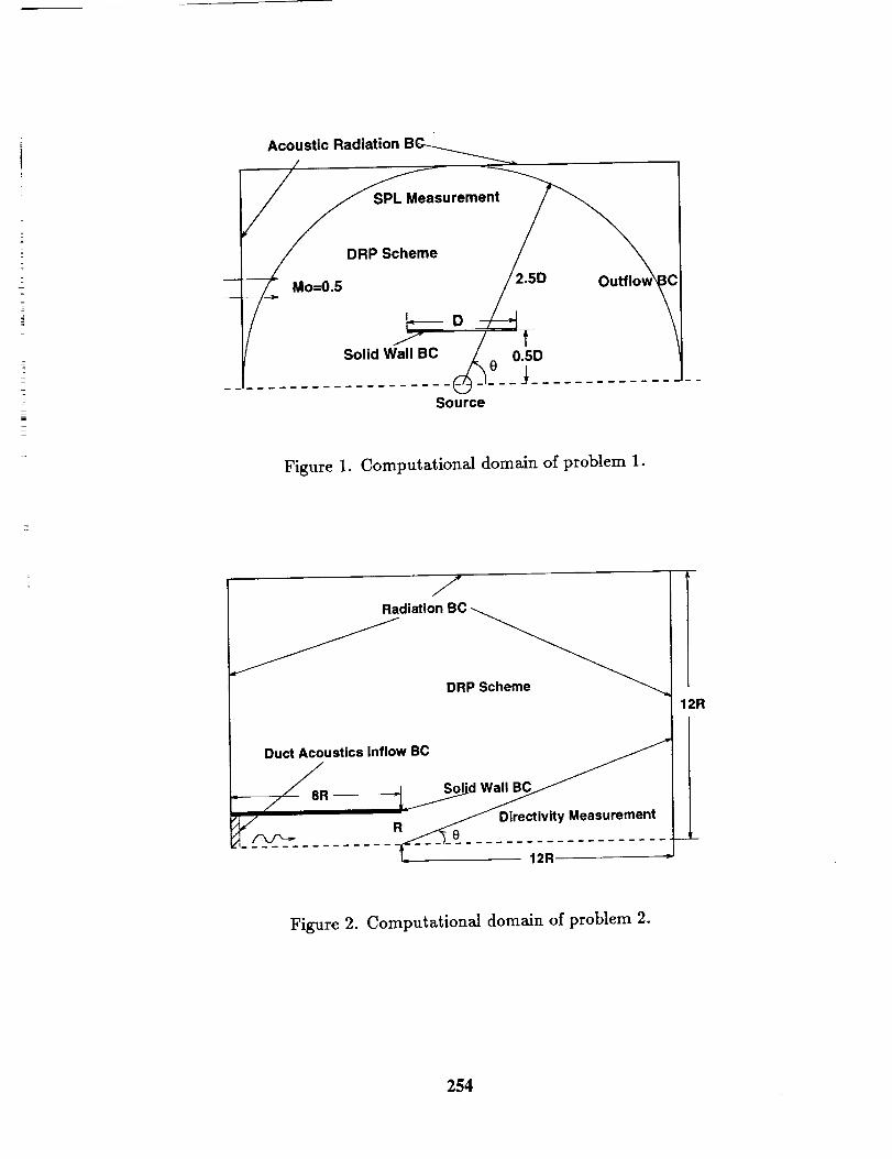
"°7"...t.on._--____
---/ 0''-- /_-- \1/_ .o.o., , /?o ou.,o._oI
_--° _ \]Solid Wall BC e 0 5D
Source
Figure I. Computational domain of problem 1.
JRadiation BC
DR
Du_[ustics Inflow BC
............... _-_---_ ...........
12R
Figure 2. Computational domain of problem 2.
254
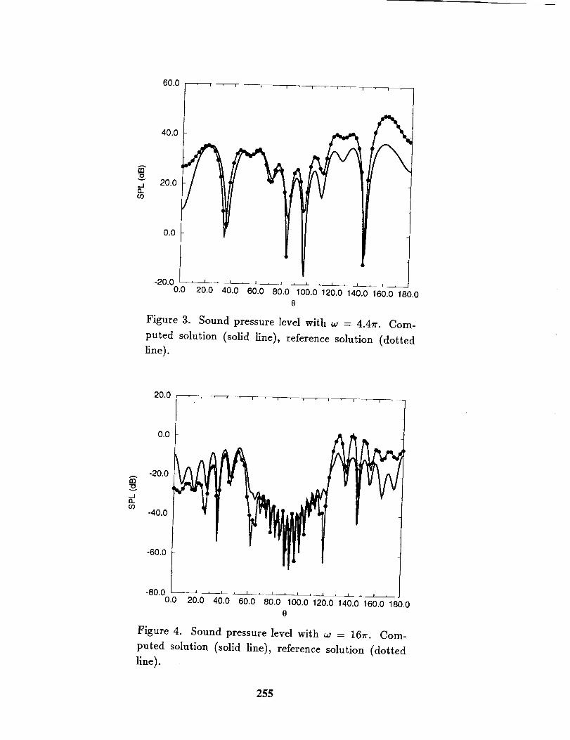
60.0 , _ , , ,. _- f ,
40.0
j 20.0Q.. ,O3
0.0
-20.0 _t , , , , , .....0.0 20.0 40.0 60.0 80.0 100.0 120.0 140.0 160.0 180.0
e
Figure 3. Sound pressure level with w = 4.47r. Com-
puted solution (solid line), reference solution (dotted
line).
m
.-IQ.O3
2oo? ....... t0.0
-20.0
-40.0
-60.0
"80"00.0 20.0 40.0 60.0 80.0 100.0 120.0 140.0 160.0 180.0
Figure 4. Sound pressure level with w = 167r. Com-
puted solution (solid line), reference solution (dotted
line).
255
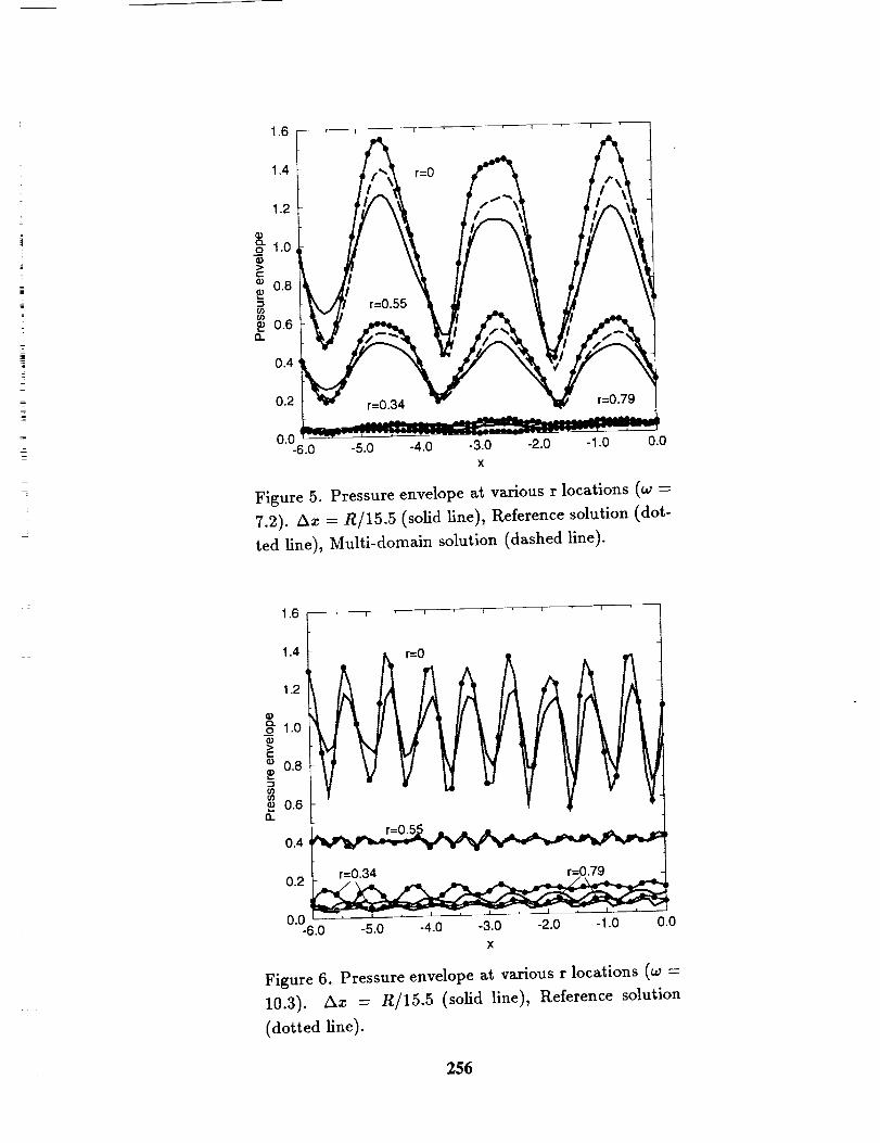
A
0"06.0 -5.0 -4.0 -3.0 -2.0 -1.0 0.0X
Figure 5. Pressure envelope at various r locations (w =
7.2). Az -- R/15.5 (solid fine), Reference solution (dot-
ted line), Multi-domain solution (dashed line).
1,6 _ T , ,
1.4
1.2
_ 0.8
_ 0.6ft.
0.4 =r=0.5
0,2 _ " _ '
0.0
-6.0 -5.0 -4.0 -3.0 -2.0 -1.0 0.0X
Figure 6. Pressure envelope at various r locations (w -
10.3). Az = R/15.5 (solid line), Reference solution
(dotted line).
256
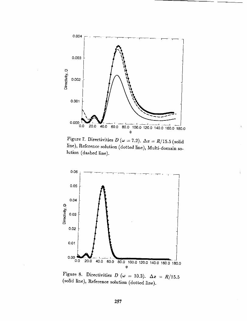
0.004 [-- ' r .... , - , ," . ....
O 0.003 f
-{ 0.002 fi5
0.001 I _ .,.......---0.000 _ ' _- -L_
0.0 20.0 40.0 60.0 80.0 100.0 120.0 140.0 160.0 180.0
0
Figure 7. Directivities D (w = 7.2). Az = R/15.5 (solid
fine), Reference solution (dotted line), Multi-domain so-
lution (dashed line).
0.06
0.05
0.04
E3
--> 0.03
o
0.02
II '
o.ol 0.00 b____ ,
0.0 20.0 40.0 60.0 80.0 100.0 120.0 140.0 160.0 i80.0
8
Figure 8. Directivities D (_ = 10.3). Az = R/15.5
(solid line), Reference solution (dotted line).
257
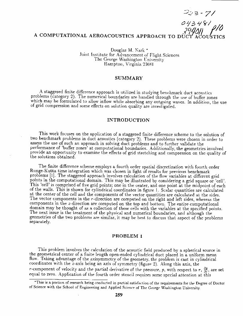
2 @1t r'"A COMPUTATIONAL AEROACOUSTICS APPROACH TO DUCT ACOUSTICS
Douglas M. Nark *Joint Institute for Advancement of Flight Sciences
The George Washington UniversityHampton, Virginia 23681
SUMMARY
A staggered finite difference approach is utilized in studying benchmark duct acousticsproblems (category 2). The numerical boundaries are handled through the use of buffer zoneswhich may be formulated to allow inflow while absorbing any outgoing waves. In addition, the useof grid compression and some effects on solution quality are investigated.
INTRODUCTION
This work focuses on the application of a staggered finite difference scheme to the solution oftwo benchmark problems in duct acoustics (category 2). These problems were chosen in order toassess the use of such an approach in solving duct problems and to further validate theperformance of 'buffer zones' at computational boundaries. Additionally, the geometries involvedprovide an opportunity to examine the effects of grid stretching and compression on the quality ofthe solutions obtained.
The finite difference scheme employs a fourth order spatial discretization with fourth orderRunge-Kutta time integration which was chosen in light of results for previous benchmarkproblems [1]. The staggered approach involves calculation of the flow variables at different gridpoints in the computational domain. This may be illustrated by considering a grid square or 'cell'.This 'cell' is comprised of five grid points; one in the center, and one point at the midpoint of eachof the walls. This is shown for cylindrical coordinates in figure 1. Scalar quantities are calculatedat the center of the cell and the components of the vector quantities are calculated at the sides.The vector components in the r-direction are computed on the right and left sides, whereas thecomponents in the z-direction are computed on the top and bottom. The entire computationaldomain may be thought of as a collection of these cells with the variables at the specified points.The next issue is the treatment of the physical and numerical boundaries, and although thegeometries of the two problems are similar, it may be best to discuss that aspect of the problemsseparately.
PROBLEM 1
This problem involves the calculation of the acoustic field produced by a spherical source inthe geometrical center of a finite length open-ended cylindrical duct placed in a uniform meanflow. Taking advantage of the axisymmetry of the geometry, the problem is cast in cylindricalcoordinates with the z-axis being an axis of symmetry (figure 2). Along this axis, the
r-component of velocity and the partial derivative of the pressure, p, with respect to r, _, are setequal to zero. Application of the fourth order stencil requires some special attention at this
"This is a portion of research being conducted in partial satisfaction of the requirements for the Degree of Doctorof Science with the School of Engineering and Applied Science of The George Washington University.
259
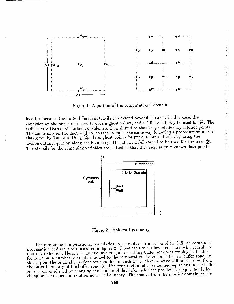
__ llW ............ 41,W ....
w.................... 0..IJ'_l._ .............
AT
eu ep
.... eW .......
eu ep
.......... eW ......
,u ep eu
...... IW___
u ep eu
......... IW .......
Figure 1" A portion of the computational domain
location because the finite difference stencils can extend beyond the axis. In this case, the
condition on the pressure is used to obtain ghost values, and a full stencil may be used for _. Theradial derivatives of the other variables are then shifted so that they include only interior points.The conditions on the duct wall are treated in much the same way following a procedure similar tothat given by Tam and Dong [2]. Here, ghost points for pressure are obtained by using the
w-momentum equation along the boundary. This allows a full stencil to be used for the term _.
The stencils for the remaining variables are shifted so that they require only known data points.
_Z
SymmetryAxis
l_
Buffer Zone
Interior Domain
__D uct
Wall
r
Figure 2: Problem 1 geometry
The remaining computational boundaries are a result of truncation of the infinite domain ofpropagation and are also illustrated in figure 2. These require outflow conditions which result inminimal reflection. Here, a technique involving an absorbing buffer zone was employed. In thisformulation, a number of points is added to the computational domain to form a buffer zone. Inthis region, the original equations are modified in such a way that no wave will be reflected fromthe outer boundary of the buffer zone [3]. The construction of the modified equations in the bufferzone is accomplished by changing the domain of dependence for the problem, or equivalently bychanging the dispersion relation near the boundary. The change from the interior domain, where
260
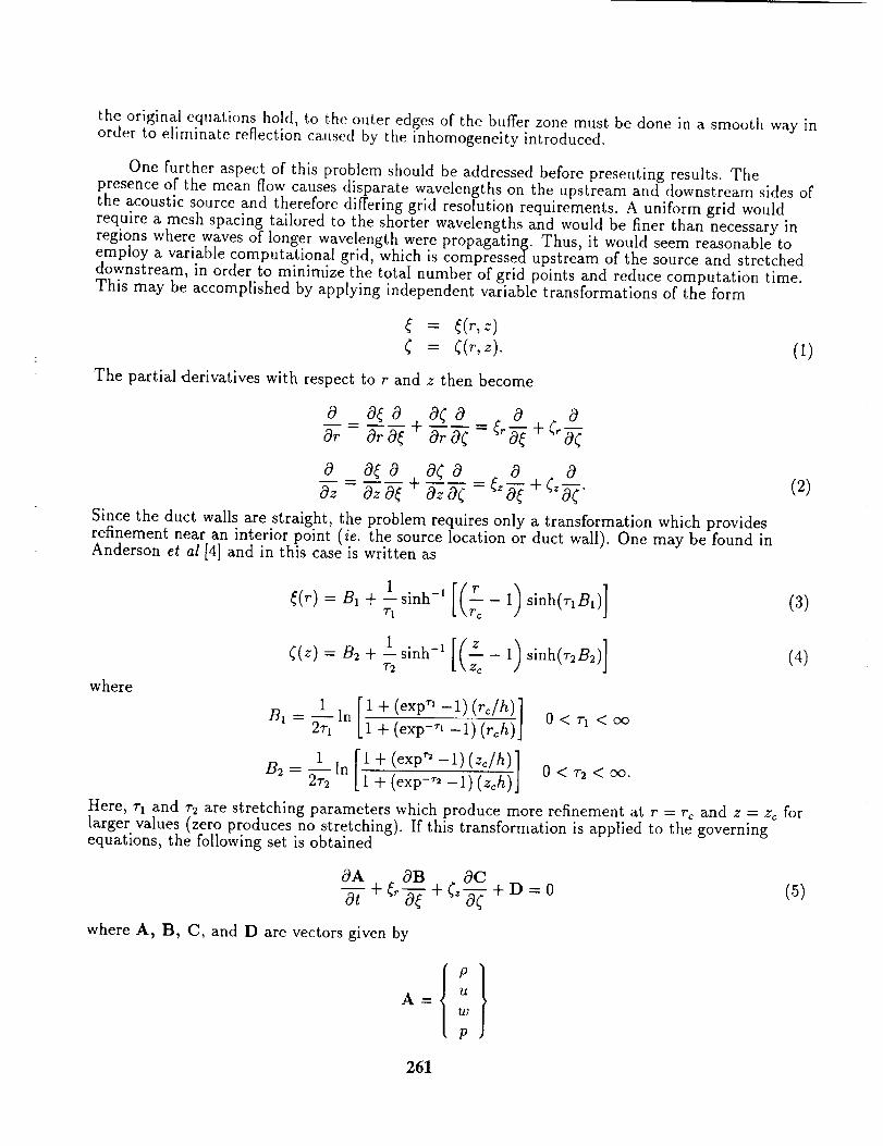
the original equations hold, to the outer edges of the buffer zone must be done in a smooth way inorder to eliminate reflection caused by the inhomogeneity introduced,
One further aspect of this problem should be addressed before presenting results. Thepresence of the mean flow causes disparate wavelengths on the upstream and downstream sides ofthe acoustic source and therefore differing grid resolution requirements. A uniform grid wouldrequire a mesh spacing tailored to the shorter wavelengths and would be finer than necessary in
regions where waves of longer wavelength were propagating. Thus, it would seem reasonable toemploy a variable computational grid, which is compressed upstream of the source and stretcheddownstream, in order to minimize the total number of grid points and reduce computation time.This may be accomplished by applying independent variable transformations of the form
= (if, z)¢ = (ff, z). (1)
The partial derivatives with respect to r and z then become
0 0f 0 0¢ 0 =_ro _;oN = NS_ + Nb-¢ 0f + 0I
b-z-b-; +_ -_'#+¢ •Since the duct walls are straight, the problem requires only a transformation which providesrefinement near an interior point (ie. the source location or duct wall). One may be found inAnderson et aI [4] and in this case is written as
(2)
_(r) = B1 +--sinh-' - 1 sinh(rlB,TI
(3)
where
((z) = B2 + --sinh -1 - 1 sinh(r_B__r2
(4)
1Bl = =---In
zrl 1 + (exp-,-1) (r_h)J
t + (e_p_-:l)_(_zo/h)]B2= _r2|n 1 +(exp-'-l)(zch)]
O<vl <oo
O< r2 <oo.
Here, rl and r2 are stretching parameters which produce more refinement at r = r_ and z = z¢ forlarger values (zero produces no s.tretching). If this transformation is applied to the governingequations, the following set is obtained
0A 0B 0C+ _-==-. + (,--z-:-. + D = 0 (5)
0--t-- o_ d_
where A, B, C, and D are vectors given by
/ }A= uw
P
261
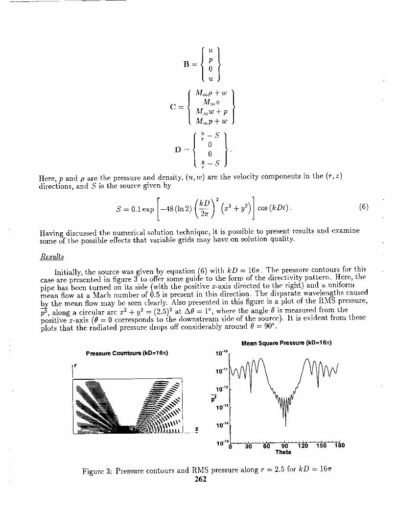
{u}B= P0
U
{ M_p+w }
M_v
ooP
D= 00
u__ Sr
Here, p and p are the pressure and density, (u, w) are the velocity components in the (r, z)directions, and 5' is the source given by
S = O'l exp [-48(ln2) (kD) 2 )](x + (6)
Having discussed the numerical solution technique, it is possible to present results and examinesome of the possible effects that variable grids may have on solution quality.
Results
Initially, the source was given by equation (6) with kD -- 167r. The pressure contours for thiscase are presented in figure 3 to offer some guide to the form of the directivity pattern. Here, the
pipe has been turned on its side (with the positive z-axis directed to the right) and a uniformmean flow at a Math number of 0.5 is present in this direction. The disparate wavelengths causedb_y the mean flow may be seen clearly. Also presented in this figure is a plot of the RMS pressure,
p2, along a circular arc x 2 + 92 = (2.5) 2 at A0 = 1°, where the angle 0 is measured from thepositive z-axis (0 = 0 corresponds to the downstream side of the source). It is evident from theseplots that the radiated pressure drops off considerably around 0 = 90 °.
Pressure Countours (kD=16_)
r
.,,."I_'¢//#/_ID. _ _ N_,
10 "10
10""
10"12
p=
10-13
101.
Mean Square Pressure (kD=16_)
10 "is .............o 3'0 6'0 9'o" i:iO i8oTheta
Figure 3: Pressure contours and RMS pressure along r = 2.5 for kD = 167r262
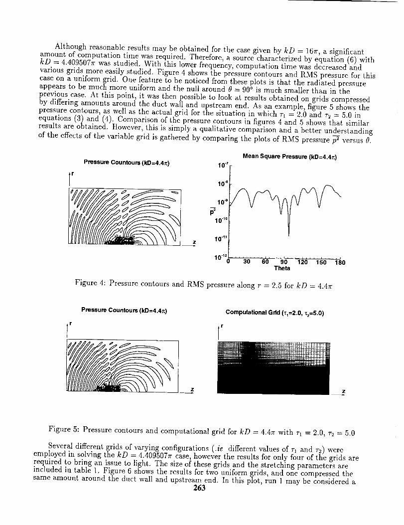
Although reasonable results may be obtained for the case given by kD = 167r, a significant
amount of computation time was required. Therefore, a source characterized by equation (6) withkD = 4.4095077r was studied. With this lower frequency, computation time was decreased andvarious grids more easily studied. Figure 4 shows the pressure contours and RMS pressure for thiscase on a uniform grid. One feature to be noticed from these plots is that the radiated pressureappears to be much more uniform and the null around 0 = 90 ° is much smaller than in theprevious case. At this point, it was then possible to look at results obtained on grids compressedby differing amounts around the duct wall and upstream end. As an example, figure 5 shows thepressure contours, as well as the actual grid for the situation in which T1 = 2.0 and r2 = 5.0 inequations (3) and (4). Comparison of the pressure contours in figures 4 and 5 shows that similar
results are obtained. However, this is simply a qualitative comparison and a better understanding
of the effects of the variable grid is gathered by comparing the plots of RMS pressure p2 versus 0.
r
Pressure Countours (kD=4.4_)
Z
10 -7
Mean Square Pressure (kD=4.4_)
104
10"9
10"1o
10"11
10 "12 _ i i , • , i ......0 "3'0 '6'0" '9'0' 12(i 15() 180
Theta
Figure 4: Pressure contours and RMS pressure along r = 2.5 for kD = 4.4rr
Pressure Countours (kD=4.4_)
r
z
Computational Grid (z1=2.0, z2=5.0)
r
Figure 5: Pressure contours and computational grid for kD = 4.47r with rl = 2.0, T2 = 5.0
Several different grids of varying configurations (.ie different values of rl and _2) wereemployed in solving the kD = 4.409507r case, however the results for only four of the grids arerequired to bring an issue to light. The size of these grids and the stretching parameters areincluded in table 1. Figure 6 shows the results for two uniform grids, and one compressed thesame amount around the duct wall and upstrcam end. In this plot, run 1 may be considered a
263
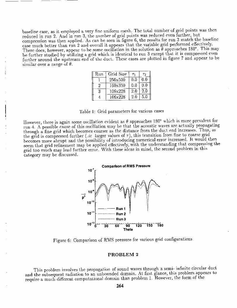
baseline case, as it employed a very fine uniform mesh. The total number of grid points was thenreduced in run 2. And in run 3, the number of grid points was reduced even further, butcompression was then applied. As can be seen in figure 6, the results for run 3 match the baseline
case much better than run 2 and overall it appears that the variable grid performed effectively.There does, however, appear to be some oscillation in the solution as 0 approaches 180 °. This may
be further studied by utilizing a grid which is identical to run 3 except that it is compressed evenfurther around the upstream end of the duct. These cases are plotted in figure 7 and appear to besimilar over a range of 0.
Run Grid Size _
1 250x500 0.0 0.0
2 i60x350 0.0 0.0
3 106x228 2.0 2.0
4 106x228 2.0 5.0
Table 1: Grid parameters for various cases
However, there is again some oscillation evident as 0 approaches 180 ° which is more prevalent forrun 4. A possible cause of this oscillation may be that the acoustic waves are actually propagatingthrough a fine grid which becomes coarser as the distance from the duct end increases. Thus, as
the grid is compressed further (.ie larger values of r), this transition from fine to coarse gridbecomes more abrupt and the possibility of introducing numerical error increased. It would thenseem that grid refinement may be applied effectively, with the understanding that compressing thegrid too much may lead further error. With these ideas in mind, the second problem in thiscategory may be discussed.
10 .7Comparison of RMS Pressure
p2
10 4 £, "
10"g1040 i:
10"11 ............. Run 2
........................ Run 3
10 "12 ...........0 '3'0' 'i0' 9'0' i 10'' i 50 'i 80
Theta
Figure 6: Comparison of RMS pressure for various grid configurations
PROBLEM 2
This problem involves the propagation of sound waves through a semi- infinite circular ductand the subsequent radiation to an unbounded domain. At first glance, this problem appears torequire a much different computational domain than problem 1. However, the form of the
264
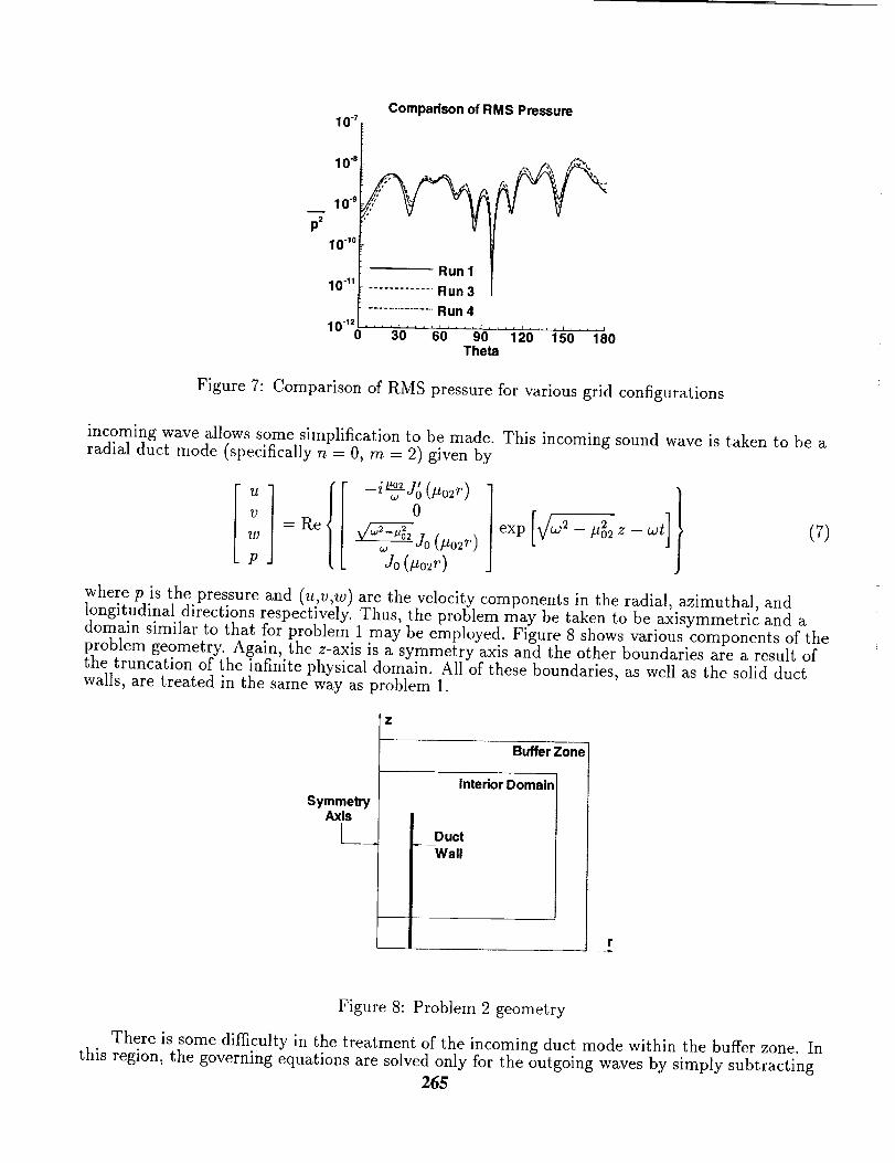
Comparison of RMS Pressure10"_
10"e _, ,_. 4_,_
............. Run3 I
.........................Run410-12 .............0 3b 60 '9'0 i20 i50 iso
Theta
10 .9
p2
10-1o
Figure 7: Comparison of RMS pressure for various grid configurations
incoming wave allows some simplification to be made. This incoming sound wave is taken to be aradial duct mode (specifically n = 0, m = 2) given by
v =Re _" (#o2r) exp 2_la2o2z_wtl/J w JO
(7)
where p is the pressure and (u,v,w) are the velocity components in the radial, azimuthal, andlongitudinal directions respectively. Thus, the problem may be taken to be axisymmetric and adomain similar to that for problem 1 may be employed. Figure 8 shows various components of theproblem geometry. Again, the z-axis is a symmetry axis and the other boundaries are a result ofthe truncation of the infinite physical domain. All of these boundaries, as well as the solid ductwalls, are treated in the same way as problem 1.
SymmetryAxis
[_
z
Buffer Zone
Interior Domain
Duct
Wall
r
Figure 8: Problem 2 geometry
There is some difficulty in the treatment of the incoming duct mode within the buffer zone. Inthis region, the governing equations are solved only for the outgoing waves by simply subtracting
265
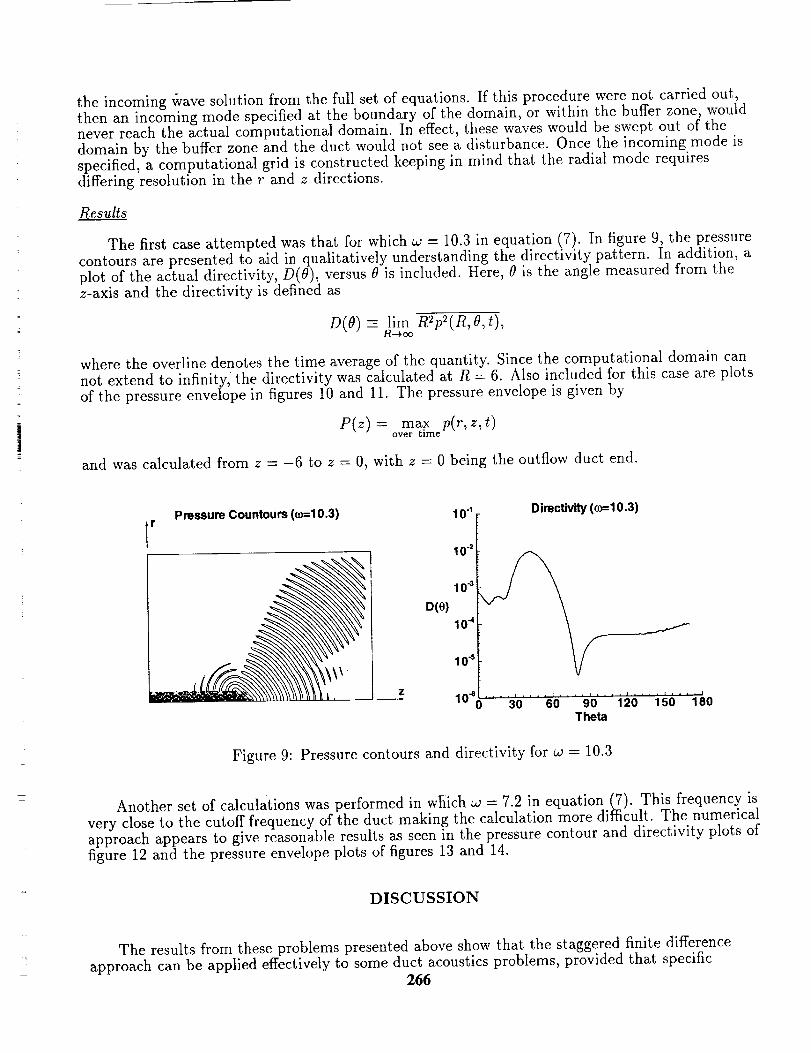
the incoming wavesolution from the full set of equations. If this procedure were not carried out,then an incoming mode specified at the boundary of the domain, or within the buffer zone, wouldnever reach the actual computational domain. In effect, these waves would be swept out of thedomain by the buffer zone and the duct would not see a disturbance. Once the incoming mode isspecified, a computational grid is constructed keeping in mind that the radial mode requiresdiffering resolution in the r and z directions.
Results
The first case attempted was that for which co = 10.3 in equation (7). In figure 9, the pressurecontours are presented to aid in qualitatively understanding the directivity pattern. In addition, aplot of the actual directivity, D(O), versus 0 is included. Here, 0 is the angle measured from thez-axis and the directivity is defined as
D(O) - lira R2p2(R,O,t),R--_ oo
where the overline denotes the time average of the quantity. Since the computational domain cannot extend to infinity, the directivity was calculated at R = 6. Also included for this case are plots
of the pressure envelope in figures 10 and 11. The pressure envelope is given by
P(z)= max p(r,z,t)over time
and was calculated from z = -6 to z = 0, with z = 0 being the outflow duct end.
Pressure Countours(m=10.3)r
z
D(O)
10_ [ Directivity(oo=10.3)
10 .2 k
10.3
104
10"s
lo% .... 3'o.... 6'o.... 9'o"'i20is0i8oTheta
Figure 9: Pressure contours and directivity for co -- 10.3
Another set of calculations was performed in which co = 7.2 in equation (7). This frequency isvery close to the cutoff frequency of the duct making the calculation more difi3cult. The numericalapproach appears to give reasonable results as seen in the pressure contour and directivity plots offigure 12 and the pressure envelope plots of figures 13 and 14.
DISCUSSION
The results from these problems presented above show that the staggered finite differenceapproach can be applied effectively to some duct acoustics problems, provided that specific
266
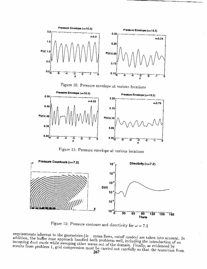
2.0
1.5
P(z) 1.0
0.5
0.O(
P(z) 0.40
Pressure Envelope (_=10.3)
r=O.0
Z
Pressure Envelope (o)=10.3)
0.30 ...................... .... • ....
r=-0.34
0,25
P(z) 0.20
0.15
°'1°-5.... -5.... -;l.... -3.... -2.... -_Z
Figure 10: Pressure envelope at various locations
Pressure Envelope ((_)=103)
0 .50 ..... ...... , ............... , ....
r=055
0.35
°'3o8 .... -5.... -_.... ._.... -_,.... -i-oZ
Pressure Envelope (_=10,3)
0,0l........................l°"l 1
P(z) o.lo_
' -6 -5 -4 -3 -2 -1 0Z
Figure 11: Pressure envelope at various locations
Pressure Countours (_=7 2)r
___z
D(O)
10 "1
10 .2
105
104
10 "s
Oirectivity (_7 2)
lO'eo''' 3'0'' ' "6'0 .... 9'0''' i2(i'' i60' ' i60
Theta
Figure 12: Pressure contours and directivity for _o = 7.2
requirements inherent to the geometries (ie. mean flows, cutoff modes) are taken into account. Inaddition, the buffer zone approach handled both problems well, including the introduction of anincoming duct mode while sweeping other waves out of the domain. Finally, as evidenced byresults from problem 1, grid compression must be carried out carefully so that the transition from
267
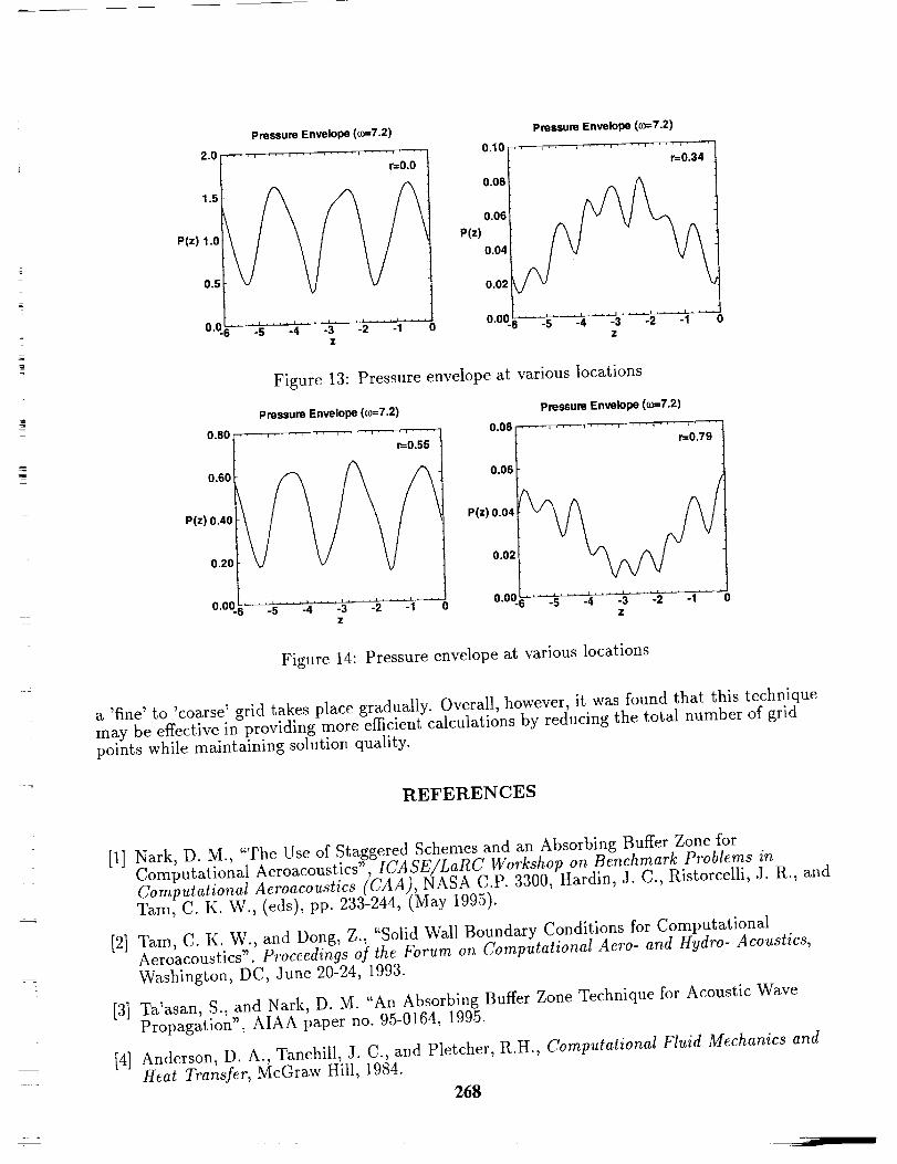
Pressure Envelope ((o=7.2)
2.0 ..............................
r=O.O
1.5
0.5
o.%.... _...............z
P(z) 1.0
Pressure Envelope (o=7.2)
0.10 .... , ......... , .... , .... , ....
r=0.34
0.08
0.06
P(z)0.04
0.02
o.o%---___....-4_i ....-i....-_z
Figure 13: Pressure envelope at various locations
0.80 0.08
0.60
P(z)0.40
0.20
Pressure Envelope (_=7.2)
r=0.55
0.06
P(z) O.O4
0.02
°'°%-'-_-L_.... -:_.... -3.... -i .... .i "_o o.oo_z
Pressure Envelope (o_=7.2)
r=0.79
-s ---_'_-3 .... -i .... -i .... 0Z
Figure 14: Pressure envelope at various locations
a 'fine' to 'coarse' grid takes place gradually. Overall, however, it was found that this techniquemay be effective in providing more efficient calculations by reducing the total number of gridpoints while maintaining solution quality.
REFERENCES
[1] Nark, D. M., "The Use of Staggered Schemes and an Absorbing Buffer Zone for
Computational Aeroacoustics", ICASE/LaRC Workshop on Benchmark Problems inComputational Aeroacoustics (CAA), NASA C.P. 3300, Hardin, J. C., Ristorcelli, J. R., andTam, C. K. W., (eds), pp. 233-244, (May 1995).
[2] Tam, C. K. W., and Dong, Z., "Solid Wall Boundary Conditions for ComputationalAeroacoustics". Proceedings of the Forum on Computational Aero- and Hydro- Acoustics,Washington, DC, June 20-24, 1993.
[3] Ta'asan, S., and Nark, D. M. "An Absorbing Buffer Zone Technique for Acoustic WavePropagation", AIAA paper no. 95-0164, 1995.
[4] Anderson, D. A., Tanehill, J. C., and Pletcher, R.H., Computational Fluid Mechanics andHeat Transfer, McGraw Hill, 1984.
268
z/-,7/
dgZ/ +'2'2.--0
A VAI_IA'FI()NAL FINITE ELEMENT METHOD F()IR, C()MPUTATIONAL AEROACOUSTIC
CALCULATI()NS ()F TURBOMACHINERY NOISE
Kenneth C. Hall I
Departtnent of Mechanical Engineering and Materials Science
Duke University
Durham, NC 27708-0300
ABSTRACT
A variational method for computing the unsteady aeroacoustic response of turbomachinery blade
rows to incident vortical gusts is presented. A variational principle which describes the harmonic small
disturbance behavior of the full potential equations about a uniform mean flow is developed. Four-node
isoparametric finite elements are used to discretize the variational principle, and the resulting discretized
equations are solved efficiently using LU decomposition. Results computed using this technique are
found to be in excellent agreement with those obtained using semi-analytical methods.
INTRODUCTION
In this paper, an exfension of Bateman's [1] variational principle - previously derived by Hall [2]
for aeroelastic calculations and later extended by Lorence and Hall [3] for aeroacoustic applications
- is used to solve for the aeroacoustic response of a two-dimensional cascade of airfoils subjected toan incident vortical gust. The variational principle describes the small disturbance behavior of the
compressible full potential equation. The small-disturbance variational principle is discretized using
bilinear four-node isoparametric finite elements, and the resulting set of linear equations is solved using
LU decomposition to obtain the unknown perturbation velocity potential.
Also presented is a numerically exact far-field boundary condition. To prevent spurious reflections
of outgoing waves as they pass through the far-field computational boundary, so-called nonxeflecting
boundary conditions must be applied. Previous investigators have found the analytical behavior of
the unsteady flow field and matched these solutions to the computational solution at the fax-field
boundary [4, 5, 6, 7]. In this paper, the exact far-field behavior of the discretized small disturbance
equations is found by performing an eigenanalysis of the discretized equations in the far-field. The
resulting eigenmodes are then used to construct perfectly nonreflecting boundary conditions.
The present variational finite element method is both accurate and computationally efficient. For
example, typical aeroacoustic calculations require less than one minute of CPU on a modern desktop
workstation computer. A number of computational examples are presented; results computed using
the present method are shown to be in excellent agreement with exact solutions.
THEORY
In the present analysis, the flow through a compressor or turbine blade row is assumed to be inviscid,
isentropic, and two-dimensional. Furthermore, the fluid is assumed to be an ideal gas with constant
specific heats. For the Category 3 turbomachinery problem, defined for the Second Computational
Aeroacoustics Workshop on Benchmark Problems, the cascade is composed of flat plate airfoils which
do no steady turning so that the mean or steady flow is uniform. Thus, the unsteady flow through
the cascade of airfoils can be modelled as the sum of three parts: a uniform steady flow, an unsteady
ICopyright @ 1997 by Kenneth C. Hall. Published by NASA with permission.
269
v.rti_'al ¢li_tlllb;tl_('v. ;t11,1_tll _111._t,';.Iv f.,vt_lvb;tti,,li vol,,,.ity. "Fh,, _la._t_'_uly p_._rt.urb_tion velocity flow is
irr,_tati_mal (._:.pt in the, wak.) .s. th.t ih. p_'rt_lrbati_m vel,,.ity may be represented by the gradient
.f a svalar w'l,.'itv pot,ontial, ,). "l'h,is th. t,_t_Ll w'lo_'ity V lll;-ly [/o ,;xpressed a.s
V(.r. !/, :) = U + v.(,r,.q, t) + V,_(s,.r/, t) (1)
where U is the (unifl)rm) steady or mean flow. vn(x, y) is the velocity associated with a divergence
free vorticity field, and c/5(x, y) is the unsteady perturb_ltion potential. Note that here we have assumed
that the unsteady quantities vn and XT,#are small compared to the mean flow U. Note also that sincethe mean flow is uniform, the vortical disturbance is simply convected through the cascade without;
distortion, and further, there is no unsteady pressure associated with the vorticity itself.
Next, the expression for the velocity field, Eq. (l), is substituted into the conservation of mass,
which is given byor)
+ = 0 (23
where # is the density of the fluid. Collecting terms which are first order in the unsteady quantities,one obtains
0p + V. (RV¢ + pU) = 0 (3)Ot
where R and p are the steady flow (zeroth-order) density and unsteady perturbation (first-order) density,
respectively. Integrating the momentum equation and making use of the isentropic assumption, one can
obtain expressions for the unsteady perturbation pressure p and density p in terms of the perturbation
potential, i.e.
o0 )p = -R_-_ = -R _- + U. V, (4)
and
P= C 2Dr =-C '_ _ +U'V¢ (5)
where D/Dt is the linearized substantial derivative operator, and C is the steady flow speed of sound.
Equation (4) is recognized as the linearized Bernoulli equation. Finally, substitution of Eq. (5) into the
conservation of mass, Eq. (3), gives the desired linearized potential equation,
v. RYe- V. _ W_V¢+-- C - _ V_V + 0t_] = 0 (6)
To complete the specification of the problem, boundary conditions must be specified on the surface
(gD bounding the solution domain D (see Fig. 1). On the airfoil surfaces, there can be no mass flux
through the airfoil surface so thato¢
R_ = -RvR. n (7)
where n is the unit normal to the airfoil. Tim wake may also be thought of as an impermeable surface.
However, since the wave will in general oscillate unsteadily, Eq. (7) must be slightly modified to account
for the upwash produced by the wake motion. On either side of the wake, we require
b-;7.,,= R, -,,,_.n+37+ o_] (8)
where r = r(s, t) is the dispbwement of tho wake normal to its mean position, s is distance along
the wake, and V is the magnitude or" the steady velocity aligned with the mean wake position. To
270
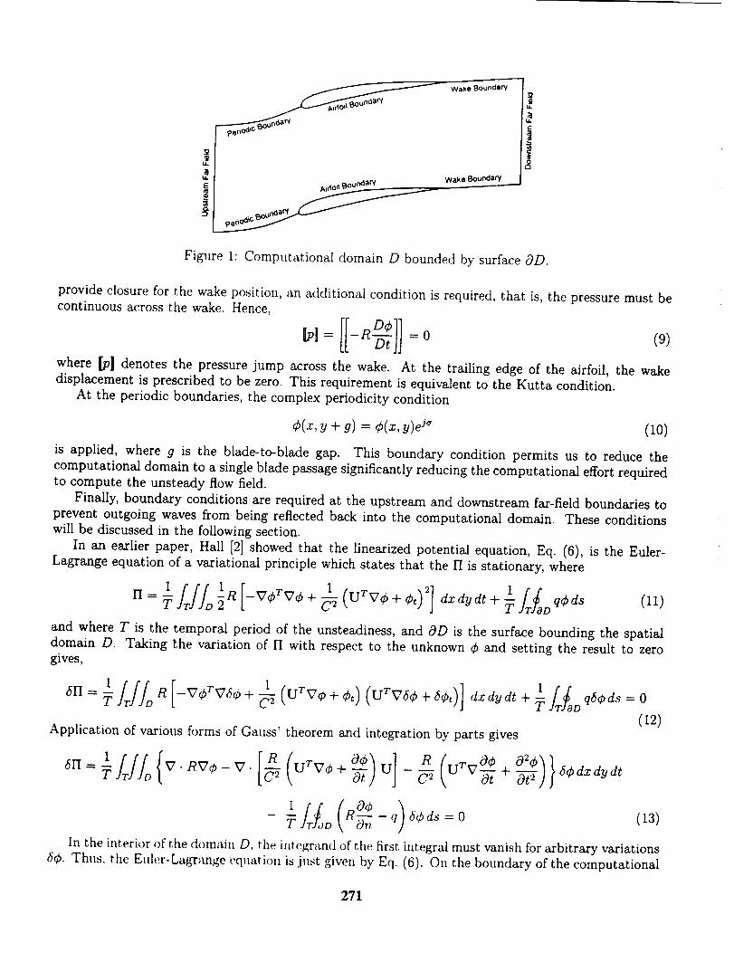
t_
E
Wake Boundary
f
Wake Boundary
u6E
8
Figure 1: Computational domain D bounded by surface OD.
provide closure for the wake position, an additional condition is required, that is, the pressure must becontinuous across the wake. Hence,
where [p] denotes the pressure jump a_ross the wake. At the trailing edge of the airfoil, the wake
displacement is prescribed to be zero. This requirement is equivalent to the Kutta condition.
At the periodic boundaries, the complex periodicity condition
¢(a:, y + g) = ¢(x, y)e j_ (10)
is applied, where g is the blade-to-blade gap. This boundary condition permits us to reduce the
computational domain to a single blade passage significantly reducing the computational effort required
to compute the unsteady flow field.
Finally, boundary conditions are required at the upstream and downstream far-field boundaries to
prevent outgoing waves from being reflected back into the computational domain. These conditions
will be discussed in the following section.
In an earlier paper, Hall [2] showed that the linearized potential equation, Eq. (6), is the Euler-
Lag-range equation of a variational principle which states that the H is stationary, where
1/T//D _1R [ 1 (uTv ¢ ] dt+_/r_ol qCds (11)l'I=_ 2 --vcT_7¢ +-_ + ¢_)_ dxdy o
and where T is the temporal period of the unsteadiness, and 0D is the surface bounding the spatial
domain D. Taking the variation of H with respect to the unknown ¢ and setting the result to zero
gives,
1 r 1
[-- v(_T VCSg} --]-= /j/oR +¢o + oo] + q6¢ ds = 0
(12)Application of various forms of Gauss' theorem and integration by parts gives
_n= frf/_ v. Rye- v. urv¢ + U - UrV_ + 6¢dxdydt
JTJoo - q _¢d_ = 0 (_3)
In the interior of the domain D, the int.egrand of the first, integral must vanish for arbitrary variations
6¢. Thus, the Euh:r-Lagrange equation is just given by gq. (6). On the boundary of the computational
271
,l,>mairlOD. the,_4,_'r_ll_[mt_'_Lr_dwillv_,iii.qlif,,'Ji.s_l_,c_ifi_,cl(Diri<'hh,tcondit.hms),or ifRO@/On I q = 0
(N_,lllnaim c_mf[itfims}. "['[1,' l,.t_,r ,',,z_,[iti,m i._ II._#,[ to mcht_l_' t.h_, iafluence of lipw_,_h on the airfoil
in_liice_l tiV the v<Jrti<'itl _ll._t vie +tnrl tlit, wake' ttit_tion r [Eels. (7) nn, l (8)].For g, il,_t distlirtJ+ul<'<,._ whi,h at',, f<'titp<Jr+tll.V [iitrlll<Jni(', l:he illisteady perturbation potential ¢ will
also be hli.rin()irlic. Thil_, it. will b(; ('<)ll'¢_',lli(,ilt, N) lift.
l
where ¢(x,!1)isnow the complex amplitude of the perturbation potential,and ¢(z, y) isitscomplex
conjugate.
Substitution of the simple harmonic motion assumption into the functional l'I yields the functional
for the variational principle which describes the behavior of the harmonic small disturbance potential,
_b. The result is
=l R{ D [v_TuuTv_ j_Hshm 2 iSo - v_Tv(_ -I- -- (v_Tu_ - _uTv_] + 032_] } dz dy
l irf_D q'¢ds-I- _ + complex conjugate terms (15)
Taking the variation of Eq. (15) and setting the result to zero and applying the divergence theorem as
before gives the desired Euler-Lagrange equation and boundary conditions which describe the harmonic
small disturbance behavior of the flow• The Euler-Lagrange is given by
Rv.nv¢-v. _
As expected, Eq. (16) is identical to Eq. (6) with the operator O/Ot replaced by -jw. On the boundaries
of the domain, we hove the natural boundary condition
0_
which can be used to describe the upwash due to the wake or the periodic boundary conditions. Foradditional details on the modifications to the variational principle required to compute unsteady flows
in cascade, the interested reader is referred to Hall [2].
NUMERICAL SOLUTION TECHNIQUE
Because the unsteady solutions are spatially periodic, the solution domain can be reduced to a single
blade passage. Within a single passage, an H-grid of quadrilateral cells is generated algebraically. The
unsteady variational principle, Eq. (15). is then discretized using conventional finite element techniques.
In the present work. a four-node isoparametric element is used. Consider the nth quadrilateral element
in the computational domain. The values of the unsteady velocity perturbation at the corners of the
element, {4_},,, are interpolated into the interior of the element using an interpolation of the form
¢(_, u) = [N], {¢h (lS)
where [N]n is a row vector of interpolation fimctions. Then, for example, the local stiffness matrix is
given by
[k] : fL-.)_, (fN'] r V'<[>[N],,
'_t Itl
1+ C--__,[[N']_r V'¢V'<Ibr [N'].
- [N], _, V'<U IN'l,,) + ..'' IN], r [Ni. ]} dx dy (19)
272
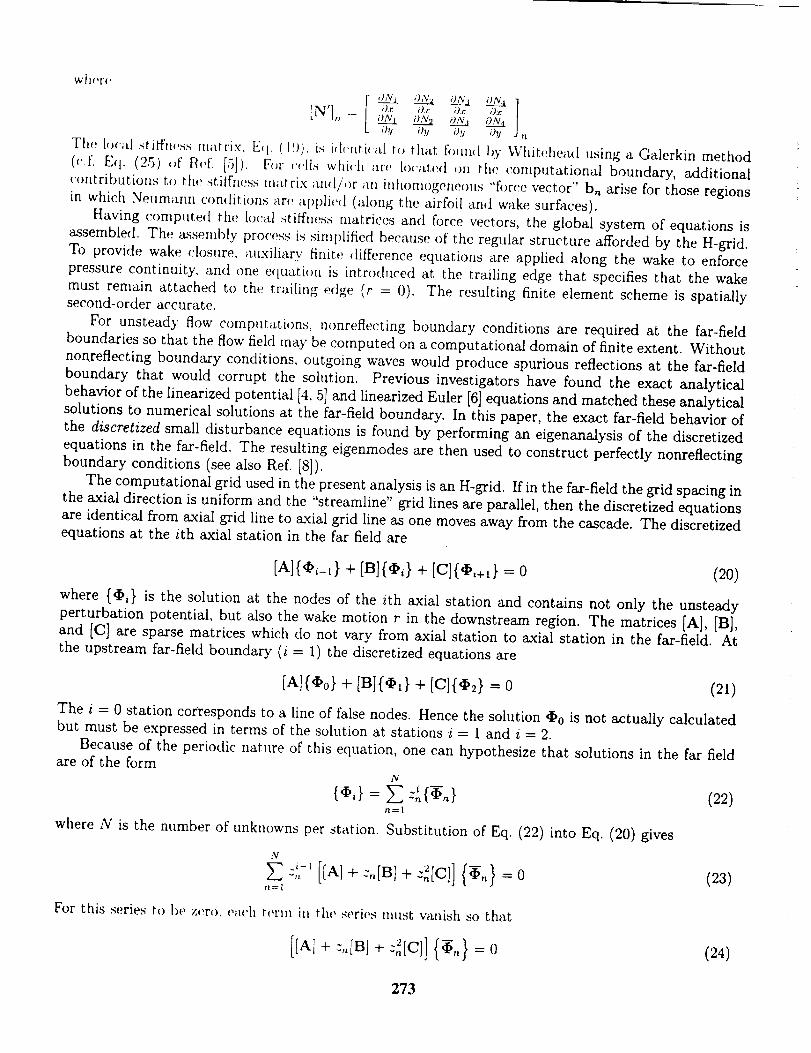
ihj i)_I i)_t 1)_I n
The loom _titfm!ss matrix, E_I. (19), i,_ i_h'aticM t(_ that t'¢)_m_[ hy W_dtehead using a Galerkin method
(¢'.f. E¢l. (25) ,,t' R¢,f. [5]). D_r ¢'¢,lls which are h_cat.ed on the con_put, ational boundary, additional
cottt.ributioas t_ the st.iffIless matri× attct/',_r an itfltomogeae()_ts "'fi)rce vector" bn arise for those regions
in which NelLmann con_[itions are apt)lion[ (along the airfoil and wake surfaces).
Having computed the local stiffness matrices and force vectors, the global system of equations is
assembled. The assembly process is simplified because of the regular structure afforded by the H-grid.
To provide wake closure, auxiliary finite difference equations are applied along the wake to enforce
pressure continuity, and one equation is introduced at the trailing edge that specifies that the wake
must remain attached to the trailing edge (r = 0). The resulting finite element scheme is spatiallysecond-order accurate.
For unsteady flow computations, nonreflecting boundary conditions are required at the far-field
boundaries so that the flow field may be computed on a computational domain of finite extent. Without
nonreflecting boundary conditions, outgoing waves would produce spurious reflections at the far-field
boundary that would corrupt the solution. Previous investigators have found the exact analytical
behavior of the linearized potential [4, 51 and linearized Euler [6] equations and matched these analytical
solutions to numerical solutions at the far-field boundary. In this paper, the exact far-field behavior of
the discretized small disturbance equations is found by performing an eigenanalysis of the discretized
equations in the far-field. The resulting eigenmodes are then used to construct perfectly non.reflecting
boundary conditions (see also Ref. [8]).
The computational grid used in the present analysis is an H-grid. If in the far-field the grid spacing in
the axial direction is uniform and the "streamline" grid lines are parallel, then the discretized equations
are identical from axial grid line to axial grid line as one moves away from the cascade. The discretized
equations at the ith axial station in the far field are
}+ + } = 0 (20)
where {¢I,,} is the solution at the nodes of the ith axial station and contains not only the unsteady
perturbation potential, but also the wake motion r in the downstream region. The matrices [A], [B],
and [C] are sparse matrices which do not vary from axial station to axial station in the far-field. AI;
the upstream far-field boundary (i = 1) the discretized equations are
[A]{*o} + [B]{¢,} + [C1{O2} = 0 (21)
The i = 0 station corresponds to a line of false nodes. Hence the solution ¢I'0 is not actually calculated
but must be expressed in terms of the solution at stations i = 1 and i = 2.
Because of the periodic nature of this equation, one can hypothesize that solutions in the far fieldare of the form
N
n=[
where N is the number of unknowns per station. Substitution of Eq. (22) into Eq. (20) gives
N
:i,-'[IAI+;oIBI+-';Ic]] --0.=1
For this series to be zero, each term in the series must vanish so that
[[AI + :,,[B] + :],[C]] = 0
(22)
(23)
(24)
273
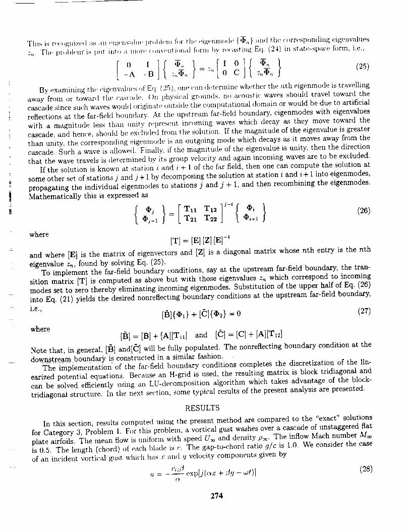
This is r,',',,g1_iz_',l a,,__zl ,q_,q_val,l,, l}r,A,b,llz f,,r th,, ,'i_'nnu,,b, {'IL, 1 and the {'orrvsponding eigenvahles
=,,. T}I,' pr,)l)h,m'is pllt illr,, _J Jn,)r,, ,,,Jw,nti,m_d f,,rm by rP,'_L_ting E(I. (24) in state-space fi>rm, i.e.,
I ](-} [ ](-}{1 I ,I.,, I 0 4.,_-A -B :,_+,_ = =" 0 C z._,, (25)
By examining ttw {'ig, mv_d,u's of E_I. (25), one can {l{,¢erminc wh,_ther the nth eigenrnode is travelling
away from or toward the c_Lsca, l,,. On l}hysi{'al grounds, no acoustic waves should travel toward the
cascade since such waves would originate outsi{le the computational domain or would be due to artificial
reflections at the far-field boundary. At the upstream far-field boundary, eigenmodes with eigenvalues
with a magnitude less than _mity represent incoming waves which decay as they move toward the
cascade, and hence, should be exchtded from the solution. If the magnitude of the eigenvalue is greater
than unity, the corresponding eigenmo{le is an outgoing mode which decays as it moves away from the
cascade. Such a wave is allowe{t. Finally, if the magnitude of the eigenvalue is unity, then the direction
that the wave travels is determined by its group velocity and again incoming waves are to be excluded.
If the solution is known at station i and i + 1 of the far field, then one can compute the solution at
some other set of stations j and j + 1 by decomposing the solution at station i and i+ 1 into eigenmodes,
propagating the individual eigenmodes to stations j and j + 1, and then recombining the eigenmodes.
Ivlathematically this is expressed as
where
{o,} [TI,T12],,{o,}{I}a+t = Tat T22 @i.t
[T] = [E][Z][E]-'and where [E] is the matrix of eigenvectors and [Z] is a diagonal matrix whose nth entry is the nth
eigenvalue zn, found by solving Eq. (25).
To implement the far-field boundary conditions, say at the upstream far-field boundary, the tran-
sition matrix IT] is computed as above but with Bhose eigenvalues z= which correspond to incomingmodes set to zero thereby eliminating incoming eigenmodes. Substitution of the upper half of Eq. (26)
into Eq. (21) yields the desired nonreflecting boundary conditions at the upstream far-field boundary,i.e.,
+ = 0 (2r)where
[13] = [B] + [a][Tt,] and [(_] = [C] + [A][T,2]
Note that, in general, [13] and{(_] will be fully populated. The nonreflecting boundary condition at the
downstream boundary is constructed in a similar fashion.
The implementation of the far-field boundary conditions completes the discretizati0n of the lin-
earized potential equations. Because an H-grid is used, the resulting matrix is block tridiagonal and
can be solved efficiently using an LU-decomposition algorithm which takes advantage of the block-
tridiagonal structure. In the next section, some typical results of the present analysis are presented.
RESULTS
In this section, results computed using the present method are compared to the "exact" solutions
for Category 3, Problem 1. For this problem, a vortical gust washes over a cascade of unstaggered flat
plate airfoils. The mean flow is uniform with speed U_ and density p_. The inflow Math number M_o
is 0.5. The length (chord) of each blade is c. The gap-to-chord ratio 9/c is [.0. We consider the case
of an im'ident vortical gust whMt has .r: an{[ !! velocity components given by
+ 3u t)l (28)
274
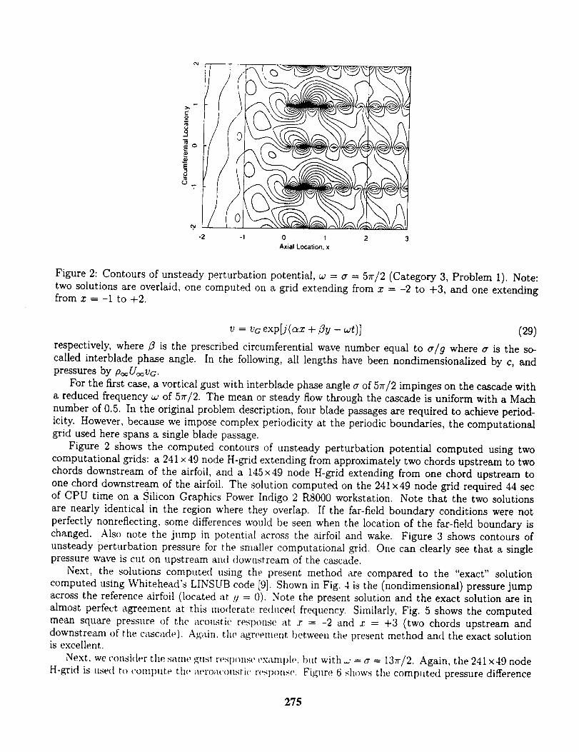
_-o •
-2 -1 0AxialLocation,x
2 3
Figure 2: Contours of unsteady perturbation potential, _ = u = 57r/2 (Category 3, Problem 1). Note:
two solutions are overlaid, one computed on a grid extending from x = -2 to +3, and one extendingfrom z = -1 to +2.
v = vcexp[j(ax +/3y-wt)] (29)
respectively, where ¢3 is the prescribed circumferential wave number equal to a/g where a is the so-
called interblade phase angle. [n the following, all lengths have been nondimensionalized by c, and
pressures by po_Uo_vc.
For the first case, a vortical gust with interblade phase angle u of 57r/2 impinges on the cascade with
a reduced frequency _ of 57r/2. The mean or steady flow through the cascade is uniform with a Mach
number of 0.5. In the original problem description, four blade passages axe required to achieve period-
icity. However, because we impose complex periodicity at the periodic boundaries, the computational
grid used here spans a single blade passage.
Figure 2 shows the computed contours of unsteady perturbation potential computed using two
computational grids: a 241 x49 node H-grid extending from approximately two chords upstream to two
chords downstream of the airfoil, and a 145x49 node H-grid extending from one chord upstream to
one chord downstream of the airfoil. The solution computed on the 241x49 node grid required 44 sec
of CPU time on a Silicon Graphics Power Indigo 2 RS000 workstation. Note that the two solutions
are nearly identical in the region where they overlap. If the far-field boundary conditions were not
perfectly nonreflecting, some differences would be seen when the location of the far-field boundary is
changed. Also note the jump in potential across the airfoil and wake. Figure 3 shows contours of
unsteady perturbation pressure for the smaller computational grid. One can clearly see that a single
pressure wave is cut on upstream and downstream of the cascade.
Next, the solutions computed using the present method are compared to the "exact" solution
computed using Whitehead's LINSUB code [9]. Shown in Fig. 4 is the (nondimensional) pressure jump
across the reference airfoil (located at g = 0). Note the present solution and the exact solution are in
almost perfect agreement at this moderate reduced frequency. Similarly, Fig. 5 shows the computed
mean square pressure of the aco_lstic response at x --- -2 and x = +3 (two chords upstream and
downstream of the cascade). Ag_fin. the agreement betweea the present method and the exact solutionis excellent.
Next, we consider the same gust t'(,Sl)(ms(, exatnple, but with _' = u = t37r/2. Again, the 241 x49 node
H-grid is use(| to COUlpUte the m, roacoLtst.ic r('sl)otl_e. Figttre 6 shows the computed pressure difference
275
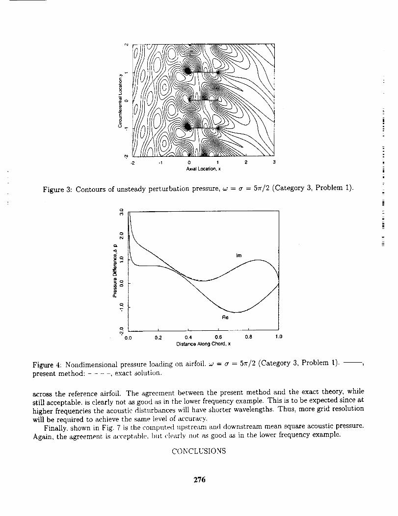
04
i..J
2o
i¢.5
-2
0 fj,o_ DDD \\\
-I 0 I 2 3Axial Location,x
Figure 3: Contours of unsteady perturbation pressure, _ = a = 57r/2 (Category 3, Problem 1).
C'q
£o
t_
i=n
"7
Re
0.0 0.2 0.4 0.6 0.8
Distance Along Chord, x
1.0
=
==
i
w
Figure 4: Nondimensional pressure loading on airfoil, _ = or = 5rr/2 (Category 3, Problem 1).
present method: .... , exact solution.
across the reference airfoil. The agreement between the present method and the exact theory, while
still acceptable, is clearly not as good as in the lower frequency example. This is to be expected since at
higher frequencies the acoustic disturbances will have shorter wavelengths. Thus, more grid resolution
will be required to achieve the same level of accuracy.
Finally, shown in Fig. 7 is r,he computed upstream and downstream mean square acoustic pressure.
Again, the agreement is acceptable, but clearly nor, as good as in the lower frequency example.
CONCLUSIONS
276

o
*t
o4Q.v
:+et
J
cJ0.0
o
2cl.
i+n
"5
gtO °0.(
i ,, I L., i ,, I , I , i _ I . .
02 0.4 06 0.8 02 0.4 06 0.8 T.O
Circumferenl=al Location, y Circumferential Localion. y
Figure 5: Mean square pressure upstream (x = -2) and downstream (a: = 3) of cascade, _o = cr = 5rr/2
(Category 3, Problem 1). , present method; .... , exact solution.
t£1
o.
O.
n
ID
Im
Re
, l .., I I ,, i ., .
"7,0.0 0.2 0.4 0.6 0.8
Oislance Along Chorcl, x
1.0
Figure 6: Nondimensional pressure loading on airfoil, _a = cr = 13_'/2 (Category 3, Problem 1). --
present method; .... , exact solution.
In this paper, a finite element method for calculating the aeroacoustic response of turbomachinery
cascades to incident gusts is presented. The method is based on a linearized version of Bateman'svariational principle. The variational principle is discretized on a computational grid of quadrilateral
cells using standard finite element techniques. Two novel features are used to improve the accuracy
of the computed results. The first is the use of wake fitting to model the motion of the wake and the
jump in potential across the wake. Wake fitting allows the discontinuity in potential across the wake to
be modelled quite accurately with only moderate grid resolution, and also automatically incorporates
the Kutta condition. The second novel feature is the use of numerically exact far-field boundary
conditions. In the present method, the far-field boundary conditions are based on the eigenmodes of
the dtscretized potential equatious, rather than on the eigenmodes of the analytical model. Thus, theboundary conditions are exact {to within round-off error) with no truncation error.
The present method is coniput+_tionatly efficient, with typical aeroacoustic calculations requiring
277
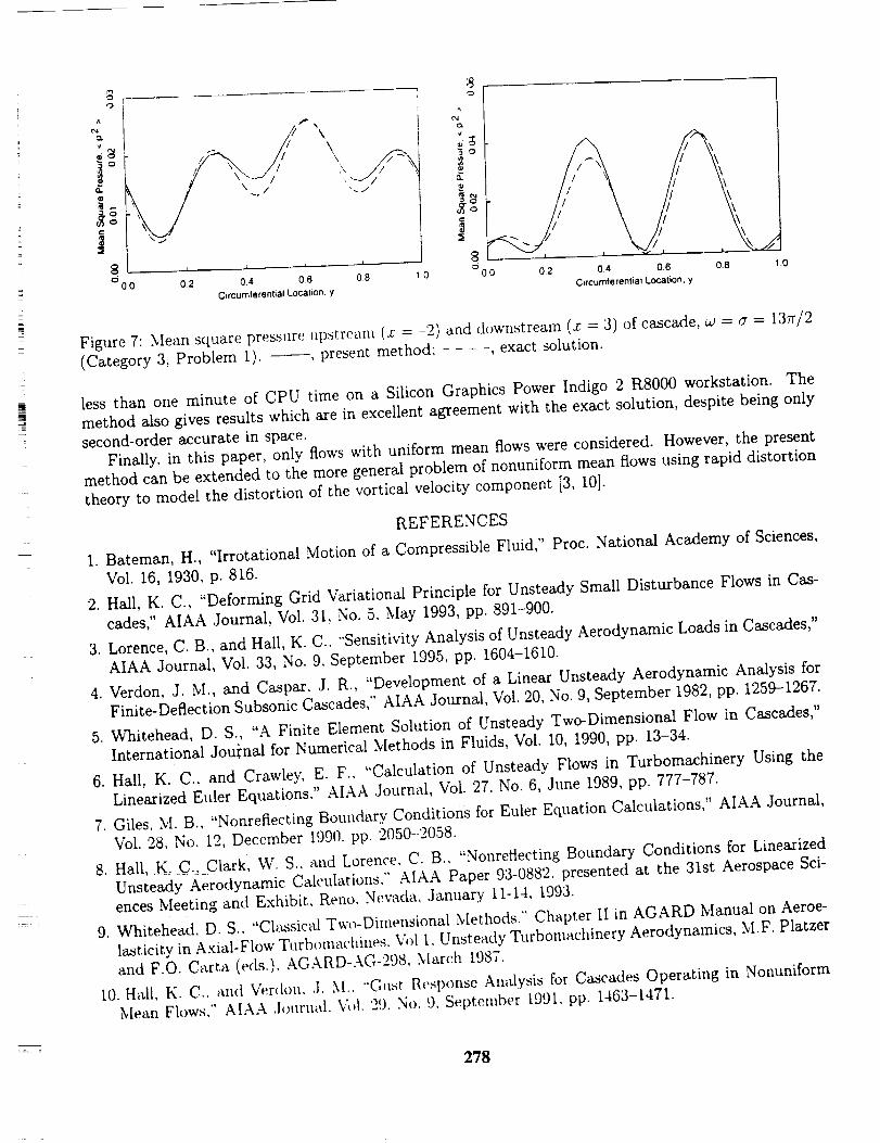
8
2
]or
o 0,0 02 0.I 0.6
CircumferentialLocation,y
\
t
08 10
o.,t
5
!0.
,go
8°0, 0
A A
02 0,4 0.6 0.8 1.0
Circumferential Location, y
Figure 7: Mean square pressure upstream (z" = -2) and downstream (z = 3) of cascade, _ = a = 137r/2(Category 3, Problem 1). ----, present method: .... , exact solution.
less than one minute of CPU time on a Silicon Graphics Power Indigo 2 R8000 workstation. The
method also gives results which are in excellent agreement with the exact solution, despite being only
second-order accurate in space.
Finally, in this paper, only flows with uniform mean flows were considered. However, the present
method can be extended to the more general problem of nonuniform mean flows using rapid distortion
theory to model the distortion of the vortical velocity component [3, 10].
REFERENCES
I. Bateman, H., "Irrotational Motion of a Compressible Fluid," Proc. National Academy of Sciences,
Vol. 16, 1930, p. 816.
2. Hall, K. C., "Deforming Grid Variational Principle for Unsteady Small Disturbance Flows in Cas-
cades," AIAA Journal, Vol. 31, No. 5, May 1993, pp. 891-900.
3. Lorence, C. B., and Hall, K. C., "'Sensitivity Analysis of Unsteady Aerodynamic Loads in Cascades,"
AIAA Journal, Vol. 33, No. 9. September 1995, pp. 1604-1610.
4. Verdon, J. M., and Caspar. J. R., "Development of a Linear Unsteady Aerodynamic Analysis for
Finite-Deflection Subsonic Cascades," AIAA Journal, Vol. 20, No. 9, September 1982, pp. 1259-1267.
Whitehead, D. S., "A Finite Element Solution of Unsteady Two-Dimensional Flow in Cascades,"
International Jou_'na! for Numerical Methods in Fluids, Vol. 10, 1990, pp. 13-34.
Hall, K. C., and Crawley, E. F.. "Calculation of Unsteady Flows in Turbomachinery Using then "Linearized Euler Equatio s. AIAA Journal, Vol. 27, No. 6, June 1989, pp. 777-787.
Giles. M. B., "Nonrefiecting Boundary Conditions for Euler Equation Calculations," AIAA Journal,
Vol. 28, No. 12, December 1990. pp. 2050-2058.
Hall, K. C, Clark, W. S.. and Lorence. C. B., "Nonreflecting Boundary Conditions for Linearized
Unsteady Aerodynamic Calculations." AIAA Paper 93-0882. presented at the 31st Aerospace Sci-
ences Meeting and Exhibit, Reao. Nevada, January 11-14, 1993.
Whitehead, D. S.. "Classical Two-Dimensional Methods." Chapter II in AGARD Manual on Aeroe-last icity in Axial-Flow Turbomachines. Vol l. Unsteady Turbomachinery Aerodynamics, M.F. Platzer
and F.O. Carta (eds.), AGARD-AG-298, March 1987.
10. Hall, K. C., and Ver_hm, d. ,_l., 'Gust Response Amtlysis for Cascades Operating in Nonuniform
Mean Flows," AIAA ,hmrmtl, _,bl. 29. No. 9, September 1991. pp. 1463-1471.
,
.
.
,
,
278
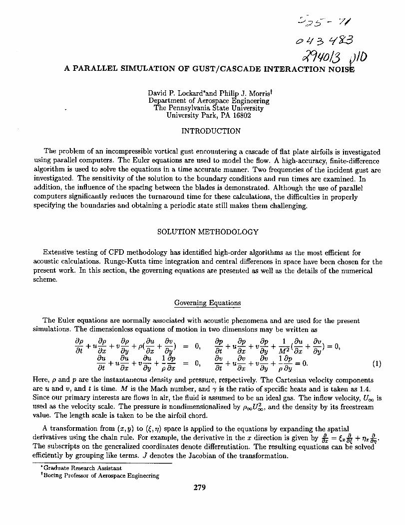
- pj- Y/
o q8-3
qo/6 .joA PARALLEL SIMULATION OF GUST/CASCADE INTERACTION NOIS_
David P. Lockard*and Philip J. Morris tDepartment of Aerospace Engineering
The Pennsylvania State UniversityUniversity Park, PA 16802
INTRODUCTION
The problem of an incompressible vortical gust encountering a cascade of flat plate airfoils is investigated
using parallel computers. The Euler equations are used to model the flow. A high-accuracy, finite-difference
algorithm is used to solve the equations in a time accurate manner. Two frequencies of the incident gust are
investigated. The sensitivity of the solution to the boundary conditions and run times are examined. In
addition, the influence of the spacing between the blades is demonstrated. Although the use of parallel
computers significantly reduces the turnaround time for these calculations, the difficulties in properly
specifying the boundaries and obtaining a periodic state still makes them challenging.
SOLUTION METHODOLOGY
Extensive testing of CFD methodology has identified high-order algorithms as the most efficient for
acoustic calculations. Runge-Kutta time integration and central differences in space have been chosen for the
present work. In this section, the governing equations are presented as well as the details of the numericalscheme.
Governing Equations
The Euler equations are normally associated with acoustic phenomena and are used for the present
simulations. The dimensionless equations of motion in two dimensions may be written as
Op Op Op Ou Ov
o-T+u_+vN+p(_+N)y = o,Ou Ou Ou lop
+--ypox = o,
op op ±(o_.0-7+ + + + = o,y M 20x Oy
Ov Ov Ov 10p
O-'-[+ U_x + V-_u + --- = O'yp Oy(1)
Here, p and p are the instantaneous density and pressure, respectively. The Cartesian velocity components
are u and v, and t is time. M is the Mach number, and 7 is the ratio of specific heats and is taken as 1.4.
Since our primary interests are flows in air, the fluid is assumed to be an ideal gas. The inflow velocity, Uc_ is
used as the velocity scale. The pressure is nondimensionalized by pooU_, and the density by its freestreamvalue. The length scale is taken to be the airfoil chord.
A transformation from (x, y) to (_, _) space is applied to the equations by expanding the spatial
derivatives using the chain rule. For example, the derivative in the x direction is given by _z -- _z _ + r/x_-{.The subscripts on the generalized coordinates denote differentiation. The resulting equations can be solved
efficiently by grouping like terms. J denotes the Jacobian of the transformation.
*Graduate Research Assistant
t Boeing Professor of Aerospace Engineering
279
Numerical Algorithm
Equations (1) can be placed in the semi-discrete, compact form
0QOt
- [7(Q) - = -n(q).
Here, _ represents the discrete form of all the spatial derivatives appearing in eqs.
artificial dissipation. Runge-Kutta time-integration of the form
Q(0) = Qn,
= Q. _ _Qn+l = _sm,,_
(1). T) denotes the
(2)
(3)
is used to advance the solution in time. The local time step is chosen based on a Courant-Freidrichs-Lewy
(CFL) constraint.
Time integration is performed using the alternating five-six stage Runge-Kutta (RK56) time integration of
Hu et al.[1]. The smallest At for the entire domain is used globally. Although the method of Hu et aI. is
technically fourth-order accurate only for linear problems, the results have been found to compare well with
those from the classical fourth-order method. The primary advantage of the alternating scheme is to increasethe allowable CFL number based on accuracy requirements. For the present scheme, this is 1.1 compared =
with 0.4 for the classical method. The spatial operator can either be sixth-order or possess the
dispersion-relation-preserving (DRP) property developed by Tam and Webb[2]. All of the results in this _"
paper are obtained using the DRP coefficients given by Lockard et al.[3]
Since central difference operators do not possess any implicit dissipation, a filter has been _ded explicitly.
A higher-order version of the adaptive dissipation of Jameson[4] has been implemented for this purpose. An _--_
optimized smoother using a seven point stencil is used as a background dissipation rather than the fourth
derivative used in Jameson's implementation. This smoother is given by Tam[5] for a Gaussian half width of
a = 0.37r. A detailed description of the dissipation is given in a previous paper by the authors[6].
Boundary Conditions
Nonreflecting boundary conditions are necessary for acoustic simulations since nonphysical reflections of
waves back into the computational domain can alter the solution significantly. The specified problems
provide a stern test for nonreflecting boundary conditions since some of the acoustic wavefronts are nearly
normal to the boundaries. Furthermore, some of the cutoff modes decay very slowly. The present simulations
use Giles[7] linearized inflow and outflow conditions. However, the location of the outer boundaries is found
to have a strong influence the solution. Other boundary conditions for unbounded domains and
one-dimensional flows were found to perform poorly. Thompson's[8] wall boundary conditions based on a
characteristics analysis are used for solid surfaces. The normal derivatives at the boundary used in the
boundary treatment are discretized using third-order fully biased operators for stability reasons.
Gust Specification
The source of the noise in the problem is the interaction of an oblique, vortical gust with a cascade. Since
it is often difficult to impose arbitrary disturbances at curved boundaries and still minimize reflections of
280
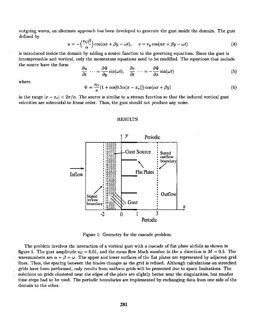
outgoing waves, an alternate approach has been developed to generate the gust inside the domain. The gust
defined by
u = -(vGP)cos(ax + _y-wt), v = v9 cos(ax + fly-wt) (4)x Ol /
is introduced inside the domain by adding a source function to the governing equations. Since the gust is
incompressible and vortical, only the momentum equations need to be modified. The equations that includethe source have the form
au .... a______sin(wt), av ... = _a_ff__sin(wt) (5)ot cOy cOt cOx
where
= vG(1 + cos[0.5a(x -- xo)]) cos(ax + fly)lr
in the range Ix - xol < 2_r/a. The source is similar to a stream function so that the induced vortical gust
velocities axe solenoidal to linear order. Thus, the gust should not produce any noise.
(6)
RESULTS
Y Periodic
Inflow
/Statedinflowboundary Gust
Source
Flat Plates
-2 0 1 3Periodic
Statedoutflowboundary
,/
Outflow
x
Figure h Geometry for the cascade problem.
The problem involves the interaction of a vortical gust with a cascade of fiat plate airfoils as shown in
figure 1. The gust amplitude VG = 0.01, and the mean flow Mach number in the x direction is M = 0.5. The
wavenumbers are a =/3 = w. The upper and lower surfaces of the fiat plates are represented by adjacent grid
lines. Thus, the spacing between the blades changes as the grid is refined. Although calculations on stretched
grids have been performed, only results from uniform grids will be presented due to space limitations. The
solutions on grids clustered near the edges of the plate are slightly better near the singularities, but smaller
time steps had to be used. The periodic boundaries are implemented by exchanging data from one side of the
domain to the other.
281
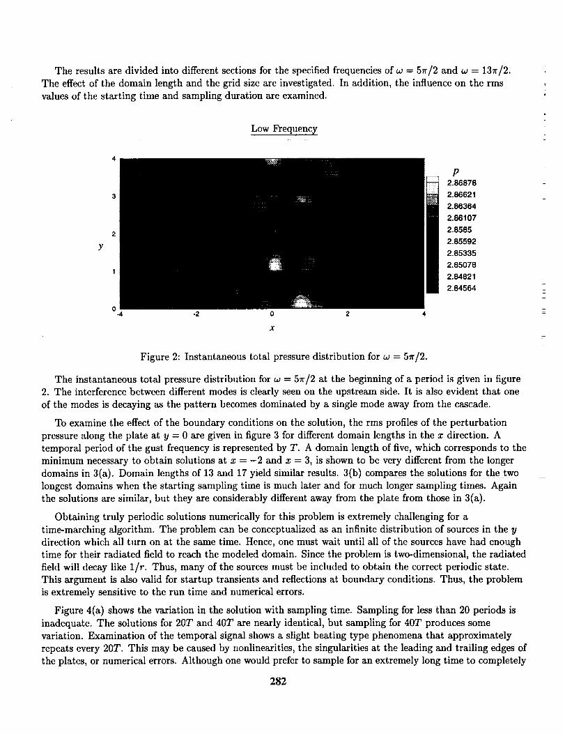
The results are divided into different sections for the specified frequencies of w = 57r/2 and w = 13_r/2.
The effect of the domain length and the grid size are investigated. In addition, the influence on the rms
values of the starting time and sampling duration are examined.
Low Frequency
o-4 -2 o 2 4
x
P2.86878
2.86621
2.86364
2.86107
2.8585
2.85592
2.85335
2.85078
2.84821
2.84564
Figure 2: Instantaneous total pressure distribution for w = 5_/2.
The instantaneous total pressure distribution for w = 57r/2 at the beginning of a period is given in figure
2. The interference between different modes is clearly seen on the upstream side. It is also evident that one
of the modes is decaying as the pattern becomes dominated by a single mode away from the cascade.
To examine the effect of the boundary conditions on the solution, the rms profiles of the perturbation
pressure along the plate at y = 0 are given in figure 3 for different domain lengths in the x direction. A
temporal period of the gust frequency is represented by T. A domain length of five, which corresponds to the
minimum necessary to obtain solutions at x = -2 and x = 3, is shown to be very different from the longer
domains in 3(a). Domain lengths of 13 and 17 yield similar results. 3(b) compares the solutions for the two
longest domains when the starting sampling time is much later and for much longer sampling times. Again
the solutions are similar, but they are considerably different away from the plate from those in 3(a).
Obtaining truly periodic solutions numerically for this problem is extremely challenging for a
time-marching algorithm. The problem can be conceptualized as an infinite distribution of sources in the y
direction which all turn on at the same time. Hence, one must wait until all of the sources have had enough
time for their radiated field to reach the modeled domain. Since the problem is two-dimensional, the radiated
field will decay like 1/r. Thus, many of the sources must be included to obtain the correct periodic state.
This argument is also valid for startup transients and reflections at boundary conditions. Thus, the problem
is extremely sensitive to the run time and numerical errors.
Figure 4(a) shows the variation in the solution with sampling time. Sampling for less than 20 periods is
inadequate. The solutions for 20T and 40T are nearly identical, but sampling for 40T produces some
variation. Examination of the temporal signal shows a slight beating type phenomena that approximately
repeats every 20T. This may be caused by nonlinearities, the singularities at the leading and trailing edges of
the plates, or numerical errors. Although one would prefer to sample for an extremely long time to completely
282
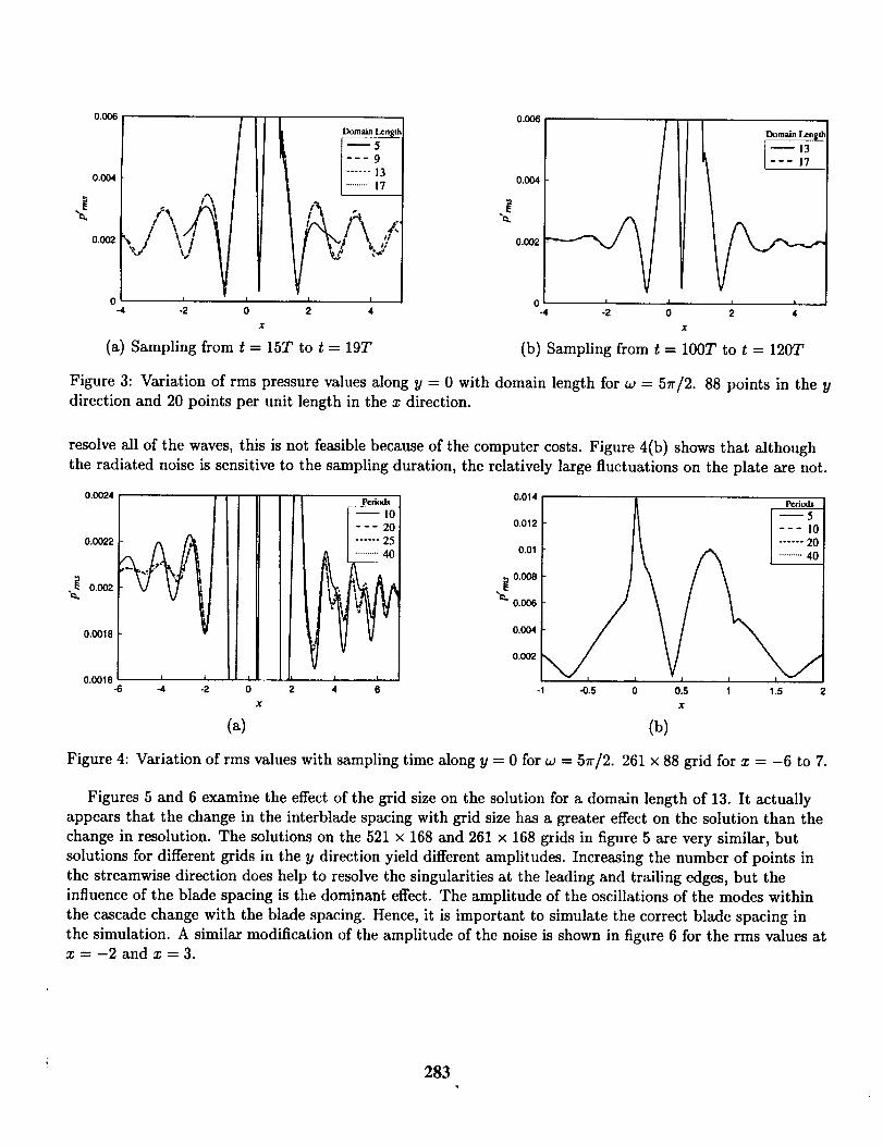
0.0_,
0.004
0.002
/
ft.- --
J
0
-4 -2 0 2 4
x
(a) Sampling from t = 15T to t = 19T
0.006
Domain [_ n___
17
0,004
-4 -2 0 2 4
X
(b) Sampling from t = 100T to t = 120T
Figure 3: Variation of rms pressure values along y = 0 with domain length for w = 5r/2. 88 points in the y
direction and 20 points per unit length in the x direction.
resolve all of the waves, this is not feasible because of the computer costs. Figure 4(b) shows that although
the radiated noise is sensitive to the sampling duration, the relatively large fluctuations on the plate are not.
0.0024
0.0022
0.002
0.0018
20
'25
40
I
I
1
-2 0 2
|
40.0016 _
-6 -4 6
0.014
0,012 --- I0
0.01 ...... 20
0.008
0.006
0.004
0.002
] I
-1 -0.5 0 0.5 1 1.5
X X
(a) (b)
Figure 4: Variation of rms values with sampling time along y = 0 for w = 57r/2. 261 × 88 grid for x = -6 to 7.
Figures 5 and 6 examine the effect of the grid size on the solution for a domain length of 13. It actually
appears that the change in the interblade spacing with grid size has a greater effect on the solution than the
change in resolution. The solutions on the 521 x 168 and 261 × 168 grids in figure 5 are very similar, but
solutions for different grids in the y direction yield different amplitudes. Increasing the number of points in
the streamwise direction does help to resolve the singularities at the leading and trailing edges, but the
influence of the blade spacing is the dominant effect. The amplitude of the oscillations of the modes within
the cascade change with the blade spacing. Hence, it is important to simulate the correct blade spacing in
the simulation. A similar modification of the amplitude of the noise is shown in figure 6 for the rms values atx -- -2 and x = 3.
283
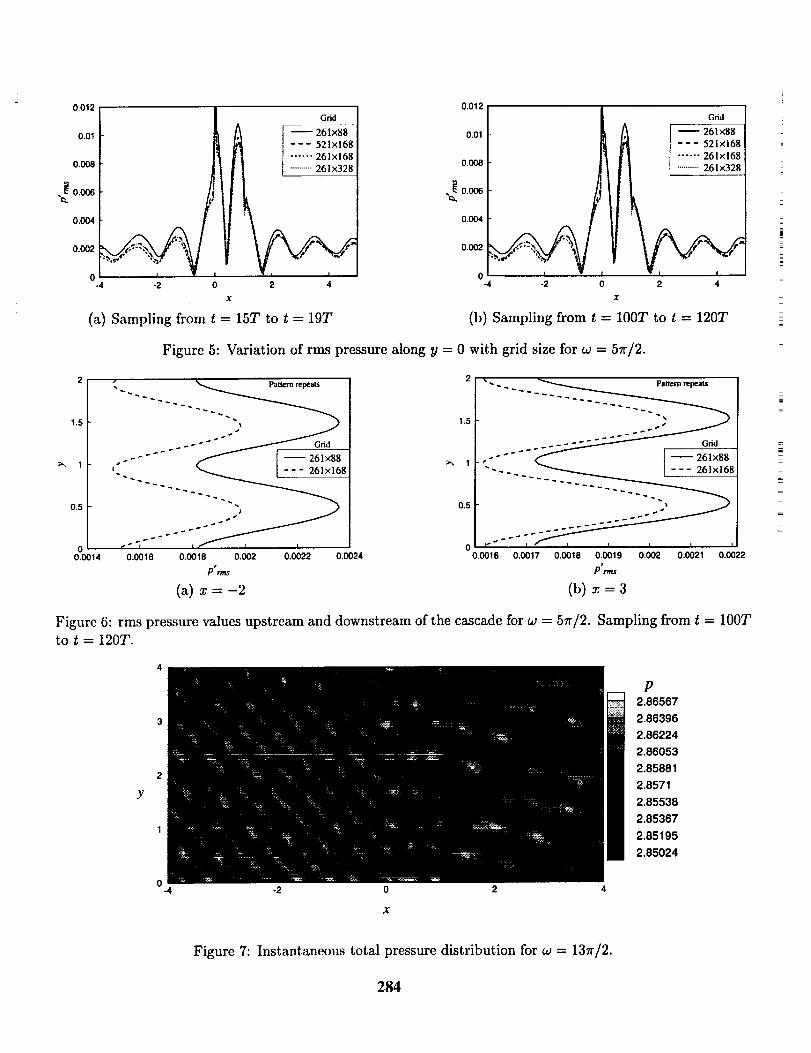
0.012
0.01
0.008
0.006
0.004
0.002
0
Grid
I !!!iTi:
-4 -2 0 2 4
X
(a) Sampling from t = 15T to t = 19T
0.012 /
0.01 I
0.008 I-
0.006-_. _
0.004
0.002:,",,,p,
0-4 -2 0
Grid
2 4
(b) Sampling from t = 100T to t = 120T
Figure 5: Variation of rms pressure along y = 0 with grid size for w = 5r/2.
1.5
0.5
oo.ool 4
...... _ trio"" _ [ --261x88
'-. _ L--- 261x168
i I
0._16 0._18 0.002 0._22 0._24
P'n_
2 • -. _ Patternrepeats
"".....0 I"_''" _ I
0,0016 0.0017 0.0018 0.0019 0.002 0.0021 0.0022
pSrtn$
(a) x=-2 (b) x=3
Figure 6: rms pressure values upstream and downstream of the cascade for w = 57r/2. Sampling from t = 100Tto t = 120T.
Y
o-4 -2 0 2 4
P2.86567
2.86396
2.86224
2.86053
2.85881
2.8571
2.85538
2.85367
2.85195
2.85024
Figure 7: Instantaneous total pressure distribution for w = 13_r/2.
284
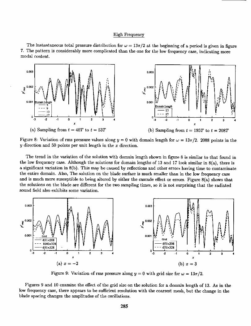
High Frequency
The instantaneous total pressure distribution for w = 13_r/2 at the beginning of a period is given in figure
7. The pattern is considerably more complicated than the one for the low frequency case, indicating moremodal content.
0.003
._ 0.002
0.001
0-3 -2 -1 0 1 2 3
x
(a) Sampling from t = 40T to t = 53T
l, :"...,,,AApI/ AAz-.,,,---9 I II; I !1 |OJ I ',t
......"1 TI v I
......... 17 ; T
4
0.003
._ 0.002
0.001
0-3 -2 -1 0 1 2 3
x
(b) Sampling from t = 195T to t = 208T
"', l',
,,
Domain Lcn U1
--13
4
Figure 8: Variation of rms pressure values along y = 0 with domain length for w = 13_r/2. 2088 points in the
y direction and 50 points per unit length in the x direction.
The trend in the variation of the solution with domain length shown in figure 8 is similar to that found in
the low frequency case. Although the solutions for domain lengths of 13 and 17 look similar in 8(a), there is
a significant variation in 8(b). This may be caused by reflections and other errors having time to contaminate
the entire domain. Also, The solution on the blade surface is much smaller than in the low frequency case
and is much more susceptible to being altered by either the cascade effect or errors. Figure 8(a) shows that
the solutions on the blade are different for the two sampling times, so it is not surprising that the radiatedsound field also exhibits some variation.
0.003
0.002
0.001
0.003
-2 -1 0 1 2 3 4
0.002
0.001
0 0-3 -3 4
Grid
65 Ix208 Ii
-2
Si
L#f
-1 0 1 2 3
(a) x=-2 (b) x=3
Figure 9: Variation of rms pressure along y = 0 with grid size for w = 131r/2.
Figures 9 and 10 examine the effect of the grid size on the solution for a domain length of 13. As in the
low frequency case, there appears to be sufficient resolution with the coarsest mesh, but the change in theblade spacing changes the amplitudes of the oscillations.
285
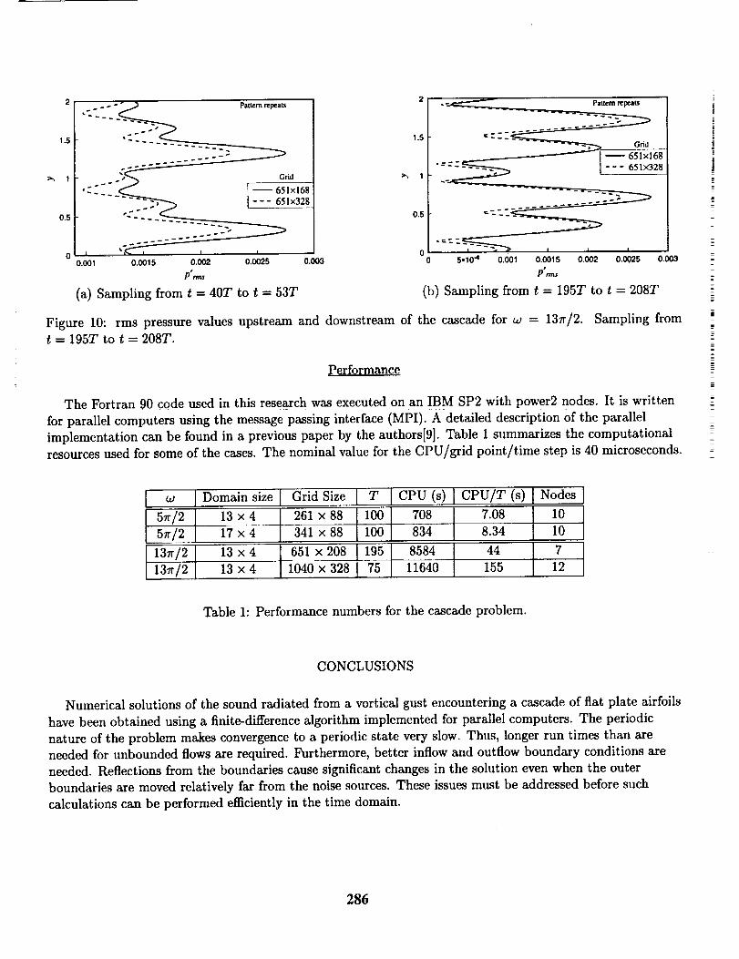
2 I... - -_ Patternrepeats
-- [ -- 651xl68
_., _-, _28
0.5 _- 0.5 "_
0 ' , 0 "='-=_ i , ,
0.001 0.0015 0.002 0.0025 0.003 0 5,I04 0.001 0.0015 0.002 0.0025 0.003
P'.as P".ns
(a) Sampling from t = 40T to t = 53T (b) Sampling from t = 195T to t = 208T
Figure 10: rms pressure values upstream and downstream of the cascade for w = 13r/2. Sampling from$ = 195T to t = 208T.
Performance
The Fortran 90 code used in this research was executed on an IBM SP2 with power2 nodes. It is written
for parallel computers using the message passing interface (MPI). A detailed description of the parallel
implementation can be found in a previous paper by the authors[9]. Table 1 summarizes the computationalresources used for some of the cases. The nominal value for the CPU/grid point/time step is 40 microseconds.
I w [ Domain size
5 /2 I 13 x 4
5_r/2. I 17 x 4
137r/2 13 x 4
131r/2 13 x 4
Grid Size I T I cPU (s)261×88 11001 708341×88 L1001 834
651 x 208 I 195 8584
1040 x 328 [ 75 11640
CPU/T .(s)[ Nodes I
7.088.34
44 /2155
Table 1: Performance numbers for the cascade problem.
CONCLUSIONS
Numerical solutions of the sound radiated from a vortical gust encountering a cascade of flat plate airfoils
have been obtained using a finite-difference algorithm implemented for parallel computers. The periodic
nature of the problem makes convergence to a periodic state very slow. Thus, longer run times than are
needed for unbounded flows are required. Furthermore, better inflow and outflow boundary conditions are
needed. Reflections from the boundaries cause significant changes in the solution even when the outer
boundaries are moved relatively far from the noise sources. These issues must be addressed before such
calculations can be performed efficiently in the time domain.
286
REFERENCES
[1] Hu, F. Q., Hussaini, M. Y., and Manthey, J. Low-dissipation and -dispersion Runge-Kutta schemes for
computational aeroacoustics. Journal of Computational Physics, 124, pp. 177-191, 1995.
[2] Tam, C. K. W., and Webb, J. C. Dispersion-relation-preserving finite difference schemes for
computational aeracoustics. Journal of Computational Physics, 107, pp. 262-281, 1993.
[3] Lockard, D. P., Brentner, K. S., and Atkins, H. L. High-accuracy algorithms for computational
aeroacoustics. AIAA Journal, 33(2), pp. 246-251, 1995.
[4] Jameson, A., Schmidt, W., and Turkel, E. Numerical solution of the Euler equations by finite-volume
methods using Runge-Kutta time-stepping schemes. AIAA-81-1259, 1981.
[5] Tam, C. K. W., and Dong, Z. Radiation and outflow boundary conditions for direct computation of
acoustic and flow disturbances in a nonumiform mean flow. CEAS/AIAA Paper-95-007, 1995.
[6] Lockard, D. P., and Morris, P. J. The radiated noise from airfoils in realistic mean flows. AIAA
Paper-97-0285, 1997.
[7] Giles, M. B. Nonreflecting boundary conditions for euler equation calculations. AIAA Journal, 28(12),pp. 2050-2057, 1990.
[8] Thompson, K. W. Time-dependent boundary conditions for hyperbolic systems, II. Journal ofComputational Physics, 89, pp. 439-461, 1989.
[9] Lockard, D. P., and Morris, P. J. A parallel implementation of a computational aeroacoustic algorithm
for airfoil noise. AIAA Paper-96-1754, 1996 (to appear Journal of Computational Acoustics, 1997).
287
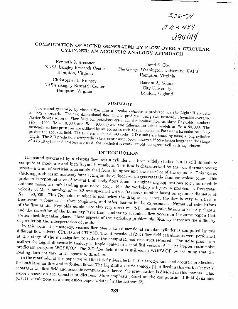
-- o26 -7/
COMPUTATION OF SOUND GENERATED BY FLOW OVER A CIRCULAR
CYLINDER: AN ACOUSTIC ANALOGY APPROACH
Kenneth S. Brentner
NASA Langley Research Center
Hampton, Virginia
Christopher L. Rumsey
NASA Langley Research Center
Hampton, Virginia
Jared S. Cox
The George Washington University, JIAFS
Hampton, Virginia
Bassam A. Younis
City University
London, England
SUMMARY
The sound generated by viscous flow past a circular cylinder is predicted via the Lighthill acousticanalogy approach. The two dimensional flow field is predicted using two unsteady Reynolds-averagedNavier-Stokes solvers. Flow field computations are made for laminar flow at three Reynolds numbers(Re = 1000, Re = 10,000, and Re = 90,.000) and two different turbulent models at Re = 90,000. Theunsteady surface pressures are utilized by an acoustics code that implements Farassat's formulation 1A topredict the acoustic field. The acoustic code is a 3-D code--2-D results are found by using a long cylinderlength. The 2-D predictions overpredict the acoustic amplitude; however, if correlation lengths in the rangeof 3 to 10 cylinder diameters are used, the predicted acoustic amplitude agrees well with experiment.
INTRODUCTION
The sound generated by a viscous flow over a cylinder has been widely studied but is still difficult to
compute at moderate and high Reynolds numbers. This flow is characterized by the yon Karman vortex
street-- a train of vorticies alternately shed from the upper and lower surface of the cylinder. This vortex
shedding produces an unsteady force acting on the cylinder which generates the familiar aeolean tones. This
problem is representative of several bluff body flows found in engineering applications (e.g., automobile
antenna noise, aircraft landing gear noise, etc.). For the workshop category 4 problem, a fl'eestream
veIocity of Maeh number M = 0.2 was specified with a Reynolds number based on cylinder diameter of
Re = 90,000. This Reynolds number is just below the drag crisis, hence, the flow is very sensitive to
freestream turbulence, surface roughness, and other factors in the experiment. Numerical calculations
of the flow at this Reynolds number are also very sensitive---2-D laminar calculations are nearly chaotic
and the transition of the boundary layer from laminar to turbulent flow occurs in the same region that
vortex shedding takes place. These aspects of the workshop problem significantly increases the difficulty
of prediction and interpretation of results.
In this work, the unsteady, viscous flow over a two-dimensional circular cylinder is computed by two
different flow solvers, CFL3D and CITY3D. Two-dimensional (2-D) flow-field calculations were performed
at this stage of the investigation to reduce thc computational resources required. The noise prediction
utilizes tile Lighthill acoustic analogy as implemented in a modified version of the helicopter rotor noise
prediction program WOPWOP. The 2-D flow field data is utilized in WOPWOP by assuming that the
loading does not vary in the spanwise direction.
In the remainder of this paper we will first briefly describe both the aerodynamic and acoustic predictions
for both laminar flow and turbulent flows. The Lighthill acoustic analogy [1] utilized in this work effectively
separates the flow field and acoustic computations, hence, the presentation is divided in this manner. This
paper focuses on the acoustic predictions. More emphasis placed on the computational fluid dynamics
(CFD) calculations in a companion paper written by the authors [2].
289
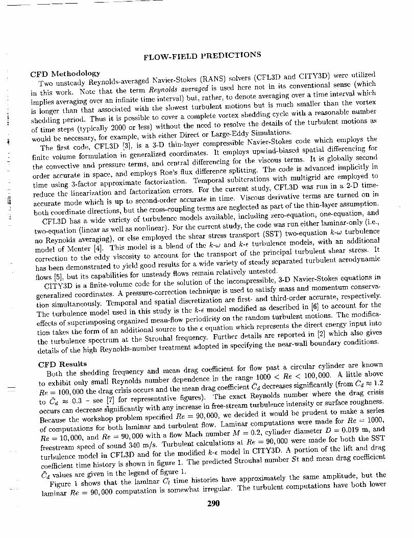
FLOW-FIELD PREDICTIONS
CFD Methodology
Two unsteady Reynolds-averaged Navier-Stokes (RANS) solvers (CFL3D and CITY3D) were utilized
in this work. Note that the term Reynolds averaged is used here not in its conventional sense (which
implies averaging over an infinite time interval) but, rather, to denote averaging over a time interval which
is longer than that associated with the slowest turbulent motions but is much smaller than the vortex
shedding period. Thus it is possible to cover a complete vortex shedding cycle with a reasonable number
of time steps (typically 2000 or less) without the need to resolve the details of the turbulent motions as
would be necessary, for example, with either Direct or Large-Eddy Simulations.
The first code, CFL3D [3], is a 3-D thin-layer compressible Navier-Stokes code which employs the
finite volume formulation in generalized coordinates. It employs upwind-biased spatial differencing for
the convective and pressure terms, and central differencing for the viscous terms. It is globally second
order accurate in space, and employs Roe's flux difference splitting. The code is advanced implicitly in
time using 3-factor approximate factorization. Temporal subiterations with multigrid are employed to
reduce the linearization and factorization errors. For the current study, CFL3D was run in a 2-D time-
accurate mode which is up to second-order accurate in time. Viscous derivative terms are turned on in
both coordinate directions, but the cross-coupling terms are neglected as part of the thin-layer assumption.
CFL3D has a wide variety of turbulence models available, including zero-equation, one-equation, and
two-equation (linear as well as nonlinear). For the current study, the code was run either laminar-only (i.e.,
no Reynolds averaging), or else employed the shear stress transport (SST) two-equation k-w turbulence
model of Menter [4]. This model is a blend of the k-_ and k-e turbulence models, with an additional
correction to the eddy viscosity to account for the transport of the principal turbulent shear stress. It
has been demonstrated to yield good results for a wide variety of steady separated turbulent aerodynamic
flows [5], but its capabilities for unsteady flows remain relatively untested.
CITY3D is a finite-volume code for the solution of the incompressible, 3-D Navier-Stokes equations in
generalized coordinates. A pressure-correction technique is used to satisfy mass and momentum conserva-
tion simultaneously. Temporal and spatial discretization are first- and third-order accurate, respectively.
The turbulence model used in this study is the k-e model modified as described in [6] to account for the
effects of superimposing organized mean-flow periodicity on the random turbulent motions. The modifica-
tion takes the form of an additional source to the e equation which represents the direct energy input into
the turbulence spectrum at the Strouhal frequency. Further details are reported in [2] which also gives
details of the high Reynolds-number treatment adopted in specifying the near-wall boundary conditions.
CFD Results
Both the shedding frequency and mean drag coefficient for flow past a circular cylinder are known
to exhibit only small Reynolds number dependence in the range 1000 < Re < 100,000. A little above
Re = 100,000 the drag crisis occurs and the mean drag coefficient C'd decreases significantly (from C'_ _ 1.2
to C'd _ 0.3 - see [7] for representative figures). The exact Reynolds number where the drag crisis
occurs can decrease significantly with any increase in free-stream turbulence intensity or surface roughness.
Because the workshop problem specified Re --- 90,000, we decided it would be prudent to make a series
of computations for both laminar and turbulent flow. Laminar computations were made for Re = 1000,
Re = 10,000, and Re = 90,000 with a flow Mach number M = 0.2, cylinder diameter D = 0.019 m, and
frecstream speed of sound 340 m/s. Turbulent calculations at Re = 90,000 were made for both the SST
turbulence model in CFL3D and for the modified k-e model in CITY3D. A portion of the lift and drag
coefficient time history is shown in figure 1. The predicted Strouhal number St and mean drag coefficient
Cu values are given in the legend of figure 1.
Figure I shows that the laminar Cl time histories have approximately the same amplitude, but the
laminar Re -- 90, 000 computation is somewhat irregular. The turbulent computations have both lower
290
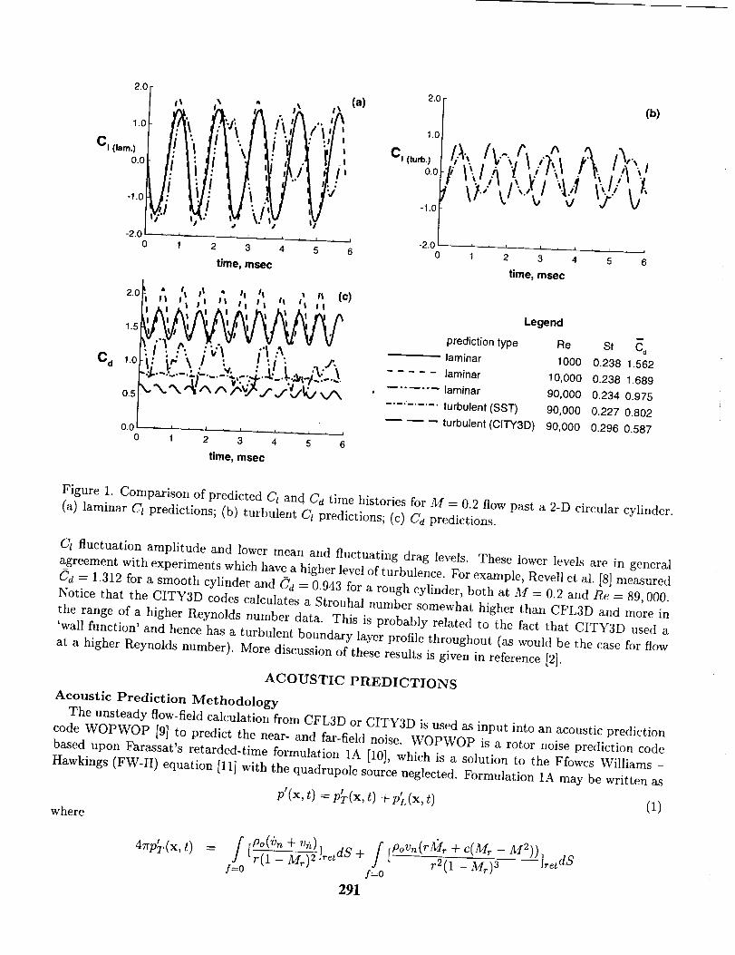
2.0
1.0i
CI (Im.)o.o i
;-1.0
-2.0 - " '0 1
"!J
i . t ,,
2 3
:iA,iP,
iI,lt,it , i .... i
4 5 6
time, mse¢
2.0
1.5
C d 1.0
0.5
0.0o
, t. rl " II II _ a (C)
i ,".. ;,. .
"'J"';-'-':'. _ ..... ½,. ".'P" "-" :'_'l .... ""
1 2 3 4 5 6
time, msec
(a)2.0
1.0
Ci (turb.)0.0
-I.0
-2.00
(b)
f -,A.,Ah 5,,,
, i , i , I , I * . r . t
1 2 3 4 5 6
time, msec
legend
prediction type Re St _
laminar 1000 0.238 1.562
laminar 10,000 0.238 1.689
laminar 90,000 0.234 0.975
.... "...... turbulent (SST) 90,000 0.227 0.802
turbulent(CITY3D) 90,000 0.296 0.587
Figure 1. Comparison of predicted CI and Ca time histories for M = 0.2 flow past a 2-D circular cylinder.
(a) laminar Cl predictions; (b) turbulent Ct predictions; (c) Ca predictions.
Cl fluctuation amplitude and lower mean and fluctuating drag levels. These lower levels are in general
agreement with experiments which have a higher level of turbulence. For example, Revellet al. [8] measured
C'd = 1.312 for a smooth cylinder and C'd = 0.943 for a rough cylinder, both at M = 0.2 and Re = 89,000.
Notice that the CITY3D codes calculates a Strouhal number somewhat higher than CFL3D and more in
the range of a higher Reynolds number data. This is probably related to the fact that CITY3D used a
'wall function' and hence has a turbulent boundary layer profile throughout (as would be the case for flow
at a higher Reynolds number). More discussion of these results is given in reference [2].
ACOUSTIC PREDICTIONS
Acoustic Prediction Methodology
The unsteady flow-field calculation from CFL3D or CITY3D is used as input into an acoustic prediction
code WOPWOP [9] to predict the near- and far-field noise. WOPWOP is a rotor noise prediction code
based upon Farassat's retarded-time formulation 1A [10], which is a solution to the Ffowcs Williams -
Hawkings (FW-H) equation [11] with the quadrupole source neglected. Formulation 1A may be written as
p'(x, t) = p_(x, t) + pk(x, t) (1)
where
4_p_(x, t) [povn(rl_/Ir + C(Mr - M2))/'r(1Ip°O)"-+Mr)2"n)]r'tds+ / r-_i---'Mrr) 5 ]retdS
f=0 /=0
291
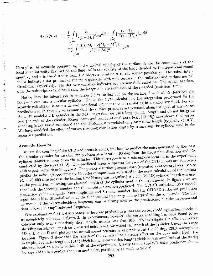
=
5
4rrp_(x,t) 1 er--gM 2]retd S.
I=o /=o
1 er (r_?r + c(Mr -f[ r2(1- '7 r' 3 12))lretdSI=O
Here pr is the acoustic pressure, vn is the normal velocity of the surface, gi are the components of the
local force intensity that act on the fluid, M is the velocity of the body divided by the freestream sound
speed c, and r is the distance from the observer position x to the source position y. The subscripts r
and n indicate a dot product of the main quantity with unit vectors in the radiation and surface normal
directions, respectively. The dot over variables indicates source-time differentiation. The square brackets
with the subscript ret indicates that the integrands are evaluated at the retarded (emission) time.
Notice that the integration in equation (1) is carried out on the surface f = 0 which describes the
body---in our case a circular cylinder. Unlike the CFD calculations, the integration performed for the
acoustic calculation is over a three-dimensional cylinder that is translating in a stationary fluid. For the
predictions in this paper, we assume that the surface pressures are constant along the span at any source
time. To model a 2-D cylinder in the 3-D integration, we use a long cylinder length and do not integrate
over the ends of the cylinder. Experiments and computational work (e.g., [12-15]) have shown that vortex
shedding is not two-dimensional and the shedding is correlated only over some length (typically < 10D).
We have modeled the effect of vortex shedding correlation length by truncating the cylinder used in the
acoustics prediction.
Acoustic Results
To test the coupling of the CFD and acoustic codes, we chose to predict the noise generated by flow past
the circular cylinder for an observer position at a location 90 deg from the freestream direction and 128
cylinder diameters away from the cylinder. This corresponds to a microphone location in the experiment
conducted by Revell et al. [8]. The predicted acoustic spectra for each of the CFD inputs are compared
with experimental data in figure 2. One period of surface pressure data (repeated as necessary) was used to
predict the noise. (Approximately 62 cycles of input data were used in the noise calculation of the laminar
Re - 90,000 case because the loading time history was irregular.) A 0.5 m (26.3D) cylinder length was used
in the prediction, matching the physical length of the cylinder used in the experiment. In figure 2 we see
that both the Strouhal number and the amplitude are overpredicted. The CFL3D turbulent (SST model)
prediction yields a slightly lower amplitude and Strouhal number, but the CITY3D turbulent prediction
again has a high Strouhal value at the fundamental frequency and overpredicts the amplitude. The first
harmonic of the vortex shedding frequency can be clearly seen in the predictions, but the experimental
data is lower in amplitude and frequency.
One explanation for ,the discrepancy in the noise predictions is that the vortex shedding has been modeled
as completely coherent in figure 2. In experiments, however, the vortex shedding has been found to be
coherent only over a relatively short length, usually less that 10D. To investigate the effect of vortex
shedding correlation length on predicted noise levels, we varied the length of the cylinder L over the range
3D < L < 250D and plotted the overall sound pressure level predicted at the 90 deg, 128D microphone
location. Figure 3 show that the length of the cylinder has a strong effect on the peak noise level. For
example, a cylinder length of 10D (which is a long correlation length) yields a peak amplitude at the 90 deg
observer location that is within 2 dB of the experiment. Clearly then a true 2-D noise prediction should
be expected to overpredict the measured noise, possibly by as much as 25 dB!
292
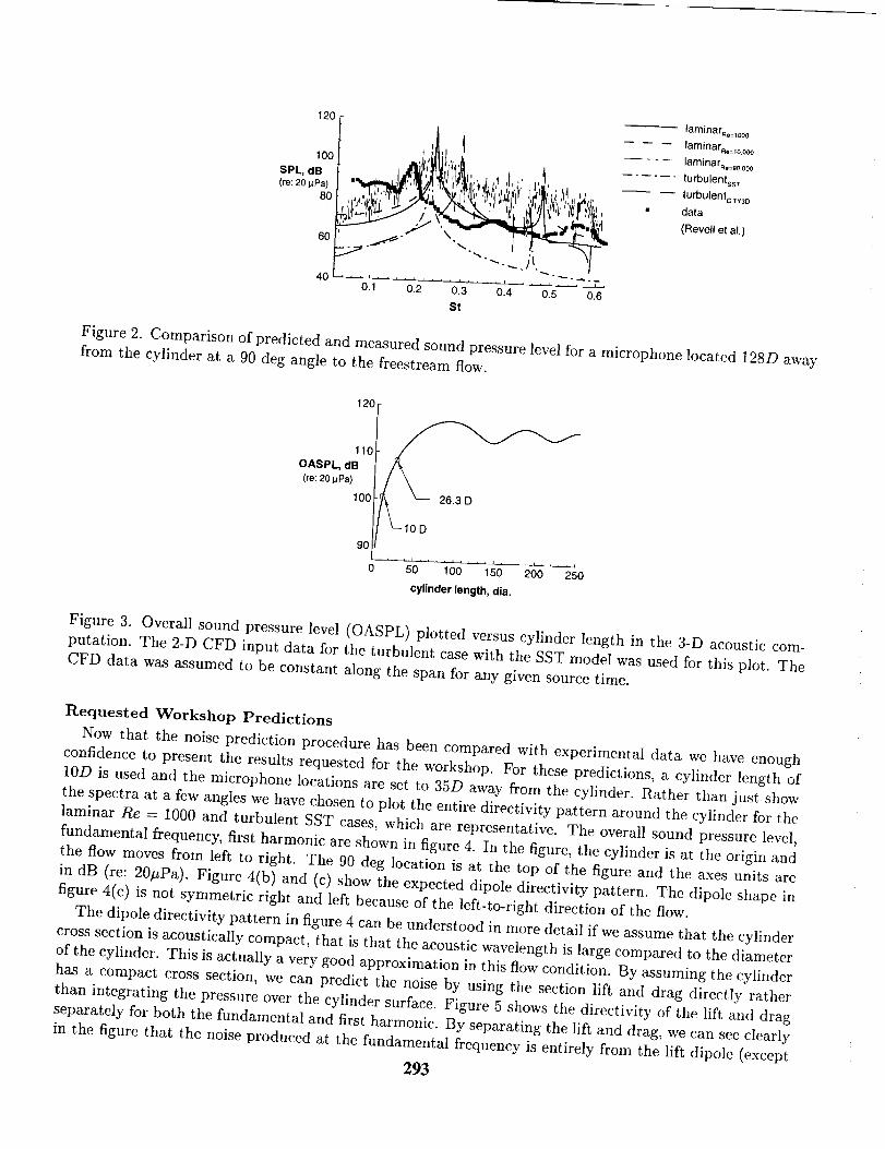
120
100
SPL, dB(re: 20 _Pa)
8O
L •
40 ..............................O.1 0.2 0.3 0.4 0.5 0.6
St
laminar_=_oo Q
laminarRe=_o,ooo
.... laminarRo=go,ooo
turbulentss T
turbulentc_-_,_D
• data
(Revellet al.)
Figure 2. Comparison of predicted and measured sound pressure level for a microphone located 128D away
from the cylinder at a 90 deg angle to the freestream flow.
120
110
OASPL, dB
(re: 20 _Pa)
100
L10D
9O
0 5'0 100 150 20_0
cylinder length, dia.
Figure 3. Overall sound pressure level (OASPL) plotted versus cylinder length in the 3-D acoustic com-
putation. The 2-D CFD input data for the turbulent case with the SST model was used for this plot. The
CFD data was assumed to be constant along the span for any given source time.
Requested Workshop Predictions
Now that the noise prediction procedure has been compared with experimental data we have enough
confidence to present the results requested for the workshop. For these predictions, a cylinder length of
10D is used and the microphone locations are set to 35D away from the cylinder. Rather than just show
the spectra at a few angles we have chosen to plot the entire directivity pattern around the cylinder for the
laminar Re = 1000 and turbulent SST cases, which are representative. The overall sound pressure level,
fundamental frequency, first harmonic are shown in figure 4. In the figure, the cylinder is at the origin and
the flow moves from left to right. The 90 deg location is at the top of the figure and the axes units are
in dB (re: 20#Pa). Figure 4(b) and (c) show the expected dipole directivity pattern. The dipole shape in
figure 4(c) is not symmetric right and left because of the left-to-right direction of the flow.
The dipole directivity pattern in figure 4 can be understood in more detail if we assume that the cylinder
cross section is acoustically compact, that is that the acoustic wavelength is large compared to the diameter
of the cylinder. This is actually a very good approximation in this flow condition. By assuming the cylinder
has a compact cross section, we can predict the noise by using the section lift and drag directly rather
than integrating the pressure over the cylinder surface. Figure 5 shows the directivity of the lift and drag
separately for both the fundamental and first harmonic. By separating the lift and drag, we can see clearly
in the figure that the noise produced at the fundamental frequency is entirely from the lift dipole (except
293

+
==
(a) (b) (c)
12 120
%%.._. /i
-- larninar.+=,_
..... turbulen|ss _
Figure 4. Predicted directivity patterns for M = 0.2 flow traveling left to right. Axes units are decibels
(dB, re:20#Pa). (a) overall sound pressure level; (b) fundamental frequency; (c) first harmonic.
(a) (b) (c) (d)
.......... _ " o ' +)o 12-_-_- .... +_o' _2o120 /" 80 8() '1 120 120 80 120
_ 80 ,-' 80
-- lamlnarR,.l_o -- larnlmarm._:_
....... tur_lent=s T ....... turbulents_ x
Figure 5. Comparison of the Cl and Cd noise components directivity pattern for M = 0.2 flow traveling
left to right. Axes units are decibels (dB, re: 20#Pa). (a) Cz fundamental frequency; (b) Cd fundamental
frequency; (c) Ci first harmonic; (d) C_ first harmonic.
at the nulls of the dipole), while the drag completely dominates the first harmonic frequency. This is what
should be expected because the period of the drag oscillation is half the lift oscillation period.
CONCLUDING REMARKS
The choice of Reynolds number Re = 90,000 makes the calculation of noise generated by flow past a
circular cylinder particularly difficult. This difficulty is due to the transitional nature of the flow at this
Reynolds number. Laminar flow caiculations at such a high Reynolds number are irregular and nearly
chaotic. The turbulent calculations are sensitive to both grid and turbulence model (See reference [2]).
Although we have performed only 2-D flow calculations in this paper, the amplitude of the noise predic-
tion seems to agree fairly well with experimental data if a reasonable correlation length of the cylinder is
used. To understand all of the details of the flow the problem must ultimately be solved as a 3-D problem
to properly account for partial coherence of vortex shedding. The acoustic model does not require any
changes for 3-D computations, but the CFD calculations will be very demanding. The CFL3D calculationsfor two dimensions already require approximately 4.5 CPU hrs on a Cray Y/MP (CITY3D - 80 hrs on
workstation) to reach a periodic solution. This will be much longer for an adequately resolved 3-D com-
putation. In contrast the acoustic calculation for a single observer position required about 70 CPU sec on
a workstation.
294
REFERENCES
1. Lighthill, M. J., "On Sound Generated Aerodynamically, I: General Theory," Proceedings of the Royal
Society, Vol. A221, I952, pp. 564-587.
2. Cox, J. S., Rumsey, C. L., Brentner, K. S., and Younis, B. A., "Computation of Sound Generated by
Viscous Flow Over A Circular Cylinder," Proceedings of the ASME/JSME/IMechE/CSME/IAHR
4th International Symposium on Fluid-Structure Interactions, Aeroelasticity, Flow-Induced Vibration
8¢ Noise, Nov. 1997. To appear.
3. Rumsey, C. L., Sanetrik, M. D., Biedron, R. T., Melson, N. D., and Parlette, E. B., "Efficiency and
Accuracy of Time-Accurate Turbulent Navier-Stokes Computations," Computers and Fluids, Vol. 25,
No. 2, 1996, pp. 217-236.
4. Menter, F. R., "Improved Two-Equation k -w Turbulence Models for Aerodynamic Flows," NASA
TM 103975, Oct. 1992.
5. Menter, F. R., and Rumsey, C. L., "Assessment of Two-Equation Turbulence Models for Transonic
Flows," AIAA Paper 94-2343, 1994.
6. Przulj, V., and Younis, B. A., "Some Aspects of the Prediction of Turbulent Vortex Shedding from
Bluff Bodies," Symposium on Unsteady Separated Flows, 1993 ASME Fluids Engineering Division
Annual Summer Meeting, Vol. 149, Washington, DC, 1993.
7. Schlichting, H., Boundary-Layer Theory, McGraw-Hill Series in Mechanical Engineering, McGraw-
Hill, New York, Seventh edition, 1979. Translated by J. Kestin.
8. Revell, J. D., Prydz, R. A., and Hays, A. P., "Experimental Study of Airframe Noise vs. Drag Rela-
tionship for Circular Cylinders," Lockheed Report 28074, Feb. 1977. Final Report for NASA ContractNAS1-14403.
9. Brentner, K. S., "Prediction of Helicopter Discrete Frequency Rotor Noise--A Computer Program
Incorporating Realistic Blade Motions and Advanced Formulation," NASA TM 87721, Oct. 1986.
10. Farassat, F., and Succi, G. P., "The Prediction of Helicopter Discrete Frequency Noise," Vertica, Vol.
7, No. 4, 1983, pp. 309-320.
11. Ffowcs Williams, J. E., and Hawkings, D. L., "Sound Generated by Turbulence and Surfaces in
Arbitrary Motion," Philosophical Transactions of the Royal Society, Vol. A264, No. 1151, 1969, pp.321-342.
12. Alemdaro_lu, N., Rebillat, J. C., and Goethals, R., "An Aeroacoustic Coherence Function Method
Applied to Circular Cylinder Flows," Journal of Sound and Vibration, Vol. 69, No. 3, 1980, pp.427-439.
13. Blackburn, H. M., and Melbourne, W. H., "The Effect of Free-Stream Turbulence on Sectional Lift
Forces on a Circular Cylinder," Journal of Fluid Mechanics, Vol. 306, Jan. 1996, pp. 267-292.
14. Kacker, S. C., Pennington, B., and Hill, R. S., "Fluctuating Lift Coefficient For a Circular Cylinder
in Cross Flow," Journal of Mechanical Engineering Science, Vol. 16, No. 4, 1974, pp. 215-224.
15. Mittal, R., and Balachandar, S., "Effect of Three-Dimensionality on the Lift and Drag of NominalIy
Two-Dimensional Cylinders," Physics of Fluids, Vol. 7, No. 8, Aug. 1995, pp. 1841-1865.
295

COMPUTATION OF NOISE DUE TO THE FLOW OVER A CIRCULAR CYLINDER
Sanjay Kumarasamy I, Richard A. Korpus 2 and Jewel B. Barlow 3
2q(o/7
pz
ABSTRACT
Noise due to the flow over a circular cylinder at a Reynolds number of 90,000 and Mach Number of 0.2 is computedusing a two step procedure. As the first step, the flow is computed using an incompressible, time dependent Reynolds
Averaged Navier-Stokes (RANS) solver. The resulting unsteady pressures are used as input to a two dimensional fre-
quency domain acoustic solver, and 3D effects are studied using the Lighthill-Curle equation. Grid and time step depen-
dency studies were performed to ascertain the accuracy of the flow computation. Computed acoustic results are compared
to experimental values and agree well over much of the spectrum although the computed peak values corresponding to 2Dacoustic simulations differ substantially from the available experimental measurements. Three dimensional acoustic simu-
lation reduce the 2D noise level by 10dB.
INTRODUCTION
The most general way to compute noise radiation by a turbulent flow is to numerically solve the Navier-Stokes equa-tions. The computation needs to be performed over a large spatial domain for long time intervals, simultaneously resolv-
ing small scales. This requirement overwhelms present day computing power. However, depending on the speed andnature of the flow certain simplifications can be made to make the computations feasible. In the case of low Math numbcr
flows, there are many interesting cases in which there is no back reaction of the acoustic pressures on the flow. Hence, the
computations can be split into two parts, namely, the computation of the flow, and the computation of noise. One advan-
tage of this splitting is that computational methods and grids can be optimized separately for the vastly different scalesinvolved.
Flow over a circular cylinder shows a variety of features which vary with Reynolds number. Williamson I reviewed
the current state of understanding on the subject. The flow regime in the Reynolds number region of 1,000 to 200,000 is
termed the "Shear-Layer Transition Regime". In this regime, transition develops in the shear layer characterized by an
increase in the base pressure. As the Reynolds number increases, the turbulent transition point in the separated shear layermoves upstream and at 200,000 the flow becomes fully turbulent. At 90,000 it is believed the wake is fully turbulent but
the attached boundary layer is essentially laminar. Unfortunately, the RANS solver used in the present work does not have
a transition model. Since the extent of turbulent and laminar flow affects the unsteady pressures, three separate simula-
tions were performed to ascertain the effect of the turbulence on the overall sound intensity predicted:Case I. Laminar flow over the entire domain
Case 2. Laminar flow + Turbulent wake (Base line Study)Case 3. Turbulent flow over the entire domain.
Once the underlying flow is computed, noise due to the flow can be computed by a two step procedure. Hardin et al 2
analyzed the sound generation due to the flow over a cavity at low Reynolds and Mach number using an incompressible,
two dimensional time dependent Navier Stokes solver to drive the acoustic radiation using the method outlined by Hardinand Pope 3. The present work employs a similar two step approach. First, the high Reynolds number, low Math number
flow is computed by an incompressible, time dependent, Reynolds Averaged Navier-Stokes solver. Second, the acoustic
radiation is determined by solving the wave equation from the Lighthill Acoustic Analogy (LAA). The acoustic solverwas previously validated against test cases for which closed form solutions exist 4'5'6.
The Computations reported in the present work refer to the Category 4 problem of the Second Computational Aeroa-coustics Workshop JS. The problem is restated for completeness. Consider uniform flow at Mach number of 0.2 ovcr a
two-dimensional cylinder of diameter D=l.9 cm. The Reynolds number based on the diameter of the cylinder is 90,000.
1.Research Associate, Glenn L. Martin Wind Tunnel, University of Maryland, College Park.2. Senior Research Scientist, Science Application International Corporation, Annapolis.
3. Director, Glenn L. Martin Wind Tunnel, University of Maryland, College Park.
297
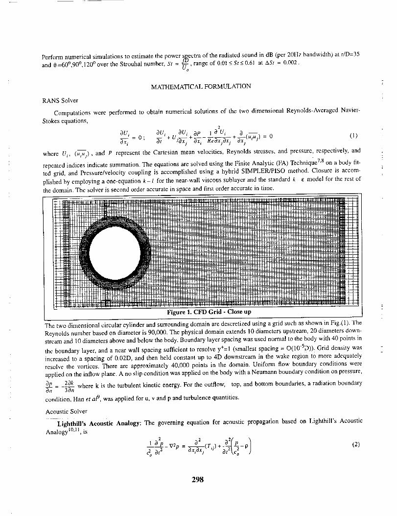
Perform numerical simulations to estimate the power s_ectra of the radiated sound in dB (per 20Hz bandwidth) at r/D=35and 0 =60°,90 °, 120 ° over the Strouhal number, St = J- , range of 0.01 -<St <_0.61 at ASt = 0.002.
Uo
MATHEMATICAL FORMULATION
RANS Solver
Computations were performed to obtain numerical solutions of the two dimensional Reynolds-Averaged Navier-
Stokes equations,2
_Ui OUi _Ui + _P 1 _ Ui + _(uiui) = 0 (l)Oxi - 0 ; 3t +-- Uj_x'-_) _x i ReOxjOx i ox) .
where U i, (uiu :) , and P represent the Cartesian mean velocities, Reynolds stresses, and pressure, respectively, and
repeated indices indicate summation. The equations are solved using the Finite Analytic (FA) Technique 7'8 on a body fit-
ted grid, and Pressure/velocity coupling is accomplished using a hybrid SIMPLER/PISO method. Closure is accom-
plished by employing a one-equation k - l for the near-wall viscous sublayer and the standard k - e model for the rest of
the domain. The solver is second order accurate in space and first order accurate in time.
1
tFigure 1. CFD Grid - Close up
i I
-__!-F-
--4--
--'--pcT-r:
-'-E
: IJ_L
_k
j -j-_
4--i
The two dimensional circular cylinder and surrounding domain are descretized using a grid such as shown in Fig.(1). The
Reynolds number based on diameter is 90,000. The physical domain extends 10 diameters upstream, 20 diameters down-
stream and 10 diameters above and below the body. Boundary layer spacing was used normal to the body with 40 points in
the boundary layer, and a near wall spacing sufficient to resolve y+=l (smallest spacing = O(10-SD)). Grid density was
increased to a spacing of 0.02D, and then held constant up to 4D downstream in the wake region to more adequately
resolve the vortices. There are approximately 40,000 points in the domain. Uniform flow boundary conditions were
applied on the inflow plane. A no slip condition was applied on the body with a Neumann boundary condition on pressure,
_p _ 2_)k_n _--_ where k is the turbulent kinetic energy. For the outflow, top, and bottom boundaries, a radiation boundary
condition, Han et al 9, was applied for u, v and p and turbulence quantities.
Acoustic Solver
Lighthill's Acoustic Analogy: The governing equation for acoustic propagation based on Lighthill's Acoustic
Analogy _°'1_, is
2 dxidxj32_-_2 12 "-21 o_ p V2p _----¢--.(T,i) - p (2)
620 _t 2 c o
298
where p is the pressure, co is the speed of sound, u) is the velocity in the j direction, and T O = 9uiu) + visous is the
Lighthill's stress tensor. Neglecting viscous terms and for linear acoustics, (p - Po) = (P - Po)C2oequation (2) becomes
2 221 _ P v2 p = _¢.._¢__(9uiuj) (3)
C_obt 2 _x,_xj
Non-dimensionalizing the variables, and applying Fourier transformation, leads to
v2_+ _ 2- 22M_p = _uiu (4)3xi3x) I
where M** is the free stream Mach number and o_s is the Strouhal number. It is noted here that the Mach number in equa-
tion (4) is a free parameter and for a consistent formulation it should be small so that the incompressibility assumption is
valid for solving the flow. For the present work, the quadrupole noise was not computed. Hence the right hand side of
Equation (4) is zero. Equation (4) is transformed to general curvilinear coordinates and descretized using the FA tech-
nique. A first order Bayliss-Turkel boundary condition for the Helmholtz equation 12'13,
_r- ik- p = 0 (5)
where r is the radial distance, was applied on the far-field boundary. The Fourier transformed unsteady pressures from the
RANS simulations are applied on the body are applied as Dirichlet boundary conditions. Equation (5) is transformed into
computational coordinates, descretized to second order accuracy, and solved implicitly. The descretized form of (4) with
boundary conditions (5) constitute a non-positive definite complex system of linear equations. Conventional relaxation
methods like Gauss-Seidal and Line relaxation fail due to the non-positive definitiveness and hence Bi-Conjugate Gradi-
ent Stabilized (BICG-STAB), Vorst 14, is applied. The acoustic grid topology is shown in Fig.(2). The grid is a polar grid
with the far field located at 20 times the wavelength of the acoustic wave. There are 20 grid points per wave length with a
total of 400 grid points radially and 36 grid points in the 0 direction.
Lighthill -Curie Equation: The acoustic computations were also performed using the LighthiII-Curle I8 integral for-
mulation. The governing equation is given by
t , t" ,_, _,0P5p(_r, t) = f __.L_|_k__2__ S|(ds)d z (6)
J 4r_c_J r ot )-I
where c is the speed of sound, p(_r, t) is the acoustic pressure at _r and time t,n_ is the surface normal, Ps is the surface
pressure and _r is the position vector from the surface to the point of observation. The integral along the spanwise direc-
tion is neglected for the 2D simulation and l is set to the experimental value for the 3D simuIation.The acoustic pressures
are Fourier transformed to obtain the acoustic spectrum.
RESULTS
RANS Results
A baseline simulation was first performed using laminar boundary layer and turbulent wake configuration. The simu-lation used 40,000 point grid and a non-dimensional time step of 0.005. Laminar and turbulent flow in the entire domain
were performed. There is no difference between the baseline and laminar flow results but the fully turbulent results showlittle in common with available experimental data. It is therefore decided to use laminar boundary layer + turbulent wake
case for all further studies. Fig.(3) shows a partial time history of the force coefficients. It takes about 5000 iterations for
the initial transients to vanish. From the spectral plot it is clear that the lift coefficient varies with a Strouhal number of
0.204 with a total variation of approximately 2.0. The drag coefficient varies at approximately twice the frequency of lift
with total variation of 0.2. Since the acoustic pressures are driven by the time dependent variation of the pressures, it is
expected that the acoustic pressure at the Strouhal number of 0.2 will be significantly higher than any other frequency.
Fig.(4) shows time averaged Cp distributions around the circular cylinder for three computed cases and two experimental
cases. 0 =0 or 2n corresponds to the front stagnation point. The experimental data corresponds to a Reynolds number of
299
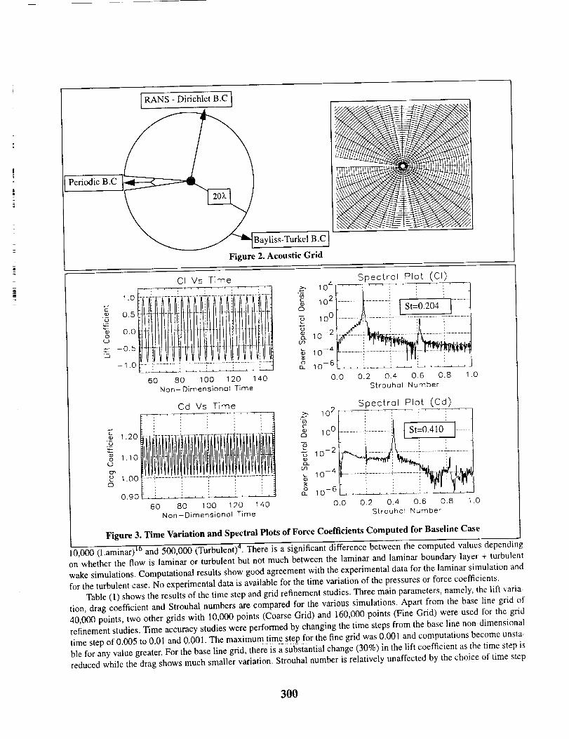
[ RANS - Dirichlet B.C [
NNNNe ,
Periodic B.C ] X _/:
ayliss-Turkel B.C [
Figure 2. Acoustic Grid
1.0
._ o,5o
0.00
(D
-0.5
Cl Vs Spectral Plot (CI)Time
- 1.0 ............................................... =.....:_ • . :
60 80 1O0 120 140
Non-Dimensional Time
c
(.,o
o£L
104i ....
10-2
10__4 _ '__.__, I_:_::_!.. ]__..........i i0.0 0.2 0.4 0.6 0.8 1.0
Strouhol Number
1.20
1.1o¢,..9
o 1.oo
0.90
Cd Vs Time• ,,.. , ,
60 80 I O0 120 140
Non-Dimensional Time
_oc
V13_
U3
g
t0 2Spectral Plot (Cd)
00....:::::::z:i i::10-2 .....................
10 -4
10 -6
0.0 0.2 0.4 0.6 0.8 ,0
Strouhol Number
Figure 3. Time Variation and Spectral Plots of Force Coefficients Computed for Baseline Case
10,000 (Laminar) l° and 500,000 (Turbulent) 4. There is a significant difference between the computed values dependinl
on whether the flow is laminar or turbulent but not much between the laminar and laminar boundary layer + turbulent
wake simulations. Computational results show good agreement with the experimental data for the laminar simulation and
for the turbulent case. No experimental data is available for the time variation of the pressures or force coefficients.
Table (I) shows the results of the time step and grid refinement studies. Three main parameters, namely, the lift varia-
tion, drag coefficient and Strouhal numbers are compared for the various simulations. Apart from the base line grid of
40,000 points, two other grids with 10,000 points (Coarse Grid) and 160,000 points (Fine Grid) were used for the grid
refinement studies. Time accuracy studies were performed by changing the time steps from the base line non-dimensional
time step of 0.005 to 0.01 and 0,001. The maximum timeste p for the fine grid was 0.001 and computations become unsta-ble for any value greater• For the base line grid, there is a substantial change (30%) in the lift coefficient as the time step is
reduced while the drag shows much smaller variation. Strouhal number is relatively unaffected by the choice of time step
3OO
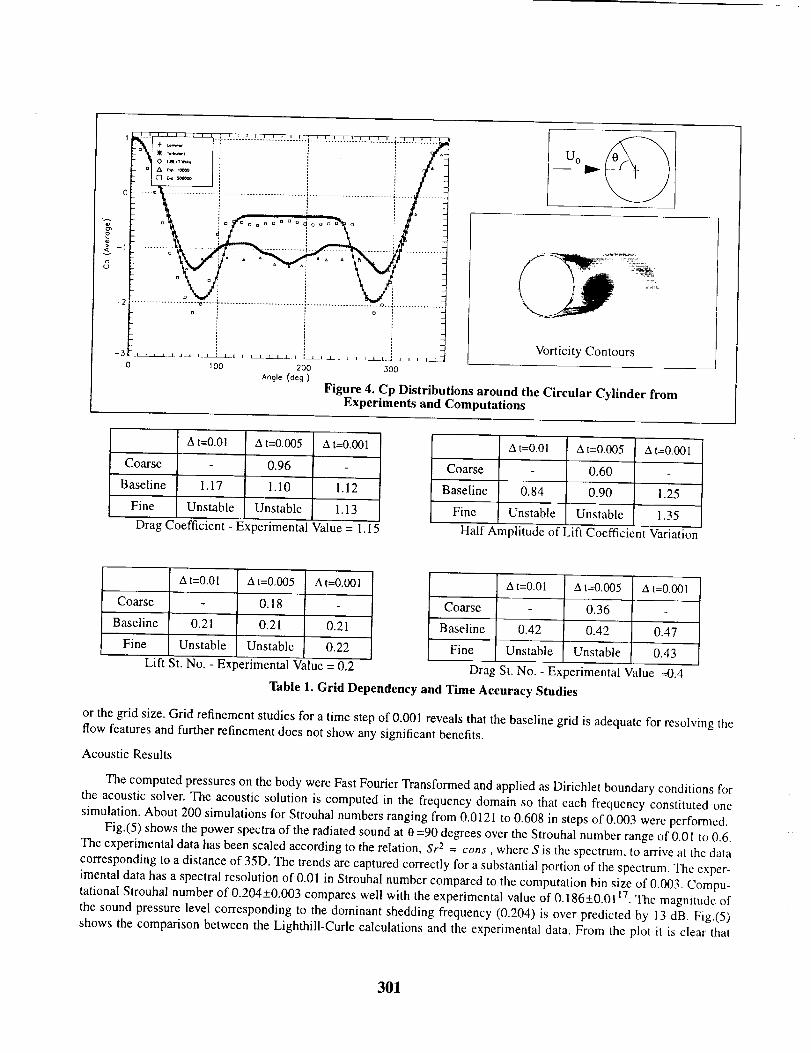
-2
-,3
0
i ! :
_ o _a_aunoc{_ao_ ¢i
o i ° !
i Vorticity Contours
1oo 200 3oo
Angle (deg.)
Figure 4. Cp Distributions around the Circular Cylinder fromExperiments and Computations
A t=0.01 A t=0.005 A t=0.001
Coarse 0.96
Baseline 1.17 1.10 1.12
Fine Unstable Unstable 1.13
Drag Coefficient - Experimental Value = I. 15
A t=0.01 A t=0.005 A t=0.001
Coarse 0.60
Baseline 0.84 0.90 1.25
Fine Unstable Unstable 1.35
Half Amplitude of Lift Coefficient Variation
A t=0.01 A t=0.005 A t=0.001
Coarse - 0.36
Baseline 0.42 0.42 0.47
Fine Unsiable Unstable 0.43
Drag St. No. - Ex _erimental Value ---0.4
A t=0.01 A t=0.005 A t=0.001
Coarse 0.18 -
Baseline 0.21 0.21 0.21
Fine Unstable Unstable 0.22
Lift St. No. - Ex )erimental Value = 0.2
Table 1. Grid Dependency and Time Accuracy Studies
or the grid size. Grid refinement studies for a time step of 0.001 reveals that the baseline grid is adequate for resolving the
flow features and further refinement does not show any significant benefits.
Acoustic Results
The computed pressures on the body were Fast Fourier Transformed and applied as Dirichlet boundary conditions for
the acoustic solver. The acoustic solution is computed in the frequency domain so that each frequency constituted one
simulation. About 200 simulations for Strouhal numbers ranging from 0.0121 to 0.608 in steps of 0.003 were performed.
Fig.(5) shows the power spectra of the radiated sound at 0 =90 degrees over the Strouhal number range of 0.01 to 0.6.
The experimental data has been scaled according to the relation, Sr 2 = cons, where S is the spectrum, to arrive at the data
corresponding to a distance of 35D. The trends are captured correctly for a substantial portion of the spectrum. The exper-
imental data has a spectral resolution of 0.01 in Strouhal number compared to the computation bin size of 0.003. Compu-tational Strouhal number of 0.204+0.003 compares well with the experimental value of 0.186+0.01 iT. The magnitude of
the sound pressure level corresponding to the dominant shedding frequency (0.204) is over predicted by 13 dB. Fig.(5)
shows the comparison between the Lighthill-Curle calculations and the experimental data. From the plot it is clear that
301
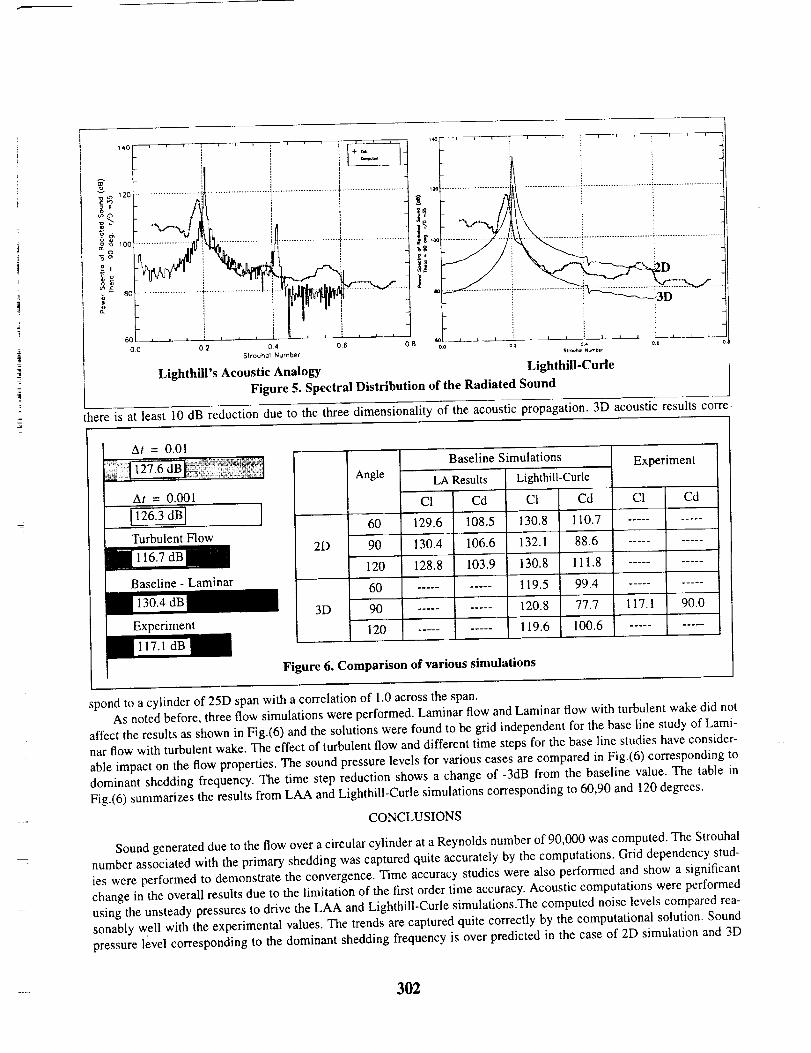
.? _i,
_ 80 ....
6O
O0 02 04 0.6 0.8
$tro_Jhal Number
Lighthill's Acoustic Analogy
J'°[so
oo
Figure 5. Spectral Distribution of the Radiated Sound
there is at least 10 dB reduction due to the three dimensionality of the acoustic propagation. 3D acoustic results corre-
At = 0.01
__, :_ i_ 6 dB_ )_:_:_ i
At = 0.001
Turbulent Flow
Baseline - Laminar
Experiment
2D
3D
Baseline Simulations
Angle LA Results Lighthill-Curle
CI Cd C1 Cd
60 129.6 108.5 130.8 110.7
90 130.4 106.6 132.1 88.6
120 128.8 103.9 130.8 111,8
60 .......... 119.5 99.4
90 .......... 120.8 77,7
120 .......... 119.6 100.6
Experiment
CI Cd
117,1 90,0
Figure 6. Comparison of various simulations
spond to a cylinder of 25D span with a correlation of 1.0 across the span.
As noted before, three flow simulations were performed. Laminar flow and Laminar flow with turbulent wake did not
affect the results as shown in Fig.(6) and the solutions were found to be grid independent for the base line study of Lami-nar flow with turbulent wake. The effect of turbulent flow and different time steps for the base line studies have consider-
able impact on the flow properties. The sound pressure levels for various cases are compared in Fig.(6) corresponding to
dominant shedding frequency. The time step reduction shows a change of -3dB from the baseline value. The table in
Fig.(6) summarizes the results from LAA and Lighthill-Curle simulations corresponding to 60,90 and 120 degrees.
CONCLUSIONS
Sound generated due to the flow over a circular cylinder at a Reynolds number of 90,000 was computed. The Strouhal
number associated with the primary shedding was captured quite accurately by the computations. Grid dependency stud-
ies were performed to demonstrate the convergence. Time accuracy studies were also performed and show a significant
change in the overall results due to the limitation of the first order time accuracy. Acoustic computations were performed
using the unsteady pressures to drive the LAA and Lighthill-Curle simulations.The computed noise levels compared rea-
sonably well with the experimental values. The trends are captured quite correctly by the computational solution. Sound
pressure level corresponding to the dominant shedding frequency is over predicted in the case of 2D simulation and 3D
302
results show a reduction of 10 dB. It is demonstrated that the turbulent flow will produce much less cyclic variation lead-
ing to a change of -13dB. The present work underlines the need for benchmark experiments that provide more information
on the flow properties as well as the acoustic properties to help in ascertaining and refining the computations in both steps,namely, source evaluation and acoustic propagation.
REFERENCES
1. Williamson,C.H.K., "Vortex dynamics in the cylinder wake", Ann. Rev. of Fluid Mech., vol. 28, 1996
2. Hardin, J.C., Pope, S.," Hardin, J.C., Pope, S.," Sound Generation by Flow over a Two-Dimensional Cavity", AIAA
Jou., Voi.33 No.3. p 407, 1995
3. Hardin, J.C., Pope, S.,"A new technique for Aerodynamic Noise Calculation" Proceedings of the DGLR/AIAA 14thAeroacoustics Conference, AIAA, Washington, D.C.,pp 448-456, 1992.
4. Kumarasamy, S., "Incompressible Flow Simulation Over a Half Cylinder with Results Used to Compute Associated
Acoustic Radiation", Ph.D Thesis, UM-AERO-95-68, Dept. of Aero. Engg., University of Maryland, CollegePark, 1995.
5. Kumarasamy, S. and Barlow, J.B., "Computation of the noise due to the flow over a half cylinder in ground effect",
Presented in the 17th AIAA Aeroacoustics Conference, State College, Penn State, PA, 1996.
6. Kumarasamy, S., Barlow,J.B.,"Computational Aeroacoustics of the Flow over a Half Cylinder", AIAA-96-0873, Pre-
sented at 34th Aerospace Sciences Meeting and Exhibit,Reno, 1996.
7. Chen, H.C. and Korpus, R., "A Multiblock Finite-Analytic Reynolds-Averaged Navier-Stokes Method for 3D Incom-
pressible Flows," ASME Summer Fluid Dynamic Conference, 1993.
8. Korpus, R.A. and Falzarano, J.M., "Prediction of viscous ship roll damping by unsteady Navier-Stokes techniques",
To be published in Offshore Mechanics and Arctic Engineering Journal, March, 1997.
9. Han,T.Y., Meng,J.C.S., and Innis,G.E.,"An Open Boundary Condition for Incompressible Stratified Flows"
J.Comp.Phy.49,276-297, 1983.
10. Lighthill,M.J., "On sound generated aei'odynamically I. General Theory", Proc. Roy. Soc. A 211, pp. 564, 1952
11. Lighthill,M.J., "On sound generated aerodynamically II. Turbulence as a source of Sound", Proc. Roy. Soc. A. 222,
pp. 114, 1952
12. Bayliss,A., Turkel,E.,"Radiation Boundary Conditions for Wave like equations", Comm. Pure. Appl. Math., vol.33,
pp. 707-725, 1980.
13. Bayliss,A., Gunzburger, Turkel,E., "Boundary conditions for the numerical solution of elliptic equations in exterior
regions", SIAM J. Appl. Math., vol.42, pp 430, 1982.
14. Vorst, H.V.D, et al.," Iterative solution methods for certain sparse linear systems with a non-symmetric matrix arising
from PDE-problems", J. Comp. Phys., 44,pp 1-19, 198 I.
15. Second Computational Aeroacoustics (CAA) Workshop on Benchmark Problems, Florida State University, Florida,Nov. 1996.
16. Kato, C, Iida, A., Takano, Y., Fujita, H., and Ikegawa, M. "Numerical Prediction of Aerodynamic Noise Radiated from
Low Mach Number Turbulent Wake," AIAA 31 st Aerospace Sciences Meeting, Reno, NV, 1993 (AIAA #93-0145).
17. Revell,J.D., Roland,A.P., and Hays, P.A., "Experimental Study of Airframe Noise vs. Drag Relationship for Circular
Cylinders", Lockheed Report LR28074 Feb 28, 1977 (NASA Contract NAS 1-14403).
18. Blake, W.K., "Mechanics of Flow-Induced Sound and Vibration Volume 1. General Concepts and ElementarySources", Academic Press, Inc., 1986.
303

=
A VISCOUS/ACOUSTIC SPLITTING
TECHNIQUE FOR AEOLIAN
TONE PREDICTION
c:,x-.B 9 7
¢/¢
D. Stuart Pope
Lockheed Martin Engineering and Sciences Company
Hampton, Virginia
INTRODUCTION
In an attempt to better understand noise generated by various airframe components such as landing gear andantennas, a precursor problem was formulated in which noise due to the passage of a steady inflow around atwo-dimensional circular cylinder was examined using a viscous/acoustic splitting method. It is believed that
this preliminary problem will lead to wider application of the method to more complex geometries of interest.Sample calculations illustrate that separate treatment of the associated hydrodynamics and acoustics leads tobetter understanding of the noise generation process, easier management of the overall computational effort,and provides results that agree well with experimental work.
Problem Description and Geometry
Consider a two-dimensional cylinder of radius G immersed in a steady, uniform flowfield of velocity Uo (see
figure 1). The flow Reynolds number(based on cylinder diameter and Uo) is taken to be 20,000. Associated
with this flow is the well-known yon Karmann vortex street which occurs in the cylinder wake due to
alternating vortex shedding from the top and bottom cylinder surfaces. The formation and subsequent motionof these vortex structures generate noise often referred to as Aeolian tones at a characteristic Strouhal number
of approximately 0.21. The goal of this work is to properly model the generation of these vortices, accuratelytrack their motions, and predict their associated noise for distant observers.
Viscous/Acoustic Splitting Method
For several reasons, Hardin 1 has proposed treating the acoustic calculation separate from the hydrodynamics
by regarding the total primitive fluids quantities p,u,v,p as composed of an incompressible mean flow and a
perturbation about that mean. It can be shown that while the perturbations represent in the nearfield thedifference between the fully compressible flow and the assumed incompressible mean fow, they are, in thefarfield, purely acoustic(see Hardin for details). By splitting the problem in this fashion, separate methods
may be used to calculate the perturbations and the mean flow. This has advantages both in terms of griddingand in application of appropriate boundary conditions. In addition, this allows greater flexibility in theindependent choice of solution method. In particular, the method can be illustrated by in'st considering thegoverning continuity and momentum equations for the cylinder flow just described:
+ +v" =o3t 3r r o38 r
3O5
C_U _U V (OU V 2 l _p r(92u l (ou _ a (92u u 2 o,_ 1
(gt+._-4 =-----r (90 r p (or +- r: (goj
Ov Ov v Ov +uv= 1 (op [(92v 1 Ov.i 1 (92v v 2 (9ul
We also assume that for low-speed flows, the isentropic relation between pressure and density may be used:
(9P = c2 _P
C,2 -.. _P
P
The total variables are now decomposed into incompressible mean flow quantities(which are, in general, timevarying) and perturbations:
u=U+u"
v=V+l/
p=P+p'
P =Po +p"
In terms of these quantities, continuity becomes
(op"_ _(ou"_ (9p'_ p (ov' v (9p" pU"+p( (oU I (OVU)(97*;Orr*U_*Ygg+rgg+ ; - k(9"+7Tff+Y) =°
Noting that the terms in parentheses are identically those of the incompressible continuity equation and sum tozero, we obtain
(op" ['-SY s'_S((Ou' l Ov" % ) + u (op" +-_=0v(oP'(gt _P,,u, +.uv + (gr r (90
Similar treatment of the momentum equations leads to
(ou" (ou" v (ou' v "2 , (OU v' (oU 2 Vv"
_- u--_r + =(ot r (90 r + u --_ + r 030 r
= vL'_r_+r-ffO÷ Y 3"_ "7 ?'_ l+-p't, (ot (or r"_ r +
up" ('(92U 1 (OU 1 (92U U 2 (OV) 1 (op'+ .__/'_-'}-+--_+
l+p _, (or r (or r _ (902 r 2 r 2 -_ l+p' (or)and
306
Ov' _" v o%' u'v' , OV v' OV Uv' Vu'
-5;-+u-g;+TTE +-7_ _+-7-+. -g; +--+--=
=_[,-grr'+7-_÷? _ 7+? oo) l+o'kat + _+7_ + _+
vp' (O_V 10V.) 1 02V V 20U) 1 01),
+l--_p'_-gT+r-gr' aO' : +: _ : 4o.+p')oo
Finally, the relation between pressure and density becomes
• t
ap'=:_ 0eOt ,gt Ot
These expressions constitute four equations in the four unknown quantifies p',u',v',p'. The incompressible
terms which also appear are determined separately and act as forcing functions to the equations. Prior tosolving, the above equations are first made nondimensional. The perturbation quantifies are
nondimensionalized by cylinder radius, ro, the ambient speed of sound co, and incompressible density, po.
The incompressible terms are treated similarly, but freestream velocity Uo is used in the nondimensionalization
rather than Co. The resulting expressions are
Mo_P'+O+p')_+(MoV+U')aP'+Ot or Or
l+p' o_" MoV+V'op' O+p')u'4 ÷ =0
r 00 r 00 r
OU t P
Mo --_- + (Mo U + u' ) _o_r "l MoV+V' aup _Mo(u,OU. vpaUr c?O _. dr r c)O
o<) (ov+vov _Mo(OauP+IOu p 1 O2u p u p 2 pPM2.
=-ff_t,-g;rr_ r-_+ : O: : :-_ l+P'k-_- Or
,gV ) 1M_p p (o_2U X c)U 1 B2U U 2 Bp"
-I Re(1 +pP)_, Or' +---÷r_r r _00 _ ? ?_ l+p'Or
r ) r
V OU V _
) +r O0 r
3¢ p Ov p Mo V + V" OV" . ., ( , OV . v' OV . Uv' . Vu" ) . uPvpMo -_t + (Mo U + u )-_r 4 r O0+M°LuT+7-_+r+rJ _ r
Mo ( O_v p 1 oarp 1 O2v , v" 2 OuP_ pPMo' ( OV + _ cgV V cgV UV _
=Re_,Or 2 +r"_+r 2 _ 7+'_ 00) l+pPl_o')t "Tr+TN+-;-) +Mo2p" (O=V IOV 10=V V 20U'_ 1 o')pp
÷Re(l+pP)_'_rSrJ+r'Or-r +r ` 005 r' +7-_J-r(l + p p) c)O
and lastly,
0p' =c2 ap' aP-5;- -57- M_W
where
307
c = +- i il+p' .f
!
In the above equations, M o refers to the freestream Mach number and Reynolds number is based on cylinder iradius. All variables are considered nondimensional throughout the remainder of this work.
Incompressible Mean Flow Calculation _ "The forcing terms appearing in the above equations may be found by any convenient method. In this work, --since the flowfield is two-dimensional, a vorticity-stream function approach is used. The governing equations -
are, in nondimensional variables [
/o _2 1 o_ 1 o32 1"_r2 +r'_-"_ 4 r 2 _'_2 I/f=-f_
_.3 1( O3210 .il °_2]1 31/z _9 1 c_V f_ = +r c90 cgr r o3r Re[,o_r 2 r-_r r 2o_02 "
and
The effects of viscosity strongly dominate the character of the incompressible flowfield. These effects are
especially important at the cylinder surface and their accurate calculation requires a fine grid. A coordinatetransformation is employed which finely spaces grid points at the cylinder surface while sparsely spacingpoints in the farfield. This transformation is
r=e°¢
0_=_
a
where a = ln(r_._), rm_ being the outer boundary of the computational domain. In these coordinates,
transformed equations for V and _ may be solved on a uniformly spaced _, r/grid, yet the surface grid point
clustering necessary in the physical domain can be realized. The transformed equations are
where
(_: _2
•_- +-_2 )V = -E 2f_
o_go_ o_g3"_ 1 (0 2 o__h
E = ae *¢.
Note that an additional relation is required to specify P which appears in the perturbation equations. This
relation can be found by differentiation of the momentum equations and adding the two. The result is, intransformed coordinates,
308
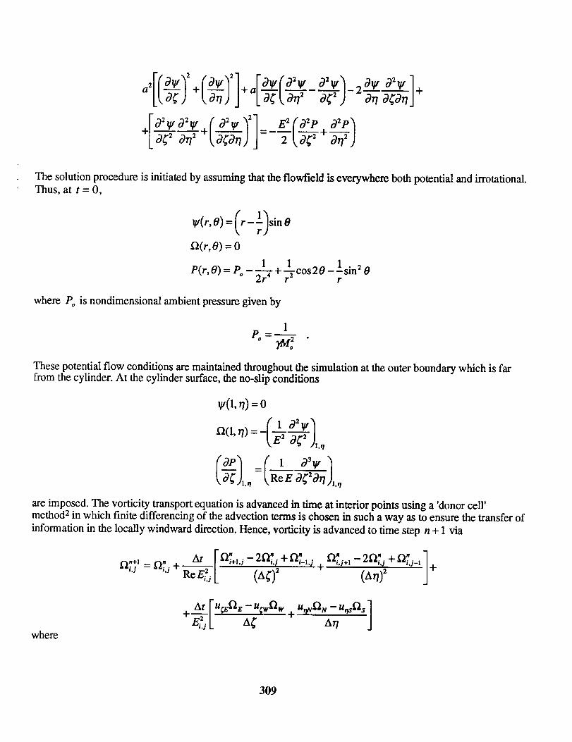
2 2 2 2
+L_ °_ _[_-_)J--T[_+d__)
The solution procedure is initiated by assuming that the flowfield is everywhere both potential and irrotational.Thus, at t = 0,
,,,rO,-(r )inO_(r, O) = 0
1_)P(r,O)=Po 2r 4 I- cos20-lsin20r
where Po is nondimensional ambient pressure given by
1Po =-7-_-._
These potential flow conditions are maintained throughout the simulation at the outer boundary which is farfrom the cylinder. At the cylinder surface, the no-slip conditions
qt(1,rl)=0
(l 02_/f/(1,r/)=- -E2b-_),..
C_)1,_ _-C 'RIE 031y ,l@_-'2"@'ilJl,,1
are imposed. The vorticity transport equation is advanced in time at interior points using a 'donor cell'
method 2 in which finite differencing of the advection terms is chosen in such a way as to ensure the transfer of
information in the locally windward direction. Hence, vorticity is advanced to time step n + 1 via
+ At FU_wQ_-U_,Dw -U_st"ls_L "q +,,_a,,A,1' ]
where
309
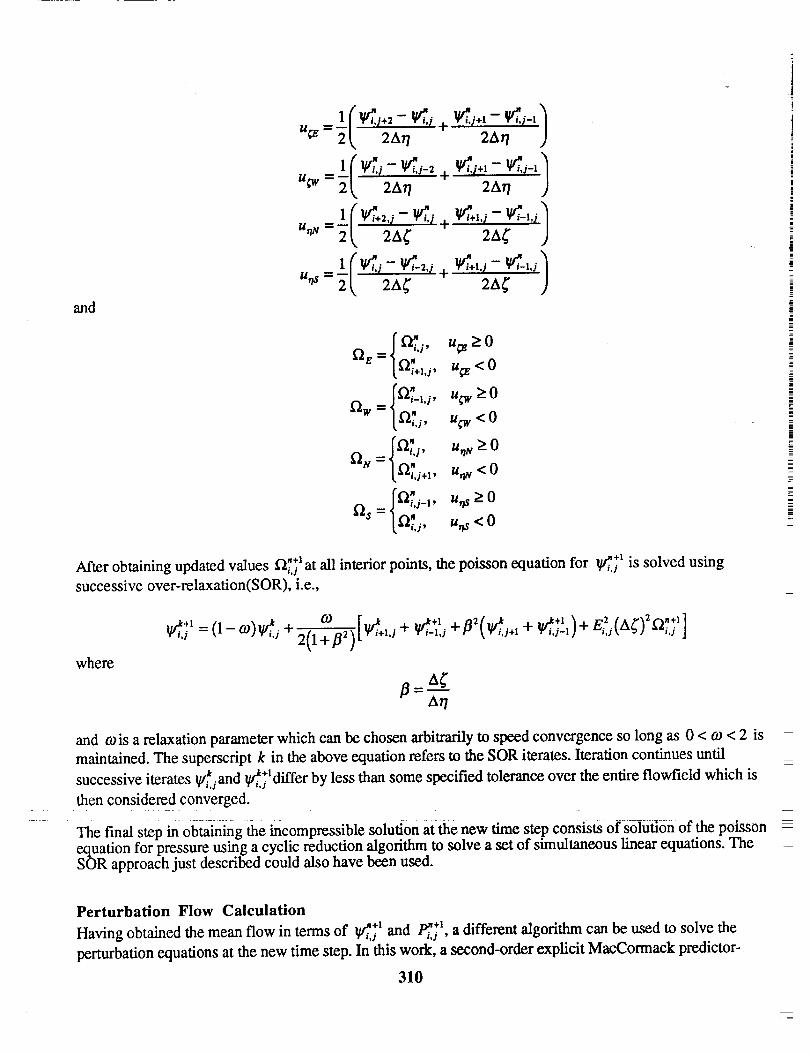
and
1(:,.i- + - )u.. 2A¢ 2A "
o -_ _2,',_, u_>O"'E _ On
--i+i.),ufE < 0
' n
o -, f2_-_'i' u_,_O
--w - f2" uoe < 0• i,j,
_ = I f_'_'o" u'm> 0l.--i,j+1,U_v < 0
" n -
f_.j__, u_ > 0f_s
O,',s' u_s< 0
After obtaining updated values n+_[2i. s at all interior points, the poisson equation for V_._._ is solved using
successive over-relaxation(SOR), i.e.,
where
I_i.;1 = (I -- 0)) l_/,j ++1 2 +1 2 2 n+l
2(1+]3 2)
fl=At/
and coisa relaxationparameter which can be chosen arbitrarilytospeed convergence so long as 0 < co< 2 is
maintained.The super_riptk intheabove equationreferstothe SOR i_rates_f_rationcontinues_til -+1 •
successiveiterates_,.,_and _.j differby lessthan some specifiedtoleranceover the entireflowfieldwhich is
thenconsideredconverged.
The finalstepinobt_hag theincompressiblesohtion atthenew time stepconsistsof soiutionof thepoisson
equationforpressureusinga cyclicreductionalgorithmtosolvea setof simultaneouslinearequations.TheSOR approach justdescribedcould alsohave been used.
Perturbation Flow Calculation
Having obtained the mean flow in terms of I/_,_._ and /_._', a different algorithm can be used to solve the
perturbation equations at the new time step. In this work, a second-order explicit MacCormack predictor-
310
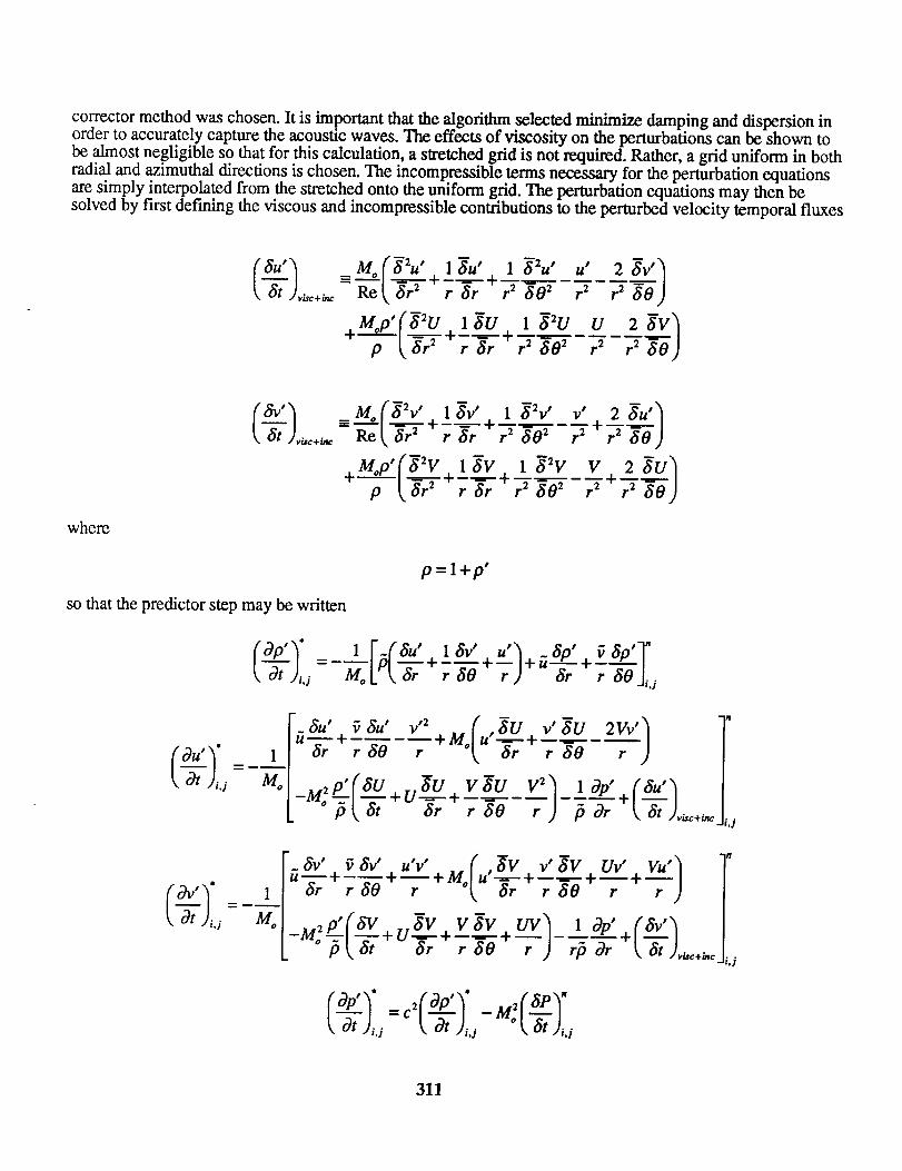
corrector method was chosen. It is important that the algorithm selected minimize damping and dispersion inorder to accurately capture the acoustic waves. The effects of viscosity on the perturbations can be shown tobe almost negligible so that for this calculation, a stretched grid is not required. Rather, a grid uniform in bothradial and azimuthal directions is chosen. The incompressible terms necessary for the perturbation equationsare simply interpolated from the stretched onto the uniform grid. The perturbation equations may then besolved by first derming the viscous and incompressible contributions to the perturbed velocity temporal fluxes
au" 1 =mo(_2u" 15"-u" 1_2u" u"at j_+_- ggel,gT"r=+TT _ r=gO= r2
M_p'(a2U l gU 1 g2U U
r 2 50)
r 2 aO)
where
--2 • --,, --2 •
(av') _Mo(Sv lay 1 5v v'---+-=-..&.,._.,.,,_ Re Lar r ar r_ 5O" "_ r 50)
+Mop'(aW+l_ _a_v v+2_7('_'r a rar +7"_ r = 7a0J
p =l+p'
so that the predictor step may be written
(o_p'_ * 1 r_ca,. _av, ,.a _a¢+v_-a¢]"=--- p --+---+-- +_, et Ji., Mo[_ & r ao r ) ar r aO Ji4
av" _&" u'v" . ( ,av v av w'+Vu']_T+r-_-_+7+Mo_.U -_--r +r-_-_+ r r j
,,=p'(av±r, aV V_V UV_ 1 cgp" i.(av')-'"" 7(,-g"-_"gT+7gg+7) r_ Or . at .,,i.,.+_,,_
(o ,y =c4ep,y -wf Yat Ji.i I, at )i.i o k, at )J.i
i./
311
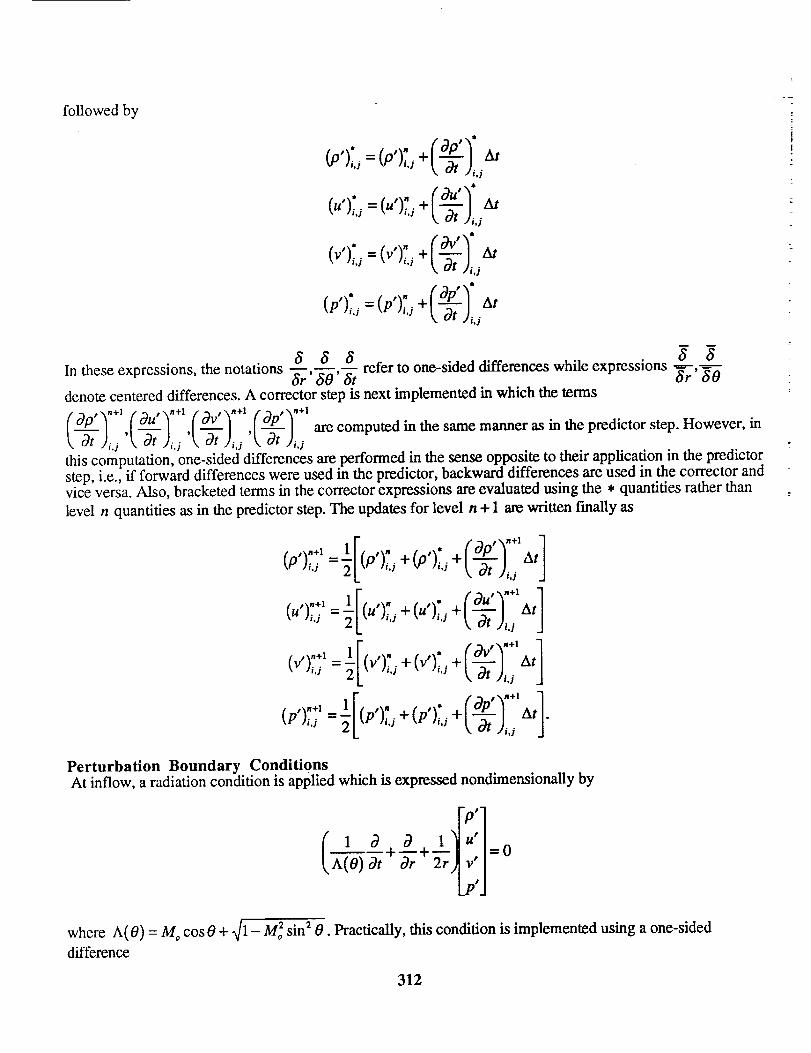
followedby
_o,L _-(p,);,+('P ] A,• k at ),a
(u,,:,= At
ij
(v,)7,=(v,):,+(_v,]"_• \ at )_a
(P')7, =(P')_, +(aP')" At• ' _.at ),.j
ii
L
=
_t_n+l 1
(v),., =_
u,],,+, 1
1
(v,);;'=_
( ,,.+, 1P )_._=
' • n+l
(0%+(o';+(°P') A,]"'" kat),a J
(au"f +1 ](u,).,.,+(u')b+I,_J,.,"'
(v'L +(v'),.,+ at ,.,
( aP" y+lAt].(P'ITj+(P')[, +k_ ),.,
Perturbation Boundary ConditionsAt inflow, a radiation condition is applied which is expressed nondimensionally by
1 aA(O) at
r ;la+l]. Ia--;2s,__,I
Lp'J
=0
where A(0) = Mo cos 0 + _/1 - Mo2 sin 2 0. PracticaUy, this condition is implemented using a one-sided
difference
312
886 8 8In these expressions, the notations 8r' 60' & refer to one-sided differences while expressions _rr"_'O
denote centered differences. A corrector step is next implemented in which the terms
_ ,_ ,__, at ),,i _,at ),,_ _,at ),,j are computed in the same manner as in the predictor step. However, in ,
this computation, one-sided differences are performed in the sense opposite to their application in the predictorstep, i.e., if forward differences were used in the predictor, backward differences are used in the corrector andvice versa. Also, bracketed terms in the corrector expressions are evaluated using the * quantities rather than [
level n quantities as in the predictor step. The updates for level n + 1 are written finally as
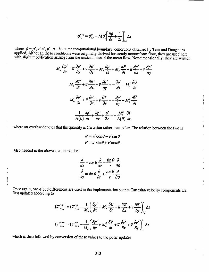
i
where # = p', u',v',p'. At the outer computational boundary, conditions obtained by Tam and Dong 3 are
applied. Although these conditions were originally derived for steady nonuniform flow, they are used herewith slight modification arising from the unsteadiness of the mean flow. Nondimensionally, they are written
+ u-_-_x+ = Mo + Mo + _ + _o_, v_ -g;
ova' ova' _o_'""°--_-+_-_x + Ox M: otv-_-= or' 2o_
_' _/_' _0_' 0p' OVM°_+u-L;+v-_-= ay M: o--7
1 Op'FOp" p' M2oOPA(0) 0t -_-r+2--;= A(0) at
where an overbar denotes that the quantity is Cartesian rather than polar. The relation between the two is
fi" = u'cos0 - v'sin 0
7' = u'sin 0 + v'cos 0.
Also needed in the above are the relations
_0_=cosO__O sinO OOx Or r O0
O O cosOO
= sin O_rr 4 O0r
Once again, one-sided differences are used in the implementation so that Cartesian velocity components arefirst updated according to
(-,r+_ __1(@' 8v+__, __,_"u,._-(_'L Motax+M:_ "W+VTyj,.,A'
(_,r+, __(@' o<-V__, _<_,';v.,.j =(v')7.,Mot@+M;7-i-+"T;+"-ffyJ,.,'_,
which is then followed by conversion of these values to the polar updates
313
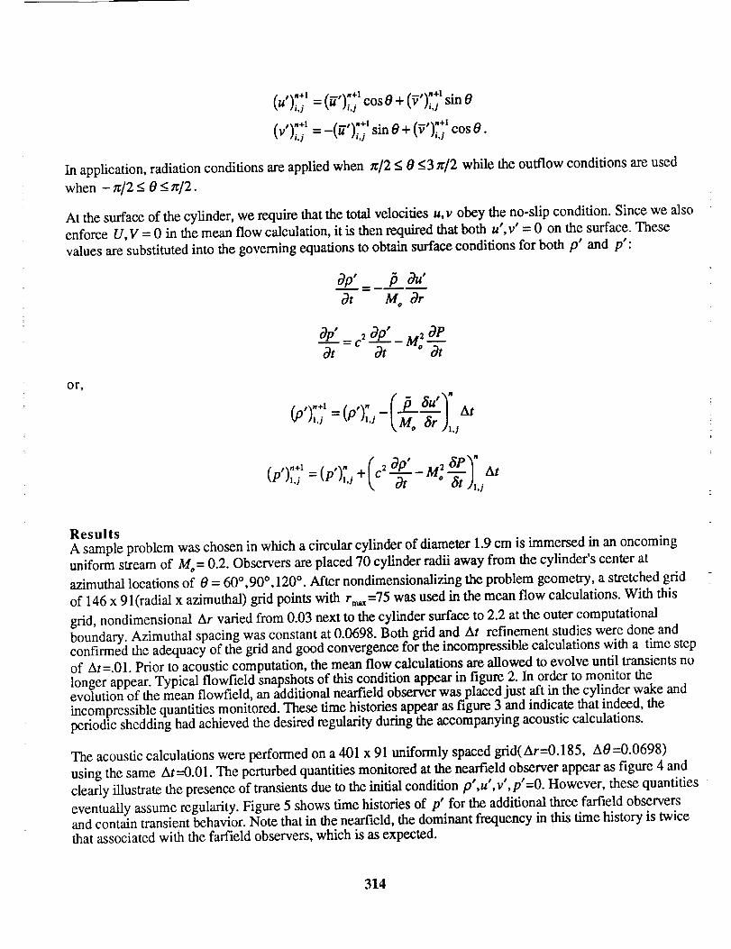
')""' '-"'"u .i,i = t u )i.j COS
(vr+, = (-,,¢,+, _, ,.-, .-i.i - u -i4 sin O + (v)i.s cos O
In application, radiation conditions are applied when tr[2 _<0 <3 n:]2 while the outflow conditions are used
when - rr]2 < 0 < zr]2.
At the surface of the cylinder, we require that the total velocities u,v obey the no-slip condition. Since we also
enforce U,V = 0 in the mean flow calculation, it is then required that both u',v" = 0 on the surface. These
values are substituted into the governing equations to obtain surface conditions for both p' and p':
or,
at," c, O,o" . 5,9t'W = at-m-g;
O"r+'= 7,.,,,., (p,),t J A,
# M, ,,.+, +(c, ,,,tP h,s = (P'),",s t, at ° 6t J,,i
Results
A sample problem was chosen in which a circular cylinder of diameter 1.9 cm is immersed in an oncoming
uniform stream of 3,to= 0.2. Observers are placed 70 cylinder radii away from the cylinder's Center at
azimuthal locations of 0 = 60 °, 90 °, 120 °. After nondimensionalizing the problem geometry, a stretched grid
of 146 x 91(radial x azimuthal) grid points with rm_=75 was used in the mean flow calculations. With this
grid, nondimensional Ar varied from 0.03 next to the cylinder surface to 2.2 at the outer computational
boundary. Azimuthal spacing was constant at 0.0698. Both grid and At refimement studies were done andconfirmed the adequacy of the grid and good convergence for the incompressible calculations with a time step
of At=.01. Prior to acoustic computation, the mean flow calculations are allowed to evolve until transients nolonger appear. Typical flowfield snapshots of this condition appear in figure 2. In order to monitor theevolution of the mean flowfield, an additional nearfield observer was placed just aft in the cylinder wake andincompressible quantities monitored. These time histories appear as figure 3 and indicate that indeed, theperiodic shedding had achieved the desired regularity during the accompanying acoustic calculations.
The acoustic calculations were performed on a 401 x 91 uniformly spaced grid( Ar=0.185, A0=0.0698)
using the same At=0.01. The perturbed quantities monitored at the nearfield observer appear as figure 4 and
clearly illustrate the presence of transients due to the initial condition p',u', v', p'=0. However, these quantities
eventually assume regularity. Figure 5 shows time histories of p' for the additional three farfield observers
and contain transient behavior. Note that in the nearfield, the dominant frequency in this time history is twicethat associated with the farfield observers, which is as expected.
314
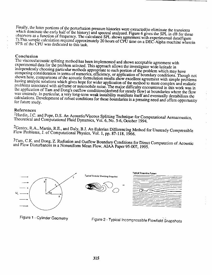
Finally, the latter portions of the perturbation pressure histories were extracted(to eliminate the transientswhich dominate the early half of the history) and spectral analyzed. Figure 6 gives the SPL in dB for theseobservers as a function of frequency. The calculated SPL shows agreement with experimental data(figure7).This sample calculation required approximately 20 hours of CPU time on a DEC-Alpha machine wherein97% of the CPU was dedicated to this task.
Conclusion
The viscous/acoustic spfitting method has been implemented and shows acceptable agreement withexperimental data for the problem selected. This approach allows the investigator wide latitude inindependently choosing particular methods appropriate to each portion of the problem which may havecompeting consideration in terms of numerics, efficiency, or application of boundary conditions. Though notshown here, comparisons of the acoustic formulation results show excellent agreement with simple problemshaving analytic solutions which gives hope for wider application of the method to more complex and realisticproblems associated with airframe or automobile noise. The major difficulty encountered in this work was inthe application of Tam and Dong's outflow conditions(derived for steady flow) at boundaries where the flowwas unsteady. In particular, a very long-term weak instability manifests itself and eventually destabilizes thecalculations. Development of robust conditions for these boundaries is a pressing need and offers opportunityfor future study.
References
1Hardin, J.C. and Pope, D.S. An Acoustic/Viscous Splitting Technique for Computational Aeroacoustics,Theoretical and Computational Fluid Dynamics, Vol. 6, No. 5-6, October 1994.
2Gentry, R.A., Martin, R.E., and Daly, B.L An Eulerian Differencing Method for Unsteady Compressible
Flow Problems, J. of Computational Physics, Vol. 1, pp. 87-118, 1966.
3Tam, C.K. and Dong, Z. Radiation and Outflow Boundary Conditions for Direct Computation of Acousticand Flow Disturbances in a Nonuniform Mean Flow, MAA Paper 95-007, 1995.
Figure 1 - Cylinder Geometry
Tfpic.a| VodiciD/Shedding Snapshot
Typ4c,_ StteQrntine Patt_n
Figure 2 - Typical Incompressible FIowfield'Snapshots
315
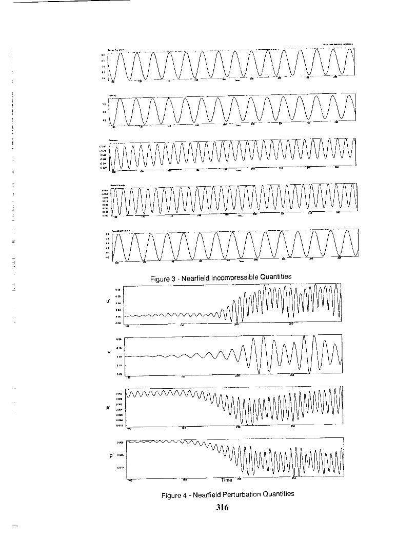
oi
_o
o*
ol
+o
o+
03
02
O,
O0
0 t
U'
Figure 3 - Nearfie+d Incompressible Quantitiesool
oo11
oo.i
o .z
+ool
V'
o +o
ooo
o io
o zo ++._ :t_
oooo
,oomP
+ool
,oooi
oo,o i_o P,+
p' oo¢_
++o,o
,k, Time _o -
Figure 4 - Nearfield Perturbation Quantities
316
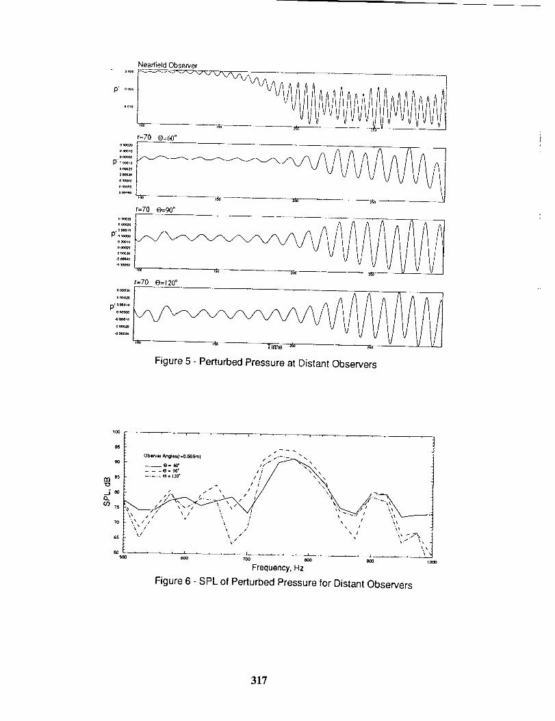
p' o oo_
Nearfield Observer
v v\_
r=70 0=60 °
1
9'3
t3O3
75
7O
65
i " i i i
/ I
.....o.,,o. ,,T__ (3 = $0" /." \
-- _ -(_= 98" t I ",
-,,,,,,,.,,."u", '--.--_" ' ,. ,',",'; ""_, , - .,,
600 700 800 _ 1000
Frequency, Hz
Figure 6 - SPL of Perturbed Pressure for Distant Observers
317
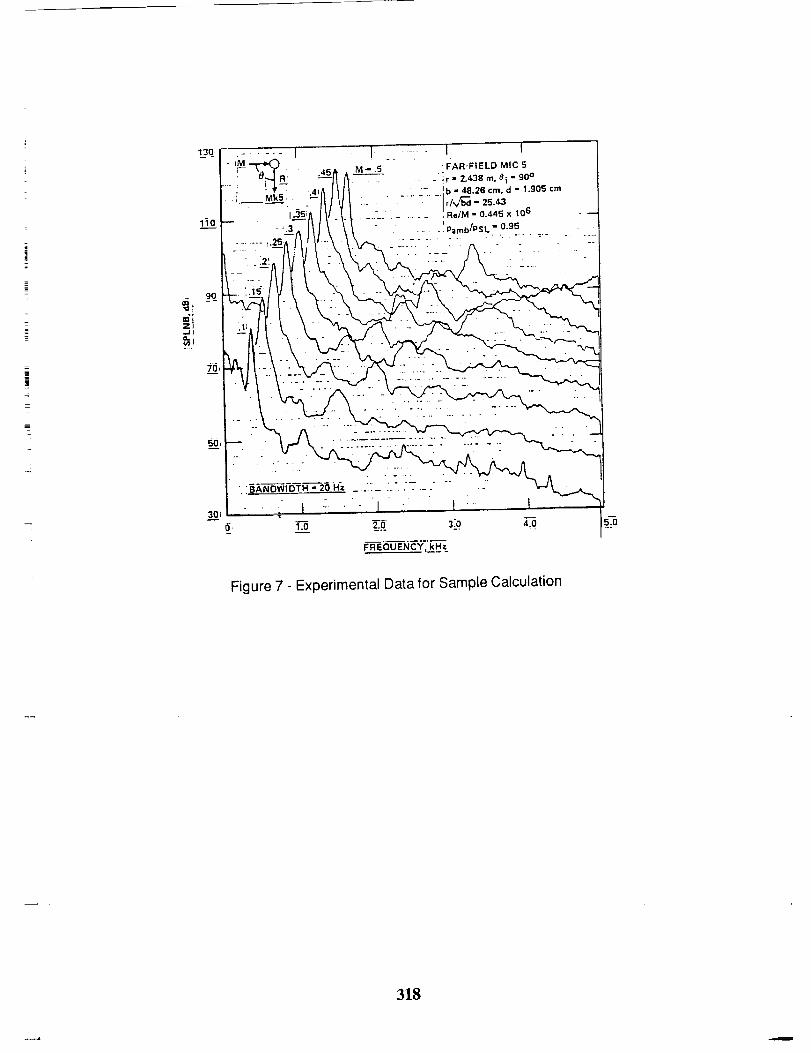
M" .5 ; FAR'FIELD MIC 5
,. _'ir = 2.438 rn, 8 i - 90 °
. "-_._ b " 48.26 cm, d - 1,905 cm
_..-_' - ....... RetM = 0.445 x 10⁶
i / ...... Pamb PSL 0.95• , . °.- .
9O
FREQUENCY, RH_
Figure 7- Experimental Data for Sample Calculation
318
LARGE-EDDY SIMULATION OF A HIGH REYNOLDS
NUMBER FLOW AROUND A CYLINDER INCLUDING
AEROACOUSTIC PREDICTIONS
Evangelos T. Spyropoulos and Bayard S. Holmes
Centric Engineering Systems, Inc., Santa Clara, CA 95054-3004
ABSTRACT
The dynamic subgrid-scale model is employed in large-eddy simulations of flow over a
cylinder at a Reynolds number, based on the diameter of the cylinder, of 90,000. The Centric
SPECTRUM TM finite element solver is used for the analysis. The far field sound pressure
is calculated from Lighthill-Curle's equation using the computed fluctuating pressure at the
surface of the cylinder. The sound pressure level at a location 35 diameters away from the
cylinder and at an angle of 90 ° with respect to the wake's downstream axis was found to have
a peak value of approximately 110 db. Slightly smaller peak values were predicted at the
60 ° and 120 ° locations. A grid refinement study suggests that the dynamic model demands
mesh refinement beyond that used here.
I. Introduction
In the past few years, there has been a resurgence of interest in performing large-eddy
simulations (LES) of flows of engineering interest. There are two roles for LES to play in the
computation of complex flows. First, it can be used to study the physics of turbulence at
higher Reynolds numbers than can currently be achieved with direct numerical simulation
(DNS), and can aid in the testing and improvement of lower order engineering turbulence
models. Second, it is hoped that LES can be used as an engineering tool rather than as
a research tool. Although it remains expensive, it may be the only means of accurately
computing complex flows for which lower order models fail.
The dynamic subgrid-scale (SGS) modeling concept was introduced by Germano et al.lfor
LES of incompressible flows and has attracted a lot of attention in the LES community during
the recent years. The main advantage of the dynamic model over other models used in the
past is that it requires little prior experience with the type of flow being considered. The
model (dynamically) adjusts to the flow conditions by employing the resolved large-scale
information to predict the effects of the small scales.
In this study, the far-field noise due to a high Reynolds number flow over a cylinder is
predicted numerically using the SPECTRUM TM finite element solver. First, the LES method
with the dynamic model is used to compute the turbulent flowfields. The results from the
CFD analysis are then used in Lighthill-Curle's 4 acoustic analogy equation to predict thesound pressure level at several locations.
319
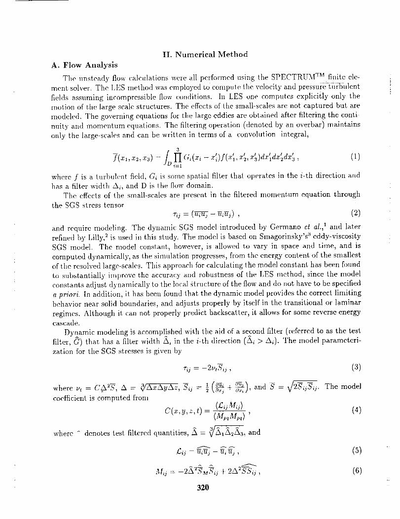
II. Numerical MethodA. Flow Analysis
The unsteadyflow calculationswere all performed using the SPECTRUMTM...... finite ele-
ment solver. The LES method was employed to compute the velocity and pressure-turbulent
fields assuming incompressible flow conditions. In LES one computes explicitly only the
motion of the large-scale structures. The effects of the small-scales are not captured but are
modeled. The governing equations for the large eddies are obtained after filtering the conti-
nuity and momentum equations. The filtering operation (denoted by an overbar) maintains
only the large-scales and can be written in terms of a convolution integral,
3
=/n I] c ,(xi ' ' ' "- '- '- 'l*
--f(xl,x2,x3) -- xi)f(xl,x2, x3)axlax2ax3, (1)i=1
where f is a turbulent field, Gi is some spatial filter that operates in the i-th direction and
has a filter width Ai, and D is the flow domain.
The effects of the small-scales are present in the filtered momentum equation through
the SGS stress tensor
= - (2)
and require modeling. The dynamic SGS model introduced by Germano st al., 1 and later
refined by Lilly, 2 is used in this study. The model is based on Smagorinsky's 3 eddy-viscosity
SGS model. The model constant, however, is allowed to vary in space and time, and is
computed dynamically, as the simulation progresses, from the energy content of the smallest
of the resolved large-scales. This approach for calculating the model constant has been found
to substantially improve the accuracy and robustness of the LES method, since the model
constants adjust dynamically to the local Structure of the flow and do not have to be specified
a priori. In addition, it has been found that the dynamic model provides the correct limiting
behavior near solid boundaries, and adjusts properly by itself in the transitional or laminar
regimes. Although it can not properly predict backscatter, it allows for some reverse energy
cascade.
Dynamic modeling is accomplished with the aid of a second filter (referred to as the test
filter, G) that has a filter width Zx, in the i-th direction (A_ > A_). The model parameteri-
zation for the SGS stresses is given by
r_j = -2ag_j, (3)
1 (a___Vs a-qS-'_ and S =where ut = C_2S, A = _/AxAyAz, Sij ---- _ \Oa:, q- Oxl]'
coefficient is computed from(£ijMo}
C(x,y,z,t)- (MpqMpq} '
where ^ denotes test-filtered quantities, A _/A1A2 3, and
The model
(4)
A AA
f-'o = u_uj - ui uj , (5)
A A A
_lij -_- --2_2"SM-Sij -}- 2A 2_-_-_ij , (6)
320 =
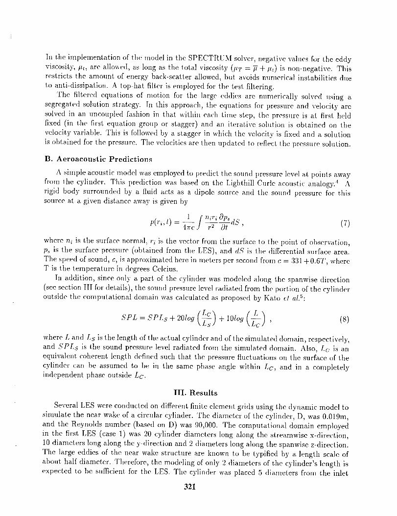
In the implementation of the model in the SPECTRUM solver, negativevaluesfor the eddyviscosity,pt, are allowed, as long as the total viscosity (ttT= ?7 +ttt) is non-negative. This
restricts the amount of energy back-scatter allowed, but avoids numerical instabilities due
to anti-dissipation. A top-hat filter is employed for the test filtering.
The filtered equations of motion for the large eddies are numerically solved using a
segregated solution strategy. In this approach, the equations for pressure and velocity are
solved in an uncoupled fashion in that within each time step, the pressure is at first held
fixed (in the first equation group or stagger) and an iterative solution is obtained on the
velocity variable. This is followed by a stagger in which the velocity is fixed and a solution
is obtained for the pressure. The velocities are then updated to reflect the pressure solution.
B. Aeroacoustic Predictions
A simple acoustic model was employed to predict the sound pressure level at points away
from the cylinder. This prediction was based on the Lighthill-Curle acoustic analogy. 4 A
rigid body surrounded by a fluid acts as a dipole source and the sound pressure for this
source at a given distance away is given by
p(ri,t)- 1 f-iri0ps4rcc r 2 Ot d5', (7)
where ni is the surface normal, ri is the vector from the surface to the point of observation,
p_ is the surface pressure (obtained from the LES), and dS' is the differential surface area.
The speed of sound, c, is approximated here in meters per second from c = 331 +0.6T, where
T is the temperature in degrees Celcius.
In addition, since only a part of the cylinder was modeled along the spanwise direction
(see section III for details), the sound pressure level radiated from the portion of the cylinder
outside the computational domain was calculated as proposed by Kato et al.S:
" + 10109 , (s)
where L and Ls is the length of the actual cylinder and of the simulated domain, respectively,
and 5PLs is the sound pressure level radiated from the simulated domain. Also, Lc, is an
equivalent coherent length defined such that the pressure fluctuations on the surface of the
cylinder can be assumed to be in the same phase angle within Lc, and in a completely
independent phase outside Lc.
III. Results
Several LES were conducted on different finite element grids using the dynamic model to
simulate the near wake of a circular cylinder. The diameter of the cylinder, D, was 0.019m,
and the Reynolds number (based on D) was 90,000. The computational domain employed
in the first LES (case 1) was 20 cylinder diameters long along the streamwise x-direction,
10 diameters long along the y-direction and 2 diameters long along the spanwise z-direction.
The large eddies of the near wake structure are known to be typified by a length scale of
about half diameter. Therefore, the modeling of only 2 diameters of the cylinder's length is
expected to be sufficient for the LES. The cylinder was placed 5 diameters from the inlet
321
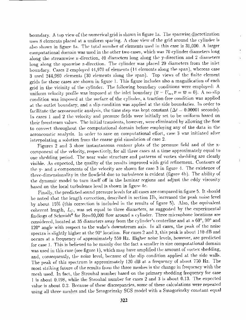
boundary. A top view of the numericalgrid is shownin figure la. The spanwisediscretizationuses8 elementsplacedat a uniform spacing.A closeview of the grid around the cylinder isalso shownin figure la. The total number of elementsusedin this caseis 31,000. A largercomputational domainwasusedin the other two cases, which was 70 cylinder diameters long
along the st reamwise x-direction, 40 diameters long along t,he y-direction and 2 diameters
long along the spanwise z-direction. The cylinder was placed 20 diameters from the inlet
boundary. Cases 2 employed 44,970 of elements (14 elements along the span), whereas case
3 used 244,980 elements (30 elements along the span). Top views of the finite element
grids for these cases are shown in figure 1. This figure includes also a magnification of each
grid in the vicinity of the cylinder. The following boundary conditions were employed: A
uniform velocity profile was imposed at the inlet boundary (g = U_, _-Y= _ = 0). A no-slip
condition was imposed at the surface of the cylinder, a traction-free condition was applied
at the outlet boundary, and a slip condition was applied at the side boundaries. In order to
facilitate tile aeroacoustic analysis, the time step was kept constant (At = 0.00001 seconds).
In cases 1 and 2 the velocity and pressure fields were initially set to be uniform based on
their freestream values. The initial transients, however, were eliminated by allowing the flow
to convect throughout the computational domain before employing any of the data in the
aeroacoustic analysis. In order to save on computational effort, case 3 was initiated after
interpolating a solution from the coarse grid simulation of case 2.
Figures 2 and 3 show instantaneous contour plots of the pressure field and of the x-
component of the velocity, respectively, for all three cases at a time approximately equal to
one shedding period. The near wake structure and patterns of vortex shedding are clearly
visible. As expected, the quality of the results improved with grid refinement. Contours of
the y- and z-components of the velocity are shown for case 3 in figure 4. The existence of
three-dimensionality in the flowfield due to turbulence is evident (figure 4b). The ability of
the dynamic model to turn itself off in the laminar regions and adjust the eddy viscosity
based on the local turbulence level is shown in figure ,tc.
Finally, the predicted sonnd pressure levels for all cases are compared in figure 5. It should
be noted that the length correction, described in section IIb, increased the peak noise level
by about, 15% (this correction is included in the results of figure 5). Also, the equivalent
coherent length, Lc, was set equal to three diameters, as suggested by the experimental
findings of Schmidt G for Re=90,000 flow around a cylinder. Three microphone locations are
considered, located at 35 diameters away from the cylinder's centerline and at a 60 °, 90 ° and
120 ° angle with respect to the wake's downstream axis. In all cases, the peak of the noise
spectra is slightly higher at the 90 ° location. For cases 2 and 3, this peak is about 110 dB and
occurs at a frequency of approximately 5.50 Hz. Higher noise levels, however, are predicted
for case 1. This is believed to be mainly due the fact a smaller in size computational domain
was used in this case (see figure 1), which may have amplified the amount of vortex shedding,
and, consequently, the noise level, becanse of the slip condition applied at the side walls.
The peak of this spectrum is approximately 120 dB at a frequency of about 750 Hz. The
most striking future of the results from the three meshes is the change in frequency with the
mesh used. In fact, the Strouhal number based on the primary shedding frequency for case
1 is about 0.198, while the Strouhal number for cases 2 and 3 is about 0.13. The expected
value is about 0.2. Because of these discrepancies, some of these calculations were repeated
using all three meshes and the Smagorinsky SGS model with a Smagorinsky constant equal
322
to Cs = C 1/2 = 0.1. These LES gave more consistent results with shedding frequencies
corresponding to Strouhal numbers of about 0.2 (results from these computations are not
presented here due to space limitations). So, it is possible that the meshes used here are
too coarse for the dynamic model and hence have produced inconsistent results. We plan to
investigate this issue more thoroughly in the future.
IV. Conclusions
The far-field sound due to vortex shedding in the turbulent wake of a Re=90,000 flow
around a cylinder is predicted based on Lighthill-Curle's Acoustic Analogy concept. The
history of the fluctuating pressure at the surface of the cylinder, required by the acoustic
analysis, was obtained by conducting LES using the dynamic SGS model. Several numeri-
cal grids were used, the finest of which contained a total of about 245,000 finite elements.
The maximum sound pressure level at a distance of 3,5 diameters away from the cylinder's
centerline was found to be equal to 105 dB, 110 dB and 108 dB at the 60 ° , 90 ° and 120 °
angle location, with respect to the wake's downstream axis, respectively. The meshes used,
however, may not be sufficiently fine for the dynamic SGS model, as is suggested by incon-
sistencies in the results found as the grid was refined.
Acknowledgements
This work was supported by the NASA Langley Research Center under SBIR contract
NAS1-20584. The authors wish to acknowledge the support of the contract monitor, Kristine
Meadows.
References
i Germano, M., Piomelli, U., Moin, P. and Cabot, W., 1991. "A dynamic subgrid-scale
eddy-viscosity model," Physics of Fluids A, 3, pp. 1760-1765.
2 Lilly, D. K., 1992. "A proposed modification of the Germano subgrid-scale closure
method," Physics of Fluids A, 4, pp. 633-63.5.
3 Smagorinsky, J. S., 1963. "General circulation experiments with the primitive equations.
I. The basic experiment," Monthly Weather Review, 91, pp. 99- 164.
4 Pierce, A., 1991. Acoustics: An Introduction to its Physical Principals and Applications,
McGraw-Hill, New York.
s Kato, C., Iida, A., Fujita, H. and Ikegawa, M. 1993. "Numerical prediction of aerody-
namic noise from low Mach Number turbulent wake," AIAA Paper 93-0145, 31st AIAA
Aerospace Sciences Meeting, Reno, NV.
6 Schmidt, L. V. 1965. "Measurements of Fluctuating Air Loads on a circular cylinder,"
Journal of Aircraft, 2, pp. 49-55.
323
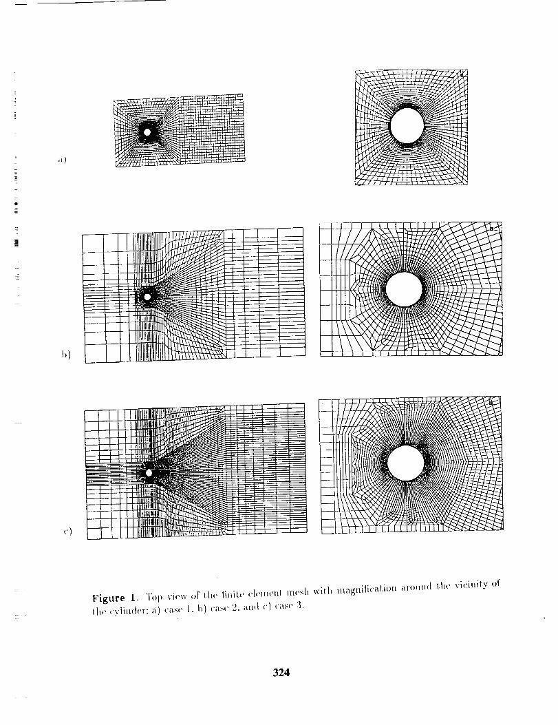
a l
I,)
i
i --_Z _
---- [' "
n
I t iUl iLit!!l 9--_ ; ! - _ _ _ "
_-_-t',l i. 1
_!i : t.,, : ! J;i _ ! i i- .t _ ..:
._._-_-_-- .____
:_ _: i r 1 L • ,
I' 't
Figure 1. To I) view of t lw lilfite (,h._Henl mesh with magtfifi('at.io_ arou,_({ th(' vicinity of
the (',,'[i_dev: a) ('as_' [. b) case 2, _[_(t c)case :_.
324
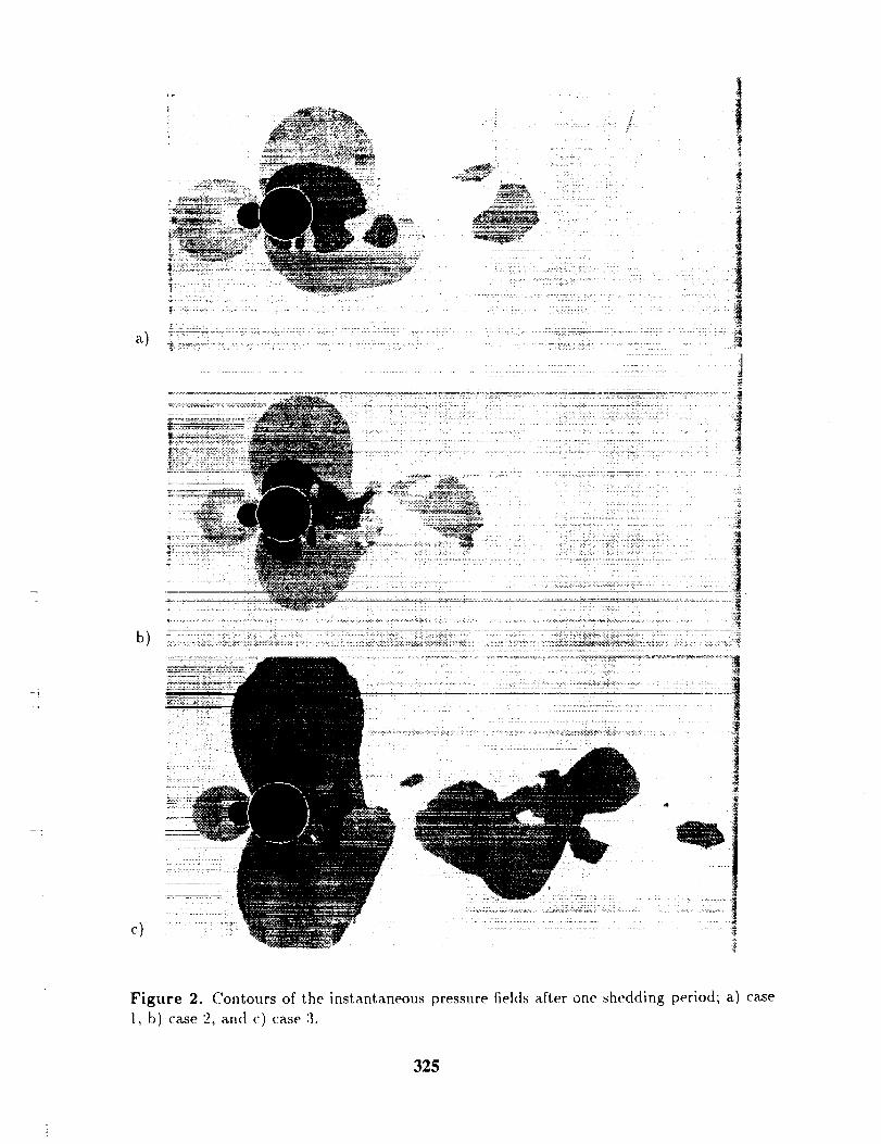
a)
!• t
r
2
i
" i
c)
!
Figure 2. Contours of the instantaneous pressure fields after one shedding period; a) case
1, b) case 2, and c) case 3.
325
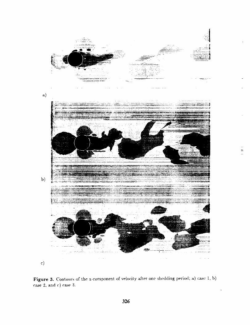
a)
b)
c)
Figure 3. Contours of the x-component of velocity after one shedding period; a) case 1, b)
case '2, and c) case 3.
326
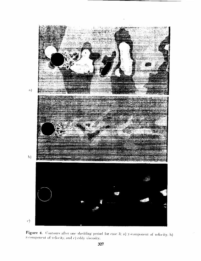
t))
<.)
327
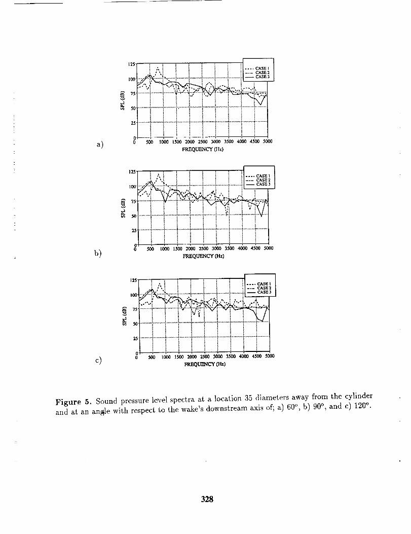
a)
b)
125 _ i i _ _ iI :, ;, i i " ? i !1 .... CASEIJ ,i ' ',i i i .: _ !1--- CASE2
100-|'"7_'"" K ......... ......... ......... ......... ......... ..'>l_ CASE3• . . _ ,,%: _ ." :
_'°l ! ! i ii!iii ...........................lii!.........!.........!........._!_'.........!.........!.........!.........!..........,_......-...................................-..i..................................................
00 5oo to00t5o02ooo25o03o0035oo4o0045oo5000
FREQUENCY (Hz)
(,O
! , ', i i i i i i ! ....CASE)] ,_A,' ,_. : : : : : : -=- CASE2
tool...,'Y..i.K................_.........i.........._........._........._........._. _ CASE3
ol :, i _ :. i i i :,0 500 too0 15co 2o00 2500 3000 35o0 40o0 45o0 5000
FREQUENCY (Hz)
c)
125
IO0-
"/5'
m 50
25
00
i ,,,i i i i i ! !1...._E, [•.k * ': : : :' : _ _l--- CASE2.... _'_ .............. )......... z......... z......... z......... ;......... :.1 _ CASE 3
i,* ....... I ......... | ......... | ......... I'*'))'*"| .................. ¢'* ....... {......... _..........
50_ _ _5'o02_ 25'00_ _5'o0,_ 4._ 5000
FIU_UENCY Olz)
Figure 5. Sound pressure level spectra at a location 35 diameters away from the cylinder
and at an an_le with respect to the wake's downstream axis of; a) 60 °, b) 90 °, and c) 120 °.
328
A COMPARATIVE STUDY OF LOW DISPERSION FINITE VOLUME
SCHEMES FOR CAA BENCHMARK PROBLEMS
D. V. Nance
USAF Wright Laboratory
Eglin AFB, FL 32542-6810
L. N. Sankar
Georgia Institute of Technology
Atlanta, GA 30332
K. Viswanathan
Dynacs Engineering Company, Inc.
Renton, WA 98055
SUMMARY
Low dispersion finite volume schemes have been developed to combine the dispersion matching
characteristics of classical dispersion relation preserving schemes with the flexibility and ease of
applicability of finite volume schemes. In this study, three types of low dispersion finite volume
schemes are applied to a series of problems selected from the first and second NASA/ICASE work-
shops in computational aeroacoustics for benchmark problems. Our schemes are cast in a general
framework designed to account for advection of the main flow field by permitting upwinding at
the cell interfaces. The application of these schemes to the linear problems of acoustics is also
straightforward. The low dispersion finite volume schemes presented here are designed to be fourth
order accurate in space. However, these schemes are easily extended to higher spatial orders. For
the first workshop, results are presented for problems in Categories 1, 2, and 4. We also present
results for Categories 1 and 4 of the second workshop. Comparisons are made with exact solutions
where available.
INTRODUCTION
Aerodynamic noise prediction and control are gaining increased attention from the aerospace
research community. This shift in emphasis is motivated by society's demand for quieter aircraft,
quieter not only in the sense of propulsion noise, but in the sense of aerodynamic noise as well.
Aeroacoustic noise is particularly difficult to resolve computationally. The numerical "noise"
created by the solution of the main flow field tends to overwhelm subtle acoustic waves. 1 As a
result, higher order numerical schemes are needed to preserve the physics of the acoustic field. Low
329
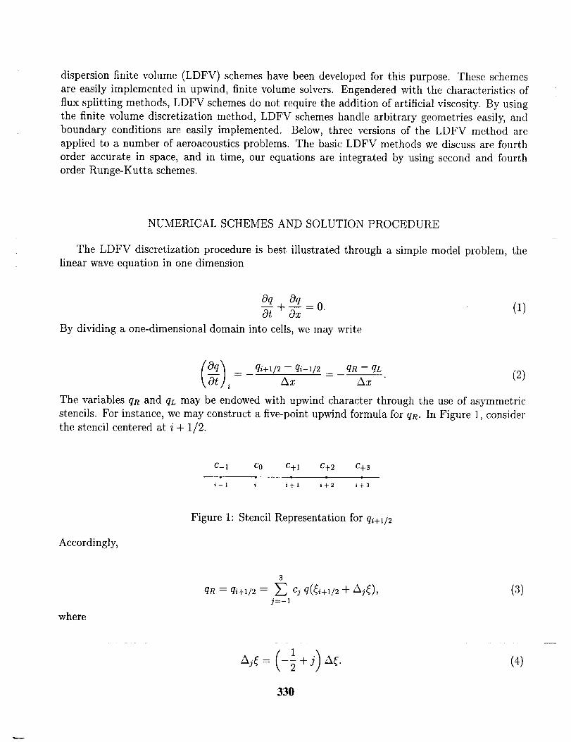
dispersionfinite volume (LDFV) schemeshavebeen developedfor this purpose. Theseschemesare easily implementedin upwind, finite volume solvers. Engenderedwith the characteristicsofflux splitting methods, LDFV schemes do not require the addition of artificial viscosity. By using
the finite volume discretization method, LDFV schemes handle arbitrary geometries easily, and
boundary conditions are easily implemented. Below, three versions of the LDFV method are
applied to a number of aeroacoustics problems, The basic LDFV methods we discuss are fourth
order accurate in space, and in time, our equations are integrated by using second and fourth
order Runge-Kutta schemes.
NUMERICAL SCHEMES AND SOLUTION PROCEDURE
The LDFV discretization procedure is best illustrated through a simple model problem, the
linear wave equation in one dimension
Oq Oq
By dividing a one-dimensional domain into cells, we may write
(1)
Oq) qi+l/2 -- qi-1/2 _ qR -- qL= - /xz Az (2)
The variables qR and qL may be endowed with upwind character through the use of asymmetric
stencils. For instance, we may construct a five-point upwind formula for qR. In Figure 1, consider
the stencil centered at i + 1/2.
C-1 Co C+I C+2 C+3
i--1 i i+l i-}-2 i+3
Accordingly,
Figure 1: Stencil Representation for qi+l/2
where
3
qR = qi+u2 = _ Cj q({i+l/2 + Aj_), (a)j=-I
Aj_ = (-2 +j) A_. (4)
330
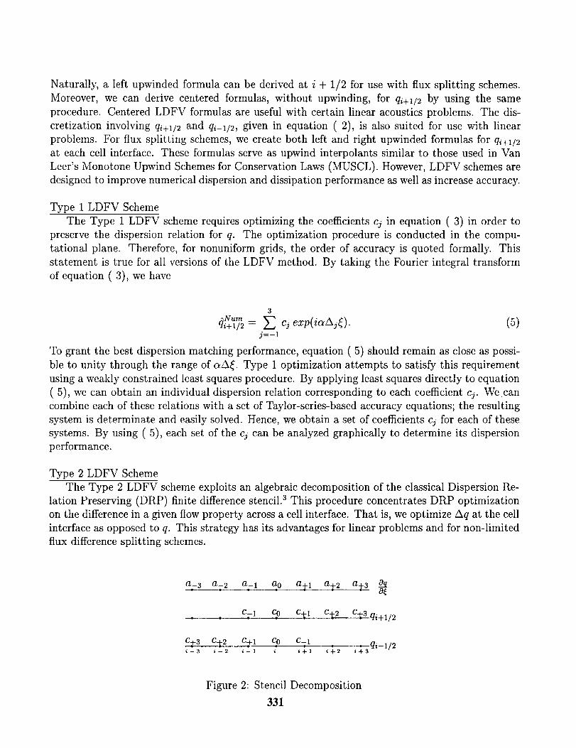
Naturally, a left upwinded formula can be derived at i + 1/2 for use with flux splitting schemes.
Moreover, we can derive centered formulas, without upwinding, for qi+l/2 by using the same
procedure. Centered LDFV formulas are useful with certain linear acoustics problems. The dis-
cretization involving qi+l/2 and qi-1/2, given in equation (2), is also suited for use with linear
problems. For flux splitting schemes, we create both left and right upwinded formulas for q_+1/2
at each cell interface. These formulas serve as upwind interpolants similar to those used in Van
Leer's Monotone Upwind Schemes for Conservation Laws (MUSCL). However, LDFV schemes are
designed to improve numerical dispersion and dissipation performance as well as increase accuracy.
Type 1 LDFV Scheme
The Type 1 LDFV scheme requires optimizing the coefficients cj in equation (3) in order to
preserve the dispersion relation for q. The optimization procedure is conducted in the compu-
tational plane. Therefore, for nonuniform grids, the order of accuracy is quoted formally. This
statement is true for all versions of the LDFV method. By taking the Fourier integral transform
of equation (3), we have
3_Num,+,/2= cj exp(i A ). (5)
j=-i
To grant the best dispersion matching performance, equation (5) should remain as close as possi-
ble to unity through the range of aA_. Type 1 optimization attempts to satisfy this requirement
using a weakly constrained least squares procedure. By applying least squares directly to equation
(5), we can obtain an individual dispersion relation corresponding to each coefficient cj. We.can
combine each of these relations with a set of Taylor-series-based accuracy equations; the resulting
system is determinate and easily solved. Hence, we obtain a set of coefficients cj for each of these
systems. By using (5), each set of the cj can be analyzed graphically to determine its dispersion
performance.
Type 2 LDFV Scheme
The Type 2 LDFV scheme exploits an algebraic decomposition of the classical Dispersion Re-
lation Preserving (DRP) finite difference stencil. 3 This procedure concentrates DRP optimization
on the difference in a given flow property across a cell interface. That is, we optimize Aq at the cell
interface as opposed to q. This strategy has its advantages for linear problems and for non-limited
flux difference splitting schemes.
a__ aT2 a:_i a0 %_
• . c;-a, Co , c-t1 c-t2 c-t3qi+l/2
c.+3 c_2 _1 Co: c-1i--3 i--2 i--1 i i+l
; -- qi-1/2i+2 i+3
Figure 2: Stencil Decomposition
331
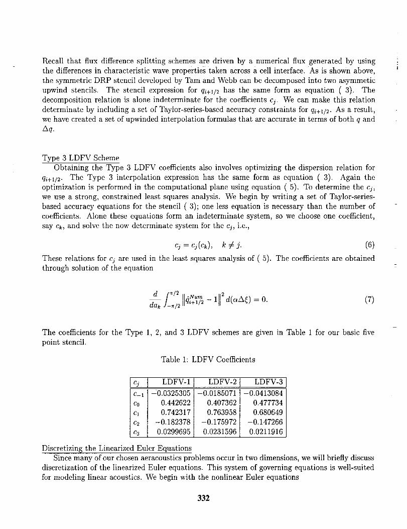
Recall that flux differencesplitting schemesare driven by a numerical flux generatedby usingthe differencesin characteristicwave propertiestaken acrossa cell interface. As is shownabove,the symmetric DRP stencil developedby Tam and Webbcanbe decomposedinto two asymmeticupwind stencils. The stencil expressionfor qi+l/2 has the same form as equation (3). The
decomposition relation is alone indeterminate for the coefficients cj. We can make this relation
determinate by including a set of Taylor-series-based accuracy constraints for qi+l/2. As a result,
we have created a set of upwinded interpolation formulas that are accurate in terms of both q and
Aq.
Type 3 LDFV Scheme
Obtaining the Type 3 LDFV coefficients also involves optimizing the dispersion relation for
qi+l/2. The Type 3 interpolation expression has the same form as equation (3). Again the
optimization is performed in the computational plane using equation (5). To determine the cj,
we use a strong, constrained least squares analysis. We begin by writing a set of Taylor-series-
based accuracy equations for the stencil ( 3); one less equation is necessary than the number of
coefficients. Alone these equations form an indeterminate system, so we choose one coefficient,
say Ck, and solve the now determinate system for the cj, i.e.,
cj = cj(ck), k _: j. (6)
These relations for cj are used in the least squares analysis of (5). The coefficients are obtained
through solution of the equation
d f,_/2 ^Numdak J-_/2 qi+1/2 -- 112 d(aA_) = 0. (7)
The coefficients for the Type 1, 2, and 3 LDFV schemes are given in Table 1 for our basic five
point stencil.
Table 1" LDFV Coefficients
I LDFV-1 LDFV-2 LDFV-3
c_1 :0.0325305
Co 0.442622
Cl 0.742317
c2 -0.182378
c3 0.0299695
-0.0185071
O.407362
0.763958
-0.175972
0.0231596
-0.0413084
O.477734
0.680649
-0.147266
0.0211916
Discretizing the Linearized Euler Equations
Since many of our chosen aeracoustics problems occur in two dimensions, we will briefly discuss
discretization of the linearized Euler equations. This system of governing equations is well-suited
for modeling linear acoustics. We begin with the nonlinear Euler equations
332
where F and G are flux vectors, and
cgq OF OG
0-7+ 7x + 0_ = 0, (8)
q = (p, pu, pv, e) T.
To linearize (8), as suggested by Hardin 4, we assume that acoustic fluctuations may be modeled
as small perturbations on the main flow field, so
q=q+4, 4 << _2.
Also, we make use of the quasi-linear form of the flux vectors, i.e.,
(9)
OF _ A Oq. OG _vvOx Ox' -_y - B v '
where A and B are flux Jacobian matrices given by
(10)
OF OGA=--" B=--.
cgq' cgq
By using (10) and (11) in equation (8) and by applying (9), we can show that
(11)
0c] 0(Aq) + a(/?_]) + 04 0(/[4) c3(/_) _ 0, (12)57 + a--Z- a--T _ + a--T- + ag
having neglected terms of the second and higher orders. The first three terms represent the Euler
equations for the main flow field, so the sum of these terms is identically zero. The remaining
terms are the linearized Euler equations
&j a(.44) + 0(/?_) _ 0; (13)o-Y+ a---Z- ay
,g, and/? depend strictly upon the main flow field propertiesP To perform a spatial discretization
of (13), we integrate (13) over a given cell area and apply the divergence theorem.
O_ Jc_u Jo(ceu)
The boundary term can be discretized as follows.
+ [_3)4" ridS = O. (14)
333
Cell
0 fc 4dV + _ (-Af_ +/)fiy)4AS' = 0. (15)Ot ell Sides
-Anx +/)fly is a diagonalizable matrix suitable for upwinding 6, i.e.,
(Aa_ + Bf_)4 = C+4L+ C-4R. (16)
C + is the upwind matrix for "right" traveling waves in the nonlinear flowfield. Accordingly, it is
used with the left upwinded 4L. C- and 4R are quantities associated with the remaining upwind
direction. Hence, the semi-discrete form is
d(4ce.) 1 Ce*ldt - Vcell _ (C+qL + C-4R)AS.
Sides
(17)
Temporal Discretization
Equation (17) must be integrated in time to render a numerical solution. To accomplish this
integration, we recognize that (17) is in the form
5D-" = n(0). (is)Ot
Equation (18) may be numerically integrated in time by using the two-step Runge-Kutta scheme
4 p = q n + AtRn;
4 (_+1) 1 , _ p) z_tpv= i(q +4 + 2"°"(19)
Of course, higher order Runge-Kutta schemes may be used in lieu of (19). Hirsch is a suitablereference for these methods. 6
Discretization of the Navier-Stokes Equations
The laminar Navier-Stokes equations are applied in the vortex-shedding noise problem, so we
will briefly discuss their two-dimensional form here. In vector form, these equations can be written
Oq OF OG OR OS (20)-b-i+ _ + _ - ox + o_
The left side of (20) is identical to the Euler equations; however, vectors R and S contain viscous
and heat conduction terms. This system is solved in full nonlinear simulation. The advective
terms are solved using Roe's flux difference splitting and LDFV interpolation. The viscous/heat
conduction terms are discretized in finite volume form using classical DRP formulas for differentials
occurring in the stress terms and in Fourier's Law. A four-stage Runge-Kutta scheme is used for
334
temporal integration of the semi-discrete form.
RESULTS AND DISCUSSION
The First Workshop
Results for the first workshop are submitted in this report, because the work on LDFV schemes
did not begin until after the publication date for the first workshop. For the linear wave equation,
Figure 3 contains the time 100 results for all three types of LDFV schemes. Clearly, the Type 1
and 3 results are poor, because neither Type 1 nor 3 optimization is tied to to the spatial differ-
encing operator. The Type 2 results are excellent, because the Type 2 scheme optimizes Au at
the cell interface. In fact, on uniform grids, the Type 2 LDFV scheme algebraically reduces to the
classical DRP scheme.
The spherical wave equation was also solved in Category 1. Our results are computed for an
angular frequency of w = 4" As with the preceding problem, the space derivatives are discretized
as in (2). The numerical results are presented at time 200 in Figure 4. All of the LDFV schemes
outperform the MacCormack and upwind schemes in the solution of this problem. 7 The Type 2
solution demonstrates the best performance among the LDFV schemes. Still, the Type 1 and 3
schemes show some improved dissipative performance while limiting group velocity errors.
For the Category 2 submission, we have solved the nonlinear Euler equations in one dimension.
The system is initiated by a Gaussian pressure pulse. In Figure 5, the results are compared with
an upwind scheme of the fifth order. A limiter was used to remove oscillations from the solution.
The Type 1 and 3 LDFV schemes perform very well, comparable with the fifth order upwind
solution. On the other hand, the Type 2 solution, omitted from Figure 5, does not perform well
when used with the limiter. The Type 1 and 3 solutions capture the shock wave very well except
near the discontinuity where small oscillations exist. These oscillations may be removed through
the use of an improved limiting strategy for the stencil.
The reflection of a Gaussian acoustic pulse from a wall in a uniform flow was chosen as a
problem from Category 4. The solutions for this problem at times 60 and 75 are shown in Figures
6 and 7, respectively. The linearized Euler equations are used in this problem, so the Type 2 LDFV
scheme performs best. In fact, this scheme performs comparably well to MacCormack's method. 7
The Type 1 and 3 schemes perform well on the smoother sections of the pulse; however, these
schemes are more dissipative near the pulse extrema. Still, the Type 1 and 3 solutions perform
better than the upwind scheme almost everywhere along the pulse profile. 7 By examining a series
of Type 2 LDFV solutions in time, it becomes apparent that the quality of the solutions improves
with time. This behavior is a desirable trait of algorithms for computational aeroacoustics (CAA).
The Second Workshop
The problems specified within the second workshop have presented an opportunity for testing
the LDFV schemes on curvilinear geometries. Problems 1 and 2 are appropriate for study since
335
they are easily cast on polar grids. Before solving Problem 1, our LDFV solver was validated for
the interaction of a plane acoustic wave with a rigid circular cylinder. The time t = _ numerical
solution, calculated in two dimensions, is compared against the exact solution in Figure 8. A 41
by 63 grid was employed for the calculation along with At = 0.01. The comparison between the
exact and numerical solutions is quite good although the solution quality does fluctuate in time.
In this case, all of the LDFV schemes outperform the MUSCL scheme.
All three LDFV schemes were used to compute solutions for Problem 1, the scattering of pe-
riodic acoustic waves generated by a Gaussian source term in the linearized Euler equations. The
grid used for this problem is 153 by 159; it has uniform spacing in the azimuthal direction. Radi-
ally, the grid stretches in the region adjacent to the body but then adopts uniform spacing in the
midfield and farfield. The minimum radial spacing is 0.01, and At = 0.005. Graphical snapshots
of the pressure field are presented in Figures 9 and 10 for solution times 5.0 and 7.5, respectively.
The Type 2 LDFV scheme was used to generate these solutions. The mean-squared pressure plots
for the farfield are given in Figure 11.
Problem 2 is an initial value problem; unlike the system in Problem 1, the nonhomogeneous
terms are set equal zero. In this case, a Gaussian pressure wave is initiated in the field at time zero.
As the solution evolves, .the pulse reflects from the cylinder and propagates out of the domain.
The grid specification and time step are identical to those used for Problem 1. All three LDFV
schemes were used to solve Problem 2. Snapshots of the acoustic field calculated by the Type
2 scheme are presented in Figures 12 and 13 for solution times 5.0 and 7.5. The pressure time
history plots for the Type 1, Type 2, and Type 3 solutions are presented in Figures 14, 15, and
16, respectively.
The Category 4 problem involved the greatest expenditure of computing resources and time
among all of the workshop problems. In order to reduce the computer memory and time re-
quirements as much as practicable, we have diverged from the problem specifications by selecting
Reynolds number 200 and 5000 for our simulations. Also, our calculations are performed using
dimensionless quantities at Mach 0.2. The flow solver is a compressible, laminar Navier-Stokes
code that employs Roe's flux difference splitting scheme with fourth order LDFV interpolation in
space. The temporal integration routine uses a fourth order Runge-Kutta scheme. This program
has been validated using archival data on this geometry; the validation information will be pub-lished elsewhere.
The calculations for both Reynolds numbers were performed on cylindrical grids. A 95 by 125
grid was used for the Reynolds number 200 case. For the Reynolds number 5000 case, a slightly
larger grid was used with dimensions 95 by 136. In both cases, the first radial increment is set
at 0.01. The initial stretching ratio is 1.08, but in the nearfield, the stretching ratio is increased
additively by 0.001 at each successive radial increment. The radial grid is progressively stretched
until the radial increment exceeds 0.25; the increment is then held constant through the midfield
and farfield. For the Reynolds number 200 case, acoustic sampling is conducted 23 diameters away
from the cylinder, and for the Reynolds number 5000 case, samples were taken 25 diameters away
from the body. In both cases, acoustic sampling is performed at locations above the cylinder and
in the cylinder wake. Nonreflecting boundary conditions are implemented in the farfield to pre-
336
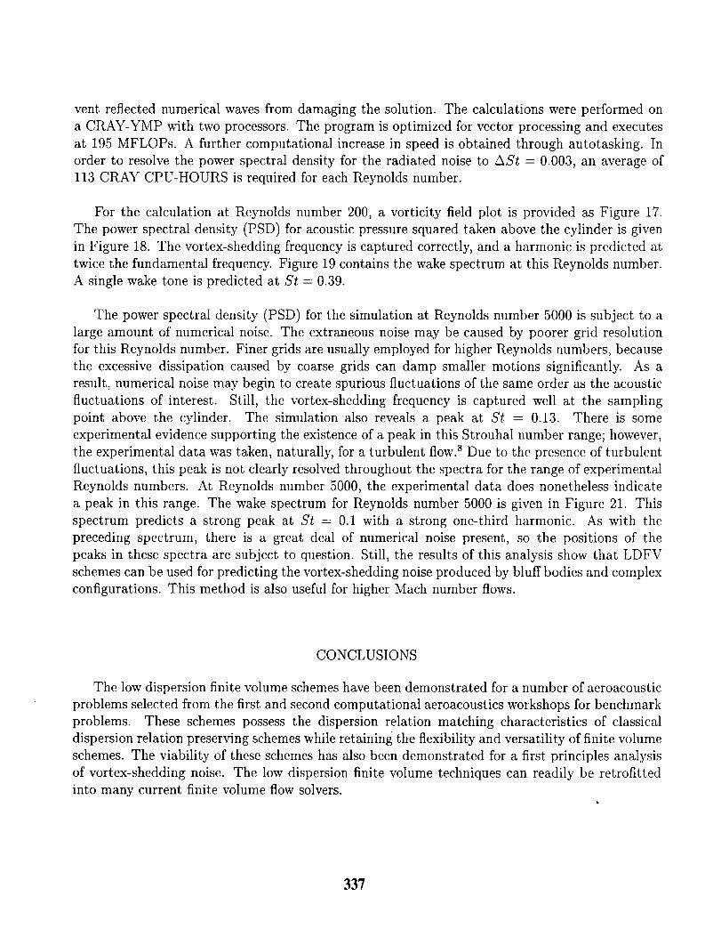
vent reflected numerical waves from damaging the solution. The calculations were performed on
a CRAY-YMP with two processors. The program is optimized for vector processing and executes
at 195 MFLOPs. A further computational increase in speed is obtained through autotasking. In
order to resolve the power spectral density for the radiated noise to ASt = 0.003, an average of
113 CRAY CPU-HOURS is required for each Reynolds number.
For the calculation at Reynolds number 200, a vorticity field plot is provided as Figure 17.
The power spectral density (PSD) for acoustic pressure squared taken above the cylinder is given
in Figure 18. The vortex-shedding frequency is captured correctly, and a harmonic is predicted at
twice the fundamental frequency. Figure 19 contains the wake spectrum at this Reynolds number.
A single wake tone is predicted at St = 0.39.
The power spectral density (PSD) for the simulation at Reynolds number 5000 is subject to a
large amount of numerical noise. The extraneous noise may be caused by poorer grid resolution
for this Reynolds number. Finer grids are usually employed for higher Reynolds numbers, because
the excessive dissipation caused by coarse grids can damp smaller motions significantly. As a
result, numerical noise may begin to create spurious fluctuations of the same order as the acoustic
fluctuations of interest. Still, the vortex-shedding frequency is captured well at the sampling
point above the cylinder. The simulation also reveals a peak at St = 0.13. There is some
experimental evidence supporting the existence of a peak in this Strouhal number range; however,
the experimental data was taken, naturally, for a turbulent flow. 8 Due to the presence of turbulent
fluctuations, this peak is not clearly resolved throughout the spectra for the range of experimental
Reynolds numbers. At Reynolds number 5000, the experimental data does nonetheless indicate
a peak in this range. The wake spectrum for Reynolds number 5000 is given in Figure 21. This
spectrum predicts a strong peak at St = 0.1 with a strong one-third harmonic. As with the
preceding spectrum, there is a great deal of numerical noise present, so the positions of the
peaks in these spectra are subject to question. Still, the results of this analysis show that LDFV
schemes can be used for predicting the vortex-shedding noise produced by bluff bodies and complex
configurations. This method is also useful for higher Mach number flows.
CONCLUSIONS
The low dispersion finite volume schemes have been demonstrated for a number of aeroacoustic
problems selected from the first and second computational aeroacoustics workshops for benchmark
problems. These schemes possess the dispersion relation matching characteristics of classical
dispersion relation preserving schemes while retaining the flexibility and versatility of finite volume
schemes. The viability of these schemes has also been demonstrated for a first principles analysis
of vortex-shedding noise. The low dispersion finite volume techniques can readily be retrofitted
into many current finite volume flow solvers.
337
REFERENCES
[1] Tam, C.K.W., "Computational Aeroacoustics:Issuesand Methods", AIAA Journal, Vol.
33, No. 10, October 1995, pp. 1788-1796.
[2] Van Leer, B., "Towards the Ultimate Conservative Difference Scheme, IV: A New Approach
to Numerical Convection", Journal o/Computational Physics, Vol. 23, 1977, pp. 276-299.
[3] Tam, C.K.W. and Webb, J. C., "Dispersion-Relation-Preserving Schemes for Computational
Aeroacoustics", Journal o/ Computational Physics, Vol. 107, 1993, pp. 262-281.
[4] Hardin, J., Invited Lecture Given at the ASME Forum on Computational Aeroacoustics and
Hydroacoustics, June 1993.
[5] Viswanathan, K. and Sankar, L.N., "Toward the Direct Calculation of Noise: Fluid/Acoustic
Coupled Simulation", AIAA Journal, Vol. 33, No. 12, December 1995, pp. 2271-2279.
[6] Hirsch, C., Numerical Computation of Internal and External Flows, Vol. 2. John Wiley &
Sons, New York,1990.
[7] Nance, D.V., Viswanathan, K., and Sankar, L.N., "A Low Dispersion Finite Volume Scheme• S"for Aeroacoustic Application , AIAA Paper 96-0278, 34 th Aerospace Sciences Meeting and
Exhibit, 1996.
[8] Chambers, F. W., "Isolated Component Testing for the Identification of Automotive Wind
Noise Sources", ASME Noise Control and Acoustics Division (NCA), Winter Annual Meeting
Dallas, TX, 1990.
338
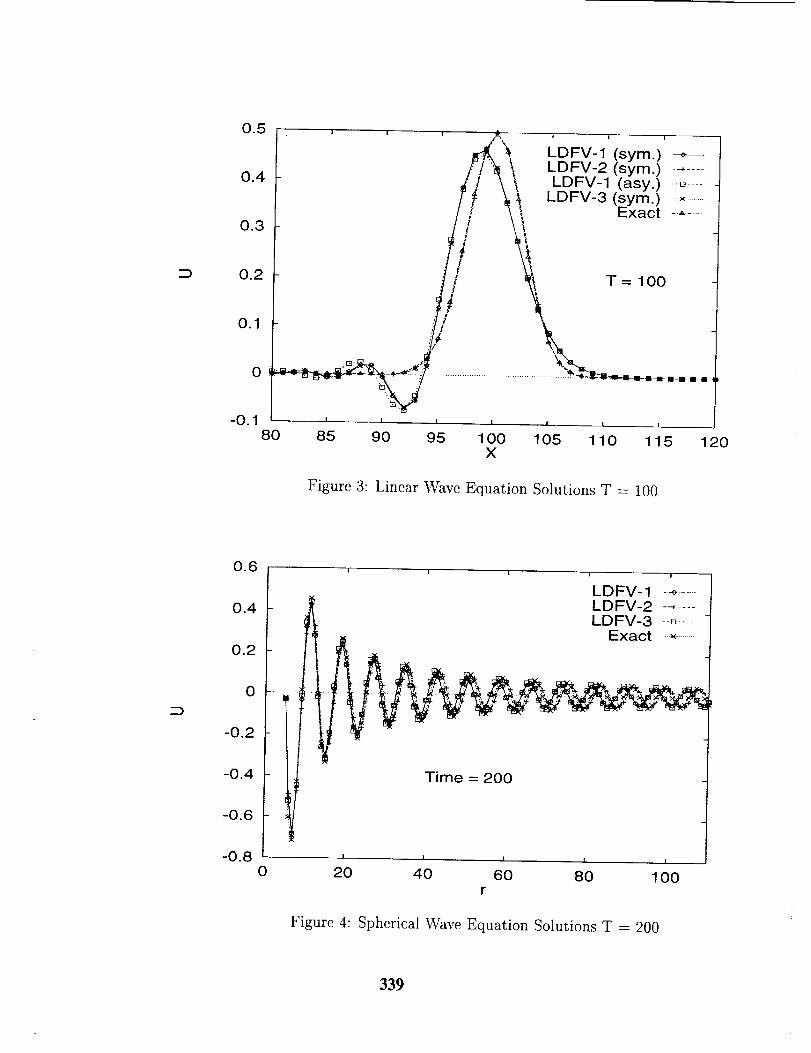
0.5
0.4
0.3
0.2
0.1
0
i , i
LDFV-1 (sym.) -_---LDFV-2 (sym.) ......LDFV-1 (asy.) +-_....
LDFV-3 (sym.) x .......Exact ......
T= 100
-0.18O
I I i I I i I
85 90 95 100 105 110 115 120X
Figure 3: Linear Wave Equation Solutions T = 100
0.6
0.4
0.2
0
-0.2
-0.4
-0.6
-0.8
i I
LDFV-1 _--LDFV-2 -+ ....LDFV-3 --+....
Exact ....x.........
Time = 200
0I I I
20 40 60 80 100
Figure 4: Spherical Wave Equation Solutions T = 200
339
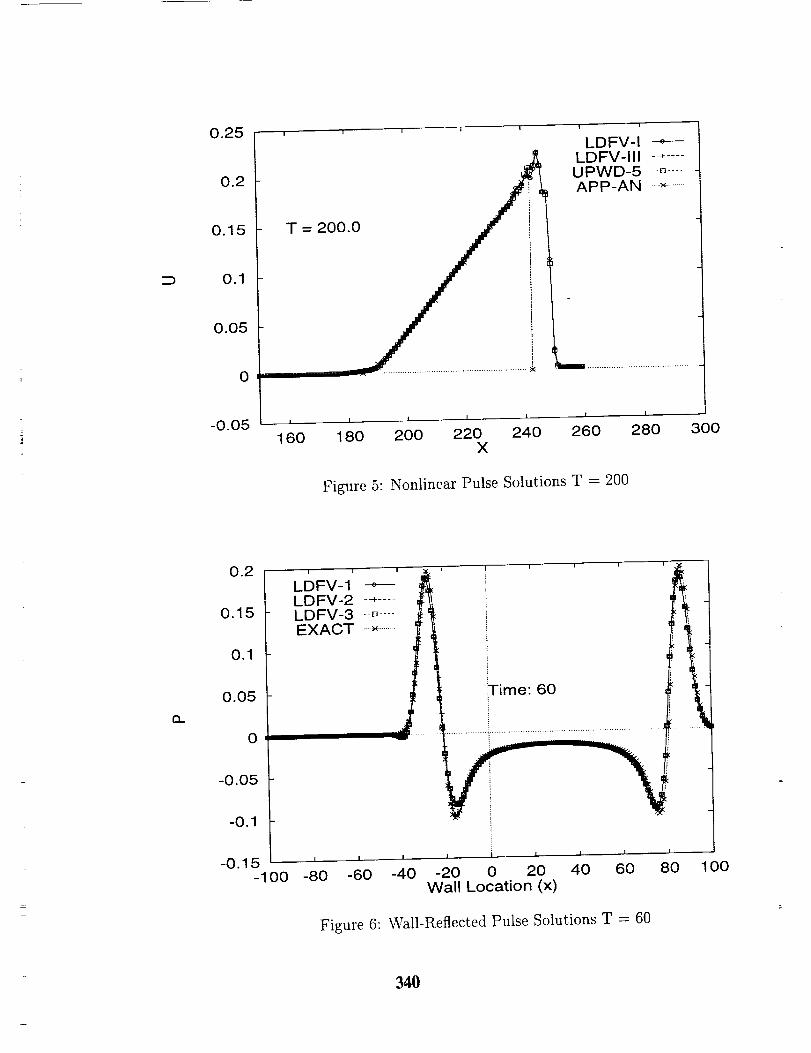
0.2
0.15 T= i2OO.
0.1
0.05
0
-0.05 ' • ' ' '160 180 200 220 240
X
i i
LDFV-ILDFV-III --* ....
UPWD-5 -o ....APP-AN ....,,.........
I I
26O 280
Figure 5: Nonlinear Pulse Solutions T = 200
3OO
13..
0.15
0.05
0
LDFV-1LDFV-2 --+....LDFV-3 --D....EXACT ....*.........
Time: 60
i
! |
-80 -60 -40 -20 0 20 40 60Wall Location (x)
Figure 6: Wall-Reflected Pulse Solutions T = 60
8O
[]
100
340
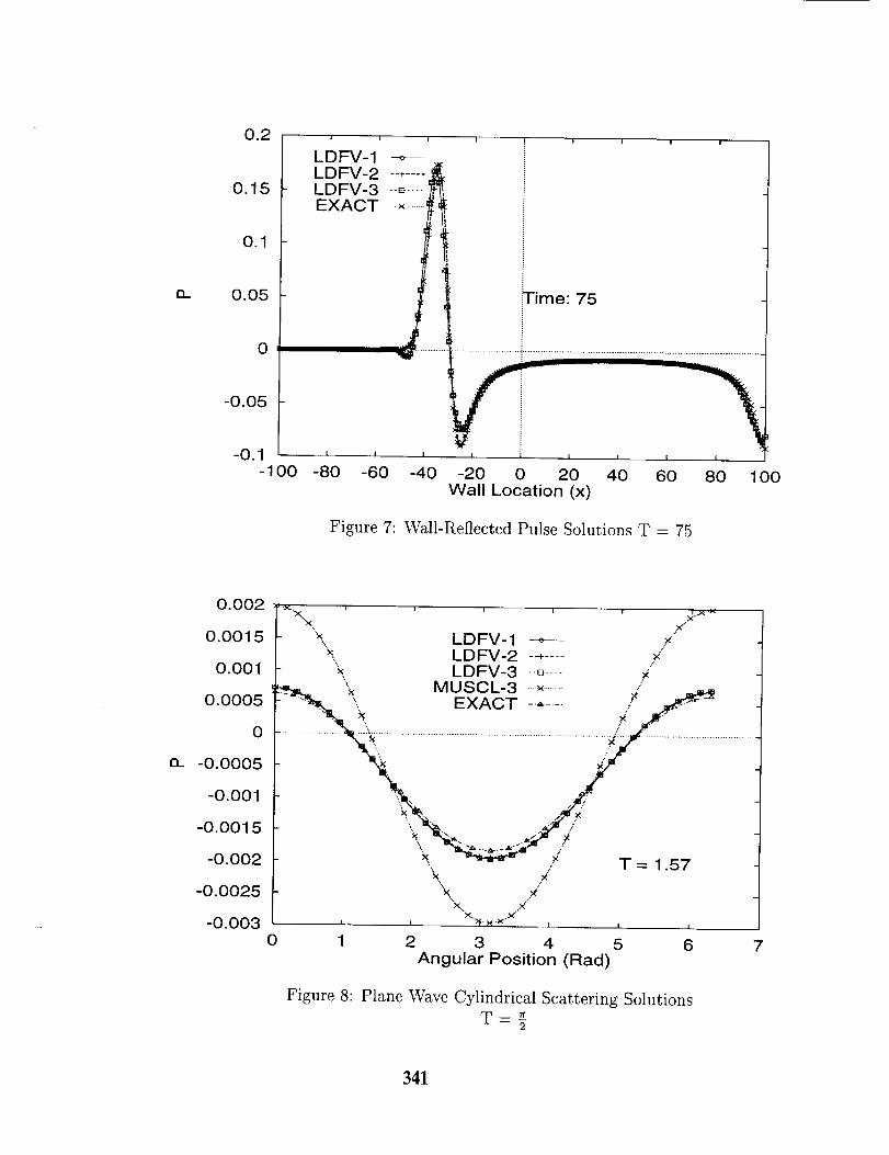
13-
0.2
0.15
0.1
0.050 [
-0.05
-0.1-100
LDFV-1 -_---i
LDFV-2 ...... _LDFV-3 --[]......
EXACT ...._i '
d ......
Time: 75
....................... i ..........................................................................................
I l II I I
-80 -60 -40 -20 0 20 40 60 80 100Wall Location (x)
Figure 7: Wall-Reflected Pulse Solutions T = 75
Q-
0.002
0.0015
0.001
0.0005
0
-0.0005
-0.001
-0.0015
-0.002
-0.0025
-O.OO30
[ ._. i i i i i /.x: --]'__c
"X ;K"
'& LDFV-1 +- .×./
LDFV-2 --+.... ×LDFV-3 -D ....
MUSCL-3 ....,',......... /
' EXACT .......
_k" . . ";
x. - /_ T = 1.57\ /
k. .x
l | X..)_. N..X..,X' I I ., !
1 2 3 4 5 6 7Angular Position (Rad)
Figure 8: Plane Wave Cylindrical Scattering Solutions
T= 7r2
341
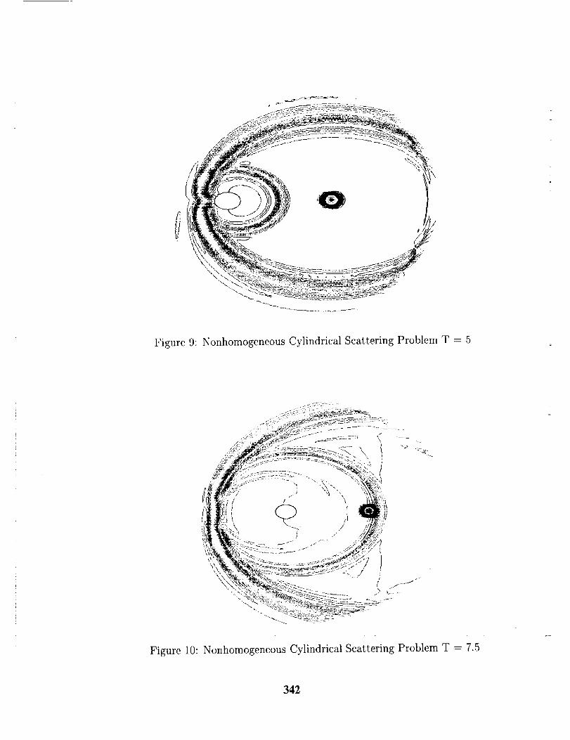
U
Figure 9: Nonhomogeneous Cylindrical Scattering Problem T = 5
Figure 10: Nonhomogeneous Cylindrical Scattering Problem T = 7.5
342
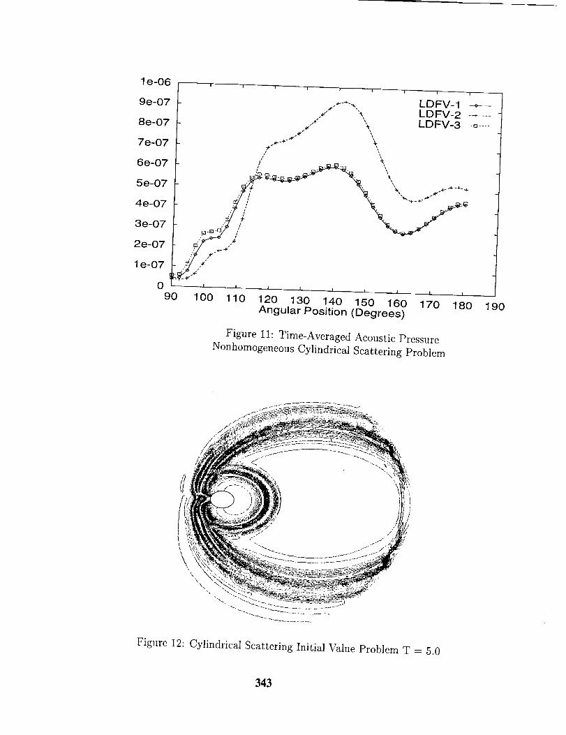
1 e-06
9e-07
8e-07
7e-07
6e-07
5e-07
4e-07
3e-07
2e-07
I e-07
09O
/I
tl
100
\
i
LDFV-1 --_- -LDFV-2 ......LDFV-3 --_ ....
I I I I 1_ I I
110 120 130 140 150 160 170Angular Position (Degrees)
Figure 11: Time-Averaged Acoustic Pressure
Nonhomogeneous Cylindrical Scattering Problem
180 190
Figure 12: Cylindrical Scattering Initial Value Problem T = 5.0
343
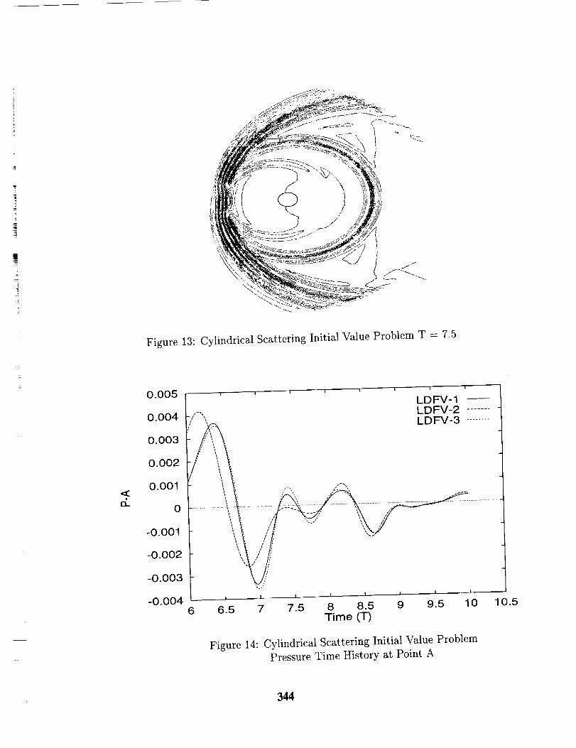
|
?
<oL
Figure 13: Cylindrical Scattering Initial Value Problem T = 7.5
0.005
0.004
0.003
0.002
0.001
0
-0.001
-0.002
-0.003
-0.004
i i
LDFV-1LDFV-2 .......LDFV-3 ........
6I
6.5 7 7.5 8 8.5 9 9.5 10Tim e (T)
Figure 14: Cylindrical Scattering Initial Value Problem
Pressure Time History at Point A
10.5
344
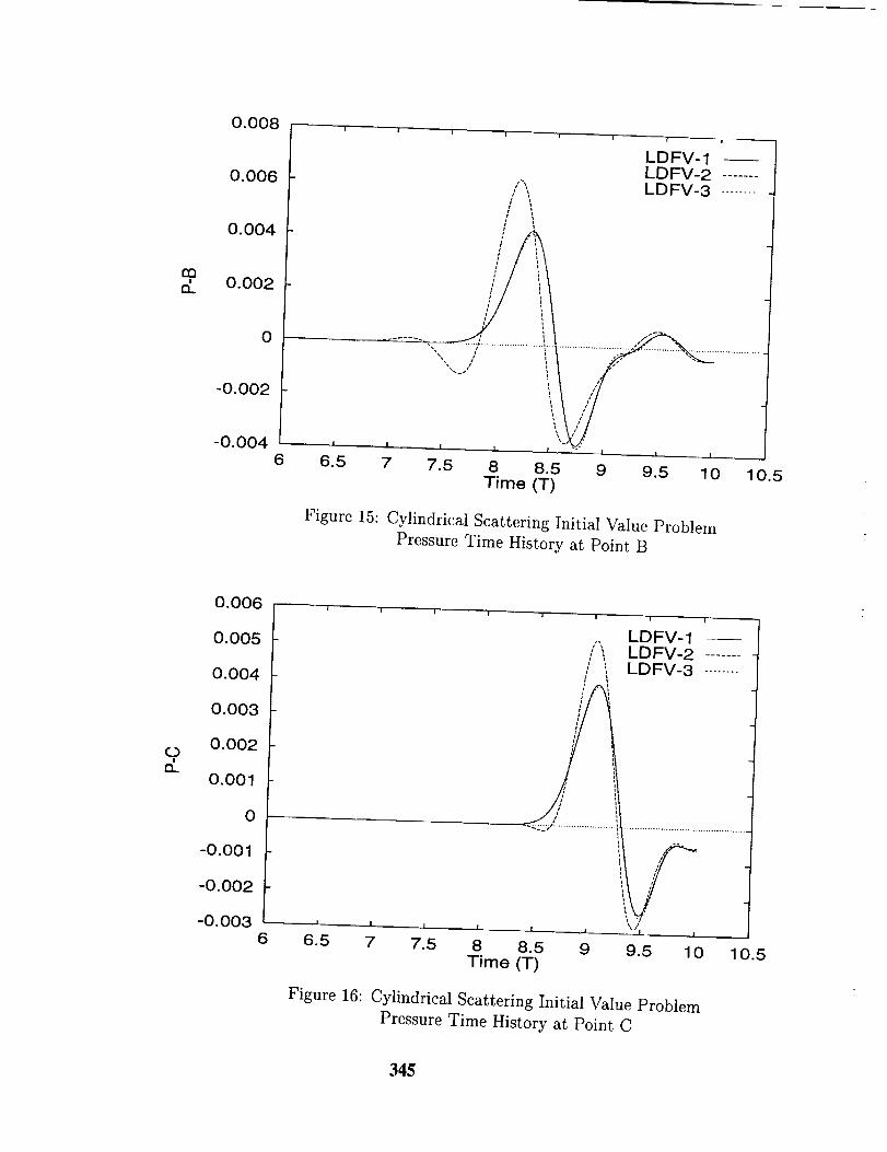
133
cL
0.008
0.006
0.004
0.002
0
-0.002
-0.004 ' •6 6.5 7
, i i"
/ \/
I
i !
LDFV-1LDFV-2 .......LDFV-3 ........
f
i
]'
/
",, / , ,,
i :t r
i I
7.5 8 8.5 9 9.5 10Time (T)
Figure 15: Cylindrical Scattering Initial Value Problem
Pressure Time History at Point B
10.5
cL
0.006
0.005
0.004
0.003
0.002
0.001
0
-0.001
-0.002
-0.0036
1 i I _ "'! • i i I
LDFV-1,, LDFV-2 ......./ i LDFV-3 ........
/f
I ,(
I I , l ., I I _ I , _'rl I
6.5 7 7.5 8 8.5 9 9.5 10Time (T)
10.5
Figure 16: Cylindrical Scattering Initial Value Problem
Pressure Time History at Point C
345
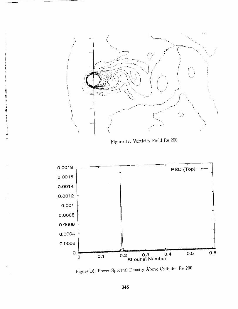
=
/
!
i
i
i
/• ,%
,.........7> T\ "\.
. t ..... "_ .......................:;:.._.. "x \ ! /,.",,__"_!_7:_:::........ " .."'.,,,,-.." ". _ .:
_ \ "-%_,....j:
: /,f j
: I_}"_x.~
-- ] "'t/
!
!
\
I \
\
\,.
<
/
i"
\
\
i
Figure 17: Vorticity Field Re 200
0.0018
0.0016
0.0014
0.0012
0.001
0.0008
0.0006
0.0004
0.0002
0
I I I I I I
PSD (Top) --*--
0 0.1 0.2 0.3 0.4 0.5 0.6Strouhal Number
Figure 18: Power Spectral Density Above Cylinder Re 200
346
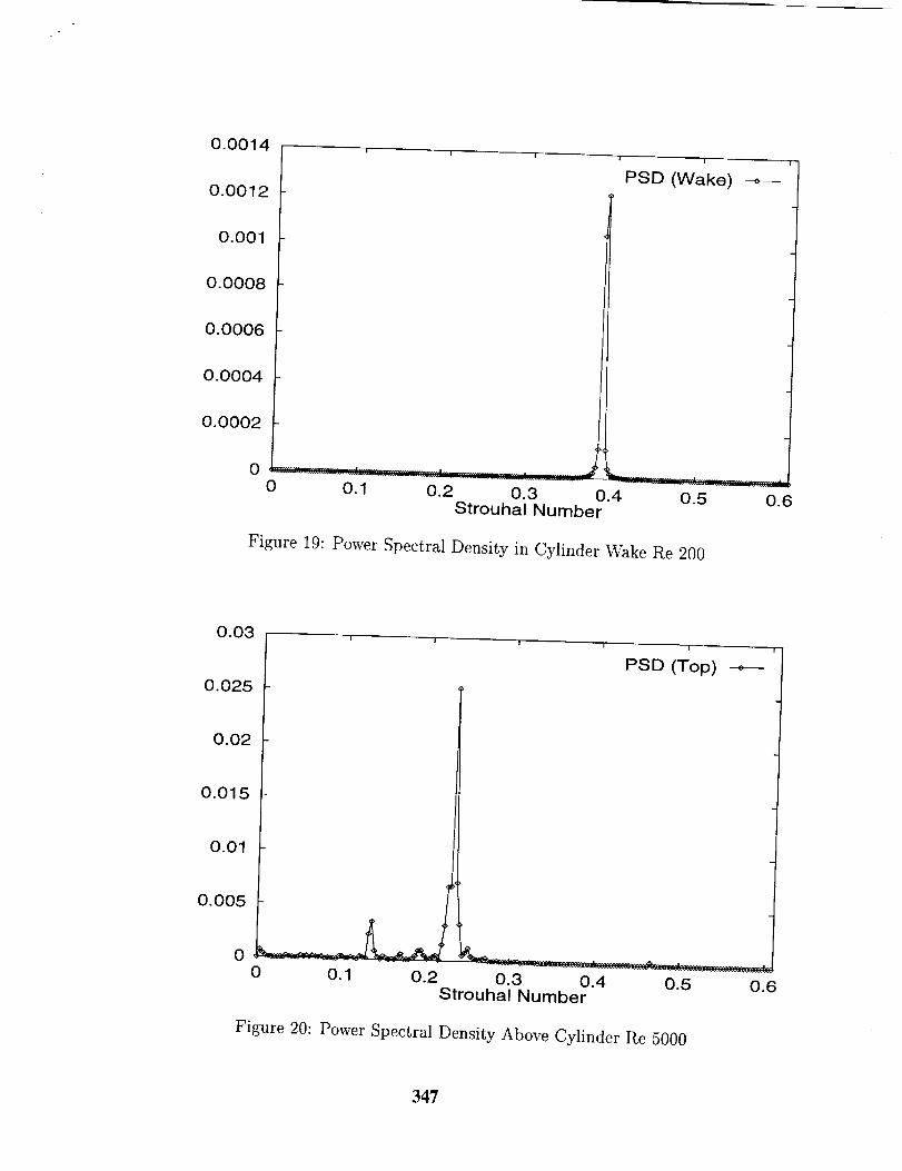
0.0014
PSD (Wake) _--
0.0012
0.001
0.0008
0.0006
0.0004
oooo t JL t0 0.1 0.2 0.3 0.4 0.5 0.6
Strouhal Number
Figure 19: Power Spectral Density in Cylinder Wake Re 200
0.03
0.025
0.02
0.015
0.01
0.005
0
PSD (Top)
0 0.1 0.2 0.3 0.4 0.5 0.6Strouhal Number
Figure 20: Power Spectral Density Above Cylinder Re 5000
347
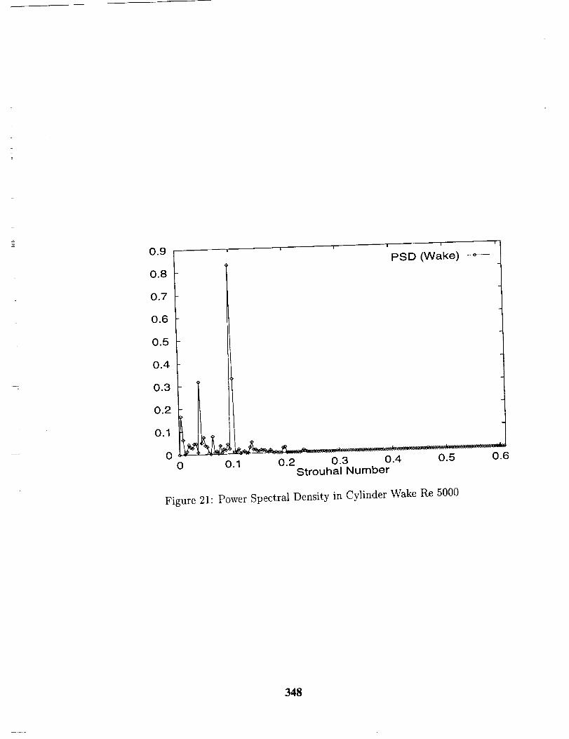
0.9
0.8
0.7
0.6
0.5
0.4
0.3
0.2
0.1
0
PSD (Wake) -_'---
0 0. 0.2 0.3 0.4 0.5 0.6Strouhal Number
Figure 21" Power Spectral Density in Cylinder Wake Re 5000
348
OVERVIEW OF COMPUTED RESULTS
Christopher K.W. Tam
Florida State University
One distinctive feature of the CAA Workshops on benchmark problems is that all
participants are required to submit a set of their computed data to the Scientific Committee for
comparisons with the exact (nearly exact) solutions or experimental measurements. The
purpose of the comparisons is to provide a measure of the quality of the numerical results.
Also it is hoped that the comparisons would offer feedback to the participants to encourage
improvements on their computational algorithms.
The benchmark problems of the First CAA Workshop were designed mainly to test the
dispersion, dissipation and anisotropy characteristics of the computational schemes. They are,
therefore, somewhat idealized and simple. The benchmark problems of the Second CAA
Workshop are more realistic and hence more difficult and challenging. The first three
categories of problems are formulated to test the design and implementation of boundary
conditions. They include open boundary conditions (radiation condition) wall boundary
conditions and radiation boundary conditions in ducted environments. Based on the
submitted data and their comparisons with exact (nearly exact) solutions, it appears that
significant advances in the development of numerical boundary conditions for CAA have
been made over the last few years. The Category 4 problem is the first benchmark problem
involving viscous flow. Viscous flow problems, by nature, have multiple length scales. They
are much more difficult to solve computationally. Perhaps, because of the intrinsic
complexity of the problem, all the contributors have chosen not to compute the radiated
sound directly. Direct computation of the radiated sound remains a challenge for the future.
The Scientific Committee wishes to thank the following individuals for their time and
effort in carrying out the comparisons on its behalf.
Category 1.Problems 1 & 2.
University.Problems 3 & 4.
Category 2.
Konstantin A. Kurbatskii and Christopher K.W. Tam, Florida State
Philip J. Morris, Penn State University.
Problem 1. Philip J. Morris, Penn State University.
Problems 2. Konstantin A. Kurbatskii and Christopher K.W. Tam, Florida State
University.
Category 3.
Problems 1, 2 & 3. Kenneth C. Hall, Duke University.
Category 4.
Problem 1. Jay C. Hardin, NASA Langley Research Center.
The Committee also wishes to thank Dennis L. Huff (NASA Lewis Research Center) for his
contribution to the formulation of the Category 3 problems.
349
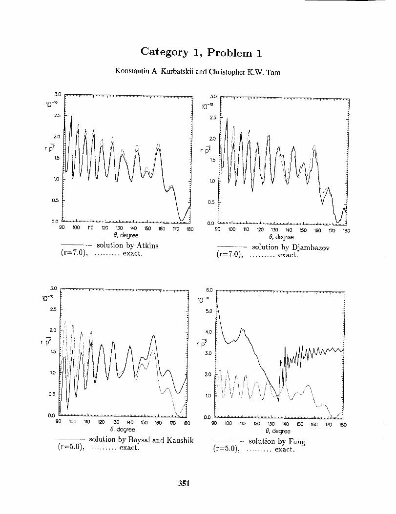
Category 1, Problem 1
Konstanfin A. Kurbatskii and Christopher K.W. Tam
......... I ......... I ......... +......... I ..... '"'1 ,+T ...... I ........ +I `++
110 -10 6.0 [, ........ I ......... , ......... I ......... l ....... q-_
10-2.5
0
iA_i° :- _ 4.0 [rP.5 i!ii!++ ii r_ _-
...... +i,'!.0.5 _ 1.o
\. ..........,\0.0
90 100 110 120 1250 14o !50 16o 170 180
O,degree
--_ solution by Baysal and Kaushik(r=5.0), ......... exact.
90 loo 11o 12o _,.,_ 14o L_O 160 _ 1SOO,degree
solution by Fung(r=5.0), ......... exact.
351
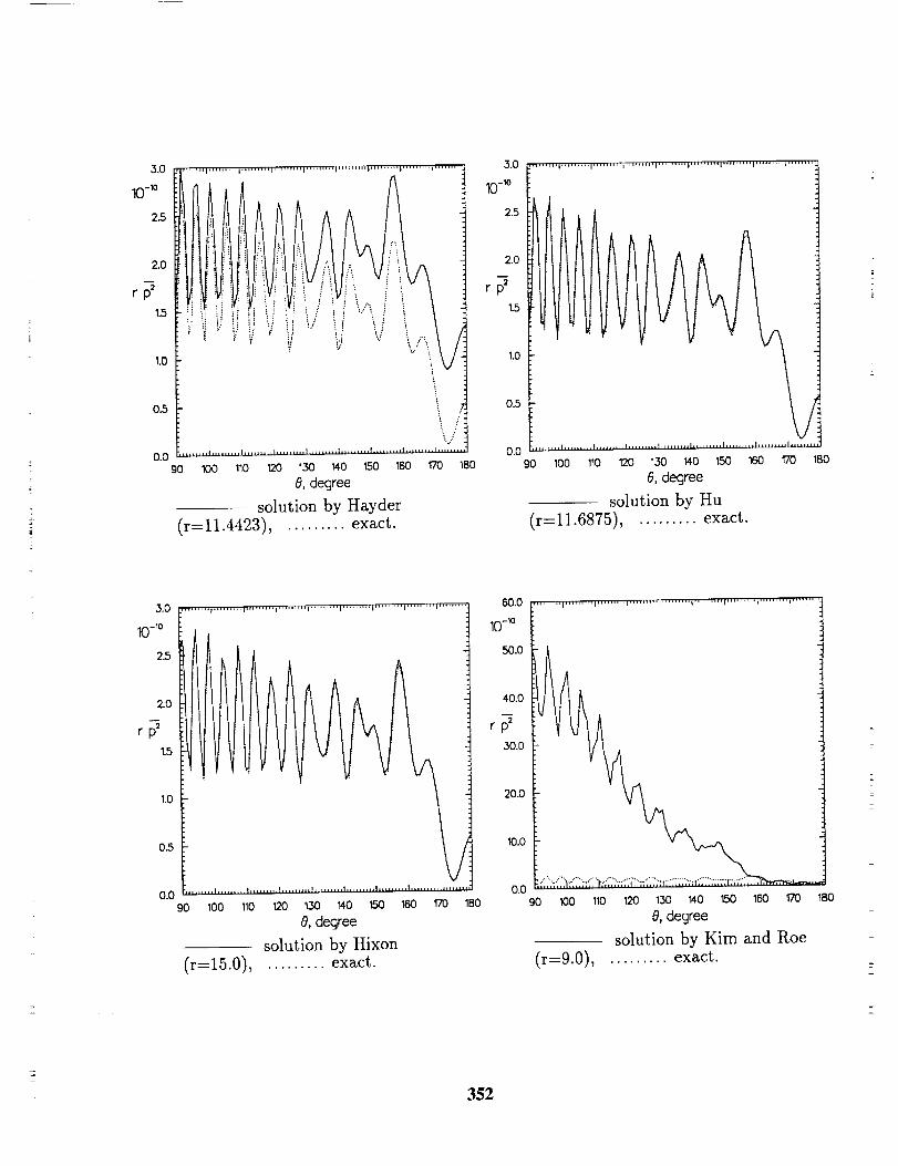
13.0 _i,i_ Illlllll, H _l,,lllll,,llllll,lll I'llll'{l][ll'_llllllllU ...... t ......... I ,,,,,,l,_
10 -10
2.5
2.0 _t0
0,5 _
0.0 _ ....... ,......... l ......... I ......... J......... ,........90 loo 1_o 12o 13o _o tso leo _ 1so
& degree
solution by Hayder(r=11.4423), ......... exact.
3.0
i0-'o
2.5
2.0
r p21.5
1,0
0.5
0,0 ....... I ......... I ......... I ......... t ......... I ......... I ......... I.,,,_j,ul .........
9o loo 11o 12o _ _o tso 1so 17o _so0, degree
solution by Hu
(r=11.6875), ......... exact.
10-1o
2.0
1.5
1.0
0.5 _
0.0 ....... ' ......... I......... I ......... , ......... ,......... ,......... t......... ,,,,9o lOO 1to _ _ _o '_o leo rm _so
0, degree
solution by Hixon
(r=l&0), ......... exact.
60.0
i0-Io
50.0
40.0
r p2
50.0
20.0
10.0
0.090 lOO _o 12o 13o _4o 15o 16o 17o 1so
0, degree
solution by Elm and Roe(r=9.0), ......... exact.
352
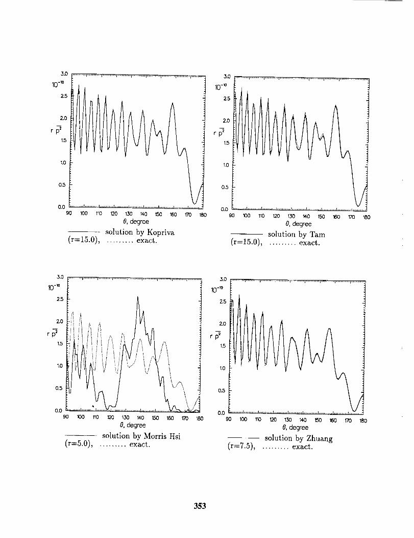
,3.0 +,+,,,,+,,l,,,++,,,,l',+,,,,,,,i,,,+,++,,+,,,,,,,,,l,,,,+,,+,l,, ..... ,,i,,,,,,,],i +.,,,,,,,.
10-_
2.5
2.0
r p2
1.5
1.0
0.5
0.090 1oo i_o 12o 13o _o t5o 18o f/o mo
0,degree
solution by Kopriva
(r=15.0), ......... exact.
3.0
i0-_o
2.5
2.0
r p2
1.5
+1.0
0.5
90 +,oo _o ",2o +30 mo 15o im 'rio IBO0, degree
solution by Tam
(r=15.0), ......... exact.
3.0 3.0 ................................................................................
i0-;o i0-+o
2.5 Z5
lo 2.0
r p_ r p21.5 1.5
1.0 1.0
0.5 0.5
0.0 0.090 100 110 120 130 _0 150 160 170 180 eo I00 110 120 130 _,0 tso too vo _BO
0, degree e, degree
solution by Morris Hsi solution by Zhuang
(r=5.0), ......... exact. (r=7.5), ......... exact.
353
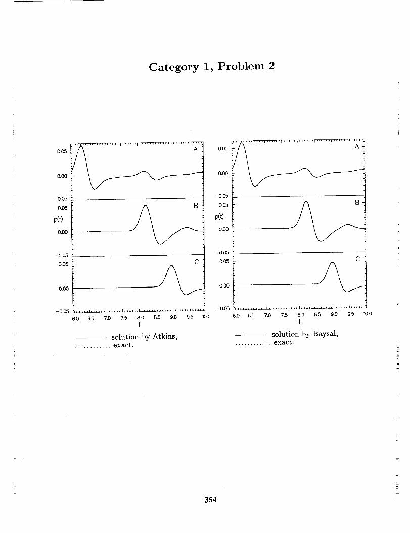
Category 1, Problem 2
0.05
0.00
-0.05
0.05
0.00
-0.05
0.05
0.00
-0.05
C
6.0 6.5 7.0 7`5 8.0 8.5 9.0 9.5 10.0
t
solution by Atkins,............ exact.
0.05
0.00
-0.05
0.05
p(t)
0.00
-0.05
0.05
0.00
-0.05
C
6.0 6,5 7.0 7.5 8.0 8-5 9.0 9.5 10.0
t
solution by Baysal,............ exact.
354
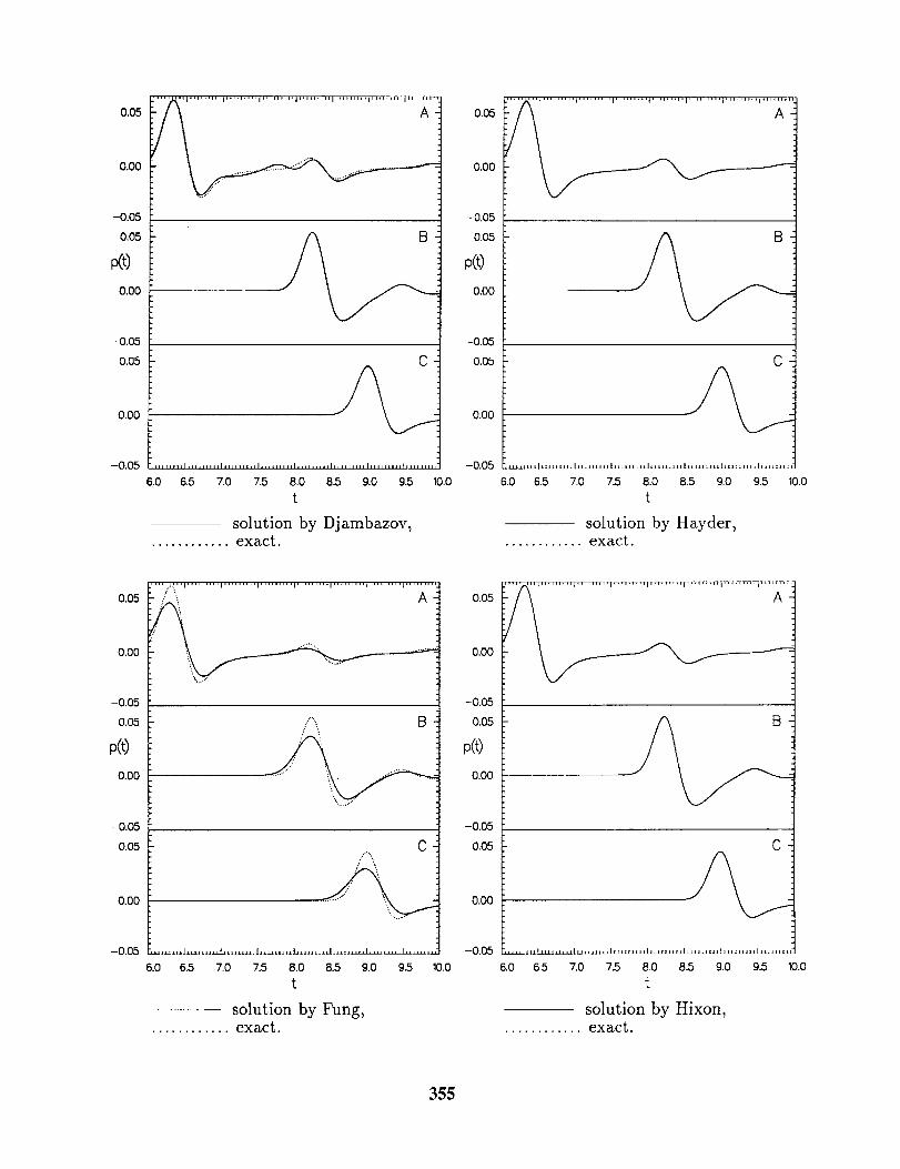
0.05
0.00
-0.05
0.05
Kt)0.00
-0.05
0.05
0.00
-0.05 ,llllll, hll+,llllh, llllllJ 11 tl 'l_lllhl'll ,lllhl II tlIIIIlIIIIIIIlllLLU.LLI+
6.0 6.5 7.0 7.5 8.0 8.5 9.0 9.5 10.0
t
solution by Djambazov,............ exact.
0.05
0.00
-0.05
0.05
Kt)0.130
-0.05
0.05
0.00
-0.05
C
_LU.._LU+ll/.l.lt Ull LZ.L_ IJ.l J I h i + I £ t+ Lt li_limiltEl U il l£JUJl £ i I l I £ t I J i J I £ I i
6.0 6.5 7.0 7.5 8.0 8.5 9.0 9.5 10+0
t
solution by Hayder,............ exact.
0.05
0.00
-0.05
0.05
p(t)
0.00
-0.05
O.O5
0.00
-0.05
[-\ B
"-..,....."
C....'"-,,
6.0 6.5 7.0 7.5 8.0 8.5 9.0 9.5
t
solution by Fung,............ exact.
10.0
0.05
0.00
-0.05
0.05
p(t)
0.00
-0.05
0.05
0.00
-0.05 .U.I._II/_LIIII/IJJ.|U I l J 11 I 1] l [l I tluJhl I IJmJ lJJJ £ £J 11 ] I 11 I I I I lJ 11 tl ill I t
6.0 6.5 7.0 7,,5 8.0 8.5 9.0 9.5 10.0
t
solution by Hixon,............ exact.
355
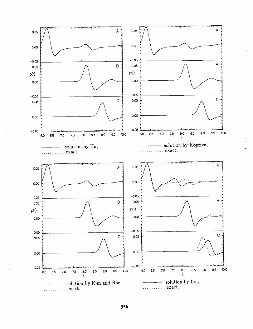
0,05
0.00
-0.05
0.05
p(t)
0.00
-0.05
0.05
0.00
-0.05
C
6.0 6.5 7.0 7.5 8.0 8.5 9.0 9.5 10.0
t
solution by Hu,............ exact,
0.05
0.00
-0.0,5
0.05
p(t)
0.00
-0.05
0.05
0.00
-0.05
C
LU_LdJ
6.0 6.5 7.0 7.5 8.0 8.5 9.0 9.5 10.0
t
solution by Kopriva,............ exact.
0.05
0,00
-0.05
0.05
p(t)
0.00
-0.05
0.05
0.00
-0.0.5
C
6.0 6,5 7.0 7.5 8.0 B.5 9.0 9.5 10.0
t
solution by Kim and Roe,............ exact.
0.05
0.00
-0.05
0.05
p(t)
0.00
-0.05
0,05
0.00
-0.05
C
6.0 6,5 7.0 7.5 B.O 8.5 g.o 9.5 10.0
t
solution by Lin,............ exact.
356
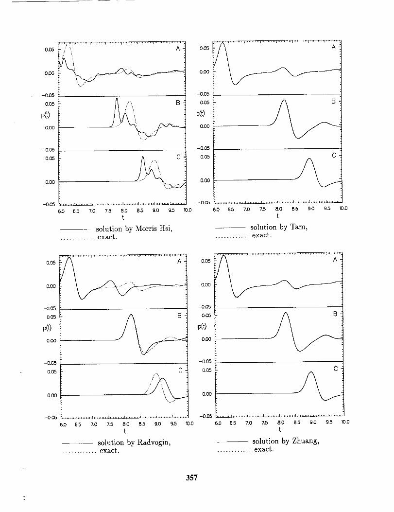
0.05
0.00
-0.05
0.05
Kt)0.00
-0.05
0.05
0.00
-0.05
/"\ A
",../
B
%......
6.0 6.5 7.0 7.5 8.0 8.5 9.0 9.5 I0.0
t
solution by Morris Hsi,............ exact.
0.05
0.00
-0,05
0.05
p(t)
0.00
-0.05
0.05
0.00
-0.05
C
i.JLi[zJl IliiiilJli_ zli_uJJ21_ J_ Iilib iLxllz _ izulllllllliuJJJLu i_uJ_.
6.0 6.5 7.0 7.5 8.0 8.5 9.0 9.5 10.0
t
solution by Tam,............ exact.
0.05
0.00
-0.05
0.05
p(t)
O.O0
-0.05
0.05
0.00
-0.05
C/'--.
%.......
6.0 6.5 7.0 7.5 8.0 8.5 9.0 9.5 10.0
t
solution by Radvogin,............ exact.
0.05
0.00
-0,05
0.05
Kt)0,00
-0.05
0,05
0.00
-0.05
C
LLLLLLLLhJ_ l ,,,,, I ......... I _L[.LLLLLLLLLLU_ LLUlLLLLU _, _bJJ_J_.uJ.u_u_.
6.0 6.5 7.0 7.5 8.0 8.5 9.0 9.5 10.0
t
solution by Zhuang,............ exact.
357

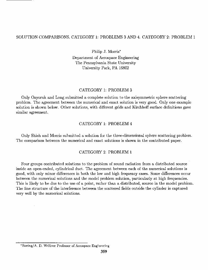
SOLUTION COMPARISONS. CATEGORY 1: PROBLEMS 3 AND 4. CATEGORY 2: PROBLEM 1
Philip J. Morris*
Department of Aerospace Engineering
The Pennsylvania State University
University Park, PA 16802
CATEGORY 1: PROBLEM 3
Only Ozyoruk and Long submitted a complete solution to the axisymmetric sphere scattering
problem. The agreement between the numerical and exact solution is very good. Only one example
solution is shown below. Other solutions, with different grids and Kirchhoff surface definitions gave
similar agreement.
CATEGORY 1: PROBLEM 4
Only Shieh and Morris submitted a solution for the three-dimensional sphere scattering problem.
The comparison between the numerical and exact solutions is shown in the contributed paper.
CATEGORY 2: PROBLEM 1
Four groups contributed solutions to the problem of sound radiation from a distributed source
inside an open-ended, cylindrical duct. The agreement between each of the numerical solutions is
good, with only minor differences in both the low and high frequency cases. Some differences occur
between the numerical solutions and the model problem solution, particularly at high frequencies.
This is likely to be due to the use of a point, rather than a distributed, source in the model problem.
The fine structure of the interference between the scattered fields outside the cylinder is captured
very well by the numerical solutions.
*Boeing/A. D. Welliver Professor of Aerospace Eng;neeriug
359
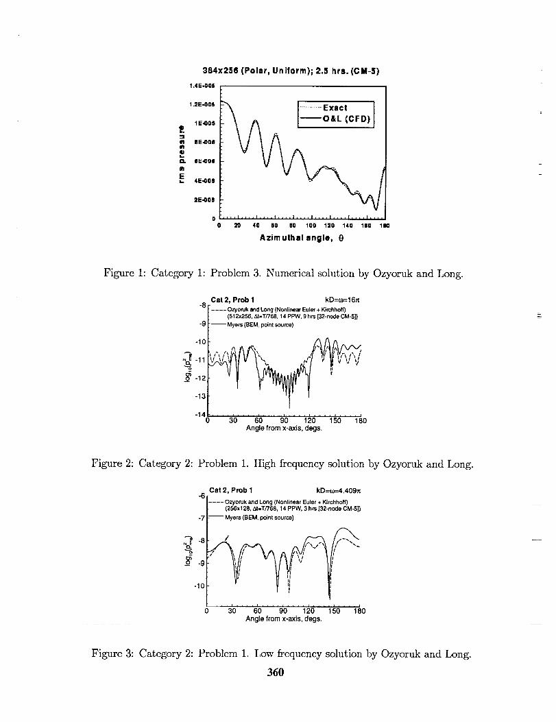
-I
el
.=rl
(4
EI=.
384x256 (Polar, Uniform); 2.5 hrs. (CM-5)
1.4 E -006
1.2E-006
1E,008
8E.006
6E.006
4E4)06
2E-00O
0
\ ........... I
I .... I .... l,,,,I .... I .... I .... 1 .... I ....
20 40 .0 eo _oo _20 _40 _0 _eo
Azimulhal angle, _)
Figure 1: Category 1: Problem 3. Numerical solution by Ozyoruk and Long.
-8
-9
-10
o
-12
-13
-140
Cat 2, Prob 1 kD=a)=16="---- Ozyoruk and Long (Nonlinear Euler + Kirchhoff)
(512}(256. At=T/768, 14 PPW, 9 hrs [32-node CM-5])
-- Myers (BEM, point source)
.... , .... , .... i .... i .... , .... i30 60 90 120 150 180
Angle from x-axis, degs.
Figure 2: Category 2: Problem 1. High frequency solution by Ozyoruk and Long.
Cat 2, Prob I kD=(o=4.409F.
-6 [____ Ozyoruk and Long (Nonlinear Euler + Kirchhoff)
t (256x128, At=T/'/68, 14 PPW, 3 hrs [32-node CM-5])
-71--- Myers (BEM, point source)
0 " 3b.... 6'0.... 9'0 i_0 i_0 1_0Angle from x-axis, degs.
Figure 3: Category 2: Problem 1. I,ow frequency solution by Ozyoruk and Long.
360
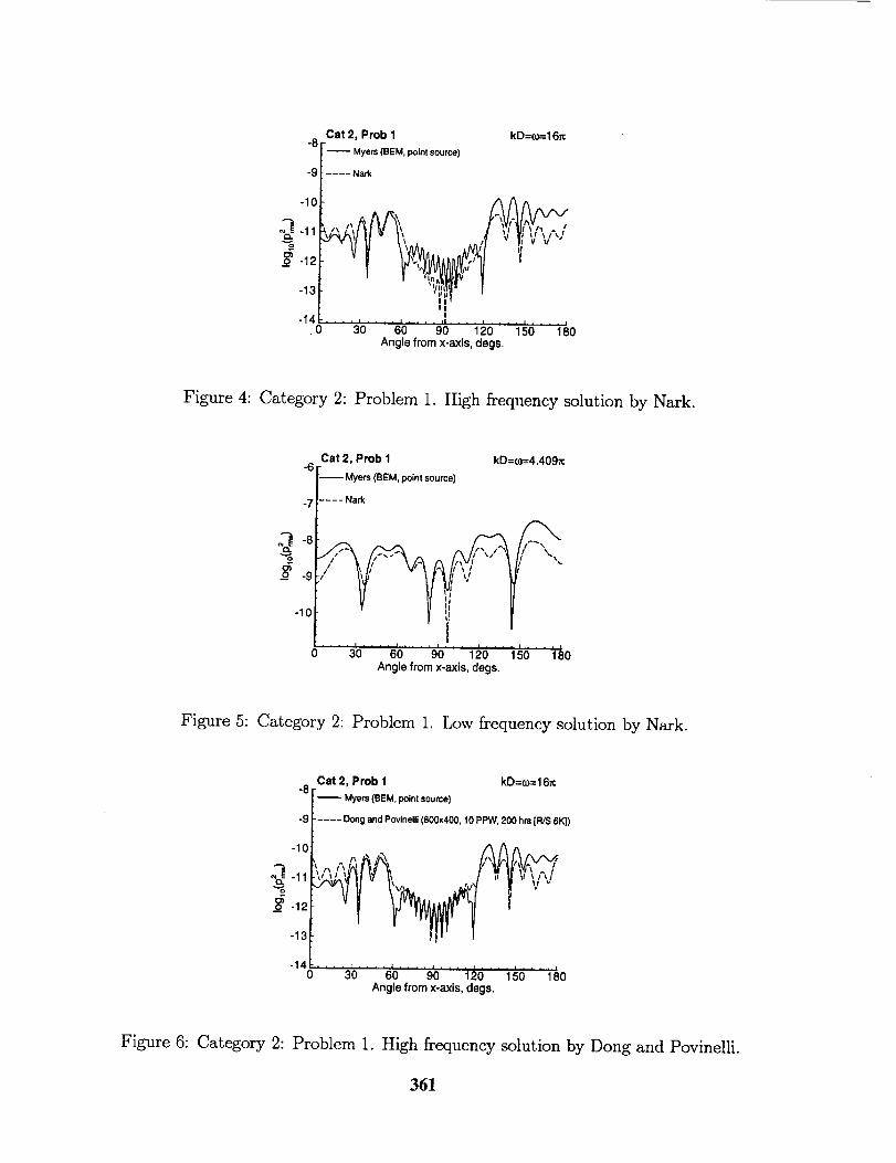
8 Cat 2, Prob 1" [_ Myers (BEM, point source)
L
-9 F.... Nark
kD=(o=16_
-10
-11
_-12
-13
-140
Ii , , , i .... i .... ii, =,,|,_ I .... i .... i
30 60 90 120 150 180Angle from x-axis, dogs.
Figure 4: Category 2: Problem 1. High frequency solution by Nark.
-6
-7
Q -8v o
o -9
-10
Cat 2, Prob 1 kD=oJ=4.409_
Myers(BEM,pointsource)
.... Nark
30 60 90 120 150 180Angle from x-axis, degs.
Figure 5: Category 2: Problem 1. Low frequency solution by Nazk.
-8
-9
-10
-11
._-12
-13
-140
Cat 2, Prob I kD=(o=16_
'_ Myers (BEM, point source)
..... Dong and Povinelli (800x400, 10 PPW, 200 hrs [R/S 61<])
""/"" i',
-vy v.... [,,.. = .... , .... J .... i .... i
30 60 90 120 150 180Angle from x-axis, degs.
Figure 6: Category 2: Problem 1. High frequency solution by Dong and Povinelli.
361
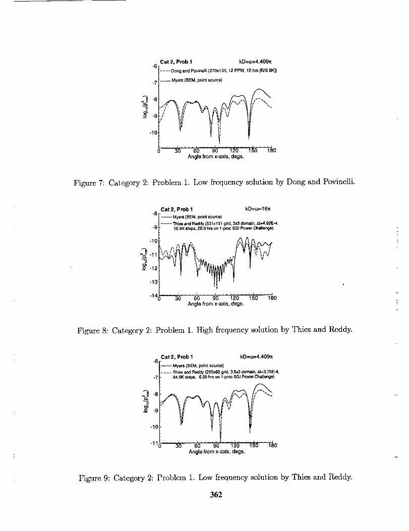
-6
-7
_'_ -8
¢$_o -9
Cat 2, Prob 1 kD=co=4.409_
.... Dong and Povinelli(270x135, 12 PPW, 12 hrs [R/S 6K])
-- Myers (BEM, point source)
v v_1 Oo .... 3'o.... a'o.... 9'o"' ?_0 igd _8o
Angle from x-axis, degs.
Figure 7: Category 2: Problem 1. Low frequency solution by Dong and Povinelli.
Cat 2, Prob I kD=(m=16_me
--- Myers (BEM, poinl source)
.... "i'hiesand Reddy(531xl 51 grid, 3x3 domain,At=4.92E-4,-9 56.9K steps,28.8 hrs on 1-procSGI Power Challenge)
Angle from x-axis, degs. -=
Figure 8: Category 2: Problem 1. High frequency solution by Thies and Reddy.
Cat 2, Prob 1 kD=(o=4,409_
-6 __ Myers (BEM, point source)
.... Thiesand Reddy (255x80 grid,3.5x3 domain, _=3.75E-4,-7 84.6K steps, 6.09 hrson 1-procSGI PowerChallenge)
-8 _ I/ ,-_-9 f_ J
' i-10
-11_ 30 60 90 120 150 180
Angle from x-axis, degs.
Figure 9: Category 2: Problem 1. Low frequency solution by Thies and Reddy.
362
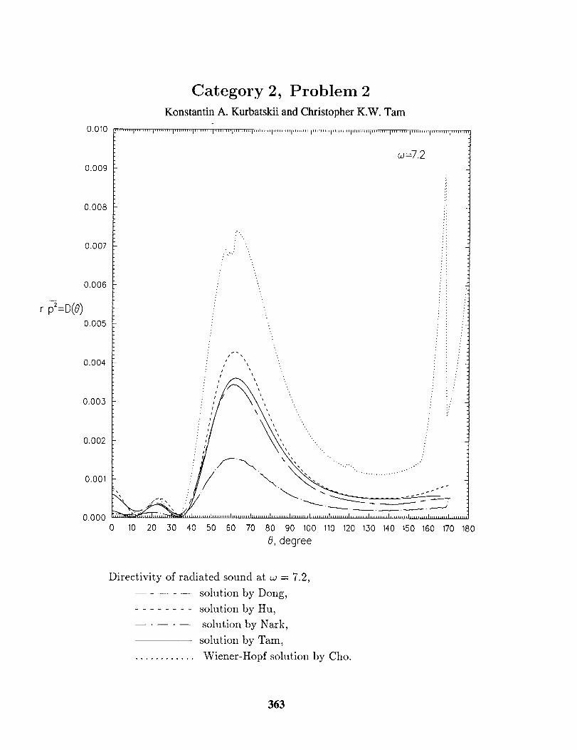
o.010
0.009
0.008
O.O07
0.006
r p2=D(8)
0.005
0.004
0.003
0.002
0.001
0.000
Category 2, Problem 2
Konstantin A. Kurbatskii and Christopher K.W. Tam
-......... I ......... I ...... "'I"'""'I" "'"" I"" "" I"' """ P m*_q_TrmTr[mm mlITml r_ 'pm"''Im'_'q*'m'' 'l''"'"'l'"'J_n| r,,,,, ,, 'I''''"''
_=72
j-.
.,....J
"L
i \
/
\
i:
, i
!/
" I f
: I " .."
: I " " :,"
: I . i "/
" r ", " ;
: ! "_ j
2" f "-, .."
10 20 30 40 50 60 70 80 90 100 110 120 1,.30 140 150 160 170 180
8, degree
Directivity of radiated sound at w = 7.2,
solution by Dong,
........ solution by Hu,
..... solution by Nark,
solution by Tam,
............ Wiener-Hopf solution by Cho.
363
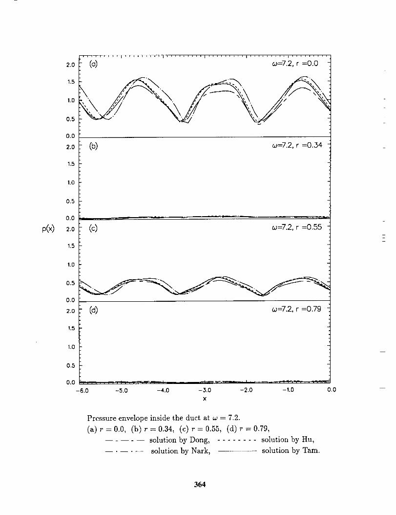
p(×)
2.0
1.5
1.0
0.5
0.0
2.0
1.5
1.0
0.5
0.0
2.0
1.5
1.0
(a) co=7.2, r =0.0
(b) w=7.2, r =0.34
(c) w=7.2, r =0.55
0.0
2.0
1.5
1.0
0.5
0.0
-6.0
(d) w=7.2, r =0.79
-5.0 -4.0 -3.0 -2.0 -1.0 0.0
X
Pressure envelope inside the duct at w = 7.2.
(a) r=0.0, (b) r=0.34, (c) r=0.55, (d) r=0.79,
..... solution by Dong, ........ solution by Hu,
..... solution by Nark, solution by Tam.
364
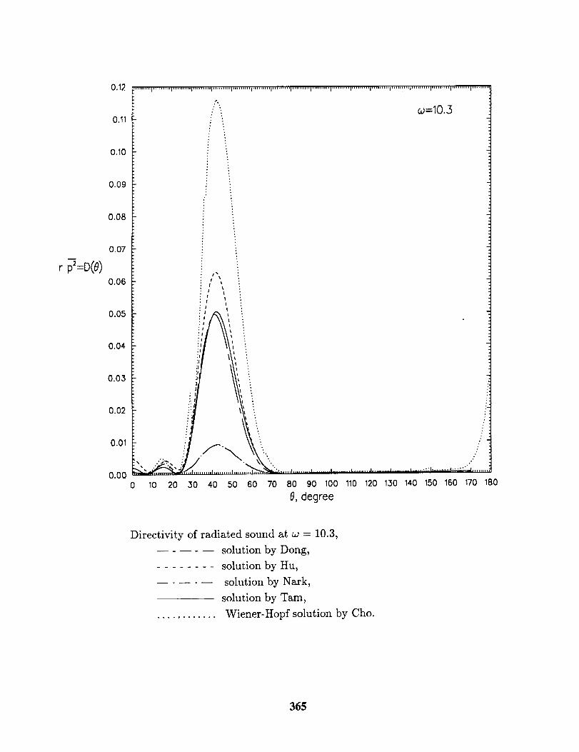
r _:D(O)
0,12
0.11
0.10
0.09
0.08
0.07
0.06
0.05
0.04
0.03
0.02
0.01
0.00
;'""'"1"'"'"'1'"'"'"t ...... '"1'"'"'"I'" ...... I ........ 'I'""""P'"'""I'""'"'I'""'"'I ......... I'""'"'1'""'"'1 ....... "1'"'"'"t' ........ I"'"'":
: o_=I0.3
I %%
' ilt
t
I | "
i i :
'1 t :
;I t ::1 t "
;s i ',
:l I :
:l I :
:1 I :
._ , :
10 20 30 40 50 60 70 80 90 100 110 120 130 140 150 160 170 180
0, degree
Directivity of radiated sound at w = 10.3,
..... solution by Dong,
........ solution by Hu,
..... solution by Nark,
solution by Tam,
............ Wiener-Hopf solution by Cho.
365
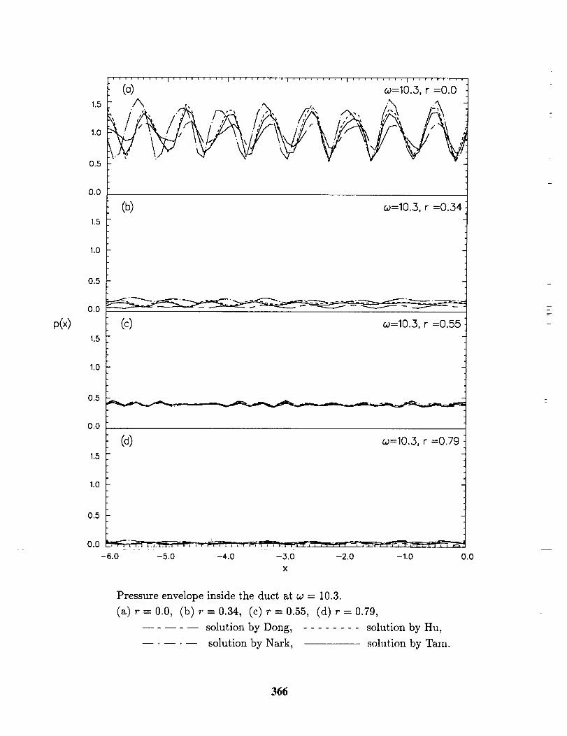
p(×)
1.5
1.0
0.5
0.0
1.5
1.0
0.5
0.0
1.5
1.0
0.5
0.0
1.5
1.0
0.5
0.0
-6.0
' ' ' ' ' ' ' ' ' I ' ' ' ' ' ' t i , I ' ' ' ' ' ' ' ' ' I ' ' ' ' ' ' ' ' ' I ' ' ' ' ' ' ' ' ' I ' ' ' ' ' ' ' ' ' I
(o) _=10.3, r =0.0 tA ,, .,, ,, .-\ ..,_ -t
i ,_ ,..,'_ /-',-A f,,k,. /z,'A .,_, /,;,:,_ t_\ 1. I _ % / I,'_ / ,/k4 I,'f/[ .','/,- t /,'2_ Y...\\ //,,_ J
(b) w=10.3, r =0.,.34
(c) ca=10.3, r =0.55
(d) w=10.,.3, r =0.79
-5,0 -4.0 -3,0 -2.0 -1.0 0.0
x
Pressure envelope inside the duct at w = 10.3.
(a) r=0.0, (b) r=0.34, (c) r=0.55, (d) r=0.79,
solution by Dong, ........ solution by Hu,
..... solution by Nark, solution by Tam.
366
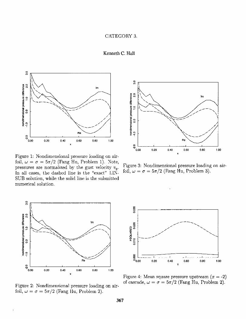
CATEGORY 3.
Kenneth C. Hall
i°o.
$£
,./
q
0.00
Im
I i 1 1
0.20 0.40 0.60 0,80 1.00
x
Figure 1: Nondimensional pressure loading on air-
foil, w = (r = 57r/2 (Fang Hu, Problem 1). Note,
pressures are normalized by the gust velocity vg.
In all cases, the dashed line is the "exact" LIN-
SUB solution, while the solid line is the submittednumerical solution.
2
"o
o
-i
q
0.00
I
Rei i . _J
0,20 0.40 0.60 0.80 1.00
x
Figure 3: Nondimensional pressure loading on air-
foil, w = (7 = 57r/2 (Fang Hu, Problem 3).
o
I -'<'__-" \
,f,"
O | , 1,
' 0.00 0.20 0.40
'_\N,,_ i/////
Re
I I
0.60 0.80 1.00
x
Figure 2: Nondimensional pressure loading on air-
foil, co = G = 57r/2 (Fang Hu, Problem 2).
n-<
o
i i t t
°0.00 0.20 0.40 0.60 0.80 1.00
Y
Figure 4: Mean square pressure upstream (z = -2)
of cascade, co = e = 57r/2 (Fang Hu, Problem 2).
367
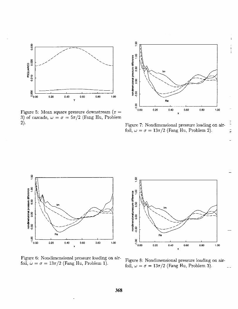
cr<
2oc_.
/
/ \/ \
/ \/ \
°0.00 0.20 0.40 0,60 0.80
7
1.00
Figure 5: Mean square pressure downstream (x =
3) of cascade, w = a = 57r/2 (Fang Hu, Problem
2).
®8
K
_8
C O
8v 0.0(
f
Re
l I [ I
0.20 0.40 0.60 0.80 1.00
x
Figure 7: Nondimensional pressure loading on air-
foil, w = a = 137r/2 (Fang Hn, Problem 2).
Im
f
Re
8"70.00 0.20 0.40 0.60 0.80 1.00
X
Figure 6: Nondimensional pressure loading on air-
foil, w -- a = 137r/2 (Fang Hu, Problem 1).
8
e_
8
":' 0,00
f
Re
I I I A
0.20 0.40 0.60 0.80 1.00
x
Figure 8: Nondimensional pressure loading on air-
foil, co = a = 137r/2 (Fang Hu, Problem 3).
368
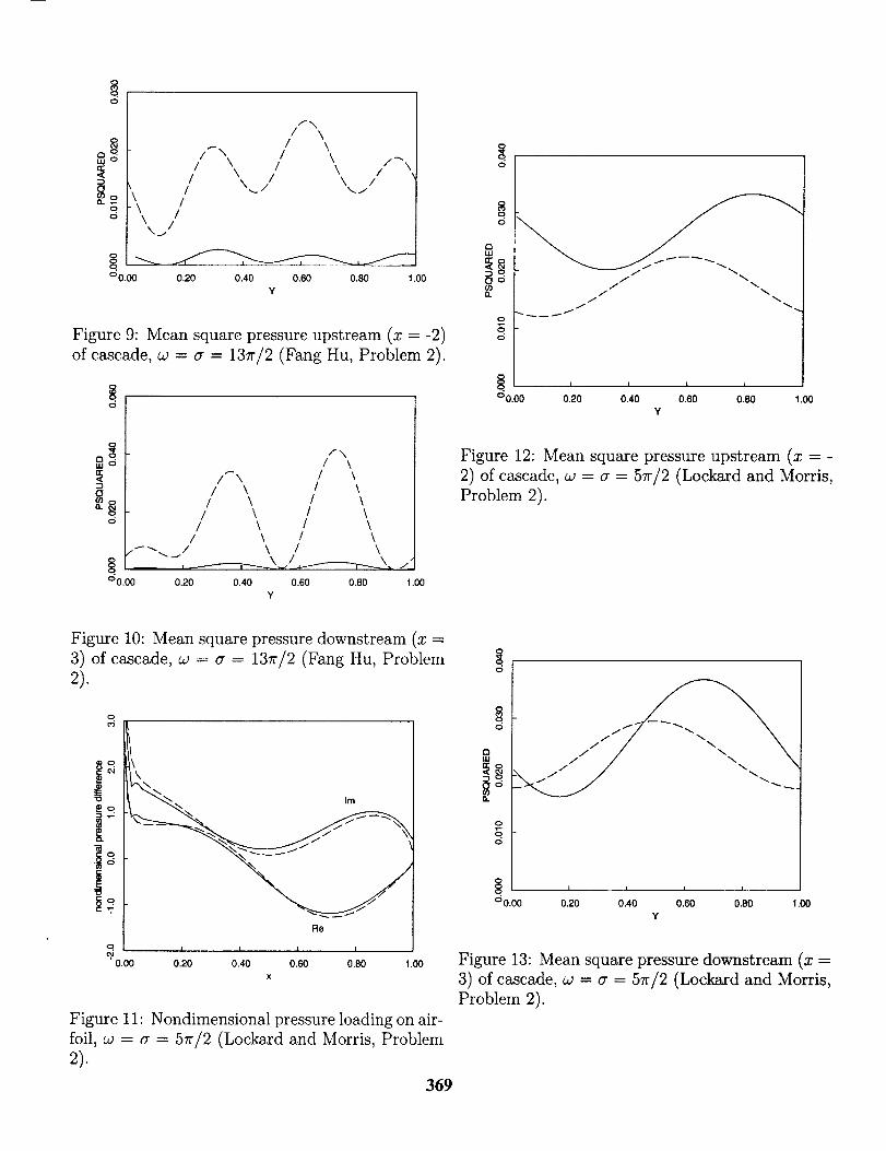
o
er.<
<2
f\I \
I \/-\ I \
I \ I \ i/-_\\I \ I \ i
I
\\\_.,/I
°0.00 0.20 0,40 0.60 0.80 1.00
Y
Figure 9: Mean square pressure upstream (x = -2)
of cascade, w = a = 13Ir/2 (Fang Hu, Problem 2).
o
f\/ \
/_\ / \/ \ / \
/ \ / \/ \ / \
/ \ / \/ \ / \
._'_-..._..I \ / \
°0.00 0.20 0.40 0.60 0.80 1.00
Y
o
¢5
S
8
o
I!. , .... , , , I°0.00 0.20 0.40 0.60
Y0.80 1.00
Figure 12: Mean square pressure upstream (x = -
2) of cascade, w = a = 57r/2 (Lockard and Morris,Problem 2).
Figure 10: Mean square pressure downstream (x =
3) of cascade, co = a = 137r/2 (Fang Hu, Problem2).
$
"O
q
_o.oo
t\
k\\ Im
xNC_
Re
i I I I
0.20 0.40 0.60 0.80 1.00
x
Figure 11: Nondimensional pressure loading on air-foil, co = a = 57r/2 (Lockard and Morris, Problem
2).369
Io
o
OI£1
Ooif)Q.
o
o.o
.-/----. .ill/Ill/i/ \\
i I I I
°0.00 0.20 0.40 0,60 0.80
Y1.00
Figure 13: Mean square pressure downstream (x =3) of cascade, w = a = 57r/2 (Loekard and Morris,
Problem 2).
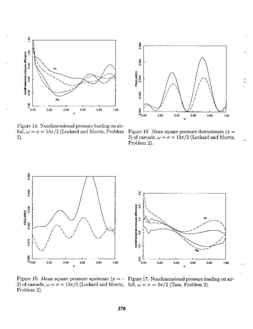
!-
s."T,0.00
Re
....... ! i 1 !
0.20 0.40 0,60 0.80 1.00
x
Figure 14: Nondimensional pressure loading on air-
foil, w = a = 1371-/2 (Lockard and Morris, Problem
2).
¢5
atu
23 .
_°el
P,°15
° 0.00 0.20 0.40 0.60 0.80 1.00
Y
Figure 16: Mean square pressure downstream (x =
3) of cascade, w = a = 137r/2 (Loekard and Morris,
Problem 2).
o
o.o
°
_s
f/'-\\ itl \\ ..,,
I \\ t \ /
\\\ tl t ,,._i ,..jX_,,/
¢00.00
........ d ...... L...... _ ....... I
0.20 0,40 0.60 0.80Y
1.00
o i i J=. ,
0.00 0.20 0.40 0.60 0.80 1.00x
Figure 15: Mean square pressure upstream (x = -
2) of cascade, w = a = 131r/2 (Lockard and Morris,Problem 2).
Figure 17: Nondimensional pressure loading on air-
foil, w = a = 5rr/2 (Tam, Problem 2).
370
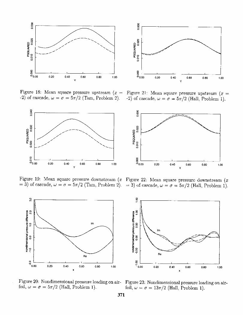
a-<
(J
O
O¢qo
O
Od
JJ
m
cr<
_oo¢i
o 0.00 0.20 0.40 0.60 0.80 1.00 o 0.00
Y
i i_. ___
0.20 0.40 0.80 0.80 1.00
Y
Figure 18: Mean square pressure upstream (x --- Figure 21: Mean square pressure upstream (x =
-2) of cascade, co = (7 = 57r/2 (Tam, Problem 2). -2) of cascade, co = (7 = 51r/2 (Hall, Problem 1).
d
m_re
<
O
<5
o
o
°0,00 O.2O
J L_.__
0.40 0.60 0.80 1.00
,,r'<:zi0
goo<5
l I I I
dO.O0 0.20 0.40 0.60 0.80 1.00
¥
Figure 19: Mean square pressure downstream (x Figure 22: Mean square pressure downstream (x
= 3) of cascade, co = (7 = 57r/2 (Tam, Problem 2). = 3) of cascade, w = a = 57c/2 (Hall, Problem 1).
_o._ o
_V
Im
Re
_8.N
$
c
Im
r
Re
"7, 0.00
I I l I I I I I
' 0.00 0.20 0.40 0.60 0.80 1.00 0.20 0.40 0.60 0.80 1.00
X X
Figure 20: Nondimensional pressure loading on air- Figure 23: Nondimensional pressure loading on air-
foil, co = (7 = 57r/2 (Hall, Problem 1). foil, w = (7 = 137r/2 (Hall, Problem 1).
371
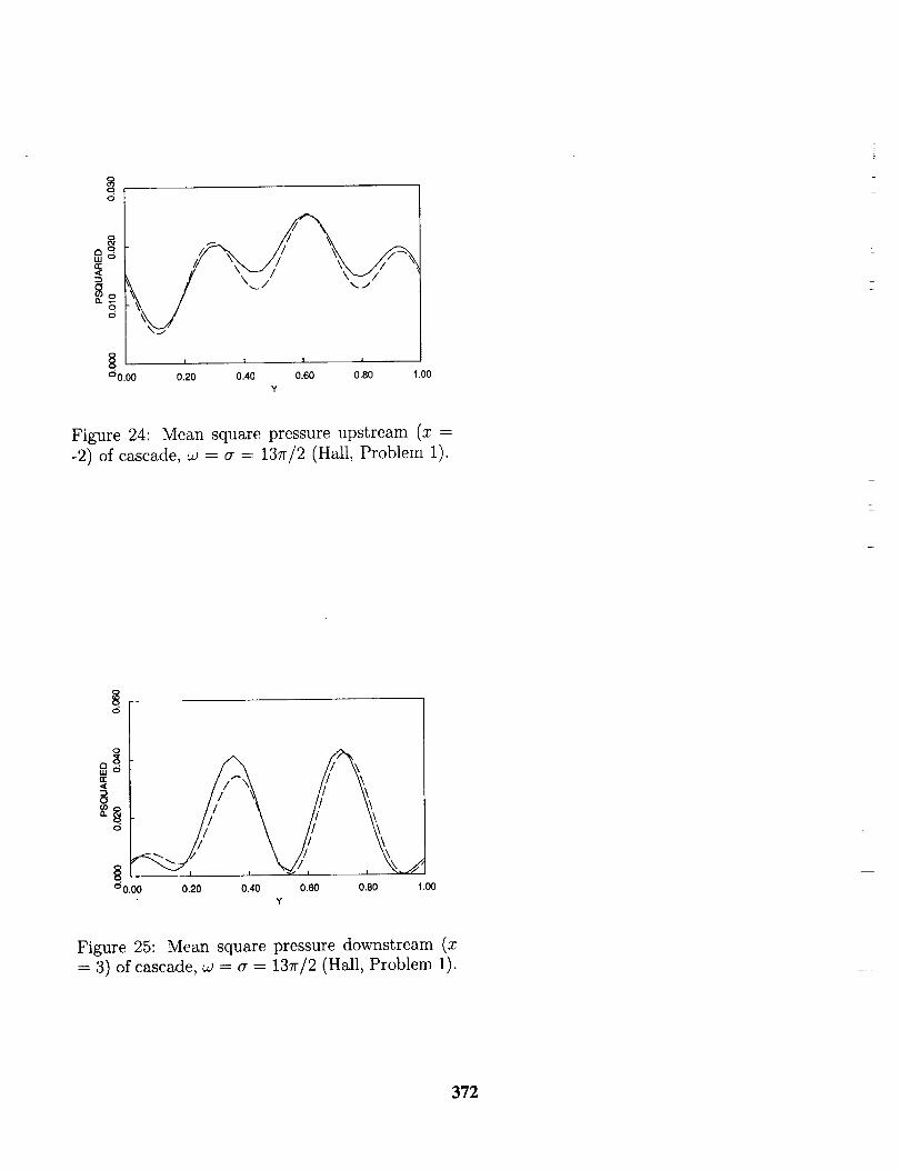
O
o
°0.00
'_ ,_ / '
i I i i
0.20 0.40 0.60 0.80 1.00
Y
Figure 24: Mean square pressure upstream (x =
-2) of cascade, w = a = 13rr/2 (Hall, Problem 1).
o
(r,,(
8
d
60.00 0,20 0.40 0.60 0.80 1.00
Y
Figure 25: Mean square pressure downstream (x
= 3) of cascade, w = a = 13rr/2 (Hall, Problem 1).
372

SOLUTION COMPARISONS: CATEGORY 4
Jay C. HardinNASA Langley Research Center
Hampton, VA 23681
The Category 4 problem was proposed as an example of the technologically importantclass of massively separated flow noise generators. Since the CAA community is presentlybeing asked to attack such sources, it was deemed appropriate to include one as abenchmark problem. Such flows are viscous, turbulent, and the source of the sound arises
from the dynamics of the flow itself. Thus, no exact solution is available for this category.However, for the Aeolian tone produced by a cylinder in a uniform flow, a substantialamount of unambiguous experimental data exists, albeit much of it for higher Reynolds andMach numbers than the problem proposed.
The Mach number of the flow in this benchmark problem was chosen because manyof the technologically important applications (automobiles, aircraft on landing approach,high speed trains, etc) have Mach numbers in this range. The Reynolds number chosenwas taken as a compromise--high enough to be realistic and for which good quality dataexisted, yet low enough that one could resolve most of the important scales without too finea grid. In hindsight, it might have been better to specify a higher Reynolds number, as theflow is still transitional at Re--90,000 whereas the turbulent models have been developedfor fully turbulent flows.
The inherent challenge of this problem lies in choosing the numerical approach withinthe limits of the computational facilities available. The flow is experimentally found to bethree dimensional with a finite correlation length in the spanwise direction. However, a3-D Direct Numerical Simulation (DNS) at a Reynolds number of 90,000 is out of thequestion due to the range of scales which must be resolved in three directions. Thus, onemust fall back on an approach such as Large Eddy Simulation (LES) or Reynolds Averaged(short-time) Navier-Stokes (RANS) to reduce the range of scales which must be resolved.This leads one into the realm of turbulent modeling, such as the Dynamic Sub-Grid Scale(DSGS) model, in order to retain the effect of the sub-grid scales on those resolved. Eventhis approach is very computationally demanding. One is tempted to reduce thedimensionality of the problem to two, as the geometry is two-dimensional. However, oneruns into two problems: First, turbulence is inherently three dimensional and the use ofturbulent models in two dimensions is problematic. Second, a 2-D acoustic field falls off
like r 1/ 2 with distance in the farfield rather than r as would be the case in 3-D.
In addition, there is the question of compressibility. Does one compute acompressible flow solution in which the flow and acoustic fields can be solvedsimultaneously? Or, noting the low Mach number requested, does one break the probleminto two parts, solving first for the flowfield (either compressibly or incompressibly) andthen using an acoustic analogy, i.e. Lighthiil (Helmholtz in the frequency domain), Curle,or Ffowcs Williams-Hawkings (FW-H) which integrate the flow induced pressures overthe surface of the cylinder, or the acoustic/viscous split (A/VS), which solves a forced setof Euler equations, for the acoustic field?
373
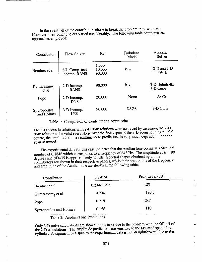
In theevent,all of thecontributorschoseto breaktheprobleminto two parts.However,their otherchoicesvariedconsiderably.Thefollowing tablecomparestheapproachesemployed:
Contributor
Brentneret al
Kumarasamyet al
Pope
SpyropoulosandHolmes
Flow Solver Re Turbulent AcousticModel Solver
1,0002-DComp.and 10,000 k-co 2-Dand3-DIncomp.RANS 90,000 FW-H
2-D Incomp. 90,000 k-e 2-DHelmholtzRANS 3-DCurie
2-D Incomp. 20,000 None A/VSDNS
3-D Incomp. 90,000 DSGS 3-DCurleLES
Table 1: Comparisonof Contributor'sApproaches
The3-D acousticsolutionswith 2-D flow solutionswereachievedby assumingthe2-Dflow solutionto bevalideverywhereoverthefinite spanof the3-D acousticintegral. Ofcourse,theamplitudeof theresultingnoisepredictionsis verymuchdependentuponthespanassumed.
Theexperimentaldatafor thiscaseindicatesthattheAeoliantoneoccursata Strouhalnumberof 0.1846whichcorrespondsto afrequencyof 643Hz. Theamplitudeat 0 = 90
degrees and r/D=35 is approximately 11 ldB. Spectral shapes obtained by all thecontributors are shown in their respective papers, while their predictions of the frequencyand amplitude of the Aeolian tone are shown in the following table:
Contributor
Brentner et al
Kumarasamy et al
Pope
Spyropoulos and Holmes
Peak St Peak Level (dB)
0.234-0.296 120
0.204 120.8
0.219 2-D
0.158 110
Table 2: Aeolian Tone Predictions
Only 3-D noise calculations are shown in this table due to the problem with the fall-off ofthe 2-D calculations. The amplitude predictions are sensitive to the assumed span of thecylinder. Assignment of a span to the experimental data is not straightforward due to the
374
presenceof thewind tunnelwalls. Thevariationin theStrouhalnumberpredictionsofBrentneret al dependedupontheturbulentmodelemployed.
All of thecontributorsfoundtheexpecteddipoledirectivitypatternwithpeakat 0 =90degrees and all predicted a reasonable spectral shape out to the maximum Strouhal number
requested of 0.6. Thus, the DNS, LES and RANS approaches all seem to retain therelevant scales. The variation of the peak Strouhal number predictions is somewhatdisappointing, but may be due to the transitional nature of the flow. Further work byBrentner et al indicates that, at higher Reynolds numbers where the flow is fully turbulent,the predictions produced by the various turbulence models coincide. The variation in the
amplitude predictions is not of as much concern due to the ambiguity of the cylinder lengthand the inherent bias and uncertainty of spectral estimates near peaks.
375
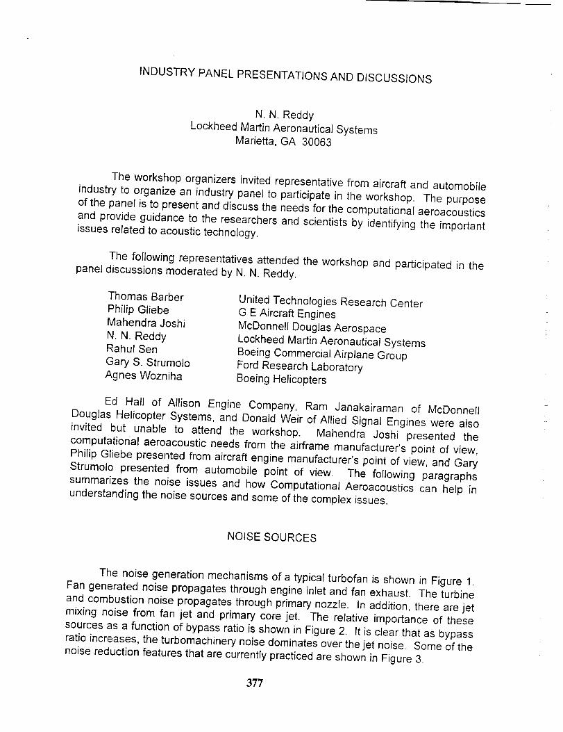
INDUSTRY PANEL PRESENTATIONS AND DISCUSSIONS
N. N. Reddy
Lockheed Martin Aeronautical Systems
Marietta, GA 30063
The workshop organizers invited representative from aircraft and automobile
industry to organize an industry panel to participate in the workshop. The purpose
of the panel is to present and discuss the needs for the computational aeroacoustics
and provide guidance to the researchers and scientists by identifying the important
issues related to acoustic technology.
The following representatives attended the workshop and participated in the
panel discussions moderated by N. N. Reddy.
Thomas Barber
Philip GliebeMahendra Joshi
N. N. ReddyRahul Sen
Gary S. Strumolo
Agnes Wozniha
United Technologies Research Center
G E Aircraft Engines
McDonnell Douglas Aerospace
Lockheed Martin Aeronautical Systems
Boeing Commercial Airplane Group
Ford Research Laboratory
Boeing Helicopters
Ed Hall of Allison Engine Company, Ram Janakairaman of McDonnell
Douglas Helicopter Systems, and Donald Weir of Allied Signal Engines were also
invited but unable to attend the workshop. Mahendra Joshi presented the
computational aeroacoustic needs from the airframe manufacturer's point of view,
Philip Gliebe presented from aircraft engine manufacturer's point of view, and Gary
Strumolo presented from automobile point of view. The following paragraphs
summarizes the noise issues and how Computational Aeroacoustics can help in
understanding the noise sources and some of the complex issues.
NOISE SOURCES
The noise generation mechanisms of a typical turbofan is shown in Figure 1.
Fan generated noise propagates through engine inlet and fan exhaust. The turbine
and combustion noise propagates through primary nozzle. In addition, there are jet
mixing noise from fan jet and primary core jet. The relative importance of these
sources as a function of bypass ratio is shown in Figure 2. It is clear that as bypass
ratio increases, the turbomachinery noise dominates over the jet noise. Some of the
noise reduction features that are currently practiced are shown in Figure 3.
377
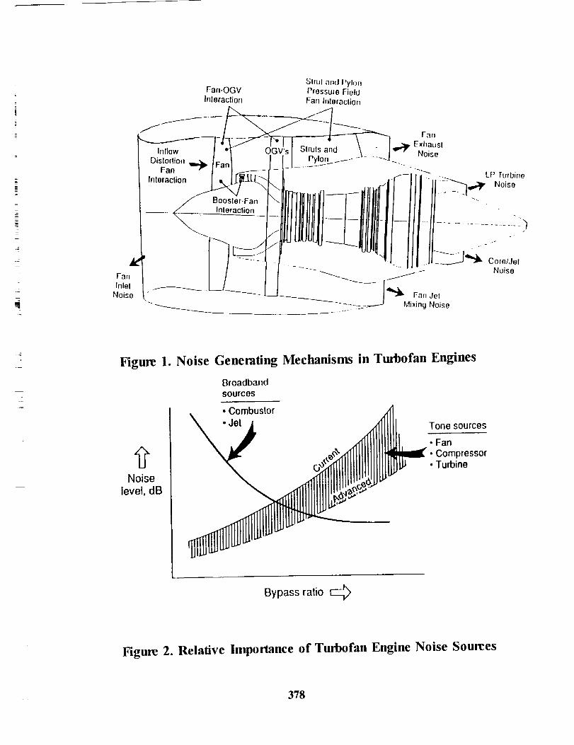
i
Slrul and PylonFan-OGV Pressule Field
Inleraclion Fan Inleraclion
It_lnlel;cli°n I ". [_'_-'-- __l__jl//[i//__///._//i_ - -II1'-'_'---"I''-I::).,.SIll -, :::___.., tP ,_.,t,i,,e
Noise L" - Fan Jel_ - _-. Mixing Noise
==
Figure 1. Noise Generating Mechanisms in Turbofan Engines
BroadbandSOUrCeS
• Combustor
• Jet Tone sources
_,o_.,_ • Fan• Compressor.Tuo,noNoise
level, dB _,-
Bypass ratio E_
Figure 2. Relative Importance of Turbofan Engine Noise Sources
378
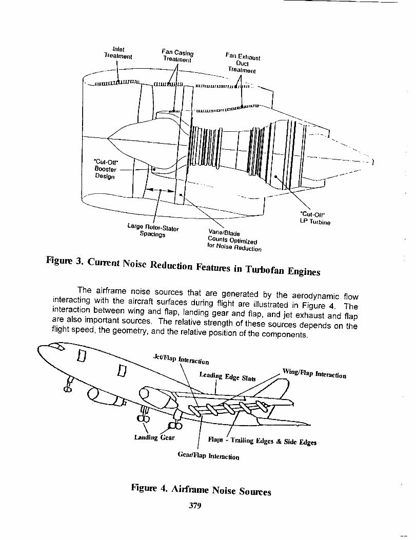
InlelTrealmen!
Large Rolor-Slalor
Spacings
Fan Casing Fan ExhauslTrealmen! OUCl
Trealmenl
JIUI|IJLIIIJ.UIIlll I'lli ".. _
Vane/Blade
Counls Oplim|zedfor Noise Reduclion
Figure 3. Current Noise Reduction Features in Turbofan Engines
The airframe noise sources that are generated by the aerodynamic flowinteracting with the aircraft surfaces during flight are illustrated in Figure 4. The
interaction between wing and flap, landing gear and flap, and jet exhaust and flapare also important sources. The relative strength of these sources depends on the
flight speed, the geometry, and the relative position of the components.
./et/Flap Inleracfon
_.Wing/Flap Interaction
Landing Gear aps -Trailing Edges & Side Edges
Geadlqap Interaction
Figure 4. Airframe Noise Sources
379
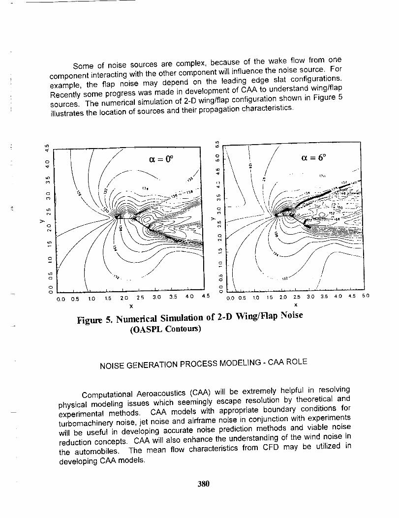
Some of noise sources are complex, because of the wake flow from one
component interacting with the other component will influence the noise source. Forexample, the flap noise may depend on the leading edge slat configurations.Recently some progress was made in development of CAA to understand wing/flapsources. The numerical simulation of 2-D wing/flap configuration shown in Figure 5illustrates the location of sources and their propagation characteristics.
O
z
I.O
O
>,O
O
O
(:3
O
>- _-- ....... _ - - .Z--_S- "%
/
0.0 0.5 1.0 1,5 2.0 2.5 3.0 35 40 4.5 0.0 05 1.0 1.5 20 2.5 3.0 3.5 4.0 4.5 5.0
X X
Figure 5. Numerical Simulation of 2-D Wing/Flap Noise
(OASPL Contours)
NOISE GENERATION PROCESS MODELING - CAA ROLE
Computational Aeroacoustics (CAA) will be extremely helpful in resolvingphysical modeling issues which seemingly escape resolution by theoretical and
experimental methods. CAA models with appropriate boundary conditions forturbomachinery noise, jet noise and airframe noise in conjunction with experimentswill be useful in developing accurate noise prediction methods and viable noise
reduction concepts. CAA will also enhance the understanding of the wind noise inthe automobiles. The mean flow characteristics from CFD may be utilized in
developing CAA models.
380
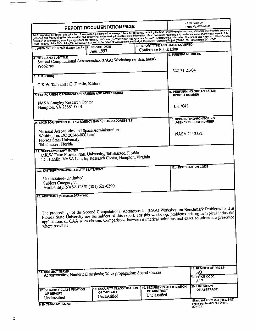
,.. ,.
Form ApprovedREPORT DOCUMENTATION PAGE oM_No,oz_-o_88
Puhiioreportingburdenforthis collectionof information is estirn_dedto average1 hourperresponse,Includingthe time for reviewing inslructions,searchingexistingdata sources,gatheringand maintainingthe dataneeded,and competingand reviewingthe collection ofinformation. Send commentsregard}_gthis burdenestimateor any _her aspectof thiscollectionof information,inoludingsuggestionsfor reducingthisburden,to WashingtonHeadquartersServices,Directorate!or InformationOperations and Reports,1215JeffersonDavis Highway,Suite1204, Arlington,VA22202-4302, andto theOff'meo!Managementand Budget,PaperworkReductionProject(0704-0188),Washington,DC 205(_.
1. A(_ENCY USE ONLY (Leave blank)' 2'. REPORT DATE _= 3. REPORTTYPE AND DATES COVEI_ED
4o
June 1997II
TITLE AND SUBTITLE
Second Computational Aeroacoustics (CAA) Workshop on BenchmarkProblems
im
6. AUTHOR(S)
C.K.W. Tam and J.C. Hardin, Editors
7. PERFORMING ORGANIZATION NAME(S) AND ADDRESS(ES)
NASA Langley Research CenterHampton, VA 23681-0001
9. SPONSORIN(JJMONITORING AGENCY NAI_IE(S) AND ADDRESS(ES)
National Aeronautics and Space AdminislrationWashington, DC 20546-0001 andFlorida State UniversityTallahassee, Florida
11'. SUPPLEMENTARY N(3TES
C.K.W. Tam: Florida State University, Tallahassee, FloridaJ.C. Hardin: NASA Langley Research Center, Hampton, Virginia
Conference Publication
5. FUNDING NUMBERS
522-31-21-04
8. PERFORMING ORGANIZATIONREPORT NUMBER
L-17641
10. SP()'NSORING/MONITORINGAGENCY REPORT NUMBER
NASA CP-3352
12a. DISTRIBUTION/AVAILABILITY STA'rEMENT 12b. DISTRIBUTION CODE
Unclassified-UnlimitedSubject Category 71Availability: NASA CASI (301) 621-0390
13. ABSTRACT (Maximum 200 words)
The proceedings of the Second Computational Aeroacoustics (CAA) Workshop on Benchmark Problems held atFlorida State University are the subject of this report. For this workshop, problems arising in typical industrialapplications of CAA were chosen. Comparisons between numerical solutions and exact solutions are presentedwhere possible.
14. SUBJECT'TERMS '
Aeroacoustics; Numerical methods; Wave propagation; Sound sources
i
17. SECURITY CLASSIFICATION 18. SECURITY CLASSIFICATION
OF REPORT OF THIS PAGE
Unclassified Unclassified
NSN 7540-01-2S0-5500 "
19. SECURITY CLASSIFICATION
OF ABSTRACT
Unclassified
lS. NUMBER OF PAGES
39016. PRICE CODE
A1720. LIMITATION
OF ABSTRACT
Standard Form 298 (Rev. 2-89)Presedbed by ANSI Sld, Z3g.18208-I (_2

]-
Related Documents


![Computational Aeroacoustics978-1-4613-8342-0/1.pdf · Computational aeroacoustics / [edited by] Jay C. Hardin and M.Y. Hussaini p. cm. --(ICASE/NASA LaRC series) Presentations at](https://static.cupdf.com/doc/110x72/5f7c9ab4ccf7c264fb7f456b/computational-aeroacoustics-978-1-4613-8342-01pdf-computational-aeroacoustics.jpg)