Sebastian Spaniol - MPG.PuRe

Department of Physics and AstronomyUniversity of Heidelberg

Bachelor Thesis in Physicssubmitted by

Sebastian Spaniol

born in Trier (Germany)

February 2018

Electron Transport System for Fast-Timing-Readoutat a Micro-Calorimeter Particle Detector

This Bachelor Thesis has been carried out by Sebastian Spaniol at theMax Planck Institute for Nuclear Physics in Heidelberg

under the supervision ofDr. Oldřich Novotný and Apl. Prof. Dr. Andreas Wolf

AbstractThe micro-calorimeter particle detector MOCCA is dedicated for position- and mass-resolved detection of neutral molecular fragments produced in electron–ion interactionsat the Cryogenic Storage Ring at the Max Planck Institute for Nuclear Physics inHeidelberg. A feasibility study is performed for 3D fragment-imaging to determine thekinetic energy released in the fragmentation. For this purpose, impact time measurementon a ns scale will be necessary in addition to the position measurement and is planned tobe realized by fast-timing-readout of secondary electrons. Simulations of the employedelectrostatic electron transport system are presented in this thesis, qualitatively approvingthe proposed concept. Within simulations at a realistic model of the electron transportsystem, a narrow electron time-of-flight distribution was found with a width of ≈ 30 ps,proving the expectation of conserved timing information of fragments by secondaryelectrons. Assignment of timing information to its corresponding fragments was found tobe likely possible under restriction of minimum distance between impinged fragments inthe range of 3.64 mm to 5.06 mm, compared to the detection area of 44.8 mm× 44.8 mm.

ZusammenfassungDer mikro-kalorimetrische Teilchendetektor MOCCA ist dem positionsauflösenden De-tektieren von neutralen Molekülfragmenten gewidmet, die durch Interaktionen zwischenElektronen und Molekülionen am Kryogenen Speicherring am Max-Planck-Institut fürKernphysik in Heidelberg produziert werden. Um die gesamte kinetische Energie zubestimmen, die bei der Molekülfragmentation freigesetzt wird, wird eine Studie zum3d Imaging der Fragmente an dieser Anlage durchgeführt. Hierfür ist zusätzlich zurPositionsmessung eine Messung der Auftreffzeiten im ns-Bereich nötig, welche durch einfast-timing-readout von Sekundärelektronen ermöglicht werden wird. Dazu wurde einelektrostatisches Elektronentransportsystem erdacht und in Simulationen getestet, welchein der vorliegenden Arbeit präsentiert werden und das erdachte Konzept qualitativ bestäti-gen. In Simulationen an einem realistischen Modell des Elektronentransportsystems wurdeeine schmale Verteilung von Elektronen-Flugzeiten festgestellt, dessen Breite von ≈ 30 pszu der Erwartung führt, dass die Timing-Informationen der Molekülfragmente durchdie Sekundärelektronen erhalten werden. Eine Zuordnung der Timing-Informationen zuihren zugehörigen Fragmenten wurde als wahrscheinlich möglich eingestuft, sofern dieaufgetroffenen Fragmente einen minimalen Abstand im Bereich von 3.64 mm bis 5.06 mmim Vergleich zur Detektionsfläche von 44.8 mm× 44.8 mm aufweisen.

i

AcknowledgementI would like to thank:

Dr. Oldřich Novotný for his supervision with a mentoring attitude throughout the wholeproject of simulations of the electron transport system for MOCCA,

Apl. Prof. Dr. Andreas Wolf for his guided tour at CSR, at which my interest for thisproject arose, and furthermore for his kind supervision of the working group with me asmember,

Prof. Dr. Klaus Blaum for the welcoming initiation into his scientific division,

my division colleagues for the friendly atmosphere,

the MPIK for the utilization of its infrastructure,

and my friends Anna, Florian and Marc for their constructive feedback on this thesis.

Moreover, for the time throughout the course of studies I would like to thank :

my family for supporting me,

all my friends for taking care of me in their individual ways,

and especially my friend Nicole and my brother Philipp for their profound support.

ii

Contents1 Introduction 1

1.1 Fragmentation Experiments . . . . . . . . . . . . . . . . . . . . . . . . . . 11.2 Fragment Detection . . . . . . . . . . . . . . . . . . . . . . . . . . . . . . 31.3 MOCCA . . . . . . . . . . . . . . . . . . . . . . . . . . . . . . . . . . . . . 41.4 Goal of this Thesis . . . . . . . . . . . . . . . . . . . . . . . . . . . . . . . 6

2 Physical Principles 92.1 Production Mechanisms and Initial Conditions of Secondary Electrons . . 92.2 Electrostatic Guiding of Secondary Electrons . . . . . . . . . . . . . . . . 13

3 Simulations Within a Simplified Model 173.1 Electron Acceleration and Micro Lensing . . . . . . . . . . . . . . . . . . . 173.2 Electron Mirror and Further Analysis . . . . . . . . . . . . . . . . . . . . 23

4 Analysis of a Realistic Electron Transport System 294.1 Correction Electrode . . . . . . . . . . . . . . . . . . . . . . . . . . . . . . 314.2 Main Analysis . . . . . . . . . . . . . . . . . . . . . . . . . . . . . . . . . . 34

4.2.1 Evaluation Method for Monte-Carlo Simulation . . . . . . . . . . . 344.2.2 Transmittance and TOF . . . . . . . . . . . . . . . . . . . . . . . . 374.2.3 Shift and Spread . . . . . . . . . . . . . . . . . . . . . . . . . . . . 38

5 Conclusion and Outlook 43

iii

List of AbbreviationsCMF center of mass frameCSR Cryogenic Storage RingETS Electron Transport SystemFWHM full width at half maximumHWHM half width at half maximumKER kinetic energy releasedMCP micro-channel plateMOCCA MOleCular CAmeraMPIK Max Planck Institute for Nuclear Physicsp.d.f. probability distribution functionTOF time-of-flight

iv

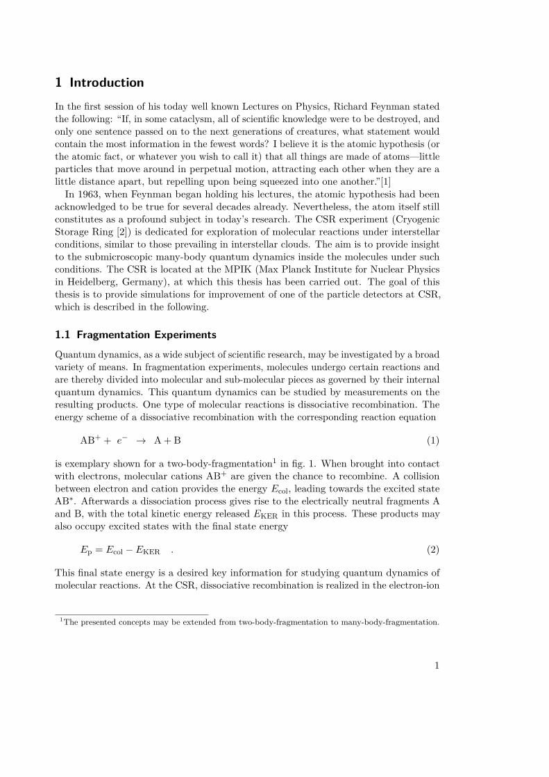
1 IntroductionIn the first session of his today well known Lectures on Physics, Richard Feynman statedthe following: “If, in some cataclysm, all of scientific knowledge were to be destroyed, andonly one sentence passed on to the next generations of creatures, what statement wouldcontain the most information in the fewest words? I believe it is the atomic hypothesis (orthe atomic fact, or whatever you wish to call it) that all things are made of atoms—littleparticles that move around in perpetual motion, attracting each other when they are alittle distance apart, but repelling upon being squeezed into one another.”[1]In 1963, when Feynman began holding his lectures, the atomic hypothesis had been

acknowledged to be true for several decades already. Nevertheless, the atom itself stillconstitutes as a profound subject in today’s research. The CSR experiment (CryogenicStorage Ring [2]) is dedicated for exploration of molecular reactions under interstellarconditions, similar to those prevailing in interstellar clouds. The aim is to provide insightto the submicroscopic many-body quantum dynamics inside the molecules under suchconditions. The CSR is located at the MPIK (Max Planck Institute for Nuclear Physicsin Heidelberg, Germany), at which this thesis has been carried out. The goal of thisthesis is to provide simulations for improvement of one of the particle detectors at CSR,which is described in the following.

1.1 Fragmentation Experiments

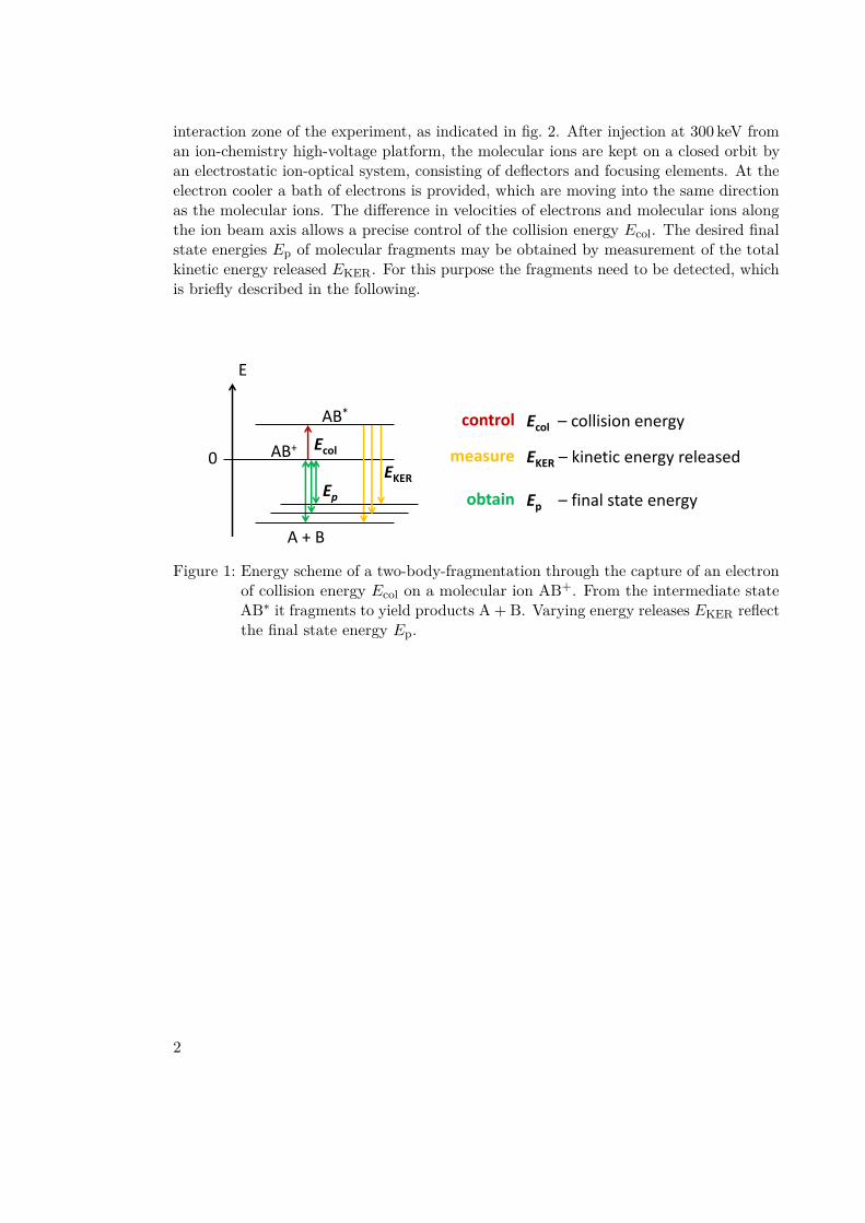
Quantum dynamics, as a wide subject of scientific research, may be investigated by a broadvariety of means. In fragmentation experiments, molecules undergo certain reactions andare thereby divided into molecular and sub-molecular pieces as governed by their internalquantum dynamics. This quantum dynamics can be studied by measurements on theresulting products. One type of molecular reactions is dissociative recombination. Theenergy scheme of a dissociative recombination with the corresponding reaction equation

AB+ + e− → A + B (1)

is exemplary shown for a two-body-fragmentation1 in fig. 1. When brought into contactwith electrons, molecular cations AB+ are given the chance to recombine. A collisionbetween electron and cation provides the energy Ecol, leading towards the excited stateAB∗. Afterwards a dissociation process gives rise to the electrically neutral fragments Aand B, with the total kinetic energy released EKER in this process. These products mayalso occupy excited states with the final state energy

Ep = Ecol − EKER . (2)

This final state energy is a desired key information for studying quantum dynamics ofmolecular reactions. At the CSR, dissociative recombination is realized in the electron-ion

1The presented concepts may be extended from two-body-fragmentation to many-body-fragmentation.

1

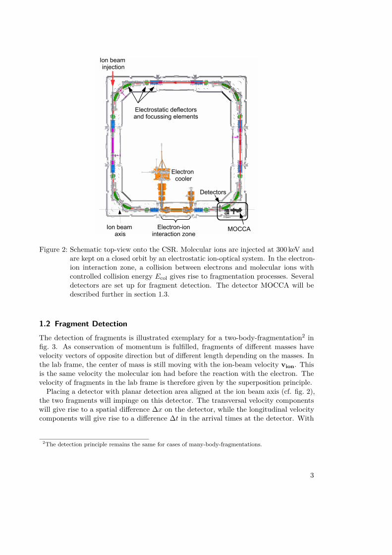
interaction zone of the experiment, as indicated in fig. 2. After injection at 300 keV froman ion-chemistry high-voltage platform, the molecular ions are kept on a closed orbit byan electrostatic ion-optical system, consisting of deflectors and focusing elements. At theelectron cooler a bath of electrons is provided, which are moving into the same directionas the molecular ions. The difference in velocities of electrons and molecular ions alongthe ion beam axis allows a precise control of the collision energy Ecol. The desired finalstate energies Ep of molecular fragments may be obtained by measurement of the totalkinetic energy released EKER. For this purpose the fragments need to be detected, whichis briefly described in the following.

Ecol – collision energy

EKER – kinetic energy released Ep – final state energy

control

measure

obtain

E

0 AB+

AB*

A + B

Ep

Ecol

EKER

Figure 1: Energy scheme of a two-body-fragmentation through the capture of an electronof collision energy Ecol on a molecular ion AB+. From the intermediate stateAB∗ it fragments to yield products A + B. Varying energy releases EKER reflectthe final state energy Ep.

2

Ion beam injection

Electron-ioninteraction zone

MOCCA

Detectors

Electron cooler

Electrostatic deflectorsand focussing elements

Ion beam axis

Figure 2: Schematic top-view onto the CSR. Molecular ions are injected at 300 keV andare kept on a closed orbit by an electrostatic ion-optical system. In the electron-ion interaction zone, a collision between electrons and molecular ions withcontrolled collision energy Ecol gives rise to fragmentation processes. Severaldetectors are set up for fragment detection. The detector MOCCA will bedescribed further in section 1.3.

1.2 Fragment Detection

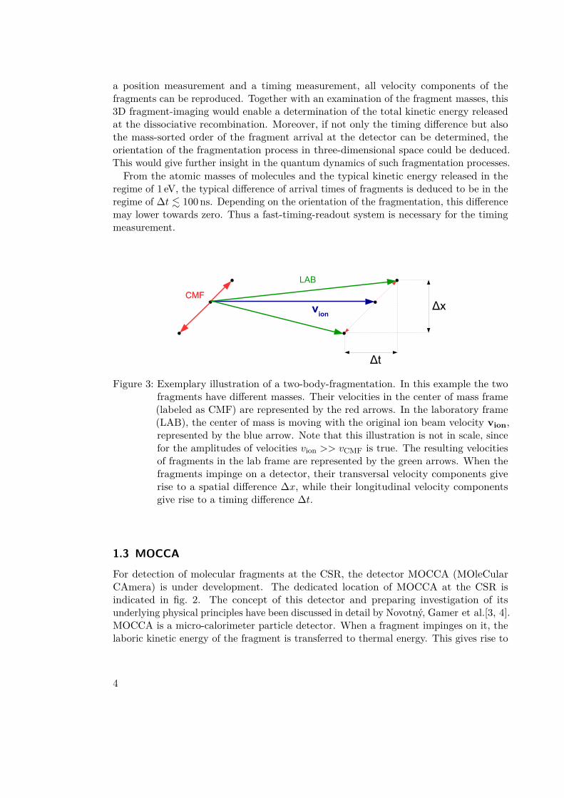
The detection of fragments is illustrated exemplary for a two-body-fragmentation2 infig. 3. As conservation of momentum is fulfilled, fragments of different masses havevelocity vectors of opposite direction but of different length depending on the masses. Inthe lab frame, the center of mass is still moving with the ion-beam velocity vion. Thisis the same velocity the molecular ion had before the reaction with the electron. Thevelocity of fragments in the lab frame is therefore given by the superposition principle.

Placing a detector with planar detection area aligned at the ion beam axis (cf. fig. 2),the two fragments will impinge on this detector. The transversal velocity componentswill give rise to a spatial difference ∆x on the detector, while the longitudinal velocitycomponents will give rise to a difference ∆t in the arrival times at the detector. With

2The detection principle remains the same for cases of many-body-fragmentations.

3

a position measurement and a timing measurement, all velocity components of thefragments can be reproduced. Together with an examination of the fragment masses, this3D fragment-imaging would enable a determination of the total kinetic energy releasedat the dissociative recombination. Moreover, if not only the timing difference but alsothe mass-sorted order of the fragment arrival at the detector can be determined, theorientation of the fragmentation process in three-dimensional space could be deduced.This would give further insight in the quantum dynamics of such fragmentation processes.

From the atomic masses of molecules and the typical kinetic energy released in theregime of 1 eV, the typical difference of arrival times of fragments is deduced to be in theregime of ∆t . 100 ns. Depending on the orientation of the fragmentation, this differencemay lower towards zero. Thus a fast-timing-readout system is necessary for the timingmeasurement.

Δx

Δt

CMFCMF

LAB

vion

Figure 3: Exemplary illustration of a two-body-fragmentation. In this example the twofragments have different masses. Their velocities in the center of mass frame(labeled as CMF) are represented by the red arrows. In the laboratory frame(LAB), the center of mass is moving with the original ion beam velocity vion,represented by the blue arrow. Note that this illustration is not in scale, sincefor the amplitudes of velocities vion >> vCMF is true. The resulting velocitiesof fragments in the lab frame are represented by the green arrows. When thefragments impinge on a detector, their transversal velocity components giverise to a spatial difference ∆x, while their longitudinal velocity componentsgive rise to a timing difference ∆t.

1.3 MOCCA

For detection of molecular fragments at the CSR, the detector MOCCA (MOleCularCAmera) is under development. The dedicated location of MOCCA at the CSR isindicated in fig. 2. The concept of this detector and preparing investigation of itsunderlying physical principles have been discussed in detail by Novotný, Gamer et al.[3, 4].MOCCA is a micro-calorimeter particle detector. When a fragment impinges on it, thelaboric kinetic energy of the fragment is transferred to thermal energy. This gives rise to

4

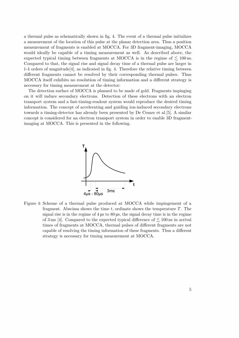
a thermal pulse as schematically shown in fig. 4. The event of a thermal pulse initializesa measurement of the location of this pulse at the planar detection area. Thus a positionmeasurement of fragments is enabled at MOCCA. For 3D fragment-imaging, MOCCAwould ideally be capable of a timing measurement as well. As described above, theexpected typical timing between fragments at MOCCA is in the regime of . 100 ns.Compared to that, the signal rise and signal decay time of a thermal pulse are larger in1-4 orders of magnitude[4], as indicated in fig. 4. Therefore the relative timing betweendifferent fragments cannot be resolved by their corresponding thermal pulses. ThusMOCCA itself exhibits no resolution of timing information and a different strategy isnecessary for timing measurement at the detector:

The detection surface of MOCCA is planned to be made of gold. Fragments impingingon it will induce secondary electrons. Detection of these electrons with an electrontransport system and a fast-timing-readout system would reproduce the desired timinginformation. The concept of accelerating and guiding ion-induced secondary electronstowards a timing-detector has already been presented by De Cesare et al.[5]. A similarconcept is considered for an electron transport system in order to enable 3D fragment-imaging at MOCCA. This is presented in the following.

T

t

4µs - 80µs3ms

Figure 4: Scheme of a thermal pulse produced at MOCCA while impingement of afragment. Abscissa shows the time t, ordinate shows the temperature T . Thesignal rise is in the regime of 4 µs to 80 µs, the signal decay time is in the regimeof 3 ms [4]. Compared to the expected typical difference of . 100 ns in arrivaltimes of fragments at MOCCA, thermal pulses of different fragments are notcapable of resolving the timing information of these fragments. Thus a differentstrategy is necessary for timing measurement at MOCCA.

5

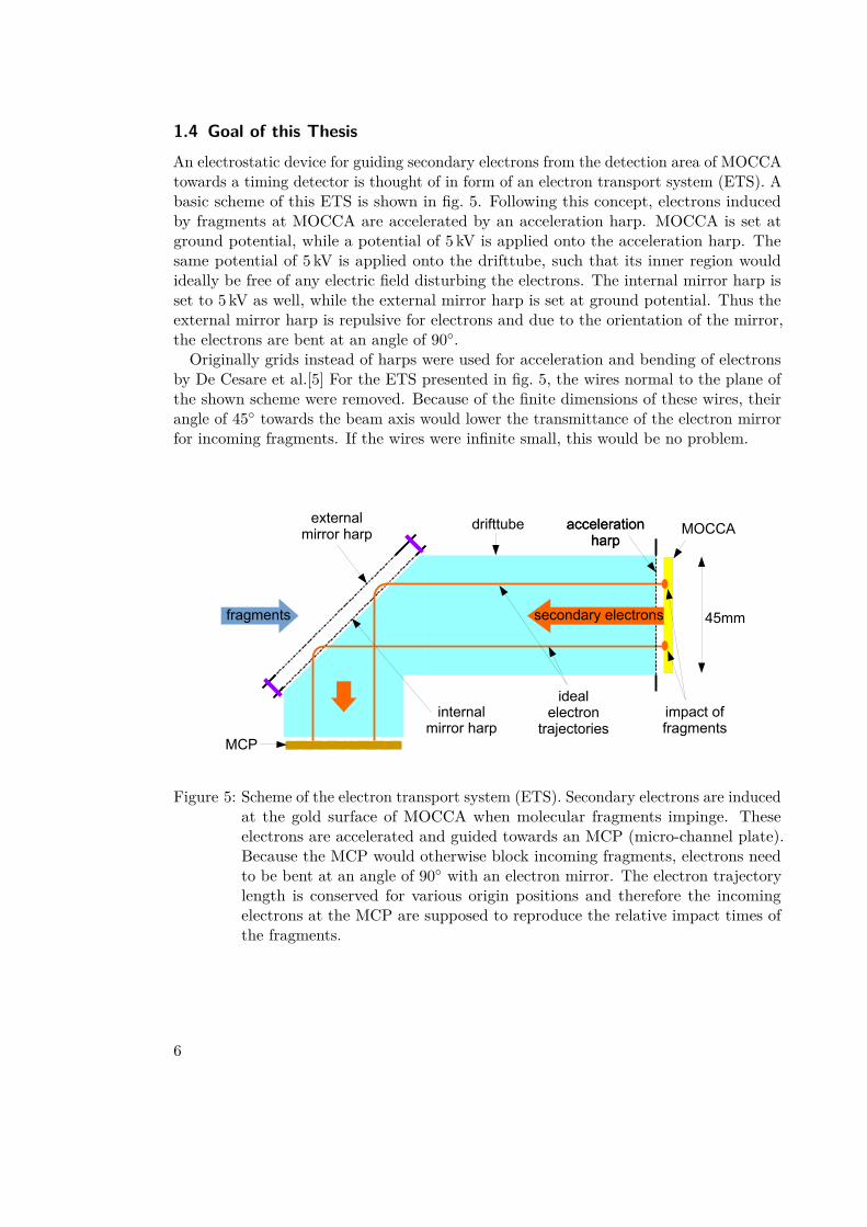
1.4 Goal of this ThesisAn electrostatic device for guiding secondary electrons from the detection area of MOCCAtowards a timing detector is thought of in form of an electron transport system (ETS). Abasic scheme of this ETS is shown in fig. 5. Following this concept, electrons inducedby fragments at MOCCA are accelerated by an acceleration harp. MOCCA is set atground potential, while a potential of 5 kV is applied onto the acceleration harp. Thesame potential of 5 kV is applied onto the drifttube, such that its inner region wouldideally be free of any electric field disturbing the electrons. The internal mirror harp isset to 5 kV as well, while the external mirror harp is set at ground potential. Thus theexternal mirror harp is repulsive for electrons and due to the orientation of the mirror,the electrons are bent at an angle of 90.Originally grids instead of harps were used for acceleration and bending of electrons

by De Cesare et al.[5] For the ETS presented in fig. 5, the wires normal to the plane ofthe shown scheme were removed. Because of the finite dimensions of these wires, theirangle of 45 towards the beam axis would lower the transmittance of the electron mirrorfor incoming fragments. If the wires were infinite small, this would be no problem.

45mm

MCP

internalmirror harp

externalmirror harp MOCCA

idealelectron

trajectories

accelerationharp

accelerationharp

drifttube

fragments secondary electrons

impact offragments

Figure 5: Scheme of the electron transport system (ETS). Secondary electrons are inducedat the gold surface of MOCCA when molecular fragments impinge. Theseelectrons are accelerated and guided towards an MCP (micro-channel plate).Because the MCP would otherwise block incoming fragments, electrons needto be bent at an angle of 90 with an electron mirror. The electron trajectorylength is conserved for various origin positions and therefore the incomingelectrons at the MCP are supposed to reproduce the relative impact times ofthe fragments.

6

After the electrostatic mirror, the electrons continue towards the MCP (micro-channelplate), constituting as timing detector and also set to 5 kV. Impingement of an electronat the MCP will give rise to an electron cascade. This will produce a measurable voltagepulse at the MCP. Voltage pulses from different electrons are capable of resolution ofthe difference in arrival times of electrons at the MCP. In contrast to the thermal pulsesat MOCCA, these voltage pulses at MCP are therefore able to reproduce the timinginformation of fragments.

A precondition for this reproduction of timing information is the conservation of timinginformation by secondary electrons. For this purpose the variance in TOF (time-of-flight)of electrons traversing the ETS would need to be small compared to the typical timingof fragments, which is in the regime of ∆t . 100 ns. The concept of the ETS in fig. 5would theoretically ensure the same trajectory length for all electrons starting at normalincident from MOCCA, giving rise to almost the same TOF for all those electrons. Theelectron cascade at the MCP will also produce a light spot at a phosphor screen setbehind the MCP. The phosphor screen thus enables position measurement of secondaryelectrons.

fragment positions at MOCCA

spatial distributions ofsecondary electrons at MCP

overlap?

(a)

fragment positions at MOCCA

spatial distributions ofsecondary electrons at MCP

mixing?

(b)

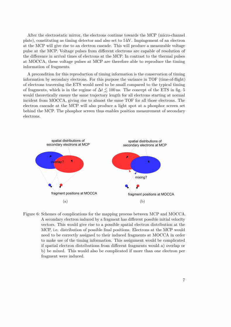
Figure 6: Schemes of complications for the mapping process between MCP and MOCCA.A secondary electron induced by a fragment has different possible initial velocityvectors. This would give rise to a possible spatial electron distribution at theMCP, i.e. distribution of possible final positions. Electrons at the MCP wouldneed to be correctly assigned to their induced fragments at MOCCA in orderto make use of the timing information. This assignment would be complicatedif spatial electron distributions from different fragments would a) overlap orb) be mixed. This would also be complicated if more than one electron perfragment were induced.

7

This is a necessary feature, because the voltage pulses at the MCP contain theinformation of relative timing difference between two fragments, but they do not containthe information to which two fragments this relative timing difference corresponds.3 Thusa mapping process between MOCCA and MCP is necessary, in which each secondaryelectron at MCP is correctly assigned to its inducing fragment at MOCCA. If the electronpositions at MCP were projected at MOCCA, the electrons and their correspondingfragments would ideally share the same position. This is assumed to be true for thetrajectories indicated in fig. 5, therefore these trajectories are called “ideal”. But thisassignment is not trivial due to the possible initial velocity vectors of secondary electrons:Possible secondary electrons from the same fragment at MOCCA would distribute atdifferent positions at MCP. This is illustrated in fig. 6. An overlap or mixing of twospatial electron distributions at MCP for two fragments at MOCCA would make themapping process difficult. The greater the overlap, the less likely the mapping would besuccessful for individual events in the case of no mixing.

The goal of this thesis is to perform a feasibility study of the ETS by means ofsimulations. The two concerns are namely: Firstly, is the timing information of fragmentsconserved by the secondary electrons in the ETS? Secondly, is a mapping process betweenMOCCA and MCP possible in order to assign the timing information to its correspondingfragments? For the purpose of addressing these two major questions, simulations ofelectron trajectories in a modeled ETS are necessary. The required data are TOF, initialposition and final position of simulated electrons. For calculation of realistic trajectoriesof electrons induced by fragments, physical initial conditions of secondary electronsare to be implemented in these simulations. At first a simplified model of the ETS issimulated in order to examine the influence of individual components of the ETS onelectron trajectories. Further simulations at a realistic model of the ETS are then neededfor testing the feasibility of the ETS under realistic conditions.

3The two-body-fragmentation is the only exception to this. But even in this case the timing differencealone cannot tell at which order the fragments arrived at MOCCA.

8

2 Physical Principles

Before a first simulative approach is presented in section 3, the underlying theoreticalfoundations are introduced. This gives rise to the following essential questions: Beginningwith the impingement of a neutral fragment into MOCCA, secondary electrons may beproduced in this process. Especially their angle towards the detector’s surface and theirkinetic energy are important to consider for calculation of realistic electron trajectoriesin the ETS. Therefore section 2.1 deals with the question: “What are the productionmechanisms and resulting initial conditions for secondary electrons at metal surfaces?”Instantly after the production of secondary electrons, the ETS guides the electrons

towards the MCP by electrostatic fields. This guiding was simulated by the softwarepackage SIMION (Scientific Instrument Services, Inc. (SIS) [6]). Therefore section 2.2deals with the question: “What is the physics on which the ETS and simulations bySIMION are based on?”

2.1 Production Mechanisms and Initial Conditions of Secondary Electrons

It is a well-known phenomenon that secondary electrons are emitted from a solid,especially a metallic surface when it undergoes bombardment by energetic particles.Often this is described by “ion-induced secondary electron emission” [7], but in spiteof the ionic reference it also includes bombardment by electrically neutral particles.Therefore secondary electrons will also be induced when molecular fragments impingethe gold surface of MOCCA. The case in which direct transfer of kinetic energy from theprojectile into the target gives rise to electron emission is schematically shown in fig. 7a.This is called “kinetic electron emission” and consists of three steps [7]:

Firstly, excited electrons are generated in the solid, but not all excited electrons giverise to secondary electron emission. At ion beam energy of 300 keV, which is in theregime of high impact energies, the main production mechanisms are contributions fromelectrons of the target: excitation of conduction electrons from the Fermi-edge on theone hand, and ionization of inner-shell electrons on the other hand. Secondly, parts ofthe excited electrons diffuse towards the surface. On their way, they loose previouslygained energy by colliding with other electrons in the target and may hereby multiplyin a cascade. Thirdly, electrons penetrate through the surface into the vacuum. This isconsidered as a refraction process.

Compared to the dimensions of the detection area of MOCCA, the electrons do notpropagate far away from the entrance point of the projectile. Thus it is approximatedthat secondary electrons emit at the the same point as the projectile has entered, asshown in fig. 7b. In the same figure, it is also indicated that secondary electrons will havedifferent initial velocity vectors. The possible direction and amplitude of the velocityvectors are represented by the distribution of the polar angle ϑ to the surface normal(cf. fig. 7a) and the distribution of kinetic energy. Experiments at impact energies up to5 keV found the following distribution of polar angle ϑ of emitted secondary electrons

9

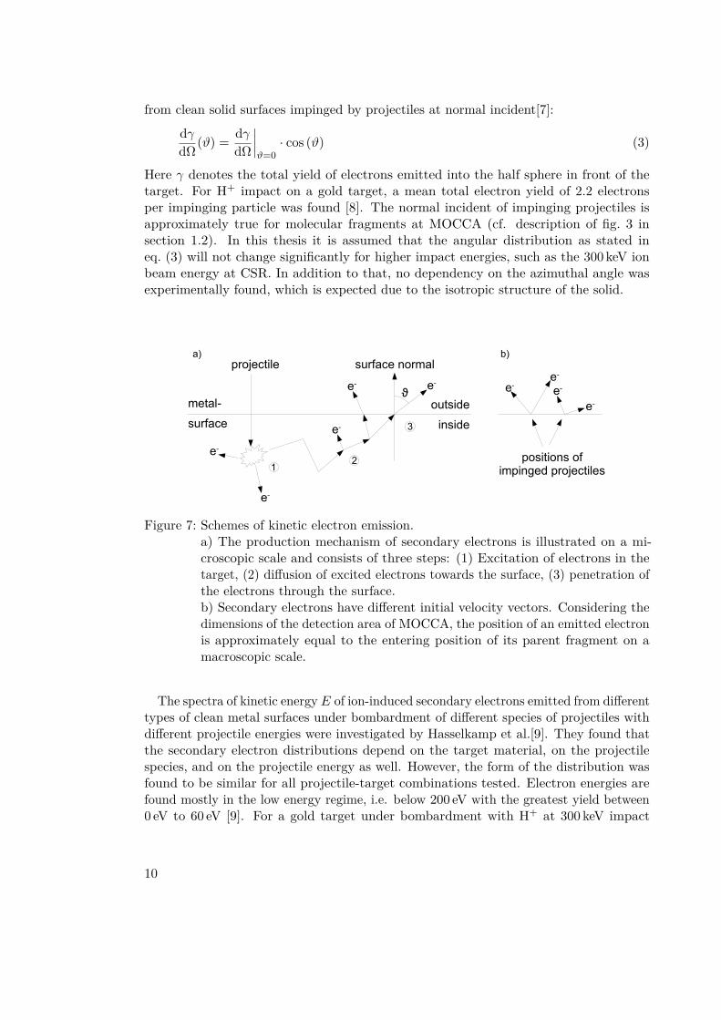
from clean solid surfaces impinged by projectiles at normal incident[7]:

dγdΩ(ϑ) = dγ

dΩ

∣∣∣∣ϑ=0· cos (ϑ) (3)

Here γ denotes the total yield of electrons emitted into the half sphere in front of thetarget. For H+ impact on a gold target, a mean total electron yield of 2.2 electronsper impinging particle was found [8]. The normal incident of impinging projectiles isapproximately true for molecular fragments at MOCCA (cf. description of fig. 3 insection 1.2). In this thesis it is assumed that the angular distribution as stated ineq. (3) will not change significantly for higher impact energies, such as the 300 keV ionbeam energy at CSR. In addition to that, no dependency on the azimuthal angle wasexperimentally found, which is expected due to the isotropic structure of the solid.

metal-

surface

outside

inside

projectile

1

ϑ

2

3

e-

e-

e- e-

surface normal

e-

positions ofimpinged projectiles

e-e-

e-

e-

a) b)

Figure 7: Schemes of kinetic electron emission.a) The production mechanism of secondary electrons is illustrated on a mi-croscopic scale and consists of three steps: (1) Excitation of electrons in thetarget, (2) diffusion of excited electrons towards the surface, (3) penetration ofthe electrons through the surface.b) Secondary electrons have different initial velocity vectors. Considering thedimensions of the detection area of MOCCA, the position of an emitted electronis approximately equal to the entering position of its parent fragment on amacroscopic scale.

The spectra of kinetic energy E of ion-induced secondary electrons emitted from differenttypes of clean metal surfaces under bombardment of different species of projectiles withdifferent projectile energies were investigated by Hasselkamp et al.[9]. They found thatthe secondary electron distributions depend on the target material, on the projectilespecies, and on the projectile energy as well. However, the form of the distribution wasfound to be similar for all projectile-target combinations tested. Electron energies arefound mostly in the low energy regime, i.e. below 200 eV with the greatest yield between0 eV to 60 eV [9]. For a gold target under bombardment with H+ at 300 keV impact

10

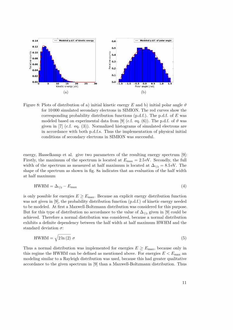
(a) (b)

Figure 8: Plots of distribution of a) initial kinetic energy E and b) initial polar angle ϑfor 10 000 simulated secondary electrons in SIMION. The red curves show thecorresponding probability distribution functions (p.d.f.). The p.d.f. of E wasmodeled based on experimental data from [9] (c.f. eq. (6)). The p.d.f. of ϑ wasgiven in [7] (c.f. eq. (3)). Normalized histograms of simulated electrons arein accordance with both p.d.f.s. Thus the implementation of physical initialconditions of secondary electrons in SIMION was successful.

energy, Hasselkamp et al. give two parameters of the resulting energy spectrum [9]:Firstly, the maximum of the spectrum is located at Emax = 2.5 eV. Secondly, the fullwidth of the spectrum as measured at half maximum is located at ∆1/2 = 8.5 eV. Theshape of the spectrum as shown in fig. 8a indicates that an evaluation of the half widthat half maximum

HWHM = ∆1/2 − Emax (4)

is only possible for energies E ≥ Emax. Because an explicit energy distribution functionwas not given in [9], the probability distribution function (p.d.f.) of kinetic energy neededto be modeled. At first a Maxwell-Boltzmann distribution was considered for this purpose.But for this type of distribution no accordance to the value of ∆1/2 given in [9] could beachieved. Therefore a normal distribution was considered, because a normal distributionexhibits a definite dependency between the half width at half maximum HWHM and thestandard deviation σ:

HWHM =√

2 ln (2) σ (5)

Thus a normal distribution was implemented for energies E ≥ Emax, because only inthis regime the HWHM can be defined as mentioned above. For energies E < Emax anmodeling similar to a Rayleigh distribution was used, because this had greater qualitativeaccordance to the given spectrum in [9] than a Maxwell-Boltzmann distribution. Thus

11

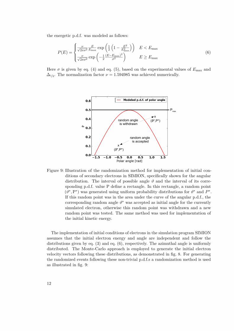
the energetic p.d.f. was modeled as follows:

P (E) =

ν√

2πσ2E

Emaxexp

(12

(1− E2

E2max

))E < Emax

ν√2πσ2 exp

(−1

2(E−Emax)2

σ2

)E ≥ Emax

(6)

Here σ is given by eq. (4) and eq. (5), based on the experimental values of Emax and∆1/2. The normalization factor ν = 1.594985 was achieved numerically.

Pmax

x

random angle is accepted

(ϑ*,P*)

x(ϑ*,P*)random angle

is withdrawn

Figure 9: Illustration of the randomization method for implementation of initial con-ditions of secondary electrons in SIMION, specifically shown for the angulardistribution. The interval of possible angle ϑ and the interval of its corre-sponding p.d.f. value P define a rectangle. In this rectangle, a random point(ϑ∗,P∗) was generated using uniform probability distributions for ϑ∗ and P ∗.If this random point was in the area under the curve of the angular p.d.f., thecorresponding random angle ϑ∗ was accepted as initial angle for the currentlysimulated electron, otherwise this random point was withdrawn and a newrandom point was tested. The same method was used for implementation ofthe initial kinetic energy.

The implementation of initial conditions of electrons in the simulation program SIMIONassumes that the initial electron energy and angle are independent and follow thedistributions given by eq. (3) and eq. (6), respectively. The azimuthal angle is uniformlydistributed. The Monte-Carlo approach is employed to generate the initial electronvelocity vectors following these distributions, as demonstrated in fig. 8. For generatingthe randomized events following these non-trivial p.d.f.s a randomization method is usedas illustrated in fig. 9:

12

As a first step, physical useful intervals for the angle ϑ and the energy E were chosen,namely ϑ ∈

[−π/2, π/2

]and E ∈ [0 eV, 300 eV]. The maximum energy of electrons was

chosen as 0.1 % of the ion beam energy of 300 keV, such that also cases of less likelyelectrons with energy E > 200 eV were included in the simulations.

The actual method is based on the “Rejection method” for random number generation[10] and is described in the following specifically for the angular distribution by reference tofig. 9. The p.d.f. as given in eq. (3) was normalized such that integration over all possiblepolar angles yielded a total probability of 1. Denoting the p.d.f. value with P, possiblevalues are between 0 and a maximum value Pmax. For each electron a random point(ϑ∗, P ∗) was produced using a uniform random number generator, with ϑ∗ ∈

[−π/2, π/2

]and P∗ ∈ [0,Pmax]. If the random point (ϑ∗, P ∗) was in the area described by the angularp.d.f., the random angle ϑ∗ was implemented as initial angle for the currently simulatedelectron, otherwise ϑ∗ was withdrawn and a new random point was produced. The sameprocedure was executed for the initial kinetic energy of each secondary electron.

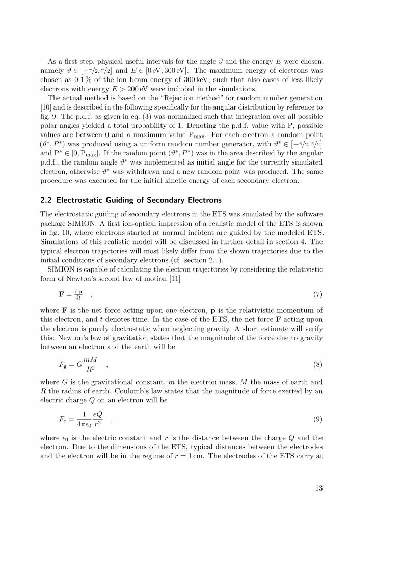
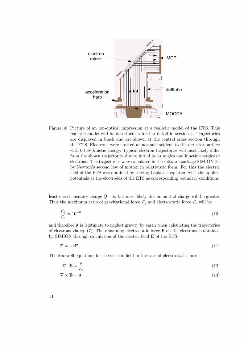
2.2 Electrostatic Guiding of Secondary ElectronsThe electrostatic guiding of secondary electrons in the ETS was simulated by the softwarepackage SIMION. A first ion-optical impression of a realistic model of the ETS is shownin fig. 10, where electrons started at normal incident are guided by the modeled ETS.Simulations of this realistic model will be discussed in further detail in section 4. Thetypical electron trajectories will most likely differ from the shown trajectories due to theinitial conditions of secondary electrons (cf. section 2.1).

SIMION is capable of calculating the electron trajectories by considering the relativisticform of Newton’s second law of motion [11]

F = dpdt , (7)

where F is the net force acting upon one electron, p is the relativistic momentum ofthis electron, and t denotes time. In the case of the ETS, the net force F acting uponthe electron is purely electrostatic when neglecting gravity. A short estimate will verifythis: Newton’s law of gravitation states that the magnitude of the force due to gravitybetween an electron and the earth will be

Fg = GmM

R2 , (8)

where G is the gravitational constant, m the electron mass, M the mass of earth andR the radius of earth. Coulomb’s law states that the magnitude of force exerted by anelectric charge Q on an electron will be

Fe = 14πε0

eQ

r2 , (9)

where ε0 is the electric constant and r is the distance between the charge Q and theelectron. Due to the dimensions of the ETS, typical distances between the electrodesand the electron will be in the regime of r = 1 cm. The electrodes of the ETS carry at

13

MOCCA

MCP

drifftubeaccelerationharp

electronmirror

Figure 10: Picture of an ion-optical impression at a realistic model of the ETS. Thisrealistic model will be described in further detail in section 4. Trajectoriesare displayed in black and are shown at the central cross section throughthe ETS. Electrons were started at normal incident to the detector surfacewith 0.1 eV kinetic energy. Typical electron trajectories will most likely differfrom the shown trajectories due to initial polar angles and kinetic energies ofelectrons. The trajectories were calculated in the software package SIMION [6]by Newton’s second law of motion in relativistic form. For this the electricfield of the ETS was obtained by solving Laplace’s equation with the appliedpotentials at the electrodes of the ETS as corresponding boundary conditions.

least one elementary charge Q = e, but most likely this amount of charge will be greater.Thus the maximum ratio of gravitational force Fg and electrostatic force Fe will be

FgFe∝ 10−6 , (10)

and therefore it is legitimate to neglect gravity by earth when calculating the trajectoriesof electrons via eq. (7). The remaining electrostatic force F on the electrons is obtainedby SIMION through calculation of the electric field E of the ETS:

F = −eE . (11)

The Maxwell-equations for the electric field in the case of electrostatics are:

∇ ·E = ρ

ε0(12)

∇×E = 0 . (13)

14

Here ρ is the spatial charge distribution. The second Maxwell-equation reveals the electricfield as a conservative field. Thus the electric potential U at point r is given as the lineintegral along any arbitrary path from a reference point r∗ to r:

U(r) = −∫ r

r∗E(r′) · dl′ . (14)

In the accomplished simulations, the reference point r∗ is on the surface of MOCCA,defining the ground potential as U = 0 V. If the potential is given, then the electric fieldmay be obtained by

E = −∇U . (15)

With eq. (12) a correlation is given between potential and spatial charge distribution,namely Poisson’s equation:

4U = − ρε0

, (16)

The charge which defines the potentials at the ETS is confined to the electrodes of theETS. Secondary electrons move in the region between electrodes, where ρ = 0 C m−3.For this region eq. (16) reduces to Laplace’s equation:

4U = 0 . (17)

This is the equation solved by SIMION in order to obtain the electric potential of theETS and thus the electric field via eq. (15). The potentials applied on the electrodesof the ETS constitute as corresponding boundary conditions for the solution of thisdifferential equation. SIMION uses the following method [11]: At point r, the value U(r)is the average value of U over a spherical surface A centered at r and with Radius R,

U(r) = 14πR2

∮U dA . (18)

simulated A grid of points is defined over the space in which the electric field is required.With the given boundary conditions, the potential on the corresponding boundary pointsis set. In several iteration loops eq. (14) is applied such that the electric potential ofany point is estimated as the average potential of its nearest neighbor points, untilthe resulting values converge. Thus a numerical solution to Laplace’s equation can beachieved [12].

15

3 Simulations Within a Simplified Model

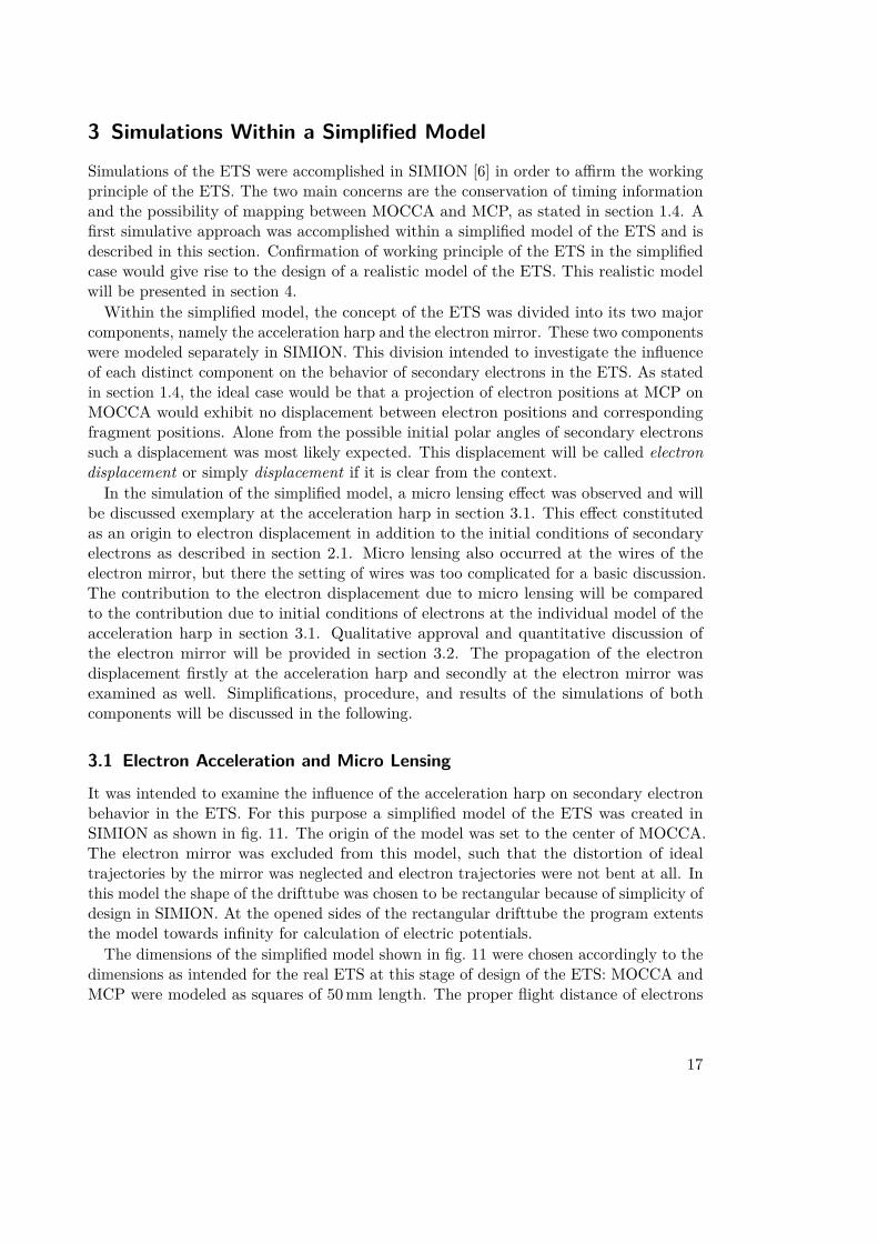
Simulations of the ETS were accomplished in SIMION [6] in order to affirm the workingprinciple of the ETS. The two main concerns are the conservation of timing informationand the possibility of mapping between MOCCA and MCP, as stated in section 1.4. Afirst simulative approach was accomplished within a simplified model of the ETS and isdescribed in this section. Confirmation of working principle of the ETS in the simplifiedcase would give rise to the design of a realistic model of the ETS. This realistic modelwill be presented in section 4.

Within the simplified model, the concept of the ETS was divided into its two majorcomponents, namely the acceleration harp and the electron mirror. These two componentswere modeled separately in SIMION. This division intended to investigate the influenceof each distinct component on the behavior of secondary electrons in the ETS. As statedin section 1.4, the ideal case would be that a projection of electron positions at MCP onMOCCA would exhibit no displacement between electron positions and correspondingfragment positions. Alone from the possible initial polar angles of secondary electronssuch a displacement was most likely expected. This displacement will be called electrondisplacement or simply displacement if it is clear from the context.

In the simulation of the simplified model, a micro lensing effect was observed and willbe discussed exemplary at the acceleration harp in section 3.1. This effect constitutedas an origin to electron displacement in addition to the initial conditions of secondaryelectrons as described in section 2.1. Micro lensing also occurred at the wires of theelectron mirror, but there the setting of wires was too complicated for a basic discussion.The contribution to the electron displacement due to micro lensing will be comparedto the contribution due to initial conditions of electrons at the individual model of theacceleration harp in section 3.1. Qualitative approval and quantitative discussion ofthe electron mirror will be provided in section 3.2. The propagation of the electrondisplacement firstly at the acceleration harp and secondly at the electron mirror wasexamined as well. Simplifications, procedure, and results of the simulations of bothcomponents will be discussed in the following.

3.1 Electron Acceleration and Micro Lensing

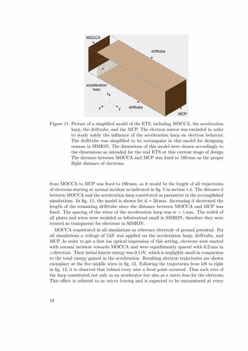
It was intended to examine the influence of the acceleration harp on secondary electronbehavior in the ETS. For this purpose a simplified model of the ETS was created inSIMION as shown in fig. 11. The origin of the model was set to the center of MOCCA.The electron mirror was excluded from this model, such that the distortion of idealtrajectories by the mirror was neglected and electron trajectories were not bent at all. Inthis model the shape of the drifttube was chosen to be rectangular because of simplicity ofdesign in SIMION. At the opened sides of the rectangular drifttube the program extentsthe model towards infinity for calculation of electric potentials.

The dimensions of the simplified model shown in fig. 11 were chosen accordingly to thedimensions as intended for the real ETS at this stage of design of the ETS: MOCCA andMCP were modeled as squares of 50 mm length. The proper flight distance of electrons

17

MOCCA

MCP

accelerationharp

drifttube

drifttubey

z

x

Figure 11: Picture of a simplified model of the ETS, including MOCCA, the accelerationharp, the drifttube, and the MCP. The electron mirror was excluded in orderto study solely the influence of the acceleration harp on electron behavior.The drifttube was simplified to be rectangular in this model for designingreasons in SIMION. The dimensions of this model were chosen accordingly tothe dimensions as intended for the real ETS at this current stage of design.The distance between MOCCA and MCP was fixed to 180 mm as the properflight distance of electrons.

from MOCCA to MCP was fixed to 180 mm, as it would be the length of all trajectoriesof electrons starting at normal incident as indicated in fig. 5 in section 1.4. The distance dbetween MOCCA and the acceleration harp constituted as parameter in the accomplishedsimulations. In fig. 11, the model is shown for d = 20 mm. Increasing d shortened thelength of the remaining drifttube since the distance between MOCCA and MCP wasfixed. The spacing of the wires of the acceleration harp was w = 1 mm. The width ofall plates and wires were modeled as infinitesimal small in SIMION, therefore they weretreated as transparent for electrons in SIMION.

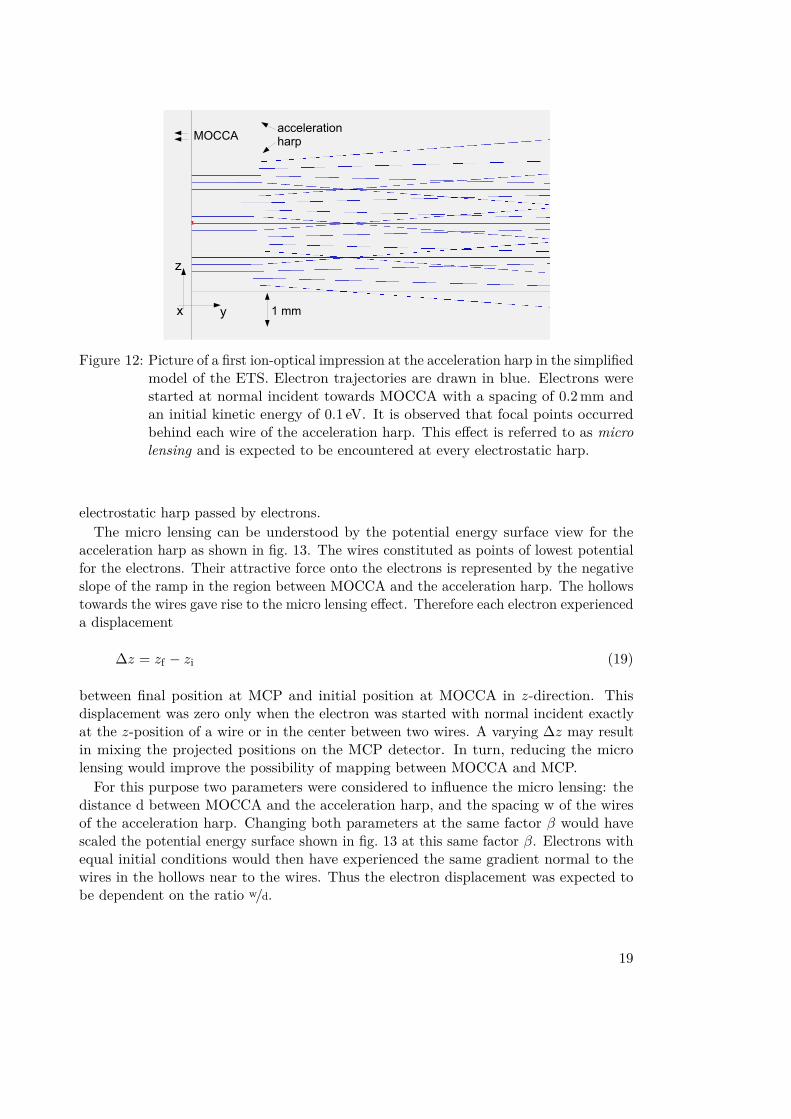
MOCCA constituted in all simulations as reference electrode of ground potential. Forall simulations a voltage of 5 kV was applied on the acceleration harp, drifttube, andMCP. In order to get a first ion optical impression of this setting, electrons were startedwith normal incident towards MOCCA and were equidistantly spaced with 0.2 mm inz-direction. Their initial kinetic energy was 0.1 eV, which is negligibly small in comparisonto the total energy gained in the acceleration. Resulting electron trajectories are shownexemplary at the five middle wires in fig. 12. Following the trajectories from left to rightin fig. 12, it is observed that behind every wire a focal point occurred. Thus each wire ofthe harp constituted not only as an accelerator but also as a micro lens for the electrons.This effect is referred to as micro lensing and is expected to be encountered at every

18

accelerationharpMOCCA

1 mmy

z

x

Figure 12: Picture of a first ion-optical impression at the acceleration harp in the simplifiedmodel of the ETS. Electron trajectories are drawn in blue. Electrons werestarted at normal incident towards MOCCA with a spacing of 0.2 mm andan initial kinetic energy of 0.1 eV. It is observed that focal points occurredbehind each wire of the acceleration harp. This effect is referred to as microlensing and is expected to be encountered at every electrostatic harp.

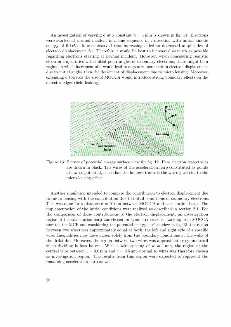
electrostatic harp passed by electrons.The micro lensing can be understood by the potential energy surface view for the

acceleration harp as shown in fig. 13. The wires constituted as points of lowest potentialfor the electrons. Their attractive force onto the electrons is represented by the negativeslope of the ramp in the region between MOCCA and the acceleration harp. The hollowstowards the wires gave rise to the micro lensing effect. Therefore each electron experienceda displacement

∆z = zf − zi (19)

between final position at MCP and initial position at MOCCA in z-direction. Thisdisplacement was zero only when the electron was started with normal incident exactlyat the z-position of a wire or in the center between two wires. A varying ∆z may resultin mixing the projected positions on the MCP detector. In turn, reducing the microlensing would improve the possibility of mapping between MOCCA and MCP.For this purpose two parameters were considered to influence the micro lensing: the

distance d between MOCCA and the acceleration harp, and the spacing w of the wiresof the acceleration harp. Changing both parameters at the same factor β would havescaled the potential energy surface shown in fig. 13 at this same factor β. Electrons withequal initial conditions would then have experienced the same gradient normal to thewires in the hollows near to the wires. Thus the electron displacement was expected tobe dependent on the ratio w/d.

19

An investigation of varying d at a constant w = 1 mm is shown in fig. 14. Electronswere started at normal incident in a line sequence in z-direction with initial kineticenergy of 0.1 eV. It was observed that increasing d led to decreased amplitudes ofelectron displacement ∆z. Therefore it would be best to increase d as much as possibleregarding electrons starting at normal incident. However, when considering realisticelectron trajectories with initial polar angles of secondary electrons, there might be aregime in which increment of d would lead to a greater increment in electron displacementdue to initial angles than the decrement of displacement due to micro lensing. Moreover,extending d towards the size of MOCCA would introduce strong boundary effects on thedetector edges (field leaking).

y

z

Epot

accelerationharp

focusing

Figure 13: Picture of potential energy surface view for fig. 12. Here electron trajectoriesare drawn in black. The wires of the acceleration harp constituted as pointsof lowest potential, such that the hollows towards the wires gave rise to themicro lensing effect.

Another simulation intended to compare the contribution to electron displacement dueto micro lensing with the contribution due to initial conditions of secondary electrons.This was done for a distance d = 10 mm between MOCCA and acceleration harp. Theimplementation of the initial conditions were realized as described in section 2.1. Forthe comparison of these contributions to the electron displacement, an investigationregion at the acceleration harp was chosen for symmetry reasons: Looking from MOCCAtowards the MCP and considering the potential energy surface view in fig. 13, the regionbetween two wires was approximately equal at both, the left and right side of a specificwire. Inequalities may have arisen solely from the boundary conditions at the walls ofthe drifttube. Moreover, the region between two wires was approximately symmetricalwhen dividing it into halves. With a wire spacing of w = 1 mm, the region at thecentral wire between z = 0.0 mm and z = 0.5 mm normal to wires was therefore chosenas investigation region. The results from this region were expected to represent theremaining acceleration harp as well.

20

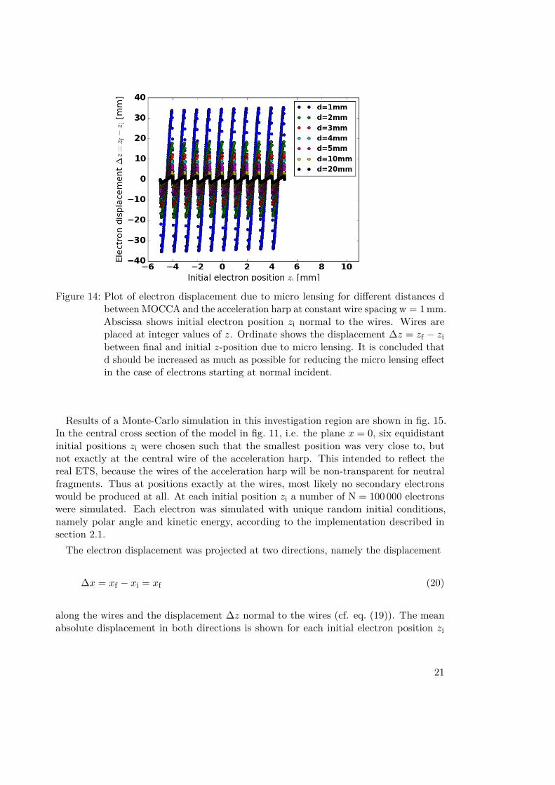
Figure 14: Plot of electron displacement due to micro lensing for different distances dbetween MOCCA and the acceleration harp at constant wire spacing w = 1 mm.Abscissa shows initial electron position zi normal to the wires. Wires areplaced at integer values of z. Ordinate shows the displacement ∆z = zf − zibetween final and initial z-position due to micro lensing. It is concluded thatd should be increased as much as possible for reducing the micro lensing effectin the case of electrons starting at normal incident.

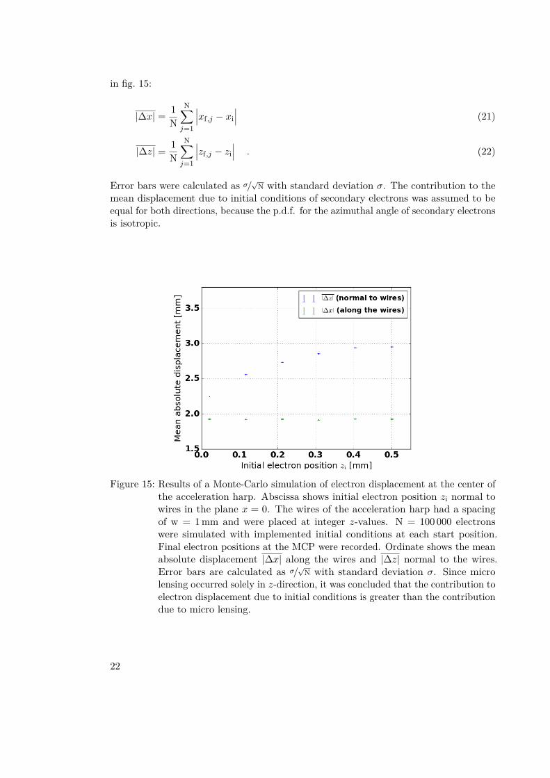
Results of a Monte-Carlo simulation in this investigation region are shown in fig. 15.In the central cross section of the model in fig. 11, i.e. the plane x = 0, six equidistantinitial positions zi were chosen such that the smallest position was very close to, butnot exactly at the central wire of the acceleration harp. This intended to reflect thereal ETS, because the wires of the acceleration harp will be non-transparent for neutralfragments. Thus at positions exactly at the wires, most likely no secondary electronswould be produced at all. At each initial position zi a number of N = 100 000 electronswere simulated. Each electron was simulated with unique random initial conditions,namely polar angle and kinetic energy, according to the implementation described insection 2.1.

The electron displacement was projected at two directions, namely the displacement

∆x = xf − xi = xf (20)

along the wires and the displacement ∆z normal to the wires (cf. eq. (19)). The meanabsolute displacement in both directions is shown for each initial electron position zi

21

in fig. 15:

|∆x| = 1N

N∑j=1

∣∣∣xf,j − xi∣∣∣ (21)

|∆z| = 1N

N∑j=1

∣∣∣zf,j − zi∣∣∣ . (22)

Error bars were calculated as σ/√N with standard deviation σ. The contribution to themean displacement due to initial conditions of secondary electrons was assumed to beequal for both directions, because the p.d.f. for the azimuthal angle of secondary electronsis isotropic.

Figure 15: Results of a Monte-Carlo simulation of electron displacement at the center ofthe acceleration harp. Abscissa shows initial electron position zi normal towires in the plane x = 0. The wires of the acceleration harp had a spacingof w = 1 mm and were placed at integer z-values. N = 100 000 electronswere simulated with implemented initial conditions at each start position.Final electron positions at the MCP were recorded. Ordinate shows the meanabsolute displacement |∆x| along the wires and |∆z| normal to the wires.Error bars are calculated as σ/

√N with standard deviation σ. Since micro

lensing occurred solely in z-direction, it was concluded that the contribution toelectron displacement due to initial conditions is greater than the contributiondue to micro lensing.

22

On the one hand, no micro lensing occurred along the wires, therefore the onlycontribution to the displacement ∆x was due to the initial conditions of electrons.Because of that, the same mean absolute displacement |∆x| was expected for each initialposition zi. This was indeed found in fig. 15. On the other hand, because micro lensingoccurred normal to the wires, the mean absolute displacement |∆z| was expected todiffer from |∆x|. Again, this was indeed found in fig. 15: The micro lensing increasedthe mean absolute displacement in z-direction. Moreover, a monotonic increment of |∆z|was observed for increasing zi.

Subtracting |∆x| from |∆z|, it was concluded that the contribution to the displacementby initial conditions was greater than the contribution by micro lensing, because microlensing occurred solely in z-direction. This conclusion could be generalized from thedescribed investigation region to the whole acceleration harp.

3.2 Electron Mirror and Further Analysis

It was intended to examine the influence of the electron mirror on secondary electronbehavior in the ETS. For this purpose the results from the Monte-Carlo simulationpresented in section 3.1 were implemented into a simulation of a simplified model of theelectron mirror.

x

z

y

internalmirror harp

externalmirror harp

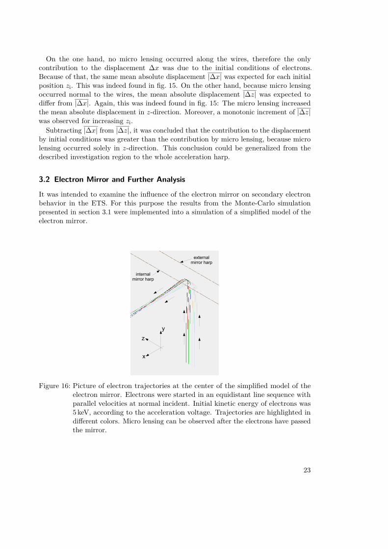
Figure 16: Picture of electron trajectories at the center of the simplified model of theelectron mirror. Electrons were started in an equidistant line sequence withparallel velocities at normal incident. Initial kinetic energy of electrons was5 keV, according to the acceleration voltage. Trajectories are highlighted indifferent colors. Micro lensing can be observed after the electrons have passedthe mirror.

23

The mirror was modeled within SIMION as two rows of harps of the same kind anddimensions as the acceleration harp in section 3.1. Thus the wire spacing was set tow = 1 mm for each harp and the direction along the wires was extended towards infinityfor calculation of electric potentials by SIMION. At the front mirror harp, where electronswere supposed to enter and exit the mirror, the voltage was set to 5 kV. At the backmirror harp the voltage was set to −5 kV. This is an exception to the proposed applicationof 0 kV in section 1.4, because this proposed value had been changed throughout thecourse of simulations. No qualitative changes are expected from this change. Withthe separation between the two harps set to 10 mm, the electrons experienced a meangradient of 1 kV mm−1 inside the mirror.

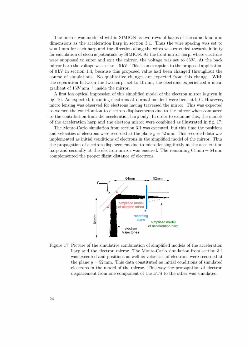
A first ion optical impression of this simplified model of the electron mirror is given infig. 16. As expected, incoming electrons at normal incident were bent at 90. However,micro lensing was observed for electrons having traversed the mirror. This was expectedto worsen the contribution to electron displacements due to the mirror when comparedto the contribution from the acceleration harp only. In order to examine this, the modelsof the acceleration harp and the electron mirror were combined as illustrated in fig. 17:

The Monte-Carlo simulation from section 3.1 was executed, but this time the positionsand velocities of electrons were recorded at the plane y = 52 mm. This recorded data wasimplemented as initial conditions of electrons in the simplified model of the mirror. Thusthe propagation of electron displacement due to micro lensing firstly at the accelerationharp and secondly at the electron mirror was ensured. The remaining 64 mm + 64 mmcomplemented the proper flight distance of electrons.

zy

x

52mm64mm

64m

m

simplified modelof acceleration harp

recordingplane

simplified modelof electron mirror

electrontrajectories

Figure 17: Picture of the simulative combination of simplified models of the accelerationharp and the electron mirror. The Monte-Carlo simulation from section 3.1was executed and positions as well as velocities of electrons were recorded atthe plane y = 52 mm. This data constituted as initial conditions of simulatedelectrons in the model of the mirror. This way the propagation of electrondisplacement from one component of the ETS to the other was simulated.

24

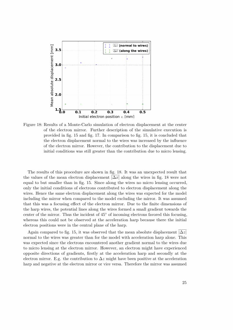
Figure 18: Results of a Monte-Carlo simulation of electron displacement at the centerof the electron mirror. Further description of the simulative execution isprovided in fig. 15 and fig. 17. In comparison to fig. 15, it is concluded thatthe electron displacement normal to the wires was increased by the influenceof the electron mirror. However, the contribution to the displacement due toinitial conditions was still greater than the contribution due to micro lensing.

The results of this procedure are shown in fig. 18. It was an unexpected result thatthe values of the mean electron displacement |∆x| along the wires in fig. 18 were notequal to but smaller than in fig. 15. Since along the wires no micro lensing occurred,only the initial conditions of electrons contributed to electron displacement along thewires. Hence the same electron displacement along the wires was expected for the modelincluding the mirror when compared to the model excluding the mirror. It was assumedthat this was a focusing effect of the electron mirror. Due to the finite dimensions ofthe harp wires, the potential lines along the wires formed a small gradient towards thecenter of the mirror. Thus the incident of 45 of incoming electrons favored this focusing,whereas this could not be observed at the acceleration harp because there the initialelectron positions were in the central plane of the harp.

Again compared to fig. 15, it was observed that the mean absolute displacement |∆z|normal to the wires was greater than for the model with acceleration harp alone. Thiswas expected since the electrons encountered another gradient normal to the wires dueto micro lensing at the electron mirror. However, an electron might have experiencedopposite directions of gradients, firstly at the acceleration harp and secondly at theelectron mirror. E.g. the contribution to ∆z might have been positive at the accelerationharp and negative at the electron mirror or vice versa. Therefore the mirror was assumed

25

to propagate the electron displacement not only by an increase of ∆z but also by adecrease of ∆z. The ratio of increment and decrement of ∆z by this propagation wasassumed to be dependent on the initial electron position zi. This is indicated by thevariation of increment of |∆z| in fig. 18 when compared to fig. 15. However, subtractingthe mean electron displacements |∆x| and |∆z| from each other, it was still concludedthat the contribution to the displacement due to initial conditions was greater than dueto micro lensing.

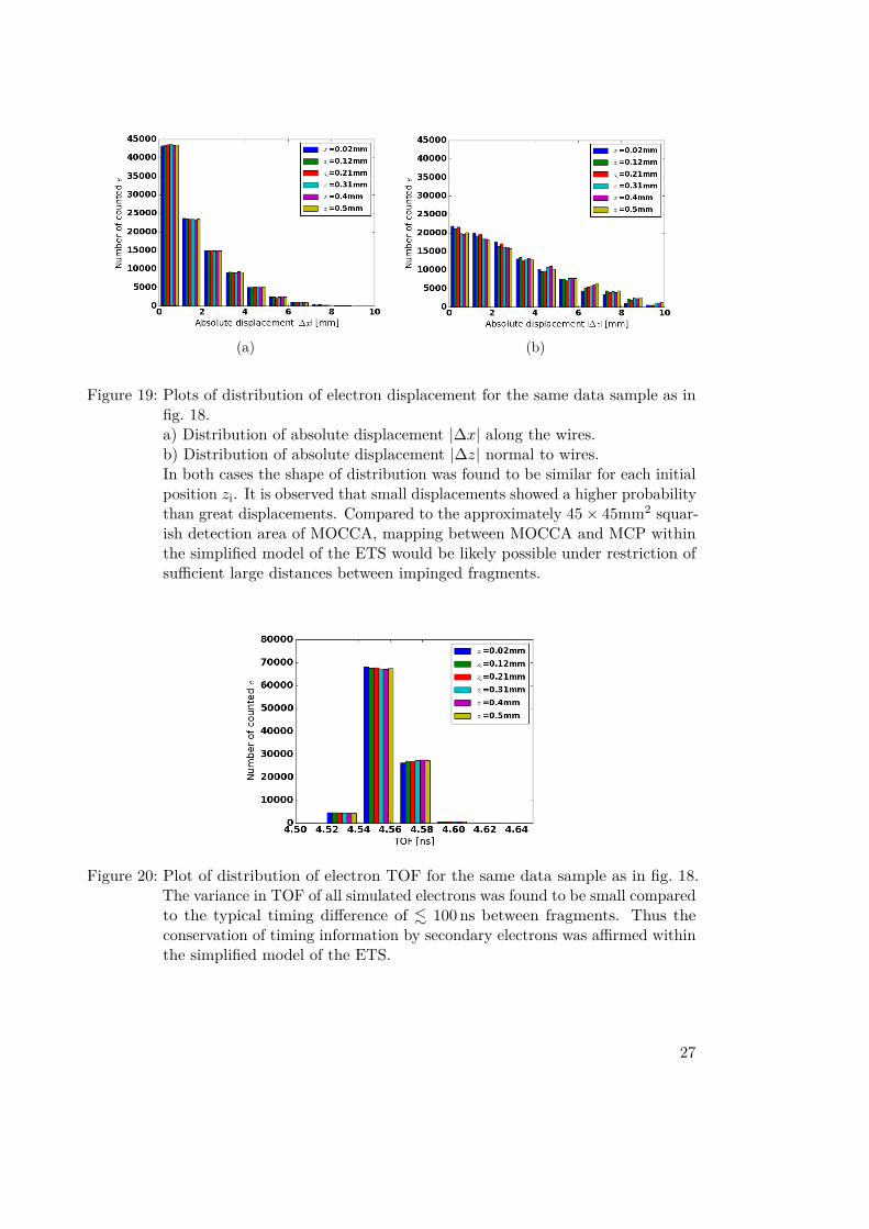
Furthermore, the distribution of electron displacement was examined in order toestimate the possibility of mapping between MOCCA and MCP within the simplifiedmodels of the ETS. Projected at both directions, the distribution of electron displacementis shown in fig. 19 for the same data sample as in fig. 18, namely N = 100 000 electronssimulated each for six initial positions zi. It is observed that the absolute displacement|∆x| along the wires was distributed approximately equally for each initial electronposition zi. This was expected due to the absence of micro lensing in x-direction. Themicro lensing in z-direction lead to small variations in the distributions of absolutedisplacement |∆z| normal to the wires, but the general shape was not affected.For both directions the number of counted electrons monotonically decreased with

increasing electron displacement, thus small displacements were more likely than greatdisplacements. This decrement was stronger along the wires and more electrons werecounted for |∆x| ≤ 2 mm than for |∆z| ≤ 2 mm. Furthermore, for both directionsthe number of electrons with a displacement greater than 8 mm was negligibly small.Compared to the length of approximately 45 mm of the squarish detection area of MOCCA,it was therefore concluded that a mapping process between secondary electrons at MCPand fragments at MOCCA would have been likely possible within the simplifications ofthe modeled ETS. This was restricted by sufficient large distances between the impingedfragments. For a typical event, minimal distances of fragments in the regime of 3.4 mmalong the wires and 6.6 mm normal to wires would have been expected to lead to asuccessful assignment in most cases. These values were estimated as twice the maximummean absolute displacement of electrons from fig. 18.

Moreover, the distribution of TOF of electrons was examined in order to judge whetherthe timing information of fragments are conserved by secondary electrons within thesimplified models of the ETS. This distribution of electron TOF is shown in fig. 20. Firstly,the distribution of TOF was found to be similar for each initial position. Secondly, almostall electrons had a TOF in the range of 4.54 ns to 4.59 ns. From this it is concluded thatneither the micro lensing nor the initial conditions of secondary electrons had a majorinfluence on the TOF. Furthermore, this affirmed the conservation of timing informationwithin the simplified model of the ETS, because the variance in electron TOF was smallcompared to the typical relative timing difference of . 100 ns between fragments (cf.section 1.2).As a result from simulations within a simplified model, the working principle of the

ETS could be affirmed. This gave rise to the design of a realistic model of the ETS, inorder to reaffirm the working principle of the ETS under realistic conditions. This willbe discussed in the following section, using the knowledge gained from this section.

26

(a) (b)

Figure 19: Plots of distribution of electron displacement for the same data sample as infig. 18.a) Distribution of absolute displacement |∆x| along the wires.b) Distribution of absolute displacement |∆z| normal to wires.In both cases the shape of distribution was found to be similar for each initialposition zi. It is observed that small displacements showed a higher probabilitythan great displacements. Compared to the approximately 45× 45mm2 squar-ish detection area of MOCCA, mapping between MOCCA and MCP withinthe simplified model of the ETS would be likely possible under restriction ofsufficient large distances between impinged fragments.

Figure 20: Plot of distribution of electron TOF for the same data sample as in fig. 18.The variance in TOF of all simulated electrons was found to be small comparedto the typical timing difference of . 100 ns between fragments. Thus theconservation of timing information by secondary electrons was affirmed withinthe simplified model of the ETS.

27

4 Analysis of a Realistic Electron Transport System

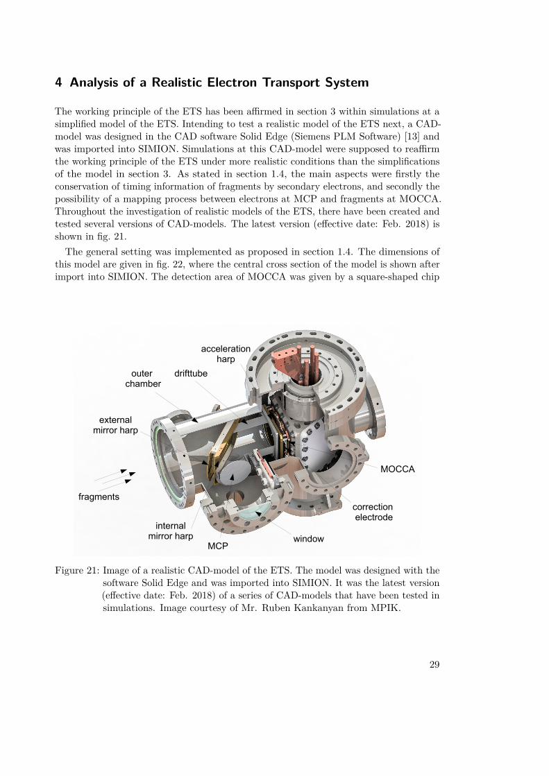
The working principle of the ETS has been affirmed in section 3 within simulations at asimplified model of the ETS. Intending to test a realistic model of the ETS next, a CAD-model was designed in the CAD software Solid Edge (Siemens PLM Software) [13] andwas imported into SIMION. Simulations at this CAD-model were supposed to reaffirmthe working principle of the ETS under more realistic conditions than the simplificationsof the model in section 3. As stated in section 1.4, the main aspects were firstly theconservation of timing information of fragments by secondary electrons, and secondly thepossibility of a mapping process between electrons at MCP and fragments at MOCCA.Throughout the investigation of realistic models of the ETS, there have been created andtested several versions of CAD-models. The latest version (effective date: Feb. 2018) isshown in fig. 21.The general setting was implemented as proposed in section 1.4. The dimensions of

this model are given in fig. 22, where the central cross section of the model is shown afterimport into SIMION. The detection area of MOCCA was given by a square-shaped chip

MCPwindow

MOCCA

fragments

internalmirror harp

externalmirror harp

outer chamber

drifttube

accelerationharp

correction electrode

Figure 21: Image of a realistic CAD-model of the ETS. The model was designed with thesoftware Solid Edge and was imported into SIMION. It was the latest version(effective date: Feb. 2018) of a series of CAD-models that have been tested insimulations. Image courtesy of Mr. Ruben Kankanyan from MPIK.

29

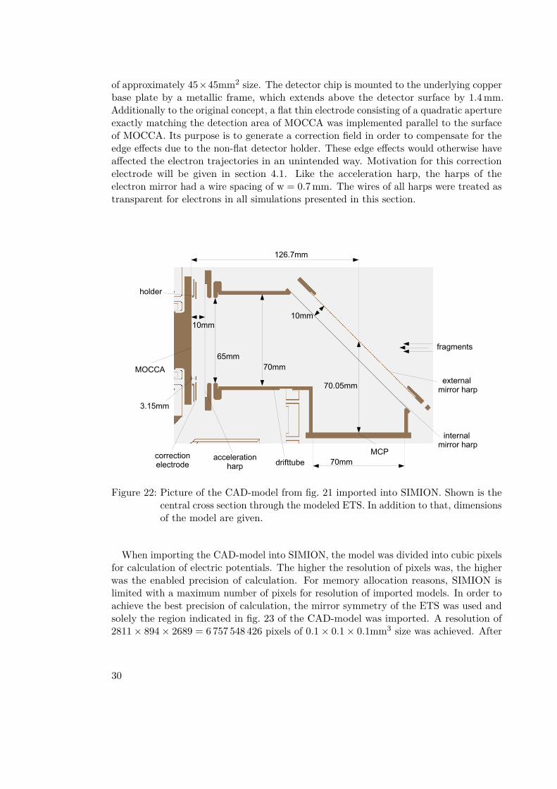
of approximately 45×45mm2 size. The detector chip is mounted to the underlying copperbase plate by a metallic frame, which extends above the detector surface by 1.4 mm.Additionally to the original concept, a flat thin electrode consisting of a quadratic apertureexactly matching the detection area of MOCCA was implemented parallel to the surfaceof MOCCA. Its purpose is to generate a correction field in order to compensate for theedge effects due to the non-flat detector holder. These edge effects would otherwise haveaffected the electron trajectories in an unintended way. Motivation for this correctionelectrode will be given in section 4.1. Like the acceleration harp, the harps of theelectron mirror had a wire spacing of w = 0.7 mm. The wires of all harps were treated astransparent for electrons in all simulations presented in this section.

MOCCA

holder

correctionelectrode

accelerationharp drifttube

MCP

external mirror harp

internal mirror harp

126.7mm

70.05mm

70mm

70mm65mm

10mm10mm

3.15mm

fragments

Figure 22: Picture of the CAD-model from fig. 21 imported into SIMION. Shown is thecentral cross section through the modeled ETS. In addition to that, dimensionsof the model are given.

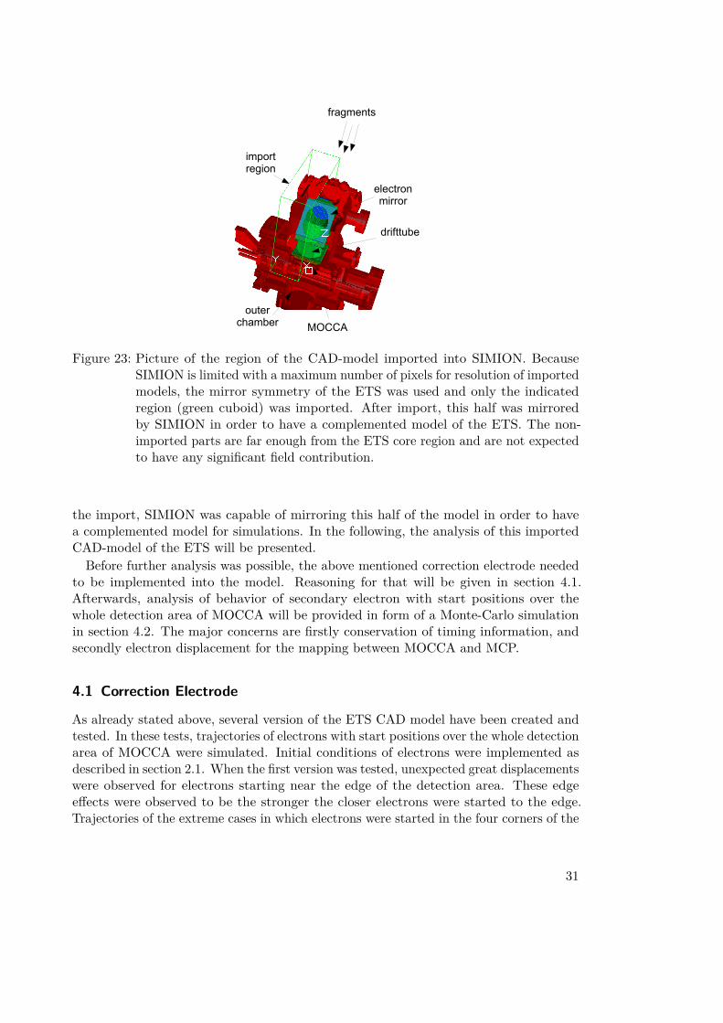
When importing the CAD-model into SIMION, the model was divided into cubic pixelsfor calculation of electric potentials. The higher the resolution of pixels was, the higherwas the enabled precision of calculation. For memory allocation reasons, SIMION islimited with a maximum number of pixels for resolution of imported models. In order toachieve the best precision of calculation, the mirror symmetry of the ETS was used andsolely the region indicated in fig. 23 of the CAD-model was imported. A resolution of2811× 894× 2689 = 6 757 548 426 pixels of 0.1× 0.1× 0.1mm3 size was achieved. After

30

fragments

MOCCA

drifttube

electronmirror

importregion

outerchamber

Figure 23: Picture of the region of the CAD-model imported into SIMION. BecauseSIMION is limited with a maximum number of pixels for resolution of importedmodels, the mirror symmetry of the ETS was used and only the indicatedregion (green cuboid) was imported. After import, this half was mirroredby SIMION in order to have a complemented model of the ETS. The non-imported parts are far enough from the ETS core region and are not expectedto have any significant field contribution.

the import, SIMION was capable of mirroring this half of the model in order to havea complemented model for simulations. In the following, the analysis of this importedCAD-model of the ETS will be presented.

Before further analysis was possible, the above mentioned correction electrode neededto be implemented into the model. Reasoning for that will be given in section 4.1.Afterwards, analysis of behavior of secondary electron with start positions over thewhole detection area of MOCCA will be provided in form of a Monte-Carlo simulationin section 4.2. The major concerns are firstly conservation of timing information, andsecondly electron displacement for the mapping between MOCCA and MCP.

4.1 Correction Electrode

As already stated above, several version of the ETS CAD model have been created andtested. In these tests, trajectories of electrons with start positions over the whole detectionarea of MOCCA were simulated. Initial conditions of electrons were implemented asdescribed in section 2.1. When the first version was tested, unexpected great displacementswere observed for electrons starting near the edge of the detection area. These edgeeffects were observed to be the stronger the closer electrons were started to the edge.Trajectories of the extreme cases in which electrons were started in the four corners of the

31

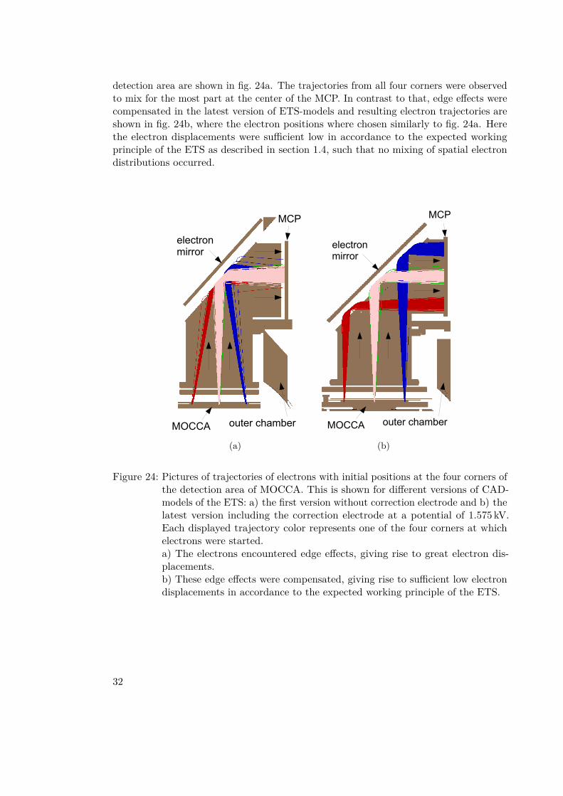
detection area are shown in fig. 24a. The trajectories from all four corners were observedto mix for the most part at the center of the MCP. In contrast to that, edge effects werecompensated in the latest version of ETS-models and resulting electron trajectories areshown in fig. 24b, where the electron positions where chosen similarly to fig. 24a. Herethe electron displacements were sufficient low in accordance to the expected workingprinciple of the ETS as described in section 1.4, such that no mixing of spatial electrondistributions occurred.

MOCCA outer chamber

electronmirror

MCP

(a)

MOCCA outer chamber

electronmirror

MCP

(b)

Figure 24: Pictures of trajectories of electrons with initial positions at the four corners ofthe detection area of MOCCA. This is shown for different versions of CAD-models of the ETS: a) the first version without correction electrode and b) thelatest version including the correction electrode at a potential of 1.575 kV.Each displayed trajectory color represents one of the four corners at whichelectrons were started.a) The electrons encountered edge effects, giving rise to great electron dis-placements.b) These edge effects were compensated, giving rise to sufficient low electrondisplacements in accordance to the expected working principle of the ETS.

32

holder

acceleration harp

detection chipof MOCCA

(a)

holderdetection chipof MOCCA

acceleration harp

correction electrode

(b)

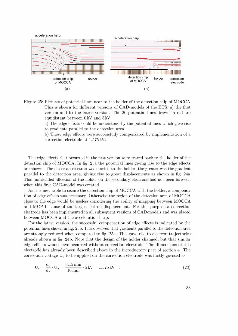
Figure 25: Pictures of potential lines near to the holder of the detection chip of MOCCA.This is shown for different versions of CAD-models of the ETS: a) the firstversion and b) the latest version. The 20 potential lines drawn in red areequidistant between 0 kV and 5 kV.a) The edge effects could be understood by the potential lines which gave riseto gradients parallel to the detection area.b) These edge effects were successfully compensated by implementation of acorrection electrode at 1.575 kV.

The edge effects that occurred in the first version were traced back to the holder of thedetection chip of MOCCA. In fig. 25a the potential lines giving rise to the edge effectsare shown. The closer an electron was started to the holder, the greater was the gradientparallel to the detection area, giving rise to great displacements as shown in fig. 24a.This unintended affection of the holder on the secondary electrons had not been foreseenwhen this first CAD-model was created.

As it is inevitable to secure the detection chip of MOCCA with the holder, a compensa-tion of edge effects was necessary. Otherwise the region of the detection area of MOCCAclose to the edge would be useless considering the ability of mapping between MOCCAand MCP because of too large electron displacement. For this purpose a correctionelectrode has been implemented in all subsequent versions of CAD-models and was placedbetween MOCCA and the acceleration harp.For the latest version, the successful compensation of edge effects is indicated by the

potential lines shown in fig. 25b. It is observed that gradients parallel to the detection areaare strongly reduced when compared to fig. 25a. This gave rise to electron trajectoriesalready shown in fig. 24b. Note that the design of the holder changed, but that similaredge effects would have occurred without correction electrode. The dimensions of thiselectrode has already been described above in the introductory part of section 4. Thecorrection voltage Uc to be applied on the correction electrode was firstly guessed as

Uc = dcda·Ua = 3.15 mm

10 mm · 5 kV = 1.575 kV . (23)

33

Here dc is the distance between MOCCA and correction electrode, da is the distancebetween MOCCA and acceleration harp, and Ua is the potential applied on the accelera-tion harp. When the estimated potential of Uc = 1.575 kV was applied on the correctionelectrode at simulations of the latest version of the CAD-model, small edge effects werestill noticed for evaluation of the electron displacement. This correction potential Uc wastherefore kept as an adjustment parameter in order to minimize such edge effects. Afterthe issue of correcting the electric field of the ETS near to the holder of MOCCA hadbeen solved, further investigation of the ETS was performed by simulation of electrontrajectories at this latest version of the CAD-model. For this simulation presented inthe following, a correction voltage of Uc = 1.77 kV was chosen, because this showed thesmallest edge effects.

4.2 Main Analysis

In this section the main analysis of the latest version of realistic models of the ETS ispresented. The method of evaluating the accomplished simulation will be described insection 4.2.1. Considering the timing information, the distribution of TOF of electronswill be discussed in section 4.2.2. Considering the possibility of mapping, the electrondisplacement will be discussed in section 4.2.3. The realistic model has already beendescribed in the introductory part of section 4.

4.2.1 Evaluation Method for Monte-Carlo Simulation

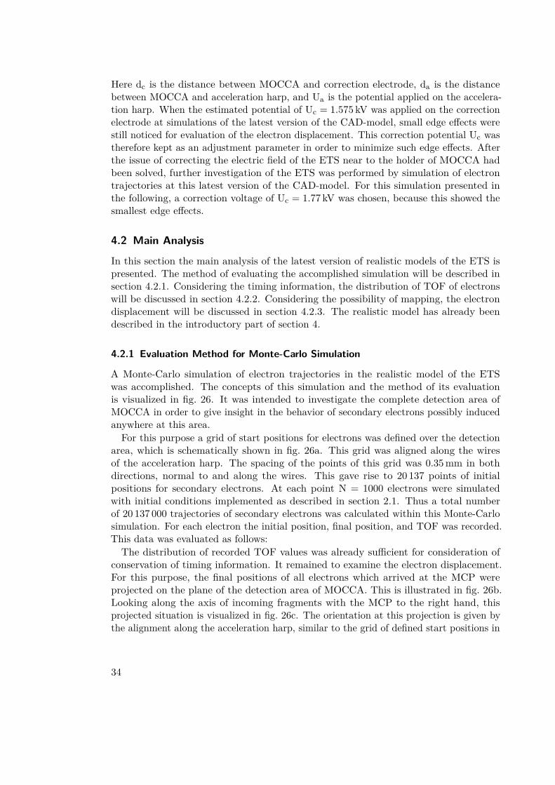
A Monte-Carlo simulation of electron trajectories in the realistic model of the ETSwas accomplished. The concepts of this simulation and the method of its evaluationis visualized in fig. 26. It was intended to investigate the complete detection area ofMOCCA in order to give insight in the behavior of secondary electrons possibly inducedanywhere at this area.For this purpose a grid of start positions for electrons was defined over the detection

area, which is schematically shown in fig. 26a. This grid was aligned along the wiresof the acceleration harp. The spacing of the points of this grid was 0.35 mm in bothdirections, normal to and along the wires. This gave rise to 20 137 points of initialpositions for secondary electrons. At each point N = 1000 electrons were simulatedwith initial conditions implemented as described in section 2.1. Thus a total numberof 20 137 000 trajectories of secondary electrons was calculated within this Monte-Carlosimulation. For each electron the initial position, final position, and TOF was recorded.This data was evaluated as follows:

The distribution of recorded TOF values was already sufficient for consideration ofconservation of timing information. It remained to examine the electron displacement.For this purpose, the final positions of all electrons which arrived at the MCP wereprojected on the plane of the detection area of MOCCA. This is illustrated in fig. 26b.Looking along the axis of incoming fragments with the MCP to the right hand, thisprojected situation is visualized in fig. 26c. The orientation at this projection is given bythe alignment along the acceleration harp, similar to the grid of defined start positions in

34

detection area of MOCCA

45mm

63.6

mm

0.35mm

0.35

mm

1000 e-

per start position

(a)

MCP

MOCCA

projection

fragments

(b)

x

y

MOCCA

MCPprojectionof wires

(c)

𝑟i

x

x

initial position

at MOCCA

δ𝑟 shift

distribution of final

positions at MCP 𝑟f

mean final position

spread

s

𝑟i + δ𝑟

(d)

Figure 26: Illustrations of evaluation method of accomplished Monte-Carlo simulation.a) A grid of start positions for electrons at the detection area of MOCCAwas defined. Note that this scheme is not in scale. For visualization reasonsonly a few start positions are shown. In fact this definition of the grid with aspacing of 0.35 mm between the points gave rise to 20 137 points. For eachpoint N = 1000 electrons were simulated.b) The final positions of electrons at MCP were projected into the plane ofthe detection area of MOCCA, such that both detection areas of MCP andMOCCA would share the same center.c) Perspective of the projection in b) when looking along the blue arrow in b).The orientation in this view is given by the two directions x, along the wires,and y, normal to wires of the acceleration harp. The wires are indicated bythe black parallel stripes.d) In the view of c), the electron displacement was divided into two quantities,namely shift and spread. Their definitions are mathematically given in thetext.

35

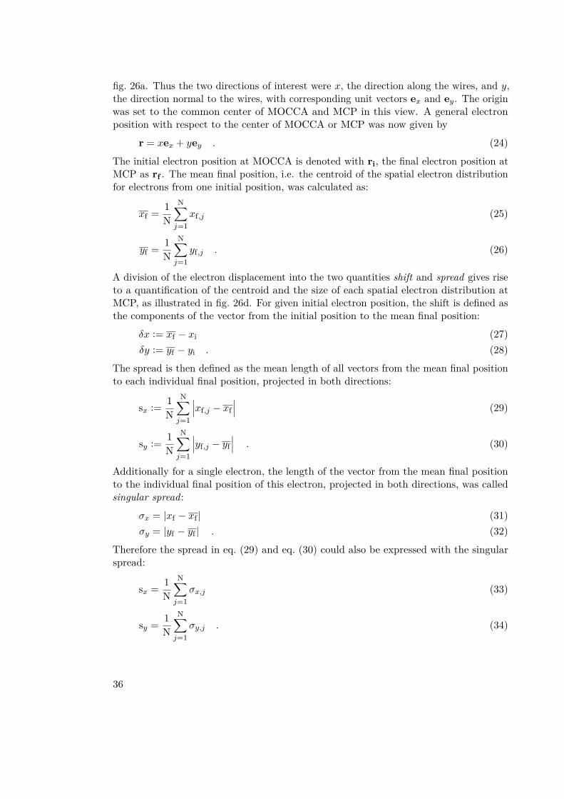
fig. 26a. Thus the two directions of interest were x, the direction along the wires, and y,the direction normal to the wires, with corresponding unit vectors ex and ey. The originwas set to the common center of MOCCA and MCP in this view. A general electronposition with respect to the center of MOCCA or MCP was now given by

r = xex + yey . (24)

The initial electron position at MOCCA is denoted with ri, the final electron position atMCP as rf . The mean final position, i.e. the centroid of the spatial electron distributionfor electrons from one initial position, was calculated as:

xf = 1N

N∑j=1

xf,j (25)

yf = 1N

N∑j=1

yf,j . (26)

A division of the electron displacement into the two quantities shift and spread gives riseto a quantification of the centroid and the size of each spatial electron distribution atMCP, as illustrated in fig. 26d. For given initial electron position, the shift is defined asthe components of the vector from the initial position to the mean final position:

δx := xf − xi (27)δy := yf − yi . (28)

The spread is then defined as the mean length of all vectors from the mean final positionto each individual final position, projected in both directions:

sx := 1N

N∑j=1

∣∣∣xf,j − xf∣∣∣ (29)

sy := 1N

N∑j=1

∣∣∣yf,j − yf∣∣∣ . (30)

Additionally for a single electron, the length of the vector from the mean final positionto the individual final position of this electron, projected in both directions, was calledsingular spread:

σx = |xf − xf | (31)σy = |yf − yf | . (32)

Therefore the spread in eq. (29) and eq. (30) could also be expressed with the singularspread:

sx = 1N

N∑j=1

σx,j (33)

sy = 1N

N∑j=1

σy,j . (34)

36

The results of the evaluation of the accomplished Monte-Carlo simulation with the justdescribed method is presented in the following.

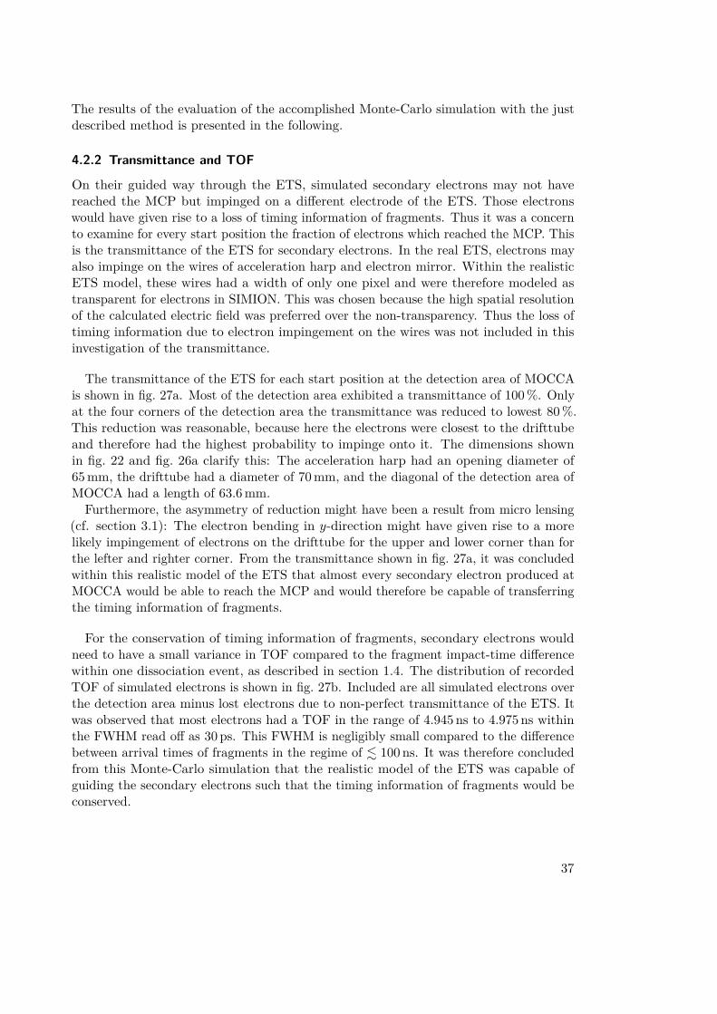
4.2.2 Transmittance and TOF

On their guided way through the ETS, simulated secondary electrons may not havereached the MCP but impinged on a different electrode of the ETS. Those electronswould have given rise to a loss of timing information of fragments. Thus it was a concernto examine for every start position the fraction of electrons which reached the MCP. Thisis the transmittance of the ETS for secondary electrons. In the real ETS, electrons mayalso impinge on the wires of acceleration harp and electron mirror. Within the realisticETS model, these wires had a width of only one pixel and were therefore modeled astransparent for electrons in SIMION. This was chosen because the high spatial resolutionof the calculated electric field was preferred over the non-transparency. Thus the loss oftiming information due to electron impingement on the wires was not included in thisinvestigation of the transmittance.

The transmittance of the ETS for each start position at the detection area of MOCCAis shown in fig. 27a. Most of the detection area exhibited a transmittance of 100 %. Onlyat the four corners of the detection area the transmittance was reduced to lowest 80 %.This reduction was reasonable, because here the electrons were closest to the drifttubeand therefore had the highest probability to impinge onto it. The dimensions shownin fig. 22 and fig. 26a clarify this: The acceleration harp had an opening diameter of65 mm, the drifttube had a diameter of 70 mm, and the diagonal of the detection area ofMOCCA had a length of 63.6 mm.

Furthermore, the asymmetry of reduction might have been a result from micro lensing(cf. section 3.1): The electron bending in y-direction might have given rise to a morelikely impingement of electrons on the drifttube for the upper and lower corner than forthe lefter and righter corner. From the transmittance shown in fig. 27a, it was concludedwithin this realistic model of the ETS that almost every secondary electron produced atMOCCA would be able to reach the MCP and would therefore be capable of transferringthe timing information of fragments.

For the conservation of timing information of fragments, secondary electrons wouldneed to have a small variance in TOF compared to the fragment impact-time differencewithin one dissociation event, as described in section 1.4. The distribution of recordedTOF of simulated electrons is shown in fig. 27b. Included are all simulated electrons overthe detection area minus lost electrons due to non-perfect transmittance of the ETS. Itwas observed that most electrons had a TOF in the range of 4.945 ns to 4.975 ns withinthe FWHM read off as 30 ps. This FWHM is negligibly small compared to the differencebetween arrival times of fragments in the regime of . 100 ns. It was therefore concludedfrom this Monte-Carlo simulation that the realistic model of the ETS was capable ofguiding the secondary electrons such that the timing information of fragments would beconserved.

37

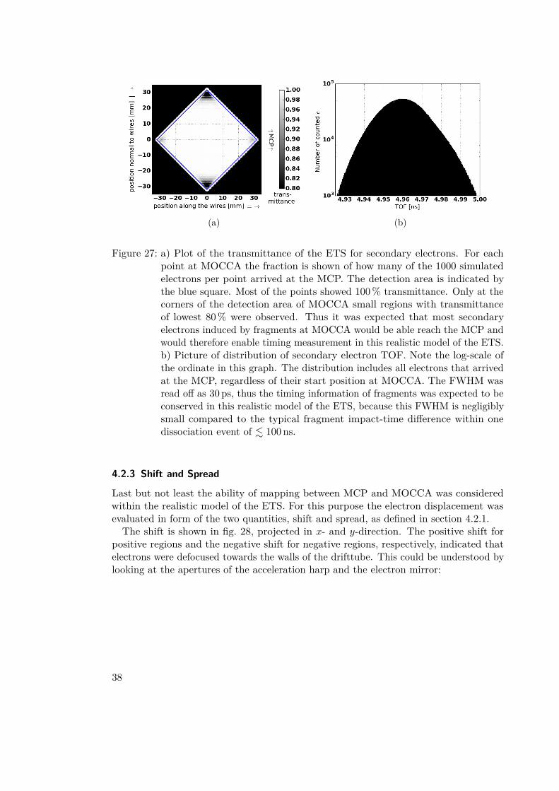
(a) (b)

Figure 27: a) Plot of the transmittance of the ETS for secondary electrons. For eachpoint at MOCCA the fraction is shown of how many of the 1000 simulatedelectrons per point arrived at the MCP. The detection area is indicated bythe blue square. Most of the points showed 100 % transmittance. Only at thecorners of the detection area of MOCCA small regions with transmittanceof lowest 80 % were observed. Thus it was expected that most secondaryelectrons induced by fragments at MOCCA would be able reach the MCP andwould therefore enable timing measurement in this realistic model of the ETS.b) Picture of distribution of secondary electron TOF. Note the log-scale ofthe ordinate in this graph. The distribution includes all electrons that arrivedat the MCP, regardless of their start position at MOCCA. The FWHM wasread off as 30 ps, thus the timing information of fragments was expected to beconserved in this realistic model of the ETS, because this FWHM is negligiblysmall compared to the typical fragment impact-time difference within onedissociation event of . 100 ns.

4.2.3 Shift and Spread

Last but not least the ability of mapping between MCP and MOCCA was consideredwithin the realistic model of the ETS. For this purpose the electron displacement wasevaluated in form of the two quantities, shift and spread, as defined in section 4.2.1.The shift is shown in fig. 28, projected in x- and y-direction. The positive shift for

positive regions and the negative shift for negative regions, respectively, indicated thatelectrons were defocused towards the walls of the drifttube. This could be understood bylooking at the apertures of the acceleration harp and the electron mirror:

38

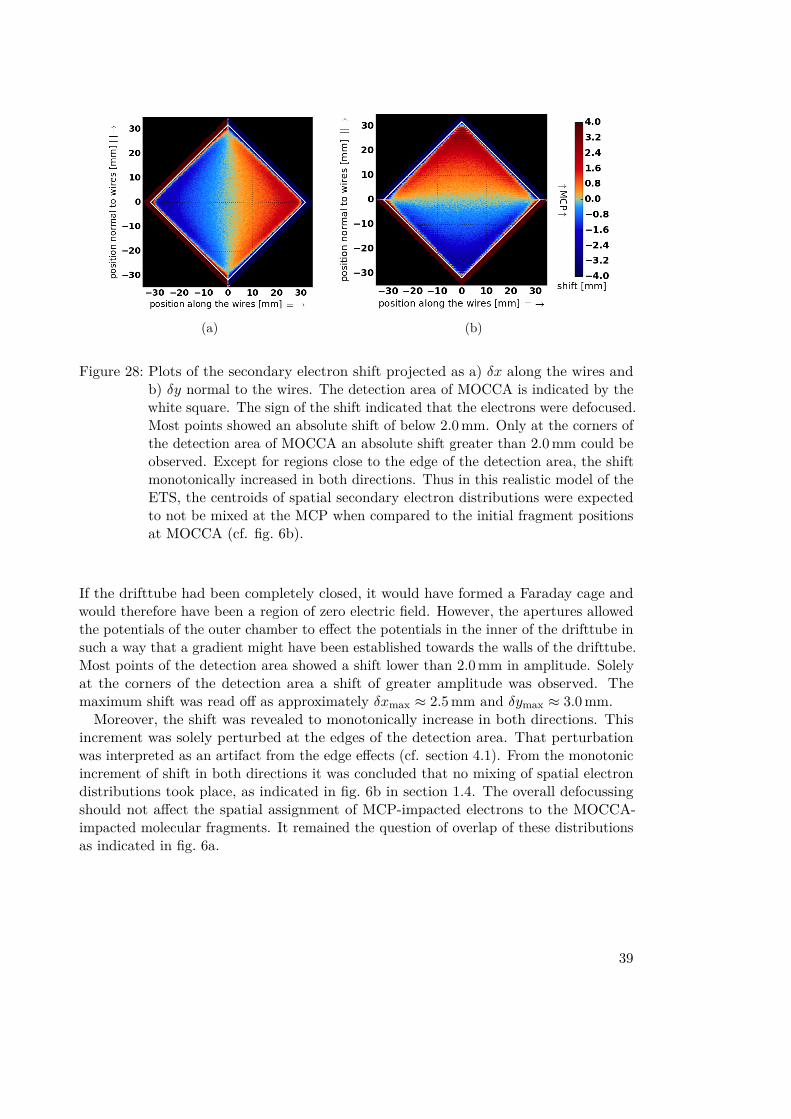
(a) (b)

Figure 28: Plots of the secondary electron shift projected as a) δx along the wires andb) δy normal to the wires. The detection area of MOCCA is indicated by thewhite square. The sign of the shift indicated that the electrons were defocused.Most points showed an absolute shift of below 2.0 mm. Only at the corners ofthe detection area of MOCCA an absolute shift greater than 2.0 mm could beobserved. Except for regions close to the edge of the detection area, the shiftmonotonically increased in both directions. Thus in this realistic model of theETS, the centroids of spatial secondary electron distributions were expectedto not be mixed at the MCP when compared to the initial fragment positionsat MOCCA (cf. fig. 6b).

If the drifttube had been completely closed, it would have formed a Faraday cage andwould therefore have been a region of zero electric field. However, the apertures allowedthe potentials of the outer chamber to effect the potentials in the inner of the drifttube insuch a way that a gradient might have been established towards the walls of the drifttube.Most points of the detection area showed a shift lower than 2.0 mm in amplitude. Solelyat the corners of the detection area a shift of greater amplitude was observed. Themaximum shift was read off as approximately δxmax ≈ 2.5 mm and δymax ≈ 3.0 mm.Moreover, the shift was revealed to monotonically increase in both directions. This

increment was solely perturbed at the edges of the detection area. That perturbationwas interpreted as an artifact from the edge effects (cf. section 4.1). From the monotonicincrement of shift in both directions it was concluded that no mixing of spatial electrondistributions took place, as indicated in fig. 6b in section 1.4. The overall defocussingshould not affect the spatial assignment of MCP-impacted electrons to the MOCCA-impacted molecular fragments. It remained the question of overlap of these distributionsas indicated in fig. 6a.

39

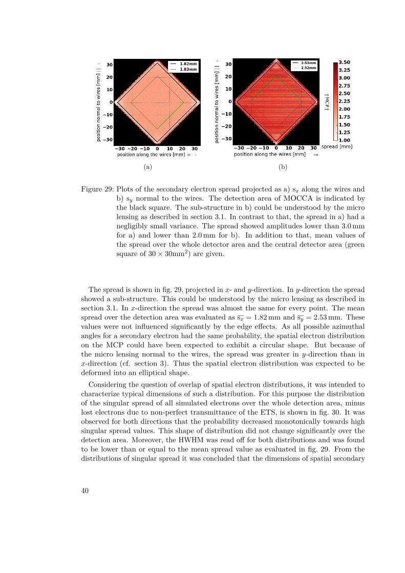
(a) (b)

Figure 29: Plots of the secondary electron spread projected as a) sx along the wires andb) sy normal to the wires. The detection area of MOCCA is indicated bythe black square. The sub-structure in b) could be understood by the microlensing as described in section 3.1. In contrast to that, the spread in a) had anegligibly small variance. The spread showed amplitudes lower than 3.0 mmfor a) and lower than 2.0 mm for b). In addition to that, mean values ofthe spread over the whole detector area and the central detector area (greensquare of 30× 30mm2) are given.

The spread is shown in fig. 29, projected in x- and y-direction. In y-direction the spreadshowed a sub-structure. This could be understood by the micro lensing as described insection 3.1. In x-direction the spread was almost the same for every point. The meanspread over the detection area was evaluated as sx = 1.82 mm and sy = 2.53 mm. Thesevalues were not influenced significantly by the edge effects. As all possible azimuthalangles for a secondary electron had the same probability, the spatial electron distributionon the MCP could have been expected to exhibit a circular shape. But because ofthe micro lensing normal to the wires, the spread was greater in y-direction than inx-direction (cf. section 3). Thus the spatial electron distribution was expected to bedeformed into an elliptical shape.

Considering the question of overlap of spatial electron distributions, it was intended tocharacterize typical dimensions of such a distribution. For this purpose the distributionof the singular spread of all simulated electrons over the whole detection area, minuslost electrons due to non-perfect transmittance of the ETS, is shown in fig. 30. It wasobserved for both directions that the probability decreased monotonically towards highsingular spread values. This shape of distribution did not change significantly over thedetection area. Moreover, the HWHM was read off for both distributions and was foundto be lower than or equal to the mean spread value as evaluated in fig. 29. From thedistributions of singular spread it was concluded that the dimensions of spatial secondary

40

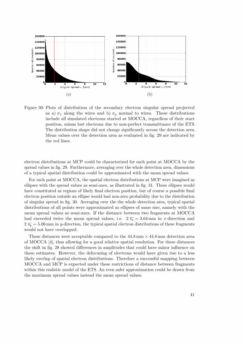
(a) (b)

Figure 30: Plots of distribution of the secondary electron singular spread projectedas a) σx along the wires and b) σy normal to wires. These distributionsinclude all simulated electrons started at MOCCA, regardless of their startposition, minus lost electrons due to non-perfect transmittance of the ETS.The distribution shape did not change significantly across the detection area.Mean values over the detection area as evaluated in fig. 29 are indicated bythe red lines.

electron distributions at MCP could be characterized for each point at MOCCA by thespread values in fig. 29. Furthermore, averaging over the whole detection area, dimensionsof a typical spatial distribution could be approximated with the mean spread values.

For each point at MOCCA, the spatial electron distributions at MCP were imagined asellipses with the spread values as semi-axes, as illustrated in fig. 31. These ellipses wouldhave constituted as regions of likely final electron position, but of course a possible finalelectron position outside an ellipse would had non-zero probability due to the distributionof singular spread in fig. 30. Averaging over the the whole detection area, typical spatialdistributions of all points were approximated as ellipses of same size, namely with themean spread values as semi-axes. If the distance between two fragments at MOCCAhad exceeded twice the mean spread values, i.e. 2 sx = 3.64 mm in x-direction and2 sy = 5.06 mm in y-direction, the typical spatial electron distributions of these fragmentswould not have overlapped.

These distances were acceptable compared to the 44.8 mm× 44.8 mm detection areaof MOCCA [4], thus allowing for a good relative spatial resolution. For these distancesthe shift in fig. 28 showed differences in amplitudes that could have minor influence onthese estimates. However, the defocusing of electrons would have given rise to a lesslikely overlap of spatial electron distributions. Therefore a successful mapping betweenMOCCA and MCP is expected under these restrictions of distance between fragmentswithin this realistic model of the ETS. An even safer approximation could be drawn fromthe maximum spread values instead the mean spread values.

41

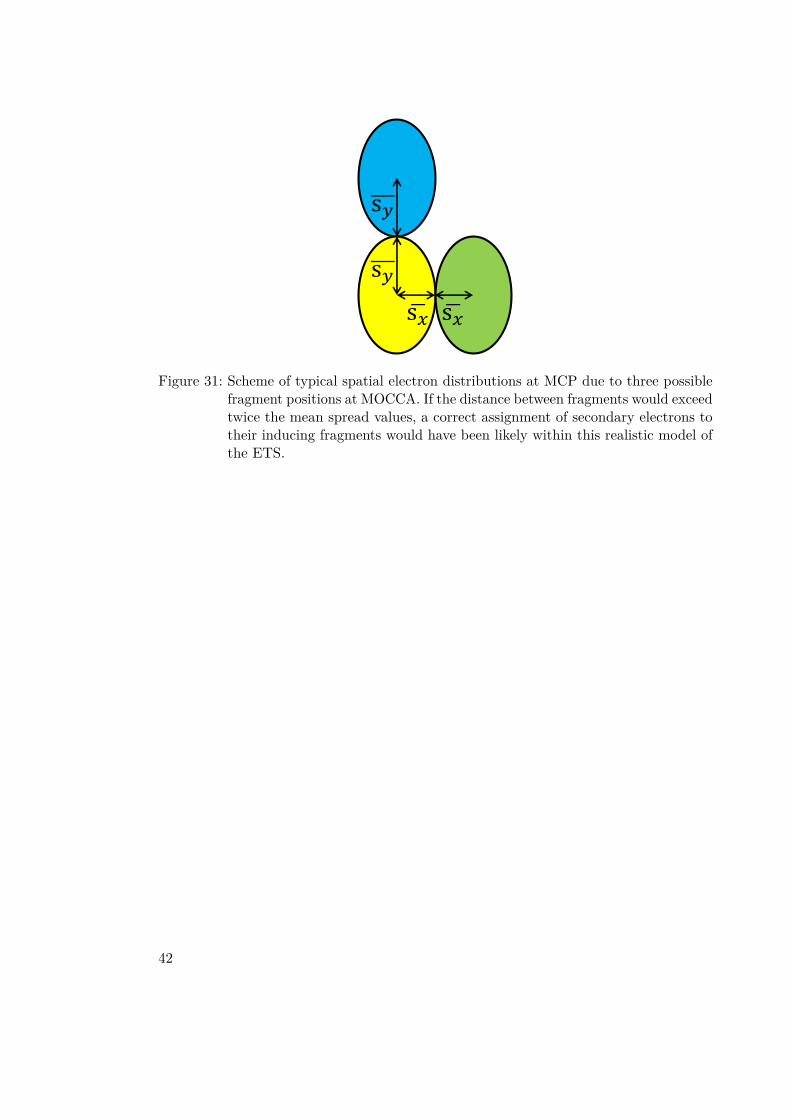
s𝑥 s𝑥

s𝑦

s𝑦

Figure 31: Scheme of typical spatial electron distributions at MCP due to three possiblefragment positions at MOCCA. If the distance between fragments would exceedtwice the mean spread values, a correct assignment of secondary electrons totheir inducing fragments would have been likely within this realistic model ofthe ETS.

42

5 Conclusion and OutlookIn this thesis simulations of an electron transport system (ETS) for the MOCCA detectorat CSR have been presented and discussed. The purpose of the ETS is to guide secondaryelectrons, induced by electrically neutral molecular fragments impinging on the micro-calorimeter detector MOCCA, towards a fast-timing detector. This allows reading outthe relative impact times between the fragments and thus enables 3D fragment-imagingfor the MOCCA detector. The electrons are supposed to transfer the impact timingdifference of fragments onto the fast-timing detector - an MCP. This transfer is successfulif firstly the relative timing information of fragments is conserved by the electrons and ifsecondly the electrons can be assigned to their respective inducing fragments. The goalof this thesis has been to provide a feasibility study of the ETS by addressing these twomajor questions, as stated in section 1.4.

Accomplished simulations within a simplified model of the ETS as described in section 3qualitatively approved the working principle of the ETS. This led to simulations of adetailed, realistic model of the ETS as described in section 4. In these simulations thetrajectories of electrons emitted at all possible positions within the detection area ofMOCCA were calculated. Initial conditions for secondary electrons have been randomizedfollowing realistic distributions of kinetic energy and polar angle towards the normaldetector surface, as described in section 2.1. Recording the final position and TOF ofelectrons when they arrived at the MCP gave rise to the following results: The electronTOF values were distributed around 4.96 ns. This distribution showed a FWHM of≈ 30 ps, which is small compared to the typical difference of . 100 ns in arrival times offragments at MOCCA. Therefore conservation of the fragment timing information bysecondary electrons was demonstrated within this realistic model of the ETS.

In addition to that, for each initial electron position at MOCCA the resulting spatialelectron distribution at the MCP, i.e. the distribution of possible final electron positions,was investigated. Each distribution was characterized by its centroid and its size. Theirshape was assumed to be elliptic with an orientation of the semi-minor axis along thewires of the acceleration harp. The defined quantity shift (displacement between initialposition and centroid position) revealed that it does not lead to mixing of spatial electrondistributions of different initial positions.

Considering an overlap of the elliptic spatial distributions, the defined quantity spread(mean distance between centroid and individual final electron position) quantified thesemi-axes of these ellipses for each initial position. Averaging over the whole detectionarea, the mean spread was used as dimensions of typical spatial electron distributions,resulting in sx = 1.82 mm and sy = 2.53 mm for the semi-minor and semi-major axis,respectively. From these results it is concluded that for fragment impact distanceslarger than 2 sx = 3.64 mm along the wires and 2 sy = 5.06 mm normal to the wires, thesecondary electrons, and their timing information, can likely be assigned to their parentfragment impacts. These dimensions, compared to detection area of 44.8 mm× 44.8 mm,result in a good relative spatial resolution of the ETS, which in turn leads to a goodtiming assignment capability of the setup.

43

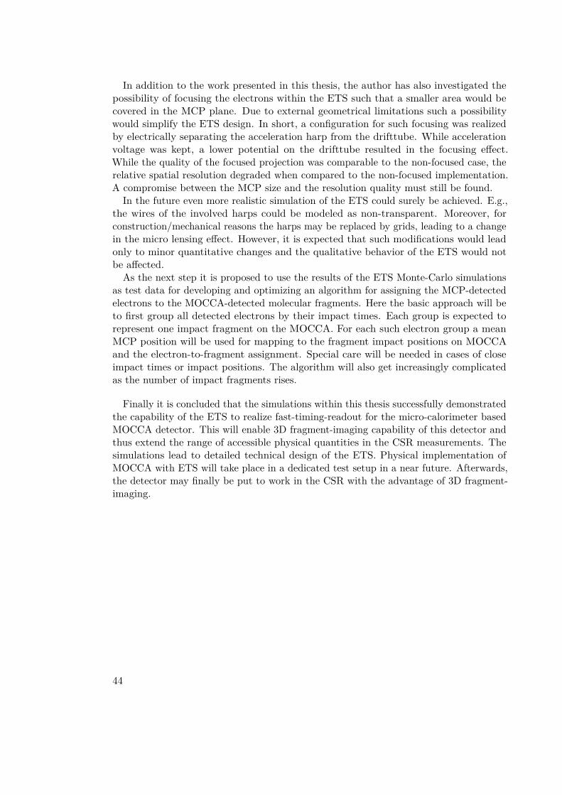
In addition to the work presented in this thesis, the author has also investigated thepossibility of focusing the electrons within the ETS such that a smaller area would becovered in the MCP plane. Due to external geometrical limitations such a possibilitywould simplify the ETS design. In short, a configuration for such focusing was realizedby electrically separating the acceleration harp from the drifttube. While accelerationvoltage was kept, a lower potential on the drifttube resulted in the focusing effect.While the quality of the focused projection was comparable to the non-focused case, therelative spatial resolution degraded when compared to the non-focused implementation.A compromise between the MCP size and the resolution quality must still be found.

In the future even more realistic simulation of the ETS could surely be achieved. E.g.,the wires of the involved harps could be modeled as non-transparent. Moreover, forconstruction/mechanical reasons the harps may be replaced by grids, leading to a changein the micro lensing effect. However, it is expected that such modifications would leadonly to minor quantitative changes and the qualitative behavior of the ETS would notbe affected.

As the next step it is proposed to use the results of the ETS Monte-Carlo simulationsas test data for developing and optimizing an algorithm for assigning the MCP-detectedelectrons to the MOCCA-detected molecular fragments. Here the basic approach will beto first group all detected electrons by their impact times. Each group is expected torepresent one impact fragment on the MOCCA. For each such electron group a meanMCP position will be used for mapping to the fragment impact positions on MOCCAand the electron-to-fragment assignment. Special care will be needed in cases of closeimpact times or impact positions. The algorithm will also get increasingly complicatedas the number of impact fragments rises.

Finally it is concluded that the simulations within this thesis successfully demonstratedthe capability of the ETS to realize fast-timing-readout for the micro-calorimeter basedMOCCA detector. This will enable 3D fragment-imaging capability of this detector andthus extend the range of accessible physical quantities in the CSR measurements. Thesimulations lead to detailed technical design of the ETS. Physical implementation ofMOCCA with ETS will take place in a dedicated test setup in a near future. Afterwards,the detector may finally be put to work in the CSR with the advantage of 3D fragment-imaging.

44

References[1] R. Feynman, R. Leighton, and M. Sands. “The Feynman Lectures on Physics”.

In: vol. I. Basic Books, 1963. Chap. 1 - Atoms in Motion. url: http://www.feynmanlectures.caltech.edu/i_01.html (visited on 09/02/2017).

[2] R. von Hahn et al. “The cryogenic storage ring CSR”. In: Review of ScientificInstruments 87 (2016).

[3] O. Novotný et al. “Cryogenic micro-calorimeters for mass spectrometric identifica-tion of neutral molecules and molecular fragments”. In: Journal of Applied Physics118 (2015).

[4] L. Gamer et al. “MOCCA: A 4k-Pixel Molecule Camera for the Position- andEnergy-Resolving Detection of Neutral Molecule Fragments at CSR”. In: Journalof Low Temperature Physics 184 (2016).

[5] M. De Cesare et al. “A TOF-E detector for ERNA recoil separator”. In: Journal ofthe Italian Astronomical Society 78 (2007).

[6] Homepage of software product SIMION R© by Scientific Instrument Services, Inc.(SIS). url: simion.com (visited on 01/31/2018).

[7] D. Hasselkamp et al. “Particle Induced Electron Emission”. In: vol. II. c©Springer-Verlag Berlin Heidelberg, 1992. Chap. Kinetic Electron Emission from Solid SurfacesUnder Ion Bombardment.

[8] Raúl A. Baragolia. “Principles and mechanisms of ion induced electron emission”.In: Nuclear Instruments and Methods in Physics Research B78 (1993).

[9] D. Hasselkamp, S. Hippler, and A. Scharmann. “Ion-Induced Secondary ElectronSpectra From Clean Metal Surfaces”. In: Nuclear Instruments and Methods inPhysics Research B18 (1987), pp. 561–565.

[10] William H. Press et al. Numerical Recipes: The Art of Scientific Computing. 3rded. New York: Cambridge University Press, 2007.

[11] SIMION R© Version 8.0/8.1 User Manual. Nov. 2011.[12] David J. Griffiths. Introduction to Electrodynamics. 4th ed. Pearson, 2013.[13] Homepage of software product Solid Edge by Siemens PLM Software. url: https:

//www.plm.automation.siemens.com/en/products/solid-edge/ (visited on01/25/2018).

45

ErklärungIch versichere, dass ich diese Arbeit selbstständig verfasst und keine anderen als dieangegebenen Quellen und Hilfsmittel benutzt habe.

Heidelberg, den 18. Februar 2018

Sebastian Spaniol