Seasoning process design optimization for an ascending flow ripening chamber

SEASONING PROCESS DESIGN OPTIMIZATION FOR AN

ASCENDING FLOW RIPENING CHAMBER

Massimo BERTOLINI §, Gino FERRETTI §, Andrea GRASSI ° 1

° Dipartimento di Scienze e Metodi dell’Ingegneria, Facoltà di Ingegneria – Sede di Reggio Emilia, Università degli Studi di Modena e Reggio Emilia, Via Fogliani 1, 42100 Reggio Emilia, Italy

§ Dipartimento di Ingegneria Industriale, Facoltà di Ingegneria, Università degli Studi di Parma, Parco Area delle Scienze 181/A, 43100 Parma, Italy

Abstract

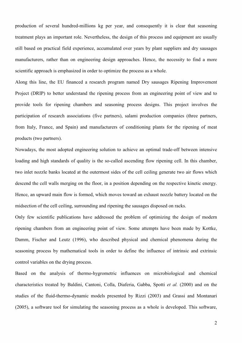
The topic of this project is the extension of the research into salami seasoning plants, with the aim of studying and improving the process from both a microbiological and a physical-chemical point of view. Based on a fluid and thermo-dynamic model of an ascending flow ripening chamber previously developed, in this paper a software for simulating the ripening process as a whole is presented. Moreover, data obtained in an experimental campaign is used to calibrate and validate the model, with the aim to obtain a flexible tool for supporting the cell design and the seasoning process as a whole, both in quantitative and qualitative terms, as a function of the boundary conditions inputted by the user. The results of the model match well with the experimental data taken from several seasoning campaigns involving different types of salami. The analysis of the variation in entering air flow conditions made it then possible to find a particular configuration which optimizes the seasoning process from the product uniformity point of view.

Keywords: ascending flow ripening chamber, sausages seasoning, sausages drying modeling, validation, simulation.

1 Corresponding author: e-mail: [email protected] tel. +39 0522 522624 fax. +39 0522 522609

SEASONING PROCESS DESIGN OPTIMIZATION FOR AN

ASCENDING FLOW RIPENING CHAMBER

Abstract

The topic of this project is the extension of the research into salami seasoning plants, with the aim of

studying and improving the process from both a microbiological and a physical-chemical point of

view.

Based on a fluid and thermo-dynamic model of an ascending flow ripening chamber previously

developed, in this paper a software for simulating the ripening process as a whole is presented.

Moreover, data obtained in an experimental campaign is used to calibrate and validate the model, with

the aim to obtain a flexible tool for supporting the cell design and the seasoning process as a whole,

both in quantitative and qualitative terms, as a function of the boundary conditions inputted by the

user. The results of the model match well with the experimental data taken from several seasoning

campaigns involving different types of salami. The analysis of the variation in entering air flow

conditions made it then possible to find a particular configuration which optimizes the seasoning

process from the product uniformity point of view.

Keywords: ascending flow ripening chamber, sausages seasoning, sausages drying modeling,

validation, simulation.

1. Introduction

Seasoning is one of the oldest techniques man has adopted to conserve meat for a long period of time.

Tradition and location influence the type of chopped meat, the spices used and the quantity of salt

added, but the seasoning treatment, viewed as the exposition of the product to opportune thermo-

hygrometric air conditions, remains the same. The primary European countries producing salami with

a traditional seasoning process are Germany, Italy, Spain, France, and Hungary, with an amount of

1

production of several hundred-millions kg per year, and consequently it is clear that seasoning

treatment plays an important role. Nevertheless, the design of this process and equipment are usually

still based on practical field experience, accumulated over years by plant suppliers and dry sausages

manufacturers, rather than on engineering design approaches. Hence, the necessity to find a more

scientific approach is emphasized in order to optimize the process as a whole.

Along this line, the EU financed a research program named Dry sausages Ripening Improvement

Project (DRIP) to better understand the ripening process from an engineering point of view and to

provide tools for ripening chambers and seasoning process designs. This project involves the

participation of research associations (five partners), salami production companies (three partners,

from Italy, France, and Spain) and manufacturers of conditioning plants for the ripening of meat

products (two partners).

Nowadays, the most adopted engineering solution to achieve an optimal trade-off between intensive

loading and high standards of quality is the so-called ascending flow ripening cell. In this chamber,

two inlet nozzle banks located at the outermost sides of the cell ceiling generate two air flows which

descend the cell walls merging on the floor, in a position depending on the respective kinetic energy.

Hence, an upward main flow is formed, which moves toward an exhaust nozzle battery located on the

midsection of the cell ceiling, surrounding and ripening the sausages disposed on racks.

Only few scientific publications have addressed the problem of optimizing the design of modern

ripening chambers from an engineering point of view. Some attempts have been made by Kottke,

Damm, Fischer and Leutz (1996), who described physical and chemical phenomena during the

seasoning process by mathematical tools in order to define the influence of intrinsic and extrinsic

control variables on the drying process.

Based on the analysis of thermo-hygrometric influences on microbiological and chemical

characteristics treated by Baldini, Cantoni, Colla, Diaferia, Gabba, Spotti et al. (2000) and on the

studies of the fluid-thermo-dynamic models presented by Rizzi (2003) and Grassi and Montanari

(2005), a software tool for simulating the seasoning process as a whole is developed. This software,

2

rather than considering the air pattern and the variation of the air speed vector as a function of space, is

able to simulate the trend of the parameters as a function of time.

The validation of the model was performed by comparing the weight loss trends proposed by the

numerical simulation with the data obtained from experimental tests executed in several seasoning

campaigns and involving different types of salami. Both from a qualitative and quantitative point of

view, the values obtained by means of the simulation show little variation from the experimental data.

Since the data generated by the software has quite good matching with empirical values, an

optimization study was carried out by varying the kinetic characteristics of the air entering the cell in

order to maximize the quality of the end product in terms of uniformity and weight loss.

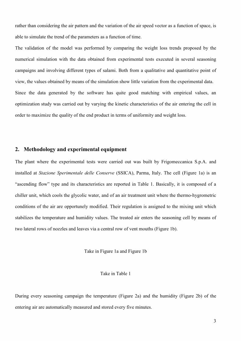
2. Methodology and experimental equipment

The plant where the experimental tests were carried out was built by Frigomeccanica S.p.A. and

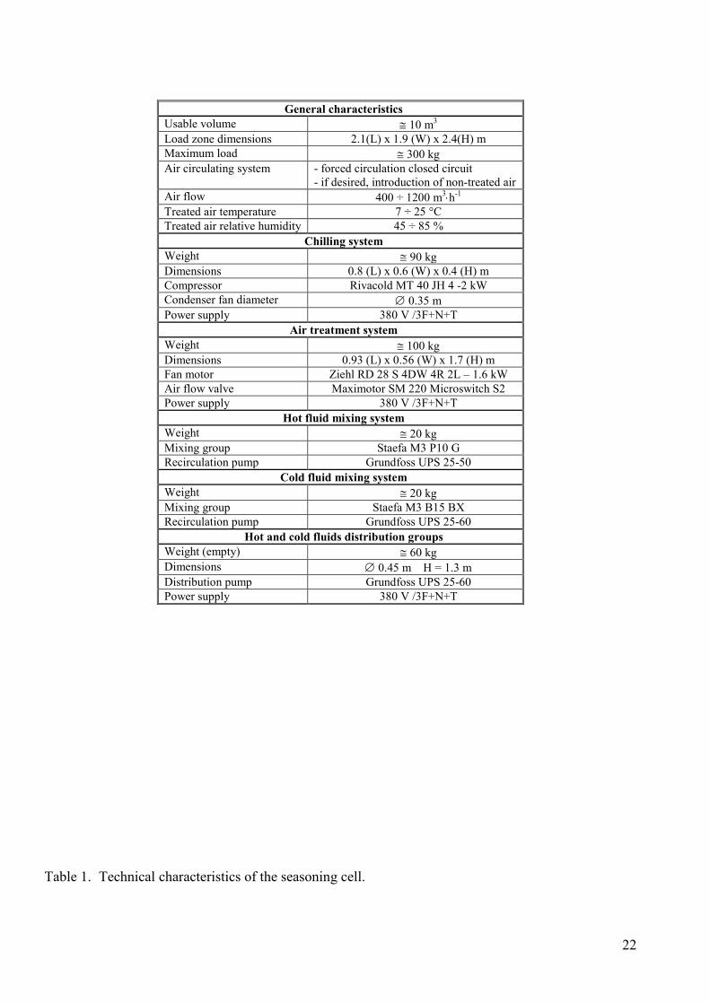
installed at Stazione Sperimentale delle Conserve (SSICA), Parma, Italy. The cell (Figure 1a) is an

“ascending flow” type and its characteristics are reported in Table 1. Basically, it is composed of a

chiller unit, which cools the glycolic water, and of an air treatment unit where the thermo-hygrometric

conditions of the air are opportunely modified. Their regulation is assigned to the mixing unit which

stabilizes the temperature and humidity values. The treated air enters the seasoning cell by means of

two lateral rows of nozzles and leaves via a central row of vent mouths (Figure 1b).

Take in Figure 1a and Figure 1b

Take in Table 1

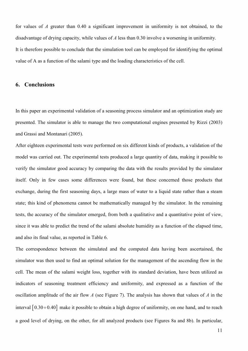
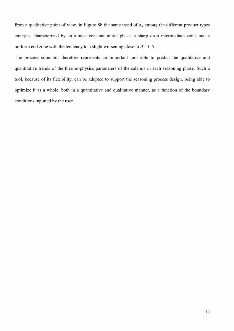
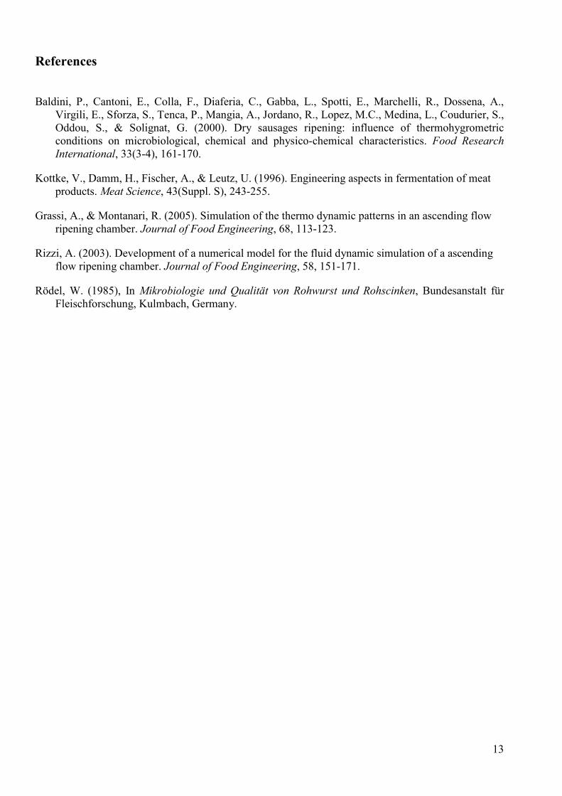
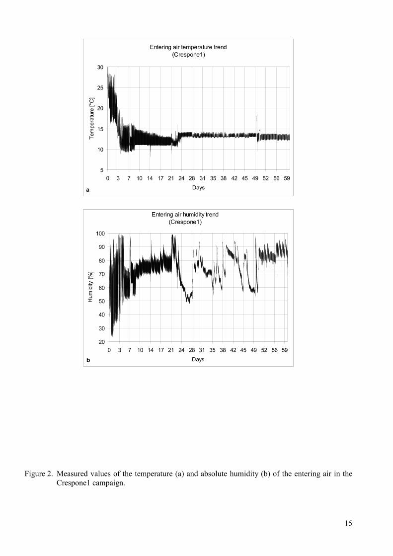
During every seasoning campaign the temperature (Figure 2a) and the humidity (Figure 2b) of the

entering air are automatically measured and stored every five minutes.

3

Take in Figure 2a and Figure 2b

Both the large variety of salami types produced in Europe and the necessity to provide a tool which is

able to best fit the different product types, have made it necessary to perform the software validation

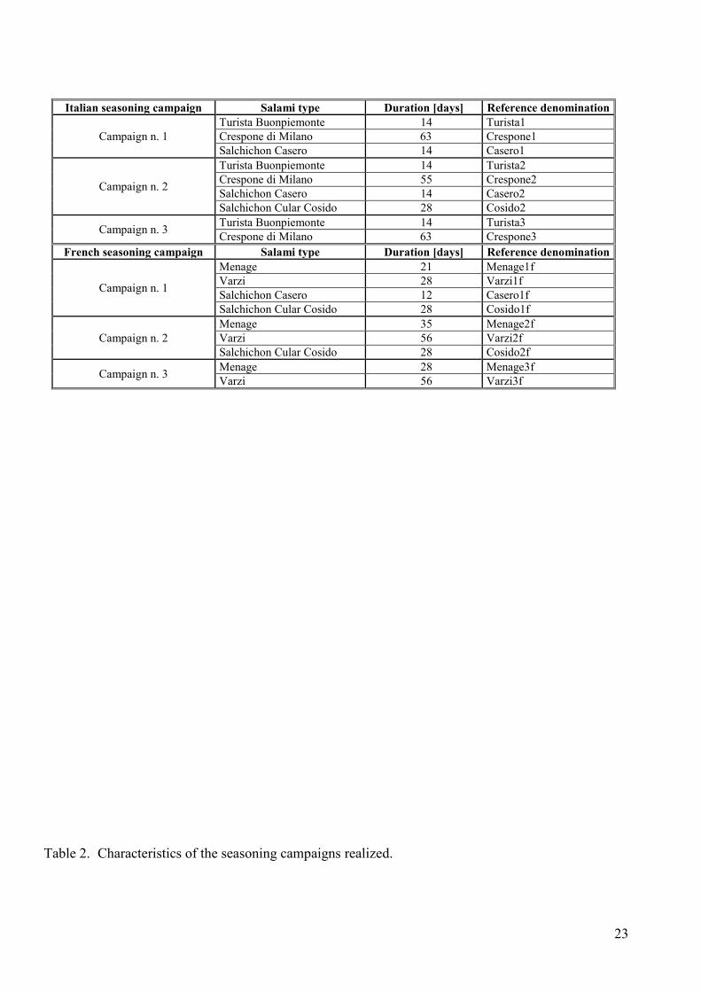
using several types of salami, two for every country involved in the project. Several seasoning

campaigns were carried out in Italy and France with six products (Turista Buonpiemonte, Crespone of

Milan, Salchichon Casero, Salchichon Cular Cosido, Menage, Varzi) with different paste, skin,

dimensions and seasoning period characteristics. In this way a huge quantity of experimental data was

obtained for the successive comparison with the data produced by the process simulator. In Table 2,

the duration, the kind of product and its reference name are reported for each seasoning campaign. In

particular, there were six seasoning campaigns involved in the project, three of which were carried out

in Italy and three in France. Furthermore, on each campaign a number of seasonings on different kinds

of products were also performed, for a total of eighteen processes. In the Italian campaigns three

seasonings were executed with the Turista Buonpiemonte, three with the Crespone of Milan, two with

the Salchichon Casero, and one with the Salchichon Cular Cosido. In France, three seasonings were

executed with the Menage, three with the Varzi, two with the Salchichon Cular Cosido and one with

the Salchichon Casero. By proceeding in such a way three experimental tests were obtained for each of

the different salami types.

Take in Table 2

The weight loss data, showing the trend of the weight variation as a function of the elapsed time, was

obtained by experimental measurements in successive process instants. In particular, with the

exception of some cases, the measurements were carried out daily during the first four days, on the

seventh and fourteenth day for the Turista Buonpiemonte and the Salchichon Casero; daily, during the

4

first four days, on the seventh day and, subsequently, every seven days for the Crespone of Milan,

Menage and Varzi; daily during the first three days, on the fourteenth, twenty-first and twenty-eighth

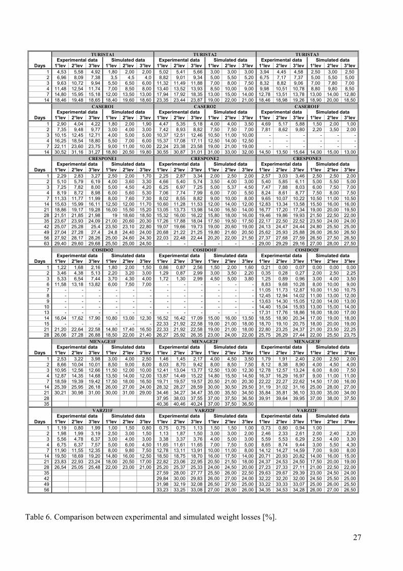
day for the Salchichon Cular Cosido. For each seasoning campaign, weight loss measurements were

carried out identifying three levels of salami on the rack. The values obtained for each level represent

the average for the products located on the same level of the rack (Table 6). As shown, a more frequent

number of measurements, therefore giving more information, is concentrated in the first seasoning

period. It is necessary to proceed in this way because of the major variations the product characteristics

exhibit in that phase, while they tend to stabilize in the final process period.

3. Model description

As stated in the introduction, the simulator is based on two models. First, the Fluid-Dynamic Model

(FDM) (Rizzi, 2003) computes the air velocity vector at each point of the seasoning cell, with respect

to the entering air conditions. Second, the Thermo-Dynamic Model (TDM) (Grassi and Montanari,

2005) uses the results to determine the temperature and humidity values both of the air and of the

salami contained in the cell, as a function of time. The process simulator (Figure 3) manages the two

models by coordinating the flow of data required by each model.

Take in Figure 3

The simulator is based on three main boxes: Interface Input Data (IID), Internal Elaboration Data

(IED), Interface Output Data (IOD). IID manages both process setup data, such as geometrical and

seasoning data, and simulation loop data, that is, the data obtained by the process in the previous

simulation step (the dot line in Figure 3). Moreover, at each step of the simulation, IID sets up the fluid

dynamic configuration of the cell and runs the FDM. IED catches the FDM output data together with

the simulation set up and loop data, it prepares them for the TDM and runs it in order to generate a

progress in the seasoning simulation. Finally, the TDM outcomes are elaborated by the IOD for

5

generating both the weight loss output for each salami (as a function of time) and the simulation loop

data for the next step.

The end of the simulation is managed by the IID as a function of the elapsed seasoning time.

3.1. The process inputs

These represent all of the data the user has to provide and which is needed for the simulation; they can

be subdivided into four categories:

physical data of the air;

physical data of the salami;

seasoning data;

geometrical data.

Physical data of the air

These represent all of the data that characterizes the air as a fluid: the dry air and the steam specific

heat, the temperature Tin, and the absolute humidity Xin of the input air. As regards the last two

parameters, they are variables during the process and their trends are characteristic for each seasoning

campaign and salami type (Figure 2a-b). The process simulator computes an average daily value, as

shown in Figure 4.

Physical data of the salami

In Table 5 the physical characteristics of the salamis are reported. Those are the type, diameter, length,

initial absolute humidity and temperature, density, and specific head of each salami.

Take in Table 5

Geometrical Data

6

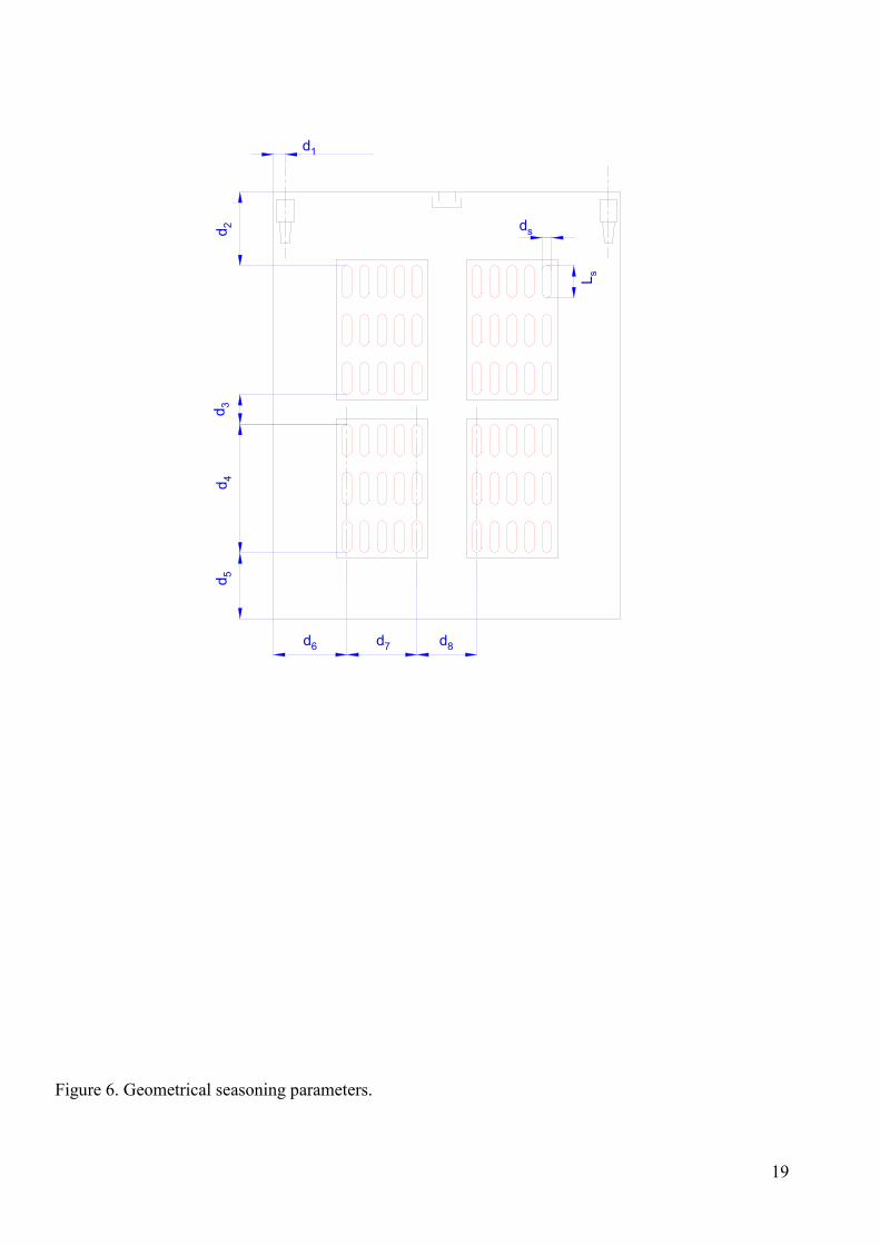
These represent all of the dimensional data describing the exact geometry of the cell, of the salamis

and their disposition in the cell itself. An overall explanation of such parameters can be found in

Figure 6. In Table 3 the independent parameters of the seasoning are reported (d3 and d8 are null

because there is only one rack in the cell), while in Table 4 the salami type dependent data are also

reported.

Take in Figure 6

Take in Table 3

Take in Table 4

Seasoning data

These are all of the data regulating the seasoning cycle, concerning the air input parameters. In Figure

5 the qualitative trend of the flow in the left nozzle is shown as a function of the total flow. Such a

nozzle, like its right hand twin, operates in a periodical manner so as to generate an ascending air flow

into the cell. The period P is the computational time step, so the number of loops drawn with a dashed

line in Figure 3 is equal to the ratio between the seasoning period PS (see “Duration” in Table 2) and

the interval P. The movement of the ascending flow is oscillatory with a period equal to the valve

period Pv (Rizzi, 2003).

Take in Figure 5

3.2. The process outputs

Since the objective of a seasoning process is the reduction of the humidity contained within the

product, the salami weight loss is one of the most important output parameters from an industrial point

7

of view. In fact, the variation of the salami weight is almost exclusively due to its progressive drying

during seasoning.

The simulator supplies the weight loss, humidity and temperature data for each seasoning time step

and for every product located in the cell, in addition to the fluid-dynamic and thermo-hygrometric air

conditions. The validation of the model is carried out by comparing the experimental data with those

provided by the model, both at the same time instant and using average values for each level.

4. Comparison between the model and the experimental data

The validation of the process simulator was carried out by comparing the data concerning the

experimental weight loss curves with those computed by the software. Both the experimental data and

the simulated ones are summarized as a function of the kind of product in Table 6.

Take in Table 6

By looking at the reported data, in the majority of the tests conducted, it can be seen that there is an

excellent correspondence between the experimental values and the simulated ones. But some initial

differences are present in a few of the tests, such as for the Turista1 and the Turista2.

From the 18 seasonings, only in the Casero1 and Cosido2 there is a poor correspondence between the

experimental and the simulated results. This is probably due to unforeseen perturbations in those

campaigns, since a good matching is identified in the Casero2, Casero1F, and Cosido1F, Cosido2F

tests respectively.

Moreover, it should be noted that in some campaigns there is a sensible initial difference between the

weight loss experimentally measured and the computed values. Such a significant difference is

probably due to factors the simulator does not take into account. One of these factors could be the

“sweating” of a large salami, exchanging water in a liquid state rather than as steam. In this way, the

huge weight loss noticed on the first seasoning day can be justified. As mentioned before, such a

8

phenomenon is not taken into account by the model. By setting the initial conditions of the simulation

in correspondence with those measured experimentally at the end of the first day, an analysis of the

performance of the model, by-passing the “sweating” problem, can be made. By proceeding in this

way, the difference between the experimentally measured weight loss curve and the computed one

becomes almost negligible, confirming the validity of the proposed model.

As concerns products with large diameter and long seasoning period, such as the Crespone and the

Varzi, the behavior of the model is characterized by an under estimation of the final salami weight

loss.

5. Process optimization

The design criteria represent a collection of parameters and indications by means of which an

optimization of the seasoning process can be performed, the work conditions being known. The

objective is to identify the best configurations; in other words, those leading to high improvements in

the process quality.

During ripening and drying, the water content should decrease homogeneously in all salamis in the

cell. Hence, the standard deviation σX of the salami absolute humidity X represents an index that is

able to quantify the uniformity of the water content loss of the salami in the cell, providing an

estimation of the dispersion of the salami absolute humidity values around the average value µX.

In particular, the simulator has here been used to identify the optimal value of the amplitude of the air

flow oscillation entering the cell from the two rows of nozzles for minimizing σX. As stated before, the

air flows entering the cell are periodically varied between the two nozzle rows by means of a valve that

regulates the flow distribution. Such a variation has been approximated in the simulations with a

harmonic law of amplitude A (see Figure 7). By varying the amplitude A from 0 to 0.5 several working

conditions can be represented, from a configuration (A=0) where the flow is constant and equally

subdivided between the two nozzle rows, to one (A=0.5) where the flow varies from 0 to QTOT.

9

Take in Figure 7

The results of the elaboration are reported in Figure 8a and 8b, concerning the products: Turista

Buonpiemonte, Crespone of Milan, Salchichon Casero, Salchichon Cular Cosido, Varzi, and Menage.

Take in Figures 8a and 8b

For each product, a number of seasoning processes were simulated by varying parameter A, thus

obtaining different drying levels at the end of the seasoning process, represented by the average value

µX. Moreover, different degrees of uniformity were reached as a function of parameter A, and were

addressed by the standard deviation σX of the absolute humidity of all salamis in the cell. Both of these

parameters are important in a seasoning process since while µX measures how the cell is able to dry the

products, σX assesses how much uniformly this process has been conduced. In other words, the aim of

the seasoning process is to reach a defined level of drying in a short time interval, while assuring a

high level of uniformity.

As shown in Figures 8a and 8b, each product is characterized by a different seasoning behavior, even

if a general trend for both the mean and the standard deviation of the absolute humidity can be noticed.

In particular, low values of A (A ∈ [0.15÷0.20]) allow to obtain best drying performances (Figure 8a),

but producing consistent non-uniformities as represented by high values of standard deviation shown

in Figure 8b. On the contrary, high degree of uniformity can be found for values of A greater than 0.30,

accepting a little increase in the mean of the absolute humidity.

Unfortunately, the behaviors of µX and σX are antithetical, hence a tradeoff solution has to be found, in

a way as to guarantee both an acceptable level of drying and a high degree of uniformity. For all the

simulation campaigns, optimal values of parameter A can be found in the interval [ ]0.30 0.40÷ , since

10

for values of A greater than 0.40 a significant improvement in uniformity is not obtained, to the

disadvantage of drying capacity, while values of A less than 0.30 involve a worsening in uniformity.

It is therefore possible to conclude that the simulation tool can be employed for identifying the optimal

value of A as a function of the salami type and the loading characteristics of the cell.

6. Conclusions

In this paper an experimental validation of a seasoning process simulator and an optimization study are

presented. The simulator is able to manage the two computational engines presented by Rizzi (2003)

and Grassi and Montanari (2005).

After eighteen experimental tests were performed on six different kinds of products, a validation of the

model was carried out. The experimental tests produced a large quantity of data, making it possible to

verify the simulator good accuracy by comparing the data with the results provided by the simulator

itself. Only in few cases some differences were found, but these concerned those products that

exchange, during the first seasoning days, a large mass of water to a liquid state rather than a steam

state; this kind of phenomena cannot be mathematically managed by the simulator. In the remaining

tests, the accuracy of the simulator emerged, from both a qualitative and a quantitative point of view,

since it was able to predict the trend of the salami absolute humidity as a function of the elapsed time,

and also its final value, as reported in Table 6.

The correspondence between the simulated and the computed data having been ascertained, the

simulator was then used to find an optimal solution for the management of the ascending flow in the

cell. The mean of the salami weight loss, together with its standard deviation, have been utilized as

indicators of seasoning treatment efficiency and uniformity, and expressed as a function of the

oscillation amplitude of the air flow A (see Figure 7). The analysis has shown that values of A in the

interval [ ]0.30 0.40÷ make it possible to obtain a high degree of uniformity, on one hand, and to reach

a good level of drying, on the other, for all analyzed products (see Figures 8a and 8b). In particular,

11

from a qualitative point of view, in Figure 8b the same trend of σX among the different product types

emerges, characterized by an almost constant initial phase, a sharp drop intermediate zone, and a

uniform end zone with the tendency to a slight worsening close to A = 0.5.

The process simulator therefore represents an important tool able to predict the qualitative and

quantitative trends of the thermo-physics parameters of the salamis in each seasoning phase. Such a

tool, because of its flexibility, can be adopted to support the seasoning process design, being able to

optimize it as a whole, both in a quantitative and qualitative manner, as a function of the boundary

conditions inputted by the user.

12

References

Baldini, P., Cantoni, E., Colla, F., Diaferia, C., Gabba, L., Spotti, E., Marchelli, R., Dossena, A., Virgili, E., Sforza, S., Tenca, P., Mangia, A., Jordano, R., Lopez, M.C., Medina, L., Coudurier, S., Oddou, S., & Solignat, G. (2000). Dry sausages ripening: influence of thermohygrometric conditions on microbiological, chemical and physico-chemical characteristics. Food Research International, 33(3-4), 161-170.

Kottke, V., Damm, H., Fischer, A., & Leutz, U. (1996). Engineering aspects in fermentation of meat products. Meat Science, 43(Suppl. S), 243-255.

Grassi, A., & Montanari, R. (2005). Simulation of the thermo dynamic patterns in an ascending flow ripening chamber. Journal of Food Engineering, 68, 113-123.

Rizzi, A. (2003). Development of a numerical model for the fluid dynamic simulation of a ascending flow ripening chamber. Journal of Food Engineering, 58, 151-171.

Rödel, W. (1985), In Mikrobiologie und Qualität von Rohwurst und Rohscinken, Bundesanstalt für Fleischforschung, Kulmbach, Germany.

13

a b

Figure 1. External (a) and internal (b) views of the pilot ascending flow ripening chamber.

14

Entering air temperature trend(Crespone1)

5

10

15

20

25

30

0 3 7 10 14 17 21 24 28 31 35 38 42 45 49 52 56 59

Days

Tem

pera

ture

[°C

]

a

Entering air humidity trend(Crespone1)

20

30

40

50

60

70

80

90

100

0 3 7 10 14 17 21 24 28 31 35 38 42 45 49 52 56 59

Days

Hum

idity

[%]

b

Figure 2. Measured values of the temperature (a) and absolute humidity (b) of the entering air in the Crespone1 campaign.

15

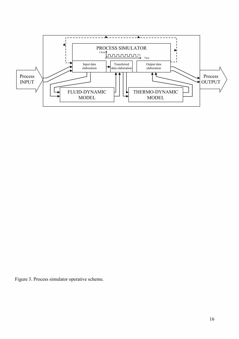
Figure 3. Process simulator operative scheme.

Process INPUT

FLUID-DYNAMIC MODEL

THERMO-DYNAMIC MODEL

PROCESS SIMULATOR

Input data elaboration

Output data elaboration

Transferred data elaboration

Time

Clock

Process OUTPUT

16

Air thermo-hygrometric parameters(Crespone1)

10

12

14

16

18

20

22

24

26

1 6 11 16 21 26 31 36 41 46 51 56

Days

Tem

pera

ture

[°C

]

0

0.002

0.004

0.006

0.008

0.01

0.012

0.014

0.016

Abs

olut

e hu

mid

ity

Entering air temperature [°C]Air absolute humidity

Figure 4. Average daily trend of the thermo-hygrometric characteristics of the entering air for the Crespone1 campaign.

17

Figure 5. Seasoning parameters.

t [s]

TOT

SXQQ

PS

Pv

P

18

d1

ds

L s

d 2d 3

d 4d 5

d6 d7 d8

Figure 6. Geometrical seasoning parameters.

19

Repartition of the air flow in the two nozzle rows

0%

25%

50%

75%

100%

A

QTOT

0 0.1 0.2 0.3 0.4 0.5

Valve period

Figure 7. Air flow repartition in the two nozzle rows as a function of amplitude A.

20

Salami absolute humidityafter the seasoning process

0.235

0.255

0.275

0.295

0.315

0.335

0.355

0.375

0.00 0.10 0.20 0.30 0.40 0.50

A

Mea

n

TuristaCresponeCosidoCaseroVarziMenage

Salami absolute humidityafter the seasoning process

0.000

0.020

0.040

0.060

0.080

0.100

0.120

0.140

0.160

0.180

0.00 0.10 0.20 0.30 0.40 0.50

A

Stan

dard

Dev

iatio

n TuristaCresponeCosidoCaseroVarziMenage

Figure 8. Mean (a) and standard deviation (b) of the absolute humidity as a function of the amplitude.

a

b

21

General characteristics Usable volume ≅ 10 m3 Load zone dimensions 2.1(L) x 1.9 (W) x 2.4(H) m Maximum load ≅ 300 kg Air circulating system - forced circulation closed circuit

- if desired, introduction of non-treated air Air flow 400 ÷ 1200 m3⋅h-1 Treated air temperature 7 ÷ 25 °C Treated air relative humidity 45 ÷ 85 %

Chilling system Weight ≅ 90 kg Dimensions 0.8 (L) x 0.6 (W) x 0.4 (H) m Compressor Rivacold MT 40 JH 4 -2 kW Condenser fan diameter ∅ 0.35 m Power supply 380 V /3F+N+T

Air treatment system Weight ≅ 100 kg Dimensions 0.93 (L) x 0.56 (W) x 1.7 (H) m Fan motor Ziehl RD 28 S 4DW 4R 2L – 1.6 kW Air flow valve Maximotor SM 220 Microswitch S2 Power supply 380 V /3F+N+T

Hot fluid mixing system Weight ≅ 20 kg Mixing group Staefa M3 P10 G Recirculation pump Grundfoss UPS 25-50

Cold fluid mixing system Weight ≅ 20 kg Mixing group Staefa M3 B15 BX Recirculation pump Grundfoss UPS 25-60

Hot and cold fluids distribution groups Weight (empty) ≅ 60 kg Dimensions ∅ 0.45 m H = 1.3 m Distribution pump Grundfoss UPS 25-60 Power supply 380 V /3F+N+T

Table 1. Technical characteristics of the seasoning cell.

22

Italian seasoning campaign Salami type Duration [days] Reference denomination

Campaign n. 1 Turista Buonpiemonte 14 Turista1 Crespone di Milano 63 Crespone1 Salchichon Casero 14 Casero1

Campaign n. 2

Turista Buonpiemonte 14 Turista2 Crespone di Milano 55 Crespone2 Salchichon Casero 14 Casero2 Salchichon Cular Cosido 28 Cosido2

Campaign n. 3 Turista Buonpiemonte 14 Turista3 Crespone di Milano 63 Crespone3

French seasoning campaign Salami type Duration [days] Reference denomination

Campaign n. 1

Menage 21 Menage1f Varzi 28 Varzi1f Salchichon Casero 12 Casero1f Salchichon Cular Cosido 28 Cosido1f

Campaign n. 2 Menage 35 Menage2f Varzi 56 Varzi2f Salchichon Cular Cosido 28 Cosido2f

Campaign n. 3 Menage 28 Menage3f Varzi 56 Varzi3f

Table 2. Characteristics of the seasoning campaigns realized.

23

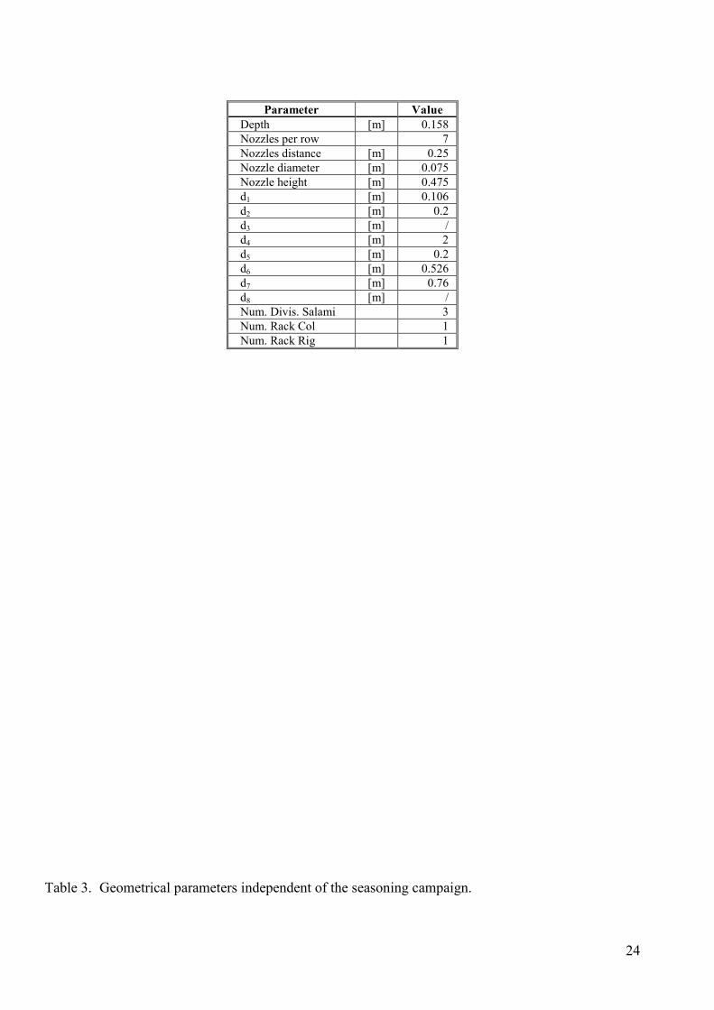
Parameter Value Depth [m] 0.158 Nozzles per row 7 Nozzles distance [m] 0.25 Nozzle diameter [m] 0.075 Nozzle height [m] 0.475 d1 [m] 0.106 d2 [m] 0.2 d3 [m] / d4 [m] 2 d5 [m] 0.2 d6 [m] 0.526 d7 [m] 0.76 d8 [m] / Num. Divis. Salami 3 Num. Rack Col 1 Num. Rack Rig 1

Table 3. Geometrical parameters independent of the seasoning campaign.

24

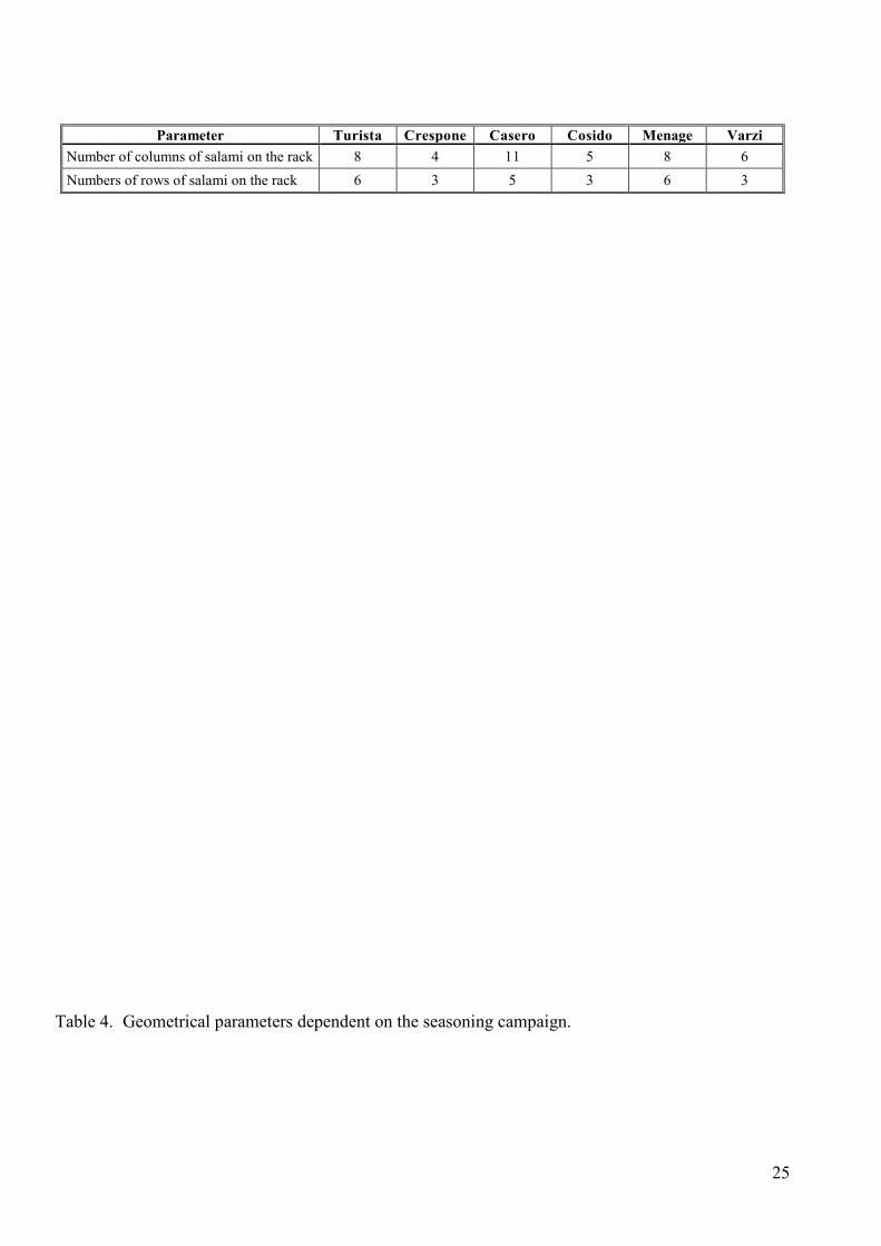
Parameter Turista Crespone Casero Cosido Menage Varzi Number of columns of salami on the rack 8 4 11 5 8 6 Numbers of rows of salami on the rack 6 3 5 3 6 3

Table 4. Geometrical parameters dependent on the seasoning campaign.

25

Salami type Diameter dS

Length LS

Initial salami absolute humidity

Initial salami temperature

Density (dry meat)

Specific heat (dry meat)

[m] [m] [kgWater⋅kgDryMeat-1] [°C] [kg⋅m-3] [kJ/(kg K)]

Turista1 0.06 0.25 1.16 10 985.8 2 Crespone1 0.095 0.49 1.23 12 985.8 2 Casero1 0.055 0.25 1.16 10 985.8 2 Turista2 0.06 0.25 1.32 10 985.8 2 Crespone2 0.095 0.49 1.23 12 985.8 2 Casero2 0.045 0.25 1.22 10 985.8 2 Cosido2 0.08 0.375 1.33 10 985.8 2 Turista3 0.06 0.25 1.16 10 985.8 2 Crespone3 0.095 0.49 1.29 12 985.8 2 Menage1 0.055 0.2 1.47 11 985.8 2 Varzi1 0.09 0.45 1.45 10 985.8 2 Casero1 0.055 0.225 1.56 10 985.8 2 Cosido1 0.08 0.375 1.35 10 985.8 2 Menage2 0.055 0.2 1.47 11 985.8 2 Varzi2 0.09 0.45 1.44 10 985.8 2 Cosido2 0.08 0.375 1.35 10 985.8 2 Menage3 0.055 0.2 1.37 11 985.8 2 Varzi3 0.09 0.45 1.44 10 985.8 2

Table 5. Physical parameters of salami.

26

Days

TURISTA1 TURISTA2 TURISTA3 Experimental data Simulated data Experimental data Simulated data Experimental data Simulated data

1°lev 2°lev 3°lev 1°lev 2°lev 3°lev 1°lev 2°lev 3°lev 1°lev 2°lev 3°lev 1°lev 2°lev 3°lev 1°lev 2°lev 3°lev 1 4,53 5,58 4,92 1,80 2,00 2,00 5,02 5,41 5,66 3,00 3,00 3,00 3,94 4,45 4,58 2,50 3,00 2,50 2 6,96 8,09 7,38 3,5 4,5 4,0 8,82 9,01 9,34 5,00 5,50 5,20 6,75 7,17 7,37 5,00 5,50 5,00 3 9,63 10,72 9,94 5,50 6,50 6,00 11,32 11,49 11,88 7,00 8,00 7,50 8,32 8,82 9,06 7,00 7,80 7,00 4 11,48 12,54 11,74 7,00 8,50 8,00 13,40 13,52 13,93 8,50 10,00 9,00 9,98 10,51 10,78 8,80 9,80 8,50 7 14,80 15,95 15,18 12,00 13,50 13,00 17,94 17,92 18,35 13,00 15,00 14,00 12,78 13,51 13,78 13,00 14,00 12,80

14 18,46 19,48 18,65 18,40 19,60 18,60 23,35 23,44 23,87 19,00 22,00 21,00 18,46 18,98 19,26 18,90 20,00 18,50

Days

CASERO1 CASERO2 CASERO1F Experimental data Simulated data Experimental data Simulated data Experimental data Simulated data

1°lev 2°lev 3°lev 1°lev 2°lev 3°lev 1°lev 2°lev 3°lev 1°lev 2°lev 3°lev 1°lev 2°lev 3°lev 1°lev 2°lev 3°lev 1 2,90 4,04 4,22 1,80 2,00 1,90 4,47 5,35 5,18 4,00 4,00 3,50 4,69 5,17 5,88 1,50 2,00 1,00 2 7,35 9,48 9,77 3,00 4,00 3,00 7,42 8,93 8,82 7,50 7,50 7,00 7,81 8,62 9,80 2,20 3,50 2,00 3 10,15 12,45 12,71 4,00 5,00 5,00 10,37 12,51 12,46 10,50 11,00 10,00 - - - - - - 4 16,25 18,54 18,80 5,50 7,00 6,00 15,37 17,08 17,11 12,50 14,00 12,50 - - - - - - 7 22,11 23,60 23,75 9,00 11,00 10,00 22,24 23,38 23,58 19,00 21,00 19,00 - - - - - -

14 30,52 31,16 31,27 18,80 20,50 19,80 30,55 30,87 31,01 31,00 33,00 32,00 14,50 13,50 15,64 14,00 15,00 13,00

Days

CRESPONE1 CRESPONE2 CRESPONE3 Experimental data Simulated data Experimental data Simulated data Experimental data Simulated data


14 15,63 15,99 16,11 12,50 12,00 11,70 10,60 11,28 11,53 12,00 14,00 12,00 12,83 13,34 13,58 15,50 16,00 16,00 21 18,86 19,17 19,28 16,00 15,50 15,20 13,05 13,73 13,98 14,00 16,50 14,00 16,77 17,20 17,34 19,00 20,00 19,50 28 21,51 21,85 21,98 19 18,60 18,50 15,32 16,00 16,22 15,80 18,00 16,00 19,46 19,86 19,93 21,50 22,50 22,00 35 23,67 23,93 24,09 21,00 20,60 20,30 17,26 17,88 18,04 17,50 19,50 17,50 22,17 22,50 22,52 23,50 24,00 24,00 42 25,07 25,28 25,4 23,50 23,10 22,80 19,07 19,66 19,73 19,00 20,60 19,00 24,13 24,47 24,44 24,80 25,50 25,00 49 27,04 27,28 27,4 24,8 24,40 24,00 20,68 21,22 21,25 19,80 21,60 20,50 25,62 25,93 25,88 26,00 26,50 26,50 56 27,92 28,17 28,26 25,00 24,60 24,30 22,03 22,48 22,44 20,20 22,00 21,50 27,37 27,68 27,59 26,50 27,50 26,50 63 29,40 29,60 29,68 25,50 25,00 24,50 - - - - - - 29,00 29,29 29,16 27,00 28,00 27,50

Days

COSIDO2 COSIDO1F COSIDO2F Experimental data Simulated data Experimental data Simulated data Experimental data Simulated data

1°lev 2°lev 3°lev 1°lev 2°lev 3°lev 1°lev 2°lev 3°lev 1°lev 2°lev 3°lev 1°lev 2°lev 3°lev 1°lev 2°lev 3°lev 1 1,22 1,68 2,16 1,80 2,00 1,50 0,86 0,87 2,56 1,50 2,00 1,60 0,21 0,00 0,07 0,00 0,00 0,00 2 3,46 4,38 5,13 2,20 3,20 3,00 1,29 0,87 2,99 3,00 3,50 2,20 0,35 0,28 0,27 2,00 2,50 2,25 3 5,33 6,54 7,44 3,70 4,30 4,00 1,72 1,30 2,99 4,50 5,00 3,80 1,25 0,89 0,96 3,00 4,00 3,50 6 11,58 13,18 13,82 6,00 7,50 7,00 - - - - - - 8,83 9,68 10,28 8,00 10,00 9,00 7 - - - - - - - - - - - - 11,05 11,73 12,87 10,00 11,50 10,75 8 - - - - - - - - - - - - 12,45 12,94 14,02 11,00 13,00 12,00 9 - - - - - - - - - - - - 13,63 14,30 15,05 12,00 14,00 13,00

10 - - - - - - - - - - - - 14,40 15,04 15,93 13,00 15,00 14,00 13 - - - - - - - - - - - - 17,31 17,76 18,86 16,00 18,00 17,00 14 16,04 17,62 17,90 10,80 13,00 12,30 16,52 16,42 17,09 15,00 16,00 13,50 18,55 18,90 20,34 17,00 19,00 18,00 15 - - - - - - 22,33 21,92 22,58 19,00 21,00 18,00 18,70 19,10 20,75 18,00 20,00 19,00 21 21,20 22,64 22,58 14,80 17,40 16,50 22,33 21,92 22,58 19,00 21,00 18,00 22,80 23,25 24,37 21,00 23,50 22,25 28 26,06 27,28 26,88 18,50 22,00 21,40 26,27 25,92 26,35 23,00 24,00 22,00 25,75 26,29 27,44 22,00 25,50 23,75

Days

MENAGE1F MENAGE2F MENAGE3F Experimental data Simulated data Experimental data Simulated data Experimental data Simulated data


14 25,39 25,95 26,18 26,00 27,00 24,00 28,32 28,27 28,59 30,00 30,50 29,50 31,19 31,02 31,16 25,00 28,00 27,00 21 30,21 30,98 31,00 30,00 31,00 29,00 34,46 34,27 34,47 35,00 35,50 34,50 35,84 35,81 36,10 33,00 35,00 34,00 28 37,95 38,03 37,55 37,00 37,50 36,50 39,91 39,64 39,95 37,00 38,00 37,50 35 40,36 40,46 40,24 37,00 37,50 36,50

Days

VARZI1F VARZI2F VARZI2F Experimental data Simulated data Experimental data Simulated data Experimental data Simulated data

1°lev 2°lev 3°lev 1°lev 2°lev 3°lev 1°lev 2°lev 3°lev 1°lev 2°lev 3°lev 1°lev 2°lev 3°lev 1°lev 2°lev 3°lev 1 1,19 0,80 1,99 1,00 1,50 0,80 0,75 0,75 1,13 1,50 1,50 1,00 0,73 0,80 0,94 1,00 2 1,98 1,99 3,19 2,50 3,00 1,50 1,13 1,87 1,50 3,00 3,00 2,00 2,46 2,33 2,61 2,00 2,40 2,20 3 5,56 4,78 6,37 3,00 4,00 3,00 3,38 3,37 3,76 4,00 5,00 3,00 5,59 5,53 6,29 2,50 4,00 3,30 4 6,75 6,37 7,57 5,00 6,00 4,50 11,65 11,61 11,65 7,00 7,50 5,00 8,65 8,74 9,44 3,00 5,50 4,30 7 11,90 11,55 12,35 8,00 9,80 7,50 12,78 13,11 13,91 10,00 11,00 8,00 14,12 14,27 14,59 7,00 9,00 8,00

14 19,50 18,69 19,20 14,80 16,00 12,50 18,50 18,75 18,70 16,00 17,50 14,00 20,71 20,93 20,82 14,00 16,00 15,00 21 23,83 22,93 23,24 18,00 20,50 17,00 22,82 23,06 22,95 20,50 21,50 18,00 24,37 24,53 24,50 17,50 20,00 19,00 28 26,54 25,05 25,48 22,00 23,00 21,00 25,20 25,37 25,33 24,00 24,50 20,00 27,23 27,33 27,11 21,00 22,50 22,00 35 27,59 28,00 27,77 25,50 26,00 22,50 29,63 29,67 29,39 23,00 24,50 24,00 42 29,84 30,00 29,83 26,00 27,00 24,00 32,22 32,20 32,00 24,50 25,50 25,00 49 31,98 32,19 32,08 26,50 27,50 25,00 33,22 33,33 33,07 25,00 26,00 25,50 56 33,23 33,25 33,08 27,00 28,00 26,00 34,35 34,53 34,28 26,00 27,00 26,50

Table 6. Comparison between experimental and simulated weight losses [%].

27

Seasoning process design optimization for an ascending flow ripening chamber

Documents