Seasonal variation in vertical volatile compounds air concentrations within a remote hemiboreal mixed forest

Atmos. Chem. Phys., 12, 3909–3926, 2012www.atmos-chem-phys.net/12/3909/2012/doi:10.5194/acp-12-3909-2012© Author(s) 2012. CC Attribution 3.0 License.

AtmosphericChemistry

and Physics

Seasonal variation in vertical volatile compounds air concentrationswithin a remote hemiboreal mixed forest

S. M. Noe, K. Huve,U. Niinemets, and L. Copolovici

Department of Plant Physiology, Institute of Agricultural and Environmental Sciences, Estonian University of Life Sciences,Kreutzwaldi 1, 51014 Tartu, Estonia

Correspondence to:S. M. Noe ([email protected])

Received: 21 December 2010 – Published in Atmos. Chem. Phys. Discuss.: 12 May 2011Revised: 28 March 2012 – Accepted: 13 April 2012 – Published: 3 May 2012

Abstract. The vertical distribution of ambient biogenicvolatile organic compounds (BVOC) concentrations withina hemiboreal forest canopy was investigated over a pe-riod of one year. Variability in temporal and spatial iso-prene concentrations, ranging from 0.1 to 7.5 µg m−3, canbe mainly explained by biogenic emissions from deciduoustrees. Monoterpene concentrations exceeded isoprene largelyand ranged from 0.01 to 140 µg m−3 and during winter timeanthropogenic contributions are likely. Variation in monoter-pene concentrations were found to be largest right abovethe ground and the vertical profiles suggest a weak mixingleading to terpene accumulation in the lower canopy. Ex-ceptionally high values were recorded during a heat wavein July 2010 with very high midday temperatures above30◦C for several weeks. During summer months, monoter-pene exceeded isoprene concentrations 6-fold and duringwinter 12-fold. During summer months, dominance ofα-pinene in the lower and of limonene in the upper part ofthe canopy was observed, both accounting for up to 70 % ofthe total monoterpene concentration. During wintertime,13-carene was the dominant species, accounting for 60 % of to-tal monoterpene concentration in January. Possible biogenicmonoterpene sources beside the foliage are the leaf litter, thesoil and also resins exuding from stems. In comparison, thehemiboreal mixed forest canopy showed similar isoprene buthigher monoterpene concentrations than the boreal forest andlower isoprene but substantially higher monoterpene concen-trations than the temperate mixed forest canopies. These re-sults have major implications for simulating air chemistryand secondary organic aerosol formation within and abovehemiboreal forest canopies. Possible effects of in-cartridgeoxidation reactions are discussed as our measurement tech-

nique did not include oxidant scavenging. A comparison be-tween measurements with and without scavenging oxidantsis presented.

1 Introduction

Emissions of biogenic hydrocarbons from forest ecosystemsare a dominant source of reduced organic gases to the atmo-sphere. They even exceed emissions of hydrocarbons by an-thropogenic pollution and biomass burning. Biogenic emis-sions play important roles in determining the global, re-gional, and local atmospheric chemistry which, in turn, feedsback to the ecosystem (Arneth et al., 2010; Kulmala et al.,2004).

Losses of instantaneously emitted hydrocarbons such asterpenes due to oxidation processes throughout the canopyheight have been reported by several studies (Holzinger et al.,2005; Fuentes et al., 2007; Stroud et al., 2005). Especiallyif the canopy height and structure together with atmosphericturbulence is such that the residence time of air parcels withinthe canopy are comparable or greater than the lifetimes ofBVOCs, chemical losses and deposition within the canopylead to reduced above canopy fluxes (Fuentes et al., 2007;Karl et al., 2004; Strong et al., 2004). Effects of ozone, ni-trogen oxides (NOx) and hydroxyl radical (OH) on the ver-tical distribution of BVOCs or vice-versa have been also as-sessed by means of 1-D canopy chemistry models includ-ing atmospheric transport terms (Forkel et al., 2006; Fuenteset al., 2007; Karl et al., 2004; Stroud et al., 2005; Stronget al., 2004). These studies mostly conclude that the dis-crepancy between upscaled leaf level BVOC emission fluxes

Published by Copernicus Publications on behalf of the European Geosciences Union.

3910 S. M. Noe et al.: Seasonal variation in vertical ambient BVOC concentrations

and canopy scale flux measurements are due to the withincanopy chemistry that lead to a reduction in above canopyBVOC flux to the boundary layer. Monoterpene uptake byleaves of deciduous tree species under high ambient concen-trations occurs and leads to altered temporal behavior of totalmonoterpene fluxes. Such processes have been described byCopolovici et al.(2005) andNoe et al.(2008).

Seasonal variations in isoprene and monoterpene emis-sions have been widely reported for a large variety of ecosys-tems and tree species (Holzinger et al., 2006; Hakola et al.,2003, 2009; Sabillon and Cremades, 2001; Mayrhofer et al.,2005) and also entered into emission models on variousscales (Schurgers et al., 2009; Guenther et al., 2006). In somecases only total monoterpene fluxes have been taken into ac-count andα-pinene is commonly used as a proxy to rep-resent all monoterpenes. This is in contrast to the findingthat monoterpenes have quite different atmospheric lifetimes(Atkinson et al., 1990; Atkinson, 2000; Lyubovtseva et al.,2005) due to differences in their chemical degradation whichimpact the subsequent processes such as secondary organicaerosol (SOA) formation (Ng et al., 2008; Kanakidou et al.,2005; Spracklen et al., 2008).

Forest trees are exposed to a huge amount of biotic andabiotic stresses and environmental factors that lead to veryheterogenous emission patterns of biogenic hydrocarbons(Niinemets, 2010a). Inclusion of process-based approaches,addressing such factors on larger scale emission fluxes ofbiogenic hydrocarbons have been reviewed recently (Ni-inemets et al., 2010d; Arneth et al., 2008; Arneth and Ni-inemets, 2010; Niinemets, 2010b). The findings ofStroudet al. (2005) and Karl et al. (2004) already led to an em-pirical term for the escape efficiency of biogenic hydrocar-bons from forest canopies into the boundary layer. That es-cape efficiency has been included to the MEGAN framework(Guenther et al., 2006) to allow to scale biogenic hydrocar-bon emissions to regional or global levels.

Estonia is located at the transition zone between the bo-real and temperate biomes which characterizes the locationof hemiboreal, mostly mixed, forests.Nilsson (1997) esti-mates the width of that transition zone over Eurasia to span atleast over 600 km (Sweden) and even wider in Siberia (Rus-sia). Given predictions on species diversity and their changeunder future climate in Scandinavia (Sætersdal et al., 1998)and the likely climatic impact on northern ecosystems (In-tergovernmental Panel on Climate Change, 2007), it seemslikely that the hemiboreal transition zone will move and en-large to north. Until now only few studies have been pointedto the atmosphere-biosphere relations within that zone. Theaim of our study was to give (1) an overview on the am-bient isoprene and monoterpene concentrations within a re-mote hemiboreal mixed forest canopy to assess (2) the sea-sonal change and reveal variations in ambient concentrationsdue to the changes in environment and to study (3) the spatialheterogeneity of isoprene and monoterpene ambient concen-trations within the canopy.

2 Materials and methods

2.1 Site description

The vertical VOC profiles were measured at a 20 m hightower located in the Jarvselja Experimental Forest in south-east Estonia (58◦25′ N, 27◦46′ E). The site is situated in thehemiboreal forest zone with a moderately cool and moist cli-mate and is described in more detail byNoe et al.(2010).These transition zones spreading between the boreal andtemperate climate zones are populated by conifer dominatedmixed forests. In terms of air pollution the area in the vicinityof the measurement tower is characterized as a remote site.The distance to the next larger town (100 000 inhabitants) is55 km to north-east direction. There are no main transit roadspassing a circle of about 50 km around the tower location.

The measurement site is dominated by Norway spruce(Picea abies(L.) Karst.) and as co-dominant species SilverBirch (Betula pendulaRoth.) and Black Alder (Alnus gluti-nosaL.) in the upper canopy layer varying between 16–20 m.The presence of a suppressed tree layer with a mean heightbetween 6–7 m is of particularly importance as it affects tur-bulent air flows within the stand. The soil is covered by adense and rather species rich layer of ground vegetation anda moss layer that consists of several species. The site has alowland character and is influenced by a high groundwatertable and water logging due to the vicinity of Lake Peipsi.Especially in humid spots we foundSphagnumspecies whichare typical for peat bogs.

The mean annual temperature varies between 4–6◦C andthe annual precipitation between 500–750 mm, about 40–80 mm of the annual precipitation is snow. The length of thegrowing season (daily air temperature above 5◦C) averagesbetween 170–180 days. Following the typical phenologicalpattern, bud break of the main deciduous tree species in thearea is in the end of April. Foliation takes place about midMay and leaf senescence in mid October. The fluctuation inthese phenological events is±14 days.

The site had typically at midday 0.2–0.8 ppbv NOx mixingratios and the midday ozone mixing ratios ranged between10–30 ppbv with maximal midday mixing ratios of 60 ppbvduring some days in summer 2010.

2.2 VOC sampling

We conducted the sampling of VOC from ambient air on 6heights (0, 4, 8, 12, 16, and 20 m above ground) over a yearstarting in October 2009 until September 2010 (Table1). Thedays of sampling have been chosen such that we obtainedsamples in each season of the year at an air pressure above1000 hPa and clear sky. The measurements conducted in au-tumn and winter (October to April) were taken at one day.During spring and summer (May to September) there havebeen several days per month measured during campaigns andwe chose one day that met the criteria given above.

Atmos. Chem. Phys., 12, 3909–3926, 2012 www.atmos-chem-phys.net/12/3909/2012/

S. M. Noe et al.: Seasonal variation in vertical ambient BVOC concentrations 3911

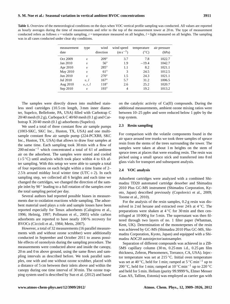
Table 1.Overview of the meteorological conditions on the days when VOC vertical profile sampling was conducted. All values are reportedas hourly averages during the time of measurements and refer to the top of the measurement tower at 20 m. The type of measurementconducted refers as followsv = volatile sampling,t = temperature measured on all heights,l = light measured on all heights. The samplingwas in all cases conducted under clear sky conditions.

measurement type wind wind speed temperature air pressuredate direction (m s−1) (◦C) (hPa)

Oct 2009 v 209◦ 3.7 7.8 1022.7Jan 2010 v 56◦ 1.9 −19.4 1042.7Apr 2010 v 285◦ 1.1 8.2 1021.1May 2010 v 61◦ 3 24.5 1012.5Jun 2010 v 270◦ 1.5 24.3 1021.1Jul 2010 v, l 167◦ 5.7 31.2 1006.5Aug 2010 v, t , l 118◦ 2.6 25.2 1020.7Sep 2010 v 193◦ 4 19.2 1013.2

The samples were directly drawn into multibed stain-less steel cartridges (10.5 cm length, 3 mm inner diame-ter, Supelco, Bellefonte, PA, USA) filled with Carbotrap C20/40 mesh (0.2 g), Carbopack C 40/60 mesh (0.1 g) and Car-botrap X 20/40 mesh (0.1 g) adsorbents (Supelco).

We used a total of three constant flow air sample pumps(1003-SKC, SKC Inc., Huston, TX, USA) and one multi-sample constant flow air sample pump (224-PCXR8, SKCInc., Huston, TX, USA) that allows to draw four samples atthe same time. Each sampling took 30 min with a flow of200 ml min−1 which concentrated a total of 6 l of ambientair on the adsorbent. The samples were stored and cooled(+5◦C) until analysis which took place within 4 to 6 h af-ter sampling. With this setup we were able to sample a totalof four repetitions on each height within a time frame of 2–2.5 h around midday local winter time (UTC+ 2). In eachsampling step, we collected all 6 heights and each time wechanged the cartridges, we changed the direction of the sam-ple inlet by 90◦ leading to a full rotation of the samples overthe total sampling period per day.

Several authors had reported possible biases in measure-ments due to oxidation reactions while sampling. The adsor-bent material used plays a role and sample losses have beenreported especially for Tenax adsorbents (Calogirou et al.,1996; Helmig, 1997; Pollmann et el., 2005) while carbonadsorbents are reported to have nearly 100 % recovery forBVOCs (Ciccioli et al., 1984; Metts, 2007).

However, a total of 32 measurements (16 parallel measure-ments with and without ozone scrubber) were additionallyconducted in September and October 2011 to assess possi-ble effects of ozonolysis during the sampling procedure. Themeasurements were conducted above and inside the canopy,20 m and 0 m above ground, using the same flows and sam-pling intervals as described before. We took parallel sam-ples, one with and one without ozone scrubber, placed witha distance of 5 cm between their inlets above and within thecanopy during one time interval of 30 min. The ozone trap-ping system used is described bySun et al.(2012) and based

on the catalytic activity of Cu(II) compounds. During theadditional measurements, ambient ozone mixing ratios werebetween 10–25 ppbv and were reduced below 1 ppbv by thetrap system.

2.3 Resin sampling

For comparison with the volatile components found in theair space around tree trunks we took three samples of spruceresin from the stems of the trees surrounding the tower. Thesamples were taken at about 1 m heights on the stem ofspruce trees at places that were exuding resin. The resin waspicked using a small spruce stick and transferred into 8 mlglass vials for transport and subsequent analysis.

2.4 VOC analysis

Adsorbent cartridges were analyzed with a combined Shi-madzu TD20 automated cartridge desorber and Shimadzu2010 Plus GC-MS instrument (Shimadzu Corporation, Ky-oto, Japan) described previously (Copolovici et al., 2009;Toome et al., 2010).

For the analysis of the resin samples, 0.2 g resin was dis-solved in 2 ml hexane and extracted over 24 h at 4◦C. Thepreparations were shaken at 4◦C for 30 min and then cen-trifuged at 10 000 g for 5 min. The supernatant was then fil-tered through two layers of no. 1 filter paper (Whatman,Kent, UK). Determination of the monoterpenes of the resinwas achieved by GC-MS (Shimadzu 2010 Plus GC-MS, Shi-madzu Corporation, Kyoto, Japan) and equipped with a Shi-madzu AOC20 autoinjector/autosampler.

Separation of different compounds was achieved in a ZB-5MS capillary column (30 m, 0.25 mm i.d., 0.25 µm filmthickness, Zebron, Phenomenex, Torrance, CA, USA). Injec-tor temperature was set at 215◦C. Initial oven temperaturewas set at 40◦C, held for 1 min; ramped at 5◦C min−1 up to200◦C, held for 1 min; ramped at 10◦C min−1 up to 220◦Cand held for 5 min. Helium (purity 99.9999 %, Elmer MesserGaas AS, Tallinn, Estonia) was employed as carrier gas with

www.atmos-chem-phys.net/12/3909/2012/ Atmos. Chem. Phys., 12, 3909–3926, 2012


a constant flow of 0.74 ml min−1. The mass spectrometer wasoperated in electron-impact mode (EI) at 70 eV, in the scanrangem/z 30–400, the transfer line temperature was set at240◦C and ion-source temperature at 150◦C. Compoundswere identified by use of the NIST spectral library and basedon retention time identity with the authentic standard (GCpurity, Sigma-Aldrich, St. Louis, MO, USA). The absoluteconcentrations of isoprene, monoterpenes and lipoxygenase(LOX) pathway products were calculated based on an exter-nal authentic standard consisting of known amount of VOCs.

2.5 Auxiliary measurements

Beside the main task of assessing vertical VOC profilesthroughout the canopy and over the seasons, we measured,predominantly under summer conditions, also ambient tem-perature, light and CO2 profiles throughout the canopy.

Temperature measurements have been conducted using aradiation shielded thermocouple sensor that was connectedto a thermocouple reader (Comark KM330, Comark Instru-ments, Hitchin, Hertfordshire, UK). When temperature wasmeasured, the sensor was placed beside the sampling pumpand during the sampling time, three to four values of temper-ature were recorded. As that was conducted by every changeof the cartridges, a maximum of 12–16 temperature measure-ments per height over sampling period were achieved.

Quantum flux density (PPFD) was measured with a LI-190SA quantum sensor (LiCor, Lincoln, NE, USA). On eachheight, PPFD was measured in shade conditions and in fullsunlight, if available. At least 5 measurements were takenduring the whole BVOC sampling interval at different loca-tions near the sampling pump and the data averaged.

To assess the ambient CO2 mixing ratios throughout thecanopy, a closed path infrared gas analyzer (IRGA) (LI-7000, Li-Cor, Lincoln, NE, USA) was used. Sample airwas drawn from each height by Teflon pipes passing a fil-ter (Acro50, Gelman, Ann Arbor, MI, USA) and the IRGA.An air flow of 10 l min−1 was provided by a vacuum pump(Samos SB 0080 D, Busch Vakuumteknik Oy, Vantaa, Fin-land). Each height level was measured with a 10 minute in-terval for 3 hours extending over the time of BVOC sam-pling. We recorded the values every minute and values havebeen averaged the values for each height separately over thesampling period.

Horizontal wind speed was measured with two 3-D sonicanemometers (CSAT3, Campbell Scientific, 168 Logan, UT,USA; Metek USA-1, Metek GmbH, Elmshorn, Germany)which have been installed on top of the tower at a heightof 20 m above ground and on a mast at a height of 2 m aboveforest floor for continuous eddy covariance measurements atthe site.

The ozone was detected using a Thermo Model 49i ozoneanalyzer and NO/NO2/NOx were detected with a ThermoModel 42i (both Thermo Scientific, Waltham,MA, USA).

2.6 Comparison of parallel measurements with andwithout ozone removal

In order to asses a possible bias by sampling reactive tracegas compounds such as terpenes in a polluted atmosphereincluding ozone we applied the method ofBland and Alt-man(1999) for paralleled samples with and without ozoneremoval. The first step is to plot the parallel measured valuesagainst each other and the one-to-one line (y = x). The dis-tribution of the data points around the identity line allow avisual assessment of outliers and bias in the data.

The quantification of a relative bias in the parallel mea-sured data is done by plotting the difference

d = (Xs − Xn), (1)

of the measurement conducted with ozone removalXs andwithout ozone removalXn against the arithmetic mean

X =Xs + Xn

2, (2)

for each pairXs,Xn measured in parallel. Assuming a nor-mal distribution of the differences, the 95 % confidence in-terval limits for bias are calculated from the mean differenced which is the relative bias and the standard deviation of thedifferencessd as

d + 1.96sd andd − 1.96sd . (3)

A linear model regression on the data set{di,Xi} with i ∈ N

whereN denote the sample size can be used to assess if thebias is constant or proportional and therefore depend on therange of the measurement. Constant bias is achieved whenthe slope of the linear model equals zero and a proportionalbias if the slope does not equal to zero.

As we assume a normal distribution of the differences be-tween the samples a measure for the precision of the esti-mated relative bias can be given by calculating the varianceof the differences scaled to the sample sizes2

d/N . The preci-sion for the limits of agreement (95 % confidence interval) isthen given by

Var(d ± 1.96sd) =

(1

N+

1.962

2(N − 1)

)s2d (4)

and reflects to what extend the random error influences thelocation of the 95 % boundaries around the relative biasd.Dividing the precision of the limits of agreement by the stan-dard deviation of the differences allows us to give a relativeestimate of the contribution of random error to the bias.

To allow a statement on the relation between the bias andozone mixing ratios during the sampling, we plot the differ-enced against the measured half hour mean ozone mixingratios.



Table 2.Seasonal ambient isoprene and plant stress signal compounds (Z)-3-hexenol and 1-hexanol (LOX) measured on six heights through-out the canopy. Values are given as means and standard deviations (SD) in µg m−3.

height Oct 2009 Jan 2010 Apr 2010 May 2010 Jun 2010 Jul 2010 Aug 2010 Sep 2010[m] mean SD mean SD mean SD mean SD mean SD mean SD mean SD mean SD

isoprene

20 0.2 0.02 0.2 0.01 0.1 0.01 0.2 0.06 2.2 0.3 5.5 0.7 1.3 0.07 0.6 0.216 0.2 0.01 0.3 0.02 0.09 0.04 0.4 0.09 2.2 0.07 4.5 0.5 2.2 0.08 0.5 0.112 0.2 0.06 0.3 0.02 0.1 0.04 0.3 0.03 1.8 0.01 4.4 0.3 2.5 0.23 0.4 0.38 0.2 0.05 0.4 0.2 0.1 0.03 0.4 0.2 1.9 0.2 5.7 2.3 3.0 0.3 0.6 0.24 0.2 0.1 0.1 0.03 0.4 0.1 0.4 0.2 1.4 0.2 7.5 4.1 3.0 0.6 0.7 0.080 0.2 0.04 0.2 0.03 0.1 0.03 0.3 0.04 1.3 0.2 5.3 4.6 2.7 1.1 0.4 0.03

(Z)-3-hexenol

20 0.06 0.03 0.08 0.05 0.05 0.004 0.04 0.02 0.1 0.07 1.3 1.0 0.3 0.3 0.1 0.0416 0.05 0.03 0.1 0.04 0.2 0.03 0.02 0.006 0.1 0.07 2.8 4.3 0.2 0.1 0.1 0.0612 0.06 0.02 0.1 0.03 0.3 0.08 0.04 0.01 0.3 0.2 0.1 0.07 0.1 0.04 0.1 0.078 0.1 0.06 0.2 0.08 0.2 0.05 0.1 0.07 0.3 0.08 0.3 0.3 0.08 0.005 0.2 0.054 0.09 0.05 0.05 0.02 0.3 0.05 0.3 0.07 0.2 0.1 0.1 0.07 0.5 0.8 0.2 0.10 0.1 0.07 0.07 0.02 0.03 0.004 0.3 0.2 0.3 0.2 0.2 0.08 0.1 0.06 0.2 0.02

1-hexanol

20 0.02 0.008 0.04 0.02 0.03 0.001 0.005 0.002 0.02 0.01 2.1 1.4 0.5 0.7 0.05 0.0116 0.02 0.004 0.05 0.003 0.1 0.05 0.005 0.002 0.04 0.01 3.4 5.4 0.3 0.2 0.04 0.0312 0.02 0.01 0.05 0.01 0.2 0.1 0.005 0.004 0.06 0.009 0.09 0.02 0.04 0.004 0.02 0.028 0.03 0.01 0.06 0.006 0.1 0.04 0.04 0.05 0.08 0.03 0.09 0.06 0.05 0.02 0.3 0.24 0.03 0.02 0.05 0.04 0.1 0.05 0.2 0.03 0.04 0.007 0.08 0.03 0.6 1.1 0.07 0.040 0.04 0.03 0.04 0.03 0.02 0.004 0.22 0.23 0.04 0.009 0.06 0.03 0.02 0.006 0.05 0.005

3 Results

3.1 Environmental factors

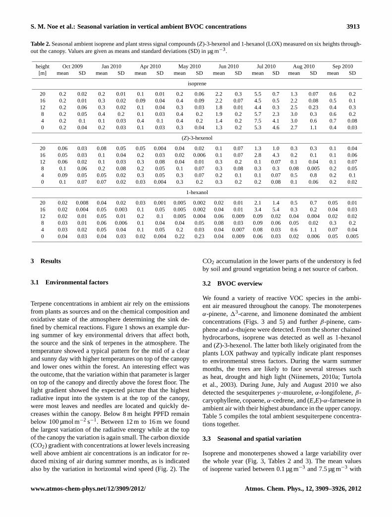
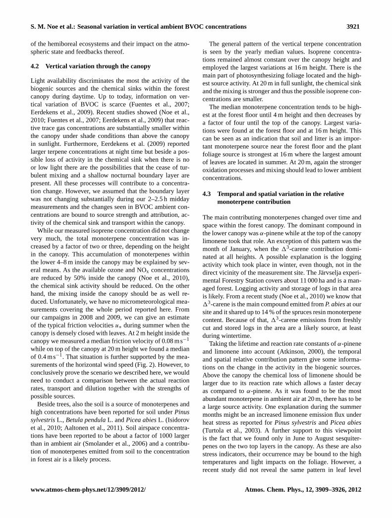
Terpene concentrations in ambient air rely on the emissionsfrom plants as sources and on the chemical composition andoxidative state of the atmosphere determining the sink de-fined by chemical reactions. Figure1 shows an example dur-ing summer of key environmental drivers that affect both,the source and the sink of terpenes in the atmosphere. Thetemperature showed a typical pattern for the mid of a clearand sunny day with higher temperatures on top of the canopyand lower ones within the forest. An interesting effect wasthe outcome, that the variation within that parameter is largeron top of the canopy and directly above the forest floor. Thelight gradient showed the expected picture that the highestradiative input into the system is at the top of the canopy,were most leaves and needles are located and quickly de-creases within the canopy. Below 8 m height PPFD remainbelow 100 µmol m−2 s−1. Between 12 m to 16 m we foundthe largest variation of the radiative energy while at the topof the canopy the variation is again small. The carbon dioxide(CO2) gradient with concentrations at lower levels increasingwell above ambient air concentrations is an indicator for re-duced mixing of air during summer months, as is indicatedalso by the variation in horizontal wind speed (Fig.2). The

CO2 accumulation in the lower parts of the understory is fedby soil and ground vegetation being a net source of carbon.

3.2 BVOC overview

We found a variety of reactive VOC species in the ambi-ent air measured throughout the canopy. The monoterpenesα-pinene,13-carene, and limonene dominated the ambientconcentrations (Figs.3 and 5) and furtherβ-pinene, cam-phene andα-thujene were detected. From the shorter chainedhydrocarbons, isoprene was detected as well as 1-hexanoland (Z)-3-hexenol. The latter both likely originated from theplants LOX pathway and typically indicate plant responsesto environmental stress factors. During the warm summermonths, the trees are likely to face several stresses suchas heat, drought and high light (Niinemets, 2010a; Turtolaet al., 2003). During June, July and August 2010 we alsodetected the sesquiterpenesγ -muurolene,α-longifolene,β-caryophyllene, copaene,α-cedrene, and (E,E)-α-farnesene inambient air with their highest abundance in the upper canopy.Table5 compiles the total ambient sesquiterpene concentra-tions together.

3.3 Seasonal and spatial variation

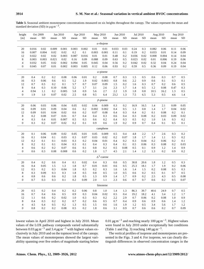
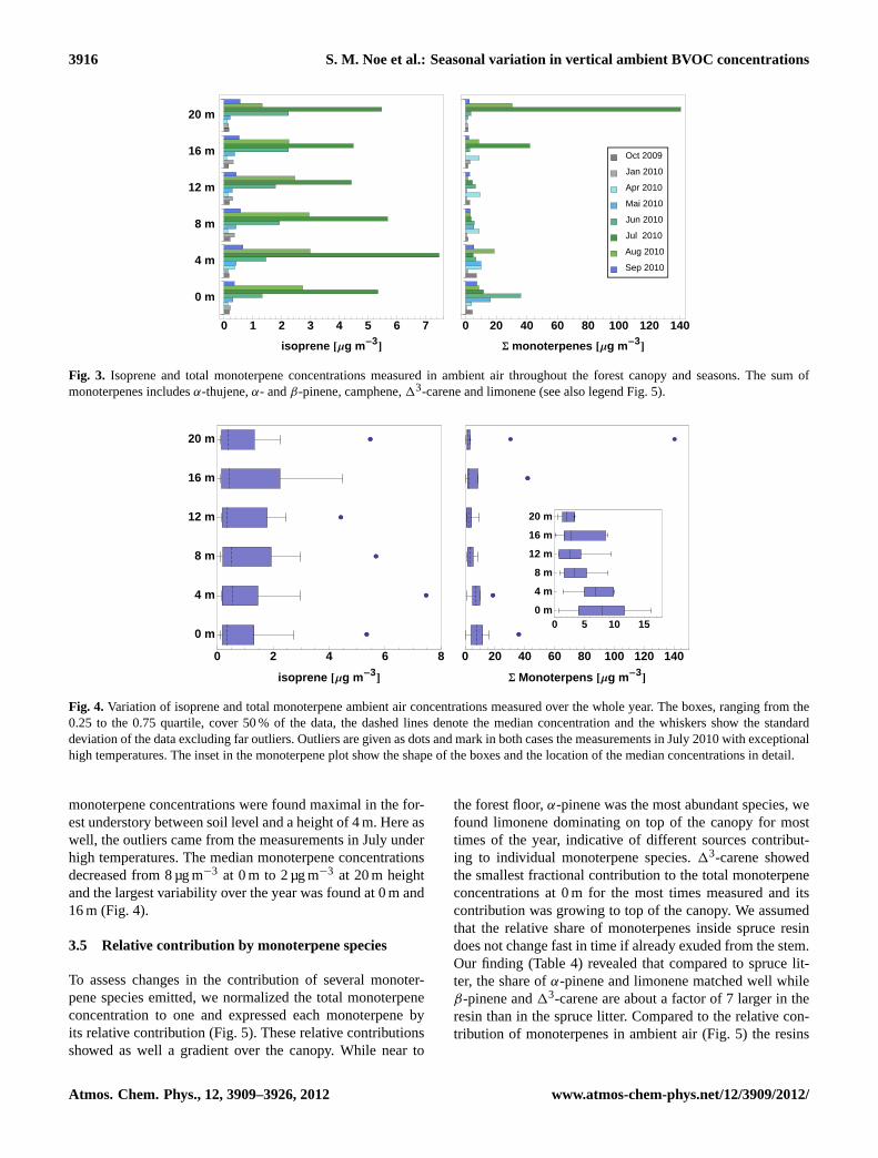
Isoprene and monoterpenes showed a large variability overthe whole year (Fig.3, Tables2 and 3). The mean valuesof isoprene varied between 0.1 µg m−3 and 7.5 µg m−3 with



Table 3.Seasonal ambient monoterpene concentrations measured on six heights throughout the canopy. The values represent the mean andstandard deviation (SD) in µ g m−3.

height Oct 2009 Jan 2010 Apr 2010 May 2010 Jun 2010 Jul 2010 Aug 2010 Sep 2010[m] mean SD mean SD mean SD mean SD mean SD mean SD mean SD mean SD

α-thujene

20 0.016 0.02 0.009 0.001 0.003 0.002 0.01 0.01 0.033 0.03 0.24 0.3 0.082 0.06 0.11 0.0616 0.007 0.004 0.02 0.02 0.2 0.1 0.003 0.001 0.11 0.1 0.19 0.2 0.033 0.01 0.14 0.0912 0.022 0.02 0.02 0.003 0.087 0.016 0.01 0.01 0.48 0.2 0.036 0.02 0.008 0.004 0.14 0.048 0.003 0.003 0.021 0.02 0.16 0.09 0.088 0.09 0.63 0.5 0.023 0.02 0.01 0.006 0.19 0.064 0.032 0.05 0.02 0.002 0.094 0.05 0.045 0.04 0.56 0.2 0.042 0.02 0.32 0.04 0.24 0.040 0.045 0.07 0.01 0.002 0.003 0.005 0.12 0.06 0.93 0.2 0.59 0.5 0.36 0.09 0.19 0.04

α-pinene

20 0.4 0.2 0.2 0.08 0.06 0.01 0.2 0.08 0.7 0.3 1.5 0.5 0.6 0.3 0.7 0.516 0.3 0.06 0.6 0.5 5.2 1.9 0.02 0.003 0.8 0.6 2.2 0.9 0.6 0.1 0.3 0.112 0.7 0.5 0.2 0.1 5.7 0.7 0.07 0.09 1.5 0.2 1.6 0.3 0.7 0.2 0.6 0.58 0.4 0.3 0.10 0.06 5.2 1.7 3.1 2.6 2.3 1.7 1.4 0.5 1.2 0.08 0.47 0.34 0.94 1.1 0.2 0.005 5.8 0.9 5.6 2.7 2.2 1.9 1.8 0.8 10.5 16.2 1.3 0.50 1.9 1.0 0.07 0.02 2.5 0.8 9.5 6.4 23.2 1.3 7.5 6.5 5.3 0.5 4.6 1.4

β-pinene

20 0.06 0.03 0.06 0.04 0.05 0.02 0.04 0.009 0.3 0.2 16.9 16.5 1.4 2.1 0.09 0.0516 0.09 0.01 0.09 0.04 0.6 0.2 0.002 0.002 0.4 0.5 1.3 0.8 1.4 1.7 0.04 0.0212 0.09 0.01 0.04 0.02 0.6 0.2 0.07 0.08 0.4 0.3 0.4 0.2 0.1 0.08 0.2 0.18 0.2 0.08 0.07 0.01 0.7 0.4 0.4 0.3 0.6 0.4 0.3 0.08 0.2 0.03 0.09 0.024 0.3 0.4 0.01 0.007 0.5 0.3 0.6 0.2 0.4 0.3 0.5 0.2 1.0 1.6 0.3 0.20 0.3 0.2 0.07 0.02 0.2 0.1 0.9 0.6 1.9 0.2 0.9 0.7 0.4 0.1 0.5 0.1

camphene

20 0.1 0.06 0.09 0.02 0.05 0.01 0.05 0.009 0.5 0.4 4.8 2.2 1.7 2.6 0.3 0.216 0.1 0.04 0.1 0.03 0.3 0.07 0.03 0.02 0.2 0.07 1.8 1.7 1.4 1.1 0.3 0.212 0.2 0.1 0.1 0.03 0.3 0.2 0.04 0.01 0.4 0.2 0.3 0.04 0.2 0.06 0.2 0.18 0.2 0.1 0.1 0.04 0.3 0.1 0.4 0.3 0.4 0.1 0.5 0.06 0.3 0.08 0.2 0.034 0.6 0.2 0.2 0.07 0.6 0.1 0.8 0.2 0.5 0.08 0.5 0.1 0.9 1.2 1.4 0.90 0.6 0.3 0.08 0.008 0.6 0.2 1.8 1.7 4.5 2.1 1.4 1.2 1.3 0.2 0.9 0.2

13-carene

20 0.4 0.2 0.6 0.4 0.1 0.02 0.4 0.3 0.6 0.5 30.8 20.6 1.8 1.2 0.5 0.316 0.4 0.05 1.5 1.3 1.8 0.7 0.01 0.01 0.6 0.5 25.3 18.1 1.7 1.9 0.2 0.0612 0.5 0.2 0.3 0.04 1.8 0.3 0.2 0.3 1.6 1.6 1.4 1.5 0.2 0.08 0.5 0.38 0.3 0.09 0.3 0.3 1.8 0.5 0.8 0.5 1.0 0.5 0.6 0.2 0.5 0.1 0.7 0.54 0.8 0.6 0.6 0.2 1.8 0.5 1.3 0.9 1.4 1.7 0.9 0.2 2.5 4.3 0.5 0.080 0.7 0.3 0.3 0.1 0.2 0.09 2.0 1.1 2.3 0.6 0.7 0.7 0.6 0.2 0.5 0.07

limonene

20 0.5 0.2 0.4 0.2 0.2 0.06 0.8 1.0 1.4 1.3 86.3 39.7 40.6 24.9 0.7 0.516 0.7 0.4 0.6 0.5 0.9 0.3 0.04 0.02 0.5 0.4 19.2 18.2 4.1 3.4 1.2 1.712 1.1 0.6 0.2 0.02 1.0 0.3 0.3 0.2 2.2 2.9 0.7 0.06 0.2 0.08 1.0 0.98 0.4 0.3 0.2 0.2 0.7 0.2 0.6 0.5 0.7 0.4 0.9 0.6 0.9 0.6 1.4 1.24 4.5 6.4 0.5 0.2 1.3 0.5 1.5 0.6 1.6 1.9 1.2 0.5 3.4 5.6 1.7 1.20 0.8 0.2 0.2 0.08 0.5 0.2 1.8 0.6 3.1 0.9 0.7 0.6 0.6 0.2 0.7 0.09

lowest values in April 2010 and highest in July 2010. Meanvalues of the LOX pathway compounds varied substantiallybetween 0.03 µg m−3 and 3.4 µg m−3 with highest values ex-clusively in July 2010 and on the topmost level of the canopy.The mean values of monoterpenes showed the largest vari-ability spanning over five orders of magnitude starting below

0.01 µg m−3 and reaching nearly 100 µg m−3. Highest valueswere found in July 2010 under exceptionally hot conditions(Table1 and Fig.3) reaching 140 µg m−3.

The vertical profiles of isoprene and monoterpenes are pre-sented in the Figs.3 and4. For isoprene, we can clearly dis-tinguish differences in observed concentration ranges in the



Table 4. Comparison of the relative contribution of monoterpenes from several possible sources near the forest floor. Resin samples havebeen taken in September 2010.

name resin [%] spruce litter [%] pine litter [%] soil efflux [%]

α-pinene 34.84 38.62 58.67 59.06β-pinene 35.38 4.83 4.59 3.7913-carene 13.91 2.07 27.04 25.91limonene 14.8 11.03 0.51 0.24

this work Isidorov et al.(2010) Isidorov et al.(2010) Aaltonen et al.(2011)

24 25 26 27 280

5

10

15

20

temperature @°CD

hei

gh

t@m

D

0 200 400 600 800 1000 1200 14000

5

10

15

20

PPFD @Ðmol m-2 s-1D

hei

gh

t@m

D

370 380 390 400 4100

5

10

15

20

CO2 @ppmD

hei

gh

t@m

D

Fig. 1. Example of key environmental drivers for isoprene andmonoterpene emissions from forest canopies in summer. Air tem-perature, quantum flux density (PPFD) and ambient CO2 mixingratio have been measured on the 12 August 2010. The lines denotemean values and the shaded areas the standard deviations. Meanshave been averaged over the period of BVOC measurements.


20 m 2 m

0.5

1.0

1.5

2.0

2.5

3.0

3.5

win

dsp

eed

@ms-

1D

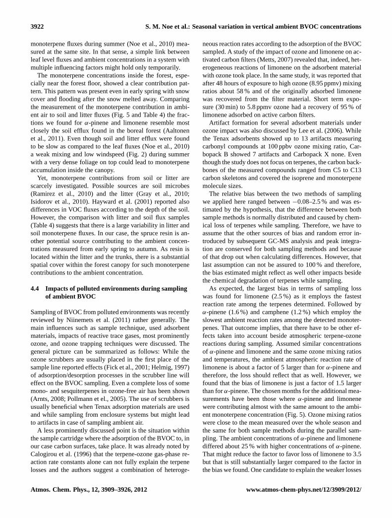
Fig. 2. Example for the variation of the wind speed above (20 m)and within the forest canopy (2 m). The data were measured duringAugust 2009. The monthly median wind speed at 20 m height was1.04 m s−1 and at 2 m height dropped to 0.25 m s−1. The boxescover 50 % of the data.

Fig. 2. Example for the variation of the wind speed above (20 m)and within the forest canopy (2 m). The data were measured dur-ing August 2009. The monthly median wind speed at 20 m heightwas 1.04 m s−1 and at 2 m height dropped to 0.25 m s−1. The boxescover 50 % of the data.

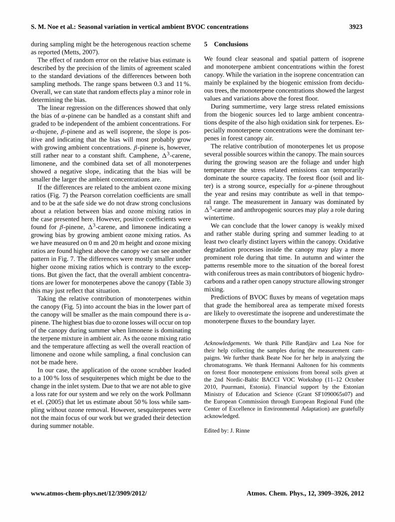
summer months (June to August) and the rest of the year.Comparing the height profile for each month, there was noclear pattern visible over the year (Fig.3). While in June thehighest concentrations were found on the topmost level ofthe canopy, the profile has changed considerably in Augustwith higher concentrations found inside the canopy. In thecase of total monoterpene concentrations, the situation is dif-ferent. Excluding the exceptionally hot periods, the monoter-penes showed higher concentrations at 0 m and 4 m heightover the whole year. Only during July 2010, when a long andexceptional hot period had occurred, the ambient monoter-pene concentrations were dramatically increased at 16 m and20 m height. The same, but much less prominent pattern wasseen in August 2010, when the concentrations of monoter-penes were slightly larger on 20 m height than below (Fig.3).

3.4 Whole year canopy profile

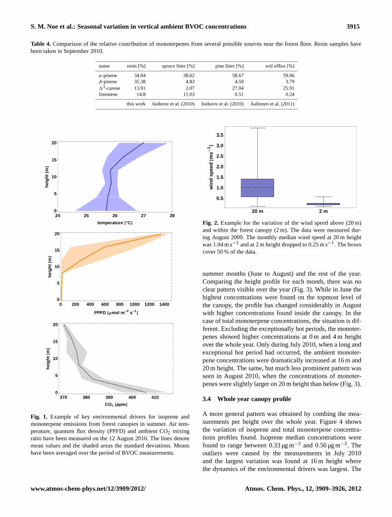
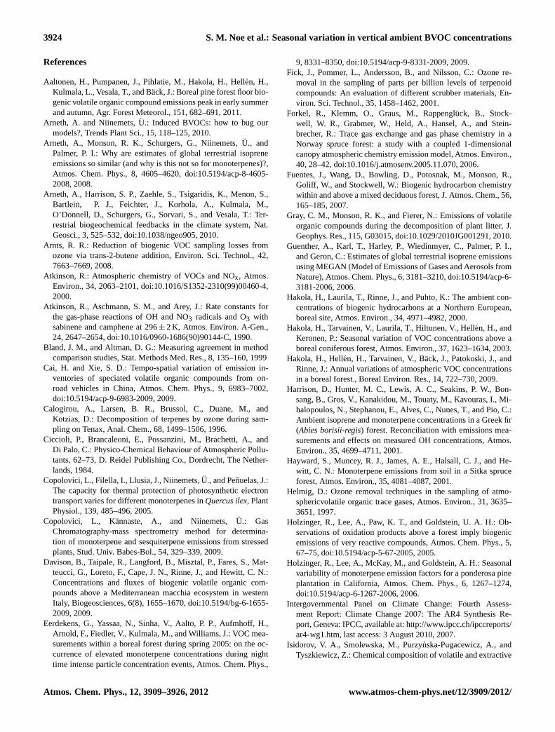
A more general pattern was obtained by combing the mea-surements per height over the whole year. Figure4 showsthe variation of isoprene and total monoterpene concentra-tions profiles found. Isoprene median concentrations werefound to range between 0.33 µg m−3 and 0.56 µg m−3. Theoutliers were caused by the measurements in July 2010and the largest variation was found at 16 m height wherethe dynamics of the environmental drivers was largest. The



0 m

4 m

8 m

12 m

16 m

20 m

0 1 2 3 4 5 6 7

isoprene @Μg m-3D

0 20 40 60 80 100 120 140

S monoterpenes @Μg m-3D

Oct 2009

Jan 2010

Apr 2010

Mai 2010

Jun 2010

Jul 2010

Aug 2010

Sep 2010

Fig. 3. Isoprene and total monoterpene concentrations measured in ambient air throughout the forest canopy and seasons. The sum ofmonoterpenes includesα-thujene,α- andβ-pinene, camphene,13-carene and limonene (see also legend Fig.5).

ææ

ææ

ææ

ææ

ææ

0 2 4 6 8

20 m

16 m

12 m

8 m

4 m

0 m

isoprene @Μg m-3D

æ æ

ææ

ææ

ææ

0 20 40 60 80 100 120 140

S Monoterpens @Μg m-3D

ææ

0 5 10 15

20 m

16 m

12 m

8 m

4 m

0 m

Fig. 4. Variation of isoprene and total monoterpene ambient air concentrations measured over the whole year. The boxes, ranging from the0.25 to the 0.75 quartile, cover 50 % of the data, the dashed lines denote the median concentration and the whiskers show the standarddeviation of the data excluding far outliers. Outliers are given as dots and mark in both cases the measurements in July 2010 with exceptionalhigh temperatures. The inset in the monoterpene plot show the shape of the boxes and the location of the median concentrations in detail.

monoterpene concentrations were found maximal in the for-est understory between soil level and a height of 4 m. Here aswell, the outliers came from the measurements in July underhigh temperatures. The median monoterpene concentrationsdecreased from 8 µg m−3 at 0 m to 2 µg m−3 at 20 m heightand the largest variability over the year was found at 0 m and16 m (Fig.4).

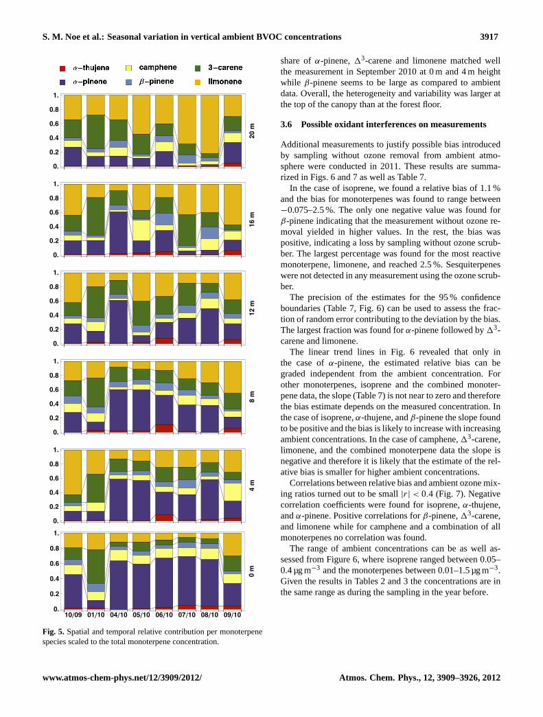
3.5 Relative contribution by monoterpene species

To assess changes in the contribution of several monoter-pene species emitted, we normalized the total monoterpeneconcentration to one and expressed each monoterpene byits relative contribution (Fig.5). These relative contributionsshowed as well a gradient over the canopy. While near to

the forest floor,α-pinene was the most abundant species, wefound limonene dominating on top of the canopy for mosttimes of the year, indicative of different sources contribut-ing to individual monoterpene species.13-carene showedthe smallest fractional contribution to the total monoterpeneconcentrations at 0 m for the most times measured and itscontribution was growing to top of the canopy. We assumedthat the relative share of monoterpenes inside spruce resindoes not change fast in time if already exuded from the stem.Our finding (Table4) revealed that compared to spruce lit-ter, the share ofα-pinene and limonene matched well whileβ-pinene and13-carene are about a factor of 7 larger in theresin than in the spruce litter. Compared to the relative con-tribution of monoterpenes in ambient air (Fig.5) the resins



0.

0.2

0.4

0.6

0.8

1.

20m

0.

0.2

0.4

0.6

0.8

1.

16m

0.

0.2

0.4

0.6

0.8

1.

12m

0.

0.2

0.4

0.6

0.8

1.

8m

0.

0.2

0.4

0.6

0.8

1.

4m

10!09 01!10 04!10 05!10 06!10 07!10 08!10 09!100.

0.2

0.4

0.6

0.8

1.

0m

Fig. 5. Spatial and temporal relative contribution per monoterpenespecies scaled to the total monoterpene concentration.

share ofα-pinene,13-carene and limonene matched wellthe measurement in September 2010 at 0 m and 4 m heightwhile β-pinene seems to be large as compared to ambientdata. Overall, the heterogeneity and variability was larger atthe top of the canopy than at the forest floor.

3.6 Possible oxidant interferences on measurements

Additional measurements to justify possible bias introducedby sampling without ozone removal from ambient atmo-sphere were conducted in 2011. These results are summa-rized in Figs.6 and7 as well as Table7.

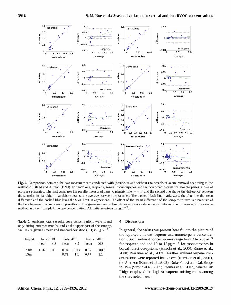
In the case of isoprene, we found a relative bias of 1.1 %and the bias for monoterpenes was found to range between−0.075–2.5 %. The only one negative value was found forβ-pinene indicating that the measurement without ozone re-moval yielded in higher values. In the rest, the bias waspositive, indicating a loss by sampling without ozone scrub-ber. The largest percentage was found for the most reactivemonoterpene, limonene, and reached 2.5 %. Sesquiterpeneswere not detected in any measurement using the ozone scrub-ber.

The precision of the estimates for the 95 % confidenceboundaries (Table7, Fig. 6) can be used to assess the frac-tion of random error contributing to the deviation by the bias.The largest fraction was found forα-pinene followed by13-carene and limonene.

The linear trend lines in Fig.6 revealed that only inthe case ofα-pinene, the estimated relative bias can begraded independent from the ambient concentration. Forother monoterpenes, isoprene and the combined monoter-pene data, the slope (Table7) is not near to zero and thereforethe bias estimate depends on the measured concentration. Inthe case of isoprene,α-thujene, andβ-pinene the slope foundto be positive and the bias is likely to increase with increasingambient concentrations. In the case of camphene,13-carene,limonene, and the combined monoterpene data the slope isnegative and therefore it is likely that the estimate of the rel-ative bias is smaller for higher ambient concentrations.

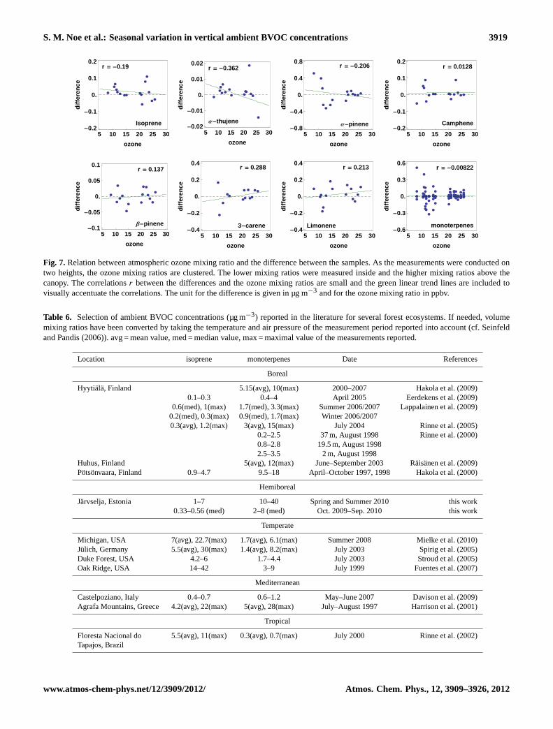
Correlations between relative bias and ambient ozone mix-ing ratios turned out to be small|r| < 0.4 (Fig. 7). Negativecorrelation coefficients were found for isoprene,α-thujene,andα-pinene. Positive correlations forβ-pinene,13-carene,and limonene while for camphene and a combination of allmonoterpenes no correlation was found.

The range of ambient concentrations can be as well as-sessed from Figure6, where isoprene ranged between 0.05–0.4 µg m−3 and the monoterpenes between 0.01–1.5 µg m−3.Given the results in Tables2 and3 the concentrations are inthe same range as during the sampling in the year before.



ææ

æ

æ

æ

æææææ

æ

æ

æ

æ

æ

0. 0.1 0.2 0.3 0.40.

0.1

0.2

0.3

0.4

no scrubber

scru

bb

er

Isoprene

æ

æ

æ

æ

æ

æ

æ

ææ

æ

æ

æ

æ

æ

æ

0. 0.1 0.2 0.3 0.4-0.1

-0.05

0.

0.05

0.1

average

dif

fere

nce

Isopreneæ

æ

æ

æ

æ

æ

ææ

æ

æ

æ

æ

æ ææ

0. 0.02 0.040.

0.02

0.04

no scrubber

scru

bb

er

Α-thujene

æ

ææ

æ

æ æææ

ææ

æ

æ

æ

æ

æ

0. 0.02 0.04-0.03

0.

0.03

average

dif

fere

nce

Α-thujene

ææ

æ

æ

æ

æ

æ

æ

æ

æ

æ

æ

æ

æ

æ

0. 0.5 1. 1.50.

0.5

1.

1.5

no scrubber

scru

bb

er

Α-pinene

ææ æ

æ

æ

æ

æ

ææ

æ

æ

æ

æ

æ

æ

0 0.5 1. 1.5-0.8

-0.4

0.

0.4

0.8

average

dif

fere

nce

Α-pineneæ

æ

æ

æ

æ æ

æ

æ

æ

ææ

æ

æ

æ

æ

æ

0 0.1 0.2 0.30

0.1

0.2

0.3

no scrubber

scru

bb

er

Camphene

ææ

æ

æ

æ

æ

æææ æ

æ

æ

æ

æ

æ

æ

0 0.1 0.2 0.3-0.1

-0.05

0.

0.05

0.1

average

dif

fere

nce

Camphene

ææ

æ

æ

æ

ææ

ææ

æ

æ

æ

æ

æ

æ

0. 0.1 0.20.

0.1

0.2

no scrubber

scru

bb

er

Β-pinene

æ

æ

æ

æ

ææ

æ

ææ

æ

æ

æ

æ

æ

æ

0 0.1 0.2-0.1

0.

0.1

average

dif

fere

nce

Β-pinene ææ

æ

æ

æ

æ

æ

ææ

æ

æ

æ

æ

æ

æ

0. 0.2 0.4 0.6 0.8 1.0.

0.2

0.4

0.6

0.8

1.

no scrubber

scru

bb

er

3-carene

ææ

ææ

æ

æ

æ

æ

ææ

æ

æ

æ

æ

æ

0. 0.2 0.4 0.6 0.8 1.-0.6

-0.3

0.

0.3

0.6

average

dif

fere

nce

3-carene

æ ææ

æææ

æ

æ

æ

æ

æ

ææ

æ

æ

0 0.4 0.8 1.20

0.4

0.8

1.2

no scrubber

scru

bb

er

Limonene

æ

æ

æ

æ

æ

æ

æ

æ

æ

æ

æ

æ

ææ

æ

0 0.4 0.8 1.2-0.4

-0.2

0.

0.2

0.4

average

dif

fere

nce

Limoneneæææææææææææææææ

ææ

æ

æ

æ

æ

æ

æ

æ

æ

æ

æ

æ

æ

æ

æææ

æ

æææææææ

æ

ææ

ææ

æææ

æææææææ

æææææ

ææ

ææ

æ

ææ

ææ

æ

æ

æ

æ

æ

æ

æ ææ

æææ

æ

ææ

æ

æ

ææ

æ

æ

0. 0.5 1. 1.50.

0.5

1.

1.5

no scrubber

scru

bb

er

monoterpenes

æææææææææææææææ

æ

æ ææ

æ

æ

æ

ææ

æ

æ

æ

æ

æ

æ

æææ

æ

æææææææ

æ

æ

æ æ

æ

ææææææææææ

æææ

ææ

ææ

ææ

æ

æ

æ

æ

ææ

æ

æ

æ

æ

æ

æ

æ

ææ

æ

æ

æ

æ

æ

æ

æ

æ

ææ

æ

0. 0.5 1. 1.5-0.6

-0.3

0.

0.3

0.6

average

dif

fere

nce

monoterpenes

Fig. 6. Comparison between the two measurements conducted with (scrubber) and without (no scrubber) ozone removal according to themethod ofBland and Altman(1999). For each one, isoprene, several monoterpenes and the combined dataset for monoterpenes, a pair ofplots are presented. The first compares the parallel measured pairs to identity line (y = x) and the second one shows the difference betweenthe samples (no scrubber – scrubber) against the average between the samples. The dashed black line marks zero, the blue line the meandifference and the dashed blue lines the 95% limit of agreement. The offset of the mean difference of the samples to zero is a measure ofthe bias between the two sampling methods. The green regression line shows a possible dependency between the difference of the samplemethod and their sampled average concentration. All units are given in µg m−3.

Table 5. Ambient total sesquiterpene concentrations were foundonly during summer months and at the upper part of the canopy.Values are given as mean and standard deviation (SD) in µgm−3.

height June 2010 July 2010 August 2010mean SD mean SD mean SD

20 m 0.02 0.01 0.04 0.03 0.02 0.00916 m 0.71 1.1 0.77 1.1

4 Discussions

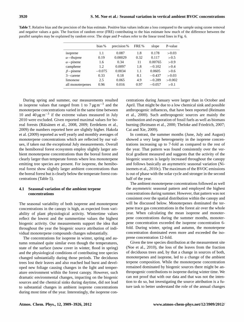
In general, the values we present here fit into the picture ofthe reported ambient isoprene and monoterpene concentra-tions. Such ambient concentrations range from 2 to 5 µg m−3

for isoprene and and 10 to 18 µg m−3 for monoterpenes inboreal forest ecosystems (Hakola et al., 2000; Rinne et al.,2000; Raisanen et al., 2009). Further ambient terpene con-centrations were reported for Greece (Harrison et al., 2001),the Amazon (Rinne et al., 2002), Duke Forest and Oak Ridgein USA (Stroud et al., 2005; Fuentes et al., 2007), where OakRidge employed the highest isoprene mixing ratios amongthe sites noted here.



ææ

æ

æ

æ

æ

ææ

æææ

æ

æ

æ

æ

æ

5 10 15 20 25 30-0.2

-0.1

0.

0.1

0.2

ozone

dif

fere

nce

Isoprene

r = -0.19

æ

æ

ææ

æ

ææ

ææ

æ

æ

æ

æ

æ

æ

æ

5 10 15 20 25 30-0.02

-0.01

0.

0.01

0.02

ozone

dif

fere

nce

Α-thujene

r = -0.362

æææ

æ

æ

æ

æ

ææ

æ

æ

æ

æ

æ

æ

5 10 15 20 25 30-0.8

-0.4

0.

0.4

0.8

ozone

dif

fere

nce

Α-pinene

r = -0.206

ææ

æ

æ

æ

æ

æææææ

æ

æ

ææ

æ

5 10 15 20 25 30-0.2

-0.1

0.

0.1

0.2

ozone

dif

fere

nce

Camphene

r = 0.0128

æ

æ

æ

æ

ææ

æ

ææ

æ

æ

æ

æ

æ

æ

5 10 15 20 25 30-0.1

-0.05

0.

0.05

0.1

ozone

dif

fere

nce

Β-pinene

r = 0.137

ææ

ææ

æ

æ

æ

æ

ææ

æ

æ

æ

5 10 15 20 25 30-0.4

-0.2

0.

0.2

0.4

ozone

dif

fere

nce

3-carene

r = 0.288

æ

æ

æ

æ

æ

æ

æ

æ

æ

æ

æ

æ

ææ

æ

5 10 15 20 25 30-0.4

-0.2

0.

0.2

0.4

ozone

dif

fere

nce

Limonene

r = 0.213

ææææ

ææææææææææææ

æ

æææ

æ

æ

æ

ææ

æ

æ

æ

æ

æ

æ

æææ

æ

ææ

ææææææ

æ

ææ

æ

ææææ

æææ

æææ

ææ

æ

ææ

ææ

ææ

æ

æ

æ

æ

ææ

æ

æ

æ

æ

æ

ææ

æ

æ

æ

æ

æ

æ

æ

æ

ææ

æ

5 10 15 20 25 30-0.6

-0.3

0.

0.3

0.6

ozone

dif

fere

nce

monoterpenes

r = -0.00822

Fig. 7. Relation between atmospheric ozone mixing ratio and the difference between the samples. As the measurements were conducted ontwo heights, the ozone mixing ratios are clustered. The lower mixing ratios were measured inside and the higher mixing ratios above thecanopy. The correlationsr between the differences and the ozone mixing ratios are small and the green linear trend lines are included tovisually accentuate the correlations. The unit for the difference is given in µg m−3 and for the ozone mixing ratio in ppbv.

Table 6. Selection of ambient BVOC concentrations (µg m−3) reported in the literature for several forest ecosystems. If needed, volumemixing ratios have been converted by taking the temperature and air pressure of the measurement period reported into account (cf.Seinfeldand Pandis(2006)). avg = mean value, med = median value, max = maximal value of the measurements reported.

Location isoprene monoterpenes Date References

Boreal

Hyytiala, Finland 5.15(avg), 10(max) 2000–2007 Hakola et al.(2009)0.1–0.3 0.4–4 April 2005 Eerdekens et al.(2009)

0.6(med), 1(max) 1.7(med), 3.3(max) Summer 2006/2007 Lappalainen et al.(2009)0.2(med), 0.3(max) 0.9(med), 1.7(max) Winter 2006/20070.3(avg), 1.2(max) 3(avg), 15(max) July 2004 Rinne et al.(2005)

0.2–2.5 37 m, August 1998 Rinne et al.(2000)0.8–2.8 19.5 m, August 19982.5–3.5 2 m, August 1998

Huhus, Finland 5(avg), 12(max) June–September 2003 Raisanen et al.(2009)Potsonvaara, Finland 0.9–4.7 9.5–18 April–October 1997, 1998 Hakola et al.(2000)

Hemiboreal

Jarvselja, Estonia 1–7 10–40 Spring and Summer 2010 this work0.33–0.56 (med) 2–8 (med) Oct. 2009–Sep. 2010 this work

Temperate

Michigan, USA 7(avg), 22.7(max) 1.7(avg), 6.1(max) Summer 2008 Mielke et al.(2010)Julich, Germany 5.5(avg), 30(max) 1.4(avg), 8.2(max) July 2003 Spirig et al.(2005)Duke Forest, USA 4.2–6 1.7–4.4 July 2003 Stroud et al.(2005)Oak Ridge, USA 14–42 3–9 July 1999 Fuentes et al.(2007)

Mediterranean

Castelpoziano, Italy 0.4–0.7 0.6–1.2 May–June 2007 Davison et al.(2009)Agrafa Mountains, Greece 4.2(avg), 22(max) 5(avg), 28(max) July–August 1997 Harrison et al.(2001)

Tropical

Floresta Nacional do 5.5(avg), 11(max) 0.3(avg), 0.7(max) July 2000 Rinne et al.(2002)Tapajos, Brazil



Table 7.Relative bias and the precision of the bias estimate. Positive bias values indicate a loss compared to the sample using ozone removaland negative values a gain. The fraction of random error (FRE) contributing to the bias estimate how much of the difference between theparallel samples may be explained by random error. The slope and P-values refer to the linear trend lines in Fig.6.

bias % precision % FRE % slope P-value

isoprene 1.1 0.087 1.8 0.178 >0.03α−thujene 0.19 0.00029 0.32 0.117 >0.5α−pinene 1.6 0.34 11 0.00765 >0.9camphene 1.2 0.0097 1.8 −0.102 >0.4β−pinene −0.075 0.0034 1.1 0.0605 >0.63−carene 0.33 0.18 8.1 −0.437 >0.03limonene 2.5 0.065 4.9 −0.289 >0.002all monoterpenes 0.96 0.016 0.97 −0.057 >0.1

During spring and summer, our measurements resultedin isoprene values that ranged from 1 to 7 µg m−3 and themonoterpene concentrations varied in the same time between10 and 40 µg m−3 if the extreme values measured in July2010 were excluded. Given reported maximal values for bo-real forests (Raisanen et al., 2008, 2009; Eerdekens et al.,2009) the numbers reported here are slightly higher.Hakolaet al.(2009) reported as well yearly and monthly averages ofmonoterpene concentrations which are reflected by our val-ues, if taken out the exceptional July measurements. Overallthe hemiboreal forest ecosystem employ slightly larger am-bient monoterpene concentrations than the boreal forest andclearly larger than temperate forests where less monoterpeneemitting tree species are present. For isoprene, the hemibo-real forest show slightly larger ambient concentrations thanthe boreal forest but is clearly below the temperate forest con-centrations (Table5).

4.1 Seasonal variation of the ambient terpeneconcentrations

The seasonal variability of both isoprene and monoterpeneconcentrations in the canopy is high, as expected from vari-ability of plant physiological activity. Wintertime valuesreflect the lowest and the summertime values the highestbiogenic activity. Our measurements support the idea thatthroughout the year the biogenic source attribution of indi-vidual monoterpene compounds changes substantially.

The concentrations for isoprene in winter, spring and au-tumn remained quite similar even though the temperatures,state of the surface (snow cover in winter, flood in spring)and the physiological conditions of contributing tree specieschanged substantially during those periods. The deciduoustrees lost their leaves and also reached bud burst and devel-oped new foliage causing changes in the light and temper-ature environment within the forest canopy. However, suchdramatic environmental changes, impacting on the biogenicsources and the chemical sinks during daytime, did not leadto substantial changes in ambient isoprene concentrationsduring most time of the year. Interestingly, the isoprene con-

centrations during January were larger than in October andApril. That might be due to a low chemical sink and possibleanthropogenic influences, that have been reported (Reimannet al., 2000). Such anthropogenic sources are mainly thecombustion and evaporation of fossil fuels as well as biomassburning (Reimann et al., 2000; Theloke and Friedrich, 2007;Cai and Xie, 2009).

In contrast, the summer months (June, July and August)showed a very large heterogeneity in the isoprene concen-trations increasing up to 7-fold as compared to the rest ofthe year. That pattern was found consistently over the ver-tical gradient measured and suggests that the activity of thebiogenic sources is largely increased throughout the canopyand follows basically an asymmetric seasonal variation (Ni-inemets et al., 2010c). The maximum of the BVOC emissionsis out of phase with the solar cycle and stronger in the secondhalf of the year.

The ambient monoterpene concentrations followed as wellthe asymmetric seasonal pattern and employed the highestconcentrations during summer. However, that pattern was notconsistent over the spatial distribution within the canopy andwill be discussed below. Monoterpenes dominated the ter-pene trace gas concentrations in the forest air over the wholeyear. When calculating the mean isoprene and monoter-pene concentrations during the summer months, monoter-pene concentration exceeded the isoprene concentration 6-fold. During winter, spring and autumn, the monoterpeneconcentration dominated even more and exceeded the iso-prene concentration 12-fold.

Given the tree species distribution at the measurement site(Noe et al., 2010), the loss of the leaves from the fractionof deciduous trees and, by that a change in sources of both,monoterpenes and isoprene, led to a change of the ambientterpene composition. While the monoterpene concentrationremained dominated by biogenic sources there might be an-thropogenic contributions to isoprene during winter time. Wecan not proof that with our data and that was not the inten-tion to do so, but investigating the source attribution is a fu-ture task to better understand the role of the annual changes



of the hemiboreal ecosystems and their impact on the atmo-spheric state and feedbacks thereof.

4.2 Vertical variation through the canopy

Light availability discriminates the most the activity of thebiogenic sources and the chemical sinks within the forestcanopy during daytime. Up to today, information on ver-tical variation of BVOC is scarce (Fuentes et al., 2007;Eerdekens et al., 2009). Recent studies showed (Noe et al.,2010; Fuentes et al., 2007; Eerdekens et al., 2009) that reac-tive trace gas concentrations are substantially smaller withinthe canopy under shade conditions than above the canopyin sunlight. Furthermore,Eerdekens et al.(2009) reportedlarger terpene concentrations at night time but beside a pos-sible loss of activity in the chemical sink when there is noor low light there are the possibilities that the cease of tur-bulent mixing and a shallow nocturnal boundary layer arepresent. All these processes will contribute to a concentra-tion change. However, we assumed that the boundary layerwas not changing substantially during our 2–2.5 h middaymeasurements and the changes seen in BVOC ambient con-centrations are bound to source strength and attribution, ac-tivity of the chemical sink and transport within the canopy.

While our measured isoprene concentration did not changevery much, the total monoterpene concentration was in-creased by a factor of two or three, depending on the heightin the canopy. This accumulation of monoterpenes withinthe lower 4–8 m inside the canopy may be explained by sev-eral means. As the available ozone and NOx concentrationsare reduced by 50% inside the canopy (Noe et al., 2010),the chemical sink activity should be reduced. On the otherhand, the mixing inside the canopy should be as well re-duced. Unfortunately, we have no micrometeorological mea-surements covering the whole period reported here. Fromour campaigns in 2008 and 2009, we can give an estimateof the typical friction velocitiesu∗ during summer when thecanopy is densely closed with leaves. At 2 m height inside thecanopy we measured a median friction velocity of 0.08 ms−1

while on top of the canopy at 20 m height we found a medianof 0.4 ms−1. That situation is further supported by the mea-surements of the horizontal wind speed (Fig.2). However, toconclusively prove the scenario we described here, we wouldneed to conduct a comparison between the actual reactionrates, transport and dilution together with the strengths ofpossible sources.

Beside trees, also the soil is a source of monoterpenes andhigh concentrations have been reported for soil underPinussylvestrisL., Betula pendulaL. andPicea abiesL. (Isidorovet al., 2010; Aaltonen et al., 2011). Soil airspace concentra-tions have been reported to be about a factor of 1000 largerthan in ambient air (Smolander et al., 2006) and a contribu-tion of monoterpenes emitted from soil to the concentrationin forest air is a likely process.

The general pattern of the vertical terpene concentrationis seen by the yearly median values. Isoprene concentra-tions remained almost constant over the canopy height andemployed the largest variations at 16 m height. There is themain part of photosynthesizing foliage located and the high-est source activity. At 20 m in full sunlight, the chemical sinkand the mixing is stronger and thus the possible isoprene con-centrations are smaller.

The median monoterpene concentration tends to be high-est at the forest floor until 4 m height and then decreases bya factor of four until the top of the canopy. Largest varia-tions were found at the forest floor and at 16 m height. Thiscan be seen as an indication that soil and litter is an impor-tant monoterpene source near the forest floor and the plantfoliage source is strongest at 16 m where the largest amountof leaves are located in summer. At 20 m, again the strongeroxidation processes and mixing should lead to lower ambientconcentrations.

4.3 Temporal and spatial variation in the relativemonoterpene contribution

The main contributing monoterpenes changed over time andspace within the forest canopy. The dominant compound inthe lower canopy wasα-pinene while at the top of the canopylimonene took that role. An exception of this pattern was themonth of January, when the13-carene contribution domi-nated at all heights. A possible explanation is the loggingactivity which took place in winter, even though, not in thedirect vicinity of the measurement site. The Jarvselja experi-mental Forestry Station covers about 11 000 ha and is a man-aged forest. Logging activity and storage of logs in that areais likely. From a recent study (Noe et al., 2010) we know that13-carene is the main compound emitted fromP. abiesat oursite and it shared up to 14 % of the spruces resin monoterpenecontent. Because of that,13-carene emissions from freshlycut and stored logs in the area are a likely source, at leastduring wintertime.

Taking the lifetime and reaction rate constants ofα-pineneand limonene into account (Atkinson, 2000), the temporaland spatial relative contribution pattern give some informa-tions on the change in the activity in the biogenic sources.Above the canopy the chemical loss of limonene should belarger due to its reaction rate which allows a faster decayas compared toα-pinene. As it was found to be the mostabundant monoterpene in ambient air at 20 m, there has to bea large source activity. One explanation during the summermonths might be an increased limonene emission flux underheat stress as reported forPinus sylvestrisandPicea abies(Turtola et al., 2003). A further support to this viewpointis the fact that we found only in June to August sesquiter-penes on the two top layers in the canopy. As these are alsostress indicators, their occurrence may be bound to the hightemperatures and light impacts on the foliage. However, arecent study did not reveal the same pattern in leaf level



monoterpene fluxes during summer (Noe et al., 2010) mea-sured at the same site. In that sense, a simple link betweenleaf level fluxes and ambient concentrations in a system withmultiple influencing factors might hold only temporarily.

The monoterpene concentrations inside the forest, espe-cially near the forest floor, showed a clear contribution pat-tern. This pattern was present even in early spring with snowcover and flooding after the snow melted away. Comparingthe measurement of the monoterpene contribution in ambi-ent air to soil and litter fluxes (Fig.5 and Table4) the frac-tions we found forα-pinene and limonene resemble mostclosely the soil efflux found in the boreal forest (Aaltonenet al., 2011). Even though soil and litter efflux were foundto be slow as compared to the leaf fluxes (Noe et al., 2010)a weak mixing and low windspeed (Fig.2) during summerwith a very dense foliage on top could lead to monoterpeneaccumulation inside the canopy.

Yet, monoterpene contributions from soil or litter arescarcely investigated. Possible sources are soil microbes(Ramirez et al., 2010) and the litter (Gray et al., 2010;Isidorov et al., 2010). Hayward et al.(2001) reported alsodifferences in VOC fluxes according to the depth of the soil.However, the comparison with litter and soil flux samples(Table4) suggests that there is a large variability in litter andsoil monoterpene fluxes. In our case, the spruce resin is an-other potential source contributing to the ambient concen-trations measured from early spring to autumn. As resin islocated within the litter and the trunks, there is a substantialspatial cover within the forest canopy for such monoterpenecontributions to the ambient concentration.

4.4 Impacts of polluted environments during samplingof ambient BVOC

Sampling of BVOC from polluted environments was recentlyreviewed byNiinemets et al.(2011) rather generally. Themain influences such as sample technique, used adsorbentmaterials, impacts of reactive trace gases, most prominentlyozone, and ozone trapping techniques were discussed. Thegeneral picture can be summarized as follows: While theozone scrubbers are usually placed in the first place of thesample line reported effects (Fick et al., 2001; Helmig, 1997)of adsorption/desorption processes in the scrubber line willeffect on the BVOC sampling. Even a complete loss of somemono- and sesquiterpenes in ozone-free air has been shown(Arnts, 2008; Pollmann et el., 2005). The use of scrubbers isusually beneficial when Tenax adsorption materials are usedand while sampling from enclosure systems but might leadto artifacts in case of sampling ambient air.

A less prominently discussed point is the situation withinthe sample cartridge where the adsorption of the BVOC to, inour case carbon surfaces, take place. It was already noted byCalogirou et al.(1996) that the terpene-ozone gas-phase re-action rate constants alone can not fully explain the terpenelosses and the authors suggest a combination of heteroge-

neous reaction rates according to the adsorption of the BVOCsampled. A study of the impact of ozone and limonene on ac-tivated carbon filters (Metts, 2007) revealed that, indeed, het-erogeneous reactions of limonene on the adsorbent materialwith ozone took place. In the same study, it was reported thatafter 48 hours of exposure to high ozone (8.95 ppmv) mixingratios about 58 % and of the originally adsorbed limonenewas recovered from the filter material. Short term expo-sure (30 min) to 5.8 ppmv ozone had a recovery of 95 % oflimonene adsorbed on active carbon filters.

Artifact formation for several adsorbent materials underozone impact was also discussed byLee et al.(2006). Whilethe Tenax adsorbents showed up to 13 artifacts measuringcarbonyl compounds at 100 ppbv ozone mixing ratio, Car-bopack B showed 7 artifacts and Carbopack X none. Eventhough the study does not focus on terpenes, the carbon back-bones of the measured compounds ranged from C5 to C13carbon skeletons and covered the isoprene and monoterpenemolecule sizes.

The relative bias between the two methods of samplingwe applied here ranged between−0.08–2.5 % and was es-timated by the hypothesis, that the difference between bothsample methods is normally distributed and caused by chem-ical loss of terpenes while sampling. Therefore, we have toassume that the other sources of bias and random error in-troduced by subsequent GC-MS analysis and peak integra-tion are conserved for both sampling methods and becauseof that drop out when calculating differences. However, thatlast assumption can not be assured to 100 % and therefore,the bias estimated might reflect as well other impacts besidethe chemical degradation of terpenes while sampling.

As expected, the largest bias in terms of sampling losswas found for limonene (2.5 %) as it employs the fastestreaction rate among the terpenes determined. Followed byα-pinene (1.6 %) and camphene (1.2 %) which employ theslowest ambient reaction rates among the detected monoter-penes. That outcome implies, that there have to be other ef-fects taken into account beside atmospheric terpene-ozonereactions during sampling. Assumed similar concentrationsof α-pinene and limonene and the same ozone mixing ratiosand temperatures, the ambient atmospheric reaction rate oflimonene is about a factor of 5 larger than forα-pinene andtherefore, the loss should reflect that as well. However, wefound that the bias of limonene is just a factor of 1.5 largerthan forα-pinene. The chosen months for the additional mea-surements have been those whereα-pinene and limonenewere contributing almost with the same amount to the ambi-ent monoterpene concentration (Fig.5). Ozone mixing ratioswere close to the mean measured over the whole season andthe same for both sample methods during the parallel sam-pling. The ambient concentrations ofα-pinene and limonenediffered about 25 % with higher concentrations ofα-pinene.That might reduce the factor to favor loss of limonene to 3.5but that is still substantially larger compared to the factor inthe bias we found. One candidate to explain the weaker losses



during sampling might be the heterogenous reaction schemeas reported (Metts, 2007).

The effect of random error on the relative bias estimate isdescribed by the precision of the limits of agreement scaledto the standard deviations of the differences between bothsampling methods. The range spans between 0.3 and 11 %.Overall, we can state that random effects play a minor role indetermining the bias.

The linear regression on the differences showed that onlythe bias ofα-pinene can be handled as a constant shift andgraded to be independent of the ambient concentrations. Forα-thujene,β-pinene and as well isoprene, the slope is pos-itive and indicating that the bias will most probably growwith growing ambient concentrations.β-pinene is, however,still rather near to a constant shift. Camphene,13-carene,limonene, and the combined data set of all monoterpenesshowed a negative slope, indicating that the bias will besmaller the larger the ambient concentrations are.

If the differences are related to the ambient ozone mixingratios (Fig.7) the Pearson correlation coefficients are smalland to be at the safe side we do not draw strong conclusionsabout a relation between bias and ozone mixing ratios inthe case presented here. However, positive coefficients werefound for β-pinene,13-carene, and limonene indicating agrowing bias by growing ambient ozone mixing ratios. Aswe have measured on 0 m and 20 m height and ozone mixingratios are found highest above the canopy we can see anotherpattern in Fig.7. The differences were mostly smaller underhigher ozone mixing ratios which is contrary to the excep-tions. But given the fact, that the overall ambient concentra-tions are lower for monoterpenes above the canopy (Table3)this may just reflect that situation.

Taking the relative contribution of monoterpenes withinthe canopy (Fig.5) into account the bias in the lower part ofthe canopy will be smaller as the main compound there isα-pinene. The highest bias due to ozone losses will occur on topof the canopy during summer when limonene is dominatingthe terpene mixture in ambient air. As the ozone mixing ratioand the temperature affecting as well the overall reaction oflimonene and ozone while sampling, a final conclusion cannot be made here.

In our case, the application of the ozone scrubber leadedto a 100 % loss of sesquiterpenes which might be due to thechange in the inlet system. Due to that we are not able to givea loss rate for our system and we rely on the workPollmannet el.(2005) that let us estimate about 50 % loss while sam-pling without ozone removal. However, sesquiterpenes werenot the main focus of our work but we graded their detectionduring summer notable.

5 Conclusions

We found clear seasonal and spatial pattern of isopreneand monoterpene ambient concentrations within the forestcanopy. While the variation in the isoprene concentration canmainly be explained by the biogenic emission from decidu-ous trees, the monoterpene concentrations showed the largestvalues and variations above the forest floor.

During summertime, very large stress related emissionsfrom the biogenic sources led to large ambient concentra-tions despite of the also high oxidation sink for terpenes. Es-pecially monoterpene concentrations were the dominant ter-penes in forest canopy air.

The relative contribution of monoterpenes let us proposeseveral possible sources within the canopy. The main sourcesduring the growing season are the foliage and under hightemperature the stress related emissions can temporarilydominate the source capacity. The forest floor (soil and lit-ter) is a strong source, especially forα-pinene throughoutthe year and resins may contribute as well in that tempo-ral range. The measurement in January was dominated by13-carene and anthropogenic sources may play a role duringwintertime.

We can conclude that the lower canopy is weakly mixedand rather stable during spring and summer leading to atleast two clearly distinct layers within the canopy. Oxidativedegradation processes inside the canopy may play a moreprominent role during that time. In autumn and winter thepatterns resemble more to the situation of the boreal forestwith coniferous trees as main contributors of biogenic hydro-carbons and a rather open canopy structure allowing strongermixing.

Predictions of BVOC fluxes by means of vegetation mapsthat grade the hemiboreal area as temperate mixed forestsare likely to overestimate the isoprene and underestimate themonoterpene fluxes to the boundary layer.

Acknowledgements.We thank Pille Randjarv and Lea Noe fortheir help collecting the samples during the measurement cam-paigns. We further thank Beate Noe for her help in analyzing thechromatograms. We thank Hermanni Aaltonen for his commentson forest floor monoterpene emissions from boreal soils given atthe 2nd Nordic-Baltic BACCI VOC Workshop (11–12 October2010, Puurmani, Estonia). Financial support by the EstonianMinistry of Education and Science (Grant SF1090065s07) andthe European Commission through European Regional Fund (theCenter of Excellence in Environmental Adaptation) are gratefullyacknowledged.

Edited by: J. Rinne



References

Aaltonen, H., Pumpanen, J., Pihlatie, M., Hakola, H., Hellen, H.,Kulmala, L., Vesala, T., and Back, J.: Boreal pine forest floor bio-genic volatile organic compound emissions peak in early summerand autumn, Agr. Forest Meteorol., 151, 682–691, 2011.

Arneth, A. and Niinemets,U.: Induced BVOCs: how to bug ourmodels?, Trends Plant Sci., 15, 118–125, 2010.

Arneth, A., Monson, R. K., Schurgers, G., Niinemets,U., andPalmer, P. I.: Why are estimates of global terrestrial isopreneemissions so similar (and why is this not so for monoterpenes)?,Atmos. Chem. Phys., 8, 4605–4620,doi:10.5194/acp-8-4605-2008, 2008.

Arneth, A., Harrison, S. P., Zaehle, S., Tsigaridis, K., Menon, S.,Bartlein, P. J., Feichter, J., Korhola, A., Kulmala, M.,O’Donnell, D., Schurgers, G., Sorvari, S., and Vesala, T.: Ter-restrial biogeochemical feedbacks in the climate system, Nat.Geosci., 3, 525–532,doi:10.1038/ngeo905, 2010.

Arnts, R. R.: Reduction of biogenic VOC sampling losses fromozone via trans-2-butene addition, Environ. Sci. Technol., 42,7663–7669, 2008.

Atkinson, R.: Atmospheric chemistry of VOCs and NOx, Atmos.Environ., 34, 2063–2101,doi:10.1016/S1352-2310(99)00460-4,2000.

Atkinson, R., Aschmann, S. M., and Arey, J.: Rate constants forthe gas-phase reactions of OH and NO3 radicals and O3 withsabinene and camphene at 296± 2 K, Atmos. Environ. A-Gen.,24, 2647–2654,doi:10.1016/0960-1686(90)90144-C, 1990.

Bland, J. M., and Altman, D. G.: Measuring agreement in methodcomparison studies, Stat. Methods Med. Res., 8, 135–160, 1999

Cai, H. and Xie, S. D.: Tempo-spatial variation of emission in-ventories of speciated volatile organic compounds from on-road vehicles in China, Atmos. Chem. Phys., 9, 6983–7002,doi:10.5194/acp-9-6983-2009, 2009.

Calogirou, A., Larsen, B. R., Brussol, C., Duane, M., andKotzias, D.: Decomposition of terpenes by ozone during sam-pling on Tenax, Anal. Chem., 68, 1499–1506, 1996.

Ciccioli, P., Brancaleoni, E., Possanzini, M., Brachetti, A., andDi Palo, C.: Physico-Chemical Behaviour of Atmospheric Pollu-tants, 62–73, D. Reidel Publishing Co., Dordrecht, The Nether-lands, 1984.

Copolovici, L., Filella, I., Llusia, J., Niinemets,U., and Penuelas, J.:The capacity for thermal protection of photosynthetic electrontransport varies for different monoterpenes inQuercus ilex, PlantPhysiol., 139, 485–496, 2005.

Copolovici, L., Kannaste, A., and Niinemets,U.: GasChromatography-mass spectrometry method for determina-tion of monoterpene and sesquiterpene emissions from stressedplants, Stud. Univ. Babes-Bol., 54, 329–339, 2009.

Davison, B., Taipale, R., Langford, B., Misztal, P., Fares, S., Mat-teucci, G., Loreto, F., Cape, J. N., Rinne, J., and Hewitt, C. N.:Concentrations and fluxes of biogenic volatile organic com-pounds above a Mediterranean macchia ecosystem in westernItaly, Biogeosciences, 6(8), 1655–1670,doi:10.5194/bg-6-1655-2009, 2009.

Eerdekens, G., Yassaa, N., Sinha, V., Aalto, P. P., Aufmhoff, H.,Arnold, F., Fiedler, V., Kulmala, M., and Williams, J.: VOC mea-surements within a boreal forest during spring 2005: on the oc-currence of elevated monoterpene concentrations during nighttime intense particle concentration events, Atmos. Chem. Phys.,

9, 8331–8350,doi:10.5194/acp-9-8331-2009, 2009.Fick, J., Pommer, L., Andersson, B., and Nilsson, C.: Ozone re-

moval in the sampling of parts per billion levels of terpenoidcompounds: An evaluation of different scrubber materials, En-viron. Sci. Technol., 35, 1458–1462, 2001.

Forkel, R., Klemm, O., Graus, M., Rappengluck, B., Stock-well, W. R., Grabmer, W., Held, A., Hansel, A., and Stein-brecher, R.: Trace gas exchange and gas phase chemistry in aNorway spruce forest: a study with a coupled 1-dimensionalcanopy atmospheric chemistry emission model, Atmos. Environ.,40, 28–42,doi:10.1016/j.atmosenv.2005.11.070, 2006.

Fuentes, J., Wang, D., Bowling, D., Potosnak, M., Monson, R.,Goliff, W., and Stockwell, W.: Biogenic hydrocarbon chemistrywithin and above a mixed deciduous forest, J. Atmos. Chem., 56,165–185, 2007.

Gray, C. M., Monson, R. K., and Fierer, N.: Emissions of volatileorganic compounds during the decomposition of plant litter, J.Geophys. Res., 115, G03015,doi:10.1029/2010JG001291, 2010.

Guenther, A., Karl, T., Harley, P., Wiedinmyer, C., Palmer, P. I.,and Geron, C.: Estimates of global terrestrial isoprene emissionsusing MEGAN (Model of Emissions of Gases and Aerosols fromNature), Atmos. Chem. Phys., 6, 3181–3210,doi:10.5194/acp-6-3181-2006, 2006.

Hakola, H., Laurila, T., Rinne, J., and Puhto, K.: The ambient con-centrations of biogenic hydrocarbons at a Northern European,boreal site, Atmos. Environ., 34, 4971–4982, 2000.

Hakola, H., Tarvainen, V., Laurila, T., Hiltunen, V., Hellen, H., andKeronen, P.: Seasonal variation of VOC concentrations above aboreal coniferous forest, Atmos. Environ., 37, 1623–1634, 2003.

Hakola, H., Hellen, H., Tarvainen, V., Back, J., Patokoski, J., andRinne, J.: Annual variations of atmospheric VOC concentrationsin a boreal forest., Boreal Environ. Res., 14, 722–730, 2009.

Harrison, D., Hunter, M. C., Lewis, A. C., Seakins, P. W., Bon-sang, B., Gros, V., Kanakidou, M., Touaty, M., Kavouras, I., Mi-halopoulos, N., Stephanou, E., Alves, C., Nunes, T., and Pio, C.:Ambient isoprene and monoterpene concentrations in a Greek fir(Abies borisii-regis) forest. Reconciliation with emissions mea-surements and effects on measured OH concentrations, Atmos.Environ., 35, 4699–4711, 2001.

Hayward, S., Muncey, R. J., James, A. E., Halsall, C. J., and He-witt, C. N.: Monoterpene emissions from soil in a Sitka spruceforest, Atmos. Environ., 35, 4081–4087, 2001.

Helmig, D.: Ozone removal techniques in the sampling of atmo-sphericvolatile organic trace gases, Atmos. Environ., 31, 3635–3651, 1997.

Holzinger, R., Lee, A., Paw, K. T., and Goldstein, U. A. H.: Ob-servations of oxidation products above a forest imply biogenicemissions of very reactive compounds, Atmos. Chem. Phys., 5,67–75,doi:10.5194/acp-5-67-2005, 2005.

Holzinger, R., Lee, A., McKay, M., and Goldstein, A. H.: Seasonalvariability of monoterpene emission factors for a ponderosa pineplantation in California, Atmos. Chem. Phys., 6, 1267–1274,doi:10.5194/acp-6-1267-2006, 2006.

Intergovernmental Panel on Climate Change: Fourth Assess-ment Report: Climate Change 2007: The AR4 Synthesis Re-port, Geneva: IPCC, available at:http://www.ipcc.ch/ipccreports/ar4-wg1.htm, last access: 3 August 2010, 2007.

Isidorov, V. A., Smolewska, M., Purzynska-Pugacewicz, A., andTyszkiewicz, Z.: Chemical composition of volatile and extractive


http://dx.doi.org/10.5194/acp-8-4605-2008


http://dx.doi.org/10.1038/ngeo905

http://dx.doi.org/10.1016/S1352-2310(99)00460-4

http://dx.doi.org/10.1016/0960-1686(90)90144-C


http://dx.doi.org/10.5194/bg-6-1655-2009

http://dx.doi.org/10.5194/bg-6-1655-2009


http://dx.doi.org/10.1016/j.atmosenv.2005.11.070

http://dx.doi.org/10.1029/2010JG001291





http://www.ipcc.ch/ipccreports/ar4-wg1.htm

http://www.ipcc.ch/ipccreports/ar4-wg1.htm


compounds of pine and spruce leaf litter in the initial stages ofdecomposition, Biogeosciences, 7, 2785–2794,doi:10.5194/bg-7-2785-2010, 2010.

Kanakidou, M., Seinfeld, J. H., Pandis, S. N., Barnes, I., Den-tener, F. J., Facchini, M. C., Van Dingenen, R., Ervens, B.,Nenes, A., Nielsen, C. J., Swietlicki, E., Putaud, J. P., Balkan-ski, Y., Fuzzi, S., Horth, J., Moortgat, G. K., Winterhalter, R.,Myhre, C. E. L., Tsigaridis, K., Vignati, E., Stephanou, E. G.,and Wilson, J.: Organic aerosol and global climate modelling: areview, Atmos. Chem. Phys., 5, 1053–1123,doi:10.5194/acp-5-1053-2005, 2005.

Karl, T., Potosnak, M., Guenther, A., Clark, D., Walker, J., Her-rick, J. D., and Geron, C.: Exchange processes of volatile organiccompounds above a tropical rain forest: implications for model-ing tropospheric chemistry above dense vegetation, J. Geophys.Res., 109, D18306,doi:10.1029/2004JD004738, 2004.

Kulmala, M., Suni, T., Lehtinen, K. E. J., Dal Maso, M., Boy, M.,Reissell, A., Rannik,U, Aalto, P., Keronen, P., Hakola, H.,Back, J., Hoffmann, T., Vesala, T., and Hari, P.: A new feedbackmechanism linking forests, aerosols, and climate, Atmos. Chem.Phys., 4, 557–562,doi:10.5194/acp-4-557-2004, 2004.

Lappalainen, H. K., Sevanto, S., Back, J., Ruuskanen, T. M., Ko-lari, P., Taipale, R., Rinne, J., Kulmala, M., and Hari, P.: Day-time concentrations of biogenic volatile organic compoundsin a boreal forest canopy and their relation to environmen-tal and biological factors, Atmos. Chem. Phys., 9, 5447–5459doi:10.5194/acp-9-5447-2009, 2009.

Lee, J. H., Batterman, S. A., Jia, C., and Chernyak, S.: Ozone Arti-facts and Carbonyl Ceasurements Using Tenax GR, Tenax TA,Carbopack B, and Carbopack X Adsorbents, J. Air & WasteManage. Assoc., 56, 1503–1517, 2006.

Lyubovtseva, Y. S., Sogacheva, L., Dal Maso, M., Bonn, B., Kero-nen, P., and Kulmala, M.: Seasonal variations of trace gases,meteorological parameters, and formation of aerosols in borealforests., Boreal Environ. Res., 10, 493–510, 2005.

Mayrhofer, S., Teuber, M., Zimmer, I., Louis, S., Fischbach, R. J.,and Schnitzler, J.-P.: Diurnal and seasonal variation of isoprenebiosynthesis-related genes in grey poplar leaves, Plant Physiol.,139, 474–484,doi:10.1104/pp.105.066373, 2005.

Metts, T. A.: Heterogeneous reactions of ozone and D-limonene onactivated carbon, Indoor Air, 17, 362–371, 2007.

Mielke, L. H., Pratt, K. A., Shepson, P. B., McLuckey, S. A.,Wisthaler, A., and Hansel, A.: Quantitative Determination ofBiogenic Volatile Organic Compounds in the Atmosphere UsingProton-Transfer Reaction Linear Ion Trap Mass Spectrometry,Analyt. Chem., 82, 7952–7957, 2010.

Ng, N. L., Kwan, A. J., Surratt, J. D., Chan, A. W. H., Chhabra, P. S.,Sorooshian, A., Pye, H. O. T., Crounse, J. D., Wennberg, P. O.,Flagan, R. C., and Seinfeld, J. H.: Secondary organic aerosol(SOA) formation from reaction of isoprene with nitrate radicals(NO3), Atmos. Chem. Phys., 8, 4117–4140,doi:10.5194/acp-8-4117-2008, 2008.

Niinemets,U.: Responses of forest trees to single and multipleenvironmental stresses from seedlings to mature plants: paststress history, stress interactions, tolerance and acclimation, For-est Ecol. Manag., 260, 1623–1639, 2010a.

Niinemets,U.: Mild versus severe stress and BVOCs: thresholds,priming and consequences, Trends Plant Sci., 15, 145–153,2010b.

Niinemets,U., Arneth, A., Kuhn, U., Monson, R. K., Penuelas, J.,and Staudt, M.: The emission factor of volatile isoprenoids:stress, acclimation, and developmental responses, Biogeo-sciences, 7, 2203–2223,doi:10.5194/bg-7-2203-2010, 2010c.

Niinemets, U., Monson, R. K., Arneth, A., Ciccioli, P.,Kesselmeier, J., Kuhn, U., Noe, S. M., Penuelas, J., andStaudt, M.: The leaf-level emission factor of volatile isoprenoids:caveats, model algorithms, response shapes and scaling, Biogeo-sciences, 7, 1809–1832,doi:10.5194/bg-7-1809-2010, 2010d.

Niinemets,U., Kuhn, U., Harley, P. C., Staudt, M., Arneth, A.,Cescatti, A., Ciccioli, P., Copolovici, L., Geron, C., Guen-ther, A., Kesselmeier, J., Lerdau, M. T., Monson, R. K., andPenuelas, J.: Estimations of isoprenoid emission capacity fromenclosure studies: measurements, data processing, quality andstandardized measurement protocols, Biogeosciences, 8, 2209–2246,doi:10.5194/bg-8-2209-2011, 2011.

Nilsson, S. G.: Forests in the temperate-boreal transition: naturaland man-made features, Ecol. Bull., 46, 61–71, 1997.

Noe, S. M., Copolovici, L., Niinemets,U., and Vaino, E.: Foliarlimonene uptake scales positively with leaf lipid content: “non-emitting” species absorb and release monoterpenes., Plant Biol.,10, 129–137, 2008.

Noe, S. M., Kimmel, V., Huve, K., Copolovici, L., Portillo-Estrada, M., Puttsepp, U., Jogiste, K., Niinemets, U.,Hortnagl, L., and Wohlfahrt, G.: Ecosystem-scale biosphere-atmosphere interactions of a hemiboreal mixed forest standat Jarvselja, Estonia, Forest Ecol. Manag., 262, 71–81,doi:10.1016/j.foreco.2010.09.013, 2010.

Pollmann, J., Ortega, J., and Helmig, D.: Analysis of atmosphericsesquiterpenes: Sampling losses and mitigation of ozone inter-ferences, Environ. Sci. Technol., 39, 9620–9629, 2005.

Raisanen, T., Ryyppo, A., and Kellomaki, S.: Impact of timberfelling on the ambient monoterpene concentration of a Scots pine(Pinus sylvestrisL.) forest, Atmos. Environ., 42, 6759–6766,2008.

Raisanen, T., Ryyppo, A., and Kellomaki, S.: Monoterpene emis-sion of a boreal Scots pine (Pinus sylvestrisL.) forest, Agr. For-est Meteorol., 149, 808–819, 2009.

Ramirez, K., Lauber, C., and Fierer, N.: Microbial consumption andproduction of volatile organic compounds at the soil-litter inter-face, Biogeochemistry, 99, 97–107, 2010.

Reimann, S., Calanca, P., and Hofer, P.: The anthropogenic contri-bution to isoprene concentrations in a rural atmosphere, Atmos.Environ., 34, 109–115, 2000.

Rinne, J., Ruuskanen, T. M., Reissell, A., Taipale R., Hakola, H.,and Kulmala, M.: On-line PTR-MS measurements of atmo-spheric concentrations of volatile organic compounds in a Euro-pean boreal forest ecosystem, Boreal Environ. Res., 10, 425–436,2005.

Rinne, H. J. I., Guenther, A. B., Greenberg, J. P., and Harley, P. C.:Isoprene and monoterpene fluxes measured above Amazonianrainforest and their dependence on light and temperature, Atmos.Environ., 36, 2421–2426, 2002.

Rinne, J., Hakola, H., Laurila, T., and Rannik,U.: Canopy scalemonoterpene emissions ofPinus sylvestrisdominated forests,Atmos. Environ., 34, 1099–1107, 2000.

Sabillon, D. and Cremades, L. V.: Diurnal and seasonal variationof monoterpene emission rates for two typical Mediterraneanspecies (Pinus pineaandQuercus ilex) from field measurements–


http://dx.doi.org/10.5194/bg-7-2785-2010

http://dx.doi.org/10.5194/bg-7-2785-2010



http://dx.doi.org/10.1029/2004JD004738



http://dx.doi.org/10.1104/pp.105.066373



http://dx.doi.org/10.5194/bg-7-2203-2010

http://dx.doi.org/10.5194/bg-7-1809-2010

http://dx.doi.org/10.5194/bg-8-2209-2011

http://dx.doi.org/10.1016/j.foreco.2010.09.013


relationship with temperature and PAR, Atmos. Environ., 35,4419–4431, 2001.

Sætersdal, M., Birks, H. J. B., and Peglar, S.: Predicting changesin Fennoscandian vascular-plant species richness as a result offuture climatic change, J. Biogeogr., 25, 111–112, 1998.

Schurgers, G., Arneth, A., Holzinger, R., and Goldstein, A. H.:Process-based modelling of biogenic monoterpene emissionscombining production and release from storage, Atmos. Chem.Phys., 9, 3409–3423,doi:10.5194/acp-9-3409-2009, 2009.

Seinfeld, J. H. and Pandis, S. N.: Atmospheric Chemistry andPhysics, John Wiley and Sons Inc., Hoboken, New Jersey, USA,2nd edn., 2006.

Smolander, A., Ketola, R. A., Kotiaho, T., Kanerva, S., Suomi-nen, K., and Kitunen, V.: Volatile monoterpenes in soil atmo-sphere under birch and conifers: effects on soil N transforma-tions, Soil Biol. Biochem., 38, 3436–3442, 2006.

Spirig, C., Neftel, A., Ammann, C., Dommen, J., Grabmer, W.,Thielmann, A., Schaub, A., Beauchamp, J., Wisthaler, A.,and Hansel, A.: Eddy covariance flux measurements of bio-genic VOCs during ECHO 2003 using proton transfer re-action mass spectrometry, Atmos. Chem. Phys., 5, 465–481,doi:10.5194/acp-5-465-2005, 2005.

Spracklen, D. V., Bonn, B., and Carslaw, K. S.: Boreal forests,aerosols and the impacts on clouds and climate, Philos. T. Roy.Soc. A, 366, 4613–4626, 2008.

Strong, C., Fuentes, J., and Baldocchi, D.: Reactive hydrocarbonflux footprints during canopy senescence, Agr. Forest Meteorol.,127, 159–173, 2004.

Stroud, C., Makar, P., Karl, T., Guenther, A., Geron, C.,Turnipseed, A., Nemitz, E., Baker, B., Potosnak, M., andFuentes, J. D.: Role of canopy-scale photochemistry in modify-ing biogenic-atmosphere exchange of reactive terpene species:results from the CELTIC field study, J. Geophys. Res., 110,D17303,doi:10.1029/2005JD005775, 2005.

Sun, Z., Copolovici, L., and Niinemets,U.: Can the capacity for iso-prene emission acclimate to environmental modifications duringautumn senescence in temperate deciduous tree speciesPopulustremula?, J. Plant Res., 125, 263–274, 2012.

Theloke, J. and Friedrich, R.: Compilation of a database on the com-position of anthropogenic VOC emissions for atmospheric mod-eling in Europe, Atmos. Environ., 41, 4148–4160, 2007.

Toome, M., Randjarv, P., Copolovici, L., Niinemets,U., Hein-soo, K., Luik, A., and Noe, S. M.: Leaf rust induced volatileorganic compounds signalling in willow during the infection,Planta, 232, 235–243, 2010.

Turtola, S., Manninen, A.-M., Rikala, R., and Kainulainen, P.:Drought stress alters the concentration of wood terpenoids inScots pine and Norway spruce seedlings, J. Chem. Ecol., 29,1981–1995, 2003.




http://dx.doi.org/10.1029/2005JD005775

Seasonal variation in vertical volatile compounds air concentrations within a remote hemiboreal mixed forest

Documents