Seasonal Movements, Aggregations and Diving Behavior of Atlantic Bluefin Tuna (Thunnus thynnus) Revealed with Archival Tags

Seasonal Movements, Aggregations and Diving Behaviorof Atlantic Bluefin Tuna (Thunnus thynnus) Revealedwith Archival TagsAndreas Walli1*, Steven L. H. Teo1, Andre Boustany1, Charles J. Farwell2, Tom Williams1, Heidi Dewar1,

Eric Prince3, Barbara A. Block1

1 Tuna Research and Conservation Center, Stanford University, Hopkins Marine Station, Pacific Grove, California, United States of America, 2 Department of Wildlife, Fish

and Conservation Biology, University of California Davis, Davis, California, United States of America, 3 Nicholas School of the Environment and Earth Sciences, Duke

University, Durham, North Carolina, United States of America, 4 Monterey Bay Aquarium, Monterey, California, United States of America, 5 National Marine Fisheries

Service, Southwest Fisheries Science Center, La Jolla, California, United States of America, 6 National Marine Fisheries Service, Southeast Fisheries Science Center, Miami,

Florida, United States of America

Abstract

Electronic tags were used to examine the seasonal movements, aggregations and diving behaviors of Atlantic bluefin tuna(Thunnus thynnus) to better understand their migration ecology and oceanic habitat utilization. Implantable archival tags(n = 561) were deployed in bluefin tuna from 1996 to 2005 and 106 tags were recovered. Movement paths of the fish werereconstructed using light level and sea-surface-temperature-based geolocation estimates. To quantify habitat utilization weemployed a weighted kernel estimation technique that removed the biases of deployment location and track length.Throughout the North Atlantic, high residence times (167633 days) were identified in four spatially confined regions on aseasonal scale. Within each region, bluefin tuna experienced distinct temperature regimes and displayed different divingbehaviors. The mean diving depths within the high-use areas were significantly shallower and the dive frequency and thevariance in internal temperature significantly higher than during transit movements between the high-use areas. Residencetime in the more northern latitude high-use areas was significantly correlated with levels of primary productivity. Theregions of aggregation are associated with areas of abundant prey and potentially represent critical foraging habitats thathave seasonally abundant prey. Throughout the North Atlantic mean diving depth was significantly correlated with thedepth of the thermocline, and dive behavior changed in relation to the stratification of the water column. In this study, withnumerous multi-year tracks, there appear to be repeatable patterns of clear aggregation areas that potentially are changingwith environmental conditions. The high concentrations of bluefin tuna in predictable locations indicate that Atlanticbluefin tuna are vulnerable to concentrated fishing efforts in the regions of foraging aggregations.

Citation: Walli A, Teo SLH, Boustany A, Farwell CJ, Williams T, et al. (2009) Seasonal Movements, Aggregations and Diving Behavior of Atlantic Bluefin Tuna(Thunnus thynnus) Revealed with Archival Tags. PLoS ONE 4(7): e6151. doi:10.1371/journal.pone.0006151

Editor: David Lusseau, University of Aberdeen, United Kingdom

Received March 10, 2009; Accepted May 19, 2009; Published July 7, 2009

This is an open-access article distributed under the terms of the Creative Commons Public Domain declaration which stipulates that, once placed in the publicdomain, this work may be freely reproduced, distributed, transmitted, modified, built upon, or otherwise used by anyone for any lawful purpose.

Funding: Funding for this study was provided by the NOAA, NSF, the David and Lucille Packard Foundation, and the Monterey Bay Aquarium Foundations. Thefunders had no role in study design, data collection and analysis, decision to publish, or preparation of the manuscript.

Competing Interests: The authors have declared that no competing interests exist.

* E-mail: [email protected]

Introduction

Atlantic bluefin tuna are large, highly migratory, endothermic

fish [1]. They occur throughout the North Atlantic, including the

Gulf of Mexico and the Mediterranean Sea and can migrate as

adults into sub polar seas. Atlantic bluefin tuna fisheries’ catches

have reached historic highs in the past two decades, and

overfishing has reduced western Atlantic population sizes of

mature bluefin tuna by 90% since 1970 [2–3].

Recently, electronic tagging studies have provided information

on the movements of bluefin tuna in the western and eastern

Atlantic [4–9]. These studies have demonstrated linkage of

western tagged fish between the waters offshore of North Carolina,

the Northwest Atlantic and Mediterranean Sea [7,10], and the

Gulf of Mexico during spawning season [9–11]. Many studies have

used fisheries-independent pop-up satellite archival tag (PSAT)

technology, which provide tracks of 1–9 month duration.

Problems of premature tag shedding shortens tracking duration

and biases positions to the western Atlantic [10,12]. Another

complexity in the interpretation of the PSAT results is that the

tagging studies have been conducted on different year classes at

various tagging locations.

On the other hand, archival tags provide the capacity to track

fish over multiple years [5,10], which can reveal subtle changes

and ontogenety in movement patterns. Based on longitude data

and recapture positions from implantable electronic archival tags,

Block et al. [5] was able to describe four movement patterns of

western tagged bluefin tuna. They were shown to reside in the

western Atlantic for one to three years post-release before moving

into spawning grounds in the Gulf of Mexico, Bahamas/

Carribean or Mediterranean Sea. Some western tagged fish

remained outside the known spawning grounds [4,5,7,10,]. Using

longitude and latitude estimates derived from both archival and

PAT tag data, Block et al. [10] demonstrated the difference in

spatial coverage between PSATs and archival tags, with archival

PLoS ONE | www.plosone.org 1 July 2009 | Volume 4 | Issue 7 | e6151

tags being able to deliver multiple year tracks which revealed

ontogenetic changes in migration patterns.

Many aspects of the ocean-scale migratory biology and

behaviors of bluefin tuna remain unknown, in particular the

extent and location of foraging grounds and quantification of

residence times throughout the Atlantic Ocean. From stomach

content studies, Atlantic bluefin tuna are known to be opportu-

nistic feeders [13–16] with many species of fish, squid, and

crustaceans in their diet. However, as highly mobile and migratory

pelagic predators, Atlantic bluefin tuna are likely to optimize their

movements to improve their foraging efficiency across regional

and ocean basin scales to adapt to the spatiotemporal variability in

prey abundance. To satisfy their high energetic demands, bluefin

tuna are hypothesized to make long migrations to take advantage

of the most productive regions in the oceans [5,16,17,18].

In this study, we examine oceanic movements of archival-tagged

bluefin tuna (n = 106) tracked with geolocation estimates [19]

between 1996–2006. We analyze patterns of spatial distribution of

western tagged individuals throughout the Atlantic with respect to

migration movements, season, year, age and origin. To remove

biases of deployment location and various track length, the

position dataset is weighted by the tracking effort for each unit

area. The specific objective is to determine the extent, duration

and composition of seasonal aggregations. Moreover, we examine

whether bluefin tuna in high-use areas exhibit site-specific diving

behaviors and experience site-specific internal/ambient tempera-

tures, and whether their presence coincides with unique

biophysical settings that would indicate their importance as

foraging habitats. We therefore analyze water temperatures and

diving behavior within the high-use areas as well as outside as

measured through electronic tags. We explore the monthly

conditions of sea surface temperature and derived primary

productivity estimates in relation to the presence of tracked

bluefin tuna within the high-use areas. In addition, we examine the

overall diving behavior in relation to the structure of the water

column. The importance of our findings is briefly discussed with

regard to migration and foraging ecology and their implications

for fisheries management.

Materials and Methods

Ethics StatementThe research presented in this manuscript was conducted

according to protocols approved by the Stanford University

Administrative Panel on Laboratory Animal Care.

Archival TaggingArchival tags (n = 561) were deployed in bluefin tunas tagged

and released offshore of Morehead City, North Carolina, USA,

between January to March from 1996 to 2005 (approx. 34.5uNand 76.3uW, Figure 1, Table 1) according to the methods

previously reported [8,10,20].

In brief, the tuna were caught using rod and reel techniques.

They were brought into the vessel and onto a wet vinyl mat,

irrigated with a deck hose with flowing seawater. During surgery,

eyes of the fish were covered, and an incision made in the

peritoneal cavity with a #22 stainless steel blade. An archival tag

(model information below) was implanted into the tuna. Two

green and white conventional Floy tags (Floy Tags Inc.) were

inserted into the base of the second dorsal fin on both the right and

left side. The conventional tags had contact information that

alerted the fishers to the presence of the internal electronic tag. A

GPS position was recorded from a receiver on the boat, at capture

and release of the fish.

Archival Tags. Three tag models were used in deployments:

Mk7 (Wildlife Computers; 1996–1999), NMT (Northwest Marine

Technology; 1996–2002) and LTD2310 (Lotek; 2002–2005). The

NMT and the LTD2310 had a stainless steel loop secured to the

stainless steel tag case. The loop was used to anchor the tag to the

inner surface of the peritoneal cavity, using either a non-

dissolvable suture (Ethilon: 4.0 metric nylon suture, with CPX

needles size K, 45 mm diameter or black monofilament, 300

(75 cm) taper CTX ). We also used a ‘‘button technique’’ in which

a modified Floy tag was tied to the stainless steel loop and attached

externally with a nylon head into the ventral muscle from the

outside of the fish (n = 226).

The NMT tags were set to record the ambient and internal

temperatures, pressure and light levels every 128 s during the

initial two months. In addition, for the duration of up to 5 years,

this brand of tags binned the time series data into temperature and

depth histograms, recording the time at depth (1 m bins at 0 to

255 m and 3 m bins at 256 to 765 m) and time at temperature

(0.2uC bins from 21.0 to 34uC).

The Mk7 tags were set to log the ambient and internal

temperatures, pressure and light levels every 120 sec. providing a

maximum record of up to 2 years. Depth is recorded with a

resolution ranging from 61 m (0 to 99.5 m) to 616 m (500 to

1000 m), and the ambient temperatures with a resolution of 0.1uCin the range from 12.00 to 26.95uC and 0.2uC from 3.00 to

11.95uC, and 27.00 to 37.95uC.

The newer Lotek LTD2310 was set to log every 120 sec., which

can potentially yield up to 3960 days of time series data. Depth is

recorded with a resolution of 1 m (0–2000 m) and the ambient

and internal temperatures with a resolution of 0.05uC (0 to 30uC).

GeolocationLongitude estimates. The estimation of daily longitudes

from the recorded light level data for the three tag models used is

described in [10] and Teo et al. [20]. Longitude estimates that

showed movements of more than three degrees per day were

Figure 1. Size distribution of tagged bluefin tuna at deploy-ment between 1996–1999 (mean6sd; 198.3616 cm CFL;n = 280; light grey bars), and 2002–2005 (203.2619 cm CFL;n = 281; dark grey bars). Dotted lines indicate corresponding means.doi:10.1371/journal.pone.0006151.g001

Movements of Bluefin Tuna


considered biologically unrealistic and were removed using a

modified version of the iterative forward/backward-averaging

filter [23].

Latitude estimates. We used an SST-based method to

obtain an improved estimate of daily latitudes as described in

detail by Teo et al. [8,20]. The remotely sensed SST data were

weekly-averaged MODIS and AVHRR Pathfinder datasets (ftp://

podaac.jpl.nasa.gov) at 4 and 9 km respectively. If cloud cover in

the search area was greater than 70% for a given day, interpolated

MCSST satellite imagery (9 km) was used to estimate latitude.

Estimation of SST-based geolocations was limited to recovered

tags that had a continuous record of light level, depth and ambient

temperature (Table S1).

The light- and SST-based geolocation methods are affected by

decay of sensors, the influence of the diving behavior on light

curves, availability of SST’s, cloud cover in the remotely sensed

SST fields, as well as removal of positions during quality

checking [10,19,26,27]. The pressure data in some of the

archival tags (Mk7 and LTD2310) drifted from initial calibrations

and had to be compensated for sensor drift prior to further

analysis. The bluefin tunas were assumed to have reached the

surface (,2 m) at least once a day and a third-order polynomial

was fitted to the minimum depth of each day of the track. The

polynomial was then used to correct the pressure data of the tag

by subtracting the polynomial from the raw pressure data. Since

the NMT tags only recorded time series data for the initial two

months, we were unable to detect or compensate for any long-

term drift in the pressure sensors. A decay of the light sensors

was not detected. The diving behavior can influence the light

curves to such a degree that the estimation of the longitude

becomes either unreliable or is not possible. The prior was dealt

with the longitude filter described previously. These known

problems limit the spatial resolution and accuracy of the

positional dataset obtained [19,20]. To maximize the spatial

information obtained, while minimizing the influence of

erroneous geolocations, we peformed the spatial analysis steps

described in the following section (steps 1–6).

AnalysesSpatial distribution. For each geolocation and recovery

position (Table 1, Figure 2) of the tracked bluefin tuna,

corresponding size of the fish for the date (based on the release

length and time at liberty) was estimated based on putative natal

origin as identified by the criteria in Block et al. [10] and by genetic

techniques [23]. The age-length relationships determined by

Turner & Restrepo [29] for western Atlantic bluefin tuna and by

Cort [30] for eastern Atlantic bluefin tuna were used to calculate

their respective length.

Movement patterns were classified into western resident

(,45uW) or transatlantic (.45uW) based on the annual migration

of an individual as determined through longitude data. To assess

the variation in longitudinal distribution between years within

each movement pattern, we calculated a coefficient of variation

(CV). We first calculated the CV for all longitudes between years

and used the mean CV for a given movement pattern along with

the number of samples to obtain a corrected CV* [31].

Kernel density estimators have been successfully used in several

tracking studies to describe habitat use and identify high use areas

for marine animals [10,32–34]. However, when using this

technique to quantify utilization distributions from tracking data

care needs to be taken to consider biases, ensure transparency and

objectivity.

In this study, distribution probabilities were calculated from the

estimated geolocations using a tracking effort-weighted kernel

density analysis to derive an index of tuna residence probability

per unit area, to identify areas of multi-individual high utilization

and to obtain real occupancy within these areas through extraction

of the tracking data (Figure 3) in several steps: 1) to provide for

equally spaced tracks that could be pooled for analysis, gaps

between consecutive dates were linearly interpolated to one

position per day based on great circle distance. 2) in order to

factor the spatial error of the geolocations in the analysis, we

randomly resampled each geolocation 100 times along the

longitudinal (SD 0.78u) and latitudinal (SD 0.90u) error distribu-

tion (Gaussian) reported [20]. 3) to retain the detail of the

distribution patterns the kernel smoothing parameter h was

selected by identifying the standard deviation from the minimum

successive distance between resampled geolocations (mean6std,

0.360.5u). We opted to keep h constant, as opposed to an adaptive

kernel, to be able to visually compare residence probabilities from

different ocean regions. For visualization purposes the grid size

was set at one-hundredth of the value of h i.e. 0.01 of a degree. 4)the density surface derived from simple kernel analysis needed to

be adjusted to reflect equal sampling effort within each grid cell

[33,34]. Due to the single deployment location in this study and

the varying individual tracking durations, the number of tracked

animals decreases randomly with distance from the deployment

location, depicting a sampling bias towards the Northwest Atlantic

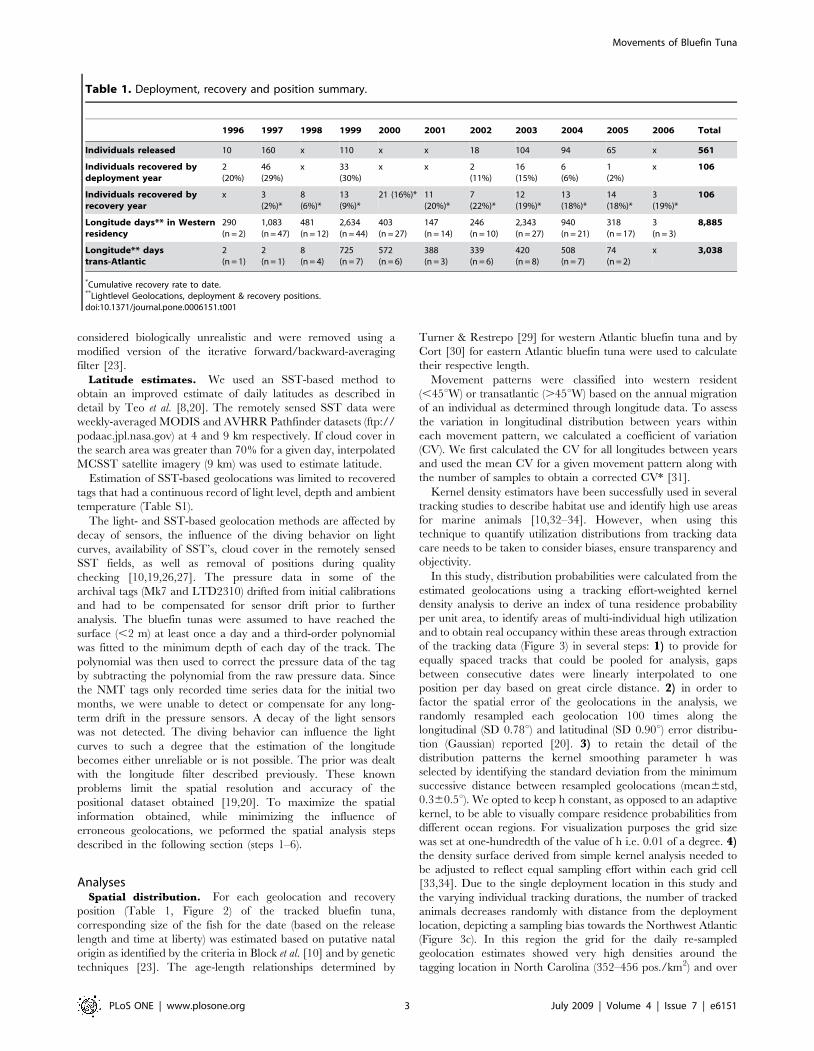
(Figure 3c). In this region the grid for the daily re-sampled

geolocation estimates showed very high densities around the

tagging location in North Carolina (352–456 pos./km2) and over

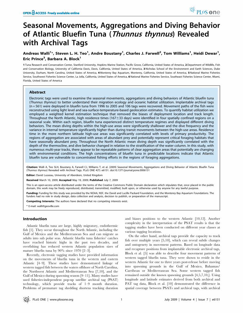
Table 1. Deployment, recovery and position summary.

1996 1997 1998 1999 2000 2001 2002 2003 2004 2005 2006 Total

Individuals released 10 160 x 110 x x 18 104 94 65 x 561

Individuals recovered bydeployment year

2(20%)

46(29%)

x 33(30%)

x x 2(11%)

16(15%)

6(6%)

1(2%)

x 106

Individuals recovered byrecovery year

x 3(2%)*

8(6%)*

13(9%)*

21 (16%)* 11(20%)*

7(22%)*

12(19%)*

13(18%)*

14(18%)*

3(19%)*

106

Longitude days** in Westernresidency

290(n = 2)

1,083(n = 47)

481(n = 12)

2,634(n = 44)

403(n = 27)

147(n = 14)

246(n = 10)

2,343(n = 27)

940(n = 21)

318(n = 17)

3(n = 3)

8,885

Longitude** daystrans-Atlantic

2(n = 1)

2(n = 1)

8(n = 4)

725(n = 7)

572(n = 6)

388(n = 3)

339(n = 6)

420(n = 8)

508(n = 7)

74(n = 2)

x 3,038

*Cumulative recovery rate to date.**Lightlevel Geolocations, deployment & recovery positions.doi:10.1371/journal.pone.0006151.t001



the Grand Banks (283–351 pos./km2, Figure 3b). We normalized

the skewed density estimate of days tracked in each cell (Figure 3b)

by dividing it by the number of individual bluefin tuna tracked

within each cell (Figure 3c). The resulting index reflects a mean

probability of tuna residency over the analyzed time domain. 5) In

order to identify areas of multi-individual utilization we reclassified

the grid of the numbers of animals tracked per unit area before

executing step 4. The area outlining 95% of animals tracked shows

the distribution of at least three animals tracked (Figure 3c). The

minimum number of animals permitted in the sampling effort grid

was therefore reclassified to 5% of the dataset. In this way we

down-weight cells frequented by less than 3 individuals and avoid

biasing our identification of multi-individual high-use areas. 6)The resulting multi-individual residence probability grid ultimately

allowed the calculation of utilization distributions (UD) as a

polygon coverage using least-squares cross validation [35,36]. This

provided probability contours that indicate the relative area

utilized by the tracked fish over the time domain of the data

analyzed. First we identified the high-use areas in the North

Atlantic as the areas corresponding to the 25% utilization

distributions of the entire tracking dataset (1996–2006,

Figure 3d). These were used to query the tracking dataset and

obtain true residence times within the high use areas as well as the

natal origin of individuals. Secondly, we examined the seasonal

utilization distributions of western resident and transatlantic fish

(Figure. 4 and 5). Seasons were delimited by the respective solstices

and equinoxes. Kernel density analysis for grid coverages and cell-

based statistics were performed using ModelBuilder in ArcGIS 9

(ESRI).

It was previously determined that when using kernel estimators

in an analysis of habitat utilization, the collection of more frequent

locations within the same region may result in increased

autocorrelation between points [37]. However, several authors

[38–42] have argued that adequate sample size is more important

than independence between points and it was therefore suggested

that .50 positions would be adequate to avoid this problem [37].

Although the spread of locations can still be autocorrelated to

some degree, the effects of spatial autocorrelation on the derived

time spent per unit area, is likely to be reduced by correcting for

tracking effort.

Oceanography of high-use areas. We examined whether

the presence of bluefin tuna within the identified high-use areas

coincided with specific physical (abiotic) and biological (biotic)

settings that would define them and indicate their importance as

foraging habitats. Sea Surface temperature was used as the abiotic

parameter and we obtained an 8-day averaged SST product

mapped at 4 km equal angle grids from the Pathfinder project

data archive in the Physical Oceanography Distributed Active

Archive Center (PODAAC, http://podaac.jpl.nasa.gov).

Estimates of vertically integrated primary productivity (PP),

which indicates the net biomass of primary producers present,

were used as the biotic parameter. PP data was obtained as 8-day

averages at a 0.1 degrees equal-angle grid served by the

OceanWatch live access server of the NOAA Coastwatch and

Environmental Research Division (http://las.pfeg.noaa.gov/

oceanWatch/).

First, we calculated the mean number of days per month that

the fish were present within each high-use area polygon of the

25% UD with the standard deviation measuring the difference

between years (1996–2005, Figure 6). We then queried the

remotely sensed sea surface temperature (SST) and derived

primary productivity (PP) estimates present within each high-use

area polygon corresponding to the tracking period (1996–2005).

For each parameter we calculated the mean values per month with

the standard deviation measuring the difference between years

(Figure 6). The mean monthly presence of bluefin tuna was then

analyzed in relation to the mean values of SST and PP using a

least- square-fit regression [43].

Temperature and depth distributions. Time-series data

from WC and Lotek tags allowed for three temperature and depth

analysis: an overall, a high-use area specific and a water-mass

specific. First, we calculated the minimum, maximum and mean of

ambient temperature (Ta), body temperature (Tb) and depth data

during the entire tracking time for each functional tag recovered

(Table 2).

We then compared the depth, Ta and Tb data of the bluefin

tunas between the identified high-use areas (25% UD) for the years

available (Figure. 7, 8, 9; Table 3). Within each polygon for these

high-use areas, the depth/temperature data for each fish present

were parsed into bins and the averages reported in histograms.

Figure 2. Recovery positions of electronic archival tags (triangles) in western Atlantic (orange, n = 64, 226621 cm CFL), easternAtlantic (white, n = 13, 218.4613 cm CFL), and Mediterranean Sea (yellow, n = 29, 234617 cm CFL). Line at the 45umeridian indicates themanagement line. Black arrow indicates location of tag deployments in North Carolina. Large triangles with inset indicate locations of multiplerecoveries. The highest recapture rates for these western tagged bluefin tuna were obtained from the region off New England (48% of totalrecaptures) followed by the Mediterranean Sea (27%). The Central and Northeast Atlantic emerged as the third area of high recovery (13%).doi:10.1371/journal.pone.0006151.g002



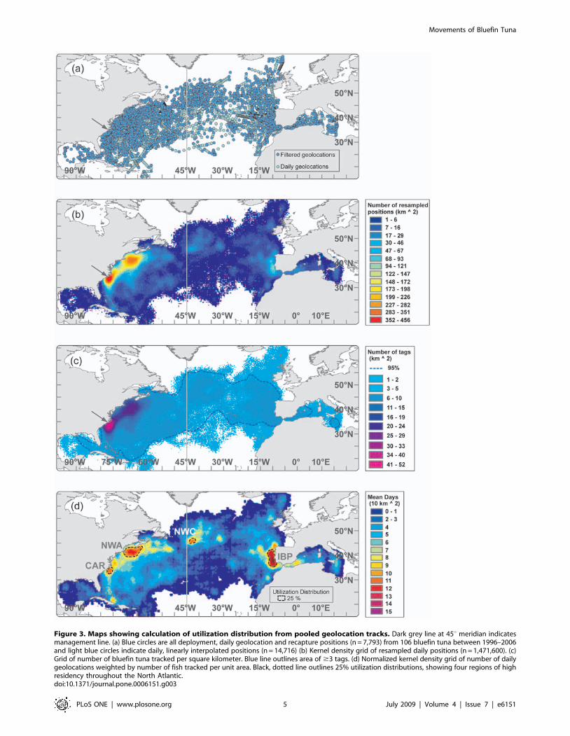
Figure 3. Maps showing calculation of utilization distribution from pooled geolocation tracks. Dark grey line at 45u meridian indicatesmanagement line. (a) Blue circles are all deployment, daily geolocation and recapture positions (n = 7,793) from 106 bluefin tuna between 1996–2006and light blue circles indicate daily, linearly interpolated positions (n = 14,716) (b) Kernel density grid of resampled daily positions (n = 1,471,600). (c)Grid of number of bluefin tuna tracked per square kilometer. Blue line outlines area of $3 tags. (d) Normalized kernel density grid of number of dailygeolocations weighted by number of fish tracked per unit area. Black, dotted line outlines 25% utilization distributions, showing four regions of highresidency throughout the North Atlantic.doi:10.1371/journal.pone.0006151.g003



Standard deviations measured the difference between the means of

individual fish. Time at depth and temperature distributions were

compared using a Kolmogorov-Smirnov two sample test [30] to

detect significant changes between years. Differences in temper-

atures experienced and diving behavior displayed were then

analyzed between day and night.

We compared the mean depth, dive frequency and variance in

Ta and Tb between the high-use areas as well as to times of transit

Figure 4. Seasonal utilization distributions of bluefin tuna in western resident migration cycle (n = 49, 224616 cm CFL). Black arrows inocean depict general direction of movements during relevant season. a) Winter. Grey arrow in North Carolina depicts approximate deploymentlocation. b) Spring c) Summer d) Fall.doi:10.1371/journal.pone.0006151.g004



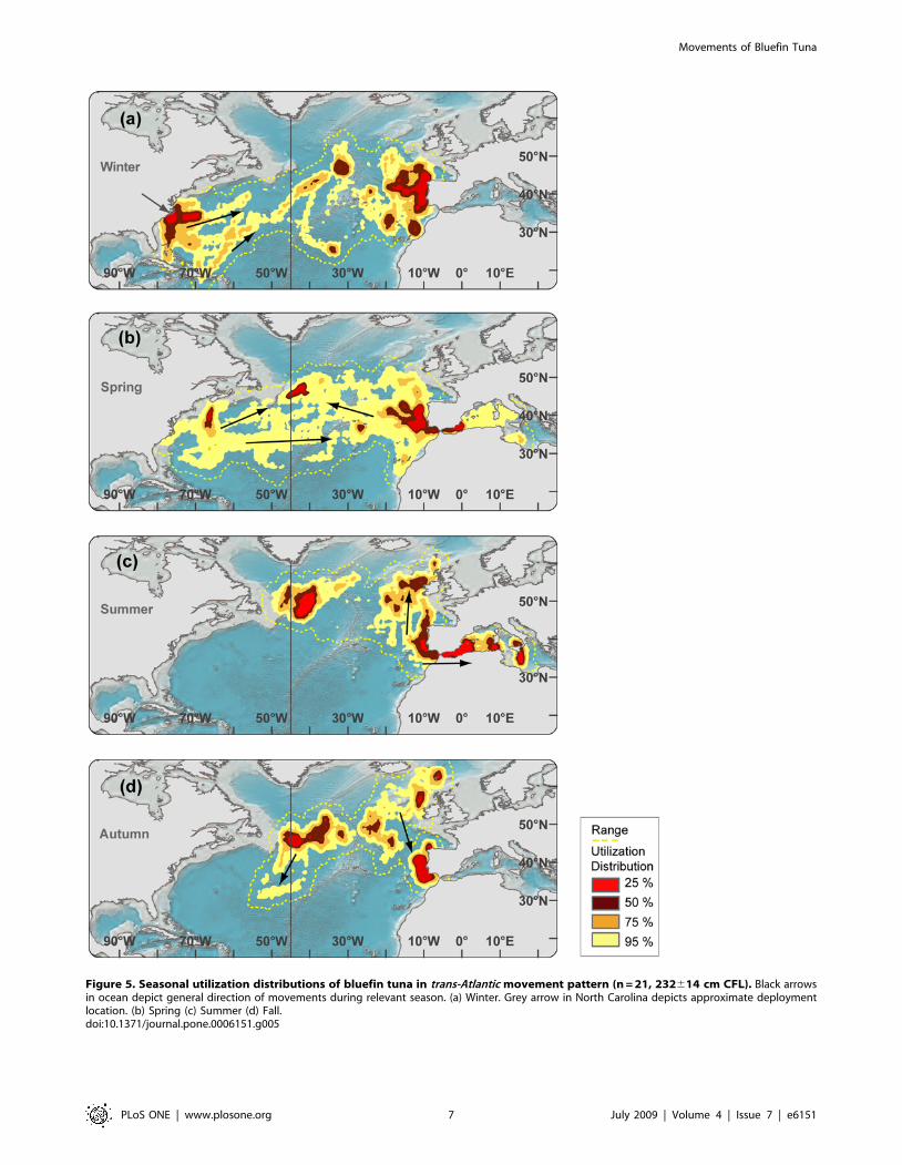
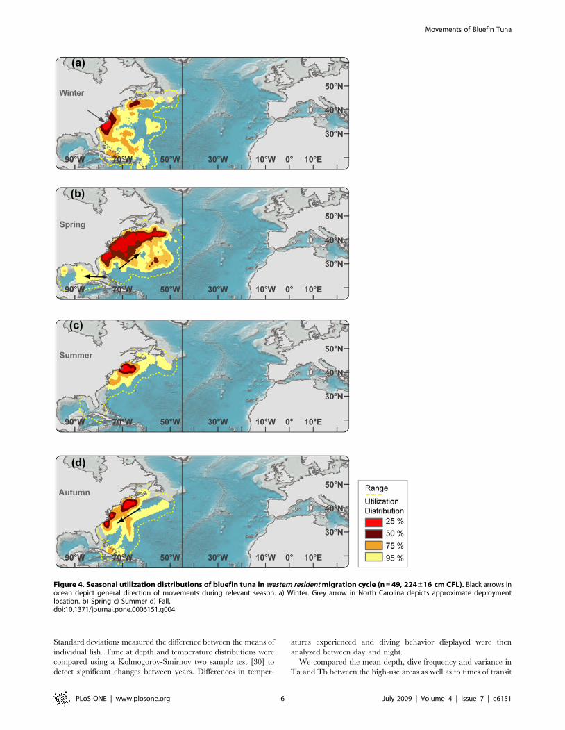
Figure 5. Seasonal utilization distributions of bluefin tuna in trans-Atlantic movement pattern (n = 21, 232614 cm CFL). Black arrowsin ocean depict general direction of movements during relevant season. (a) Winter. Grey arrow in North Carolina depicts approximate deploymentlocation. (b) Spring (c) Summer (d) Fall.doi:10.1371/journal.pone.0006151.g005



(Table 3) to establish whether the animals display a behavior that

would be indicative of foraging. Increased diving activity has been

previously described to be indicative of foraging behavior in

bluefin tuna [4]. Here we defined diving frequency as the number

of descents per day that were longer than 15 m in depth,

regardless of the depth from which they started. Further, the

digestion of food is associated with an increase in basal metabolism

[44,45] and in bluefin tuna the amount of increase in visceral

warming (Tb) as measured through archival tags has been found to

be proportional to the amount of food ingested [46,47]. Here we

employ the daily measured variance in Tb relative to the variance

in Ta to obtain an indication of feeding activity. To isolate

differences in obtained mean values of depth, dive frequency and

variance in Ta and Tb between regions and during transit, we

used a multi-comparison Analysis of Variance with a set of

Bonferroni corrected t-tests [48] and reported when significant.

We examined diving behavior displayed by individuals along

their tracks in relation to the temperature structure of the water

column. For each 4 hr. time period a depth/temperature profile

corresponding to the maximum diving depth was re-constructed

with the average temperature experienced for each meter fitted

using a locally weighted polynomial regression (loess fit; [49]).

These depth/temperature profiles were stacked to show the

differences in water-mass-specific diving depth between western

resident and transatlantic migrant bluefin tuna (Figure 10). From

these profiles we calculated the water-mass-specific vertical

temperature gradients and the depth of the thermoclines. To

estimate the depth of the thermocline (TC) for each profile we

used a criterion of D1.0uC per 2 m and selected the depth at which

this criterion first occurred [50, pers.comm.]. The daily mean,

median and maximum diving depth were then analyzed in relation

to the daily thermocline depth using a least-squares-fit Regression

(LSFR, [43]) and reported when significant (Figure 11).

All statistical tests in this study were performed with the

Statistics Toolbox in Matlab 7.0.1 (The Mathworks).

Results

Deployments and RecoveriesBluefin tuna captured and released in North Carolina coastal

waters in 1996–1999 had mean curved fork lengths (CFL) of

198.3616 cm (mean6sd; n = 561). Fish tagged in 2002–2005 had

a mean CFL of 203.2619 cm, indicating they were significantly

larger from the first cohort of tagged fish (Wilcoxon rank sum test,

P,0.05; Figure 1). Overall, the size of the archival tagged bluefin

tuna released between 1996–2005, based on measured CFL,

ranged from 138 cm to 268 cm.

Figure 6. Mean (6SD) monthly number of days that bluefin tuna were present (1996–2005) within high use areas (grey shaded) inrelation to mean (6SD) monthly level of primary productivity (green line) and sea surface temperature (blue line). (a) NortwestAtlantic (n = 32) (b) Nortwestern Corner (n = 5) (c) Carolina (n = 52) (d) Iberian Peninsula (n = 4).doi:10.1371/journal.pone.0006151.g006



Table 2. Descriptive statistics for functional recovered archival tags with timeseries data (n = 44, 184–276 cm CFL).

TagReleaseDate

TaDays

Ta (Cu)Min

Ta (Cu)Max

Ta (Cu)Mean

Ta (Cu)StdDev

TbDays

Tb (Cu)Min

Tb (Cu)Max

Tb (Cu)Mean

Tb (Cu)StdDev

Depthdays

Depth(m)Max

Depth(m)Mean

Depth(m)StdDev

97-016 3/7/1997 59 3.00 25.40 20.62 3.23 95 13.50 29.40 23.17 2.61 95 693 30.35 55.72

97-017 3/7/1997 71 4.60 24.50 17.49 4.83 313 15.20 30.20 24.05 2.63 313 786 28.20 49.34

97-019 3/7/1997 92 4.40 24.80 18.15 4.27 344 12.90 30.50 24.21 2.74 344 789 25.71 42.55

97-027 3/7/1997 32 6.00 24.70 19.56 2.51 374 12.40 31.70 24.08 2.85 374 787 29.84 57.67

97-028 3/7/1997 69 3.20 26.60 17.93 3.49 389 12.80 31.80 23.84 2.55 389 766 22.81 44.24

97-030 3/7/1997 59 3.20 25.40 16.59 3.49 371 12.50 31.20 23.86 2.95 371 770 34.31 53.14

97-037 3/7/1997 11 12.40 24.30 21.35 1.90 261 12.90 30.30 25.06 2.09 261 768 24.86 43.77

97-038 3/7/1997 72 3.00 25.20 19.56 3.98 383 13.30 32.00 24.97 2.48 383 789 42.27 58.35

97-048 3/7/1997 50 5.20 24.90 19.57 3.06 280 13.00 31.40 25.61 2.37 280 794 40.01 73.00

97-067 3/8/1997 5 15.80 25.90 21.19 0.89 379 13.20 32.10 24.50 2.90 379 790 29.03 38.23

97-011 3/16/1997 19 11.50 24.50 22.28 1.41 139 12.10 30.70 23.27 2.83 139 759 38.94 61.58

97-022 3/17/1997 115 3.00 25.57 18.24 4.23 157 15.30 31.30 23.56 3.09 157 789 35.85 60.97

97-089 3/17/1997 42 4.80 25.10 21.59 2.92 315 16.40 31.60 25.73 2.31 315 740 15.10 43.36

97-102 3/17/1997 12 13.40 24.70 21.99 1.71 330 14.80 32.20 24.80 2.21 330 785 30.30 27.84

97-103 3/17/1997 20 12.70 24.80 20.92 2.17 363 12.80 30.10 23.52 2.51 363 736 20.64 48.09

97-043 3/20/1997 1 13.10 23.60 20.32 7.50 448 14.20 31.50 24.02 2.78 448 656 36.24 55.64

97-112 3/21/1997 42 5.83 25.60 13.95 9.51 68 13.45 28.90 25.24 1.48 68 642 22.20 53.04

98-521 1/1/1999 461 3.00 25.60 16.55 4.72 461 11.00 31.80 24.34 2.35 461 989 73.98 136.34

98-492 1/6/1999 468 4.00 26.80 18.70 4.59 625 11.00 30.60 24.28 2.66 625 973 47.19 103.02

98-502 1/14/1999 205 3.00 25.80 18.12 4.46 204 15.00 33.50 23.60 2.83 204 899 37.33 68.56

98-510 1/14/1999 55 6.20 24.30 20.23 2.85 55 18.10 31.20 24.93 1.92 55 676 13.41 32.51

98-507 1/16/1999 192 3.00 28.20 16.72 5.50 503 11.10 32.30 23.14 3.11 503 820 66.55 97.21

98-518 1/16/1999 136 3.00 25.20 15.54 5.12 451 11.00 32.90 24.12 3.07 451 884 30.85 64.10

98-508 1/17/1999 292 3.00 26.70 17.68 4.41 578 13.60 30.60 24.07 2.66 578 994 32.61 62.34

98-512 1/17/1999 237 3.00 29.80 19.12 4.68 583 14.60 32.10 25.09 2.30 583 993 57.49 99.13

98-516 1/17/1999 235 4.40 25.80 17.58 4.06 1598 15.30 32.60 24.22 2.55 1598 996 43.05 73.51

98-485 1/21/1999 480 3.00 26.70 15.97 4.27 478 13.60 29.20 22.55 2.34 478 996 55.22 79.85

98-504 12/31/1999 520 3.40 25.60 16.93 4.59 686 11.00 26.30 20.65 2.59 686 882 51.34 87.88

14 2/1/2002 482 4.22 26.83 17.36 4.00 482 10.69 28.02 20.70 2.84 482 879 31.49 58.81

793 1/13/2003 78 10.12 25.24 21.22 1.94 398 14.12 29.94 23.79 2.65 398 855 30.47 51.66

1025 1/13/2003 327 0.04 26.11 16.84 4.14 327 13.86 31.48 24.57 2.79 73 234 32.40 3.19

781 1/14/2003 223 4.36 28.71 16.78 4.84 223 15.51 32.04 24.28 2.54 223 559 32.69 50.86

1013 1/16/2003 108 5.15 24.85 19.16 3.06 108 14.55 29.48 23.07 2.41 108 695 25.02 48.71

744 1/18/2003 385 1.48 28.27 17.47 4.77 385 14.82 29.61 23.23 2.50 385 721 23.07 41.48

1016 1/18/2003 396 0.04 29.29 17.50 4.47 396 12.95 30.23 23.48 2.81 396 995 46.09 89.24

1005 1/18/2003 526 3.43 26.71 18.31 4.50 526 11.29 32.19 23.97 2.84 526 1217 28.00 51.34

1000 1/21/2003 388 2.85 29.16 17.57 4.69 388 14.43 32.22 24.29 2.53 388 658 32.50 0.02

532 1/25/2003 510 1.53 29.81 17.80 5.32 720 9.66 30.81 24.41 2.24 720 925 48.14 90.98

566 1/25/2003 33 6.27 24.10 20.23 1.86 353 12.29 32.04 24.52 2.73 353 994 32.31 50.27

1021 1/26/2003 410 4.07 28.35 17.20 4.40 410 15.44 31.79 24.25 2.37 410 909 28.47 48.83

2217 1/9/2004 352 0.08 26.52 16.00 4.63 352 10.20 27.31 21.99 2.57 352 1107 37.52 75.65

2159 1/17/2004 29 15.46 24.28 21.27 1.39 525 15.08 33.11 23.35 2.73 416 119 18.81 14.81

2158 1/22/2004 433 3.08 26.21 16.57 4.35 594 12.14 31.28 22.87 3.02 594 775 26.75 55.34

219 1/12/2005 313 1.77 26.08 17.27 4.16 313 12.66 30.63 22.68 3.13 313 687 24.63 42.59

Total 8986 0.04 29.8 18.4 2.0 17636 9.7 33.5 23.9 1.1 17273 1217 34.5 12.8

doi:10.1371/journal.pone.0006151.t002



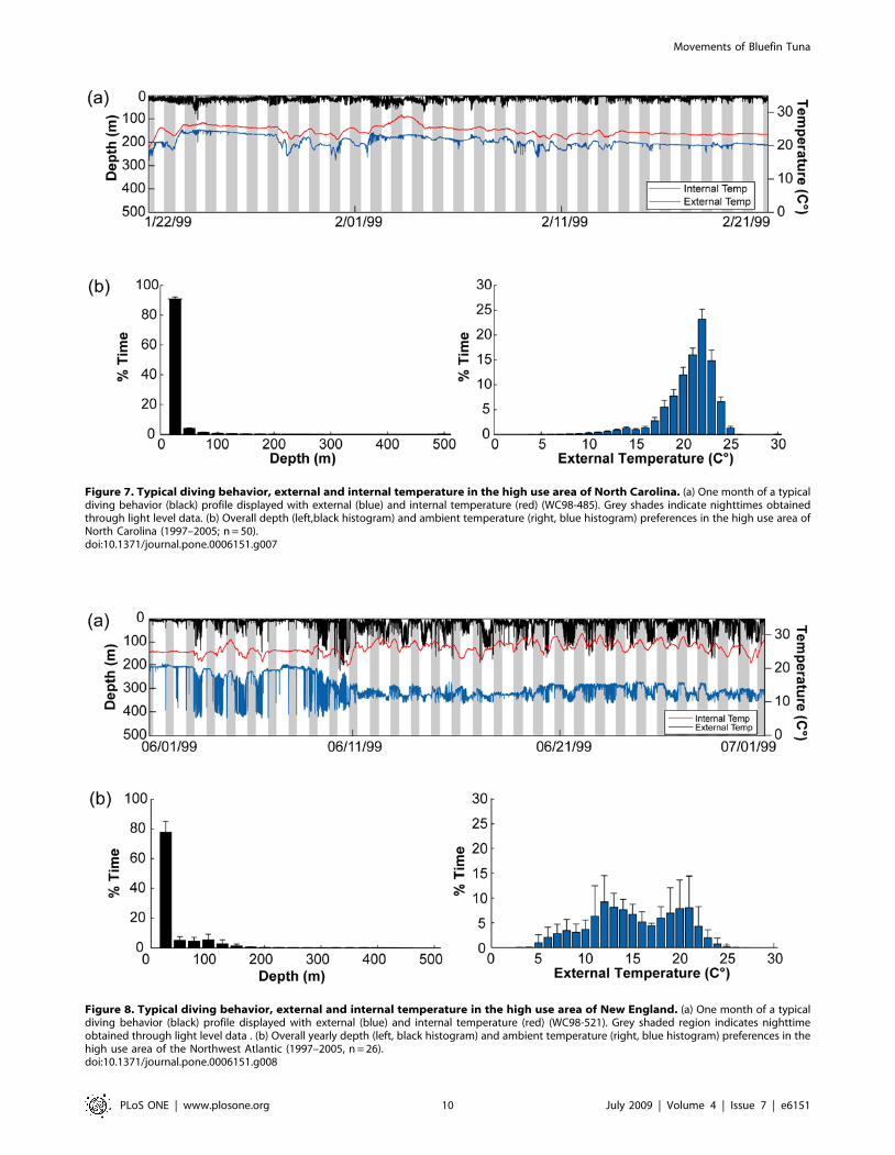
Figure 7. Typical diving behavior, external and internal temperature in the high use area of North Carolina. (a) One month of a typicaldiving behavior (black) profile displayed with external (blue) and internal temperature (red) (WC98-485). Grey shades indicate nighttimes obtainedthrough light level data. (b) Overall depth (left,black histogram) and ambient temperature (right, blue histogram) preferences in the high use area ofNorth Carolina (1997–2005; n = 50).doi:10.1371/journal.pone.0006151.g007

Figure 8. Typical diving behavior, external and internal temperature in the high use area of New England. (a) One month of a typicaldiving behavior (black) profile displayed with external (blue) and internal temperature (red) (WC98-521). Grey shaded region indicates nighttimeobtained through light level data . (b) Overall yearly depth (left, black histogram) and ambient temperature (right, blue histogram) preferences in thehigh use area of the Northwest Atlantic (1997–2005, n = 26).doi:10.1371/journal.pone.0006151.g008



To date, 106 (19%) of the archival tagged bluefin tuna have

been recaptured by commercial fishers from the 1996–2005

deployments (Supplementary material, Table 1) and recapture

rates varied from 2–30% between years (Table 1). Recovery rate

was higher for fish released in the period from 1996–1999

(26.365.5%) than from the 2002–2005 deployments (1063.6%,

Table2). Tagged fish spent on average 1,1616868 days at large

before recapture (Supplementary material, Table 1).

The recapture positions of western tagged bluefin tuna (Figure 2)

demonstrates that archival tagged fish were recaptured throughout

the extent of the fishery across the North Atlantic and into both

known spawning areas. Of the 106 recaptured archival tagged

bluefin tuna, 42 (40%) were reported east of the 45 meridian stock

boundary, and 29 (27%) were recaptured in the Mediterranean

Sea.

Tag return and tag performance played a role in acquiring time

series records from the archival tags. Although 106 recaptures

were reported through the recapture of tuna and reporting of the

associated floy tags, 81 archival tags were actually returned by

fishers to scientists, and of these 62 tags recorded data. Physical

failures included over-pressurization of early generation tags,

water intrusion into the Teflon external light stalk, or tag body,

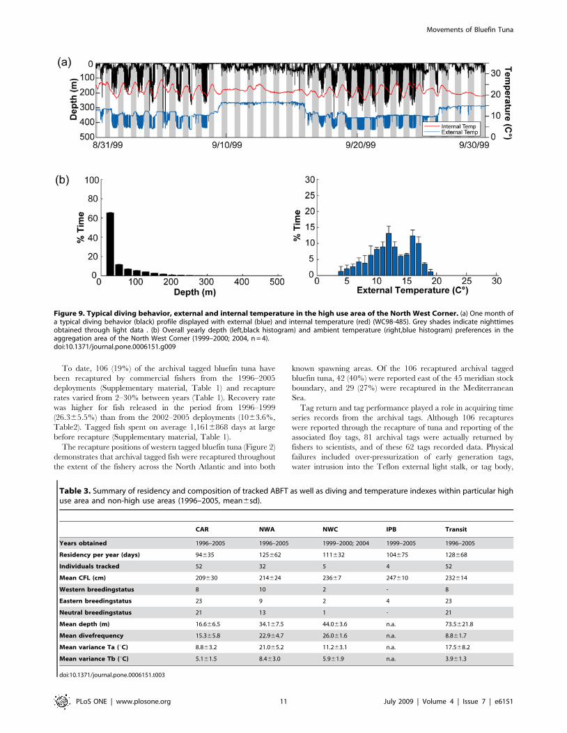
Figure 9. Typical diving behavior, external and internal temperature in the high use area of the North West Corner. (a) One month ofa typical diving behavior (black) profile displayed with external (blue) and internal temperature (red) (WC98-485). Grey shades indicate nighttimesobtained through light data . (b) Overall yearly depth (left,black histogram) and ambient temperature (right,blue histogram) preferences in theaggregation area of the North West Corner (1999–2000; 2004, n = 4).doi:10.1371/journal.pone.0006151.g009

Table 3. Summary of residency and composition of tracked ABFT as well as diving and temperature indexes within particular highuse area and non-high use areas (1996–2005, mean6sd).

CAR NWA NWC IPB Transit

Years obtained 1996–2005 1996–2005 1999–2000; 2004 1999–2005 1996–2005

Residency per year (days) 94635 125662 111632 104675 128668

Individuals tracked 52 32 5 4 52

Mean CFL (cm) 209630 214624 23667 247610 232614

Western breedingstatus 8 10 2 - 8

Eastern breedingstatus 23 9 2 4 23

Neutral breedingstatus 21 13 1 - 21

Mean depth (m) 16.666.5 34.167.5 44.063.6 n.a. 73.5621.8

Mean divefrequency 15.365.8 22.964.7 26.061.6 n.a. 8.861.7

Mean variance Ta (uC) 8.863.2 21.065.2 11.263.1 n.a. 17.568.2

Mean variance Tb (uC) 5.161.5 8.463.0 5.961.9 n.a. 3.961.3

doi:10.1371/journal.pone.0006151.t003



broken thermistor wires and broken thermistor bulbs. Several tags

had memory failures and one tag was cut up by a band saw at the

Tokyo fish market. The pressure sensors on 42% of the Mk7

archival tags and 29% of the LTD2310 drifted and was corrected

before analysis of the data, with the largest drift experienced being

18 m over 1.3 years

Geolocation dataWe obtained 561 GPS positions at deployment and 103 at

recapture from fishers or scientists who recovered and reported the

tags. In addition, 3 recapture positions had to be estimated based

on the descriptive information on the location provided by the

fishermen. For 57 individual bluefin tuna a total of 11,391 filtered

longitude estimates spanning 1996–2006 were estimated, and for

52 bluefin tuna the combination of the daily light, depth and

external temperature record allowed SST geolocation (Supple-

mentary material, Table 1) and hence spatial analysis of

movements. After linear interpolation of the filtered geolocation

dataset (mean gaps 1.864.6 days) the mean track length was

3686139 days (n = 52). The longest track record spanned 1627

days (NMT603).

Spatial distributionMulti-individual high-use areas. The tracking effort

corrected utilization distribution of bluefin tuna revealed four

hot spot areas in the North Atlantic that were visited most

frequently between 1996–2006 and in which western tracked

bluefin tuna resided for extended periods (Figure.3d, 4b and 6;

Table 3). Bluefin tuna were consistently tracked within the overall

high-use area off the coast of North Carolina for 94635 days per

year, with fish aggregating in these waters from as early as mid

October to as late as the middle of May depending upon the year

(Figure.3, 4 and 6; Table 3). The months of highest residency in

this region were December through March. Bluefin tuna were

recorded in a second high-use area in the North Western Atlantic

(Gulf of Maine, Georges Banks and south of Nova Scotia) for

164662 days per year, with fish aggregating in this area from early

March to late December (Figure.3, 4 and 6a; Table 3). The highest

residency in this region occurred in June through October. In the

central North Atlantic, a region of high-use was identified to the

east of the Flemish Cap, known as the North Western Corner [49],

for 167633 days (Figure. 3d and 5; Table 3). Fish aggregated in

this region as early as April and remaining through December,

with peak occupancy in June (Figure. 5 and 6c; Table 3). In the

Northeast Atlantic, a fourth high-use area was identified off the

western coast of the Iberian Peninsula (Portugal and southwest

Spain) where fish were consistently present 126675 days per year

(Figure. 3d and 4; Table 3). However, peak presence in this region

occurred from September to December as well as in May (Figure.5

and 6d;). Bluefin tuna were absent from the overall high-use areas

an average of 128668 days per year with peak times of transit

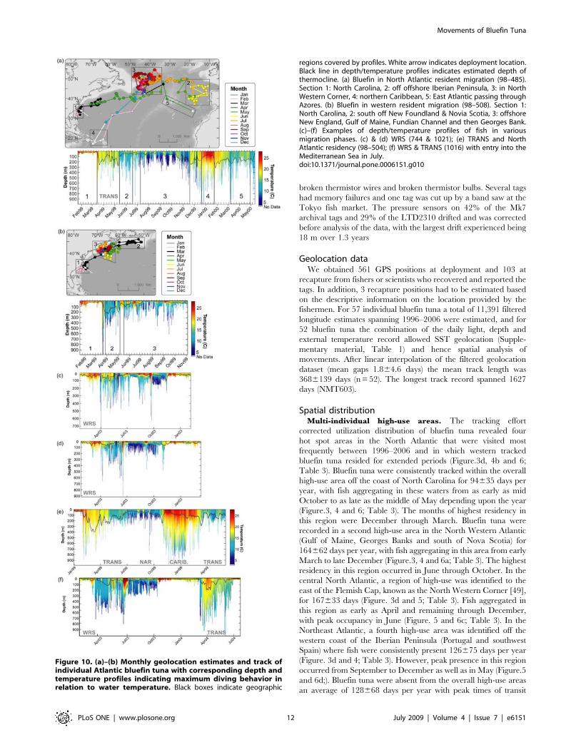
Figure 10. (a)–(b) Monthly geolocation estimates and track ofindividual Atlantic bluefin tuna with corresponding depth andtemperature profiles indicating maximum diving behavior inrelation to water temperature. Black boxes indicate geographic

regions covered by profiles. White arrow indicates deployment location.Black line in depth/temperature profiles indicates estimated depth ofthermocline. (a) Bluefin in North Atlantic resident migration (98–485).Section 1: North Carolina, 2: off offshore Iberian Peninsula, 3: in NorthWestern Corner, 4: northern Caribbean, 5: East Atlantic passing throughAzores. (b) Bluefin in western resident migration (98–508). Section 1:North Carolina, 2: south off New Foundland & Novia Scotia, 3: offshoreNew England, Gulf of Maine, Fundian Channel and then Georges Bank.(c)–(f) Examples of depth/temperature profiles of fish in variousmigration phases. (c) & (d) WRS (744 & 1021); (e) TRANS and NorthAtlantic residency (98–504); (f) WRS & TRANS (1016) with entry into theMediterranean Sea in July.doi:10.1371/journal.pone.0006151.g010



between these areas occurring during spring months (Table 3;

Figure.4b and 5b). The size of fish (mean curved length) was

significantly different between the high-use areas (multi-

comparison ANOVA, P,0.05; Table. 3).

Movement patterns. Based on the annual longitudinal

distribution of individuals (n = 57) we differentiated between

tuna (n = 49) that displayed western residency (herafter called

WRS) within the western North Atlantic (west of 45uW meridian,

Figure 4) and individuals (n = 21) that moved trans-Atlantic

(hereafter called TRANS, Figure 5) for the given year of

tracking. Western residency as well as trans-Atlantic movements

from west to east were consistently observed throughout the

tracking years (Table 1) with minor variability in longitude

distribution between years. Bluefin tuna in western resident phase

had a relatively small coefficient of variation in longitudinal

distribution (CV* = 5.4%) between years while the trans-Atlantic

migration phase had higher variation (CV* = 20.2%).

Seasonal movement patterns connect high-use areas. In

winter, western resident bluefin (WRS) aggregated in the high-use

area off the North Carolina waters as well as south of Nova Scotia

(Figure 4a). Individual tuna were also present ranging from the

Grand Banks in the north to offshore waters of the Bahamas, Cuba

and Puerto Rico in the south. The range (100% UD) of WRS

bluefin was greatest in spring, extending westward into the Gulf of

Mexico and eastward almost to the 45uW Meridian. In summer,

the range retracted and a high-use area emerged over Georges

Bank and the southern Gulf of Maine (Figure 4c), which remained

there throughout autumn. During fall, fish migrated down the

coast to aggregate in North Carolina but individual fish were also

present in the Sargasso Sea and the northern Caribbean

(Figure 4d).

The range (100% UD) of bluefin tuna undergoing trans-Atlantic

migrations (TRANS) spanned the North Atlantic, from the North

Carolina high-use area to the Mediterranean Sea. For bluefin tuna

that had moved trans-Atlantic the previous year, the winter high-

use area was off the Atlantic coast of the Iberian Peninsula from

45uN to 35uS (Figure 5a). Notably, departure time from the

American Continental Shelf was correlated with latitude, starting

in January from the Sargasso Sea and lasting to May from Nova

Scotia. This coincides with the seasonal, latitudinal productivity

regime of the North Atlantic [51] and might explain the variability

in departure time (Figure. 5a and b). In summer the full range of

all TRANS fish had moved from the Western to the Central and

Eastern North Atlantic (Figure 5c). Individuals in the Central

North Atlantic (n = 5) formed a large high-use area in the North

Western Corner centered at 43uN–60uN (Figure 5b). In autumn,

no western tagged bluefin tuna remained in the Mediterranean

Sea, but individuals had moved back into the Atlantic aggregating

off the Iberian Peninsula (Figure 4d). Two (NMT779, WC98-485)

individuals were seen to migrate from the North Western Corner

to the northern Caribbean where they remained for three weeks

during the winter months before returning again to the North

West Corner in spring (Figure. 4a and 9a).

Abiotic and biotic factors in high-use areasThe average number of days per month that tracked bluefin

tuna were present within each high-use area (Table 3) was related

with the mean monthly patterns of SST and primary productivity

between1996–2005 (Figure 6). Monthly SST’s were significantly

positively correlated with the presence of bluefin tuna in the high-

use area of the North Western Atlantic (LSFR, P,0.01, R2 = 0.94)

and negatively correlated in the North Carolina waters (P,0.01,

R2 = 20.83; Figure 6). In the two northern high-use areas, the

North Western Atlantic and the North Western Corner, the

monthly level of primary productivity was highly correlated with

the presence of bluefin tuna (P,0.01, R2 = 0.94; P,0.01,

R2 = 0.77 respectively; Figure 6a, c). In the lower latitude high-

use areas this relationship was weaker (CAR, P,0.01, R2 = 0.53)

or not significant (IPB, P,0.24, R2 = 0.34).

Ambient temperature and depth preferencesOverall temperature and depth preferences. The

ambient water temperatures experienced by tagged bluefin tuna

had a range of 0.04u–31.0uC and a mean that varied between

18.2u62.0uC obtained from tags that recorded a complete time

series (n = 44; 8,986 days; 202613 cm CFL; Table 2) and 1665uCobtained through binned data (n = 8, 8,748 days; 207615 cm

CFL). For the entire temperature dataset, the bluefin spent 87% of

occupancy in waters ranging from 10u to 23uC with peak times at

13u–20uC (60%). The three Lotek tags that recorded the extreme

minimum temperatures of 0.04–0.08uC (LTD1025, 1016, 2217)

were factory inspected, recalibrated and showed full functionality

of their sensors. At the time these low temperatures were recorded

two of these fish were at the entrance of the Gulf of Saint

Lawrence where the mean water temperature at 100 m is

1.2361.00uC (Hydrographic database, Bedford Institute of

Oceanography). While temperatures ,1uC represent rare

encounters, ambient temperatures around 2–4uC were

commonly recorded during deep dives in waters off Nova Scotia

and west of the Flemish Cap.

The internal body temperatures for bluefin reporting timeseries

data showed a mean of 23.9u61.1uC (n = 44; 17,636 days; Table 2)

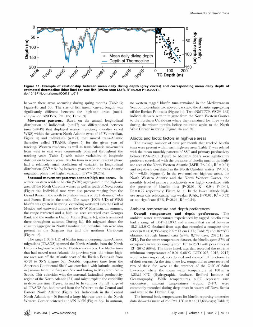
Figure 11. Example of relationship between mean daily diving depth (grey circles) and corresponding mean daily depth ofestimated thermocline (blue line) for one fish (WC98-508; LSFR, R2 = 0.92; P,0.0001).doi:10.1371/journal.pone.0006151.g011



and 24u61.6uC for tags reporting binned data (n = 8; 8748 days;

207615 cm CFL).

Overall, the mean diving depths of bluefin tuna was

34.5612.8 m (Table 2), with most of their time spent between

the surface and 50 meters (7968%; binned NMT data) and a

exponential decrease in time spent at greater depths. Maximum

depth in excess of 1,200 m was recorded by one fish (LTD1005,

Table 2). Depth preferences of the 44 fish reporting time series

data differed significantly between day and night (Kolmogorov-

Smirnov test, P,0.05); fish spent more time in surface waters

(,50 m) during the night than during the day.

High-use area specific temperature and depth

preferences. The diving behaviors and water temperatures

encountered by the archival tagged bluefin tuna were site specific

and differed between the four overall high-use areas (Figs. 7–9a;

Table 3). However, within the high-use areas the mean diving

depth was significantly shallower and the dive frequency and the

variance in internal temperature significantly higher than

compared to times in transit outside the high-use areas (multi-

comparison ANOVA, P,0.01; Table 3).

In the high-use area off North Carolina, diving behavior was

limited by bathymetry, although deeper dives up to 550 m

occurred when the fish moved on occasion offshore beyond the

continental shelf (Figure 7; Figure 10, section1). Fish in this region

spent $95% of their time within the upper 50 m and significantly

more time near the surface (,10 m) during the day than during

the night (Kolmogorov-Smirnov test, P,0.05). Depth and

ambient temperature distributions in this region did not differ

significantly among years (Kolmogorov-Smirnov test, P,0.05).

Peak time was spent in waters of 20u–23uC (71%) with a range of 7

to 27.8uC (Figure 7b). There was no difference between day and

night temperature preferences for any of the tagging years.

In the Northwest Atlantic (Gulf of Maine, Georges Banks and

south of Nova Scotia), the largest of the observed high-use areas

(Figure 3d), diving preferences and thermal data were highly

variable (Figure 8) and most likely influenced by season and

location. In spring (Apr-May) the fish were either located offshore

associated with the northern wall of the Gulf Stream or in colder

inshore waters over the Continental shelf south off Nova Scotia

(Figs. 4b and 10b). In June-July many bluefin tuna started to move

inshore over Georges Bank, showing a much shallower diving

distribution (91.264% of time at 0–50 m), with a further inshore

movement into the Gulf of Maine as the season progressed

(Figure. 4c and 10b–d). In Oct-Nov, these bluefin moved out of

the Gulf of Maine and occupied waters offshore from Georges

Bank to Nova Scotia. Depth and temperature distributions differed

significantly among years (Kolmogorov-Smirnov test, P,0.05)

which was likely a result of different seasonal tracking times

between the years. For all fish aggregating in this region, there was

no significant difference of diving depth between day and night.

In the North Western Corner east of the Flemish Cap

(Figure 3d), bluefin tuna displayed a very distinctive diving

behavior in relation to water masses encountered. In the cold

water of the North Wall (3–13uC, 42.5% total occupancy),

repetitive dives to 50–300 m were made during the day

(61.267.1% of time) with significantly more time (Kolmogorov-

Smirnov test, P,0.05) spent between 0–50 m after sunset

(95.162.8% of time; Figure 9). Here the depth of the thermocline

was between 50 (summer)–200 m (fall). In the comparatively warm

North Atlantic Current (15–19uC, 29% of time; Figure 9) bluefin

showed an irregular diving behavior that was most often limited to

the upper 50 m (98.161.4% of time) with no difference between

night and day. Overall, a significantly deeper depth distribution

was displayed on the cold side (,15uC) of the front and shallower

diving on the warm side (Kolmogorov-Smirnov test, P,0.05;

Figure 10a, section 3).

The overall high-use area off the western coast of the Iberian

Peninsula (Figure 3d) was occupied by bluefin tuna tagged with

NMT tags which were set to return binned data after 3 months of

sampling to avoid memory shortage on long-term missions.

Therefore, no dive and temperature analysis could be performed

for this region.

Diving behavior in relation to thermal structure of water

column. Depth/temperature profiles were used to reconstruct

the ocean water column profiles (8,986 daily profiles; n = 44) to

obtain estimation of the depth of the thermocline and water

masses encountered by bluefin tuna (Figure 10). While the

maximum diving depths were limited by bathymetry during on-

shelf phases, they were highly variable in relation to thermal

structure of the water column in both on- and off-shelf phases

(Figure 10). However, the time spent at depth was influenced by

the degree of stratification of the water column. In the Gulf of

Maine, for example, the preference for surface waters (91.264%

of time at 0–50 m) was associated with the highly stratified water

column (DuC 0.260.03uC/m) characterized by a very shallow

thermocline (TC 1264.2 m; n = 25; Figure. 10b, c and d end Jul.-

Aug.). In contrast, tuna that moved trans-Atlantic entered the

weakly stratified (DuC 0.0660.01uC/m; TC 38622 m) water

mass of the Northeast Atlantic Boundary Current (1461.5uC)

where they spent less time (64.267%, n = 4) above the

thermocline (Figure 10a, section 2). In summary, we found the

mean diving depth of bluefin tuna to be significantly correlated

(LSFR, P,0.01; R2 = 0.72; n = 44) with the depth of the

thermocline throughout the North Atlantic (Figure. 11). In

waters with a shallow thermocline, fish remained significantly

shallower in mean depth, while in waters with a deeper

thermocline they occupied deeper mean depths.

Discussion

The deployment and recovery of electronic archival tags from

1996 to 2006 on western tagged Atlantic bluefin from ages 7.1 to

14.2 years provides a long-term observation series. In this study we

employed this dataset to examine the seasonal movements,

aggregations and diving behaviors to better understand their

migration ecology and oceanic habitat utilization.

Bluefin tuna horizontal and vertical focal areasDistribution behavior was characterized by seasonal aggrega-

tions and rapid movement phases. Throughout the North Atlantic,

high residence times (167633 days) were identified in four

spatially confined regions on a seasonal scale. Within these areas,

the bluefin tuna (219620 cm) display unique diving behavior with

significantly shallower diving depths and higher dive frequencies as

compared to times in transit (Table 3; Figure 3d, 7–9). Moreover,

the visceral temperatures (Tb) of bluefin tuna within these areas

showed a significantly higher variance that occurred independent-

ly of the variation in external temperature (Table 3). The

magnitude of variances in Tb within the high-use areas suggest

an increase in visceral warming events likely caused by higher

feeding activity. High-use areas likely represent critical foraging

habitats where tuna can access enough prey to satisfy their

energetic needs and remain within their preferred temperatures.

The location and timing of the high-use areas in the North

Atlantic revealed by electronic tags coincides with favorable

biophysical settings and the timing of high prey availability in each

area of aggregation. Seasonality of prey availability in these

foraging habitats necessitates migration between them. Starting at



the deployment location, the presence of bluefin tuna over the

Continental Shelf in North Carolina region (Figure 5a) was

documented both historically through catch in the offshore waters

of North and South Carolina region by Japanese longliners

[54,55], and more recently through acoustic and pop-up satellite

tagging technologies [5,7,10,21,56]. Boustany [24] showed that

the presence of bluefin tuna coincides with a large number of prey

species, namely Atlantic menhaden (Brevoortia tyrannus), spot

(Leiostomus xanthurus) and Atlantic croaker (Micropogonias undulates),

that spawn in this region at the bottom during the night between

November and March in waters of 18–24uC [57]. Multi-year

records obtained through archival tags in this study show ambient

temperature preferences of bluefin tuna in the region to be

consistently between 20–23uC and the tuna to have a significantly

deeper depth distribution during the night (Figure 6); further, the

records show that bluefin tuna have fidelity to the region, return

by October and reach peak residence in the months of December

and January (Table 3; Figure 6a). The repeatability of these

patterns year to year [5,18,this study] and the strong seasonal

patterns of movements, suggest that there is a predictable food

supply attracting the tunas to this region. Multi year stomach

content analyses of bluefin tuna caught in this region revealed

Atlantic menhaden to be the most common (96%) prey item [58].

The attraction of bluefin tuna to these menhaden spawning

aggregations might also explain the de-coupled link to primary

productivity and the weaker relationship observed in this region

(Figure 6b). Specifically, the local spring bloom coincides with a

breakdown of the cross-shelf thermal gradient which has been

attributed to aggregate high densities of prey items [59]. Here, the

warming of SST’s beyond 21uC (Figure 6b) was consistently linked

to the spring departure of bluefin tuna [23] which might explain

the strong correlation between monthly SST’s and residence days

in this region.

By the end of March the first bluefin tuna in western resident

phase arrived in the New England and Scotian Shelf waters. These

fish stayed in the warmer offshore waters during spring months

and it is not until the early summer months that most of the tuna

moved into the Gulf of Maine area (Figure 4c). These movements

follow closely the known migrations of pelagic forage fish

(eg.herring species, mackerel species) and squid specis from

offshore waters across Georges Bank into the Gulf of Maine

[60]. Here dramatic increases in primary productivity and sea

surface temperatures during the summer and fall month (Figure 6a)

foster favorable habitats that attract and support a high abundance

of prey species. Specifically, the presence of bluefin tuna in this

region has been linked to the summer & fall aggregations of

mackerel (Scomber scombrus), herring (Clupea harengus), squid species

[16,61–64] and sandlances (Ammodytes americanus; [15,65]. Hence,

the residence of bluefin tuna in this region was highly correlated

with increase in primary productivity and sea surface temperatures

(Figure 6a). While the diving behavior in the Gulf of Maine was

dependent on the location, we found that it was generally

characterized by shallower dives associated with well stratified

waters (Figure. 10b, c and d end Jul.-Aug.). The strong thermal

stratification may provide the physical means to aggregate primary

food sources for prey (Figure 10b, c, d, summer months) and allow

easier detection, access and successful encounters for bluefin tuna

forage in this region.

Some bluefin tuna of larger body size demonstrated a trans-

Atlantic migration pattern into the central North Atlantic that was

distinct from the direct west to east movement (Figure 10a;

Table 1). Starting in spring they migrated to the region in North

Western Corner (NWC) where they resided for up to 8 month

(Figure. 5a, b, c and 6c). The long residence times of bluefin tuna

in this area are supported by the consistently high-catch-per-unit-

effort results of the Japanese longlining fleet in this region [66].

Considering these extensive migration movements (.6000 km),

the energetic revenue of foraging in this region must be very high.

It is well established that the region north of 45uN is the site of very

productive spring blooms which are associated with mesoscale

eddies and meanders that concentrate the primary productivity to

support very large secondary and tertiary trophic biomasses [67–

70]. Here monthly primary productivity patterns were also directly

related to the time spent by tracked bluefin tuna in this study

(Figure 6c). Depth and temperature records (Figure 9a; 10a,

section 3) indicate that bluefin in the NWC display a unique

foraging behavior in relation to the North Wall of the North

Atlantic current that can be identified by diving behaviors,

ambient temperature and thermoregulatory biology observed

through the archival tag records. Significantly deeper dives

occurred on the cold side of fronts during the day, potentially to

access mesopelagic fish species. The diving behavior displayed in

the region appears to be a foraging behavior because body

temperature (Tb) shows numerous events of sharp thermal decline

at a fast rate, that potentially indicate peritoneal cooling upon

ingestion of cold prey [18,71]. These bluefin repeatedly moved

back and forth across frontal features on a weekly basis (Figure 10a,

section 3). While residing in the warm North Atlantic current they

showed reduced diving activity with no diel behavior and few

changes in Tb.

Western tagged bluefin tuna of very large size (247610 cm

CFL, n = 16) exhibited a direct trans-Atlantic movement (TRANS)

during spring month (Figure. 5b, 10f, section TRANS). This shift

in residence from the Northwest Atlantic into the eastern Atlantic

was age dependent and only individuals larger than 200 cm (CFL,

,8.1 years of age) at the time of trans-Atlantic movement showed

this behavior [10]. While residing in the East Atlantic these fish

displayed aggregations off the Atlantic coast of the Iberian

Peninsula (IBP), the Azores, Ireland and remote offshore locations

over the Mid-Atlantic Ridge (Figure 5a–d). However, all tagged

bluefin tuna in eastern resident phase spent considerable time

(126675 days) off the IBP, where they showed the highest

presence from fall to winter and in spring (Table 3, Figure 6d).

Upwelling and primary productivity peak in IBP waters during

spring and fall month [72–75] attract spawning aggregations of

sardines [76] and high abundances of mackerel species [77] and

blue whiting [78]. Individuals residing off the IBP were

subsequently tracked to known spawning grounds in the

Mediterranean Sea (n = 12).We hypothesize that the highly

productive waters off the IBP act as an important foraging region

for large, mature bluefin tuna on their way to and from spawning

grounds in the Mediterranean Sea [87].

The focus in this paper has been to highlight the foraging

aggregations and provide an overall view of the distinctive

behavior and biology in these regions. Here, the depth/

temperature analyses were determined by the movement patterns

of individuals as opposed to previous observations of diving

behavior in relation to the continental shelf [5,7]. There were also

clear distinctions in the diving behaviors in relation to the thermal

structure of the water column throughout the North Atlantic

(Figure 10). Overall, the mean diving depth of bluefin tuna in the

North Atlantic was significantly correlated with the depth of the

thermocline (Figure 11). The thermal stratification at the depth of

the thermocline provides physical means to vertically aggregate

food for prey species [79,80]. By focusing diving depths around the

thermocline Atlantic bluefin tuna potentially maximize the

probability of encountering prey. Such a strategy was further

reflected in the diel behavior away from the continental shelves



where there was a strong affinity for deeper waters during the day,

when the deep scattering layer is at depth. Overall, the observed

vertical and horizontal movement behaviors suggest an optimiza-

tion towards maximizing forage encounter. The ability to adapt to

the variability of prey abundance in time, space and vertical

dimension is essential to bluefin tuna as a highly migratory pelagic

predator.

Interpretation of dispersal patternsCharacteristics of the geolocation dataset, ontogenetic changes

of movement patterns and the size range of the fish tracked require

a cautious interpretation of the spatial distribution patterns

revealed. The overall patterns that emerge however are striking

as they reveal key hot spots for adolescent and mature bluefin tuna

in the North Atlantic.

The assessment of the inter-annual variability in distributions of

tracked bluefin tuna was hindered by a significant variation in the

number of geolocation estimates obtained per year (Table 1).

Nonetheless, both western residency and the trans-Atlantic

movements were consistently observed in each year using

longitude records and recapture positions alone (Table 1). The

inter-annual variability in longitude distributions of the trans-

Atlantic migration patterns was found to be higher than that of the

western resident migration pattern. This was mainly due to 1)

variation in departure times between years; 2) incomplete trans-

Atlantic tracks due to recapture or tag failure and 3) a higher

proportion of transatlantic movements during the 2002–2005

period in comparison to the 1997–2001 period.

The latter requires consideration of the measured size and natal

origin of the tracked bluefin tuna. The data on length indicate that

the electronic tagging of younger fish in the earlier years of the

program (1997–2001) may have resulted in a higher proportion of

western residency recorded by immature fish of eastern origin,

which subsequently moved to or were recaptured at known

spawning grounds in the Mediterranean Sea; these fish (n = 12)

were significantly smaller than western fish (n = 10; Wilcoxon rank

sum test, P,0.05, mean CFL 210 and 222 cm respectively). In

contrast, during 2002–2005 tagged fish were of significantly larger

size and displayed a higher trans-Atlantic movement rate which

resulted in increased recapture rates in the Mediterranean Sea.

Supported by the observations of size related dispersal patterns by

[10,12] and [87] this provides further evidence for the ontogenetic

change in movement patterns that is also evident in western fish

[10,19].

Further, ontogenetic movement patterns need to be considered

when comparing results from tracking studies to distributions

obtained through CPUE data. The size range of fish tagged in this

study and the relatively small proportion of animals tracked might

explain the lack of high-use areas identified in the known fishing

grounds such as Canada and the Bay of Biscay. For example, in

recent years distribution patterns of a larger cohort (248612 cm)

of PSAT tagged bluefin tuna off North Carolina showed a range

expansion and residency in the more northern waters of Canada

(Block, et al., unpublished data) that is also manifest through a

recent increase in CPUE’s in this fishery [81]. However, the mean

size of tagged bluefin tuna in this study was well below that caught

in the Canadian fishery (.250 FL cm, [80]) and well above that

for the Bay of Biscay (54–105 FL cm, [82]), hence reduced the

likelihood of identifying these fishery regions as high-use areas.

Management implicationsThe high concentrations of bluefin tuna in predictable locations

indicate that Atlantic bluefin tuna are vulnerable to concentrated

fishing efforts in the regions of foraging aggregations. This has

important implication for national and international management

of the fishery. Bluefin tuna electronically tracked spent an average

of 246651 days per year in the spatially confined high-use areas

identified in this study (Table 3). This aggregation behavior

indicates that the CPUE of a particular fishery (e.g. Purse Seining)

most likely will serve poorly as an index for population abundance

[83–85]. Future biomass estimations of adults or juveniles should

consider spatiotemporal variation in abundance when drawing on

population indices.

Our studies have shown clear evidence of mixing between

eastern and western populations in foraging aggregation zones

[5,10,86], which are well supported by recent findings through

otolith based stable isotope analysis [87]. Identifying the degree of

mixing within an aggregated region will increasingly be of high

importance. Genetic testing of DNA samples collected during

release will in the future be useful for assessing population status

[86,88] and potentially confirming the ratio of western fish to

eastern fish in all regions of high utilization. Ideally, natal origin

and age dependent spatial components should be incorporated in

the stock assessments to facilitate more realistic biomass estimates.

Both electronic tracking data and DNA analyses can aid in the

development of future models that incorporate this information.

For trans-Atlantic bluefin tuna that returned to the Mediterra-

nean Sea there was a high chance of capture. Only 10% of all fish

moving into the Mediterranean Sea were not caught and could be

tracked beyond the spawning season exiting the Mediterranean

Sea. These fish (n = 4) remained in the eastern Atlantic close to

their natal spawning ground, potentially to maximize their

reproductive output. Because of their annual spawning behavior

[10] and the associated high reproductive value, the protection of

these large fish is probably of particular importance to the

conservation management of the eastern stock.

The documented high-use areas may represent a network of

critical foraging habitats that are essential collectively to the

persistence of bluefin tuna populations in the North Atlantic.

Further, the apparent dependence of their seasonal movements on

the productivity and high abundance of prey species in a given

high-use area potentially makes the presence of bluefin tuna

sensitive to changes in regional ecosystem productivity. Sibert et

al. [12] hypothesized recently that bluefin tuna migrations and

inter-annual shifts noted with satellite tagging datasets may in part

be linked to shifts in oceanographic conditions. In this study, with

numerous multi-year tracks, there appear to be repeatable patterns

of clear aggregation areas that potentially are changing with

environmental conditions. The apparent stability of these regions

to be seasonally productive may provide predictable foraging

habitats for bluefin tuna. Identifying the underlying processes that

make the seasonal ecosystem productivity of oceanic regions

predictive for pelagic animals, versus areas that are highly

ephemeral will aid in our understanding of identifying vital

bluefin tuna habitat.

Supporting Information

Table S1 Release and recapture information of archival tagged

Atlantic bluefin tuna.

Found at: doi:10.1371/journal.pone.0006151.s001 (0.05 MB

XLS)

Acknowledgments

This study could not have been conducted without the dedication and

perseverance of the Tag-A-Giant (TAG) scientific team. We thank the

captains and crews of the Fishing Vessels Calcutta, Bullfrog, Raptor,

Tightline, Leslie Anne, and 40 Something. We also thank A. Seitz, T.



Sippel, R.Schallert, M. Price, G.Rosenwaks, S. Miller, and numerous

others for long hours at sea tagging bluefin that helped to generate the data

set. The manuscript was improved through helpful comments from G.

Sharp, G. Lawson and H. Peckham. The paper is dedicated to the memory

of Seth Carey.

Author Contributions

Conceived and designed the experiments: CJF BB. Performed the

experiments: AW SLHT AB CJF TW HD. Analyzed the data: AW.

Contributed reagents/materials/analysis tools: AW SLHT. Wrote the

paper: AW. Conducted fieldwork: AW SLHT AB CJF TW HD BB.

Collected the data: AW SLHT AB CJF TW HD EP BB.

References

1. Magnuson JJ, Block BA, Deriso RB, Gold JR, Grant, et al. (1994) An assessmentof Atlantic Bluefin tuna. National Academy Press.

2. ICCAT (2005) Executive summary BFT: ICCAT Report 2004–2005. ICCAT,Biennial Reports 2: 44–50.

3. ICCAT (2006) Report of the 2006 Atlantic Bluefin tuna Stock AssessmentSession. Col Vol Sci Pap ICCAT 13: 1–137.

4. Lutcavage M, Brill R, Skomal G, Chase B, Howey P (1999) Results of pop-up

satellite tagging of spawning size class fish in the Gulf of Maine: Do North

Atlantic bluefin tuna spawn in the mid-Atlantic? Can J Fish Aquat Sci 56(2):173–177.

5. Block BA, Dewar H, Blackwell SB, Williams TD, Prince ED, et al. (2001)

Migratory movements, depth preferences, and thermal biology of Atlantic

bluefin tuna. Science (Wash D C) 293(5533): 1310–1314.

6. De Metrio G, Arnold GP, Block BA, De la Serna JM, Deflorio M, et al. (2001)Behavior of post-spawning Atlantic Bluefin tuna tagged with pop-up satellite tags

in the Mediterranean and Eastern Atlantic. Col Vol Sci Pap ICCAT 54 (2):

415–424.

7. Wilson SG, Lutcavage ME, Brill RW, Genovese MP, Cooper AB, et al. (2005)Movements of bluefin tuna (Thunnus thynnus) in the northwestern Atlantic

Ocean recorded by pop-up satellite archival tags. Mar Bio 146(2): 409–423.

8. Teo SLH, Boustany A, Dewar H, Stokesbury MJ, Weng KC, et al. (2007a)

Movement patterns, diving behavior and thermal biology of Atlantic bluefintuna (Thunnus thynnus) on their breeding grounds in the Gulf of Mexico. Mar

Biol 151: 1–18.

9. Teo SLH, Boustany A, Block BA (2007b) Oceanographic preferences of Atlantic

bluefin tuna,Thunnus thynnus, on their Gulf of Mexico breeding grounds. MarBiol 152: 1105–1119.

10. Block BA, Teo SLH, Walli A, Boustany A, Stokesbury MJ, et al. (2005)Electronic tagging and population structure of Atlantic bluefin tuna. Nature 434:

1053–1164.

11. Stokesbury MJ, Teo SLH, Seitz A, O’Dor RK, Block BA (2004) Movement of

Atlantic bluefin tuna (Thunnus thynnus) as determined by satellite taggingexperiments initiated off New England. Can J Fish Aquat Sci 61: 1976–1987.

12. Sibert JR, Lutcavage ME, Nielsen A, Brill RW, Wilson STG (2006) Interannualvariation in large-scale movement of Atlantic bluefin tuna (Thunnus thynnus)

determined from pop-up satellite archival tags. Can J Fish Aquat Sci 63:2154–2166.

13. Dragovich A (1970) The food of bluefin tuna (Thunnus thynnus) in the WesternNorth Atlantic ocean. Trans Am Fish Soc 1970(4): 726–731.

14. Matthews FD, Damkaer DM, Knapp LW, Collette BB (1977) Food of Western

North Atlantic Tunas (Thunnus) and Lancetfishes (Alepisaurus). Noaa (National

Oceanic & Atmospheric Administration) Technical Report Nmfs (NationalMarine Fisheries Service) SSRF-7006. pp 19.

15. Eggleston DB, Bochenek EA (1990) Stomach Contents and Parasite Infestation

of School Bluefin tuna Thunnus-Thynnus Collected From the Middle Atlantic

Bight Virginia Usa. U S Natl Mar Fish Serv Fish Bull 88(2): 389–396.

16. Chase BC (2002) Differences in diet of Atlantic bluefin tuna (Thunnus thynnus)at five seasonal feeding grounds on the New England continental shelfs. Fishery

Bulletin 100(2): 168–180.

17. Polovina JJ (1996) Decadal variation in the trans-Pacific migration of northern

bluefin tunas (Thunnus Thynnus) coherent with climate- induced change in preyabundance. Fish Oceanogr 5(2): 114–119.

18. Kitagawa T, Nakata H, Kimura S, Itoh T, Tsuji S, Nitta A (2000) Effect ofambient temperature on the vertical distribution and movement of Pacific

bluefin tuna Thunnus orientalis. Mar Eco Progr Ser 206: 251–260.

19. Gunn JS, Block BA (2001) Advances in acoustic, archival and satellite tagging of

tunas. In: Tunas: Ecological Physiology and Evolution, eds Block BA,Stevens ED.

20. Teo SLH, Boustany A, Blackwell S, Walli A, Weng KC, Block BA (2004)

Validation of geolocation estimates based on light level and sea surface

temperature from electronic tags. Mar Ecol Prog Ser 283: 81–98.

21. Block BA, Dewar H, Farwell C, Prince ED (1998a) A new satellite technology fortracking the movements of Atlantic bluefin tuna. Proc Natl Acad Sci U S A

95(16): 9384–9389.

22. Block BA, Dewar H, Williams T, Prince ED, Farwell C, Fudge D (1998c)

Archival tagging of Atlantic bluefin tuna (Thunnus thynnus thynnus). Mar

Technol Soc J 32(1): 37–46.

23. Boustany A (2006) An Examination of Population Structure, Movement Patternsand Environmental Preferences in Northern Bluefin tuna. PhD thesis, Hopkins

Marine Station, Pacific Grove: Stanford University.

24. Boustany A, Marcinek DJ, Keen JE, Dewar H, Block BA (2001) Movements and

temperature preference of Atlantic bluefin tuna (Thunnus thynnus) off NorthCarolina: a comparison of acoustic, archival and pop-up satellite tagging. In:

Electronic tagging and tracking in marine fishes, eds Sibert JR, Nielsen JL.Dordrecht: Kluwer Academic Publishers. pp 89–108.

25. McConnell BJ, Chambers RC, Nicholas KS, Fedak MA (1992) Satellite tracking

of grey seals (Halichoerus grypus). J Zool (Oxf) 226: 271–282.

26. Welch DW, Eveson JP (1999) An assessment of light-based geoposition estimatesfrom archival tags. Can J Fish Aquat Sci 56(7): 1317–1327.

27. Block B, Stevens ED (2001) Tunas: Ecological, Phsyiology and Evolution. San

Diego: Academic Press.

28. Musyl MK, Brill RW, Curran DS, Gunn JS, Hartog JR, et al. (2001) Ability ofarchival tags to provide estimates of geographical position based on light

intensity. In: Electronic tagging and tracking in marine fisheries, eds Sibert JR,

Nielsen JL. Dordrecht: Kluwer Academic Publishers. pp 343–367.

29. Turner SC, Restrepo VR (1994) A review of the growth rate of west Atlanticbluefin tuna, Thunnus thynnus, estimated from marked and recaptured fish.

ICCAT Coll Vol Sci Pap 42: 170–172.

30. Cort JL (1991) Age and growth of the bluefin tuna, Thunnus thynnus (L.) of theNortheast Atlantic. Col Vol Sci Pap ICCAT 35(2): 213–230.

31. Sokal RR, Rohlf FJ (1995) Biometry. New York: W. H. Freeman and Company.

32. Wood AG, Naef-Daenzer B, Prince PA, Croxall JP (2000) Quantifying habitat

use in satellite-tracked pelagic seabirds: application of kernel estimation toalbatross locations. Journal of Avian Biology 31: 278–286.

33. BirdLife International (2004) Tracking ocean wanderers: the global distribution

of albatrosses and petrels. Results from the Global Procellariiform Tracking

Workshop, 15 September, 2003, Gordon?s Bay, South Africa. Cambridge, UK:BirdLifeInternational.

34. Peckham SH, Diaz DM, Walli A, Ruiz G, Crowder LB, et al. (2007) Small-Scale

Fisheries Bycatch Jeopardizes Endangered Pacific Loggerhead Turtles. PLoSONE 2(10): e1041. doi:10.1371/journal.pone.0001041.

35. Silverman BW (1986) Density analysis for statistics and density estimation.

London, England: Chapman and Hall.

36. Worton BJ (1989) Kernel methods for estimating the utilization distribution inhome-range studies. Ecology 70(1): 164–168.

37. Seaman DE, Millspaugh JJ, Kernohan BJ, Brundige GC, Raedeke, et al. (1999)

Effects of Sample Size on Kernel Home Range Estimates. The Journal of

Wildlife Management 63 (2): 739–747.

38. Reynolds TD, Laundre JW (1990) Time intends for estimating pronghorn and

coyote home ranges and daily movements. Journal of Wildlife Management 54:

31&322.

39. Minta SC (1992) Tests of spatial and temporal interaction among animals.Ecological Applications 2: 178–188.

40. McNay SR, Morgan JA, Bunnell FL (1994) Characterizing independence of

observations in movements of columbian black-tailed deer. Journal of WildlifeManagement 58: 422–429.

41. Swihart RK, Slade NA (1997) On testing for independence of animal

movements. Journal of Agricultural, Biological, and Environmental Statistics2: l–16.

42. Otis DL, White GC (1999) Autocorrelation of location estimates and the analysis

of radio-tracking data. Journal of Wildlife Management 63: 1039–1044.

43. Draper NR, Smith H (1998) Applied regression analysis. New York, , USA:

Wiley.

44. Carey FG, Kanwisher JW, Stevens ED (1984) Bluefin tuna (Thunnus thynnus)warm their viscera during digestion. Journal of Experimental Biology 109: 1–20.

45. Fitzgibbon QP, Seymour RS, Ellis D, Buchanan J (2007) The energetic

consequences of specific dynamic action in Southern bluefin tuna Thunnusmaccoyii. Journal of Experimental Biology 210: 290–298.

46. Gunn J, Hartog JR, Rough K (2001) The relationship between food intake and

visceral warming in southern bluefin tuna (Thunnus maccoyii). In: ElectronicTagging and Tracking in Marine Fisheries, eds Sibert J, Nielsen JL,

Netherlands: Kluwer Academic Publishers. pp 109–130.

47. Walli A (2007) On the movements, aggregations and the foraging habitat of

Atlantic bluefin tuna (Thunnus thynnus). PhD. thesis, University of California,Santa Cruz, CA.

48. Hochberg Y, Tamhane AC (1987) Multiple Comparison Procedures. Wiley.

49. Cleveland WS (1993) Visualizing data. Summit, N.J.: Hobart Press.

50. Rao RR, Molinari RL, Festa JF (1989) Evolution of the climatological near-

surface thermal structure of the tropical Indian Ocean: 1. Description of meanmonthly mixed layer depth, and sea surface temperature, surface current, and

surface meteorological fields. J Geophys Res 94: 10801–10815.

51. Rossby T (1996) The North Atlantic currents and surrounding waters: At thecrossroads. Reviews of Geophysics 34(4): 463–481.

52. Campell JW, Thorkild A (1992) New production in the North Atlantic dervied

from seasonal patterns of surface chlorophyll. Deep-Sea Res Oceanogr Abstr39(10): 1669–1695.



53. WWF (2006) The plunder of bluefin tuna in the Mediterranean and East

Atlantic in 2004 and 2005. Rome, Italy: WWF-World Wide Fund for Nature.

54. Butler MJA (1964) A contribution to the biology of Thunnus thynnus in

Conception Bay, New Foundland. In: Biology: Memorial University of New

Foundland.

55. Fuss CM (1971) Foreign fishing off southeastern United States under the

currently accepted contiguous sea limitation. Proc Gulf Caribb Fish Inst 24th

Annual Session. pp 19–32.

56. Block BA, Dewar H, Williams T, Prince ED, Farwell C, et al. (1998b) Archival

and pop-up satellite tagging of bluefin tuna. FASEB Journal 12(5): A676.

57. Warlen SM (1994) Spawning time and recruitment dynamics of larval Atlantic

menhaden, Brevoortia tyrannus, into a North Carolina estuary. U S Natl Mar

Fish Serv Fish Bull 92(2): 420–433.

58. Butler CM (2007) Atlantic Bluefin tuna (Thunnus thynnus) Feeding Ecology and

Potential Ecosystem Effects During Winter in North Carolina. Masters thesis,

Zoology Department, Raleigh: North Carolina State University.

59. Checkley DM Jr, Ortner PB, Werner FE, Settle LR, et al. (1999) Spawning

habitat of the Atlantic menhaden in Onslow Bay, North Carolina. Fisheries

Oceanography 8(Suppl. 2): 22–36.

60. Garrison LP, Michaels W, Link JS, Fogarty JM (2002) Spatial distribution and

overlap between ichthyoplankton and pelagic fish and squids on the southern

flank of Georges Bank. Fish Oceanogr 11(5): 267–285.

61. Bigelow HB, Schroeder CS, eds (1953) Fishes of the Gulf of Maine. United

States Government Printing Office.

62. Townsend DW (1992) Ecology of larval herring in relation to the oceanography

of the Gulf of Maine. J Plankton Res 14: 467–493.

63. Lutcavage M, Brill R, Skomal GB, Chase BC, Goldstein JL, et al. (2000)

Tracking adult North Atlantic bluefin tuna (Thunnus thynnus) in the

northwestern Atlantic using ultrasonic telemetry. Mar Biol 137: 347–358.

64. Estrada JA, Lutcavage M, Thorrold SR (2005) Diet and trophic position of

Atlantic bluefin tuna ( Thunnus thynnus) inferred from stable carbon and

nitrogen isotope analysis. Mar Bio 147: 37–45.

65. Nicholson WR (1975) Age and Size Composition of the Atlantic Menhaden,

Brevoortia tyrannus, Purse Seine Catch, 1963-71, with a Brief Discussion of the

Fishery. Noaa (National Oceanic & Atmospheric Administration) Technical

Report Nmfs (National Marine Fisheries Service) SSRF 684.

66. ICCAT (2001) ICCAT Workshop on Bluefin Mixing. Col Vol Sci Pap ICCAT

20: 261–352.

67. Robinson GA (1970) Continuous plankton recors: Variation in the seasonal

cycles of phytoplankton in the North Atlantic. Bull Mar Ecol 6: 333–345.

68. Ducklow HW, Harris RP (1993) Introduction to the JGOFS North Atlantic

Bloom Experiment. In: JGOFS: THE NORTH ATLANTIC BLOOM

EXPERIMENT, Deep Sea Res Part II, eds. H. W. Ducklow & R. P. Harris.

pp 1–8.

69. Behrenfeld MJ, Falkowski PG (1997) Photosynthetic rates derived from satellite-

based chlorophyll concentration. Limnol Oceanogr 42(1): 1–20.

70. Li WKW (2002) Macroecological patterns of phytoplankton in the northwestern

North Atlantic Ocean. Nature 419: 154–157.

71. Kitagawa T, Kimura S, Nakata H, Yamada H (2004) Diving behavior of

immature, feeding Pacific bluefin tuna (Thunnus thynnus orientalis) in relation

to season and area: the East China Sea and the Kuroshio-Oyashio transition

region. Fisheries Oceanography 13: 161–180.

72. Smyth TJ, Miller PI, Groom S, Lavorel S (2001) Remote Sensing of sea surface

temperature and chlorophyll during Lagrangian experiments at the Iberianmargin. Progress in Oceanography 51: 269–281.

73. Joint I, Groom SB, Wollast R, Chou L, Tilstone, et al. (2002) The response of

phytoplankton production to periodic upwelling and relaxation events at theIberian shelf break: estimates by the14C method and by satellite remote sensing.

Journal Of Marine Systems 32: 219–238.74. Cavaco MH, Cabecadas G (2003) Primary Productivity off western and

southern Portugese waters. Bulletin of the Sea Fisheries Institute, Gdynia.

Gdynia [Bull Sea Fish Inst Gdynia]. no. 1(158): 49–59.75. Tilstone GH, Figueiras FG, Lorenzo LM, Arbones B (2003) Phytoplankton

composition, photosynthesis and primary productivity during different hydro-graphic conditions at the Northwest Iberian upwelling system. Marine Ecology

Progress Series 252: 89–104.76. Bode A, Alvarez-Ossorio MT, Carrera P, Lorenzo J (2004) Reconstruction of

trophic pathways between plankton and the North Iberian sardine (Sardina

pilchardus) using stable isotopes. Sci Mar 68(1): 165–178.77. Meneses I (1996) Distribution of blue whiting larvae off the Portugese coast by

length and age. ICES (International Council for the Exploration of the Sea)Journal of Marine Science 27.

78. Carrera P, Meixide M, Porteiro C, Miquel J (2001) Study of the blue whiting

movements around the Bay of Biscay using accoustic methods. Fish Res 50(1–2):153–163.

79. Gray CA (2003) Variability in thermocline depth and strength, and relationshipswith vertical distributions of fish larvae and mesozooplankton in dynamic coastal

waters. Mar Eco Prog Ser 247: 211.80. Crocker DE, Costa DP, Le Boeuf BJ, Webb PM, Houser DS (2006) Impact of El

Ni¤o on the foraging behavior of female northern elephant seals. Marine

Ecological Progress Series 309: 1–10.81. Neilson JD, Paul SD, Ortiz M (2006) Indices of stock status obtained from the

Canadian bluefin tuna fishery. Col Vol Sci Pap ICCAT 76.82. Rodriguez-Marin E, Rodriguez-Cabello C, Barreiro S, Quintans M, Valeiras J,

et al. (2006) Bluefin tuna (Thunnus thynnus) tagging study in the Bay of Biscay in

summer 2005. Col Vol Sci Pap ICCAT 59(3): 858–863.83. Hilborn R, Walters CJ (1992) Quantitative Fisheries Stock Assessment: Choice,

Dynamics and Uncertainty. New York: Chapman & Hall.84. Dagorn L, Freon P (1999) Tropical tuna associated with floating objects: A

simulation study of the meeting point hypothesis. Can J Fish Aquat Sci 56(6):984–993.

85. Whitehead H (2000) Density-dependent habitat selection and the modeling of

sperm whale (Physeter macrocephalus) exploitation. Can J Fish Aquat Sci 57(1):223–230.

86. Boustany A, Reeb CA, Teo SLH, DeMetrio G, Block B (2006) Genetic data andelectronic tagging indicate that the Gulf of Mexico and Mediterranean Sea are

reproductively isolated stocks o bluefin tuna (Thunnus thynnus). Col Vol Sci Pap

ICCAT 89.87. Rooker JR, Secor DH, Metrio G, Schloesser R, Block BA, et al. (2008) Natal

Homing and Connectivity in Atlantic Bluefin Tuna Populations. Science 322:742.

88. Carlsson J, McDowell JR, Carlsson JEL, Olafsdottir D, Graves JE (2006)Genetic heterogeneity of Atlantic bluefin tuna caught in the eastern North

Atlantic Ocean south of Iceland. ICES Journal of Marine Science 63:

1111–1117.



ID Type Tag Number

Release Date Lat. Long.

Curved Length

(cm)

Estim. Age1

(years)

Recapture Date Lat. Long. Days At

LibertyTag

ReturnedMovements across 45°

Breeding status

1 NMT X 1-Mar-96 35.00 -75.00 n.a. n.a. 1-Jun-97 36.87 12.85 457 N 1 East2 WC 97-112* 21-Mar-97 35.05 -75.32 210 8.6 28-Aug-97 42.08 -65.55 160 Y n.a. Neutral3 WC 97-041 8-Mar-97 35.10 -75.29 196 7.8 13-Sep-97 43.12 -70.07 189 Y n.a. Neutral4 WC 97-030* 7-Mar-97 35.02 -75.45 202 8.1 3-May-98 40.96 -48.36 422 Y n.a. Neutral5 WC 97-X 1-Mar-97 35.00 -75.00 n.a. n.a. 3-Jun-98 36.57 12.53 459 N 1 East6 NMT 275 7-Mar-97 35.03 -75.40 192 7.5 4-Jul-98 39.91 -70.62 484 Y n.a. Neutral7 WC 97-043 20-Mar-97 35.11 -75.23 180 6.8 17-Sep-98 41.45 -69.23 546 Y n.a. Neutral8 NMT 267 21-Feb-97 35.02 -75.42 176 6.6 25-Sep-98 41.27 -69.14 581 Y n.a. Neutral9 WC 97-102* 17-Mar-97 35.05 -75.35 210 8.6 7-Oct-98 45.19 -61.01 569 Y n.a. Neutral10 WC 97-019* 7-Mar-97 35.02 -75.41 193 7.6 14-Nov-98 37.37 -74.42 617 Y n.a. Neutral11 WC 97-036 8-Mar-97 35.11 -75.29 197 7.8 24-Dec-98 43.37 -52.00 656 N n.a. Neutral12 WC 97-027* 7-Mar-97 35.02 -75.45 171 6.3 16-Apr-99 24.00 -83.00 770 Y n.a. West13 WC 97-X 1-Mar-97 35.00 -75.00 n.a. n.a. 1-Jun-99 34.97 14.13 822 N 1 East14 NMT 268 16-Mar-97 35.02 -75.33 190 8.0 16-Jun-99 34.89 14.08 822 N 1 East15 NMT 719 30-Jan-99 34.42 -76.67 208 8.5 10-Jul-99 41.16 -70.67 161 N n.a. Neutral16 NMT 350 7-Mar-97 35.03 -75.41 198 7.9 15-Aug-99 42.06 -65.58 891 Y n.a. Neutral17 NMT 720 7-Feb-99 34.46 -76.61 220 9.3 20-Aug-99 42.26 -69.95 194 N n.a. Neutral18 WC 98-491 16-Jan-99 34.52 -76.67 209 8.6 29-Aug-99 42.16 -69.57 225 N n.a. Neutral19 NMT 396 4-Mar-97 35.12 -75.28 197 7.8 17-Sep-99 58.52 -27.24 927 Y 1 Neutral20 NMT 602 21-Jan-99 34.55 -76.64 212 8.8 21-Sep-99 41.27 -69.25 243 N n.a. Neutral21 NMT 153* 23-Mar-96 34.56 -75.75 183 7.0 27-Sep-99 41.29 -69.22 1283 Y n.a. Neutral22 WC 97-089* 17-Mar-97 35.03 -75.37 203 8.2 28-Sep-99 41.17 -69.13 925 Y n.a. Neutral23 WC 97-022* 17-Mar-97 35.05 -75.35 186 7.2 8-Oct-99 41.25 -69.07 935 Y n.a. Neutral24 WC 97-048* 7-Mar-97 35.02 -75.45 200 8.0 8-Oct-99 53.88 -44.88 945 Y 1 Neutral25 NMT 273 5-Mar-97 34.97 -75.41 169 6.2 27-Mar-00 33.4 -21.25 1118 N 1 Neutral26 WC 98-521* 1-Jan-99 34.58 -76.37 219 9.3 6-Apr-00 37.41 -19.72 461 Y 1 West27 NMT 382 7-Mar-97 35.02 -75.45 190 7.4 1-May-00 23.90 -84.08 1151 Y n.a. West28 WC 98-500 31-Dec-99 34.53 -76.43 249 13.6 8-May-00 34.53 13.59 494 N 1 East29 WC 97-063 21-Mar-97 35.11 -75.23 185 7.1 15-May-00 33.42 -15.03 1151 N 1 Neutral30 NMT 1233 9-Feb-99 34.39 -76.58 224 10.9 24-May-00 35.22 -6.20 470 Y 1 East31 NMT 408* 3-Mar-97 35.09 -75.26 203 9.0 15-Jun-00 35.37 12.53 1200 Y 1 East32 NMT 667* 20-Jan-99 34.52 -76.66 226 9.7 12-Jul-00 41.40 -69.29 539 Y n.a. West33 NMT 363 7-Mar-97 35.04 -75.40 208 8.5 30-Jul-00 42.41 -70.47 1241 N n.a. Neutral34 WC 97-038* 7-Mar-97 35.03 -75.43 195 7.7 3-Aug-00 42.00 -70.00 1245 Y n.a. Neutral35 WC 98-507* 16-Jan-99 34.51 -76.64 217 9.1 8-Aug-00 42.00 -70.00 570 Y n.a. West36 WC 98-512* 17-Jan-99 34.53 -76.63 207 8.4 22-Aug-00 41.18 -69.10 583 Y n.a. West37 WC 97-051 20-Mar-97 35.11 -75.23 198 7.9 9-Sep-00 40.50 -69.42 1269 Y n.a. Neutral38 WC 97-016* 7-Mar-97 35.02 -75.42 n.a. n.a. 10-Sep-00 41.16 -70.67 1283 Y n.a. Neutral39 WC 97-017* 7-Mar-97 35.02 -75.45 200 8.0 12-Sep-00 41.68 -69.97 1285 Y n.a. Neutral40 WC 97-037* 7-Mar-97 35.03 -75.44 195 7.7 17-Sep-00 40.50 -69.42 1290 Y n.a. Neutral41 WC 98-492* 6-Jan-99 34.39 -76.28 229 10.0 22-Sep-00 40.50 -69.40 625 Y n.a. West42 NMT 277 4-Mar-97 35.12 -75.28 178 6.7 2-Oct-00 40.50 -69.42 1308 Y n.a. Neutral43 NMT 715* 27-Jan-99 34.89 -75.73 201 8.1 4-Oct-00 40.50 -69.42 616 Y n.a. Neutral44 WC 97-067* 8-Mar-97 35.10 -75.32 202 8.1 8-Oct-00 41.16 -70.67 1310 Y n.a. Neutral45 WC 98-485* 21-Jan-99 34.51 -76.66 208 8.5 15-Oct-00 52.03 -32.14 633 Y 3 West46 WC 98-502* 14-Jan-99 34.63 -76.30 214 8.9 26-Apr-01 29.31 -13.08 833 Y 1 Neutral47 WC 98-504* 31-Dec-99 34.55 -76.37 227 11.2 5-May-01 35.46 -6.16 856 Y 1 East48 NMT 779* 20-Jan-99 34.50 -76.67 218 10.3 3-Jun-01 38.36 2.27 865 Y 3 East49 WC 98-495 15-Feb-99 34.38 -76.58 213 9.9 15-Jun-01 35.20 -6.20 851 Y 1 East50 WC 98-508* 17-Jan-99 34.54 -76.65 199 8.7 15-Jun-01 38.89 15.65 880 Y 1 East51 WC 97-091 17-Mar-97 35.03 -75.37 190 7.4 30-Jun-01 43.21 -69.66 1566 Y n.a. Neutral52 WC 98-480 21-Jan-99 34.50 -76.66 210 8.6 4-Aug-01 42.25 -70.25 926 Y n.a. Neutral

53 WC 97-045 20-Mar-97 35.11 -75.23 200 8.0 8-Aug-01 43.23 -51.63 1602 Y n.a. Neutral54 NMT 391 7-Mar-97 35.03 -75.40 193 7.6 16-Aug-01 42.07 -65.61 1623 Y n.a. Neutral55 NMT 921 17-Jan-99 34.50 -76.63 184 7.0 28-Aug-01 42.72 -69.83 954 Y n.a. Neutral56 NMT 942 20-Jan-99 34.52 -76.65 229 10.0 1-Sep-01 41.16 -70.67 955 Y n.a. Neutral57 WC 98-511 6-Jan-99 34.37 -76.28 201 8.9 15-Jun-02 33.98 14.00 891 N 1 East58 WC 98-518* 16-Jan-99 34.52 -76.64 209 8.6 30-Aug-02 40.50 -69.41 1322 Y n.a. Neutral59 NMT 705* 11-Feb-99 34.40 -76.59 222 10.7 31-Aug-02 35.95 -5.55 1297 Y 1 East60 NMT 1143* 9-Feb-99 34.40 -76.59 210 8.6 22-Sep-02 41.16 -70.67 1321 Y n.a. West61 NMT 952 11-Feb-99 34.36 -76.58 201 8.1 16-Oct-02 41.16 -70.67 1343 Y n.a. Neutral62 WC 97-028* 7-Mar-97 35.02 -75.44 n.a. n.a. 23-Oct-02 41.14 -69.04 2056 Y n.a. Neutral63 WC 97-103* 17-Mar-97 35.05 -75.35 185 7.1 24-Oct-02 40.50 -69.42 2412 Y n.a. Neutral64 WC 97-011* 16-Mar-97 35.02 -75.03 201 8.1 23-Feb-03 23.66 -83.47 2170 Y n.a. West65 NMT X 1-Mar-97 35.00 -75.00 n.a. n.a. 1-May-03 35.82 13.55 2252 Cut up 1 East66 WC 98-510* 14-Jan-99 34.63 -76.30 218 10.3 3-May-03 36.80 12.50 1570 Y n.a. East67 LTD 1013* 16-Jan-03 34.56 -76.31 189 7.3 4-May-03 41.58 -34.42 108 Y 1 Neutral68 WC 98-516* 17-Jan-99 34.56 -76.65 191 8.1 3-Jun-03 35.12 14.09 1598 Y 1 East69 NMT 603* 17-Jan-99 34.55 -76.65 191 8.1 2-Jul-03 38.47 0.98 1627 Y 1 East70 LTD 553 14-Jan-03 34.33 -76.52 189 7.3 16-Jul-03 43.61 -57.84 183 Y n.a. Neutral71 NMT 439 17-Mar-97 35.05 -75.36 195 7.7 30-Aug-03 41.16 -70.67 2357 Y n.a. Neutral72 LTD 902* 26-Jan-03 34.56 -76.28 176 6.6 6-Sep-03 44.59 -66.47 223 N n.a. Neutral73 WC 97-082 8-Mar-97 35.10 -75.30 184 7.0 20-Oct-03 40.50 -69.43 2417 Y n.a. Neutral74 NMT 796 30-Jan-99 34.88 -75.74 209 8.6 24-Oct-03 41.16 -70.67 1728 Y n.a. Neutral75 WC 97-073 17-Mar-97 35.05 -75.36 185 7.6 25-Oct-03 36.50 12.40 2357 Y n.a. East76 NMT 947 9-Feb-99 34.40 -75.61 191 8.1 4-Jan-04 33.98 14.00 1790 N 1 East77 LTD 793* 13-Jan-03 34.37 -76.75 218 9.2 9-Feb-04 28.79 -79.15 392 Y n.a. Neutral78 WC 97-047 17-Mar-97 35.06 -75.38 202 8.9 6-May-04 35.03 15.26 2607 N 1 East79 LTD 1025* 13-Jan-03 34.40 -76.56 190 7.4 5-Jun-04 45.37 -30.08 509 Y 1 Neutral80 LTD 5 28-Jan-02 34.02 -76.41 186 7.7 1-Jul-04 38.00 1.23 885 N 1 East81 LTD 2162 17-Jan-04 34.44 -76.17 202 8.1 17-Aug-04 42.72 -69.83 213 N n.a. Neutral82 NMT 378 3-Mar-97 35.09 -75.28 178 6.7 7-Sep-04 35.10 -75.37 2745 Y n.a. Neutral83 LTD 2250 22-Jan-04 34.42 -76.22 240 10.8 22-Sep-04 41.16 -70.67 244 N n.a. Neutral84 WC 97-094 17-Mar-97 35.03 -75.37 193 7.6 2-Oct-04 41.16 -70.67 2756 Y n.a. Neutral85 WC 98-487 13-Jan-99 34.60 -76.36 204 9.1 23-Oct-04 35.13 14.39 2110 Y 1 East86 LTD 14* 1-Feb-02 35.04 -76.00 201 8.9 30-Nov-04 35.95 -5.49 1033 N 1 East87 LTD 781* 14-Jan-03 34.41 -76.53 213 8.8 26-Dec-04 46.48 -39.98 712 Y 1 Neutral88 LTD 744* 18-Jan-03 34.58 -76.32 207 8.4 30-Dec-04 44.50 -30.28 712 Y 1 Neutral89 LTD 528 25-Jan-03 34.55 -76.31 204 8.3 4-Apr-05 33.96 -21.57 800 Y 1 Neutral90 NMT 716 27-Jan-99 34.89 -75.73 201 8.1 08-May-05 35.55 -6.09 2293 Y n.a. Neutral91 WC 97-087 20-Mar-97 35.08 -75.27 184 7.0 08-May-05 35.55 -6.09 2971 Y n.a. Neutral92 WC 97-015 07-Mar-97 35.02 -75.45 189 7.9 09-May-05 35.95 -5.75 2985 Y 1 East93 LTD 2159* 17-Jan-04 34.44 -76.15 218 10.3 20-Apr-05 42.16 -9.74 459 Y 1 East94 LTD 524 16-Jan-03 34.66 -76.31 209 8.6 8-Aug-05 42.00 -67.44 935 N n.a. Neutral95 LTD 755 16-Jan-03 34.58 -76.30 207 8.4 8-Aug-05 42.00 -67.44 935 N n.a. Neutral96 LTD 2211 05-Jan-04 34.50 -76.26 222 9.5 8-Aug-05 42.00 -67.88 581 N n.a. Neutral97 LTD 1021* 26-Jan-03 34.66 -76.28 190 7.4 12-Aug-05 42.00 -67.44 929 Y n.a. Neutral98 WC 97-120 17-Mar-97 35.10 -75.31 206 8.4 15-Aug-05 43.02 -70.04 3073 Y n.a. Neutral99 LTD 1000* 21-Jan-03 34.39 -76.35 199 7.9 27-Aug-05 41.00 -71.00 949 Y 1 Neutral100 LTD 2158* 22-Jan-04 34.44 -76.19 180 6.8 03-Sep-05 41.16 -70.67 590 N n.a. Neutral101 LTD 532* 25-Jan-03 34.55 -76.32 208 8.5 12-Oct-05 44.61 -63.07 991 Y n.a. West102 LTD 556 25-Jan-03 34.48 -76.28 172 6.8 01-Nov-05 32.68 32.15 1011 Y 1 East103 LTD 2217* 09-Jan-04 34.51 -76.25 222 9.5 n.a. n.a. n.a. n.a. Y n.a. Neutral104 LTD 219* 12-Jan-05 34.47 -76.34 200 8.0 16-Mar-06 36.00 -74.44 428 Y n.a. Neutral105 LTD 1016* 18-Jan-03 34.49 -76.27 209 9.5 10-Jun-06 35.32 15.20 1241 Y 1 East106 LTD 1005* 18-Jan-03 34.46 -76.29 185 7.6 26-Jun-06 35.32 15.87 1255 Y 1 East

* Tags for which daily geo-locations could be calculated.1 Western growth model (Turner, 1994) applied to western & neutral breedingstatus, eastern growth model (Cort, 1991) for eastern breedingstatus.

Seasonal Movements, Aggregations and Diving Behavior of Atlantic Bluefin Tuna (Thunnus thynnus) Revealed with Archival Tags

Documents