Seasonal Influence of Insolation on Fine-Resolved Air Temperature Variation and Snowmelt

Seasonal Influence of Insolation on Fine-Resolved Air TemperatureVariation and Snowmelt

NIKKI VERCAUTEREN

Department of Mathematics and Computer Sciences, Freie Universit€at Berlin, Berlin, Germany, and

Department of Physical Geography and Quaternary Geology, and Bert Bolin Center for Climate Research,

Stockholm University, Stockholm, Sweden

STEVE W. LYON AND GEORGIA DESTOUNI

Department of Physical Geography and Quaternary Geology, and Bert Bolin Center for Climate Research,

Stockholm University, Stockholm, Sweden

(Manuscript received 3 July 2013, in final form 2 October 2013)

ABSTRACT

This study uses GIS-based modeling of incoming solar radiation to quantify fine-resolved spatiotemporal

responses of year-roundmonthly average temperature within a field study area located on the eastern coast of

Sweden. A network of temperature sensors measures surface and near-surface air temperatures during a year

from June 2011 to June 2012. Strong relationships between solar radiation and temperature exhibited during

the growing season (supporting previous work) break down in snow cover and snowmelt periods. Surface

temperature measurements are here used to estimate snow cover duration, relating the timing of snowmelt to

low performance of an existing linear model developed for the investigated site. This study demonstrates that

linearity between insolation and temperature 1) may only be valid for solar radiation levels above a certain

threshold and 2) is affected by the consumption of incoming radiation during snowmelt.

1. Introduction

Temperature varies over small temporal and spatial

scales in a landscape with many factors influencing it at

any given location (Geiger 1965). Our ability to repre-

sent microclimatic variations is, however, limited by

the coarse resolution (.10–100 km) provided by global

circulation models (GCMs) and regional circulation

models (RCMs). While this inability may be acceptable

for large-scale climatic simulations, planning strate-

gies that involve ecosystems and their adaptation to a

changing climate need to account for much smaller

spatiotemporal variability. Determining the relative

role of the main parameters influencing small-scale

variations of temperature, especially in landscapes

that are relatively complex and experience the most

variability (e.g., Mahrt 2006; Broxton et al. 2009; Simoni

et al. 2011), can be a step toward the goal of accounting

for the small-scale spatiotemporal variability.

As several of the factors that drive microclimatic

variations in temperature experience seasonal varia-

tions, the relative influence of these factors on temper-

ature could in turn differ depending on the time of the

year. Among themajor factors influencing average near-

surface air temperature, direct beam solar radiation,

for example, has a very marked seasonal behavior in

northern latitudes (Yang et al. 2011; Pike et al. 2012). This

seasonal cycle is controlled by different physical param-

eters such as the course of the sun, duration of sunshine

hours, slope aspect, and shading by adjacent hill slopes

(Pierce et al. 2005), many of which can be easily ac-

counted for using the current generation of models based

on geographical information systems (GIS) (e.g., Fu and

Rich 1999a,b, 2002).

Previous work by Vercauteren et al. (2013) developed

and used a network of temperature measurements to

assess the impact of topography and the nearby sea

on the spatiotemporal variations of local temperature.

This allowed for explicit investigation of microscale

Corresponding author address: Nikki Vercauteren, Department

of Mathematics and Computer Sciences, Freie Universit€at Berlin,

Arnimallee 6, 14195 Berlin, Germany.

E-mail: [email protected]

FEBRUARY 2014 VERCAUTEREN ET AL . 323

DOI: 10.1175/JAMC-D-13-0217.1

� 2014 American Meteorological Society

temperature variations in space and time in a forested

landscape on the coast of the Baltic Sea. Specifically, the

results of that study showed a strong linear influence of

insolation on the evolution of mean monthly tempera-

ture during the growing season (June–September) in the

studied coastal site in northern Sweden. In addition,

a time lag of approximately one month was observed

between incoming mean solar radiation and subsequent

mean air temperature. This lag time decreases expo-

nentially with increasing distance to the sea. The linear

relationship between mean monthly temperature and

insolation was shown to be robust for a large number

of measurement sites over the growing season.

In the present study, we extend the modeling pro-

cedure developed by Vercauteren et al. (2013) outside

of the growing season to test its applicability during

periods of the year when the influence of solar radiation

on average monthly temperature could change drasti-

cally. Indeed, the amount of incoming solar radiation

received at the surface decreases sharply after the

growing season and other factors influencing tempera-

ture could, thus, become more important. These factors

include synoptic meteorology and snow cover, among

others (Stahl et al. 2006; Yang et al. 2011). Furthermore,

snow cover is also itself influenced by insolation and will

in turn affect near surface temperature. We therefore

here investigate if the solar radiation influences the

spatiotemporal snow cover variation in a clear way, and

if the distance to the sea affects snowmelt patterns. We

found previously (Vercauteren et al. 2013) that the

presence of the sea affects the time lag between mean

air temperature and mean solar radiation. In this con-

tinuation study, we also assess to what extent the pres-

ence of the sea affects the snow cover duration and its

dependence on the solar radiation.

2. Material and methods

a. Site description and location

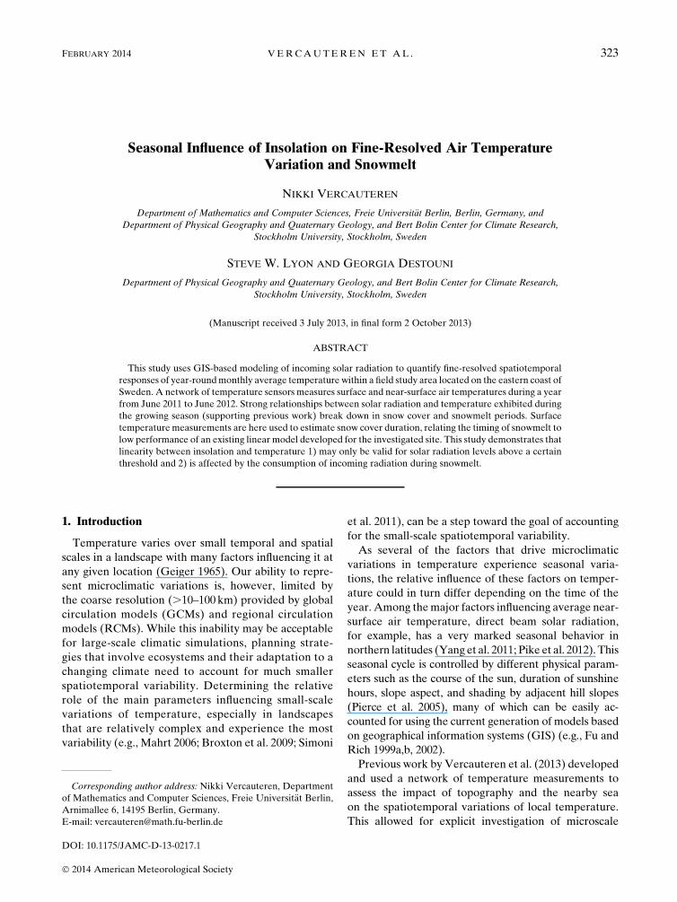
The study area is located in Sweden on theHigh Coast

(H€oga Kusten) of the Baltic Sea, in the municipalities

of Kramfors and H€arn€osand and is described in

Vercauteren et al. (2013). Sampling in this area is pos-

sible at a wide range of elevations, irrespective of the

distance to the coast because of the unique geological

settings offered by H€oga Kusten. Instrumentation con-

sists of a total of 98 Maxim 1922L iButton temperature

sensors (63 measuring air temperature and 35measuring

ground temperature) (Hubbart et al. 2005) placed in

a 2500m2 area ranging from latitude 62840 to 63810Nand from longitude 178140 to 188330E (Fig. 1). The lo-

cations of temperature measurements are chosen to

represent prevailing differences in slope orientation and

elevation. Elevation in the study area ranges from

0 to 470m above sea level. The area is characterized by

a wide coniferous forest cover, ensuring natural shield-

ing for the temperature sensors (Lundquist and Huggett

2008) and land cover homogeneity across the sampling

sites. All the sampling points are located under the tree

line under forest cover, and the forest density is rather

FIG. 1. Location and digital elevation model (DEM; 50-m resolution) of the forested

study site.

324 JOURNAL OF APPL IED METEOROLOGY AND CL IMATOLOGY VOLUME 53

homogeneous across sites, with slightly higher density

of forest cover on the north-facing slopes.

Air temperature was collected at about 1m above the

ground. In addition, ground temperature was collected

by placing sensors under the moss cover (applicable for

half of the sites). Temperature was recorded every half

hour between the end of May 2011 and the beginning of

October 2011 and every hour betweenOctober 2011 and

the beginning of June 2012.

b. Temperature analysis

Vercauteren et al. (2013) derived a linear model to

predict average (approximately monthly) temperature

from average insolation and elevation at each location

in the study area incorporating a time period for aver-

aging given by an exponential time-lag decay function

that varied in relation with the distance to the sea:

TN 5ARN 1B1Elevation3LR, (1)

where N 5 T0 exp(2aD) 1 C is the time lag in days

given as a function of the distance to the seaD and LR is

the lapse rate. A time lag ofN days between the average

solar radiation R (averaged overN days) and the average

temperature T (averaged over N days) is thus accounted

for in Eq. (1). The coefficients of the exponential decay

curve N were found in Vercauteren et al. (2013) to be

T05 4.00, a5 0.09, and C5 27.39 for the growing season

from June to September 2011. Details about the calcula-

tion of the solar radiation, which uses the ArcGIS solar

radiation tool (Dubayah andRich 1995; see also the online

information at http://webhelp.esri.com/arcgiSDEsktop/

9.3/index.cfm?TopicName5Area_Solar_Radiation), can

be found in Vercauteren et al. (2013) along with details

about the constants A and B in Eq. (1). In all our results,

the temperature is in degrees Celsius and insolation is in

kilowatt hours per meter squared, taken as daily average

(24 h).The work in Vercauteren et al. (2013) investi-

gated the seasonal evolution of the lapse rate and its

dependence on the distance to the sea. The absence of

a clear relationship among the lapse rate, the distance to

the sea, and the time of the year led to the use of a

constant lapse rate (LR524.08Ckm21) throughout the

analysis. This value is the average lapse rate that was

computed from our dataset and is very close to other

yearly averaged lapse rates computed in mountainous

environments [see Blandford et al. (2008), who give a de-

tailed analysis of the yearly variations of lapse rate]. The

calculation of the solar radiation is based on a digital ele-

vation model of 50-m resolution (Fig. 1), leading to solar

radiation maps of 50-m resolution.

During the growing season between June and

September, the slope A of the linear model in Eq. (1),

which determines the delayed temporal response of

average temperature T to a change in average incoming

solar radiation R, was found to be relatively robust

among sites, unlike the interceptB that varied much more

among sites. This previous result implies that the in-

solation model in Eq. (1) can be used to predict the

temporal evolution of mean temperature on a monthly

scale rather accurately without requiring toomany input

data. With regard to spatial variability, however, the

quantification of the spatially variable term B (which can

be viewed as a spatial correction term) shows that also

other variables, such as soil moisture, canopy properties,

and/or (perhapsmost importantly) local airflows that lead

to a mixing of warm and cold air across the landscape,

may considerably modify spatial temperature patterns.

In the present analysis, we test if the linear Eq. (1) and

the delayed temporal response represented by the lag

time N (number of days) still hold outside the growing

season period for which they were developed. We sepa-

rate the analysis into different 4-month periods to assess

the variability of the results during the course of a year.

c. Snow cover analysis

Temperature sensors of the type employed in the

present study can be used to monitor the spatial and

temporal pattern of snow cover in an inexpensive way

(Lundquist and Lott 2008; Lyon et al. 2008).Our sampling

design (which included temperature sensors placed under

a moss cover) thus provided a record of the presence or

absence of snow cover because snow acts as a strong in-

sulating layer dampening near-surface soil temperature

oscillations. Isolating the periods with negligible temper-

ature oscillations was shown byLundquist and Lott (2008)

to give a reliable estimate of snow cover periods.

In the present analysis, we use a similar threshold

method such that periods with oscillations of temperature

that are smaller than the threshold value are defined as

snow-covered periods. To define the threshold value, we

first compute the standard deviation of temperature for

a snow-free period of two months, for eachmeasurement

location. We then compute the standard deviation of

temperature for successive periods of three days, in

a moving window approach. The first period of three

consecutive days for which the standard deviation of

temperature is smaller than one-tenth of the previously

computed snow-free standard deviation is defined as the

start of the snow cover season, and the last such period of

three days is defined as the end of the snow cover period.

We also use remotely sensed observations of snow cover

from the Moderate Resolution Imaging Spectroradi-

ometer (MODIS) in order to have an independent spatial

assessment of the snow cover for comparison with our

temperature-derived estimates.

FEBRUARY 2014 VERCAUTEREN ET AL . 325

3. Results

a. Monthly temperature

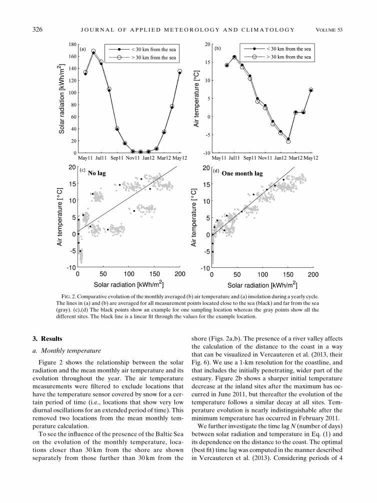
Figure 2 shows the relationship between the solar

radiation and the mean monthly air temperature and its

evolution throughout the year. The air temperature

measurements were filtered to exclude locations that

have the temperature sensor covered by snow for a cer-

tain period of time (i.e., locations that show very low

diurnal oscillations for an extended period of time). This

removed two locations from the mean monthly tem-

perature calculation.

To see the influence of the presence of the Baltic Sea

on the evolution of the monthly temperature, loca-

tions closer than 30 km from the shore are shown

separately from those further than 30 km from the

shore (Figs. 2a,b). The presence of a river valley affects

the calculation of the distance to the coast in a way

that can be visualized in Vercauteren et al. (2013, their

Fig. 6). We use a 1-km resolution for the coastline, and

that includes the initially penetrating, wider part of the

estuary. Figure 2b shows a sharper initial temperature

decrease at the inland sites after the maximum has oc-

curred in June 2011, but thereafter the evolution of the

temperature follows a similar decay at all sites. Tem-

perature evolution is nearly indistinguishable after the

minimum temperature has occurred in February 2011.

We further investigate the time lagN (number of days)

between solar radiation and temperature in Eq. (1) and

its dependence on the distance to the coast. The optimal

(best fit) time lag was computed in themanner described

in Vercauteren et al. (2013). Considering periods of 4

FIG. 2. Comparative evolution of themonthly averaged (b) air temperature and (a) insolation during a yearly cycle.

The lines in (a) and (b) are averaged for all measurement points located close to the sea (black) and far from the sea

(gray). (c),(d) The black points show an example for one sampling location whereas the gray points show all the

different sites. The black line is a linear fit through the values for the example location.

326 JOURNAL OF APPL IED METEOROLOGY AND CL IMATOLOGY VOLUME 53

months that start from each month of the year, we first

compute the number of days N of lag between solar

radiation and temperature that maximizes the correla-

tion between averaged radiation and lagged averaged

temperature for each location. We thus obtain values

of N for each point in the landscape for each period of

4 months. We then try to fit of an exponential decay

(relative to the distance to the sea) on these values of

N for each successive period of 4 months, in the same

manner that is described in Vercauteren et al. (2013).

The previously analyzed period from June to September

shows an r2 of 80% for the exponential best fit, whereas

the r2 for the exponential best fit for the period July–

October drops to 30%, and this coefficient continues to

drop for the later periods (analysis not shown).

We therefore considered a constant delayN of 30 days

for all the analyzed 4-month periods at the exception of

the period from June to September for which we con-

sider the fitted exponential decay of N. The slopeA and

intercept B of the linear model [Eq. (1)], computed at

each location for each period of 4 consecutive months,

vary during the course of the year (Fig. 3). In a similar

analysis as in Vercauteren et al. (2013), we determine

the standard deviation of A and B across the different

sites to assess if the model is robust across sites or not.

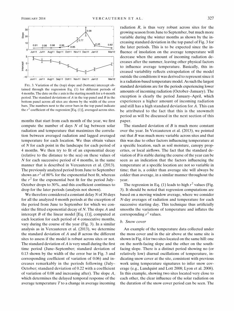
The standard deviation ofA is very small during the first

time period (June–September; standard deviation of

0.13 shown by the width of the error bar in Fig. 3 and

corresponding coefficient of variation of 0.06) and in-

creases remarkably in the periods following (July–

October; standard deviation of 0.22 with a coefficient

of variation of 0.08 and increasing after). The slope A,

which determines the delayed temporal response of the

average temperature T to a change in average incoming

radiation R, is thus very robust across sites for the

growing season from June to September, but muchmore

variable during the winter months as shown by the in-

creasing standard deviation in the top panel of Fig. 3 for

the later periods. This is to be expected since the in-

fluence of insolation on the average temperature will

decrease when the amount of incoming radiation de-

creases after the summer, leaving other physical factors

to influence average temperature. Basically, this in-

creased variability reflects extrapolation of the model

outside the conditions it was derived to represent since it

is a radiation-based temperaturemodel.As such the largest

standard deviations are for the periods experiencing lower

amounts of incoming radiation (October–January). The

exception is clearly the period January–April, which

experiences a higher amount of incoming radiation

and still has a high standard deviation for A. This can

be attributed to the fact that this is the snowmelt

period as will be discussed in the next section of this

paper.

The standard deviation of B is much more constant

over the year. In Vercauteren et al. (2013), we pointed

out that B was much more variable across sites and that

this was due to other factors influencing temperature at

a specific location, such as soil moisture, canopy prop-

erties, or local airflows. The fact that the standard de-

viation ofB is stable during the course of the year can be

seen as an indication that the factors influencing the

temperature at a specific location are not so variable in

time; that is, a colder than average site will always be

colder than average, in a similar manner throughout the

year.

The regression in Eq. (1) leads to high r2 values (Fig.

3). It should be noted that regression computations are

based on a moving window average, where we consider

N-day averages of radiation and temperature for each

successive starting day. This technique thus artificially

smooths the variations of temperature and inflates the

corresponding r2 values.

b. Snow cover

An example of the temperature data collected under

the moss cover and in the air above at the same site is

shown in Fig. 4 for two sites located on the same hill: one

on the north-facing slope and the other on the south-

facing slope. There is a distinct period showing no (or

relatively low) diurnal oscillations of temperature, in-

dicating snow cover at the site, consistent with previous

work using temperature signatures to infer snow cov-

erage (e.g., Lundquist and Lott 2008; Lyon et al. 2008).

In this example, showing two sites located very close to

each other, the clear influence of the solar radiation on

the duration of the snow cover period can be seen. The

FIG. 3. Variation of the (top) slope and (bottom) intercept ob-

tained through the regression Eq. (1) for different periods of

4 months. The date on the x axis is the startingmonth for a 4-month

period. The standard deviations of A in the top panel and B in the

bottom panel across all sites are shown by the width of the error

bars. The numbers next to the error bars in the top panel indicate

the r 2 coefficient of the regression [Eq. (1)], averaged across sites.

FEBRUARY 2014 VERCAUTEREN ET AL . 327

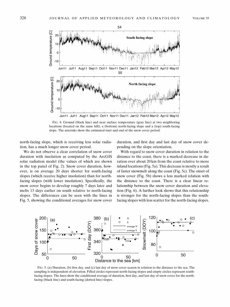
north-facing slope, which is receiving less solar radia-

tion, has a much longer snow cover period.

We do not observe a clear correlation of snow cover

duration with insolation as computed by the ArcGIS

solar radiation model (the values of which are shown

in the top panel of Fig. 2). Snow cover duration, how-

ever, is on average 20 days shorter for south-facing

slopes (which receive higher insolation) than for north-

facing slopes (with lower insolation). Specifically, the

snow cover begins to develop roughly 7 days later and

melts 13 days earlier on south relative to north-facing

slopes. The differences can be seen with the lines in

Fig. 5, showing the conditional averages for snow cover

duration, and first day and last day of snow cover de-

pending on the slope orientation.

With regard to snow cover duration in relation to the

distance to the coast, there is a marked decrease in du-

ration over about 20 km from the coast relative to more

inland locations (Fig. 5a). This decrease is mostly a result

of faster snowmelt along the coast (Fig. 5c). The onset of

snow cover (Fig. 5b) shows a less marked relation with

the distance to the coast. There is a clear linear re-

lationship between the snow cover duration and eleva-

tion (Fig. 6). A further look shows that this relationship

is stronger for the north-facing slopes than the south-

facing slopes with less scatter for the north-facing slopes.

FIG. 4. Ground (black line) and near surface temperature (gray line) at two neighboring

locations (located on the same hill), a (bottom) north-facing slope and a (top) south-facing

slope. The asterisks show the estimated start and end of the snow cover period.

FIG. 5. (a) Duration, (b) first day, and (c) last day of snow cover season in relation to the distance to the sea. The

sampling is independent of elevation. Filled circles represent north-facing slopes and empty circles represent south-

facing slopes. The lines show the conditional average of duration, first day, and last day of snow cover for the north-

facing (black line) and south-facing (dotted line) slopes.

328 JOURNAL OF APPL IED METEOROLOGY AND CL IMATOLOGY VOLUME 53

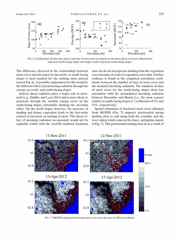
The difference observed in the relationships between

snow cover and elevation for the north- or south-facing

slopes is most marked for the melting snow pattern

seen in Fig. 6c. A possible explanation for this would be

the different effect of penetrating radiation through the

canopy on north- and south-facing slopes.

Indeed, direct radiation plays a major role in snow-

melt (e.g., Dahlke and Lyon 2013) and is more likely to

penetrate through the variable canopy cover on the

south-facing slopes, potentially masking the elevation

effect. On the north slopes, however, the presence of

shading and denser vegetation leads to the first-order

control of elevation on melting of snow. This direct ef-

fect of incoming radiation on snowmelt would not be

explicitly visible with the ArcGIS modeled insolation

since we do not incorporate shading from the vegetation

cover because of a lack of vegetation cover data. Further

evidence is found in the computed correlation coeff-

icients between the number of days of snow cover and

the modeled incoming radiation. The numbers of days

of snow cover for the north-facing slopes show less

correlation with the accumulated incoming radiation

between December and March (i.e., the snow season)

relative to south-facing slopes (r2 coefficients of 2% and

32%, respectively).

Spatial estimation of fractional snow cover obtained

from MODIS (Fig. 7) supports preferential spring

melting close to and along both the coastline and the

river valleys (dark zones in the lower, springtime panels

of Fig. 7). This preferential melting may be as a result of

FIG. 6. (a) Duration, (b) first day, and (c) last day of snow cover in relation to elevation above sea level. Filled circles

represent north-facing slopes and empty circles represent south-facing slopes.

FIG. 7. MODIS estimated fractional snow cover over the area at 500-m resolution.

FEBRUARY 2014 VERCAUTEREN ET AL . 329

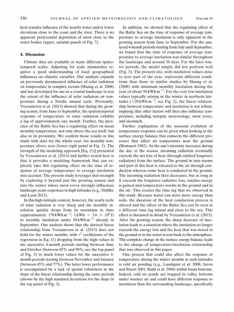
heat transfer influence of the nearby water and/or lower

elevations close to the coast and the river. There is no

apparent preferential deposition of snow close to the

water bodies (upper, autumn panels of Fig. 7).

4. Discussion

Climate data are available at many different spatio-

temporal scales. Adjusting for scale mismatches re-

quires a good understanding of local geographical

influences on climatic variables. Our analysis expands

on previously documented influence of solar radiation

on temperature in complex terrain (Huang et al. 2008)

and was developed for use in a coastal landscape to test

the extent of the influence of solar radiation on tem-

perature during a Nordic annual cycle. Previously,

Vercauteren et al. (2013) showed that during the grow-

ing season, from June to September, the spatiotemporal

response of temperature to solar radiation exhibits

a lag of approximately one month. Further, the pres-

ence of the Baltic Sea has a regulating effect on mean

monthly temperature, not only above the sea itself, but

also in its proximity. We confirm those results in this

study with data for the whole year, for monthly tem-

perature above zero (lower right panel in Fig. 2). The

strength of the modeling approach [Eq. (1)] presented

by Vercauteren et al. (2013) and further tested here is

that it provides a modeling framework that can ex-

plicitly take this regulating effect on the time of re-

sponse of average temperature to average insolation

into account. The present study leverages that strength

by exploring it beyond just the growing season and

into the winter where snow cover strongly influences

landscape-scale responses in high latitudes (e.g., Dahlke

and Lyon 2013).

In this high-latitude context, however, the yearly cycle

of solar radiation is very sharp and the monthly in-

solation quickly drops from its maximum in June

(approximately 170 kWhm22; 1 kWh 5 3.6 3 106 J)

to monthly insolation under 50 kWhm22 already in

September. Our analysis shows that the derived linear

relationship from Vercauteren et al. (2013) does not

hold for the winter months, with r2 coefficients of the

regression in Eq. (1) dropping from the high values in

the successive 4-month periods starting between June

and October (between 85% and 98%; see the top panel

of Fig. 3) to much lower values for the successive 4-

month periods starting between November and January

(between 45% and 77%). The latter lower performance

is accompanied by a lack of spatial robustness in the

slope of the linear relationship during the same periods

(shown by the high standard deviations for the slope in

the top panel of Fig. 3).

In addition, we showed that the regulating effect of

the Baltic Sea on the time of response of average tem-

perature to average insolation is only apparent in the

growing season from June to September. For the ana-

lyzed 4-month periods starting from July until September,

we found that the time of response of average tem-

perature to average insolation was similar throughout

the landscape and around 30 days. For the later win-

ter periods, the model simply did not perform well

(Fig. 3). The present site, with insolation values close

to zero part of the year, represents different condi-

tions than those in similar studies by Huang et al.

(2008) with minimum monthly insolation during the

year of about 50 kWhm22. For the very low insolation

values typically arising in the winter in northern lati-

tudes (,20 kWhm22; see Fig. 2), the linear relation-

ship between temperature and insolation is not robust,

implying that other factors will then also influence tem-

perature, including synoptic meteorology, snow cover,

and snowmelt.

Further explanation of the seasonal evolution of

temperature response can be given when looking at the

surface energy balance that connects the different pro-

cesses that affect air temperature near the ground

(Brutsaert 1982). As the sun’s intensity increases during

the day or the season, incoming radiation eventually

exceeds the net loss of heat (through emitted longwave

radiation) from the surface. The ground in turn warms

and part of this heat is released to the air through con-

duction whereas some heat is conducted in the ground.

The incoming radiation then decreases, but as long as

it exceeds the longwave radiative loss, surplus energy

is gained and temperature warms in the ground and in

the air. This creates the time lag that we observed in

this study. Because water can store more energy than

soils, the duration of the heat conduction process is

altered and the effect of the Baltic Sea can be seen in

a different time lag inland and close to the sea. This

effect is discussed in detail by Vercauteren et al. (2013).

After the growing season, the sharp decrease of inso-

lation leads to a situation where the insolation no longer

exceeds the energy loss and the heat that was stored in

the ground or in the water is sent back to the atmosphere.

This complete change in the surface energy balance leads

to the change of temperature/insolation relationship

that was observed in this paper.

One process that could also affect the response of

temperature during the winter months at such latitudes

is cold air ponding (e.g., Lundquist et al. 2008; Jarvis

and Stuart 2001; Stahl et al. 2006) within basin bottoms.

Indeed, cold air ponds are trapped in valley bottoms

under warmer air and could have different response to

insolation than the surrounding landscape, specifically

330 JOURNAL OF APPL IED METEOROLOGY AND CL IMATOLOGY VOLUME 53

in terms of the response of temperature with elevation.

Our dataset unfortunately did not include elevation

transects on each slopes so that we could not investigate

this phenomenon in detail.

Our dataset, however, enabled us to investigate the

snow cover and its relation to incoming radiation.

Rather than just showing a threshold of incoming ra-

diation above which the proposed linear relationship

between temperature and insolation is valid, our anal-

ysis further showed that the performance of the linear

relationship was dependent on the snowmelt period

(Fig. 3). Indeed, for a similar amount of insolation re-

ceived in the fall (September–December) and in the late

winter (January–April), the proposed linear relation-

ship gave less satisfactory results for the late winter

months than for the autumn months. In terms of surface

energy balance, the main difference between those two

periods is that the late winter is a period of snowmelt.

During this period, a large part of the incoming radiation

will be consumed to melt snow. This energy is thus no

longer available to be transferred back to the atmosphere

in the form of heat. For the same reason, the influence of

solar radiation was highly visible in the snow cover data.

We found that north-facing slopes are covered by snow

on average 20 days longer than south-facing slopes, which

receive higher loads of solar radiation. Among these

20 days, the timing of snowmelt, which requires an

energy input, is the major difference, happening on av-

erage 13 days later for north-facing slopes compared to

south-facing slopes.

Because of the different energy budget of a water

body or a snow-covered landscape, the presence of the

Baltic Sea also has a clear effect on the melting pattern.

Indeed, we observe a clearly faster melt near the coast,

where the temperature is regulated by the presence of

a large water body. The increase of melting time with

increasing distance to the sea is seen in the first 20 km.

This was the distance over which we also observed an

effect of the sea on the time of reaction of temperature

to insolation during the growing season at this site.

5. Conclusions

Advanced models are readily available as GIS tools

(such as the solar radiation tool of ArcGIS) that can

estimate solar radiation. These insolation estimates can

be used to predict the temporal evolution of tempera-

ture in a landscape. However, care is needed, as the

linearity between insolation and temperature is poten-

tially valid only for solar radiation levels above a certain

threshold, and is affected by snowmelt, which absorbs

incoming radiation. This threshold is not attained under

winter conditions in northern latitudes, and solar radiation

will then not be the single dominant controlling factor of

mean temperature at these latitudes.

We show that at the present investigation site, av-

erage solar radiation has a linear influence on average

temperature for monthly insolation values above

20 kWhm22. We also show that for similar insolation,

the average temperature is influenced linearly by in-

solation during the fall but not during the snowmelt

period, where the slope of the linear model is no longer

robust across sites.

Acknowledgments. This work has been funded by the

strategic research project EkoKlim (a multiscale cross-

disciplinary approach to the study of climate change ef-

fects on ecosystem services and biodiversity) at Stockholm

University. The authors thank Kristoffer Hylander for

his participation in framing the project and thank Johan

Dahlberg, Norris Lam, Johannes Forsberg, and Liselott

Wilin for their help in the field.

REFERENCES

Blandford, T., K. Humes, B. J. Harshburger, B. C. Moore, V. P.

Walden, and H. Ye, 2008: Seasonal and synoptic variations in

near-surface air temperature lapse rates in a mountainous

basin. J. Appl. Meteor. Climatol., 47, 249–261.

Broxton, P. D., P. A. Troch, and S. W. Lyon, 2009: On the role of

aspect to quantify water transit times in small mountainous

catchments. Water Resour. Res., 45, W08427, doi:10.1029/

2008WR007438.

Brutsaert, W., 1982: Evaporation into the Atmosphere: Theory,

History, and Applications. D. Reidel, 229 pp.

Dahlke, H. E., and S. W. Lyon, 2013: Early melt season snowpack

isotopic evolution in the Tarfala valley, northern Sweden.

Ann. Glaciol., 54, 149–156, doi:10.3189/2013AoG62A232.

Dubayah, R., and P. M. Rich, 1995: Topographic solar radiation

models for GIS. Int. J. Geogr. Info. Syst., 9, 405–419, doi:10.1080/

02693799508902046.

Fu, P., andP.M.Rich, 1999a:Design and implementation of the Solar

Analyst: An ArcView extension for modeling solar radiation at

landscape scales. Proc. 19th ESRI User Conf., San Diego, CA,

ESRI. [Available online at http://proceedings.esri.com/librsary/

userconf/proc99/proceed/papers/pap867/p867.htm.]

——, and ——, 1999b: TopoView, version 1.0 manual. Helios

Environmental Modeling Institute, 48 pp.

——, and ——, 2002: A geometric solar radiation model with ap-

plications in agriculture and forestry. Comput. Electron. Ag-

ric., 37, 25–35.

Geiger, R., 1965: The Climate near the Ground. 4th ed. Harvard

University Press, 642 pp.

Huang, S., P. M. Rich, R. L. Crabtree, C. S. Potter, and P. Fu, 2008:

Modeling monthly near-surface air temperature from solar

radiation and lapse rate: Application over complex terrain in

YellowstoneNational Park.Phys.Geogr., 29, 158–178, doi:10.2747/

0272-3646.29.2.158.

Hubbart, J., T. Link, C. Campbell, and D. Cobos, 2005: Evaluation

of a low-cost temperature measurement system for environ-

mental applications.Hydrol. Processes, 19, 1517–1523, doi:10.1002/

hyp.5861.

FEBRUARY 2014 VERCAUTEREN ET AL . 331

Jarvis, C. H., and N. Stuart, 2001: A comparison among strategies

for interpolating maximum and minimum daily air temper-

atures. Part I: The selection of ‘‘guiding’’ topographic and

land cover variables. J. Appl. Meteor., 40, 1060–1074.Lundquist, J. D., and B. Huggett, 2008: Evergreen trees as in-

expensive radiation shields for temperature sensors. Water

Resour. Res., 44, W00D04, doi:10.1029/2008WR006979.

——, and F. Lott, 2008: Using inexpensive temperature sensors to

monitor the duration and heterogeneity of snow-covered areas.

Water Resour. Res., 44, W00D16, doi:10.1029/2008WR007035.

——, N. Pepin, and C. Rochford, 2008: Automated algorithm for

mapping regions of cold-air pooling in complex terrain.

J. Geophys. Res., 113, D22107, doi:10.1029/2008JD009879.

Lyon, S. W., P. A. Troch, P. D. Broxton, N. P. Molotch, and P. D.

Brooks, 2008: Monitoring the timing of snowmelt and the

initiation of streamflow using a distributed network of

temperature/light sensors.Ecohydrology, 1, 215–224, doi:10.1002/

eco.18.

Mahrt, L., 2006: Variation of surface air temperature in complex

terrain. J. Appl. Meteor. Climatol., 45, 1481–1493.

Pierce, K. B., Jr., T. Lookingbill, and D. Urban, 2005: A simple

method for estimating potential relative radiation (PRR) for

landscape-scale vegetation analysis.Landscape Ecol., 20, 137–

147, doi:10.1007/s10980-004-1296-6.

Pike, G., N. C. Pepin, and M. Schaefer, 2012: High latitude local

scale temperature complexity: The example of Kevo Valley,

Finnish Lapland. Int. J. Climatol., 33, 2050–2067.

Simoni, S., and Coauthors, 2011: Hydrologic response of an alpine

watershed: Application of a meteorological wireless sensor

network to understand streamflow generation. Water Resour.

Res., 47, W10524, doi:10.1029/2011WR010730.

Stahl, K., R. D. Moore, J. A. Floyer, M. G. Asplin, and I. G.

McKendry, 2006: Comparison of approaches for spatial inter-

polation of daily air temperature in a large region with complex

topography and highly variable station density. Agric. For. Me-

teor., 139, 224–236, doi:10.1016/j.agrformet.2006.07.004.

Vercauteren, N., G. Destouni, C. J. Dahlberg, and K. Hylander,

2013: Fine-resolved, near-coastal spatiotemporal variation of

temperature in response to insolation. J. Appl. Meteor. Cli-

matol., 52, 1208–1220.

Yang, Z., E. Hanna, and T. V. Callaghan, 2011: Modelling surface-

air temperature variation over complex terrain around

Abisko, Swedish Lapland: Uncertainties of measurements

and models at different scales. Geogr. Ann., 93, 89–112.

332 JOURNAL OF APPL IED METEOROLOGY AND CL IMATOLOGY VOLUME 53