1 Search: Uninformed Search Material in part from http://www.cs.cmu.edu/~awm/tutorials Russel & Norvig Chap. 3 A Search Problem • Find a path from START to GOAL • Find the minimum number of transitions b a d p q h e c f r START GOAL

Welcome message from author
This document is posted to help you gain knowledge. Please leave a comment to let me know what you think about it! Share it to your friends and learn new things together.
Transcript
1
Search: Uninformed Search
Material in part from http://www.cs.cmu.edu/~awm/tutorials
Russel & Norvig Chap. 3
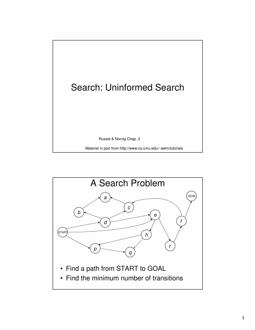
A Search Problem
• Find a path from START to GOAL
• Find the minimum number of transitions
b
a
d
pq
h
e
c
f
r
START
GOAL
2
Example
28
31
6
4
7
5 2
8
3
1
6
4
7
5
START GOAL
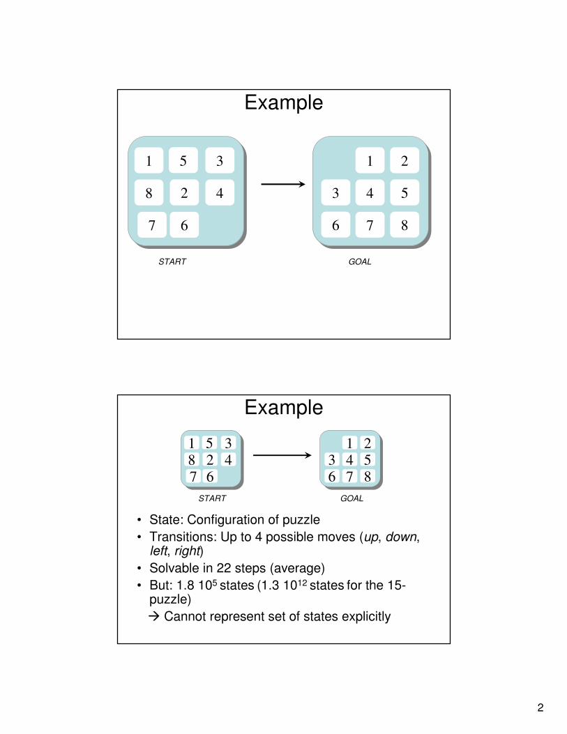
Example
• State: Configuration of puzzle
• Transitions: Up to 4 possible moves (up, down, left, right)
• Solvable in 22 steps (average)
• But: 1.8 105 states (1.3 1012 states for the 15-puzzle)
� Cannot represent set of states explicitly
28
31
6
4
7
5 2
8
3
1
6
4
7
5
START GOAL
3
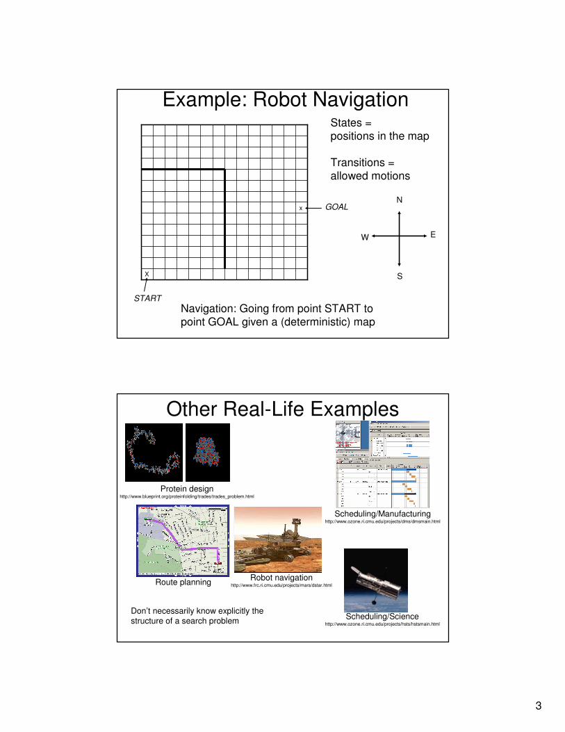
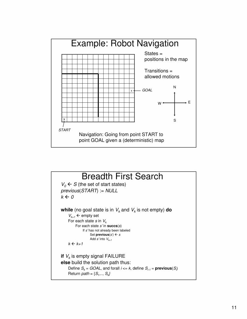
Example: Robot Navigation
X
x
START
GOAL
States =
positions in the map
Transitions =
allowed motions
N
E
S
W
Navigation: Going from point START to
point GOAL given a (deterministic) map
Other Real-Life Examples
Protein designhttp://www.blueprint.org/proteinfolding/trades/trades_problem.html
Scheduling/Manufacturinghttp://www.ozone.ri.cmu.edu/projects/dms/dmsmain.html
Scheduling/Sciencehttp://www.ozone.ri.cmu.edu/projects/hsts/hstsmain.html
Route planningRobot navigation
http://www.frc.ri.cmu.edu/projects/mars/dstar.html
Don’t necessarily know explicitly the
structure of a search problem
4
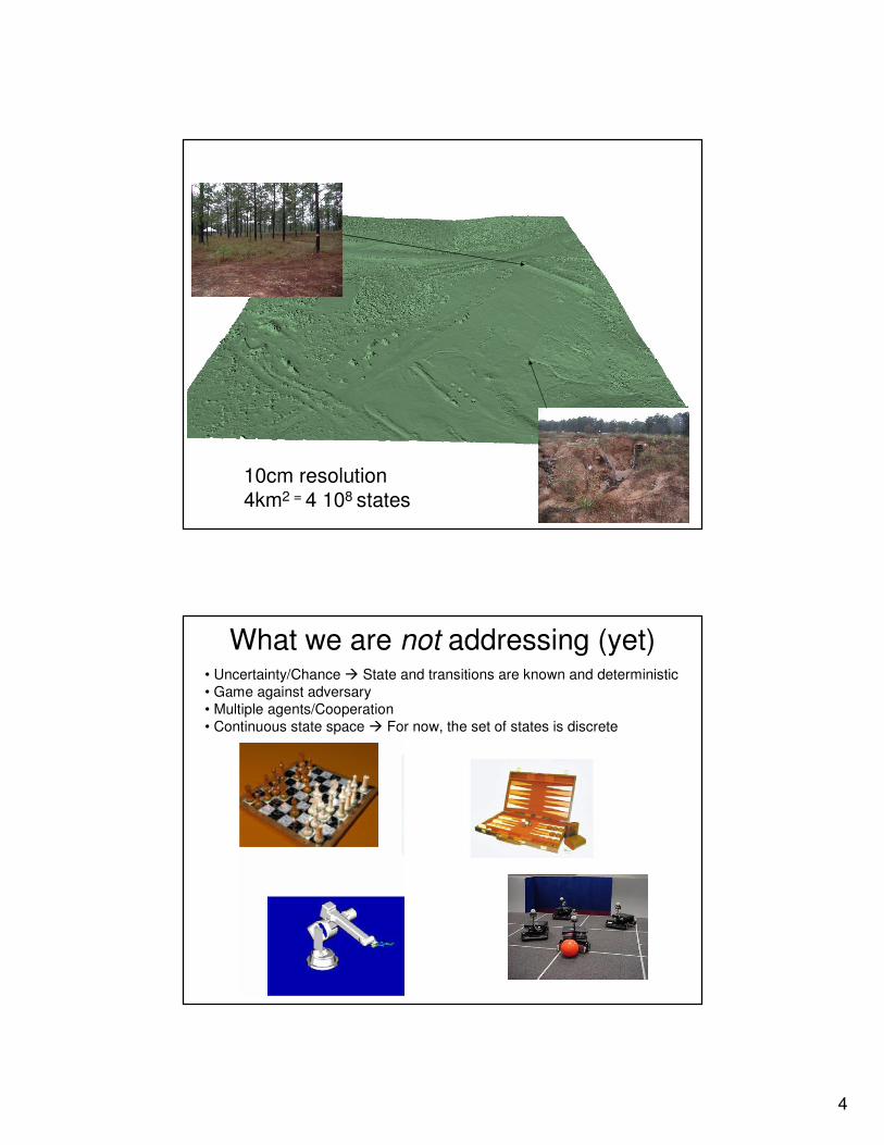
10cm resolution4km2 = 4 108 states
What we are not addressing (yet)• Uncertainty/Chance � State and transitions are known and deterministic
• Game against adversary
• Multiple agents/Cooperation
• Continuous state space � For now, the set of states is discrete
5
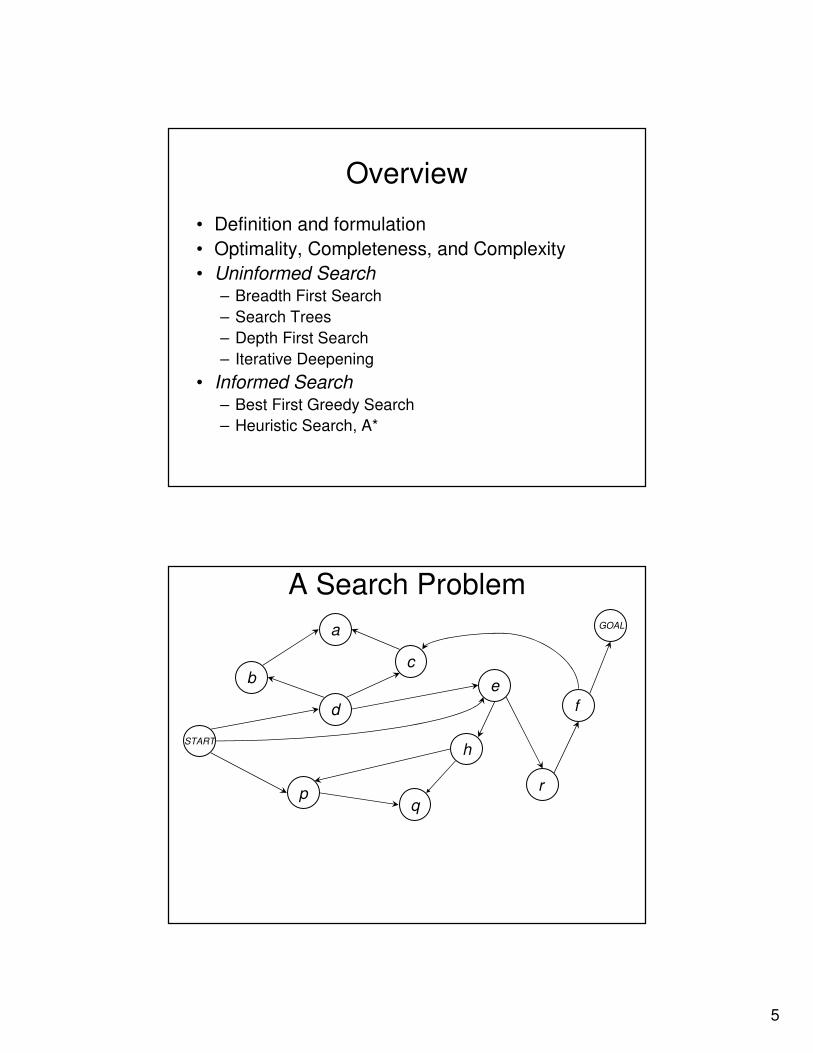
Overview
• Definition and formulation
• Optimality, Completeness, and Complexity
• Uninformed Search– Breadth First Search
– Search Trees
– Depth First Search
– Iterative Deepening
• Informed Search– Best First Greedy Search
– Heuristic Search, A*
A Search Problem
b
a
d
pq
h
e
c
f
r
START
GOAL
6
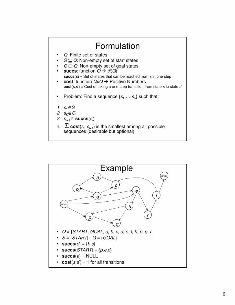
Formulation• Q: Finite set of states
• S Q: Non-empty set of start states
• G Q: Non-empty set of goal states• succs: function Q � P(Q)
succs(s) = Set of states that can be reached from s in one step
• cost: function QxQ � Positive Numbers cost(s,s’) = Cost of taking a one-step transition from state s to state s’
• Problem: Find a sequence {s1,…,sK} such that:
1. s1 S
2. sK G
3. si+1 succs(si)
4. Σ cost(si, si+1) is the smallest among all possible sequences (desirable but optional)
⊆⊆
∈
∈∈
Example
• Q = {START, GOAL, a, b, c, d, e, f, h, p, q, r}
• S = {START} G = {GOAL}
• succs(d) = {b,c}
• succs(START) = {p,e,d}
• succs(a) = NULL
• cost(s,s’) = 1 for all transitions
b
a
d
p
q
h
e
c
f
r
START
GOAL
7
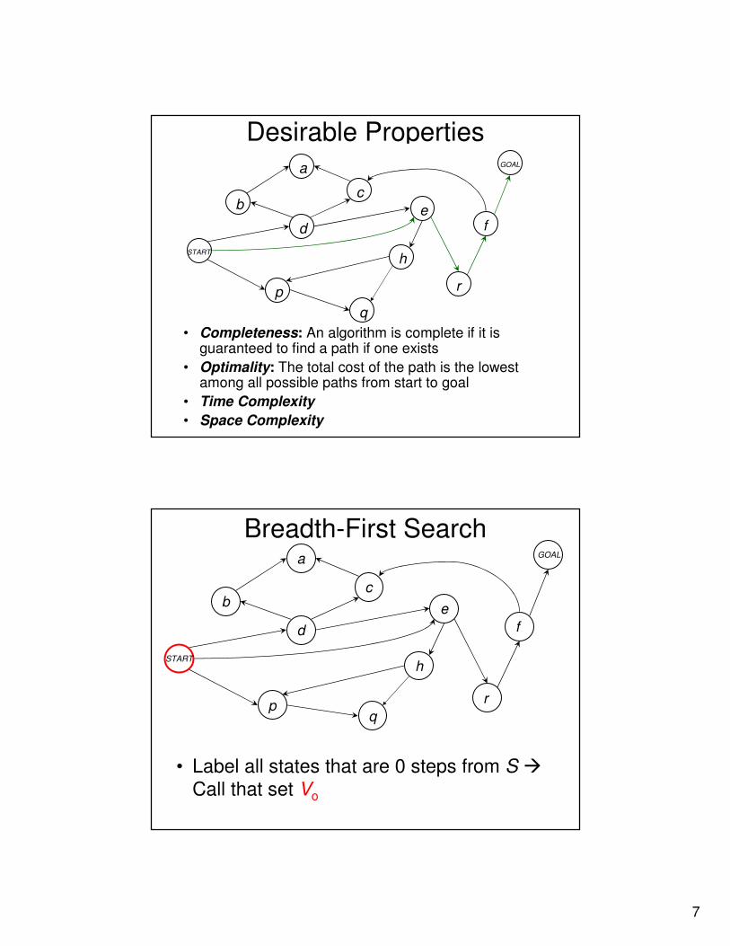
Desirable Properties
• Completeness: An algorithm is complete if it is guaranteed to find a path if one exists
• Optimality: The total cost of the path is the lowest among all possible paths from start to goal
• Time Complexity
• Space Complexity
b
a
d
p
q
h
e
c
f
r
START
GOAL
b
a
d
p
q
h
e
c
f
r
START
GOAL
Breadth-First Search
• Label all states that are 0 steps from S �
Call that set Vo
b
a
d
pq
h
e
c
f
r
START
GOAL
8
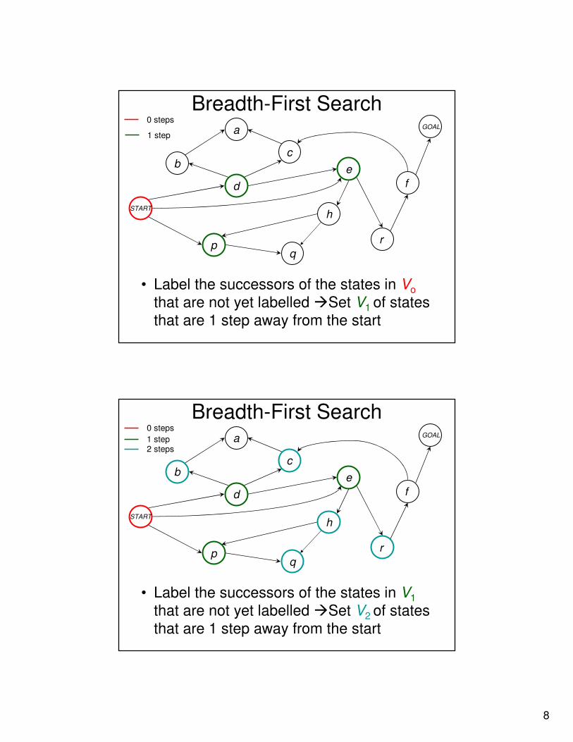
Breadth-First Search
• Label the successors of the states in Vo
that are not yet labelled �Set V1 of states
that are 1 step away from the start
b
a
d
pq
h
e
c
f
r
START
GOAL0 steps
1 step
Breadth-First Search
• Label the successors of the states in V1
that are not yet labelled �Set V2 of states
that are 1 step away from the start
b
a
d
pq
h
e
c
f
r
START
GOAL0 steps
1 step2 steps
9
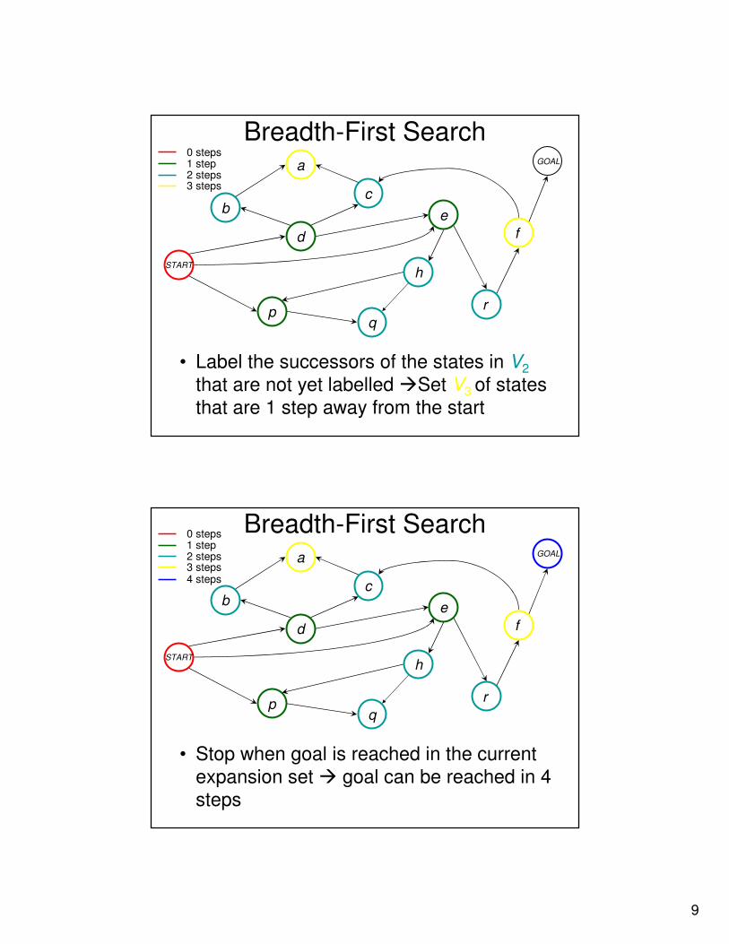
Breadth-First Search
• Label the successors of the states in V2
that are not yet labelled �Set V3 of states
that are 1 step away from the start
b
a
d
pq
h
e
c
f
r
START
GOAL0 steps1 step2 steps3 steps
Breadth-First Search
• Stop when goal is reached in the current
expansion set � goal can be reached in 4
steps
b
a
d
pq
h
e
c
f
r
START
GOAL
0 steps1 step2 steps3 steps4 steps
10
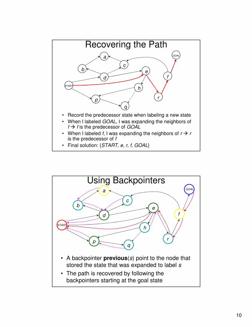
Recovering the Path
• Record the predecessor state when labeling a new state
• When I labeled GOAL, I was expanding the neighbors of f � f is the predecessor of GOAL
• When I labeled f, I was expanding the neighbors of r � ris the predecessor of f
• Final solution: {START, e, r, f, GOAL}
b
a
d
p
q
h
e
c
f
r
START
GOAL
Using Backpointers
• A backpointer previous(s) point to the node that stored the state that was expanded to label s
• The path is recovered by following the backpointers starting at the goal state
b
a
d
pq
h
e
c
f
r
START
GOAL
11
Example: Robot Navigation
X
x
START
GOAL
States =
positions in the map
Transitions =
allowed motions
N
E
S
W
Navigation: Going from point START to
point GOAL given a (deterministic) map
Breadth First SearchV0 S (the set of start states)
previous(START) := NULL
k 0
while (no goal state is in Vk and Vk is not empty) doVk+1 empty set
For each state s in Vk
For each state s’ in succs(s)
If s’ has not already been labeled
Set previous(s’) s
Add s’ into Vk+1
k k+1
if Vk is empty signal FAILURE
else build the solution path thus: Define Sk = GOAL, and forall i <= k, define Si-1 = previous(Si)
Return path = {S1,.., Sk}
12
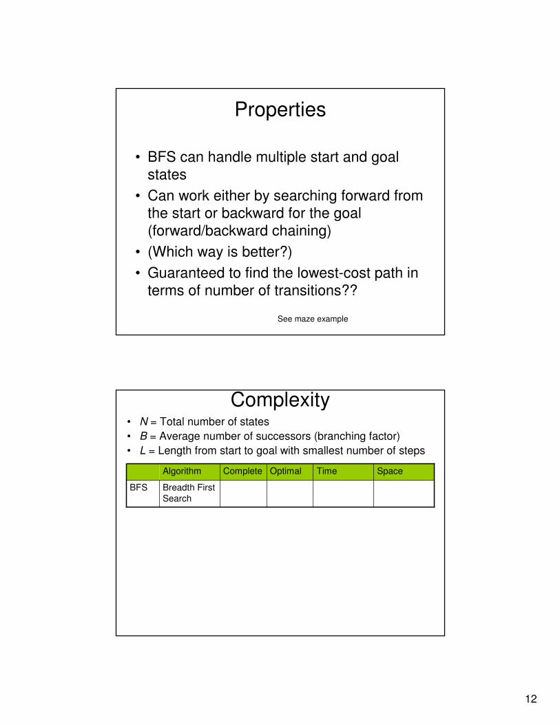
Properties
• BFS can handle multiple start and goal
states
• Can work either by searching forward from the start or backward for the goal
(forward/backward chaining)
• (Which way is better?)
• Guaranteed to find the lowest-cost path in
terms of number of transitions??
See maze example
Complexity• N = Total number of states
• B = Average number of successors (branching factor)
• L = Length from start to goal with smallest number of steps
Breadth First
Search
BFS
SpaceTimeOptimalCompleteAlgorithm
13
V3
V’3
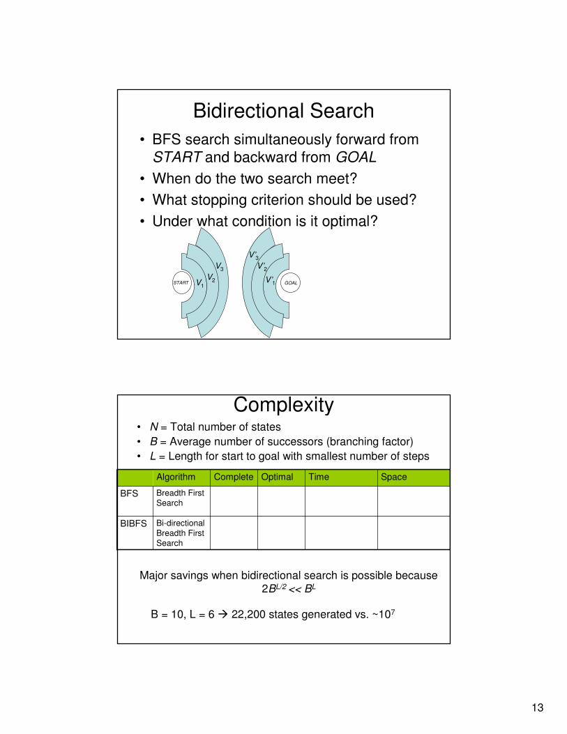
Bidirectional Search
• BFS search simultaneously forward from
START and backward from GOAL
• When do the two search meet?
• What stopping criterion should be used?
• Under what condition is it optimal?
START GOALV1V’1
V2
V’2
Complexity• N = Total number of states
• B = Average number of successors (branching factor)
• L = Length for start to goal with smallest number of steps
Bi-directional
Breadth First
Search
BIBFS
Breadth First
SearchBFS
SpaceTimeOptimalCompleteAlgorithm
B = 10, L = 6 � 22,200 states generated vs. ~107
Major savings when bidirectional search is possible because
2BL/2 << BL
14
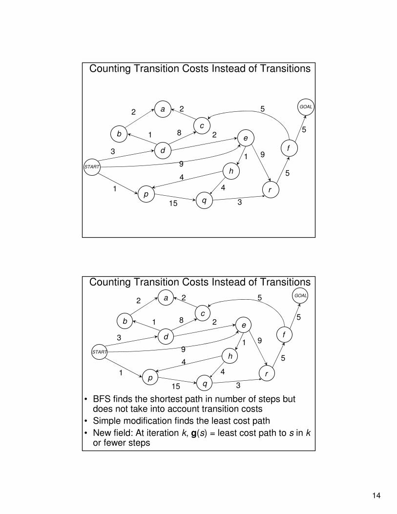
Counting Transition Costs Instead of Transitions
b
a
d
pq
h
e
c
f
r
START
GOAL
2
1
3
1
9
15
8
2
2
4
9
5
5
5
4
1
3
Counting Transition Costs Instead of Transitions
• BFS finds the shortest path in number of steps but does not take into account transition costs
• Simple modification finds the least cost path
• New field: At iteration k, g(s) = least cost path to s in kor fewer steps
b
a
d
pq
h
e
c
f
r
START
GOAL
2
1
3
1
9
15
8
2
2
4
9
5
5
5
4
1
3
15
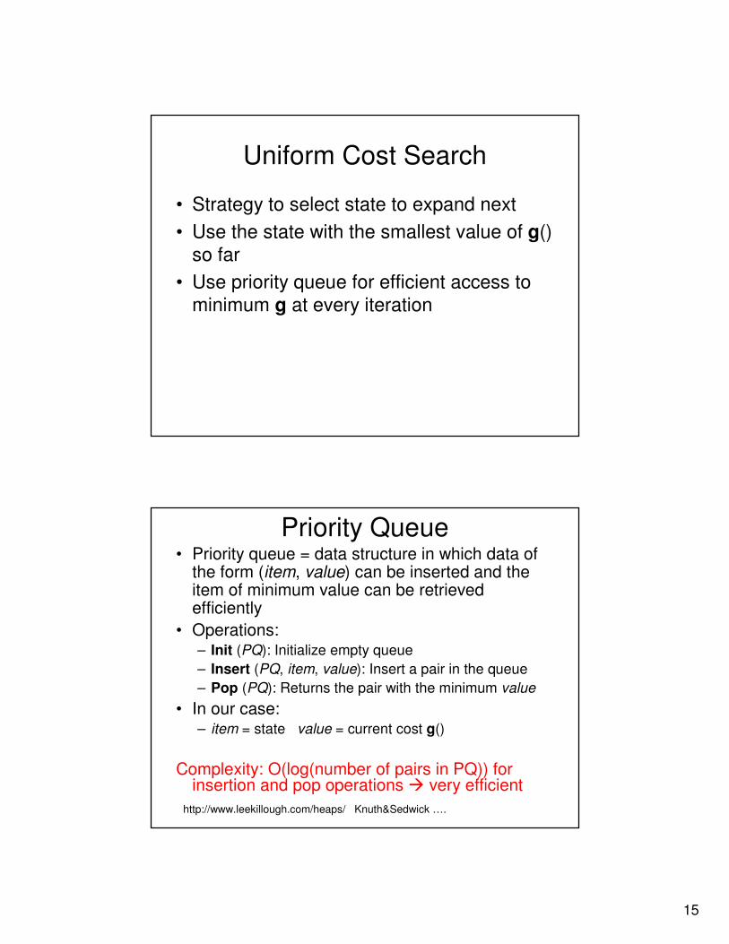
Uniform Cost Search
• Strategy to select state to expand next
• Use the state with the smallest value of g()
so far
• Use priority queue for efficient access to
minimum g at every iteration
Priority Queue• Priority queue = data structure in which data of
the form (item, value) can be inserted and the item of minimum value can be retrieved efficiently
• Operations:– Init (PQ): Initialize empty queue
– Insert (PQ, item, value): Insert a pair in the queue
– Pop (PQ): Returns the pair with the minimum value
• In our case:– item = state value = current cost g()
Complexity: O(log(number of pairs in PQ)) for insertion and pop operations � very efficient
http://www.leekillough.com/heaps/ Knuth&Sedwick ….
16
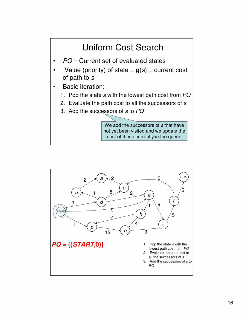
Uniform Cost Search
• PQ = Current set of evaluated states
• Value (priority) of state = g(s) = current cost
of path to s
• Basic iteration:
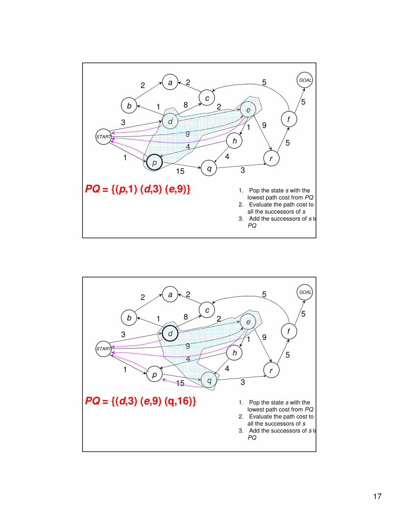
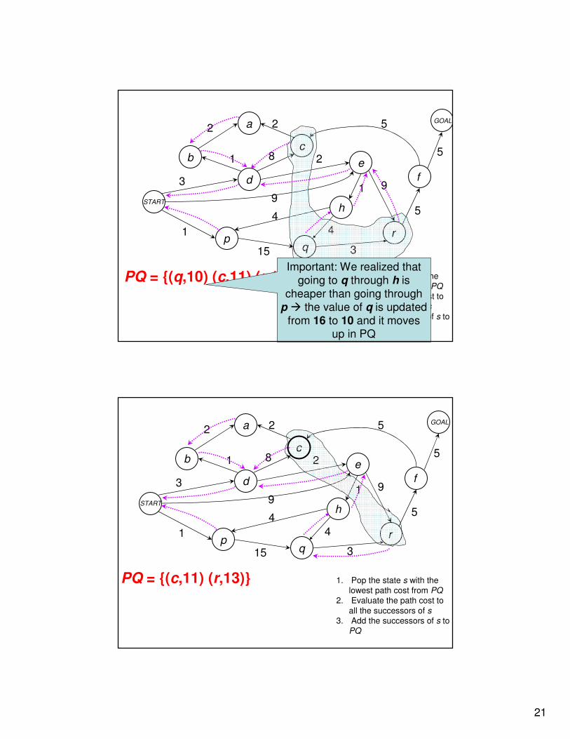
1. Pop the state s with the lowest path cost from PQ
2. Evaluate the path cost to all the successors of s
3. Add the successors of s to PQ
We add the successors of s that have
not yet been visited and we update the
cost of those currently in the queue
b
a
d
pq
h
e
c
f
r
START
GOAL
2
1
3
1
9
15
8
2
2
4
9
5
5
5
4
1
3
1. Pop the state s with the
lowest path cost from PQ
2. Evaluate the path cost to
all the successors of s
3. Add the successors of s to
PQ
PQ = {(START,0)}
17
b
a
d
pq
h
e
c
f
r
START
GOAL
2
1
3
1
9
15
8
2
2
4
9
5
5
5
4
1
3
1. Pop the state s with the
lowest path cost from PQ
2. Evaluate the path cost to
all the successors of s
3. Add the successors of s to
PQ
PQ = {(p,1) (d,3) (e,9)}
b
a
d
pq
h
e
c
f
r
START
GOAL
2
1
3
1
9
15
8
2
2
4
9
5
5
5
4
1
3
1. Pop the state s with the
lowest path cost from PQ
2. Evaluate the path cost to
all the successors of s
3. Add the successors of s to
PQ
PQ = {(d,3) (e,9) (q,16)}
18
b
a
d
pq
h
e
c
f
r
START
GOAL
2
1
3
1
9
15
8
2
2
4
9
5
5
5
4
1
3
1. Pop the state s with the
lowest path cost from PQ
2. Evaluate the path cost to
all the successors of s
3. Add the successors of s to
PQ
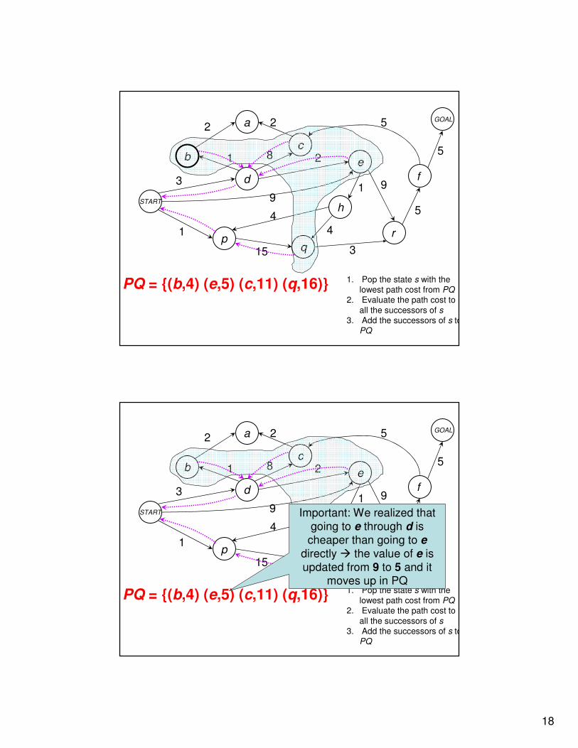
PQ = {(b,4) (e,5) (c,11) (q,16)}
b
a
d
pq
h
e
c
f
r
START
GOAL
2
1
3
1
9
15
8
2
2
4
9
5
5
5
4
1
3
1. Pop the state s with the
lowest path cost from PQ
2. Evaluate the path cost to
all the successors of s
3. Add the successors of s to
PQ
PQ = {(b,4) (e,5) (c,11) (q,16)}
Important: We realized that
going to e through d is
cheaper than going to e
directly � the value of e is
updated from 9 to 5 and it moves up in PQ
19
b
a
d
pq
h
e
c
f
r
START
GOAL
2
1
3
1
9
15
8
2
2
4
9
5
5
5
4
1
3
1. Pop the state s with the
lowest path cost from PQ
2. Evaluate the path cost to
all the successors of s
3. Add the successors of s to
PQ
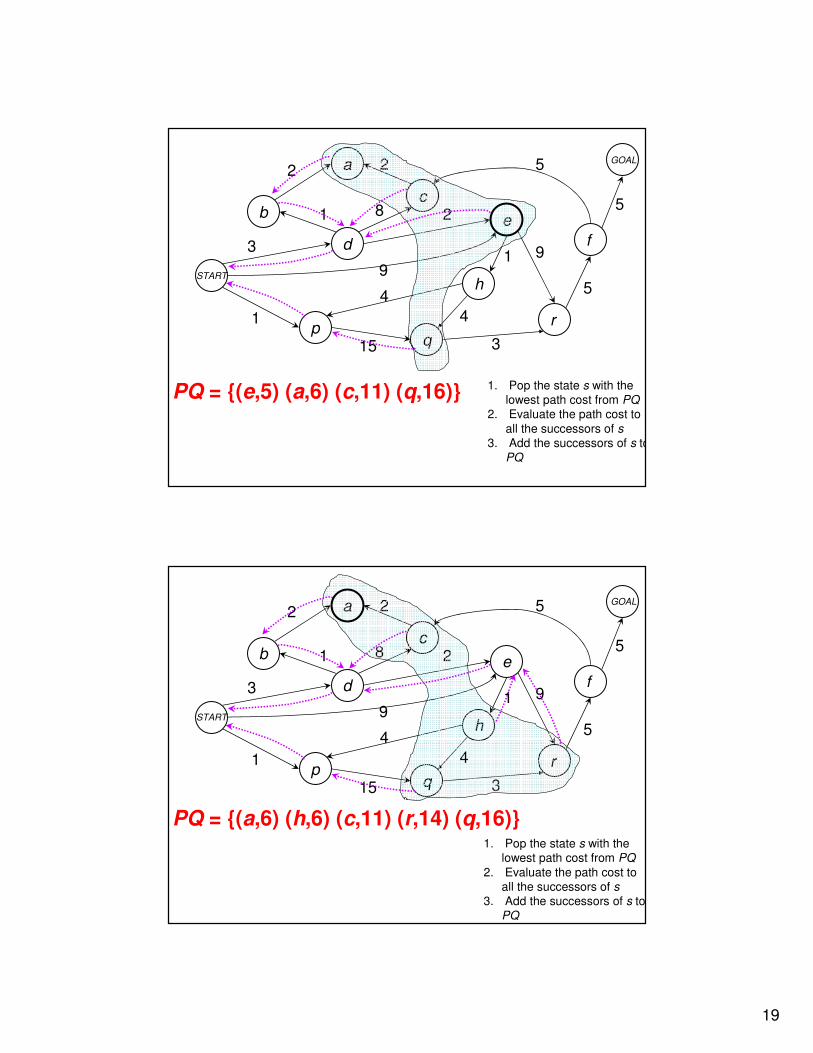
PQ = {(e,5) (a,6) (c,11) (q,16)}
b
a
d
pq
h
e
c
f
r
START
GOAL
2
1
3
1
9
15
8
2
2
4
9
5
5
5
4
1
3
1. Pop the state s with the
lowest path cost from PQ
2. Evaluate the path cost to
all the successors of s
3. Add the successors of s to
PQ
PQ = {(a,6) (h,6) (c,11) (r,14) (q,16)}
20
b
a
d
pq
h
e
c
f
r
START
GOAL
2
1
3
1
9
15
8
2
2
4
9
5
5
5
4
1
3
1. Pop the state s with the
lowest path cost from PQ
2. Evaluate the path cost to
all the successors of s
3. Add the successors of s to
PQ
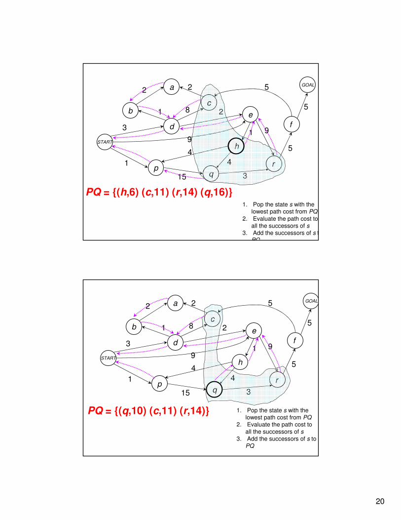
PQ = {(h,6) (c,11) (r,14) (q,16)}
b
a
d
pq
h
e
c
f
r
START
GOAL
2
1
3
1
9
15
8
2
2
4
9
5
5
5
4
1
3
1. Pop the state s with the
lowest path cost from PQ
2. Evaluate the path cost to
all the successors of s
3. Add the successors of s to
PQ
PQ = {(q,10) (c,11) (r,14)}
21
b
a
d
pq
h
e
c
f
r
START
GOAL
2
1
3
1
9
15
8
2
2
4
9
5
5
5
4
1
3
1. Pop the state s with the
lowest path cost from PQ
2. Evaluate the path cost to
all the successors of s
3. Add the successors of s to
PQ
PQ = {(q,10) (c,11) (r,14)}Important: We realized that
going to q through h is
cheaper than going through
p � the value of q is updated
from 16 to 10 and it moves up in PQ
b
a
d
pq
h
e
c
f
r
START
GOAL
2
1
3
1
9
15
8
2
2
4
9
5
5
5
4
1
3
PQ = {(c,11) (r,13)} 1. Pop the state s with the
lowest path cost from PQ
2. Evaluate the path cost to
all the successors of s
3. Add the successors of s to
PQ
22
b
a
d
pq
h
e
c
f
r
START
GOAL
2
1
3
1
9
15
8
2
2
4
9
5
5
5
4
1
3
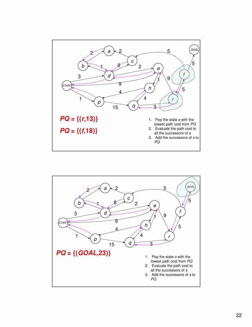
PQ = {(r,13)} 1. Pop the state s with the
lowest path cost from PQ
2. Evaluate the path cost to
all the successors of s
3. Add the successors of s to
PQ
PQ = {(f,18)}
b
a
d
pq
h
e
c
f
r
START
GOAL
2
1
3
1
9
15
8
2
2
4
9
5
5
5
4
1
3
1. Pop the state s with the
lowest path cost from PQ
2. Evaluate the path cost to
all the successors of s
3. Add the successors of s to
PQ
PQ = {(GOAL,23)}
23
b
a
d
pq
h
e
c
f
r
START
GOAL
2
1
3
1
9
15
8
2
2
4
9
5
5
5
4
1
3
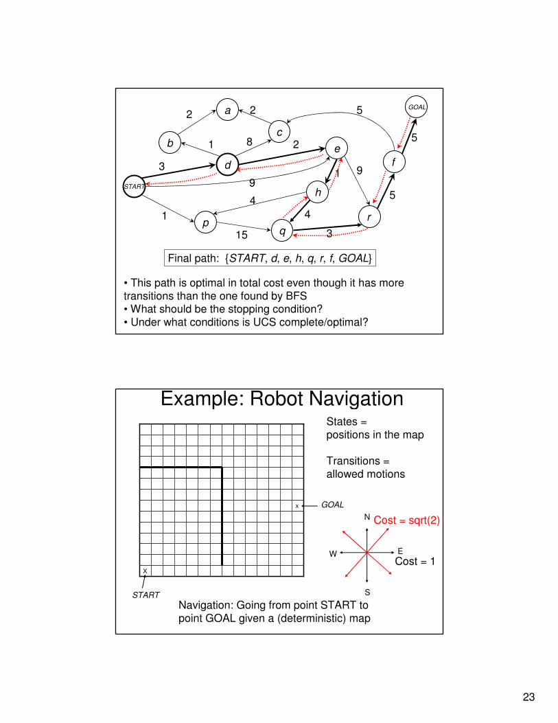
Final path: {START, d, e, h, q, r, f, GOAL}
• This path is optimal in total cost even though it has more
transitions than the one found by BFS• What should be the stopping condition?
• Under what conditions is UCS complete/optimal?
Example: Robot Navigation
X
x
START
GOAL
States =
positions in the map
Transitions =
allowed motions
N
E
S
W
Navigation: Going from point START to
point GOAL given a (deterministic) map
Cost = sqrt(2)
Cost = 1
24
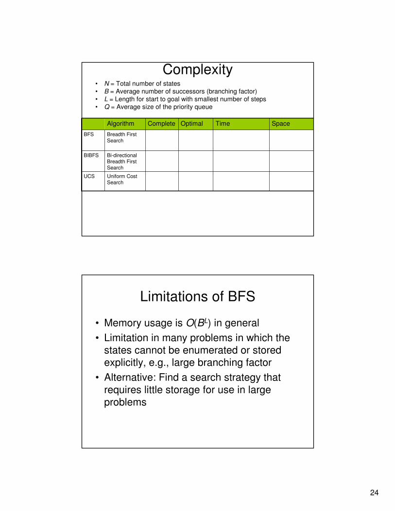
Complexity• N = Total number of states
• B = Average number of successors (branching factor)
• L = Length for start to goal with smallest number of steps
• Q = Average size of the priority queue
Bi-directional Breadth First Search
BIBFS
Uniform Cost Search
UCS
Breadth First
Search
BFS
SpaceTimeOptimalCompleteAlgorithm
Limitations of BFS
• Memory usage is O(BL) in general
• Limitation in many problems in which the
states cannot be enumerated or stored explicitly, e.g., large branching factor
• Alternative: Find a search strategy that
requires little storage for use in large
problems
25
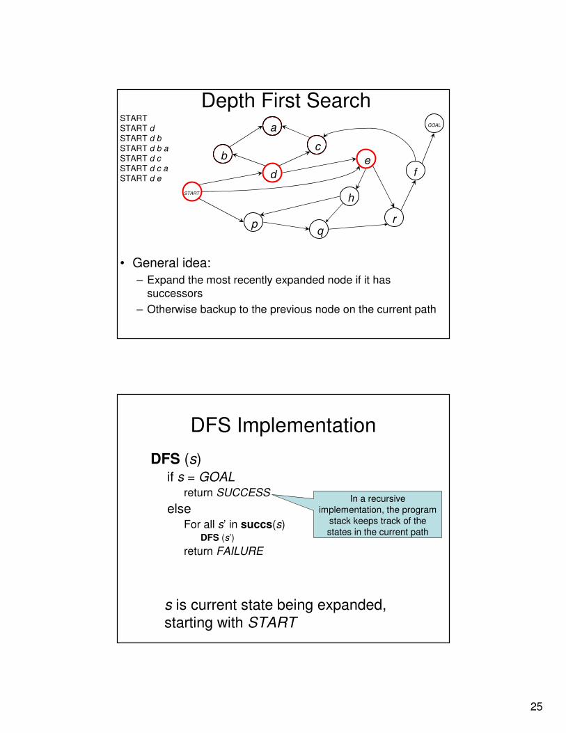
Depth First Search
• General idea:
– Expand the most recently expanded node if it has
successors
– Otherwise backup to the previous node on the current path
START
START d
START d b
START d b a
START d c
START d c a
START d e
START d e r
START d e r f
START d e r f c
START d e r f c a
START d e r f GOAL
b
a
d
pq
h
e
c
f
r
GOAL
START
DFS Implementation
DFS (s)if s = GOAL
return SUCCESS
elseFor all s’ in succs(s)
DFS (s’)
return FAILURE
In a recursive
implementation, the program
stack keeps track of the
states in the current path
s is current state being expanded,
starting with START
26
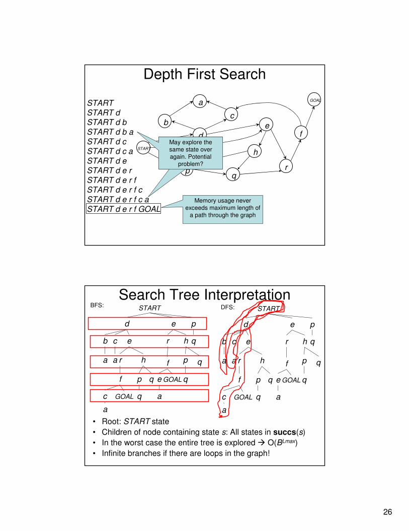
Depth First Search
START
START dSTART d b
START d b a
START d c
START d c a
START d eSTART d e r
START d e r f
START d e r f c
START d e r f c a
START d e r f GOALMemory usage never
exceeds maximum length of
a path through the graph
b
a
d
pq
h
e
c
f
r
START
GOAL
4
May explore the
same state over
again. Potential
problem?
Search Tree Interpretation
• Root: START state
• Children of node containing state s: All states in succs(s)
• In the worst case the entire tree is explored � O(BLmax)
• Infinite branches if there are loops in the graph!
START
d e p
r hb c e q
a a r h
f
c GOAL
a
p q
q
f
GOALe
a
p q
q
BFS:START
d e p
r hb c e q
a a r h
f
c GOAL
a
p q
q
f
GOALe
a
p q
q
DFS:
27
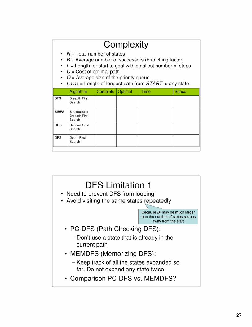
Complexity• N = Total number of states
• B = Average number of successors (branching factor)
• L = Length for start to goal with smallest number of steps• C = Cost of optimal path
• Q = Average size of the priority queue
• Lmax = Length of longest path from START to any state
Bi-directional Breadth First Search
BIBFS
Depth First Search
DFS
Uniform Cost Search
UCS
Breadth First
Search
BFS
SpaceTimeOptimalCompleteAlgorithm
DFS Limitation 1• Need to prevent DFS from looping• Avoid visiting the same states repeatedly
• PC-DFS (Path Checking DFS):
– Don’t use a state that is already in the current path
• MEMDFS (Memorizing DFS):
– Keep track of all the states expanded so far. Do not expand any state twice
• Comparison PC-DFS vs. MEMDFS?
Because Bd may be much larger
than the number of states d steps
away from the start
28
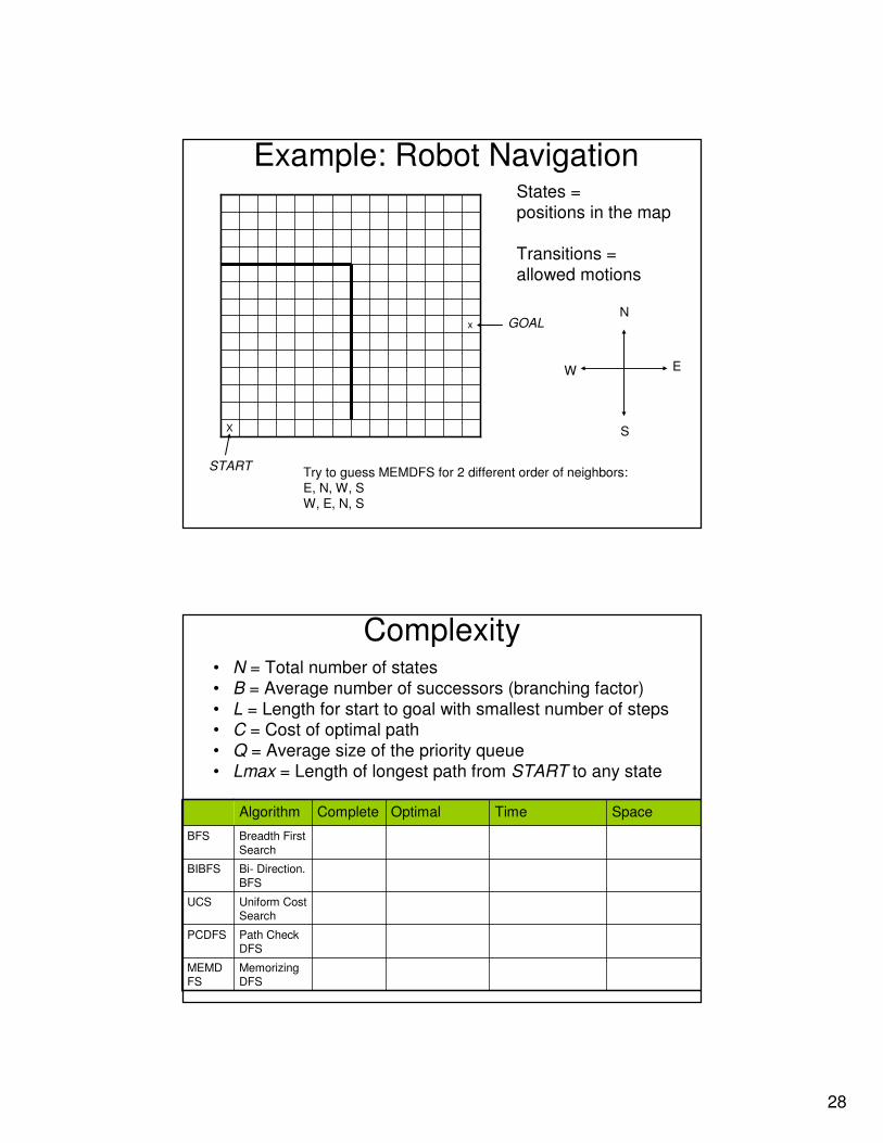
Example: Robot Navigation
X
x
START
GOAL
States =
positions in the map
Transitions =
allowed motions
N
E
S
W
Try to guess MEMDFS for 2 different order of neighbors:
E, N, W, S
W, E, N, S
Complexity
Bi- Direction.
BFS
BIBFS
Memorizing DFS
MEMDFS
Path Check DFS
PCDFS
Uniform Cost Search
UCS
Breadth First
Search
BFS
SpaceTimeOptimalCompleteAlgorithm
• N = Total number of states
• B = Average number of successors (branching factor)
• L = Length for start to goal with smallest number of steps• C = Cost of optimal path
• Q = Average size of the priority queue
• Lmax = Length of longest path from START to any state
29
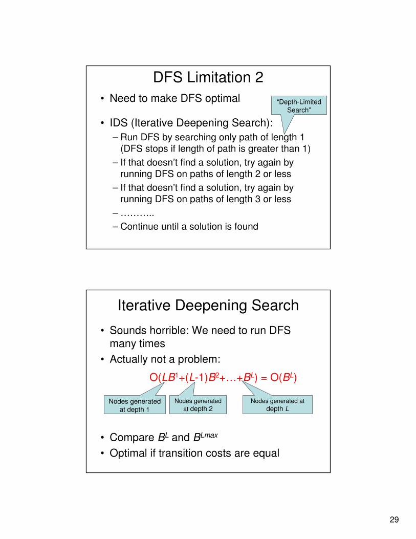
DFS Limitation 2
• Need to make DFS optimal
• IDS (Iterative Deepening Search):
– Run DFS by searching only path of length 1 (DFS stops if length of path is greater than 1)
– If that doesn’t find a solution, try again by running DFS on paths of length 2 or less
– If that doesn’t find a solution, try again by running DFS on paths of length 3 or less
– ………..
– Continue until a solution is found
“Depth-Limited
Search”
Iterative Deepening Search
• Sounds horrible: We need to run DFS
many times
• Actually not a problem:
• Compare BL and BLmax
• Optimal if transition costs are equal
O(LB1+(L-1)B2+…+BL) = O(BL)
Nodes generated
at depth 1
Nodes generated
at depth 2Nodes generated at
depth L
30
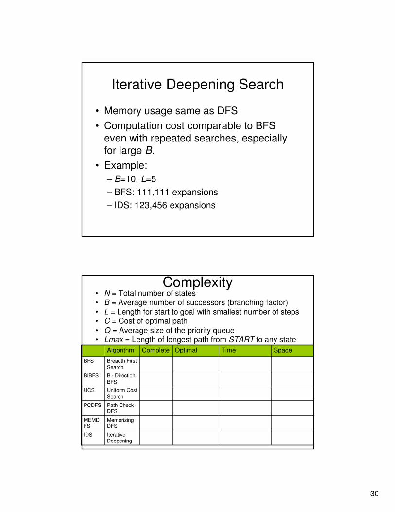
Iterative Deepening Search
• Memory usage same as DFS
• Computation cost comparable to BFS
even with repeated searches, especially for large B.
• Example:
– B=10, L=5
– BFS: 111,111 expansions
– IDS: 123,456 expansions
Complexity
Bi- Direction.
BFS
BIBFS
Iterative Deepening
IDS
Memorizing DFS
MEMDFS
Path Check DFS
PCDFS
Uniform Cost Search
UCS
Breadth First
Search
BFS
SpaceTimeOptimalCompleteAlgorithm
• N = Total number of states
• B = Average number of successors (branching factor)
• L = Length for start to goal with smallest number of steps• C = Cost of optimal path
• Q = Average size of the priority queue
• Lmax = Length of longest path from START to any state
31
Summary
• Basic search techniques: BFS, UCS, PCDFS, MEMDFS, ….
• Property of search algorithms: Completeness, optimality, time and space complexity
• Iterative deepening and bidirectional search ideas
• Trade-offs between the different techniques and when they might be used
Related Documents


