Search for gravitational waves from low mass binary coalescences in the first year of LIGO's S5 data

arX

iv:0

901.

0302

v4 [

gr-q

c] 6

May

200

9

Search for Gravitational Waves from Low Mass Binary Coalescences in the First Year of LIGO’s S5Data

B. P. Abbott,17 R. Abbott,17 R. Adhikari,17 P. Ajith,2 B. Allen,2, 60 G. Allen,35 R. S. Amin,21 S. B. Anderson,17

W. G. Anderson,60 M. A. Arain,47 M. Araya,17 H. Armandula,17 P. Armor,60 Y. Aso,17 S. Aston,46 P. Aufmuth,16 C. Aulbert,2

S. Babak,1 P. Baker,24 S. Ballmer,17 C. Barker,18 D. Barker,18 B. Barr,48 P. Barriga,59 L. Barsotti,20 M. A. Barton,17

I. Bartos,10 R. Bassiri,48 M. Bastarrika,48 B. Behnke,1 M. Benacquista,42 J. Betzwieser,17 P. T. Beyersdorf,31 I. A. Bilenko,25

G. Billingsley,17 R. Biswas,60 E. Black,17 J. K. Blackburn,17 L. Blackburn,20 D. Blair,59 B. Bland,18 T. P. Bodiya,20 L. Bogue,19

R. Bork,17 V. Boschi,17 S. Bose,61 P. R. Brady,60 V. B. Braginsky,25 J. E. Brau,53 D. O. Bridges,19 M. Brinkmann,2

A. F. Brooks,17 D. A. Brown,36 A. Brummit,30 G. Brunet,20 A. Bullington,35 A. Buonanno,49 O. Burmeister,2 R. L. Byer,35

L. Cadonati,50 J. B. Camp,26 J. Cannizzo,26 K. C. Cannon,17 J. Cao,20 C. D. Capano,36 L. Cardenas,17 S. Caride,51

G. Castaldi,56 S. Caudill,21 M. Cavaglia,39 C. Cepeda,17 T. Chalermsongsak,17 E. Chalkley,48 P. Charlton,9 S. Chatterji,17

S. Chelkowski,46 Y. Chen,1, 6 N. Christensen,8 C. T. Y. Chung,38 D. Clark,35 J. Clark,7 J. H. Clayton,60 T. Cokelaer,7

C. N. Colacino,12 R. Conte,55 D. Cook,18 T. R. C. Corbitt,20 N. Cornish,24 D. Coward,59 D. C. Coyne,17 J. D. E. Creighton,60

T. D. Creighton,42 A. M. Cruise,46 R. M. Culter,46 A. Cumming,48 L. Cunningham,48 S. L. Danilishin,25 K. Danzmann,2,16

B. Daudert,17 G. Davies,7 E. J. Daw,40 D. DeBra,35 J. Degallaix,2 V. Dergachev,51 S. Desai,37 R. DeSalvo,17

S. Dhurandhar,15 M. Dıaz,42 A. Dietz,7 F. Donovan,20 K. L. Dooley,47 E. E. Doomes,34 R. W. P. Drever,5 J. Dueck,2

I. Duke,20 J. -C. Dumas,59 J. G. Dwyer,10 C. Echols,17 M. Edgar,48 A. Effler,18 P. Ehrens,17 G. Ely,8 E. Espinoza,17

T. Etzel,17 M. Evans,20 T. Evans,19 S. Fairhurst,7 Y. Faltas,47 Y. Fan,59 D. Fazi,17 H. Fehrmann,2 L. S. Finn,37 K. Flasch,60

S. Foley,20 C. Forrest,54 N. Fotopoulos,60 A. Franzen,16 M. Frede,2 M. Frei,41 Z. Frei,12 A. Freise,46 R. Frey,53 T. Fricke,19

P. Fritschel,20 V. V. Frolov,19 M. Fyffe,19 V. Galdi,56 J. A. Garofoli,36 I. Gholami,1 J. A. Giaime,21, 19 S. Giampanis,2

K. D. Giardina,19 K. Goda,20 E. Goetz,51 L. M. Goggin,60 G. Gonzalez,21 M. L. Gorodetsky,25 S. Goßler,2 R. Gouaty,21

A. Grant,48 S. Gras,59 C. Gray,18 M. Gray,4 R. J. S. Greenhalgh,30 A. M. Gretarsson,11 F. Grimaldi,20 R. Grosso,42

H. Grote,2 S. Grunewald,1 M. Guenther,18 E. K. Gustafson,17 R. Gustafson,51 B. Hage,16 J. M. Hallam,46 D. Hammer,60

G. D. Hammond,48 C. Hanna,17 J. Hanson,19 J. Harms,52 G. M. Harry,20 I. W. Harry,7 E. D. Harstad,53 K. Haughian,48

K. Hayama,42 J. Heefner,17 I. S. Heng,48 A. Heptonstall,17 M. Hewitson,2 S. Hild,46 E. Hirose,36 D. Hoak,19 K. A. Hodge,17

K. Holt,19 D. J. Hosken,45 J. Hough,48 D. Hoyland,59 B. Hughey,20 S. H. Huttner,48 D. R. Ingram,18 T. Isogai,8 M. Ito,53

A. Ivanov,17 B. Johnson,18 W. W. Johnson,21 D. I. Jones,57 G. Jones,7 R. Jones,48 L. Ju,59 P. Kalmus,17 V. Kalogera,28

S. Kandhasamy,52 J. Kanner,49 D. Kasprzyk,46 E. Katsavounidis,20 K. Kawabe,18 S. Kawamura,27 F. Kawazoe,2 W. Kells,17

D. G. Keppel,17 A. Khalaidovski,2 F. Y. Khalili,25 R. Khan,10 E. Khazanov,14 P. King,17 J. S. Kissel,21 S. Klimenko,47

K. Kokeyama,27 V. Kondrashov,17 R. Kopparapu,37 S. Koranda,60 D. Kozak,17 B. Krishnan,1 R. Kumar,48 P. Kwee,16

V. Laljani,5 P. K. Lam,4 M. Landry,18 B. Lantz,35 A. Lazzarini,17 H. Lei,42 M. Lei,17 N. Leindecker,35 I. Leonor,53 C. Li,6

H. Lin,47 P. E. Lindquist,17 T. B. Littenberg,24 N. A. Lockerbie,58 D. Lodhia,46 M. Longo,56 M. Lormand,19 P. Lu,35

M. Lubinski,18 A. Lucianetti,47 H. Luck,2, 16 A. Lundgren,36 B. Machenschalk,1 M. MacInnis,20 M. Mageswaran,17

K. Mailand,17 I. Mandel,28 V. Mandic,52 S. Marka,10 Z. Marka,10 A. Markosyan,35 J. Markowitz,20 E. Maros,17 I. W. Martin,48

R. M. Martin,47 J. N. Marx,17 K. Mason,20 F. Matichard,21 L. Matone,10 R. A. Matzner,41 N. Mavalvala,20 R. McCarthy,18

D. E. McClelland,4 S. C. McGuire,34 M. McHugh,23 G. McIntyre,17 D. J. A. McKechan,7 K. McKenzie,4 M. Mehmet,2

A. Melatos,38 A. C. Melissinos,54 D. F. Menendez,37 G. Mendell,18 R. A. Mercer,60 S. Meshkov,17 C. Messenger,2

M. S. Meyer,19 J. Miller,48 J. Minelli,37 Y. Mino,6 V. P. Mitrofanov,25 G. Mitselmakher,47 R. Mittleman,20 O. Miyakawa,17

B. Moe,60 S. D. Mohanty,42 S. R. P. Mohapatra,50 G. Moreno,18 T. Morioka,27 K. Mors,2 K. Mossavi,2 C. MowLowry,4

G. Mueller,47 H. Muller-Ebhardt,2 D. Muhammad,19 S. Mukherjee,42 H. Mukhopadhyay,15 A. Mullavey,4 J. Munch,45

P. G. Murray,48 E. Myers,18 J. Myers,18 T. Nash,17 J. Nelson,48 G. Newton,48 A. Nishizawa,27 K. Numata,26 J. O’Dell,30

B. O’Reilly,19 R. O’Shaughnessy,37 E. Ochsner,49 G. H. Ogin,17 D. J. Ottaway,45 R. S. Ottens,47 H. Overmier,19 B. J. Owen,37

Y. Pan,49 C. Pankow,47 M. A. Papa,1, 60 V. Parameshwaraiah,18 P. Patel,17 M. Pedraza,17 S. Penn,13 A. Perraca,46 V. Pierro,56

I. M. Pinto,56 M. Pitkin,48 H. J. Pletsch,2 M. V. Plissi,48 F. Postiglione,55 M. Principe,56 R. Prix,2 L. Prokhorov,25 O. Punken,2

V. Quetschke,47 F. J. Raab,18 D. S. Rabeling,4 H. Radkins,18 P. Raffai,12 Z. Raics,10 N. Rainer,2 M. Rakhmanov,42

V. Raymond,28 C. M. Reed,18 T. Reed,22 H. Rehbein,2 S. Reid,48 D. H. Reitze,47 R. Riesen,19 K. Riles,51 B. Rivera,18

P. Roberts,3 N. A. Robertson,17,48 C. Robinson,7 E. L. Robinson,1 S. Roddy,19 C. Rover,2 J. Rollins,10 J. D. Romano,42

J. H. Romie,19 S. Rowan,48 A. Rudiger,2 P. Russell,17 K. Ryan,18 S. Sakata,27 L. Sancho de la Jordana,44 V. Sandberg,18

V. Sannibale,17 L. Santamarıa,1 S. Saraf,32 P. Sarin,20 B. S. Sathyaprakash,7 S. Sato,27 M. Satterthwaite,4 P. R. Saulson,36

R. Savage,18 P. Savov,6 M. Scanlan,22 R. Schilling,2 R. Schnabel,2 R. Schofield,53 B. Schulz,2 B. F. Schutz,1, 7 P. Schwinberg,18

J. Scott,48 S. M. Scott,4 A. C. Searle,17 B. Sears,17 F. Seifert,2 D. Sellers,19 A. S. Sengupta,17 A. Sergeev,14 B. Shapiro,20

2

P. Shawhan,49 D. H. Shoemaker,20 A. Sibley,19 X. Siemens,60 D. Sigg,18 S. Sinha,35 A. M. Sintes,44 B. J. J. Slagmolen,4

J. Slutsky,21 J. R. Smith,36 M. R. Smith,17 N. D. Smith,20 K. Somiya,6 B. Sorazu,48 A. Stein,20 L. C. Stein,20 S. Steplewski,61

A. Stochino,17 R. Stone,42 K. A. Strain,48 S. Strigin,25 A. Stroeer,26 A. L. Stuver,19 T. Z. Summerscales,3 K. -X. Sun,35

M. Sung,21 P. J. Sutton,7 G. P. Szokoly,12 D. Talukder,61 L. Tang,42 D. B. Tanner,47 S. P. Tarabrin,25 J. R. Taylor,2

R. Taylor,17 J. Thacker,19 K. A. Thorne,19 K. S. Thorne,6 A. Thuring,16 K. V. Tokmakov,48 C. Torres,19 C. Torrie,17

G. Traylor,19 M. Trias,44 D. Ugolini,43 J. Ulmen,35 K. Urbanek,35 H. Vahlbruch,16 M. Vallisneri,6 C. Van Den Broeck,7

M. V. van der Sluys,28 A. A. van Veggel,48 S. Vass,17 R. Vaulin,60 A. Vecchio,46 J. Veitch,46 P. Veitch,45 C. Veltkamp,2

A. Villar,17 C. Vorvick,18 S. P. Vyachanin,25 S. J. Waldman,20 L. Wallace,17 R. L. Ward,17 A. Weidner,2 M. Weinert,2

A. J. Weinstein,17 R. Weiss,20 L. Wen,6, 59 S. Wen,21 K. Wette,4 J. T. Whelan,1, 29 S. E. Whitcomb,17 B. F. Whiting,47

C. Wilkinson,18 P. A. Willems,17 H. R. Williams,37 L. Williams,47 B. Willke,2, 16 I. Wilmut,30 L. Winkelmann,2 W. Winkler,2

C. C. Wipf,20 A. G. Wiseman,60 G. Woan,48 R. Wooley,19 J. Worden,18 W. Wu,47 I. Yakushin,19 H. Yamamoto,17 Z. Yan,59

S. Yoshida,33 M. Zanolin,11 J. Zhang,51 L. Zhang,17 C. Zhao,59 N. Zotov,22 M. E. Zucker,20 H. zur Muhlen,16 and J. Zweizig17

(The LIGO Scientific Collaboration, http://www.ligo.org)1Albert-Einstein-Institut, Max-Planck-Institut fur Gravitationsphysik, D-14476 Golm, Germany

2Albert-Einstein-Institut, Max-Planck-Institut fur Gravitationsphysik, D-30167 Hannover, Germany3Andrews University, Berrien Springs, MI 49104 USA

4Australian National University, Canberra, 0200, Australia5California Institute of Technology, Pasadena, CA 91125, USA

6Caltech-CaRT, Pasadena, CA 91125, USA7Cardiff University, Cardiff, CF24 3AA, United Kingdom

8Carleton College, Northfield, MN 55057, USA9Charles Sturt University, Wagga Wagga, NSW 2678, Australia

10Columbia University, New York, NY 10027, USA11Embry-Riddle Aeronautical University, Prescott, AZ 86301USA

12Eotvos University, ELTE 1053 Budapest, Hungary13Hobart and William Smith Colleges, Geneva, NY 14456, USA

14Institute of Applied Physics, Nizhny Novgorod, 603950, Russia15Inter-University Centre for Astronomy and Astrophysics, Pune - 411007, India

16Leibniz Universitat Hannover, D-30167 Hannover, Germany17LIGO - California Institute of Technology, Pasadena, CA 91125, USA

18LIGO - Hanford Observatory, Richland, WA 99352, USA19LIGO - Livingston Observatory, Livingston, LA 70754, USA

20LIGO - Massachusetts Institute of Technology, Cambridge, MA 02139, USA21Louisiana State University, Baton Rouge, LA 70803, USA

22Louisiana Tech University, Ruston, LA 71272, USA23Loyola University, New Orleans, LA 70118, USA

24Montana State University, Bozeman, MT 59717, USA25Moscow State University, Moscow, 119992, Russia

26NASA/Goddard Space Flight Center, Greenbelt, MD 20771, USA27National Astronomical Observatory of Japan, Tokyo 181-8588, Japan

28Northwestern University, Evanston, IL 60208, USA29Rochester Institute of Technology, Rochester, NY 14623, USA

30Rutherford Appleton Laboratory, HSIC, Chilton, Didcot, Oxon OX11 0QX United Kingdom31San Jose State University, San Jose, CA 95192, USA

32Sonoma State University, Rohnert Park, CA 94928, USA33Southeastern Louisiana University, Hammond, LA 70402, USA

34Southern University and A&M College, Baton Rouge, LA 70813,USA35Stanford University, Stanford, CA 94305, USA36Syracuse University, Syracuse, NY 13244, USA

37The Pennsylvania State University, University Park, PA 16802, USA38The University of Melbourne, Parkville VIC 3010, Australia39The University of Mississippi, University, MS 38677, USA

40The University of Sheffield, Sheffield S10 2TN, United Kingdom41The University of Texas at Austin, Austin, TX 78712, USA

42The University of Texas at Brownsville and Texas Southmost College, Brownsville, TX 78520, USA43Trinity University, San Antonio, TX 78212, USA

44Universitat de les Illes Balears, E-07122 Palma de Mallorca, Spain45University of Adelaide, Adelaide, SA 5005, Australia

46University of Birmingham, Birmingham, B15 2TT, United Kingdom47University of Florida, Gainesville, FL 32611, USA

48University of Glasgow, Glasgow, G12 8QQ, United Kingdom

3

49University of Maryland, College Park, MD 20742 USA50University of Massachusetts - Amherst, Amherst, MA 01003, USA

51University of Michigan, Ann Arbor, MI 48109, USA52University of Minnesota, Minneapolis, MN 55455, USA

53University of Oregon, Eugene, OR 97403, USA54University of Rochester, Rochester, NY 14627, USA

55University of Salerno, 84084 Fisciano (Salerno), Italy56University of Sannio at Benevento, I-82100 Benevento, Italy

57University of Southampton, Southampton, SO17 1BJ, United Kingdom58University of Strathclyde, Glasgow, G1 1XQ, United Kingdom59University of Western Australia, Crawley, WA 6009, Australia

60University of Wisconsin-Milwaukee, Milwaukee, WI 53201, USA61Washington State University, Pullman, WA 99164, USA

We have searched for gravitational waves from coalescing low mass compact binary systems with a totalmass between2 and35 M⊙ and a minimum component mass of1 M⊙ using data from the first year of thefifth science run (S5) of the three LIGO detectors, operatingat design sensitivity. Depending on mass, we aresensitive to coalescences as far as 150 Mpc from the Earth. Nogravitational wave signals were observed abovethe expected background. Assuming a compact binary objectspopulation with a Gaussian mass distributionrepresenting binary neutron star systems, black hole-neutron star binary systems, and binary black hole systems,we calculate the 90%-confidence upper limit on the rate of coalescences to be3.9 × 10−2 yr−1

L−1

10, 1.1 ×

10−2 yr−1L

−1

10, and2.5 × 10−3 yr−1

L−1

10respectively, whereL10 is 1010 times the blue solar luminosity. We

also set improved upper limits on the rate of compact binary coalescences per unit blue-light luminosity, as afunction of mass.

PACS numbers: 95.85.Sz, 04.80.Nn, 07.05.Kf, 97.60.Jd, 97.60.Lf, 97.80.-d

I. INTRODUCTION

Among the most promising candidates for the first detec-tion of gravitational waves (GW) are signals from compact bi-nary coalescences (CBC), which include binary neutron stars(BNS), binary black holes (BBH), and black hole-neutron starbinaries (BHNS). The inspiral waveforms generated by thesesystems can be reliably predicted using post-Newtonian (PN)perturbation theory, until the last fraction of a second prior tomerger. These waveforms can be used in matched filtering ofnoisy data from gravitational wave detectors to identify GWcandidate events.

Astrophysical estimates for CBC rates depend on a numberof assumptions and unknown model parameters, and are stilluncertain at present. In the simplest models, the coalescencerates should be proportional to the stellar birth rate in nearbyspiral galaxies, which can be estimated from their blue lumi-nosity [1]; we therefore express the coalescence rates per unitL10, whereL10 is 1010 times the blue solar luminosity (theMilky Way contains∼ 1.7L10 [2]). The most confident BNSrate predictions are based on extrapolations from observedbi-nary pulsars in our Galaxy; these yield realistic BNS rates of5 × 10−5 yr−1L−1

10 , although rates could plausibly be as highas5 × 10−4 yr−1L−1

10 [3, 4]. Predictions for BBH and BHNSrates are based on population synthesis models constrainedby these and other observations. Realistic rate estimates are2 × 10−6 yr−1L−1

10 for BHNS [5] and4 × 10−7 yr−1L−110 for

BBH [6]; both BHNS and BBH rates could plausibly be ashigh as6 × 10−5 yr−1L−1

10 [5, 6].The Laser Interferometer Gravitational-wave Observatory

(LIGO) detectors achieved design sensitivity in 2005, andcompleted a two-year-long science run (S5) in November2007. Results from searches for GW from CBC by the

LIGO Scientific Collaboration (LSC) using data from previ-ous science runs with ever-increasing sensitivity are reportedin Refs. [7, 8, 9, 10, 11].

This paper summarizes the search for GW signals fromCBC with component masses greater than or equal to 1 so-lar mass (M⊙) and total mass ranging from2 to 35M⊙, usingthe first year of data from LIGO’s S5 run, between Novem-ber 4th, 2005 and November 14th, 2006. During this time,the LIGO detectors were sensitive to signals from CBC withhorizon distances (Table II) of 30 Mpc for BNS (25 secondsin the LIGO detection band) and 150 Mpc for systems with atotal mass of∼ 28M⊙ (0.5 seconds in the LIGO band). Sub-sequent papers will report the results of similar searches usingthe data from the second year (during which time the Virgodetector was in observational mode), searches for higher-masssystems (between25 and100 M⊙), and specialized searchestargeting particular subsets of signals.

The component objects of true astrophysical compact bina-ries will in general have some angular momentum, for whichPN waveforms that incorporate non-zero values for the spinparameters are available [12, 13]. However, for most of theparameter space, the effect of spin on the waveforms is small,and the signals can be captured using non-spinning waveformtemplates (Appendix I) with only a small loss in the signal-to-noise ratio (SNR); this is the approach taken in the searchdescribed here. In some regions of parameter space, the effectof spin is larger, and dedicated searches [13, 14, 15, 16] maybe more effective. The LSC continues to develop more effec-tive methods for searching for signals with strong modulationsdue to spin.

The rest of this paper is organized as follows. Section IIsummarizes the search pipeline that was employed. SectionIII describes the output of the search: detection candidate

4

events which are examined and rejected using a detection con-fidence procedure. Section IV describes the evaluation of ourdetection efficiency using simulated GW signals injected intothe detectors’ data streams. Section V discusses the upperlimit calculation that was performed, and the resulting upperlimits on CBC rates neglecting spin of the coalescing objects.Section VI discusses how our sensitivity is affected when spinis included. Finally, Section VII presents the conclusions, fol-lowed by several appendices on certain technical aspects ofthe search.

II. THE DATA ANALYSIS PIPELINE

The pipeline used for this analysis has been described inprevious documents [17, 18, 19, 20], and was used to searchfor BNS in LIGO’s third and fourth science runs [11]. Themain aspects of the pipeline and new features used here aredetailed below.

The data analysis proceeds as follows. The gravita-tional wave strain data are recorded from each of the threeLIGO detectors: the H1 and H2 detectors at LIGO HanfordObservatory (LHO) and the L1 detector at LIGO LivingstonObservatory (LLO). These data are matched filtered throughbanks of templates that model the expected signal from a bi-nary coalescence of two compact massive objects with massesm1 andm2, resulting in triggers that pass a pre-set SNRthreshold. We search for coincident triggers in time and tem-plate masses, between two or three detectors. We subject thesecoincident triggers to several tests to suppress noise fluctua-tions (including theχ2 test described in [21]), and rank-orderthe remaining coincident triggers according to their inconsis-tency with the background.

We estimate the background from accidental coincidencesby looking at time-shifted coincident triggers, as detailed inSection II D. Coincident triggers that are not consistent withthe estimated background are followed up with many addi-tional consistency checks, designed to identify strong butrarenoise fluctuations. We estimate our sensitivity to GW signalsthrough injections of simulated waveforms into the LIGO datastream which are analyzed identically to the data.

A. Template Bank

The templates used for this search are waveforms from non-spinning compact binaries calculated in the frequency domainusing the stationary-phase approximation (SPA) [22, 23, 24].The waveforms are calculated to Newtonian order in ampli-tude and second PN order in phase, and extend until theSchwarzschild innermost stable circular orbit (ISCO). Thetemplates for this single search cover a larger binary mass re-gion than in previous searches [11], with a total mass (M ) of2M⊙ < M < 35M⊙ and a minimum component mass of1 M⊙. The templates are placed with a hexagonal spacing[25] such that we lose less than3% of the SNR due to usinga discrete template bank to cover the continuous parameterspace spanned by the two component masses.

B. Analyzed and Vetoed Times

The pipeline is applied to data from the first year of theLIGO S5 run for which more than one detector was in ob-servation mode. This comprises 0.419 yr of triple coincidentdata (H1H2L1), 0.232 yr of H1H2 coincident data, 0.037 yr ofH1L1 coincident data, and 0.047 yr of H2L1 coincident data.In determining our upper limits, we exclude approximately9.5% of the data that were used to tune the pipeline [18] (theplaygrounddata). We also exclude all the data when only theH1 and H2 detectors were in observation mode, because ofthe difficulty in determining the background from coincidentnoise triggers in these collocated detectors (Section II D). Wemake use of the (rather large amount of) additional informa-tion on the state of the detectors and the physical environmentto define data quality (DQ) criteria (Appendix A). We usethese DQ criteria to veto triggers in times when an individualdetector was in observation mode, but we have reason to be-lieve the data were contaminated by instrumental or environ-mental problems. We define four categories of vetoes fromthese DQ criteria, based on severity of the data quality issue,and how well we understand its origin, explained in AppendixA. We follow up detection candidates after successively ap-plying each veto category (Appendix B). We exclude fromthe upper limit calculation times flagged with DQ vetoes inthe first three categories, along with triggers recorded in thosetimes. This results in non-vetoed, non-playground observa-tion times of 0.336 yr for H1H2L1, 0.020 yr for H1L1, and0.041 yr for H2L1.

C. Coincidence Test and Clustering

Our analysis applies a more sophisticated coincidence testthan the one used in the past. Previously, in order for trig-gers from different interferometers to be consideredcoinci-dent triggers, they needed to pass a series of independent win-dows in time, chirp mass (Mc = η3/5M ), and symmetricmass ratio (η = m1m2/M

2). These windows were definedindependently of the parameters of the triggers (e.g.Mc, η).

We have replaced this coincidence test with the one [26]that is based on the metric used in constructing a templatebank [20, 27, 28, 29]. The metric contains terms necessary formeasuring distances and determining coincidence in massesand time as well as the correlations between the parametersexpected for real signal events in the 3-dimensional parame-ter space. This provides improved separation between signalsand background from accidental coincidence of noise triggers,compared to the above independent windows.

We have also changed the algorithm used to cluster single-detector triggers in our pipeline. Previously, the triggers wereclustered by retaining the trigger with the largest SNR fromall the templates over a fixed window of time. At present,we use a new method [30] to cluster triggers, analogous tothe coincidence algorithm, again retaining the trigger with thelargest SNR from a particular cluster.

5

D. Background Estimation

As in the previous searches, we estimate the backgrounddue to accidental coincidences of noise triggers by repeatingthe analysis with the triggers from different detectors shiftedin time relative to each other, forming 100 experimental trialswith no true signals. We refer to these astime-shifted coin-cident triggers, as opposed to thein-time coincident triggersobtained without the use of time-shifts.

This procedure is known to underestimate the rate of ac-cidental coincidences of noise triggers from the H1 andH2 detectors, since they are collocated and exhibit time-correlated noise excursions. We therefore exclude H1H2double-coincident data from the upper limit calculation. Weexamine only the very strongest H1H2 double-coincident de-tection candidates (including H1H2 coincidences that did notappear in L1), and subject them to very stringent scrutiny.There were no H1H2 candidates that survived these checks.(See Section III for details.)

E. Detection Statistic

In this search, we employ a new detection statistic which al-lows us to search over a large region of parameter space with-out being limited by a high background false alarm rate (FAR)from a smaller subregion. In Ref. [11], coincident triggerswere ranked by combined effective SNR (Appendix C). Here,instead, we use a statistic derived from the background FAR,as detailed in Appendix D. The time-shifted triggers providean estimate of the FAR for each in-time coincident trigger. Bycounting the number of time-shifted triggers with an effectiveSNR greater than or equal to the in-time coincident triggers’effective SNR, and dividing by the total amount of time wesearched for time-shifted triggers, we calculate the FAR foreach in-time coincident trigger. This procedure is done sepa-rately for different regions of parameter space with the resultthat the FAR as a function of effective SNR varies over theparameter space. In-time coincident triggers with the largestinverse false alarm rate (IFAR) are our best detection candi-dates.

III. DETECTION CANDIDATES

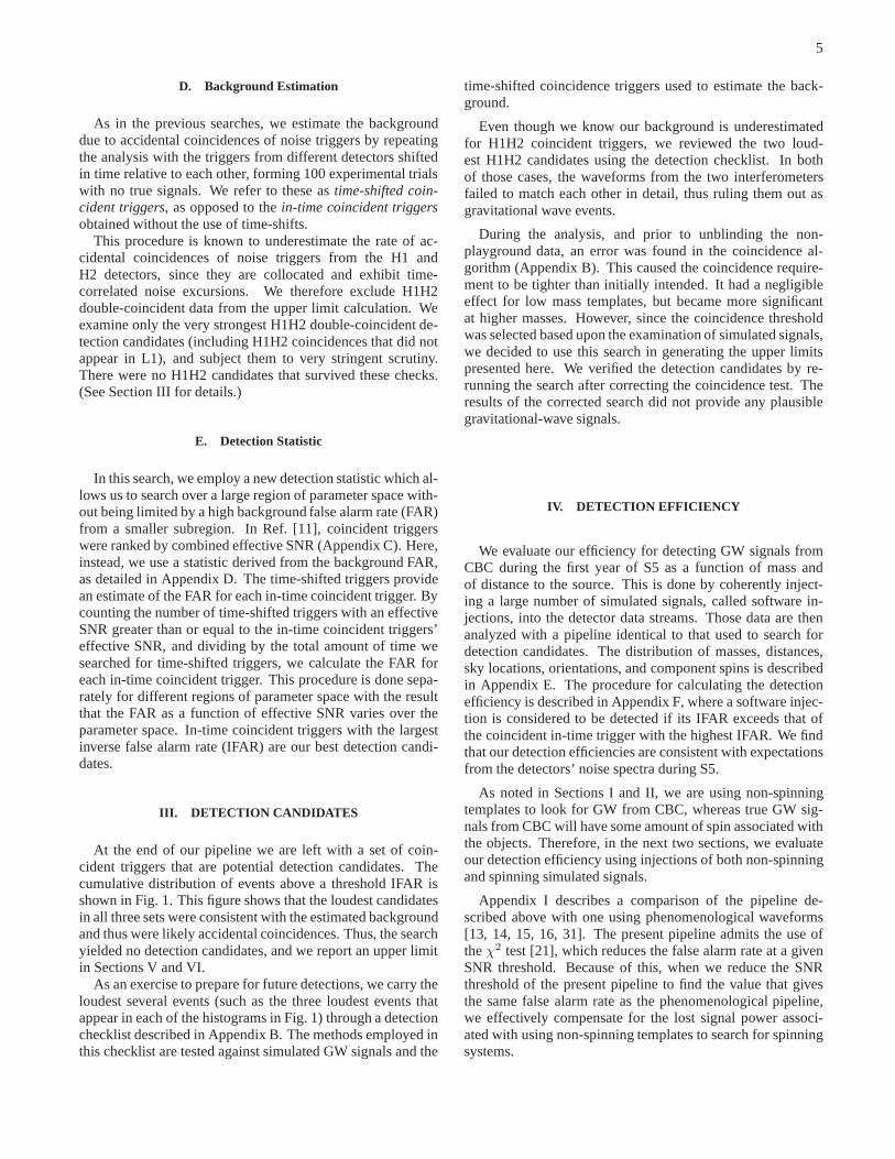
At the end of our pipeline we are left with a set of coin-cident triggers that are potential detection candidates. Thecumulative distribution of events above a threshold IFAR isshown in Fig. 1. This figure shows that the loudest candidatesin all three sets were consistent with the estimated backgroundand thus were likely accidental coincidences. Thus, the searchyielded no detection candidates, and we report an upper limitin Sections V and VI.

As an exercise to prepare for future detections, we carry theloudest several events (such as the three loudest events thatappear in each of the histograms in Fig. 1) through a detectionchecklist described in Appendix B. The methods employed inthis checklist are tested against simulated GW signals and the

time-shifted coincidence triggers used to estimate the back-ground.

Even though we know our background is underestimatedfor H1H2 coincident triggers, we reviewed the two loud-est H1H2 candidates using the detection checklist. In bothof those cases, the waveforms from the two interferometersfailed to match each other in detail, thus ruling them out asgravitational wave events.

During the analysis, and prior to unblinding the non-playground data, an error was found in the coincidence al-gorithm (Appendix B). This caused the coincidence require-ment to be tighter than initially intended. It had a negligibleeffect for low mass templates, but became more significantat higher masses. However, since the coincidence thresholdwas selected based upon the examination of simulated signals,we decided to use this search in generating the upper limitspresented here. We verified the detection candidates by re-running the search after correcting the coincidence test. Theresults of the corrected search did not provide any plausiblegravitational-wave signals.

IV. DETECTION EFFICIENCY

We evaluate our efficiency for detecting GW signals fromCBC during the first year of S5 as a function of mass andof distance to the source. This is done by coherently inject-ing a large number of simulated signals, called software in-jections, into the detector data streams. Those data are thenanalyzed with a pipeline identical to that used to search fordetection candidates. The distribution of masses, distances,sky locations, orientations, and component spins is describedin Appendix E. The procedure for calculating the detectionefficiency is described in Appendix F, where a software injec-tion is considered to be detected if its IFAR exceeds that ofthe coincident in-time trigger with the highest IFAR. We findthat our detection efficiencies are consistent with expectationsfrom the detectors’ noise spectra during S5.

As noted in Sections I and II, we are using non-spinningtemplates to look for GW from CBC, whereas true GW sig-nals from CBC will have some amount of spin associated withthe objects. Therefore, in the next two sections, we evaluateour detection efficiency using injections of both non-spinningand spinning simulated signals.

Appendix I describes a comparison of the pipeline de-scribed above with one using phenomenological waveforms[13, 14, 15, 16, 31]. The present pipeline admits the use oftheχ2 test [21], which reduces the false alarm rate at a givenSNR threshold. Because of this, when we reduce the SNRthreshold of the present pipeline to find the value that givesthe same false alarm rate as the phenomenological pipeline,we effectively compensate for the lost signal power associ-ated with using non-spinning templates to search for spinningsystems.

6

FIG. 1: The cumulative distribution of events above a threshold IFAR, for in-time coincident events, shown as blue triangles, from allcoincidence categories for the observation times H1H2L1, H1L1, and H2L1 respectively. The expected background (by definition) is shown asa dashed black line. The 100 experimental trials that make upour background are also plotted individually as the solid grey lines. The shadedregion denotes theN1/2 errors.

Coincidence Time H1H2L1 H1L1 H2L1Observation Time (yr) 0.336 0.020 0.041

Cumulative Luminosity(L10) ∼ 250 ∼ 230 ∼ 120Calibration Error 21% 3.9% 16%

Monte Carlo Error 5.4% 16% 13%Waveform Error 26% 11% 20%

Galaxy Distance Error 14% 13% 6.1%Galaxy Magnitude Error 17% 17% 16%

Λ [Eq. G2] 0.30 0.41 0.72

TABLE I: Detailed Results of the BNS Upper Limit CalculationSummary of the search for BNS systems. The observation time isreported after category 3 vetoes. The cumulative luminosity is theluminosity to which the search is sensitive above the loudest eventfor each coincidence time and is rounded to two significant figures.

The errors in this table are listed as logarithmic errors in theluminosity multiplier based on the cited sources of error.

V. UPPER LIMITS NEGLECTING SPIN

In the absence of detection, we set upper limits on the rateof CBC per unitL10, for several canonical binary systems andas a function of mass of the compact binary system.

For each mass range of interest, we calculate the rate upperlimit at 90% confidence level (CL) using the loudest event for-malism [32, 33], described in Appendix G. In the limit wherethe loudest event is consistent with the background, the upperlimit we obtain tends towardR90% ∼ 2.303/(TCL), whereTis the total observation time (in years) andCL is the cumula-tive luminosity (inL10) to which this search is sensitive aboveits loudest event. We derive a Bayesian posterior distributionfor the rate as described in Ref. [33].

In order to evaluate the cumulative luminosity we multiplythe detection efficiency, as a function of mass and distance,by the luminosity calculated from a galaxy population [1] forthe nearby universe. The cumulative luminosity is then thisproduct integrated over distance. The cumulative luminosityfor this search can be found in Table II.

System BNS BBH BHNSComponent Masses

(M⊙)1.35/1.35 5.0/5.0 5.0/1.35

Dhorizon (Mpc) ∼ 30 ∼ 80 ∼ 50Cumulative Luminosity

(L10)250 4900 990

Λ [Eq. G2] 0.30 0.59 0.45Marginalized UpperLimit

`

yr−1L

−1

10

´ 3.9 × 10−2 2.5 × 10−3 1.1 × 10−2

TABLE II: Overview of Results of the Upper Limit CalculationsSummary of the search for BNS, BBH, and BHNS systems. The

horizon distance is the distance at which an optimally oriented andoptimally located source with the appropriate mass would produce

an trigger with an SNR of8 in the 4 km detectors and averaged overthe search. The cumulative luminosity from H1H2L1 time is

rounded to two significant figures.

We apply the above upper limit calculation to three canon-ical binary masses as well as calculating the upper limit asa function of mass. Our three canonical binary masses areBNS (m1 = m2 = (1.35 ± 0.04) M⊙), BBH (m1 =m2 = (5 ± 1) M⊙), and BHNS(m1 = (5 ± 1) M⊙, m2 =(1.35± 0.04)M⊙). We use Gaussian distributions in compo-nent mass centered on these masses, with standard deviationsgiven above following the± symbols.

We combine the results of this search from the three differ-ent observation times in a Bayesian manner, described in Ap-pendix G, and the results from previous science runs [11, 13]are incorporated in a similar way.

Assuming that spin is not important in these systems, wecalculate upper limits on the rate of binary coalescences usingour injection families that neglect spin (Appendix E). Thereare a number of uncertainties which affect the upper limit, in-cluding systematic errors associated with detector calibration,simulation waveforms, Monte Carlo statistics, and galaxy cat-alog distances and magnitudes [19]. We marginalize overthese, as described in Appendix H and obtain upper limits on

7

the rate of binary coalescences of

R90%,BNS = 3.9 × 10−2 yr−1L10−1 (1)

R90%,BBH = 2.5 × 10−3 yr−1L10−1 (2)

R90%,BHNS = 1.1 × 10−2 yr−1L10−1 (3)

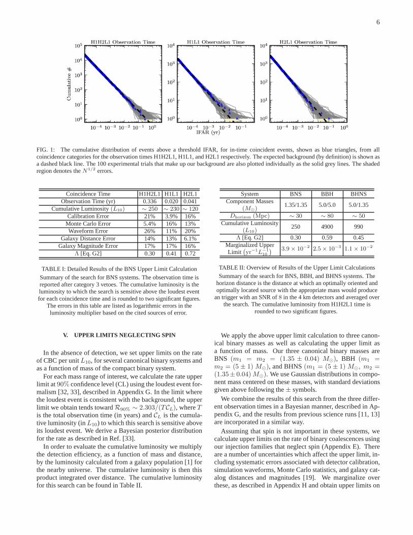
We also calculate upper limits for two additional cases: asa function of the total mass of the binary, with a uniform dis-tribution in the mass ratioq = m1/m2, and as a function ofthe mass of the black hole in a BHNS system, holding fixedthe mass of the neutron star atmNS = 1.35 M⊙ (Fig. 2).

VI. UPPER LIMITS INCLUDING SPIN

Above we have reported upper limits on the rate of merg-ers for different classes of objects using injection waveformsgenerated assuming non-spinning objects. We can also eval-uate the upper limits using injection waveforms that take intoaccount the effects of spinning bodies.

Since the maximum possible rotational angular momentumS for a black hole of massm isGm2/c, it is useful to describethe spin of a compact object in terms of the dimensionless spinparametera = (cS) /

(

Gm2)

. The distribution of black holespin magnitudes within the range0 ≤ a ≤ 1, as well as theirorientations relative to binary orbits, is not well constrainedby observations. To illustrate the possible effects of BH spinson our sensitivity to BBH and BHNS signals, we provide anexample calculation using a set of injections of signals sim-ulating systems whose component objects havea uniformlydistributed between 0 and 1 (Appendix E). On the other hand,assuming a canonical mass and uniform density, astrophysicalobservations of neutron stars show typical angular momentacorresponding toa ≪ 1 [34]. In addition, the spin effectsare found to be weak for the frequency range of interest forLIGO [35] so the BNS upper limits in Section V are valideven though we have ignored the effects of spin.

Using the above injections, we obtain marginalized upperlimits on the rate of binary coalescences of

R90%,BBH = 3.2 × 10−3 yr−1L10−1 (4)

R90%,BHNS = 1.4 × 10−2 yr−1L10−1 (5)

VII. CONCLUSIONS

We have searched for gravitational waves from coalesc-ing compact binary systems with total mass ranging from2to 35 M⊙, using data from the first year of the fifth sciencerun (S5) of the three Initial LIGO detectors. In doing so, wehave investigated the efficacy of searching for BBH signalswith 2PN SPA non-spinning templates and have found themto be effective even at the relatively high total mass of35M⊙.Additionally, we have found the non-spinning templates caneffectively capture spinning signals with some loss of effi-ciency. The result of the search was that no plausible grav-itational wave signals were observed above the background.

We set upper limits on the rate of these types of events thatare two orders of magnitude smaller than the previous obser-vational upper limits [11, 13], although they are still severalorders of magnitude above the range of astrophysical esti-mates [3, 4, 6, 36]. In the coming years, LIGO and otherground-based detectors will undergo significant upgrades.Weexpect to be able to significantly improve our sensitivity togravitational waves from compact binary coalescences and arepreparing for the first detections and studies.

Acknowledgments

The authors thank Marie Anne Bizouard for her time andhelp in reviewing the accuracy of this search. The authorsgratefully acknowledge the support of the United States Na-tional Science Foundation for the construction and operationof the LIGO Laboratory and the Science and TechnologyFacilities Council of the United Kingdom, the Max-Planck-Society, and the State of Niedersachsen/Germany for supportof the construction and operation of the GEO600 detector.The authors also gratefully acknowledge the support of theresearch by these agencies and by the Australian ResearchCouncil, the Council of Scientific and Industrial Research ofIndia, the Istituto Nazionale di Fisica Nucleare of Italy, theSpanish Ministerio de Educacion y Ciencia, the Conselleriad’Economia, Hisenda i Innovacio of the Govern de les IllesBalears, the Royal Society, the Scottish Funding Council, theScottish Universities Physics Alliance, The National Aero-nautics and Space Administration, the Carnegie Trust, theLeverhulme Trust, the David and Lucile Packard Foundation,the Research Corporation, and the Alfred P. Sloan Foundation.

APPENDIX A: DATA QUALITY CRITERIA

When analyzing data from LIGO’s detectors, it is impor-tant to know the status of the detectors at different times. Wedefine data quality flags as time intervals containing knownartifacts introduced into the data by instrumental or environ-mental effects. We examine the correlation between triggersfrom an individual detector and the DQ flags, and if we finda correlation by comparing the rate of triggers vetoed to therate we would expect from fraction of time vetoed (we callthedead-time), we use them as vetoes. Our understanding ofthe coupling between the effect that prompted the DQ flag andthe resulting triggers in the pipeline is measured in part bythefraction of the DQ flags that are used to veto triggers (calledtheuse percentage). We define four different categories of DQvetoes based on the above criteria.

We categorize DQ vetoes ascategory 1 vetoeswhen weknow of a severe problem with the data, bringing in to ques-tion whether the detector was actually in observation mode.An example case for H2 is when loud vibrations were causedin the detector environment in order to test the response ofthe seismic isolation systems. We categorize DQ vetoes ascategory 2 vetoeswhen there is a known coupling betweenthe GW channel and the auxiliary channel, the veto is corre-

8

FIG. 2: Upper limits on the binary coalescence rate per year and perL10 as a function of total mass of the binary system with a uniformdistribution in the mass ratio (left) and as a function of themass of a black hole in a BHNS system with a neutron star mass of1.35 M⊙ (right).The darker area shows the excluded region after accounting for marginalization over the estimated systematic errors. The lighter area showsthe additional region that would have been if the systematicerrors had been ignored.

lated with triggers from the individual detector, particularlyat high SNR, and when there is a use percentage of 50% orgreater. An example is when any of the data channels in thelength sensing and control servo reach their digital limit.Wecategorize DQ vetoes ascategory 3 vetoeswhen the couplingbetween the auxiliary channel and the GW channel is less es-tablished or when the use percentage is low, but we still finda strong correlation between the vetoes and the triggers. Anexample is when the winds at the detector site are over 30Mph. We categorize DQ vetoes ascategory 4 vetoeswhenthe coupling between the auxiliary channel and the GW chan-nel is not well established, when the use percentage is low,when the overall dead-time is several percent or greater, orthe correlation is weak. An example is when nearby aircraftpass overhead. We compare all of these vetoes with the timesof hardware injections, which measure the response of the de-tector to a simulated gravitational wave signal, in order tocon-firm that the DQ vetoes are not sensitive to real signals in thedata.

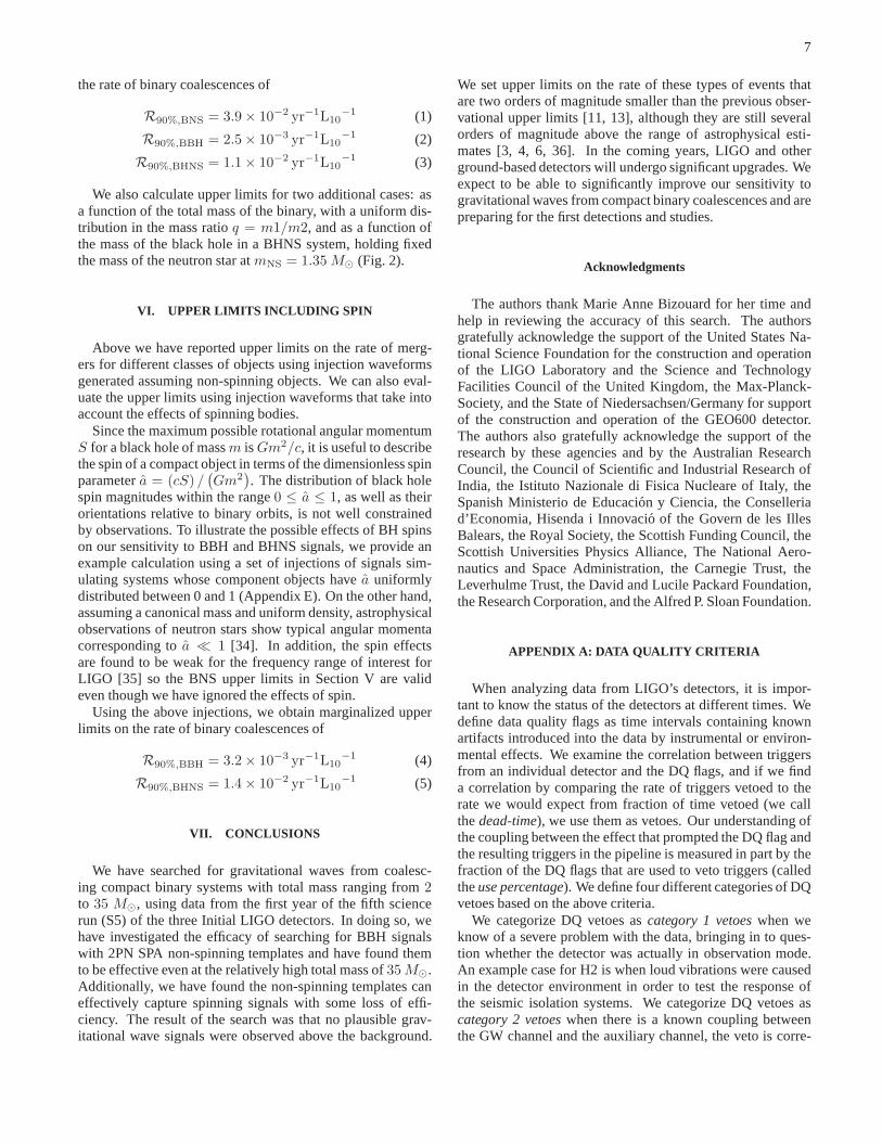
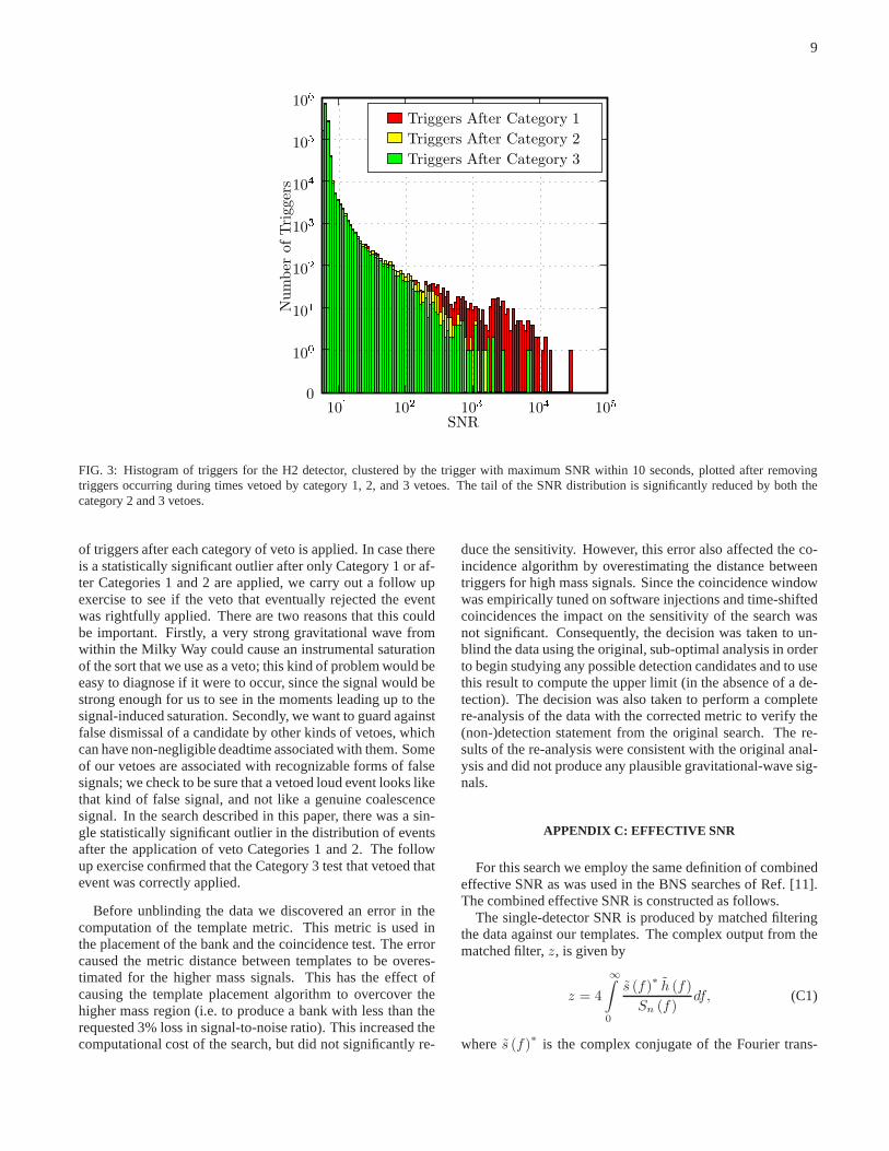
We do not analyze data vetoed by category 1 DQ vetoes.We remove triggers in times defined by category 2 and 3 DQvetoes from the upper limit calculation. These veto categoriessignificantly reduce the SNR of outlying triggers (Fig. 3). Asan exercise, we follow up the loudest coincident triggers aftereach category of veto is applied, including after Category 4vetoes (See Appendix B). This allows us to investigate theaction of the vetoes by a “case study” method.

APPENDIX B: FOLLOW-UP PROCEDURE FORCOINCIDENT TRIGGERS

As an exercise, we check our loudest coincident triggerswith a list of tests designed to see if a statistically significanttrigger is believable as a detection candidate. Ref. [37] de-scribes the tests that we perform on the trigger and the datasurrounding it. At present, our standard tests include the fol-lowing: We check the integrity of the data for corruption. Wealso check the status of the detectors and the presence of anydata quality flags in the surrounding data. We assess whetherthere could have been environmental or instrumental causesfound in auxiliary channels at the time of the trigger. Wecheck the appearance of the data at the time of the triggerin the form of SNR time series, theχ2 time series, and time-frequency spectrograms.

In addition, for any statistically significant candidate thatsurvives the tests listed above, we plan to do the following:Assess the coherence between the signals recorded by each in-dividual detector operating at the time of the event. Verifytherobustness of the trigger against small changes in the pipeline(i.e. changes in the adjacent Fourier transform boundariesorchanges in the calibration of the data). Check the robustnessacross pipelines by employing other search techniques to an-alyze the same data (i.e. CBC pipelines using different tem-plates or algorithms designed to search for unmodeled bursts).Finally, we will check for coincidence with external searchesfor gamma-ray bursts, optical transients, or neutrino events.(This last test is for information only, as a genuine GW eventmight or might not be accompanied by other signals.)

As mentioned in Appendix A, we examine the distribution

9

FIG. 3: Histogram of triggers for the H2 detector, clusteredby the trigger with maximum SNR within 10 seconds, plotted after removingtriggers occurring during times vetoed by category 1, 2, and3 vetoes. The tail of the SNR distribution is significantly reduced by both thecategory 2 and 3 vetoes.

of triggers after each category of veto is applied. In case thereis a statistically significant outlier after only Category 1or af-ter Categories 1 and 2 are applied, we carry out a follow upexercise to see if the veto that eventually rejected the eventwas rightfully applied. There are two reasons that this couldbe important. Firstly, a very strong gravitational wave fromwithin the Milky Way could cause an instrumental saturationof the sort that we use as a veto; this kind of problem would beeasy to diagnose if it were to occur, since the signal would bestrong enough for us to see in the moments leading up to thesignal-induced saturation. Secondly, we want to guard againstfalse dismissal of a candidate by other kinds of vetoes, whichcan have non-negligible deadtime associated with them. Someof our vetoes are associated with recognizable forms of falsesignals; we check to be sure that a vetoed loud event looks likethat kind of false signal, and not like a genuine coalescencesignal. In the search described in this paper, there was a sin-gle statistically significant outlier in the distribution of eventsafter the application of veto Categories 1 and 2. The followup exercise confirmed that the Category 3 test that vetoed thatevent was correctly applied.

Before unblinding the data we discovered an error in thecomputation of the template metric. This metric is used inthe placement of the bank and the coincidence test. The errorcaused the metric distance between templates to be overes-timated for the higher mass signals. This has the effect ofcausing the template placement algorithm to overcover thehigher mass region (i.e. to produce a bank with less than therequested 3% loss in signal-to-noise ratio). This increased thecomputational cost of the search, but did not significantly re-

duce the sensitivity. However, this error also affected theco-incidence algorithm by overestimating the distance betweentriggers for high mass signals. Since the coincidence windowwas empirically tuned on software injections and time-shiftedcoincidences the impact on the sensitivity of the search wasnot significant. Consequently, the decision was taken to un-blind the data using the original, sub-optimal analysis in orderto begin studying any possible detection candidates and to usethis result to compute the upper limit (in the absence of a de-tection). The decision was also taken to perform a completere-analysis of the data with the corrected metric to verify the(non-)detection statement from the original search. The re-sults of the re-analysis were consistent with the original anal-ysis and did not produce any plausible gravitational-wave sig-nals.

APPENDIX C: EFFECTIVE SNR

For this search we employ the same definition of combinedeffective SNR as was used in the BNS searches of Ref. [11].The combined effective SNR is constructed as follows.

The single-detector SNR is produced by matched filteringthe data against our templates. The complex output from thematched filter,z, is given by

z = 4

∞∫

0

s (f)∗h (f)

Sn (f)df, (C1)

wheres (f)∗ is the complex conjugate of the Fourier trans-

10

form of the data,h (f) is the Fourier transform of the tem-plate, andSn (f) is the power spectral density of the noise inthe detector. The template normalizationσ is given by

σ2 = 4

∞∫

0

h (f)∗h (f)

Sn (f)df. (C2)

Thez andσ are combined to give the single-detector SNR,ρ,using

ρ =|z|

σ. (C3)

Fromρ we define theeffective SNR, ρeff , as:

ρ2eff =

ρ2

√

(

χ2

2p−2

) (

1 + ρ2

250

)

, (C4)

wherep is the number of bins used in theχ2 test, which isa measure of how much the signal in the data looks like thetemplate we are searching for. In the effective SNR, we nor-malize theχ2 by 2p − 2 since it is the number of degrees offreedom of this test.

We then combine the effective SNRs for the single-detectortriggers that form a coincident trigger into thecombined effec-tive SNR, ρc, for that coincident trigger using:

ρ2c =

N∑

i=1

ρ2eff,i. (C5)

This definition of the combined effective SNR reduces theapparent significance of non-Gaussian instrumental artifactssince it weights the SNR by theχ2. This effectively cuts downon outliers from the expected SNR distribution due to Gaus-sian noise. In addition, we test this definition of the combinedeffective SNR using software injections and find it does notsignificantly affecting the apparent significance of real sig-nals.

APPENDIX D: FALSE ALARM RATE

Previously [11], we defined the loudest event for the en-tire parameter space based on the combined effective SNR,ρc

(Appendix C). Since we are searching over a larger portion ofparameter space than before, we find that the distribution ofcombined effective SNR for time-shifted coincident triggersvaries significantly over different portions of the parameterspace. In general, this seems to be affected by two factors.We see a suppression of the combined effective SNR distri-butions for time-shifted coincident triggers when lookingattriple coincident triggers compared to double coincident trig-gers. Also, we find smaller combined effective SNR distri-butions for time-shifted coincident triggers in the lower massregions than in the higher mass regions.

For this search, we have decided to divide the parameterspace into regions with similar combined effective SNR dis-tributions for time-shifted coincident triggers. We separate

the triggers into different categories, where the categories aredefined by the mean template masses of the triggers and trig-gers types (triple coincident triggers found in triple coinci-dent time, double coincident triggers found in triple coinci-dent time, and double coincident triggers found in double co-incident time). The categories for this search are given by thecombination of three template mass regions with divisions inchirp mass atMc = (3.48, 7.40)M⊙ with trigger types givenby H1H2L1, H1L1, and H2L1 triggers from H1H2L1 triplecoincident time, H1L1 triggers from H1L1 double coincidenttime, and H2L1 triggers from H2L1 double coincident time.

Within each category, the time-shifted coincident triggersprovide an estimate of the FAR for each in-time coincidenttrigger. When we recombine the categories from the same ob-servation time, the FAR of each trigger then needs to be nor-malized by the number of trials (i.e. the number of categories).This normalization bestows a FAR of1/T with the meaningthat during the observation time covered by this search (T ),there is expected to be a single coincidence trigger due tobackground with a combined effective SNR at that level.

The IFAR is used as our detection statistic and in-time co-incident triggers with the largest IFAR (across all categories)are our best detection candidates.

APPENDIX E: SIMULATED WAVEFORM INJECTIONS

In order to measure the efficiency of our pipeline to re-covering GW signals from CBC, we inject several differentPN families of waveforms into the data and check to see thefraction of signals that are recovered. The different wave-form families used for injections in this search include Gener-atePPN computed to Newtonian order in amplitude and 2PNorder in phase using formulae from Ref. [38], EOB com-puted to Newtonian order in amplitude and 3PN order in phaseusing formulae from Refs. [39, 40, 41, 42], PadeT1 com-puted to Newtonian order in amplitude and 3.5PN order inphase using formulae from Refs. [43, 44], and SpinTaylorcomputed to Newtonian order in amplitude and 3.5PN or-der in phase using formulae from Refs. [12] and based uponRefs. [35, 38, 43, 45, 46, 47, 48, 49]; using code fromRef. [50]. Each of these families except for SpinTaylor ig-nores the effects of spin on the orbital evolution.

Each of these waveform families are injected from a distri-bution uniform in sky location (right ascension, declination),uniform in the cosine of the inclination angle (ι), and uniformin polarization azimuthal angle (ψ). Each of these waveformfamilies are injected from a distribution uniform in the totalmass of the system. Each of these waveform families are alsoinjected uniform inlog10D whereD is the physical distancefrom the Earth to the source in Mpc. This non-physical dis-tance distribution was chosen in order to test our pipeline ona large range of signal amplitudes.

For the SpinTaylor waveform family, each of the compo-nent objects’ spin magnitudes are chosen from a distributionuniform in the unitless spin parametera ≡ (cS) /

(

Gm2)

,ranging from 0 to 1. The component objects’ spin orienta-tions relative to the initial orbital angular momentum are cho-

11

sen from a distribution uniform on a sphere.

APPENDIX F: CHIRP DISTANCE

In the adiabatic regime of binary inspiral, gravitationalwave radiation is modeled accurately. We make use of a va-riety of approximation techniques [38, 39, 40, 43, 44, 46, 48,51, 52] which rely, to some extent, on the slow motion of thecompact objects which make up the binary. We can representthe known waveform by:

h(t) =1Mpc

Deff

A(t) cos (φ(t) − φ0) (F1)

whereφ0 is some unknown phase. For this search the func-tionsA(t) andφ(t) are the Newtonian amplitude and 2PNphase evolution respectively, which depend on the masses andspins of the binary.

The template matched filtering will identify the masses andcoalescence time of the binary but not its physical distanceD.The signal amplitude received by the detector depends on thedetector response functionsF+ andF×, and the inclinationangle of the sourceι, which are unknown. We can only obtaintheeffective distanceDeff , which appears in Eq. (F1) definedas [22]:

Deff =D

√

F 2+(1 + cos2 ι)2/4 + F 2

×(cos ι)2. (F2)

The effective distance of a binary may be larger than its phys-ical distance.

Since the amplitude of a gravitational wave scales as thechirp massMc to the five sixths power, it is convenient tonormalize the effective distance by this, obtaining thechirpdistance, which is given by:

Dchirp = Deff

(

Mc,BNS

Mc

)5

6

. (F3)

whereMc,BNS is the chirp mass of a canonical BNS sys-tem. This distance is useful in evaluating the efficiency ofthe search as a function of distance since the efficiency willthen be approximately independent of mass.

APPENDIX G: POSTERIOR AND UPPER LIMITCALCULATION

Calculating an upper limit on a rate of coalescences in theloudest-event formalism requires knowledge of the cumula-tive luminosity to which the search is sensitive and a mea-sure of the likelihood that the loudest event was due to theobserved background. The cumulative luminosity quantifiesthe potental sources of observable CBC, as measured by blue-light luminosity of the galaxies, which can be detected by oursearch. It is calculated by multiplying the efficiency of signalrecovery for the search as a function of distance by the phys-ical luminosity as a function of distance and integrating their

product over distance. We combine these with the time ana-lyzed to calculate the posterior on the rate for the search. Thisis, assuming a uniform prior on the rate, given by [33]:

p (µ|CL, T,Λ) =CLT

1 + Λ(1 + µCLTΛ) e−µCLT (G1)

whereµ is the rate,CL is the cumulative luminosity,T is theanalyzed time, andΛ is a measure of the likelihood of detect-ing a single event with loudness parameterx versus such anevent occurring due to the experimental background, given by[33]:

Λ (x) =

(

−1

CL

dCL

dx

) (

1

P0

dP0

dx

)−1

(G2)

The posterior (G1) assumes a known value ofCL associatedwith the search. In reality,CL has associated with it system-atic uncertainties, which we model as unknown multiplicativefactors, each log-normally distributed about1 with errors de-scribed in Appendix H. The widths of those distributions aregiven in Table I. Marginalizing over all of those unknownfactors, and thus overCL, gives a marginalized posterior:

p (µ|T,Λ) =

∫

pd (CL) p (µ|CL, T,Λ)dCL (G3)

wherepd (CL) is the combined probability distribution func-tion for CL given all of those unknown factors.

The results of several experiments (e.g. different types ofS5observing time and previous runs such as S3 and S4) can becombined by taking the product of their likelihood functions;in the case of uniform priors, this is equivalent to taking theproduct of their posteriors, allowing us to define the rate upperlimit µ at a confidence levelα by solving:

α =

∫ µ

0

∏

i

pi (µ′)dµ′ (G4)

where thepi (µ′) are the marginalized posteriors from differ-ent experiments calculated using a uniform prior on the rate.

APPENDIX H: SYSTEMATIC ERROR CALCULATION

Systematic errors associated with CBC searches for GWsignals include errors associated with detector calibrations,simulation waveforms, Monte Carlo statistics, and galaxy cat-alog distances and magnitudes. Calculating these errors interms of the cumulative luminosity is described below [19].

We refer to statistical errors associated with the efficiencycalculation asMonte Carlo errors. Since we calculate the ef-ficiency as a function of distance, we calculate the error fora particular distance bin using the binomial formula, whichgives an error of zero when the efficiency is zero or one, orwhen there are no injections in that bin. This error is then mul-tiplied by the physical luminosity as a function of distanceandintegrated over distance to get the Monte Carlo error in unitsof luminosity.

12

Calibration errors in the detectors are errors on the ampli-tude of the noise floor. These errors affect the amplitude, andin turn the distance, at which we made injections to calculatethe efficiency of our search, since the injections we made as-suming a specific value of the noise floor. The one-sigma un-certainty in the amplitude (and thus the distance) associatedwith the calibration was8.1% for H1, 7.2% for H2, and6.0%for L1. We use these numbers to calculate the calibration er-ror given in Table I in units of luminosity by combining thelogarithmic errors in quadrature.

Waveform errorsare associated with how different the truesignals are from what we use to measure the efficiency of ourpipeline (i.e. the mismatch between the true signals and ourinjections). This error effectively reduces the distancesin ourefficiency calculation since we don’t recover all of the poweravailable in the signal due to the mismatch between the signaland our injections. We calculate the waveform error in unitsofluminosity assuming a waveform mismatch of10%[43, 53].

Galaxy errorsare errors associated with our galaxy catalog[1] used to construct the physical luminosity. Galaxy errorscome in two types:distance errorsandmagnitude errors. Tocalculate the error on the luminosity due to distance errors,the physical luminosity calculation is modified such that thegalaxies’ distances are increased by a factor1 + κj , whereκj is the uncertainty in thejth galaxy’s distance given in thegalaxy catalog. The galaxies’ luminosities are also increasedby a factor(1 + κj)

2 since the galaxies’ luminosity is onlyknown in terms of its magnitude and distance. To calculatethe error on the luminosity due to magnitude errors, the phys-ical luminosity calculation is changed such that the galaxies’luminosities are increased by an amount associated with themagnitude errors given in the galaxy catalog.

APPENDIX I: SPINNING SEARCH COMPARISON

The SPA template waveforms used in this search and de-scribed in this paper do not take spin into account. A phe-nomenological template family to search for spinning blackhole and neutron star binaries was developed in [12], referredto asBCVSpin, and has been used in a search of S3 data [13].Using both of these template banks to compute the efficiencyof recovering signals from spinning waveforms for the differ-ent search methods, we find that for a comparable number of

false alarms, SPA and BCVSpin have approximately the sameefficiencies, implying it is not necessary to perform a searchusing BCVSpin templates in order to target spinning signals.The comparison of searches for spinning binaries using differ-ent signal models and template banks is discussed further inRef. [31].

What is important for a search is how efficient banks arein picking up signals in the data. Given a large number ofinjections in the data, the efficiency is the ratio of the numberof found injections to the total number of injections made. Afair comparison requires that efficiencies be evaluatedfor thesame FAR. To estimate the background rate, we counted thenumber of coincident triggers in time-shifted data betweenH1and L1.

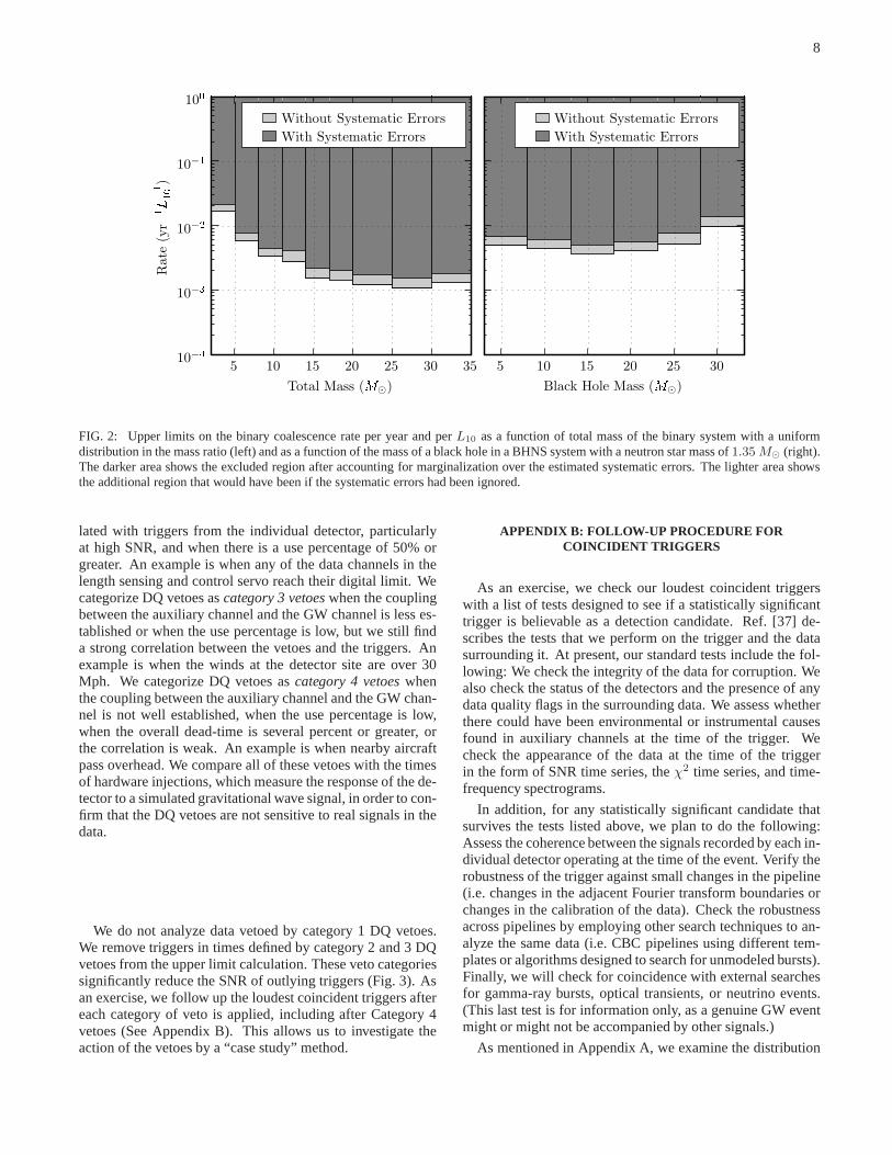
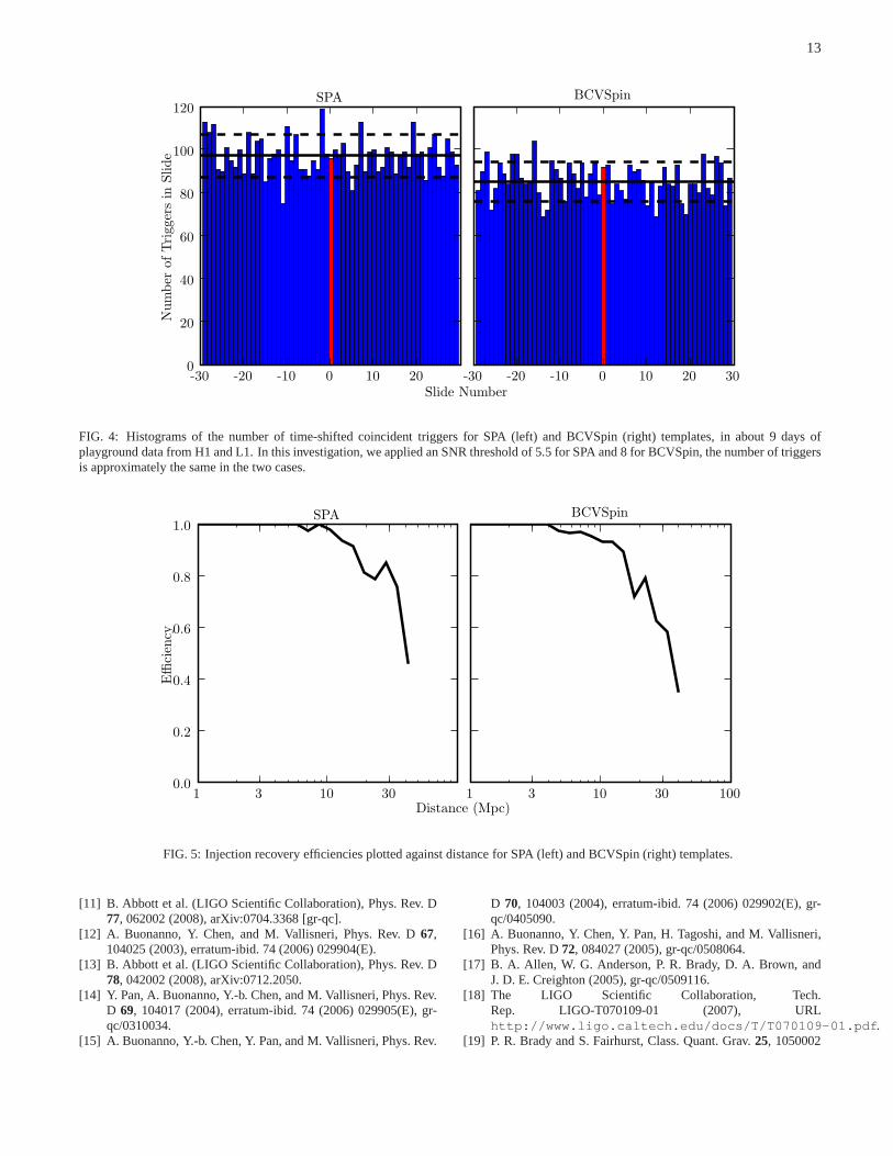
The SNR for BCVSpin involves six degrees of freedom,compared to only two for SPA. As a consequence, BCVSpinpicks up glitches more easily, and to have the same back-ground rate as for SPA, it needs a higher SNR threshold. (Thisproblem had already been pointed out and discussed in [12];here we are seeing it in real data.) It was found that SPA withan SNR threshold of 5.5 and BCVSpin with an SNR thresholdof 8 lead to comparable FARs (Fig. 4).

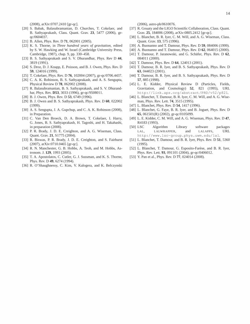
With these SNR thresholds, we are in a position to comparethe efficiencies of SPA and BCVSpin banks for a given FAR.For our purposes, an injection will be considered found if ithad an SNR above the chosen threshold with at least one tem-plate in the bank, within a certain time interval around the timewhen the injection was actually made. In the case of SPA, thewidth of this interval can be chosen to be 40 ms. BCVSpintemplates, being phenomenological, turn out to have a largertiming inaccuracy, and an interval of 100 ms was found to bemore appropriate. We made 1128 injections distributed loga-rithmically in distance between 1 Mpc and 50 Mpc, with com-ponent masses randomly chosen between1M⊙ and30M⊙

but restricting total mass to30M⊙, component spin magni-tudes0.7 < ai < 1, i = 1, 2, and arbitrary directions forthe initial spin vectors. For the SNR thresholds of 5.5 for SPAand 8 for BCVSpin, in H1 the efficiency of SPA came out to be0.93, versus 0.89 for BCVSpin; for L1 the numbers are sim-ilar. Fig. 5 shows the efficiencies binned in distance. Hence,for comparable FARs, SPA and BCVSpin have approximatelythe same efficiencies showing it is not necessary to performa search using BCVSpin templates in order to target spinningsignals.

[1] R. K. Kopparapu, C. Hanna, V. Kalogera, R. O’Shaughnessy,G. Gonzalez, P. R. Brady, and S. Fairhurst, Astrophys. J.675,1459 (2008).

[2] V. Kalogera, R. Narayan, D. N. Spergel, and J. H. Taylor, As-trophys. J.556, 340 (2001).

[3] V. Kalogera, C. Kim, D. R. Lorimer, M. Burgay, N. D’Amico,A. Possenti, R. N. Manchester, A. G. Lyne, B. C. Joshi, M. A.McLaughlin, et al., Astrophys. J.601, L179 (2004), erratum-ibid. 614 (2004) L137.

[4] V. Kalogera et al., Astrophys. J. Lett.614, L137 (2004).[5] R. O’Shaughnessy, C. Kim, V. Kalogera, and K. Belczynski,

Astrophys. J.672, 479 (2008).[6] R. O’Shaughnessy, C. Kim, T. Fragos, V. Kalogera, and K. Bel-

czynski, Astrophys. J.633, 1076 (2005).[7] B. Abbott et al. (LIGO Scientific Collaboration), Phys. Rev. D

69, 122001 (2004), gr-qc/0308069.[8] B. Abbott et al. (LIGO Scientific Collaboration), Phys. Rev. D

72, 082001 (2005), gr-qc/0505041.[9] B. Abbott et al. (LIGO Scientific Collaboration), Phys. Rev. D

72, 082002 (2005), gr-qc/0505042.[10] B. Abbott et al. (LIGO Scientific Collaboration), Phys.Rev. D

73, 062001 (2006), gr-qc/0509129.

13

FIG. 4: Histograms of the number of time-shifted coincidenttriggers for SPA (left) and BCVSpin (right) templates, in about 9 days ofplayground data from H1 and L1. In this investigation, we applied an SNR threshold of 5.5 for SPA and 8 for BCVSpin, the number of triggersis approximately the same in the two cases.

FIG. 5: Injection recovery efficiencies plotted against distance for SPA (left) and BCVSpin (right) templates.

[11] B. Abbott et al. (LIGO Scientific Collaboration), Phys.Rev. D77, 062002 (2008), arXiv:0704.3368 [gr-qc].

[12] A. Buonanno, Y. Chen, and M. Vallisneri, Phys. Rev. D67,104025 (2003), erratum-ibid. 74 (2006) 029904(E).

[13] B. Abbott et al. (LIGO Scientific Collaboration), Phys.Rev. D78, 042002 (2008), arXiv:0712.2050.

[14] Y. Pan, A. Buonanno, Y.-b. Chen, and M. Vallisneri, Phys. Rev.D 69, 104017 (2004), erratum-ibid. 74 (2006) 029905(E), gr-qc/0310034.

[15] A. Buonanno, Y.-b. Chen, Y. Pan, and M. Vallisneri, Phys. Rev.

D 70, 104003 (2004), erratum-ibid. 74 (2006) 029902(E), gr-qc/0405090.

[16] A. Buonanno, Y. Chen, Y. Pan, H. Tagoshi, and M. Vallisneri,Phys. Rev. D72, 084027 (2005), gr-qc/0508064.

[17] B. A. Allen, W. G. Anderson, P. R. Brady, D. A. Brown, andJ. D. E. Creighton (2005), gr-qc/0509116.

[18] The LIGO Scientific Collaboration, Tech.Rep. LIGO-T070109-01 (2007), URLhttp://www.ligo.caltech.edu/docs/T/T070109-01.pdf.

[19] P. R. Brady and S. Fairhurst, Class. Quant. Grav.25, 1050002

14

(2008), arXiv:0707.2410 [gr-qc].[20] S. Babak, Balasubramanian, D. Churches, T. Cokelaer, and

B. Sathyaprakash, Class. Quant. Grav.23, 5477 (2006), gr-qc/0604037.

[21] B. Allen, Phys. Rev. D71, 062001 (2005).[22] K. S. Thorne, inThree hundred years of gravitation, edited

by S. W. Hawking and W. Israel (Cambridge University Press,Cambridge, 1987), chap. 9, pp. 330–458.

[23] B. S. Sathyaprakash and S. V. Dhurandhar, Phys. Rev D44,3819 (1991).

[24] S. Droz, D. J. Knapp, E. Poisson, and B. J. Owen, Phys. Rev. D59, 124016 (1999).

[25] T. Cokelaer, Phys. Rev. D76, 102004 (2007), gr-qc/0706.4437.[26] C. A. K. Robinson, B. S. Sathyaprakash, and A. S. Sengupta,

Physical Review D78, 062002 (2008).[27] R. Balasubramanian, B. S. Sathyaprakash, and S. V. Dhurand-

har, Phys. Rev.D53, 3033 (1996), gr-qc/9508011.[28] B. J. Owen, Phys. Rev. D53, 6749 (1996).[29] B. J. Owen and B. S. Sathyaprakash, Phys. Rev. D60, 022002

(1999).[30] A. S. Sengupta, J. A. Gupchup, and C. A. K. Robinson (2008),

in Preparation.[31] C. Van Den Broeck, D. A. Brown, T. Cokelaer, I. Harry,

G. Jones, B. S. Sathyaprakash, H. Tagoshi, and H. Takahashi,in preparation (2008).

[32] P. R. Brady, J. D. E. Creighton, and A. G. Wiseman, Class.Quant. Grav.21, S1775 (2004).

[33] R. Biswas, P. R. Brady, J. D. E. Creighton, and S. Fairhurst(2007), arXiv:0710.0465 [gr-qc].

[34] R. N. Manchester, G. B. Hobbs, A. Teoh, and M. Hobbs, As-tronom. J.129, 1993 (2005).

[35] T. A. Apostolatos, C. Cutler, G. J. Sussman, and K. S. Thorne,Phys. Rev. D49, 6274 (1994).

[36] R. O’Shaughnessy, C. Kim, V. Kalogera, and K. Belczynski

(2006), astro-ph/0610076.[37] R. Gouaty and the LIGO Scientific Collaboration, Class.Quant.

Grav.25, 184006 (2008), arXiv:0805.2412 [gr-qc].[38] L. Blanchet, B. R. Iyer, C. M. Will, and A. G. Wiseman, Class.

Quant. Grav.13, 575 (1996).[39] A. Buonanno and T. Damour, Phys. Rev. D59, 084006 (1999).[40] A. Buonanno and T. Damour, Phys. Rev. D62, 064015 (2000).[41] T. Damour, P. Jaranowski, and G. Schafer, Phys. Rev. D62,

084011 (2000).[42] T. Damour, Phys. Rev. D64, 124013 (2001).[43] T. Damour, B. R. Iyer, and B. S. Sathyaprakash, Phys. Rev. D

63, 044023 (2001).[44] T. Damour, B. R. Iyer, and B. S. Sathyaprakash, Phys. Rev. D

57, 885 (1998).[45] L. E. Kidder, Physical Review D (Particles, Fields,

Gravitation, and Cosmology)52, 821 (1995), URLhttp://link.aps.org/abstract/PRD/v52/p821.

[46] L. Blanchet, T. Damour, B. R. Iyer, C. M. Will, and A. G. Wise-man, Phys. Rev. Lett.74, 3515 (1995).

[47] L. Blanchet, Phys. Rev. D54, 1417 (1996).[48] L. Blanchet, G. Faye, B. R. Iyer, and B. Joguet, Phys. Rev. D

65, 061501(R) (2002), gr-qc/0105099.[49] L. E. Kidder, C. M. Will, and A. G. Wiseman, Phys. Rev. D47,

R4183 (1993).[50] LSC Algorithm Library software packages

LAL , LALWRAPPER, and LALAPPS, URLhttp://www.lsc-group.phys.uwm.edu/lal.

[51] L. Blanchet, T. Damour, and B. R. Iyer, Phys. Rev. D51, 5360(1995).

[52] L. Blanchet, T. Damour, G. Esposito-Farese, and B. R. Iyer,Phys. Rev. Lett.93, 091101 (2004), gr-qc/0406012.

[53] Y. Pan et al., Phys. Rev. D77, 024014 (2008).